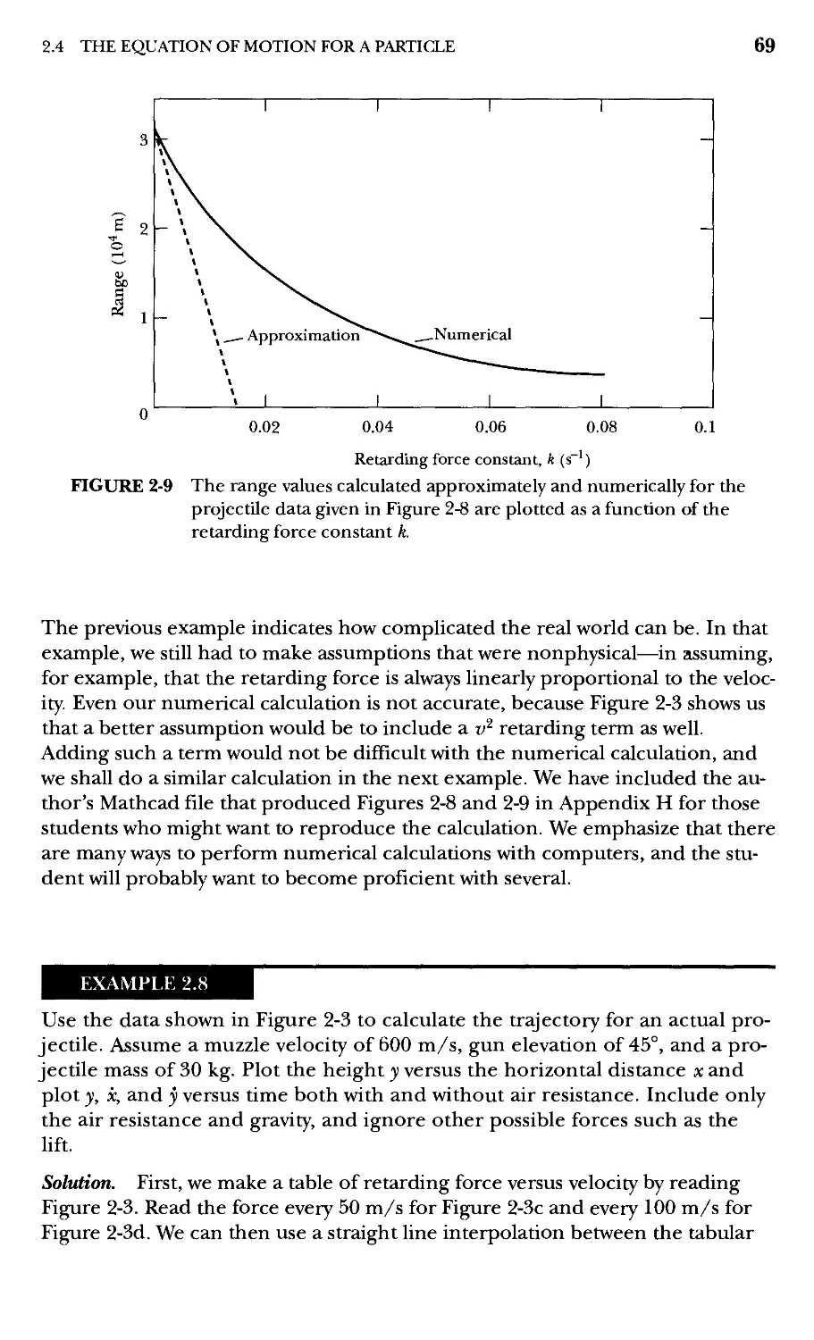
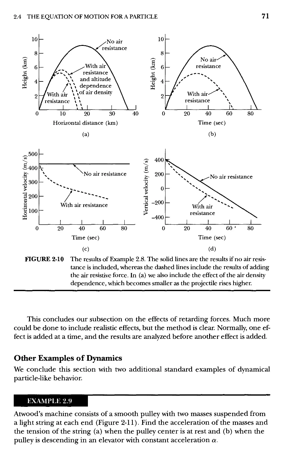
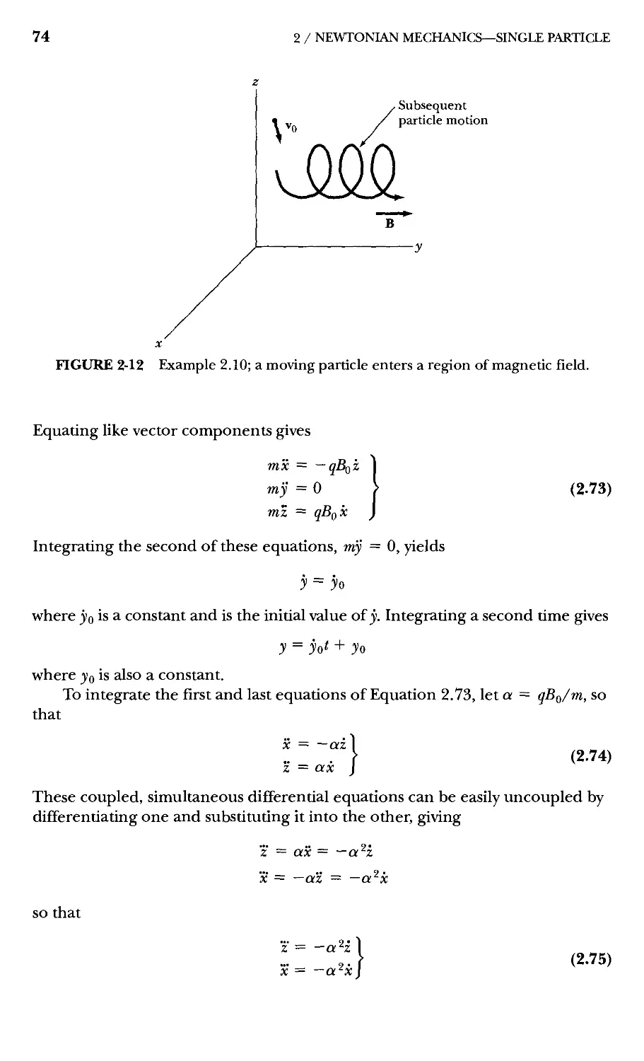
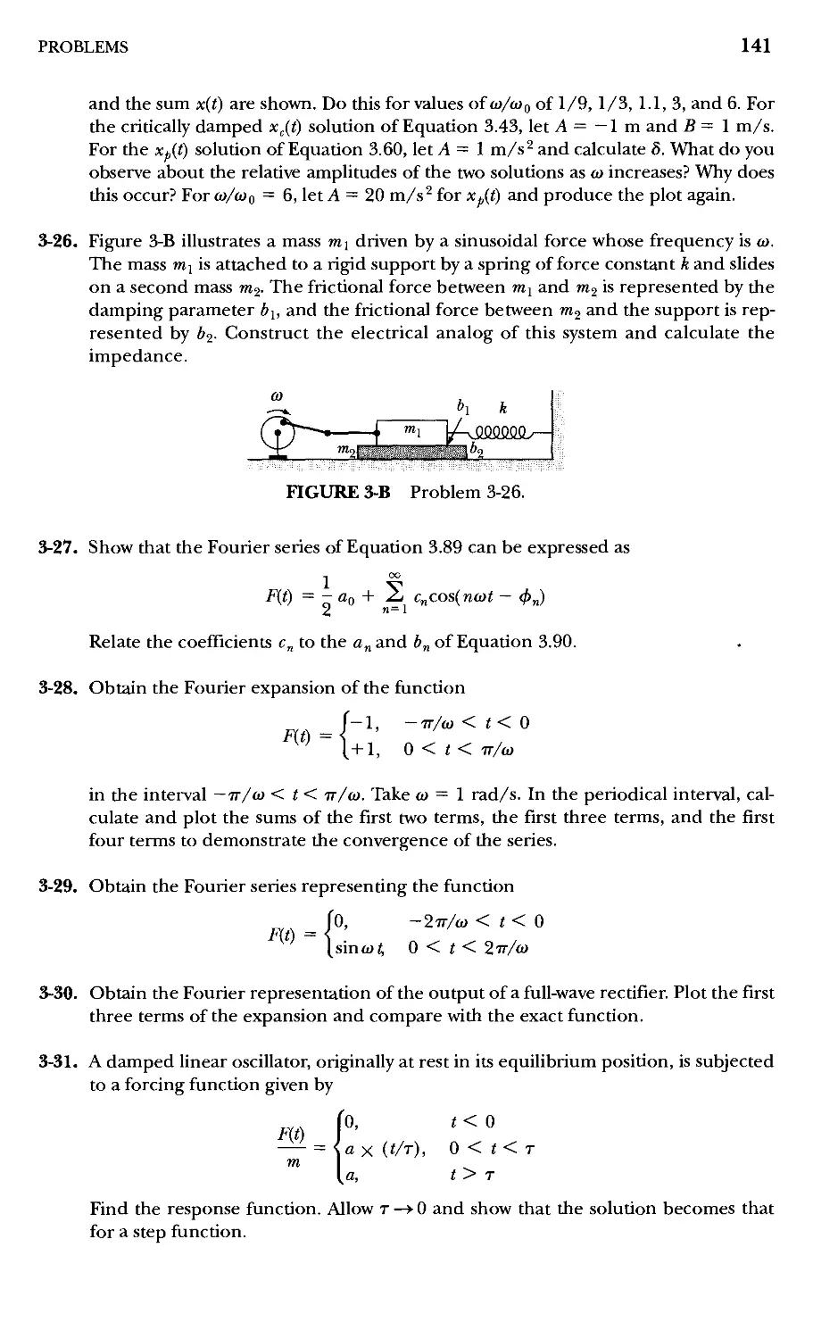
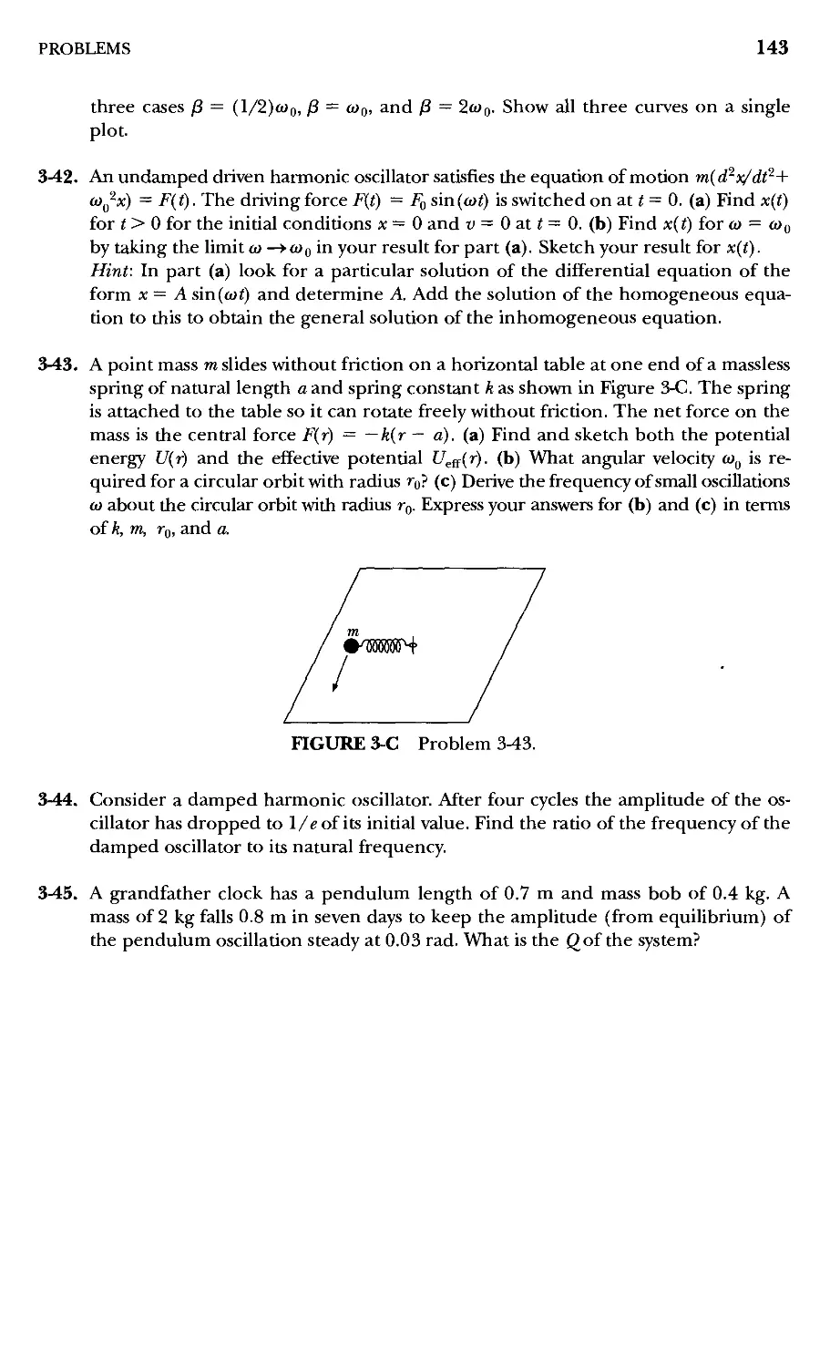
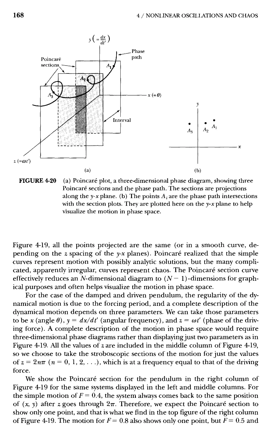
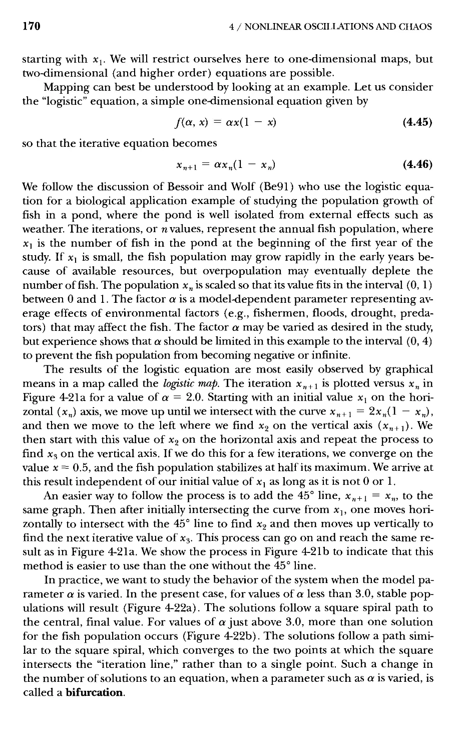
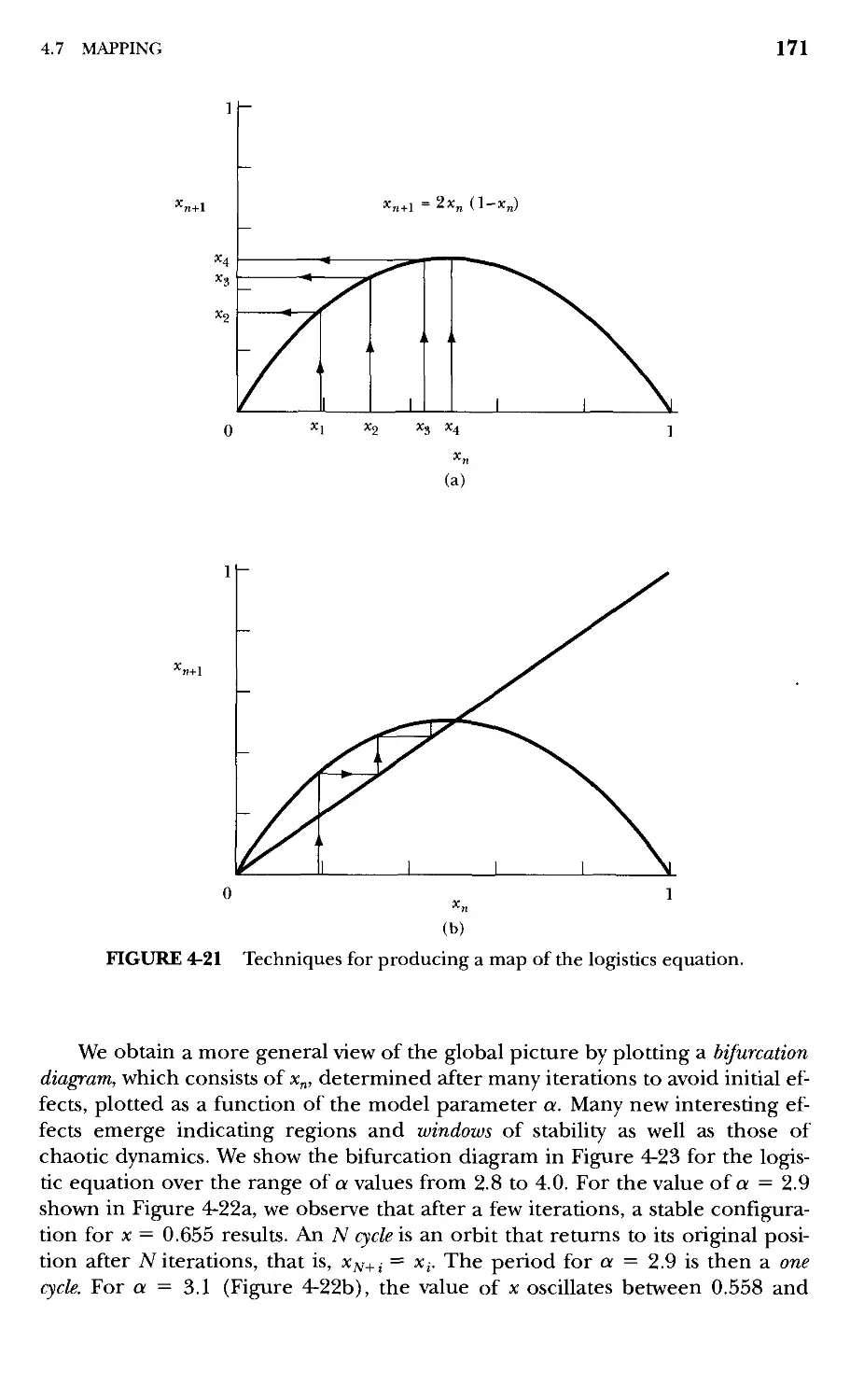
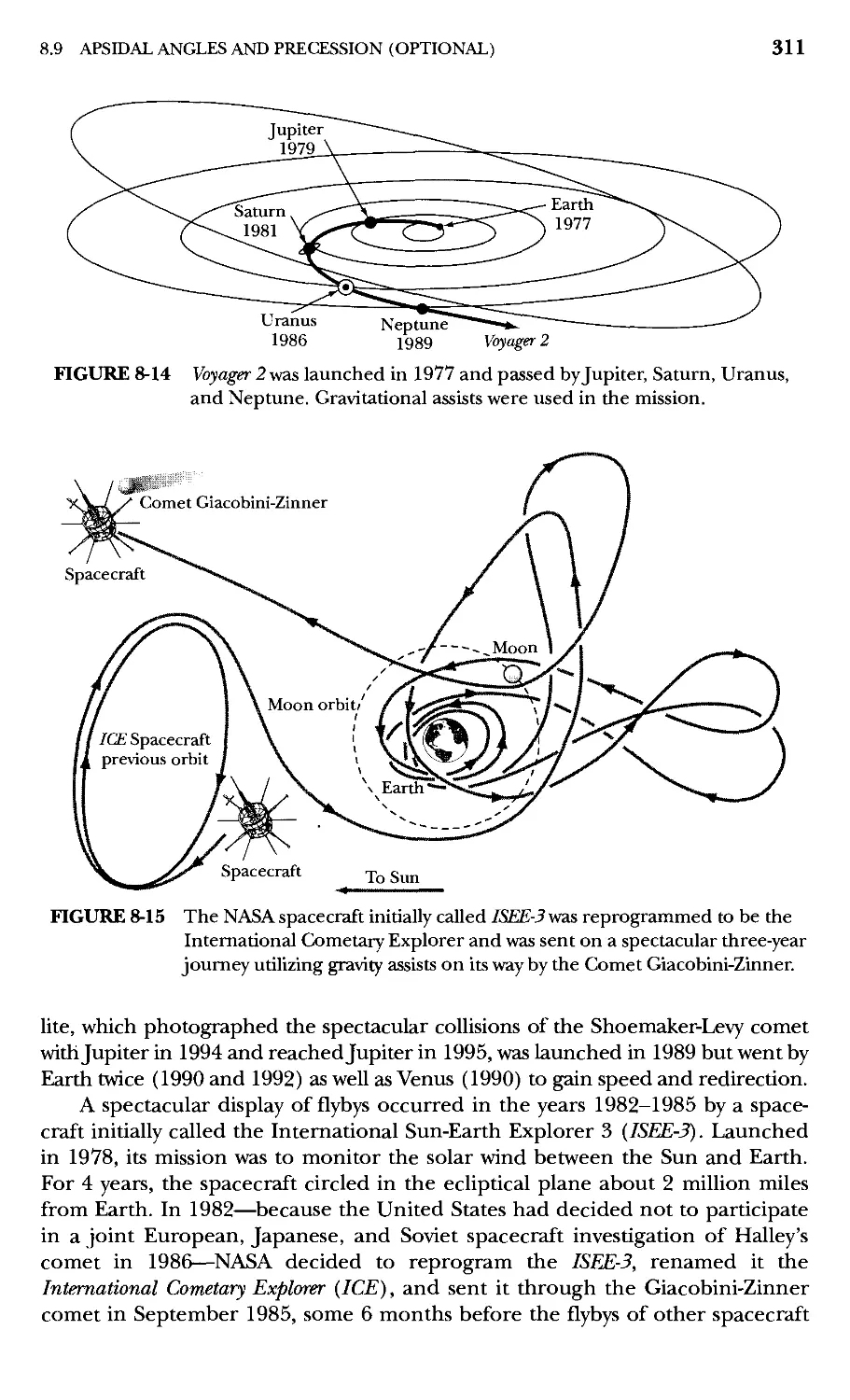
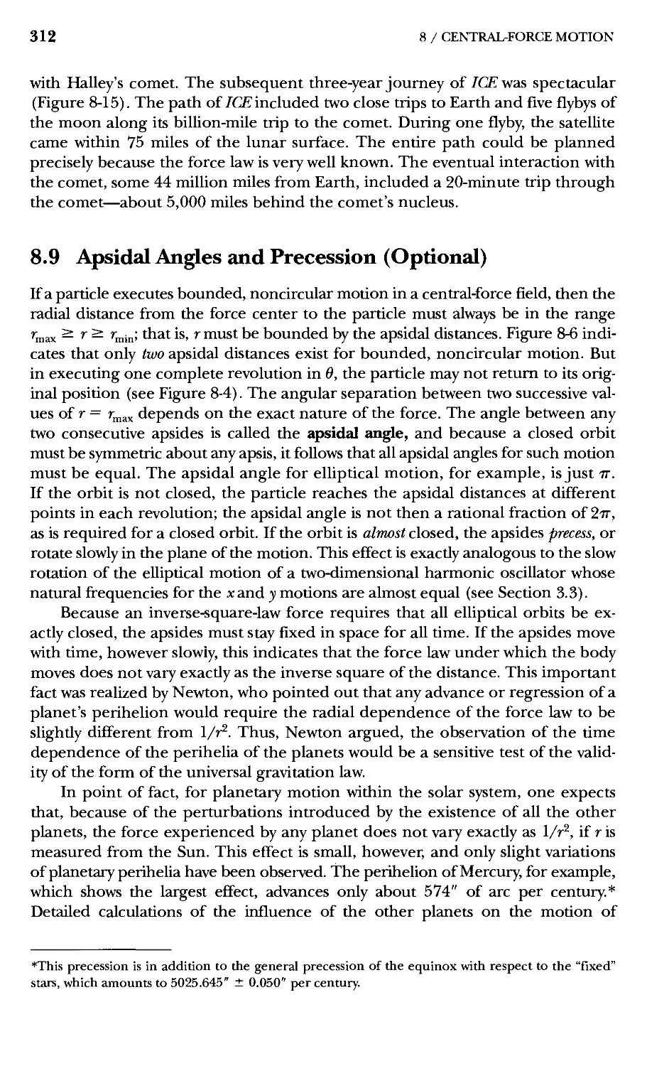
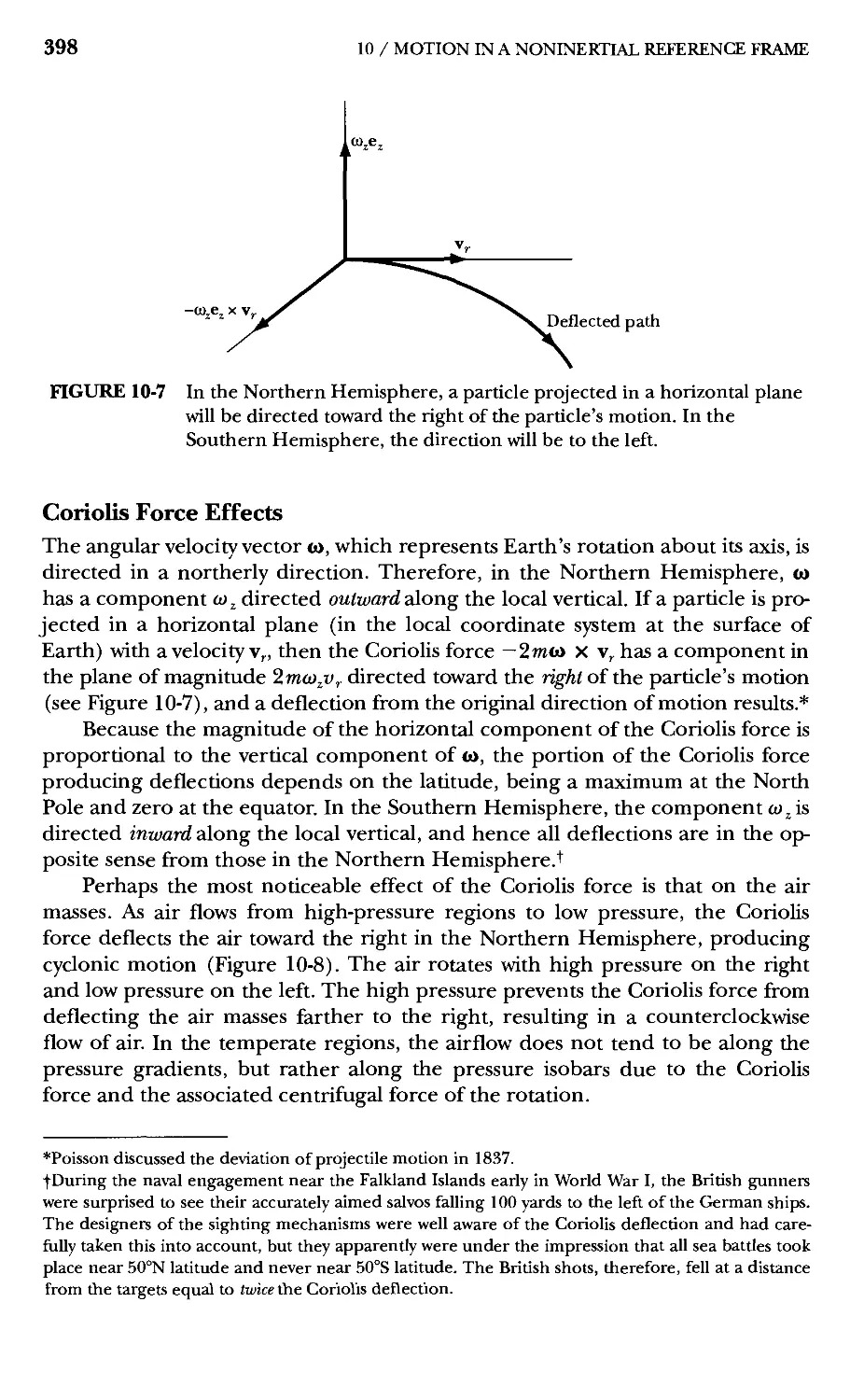
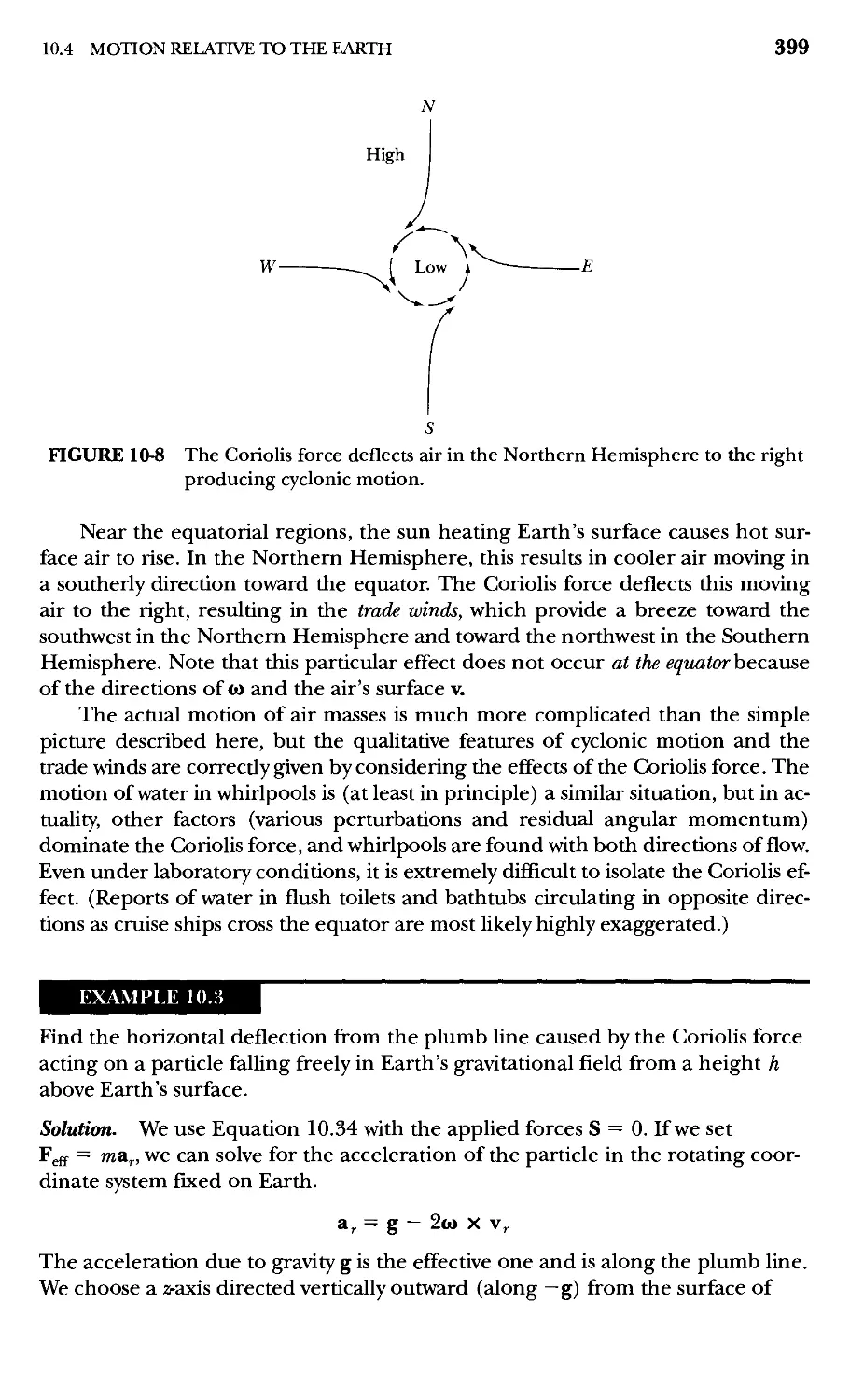
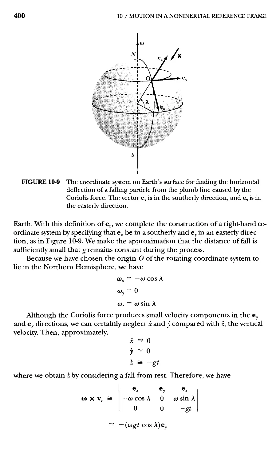
/


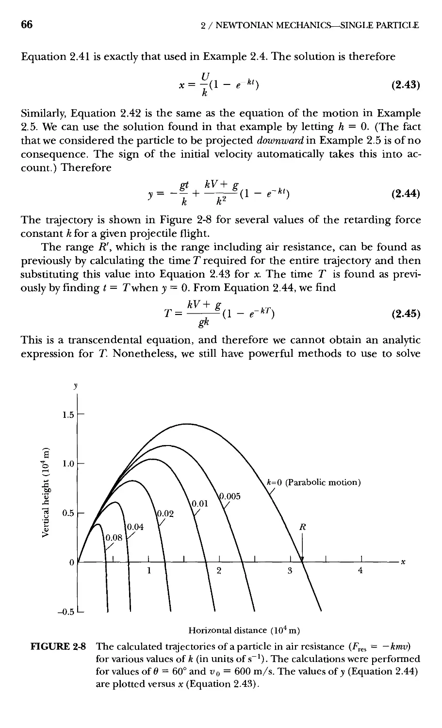


Автор: Thornton S.T. Marion J.B.
Теги: physics mathematical physics particle physics theoretical physics thomson brooks colem
ISBN: 0-534-40896-6
Год: 2003


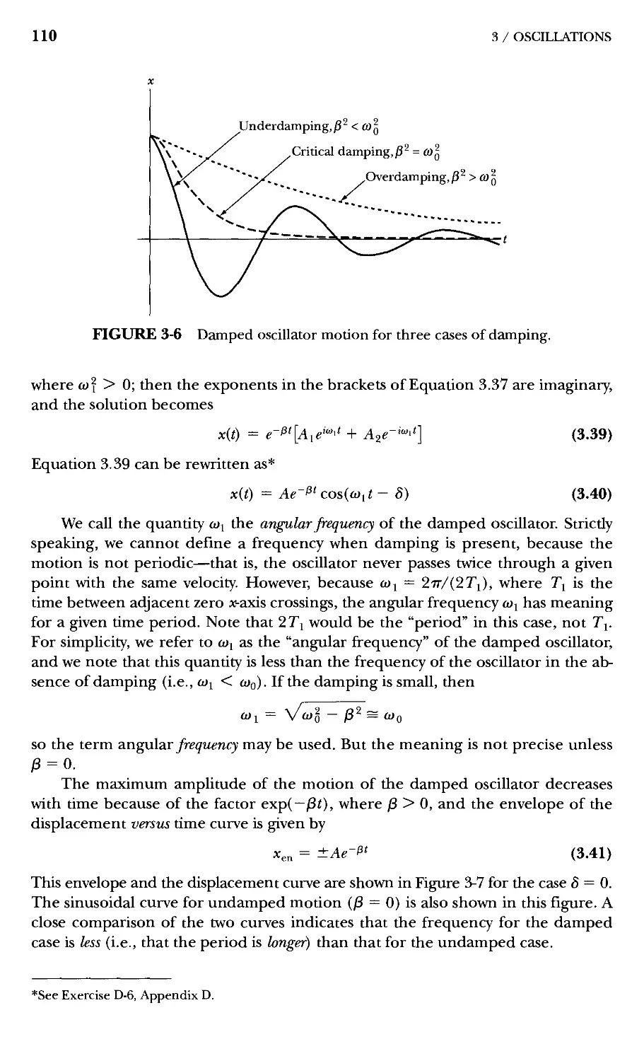
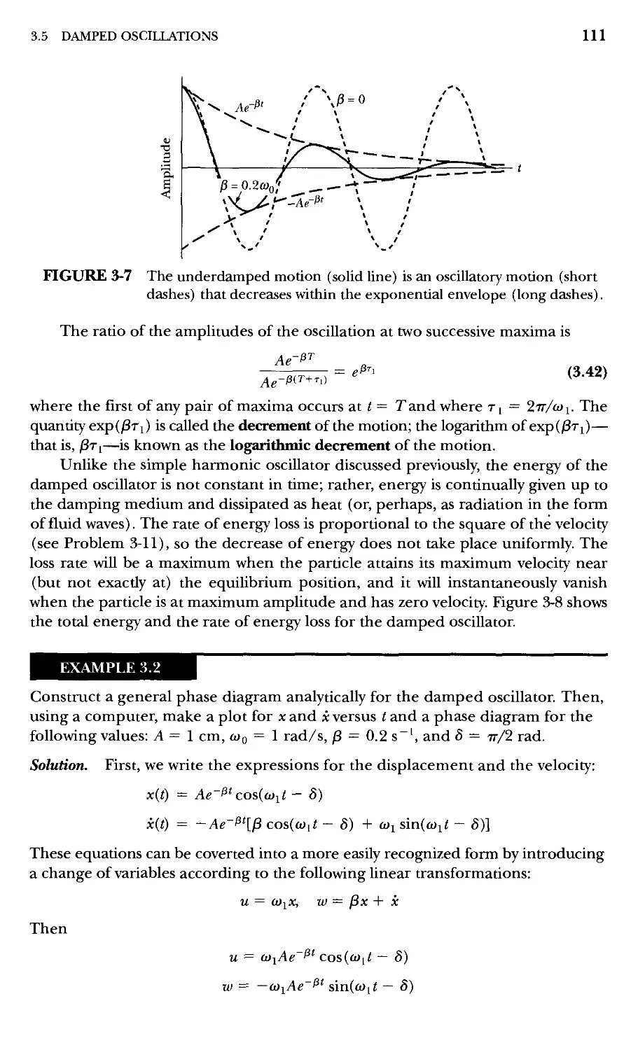
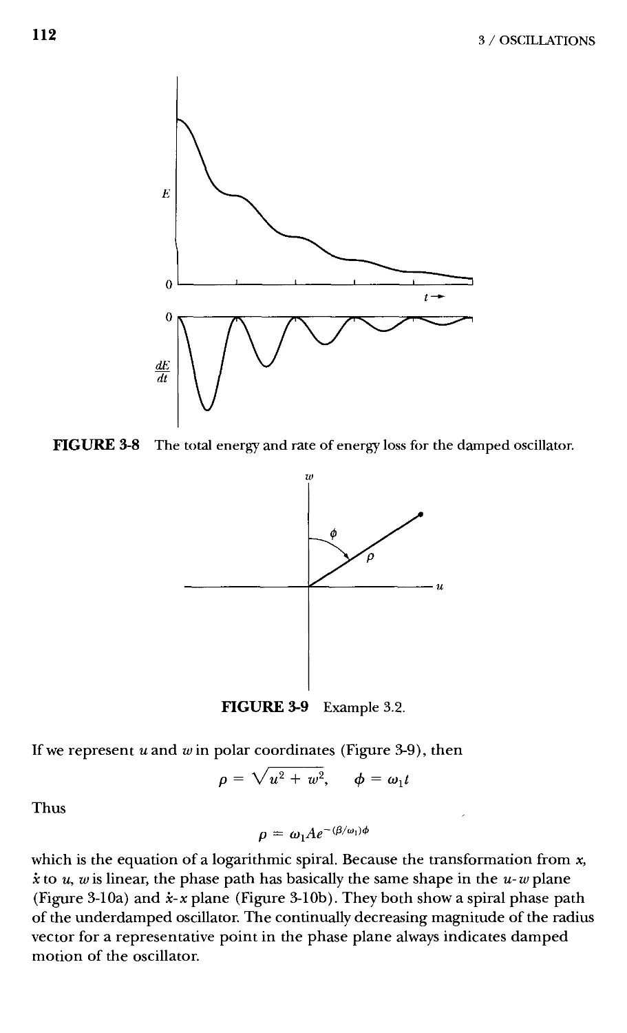
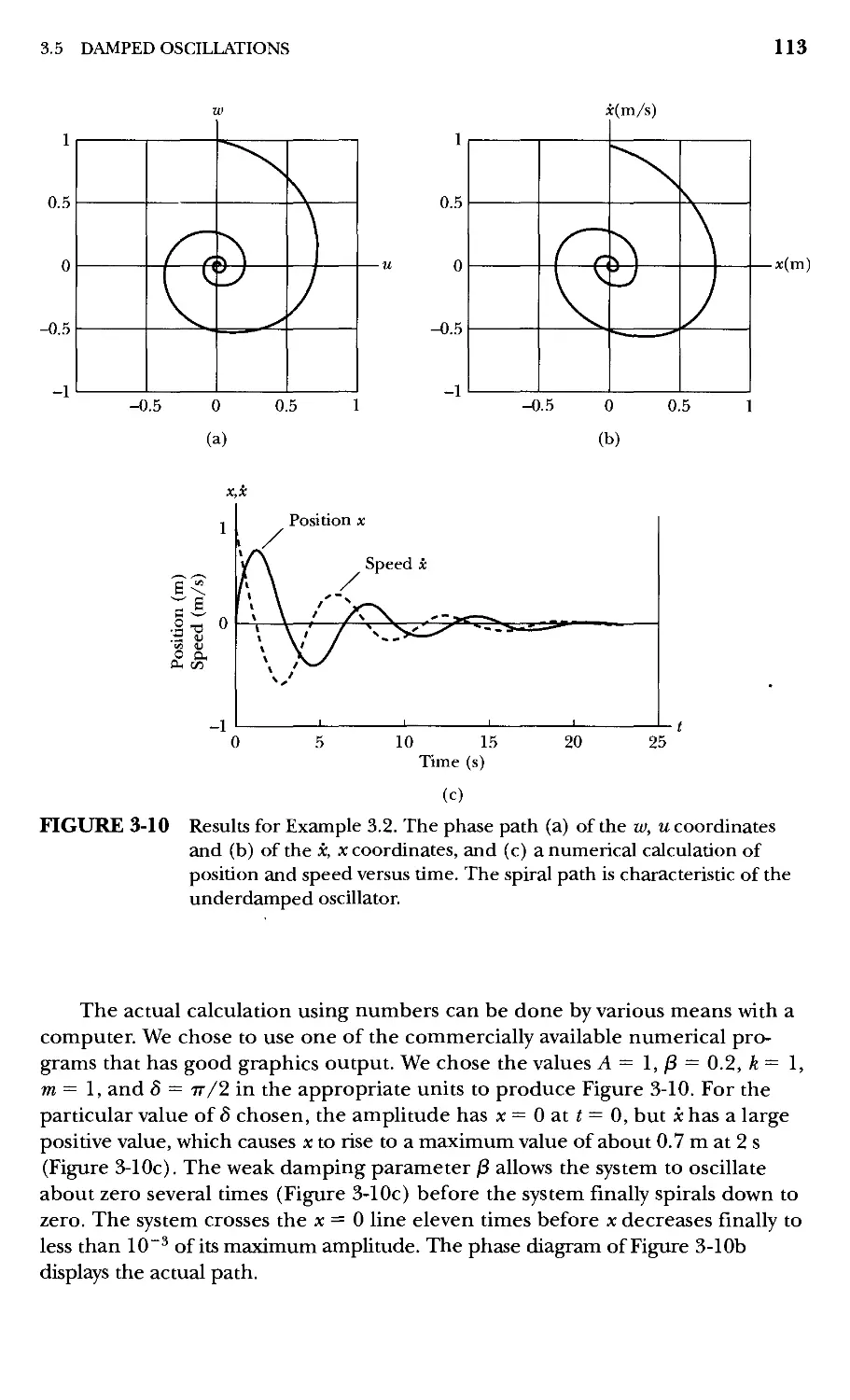
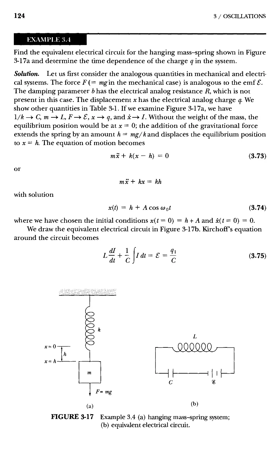
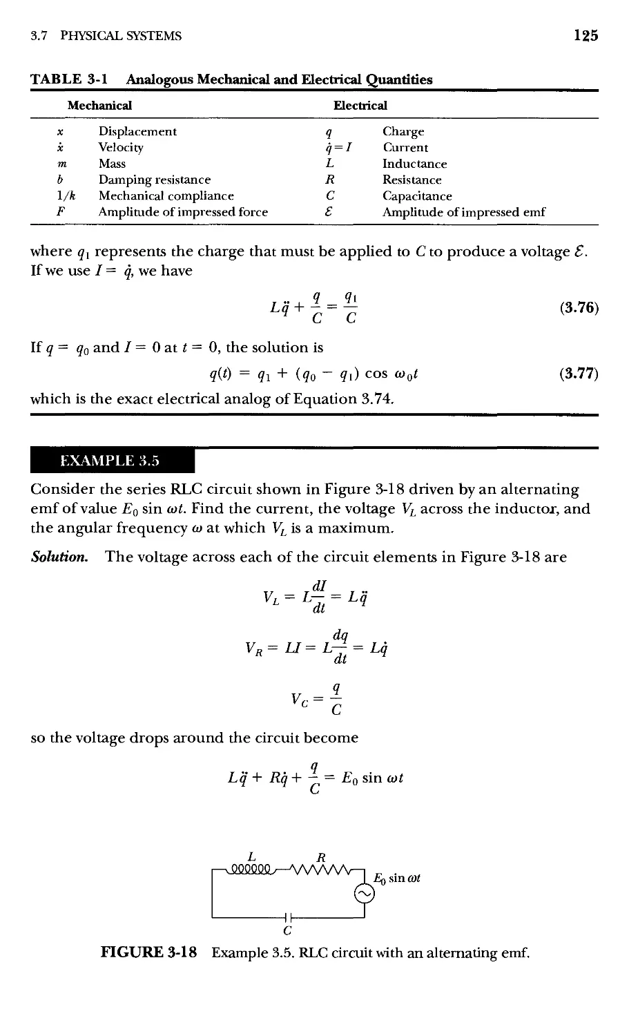
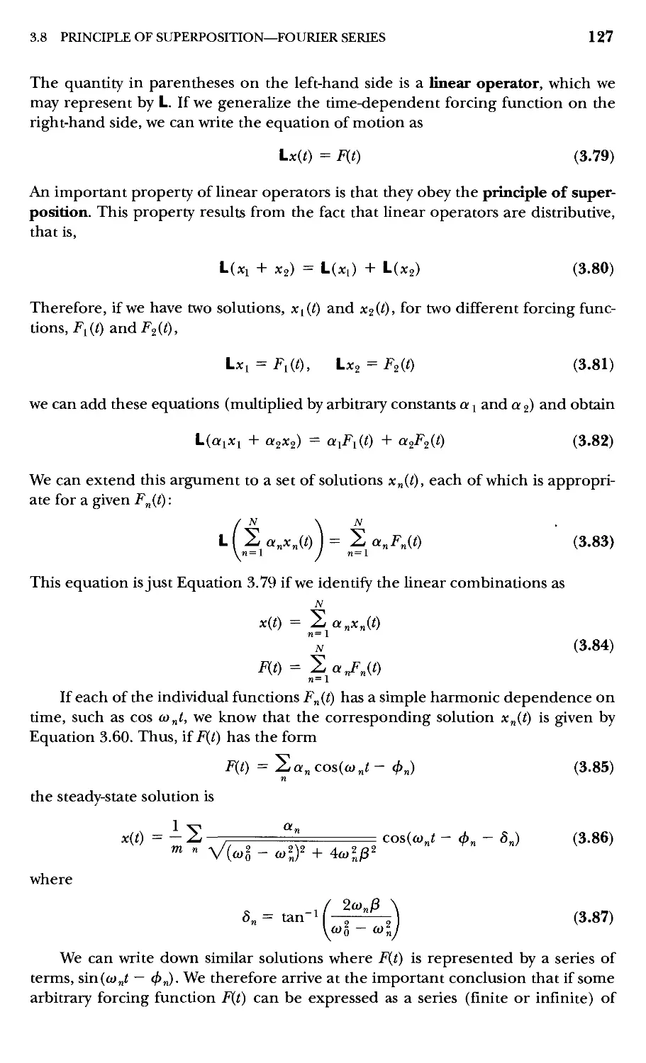
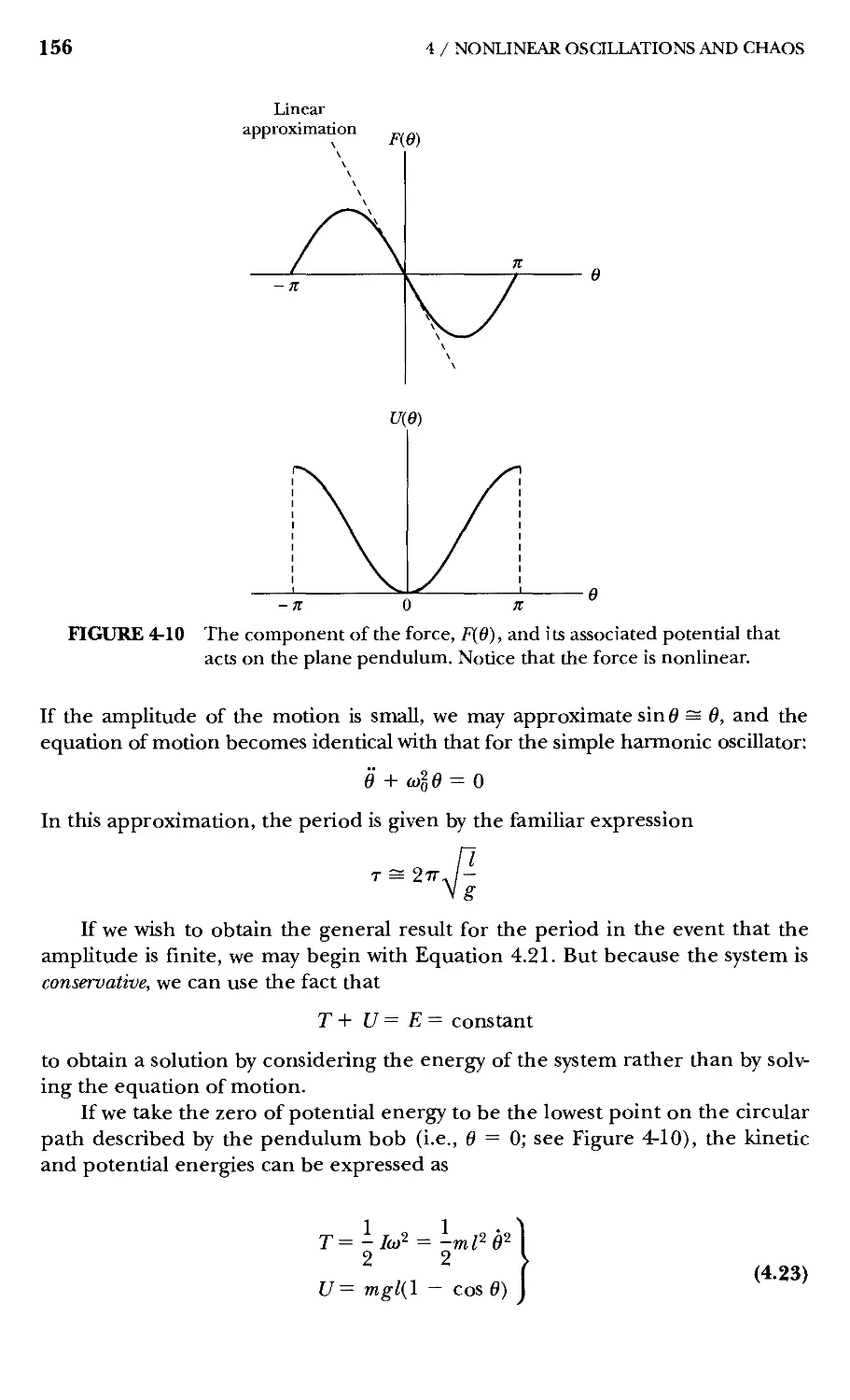
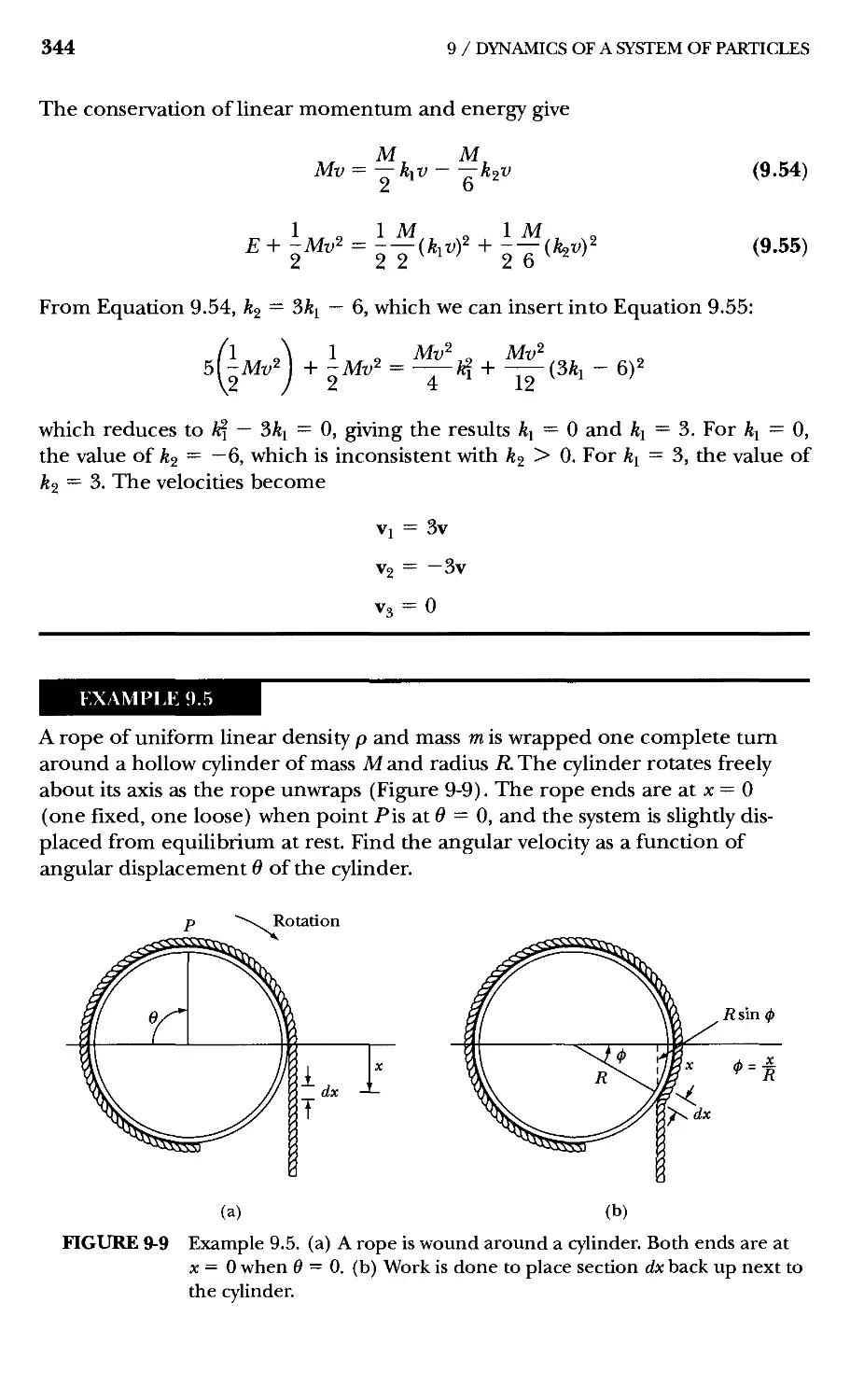
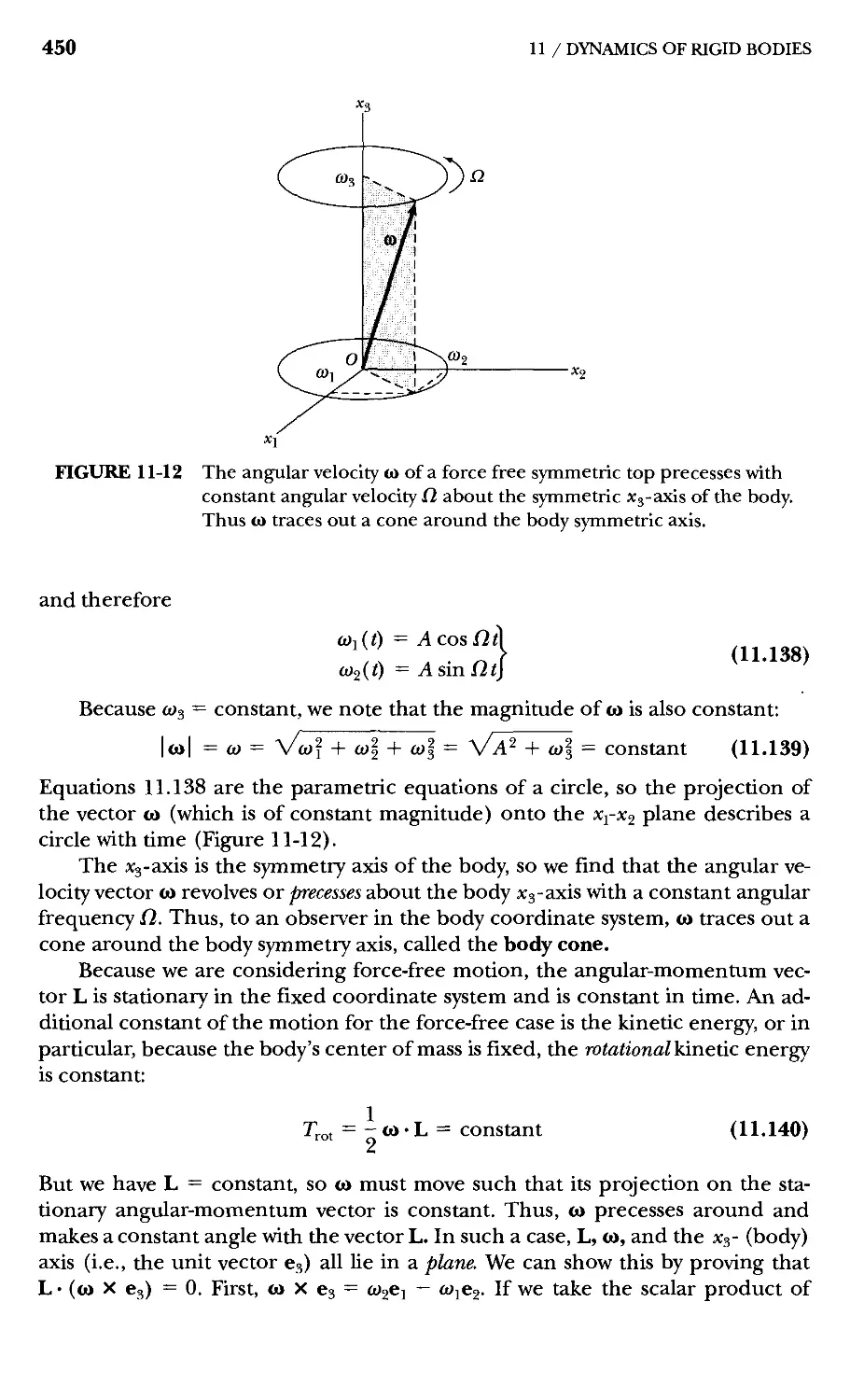
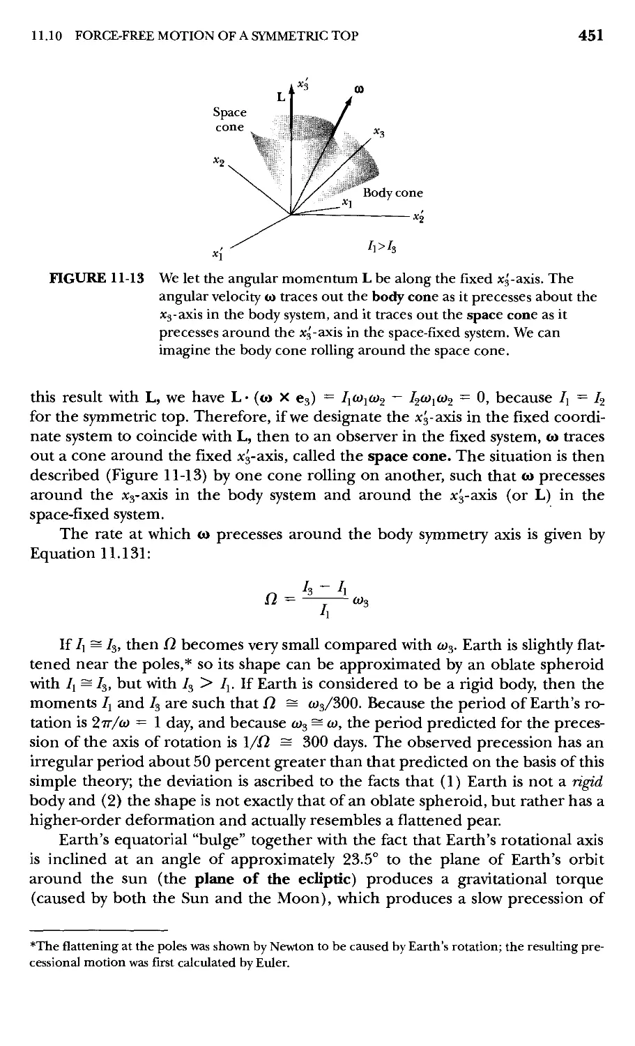
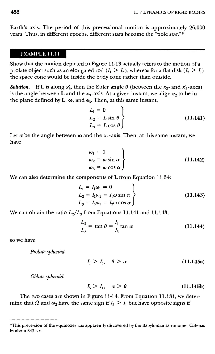
Текст
CLASSICA
DYNAMIC
OF PARTICLES
AND SYSTEMS
FIFTH EDITION
Stephen T. Thornton
Professor of Physics, University of Virginia
Jerry B. Marion
Late Professor of Physics, University of Maryland
THOIVISOIM
^
BROOKS/COLE a . i- ^ j . m ■ . c c ■
Australia • Canada • Mexico • Singapore • Spam
United Kingdom • United States
THOIVISOM
^
BROOKS/COLE
Acquisitions Editor; Chris Hall
Assistant Editor: Alyssa White
Editorial Assistant: Seth Dobrin
Technology Project Manager: Sam Subity
Marketing Manager: Kelley McAllister
Marketing Assistant: Sandra Perin
Project Manager, Editorial Production:
Karen Haga
Print/Media Buyer: Kris Waller
COPYRIGHT © 2004 Brooks/Cole, a division
of Thomson Learning, Inc. Thomson
Leaming^^ is a trademark used herein under
license.
ALL RIGHTS RESERVED. No part of this work
covered by the copyright hereon may be
reproduced or used in any form or by any means—
graphic, electronic, or mechanical, including
but not limited to photocopying, recording,
taping, Web distribution, information
networks, or information storage and retrieval
systems—without the written permission of the
publisher
Printed in the United States of America
1 2 3 4 5 6 7 07 06 05 04 03
For more information about our products,
contact us at;
Thomson Learning Academic Resource Center
1-800-423-0563
For permission to use material from this text,
contact us by: Phone: 1-800-730-2214
Fax: 1-800-730-2215
Web; http;//www.thomsonrights.com
Library of Congress Control Number:
2003105243
ISBN 0-534-40896-6
Permissions Editor; Joohee Lee
Production Service and Compositor:
Nesbitt Graphics, Inc.
Copy Editor; Julie M. DeSilva
Illustrator; Rolin Graphics, Inc.
Cover Designer: Ross Carron
Text Printer: Maple-Vail Book Mfg. Group
Cover Printer: Lehigh Press
Brooks/Cole—Thomson Learning
10 Davis Drive
Belmont, CA 94002
USA
Asia
Thomson Learning
5 Shenton Way #01-01
UIC Building
Singapore 068808
Australia/New Zealand
Thomson Learning
102 Dodds Street
Southbank, Victoria 3006
Australia
Canada
Nelson
1120 Birchmount Road
Toronto, Ontario MIK 5G4
Canada
Europe/Middle East/Africa
Thomson Learning
High Holbom House
50/51 Bedford Row
London WC1R4LR
United Kingdom
Latin America
Thomson Learning
Seneca, 53
Colonia Polanco
11560 Mexico D.F.
Mexico
Spain/Portugal
Paraninfo
Calle/Magallanes, 25
28015 Madrid, Spain
To
Dr. Kathryn C. Thornton
Astronaut and Wife
As she soars and walks through space,
May her life be safe and fulfilling.
And let our children's minds be open
for all that life has to offer.
Preface
Of the five editions of this text, this is the third edition that I have prepared. In
doing so, I have attempted to adhere to the late Jerry Marion's original purpose of
producing a modem and reasonably complete account of the classical mechanics
of particles, systems of particles, and rigid bodies for physics students at the
advanced undergraduate level. The purpose of the book continues to be threefold:
1. To present a modem treatment of classical mechanical systems in such a way
that the transition to the quantum theory of physics can be made with the
least possible difficulty.
2. To acquaint the student with new mathematical techniques wherever
possible, and to give him/her sufficient practice in solving problems so that the
student may become reasonably proficient in their use.
3. To impart to the student, at the crucial period in the student's career
between "introductory" and "advanced" physics, some degree of sophistication
in handling both the formalism of the theory and the operational technique
of problem solving.
After a firm foundation in vector methods is presented in Chapter 1, further
mathematical methods are developed in the textbook as the occasion demands.
It is advisable for students to continue studying advanced mathematics in
separate courses. Mathematical rigor must be learned and appreciated by students of
physics, but where the continuity of the physics might be disturbed by insisting
on complete generality and mathematical rigor, the physics has been given
precedence.
Changes for the Fifth Edition
The comments and suggestions of many users of Classical Dynamics have been
incorporated into this fifth edition. Without the feedback of the many instructors
V
VI PREFACE
who have used this text, it would not be possible to produce a textbook of
significant value to the physics community. After the extensive revision for the fourth
edition, the changes in this edition have been relatively minor. Only a few
rearrangements of material have been made. But several examples, especially
numerical ones, and many end-of-chapter problems have been added. Users have
not wanted extensive changes in the topics covered, but more examples for
students and a wider range of problems are always requested.
A strong effort continues to be made to correct the problem solutions
available in the Instructor and Student Solutions Manuals. I thank the many users
who sent comments concerning various problem solutions, and many of their
names are listed below. Answers to even-numbered problems have again been
included at the end of the book, and the selected references and general
bibliography have been updated.
Course Suitability
The book is suitable for either a one-semester or two-semester upper level
(junior or senior) undergraduate course in classical mechanics taken after an
introductory calculus-based physics course. At the University of Virginia we teach a
one-semester course based mostly on the first 12 chapters with several omissions
of certain sections according to the Instructor's wishes. Sections that can be
omitted without losing continuity are denoted as optional, but the instructor can
also choose to skip other sections (or entire chapters) as desired. For example,
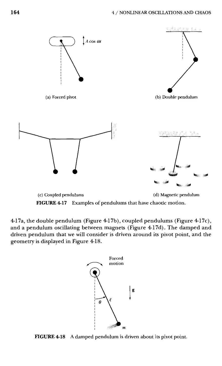
Chapter 4 (Nonlinear Oscillations and Chaos) might be skipped in its entirety
for a one-semester course. Some instructors choose not to cover the calculus of
variations material in Chapter 6. Other instructors may want to begin with
Chapter 2, skip the mathematical introduction of Chapter 1, and introduce the
mathematics as needed. This technique of dealing with the mathematics
introduction is perfectly acceptable, and the community is divided on this issue with a
slight preference for the method used here. The textbook is also suitable for a
full academic year course with an emphasis on mathematical and numerical
methods as desired by the instructor.
The textbook is appropriate for those who choose to teach in the traditional
manner without computer calculations. However, more and more instructors
and students are both familiar and adept with numerical calculations, and much
can be learned by doing calculations where parameters can be varied and real-
world conditions like friction and air resistance can be included. I decided
before the 4th edition to leave the choice of method to the instructor and/or
student to choose the computer techniques to be used. That decision has been
confirmed, because there are many excellent software programs (including
Mathematica, Maple, and Mathcad to mention three) available to use. In
addition, some Instructors have students write computer programs, which is an
important skill to obtain.
PREFACE Vii
Special Feature
The author has kept one popular feature of Jerry Marion's original book: the
addition of historical footnotes spread throughout. Several users have indicated
how valuable these historical comments have been. The history of physics has
been almost eliminated from present-day curricula, and as a result, the student is
frequently unaware of the background of a particular topic. These footnotes are
intended to whet the appetite and to encourage the student to inquire into the
history of his field.
Teaching Aids
Teaching aids to accompany the textbook are available online at
http://info.brookscole.com/thomton. The Instructor's Manual (ISBN 0-534-
40898-2) contains solutions to all the end-of-chapter problems in addition to
Transparency Masters of selected key figfures from the text. This password-
protected resource is easily printable in .pdf format. To receive your password,
just go to the above website and register; a usemame and password will be sent to
you once the information you have provided is verified. The verification
procedure ensures that you are an instructor teaching this course. If you are not
able to download the Instructor's Manual files and would like a printed copy sent
to you, please contact your local sales representative. If you do not know who
your sales representative is, please visit www.brookscole.com, and click on the
Find your Rep tab, which is located at the top of the web page. Please do not
distribute the Instructor's Manual to students, or post the solutions on the Internet.
Students are not permitted to access the Instructor's Manual.
Student Solutions Manual
A Student Solutions Manual by Stephen T Thornton, which contains solutions to
25% of the problems, is av^lable for sale to the students. Instructors are
encouraged to order the Student Solutions Manual for their students to purchase at the
school bookstore. To package the Student Solutions Manual with the text, use
ISBN 0-534-08378-1, or to order the Student Solutions Manual separately use ISBN
0-534-40897-4. Students can also purchase the manual online at the publisher's
website www.brookscole.com/physics.
Acknowledgments
I would like to graciously thank those individuals who wrote me with suggestions
on the text or problems, who returned questionnaires, or who reviewed parts of
the 4th edition. They include
William L. Alford, Auburn University
Philip Baldwin, University of Akron
Robert P. Bauman, University of
Alabama, Birmingham
Michael E. Browne, University of Idaho
Melvin G. Calkin, Dalhousie University
F. Edward Cecil, Colorado School of Mines
Arnold J. Dahm, Case Western Reserve
University
George Dixon, Oklahoma State University
John J. Dykla, Loyola University of
Chicago
Thomas A. Fergfuson, Carnegie Mellon
University
Shun-fu Gao, University of Minnesota,
Morris
Reinhard Graetzer, Pennsylvania State
University
Thomas M. Helliwell, Harvey Mudd
College
Stephen Houk, College of the Sequoias
Joseph Klarmann, Washington
University at St. Louis
Kaye D. Lathrop, Stanford University
Robert R. Marchini, Memphis State
University
The present 5th edition would not have been possible without the assistance
of many people who made suggestions for text changes, sent me problem
solution comments, answered a questionnaire, or reviewed chapters. I sincerely
appreciate their help and gratefully acknowledge them:
PREFACE
Robert B. Muir, University of North
Carolina, Greensboro
Richard P. Olenick, University of Texas,
Dallas
Tao Pang, University of Nevada, Las
Vegas
Peter Parker, Yale University
Peter Rolnick, Northeast Missouri State
University
Albert T Rosenberger, University of
Alabama, Huntsville
Wm. E. Slater, University of California,
Los Angeles
Herschel Snodgrass, Lewis and Clark
College
J. C. Spfott, University of Wisconsin,
Madison
Paul Stevenson, Rice University
Larry Tankersley, United States Naval
Academy
Joseph S. Tenn, Sonoma State
University
Dan de Vries, University of Colorado
Jonathan Bagger, yoAws Hopkins
University
Arlette Baljon, San Diego State
University
Roger Bland, San Francisco State
University
John Bloom, Biola University
Theodore Burkhardt, Temple
University
Kelvin Chu, University of Vermont
Douglas Cline, University of Rochester
Bret Crawford, Gettysburg College
Alfonso Diaz-Jimenez, Universidad
Militar Nueva Granad, Colombia
Avijit Gangopadhyay, University of
Massachusetts, Dartmouth
Tim Gfroerer, Davidson College
Kevin Haglin, Saint Cloud State
University
Dennis C. Henry, Gustavv^ Adolphus
College
John Hermanson, Montana State
University
Yue Hu, Wellesley College
Pawa Kahol, Wichita State University
Robert S. Knox, University of Rochester
Michael Kruger, University of Missouri
Whee Ky Ma, Groningen University
PREFACE ix
Steve Mellema, Gustavus Adolphus Keith Riles, University of Michigan
College Lyle Roelofs, Haverford College
Adrian Melott, University of Kansas Sally Seidel, University of New Mexico
William A. Mendoza, Jacksonville Mark Semon, Bates College
University Phil Spickler, Bridgewater College
Colin Momingstar, Carnegie Mellon Larry Tankersley, United States Naval
University Academy
Martin M. Ossowski, Naval Research Li You, Georgia Tech
Laboratory
I would especially like to thank Theodore Burkhardt of Temple University
who graciously allowed me to use several of his problems (and provided solutions)
for the new end-of-chapter problems. The help of Patrick J. Papin, San Diego State
University, and Lyle Roelofs, Haverford College, in checking the accuracy of the
manuscript is gratefully acknowledged. In addition I would like to acknowledge
the assistance of Tran ngoc Khanh who helped considerably with the problem
solutions for the fifth edition as well as Warren Griffith and Brian Giambattista who
did a similar service for the fourth and third editions, respectively.
The guidance and help of the Brooks/Cole Publishing professional staff is
greatly appreciated. These persons include Alyssa White, Assistant Editor; Chris
Hall, Acquisitions Editor; Karen Haga, Project Manager; Kelley McAllister,
Marketing Manager; Stacey Purviance, Advertising Project Manager; Samuel
Subity, Technology Project Manager; Seth Dobrin, Editorial Assistant, and Maria
McColligan and staff at Nesbitt Graphics, Inc. for their production help.
I would appreciate receiving suggestions or notices of errors in any of these
materials. I can be contacted by electronic mail at STT@Virginia.edu.
Stephen T Thornton
Charlottesville, Virginia
Contents
Matrices, Vectors, and Vector Calculus 1
1.1 Introduction 1
1.2 Concept of a Scalar 2
1.3 Coordinate Transformations 3
1.4 Properties of Rotation Matrices 6
1.5 Matrix Operations 9
1.6 Further Definitions 12
1.7 Geometrical Significance of Transformation Matrices 14
1.8 Definitions of a Scalar and a Vector in Terms of
Transformation Properties 20
1.9 Elementary Scalar and Vector Operations 20
1.10 Scalar Product of Two Vectors 21
1.11 Unit Vectors 23
1.12 Vector Product of Two Vectors 25
1.13 Differentiation of a Vector with Respect to a Scalar 29
1.14 Examples of Derivatives—Velocity and Acceleration 30
1.15 Angular Velocity 34
1.16 Gradient Operator 37
1.17 Integration of Vectors 40
Problems 43
Newtonian Mechanics—Single Particle 48
2.1 Introduction 48
2.2 Newton's Laws 49
2.3 Frames of Reference 53
2.4 The Equation of Motion for a Particle 55
xi
xii CONTENTS
2.5 Conservation Theorems 76
2.6 Energy 82
2.7 Limitations of Newtonian Mechanics 88
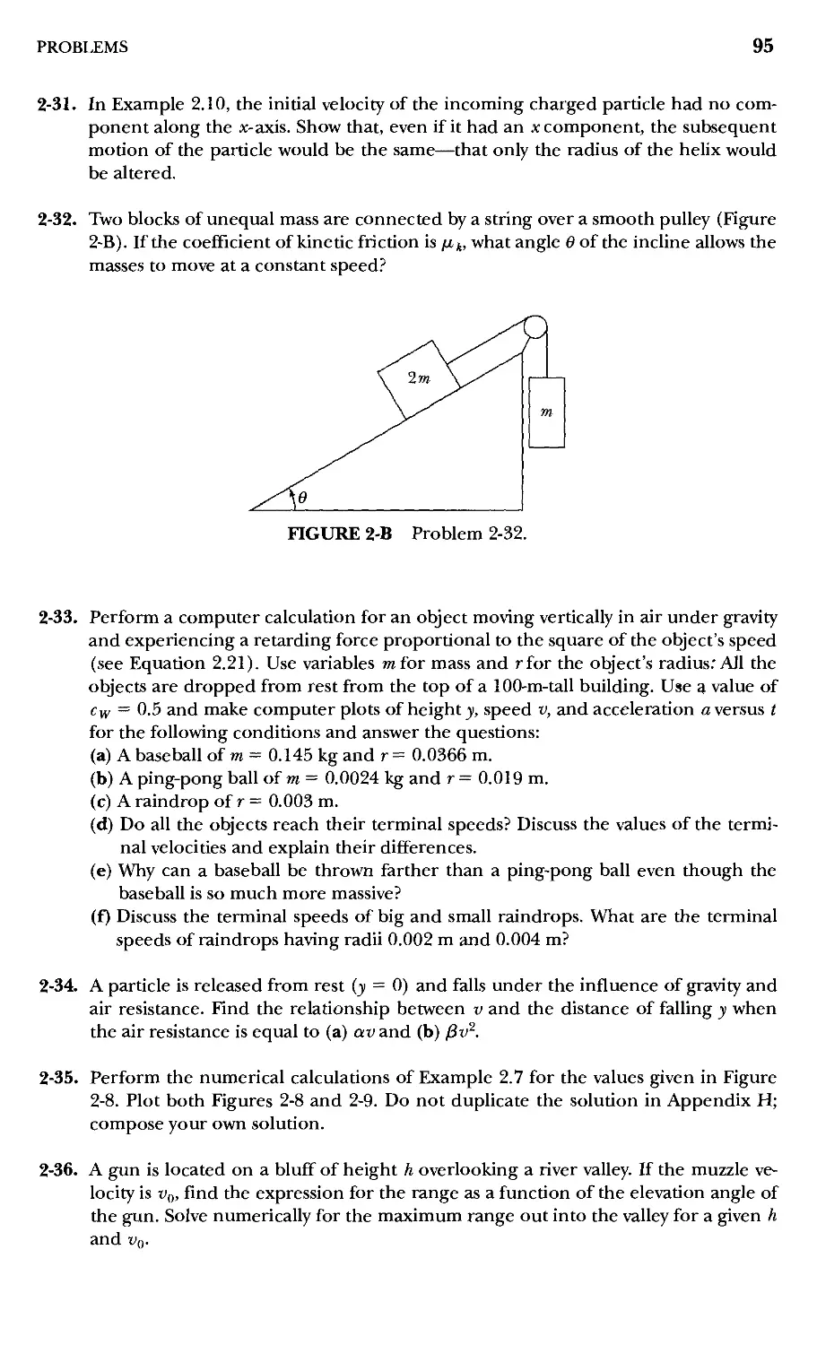
Problems 90
Oscillatioiis 99
3.1 Introduction 99
3.2 Simple Harmonic Oscillator 100
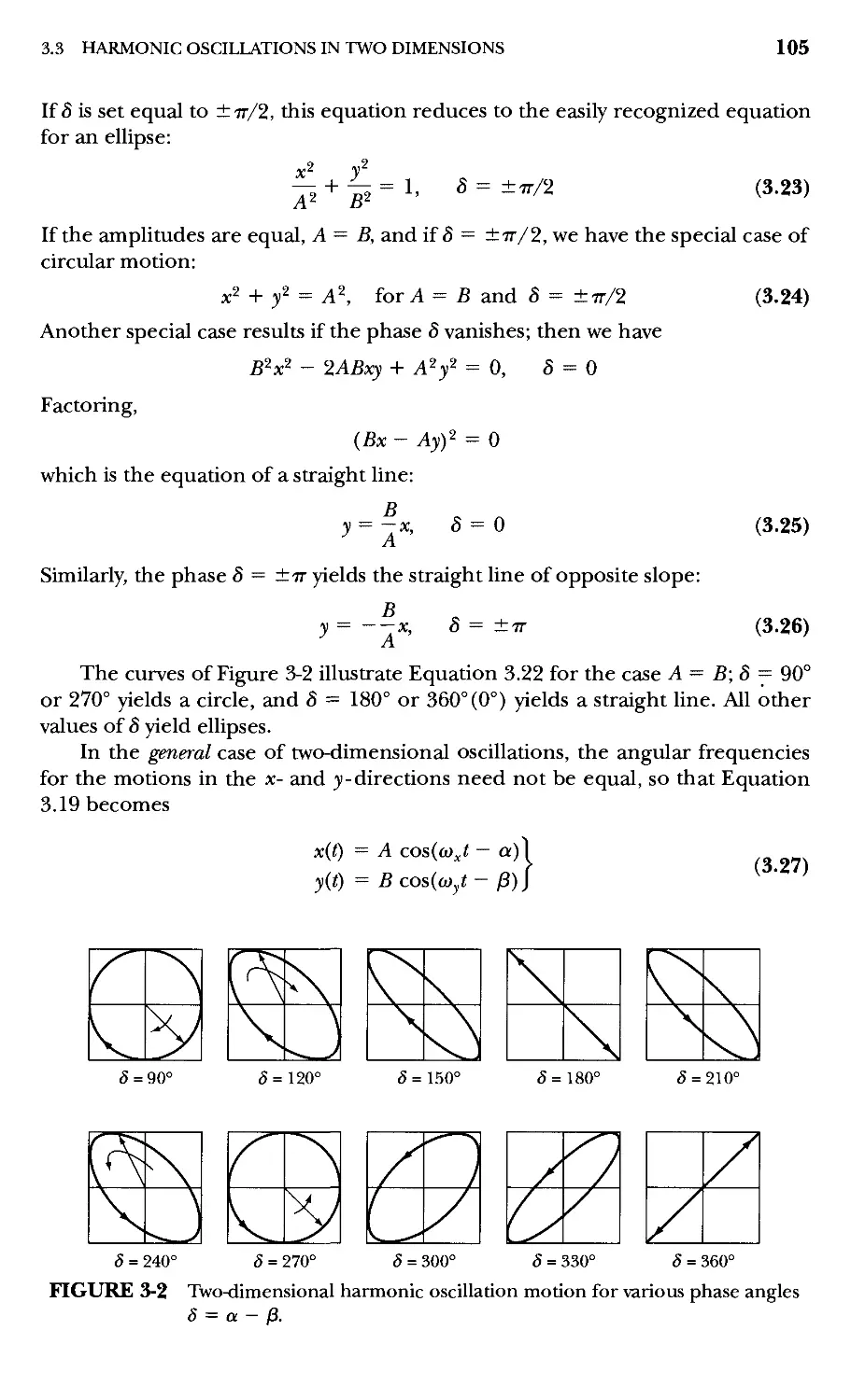
3.3 Harmonic Oscillations in Two Dimensions 104
3.4 Phase Diagrams 106
3.5 Damped Oscillations 108
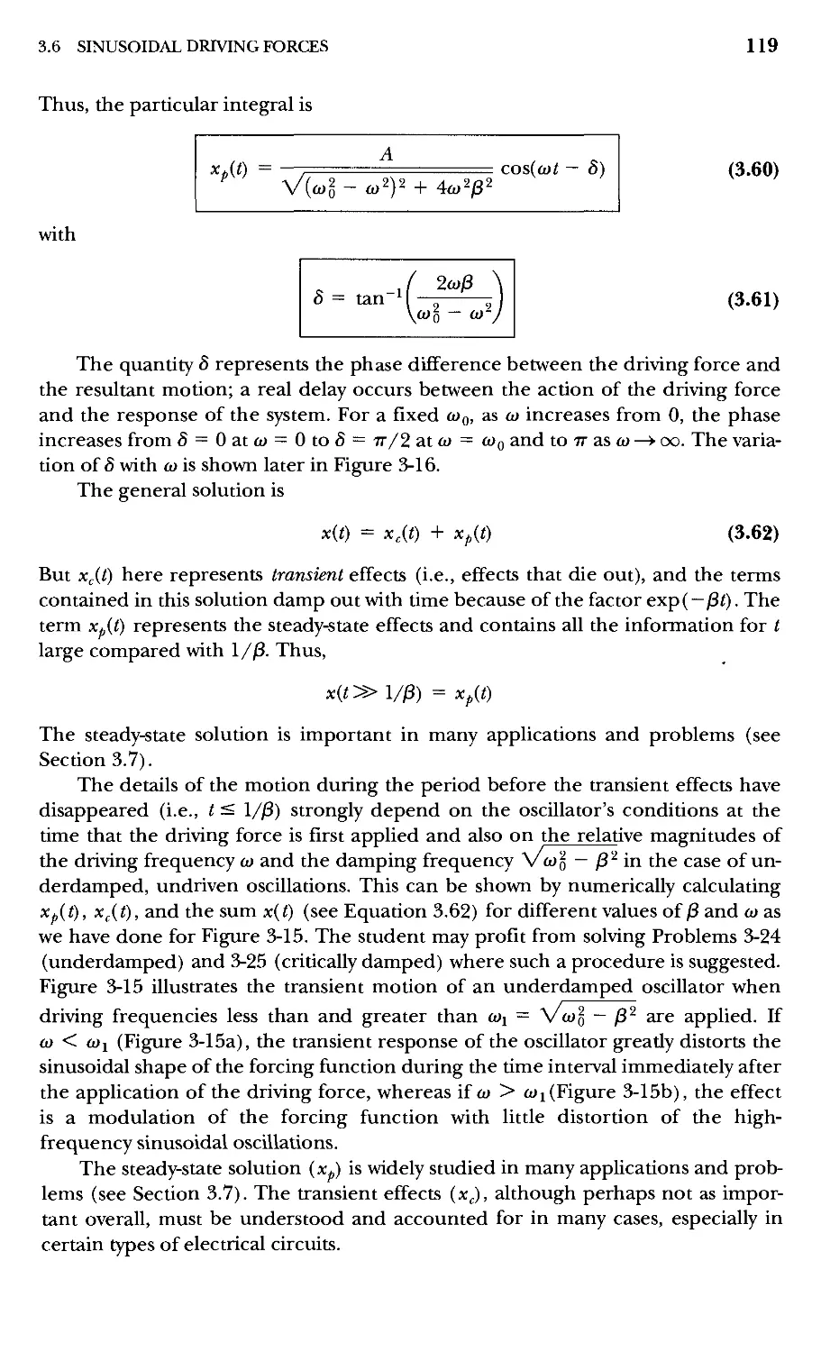
3.6 Sinusoidal Driving Forces 117
3.7 Physical Systems 123
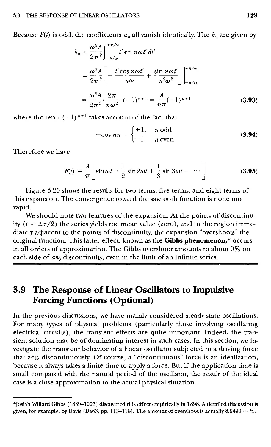
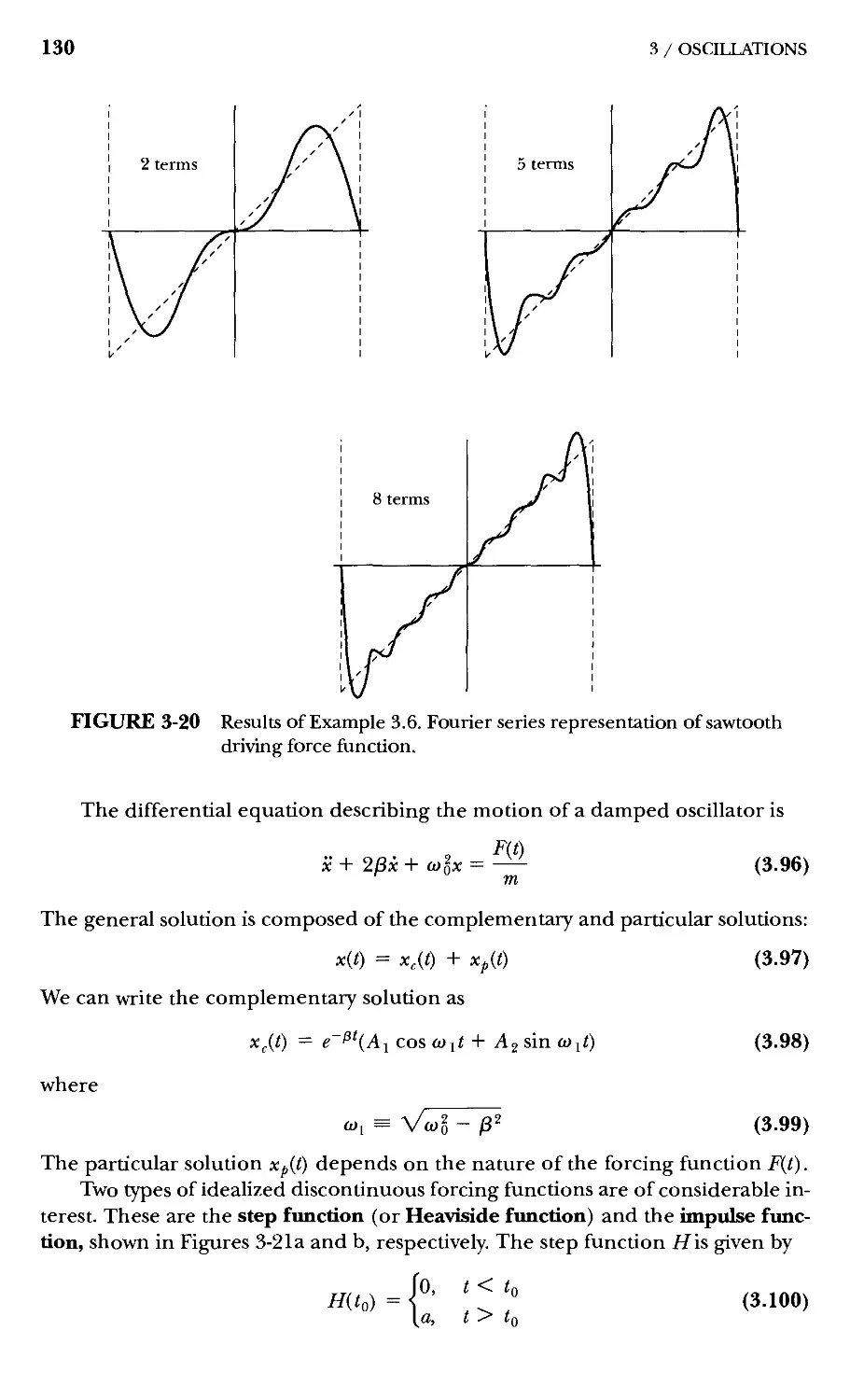
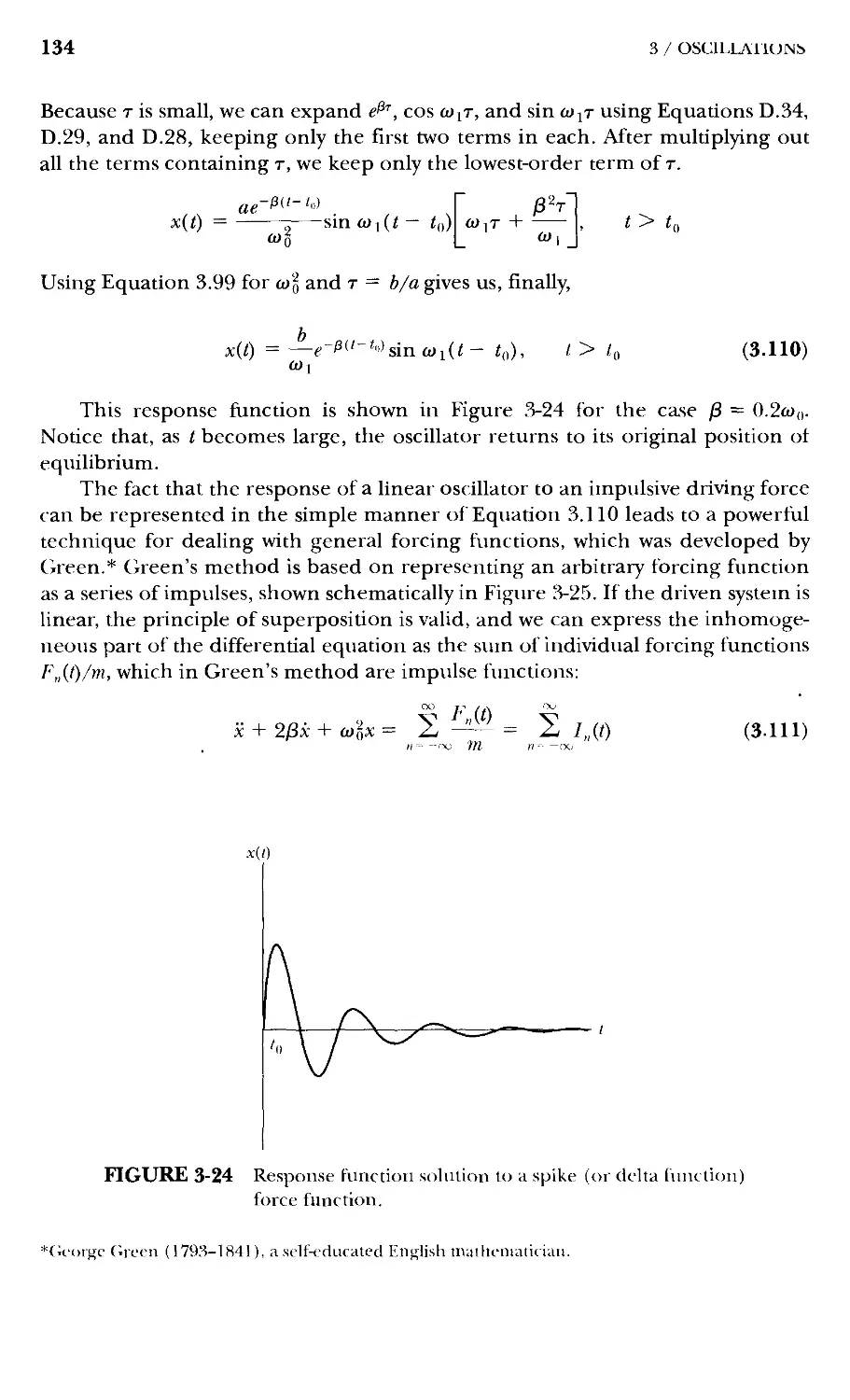
3.8 Principle of Superposition—^Fourier Series 126
3.9 The Response of Linear Oscillators to Impulsive Forcing
Functions (Optional) 129
Problems 138
Nonlinear Oscillations and Chaos 144
4.1 Introduction 144
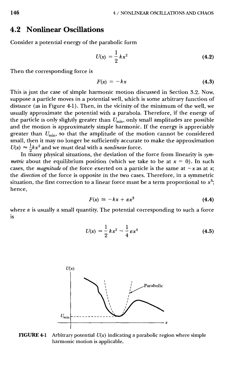
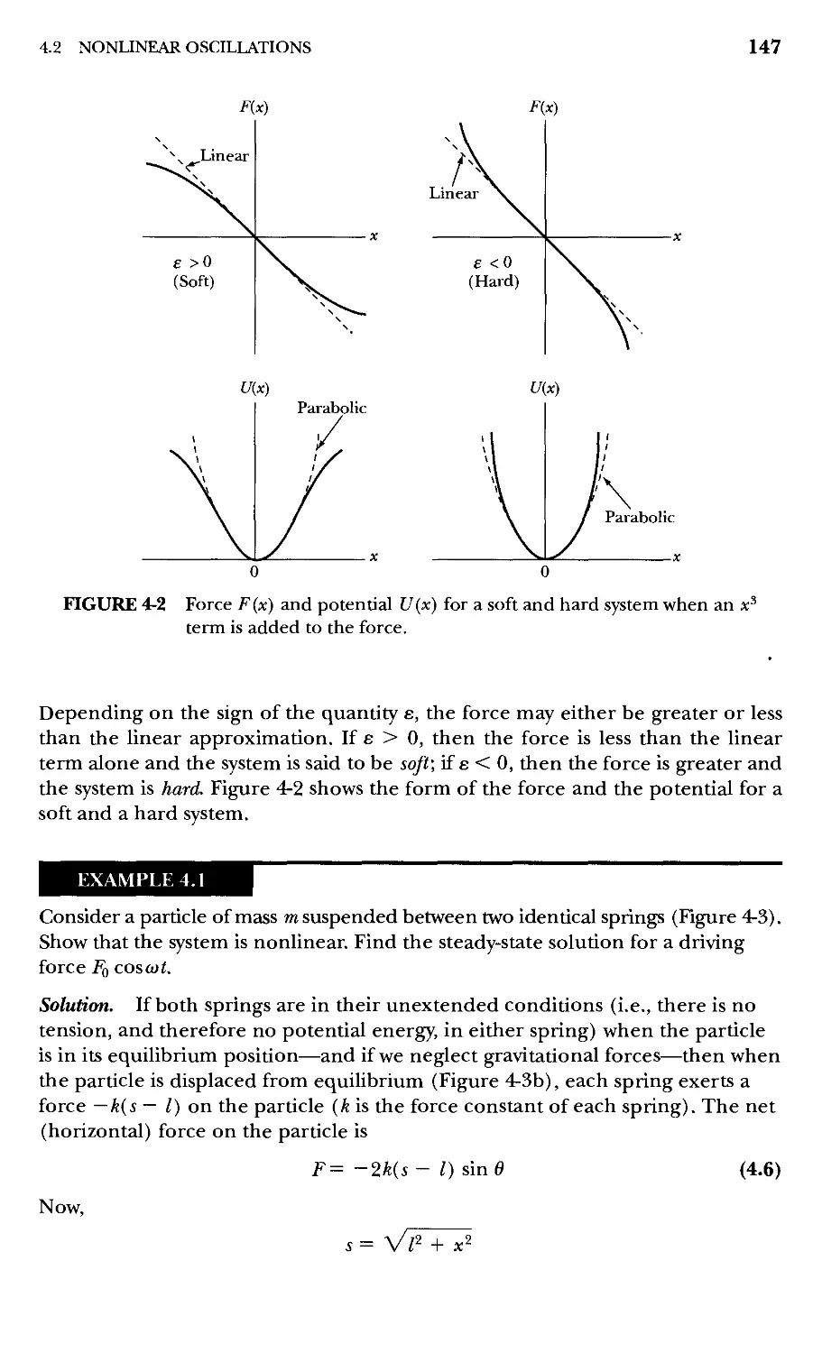
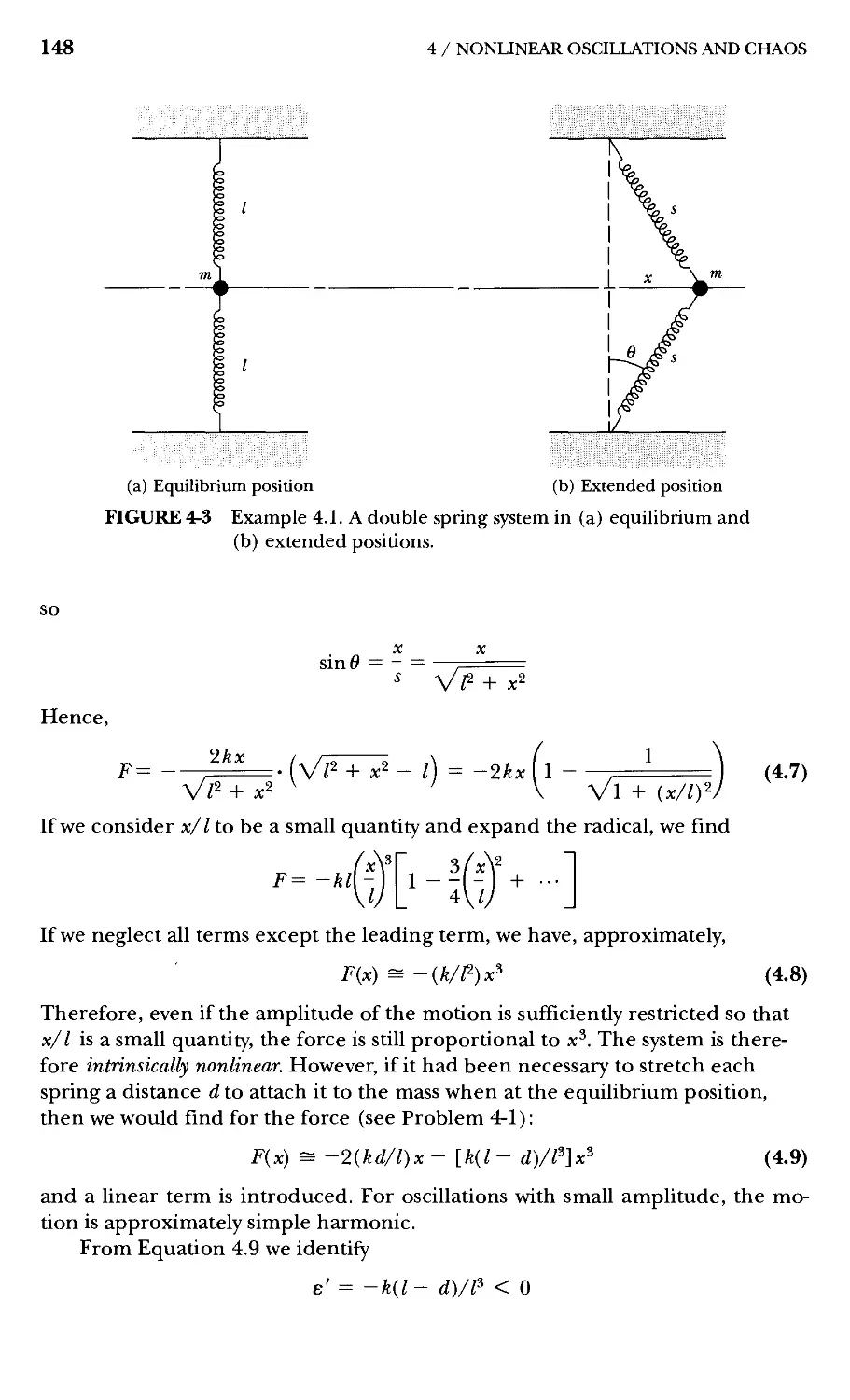
4.2 Nonlinear Oscillations 146
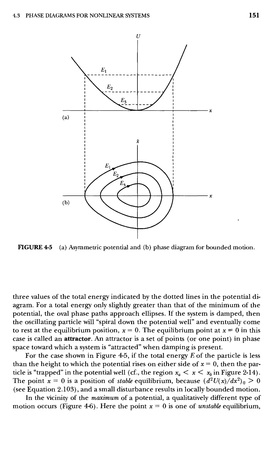
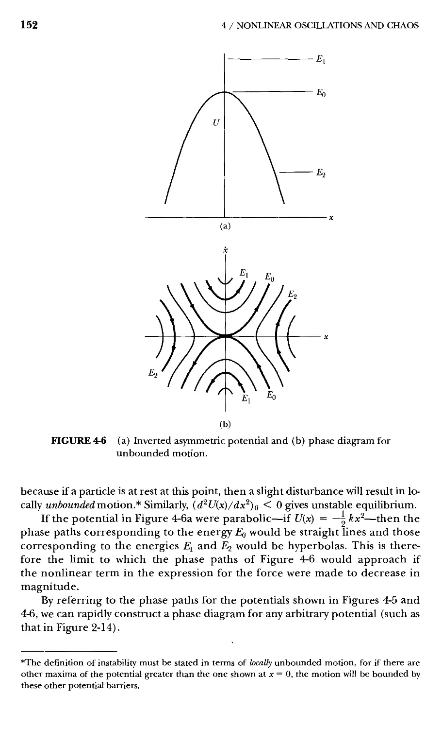
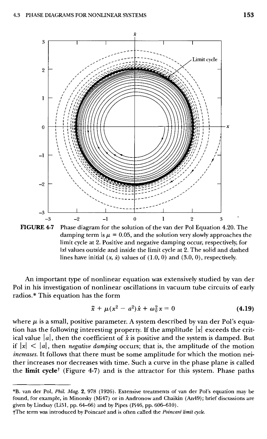
4.3 Phase Diagrams for Nonlinear Systems 150
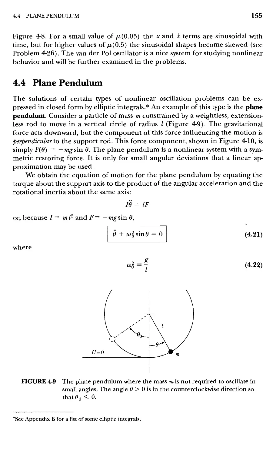
4.4 Plane Pendulum 155
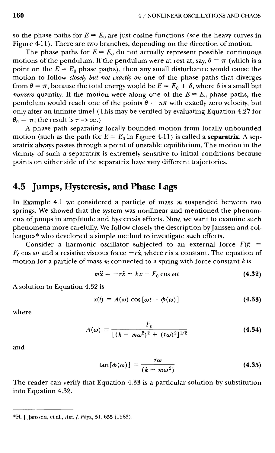
4.5 Jumps, Hysteresis, and Phase Lags 160
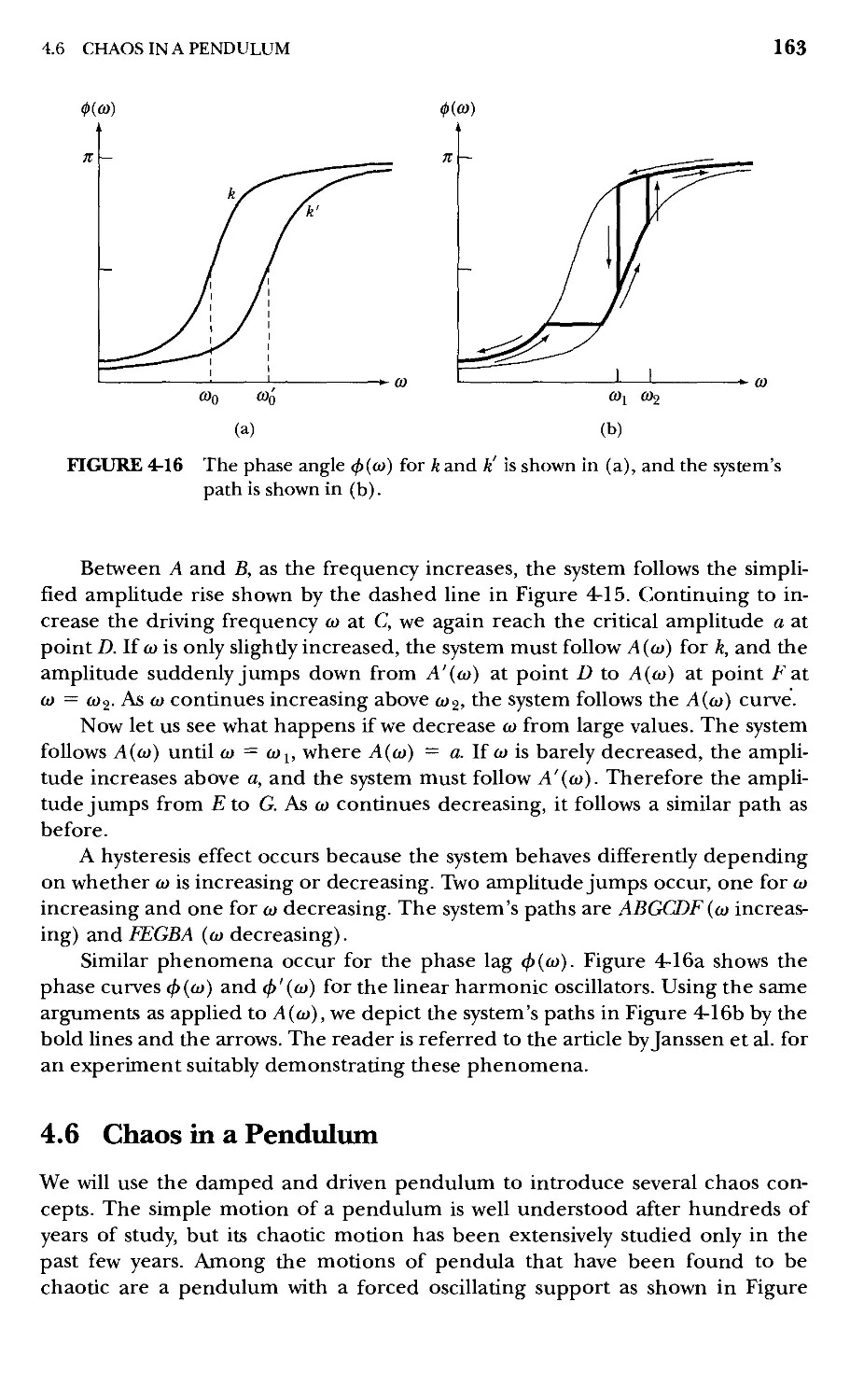
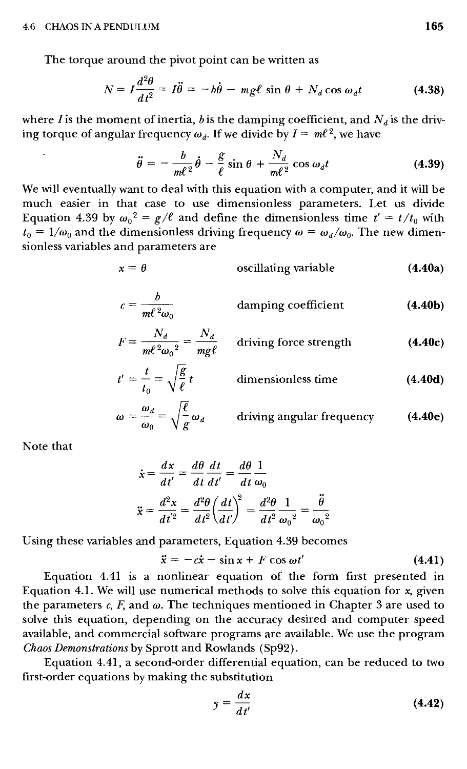
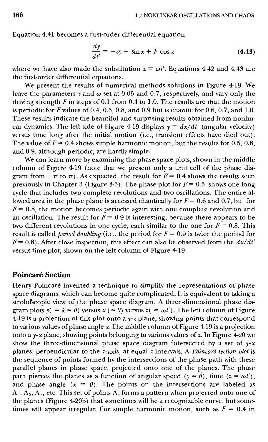
4.6 Chaos in a Pendulum 163
4.7 Mapping 169
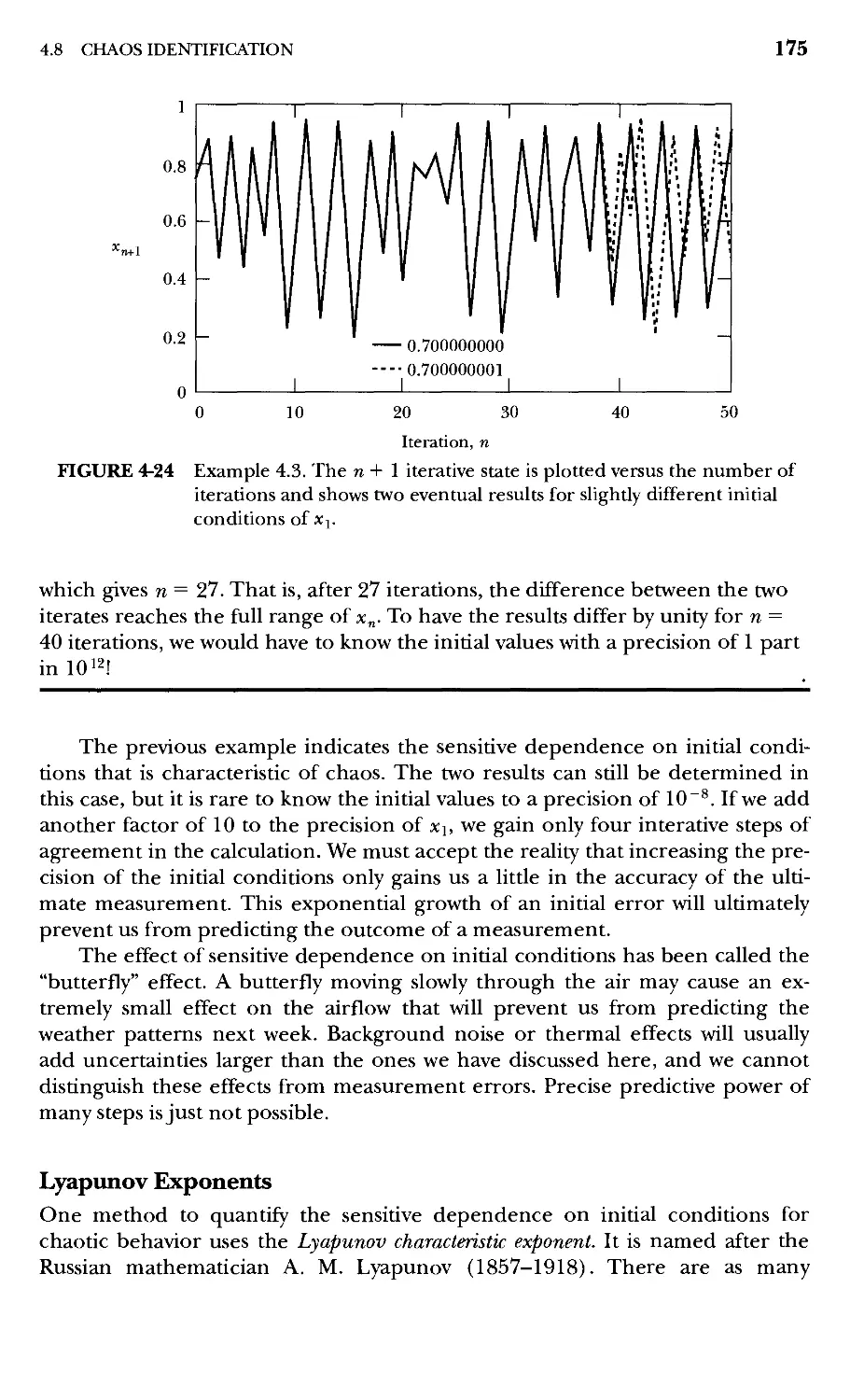
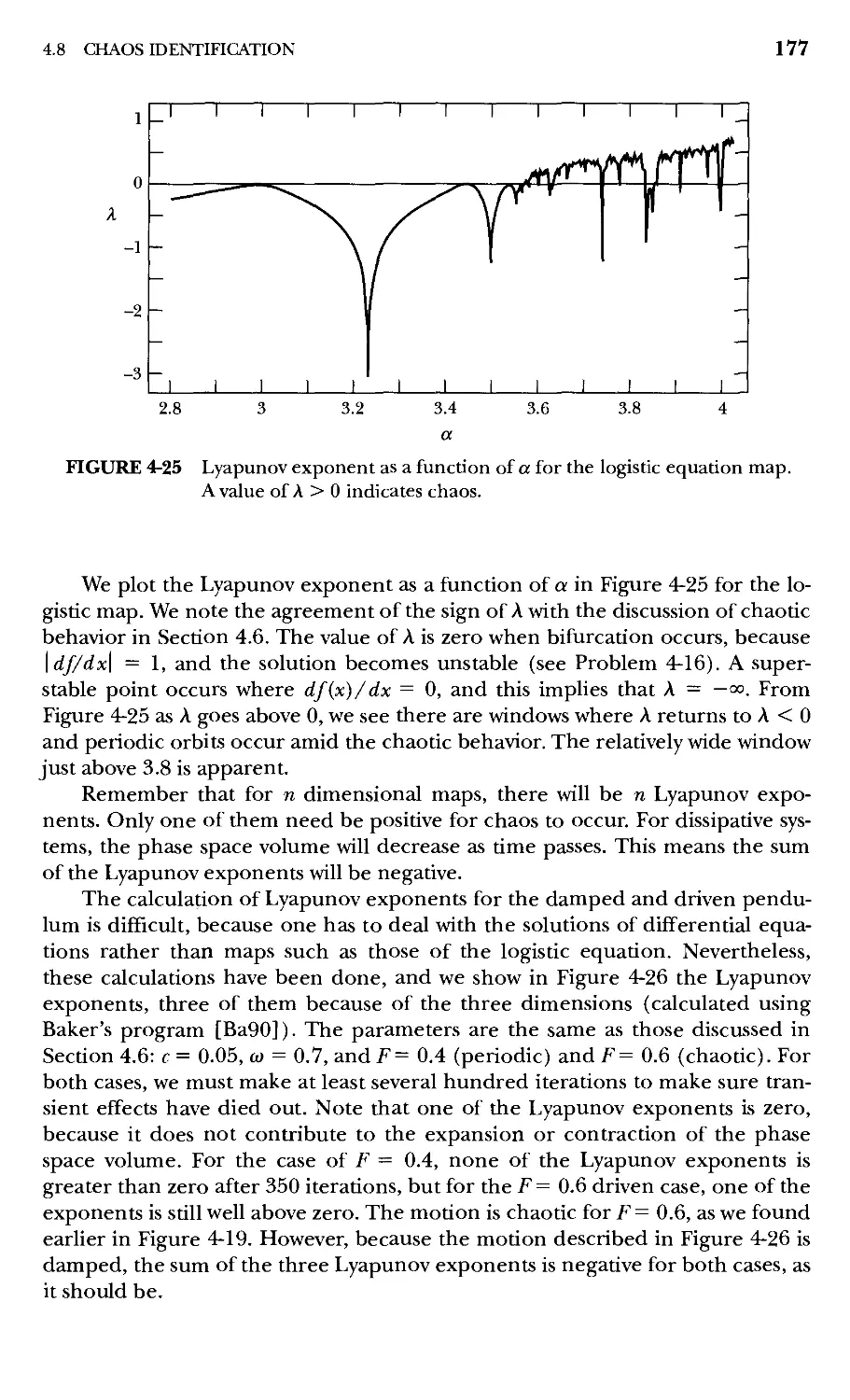
4.8 Chaos Identification 174
Problems 178
Gravitation 182
5.1 Introduction 182
5.2 Gravitational Potential 184
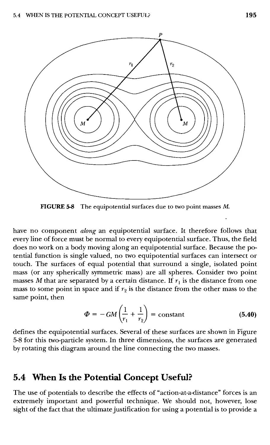
5.3 Lines of Force and Equipotential Surfaces 194
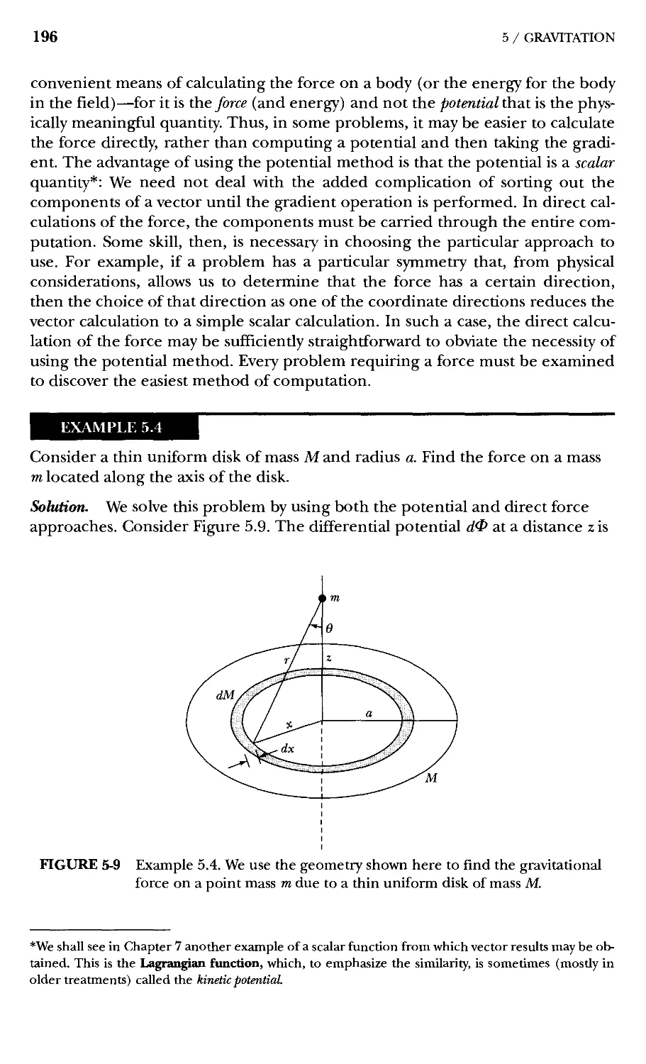
5.4 When Is the Potential Concept Useful? 195
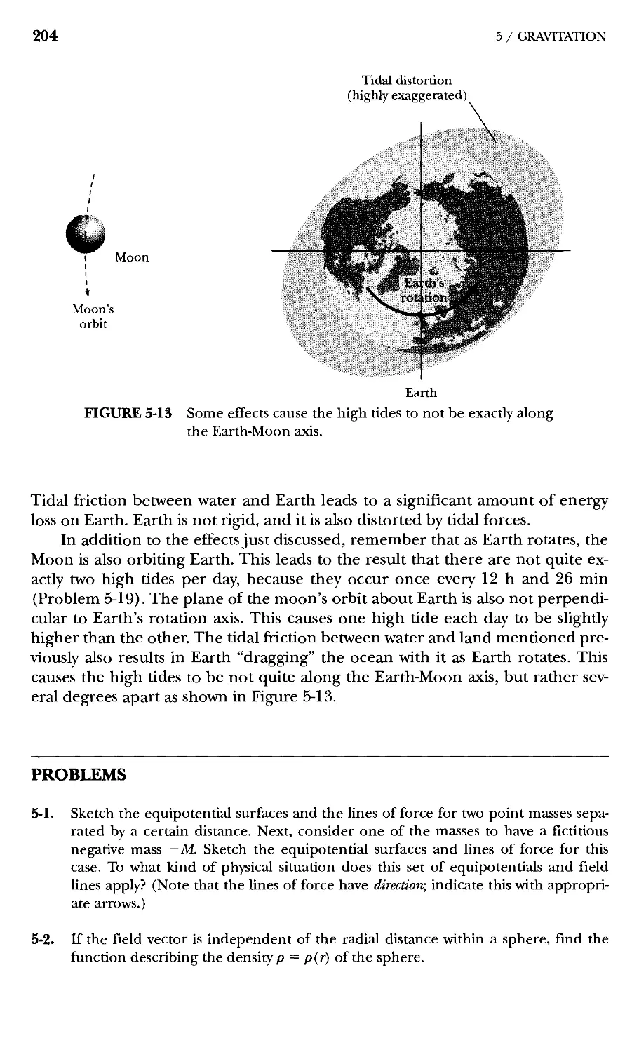
5.5 Ocean Tides 198
Problems 204
Some Methods in the Calculus of Variations 207
6.1 Introduction 207
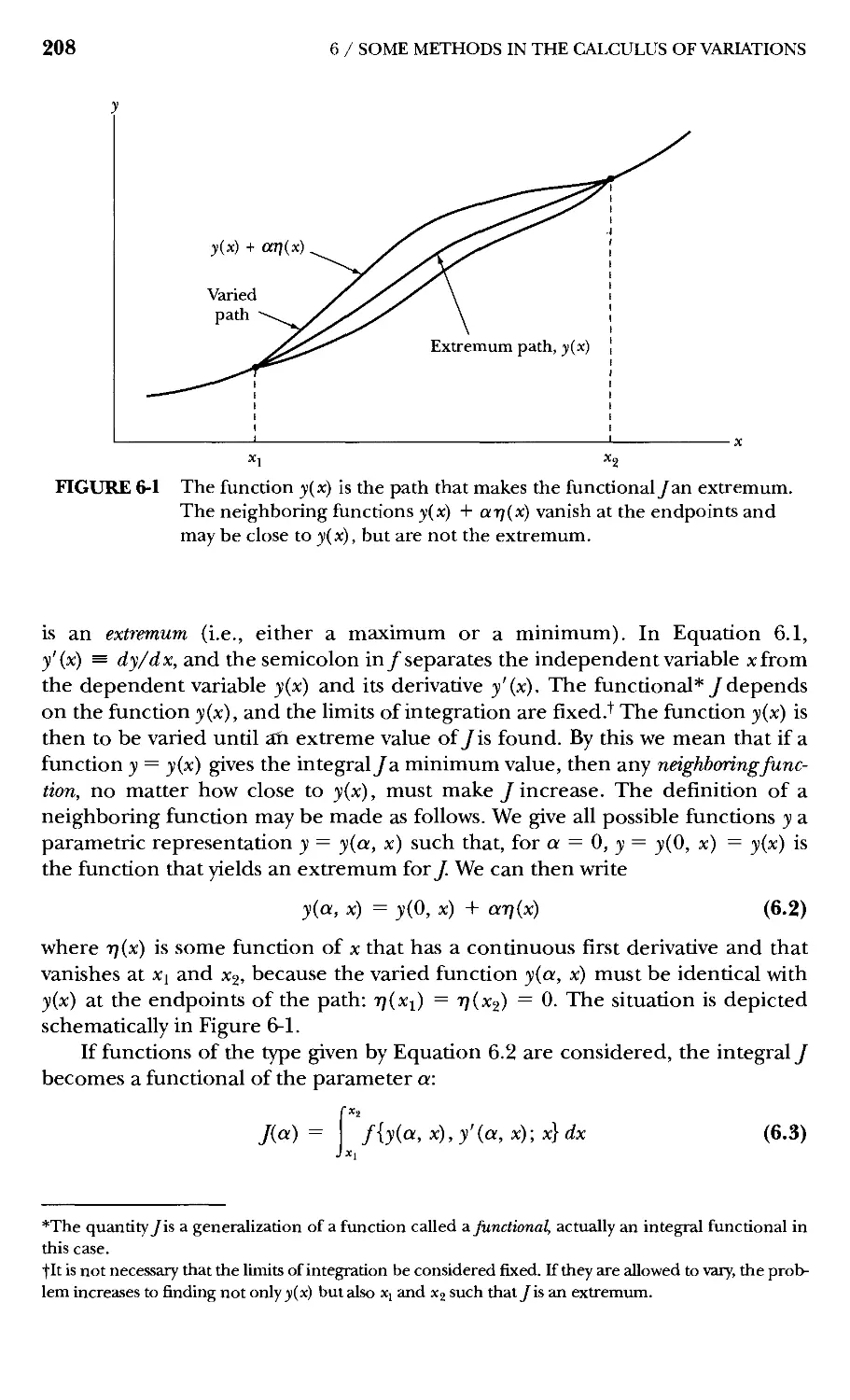
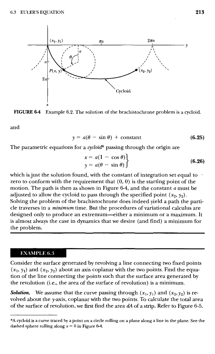
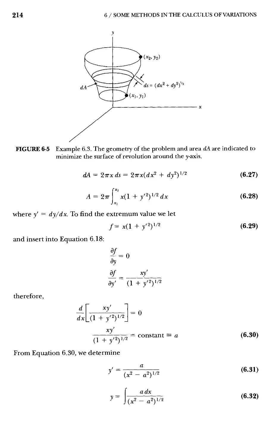
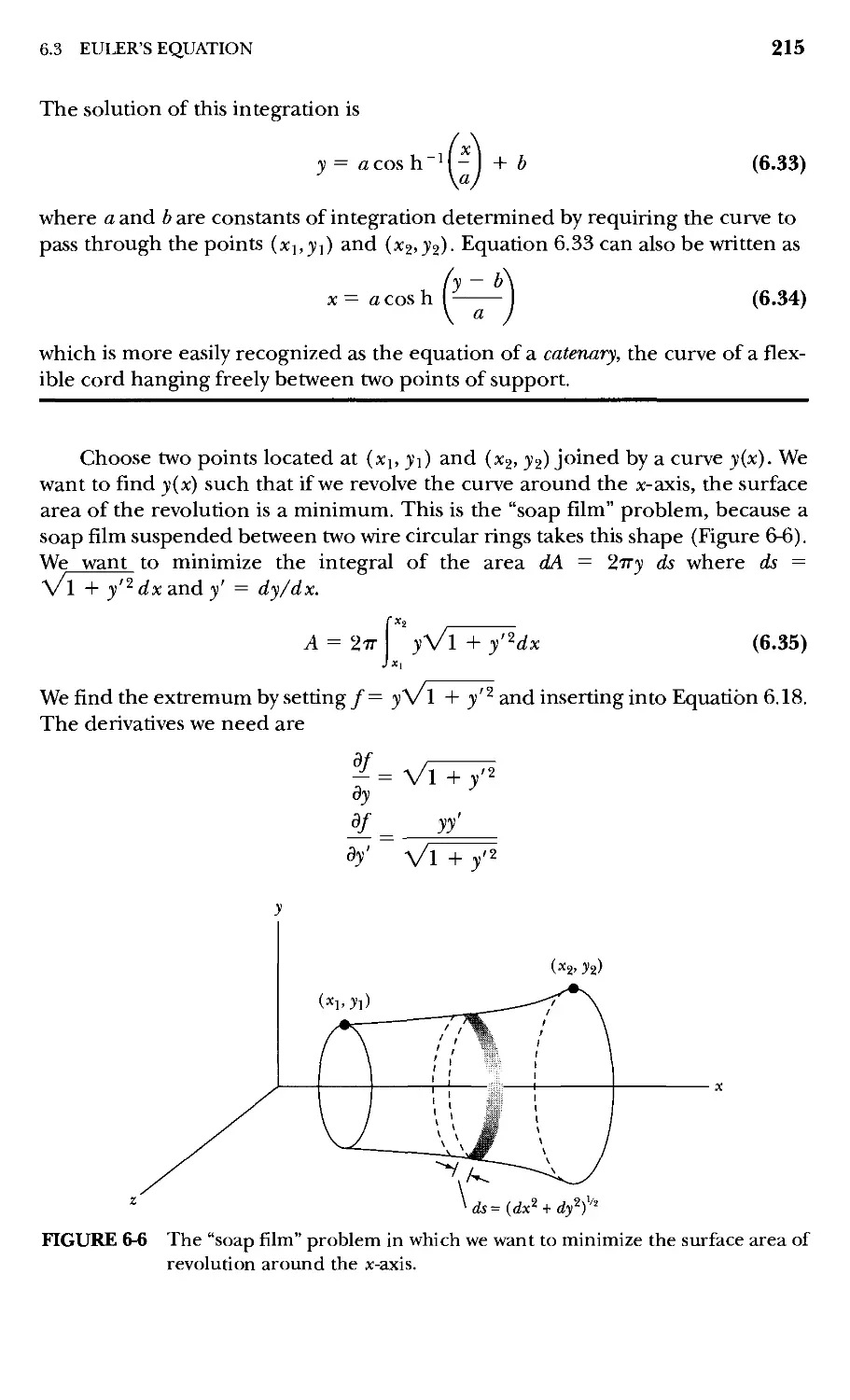
6.2 Statement of the Problem 207
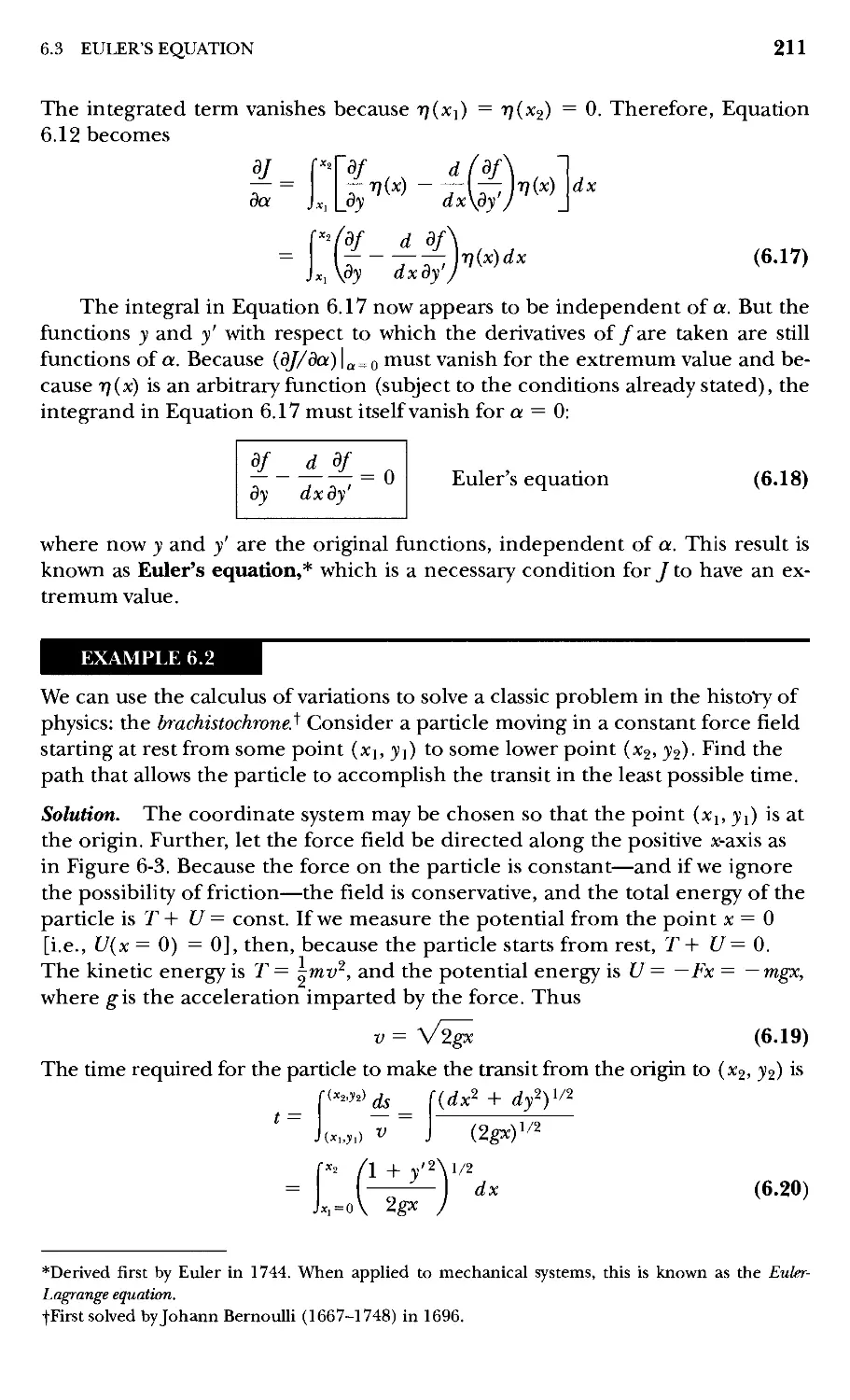
6.3 Euler's Equation 210
CONTENTS Xiii
6.4 The "Second Form" of the Euler Equation 216
6.5 Functions with Several Dependent Variables 218
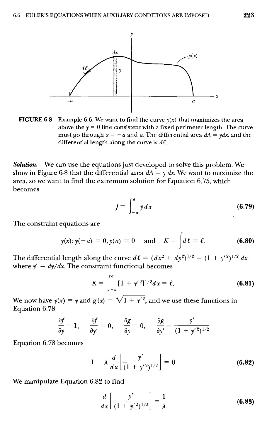
6.6 Euler Equations When Auxiliary Conditions Are Imposed 219
6.7 The 8 Notation 224
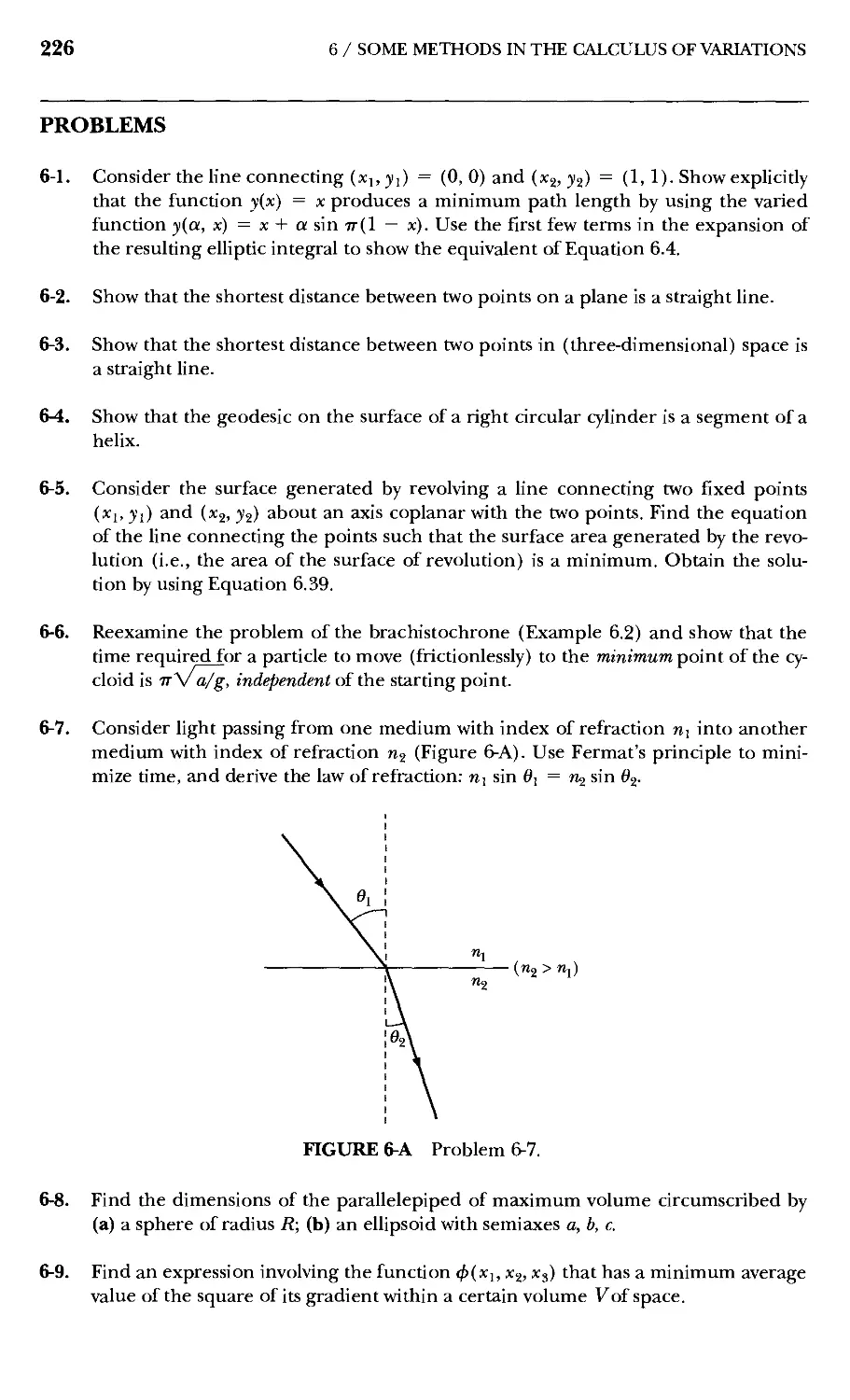
Problems 226
7 Hamilton's Principle—^Lagrangian and
Hamiltonian Dynamics 228
7.1 Introduction 228
7.2 Hamilton's Principle 229
7.3 Generalized Coordinates 233
7.4 Lagrange's Equations of Motion in
Generalized Coordinates 237
7.5 Lagrange's Equations with Undetermined Multipliers 248
7.6 Equivalence of Lagrange's and Newton's Equations 254
7.7 Essence of Lagrangian Dynamics 257
7.8 A Theorem Concerning the Kinetic Energy 258
7.9 Conservation Theorems Revisited 260
7.10 Canonical Equations of Motion—Hamiltonian Dynamics 265
7.11 Some Comments Regarding Dynamical Variables and
Variational Calculations in Physics 272
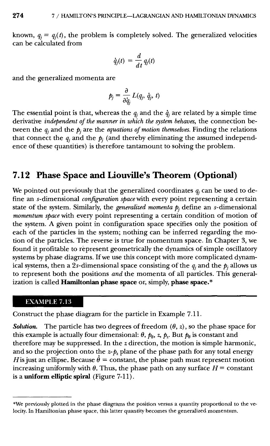
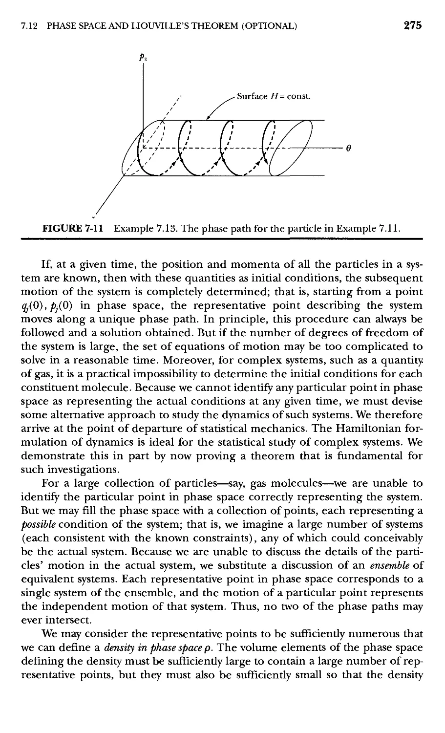
7.12 Phase Space and Liouville's Theorem (Optional) 274
7.13 Virial Theorem (Optional) 277
Problems 280
8 Central-Force Motion 287
8.1 Introduction 287
8.2 Reduced Mass 287
8.3 Conservation Theorems—First Integrals of the Motion 289
8.4 Equations of Motion 291
8.5 Orbits in a Central Field 295
8.6 Centrifugal Energy and the Effective Potential 296
8.7 Planetary Motion—Kepler's Problem 300
8.8 Orbital Dynamics 305
8.9 Apsidal Angles and Precession (Optional) 312
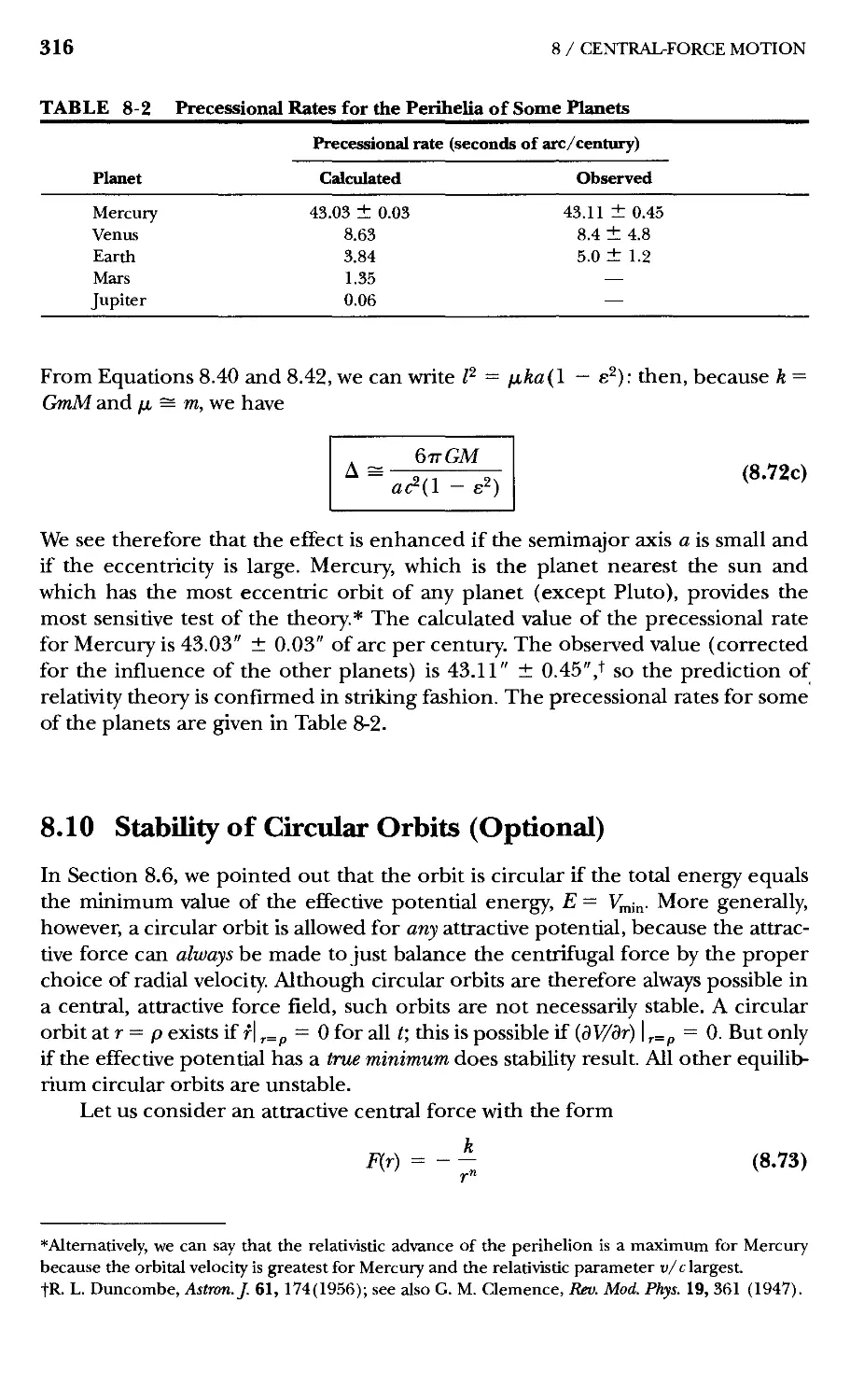
8.10 Stability of Circular Orbits (Optional) 316
Problems 323
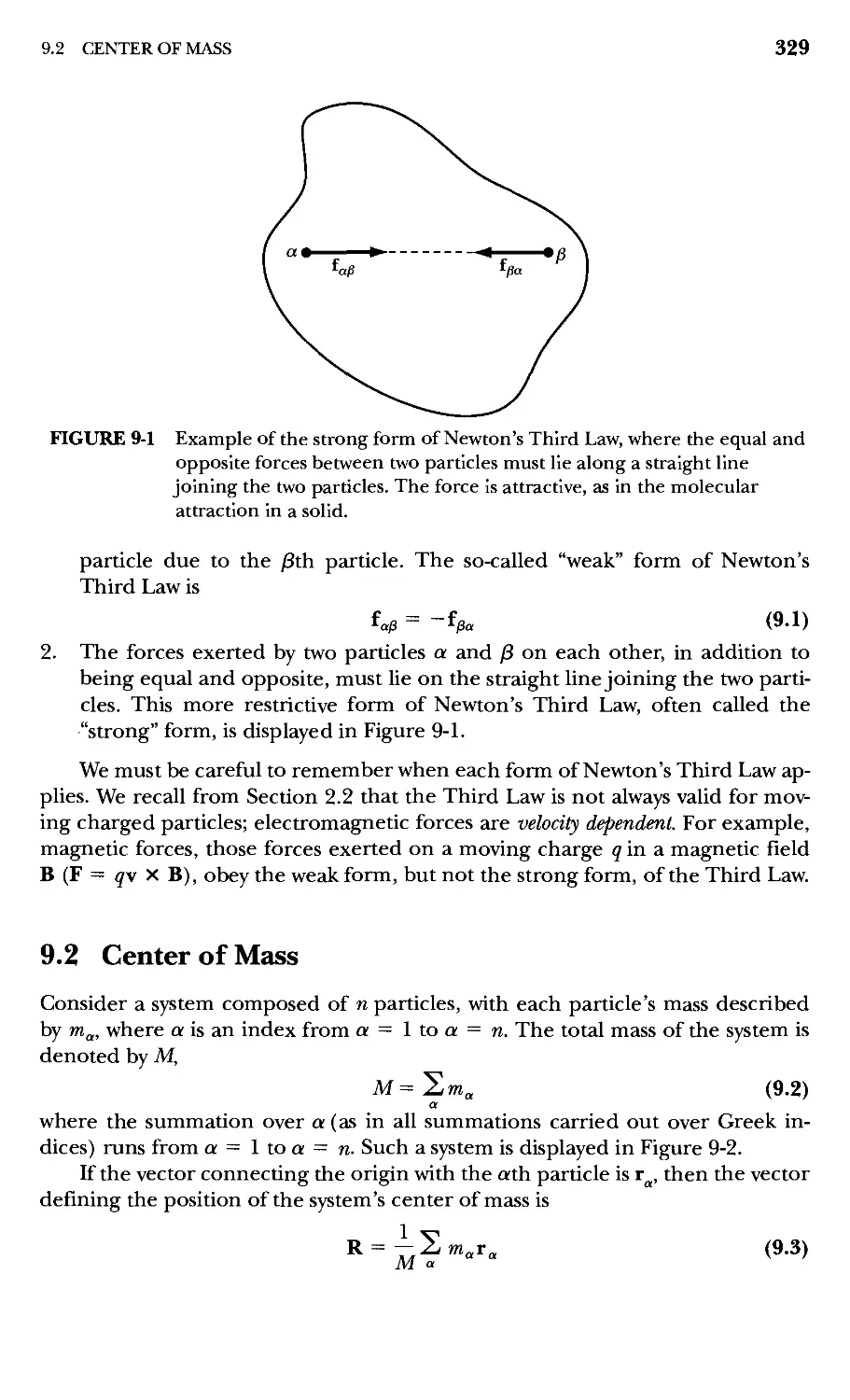
z) Dynamics of a System of Particles 328
9.1 Introduction 328
9.2 Center of Mass 329
9.3 Linear Momentum of the System 331
XiV CONTENTS
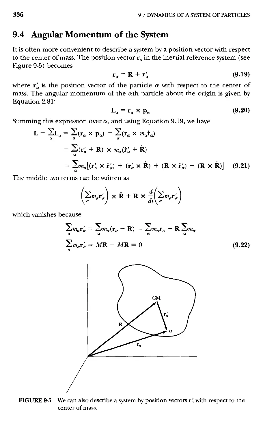
9.4 Angular Momentum of the System 336
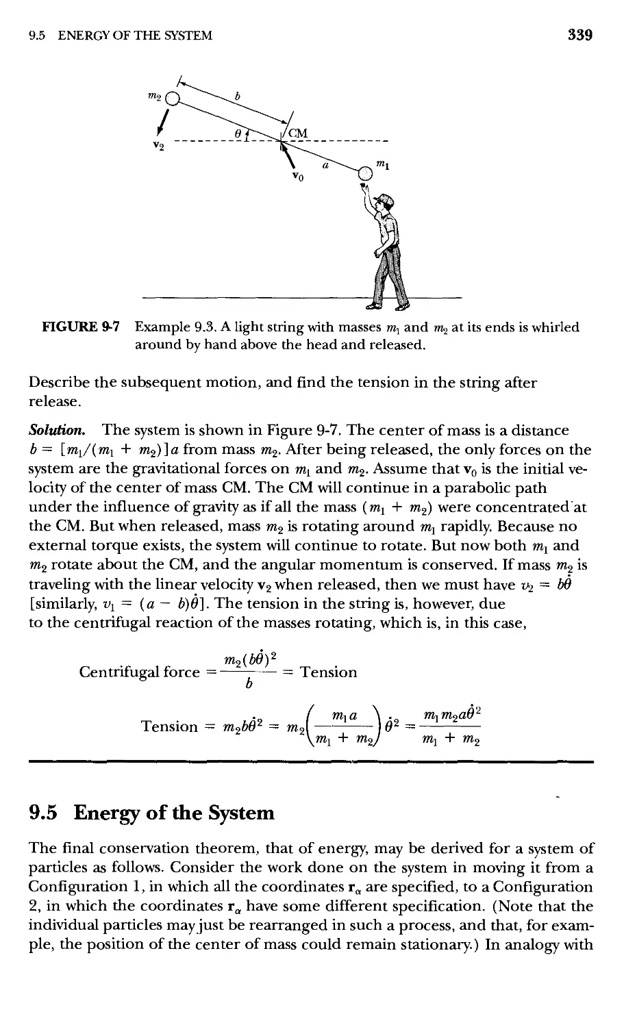
9.5 Energy of the System 339
9.6 Elastic Collisions of Two Particles 345
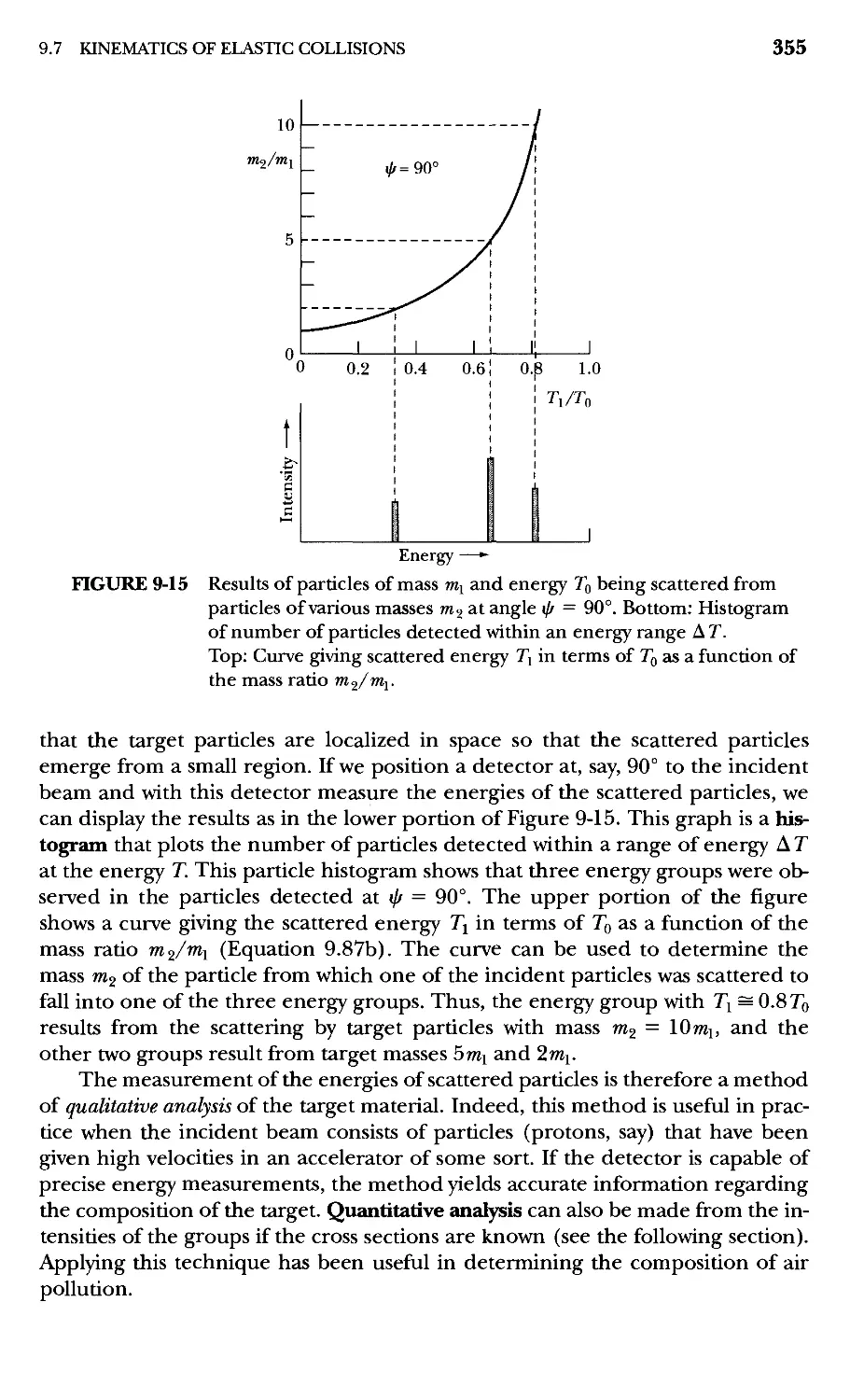
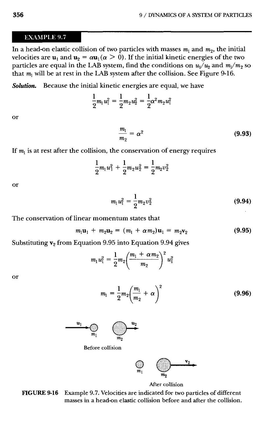
9.7 Kinematics of Elastic Collisions 352
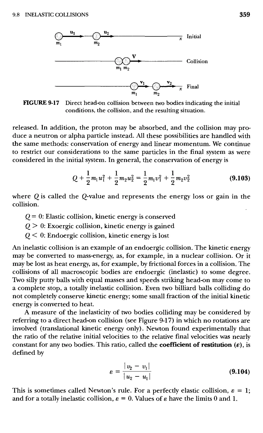
9.8 Inelastic Collisions 358
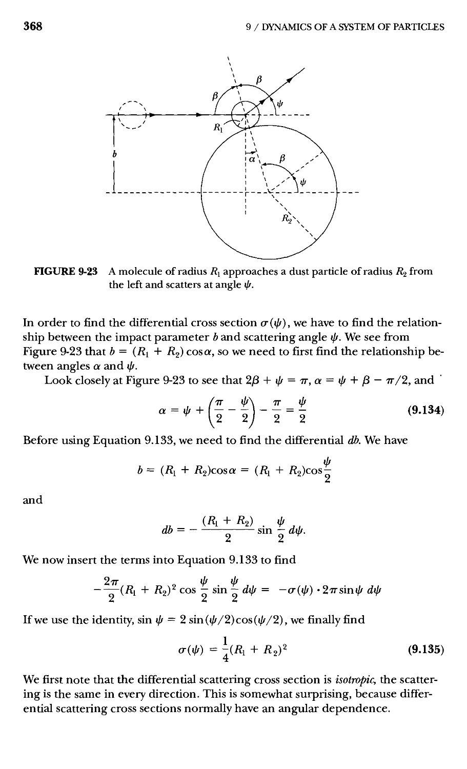
9.9 Scattering Cross Sections 363
9.10 Rutherford Scattering Formula 369
9.11 Rocket Motion 371
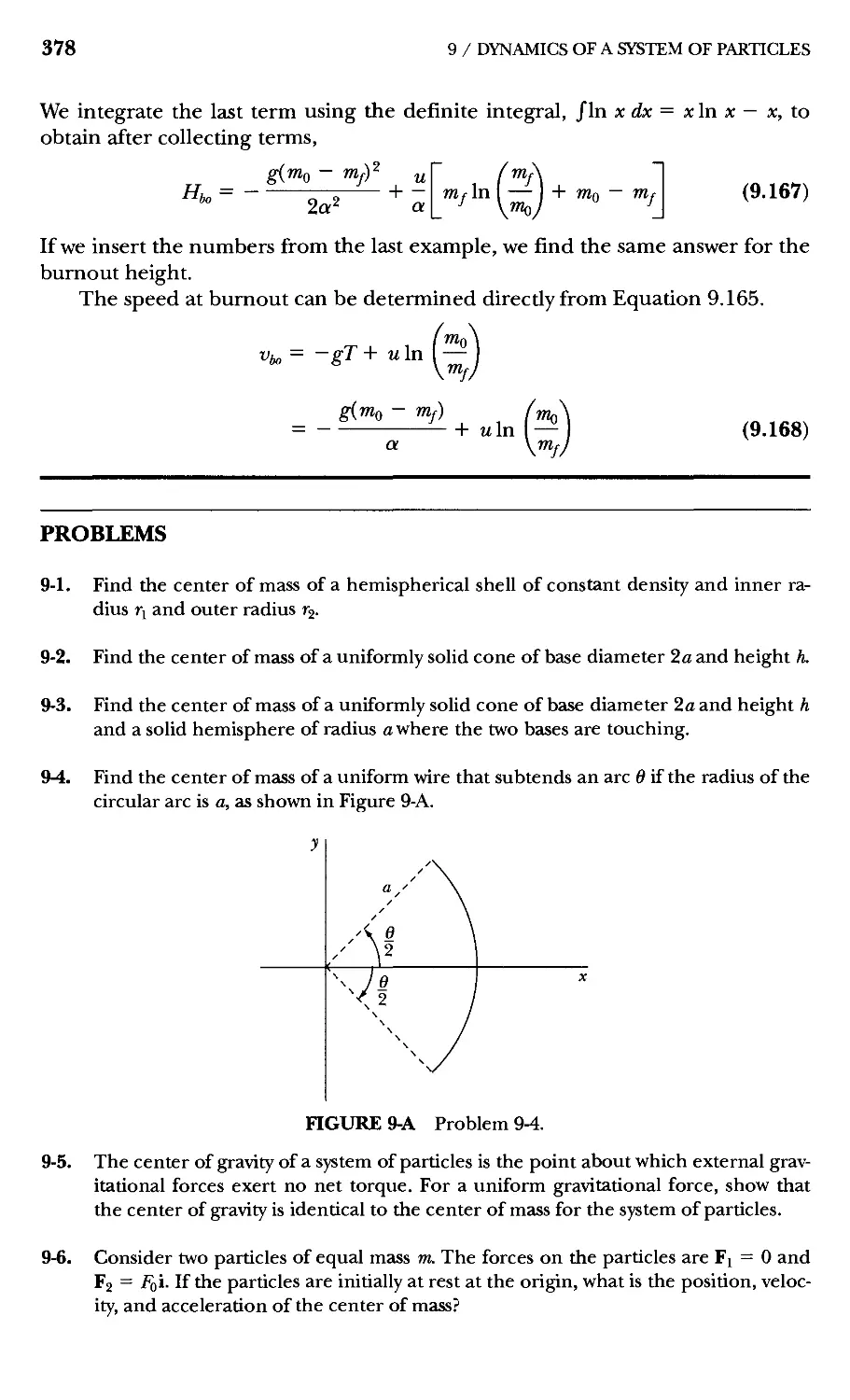
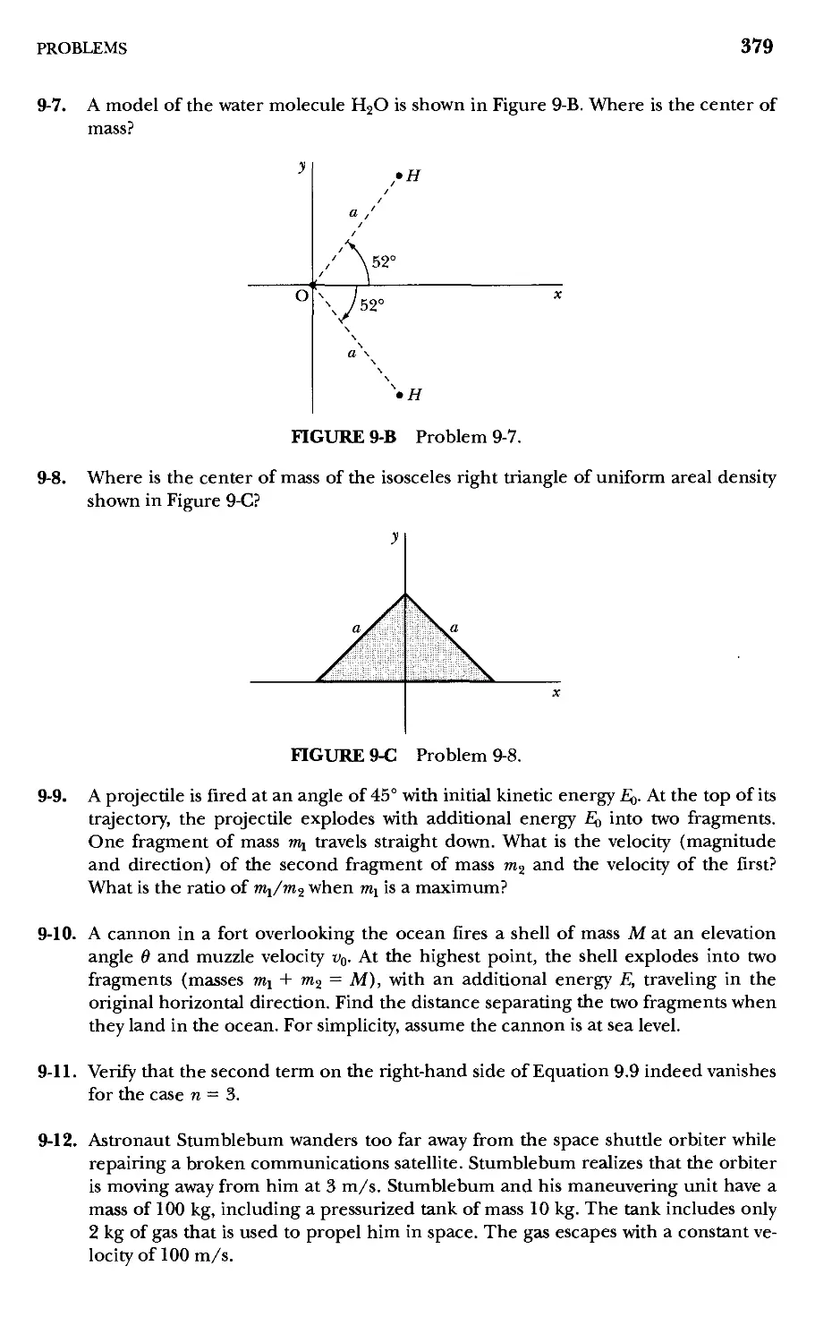
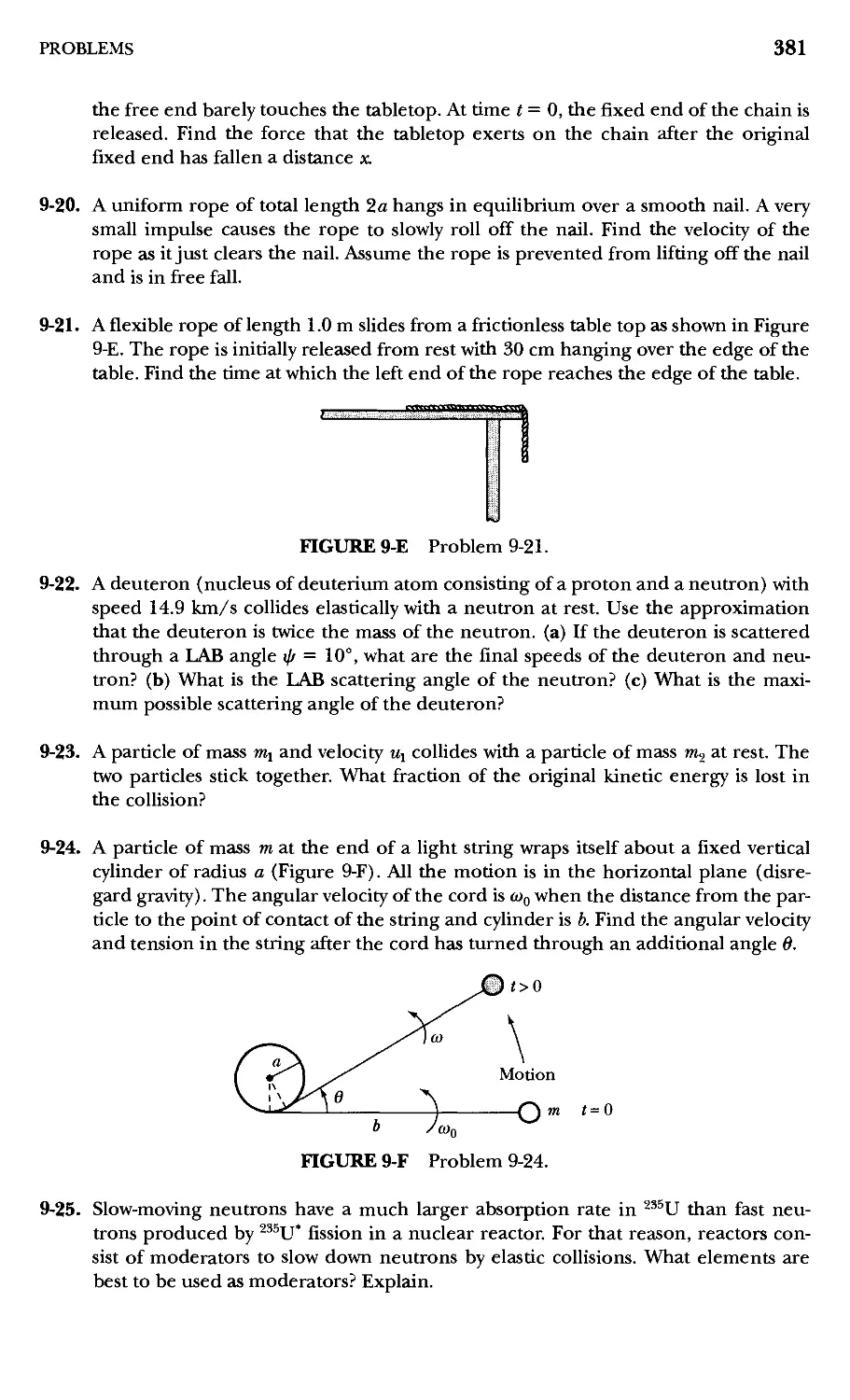
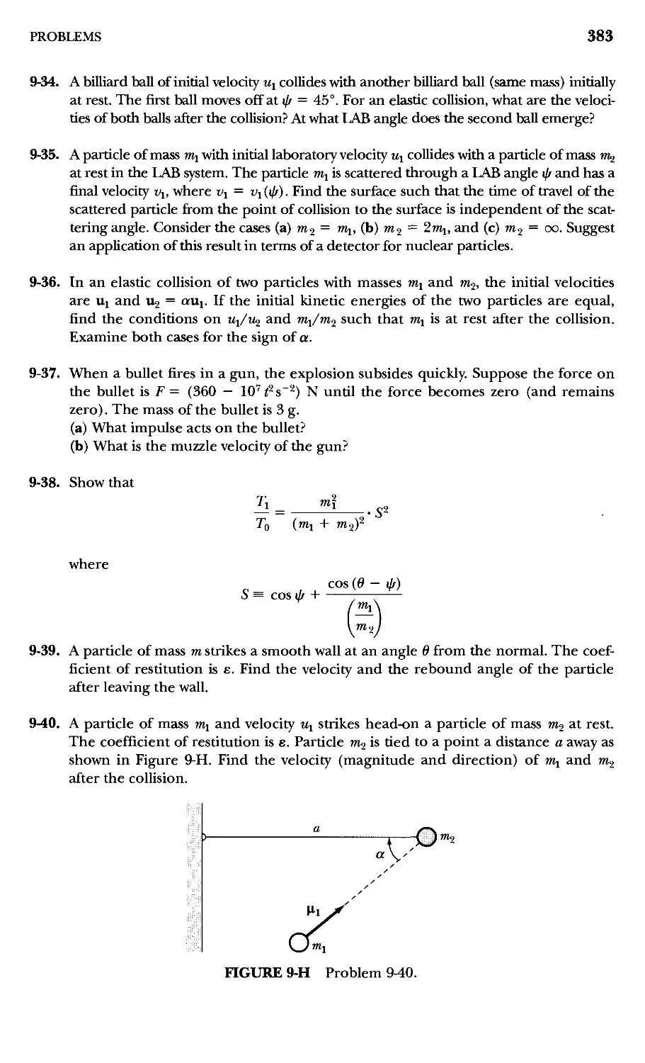
Problems 378
10 Motion in a Nonintertial Reference Frame 387
10.1 Introduction 387
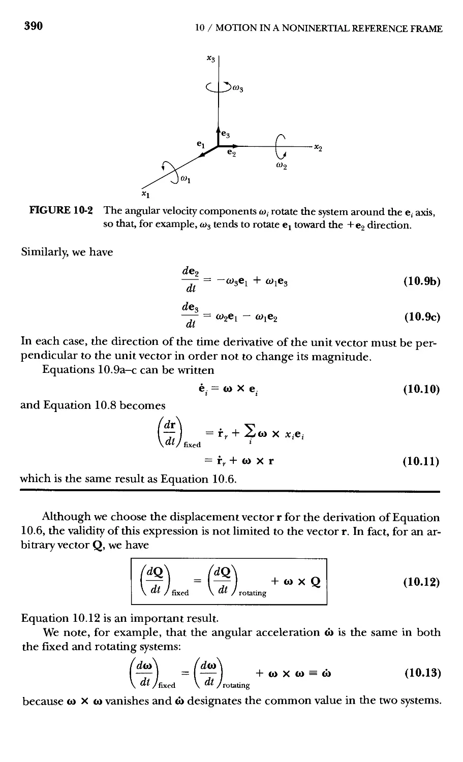
10.2 Rotating Coordinate Systems 388
10.3 Centrifugal and Coriolis Forces 391
10.4 Motion Relative to the Earth 395
Problems 408
11 Dynamics of Rigid Bodies 411
11.1 Introduction 411
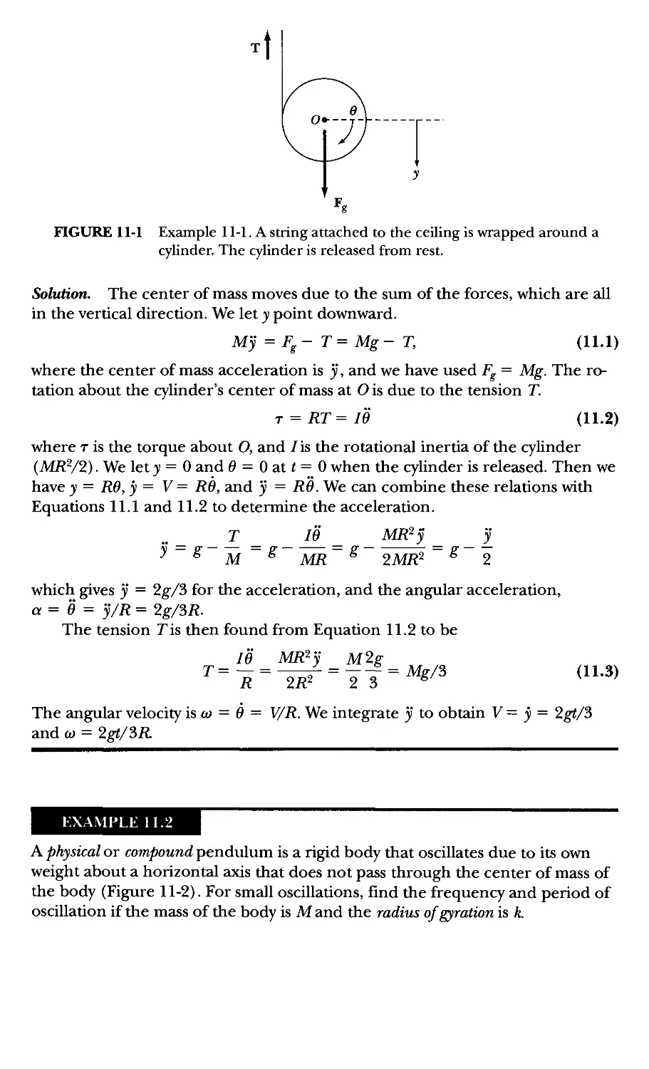
11.2 Simple Planar Motion 412
11.3 Inertia Tensor 415
11.4 Angular Momentum 419
11.5 Principal Axes of Inertia 424
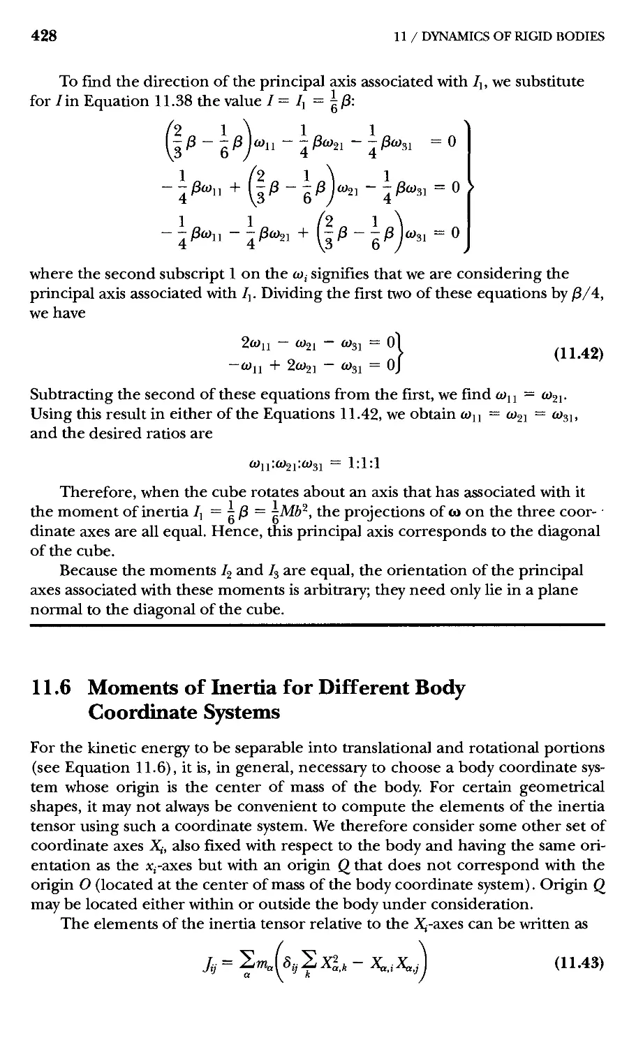
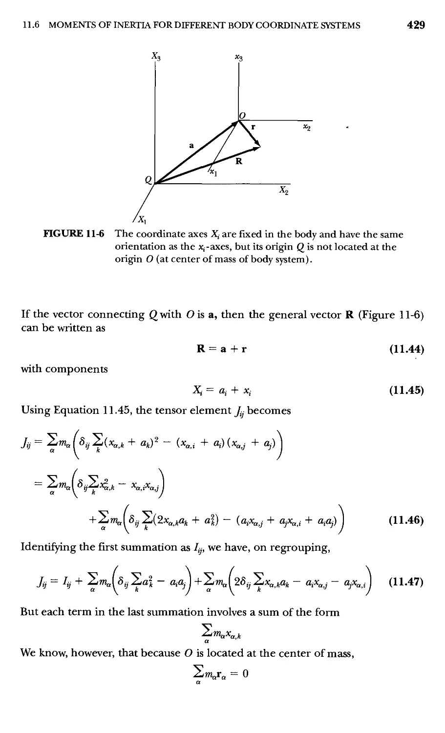
11.6 Moments of Inertia for Different Body Coordinate Systems 428
11.7 Further Properties of the Inertia Tensor 433
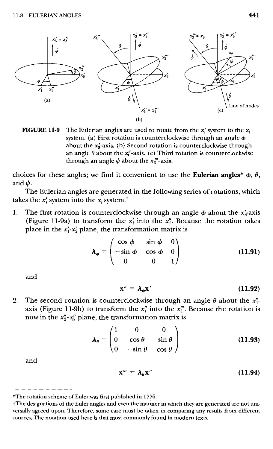
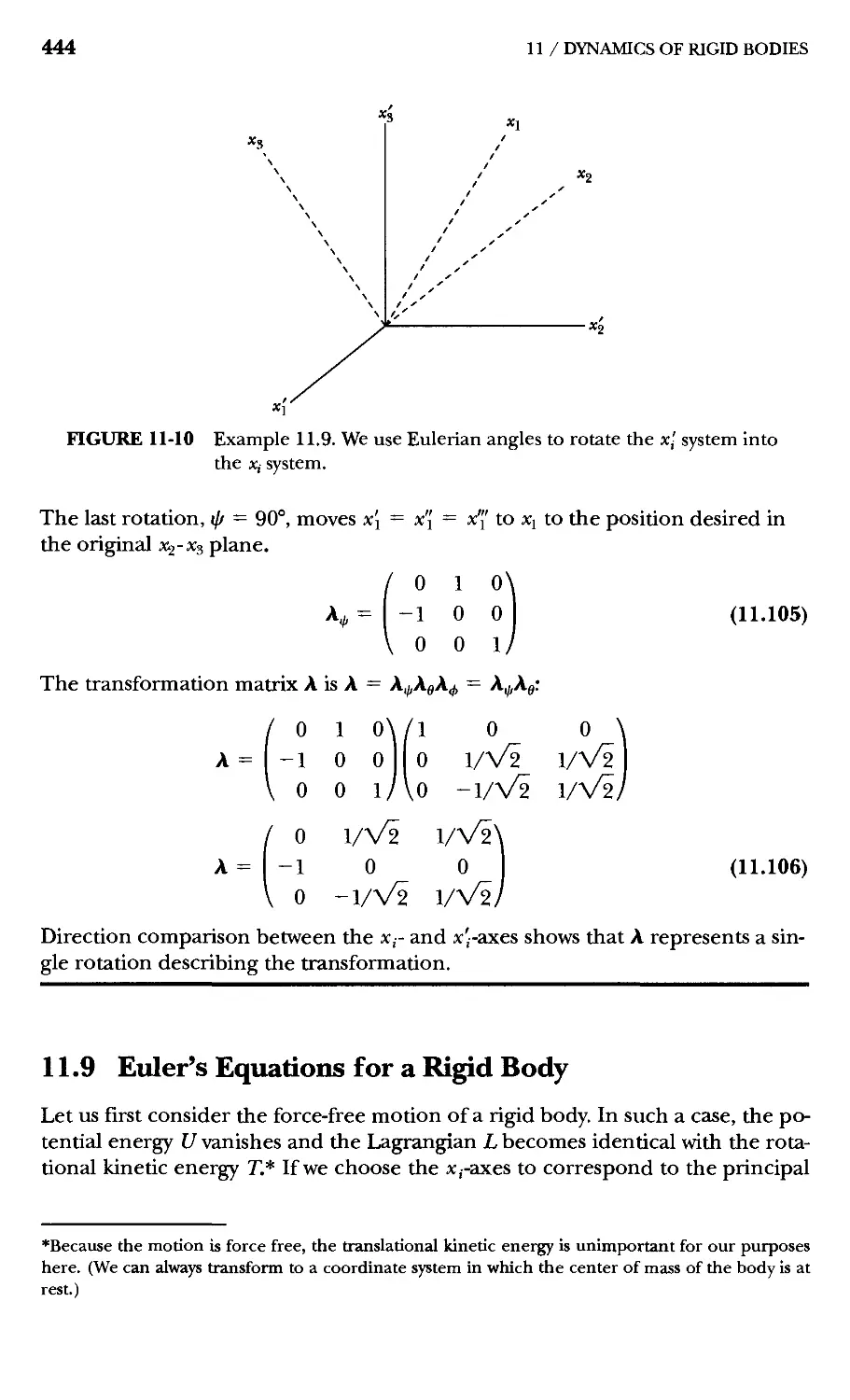
11.8 Eulerian Angles 440
11.9 Euler's Equations for a Rigid Body 444
11.10 Force-Free Motion of a Symmetric Top 448
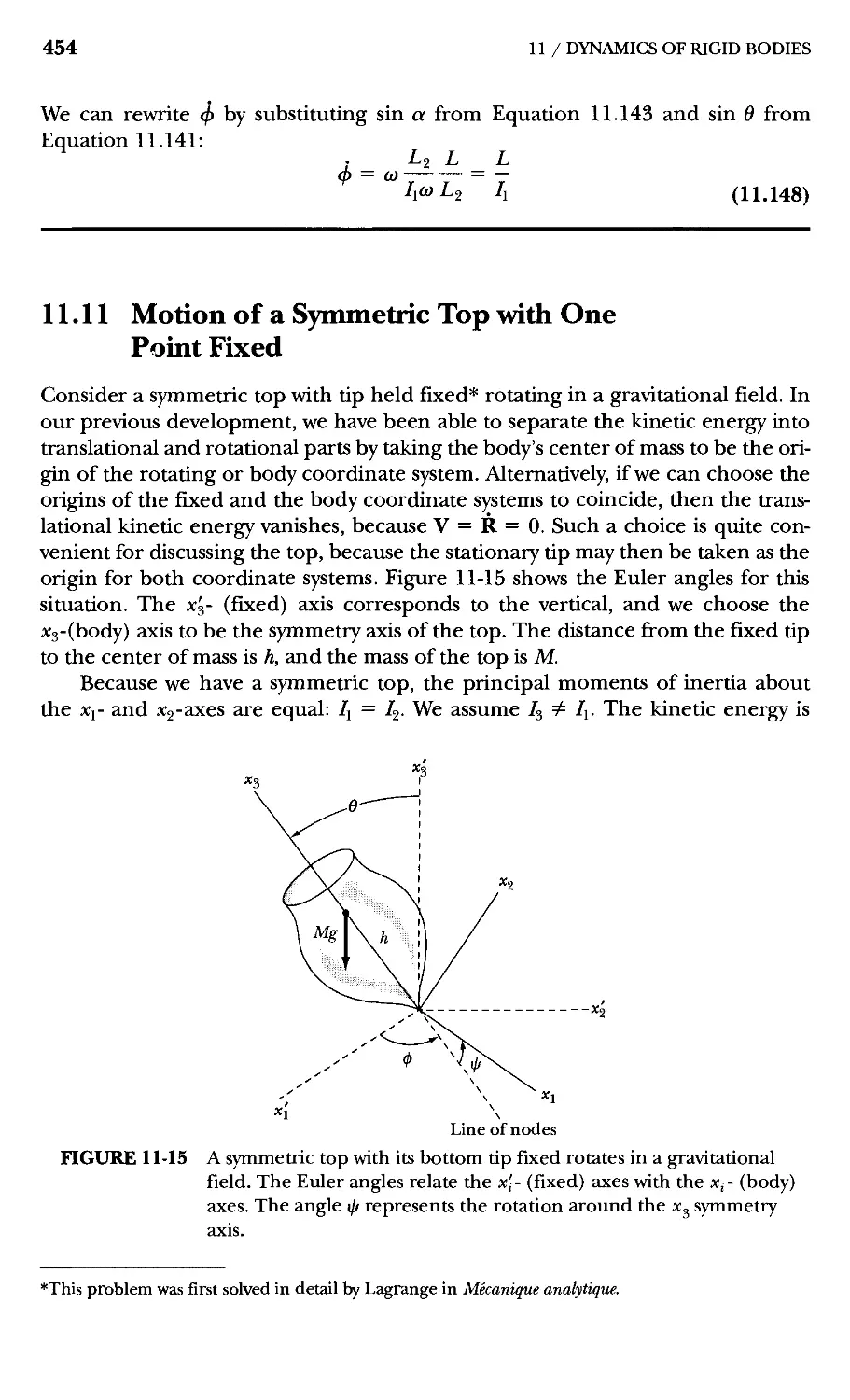
11.11 Motion of a Symmetric Top with One Point Fixed 454
11.12 Stability of Rigid-Body Rotations 460
Problems 463
12 Coupled Oscillations 468
12.1 Introduction 468
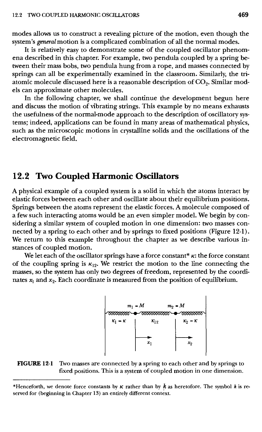
12.2 Two Coupled Harmonic Oscillators 469
12.3 Weak Coupling 473
12.4 General Problem of Coupled Oscillations 475
12.5 Orthogonality of the Eigenvectors (Optional) 481
12.6 Normal Coordinates 483
12.7 Molecular Vibrations 490
12.8 Three Linearly Coupled Plane Pendula—an Example of
Degeneracy 495
CONTENTS XV
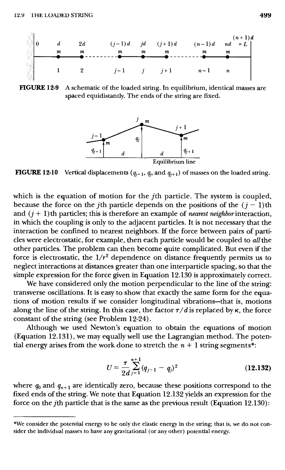
12.9 The Loaded String 498
Problems 507
13 Continuous Systems; Waves 512
13.1 Introduction 512
13.2 Continuous String as a Limiting Case of the
Loaded String 513
13.3 Energy of a Vibrating String 516
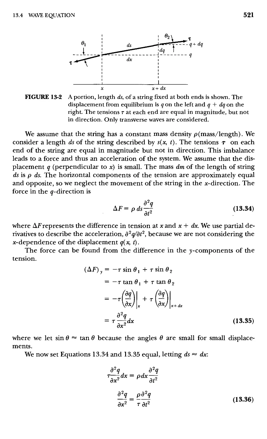
13.4 Wave Equation 520
13.5 Forced and Damped Motion 522
13.6 General Solutions of the Wave Equation 524
13.7 Separation of the Wave Equation 527
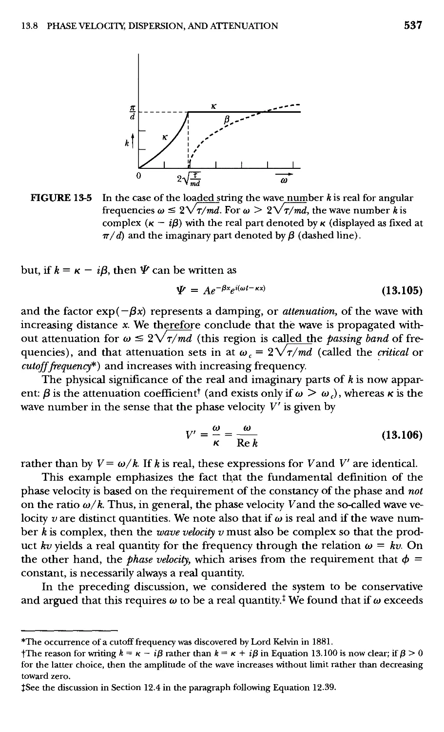
13.8 Phase Velocity, Dispersion, and Attenuation 533
13.9 Group Velocity and Wave Packets 538
Problems 542
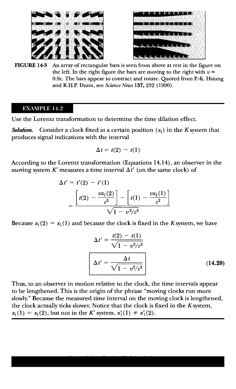
14 Special Theory of Relativity 546
14.1 Introduction 546
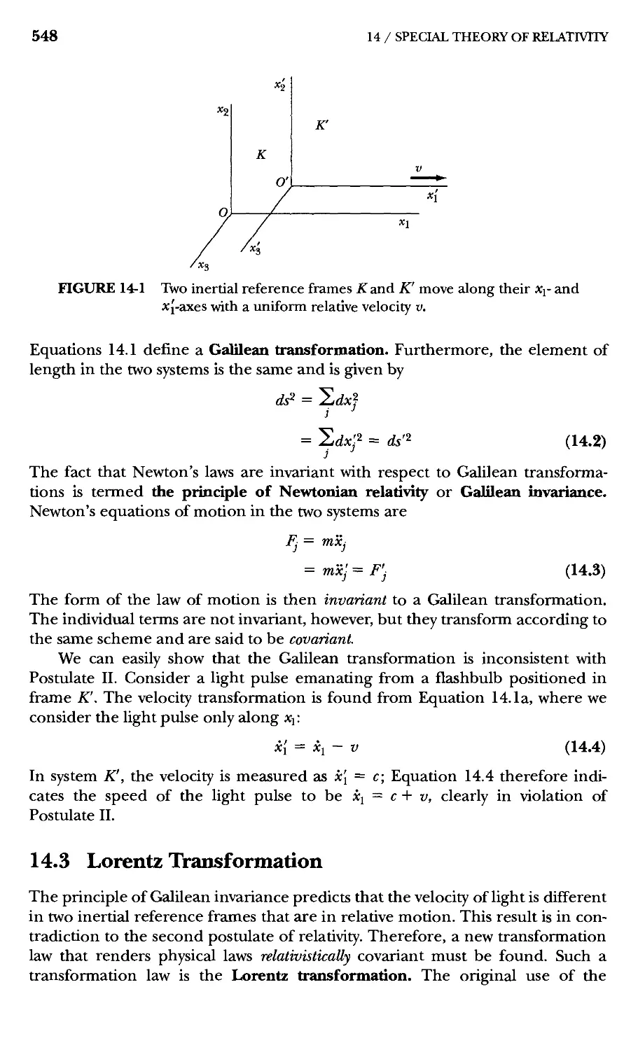
14.2 Galilean Invariance 547
14.3 Lorentz Transformation 548
14.4 Experimental Verification of the Special Theory 555
14.5 Relativistic Doppler Effect 558
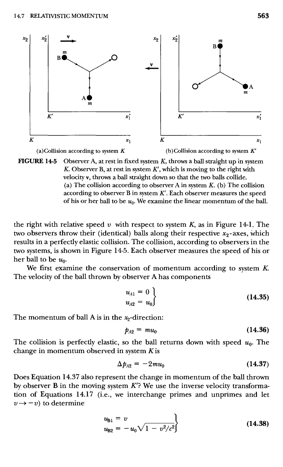
14.6 Twin Paradox 561
14.7 Relativistic Momentum 562
14.8 Energy 566
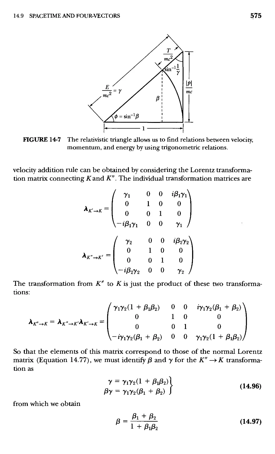
14.9 Spacetime and Four-Vectors 569
14.10 Lagrangian Function in Special Relativity 578
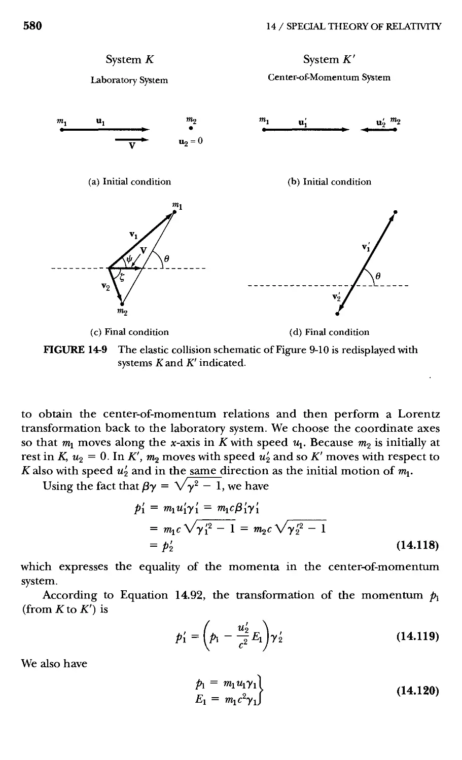
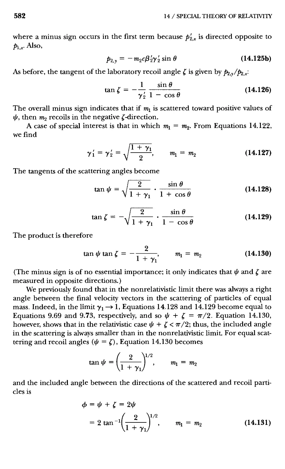
14.11 Relativistic Kinematics 579
Problems 583
Appendices
A Taylor's Theorem 589
Problems 593
B Elliptic Integrals 594
B.l Elliptic Integrals of the First Kind 594
B.2 Elliptic Integrals of the Second Kind 595
B.3 Elliptic Integrals of the Third Kind 595
Problems 598
XVI CONTENTS
Ordinary Differential Equations of Second Order 599
C.l Linear Homogeneous Equations 599
C.2 Linear Inhomogeneous Equations 603
Problems 606
D Useful Formulas 608
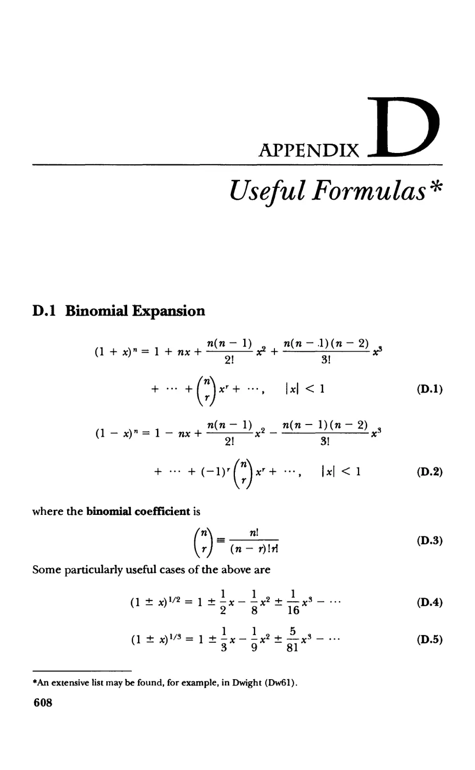
D.l Binomial Expansion 608
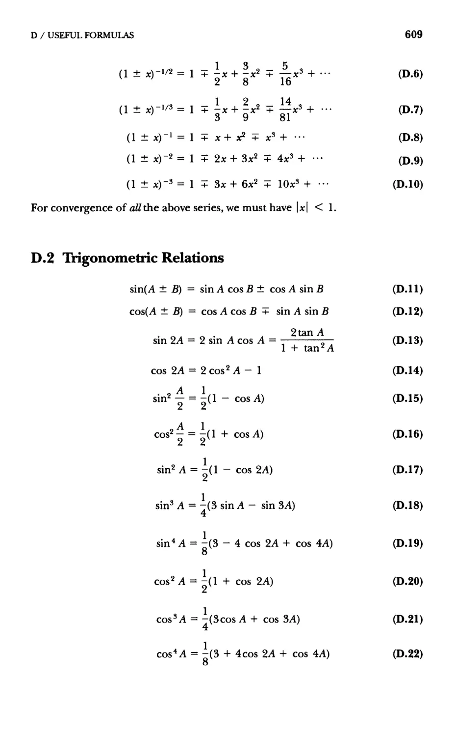
D.2 Trigonometric Relations 609
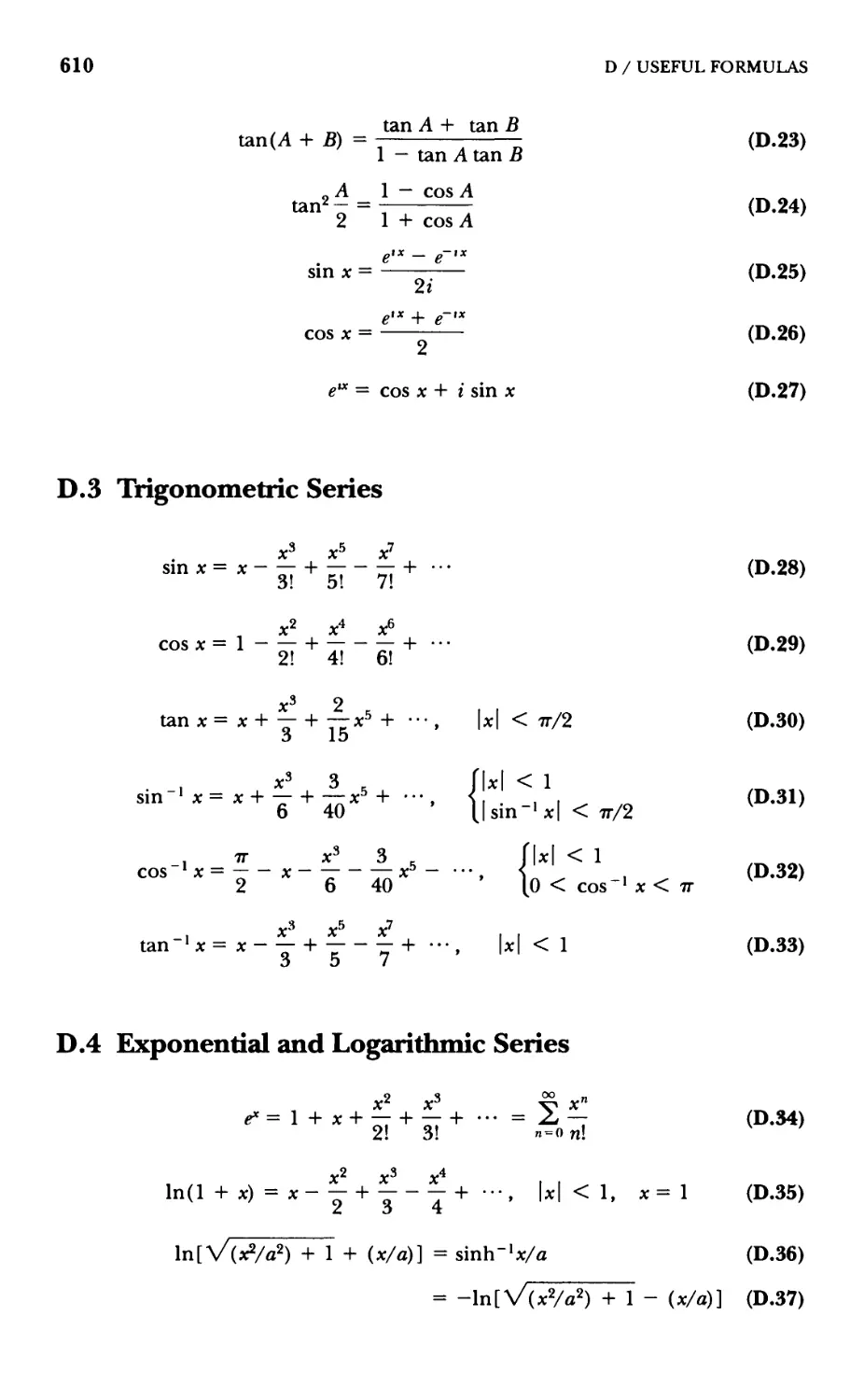
D.3 Trigonometric Series 610
D.4 Exponential and Logarithmic Series 610
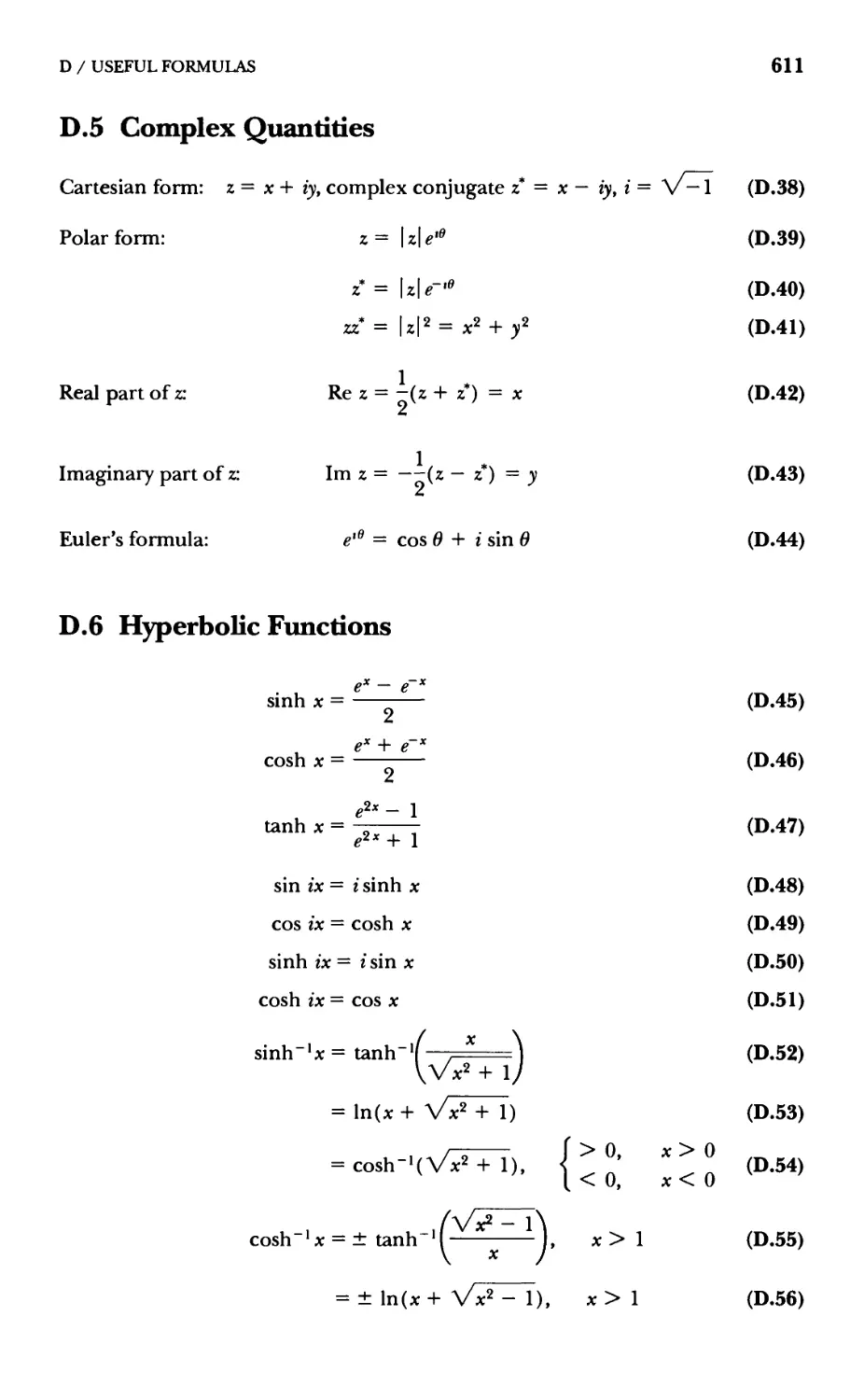
D.5 Complex Quantities 611
D.6 Hyperbolic Functions 611
Problems 612
Useful Integrals 613
E.l Algebraic Functions 613
E.2 Trigonometric Functions 614
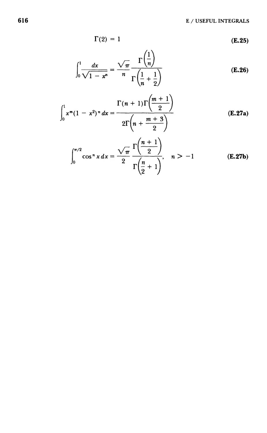
E.3 Gamma Functions 615
r Differential Relations in Different Coordinate Systems 617
F.l Rectangular Coordinates 617
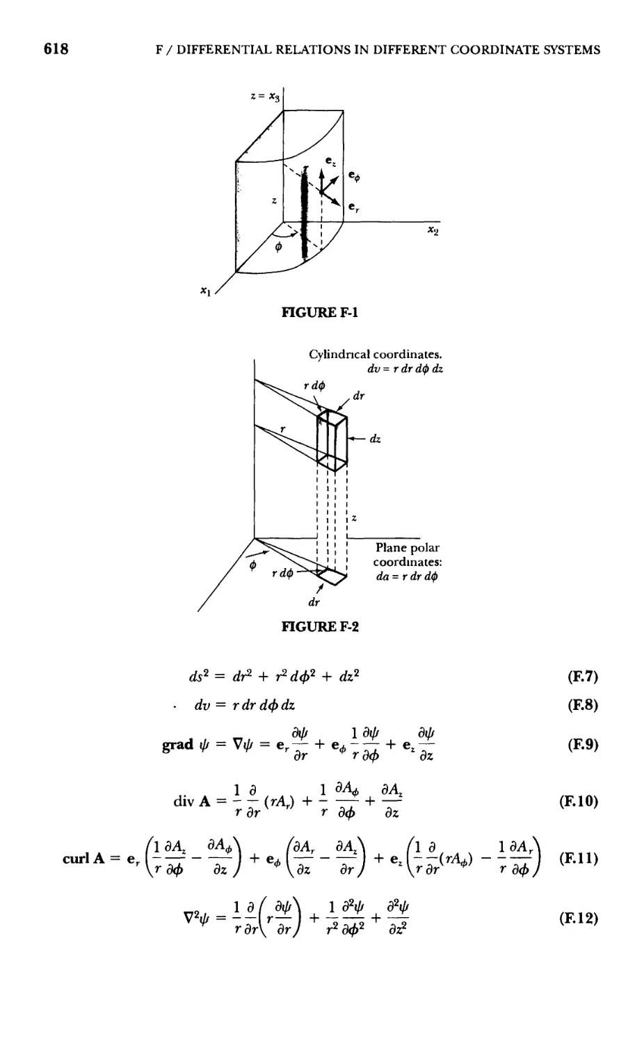
F.2 Cylindrical Coordinates 617
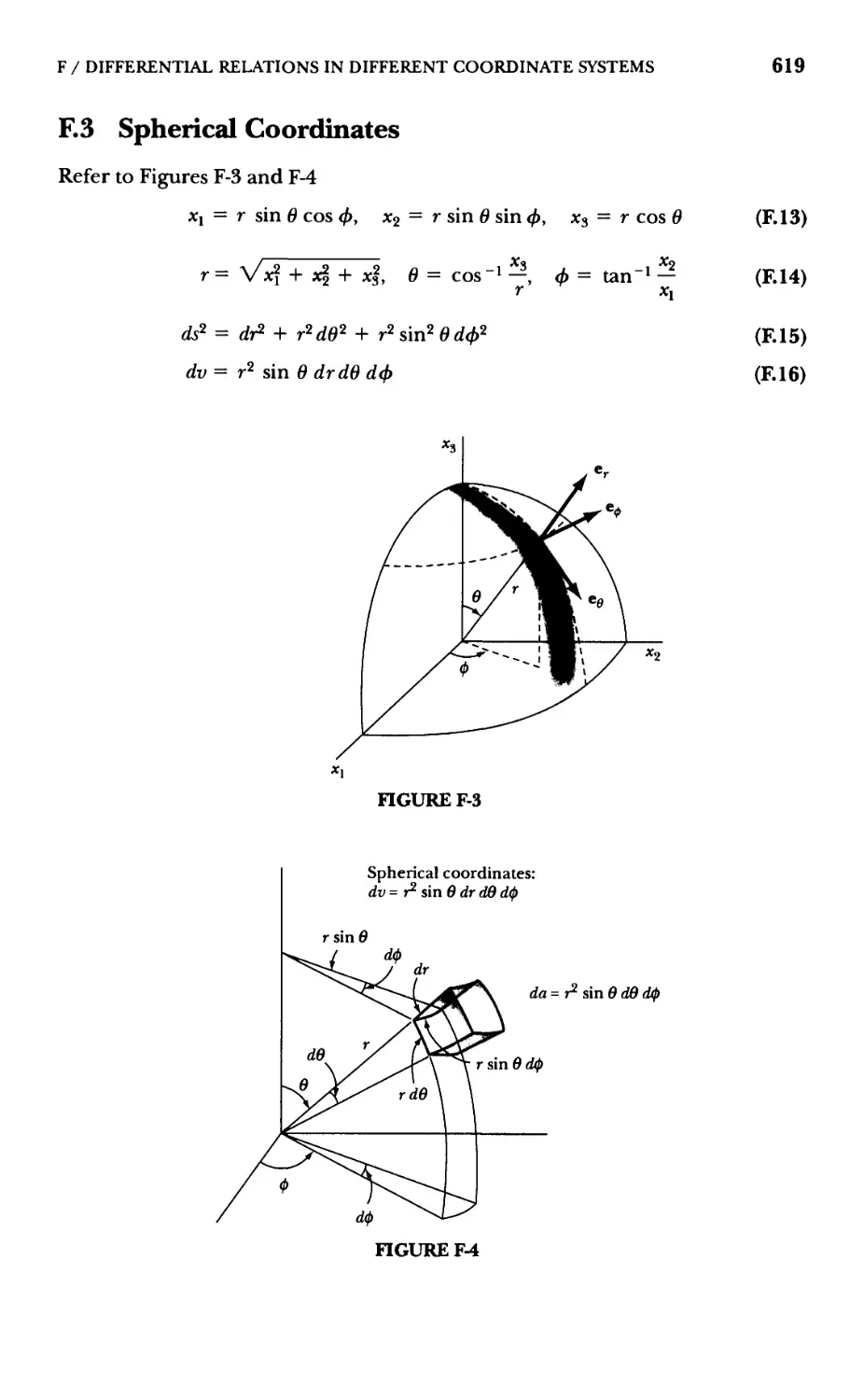
F.3 Spherical Coordinates 619
G A "Proof of the Relation 1x1 = '^<^ 621
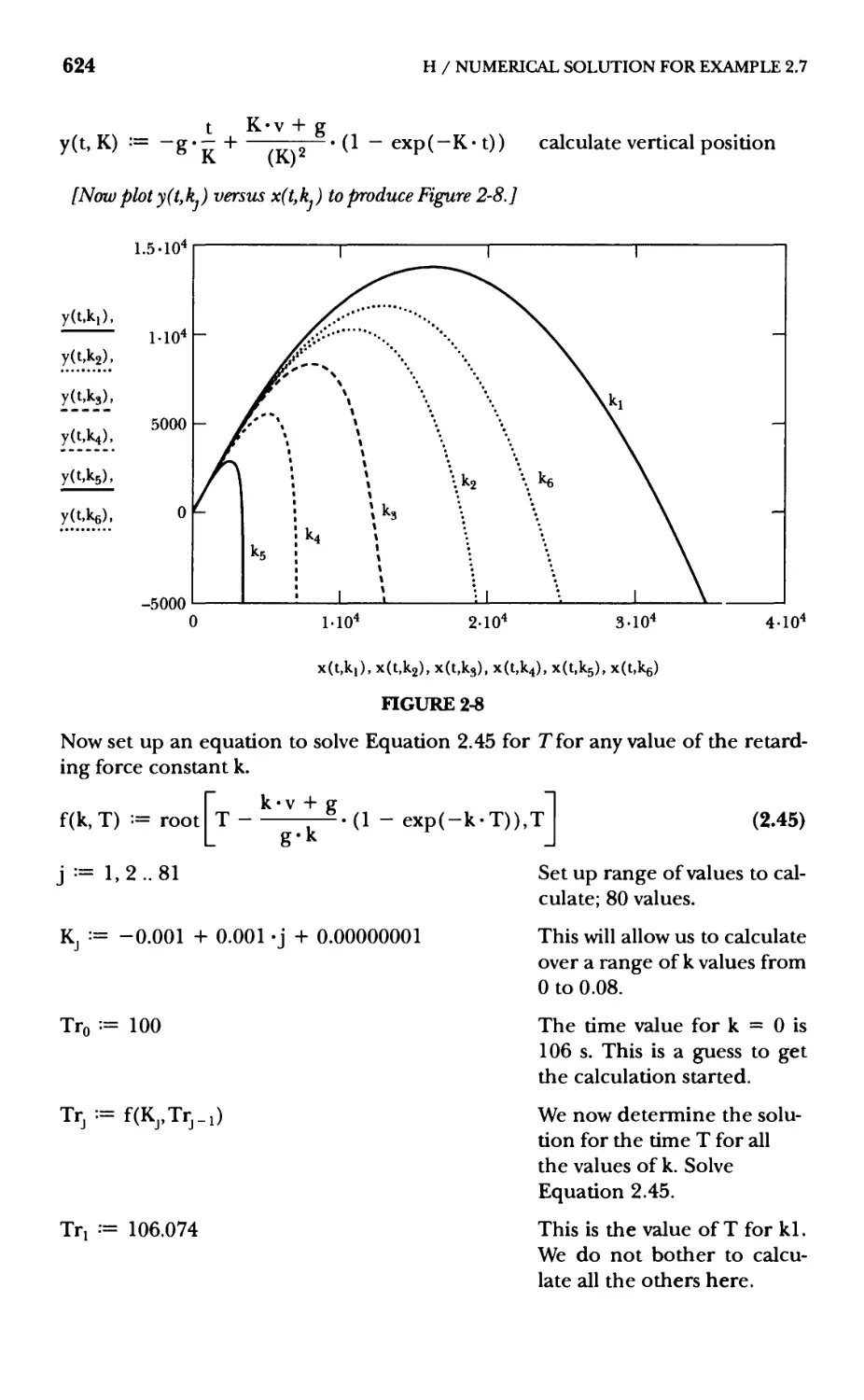
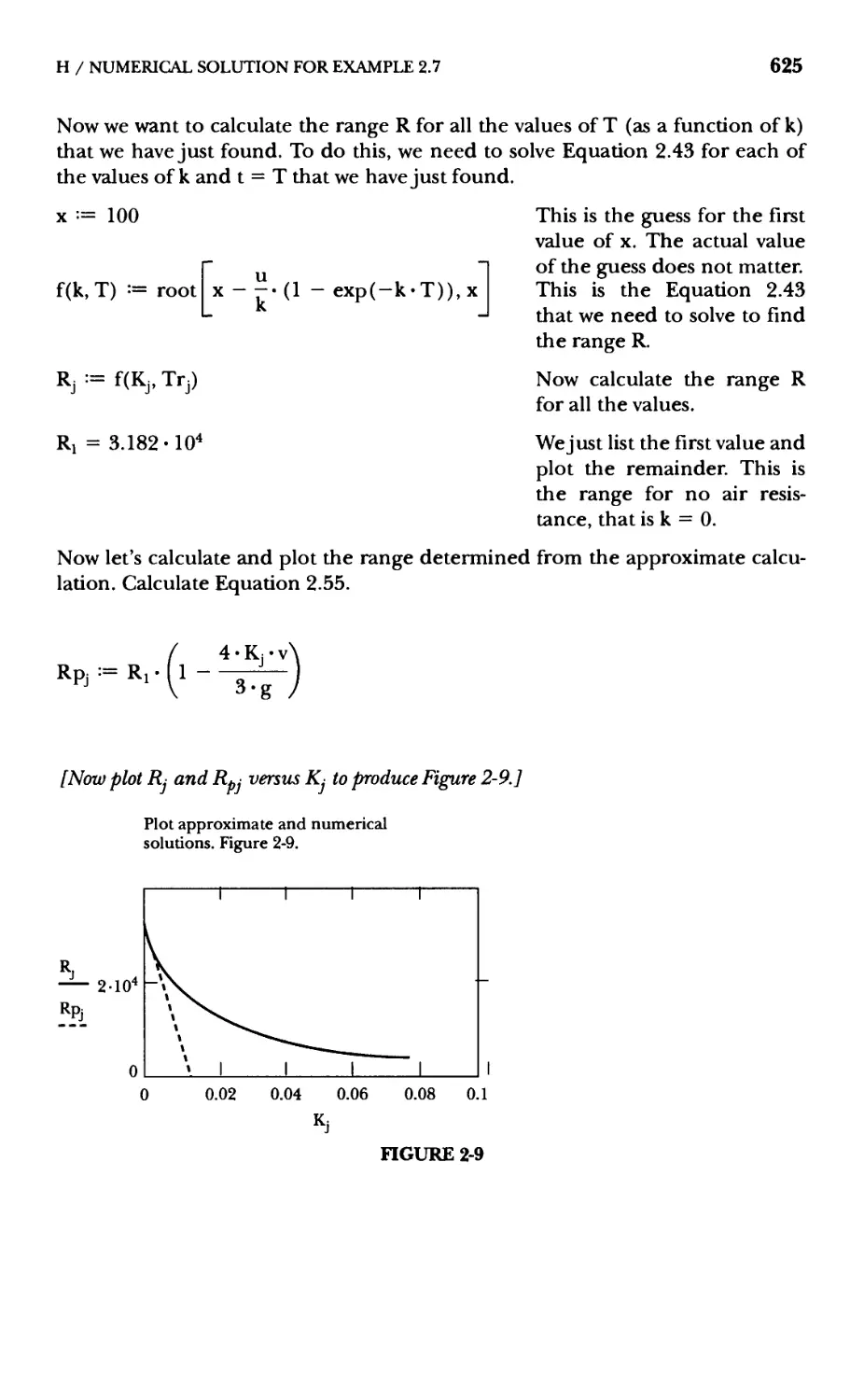
H Numerical Solution for Example 2.7 623
Selected References 626
BibUography 628
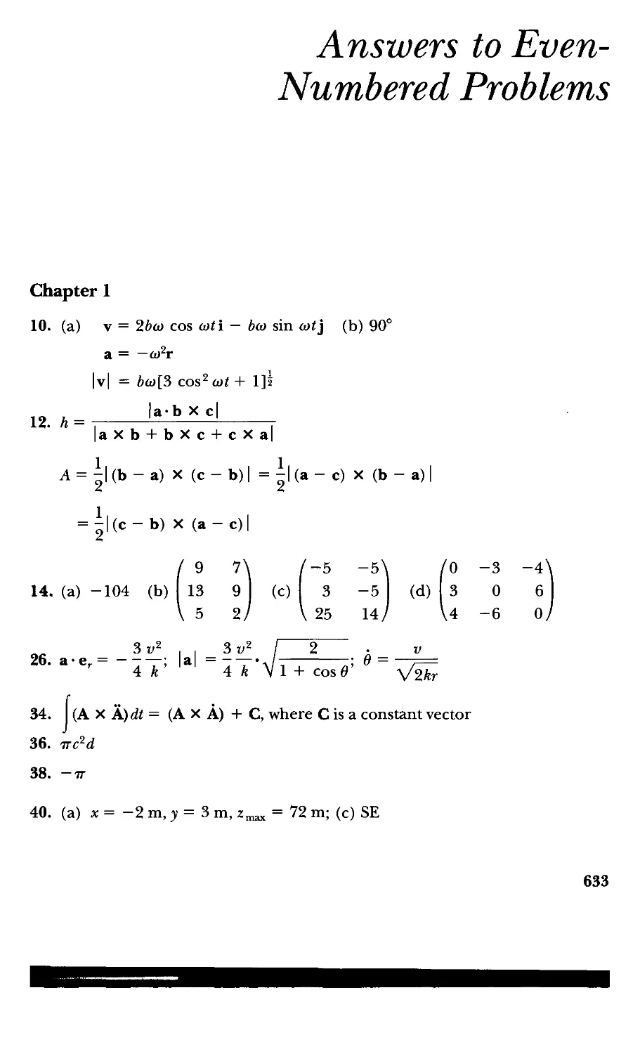
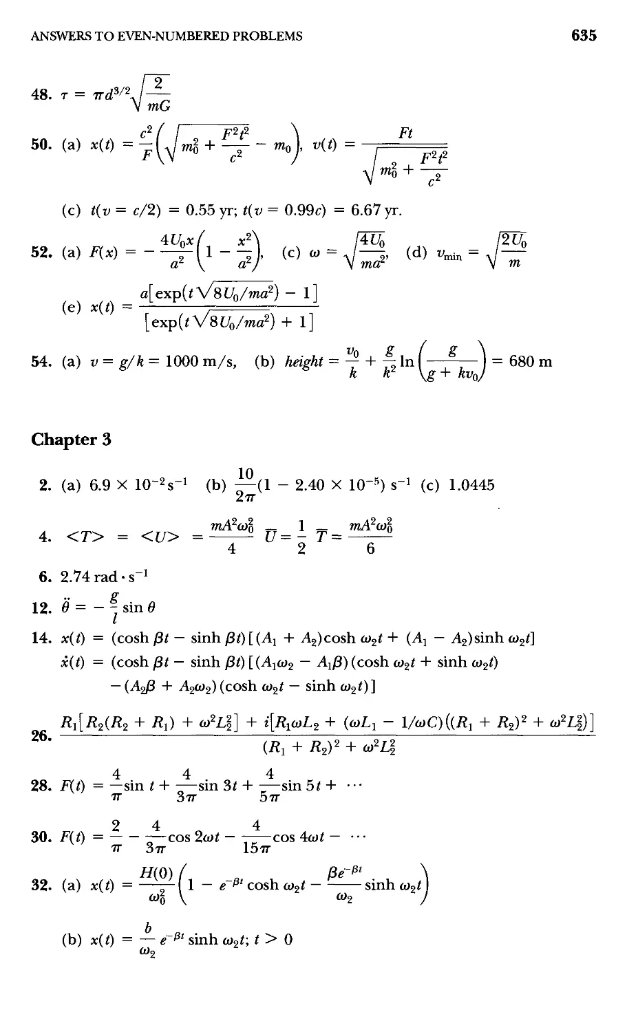
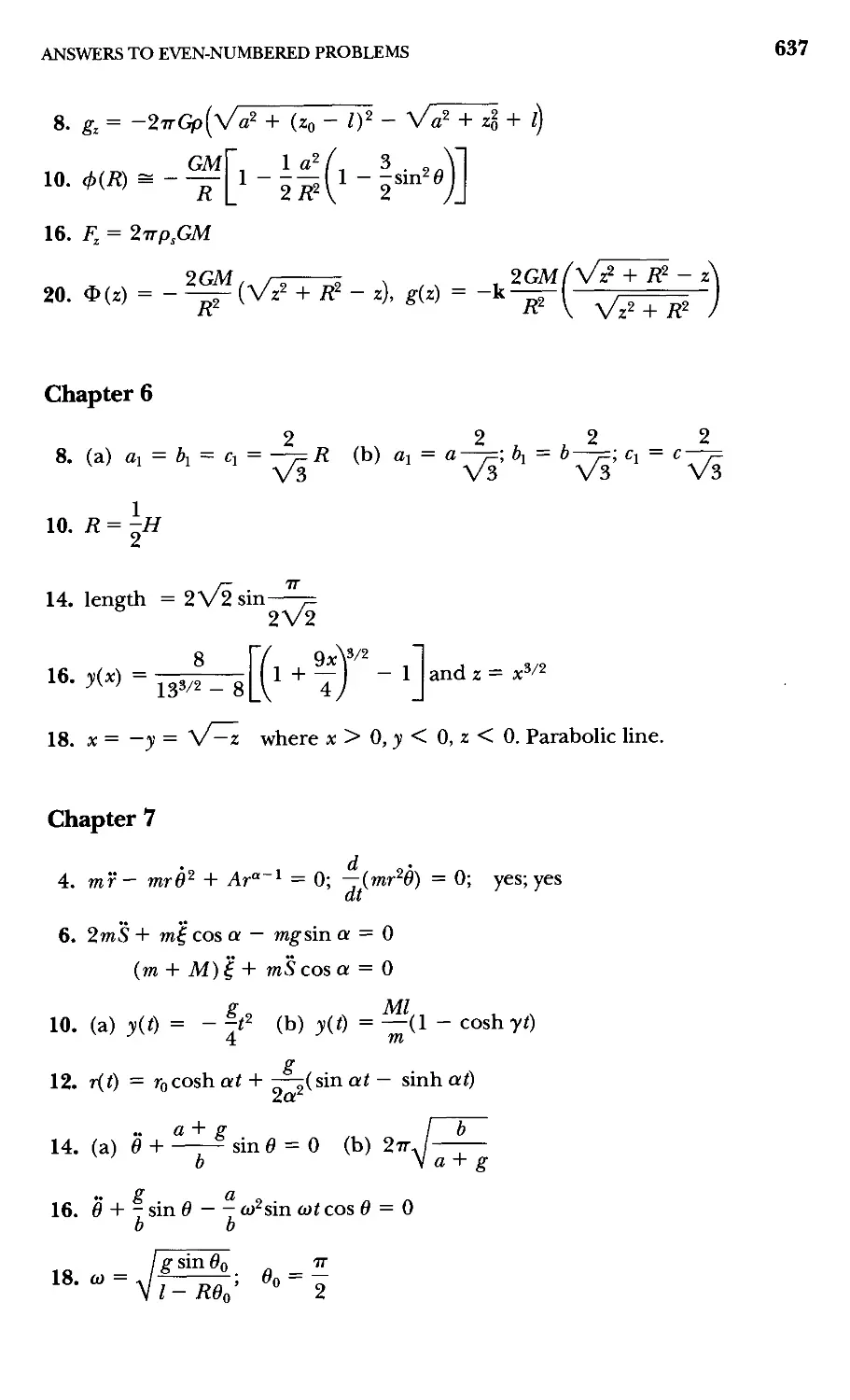
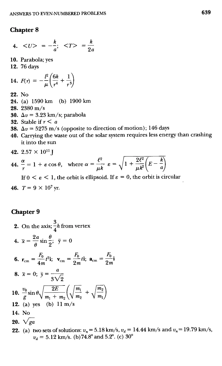
Answers to Even-Numbered Problems 633
Index 643
CHAPTER
1
Matrices, Vectors,
and Vector Calculus
1.1 Introduction
Physical phenomena can be discussed concisely and elegantly through the use of
vector methods.* In applying physical "laws" to particular situations, the results
must be independent of whether we choose a rectangular or bipolar cylindrical
coordinate system. The results must also be independent of the exact choice of
origin for the coordinates. The use of vectors gives us this independence. A
given physical law will still be correctly represented no matter which coordinate
system we decide is most convenient to describe a particular problem. Also, the
use of vector notation provides an extremely compact method of expressing
even the most complicated results.
In elementary treatments of vectors, the discussion may start with the
statement that "a vector is a quantity that can be represented as a directed line
segment." To be sure, this type of development will yield correct results, and it is
even beneficial to impart a certain feeling for the physical nature of a vector We
assuttie that the reader is familiar with this type of development, but we forego
the approach here because we wish to emphasize the relationship that a vector
bears to a coordinate transformation. Therefore, we introduce matrices and
matrix notation to describe not only the transformation but the vector as well. We
also introduce a type of notation that is readily adapted to the use of tensors,
although we do not encounter these objects until the normal course of events
requires their use (see Chapter 11).
*Josiah Willard Gibbs A839-1903) deserves much of the credit for developing vector analysis
around 1880-1882. Much of the present-day vector notation was originated by Oliver Heaviside
A850-1925), an English electrical engineer, and dates from about 1893.
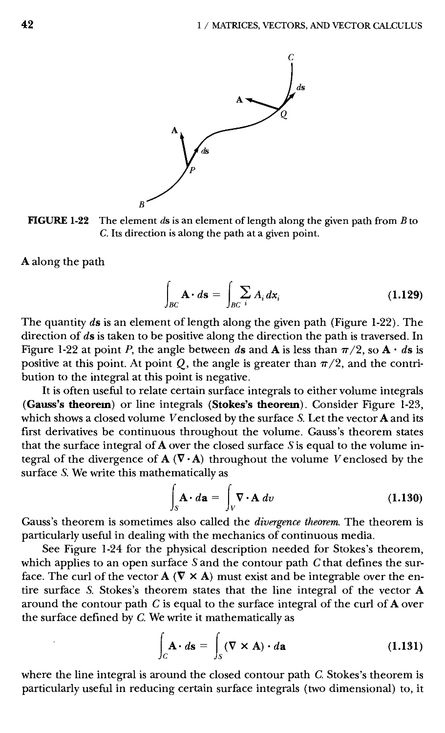
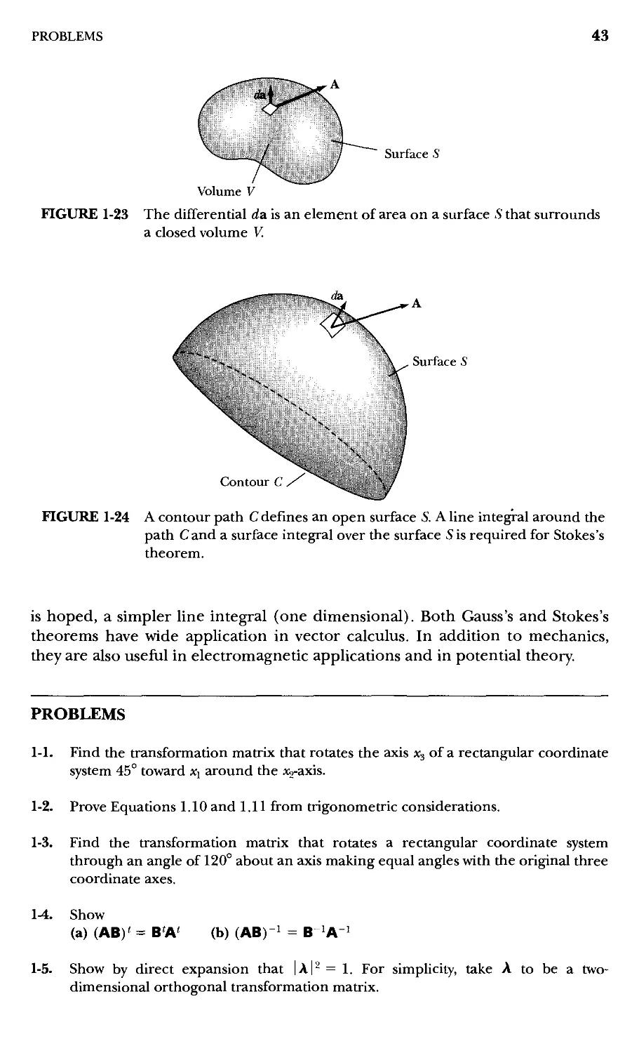
1 / MATRICES, VECTORS, AND VECTOR CALCULUS
We do not attempt a complete exposition of vector methods; instead, we
consider only those topics necessary for a study of mechanical systems. Thus in
this chapter, we treat the fundamentals of matrix and vector algebra and vector
calculus.
1.2 Concept of a Scalar
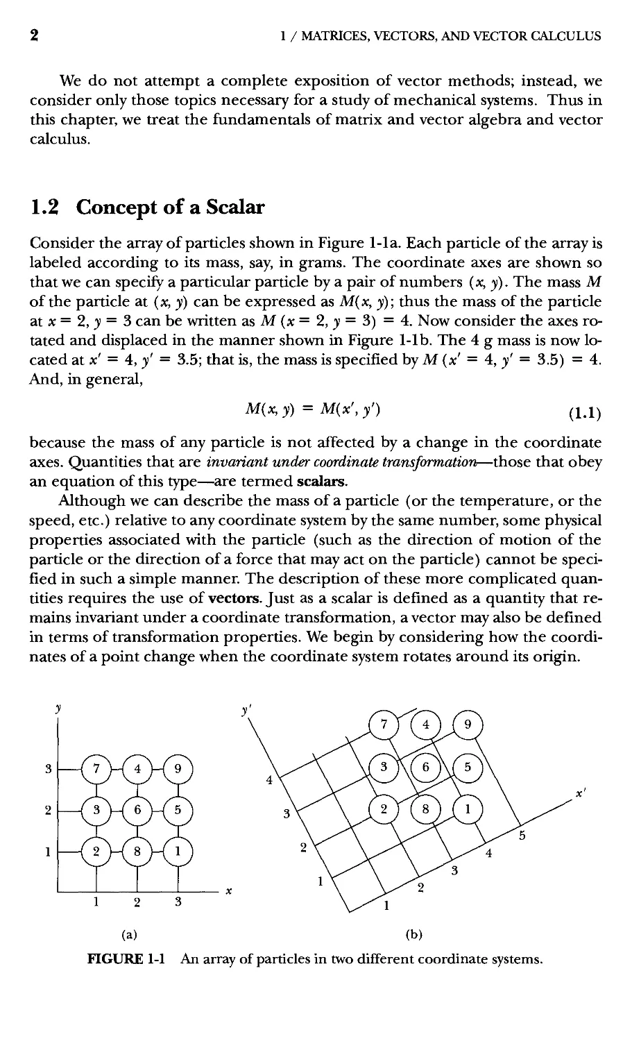
Consider the array of particles shown in Figure 1-la. Each particle of the array is
labeled according to its mass, say, in grams. The coordinate axes are shown so
that we can specify a particular particle by a pair of numbers {x, y). The mass M
of the particle at (x, y) can be expressed as M{x, y); thus the mass of the particle
at X = 2, ji = 3 can be written as M {x = 2, y = 5) =4. Now consider the axes
rotated and displaced in the manner shown in Figfure 1-lb. The 4 g mass is now
located at x' = 4, y' = 3.5; that is, the mass is specified by M (x' = 4, y' = 3.5) = 4.
And, in general.
M{x, y) = M{x', y')
A.1)
because the mass of any particle is not affected by a change in the coordinate
axes. Quantities that are invariant under coordinate transformation—those that obey
an equation of this type—are termed scalars.
Although we can describe the mass of a particle (or the temperature, or the
speed, etc.) relative to any coordinate system by the same number, some physical
properties associated with the particle (such as the direction of motion of the
particle or the direction of a force that may act on the particle) cannot be
specified in such a simple manner. The description of these more complicated
quantities requires the use of vectors. Just as a scalar is defined as a quantity that
remains invariant under a coordinate transformation, a vector may also be defined
in terms of transformation properties. We begin by considering how the
coordinates of a point change when the coordinate system rotates around its origin.
(a) (b)
FIGURE 1-1 An array of particles in two different coordinate systems.
1.3 COORDINATE TRANSFORMATIONS
1.3 Coordinate Transformations
Consider a point Pwith coordinates (xj, X2, x^) with respect to a certain
coordinate system.* Next consider a different coordinate system, one that can be
generated from the original system by a simple rotation; let the coordinates of the
point Pwith respect to the new coordinate system be {x[, x^, x'^). The situation is
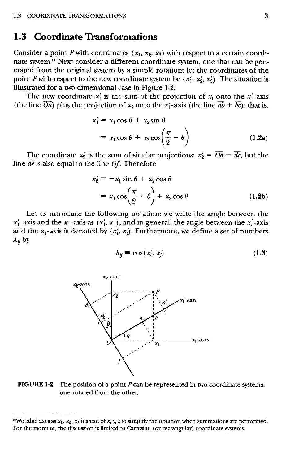
illustrated for a two-dimensional case in Figure 1-2.
The new coordinate x[ is the sum of the projection of x^ onto the xj-axis
(the line Oa) plus the projection of x^ onto the xj-axis (the line ab + be); that is,
x[ = X\ cos 6 + X2 sin 6
= Xi cos 6 + X2Cos( 'Z ~ 0
IT
A.2a)
The coordinate x^ is the sum of similar projections: ^2 = Od — de, but the
line de is also equal to the line Of. Therefore
^2 = — Xi sin 6 + X2 cos 6
= Xi COsI TT + ^ I + X2COS 6
A.2b)
Let us introduce the following notation: we write the angle between the
x{-axis and the Xj-axis as {x[, Xi), and in general, the angle between the x--axis
and the x^-axis is denoted by (x'j, xj). Furthermore, we define a set of numbers
Ayby
A;, = cos(x,', Xj)
A.3)
A:2-axis
xj-axis
Xj-axis
FIGURE 1-2 The position of a point Pcan be represented in two coordinate systems,
one rotated from the other.
*We label instead of x, y, z to simplify the notation when summations are performed.
For the moment, the discussion is limited to Cartesian (or rectangular) coordinate systems.
1 / MATRICES, VECTORS, AND VECTOR CALCULUS
Therefore, for Figure 1-2, we have
All — cos(x{, Xi) = cos 6
Ai2 = cos(x{, X2) = cosi — — 6 j = sin 6
IT
IT
A21 = cos(x2, Xi) = cosI — + 6 j = —sin 6
A22 = cos(x2, X2) = cos 0
The equations of transformation (Equation 1.2) now become
x[ = XiCos(x{, Xi) + X2Cos(xI, X2)
^ ^11^1 ' Ai2^2
X2 = XiCOS(X2, Xj) -I- X2 COS(X2, X2)
Thus, in general, for three dimensions we have
X^ — ^ll*^! ' A.29X9 I Ai aXa
^3 ~ ^31^1 "'" ^32^2 "*" ^33^3^
or, in summation notation.
x;= 2 a,, X,, ?•= 1,2,3
j=i
The inverse transformation is
Xi = x[ COS(xI, Xi) + x'2 COS(X2, Xi) + X3 COS(X3, x{)
or, in general,
x,= 2a,,x,', i= 1,2,3
y=i
A.4)
A.5a)
A.5b)
A.6)
A.7)
A.8)
The quantity A,y is called the direction cosine of the x,'-axis relative to the
x,-axis. It is convenient to arrange the A,y into a square array called a matrix. The
boldface symbol A denotes the totcility of the individual elements A,y when
arranged as follows:
All ■^12 ■^is
A = A
■21
■^31
A22
^32
■^23
A.9)
Once we find the direction cosines relating the two sets of coordinate axes.
Equations 1.7 and 1.8 give the general rules for specifying the coordinates of a
point in either system.
When A is defined this way and when it specifies the transformation
properties of the coordinates of a point, it is called a transformation matrix or a
rotation matrix.
1.3 COORDINATE TRANSFORMATIONS
KXAMI'Li: 1.1
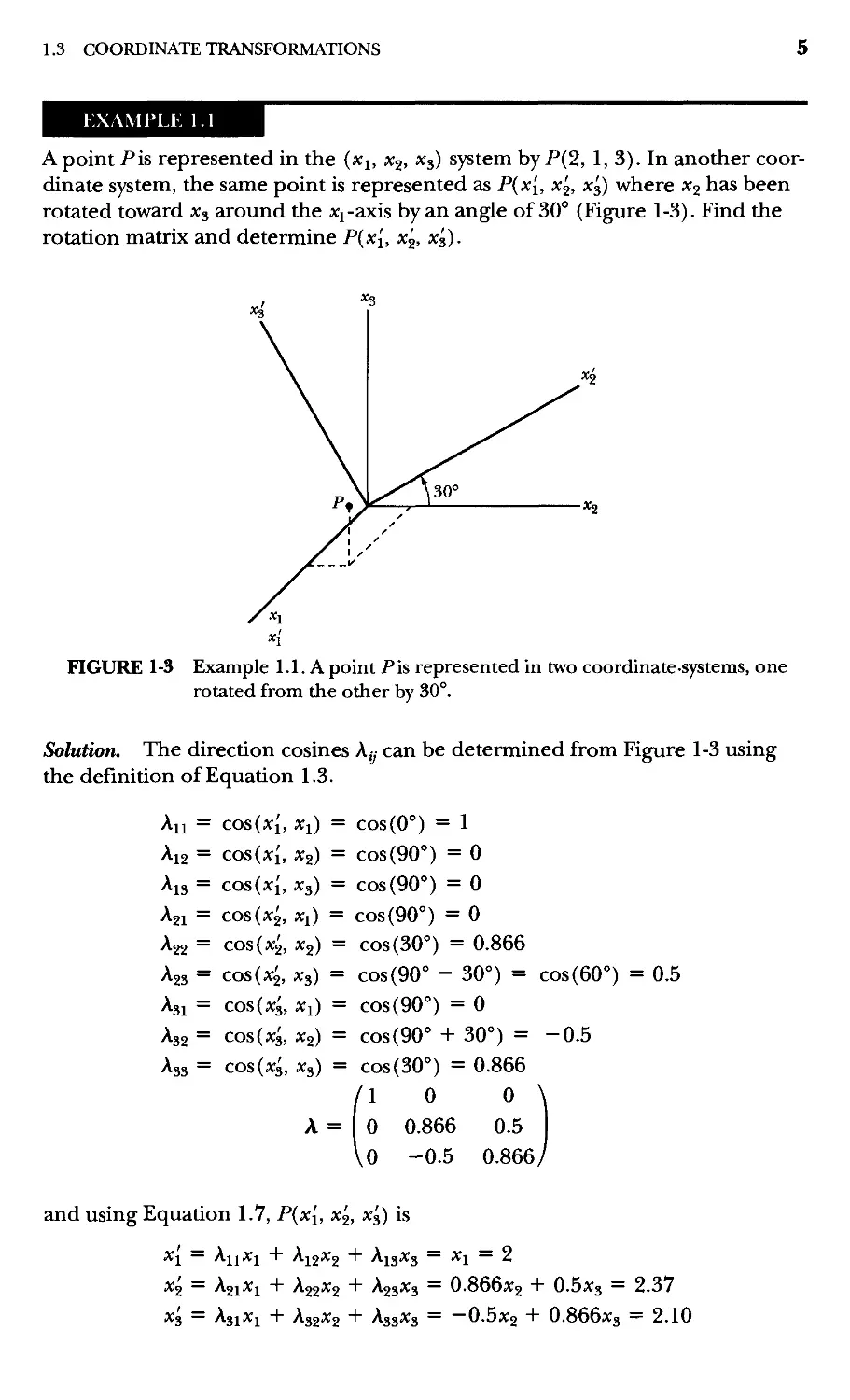
A point Pis represented in the (xj, x^, x^) system by PB, 1, 3). In another
coordinate system, the same point is represented as P{x[, x'^, x'^) where x^ has been
rotated toward x^ around the Xj-axis by an angle of 30° (Figure 1-3). Find the
rotation matrix and determine P{x[, x^, x^).
FIGURE 1-3 Example 1.1. A point Pis represented in two coordinate .systems, one
rotated from the other by 30°.
Solution. The direction cosines A,y can be determined from Figure 1-3 using
the definition of Equation 1.3.
All = cos(x{, Xi) = cos@°) = 1
Ai2 = cos(x{, X2) = cos(90°) = 0
Ai3 = cos(x{, X3) = cos(90°) = 0
A21 = COS(X2, Xi) = COS(90°) = 0
A22 = cos(x^, X2) = cosC0°) = 0.866
A23 = cosD, X3) = cos(90° - 30°) = cosF0°) = 0.5
A31 = COS(X3, Xi) = COS(90°) = 0
A32 = cos(x^, X2) = cos(90° + 30°) = -0.5
A33 = cos(x^, X3) = cosC0°) = 0.866
/I 0 0
A = 0 0.866 0.5
lo -0.5 0.866 y
and using Equation 1.7, P{x{, x^, x^) is
Xi ^11^1 ' Aj2^2 ^13^3 ^ ^1 — ^
X2 = A21X1 -I- A22X2 + ^23*^3 — 0.866x2 + 0.5x3 = 2.37
"^3 — ^31*^1 + A32X2 + A33X3 = —0.5^2 + 0.866x3 = 2.10
1 / MATRICES, VECTORS, AND VECTOR CALCULUS
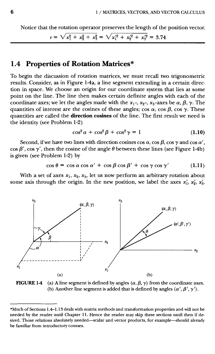
Notice that the rotation operator preserves the length of the position vector.
r = Vxf + xl+ xl = VxJ^ + x^2 + x^2 = 3 74
1.4 Properties of Rotation Matrices*
To begin the discussion of rotation matrices, we must recall two trigonometric
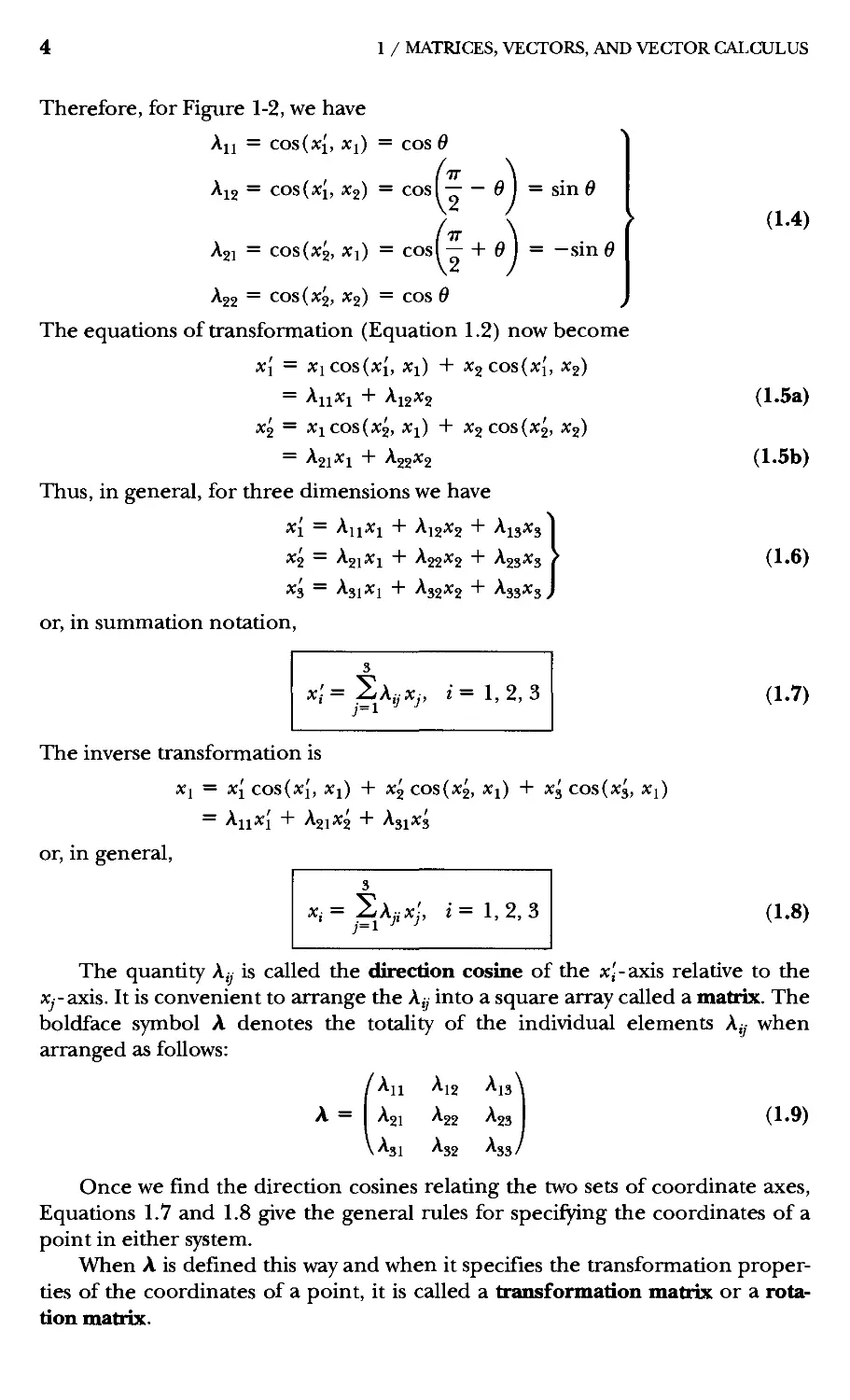
results. Consider, as in Figure l-4a, a line segment extending in a certain
direction in space. We choose an origin for our coordinate system that lies at some
point on the line. The line then makes certain definite angles with each of the
coordinate axes; we let the angles made with the Xj-, X2-, x^-axes be a, j8, y. The
quantities of interest are the cosines of these angles; cos a, cos j8, cos y. These
quantities are called the direction cosines of the line. The first result we need is
the identity (see Problem 1-2)
cos^a + cos^jS + cos^y = 1 (I-IO)
Second, if we have two lines with direction cosines cos a, cos j8, cos y and cos a',
cos j8', cos y', then the cosine of the angle 0 between these lines (see Figure l-4b)
is given (see Problem 1-2) by
cos 6 = cos a cos a' + cos j8 cos j8' + cos y cos y' (l-ll)
With a set of 3XCS Xjj Xgj X^j let us now perform an arbitrary rotation about
some axis through the origin. In the new position, we label the axes x[, x^, x'^.
{a,P,y)
{a',P',r)
FIGURE 1-4 (a) A line segment is defined by angles (a, /3, y) from the coordinate axes,
(b) Another line segment is added that is defined by angles (a', /3', y') •
*Much of Sections 1.4-1.13 deals with matrix methods and transformation properties and will not be
needed by the reader until Chapter 11. Hence the reader may skip these sections until then if
desired. Those relations absolutely needed—scalar and vector products, for example—should already
be familiar from introductory courses.
1.4 PROPERTIES OF ROTATION MATRICES 7
The coordinate rotation may be specified by giving the cosines of all the angles
between the various axes, in other words, by the A^,.
Not all of the nine quantities Aj, are independent; in fact, six relations exist
among the A,-,, so only three are independent. We find these six relations by
using the trigonometric results stated in Equations 1.10 and 1.11.
First, the x{-axis maybe considered alone to be a line in the {xi, x^, Xj)
coordinate system; the direction cosines of this line are (An, A12, A13). Similarly, the
direction cosines of the X2-axis in the (xj, x^, X3) system are given by (A21, A22, A23).
Because the angle between the x{-axis and the X2-axis is it/2, we have, from
Equation 1.11,
■^ll'^21 + ■^12'^22 + ■^13'^23 ~ COS 0 = COS(it/2) = 0
or^
2ai,.A2-o
And, in general.
2AyAi^ = 0, ii-k A.12a)
Equation 1.12a gives three (one for each value of i or ^) of the six relations
among the A,,.
Because the sum of the squares of the direction cosines of a line equals unity
(Equation 1.10), we have for the xj-axis in the {x^, x^, X3) system, •
Afi + A?2 + A?3 = 1
2Af, = 2Ai^.Ai,= 1
and, in general,
%K^Kj =1, i=k A.12b)
which are the remaining three relations among the A^.
We may combine the results given by Equations 1.12a and 1.12b as
A' ^ijKj — ^ik
A.13)
where S^^ is the Kronecker delta symbol^
'-{":
^''^- lit:
The validity of Equation 1.13 depends on the coordinate axes in each of the
systems being mutually perpendicular. Such systems are said to be orthogonal.
*A11 summations here are understood to run from 1 to 3.
■^Introduced by Leopold Kronecker A823-1891).
8 1 / MATRICES, VECTORS, AND VECTOR CALCULUS
and Equation 1.13 is the orthogonality condition. The transformation matrix A
specifying the rotation of any orthogonal coordinate system must then obey
Equation 1.13.
If we were to consider the X;-axes as lines in the x,' coordinate system and
perform a calculation analogous to our preceding calculations, we would find
the relation
^Ki^ik ~ ^H
A.15)
The two orthogonality relations we have derived (Equations 1.13 and 1.15)
appear to be different. {Note: In Equation 1.13 the summation is over the second
indices of the A,-,, whereas in Equation 1.15 the summation is over the first
indices.) Thus, it seems that we have an overdetermined system: twelve equations
in nine unknowns.* Such is not the case, however, because Equations 1.13 and
1.15 are not actually different. In fact, the validity of either of these equations
implies the validity of the other. This is clear on physical grounds (because the
transformations between the two coordinate systems in either direction are
equivalent), and we omit a formal proof. We regard either Equation 1.13 or 1.15
as providing the orthogonality relations for our systems of coordinates.
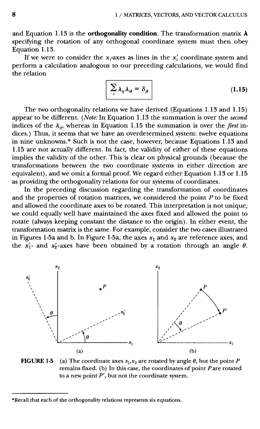
In the preceding discussion regarding the transformation of coordinates
and the properties of rotation matrices, we considered the point P to be fixed
and allowed the coordinate axes to be rotated. This interpretation is not unique;
we could equally well have maintained the axes fixed and allowed the point to
rotate (always keeping constant the distance to the origin). In either event, the
transformation matrix is the same. For example, consider the two cases illustrated
in Figures l-5a and b. In Figure l-5a, the axes Xi and X2 are reference axes, and
the x'l- and X2-axes have been obtained by a rotation through an angle 6.
«2
.Xi
"S
(a)
(b)
FIGURE 1-5
(a) The coordinate axes Xi,X2 are rotated by angle 6, but the point P
remains fixed, (b) In this case, the coordinates of point Pare rotated
to a new point P', but not the coordinate system.
*Recall that each of the orthogonality relations represents six equations.
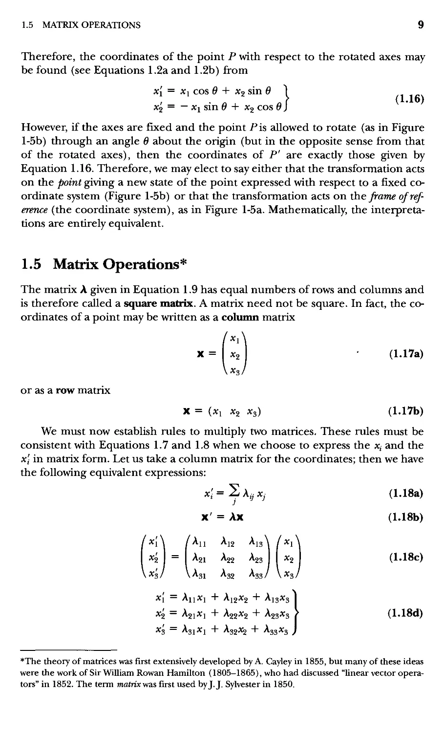
1.5 MATRIX OPERATIONS
Therefore, the coordinates of the point P with respect to the rotated axes may
be found (see Equations 1.2a and 1.2b) from
x'l = Xi cos 6 + x^ sin 6
X2 = — Xi sin 6 + X2 cos 6,
A.16)
However, if the axes are fixed and the point P is allowed to rotate (as in Figure
l-5b) through an angle Q about the origin (but in the opposite sense from that
of the rotated axes), then the coordinates of P' are exactly those given by
Equation 1.16. Therefore, we may elect to say either that the transformation acts
on the point giving a new state of the point expressed with respect to a fixed
coordinate system (Figure l-5b) or that the transformation acts on the frame of
reference (the coordinate system), as in Figure l-5a. Mathematically, the
interpretations are entirely equivalent.
1.5 Matrix Operations*
The matrix A given in Equation 1.9 has equal numbers of rows and columns and
is therefore called a square matrix. A matrix need not be square. In fact, the
coordinates of a point may be written as a column matrix
X =
A.17a)
or as a row matrix
X ^ \^\ '^2 ^%/
A.17b)
We must now establish rules to multiply two matrices. These rules must be
consistent with Equations 1.7 and 1.8 when we choose to express the x, and the
x\ in matrix form. Let us take a column matrix for the coordinates; then we have
the following equivalent expressions:
x'i = ^ A,, Xi
X' = Ax
"^1 \ / '^ll ^^12 '^IS \ / ""^l
"^2 I ~ I ^^21 ^^22 ■^23 I ^.
, X3 / \ A31 A32 A33 / \ X3
X\ ^ ^11^1 ' A22^2 ^13^3
Xn — AojXj I" A99X9 I" A93X3
^% ~ A31XJ -I- A32X2 -I- A33X3 ^
A.18a)
A.18b)
A.18c)
A.18d)
*The theory of matrices was first extensively developed by A. Cayley in 1855, but many of these ideas
were the work of Sir William Rowan Hamilton A805-1865), who had discussed "linear vector
operators" in 1852. The term matnx\i2s, first used by J. J. Sylvester in 1850.
10 1 / MATRICES, VECTORS, AND VECTOR CALCULUS
Equations 1.18a-d completely specify the operation of matrix multiplication
for a matrix of three rows and three columns operating on a matrix of three
rows and one column. (To be consistent with standard matrix convention we
choose X and x' to be column matrices; multiplication of the type shown in
Equation 1.18c is not defined if X and x' are row matrices.)* We must now
extend our definition of multiplication to include matrices with arbitrary numbers
of rows and columns.
The multiplication of a matrix A and a matrix B is defined only if the
number of columns of A is equal to the number of mws of B. (The number of rows of
A and the number of columns of B are each arbitrary.) Therefore, in analogy
with Equation 1.18a, the product AB is given by
C = AB
A.19)
As an example, let the two matrices A and B be
^3 -2 2^
We multiply the two matrices by
AB = (: : :]\d e f\ A.20)
.s
4
-2
-3
''^\
5J
a
h c'
e J
h jj
The product of the two matrices, C, is
C= AB = (^^^"^'^+^^ 36-2.+ 2A 3C-2/+2A
\4a - 3d+ 5g 4b- 3e+ 5h 4c - 3/+ 5jJ ^ '
To obtain the Cy element in the ixh row and jxh column, we first set the two
matrices adjacent as we did in Equation 1.20 in the order A and then B. We then
multiply the individual elements in the ixh row of A, one by one from left to
right, times the corresponding elements in the ^th column of B, one by one
from top to bottom. We add all these products, and the sum is the C^ element.
Now it is easier to see why a matrix A with m rows and n columns must be
multiplied times another matrix B with n rows and any number of columns, say p. The
result is a matrix C of w rows and p columns.
*Although whenever we operate on x with the A matrix the coordinate matrix x must be expressed
as a column matrix, we may also write x as a row matrix (xi, x^, x^), for other applications.
1.5 MATRIX OPERATIONS
11
EXAMPLE
Solution. We follow the example of Equations 1.20 and 1.21 to multiply the two
matrices together.
/ 2 1 3\/-l -2^
AB= -2 2 4 1 2
V-1 -3 -4/V 3 4j
1-2 +1+9 -4 + 2+12^
AB=2 + 2+12 4 + 4+16
\ 1 - 3 - 12 2 - 6 - 16y
The result of multiplying a 3 X 3 matrix times a 3 X 2 matrix is a 3 X 2 matrix.
It should be evident from Equation 1.19 that matrix multiplication is not
commutative. Thus, if A and B are both square matrices, then the sums
"^Ai^B^j and SSitA^^
are both defined, but, in general, they will not be equal.
8
16
-14
10
24
-20
EXAMPLE L.}
Show that the multiplication of the matrices A and B in this example is non-
commutative.
Solution. If A and B are the matrices
then
AB =
2 2
13 -8
12 1 / MATRICES, VECTORS, AND VECTOR CALCULUS
but
BA = (-' '
VlO -2
thus
ABt^ BA
1.6 Further Definitions
A transposed matrix is a matrix derived from an original matrix by interchange
of rows and columns. We denote the transpose of a matrix A by A'. According to
the definition, we have
^ ~ h
A.22)
Evidently,
(A')'=A A.23)
Equation 1.8 may therefore be written as any of the following equivalent
expressions:
x, = 2a,,x; A.24a)
A.24b)
A.24c)
A.24d)
The identity matrix is that matrix which, when multiplied by another matrix,
leaves the latter unaffected. Thus
1A = A, B1 = B A.25)
that is.
Let us consider the orthogonal rotation matrix A for the case of two dimensions:
[All Ai2
A =
A21 A22
1.6 FURTHER DEFINITIONS 13
Then
AA' =
it — ( ^11 ^12 11 ^11 ^21
^^21 ^22/ \^12 ^22/
^11 + ^12 ^11^21 "*" ^12^22
^AgiAji + "-22^12 Agl '' ^^22
Using the orthogonality relation (Equation 1.13), we find
Aji I Aj2 ^ Agi I Agg ^ 1
^21 11 ^22 12 ^ ^11^21 ^12 22 ^
SO that for the special case of the orthogonal rotation matrix A we have*
AA'.(J ^).l A.26)
The inverse of a matrix is defined as that matrix which, when multiplied by
the original matrix, produces the identity matrix. The inverse of the matrix A is
denoted by A"^:
A A-i = 1 A.27)
By comparing Equations 1.26 and 1.27, we find
for orthogonal matrices ' A>28)
A' = A
Therefore, the transpose and the inverse of the rotation matrix A are identical.
In fact, the transpose of any orthogonal matrix is equal to its inverse.
To summarize some of the rules of matrix algebra:
1. Matrix multiplication is not commutative in general:
AB ¥= BA A.29a)
The special case of the multiplication of a matrix and its inverse is
commutative:
AA 1 = A 1 A = 1 A.29b)
The identity matrix always commutes:
1A = A1 = A A.29c)
2. Matrix multiplication is associative:
[AB]C = A[BC] A.30)
3. Matrix addition is performed by adding corresponding elements of the two
matrices. The components of C from the addition C = A + B are
C^=A^.+ By A.31)
Addition is defined only if A and B have the same dimensions.
*This result is not valid for matrices in general. It is true only for orthogonal matrices.
14 1 / MATRICES, VECTORS, AND VECTOR CALCULUS
1.7 Geometrical Significance
of Transformation Matrices
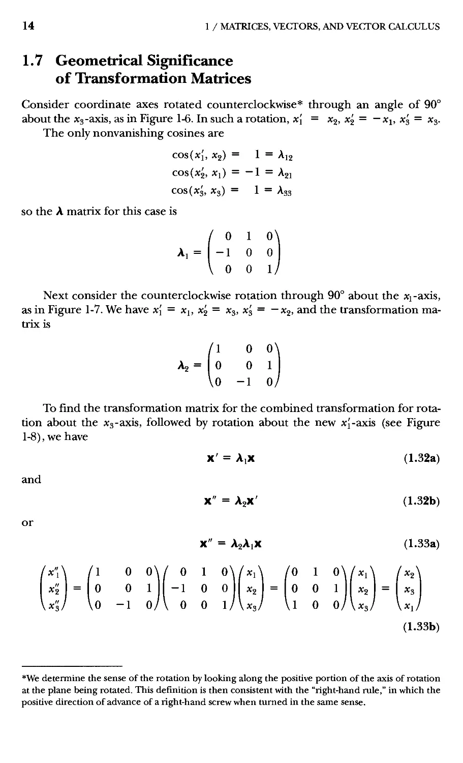
Consider coordinate axes rotated counterclockwise* through an angle of 90°
about the Xs-axis, as in Figfure 1-6. In such a rotation, x[ = X2, x^ = —Xi, x'^ = x^.
The only nonvanishing cosines are
cos(xI, X2) = 1 = A12
COs(X2, X]) = —1 = A21
COS(X3, X3) = 1 = A33
SO the A matrix for this case is
Next consider the counterclockwise rotation through 90° about the xj-axis,
as in Figure 1-7. We have x[ = x^, x'^ = x^, x'^ = —x^, and the transformation
matrix is
To find the transformation matrix for the combined transformation for
rotation about the X3-axis, followed by rotation about the new xj-axis (see Figfure
1-8), we have
and
x' = AjX A.32a)
x" = A2X' A.32b)
x" = A2A1X A.33a)
'x\\ /I 0 0\/ 0 1 0
x^ = 0 0 1-1 0 0
^xlj \0 -1 0/\ 0 0 1
*We determine the sense of the rotation by looking along the positive portion of the axis of rotation
at the plane being rotated. This definition is then consistent with the "right-hand rule," in which the
positive direction of advance of a right-hand screw when turned in the same sense.
1.7 GEOMETRICAL SIGNIFICANCE OF TRANSFORMATION MATRICES
15
»i
C3
»i
90° rotation
about jcj-axis
«2
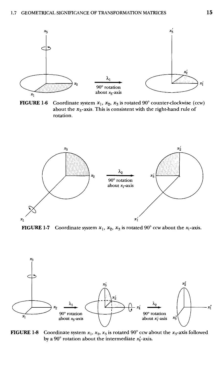
FIGURE 1-6 Coordinate system Xj, X2, x^ is rotated 90° counter-clockwise (ccw)
about the Xs-axis. This is consistent with the right-hand rule of
rotation.
h
90° rotation
about Xj-axis
FIGURE 1-7 Coordinate system x^, x^, x^ is rotated 90° ccw about the Xj-axis.
xs
c:2>
«2
90° rotation
about Xj-axis
90° rotation
about Xj-axis *3
FIGURE 1-8 Coordinate system xj, X2, Xj is rotated 90° ccw about the Xj-axis followed
by a 90° rotation about the intermediate Xi'-axis.
16
1 / MATRICES, VECTORS, AND VECTOR CALCULUS
Therefore, the two rotations already described may be represented by a single
transformation matrix:
'0 1 0'
As = A2A1 = I 0 0 1
.1 0 Oy
A.34)
and the final orientation is specified by x'{ = x^, x\ = X3, x\ = x^. Note that the
order in which the transformation matrices operate on X is important because
the multiplication is not commutative. In the other order,
A4 ^ AjAg
0 1 0\/l 0 0'
=1-1 0 0 0 0 1
0 0 lAo -1 0/
0
1
0
0
0
-1
1
0
0
+ A,
A.35)
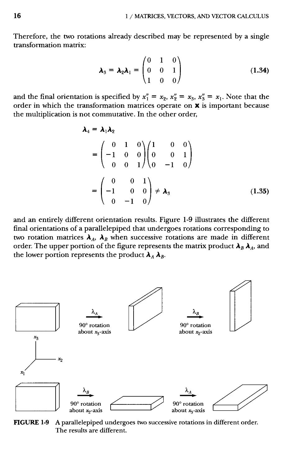
and an entirely different orientation results. Figfure 1-9 illustrates the different
final orientations of a parallelepiped that undergoes rotations corresponding to
two rotation matrices A^, A^ when successive rotations are made in different
order. The upper portion of the figure represents the matrix product A^ A^, and
the lower portion represents the product A^ A^.
»i
■H
90° rotation
^^
90° rotation
about x^-'xas,
90° rotation
about x^-'dxss,
^
90° rotation
FIGURE 1-9 A parallelepiped undergoes two successive rotations in different order.
The results are different.
1.7 GEOMETRICAL SIGNIFICANCE OF TRANSFORMATION MATRICES
17
Next, consider the coordinate rotation pictured in Figure 1-10 (which is the
same as that in Figure 1-2). The elements of the transformation matrix in two
dimensions are given by the following cosines:
cos(xI, Xi) = cos 6 = All
IT
cos(xJ, X2) = cos( ~Z ~ ^] ~ sin 0 = A12
IT
cos(x2, Xi) = cos[ ~z + 0] = ~ sin 6 = A21
cos(x2, X2) = cos 6 = A22
Therefore, the matrix is
A, =
cos 6 sin 6
— sin 0 cos 0
A.36a)
If this rotation were a three-dimensional rotation with would
have the following additional cosines:
COS(xI, X3) = 0 = Ai3
COs(X2, X3) = 0 = A23
COS(X3, X3) = 1 = A33
COS(X3, Xi) = 0 = A31
COS(X3, X2) = 0 = A32
and the three-dimensional transformation matrix is
cosO sine 0>
Ac = I — sin 0 cos 0 0
A.36b)
*3- *3
FIGURE 1-10 Coordinate system xj, X2, Xj is rotated an angle 6 ccw about the Xj-axis.
18
1 / MATRICES, VECTORS, AND VECTOR CALCULUS
X
^'
3
^
«2
(Inversion)
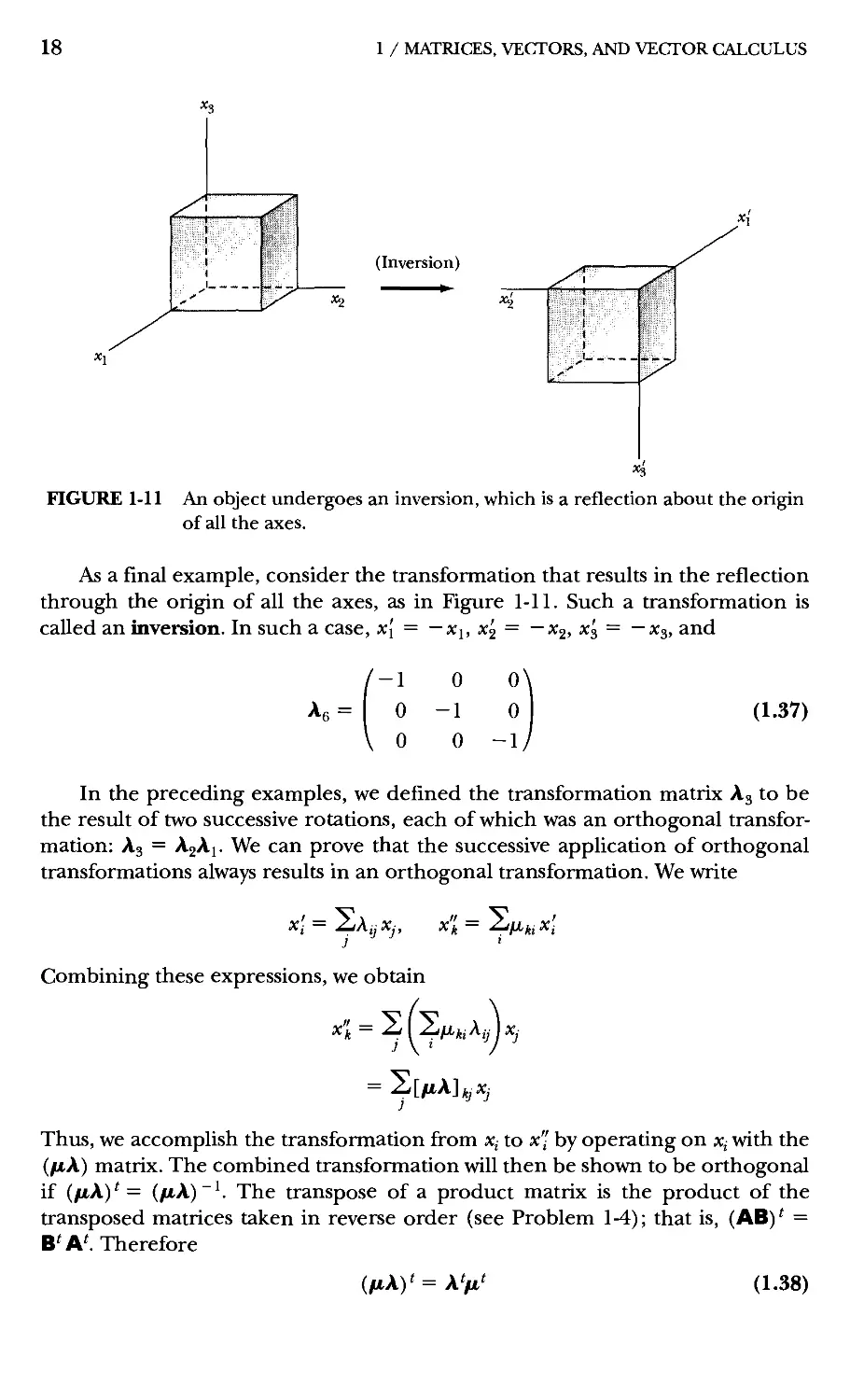
FIGURE 1-11 An object undergoes an inversion, which is a reflection about the origin
of all the axes.
As a final example, consider the transformation that results in the reflection
through the origin of all the axes, as in Figure 1-11. Such a transformation is
called an inversion. In such a case, x[ = —Xj, X2 = —x^, x'^ = —x^, and
A.37)
In the preceding examples, we defined the transformation matrix A3 to be
the result of two successive rotations, each of which was an orthogonal
transformation: A3 = AgAj. We can prove that the successive application of orthogonal
transformations always results in an orthogonal transformation. We write
x'i = 2j\ijXj, 4 = 2jfj,^iX'i
J '
Combining these expressions, we obtain
= 2j[fiX]^^xj
Thus, we accomplish the transformation from x, to x" by operating on x, with the
(fiX) matrix. The combined transformation will then be shown to be orthogonal
if (fiX)' = {fiX)~^. The transpose of a product matrix is the product of the
transposed matrices taken in reverse order (see Problem 1-4); that is, (AB)* =
B* A*. Therefore
(mA)*=A*M
A.38)
1.7 GEOMETRICAL SIGNIFICANCE OF TRANSFORMATION MATRICES
19
But, because A and ft, are orthogonal. A* = A ' and fi' = fi ^ Multiplying the
above equation by fiX from the right, we obtain
ifiXYfiX = x'fi^fiX
= X'lX
= X'X
= 1
= ifixy'fix
Hence
(mAO = (mA)-'
A.39)
and the fiX matrix is orthogonal.
The determinants of all the rotation matrices in the preceding examples can
be calculated according to the standard rule for the evaluation of determinants
of second or third order:
All
A21
All
A21
A31
A12
A22
— A11A22 A12A2
= Ai
A12 Ai3
A22 A23
A32 A33
2 A23
2 A33
Aii
A21
A31
A23
A33
+ An
A21
A31
A22
A32
A.40)
A.41)
where the third-order determinant has been expanded in minors of the first
row. Therefore, we find, for the rotation matrices used in this section.
I Ai I — IA21 —
= AJ = 1
but
AJ = -1
Thus, all those transformations resulting from rotations starting from the original set
of axes have determinants equal to +1. But an inversion cannot be generated by
any series of rotations, and the determinant of an inversion matrix is equal to — 1.
Orthogonal transformations, the determinant of whose matrices is -1-1, are
called proper rotations; those with determinants equal to —1 are called
improper rotations. AU orthogonal matrices must have a determinant equal to either
-1-1 or —1. Here, we confine our attention to the effect of proper rotations and do
not concern ourselves with the special properties of vectors manifest in improper
rotations.
20
1 / MATRICES, VECTORS, AND VECTOR CALCULUS
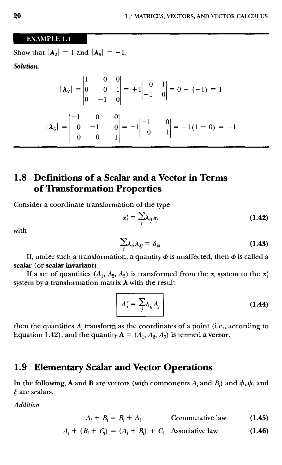
KXAMPLE 1.4
Show that IA21 = 1 and | A51 = — 1.
Solution.
AJ =
1
u
u
0
u
-1
0
1
u
= +1
0
-1
1
0
1
0
0
0
-1
u
0
0
-1
= -1
-1
0
0
-1
0- (-1) =1
= -1A -0)
1.8 Definitions of a Scalar and a Vector in Terms
of Transformation Properties
Consider a coordinate transformation of the type
X'i = 2j\ii X:
with
2a,:,A
ij"-kj ~ "ik
A.42)
A.43)
If, under such a transformation, a quantity (f) is unaffected, then (f) is called a
scalar (or scalar invariant).
If a set of quantities (Aj, A^, A3) is transformed from the Xj system to the x-
system by a transformation matrix A with the result
Aj — 2j\jjAj
A.44)
then the quantities A; transform as the coordinates of a point (i.e., according to
Equation 1.42), and the quantity A = (Aj, A2, A3) is termed a vector.
1.9 Elementary Scalar and Vector Operations
In the following, A and B are vectors (with components A, and Bj) and <f), ifi, and
^ are scalars.
Addition
Aj + Bj = Bj + A, Commutative law A.45)
Aj + E; + Q = (A, + B,) + Cj Associative law A.46)
1.10 SCALAR PRODUCT OF TWO VECTORS 21
(f) + ill = ill + (f) Commutative law A'47)
(t> + (^ + i) = {(t> + ^) + i Associative law A.48)
Multiplication by a scalar ^
^A = B is a vector A-49)
^(f> = ij/ is a scalar A.50)
Equation 1.49 can be proved as follows:
B',= l,\,jBj=l,\,jUj
= iI,KjAj=Ul A.51)
J
and ^A transforms as a vector. Similarly, ^(f) transforms as a scalar
1.10 Scalar Product of Two Vectors
The multiplication of two vectors A and B to form the scalar product is defined
to be
A-B = Sa,B,
A.52)
where the dot between A and B denotes scalar multiplication; this operation is
sometimes called the dot product.
The vector A has components Aj, A^, A3, and the magnitude (or length) of A
is given by
|A| = +VAf + A| + A| = A A.53)
where the magnitude is indicated by |A| or, if there is no possibility of
confusion, simply by A. Dividing both sides of Equation 1.52 by AB, we have
A-B v4-B,
= 2. — - A.54)
AB i A B ^ '
Ai/A is the cosine of the angle a between the vector A and the Xj-axis (see
Figure 1-12). In general, A^/A and B^/B are the direction cosines A^* and Af of
the vectors A and B:
^-^ = ^AfAf A.55)
AB i ' ' ^ '
The sum Zj^AfAf is just the cosine of the angle between A and B (see Equation
1.11):
cos (A, B) = 2Af Af
A- B = ABcos(A,B) | A.56)
22
1 / MATRICES, VECTORS, AND VECTOR CALCULUS
»i
A3
\
^^
\^A
y\ i ^2
/ ^ a 1 /
' \ 1 /
^N 1/
«2
«1
FIGURE 1-12 A vector A is shown in coordinate system X], x^, Xj with its vector
components Aj, Aj, and A3. The vector A is oriented at an angle a
with the X] -axis.
That the product A • B is indeed a scalar may be shown as follows. A and B
transform as vectors:
A; = SAi,A,, b; = Sa„b,
Therefore the product A' • B' becomes
A'-B' =Sa'B'
A.57)
Rearranging the summations, we can write
s(Sa,a,)(Sa,5.)
;e
A'-B' = SfSA,AjA,B,
But according to the orthogonality condition, the term in parentheses is just S^^.
Thus,
A'.B' = S(SS,,A,.B,)
= Sa,^,
= AB
A.58)
Because the value of the product is unaltered by the coordinate transformation,
the product must be a scalar
Notice that the distance from the origin to the point (xj, x^, %) defined by
the vector A, called the position vector, is given by
|A| = VaTa = Vxf + xl + xl = V^xf
(«1, *2' *3)
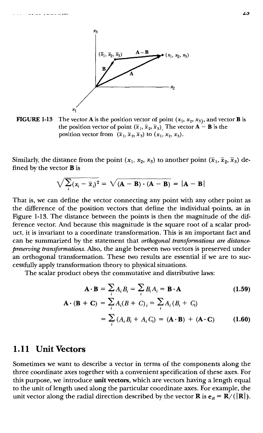
FIGURE 1-13 The vector A is the position vector of point (xj, x^, x^\, and vector B is
the position vector of point (xj, Xj, Xj) The vector A — B is the
position vector from (xj, Xj, Xj) to (xj, Xj, Xj).
Similarly the distance from the point (xj, ^2, x^) to another point (xj, x^, x^)
defined by the vector B is
V2(x,-x,J = V(A - B) . (A - i)" = |A -
B
That is, we can define the vector connecting any point with any other point as
the difference of the position vectors that define the individual -points, as in
Figure 1-13. The distance between the points is then the magnitude of the
difference vector. And because this magnitude is the square root of a scalar
product, it is invariant to a coordinate transformation. This is an important fact and
can be summarized by the statement that orthogonal transformations are distance-
preserving transformations. Also, the angle between two vectors is preserved under
an orthogonal transformation. These two results are essential if we are to
successfully apply transformation theory to physical situations.
The scalar product obeys the commutative and distributive laws:
A • B = S A, B, = S B, A, = B • A A.59)
i i
A. (B + C) = Sa,(B + C),. = Sa,{B, + Q
I i
= S (A, B, + A; Q = (A • B) + (A. C) A.60)
1.11 Unit Vectors
Sometimes we want to describe a vector in terms of the components along the
three coordinate axes together with a convenient specification of these axes. For
this purpose, we introduce luiit vectors, which are vectors having a length equal
to the unit of length used along the particular coordinate axes. For example, the
unit vector along the radial direction described by the vector R is e/^ = R/(|R| ).
24
1 / MATRICES, VECTORS, AND VECTOR CALCULUS
There are several variants of the symbols for unit vectors; examples of the most
common sets are (i, j, k), (ej, 62, 63), (e,., eg, e^), and (r, 0, <^). The following
ways of expressing the vector A are equivalent:
(Aj, A2, A3) or A = ei Ai + 62 A2 + 63 A3
or A = Aji + A2J + A3k
2e,.
jAl
A.61)
Although the unit vectors (i, j, k) and (r, 0,^) are somewhat easier to use, we
tend to use unit vectors such as (ej, e^, 63), because of the ease of summation
notation. We obtain the components of the vector A by projection onto the axes:
e,'A
A.62)
We have seen (Equation 1.56) that the scalar product of two vectors has a
magnitude equal to the product of the individual magnitudes multiplied by the
cosine of the angle between the vectors:
A-B = ABcos(A, B)
If any two unit vectors are orthogonal, we have
ei-ej=Sy
A.63)
A.64)
EXAMPLK
Two position vectors are expressed in Cartesian coordinates as A = i + 2j — 2k
and B = 4i + 2j — 3k. Find the magnitude of the vector from point A to point
B, the angle 6 between A and B, and the component of B in the direction of A,
Solution. The vector from point A to point B is B — A (see Figure 1-13).
B - A = 4i -I- 2j - 3k - (i -I- 2j - 2k) = 3i - k
|B - Al
V9 -I-1 = vTo
From Equation 1.56
cos 6 =
cos 6
A-B _ (i -H 2j - 2k) • Di + 2j - 3k)
AB ~ V9 ^
4-1-4-1-6
29
3(
e = 30°
= 0.867
29)
The component of B in the direction of A is B cos 6 and, from Equation
1.56,
A-B 14
Bcose = = — = 4.67
A 3
1.12 VECTOR PRODUCT OF TWO VECTORS 25
1.12 Vector Product of Two Vectors
We next consider another method of combining two vectors—the vector
product (sometimes called the cross product). In most respects, the vector product of
two vectors behaves like a vector, and we shall treat it as such.* The vector
product of A and B is denoted by a bold cross X,
C = A X B A.65)
where C is the vector resulting from this operation. The components of C are
defined by the relation
C,= SfiyiASi
j,k
A.66)
where the symbol Sy^ is the permutation symbol or (Levi-Civita density) and has
the following properties:
0, if any index is equal to any other index
^ijk = +1, iiij,k form an even permutation of 1, 2, 3 / A'67)
— 1, Hi, j, k form an odd permutation of 1, 2, 3
An even permutation has an even number of exchanges of position of two
symbols. Cyclic permutations (for example, 123 —> 231 —> 312) are always even.
Thus
^122 = ^313 = £211 = 0, etc.
^123 = ^231 ~ ^312 = +1
^132 ~ ^213 ~ ^321 ~ ~1
Using the preceding notation, the components of C can be explicitly evaluated.
For the first subscript equal to 1, the only nonvanishing By^ are 8123 and 8132—
that is, for^', ^ = 2, 3 in either order. Therefore
Ci = 2jeij^AjB^ = £123^2^3 + £132^3^2
j.k •'
= A2B3 - A3B2 A.68a)
Similarly,
C2 = A3B1 - A1B3 A.68b)
Cs = A1B2 - A2B1 A.68c)
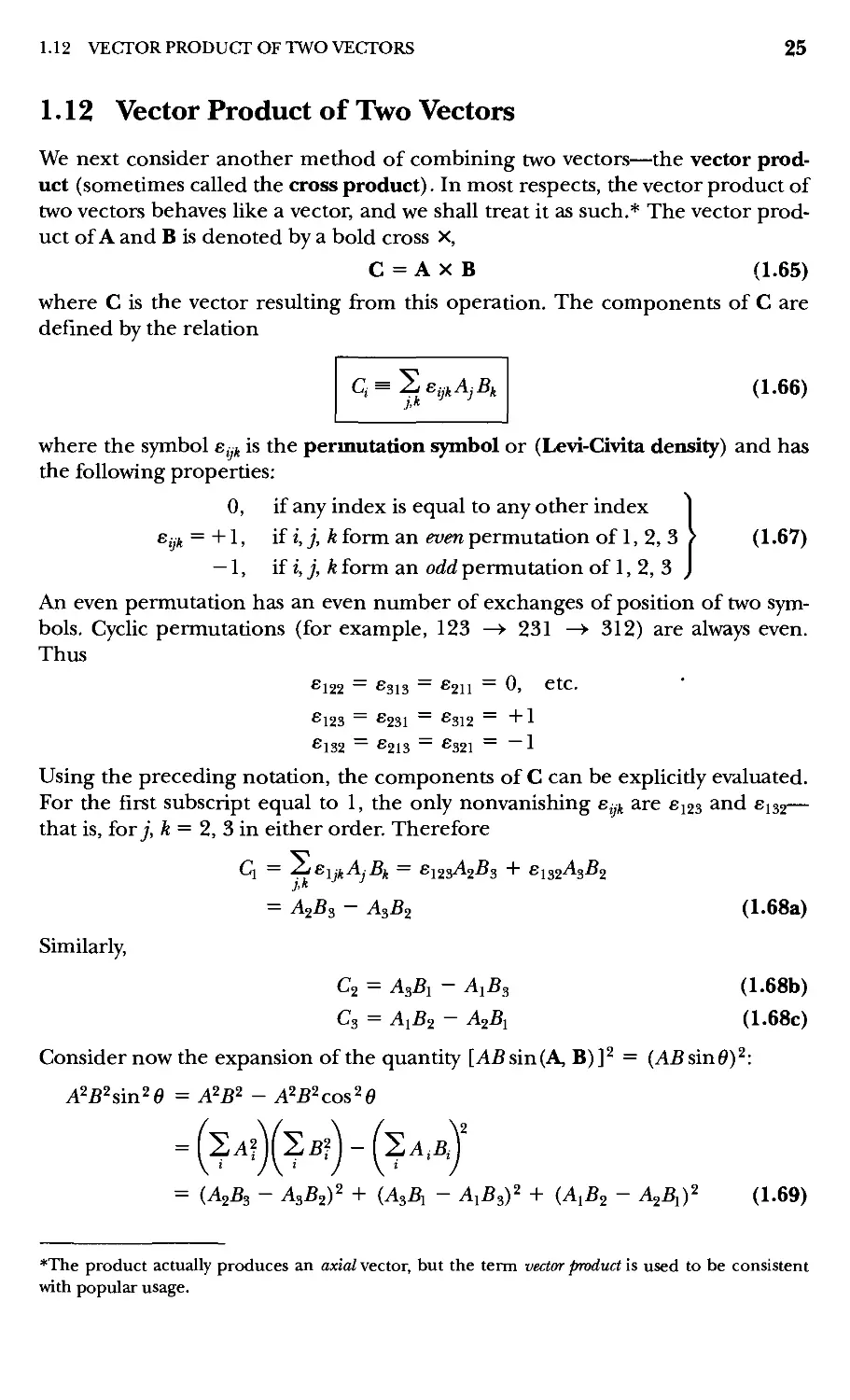
Consider now the expansion of the quantity [AS sin (A, B)]^ = {ABsmO)^:
A^B^sin'^e = A^B"^ - A^B^cos^e
= B.f)(s.F)-B.,.,J
= (A2B3 - A3S2)' + (A3A - A.B^y + (A1B2 - A2A)' A-69)
*The product actually produces an axial vector, but the term vector product is used to be consistent
with popular usage.
26 1 / MATRICES, VECTORS, AND VECTOR CALCULUS
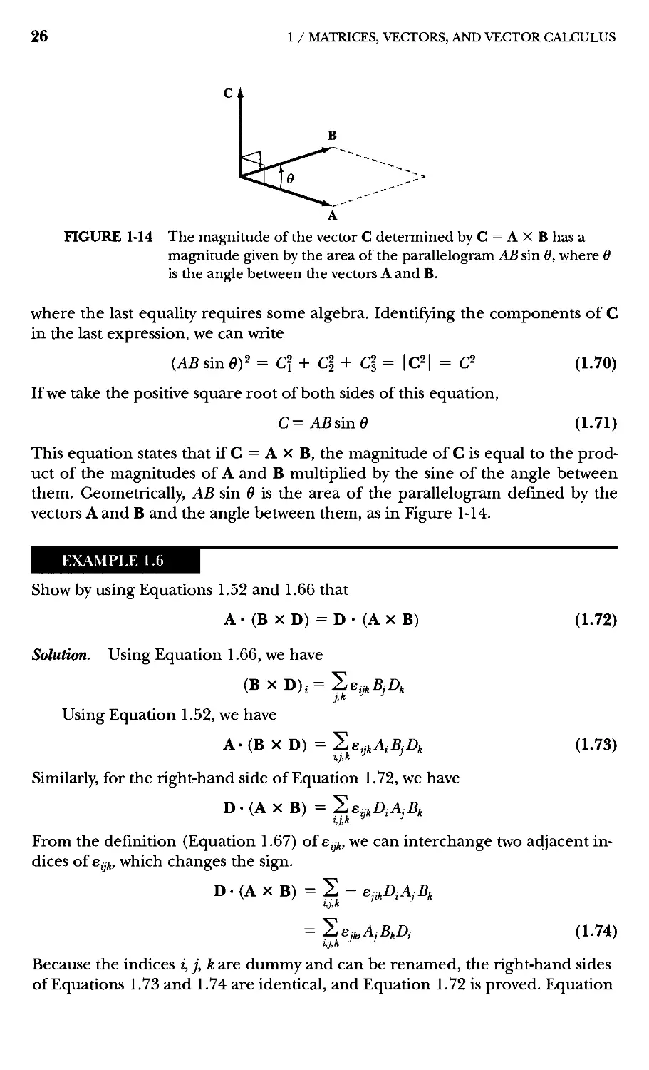
A
FIGURE 1-14 The magnitude of the vector C determined by C = A X B has a
magnitude given by the area of the parallelogram AB sin 6, where 6
is the angle between the vectors A and B.
where the last equality requires some algebra. Identifying the components of C
in the last expression, we can write
{AB sin 0J = Cf + Ci + Ci = IC^I = C^ A.70)
If we take the positive square root of both sides of this equation,
C=ABsine A.71)
This equation states that if C = A X B, the magnitude of C is equal to the
product of the magnitudes of A and B multiplied by the sine of the angle between
them. Geometrically, AB sin 6 is the area of the parallelogram defined by the
vectors A and B and the angle between them, as in Figure 1-14.
EXAMPLE 1.6
Show by using Equations 1.52 and 1.66 that
A • (B X D) = D • (A X B) A.72)
Solution. Using Equation 1.66, we have
(B X D), = Se^,B,A
j.k
Using Equation 1.52, we have
A-(BXD) =Se,,A,B,A A-73)
Similarly, for the right-hand side of Equation 1.72, we have
D-(AXB) =l>Sij,D,AjB,
From the definition (Equation 1.67) of e^t, we can interchange two adjacent
indices of fiyt, which changes the sign.
D.(AXB) =S-e,„AA,B,
= l,ej„AjB,D, A.74)
Because the indices i, j, k are dummy and can be renamed, the right-hand sides
of Equations 1.73 and 1.74 are identical, and Equation 1.72 is proved. Equation
1.12 VECTOR PRODUCT OF TWO VECTORS 2?
1.72 can also be written as A • (B X D) = (A X B) • D, indicating that the scalar
and vector products can be interchanged as long as the vectors stay in the order
A, B, D. Notice that, if we let B = A, we have
A • (A X D) = D • (A X A) = 0
showing that A X D must be perpendicular to A.
A X B (i.e., C) is perpendicular to the plane defined by A and B because
A • (A X B) = 0 and B • (A X B) = 0. Because a plane area can be represented
by a vector normal to the plane and of magnitude equal to the area, C is
evidently such a vector. The positive direction of C is chosen to be the direction of
advance of a right-hand screw when rotated from A to B.
The definition of the vector product is now complete; components,
magnitude, and geometrical interpretation have been given. We may therefore
reasonably expect that C is indeed a vector The ultimate test, however, is to examine
the transformation properties of C, and C does, in fact, transform as a vector
under a proper rotation.
We should note the following properties of the vector product that result
from the definitions:
(a) A X B = -B X A A.75)
but, in general,
(b) A X (B X C) 7^ (A X B) X C A.76)
Another important result (see Problem 1-22) is
A X (B X C) = (A • C)B - (A • B)C A.77)
EXAMPLE 1.7
Find the product of (A X B) • (C X D).
Solution.
J,k •' ■'
(CxD), = Se,,„QZ)„
The scalar product is then computed according to Equation 1.52:
(A X B) • (C X D) = SfSei,,A,BjfSe;,„QZ)J
Rearranging the summations, we have
(A X B) • (C X D) =S \le,uBiJ\A,B^CiD^
l,m \ t ^ I ^
where the indices of the e's have been permuted (twice each so that no sign
change occurs) to place in the third position the index over which the sum is
-I / iVlrt.1 J^H_iI!ji3, \ nXjX\JI^i3, ^\1^LJ VrjVj-lV-'I^ V-jrVl_i\_jUl_,Ui3
carried out. We can now use an important property of the e,-j (see Problem 1-22):
A.78)
■^^ijk^lmk ~ ^il^jm "im^jl
We therefore have
(A X B) • (C X D) =S (Sj,S,„ - Sj„du)AjB,QD„
l,m
Carrying out the summations over ^'and k, the Kronecker deltas reduce the
expression to
(A X B) • (C X D) = S (AB^QD^ - A^BiQDJ
This equation can be rearranged to obtain
(A X B) . (C X D) = \^aA\^B^d}j - \^bA\^A„d}j
Because each term in parentheses on the right-hand side is just a scalar product,
we have, finally,
(AX B)-(C X D) = (A-C)(B-D) - (B-C)(A-D)
The orthogonality of the unit vectors e; requires the vector product to be
Cj X ej = e^ i,], k in cyclic order A.79a)
We can now use the permutation symbol to express this result as
-Xe^.= Se,e^,
A.79b)
The vector product C = A X B, for example, can now be expressed as
C = Se^,e,A,B, A.80a)
By direct expansion and comparison with Equation 1.80a, we can verify a de-
terminantal expression for the vector product:
ei 62 as
C = A X B = Ai A2 A3
5i ^ £3
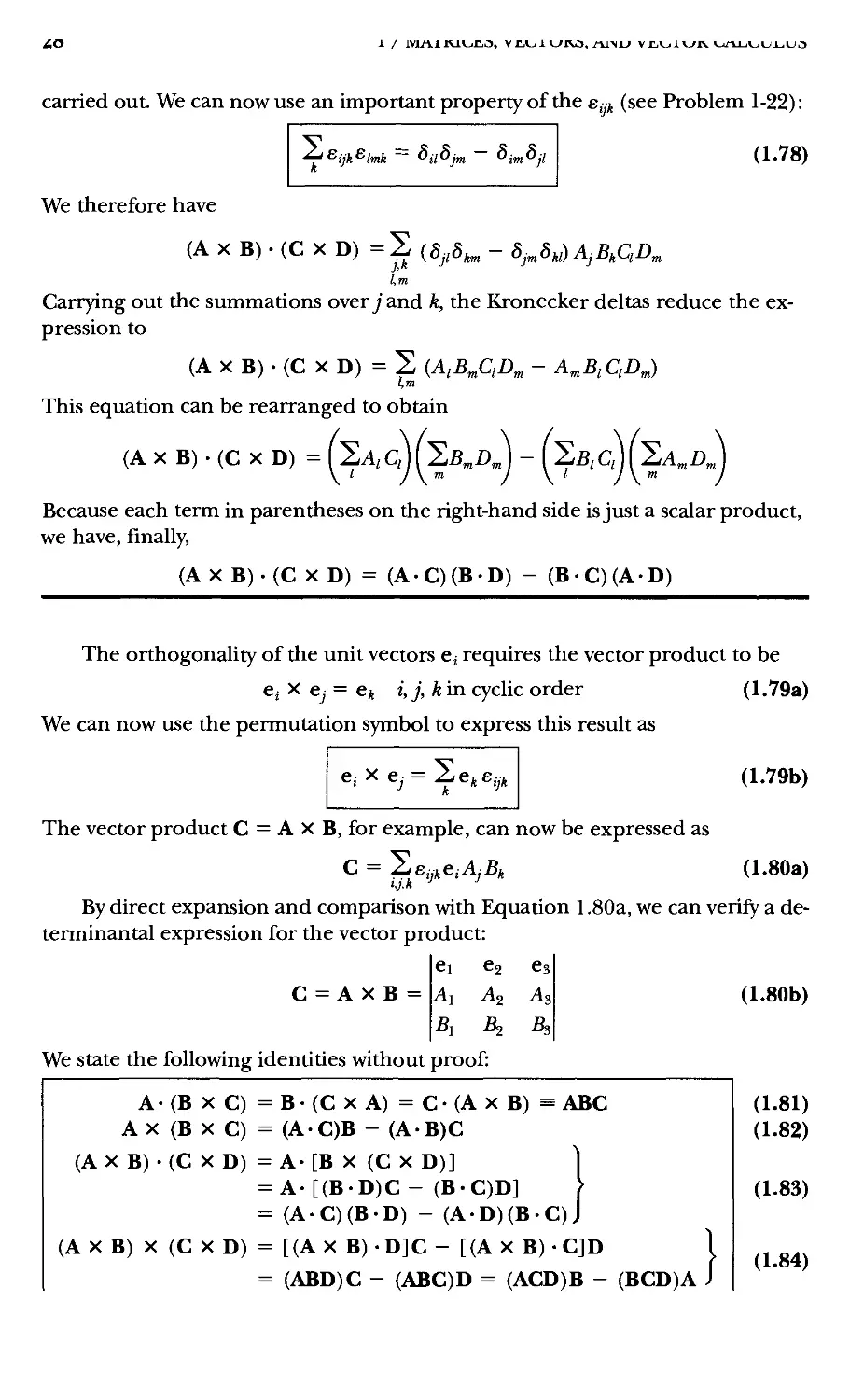
We state the following identities without proof:
A(B X C) = B(C X A) = C(A X B) = ABC
A X (B X C) = (AC)B - (AB)C
(A X B) • (C X D) = A- [B X (C X D)]
= A-[(B-D)C - (B-C)D]
= (A-C)(B-D) - (A-D)(B-C)
(AX B) X (C X D) = [(AX B)-D]C - [(A X B)-C]D
= (ABD)C - (ABC)D = (ACD)B - (BCD)A
}
A.80b)
A.81)
A.82)
A.83)
A.84)
1.13 DIFFERENTIATION OF A VECTOR WITH RESPECT TO A SCALAR
29
1.13 Differentiation of a Vector
witii Respect to a Scalar
If a scalar function (f) = <^(s) is differentiated with respect to the scalar variable s,
then, because neither part of the derivative can change under a coordinate
transformation, the derivative itself cannot change and must therefore be a
scalar; that is, in the x^ and x- coordinate systems, (f) = (f)' and s = s', so rf<^ = d(f)'
and ds = ds'. Hence
d4>
ds
d4>'
ds'
d^\
ds)
Similarly, we can formally define the differentiation of a vector A with
respect to a scalar s. The components of A transform according to
A'i = S A,-,A, A.85)
j
Therefore, on differentiation, we obtain (because the A,-, are independent of s')
dA'i _ d
ds' as J - ' J
■^ -^ dAj
Because s and s' are identical, we have
ds' \ds) j \ds)
Thus the quantities dAj/ds transform as do the components of a vector and
hence are the components of a vector, which we can write as dA/ds.
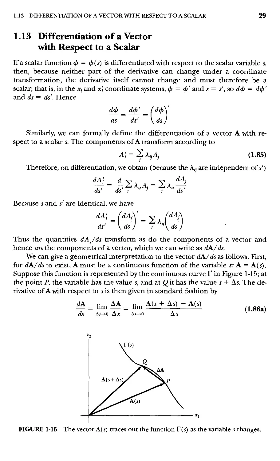
We can give a geometrical interpretation to the vector dA/ds as follows. First,
for dA/ds to exist, A must be a continuous function of the variable s: A = A{s).
Suppose this function is represented by the continuous curve F in Figfure 1-15; at
the point P, the variable has the value s, and at Qit has the value s + As. The
derivative of A with respect to s is then given in standard fashion by
^= lim ^= lim Ms+As)-Ais)
ds Ai->o As Aj->o As
A.86a)
FIGURE 1-15 The vector A(i) traces out the function r(s) as the variable i changes.
30 1 / MATRICES, VECTORS, AND VECTOR CALCULUS
The derivatives of vector sums and products obey the rules of ordinary
vector calculus. For example,
d dA rfB
-(A + B) = — + — A.86b)
ds ds ds
d dB dA
-(A-B) =A-—+ —-B A.86c)
ds ds ds
d ^ ^ dB dA
-~(A XB)=AX-- + --XB A.86d)
ds ds ds
d , , , dA d(f>
~-{4>A)=4>— + ^A A.86e)
ds ds ds
and similarly for total differentials and for partial derivatives.
1.14 Examples of Derivatives—
Velocity and Acceleration
Of particular importance in the development of the dynamics of point particles
(and of systems of particles) is the representation of the motion of these
particles by vectors. For such an approach, we require vectors to represent the
position, velocity, and acceleration of a given particle. It is customary to specify the
position of a particle with respect to a certain reference frame by a vector r, which
is in general a function of time: r = r(t). The velocity vector v and the acceleration
vector a are defined according to
v^- = r A.87)
d\ d^r
where a single dot above a symbol denotes the first time derivative, and two dots
denote the second time derivative. In rectangular coordinates, the expressions
for r, V, and a are
r = Xjei -I- ^262 + Xjej = 2j x^Ci Position
V = f = 2jXiei = 2j — Ci Velocity
' ' dt
a = V = r = 2jXi ei = 2j —- e; Acceleration
• i dt^
A.89)
Calculating these quantities in rectangfular coordinates is straightforward because
the unit vectors e, are constant in time. In nonrectangfular coordinate systems,
however, the unit vectors at the position of the particle as it moves in space are
1.14 EXAMPLES OF DERIVATIVES—VELOCITY AND ACCELERATION
31
not necessarily constant in time, and the components of the time derivatives of r
are no longer simple relations, as in Equation 1.89. We do not discuss general
curvilinear coordinate systems here, but plane polar coordinates, spherical
coordinates, and cylindrical coordinates are of sufficient importance to warrant a
discussion of velocity and acceleration in these coordinate systems.*
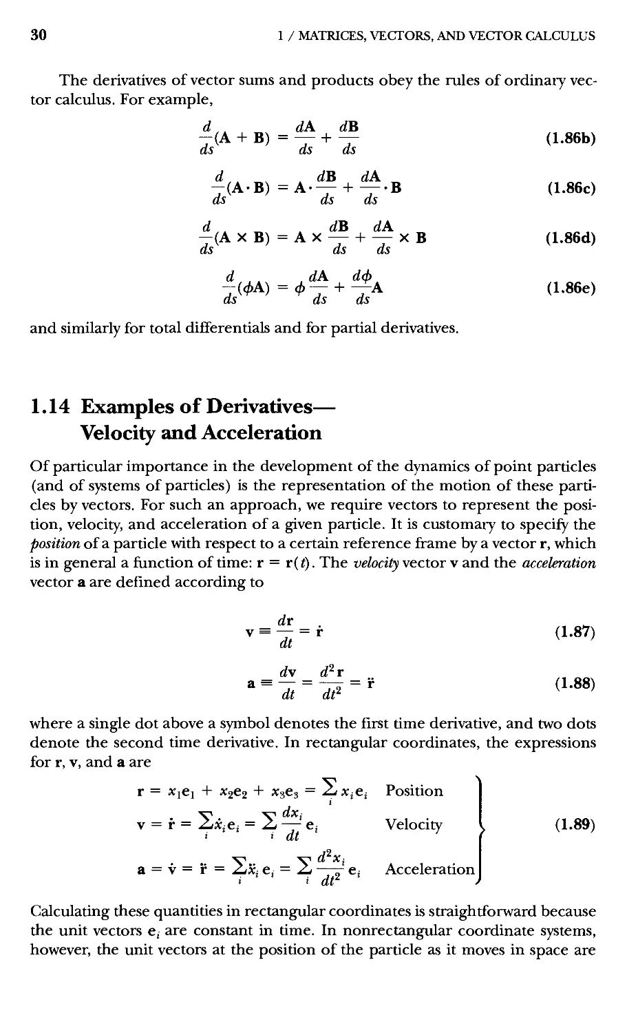
To express v and a in plane polar coordinates, consider the situation in
Figure 1-16. A point moves along the curve s{t) and in the time interval
t^ — t^ = dt moves from P*'' to P*^'. The unit vectors, e^ and eg, which are
orthogonal, change from ej^'' to e*^' and from e^'' to e^^' . The change in e^ is
e^2) _ e(i) = de, A.90)
which is a vector normal to e^ (and, therefore, in the direction of eg). Similarly,
the change in e^ is
eB) - e(i) = rfe.
which is a vector normal to eg. We can then write
and
de^ = dOeg
den = —dOe^
A.91)
A.92)
A.93)
where the minus sign enters the second relation because de^ is directed opposite
to e^ (see Figure 1-16).
FIGURE 1-16 An object traces out the curve s{f) over time. The unit vectors e^ and eg
and their differentials are shown for two position vectors rj and r^.
* Refer to the figures in Appendix F for the geometry of these coordinate systems.
32
1 / MATRICES, VECTORS, AND VECTOR CALCULUS
Equations 1.92 and 1.93 are perhaps easier to see by referring to Figure 1-16.
In this case, de^ subtends an angle dO with unit sides, so it has a magnitude of dd.
It also points in the direction of eg, so we have de^ = dOcg. Similarly, dcg subtends
an angle d6 with unit sides, so it also has a magnitude of dO, but from Figure 1-16
we see that dcg points in the direction of — e^ so we have dcg = —dOCr.
Dividing each side of Equations 1.92 and 1.93 by dt, we have
A.94)
A.95)
If we express v as
dr d
= rcr + re^
we have immediately, using Equation 1.94,
V = r = fe. -I- rdcg
A.96)
A.97)
so that the velocity is resolved into a radial component f and an angular (or
transverse) component rO.
A second differentiation yields the acceleration:
dt
(re, + re eg)
= rCr + fe, + rOeg + rOcg + rOcg
= (r - re^)er + (r0 + 2re)eg
A.98)
so that the acceleration is resolved into a radial component (r — r6^) and an
angfular (or transverse) component {rO + 2f6).
The expressions for ds, ds^, v'^, and v in the three most important
coordinate systems (see also Appendix F) are
Rectangular coordinates {x, y, z)
ds = dx^ei + dx'^e^ + dx^e^
ds^ = rfxf + dx\ + dx\
v^ = x\ + x\ + x\
A.99)
Spherical coordinates (r, 0, <f))
ds = drCr + rdOeg + r sin 0 d4>e^
ds^ = dr^ + r^dO^ + r^sin^e d<f)^
V = fe, + rOeg + r sin 0 <^e^
A.100)
1.14 EXAMPLES OF DERIVATIVES—VELOCITY AND ACCELERATION
33
(The expressions for plane polar coordinates result from Equation 1.100 by
setting dcl> = 0.)
Cylindrical coordinates (r, <f), z)
ds = drCr + rd<f)e^ + dze,
ds^ = dr^ + r^dcf)^ + rfz?
v^ = f^ + r^^ + z2
y = rer+ r^e^ + ze^
A.101)
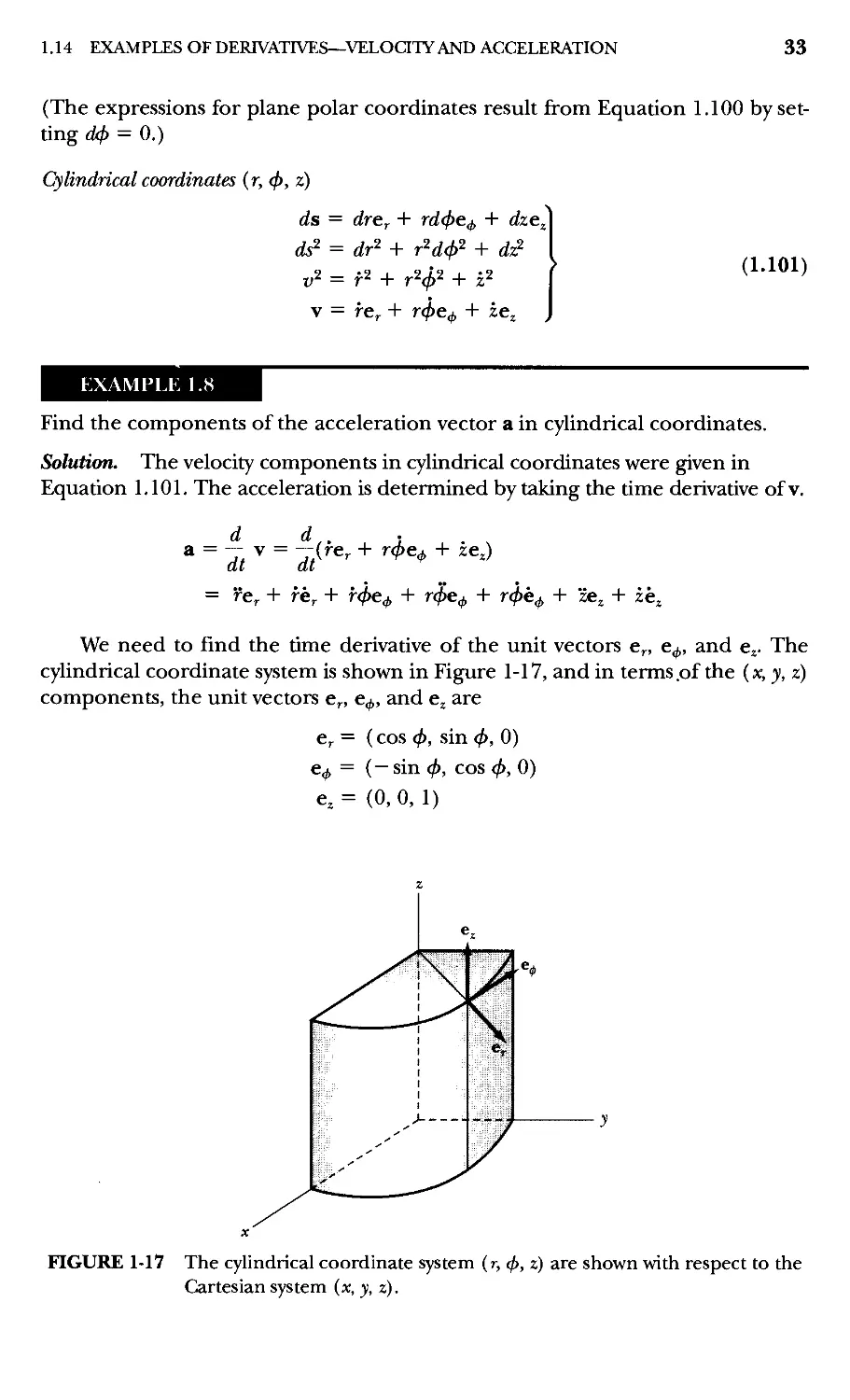
EXAMPLi: 1.8
Find the components of the acceleration vector a in cylindrical coordinates.
Solution. The velocity components in cylindrical coordinates were given in
Equation 1.101. The acceleration is determined by taking the time derivative of v.
d d,. . .
a = -T V = —(re, -I- r<^e^ -I- ze,)
dt dt
= rer + rkr + f<^e^ -I- r4>e^ + r^e^ + ze, -I- ze.
We need to find the time derivative of the unit vectors e^, e^, and e^. The
cylindrical coordinate system is shown in Figfure 1-17, and in terms .of the {x, y, z)
components, the unit vectors e^, e^, and e^ are
e^ = (cos <^, sin <^, 0)
e^ = (-sin<^, cos<^, 0)
e, = @,0,1)
FIGURE 1-17 The cylindrical coordinate system (r, <^, z) are shown with respect to the
Cartesian system (x, j, z).
34 1 / MATRICES, VECTORS, AND VECTOR CALCULUS
The time derivatives of the unit vectors are found by taking the derivatives of
the components.
e,. = (-(^ sin (f), 4> cos 4>, 0) = —<^e^
^4, — i~4> COS (t),~4> sin (f>, 0) = —<f>e^
e, = 0
We substitute the unit vector time derivatives into the above expression for a.
a = re^ + f(^e^ + fc^e^ + r^e^ - r<j>^e, + ze,
= (r - r^^)e^ + (r<^ + 2f<^)e^ + ze^
1.15 Angular Velocity
A point or a particle moving arbitrarily in space may alwa)« be considered, at a
given instant, to be moving in a plane, circular path about a certain axis; that is,
the path a particle describes during an infinitesimal time interval St may be
represented as an infinitesimal arc of a circle. The line passing through the center
of the circle and perpendicular to the instantaneous direction of motion is
called the instantaneous axis of rotation. As the particle moves in the circular
path, the rate of change of the angular position is called the angular velocity:
co = — = e A.102)
dt
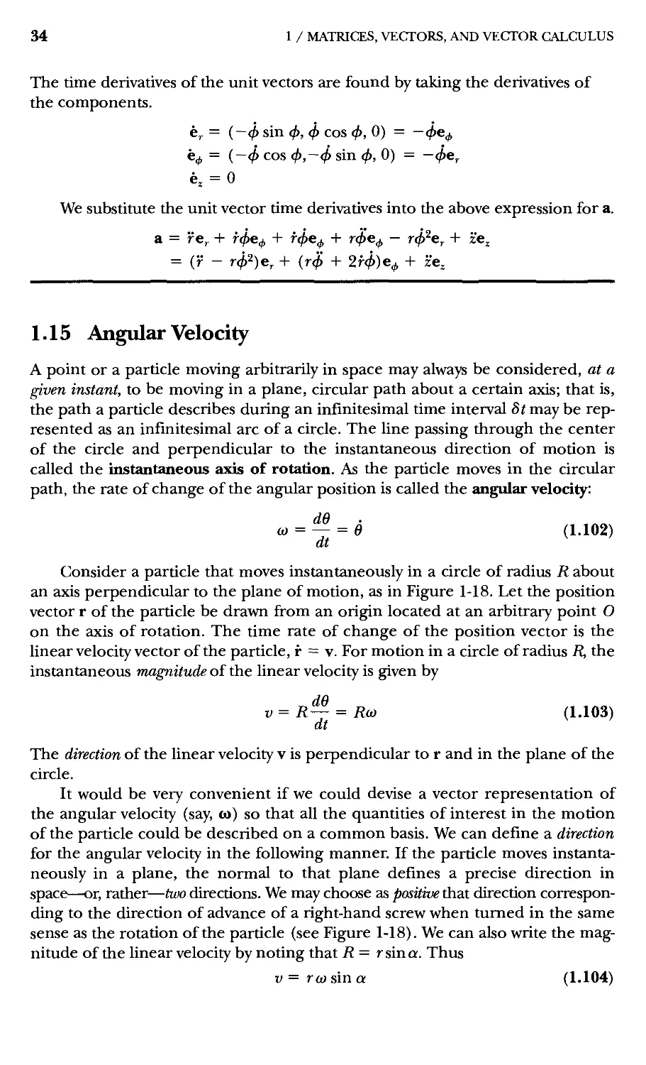
Consider a particle that moves instantaneously in a circle of radius R about
an axis perpendicular to the plane of motion, as in Figure 1-18. Let the position
vector r of the particle be drawn from an origin located at an arbitrary point O
on the axis of rotation. The time rate of change of the position vector is the
linear velocity vector of the particle, r = v. For motion in a circle of radius R, the
instantaneous magnitude of the linear velocity is given by
v=R^ = Ra) A.103)
dt
The direction of the linear velocity v is perpendicular to r and in the plane of the
circle.
It would be very convenient if we could devise a vector representation of
the angular velocity (say, to) so that all the quantities of interest in the motion
of the particle could be described on a common basis. We can define a direction
for the angular velocity in the following manner. If the particle moves
instantaneously in a plane, the normal to that plane defines a precise direction in
space—or, rather—two directions. We may choose as positive that direction
corresponding to the direction of advance of a right-hand screw when turned in the same
sense as the rotation of the particle (see Figure 1-18). We can also write the
magnitude of the linear velocity by noting that R = r sina. Thus
V = ro) sin a A.104)
1.15 ANGULAR VELOCITY
35
FIGURE 1-18 A particle moving ccw about an axis according to the right-hand rule
has an angular velocity (o = v X r about that axis.
Having defined a direction and a magnitude for the angular velocity, we note
that if we write
V = to X r
A.105)
then both of these definitions are satisfied, and we have the desired vector
representation of the angular velocity.
We should note at this point an important distinction between finite and
infinitesimal rotations. An infinitesimal rotation can be represented by a vector
(actually, an axial vector), but a finite rotation cannot. The impossibility of
describing a finite rotation by a vector results from the fact that such rotations do
not commute (see the example of Figure 1-9), and therefore, in general,
different results will be obtained depending on the order in which the rotations are
made. To illustrate this statement, consider the successive application of two
finite rotations described by the rotation matrices Aj and A2. Let us associate the
vectors A and B in a one-to-one manner with these rotations. The vector sum is C =
A -I- B, which is equivalent to the matrix A3 = AgAj. But because vector addition
is commutative, we also have C = B -I- A, with A4 = AjA2. But we know that
matrix operations are not commutative, so that in general A3 ¥= A4. Hence, the
vector C is not unique, and therefore we cannot associate a vector with a finite
rotation.
Infinitesimal rotations do not suffer from this defect of noncommutation. We
are therefore led to expect that an infinitesimal rotation can be represented by a
vector. Although this expectation is, in fact, fulfilled, the ultimate test of the
vector nature of a quantity is contained in its transformation properties. We give
only a qualitative argfument here.
Refer to Figfure 1-19. If the position vector of a point changes from r to r -I-
Sr, the geometrical situation is correctly represented if we write
Sr = Se X r
A.106)
36
1 / MATRICES, VECTORS, AND VECTOR CALCULUS
FIGURE 1-19 The position vector r changes to r + Sr by an infinitesimal
rotation angle SO.
where S6 is a quantity whose magnitude is equal to the infinitesimal rotation
angle and that has a direction along the instantaneous axis of rotation. The
mere fact that Equation 1.106 correctly describes the situation illustrated in
Figfure 1-19 is not sufficient to establish that SQ is a vector. (We reiterate that the
true test must be based on the transformation properties of S6.) But if we show
that two infinitesimal rotation "vectors"—SOj and SQ^—actually commute, the sole
objection to representing a finite rotation by a vector wll have been removed.
Let us consider that a rotation SOj takes r into r -I- Srj, where Srj = SOj X r.
If this is followed by a second rotation SQ^ around a different axis, the initial
position vector for this rotation ig r -I- Srj. Thus
Sr2 = SQ2 X {r + Sri)
and the final position vector for SOj followed by S62 is
r -I- Sri2 = »■ + [8Q1 X r + 862 X (r -I- Sr^)]
Neglecting second-order infinitesimals, then,
Sri2 = SOi X r + 862 X r A.107)
Similarly, if S62 is followed by SOj, we have
luiiuwcu uy uuj, wc iiavc
r -I- Sr2i = r -I- [862 X r + SOj X (r -I- Sr.
.)]
Sr2i = 862 X r -I- SOi X r
A.108)
Rotation vectors Sri2 and Sr2i are equal, so the rotation "vectors" S61 and S62 do
commute. It therefore seems reasonable that S6 in Equation 1.106 is indeed a
vector
1.16 GRADIENT OPERATOR 37
It is the fact that S6 is a vector that allows angular velocity to be represented
by a vector, because angfular velocity is the ratio of an infinitesimal rotation angle
to an infinitesimal time:
se
St
Therefore, dividing Equation 1.106 by Sf, we have
Sr se
— = — X r
St St
or, in passing to the limit, St —> 0,
V = to X r
as before.
1.16 Gradient Operator
We now turn to the most important member of a class called vector differential
operators—the gradient operator.
Consider a scalar <f) that is an explicit function of the coordinates Xj and,
moreover, is a continuous, single-valued function of these coordinates
throughout a certain region of space. Under a coordinate transformation that carries the
Xj into the x,', <f)'{x[, x^, X3) = <f){xi, x^, X3), and by the chain rule of
differentiation, we can write
^ = 2. ——7 A.109)
dXi j dXjdXi
The case is similar for d<f)'/dx2 and d<f)'/dx^, so in general we have
S^^^S^dx, ^^^^^^
dXi j dXjdXi
The inverse coordinate transformation is
Xj = ^Kj< A.111)
Differentiating,
dx- dx- \ k
¥^* I - ^^"Aq^'
SA,,xn = SAJ--^ A.112)
But the term in the last parentheses is just S^, so
3Xj
dx': ~
I = Sa,/,, = A^. A.113)
38 1 / MATRICES, VECTORS, AND VECTOR CALCULUS
Substituting Equation 1.113 into Equation 1.110, we obtain
d<f)' ^ deb
fr = 2a^t^ A.114)
Because it follows the correct transformation equation of a vector (Equation
1.44), the function d<f)/dxj is the^'th component of a vector termed the gradient
of the function <f). Note that even though <^ is a scalar, the gradient of <^ is a vector.
The gradient of <^ is written either as grad (f> or as V<^("del" (fy).
Because the function (f) is an arbitrary scalar function, it is convenient to
define the differential operator described in the preceding in terms of the gradient
operator:
(grad), = V, = £ A.115)
We can express the complete vector gradient operator as
grad = V = 2.6,— Gradient A.116)
t dXi
The gradient operator can (a) operate directly on a scalar function, as in
V<f); (b) be used in a scalar product with a vector function, as in V • A (the
divergence (div) of A); or (c) be used in a vector product with a vector function, as in
V X A (the curloiA). We present the grad, divergence, and curl:
grad<^ = V<^ = Se,^ (LlHa)
divA = V-A = 2.— A.117b)
i dXi
curl A = V X A = lie.^ —^e, A.117c)
>,j,k dXj
To see a physical interpretation of the gradient of a scalar function, consider
the three-dimensional and topographical maps of Figure 1-20. The closed loops
of part b represent lines of constant height. Let cf) denote the height at any point
(f) = <f){xi, x^, Xs). Then
dfj) = Zj—dXi = 2j(V(f>)idXi
• dXj >
The components of the displacement vector ds are the incremental
displacements in the direction of the three orthogonal axes:
ds = {dxi, dx^, dx^) A.118)
Therefore
# = (V(f>)-ds I A.119)
1.16 GRADIENT OPERATOR
39
(a)
(b)
FIGURE 1-20 (a) A three-dimensional contour map can be represented by (b) a
topographical map of lines (f) representing constant height. The
gradient V(f) represents the direction perpendicular to the constant
cf> lines.
Let ds be directed tangentially along one of the isolatitude lines (i.e., along
a line for which <f) = const.), as indicated in Figure 1-20. Because (f) = const, for
this case, dcf) = 0. But, because neither V<^ nor ds is in general zero, they must
therefore be perpendicular to each other. Thus V<^ is normal to the line (or in three
dimensions, to the surface) for which <^ = const.
40 1 / MATRICES, VECTORS, AND VECTOR CALCULUS
The maximum value of dcf) results when Vcf) and ds are in the same
direction; then,
(rf<^)max= |V<^|ds, for V<f,\\ds
or
|V<^|=(^) A.120)
Therefore, V<^ is in the direction of the greatest change in <^.
We can summarize these results as follows:
1. The vector Vcf) is, at any point, normal to the lines or surfaces for which (f) =
const.
2. The vector V(f> has the direction of the maximum change in (f>.
3. Because any direction in space can be specified in terms of the unit vector n
in that direction, the rate of change of <^ in the direction of n (the directional
derivative of <^) can be found from n • V<f) = d<f)/dn.
The successive operation of the gradient operator produces
V-V = 2. = -^^ A-121)
i 3x, dXj > dxf
This important product operator, called the Laplacian,* is also written
A.122)
When the Laplacian operates on a scalar, we have, for example.
VV = 2-^ A.123)
1.17 Integration of Vectors
The vector resulting from the volume integration of a vector function A = A( X;)
throughout a volume V is given by^^
Adv = I A^dv, A^dv, A^dv] A.124)
*After Pierre Simon Laplace A749-1827); the notation V^ is ascribed to Sir William Rowan
Hamilton.
'The symbol Jy actually represents a triple integral over a certain volume V. Similarly, the symbol /j
stands for a double integral over a certain surface S.
1.17 INTEGRATION OF VECTORS
41
FIGURE 1-21 The differential dn is an element of area of the surface. Its direction is
normal to the surface.
Thus, we integrate the vector A throughout V simply by performing three
separate, ordinary integrations.
The integral over a surface S of the projection of a vector fiinction A = A(x;)
onto the normal to that surface is defined to be
A- da
where rfa is an element of area of the surface (Figure 1-21). We write rfaasavec-
tor quantity because we may attribute to it not only a magnitude da but also a
direction corresponding to the normal to the surface at the point in question. If
the unit normal vector is n, then
rfa = nda A.125)
Thus, the components of da are the projections of the element of area on the
three mutually perpendicular planes defined by the rectangular axes:
dai = dx^dx^, etc. A.126)
Therefore, we have
or
A- da
A- da
A- nda
ZjAi dai
A.127)
A.128)
Equation 1.127 states that the integral of A over the surface S is the integral of
the normal component of A over this surface.
The normal to a surface may be taken to lie in either of two possible
directions ("up" or "down"); thus the sign of n is ambigfuous. If the surface is dosed, we
adopt the convention that the outward normal is positive.
The line integral of a vector function A = A(x,) along a given path
extending from the point B to the point C is given by the integral of the component of
42 1 / MATRICES, VECTORS, AND VECTOR CALCULUS
FIGURE 1-22 The element ds is an element of length along the given path from B to
C. Its direction is along the path at a given point.
A along the path
A-ds= ^Adx, A.129)
The quantity ds is an element of length along the given path (Figure 1-22). The
direction of ds is taken to be positive along the direction the path is traversed. In
Figure 1-22 at point P, the angle between ds and A is less than tt/2, so A • ds is
positive at this point. At point Q, the angle is greater than 7r/2, and the
contribution to the integral at this point is negative.
It is often usefiil to relate certain surface integrals to either volume integrals
(Gauss's theorem) or line integrals (Stokes's theorem). Consider Figure 1-23,
which shows a closed volume Fenclosed by the surface S. Let the vector A and its
first derivatives be continuous throughout the volume. Gauss's theorem states
that the surface integral of A over the closed surface S is equal to the volume
integral of the divergence of A (V • A) throughout the volume V enclosed by the
surface S. We write this mathematically as
A-rfa= V-Adv A.130)
s Jv
Gauss's theorem is sometimes also called the divergence theorem. The theorem is
particularly useful in dealing with the mechanics of continuous media.
See Figure 1-24 for the physical description needed for Stokes's theorem,
which applies to an open surface S and the contour path C that defines the
surface. The curl of the vector A (V X A) must exist and be integrable over the
entire surface S. Stokes's theorem states that the line integral of the vector A
around the contour path C is equal to the surface integral of the curl of A over
the surface defined by C. We write it mathematically as
A-ds= (V X A)-rfa A.131)
c Js
where the line integral is around the closed contour path C. Stokes's theorem is
particularly useful in reducing certain surface integrals (two dimensional) to, it
PROBLEMS
43
Surface S
Volume V
FIGURE 1-23 The differential da is an element of area on a surface S that surrounds
a closed volume V.
Surface S
Contour
FIGURE 1-24 A contour path C defines an open surface S. A line integral around the
path Cand a surface integral over the surface S is required for Stokes's
theorem.
is hoped, a simpler line integral (one dimensional). Both Gauss's and Stokes's
theorems have wide application in vector calculus. In addition to mechanics,
they are also usefiil in electromagnetic applications and in potential theory.
PROBLEMS
1-1. Find the transformation matrix that rotates the axis Xj of a rectangular coordinate
system 45° toward Xj around the Xg-axis.
1-2. Prove Equations 1.10 and 1.11 from trigonometric considerations.
1-3. Find the transformation matrix that rotates a rectangular coordinate system
through an angle of 120° about an axis making equal angles with the original three
coordinate axes.
1-4. Show
(a) (AB)' = B'A' (b) (AB)"' = B^A-^
1-5. Show by direct expansion that IaI'^ = 1. For simplicity, take A to be a two-
dimensional orthogonal transformation matrix.
44 1 / MATRICES, VECTORS, AND VECTOR CALCULUS
1-6. Show that Equation 1.15 can be obtained by using the requirement that the
transformation leaves unchanged the length of a line segment.
1-7. Consider a unit cube with one corner at the origin and three adjacent sides lying
along the three axes of a rectangular coordinate system. Find the vectors
describing the diagonals of the cube. What is the angle between any pair of diagonals?
1-8. Let A be a vector from the origin to a point P fixed in space. Let r be a vector from
the origin to a variable point QCxj, X2, Xj). Show that
At = A2
is the equation of a plane perpendicular to A and passing through the point P.
1-9. For the two vectors
A = i + 2j - k, B = -2i + 3j + k
find
(a) A — B and |A — B| (b) component of B jilong A (c) angle between A and B
(d) A X B (e) (A - B) X (A + B)
1-10. A particle moves in a plane elliptical orbit described by the position vector
r = 26 sin 0)ti + b cos cotj
(a) Find v, a, and the particle speed.
(b) What is the angle between v and a at time t = 7r/2ft)?
1-11. Show that the triple scalar product (A X B) • C can be written as
(A X B) • C
Aj Ag Aj
Bi Be, B^
Q C^ Cg
Show also that the product is unaffected by an interchange of the scalar and vector
product operations or by a change in the order of A, B, C, as long as they are in
cyclic order; that is,
(A X B) • C = A- (B X C) = B • (C X A) = (C X A) • B, etc.
We may therefore use the notation ABC to denote the triple scalar product. Finally,
give a geometric interpretation of ABC by computing the volume of the
parallelepiped defined by the three vectors A, B, C.
1-12. Let a, b, c be three constant vectors drawn from the origin to the points A, B, C.
What is the distance from the origin to the plane defined by the points A, B, C?
What is the area of the triangle ABC?
1-13. X is an unknown vector satisfying the following relations involving the known
vectors A and B and the scalar 4>,
AXX = B, A-X = <^.
Express X in terms of A, B, cf>, and the magnitude of A.
PROBLEMS 45
1-14. Consider the following matrices:
1
0
2
2
3
0
-1
1
1
2
0
1
1
-1
1
0
2
3
Find the following
(a) |AB| (b)AC (c) ABC (d) AB - B'A'
1-15. Find the values of a needed to make the following transformation orthogonal.
1-16. What surface is represented by r • a = const, that is described if a is a vector of
constant magnitude and direction from the origin and r is the position vector to the
point P(xi, X2, Xj) on the surface?
1-17. Obtain the cosine law of plane trigonometry by interpreting the product (A — B) •
(A — B) and the expansion of the product.
1-18. Obtain the sine law of plane trigonometry by interpreting the product A X B and
the alternate representation (A — B) X B.
1-19. Derive the following expressions by using vector jilgebra:
(a) cos (« — /?)= cos a cos /3 + sin a sin /3
(b) sin (a — P) = sin a cos /? — cos a sin /3
1-20. Show that
(a) Se^t S,y = 0 (bJei,tep= 2Si, (c) ^e^j^ e^j^ = 6
1-21. Show (see also Problem 1-11) that
ABC = 2e„tAifi,qi
1-22. Evaluate the sum .Z^ey^e,^ (which contains 3 terms) by considering the result for
Jill possible combinations of i, j, 4 m; that is,
(a) i = j (b) i= I (c) i—m (d) j = I (e) j = m (f) 1= m
(g) i¥^ lor m (h) j ¥^ lor m
Show that
and then use this result to prove
A X (B X C) = (A • C)B - (A • B)C
46 1 / MATRICES, VECTORS, AND VECTOR CALCULUS
1-23. Use the 6,^^ notation and derive the identity
(A X B) X (C X D) = (ABD)C - (ABC)D
1-24. Let A be an arbitrary vector, and let e be a unit vector in some fixed direction. Show
that
A = e(A • e) + e X (A X e)
What is the geometrical significance of each of the two terms of the expansion?
1-25. Find the components of the acceleration vector a in spherical coordinates.
1-26. A particle moves with v = const, along the curve r = k(l + cos 6) (a cardioid). Find
r • e,- = a • e,-, I a I, and 0.
1-27. If r and f = v are both explicit functions of time, show that
—[r X (v X r)] = r^a + (r-v)v - (v^ + r-a)r
dt
1-28. Show that
V(ln|r|) =-
r'-
1-29. Find the angle between the surfaces defined by r^ = 9 and x + 3) + z^ = 1 at the
pointB,-2, 1).
1-30. Show that VCc^i/^) = (^Vi/^ + i/'Vc^.
1-31. Show that
(a) Vr" = nr(''-2)r (b) V/(r) = -^ (c) V^Cln r) = ^
rdf 1
f (c) V2(ln r) = -
r dr r'-
1-32. Show that
Bar-r + 2br-r)dt = ar^ + br'^ + const.
where ris the vector from the origin to the point (x,, X2, x^). The quantities rand r
are the magnitudes of the vectors r and r, respectively, and a and b are constants.
1-33. Show that
/f rA , r „
-]dt=- + C
■ V ^ ) ^
where C is a constant vector
PROBLEMS 47
1-34. Evaluate the integral
A X Adt
1-35. Show that the volume common to the intersecting cylinders defined by x^ + y^ = a^
and x'^ + z^ = a^\&V= 16ay3.
1-36. Find the value of the integral /jA- da, where A= x\ — y] + zk and Sis the closed
surface defined by the cylinder c^ = x'^ + y'^. The top and bottom of the cylinder
are at 2 = rf and 0, respectively.
1-37. Find the value of the integral /jA- da, where A= {x^ + y'^ + z^) (xi + y'} + zk) and
the surface S is defined by the sphere B? = x'^ + y'^ + z^. Do the integral direcdy
and also by using Gauss's theorem.
1-38. Find the value of the integral Ss (V X A) • da if the vector A = yi + z] + xk and S is
the surface defined by the paraboloid 2 = 1 — x^ — 31^, where 2 > 0.
1-39. A plane passes through the three points (x, y, 2) = A, 0, 0), @, 2, 0), @, 0, 3).
(a) Find a unit vector perpendicular to the plane, (b) Find the distance from the
point A, 1, 1) to the closest point of the plane and the coordinates of the closest
point.
1-10. The height of a hill in meters is given by 2 = 2xy — 3x^ — Af — \Sx + 283) +12,
where x is the distance east and y is the distance north of the origin, (a) Where is
the top of the hill and how high is it? (b) How steep is the hill at x = 3) = 1, that is,
what is the angle between a vector perpendicular to the hill and the 2 axis? (c) In
which compass direction is the slope at x = 31 = 1 steepest?
1-41. For what values of a are the vectors A = 2ai — 2j + ak and B = ai + 2aj + 2k
perpendicular?
CHAPTER
Newtonian Mechanics-
Single Particle
2.1 Introduction
The science of mechanics seeks to provide a precise and consistent
description of the dynamics of particles and systems of particles, that is, a set of
physical laws mathematically describing the motions of bodies and aggregates of
bodies. For this, we need certain fundamental concepts such as distance and
time. The combination of the concepts of distance and time allows us to
define the velocity and acceleration of a particle. The third fundamental
concept, mass, requires some elaboration, which we give when we discuss
Newton's laws.
Physical laws must be based on experimental fact. We cannot expect a
priori that the gravitational attraction between two bodies must vary exactly as
the inverse square of the distance between them. But experiment indicates
that this is so. Once a set of experimental data has been correlated and a
postulate has been formulated regarding the phenomena to which the data refer,
then various implications can be worked out. If these implications are all
verified by experiment, we may believe that the postulate is generally true. The
postulate then assumes the status of a physical law. If some experiments
disagree with the predictions of the law, the theory must be modified to be
consistent with the facts.
Newton provided us with the fundamental laws of mechanics. We state these
laws here in modem terms, discuss their meaning, and then derive the implications
48
2.2 NEWTON'S LAWS 49
of the laws in various situations.* But the logical structure of the science of
mechanics is not straightforward. Our line of reasoning in interpreting Newton's laws
is not the only one possible.^ We do not pursue in any detail the philosophy of
mechanics but rather give only sufficient elaboration of Newton's laws to allow us to
continue with the discussion of classical dynamics. We devote our attention in this
chapter to the motion of a single particle, leaving systems of particles to be
discussed in Chapters 9 and 11-13.
2.2 Newton's Laws
We begin by simply stating in conventional form Newton's laws of mechanics^:
I. A body remains at rest or in uniform motion unless acted upon by a force.
II. A body acted upon by a force moves in such a manner that the time rate of change of
momentum equals the force.
in. If two bodies exert forces on each other, these forces are equal in magnitude and
opposite in direction.
These laws are so familiar that we sometimes tend to lose sight of their true
significance (or lack of it) as physical laws. The First Law, for example, is
meaningless without the concept of "force," a word Newton used in all three laws. In
fact, standing alone, the First Law conveys a precise meaning only for zero force;
that is, a body remaining at rest or in uniform (i.e., unaccelerated, rectilinear)
motion is subject to no force whatsoever A body moving in this manner is
termed a free body (or free particle). The question of the frame of reference
with respect to which the "uniform motion" is to be measured is discussed in the
following section.
In pointing out the lack of content in Newton's First Law, Sir Arthur
Eddington§ observed, somewhat facetiously, that all the law actually says is that
"every particle continues in its state of rest or uniform motion in a straight line
*Truesdell (Tr68) points out that Leonhard Euler A707-1783) clarified and developed the
Newtonian concepts. Euler "put most of mechanics into its modern form" and "made mechanics
simple and easy" (p. 106).
fErnst Mach A838-1916) expressed his view in his famous book first published in 1883; E. Mach, Die
Mechanic in ihrerEntwicklung historisch-kritisch dargestellt [The science of mechanics] (Prague, 1883).
A translation of a later edition is available (Ma60). Interesting discussions are also given by
R. B. Lindsay and H. Margeneau (Li36) and N. Feather (Fe59).
{Enunciated in 1687 by Sir Isaac Newton A642-1727) in his Philosophiae naturalis principia mathemat-
ica [Mathematical principles of natural philosophy, normally called Principia] (London, 1687). Previously,
Galileo A564—1642) generalized the results of his own mathematical experiments with statements
equivalent to Newton's First and Second Laws. But Galileo was unable to complete the description of
dynamics because he did not appreciate the significance of what would become Newton's Third
Law—and therefore lacked a precise meaning of force.
§Sir Arthur Eddington (Ed30, p. 124).
50 2 / NEWTONIAN MECHANICS—SINGLE PARTICLE
except insofar as it doesn't." This is hardly fair to Newton, who meant something
very definite by his statement. But it does emphasize that the First Law by itself
provides us with only a qualitative notion regarding "force."
The Second Law provides an explicit statement: Force is related to the time
rate of change of momentum. Newton appropriately defined momentum
(although he used the term quantity of motion) to be the product of mass and
velocity, such that
p = my B.1)
Therefore, Newton's Second Law can be expressed as
dp d
F = ^ = -(my) B.2)
at at
The definition of force becomes complete and precise only when "mass" is
defined. Thus the First and Second Laws are not really "laws" in the usual sense;
rather, they may be considered definitions. Because length, time, and mass are
concepts normally already understood, we use Newton's First and Second Laws
as the operational definition of force. Newton's Third Law, however, is indeed a
law. It is a statement concerning the real physical world and contains all of the
physics in Newton's laws of motion.*
We must hasten to add, however, that the Third Law is not a general law of
nature. The law does apply when the force exerted by one (point) object on
another (point) object is directed along the line connecting the objects. Such
forces are called central forces; the Third Law applies whether a central force is
attractive or repulsive. Gravitational and electrostatic forces are central forces,
so Newton's laws can be used in problems involving these types of forces.
Sometimes, elastic forces (which are actually macroscopic manifestations of
microscopic electrostatic forces) are central. For example, two point objects
connected by a straight spring or elastic string are subject to forces that obey the
Third Law. Any force that depends on the velocities of the interacting bodies is
noncentral, and the Third Law may not apply. Velocity-dependent forces are
characteristic of interactions that propagate with finite velocity. Thus the force
between moving electric charges does not obey the Third Law, because the force
propagates with the velocity of light. Even the gravitational force between
moving bodies is velocity dependent, but the effect is small and difficult to detect.
The only observable effect is the precession of the perihelia of the inner planets
(see Section 8.9). We will return to a discussion of Newton's Third Law in
Chapter 9.
To demonstrate the significance of Newton's Third Law, let us paraphrase it
in the following way, which incorporates the appropriate definition of mass:
*The reasoning presented here, viz., that the First and Second Laws are actually definitions and that
the Third Law contains the physics, is not the only possible interpretation. Lindsay and Margenau
(Li36), for example, present the first two Laws as physical laws and then derive the Third Law as a
consequence.
2.2 NEWTON'S LAWS 51
III'. If two bodies constitute an ideal, isolated system, then the accelerations of these bodies
are always in apposite directions, and the ratio of the magnitudes of the accelerations
is constant. This constant ratio is the inverse ratio of the masses of the bodies.
With this statement, we can give a practical definition of mass and therefore give
precise meaning to the equations summarizing Newtonian dynamics. For two
isolated bodies, 1 and 2, the Third Law states that
B.3)
B.4a)
Using the definition of force
or, with constant masses,
and, because acceleration is
Hence,
Fi =
; as given by
dpi _
dt
'•m-
-F2
the Second Law, we
dp2
dt
( dy^
the time derivative of velocity.
Wi(ai) =
m^
mi
W2(-a2)
_ai
a^
have
B.4b)
B.4c)
B.5)
where the negative sign indicates only that the two acceleration vectors are
oppositely directed. Mass is taken to be a positive quantity.
We can always select, say, mi as the unit mass. Then, by comparing the ratio
of accelerations when mi is allowed to interact with any other body, we can
determine the mass of the other body. To measure the accelerations, we must have
appropriate clocks and measuring rods; also, we must choose a suitable
coordinate system or reference frame. The question of a "suitable reference frame" is
discussed in the next section.
One of the more common methods of determining the mass of an object is
by weighing—for example, by comparing its weight to that of a standard by
means of a beam balance. This procedure makes use of the fact that in a
gravitational field the weight of a body is just the gravitational force acting on the body;
that is, Newton's equation F = ma. becomes W = mg, where g is the acceleration
due to gravity. The validity of using this procedure rests on a fundamental
assumption: that the mass m appearing in Newton's equation and defined
according to Statement III' is equal to the mass m that appears in the gravitational force
equation. These two masses are called the inertial mass and gravitational mass,
respectively. The definitions may be stated as follows:
Inertial Mass: That mass determining the acceleration of a body under the action of a
given force.
Gravitational Mass: That mass determining the gravitational forces between a body
and other bodies.
52 2 / NEWTONIAN MECHANICS—SINGLE PARTICLE
Galileo was the first to test the equivalence of inertial and gravitational mass
in his (perhaps apocryphal) experiment with falling weights at the Tower of Pisa.
Newton also considered the problem and measured the periods of pendula of
equal lengths but with bobs of different materials. Neither Newton nor Galileo
found any difference, but the methods were quite crude.* In 1890 Eotvos^
devised an ingenious method to test the equivalence of inertial and gravitational
masses. Using two objects made of different materials, he compared the effect of
the Earth's gravitational force (i.e., the weight) with the effect of the inertial
force caused by the Earth's rotation. The experiment involved a null method
using a sensitive torsion balance and was therefore highly accurate. More recent
experiments (notably those of Dicke^), using essentially the same method, have
improved the accuracy, and we know now that inertial and gravitational mass are
identical to within a few parts in 10^^. This result is considerably important in the
general theory of relativity.^ The assertion of the exact equality of inertial and
gravitational mass is termed the principle of equivalence.
Newton's Third Law is stated in terms of two bodies that constitute an
isolated system. It is impossible to achieve such an ideal condition; every body in the
universe interacts with every other body, although the force of interaction may be
far too weak to be of any practical importance if great distances are involved.
Newton avoided the question of how to disentangle the desired effects from all
the extraneous effects. But this practical difficulty only emphasizes the enormity
of Newton's assertion made in the Third Law. It is a tribute to the depth of his
perception and physical insight that the conclusion, based on limited
observations, has successfully borne the test of experiment for 300 years. Only within the
20th century did measurements of sufficient detail reveal certain discrepancies
with the predictions of Newtonian theory. The pursuit of these details led to the
development of relativity theory and quantum mechanics."
Another interpretation of Newton's Third Law is based on the concept of
momentum. Rearranging Equation 2.4a gives
|(Pl + P2) = 0
or
Pi + P2 = constant B.6)
The statement that momentum is conserved in the isolated interaction of two
particles is a special case of the more general conservation of linear
momentum. Physicists cherish general conservation laws, and the conservation of
linear momentum is believed always to be obeyed. Later we shall modify our defi-
*In Newton's experiment, he could have detected a difference of only one part in 10^.
fRoland von Eotvos A848-1919), a Hungarian baron; his research in gravitational problems led to
the development of a gravimeter, which was used in geological studies.
JR G. Roll, R Krotkov, and R. H. Dicke, Ann. Phys. (N.Y.) 26, 442 A964). See also Braginsky and
Pavov, Sov Phys.-JETP 34, 463 A972).
§See, for example, the discussions by P. G. Bergmann (Be46) and J. Weber (We61). Weber's book
also provides an analysis of the Eotvos experiment.
llSee also Section 2.8.
2.3 FRAMES OF REFERENCE 53
nition of momentum from Equation 2.1 for high velocities approaching the
speed of light.
2.3 Frames of Reference
Newton realized that, for the laws of motion to have meaning, the motion of
bodies must be measured relative to some reference frame. A reference frame is
called an inertial frame if Newton's laws are indeed valid in that frame; that is, if
a body subject to no external force moves in a straight line with constant velocity
(or remains at rest), then the coordinate system establishing this fact is an
inertial reference frame. This is a clear-cut operational definition and one that also
follows from the general theory of relativity.
If Newton's laws are valid in one reference frame, then they are also valid in
any reference frame in uniform motion (i.e., not accelerated) with respect to
the first system.* This is a result of the fact that the equation F = mr involves the
second time derivative of r: A change of coordinates involving a constant velocity
does not influence the equation. This result is called Galilean invariance or the
principle of Newtonian relativity.
Relativity theory has shown us that the concepts of absolute rest and an
absolute inertial reference frame are meaningless. Therefore, even though we
conventionally adopt a reference frame described with respect to the "fixed" stars—
and, indeed, in such a frame the Newtonian equations are valid to a high degree
of accuracy—such a frame is, in fact, not an absolute inertial frame. We may,
however, consider the "fixed" stars to define a reference frame that
approximates an "absolute" inertial frame to an extent quite sufficient for our present
purposes.
Although the fixed-star reference frame is a conveniently definable system
and one suitable for many purposes, we must emphasize that the fundamental
definition of an inertial frame makes no mention of stars, fixed or otherwise. If a
body subject to no force moves with constant velocity in a certain coordinate
system, that system is, by definition, an inertial frame. Because precisely describing
the motion of a real physical object in the real physical world is normally
difficult, we usually resort to idealizations and approximations of varying degree;
that is, we ordinarily neglect the lesser forces on a body if these forces do not
significantly affect the body's motion.
If we wish to describe the motion of, say, a free particle and if we choose for
this purpose some coordinate system in an inertial frame, then we require that
the (vector) equation of motion of the particle be independent of the position of
the origin of the coordinate system and independent of its orientation in space.
We further require that time be homogeneous; that is, a free particle moving
with a certain constant velocity in the coordinate system during a certain time
*In Chapter 10, we discuss the modification of Newton's equations that must be made if it is desired
to describe the motion of a body with respect to a noninertial frame of reference, that is, a frame that
is accelerated with respect to an inertial frame.
54
2 / NEWTONIAN MECHANICS—SINGLE PARTICLE
FIGURE 2-1 We choose to describe the path of a free particle moving along the path
AC in a rectangular coordinate system whose origin moves in a circle.
Such a system is not an inertial reference frame.
interval must not, during a later time interval, be found to move with a different
velocity.
We can illustrate the importance of these properties by the following
example. Consider, as in Figure 2-1, a free particle moving along a certain path AC. To
describe the particle's motion, let us choose a rectangular coordinate system
whose origin moves in a circle, as shown. For simplicity, we let the orientation of
the axes be fixed in space. The particle moves with a velocity v^ relative to an
inertial reference frame. If the coordinate system moves with a linear velocity v^
when at the point B, and if v^ = v^, then to an observer in the moving coordinate
system the particle (at A) will appear to be at rest. At some later time, however,
when the particle is at C and the coordinate system is at D, the particle will
appear to accelerate with respect to the observer. We must, therefore, conclude
that the rotating coordinate system does not qualify as an inertial reference
frame.
These observations are not sufficient to decide whether time is
homogeneous. To reach such a conclusion, repeated measurements must be made in
identical situations at various times; identical results would indicate the
homogeneity of time.
Newton's equations do not describe the motion of bodies in noninertial
systems. We can devise a method to describe the motion of a particle by a rotating
coordinate system, but, as we shall see in Chapter 10, the resulting equations
contain several terms that do not appear in the simple Newtonian equation F = ma.
For the moment, then, we restrict our attention to inertial reference frames to
describe the dynamics of particles.
2.4 THE EQUATION OF MOTION FOR A PARTICLE
55
2.4 The Equation of Motion for a Particle
Newton's equation F = dp/dtca.n be expressed alternatively as
17 ^/ X ^^
F = —(my) = m —
dt dt
mr
B.7)
if we assume that the mass m does not vary with time. This is a second-order
differential equation that may be integrated to find r = r{t) if the function F is
known. Specifying the initial values of r and r = v then allows us to evaluate the
two arbitrary constants of integration. We then determine the motion of a
particle by the force function F and the initial values of position r and velocity v.
The force F may be a function of any combination of position, velocity, and
time and is generally denoted as F(r, v, t). For a given dynamic system, we
normally want to know r and v as a function of time. Solving Equation 2.7 will help
us do this by solving for f. Applying Equation 2.7 to physical situations is an
important part of mechanics.
In this chapter, we examine several examples in which the force function is
known. We begin by looking at simple force functions (either constant or
dependent on only one of r, v, and t) in only one spatial dimension as a refresher
of earlier physics courses. It is important to form good habits in problem solving.
Here are some useful problem-solving techniques.
Make a sketch of the problem, indicating forces, velocities, and so forth.
Write down the given quantities.
Write down useful equations and what is to be determined.
Strategy and the principles of physics must be used to manipulate the
equations to find the quantity sought. Algebraic manipulations as well as
differentiation or integration is usually required. Sometimes numerical
calculations using a computer are the easiest, if not the only, method of solution.
Finally, put in the actual values for the assumed variable names to determine
the quantity sought.
Let us first consider the problem of a block sliding on an inclined plane. Let
the angle of the inclined plane be 6 and the mass of the block be 100 g. The
sketch of the problem is shown in Figure 2-2a.
1.
2.
3.
4.
5.
(a) (b)
FIGURE 2-2 Examples 2.1 and 2.2.
56 2 / NEWTONIAN MECHANICS—SINGLE PARTICLE
KXAMPLK
If a block slides without friction down a fixed, inclined plane with 6 = 30°, what
is the block's acceleration?
Solution. Two forces act on the block (see Figure 2-2a): the gravitational force F^
and the plane's normal force N pushing upward on the block (no friction in this
example). The block is constrained to be on the plane, and the only direction the
block can move is the ^direction, up and down the plane. We take the + x-direc-
tion to be down the plane. The total force F^^t is constant; Equation 2.7 becomes
F = F + N
*■ net '^g ^ '■^
and because F^et is the net resultant force acting on the block,
Fnet = mr
or
F^ + N = wr B.8)
This vector must be applied in two directions: x and y (perpendicular to x).
The component of force in the 3)-direction is zero, because no acceleration
occurs in this direction. The force F^ is divided vectorially into its x- and 3)-compo-
nents (dashed lines in Figure 2-2a). Equation 2.8 becomes
y-direction
-Fg cos 0 + iV = 0 B.9)
x-direction
Fg sin e = mx B.10)
with the required result
Fg mg sin 6
X = — sin 6 = = e sin 6
m m
X = g-sinC0°) = - = 4.9 m/s^ B.11)
Therefore the acceleration of the block is a constant.
We can find the velocity of the block after it moves from rest a distance Xq
down the plane by multiplying Equation 2.11 by 2x and integrating
2xx = 2xg sin 6
d „ dx
-(x2) = 2g sin 6 —
dt * dt
d{x^) = 2gsm.e
0
dx
0
2.4 THE EQUATION OF MOTION FOR A PARTICLE 57
Att=0, both X = X = 0, and, at t = tf^^^, x = Xq, and the velocity x = Vq.
Vq = 2g sin 6 Xq
Vq = v2g sin 6 Xq
EXAMPLE 2.2
If the coefficient of static friction between the block and plane in the previous
example is /ji,, = 0.4, at what angle 6 will the block start sliding if it is initially at
rest?
Solution. We need a new sketch to indicate the additional frictional force/(see
Figure 2-2b). The static frictional force has the approximate maximum value
/„>ax = M.iV B.12)
and Equation 2.7 becomes, in component form,
y-direction
-FgCOsO + N= 0 B.13)
x-direction
-/ + FgSinO = mx B.14)
The static frictional force / will be some value / S f^^ required to keep x = 0
—that is, to keep the block at rest. However, as the angle 6 of the plane
increases, eventually the static frictional force will be unable to keep the block at
rest. At that angle 6', f, becomes
/@ = e')=f^^ = iJi,N= iJL,F^cos 6
and
mx = FgSinO - f^ax
mx = Fg sin 6 — /ji.FgCos 6 B.15)
X = gisin 6 — /x, cos 6)
Just before the block starts to slide, the acceleration x = 0, so
sin 6 — fjis cos 0 = 0
tan e = iJi, = 0.4
e = tan-i@.4) = 22°
EXAMPLE 2.^
After the block in the previous example begins to slide, the coefficient of
kinetic (sliding) friction becomes fx^ = 0.3. Find the acceleration for the angle
6 = 30°.
58 2 / NEWTONIAN MECHANICS—SINGLE PARTICLE
Solution. Similarly to Example 2.2, the kinetic friction becomes
(approximately)
f, = ti,N=ti,F^cose B.16)
and
mx = Fg sin 6 — fk = mg (sin 6 — /u,^ cos 6) B-17)
■x = gisinO -/x^cose) = 0.24g B.18)
Generally, the force of static friction (Xiax = Ms ^) is greater than that of
kinetic friction {fj, = /Xj^N). This can be observed in a simple experiment. If we
lower the angle 6 below 16.7°, we find that X < 0, and the block eventually
stops. If we raise the block back up above 6 = 16.7°, we find that the block does
not start sliding again until 6 S 22° (Example 2.2). The static friction
determines when it starts moving again. There is not a discontinuous acceleration as
the block starts moving, because of the difference between /ji,, and ;u,^. For small
speeds, the coefficient of friction changes rather quickly from /u,, to /u,^.
The subject of friction is still an interesting and important area of research.
There are still surprises. For example, even though we calculate the absolute
value of the frictional force as/= /xN, research has shown that the frictional
force is directly proportional, not to the load, but to the microscopic area of
contact between the two objects (as opposed to the apparent contact area). We
use /jiNas an approximation because, as A''increases, so does the actual contact
area on a microscopic level. For hundreds of years before the 1940s, it was
accepted that the load—and not the area—was directly responsible. We also
believe that the static frictional force is larger than that of kinetic friction because
the bonding of atoms between the two objects does not have as much time to
develop in kinetic motion.
Effects of Retarding Forces
We should emphasize that the force F in Equation 2.7 is not necessarily constant,
and indeed, it may consist of several distinct parts, as seen in the previous
examples. For example, if a particle falls in a constant gravitational field, the
gravitational force is F^ = mg, where g is the acceleration of gravity. If, in addition, a
retarding force F,. exists that is some function of the instantaneous speed, then
the total force is
F = F„ + F,
B.19)
= mg + FXv)
It is frequently sufficient to consider that F^v) is simply proportional to some
power of the speed. In general, real retarding forces are more complicated, but
the power-law approximation is useful in many instances in which the speed
does not vary greatly. Even more to the point, if F^ oc v", then the equation of
motion can usually be integrated directly, whereas, if the true velocity
dependence were used, numerical integration would probably be necessary. With the
2.4 THE EQUATION OF MOTION FOR A PARTICLE 59
power-law approximation, we can then write
F = wg - w^t;"- B.20)
t;
where ^ is a positive constant that specifies the strength of the retarding force
and where v/t; is a unit vector in the direction of v. Experimentally, we find
that, for a relatively small object moving in air, n = \ for velocities less than
about 24 m/s (~ 80 ft/s). For higher velocities but below the velocity of sound
(~ 330 m/s or 1,100 ft/s), the retarding force is approximately proportional to
the square of the velocity.* For simplicity, the v'^ dependence is usually taken
for speeds up to the speed of sound.
The effect of air resistance is important for a ping-pong ball smashed to an
opponent, a high-flying softball hit deep to the outfield, a golfer's chip shot, and
a mortar shell lofted against an enemy. Extensive tabulations have been made
for military ballistics of projectiles of various sorts for the velocity as a function of
flight time. There are several forces on an actual projectile in flight. The air
resistance force is called the drag W and is opposite to the projectile's velocity as
shown in Figure 2-3a. The velocity v is normally not along the symmetry axis of
the shell. The component of force acting perpendicular to the drag is called the
lift L^. There may also be various other forces due to the projectile's spin and
oscillation, and a calculation of a projectile's ballistic trajectory is quite complex.
The Prandtl expression for the air resistance^ is
W=\:^pAv^ B.21)
where c-w'\s the dimensionless drag coefficient, p is the air density, t; is the
velocity, and A is the cross-sectional area of the object (projectile) measured
perpendicularly to the velocity. In Figure 2-3b, we plot some typical values for Cy^, and in
Figures 2-3c and d we display the calculated air resistance Wusing Equation 2.21
for a projectile diameter of 10 cm and using the values of Cyf shown. The air
resistance increases dramatically near the speed of sound (Mach number M =
speed/speed of sound). Below speeds of about 400 m/s it is evident that an
equation of at least second degree is necessary to describe the resistive force. For
higher speeds, the retarding force varies approximately linearly with speed.
Several examples of the motion of a particle subjected to various forces are
given below. These examples are particularly good to begin computer
calculations using any of the available commercial math programs and spreadsheets or
for the students to write their own programs. The computer results, especially
the plots, can often be compared with the analytical results presented here.
Some of the figures shown in this section were produced using a computer, and
*The motion of a particle in a medium in which there is a resisting force proportional to the speed
or to the square of the speed (or to a linear combination of the two) was examined by Newton in his
Prindpia A687). The extension to any power of the speed was made byjohann Bernoulli in 1711.
The term Stokes' law of resistance is sometimes applied to a resisting force proportional to the speed;
Newton's law of resistance is a retarding force proportional to the square of the speed.
fSee the article by E. Melchior and M. Reuschel in Handbook on Weaponry (Rh82, p. 137).
60
2 / NEWTONIAN MECHANICS—SINGLE PARTICLE
(a)
600
100 200 300 400
Velocity (m/s)
(c)
500
o
0.5
0.4
0.3
0.2
0.1
1 1
<^
/
1 1
v^
\.
1 III
0.1 0.2 0.5 1 2
Mach number M
(b)
10
g 3000
u
=5 2000
1
1 1000
•-5
500 1000 1500
Velocity (m/s)
(d)
2000
FIGURE 2-3 (a) Aerodynamic forces acting on projectile. W is the drag (air resistive
force) and is opposite the velocity of the projectile v. Notice that v may
be at an angle a from the symmetry axis of projectile. The component
of force acting perpendicular to the drag is called the lift L„. The point
D is the center of pressure. Finally, the gravitational force F^ acts down.
If the center of pressure is not at the projectile's center of mass, there is
also a torque about the center of mass, (b) The drag coefficient Ct^,
from the Rheinmetall resistance law (Rh82), is plotted versus the Mach
number M. Notice the large change near the speed of sound where
M = 1. (c) The air resistive force W(drag) is shown as a function of
velocity for a projectile diameter of 10 cm. Notice the inflection near
the speed of sound, (d) Same as (c) for higher velocities.
several end-of-chapter problems are meant to develop the student's computer
experience if so desired by the instructor or student.
EXAMPLE 2.4
As the simplest example of the resisted motion of a particle, find the
displacement and velocity of horizontal motion in a medium in which the retarding
force is proportional to the velocity.
Solution. A sketch of the problem is shown in Figure 2-4. The Newtonian
equation F— »M provides us with the equation of motion:
2.4 THE EQUATION OF MOTION FOR A PARTICLE 61
J) » < Resisting force F = kmv
FIGURE 2-4 Example 2.4.
x-direction
dv
ma = m— = —kmv B.22)
dt
where kmvis, the magnitude of the resisting force {k = constant). We are not
implying by this form that the retarding force depends on the mass w; this form
simply makes the math easier Then
— = -k\dt
V J B.23)
In t; = —kt-\- Q
The integration constant in Equation 2.23 can be evaluated if we prescribe the
initial condition v{t = Q) = Vq. The Q = In Vq, and
t; = t^oe"*' ■ B.24)
We can integrate this equation to obtain the displacement x as a function of
time:
^^ -kt
dt
X = Vn
Vo
-'"dt= --fe-'"+ C^ B.25a)
k
The initial condition x{t = 0) =0 implies C2 = v^/k. Therefore
x=%i-e-'") B.25b)
k
This result shows that x asymptotically approaches the value Vo/k as i —> 00.
We can also obtain the velocity as a function of displacement by writing
dv _ dv dt _ dv 1
dx dt dx dt V
so that
dv dv
V— = — = —kv
dx dt
or
dv
-k
dx
62
2 / NEWTONIAN MECHANICS—SINGLE PARTICLE
from which we find, by using the same initial conditions,
V = Vq — kx
Therefore, the velocity decreases linearly with displacement.
B.26)
EXAMPLE 2.5
Find the displacement and velocity of a particle undergoing vertical motion in a
medium having a retarding force proportional to the velocity.
Solution. Let us consider that the particle is falling downward with an initial
velocity Vq from a height /i in a constant gravitational field (Figure 2-5). The
equation of motion is
z-direction
F= m — = — me — kmv
dt ^
B.27)
where — kmv represents a positive upward force since we take z and t; = z to be
positive upward, and the motion is downward—that is, t; < 0, so that —kmv > 0.
From Equation 2.27, we have
dv
-r-— =-dt B.28)
kv + g
Integrating Equation 2.28 and setting v{t = 0) = Vq, we have (noting that t^o < 0)
-ln(^t; + g) = -t + c
kv + g = e
— „-kt+kc
dz g kvo + g
V = — = 1 e
dt k k
■kt
B.29)
1
I Gravitational force = mg
I Resisting force = kmv
FIGURE 2-5 Example 2.5.
2.4 THE EQUATION OF MOTION FOR A PARTICLE
63
Terminal speed, v,
v„| < |v,|
Time
FIGURE 2-6 Results for Example 2.5 indicating the downward speeds for various
initial speeds Vq as they approach the terminal velocity.
Integrating once more and evaluating the constant by setting z{t = 0) = h, we
find
z= h-- +
k
A - e '^')
k^
B.30)
Equation 2.29 shows that as the time becomes very long, the velocity
approaches the limiting value —g/k; this is called the terminal velocity, v^.
Equation 2.27 yields the same result, because the force will vanish—and hence
no further acceleration will occur—^when t; = —g/k. If the initial velocity
exceeds the terminal velocity in magnitude, then the body immediately begins to
slow down and t; approaches the terminal speed from the opposite direction.
Figure 2-6 illustrates these results for the downward speeds (positive values).
EXAMPLE 2.6
Next, we treat projectile motion in two dimensions, first without considering air
resistance. Let the muzzle velocity of the projectile be vq and the angle of
elevation be 6 (Figure 2-7). Calculate the projectile's displacement, velocity, and range.
Solution. Using F = mg, the force components become
x-direction
0 = mx
B.31a)
y-direction
■ mg = my
B.31b)
64
2 / NEWTONIAN MECHANICS—SINGLE PARTICLE
rO-
x\,
FIGURE 2-7 Example 2.6.
Neglect the height of the gun, and assume x=y = Oa.tt=0. Then
x= 0
X = Vq cos 6
X = VqI cos 6
and
B.32)
y = -g
y = —gt + Vq sin 6
-gt^
y = — h VqI sin 6
The speed and total displacement as functions of time are found to be
y = Vx2 + f = (yl + gtf _ 2yQgt sin 0I/2
and
tt
2/2
■= Vx2 + :y2 = [ ^2^2 + ^ - t^ogt^sinej
\l/2
B.33)
B.34)
B.35)
We can find the range by determining the value of x when the projectile falls
back to ground, that is, when y = 0.
y=t\^+ Vosin6) = 0
One value oiy = 0 occurs for t = 0 and the other one for t = T.
-gT
B.36)
+ t^o sin 0 = 0
T =
2fo sin 6
g
B.37)
2.4 THE EQUATION OF MOTION FOR A PARTICLE 65
The range R is found from
x(t=T) = range = sin 0 cos 6 B.38)
R = range = — sin 26 B.39)
Notice that the maximum range occurs for 6 = 45°.
Let us use some actual numbers in these calculations. The Germans used a
long-range gun named Big Bertha in World War I to bombard Paris. Its muzzle
velocity was 1,450 m/s. Find its predicted range, maximum projectile height,
and projectile time of flight if 0 = 55°. We have Vq = 1450 m/s and 6 = 55°, so
the range (from Equation 2.39) becomes
A450 m/s) 2
^ = OQ ,2 [sinA10°)] = 202 km
9.8 m/s'^
Big Bertha's actual range was 120 km. The difference is a result of the real
effect of air resistance.
To find the maximum predicted height, we need to calculated y for the
time r/2 where Tis the projectile time of flight:
B) A450 m/s) (sin55°) _
9.8m/s2 ^*^'
_ -(9.8 m/s) B42 sJ A450 m/s) B42 s) sinE5°)
~ 8 ^ 2
= 72 km
EXAMPLE 2.
Next, we add the effect of air resistance to the motion of the projectile in the
previous example. Calculate the decrease in range under the assumption that
the force caused by air resistance is directly proportional to the projectile's
velocity.
Solution. The initial conditions are the same as in the previous example.
x{t= 0) = 0 = y{t = 0) "
x{t = 0) = VqCOsO = U} B.40)
y{t= 0) = VosinO = V,
However, the equations of motion. Equation 2.31, become
mx = —kmx B-41)
my = —kmy — mg B.42)
66
2 / NEWTONIAN MECHANICS—SINGLE PARTICLE
Equation 2.41 is exactly that used in Example 2.4. The solution is therefore
X = -A - «-*')
k
B.43)
Similarly, Equation 2.42 is the same as the equation of the motion in Example
2.5. We can use the solution found in that example by letting h = 0. (The fact
that we considered the particle to be projected downward in Example 2.5 is of no
consequence. The sign of the initial velocity automatically takes this into
account.) Therefore
St kV+ e
- + ^A
-kt
B.44)
The trajectory is shown in Figure 2-8 for several values of the retarding force
constant k for a given projectile flight.
The range R!, which is the range including air resistance, can be found as
previously by calculating the time T required for the entire trajectory and then
substituting this value into Equation 2.43 for x. The time T is found as
previously by finding t = Twhen y = 0. From Equation 2.44, we find
kV+ g
gk
(l
-kT
B.45)
This is a transcendental equation, and therefore we cannot obtain an analytic
expression for T. Nonetheless, we still have powerful methods to use to solve
E
O
/j=0 (Parabolic motion)
-0.5
Horizontal distance A0 m)
FIGURE 2-8 The calculated trajectories of a particle in air resistance (iVes = —kmv)
for various values of k (in units of s~'). The calculations were performed
for values of S = 60° and Vq = 600 m/s. The values of y (Equation 2.44)
are plotted versus x (Equation 2.43).
2.4 THE EQUATION OF MOTION FOR A PARTICLE 67
such problems. We present two of them here: A) di perturbation method to find an
approximate solution, and B) a numerical method, which can normally be as
accurate as desired. We will compare the results.
Perturbation Method To use the perturbation method, we find an expansion
parameter or coupling constant that is normally small. In the present case, this
parameter is the retarding force constant k, because we have already solved the present
problem with ^ = 0, and now we would like to turn on the retarding force, but
let ^be small. We therefore expand the exponential term of Equation 2.45 (see
Equation D.34 of Appendix D) in a power series with the intention of keeping
only the lowest terms of k", where k is our expansion parameter.
kV+ gf I I \
T= -\kT--k^T^ + -k^T^ - ■■■] B.46)
gk \ 2 6 J
If we keep only terms in the expansion through ^, this equation can be
rearranged to yield
'i.V/g 1
T = ^_ + _^7-2 B,47)
1 + kV/g 3 ^ '
We now have the expansion parameter k in the denominator of the first term on
the right-hand side of this equation. We need to expand this term in a power
series (Taylor series, see Equation D.8 of Appendix D):
—^ = 1 - {kV/g) + {kV/gY - ■■■ B.48)
where we have kept only terms through k"^, because we only have terms through
k in Equation 2.47. If we insert this expansion of Equation 2.48 into the first
term on the right-hand side of Equation 2.47 and keep only the terms in ^to first
order, we have
T =
2V (T^ 2yA
-+(^y-^j^+0(^^) B.49)
where we choose to neglect 0{k^), the terms of order k"^ and higher In the limit
^ —> 0 (no air resistance). Equation 2.49 gives us the same result as in the
previous example:
2V 2fosin0
Therefore, if k is small (but nonvanishing), the flight time will be approximately
equal to Tq. If we then use this approximate value for T = Tq in the right-hand
side of Equation 2.49, we have
2V[ kV\
r=.-(i--J ,a.50,
which is the desired approximate expression for the flight time.
68 2 / NEWTONIAN MECHANICS—SINGLE PARTICLE
Next, we write the equation for x (Equation 2.43) in expanded form:
x=^\kt-^kH'' + ^kh^- ■■■ j B.51)
Because x{t= T) = R', we have approximately for the range
1
R'=U[T-^kT^] B.52)
where again we keep terms only through the first order of k. We can now
evaluate this expression by using the value of Tfrom Equation 2.50. If we retain only
terms linear in k, we find
, 2UVf 4:kV\
«■» — (!--) ,2.55,
The quantity 2UV/gcan now be written (using Equations 2.40) as
2UV 2vl vl
= —-smOcosO = -^ sm 26 = R B.54)
g g g
which will be recognized as the range R of the projectile when air resistance is
neglected. Therefore
^' ^ ^(l - ^) B-55)
Over what range of values for k would we expect our perturbation method to be
correct? If we look at the expansion in Equation 2.48, we see that the expansion
will not converge unless kV/g < 1 or ^ < g/V, and in fact, we would like k <S^
g/V= g/ivosinO).
Numerical Method Equation 2.45 can be solved numerically using a computer
by a variety of methods. We set up a loop to solve the equation for T for many
values of k up to 0.08 s~^: T;(^,). These values of T; and ^, are inserted into
Equation 2.43 to find the range i?,', which is displayed in Figure 2-9. The range
drops rapidly for increased air resistance, just as one would expect, but it does
not display the linear dependence suggested by the perturbation method
solution of Equation 2.55.
For the projectile motion described in Figures 2-8 and 2-9, the linear
approximation is inaccurate for lvalues as low as 0.01 s~^ and incorrectly shows
the range is zero for all values of k larger than 0.014 s~ ^ This disagreement with
the perturbation method is not surprising because the linear result for the range
R' was dependent on ^ <^ g/i^o sin 6) = 0.02 s~^ which is hardly true for even
k = 0.01 s~^ The agreement should be adequate for k = 0.005 s~^ The results
shown in Figure 2-8 indicate that for values of ^ > 0.005 s~\ the drag can hardly
be considered a perturbation. In fact, for k > 0.01 s~^ the drag becomes the
dominant factor in the projectile motion.
2.4 THE EQUATION OF MOTION FOR A PARTICLE
69
0
\ L
J_
_L
0.02
0.1
0.04 0.06 0.08
Retarding force constant, k (s"^)
FIGURE 2-9 The range values calculated approximately and numerically for the
projectile data given in Figure 2-8 are plotted as a function of the
retarding force constant k.
The previous example indicates how complicated the real world can be. In that
example, we still had to make assumptions that were nonphysical—in assuming,
for example, that the retarding force is always linearly proportional to the
velocity. Even our numerical calculation is not accurate, because Figure 2-3 shows us
that a better assumption would be to include a v^ retarding term as well.
Adding such a term would not be difficult with the numerical calculation, and
we shall do a similar calculation in the next example. We have included the
author's Mathcad file that produced Figures 2-8 and 2-9 in Appendix H for those
students who might want to reproduce the calculation. We emphasize that there
are many ways to perform numerical calculations with computers, and the
student will probably want to become proficient with several.
EXAMPLE 2.8
Use the data shown in Figure 2-3 to calculate the trajectory for an actual
projectile. Assume a muzzle velocity of 600 m/s, gun elevation of 45°, and a
projectile mass of 30 kg. Plot the height y versus the horizontal distance x and
plot y, X, and y versus time both with and without air resistance. Include only
the air resistance and gravity, and ignore other possible forces such as the
lift.
Solution. First, we make a table of retarding force versus velocity by reading
Figure 2-3. Read the force every 50 m/s for Figure 2-3c and every 100 m/s for
Figure 2-3d. We can then use a straight line interpolation between the tabular
70
2 / NEWTONIAN MECHANICS—SINGLE PARTICLE
values. We use the coordinate system shown in Figure 2-7. The equations of
motion become
y =
m
g
B.56)
B.57)
where F^ and Fy are the retarding forces. Assume gis constant. F^ will always be a
positive number, but Fy > 0 for the projectile going up, and F < 0 for the
projectile coming back down. Let 6 be the projectile's elevation angle from the
horizontal at any instant.
t; = vx^ + y^
B.58)
tanO =
F^ = F cos 6
Fy = Fsin6
B.59)
B.60)
B.61)
We can calculate F^ and Fy at any instant by knowing x and y. Over a small time
interval, the next x and y can be calculated.
X dt + Vq cos 6
y dt + Vq sin 6
X dt
y dt
B.62)
B.63)
B.64)
B.65)
We wrote a short computer program to contain our table for the retarding
forces and to perform the calculations for x, y, x, and )) as a function of time. We
must perform the integrals by summations over small time intervals, because
the forces are time dependent. Figure 2-10 shows the results.
Notice the large difference that the air resistance makes. In Figure 2-lOa,
the horizontal distance (range) that the projectile travels is about 16 km
compared to almost 37 km with no air resistance. Our calculation ignored the fact
that the air density depends on the altitude. If we take account of the decrease
in the air density with altitude, we obtain the third curve with a range of 18 km
shown in Figure 2-lOa. If we also included the lift, the range would be still
greater Notice that the change in velocities in Figures 2-lOc and 2-lOd mirror
the air resistive force of Figure 2-3. The speeds decrease rapidly until the speed
reaches the speed of sound, and then the rate of change of the speeds levels off
somewhat.
2.4 THE EQUATION OF MOTION FOR A PARTICLE
71
bo
8
6
/|
9
/No air
><^ >X' resistance
— X ^v
- / ^With air\
/■-'-""^'^v*'^^ resistance \
_ / \\ and altitude \
/ /\^> dependence \
-Vwithair \\of air density \
/resistance i > \
\ \ \\\ 1 \ 1
10 20 30
Horizontal distance (km)
(a)
40
,500
5-400
J 300
3 200
c
S
■gioo
^No air resistance
With air resistance
!
400
200
0
-200
-400
VS^
^■^^^s. ^^No air resistance
With air *»\„,^
resistance v.
~ 1 1 1 1
0 20 40 60 80 0 20 40 60 ' 80
Time (sec) Time (sec)
(c) (d)
FIGURE 2-10 The results of Example 2.8. The solid lines are the results if no air
resistance is included, whereas the dashed lines include the results of adding
the air resistive force. In (a) we also include the effect of the air density
dependence, which becomes smaller as the projectile rises higher
This concludes our subsection on the effects of retarding forces. Much more
could be done to include realistic effects, but the method is clear Normally, one
effect is added at a time, and the results are analyzed before another effect is added.
Other Examples of Dynamics
We conclude this section with two additional standard examples of dynamical
particle-like behavior
EXAMPLE 2.9
Atwood's machine consists of a smooth pulley with two masses suspended from
a light string at each end (Figure 2-11). Find the acceleration of the masses and
the tension of the string (a) when the pulley center is at rest and (b) when the
pulley is descending in an elevator with constant acceleration a.
72
2 / NEWTONIAN MECHANICS—SINGLE PARTICLE
*l"
"l
Fixed
^Elevator
-^-
' " / \
"i
" ' t
v_^
mj
mj
*2
" 1
*2 I
v"
*2
'
(a) (b)
FIGURE 2-11 Example 2.9; Atwood's machine.
Solution. We neglect the mass of the string and assume that the pulley is
smooth—that is, no friction on the string. The tension Tmust be the same
throughout the string. The equations of motion become, for each mass, for
case (a).
niiXi = niig — T
B.66)
B.67)
Notice again the advantage of the force concept: We need only identify the
forces acting on each mass. The tension Tis the same in both equations. If
the string is inextensible, then and Equations 2.66 and 2.67 may be
combined
Rearranging,
= mig- {m2g+ m{x{)
.. ^ g(Wi - OTg) ^ _ .,
Xj^ Xo
Wj + W2
B.68)
If Wi > m^, then x^ > 0, and j^ < 0. The tension can be obtained from
Equations 2.68 and 2.66:
T = rriig — mi'xi
{mi — m^)
T =
mig- mig-
2m,im,2g
nil + »*2
nil + w*2
B.69)
2.4 THE EQUATION OF MOTION FOR A PARTICLE 73
For case (b), in which the pulley is in an elevator, the coordinate system
with origins at the pulley center is no longer an inertial system. We need an in-
ertial system with the origin at the top of the elevator shaft (Figure 2-llb). The
equations of motion in the inertial system (x'i = x{ + x^, xj = x| + xj) are
niiXi = Wi(X{ + Xi) = niig — T
m,2x\ = w?2(x2 + X2) = m^g — T
so
niiXi = niig — T— mix'i = niiig —
-a) -T]
-a)-T]
^ .., , s ^, B-70)
W2X2 = m^g — 1 — m^x^ = m-iig ■ - '
where x[ — x'2 = a. We have x^— — x^, so we solve forx^ as before by
eliminating T:
{nil " '^t)
Xi=-X2=ig-a) 7 B.71)
mi + W2
and
2mim2ig — a)
T = ——^ B.72)
mi + W2
Notice that the results for the acceleration and tension are just as if the
acceleration of gravity were reduced by the amount of the elevator acceleration a.
The change for an ascending elevator should be obvious.
EXAMPLE 2.10
In our last example in this lengthy review of the equations of motion for a
particle, let us examine particle motion in an electromagnetic field. Consider a
charged particle entering a region of uniform magnetic field B—for example,
the earth's field—as shown in Figure 2-12. Determine its subsequent motion.
Solution. Choose a Cartesian coordinate system with its y-a.xis parallel to the
magnetic field. If q is the charge on the particle, v its velocity, a its acceleration,
and B the earth's magnetic field, then
V = xi -I- jj -I- zk
a = Xi -I- ^j -I- zk
ma, so
The magnetic force F = ^v X B = ma, so
m{x\ + yj + zk) = q{xi + yj + zk) X BqJ = qBoixk — zi)
74
2 / NEWTONIAN MECHANICS—SINGLE PARTICLE
\"
, Subsequent
particle motion
vMl
FIGURE 2-12 Example 2.10; a moving particle enters a region of magnetic field.
Equating like vector components gives
mx = —qBgi
my = 0
mz = qBgX
B.73)
Integrating the second of these equations, my = 0, yields
y = yo
where jo is a constant and is the initial value of j. Integrating a second time gives
y = yot + yo
where yg is also a constant.
To integrate the first and last equations of Equation 2.73, let a = qB^/m, so
that
X = —ail
'i = ax J
B.74)
These coupled, simultaneous differential equations can be easily uncoupled by
differentiating one and substituting it into the other, giving
so that
z' = —a^z 1
X = —a'^x]
B.75)
2.4 THE EQUATION OF MOTION FOR A PARTICLE
75
Both of these differential equations have the same form of solution. Using the
technique of Example C.2 of Appendix C, we have
X = A cos at + B sin at + Xq
z = A' cos at + B' sin at + Zg
where A,A',B,B', xq, and Zq are constants of integration that are determined by
the particle's initial position and velocity and by the equations of motion,
Equation 2.74. These solutions can be rewritten
(x — Xq) = A COS at + B sin at
iy - yo) = yot > B.76)
(z - Zq) = A' COS at + B' sin at ^
The X- and z-coordinates are connected by Equation 2.74, so substituting
Equations 2.76 into the first equation of Equation 2.74 gives
-a^A cos at — a^B sin at = -a{-aA' sin at + aB' cos at) B.77)
Because Equation 2.77 is valid for all t, in particular t = 0 and t = 7T/2a,
Equation 2.77 yields
i^A
so that
and
-a
B'
2£'
-a^B = a^A'
gives
We now have
B= -A'
(x — Xq) = A COS at + B sin at
iy - yo) = yo <■
(z — Zq) = —B cos at -\- A sin at
B.78)
If at i = 0, z = Zq and x= 0, then from Equation 2.78, differentiating and
setting t = 0 gives
and
aB=Q
aA = Zq
76
2 / NEWTONIAN MECHANICS—SINGLE PARTICLE
SO
(x — Xq) = — COS at
iy - yo) = yot
(z — Zq) = — sin at
Finally,
Xq
cos
qBoJ
iy - yo) = yot
fzom\ . fqBoi
(z — zo) = sin
\qBoJ \ m
B.79)
These are the parametric equations of a circular helix of radius ZQm/qBQ. Thus,
the faster the particle enters the field or the greater its mass, the larger the
radius of the helix. And the greater the charge on the particle or the stronger
the magnetic field, the tighter the helix. Notice also how the charged particle is
captured by the magnetic field—just drifting along the field direction. In this
example, the particle had no initial component of its velocity along the x-axis,
but even if it had it would not drift along this axis (see Problem 2-31). Finally,
notice that the magnetic force on the particle always acts perpendicular to its
velocity and hence cannot speed it up. Equation 2.79 verifies this fact.
The earth's magnetic field is not as simple as the uniform field of this
example. Nevertheless, this example gives some insight into one of the mechanisms by
which the earth's magnetic field traps low-energy cosmic rays and the solar wind to
create the Van Allen belts.
2.5 Conservation Theorems
We now turn to a detailed discussion of the Newtonian mechanics of a single
particle and derive the important theorems regarding conserved quantities. We
must emphasize that we are not proving the conservation of the various
quantities. We are merely deriving the consequences of Newton's laws of dynamics.
These implications must be put to the test of experiment, and their verification
then supplies a measure of confirmation of the original dynamical laws. The fact
that these conservation theorems have indeed been found to be valid in many
instances furnishes an important part of the proof for the correctness of
Newton's laws, at least in classical physics.
The first of the conservation theorems concerns the linear momentum of a
particle. If the particle is free, that is, if the particle encounters no force, then
Equation 2.2 becomes simply p = 0. Therefore, p is a vector constant in time,
and the first conservation theorem becomes
2.5 CONSERVATION THEOREMS
77
I. The total linear momentum p of a particle is conserved when the total force on it is
zero.
Note that this result is derived from a vector equation, p = 0, and therefore
applies for each component of the linear momentum. To state the result in
other terms, we let s be some constant vector such that F • s = 0, independent of
time. Then
P'S = F'S = 0
or, integrating with respect to time,
p • s = constant B.80)
which states that the component of linear momentum in a direction in which the force
vanishes is constant in time.
The angular momentum L of a particle with respect to an origin from which
the position vector r is measured is defined to be
L = r X p
B.81)
The torque or moment of force N with respect to the same origin is defined
to be
N = r X F
B.82)
where r is the position vector from the origin to the point where the force F is
applied. Because F = m\ for the particle, the torque becomes
N = r X my = r X p
Now
but
so
L = -r(r X p) = (f X p) + (r X p)
dt
rXp = rXwv= m{i X f) = 0
r X p = N
B.83)
If no torques act on a particle (i.e., if N = 0), then L = 0 and L is a vector
constant in time. The second important conservation theorem is
II. The angular momentum of a particle subject to no torque is conserved.
We remind the student that a judicious choice of the origin of a coordinate
system will often allow a problem to be solved much more easily than a poor
choice. For example, the torque will be zero in coordinate systems centered
78
2 / NEWTONIAN MECHANICS—SINGLE PARTICLE
along the resultant line of force. The angular momentum will be conserved in
this case.
If work is done on a particle by a force F in transforming the particle from
Condition 1 to Condition 2, then this work is defined to be
B.84)
Wi2-
(•2
F-dr
1
If F is the net resultant force acting on the particle,
dv dr dv
¥• dr = m— ~ dt = m—~ • vdt
dt dt dt
m d,
^-i...)dt
'm d , „^ ,
d I -mv'^
B.85)
The integrand in Equation 2.84 is thus an exact differential, and the work done
by the total force F acting on a particle is equal to its change in kinetic energy:
W,.
—mv
2
-m{v\
ff)
T,
B.86)
where T =
rWf
is the kinetic energy of the particle. If Tj > T^ then W12 < 0,
and the particle has done work with a resulting decrease in kinetic energy. It is
important to realize that the force F leading to Equation 2.85 is the total (i.e.,
net resultant) force on the particle.
Let us now examine the integral appearing in Equation 2.84 from a
different standpoint. In many physical problems, the force F has the property that the
work required to move a particle from one position to another without any
change in kinetic energy depends only on the original and final positions and
not on the exact path taken by the particle. For example, assume the work done
to move the particle from point 1 in Figure 2-13 to point 2 is independent of the
actual paths a, b, or c taken. This property is exhibited, for example, by a
constant gravitational force field. Thus, if a particle of mass m is raised through a
height h (by any path), then an amount of work mgh has been done on the
particle, and the particle can do an equal amount of work in returning to its original
position. This capacity to do work is called the potential energy of the particle.
We may define the potential energy of a particle in terms of the work (done
by the force F) required to transport the particle from a point 1 to a point 2
(with no net change in kinetic energy):
n
Y-dr^ Ui
U,
B.87)
The work done in moving the particle is thus simply the difference in the
potential energy C/at the two points. For example, if we lift a suitcase from position 1
on the ground to position 2 in a car trunk, we as the external agent are doing
2.5 CONSERVATION THEOREMS
79
■^
Origin
FIGURE 2-13 For some forces (identified later as conservative), the work done by the
force to move a particle from one position 1 to another position 2 is
independent of the path (a, b, or c).
work against the force of gravity. Let the force F in Equation 2.87 be the
gravitational force, and in raising the suitcase, F • dr becomes negative. The result of
the integration in Equation 2.87 is that Ui — L^ is negative, so that the potential
energy at position 2 in the car's trunk is greater than that at position 1 on the
ground. The change in potential energy C^ — C/j is the negative of the work
done by the gravitational force, as can be seen by multiplying both sides of
Equation 2.87 by —1. As the external agent, we do positive work (against gravity)
to raise the potential energy of the suitcase.
Equation 2.87 can be reproduced* if we write F as the gradient of the scalar
function U:
F = -grad U= -VU
B.88)
Then
r2
¥-dr =
C^U)-dr= -
dU= Ui- C/g
B.89)
In most systems of interest, the potential energy is a function of position
and, possibly, time: U= U{r) or U = U{r, t). We do not consider cases in which
the potential energy is a function of the velocity.^
It is important to realize that the potential energy is defined only to within an
additive constant; that is, the force defined by — VC/is no different from that
defined by —V{U+ constant). Potential energy therefore has no absolute meaning;
only differences of potential energy are physically meaningfiil (as in Equation 2.87).
*The necessary and sufficient condition that permits a vector function to be represented by the
gradient of a scalar function is that the curl of the vector function vanishes identically.
fVelocity-dependent potentials are neccessary in certain situations, e.g., in electromagnetism (the
so-called Lienard-Wiechert potentials).
80 2 / NEWTONIAN MECHANICS—SINGLE PARTICLE
If we choose a certain inertial frame of reference to describe a mechanical
process, the laws of motion are the same as in any other reference frame in
uniform motion relative to the original frame. The velocity of a particle is in general
different depending on which inertial reference frame we chose as the basis for
describing the motion. We therefore find that it is impossible to ascribe an
absolute kinetic energy to a particle in much the same way that it is impossible to
assign any absolute meaning to potential energy. Both of these limitations are
the result of the fact that selecting an origin of the coordinate system used to
describe physical processes is always arbitrary. The nineteenth-century
Scottish physicist James Clerk Maxwell A831—1879) summarized the situation
as follows.*
We must, therefore, regard the energy of a material system as a quantity of
which we may ascertain the increase or diminution as the system passes from
one definite condition to another. The absolute value of the energy in the
standard condition is unknown to us, and it would be of no value to us if we did
know it, as all phenomena depend on the variations of energy and not on its
absolute value.
Next, we define the total energy of a particle to be the sum of the kinetic
and potential energies:
T+ U
B.90)
The total time derivative of fis
dE dT dU
— = — + — B.91)
dt dt dt
To evaluate the time derivatives appearing on the right-hand side of this
equation, we first note that Equation 2.85 can be written as
F- dr = di-mvA = dT B.92)
Dividing through by dt.
We have also
dT
dt
dU _
dt
dt
■^ dUdx,
' dXi dt
F f
dU
+ —
dt
^dU dU
2j — Xi + —
' dXi dt
(Vf/)-r
dU
+ —
dt
B.93)
B.94)
*J. C. Maxwell, Matter and Motion (Cambridge, 1877), p. 91.
2.5 CONSERVATION THEOREMS 81
Substituting Equations 2.93 and 2.94 into 2.91, we find
dE „ dU
— = F-f + (VC/)-r + —
dt ' dt
= (F + VC/)-r + —
dt
dU
p^- B.95)
because the term F + VC/vanishes in view of the definition of the potential
energy (Equation 2.88) if the total force is the conservative force F = — VCZ
If C/is not an explicit function of the time (i.e., ifdU/dt = 0; recall that we do
not consider velocity-dependent potentials), the force field represented by F is
conservative. Under these conditions, we have the third important conservation
theorem:
III. The total energy E of a particle in a conservative force field is a constant in time.
It must be reiterated that we have not proved the conservation laws of linear
momentum, angular momentum, and energy. We have only derived various
consequences of Newton's laws; that is, if these laws are valid in a certain situation,
then momentum and energy will be conserved. But we have become so
enamored with these conservation theorems that we have elevated them to the .status
of laws and we have come to insist that they be valid in any physical theory, even
those that apply to situations in which Newtonian mechanics is not valid, as, for
example, in the interaction of moving charges or in quantum-mechanical
systems. We do not actually have conservation laws in such situations, but rather
conservation postulates that we force on the theory. For example, if we have two
isolated moving electric charges, the electromagnetic forces between them are
not conservative. We therefore endow the electromagnetic field with a certain
amount of energy so that energy conservation will be valid. This procedure is
satisfactory only if the consequences do not contradict any experimental fact, and
this is indeed the case for moving charges. We therefore extend the usual
concept of energy to include "electromagnetic energy" to satisfy our preconceived
notion that energy must be conserved. This may seem an arbitrary and drastic
step to take, but nothing, it is said, succeeds as does success, and these
conservation "laws" have been the most successful set of principles in physics. The refusal
to relinquish energy and momentum conservation led Wolfgang Pauli
A900-1958) to postulate in 1930 the existence of the neutrino to account for
the "missing" energy and momentum in radioactive )8 decay. This postulate
allowed Enrico Fermi A901—1954) to construct a successful theory of )8 decay in
1934, but direct observation of the neutrino was not made until 1953 when
Reines and Cowan performed their famous experiment.* By adhering to the
conviction that energy and momentum must be conserved, a new elementary
*C. L. Cowan, F. Reines, F. B. Harrison, H. W. Kruse, and A. D. McGuire, Science 124, 103 A956).
82 2 / NEWTONIAN MECHANICS—SINGLE PARTICLE
particle was discovered, one that is of great importance in modern theories of
nuclear and particle physics. This discovery is only one of the many advances in
the understanding of the properties of matter that have resulted directly from
the application of the conservation laws.
We shall apply these conservation theorems to several physical situations in
the remainder of this book, among them Rutherford scattering and planetary
motion. A simple example here indicates the usefulness of the conservation
theorems.
EXAMPLE2.il
A mouse of mass wjumps on the outside edge of a freely turning ceiling fan of
rotational inertia /and radius R. By what ratio does the angular velocity
change?
Solution. Angular momentum must be conserved during the process. We are
using the concept of rotational inertia learned in elementary physics to relate
angular momentum L to angular velocity w. L= I(o. The initial angular
momentum Lg = /wq must be equal to the angular momentum L (fan plus mouse)
after the mouse jumps on. The velocity of the outside edge is f = wR.
L= lo) + mvR = -{I + mR^)
R
L= Lq = Imq
^iI+mR^)=A
R^ ' R
V I
fo 1+ mR^
and
0) _ I
Wo /+ mR^
2.6 Energy
The concept of energy was not nearly as popular in Newton's time as it is today.
Later we shall study two new formulations of dynamics, different from Newton's,
based on energy—the Lagrangian and Hamiltonian methods.
Early in the nineteenth century, it became clear that heat was another form
of energy and not a form of fluid (called "caloric") that flowed between hot and
cold bodies. Count Rumford* is generally given credit for realizing that the
*Benjamin Thompson A753-1814) was born in Massachusetts and emigrated to Europe in 1776 as a
loyalist refugee. Among the activities of his distinguished military and, later, scientific career, he
supervised the boring of cannons as head of the Bavarian war department.
2.6 ENERGY 83
great amount of heat generated during the boring of a cannon was caused by
friction and not the caloric. If frictional energy is just heat energy,
interchangeable with mechanical energy, then a total conservation of energy can occur
Throughout the nineteenth century, scientists performed experiments on
the conservation of energy, resulting in the prominence given energy today.
Hermann von Helmholtz A821-1894) formulated the general law of
conservation of energy in 1847. He based his conclusion largely on the calorimetric
experiments of James Prescott Joule A818-1889) begun in 1840.
Consider a point particle under the influence of a conservative force with
potential U. The conservation of energy (actually, mechanical energy, to be
precise in this case) is reflected in Equation 2.90.
E= T+ U= -mv^ + U{x) B.96)
where we consider only the one-dimensional case. We can rewrite Equation 2.96
as
and by integrating
dx /2
v{t) =-= ±J-[E- Uix)] B.97)
dt V w
±dx
t-to= I , B.98)
where x = Xq dX t = t^. We have formally solved the one-dimensional case in
Equation 2.98; that is, we have found x{t). All that remains is to insert the
potential U{x) into Equation 2.98 and integrate, using computer techniques if
necessary. We shall study later in some detail the potentials U = ^kx^ for
harmonic oscillations and U= —V» for the gravitational force.
We can learn a good deal about the motion of a particle simply by
examining a plot of an example of U{x) as shown in Figure 2-14. First, notice that,
because ^mv^ = r> 0, £S: U{x) for any real physical motion. We see in Figure 2-14
that the motion is bounded for energies £i and E^. For Ei, the motion is periodic
between the turning points x^ and Xj. Similarly, for £2 the motion is periodic, but
there are two possible regions: x^^ x^ x^ and x^ ^ x-^ Xj. The particle cannot
"jump" from one "pocket" to the other; once in a pocket, it must remain there
forever if its energy remains at E^. The motion for a particle with energy £0 has
only one value, x = Xq. The particle is at rest with T= 0 [Eq = U{xq) ].
The motion for a particle with energy £3 is simple: The particle comes in
from infinity, stops and turns at x = x , and returns to infinity—much like a
tennis ball bouncing against a practice wall. For the energy £4, the motion is
unbounded and the particle may be at any position. Its speed will change because it
depends on the difference between £4 and U{x). If it is moving to the right, it
will speed up and slow down but continue to infinity.
84
2 / NEWTONIAN MECHANICS—SINGLE PARTICLE
U(x)
FIGURE 2-14 Potential energy U{x) curve with various energies E indicated. For
certain energies, for example E^ and E^, the motion is bounded.
The motion of a particle of energy E^ is similar to that of a mass at the end
of a spring. The potential in the region x^ < x < x,, can be approximated by
U{x) = -k{x — Xq)^. a particle with energy barely above £0 will oscillate about the
point X = Xq. We refer to such a point as an equilibrium point, because if the
particle is placed at x = Xq it remains there. Equilibrium may be stable, unstable, or
neutral. The equilibrium just discussed is stable because if the particle were
placed on either side of x = Xg it would eventually return there. We can use a
hemispherical mixing bowl with a steel ball as an example. With the bowl right
side up, the ball can roll around inside the bowl; but it will eventually settle to
the bottom—in other words, there is a stable equilibrium. If we turn the bowl
upside down and place the ball precisely outside at x = Xg, the ball remains there
in equilibrium. If we place the ball on either side of x = Xq on the rounded
surface, it rolls off; we call this unstable equilihrium. MMft-a/equilibrium would apply
when the ball rolls on a flat, smooth, horizontal surface.
In general, we can express the potential U{x) in a Taylor series about a
certain equilibrium point. For mathematical simplicity, let us assume that the
equilibrium point is at x = 0 rather than x = Xq (if not, we can always redefine
the coordinate system to make it so). Then we have
U{x) = Uo + xi —
\dx I
-h
>c/^
-h
x'
1\\dx^). SlVrfx^
>C/^
-h
B.99)
The zero subscript indicates that the quantity is to be evaluated at x = 0. The
potential energy lJ^2Xx= 0 is simply a constant that we can define to be zero without
any loss of generality. If x = 0 is an equilibrium point, then
2.6 ENERGY 85
— 1=0 Equilibrium point B.100)
and Equation 2.99 becomes
Near the equilibrium point x = 0, the value of x is small, and each term in
Equation 2.101 is considerably smaller than the previous one. Therefore, we
keep only the first term in Equation 2.101:
2 V^Vo
Ui^)=-^\^\ B-102)
We can determine whether the equilibrium at x = 0 is stable or unstable by
examining {d^U/dx^)o. If x = 0 is a stable equilibrium, U{x) must be greater
(more positive) on either side of x = 0. Because x^ is always positive, the
conditions for the equilibrium are
2 y > 0 Stable equilibrium
dx^Jo
dnA
dx^ Jq
B.103)
< 0 Unstable equilibrium
If {d^U/dx^)Q is zero, higher-order terms must be examined (see Problems 2-45
and 2-46).
KXAMPLF.2.r2
Consider the system of pulleys, masses, and string shown in Figure 2-15. A light
string of length b is attached at point A, passes over a pulley at point B located a
distance 2d away, and finally attaches to mass nii. Another pulley with mass m^
attached passes over the string, pulling it down between A and B. Calculate the
distance x^ when the system is in equilibrium, and determine whether the
equilibrium is stable or unstable. The pulleys are massless.
Solution. We can solve this example by either using forces (i.e., when x^ = 0 =
Xi) or energy. We choose the energy method, because in equilibrium the
kinetic energy is zero and we need to deal only with the potential energy when
Equation 2.100 applies.
We let C/= 0 along the line AB.
U= —migxi — m^gix^ + c) B.104)
86
2 / NEWTONIAN MECHANICS—SINGLE PARTICLE
FIGURE 2-15 Example 2.12.
We assume that the pulley holding mass m^ is small, so we can neglect the
pulley radius. The distance c in Figure 2-15 is constant.
x2= V[ib - Xi)V4] - d^
U= —niigXi — m2gv[{b — Xi)V4] — d^ — m^gc
By setting dU/dxi = 0, we can determine the equilibrium position (xi)o = Xq:
dxijo
-mig +
m^gib - Xq)
4V[{b - Xo)V4] - ^2
4wiV[F- Xo)V4] - d^ = m^(b - Xq)
(b — XoJDwf — mf) = Idmld^
Amid
Xq
Vi^
2 2
B.105)
Notice that a real solution exists only when 4wf > m\.
Under what circumstances will the mass m^ pull the mass Wi up to the
pulley B(\.e., Xi = 0O We can use Equation 2.103 to determine whether the
equilibrium is stable or unstable:
d'^U
-m^g
+
m^gib - Xif
dA 4{[ F - Xi)V4] - d^y^^ 16{[ F - xi)V4] - d-'f^
Now insert x^ = Xq.
dx\ Jo Am\d
The condition for the equilibrium (real motion) previously was for 4»^ > m\,
so the equilibrium, when it exists, will be stable, because {d'^U/dx^)^ > 0.
2.6 ENERGY 87
EXAMPLE 2.IS
Consider the one-dimensional potential
^(^) = 4^ 0^4 B-106)
X* -I- ad*
Sketch the potential and discuss the motion at various values of x Is the motion
bounded or unbounded? Where are the equilibrium values? Are they stable or
unstable? Find the turning points for E= — W/8. The value of Wis a positive
constant.
Solution. Rewrite the potential as
Uix) -(/ + 1)
X
Ziy) = -^-^ = —7 where y = - B.107)
First, find the equilibrium points, which will help guide us in sketching the
potential.
dZ -2y 4/(f +1)
This is reduced to
so
dy / -H 8 (/ + 8y
y^yt + 2y^ -8) =0
y{y^ + 4){y^-2) =0
yl = 2,o
Xqi — 0
Xq2 = v2d
^03 = — V 2d
B.108)
There are three equilibrium points. We sketch U{x)/Wversus x/din Figure 2-16.
The equilibrium is stable at Xq^ and Xq^ but unstable at Xqi. The motion is
bounded for all energies £ < 0. We can determine turning points for any
energy E by setting E= U{x).
W -Wiy^ + 1)
^--^-u(y)=^^r- B.109)
y* + 8 = 8y^ + 8
f = 8y^
y= ± 2V2, 0 B.110)
The turning points for E= — W/8 are x = —2 V 2d and + 2 V 2d, as well as x = 0 —
which is the unstable equilibrium point.
88
2 / NEWTONIAN MECHANICS—SINGLE PARTICLE
U{x)/W
1
-10—^
1
-5 0
\-0.10
-0.201 1
-0.25
5
1
10
x/d
FIGURE 2-16 Example 2.13. Sketch of U{x)/W.
2.7 Limitations of Newtonian Mechanics
In this chapter, we have introduced such concepts as position, time, momentum,
and energy. We have implied that these are all measurable quantities and that
they can be specified with any desired accuracy, depending only on the degree
of sophistication of our measuring instruments. Indeed, this implication appears
to be verified by our experience with all macroscopic objects. At any given
instant of time, for example, we can measure with great precision the position of,
say, a planet in its orbit about the sun. A series of such measurements allows us to
determine (also with great precision) the planet's velocity at any given position.
When we attempt to make precise measurements on microscopic objects,
however, we find a fundamental limitation in the accuracy of the results. For
example, we can conceivably measure the position of an electron by scattering a
light photon from the electron. The wave character of the photon precludes an
exact measurement, and we can determine the position of the electron only
within some uncertainty Ax related to the extent (i.e., the wavelength) of the
photon. By the very act of measurement, however, we have induced a change in
the state of the electron, because the scattering of the photon imparts
momentum to the electron. This momentum is uncertain by an amount Ap. The product
Ax Ap is a measure of the precision with which we can simultaneously determine
the electron's position and momentum; Ax—>-0, A/?—>-0 implies a measurement
with all imaginable precision. It was shown by the German physicist Werner
Heisenberg A901-1976) in 1927 that this product must always be larger than a
certain minimum value.* We cannot, then, simultaneously specify both the position
*This result also applies to the measurement of energy at a particular time, in which case the
product of the uncertainties is A£A( (which has the same dimensions as Ax A/)).
2.7 LIMITATIONS OF NEWTONIAN MECHANICS 89
and momentum of the electron with infinite precision, for if Ax—>-0, then we
must have A/?—> oo for Heisenberg's uncertainty principle to be satisfied.
The minimum value of Ax Ap is of the order of 10~^*J • s. This is extremely
small by macroscopic standards, so for laboratory-scale objects there is no
practical difficulty in performing simultaneous measurements of position and
momentum. Newton's laws can therefore be applied as if position and momentum were
precisely definable. But because of the uncertainty principle, Newtonian
mechanics cannot be applied to microscopic systems. To overcome these fundamental
difficulties in the Newtonian system, a new method of dealing with microscopic
phenomena was developed, beginning in 1926. The work of Erwin Schrodinger
A887-1961), Heisenberg, Max Born A872-1970), Paul Dirac A902-1984), and
others subsequently placed this new discipline on a firm foundation. Newtonian
mechanics, then, is perfectly adequate for describing large-scale phenomena. But
we need the new mechanics (quantum mechanics) to analyze processes in the
atomic domain. As the size of the system increases, quantum mechanics goes over
into the limiting form of Newtonian mechanics.
In addition to the fundamental limitations of Newtonian mechanics as
applied to microscopic objects, there is another inherent difficulty in the
Newtonian scheme—one that rests on the concept of time. In the Newtonian
view, time is absolute, that is, it is supposed that it is always possible to determine
unambiguously whether two events have occurred simultaneously or whether
one has preceded the other. To decide on the time sequence of events, the two
observers of the events must be in instantaneous communication,- either
through some system of signals or by establishing two exactly synchronous clocks
at the points of observation. But the setting of two clocks into exact synchronism
requires the knowledge of the time of transit of a signal in one direction from one
observer to the other (We could accomplish this if we already had two
synchronous clocks, but this is a circular argument.) When we actually measure signal
velocities, however, we always obtain an average velocitY for propagation in
opposite directions. And to devise an experiment to measure the velocity in only one
direction inevitably leads to the introduction of some new assumption that we
cannot verify before the experiment.
We know that instantaneous communication by signaling is impossible:
Interactions between material bodies propagate with finite velocity, and an
interaction of some sort must occur for a signal to be transmitted. The maximum
velocity with which any signal can be propagated is that of light in free space:
c = 3 X 10^ m/s.*
The difficulties in establishing a time scale between separate points lead us
to believe that time is, after all, not absolute and that space and time are
somehow intimately related. The solution to the dilemma was found during the
period 1904-1905 by Hendrik Lorenz A853-1928), Henri Poincare A854-1912),
and Albert Einstein A879-1955) and is embodied in the special theory of
relativity (see Chapter 14).
*The speed of light has now been defined to be 299,792,458.0 m/s to make comparisons of other
measurements more standard. The meter is now defined as the distance traveled by light in a
vacuum during a time interval of 1/299,792,458 of a second.
90 2 / NEWTONIAN MECHANICS—SINGLE PARTICLE
Newtonian mechanics is therefore subject to fundamental limitations when
small distances or high velocities are encountered. Difficulties with Newtonian
mechanics may also occur when massive objects or enormous distances are involved.
A practical limitation also occurs when the number of bodies constituting the
system is large. In Chapter 8, we see that we cannot obtain a general solution in
closed form for the motion of a system of more than two interacting bodies even
for the relatively simple case of gravitational interaction. To calculate the motion in
a three-body system, we must resort to a numerical approximation procedure.
Although such a method is in principle capable of any desired accuracy, the labor
involved is considerable. The motion in even more complex systems (for
example, the system composed of all the major objects in the solar system) can
likewise be computed, but the procedure rapidly becomes too unwieldy to be of
much use for any larger system. To calculate the motion of the individual
molecules in, say, a cubic centimeter of gas containing = 10^^ molecules is clearly out
of the question. A successful method of calculating the average properties of such
systems was developed in the latter part of the nineteenth century by Boltzmann,
Maxwell, Gibbs, Liouville, and others. These procedures allowed the dynamics
of systems to be calculated from probability theory, and a statistical mechanics was
evolved. Some comments regarding the formulation of statistical concepts in
mechanics are found in Section 7.13.
PROBLEMS
2-1. Suppose that the force acting on a particle is factorable into one of the following
forms:
(a) FlXi, t) = fixdgit) (b) F{xi, t) = fixdgit) (c) Flx^, x,) = f{x,)g{x.)
For which cases are the equations of motion integrable?
2-2. A particle of mass m is constrained to move on the surface of a sphere of radius R
by an applied force F{6, 4>). Write the equation of motion.
2-3. If a projectile is fired from the origin of the coordinate system with an initial
velocity Vq and in a direction making an angle a with the horizontal, calculate the time
required for the projectile to cross a line passing through the origin and making an
angle P < a with the horizontal.
2-4. A clown is juggling four balls simultaneously. Students use a video tape to
determine that it takes the clown 0.9 s to cycle each ball through his hands (including
catching, transferring, and throwing) and to be ready to catch the next ball. What
is the minimum vertical speed the clown must throw up each ball?
2-5. A jet fighter pilot knows he is able to withstand an acceleration of 9g before
blacking out. The pilot points his plane vertically down while traveling at Mach 3 speed
and intends to pull up in a circular maneuver before crashing into the ground.
(a) Where does the maximum acceleration occur in the maneuver? (b) What is the
minimum radius the pilot can take?
PROBLEMS 91
2-6. In the blizzard of '88, a rancher was forced to drop hay bales from an airplane to
feed her cattle. The plane flew horizontally at 160 km/hr and dropped the bales
from a height of 80 m above the flat range, (a) She wanted the bales of hay to land
30 m behind the catde so as to not hit them. Where should she push the bales out
of the airplane? (b) To not hit the catde, what is the largest time error she could
make while pushing the bales out of the airplane? Ignore air resistance.
2-7. Include air resistance for the bales of hay in the previous problem. A bale of hay
has a mass of about 30 kg and an average area of about 0.2 m^. Let the resistance be
proportional to the square of the speed and let % = 0.8. Plot the trajectories with a
computer if the hay bales land 30 m behind the catde for both including air
resistance and not. If the bales of hay were released at the same time in the two cases,
what is the distance between landing positions of the bales?
2-8. A projectile is fired with a velocity Vq such that it passes through two points both a
distance h above the horizontal. Show that if the gun is adjusted for maximum
range, the separation of the points is
d = —Vvg - 4:gh
2-9. Consider a projectile fired vertically in a constant gravitational field. For the same
initial velocities, compare the times required for the projectile to reach its
maximum height (a) for zero resisting force, (b) for a resisting force proportional to the
instantaneous velocity of the projectile.
2-10. Repeat Example 2.4 by performing a calculation using a computer to solve
Equation 2.22. Use the following values: m = \ kg, vq= \Q m/s, Xq = 0, and k =
0.1 s"'. Make plots of w versus t, x versus t, and w versus x. Compare with the results
of Example 2.4 to see if your results are reasonable.
2-11. Consider a particle of mass m whose motion starts from rest in a constant
gravitational field. If a resisting force proportional to the square of the velocity (i.e., kmv^)
is encountered, show that the distance s the particle falls in accelerating from Vg to
Vi is given by
1
s{Vf)-^ Vi) = ~ In
kvl'
2k l^-kvl
2-12. A particle is projected vertically upward in a constant gravitational field with an
initial speed Vq. Show that if there is a retarding force proportional to the square
of the instantaneous speed, the speed of the particle when it returns to the initial
position is
VoVt
where V( is the terminal speed.
2-13. A particle moves in a medium under the influence of a retarding force equal to
mk{v^ + a^v), where k and a are constants. Show that for any value of the initial
92 2 / NEWTONIAN MECHANICS—SINGLE PARTICLE
speed the particle will never move a distance greater than ■n/2ha and that the
particle comes to rest only for Z —> oo.
2-14. A projectile is fired with initial speed Wo ^t ^n elevation angle of a up a hill of slope
/3(a>/3).
(a) How far up the hill will the projectile land?
(b) At what angle a will the range be a maximum?
(c) What is the maximum range?
2-15. A particle of mass m slides down an inclined plane under the influence of gravity. If
the motion is resisted by a force / = kvmp-, show that the time required to move a
distance d after starting from rest is
_ cosh"•(«*'')
y kg sin Q
where Q is the angle of inclination of the plane.
2-16. A particle is projected with an initial velocity v^ up a slope that makes an angle a
with the horizontal. Assume frictionless motion and find the time required for the
particle to return to its starting position. Find the time for Wq = 2.4 m/s and a = 26°.
2-17. A strong softball player smacks the ball at a height of 0.7 m above home plate. The
ball leaves the player's bat at an elevation angle of 35° and travels toward a fence 2
m high and 60 m away in center field. What must the initial speed of the softball be
to clear the center field fence? Ignore air resistance.
2-18. Include air resistance proportional to the square of the ball's speed in the previous
problem. Let the drag coefficient be % = 0.5, the softball radius be 5 cm and the
mass be 200 g. (a) Find the initial speed of the softball needed now to clear the
fence, (b) For this speed, find the initial elevation angle that allows the ball to most
easily clear the fence. By how much does the ball now vertically clear the fence?
2-19. If a projectile moves such that its distance from the pbint of projection is always
increasing, find the maximum angle above the horizontal with which the particle
could have been projected. (Assume no air resistance.)
2-20. A gun fires a projectile of mass 10 kg of the type to which the curves of Figure 2-3
apply. The muzzle velocity is 140 m/s. Through what angle must the barrel be
elevated to hit a target on the same horizontal plane as the gun and 1000 m away?
Compare the results with those for the case of no retardation.
2-21. Show directly that the time rate of change of the angular momentum about the
origin for a projectile fired from the origin (constant g) is equal to the moment of
force (or torque) about the origin.
2-22. The motion of a charged particle in an electromagnetic field can be obtained from
the Lorentz equation* for the force on a particle in such a field. If the electric field
vector is E and the magnetic field vector is B, the force on a particle of mass m that
*See, for example, Heald and Marion, Classical Electromagnetic Radiation (95, Section 1.7).
PROBLEMS 93
carries a charge q and has a velocity v is given by
F = ^E + ^v X B
where we assume that v <S^ c(speed of light).
(a) If there is no electric field and if the particle enters the magnetic field in a
direction perpendicular to the lines of magnetic flux, show that the trajectory is a
circle with radius
mv V
qB (o,
where oi^ = qB/m is the cyclotron frequency.
(b) Choose the z-axis to lie in the direction of B and let the plane containing E and
B be the 3)z-plane. Thus
B = Sk, E = E,j + £,k
Show that the z component of the motion is given by
zit) = zo + zot + ~t^
2m
where
z@) = Zo and z@) = Zq
(c) Continue the calculation and obtain expressions for x{t) and y{t). Show that the
time averages of these velocity components are
E,
(Show that the motion is periodic and then average over one complete period.)
(d) Integrate the velocity equations found in (c) and show (with the initial
conditions x@) = -A/(o„ x@) = Ey/B, y{0) = 0, y{0) = A) that
,, -A Ey ,^ A .
x(t) = cos (o.t H—- t, y(t) = — sm (o.t
oic B CO,
These are the parametric equations of a trochoid. Sketch the projection of the
trajectory on the ry — plane for the cases (i) A > \Ey/B\, (ii) A < \Ey/B\, and
(iii) A = |£,/5|. (The last case yields a cycloid.)
2-23. A particle of mass ?7i = 1 kg is subjected to a one-dimensional force F{t) = kte~°',
where k= \ N/s and a = 0.5 s~'. If the particle is initially at rest, calculate and plot
with the aid of a computer the position, speed, and acceleration of the particle as a
function of time.
2-24. A skier weighing 90 kg starts from rest down a hill inclined at 17°. He skis 100 m
down the hill and then coasts for 70 m along level snow until he stops. Find the coei-
ficient of kinetic friction between the skis and the snow. What velocity does the skier
have at the bottom of the hill?
94
2 / NEWTONIAN MECHANICS—SINGLE PARTICLE
2-25. A block of mass m = 1.62 kg slides down a frictionless incline (Figure 2-A). The
block is released a height h = 3.91 m above the bottom of the loop.
(a) What is the force of the inclined track on the block at the bottom (point A)?
(b) What is the force of the track on the block at point 5?
(c) At what speed does the block leave the track?
(d) How far away from point A does the block land on level ground?
(e) Sketch the potential energy U(x) of the block. Indicate the total energy on the
sketch.
FIGURE 2-A Problem 2-25.
2-26. A child slides a block of mass 2 kg along a slick kitchen floor. If the initial speed is 4
m/s and the block hits a spring with spring constant 6 N/m, what is the maximum
compression of the spring? What is the result if the block slides across 2 m of a
rough floor that has /Hj = 0.2?
2-27. A rope having a total mass of 0.4 kg and total length 4 m has 0.6 m of the rope
hanging vertically down off a work bench. How much work must be done to place
all the rope on the bench?
2-28. A superball of mass M and a marble of mass m are dropped from a height h with the
marble just on top of the superball. A superball has a coefficient of restitution of
nearly 1 (i.e., its collision is essentially elastic). Ignore the sizes of the superball and
marble. The superball collides with the fioor, rebounds, and smacks the marble,
which moves back up. How high does the marble go if all the motion is vertical?
How high does the superball go?
2-29. An automobile driver traveling down an 8% grade slams on his brakes and skids 30
m before hitting a parked car. A lawyer hires an expert who measures the
coefficient of kinetic friction between the tires and road to be /Hj = 0.45. Is the lawyer
correct to accuse the driver of exceeding the 25-MPH speed limit? Explain.
2-30. A student drops a water-filled balloon from the roof of the tallest building in town
trying to hit her roommate on the ground (who is too quick). The first student
ducks back but hears the water splash 4.021 s after dropping the balloon. If the
speed of sound is 331 m/s, find the height of the building, neglecting air resistance.
PROBLEMS
95
2-31. In Example 2.10, the initial velocity of the incoming charged particle had no
component along the x-axis. Show that, even if it had an x component, the subsequent
motion of the particle would be the same—that only the radius of the helix would
be altered.
2-32. Two blocks of unequal mass are connected by a string over a smooth pulley (Figure
2-B). If the coefficient of kinetic friction is fi^, what angle 0 of the incline allows the
masses to move at a constant speed?
FIGURE 2-B Problem 2-32.
2-33. Perform a computer calculation for an object moving vertically in air under gravity
and experiencing a retarding force proportional to the square of the object's speed
(see Equation 2.21). Use variables mtor mass and rfor the object's radius.'All the
objects are dropped from rest from the top of a 100-m-tall building. Use a value of
Ciy = 0.5 and make computer plots of height 31, speed v, and acceleration a versus t
for the following conditions and answer the questions:
(a) A baseball of to = 0.145 kg and r = 0.0366 m.
(b) A ping-pong ball of to = 0.0024 kg and r = 0.019 m.
(c) A raindrop of r = 0.003 m.
(d) Do all the objects reach their terminal speeds? Discuss the values of the
terminal velocities and explain their differences.
(e) Why can a baseball be thrown farther than a ping-pong ball even though the
baseball is so much more massive?
(f) Discuss the terminal speeds of big and small raindrops. What are the terminal
speeds of raindrops having radii 0.002 m and 0.004 m?
2-34. A particle is released from rest C1 = 0) and falls under the influence of gravity and
air resistance. Find the relationship between v and the distance of falling y when
the air resistance is equal to (a) av and (b) jSv^.
2-35. Perform the numerical calculations of Example 2.7 for the values given in Figure
2-8. Plot both Figures 2-8 and 2-9. Do not duplicate the solution in Appendix H;
compose your own solution.
2-36. A gun is located on a bluff of height h overlooking a river valley. If the muzzle
velocity is Vq, find the expression for the range as a function of the elevation angle of
the gun. Solve numerically for the maximum range out into the valley for a given h
and Vq.
96 2 / NEWTONIAN MECHANICS—SINGLE PARTICLE
2-37. A particle of mass m has speed v = a/x, where x is its displacement. Find the force
F{x) responsible.
2-38. The speed of a particle of mass wvaries with the distance xas v{x) = ax'". Assume
v{x =0) = 0 at Z = 0. (a) Find the force F{x) responsible, (b) Determine x{i) and
2-39. A boat with initial speed Vq is launched on a lake. The boat is slowed by the water by
a force F= —ae^". (a) Find an expression for the speed v(t). (b) Find the time and
(c) distance for the boat to stop.
2-40. A particle moves in a two-dimensional orbit defined by
x{t) = A{2at - sin at)
y{t) = A{\ — cos at)
(a) Find the tangential acceleration at and normal acceleration ffl„ as a function of
time where the tangential and normal components are taken with respect to the
velocity.
(b) Determine at what times in the orbit ffl„ has a maximum.
2-41. A train moves along the tracks at a constant speed u. A woman on the train throws
a ball of mass m straight ahead with a speed w with respect to herself, (a) What is the
kinetic energy gain of the ball as measured by a person on the train? (b) by a
person standing by the railroad track.' (c) How much work is done by the woman
throwing he ball and (d) by the train?
2-42. A solid cube of uniform density and sides of b is in equilibrium on top of a cylinder
of radius R (Figure 2-C). The planes of four sides of the cube are parallel to the axis
of the cylinder. The contact between cube and sphere is perfectly rough. Under
what conditions is the equilibrium stable or not stable?
FIGURE 2-C Problem 2-42.
2-43. A particle is under the influence of a force F = —kx+ kx'/a'^, where k and a are
constants and k is positive. Determine [/(x) and discuss the motion. What happens
when£= {l/4)ka^?
2-44. Solve Example 2.12 by using forces rather than energy. How can you determine
whether the system equilibrium is stable or unstable?
PROBLEMS 97
2-45. Describe how to determine whether an equilibrium is stable or unstable when
(cPU/dx^)a = 0.
2-46. Write the criteria for determining whether an equilibrium is stable or unstable
when all derivatives up through order n, {d''U/dx")o = 0.
2-47. Consider a particle moving in the region x > 0 under the influence of the potential
fa X
U{x) = t/o - + -
\x a
where Uq = 1 J and a = 2 m. Plot the potential, find the equilibrium points, and
determine whether they are maxima or minima.
2-48. Two gravitationally bound stars with equal masses m, separated by a distance d,
revolve about their center of mass in circular orbits. Show that the period t is
proportional to d^^'^ (Kepler's Third Law) and find the proportionality constant.
2-49. Two gravitationally bound stars with unequal masses rrii and wij, separated by a
distance d, revolve about their center of mass in circular orbits. Show that the period t
is proportional to d^'"^ (Kepler's Third Law) and find the proportionality constant.
2-50. According to special relativity, a particle of rest mass TOo accelerated in one
dimension by a force F obeys the equation of motion dp/dt = F. Here p = mov/{l —
v^/c^) '''^ is the relativistic momentum, which reduces to m^v for v^/c^ <SC L (a) For
the case of constant Fand initial conditions x@) = 0 = v@), find x(t) and v(t).
(b) Sketch your result for v{t). (c) Suppose that F/rriQ =10 m/s^ ( = g- on Earth).
How much time is required for the particle to reach half the speed of light and of
99% the speed of light?
2-51. Let us make the (unrealistic) assumption that a boat of mass m gliding with initial
velocity Vq in water is slowed by a viscous retarding force of magnitude bv'^, where b
is a constant, (a) Find and sketch v{t). How long does it take the boat to reach a
speed of Wq/IOOO? (b) Find x{t). How far does the boat travel in this time? Let m =
200 kg, Wo = 2 m/s, and * = 0.2 Nm'V.
2-52. A particle of mass m moving in one dimension has potential energy U{x) =
t/o[2(x/ffl)^ — (x/ffl)*], where Uq and a are positive constants, (a) Find the force
F{x), which acts on the particle, (b) Sketch U{x). Find the positions of stable and
unstable equilibrium, (c) What is the angular frequency o) of oscillations about the
point of stable equilibrium? (d) What is the minimum speed the particle must have
at the origin to escape to infinity? (e) At i = 0 the particle is at the origin and its
velocity is positive and equal in magnitude to the escape speed of part (d). Find x{t)
and sketch the result.
2-53. Which of the following forces are conservative? If conservative, find the potential
energy U{t). (a) F^ = ayz + bx + c, Fy = axz + fe, F^ = axy + by. (b) F^ =
— ze", Fy = Inz, F^ = e" + y/z. (c) F = e^a/r{a, b, care constants).
2-54. A potato of mass 0.5 kg moves under Earth's gravity with an air resistive force of
— kmv. (a) Find the terminal velocity if the potato is released from rest and k =
0.01 s"'. (b) Find the maximum height of the potato if it has the same value of k,
98 2 / NEWTONIAN MECHANICS—SINGLE PARTICLE
but it is initially shot direcdy upward with a student-made potato gun with an initial
velocity of 120 m/s.
2-55. A pumpkin of mass 5 kg shot out of a student-made cannon under air pressure at
an elevation angle of 45° fell at a distance of 142 m from the cannon. The students
used light beams and photocells to measure the initial velocity of 54 m/s. If the air
resistive force was F= — kmv, what was the value of k}
:>
CHAPTER
Oscillations
3.1 Introduction
We begin by considering the oscillatory motion of a particle constrained to
move in one dimension. We assume that a position of stable equilibrium exists
for the particle, and we designate this point as the origin (see Section 2.6). If the
particle is displaced from the origin (in either direction), a certain force tends
to restore the particle to its original position. An example is an atom in a long
molecular chain. The restoring force is, in general, some complicated function
of the displacement and perhaps of the particle's velocity or even of some
higher time derivative of the position coordinate. We consider here only cases
in which the restoring force F is a. function only of the displacement: F= F{x).
We assume that the function Fix) that describes the restoring force possesses
continuous derivatives of all orders so that the function can be expanded in a
Taylor series:
where Fq is the value of Fix) at the origin (x = 0), and {d''F/dx'')o is the value of
the nth derivative at the origin. Because the origin is defined to be the
equilibrium point, Fq must vanish, because otherwise the particle would move away from
the equilibrium point and not return. If, then, we confine our attention to
displacements of the particle that are sufficiently small, we can normally neglect all
terms involving x^ and higher powers of x. We have, therefore, the approximate
relation
F{x) = -kx C.2)
99
100 3 / OSCILLATIONS
where we have substituted k = —{dF/dx)^. Because the restoring force is always
directed toward the equilibrium position (the origin), the derivative {dF/dx)^ is
negative, and therefore ^ is a positive constant. Only the first power of the
displacement occurs in F{x), so the restoring force in this approximation is a linear force.
Physical systems described in terms of Equation 3.2 obey Hooke's Law.* One
of the classes of physical processes that can be treated by applying Hooke's Law is
that involving elastic deformations. As long as the displacements are small and the
elastic limits are not exceeded, a linear restoring force can be used for problems
of stretched springs, elastic springs, bending beams, and the like. But we must
emphasize that such calculations are only approximate, because essentially every real
restoring force in nature is more complicated than the simple Hooke's Law force.
Linear forces are only useful approximations, and their validity is limited to cases in
which the amplitudes of the oscillations are small (but see Problem 3-8).
Damped oscillations, usually resulting from friction, are almost always the
type of oscillations that occur in nature. We learn in this chapter how to design an
efficiently damped system. This damping of the oscillations may be counteracted
if some mechanism supplies the system with energy from an external source at a
rate equal to that absorbed by the damping medium. Motions of this type are
called driven (or forced) oscillations. Normally sinusoidal, they have important
applications in mechanical vibrations as well as in electrical systems.
The extensive discussion of linear oscillatory systems is warranted by the
great importance of oscillatory phenomena in many areas of physics and
engineering. It is frequently permissible to use the linear approximation in the
analysis of such systems. The usefulness of these analyses is due in large measure to
the fact that we can usually use analytical methods.
When we look more carefully at physical systems, we find that a large number
of them are nonlinear in general. We will discuss nonlinear systems in Chapter 4.
3.2 Simple Harmonic Oscillator
The equation of motion for the simple harmonic oscillator may be obtained by
substituting the Hooke's Law force into the Newtonian equation F = ma. Thus
If we define
Equation 3.3 becomes
— kx= mx C.3)
col = k/m C.4)
C.5)
*Robert Hooke A635-1703). The equivalent of this force law was originally announced by Hooke in
1676 in the form of a Latin cryptogram: CEIIINOSSSTTUV. Hooke later provided a translation: ut
tensio sic vis [the stretch is proportional to the force].
3.2 SIMPLE HARMONIC OSCILLATOR 101
According to the results of Appendix C, the solution of this equation can be
expressed in either of the forms
x{t) = A sin{a)Qt - 8) C.6a)
x{t) = A cos{a)Qt — cj)) C.6b)
where the phases* 8 and (f) differ by 7r/2. (An alteration of the phase angle
corresponds to a change of the instant that we designate t = 0, the origin of the time
scale.) Equations 3.6a and b exhibit the well-known sinusoidal behavior of the
displacement of the simple harmonic oscillator
We can obtain the relationship between the total energy of the oscillator
and the amplitude of its motion as follows. Using Equation 3.6a for x{t), we find
for the kinetic energy,
T= - mx^ = - mMlA? cos^(wo^ ~ 8)
= -kA^cos^icoot- 8) C.7)
The potential energy may be obtained by calculating the work required to
displace the particle a distance x. The incremental amount of work dWnecessary
to move the particle by an amount dx against the restoring force F is
dW= -Fdx= kxdx .C.8)
Integrating from 0 to x and setting the work done on the particle equal to the
potential energy, we have
U= -kx^ C.9)
Then
U= -kA^sinHcoot- S) C.10)
Combining the expressions for Tand Uto find the total energy E, we have
E= T+ U= -kAHcos^icoot- 8) + sin^iwot- 8)]
E= T+ U=-kA^
2
C.11)
so that the total energy is proportional to the square of the amplitude; this is a
general result for linear systems. Notice also that £ is independent of the time; that is,
*The symbol S is often used to represent phase angle, and its value is either assigned or determined
within the context of an application. Be careful when using equations within this chapter because S
in one application may not be the same as the S in another. It might be prudent to assign subscripts,
for example, S^ and S^, when using different equations.
102
3 / OSCILLATIONS
energy is conserved. (Energy conservation is guaranteed, because we have been
considering a system without frictional losses or other external forces.)
The period Tq of the motion is defined to be the time interval between
successive repetitions of the particle's position and direction of motion. Such an
interval occurs when the argument of the sine in Equation 3.6a increases by Stt:
WqTo = 27r
C.12)
or
m
^0 = 27rJ-
k
C.13)
From this expression, as well as from Equation 3.6, it should be clear that Wq
represents the angular frequency of the motion, which is related to the frequency Vq
by*
C.14)
Wo = 2'3TVq = ^
1 1
Pf, = — =
To 2it\
fk
/ —
\j m
fk
/
/ m
C.15)
Note that the period of the simple harmonic oscillator is independent of the
amplitude (or total energy); a system exhibiting this property is said to be
isochronous.
For many problems, of which the simple pendulum is the best example,
the equation of motion results in 0 -I- Wq sin 6 = 0, where 6 is the displacement
angle from equilibrium, and Wg = y g/i, where € is the length of the
pendulum arm. We can make this differential equation describe simple harmonic
motion by invoking the small oscillation assumption. If the oscillations about
the equilibrium are small, we expand sin 6 and cos 6 in power series (see
Appendix A) and keep only the lowest terms of importance. This often means
sin 6 — 6 and cos 6 — \ — 6y2, where 6 is measured in radians. If we use the
small oscillation approximation for the simple pendulum, the equation of
motion above becomes 6 + 0)l6 = 0, zn equation that does represent simple
harmonic motion. We shall often invoke this assumption throughout this text and
in its problems.
*Henceforth we shall denote angular frequencies by o) (units: radians per unit time) and frequencies
by V (units: vibrations per unit time or Hertz, Hz). Sometimes u> will be referred to as a "frequency"
for brevity, although "angular frequency" is to be understood.
3.2 SIMPLE HARMONIC OSCILLATOR
103
EX.VMPLE3.1
Find the angular velocity and period of oscillation of a solid sphere of mass m
and radius R about a point on its surface. See Figure 3-1.
Solution. Let the rotational inertia of the sphere be I about the pivot point. In
elementary physics we learn that the value of the rotational inertia about an axis
through the sphere's center is 2/5 mB?. If we use the parallel-axis theorem, the
rotational inertia about the pivot point on the surface is 2/5 mR^ + mR^ = 7/5 mR^.
The equilibrium position of the sphere occurs when the center of mass (center of
sphere) is hanging directly below the pivot point. The gravitational force F= mg
pulls the sphere back towards the equilibrium position as the sphere swings back
and forth with angle 6. The torque on the sphere is A^= la, where a = 6 is the
angular acceleration. The torque is also N = R X F, with A^= RFsin 6 — Rmgsin 6.
For small oscillations, we have A^= RmgO. We must have 16 = —Rmg 6 for the
equation of motion in this case, because as 6 increases, 6 is negative. We need to
solve the equation of motion for 6.
Rms
6 + -6
0
This equation is similar to Equation 3.5 and has solutions for the angular
frequency and period from Equations 3.14 and 3.15,
and
T = 2-77.
Rmg
5 PtR
Rmg V 5^^
Pivot
FIGURE 3-1 Example S.l. The physical pendulum (sphere).
104 3 / OSCILLATIONS
Note that the mass m does not enter Only the distance R to the center of
mass determines the oscillation frequency.
3.3 Harmonic Oscillations in Two Dimensions
We next consider the motion of a particle that is allowed two degrees of freedom.
We take the restoring force to be proportional to the distance of the particle from
a force center located at the origin and to be directed toward the origin:
F = -kr C.16)
which can be resolved in polar coordinates into the components
F^ = —krcos 6 = —kx\
Fy = —kr sin 6 = —ky
The equations of motion are
X + coqX = 0\
y + a)ly= oj
where, as before, coq = k/m. The solutions are
C.17)
C.18)
x{t) = A cos{coQt — a)
y(t) = Bcos{coot- /3)
C.19)
Thus, the motion is one of simple harmonic oscillation in each of the two
directions, both oscillations having the same frequency but possibly differing in
amplitude and in phase. We can obtain the equation for the path of the particle by
eliminating the time ^between the two equations (Equation 3.19). First we write
y{t) = B cos[«o^ - a + (a - /3)]
= B cos{a)ot - a)cos{a - fi) - B sin(wo< - Q;)sin(Q; - /3) C.20)
Defining 8 = a — fi and noting that cos(wo< — a) = x/A, we have
B I 7~~
Y = — X COS 8 — B,l\ — - „
^ A S W
or
Ay - Bx cos 8 = -B^/a"^ - x^ sin 8 C.21)
On squaring, this becomes
A^y^ - 2ABxy cos 8 + B^x^ cos^8 = A^B^ sm^8 - B^x^ sm^8
so that
£2^2 _ 2ABxy cos 8 + A^y^ = A^B^ sin^ 8 C.22)
3.3 HARMONIC OSCILLATIONS IN TWO DIMENSIONS
105
If 8 is set equal to ±7r/2, this equation reduces to the easily recognized equation
for an ellipse:
-.it/2
C.23)
If the amplitudes are equal, A= B, and if 5 = ±7r/2, we have the special case of
circular motion:
x2 + 3J = ^2, iorA = B and 8 = ±7r/2
Another special case results if the phase 8 vanishes; then we have
£2^2 - 2ABxy + ^2^J = 0, 5 = 0
Factoring,
{Bx - AyY = 0
which is the equation of a straight line:
V = — X, 0 = 0
^ A
Similarly, the phase 8 = ±7r yields the straight line of opposite slope:
y = X, o=±7r
C.24)
C.25)
C.26)
The curves of Figure 3-2 illustrate Equation 3.22 for the case A= B;8 = ^0°
or 270° yields a circle, and 5 = 180° or 360°@°) yields a straight line. All other
values of 8 yield ellipses.
In the general case of two-dimensional oscillations, the angular frequencies
for the motions in the x- and 3)-directions need not be equal, so that Equation
3.19 becomes
x{t) = A cos(a)
y(t) = B cos(Wj
x«-a)l
C.27)
r
^
^
V
5 = 90°
C^
\
\
^.J
t^
v
\
^—>
8 = 120°
8 = 150°
/
f
' \
\
\
8 = 180°
5 = 210°
/
/
8 = 300°
8 = 330°
8 = 360°
8 = 240° 8 = 270°
FIGURE 3-2 Two-dimensional harmonic oscillation motion for various phase angles
8 = a- p.
106
3 / OSCILLATIONS
FIGURE 3-3 Closed two-dimensional oscillatory motion (called Lissajous curves)
occurs under certain conditions for the x and y coordinates.
The path of the motion is no longer an ellipse but a Lissajous curve.* Such a
curve will be closed if the motion repeats itself at regular intervals of time. This
will be possible only if the angular frequencies w^ and Wy are commensurable, that
is, if co^/cOy is a rational fraction. Such a case is shown in Figure 3-3, in which «>, = |«,
(also a = /3). If the ratio of the angular frequencies is not a rational fraction, the
curve will be open; that is, the moving particle will never pass twice through the
same point with the same velocity. In such a case, after a sufficiently long time
has elapsed, the curve will pass arbitrarily close to any given point lying within
the rectangle 2A X 2B and will therefore "fill" the rectangle.^
The two-dimensional oscillator is an example of a system in which an
infinitesimal change can result in a qualitatively different type of motion. The motion
will be along a closed path if the two angular frequencies are commensurable.
But if the angular frequency ratio deviates from a rational fraction by even an
infinitesimal amount, then the path will no longer be closed and it will "fill" the
rectangle. For the path to be closed, the angular frequency ratio must be known to
be a rational fraction with infinite precision.
If the angular frequencies for the motions in the x- and ))-directions are
different, the shape of the resulting Lissajous curve strongly depends on the phase
difference S = a — p. Figure 3-4 shows the results for the case Wy = 2&)x for
phase differences of 0, it/3, and -jt/2.
3.4 Phase Diagrams
The state of motion of a one-dimensional oscillator, such as that discussed in
Section 3.2, will be completely specified as a function of time if two quantities
*The French physicist Jules Lissajous A822-1880) demonstrated this in 1857 and is generally given
credit, although Nathaniel Bowditch seems to have reported in 1815 two mutually orthogonal
oscillations displaying the same motion (Cr81).
fA proof is given, for example, by Haag (Ha62, p. 36).
3.4 PHASE DIAGRAMS
107
//
//
Wy = 2«,; 5 = 0
a)y= 2co^;S = it/'i
Wy = 2co^; S = n/t
FIGURE 3-4 Lissajous curves depend strongly on the phase differences of the angle S.
are given at one instant of time, that is, the initial conditions x{t(^ and x(io)-
(Two quantities are needed because the differential equation for the motion is of
second order.) We may consider the quantities x(t) and x(i) to be the coordinates of
a point in a two-dimensional space, called phase space. (In two dimensions, the
phase space is a phase plane. But for a general oscillator with n degrees of freedom,
the phase space is a 2n-dimensional space.) As the time varies, the point P(x, x)
describing the state of the oscillating particle will move along a certain phase path in
the phase plane. For different initial conditions of the oscillator, the motion will be
described by different phase paths. Any given path represents the complete time
history of the oscillator for a certain set of initial conditions. The totality of all possible
phase paths constitutes the phase portrait or the phase diagram of the oscillator.*
According to the results of the preceding section, we have, for the simple
harmonic oscillator.
x(i) = A sin(a»oi — 5)
xA) = Au>Q cos(a»oi — S)
C.28a)
C.28b)
If we eliminate t from these equations, we find for the equation of the path
X'- x^
= 1
C.29)
This equation represents a family of ellipses,^ several of which are shown in Figure 3-5.
We know that the total energy £of the oscillator is ^M^ (Equation 3.11), and
because u)% = k/m. Equation 3.29 can be written as
-h
2£/fe 2£/ot
= 1
C.30)
Each phase path, then, corresponds to a definite total energy of the oscillator. This
result is expected because the system is conservative (i.e., E = const.).
No two phase paths of the oscillator can cross. If they could cross, this would
imply that for a given set of initial conditions x{t(^, x{t^ (i.e., the coordinates of the
*These considerations are not restricted to oscillating particles or oscillating systems. The concept of
phase space is applied extensively in various fields of physics, particularly in statistical mechanics.
fThe ordinate of the phase plane is sometimes chosen to be x/oif^ instead of x\ the phase paths are
then circles.
108
3 / OSCILLATIONS
FIGURE 3-5 Phase diagram for a simple harmonic oscillator for a variety of total
energies E.
crossing point), the motion could proceed along different phase paths. But this is
impossible because the solution of the differential equation is unique.
If the coordinate axes of the phase plane are chosen as in Figure 3-5, the
motion of the representative point P{x, x) will always be in a clockwise direction,
because for x> Q the velocity x is always decreasing and for x< 0 the velocity is
always increasing.
To obtain Equations 3.28 for x{t) and x{t), we must integrate Equation 3.5, a
second-order differential equation:
dP-x „
C.31)
We can obtain the equation for the phase path, however, by a simpler procedure,
because Equation 3.31 can be replaced by the pair of equations
dx
dt
dx
dt
= —(xi\x
If we divide the second of these equations by the first, we obtain
dx „x
dx X
C.32)
C.33)
This is a first-order differential equation for x = x(x), the solution to which is jtist
Equation 3.29. For the simple harmonic oscillator, there is no difficulty in obtaining
the general solution for the motion by solving the second-order equation. But in more
complicated situations, it is sometimes considerably easier to directly find the equation
of the phase path x = x(x) without proceeding through the calculation oixA).
3.5 Damped Oscillations
The motion represented by the simple harmonic oscillator is termed a free
oscillation; once set into oscillation, the motion would never cease. This oversimplifies
the actual physical case, in which dissipative or frictional forces would eventually
damp the motion to the point that the oscillations would no longer occur. We can
analyze the motion in such a case by incorporating into the differential equation a
3.5 DAMPED OSCILLATIONS
109
term representing the damping force. It does not seem reasonable that the damping
force should, in general, depend on the displacement, but it could be a function
of the velocity or perhaps of some higher time derivative of the displacement. It is
frequently assumed that the damping force is a linear function of the velocity,*
F^ = av. We consider here only one-dimensional damped oscillations so that we
can represent the damping term by —bx. The parameter b must be positive in order
that the force indeed be resisting. (A force —bx with b<0 would act to increase the
speed instead of decreasing it as any resisting force must.) Thus, if a particle of
mass OT moves under the combined influence of a linear restoring force —kx and a
resisting force — bx, the differential equation describing the motion is
mx + bx + kx = 0
C.34)
which we can write as
X + 2/3x -I- co^x = 0
C.35)
Here /3 = b/2m is the damping parameter and a»o = vk/m is the characteristic
angular frequency in the absence of damping. The roots of the auxiliary equation
are (cf. Equation C.8, Appendix C)
r,= -p+ \/^2 - cjI
r,= -l3- V^2 - col
The general solution of Equation 3.35 is therefore
C.36)
x(t) = e-'3<[Aiexp(V'/32 - (alt) -h AgexpC-V/S^ - wg^)]
C.37)
There are three general cases of interest:
Underdamping: oi\> ^"^
Critical damping: u>l = /3^
Overdamping: w^ < /3^
The motion of the three cases is shown schematically in Figure 3-6 for specific initial
conditions. We shall see that only the case of underdamping results in oscillatory
motion. These three cases are discussed separately.
Underdamped Motion
For the case of underdamped motion, it is convenient to define
o;g-«2
?''
C.38)
*See Section 2.4 for a discussion of the dependence of resisting forces on velocity.
no
3 / OSCILLATIONS
Underdamping,j3^ <C0^
^Critical damping,;?^ = (Oq
^Overdamping,j3^ > CO^
FIGURE 3-6 Damped oscillator motion for three cases of damping.
where a»f > 0; then the exponents in the brackets of Equation 3.37 are imaginary,
and the solution becomes
x{t) = e-^'lA^e''"'' + Age"''"'']
Equation 3.39 can be rewritten as*
x(t) = Ae~l^' cosiio^t - S)
C.39)
C.40)
We call the quantity Wj the angular frequency of the damped oscillator. Strictly
speaking, we cannot define a frequency when damping is present, because the
motion is not periodic—that is, the oscillator never passes twice through a given
point with the same velocity. However, because a»i = 27r/BTi), where Tj is the
time between adjacent zero x-axis crossings, the angular frequency Wj has meaning
for a given time period. Note that 2Ti would be the "period" in this case, not Tj.
For simplicity, we refer to Wj as the "angular frequency" of the damped oscillator,
and we note that this quantity is less than the frequency of the oscillator in the
absence of damping (i.e., a»i < coq). If the damping is small, then
Wi = V Wo ^ /3^ — ^0
so the term angular frequency may be used. But the meaning is not precise unless
^ = 0.
The maximum amplitude of the motion of the damped oscillator decreases
with time because of the factor exp(—/30, where /3 > 0, and the envelope of the
displacement versus time curve is given by
Xen = ±Ae-l3' C.41)
This envelope and the displacement curve are shown in Figure 3-7 for the case 5 = 0.
The sinusoidal curve for undamped motion (/3 = 0) is also shown in this figure. A
close comparison of the two curves indicates that the frequency for the damped
case is less (i.e., that the period is longer) than that for the undamped case.
*See Exercise D-6, Appendix D.
3.5 DAMPED OSCILLATIONS
111
1
= 0.2<' __--^
FIGURE 3-7 The underdamped motion (solid line) is an oscillatory motion (short
dashes) that decreases within the exponential envelope (long dashes).
The ratio of the amplitudes of the oscillation at two successive maxima is
where the first of any pair of maxima occurs at i = T and where Tj = 277/a»i. The
quantity exp(/3Ti) is called the decrement of the motion; the logarithm of exp(/3Ti)—
that is, /3ti—is known as the log^arithmic decrement of the motion.
Unlike the simple harmonic oscillator discussed previously, the energy of the
damped oscillator is not constant in time; rather, energy is continually given up to
the damping medium and dissipated as heat (or, perhaps, as radiation in the form
of fluid waves). The rate of energy loss is proportional to the square of the velocity
(see Problem 3-11), so the decrease of energy does not take place uniformly. The
loss rate will be a maximum when the particle attains its maximum velocity near
(but not exactly at) the equilibrium position, and it will instantaneously vanish
when the particle is at maximum amplitude and has zero velocity. Figure 3-8 shows
the total energy and the rate of energy loss for the damped oscillator
EXAMPLE 3.2
Construct a general phase diagram analytically for the damped oscillator Then,
using a computer, make a plot for x and x versus t and a phase diagram for the
following values: A = I cm, a»o = 1 rad/s, /3 = 0.2 s~\ and S = 77'/2 rad.
Solution. First, we write the expressions for the displacement and the velocity:
x{t) = Ae'l^'cos(o)it - S)
x(t) = —Ae'^'llS cos(a»ii — S) + coi sm(coit — S)]
These equations can be coverted into a more easily recognized form by introducing
a change of variables according to the following linear transformations:
Then
u = (OiX, w = /3a: -I- X
u = o)iAe~^' cos(a»ii — S)
w = —0)iAe~^' sin(a»ii — S)
112
3 / OSCILLATIONS
FIGURE 3-8 The total energy and rate of energy loss for the damped oscillator.
FIGURE 3-9 Example 3.2.
If we represent wand win polar coordinates (Figure 3-9), then
p = VM^ -I- W^, (f) = (Oit
Thus
which is the equation of a logarithmic spiral. Because the transformation from x,
xto u, w is linear, the phase path has basically the same shape in the u- w plane
(Figure 3-1 Oa) and x-x plane (Figure 3-1 Ob). They both show a spiral phase path
of the underdamped oscillator The continually decreasing magnitude of the radius
vector for a representative point in the phase plane always indicates damped
motion of the oscillator.
3.5 DAMPED OSCILLATIONS
113
i:(m/s)
u 0
-0.5
x{m)
10 15
Time (s)
(c)
FIGURE 3-10 Results for Example 3.2. The phase path (a) of the w, u coordinates
and (b) of the x, x coordinates, and (c) a numerical calculation of
position and speed versus time. The spiral path is characteristic of the
underdamped oscillator.
The actual calculation using numbers can be done by various means with a
computer. We chose to use one of the commercially available numerical
programs that has good graphics output. We chose the values A = 1, /3 = 0.2, k= I,
m= \, and 8 = 7r/2 in the appropriate units to produce Figure 3-10. For the
particular value of 8 chosen, the amplitude has x = 0 at i = 0, but x has a large
positive value, which causes x to rise to a maximum value of about 0.7 m at 2 s
(Figure 3-1 Oc). The weak damping parameter /3 allows the system to oscillate
about zero several times (Figure 3-1 Oc) before the system finally spirals down to
zero. The system crosses the x = 0 line eleven times before x decreases finally to
less than 10""^ of its maximum amplitude. The phase diagram of Figure 3-lOb
displays the actual path.
114 3 / OSCILLATIONS
CriticaUy Damped Motion
If the damping force is sufficiently large (i.e., if/3^ > col), the system is prevented
from undergoing oscillatory motion. If zero initial velocity occurs, the
displacement decreases monotonicaUy from its initial value to the equilibrium position (x= 0).
The case of critical damping occurs when /3^ is just equal to col. The roots of the
auxiliary equation are then equal, and the function x must be written as (cf.
Equation C.ll, Appendix C)
x(t) = (A + Bt)e-I^' C.43)
This displacement curve for critical damping is shown in Figure 3-6 for the case in
which the initial velocity is zero. For a given set of initial conditions, a critically
damped oscillator will approach equilibrium at a rate more rapid than that for either
an overdamped or an underdamped oscillator. This is important in designing certain
practical oscillatory systems (e.g., galvanometers) when the system must return to
equilibrium as rapidly as possible. A pneumatic-tube screen-door closure system is a
good example of a device that should be critically damped. If the closure were under-
damped, the door would slam shut as other doors with springs always seem to do. If
it were overdamped, it might take an unreasonably long time to close.
Overdamped Motion
If the damping parameter /3 is even larger than coq, then overdamping results.
Because /3^ > col, the exponents in the brackets of Equation 3.37 become real
quantities'.
x{t) = e-^\Aie'"tt + A^e-'"^'] C.44)
where
W2 = V/32 - col C.45)
Note that co^ does not represent an angular frequency, because the motion is not
periodic. The displacement asymptotically approaches the equilibrium position
(Figure 3-6).
Overdamping results in a decrease of the amplitude to zero that may have
some strange behavior as shown in the phase space diagram of Figure 3-11. Notice
that for all the phase paths of the initial positions shown, the asymptotic paths at
longer times are along the dashed curve x= — (/3 — cio^) x. Only a special case (see
Problem 3-22) has a phase path along the other dashed curve. Depending on the
initial values of the position and the velocity, a change in sign of both x and x may
occur; for example, see the phase path labeled III in Figure 3-11. Figure 3-12
displays X and it as a function of time for the three phase paths labeled I, II, and III in
Figure 3-11. All three cases have initial positive displacements, a:@) = Xq> 0. Each
of the three phase paths has interesting behavior depending on the initial value,
x{Q) = Xq, of the velocity:
I. Xq > 0, so that x{t) reaches a maximum at some t> Q before approaching
zero. The velocity x decreases, becomes negative, and then approaches zero.
3.5 DAMPED OSCILLATIONS
115
X = —(fi+@2)x
Dots represent
initial values
x = -(^-aJix
FIGURE 3-11 The phase paths for overdamped motion are shown for several initial
values of (a; x). We examine more closely the paths labeled I, II, and III.
II. Xq < 0, with x(t) and x(t) monotonically approaching zero.
HI. Xq < 0, but below the curve x = — (/3 + Wg) x, so that x{t) goes negative before
approaching zero, and x{t) goes positive before approaching zero. The motion
in this case could be considered oscillatory.
The initial points lying between the two dashed curves in Figure 3-11 seem to
have phase paths decreasing monotonically to zero, whereas those lying outside
those two lines do not. Critical damping has phase paths similar to the overdamp-
ing curves shown in Figure 3-11 (see Problem 3-21), rather than the spiral paths of
Figure 3-lOb.
EXAMPLE 3.3
Consider a pendulum of length € and a bob of mass m at its end (Figure 3-13)
moving through oil with d decreasing. The massive bob undergoes small
oscillations, but the oil retards the bob's motion with a resistive force proportional to
the speed with F^^^ = ^rriw g/( {(d). The bob is initially pulled back at i = 0 with 6 =
a and 6 = 0. Find the angular displacement 6 and velocity 0 as a function of time.
Sketch the phase diagram if Vg/( = 10 s""^ and a = 10 "^ rad.
Solution. Gravity produces the restoring force, and the component pulling the
bob back to equilibrium is mgsin 6. Newton's Second Law becomes
Force = m(F) = Restoring force -I- Resistive force
m(e = -mgsine - 2mVg/(((e) C.46)
116
3 / OSCILLATIONS
Position
t 0
Velocity
V
"^
Case I
*o> 0
1 1
Case II
*o <0
Case III
*o< 0
FIGURE 3-12 The position and velocity as functions of time for the three phase
paths labeled I, II, and III shown in Figure 3-11.
Check that the force direction is correct, depending on the signs of d and d. For
small oscillations sin d == d, and Equation 3.46 becomes
S.
e + 2 Vg-/€ 0 + ^0 = 0
C.47)
Comparing this equation with Equation 3.35 reveals that Wg = g/(, and /3^ = g/(.
Therefore, w^ = /3^ and the pendulum is critically damped. After being initially
pulled back and released, the pendulum accelerates and then decelerates as 6
goes to zero. The pendulum moves only in one direction as it returns to its
equilibrium position.
3.6 SINUSOIDAL DRIVING FORCES
117
(rad/s)
0.05
2m-^gl>e
m^siiid
JlOUKti 3-13 Example 3.3. i'he
bob is moving with decreasing 6.
0(rad)
-0.05
FIGURE 3-14 Phase diagram for Example 3.3.
The solution of Equation 3.47 is Equation 3.43. We can determine the
values oi A and Bhy substituting Equation 3.43 into Equation 3.47 using the initial
conditions.
e(t) = {A + Bt)e-P'
d(t= 0) = a = A
e(t) = Be-I^' - I3(A + Bt)e-^'
d(t = 0) = 0 = B - I3A
B= I3A = 13a
e(t) = a(l + Vg/( t)e-^^^'
d(t)
-ag
te-^g/(t
C.43)
C.48)
C.49)
C.50)
If we calculate 6(t) and 6(t) for several values of time up to about 0.5 s, we can
sketch the phase diagram of Figure 3-14. Notice that Figure 3-14 is consistent with
the typical paths shown in Figure 3-11. The angular velocity is always negative after
the bob starts until it returns to equilibrium. The bob speeds up quickly and then
slows down.
3.6 Sinusoidal Driving Forces
The simplest case of driven oscillation is that in which an external driving force
varying harmonically with time is applied to the oscillator. The total force on the
particle is then
F= —kx— bx+ FqCoscoI C.51)
118
3 / OSCILLATIONS
where we consider a linear restoring force and a viscous damping force in addition
to the driving force. The equation of motion becomes
mx + bx + kx = Fq cos (ot
or, using our previous notation,
X + 2/3x + Wqa: = A cos (ot
C.52)
C.53)
where A = Fg/m and where (o is the angular frequency of the driving force. The
solution of Equation 3.53 consists of two parts, a complementary function x^it),
which is the solution of Equation 3.53 with the right-hand side set equal to zero,
and a particular solution Xp(t), which reproduces the right-hand side. The
complementary solution is the same as that given in Equation 3.37 (see Appendix C):
x,(t) = e-'3'[Aiexp(\//32 - wl t) + A2exp(-\//32 - wg i)]
For the particular solution, we try
Xp{t) = D co&{(ot — 8)
C.54)
C.55)
Substituting Xp{t) in Equation 3.53 and expanding co&{(ot — 8) and s\n{(x)t — 5), we
obtain
{a — D\_ (wq " w^)cos 8 + 2w/3 sin 5]} cos (ot
— {Z)[(wo " w^)sin 8 — 2w/3 cos 5]} sin ott — 0
C.56)
Because sin cot and cos (ot are linearly independent functions, this equation can be
satisfied in general only if the coefficient of each term vanishes identically. From
the sin (x)t term, we have
tan 5 =
so we can write
sin 5 =
2toj3
2w/3
C.57)
V(wg - W2J + 4^2^2
i8 =
(xI — O)^
C.58)
V{wl - w2J + 4^2^2^
And from the coefficient of the cos cot term, we have
A
D =
oi% — a)^)cos 8 + 2w/3 sin 8
A
C.59)
3.6 SINUSOIDAL DRIVING FORCES
119
Thus, the particular integral is
xJt) =
Vicol - w2J + 4^2^2
cos(cot — S)
C.60)
with
C.61)
The quantity S represents the phase difference between the driving force and
the resultant motion; a real delay occurs between the action of the driving force
and the response of the system. For a fixed cdq, as o) increases from 0, the phase
increases from 5 = 0ata» = 0to5 = tt/2 at a» = Wq and to tt as w —^ oo. The
variation of 5 with CO is shown later in Figure 3-16.
The general solution is
x{t) = xXt) + xAt)
C.62)
But x^t) here represents transient effects (i.e., effects that die out), and the terms
contained in this solution damp out with time because of the factor exp (—/30. The
term Xp{t) represents the steady-state effects and contains all the information for t
large compared with 1//3. Thus,
x(t:» 1//3) = xp{t)
The steady-state solution is important in many applications and problems (see
Section 3.7).
The details of the motion during the period before the transient effects have
disappeared (i.e., t :£ 1//3) strongly depend on the oscillator's conditions at the
time that the driving force is first applied and also on the relative magnitudes of
the driving frequency o) and the damping frequency v Wq "" /3^ in the case of un-
derdamped, undriven oscillations. This can be shown by numerically calculating
Xp{t), xXt), and the sum x{t) (see Equation 3.62) for different values of/3 and cj as
we have done for Figure 3-15. The student may profit from solving Problems 3-24
(underdamped) and 3-25 (critically damped) where such a procedure is suggested.
Figure 3-15 illustrates the transient motion of an underdamped oscillator when
driving frequencies less than and greater than a»i = v w^ "" /3^ are applied. If
(X) < (x)i (Figure 3-15a), the transient response of the oscillator greatly distorts the
sinusoidal shape of the forcing function during the time interval immediately after
the application of the driving force, whereas if w > a»i (Figure 3-15b), the effect
is a modulation of the forcing function with little distortion of the high-
frequency sinusoidal oscillations.
The steady-state solution {xp) is widely studied in many applications and
problems (see Section 3.7). The transient effects {x^), although perhaps not as
important overall, must be understood and accounted for in many cases, especially in
certain types of electrical circuits.
120
3 / OSCILLATIONS
«t@
(a) (b)
FIGURE 3-15 Examples of sinusoidal driven oscillatory motion with damping. The
steady-state solution Xp, transient solution x„ and sum x are shown in
(a) for driving frequency w greater than the damping frequency
ft>i(ft> > Wi) and in (b) for &><&>!.
Resonance Phenomena
To find the angular frequency (Oj^ at which the amplitude D (Equation 3.59) is a
maximum (i.e., the amplitude resonance frequency), we set
dD
d(o
Performing the differentiation, we find
= 0
.« = ^(ol - 2^2
C.63)
Thus, the resonance frequency (Oj^ is lowered as the damping coefficient /3 is
increased. No resonance occurs if /3 > a»o/2, for then w^ is imaginary and D
decreases monotonically with increasing (o.
We may now compare the oscillation frequencies for the various cases we have
considered:
1. Free oscillations, no damping (Equation 3.4):
^0 = ~
m
2. Free oscillations, damping (Equation 3.38):
a)\ = 0I- ^
3.6 SINUSOIDAL DRIVING FORCES
121
3. Driven oscillations, damping (Equation 3.63):
.2 = ,.,2 _
2^2
and we note that a»o > a»i > W/{.
We customarily describe the degree of damping in an oscillating system in
terms of the "quality factor" Qof the system:
^ 2/3
C.64)
If little damping occurs, then Qis very large and the shape of the resonance curve
approaches that for an undamped oscillator But the resonance can be completely
destroyed if the damping is large and Qis very small. Figure 3-16 shows the
resonance and phase curves for several different values of Q. These curves indicate the
lowering of the resonance frequency with a decrease in Q (i.e., with an increase of
the damping coefficient /3). The effect is not large, however; the frequency shift is
less than 3% even for Qas small as 3 and is about 18% for Q= l-
For a lightly damped oscillator, we can show (see Problem 3-19) that
Q^
C.65)
where Aa» represents the frequency interval between the points on the amplitude
resonance curve that are 1/V2 = 0.707 of the maximum amplitude.
1- 1'
II
ll
III
III
\f
ll'
ill
ill
1 1
1 '
ill
1
1 Q=7
j'lii
/i"\/e=3
^^^"^ 1
1 1 1 1
«0
(a)
(b)
FIGURE 3-16 (a) The amplitude Z) is displayed as a function of the driving frequency
(a for various values of the quality factor Q. Also shown is (b) the phase
angle 5, which is the phase angle between the driving force and the
resultant motion.
122 3 / OSCILLATIONS
The values of Q found in real physical situations vary greatly. In rather
ordinary mechanical systems (e.g., loudspeakers), the values may be in the range from
a few to 100 or so. Quartz crystal oscillators or tuning forks may have Qs of lO'*.
Highly tuned electrical circuits, including resonant cavities, may have values of lO'*
to 10^. We may also define Qs for some atomic systems. According to the classical
picture, the oscillation of electrons within atoms leads to optical radiation. The
sharpness of spectral lines is limited by the damping due to the loss of energy
by radiation (radiation damping). The minimum width of a line can be calculated
classically and is* Aco = 2 X I0~^co. The Q of such an oscillator is therefore
approximately 5 X 10^. Resonances with the largest known Qs occur in the
radiation from gas lasers. Measurements with such devices have yielded Qs of
approximately 10^*.
Equation 3.63 gives the frequency for amplitude resonance. We now calculate
the frequency for kinetic energy resonance—that is, the value of w for which T is a
maximum. The kinetic energy is given by T = ^mx^, and computing x from
Equation 3.60, we have
—A(o
sm(cot - S) C.66)
so that the kinetic energy becomes
2 (wo - w'^)'^ + 4:0)^13^
To obtain a value of ^independent of the time, we compute the average of Tover
one complete period of oscillation:
The average value of the square of the sine function taken over one period is+
{sin^iwt - S)) = — sin^iwt- S)dt= - C.69)
Therefore,
The value of to for (T) a maximum is labeled w^ and is obtained from
d(T)
= 0 C.71)
dw
M = Mr
*See Marion and Heald (Ma80).
fThe reader should prove the important resuh that the average over a complete period of sin^coi or
cos^coi is equal to 5: (sin^coi) = (cos^cot) = 5.
3.7 PHYSICAL SYSTEMS 123
Differentiating Equation 3.70 and equating the result to zero, we find
(ii)f = On
C.72)
so the kinetic energy resonance occurs at the natural frequency of the system for
undamped oscillations.
We see therefore that the amplitude resonance occurs at a frequency V Wq ~" 2/3^,
whereas the kinetic energy resonance occurs at Wq. Because the potential energy is
proportional to the square of the amplitude, the potential energy resonance must
also occur at V Wq ~ 2/3^- That the kinetic and potential energies resonate at
different frequencies is a result of the fact that the damped oscillator is not a
conservative system. Energy is continually exchanged with the driving mechanism, and
energy is being transferred to the damping medium.
3.7 Physical Systems
We stated in the introduction to this chapter that linear oscillations apply to more
systems than just the small oscillations of the mass-spring and the simple pendulum.
The same mathematical formulation applies to a whole host of physical systems.
Mechanical systems include the torsion pendulum, vibrating string or membrane,
and elastic vibrations of bars or plates. These systems may have overtones, and
each overtone can be treated much the same as we did in the previous discussion.
We can apply our mechanical system analog to acoustic systems. In this case,
the air molecules vibrate. We can have resonances that depend on the properties
and dimensions of the medium. Several factors cause the damping, including
friction and sound-wave radiation. The driving force can be a tuning fork or vibrating
string, among many sources of sound.
Atomic systems can also be represented classically as linear oscillators. When
light (consisting of electromagnetic radiation of high frequency) falls on matter, it
causes the atoms and molecules to vibrate. When light having one of the resonant
frequencies of the atomic or molecular system falls on the material,
electromagnetic energy is absorbed, causing the atoms or molecules to oscillate with large
amplitude. Large electromagnetic fields of the same frequency are produced by
the oscillating electric charges. Wave mechanics (or quantum mechanics) uses
linear oscillator theory to explain many of the phenomena associated with light
absorption, dispersion, and radiation.
Even to describe nuclei, linear oscillator theory is used. One of the modes of
excitation of nuclei is collective excitation. Neutrons and protons vibrate in
various collective motions. Resonances occur, and damping exists. The classical
mechanical analog is very useful in describing the motion.
Electrical circuits are, however, the most noted examples of nonmechanical
oscillations. Indeed, because of its great practical importance, the electrical example
has been so thoroughly investigated that the situation is frequently reversed, and
mechanical vibrations are analyzed in terms of the "equivalent electrical circuit."
We devote two examples to electrical circuits.
124
3 / OSCILLATIONS
KXAMPl.E 3.4
Find the equivalent electrical circuit for the hanging mass-spring shown in Figure
3-17a and determine the time dependence of the charge q in the system.
Solution. Let us first consider the analogous quantities in mechanical and
electrical systems. The force F{= mg'm the mechanical case) is analogous to the emiE.
The damping parameter b has the electrical analog resistance R, which is not
present in this case. The displacement x has the electrical analog charge q. We
show other quantities in Table 3-1. If we examine Figure 3-17a, we have
\/k -^ C, m ^>- L, F^>- £, X ^>- q, and x—^ /. Without the weight of the mass, the
equilibrium position would be at x = 0; the addition of the gravitational force
extends the spring by an amount h = mg/k and displaces the equilibrium position
to X = h. The equation of motion becomes
mx + k{x — h) = 0
C.73)
with solution
■ + kx = kh
x(t) = h + A cos (Ogt
C.74)
where we have chosen the initial conditions x(t = 0) = h + A and x(t = 0) =0.
We draw the equivalent electrical circuit in Figure 3-17b. KirchofFs equation
around the circuit becomes
dt C] C
C.75)
x = 0-
^smmu
^i^y
F= mg
(a)
(b)
FIGURE 3-17 Example 3.4 (a) hanging mass-spring system;
(b) equivalent electrical circuit.
3.7 PHYSICAL SYSTEMS
125
TABLE 3-1 Analogous Mechanical and Electrical Quantities
Mechanical
Electrical
X
X
m
b
1/k
F
Displacement
Velocity
Mass
Damping resistance
Mechanical compliance
Amplitude of impressed force
1
q = I
L
R
C
£
Charge
Current
Inductance
Resistance
Capacitance
Amplitude of impressed emf
where q^ represents the charge that must be applied to C to produce a voltage £.
If we use / = ^, we have
Lq + l=^ C-76)
li q = qo and / = 0 at i = 0, the solution is
q(t) = qi+ (qo - ?i) cos cogt C.77)
which is the exact electrical analog of Equation 3.74.
EXAMPLE 3.5
Consider the series RLC circuit shown in Figure 3-18 driven by an alternating
emf of value Eq sin cot. Find the current, the voltage V^ across the inductor, and
the angular frequency (o at which V^ is a maximum.
Solution. The voltage across each of the circuit elements in Figure 3-18 are
dl
dq
Vr =
SO the voltage drops around the circuit become
Lq + Rq-\ = Eq sin o)t
OJfi
Ef) sin cot
FIGURE 3-18 Example 3.5. RLC circuit with an alternating emf.
126 3 / OSCILLATIONS
We identify this equation as similar to Equation 3.53, which we have already
solved. In addition to the relationships in Table 3-1, we also have /3 = h/tm —^ IV2L,
a»o = y k/m^y l/w LC, and A = Fo/m^*-Eo/L. The solution for the charge ^is
given by transcribing Equation 3.60, and the equation for the current /is given by
transcribing Equation 3.66, which allows us to write
-Eo
== sin(a)i — S)
R'^\^,-.lY
where S can be found by transcribing Equation 3.61.
The voltage across the inductor is found from the time derivative of the current.
dl —coLEq
Vi^= L—r = , == cos(a)i — 8)
= V{(i)) COS {(i)t — 8)
To find the driving frequency (o „^„ which makes V^ a maximum, we must take the
derivative of V^ with respect to to and set the result equal to zero. We only need to
consider the amplitude V(co) and not the time dependence.
leJr'- — +
dV(co) \ <- ^^^2
dw
R' + \^- col}'
toC
3/2
We have skipped a few intermediate steps to arrive at this result. We determine
the value a»n,ax sought by setting the term in parentheses in the numerator equal
to zero. By doing so and solving for (o^^ gives
1
LC^^
which is the result we need. Note the difference between this frequency and those
given by the natural frequency, co^ = l/vLC, and the charge resonance frequency
(given by transcribing Equation 3.63), co^ = Vl/LC - 2R^/L^.
3.8 Principle of Superposition—Fourier Series
The oscillations we have been discussing obey a differential equation of the form
d^ d \
—^ + a— + b] x{t) = A cos (ot C.78)
dr dt I
3.8 PRINCIPLE OF SUPERPOSITION—FOURIER SERIES 127
The quantity in parentheses on the left-hand side is a linear operator, which we
may represent by L. If we generalize the time-dependent forcing function on the
right-hand side, we can write the equation of motion as
Lx(t) = F{t) C.79)
An important property of linear operators is that they obey the principle of
superposition. This property results from the fact that linear operators are distributive,
that is,
L(xi -I- x^) = L(xi) + L(x2) C.80)
Therefore, if we have two solutions, Xi(t) and x^it), for two different forcing
functions, Fi(t) andF^it),
Lxi = Fi@, Lx2 = F^(t) C.81)
we can add these equations (multiplied by arbitrary constants a i and a 2) and obtain
L(aiXi -I- a^x^) = aiFi@ + ^2^2@ C.82)
We can extend this argument to a set of solutions Xn{t), each of which is
appropriate for a given F„(t):
/ N \ N
L 2a„x„@ = ^a„F„(t) C.83)
\n=l y n=l
This equation isjust Equation 3.79 if we identify the linear combinations as
N
x(t) = 2 a„A:„@
"^ C.84)
F{t) = ^aJ^M
n= 1
If each of the individual functions F„(t) has a simple harmonic dependence on
time, such as cos o)„t, we know that the corresponding solution x„(t) is given by
Equation 3.60. Thus, if i^O has the form
F(t) = 2a„ cos{(oj - <PJ C.85)
n
the steady-state solution is
x(t) = - 2 , ^ "" cos(coj -</,„- 5J C.86)
where
S„= tan-if l'^"^ )\ C.87)
We can write down similar solutions where F{t) is represented by a series of
terms, sin(co„t — </)„). We therefore arrive at the important conclusion that if some
arbitrary forcing function F{t) can be expressed as a series (finite or infinite) of
128
3 / OSCILLATIONS
harmonic terms, the complete solution can also be written as a similar series of
harmonic terms. This is an extremely useful result, because, according to Fourier's
theorem, any arbitrary periodic function (subject to certain conditions that are
not very restrictive) can be represented by a series of harmonic terms. Thus, in the
usual physical case in which F{t) is periodic with period t = 27r/o),
we then have
where
F(t + t) = Fit)
1 °°
F{t) = -Oq + -^ {a„ cosnwt + b„ sin n(of)
2 1=1
F(t')cos ncot' dt'
C.88)
C.89)
)sin ncot' dt'
C.90)
or, because F{t) has a period t, we can replace the integral limits 0 and t by the
limits ~"9 ^ ~ —tt/co and +-^t = + tt/co:
b =
77,
(X)
F(t')cos ncjt' dt'
— tt/o}
r+tr/o)
F(t')sin ncot'dt'
-tt/o)
C.91)
Before we discuss the response of damped systems to arbitrary forcing
functions (in the following section), we give an example of the Fourier representation
of periodic functions.
KXAMPLE 3.(i
A sawtooth driving force function is shown in Figure 3-19. Find the coefficients
a„ and b„, and express F(t) as a Fourier series.
Solution. In this case, F{t) is an odd function, F( — t) = —F{t), and is expressed by
C.92)
t cjA
F{t) = A-- = — t, -t/2 < t < t/2
FIGURE 3-19 Example 3.6. A sawtooth driving force function.
3.9 THE RESPONSE OF LINEAR OSCILLATORS 129
Because F(t) is odd, the coefficients a„ all vanish identically. The b„ are given by
b„ = ~ t'sin mot' dt'
(o^A
277^
t'cosnwt' sinncDt'
+ —rr-
■tt/w
^•^•(-l)-i = 4(-l)-i C.93)
where the term ( —1) "^^ takes account of the fact that
f + 1, ni
\-l, n(
Therefore we have
m
, -, n odd
-cos nTT- = < ^ C.94)
C.95)
/\
—
77
sinwi —
1 1
- sin2wi -1— sinSwi —
2 3
Figure 3-20 shows the results for two terms, five terms, and eight terms of
this expansion. The convergence toward the sawtooth function is none too
rapid.
We should note two features of the expansion. At the points of
discontinuity (t — ±t/2) the series yields the mean value (zero), and in the region
immediately adjacent to the points of discontinuity, the expansion "overshoots" the
original function. This latter effect, known as the Gibbs phenomenon,* occurs
in all orders of approximation. The Gibbs overshoot amounts to about 9% on
each side of an-^ discontinuity, even in the limit of an infinite series.
3.9 The Response of Linear Oscillators to Impulsive
Forcing Functions (Optional)
In the previous discussions, we have mainly considered steady-state oscillations.
For many types of physical problems (particularly those involving oscillating
electrical circuits), the transient effects are quite important. Indeed, the
transient solution may be of dominating interest in such cases. In this section, we
investigate the transient behavior of a linear oscillator subjected to a driving force
that acts discontinuously. Of course, a "discontinuous" force is an idealization,
because it always takes a finite time to apply a force. But if the application time is
small compared with the natural period of the oscillator, the result of the ideal
case is a close approximation to the actual physical situation.
*Josiah Willard Gibbs A839-1903) discovered this effect empirically in 1898. A detailed discussion is
given, for example, by Davis (Da63, pp. 113-118). The amount of overshoot is actually 8.9490 ••• %.
130
3 / OSCILLATIONS
FIGURE 3-20 Results of Example 3.6. Fourier series representation of sawtooth
driving force function.
The differential equation describing the motion of a damped oscillator is
m
X + 2/3x + coqX
C.96)
The general solution is composed of the complementary and particular solutions:
x(t) = x,(t) + xp{t) C.97)
We can write the complementary solution as
xXt) = e~^\Ai cos cj^t + A2 sin (o^t) C.98)
where
' C.99)
.1 - ^<ol - ^^
The particular solution Xp(t) depends on the nature of the forcing function F\t).
Two types of idealized discontinuous forcing functions are of considerable
interest. These are the step function (or Heaviside function) and the impulse
function, shown in Figures 3-21a and b, respectively. The step function //is given by
Hih) = f'
[a,
t< to
t> to
C.100)
3.9 THE RESPONSE OF LINEAR OSCILLATORS
131
m
H(to)
m
I(to,h)
'0 '0 h
(a) (b)
FIGURE 3-21 (a) Step function; (b) impulse function.
where a is a constant with the dimensions of acceleration and where the
argument Iq indicates that the time of application of the force is i = ^o-
The impulse function /is a positive step function applied at i = to, followed
by a negative step function applied at some later time tx. Thus
/«o, ^i) = H{t,) - H{t,)
'O, t < to
I(to, ti) = la, to < t < ti C.101)
0, t > t^
Although we write the Heaviside and impulse functions as H(to) and I(to, ti) for
simplicity, these functions depend on the time t and are more properly written
as H(t; to) and I(t; to, ti).
Response to a Step Function
For step functions, the differential equation that describes the motion for t > tois
X + 2/3x + Wqa: = a, t > to
C.102)
We consider the initial conditions to be x(to) = 0 and x(to) = 0. The particular
solution isjust a constant, and examination of Equation 3.102 shows that it must
be a/cjo- Thus, the general solution for t > to is
x(t) = e"'3<'"«[Ai cos<Ui(i - to) + A^sinwiit- to)] +
2
Wo
Applying the initial conditions yields
Ai = -
2 '
Wo
A, =
/3a
Therefore, for t > to, we have
x(t) =
2
1 - e"'3«-«cos (Ui(i - ^o) sin(Ui(i- to)
C.103)
C.104)
C.105)
and x{t) =0 for t < to-
132
3 / OSCILLATIONS
2a/(oi
a/@^
FIGURE 3-22 Response function solution to the step force function.
If, for simplicity, we take to = 0, the solution can be expressed as
H@)
x(t)
2
Wo
\ — e '^'cos (x)it sin (o^t
C.106)
This response function is shown in Figure 3-22 for the case /3 = 0.2wo. It should be
clear that the ultimate condition of the oscillator (i.e., the steady-state
condition) is simply a displacement by an amount a/cjl.
If no damping occurs, /3 = 0 and Wj = Wq. Then, for t^ = 0, we have
x(t) = r^[l - COS Wot], /3 = 0
(Of,
C.107)
The oscillation is thus sinusoidal with amplitude extremes x = 0 and x = 2a/coo
(see Figure 3-22).
Response to an Impulse Function
If we consider the impulse function as the difference between two step functions
separated by a time ti — to = t, then, because the system is linear, the general
solution for t> ^1 is given by the superposition of the solutions (Equation 3.105)
for the two step functions taken individually:
x{t) =
'OL
flg-/3((-<o)
1 - e"'3((-(„)(.Qs^^(^_ Q sin (Ui(i - to)
2
Wo
Qg-Pd-to-r)
1 - e-/3«-<o-T) cos o)^(t - to - t) sin (o^it - to - t)
a^-/3((-«
2
e^"^ cos o)i(t — to — t) — COS o)i{t — to)
-\ sin o)i(t — to — t) sin o)i(t — to)
t > t^ C.108)
3.9 THE RESPONSE OF LINEAR OSCILLATORS
133
The tote/response (i.e., Equations 3.105 and 3.108) to an impulse function of
duration t = 5 X 277-/wi applied zt t = tg is shown in Figure 3-23 for /3 = O.2@o.
If we allow the duration t of the impulse function to approach zero, the
response function will become vanishingly small. But if we allow a—^ oo as t —^0 so
that the product ar is constant, then the response will be finite. This particular
limiting case is considerably important, because it approximates the application
of a driving force that is a "spike" zt t = to (i.e., t <K 27r/a»i).* We want to
expand Equation 3.108 by letting t —^ 0, but with b = ar = constant. Let A = t — to
and B= t, then use Equations D.ll and D.12 (from Appendix D) to obtain
x(t)
Wo I
[cos o)i(t — to) COS coiT + sin o)i(t — to) sin cjit]
cos o) 1 (i — ^o) "I [sin o)i(t — to) cos a» jT — cos o) j(i — ig) sin a»jt]
0)i
sin o)i(t — to)
t> to
C.109)
x{t)
T = 5 B7[/(Oi)
FIGURE 3-23 Response function solution to the impulse force function.
*A "spike" of this type is usually termed a delta function and is written S{t — to). The delta function
has the property that S@ = Oior t ¥= 0 and S@) = <», but
S{t-to)dt=l
J-oo
This is therefore not a proper function in the mathematical sense, but it can be defined as the limit
of a well-behaved and highly local function (such as a Gaussian function) as the width parameter
approaches zero. See also Marion and Heald (Ma80, Section 1.11).
134
3 / OSClLLAllUN!^
Because t is small, we can expand e^'^, cos a»iT, and sin Wjt using Equations D.34,
D.29, and D.28, keeping only the first two terms in each. After multiplying out
all the terms containing t, we keep only the lowest-order term of t.
x{t) =
3{t-t„)
col
-sin o)^(t — to)
(O^T +
/S^T
Using Equation 3.99 for col ^nd t = b/a gives us, finally.
t > t„
x(t) = —e'
0I
'3('^*»)sin wi(i- to), t > to
C.110)
This response function is shown in Figure 3-24 for the case /3 = 0.2a»().
Notice that, as t becomes large, the oscillator returns to its original position ot
equilibrium.
The fact that the response of a linear oscillator to an impulsive driving force
can be represented in the simple manner of Equation 3.110 leads to a powerful
technique for dealing with general forcing functions, which was developed by
Green.* Green's method is based on representing an arbitrary forcing function
as a series of impulses, shown schematically in Figure 3-25. If the driven system is
linear, the principle of superposition is valid, and we can express the inhomoge-
neoiis part of the differential equation as the sum of individual forcing functions
F„(l)/m, which in Green's method are impulse functions:
X + 2/3x + coox = Zj
f\it)
= 2
I At)
C.111)
FIGURE 3-24 Response function sohilion lo a spike (or delta f\inctioii)
force function.
*(;eorgc (^rcen A793-1841), a self-educated English mallieiiuiticiaii.
3.9 THE RESPONSE OF LINEAR OSCILLATORS
135
Fn(t)/m
T\
FIGURE 3-25 An arbitrary force function can be represented as a series of impulses,
a method known as Green's methods.
where
I„(t) = I(t„, t„+i)
\a„(t„), t„< t< t„+i
lo, Otherwise
C.112)
The interval of time over which I„ acts is t„+i — t„ — t, and t <i^ 27r/a»i. The
solution for the nth impulse is, according to Equation 3.110,
a„(t„)T
Xn(t)
3(t-tn)
sin (x)i{t — t„), t > t„ + T
C.113)
and the solution for all the impulses up to and including the Mh impulse is
x(t)
a„{t„)T
71= —OO (X) 1
e-/3(«-«n)sinwi(i- ij, tN<t<tN+i C.114)
If we allow the interval t to approach zero and write t„ as if, then the sum
becomes an integral:
x(t)
-e-^(t-t')sin @^A- t')dt'
C.115)
136
3 / OSCILLATIONS
We define
G(t, t') = <
1
m(x)x
0,
-'3«^<')sinwi(i- t'), t^ t'
t< t'
Then, because
we have
ma(t') = F(t')
x(t) =
F{t')G{t,t')dt'
C.116)
C.117)
C.118)
The function G{t, t') is known as the Green's function for the linear oscillator
equation (Equation 3.96). The solution expressed by Equation 3.118 is valid
only for an oscillator initially at rest in its equilibrium position, because the
solution we used for a single impulse (Equation 3.110) was obtained for just such an
initial condition. For other initial conditions, the general solution may be
obtained in an analogous manner.
Green's method is generally useful for solving linear, inhomogeneous
differential equations. The main advantage of the method lies in the fact that the
Green's function G{t, f), which is the solution of the equation for an
infinitesimal element of the inhomogeneous part, already contains the initial conditions—so
the general solution, expressed by the integral oiF{t') G(t, t'), automatically also
contains the initial conditions.
EXAMPLE 3.7
Find x{ t) for an exponentially decaying forcing function beginning at i = 0 and
having the following form for t> Q:
F(t) = Foe-y, t > 0
C.119)
Solution. The solution for x(t) according to Green's method is
Fo
x(t) =
-yt'-l3(t-t')
sin o)i(t — t')dt'
Making a change of variable to z = coi(t — t'),'we find
C.120)
x(t) = -
Fo
g-T<gt(T-/3)/a„]zsijj2^2
Fo/m
(r - py + col
-T(_ „-/3(
COS (Oit
r-/3 .
sin coi t
C.121)
3.9 THE RESPONSE OF LINEAR OSCILLATORS
137
Fg/m
i7-py+ cot
Fg/m
(r-pf+ cof
Fg/m
i7-Pf+ cof
O.lcoo
O.SCOg
FIGURE 3-26 Response function for Example 3.7.
This response function is illustrated in Figure 3-26 for three different
combinations of the damping parameters /3 and y. When y is large compared with
/3, and if both are small compared with coq, then the response approaches that
for a "spike"; compare Figure 3-24 with the upper curve in Figure 3-26. When
y is small compared with /3, the response approaches the shape of the forcing
function itself—that is, an initial increase followed by an exponential decay.
The lower curve in Figure 3-26 shows a decaying amplitude on which is
superimposed a residual oscillation. When /3 and y are equal, Equation 3.121
becomes
x(t) =
m(x)\
e^l^'il - coswiO, /3 = r
C.122)
Thus, the response is oscillatory with a "period" equal to 27r/a»i but with an
exponentially decaying amplitude, as shown in the middle curve of Figure
3-26.
A response of the type given by Equation 3.121 could result, for example, if
a quiescent but intrinsically oscillatory electronic circuit were suddenly driven
by the decaying voltage on a capacitor
138 3 / OSCn.IATIONS
PROBLEMS
3-1. A simple harmonic oscillator consists of a 100-g mass attached to a spring whose
force constant is 10* dyne/cm. The mass is displaced 3 cm and released from rest.
Calculate (a) the natural frequency Vf, and the period Tq, (b) the total energy, and
(c) the maximum speed.
3-2. Allow the motion in the preceding problem to take place in a resisting medium.
After oscillating for 10 s, the maximum amplitude decreases to half the initial
value. Calculate (a) the damping parameter /3, (b) the frequency Vi (compare with
the undamped frequency v^), and (c) the decrement of the motion.
3-3. The oscillator of Problem 3-1 is set into motion by giving it an initial velocity of
1 cm/s at its equilibrium position. Calculate (a) the maximum displacement and
(b) the maximum potential energy.
3-4. Consider a simple harmonic oscillator. Calculate the time averages of the kinetic
and potential energies over one cycle, and show that these quantities are equal.
Why is this a reasonable result? Next calculate the space averages of the kinetic and
potential energies. Discuss the results.
3-5. Obtain an expression for the fraction of a complete period that a simple harmonic
oscillator spends within a small interval A* at a position x. Sketch curves of this
function versus * for several different amplitudes. Discuss the physical significance
of the results. Comment on the areas under the various curves.
3-6. Two masses mx = 100 g and m,^ = 200 g slide freely in a horizontal frictionless track
and are connected by a spring whose force constant is A = 0.5 N/m. Find the
frequency of oscillatory motion for this system.
3-7. A body of uniform cross-sectional area A = 1 cm^ and of mass density p = 0.8
g/cm' floats in a liquid of density Po = 1 g/cm' and at equilibrium displaces a
volume V = 0.8 cm'. Show that the period of small oscillations about the equilibrium
position is given by
where g'is the gravitational field strength. Determine the value of t.
3-8. A pendulum is suspended from the cusp of a cycloid* cut in a rigid support (Figure
3-A). The path described by the pendulum bob is cycloidal and is given by
* = a(<j> — sin (/)), 31 = a(cos <j> — \)
where the length of the pendulum is I = 4a, and where 4> is the angle of rotation
of the circle generating the cycloid. Show that the oscillations are exactly
isochronous with a frequency Wq ~ ^g/U independent of the amplitude.
*The reader unfamiliar with the properties of cycloids should consult a text on analytic geometry.
PROBLEMS
139
X
FIGURE 3-A Problem 3-8.
3-9. A particle of mass m is at rest at the end of a spring (force constant = k) hanging
from a fixed support. At < = 0, a constant downward force Fis applied to the mass
and acts for a time <q. Show that, after the force is removed, the displacement of the
mass from its equilibrium position (* = Xq, where xis down) is
* — *Q = - [COSft>Q(<
k
to) — COSft>Q<]
where Wq ~ k/m.
3-10. If the amplitude of a damped oscillator decreases to 1/e of its initial value after
n periods, show that the frequency of the oscillator must be approximately
[1 — (Stt^w^)"'] times the frequency of the corresponding undamped oscillator.
3-11. Derive the expressions for the energy and energy-loss curves shown in Figure 3-8
for the damped oscillator. For a lighdy damped oscillator, calculate the average rate
at which the damped oscillator loses energy (i.e., compute a time average over one
cycle).
3-12. A simple pendulum consists of a mass m suspended from a fixed point by a
weightless, extensionless rod of length I. Obtain the equation of motion and, in the
approximation that sin 6 = 6, show that the natural frequency is Wq = v g/l, where g
is the gravitational field strength. Discuss the motion in the event that the motion
takes place in a viscous medium with retarding force 2mvgl 6.
3-13. Show that Equation 3.43 is indeed the solution for critical damping by assuming a
solution of the form x{t) = y{t)exp{—pt) and determining the function y{t).
3-14. Express the displacement x(t) and the velocity x(t) for the overdamped oscillator in
terms of hyperbolic functions.
3-15. Reproduce Figures 3-1 Ob and c for the same values given in Example 3.2, but
instead let /3 = 0.1 s ~' and 5 = tt rad. How many times does the system cross the * =
0 line before the amplitude finally falls below 10~^ of its maximum value? Which
plot, b or c, is more useful for determining this number? Explain.
3-16. Discuss the motion of a particle described by Equation 3.34 in the event that b < 0
(i.e., the damping resistance is negative).
140 3 / OSCILLATIONS
3-17. For a damped, driven oscillator, show that the average kinetic energy is the same at
a frequency of a given number of octaves* above the kinetic energy resonance as at
a frequency of the same number of octaves below resonance.
3-18. Show that, if a driven oscillator is only lighdy damped and driven near resonance,
the Q of the system is approximately
/ TotJiil energy
yEnergy loss during one period i
3-19. For a lighdy damped oscillator, show that Q= (Oq/Ao) (Equation 3.65).
3-20. Plot a velocity resonance curve for a driven, damped oscillator with Q = 6, and show
that the full width of the curve between the points corresponding to x^^/Wi is
approximately equal to (Oo/6.
3-21. Use a computer to produce a phase space diagram similar to Figure 3-11 for the
case of critical damping. Show analytically that the equation of the line that the
phase paths approach asymptotically is * = —/3*. Show the phase paths for at least
three initial positions above and below the line.
3-22. Let the initial position and speed of an overdamped, nondriven oscillator be Xq and
Vq, respectively.
(a) Show that the values of the amplitudes Aj and Ag in Equation 3.44 have the values
Ai = — and A2 = ~ —where /3i = /3 — ft>2^r"i/32 ~ P ~^ ^i-
Pi ~ Pi Pi^ Pi
(b) Show that when Aj = 0, the phase paths of Figure 3-11 must be along the
dashed curve given by * = —/32*' otherwise the asymptotic paths are along the
other dashed curve given by * = —/3i*. Hint: Note that /32 > P\ and find the
asymptotic paths when <—>• 00.
3-23. To better understand underdamped motion, use a computer to plot x(t} of Equation
3.40 (with A = 1 m) and its two components [e~^' and cos(ft>i« — 5)] and
comparisons (with /3 = 0) on the same plot as in Figure 3-6. Let Wq = 1 rad/s and make
separate plots for /3 Vft>o = 0.1, 0.5, and 0.9 and for 5 (in radians) = 0, tt/2, and tt. Have
only one value of 5 and /3 on each plot (i.e., nine plots). Discuss the results.
3-24. For /3 = 0.2 s"', produce computer plots like those shown in Figure 3-15 for a
sinusoidal driven, damped oscillator where Xp(t), Xc(t), and the sum x(t) are shown. Let
A = 1 kg/s^ and to = 1 kg. Do this for values of w/wi of 1/9, 1/3, 1.1, 3, and 6. For
the xJJ) solution (Equation 3.40), let the phase angle 5 = 0 and the amplitude
A = — 1 m. For the Xp(t) solution (Equation 3.60), let A = 1 m/s^ but calculate 5.
What do you observe about the relative amplitudes of the two solutions as o)
increases? Why does this occur? For w/wi = 6, let A = 20 m/s^ for Xp(t) and produce
the plot again.
3-25. For values of/3 = ls"',A= lkg/s^,andTO= 1 kg, produce computer plots like those
shown in Figure 3-15 for a sinusoidal driven, damped oscillator where Xp(t), x^t),
*An octave is a frequency interval in which the highest frequency is just twice the lowest frequency.
PROBLEMS 141
and the sum x(t) are shown. Do this for values of w/wq of 1/9, 1/3, 1.1, 3, and 6. For
the critically damped x^{t) solution of Equation 3.43, let A = — 1 m and B = I m/s.
For the Xp(f) solution of Equation 3.60, let A = 1 m/s^ and calculate 5. What do you
observe about the relative amplitudes of the two solutions as (o increases? Why does
this occur? For w/wq = 6, let A = 20 m/s^ for Xp(t) and produce the plot again.
3-26. Figure 3-B illustrates a mass mi driven by a sinusoidal force whose frequency is (o.
The mass TOj is attached to a rigid support by a spring of force constant k and slides
on a second mass m^- The frictional force between mi and m^ is represented by the
damping parameter bi, and the frictional force between m^ and the support is
represented by b^- Construct the electrical analog of this system and calculate the
impedance.
(gr-
™2E
'"I IjAgOOfififly-
ITx-
FIGURE 3-B Problem 3-26.
3-27. Show that the Fourier series of Equation 3.89 can be expressed as
1 °°
F(t) = -ao+ 2 c„cos{n(ot - <j>„)
2, n— 1
Relate the coefficients c„ to the a„ and 6„ of Equation 3.90.
3-28. Obtain the Fourier expansion of the function
_ J-1, - tt/o) < t ■
~ 1+1, 0 < t< IT/
. _, ,_- :< 0
ir/ft)
in the interval —tt/(o < t < tt/(o. Take w = 1 rad/s. In the periodical interval,
calculate and plot the sums of the first two terms, the first three terms, and the first
four terms to demonstrate the convergence of the series.
3-29. Obtain the Fourier series representing the function
-2Tr/(o < t< 0
= {"■
(^sin
Fit)
(sin(ot, 0 < < < 2v/(o
3-30. Obtain the Fourier representation of the output of a full-wave rectifier. Plot the first
three terms of the expansion and compare with the exact function.
3-31. A damped linear oscillator, originally at rest in its equilibrium position, is subjected
to a forcing function given by
m f'' '^°
-^ = <ax (t/T), 0 < t<T
m ^
Find the response function. Allow t —>• 0 and show that the solution becomes that
for a step function.
142 3 / OSCILLATIONS
3-32. Obtain the response of a linear oscillator to a step function and to an impulse
function (in the limit t —> 0) for overdamping. Sketch the response functions.
3-33. Calculate the maximum values of the amplitudes of the response functions shown
in Figures 3-22 and 3-24. Obtain numerical values for /3 = 0.2wo when a = 2 m/s^,
ft>o = 1 rad/s, and <q = 0.
3-34. Consider an undamped linear oscillator with a natural frequency (Oq = 0.5 rad/s
and the step function a = 1 m/s^. Calculate and sketch the response function for
an impulse forcing function acting for a time t = 2i7'/ft>o- Give a physical
interpretation of the results.
3-35. Obtain the response of a linear oscillator to the forcing function
m {'' '^'
= \a sm (ot, 0 < t < -7t/(o
m
[O, t > tt/w
3-36. Derive an expression for the displacement of a linear oscillator analogous to
Equation 3.110 but for the initial conditions *(<o) = *o ^r"i *('o) ~ *o-
3-37. Derive the Green's method solution for the response caused by an arbitrary forcing
function. Consider the function to consist of a series of step functions—that is, start
from Equation 3.105 rather than from Equation 3.110.
3-38. Use Green's method to obtain the response of a damped oscillator to a forcing
function of the form
F _ Jo t< 0
^^' " \Fo«'^' sin (Ot t> 0
3-39. Consider the periodic function
I sin (Ot, 0 < t < tt/o)
__ Jsir
"to,
tt/(o < t < 2tt/(o
which represents the positive portions of a sine function. (Such a function
represents, for example, the output of a half-wave rectifying circuit.) Find the Fourier
representation and plot the sum of the first four terms.
3-40. An automobile with a mass of 1000 kg, including passengers, setdes 1.0 cm closer to
the road for every additional 100 kg of passengers. It is driven with a constant
horizontal component of speed 20 km/h over a washboard road with sinusoidal bumps.
The amplitude and wavelength of the sine curve are 5.0 cm and 20 cm, respectively.
The distance between the front and back wheels is 2.4 m. Find the amplitude of
oscillation of the automobile, assuming it moves vertically as an undamped driven
harmonic oscillator. Neglect the mass of the wheels and springs and assume that
the wheels are always in contact with the road.
3-41. (a) Use the general solutions x{t) to the differential equation (P-x/dt^ + 2Pdx/dt +
(OqX = 0 for underdamped, critically damped, and overdamped motion and choose
the constants of integration to satisfy the initial conditions * = *q and v = Wq = 0 at
t = 0. (b) Use a computer to plot the results for x(t)/xQ as a function oi (o^t in the
PROBLEMS 143
three cases /3 = (l/2)wo> P — <^0' ^nd P ~ 2wo- Show all three curves on a single
plot.
3-42. An undamped driven harmonic oscillator satisfies the equation of motion m(cPx/dt'^+
(Og^x) = F(t). The driving force F{t) = Fq sin(ft><) is switched on at < = 0. (a) Find x(t)
for t> 0 for the initial conditions * = 0 and w = 0 at < = 0. (b) Find x{t) for w = Wq
by taking the limit w —>-ft>Q in your result for part (a). Sketch your result for x(t).
Hint: In part (a) look for a particular solution of the differential equation of the
form x= A sin(ft><) and determine A. Add the solution of the homogeneous
equation to this to obtain the general solution of the inhomogeneous equation.
3-43. A point mass m slides without friction on a horizontal table at one end of a massless
spring of natural length a and spring constant k as shown in Figure 3-C. The spring
is attached to the table so it can rotate freely without friction. The net force on the
mass is the central force F(r) = —k(r — a), (a) Find and sketch both the potential
energy U(r) and the effective potential U^{r). (b) What angular velocity w^ is
required for a circular orbit with radius ^q? (c) Derive the frequency of small oscillations
b) about the circular orbit with radius r^,. Express your answers for (b) and (c) in terms
oik, m, Tq, and a.
m ,
FIGURE 3-C Problem 3-43.
3-44. Consider a damped harmonic oscillator. After four cycles the amplitude of the
oscillator has dropped to \/e of its initial value. Find the ratio of the frequency of the
damped oscillator to its natural frequency.
3-45. A grandfather clock has a pendulum length of 0.7 m and mass bob of 0.4 kg. A
mass of 2 kg falls 0.8 m in seven days to keep the amplitude (from equilibrium) of
the pendulum oscillation steady at 0.03 rad. What is the Qof the system?
CHAPTER
4
Nonlinear Oscillations
and Chaos
4.1 Introduction
The discussion of oscillators in Chapter 3 was limited to linear systems. When
pressed to divulge greater detail, however, nature insists of being nonlinear;
examples are the flapping of a flag in the wind, the dripping of a leaky water
faucet, and the oscillations of a double pendulum. The techniques learned thus
far for linear systems may not be useful for nonlinear systems, but a large
number of techniques have been developed for nonlinear systems, some of which we
address in this chapter. We use numerical techniques to solve some of the
nonlinear equations in this chapter.
The equation of motion for the damped and driven oscillator of Chapter 3
moving in only one dimension can be written as
mx + fix) + g{x) = h{t) D.1)
If/(x) or g{x) contains powers of xor x, respectively, higher than linear, then the
physical system is nonlinear. Complete solutions are not always available for
Equation 4.1, and sometimes special treatment is needed to solve such
equations. For example, we can learn much about a physical system by considering
the deviation of the forces from linearity and by examining phase diagrams.
Such a system is the simple plane pendulum, a system that is linear only when
small oscillations are assumed.
In the beginning of the nineteenth century, the famous French
mathematician Pierre Simon de Laplace espoused the view that if we knew the position and
velocities of all the particles in the universe, then we would know the future for
all time. This is the deterministic view of nature. In recent years, researchers in
144
4.1 INTRODUCTION 145
many disciplines have come to realize that knowing the laws of nature is not
enough. Much of nature seems to be chaotic. In this case, we refer to
deterministic chaos, as opposed to randomness, to be the motion of a system whose time
evolution has a sensitive dependence on initial conditions. The deterministic
development refers to the way a system develops from one moment to the next, where
the present system depends on the one just past in a well-determined way
through physical laws. We are not referring to a random process in which the
present system has no causal connection to the previous one (e.g., the flipping
of a coin).
Measurements made on the state of a system at a given time may not allow us
to predict the future situation even moderately far ahead, despite the fact that the
governing equations are known exactly. Deterministic chaos is always associated
with a nonlinear system; nonlinearity is a necessary condition for chaos but not a
sufficient one. Chaos occurs when a system depends in a sensitive way on its
previous state. Even a tiny effect, such as a butterfly flying nearby, may be enough to
vary the conditions such that the future is entirely different than what it might
have been, noijust a tiny bit different. The advent of computers has allowed chaos
to be studied because we now have the capability of performing calculations of
the time evolution of the properties of a system that includes these tiny variations
in the initial conditions. Chaotic systems can only be solved numerically, and
there are no simple, general ways to predict when a system will exhibit chaos.
Chaotic phenomena have been uncovered in practically all areas of science
and engineering—in irregular heartbeats; the motion of planets in our solar
system; water dripping from a tap; electrical circuits; weather patterns; epidemics;
changing populations of insects, birds, and animals; and the motion of electrons
in atoms. The list goes on and on. Henri Poincare* is generally given credit for
first recognizing the existence of chaos during his investigation of celestial
mechanics at the end of the nineteenth century. He came to the realization that the
motion of apparently simple systems, such as the planets in our solar system, can
be extremely complicated. Although various investigators also eventually came
to understand the existence of chaos, tremendous breakthroughs did not
happen until the 1970s, when computers were readily available to calculate the
longtime histories required to document the behavior.
The study of chaos has become widespread, and we will only be able to look
at the rudimentary aspects of the phenomena. Specialized textbooks^ on the
subject have become abundant for those desiring further study. For example,
space does not permit us to discuss the fascinating area of fractals, the
complicated patterns that arise from chaotic processes.
*Henri Poincare A854—1912) was a mathematician who could also be considered a physicist and
philosopher. His career spanned the era when classical mechanics was at its height, soon to be
overtaken by relativity and quantum mechanics. He searched for precise mathematical formulas that
would allow him to understand the dynamic stability of systems.
^Particularly useful books are by Baker and GoUub (Ba96), Moon (Mo92), Hilborn (HiOO), and
Strogatz (St94).
146
4 / NONLINEAR OSCILLATIONS AND CHAOS
4,2 Nonlinear Oscillations
Consider a potential energy of the parabolic form
1 „
U(x) = — kx'^
' 2
Then the corresponding force is
F(x) = ~kx
D.2)
D.3)
This is just the case of simple harmonic motion discussed in Section 3.2. Now,
suppose a particle moves in a potential well, which is some arbitrary function of
distance (as in Figure 4-1). Then, in the vicinity of the minimum of the well, we
usually approximate the potential with a parabola. Therefore, if the energy of
the particle is only slightly greater than [/„!„, only small amplitudes are possible
and the motion is approximately simple harmonic. If the energy is appreciably
greater than [/„;„, so that the amplitude of the motion cannot be considered
small, then it may no longer be sufficiently accurate to make the approximation
U{x) = zkx"^ and we must deal with a nonlinear iorce.
In many physical situations, the deviation of the force from linearity is
symmetric about the equilibrium position (which we take to be at x = 0). In such
cases, the magnitude of the force exerted on a particle is the same at — x as at x;
the direction of the force is opposite in the two cases. Therefore, in a symmetric
situation, the first correction to a linear force must be a term proportional to x^;
hence.
F(x) s ~kx + ex^
D.4)
where e is usually a small quantity. The potential corresponding to such a force
U(x)
ex
D.5)
Uix)
Parabolic
FIGURE 4-1 Arbitrary potential U{x) indicating a parabolic region where simple
harmonic motion is applicable.
4.2 NONLINEAR OSCILLATIONS
147
U{x)
U(x)
\
Parabolic
V
/ Parabolic
0
0
FIGURE 4-2 Force F(x) and potential U(x) for a soft and hard system when an *'
term is added to the force.
Depending on the sign of the quantity e, the force may either be greater or less
than the linear approximation. If e > 0, then the force is less than the linear
term alone and the system is said to be soft; if e < 0, then the force is greater and
the system is hard. Figure 4-2 shows the form of the force and the potential for a
soft and a hard system.
EXAMPLE 4.1
Consider a particle of mass m suspended between two identical springs (Figure 4-3).
Show that the system is nonlinear. Find the steady-state solution for a driving
force Fq co&(ot.
Solution. If both springs are in their unextended conditions (i.e., there is no
tension, and therefore no potential energy, in either spring) when the particle
is in its equilibrium position—and if we neglect gravitational forces—then when
the particle is displaced from equilibrium (Figure 4-3b), each spring exerts a
force —k{s — I) on the particle {k is the force constant of each spring). The net
(horizontal) force on the particle is
F= -2k(s- I) sine
D.6)
Now,
VT^
+ x'
148
4 / NONLINEAR OSCILLATIONS AND CHAOS
(a) Equilibrium position (b) Extended position
FIGURE 4-3 Example 4.1. A double spring system in (a) equilibrium and
(b) extended positions.
so
sin0 = - =
\rp +
Hence,
F= --
^ (VFT^ - l) = -2kx (l
VF+V^ ^ ^ \ Vi + (x/iy.
If we consider x/l to be a small quantity and expand the radical, we find
D.7)
F= -kl
^-fh
If we neglect all terms except the leading term, we have, approximately,
F(x) = -{k/J?)x^
D.8)
Therefore, even if the amplitude of the motion is sufficiently restricted so that
x/l is a small quantity, the force is still proportional to x^. The system is
therefore intrinsically nonlinear. However, if it had been necessary to stretch each
spring a distance d to attach it to the mass when at the equilibrium position,
then we would find for the force (see Problem 4-1):
F{x) = -2{kd/l)x- [k(l- d)/P]x^
D.9)
and a linear term is introduced. For oscillations with small amplitude, the
motion is approximately simple harmonic.
From Equation 4.9 we identify
e' = -k(l- d)/l^ < 0
4.2 NONLINEAR OSCILLATIONS 149
Thus the system is hard.
If we have a driving force Fq cos tot, the equation of motion for the
stretched spring (force of Equation 4.9) becomes
2kd k(l- d)
mx = —X r x' + 7*0 cos cot D.10)
( P
Let
e = —, a = , and G=— D.11)
m ml m
then
X = —ax + ex^ + G cos (ot D.12)
Equation 4.12 is a difficult differential equation to solve. We can find the
important characteristics of the solution by a method of successive approximations
(perturbation technique). First, try a solution x^ = A cos (ot, and insert x^ into
the right-hand side of Equation 4.12, which becomes
x^ = —aA cos (ot + eA* cos* (ot + G cos (ot D.13)
where the solution of Equation 4.13 is x= x^. This equation can be solved for
^2 using the identity
3 1
cos^ cot = — COS (ot -\— cos 3cot
4 4
Using this equation in Equation 4.13 gives
/ 3 \ 1
3c2 = —( aA eA* — G jcos <ot + - eA* cos 3(ot D.14)
Integrating twice (with integration constants set equal to zero) gives
if 3 , \ eA*
x^ = —5 aA eA' — G cos tot —-5 cos 3(ot D.15)
(o'^\ 4 / 36@'^
This is already a complicated solution. Under what conditions for e, a, and x is
X2 a suitable solution? Numerical techniques with a computer can quickly yield
a perturbative solution quite accurately. We have found that the amplitude
depends on the driving frequency, but no resonance occurs at the natural
frequency of the system.
Further discussion of solution methods for Equation 4.12 would take us too
far afield of our present discussion. The result is that for some values of the
driving frequency to, three different amplitudes may occur with "jumps"
between the amplitudes. The amplitude may have a different value for a given to
depending on whether to is increasing or decreasing (hysteresis). We present a
simple case of this effect in Section 4.5.
150
4 / NONLINEAR OSCILLATIONS AND CHAOS
Linear
Fix)
U{x)
<j^
(Soft) (Hard) ^ 0
FIGURE 4-4 Example of asymmetric forces and potentials.
In real physical situations, we are often concerned with symmetric forces
and potentials. But some cases have asymmetric forms. For example,
F(x) — —kx + kx^
The potential for which is
U(x) = — kx^ kx^
'2 3
D.16)
D.17)
This case is illustrated in Figure 4-4 for A < 0; the system is hard for x> 0 and
soft for x< 0.
4.3 Phase Diagrams for Nonlinear Systems
The construction of a phase diagram for a nonlinear system may be
accomplished by using Equation 2.97:
x(x) oc Ve - U(x) D.18)
When U(x) is known, it is relatively easy to make a phase diagram for x(x).
Computers, with their ever-improving graphics capability, make this a
particularly easy task. However, in many cases it is difficult to obtain U(x), and we must
resort to approximation procedures to eventually produce the phase diagram.
On the other hand, it is relatively easy to obtain a qualitative picture of the phase
diagram for the motion of a particle in an arbitrary potential. For example,
consider the asymmetric potential shown in Figure 4-5a, which represents a system
that is soft for x < 0 and hard for x > 0. If no damping occurs, then because x is
proportional to V£ — U(x), the phase diagram must be of the form shown in
Figure 4-5b. Three of the oval phase paths are drawn, corresponding to the
4.3 PHASE DIAGRAMS FOR NONLINEAR SYSTEMS
151
FIGURE 4-5 (a) Asymmetric potential and (b) phase diagram for bounded motion.
three values of the total energy indicated by the dotted lines in the potential
diagram. For a total energy only slightly greater than that of the minimum of the
potential, the oval phase paths approach ellipses. If the system is damped, then
the oscillating particle will "spiral down the potential well" and eventually come
to rest at the equilibrium position, x = 0. The equilibrium point at x = 0 in this
case is called an attractor. An attractor is a set of points (or one point) in phase
space toward which a system is "attracted" when damping is present.
For the case shown in Figure 4-5, if the total energy E of the particle is less
than the height to which the potential rises on either side oi x= 0, then the
particle is "trapped" in the potential well (cf., the region x^ < x < Xj in Figure 2-14).
The point x = 0 is a position of stable equilibrium, because (d^U(x)/dx^)Q > 0
(see Equation 2.103), and a small disturbance results in locally bounded motion.
In the vicinity of the maximum of a potential, a qualitatively different type of
motion occurs (Figure 4-6). Here the point x = 0 is one of unstable equilibrium.
152
4 / NONLINEAR OSCILLATIONS AND CHAOS
(b)
FIGURE 4-6 (a) Inverted asymmetric potential and (b) phase diagram for
unbounded motion.
because if a particle is at rest at this point, then a slight disturbance will result in
locally unbounded motion* Similarly, (d^U(x)/dx^)g < 0 gives unstable equilibrium.
If the potential in Figure 4-6a were parabolic—if U(x) = ~ kx^—then the
phase paths corresponding to the energy Eq would be straight lines and those
corresponding to the energies Ex and E^ would be hyperbolas. This is
therefore the limit to which the phase paths of Figure 4-6 would approach if
the nonlinear term in the expression for the force were made to decrease in
magnitude.
By referring to the phase paths for the potentials shown in Figures 4-5 and
4-6, we can rapidly construct a phase diagram for any arbitrary potential (such as
that in Figure 2-14).
*The definition of instability must be stated in terms of locally unbounded motion, for if there are
other maxima of the potential greater than the one shown at x = 0, the motion will be bounded by
these other potential barriers.
4.3 PHASE DIAGRAMS FOR NONLINEAR SYSTEMS
153
-2 -
FIGURE 4-7
-2-1 0 1 2 3 ■
Phase diagram for the solution of the van der Pol Equation 4.20. The
damping term is /x = 0.05, and the solution very slowly approaches the
limit cycle at 2. Positive and negative damping occur, respectively, for
1*1 values outside and inside the limit cycle at 2. The solid and dashed
lines have initial (*, *) values of A.0, 0) and C.0, 0), respectively.
An important type of nonlinear equation was extensively studied by van der
Pol in his investigation of nonlinear oscillations in vacuum tube circuits of early
radios.* This equation has the form
+ fjb(x^ — a^)x + wg x = 0
D.19)
where /x is a small, positive parameter. A system described by van der Pol's
equation has the following interesting property. If the amplitude |a:| exceeds the
critical value |a|, then the coefficient of x is positive and the system is damped. But
if Ul < |a|, then negative damping occurs; that is, the amplitude of the motion
increases. It follows that there must be some amplitude for which the motion
neither increases nor decreases with time. Such a curve in the phase plane is called
the limit cycle^^ (Figure 4-7) and is the attractor for this system. Phase paths
*B. van der Pol, Phil. Mag. 2, 978 A926). Extensive treatments of van der Pol's equation may be
found, for example, in Minorsky (Mi47) or in Andronow and Chaikin (An49); brief discussions are
given by Lindsay (Li51, pp. 64-66) and by Pipes (Pi46, pp. 606-610).
fXhe term was introduced by Poincare and is often called the Poincare limit cycle.
154
4 / NONLINEAR OSCILLATIONS AND CHAOS
outside the limit cycle spiral inward, and those inside the limit cycle spiral outward.
Inasmuch as the limit cycle defines locally bounded motion, we may refer to the
situation it represents as stable.
A system described by van der Pol's equation is self-limiting; that is, once set
into motion under conditions that lead to an increasing amplitude, the
amplitude is automatically prevented from growing without bound. The system has
this property whether the initial amplitude is greater or smaller than the critical
(limiting) amplitude Xq.
Now let us turn to the numerical calculation of van der Pol's Equation 4.19.
In order to make the calculation simpler and to be able to examine the system's
motion, we let a = 1 and Wg = 1 with appropriate units. Equation 4.19 becomes
X + jJ-ix^ — l)x + X = 0
D.20)
In our case, we used Mathcad to solve this differential equation. We use a value
of/x = 0.05, which will give a small damping term. It will take some time for the
solution to reach the limit cycle. We show the calculation for two initial values of
x(xg =1.0 and 3.0) in Figure 4-7; in both cases, we let the initial value of x = 0.
Note that in this case the limit cycle is a circle of radius 2. In both cases, when
the initial values are both inside and outside the limit cycle, the solution spirals
toward the limit cycle. If we set Xg = 2 (with Xq = 0), the motion remains at the
limit cycle. The solution of the circle in this case is a result of our special values
for a and cjq above. If we use a large damping term, fju — 0.5, the solution reaches
the limit cycle much more quickly, and the limit cycle is distorted ais shown in
-3-2-10 1 2 3
FIGURE 4-8 Similar calculation to Figure 4-7 for the solution of the van der Pol
Equation 4.20. In this case the damping parameter /x = 0.5. Note that
the solution reaches the limit cycle (now skewed) much more quickly.
4.4 PLANE PENDULUM
155
Figure 4-8. For a small value of /x@.05) the x and k terms are sinusoidal with
time, but for higher values of )U.@.5) the sinusoidal shapes become skewed (see
Problem 4-26). The van der Pol oscillator is a nice system for studying nonlinear
behavior and will be further examined in the problems.
4.4 Plane Pendulum
The solutions of certain types of nonlinear oscillation problems can be
expressed in closed form by elliptic integrals.* An example of this type is the plane
pendulum. Consider a particle of mass m constrained by a weightless, extension-
less rod to move in a vertical circle of radius I (Figure 4-9). The gravitational
force acts downward, but the component of this force influencing the motion is
perpendicular X.O the support rod. This force component, shown in Figure 4-10, is
simply F{id) = — mg-sin Q. The plane pendulum is a nonlinear system with a
symmetric restoring force. It is only for small angular deviations that a linear
approximation may be used.
We obtain the equation of motion for the plane pendulum by equating the
torque about the support axis to the product of the angular acceleration and the
rotational inertia about the same axis:
m= IF
or, because I = ml^ and F= —mg sin 6,
d + wisine = 0
where
g
D.21)
D.22)
FIGURE 4-9 The plane pendulum where the mass m is not required to oscillate in
small angles. The angle ^ > 0 is in the counterclockwise direction so
that^o < 0.
*See Appendix B for a list of some elliptic integrals.
156
4 / NONLINEAR OSCILLATIONS AND CHAOS
Linear
approximation
F{e)
u(e)
FIGURE 4-10 The component of the force, F{0), and its associated potential that
acts on the plane pendulum. Notice that the force is nonlinear.
If the amplitude of the motion is small, we may approximate sin 6 = 6, and the
equation of motion becomes identical with that for the simple harmonic oscillator:
6 + (x)l6 = 0
In this approximation, the period is given by the familiar expression
If we wish to obtain the general result for the period in the event that the
amplitude is finite, we may begin with Equation 4.21. But because the system is
conservative, we can use the fact that
T + U= E= constant
to obtain a solution by considering the energy of the system rather than by
solving the equation of motion.
If we take the zero of potential energy to be the lowest point on the circular
path described by the pendulum bob (i.e., 6 = 0; see Figure 4-10), the kinetic
and potential energies can be expressed as
2 2
U= mgl{\ — cos 6)
D.23)
4.4 PLANE PENDULUM 157
If we let 6 = dgSt the highest point of the motion, then
T(e = 0o) = 0
U(e = do) = E= mgl(l - cos do)
Using the trigonometric identity
cos0= 1 - 2sin2(ft/2)
we have
E= 2mglsin^(do/2) D.24)
and
U = 2mgl sin2@/2) D.25)
Expressing the kinetic energy as the difference between the total energy and the
potential energy, we have T= E — U,
-ml^d^ = 2mgl[sm^(eo/2) - sin2@/2)]
or
0 = 2 j| [sin2@o/2) - sin2@/2)]i/2 D.^6)
from which
^^= oa/- [sin2@o/2) - sin2@/2)]-1/2^0
2\l g
This equation may be integrated to obtain the period t. Because the motion is
symmetric, the integral over 6 from 6 = 0 to 6 = dg yields t/4; hence
T = 2
So
[sin2@o/2) - sin2@/2)]-1/2^0 D.27)
That this is actually an elliptic integral of the first kind* may be seen more clearly by
making the substitutions
sin@/2)
" = ■ 1 /oV ^ = sin@o/2)
sin@o/2)
Then
cos@/2) Vl - k^z^
dz = ; de = de
2 sin@o/2) 2k
*Refer to Equation B.2, Appendix B.
158
4 / NONLINEAR OSCILLATIONS AND CHAOS
from which
T = 4
gjo
[A - z2)(l - ^22)]-l/2^^
D.28)
Numerical values for integrals of this type can be found in various tables.
For oscillatory motion to result, l^gl < '"'. or, equivalently, sin@o/2) = k,
where —1 < k< +1. For this case, we can evaluate the integral in Equation 4.28
by expanding A — k^z^)^^^^ in a power series:
a a I/O nTZ C) TV Z
' 2 8
Then, the expression for the period becomes
T = 4
= 4
dz
ghil-^)
1/2
1 + — + +
2 8
- + + +
2 2 2 2 8 8 2
= 277-
g
1 + — + — +
4 64
If 1^1 is large (i.e., near 1), then we need many terms to produce a reasonably
accurate result. But for small k, the expansion converges rapidly. And because
k= sin@o/2), then k s @o/2) - @^/48); the result, correct to the fourth
order, is
tS 277-
'^fe'"
11
3072
D.29)
Therefore, although the plane pendulum is not isochronous, it is very nearly so
for small amplitudes of oscillation.*
We may construct the phase diagram for the plane pendulum in Figure 4-11
because Equation 4.26 provides the necessary relationship d = 6F). The
parameter 6g specifies the total energy through Equation 4.24. If 6 and 6g are small
angles, then Equation 4.26 can be written as
D.30)
If the coordinates of the phase plane are 6 and d/V'g/l, then the phase paths
near 6=0 are approximately circles. This result is
expected, because for small 6q, the motion is approximately simple harmonic.
For —TT<6<TT and E < 2mgl = Eq, the situation is equivalent to a particle
bound in the potential well UF) = mgl(l — cos 6) (see Figure 4-10). The phase
*This was discovered by Galileo in the cathedral at Pisa in 1581. The expression for the period of
small oscillations was given by Christiaan Huygens A629-1695) in 1673. Finite oscillations were first
treated by Euler in 1736.
4.4 PLANE PENDULUM
159
Stable equilibrium Unstable equilibrium
FIGURE 4-11 The phase diagram for the plane pendulum. Note the stable and
unstable equilibrium points and the regions of bounded and
unbounded motion.
paths are therefore closed curves for this region and are given by Equation 4.26.
Because the potential is periodic in 6, exactly the same phase paths exist for the
regions tt < 6 < Sn, —Stt < 6 < —tt, and so forth. The points 6 = ■■,
— 277", 0, 277, ■ ■ • along the 0-axis are positions of stable equilibrium and are the at-
tractors when the undriven pendulum is damped.
For values of the total energy exceeding Eq, the motion is no longer
oscillatory—although it is still periodic. This situation corresponds to the
pendulum executing complete revolutions about its support axis. Normally the
phase space diagram is plotted for only one complete cycle or a "unit cell," in
this case over the interval —tt < 6 < tt. We denote this region in Figure 4-11
between the dashed lines at angles — tt and tt. One can follow a phase path by
noting that motion that exits on the left of the cell re-enters on the right and
vice versa.
If the total energy equals Eq, then Equation 4.24 shows that ^q = ± '"'• In this
case. Equation 4.26 reduces to
6 =
cos@/2)
D.31)
160 4 / NONLINEAR OSCILLATIONS AND CHAOS
SO the phase paths for E = Eq are just cosine functions (see the heavy curves in
Figure 4-11). There are two branches, depending on the direction of motion.
The phase paths for E = Eq do not actually represent possible continuous
motions of the pendulum. If the pendulum were at rest at, say, 6 = tt (which is a
point on the E = Eq phase paths), then any small disturbance would cause the
motion to follow closely but not exactly on one of the phase paths that diverges
from 6 = TT, because the total energy would he E = Eq + S, where 5 is a small but
nonzero quantity. If the motion were along one of the E= Eq phase paths, the
pendulum would reach one of the points d = mr with exactly zero velocity, but
only after an infinite time! (This may be verified by evaluating Equation 4.27 for
00 = '"■; the result is t -^ oo.)
A phase path separating locally bounded motion from locally unbounded
motion (such as the path for £ = Eg in Figure 4-11) is called a separatrix. A
separatrix always passes through a point of unstable equilibrium. The motion in the
vicinity of such a separatrix is extremely sensitive to initial conditions because
points on either side of the separatrix have very different trajectories.
4.5 Jumps, Hysteresis, and Phase Lags
In Example 4.1 we considered a particle of mass m suspended between two
springs. We showed that the system was nonlinear and mentioned the
phenomena of jumps in amplitude and hysteresis effects. Now, we want to examine such
phenomena more carefully. We follow closely the description byjanssen and
colleagues* who developed a simple method to investigate such effects.
Consider a harmonic oscillator subjected to an external force F{t) =
Fg cos (i)t and a resistive viscous force —rx, where ris a constant. The equation of
motion for a particle of mass m connected to a spring with force constant k is
mx = —rx — kx + Fq cos wt D.32)
A solution to Equation 4.32 is
x(t) = A(co) cos [iot - </)(w)] D.33)
where
and
^0
^(^) = 771 2^2\ . ^211/2 (^.34)
[(ft - mo)'^)'^ + (rw)^]'/^
tan[</,(w)] = D.35)
(ft — mco'^)
The reader can verify that Equation 4.33 is a particular solution by substitution
into Equation 4.32.
*H.J.Janssen, et al., Am. J. Phys., 51, 655 A983).
4.5 JUMPS, HYSTERESIS, AND PHASE LAGS
161
A{a)
<t>ico)
FIGURE 4-12 The amplitude A{o}) and phase angle </)(w) as a function of the
angular frequency o). Notice the "jumps" at ft>i and Wj depending
on the direction of change of lo.
If the spring constant k depends on xzs k(x), then we have a nonlinear
oscillator. An often used dependence is
k(x) = A + I3x^)ki
D.36)
and the resulting equation of motion in Equation 4.32 is known as the Duffing
equation. It has been widely studied through perturbation techniques with
solutions similar to Equation 4.33 but with complicated results for A(co) and </)(a») as
shown in Figure 4-12. As w increases, A(co) increases to its peak until it reaches
CO — 0J, where the amplitude suddenly decreases by a large factor.' As co
decreases from large values, the amplitude slowly increases until w = Wj, where the
amplitude suddenly approximately doubles. These are the "jumps" referred to
earlier. The amplitude between Wj and Wg depends on whether w is increasing
or decreasing (hysteresis effect). Similarly strange phenomena occur for the
phase </)(a») in Figure 4-12. The physical explanation of Figure 4-12 is not very
transparent, so we consider a simpler dependence of k as shown in Figure 4-13.
F(x) = —kx x < a
— —k'X — c x^ a
D.37)
-Fix)
FIGURE 4-13 A simpler dependence of F(*) on the spring constant k than that in
Equation 4.36,
162
4 / NONLINEAR OSCILLATIONS AND CHAOS
A{w)
*-co
«0 0H
FIGURE 4-14 The values of A(ft>) for the two values of k shown in Figure 4-12.
The Duffing equation represents a situation with many values of a, because k(x)
continuously varies in Equation 4.36. Our example of an anharmonic oscillator
allows simpler mathematics.
Figure 4-14 shows the harmonic response curves A(co) for k and k' (with
k < k'). For very large values of a(a —> oo), we have a linear oscillator with force
constant k (because x<a, see Figure 4-13) and a resonance frequency
^0 ~ (k/my^^. For very small values of a(a —> 0), the force constant is k' and
We want to consider intermediate values of a, where both k and k' are
effective. We consider the situation in which a is much smaller than the maximum
amplitude oi A(o)). If we start at small values of a», our system has small vibrations
that follow the amplitude curve for k. The amplitude moves up the tail of the
A(o)) curve for k as shown in Figure 4-15.
However, when the vibration amplitude A(co) is larger than the critical
amplitude a, the force constant k' is effective. For these larger amplitudes, the
system follows A'(co) for force constant k'. This is represented by the solid bold line
from Bto Cin Figure 4-15.
A{co)
FIGURE 4-15 The bold lines and arrows help follow the path as (o increases
and decreases.
4.6 CHAOS IN A PENDULUM
163
<t>{co)
(Pico)
FIGURE 4-16 The phase angle 4){u>) for k and k' is shown in (a), and the system's
path is shown in (b).
Between A and B, as the frequency increases, the system follows the
simplified amplitude rise shown by the dashed line in Figure 4-15. Continuing to
increase the driving frequency w at C, we again reach the critical amplitude a at
point D. If w is only slightly increased, the system must follow A((o) for k, and the
amplitude suddenly jumps down from A'((o) at point D to A{(o) at point Fat
o) = 0J- As o) continues increasing above wg, the system follows the A(co) curve.
Now let us see what happens if we decrease co from large values. The system
follows A{o)) until o) = Wj, where A(o)) = a. li to is barely decreased, the
amplitude increases above a, and the system must follow A'(co). Therefore the
amplitude jumps from £ to G. As to continues decreasing, it follows a similar path as
before.
A hysteresis effect occurs because the system behaves differently depending
on whether to is increasing or decreasing. Two amplitude jumps occur, one for to
increasing and one for to decreasing. The system's paths are ABGCDF (to
increasing) and FEGBA {to decreasing).
Similar phenomena occur for the phase lag tpito). Figure 4-16a shows the
phase curves tpito) and tp'ito) for the linear harmonic oscillators. Using the same
arguments as applied to A(to),-we depict the system's paths in Figure 4-16b by the
bold lines and the arrows. The reader is referred to the article byjanssen et al. for
an experiment suitably demonstrating these phenomena.
4.6 Chaos in a Pendulum
We will use the damped and driven pendulum to introduce several chaos
concepts. The simple motion of a pendulum is well understood after hundreds of
years of study, but its chaotic motion has been extensively studied only in the
past few years. Among the motions of pendula that have been found to be
chaotic are a pendulum with a forced oscillating support as shown in Figure
164
4 / NONLINEAR OSCILLATIONS AND CHAOS
C^3 I
A cos cot
(a) Forced pivot
(b) Double pendulum
(c) Coupled pendulums (d) Magnetic pendulum
FIGURE 4-17 Examples of pendulums that have chaotic motion.
4-17a, the double pendulum (Figure 4-17b), coupled pendulums (Figure 4-17c),
and a pendulum oscillating between magnets (Figure 4-17d). The damped and
driven pendulum that we will consider is driven around its pivot point, and the
geometry is displayed in Figure 4-18.
FIGURE 4-18 A damped pendulum is driven about its pivot point.
4.6 CHAOS IN A PENDULUM 165
The torque around the pivot point can be written as
N = /—^ = Id = -be - mg( sin 0 + N^ cos (D^t D.38)
where /is the moment of inertia, bis the damping coefficient, and N^ is the
driving torque of angular frequency (o^. If we divide by / = ot€^, we have
We will eventually want to deal with this equation with a computer, and it will be
much easier in that case to use dimensionless parameters. Let us divide
Equation 4.39 by Wg^ ~ g/^ ^rid define the dimensionless time t' = t/t^ with
<o = I/wq and the dimensionless driving frequency w = w^/wq- The new
dimensionless variables and parameters are
x= d oscillating variable D.40a)
c = —-:;— damping coefficient D.40b)
F = —^—^ = ^^j-^ driving force strength D.40c)
nd^cog^ mg(
t [g
■\l J, t dimensionless time D.40d)
o) = — = ^ - o)j driving angular frequency D.40e)
Note that
. _ dx^ _ ddd^ _ de 1
dt' dt df dt Wo
""" di^ " df [dt'J " df Wo' ~ Wo'
Using these variables and parameters. Equation 4.39 becomes
X = — ex — &\n X + F cos (x)t' D.41)
Equation 4.41 is a nonlinear equation of the form first presented in
Equation 4.1. We will use numerical methods to solve this equation for x, given
the parameters c, F, and o). The techniques mentioned in Chapter 3 are used to
solve this equation, depending on the accuracy desired and computer speed
available, and commercial software programs are available. We use the program
Chaos Demonstrations by Sprott and Rowlands (Sp92) •
Equation 4.41, a second-order differential equation, can be reduced to two
first-order equations by making the substitution
dx
y = - D.42)
166 4 / NONLINEAR OSCILLATIONS AND CHAOS
Equation 4.41 becomes a first-order differential equation
dy
—- = —cy — sinx + F cos z D.43)
where we have also made the substitution z = cjt'. Equations 4.42 and 4.43 are
the first-order differential equations.
We present the results of numerical methods solutions in Figure 4-19. We
leave the parameters c and cj set at 0.05 and 0.7, respectively, and vary only the
driving strength Fin steps of 0.1 from 0.4 to 1.0. The results are that the motion
is periodic for lvalues of 0.4, 0.5, 0.8, and 0.9 but is chaotic for 0.6, 0.7, and 1.0.
These results indicate the beautiful and surprising results obtained from
nonlinear dynamics. The left side of Figure 4-19 displays y = dx/dt' (angular velocity)
versus time long after the initial motion (i.e., transient effects have died out).
The value of F= 0.4 shows simple harmonic motion, but the results for 0.5, 0.8,
and 0.9, although periodic, are hardly simple.
We can learn more by examining the phase space plots, shown in the middle
column of Figure 4-19 (note that we present only a unit cell of the phase
diagram from —77 to tt). As expected, the result for F = 0.4 shows the results seen
previously in Chapter 3 (Figure 3-5). The phase plot for F= 0.5 shows one long
cycle that includes two complete revolutions and two oscillations. The entire
allowed area in the phase plane is accessed chaotically for F= 0.6 and 0.7, but for
F = 0.8, the motion becomes periodic again with one complete revolution and
an oscillation. The result for F = 0.9 is interesting, because there appears to be
two different revolutions in one cycle, each similar to the one for F= 0.8. This
result is called period doubling (i.e., the period for F = 0.9 is twice the period for
F= 0.8). After close inspection, this effect can also be observed from the dx/dt'
versus time plot, shown on the left column of Figure 4-19.
Poincare Section
Henry Poincare invented a technique to simplify the representations of phase
space diagrams, which can become quite complicated. It is equivalent to taking a
strobdfecopic view of the phase space diagram. A three-dimensional phase
diagram plots y( = x= 6) versus x (= 6) versus z( = cot'). The left column of Figure
4-19 is a projection of this plot onto a y-z plane, showing points that correspond
to various values of phase angle x The middle column of Figure 4-19 is a projection
onto a 3)-a: plane, showing points belonging to various values of z. In Figure 4-20 we
show the three-dimensional phase space diagram intersected by a set of y-x
planes, perpendicular to the z-axis, at equal z intervals. A Poincare section plot is
the sequence of points formed by the intersections of the phase path with these
parallel planes in phase space, projected onto one of the planes. The phase
path pierces the planes as a function of angular speed (y = 6), time (z = (ot'),
and phase angle {x = d). The points on the intersections are labeled as
Aj, Ag, A3, etc. This set of points A, forms a pattern when projected onto one of
the planes (Figure 4-20b) that sometimes will be a recognizable curve, but
sometimes will appear irregular. For simple harmonic motion, such as F = 0.4 in
4.6 CHAOS IN A PENDULUM
167
Phase-space plot
Poincare section
FIGURE 4-19 The damped and driven pendulum for various values of the driving
force strength. The angular velocity versus time is shown on the left,
and phase diagrams are in the center Poincare sections are shown on
the right. Note that motion is chaotic for the driving force F values of
0.6, 0.7, and 1.0.
168
4 / NONLINEAR OSCILLATIONS AND CHAOS
Poincare
sections.
Phase
path
x(=e)
Z (=C0(')
(a)
(b)
FIGURE 4-20 (a) Poincare plot, a three-dimensional phase diagram, showing three
Poincare sections and the phase path. The sections are projections
along the y-x plane, (b) The points A, are the phase path intersections
with the section plots. They are plotted here on the y-x plane to help
visualize the motion in phase space.
Figure 4-19, all the points projected are the same (or in a smooth curve,
depending on the z spacing of the y-x planes). Poincare realized that the simple
curves represent motion with possibly analytic solutions, but the many
complicated, apparently irregular, curves represent chaos. The Poincare section curve
effectively reduces an A'-dimensional diagram to (N — 1)-dimensions for
graphical purposes and often helps visualize the motion in phase space.
For the case of the damped and driven pendulum, the regularity of the
dynamical motion is due to the forcing period, and a complete description of the
dynamical motion depends on three parameters. We can take those parameters
to be X (angle 6), y = dx/dt' (angular frequency), and z = cjt' (phase of the
driving force). A complete description of the motion in phase space would require
three-dimensional phase diagrams rather than displaying just two parameters as in
Figure 4-19. All the values of z are included in the middle column of Figure 4-19,
so we choose to take the stroboscopic sections of the motion for just the values
of z = 2mT (n = 0, 1, 2, . . .), which is at a frequency equal to that of the driving
force.
We show the Poincare section for the pendulum in the right column of
Figure 4-19 for the same systems displayed in the left and middle columns. For
the simple motion of 7^ = 0.4, the system always comes back to the same position
of (x, y) after z goes through 277. Therefore, we expect the Poincare section to
show only one point, and that is what we find in the top figure of the right column
of Figure 4-19. The motion for F = 0.8 also shows only one point, but F = 0.5 and
4.7 MAPPING 169
0.9 show three and two points, respectively, because of the more complex
motion. The number of points n on the Poincare section here shows that the new
period T = TQ-n/m, where Tq = tir/oi is the period of the driven force and m is
an integer (w = 2 for the F = 0.5 plot and w = 1 for the F = 0.9 plot). The
chaotic motions for F = 0.6, 0.7, and 1.0 display the complicated variation of
points expected for chaotic motion with a period 7"^ oo. The Poincare sections
are also rich in structure for chaotic motion.
On three occasions thus far (Figures 4-5, 4-7, and 4-11), we have pointed out
attractors, a set of points (or a point) on which the motion converges for dissipa-
tive systems. The regions traversed in phase space are strictly bounded when
there is an attractor In chaotic motion, nearby trajectories in phase space are
continually diverging from one another but must eventually return to the
attractor Because the attractors in these chaotic motions, called strange or chaotic
attractors, are necessarily bounded in phase space, the attractors must fold back
into the nearby regions of phase space. Strange attractors create intricate
patterns, because the folding and stretching of the trajectories must occur such that
no trajectory in phase space intersects, which is ruled out by the deterministic
dyamical motion. The Poincare sections of Figure 4-19 reveal the folded, layered
structure of the attractors. Chaotic attractors are fractals, but space does not
permit further discussion of this extremely interesting phenomenon.
4.7 Mapping
If we use n to denote the time sequence of a system and x to denote a physical
observable of the system, we can describe the progression of a nonlinear system
at a particular moment by investigating how the {n + l)th state (or iterate)
depends on the Mth state. An example of such a simple, nonlinear behavior is
x„+] = Bx„ -I- 3)^. This relationship, x„+] = f{x„), is called mapping and is
often used to describe the progression of the system. The Poincare section plots
previously discussed are examples of two-dimensional maps. A physical example
appropriate for mapping might be the temperature of the space shuttle orbiter
tiles while the shuttle descends through the atmosphere. After the orbiter has
been on the ground for some time, the temperature 7"„+] is the same as T„, but
this was not true while the shuttle plummeted through the atmosphere from its
earth orbit. Modeling the tile temperatures correctly with a mathematical model
is difficult, and linear assumptions are often first assumed in such calculations
with nonlinear terms added to make more realistic calculations.
We can write a difference equation using f(a, x„) where x„ is restricted to a real
number in the interval @, 1) between 0 and 1, and a is a model-dependent
parameter
Xn+i = f(a,x„) D.44)
The function f(a, x„) generates the value of x„+] from x„, and the collection
of points generated is said to be a map of the function itself. The equations,
which are often nonlinear, are amenable to numerical solution by iteration,
170 4 / NONLINEAR OSCILLATIONS AND CHAOS
Starting with x^. We will restrict ourselves here to one-dimensional maps, but
two-dimensional (and higher order) equations are possible.
Mapping can best be understood by looking at an example. Let us consider
the "logistic" equation, a simple one-dimensional equation given by
f(a, x) = ax(l — x) D.45)
so that the iterative equation becomes
Xn+l = ««n(l ~ X„) D.46)
We follow the discussion of Bessoir and Wolf (Be91) who use the logistic
equation for a biological application example of studying the population growth of
fish in a pond, where the pond is well isolated from external effects such as
weather. The iterations, or w values, represent the annual fish population, where
X] is the number of fish in the pond at the beginning of the first year of the
study. If X] is small, the fish population may grow rapidly in the early years
because of available resources, but overpopulation may eventually deplete the
number offish. The population x„ is scaled so that its value fits in the interval @, 1)
between 0 and 1. The factor a is a model-dependent parameter representing
average effects of environmental factors (e.g., fishermen, floods, drought,
predators) that may affect the fish. The factor a may be varied as desired in the study,
but experience shows that a should be limited in this example to the interval @, 4)
to prevent the fish population fi"om becoming negative or infinite.
The results of the logistic equation are most easily observed by graphical
means in a map called the logistic map. The iteration x„+i is plotted versus x„m
Figure 4-21a for a value of a = 2.0. Starting with an initial value Xj on the
horizontal (x„) axis, we move up until we intersect with the curve x„+] = 2x„(l — x„),
and then we move to the left where we find X2 on the vertical axis (x„+]). We
then start with this value of X2 on the horizontal axis and repeat the process to
find X3 on the vertical axis. If we do this for a few iterations, we converge on the
value X = 0.5, and the fish population stabilizes at half its maximum. We arrive at
this result independent of our initial value of Xj as long as it is not 0 or 1.
An easier way to follow the process is to add the 45° line, x„+] = x„, to the
same graph. Then after initially intersecting the curve from x^, one moves
horizontally to intersect with the 45° line to find x^ and then moves up vertically to
find the next iterative value of x^. This process can go on and reach the same
result as in Figure 4-2la. We show the process in Figure 4-2lb to indicate that this
method is easier to use than the one without the 45° line.
In practice, we want to study the behavior of the system when the model
parameter a is varied. In the present case, for values of a less than 3.0, stable
populations will result (Figure 4-22a). The solutions follow a square spiral path to
the central, final value. For values of a just above 3.0, more than one solution
for the fish population occurs (Figure 4-22b). The solutions follow a path
similar to the square spiral, which converges to the two points at which the square
intersects the "iteration line," rather than to a single point. Such a change in
the number of solutions to an equation, when a parameter such as a is varied, is
called a bifurcation.
4.7 MAPPING
171
-
'
-
/
''^n+1
1 1
-2x„(l-x„)
, ,
1 1 \
Xj ^2 ^9, ^4
(a)
FIGURE 4-21 Techniques for producing a map of the logistics equation.
We obtain a more general view of the global picture by plotting a bifurcation
diagram, which consists of x„, determined after many iterations to avoid initial
effects, plotted as a function of the model parameter a. Many new interesting
effects emerge indicating regions and windows of stability as well as those of
chaotic dynamics. We show the bifurcation diagram in Figure 4-23 for the
logistic equation over the range of a values from 2.8 to 4.0. For the value of a = 2.9
shown in Figure 4-22a, we observe that after a few iterations, a stable
configuration for X = 0.655 results. An A' cycle is an orbit that returns to its original
position after A'iterations, that is, Xjv+, = x,-. The period for a = 2.9 is then a one
cycle. For a = 3.1 (Figure 4-22b), the value of x oscillates between 0.558 and
172
4 / NONLINEAR OSCILLATIONS AND CHAOS
FIGURE 4-22 Logistic equation map for a values of 2.9 and 3.1, indicating stable
populations in (a) and multiple possible solutions for a > 3.0 in (b).
0.765 (two cycle) after a few iterations evolve. The bifurcation occuring at 3.0 is
called a pitchfork bifurcation because of the obvious shape of the diagram caused
by the splitting. At a = 3.1, the period doubling effect has x„+2 ~ ^n- At a =
3.45, the two-cycle bifurcation evolves into a four cycle, and the bifurcation and
period doubling continues up to an infinite number of cycles near a = 3.57.
Chaos occurs for many of the a values between 3.57 and 4.0, but there are still
windows of periodic motion, with an especially wide window around 3.84. A
really interesting behavior occurs for a = 3.82831 (Problem 4-11). An apparent
periodic cycle of 3 years seems to occur for several periods, but then it suddenly
violently changes for a few years, and then returns again to the 3-year cycle. This
intermittent behavior could certainly prove devastating to a biological study
operating over several years that suddenly turns chaotic without apparent reason.
4.7 MAPPING
173
2.8 3.0 3.2 3.4 3.6 3.8
FIGURE 4-23 Bifurcation diagram for the logistic equation map.
4.0
EXAMPLE 4.2
Let Aa„ = a„ — a„_] be the width between successive period doubling
bifurcations of the logistic map that we have been discussing. For example, from
Figure 4-23, we let a, = 3.0 where the first bifurcation occurs and a^ =
3.449490 where the next one occurs. Let 5„ be defined as the ratio
Aa„+
D.47)
and let S„ ^ S as w ^ oo. Find S„ for the first few bifurcations and the limit S.
Solution. Although we could program this numerical calculation with a
computer, we will use one of the commercially available software programs (Be91)to
work this example. We make a table of the a„ values using the computer
program, find Aa„, and then determine a few values of a„.
n
1
2
3
4
5
oo
a„
3.0
3.449490
3.544090
3.564407
3.568759
3.5699456
Aa
0.449490
0.094600
0.020317
0.004352
s„
4.7515
4.6562
4.6684
4.6692
As a„ approaches the limit 3.5699456, the number of period doublings
approaches infinity, and the ratio S„, called Feigenbaum's number, approaches
4.669202. This result was first found by Mitchell Feigenbaum in the 1970s, and
he found that the limit S was a universal property of the period doubling route
174 4 / NONLINEAR OSCILLATIONS AND CHAOS
to chaos when the function/(a, x) has a quadratic maximum. It is a remarkable
fact that this universality is not confined to one-dimensional mappings; it is also
true for two-dimensional maps and has been confirmed for several cases.
Feigenbaum claims to have found this result using a programmable hand
calculator. The calculation obviously has to be carried to many significant figures to
establish its accuracy, and such a calculation was not possible before such
calculators (or computers) were available.
4.8 Chaos Identification
In our driven and damped pendulum, we found that chaotic motion occurs for
some values of the parameters, but not for others. What are the characteristics of
chaos and how can we identify them? Chaos does not represent periodic motion,
and its limiting motion will not be periodic. Chaos can generally be described as
having a sensitive dependence on initial conditions. We can demonstrate this
effect by the following example.
EXAMPLE 4.3
Consider the nonlinear relation x„+-[ = f(a, x„) = oix„{l — x„^). Let a = 2.5
and make two numerical calculations with initial xi values of 0.700000000 and
0.700000001. Plot the results and find the iteration w where the solutions have
clearly diverged.
Solution. The iterative equation that we are considering is
x„+] = ax„(l - x/) D.48)
We perform a short numeric calculation and plot the results of iterations for
the two initial values on the same graph. The result is shown in Figure 4-24
where there is no observed difference for x„+] until n reaches at least 30. By
n = 39, the difference in the two results is marked, despite the original values
differing by only 1 part in 10^.
If the computations are made without error, and the difference between
iterated values doubled on the average for each iteration, then there will be an
exponential increase such as
on
„nln2
where n is the number of iterations undergone. For the iterates to be separated
by the order of unity (the size of the attractor), we will have
20-8~1
4.8 CHAOS IDENTIFICATION
175
1
0.8
0.6
0.4 -
1
1 1 1
fl/ll 1/ 1/1/ 1/ V
0.700000000
---■0.700000001
1 1 1
1 .
1 M
■ fl' 1
' f
1
Ij i i
'It I'r
10
20 30
Iteration, n
40
50
FIGURE 4-24 Example 4.3. The n + 1 iterative state is plotted versus the number of
iterations and shows two eventual results for slightly different initial
conditions of Xj.
which gives n = 27. That is, after 27 iterations, the difference between the two
iterates reaches the full range of x„. To have the results differ by unity for n =
40 iterations, we would have to know the initial values with a precision of 1 part
in 1012!
The previous example indicates the sensitive dependence on initial
conditions that is characteristic of chaos. The two results can still be determined in
this case, but it is rare to know the initial values to a precision of 10"^. If we add
another factor of 10 to the precision of X], we gain only four interative steps of
agreement in the calculation. We must accept the reality that increasing the
precision of the initial conditions only gains us a little in the accuracy of the
ultimate measurement. This exponential growth of an initial error will ultimately
prevent us from predicting the outcome of a measurement.
The effect of sensitive dependence on initial conditions has been called the
"butterfly" effect. A butterfly moving slowly through the air may cause an
extremely small effect on the airflow that will prevent us from predicting the
weather patterns next week. Background noise or thermal effects will usually
add uncertainties larger than the ones we have discussed here, and we cannot
distinguish these effects from measurement errors. Precise predictive power of
many steps is just not possible.
Lyapunov Exponents
One method to quantify the sensitive dependence on initial conditions for
chaotic behavior uses the Lyapunov characteristic exponent. It is named after the
Russian mathematician A. M. Lyapunov A857-1918). There are as many
176
4 / NONLINEAR OSCILLATIONS AND CHAOS
Lyapunov exponents for a particular system as there are variables. We will limit
ourselves at first to considering only one variable and therefore one exponent.
Consider a system with two initial states differing by a small amount; we call the
initial states Xq and Xq + e. We want to investigate the eventual values of x„
after n iterations from the two initial values. The Lyapunov exponent A
represents the coefficient of the average exponential growth per unit time between
the two states. After n iterations, the difference d„ between the two x„ values is
approximately
dn = ee"
D.49)
From this equation, we can see that if A is negative, the two orbits will eventually
converge, but if positive, the nearby trajectories diverge and chaos results.
Let us look at a one-dimensional map described by x„+i = fix„). The initial
difference between the states is rfg ~ s, and after one iteration, the difference d^
is
^1 ==/(*o + ^) ~ A^o^ "= s
df
dx
where the last result on the right side occurs because s is very small. After n
iterations, the difference rf„ between the two initially nearby states is given by
d,=p{x+e) -pixo) =se"
D.50)
where we have indicated the wth iterate of the map/(x) by the superscript n. If
we divide by s and take the logarithm of both sides, we have
In
r(x + 8) - /"(xo)
ln(e'^) = wA
and because s is
very
small, we have for A,
n \ E / n
dfix)
dx
D.51)
The value of/"(xq) is obtained by iterating the function /(xq) n times.
/"(*o) =/(/(--(/(*o))--))
We use the derivative chain rule of the wth iterate to obtain
dfix)
df
dx
df
dx
We take the limit as w ^ oo and finally obtain
1 ^i~}
- lim — ^In
n—>CX) M 1=0
dfix,)
df
dx
D.52)
4.8 CHAOS IDENTIFICATION
177
1
1
0
-1
-2
-3
_l 1 1 1 1 1 1 1 1 1
^^ .. ,V»V^
: \^\
~i i 1 1 1 1 1 1 1 1
1 1 1 _
rf\tTM'
p L
1 1 1'
2.8
3.2
3.4
a
3.6
3.8
FIGURE 4-25 Lyapunov exponent as a function of a for the logistic equation map.
A value of A > 0 indicates chaos.
We plot the Lyapunov exponent as a function of a in Figure 4-25 for the
logistic map. We note the agreement of the sign of A with the discussion of chaotic
behavior in Section 4.6. The value of A is zero when bifurcation occurs, because
\df/dx\ = 1, and the solution becomes unstable (see Problem 4-16). A super-
stable point occurs where df{x)/dx = 0, and this implies that A = —<». From
Figure 4-25 as A goes above 0, we see there are windows where A returns to A < 0
and periodic orbits occur amid the chaotic behavior. The relatively wide window
just above 3.8 is apparent.
Remember that for n dimensional maps, there will be n Lyapunov
exponents. Only one of them need be positive for chaos to occur. For dissipative
systems, the phase space volume will decrease as time passes. This means the sum
of the Lyapunov exponents will be negative.
The calculation of Lyapunov exponents for the damped and driven
pendulum is difficult, because one has to deal with the solutions of differential
equations rather than maps such as those of the logistic equation. Nevertheless,
these calculations have been done, and we show in Figure 4-26 the Lyapunov
exponents, three of them because of the three dimensions (calculated using
Baker's program [Ba90]). The parameters are the same as those discussed in
Section 4.6: c = 0.05, w = 0.7, and 7^= 0.4 (periodic) and 7^= 0.6 (chaotic). For
both cases, we must make at least several hundred iterations to make sure
transient effects have died out. Note that one of the Lyapunov exponents is zero,
because it does not contribute to the expansion or contraction of the phase
space volume. For the case of 7^ = 0.4, none of the Lyapunov exponents is
greater than zero after 350 iterations, but for the 7<" = 0.6 driven case, one of the
exponents is still well above zero. The motion is chaotic for 7^ = 0.6, as we found
earlier in Figure 4-19. However, because the motion described in Figure 4-26 is
damped, the sum of the three Lyapunov exponents is negative for both cases, as
it should be.
178
4 / NONLINEAR OSCILLATIONS AND CHAOS
0.2 -
1 0
-0.2
-0.4
-0.6
-0.8
0.4
0.2
1 0
-0.2
-0.4
-0.6
-0.8
0
)
-
-
-
-
1
1
100
1
200
1 1
F=Q.6
300
400
-
-
-
1
400
100 200 300
Number of drive cycles
FIGURE 4-26 The three Lyapunov exponents for the damped and driven
pendulum. The values of A are those approached as <—>oo
(large number of cycles).
PROBLEMS
4-1. Refer to Example 4.1. If each of the springs must be stretched a distance dto attach
the particle at the equilibrium position (i.e., in its equilibrium position, the particle
is subject to two equal and oppositely directed forces of magnitude kd), then show
that the potential in which the particle moves is approximately
U(x) = (kd/l)x^ + [k(l- d)/4:l^]x*
4-2. Construct a phase diagram for the potential in Figure 4-1.
4-3. Construct a phcise diagram for the potential U(x) = —(\/S)x^.
4-4. Lord Rayleigh used the equation
X — (a — bx^) x+ (olx= 0
in his discussion of nonlinear effects in acoustic phenomena.* Show that
differentiating this equation with respect to time and making the substitution y = ygvSb/ax
*J. W. S. Rayleigh, Phil. Mag. 15 (April 1883); see also Ra94, Section 68a.
PROBLEMS 179
results in van der Pol's equation:
y- -^iyl - y^)y+ io^y= o
yo
4-5. Solve by a successive approximation procedure, and obtain a result accurate to four
significant figures:
(a) X + x^ + 1 = tanx, 0 < x < tt/2
(b) x(x+ 3) = 10 sin X, x>0
(c) 1 + X + cosx = «^, x> 0
(It may be profitable to make a crude graph to choose a reasonable first
approximation.)
4-6. Derive the expression for the phase paths of the plane pendulum if the total energy
is £ > 2mgl. Note that this is just the case of a particle moving in a periodic
potential U(e) = mgl(l -COS 61).
4-7. Consider the free motion of a plane pendulum whose amplitude is not small. Show
that the horizontal component of the motion may be represented by the approximate
expression (components through the third order are included)
X + a>\\\ + "^ p ~ Bx^ = 0
where (ol = g/l and 8 = 3g-/2/', with I equal to the length of the suspension.
4-8. A mass m moves in one dimension and is subject to a constant force +Fq when
X < 0 and to a constant force —Fg when x> Q. Describe the motion by constructing
a phase diagram. Calculate the period of the motion in terms of m, Fg, and the
amplitude A (disregard damping).
4-9. Investigate the motion of an undamped particle subject to a force of the form
„, , i-kx, Ul < a
F(x) = < II
' [-(k+ S)x+ Sa, \x\ > a
where k and 8 are positive constants.
4-10. The parameters F= 0.7 and c = 0.05 are fixed for Equation 4.43 describing the
driven, damped pendulum. Determine which of the values for (o @.1, 0.2, 0.3, . . . ,
1.5) produce chaotic motion. Produce a phase plot for (o = 0.3. Do this problem
numerically.
4-11. A really interesting situation occurs for the logistic equation. Equation 4.46, when
a = 3.82831 and x^ = 0.51. Show that a three cycle occurs with the approximate x
values 0.16, 0.52, and 0.96 for the first 80 cycles before the behavior apparently
turns chaotic. Find for what iteration the next apparently periodic cycle occurs and
for how many cycles it stays periodic.
180 4 / NONLINEAR OSCILLATIONS AND CHAOS
4-12. Let the value of a in the logistic equation. Equation 4.46, be equal to 0.9. Make a
map like that in Figure 4-21 when Xi = 0.4. Make the plot for three other values of
Xi for which 0 < xj < 1.
4-13. Perform the numerical calculation done in Example 4.3 and show that the two
calculations clearly diverge by n = 39. Next, let the second initial value agree to within
another factor of 10 (i.e., 0.700 000 000 1), and confirm the statement in the text
that only four more iterations are gained in the agreement between the two initial
values.
4-14. Use the function described in Example 4.3, x„+i = ax„(l — x„^) where a = 2.5.
Consider two starting values of x^ that are similar, 0.900 000 0 and 0.900 000 1.
Make a plot of x„ versus n for the two starting values and determine the lowest
value of n for which the two values diverge by more than 30%.
4-15. Use direct numerical calculation to show that the map/(x) = a sin Trxalso leads to
the Feigenbaum constant, where xand a are limited to the interval @, 1).
4-16. The curve x„+i = f(x„) intersects the curve x„+i = x„ at Xg. The expansion of x„+i
about Xq is x„+i — Xg = I3(x„ — Xg) where p = (df/dx) at x = Xg.
(a) Describe the geometrical sequence that the successive values of x„+i — Xg form.
(b) Show that the intersection is stable when |;8| < 1 and unstable when |;8| > 1.
4-17. The tent map is represented by the following iterations:
x„+i = 2ax„ forO < X < 1/2
x„+i = 2a(l - x„) for 1/2 < x < 1
where 0 < a < 1. Make a map up to 20 iterations for a = 0.4 and 0.7 with Xj = 0.2.
Does it appear that either of the maps represent chaotic behavior?
4-18. Plot the bifurcation diagram for the tent map of the previous problem. Discuss the
results for the various regions.
4-19. Show analytically that the Lyapunov exponent for the tent maps is A = In Ba). This
indicates that chaotic behavior occurs for a > 1/2.
4-20. Consider the Henon map described by
Xn+\ = yn+ 'i - axl
y„+i = bx„
Let a = 1.4 and b = 0.3, and use a computer to plot the first 10,000 points (x„, y„)
starting from the initial values Xg = 0, y^ = 0. Choose the plot region cis — 1.5 < x <
1.5 and-0.45 < 31 < 0.45.
4-21. Make a plot of the Henon map, this time starting from the initial values
Xq = 0.63135448,310 = 0.18940634. Compare the shape of this plot with that
obtained in the previous problem. Is the shape of the curves independent of the
initial conditions?
PROBLEMS 181
4-22. A circuit with a nonlinear inductor can be modeled by the first-order differential
equations
dx _
~dt~ ^
dy
—- = —ky — x^ + B cost
dt ^
Chaotic oscillations for this situation have been extensively studied. Use a
computer to construct the Poincare section plot for the case k = 0.1 and 9.8 S B S 13.4.
Describe the map.
4-23. The motion of a bouncing ball, on successive bounces, when the floor oscillates
sinusoidally can be described by the Chirikov map:
Pn + \ = Pn- Ksinq„
?n+l = ?n + Pn+1
where —t7 < /< < t7 and —T7 < ^ < tt. Construct two-dimensional maps ior K= 0.8,
3.2, and 6.4 by starting with random values of/(and q and iterating them. Use
periodic boundary conditions, which means that if the iterated values of p or q exceed
77, a value of 2i7 is subtracted and whenever they are less than — t7, a value of 2i7 is
added. Examine the maps after thousands of iterations and discuss the differences.
4-24. Assume that x(f) = b cos (@(,t) + u(t) is a solution of the van der Pol Equation 4.19.
Assume that the damping parameter /j. is small and keep terms in u(t) to first order
in /J.. Show that b = 2a and u(t) = — (fia^/^cog) sin (S@(,t) is a solution. Produce a
phase diagram of x versus x and produce plots of x(t) and x(t) for values of fl = 1,
ftjo = 1, and /J. = 0.05.
4-25. Use numerical calculations to find a solution for the van der Pol oscillator of
Equation 4.19. Let Xg and (Og equal 1 for simplicity. Plot the phase diagram, x(t),
and x(t) for the following conditions: (a) /i. = 0.07, Xq = l.O, Xq = 0 at t = 0; (b) /j. =
0.07, X(, = 3.0, X(, = 0 at t = 0. Discuss the motion; does the motion appear to ap
proach a limit cycle?
4-26. Repeat the previous problem with /i. = 0.5. Discuss also the appearance of the limit
cycle, x(t), and x(f).
CHAPTER \^
Gravitation
5.1 Introduction
By 1666, Newton had formulated and numerically checked the gravitation law
he eventually published in his book Principia in 1687. Newton waited almost 20
years to publish his results because he could not justify his method of numerical
calculation in which he considered Earth and the Moon as point masses. With
mathematics formulated on calculus (which Newton later invented), we have a
much easier time proving the problem Newton found so difficult in the
seventeenth century.
Newton's law of universal gravitation states that each mass particle attracts every
other particle in the universe with a force that varies directly as the product of the two
masses and inversely as the square of the distance between them. In mathematical form,
we write the law as
F =
mM
G—— e^
E.1)
where at a distance r from a particle of mass Ma second particle of mass m
experiences an attractive force (see Figure 5-1). The unit vector e^ points from M to m,
and the minus sign ensures that the force is attractive—that is, that m is attracted
toward M.
A laboratory verification of the law and a determination of the value of G was
made in 1798 by the English physicist Henry Cavendish A731-1810). Cavendish's
experiment, described in many elementary physics texts, used a torsion balance
with two small spheres fixed at the ends of a light rod. The two spheres were
attracted to two other large spheres that could be placed on either side of the
smaller spheres. The official value for G is 6.673 ± 0.010 X 10"" N • mVkg^.
Interestingly, although G is perhaps the oldest known of the fundamentJil constants,
182
5.1 INTRODUCTION
183
M
FIGURE 5-1 Particle m feels an attractive gravitational force toward M.
we know it with less precision than we know most of the modem fundamental
constants such as e, c, and h. Considerable research is ongoing today to improve
the precision of G.
In the form of Equation 5.1, the law strictly applies only to point particles. If
one or both of the particles is replaced by a body with a certain extension, we
must make an additional hypothesis before we can calculate the force. We must
assume that the gravitational force field is a linear field. In other words, we
assume that it is possible to calculate the net gravitational force on a particle due
to many other particles by simply taking the vector sum of all the individual
forces. For a body consisting of a continuous distribution of matter, the sum
becomes an integral (Figure 5-2):
F = —Gm —dv
E.2)
where p(r') is the mass density and dv' is the element of volume at the position
defined by the vector r' from the (arbitrary) origin to the point within the mass
distribution.
If both the body of mass M and the body of mass m have finite extension, a
second integration over the volume of m will be necessary to compute the total
gravitational force.
FIGURE 5-2 To find the gravitational force between a point mass m and a continuous
distribution of matter, we integrate the mass density over the volume.
184
5 / GRAVITATION
The gravitational field vector g is the vector representing the force per unit
mass exerted on a particle in the field of a body of mass M. Thus
F M
g = ~ = ~G — e^
E.3)
or
p(r')e ,
g=-G|^-^rf.
E.4)
Note that the direction of e^ varies with r' (in Figure 5-2).
The quantity g has the dimensions oi force per unit mass, also equal to
acceleration. In fact, near the surface of the earth, the magnitude of g is just the quantity
that we call the gravitational acceleration constant. Measurement with a simple
pendulum (or some more sophisticated variation) is sufficient to show that Igl is
approximately 9.80 m/s^ (or 9.80 N/kg) at the surface of the earth.
5.2 Gravitational Potential
The gravitational field vector g varies as 1/r^ and therefore satisfies the
requirement* that permits g to be represented as the gradient of a scalar function.
Hence, we can write
g^-V0
E.5)
where 0 is called the gra^tational potential and has dimensions of {force per unit
mass) X (distance), or energy per unit mass.
Because g has only a radial variation, the potential <P can have at most a
variation with r. Therefore, using Equation 5.3 for g, we have
dr
M
Integrating, we obtain
0 = -G
M
E.6)
The possible constant of integration has been suppressed, because the potential
is undetermined to within an additive constant; that is, only differences in
potential are meaningful, not particular values. We usually remove the ambiguity in
the value of the potential by arbitrarily requiring that 0^0 as r^oo; then
Equation 5.6 correctly gives the potential for this condition.
*That is, V X g s 0.
5.2 GRAVITATIONAL POTENTIAL 185
The potential due to a continuous distribution of matter is
0 = -g\ '^^-^dv' E.7)
IV r
Similarly, if the mass is distributed only over a thin shell (i.e., a 5M?/ace
distribution), then
<P = -G\ -da' E.8)
is r
where p^ is the surface density of mass (or ureal mass density).
Finally, if there is a line source with linear mass density p;, then
<P = -g\ -ds' E.9)
Jr r
The physical significance of the gravitational potential function becomes
clear if we consider the work per unit mass dW that must be done by an outside
agent on a body in a gravitational field to displace the body a distance dr. In this
case, work is equal to the scalar product of the force and the displacement.
Thus, for the work done on the body per unit mass, we have
dW = -g-dr= (V0) • dr
= ^'^dx.= d0 ^'-''^
> dXi
because 0 is a function only of the coordinates of the point at which it is
measured: <P = <P(x^, X2, x^) = <P(Xi). Therefore the amount of work per unit mass
that must be done on a body to move it from one position to another in a
gravitational field is equal to the difference in potential at the two points.
If the final position is farther from the source of mass M than the initial
position, work has been done on the unit mass. The positions of the two points are
arbitrary, and we may take one of them to be at infinity. If we define the potential to
be zero at infinity, we may interpret <P at any point to be the work per unit mass
required to bring the body from infinity to that point. The potential energy is
equal to the mass of the body multiplied by the potential <P. If U is the potential
energy, then
U= m0 E.11)
and the force on a body is given by the negative of the gradient of the potential
energy of that body,
F= -Vi7 E.12)
which is just the expression we have previously used (Equation 2.88).
We note that both the potential and the potential energy increase when work
is done on the body. (The potential, according to our definition, is always
negative and only approaches its maximum value, that is, zero, as r tends to infinity.)
186 5 / GRAVITATION
A certain potential energy exists whenever a body is placed in the
gravitational field of a source mass. This potential energy resides in the field* but it is
customary under these circumstances to speak of the potential energy "of the
body." We shall continue this practice here. We may also consider the source
mass itself to have an intrinsic potential energy. This potential energy is equal to
the gravitational energy released when the body was formed or, conversely, is
equal to the energy that must be supplied (i.e., the work that must be done) to
disperse the mass over the sphere at infinity. For example, when interstellar gas
condenses to form a star, the gravitational energy released goes largely into the
initial heating of the star As the temperature increases, energy is radiated away
as electromagnetic radiation. In all the problems we treat, the structure of the
bodies is considered to remain unchanged during the process we are studying.
Thus, there is no change in the intrinsic potential energy, and it may be
neglected for the purposes of whatever calculation we are making.
EXAMPLE
What is the gravitational potential both inside and outside a spherical shell of
inner radius b and outer radius a?
Solution. One of the important problems of gravitational theory concerns the
calculation of the gravitational force due to a homogeneous sphere. This
problem is a special case of the more general calculation for a homogeneous
spherical shell. A solution to the problem of the shell can be obtained by directly coni-
puting the force on an arbitrary object of unit mass brought into the field (see
Problem 5-6), but it is easier to use the potential method.
We consider the shell shown in Figure 5-3 and calculate the potential at
point P a distance R from the center of the shell. Because the problem has
symmetry about the line connecting the center of the sphere and the field point P,
the azimuthal angle <p is not shown in Figure 5-3 and we can immediately
integrate over d4> in the expression for the potential. Thus,
[" C^ sin 6
= -2'7TpG\ r'^dr'l dd E.13)
Jb Jo r
where we have assumed a homogeneous mass distribution for the shell,
p{r') = p. According to the law of cosines,
r2 = r'2 + R^ - 2r'R cos d E.14)
Because i? is a constant, for a given r' we may differentiate this equation and
obtain
2rdr= 2r'Rsmddd
*See, however, the remarks at the end of Section 9.5 regarding the energy in a field.
5.2 GRAVITATIONAL POTENTIAL
187
• p
FIGURE 5-3 The geometry for finding the gravitational potential at point Pdue to a
spherical shell of mass.
or
sin 0 dr
dv — ~—
r r'R
Substituting this expression into Equation 5.13, we have
<p = ~-\ r'dr'l dr
E.15)
E.16)
The limits on the integral over rfr depend on the location of point P. If Pis
outside the shell, then
0(P > a) = ^— r'dr' dr
R h
= " 3 "F^" " ' ^
E.17)
But the mass M of the shell is
M=--7rp{a^ - b^)
so the potential is
E.18)
4>{R > a) = -
GM
R
E.19)
188 5 / GRAVITATION
If the field point lies inside the shell, then
0{R < b) = ^ r'dr' dr
R Jb Jr'-R
-47rpG\ r'dr'
= -27rpG(a^ - b^) E.20)
The potential is therefore constant and independent of position inside the shell.
Finally, if we wish to calculate the potential for points within the shell, we
need only replace the lower limit of integration in the expression for 0(R< b)
by the variable R replace the upper limit of integration in the expression for
4>{R> a)hy R and add the results. We find
4>{b< R< a) = - -^(i?^ - b^) - 27rpG(a2 - R^)
3R
fa^ b^ R^\
We see that if i?^ a, then Equation 5.21 yields the same result as Equation 5.19
for the same limit. Similarly, Equations 5.21 and 5.20 produce the same result
for the limit R^^ b. The potential is therefore continuous. If the potential were
not continuous at some point, the gradient of the potential—and hence, the
force—^would be infinite at that point. Because infinite forces do not represent
physical reality, we conclude that realistic potential functions must always be
continuous.
Note that we treated the mass shell as homogeneous. In order to perform
calculations for a solid, massive body like a planet that has a spherically
symmetric mass distribution, we could add up a number of shells or, if we choose, we
could allow the density to change as a function of radius.
The results of Example 5.1 are very important. Equation 5.19 states that the
potential at any point outside of a spherically symmetric distribution of matter
(shell or solid, because solids are composed of many shells) is independent of
the size of the distribution. Therefore, to calculate the external potential (or the
force), we consider all the mass to be concentrated at the center. Equation 5.20
indicates that the potential is constant (and the force zero) anywhere inside a
spherically symmetric mass shell. And finally, at points within the mass shell, the
potential given by Equation 5.21 is consistent with both of the previous results.
The magnitude of the field vector g may be computed from g = —d<P/dRior
each of the three regions. The results are
g{R<b)=0
jpOfb^ \\
E.22)
ATTpGfb^ \
g{b<R<a)=-^[^^-R^
CM
g{R> a) = --^
5.2 GRAVITATIONAL POTENTIAL
189
FIGURE 5-4 The results of Example 5.1 indicating the gravitational potential
and magnitude of the field vector g (actually —g) as a function
of radial distance.
We see that not only the potential but also the field vector (and hence, the
force) are continuous. The derivative of the field vector, however, is not
continuous across the outer and inner surfaces of the shell.
All these results for the potential and the field vector can be summarized as
in Figure 5-4.
EXAMPLE 5.2
Astronomical measurements indicate that the orbital speed of masses in many
spiral galaxies rotating about their centers is approximately constant as a
function of distance from the center of the galaxy (like our own Milky Way and our
nearest neighbor Andromeda) as shown in Figure 5-5. Show that this
experimental result is inconsistent with the galaxy having its mass concentrated near
the center of the galaxy and can be explained if the mass of the galaxy increases
with distance R.
Solution. We can find the expected orbital speed v due to the galaxy mass M
that is within the radius R. In this case, however, the distance R may be hundreds
of light years. We only assume the mass distribution is spherically symmetric.
The gravitational force in this case is equal to the centripetal force due to the
190
5 / GRAVITATION
300
200
o.
3 100
O
-
if
if
If
It
1/
// "^^ ^*x»,^^
if "^ -^ ~.
/ l7'—'
^/R
1 1 1 1 1 .
20 40 60 80
Radius from galactic center
(thousands of light years)
100
FIGURE 5-5 Example 5.2. The solid line represents data for the orbital speed of mass
as a function of distance from the center of the Andromeda galaxy. The
dashed line represents the behavior expected from the Keplerian
result of Newton's laws.
mass m having orbital speed v.
We solve this equation for v.
GMm
mv
GM
R
If this were the case, we would expect the orbital speed to decrease as 1/V i? as
shown by the dashed line in Figure 5-5, whereas what is found experimentally is
that V is constant as a fiinction of i?. This can only happen in the previous
equation if the mass M of the galaxy itself is a linear function of i?, M{R) <x R.
Astrophysicists conclude from this result that for many galaxies there must be
matter other than that observed, and that this unobserved matter, often called
"dark matter," must account for more than 90 percent of the known mass in the
universe. This area of research is at the forefront of astrophysics today.
EXAMPLE 5.3
Consider a thin uniform circular ring of radius a and mass M. A mass m is
placed in the plane of the ring. Find a position of equilibrium and determine
whether it is stable.
Solution. From symmetry, we might believe that the mass m placed in the
center of the ring (Figure 5-6) should be in equilibrium because it is uniformly
surrounded by mass. Put mass w at a distance r' from the center of the ring, and
place the x-axis along this direction.
5.2 GRAVITATIONAL POTENTIAL
191
FIGURE 5-6 Example 5.3. The geometry of the point mass m and ring of mass M.
The potential is given by Equation 5.7 where p = M/2iTa:
,^ ^dM Gap
d<P = -G— = —dS
b b
E.23)
where b is the distance between dMand m, and dM = padcf). Let r and r' be the
position vectors to dM and m, respectively.
b= |r — r'l = \a cos cf>e^ + a sin (^Cg — r'^^^ \
= I (a cos (^ — r')e] + a sin (^Cgl = [(a cos ^ — r')^ + a^ sin^c^]'/^
= (a^ + r'2 - 2ar'cos i^y^ = a
Integrating Equation 5.23 gives
, .'V 2r'
1 + I — cos d>
a I a
1/2
E.24)
0(/) = -G|-=-paG[ f
-pG
%1T
#
1 +
_
A'V
- -
V«/
2/
COS (p
a
1/2
E.25)
The integral in Equation 5.25 is difficult, so let us consider positions close to
the equilibrium point, r' = 0. If r' <3^ a, we can expand the denominator in
Equation 5.25.
.'V 2r'
1 + I — cos S
a I a
-1/2
1
= 1-2
3
+ -
8
K
,'\2
V'^
:^j
>
\'
-
/
2r'
a
2r'
—
a
cos
cos (^
_
4>
2
+
r' l/r'\2
= 1 + - coS(^ + -I-I Ccos2(^ - 1) +
E.26)
192
5 / GRAVITATION
Equation 5.25 becomes
cos(t> + - I-I C cos2<^ - 1) + ••• }d(l) E.27)
which is easily integrated with the result
MG
a
-K^r^
*(r') =
The potential energy U{r') is from Equation 5.11, simply
i7(r') = m€>{r') = -
mMG
'4C:r^
E.28)
E.29)
The position of equilibrium is found (from Equation 2.100) by
rfi7(r') mMGl r'
—h^ = 0 = - ——-^ + ••• E.30)
dr a 2 a'^
so r' = 0 is an equilibrium point. We use Equation 2.103 to determine the stability:
d^Uir")
dr"
)%
mMG
2a^
< 0
E.31)
so the equilibrium point is unstable.
This last result is not obvious, because we might be led to believe that a small
displacement from r' = 0 might still be returned to r' = 0 by the gravitational
forces from all the mass in the ring surrounding it.
Poisson's Equation
It is useful to compare these properties of gravitational fields with some of the
familiar results from electrostatics that were determined in the formulation of
Maxwell's equations. Consider an arbitrary surface as in Figure 5-7 with a mass m
placed somewhere inside. Similar to electric flux, let's find the gravitational flux
0„ emanating from mass m through the arbitrary surface S.
*m= Vi'gda
E.32)
where the integral is over the surface S and the unit vector n is normal to the
surface at the differential area da. If we substitute g from Equation 5.3 for
5.2 GRAVITATIONAL POTENTIAL 193
.■jS,'■»»'"'-n«. Sill I.Ill- S
FIGURE 5-7 An arbitrary surface with a mass m placed inside. The unit vector n is
normal to the surface at the differential area da.
the gravitational field vector for a body of mass m, we have for the scalar
product n • g,
cos Q
n-g = —Gm—;—
where & is the angle between n and g. We substitute this into Equation 5.32 and
obtain
f cos Q
9>„ = -Gm\ —^rfa
The integral is over the solid angle of the arbitrary surface and has the value Att
steradians, which gives for the mass flux
0„= \r\-gda=-AiTGm E.33)
Note that it is immaterial where the mass is located inside the surface S. We can
generalize this result for many masses W; inside the surface S by summing over
the masses.
Tygda= -ATTGZjmi E.34)
If we change to a continuous mass distribution within surface S, we have
Vi'gda= -47rG pdv E.35)
S Iv
where the integral on the right-hand side is over the volume V enclosed by S, p is
the mass density, and dv is the differential volume. We use Gauss's divergence
theorem to rewrite this result. Gauss's divergence theorem, Equation 1.130
where rfa = n da, is
n'gda= V-gdv E.36)
s Jv
194 5 / GRAVITATION
If we set the right-hand sides of Equations 5.35 and 5.36 equal, we have
(-4770) pdv= V'gdv
V Jv
and because the surface S, and its volume V, is completely arbitrary, the two
integrands must be equal.
V-g = -47r Gp E.37)
This result is similar to the differential form of Gauss's law for electric field,
V • E = p/e, where p in this case is the charge density.
We insert g = ~ V^ from Equation 5.5 into the left-hand side of Equation
5.37 and obtain V • g = - V • V^ = - V^^. Equation 5.37 becomes
V2$ = 47rGp E.38)
which is known as Poisson's equation and is useful in a number of potential theory
applications. When the right-hand side of Equation 5.38 is zero, the result
V^0 = 0 is an even better known equation called Laplace's equation. Poisson's
equation is useful in developing Green's functions, whereas we often encounter
Laplace's equation when dealing with various coordinate systems.
5.3 Lines of Force and Equipotential Surfaces
Let us consider a mass that gives rise to a gravitational field that can be described
by a field vector g. Let us draw a line outward from the surface of the mass such
that the direction of the line at every point is the same as the direction of g at
that point. This line will extend from the surface of the mass to infinity. Such a
line is called a line of force.
By drawing similar lines from every small increment of surface area of the
mass, we can indicate the direction of the force field at any arbitrary point in
space. The lines of force for a single point mass are all straight lines extending
from the mass to infinity. Defined in this way, the lines of force are related only
to the direction of the force field at any point. We may consider, however, that the
density of such lines—that is, the number of lines passing through a unit area
oriented perpendicular to the lines—is proportional to the magnitude of the force
at that area. The lines-of-force picture is thus a convenient way to visualize both
the magnitude and the direction (i.e., the wctor property) of the field.
The potential function is defined at every point in space (except at the
position of a point mass). Therefore, the equation
<P = <P(xi, Xi, X3) = constant E.39)
defines a surface on which the potential is constant. Such a surface is called an
equipotential surface. The field vector g is equal to the gradient of 0, so g can
5.4 WHEN IS THE POTENTIAL CONCEPT USEFUL?
195
FIGURE 5-8 The equipotential surfaces due to two point masses M.
have no component along an equipotential surface. It therefore follows that
every line of force must be normal to every equipotential surface. Thus, the field
does no work on a body moving along an equipotential surface. Because the
potential function is single valued, no two equipotential surfaces can intersect or
touch. The surfaces of equal potential that surround a single, isolated point
mass (or any spherically symmetric mass) are all spheres. Consider two point
masses M that are separated by a certain distance. If rj is the distance from one
mass to some point in space and if r2 is the distance from the other mass to the
same point, then
<P = - GM I — + — I = constant
E,40)
defines the equipotential surfaces. Several of these surfaces are shown in Figure
5-8 for this two-particle system. In three dimensions, the surfaces are generated
by rotating this diagram around the line connecting the two masses.
5.4 When Is the Potential Concept Useful?
The use of potentials to describe the effects of "action-at-a-distance" forces is an
extremely important and powerful technique. We should not, however, lose
sight of the fact that the ultimate justification for using a potential is to provide a
196
5 / GRAVITATION
convenient means of calculating the force on a body (or the energy for the body
in the field)—for it is ihe force (and energy) and not the potential that is the
physically meaningful quantity. Thus, in some problems, it may be easier to calculate
the force directly, rather than computing a potential and then taking the
gradient. The advantage of using the potential method is that the potential is a scalar
quantity*: We need not deal with the added complication of sorting out the
components of a vector until the gradient operation is performed. In direct
calculations of the force, the components must be carried through the entire
computation. Some skill, then, is necessary in choosing the particular approach to
use. For example, if a problem has a particular symmetry that, from physical
considerations, allows us to determine that the force has a certain direction,
then the choice of that direction as one of the coordinate directions reduces the
vector calculation to a simple scalar calculation. In such a case, the direct
calculation of the force may be sufficiently straightforward to obviate the necessity of
using the potential method. Every problem requiring a force must be examined
to discover the easiest method of computation.
EXAMPLE 5.4
Consider a thin uniform disk of mass M and radius a. Find the force on a mass
m located along the axis of the disk.
Solution. We solve this problem by using both the potential and direct force
approaches. Consider Figure 5.9. The differential potential d<P at a distance z is
FIGURE 5-9 Example 5.4. We use the geometry shown here to find the gravitational
force on a point mass m due to a thin uniform disk of mass M.
*We shall see in Chapter 7 another example of a scalar function from which vector results may be
obtained. This is the Lagrangian function, which, to emphasize the similarity, is sometimes (mostly in
older treatments) called the kinetic potential
5.4 WHEN IS THE POTENTIAL CONCEPT USEFUL?
197
given by
d<P= -G
dM
E.41)
The differential mass dM is a thin ring of width dx, because we have azimuthal
symmetry.
dM - pdA = p2ttx dx
E.42)
.^=-2.pG^^=-2.pG^^^4^
0(z) = -irpG
2x dx
= -2TTpG(x^ + z2)l/2
JO ix^ + z2)l/2
= -27rpG[(a2 + z2)i/2 _ ^j
We find the force from
F = -Vi7= -mV<P
From symmetry, we have only a force in the z direction
d<P{z)
F, = —m—:— = +'2.iTmpG
dz
2 , .2x1/2
l(a' + z2)
1
E.43)
E.44)
E.45)
In our second method, we compute the force directly using Equation 4.2:
E.46)
^ dM'
dF = — Gm —r- e^
where dM refers to the mass of a small differential area more like a square than
a thin ring. The vectors complicate matters. How can symmetry help? For every
small dM on one side of the thin ring of width dx, another dM exists on the
other side that exactly cancels the horizontal component of dF on m. Similarly,
all horizontal components cancel, and we need only consider the vertical
component of dF along z.
^1 ,^i ^cos d dM'
dF,= cose\dF\ = -mG
and, because cos 0 = z/r,
dR = —mG
zdM
Now we integrate over the mass dM = p2iTx dx around the ring and obtain
27rxz dx
dF^ = —mGp —
198 5 / GRAVITATION
and
F^ = —TTmpGz
= — TTmpGz
2iTmpG
2xdx
2 ~
- 1
_(a2 + z2)i/2
E.47)
which is identical to Equation 5.45. Notice that the value of 7^^ is negative,
indicating that the force is downward in Figure 5-9 and attractive.
5.5 Ocean Tides
The ocean tides have long been of interest to humans. Galileo tried
unsuccessfully to explain ocean tides but could not account for the timing of the
approximately two high tides each day. Newton finally gave an adequate explanation.
The tides are caused by the gravitational attraction of the ocean to both the
Moon and the Sun, but there are several complicating factors.
The calculation is complicated by the fact that the surface of Earth is not an
inertial system. Earth and Moon rotate about their center of mass (and move
about the Sun), so we may regard the water nearest the Moon as being pulled
away from Earth, and Earth as being pulled away from the water farthest from
the Moon. However, Earth rotates while the Moon rotates about Earth. Let's first
consider only the effect of the Moon, adding the effect of the Sun later. We will
assume a simple model whereby Earth's surface is completely covered with
water, and we shall add the effect of Earth's rotation at an appropriate time. We
set up an inertial frame of reference x'y'z' as shown in Figure 5.10a. We let M„
be the mass of the Moon, r the radius of a circular Earth, and D the distance
from the center of the Moon to the center of Earth. We consider the effect of
both the Moon's and Earth's gravitational attraction on a small mass m placed on
the surface of Earth. As displayed in Figure 5-1 Oa, the position vector of the mass
wfrom the Moon is R, from the center of Earth is r, and from our inertial system
r'„. The position vector from the inertial system to the center of Earth is r^. As
measured from the inertial system, the force on m, due to the earth and the
Moon, is
GmM^ GmM„
^^m= ^ e, ^^ e^ E.48)
Similarly, the force on the center of mass of Earth caused by the Moon is
MeV'e= ]^^D E.49)
5.5 OCEAN TIDES
199
Moon
(a)
Earth
o-
Moon
(b)
FIGURE 5-10 (a) Geometry to find ocean tides on Earth due to the Moon,
(b) Polar view with the polar axis along the z-axis.
bl
f7\
c
d
y
r ^
,y^
Polar
axis
'**^e^
V e
\a
j F
We want to find the acceleration r as measured in the noninertial system
placed at the center of Earth. Therefore, we want
mr„
M/t'e
tl fE~
GMe
9 ®r
GMe
9 ®r
m Me
GM„ GM„
i?2 *^ iJ
="■A-^)
E.50)
The first part is due to Earth, and the second part is the acceleration from the
tidal force, which is responsible for producing the ocean tides. It is due to the
difference between the Moon's gravitational pull at the center of Earth and on
Earth's surface.
200 5 / GRAVITATION
We next find the effect of the tidal force at various points on Earth as
noted in Figure 5-1 Ob. We show a polar view of Earth with the polar axis along
the z-axis. The tidal force Fj,on the mass m on Earth's surface is
¥r=-GmM„(^^-^j E.51)
where we have used only the second part of Equation 5.50. We look first at point
a, the farthest point on Earth from the Moon. Both unit vectors e^ and e^ are
pointing in the same direction away from the Moon along the x-axis. Because R
> D, the second term in Equation 5.51 predominates, and the tidal force is
along the +x-axis as shown in Figure 5-lOb. For point b, R < D and the tidal
force has approximately the same magnitude as at point a because r/D « 1, but
is along the — x-axis. The magnitude of the tidal force along the x-axis, F^x, is
Ft^ = -GmMj^:;, - zr^\ = -^GmM
i?2 D^) \iD + rf D\
\
GmM„
D^
'*!,
- 1
/
We expand the first term in brackets using the (l + x) ^ expansion in Equation
D.9.
_ GmM„
1-2- + 3-I 1
2GwM„r
where we have kept only the largest nonzero term in the expansion, because r/D =
0.02.
For point c, the unit vector e^ (Figure 5-lOb) is not quite exactly along e^,
but the X-axis components approximately cancel, because R— Dand the x-com-
ponents of e^ and e^ are similar There will be a small component of e^ along
the 3)-axis. We approximate the 3)-component of e^ by (r/Z))j, and the tidal force
at point c, call it Fj.^, is along the 3)-axis and has the magnitude
f I r\ GmMjr
Fry = -GmM^[-^-j = - —^ E.53)
Note that this force is along the —3)-axis toward the center of Earth at point c. We
find similarly at point D the same magnitude, but the component of e^ will be
along the —3)-axis, so the force itself, with the sign of Equation 5.53, will be along
the +3)-axis toward the center of Earth. We indicate the tidal forces at points a, b,
c, and don Figure 5-11 a.
5.5 OCEAN TIDES
201
To
Moon
Tidal
force -
/"
\
(a)
~-^y
Sphere
To
Moon
Ocean
(b)
FIGURE 5-11 (a) The tidal forces are shown at various places on Earth's surface
including the points a, b, c, and d of Figure 5-10. (b) An exaggerated
view of Earth's ocean tides.
We determine the force at an arbitrary point e by noting that the x- and y-
components of the tidal force can be found by substituting x and y for r in F-r^
and Fj-y, respectively, in Equations 5.52 and 5.53.
Fr.=
T,
2GmM„
GmM^y
£K
202 5 / GRAVITATION
Then at an arbitrary point such as e, we let x = rcos Q and 3) = r sin Q, so we have
2GmMjr COS0
GmMjr sin 6
Ft. = ^, E.54a)
Pt, = 1. E.54b)
Equations 5.54a and b give the tidal force around Earth for all angles 0. Note
that they give the correct result at points a, b, c, and d.
Figure 5-11 a gives a representation of the tidal forces. For our simple model,
these forces lead to the water along the 3)-axis being more shallow than along
the X-axis. We show an exaggerated result in Figure 5-1 lb. As Earth makes a
revolution about its own axis every 24 hours, we will observe two high tides a day.
A quick calculation shows that the Sun's gravitational attraction is about 175
times stronger than the Moon's on Earth's surface, so we would expect tidal
forces from the Sun as well. The tidal force calculation is similar to the one we
have just performed for the Moon. The result (Problem 5-18) is that the tidal
force due to the Sun is 0.46 that of the Moon, a sizable effect. Despite the
stronger attraction due to the Sun, the gravitational force gradient over the
surface of Earth is much smaller, because of the much larger distance to the Sun.
EXAMPLE .5.5
Calculate the maximum height change in the ocean tides caused by the Moon.
Solution. We continue to use our simple model of the ocean surrounding
Earth. Newton proposed a solution to this calculation by imagining that two
wells be dug, one along the direction of high tide (our x-axis) and one along
the direction of low tide (our 3)-axis). If the tidal height change we want to
determine is h, then the difference in potential energy of mass m due to the
height difference is mgh. Let's calculate the difference in work if we move the
mass wfrom point c in Figure 5-12 to the center of Earth and then to point a.
This work W done by gravity must equal the potential energy change mgh. The
work Wis
W--
•0
Frydy +
rr+S,
pTxdx
0
where we use the tidal forces Fj. and Fj.^ of Equations 5.54. The small distances
S] and 82 are to account for the small variations from a spherical Earth, but
these values are so small they can be henceforth neglected. The value for W
becomes
GmM„
W =
D
3
i-y)dy +
2xdx
0
GmM„ /r^ _^^^ SGmMy
D^ \2 j 2D
5.5 OCEAN TIDES
203
Earth
FIGURE 5-12 Example 5.5. We calculate the work done to move a point mass wfrom
point c to the center of Earth and then to point a.
Because this work is equal to mgh, we have
2,GmMy
mgh
h =
2D'
2gD'
E.55)
Note that the mass m cancels, and the value of h does not depend on m. Nor
does it depend on the substance, so to the extent Earth is plastic, similar tidal
effects should be (and are) observed for the surface land. If we insert the
known values of the constants into Equation 5.55, we find
h =
3F.67 X 10-11 m^Ag-s^) G.350 X 1022kg)F.37 X lO^m)
2(9.80 m/s2) C.84 X lOSm)^
= 0.54 m
The highest tides (called springtides) occur when Earth, the Moon, and the
Sun are lined up (new moon and full moon), and the smallest tides (called neap
tides) occur for the first and third quarters of the Moon when the Sun and
Moon are at right angles to each other, partially cancelling their effects. The
maximum tide, which occurs every 2 weeks, should be lA6h = 0.83 m for the
spring tides.
An observer who has spent much time near the ocean has noticed that
typical oceanshore tides are greater than those calculated in Example 5.5. Several
other effects come into play. Earth is not covered completely with water, and the
continents play a significant role, especially the shelfs and narrow estuaries.
Local effects can be dramatic, leading to tidal changes of several meters. The
tides in midocean, however, are similar to what we have calculated. Resonances
can affect the natural oscillation of the bodies of water and cause tidal changes.
204
5 / GRAVITATION
Tidal distortion
(highly exaggerated)
I
Moon
Moon's
orbit
Earth
FIGURE 5-13 Some effects cause the high tides to not be exactly along
the Earth-Moon axis.
Tidal friction between water and Earth leads to a significant amount of energy
loss on Earth. Earth is not rigid, and it is also distorted by tidal forces.
In addition to the effects just discussed, remember that as Earth rotates, the
Moon is also orbiting Earth. This leads to the result that there are not quite
exactly two high tides per day, because they occur once every 12 h and 26 min
(Problem 5-19). The plane of the moon's orbit about Earth is also not
perpendicular to Earth's rotation axis. This causes one high tide each day to be slightly
higher than the other. The tidal friction between water and land mentioned
previously also results in Earth "dragging" the ocean with it as Earth rotates. This
causes the high tides to be not quite along the Earth-Moon axis, but rather
several degrees apart as shown in Figure 5-13.
PROBLEMS
5-1. Sketch the equipotential surfaces and the lines of force for two point masses
separated by a certain distance. Next, consider one of the masses to have a fictitious
negative mass —M. Sketch the equipotential surfaces and lines of force for this
case. To what kind of physical situation does this set of equipotentials and field
lines apply? (Note that the lines of force have direction; indicate this with
appropriate arrows.)
5-2. If the field vector is independent of the radial distance within a sphere, find the
function describing the density p = p(r) of the sphere.
PROBLEMS 205
5-3. Assuming that air resistance is unimportant, calculate the minimum velocity a
particle must have at the surface of Earth to escape from Earth's gravitational field.
Obtain a numerical value for the result. (This velocity is called the escape velocity.)
5-4. A particle at rest is attracted toward a center of force according to the relation F =
— mi?-/)?. Show that the time required for the particle to reach the force center
from a distance rfis d'^/k.
5-5. A particle falls to Earth starting from rest at a great height (many times Earth's
radius). Neglect air resistance and show that the particle requires approximately tt
of the total time of fall to traverse the first half of the distance.
5-6. Compute directly the gravitational force on a unit mass at a point exterior to a
homogeneous sphere of matter.
5-7. Calculate the gravitational potential due to a thin rod of length I and mass M at a
distance R from the center of the rod and in a direction perpendicular to the rod.
5-8. Calculate the gravitational field vector due to a homogeneous cylinder at exterior
points on the axis of the cylinder. Perform the calculation (a) by computing the
force directly and (b) by computing the potential first.
5-9. Calculate the potential due to a thin circular ring of radius a and mass M for points
lying in the plane of the ring and exterior to it. The result can be expressed as an
elliptic integral.* Assume that the distance from the center of the ring to the field
point is large compared with the radius of the ring. Expand the expression for the
potential and find the first correction term.
5-10. Find the potential at off-axis points due to a thin circular ring of radius a and mass
M. Let R be the distance from the center of the ring to the field point, and let d be
the angle between the line connecting the center of the ring with the field point
and the axis of the ring. Assume R^S> a so that terms of order (a/R)^ and higher
may be neglected.
5-11. Consider a massive body of arbitrary shape and a spherical surface that is exterior
to and does not contain the body. Show that the average value of the potential due
to the body taken over the spherical surface is equal to the value of the potential at
the center of the sphere.
5-12. In the previous problem, let the massive body be inside the spherical surface. Now
show that the average value of the potential over the surface of the sphere is equal
to the value of the potential that would exist on the surface of the sphere if all the
mass of the body were concentrated at the center of the sphere.
5-13. A planet of density Pi (spherical core, radius R^) with a thick spherical cloud of
dust (density P2! radius R^) is discovered. What is the force on a particle of mass m
placed within the dust cloud?
*See Appendix B for a list of some elliptic integrals.
206 5 / GRAVITATION
5-14. Show that the gravitational self-energy (energy of assembly piecewise from infinity)
of a uniform sphere of mass M and radius R is
_ 3 GAP
" 5 R
5-15. A particle is dropped into a hole drilled straight through the center of Earth.
Neglecting rotational effects, show that the particle's motion is simple harmonic if
you assume Earth has uniform density. Show that the period of the oscillation is
about 84 min.
5-16. A uniformly solid sphere of mass M and radius R is fixed a distance h above a thin
infinite sheet of mass density p, (mass/area). With what force does the sphere
attract the sheet?
5-17. Newton's model of the tidal height, using the two water wells dug to the center of
Earth, used the fact that the pressure at the bottom of the two wells should be the
same. Assume water is incompressible and find the tidal height difference h,
Equation 5.55, due to the Moon using this model. {Hint: So'°"Pgydy = So""pgxdx;
h = JCmax - 3'max. where x,^ + y,^ = 2i?earth. and i?earth is Earth's median radius.)
5-18. Show that the ratio of maximum tidal heights due to the Moon and Sun is given by
and that this value is 2.2. Res is the distance between the Sun and Earth, and M^ is
the Sun's mass.
5-19. The orbital revolution of the Moon about Earth takes about 27.3 days and is in the
same direction as Earth's rotation B4 h). Use this information to show that high
tides occur everywhere on Earth every 12 h and 26 min.
5-20. A thin disk of mass Mand radius R lies in the (x, f) plane with the z-axis passing
through the center of the disk. Calculate the gravitational potential $(z) and the
gravitational field g(z) = —V$(z) = —trf$(z)/<fe on the z-axis.
5-21. A point mass m is located a distance Dfrom the nearest end of a thin rod of mass M
and length L along the axis of the rod. Find the gravitational force exerted on the
point mass by the rod.
CHAPTER
Some Methods in the
Calculus of Variations
6.1 Introduction
Many problems in Newtonian mechanics are more easily analyzed by means of
alternative statements of the laws, including Lagrange's equation and Hamilton's
principle.* As a prelude to these techniques, we consider in this chapter some
general principles of the techniques of the calculus of variations.
Emphasis will be placed on those aspects of the theory of variations that
have a direct bearing on classical systems, omitting some existence proofs. Our
primary interest here is in determining the path that gives extremum solutions,
for example, the shortest distance (or time) between two points. A well-known
example of the use of the theory of variations is Fermat's principle: Light travels
by the path that takes the least amount of time (see Problem 6-7).
6.2 Statement of the Problem
The basic problem of the calculus of variations is to determine the function y{x)
such that the integral
p2
/= f{y{x),y'{x);x]dx F.1)
JXi
*The development of the calculus of variations was begun by Newton A686) and was extended by
Johann and Jakob BernoulU A696) andbyEuler A744). Adrien Legendre A786), Joseph Lagrange
A788), Hamilton A833), and Jacobi A837) all made important contributions. The names of Peter
Dirichlet A805-1859) and Karl Weierstrass A815-1879) are particularly associated with the
establishment of a rigorous mathematical foundation for the subject.
207
208
6 / SOME METHODS IN THE CALCULUS OF VAIUATIONS
FIGURE 6-1 The function y(x) is the path that makes the functional/an extremum.
The neighboring functions y(x) + ari(x) vanish at the endpoints and
maybe close to y(x), but are not the extremum.
is an extremum (i.e., either a maximum or a minimum). In Equation 6.1,
y'{x) = dy/dx, and the semicolon in/separates the independent variable xfrom
the dependent variable y(x) and its derivative y'(x). The functional* / depends
on the function y(x), and the limits of integration are fixed.^ The function y{x) is
then to be varied until ah extreme value of/is found. By this we mean that if a
function y = y(x) gives the integral/a minimum value, then any neighboring
function, no matter how close to y(x), must make / increase. The definition of a
neighboring function may be made as follows. We give all possible functions y a
parametric representation y = y(a, x) such that, for a = 0, y = 3)@, x) = y{x) is
the function that yields an extremum for/. We can then write
y{a, x) = 3)@, x) + ar]{x)
F.2)
where r]{x) is some function of x that has a continuous first derivative and that
vanishes at X] and X2, because the varied function y(a, x) must be identical with
y{x) at the endpoints of the path: r]{xi) = rjix^) = 0. The situation is depicted
schematically in Figure 6-1.
If functions of the type given by Equation 6.2 are considered, the integral/
becomes a functional of the parameter a:
/(«)
f{y(a, x), y'(a, x); x} dx
F.3)
*The quantity/is a generalization of a function called afunctional, actually an integral functional in
this case.
tit is not necessary that the limits of integration be considered fixed. If they are zillowed to vary, the
problem increases to finding not only ))Cc) but also Xj and x^ such that/is an extremum.
6.2 STATEMENT OF THE PROBLEM
209
The condition that the integral have a stationary value (i.e., that an extremum
results) is that / be independent of a in first order along the path giving the
extremum (a = 0), or, equivalently, that
3/
da
0
F.4)
for all functions Tjix). This is only a necessary condition; it is not sufficient.
EXAMPLE ft. 1
Consider the function /= (dy/dx)^, where y{x) = x. Add to y{x) the function
77 (x) = sin X, and find/(a) between the limits of x = 0 and x = Stt. Show that
the stationary value of/(a) occurs for a = 0.
Solution. We may construct neighboring varied paths by adding to y{x),
y{x) = X F.5)
the sinusoidal variation a sin x,
y{a, x) = X -\- asinx F.6)
These paths are illustrated in Figure 6-2 for a = 0 and for two different nonvan-
ishing values of a. Clearly, the function i7(x) = sin x obeys the endpoint
conditions, that is, 17@) = 0 = Tji'Z'Tr). To determine f{y, y'; x) we first determine.
dy{a, x)
dx
1 + a cos
F.7)
FIGURE 6-2 Example 6.1. The various paths y{a, x) = x+ a sin x. The extremum
path occurs for a = 0.
210 6 / SOME METHODS IN THE CALCULUS OF VAIUATIONS
then
(dy{a, x)V
/= I I = 1 + 2a cos X + a"^ cos^ x F.8)
\ dx J
Equation 6.3 now becomes
r'iiT
J{a) = A + 2a cos x + a"^ cos^ x)dx F.9)
Jo
= 27r + aV F.10)
Thus we see the value of/(a) is always greater than/@), no matter what value
(positive or negative) we choose for a. The condition of Equation 6.4 is also
satisfied.
6.3 Euler's Equation
To determine the result of the condition expressed by Equation 6.4, we perform
the indicated differentiation in Equation 6.3:
— = — f{y,y';i^dx F.11)
da aaj./^-"-' J
Because the limits of integration are fixed, the differential operation affects only
the integrand. Hence,
— = \-— + —,— \dx F.12)
da ]x, \dyda dy da J
From Equation 6.2, we have
Equation 6.12 becomes
dy 3v' dri
~ = vix); T- = -~ F.13)
da da ax
dj ddf df d'n\
T-= [ivix) +T-,-r]dx F.14)
da Jx, spy 03) dxj
The second term in the integrand can be integrated by parts:
\udv=uv— \v du F.15)
d (df\
-\T]{x)dx F.16)
"' dfdv df
—; — dx = —~V{x)
t, 3)) dx 33)
=ti
:, dx\dy
6.3 EULER'S EQUATION
211
The integrated term vanishes because 17(x]) = 17(X2) = 0. Therefore, Equation
6.12 becomes
da
— rjix) 1—' jVW
_dy dx\dy '
dx
d df
T]{x)dx
F.17)
v_
\dy dxdy'J
The integral in Equation 6.17 now appears to be independent of a. But the
functions y and y' with respect to which the derivatives of/are taken are still
functions of a. Because (9//9a) 1^ = 0 must vanish for the extremum value and
because 77 (x) is an arbitrary function (subject to the conditions already stated), the
integrand in Equation 6.17 must itself vanish for a = 0:
dy
dxdy'
Euler's equation
F.18)
where now y and y' are the original functions, independent of a. This result is
known as Euler's equation,* which is a necessary condition for / to have an
extremum value.
EXAMPLE 6.2
We can use the calculus of variations to solve a classic problem in the history of
physics: the brachistochrone^ Consider a particle moving in a constant force field
starting at rest from some point {x\,y{) to some lower point {x^, y^). Find the
path that allows the particle to accomplish the transit in the least possible time.
Solution. The coordinate system may be chosen so that the point (xi, 3I) is at
the origin. Further, let the force field be directed along the positive x-axis as
in Figure 6-3. Because the force on the particle is constant—and if we ignore
the possibility of friction—the field is conservative, and the total energy of the
particle is 7" + U = const. If we measure the potential from the point x = 0
[i.e., U{x =0) =0], then, because the particle starts from rest, 7"+ i7= 0.
The kinetic energy is 7" = ^mv^, and the potential energy is U =
-Fx
-mgx,
where gis the acceleration imparted by the force. Thus
V = \/2pc F.19)
The time required for the particle to make the transit from the origin to (x2, 3J) is
*~ J(...,.)^~ J Bgx)V2
P^ A + 3)'2\l/2
k=o\ 2gx
dx
F.20)
*Derived first by Euler in 1744. When applied to mechanical systems, this is known as the Eukr-
Lagrange equation.
tFirst solved byjohann BernoulU A667-1748) in 1696.
212
6 / SOME METHODS IN THE CALCULUS OF VAIUATIONS
("vyi)
FIGURE 6-3 Example 6.2. The brachistochrone prohlem is to find the path of a particle
moving from (xi,yi\ to (X2, 3J) that occurs in the least possible time.
The force field acting on the particle is F, which is down and constant.
The time of transit is the quantity for which a minimum is desired. Because the
constant Bg) ~'^^ does not affect the final equation, the function /may be
identified as
1 + v'2\l/2
/ =
And, because df/dy = 0, the Euler equation (Equation 6.18) becomes
d df
F.21)
dxdy'
0
or
df
- = constant = Ba) "'/^
dy'
where a is a new constant.
Performing the differentiation df/dy' on Equation 6.21 and squaring the
result, we have
V'2 1
F.22)
This may be put in the form
x(l + 3)'2) 2a
t\ U' J\
lBax- x2)V2
We now make the following change of variable:
X = a(l — cos 6)
dx= a sin 6 dO
The integral in Equation 6.23 then becomes
F.23)
F.24)
y= \a{\ - cose)de
6.3 EULER'S EQUATION
213
1
f
1
f
/
/ «
/
/
2a
iH'"i\)
\; "A ':
na
\
Cycloid
Ina
1 \
f \
1 \
/ \
/ \
/ \
/ N
/ N
FIGURE 6-4 Example 6.2. The solution of the brachistochrone problem is a q^cloid.
and
a{d — sin 6) + constant
F.25)
F.26)
The parametric equations for a cycloid!*' passing through the origin are
X = a{\ — cos d)}
y=a(d- sin d) J
which is just the solution found, with the constant of integration set equal to •
zero to conform with the requirement that @, 0) is the starting point of the
motion. The path is then as shown in Figure 6-4, and the constant a must be
adjusted to allow the cycloid to pass through the specified point (x2, y^)-
Solving the problem of the brachistochrone does indeed yield a path the
particle traverses in a minimum time. But the procedures of variational calculus are
designed only to produce an extremum—either a minimum or a maximum. It
is almost always the case in dynamics that we desire (and find) a minimum for
the problem.
EXAMPLE ti.S
Consider the surface generated by revolving a line connecting two fixed points
(x], 3)x) and (x2, y-z) about an axis coplanar with the two points. Find the
equation of the line connecting the points such that the surface area generated by
the revolution (i.e., the area of the surface of revolution) is a minimum.
Solution. We assume that the curve passing through {X],y]) and {x2,y2) is
revolved about the 3)-axis, coplanar with the two points. To calculate the total area
of the surface of revolution, we first find the area <M of a strip. Refer to Figure 6-5.
*A cycloid is a curve traced by a point on a circle rolling on a plane along a line in the plane. See the
dashed sphere rolling along x = 0 in Figure 6-4.
214
6 / SOME METHODS IN THE CALCULUS OF VAIUATIONS
(xi, yi)
ds= (dx^ + dy'-
{xi.yi)
FIGURE 6-5 Example 6.3. The geometry of the problem and area dA are indicated to
minimize the surface of revolution around the 31-axis.
dA = 2iTxds = 2TTx(dx^ + dy^^^
A = 2tt\ xA + y'y/^dx
where y' = dy/dx. To find the extremum value we let
/= x{l + 3)'2)l/2
and insert into Equation 6.18:
dy
0
xy
dy' A + ^'2I/2
therefore,
xy
dxiil + 3)'2)i''2_
xy'
From Equation 6.30, we determine
= 0
= constant = a
(x^ - a2)V2
adx
y =
(x' - a')
2\l/2
F.27)
F.28)
F.29)
F.30)
F.31)
F.32)
6.3 EULER'S EQUATION
215
The solution of this integration is
3) = a cos h M - I + 6
F.33)
where a and b are constants of integration determined by requiring the curve to
pass through the points (x],))]) and (x2>3'2)- Equation 6.33 can also be written as
I J — o\
x= a cos h
F.34)
which is more easily recognized as the equation of a catenary, the curve of a
flexible cord hanging freely between two points of support.
Choose two points located at (x], y\) and {x^, y<i) joined by a curve y{x). We
want to find y{x) such that if we revolve the curve around the x-axis, the surface
area of the revolution is a minimum. This is the "soap film" problem, because a
soap film suspended between two wire circular rings takes this shape (Figure 6-6).
We want to minimize the integral of the area dA = 2iTy ds where ds =
VI + y''^dxa.nd y' = dy/dx.
A = 2it\ 3)Vi + y''^dx
F.35)
We find the extremum by setting / = 3)V1 -I- 3)'^ and inserting into Equation 6.18.
The derivatives we need are
dy
df 3K)'
Vl +y'
¥ Vl + y'^
{, yi)
FIGURE 6-6 The "soap film" problem in which we want to minimize the surface area of
revolution around the x-axis.
216 6/SOME METHODS IN THE CALCULUS OF VAIUATIONS
Equation 6.18 becomes
Vl + y
'2
3K,
rfxLVl + y'^.
F.36)
Equation 6.36 does not appear to be a simple equation to solve for y(x). Let's
stop and think about whether there might be an easier method of solution. You
may have noticed that this problem is just like Example 6.3, but in that case we
were minimizing a surface of revolution about the ^^-axis rather than around the
»-axis. The solution to the soap film problem should be identical to Equation
6.34 if we interchange x and y. But how did we end up with such a complicated
equation as Equation 6.36? We blindly chose x as the independent variable and
decided to find the function y{x). In fact, in general, we can choose the
independent variable to be anything we want: x, 6, t, or even y. If we choose y as the
independent variable, we would need to interchange x and y in many of the
previous equations that led up to Euler's equation (Equation 6.18). It might be
easier in the beginning to just interchange the variables that we started with (i.e.,
call the horizontal axis y in Figure 6-6 and let the independent variable be x). (In
a right-handed coordinate system, the ^-direction would be down, but that
presents no difficulty in this case because of symmetry.) No matter what we do, the
solution of our present problem would just parallel Example 6.3. Unfortunately,
it is not always possible to look ahead to make the best choice of independent
variable. Sometimes we just have to proceed by trial and error
6.4 The "Second Form" of the Euler Equation
A second equation may be derived from Euler's equation that is convenient for
functions that do not explicitly depend on x: df/dx = 0. We first note that for any
function f{y, y'; x) the derivative is a sum of terms
df d . . dfdy dfdy' df
— = —/ \y, y ', xj = H 1—
dx dx dy dx dy' dx dx
df df df
'— + y— + —
dy 63)' dx
df df df
y'T- + y"~^, + — F.37)
Also
A '!]= .K+ ,AK
dx\dy') ^ a))' ^ dxdy'
or, substituting from Equation 6.37 for y"{df/dy').
d( ,df\_ df df df ^d df
dx\ dy J dx dx d)) dxdy
6.4 THE "SECOND FORM" OF THE EULER EQUATION
217
The last two terms in Equation 6.38 may be written as
^ \dxdy' dyj
which vanishes in view of the Euler equation (Equation 6.18). Therefore,
F.39)
We can use this so-called "second form" of the Euler equation in cases in which/
does not depend explicitly on x, and df/dx = 0. Then,
3/
/— y'—; = constant
dy
for—= 0
dx
F.40)
EXAMPLE 6.4
A geodesic is a line that represents the shortest path between any two points
when the path is restricted to a particular surface. Find the geodesic on a
sphere.
Solution. The element of length on the surface of a sphere of radius p is given •
(see Equation E15 with dr = 0) by
ds = pidd^ + sin2 0rf<^2)V2
The distance 5 between points 1 and 2 is therefore
F.41)
5= p
dd^
d<l>
+ sin2 d
1/2
d(l)
F.42)
and, if 5 is to be a minimum, / is identified as
/= @'2+ sin2 0I/2
where d' = dd/dcf>. Because df/dcj) = 0, we may use the second form of the
Euler equation (Equation 6.40), which yields
F.43)
@'2 + sin2 0I/2 - 0'. —;@'2 + sin2 0)i/2 = constant = a F.44)
Differentiating and multiplying through by/ we have
sin2 0 = a@'2 + sin2 0I/2
This may be solved for d(j)/dd = d'~^, with the result
dcf> _ acsc^d
dd ~ A - a2csc20I/2
F.45)
F.46)
218 6/SOME METHODS IN THE CALCULUS OF VAIUATIONS
Solving for cj), we obtain
, /cot e\
4> = sin~M—^1 + a F.47)
where a is the constant of integration and ^^ = A — a^)/a^. Rewriting
Equation 6.47 produces
cot 0 = K sin {4> - a) F.48)
To interpret this result, we convert the equation to rectangular coordinates by
multiplying through by p sin 6 to obtain, on expanding sin((^ — a),
(K cos a)p sin 0 sin (^ — (K sin a)p sin d cos 4> = p cos d F.49)
Because a and K are constants, we may write them as
Pcosa = A, Psma = B F.50)
Then Equation 6.49 becomes
A{p sin 6 sin cf>) — B{p sin 6 cos (j)) = (p cos 0) F.51)
The quantities in the parentheses are just the expressions for 3), x, and z,
respectively, in spherical coordinates (see Figure F-3, Appendix F); therefore Equation
6.51 may be written as
Ay- Bx= z F.52)
which is the equation of a plane passing through the center of the sphere.
Hence the geodesic on a sphere is the path that the plane forms at the
intersection with the surface of the sphere—a great circle. Note that the great circle is the
maximum as well as the minimum "straight-line" distance between two points
on the surface of a sphere.
6.5 Functions with S everal D ependent Variables
The Euler equation derived in the preceding section is the solution of the
variational problem in which it was desired to find the single function y(x) such that
the integral of the functional/was an extremum. The case more commonly
encountered in mechanics is that in which/is a functional of several dependent
variables:
f=f{yAx),y\ix),y2ix),y'2ix),--- ; x} F.53)
or simply
/= AjAx), y'iix); 4, z = 1, 2, • • •, M F.54)
In analogy with Equation 6.2, we write
yi{a, x) = 3)j@, x) + ai?,(x) F.55)
6.6 EULER'S EQUATIONS WHEN AUXILIARY CONDITIONS ARE IMPOSED
219
The development proceeds analogously (cf. Equation 6.17), resulting in
da
2 7^- --T^lvi(x)dx
\dyi dxdji'
F.56)
Because the individual variations—the 17 j(x)—are all independent, the vanishing
of Equation 6.56 when evaluated at a = 0 requires the separate vanishing of each
expression in the brackets:
F.57)
df
dji
d df
dxdy'i
= 0.
i= 1,
V, ••
• . n
6.6 Euler's Equations When Auxiliary Conditions
Are Imposed
Suppose we want to find, for example, the shortest path between two points on a
surface. Then, in addition to the conditions already discussed, there is the
condition that the path must satisfy the equation of the surface, say, g{yi; x\ = 0.
Such an equation was implicit in the solution of Example 6.4 for the geodesic on
a sphere where the condition was
g
2.f
0
that is.
constant
F.58)
F.59)
But in the general case, we must make explicit use of the auxiliary equation or
equations. These equations are also called equations of constraint. Consider the
case in which
f=f{yi,y'i;x}=f{y,y',z,z';x} F.60)
The equation corresponding to Equation 6.17 for the case of <wo variables is
da
1 _\^3' dxdy'Jda \dz dxdz'J
dz
da
dx
F.61)
But now there also exists an equation of constraint of the form
g{yi> x} = g{y, z; x} = 0 F.62)
and the variations dy/da and dz/da are no longer independent, so the
expressions in parentheses in Equation 6.61 do not separately vanish at a = 0.
Differentiating gfrom Equation 6.62, we have
dg =
dgdy dgdz\
1 ]da
93) da dz da J
0
F.63)
220
6 / SOME METHODS IN THE CALCULUS OF VAIUATIONS
F.64)
where no term in x appears since dx/da = 0. Now
y(a, x) = y{x) + ar]^{x)]
z(a, x) = z{x) + 0772 (x) J
Therefore, by determining dy/da and dz/da from Equation 6.64 and inserting
into the term in parentheses of Equation 6.63, which, in general, must be zero,
we obtain
dg
— i?i (x)
d df\
mix)
F.65)
vAx) +
df d df
772 (x)
dx
Equation 6.61 becomes
da ]xi \_\^y dxdy'J " ' \3z dxdz'^
Factoring 771 (x) out of the square brackets and writing Equation 6.65 as
772 (x) dg/dy
77] (x)
we have
da
dy
dxdy'
dz
dg/dz
J_df^
dxdz'
'dg/dy\
dg/dzj_
77] (x) dx
F.66)
This latter equation now contains the single arbitrary function 771 (x), which is
not in any way restricted by Equation 6.64, and on requiring the condition of
Equation 6.4, the expression in the brackets must vanish. Thus we have
fdf_ j^df\ fdjY ^ (df_ ±df}
\^y dxdy'J \dyj \dz dxdz'j
The left-hand side of this equation involves only derivatives of/and gwith
respect to y and y', and the right-hand side involves only derivatives with respect to
z and z'. Because y and z are both functions of x, the two sides of Equation 6.67
may be set equal to a function of x, which we write as —X{x):
F.67)
93)
az
±dj_
dxdy'
±dj_
dxdz'
+ A(x)
+ X{x)
dg
33)
dg
az"
0
F.68)
The complete solution to the problem now depends on finding three functions:
y(x), z(x), and \(x). But there are three relations that may be used: the two
equations (Equation 6.68) and the equation of constraint (Equation 6.62). Thus,
there is a sufficient number of relations to allow a complete solution. Note that
here \(x) is considered to be undetermined* and is obtained as a part of the
solution. The function A(x) is known as a Lagrange undetermined multiplier.
*The function ACc) was introduced in Lagrange's Mecanique analytique (Paris, 1788).
6.6 EULER'S EQUATIONS WHEN AUXILIARY CONDITIONS ARE IMPOSED
221
For the general case of several dependent variables and several auxiliary
conditions, we have the following set of equations:
3/ d df y dgj
dji axdji j dji
gjiji, 4 = 0
F.69)
F.70)
If f = 1,2, ■■■ ,rn, and j = 1,2, •••,«, Equation 6.69 represents m equations in
m + n unknowns, but there are also the n equations of constraint (Equation
6.70). Thus, there are m + n equations in m + n unknowns, and the system is
soluble.
Equation 6.70 is equivalent to the set of n differential equations
0,
U=i,
b=i.
F.71)
In problems in mechanics, the constraint equations are frequently differential
equations rather than algebraic equations. Therefore, equations such as Equation
6.71 are sometimes more useful than the equations represented by Equation 6.70.
(See Section 7.5 for an amplification of this point.)
EXAMPLE 6.
Consider a disk rolling without slipping on an inclined plane (Figure 6-7).
Determine the equation of constraint in terms of the "coordinates"* y and d.
Solution. The relation between the coordinates (which are not independent) is
y= Re F.72)
where R is the radius of the disk. Hence the equation of constraint is
g{y,d) = y- Rd = 0 F.73)
FIGURE 6-7 Example 6.5. A disk rolls down an inclined plane without slipping.
*These are actually the generalized coordinates discussed in Section 7.3; see also Example 7.9.
222 6 / SOME METHODS IN THE CALCULUS OF VAIUATIONS
and
are the quantities associated with A, the single undetermined multiplier for this
case.
The constraint equation can also appear in an integral form. Consider the
isoperimetric problem that is stated as finding the curve y = y(x) for which the
functional
M = f fb' y'-' ^)dx F.75)
Ja
has an extremum, and the curve y{x) satisfies boundary conditions y{a) = A and
y{b) = fi as well as the second functional
K[y] = ^y, y'\ x)dx F.76)
la
that has a fixed value for the length of the curve (€). This second functional rep
resents an integral constraint.
Similarly to what we have done previously,* there will be a constant A such
xhdilyix) is the extremal solution of the functional
fb
(/+ \g)dx. F.77)
The curve y{x) then will satisfy the differential equation
¥ d df fdg d dg\
^+A— ^ =0 F.78)
dy dxdy \dy dxdy J
subject to the constraints y(a) = A, y{b) = B, and K[y] = i. We will work an
example for this so-called Dido Problem^
EXAMPLE 6.6
One version of the Dido Problem is to find the curve y{x) of length (. bounded
by the x-axis on the bottom that passes through the points { — a, 0) and (a, 0)
and encloses the largest area. The value of the endpoints a is determined by the
problem.
*For a proof, see Ge63, p. 43.
tThe isoperimetric problem was made famous by Virgil's poem Aeneid, which described Queen Dido
of Carthage, who in 900 b.c. was given by a local king as much land as she could enclose with an ox's
hide. In order to maximize her claim, she had the hide cut into thin strips and tied them end to end.
She apparently knew enough mathematics to know that for a perimeter of a given length, the
maximum area enclosed is a circle.
6.6 EULER'S EQUATIONS WHEN AUXILIARY CONDITIONS ARE IMPOSED
223
FIGURE 6-8 Example 6.6. We want to find the curve y(x) that maximizes the area
above the y = 0 line consistent with a fixed perimeter length. The curve
must go through x= -a and a. The differential area dA = ydx, and the
differential length along the curve is di.
Solution. We can use the equations just developed to solve this problem. We
show in Figure 6-8 that the differential area dA = y dx. We want to maximize the
area, so we want to find the extremum solution for Equation 6.75, which
becomes
F.79)
/= I ydx
The constraint equations are
y{x):y{-a) = Q,y{a) =Q and K= \d( = ^.
F.80)
The differential length along the curve di = (dx^ + dy^^"^ = A + y'^^^ dx
where y' = dy/dx. The constraint functional becomes
K
[1 +3)'2]V2rf^=^.
F.81)
We now have y{x) = y and g{x) = V , and we use these functions in
Equation 6.78.
df df dgr ds:
dy
Equation 6.78 becomes
0 — = 0
dy' ' dy ' dy' A -|- y'^/^
dx
A -I- 3,'2)V2
We manipulate Equation 6.82 to find
_d_ y ^l
dxiii + y2)V2j -^
F.82)
F.83)
224 6 / SOME METHODS IN THE CALCULUS OF VAIUATIONS
We integrate over x to find
Ay _^
V(l + y'^)
where Cj is an integration constant. This can be rearranged to be
±(x — C^)dx
dy = . =
Va2 - (x - C,f
This equation is integrated to find
y= + Va2 - (x- C]J + Cg F.84)
where C2 is another integration constant. We can rewrite this as the equation of
a circle of radius A.
(x- CiJ+ (y- C2J = A2 F.85)
The maximum area is a semicircle bounded by the 3) = 0 line. The semicircle
must go through (x, y) points of { — a, 0) and (a, 0), which means the circle
must be centered at the origin, so that Cj = 0 = C2, and the radius = a = A.
The perimeter of the top half of the semicircle is what we called €, and the
perimeter length of a half circle is it a. Therefore, we have rra = (., and a = (./tt.
6.7 The 5 Notation
In analyses that use the calculus of variations, we customarily use a shorthand
notation to represent the variation. Thus, Equation 6.17, which can be written as
— da=\ -]—dadx F.86)
da )x, \dy dxdy J da
may be expressed as
where
-da = 81
da
dy
—da = 8y
da ^
F.88)
The condition of extremum then becomes
8J= S\ f{y, y'; x}dx = 0 F.89)
6.7 THE S NOTATION
225
Varied path
8y
{x2, yi)
Actual path
("pyO
FIGURE 6-9 The varied path is a virtual displacement 8y from the actual path consistent
with all the forces and constraints.
Taking the variation symbol S inside the integral (because, by hypothesis, the
limits of integration are not affected by the variation), we have
8J
8f dx
1
'^3/ df
Xiy^y^^^y'^'^''
But
so
8y'
dy
dx
dx
{8y)
8J
— Sy -\ Sy
X, \dy dy dx
dx
Integrating the second term by parts as before, we find
fdf d df]
sj-
^dy dxdy'
Sydx
F.90)
F.91)
F.92)
F.93)
Because the variation Sy is arbitrary, the extremum condition SJ= 0 requires the
integrand to vanish, thereby yielding the Euler equation (Equation 6.18).
Although the S notation is frequently used, it is important to realize that it is
only a shorthand expression of the more precise differential quantities. The varied
path represented by Sy can be thought of physically as a virtual displacement from
the actual path consistent with all the forces and constraints (see Figure 6-9). This
variation Sy is distinguished from an actual differential displacement dy by the
condition that dt = 0— that is, that time is fixed. The varied path Sy, in fact, need
not even correspond to a possible path of motion. The variation must vanish at the
endpoints.
226
6 / SOME METHODS IN THE CALCULUS OF VAIUATIONS
PROBLEMS
6-1. Consider the line connecting (xi,yi) = @, 0) and (x^, y^) = A, 1)- Show explicitly
that the function y(x) = x produces a minimum path length by using the varied
function y(a, x) = x + a sin Tr(l — x). Use the first few terms in the expansion of
the resulting elliptic integral to show the equivalent of Equation 6.4.
6-2. Show that the shortest distance between two points on a plane is a straight line.
6-3. Show that the shortest distance between two points in (three-dimensional) space is
a straight line.
6-4. Show that the geodesic on the surface of a right circular cylinder is a segment of a
helix.
6-5. Consider the surface generated by revolving a line connecting two fixed points
(xi, yi) and (x^, y^) about an axis coplanar vnth the two points. Find the equation
of the line connecting the points such that the surface area generated by the
revolution (i.e., the area of the surface of revolution) is a minimum. Obtain the
solution by using Equation 6.39.
6-6. Reexamine the problem of the brachistochrone (Example 6.2) and show that the
time required for a particle to move (frictionlessly) to the minimum point of the
cycloid is TTva/g, independent of the starting point.
6-7. Consider light passing from one medium with index of refraction n, into another
medium with index of refraction n^ (Figure 6-A). Use Fermat's principle to
minimize time, and derive the law of refraction: n, sin d^ = n^ sin d.^.
(«2>«l)
FIGURE 6-A Problem 6-7.
6-8. Find the dimensions of the parallelepiped of maximum volume circumscribed by
(a) a sphere of radius R; (b) an ellipsoid with semiaxes a, b, c.
6-9. Find an expression involving the function <^(xi, X2) ''s) that has a minimum average
value of the square of its gradient within a certain volume Vof space.
PROBLEMS 227
6-10. Find the ratio of the radius R to the height H ot a right-circular cylinder of fixed
volume V that minimizes the surface area A.
6-11. A disk of radius R rolls without slipping inside the parabola y = ax^. Find the
equation of constraint. Express the condition that allows the disk to roll so that it
contacts the parabola at one and only one point, independent of its position.
6-12. Repeat Example 6.4, finding the shortest path between any two points on the
surface of a sphere, but use the method of the Euler equations with an auxiliary
condition imposed.
6-13. Repeat Example 6.6 but do not use the constraint that the 3) = 0 line is the bottom
part of the area. Show that the plane curve of a given length, which encloses a
maximum area, is a circle.
6-14. Find the shortest path between the (x, y, z) points @, —1, 0) and @, 1,0) on the
conical surface z = 1 — v x^ + y^. What is the length of the path? Note: this is the
shortest mountain path around a volcano.
6-15. (a) Find the curve y{x) that passes through the endpoints @, 0) and A,1) and
minimizes the functional liy] = Sliidy/dx)"^ — y'^'\dx. (b) What is the minimum value
of the integral? (c) Evaluate I[y} for a straight line y = x between the points @, 0)
and A,1).
6-16. (a) What curve on the surface z = x'*'^^ joining the points (x, y, z) = @, 0, 0) and
A, 1, 1) has the shortest arc length? (b) Use a computer to produce a plot showing
the surface and the shortest curve on a single plot.
6-17. The corners of a rectangle lie on the ellipse (x/a) - + (y/b) ^ = 1. (a) Where should
the corners be located in order to maximize the area of the rectangle? (b) What
fraction of the area of the ellipse is covered by the rectangle with maximum area?
6-18. A particle of mass m is constrained to move under gravity with no friction on the
surface xy = z. What is the trajectory of the particle if it starts from rest at (x, y, z) =
A, —1, —1) with the z-axis vertical?
CHAPTER
1
Hamilton's Principle—
Lagrangian and
Hamiltonian Dynamics
7.1 Introduction
Experience has shown that a particle's motion in an inertial reference frame is
correctly described by the Newtonian equation F = p. If the particle is not
required to move in some complicated manner and if rectangular coordinates are
used to describe the motion, then usually the equations of motion are relatively
simple. But if either of these restrictions is removed, the equations can become
quite complex and difficult to manipulate. For example, if a particle is
constrained to move on the surface of a sphere, the equations of motion result from
the projection of the Newtonian vector equation onto that surface. The
representation of the acceleration vector in spherical coordinates is a formidable
expression, as the reader who has worked Problem 1-25 can readily testify.
Moreover, if a particle is constrained to move on a given surface, certain
forces must exist (called forces of constraint) that maintain the particle in
contact with the specified surface. For a particle moving on a smooth horizontal
surface, the force of constraint is simply F^ = — mg. But, if the particle is, say, a bead
sliding down a curved wire, the force of constraint can be quite complicated.
Indeed, in particular situations it may be difficult or even impossible to obtain
explicit expressions for the forces of constraint. But in solving a problem by using
the Newtonian procedure, we must know all the forces, because the quantity F
that appears in the fundamental equation is the total force acting on a body.
To circumvent some of the practical difficulties that arise in attempts to
apply Newton's equations to particular problems, alternate procedures may be
228
7.2 HAMILTON'S PRINCIPLE 229
developed. All such approaches are in essence a posteriori, because we know
beforehand that a result equivalent to the Newtonian equations must be obtained. Thus,
to effect a simplification we need not formulate a new theory of mechanics—the
Newtonian theory is quite correct—but only devise an alternate method of
dealing with complicated problems in a general manner. Such a method is
contained in Hamilton's Principle, and the equations of motion resulting from the
application of this principle are called Lagrange's equations.
If Lagrange's equations are to constitute a proper description of the
dynamics of particles, they must be equivalent to Newton's equations. On the other
hand, Hamilton's Principle can be applied to a wide range of physical
phenomena (particularly those involving fields) not usually associated with Newton's
equations. To be sure, each of the results that can be obtained from Hamilton's
Principle was first obtained, as were Newton's equations, by the correlation of
experimental facts. Hamilton's Principle has not provided us with any new physical
theories, but it has allowed a satisfying unification of many individual theories by
a single basic postulate. This is not an idle exercise in hindsight, because it is the
goal of physical theory not only to give precise mathematical formulation to
observed phenomena but also to describe these effects with an economy of
fundamental postulates and in the most unified manner possible. Indeed, Hamilton's
Principle is one of the most elegant and far-reaching principles of physical theory.
In view of its wide range of applicability (even though this is an after-the-fact
discovery), it is not unreasonable to assert that Hamilton's Principle is more
"fundamental" than Newton's equations. Therefore, we proceed by first
postulating Hamilton's Principle; we then obtain Lagrange's equations and show that
these are equivalent to Newton's equations.
Because we have already discussed (in Chapters 2, 3, and 4) dissipative
phenomena at some length, we henceforth confine our attention to conservative
systems. Consequently, we do not discuss the more general set of Lagrange's
equations, which take into account the effects of nonconservative forces. The
reader is referred to the literature for these details.*
7.2 Hamilton's Principle
Minimal principles in physics have a long and interesting history. The search for
such principles is predicated on the notion that nature always minimizes certain
important quantities when a physical process takes place. The first such
minimum principles were developed in the field of optics. Hero of Alexandria, in the
second century B.C., found that the law governing the reflection of light could be
obtained by asserting that a light ray, traveling from one point to another by a
reflection from a plane mirror, always takes the shortest possible path. A simple
geometric construction verifies that this minimum principle does indeed lead to
*See, for example, Goldstein (Go80, Chapter 2) or, for a comprehensive discussion, Whittaker
(Wh37, Chapters).
230 7 / HAMILTON'S PRINCIPLE—LAGRANGIAN AND HAMILTONIAN DYNAMICS
the equality of the angles of incidence and reflection for a light ray reflected
from a plane mirror. Hero's principle of the shortest path cannot, however, yield a
correct law for refraction. In 1657, Fermat reformulated the principle by
postulating that a light ray always travels from one point to another in a medium by a
path that requires the least time.* Fermat's principle of least time leads
immediately, not only to the correct law of reflection, but also to Snell's law of refraction
(see Problem 6-7).^
Minimum principles continued to be sought, and in the latter part of the
seventeenth century the beginnings of the calculus of variations were developed by
Newton, Leibniz, and the Bernoullis when such problems as the brachistochrone
(see Example 6.2) and the shape of a hanging chain (a catenary) were solved.
The first application of a general minimum principle in mechanics was made
in 1747 by Maupertuis, who asserted that dynamical motion takes place with
minimum action.^ Maupertuis's principle of least action was based on theological
grounds (action is minimized through the "wisdom of God"), and his concept of
"action" was rather vague. (Recall that action is a quantity with the dimensions of
length X momentum or energy X tims.) Only later was a firm mathematic foundation
of the principle given by Lagrange A760). Although it is a useful form from which
to make the transition from classical mechanics to optics and to quantum
mechanics, the principle of least action is less general than Hamilton's Principle
and, indeed, can be derived from it. We forego a detailed discussion here.§
In 1828, Gauss developed a method of treating mechanics by his principle of
least constraint; a modification was later made by Hertz and embodied in his
principle of least curvature. These principles" are closely related to Hamilton's
Principle and add nothing to the content of Hamilton's more general
formulation; their mention only emphasizes the continual concern with minimal
principles in physics.
In two papers published in 1834 and 1835, Hamilton' announced the
dynamical principle on which it is possible to base all of mechanics and, indeed,
most of classical physics. Hamilton's Principle may be stated as follows**:
Of all the possible paths along which a dynamical system may move from one
point to another within a specified time interval (consistent with any
constraints), the actual path followed is that which minimizes the time integral of the
difference between the kinetic and potential energies.
*Pierre de Fermat A601-1665), a French lawyer, linguist, and amateur mathematician.
tin 1661, Fermat correctly deduced the law of refraction, which had been discovered experimentally
in about 1621 by Willebrord Snell A591-1626), a Dutch mathematical prodigy.
JPierre-Louise-Moreau de Maupertuis A698-1759), French mathematician and astronomer The
first use to which Maupertuis put the principle of least action was to restate Fermat's derivation of
the law of refraction A744).
§See, for example, Goldstein (Go80, pp. 365-371) or Sommerfeld (So50, pp. 204-209).
llSee, for example, Lindsay and Margenau (Li36, pp. 112-120) or Sommerfeld (So50, pp.
210-214).
KSir William Rowan Hamilton A805-1865), Irish mathematician and astronomer, and later, Irish
Astronomer Royal.
**The general meaning of "the path of a system" is made clear in Section 7.3.
7.2 HAMILTON'S PRINCIPLE
231
In terms of the calculus of variations, Hamilton's Principle becomes
8\ (T- U)dt= 0
G.1)
where the symbol 5 is a shorthand notation to describe the variation discussed in
Sections 6.3 and 6.7. This variational statement of the principle requires only
that the integral of T — C/ be an extremum, not necessarily a minimum. But in
almost all important applications in dynamics, the minimum condition occurs.
The kinetic energy of a particle expressed in fixed, rectangular coordinates
is a function only of the x^, and if the particle moves in a conservative force field,
the potential energy is a function only of the x,:
r= T{x,), U= Uix,)
If we define the difference of these quantities to be
L= T- U= L(x„ X,) G.2)
then Equation 7.1 becomes
G.3)
The function L appearing in this expression may be identified with the function
/of the variational integral (see Section 6.5),
S f{yi{x),y'iix);x}dx
Jxi
if we make the transformations
X—>■ <
ytix) -> Xiit)
y'iix) -^ Xiit)
AyAx), y'iix); x} ->• l(x,-, x,)
The Euler-Lagrange equations (Equation 6.57) corresponding to Equation 7.3
are therefore
dr.
— -
ax,
d dL
dt dxj
0
t =
1,
y
.3
Lagrange equations of motion G.4)
These are the Lagrange equations of motion for the particle, and the quantity L
is called the Lagrange function or Lagrangian for the particle.
232 7 / HAMILTON'S PRINCIPLE—LAGRANGIAN AND HAMILTONIAN DYNAMICS
By way of example, let us obtain the Lagrange equation of motion for the
one-dimensional harmonic oscillator. With the usual expressions for the kinetic
and potential energies, we have
-mx^ - -J
dL__
dx
dL
—r = mx
dx
dfdL\
—I — = mx
dt\dxj
Substituting these results into Equation 7.4 leads to
mx + kx = 0
which is identical with the equation of motion obtained using Newtonian
mechanics.
The Lagrangian procedure seems needlessly complicated if it can only
duplicate the simple results of Newtonian theory. However, let us continue
illustrating the method by considering the plane pendulum (see Section 4.4). Using
Equation 4.23 for Tand U, we have, for the Lagrangian function
L = - wW _ mgl{l - cos 6)
We now treat 6 as if it were a rectangular coordinate and apply the operations
specified in Equation 7.4; we obtain
dL
dd "
dL_
d /azA _
dt\de) ~
6 + - sine =
— mgl sin 8
ml^
mpe
0
which again is identical with the Newtonian result (Equation 4.21). This is a
remarkable result; it has been obtained by calculating the kinetic and potential
energies in terms of 6 rather than x and then applying a set of operations
designed for use with rectangular rather than angular coordinates. We are therefore
led to suspect that the Lagrange equations are more general and useful than the
form of Equation 7.4 would indicate. We pursue this matter in Section 7.4.
Another important characteristic of the method used in the two preceding
simple examples is that nowhere in the calculations did there enter any statement
7.3 GENERALIZED COORDINATES 233
regarding/orce. The equations of motion were obtained only by specifying certain
properties associated with the particle (the kinetic and potential energies), and
without the necessity of explicitly taking into account the fact that there was an
external agency acting on the particle (the force). Therefore, insofar as energy can
be defined independently of Newtonian concepts, Hamilton's Principle allows us
to calculate the equations of motion of a body completely without recourse to
Newtonian theory. We shall return to this important point in Sections 7.5 and 7.7.
7.3 Generalized Coordinates
We now seek to take advantage of the flexibility in specifying coordinates that
the two examples of the preceding section have suggested is inherent in
Lagrange's equations.
We consider a general mechanical system consisting of a collection of n
discrete point particles, some of which may be connected to form rigid bodies. We
discuss such systems of particles in Chapter 9 and rigid bodies in Chapter 11. To
specify the state of such a system at a given time, it is necessary to use n radius
vectors. Because each radius vector consists of three numbers (e.g., the
rectangular coordinates), 3n quantities must be specified to describe the positions of
all the particles. If there exist equations of constraint that relate some of these
coordinates to others (as would be the case, for example, if some of the particles'
were connected to form rigid bodies or if the motion were constrained to lie
along some path or on some surface), then not all the Sn coordinates are
independent. In fact, if there are m equations of constraint, then 3n — m coordinates
are independent, and the system is said to possess Sn— m degrees of freedom.
It is important to note that ii s = 3n — m coordinates are required in a given
case, we need not choose s rectangular coordinates or even s curvilinear
coordinates (e.g., spherical, cylindrical). We can choose awy 5 independent parameters,
as long as they completely specify the state of the system. These s quantities need
not even have the dimensions of length. Depending on the problem at hand, it
may prove more convenient to choose some of the parameters with dimensions
of energy, some with dimensions of (length)^, some that are dimensionless, and so
forth. In Example 6.5, we described a disk rolling down an inclined plane in
terms of one coordinate that was a length and one that was an angle. We give the
name generalized coordinates to any set of quantities that completely specifies
the state of a system. The generalized coordinates are customarily written as
qi, q^, . . . , or simply as the qj. A set of independent generalized coordinates
whose number equals the number 5 of degrees of freedom of the system and not
restricted by the constraints is called a proper set of generalized coordinates. In
certain instances, it may be advantageous to use generalized coordinates whose
number exceeds the number of degrees of freedom and to explicitly take into
account the constraint relations through the use of the Lagrange undetermined
multipliers. Such would be the case, for example, if we desired to calculate the
forces of constraint (see Example 7.9).
234 7 / HAMILTON'S PRINCIPLE—LAGRANGIAN AND HAMILTONIAN DYNAMICS
The choice of a set of generalized coordinates to describe a system is not
unique; there are in general many sets of quantities (in fact, an in/znite number!)
that completely specify the state of a given system. For example, in the problem
of the disk rolling down the inclined plane, we might choose as coordinates the
height of the center of mass of the disk above some reference level and the
distance through which some point on the rim has traveled since the start of the
motion. The ultimate test of the "suitability" of a particular set of generalized
coordinates is whether the resulting equations of motion are sufficiently simple
to allow a straightforward interpretation. Unfortunately, we can state no general
rules for selecting the "most suitable" set of generalized coordinates for a given
problem. A certain skill must be developed through experience, and we present
many examples in this chapter.
In addition to the generalized coordinates, we may define a set of quantities
consisting of the time derivatives of qf. qi, q^, . . . ,or simply qj. In analogy with the
nomenclature for rectangular coordinates, we call qj the generalized velocities.
If we allow for the possibility that the equations connecting x„, and ^
explicitly contain the time, then the set of transformation equations is given by*
fa = 1, 2,
[i^l, 2,
= X^Alj'*)' j=l,2, ...,i G.5)
In general, the rectangular components of the velocities depend on the
generalized coordinates, the generalized velocities, and the time:
We may also write the inverse transformations as
ft = qjixaj. t) G.7)
ft = ft(*^a,<. Xa,i, t) G.8)
Also, there are m = 2>n — s equations of constraint of the form
/*(V.. 0=0, k=\,2,...,m G.9)
EXAMPLE
Find a suitable set of generalized coordinates for a point particle moving on the
surface of a hemisphere of radius R whose center is at the origin.
Solution. Because the motion always takes place on the surface, we have
x2 + 3J + z2 _ ^2 = 0, z > 0 G.10)
Let us choose as our generalized coordinates the cosines of the angles between
the X-, y-, and z-axes and the line connecting the particle with the origin.
*In this chapter, we attempt to simplify the notation by reserving the subscript i to designate
rectangular axes; therefore, we always have i = 1, 2, 3.
7.3 GENERALIZED COORDINATES
235
Therefore,
ft
X
R'
12
I
R'
Is
z
G.11)
But the sum of the squares of the direction cosines of a line equals unity. Hence,
q! + ql+ql=l
G.12)
This set of a does not constitute a proper set of generalized coordinates, because
we can write ^3 as a function of qi and q^.
Is
vr
?!
?i
G.13)
We may, however, choose qi = x/R and q^ = y/R as proper generalized
coordinates, and these quantities, together with the equation of constraint (Equation
7.13)
z = Vr^ - x^ - y^ G.14)
are sufficient to uniquely specify the position of the particle. This should be an
obvious result, because only two coordinates (e.g., latitude and longitude) are
necessary to specify a point on the surface of a sphere. But the example
illustrates the fact that the equations of constraint can always be used to reduce a
trial set of coordinates to a proper set of generalized coordinates.
EXAMPI.E
Use the (x, y) coordinate system of Figure 7-1 to find the kinetic energy T,
potential energy U, and the Lagrangian L for a simple pendulum (length €, mass
bob rri) moving in the x, y plane. Determine the transformation equations from
the (x, y) rectangular system to the coordinate 6. Find the equation of motion.
Solution. We have already examined this general problem in Sections 4.4 and
7.1. When using the Lagrangian method, it is often useful to begin with
FIGURE 7-1 Example 7.2. A simple pendulum of length € and bob of mass m.
236 7 / HAMILTON'S PRINCIPLE—LAGRANGIAN AND HAMILTONIAN DYNAMICS
rectangular coordinates and transform to the most obvious system with the
simplest generalized coordinates. In this case, the kinetic and potential energies
and the Lagrangian become
r =
u =
L =
■ - mx'^ +
2
■ mgy
T- U =
1 -2
-my'
2 2 -^
mgy
Inspection of Figure 7-1 reveals that the motion can be better described by
using 6 and 6. Let's transform x and y into the coordinate 6 and then find L in
terms of 8.
X = € sin 8
y= —i cos 8
We now find for x and y
X = €0 cos 8
j) = €0 sin 0
L = -(€202 cos2 0 + €202 sin2 0) + ^g.^ COS 0 = - €202 + ^g.^ J.QS 0
The only generalized coordinate in the case of the pendulum is the angle 8,
and we have expressed the Lagrangian in terms of 8 by following a simple
procedure of finding L in terms of x and y, finding the transformation equations,
and then inserting them into the expression for L. If we do as we did in the
previous section and treat 8 as if it were a rectangular coordinate, we can find the
equation of motion as follows:
dL
dL
38
d^fdL
dt\de
w€20
w€20
We insert these relations into Equation 7.4 to find the same equation of motion
as found previously.
8 +|sin0 = 0
7.4 LAGRANGE'S EQUATIONS OF MOTION IN GENERALIZED COORDINATES 237
The state of a system consisting of n particles and subject to m constraints
that connect some of the Sn rectangular coordinates is completely specified by
5 = 3n — m generalized coordinates. We may therefore represent the state of
such a system by a point in an 5-dimensional space called configuration space.
Each dimension of this space corresponds to one of the qj coordinates. We may
represent the time history of a system by a curve in configuration space, each
point specifying the configuration of the system at a particular instant. Through
each such point passes an infinity of curves representing possible motions of
the system; each curve corresponds to a particular set of initial conditions. We
may therefore speak of the "path" of a system as it "moves" through configuration
space. But we must be careful not to confuse this terminology with that applied to
the motion of a particle along a path in ordinary three-dimensional space.
We should also note that a dynamical path in a configuration space
consisting of proper generalized coordinates is automatically consistent with the
constraints on the system, because the coordinates are chosen to correspond only to
realizable motions of the system.
7.4 Lagrange's Equations of Motion
in Generalized Coordinates
In view of the definitions in the preceding sections, we may now restate Hamilton's
Principle as follows:
Of all the possible paths along which a dynamical system may mave firom one
point to another in configuration space within a specified time interval, the
actual path followed is that which minimizes the time integral of the Lagrangian
function for the system.
To set up the variational form of Hamilton's Principle in generalized
coordinates, we may take advantage of an important property of the Lagrangian we
have not so far emphasized. The Lagrangian for a system is defined to be the
difference between the kinetic and potential energies. But energy is a scalar quantity
and so the Lagran^an is a scalar function. Hence the Lagrangian must be
invariant with respect to coordinate transformations. However, certain transformations that
change the Lagrangian but leave the equations of motion unchanged are allowed.
For example, equations of motion are unchanged if L is replaced by
L + d/dt\J(qi, t)'\ for a function /(^„ t) with continuous second partial
derivatives. As long as we define the Lagrangian to be the difference between the
kinetic and potential energies, we may use different generalized coordinates. (The
Lagrangian is, however, indefinite to an additive constant in the potential energy
U.) It is therefore immaterial whether we express the Lagrangian in terms of x„ ^
and x„, or q^ and qf.
L = T{x^^i) - C/(x„_,)
= T{qj, qj, t) - Uiqj, t) G.15)
238
7 / HAMILTON'S PRINCIPLE—LAGRANGIAN AND HAMILTONIAN DYNAMICS
that is,
L = L{qi, q^,.-., q,; qi, q^,---, q^l t)
= L(qj, qj, t)
Thus, Hamilton's Principle becomes
Hamilton's Principle
G.16)
G.17)
If we refer to the definitions of the quantities in Section 6.5 and make the
identifications
X
yAx)
y'iix)
-^t
-^ qj{t)
-^ qjit)
f{yi,yi'X}^L{qj,qj,t)
then the Euler equations (Equation 6.57) corresponding to the variational
problem stated in Equation 7.17 become
dL _ d^dL
dqj dtdqj
j - 1,2,...,
G.18)
These are the Euler-Lagrange equations of motion for the system (usually called
simply Lagrange's equations*). There are s of these equations, and together with
the m equations of constraint and the initial conditions that are imposed, they
completely describe the motion of the system.^
It is important to realize that the validity of Lagrange's equations requires
the following two conditions:
1. The forces acting on the system (apart from any forces of constraint) must
be derivable from a potential (or several potentials).
The equations of constraint must be relations that connect the coordinates of
the particles and may be functions of the time—that is, we must have
constraint relations of the form given by Equation 7.9.
If the constraints can be expressed as in condition 2, they are termed holonomic
constraints. If the equations do not explicitly contain the time, the constraints
are said to be fixed or scleronomic; moving constraints are rheonomic.
2.
*First derived for a mechanical system (although not, of course, by using Hamilton's Principle) by
Lagrange and presented in his famous treatise Mecanique analytique in 1788. In this monumental
work, which encompasses all phases of mechanics (statics, dynamics, hydrostatics, and
hydrodynamics), Lagrange placed the subject on a firm and unified mathematical foundation. The treatise is
mathematical rather than physical; Lagrange was quite proud of the fact that the entire work
contains not a single diagram.
^Because there are s second-order differential equations, 2i initial conditions must be supplied to
determine the motion uniquely.
7.4 LAGRANGE'S EQUATIONS OF MOTION IN GENERALIZED COORDINATES
239
Here we consider only the motion of systems subject to conservative forces.
Such forces can always be derived from potential functions, so that condition 1 is
satisfied. This is not a necessary restriction on either Hamilton's Principle or
Lagrange's equations; the theory can readily be extended to include nonconser-
vative forces. Similarly, we can formulate Hamilton's Principle to include certain
types of nonholonomic constraints, but the treatment here is confined to holo-
nomic systems. We return to nonholonomic constraints in Section 7.5.
We now want to work several examples using Lagrange's equations. Experience
is the best way to determine a set of generalized coordinates, realize the
constraints, and set up the Lagrangian. Once this is done, the remainder of the
problem is for the most part mathematical.
EXAMPLE
Consider the case of projectile motion under gravity in two dimensions as was
discussed in Example 2.6. Find the equations of motion in both Cartesian and
polar coordinates.
Solution. We use Figure 2-7 to describe the system. In Cartesian coordinates, we
use X (horizontal) and y (vertical). In polar coordinates we use r (in radial
direction) and 6 (elevation angle from horizontal). First, in Cartesian coordinates we
have
1
T — - m
2
C/= mgy
x^ + — my'
G.19)
where U= 0 at 3) = 0.
U ■
1 .2,1 .2
2 2 -^
mgy
G.20)
We find the equations of motion by using Equation 7.18:
x:
dL _ d^dL
dx dt dx
0
0
dt
-mx = 0
G.21)
dL
dy
d^dL
dtdy
= 0
mg - —(my) = 0
dt
G.22)
240 7 / HAMILTON'S PRINCIPLE—LAGRANGIAN AND HAMILTONIAN DYNAMICS
By using the initial conditions, Equations 7.21 and 7.22 can be integrated to
determine the appropriate equations of motion.
In polar coordinates, we have
2 2
U = mgr sin 8
where C/=Ofor0 = 0.
d:
T- U= -mr^ + -mr^e^ - mgr sin 6 G.23)
dL _ d^SL _
dr dt df
mrd^ — mg sin 6 (mf) = 0
dt
re^ - gsmO - r = 0 G.24)
dL _ d^dL _
dd dtde~
— mgr cos 6 (mr^d) = 0
dt
-gr cos e - 2rrd - r^d = 0 G.25)
The equations of motion expressed by Equations 7.21 and 7.22 are clearly
simpler than those of Equations 7.24 and 7.25. We should choose Cartesian
coordinates as the generalized coordinates to solve this problem. The key in
recognizing this was that the potential energy of the system only depended on the
y coordinate. In polar coordinates, the potential energy depended on both r and 6.
EXAMPLF 7.4
A particle of mass m is constrained to move on the inside surface of a smooth
cone of half-angle a (see Figure 7-2). The particle is subject to a gravitational
force. Determine a set of generalized coordinates and determine the
constraints. Find Lagrange's equations of motion, Equation 7.18.
Solution. Let the axis of the cone correspond to the z-axis and let the apex of
the cone be located at the origin. Since the problem possesses cylindrical
symmetry, we choose r, 8, and z as the generalized coordinates. We have, however,
the equation of constraint
z=rcota G.26)
7.4 LAGRANGE'S EQUATIONS OF MOTION IN GENERALIZED COORDINATES
241
FIGURE 7-2 Example 7.4. A smooth cone of half-angle a. We choose r, 6, and z as the
generalized coordinates.
SO there are only two degrees of freedom for the system, and therefore only two
proper generalized coordinates. We may use Equation 7.26 to eliminate either the
coordinate z or r; we choose to do the former. Then the square of the velocity is
= f2 + r^e^+ r^cot^a
= f^csc^a + 7^6^
The potential energy (if we choose C/= 0 at z = 0) is
U = mgz = mgr cot a
so the Langrangian is
-m (f^ csc^a + 7^6^) — mgr cot a
mr^d
0
constant
G.27)
G.28)
We note first that L does not explicitly contain 8. Therefore dL/dd = 0, and
the Lagrange equation for the coordinate 6 is
dtdO
Hence
dL
dO
But mr^d = mr^o) is just the angular momentum about the z-axis. Therefore,
Equation 7.29 expresses the conservation of angular momentum about the axis
of symmetry of the system.
The Lagrange equation for r is
dL _ d^dL
dr dt dr
G.29)
0
G.30)
242
7 / HAMILTON'S PRINCIPLE—LAGRANGIAN AND HAMILTONIAN DYNAMICS
Calculating the derivatives, we find
r — rd^ sin^a + g- sin a cos a = 0
G.31)
which is the equation of motion for the coordinate r.
We shall return to this example in Section 8.10 and examine the motion in
more detail.
F.XAMPLE
The point of support of a simple pendulum of length b moves on a massless rim
of radius a rotating with constant angular velocity (a. Obtain the expression for
the Cartesian components of the velocity and acceleration of the mass m.
Obtain also the angular acceleration for the angle 6 shown in Figure 7-3.
Solution. We choose the origin of our coordinate system to be at the center of
the rotating rim. The Cartesian components of mass m become
The velocities are
X = a cos (ot + b sin fll
y = a sin (ot — b cos 6 J
X
y
— aw sin wt + bd cos 6
ao) cos cat + bd sin 6
}
G.32)
G.33)
FIGURE 7-3 Example 7.5. A simple pendulum is attached to a rotating rim.
7.4 LAGRANGE'S EQUATIONS OF MOTION IN GENERALIZED COORDINATES 243
Taking the time derivative once again gives the acceleration:
5c = —aoi'^ cos (Jit + h(Q cos Q - 0^sin Q)
y = -aco^ sin cot + b(d sin 6 + O'^cos 6)
It should now be clear that the single generalized coordinate is 6. The kinetic and
potential energies are
C/= mgy
where C/ = 0 at 3) = 0. The Lagrangian is
L = T- U= -[a^w^ + 6^02 + 2bdaoi sin @ - oit)]
— mg{a sin cot — b cos 0) G.34)
The derivatives for the Lagrange equation of motion for 6 are
d dL
r = mb'^d + m.baca{d — co) cos@ — cot)
dt dO
dL
— = mbdaca cosF — cot) — rngb sin 6
which results in the equation of motion (after solving for 6)
co^a g
e = cos@ - cat) -- sin d G,35)
b b
Notice that this result reduces to the well-known equation of motion for a
simple pendulum if w = 0.
EXAMPLE 7.6
Find the frequency of small oscillations of a simple pendulum placed in a
railroad car that has a constant acceleration a in the x-direction.
Solution. A schematic diagram is shown in Figure 7-4a for the pendulum of
length €, mass m, and displacement angle 6. We choose a fixed cartesian
coordinate system with x — 0 and x = iiq at < = 0. The position and velocity of m become
X = T^o^ + ~a,t'^ + €sin 6
y = —(, cos 6
X = Vq + at -\- @ cos 6
y= €6 sin 6
244
7 / HAMILTON'S PRINCIPLE—LAGRANGIAN AND HAMILTONIAN DYNAMICS
(a)
(b)
FIGURE 7-4 Example 7.6. (a) A simple pendulum swings in an accelerating railroad
car. (b) The angle 6g is the equilibrium angle due to the car's
acceleration a and acceleration of gravity g.
The kinetic and potential energies are
T = -m{x^ + i^) U= —mg£ cos 6
and the Lagrangian is
L= T- U= -m{vo + at+ €0cos0J + -m{€dsmd)^ + mg€cosd
The angle 6 is the only generalized coordinate, and after taking the
derivatives for Lagrange's equations and suitable collection of terms, the equation of
motion becomes (Problem 7-2)
.. g a
9 = - - sind - - cos 6
We determine the equilibrium angle 6 = d^hy setting 6 = 0,
0 = g'sin 0j + a cos 6^
The equilibrium angle 6^, shown in Figure 7-4b, is obtained by
G.36)
G.37)
tan 0. =
g
G.38)
Because the oscillations are small and are about the equilibrium angle, let
^ — Se'^ V' where tj is a small angle.
- g a
6 = 7]=-- sm{6e + V) --^ cos{6e + v)
G.39)
7.4 LAGRANGE'S EQUATIONS OF MOTION IN GENERALIZED COORDINATES 245
We expand the sine and cosine terms and use the small angle approximation
for sin tj and cos tj, keeping only the first terms in the Taylor series expansions.
S a
r) = — ~(sin0j cos rj + cos dg sin tj) — -(cos 8^ cos tj — sin dg sin tj)
g a
= - -(sin 6^+ -q cos 6^) - -(cos 0^ - tj sin de)
= — ~[{g sin de+ a cos 6^) + r}{g cos 6^ - a sin 6^)]
The first term in the brackets is zero because of Equation 7.37, which leaves
V = -^{gcosde- a sin 0,Oj G.40)
We use Equation 7.38 to determine sin 8^ and cos 6^ and after a little
manipulation (Problem 7-2), Equation 7.40 becomes
V= ^-^V G-41)
Because this equation now represents simple harmonic motion, the frequency
o) is determined to be
o>' = ^ G.42)
This result seems plausible, because w —> vg/€ for a = 0 when the railroad car
is at rest.
i:\AMPLF, /.
A bead slides along a smooth wire bent in the shape of a parabola z = cr^
(Figure 7-5). The bead rotates in a circle of radius R when the wire is rotating
about its vertical symmetry axis with angular velocity co. Find the value of c.
Solution. Because the problem has cylindrical symmetry, we choose r, 6, and z as
the generalized coordinates. The kinetic energy of the bead is
fit •
r=-[f2-h z2-h (r02)] G.43)
If we choose C/= 0 at z = 0, the potential energy term is
U= mgz G.44)
But r, z, and 6 are not independent. The equation of constraint for the parabola is
z= C7^ G.45)
z = 2cfr G.46)
246
7 / HAMILTON'S PRINCIPLE—LAGRANGIAN AND HAMILTONIAN DYNAMICS
FIGURE 7-5 Example 7.7. A bead slides along a smooth wire that rotates about the z-axis.
We also have an explicit time dependence of the angular rotation
e = oit
e = oi
G.47)
We can now construct the Lagrangian as being dependent only on r, because
there is no direct 6 dependence.
L= T- U
G.48)
The problem stated that the bead moved in a circle of radius R. The reader
might be tempted at this point to let r = i? = const, and f = 0. It would be a
mistake to do this now in the Lagrangian. First, we should find the equation
of motion for the variable r and then let r = i? as a condition of the particular
motion. This determines the particular value of c needed for r = R.
dL m
dr
Br -I- 8cVf)
= -Bf -I- 16c2rf2 -I- 8cVf)
dtdr 2
— = mDc^rr^ -I- ro)^ — 2gcr)
dr
Lagrange's equation of motion becomes
r(l -I- 4c^r^) + f2DcV) -I- r{2gc - co^)
which is a complicated result. If, however, the bead rotates with r= R= constant,
then f = f = 0, and Equation 7.49 becomes
RBgc - w2) = 0
0
G.49)
7.4 LAGRANGE'S EQUATIONS OF MOTION IN GENERALIZED COORDINATES
247
and
2^
G.50)
is the result we wanted.
EXAMPLF,
Consider the double pulley system shown in Figure 7-6. Use the coordinates
indicated, and determine the equations of motion.
Solution. Consider the pulleys to be massless, and let Zj and 4 be the lengths of
rope hanging freely from each of the two pulleys. The distances x and y are
measured from the center of the two pulleys.
mf.
Vi = X
G.51)
m^:
V2
dt
D — X + y) = —x+y
G.52)
FIGURE 7-6 Example 7.8. The double pulley system.
248 7 / HAMILTON'S PRINCIPLE—LAGRANGIAN AND HAMILTONIAN DYNAMICS
Vi = —(^1 - x+ l.^- y) = -X- y G.53)
1 9 1 9 1 9
T = -nhvi + -m^vi + -m^vi
= -mix2 + -m^{y - x)^ + -m^{'X - y)^ G.54)
Let the potential energy C/ = 0 at x = 0.
[/ = C/i + C/2 + C^3
= —m^gx — m^gili — X + y) — m3g{li — x + l^ — y) G.55)
Because T and U have been determined, the equations of motion can be
obtained using Equation 7.18. The results are
mi'x + m^i'x — y) + mi{x + y) = {m^ — m^ — ni^)g G.56)
— m^i'x — y) + m^Cx + 'y) = (m^ — 'm,^)g G.57)
Equations 7.56 and 7.57 can be solved for 5c and y.
Examples 7.2-7.8 indicate the ease and usefulness of using Lagrange's
equations. It has been said, probably unfairly, that Lagrangian techniques are simply
recipes to follow. The argument is that we lose track of the "physics" by their use.
Lagrangian methods, on the contrary, are extremely powerful and allow us to
solve problems that otherwise would lead to severe complications using Newtonian
methods. Simple problems can perhaps be solved just as easily using Newtonian
methods, but the Lagrangian techniques can be used to attack a wide range of
complex physical situations (including those occurring in quantum mechanics*).
7.5 Lagrange's Equations with Undetermined
Multipliers
Constraints that can be expressed as algebraic relations among the coordinates
are holonomic constraints. If a system is subject only to such constraints, we can
always find a proper set of generalized coordinates in terms of which the
equations of motion are free from explicit reference to the constraints.
Any constraints that must be expressed in terms of the velocities of the
particles in the system are of the form
/(^a,» ia,.> 0=0 G.58)
*See Feynman and Hibbs (Fe65).
7.5 LAGRANGE'S EQUATIONS WITH UNDETERMINED MULTIPLIERS 249
and constitute nonholonomic constraints unless the equations can be integrated
to yield relations among the coordinates.*
Consider a constraint relation of the form
2AiX, + 5=0, i = 1, 2, 3 G.59)
z
In general, this equation is nonintegrable, and therefore the constraint is
nonholonomic. But if Ai and B have the forms
Ai = T-' B=£, f=M,t) G.60)
aXj at
then Equation 7.59 may be written as
^ a/ dx, , df
i
But this is just
V of dX: dt
Z ——' + - = 0 G.61)
• dXi dt dt
df
— = 0
dt
which can be integrated to yield
f{Xi, t) - constant = 0 G.62)
so the constraint is actually holonomic.
From the preceding discussion, we conclude that constraints expressible in
differential form as
V ¥* 3/*
Z,— dq=+ — dt=0 G.63)
i dqj ^' dt
are equivalent to those having the form of Equation 7.9.
If the constraint relations for a problem are given in differential form rather
than as algebraic expressions, we can incorporate them directly into Lagrange's
equations by using the Lagrange undetermined multipliers (see Section 6.6)
without first performing the integrations; that is, for constraints expressible as in
Equation 6.71,
i dqj^' \k=l,2,...,m
the Lagrange equations (Equation 6.69) are
G.65)
dL ddL ^ Sfk „
r + 2,K{t) — = 0
dqj dtdqj * dqj
In fact, because the variation process involved in Hamilton's Principle holds the
time constant at the endpoints, we could add to Equation 7.64 a term {dfjdt)dt
*Such constraints are sometimes called "semiholonomic."
250 7 / HAMILTON'S PRINCIPLE—LAGRANGIAN AND HAMILTONIAN DYNAMICS
without affecting the equations of motion. Thus constraints expressed by Equation
7.63 also lead to the Lagrange equations given in Equation 7.65.
The great advantage of the Lagrangian formulation of mechanics is that the
explicit inclusion of the forces of constraint is not necessary; that is, the
emphasis is placed on the dynamics of the system rather than the calculation of the
forces acting on each component of the system. In certain instances, however, it
might be desirable to know the forces of constraint. For example, from an
engineering standpoint, it would be useful to know the constraint forces for design
purposes. It is therefore worth pointing out that in Lagrange's equations
expressed as in Equation 7.65, the undetermined multipliers Xj,{t) are closely
related to the forces of constraint.* The generalized forces of constraint Qj are
given by
B-2a,^ G.66)
KXAMPLE 7.9
Let us consider again the case of the disk rolling down an inclined plane (see
Example 6.5 and Figure 6-7). Find the equations of motion, the force of
constraint, and the angular acceleration.
Solution. The kinetic energy may be separated into translational and rotational
terms^^
2 4
where Mis the mass of the disk and R is the radius; I = -^ MR^ is the moment of
inertia of the disk about a central axis. The potential energy is
U = Mg(l - y) sm a G.67)
where I is the length of the inclined surface of the plane and where the disk is
assumed to have zero potential energy at the bottom of the plane. The
Lagrangian is therefore
L= T- U
= -Mf + -MB?e^ + Mg(y - I) sin a G.68)
*See, for example, Goldstein (Go80, p. 47). Explicit calculations of the forces of constraint in some
specific problems are carried out by Becker (Be54, Chapters 11 and 13) and by Symon (Sy71,
p. 372fF).
fWe anticipate here a well-known result from rigid-body dynamics discussed in Chapter 11.
dL
dy
dL
ddL df
+ A- =
dt dy dy
dtdd dd
0
0
7.5 LAGRANGE'S EQUATIONS WITH UNDETERMINED MULTIPLIERS 251
The equation of constraint is
fiy, d) = y- Rd = 0 G.69)
The system has only one degree of freedom if we insist that the rolling takes
place without slipping. We may therefore choose either 3) or 0 as the proper
coordinate and use Equation 7.69 to eliminate the other. Alternatively, we may
continue to consider both y and 8 as generalized coordinates and use the
method of undetermined multipliers. The Lagrange equations in this case are
G.70)
Performing the differentiations, we obtain, for the equations of motion,
Afg-sin a - Af^ + A = 0 G.71a)
- - MR^d - XR=0 G.71b)
Also, from the constraint equation, we have
y = Rd CI.12)
These equations (Equations 7.71 and 7.72) constitute a soluble system for the
three unknowns y, 6, A. Differentiating the equation of constraint (Equation
7.72), we obtain
y
e = - G.73)
R
Combining Equations 7.71b and 7.73, we find
A = - -My G.74)
and then using this expression in Equation 7.71a there results
2g sin a
y = -^^ G.75)
with
so that Equation 7.71b yields
Me sin a
A = —^ G.76)
2ff sin a
e = ^ G.77)
Thus, we have three equations for the quantities y, 6, and A that can be
immediately integrated.
252 7 / HAMILTON'S PRINCIPLE—LAGRANGIAN AND HAMILTONIAN DYNAMICS
We note that if the disk were to slide without friction down the plane, we
would have y = g sin a. Therefore, the rolling constraint reduces the accelera-
tion to 3 of the Vcilue of frictionless sliding. The magnitude of the force of
friction producing the constraint is just A—that is, (Mg/3) sina.
The generalized forces of constraint. Equation 7.66, are
df Mgsina
df MgR sin a
Qa = \—= -\R = —2—
^ de 3
Note that Qy and Qa ^re a force and a torque, respectively, and they are the
generalized forces of constraint required to keep the disk rolling down the plane
without slipping.
Note that we may eliminate 6 fi'om the Lagrangian by substituting 6 = y/R
from the equation of constraint:
3
L = -Mf + Mg(y - I) sin a G.78)
The Lagrangian is then expressed in terms of only one proper coordinate, and
the single equation of motion is immediately obtained from Equation 7.18:
3
Mgsina - -M'y = 0 G.79)
which is the same as Equation 7.75. Although this procedure is simpler, it
cannot be used to obtciin the force of constraint.
KXAMPLE
A particle of mass m starts at rest on top of a smooth fixed hemisphere of radius
a. Find the force of constraint, and determine the angle at which the particle
leaves the hemisphere.
Solution. See Figure 7-7. Because we are considering the possibility of the
particle leaving the hemisphere, we choose the generalized coordinates to be r and
6. The constraint equation is
f{r,e) = r- a= 0 G.80)
The Lagrangian is determined from the kinetic and potential energies:
U = mgr cos 6
L= T- U
7.5 LAGRANGE'S EQUATIONS WITH UNDETERMINED MULTIPLIERS
253
FIGURE 7-7 Ejcample 7.10. A particle of mass m moves on the surface of a fixed
smooth hemisphere.
where the potential energy is zero at the bottom of the hemisphere. The
Lagrange equations, Equation 7.65, are
dL ddL df
dr dt dr dr
dL d dL , df
r + A— = 0
66 dtSe dd
Performing the differentiations on Equation 7.80 gives
df
dr
dd
= 0
Equations 7.82 and 7.83 become
mrd'^ — mgcos 8 — mr + A = 0
mgr sin 8 — mr^8 — 2mrrd = 0
Next, we apply the constraint r = a to these equations of motion:
r= a, r= 0 = r
Equations 7.85 and 7.86 then become
mad^ — mg cos 6 + X = 0
mga sin 6 — mc^d = 0
From Equation 7.88, we have
§ = - sin e
a
We can integrate Equation 7.89 to determine 6^.
d dd dd dd dd . dd
dt dt dt dd dt dd
We integrate Equation 7.89,
d dd = -\s\nddd
G.82)
G.83)
G.84)
G.85)
G.86)
G.87)
G.88)
G.89)
G.90)
G.91)
254 7 / HAMILTON'S PRINCIPLE—LAGRANGIAN AND HAMILTONIAN DYNAMICS
which results in
— = -^ cos 0 + - G.92)
2 a a
where the integration constant is g/a, because 0 = 0 at < = 0 when 6 = 0.
Substituting 6'^ from Equation 7.92 into Equation 7.87 gives, after solving for A,
A = wg-C cos e-2) G.93)
which is the force of constraint. The particle falls off the hemisphere at angle Oq
when A = 0.
A = 0 = mg<3 cos 00 - 2) G.94)
0o=cos-i(^|j G.95)
As a quick check, notice that the constraint force is A = mg-at 6 = 0 when the
particle is perched on top of the hemisphere.
The usefulness of the method of undetermined multipliers is twofold:
1. The Lagrange multipliers are closely related to the forces of constraint that
are often needed.
2. When a proper set of generalized coordinates is not desired or too difficult
to obtain, the method may be used to increase the number of generalized
coordinates by including constraint relations between the coordinates.
7.6 Equivalence of Lagrange's
and Newton's Equations
As we have emphasized from the outset, the Lagrangian and Newtonian
formulations of mechanics are equivalent: The viewpoint is different, but the content
is the same. We now explicitly demonstrate this equivalence by showing that the
two sets of equations of motion are in fact the same.
In Equation 7.18, let us choose the generalized coordinates to be the
rectangular coordinates. Lagrange's equations (for a single particle) then become
f-if=0, ^=1,2,3 G.96)
or
d(T- U) dd(T- U) ^
dXi dt dXi
7.6 EQUIVALENCE OF LAGRANGE'S AND NEWTON'S EQUATIONS 255
But in rectangular coordinates and for a conservative system, we have T = TXx,)
and U= U(,Xi), so
dT , 3C/ ^
— = 0 and — = 0
dXi dXi
Lagrange's equations therefore become
dXi dtdXj
G.97)
We also have (for a conservative system)
dU
dXi
and
ddT rf a / V 1 9^ d
= ——- 2j - rnxf = —
I \ n
dtdXj dtdXi\j=i2 J dt
so Equation 7.97 yields the Newtonian equations, as required:
F, = A G.98)
Thus, the Lagrangian and Newtonian equations are identical if the generalized
coordinates are the rectangular coordinates.
Now let us derive Lagrange's equations of motion using Newtonian
concepts. Consider only a single particle for simplicity. We need to transform from
the Xj-coordinates to the generalized coordinates qj. From Equation 7.5, we have
Xi = xAqj, t) G.99)
X-< dXj dXj
x, = l^j^q^+-^ G.100)
] dqj -^ at
and
dXi dXi
dqi Sqt
A generalized momentum pj associated with q is easily determined by
G.101)
pj = jr G.102)
dqj
For example, for a particle moving in plane polar coordinates, T = (f^ + r^^) m/2,
we have pr = mr for coordinate r and pg = mr^O for coordinate 6. Obviously p^ is a
linear momentum and pg is an angular momentum, so our generalized
momentum definition seems consistent with Newtonian concepts.
256 7 / HAMILTON'S PRINCIPLE—LAGRANGIAN AND HAMILTONIAN DYNAMICS
We can determine a generalized force by considering the virtual vfork SW
done by a varied path Sx, as described in Section 6.7.
5 W = 2 FM = 2 /; — 5a G.103)
t a dqj
^ 2 QjSqj G.104)
SO that the generalized force Qy associated with qj is
Qj=2.F,-^ G.105)
Just as work is always energy, so is the product of Qq. If qis length, Qis force; if q
is an angle, Q is torque. For a conservative system, Qy is derivable from the
potential energy:
Q. = - f G.106)
dq^
Now we are ready to obtain Lagrange's equations:
dT a /y 1 .,
^' ^j dq\ ^ 2
\
= 2
i
= s
z
dXi
mXi^
dqj
dXi
mXi —
dqj
G.107)
where we use Equation 7.101 for the last step. Taking the time derivative of
Equation 7.107 gives
■y / .. Sx; , rf dXi
^ = ^r"^^. + "V.^v' ^'-'^^^
Expanding the last term gives
d dXi s-y d^Xj d^Xi
= 2j ffi +
*
dtdqj k dq^dqj dqjdt
and Equation 7.108 becomes
>ri dXi s-y d^Xi >ri . d^Xi
pj = Zj mXi 1- 2j mXi 5/,+ Zj mxi G.109)
^ ' dqj i,k dq^dqj ' dqjdt
The first term on the right side of Equation 7.109 is just QjiF^ = rnXj and
Equation 7.105). The sum of the other two terms is dT/dqf.
jLi mXi
dqj i dqj
V d / V dx, dxA
= l.mx,-[l.-^q,+ -^] G.110)
dqj\ k dq^ dtj
where we have used T = 2i 1/2 mx} and Equation 7.100.
7.7 ESSENCE OF LAGRANGIAN DYNAMICS 257
Equation 7.109 can now be written as
pj = aj + T- G-111)
or, using Equations 7.102 and 7.106,
dfdf\ dT ^ dU
— {—] =<2,= G.112)
dt\dqjj dqj ^' dq^
Because C/does not depend on the generalized velocities qj, Equation 7.112 can
be written
d{T- U)
dt\_ dqj
and using L= T— U,
d{T- U)
= 0 G.113)
dt\dqj dqj
which are Lagrange's equations of motion.
7.7 Essence of Lagrangian Dynamics
In the preceding sections, we made several general and important statements
concerning the Lagrange formulation of mechanics. Before proceeding further,
we should summarize these points to emphasize the differences between the
Lagrange and Newtonian viewpoints.
Historically, the Lagrange equations of motion expressed in generalized
coordinates were derived before the statement of Hamilton's Principle.* We
elected to deduce Lagrange's equations by postulating Hamilton's Principle
because this is the most straightforward approach and is also the formal method
for unifying classical dynamics.
First, we must reiterate that Lagrangian dynamics does not constitute a new
theory in any sense of the word. The results of a Lagrangian analysis or a
Newtonian analysis must be the same for any given mechanical system. The only
difference is the method used to obtain these results.
Whereas the Newtonian approach emphasizes an outside agency acting on a
body (the force), the Lagrangian method deals only with quantities associated
with the body (the kinetic and potential energies). In fact, nowhere in the
Lagrangian formulation does the concept oi force enter. This is a particularly
important property—and for a variety of reasons. First, because energy is a scalar
quantity, the Lagrangian function for a system is invariant to coordinate
transformations. Indeed, such transformations are not restricted to be between various
*Lagrange's equations, 1788; Hamilton's Principle, 1834.
258 7 / HAMILTON'S PRINCIPLE—LAGRANGIAN AND HAMILTONIAN DYNAMICS
orthogonal coordinate systems in ordinary space; they may also be transformations
between ordinary coordinates and generalized coordinates. Thus, it is possible to
pass from ordinary space (in which the equations of motion may be quite
complicated) to a configuration space that can be chosen to yield maximum
simplification for a particular problem. We are accustomed to thinking of mechanical
systems in terms of t/ector quantities such as force, velocity, angular momentum,
and torque. But in the Lagrangian formulation, the equations of motion are
obtained entirely in terms of icaZar operations in configuration space.
Another important aspect of the force-versus-energy viewpoint is that in
certain situations it may not even be possible to state explicidy all the forces acting
on a body (as is sometimes the case for forces of constraint), whereas it is still
possible to give expressions for the kinetic and potential energies. It is just this
fact that makes Hamilton's Principle useful for quantum-mechanical systems
where we normally know the energies but not the forces.
The differential statement of mechanics contained in Newton's equations or
the integral statement embodied in Hamilton's Principle (and the resulting
Lagrangian equations) have been shown to be entirely equivalent. Hence, no
distinction exists between these viewpoints, which are based on the description of
physical effects. But from a philosophical standpoint, we can make a distinction. In
the Newtonian formulation, a certain force on a body produces a definite
motion—that is, we always associate a definite effect with a certain cause.
According to Hamilton's Principle, however, the motion of a body results from
the attempt of nature to achieve a certain purpose, namely, to minimize the time
integral of the difference between the kinetic and potential energies. The
operational solving of problems in mechanics does not depend on adopting one or
the other of these views. But historically such considerations have had a
profound influence on the development of dynamics (as, for example, in
Maupertuis's principle, mentioned in Section 7.2). The interested reader is
referred to Margenau's excellent book for a discussion of these matters.*
7.8 A Theorem Concerning the Kmetic Energy
If the kinetic energy is expressed in fixed, rectangular coordinates, the result is a
homogeneous quadratic function of x^/.
T=- 2 2m„xl, G.115)
2; a — li=l
We now wish to consider in more detail the dependence of Ton the generalized
coordinates and velocities. For many particles. Equations 7.99 and 7.100 become
Xa.i = XocMj' t)' ;■ = 1, 2,..., i G.116)
x„,= i'^'^, + '^" G.117)
7=1 aqj at
*Margenau (Ma77, Chapter 19).
7.8 A THEOREM CONCERNING THE KINETIC ENERGY
259
Evaluating the square of x„;, we obtain
xi, = Z-^-^q^q,+ 2Z- 77 ?, + Kr G-118
j.k dqj dqi, '^ J dqj dt ^ \ ^t J
and the kinetic energy becomes
Sx^A^
T= 2a 2a- m^ <7,<7t -V 2a 2am„ qi -V 2j 2a- m„.
cc ij.k 2 " dqj dq^ ^^^* a y " dq- dt ^' cc i 2 \ dt
Thus, we have the general result
"^ = ^ aj^q^q^ + 2 6,^^ + c
A particularly important case occurs when the system is scleronomic, so that the
time does not appear explicitly in the equations of transformation (Equation 7.116);
then the partial time derivatives vanish:
G.119)
G.120)
dx^
dt
= 0, bj=0, c = 0
Therefore, under these conditions, the kinetic energy is a homogeneous quadratic
function of the generalized velocities:
T=2
j.k
"■ikWk
G.121)
Next, we differentiate Equation 7.121 with respect to ^,:
dT
Sqt
= 2
aikqk
■S «/4
Multiplying this equation by qi and summing over I, we have
dT
2 ^, — = 2 a^Mi + 2 aiqjqi
I aqi Ki ],i
In this case, all the indices are dummies, so both terms on the right-hand side
are identical:
' aqi j,k
G.122)
This important result is a special case of Euler's theorem, which states that if fiy/,) is
a homogeneous function of the y,, that is of degree n, then
^yk— - nf
G.123)
260 7 / HAMILTON'S PRINCIPLE—LAGRANGIAN AND HAMILTONIAN DYNAMICS
7.9 Conservation Theorems Revisited
Conservation of Energy
We saw in our previous arguments* that tim£ is homogeneous within an inertial
reference frame. Therefore, the Lagrangian that describes a closed system (i.e., a
system not interacting with anything outside the system) cannot depend
explicitly on time,+ that is,
dL
— = 0 G.124)
at
SO that the total derivative of the Lagrangian becomes
— = 2.-q^+Z-qj G.125)
dt J dqj '^ J dqj '^
where the usual term, dL/dt, does not now appear. But Lagrange's equations are
— - — —
dqj dtdcjj
Using Equation 7.126 to substitute for dL/dqj in Equation 7.125, we have
dL s^ , d dL •ST' dL
~r = -^ Q,~,—r + ■^~r Qi
dt j ^^ dtdqj j dqj ^^
dL ■^ d I .dL
or
dt j dt^'dqj
so that
The quantity in the parentheses is therefore constant in time; denote this
constant by -H:
L- 2jq.— = -H= constant G.128)
j 'dqj
If the potential energy U does not depend explicitly on the velocities x„ ^ or the
time t, then U= U{x^i). The relations connecting the rectangular coordinates
and the generalized coordinates are of the form x^i = x^iiq^ or qj = qjix^^i),
*See Section 2.3.
fThe Lagrangian is likewise independent of the time if the system exists in a uniform force field.
7.9 CONSERVATION THEOREMS REVISITED 261
where we exclude the possibility of an explicit time dependence in the
transformation equations. Therefore, U = U{qj), and dU/dqj = 0. Thus
dL_ d{T- U) _ dT
dqj dqj dqj
Equation 7.128 can then be written as
(T- U) -I.qj^= -H G.129)
and, using Equation 7.122, we have
(T- U) - 2T= -H
or
T+ U= E= H= constant G.130)
The total energy £ is a constant of the motion for this case.
The function H, called the Hamiltonian of the system, may be defined as in
Equation 7.128 (but see Section 7.10). It is important to note that the Hamiltonian
//is equal to the total energy £ only if the following conditions are met:
1. The equations of the transformation connecting the rectangular and
generalized coordinates (Equation 7.116) must be independent of the time,
thus ensuring that the kinetic energy is a homogeneous quadratic function
of the qj.
2. The potential energy must be velocity independent, thus allowing the
elimination of the terms dU/dqj from the equation for H (Equation 7.129).
The questions "Does H= E for the system?" and "Is energy conserved for the
system?," then, pertain to two different aspects of the problem, and each question
must be examined separately. We may, for example, have cases in which the
Hamiltonian does not equal the total energy, but nevertheless, the energy is
conserved. Thus, consider a conservative system, and let the description be made in
terms of generalized coordinates in motion with respect to fixed, rectangular
axes. The transformation equations then contain the time, and the kinetic
energy is not a homogeneous quadratic function of the generalized velocities. The
choice of a mathematically convenient set of generalized coordinates cannot
alter the physical fact that energy is conserved. But in the moving coordinate
system, the Hamiltonian is no longer equal to the total energy.
Conservation of Linear Momentum
Because space is homogeneous in an inertial reference frame, the Lagrangian of
a closed system is unaffected by a translation of the entire system in space. Consider
an infinitesimal translation of every radius vector r„ such that r„ —>■ r„ + 5r; this
amounts to translating the entire system by 8r. For simplicity, let us examine a
system consisting of only a single particle (by including a summation over a we
could consider an re-particle system in an entirely equivalent manner), and let us
262 7 / HAMILTON'S PRINCIPLE—LAGRANGIAN AND HAMILTONIAN DYNAMICS
write the Lagrangian in terms of rectangular coordinates L= L{xi,Xi). The
change in L caused by the infinitesimal displacement dr = 2i ^Xi^i is
5L= 2/ —5x+2/-t5x= 0 G.131)
i dXj i dXj
We consider only a varied displacement, so that the 5x, are not explicit or implicit
functions of the time. Thus,
dxt d
Sxi = S-j^ = —Sxi=0 G.132)
dt dt
Therefore, 8L becomes
8L=2, — 8xi=0 G.133)
' dXi
Because each of the Sx^ is an independent displacement, 8L vanishes identically
only if each of the partial derivatives of L vanishes:
dL
— = 0 G.134)
dXi
Then, according to Lagrange's equations,
dtdxi
and
G.135)
dx,
or
d{T- U) dT d (I
dL
-7 = constant G.136)
rr = T7[~ mZjxl
dXi dXj dXi\^ j ^ J
= mxi = Pi = constant G.137)
Thus, the homogeneity of space implies that the linear momentum p of a closed
system is constant in time.
This result may also be interpreted according to the following statement: If
the Lagrangian of a system (not necessarily closed) is invariant with respect to
translation in a certain direction, then the linear momentum of the system in
that direction is constant in time.
Conservation of Angular Momentum
We stated in Section 2.3 that one characteristic of an inertial reference frame is that
space is isotropic—that is, that the mechanical properties of a closed system are
unaffected by the orientation of the system. In particular, the Lagrangian of a closed
system does not change if the system is rotated through an infinitesimal angle.*
*We limit the rotation to an infinitesimal angle because we wish to be able to represent the rotation
by a vector; see Section 1.15.
7.9 CONSERVATION THEOREMS REVISITED
263
FIGURE 7-8 A system is rotated by an infinitesimal angle SB.
If a system is rotated about a certain axis by an infinitesimal angle 86 (see
Figure 7-8), the radius vector r to a given point changes to r + Sr, where (see
Equation 1.106)
5r = 50 X r
G.138)
The velocity vectors also change on rotation of the system, and because the
transformation equation for all vectors is the same, we have
5f = 50 X f
G.139)
We consider only a single particle and express the Lagrangian in rectangular
coordinates. The change in L caused by the infinitesimal rotation is
'dL
'dL,
5L = 2/ — 5xi + 2/ —8xi = 0
' dX; ' dX:
G.140)
Equations 7.136 and 7.137 show that the rectangular components of the
momentum vector are given by
_ dL
Lagrange's equations may then be expressed by
. dL
dXi
Hence, Equation 7.140 becomes
5L = 2 piSxi + 2 piSxi = 0
or
p • 5r + p • 5f = 0
G.141)
G.142)
G.143)
G.144)
264 7 / HAMILTON'S PRINCIPLE—LAGRANGIAN AND HAMILTONIAN DYNAMICS
Using Equations 7.138 and 7.139, this equation may be written as
p- E0 X r) + p- E0 X f) = 0 G.145)
We may permute in cyclic order the factors of a triple scalar product without
altering the value. Thus,
50 • (r X p) + 50 • (r X p) = 0
or
50- [(r X p) + (r X p)] = 0 G.146)
The terms in the brackets are just the factors that result from the differentiation
with respect to time of r X p:
d
50-— (r X p) =0 G.147)
at
Because 50 is arbitrary, we must have
y(r X p) = 0 G.148)
at
so
r X p = constant G.149)
But r X p = L; the angular momentum of the particle in a closed system is
therefore constant in time.
An important corollary of this theorem is the following. Consider a system in
an external force field. If the field possesses an axis of symmetry, then the
Lagrangian of the system is invariant with respect to rotations about the
symmetry axis. Hence, the angular momentum of the system about the axis of symmetry
is constant in time. This is exactly the case discussed in Ejcample 7.4; the vertical
direction was an axis of symmetry of the system, and the angular momentum
about that axis was conserved.
The importance of the connection between symmetry properties and the invari-
arwe of physical quantities can hardly be overemphasized. The association goes
beyond momentum conservation—indeed beyond classical systems—and finds wide
application in modem theories of field phenomena and elementary particles.
We have derived the conservation theorems for a closed system simply by
considering the properties of an inertial reference frame. The results,
summarized in Table 7-1, are generally credited to Emmy Noether*
There are then seven constants (or integrals) of the motion for a closed
system: total energy, linear momentum (three components), and angular
momentum (three components). These and only these seven integrals have the
property that they are additive for the particles composing the system; they possess
this property whether or not there is an interaction among the particles.
*Emmy Noether A882-1935), one of the first female German mathematical physicists, endured
poor treatment by German mathematicians early in her career. She is the originator of Noether's
Theorem, which proves a relationship between symmetries and conservation principles.
7.10 CANONICAL EQUATIONS OF MOTION—HAMILTONIAN DYNAMICS
265
TABLE 7-1
Characteristic
of inertial frame
Time homogeneous
Space homogeneous
Space isotropic
Property of Ls^rangian
Not explicit function of time
Invariant to translation
Invariant to rotation
Conserved quantity
Total energy
Linear momentum
Angular momentum
7.10 Canonical Equations of Motion—Hamiltonian
Dynamics
In the previous section, we found that if the potential energy of a system is
velocity independent, then the linear momentum components in rectangular
coordinates are given by
P' = % ^'-'"'^
By analogy, we extend this result to the case in which the Lagrangian is expressed
in generalized coordinates and define the generalized momenta* according to
G.151)
(Unfortunately, the customary notations for ordinary momentum and
generalized momentum are the same, even though the two quantities may be quite
different.) The Lagrange equations of motion are then expressed by
G.152)
Using the definition of the generalized momenta, Equation 7.128 for the
Hamiltonian may be written as
H=^Pjqj-L G.153)
The Lagrangian is considered to be a function of the generalized coordinates,
the generalized velocities, and possibly the time. The dependence of L on the
time may arise either if the constraints are time dependent or if the
transformation equations connecting the rectangular and generalized coordinates explicitly
contain the time. (Recall that we do not consider time-dependent potentials.) We
may solve Equation 7.151 for the generalized velocities and express them as
%= qMk,pk>t)
G.154)
*The terms generalized coordinates, generalized velocities, and generalized momenta were introduced in
1867 by Sir William Thomson (later, Lord Kelvin) and P. G. Tait in their famous treatise Natural
Philosophy.
266
7 / HAMILTON'S PRINCIPLE—LAGRANGIAN AND HAMILTONIAN DYNAMICS
Thus, in Equation 7.153, we may make a change of variables from the (qj, qj, t)
set to the {q., p., t) set* and express the Hamiltonian as
fiiqk, Pk> t) = ^pflj - Uq,,, q^, t)
G.155)
This equation is written in a manner that stresses the fact that the Hamiltonian is
always considered as a function of the (^^, /)^, t) set, whereas the Lagrangian is a function
of the (q,,, q^, t) set.
H = H{q^, Pi,, t), L = L{q,„ q,,, t)
G.156)
G.157)
The total differential of//is therefore
dH= ^~dq, + — dpA + —dt
k \dq,, dp^ J dt
According to Equation 7.155, we can also write
dH= 2.[q, dp, + pkdqk- — dqk- T^ dqA- — dt G.158)
Using Equations 7.151 and 7.152 to substitute for dL/dq, and dL/dq,, the second
and fourth terms in the parentheses in Equation 7.158 cancel, and there remains
dH = Z^iqkdp, - pkdqk) - —dt
* at
G.159)
If we identify the coefficients^ of dq,,, dpi,, and dt between Equations 7.157 and
7.159, we find
qk
-pk
dH
~ dpk
dH
dqk
Hamilton's equations of motion
and
dL _dH
dt dt
G.160)
G.161)
G.162)
Furthermore, using Equations 7.160 and 7.161 in Equation 7.157, the term in
the parentheses vanishes, and it follows that
dH dH
-— = — G.163)
dt dt
*This change of variables is similar to that frequently encountered in thermodynamics and falls in
the general class of the so-called Legendre transformations (used first by Euler and perhaps even by
Leibniz). A general discussion of Legendre transformations with emphasis on their importance in
mechanics is given by Lanczos (La49, Chapter 6).
f The assumptions implicitly contained in this procedure are examined in the following section.
7.10 CANONICAL EQUATIONS OF MOTION—HAMILTONIAN DYNAMICS 267
Equations 7.160 and 7.161 are Hamilton's equations of motion.* Because of
their symmetric appearance, they are also known as the canonical equations of
motion. The description of motion by these equations is termed Hamiltonian dynamics.
Equation 7.163 expresses the fact that if H does not explicitly contain the
time, then the Hamiltonian is a conserved quantity. We have seen previously
(Section 7.9) that the Hamiltonian equals the total energy T+ U if the potential
energy is velocity independent and the transformation equations between x„ ^ and qj
do not explicitly contain the time. Under these conditions, and if dH/dt = 0, then
H= E= constant.
There are 2s canonical equations and they replace the s Lagrange equations.
(Recall that s = 3n — wis the number of degrees of freedom of the system.) But
the canonical equations are ^w^oritfer differential equations, whereas the Lagrange
equations are of second orderJ To use the canonical equations in solving a problem,
we must first construct the Hamiltonian as a function of the generalized
coordinates and momenta. It may be possible in some instances to do this directly. In
more complicated cases, it may be necessary first to set up the Lagrangian and
then to calculate the generalized momenta according to Equation 7.151. The
equations of motion are then given by the canonical equations.
EXAMPLE
Use the Hamiltonian method to find the equations of motion of a particle of
mass m constrained to move on the surface of a cylinder defined by
x^ + y^ = R^. The particle is subject to a force directed toward the origin and
proportional to the distance of the particle from the origin: F = —kr.
Solution. The situation is illustrated in Figure 7-9. The potential corresponding
to the force F is
2 2 ^
= - h(E? + z2) G.164)
We can write the square of the velocity in cylindrical coordinates (see Equation
1.101) as
v^ = R^ + k^^ + £2 G.165)
But in this case, i?is a constant, so the kinetic energy is
r=|m(i?202+ £2) G.166)
*This set of equations was first obtained by Lagrange in 1809, and Poisson also derived similar
equations in the same year. But neither recognized the equations as a basic set of equations of motion;
this point was first realized by Cauchy in 1831. Hamilton first derived the equations in 1834 from a
fundamental variational principle and made them the basis for a far-reaching theory of dynamics.
Thus the designation "Hamilton's" equations is fully deserved.
fThis is not a special result; any set of s second-order equations can always be replaced by a set of 2s
first-order equations.
268
7 / HAMILTON'S PRINCIPLE—LAGRANGIAN AND HAMILTONIAN DYNAMICS
FIGURE 7-9 Example 7.11. A particle is constrained to move on the surface of a cylinder
We may now write the Lagrangian as
L= T- U=- m{R^d^ + z^) - o f^i^^ + 2^)
G.167)
The generalized coordinates are 6 and z, and the generalized momenta are
dL
pe = — = mR?6
dd
dL
^' dz
G.168)
G.169)
Because the system is conservative and because the equations of transformation
between rectangular and cylindrical coordinates do not explicitly involve the
time, the Hamiltonian //is just the total energy expressed in terms of the
variables 6, pg, z, and p^. But 6 does not occur explicitly, so
Hiz,pe,p,) = T+ U
2mR' 2m 2
G.170)
where the constant term - kR^ has been suppressed. The equations of motion
are therefore found from the canonical equations:
dH ^
Pe = = 0
dH
P^=-Tz-
-kz
G.171)
G.172)
7.10 CANONICAL EQUATIONS OF MOTION—HAMILTONIAN DYNAMICS 269
dH
dpe mR^
G.173)
i=^-^=^ G.174)
dp, m
Equations 7.173 and 1.174 just duplicate Equations 7.168 and 7.169. Equations
7.168 and 7.171 give
pe = mB?e = constant G.175)
The angular momentum about the z-axis is thus a constant of the motion. This
result is ensured, because the z-axis is the symmetry axis of the problem.
Combining Equations 7.169 and 7.172, we find
z + w|z = 0 G.176)
where
Oil - k/m G.177)
The motion in the z direction is therefore simple harmonic.
The equations of motion for the preceding problem can also be found by
the Lagrangian method using the function L defined by Equation 7.167. In this
case, the Lagrange equations of motion are easier to obtain than are the
canonical equations. In fact, it is quite often true that the Lagrangian method leads
more readily to the equations of motion that does the Hamiltonian method. But
because we have greater freedom in choosing the variable in the Hamiltonian
formulation of a problem (the q;, and the pi, are independent, whereas the qi, and
the qi, are not), we often gain a certain practical advantage by using the Hamiltonian
method. For example, in celestial mechanics—^particularly in the event that the
motions are subject to perturbations caused by the influence of other bodies—it
proves convenient to formulate the problem in terms of Hamiltonian dynamics.
Generally speaking, however, the great power of the Hamiltonian approach to
dynamics does not manifest itself in simplifying the solutions to mechanics
problems; rather, it provides a base we can extend to other fields.
The generalized coordinate q;, and the generalized momentum pj, are canon-
ically conjugate quantities. According to Equations 7.160 and 7.161, if qi, does
not appear in the Hamiltonian, then pi, = 0, and the conjugate momentum pj, is
a constant of the motion. Coordinates not appearing explicitly in the
expressions for Tand C/are said to be cyclic. A coordinate cyclic in His also cyclic in L.
But, even if qi, does not appear in L, the generalized velocity qi, related to this
coordinate is in general still present. Thus
L = L(^i, ..., ^;t_i, ^;t+i q„ qi...,qs, t)
and we accomplish no reduction in the number of degrees of freedom of the
system, even though one coordinate is cyclic; there are still s second-order equations
270 7 / HAMILTON'S PRINCIPLE—LAGRANGIAN AND HAMILTONIAN DYNAMICS
to be solved. However, in the canonical formulation, if q;, is cyclic, p;, is constant,
Pk = oik, and
H= //(^i,..., ^;t_i, qk+i,---,q„pi,-.-,pk~\, a^,pi,+ i,--.,p„ t)
Thus, there are 2s — 2 first-order equations to be solved, and the problem has, in
feet, been reduced in complexity; there are in effect only s— \ degrees of fireedom
remaining. The coordinate qi^ is completely separated, and it is ignorahleas far as the
remainder of the problem is concerned. We calculate the constant U/^ by applying
the initial conditions, and the equation of motion for the cyclic coordinate is
dH „ „
qk = — ^<^k G.178)
doik
which can be immediately integrated to yield
q,{t) = ja>,dt G.179)
The solution for a cyclic coordinate is therefore trivial to reduce to quadrature.
Consequently, the canonical formulation of Hamilton is particularly well suited
for dealing with problems in which one or more of the coordinates are cyclic.
The simplest possible solution to a problem would result if the problem could
be formulated in such a way that all the coordinates were cyclic. Then, each
coordinate would be described in a trivial manner as in Equation 7.179. It is, in
fact, possible to find transformations that render all the coordinates cyclic,* and
these procedures lead naturally to a formulation of dynamics particularly useful
in constructing modern theories of matter. The general discussion of these
topics, however, is beyond the scope of this book.^^
Use the Hamiltonian method to find the equations of motion for a spherical
pendulum of mass mand length b (see Figure 7-10).
Solution. The generalized coordinates are 6 and (/>. The kinetic energy is
T=- nd)^d^ + - mb^ sin^ 0<^2
The only force acting on the pendulum (other than at the point of support) is
gravity, and we define the potential zero to be at the pendulum's point of
attachment.
U= -msb cos 6
*Transformations of this type were derived by Carl Gustav Jacob Jacobi A804-1851). Jacobi's
investigations greatly extended the usefulness of Hamilton's methods, and these developments are known
as Hamilton-Jacobi theory.
fSee, for example, Goldstein (Go80, Chapter 10).
7.10 CANONICAL EQUATIONS OF MOTION—HAMILTONIAN DYNAMICS
271
CO^
[7=0
FIGURE 7-10 Example 7.12. A spherical pendulum with generalized coordinates
8 and (f).
The generalized momenta are then
dL
Pe = — = mb^e
dd
dL
ps = ~r = mb^ sin^ d(t>
We can solve Equations 7.180 and 7.181 for 0 and 4> in terms oipg and p^-
We determine the Hamiltonian from Equation 7.155 or from H =
T + [/(because the conditions for Equation 7.130 apply).
G.180)
G.181)
H= T+ U
= —mb^
1 .„ Pi
+ -
1 mb^ sin ^ dp^
2"" (w62J 2 (mb^ sin^ey
Pi
— mgb cos 6
Pi
+
2mb^ 2mb^sm^d
The equations of motion are
— mgb cos 6
e
4>
Pe
h
_dH _ pe
dpg mb^
dH P^
dp^ mb^ sin^ 6
dH Pi cos e
86 mb^ sin' 6
del)
mgb sin d
Because cf) is cyclic, the momentum p^ about the symmetry axis is constant.
272 7 / HAMILTON'S PRINCIPLE—LAGRANGIAN AND HAMILTONIAN DYNAMICS
7.11 Some Comments Regarding Dynamical Variables
and Variational Calculations in Physics
We originally obtained Lagrange's equations of motion by stating Hamilton's
Principle as a variational integral and then using the results of the preceding
chapter on the calculus of variations. Because the method and the application
were thereby separated, it is perhaps worthwhile to restate the argument in an
orderly but abbreviated way.
Hamilton's Principle is expressed by
S\ Liq^, q^, t) dt = 0 G.182)
Applying the variational procedure specified in Section 6.7, we have
C' fdL dL \
J, \dq^ ^^ dqj •'V
Next, we assert that the Sqj and the Sqj are not independent, so the variation
operation and the time differentiation can be interchanged:
The varied integral becomes (after the integration by parts in which the 8qj are
set equal to zero at the endpoints)
{'' (dL d dL\
The requirement that the Sqj be independent variations leads immediately to
Lagrange's equations.
In Hamilton's Principle, expressed by the variational integral in Equation
7.182, the Lagrangian is a function of the generalized coordinates and the
generalized velocities. But only the qj are considered as independent variables; the
generalized velocities are simply the time derivatives of the qj. When the integral
is reduced to the form given by Equation 7.184, we state that the Sq^ are
independent variations; thus the integrand must vanish identically, and Lagrange's
equations result. We may therefore pose this question: Because the dynamical
motion of the system is completely determined by the initial conditions, what is
the meaning of the variations 8qp Perhaps a sufficient answer is that the
variables are to be considered geometrically feasible within the limits of the given
constraints—although they are not dynamically possible; that is, when using a
variational procedure to obtain Lagrange's equations, it is convenient to ignore
temporarily the fact that we are dealing with a physical system whose motion is
completely determined and subject to no variation and to consider instead only
a certain abstract mathematical problem. Indeed, this is the spirit in which any
variational calculation relating to a physical process must be carried out. In
adopting such a viewpoint, we must not be overly concerned with the fact that
7.11 SOME COMMENTS REGARDING DYNAMICAL VARIABLES 273
the variational procedure may be contrary to certain known physical properties
of the system. (For example, energy is generally not conserved in passing from
the true path to the varied path.) A variational calculation simply tests various
possible solutions to a problem and prescribes a method for selecting the correct
solution.
The canonical equations of motion can also be obtained directly from a
variational calculation based on the so-called modified Hamilton's Principle. The
Lagrangian function can be expressed as (see Equation 7.153):
L = ^ p^q^ - H{qj, Pj, t) G.185)
and the statement of Hamilton's Principle contained in Equation 7.182 can be
modified to read
G.186)
Carrying out the variation in the standard manner, we obtain
r ? (^^^* + ^^A - '^H - %^P) d^ = 0 G.187)
In the Hamiltonian formulation, the qj and the pj are considered to be
independent. The qj are again not independent of the q^, so Equation 7.183 can be
used to express the first term in Equation 7.187 as
[^^p,8q,dt=[^^p,j^8q,dt
Integrating by parts, the integrated term vanishes, and we have
^p.dq.dt= -\ ^pfSqjdt G.188)
Equation 7.187 then becomes
If 5^^ and Spj represent independent variations, the terms in the parentheses must
separately vanish and Hamilton's canonical equations result.
In the preceding section, we obtained the canonical equations by writing
two different expressions for the total differential of the Hamiltonian
(Equations 7.157 and 7.159) and then equating the coefficients of dqj and dpj.
Such a procedure is valid if the qj and the pj are independent variables.
Therefore, both in the previous derivation and in the preceding variational
calculation, we obtained the canonical equations by exploring the independent
nature of the generalized coordinates and the generalized momenta.
The coordinates and momenta are not actually "independent" in the
ultimate sense of the word. For if the time dependence of each of the coordinates is
274 7 / HAMILTON'S PRINCIPLE—LAGRANGIAN AND HAMILTONIAN DYNAMICS
known, qj = qj{t), the problem is completely solved. The generalized velocities
can be calculated from
and the generalized momenta are
a
The essential point is that, whereas the q^ and the q^ are related by a simple time
derivative independent of the manner in which the system behaves, the connection
between the qj and the pj are the equations of motion themselves. Finding the relations
that connect the q^ and the pj (and thereby eliminating the assumed
independence of these quantities) is therefore tantamount to solving the problem.
7.12 Phase Space and Liouville's Theorem (Optional)
We pointed out previously that the generalized coordinates qj can be used to
define an 5-dimensionaI configuration spacevAxh every point representing a certain
state of the system. Similarly, the generalized momenta pj define an i-dimensional
momentum space with every point representing a certain condition of motion of
the system. A given point in configuration space specifies only the position of
each of the particles in the system; nothing can be inferred regarding the
motion of the particles. The reverse is true for momentum space. In Chapter 3, we
found it profitable to represent geometrically the dynamics of simple oscillatory
systems by phase diagrams. If we use this concept with more complicated
dynamical systems, then a 2i-dimensional space consisting of the qj and the pj allows us
to represent both the positions and the momenta of all particles. This
generalization is called Hamiltonian phase space or, simply, phase space.'*'
EXAMPLE
Construct the phase diagram for the particle in Example 7.11.
Solution. The particle has two degrees of freedom F, z), so the phase space for
this example is actually four dimensional: 6, pg, z, p^. But pg is constant and
therefore may be suppressed. In the z direction, the motion is simple harmonic,
and so the projection onto the z-p^ plane of the phase path for any total energy
//is just an ellipse. Because 8 = constant, the phase path must represent motion
increasing uniformly with 8. Thus, the phase path on any surface H = constant
is a imiform elliptic spiral (Figure 7-11).
*We previously plotted in the phase diagrams the position versus a quantity proportional to the
velocity. In Hamiltonian phase space, this latter quantity becomes the generalized momentum.
7.12 PHASE SPACE AND LIOUVILLE'S THEOREM (OPTIONAL)
275
Surface H= const.
FIGURE 7-11 Example 7.13. The phase path for the particle in Example 7.11.
If, at a given time, the position and momenta of all the particles in a
system are known, then with these quantities as initial conditions, the subsequent
motion of the system is completely determined; that is, starting from a point
qj{0),pj{0) in phase space, the representative point describing the system
moves along a unique phase path. In principle, this procedure can always be
followed and a solution obtained. But if the number of degrees of freedom of
the system is large, the set of equations of motion may be too complicated to
solve in a reasonable time. Moreover, for complex systems, such as a quantity
of gas, it is a practical impossibility to determine the initial conditions for each
constituent molecule. Because we cannot identify any particular point in phase
space as representing the actual conditions at any given time, we must devise
some alternative approach to study the dynamics of such systems. We therefore
arrive at the point of departure of statistical mechanics. The Hamiltonian
formulation of dynamics is ideal for the statistical study of complex systems. We
demonstrate this in part by now proving a theorem that is fundamental for
such investigations.
For a large collection of particles—say, gas molecules—we are unable to
identify the particular point in phase space correctly representing the system.
But we may fill the phase space with a collection of points, each representing a
possible condition of the system; that is, we imagine a large number of systems
(each consistent with the known constraints), any of which could conceivably
be the actual system. Because we are unable to discuss the details of the
particles' motion in the actual system, we substitute a discussion of an ensemble of
equivalent systems. Each representative point in phase space corresponds to a
single system of the ensemble, and the motion of a particular point represents
the independent motion of that system. Thus, no two of the phase paths may
ever intersect.
We may consider the representative points to be sufficiently numerous that
we can define a density in phase space p. The volume elements of the phase space
defining the density must be sufficiently large to contain a large number of
representative points, but they must also be sufficiently small so that the density
276
7 / HAMILTON'S PRINCIPLE—LAGRANGIAN AND HAMILTONIAN DYNAMICS
Pk
ik
(?*.
t
Pk) \ .
—
?*
FIGURE 7-12 An element of area dA = dq^dpi, in the ^^-/'j plane in phase space.
varies continuously. The number N of systems whose representative points lie
within a volume rfn of phase space is
A^= pdv
where
G.190)
G.191)
dv = dqi dq2 • • • dq^ dpi dp^ ■ • • dp^
As before, sis the number of degrees of freedom of each system in the ensemble.
Consider an element of area in the q^p^ plane in phase space (Figure 7-12)..
The number of representative points moving across the left-hand edge into the
area per unit time is
dqk _,
and the number moving across the lower edge into the area per unit time is
dpk
P -^ ^?* = Ppk dqk
so that the total number of representative points moving into the area dqk dpk per
unit time is
Piqkdpk + pkdqk)
G.192)
By a Taylor series expansion, the number of representative points moving out of
the area per unit time is (approximately)
pqk + —{pqk)dqk
°qk
dpk +
P^i' + ~ (ppk) dpk
dqk
G.193)
Thus, the total increase in density in dqk dpk per unit time is the difference
between Equations 7.192 and 7.193:
dp
— dqk dpk
d d .
—(pqk) + rr(pft)
Jqk dpk .
dqk dpk
G.194)
7.13 VIRIAL THEOREM (OPTIONAL) 277
After dividing by dq,, dpi, and summing this expression over all possible values of
k, we find
^+i:f^^. + p^* + ^A+p,t) = 0 G.195)
dt *=iVa?* '^dq, dp/' ''dpJ
From Hamilton's equations (Equations 7.160 and 7.161), we have (if the second
partial derivatives of//are continuous)
— + — = 0 G.196)
dqk dpk
so Equation 7.195 becomes
ap y / 3p ^ dp dpk
dt k \dqi^ dt dpi, dt
But this is just the total time derivative of p, so we conclude that
+ 2^^* + ^^ =0 G.197)
dt k \dqi^ dt dpi, dt)
dp
dt
G.198)
This important result, known as Liouville's theorem,* states that the density of
representative points in phase space corresponding to the motion of a system of
particles remains constant during the motion. It must be emphasized that we
have been able to establish the invariance of the density p only because the
problem was formulated in phase space; an equivalent theorem for configuration
space does not exist. Thus, we must use Hamiltonian dynamics (rather than
Lagrangian dynamics) to discuss ensembles in statistical mechanics.
Liouville's theorem is important not only for aggregates of microscopic
particles, as in the statistical mechanics of gaseous systems and the focusing
properties of charged-particle accelerators, but also in certain macroscopic systems. For
example, in stellar dynamics, the problem is inverted and by studying the
distribution function p of stars in the galaxy, the potential U of the galactic gra\dta-
tional field may be inferred.
7.13 Virial Theorem (Optional)
Another important result of a statistical nature is worthy of mention. Consider a
collection of particles whose position vectors r„ and momenta p„ are both
bounded (i.e., remain finite for all values of the time). Define a quantity
5-2p„.r„ G.199)
*Published in 1838 by Joseph Liouville A809-1882).
278 7 / HAMILTON'S PRINCIPLE—LAGRANGIAN AND HAMILTONIAN DYNAMICS
The time derivative of S is
— = 2(p„-f„ + p„Tj G.200)
at a
If we calculate the average value of dS/dt over a time interval t, we find
dS\ I {'dS 5(t) - 5@)
-) = -\ —dt= -^-^ ^ G.201)
dt/ TJodt T
If the system's motion is periodic—and if t is some integer multiple of the
period—then S{t) = 5@), and E) vanishes. But even if the system does not
exhibit any periodicity, then—because 5 is by hypothesis a bounded function—we
can make E) as small as desired by allowing the time t to become sufficiently
long. Therefore, the time average of the right-hand side of Equation 7.201 can
always be made to vanish (or at least to approach zero). Thus, in this limit, we have
= -Bp„T„\ G.202)
On the left-hand side of this equation, p„ • f„ is twice the kinetic energy. On the
right-hand side, p„ is just the force F„ on the ath particle. Hence,
22r„\=-BF„-f \ G.203)
The sum over T„ is the total kinetic energy T of the system, so we have the
general result
<r)=-^BF„.r„) G.204)
The right-hand side of this equation was called by Clausius* the virial of the
system, and the virial theorem states that the average kinetic energy of a system of particles
is equal to its virial
Consider an ideal gas containing A?^ atoms in a container of volume V, pressure
P, and absolute temperature Tj (not to be confused with the kinetic energy T).
Use the virial theorem to derive the equation of state for a perfect gas.
Solviion. According to the equipartition theorem, the average kinetic energy
of each atom in the ideal gas is 3/2 kT^, where k is the Boltzmann constant. The
total average kinetic energy becomes
(T) = ^NkT, G.205)
* Rudolph Julius Emmanuel Clausius A822-1888), a German physicist and one of the founders of
thermodynamics.
7.13 VIRIAL THEOREM (OPTIONAL) 279
The right-hand side of the virial theorem (Equation 7.204) contains the
forces F„. For an ideal perfect gas, no force of interaction occurs between
atoms. The only force is represented by the force of constraint of the walls.
The atoms bounce elastically off the walls, which are exerting a pressure on the
atoms.
Because the pressure is force per unit area, we find the instantaneous
differential force over a differential area to be
dF„ = - nPdA G.206)
where n is a unit vector normal to the surface dA and pointing outward. The
right-hand side of the virial theorem becomes
-|BF„T„) = |jnT^ G.207)
We use the divergence theorem to relate the surface integral to a volume integral.
\n-rdA= \V'rdV= 3\dV= SV G.208)
The virial theorem result is
-NkT= -—
2 2
NkT=PV G.209)
which is the ideal gas law.
If the forces F„ can be derived from potentials C4, Equation 7.204 may be
rewritten as
<r) = iBr„-VC4) G.210)
Of particular interest is the case of two particles that interact according to a
central power-law force: F ex r". Then, the potential is of the form
U=kr''^^ G.211)
Therefore
r-VU= — = kin+ l)r''^^ = {n+ l)U G.212)
dr
and the virial theorem becomes
(T) = ^^{U) G.213)
280 7 / HAMILTON'S PRINCIPLE—LAGRANGIAN AND HAMILTONIAN DYNAMICS
If the particles have a gravitational interaction, then n = — 2, and
(T}=-^{U}, n=-2
This relation is useful in calculating, for example, the energetics in planetary
motion.
PROBLEMS
7-1. A disk rolls without slipping across a horizontal plane. The plane of the disk
remains vertical, but it is free to rotate about a vertical axis. What generalized
coordinates may be used to describe the motion? Write a differential equation describing
the rolling constraint. Is this equation integrable? Justify your answer by a physical
argument. Is the constraint holonomic?
7-2. Work out Example 7.6 showing all the steps, in particular those leading to
Equations 7.36 and 7.41. Explain why the sign of the acceleration a cannot affect
the frequency CO. Give an argument why the signs of a^ and g^ in the solution of w^
in Equation 7.42 are the same.
7-3. A sphere of radius p is constrained to roll without slipping on the lower half of the
inner surface of a hollow cylinder of inside radius R. Determine the Lagrangian
function, the equation of constraint, and Lagrange's equations of motion. Find the
frequency of small oscillations.
7-4. A particle moves in a plane under the influence of a force / = —Ar"~' directed
toward the origin; A and a (> 0) are constants. Choose appropriate generalized
coordinates, and let the potential energy be zero at the origin. Find the Lagrangian
equations of motion. Is the angular momentum about the origin conserved? Is the
total energy conserved?
7-5. Consider a vertical plane in a constant gravitational field. Let the origin of a
coordinate system be located at some point in this plane. A particle of mass m moves in
the vertical plane under the influence of gravity and under the influence of an
additional force /= — Ar"~' directed toward the origin (r is the distance from the
origin; A and a [=7^ 0 or 1] are constants). Choose appropriate generalized
coordinates, and find the Lagrangian equations of motion. Is the angular momentum
about the origin conserved? Explain.
7-6. A hoop of mass m and radius R rolls without slipping down an inclined plane of
mass M, which makes an angle a with the horizontal. Find the Lagrange equations
and the integrals of the motion if the plane can slide without friction along a
horizontal surface.
7-7. A double pendulum consists of two simple pendula, with one pendulum suspended
from the bob of the other. If the two pendula have equal lengths and have bobs of
equal mass and if both pendula are confined to move in the same plane, find
Lagrange's equations of motion for the system. Do not assume small angles.
PROBLEMS 281
7-8. Consider a region of space divided by a plane. The potential energy of a particle in
region 1 is t/j and in region 2 it is U^. If a particle of mass m and with speed v^ in
region 1 passes from region 1 to region 2 such that its path in region 1 makes an
angle 6^ with the normal to the plane of separation and an angle 6^ with the normal
when in region 2, show that
sin Oi f Ui- t/2\i/2
sin Of \ Ti
where TJ = ^mv^. What is the optical analog of this problem?
7-9. A disk of mass M and radius R rolls without slipping down a plane inclined from
the horizontal by an angle a. The disk has a short weightless axle of negligible
radius. From this axis is suspended a simple pendulum of length l< Rand whose bob
has a mass m. Consider that the motion of the pendulum takes place in the plane of
the disk, and find Lagrange's equations for the system.
7-10. Two blocks, each of mass M, are connected by an extensionless, uniform string of
length I. One block is placed on a smooth horizontal surface, and the other block
hangs over the side, the string passing over a frictionless pulley. Describe the
motion of the system (a) when the mass of the string is negligible and (b) when the
string has a mass m.
7-11. A particle of mass m is constrained to move on a circle of radius R The circle rotates
in space about one point on the circle, which is fixed. The rotation takes place in
the plane of the circle and with constant angular speed O). In the absence of a
gravitational force, show that the particle's motion about one end of a diameter passing
through the pivot point and the center of the circle is the same as that of a plane
pendulum in a uniform gravitational field. Explain why this is a reasonable result.
7-12. A particle of mass m rests on a smooth plane. The plane is raised to an inclination
angle 0 at a constant rate a F = 0 at t = 0), causing the particle to move down the
plane. Determine the motion of the particle.
7-13. A simple pendulum of length b and bob with mass m is attached to a massless sup
port moving horizontally with constant acceleration a. Determine (a) the equations
of motion and (b) the period for small oscillations.
7-14. A simple pendulum of length b and bob with mass m is attached to a massless sup
port moving vertically upward with constant acceleration a. Determine (a) the
equations of motion and (b) the period for small oscillations.
7-15. A pendulum consists of a mass m suspended by a massless spring with unextended
length b and spring constant k. Find Lagrange's equations of motion.
7-16. The point of support of a simple pendulum of mass m and length b is driven
horizontally hy X = a sin cot. Find the pendulum's equation of motion.
7-17. A particle of mass m can slide freely along a wire AB whose perpendicular distance
to the origin Ois h (see Figure 7-A, page 282). The line OC rotates about the origin
282
7 / HAMILTON'S PRINCIPLE—LAGRANGIAN AND HAMILTONIAN DYNAMICS
FIGURE 7-A Problem 7-17.
at a constant angular velocity 6 = 0). The position of the particle can be described
in terms of the angle 6 and the distance q to the point C. If the particle is subject to
a gravitational force, and if the initial conditions are
6@) = 0, q@) = 0, ^@) = 0
show that the time dependence of the coordinate q is
g
q(t) = —- (coshait — coswt)
Sketch this result. Compute the Hamiltonian for the system, and compare with the
total energy. Is the total energy conserved?
7-18. A pendulum is constructed by attaching a mass m to an extensionless string of
length L The upper end of the string is connected to the uppermost point on a
vertical disk of radius R (R < I/tt) as in Figure 7-B. Obtain the pendulum's equation
of motion, and find the frequency of small oscillations. Find the line about which
the angular motion extends equally in either direction (i.e., di = O^)-
)D
FIGURE 7-B Problem 7-18.
PROBLEMS 283
7-19. Two masses rrii and m^(mi ¥" m^) are connected by a rigid rod of length d and of
negligible mass. An extensionless string of length 4 is attached to rrii and
connected to a fixed point of support P. Similarly, a string of length 4D '^ h)
connects m^ and P. Obtain the equation describing the motion in the plane of m^, m^,
and P, and find the frequency of small oscillations around the equilibrium position.
7-20. A circular hoop is suspended in a horizontal plane by three strings, each of length
I, which are attached symmetrically to the hoop and are connected to fixed points
lying in a plane above the hoop. At equilibrium, each string is vertical. Show that
the frequency of small rotational oscillations about the vertical through the center
of the hoop is the same as that for a simple pendulum of length L
7-21. A particle is constrained to move (without friction) on a circular wire rotating with
constant angular speed (i) about a vertical diameter. Find the equilibrium position
of the particle, and calculate the frequency of small oscillations around this
position. Find and interpret physically a critical angular velocity o = o,. that divides the
particle's motion into two distinct types. Construct phase diagrams for the two cases
o) < o)c and u) > w^.
7-22. A particle of mass m moves in one dimension under the influence of a force
F(x, t) =^ e-("-''>
where k and t are positive constants. Compute the Lagrangian and Hamiltonian
functions. Compare the Hamiltonian and the total energy, and discuss the
conservation of energy for the system.
7-23. Consider a particle of mass m moving freely in a conservative force field whose
potential function is U. Find the Hamiltonian function, and show that the canonical
equations of motion reduce to Newton's equations. (Use rectangular coordinates.)
7-24. Consider a simple plane pendulum consisting of a mass m attached to a string of
length I. After the pendulum is set into motion, the length of the string is
shortened at a constant rate
dl
— = —a = constant
dt
The suspension point remains fixed. Compute the Lagrangian and Hamiltonian
functions. Compare the Hamiltonian and the total energy, and discuss the
conservation of energy for the system.
7-25. A particle of mass m moves under the influence of gravity along the helix z = kQ, r =
constant, where A is a constant and z is vertical. Obtain the Hamiltonian equations
of motion.
7-26. Determine the Hamiltonian and Hamilton's equations of motion for (a) a simple
pendulum and (b) a simple Atwood machine (single pulley).
7-27. A massless spring of length b and spring constant k connects two particles of masses
TOi and m^. The system rests on a smooth table and may oscillate and rotate.
284 7 / HAMILTON'S PRINCIPLE—LAGRANGIAN AND HAMILTONIAN DYNAMICS
(a) Determine Lagrange's equations of motion.
(b) What are the generalized momenta associated with any cyclic coordinates?
(c) Determine Hamilton's equations of motion.
7-28. A particle of mass m is attracted to a force center with the force of magnitude k/ r"^.
Use plane polar coordinates and find Hamilton's equations of motion.
7-29. Consider the pendulum described in Problem 7-15. The pendulum's point of sup
port rises vertically with constant acceleration a.
(a) Use the Lagrangian method to find the equations of motion.
(b) Determine the Hamiltonian and Hamilton's equations of motion.
(c) What is the period of small oscillations?
7-30. Consider any two continuous functions of the generalized coordinates and
momenta g{q^, p^) and h{q^, p^). The Poisson brackets are defined by
Verify the following properties of the Poisson brackets:
(a) J = [g-. ^ + 5 (b)qj=[q„H], Pj = Ipj, H]
(c) {pi, pj] = 0, [qi, qj] = 0 (d) [q„ Pjl = S,j
where His the Hamiltonian. If the Poisson bracket of two quantities vanishes, the
quantities are said to commute. If the Poisson bracket of two quantities equals unity,
the quantities are said to be canonically conjugate, (e) Show that any quantity that
does not depend explicitly on the time and that commutes with the Hamiltonian is
a constant of the motion of the system. Poisson-bracket formalism is of
considerable importance in quantum mechanics.
7-31. A spherical pendulum consists of a bob of mass m attached to a weightless, exten-
sionless rod of length /. The end of the rod opposite the bob pivots freely (in all
directions) about some fixed point. Set up the Hamiltonian function in spherical
coordinates. (If p^ = 0, the result is the same as that for the plane pendulum.)
Combine the term that depends on p^ with the ordinary potential energy term to
define as effective potential VF, p^). Sketch V as a function of 6 for several values of
p^, including p^ = 0. Discuss the features of the motion, pointing out the
differences between p^ = 0 and p^ + 0. Discuss the limiting case of the conical
pendulum F = constant) with reference to the V-Q diagram.
7-32. A particle moves in a spherically symmetric force field with potential energy given
by t/(r) = —k/r. Calculate the Hamiltonian function in spherical coordinates, and
obtain the canonical equations of motion. Sketch the path that a representative
point for the system would follow on a surface H = constant in phase space. Begin
by showing that the motion must lie in a plane so that the phase space is four
dimensional (r, 6, p„ pg, but only the first three are nontrivial). Calculate the
projection of the phase path on the r-p, plane, then take into account the variation with 6.
PROBLEMS 285
7-33. Determine the Hamiltonian and Hamilton's equations of motion for the double
Atwood machine of Example 7.8.
7-34. A particle of mass m slides down a smooth circular wedge of mass M as shown in
Figure 7-C. The wedge rests on a smooth horizontal table. Find (a) the equation of
motion of m and M and (b) the reaction of the wedge on m.
FIGURE 7-C Problem 7-34.
7-35. Four particles are directed upward in a uniform gravitational field with the
following initial conditions:
A) z@) = zo; A@) = po
B) z@) = Zo + A^; p,{0) = p,
C) z@) = Zo; A@) =Po + Apo
D) z@) = Zo + Azo; A@) = Po+ Apo
Show by direct calculation that the representative points corresponding to these
particles always define an area in phase space equal to Az(, Apg. Sketch the phase
paths, and show for several times t> 0 the shape of the region whose area remains
constant.
7-36. Discuss the implications of Liouville's theorem on the focusing of beams of
charged particles by considering the following simple case. An electron beam of
circular cross section (radius Rq) is directed along the z-axis. The density of
electrons across the beam is constant, but the momentum components transverse to
the beam (p^ and p) are distributed uniformly over a circle of radius pg in
momentum space. If some focusing system reduces the beam radius from Rf, to i?i, find the
resulting distribution of the transverse momentum components. What is the
physical meaning of this result? (Consider the angular divergence of the beam.)
7-37. Use the method of Lagrange undetermined multipliers to find the tensions in both
strings of the double Atwood machine of Example 7.8.
7-38. The potential for an anharmonic oscillator is U = kx^/2 + bxVA where k and b are
constants. Find Hamilton's equations of motion.
7-39. An extremely limber rope of uniform mass density, mass m and total length b lies on
a table with a length z hanging over the edge of the table. Only gravity acts on the
rope. Find Lagrange's equation of motion.
286
7 / HAMILTON'S PRINCIPLE—LAGRANGIAN AND HAMILTONIAN DYNAMICS
7-40. A double pendulum is attached to a cart of mass 2m that moves without friction on
a horizontal surface. See Figure 7-D. Each pendulum has length 6 and mass bob m.
Find the equations of motion.
LQ:
iQiJ
-''0
FIGURE 7-D Problem 7-40.
7-41. A pendulum of length b and mass bob m is oscillating at small angles when the
length of the pendulum string is shortened at a velocity of a {db/dt = —a). Find
• Lagrange's equations of motion.
5
CHAPTER
Central-Force Motion
8.1 Introduction
The motion of a system consisting of two bodies affected by a force directed
along the line connecting the centers of the two bodies (i.e., a central force) is an
extremely important physical problem—one we can solve completely. The
importance of such a problem lies in large measure in two quite different realms of
physics: the motion of celestial bodies—planets, moons, comets, double stars,
and the like—and certain two-body nuclear interactions, such as the scattering
of a particles by nuclei. In the prequantum-mechanics days, physicists also
described the hydrogen atom in terms of a classical two-body central force.
Although such a description is still useful in a qualitative sense, the quantum-
theoretical approach must be used for a detailed description. In addition to
some general considerations regarding motion in central-force fields, we discuss
in this and the following chapter several of the problems of two bodies
encountered in celestial mechanics and in nuclear and particle physics.
8.2 Reduced Mass
Describing a system consisting of two particles requires the specification of six
quantities; for example, the three components of each of the two vectors ri and
r^ for the particles.* Alternatively, we may choose the three components of the
center-of-mass vector R and the three components of r = rj — rg (see Figure 8-la).
Here, we restrict our attention to systems without frictional losses and for which
*The orientation of the particles is assumed to be unimportant; that is, they are spherically
symmetric (or are point particles).
287
288
8 / CENTRAL-FORCE MOTION
(a)
(b)
FIGURE 8-1 Two methods to describe the position of two particles, (a) From an
arbitrary coordinate system origin, and (b) from the center of mass.
The position vectors are ri and r2, the center-of-mass vector is R, and
the relative vector r = ri - i^.
the potential energy is a function only of r = | rj — r21. The Lagrangian for such
a system may be written as
L= -wiilfiP + -m^lhl^ - U{r)
(8.1)
Because translational motion of the system as a whole is uninteresting from
the standpoint of the particle orbits with respect to one another, we may choose
the origin for the coordinate system to be the particles' center of mass—that is,
R = 0 (see Figure 8-lb). Then (see Section 9.2)
WllFi + Wl2r2 = 0
This equation, combined with r = rj — r2, yields
wi2 "■
ri = r
Wll + Wl2
nil
(8.2)
(8.3)
Wll + Wl2
Substituting Equation 8.3 into the expression for the Lagrangian gives
L=-Mr\
U{r)
(8.4)
where fx, is the reduced mass,
M
WllWl2
Wll + Wl2
(8.5)
We have therefore formally reduced the problem of the motion of two
bodies to an equivalent one-body problem in which we must determine only the motion
of a "particle" of mass fx, in the central field described by the potential function
8.3 CONSERVATION THEOREMS—FIRST INTEGRALS OF THE MOTION
289
U{r). Once we obtain the solution for r(t) by applying the Lagrange equations to
Equation 8.4, we can find the individual motions of the particles, ri{t) and 12A),
by using Equation 8.3. This latter step is not necessary if only the orbits relative
to one another are required.
8.3 Conservation Theorems—
First Integrals of the Motion
The system we wish to discuss consists of a particle of mass 11 moving in a central-
force field described by the potential function U{r). Because the potential
energy depends only on the distance of the particle from the force center and not
on the orientation, the system possesses spherical symmetry; that is, the system's
rotation about any fixed axis through the center of force cannot affect the
equations of motion. We have already shown (see Section 7.9) that under such
conditions the angular momentum of the system is conserved:
L = r X p = constant
(8.6)
From this relation, it should be clear that both the radius vector and the linear
momentum vector of the particle lie always in a plane normal to the angular
momentum vector L, which is fixed in space (see Figure 8-2). Therefore, we have
only a two-dimensional problem, and the Lagrangian may then be conveniently
expressed in plane polar coordinates:
(8.7)
Because the Lagrangian is cyclic in 0, the angular momentum conjugate to
the coordinate 0 is conserved:
^- 0 - — —
86 " " dt m
(8.8)
FIGURE 8-2 The motion of a particle of mass /j. moving in a central-force field is
described by the position vector r, linear momentum p, and constant
angular momentum L.
290
8 / CENTRAL-FORCE MOTION
FIGURE 8-3 The path of a particle is described by r{t). The radius vector sweeps out
an area dA = j: r^dd in a time interval dt.
or
dL
pa =—T = ULT^O = constant
(8.9)
The system's symmetry has therefore permitted us to integrate immediately
one of the equations of motion. The quantity pg is a first integral of the motion,
and we denote its constant value by the symbol I:
I = /ir^d = constant
(8.10)
Note that I can be negative as well as positive. That I is constant has a simple
geometric interpretation. Referring to Figure 8-3, we see that in describing the
path r(t), the radius vector sweeps out an area ^r^dd in a time interval dt:
dA
r^dO
(8.11)
On dividing by the time interval, the area! velocity is shown to be
dA
dt
r.. = .,.^=l.^
2
J_
2m
dt
constant
(8.12)
Thus, the areal velocity is constant in time. This result was obtained empirically
by Kepler for planetary motion, and it is known as Kepler's Second Law.* It is
important to note that the conservation of the areal velocity is not limited to an
inverse-square-law force (the case for planetary motion) but is a general result
for central-force motion.
Because we have eliminated from consideration the uninteresting uniform
motion of the system's center of mass, the conservation of linear momentum
adds nothing new to the description of the motion. The conservation of energy
is thus the only remaining first integral of the problem. The conservation of the
*Published by Johannes Kepler A571-1630) in 1609 after an exhaustive study of the compilations
made by Tycho Brahe A546-1601) of the positions of the planet Mars. Kepler's First Law deals with
the shape of planetary orbits (see Section 8.7).
8.4 EQUATIONS OF MOTION
291
total energy E is automatically ensured because we have limited the discussion to
nondissipative systems. Thus,
and
T+ C/ = £ = constant
E = -)U,(f2 + r202) + c/(r)
(8.13)
or
^=^^'^4^+^^'')
(8.14)
8.4 Equations of Motion
When U{r) is specified, Equation 8.14 completely describes the system, and the
integration of this equation gives the general solution of the problem in terms of
the parameters £and I. Solving Equation 8.14 for f, we have
dr
dt
'-{E- U)
M
(8.15)
This equation can be solved for dt and integrated to yield the solution t = t{r).
An inversion of this result then gives the equation of motion in the standard
form r = r( <). At present, however, we are interested in the equation of the path
in terms of rand 0. We can write
d6
d6 dt ,
dr
dt dr
6
(8.16)
Into this relation, we can substitute 6 = l/fj.r'^ (Equation 8.10) and the
expression for r from Equation 8.15. Integrating, we have
e(r)
:{l/r^)dr
2/4 £ - U-
(8.17)
Furthermore, because I is constant in time, 6 cannot change sign and
therefore 6{t) must increase or decrease monotonically with time.
Although we have reduced the problem to the formal evaluation of an
integral, the actual solution can be obtained only for certain specific forms of the
force law. If the force is proportional to some power of the radial distance,
F{r) en r", then the solution can be expressed in terms of elliptic integrals for
certain integer and fractional values of n. Only for n = 1, —2, and —3 are the
solutions expressible in terms of circular functions (sines and cosines).* The case
*See, for example, Goldstein (Go80, pp. 88-90).
292
8 / CENTRAL-FORCE MOTION
n = 1 is just that of the harmonic oscillator (see Chapter 3), and the case n = — 2
is the important inverse-square-law force treated in Sections 8.6 and 8.7. These
two cases, n = 1, —2, are of prime importance in physical situations. Details of
some other cases of interest will be found in the problems at the end of this
chapter
We have therefore solved the problem in a formal way by combining the
equations that express the conservation of energy and angular momentum into
a single result, which gives the equation of the orbit 0 = 6(r). We can also attack
the problem using Lagrange's equation for the coordinate r:
dL
dr
dt dr
0
Using Equation 8.7 for L, we find
fxir- rO^)
dU
dr '
Fir)
(8.18)
Equation 8.18 can be cast in a form more suitable for certain types of
calculations by making a simple change of variable:
First, we compute
du
1
M = -
r
1 dr 1 dr dt
r^'dd" "^ dt~dd~
1 r
r^ e
But from Equation 8.10, 6 = l/ixr^, so
Next, we write
d^u
de\
du
He
'ih
= y
I
dt d f
d0dt\
-l)-
7 r
le
and with the same substitution for 0, we have
d^u _ _ M^ 9 ..
— - -jr'r
Therefore, solving for r and rO^ in terms of u, we find
rO^
M^" de^
(8.19)
8.4 EQUATIONS OF MOTION
293
Substituting Equation 8.19 into Equation 8.18, we obtain the transformed
equation of motion:
+ u
M 1
F{l/u)
which we may also write as
(8.20)
(8.21)
This form of the equation of motion is particularly useful if we wish to find the
force law that gives a particular known orbit r = r{6).
EX.\MPLE8.1
Find the force law for a central-force field that allows a particle to move in a
logarithmic spiral orbit given by r = ke"^, where k and a are constants.
Solution. We use Equation 8.21 to determine the force law F{r). First, we
determine
d (e-
de\ k
All
de \r
d^(l
d8^ \rj k r
From Equation 8.21, we now determine F{r).
-l^ (a^ 1
F{r) =—^ —+ -
-ae
F(r)
(a2 -I- 1)
Thus, the force law is an attractive inverse cube.
(8.22)
EX.\MPLE S.2
Determine r{t) and 6(t) for the problem in Example 8.1.
Solution. From Equation 8.10, we find
I I
e
ixr^ ixk^e^"'
Rearranging Equation 8.23 gives
e^^dO = ^dt
(8.23)
294
8 / CENTRAL-FORCE MOTION
and integrating gives
2a ' ixl^
+ C
where C is an integration constant. Multiplying by 2a and letting C = 2aC'
gives
9 « 2aft ^
We solve for 6{t) by taking the natural logarithm of Equation 8.24:
1 [2alt
We can similarly solve for r{t) by examining Equations 8.23 and 8.24:
2alt
r2
n^.2ae^^+C
r{t)
1/2
(8.24)
(8.25)
(8.26)
The integration constant Cand angular momentum I needed for Equations
8.25 and 8.26 are determined from the initial conditions.
EXAMPLE 8.3
What is the total energy of the orbit of the previous two examples?
Solution. The energy is found from Equation 8.14. In particular, we need r
and U(r).
U{r) = - Fdr = —(a2 + i) ^-s^^
M
U{r)
P(a^ + 1) 1
2m r2
where we have let C/(°°) = 0.
We rewrite Equation 8.10 to determine f:
6
M_de dr_ J_
dt dr dt ixr^
dr I , a I al
r = = ake""—- = —
d9 fxr'^ ix-r fxr
(8.27)
(8.28)
8.5 ORBITS IN A CENTRAL FIELD 295
Substituting Equations 8.27 and 8.28 into Equation 8.14 gives
1 falV P P(a^ + 1)
£ = 0 (8,29)
The total energy of the orbit is zero if C/(r = 0°) = 0.
8.5 Orbits in a Central Field
The radial velocity of a particle moving in a central field is given by Equation
8.15. This equation indicates that f vanishes at the roots of the radical, that is, at
points for which
E-U(r)-^^ = 0 (8.30)
The vanishing of r implies that a turning point in the motion has been reached
(see Section 2.6). In general. Equation 8.30 possesses two roots: r^^ and r^j^.
The motion of the particle is therefore confined to the annular region specified
by r^ax — r^ r^i^. Certain combinations of the potential function U{r) and. the
parameters £ and I produce only a single root for Equation 8.30. In such a case,
f = 0 for all values of the time; hence, r = constant, and the orbit is circular.
If the motion of a particle in the potential U{r) is periodic, then the orbit is
closed; that is, after a finite number of excursions between the radial limits r^;,,
and r„ax> the motion exactly repeats itself. But if the orbit does not close on itself
after a finite number of oscillations, the orbit is said to be open (Figure 8-4).
From Equation 8.17, we can compute the change in the angle 6 that results from
one complete transit of r from r^j^ to r^^ and back to r^j^. Because the motion is
FIGURE 8-4 An orbit that does not close on itself after a finite number of oscillations
is said to be open.
296 8 / CENTRAL-FORCE MOTION
symmetric in time, this angular change is twice that which would result from the
passage from r^;,, to r^^; thus
A0 = 21 ^ (8.31)
The path is closed only if Ad is a rational fraction of 2ir—that is, if A0 = 277 •
{a/b), where a and b are integers. Under these conditions, after b periods the
radius vector of the particle will have made a complete revolutions and will have
returned to its original position. We can show (see Problem 8-35) that if the
potential varies with some integer power of the radial distance, U{r) oc r'''^\thena
closed noncircular path can result only* if n = — 2 or +1. The case n = — 2
corresponds to an inverse-square-law force—for example, the gravitational or
electrostatic force. The n = +1 case corresponds to the harmonic oscillator
potential. For the two-dimensional case discussed in Section 3.4, we found that a
closed path for the motion resulted if the ratio of the angular frequencies for
the X and y motions were rational.
8.6 Centrifugal Energy and the Effective Potential
In the preceding expressions for f, A0, and so forth, a common term is the radical
P
E- U
2ixr^
The last term in the radical has the dimensions of energy and, according to
Equation 8.10, can also be written as
If we interpret this quantity as a "potential energy,"
then the "force" that must be associated with U^ is
/V =-—' = — = Mr02 (8.33)
*Certain fractional values of n also lead to closed orbits, but in general these cases are uninteresting
from a physical standpoint.
8.6 CENTRIFUGAL ENERGYAND THE EFFECTIVE POTENTIAL 297
This quantity is traditionally called the centrifugal force,* although it is not a
force in the ordinary sense of the word.^^ We shall, however, continue to use this
unfortunate terminology, because it is customary and convenient.
We see that the term l^/2ixr^ can be interpreted as the centrifugal potential
energy of the particle and, as such, can be included with U(r) in an effective potential
energy defined by
V(r) = U(r) +
S^r^
(8.34)
V{r) is therefore 2i fictitious potential that combines the real potential function
U{r) with the energy term associated with the angular motion about the center
of force. For the case of inverse-square-law central-force motion, the force is
given by
F(r) = -\ (8.35)
r^
from which
r k
U(r) = -\F(r)dr = -- (8.36)
The effective potential function for gravitational attraction is therefore
^(^) = - ; + ^ (8-37)
This effective potential and its components are shown in Figure 8-5. The value of
the potential is arbitrarily taken to be zero at r = oo. (This is implicit in Equation
8.36, where we omitted the constant of integration.)
We may now draw conclusions similar to those in Section 2.6 on the motion
of a particle in an arbitrary potential well. If we plot the total energy E of the
particle on a diagram similar to Figure 8-5, we may identify three regions of interest
(see Figure 8-6). If the total energy is positive or zero (e.g., £i ^ 0), then the
motion is unbounded; the particle moves toward the force center (located at r = 0)
from infinitely far away until it "strikes" the potential barrier at the turning point
r = Tx and is reflected back toward infinitely large r. Note that the height of the
constant total energy line above V{ r) at any r, such as rg in Figure 8-6, is equal to
gAir^. Thus the radial velocity r vanishes and changes sign at the turning point
(or points).
*The expression is more readily recognized in the form F^ = mroj^. The first real appreciation of
centrifugal force was by Huygens, who made a detailed examination in his study of the conical
pendulum in 1659.
fSee Section 10.3 for a more critical discussion of centrifugal force.
298
8 / CENTRAL-FORCE MOTION
• -^ = We'
FIGURE 8-5 The effective potential for gravitational attraction V{r) is composed of
the real potential —k/rterm and the centrifugal potential energy
go
u
a
0
V{r)
\ ^2 rs r^ rj
^^ \ i
"^1
£2
"■'^3
FIGURE 8-6 We can tell much about motion by looking at the total energy £ on a
potential energy plot. For example, for energy E^ the particle's motion
is unbounded. For energy E2 the particle is bounded with r2 ^ r :£ r^.
For energy £3 the motion has r = r^ and is circular.
8.6 CENTRIFUGAL ENERGY AND THE EFFECTIVE POTENTIAL
299
6 8 10 12 14
Distance between nuclei centers A0"'* m)
FIGURE 8-7 The total potential (coulomb, nuclear, and centrifugal) for scattering ^^Si
nuclei from '^C for various angular momentum /values as a function of
distance between nuclei. For / = 20h a shallow pocket exists where the
two nuclei may be bound together for a short time. For / = 25^ the
nuclei are not bound together.
If the total energy is negative* and lies between zero and the minimum
value of V{r), as does E2, then the motion is bounded, with r2^ r^ r^. The
values rg and r^ are the turning points, or the apsidal distances, of the orbit. If E
equals the minimum value of the effective potential energy (see £3 in Figure 8-6),
then the radius of the particle's path is limited to the single value r^, and then
f = 0 for all values of the time; hence the motion is circular.
Values of £ less than V^i^ — —{lJil^/2P) do not result in physically real
motion; for such cases f^ < 0 and the velocity is imaginary.
The methods discussed in this section are often used in present-day research
in general fields, especially atomic, molecular, and nuclear physics. For example,
Figure 8-7 shows effective total nucleus-nucleus potentials for the scattering of
^^Si and '^C. The total potential includes the coulomb, nuclear, and the
centrifugal contributions. The potential for I = Oh indicates the potential vnth no
centrifugal term. For a relative angular momentum value of I = 20h, a "pocket"
exists where the two scattering nuclei may be bound together (even if only for a
short time). For I = 25h, the centrifugal "barrier" dominates, and the nuclei
cannot form a bound state at all.
*Note that negative values of the total energy arise only because of the arbitrary choice of V{r) = 0 at
300 8 / CENTRAL-FORCE MOTION
8.7 Planetary Motion—Kepler's Problem
The equation for the path of a particle moving under the influence of a central
force whose magnitude is inversely proportional to the square of the distance
between the particle and the force center can be obtained (see Equation 8.17) from
e{r) = I , + constant (8,38)
The integral can be evaluated if the variable is changed to m = l/r (see Problem
8-2). If we define the origin of 6 so that the minimum value of r is at 0 = 0, we
find
V->
ak r
COS0 = , (8,39)
2f72
Let us now define the following constants:
a = —
1 + 2^'^
(8,40)
Equation 8.39 can thus be written as
a
— = 1 + 8 cos Q
r
(8,41)
This is the equation of a conic section with one focus at the origin.* The
quantity 8 is called the eccentricity, and 2a is termed the latus rectum of the orbit.
Conic sections are formed by the intersection of a plane and a cone. A conic
section is formed by the loci of points (formed in a plane), where the ratio of the
distance from a fixed point (the focus) to a fixed line (called the directrix) is a
constant. The directrix for the parabola is shown in Figure 8-8 by the vertical
dashed line, drawn so that r/r" = 1.
The minimum value for r in Equation 8.41 occurs when 0 = 0, or when cos 0
is a maximum. Thus the choice of the integration constant in Equation 8.38
corresponds to measuring 6 from r^i^, which position is called the pericenter; r^^
corresponds to the apocenter. The general term for turning points is apsides.
The corresponding terms for motion about the Sun are perihelion and aphelion,
and for motion about Earth, perigee and apogee.
*Johann Bernoulli A667-1748) appears to have been the first to prove that all possible orbits of a
body moving in a potential proportional to l/r are conic sections A710).
8.7 PLANETARY MOTION—KEPLER'S PROBLEM
301
Directrix
for parabola
FIGURE 8-8 The orbits of the various conic sections are shown together with th,eir
eccentricities e.
Various values of the eccentricity (and hence of the energy E) classify the
orbits according to different conic sections (see Figure 8-8):
8 > 1, £ > 0 Hyperbola
8=1, £=0 Parabola
0 < 8 < 1, Kni„ < £ < 0 Ellipse
8 = 0, £ = Kni„ Circle
For planetary motion, the orbits are ellipses vsdth major and minor axes
(equal to 2a and 2b, respectively) given by
2|£|
(8.42)
Vl -8^ V2(x\E\
(8.43)
Thus, the major axis depends only on the energy of the particle, whereas the
minor axis is a function of both first integrals of the motion, £and L The geometry
of elliptic orbits in terms of the parameters a, e, a, and b is shown in Figure 8-9; P
302
8 / CENTRAL-FORCE MOTION
FIGURE 8-9 The geometry of elliptic orbits is shown in terms of parameters a, e, a,
and b. Pand P' are the foci.
and P' are the foci. From this diagram, we see that the apsidal distances (r^in and
r„2x as measured from the foci to the orbit) are given by
a(l - 8)
a(l + e)
a
1 + 8
a
1 - e
(8.44)
To find the period for elliptic motion, we rewrite Equation 8.12 for the areal
velocity as
2u
dt= -^dA
I
Because the entire area A of the ellipse is swept out in one complete period t,
dt= -^\ dA
0 I Jo
T = A
I
(8.45)
The area of an ellipse is given by A = irab, and using a and b from Equations
8.42 and 8.43, we find
2m tix k I
T = • TTab = IT j 7 ,
I I 2|£| V2mW
7rAj|-|£|
-3/2
(8.46)
We also note from Equations 8.42 and 8.43 that the semiminor axis* can be
written as
b = waa
(8.47)
*The quantities a and b are called semimajor and semiminor axes, respectively.
8.7 PLANETARY MOTION—KEPLER'S PROBLEM 303
Therefore, because a = l^/fxk, the period t can also be expressed as
47J-V
(8.48)
This result, that the square of the period is proportional to the cube of the
semimajor axis of the elliptic orbit, is known as Kepler's Third Law.* Note that
this result is concerned with the equivalent one-body problem, so account must
be taken of the fact that it is the reduced mass /i that occurs in Equation 8.48.
Kepler actually concluded that the squares of the periods of the planets were
proportional to the cubes of the major axes of their orbits—with the same
proportionality constant for all planets. In this sense, the statement is only
approximately correct, because the reduced mass is different for each planet. In
particular, because the gravitational force is given by
Gm^m^ k
Fir) = - —^ =--
we identify k = Gm^m^. The expression for the square of the period therefore
becomes
t2 = — s -^, m^ « m^ (8.4«)
G(wii + m^i) Gw2
and Kepler's statement is correct only if the mass m^ of a planet can be neglected
with respect to the mass m^ of the Sun. (But note, for example, that the mass of
Jupiter is about 1/1000 of the mass of the Sun, so the departure from the
approximate law is not difficult to observe in this case.)
Kepler's laws can now be summarized:
I. Planets move in elliptical orbits about the Sun with the Sun at one focus.
II. The area per unit time swept out by a radius vector from the Sun to a planet is
constant.
III. The square of a planet's period is proportional to the cube of the major axis of the
planet's orbit.
See Table 8-1 for some properties of the principal objects in the solar system.
*Published by Kepler in 1619. Kepler's Second Law is stated in Section 8.3. The First Law A609)
dictates that the planets move in elliptical orbits with the Sun at one focus. Kepler's work preceded by
almost 80 years Newton's enunciation of his general laws of motion. Indeed, Newton's conclusions
were based to a great extent on Kepler's pioneering studies (and on those of Galileo and Huygens).
304
8 / CENTRAL-FORCE MOTION
TABLE 8-1 Some Properties of the Principal Objects in the Solar System
Name
Sun
Mercury
Venus
Earth
Eros (asteroid)
Mars
Ceres (asteroid)
Jupiter
Saturn
Uranus
Neptune
Pluto
Halley (comet)
Semimajor axis of orbit
(in astronomical wuts")
—
0.3871
0.7233
1.0000
1.4583
1.5237
c
5.2028
9.5388
19.191
30.061
39.529
18
Period (yr)
—
0.2408
0.6152
1.0000
1.7610
1.8809
4.6035
c
29.456
84.07
164.81
248.53
76
Eccentricity
—
0.2056
0.0068
0.0167
0.2229
0.0934
0.0789
0.0483
0.0560
0.0461
0.0100
0.2484
0.967
Mass (in wiits of
Eartli's mass')
332,830
0.0552
0.814
1.000
2 X 10-« (?)
0.1074
1/8000 (?)
317.89
c
14.56
17.15
0.002
„10-io
"One astronomical unit {A.U.) is the length of the semimajor axis of Earth's orbit. One A.U. = 1.495 X 10^' m =
93 X 10« miles.
'' Earth's mass is approximately 5.976 X 10^* kg.
'See Problem 8-19.
EXAMPLE 8.4
Halley's comet, which passed around the sun early in 1986, moves in a highly
elliptical orbit with an eccentricity of 0.967 and a period of 76 years. Calculate its
minimum and maximum distances from the Sun.
Solution. Equation 8.49 relates the period of motion with the semimajor axes.
Because m (Halley's comet) <SC wisun>
Gwis
2\l/3
4772
6.67 X 10⁻¹¹
Nm2
kg^
A.99 X 1030 kg) 76 yr
365 day 24 hr 3600 s
yr
day hr
4772
a = 2.68 X 10¹² m
Using Equation 8.44, we can determine r^^^ and r^^.
r„i„ = 2.68 X 10¹² m(l - 0.967) = 8.8 X lO"* m
1/3
= 2.68 X 10¹² m(l + 0.967) = 5.27 X IO12 m
This orbit takes the comet inside the path of Venus, almost to Mercury's orbit,
and out past even the orbit of Neptune and sometimes even to the moderately
eccentric orbit of Pluto. Edmond Halley is generally given the credit for bringing
8.8 ORBITAL DYNAMICS 305
Newton's work on gravitational and central forces to the attention of the world.
After observing the comet personally in 1682, Halley became interested. Partly
as a result of a bet between Christopher Wren and Robert Hooke, Halley asked
Newton in 1684 what paths the planets must follow if the Sun pulled them with
a force inversely proportional to the square of their distances. To the
astonishment of Halley, Newton replied, "Why, in ellipses, of course." Newton had
worked it out 20 years previously but had not published the result. With
painstaking effort, Halley was able in 1705 to predict the next occurrence of the
comet, now bearing his name, to be in 1758.
8.8 Orbital Dynamics
The use of central-force motion is nowhere more useful, important, and
interesting than in space dynamics. Although space dynamics is actually quite
complex because of the gravitational attraction of a spacecraft to various bodies and
the orbital motion involved, we examine two rather simple aspects: a proposed
trip to Mars and flybys past comets and planets.
Orbits are changed by single or multiple thrusts of the rocket engines. The
simplest maneuver is a single thrust applied in the orbital plane that does not
change the direction of the angular momentum but does change the
eccentricity and energy simultaneously. The most economical method of interplanetary
transfer consists of moving from one circular heliocentric (Sun-oriented
motion) orbit to another in the same plane. Earth and Mars represent such a system
reasonably well, and a Hohmann transfer (Figure 8-10) represents the path of
minimum total energy expenditure.* Two engine burns are required: A) the
first burn injects the spacecraft from the circular Earth orbit to an elliptical
transfer orbit that intersects Mars' orbit; B) the second burn transfers the
spacecraft from the elliptical orbit into Mars' orbit.
We can calculate the velocity changes needed for a Hohmann transfer by
calculating the velocity of a spacecraft moving in the orbit of Earth around the
Sun (rj in Figure 8-10) and the velocity needed to "kick" it into an elliptical
transfer orbit that can reach Mars' orbit. We are considering only the
gravitational attraction of the Sun and not that of Earth and Mars.
For circles and ellipses we have, from Equation 8.42,
2a
For a circular path around the Sun, this becomes
E= = -mv\ (8.50)
2ri 2 ' n ^ '
*See Kaplan (Ka76, Chapter 3) for the proof. Walter Hohmann, a German pioneer in space travel
research, proposed in 1925 the most energy-efficient method of transferring between elliptical
(planetary) orbits in the same plane using only two velocity changes.
306
8 / CENTRAL-FORCE MOTION
Mars at
departure
FIGURE 8-10 The Hohmann transfer for a round trip between Earth and Mars. It
represents the minimum energy expenditure.
where we have E= T+ U. We solve Equation 8.50 for Vi.
mri
We denote the semimajor axis of the transfer ellipse by af.
2ai = n + r^
If we calculate the energy at the perihelion for the transfer ellipse, we have
wi
(8.51)
-k 1 2 k
E, = = - mvi-i
' n + r2 2 n
(8.52)
where v^x is the perihelion transfer speed. The direction of W(i is along Vi in
Figure 8-10. Solving Equation 8.52 for W(i gives
W(i
2k
The speed transfer Awj needed is just
Awi = Va - wi
(8.53)
(8.54)
Similarly, for the transfer from the ellipse to the circular orbit of radius r2,
we have
Awg = W2 ~ V(i
(8.55)
8.8 ORBITAL DYNAMICS
307
where
and
W2
Vt2 =
vn =
- 2k
n
(8.56)
mr2 \ri + rg.
(8.57)
The direction of WB is along V2 in Figure 8-10. The total speed increment can be
determined by adding the speed changes, Aw = Awi + Awj.
The total time required to make the transfer 7) is a half-period of the
transfer orbit. From Equation 8.48, we have
T,= IT.
7.3/2
(8.58)
EXAMPLE 8.5
Calculate the time needed for a spacecraft to make a Hohmann transfer from
Earth to Mars and the heliocentric transfer speed required assuming both
planets are in coplanar orbits.
Solution. We need to insert the appropriate constants in Equation 8.58.
m
1
GmM^,
GM^,
1
F.67 X 10-11 mVs2-kg) A.99 ^ iQSOkg)
= 7.53 X 10⁻²¹ sVm^ (859)
Because k/m occurs so often in solar system calculations, we write it as well.
k
m
at
Tt
= 1.33 X 10²⁰ „i3/s2
_ 1
~ g(''Earth-Sun "■" ''Mars-Sun)
= -A.50 X 1011 m + 2.28 X lOi
2
= 1.89 X lO'im
= 77G.53 X 10^21^2/^3) 1/2A 89
= 2.24 X 10^ s
= 259 days
m)
X 1011
mK/2
(8.60)
308 8 / CENTRAL-FORCE MOTION
The heliocentric speed needed for the transfer is given in Equation 8.53.
A.33 X 1020mVs2)B.28 ^ iQiim)"
1/2
'^ L A-50 X 10" m) C.78 x lOHm)
= 3.27 X 10* m/s = 32.7 km/s
We can compare Vn with the orbital speed of Earth (Equation 8.51).
Vl =
.33 X lO^OmVs^"
1.50 X 10¹¹ m
1/2
= 29.8 km/s
For transfers to the outer planets, the spacecraft should be launched in the
direction of Earth's orbit in order to gain Earth's orbital velocity. To transfer to
the inner planets (e.g., to Venus), the spacecraft should be launched opposite
Earth's motion. In each case, it is the relative velocity Awi that is important to the
spacecraft (i.e., relative to Earth).
Although the Hohmann transfer path represents the least energy
expenditure, it does not represent the shortest time. For a round trip from Earth to
Mars, the spacecraft would have to remain on Mars for 460 days until Earth and
Mars were positioned correctly for the return trip (see Figure 8-1 la). The total
trip B59 + 460 + 259 = 978 days = 2.7 yr) would probably be too long. Other
schemes either use more fuel to gain speed (Figure 8-1 lb) or use the slingshot
effect of flybys. Such a flyby mission past Venus (see Figure 8-1 Ic) could be done
in less than 2 years with only a few weeks near (or on) Mars.
Several spacecraft in recent years have escaped Earth's gravitational
attraction to explore our solar system. Such interplanetary transfer can be divided
into three segments: A) the escape from Earth, B) a heliocentric transfer to the
area of interest, and C) an encounter with another body—so far, either a planet
or a comet. The spacecraft fuel required for such missions can be enormous, but
a clever trick has been designed to "steal" energy from other solar system bodies.
Because the mass of a spacecraft is so much smaller than the planets (or their
moons), the energy loss of the heavenly body is negligible.
We examine a simple version of this flyby or slingshot effect that utilizes
gravity assist. A spacecraft coming from infinity approaches a body (labeled B),
interacts with B, and recedes. The path is a hyperbola (Figure 8-12). The initial
and final velocities, with respect to B, are denoted by w,' and v'r, respectively. The
net effect on the spacecraft is a deflection angle of S with respect to B.
If we examine the system in some inertial frame in which the motion of B
occurs, the velocities of the spacecraft can be quite different because of the motion of
B. The initial velocity Wj is shown in Figure 8-13a, and both Wj and Vj are shown in
Figure 8-13b. Notice that the spacecraft has increased its speed as well as
changed its direction. An increase in velocity occurs when the spacecraft passes
behind B's direction of motion. Similarly, a decrease in velocity occurs when the
spacecraft passes in/roni of B's motion.
During the 1970s, scientists at the Jet Propulsion Laboratory of the National
Aeronautics and Space Administration (NASA) realized that the four largest
planets of our solar system would be in a fortuitous position to allow a spacecraft
8.8 ORBITAL DYNAMICS
309
1. Earth departure
2. Mars arrival
3. Mars departure
4. Earth arrival
(a)
1. Earth departure
2. Mars arrival
3. Mars departure
4. Venus passage
5. Earth arrival
(b)
FIGURE 8-11
(c)
Round trips from Earth to Mars, (a) The minimum energy mission
(Hohmjmn transfer) requires a long stopover on Mars before returning
to Earth, (b) A shorter mission to Mars requires more ftiel jmd a closer
orbit to the Sun. (c) The ftiel required for the shorter mission of (b) cjm
be fiirther improved if Venus is positioned for a gravity assist during flyby.
to fly past them and many of their 32 known moons in a single, relatively short
"Grand Tour" mission using the gravity-assist method just discussed. This
opportunity of the planets' alignment would not occur again for 175 years. Because of
budget constraints, there was not time to develop the new technology needed,
and a mission to last only 4 years to visit just Jupiter and Saturn was approved
and planned. No special equipment was put on board the twin Voyager
spacecrafts for an encounter with Uranus and Neptune. Voyagers 1 and 2 were
launched in 1977 for visits to Jupiter in 1979 and Saturn in 1980 (Voyager 1) and
\9S\{Voyager 2). Because of the success of these visits to Jupiter and Saturn,
funding was later approved to extend Voyager 2's mission to include Uranus and
Neptune. The Voyagers are now on their way out of our solar system.
The path of Voyager 2 \^ shown in Figure 8-14. The slingshot effect of gravity
allowed the path of Voyager 2 to be redirected, for example, toward Uranus as it
passed Saturn by the method shown in Figure 8-12. The gravitational attraction
from Saturn was used to pull the spacecraft off its straight path and redirect it at a
different angle. The effect of the orbital motion of Saturn allows an increase in the
310
8 / CENTRAL-FORCE MOTION
Direction of
inertial motion
ofB
Spacecraft
FIGURE 8-12 A spacecraft flies by a large body B (like a planet) and gains speed when
it flies behind 5's direction of motion. Similarly, the spacecraft loses
speed when it passes in front of B's direction of motion. The direction
of the spacecraft also changes.
FIGURE 8-13 The vectors v,' and \'^ are the initial and final velocities of the spacecraft
with respect to B. The vectors V; and v^ are the velocities in an inertial
frame, (a) v, = v^ + v,'. (b) v^ = v^ + v^.
spacecraft's speed. It was only by using this gravity-assist technique that the
spectacular mission of Voyager 2 was made possible in only a brief 12-year period. Voyager 2
passed Uranus in 1986 and Neptune in 1989 before proceeding into interstellar
space in one of the most successflil space missions ever undertaken. Most planetary
missions now take advantage of gravitational assists; for example, the Galileo satel-
8.9 APSIDAL ANGLES AND PRECESSION (OPTIONAL)
311
Uranus
1986
Neptune
1989
Voyager 2
FIGURE 8-14 Voyager 2 was launched in 1977 and passed by Jupiter, Saturn, Uranus,
and Neptune. Gravitational assists were used in the mission.
FIGURE 8-15 The NASA spacecraft initially called ISEE-3vfas reprogrammed to be the
International Cometary Explorer and was sent on a spectacular three-year
journey utilizing gravity assists on its way by the Comet Giacobini-Zinnen
lite, which photographed the spectacular collisions of the Shoemaker-Levy comet
with Jupiter in 1994 and reached Jupiter in 1995, was launched in 1989 but went by
Earth twice A990 and 1992) as well as Venus A990) to gain speed and redirection.
A spectacular display of flybys occurred in the years 1982-1985 by a
spacecraft initially called the International Sun-Earth Explorer 3 (ISEE-J). Launched
in 1978, its mission was to monitor the solar vsdnd between the Sun and Earth.
For 4 years, the spacecraft circled in the ecliptical plane about 2 million miles
from Earth. In 1982—because the United States had decided not to participate
in a joint European, Japanese, and Soviet spacecraft investigation of Halley's
comet in 1986—NASA decided to reprogram the ISEE-3, renamed it the
International Cometary Explorer (ICE), and sent it through the Giacobini-Zinner
comet in September 1985, some 6 months before the flybys of other spacecraft
312 8 / CENTRAL-FORCE MOTION
with Halley's comet. The subsequent three-year journey of ICE was spectacular
(Figure 8-15). The path of/CE included two close trips to Earth and five flybys of
the moon along its billion-mile trip to the comet. During one flyby, the satellite
came within 75 miles of the lunar surface. The entire path could be planned
precisely because the force law is very well known. The eventual interaction with
the comet, some 44 million miles from Earth, included a 20-minute trip through
the comet—about 5,000 miles behind the comet's nucleus.
8.9 Apsidal Angles and Precession (Optional)
If a particle executes bounded, noncircular motion in a central-force field, then the
radial distance from the force center to the particle must always be in the range
^max — '' — ^min! ^^^ !*> ^ must be bounded by the apsidal distances. Figure 8-6
indicates that only two apsidal distances exist for bounded, noncircular motion. But
in executing one complete revolution in 0, the particle may not return to its
original position (see Figure 8-4). The angular separation between two successive
values of r = r^^ depends on the exact nature of the force. The angle between any
two consecutive apsides is called the apsidal angle, and because a closed orbit
must be symmetric about any apsis, it follows that all apsidal angles for such motion
must be equal. The apsidal angle for elliptical motion, for example, is just tt.
If the orbit is not closed, the particle reaches the apsidal distances at different
points in each revolution; the apsidal angle is not then a rational fraction of 277,
as is required for a closed orbit. If the orbit is almost closed, the apsides precess, or
rotate slowly in the plane of the motion. This effect is exactiy analogous to the slow
rotation of the elliptical motion of a two-dimensional harmonic oscillator whose
natural frequencies for the xand y motions are almost equal (see Section 3.3).
Because an inverse-square-law force requires that all elliptical orbits be
exactly closed, the apsides must stay fixed in space for all time. If the apsides move
with time, however slowly, this indicates that the force law under which the body
moves does not vary exactiy as the inverse square of the distance. This important
fact was realized by Newton, who pointed out that any advance or regression of a
planet's perihelion would require the radial dependence of the force law to be
slightiy different from 1/r^. Thus, Newton argued, the observation of the time
dependence of the perihelia of the planets would be a sensitive test of the
validity of the form of the universal gravitation law.
In point of fact, for planetary motion within the solar system, one expects
that, because of the perturbations introduced by the existence of all the other
planets, the force experienced by any planet does not vary exactiy as 1/r^, if r is
measured from the Sun. This effect is small, however, and only slight variations
of planetary perihelia have been observed. The perihelion of Mercury, for example,
which shows the largest effect, advances only about 574" of arc per century.*
Detailed calculations of the influence of the other planets on the motion of
*This precession is in addition to the general precession of the equinox with respect to the "fixed"
stars, which amounts to 5025.645" ± 0.050" per century.
8.9 APSIDAL ANGLES AND PRECESSION (OPTIONAL) 313
Mercury predict that the rate of advance of the perihelion should be approximately
531" per century. The uncertainties in this calculation are considerably less than
the difference of 43" between observation and calculation,* and for a considerable
time, this discrepancy was the outstanding unresolved difficulty in the Newtonian
theory. We now know that the modification introduced into the equation of motion
of a planet by the general theory of relativity almost exactiy accounts for the
difference of 43". This result is one of the major triumphs of relativity theory.
We next indicate the way the advance of the perihelion can be calculated
from the modified equation of motion. To perform this calculation, it is
convenient to use the equation of motion in the form of Equation 8.20. If we use the
universal gravitational law for F{r), we can write
(Pu m 1
^ +«- - ii ^^''(i/")
= ^ (S.61,
where we consider the motion of a body of mass m in the gravitational field of a
body of mass M. The quantity u is therefore the reciprocal of the distance
between m and M.
The modification of the gravitational force law required by the general
theory of relativity introduces into the force a small component that varies as
l/r*{ = u*). Thus, we have
d^u Grr?M 3GM „
where c is the velocity of propagation of the gravitational interaction and is
identified vsdth the velocity of light.+ To simplify the notation, we define
„ 3GM
8 = ^ir-
(8.63)
*In 1845, the French astronomer Urbain Jean Joseph Le Verrier A811-1877) first called attention to
the irregularity in the motion of Mercury. Similar studies by Le Verrier and by the English astronomer
John Couch Adams of irregularities in the motion of Uranus led to the discovery of the planet Neptune
in 1846. An interesting account of this episode is given by Turner (Tu04, Chapter 2). We must note, in
this regard, that perturbations may be either periodic or secular (i.e., ever increasing with time). Laplace
showed in 1773 (published, 1776) that any perturbation of a planet's mean motion that is caused by
the attraction of another planet must be periodic, although the period may be extremely long. This is
the case for Mercury; the precession of 531" per century is periodic, but the period is so long that the
change from century to century is small compared with the residual effect of 43".
fOne half of the relativistic term results from effects understandable in terms of special relativity,
viz., time dilation A/3) and the relativistic momentum effect A/6); the velocity is greatest at
perihelion and least at aphelion (see Chapter 14). The other half of the term arises from general
relativistic effects and is associated with the finite propagation time of gravitational interactions. Thus,
the agreement between theory and experiment confirms the prediction that the gravitational
propagation velocity is the same as that for light.
314
8 / CENTRAL-FORCE MOTION
and we can write Equation 8.62 as
+ M = - + 8u^
d6^ a
(8.64)
This is a nonlinear equation, and we use a successive approximation procedure
to obtain a solution. We choose the first solution to be the solution of Equation
8.64 in the case that the term 8i? is neglected*:
M, = ^ A + ecos0)
a
(8.65)
This is the familiar result for the pure inverse-square-law force (see Equation 8.41).
Note that a is here the same as that defined in Equation 8.40 except that fj, has
been replaced by m. If we substitute this expression into the right-hand side of
Equation 8.64, we find
d'^u I 8 „ „
-— -I- M = - + — [1 + 2e cos 0 + e2 cos^ 0]
dd^ a a^
1 8
- + ^
1 + 2ecos0 + — A + cos 20)
(8.66)
where cos^ 6 has been expanded in terms of cos 20. The first trial function mj,
when substituted into the left-hand side of Equation 8.64, reproduces only the
first term on the right-hand side: \/a. We can therefore construct a second trial
function by adding to u^ a term that reproduces the remainder of the right-hand
side (in Equation 8.66). We can verify that such a particular integral is
1 + — )+ 60 sin 0 - — COS 20
2/ 6
(8.67)
The second trial function is therefore
U^ = Ux + Up
If we stop the approximation procedure at this point, we have
U = U^ = Ui + Up
1 8e
-A + ecos0) -I- —0sin0
8 f eA Se2
where we have regrouped the terms in u^ and Up.
(8.68)
*We eliminate the necessity of introducing an arbitrary phase into the argument of the cosine term
by choosing to measure B from the position of perihelion; i.e., % is a maximum (and hence r^ is a
minimum) at S = 0.
8.9 APSIDAL ANGLES AND PRECESSION (OPTIONAL) 315
Consider the terms in the second set of brackets in Equation 8.68: the first
of these is just a constant, and the second is only a small and periodic
disturbance of the normal Keplerian motion. Therefore, on a long time scale neither
of these terms contributes, on the average, to any change in the positions of the
apsides. But in the first set of brackets, the term proportional to 0 produces
secular and therefore observable effects. Let us consider the first set of brackets:
_ I
^secular
Se
1 + ecose + —Bsme
a
(8.69)
Next, we can expand the quantity
f S \ ( 8 8
1 + e cos \d 6 \ = 1 +e cos 6 cos — 0 + sin 6 sin — 6
\ a J \ a a
Se
= 1 + e cose + —e smO (8.70)
a
where we have used the fact that 8 is small to approximate
8 8 8
cos — 6 = 1, sin— 6 = — 6
a a a
Hence, we can write m secular as
1
" secular
1 + e cos I 0 e
a
(8.71)
We have chosen to measure 6 from the position of perihelion at t = 0.
Successive appearances at perihelion result when the argument of the cosine
term in Wjecuiar increases to 277, 477,... , and so forth. But an increase of the
argument by 277 requires that
8
6 - -6 = 2Tr
a
or
27J- 18
6 = - -^s27j- 1 + -
1 - (S/a) V «
Therefore, the effect of the relativistic term in the force law is to displace the
perihelion in each revolution by an amount
A^^ (8.72a)
a
that is, the apsides rotate slowly in space. If we refer to the definitions of a and 8
(Equations 8.63), we find
A=67j-( 1 (8.72b)
316
8 / CENTRAL-FORCE MOTION
TABLE 8-2 Precessional Rates for the Perihelia of Some Planets
Precessional rate (seconds of arc/century)
Planet
Mercury
Venus
Earth
Mars
Jupiter
Calculated
43.03 ± 0.03
8.63
3.84
1.35
0.06
Observed
43.11 ± 0.45
8.4 ± 4.8
5.0 ± 1.2
—
—
From Equations 8.40 and 8.42, we can write P = ixka{\ — e^): then, because k =
GmM and fx = m, we have
As
677 GM
ac2(l - e2)
(8.72c)
We see therefore that the effect is enhanced if the semimajor axis a is small and
if the eccentricity is large. Mercury, which is the planet nearest the sun and
which has the most eccentric orbit of any planet (except Pluto), provides the
most sensitive test of the theory.* The calculated value of the precessional rate
for Mercury is 43.03" ± 0.03" of arc per century. The observed value (corrected
for the influence of the other planets) is 43.11" ± 0.45",+ so the prediction of
relativity theory is confirmed in striking fashion. The precessional rates for some
of the planets are given in Table 8-2.
8.10 Stability of Circular Orbits (Optional)
In Section 8.6, we pointed out that the orbit is circular if the total energy equals
the minimum value of the effective potential energy, E = V^i^- More generally,
however, a circular orbit is allowed for any attractive potential, because the
attractive force can always be made to just balance the centrifugal force by the proper
choice of radial velocity. Although circular orbits are therefore always possible in
a central, attractive force field, such orbits are not necessarily stable. A circular
orbit at r = p exists if r| r=p = 0 for all t; this is possible if (dV/dr) | r=p = 0. But only
if the effective potential has a true minimum does stability result. All other
equilibrium circular orbits are unstable.
Let us consider an attractive central force with the form
F{r) = -
(8.73)
*Altematively, we can say that the relativistic advance of the perihelion is a maximum for Mercury
because the orbital velocity is greatest for Mercury and the relativistic parameter v/ c largest.
tR. L. Duncombe, Astron.J. 61, 174A956); see also G. M. Clemence, Rev. Mod. Phys. 19, 361 A947).
8.10 STABILITY OF CIRCULAR ORBITS (OPTIONAL)
317
The potential for such a force is
U{r) = -
and the effective potential function is
V(r) = - ^
n- \ r^""!'
1 ^2
+
(8.74)
(8.75)
n - 1 rt"-!) 2)U,r2
The conditions for a minimum of Y{r) and hence for a stable circular orbit with
a radius p are
(8.76)
Applying these criteria to the effective potential of Equation 8.75, we have
?iV
dr
= 0
r=p
and
ffV
dr^
> 0
r = p
dV\
dr
_ k l^
r=p P" MP^
= 0
i(«-3) =
and
so
ar2
r^
nk 3f
+ —: > 0
(8.77)
p("+i) ■ MP'
nk 3/2
+ — > 0
pin-3) ^
Substituting p^" ^) from Equation 8.77 into Equation 8.78, we have
C - n)-> 0
(8.78)
(8.79)
The condition that a stable circular orbit exists is thus n < 3.
Next, we apply a more general procedure and inquire about the frequency
of oscillation about a circular orbit in a general force field. We write the force as
m = -txg(r) = - ^ (8.80)
dr
Equation 8.18 can now be written as
r — rd^ = —g{r)
Substituting for 6 from Equation 8.10,
M
2^ = -^W
(8.81)
(8.82)
318 8 / CENTRAL-FORCE MOTION
We now consider the particle to be initially in a circular orbit with radius p and
apply a perturbation of the form r^^ p + x, where x is small. Because p =
constant, we also have r —> 3c. Thus
2 3n ^ . / M3= -^(P + ^) (8-83)
)u,V[l + (x/p)Y
But by hypothesis (x/p) <^ 1, so we can expand the quantity:
[1 + (x/p)]-3 = 1 - 3(x/p) + ••• (8.84)
We also assume that g{r) = g{p + x) can be expanded in a Taylor series about
the point r=p:
g{p+ x) = gip) + xg'ip) + ••■ (8.85)
where
dg
dr r=p
If we neglect all terms in x^ and higher powers, then the substitution of
Equations 8.84 and 8.85 into Equation 8.83 yields
P
^'- -^l[l - 3(x/p)] = -igip) + xg'(p)} (8.86)
MP
Recall that we assumed the particle to be initially in a circular orbit with r = p.
Under such a condition, no radial motion occurs—that is, r\r=p = 0. Then, also,
'f\=p = 0. Therefore, evaluating Equation 8.82 3.tr=p, we have
gip) = -^1 (8-87)
MP
Substituting this relation into Equation 8.86, we have, approximately,
i'- g(p)[l - 3(Vp)] = -igip) + xg'ip)]
or
g(p)
X +
If we define
+ g'ip)
X = 0 (8.88)
o^l^-^ + g'ip) (8.89)
then Equation 8.88 becomes the familiar equation for the undamped harmonic
oscillator:
x + Q)lx= 0 (8.90)
The solution to this equation is
x{t) = Ae+*"°' + Be-^o' (8.91)
8.10 STABILITY OF CIRCULAR ORBITS (OPTIONAL)
319
If ft) I < 0, so that (Oq is imaginary, then the second term becomes Bexp(|ft)ol f),
which clearly increases without limit as time increases. The condition for
oscillation is therefore ftjg > 0, or
3g(p)
+ g'ip) > 0
(8.92a)
Because g{p) > 0 (see Equation 8.87), we can divide through by g{p) and write
this inequality as
gip) P
(8.92b)
or, because g{r) and F{r) are related by a constant multiplicative factor, stability
results if
F'ip) 3
F{P) P
(8.93)
We now compare the condition on the force law imposed by Equation 8.93
with that previously obtained for a power-law force:
F{r) = -
y-n
(8.94)
Equation 8.93 becomes
or
—^ + - > 0
-ftp-" p
C - n)-- > 0
P
(8.95)
and we are led to the same condition as before—that is, n < 3. (We must note,
however, that the case n = 3 needs further examination; see Problem 8-22.)
EXAMPLE 8.6
Investigate the stability of circular orbits in a force field described by the
potential function
U{r) = —«-('■/'')
(8.96)
where ft > 0 and a > 0.
Solution. This potential is called the screened Coulomb potential (when
ft = ZeV47reo, where Zis the atomic number and eis the electron charge)
320 8 / CENTRAL-FORCE MOTION
because it falls off with distance more rapidly than 1/r and hence approximates
the electrostatic potential of the atomic nucleus in the vicinity of the nucleus by
taking into account the partial "cancellation" or "screening" of the nuclear
charge by the atomic electrons. The force is found from
^ ' dr \ar r^ I
and
f=W^ + A + 4i.-(-)
The condition for stability (see Equation 8.93) is
P'ip)
3 + p-^> 0
F{p)
Therefore
which simplifies to
We may write this as
1 2 ^
\cPp ap^ p^ J
3 + ^^ —e^^> 0
\ap p2
a2 + op - p2 > 0
- + -- 1 > 0
p2 p
Stability thus results for all ^ = a/p that exceed the value satisfying the equation
^2+^-1=0
The positive (and therefore the only physically meaningful) solution is
= -(V^- 1) sO.62
^ 2
If, then, the angular momentum and energy allow a circular orbit at r = p, the
motion is stable if
- a 0.62
P
p S 1.62a (8.97)
The stability condition for orbits in a screened potential is illustrated
graphically in Figure 8-16, which shows the potential V(r) for various values of p/a.
The force constant k is the same for all the curves, but f/2ix has been adjusted
8.10 STABILITY OF CIRCULAR ORBITS (OPTIONAL)
321
V{r)
Curve
1
2
3
4
5
6
p/a
0.09
0.40
0.61
0.92
1.62
3.40
/V2/i
1.93Vo
1.82 Vo
1.75Vo
l.SOVo
^Vo
0.59 Vo
FIGURE 8-16 Example 8.7. Potentials 1-4 produce a stable, circular orbit for values of
p/aS 1.62.
to maintain the minimum of the potential at the same value of the radius as a is
changed. For p/a < 1.62, a true minimum exists for the potential, indicating
that the circular orbit is stable with respect to small oscillations. For p/a > 1.62,
there is no minimum, so circular orbits cannot exist. For p/a = 1.62, the
potential has zero slope at the position that a circular orbit would occupy. The orbit is
unstable at this position, because (ol is zero in Equation 8.90 and the
displacement X increases linearly vsdth time.
An interesting feature of this potential function is that under certain
conditions there can exist bound orbits for which the total energy is positive (see, for
example, curve 4 in Figure 8-16).
EXAMPLE 8.7
Determine whether a particle moving on the inside surface of a cone under the
influence of gravity (see Example 7.4) can have a stable circular orbit.
322 8 / CENTRAL-FORCE MOTION
Solution. In Example 7.4, we found that the angular momentum about the
z-axis was a constant of the motion:
I = mr^O = constant
We also found the equation of motion for the coordinate r:
r — rd^ sin^ « + g" sin a cos a = 0 (8.98)
If the initial conditions are appropriately selected, the particle can move in
a circular orbit about the vertical axis with the plane of the orbit at a constant
height Zfl above the horizontal plane passing through the apex of the cone.
Although this problem does not involve a central force, certain aspects of the
motion are the same as for the central-force case. Thus we may discuss, for
example, the stability of circular orbits for the particle. To do this, we perform a
perturbation calculation.
First, we assume that a circular orbit exists for r= p. Then, we apply the
perturbation r^^ p + x. The quantity rd^ in Equation 8.98 can be expressed as
= —(p + x)-3 = -^(l +
'" ^-3^
m^p^ \ p
where we have retained only the first term in the expansion, because x/p is by
hypothesis a small quantity.
Then, because p = 0, Equation 8.98 becomes, approximately,
P sin^ a( x\
X „ „ 1 — 3— I + ff sm a cos a = Q
m^p \ Pj
(SP sir? a\ Psma .
X + \ ^-^— jx ^—^—h P- sm a cos a = 0 (8.99)
\ m^p^ ' mfp^
If we evaluate Equation 8.98 at r = p, then f = 0, and we have
g sin a cos a = pd^ shn? a
nrp
In view of this result, the last two terms in Equation 8.99 cancel, and there remains
X + I "", Ix = 0 (8.100)
PROBLEMS 323
The solution to this equation is just a harmonic oscillation with a frequency a),
where
Vsi
0) = rsina (8.101)
Thus, the circular orbit is stable.
PROBLEMS
8-1. In section 8.2, we showed that the motion of two bodies interacting only v«th each
other by central forces could be reduced to an equivalent one-body problem. Show
by explicit calculation that such a reduction is also possible for bodies moving in an
external uniform gravitational field.
8-2. Perform the integration of Equation 8.38 to obtain Equation 8.39.
8-3. A particle moves in a circular orbit in a force field given by
F(r) = -k/r^
Show that, if k suddenly decreases to half its original value, the particle.'s orbit
becomes parabolic.
8-4. Perform an explicit calculation of the time average (i.e., the average over one
complete period) of the potential energy for a particle moving in an elliptical orbit in a
central inverse-square-law force field. Express the result in terms of the force constant
of the field and the semimajor axis of the ellipse. Perform a similar calculation for the
kinetic energy. Compare the results and thereby verify the virial theorem for this case.
8-5. Two particles moving under the influence of their mutual gravitational force
describe circular orbits about one another with a period T. If they are suddenly
stopped in their orbits and allowed to gravitate toward each other, show that they
will collide after a time T/4V2.
8-6. Two gravitating masses nii and m2{ini + m2 = M) are separated by a distance Tq and
released from rest. Show that when the separation is r(< Tq), the speeds are
/2G/1 1\ /2G/1 1
8-7. Show that the areal velocity is constant for a particle moving under the influence of
an attractive force given by F{r) = —kr. Calculate the time averages of the kinetic
and potential energies and compare with the results of the virial theorem.
8-8. Investigate the motion of a particle repelled by a force center according to the law
F{r) = kr. Show that the orbit can only be hyperbolic.
324 8 / CENTRAL-FORCE MOTION
8-9. A communications satellite is in a circular orbit around Earth at radius R and
velocity V. A rocket accidentally fires quite suddenly, giving the rocket an outward radial
velocity v in addition to its original velocity.
(a) Calculate the ratio of the new energy and angular momentum to the old.
(b) Describe the subsequent motion of the satellite and plot T{r), V(r), U(r), and
E{r) after the rocket fires.
8-10. Assume Earth's orbit to be circular and that the Sun's mass suddenly decreases by
half. What orbit does Earth then have? Will Earth escape the solar system?
8-11. A particle moves under the influence of a central force given by F(r) = —h/r". If
the particle's orbit is circular and passes through the force center, show that n = 5.
8-12. Consider a comet moving in a parabolic orbit in the plane of Earth's orbit. If the
distance of closest approach of the comet to the Sun is jBr^, where r^ is the radius of
Earth's (assumed) circular orbit and where /3 < 1, show that the time the comet
spends within the orbit of Earth is given by
V2(l - /3) • A + 2/3)/3-n- X lyear
If the comet approaches the Sun to the distance of the perihelion of Mercury, how
many days is it within Earth's orbit?
1-13. Discuss the motion of a particle in a central inverse-square-law force field for a
superimposed force whose magnitude is inversely proportional to the cube of the
distance from the particle to the force center; that is.
k A.
^W = -V2--^ ^-^^o
Show that the motion is described by a precessing ellipse. Consider the cases
A < P/tJi, A = P/tJi, and A > P/fJ-
8-14. Find the force law for a central-force field that allows a particle to move in a spiral
orbit given by r = kO^, where ft is a constant.
8-15. A particle of unit mass moves from infinity along a straight line that, if continued,
would allow it to pass a distance from a point P. If the particle is attracted
toward Pwith a force varying as h/r^, and if the angular momentum about the point
Pis vh/b, show that the trajectory is given by
r= 6coth(fl/V2)
8.16. A particle executes elliptical (but almost circular) motion about a force center. At
some point in the orbit a tangentialimpuhe is applied to the particle, changing the
velocity from w to n -I- Sv. Show that the resulting relative change in the major and
minor axes of the orbit is twice the relative change in the velocity and that the axes
are increased if Sv > 0.
8-17. A particle moves in an elliptical orbit in an inverse-square-law central-force field. If
the ratio of the maximum angular velocity to the minimum angular velocity of the
PROBLEMS 325
particle in its orbit is n, then show that the eccentricity of the orbit is
_ Vw- 1
Vn+ 1
8-18. Use Kepler's results (i.e., his first and second laws) to show that the gravitational
force must be central and that the radial dependence must be 1/r^. Thus, perform
an inductive derivation of the gravitational force law.
8-19. Calculate the missing entries denoted by c in Table 8-1.
8-20. For a particle moving in an eUiptical orbit wth semimajor axis a and eccentricity e,
show that
((a/r)^cosfl> = e/A - e^)^/^
where the angular brackets denote a time average over one complete period.
8-21. Consider the family of orbits in a central potential for which the total energy is a
constant. Show that if a stable circular orbit exists, the angular momentum
associated with this orbit is larger than that for any other orbit of the family.
8-22. Discuss the motion of a particle moving in an attractive central-force field
described hy F{r) = — k/r'.* Sketch some of the orbits for different values of the total
energy. Can a circular orbit be stable in such a force field?
8-23. An Earth satellite moves in an eUiptical orbit with a period t, eccentricity e, and
semimajor axis a. Show that the maximum radial velocity of the sateUite is
STToe/irVl - e2).
8-24. An Earth sateUite has a perigee of 300 km and an apogee of 3,500 km above Earth's
surface. How far is the sateUite above Earth when (a) it has rotated 90° around
Earth from perigee and (b) it has moved halfway from perigee to apogee?
8-25. An Earth satellite has a speed of 28,070 km/hr when it is at its perigee of 220 km
above Earth's surface. Find the apogee distance, its speed at apogee, and its period
of revolution.
8-26. Show that the most efficient way to chjmge the energy of an eUiptical orbit for a
single short engine thrust is by firing the rocket along the direction of travel at
perigee.
8-27. A spacecraft in an orbit about Earth has the speed of 10,160 m/s at a perigee of
6,680 km from Earth's center. What speed does the spacecraft have at apogee of
42,200 km?
8-28. What is the minimum escape velocity of a spacecraft from the moon?
*This particular force law was extensively investigated by Roger Cotes A682-1716), and the orbits
are known as Cotes' spirals.
326 8 / CENTRAL-FORCE MOTION
8-29. The minimum and maximum velocities of a moon rotating around Uranus are
I'min — V — Vq and Umax = V + Vq. Find the eccentricity in terms of v and Vg.
8-30. A spacecraft is placed in orbit 200 km above Earth in a circular orbit. Calculate the
minimum escape speed from Earth. Sketch the escape trajectory, showing Earth
and the circular orbit. What is the spacecraft's trajectory with respect to Earth?
8-31. Consider a force law of the form
k h'
Show that \i p^k > k', then a particle can move in a stable circular orbit at r = p.
8-32. Consider a force law of the form f(r) = —(ft/Oexp( — r/B). Investigate the stability
of circular orbits in this force field.
8-33. Consider a particle of mass m constrained to move on the surface of a paraboloid
whose equation (in cylindrical coordinates) is r^ = 4BZ. If the particle is subject to a
gravitational force, show that the frequency of small oscillations about a circular
orbit with radius p = V 4BZo is
2g
a + Zq
8-34. Consider the problem of the particle moving on the surface of a cone, as discussed
in Examples 7.4 and 8.7. Show that the effective potential is
P
n^) ~ ~^—^ + "i^T cot a
2mH
(Note that here r is the radial distance in cylindrical coordinates, not spherical
coordinates; see Figure 7-2.) Show that the turning points of the motion can be found
from the solution of a cubic equation in r. Show further that only two of the roots
are physically meaningfiil, so that the motion is confined to lie within two
horizontal planes that cut the cone.
8-35. An almost circular orbit (i.e., e <S; I) can be considered to be a circular orbit to
which a small perturbation has been applied. Then, the frequency of the radial
motion is given by Equation 8.89. Consider a case in which the force law is
F{r) = —k/r" (where n is an integer), and show that the apsidal angle is tt/V3 — n.
Thus, show that a closed orbit generally results only for the harmonic oscillator
force and the inverse-square-law force (if values of n equal to or smaller than —6
are excluded).
8-36. A particle moves in an almost circular orbit in a force field described by
F{r) = — {k/r^)exp{ — r/a). Show that the apsides advance by an amount
approximately equal to np/a in each revolution, where p is the radius of the circular orbit
and where p<^ a.
8-37. A communication satellite is in a circular orbit around Earth at a distance above
Earth equal to Earth's radius. Find the minimum velocity Aw required to double the
height of the satellite and put it in another circular orbit.
PROBLEMS 327
8-38. Calculate the minimum Av required to place a satellite already in Earth's
heliocentric orbit (assumed circular) into the orbit of Venus (also assumed circular and
coplanar with Earth). Consider only the gravitational attraction of the Sun. What
time of flight would such a trip take?
8-39. Assuming a rocket engine can be fired only once from a low Earth orbit, does a
Mars flyby or a Venus flyby require a larger An? Explain.
8-40. A spacecraft is being designed to dispose of nuclear waste either by carrying it out
of the solar system or crashing into the Sun. Assume that no planetary flybys are
permitted and that thrusts occur only in the orbital plane. Which mission requires
the least energy? Explain.
8-41. A spacecraft is parked in a circular orbit 200 km above Earth's surface. We want to
use a Hohmann transfer to send the spacecraft to the Moon's orbit. What are the
total Av and the transfer time required?
8-42. A spacecraft of mass 10,000 kg is parked in a circular orbit 200 km above Earth's
surface. What is the minimum energy required (neglect the fuel mass burned) to
place the satellite in a synchronous orbit (i.e., t = 24 hr)?
8-43. A satellite is moving in circular orbit of radius R about Earth. By what fraction must
its velocity v be increased for the satellite to be in an elliptical orbit with r^^^ = R
8-44. The Yukawa potential adds an exponential term to the long-range Coulomb
potential, which greatly shortens the range of the Coulomb potential. It has great
usefulness in atomic and nuclear calculations.
V(r) = ^,-A. = - *,-/«
r r
Find a particle's trajectory in a bound orbit of the Yukawa potential to first order in
r/a.
8-45. A particle of mass m moves in a central force field that has a constant magnitude Fa,
but always points toward the origin, (a) Find the angular velocity (o^ required for
the particle to move in a circular orbit of radius r^. (b) Find the frequency w, of
small radial oscillations about the circular orbit. Both answers should be in terms of
Fq, m, and r^.
8-46. Two double stars of the same mass as the sun rotate about their common center of
mass. Their separation is 4 light years. What is their period of revolution?
8-47. Two double stars, one having mass 1.0 M^nn and the other 3.0 M^^^, rotate about
their common center of mass. Their separation is 6 light years. What is their period
of revolution?
CHAPTER
V
Dynamics of a System
of Particles
9.1 Introduction
Thus far, we have treated our dynamical problems primarily in terms of single
particles. Even though we have considered extended objects such as projectiles
and planets, we have been able to treat them as single particles. Generally, we
have not had to deal with the internal interactions between the many particles
that make up the extended body.
Later, when we treat the dynamics of rigid bodies, we must describe
rotational as well as translational motion. We need to prepare the techniques that
will allow us to do this.
We first extend our discussion to describe the system of n particles. These
particles may form a loose aggregate—such as a pile of rocks or a volume of gas
molecules—or form a rigid body in which the constituent particles are
restrained from moving relative to one another. We devote the latter part of the
chapter to a study of the interaction of two particles {n= 2). For the three-body
problem (n = 3), the solutions become formidable. Perturbation techniques
often are used, although great progress has been made through the use of
numerical methods with high-speed computers. Finally, we shall examine rocket
motion.
Newton's Third Law plays a prominent role in the dynamics of a system of
particles because of the internal forces between the particles in the system. We
need to make two assumptions concerning the internal forces:
1. The forces exerted by two particles a and )8 on each other are equal in
magnitude and opposite in direction. Let iap represent the force on the ath
328
9.2 CENTER OF MASS 329
FIGURE 9-1 Example of the strong form of Newton's Third Law, where the equal and
opposite forces between two particles must lie along a straight line
joining the two particles. The force is attractive, as in the molecular
attraction in a solid.
particle due to the )8th particle. The so-called "weak" form of Newton's
Third Law is
fa/3 ~ ~"f/3a (9'1)
2. The forces exerted by two particles a and )8 on each other, in addition to
being equal and opposite, must lie on the straight line joining the two
particles. This more restrictive form of Newton's Third Law, often called the
"strong" form, is displayed in Figure 9-1.
We must be careful to remember when each form of Newton's Third Law
applies. We recall from Section 2.2 that the Third Law is not always valid for
moving charged particles; electromagnetic forces are velocity dependent. For example,
magnetic forces, those forces exerted on a moving charge ^ in a magnetic field
B (F = ^v X B), obey the weak form, but not the strong form, of the Third Law.
9.2 Center of Mass
Consider a system composed of n particles, with each particle's mass described
by m„, where a is an index from a = 1 to a = n. The total mass of the system is
denoted by M,
M=1>m„ (9.2)
a
where the summation over a (as in all summations carried out over Greek
indices) runs from a = 1 to a = n. Such a system is displayed in Figure 9-2.
If the vector connecting the origin with the ath particle is r^, then the vector
defining the position of the system's center of mass is
R = l2
wi„r„ (9.3)
M a
330
9 / DYNAMICS OF A SYSTEM OF PARTICLES
FIGURE 9-2 The position vectors to particles 1, 2, and 3 in the body are indicated,
along with the center of mass position vector R.
For a continuous distribution of mass, the summation is replaced by an integral.
(9.4)
R = — rdm
Ml
The location of the center of mass of a body is uniquely defined, but the position
vector R depends on the coordinate system chosen. If the origin in Figure 9-2
were chosen elsewhere, the vector R would be different.
EXAMPLES.!
Find the center of mass of a solid hemisphere of constant density.
Solution. Let the density be p, the hemispherical mass be M, and the radius be a.
M
P =
2 ^
— Trar
3
We want to choose the origin of our coordinate system carefully (Figure 9-3)
to make the problem as simple as possible. The position coordinates of i? are
(X, Y, Z). From symmetry, X = 0, Z = 0. This should be obvious from
Equation 9.4,
X =
Z =
M
M
X dm
z dm
9.3 LINEAR MOMENTUM OF THE SYSTEM
331
(a)
(b)
FIGURE 9-3 Example 9.1. (a) We choose a thin slice dy of a solid hemisphere of
constant density to find the center of mass position value Y.
(b) The area of the slice dy is circular.
because we are integrating over an odd power of a variable with symmetric
limits. For Y, however, the limits are asymmetric.
1
F = — V dm
Construct dm so it is placed at a constant value of y. A circular slice
perpendicular to the 3)-axis suffices (see Figure 9-3).
dm = pdV= p7j-(a^ — y^)dy
1 C
Y =
TTpa^
3a
4M 8
The position of the center of mass is @, 3a/8, 0).
9.3 Linear Momentum of the System
If a certain group of particles constitutes a system, then the resultant force acting
on a particle within the system (say, the ath particle) is in general composed of
two parts. One part is the resultant of all forces whose origin lies outside of the
system; this is called the external force, F^f*. The other part is the resultant of
the forces arising from the interaction of all of the other n — 1 particles with the
ath particle; this is called the internal force, £„. Force f„ is given by the vector
sum of all the individual forces f„^,
2f,
a/3
(9.5)
332 9/DYNAMICS OF A SYSTEM OF PARTICLES
where f„^ represents the force on the ath particle due to the )8th particle. The
total force acting on the ath particle is therefore
F„ = FW + f„ (9.6)
Also, according to the weak statement of Newton's Third Law, we have
fa/3 ~ ~"f/3a (9'1)
Newton's Second Law for the ath particle can be written as
Pa = rnj, = FW + f„ (9.7)
or
^(m„rj =FW+2f„^ (9.8)
Summing this expression over a, we have
^ 2 m„r„ = 2fW + 22f„^ (9.9)
at a a a /3 ^
a#/3
where the terms a = )8 do not enter in the second sum on the right-hand side,
because f„„ = 0. The summation on the left-hand side just yields MR (see
Equation 9.3), and the second time derivative is MR. The first term on the right-
hand side is the sum of all the external forces and can be written as
2fW = F (9.10)
a
The second term on the right-hand side in Equation 9.9 can be expressed* as
a /3 a,p + a ^ a</3
a#/3
which vanishes''' according to Equation 9.1. Thus, we have the first important
result
MR = F (9.11)
*This equation can be verified by explicidy calculating both sides for a single case (e.g., W = 3).
fThe last summation symbol means "sum over all a and /3 subject to the restrictions a < /3." Note
that we can prove the vanishing of
by appealing to the following argument. Because the summations are carried out over both a and /3,
these indices are dummies; in particular, we may interchange a and /3 without affecting the sum.
Using the more compact notation, we have
■^ f/*fi ~ -^ ffia
But, by hypothesis, f„p = — f^, so
and if a quantity is equal to its negative, it must vanish identically.
9.3 LINEAR MOMENTUM OF THE SYSTEM 333
which we can express as follows:
I. The center of mass of a system moves as if it were a single particle of mass equal to the
total mass of the system, acted on by the total external force, and independent of
the nature of the internal forces (as long as they follow iap ~ ~"f/3a) ^^^ weak form of
Newton's Third Law).
The total linear momentum of the system is
P = 2OT„r„ = - 2ot„r„ = -(M-B.) = MR (9.12)
a dt a dt
and
P = MR = F (9.13)
Thus, the total linear momentum of the system is conserved if there is no
external force. From Equations 9.12 and 9.13, we note our second and third
important results:
II. The linear momentum of the system is the same as if a single particle of mass M were
located at the position of the center of mass and moving in the manner the center of
mass moves.
III. The total linear momentum for a system free of external forces is constant and equal to
the linear momentum of the center of mass (the law of conservation of linear
momentum for a system).
All measurements must be made in an inertial reference system. An
example of the linear momentum of a system is given by the explosion of an artillery
shell above ground. Because the explosion is an internal effect, the only external
force affecting the center of mass velocity is due to gravity. The center of mass of
the artillery shell fragments immediately after the explosion must continue with
the velocity of the shell just before the explosion.
EXAMPLE 9.2
A chain of uniform linear mass density p, length b, and mass M {p = M/b) hangs
as shown in Figure 9-4. At time t—0, the ends A and B are adjacent, but end B
is released. Find the tension in the chain at point A after end B has fallen a
distance xby (a) assuming free fall and (b) by using energy conservation.
Solution, (a) In the case of free fall, let's assume the only forces acting on the
system at time iare the tension T acting vertically upward at point A and the
gravitational force Mg pulling the chain down. The center of mass momentum
reacts to these forces such that
P= Mg- T (9.14)
The right side of the chain, with mass p{b — x)/2, is moving at the speed x, and
the left side of the chain is not moving. The total momentum of the system is
334
9 / DYNAMICS OF A SYSTEM OF PARTICLES
A B
CM
t=Q
CM
time t>0
(a) (b)
FIGURE 9-4 Example 9.2. (a) A chain of uniform linear mass density hangs at points
A and B before B is released at time t= 0. (b) At time t the end B has
fallen a distance x.
therefore
and
P= -[-x2 + x{b~ x)]
For free fall, we have x = gt^/2, so that
X— gt — V2g"x
and
(9.15)
P-\{gb-?>gx) = Mg~ T
and finally.
2 \b
(9.16)
(b) Calkin and March {Am. J. Phys. 57, 154 [1989]) have found that
chains act much like a perfectly flexible, inextensible rope that conserves
energy when it falls, with no dissipative mechanisms. We treat the chain as one-
dimensional motion, ignoring the small horizontal motion. Let the potential
energy f/be measured relative to the fixed end of the chain, so that the initial
potential energy f/(< = 0) — Uq — —pg6V4. A careful geometric construction
shows that the potential energy after the chain has dropped a distance x is
9.3 LINEAR MOMENTUM OF THE SYSTEM 335
f/= --pg(l^ + 2bx- x2)
The kinetic energy (where we use K instead of T to avoid confusion with
tension) is determined from the speed x of the right side of the chain, so that
K=j{b- x)x^
Because energy is conserved, we must have K+ f/ = Uq.
— F — x)x^ — 'zpgib^ + 2bx — x^) = — IPS^
We solve for x^ to obtain
g{2bx - x^)
x^ =
b — X
(9.17)
To find the tension from Equations 9.14 and 9.15, we need to determine x. We
take the derivative of Equation 9.17 and find
g{'2.bx — x^)
'^^^^ 2ib~xf
We now insert x^ and x from the two previous equations into Equation 9.15 to
determine P and insert this value of Pinto Equation 9.14. After collection of
terms and solving for T, we obtain
Mg 1
T=-~ B^2 + 2bx - 3x2) (9 j8)
4o (o — x)
Note the difference between the two results, Equations 9.16 and 9.18, for the
free fall and energy conserving methods. It should be rather easy by
experimentation to determine which is correct, because the latter result has the tension
rising dramatically (T—> oo) at the end when x—> 6. Experiments by Calkin and
March confirm that the tension does increase rapidly at the end to a maximum
of about 25 times the chain's weight, and the observations as a function of x
agree well with the calculations. Real chains cannot have an infinite tension.
For the free fall case, the tension in the chain is discontinuous on either
side of the bottom bend; the tension is 7\ = pxV2 on the fixed side and 7^2 = 0
on the free side. For the energy conserving case, the tension T^ on the free side
is not zero, and this tension helps gravity pull the chain down. The result is that
the chain falls about 15% faster than calculated for the free fall case. For
energy-conserving chains, the tension is continuous: 7\ = 7^2 = pxV4. We
examine further properties of the falling chain in the problems.
336
9 / DYNAMICS OF A SYSTEM OF PARTICLES
9.4 Angular Momentum of the System
It is often more convenient to describe a system by a position vector with respect
to the center of mass. The position vector r„ in the inertial reference system (see
Figure 9-5) becomes
r„ = R + r; (9.19)
where r'„ is the position vector of the particle a with respect to the center of
mass. The angular momentum of the ath particle about the origin is given by
Equation 2.81:
L„ = r„ X p„ (9.20)
Summing this expression over a, and using Equation 9.19, we have
L = 2jL„ = 2(r„ X p„) = 2(r„ X m„r„)
a a a
= 2(r; + R) X m„{K + R)
a
= 2m„[(r; X f;) + (r; X R) + (R X f;) + (R X R)] (9.21)
a
The middle two terms can be written as
jm„r.
X R + R X
dt
jm„r.
which vanishes because
2^171^1 a = 2jm„{ra — R) = 2^171^1 „ — KZjm„
a a a a
2wi„r' = MR - MR = 0
(9.22)
FIGURE 9-5 We can also describe a system by position vectors r^ with respect to the
center of mass.
9.4 ANGULAR MOMENTUM OF THE SYSTEM 337
This indicates that "Siam^r^ specifies the position of the center of mass in the
center-of-mass coordinate system and is therefore a null vector. Thus, Equation
9.21 becomes
L = MR X R + 2r; X p; = R X P + 2r; X p; (9.23)
a a
Our fourth important result is
IV. The total angular momentum about an origin is the sum of the angular momentum
of the center of mass about that origin and the angular momentum of the system about
the position of the center of mass.
The time derivative of the angular momentum of the ath particle is, from
Equation 2.83,
La = >•„ X p„ (9.24)
and, using Equations 9.7 and 9.8, we have
L„ = r„ X fpw + 2f„J (9.25)
Summing this expression over a, we have
L = 2 L„ = 2 (r„ X FW) + 2 (r„ X f„^) (9.26)
The last term may be written as
2 (r„ X f„^) = 2 [(r„ X f„^) + (r^ X f^J]
The vector connecting the ath and )8th particles (see Figure 9-6) is defined to be
rap - ra - r^ (9-27)
and then, because f„^ = ~"f/3a. we have
2 (r„ X f„^) = 2 (r„ - r^) X f„^
a,pra ^ a</3
= 2 (r„^ X i^) (9.28)
a<p
Now we want to limit the discussion to central internal forces and apply the
"strong" version of Newton's Third Law. Hence, f„^ is along the same direction
as ±r„^ and
r„^ X f„^ ^ 0 (9.29)
and
L = 2[r„xFW] (9.30)
a
The right-hand side of this expression is just the sum of all the external torques:
L = 2nW = N('> (9.31)
338
9 / DYNAMICS OF A SYSTEM OF PARTICLES
FIGURE 9-6 The vector from the Kth particle to the ath particle in the system is
represented by r^^jg.
This leads to our next important result:
V. If the net resultant external torques about a given axis vanish, then the total angular
momentum of the system about that axis remains constant in time.
Note also that the term
2r„ X f„
(9.32)
is the torque on the ath particle due to all the internal forces—that is, it is the
internal torque. Because the sum of this quantity over all the particles a vanishes
(see Equation 9.28),
2 (r„ X f„^) = 2 (r„^ X f„^) = 0
the total internal torque must vanish, which we can state as
(9.33)
VI. The total internal torque must vanish if the internal forces are central—that is, if
f„^ = ~f/3a, and the angular momentum of an isolated system cannot be altered
without the application of external forces.
EXAMPLE 9.3
A light string of length a has bobs of mass wij and m^im^ > m{) on its ends. The
end with % is held and m^ is whirled vigorously by hand above the head in a
counterclockwise direction (looking down from above) and then released.
9.5 ENERGY OF THE SYSTEM 339
FIGURE 9-7 Example 9.3, A light string with masses mj and m^ at its ends is whirled
around by hand above the head and released.
Describe the subsequent motion, and find the tension in the string after
release.
Solution. The system is shown in Figure 9-7. The center of mass is a distance
b = [mi/{mi + wi2)]a from mass m^. After being released, the only forces on the
system are the gravitational forces on mi and wi2. Assume that Vq is the initial
velocity of the center of mass CM. The CM will continue in a parabolic path
under the influence of gravity as if all the mass {mi + wig) were concentrated at
the CM. But when released, mass Wg is rotating around mi rapidly. Because no
external torque exists, the system will continue to rotate. But now both mi and
wig rotate about the CM, and the angular momentum is conserved. If mass wig is
traveling with the linear velocity Vg when released, then we must have v^—bO
[similarly, Vi = {a — bN^. The tension in the string is, however, due
to the centrifugal reaction of the masses rotating, which is, in this case,
WlgF^J
Centrifugal force = = Tension
b
Tension = m2bO^ = wigl \ \0'^ =-
mi + wig/ wii + wig
9.5 Energy of the System
The final conservation theorem, that of energy, may be derived for a system of
particles as follows. Consider the work done on the system in moving it from a
Configuration 1, in which all the coordinates r„ are specified, to a Configuration
2, in which the coordinates r„ have some different specification. (Note that the
individual particles may just be rearranged in such a process, and that, for
example, the position of the center of mass could remain stationary.) In analogy with
340
9 / DYNAMICS OF A SYSTEM OF PARTICLES
Equation 2.84, we write
Wy.
= 2 F„-rfr„
(9.34)
where F„ is the net resultant force acting on particle a. Using a procedure
similar to that used to obtain Equation 2.86, we have
where
Wi2 = 2| d\Kny}j ==T,-T,
a a 2
Using the relation (see Equation 9.19)
r„ = f; + R
we have
ra-K= -4= ir'a + R) •(!•; + R)
= (r;.f;) + 2(f;.R) + (r-r)
= w;2 + 2(f;.R) + v^
where v' = f' and where Vis the velocity of the center of mass. Then
T= Zj- m„v
a I
2
2 - m^^ + 2 o w«a^^ + R'T,2w«ar;
a 2 « 2 at a
(9.35)
(9.36)
(9.37)
(9.38)
But, by a previous argument, 2a wJ^r^ = 0, and the last term vanishes. Thus,
T = Zj— mjv
...„.;2 + _^y2
9 « « 9
(9.39)
which can be stated:
VII. The total kinetic energy of the system is equal to the sum of the kinetic energy of a
particle of mass M moving with the velocity of the center of mass and the kinetic energy of
motion of the individual particles relative to the center of mass.
9.5 ENERGY OF THE SYSTEM 341
Next, the total force in Equation 9.34 can be separated as in Equation 9.6:
Wi2 = 2r FW.rfr„+ g I f^-rfr„ (9.40)
If the forces F*,'* and f„^ are conservative, then they are derivable from potential
functions, and we can write
fa/3 ~ ~"^a^a/3 J
(9.41)
where U„ and U^^ are the potential functions but which do not necessarily have
the same form. The notation V„ means that the gradient operation is performed
with respect to the coordinates of the ath particle.
The first term in Equation 9.40 becomes
2 FW . dra = -2 (V„a) • dra
« Ji « Ji
2
= -2f/„ (9.42)
« 1
The second term* in Equation 9.40 is
= 2 I f„^. (rfr„ - rfr^) = 2 f f„^. rfr„^ (9.43)
where, following the definition in Equation 9.27, rfr„^ = dr„ — dr^.
Because U^^ is a function only of the distance between wi„ and m^, it
therefore depends on six quantities—that is, the three coordinates of wi„ (the x„,) and
the three coordinates of m^ (the x^i). The total derivative oiUa^ is therefore the
sum of six partial derivatives and is given by
- V/^^«^ ^^«^ I
dUa^ = M -—dx„j + -—dx^i (9.44)
where the ;)ij3 ,■ are held constant in the first term and the x„, are held constant in
the second. Thus,
dU^ = (V„f7„^). rfr„ + (V^f7„^). rfr^ (9.45)
*Note that, unlike the term ^a.fi*a tap that appears in Equation 9.9, the term
is not antisymmetric in a and /3 and therefore does not, in general, vanish.
342
9 / DYNAMICS OF A SYSTEM OF PARTICLES
Now
but Ua^ = U^a . SO
^a^a/3 ~" fa/3
^/3^»/3 ~ ^pUfia — f/3a ~ ^a/S
Therefore,
dU„p = -f„^- (dr„ - dtp)
Using this result in Equation 9.43, we have
2 f„^• dr„ = - 2 rff4^ = ""^ U„p
(9.46)
(9.47)
(9.48)
(9.49)
Combining Equations 9.42 and 9.49 to evaluate W12 in Equation 9.40, we find
w,o = -2f/„
- 2 n
a</3
(9.50)
We obtained this equation assuming that both the external and internal
forces were derivable from potentials. In such a case, the total potential energy
(both internal and external) for the system can be written as
U = 1>U„ +1>a
a</3
a/3
Then,
Combining this result with Equation 9.35, we have
T,- T,= U,- U,
(9.51)
(9.52)
Ti + f/i = Tg + U2
so that
El - E2
(9.53)
which expresses the conservation of energy for the system. This result is valid for
a system in which all the forces are derivable from potentials that do not depend
explicitly on the time; we say that such a system is conservative.
VIII. The total energy for a conservative system is constant.
9.5 ENERGY OF THE SYSTEM 343
In Equation 9.51, the term
represents the internal potential energy of the system. If the system is a rigid body
with the constituent particles restrained to maintain their relative positions, then,
in any process involving the body, the internal potential energy remains constant.
In such a case, the internal potential energy can be ignored when computing the
total potential energy of the system. This amounts simply to redefining the position
of zero potential energy, but this position is arbitrarily chosen anyway; that is, it is
only the difference in potential energy that is physically significant. The absolute
value of the potential energy is an arbitrary quantity.
EXAMPLE 9.4
A projectile of mass M explodes while in flight into three fragments (Figure 9-8).
One mass (wij = M/2) travels in the original direction of the projectile, mass m^
(= M/6) travels in the opposite direction, and mass m^, (= M/3) comes to rest.
The energy £ released in the explosion is equal to five times the projectile's
kinetic energy at explosion. What are the velocities?
Solution. Let the velocity of the projectile of mass Mbe v. The three fragments
have the following masses and velocities:
M
mi = —, Vi = kiV Forward direction, Ai > 0
2
M
Vg = — A2V Opposite direction, ^2 > 0
.... g, ■.
M
w«3 = y. V3 = 0
^^
*
^j^j^ ^^ «.^^^^. , ,„2
At rest
/ 1 X
'''"--K^
m. ^3
C^
Before
explosion
After
explosion
H ^
FIGURE 9-8 Example 9.4. A projectile of mass M explodes in flight into three
fragments of masses mi, m^, and m^.
344
9 / DYNAMICS OF A SYSTEM OF PARTICLES
The conservation of linear momentum and energy give
M M
Mv = — k^v —~k2V
2 6
(9.54)
(9.55)
E + -Mv'^ = ^ — {hvf + - —(M^
2 2 2 2 6^^^
From Equation 9.54, k^ = 3Ai — 6, which we can insert into Equation 9.55:
A o\ 1 o Mw2 ^ Mw2
\2 ) ^ 2 ^ ^ ' ^ l2"^^*' ~ ^^
which reduces to ^ — 3Ai = 0, giving the results Aj = 0 and Ai = 3. For k^ = 0,
the value of k^ = ~6, which is inconsistent with k^ > 0. For ki = 3, the value of
^2 = 3. The velocities become
Vi = 3v
V2 = —3v
V3 = 0
EXAMPLE 9.5
A rope of uniform linear density p and mass m is wrapped one complete turn
around a hollow cylinder of mass M and radius K The cylinder rotates freely
about its axis as the rope unwraps (Figure 9-9). The rope ends are at x = 0
(one fixed, one loose) when point Pis at 0 = 0, and the system is slightly
displaced from equilibrium at rest. Find the angular velocity as a function of
angular displacement 6 of the cylinder.
Rotation
R sin <l>
(a) (b)
FIGURE 9-9 Example 9.5. (a) A rope is wound around a cylinder. Both ends are at
X = 0 when 6 = 0. (b) Work is done to place section dx back up next to
the cylinder.
9.6 ELASTIC COLLISIONS OF TWO PARTICLES
345
Solution. Gravity has done work on the system to unwind the rope. Consider a
section dx of the rope located a distance x from where it unwinds. The mass of
this section is p dx. If we were to perform work by reaching up and wrapping
this loose end of the rope against the cylinder, how far up would the section dx
actually travel? The distance x would be on the circumference of the cylinder
(see Figure 9-9), and dx would be R sin{x/R) below x= 0. The total distance
the section dx would move up is
Distance dx moves = x — R sin
R
Work done = {pdx)g
X — R sin I —
(9.56)
The total work done by gravity in unwrapping the rope through an angle 6 is,
therefore.
W-
m
pgj X - i? sin [ -
dx
W= pgR^[— + cose - 1
(9.57)
The work done by gravity must equal the kinetic energy gained by the rope and
the cylinder.
T= -m(R0f + -M(R0Y
(9.58)
Because W= Tandp = m/{2TTR),
mgR
27r
02
+ cos 0 - 1
= Hm + M)R^e^
2
and
mgie^ + 2 cos 0 - 2)
27rRim + M)
(9.59)
9.6 Elastic Collisions of Two Particles
For the next few sections, we apply the conservation laws to the interaction of two
particles. When two particles interact, the motion of one particle relative to the
other is governed by the force law that describes the interaction. This interaction
may result from actual contact, as in the collision of two billiard balls, or the
interaction may take place through the intermediary of a force field. For example,
a^ee object (i.e., one not bound in a solar orbit) may "scatter" from the sun by a
346 9 / DYNAMICS OF A SYSTEM OF PARTICLES
gravitational interaction, or an a-particle may be scattered by the electric field of
an atomic nucleus. We demonstrated in the previous chapter that once the force
law is known, the two-body problem can be completely solved. But even if the
force of interaction between two particles is not known, a great deal can still be
learned about the relative motion by using only the results of the conservation of
momentum and energy. Thus, if the initial state of the system is known (i.e., if the
velocity vector of each of the particles is specified), the conservation laws allow us
to obtain information regarding the velocity vectors in the final state.*
On the basis of the conservation theorems alone, it is not possible to predict,
for example, the angle between the initial and final velocity vectors of one of the
particles; knowledge of the force law is required for such details. In this section
and the next, we derive those relationships that require only the conservation of
momentum and energy. Then, we examine the features of the collision process,
which demand that the force law be specified. We limit our discussion primarily
to elastic collisions, because the essential features of two-particle kinematics are
adequately demonstrated by elastic collisions. The results obtained under the
assumption only of momentum and energy conservation are valid (in the non-
relativistic velocity region) even for quantum mechanical systems, because
these conservation theorems are applicable to quantum as well as to classical
systems.
We demonstrated on several occasions that the description of many physical
processes is considerably simplified if one chooses coordinate systems at rest
with respect to the system's center of mass. In the problem we now discuss—the
elastic collision of two particles—the usual situation (and the one to which we
confine our attention) is one in which the collision is between a moving particle
and a particle at rest.^^ Although it is indeed simpler to describe the effects of the
collision in a coordinate system in which the center of mass is at rest, the actual
measurements are made in the laboratory coordinate system in which the
observer is at rest. In this system, one of the particles is normally moving, and the
struck particle is normally at rest. We here refer to these two coordinate systems
simply as the CM and the LAB systems.
We wish to take advantage of the simplifications that result by describing an
elastic collision in the CM system. It is therefore necessary to derive the
equations connecting the CM and LAB systems.
*The "initial state" of the system is the condition of the particles when they are not yet sufficiently
close to interact appreciably; the "final state' is the condition after the interaction has taken place. For
a contact interaction, these conditions are obvious. But if the interaction takes place by a force field,
then the rate of decrease of the force with distance must be taken into account in specifying the initial
and final states.
fA collision is elastic if no change in the internal energy of the particles results; thus, the
conservation of energy may be applied without regard to the internal energy. Notice that heat may be
generated when two mechanical bodies collide inelastically. Heat is just a manifestation of the agitation of
a body's constituent particles and may therefore be considered a part of the internal energy. The
laws governing the elastic collision of two bodies were first investigated by John Wallis A668), Wren
A668), andHuygens A669).
9.6 ELASTIC COLLISIONS OF TWO PARTICLES 347
We use the following notation:
OTi = _ , Jmovingl
Mass of the < > particle
OT2 ~ (^ struck J
In general, primed quantities refer to the CM system:
Ui = Initial!
> velocity of rrii in the LAB system
u{ = Initial!
> velocity of ot, in the CM system
v; = Final J
and similarly for U2, V2, Ug, and V2 (but U2 = 0):
To= r^ ,•..,,• . • /lab!
, _ Total iniaal kinetic energy in < > systei
, Final kinetic energy of Wi in •^ ^^^ ^ system
Tlab!
\CMJ'
and similarly for T2 and T^,
V = velocity of the center of mass in the LAB system
ij/ = angle through which mi is deflected in the LAB system
^ = angle through which OT2 is deflected in the LAB system
d = angle through which mi and OT2 are deflected in the CM system
Figure 9-10 illustrates the geometry of an elastic collision* in both the LAB
and CM systems. The final state in the LAB and CM systems for the scattered
particle OTi may be conveniently summarized by the diagrams in Figure 9-11. We can
interpret these diagrams in the following manner. To the velocity V of the CM,
we can add the final CM velocity vj of the scattered particle. Depending on the
angle 6 at which the scattering takes place, the possible vectors vJ lie on the
circle of radius v'l whose center is at the terminus of the vector V. The LAB velocity
Vi and LAB scattering angle ijj are then obtained by connecting the point of
origin of V with the terminus of vJ.
If y < v'l, only one possible relationship exists between V, Vi, vJ and d (see
Figure 9-1 la). But if V > v[, then for every set V, v{, there exists two possible
scattering angles and laboratory velocities: Vi j, df, and Viy, df (see Figure 9-1 lb),
where the designations b and /stand for backward and forward. This situation
results from the fact that if the final CM velocity vJ is insufficient to overcome the
velocity V of the center of mass, then, even if mi is scattered into the backward
direction in the CM system (d > ■7t/2), the particle will appear at a forward angle
*We assume throughout that the scattering is axially symmetric so that no azimuthal angle need be
introduced. However, axial symmetry is not always found in scattering problems; this is particularly
true in certain quantum mechanical systems.
348
9 / DYNAMICS OF A STOTEM OF PARTICLES
Laboratory System
Center-of-Msiss System
mi
u, "^
(a) Initial condition
mi
"i
(b) Initial condition
7n2
(c) Final condition
(d) Final condition
FIGURE 9-10 CJeometry and notations of an elastic collision in the LAB and CM systems,
(a) Initial condition with U2 = 0 in the LAB system, (b) initial condition
in the CM system, (c) final condition in the LAB system, and (d) final
condition in the CM system. Note carefully the scattering angles.
e-il>
V <v{
(a)
V > v{
(b)
FIGURE 9-11 The final state of mass »ij for the elastic collision of two particles for the
case (a) V< v{ for which there is one trajectory and (b) V> vi for
which there are two possible trajectories (b stands for backward and/
for forward).
in the LAB system {if/ < Tr/2). Thus, for V > v'l, the velocity Vj in the LAB system
is a double-valued function of vj. In an experiment, we usually mesisure ij/, not
the velocity vector Vi, so that a single value of i/' can correspond to two different
values of 6. Note, however, that a specification of the vectors V and v{ always
leads to a unique combination Vj, 6; but a specification of V and only the
direction of Vj (i.e., ij/) allows the possibility of two final vectors, Vi j and Vj <■, if V > nj.
9.6 ELASTIC COLLISIONS OF TWO PARTICLES 349
Having given a qualitative description of the scattering process, we now
obtain some of the equations relating the various quantities.
According to the definition of the center of mass (Equation 9.3), we have
OTiri + OTgrg = MR (9.60)
Differentiating with respect to the time, we find
OTiUi + OT2U2 = MV (9.61)
But U2 = 0 and M = mi + m^, the center of mass must therefore be moving (in
the LAB system) toward m^ with a velocity
V = -^ (9.62)
mi + OT2
By the same resisoning, because m^ is initially at rest, the initial CM speed of m^
must just equal V:
uL = V= i-^— (9.63)
OTj + OT2
Note, however, that the motion and the velocities are opposite in direction and
that vectorially U2 = —V.
The great advantage of using the CM coordinate system is because the total
linear momentum in such a system is zero, so that before the collision the
particles move directly toward each other and after the collision they move in exactly
opposite directions. If the collision is elsistic, as we have specified, then the msisses
do not change, and the conservation of linear momentum and kinetic energy is
sufficient to provide that the CM speeds before and after collision are equal:
u[ = v[, M2 = 1^2 (9-64)
Term mj is the relative speed of the two particles in either the CM or the LAB
system, ui = u[ + u'^. We therefore have, for the final CM speeds.
miUi
OTj + OT2
(9.65a)
v'i = ui- u'z = -^— (9.65b)
OTj + OT2
We have (see Figure 9-1 la)
v'l sin d = Vi sin ip (9.66a)
and
wl cos 0 + V= wi cos ip (9.66b)
Dividing Equation 9.66a by Equation 9.66b,
v'l sin 6 sind
tan<A = = (9.67)
^ t;icos0 + y cos0 + (y/t;;) ^ '
350
9 / DYNAMICS OF A STOTEM OF PARTICLES
According to Equations 9.62 and 9.65b, V/v[ is given by
V miUi/{mi + m^) mi
v[ m2Ui/{mi -!- m^) m^
(9.68)
Thus, the ratio mx/m^ governs whether Figure 9-1 la or Figure 9-1 lb describes
the scattering process:
Figure 9-1 la: V< v[, m^ < m^
Figure 9-1 lb: V> v[, m^ > m^
If we combine Equations 9.67 and 9.68 and write
tani/' =
sin d
cos 6 + (OT1/OT2)
(9.69)
we see that if mx <SC m^, the LAB and CM scattering angles are approximately
equal; that is, the particle m^ is but little affected by the collision with mx and acts
essentially as a fixed scattering center Thus
ip = d, mx <SC OT2
(9.70)
However, if mx = m^, then
sine e
tanw = = tan—
cos 0 + 1 2
so that
V 2'
mx = m^
(9.71)
and the LAB scattering angle is one half the CM scattering angle. Because the
maximum value oid is 180°, Equation 9.71 indicates that for mx = m^, there can
be no scattering in the LAB system at angles greater than 90°.
Let us now refer to Figure 9-1 Oc and construct a diagram for the recoil
particle OT2 similar to Figure 9-1 la. The situation is illustrated in Figure 9-12, from
which we find
D2 sin ^ = 1^2 sin d
1^2 cos ^ = V — V2 cos 6
Dividing Equation 9.72a by Equation 9.72b, we have
(9.72a)
(9.72b)
tan^ =
1^2 sin 6
sin 6
V- 1^2 cos 0 (V/V^) - COS0
But, according to Equations 9.63 and 9.65a, Vand V2 are equal. Therefore,
tan ^ =
sine e
= cot -
- COS0 2
(9.73)
9.6 ELASTIC COLLISIONS OF TWO PARTICLES
351
0 =:T^-e
FIGURE 9-12 The final state of recoil mass »i2 in the elastic collision of two particles.
which we may write as
tan^ = tan
■77 e
Thus,
2C = TT - e = (f)
(9.74)
For particles with equal mass, mi = m^, we have 6 = 2ip. Combining this result
in Equation 9.74, we have
C + >p =
nil ~ ''^2
(9.75)
Hence, the scattering of particles of equal mass always produces a final state in
which the velocity vectors of the particles are at right angles if one of the
particles is initially at rest (see Figure 9-13).*
mj
mj
—►■
FIGURE 9-13 For the elastic scattering of two particles of equal mass (»ii = m^) with
one of them initially at rest in the LAB system, the final velocities
(trajectories) of the two masses are at right angles to each other. Two
such possibilities are shown.
*This result is valid only in the nonrelativistic limit; see Equation 14.131 for the relativistic
expression governing this case.
352 9/DYNAIvlICSOFASraTEMOFPARTICLES
FIGURE 9-14 Example 9.6. The case of Figure 9-1 lb is shown for iJ/„
EXAMPLE 9.«
What is the maximum angle that ij/ can attain for the case V > v[? What is ipj^ax.
for Ml ;S> OT2 and rrii = OT2?
Solution. For the case of i/'max- Figure 9-llb becomes as shown in Figure 9-14.
The angle between \[ and Vi is 90° for ijj to he a. maximum.
sin 'Amax = ^ (9-76)
According to Equation 9.68, this is just
sin ijj,
from which
""^ OTi
V'„^=sin-iM) (9.77)
For OTi ;S> OT2, (Amax ~ 0 (no scattering), and for mi = m^, (/'max ~ 90°- Generally,
for rrix > OT2, no scattering of rrix backward of 90° can occur.
9.7 Kinematics of Elastic Collisions
Relationships involving the energies of the particles may be obtained as follows.
First, we have simply
To = ^m,u\ (9.78)
and, in the CM system.
^0 = 2 (»*i"f + m^u'^)
which, on using Equations 9.65a and 9.65b, becomes
1 OT1OT2 „ rrin
n = - -^^ A = -^- To (9.79)
2 OTi + OT2 mi + m2
9.7 KINEMATICS OF ELASTIC COLLISIONS 353
This result shows that the initial kinetic energy in the CM system Tg is always a
fraction m^{mi + m^) < 1 of the initial LAB energy. For the final CM energies,
we find
T\ = -miv/ = -OTi Ml = 7 ^0 (9-80)
and
T' 1 '2 1 / Wi \2 ^ _ OT1OT2
T2 = -^2^2^ = -OT2 7 Mf = -^ 7 -^Tq (9.81)
To obtain T^ in terms of Tg, we write
Referring to Figure 9-1 la and using the cosine law, we can write
v[^ = vl+ V^- 2wiVcos<A
or
(9.82)
the
previous
^1.
To'
definitions, we
Ml
OT2
OTl +
y2
1/2
Ml
• have
OT2
and
+ 2
Ml
—7 cos
«1
OTl
OTl
+
•A
OT2
(9.83)
(9.84)
The squares of these quantities give the desired expressions for the first two
terms on the right-hand side of Equation 9.83. To evaluate the third term, we
write, using Equation 9.66a.
ViV J , sine'
Ml \ Sin ^ij Ml
2-V cos </^ = 2 w'l ^—- •—cos<A (9.85)
The quantity of v\ V/u\ can be obtained from the product of the equations in
Equation 9.84, and using Equation 9.69, we have
sin 6 cos ip sin d rrix
= = cos 6 -\
sin ill tan </^ m^
so that
V\^V 2'mim2 ( my
'—^ cos Ip = -7 COS 0 +
Mf (oti + m^Yx OT2
2-^ cos <A = , -A cos 0 + — (9.86)
■■4 I'm. ■+■ i«„l^\ *" '
354
9 / DYNAMICS OF A SYSTEM OF PARTICLES
Substituting Equations 9.84 and 9.86 into Equation 9.83, we obtain
OTo
Tq \mx + m^
which simplifies to
+
2OTiOT2
OTi + m^J (rrii + OT2)^
' ;A - cos 8)
cos 6 +
nil
rrin
, ^ ,,.- ---, (9.87a)
Similarly, we can also obtain the ratio Ti/Tq in terms of the LAB scattering
angle i/':
Ti
ml
(OTi + OT2)^
cos ij/
— — sin ^dj
mj
(9.87b)
where the plus (+) sign for the radical is to be taken unless mi > m^—in which
case the result is double-valued, and Equation 9.77 specifies the maximum value
allowed for ip.
The LAB energy of the recoil particle m^ can be calculated from
To To (oti + OTg)^
If mi = m^, we have the simple relation
cos''^.
C^Trn
II
To
= cos^ ij/.
mi
mn
(9.88)
(9.89a)
with the restriction noted in the discussion following Equation 9.71 that \\i ^ 90°.
Also,
^ cir»^
To
sin^ ijj,
mi
mn
Several further relationships are
miTi
sin^ = ^ ——sinil/
OT2T2
sin 2^
tan ij/ =
tan (p =
(OT1/OT2) — cos 2^
sin </)
(OT1/OT2) — cos (f)
(9.89b)
(9.90)
(9.91)
(9.92)
As an example of applying the kinematic relations we have derived, consider
the following situation. Suppose that we have a beam of projectiles, all with mass
mi and energy To. We direct this beam toward a target consisting of a group of
particles whose masses ot2 may not all be the same. Some of the incident
particles interact with the target particles and are scattered. The incident particles all
move in the same direction in a beam of small cross-sectional area, and we sissume
9.7 KINEMATICS OF ELASTIC COLLISIONS
355
Energy —>-
FIGURE 9-15 Results of particles of mass nii and energy Tq being scattered from
particles of various masses m^ at angle ij/ = 90°. Bottom; Histogram
of number of particles detected within an energy range AT.
Top: Curve giving scattered energy Ti in terms of Tq as a function of
the mass ratio m^/m^.
that the target particles are localized in space so that the scattered particles
emerge from a small region. If we position a detector at, say, 90° to the incident
beam and with this detector measure the energies of the scattered particles, we
can display the results as in the lower portion of Figure 9-15. This graph is a
histogram that plots the number of particles detected within a range of energy A T
at the energy T. This particle histogram shows that three energy groups were
observed in the particles detected at i/^ = 90°. The upper portion of the figure
shows a curve giving the scattered energy Tj in terms of Tq as a function of the
mass ratio OT2/OT1 (Equation 9.87b). The curve can be used to determine the
mass OT2 of the particle from which one of the incident particles was scattered to
fall into one of the three energy groups. Thus, the energy group with Ti = 0.8 Tq
results from the scattering by target particles vsdth mass OT2 = lOwi, and the
other two groups result from target masses 5oti and 2mi.
The measurement of the energies of scattered particles is therefore a method
of qualitative analysis of the target material. Indeed, this method is useful in
practice when the incident beam consists of particles (protons, say) that have been
given high velocities in an accelerator of some sort. If the detector is capable of
precise energy measurements, the method yields accurate information regarding
the composition of the target. Quantitative analysis can also be made from the
intensities of the groups if the cross sections are known (see the following section).
Applying this technique has been useful in determining the composition of air
pollution.
356 9 / DYNAMICS OF A STOTEM OF PARTICLES
EXiVMPLE 9.
In a head-on elastic collision of two particles with masses rrii and OT2, the initial
velocities are Ui and U2 = caii (a > 0). If the initial kinetic energies of the two
particles are equal in the LAB system, find the conditions on Ui/u^ and mx/m^ so
that OTi will be at rest in the LAB system after the collision. See Figure 9-16.
Solution. Because the initial kinetic energies are equal, we have
-OTiwf = -OT2m| = -a^m^ul
or
— = a2 (9.93)
OT2
If Ml is at rest after the collision, the conservation of energy requires
-miu\ + -m^ul = -m^vl
or
rriiUi = —m^v\ (9.94)
The conservation of linear momentum states that
m^Ux + OT2U2 = (oti + aOT2)ui = OT2V2 (9.95)
Substituting V2 from Equation 9.95 into Equation 9.94 gives
1 M + am^y
m^ui = -m^{ ) u{
or
OTi = -mj— + a 1 (9.96)
m
2
mj ^—y
m2
Before collision
O C ^'—^
J ■
v y
After collision
FIGURE 9-16 Example 9.7. Velocities are indicated for two particles of different
masses in a head-on elastic collision before and after the collision.
9.7 KINEMATICS OF ELASTIC COLLISIONS 357
Substituting mx/rrii = cP- from Equation 9.93 gives
with the result
so that
and
2a2 = (a2 + a) 2
a = V^ - 1 = 0.414
a2 = 0.172
^ = a^ = 0.172
Mo
— = a = 0.414
Ml
Because a > 0, both particles are traveling in the same direction; the collision is
shown in Figure 9-16.
EXAMPLE 9.8
Particles of mass m^ elastically scatter from particles of mass OT2 at rest, (a) At
what LAB angle should a magnetic spectrometer be set to detect particles that
lose one-third of their momentum? (b) Over what range OTi/ot2 is this possible?
(c) Calculate the scattering angle for OTi/ot2 = 1.
Solution. We have
2^2
rriiVi = —rrixUx and v^ = — u^
3 3
Using Equations 9.82 and 9.87a, we have
Ti v\ /2Y 2otiOT2
*9
^ = -i = l^) =1- , ; ,2A- cosg) (9.97)
This equation can be solved for cos d, yielding
where
5(ot, + OTo)^
cos 0 = 1 -i — =1-3) (9.98)
I8OT1OT2
5(ot, + OTo)^
y = —7^ — (9-99)
I8OT1OT2
358 9 / DYNAMICS OF A STOTEM OF PARTICLES
But we need if/, which can be obtained from Equation 9.69.
sine V2y - f
tan iff = = ~ ^ (9.100)
cos 8 + OT1/OT2 1 — y + OT1/OT2
where we have used Equation 9.98 for cos 6 and found sin d = V2y - f.
Because tan ijj must be a real number, only values for OTi/ot2 where 2 — y^ 0
are possible. Therefore,
2 - ^T^ — ^ 0 (9.101)
which can be reduced to
mA\^Jrn,
-51—\ + 26(—1 - 5>0
or
-5x2 + 26x - 5 > 0 (9.102)
where x = rrix/mi- The solutions for xwhen Equation 9.102 is equal to zero are
X = 1/5, 5. Substitution verifies that
1 OTi
-<-i<5
5 OT2
satisfies Equation 9.101, but values of OTi/ot2 outside this range do not.
Substituting OTi/ot2 = 1 into Equation 9.99 gives
„ 51— + 1
5(oti + OT2J \m-z
ISmiin^ 18oti/ot2
^5A + 1J _ 10
18 ~ 9
and substituting for y into Equation 9.100 gives ijj = 48°
9.8 Inelastic Collisions
When two particles interact, many results are possible, depending on the forces
involved. In the previous two sections, we were restricted to elastic collisions.
But, in general, multiparticles may be produced if large changes of energy are
involved. For example, when a proton collides with some nuclei, energy may be
9.8 INELASTIC COLLISIONS 359
O—^^^-- O^^^* X Initial
V
OO * Collision
FIGURE 9-17 Direct head-on collision between two bodies indicating the initial
conditions, the collision, and the resulting situation.
released. In addition, the proton may be absorbed, and the collision may
produce a neutron or alpha particle instead. All these possibilities are handled with
the same methods: conservation of energy and linear momentum. We continue
to restrict our considerations to the same particles in the final system as were
considered in the initial system. In general, the conservation of energy is
Q. + o'"!"! + 2'"i = Z^x-^l + -^m^-^l (9.103)
where Q is called the Q-value and represents the energy loss or gain in the
collision.
B=0: Elastic collision, kinetic energy is conserved
B > 0: Exoergic collision, kinetic energy is gained
Q_< 0: Endoergic collision, kinetic energy is lost
An inelastic collision is an example of an endoergic collision. The kinetic energy
may be converted to mass-energy, as, for example, in a nuclear collision. Or it
may be lost as heat energy, as, for example, by frictional forces in a collision. The
collisions of all macroscopic bodies are endoergic (inelastic) to some degree.
Two silly putty balls with equal masses and speeds striking head-on may come to
a complete stop, a totally inelastic collision. Even two billiard balls colliding do
not completely conserve kinetic energy; some small fraction of the initial kinetic
energy is converted to heat.
A measure of the inelasticity of two bodies colliding may be considered by
referring to a direct head-on collision (see Figure 9-17) in which no rotations are
involved (translational kinetic energy only). Newton found experimentally that
the ratio of the relative initial velocities to the relative final velocities was nearly
constant for any two bodies. This ratio, called the coefficient of restitution (c), is
defined by
I 1J - fi I
e = -r^ -T (9.104)
1 ~ "l I
This is sometimes called Newton's rule. For a perfectly elastic collision, e = 1;
and for a totally inelastic collision, e = 0. Values of e have the limits 0 and 1.
360
9 / DYNAMICS OF A STOTEM OF PARTICLES
vi
^2
FIGURE 9-18 An oblique collision between two bodies. For smooth surfaces, the
velocity components along the plane of contact bb' are hardly
changed by the collision.
We must be careful when applying Equation 9.104 to oblique collisions,
because Newton's rule applies only to the velocity components along the normal
(aa') to the plane of contact (bb') between the two bodies, as shown in Figure
9-18. For smooth surfaces, the velocity components along the plane of contact are
hardly changed by the collision.
EXAMPLE 9.9
For an elastic head-on collision described in Sections 9.6 and 9.7, show that e = 1.
The mass OT2 is initially at rest.
Solution. Because the final velocities are along the same direction as Ui, we
state the conservation of linear momentum and energy as
miUi = niiVi + OT2i'2
We solve Equation 9.105 for V2 and substitute into the equation for e
rriiUi — rriiVi
(9.105)
(9.106)
V2 - Vi
nil OTi Vi Vi
OT2 ''^2 **1 **1
(9.107)
We can find the ratio Vi/ui from Equation 9.106 after substituting for V2 from
Equation 9.105:
V
1 2 1 2,1 / '"l"! ~ '"I'^l
2 ^ 2 ^ ^ 2 n OT2 J
2
9.8 INELASTIC COLLISIONS 361
Dividing by WiMf and letting x = Vi/ui gives
1 = x2 + —A + x2 - 2x)
Collecting terms,
fl+^)x^-^.+ f^-l)=0
Using the quadratic equation to solve for x, we find
x= \
and
'2
X =
rrin
^+1
The solution x = 1 is trivial {v^ = Mi, 1J = 0), so we substitute the other solution
for xinto Equation 9.107:
B = h
—i + 1 — + 1
OT2 ?»2
wf OTi wf OTi OTi
ot| OT2 ot| OT2 OT2
e = = 1
^+1
During a collision (elastic or inelastic), the forces involved may act over a
very short period of time and are called impulsive forces. A hammer striking a
nail and two billiard balls colliding are examples of impulsive forces. Newton's
Second Law is still valid throughout the time period At of the collision:
F = -(otv) (9.108)
dt
After multiplying by dt and integrating, we have
fk
Fdt=P (9.109)
where At = t^— t^. Equation 9.109 defines the term impulse P. The impulse may
be measured experimentally by the change of momentum. An ideal impulse
362
9 / DYNAMICS OF A SYSTEM OF PARTICLES
represented by no displacement during the collision would be caused by an
infinite force acting during an infinitesimal time.
EXAMPLE 9.10
Consider a rope of mass per unit length p and length a suspended just above a
table as shown in Figure 9-19. If the rope is released from rest at the top, find
the force on the table when a length x of the rope has dropped to the table.
Solution. We have a gravitational force of mg = px^ because the rope lies on
the table, but we need to consider the impulsive force as well.
dp
F= —
dt
(9.110)
During the time interval dt, the mass of rope equal to p{v dt) drops to the table.
The change in momentum imparted to the table is
and
dp = {pvdt)v = pv^dt
dp
dt
2 J?
P^ -* impulse
(9.111)
The velocity v is related to x at time thy v^ = 2gx, because each part of the
remaining rope is under constant acceleration g.
impulse = Py^ = ^PXg
The total force is the sum of the gravitational and impulsive forces:
F= Fg+ /:„p„i3e = Spxg
which is equivalent to the weight of a length Sx of the rope.
(9.112)
(9.113)
FIGURE 9-19 Example 9.10. A rope of length a is released while suspended just above
a table. We want to find the force Fon the table after the rope has
dropped a distance x.
9.9 SCATTERING CROSS SECTIONS 363
9.9 Scattering Cross Sections
In the preceding sections, we derived various relationships connecting the initial
state of a moving particle with the final states of the original particle and a struck
particle. Only kinematic relationships were involved; that is, no attempt was
made to predict a scattering angle or a final velocity—only equations connecting
these quantities were obtained. We now look more closely at the collision
process and investigate the scattering in the event that the particles interact with
a specified force field. Consider the situation depicted in Figure 9-20, which
illustrates such a collision in the LAB coordinate system when a repulsive force
exists between rrix and m^. The particle rrix approaches the vicinity of m^ in such a
way that if there were no force acting between the particles, rrix would pass m^
with a distance of closest approach b. The quantity b is called the impact parameter.
If the velocity of rrix is u^, then the impact parameter b determines the angular
momentum i of particle rrix about m^:
1= m^u^b (9.114)
We may express % in terms of the incident energy Tq by using Equation 9.78:
l=bV2mji (9.115)
Evidently, for a given energy Tq, the angular momentum and hence the
scattering angle d (or ijj) is uniquely specified by the impact parameter b if the force law
is known. In the scattering of atomic or nuclear particles, we can neither choose
nor measure directly the impact parameter. We are therefore reduced, in such
situations, to speaking in terms of the probability for scattering at various angles 6.
We now consider the distribution of scattering angles that result from
collisions with various impact parameters. To accomplish this, let us assume that we
have a narrow beam of particles, each having mass mi and energy Tq. We direct
this beam toward a small region of space containing a collection of particles, each
of which has mass OT2 and is at rest (in the LAB system). We define the intensity
(or flux density) / of the incident particles as the number of particles passing in
unit time through a unit area normal to the direction of the beam. If we assume
that the force law between rrii and OT2 falls off with distance sufficiently rapidly.
FIGURE 9-20 Particle wi, approaches »i2, initially at rest, in the LAB system, and the
repulsive force between particles results in scattering. Had rui
continued in a straight line, its closest distance of approach to »i2
would have been b, the impact parameter.
364 9 / DYNAMICS OF A STOTEM OF PARTICLES
then after an encounter, the motion of a scattered particle asymptotically
approaches a straight line with a well-defined angle 6 between the initial and final
directions of motion. We now define a differential scattering cross section a{d)
in the CM system for the scattering into an element of solid angle dil' a.ta.
particular CM angle d:
(Number of interactions per target particle that
lead to scattering into dil'at the angled
^@) = ^ ^ ^ (9.116)
Number or incident parades per unit area
If dNis the number of particles scattered into dil' per unit time, then the
probability of scattering into dfl' for a unit area of the incident beam is
dN
a{d)da' = — (9.117a)
We sometimes write, alternatively,
da I dN
The fact that a{d) has the dimensions of area per steradian gives rise to the term
cross section. If the scattering has axial symmetry (as for central forces), we can
immediately perform the integration over the azimuthal angle to obtain 2iT, and
then the element of solid angle dil' is given by
dO,' = 2Trsmede (9.118)
If we return, for the moment, to the equivalent one-body problem discussed
in the preceding chapter, we can consider the scattering of a particle of mass /x
by a force center. For such a case, Figure 9-21 shows that the number of particles
with impact parameters within a range dbata distance b must correspond to the
number of particles scattered into the angular range dd at an angle d. Therefore,
/• 27rbdb = -I- aid) • 2tt sin ddd (9.119)
where db/dd is negative, because we assume that the force law is such that the
amount of angular deflection decreases (monotonically) with increasing impact
parameter. Hence,
aid) =
sin 6
dd
(9.120)
We can obtain the relationship between the impact parameter b and the
scattering angle 6 by using Figure 9-22. In the preceding chapter, we found (in Equation
8.31) that the change in angle for a particle of mass /x moving in a central-force field
was given by
('-"- {l/r^)dr
A0 = , (9.121)
Jr„,„V2M[£- U- {P/2iJLr^)]
9.9 SCATTERING CROSS SECTIONS 365
-dA = 2nbdb
Scattering
center
FIGURE 9-21 The equivalent one-body problem has mass /a scattered by a force center
in the CM system. Particles within a range db around impact parameter
b scatter into the angular range dd at the angle 6.
The motion of a particle in a central-force field is symmetric about the point
of closest approach to the force center (see point A in Figure 9-22). The angles a
and fi are therefore equal and, in fact, are equal to O. Thus,
e = TT -20 (9.122)
For the case that r^ax =^ co. the angle O is given by
^ r {b/r^)dr
0= , (9.123)
k„Vl - (^/r^) - (U/n)
where use has been made of the one-body equivalent of Equation 9.115:
1= bV2iIV>
where, as in Equation 9.79, Tq = oMMf. We have also used E= T'q because the
total energy E must equal the kinetic energy Tq at r = oo where U= 0. The
value of Tniin is a root of the radical in the denominator in Equations 9.121 or
9.123—that is, r^:,^ is a turning point of the motion and corresponds to the
distance of closest approach of the particle to the force center. Thus, Equations
9.122 and 9.123 give the dependence of the scattering angle d on the impact
parameter b. Once we know b = b{d) for a given potential U{r) and a given
value of To, we can calculate the differential scattering cross section from
Equation 9.120. This procedure leads to the scattering cross section in the CM
system, because we have been considering m^ as a fixed force center. If
OT2 ^S> rrix, the cross section so obtained is very close to the LAB system cross
Scattering
center
FIGURE 9-22 The geometry of particle scattering in a central-force field. Point A is
the distance of closest approach.
366 9 / DYNAMICS OF A SYSTEM OF PARTICLES
section; but if mi cannot be considered negligible compared with OT2, the proper
transformation of solid angles must be made. We now obtain the general relations.
Because the total number of particles scattered into a unit solid angle must
be the same in the LAB system as in the CM system, we have
(Tie)dn' = cr{ip)dn
cr(e) ■ 2tt sin ddd = cr((/^) • 2tt sin ipdili (9.124)
where d and ifi represent the sam^ scattering angle but measured in the CM or
LAB system, respectively, and where (Kl' and dD, represent the sam^ element, of
solid angle but measured in the CM or LAB system, respectively. Therefore, cr{d)
and a{ip) are the differential cross sections for the scattering in the CM and LAB
systems, respectively. Thus,
sine dd
aiiP) =a{d)-^—-- (9.125)
sm If/ dip
The derivative dd/dijj can be evaluated by first referring to Figure 9-11 a and
writing, from the sine law (and using Equations 9.63 and 9.65b),
sin@ - il/) m,
—. / = — ^x (9.126)
sm ijj m^
We set the differential dx= 0 and find
dx dx
dx= 0 = ~dd/ + —dd
dip ^ 36
which gives, after taking the partial derivatives and collecting terms,
dd sin@ — ij/) cos (p
dip cos@ — </^) sin ip
Expanding sin {6 — ip) and simplifying, we have
dd sin d
+ 1
dip cos{6 — ip) sin ip
and so
^W = ^(^) m TV^TT (9.127)
cos@ — ^ijsin'^ ip
Multiplying both sides of Equation 9.126 by cos ip and then adding cos@ — (/')to
both sides, we have
sin@ — </^) cos ip
1- cos@ — ip) = X cos ip + cos@ — ip)
sin ip
Expanding sin@ — ip) and cos@ — ip) on the left-hand side, we obtain
sin d
= X cos ip + cos@ — ip)
sin ip
9.9 SCATTERING CROSS SECTIONS
367
Substituting this result into Equation 9.127,
,,. ... [xcosiA + cos(g -<A)]^ f ^ ^^
aiijj) = aid) -^7; — , {x < 1)
cos@ - (A)
(9.128)
And from Equation 9.126, we have
cos{6 — if/) = VI — x^ sin^ </^
Hence,
crW =
= aid)
[ X cos ij/ +
vr
Vi
- x2
— x^ sin'
sin^ i/'
'^Y
Equation 9.126 can be used to write
d = sin ^{x sin ij/) + ijj
(9.129)
(9.130)
Equations 9.129 and 9.130 therefore specify the cross section entirely in terms of
the angle if/.* For the general case (i.e., for an arbitrary value of x), the
evaluation of cr((/^) is complicated. Tables exist, however, so the particular cases can be
computed with relative ease.^
The transformation represented by Equations 9.129 and 9.130 assumes a
simple form for two cases. For x = rrix/m^ = 1, we have from Equation 9.71, 0 =
2(/', and Equation 9.129 becomes
(T{4i) = O-@)|e = 2i/''4cOS</^, OTi = OT2
and for rrix <SC m^, x= 0, and d = ijj, so that
(9.131)
(9.132)
EXAMPLE9.il
Consider molecules of radius Ri moving toward the right with identical
velocities scattering from dust particles of radius R2 that are at rest. Consider both as
hard spheres and find the differential and total cross sections.
Solution. The dust particles are at rest, and we will solve this scattering
problem in the LAB system. Consider the geometry of scattering in Figure 9-23. The
particles with impact parameter b will be scattered at angle ij/. Similarly to
Equation 9.119, incident particles entering within a range of impact parameters
db scatter into an angular range dif/, and we have
2Trb db = -aiijj) ■ 2tt sin 41 dip (9.133)
*These equations apply not only for elastic collisions but also for inelastic collisions (in which the
internal potential energy of one or both of the particles is altered as a result of the interaction) if the
parameter x is written as V/v\ instead of m/mj (see Equation 9.68). Note that the preceding
equations refer only to the usual case x< I.
fSee, for example, the tables by Marion et al. {Ma59).
368
9 / DYNAMICS OF A STOTEM OF PARTICLES
FIGURE 9-23 A molecule of radius Ri approaches a dust particle of radius R^ from
the left and scatters at angle ij/.
In order to find the differential cross section cr{ip), we have to find the
relationship between the impact parameter b and scattering angle ifi. We see from
Figure 9-23 that b = {Rx + R2) cos a, so we need to first find the relationship
between angles a and ijj.
Look closely at Figure 9-23 to see that 2^ + ili = 'Tr,a = ili + fi — it/I, and
(it >\l\ TT \\l
«^^^B-2)-i = I ^^-^^^^
Before using Equation 9.133, we need to find the differential db. We have
Z> = (/?i + R^co^a = (Rx + /?2)cos-
and
(U) = ^ sin - dill.
We now insert the terms into Equation 9.133 to find
—^(^1 + ^2)^ cos - sin ~ dip = -a{il/) •2Trsiinl/ dip
If we use the identity, sin i/' = 2 sin(</'/2)cos(</^/2), we finally find
cr(V') = -(/?i + R^)''
(9.135)
We first note that the differential scattering cross section is isotropic, the
scattering is the same in every direction. This is somewhat surprising, because
differential scattering cross sections normally have an angular dependence.
9.10 RUTHERFORD SCATTERING FORMULA 369
We will discuss the total cross section in the next section, but briefly it is
proportional to the probability that any scattering takes place. In order to
determine the total cross section, we must integrate Equation 9.135 over all possible
(f/. Note that we have already done so over the azimuthal angle to determine
Equation 9.118. We have
a,= \^dil= \a{ilj)dn.
-(/?i + /?2)^2i7 sin (l/dil/
0 4
= ^{Ri + R^)^ smijjdilj = - ^(/?i + R2)^cos ip
2 Jo 2
a, = 7r{R, + /?2J
This is precisely what we would expect for the total cross section for scattering
of two hard spheres. The maximum area occurs when the molecule and dust
particle have just a glancing blow, angle a = 0. The impact parameter will be
simply b = Ri + R^, and the area is ttIt^.
9.10 Rutherford Scattering Formula*
One of the most important problems that makes use of the formulas developed
in the preceding section is the scattering of charged particles in a Coulomb or
electrostatic field. The potential for this case is
U{r) = - (9.136)
where k = qxq^/^TTEQ, with qx and q^ the amounts of charge that the two particles
carry {k may be either positive or negative, depending on whether the charges
are of the same or opposite sign; ^ > 0 corresponds to a repulsive force and ^ < 0
to an attractive force). Equation 9.123 then becomes
r {b/r)dr
e= ' (9.137)
Jr„,„Vr2 - {k/T'o)r- IP-
which can be integrated to obtain (see the integration of Equation 8.38):
cos Q = , -- (9.138)
VI + (k/*J
*E. Rutherford, Phil. Mag. 21, 669 A911).
370 9 / DYNAMICS OF A STOTEM OF PARTICLES
where
k
Equation 9.138 can be rewritten as
b^ = K^tan^O
But Equation 9.122 states that 0 = it/I - 6/2, so
b= K cot@/2) (9.139)
Thus,
db__K 1
de~ 2 sin2@/2)
Equation 9.120 thus becomes
k2 cot@/2)
(r{d)
2 sin e sin2@/2)
Now,
sine = 2sin@/2)cos@/2)
Hence,
or
(r{d)
aid) =
k2
4 s
/e2
D^J
1
in4@/2)
1
sin4@/2)
(9.140)
which is the Rutherford scattering formula* and demonstrates the dependence
of the CM scattering cross section on the inverse fourth power of sin F/2). Note
that (T{d) is independent of the sign of k, so that the form of the scattering
distribution is the same for an attractive force as for a repulsive one. It is also rather
remarkable that the quantum-mechanical treatment of Coulomb scattering leads to
exactly the same result as does the classical derivation.1^ This is indeed a fortunate
circumstance because, if it were otherwise, the disagreement at this early stage
between classical theory and experiment might have seriously delayed the progress
of nuclear physics.
For the case Wj = OT2, Equation 9.79 states that Tq = ^Tq, so that
4Tl sin4@/2)'
^W=7^-—17^7^' ^^ = ^2 (9.141)
*This form of the scattering law was verified for the interaction of a particles and heavy nuclei by the
experiments of H. Geiger and E. Marsden, PhiL Mag. 25, 605 A913).
fN. Bohr showed that the identity of the results is a consequence of the 1/r^ nature of the force; it
cannot be expected for any other type of force law.
9.11 ROCKET MOTION 371
Or, from Equation 9.131,
fc" COS l/f
o-(</') = ^—T7' '"I = ' (9-142)
Tg sm* ill
All the preceding discussion applies to the calculation of differential scattering
cross sections. If it is desired to know the probability that any interaction whatsoever
will take place, it is necessary to integrate cr{d) [or cr{4i) ] over all possible scattering
angles. The resulting quantity is called the total scatterii^ cross section (cr,) and is
equal to the effective area of the target particle for producing a scattering event:
cr{e)dO.' = Itt aid)sin Odd (9.143)
4ir Jo
where the integration over 6 runs from 0 to tt. The total cross section is the same
in the LAB as in the CM system. If we wish to express the total cross section in
terms of an integration over the LAB quantities.
a,= j(T{ilf)da
then if Wi < OT2, iA ^Iso runs from 0 to tt. If mi ^ OT2, lA runs only up to <An
(given by Equation 9.77), and we have
o-j = Sir aiijj) sin <A dil/ (9.144)
Jo
If we attempt to calculate a, for the case of Rutherford scattering, we find
that the result is infinite.This occurs because the Coulomb potential, which varies
as 1/r, falls off so slowly that, as the impact parameter b becomes indefinitely
large, the decrease in scattering angle is too slow to prevent the integral from
diverging. We have, however, pointed out in Example 8.6 that the Coulomb field of
a real atomic nucleus is screened by the surrounding electrons so that the
potential is effectively cut off at large distances. The evaluation of the scattering cross
section for a screened Coulomb potential according to the classical theory is
quite complicated and is not discussed here; the quantum-mechanical treatment
is actually easier for this csise.
9.11 Rocket Motion
The motion of a simple rocket is an interesting application of elementary
Newtonian dynamics and might have been covered in Chapter 2. However, we
want to include more complicated rockets with exhaust masses and multiple
rocket stages, so we deferred the discussion to this chapter on systems of particles.
The two cases we examine are rocket motion in free space and the vertical
ascent of rockets under gravity. The first case requires an application of the
conservation of linear momentum. The second case requires a more complicated
application of Newton's Second Law.
372
9 / DYNAMICS OF A STOTEM OF PARTICLES
Free space
F=Q
Inertial reference system
FIGURE 9-24 A rocket moves in free space at velocity v. In the time interval dt, a mass
dm' is ejected from the rocket engine with velocity u with respect to the
rocket ship.
Rocket Motion in Free Space
We assume here that the rocket (space ship) moves under the influence of no
external forces. We choose a closed system in which Newton's Second Law can
be applied. In outer space, the motion of the space ship must depend entirely
on its own energy. It moves by the reaction of ejecting mass at high velocities. To
conserve linear momentum, the space ship will have to move in the opposite
direction. The diagram of the space ship motion is shown in Figure 9-24. At some
time t, the instantaneous total mass of the space ship in m, and the instantaneous
speed of the space ship is v with respect to an inertial reference system. We
assume that all motion is in the x direction and eliminate the vector notation.
During a time interval dt, a positive mass dm' is ejected from the rocket engine
with a speed — u with respect to the space ship. Immediately after the mass dm' is
ejected, the space ship's mass and speed are m — dm' and v + dv, respectively.
Initial momentum = mv (at time t)
(9.145)
Final momentum
{m — dm') (v + dv) + dm'{v — u) (at time t + dt)
space ship less dm' rocket exhaust dm' (9.146)
Notice that the speed of the ejected mass dm' with respect to the reference
system is V — u. The conservation of linear momentum requires that Equations
9.145 and 9.146 be equal. There are no external forces (i^^^t = 0)-
rinitial /'final
pit) = pit + dt)
mv= im- dm')iv + dv) + dm'iv - u) (9.147)
mv = mv + m dv — V dm' — dm' dv + v dm' — u dm'
mdv = u dm'
dm'
dv = u (9.148)
9.11 ROCKET MOTION 373
where we have neglected the product of two differentials dm'dv. We have
considered dm' to be a positive mass ejected from the space ship. The change in mass
of the space ship itself is dm, where
dm = -dm' (9.149)
and
dv= -u— (9.150)
m
because dm must be negative. Let otq and v^ be the initial mass and speed of the
space ship, respectively, and integrate Equation 9.150 to its final values m and v.
f" dm
dv = —u\ —
u ^
V- Vo= Mln( —j (9.151)
v= Vo+ uln(—\ (9.152)
ym^
The exhaust velocity u is assumed constant. Thus, to maximize the space ship's
speed, we need to maximize the exhaust velocity u and the ratio m^/m.
Because the terminal speed is limited by the ratio m^/m, engineers have
constructed multistage rockets. The minimum mass (less fuel) of the space ship is
limited by structural material. However, if the fuel container itself is jettisoned
after its fuel has been burned, the mass of the remaining space ship is even less.
The space ship can contain two or more fuel containers, each of which can be
jettisoned.
For example, let
OTq = Initial total mass of space ship
OTo = Mass of first-stage payload
OTj = Meiss of first-stage fuel containers, etc.
Vi = Terminal speed of first stage of "burnout"
after all fuel is burned
— 1 (9.153)
At burnout, the terminal speed Vi of the first stage is reached, and the mass m^ is
released into space. Next, the second-stage rocket ignites with the same exhaust
374 9 / DYNAMICS OF A STOTEM OF PARTICLES
velocity, and we have
nia = Initial total mass of space ship second stage
m^ = Mass of second-stage payload
rriii = Mass of second-stage fuel container, etc.
Vx = Initial speed of second stage
1^2 = Terminal speed of second stage at burnout
v^= vx + u\n\ — ] (9.154)
dv
m— =
dt
dm
— u—
dt
m^
I rrin m„\
tfe = fo + MlnM-^ (9.155)
\m1m2J
The product {mQma/mim:^ can be made much larger than just n%/mx.
Multistage rockets are more commonly used in ascent under gravity than in free
space.
We have seen that the space ship is propelled as a result of the conservation
of linear momentum. But engineers and scientists like to refer to the force term
as rocket "thrust." If we multiply Equation 9.150 by m and divide by dt, we have
(9.156)
Since the left side of this equation "appears" as OTa(force), the right side is called
thrust:
Thrust^ -M— (9.157)
dt
Because dm/dt is negative, the thrust is actually positive.
Vertical Ascent Under Gravity
The actual motion of a rocket attempting to leave Earth's gravitational field is
quite complicated. For analytical purposes, we begin by making several
assumptions. The rocket will have only vertical motion, with no horizontal component.
We neglect air resistance and assume that the acceleration of gravity is constant
with height. We also assume that the bum rate of the fuel is constant. All these
factors that are neglected can reasonably be included with a numerical analysis
by computer.
We can use the results of the previous case of rocket motion in free space,
but we no longer have F^^^ = 0. The geometry is shown in Figure 9-25. We again
have dm' as positive, with dm = —dm'. The external force i^^^t is
dt
9.11 ROCKET MOTION
375
Earth
FIGURE 9-25 A rocket in vertical ascent under Earth's gravity. Mass dm' is ejected
from the rocket engine with velocity u with respect to the rocket ship.
or
F^^idt = d{mv) = dp= p{t + dt) - p{t) (9.158)
over a small differential time.
For the space ship system, we found the initial and final momenta in
Equations 9.145-9.150. We now use the results leading up to Equation 9.150 to
obtain
p{t + dt) — p{i) = mdv + udm
(9.159)
In free space, i^ext ~ 0> but in ascent, F^^i = —mg. Combining Equations 9.158
and 9.159 gives
Fg^idt = —mgdt = m dv + u dm
— mg = mil + um
Because the fuel burn rate is constant, let
dm
m
dt
a> 0
(9.160)
(9.161)
and Equation 9.160 becomes
dv = [ —g H ujdt
This equation, however, has three unknowns (i;, m, t), so we use Equation 9.161
to eliminate time, giving
dv = I ]dm
a ml
(9.162)
376 9 / DYNAMICS OF A STOTEM OF PARTICLES
Assume the initial and final values of the velocity to be 0 and v respectively and
of the mass OTq and m respectively, so that
dv = I \dm
0 im, \a mj
V = --{mo - m) + uln(—\ (9.163)
a \ "^ I
We can integrate Equation 9.161 to find the time:
r
dm = —a dt
m„ Jo
mo — m = at (9.164)
-gt+ u\nl—] (9.165)
Equation 9.163 becomes
We could continue with Equation 9.163 and integrate once more to
determine the height of the rocket, but we leave that to Example 9.13 and the
problems. Such integrations are tedious, and the problem is more easily handled by
computer methods. Even at burnout, the rocket will continue rising because it
still has an upward velocity. Eventually, with the preceding assumptions, the
gravitational force will stop the rocket (because we assumed a constant g not
decreasing with height).
An interesting situation occurs if the exhaust velocity u is not sufficiently
great to make v in Equation 9.165 positive. In this case, the rocket would remain
on the ground. This situation occurs because of the limits of integration we
assumed leading to Equation 9.163. We would need to burn off sufficient fuel
before the rocket thrust would lift it off the ground (see Problem 9-59). Of course,
rockets are not designed this way; they are made to lift off as the rockets reach a
full bum rate.
KXAMPLi:9.12
Consider the first stage of a Saturn brocket used for the Apollo moon program.
The initial mass is 2.8 X 10^ kg, and the mass of the first-stage fuel is 2.1 X 10^
kg. Assume a mean thrust of 37 X 10^ N. The exhaust velocity is 2600 m/s.
Calculate the final speed of the first stage at burnout. Using the result of
Problem 9-57 (Equation 9.166), also calculate the vertical height at burnout.
Solution. From the thrust (Equation 9.157), we can determine the fuel burn
rate:
dm thrust 37 X lO'^N , _ , .,
— = = = -1.42 X 10* kg/s
dt -u -2600 m/s ^
9.11 ROCKET MOTION
377
The final rocket mass is B.8 X lO'' kg - 2.1 X lO'' kg) or 0.7 x 10*^ kg. We can
determine the rocket speed at burnout (Vj,) using Equation 9.163.
9.8m/s2B.1 X 10" kg)
+ B600 m/s) In
* 1.42 X 10*kg/s
v^ = 2.16 X 10³ m/s
The time to burnout tj„ fi-om Equation 9.164, is
mo- m 2.1 X 10⁶kg
.8 X 10*^ kg'
_0.7 X 10''kg_
4 =
148 s
t 1.42 X lO^kg/s
or about 2.5 min.
We use the result of Problem 9-57 to obtain the height at burnout yi,:
1 „ OTM, /OTo
(9.166)
yt = B600 m/s) A48 s) - -(9.8 m/s^) • A48 sJ
@.7 X lO'^kg) • B600 m/s) /2.8 x 106kg\
1.42 X lO^kg/s " VO.7 X lO^kgj
3)j = 9.98 X 10* m = 100 km
The actual height is only about two-thirds of this value.
KXAMPLK9.1.5
A sounding rocket leaves Earth's surface under gravity, typically in a vertical
direction and returns to Earth. The exhaust velocity is u, and the constant fuel
bum rate is a. Let the initial mass be OTq and the mass at fuel burnout be mj^.
Calculate the altitude and speed of the rocket at fuel burnout in terms of
u, a, mi, OTq, and g.
Solution. We determine the time Tat burnout from Equation 9.164,
T = (otq — mj)/a. We integrate over the velocity. Equation 9.165, to find //j„,
the height at fuel burn out.
H,= vdt =
'0
—gt + win
OTO
m
dt
We use Equation 9.161, dt= — {dm)/a, for the last integral and integrate over dm.
rT
lnl^^]dm
^-=-^jo^^+ir
378
9 / DYNAMICS OF A STOTEM OF PARTICLES
We integrate the last term using the definite integral, /In x dx = xln x — x, to
obtain after collecting terms.
Hi,,
g{mo - rrifY u
2a2
+ -
a
'«/lnl^|+ '"o- rrif
(9.167)
If we insert the numbers from the last example, we find the same answer for the
burnout height.
The speed at burnout can be determined directly from Equation 9.165.
'"bo = -gT+ win
giniQ- nif)
mo
+ win
(9.168)
PROBLEMS
9-1. Find the center of mass of a hemispherical shell of constant density and inner
radius Ti and outer radius r^.
9-2. Find the center of mass of a uniformly solid cone of base diameter 2a and height h.
9-3. Find the center of mass of a uniformly solid cone of base diameter 2a and height h
and a solid hemisphere of radius a where the two bases are touching.
9-4. Find the center of mass of a uniform wire that subtends an arc 6 if the radius of the
circular arc is a, as shown in Figure 9-A.
A
^7
0
's2
FIGURE 9-A Problem 9-4.
9-5. The center of gravity of a system of particles is the point about which external
gravitational forces exert no net torque. For a uniform gravitational force, show that
the center of gravity is identical to the center of mass for the system of particles.
9-6. Consider two particles of equal mass m. The forces on the particles are Fi = 0 and
Fj = Foi. If the particles are initially at rest at the origin, what is the position,
velocity, and acceleration of the center of mass?
PROBLEMS
379
9-7. A model of the water molecule HjO is shown in Figure 9-B. Where is the center of
mass?
>
o
• H
a /
\Jsr
\
\
\
a \
\
\
X
FIGURE 9-B Problem 9-7.
9-8. Where is the center of mass of the isosceles right triangle of uniform areal density
shown in Figure 9-C?
FIGURE 9-C Problem 9-8.
9-9. A projectile is fired at an angle of 45° with initial kinetic energy E^. At the top of its
trajectory, the projectile explodes with additional energy E(, into two fragments.
One fragment of mass m^ travels straight down. What is the velocity (magnitude
and direction) of the second fragment of mass m^ and the velocity of the first?
What is the ratio of mi/m2 when vii is a maximum?
9-10. A cannon in a fort overlooking the ocean fires a shell of mass M at an elevation
angle d and muzzle velocity vq. At the highest point, the shell explodes into two
fragments (masses nii + m^ = M), with an additional energy E, traveling in the
original horizontal direction. Find the distance separating the two fragments when
they land in the ocean. For simplicity, assume the cannon is at sea level.
9-11. Verify that the second term on the right-hand side of Equation 9.9 indeed vanishes
for the case ra = 3.
9-12. Astronaut Stumblebum wanders too far away from the space shuttie orbiter while
repairing a broken communications satellite. Stumblebum realizes that the orbiter
is moving away from him at 3 m/s. Stumblebum and his maneuvering unit have a
mass of 100 kg, including a pressurized tank of mass 10 kg. The tank includes only
2 kg of gas that is used to propel him in space. The gas escapes with a constant
velocity of 100 m/s.
380
9 / DYNAMICS OF A STOTEM OF PARTICLES
(a) Will Stumblebum run out of gas before he reaches the orbiter?
(b) With what velocity will Stumblebum have to throw the empty tank away to reach
the orbiter?
9-13. Even though the total force on a system of particles (Equation 9.9) is zero, the net
torque may not be zero. Show that the net torque has the same value in any
coordinate system.
9-14. Consider a system of particles interacting by magnetic forces. Are Equations 9.11
and 9.31 valid? Explain.
9-15. A smooth rope is placed above a hole in a table (Figure 9-D). One end of the rope
falls through the hole at < = 0, pulling steadily on the remainder of the rope. Find
the velocity and acceleration of the rope as a function of the distance to the end of
the rope x. Ignore all friction. The total length of the rope is L.
FIGURE 9-D Problem 9-15.
9-16. For the energy-conserving case of the falling chain in Example 9.2, show that the
tension on either side of the bottom bend is equal and has the value px^/4.
9-17. Integrate Equation 9.17 in Example 9.2 numerically and make a plot of
the speed versus the time using dimensionless parameters, A/v2gft vs. t/v2b/g
where V2b/g is the free fall time, ffree faii- Find the time it takes for the free end to
reach the bottom. Define natural units by t s tVg/2b, a s x/2b and integrate
dr/da from a = e (some small number greater than 0) to a = 1/2. One can't
integrate numerically from a = 0 because of a singularity in dr/da. The expression
dr/da is
da
1 - 2a
2a(l - a)
9-18. Use a computer to make a plot of the tension versus time for the falling chain in
Example 9.2. Use dimensionless parameters {T/Mg) versus (/«&„&]!, where
'freefaii = V2b/g. Stop the plot before T/M^ becomes greater than 50.
9-19. A chain such as the one in Example 9.2 (with the same parameters) of length b and
mass pb is suspended from one end at a point that is a height b above a table so that
PROBLEMS 381
the free end barely touches the tabletop. At time t= 0, the fixed end of the chain is
released. Find the force that the tabletop exerts on the chain after the original
fixed end has fallen a distance x.
9-20. A uniform rope of total length 2a hangs in equilibrium over a smooth nail. A very
small impulse causes the rope to slowly roll off the nail. Find the velocity of the
rope as it just clears the nail. Assume the rope is prevented from lifting off the nail
and is in free fall.
9-21. A flexible rope of length 1.0 m slides from a frictionless table top as shown in Figure
9-E. The rope is initially released from rest with 30 cm hanging over the edge of the
table. Find the time at which the left end of the rope reaches the edge of the table.
FIGURE 9-E Problem 9-21.
9-22. A deuteron (nucleus of deuterium atom consisting of a proton and a neutron) with
speed 14.9 km/s collides elastically with a neutron at rest. Use the approximation
that the deuteron is twice the mass of the neutron, (a) If the deuteron is scattered
through a LAB angle ip = 10°, what are the final speeds of the deuteron and
neutron? (b) What is the LAB scattering angle of the neutron? (c) What is the
maximum possible scattering angle of the deuteron?
9-23. A particle of mass wij and velocity Mj collides with a particle of mass m^ at rest. The
two particles stick together. What fraction of the original kinetic energy is lost in
the collision?
9-24. A particle of mass m at the end of a light string wraps itself about a fixed vertical
cylinder of radius a (Figure 9-F). All the motion is in the horizontal plane
(disregard gravity). The angular velocity of the cord is (Dq when the distance from the
particle to the point of contact of the string and cylinder is b. Find the angular velocity
and tension in the string after the cord has turned through an additional angle 6.
FIGURE 9-F Problem 9-24.
9-25. Slow-moving neutrons have a much larger absorption rate in ^'^U than fast
neutrons produced by ^ssy* fission in a nuclear reactor For that reason, reactors
consist of moderators to slow down neutrons by elastic collisions. What elements are
best to be used as moderators? Explain.
382 9 / DYNAMICS OF A SYSTEM OF PARTICLES
9-26. The force of attraction between two particles is given by
r
fi2 = k (rj - ri) (fj - fi)
where A is a constant, Vg is a constant velocity, and r = | r2 - rj |. Calculate the internal
torque for the system; why does this quantity not vanish? Is the system conservative?
9-27. Derive Equation 9.90.
9-28. A particle of mass wij elastically collides with a particle of mass m^ at rest. What is
the maximum fraction of kinetic energy loss for »ii? Describe the reaction.
9-29. Derive Equation 9.91.
9-30. A tennis player strikes an incoming tennis ball of mass 60 g as shown in Figure 9-G.
The incoming tennis ball velocity is v^ = 8 m/s, and the outgoing velocity is
ty = 16 m/s.
(a) What impulse was given to the tennis ball?
(b) If the collision time was 0.01 s, what was the average force exerted by the tennis
racket?
FIGURE 9-G Problem 9-30.
9-31. Derive Equation 9.92.
9-32. A particle of mass m and velocity Mj makes a head-on collision with another particle
of mass 2»i at rest. If the coefficient of restitution is such to make the loss of total
kinetic energy a maximum, what are the velocities Wj and t^ after the collision?
9-33. Show that 7J/ Tg can be expressed in terms of m^/rtii = a and cos i/f = 31 as
-^ = A + a)-2 B312 + a2 _ 1 + 23, Va^ + / - 1)
Plot Tj/Tq as a function oitj/ for a = 1, 2, 4, and 12. These plots correspond to the
energies of protons or neutrons after scattering from hydrogen (a = 1), deuterium
(a = 2), helium (a = 4), and carbon (a = 12), or of alpha particles scattered from
helium (a = 1), oxygen (a = 4), and so forth.
PROBLEMS
383
9-34. A billiard ball of initial velocity Mj collides with another billiard ball (same mass) initially
at rest. The first ball moves off at ip = 45°. For an elastic collision, what are the
velocities of both balls after the collision? At what LAB angle does the second ball emerge?
9-35. A particle of mass wij with initial laboratory velocity Mj collides with a particle of mass m^
at rest in the LAB system. The particle m^ is scattered through a LAB angle ij/ and has a
final velocity wj, where Vi = Wi(i/'). Find the surface such that the time of travel of the
scattered particle from the point of collision to the surface is independent of the
scattering angle. Consider the cases (a) m^ = rrii, (b) m^ — 2»ii, and (c) m^ = oo. Suggest
an application of this result in terms of a detector for nuclear particles.
9-36. In an elastic collision of two particles with masses wij and m^, the initial velocities
are Uj and U2 = auj. If the initial kinetic energies of the two particles are equal,
find the conditions on u^/u^ and wij/wij such that wij is at rest after the collision.
Examine both cases for the sign of a.
9-37. When a bullet fires in a gun, the explosion subsides quickly. Suppose the force on
the bullet is F = C60 — lO^f^s"^) N until the force becomes zero (and remains
zero). The mass of the bullet is 3 g.
(a) What impulse acts on the bullet?
(b) What is the muzzle velocity of the gun?
9-38. Show that
ml
{nil + ^2)^
•52
where
S = cos ip +
cos F - ip)
9-39. A particle of mass m strikes a smooth wall at an angle 6 from the normal. The
coefficient of restitution is c. Find the velocity and the rebound angle of the particle
after leaving the wall.
9-40. A particle of mass wij and velocity Mj strikes head-on a particle of mass m^ at rest.
The coefficient of restitution is e. Particle m^ is tied to a point a distance a away as
shown in Figure 9-H. Find the velocity (magnitude and direction) of »ij and m^
after the collision.
Hi
A-
-Qmj
FIGURE 9-H Problem 9-40.
384 9 / DYNAMICS OF A SYSTEM OF PARTICLES
9-41. A rubber ball is dropped from rest onto a linoleum floor a distance hi away. The
rubber ball bounces up to a height h^. What is the coefficient of restitution? What
fraction of the original kinetic energy is lost in terms of c?
9-42. A steel ball of velocity 5 m/s strikes a smooth, heavy steel plate at an angle of 30°
from the normal. If the coefficient of restitution is 0.8, at what angle and velocity
does the steel ball bounce off the plate?
9-43. A proton (mass m) of kinetic energy Tq collides with a helium nucleus (mass im) at
rest. Find the recoil angle of the helium if i/f = 45° and the inelastic collision has
Q = -To/6.
9-44. A uniformly dense rope of length b and mass density /j, is coiled on a smooth table.
One end is lifted by hand with a constant velocity vq. Find the force of the rope
held by the hand when the rope is a distance a above the table {b> a).
9-45. Show that the equivalent of Equation 9.129 expressed in terms of 6 rather than ip is
, ,, 1 + X cos 6
-(e)=-W-(^^2.cose + .^)V2
9-46. Calculate the differential cross section a F) and the total cross section cr, for the
elastic scattering of a particle from an impenetrable sphere; the potential is given
by
= {"■
loo,
r < a
9-47. Show that the Rutherford scattering cross section (for the case »ij = m^) can be
expressed in terms of the recoil angle as
_ A2 1
Tg cos^ (
9-48. Consider the case of Rutherford scattering in the event that wij ^^ m^. Obtain an
approximate expression for the dififerential cross section in the LAB coordinate system.
9-49. Consider the case of Rutherford scattering in the event that m^ ^^ wij. Obtain an
expression of the differential cross section in the CM system that is correct to first
order in the quantity mj/m^. Compare this result with Equation 9.140.
9-50. A fixed force center scatters a particle of mass m according to the force law
F{r) = k/r^. If the initial velocity of the particle is Ug, show that the differential
scattering cross section is
_ httHtt - e)
'^^ mup^2Tr - ey sin 6
9-51. It is found experimentally that in the elastic scattering of neutrons by protons
(m„= nip) at relatively low energies, the energy distribution of the recoiling
protons in the LAB system is constant up to a maximum energy, which is the energy of
the incident neutrons. What is the angular distribution of the scattering in the CM
system?
PROBLEMS 385
9-52. Show that the energy distribution of particles recoiling from an elastic collision is
always directiy proportional to the differential scattering cross section in the CM
system.
9-53. The most energetic a-particles available to Ernest Rutherford and his colleagues
for the famous Rutherford scattering experiment were 7.7 MeV. For the
scattering of 7.7 MeV a-particles from ^'^U (initially at rest) at a scattering angle in the
lab of 90° (all calculations are in the LAB system unless otherwise noted), find
the following:
(a) the recoil scattering angle of ^'^U.
(b) the scattering angles of the a-particle and ^'*U in the CM system.
(c) the kinetic energies of the scattered a-particle and ^'^U.
(d) the impact parameter b.
(e) the distance of closest approach r^^^.
(f) the differential cross section at 90°.
(g) the ratio of the probabilities of scattering at 90° to that of 5°.
9-54. A rocket starts from rest in free space by emitting mass. At what fraction of the
initial mass is the momentum a maximum?
9-55. An extremely well-constructed rocket has a mass ratio (wiq/wi) of 10. A new fuel is
developed that has an exhaust velocity as high as 4500 m/s. The fuel burns at a
constant rate for 300 s. Calculate the maximum velocity of this single-stage rocket,
assuming constant acceleration of gravity. If the escape velocity of a particle from the
earth is 11.3 km/s, can a similar single-stage rocket with the same mass ratio and
exhaust velocity be constructed that can reach the moon?
9-56. A water droplet falling in the atmosphere is spherical. Assume that as the droplet
passes through a cloud, it acquires mass at a rate equal to A A where A is a con-
stant(>0) and A its cross-sectional area. Consider a droplet of initial radius Tq that
enters a cloud with a velocity Vq. Assume no resistive force and show (a) that the
radius increases linearly with the time, and (b) that if rg is negligibly small then the
speed increases linearly with the time within the cloud.
9-57. A rocket in outer space in a negligible gravitational field starts from rest and
accelerates uniformly at a until its final speed is v. The initial mass of the rocket is wig.
How much work does the rocket's engine do?
9-58. Consider a single-stage rocket taking off from Earth. Show that the height of the
rocket at burnout is given by Equation 9.166. How much farther in height will the
rocket go after burnout?
9-59. A rocket has an initial mass of m and a fuel burn rate of a (Equation 9.161). What is
the minimum exhaust velocity that will allow the rocket to lift off immediately after
firing?
9-60. A rocket has an initial mass of 7 X 10* kg and on firing burns its fuel at a rate of 250
kg/s. The exhaust velocity is 2500 m/s. If the rocket has a vertical ascent from
resting on the earth, how long after the rocket engines fire will the rocket lift off? What
is wrong with the design of this rocket?
386 9 / DYNAMICS OF A SYSTEM OF PARTICLES
9-61. Consider a multistage rocket of n stages, each with exhaust speed u. Each stage of
the rocket has the same mass ratio at burnout {k = nii/mj). Show that the final
speed of the rath stage is nu In k.
9-62. To perform a rescue, a lunar landing craft needs to hover just above the surface of
the moon, which has a gravitational acceleration of g/6. The exhaust velocity is
2000 m/s, but fuel amounting to only 20 percent of the total mass may be used.
How long can the landing craft hover?
9-63. A new projectile launcher is developed in the year 2023 that can launch a 10* kg
spherical probe with an initial speed of 6000 m/s. For testing purposes, objects are
launched vertically.
(a) Neglect air resistance and assume that the acceleration of gravity is constant.
Determine how high the launched object can reach above the surface of Earth.
(b) If the object has a radius of 20 cm and the air resistance is proportional to the
square of the object's speed with c^ = 0.2, determine the maximum height
reached. Assume the density of air is constant.
(c) Now also include the fact that the acceleration of gravity decreases as the object
soars above Earth. Find the height reached.
(d) Now add the effects of the decrease in air density with altitude to the
calculation. We can very roughly represent the air density by logio{p) = - 0.05ft + 0.11
where p is the air density in kg/m' and h is the altitude above Earth in km.
Determine how high the object now goes.
9-64. A new single-stage rocket is developed in the year 2023, having a gas exhaust
velocity of 4000 m/s. The total mass of the rocket is 10^ kg, with 90% of its mass being
fuel. The fuel burns quickly in 100 s at a constant rate. For testing purposes, the
rocket is launched vertically at rest from Earth's surface. Answer parts (a) through
(d) of the previous problem.
9-65. In a typical model rocket (Estes Alpha III) the Estes C6 solid rocket engine provides
a total impulse of 8.5 N-s. Assume the total rocket mass at launch is 54 g and that it
has a rocket engine of mass 20 g that bums evenly for 1.5 s. The rocket diameter is
24 mm. Assume a constant bum rate of the propellent mass A1 g), a rocket exhaust
speed 800 m/s, vertical ascent, and drag coefficient c^ = 0.75. Determine
(a) The speed and altitude at engine burnout,
(b) Maximum height and time it occurs,
(c) Maximum acceleration,
(d) Total flight time, and
(e) Speed at ground impact.
Produce a plot of altitude and speed versus time. For simplicity, because the
propellent mass is only 20% of the total mass, assume a constant mass during rocket
burning.
9-66. For the previous problem, take into account the change of rocket mass with time
and omit the effect of gravity, (a) Find the rocket's speed at burn out. (b) How far
has the rocket traveled at that moment?
9-67. Complete the derivation for the burnout height i/j„ in Example 9.13. Use the
numbers for the Saturn Vrocket in Example 9.12 and use Equations 9.167 and 9.168 to
determine the height and speed at burnout.
CHAPTER
W
Motion in a Noninertial
Reference Frame
10.1 Introduction
The advantage of choosing an inertial reference frame to describe dynamic
processes was made evident in the discussions in Chapters 2 and 7. It is always
possible to express the equations of motion for a system in an inertial firame. But there
are types of problems for which these equations would be extremely complex, and it
becomes easier to treat the motion of the system in a noninertial frame of reference.
To describe, for example, the motion of a particle on or near the surface of
Earth, it is tempting to do so by choosing a coordinate system fixed with respect
to Earth. We know, however, that Earth undergoes a complicated motion,
compounded of many different rotations (and hence accelerations) with respect to
an inertial reference frame identified with the "fixed" stars. Earth's coordinate
system is, therefore, a noninertial irdime of reference; and, although the solutions
to many problems can be obtained to the desired degree of accuracy by ignoring
this distinction, many important effects result from the noninertial nature of the
Earth coordinate system.
In fact, we have already studied noninertial systems when we studied ocean
tides (Section 5.5). Tidal forces due to Earth-Moon and Sun-Earth orbits are
observed on Earth's surface, which is a noninertial system. Space does not allow
us further study in this chapter of this interesting subject, but quite reasonable
accounts can be found elsewhere.*
*See, for example, Knudsen and Hjorth (KnOO, Chapter 6) and M. S. Tiersten and H. Soodak, Am. J.
Phys.SS, 129 B000).
387
388 10 / MOTION IN A NONINERTIAL REFERENCE FRAME
FIGURE 10-1 The x,' are coordinates in the fixed system, and x, are coordinates in
the rotating system. The vector R locates the origin of the rotating
system in the fixed system.
In analyzing the motion of rigid bodies in the following chapter, we also find
it convenient to use noninertial reference frames and therefore make use of
much of the development presented here.
10.2 Rotating Coordinate Systems
Let us consider two sets of coordinate axes. Let one set be the "fixed" or inertial
axes, and let the other be an arbitrary set that may be in motion with respect to
the inertial system. We designate these axes as the "fixed" and "rotating" axes,
respectively. We use x'i as coordinates in the fixed system and x^ as coordinates in
the rotating system. If we choose some point P, as in Figure 10-1, we have
r' = R + r A0.1)
where r' is the radius vector of Pin the fixed system and r is the radius vector of
Pin the rotating system. The vector R locates the origin of the rotating system in
the fixed system.
We may always represent an arbitrary infinitesimal displacement by a pure
rotation about some axis called the instantaneous axis of rotation. For example,
the instantaneous motion of a disk rolling down an inclined plane can be
described as a rotation about the point of contact between the disk and the plane.
Therefore, if the x, system undergoes an infinitesimal rotation S0,
corresponding to some arbitrary infinitesimal displacement, the motion of P (which, for
the moment, we consider to be at rest in the X; system) can be described in terms
of Equation 1.106 as
(^r)fi,ed = ^e X r A0.2)
where the designation "fixed" is explicitly included to indicate that the quantity
dr is measured in the x-, or fixed, coordinate system. Dividing this equation by dt,
the time interval during which the infinitesimal rotation takes place, we obtain
the time of rate change of r as measured in the fixed coordinate system:
dr\ dQ
"Vfixed at
10.2 ROTATING COORDINATE STOTEMS 389
or, because the angular velocity of the rotation is
dQ
co^- A0.4)
We have
/dr\
to X r (forPfixedin x; system) A0.5)
V«^^/fixed
This same result was determined in Section 1.15.
If we allow the point P to have a velocity {dr/dt)rot3.ting with respect to the x,
system, this velocity must be added to to X r to obtain the time rate of change of
r in the fixed system:
dr\ fdr\
"V fixed \ "V rotating
KXAMPLi:
Consider a vector r = XjCi + ^262 + x^e^ in the rotating system. Let the fixed
and rotating systems have the same origin. Find f' in the fixed system by direct
differentiation if the angular velocity of the rotating system is (a in the fixed
system.
Solution, We begin by taking the time derivative directly
(f)fixed = l(?'^''')
= S(x,.e,. + x,e,) A0.7)
I
The first term is simply f^ in the rotating system, but what are the e^?
'^ = A)
rotating
(^) =f,+ Sx,e, A0.8)
V"V fixed '
Look at Figure 10-2 and examine which components of W; tend to rotate Cj.
We see that W2 tends to rotate Ci toward the — Cj direction and that W3 tends to
rotate Cj toward the +62 direction. We therefore have
dci
-— = 0K62 — W263 A0.9a)
dt
390
10 / MOTION IN A NONINERTIAL REFERENCE FRAME
*3
FIGURE 10-2 The angular velocity components tu, rotate the system around the e, axis,
so that, for example, o)^ tends to rotate Cj toward the +62 direction.
Similarly, we have
dt
dt
= —0K61 + 0I63
0J61 — 0I62
A0.9b)
A0.9c)
In each case, the direction of the time derivative of the unit vector must be
perpendicular to the unit vector in order not to change its magnitude.
Equations 10.9a-c can be written
e. = (ax e. A0.10)
and Equation 10.8 becomes
V«^/fixed '
= f r + to X r
which is the same result as Equation 10.6.
A0.11)
(dQ^
—
\dt^
\
1
fixed
(dQ)
—
\dtj
rotating
+
M
X
^
Although we choose the displacement vector r for the derivation of Equation
10.6, the validity of this expression is not limited to the vector r. In fact, for an
arbitrary vector Q, we have
A0.12)
Equation 10.12 is an important result.
We note, for example, that the angular acceleration to is the same in both
the fixed and rotating systems:
'^) =(^) + cox CO-co A0.13)
dt /fixed \ dt /rotating
because co X co vanishes and cb designates the common value in the two systems.
10.3 CENTRIFUGAL AND CORIOLIS FORCES
391
Equation 10.12 may now be used to obtain the expressions for the velocity of
the point Pas measured in the fixed coordinate system. From Equation 10.1, we
have
so that
If we define
we may write
where
\dt J fixed V ^^ / fixed \dtj{
dr;\
dt ) fixed
— 1 + 1—1 + to X r
"' / fixed \"v rotating
, dt J fixed
yj-rj-
(dR\
dtj
fixed
^ " V rotating
V + V, + to X r
Vf = Velocity relative to the fixed axes
V = Linear velocity of the moving origin
Vr = Velocity relative to the rotating axes
ta = Angular velocity of the rotating axes
to X r = Velocity due to the rotation of the moving axes
A0.14)
A0.15)
A0.16a)
A0.16b)
A0.16c)
A0.17)
10.3 Centrifugal and Coriolis Forces
We have seen that Newton's equation F = wa is valid only in an inertial frame of
reference. The expression for the force on a particle can therefore be obtained
from
i\ —
F = m&f = m\-
^ \dtj
A0.18)
fixed
where the differentiation must be carried out with respect to the fixed system.
Differentiating Equation 10.17, we have
.dt)fi,LeA V<i^/fixed \dt)
+ tbXr + tox I—I A0.19)
fixed \"V fixed
dr\
392 10 / MOTION IN A NONINERTIAL REFERENCE FRAME
We denote the first term by K/.
*'-©,
A0.20)
fixed
The second term can be evaluated by substituting v^ for Q in Equation 10.12:
+ to X Vr
"' /fixed \ "' /rotating
= a,+ <oXv, A0.21)
where a^ is the acceleration in the rotating coordinate system. The last term in
Equation 10.19 can be obtained directly from Equation 10.6:
fdr\ _ ^dr
V^^Vfixed \dt,
<ox| —/ =*«>><l~/ +<oX(<oXr)
/rotating
= to X V, + to X (to X r) A0.22)
Combining Equations 10.18-10.22, we obtain
F = way = mRj-+ wa^ + wtb X r + m(a X (to X r) + 2OTto X v^ A0.23)
To an observer in the rotating coordinate system, however, the effective
force on a particle is given by*
Feff-wa, A0.24)
= F - mRf - mbi X r - m(a X (to X r) - 2OTto X v^ A0.25)
The first term, F, is the sum of the forces acting on the particle as measured in
the fixed inertial system. The second (— mKj) and third (— vna X r) terms result
because of the translational and angular acceleration, respectively, of the
moving coordinate system relative to the fixed system.
The quantity — m(a X (to X r) is the usual centrifugal force term and reduces
to nuo^r for the case in which bi is normal to the radius vector. Note that the
minus sign implies that the centrifugal force is directed outward from the center
of rotation (Figure 10-3).
The last term in Equation 10.25 is a totally new quantity that arises from the
motion of the particle in the rotating coordinate system. This term is called the
Coriolis force. Note that the Coriolis force does indeed arise from the motion of
the particle, because the force is proportional to v^ and hence vanishes if there
is no motion.
Because we have used (on several occasions) the term centrifugal force and
have now introduced the Coriolis force, we must now inquire about the physical
meaning of these quantities. It is important to realize that the centrifugal and
Coriolis forces are not forces in the usual sense of the word; they have been
*This result was published by G. G. Coriolis in 1835. The theory of the composition of accelerations
was an outgrowth of Coriolis's study of water wheels.
10.3 CENTRIFUGAL AND CORIOLIS FORCES
393
CO X (co X r)
FIGURE 10-3 Diagram indicating that the vector — co X (co X r) points outward,
away from the axis of rotation along to. The term — nua X (co X r)
is the usual centrifugal force.
introduced in an artificial manner as a result of our arbitrary requirement that
we be able to write an equation resembling Newton's equation that is at the same
time valid in a noninertial reference frame; that is, the equation
F = maj^
is valid only in an inertia! frame. If, in a rotating reference frame, we wish to
write (let R^ and to be zero for simplicity)
■e£f
wa.
then we can express such an equation in terms of the real force ma.r as
Fg£j = maj^ + (noninertial terms)
where the "noninertial terms" are identified as the centrifugal and Coriolis
"forces." Thus, for example, if a body rotates about a fixed force center, the only
real force on the body is the force of attraction toward the force center (and
gives rise to the cCTi^njb^to^ acceleration). An observer moving with the rotating
body, however, measures this central force and also notes that the body does not
fall toward the force center. To reconcile this result with the requirement that
the net force on the body vanish, the observer must postulate an additional
force—the centrifugal force. But the "requirement" is artificial; it arises solely
from an attempt to extend the form of Newton's equation to a noninertial
system, and this can be done only by introducing a fictitious "correction force."
The same comments apply for the Coriolis force; this "force" arises when an
attempt is made to describe motion relative to the rotating body.
Despite their artificiality, the concepts of centrifugal and Coriolis forces are
useful. To describe the motion of a particle relative to a body rotating with
respect to an inertial reference frame is a complicated matter. But the problem
can be made relatively easy by the simple expedient of introducing the
"noninertial forces," which then allows the use of an equation of motion resembling
Newton's equation.
394 10 / MOTION IN A NONINERTIAL REFERENCE FRAME
EXAMPLE 10.2
A student is performing measurements with a hockey puck on a large merr)^
go-round with a smooth (frictionless) horizontal, flat surface. The merry-go-
round has a constant angular velocity to and rotates counterclockwise as seen
from above, (a) Find the effective force on the hockey puck after it is given a
push, (b) Plot the path for various initial directions and velocities of the puck as
observed by the person on the merry-go-round that pushes the puck.
Solution. The first three terms for F^fj in Equation 10.25 are zero, so the
effective force as observed by the person on the merry-go-round is
Feff = -mta X (to X r) - 2mta X v^ A0.26)
We have taken the frictional force to be zero. Remember that v^ is the velocity
as measured by the observer on the rotating surface. The effective
acceleration is
a^ff = -^ = -to X (to X r) - 2to X v, A0.27)
The velocity and position are given by integration, in turn, of the acceleration.
eff= l^efidt A0.28a)
reff = JVeffrf^ . A0.28b)
We put the origin of our rotating coordinate system at the center of the
merry-go-round. We will need the initial positions and velocities of the puck to
plot the motion. For this example, we let the radius of the merry-go-round be
R and the velocities be in units of cjR. The initial position of the puck will always
be at an {x, y) position of (—0.5/?, 0).
We perform a numerical calculation to determine the motion and show
the results for several directions and values of the initial velocity in Figure 10-4.
For purposes of calculation, we let w = 1 rad/s and /? = 1 m, so the units of Vg
(initial speed) and T (time for puck to slide off the surface) shown in Figure
10-4 are in m/s and s, respectively. For parts (a)-(d), the initial velocity is in
the +})-direction, and the initial speed decreases in each succeeding view. In
(a), the puck slides off quickly. For (b) and (d), the puck slides off at similar
positions, but note the differences in initial speeds as well as the time it takes
the puck to reach the edge. For a speed intermediate between these two
speeds, as seen in (c), the puck may make several paths around the merry-go-
round; at some speed, the puck must stay on. The last two views show the
initial velocity at an angle of 45° to the x!-axis. In (e), the puck loops around its
path along the way to exiting the merry-go-round, and in (f), it changes
direction rather abruptly.
The real challenge is to perform such experiments to compare the actual
paths in the fixed and rotating coordinate systems with the computer calculations.
10.4 MOTION RELATIVE TO THE EARTH
395
(d)
(e)
@
FIGURE 10-4 The motion of the hockey puck of Example 10.2 as observed in the
rotating system for various initial directions and velocities vq at the
times Tnoted. The angular velocity (u(l rad/s) is out of the page.
In each of the csises above, the puck will move in a straight line in the fixed
system, because there is no friction or external force in the plane.
10.4 Motion Relative to tiie Eartii
The motion of Earth with respect to an inertial reference frame is dominated by
Earth's rotation about its own axis. The effects of the other motions (e.g., the
revolution about the Sun and the motion of the solar system with respect to the
local galaxy) are small by comparison. If we place the fixed inertial frame x'y'z'
at the center of Earth and the moving reference frame xyz on the surface of
Earth, we can describe the motion of a moving object close to the surface of
Earth as shown in Figure 10-5. We then apply Equation 10.25 to the dynamical
motion. We denote the forces as measured in the fixed inertial system as
F = S + OTgo, where S represents the sum of the external forces (e.g., impulse,
electromagnetic, friction) other than gravitation, and mgo represents the
gravitational attraction to Earth. In this case, go represents Earth's gravitational field
vector (Equation 5.3),
Me
go = ~^~^^R
A0.29)
where M^ is the mass of Earth, Ris the radius of Earth, and the unit vector e^ is
a unit vector along the direction of R in Figure 10-5. We are assuming Earth is
396
10 / MOTION IN A NONINERTIAL REFERENCE FRAME
FIGURE 10-5 In order to study the motion of an object near Earth's surface, we
place a fixed inertial frame x'j'z' at the center of Earth and the
moving frame ryz on Earth's surface.
spherical and isotropic and that R originates from the center of Earth. The
acceleration of gravity varies over the surface of Earth due to Earth's oblateness,
density nonuniformities, and altitude. We choose, at the present time, not to
add this complexity to motion relative to Earth, but we have previously pointed
out that effects such as these can be considered in due course by performing
computer calculations.
The effective force F^fj as measured in the moving system placed on the
surface of Earth becomes, from Equation 10.25,
Fgff = S + OTgo - rrCkj- md X r - wto X (to X r) - 2ot<o X v^ A0.30)
We let Earth's angular velocity to be along the inertial system's z'-direction (e'J.
The value of w is 7.3 X 10 ~^ rad/s, which is a relatively slow rotation, but it is
365 times greater than the rotation frequency of Earth about the Sun. The value
of to is practically constant in time, and the term to X r will be neglected.
According to Equation 10.12, we have for the third term above.
Ry^= to
X R,
R^= to X (to X R) A0.31)
Equation 10.30 now becomes
F^jf = S + OTgo - mvi X [to X (r -(- R)] - 2OTto X v^ A0.32)
The second and third terms (divided by w) are what we experience (and
measure) on the surface of Earth as the effective g, and we will henceforth denote it
2& g. Its value is
g= go- to X [to X (r-I-R)]
A0.33)
10.4 MOTION RELATIVE TO THE EARTH
397
The second term of Equation 10.33 is the centrifugal force. Because we are
limiting our present consideration to motion near the surface of Earth, we have
r<3C /?, and the to X (to X R) term totally dominates the centrifugal force. For
situations far away from the surface of Earth, we would have to consider both
the variation of ^with altitude as well as the to X (to X r) term. The centrifugal
force is responsible for the oblateness of Earth. Earth is not really a solid
spheroid; it is more like a strongly viscous liquid with a solid crust. Because of
Earth's rotation. Earth has deformed so that its equatorial radius is 21.4 km
greater than its polar radius, and the acceleration of gravity is 0.052 m/s^
greater at the poles than at the equator. The surface of calm ocean water is
perpendicular to g, not go and on the average, the plane of Earth's surface is also
perpendicular to g.
We rewrite Equation 10.32 in simpler terms as
Fgff = S -I- OTg - 2OTtO X Vr
A0.34)
It is this equation that we will use to discuss the motion of objects close to the
surface of Earth.
But first, let's return to the effective g of Equation 10.33. The period of a
pendulum determines the magnitude of g, and the direction of a plumb bob in
equilibrium determines the direction of g. The value of co^R is 0.034 m/s^, and
this is a significant enough amount @.35%) of the magnitude of g to be
considered. We determined the direction of the centrifugal term (a X [bi X (r + R) ]
in Figure 10-3 (where the r is our r' of Figure 10-5). The direction of the
centrifugal term {—OiX [ta X (r + R)] is outward from the axis of the rotating
Earth. The direction of a plumb bob will include the centrifugal term. Because
of this fact, the direction of g at a given point is in general slightly different from
the true vertical (defined as the direction of the line connecting the point with
the center of Earth; see Problem 10-12). The situation is represented
schematically (with considerable exaggeration) in Figure 10-6.
CO X (co X R)
FIGURE 10-6 Near Earth's surface the terms go (Earth's gravitational field vector)
and —«o X (co X R) (main centrifugal term) make up the effective g
(other smaller terms have been neglected). The effect of the
centrifugal term on g is exaggerated here.
398 10 / MOTION IN A NONINERTIAL REFERENCE FRAME
Deflected path
FIGURE 10-7 In the Northern Hemisphere, a particle projected in a horizontal plane
will be directed toward the right of the particle's motion. In the
Southern Hemisphere, the direction will be to the left.
Coriolis Force Effects
The angular velocity vector to, which represents Earth's rotation about its axis, is
directed in a northerly direction. Therefore, in the Northern Hemisphere, to
has a component w^ directed outward along the local vertical. If a particle is
projected in a horizontal plane (in the local coordinate system at the surface of
Earth) with a velocity v^, then the Coriolis force —2nna X v^ has a component in
the plane of magnitude 2mco^Vr directed toward the right of the particle's motion
(see Figure 10-7), and a deflection from the original direction of motion results.*
Because the magnitude of the horizontal component of the Coriolis force is
proportional to the vertical component of ta, the portion of the Coriolis force
producing deflections depends on the latitude, being a maximum at the North
Pole and zero at the equator. In the Southern Hemisphere, the component w^ is
directed inward along the local vertical, and hence all deflections are in the
opposite sense from those in the Northern Hemisphere.1^
Perhaps the most noticeable effect of the Coriolis force is that on the air
masses. As air flows from high-pressure regions to low pressure, the Coriolis
force deflects the air toward the right in the Northern Hemisphere, producing
cyclonic motion (Figure 10-8). The air rotates with high pressure on the right
and low pressure on the left. The high pressure prevents the Coriolis force from
deflecting the air masses farther to the right, resulting in a counterclockwise
flow of air In the temperate regions, the airflow does not tend to be along the
pressure gradients, but rather along the pressure isobars due to the Coriolis
force and the associated centrifugal force of the rotation.
*Poisson discussed the deviation of projectile motion in 1837.
fDuring the naval engagement near the Falkland Islands early in World War I, the British gunners
were surprised to see their accurately aimed salvos falling 100 yards to the left of the German ships.
The designers of the sighting mechanisms were well aware of the Coriolis deflection and had
carefully taken this into account, but they apparently were under the impression that all sea battles took
place near 50°N latitude and never near 50°S latitude. The British shots, therefore, fell at a distance
from the targets equal to twice the Coriolis deflection.
10.4 MOTION RELATIVE TO THE EARTH 399
S
FIGURE 10-8 The Coriolis force deflects air in the Northern Hemisphere to the right
producing cyclonic motion.
Near the equatorial regions, the sun heating Earth's surface causes hot
surface air to rise. In the Northern Hemisphere, this results in cooler air moving in
a southerly direction toward the equator The Coriolis force deflects this moving
air to the right, resulting in the trade xvinds, which provide a breeze toward the
southwest in the Northern Hemisphere and toward the northwest in the Southern
Hemisphere. Note that this particular effect does not occur at the eqimtor because
of the directions of to and the air's surface v.
The actual motion of air masses is much more complicated than the simple
picture described here, but the qualitative features of cyclonic motion and the
trade winds are correctly given by considering the effects of the Coriolis force. The
motion of water in whirlpools is (at least in principle) a similar situation, but in
actuality, other factors (various perturbations and residual angular momentum)
dominate the Coriolis force, and whirlpools are found with both directions of flow.
Even under laboratory conditions, it is extremely difficult to isolate the Coriolis
effect. (Reports of water in flush toilets and bathtubs circulating in opposite
directions as cruise ships cross the equator are most likely highly exaggerated.)
EXAMPLE lO.S
Find the horizontal deflection from the plumb line caused by the Coriolis force
acting on a particle falling freely in Earth's gravitational field from a height h
above Earth's surface.
Solution. We use Equation 10.34 with the applied forces S = 0. If we set
Feff = ina^, we can solve for the acceleration of the particle in the rotating
coordinate system fixed on Earth.
a^ = g — 2<o X v^
The acceleration due to gravity g is the effective one and is along the plumb line.
We choose a z-axis directed vertically outward (along — g) from the surface of
400
10 / MOTION IN A NONINERTIAL REFERENCE FRAME
FIGURE 10-9 The coordinate system on Earth's surface for finding the horizontal
deflection of a falling particle from the plumb line caused by the
Coriolis force. The vector e^ is in the southerly direction, and e, is in
the easterly direction.
Earth. With this definition of e^, we complete the construction of a right-hand
coordinate system by specifying that e^ be in a southerly and e^, in an easterly
direction, as in Figure 10-9. We make the approximation that the distance of fall is
sufficiently small that ^remains constant during the process.
Because we have chosen the origin O of the rotating coordinate system to
lie in the Northern Hemisphere, we have
o)^ = —w cos A
w, = 0
0)^ = 0) sin A
Although the Coriolis force produces small velocity components in the e^,
and e^ directions, we can certainly neglect x and y compared with z, the vertical
velocity. Then, approximately,
X = 0
y = 0
z s -gt
where we obtain z by considering a fall from rest. Therefore, we have
to X Vr
e, Cy
-0) cos A 0
0 0
{cjgt cos A)e^
Cz
CO sin A
-gt
10.4 MOTION RELATIVE TO THE EARTH 401
The components of g are
gz= -g
so the equations for the components of a^ (neglecting terms* in w^; see
Problem 10-13) become
{a.r)y = y = 2o)gt cos A
(a,), = z = -g
Thus, the effect of the Coriolis force is to produce an acceleration in the e^,
or easterly, direction. Integrating y twice, we have
yit) = -cjgt^cosX
3
where y = 0 and y = 0 at t = 0. The integration of z yields the familiar result for
the distance of fall,
z@ s 2@) - igt2
and the time of fall from a height h = z@) is given by
t 3 V2h/g
Hence the result for the eastward deflection dofa particle dropped from rest at
a height h and at a northern latitude A is^^
A0.35)
g
An object dropped from a height of 100 m at latitude 45° is deflected
approximately 1.55 cm (neglecting the effects of air resistance).
*According to M. S. Tiersten and H. Soodak, Am. J. Phys. 68, 129 B000), the southerly deflection is on
the order of a million times smaller than the easterly deflection for a drop of about 100 m, and there is
no credible evidence that the southerly deflection has been correctly measured, despite many attempts.
fThe eastward deflection was predicted by Newton A679), and several experiments (notably those
of Robert Hooke) appeared to confirm the results. The most careful measurements were probably
those of F. Reich A831; published 1833), who dropped pellets down a mine shaft 188 m deep and
observed a mean deflection of 28 mm. This is smaller than the value calculated from Equation 10.35,
the decrease being due to air resistance effects. In all the experiments, a small southerly component
of the deflection was observed—and remained unaccounted for until Coriolis's theorem was
appreciated (see Problems 10-13 and 10-14).
402 10 / MOTION IN A NONINERTIAL REFERENCE FRAME
KXAMPLE 10.4
To demonstrate the power of the Coriolis method for obtaining the equations
of motion in anoninertial reference frame, rework the last example but use
only the formalism previously developed—the theory of central-force motion.
Solution. If we release a particle of small mass from a tower of height h above
Earth's surface, the path the particle describes is a conic section—an ellipse
with e=l and with one focus very close to Earth's center If/?is Earth's radius
and A the (northern) latitude, then at the moment of release, the particle has a
horizontal velocity in the eastward direction:
"^hoT ~ "f"^ COS \ = {R+ h)(a cos A
and the angular momentum about the polar axis is
I = wrwhor = MR + h)^<^ cos A A0.36)
The equation of the path is*
a
r
= 1 - e cos 0 A0.37)
if we measure d from the initial position of the particle (see Figure 10-10). At <= 0,
we have
rv
= 1 - e
A0.38)
R+ h
so Equation 10.37 can be written as
A - B){R+ h)
f =
1 — e cos d
From Equation 8.12 for the areal velocity, we can write
2 dt " 2m
Thus, the time t required to describe an angle 6 is
I Jo
Substituting into this expression the value of ^ from Equation 10.36 and r from
Equation 10.38, we find
t = —^— 1—^—-^—) de A0.39)
CO cos A J0Vl — e cos 6/
*Notice that there is a change of sign between Equation 10.37 and Equation 8.41 due to the
different origins for 0 in the two cases.
10.4 MOTION RELATIVE TO THE EARTH
403
FIGURE 10-10 The rather complicated geometry for describing the motion of a
falling particle in a noninertial system using central-force motion.
If we let 6 = do when the particle has reached Earth's surface (r = R), then
Equation 10.38 becomes
R
1 - B
R+ h 1 — e cos dn
or, inverting,
h 1 — e cos On
I + - = »
R 1 - e
1 -e[l -2sin2(V2)]
1 - B
= 1 -I-
2e
,^0
sin'
1 - e 2
from which we have
h 2e . „0o
= sin^ —
R 1 - E 2
A0.40)
Because the path described by the particle is almost vertical, little change
occurs in the angle 6 between the position of release and the point at which the
particle reaches the surface of Earth; ^o is therefore small and sin@o/2) can be
approximated by its argument:
h Bdl
R~ 2{l ~ s)
A0.41)
404 10 / MOTION IN A NONINERTIAL REFERENCE FRAME
If we expand the integrand in Equation 10.39 by the same method used to
obtain Equation 10.40, we find
dd
(o cos A Jo {l + [2e/(l - e)]sm^{e/2)Y
and because 6 is small, we have
1 f^ de
wcosAJo [1 + e0V2(l - e)]2
Substituting for e/2(l — e) from Equation 10.41 and writing t{d = ^o) ~ Tfor
the total time of fall, we obtain
1 r^° dd
1
Solving for ^o. we find
Oo =
w cos A Jo [1 + {hd^/Rdl)Y
- 1 fYl ^''0^I0
- ccosaJoV m ) ^
w cos A V ^RJ "
wTcosA _ ^ J^ ^ 2h
s coTcos AM H
1 - 2h/3R \ 2,R,
During the time of fall T, Earth turns through an angle wT, so the point on
Earth directly beneath the initial position of the particle moves toward the east
by an amount RcoTcos A. During the same time, the particle is deflected toward
the east by an amount Rdg. Thus, the net easterly deviation d'ls
d= Rdo- RcjTcosX.
= — hoiT cos A
3
and using T = y'i.h/g as in the preceding example, we have, finally,
1 /8P
d = — wcosA^/
3 V ^
which is identical with the result obtained previously (Equation 10.35).
KXAMin.F. 10.
The effect of the Coriolis force on the motion of a pendulum produces a
precession, or rotation with time of the plane of oscillation. Describe the motion of
this system, called a. Foucault pendulum*
*Devised in 1851 by the French physicist Jean-Bemard-Leon Foucault, pronounced Foo<o
A819-1868).
10.4 MOTION RELATIVE TO THE EARTH
405
Solution. To describe this effect, let us select a set of coordinate axes with
origin at the equilibrium point of the pendulum and z-axis along the local vertical.
We are interested only in the rotation of the plane of oscillation—that is, we
wish to consider the motion of the pendulum bob in the x-y plane (the
horizontal plane). We therefore limit the motion to oscillations of small amplitude,
with the horizontal excursions small compared with the length of the
pendulum. Under this condition, z is small compared with x and y and can be
neglected.
The equation of motion is
" m
A0.42)
where T/mis the acceleration produced by the force of tension T in the
pendulum suspension (Figure 10-11). We therefore have, approximately.
As before.
T = -T--
l
T =
y
A0.43)
and
(^x
o>,
Oi,
gx
gy
g^
= -
= 0
= 0
= 0
= -g
(o cos
= 0) sin A
A
1 Suspension point
at great height
FIGURE 10-11 Geometry for the Foucault pendulum. The acceleration g vector is
along the —z-direction, and the tension T is separated into x-, y-,
and z-components.
406
10 / MOTION IN A NONINERTIAL REFERENCE FRAME
with
Therefore,
to X V s
(Vr)x = X
(Vr), = y
(Vr)z = Z
-0) COS A 0 o) sin A
X 5 0
so that
(to X V,) ^ = — ji 0) sin A
{(a X v,)j, s X w sin A
{(axvr)^ = -jiwcosAj
Thus, the equations of interest are
T X
(a,) ,=x= - + 2y<a sin A
ml -^
A0.44)
(a,).
y =
m I
— 2x0) sin A
i
A0.45)
For small displacements, T = mg. Defining a^ = T/ml = g/l, and writing w^ =
(a sin A, we have
X + a^x = SWjjil
y + a^y = —2(o^x)
A0.46)
We note that the equation for x contains a term in y and that the equation
for y contains a term in x. Such equations are called coupled equations. A
solution for this pair of coupled equations can be effected by adding the first of the
above equations to i times the second:
(x + iy) + a^{x + iy) = -2cj^{ix— y) = ~2io)^{x+ iy)
If we write
we then have
q= X + iy
q + 2icj^q + a^q = 0
This equation is identical with the equation that describes damped oscillations
(Equation 3.35), except that here the term corresponding to the damping factor
10.4 MOTION RELATIVE TO THE EARTH 407
is purely imaginary. The solution (see Equation 3.37) is
q{t) = exp[-iM[Aexp(V-w2 - a^ t) + £exp( -V-w? - a^ t)] A0.47)
If Earth were not rotating, so that w^ = 0, then the equation for ^ would
become
q' + a^q' = 0, w, = 0
from which it is seen that a corresponds to the oscillation frequency of the
pendulum. This frequency is clearly much greater than the angular frequency of
Earth's rotation. Therefore, a ^ w„ and the equation for q{t) becomes
q{t) = e-'^''{Ae'"'+ Be-^') A0.48)
We can interpret this equation more easily if we note that the equation for
q' has the solution
q'{t) = x'{t) + iy'it) = Ae^' + Be'^'
Thus,
q{t) = q'{t).e-''-'^'
or
x{t) + iy{t) = [{x'{t) + iy'it)] •e-'"^'
= {x' + iy') {cos CO J — i sin (dJ)
= (x'cos oij, + y'sin coj) + i{—x'sm coj + y'cos coj)
Equating real and imaginary parts,
x{t) = x' cos coj + y' sin w^t
y{t) = —x' sin coj + y' cos
We can write these equations in matrix form as
x(i)\ I cos oi^ sin oij,\l x'(t)
'■'1
, , 11 w 1 A0.49)
ywj \~sina)J cos (aJ.J \y {t),
from which (x, y) may be obtained from (x', y') by the application of a rotation
matrix of the familiar form
A = ( '^'l ^^"^J A0.50)
\— sm 0 cos 6J
Thus, the angle of rotation is 0 = (aj., and the plane of oscillation of the
pendulum therefore rotates with a frequency w ^ = w sin A. The observation of this
rotation gives a clear demonstration of the rotation of Earth.*
*Vincenzo Viviani A622-1703), a pupil of Galileo, had noticed as early as about 1650 that a
pendulum undergoes a slow rotation, but there is no evidence that he correctly interpreted the
phenomenon. Foucault's invention of the gyroscope in the year following the demonstration of his pendulum
provided even more striking visual proof of Earth's rotation.
408 10 / MOTION IN A NONINERTIAL REFERENCE FRAME
PROBLEMS
10-1. Calculate the centrifugal acceleration, due to Earth's rotation, on a particle on the
surface of Earth at the equator Compare this result with the gravitational
acceleration. Compute also the centrifugal acceleration due to the motion of Earth about
the Sun and justify the remark made in the text that this acceleration may be
neglected compared with the acceleration caused by axial rotation.
10-2. An automobile drag racer drives a car with acceleration a and instantaneous
velocity V. The tires (of radius Tq) are not slipping. Find which point on the tire has the
greatest acceleration relative to the ground. What is this acceleration?
10-3. In Example 10.2, assume that the coefficient of static friction between the hockey
puck and a horizontal rough surface (on the merry-go-round) is y^j. How far away
from the center of the merry-go-round can the hockey puck be placed without
sliding?
10-4. In Example 10.2, for what initial velocity and direction in the rotating system will
the hockey puck appear to be subsequendy motionless in the fixed system? What
will be the motion in the rotating system? Let the initial position be the same as in
Example 10.2. You may choose to do a numerical calculation.
10-5. Perform a numerical calculation using the parameters in Example 10.2 and Figure
10-4e, but find the initial velocity for which the path of motion passes back over the
initial position in the rotating system. At what time does the puck exit the merry-go-
round?
10-6. A bucket of water is set spinning about its symmetry axis. Determine the shape of
the water in the bucket.
10-7. Determine how much greater the gravitational field strength g-is at the pole than at
the equator. Assume a spherical Earth. If the actual measured difference is
Ag-= 52 mm/s^, explain the difference. How might you calculate this difference
between the measured result and your calculation?
10-8. If a particle is projected vertically upward to a height h above a point on Earth's
surface at a northern latitude A, show that it strikes the ground at a point , (a cos A •
VS^Vg" to the west. (Neglect air resistance, and consider only small vertical
heights.)
10-9. If a projectile is fired due east from a point on the surface of Earth at a northern
latitude A with a velocity of magnitude Vq ^nd at an angle of inclination to the
horizontal of a, show that the lateral deflection when the projectile strikes Earth is
d = —— • (I) sin A • sin 'a cos a
r
where u> is the rotation frequency of Earth.
PROBLEMS 409
10-10. In the preceding problem, if the range of the projectile is Rl) for the case o) = 0,
show that the change of range due to the rotation of Earth is
j}^R' = ^ /=^^^. ftj cos A ( cot '/^a - - tan^/^a
10-11. Obtain an expression for the angular deviation of a particle projected from the
North Pole in a path that lies close to Earth. Is the deviation significant for a
missile that makes a 4,800-km flight in 10 minutes? What is the "miss distance" if the
missile is aimed directly at the target? Is the miss distance greater for a 19,300-km
flight at the same velocity?
10-12. Show that the small angular deviation e of a plumb line from the true vertical (i.e.,
toward the center of Earth) at a point on Earth's surface at a latitude A is
Ro)^ sin A cos A
go — Ro)^ cos^ A
where R is the radius of Earth. What is the value (in seconds of arc) of the
maximum deviation? Note that the entire denominator in the answer is actually the
effective g, and gd denotes the pure gravitational component.
10-13. Refer to Example 10.3 concerning the deflection from the plumb line of a particle
falling in Earth's gravitational field. Take gto be defined at ground level and use
the zeroth order result for the time-of-fall, T = vlh/g. Perform a calculation in
second approximation (i.e., retain terms in oi^) and calculate the southerly
deflection. There are three components to consider; (a) Coriolis force to second order
(Ci), (b) variation of centrifugal force with height (C2), and (c) variation of
gravitational force with height (C3). Show that each of these components gives a result
equal to
Q— (X)'- Sin A cos A
g
with C■^ = 2/3, C2 = 5/6, and C3 = 5/2. The total southerly deflection is therefore
D^^ftj^ sin A cos X)/g.
10-14. Refer to Example 10.3 and the previous problem, but drop the particle at Earth's
surface dovm a mineshaft to a depth h. Show that in this case there is no southerly
deflection due to the variation of gravity and that the total southerly deflection is only
sin A cos A
2 g
10-15. Consider a particle moving in a potential l]{r). Rewrite the Lagrangian in terms of
a coordinate system in uniform rotation with respect to an inertial frame.
Calculate the Hamiltonian and determine whether H = E. Is Ha. constant of the
motion? If E is not a constant of motion, why isn't it? The expression for the
Hamiltonian thus obtained is the standard formula 1/2 mv^ + U plus an
additional term. Show that the extra term is the centrifugal potential energy. Use the
Lagrangian you obtained to reproduce the equations of motion given in Equation
10.25 (without the second and third terms).
410 10 / MOTION IN A NONINERTIAL REFERENCE FRAME
10-16. Consider Problem 9-63 but include the effects of the Coriolis force on the probe.
The probe is launched at a latitude of 45° straight up. Determine the horizontal
deflection in the probe at its maximum height for each part of Problem 9-63.
10-17. Approximate Lake Superior by a circle of radius 162 km at a latitude of 47°.
Assume the water is at rest with respect to Earth and find the depth that the center
is depressed with respect to the shore due to the centrifugal force.
10-18. A British warship fires a projectile due south near the Falkland Islands during
World War I at latitude 50°S. If the shells are fired at 37° elevation with a speed of
800 m/s, by how much do the shells miss their target and in what direction?
Ignore air resistance.
10-19. Find the Coriolis force on an automobile of mass 1300 kg driving north near
Fairbanks, Alaska (latitude 65°N) at a speed of 100 km/h.
10-20. Calculate the effective gravitational field vector g at Earth's surface at the poles
and the equator. Tjike account of the difference in the equatorial F378 km)
and polar F357 km) radius as well as the centrifugal force. How well does the
result agree with the difference calculated with the result g = 9.780356[1 +
0.0052885 sin ^A - 0.0000059 sin2BA)]m/s2 where A is the latitude?
10-21. Water being diverted during a flood in Helsinki, Finland (latitude 60°N) flows along
a diversion channel of width 47 m in the south direction at a speed of 3.4 m/s. On
which side is the water the highest (from the standpoint of noninertial systems) and
by how much?
10-22. Shot towers were popular in the eighteenth and nineteenth centuries for
dropping melted lead down tall towers to form spheres for bullets. The lead solidified
while falling and often landed in water to cool the lead bullets. Many such shot
towers were built in New York State. Assume a shot tower was constructed at
latitude 42°N, and the lead fell a distance of 27 m. In what direction and how far did
the lead bullets land from the direct vertical?
CHAPTER
11
Dynamics of Rigid Bodies
11.1 Introduction
We define a rigid body as a collection of particles whose relative distances are
constrained to remain absolutely fixed. Such bodies do not exist in nature,
because the ultimate component particles composing every body (the atoms) are
always undergoing some relative motion like vibrations. This motion, however, is
microscopic, and it therefore usually may be ignored when describing the
macroscopic motion of the body. However, macroscopic displacement within the
body (such as elastic deformations) can take place. For many bodies of interest,
we can safely neglect the changes in size and shape caused by such deformations
and obtain equations of motion valid to a high degree of accuracy.
We use here the idealized concept of a rigid body as a collection of discrete
particles or as a continuous distribution of matter interchangeably. The only
change is the replacement of summations over particles by integrations over
mass density distributions. The equations of motion are equally valid for either
viewpoint.
We have studied rigid bodies in introductory physics and have already seen
examples in this book of hoops and cylinders rolling down inclined planes. We
also know how to find the center of mass of various rigid objects (Section 9.2).
Such problems can be handled with concepts already presented including
rotational inertia, angular velocity and momentum, and torque. We can use these
techniques to solve many problems, such as some simple examples of planar
motion in Section 11.2. When we allow complete three-dimensional motion, the
mathematical complexity considerably escalates. The classic example, of course,
is of the cat, who invariably lands on its feet after being dropped (under a
carefully controlled experimental situation) with its feet initially pointing upwards.
411
412 11/ DYNAMICS OF RIGID BODIES
We have learned to describe the motion of a body by the sum of two
independent motions—a linear translation of some point of the body plus a rotation
about that point.* If the point is chosen to be the center of mass of the body, then
such a separation of the motion into two parts allows the use of the development
in Chapter 9, which indicates that the angular momentum (see Equation 9.39)
can be separated into portions relating to the motion of the center of mass and
to the motion around the center of mass.
It is the general rotation that increases the complexity. We will find it useful
to have two coordinate systems, one an inertia! coordinate system (fixed) and
the other a coordinate system fixed with respect to the body. Six quantities must
be specified to denote the position of the body. We normally use three
coordinates to describe the position of the center of mass (which can often
conveniently be made to coincide with the origin of the body coordinate system) and
three independent angles that give the orientation of the body coordinate
system with respect to the fixed (or inertial) system.^ The three independent angles
are normally taken to be the Eulerian angles, described in Section 11.8.
Unfortunately, the mathematical level increases in this chapter We will find
it prudent to introduce tensor and matrix algebra in order to describe the
complete motion of simple looking dynamical systems like rotating tops (either free
or in a gravitational field), dumbbells, gyroscopes, flywheels, and automobile
wheels out-of-balance. We will use the dumbbell, because of its simplicity, as our
system of interest as we introduce the needed mathematics.
11.2 Simple Planar Motion
We have already solved the problem of a disk rolling down an inclined plane
(see Examples 6.5 and 7.9, and Figure 6-7). Several end-of-chapter problems in
Chapter 7 concerned simple rigid bodies. We discussed center of mass in Section
9.2, angular momentum of a system of particles in Section 9.4, and the energy of
the system in Section 9.5. We restrict ourselves in this section to the motion of a
rigid body in a plane and present examples as a review of our introductory
physics.
KXAMFLK ll.l
A string attached to the ceiling is wrapped around a homogenous cylinder of
mass Mand radius R (see Figure 11-1). At time t= Q, the cylinder is dropped
from rest and rotates as the string unwinds. Find the tension T in the string, the
linear and angular accelerations of the cylinder, and the angular velocity about
the cylinder's center
*Chasks' Theorem, which is even more general than this statement (it says that the line of translation
and the axis of rotation can be made to coincide), was proven by the French mathematician Michel
Chasles A793-1880) in 1830. The proof is given, e.g., by E. T. Whittaker (Wh37, p. 4).
fin this chapter, we use the designation body system in place of the term rotating system used in the
preceding chapter. The term fixed system will be retained.
FIGURE 11-1 Example 11-1. A string attached to the celling Is wrapped around a
cylinder. The cylinder Is released from rest.
Solution. The center of mass moves due to the sum of the forces, which are all
in the vertical direction. We let y point downward.
My =Fg- T= Mg- T, A1.1)
where the center of mass acceleration is y, and we have used Fg = Mg. The
rotation about the cylinder's center of mass at O is due to the tension T.
T = RT=ie A1.2)
where t is the torque about O, and /is the rotational inertia of the cylinder
{MR^/2). We lety = 0 and 0 = 0 at« = 0 when the cylinder is released. Then we
have y = R6, y = V= RO, and y = R9. We can combine these relations with
Equations 11.1 and 11.2 to determine the acceleration.
MR^y
y = g-
M
= g-
le
MR
g-
2MR^
g-
which gives y = 2g/3 for the acceleration, and the angular acceleration,
a= e = y/R = 2g/3R.
The tension Tis then found from Equation 11.2 to be
M2g
2 3
le MR^y
T= — =
R 2R^
Mg/3
The angular velocity isw = 6 = V/R. We integrate y to obtain V— y
and o) = 2gt/5R
A1.3)
2gt/3
EXAMPLE 11.2
A physical or compound pendulum is a rigid body that oscillates due to its own
weight about a horizontal axis that does not pass through the center of mass of
the body (Figure 11-2). For small oscillations, find the frequency and period of
oscillation if the mass of the body is M and the radius of gyration is k.
414
11 / DYNAMICS OF RIGID BODIES
FIGURE 11-2 Example 11-2. The physical or compound pendulum. The body
rotates about an axis passing through O. The body rotates due to
the gravitational force acting at the center of mass.
Solution. We use the Lagrangian method to solve this example, although we
could just as easily solve for the torque to find the equation of motion. The
rotation axis passes through the point O of the body. The radius of gyration is
defined such that the rotational inertia /about the given axis of rotation (Oin this
case) is given by / = Mk^.
The kinetic energy of rotation and the potential energy is
r=-/02
2
U= -MgL cos e = -Mgdl - —
where we have defined the zero of the potential energy to be at point O and
have used the small angle approximation for cos 6. We find the Lagrangian
function and take the appropriate derivatives to form the Lagrange equation of
motion. The generalized coordinate is clearly 6.
L=T- t7=-/02 + MgLl --
02
2
dL
de
= -Mgl£
dL
= le
d^dL
dtdO
= le
11.3 INERTIA TENSOR 415
The Lagrange equation of motion is
.. MgL
e + -^e = 0
We have seen this equation several times, and the angular frequency is given by
co^ = MgL/1. From this we find the frequency v and period T,
_ w _ 1 iMgL _
" ~ 2-77 ~ 2-77 V /
r= - = 2ttJ—
V ^ gL
27r>
iMgL
1 Mk^
1 f^
27rVA2
Now that we have briefly reviewed our previous study of rigid body motion,
let's proceed to the more general cases. For this we will need the inertia tensor.
11.3 Inertia Tensor
We now direct our attention to a rigid body composed of n particles of masses wi^,
a = 1, 2, 3,...,n. If the body rotates with an instantaneous angular velocity (o
about some point fixed with respect to the body coordinate system and if this
point moves with an instantaneous linear velocity V with respect to the fixed
coordinate system, then the instantaneous velocity of the ath particle in the fixed
system can be obtained by using Equation 10.17. But we are now considering a
rigid body, so
= 0
rotating
Therefore,
'" Ujr
= V + to X r„
A1.4)
where the subscript / denoting the fixed coordinate system, has been deleted
from the velocity v„, it now being understood that all velocities are measured in
the fixed system. All velocities with respect to the rotating or body system now
vanish because the body is ri^d.
Because the kinetic energy of the ath particle is given by
1
we have, for the total kinetic energy.
r=-2m„(V+w Xrj2
4 a
416
11 / DYNAMICS OF RIGID BODIES
Expanding the squared term, we find
2 a a A ^
A1.5)
This is a general expression for the kinetic energy and is valid for any choice of
the origin from which the vectors r„ are measured. But if we make the origin of
the body coordinate system coincide with the center of mass of the object, a
considerable simplification results. First, we note that in the second term on the
right-hand side of this equation neither V nor to is characteristic of the ath
particle, and therefore, these quantities may be taken outside the summation:
2jm^- (a X r^ = V- to X I .^wi^r^ 1
But now the term
2jm„r„ = MR
is the center-of-mass vector (see Equation 9.3), which vanishes in the body
system because the vectors r^ are measured from the center of mass. The kinetic
energy can then be written as
T = T + T
^ ^ trans ' ^ rot
where
^ a I
r„t = -2OT„(to X r„J
A1.6a)
A1.6b)
^trans and ^rot designate the translational and rotational kinetic energies,
respectively. Thus, the kinetic energy separates into two independent parts.
The rotational kinetic energy term can be evaluated by noting that
(A X BJ = (A X B) • (A X B)
= A2£2- (A-BJ
Therefore,
I a
A1.7)
We now express T^ot by using the components (a^ and r„; of the vectors to and
r„. We also note that r„ = (x„ j, x„_2, ^a.s) in the body system, so we can write
r„; = x„,. Thus,
5 2:
2 a
2wf 2x2 J _ 2w,X„,, 2w^X„j
A1.8)
11.3 INERTIA TENSOR
417
Now, we can write w, = 2jW^5y, so that
Trot = 2ar^'' '^''^i^n?^".*) ~ ^i^J^a,.Vj
= 2^<^i<^jf'^a\8,j^xl_k - X^_iX^jj
If we define the ijth element of the sum over a to be 4.
4 = ^^a\Sij2jxli, - X^iX^jj
A1.9)
A1.10)
then we have
^l^-.-;
This equation in its most restricted form becomes
Trot = n-^W^
A1.11)
A1.12)
where /is the (scalar) rotational inertia (moment of inertia) about the axis of
rotation. This equation will be recognized as the familiar expression for the
rotational kinetic energy given in elementary treatments.
The nine terms /y constitute the elements of a quantity we designated by {I}.
In form, {1} is similar to a 3 X 3 matrix. It is the proportionality factor between
the rotational kinetic energy and the angular velocity and has the dimensions
(mass) X (length) 2. Because {1} relates two quite different physical quantities,
we expect that it is a member of a somewhat higher class of functions than has
heretofore been encountered. Indeed, {1} is a tensor and is known as the inertia
tensor.* Note, however, that T^ot can be calculated without regard to any of the
special properties of tensors, by using Equation 11.9, which completely specifies
the necessary operations.
The elements of {1} can be obtained directly from Equation 11.10. We write
the elements in a 3 X 3 array for clarity:
{!} = <
Z/OT„D,2 + 4,3)
a
a
a
2ot„(x|i + 43)
a
—^m„x„aX„
"a'*a,3'*a,2
-.Z/ffl„X„iX„3
a
-^m^X^2^a,3
a
> A1.13a)
*The true test of a tensor lies in its behavior under a coordinate transformation (see Section 11.7).
418
11 / DYNAMICS OF RIGID BODIES
Equation 11.10 is a compact way to write the inertia tensor components, but
Equation 11.13a is an imposing equation. By using components {x^, ya, z^)
instead of (x„i, Xa_2, Xa.3) and letting 1^ = x^ + ^ + ^, Equation 11.13a can be
written as
Z,m^{rl - xl) -Zjm^x^y^ -Zjm^x^z^
a a a
{1} = < -Zjm^y^x^ ^m^{rl - yl) -Z^m^y^z^
a a a
-Zjm^z^x^ -Zjm^z^y^ Z,m^{rl - zl)
A1.13b)
which is less imposing and more recognizable. We continue, however, with the
x„, notation because of its utility.
The diagonal elements. In, I22, and 733, are called the moments of inertia
about the Xj-, x^, and Xj-axes, respectively, and the negatives of the off-diagonal
elements /12, /13, and so forth, are termed the products of inertia.* It should be
clear that the inertia tensor is symmetric; that is,
4=7,, A1.14)
and, therefore, that there are only six independent elements in {I}. Furthermore,
the inertia tensor is composed of additive elements; the inertia tensor for a body
can be considered to be the sum of the tensors for the various portions of the
body. Therefore, if we consider a body as a continuous distribution of matter
with mass density p = p(r), then
Iij= P(r) i^.jf'^ ' XixAdv
A1.15)
where dv = dxi dx^ dx^ is the element of volume at the position defined by the
vector r, and where Vis the volume of the body.
EXAMPLE 11.3
Calculate the inertia tensor of a homogeneous cube of density p, mass M, and
side of length b. Let one corner be at the origin, and let three adjacent edges lie
along the coordinate axes (Figure 11-3). (For this choice of the coordinate
axes, it should be obvious that the origin does not lie at the center of mass; we
return to this point later)
Solution. According to Equation 11.15, we have
rb rb rb
In — P \ dx^ dx2{x\ + X3) dxi
Jo Jo Jo
2 2
= ^pb^ = ±Mb^
♦Introduced by Huygens in 1673; Euler coined the name.
11.4 ANGULAR MOMENTUM
419
FIGURE 11-3 Example 11-3. A homogeneous cube of sides 6 with the origin at
one comer.
h h h
pb^
Mb^
It should be easy to see that all the diagonal elements are equal and,
furthermore, that all the off-diagonal elements are equal. If we define K = Mb^, we
have
h\ ~ hi ~ hi ~ o P
hi — hs ~ hi ~
The moment-of-inertia tensor then becomes
K
1*^ -\^ -\^
{!} = <
4"^ 3"^
4'^ 4'^
We shall continue the investigation of the moment-of-inertia tensor for the
cube in later sections.
11.4 Angular Momentum
With respect to some point O fixed in the body coordinate system, the angular
momentum of the body is
L = 2r„xp„ A1.16)
420 11/ DYNAMICS OF RIGID BODIES
The most convenient choice for the position of the point O depends on the
particular problem. Only two choices are important: (a) if one or more points of
the body are fixed (in the fixed coordinate system), Ois chosen to coincide with
one such point (as in the case of the rotating top. Section 11.11); (b) if no point
of the body is fixed, O is chosen to be the center of mass.
Relative to the body coordinate system, the linear momentum p„ is
Hence, the angular momentum of the body is
L = ^mjc^ X (to X r^) A1-17)
a
The vector identity
A X (B X A) = A^-R - A(A-B)
can be used to express L:
2jmJ^ri<a - r„(r„-ci>)]
A1.18)
The same technique we used to write Trot in tensor form can now be applied
here. But the angular momentum is a vector, so for the ixh component, we write
Li = 2ot„( w, 2 xlk - x„j Zj x„ja)jj
= 2ot„2 w,5,:,Z/x2
J
"j^'j "T" '^".* ^i ^".' ^"t/
= ^oi^m^i-^ixlf, - x„,,x„ J A1.19)
The summation over a can be recognized (see Equation 11.10) as the i/th
element of the inertia tensor. Therefore,
U = St^w^
A1.20a)
or, in tensor notation,
L = {l}-w A1.20b)
Thus, the inertia tensor relates a sum over the components of the angular
velocity vector to the ith component of the angular momentum vector. This may at
first seem a somewhat unexpected result; for, if we consider a rigid body for
which the inertia tensor has nonvanishing off-diagonal elements, then even if to
is directed along, say, the Xj-direction, to = (wi, 0, 0), the angular momentum
vector in general has nonvanishing components in all three directions: L =
(Lj, L2, L3); that is, the angular momentum vector does not in general have the
same direction as the angular velocity vector. (It should be emphasized that this
statement depends on /^ # 0 for i + j\ we return to this point in the next section.)
11.4 ANGULAR MOMENTUM
421
Rotation axis
FIGURE 11-4 A dumbbell connected by masses Wi and W2 at the ends of its shaft. Note
that CO is not along the shaft, and that ca and L are not collinear.
As an example of to and L not being collinear, consider the rotating
dumbbell in Figure 11-4. (We consider the shaft connecting % and m^ to be weightless
and extensionless.) The relation connecting r„, v„, and to is
v„ = to X r„
and the relation connecting r„, v„, and L is
L = 2 OT„r„ X v„
a
It should be clear that to is directed along the axis of rotation and that L is
perpendicular to the line connecting wii and m^.
We note, for this example, that the angular-momentum vector L does not
remain constant in time but rotates with an angular velocity w in such a way that it
traces out a cone whose axis is the axis of rotation. Therefore L # 0. But
Equation 9.31 states that
N
A1.21)
where N is the external torque applied to the body. Thus, to keep the dumbbell
rotating as in Figure 11-4, we must constantly apply a torque.
We can obtain another result from Equation 11.20a by multiplying L, by ^w^
and summing over i:
2 i 2 y ■' -'
A1.22a)
422
11 / DYNAMICS OF RIGID BODIES
where the second equality is just Equation 11.11. Thus,
?;„, = - w L
A1.22b)
Equations 11.20b and 11.22b illustrate two important properties of tensors.
The product of a tensor and a vector yields a vector, as in
L = {1} ■ to
and the product of a tensor and two vectors yields a scalar, as in
1
1
r,o, = -wL = -w{l}-w
We shall not, however, have occasion to use tensor equations in this form. We
use only the summation (or integral) expressions as in Equations 11.11, 11.15,
and 11.20a.
EXAMPLK 11.4
Consider the pendulum shown in Figure 11-5 composed of a rigid rod of length
6 with a mass mi at its end. Another mass (ffi2) is placed halfway down the rod.
Find the frequency of small oscillations if the pendulum swings in a plane.
Solution. We use the methods of this chapter to analyze the system. Let the
fixed and body systems have their origin at the pendulum pivot point. Let Cj be
along the rod, Cg be in the plane, and Cg be out of the plane (Figure 11-5). The
angular velocity is
to = ^363 = ^63
A1.23)
We use Equation 11.10 to find the inertia tensor. All the mass is along Cj, with
Xi 1 = b and X24 = b/2- All other components of x„ ^ equal zero.
ly = mi{8ijx\i - xi,,xi,^.) + m^iSyxli - x^^x^j) A1.24)
The inertia tensor. Equation 11.13a, becomes
63
Out of
plane
FIGURE 11-5 Example 11.4. A rigid rod rotating as a pendulum has a mass Wi at its
end and another mass m^ halfway.
11.4 ANGULAR MOMENTUM
423
{!} = <
0
0
0
62
rriib'^ + wig—-
0
0
ffii b"^ + m^-
A1.25)
We determine the angular momentum from Equation 11.20a:
Li = 0
La = 0
( b^\-
L3 = /33W3 = I OTi62 + TOg— ]9
A1.26)
The only external force is gravity, which causes a torque N on the system.
Because L = N, we have
OTi62 + ^2—He3 = 2r„ X F„ A1.27)
Because the gravitational force is down,
g= g cos Bci — g sin 6 Cg
Thus,
ri X Fj = bci X (cosflci — sin flcg) wiig = — wiigft sin ^63
r2 X Fg = - Cj X (cos 6ei — sin 9e2)m2g = —nhg- sin ^63
Equation 11.27 becomes
ffl2
62( TOi + ^ I ^ = -6g sin 0 I OTi +
rric
and the frequency of small oscillations is
m^
2_ 2 g
Wo =
nil +
fflo 6
A1.28)
A1.29)
We can check Equation 11.29 by noting that Wq °" g/b for m^ ^ ffi2 and
wq °" 2g"/6 for ffi2 ^S> ffij as it should.
This example could have just as easily been solved by finding the kinetic
energy from Equation 11.22a and using Lagrange's equations of motion. We
424 11 / DYNAMICS OF RIGID BODIES
would then have
= Hoti62 + ^2—J02 A1.30)
U — —rriigb cos 6 — m^^" cos 9 A1.31)
Where t/= 0 at the origin. The equation of motion (Equation 11.28) follows
directly from a straightforward application of the Lagrangian technique.
11.5 Principal Axes of Inertia*
It should be clear that a considerable simplification in the expressions for Tand
L would result if the inertia tensor consisted only of diagonal elements. If we
could write
A1.32)
/
then the inertia tensor would be
{l} =
We would then have
j
0
lo
kh
0 0]
4 0
0 h\
A1.33)
L, = 2/,5i,w, =/;W; A1.34)
1
and
r„, = i 2/,5^ w.w, = i 2/,wf A1.35)
2 y 2 '
Thus, the condition that {1} have only diagonal elements provides quite
simple expressions for the angular momentum and the rotational kinetic energy.
We now determine the conditions under which Equation 11.32 becomes the
description of the inertia tensor. This involves finding a set of body axes for which
the products of inertia (i.e., the off-diagonal elements of {I}) vanish. We call
such axes the principal axes of inertia.
If a body rotates around a principal axis, both the angular velocity and the
angular momentum are, according to Equation 11.34, directed along this axis.
*Discovered by Euler in 1750.
11.5 PRINCIPAL AXES OF INERTIA
425
Then, if/is the rotational inertia (moment of inertia) about this axis, we can write
L = 7@ A1.36)
Equating the components of L in Equations 11.20a and 11.36, we have
Li = Iwi — /n^i + /12W2 + /13W3
L2 = 1@2 ~ 4l^l + ^2^2 + ^23^3 } A1.37)
L3 = /W3 = /31W1 + /32W2 + ^3^3 .
Or, collecting terms, we obtain
(/„ - I)cOi + Ii2@2 + /13W3 = 0
/21W1 + (/22 - IHJ + /23W3 = 0 > A1.38)
-^l^i + /32W2 + (/33 - I)<^3'= 0 ^
The condition that these equations have a nontrivial solution is that the
determinant of the coefficients vanish:
(/„ - /) In lis
h\ (^22 ~ I) hi
= 0
A1.39)
The expansion of this determinant leads to the secular or characteristic
equation* for I, which is a cubic. Each of the three roots corresponds to a moment of
inertia about one of the principal axes. These values, /j, 4, and I^, are called the
principal moments of inertia. If the body rotates about the axis corresponding to
the principal moment Ii, then Equation 11.36 becomes L = /jto—that is, both to
and L are directed along this axis. The direction of to with respect to the body
coordinate system is then the same as the direction of the principal axis
corresponding to /j. Therefore, we can determine the direction of this principal axis
by substituting /j for /in Equation 11.38 and determining the ratios of the
components of the angular-velocity vector: Wi:w2-^3- ^^ thereby determine the
direction cosines of the axis about which the moment of inertia is /j. The directions
corresponding to 4 and I3 can be found in a similar fashion. That the principal
axes determined in this manner are indeed real and orthogonal is proved in
Section 11.7; these results also follow from the more general considerations
given in Section 12.4.
The fact that the diagonalization procedure just described yields only the
ratios of the components of to is no handicap, because the ratios completely
determine the direction of each of the principal axes, and it is only the directions
of these axes that are required. Indeed, we would not expect the magnitudes of
the Wj to be determined, because the actual rate of the body's angular motion
cannot be specified by the geometry alone. We are free to impress on the body
any magnitude of the angular velocity we wish.
*So called because a similar equation describes secular perturbations in celestial mechanics. The
mathematical terminology is the characteristic polynomial
426
11 / DYNAMICS OF RIGID BODIES
For most of the problems encountered in rigid-body dynamics, the bodies
are of some regular shape, so we can determine the principal axes merely by
examining the symmetry of the body. For example, any body that is a solid of
revolution (e.g., a cylindrical rod) has one principal axis that lies along the symmetry
axis (e.g., the center line of the cylindrical rod), and the other two axes are in a
plane perpendicular to the symmetry axis. It should be obvious that because the
body is symmetrical, the choice of the angular placement of these other two axes
is arbitrary. If the moment of inertia along the symmetry axis is /j, then 4 = /s
for a solid of revolution—that is, the secular equation has a double root.
If a body has /j = 4 = 4, it is termed a spherical top; if /j = 4 # 4, it is
termed a symmetric top; if the principal moments of inertia are all distinct, it is
termed an asymmetric top. If a body has 4 = 0, 4 = 4, as, for example, two
point masses connected by a weightless shaft, or a diatomic molecule, it is called
a rotor.
EXAMPLE 11.5
Find the principal moments of inertia and the principal axes for the cube in
Example 11.3.
Solution. In Example 11.3, we found that the moment-of-inertia tensor for a
cube (with origin at one corner) had nonzero off-diagonal elements. Evidently,
the coordinate axes chosen for that calculation were not principal axes. If, for .
example, the cube rotates about the x3-axis, then to = 0K^^ and the angular
momentum vector L (see Equation 11.37) has the components
Li = - - /3w3
L2 = - - /3w3
•L3 = 3 /3w3
Thus,
L = Mb^coA- - ei - - eg -H - e3
which is not in the same direction as to.
To find the principal moments of inertia, we must solve the secular equation
l^-'
-\^
~\^
-\^
1^-
->
1 _
I3-I
= 0
A1.40)
11.5 PRINCIPAL AXES OF INERTIA
427
The value of a determinant is not affected by adding (or subtracting) any row
(or column) from any other row (or column). Equation 11.40 can be solved
more easily if we subtract the first row from the second:
4'^ 4'^
12 12^
1
1
/ii
We can factor (t^/S — /) from the second row:
= 0
K-/
I3-I
4^
0
= 0
Expanding, we have
|,_,y_i,._i,|,_,
which can be factored to obtain
1^-0-P-)-
Thus, we have the following roots, which give the principal moments of inertia:
L =-B, Z, ^ — fi, h=^—B
1 gP. 2 j2^' ^ 12'^
The diagonalized moment-of-inertia tensor becomes
{1}
\^
0
0
0
12'^
0
0
0
11
12'
A1.41)
Because two of the roots are identical, 4 = 1%, the principal axis associated with
/i must be an axis of symmetry.
428 11 / DYNAMICS OF RIGID BODIES
To find the direction of the principal axis associated with /j, we substitute
for /in Equation 11.38 the value I = I\ = g'^'
-\^<^n + f|K-iK1^21-^K^31 = 0
-iKw„-iKw2i + QK-iKJw3i = 0
where the second subscript 1 on the Wj signifies that we are considering the
principal axis associated with /j. Dividing the first two of these equations by K/4,
we have
21 - W31 = Ol
21 - W31 = Oj
'""~r^ - :> A1.42)
-Wil + 2^21
Subtracting the second of these equations from the first, we find Wn = ^21-
Using this result in either of the Equations 11.42, we obtain Wn = W21 ~ ^31 >
and the desired ratios are
^11:^21-^31 ~ 1:1=1
Therefore, when the cube rotates about an axis that has associated with it
the moment of inertia /i = ^ K = -^Mb^, the projections of to on the three
coordinate axes are all equal. Hence, this principal axis corresponds to the diagonal
of the cube.
Because the moments I2 and I^ are equal, the orientation of the principal
axes associated with these moments is arbitrary; they need only lie in a plane
normal to the diagonal of the cube.
11.6 Moments of Inertia for Different Body
Coordinate Systems
For the kinetic energy to be separable into translational and rotational portions
(see Equation 11.6), it is, in general, necessary to choose a body coordinate
system whose origin is the center of mass of the body. For certain geometrical
shapes, it may not always be convenient to compute the elements of the inertia
tensor using such a coordinate system. We therefore consider some other set of
coordinate axes X,-, also fixed with respect to the body and having the same
orientation as the Xj-axes but with an origin Q that does not correspond with the
origin O (located at the center of mass of the body coordinate system). Origin Q
may be located either within or outside the body under consideration.
The elements of the inertia tensor relative to the X,-axes can be written as
Jy = |:m„(^5^.|:x2,, - X„,X„] A1.43)
11.6 MOMENTS OF INERTIA FOR DIFFERENT BODY COORDINATE SYSTEMS
429
FIGURE 11-6 The coordinate axes Xj are fixed in the body and have the same
orientation as the x,-axes, but its origin Q is not located at the
origin O (at center of mass of body system).
If the vector connecting Q with O is a, then the general vector R (Figure 11-6)
can be written as
R= a -Hr
with components
X,- = flj -H Xi
Using Equation 11.45, the tensor element J^j becomes
Jij = 2OT„|5,y2/(x„,s + ajJ - (x„,; + a,){x„j + aj) |
Identifying the first summation as /^, we have, on regrouping.
But each term in the last summation involves a sum of the form
a
We know, however, that because O is located at the center of mass,
Zjm„r„ = 0
A1.44)
A1.45)
A1.46)
A1.47)
430
11 / DYNAMICS OF RIGID BODIES
or, for the Mi component.
2ot„x„,s = 0
a
Therefore, all such terms in Equation 11.47 vanish and we have
A1.48)
But
2jm„ — M and ^a\ = a^
Solving for 4, we have the result
ly^Jij- M{a%j - afij)
A1.49)
which allows the calculation of the elements ly of the desired inertia tensor (with
origin at the center of mass) once those with respect to the Xj-axes are known.
The second term on the right-hand side of Equation 11.49 is the inertia tensor
referred to the origin Q for a point mass M.
Equation 11.49 is the general form of Steiner's parallel-axis theorem,* the
simplified form of which is given in elementary treatments. Consider, for
example. Figure 11-7. Element I^ is
III = Jn - M[{al + al + al)du - al]
FIGURE 11-7 The elements I^ in the x,-axes are related to those (Jy) in the ^y-axes
by Equation 11.49. The vector a connects the origin Qwith the origin O.
*Jacob Steiner A796-1863).
11.6 MOMENTS OF INERTIA FOR DIFFERENT BODY COORDINATE SYSTEMS
431
which states that the difference between the elements is equal to the mass of the
body multiplied by the square of the distance between the parallel axes (in this
case, between the xj- and Xj-axes).
EXAMPLE 11.6
Find the inertia tensor of the cube of Example 11.3 in a coordinate system with
origin at the center of mass.
Solution. In Example 11.3, with the origin at the corner of the cube, we found
the inertia tensor to be
{J} = <
-Mb^ -- Mb^ - - Mb^
3 4 4
Mb^
Mb^
-Mb^ - 7 Mb^
3 4
]Mb^
4
Mb^
A1.50)
We may now use Equation 11.49 to obtain the inertia tensor {1} referred to a
coordinate system with origin at the center of mass. In keeping with the notation
of this section, we call the new axes x^ with origin O and call the previous axes X^
with origin Q at one corner of the cube (Figure 11-8).
The center of mass of the cube is at the point {b/2, b/2, b/2) in the Xj
coordinate system, and the components of the vector a therefore are
fli = a2 ~ ^3 ~ V2
From Equation 11.50, we have
/n =/22 =/33 = -Mb^
Jn = /i3 = /23 = - ^ Mb^
\<i *3
FIGURE 11-8 Example 11.6. The X,-axes have their origin Qat one comer of a cube of
sides b. The system Xj has its origin O at the cube's center of mass.
432
11 / DYNAMICS OF RIGID BODIES
And applying Equation 11.49, we find
/„=/„-M(a2
2
3
2 6
and
Altogether, we have
= - i M62 + i M62 = 0
4 4
1
6
In
I\2 ~ In ~ hs ~ ^
The inertia tensor is therefore diagonal:
0
'Mb^
6
{l} = <
0
1
Mb^
'Mb^
6
A1.51)
If we factor out the common term ^Mb^ from this expression, we can write
[l}=^MbHV
6
where {1} is the unit tensor:
{1}^S
0
1
0
A1.52)
A1.53)
Thus, we find that, for the choice of the origin at the center of mass of the
cube, the principal axes are perpendicular to the faces of the cube. Because,
from a physical standpoint, nothing distinguishes any one of these axes from
another, the principal moments of inertia are all equal for this case. We note
further that, as long as we maintain the origin at the center of mass, then the inertia
tensor is the same for any orientation of the coordinate axes and these axes are
equally valid principal axes.*
*In this regard, the cube is similar to a sphere as far as the inertia tensor is concerned (i.e., for an
origin at the center of mass, the structure of the inertia tensor elements is not sufficiently detailed to
discriminate between a cube and a sphere).
11.7 FURTHER PROPERTIES OF THE INERTIA TENSOR 433
11.7 Further Properties of the Inertia Tensor
Before attacking the problems of rigid-body dynamics by obtaining the general
equations of motion, we should consider the fundamental importance of some
of the operations we have been discussing. Let us begin by examining the
properties of the inertia tensor under coordinate transformations.*
We have already obtained the fundamental relation connecting the inertia
tensor and the angular momentum and angular velocity vectors (Equation
1L20), which we can write as
L, = 24 w, (n.54a)
Because this is a vector equation, in a coordinate system rotated with respect to
the system for which Equation lL54a applies, we must have an entirely
analogous relation,
l; = 24^; (n.54b)
J
where the primed quantities all refer to the rotated system. Both L and to obey
the standard transformation equation for vectors (Equation L8):
j j
l, = 2a^l; (n.55a)
We can therefore write
and
w, = 2a,,w; (n.55b)
j
If we substitute Equations lL55a and b into Equation lL54a, we obtain
1k^V^ = ^Iu^kj,o>] (n.56)
m I ] ^ ^
Next, we multiply both sides of this equation by Aj^ and sum over k:
E/'Sa^a A l; = ^(j.k^kjj^co; (n.57)
The term in parentheses on the left-hand side is just S^^, so performing the
summation over m we obtain
l; = ^fl.\^\j,i,}jco'j (n.58)
For this equation to be identical with Equation 11.54b, we must have
4 = 2a^A/« A1.59)
This is therefore the rule that the inertia tensor must obey under a coordinate
transformation. Equation 1L59 is, in fact, the general rule specifying the manner
*We confine our attention to rectangular coordinate systems so that we may ignore some of the
more complicated properties of tensors that manifest themselves in general curvilinear coordinates.
434
11 / DYNAMICS OF RIGID BODIES
in which any second-rank tensor must transform. For a tensor {T} of arbitrary
rank, the statement is*
T'
- . ^ ^ai^bj^ck^dl ■■■ Ti
i,j,k,l,
ijkl...
Note that we can write Equation 11.59 as
A ~ ^,^ikhl^
hi
A1.60)
A1.61)
Although matrices and tensors are distinct types of mathematical objects, the
manipulation of tensors is in many respects the same as for matrices. Thus,
Equation 11.61 can be expressed as a matrix equation:
I' = AIA' A1.62)
where we understand I to be the matrix consisting of the elements of the tensor
{I}. Because we are considering only orthogonal transformation matrices, the
transpose of X. is equal to its inverse, so we can express Equation 11.62 as
A.IA.
A1.63)
A transformation of this general type is called a similarity transformation (I' is
similar to I).
EXAMPLE 11.7
Prove the assertion stated in Example 11.6 that the inertia tensor for a cube
(with origin at the center of mass) is independent of the orientation of the
axes.
Solution. The change in the inertia tensor under a rotation of the coordinate
axes can be computed by making a similarity transformation. Thus, if the
rotation is described by the matrix X., we have
I' = AlA-i A1.64)
But the matrix I, which is derived from the elements of the tensor {1} (Equation
11.52 of Example 11.4), is just the identity matrix 1 multiplied by a constant:
1 I' ' '] I
6 6
Vo 0 1/
A1.65)
*Note that a tensor of the first rank transforms as
Such a tensor is in fact a vector. A tensor of zero rank implies that T' = T, or that such a tensor is a
scalar. The properties of quantities that transform in this manner were first discussed by C. Niven in
1874. The application of the term tensorto such quantities can be traced toj. Willard Gibbs.
11.7 FURTHER PROPERTIES OF THE INERTIA TENSOR 435
Therefore, the operations specified in Equation 11.64 are trivial:
I' = 1 M62A1A-1 = - Mb^W^ = - Mb^^ = I A1.66)
6 6 6
Thus, the transformed inertia tensor is identical to the original tensor,
independent of the details of the rotation.
Let us next determine what condition must be satisfied if we take an
arbitrary inertia tensor and perform a coordinate rotation in such a way that the
transformed inertia tensor is diagonal. Such an operation implies that the
quantity I'ij in Equation 11.59 must satisfy (see Equation 11.32) the relation
/;, = lAj A1.67)
Thus,
I,dy = 2a^/« A1.68)
If we multiply both sides of this equation by A,v„ and sum over i, we obtain
^I,K„Sy = 2f2A,,„A JA,,4 A1.69)
The term in parentheses is just d^j^, so the summation over i on the left-hand side
of the equation and the summation over k on the right-hand side yield
IjXj^ = 2a^,4, A1.70)
Now the left-hand side of this equation can be written as
IjXj^ = ^IjXjid^i A1.71)
so Equation 11.70 becomes
2/,A,,5„,= 2a,,4, A1.72a)
or
^(Li- Ij8jXji=0 A1.72b)
This is a set of simultaneous linear algebraic equations; for each value of j there
are three such equations, one for each of the three possible values of m. For a
nontrivial solution to exist, the determinant of the coefficients must vanish, so
the principal moments of inertia, I^, 4, and I^, are obtained as roots of the
secular determinant for /:
\L,- I8J =0
A1.73)
This equation is just Equation 11.39; it is a cubic equation that yields the principal
moments of inertia.
436
11 / DYNAMICS OF RIGID BODIES
Thus, for any inertia tensor, the elements of which are computed for a given
origin, it is possible to perform a rotation of the coordinate axes about that
origin in such a way that the inertia tensor becomes diagonal. The new coordinate
axes are then the principal axes of the body, and the new moments are the
principal moments of inertia. Thus, for any body and for any choice of origin, there
always exists a set of principal axes.
EXAM PI,E
For the cube of Example 11.3, diagonalize the inertia tensor by rotating the
coordinate axes.
Solution. We choose the origin to lie at one corner and perform the rotation
in such a manner that the Xj-axis is rotated to the original diagonal of the cube.
Such a rotation can conveniently be made in two steps: first, we rotate through
an angle of 45° about the X^ - 3X1S ; second, we rotate through an angle of
cos~^(\/|) about the Xg-axis. The first rotation matrix is
' V2 V2
A
Ai
1 1
, V2 V2
\ 0 0 1/
and the second rotation matrix is
0
The complete rotation matrix is
Jx — A.9A.2
1
1
1
1
v^
0
1 0
0
/
1
\ V2
A1.74)
A1.75)
^^
A1.76)
The matrix form of the transformed inertia tensor (see Equation 11.62) is
I' = AIA' A1.77)
11.7 FURTHER PROPERTIES OF THE INERTIA TENSOR
437
or, factoring K out of 1,
-f
\ V2 V2
\l
__!. __!. V^
41/^ V2 Vi
2
3
V2
1_
\-^ - ^
1
3
1_
V2
\ /i _li /I 11 V2\
\/6 12V 2 12 2
^/
V
11
12
11 \/2
' 12 2
/
/I
0
0
^'^
0
11
A1.78)
n'l
Equation 11.78 is just the matrix form of the inertia tensor found by the
diagonalization procedure using the secular determinant (Equation 11.41 of
Example 11.5).
We have demonstrated two general procedures to diagonalize the inertia
tensor. We previously pointed out that these methods are not limited to the
inertia tensor but are generally valid. Either procedure can be very complicated. For
example, if we wish to use the rotation procedure in the most general case, we
must first construct a matrix that describes an arbitrary rotation. This entails
three separate rotations, one about each of the coordinate axes. This rotation
matrix must then be applied to the tensor in a similarity transformation. The off-
diagonal elements of the resulting matrix* must then be examined and values of
the rotation angles determined so that these off-diagonal elements vanish. The
actual use of such a procedure can tax the limits of human patience, but in some
simple situations, this method of diagonalization can be used with profit. This is
particularly true if the geometry of the problem indicates that only a simple
rotation about one of the coordinate axes is necessary; the rotation angle can then be
evaluated without difficulty (see, for example. Problems 11-16, 11-18, and 11-19).
*A large sheet of paper should be used!
438 11 / DYNAMICS OF RIGID BODIES
In practice, there are systematic procedures for finding principal moments
and principal axes of any inertia tensor. Standard computer programs and hand-
calculator methods are available to find the n roots of an nth-order polynomial
and to diagonalize a matrix. When the principal moments are known, the
principal axes are easily found.
The example of the cube illustrates the important point that the elements of
the inertia tensor, the values of the principal moments of inertia, and the
orientation of the principal axes for a rigid body all depend on the choice of origin
for the system. Recall, however, that for the kinetic energy to be separable into
translational and rotational portions, the origin of the body coordinate system
must, in general, be taken to coincide with the center of mass of the body.
However, for any choice of the origin for any body, there always exists an
orientation of the axes that diagonalizes the inertia tensor. Hence, these axes become
principal axes for that particular origin.
Next, we seek to prove that the principal axes actually form an orthogonal
set. Let us assume that we have solved the secular equation and have determined
the principal moments of inertia, all of which are distinct. We know that for each
principal moment there exists a corresponding principal axis with the property
that, if the angular velocity vector to lies along this axis, then the angular
momentum vector L is similarly oriented; that is, to each Ij there corresponds an
angular velocity oij with components Wij, ctJj, cdsj. (We use the subscript on the
vector to and the second subscript on the components of to to designate the
principal moment with which we are concerned.) For the with principal
moment, we have
Lim = 4w,m A1.79)
In terms of the elements of the moment-of-inertia tensor, we also have
L,„ = 24w,„ A1.80)
Combining these two relations, we have
^Iik<^km = 4w,m A1.81a)
Similarly, we can write for the nth principal moment:
24w,„ = 4Wfe, A1.81b)
If we multiply Equation 11.81a by w,„ and sum over iand then multiply Equation
11.81b by wj„ and sum over k, we have
, COi„ COi,
'■m ^^im^^m
i,k I
A1.82)
The left-hand sides of these equations are identical, because the inertia tensor is
symmetrical D = 4). Therefore, on subtracting the second equation from the
11.7 FURTHER PROPERTIES OF THE INERTIA TENSOR 439
first, we have
4 2w» W,„ - In ^0)km Wfa = 0 A1.83)
Because i and k are both dummy indices, we can replace them by I, say, and
obtain
D - 4Jw,„w,„ = 0 A1.84)
By hypothesis, the principal moments are distinct, so that /„ "^ 4- Therefore,
Equation 11.84 can be satisfied only if
2w,„w,„ = 0 A1.85)
But this summation is just the definition of the scalar product of the vectors (a^
and <«>„. Hence,
w.-w„ = 0 A1.86)
Because the principal moments I„ and /„ were picked arbitrarily from the set of
three moments, we conclude that each pair of principal axes is perpendicular;
the three principal axes therefore constitute an orthogonal set.
If a double root of the secular equation exists, so that the principal moments
are /j, 4 = 4, then the preceding analysis shows that the angular velocity vectors
satisfy the relations
tOi J. Ci>2, Ci>i J. Ci>3
but that nothing may be said regarding the angle between ci>2 and ci>3. But the
fact that I2 = 73 implies that the body possesses an axis of symmetry. Therefore,
tOi lies along the symmetry axis, and (a^ and ci>3 are required only to lie in the
plane perpendicular to tOj. Consequently, there is no loss of generality if we also
choose Ci>2-L<i>3. Thus, the principal axes for a rigid body with an axis of
symmetry can also be chosen to be an orthogonal set.
We have previously shown that the principal moments of inertia are
obtained as the roots of the secular equation—a cubic equation. Mathematically, at
least one of the roots of a cubic equation must be real, but there may be two
imaginary roots. If the diagonalization procedures for the inertia tensor are to
be physically meaningful, we must always obtain only real values for the principal
moments. We can show in the following way that this is a general result. First, we
assume the roots to be complex and use a procedure similar to that used in the
preceding proof. But now we must also allow the quantities Wj„ to become
complex. There is no mathematical reason why we cannot do this, and we are not
concerned with any physical interpretation of these quantities. We therefore
write Equation 11.81a as before, but we take the complex conjugate of Equation
11.81b:
A1.87)
Next, we multiply the first of these equations by w*„ and sum over i and
multiply the second by (a^„ and sum over k. The inertia tensor is symmetrical, and its
440 11 / DYNAMICS OF RIGID BODIES
elements are all real, so that 7,^ = 7^,. Therefore, subtracting the second of
these equations from the first, we find
G„ - O^wi^wl = 0 A1.88)
For the case m= n, we have
{I„ - O^co^^col = 0 A1.89)
The sum is just the definition of the scalar product of to^ and to*:
o>„.<=|o>„|2>0 A1.90)
Therefore, because the squared magnitude of to^ is in general positive, it
must be true that 7„ — 7^ for Equation 11.89 to be satisfied. If a quantity and its
complex conjugate are equal, then the imaginary parts must vanish identically.
Thus, the principal moments of inertia are all real. Because {1} is real, the
vectors <!>„ must also be real.
If m¥= n in Equation 11.88 and if 7„ ¥= 7„, then the equation can be satisfied
only if to^' <!>„ = 0; that is, these vectors are orthogonal, as before.
In all the proofs carried out in this section, we have referred to the inertia
tensor. But examining these proofs reveals that the only properties of the inertia
tensor that have actually been used are the facts that the tensor is symmetrical
and that the elements are real. We may therefore conclude that any real,
symmetric tensor* has the following properties:
1. Diagonalization may be accomplished by an appropriate rotation of axes,
that is, a similarity transformation.
2. The eigenvalues^ are obtained as roots of the secular determinant and are
real.
3. The eigenvectors^ are real and orthogonal.
11.8 Eiilerian Angles
The transformation from one coordinate system to another can be represented
by a matrix equation of the form
X = Ax'
If we identify the fixed system with X' and the body system with X, then the
rotation matrix A completely describes the relative orientation of the two systems. The
rotation matrix A contains three independent angles. There are many possible
*To be more precise, we require only that the elements of the tensor obey the relation 4, = Iki', thus
we allow the possibility of complex quantities. Tensors (and matrices) with this property are said to
be Hermitean.
fThe terms eigenvalues and eigenvectors are the generic names of the quantities, which, in the case of
the inertia tensor, are the principal moments and the principal axes, respectively. We shall encounter
these terms again in the discussion of small oscillations in Chapter 12.
11.8 EULERIAN ANGLES
441
^3 - ^3
tA
(a)
(b)
FIGURE 11-9 The Eulerian angles are used to rotate from the x^ system to the x,
system, (a) First rotation is counterclockwise through an angle <^
about the Xs-axis. (b) Second rotation is counterclockwise through
an angle 6 about the x/'-axis. (c) Third rotation is counterclockwise
through an angle if/ about the x^-axis.
choices for these angles; we find it convenient to use the Eulerian an^es* (f), 6,
andi/f.
The Eulerian angles are generated in the following series of rotations, which
takes the xj system into the x, system.^
1. The first rotation is counterclockwise through an angle (f) about the X3-axis
(Figure ll-9a) to transform the xj into the x". Because the rotation takes
place in the x[-x'2 plane, the transformation matrix is
cos (f) sin (f) 0^
— sin (f) cos (f) 0
0 0 1,
A1.91)
and
X" = A^x' A1.92)
The second rotation is counterclockwise through an angle 6 about the x'{-
axis (Figure ll-9b) to transform the x" into the x'{'. Because the rotation is
now in the plane, the transformation matrix is
A1.93)
and
x'" = AflX"
A1.94)
*The rotation scheme of Euler was first published in 1776.
fThe designations of the Euler angles and even the manner in which they are generated are not
universally agreed upon. Therefore, some care must be taken in comparing any results from different
sources. The notation used here is that most commonly found in modern texts.
442
11 / DYNAMICS OF RIGID BODIES
3. The third rotation is counterclockwise through an angle if/ about the x'3-axis
(Figure ll-9c) to transform the x'" into the x,. The transformation matrix is
cos if/ sin i/f 0 ^
A^ = I — sin i/f cos ij/ 0
0 0 1,
and
A1.95)
A^
A1.96)
The line common to the planes containing the Xj- and Xj-axes and the xj-
and X2-axes is called the line of nodes. The complete transformation from the xj
system to the x, system is given by
and the rotation matrix A is
X — A^x — A^A^"
~ A^AgA^x'
A = A^AgA^
A1.97)
A1.98)
A22 -
'^32 ~
The components of this matrix are
All = cos ip cos (f) — cos 6 sin (f) sin if/
A21 = — sini/f cos (f) — cos 6 sin (f) cos if/
A31 = sin 6 sin (f)
A12 = cos if/ sin <p + cos 6 cos (f) sin if/
sin if/ siiKJ) + cos 6 cos (f) cos ij/ \ A1.99)
sin 6 cos (f)
Ai3 = sin if/ sin 6
A23 = cos if/ sin 9
A33 = cos 9
(The components A^y are offset in the preceding equation to assist in the
visualization of the complete X. matrix.)
Because we can associate a vector with an infinitesimal rotation, we can
associate the time derivatives of these rotation angles with the components of the
angular velocity vector to. Thus,
0)^ = (p
COg = 9
A1.100)
The rigid-body equations of motion are most conveniently expressed in the
body coordinate system (i.e., the x, system), and therefore we must express the
components of to in this system. We note that in Figure 11-9 the angular velocities
11.8 EULERIAN ANGLES
443
<j>, 0, and i|< are directed along the following axes:
<j> along the X3- (fixed) axis
0 along the line of nodes
i|i along the X3- (body) axis
The components of these angular velocities along the body coordinate axes are
(pi = (p sin 9 sin if/
4>2 = 4> sin 9 cos if/ > A1.101a)
(p^ = (p cos 9
• • >
9i = 9 cos if/
02 = -9sinif/ > A1.101b)
^3 = 0
•^1 = 0'
1A2 = 0 > A1.101c)
•As = "A.
Collecting the individual components of to, we have, finally,
A1.102)
These relations will be of use later in expressing the components of the angular
momentum in the body coordinate system.
Wi
W2
W3
= <Al
= <^2
= (t>3
+ 9,
+ 02
+ 03
+
+
+
•Ai
if/2
•As
=
=
=
4>
<t>
<t>
sin 9 sin if/
sin 9 cos if/
cos 9 + if/
+ 9
- 9
cos
sin
•A
•A
EXAMPLE 11.9
Using the Eulerian angles, find the transformation that moves the original x'l-
axis to the x'2-x'^ plane halfway between x'2 and x'3 and moves x'2 perpendicular
to the X2-X3 plane (Figure 11-10).
Solution. The key to transformations using Eulerian angles is the second
rotation about the line of nodes, because this single rotation must move X3 to %.
From the statement of the problem, X3 must be in the X2-X3 plane, rotated 45°
from X3. The first rotation must move xj to x'J to have the correct position to
rotate X3 = x'3 to x™ = X3.
In this case, X3 = x'3 is rotated 9 = 45° about the original x'l = x'l'-axis so
that cp = 0 and
A^ = 1 A1.103)
1 0 0
As = I 0 l/Vs I/V2
.0 -i/Vs 1/V2J
A1.104)
444
11 / DYNAMICS OF RIGID BODIES
«3
«3
Xl
X2
-xi
Xl
FIGURE 11-10 Example 11.9. We use Eulerian angles to rotate the x,' system into
the Xj system.
The last rotation, ij/ = 90°, moves x[ = x'[ = x'" to Xj to the position desired in
the original x^-x^ plane.
0 1 0\
A,„ =1-1 0 0 A1.105)
0 0 1/
The transformation matrix A is A = A^AgA^ = A^A^:
0 1 OWl 0 0
-1 0 0 0 i/Vs 1/V2
0 0 l/\0 -l/\/2 I/V2/
0 l/Vs 1/V2\
-10 0 A1.106)
0 -i/Vs 1/V2/
Direction comparison between the X;- and x'-axes shows that A represents a
single rotation describing the transformation.
11.9 Eiiler's Equations for a Rigid Body
Let us first consider the force-free motion of a rigid body. In such a case, the
potential energy U vanishes and the Lagrangian L becomes identical with the
rotational kinetic energy T.* If we choose the x,-axes to correspond to the principal
♦Because the motion is force free, the translational kinetic energy is unimportant for our purposes
here. (We can always transform to a coordinate system in which the center of mass of the body is at
rest.)
11.9 EULER'S EQUATIONS FOR A RIGID BODY
445
axes of the body, then from Equation 11.35 we have
2 ;
A1.107)
If we choose the Eulerian angles as the generalized coordinates, then Lagrange's
equation for the coordinate i/f is
dif/ dt ^
A1.108)
which can be expressed as
' du)i ^ dt i dcJi dip
A1.109)
If we differentiate the components of <o (Equation 11.102) with respect to ip and
ip, we have
= (p sin 6 cos ip — 6 sin ip — ca^
dip
dip "
-^ = 0
dip
sin 9 sin ip — 6 cos ip = —Wj >
A1.110)
and
da)i daJ
dip ~ dip
du)-,
—? = 1
dip
A1.111)
From Equation 11.107, we also have
dT
dcoi
= Lwi
A1.112)
Equation 11.109 therefore becomes
/1W1W2 + 4w2(~Wi) /3W3 = 0
dt
or
(/l - /2)WiW2 ~ k<^3 = 0
A1.113)
446
11 / DYNAMICS OF RIGID BODIES
Because the designation of any particular principal axis as the Xg-axis is
entirely arbitrary, Equation 11.113 can be permuted to obtain relations for Wj and
A1.114)
Equations 11.114 are called Euler's equations for force-free motion.* It must be
noted that, although Equation 11.113 for Wj is indeed the Lagrange equation for
the coordinate \\i, the Euler equations for Wj and Coi are not the Lagrange
equations for Q and <^.
To obtain Euler's equations for motion in a force field, we may start with the
fundamental relation (see Equation 2.83) for the torque N:
dt) fixed
N
A1.115)
where the designation "fixed" has been explicitly appended to L because this
relation is derived from Newton's equation and is therefore valid only in an iner-
tial frame of reference. From Equation 10.12 we have
d\.
dtj
\ J'^\
or
fixed
dL\
dt)
-I- to X L
body
-H to X L = N
A1.116)
A1.117)
. '^^ / body
The component of this equation along the X3-axis (note that this is a body axis) is
L3 + co^L^ - co^Li = A^3 A1.118)
But because we have chosen the X;-axes to coincide with the principal axes of
the body, we have, from Equation 11.34,
L, = Ii(o,
so that
/3W3 - (/i - 4)^1^2 = ^3 A1.119)
By permuting the subscripts, we can write all three components of N:
/jWi - (/2 - 73)^2^3 = A^i
4^2 ~ ik - 4)^3^1 = A^2
/3W3 - (/i - /2)WiW2 = Nsj
A1.120)
*Leonard Euler. 1758.
11.9 EULER'S EQUATIONS FOR A RIGID BODY
447
Using the permutation symbol, we can write, in general
{li - Ij)o),a)j - 2(/sWs - iVs)eys = 0
A1.121)
Equations 11.120 and 11.121 are the desired Euler equations for the motion of a
rigid body in a force field.
The motion of a rigid body depends on the structure of the body only
through the three numbers /j, I2, and I3—that is, the principal moments of
inertia. Thus, any two bodies with the same principal moments move in exactly the
same manner, regardless of the fact that they may have quite different shapes.
(However, effects such as frictional retardation may depend on the shape of a
body.) The simplest geometrical shape that a body having three given principal
moments may possess is a homogeneous ellipsoid. The motion of any rigid body
can therefore be represented by the motion of the equivalent ellipsoid.* The
treatment of rigid-body dynamics from this point of view was originated by
Poinsot in 1834. The Poinsot construction is sometimes useful for depicting the
motion of a rigid body geometrically.^
EXAMPLE 11.10
Consider the dumbbell of Section 11.4. Find the angular momentum of the
system and the torque required to maintain the motion shown in Figures 11-4 and
11-11.
FIGURE 11-11 Example 11.10. The dumbbell with masses Wj and ^2 at the ends of
its shaft has its angular momentum L perpendicular to the shaft and
L rotates around to. The shaft maintains an angle a with to.
*The momental ellipsoid was introduced by the French mathematician Baron Augustin Louis Cauchy
A789-1857) in 1827.
tSee, for example, Goldstein (G08O, p. 205).
448
11 / DYNAMICS OF RIGID BODIES
Solution. Let | rj | = | r21 = b. Let the body fixed coordinate system have its
origin at Oand the symmetry axis x^ be along the weightless shaft toward wii.
L = 'Emjr^ X v„ (n.l22)
a
Because L is perpendicular to the shaft and L rotates around to as the shaft
rotates, let 62 be along L:
L = LgCa A1.123)
If a is the angle between to and the shaft, the components of to are
Wi = 0
0J = CO sina > A1.124)
W3 = w cos a ^
The principal axes are Xj, Xg, and X3, and the principal moments of inertia are,
from Equation lL13a,
Ii = (mi + m2)b^
I2 = {mi + m2)b^
Combining Equations 1L124 and 1L125
Lj = /jWi = 0
Lg = /2W2 ~ (^1 + m2)b^cosma ^ A1.126)
L3 = /3W3 = 0
which agrees with Equation 1L123.
Using Euler's equations (Equation n.l20) and w = 0, the torque
components are
A'l = —{mi + wig) 6 W sin a cos a
iVa = 0 > A1.127)
iV3 = 0
The torque required to maintain the motion if w = 0 is directed along the
Xj-axis.
A1.125)
11.10 Force-Free Motion of a Symmeti-ic Top
If we consider a symmetric top, that is, a rigid body with /j = /g # I^, then the
force-free Euler equations (Equation 1L114) become
(/i - 13HJ0K - /jWi = 0
{I3 - IiHK0I - IiOJ = 0
/3W3 = 0 ^
A1.128)
11.10 FORCE-FREE MOTION OF A SYMMETRIC TOP 449
where /j has been substituted for I^. Because for force-free motion the center of
mass of the body is either at rest or in uniform motion with respect to the fixed
or inertial frame of reference, we can, without loss of generality, specify that the
body's center of mass is at rest and located at the origin of the fixed coordinate
system. We consider the case in which the angular velocity vector to does not lie
along a principal axis of the body, otherwise, the motion is trivial.
The first result for the motion follows from the third part of Equations
11.128,^3 = 0, or
oizit) = const. A1.129)
The first two parts of Equation 11.128 can be written as
Wi = -\ J Wj jW2
W2 = \ -J W3 jWi
A1.130)
Because the terms in the parentheses are identical and composed of constants,
we may define
n^^—^a)^ A1.131)
so that
ri), -I- fl(l)a = 01
A1.132)
Wi -I- f2aJ = 0l
0J — /2wi = Oj
These are coupled equations of familiar form, and we can effect a solution by
multiplying the second equation by i and adding to the first:
(wi + ia)^) - i/2(wi + ico^) = 0 A1.133)
7} = a)i + iaJ A1.134)
t; - i/2Tj = 0 A1.135)
7}{t) = Ae'^t A1.136)
If we define
then
with solution*
Thus,
(x)^ + 10J = Acosnt+ iAsinQt A1.137)
*In general, the constant coefficient is complex, so we should properly write A exp(tS). For
simplicity, however, we set the phase S equal to zero; this can always be done by choosing an appropriate
instant to call ( = 0.
450
11 / DYNAMICS OF RIGID BODIES
*3
«3
o
>\y
-^
(o/
■^-v^
!>-
"\GJ
^J
Xg
FIGURE 11-12 The angular velocity to of a force free symmetric top precesses with
constant angular velocity/2 about the symmetric Xj-axls of the body.
Thus to traces out a cone around the body symmetric axis.
and therefore
0JA) = Asinflt)
A1.138)
Because W3 = constant, we note that the magnitude of to is also constant:
|to| = CO = Vwf + col + col = Va^ + col = constant A1.139)
Equations 11.138 are the parametric equations of a circle, so the projection of
the vector to (which is of constant magnitude) onto the X1-X2 plane describes a
circle with time (Figure 11-12).
The X3-axis is the symmetry axis of the body, so we find that the angular
velocity vector to revolves or precesses about the body X3-axis with a constant angular
frequency fl. Thus, to an observer in the body coordinate system, to traces out a
cone around the body symmetry axis, called the body cone.
Because we are considering force-free motion, the angular-momentum
vector L is stationary in the fixed coordinate system and is constant in time. An
additional constant of the motion for the force-free case is the kinetic energy, or in
particular, because the body's center of mass is fixed, the rotational kinetic energy
is constant:
Trot = - to • L = constant
A1.140)
But we have L = constant, so to must move such that its projection on the
stationary angular-momentum vector is constant. Thus, to precesses around and
makes a constant angle with the vector L. In such a case, L, to, and the X3- (body)
axis (i.e., the unit vector 63) all lie in a plane. We can show this by proving that
L • (to X 63) = 0. First, to X 63 = ^2^1 ~ ^162. If we take the scalar product of
11.10 FORCE-FREE MOTION OF A SYMMETRIC TOP
451
FIGURE 11-13 We let the angular momentum L be along the fixed Xs-axis. The
angular velocity to traces out the body cone as it precesses about the
Xj-axis in the body system, and it traces out the space cone as it
precesses around the Xs-axis in the space-fixed system. We can
imagine the body cone rolling around the space cone.
this result with L, we have L- (to X 63) = /1W1W2 ~ /2^i^2 ~ 0- because /j = I-^
for the symmetric top. Therefore, if we designate the X3-axis in the fixed
coordinate system to coincide with L, then to an observer in the fixed system, to traces
out a cone around the fixed called the space cone. The situation is then
described (Figure 11-13) by one cone rolling on another, such that to precesses
around the X3-axis in the body system and around the X3-axis (or L) in the
space-fixed system.
The rate at which to precesses around the body symmetry axis is given by
Equation 11.131:
n =
h
h
W3
If /i = Is, then /2 becomes very small compared with W3. Earth is slightly
flattened near the poles,* so its shape can be approximated by an oblate spheroid
with /i = I3, but with I^ > /j. If Earth is considered to be a rigid body, then the
moments /j and I3 are such that /2 = W3/3OO. Because the period of Earth's
rotation is 27r/w = 1 day, and because W3 = co, the period predicted for the
precession of the axis of rotation is 1//2 = 300 days. The observed precession has an
irregular period about 50 percent greater than that predicted on the basis of this
simple theory; the deviation is ascribed to the facts that A) Earth is not a rigid
body and B) the shape is not exactly that of an oblate spheroid, but rather has a
higher-order deformation and actually resembles a flattened pear
Earth's equatorial "bulge" together with the fact that Earth's rotational axis
is inclined at an angle of approximately 23.5° to the plane of Earth's orbit
around the sun (the plane of the ecliptic) produces a gravitational torque
(caused by both the Sun and the Moon), which produces a slow precession of
*The flattening at the poles was shown by Newton to be caused by Earth's rotation; the resulting pre-
cessional motion was first calculated by Euler.
452
11 / DYNAMICS OF RIGID BODIES
Earth's axis. The period of this precessional motion is approximately 26,000
years. Thus, in different epochs, different stars become the "pole star."*
F.XAMPI.E
Show that the motion depicted in Figure 11-13 actually refers to the motion of a
prolate object such as an elongated rod (/j > 4), whereas for a flat disk {I^ > /j)
the space cone would be inside the body cone rather than outside.
Solution. If L is along x'^, then the Euler angle 6 (between the x^- and x'3-axes)
is the angle between L and the X3-axis. At a given instant, we align 62 to be in
the plane defined by L, to, and 63. Then, at this same instant.
Li = 0
L2 = Lsin 6
L-, = L cos 6
A1.141)
Let a be the angle between to and the Then, at this same instant, we
have
Wi = 0
W2 ~ w sin a
W3 = w cos a ^
We can also determine the components of L from Equation 11.34:
Lj = /jWi = 0
L2 = /1W2 — Ii^ sin a
L3 = /3W3 = /3W cos a ^
We can obtain the ratio L2/L3 from Equations 11.141 and 11.143,
L2 /i
— = tan 0 = — tan a
A1.142)
A1.143)
A1.144)
so we have
Prolate spheroid
h> h, e> a
A1.145a)
Oblate spheroid
/3 > /i, a> 9
A1.145b)
The two cases are shown in Figure 11-14. From Equation 11.131, we
determine that fl and W3 have the same sign if I^ > /j but have opposite signs if
*This precession of the equinoxes was apparently discovered by the Babylonian astronomer Cidenas
in about 343 B.C.
11.10 FORCE-FREE MOTION OF A SYMMETRIC TOP
453
Prolate, /i>/3
£i, (O3 have opposite signs.
(a)
Oblate, /3>/i
£i, (Oshave same sign.
(b)
nCURE 11-14
Example 11.11. (a) When the body is prolate (/j > /j), we have the
situation here and in Figure 11-13. (b) When the body is oblate
D > /i), the inside of the body cone rotates around the outside of
the space cone. The space cone is at rest in either case.
/i > 4. Thus, the sense of precession is opposite for the two cases. This fact and
Equation 11.145 can be reconciled only if the space cone is outside the body
cone for the prolate case but inside the body cone for the oblate case. The
angular velocity to defines both cones as it rotates about L (space cone) and the
symmetry axis X3 (body cone). The line of contact between the space aind body
cones is the instantaneous axis of rotation (along to). At any instant, this axis is
at rest, so that the body cone rolls around the space cone without slipping. In
both cases, the space cone is fixed, because L is constant.
EXAMPLE
With what angular velocity does the symmetry axis (x^) and to rotate about the
fixed angular momentum L?
Solution. Because 63, to, and L are in the same plane, 63 and to precess about
Lwith the same angular velocity. In Section 11.8 we learned that </> is the
angular velocity along the If we use the same instant of time considered in
the previous example (when 62 was in the plane of 63, to, and L), then the Euler
angle i/f = 0, and from Equation 11.102
0J = 4> sin 6
and
COo
sin 6
Substituting for co^ from Equation 11.142, we have
o) sin a
<P — ' "
sine
A1.146)
A1,147)
454
11 / DYNAMICS OF RIGID BODIES
We can rewrite <j> by substituting sin a from Equation 11.143 and sin 6 from
Equation 11.141:
. L^ L L
<p = o) = —
-'1WL2 Ii A1.148)
11.11 Motion of a Symmetiic Top witii One
Point Fixed
Consider a symmetric top with tip held fixed* rotating in a gravitational field. In
our previous development, we have been able to separate the kinetic energy into
translational and rotational parts by taking the body's center of mass to be the
origin of the rotating or body coordinate system. Alternatively, if we can choose the
origins of the fixed and the body coordinate systems to coincide, then the
translational kinetic energy vanishes, because V = R = 0. Such a choice is quite
convenient for discussing the top, because the stationary tip may then be taken as the
origin for both coordinate systems. Figure 11-15 shows the Euler angles for this
situation. The X3- (fixed) axis corresponds to the vertical, and we choose the
X3-(body) axis to be the symmetry axis of the top. The distance from the fixed tip
to the center of mass is h, and the mass of the top is M.
Because we have a symmetric top, the principal moments of inertia about
the Xj- and Xg-axes are equal: /j = 4. We assume 4 ¥= /j. The kinetic energy is
Line of nodes
FIGURE 11-15 A symmetric top with its bottom tip fixed rotates in a gravitational
field. The Euler angles relate the x-- (fixed) axes with the x,- (body)
axes. The angle if/ represents the rotation around the x^ symmetry
axis.
*This problem was first solved in detail by Lagrange in Mkanique analytique.
11.11 MOTION OF A SYMMETRIC TOP WITH ONE POINT FIXED 455
then given by
T= \^Wi =\lM + o>l) +\W, A1.149)
According to Equation 11.102, we have
(d\ = (<^ sin 9 sin if/ + 9 cos if/)^
= (p^ sin^ 9 sin^ ip + 2^9 sin 9 sin ip cos ij/ + 9^ cos^ i/f
w| = {(p sin 0 cos if/ — 9 sin ifj)^
= 4>^ sin^ 9 cos^ i/f — 2<^^ sin 9 sin i/f cos ij/ + 9^ sin^ i/f
so that
and
Therefore,
wf + wi = <^2 sin2 9 + 9^ A1.150a)
wf = (<^ cos 9 + if/f A1.150b)
r=|/i(<^2sin20 + 02) +-/3(<^cos0 +1^J A1,151)
Because the potential energy is Mgh cos 9, the Lagrangian becomes
L = ^/i(<^2sin20 + 02) +l/3(<^cos0 + iAJ- Mgh COS 9 A1.152)
The Lagrangian is cyclic in both the cf)- and i/f-coordinates. The momenta
conjugate to these coordinates are therefore constants of the motion:
j&j, = —T = (/i sin2 0 + 4 cos2 9L) + Isip cos 9 = constant A1,153)
def)
dL
p^ = —r = I^iif/ + (f) COS 9) = constant A1,154)
dif/
Because the cyclic coordinates are angles, the conjugate momenta are
angular momenta—the angular momenta along the axes for which (f) and if/ are the
rotation angles, that is, the Xj- (or vertical) axis and the %- (or body symmetry)
axis, respectively. We note that this result is ensured by the construction shown
in Figure 11-15, because the gravitational torque is directed along the line of
nodes. Hence, the torque can have no component along either the x^- or the
both of which are perpendicular to the line of nodes. Thus, the angular
momenta along these axes are constants of the motion.
456 11 / DYNAMICS OF RIGID BODIES
Equations 11.153 and 11.154 can be solved for <^ and ip in terms of 9. From
Equation 11.154, we can write
. p^- Is<j) cos 9
•A = -^ A1.155)
and substituting this result into Equation 11.153, we find
(/i sin2 9 + I3 cos2 9)(j) + {p^ - I^4> cos 9)cos 9 = p^
or
{I,sm^9)<p+p^cos9 = p^
so that
. P<t> ~ /'^cos 9
/j sin"^ 9
Using this expression for <^ in Equation 11.155, we have
p^ {p^- p^ cos 9) cos 9
<P = T , . 2a A1.157)
4 /i sin"^ 9
By hypothesis, the system we are considering is conservative; we therefore
have the further property that the total energy is a constant of the motion:
E=- /i(<^2sin2 e + 9^) +-/jwf + Mgh cos 9 = constant A1.158)
Using the expression for W3 (e.g., see Equation 11.102), we note that Equation
11.154 can be written as
p^ = /3W3 = constant A1.159a)
or
Pi
4^1 — "T — constant A1.159b)
Therefore, not only is £a constant of the motion, but so is £ — x 4^1; we let this
quantity be E':
£' ^ £ - 11^0I = ^ /i(<^2 sin2 0 + 02) + Mgh cos 9 = constant A1.160)
Substituting into this equation the expression for <^ (Equation 11.156), we have
^1 ,A, , iP^- P^cos9)^
which we can write as
^' = 2^^^' ^ '^2Wg + ^^^ "°' ^ <^^-^^^^
E' = ^/i02 + V{9) A1.162)
11.11 MOTION OF A SYMMETRIC TOP WITH ONE POINT FIXED
457
where V{9) is an "effective potential" given by
ViO) -
2/1 sin 2 e
+ Mgh cos 9
Equation 11.162 can be solved to yield t{6):
m =
dO
A1.163)
A1.164)
VB//i)[£'- v(e)]
This integral can (formally, at least) be inverted to obtain 9{t), which, in turn,
can be substituted into Equations 11.156 and 11.157 to yield <^@ and ip{t).
Because the Euler angles 9, (f), ip completely specify the orientation of the top,
the results for 9{t), ct>{f), and ij/it) constitute a complete solution for the
problem. It should be clear that such a procedure is complicated and not very
illuminating. But we can obtain some qualitative features of the motion by examining
the preceding equations in a manner analogous to that used for treating the
motion of a particle in a central-force field (see Section 8.6).
Figure 11-16 shows the form of the effective potential V{9) in the range 0 ^
0 < TT, which clearly is the physically limited region for 9. This energy diagram
indicates that for any general values of £' (e.g., the value represented by E[) the
motion is limited by two extreme values of 9—that is, 9i and 02. which correspond
to the turning points of the central-force problem and are roots of the
denominator in Equation 11.164. Thus we find that the inclination of the rotating top is.
FIGURE 11-16 The effective potential ¥F) for the rotating top of Figure 11-15 is
plotted versus the angle 6. We can study the angular limits of the
inclination of the top by knowing the modified energy £'.
458 11 / DYNAMICS OF RIGID BODIES
in general, confined to the region 0j < 0 < O^- For the case that E' = E^ = Knin,
6 is limited to the single value 6q, and the motion is a steady precession at a fixed
angle of inclination. Such motion is similar to the occurrence of circular orbits
in the central-force problem.
The value of Bq can be obtained by setting the derivative of V{9) equal to
zero. Thus,
dV
- cos Ooip^ - p^ cos 0o)^ + P^ sin2 Ooip^ - p^ cos Oq)
— Mgh sin 00 = 0
e=e„ Ii sin^ ^o
A1.165)
If we define
^^p^- p^cosOo A1.166)
then Equation 11.165 becomes
(cos 0o)K2 - (p^ sin2 0o)K + (Mghl^ sin* Oq) = 0 A1.167)
This is a quadratic in K and can be solved with the result
2 cos 00 V V Pi J
Because K must be a real quantity, the radicand in Equation 11.168 must be
positive. If 00 < """/S, we have
Pl > 4MghIi cos 00 A1.169)
But from Equation 11.159a, p^ = I^co^; thus,
2
W3 > -VMghl^ cos 00 A1.170)
We therefore conclude that a steady precession can occur at the fixed angle of
inclination 0o only if the angular velocity of spin is larger than the limiting value
given by Equation 11.170.
From Equation 11.156, we note that we can write (for 0 = 0o)
ft
A1.171)
/i sin^ 00
We therefore have two possible values of the precessional angular velocity <J)q,
one for each of the values of K given by Equation 11.168:
<^o( + ) —>Fast precession
and
'M-) ■
• Slow precession
If W3 (or p^) is large (a fast top), then the second term in the radicand of
Equation 11.168 is small, and we may expand the radical. Retaining only the first
11.11 MOTION OF A SYMMETRIC TOP WITH ONE POINT FIXED
459
nonvanishing term in each case, we find
/aWa
( + )
(^) ^
/i cos 6q
Mgh
4^3
A1.172)
It is the slower of the two possible precessional angular velocities, <^o(-)> that is
usually observed.
The preceding results apply if 6q < 7r/2; but if* Oq > 7r/2, the radicand in
Equation 11.168 is always positive and there is no limiting condition on Wj.
Because the radical is greater than unity in such a case, the values of 4>q for fast
and slow precession have opposite signs; that is, for 6q > 7r/2, the fast precession
is in the same direction as that for Oq < v/2, but the slow precession takes place
in the opposite sense.
For the general case, in which 6i < 9 < 0^, Equation 11.156 indicates that <^
may or may not change sign as 6 varies between its limits—depending on the
values of p^ and p^. If <^ does not change sign, the top precesses monotonically
around the Xs-axis (see Figure 11-15), and the x^- (or symmetry) axis oscillates
between 9 = 6^ and 9 = 02- This phenomenon is called nutation; the path
described by the projection of the body symmetry axis on a unit sphere in the fixed
system is shown in Figure 11-17a.
If <p does change sign between the limiting values of 9, the precessional
angular velocity must have opposite signs a.t9 = 9i and 9 = 9^. Thus, the nutational-
(a)
(c)
FIGURE 11-17 The rotating top also nutates between the limit angles 0^ and 6^. In
(a) (^ does not change sign. In (b) 4> does change sign, and we see
looping motion. In (c) the initial conditions include 0 = <^ = 0; this
is the normal cusplike motion when we spin a top and release it.
*If 00 > ''■/2, the fixed tip of the top is at a position above the center of mass. Such motion is possible,
for example, with a gyroscopic top whose tip is actually a ball and rests in a cup that is fixed atop a
pedestal.
460 11 / DYNAMICS OF RIGID BODIES
precessional motion produces the looping motion of the symmetry axis depicted
in Figure 11-17b.
Finally, if the values of p^ and p^ are such that
{p^-p^cose)\e^g^ = 0 A1,173)
then
<Ale=e, = 0, 0|e=e, = 0 A1.174)
Figure 11-17c shows the resulting cusplike motion. It is just this case that
corresponds to the usual method of starting a top. First, the top is spun around its
axis, then it is given a certain initial tilt and released. Thus, initial conditions are
9 = di and 0 = 0 = <^. Because the first motion of the top is to begin to fall in
the gravitational field, the conditions are exactly those of Figure 11-17c, and the
cusplike motion ensues. Figures 11-17a and 11-17b correspond to the motion in
the event that there is an initial angular velocity 4> either in the direction of or
opposite to the direction of precession.
11.12 Stability of Rigid-Body Rotations
We now consider a rigid body undergoing force-free rotation around one of its
principal axes and inquire whether such motion is stable. "Stability" here means,
as before (see Section 8.10), that if a small perturbation is applied to the system,
the motion will either return to its former mode or will perform small
oscillations about it.
We choose for our discussion a general rigid body for which all the principal
moments of inertia are distinct, and we label them such that 4 > 4 > /i. We let
the body axes coincide with the principal axes, and we start with the body
rotating around the Xj-axis—that is, around the principal axis associated with the
moment of inertia /j. Then,
<a = wiCi A1.175)
If we apply a small perturbation, the angular velocity vector assumes the form
to = WiCi -I- Ae2 -I- /ACs A1.176)
where A and /x are small quantities and correspond to the parameters used
previously in other perturbation expansions. (A and /a are sufficiently small so that
their product can be neglected compared with all other quantities of interest to
the discussion.)
The Euler equations (see Equation 11.114) become
D - /3)A/A - /iWi = 0 '
D - 4)MWi - ZgA = 0
(Zi - /2)Awi - ZsA = 0
A1.177)
11.12 STABILITY OF RIGID-BODY ROTATIONS 461
Because A/a == 0, the first of these equations requires Wi = 0, or Wi = constant.
Solving the other two equations for A and /x, we find
~w,y A1.178)
lx = r~^w,jX A1.179)
where the terms in parentheses are both constants. These are coupled
equations, but they cannot be solved by the method used in Section 11.10, because
the constants in the two equations are different. The solution can be obtained by
first differentiating the equation for A:
'y-^WiJA A1.180)
The expression for /x can now be substituted in this equation:
-j(/.-/)(/.-/,) A ^^ ai..s.)
The solution to this equation is
A@ = Ae'"^'' + Be-'"''* A1.182)
where
and where the subscripts 1 and A indicate that we are considering the solution
for A when the rotation is around the Xj-axis.
By hypothesis, /i < 4 and /j < 4, so ^^^ is real. The solution for A(^)
therefore represents oscillatory motion with a frequency /2l;^. We can similarly
investigate /a@, with the result that /2i^ = CId, = fli. Thus, the small perturbations
introduced by forcing small X2- and Xj-components on to do not increase with
time but oscillate around the equilibrium values A = 0 and /a = 0.
Consequently, the rotation around the Xj-axis is stable.
If we consider rotations around the Xg- and X3-axes, we can obtain
expressions for fl2 ^nd fl^ from Equation 11.183 by permutation:
^3 = ^3./^^ fr A1.184c)
< M"
'w
, /(^2-
'^v
Kk-
-h){h-
hh
-h){k-
hh
-h){h-
-h)
-h)
-h)
462 11 / DYNAMICS OF RIGID BODIES
But because I^ < I^ < 1%, we have
/2i, /ij real, fl^ imaginary
Thus, when the rotation takes place around either the Xj- or X3-axes, the
perturbation produces oscillatory motion and the rotation is stable. When the rotation
takes place around x^, however, the fact that O,^ is imaginary results in the
perturbation increasing with time without limit; such motion is unstable.
Because we have assumed a completely arbitrary rigid body for this
discussion, we conclude that rotation around the principal axis corresponding to
either the greatest or smallest moment of inertia is stable and that rotation around
the principal axis corresponding to the intermediate moment is unstable. We
can demonstrate this effect with, say, a book (kept closed by tape or a rubber
band). If we toss the book into the air with an angular velocity around one of the
principal axes, the motion is unstable for rotation around the intermediate axis
and stable for the other two axes.
If two of the moments of inertia are equal (/j = 4, say), then the coefficient
of A in Equation 11.179 vanishes, and we have /x = 0 or /a(^) = constant.
Equation 11.178 for A can therefore be integrated to yield
A@ = C+ Dt A1.185)
and the perturbation increases linearly with the time; the motion around the Xj-
axis is therefore unstable. We find a similar result for motion around the
Stability exists only for the Xj-axis, independent of whether 4 is greater or less
than /j = 4.
A good example of the stability of rotating objects is seen by the satellites
put into space by the space shuttle orbiter When the satellites are ejected from
the payload bay, they are normally spinning in a stable configuration. In May
1992, when the astronauts attempted to grab in space the /nteto^ satellite (which
originally had failed to go into its designed orbit) to attach a rocket that would
insert it into geosynchronous orbit, the spinning satellite was slowed down and
stopped before the astronaut attempted to attach a grappling fixture to bring it
into the payload bay. After each futile attempt, when the grappling fixture failed,
the satellite tumbled even more. After spending two unsuccessful days trying to
attach the grappling fixture, the astronauts had to abort their attempts because
of the increased tumbling. Ground controllers required a few hours to restabi-
lize the satellite using jet thrusters. The satellite was left in a stable configuration
of spinning slowly about its cyclindrical symmetry axis (a principal axis) until the
next recovery attempt. Finally, on the third day, three astronauts went outside
the orbiter, grabbed the slightly rotating satellite, stopped it, and put it into the
payload bay where the rocket skirt was attached. The /ntete^ satellite was finally
successfully placed into orbit in time to broadcast the 1992 Barcelona Olympic
summer games.
PROBLEMS 463
PROBLEMS
11-1. Calculate the moments of inertia /i, 4, and /j for a homogeneous sphere of radius
i?and mass M. (Choose the origin at the center of the sphere.)
11-2. Calculate the moments of inertia /j, I2, and /j for a homogeneous cone of mass
M whose height is h and whose base has a radius R Choose the xs-axis along the
axis of symmetry of the cone. Choose the origin at the apex of the cone, and
calculate the elements of the inertia tensor. Then make a transformation such
that the center of mass of the cone becomes the origin, and find the principal
moments of inertia.
11-3. Calculate the moments of inertia /i, 4, and I^ for a homogeneous ellipsoid of mass
Mwith axes' lengths 2a> 2b> 2c.
11-4. Consider a thin rod of length / and mass m pivoted about one end. Calculate the
moment of inertia. Find the point at which, if all the mass were concentrated, the
moment of inertia about the pivot axis would be the same as the real moment of
inertia. The distance from this point to the pivot is called the radius of gyration.
11-5. (a) Find the height at which a billiard ball should be struck so that it will roll with
no initial slipping, (b) Calculate the optimum height of the rail of a billiard table.
On what basis is the calculation predicated?
11-6. Two spheres are of the same diameter and same mass, but one is solid and the
other is a hollow shell. Describe in detail a nondestructive experiment to
determine which is solid and which is hollow.
11-7. A homogeneous disk of radius R and mass M rolls without slipping on a horizontal
surface and is attracted to a point a distance d below the plane. If the force of
attraction is proportional to the distance from the disk's center of mass to the force
center, find the frequency of oscillations around the position of equilibrium.
11-8. A door is constructed of a thin homogeneous slab of material: it has a width of 1
m. If the door is opened through 90°, it is found that on release it closes itself in 2
s. Assume that the hinges are frictionless, and show that the line of hinges must
make an angle of approximately 3° with the vertical.
11-9. A homogeneous slab of thickness a is placed atop a fixed cylinder of radius R
whose axis is horizontal. Show that the condition for stable equilibrium of the
slab, assuming no slipping, is R> a/2- What Is the frequency of small oscillations?
Sketch the potential energy t/as a function of the angular displacement 9. Show
that there Is a m^Inlmum at 0 = 0 for R > a/2 but not for R < a/2.
11-10. A solid sphere of mass M and radius R rotates freely In space with an angular
velocity o) about a fixed diameter. A particle of mass m, Initially at one pole, moves
with a constant velocity v along a great circle of the sphere. Show that, when the
particle has reached the other pole, the rotation of the sphere will have been retarded
464
11 / DYNAMICS OF RIGID BODIES
by an angle
a = mT I -
2M
2M+ 5m
where T Is the total time required for the particle to move from one pole to the
other.
11-11. A homogeneous cube, each edge of which has a length /, Is Initially In a position of
unstable equilibrium with one edge In contact with a horizontal plane. The cube
Is then given a small displacement and allowed to fall. Show that the angular
velocity of the cube when one face strikes the plane Is given by
g
= A^(V2-l)
where A = 3/2 If the edge cannot slide on the plane and where A = 12/5 if
sliding can occur without friction.
11-12. Show that none of the principal moments of inertia can exceed the sum of the
other two.
11-13. A three-particle system consists of masses % and coordinates (xi, X2, x^) as follows:
Ml = Sm, {b, 0, b)
m^ = 4m, (b, b, —b)
m^ = 2m, {-b, b, 0)
Find the Inertia tensor, principal axes, and principal moments of inertia.
11-14. Determine the principal axes and principal moments of Inertia of a uniformly
solid hemisphere of radius b and mass m about Its center of mass.
11-15. If a physical pendulum has the same period of oscillation when pivoted about
either of two points of unequal distances from the center of mass, show that the
length of the simple pendulum with the same period Is equal to the sum of
separations of the pivot points from the center of mass. Such a physical pendulum,
called Kater's reversible pendultun, at one time provided the most accurate way
(to about 1 part in 10*) to measure the acceleration of gravity.* Discuss the
advantages of Kater's pendulum over a simple pendulum for such a purpose.
11-16. Consider the following Inertia tensor:
^{A + B) ^{A -B) 0
{!} = <
^{A - B) ^(A + B) 0
*First used in 1818 by Captain Henry Kater A777-1835), but the method was apparently suggested
somewhat earlier by Bohnenberger. The theory of Kater's pendulum was treated in detail by
Friedrich Wilhelm Bessel A784-1846) in 1826.
PROBLEMS
465
Perform a rotation of the coordinate system by an angle 6 about the X3-axis.
Evaluate the transformed tensor elements, and show that the choice 9 = 7r/4
renders the inertia tensor diagonal ^fnth elements A, B, and C.
11-17. Consider a thin homogeneous plate that lies in the X1-X2 plane. Show that the
inertia tensor takes the form
{!} = <
A -C 0
-C B 0
0 0 A+ B
11-18. If, in the previous problem, the coordinate axes are rotated through an angle 9
about the Xs-axis, show that the new inertia tensor is
{1}
A' -C 0
-C B' 0
0 0 A' + B'
where
A' = A cos^ 9 - Csin29 + B sin^ 9
B' = A sin^ 0-1- C sin 20 + B cos^ 9
C = C cos 29 --{B- A) sin 29
and hence show that the Xj- and x2-axes become principal axes if the angle of
rotation is
9 = -tan M ,
2 [b- A
11-19. Consider a plane homogeneous plate of density p bounded by the logarithmic
spiral r = ke"^ and the radii 9 = 0 and 9 = ir. Obtain the inertia tensor for the origin
at r = 0 if the plate lies in the Xi-x^ plane. Perform a rotation of the coordinate
axes to obtain the principal moments of inertia, and use the results of the
previous problem to show that they are
where
/; = pk*p{Q - R), li = pk*P{Q + R), /^ = /; + li
e*^" - 1 I + 4a^ /
P = 5-, O = , i? = V1 + 4a2
16A -I- 4a2)' ^ 2a '
11-20. A uniform rod of length b stands vertically upright on a rough floor and then tips
over. What is the rod's angular velocity when it hits the floor?
11-21. The proof represented by Equations 11.54-11.61 is expressed entirely in the
summation convention. Rewrite this proof in matrix notation.
466 11 / DYNAMICS OF RIGID BODIES
11-22. The trace of a tensor is defined as the sum of the diagonal elements:
tr{l} = 2/,,
Show^ by performing a similarity transformation, that the trace is an invariant
quantity. In other words, show that
tr{l} = tr{l'}
where {1} is the tensor in one coordinate system and {I}' is the tensor in a
coordinate system rotated with respect to the first system. Verify this result for the
different forms of the inertia tensor for a cube given in several examples in the text.
11-23. Show by the method used in the previous problem that the determinant of the
elements of a tensor is an invariant quantity under a similarity transformation. Verify
this result also for the case of the cube.
11-24. Find the frequency of small oscillations for a thin homogeneous plate if the
motion takes place in the plane of the plate and if the plate has the shape of an
equilateral triangle and is suspended (a) from the midpoint of one side and (b) from
one apex.
11-25. Consider a thin disk composed of two homogeneous halves connected along a
diameter of the disk. If one half has density p and the other has density 2p, find the
expression for the Lagrangian when the disk rolls without slipping along a
horizontal surface. (The rotation takes place in the plane of the disk.)
11-26. Obtain the components of the angular velocity vector to (see Equation 11.102)
directly from the transformation matrix A (Equation 11.99).
11-27. A symmetric body moves without the influence of forces or torques. Let x^ be the
symmetry axis of the body and L be along x^. The angle between to and x^ is a. Let
@ and L initially be in the x^-x^ plane. What is the angular velocity of the symmetry
11-28. Show from Figure ll-9c that the components of to along the fixed (x,') axes are
ftJi = 6 cos (j) + if/ sin 9 sin (j>
0J = B sin <l> — ip sin 9 cos (f>
o)^ = ip cos 9 + ^
11-29. Investigate the m^otion of the symmetric top discussed in Section 11.11 for the
case in which the axis of rotation is vertical (i.e., the x^- and Xs-axes coincide).
Show that the motion is either stable or unstable depending on whether the
quantity 4:IiMhg/I%o)\ is less than or greater than unity. Sketch the effective potential
V{9) for the two cases, and point out the features of these curves that determine
whether the motion is stable. If the top is set spinning in the stable configuration,
what is the effect as friction gradually reduces the value of Wj? (This is the case of
the "sleeping top.")
PROBLEMS 467
11-30. Refer to the discussion of the symmetric top in Section 11.11. Investigate the
equation for the turning points of the nutational motion by setting ^ = 0 in Equation
11.162. Show that the resulting equation is a cubic in cos 6 and has two real roots
and one imaginary root for 6.
11-31. Consider a thin homogeneous plate with principal momenta of inertia
/i along the principal axis Xj
4 > I\ along the principal axis x^
I^ = Ii + 4 along the principal axis x^
Let the origins of the x^ and x/ systems coincide and be located at the center of
mass O of the plate. At time t = 0, the plate is set rotating in a force-free manner
with an angular velocity O about an axis inclined at an angle a from the plane of
the plate and perpendicular to the Xg-axis. If /j/Zg = cos 2a, show that at time t
the angular velocity about the X2-axis is
ft>2@ = flcos a tanh(/2 t sin a)
11-32. Solve Example 11.2 for the case when the physical pendulum does not undergo
small oscillations. The pendulum is released from rest at 67° at time t = 0. Find
the angular velocity when the pendulum angle is at 1°. The mass of the pendulum
is 340 g, the distance L is 13 cm, and the radius of gyration ^ is 17 cm.
11-33. Do a literature search and explain how a cat can always land on its feet when
dropped from a position at rest with its feet pointing upward. Estimate the
minimum height a cat needs to fall in order to execute such a maneuver
11-34. Consider a symmetrical rigid body rotating freely about its center of mass. A fric-
tional torque (A^ = —bo)) acts to slow down the rotation. Find the component of
the angular velocity along the symmetry axis as a function of time.
CHAPTER
Coupled Oscillations
12.1 Introduction
In Chapter 3, we examined the motion of an oscillator subjected to an extemjd
driving force. The discussion was limited to the case in which the driving force is
periodic; that is, the driver is itself a harmonic oscillator We considered the action
of the driver on the oscillator, but we did not include the feedback effect of the
oscillator on the driver. In many instances, ignoring this effect is unimportant, but if
two (or many) oscillators are connected in such a way that energy can be
transferred back and forth between (or Jimong) them, the situation becomes the more
complicated case of coupled oscillatioiis.* Motion of this type can be quite
complex (the motion may not even be periodic), but we can jdways describe the
motion of any oscillatory system in terms of normal coordinates, which have the
property that each oscillates with a single, well-defined frequency; that is, the nor-
mjd coordinates are constructed in such a way that no coupling occurs jimong
them, even though there is coupling Jimong the ordinary (rectangular)
coordinates describing the positions of particles. Initial conditions can always be
prescribed for the system so that in the subsequent motion only one normal
coordinate varies with time. In this circumstance, we say that one of the normal modes
of the system has been excited. If the system has n degrees of freedom (e.g., n-cou-
pled one-dimensional oscillators or n/3-coupled three-dimensional oscillators),
there are in general n normal modes, some of which may be identical. The
general motion of the system is a complicated superposition of all the normal modes
of oscillation, but we can always find initial conditions such that any given one of
the normjd modes is independendy excited. Identifying each of a system's normjd
*The general theory of the oscillatory motion of a system of particles with a finite number of degrees
of freedom was formulated by Lagrange during the period 1762-1765, but the pioneering work had
been done in 1753 by Daniel Bernoulli A700-1782).
468
12.2 TWO COUPLED HARMONIC OSCILLATORS
469
modes jdlows us to construct a revejding picture of the motion, even though the
system's general motion is a complicated combination of jdl the normjd modes.
It is relatively easy to demonstrate some of the coupled oscillator
phenomena described in this chapter. For example, two pendula coupled by a spring
between their mass bobs, two pendula hung from a rope, and masses connected by
springs can all be experimentally examined in the classroom. Similarly, the tri-
atomic molecule discussed here is a reasonable description of CO2. Similar
models can approximate other molecules.
In the following chapter, we shall continue the development begun here
and discuss the motion of vibrating strings. This example by no means exhausts
the usefulness of the normal-mode approach to the description of oscillatory
systems; indeed, applications can be found in many areas of mathematical physics,
such as the microscopic motions in crystalline solids and the oscillations of the
electromagnetic field.
12.2 Two Coupled Harmonic Oscillators
A physical example of a coupled system is a solid in which the atoms interact by
elastic forces between each other and oscillate about their equilibrium positions.
Springs between the atoms represent the elastic forces. A molecule composed of
a few such interacting atoms would be an even simpler model. We begin by
considering a similar system of coupled motion in one dimension: two masses
connected by a spring to each other and by springs to fixed positions (Figure 12-1).
We return to this example throughout the chapter as we describe various
instances of coupled motion.
We let each of the oscillator springs have a force constant* k: the force constant
of the coupling spring is K12. We restrict the motion to the line connecting the
masses, so the system has only two degrees of freedom, represented by the
coordinates Xi and X2. Each coordinate is measured from the position of equilibrium.
■wssoooooo •^-•-nsassssssmsiT^-*^ 000000000 •
Ki=K
M2
FIGURE 12-1 Two masses are connected by a spring to each other and by springs to
fixed positions. This is a system of coupled motion in one dimension.
♦Henceforth, we denote force constants by K rather than by ^ as heretofore. The symbol k is
reserved for (beginning in Chapter 13) an entirely different context.
470 12 / COUPLED OSCILLATIONS
If OTi and OT2 ^r^ displaced from their equilibrium position by amounts Xj
and X2, respectively, the force on wj is —kxi—Ki2(xi — X2), and the force on ot2 is
—KX2 — Ki2{x2 — Xi). Therefore the equations of motion are
K12X2 = Ol
K12X1 = 0}
MXi + {k + Ki2)Xi ..,,.., .
MX2 + (k + Ki2)X2 " - — "'
Because we expect the motion to be oscillatory, we attempt a solution of the
form
S2«'"''J
''^^'^=^^^ S A2.2)
where the frequency co is to be determined and where the amplitudes Bj and B2
may be complex.* These trial solutions are complex functions. Thus, in the final
step of the solution, the real parts of Xi{t) and X2{t) will be taken, because the
real part is all that is physically significant. We use this method of solution
because of its great efficiency, and we use it again later, leaving out most of the
details. Substituting these expressions for the displacements into the equations of
motion, we find
Mco^Bie'"'' + {k + Ki2)Bie^' - Ki2B2«'"'' -
M-J A2-3)
:}
-M(o^B2e^' + {k + Ki2)B2«'"'' ~ Ki2Bie
Collecting terms and canceling the common exponential factor, we obtain
(k + K12 - M(o^)Bi - K12B2
:}
A2.4)
K12B1 + {k + K12 - Mo^)B2 - "
For a nontrivial solution to exist for this pair of simultaneous equations, the
determinant of the coefficients of Bj and B2 must vanish:
0 A2.5)
K + K12 — M@^ ~Ki2
— K12 K + K12 ~ M@^
The expansion of this secular determinant yields
(k -I- K12 - M(oY - Kf2 = 0 A2.6)
Hence,
K + K12 ~ MCO^ = ± K12
Solving for co, we obtain
K + K12 ± K12
"^ = ^1 M ^^^-^^
*Because a complex amplitude has a magnitude and a phase, we have the two arbitrary constants
necessary in the solution of a second-order differential equation; that is, we could equally well write
x{t) = \B\ exp [i{(Ot — S)] or x{t) = \B\ cos (cot — S), as in Equation 3.6b. Later (see Equation 12.9),
we shall find it more convenient to use two distinct real amplitudes and the time-varying factors
exp(uof) and exp{ — i(ot). These various forms of solution are all entirely equivalent.
12.2 TWO COUPLED HARMONIC OSCILLATORS 471
We therefore have two characteristic frequencies (or eigenfrequencies) for the
system:
Ik + 2ki2
<oi = J-^^' ^2 = J-. A2.8)
Thus, the general solution to the problem is
x^it) = B|ie''">' + B2~i«~'"'' + -B2V"'' + B2~2«~""''J
A2.9)
where we have explicidy written both positive and negative frequencies, because
the radicals in Equations 12.7 and 12.8 can carry either sign.
In Equation 12.9, the amplitudes are not all independent, as we may verify
by substituting Wj and (O2 into Equation 12.4. We find
for
for
w =
w =
Wj:
U)^'-
Bu =
B12 =
-B21
B22
The only subscripts necessary on the Bs are those indicating the particular eigen-
frequency (i.e., the second subscripts). We can therefore write the general solution
as
xi@ = Bi+e'">' + Bf «-'■">' + Bi-e'""^^ + B2 e'
X2(t) = -Bi+e''">' - Bf «-'">' + Bie'"'' + B2 ~
Thus, we have yowr arbitrary constants in the general solution—just as we expect—
because we have two equations of motion that are of second order.
We mentioned earlier that we could always define a set of coordinates that
have a simple time dependence and that correspond to the excitation of the
various oscillation modes of the system. Let us examine the pair of coordinates
defined by
Vi = Xi -
172 — *^l +
X2 I
X2)
A2.11)
or
1
»i = 2(^2 + 171)
Substituting these expressions for Xi and X2 into Equation 12.1, we find
M(t7i +1J) + {k + 2Ki2)i7i + K172
MiJii - 7J) + (k + 2Ki2)i7i - K172
which can be solved (by adding and subtracting) to yield
A2.12)
0I
(k + 2ki2)tji = Ol
MtJ2 + K172 = 0/
A2.13)
A2.14)
472
12 / COUPLED OSCILLATIONS
Antisymmetrical mode
(out of phase)
^^QJiJlSl^O-^m^O-Mh-
Symmetrical mode
(in phase)
FIGURE 12-2 The two characteristic frequencies are indicated schematically. One is
the antisymmetrical mode (masses are out of phase) and the other is
the symmetrical mode (masses are in phase).
The coordinates tjj and 172 ^^e now uncoupled and are therefore independent. The
solutions are
Viit)
17 2@
C^e'"
Cte''
+ C^e-*''^^\
A2.15)
where the frequencies wj and 0J are given by Equations 12.8. Thus, tji and 172
are the normal coordinates of the problem. In a later section, we establish a
general method for obtaining the normal coordinates.
If we impose the special initial conditions Xi@) = — X2@) and Xi@) =
-^2@), we find 172@) = 0 and 772@) = 0, which leads to CJ = C^ = 0; that is,
Vii^) = 0 for all values of t. Thus, the particles oscillate always out of phase and
with frequency Wj; this is the antisymmetrical mode of oscillation. However, if we
begin with Xi@) = X2@) and Xi@) = ^2@), we find r]i{t) =0, and the particles
oscillate in phase and with frequency (O2; this is the symmetrical mode of
oscillation. These results are illustrated schematically in Figure 12-2. The general
motion of the system is a linear combination of the symmetrical and
antisymmetrical modes.
The fact that the antisymmetrical mode has the higher frequency and the
symmetrical mode has the lower frequency is actually a general result. In a
complex system of linearly coupled oscillators, the mode possessing the
highest degree of symmetry has the lowest frequency. If the symmetry is destroyed,
then the springs must "work harder" in the antisymmetrical modes, and the
frequency is raised.
Notice that if we were to hold OT2 fixed and allow wj to oscillate, the
frequency would be V (k -I- ki2)/M. We would obtain the same result for the
frequency of oscillation of ot2 if "*i were held fixed. The oscillators are identical
and in the absence of coupling have the same oscillation frequency. The effect
of coupling is to separate the common frequency, with one characteristic
frequency becoming larger and one becoming smaller than the frequency for
uncoupled motion. If we denote by (Oq the frequency for uncoupled motion,
then Wi > (Oq > @2, and we may schematically indicate the effect of the
coupling as in Figure 12-3a. The solution for the characteristic frequencies in the
problem of three coupled identical masses is illustrated in Figure 12-3b. .^ain,
12.3 WEAK COUPLING 473
■ m
•0).
'2
/
/
/
Q)q f 0J = (Oq
\
\
n=2 n=3
(a) (b)
FIGURE 12-3 (a) Coupling separates the common frequency for two identical masses,
with one characteristic frequency being higher and one being lower
than the frequency ft>o for uncoupled motion, (b) For three coupled
identical masses, one characteristic frequency is smaller than Mq and
one is larger. For n (number of oscillators) odd, one characteristic
frequency is equal to cog. The separations are only schematic.
we have a splitting of the characteristic frequencies, with one greater and one
smaller than coq. This is a general result: For an even number n of identical
nearest neighbor coupled oscillators, n/2 characteristic frequencies are greater than
Wo, and n/2 characteristic frequencies are smaller than (Oq. If n is odd, one
characteristic frequency is equal to coq, and the remaining n — \ characteristic
frequencies are symmetricjdly distributed above and below Wq. The reader familiar
with the phenomenon of the Zeeman effect in atomic spectra will appreciate the
similarity with this result: In each case, there is a symmetrical splitting of the
frequency caused by the introduction of an interaction (in one case by the
application of a magnetic field and in the other by the coupling of particles through the
intermediary of the springs).
12.3 Weak Coupling
Some of the more interesting cases of coupled oscillations occur when the
coupling is weak—xhzt is, when the force constant of the coupling spring is small
compared with that of the oscillator springs: k^^ *^ **• According to Equations 12.8,
the frequencies Wj and (x)^ are
—^'^^ -, = J- A2.16)
M
If the coupling is weak, we may expand the expression for wj
O),
where
8-^«l A2.17)
2k
474
12 / COUPLED OSCILLATIONS
The frequency Wj now reduces to
co,^,l-il + 2e)
A2.18)
The natural frequency of either oscillator, when the other is held fixed, is
A2.19)
(On
K + K
12
M
A + 8)
or
-^<Oo{l-e)
Therefore, the two characteristic frequencies are given approximately by
K
M
A2.20)
a,-,/-(l+2s).
= @o{l- e){l + 2e) = (Oo{l - e)
= a)o(l + e)
A2.21)
We can now examine the way a weakly coupled system behaves. If we
displace Oscillator 1 a distance D and release it from rest, the initial conditions for
the system are
xi@) = A «2@) = 0, xi@) = 0, X2@) = 0
A2.22)
If we substitute these initial conditions into Equation 12.10 for Xi{t) and X2(t),
we find the amplitudes to be
Bi — Bi — B^ — -
D
A2.23)
Then, Xi{t) becomes
Xi{t) =—[(«"">'+ «""">') + (e''+ e''"'')]
)
-{cos (Oit + COS 0J<)
D
i'
r 0I + 0J \ / 0I - 0J
D cos t cos <
But, according to Equation 12.21,
0)i + 0J
0I — 0J
Wo; = eo)o
A2.24)
A2.25)
Therefore,'
Xi{t) = (D cos e@()t)cos coot
A2.26a)
*Note that in this fortuitous case, Xj and x^ were always real, so the real part did not have to be
expressly taken in the final step as outlined after Equation 12.2.
12.4 GENERAL PROBLEM OF COUPLED OSCILLATIONS
475
Xi(t)
x^it)
FIGURE 12-4 The solutions for Xi(t) and Xiit) have a high frequency component (ft>g)
that oscillates inside a slowly varying component (eft>o). Energy is
transferred back and forth between the two oscillators.
Similarly,
Xiit) = {D sin siOgt) sin (OqI
A2.26b)
Because e is small, the quantities D cos bcoqI and D sin ecoot vary slowly with
time. Therefore, Xi{t) and X2{t) are essentially sinusoidal functions with slowly
varying amplitudes. Although only Xj is initially different from zero, as time
increases the amplitude of Xj decreases slowly with time, and the amplitude of X2
increases slowly from zero. Hence, energy is transferred from the first oscillator to
the second. When t = 'tt/2s@q, then D cos scjQt = 0, and all the energy has been
transferred. As time increases further, energy is transferred back to the first
oscillator. This is the familiar phenomenon of beats and is illustrated in Figure 12-4.
(In the case illustrated, e = 0.08.)
12.4 General Problem of Coupled Oscillations
In the preceding sections, we found that the effect of coupling in a simple
system with two degrees of freedom produced two characteristic frequencies and
two modes of oscillation. We now turn our attention to the general problem of
coupled oscillations. Let us consider a conservative system described in terms of
a set of generalized coordinates q^ and the time t. If the system has n degrees of
freedom, then k = 1, 2,..., n. We specify that a configuration of stable
equilibrium exists for the system and that at equilibrium the generalized coordinates
have values q^g. In such a configuration, Lagrange's equations are satisfied by
qk - qko,
Ik
0,
Ik
0,
1,2,
476
12 / COUPLED OSCILLATIONS
Every nonzero term of the form (d/dt) (dL/dq^) must contain at least either q^ or q^,
so Jill such terms vanish at equilibrium. From Lagrange's equation, we therefore
have
dL
dqk
dT
dqk
dU
dq
0
A2.27)
where the subscript 0 designates that the quantity is evaluated at equilibrium.
We assume that the equations connecting the generjdized coordinates and
the rectangular coordinates do not explicitly contain the time; that is, we have
The kinetic energy is thus a homogeneous quadratic function of the generalized
velocities (see Equation 7.121):
is
2 i.k
Therefore, in generjd.
dT_
dqk
0,
'^jkWi'
1,2,
A2.28)
A2.29)
1,2,
A2.30)
and hence, from Equation 12.27, we have
dU
— =0, k =
We may further specify that the generalized coordinates qi^ be measured
from the equilibrium positions; that is, we choose qi^o = 0. (If we originally had
chosen a set of coordinates q'^ such that q'^Q ¥' 0, we could jdways effect a simple
linear transformation of the form qi, = q'k '^ «* such that qi^Q = 0,)
The expansion of the potentijd energy in a Taylor series about the
equilibrium configuration yields
U{qi,q2,..., qn) = Uq
* dqk
iv d^u
q. + -Zi
,^* 2 j,k dqjdq,
Iflk
+
A2.31)
The second term in the expansion vanishes in view of Equation 12.30,
and—without loss of generality—we may choose to measure U in such a way that Uq = 0.
Then, if we restrict the motion of the generalized coordinates to be small, we may
neglect all terms in the expansion containing products of the q^ of degree higher
than second. This is equivalent to restricting our attention to simple harmonic
oscillations, in which case only terms quadratic in the coordinates appear. Thus,
U
2^^^"
where we define
^jk —
d^U
dqjdq^
A2.32)
A2.33)
12.4 GENERAL PROBLEM OF COUPLED OSCILLATIONS
477
Because the order of differentiation is immaterial (if U has continuous second
partijd derivatives), the quantity A,^ is symmetricjd; that is, Aj^ ~ A^.
We have specified that the motion of the system is to take place in the
vicinity of the equilibrium configuration, and we have shown (Equation 12.30) that
L'^must have a minimum value when the system is in this configuration. Because
we have chosen L'^= 0 at equilibrium, we must have, in generjd, L'^^ 0. It should
be clear that we must jdso have T ^ 0.*
Equations 12.28 and 12.32 are of a similar form:
A2.34)
The quantities Aj^ are just numbers (see Equation 12.33); but the rrij^ may be
functions of the coordinates (see Equation 7.119):
a i dqj dq^
We can expand the nij^ about the equilibrium position with the result
dma
mjkiqi, ?2> •••. qn) = mj^iqio) + ^-^
qi+ ■■
A2.35)
We vnsh to retain only the first nonvanishing term in this expansion; but, unlike
the expansion of the potentijd energy (Equation 12.31), we cannot choose the
constant term mj^{qio) to be zero, so this leading term becomes the constant value
of Mj^ in this approximation. This is the same order of approximation as that
used for U, because the next higher order term in T would involve the cubic
quantity qjqkqi and the next higher order term in L'^ would contain qjqkqi- In the
smjdl oscillation approximation, T should be treated similarly to U, and just like
L'^is normjdly expanded to order q^, one needs to expand Tto order q^, and mj^ is
evaluated at equilibrium. Thus, in Equation 12.34, the mj^ and the Aj^ are nX n
arrays of numbers specifying the way the motions of the various coordinates are
coupled. For example, if ot„ t^ 0 for r^^ s, then the kinetic energy contains a term
proportioned to q^q,, and a coupling exists between the rth and sth coordinate. If,
however, mjii is diagonal, so that^ mj^ t^ 0 torj = k but vanishes otherwise, then the
kinetic energy is of the form
ix
^rq;
*That is, both Uand Tare positive definile quantities, in that they are always positive unless the
coordinates (in the case of U) or the velocities (in the case of T) are zero, in which case they vanish,
flf a diagonal element of m,j (say, m„) vanishes, then the problem can be reduced to one of n — 1
degrees of freedom.
478 12 / COUPLED OSCILLATIONS
where m„ has been abbreviated to m^. Thus, the kinetic energy is a simple sum of
the kinetic energies associated with the various coordinates. As we see below, if,
in addition, Aj^ is diagonal so that L'^is also a simple sum of individual potential
energies, then each coordinate behaves in an uncomplicated manner,
undergoing oscillations with a single, well-defined frequency. The problem is therefore
to find a coordinate transformation that simultaneously diagonalizes both m.^
and Aj^ and thereby renders the system describable in the simplest possible
terms. Such coordinates are the normal coordinates.
The equations of motion of the system with kinetic and potential energies
given by Equation 12.34 are obtained from Lagrange's equation
aL _ ^aL
dq^ dtdq^
But because T is a function only of the generalized velocities and L'^is a function
only of the generalized coordinates, Lagrange's equation for the ^h coordinate
becomes
A2.36)
dU d dT __
dq^ dtdq^
0
From Equations 12.34, we evaluate the derivatives:
— = 2^A0j
oqk 1
dT V
— = Z^m^^qj
oqk }
>
The equations of motion then become
2(A^*9y + riij^j) - 0
A2.37)
A2.38)
This is a set of n second-order linear homogeneous differential equations with
constant coefficients. Because we are dealing with an oscillatory system, we
expect a solution of the form
qj(t) = a,e'<"'-*) A2.39)
where the a. are real amplitudes and where the phase S has been included to
give the two arbitrary constants {a: and S) required by the second-order nature
of each of the differential equations.* (Only the real part of the right-hand side
is to be considered.) The frequency w and the phase S are to be determined by
the equations of motion. If w is a real quantity, then the solution (Equation
12.39) represents oscillatory motion. That co is indeed real may be seen by the
following physical argument. Suppose that co contains an imaginary part i(Oi (in
which o), is real). This produces terms of the form «"■' and e""' in the expression
*Thisisentirely equivalent to our previous procedure of writing 3i:(() = Bexp(i(ot) (see Equations 12.2)
with B allowed to be complex. In Equations 12.9, we exhibited the requisite arbitrary constants as real
amplitudes by using exp{i(ot) and exp( —jo)*) rather than by incorporating a phase factor as in
Equation 12.39.
12.4 GENERAL PROBLEM OF COUPLED OSCILLATIONS
479
of qj. Thus, when the total energy of the system is computed, T + L'^ contains
factors that increase or decrease monotonically with the time. But this violates the
assumption that we are dealing with a conservative system: therefore, the
frequency o) must be a real quantity.
With a solution of the form given by Equation 12.39, the equations of motion
become
2(A,
O)
■mjk) aj
0
A2.40)
where the common factor exp[i{(ot — S)] has been canceled. This is a set of n
linear, homogeneous, algebraic equations that the aj must satisfy. For a nontrivial
solution to exist, the determinant of the coefficients must vanish:
\Aj^- (o^mj^l = 0
To be more explicit, this is an n X n determinant of the form
All ~ w^Wii Ai2 — a)^OTi2 Ai3
Ai2
^13
(o^mii
@^mi2
(o^rrii^
'22
'23
^23
^33
a)^OTi3 ■
0J^33
A2.41)
A2.42)
where the symmetry of the Aj,, and nij,, has been explicitly included.
The equation represented by this determinant is called the characteristic
equation or secular equation of the system and is an equation of degree n in o)^.
There are, in general, n roots we may label u>% The w^ are called the characteristic
frequencies or eigenfrequencies of the system. (In some situations, two or more
of the 0)^ can be equjd; this is the phenomenon of degeneracy and is discussed
later.) Just as in the procedure for determining the directions of the principal
axes for a rigid body, each of the roots of the characteristic equation may be
substituted into Equation 12.40 to determine the ratios ai.a2.a^\ ■" ^a^ for each value
of 0)^. Because there are n values of w^, we can construct n sets of ratios of the a,.
Each of the sets defines the components of the n-dimensional vector a^, called an
eigenvector of the system. Thus a^ is the eigenvector associated with the eigenfre-
quency w^. We designate by a^y the jth component of the rth eigenvector.
Because the principle of superposition applies for the differential equation
(Equation 12.38), we must write the general solution for q^ as a linear
combination of the solutions for each of the n values of r:
qj{t) = 2 Ayr «'<"''-*')
A2.43)
Because it is only the real part of qj{t) that is physically meaningful, we actually
have*
qj{t) = Re2a^e'<"''-*') = 2 a^, cos {ui^t - 8^)
A2.44)
*Notice here, unlike the example of weak coupling described in Section 12.3 (Equation 12.26), the
real part of qj(t) has to be explicitly taken so that the qj{t) in Equation 12.44 is not the same as the
qj{t) in Equation 12.43. But here and elsewhere, because of their close relationship, we use the same
symbol (e.g., qj(t)) for convenience.
480
12 / COUPLED OSCILLATIONS
The motion of the coordinate qj is therefore compounded of motions with each
of the n values of the frequencies w^. The q^ evidendy are not the normal
coordinates that simplify the problem. We continue the search for normal coordinates
in Section 12.6.
KXAMPLK 12
Find the characteristic frequencies for the case of the two masses connected by
springs of Section 12.2 by means of the generjd formalism just developed.
Solution. The situation is that shown in Figure 12-1- The potentijd energy of
the system is
U=-KX\ + - Ki2(X2 - Xi)^ + - KXI
= -{k + Kn)x\ + -(k + Ki2)x| - K12X1X2
A2.45)
The term proportional to x^x^ is the factor that expresses the coupling in the
system. Cjdculating the Ap we find
/ill
A12
d^U
dx\
dxid
0
J
X<2
K + K
12
'■12
dxl
K + K,
0
The kinetic energy of the system is
r = - Mx\ + - Mil
According to Equation 12.28,
is,
Identifying terms between these two expressions for T, we find
OTll = OT22 = Afl
OT12 = OT21 = 0 J
Thus, the secular determinant (Equation 12.42) becomes
K + K12 — Mu>^ —K,
M2
K + K
12
Mu)'
0
A2.46)
A2.47)
A2.48)
A2.49)
A2.50)
12.5 ORTHOGONALITY OF THE EIGENVECTORS (OPTIONAL) 481
This is exactly Equation 12.5, so the solutions are the same (see Equations 12.7
and 12.8) as before:
K + Ki2 ± Ki2
M
The eigenfrequencies are
Ik + 2ki2
O), = ,/ , O),
The results of the two procedures are identical.
12.5 Orthogonality of the Eigenvectors (Optional)*
We now wish to show that the eigenvectors a^ form an orthonormal set. Rewriting
Equation 12.40 for the sth root of the secular equation, we have
0)? 2 mjT,a^ = 2 Aj^a^ A2.51)
Next, we write a comparable equation for the rth root by substituting rfor s and
interchanging J and k:
0J 2 mj^ajr = Z^Aj^ajr A2.52)
where we have used the symmetry of the rriji; and Aa. We now multiply Equation
12.51 by ttjy and sum over jand also multiply Equation 12.52 by a^ and sum over k:
j,k ],k
],R ],R
A2.53)
The right-hand sides of Equations 12.53 are now equal, so subtracting the first of
these equations from the second, we have
@J - a)?JOTftayj;fc = 0 A2-54)
We now examine the two possibilities r = s and r =^ s. For r =^ s, the term
@J — o)f) is, in general, different from zero. (The case of degeneracy, or
multiple roots, is discussed later.) Therefore the sum must vanish identically:
Zjiriji^aui^ =0, r# 5 A2.55)
j,k ^ ^
♦Section 12.5 may be omitted without losing physical understanding. This highly mathematical
section is included for completeness. The method used here is a generalization of the steps used in
Section 11.6 for the inertia tensor.
482
12 / COUPLED OSCILLATIONS
For the case r= s, the term (w^ — wf) vanishes and the sum is indeterminate. The
sum, however, cannot vanish identically. To show this, we write the kinetic energy
for the system and substitute the expressions for qj and qi, from Equation 12.44:
2 J.I'
2;>*
'^jk^j^k
m,i, 2j(a/ij^ syn{(x)^t — 8^) 2j(o^a^^ sm{(o^t — SJ
L ^ J [_ 5
= - 2 @,@, sm{(o,t - S^) sm{(o,t - d,) 2 WaOwafc
Thus, for r=s, the kinetic energy becomes
r = - 2 0J sin 2 @)^« - Sr) 2 Mj^aj/i^, A2.56)
Z r ],k
We note first that
0J sin2(o),« - S,) > 0
We also know that Tis positive and can become zero only if all the velocities
vanish identically. Therefore,
2 nij^apa^ > 0
Thus, the sum is, in general, positive and can vanish only in the trivial instance
that the system is not in motion—that is, that the velocities vanish identically and
T=0.
We previously remarked that only the ratios of the Uj, are determined when
the (a, are substituted into Equation 12.40. We now remove this indeterminacy
by imposing an additional condition on the Uj,. We require that
2jmji,aj/ii,,
1
A2.57)
The a^y are then said to be normalized. Combining Equations 12.55 and 12.57, we
may write
J.k
A2.58)
Because Uj, is the jth component of the rth eigenvector, we represent a,, by
= 2
ajrej
A2.59)
The vectors a^ defined in this way constitute an orthonormal set; that is, they are
orthogonal according to the result given by Equation 12.55, and they have been
normalizedhy setting the sum in Equation 12.57 equal to unity.
All the preceding discussion bears a striking resemblance to the procedure
given in Chapter 11 for determining the principal moments of inertia and the
principal axes for a rigid body. Indeed, the problems are mathematically
identical, except that we are now dealing with a system with n degrees of freedom.
12.6 NORMAL COORDINATES 483
The quantities wy^ and Aji, are actually tensor elements, because m and A are two-
dimensional arrays that relate different physical quantities,* and as such, we write
them as {m} and {A}. The secular equation for determining the
eigenfrequencies is the same as that for obtaining the principal moments of inertia, and the
eigenvectors a^ correspond to the principal axes. Indeed, the proof of the
orthogonality of the eigenvectors is merely a generalization of the proof given in Section
11.6 of the orthogonality of the principal axes. Although we have made a physical
argument regarding the reality of the eigenfrequencies, we could carry out a
mathematical proof using the same procedure used to show that the principal
moments of inertia are real.
12.6 Normal Coordinates
As we have seen (Equation 12.43), the general solution for the motion of the
coordinate qj must be a sum over terms, each of which depends on an individual eigen-
frequency. In the previous section, we showed that the vectors a^ are orthogonal
(Equation 12.55) and, as a matter of convenience, we even normalized their
components o^r (Equation 12.57) to arrive at Equation 12.58; that is, we have removed
all ambiguity in the solution for the qj, so it is no longer possible to specify an
arbitrary displacement for a particle. Because such a restriction is not physically
meaningful, we must introduce a constant scale factor a^ (which depends on the initial
conditions of the problem) to account for the loss of generality introduced by the
arbitrary normalization. Thus,
qj{t) =^a/ij,e'(''''-^r) A2.60)
To simplify the notation, we write
qj{t) = J^p^a^e"^-' A2.61)
where the quantities p,. are new scale factorsf (now complex) that incorporate
the phases of S^.
We now define a quantity rj^,
VM ^ Pre""
so that
qj(t) = Zja0^(t)
A2.62)
A2.63)
The Tjr. by definition, are quantities that undergo oscillation at only one
frequency. They may be considered as new coordinates, called normal coordinates,
for the system. The tj^ satisfy equations of the form
7j, + (olvr = 0 A2.64)
*See the discussion in Section 11.7 concerning the mathematical definition of a tensor.
fThere is a certain advantage in normalizing the a,, to unity and introducing the scale factors a^and
/3, rather than leaving the normalization unspecified. The a^ are then independent of the initial
conditions, and a simple orthonormality equation results.
484 12/ COUPLED OSCILLATIONS
There are n independent such equations, so the equations of motion expressed
in normal coordinates become completely separable.
Derive Equation 12.64 directly by using Lagrange's equations of motion.
Solution. We note that from Equation 12.63
J
and from Equation 12.34 we have, for the kinetic energy.
The sum in the parentheses is just S„, according to the orthonormality condition
(Equation 12.58). Therefore,
T=lj.r,,r,As=l^v'r A2.65)
2 ns 2 r
Similarly, from Equations 12.34 we have for the potential energy,
?(?'^^*''^'^N''^''^
The first equation in Equation 12.53 is
= w?S„
so the potential energy becomes
[/=^2a,?7,,7,A = i2a,2T,2 A2.66)
2 ns 2 r
Using Equations 12.65 and 12.66, the Lagrangian is
L = ^2G7?-a,?7,2) A2.67)
2 r
12.6 NORMAL COORDINATES 485
and Lagrange's equations are
aL _ d.dL
or
7j, + a)?i7, = 0
as found in Equation 12.64.
Thus, when the configuration of a system is expressed in normal
coordinates, both the potential and kinetic energies become simultaneously diagonal.
Because it is the off-diagonal elements of {m} and {A} that give rise to the
coupling of the particles' motions, it should be evident that a choice of coordinates
that renders these tensors diagonal uncouples the coordinates and makes the
problem completely separable into the independent motions of the normal
coordinates, each with its particular normal frequency*
The foregoing has been a mathematical description of the methods used to
determine the characteristic frequencies w^ and to describe the coordinates tj^ of
the normal mode motion. The actual application of the method can be
summarized by several statements:
1. Choose generalized coordinates and find Tand f/in the normal Lagrangian
method. This corresponds to using Equations 12.34.
2. Represent A» and ot» as tensors in n X n arrays, and use Equation 12.42 to
determine the n values of eigenfrequencies w^.
3. For each value of (x)„ determine the ratios a^^ -.a.^^-.a^^: •••: a„ by substituting
into Equation 12.40:
^{Aj,-a>lmj,)ajr=0 A2.68)
4. If needed, determine the scale factors ji^ (Equation 12.60) from the initial
conditions.
5. Determine the normal coordinates tj^ by appropriate linear combinations of
the ff, coordinates that display oscillations at the single eigenfrequency w^.
The description of motion for this single normal coordinate tj^ is called a
normal mode. The general motion (Equation 12.63) of the system is a
complicated superposition of the normal modes.
We now apply these steps in several examples.
KXAMI'I.K Vl:^
Determine the eigenfrequencies, eigenvectors, and normal coordinates of the
mass-spring example in Section 12.2 by using the procedure just described.
Assume k^^ ^ **•
*The German mathematician Karl Weierstrass A815-1897) showed in 1858 that the motion of a
dynamical system can always be expressed in terms of normal coordinates.
486 12/COUPLED OSCILLATIONS
Solution. The eigenfrequencies were determined in Example 12.1, where we
found Tand U (step 1). We can find the components for Aji, directly from
Equation 12.46 or by inspection from Equation 12.45, making sure Aji, is
symmetrical.
{A} = < '' ^'^ } A2.69)
[ -Ki2 K + K12J
The array ot^^ can easily be determined from Equation 12.47:
[m 0I
{»">= n ,, A2-70)
We use Equation 12.42 to determine the eigenfrequencies co^.
K + K12 — M@^ ~Ki2
— K12 K + K12 — M@^
= 0
which is identical to Equation 12.50 with the results of Equation 12.8 for Wj and 0J.
We use Equation 12.68 to determine the eigenvector components o^. We
have two equations for each value of r, but because we can determine only the
ratios a^^/a^r, one equation for each ris sufficient. For r = 1, ^ = 1, we have
(All ~ <^i»»ii)«ii + (^21 ~ WiTO2i)a2i = 0 A2.71)
or, inserting the values for A^, A^i, wf, and Wn, and using the simplification that
K12 = K,
2k -Mjail - '<«2i = 0
with the result
For r = 2, ^ = 1, we have
with the result
flu = -021 A2.72)
2k M)ai2 — Ka22 = 0
«12 = ^''22 A2.73)
The general motion (Equation 12.63) becomes
^^i = a\\f]\ + «i2'^2l
Xo ^ ^2l''?l ^'I'l^21
Using Equations 12.72 and 12.73, this becomes
^\ = «ll'^l + «22'^2 1
X2 = -fliiTJi + 022"^ 2 j
A2.74)
A2.75)
12.6 NORMAL COORDINATES
487
TABLE 12-1 Normal Mode Motions
Normal
mode
1
2
Eigenfrequency
[3k
' VM
Fk
^ VM
Particle
oscillation
Out of phase
In phase
Particle velocities
Equal but opposite
Equal
Adding Xj and X2 gives
172 =
2a
\X-^ I X<2)
22
Subtracting x^ from Xj gives
171
^^^^
X2)
A2.76)
A2.77)
The normal coordinate 17 2 can be determined by finding the conditions
when the other normal coordinate tji remains equal to zero. From Equation
12.77, Tji = 0 when xj = X2. Thus, for normal mode 2A72), the two masses
oscillate in phase (the symmetrical mode). The distance between the particles is
always the same, and they oscillate as if the spring connecting them were a rigid,
weightless rod.
Similarly, we can find the conditions for the normal coordinate 171 by
determining when 172 = 0(x2 = — Xi). In normal mode 1 A71), the particles oscillate
out of phase (the antisymmetrical mode).
This analysis (summarized in Table 12-1) confirms our previous results
(Section 12.2), and the particle motion is as shown in Figure 12-2. Such
motions for atoms in molecules are common. Remember that we let k = K12
during this example.
We may determine the components of the eigenvectors (Equation 12.59),
(Oil ai = aiiCi -I- 021^2!
@2'- &2 ~ ^12^1 "*" ^22^2]
by using Equations 12.72 and 12.73.
ai = an(ei - 62)!
a2 = 022(^1 + 62)]
A2.78)
A2.79)
Although normally not required, we may determine the values of a^ and 022
from the orthonormality condition of Equation 12.58 with the result
1
«ii -
-a,, =
^12 — ^22
2M
A2.80)
488
12 / COUPLED OSCILLATIONS
In this example, it was not necessary to determine the scale factors p,. nor to
write down the complete solution, because the initial conditions were not given.
Determine the eigenfrequencies and describe the normal mode motion for two
pendula of equal lengths b and equal masses m connected by a spring of force
constant k as shown in Figure 12-5. The spring is unstretched in the equilibrium
position.
Solution. We choose 9i and 02 (Figure 12-5) as the generalized coordinates.
The potential energy is chosen to be zero in the equilibrium position. The kinetic
and potential energies of the system are, for small angles.
T=^m{b0,)^ + ^m{b02)^
1
A2.81)
U= mgb(l - cos 0i) -I- mgb(l - cos ^2) + ^K{b sin 9^ - b sin ^2)^ A2.82)
Using the small oscillation assumption sin 9 = 9 and cos 0 = 1— 9^/2, we can
write
mgb
U= -4-(9\ + 01) + ^ @1 - 02)^
2
The components of {A} and {ITI} are
{m}
_ {mb'^ 0 1
~ t 0 mb^
[ —Kb'' mgb
Kb^ 1
+ Kb^
The determinant needed to find the eigenfrequencies w is
mgb + Kb^ — (o^mb^ —Kb^
— Kb'^ m^ + Kb'^ — (o^mb'^
which gives the characteristic equation
b'^{mg+ Kb - co^mb)^ - (Kb^)^ = 0
{mg + Kb — (o^mb)^ = (Kb)^
or
mg + Kb — (o^mb = ±Kb
= 0
A2.83)
A2.84)
A2.85)
A2.86)
A2.87)
12.6 NORMAL COORDINATES
489
FIGURE 12-5 Example 12.4. Two pendula of equal lengths having equal masses are
connected by a spring.
Taking the plus sign, w = Wj,
mg + Kb — u)\mb = Kb
g
0,! =
Taking the minus sign in Equation 12.87, (o = @2,
mg + Kb — u)\mb = — Kb
^ b m
Putting the values of Wj and Wg into Equation 12.40 gives, for ^ = 1,
{mgb + Kb'^ — (o^mb^)ai^ — Kb'^a^r = 0
If r = 1, then
and
If r = 2, then
and
mgb + Kb^ — -mb^ Ian — Kb^a^i = 0
b
^n ~ ^''21
mgb + Kb^ mh^ ml)^ la, 2 ~ Kb'^a«« = 0
b m '
A2.88)
A2.89)
A2.90)
A2.91)
ai2 = -«22 A2.92)
We write the coordinates 0, and ^2 in terms of the normal coordinates by
0^ =
e
h = «2l'^l + «22'^2j
A2.93)
490
12 / COUPLED OSCILLATIONS
nmu^
Spring not
compressed or
extended
(symmetric)
Spring is extended
and then compressed
(antisymmetric)
Normal mode 1 Normal mode 2
FIGURE 12-6 Example 12.4. The two normal mode motions are shown.
Using Equations 12.91 and 12.92, Equations 12.93 become
fllll?! + «22'^2|
A2.94)
The normal modes are easily determined, by adding and subtracting 6i and 62,
to be
A2.95)
172
2a.
-{02 - 9i)
Because normal coordinate tji occurs when 172 = 0, then 62 = Si for normal
mode 1 (symmetrical). Similarly, normal coordinate 172 occurs when tjj = 0
{61 = —O2), and normal mode 2 is antisymmetrical. The normal mode motions
are shown in Figure 12-6. Notice that for mode 1, the spring is neither
compressed nor extended. The two pendula merely oscillate in unison with their
natural frequencies (wj = coq = vg/b). These motions can be easily
demonstrated in the laboratory or classroom. The higher frequency of normal mode 2
is easily displayed for a stiff spring.
12.7 Molecular Vibrations
We mentioned previously that molecular vibrations are good examples of the
applications of the small oscillations discussed in this chapter. A molecule containing
n atoms generally has 3 n degrees of freedom. Three of these degrees of freedom
are needed to describe the translational motion, and, generally, three are
needed to describe rotations. Thus, there are 3n — 6 vibrational degrees of
freedom. For molecules with collinear atoms, only two possible rotational degrees of
12.7 MOLECULAR VIBRATIONS 491
freedom exist, because rotation about the axis through the atoms is
insignificant. In this case, there are 3n — 5 degrees of freedom for vibrations.
We want to consider here only the vibrations occurring in a plane. We
eliminate the translational and rotational degrees of freedom by appropriate
transformations and choice of coordinate systems. For motion in a plane, there are
2n degrees of freedom. Because two are translational and one is rotational,
generally 2n — 3 normal vibrations occur in the plane [leaving Cn — 6) — Bn — 3)
= n — 3 degrees of freedom for vibrations of the atoms out of the plane].
Linear molecules may have both longitudinal and transverse vibrations. The
longitudinal vibrations occur along the line of the atoms. For n atoms, there are
n degrees of freedom along the line, but one of them corresponds to translation.
Thus, there are n — 1 possible vibrations in the longitudinal direction for n
atoms in a linear molecule. If a total of 3n — 5 vibrational degrees of freedom
exist for a linear molecule, there must be Cn — 5) — (n—1) =2n—4 transverse
vibrations causing the atoms to vibrate perpendicular to the line of atoms. But
from symmetry, any two mutually perpendicular directions suffice—so there are
really only half the number of transverse frequencies, or n — 2.
EXAMPLE 12.5
Determine the eigenfrequencies and describe the normal mode motion of a
symmetrical linear triatomic molecule (Figure 12-7) similar to CO2. The central
atom (carbon) has mass M, and the symmetrical atoms (oxygen) have masses m.
Both longitudinal and transverse vibrations are possible.
Solution. For three atoms, the preceding analysis indicates that we have two
longitudinal and one transverse vibrational degrees of freedom if we eliminate
the translational and rotational degrees of freedom.
'^1
M
6---0----0
I 2 3
(a) Linear triatomic molecule (b) Longitudinal description
I *- «1 I »- «2 I *- «3
o— ^O ^>^
Mode 1
to£
y2[
^ y3
O—.- Q -I—OMode2 y^\0 0\
(c) Longitudinal normal modes (d) Transverse normal mode
FIGURE 12-7 Example 12.5. (a) A linear triatomic molecule (for example, CO2 with
central mass Mand symmetrical masses m. (b) The elastic forces
between atoms are represented by springs; the atomic displacements
from equilibrium are Xj, X2. and X3. (c) The two longitudinal normal
modes, (d) The transverse normal mode.
492
12 / COUPLED OSCILLATIONS
We can solve the longitudinal and transverse motions separately, because
they are independent. In Figure 12-7b, we represent the atomic displacements
from equilibrium by xj, x<i, x^. The elastic forces between atoms are represented
by springs of force constant Kj. We have three longitudinal variables but only two
degrees of freedom. We must eliminate the translational possibility by requiring
the center of mass to be constant during the vibrations. This is satisfied if
m{xx + X3) + M(x2) = 0
Therefore, we can eliminate the variable X2:
A2.96)
m
»2 = ~]^(*^1 + *^3)
The kinetic energy becomes
A2.97)
T = -mk\ + —mkl + -Mx\
1 1 \ n^
= - mx\ + - mxl ^ (x% + xf + 2x(.Xi)
2 2 2M
A2.98)
Having the x^x-^ coupling term in the kinetic energy (called "dynamic
coupling") can be inconvenient when solving Equation 12.42 for the eigenfrequen-
cies. We use a transformation to eliminate the dynamic coupling. Let
9l = X3 + Xil
Then
A2.99a)
*^3 = -^{q\ + qz)
*^i = 2(^1
?2)
and
_ m
X9 —
M
?i
A2.99b)
and the kinetic energy (Equation 12.98) becomes
m
7^=7?i +
(otM + 2rr?) „
4M
A2.100)
The potential energy is
[/= -Ki(X2 - Xl)^ + -K\{Xz - X2Y
A2.101)
12.7 MOLECULAR VIBRATIONS
493
and with the transformations. Equations 12.99, the potential energy becomes
(after considerable reduction)
U =
2m + MY .1 ,
A2.102)
The eigenfrequencies are determined by inspection, using Equation 12.42
to be
1
2
Bm + MV
I M ]'-■
, fmM + 2m^\
'^ \ 2M )
0
, Bm+M) \
mM 1
2 '*^1 1
2
U
-0J
OT
= 0
A2.103)
A2.104)
m
Because the tensor formed by the coefficients of Equation 12.40 is already
diagonal, the variables q^ and ^2 represent the normal coordinates (unnormalized).
q\ = «iii7i + «i2i72 I
?2 = «2l'^l + «22'^2j
A2.105)
But
ai2 = 0 and 021 ~ ^
q\ = «iii7i
?2 ~ <''22''72
As usual, we determine the motion of one normal mode when the other is zero.
The descriptions of the longitudinal normal mode motion are given in Table 12-2.
Normal mode 1 has the end atoms in symmetrical motion, but the central atom
(from Equation 12.97) moves opposite to xj and X3. Normal mode 2 has the
end atoms vibrating antisymmetrically, but the central atom is at rest. This
motion is displayed in Figure 12-7c.
TABLE 12-2 Longitudinal Normal Mode Motions
Mode
Eigenfrequendes
Variable
Motion
Bm + Af)
mM
5, = X3 + X,
^2 - X3 ■
X3 =
.,=
*3 ~
X2 =
«1 {% =
2m
M '
-«i (?i
0
0)
= 0)
494 12/COUPLED OSCILLATIONS
Because we have eliminated rotations in our system, the transverse
vibrations must be as shown in Figure 12-7d, with the end atoms moving in phase
C'i — ys) opposite to that of 3J. An equation similar to Equation 12.97 relates 3J
to 3I and 33 to keep the center of mass constant.
wCi + 33) + MC2) = 0 A2.106)
^2 =-^(^1+^3) A2.107)
We represent the single degree of freedom for the transverse vibration by the
angle a representing the bending of the line of atoms. We assume a is small.
C'i - 3'2) + C'3 - yz)
a =
b
The kinetic energy for the transverse mode is
T=Kn{y\ + yl) +^Myl
Because 31 = 33 and using Equation 12.107, a and T become
a = -^Bm+ M) A2.108)
oM
T=-r77: —a^ A2.109)
The potential energy represents the binding of the line of atoms. We assume
the restoring force to be proportional to the total deviation from a straight line
{ba), so the potential energy is
[/=-K2(to)^ A2.110)
Equations 12.109 and 12.110 are similar to those for the mass-spring, with the
vibrational frequency determined to be
, 2(M+2ot)
0I = ^ Vr-^X2 A2.111)
mM
The transverse normal mode is represented by
3i = 33 A2.112)
^2 =-^(^1+^3) A2.113)
as already discussed and shown in Figure 12-7d.
12.8 THREE LINEARLY COUPLED PLANE PENDULA
495
The CO2 molecule is an example of the symmetrical linear molecule just
discussed. Electromagnetic radiation resulting from the first and third normal
modes is observed, because the electrical center of the molecule deviates from
the center of mass {m: 0~; M: C"'""'"). But no radiation emanates from normal
mode 2, because the electrical center is coincident with the center of mass and
thus the system has no dipole moment.*
12.8 Three Linearly Coupled Plane Pendula—
an Example of Degeneracy
EXAMPLE 12.6
Consider three identical pendula suspended from a slightly yielding support.
Because the support is not rigid, a coupling occurs between the pendula, and
energy can be transferred from one pendulum to the other Find the eigenfre-
quencies and eigenvectors and describe the normal mode motion. Figure 12-8
shows the geometry of the problem.
Solution. To simplify the notation, we adopt a system of units (sometimes
called natural units) in which all lengths are measured in units of the length of
the pendula /, all masses in units of the pendula masses M, and accelerations in
units of g. Therefore, in our equations the values of the quantities M, /, and g
are numerically equal to unity. If the coupling between each pair of the
pendula is the same, we have
U= -{e\ + 0l + el- 2e0i02 - 2e0i03 - 2e02^3)|
A2.114)
/, = /
m3 = M
FIGURE 12-8 Example 12.6. Three identical pendula are suspended from a slightly
yielding support that allows energy to be transferred between pendula.
Such an experiment is easy to set up and demonstrate.
*For an interesting discussion of polyatomic molecules, see D. M. Dennison, Rev. Mod. Phys. 3, 280
A931).
496
12 / COUPLED OSCILLATIONS
Thus, the tensor {m} is diagonal.
{m} = <
1
0
.0
but {A} has the form
{A} = <
' 1
— 8
.-e
The secular determinant is
1-0J -8
-8 1-0J
— 8 —8
Expanding, we have
A - 0JK _ 2e3 -
which can be factored to
@J - 1 - 8J@J
and hence the roots are
0I = "^
A
0J = Vl
0K = Vl
0 0
1 0
0 1
>
A
— 8 —8
1 -8
-8 1
>
— 8
— 8
1 -0J
= 0
382A - 0J) = 0
- 1 + 28) = 0
+ e
+ 8
- 28 J
A2.115)
A2.116)
A2.117)
A2.118)
Notice that we have a double root: coi = @2 — v 1 + 8. The normal modes
corresponding to these frequencies are therefore degenerate—that is, these two modes
are indistinguishable.
We now evaluate the quantities a^„ beginning with 0^3. Again we note that,
because the equations of motion determine only the ratios, we need consider
only two of the three available equations; the third equation is automatically
satisfied. Using the equation
^{Aji, - (olmp)aj3 = 0
we find
Equations 12.119 yield
28ai3 ea23 ^^''ss —
8flj3 -p ^8^93 8^/33 —
:}
^13 ~ ^''23 — «33
and from the normalization condition we have
«13 + ^23 + ^''33 ~ 1
A2.119)
A2.120)
12.8 THREE LINEARLY COUPLED PLANE PENDULA 497
or
«13 = «23 = «33 = —F A2.121)
Thus, we find that for r = 3 there is no problem in evaluating the
components of the eigenvector as. (This is a general rule: There is no indefiniteness in
evaluating the eigenvector components for a nondegenerate mode.) Because
all the components of 83 are equal, this corresponds to the mode in which all
three pendula oscillate in phase.
Let us now attempt to evaluate the Uji and a^2- From the six possible
equations of motion (three values of j and two values of r), we obtain only two
different relations:
e{au + 021 + «3i) = 0 *A2.122)
e(ai2 + «22 + «32) = 0 *A2.123)
The orthogonality equation is
Swaa/r^fo = 0> r^ s
but, because w^^ = bp this becomes
2a,/z,i = 0, r # 5 A2.124)
which leads to only one new equation:
aii«i2 + ai\(^ii + «3i«32 = 0 *A2.125)
(The other two possible equations are identical with Equations 12.122 and
12.123 above.) Finally, the normalization conditions yield
afi -I- all + all = 1 *A2.126)
a\i + a22 + 032 = 1 *A2.127)
Thus, we have a total of only ^w (starred,*) equations for the six unknowns
ttj^ and aj2. This indeterminacy in the eigenvectors corresponding to a double
root is exactly the same as that encountered in constructing the principal axes
for a rigid body with an axis of symmetry; the two equivalent principal axes may
be placed in any direction as long as the set of three axes is orthogonal.
Therefore, we are at liberty to arbitrarily specify the eigenvectors ai and a2, as long as
the orthogonality and normalizing relations are satisfied. For a simple system
such as we are discussing, it should not be difficult to construct these vectors, so
we do not give any general rules here.
If we arbitrarily choose asi = 0, the indeterminacy is removed. We then find
ai = 7^A,-1,0), a2 = 7^A, 1,-2) A2.128)
from which we can verify that the starred relations are all satisfied.
498 12 / COUPLED OSCILLATIONS
Recall that the nondegenerate mode corresponds to the in-phase
oscillation of all three pendula:
as = ^A,1,1) A2.129)
V3
We now see that the degenerate modes each correspond to out-of-phase
oscillation. For example, a2 in Equation 12.128 represents two pendula oscillating
together with a certain amplitude, whereas the third is out of phase and has
twice the amplitude. Similarly, aj in Equation 12.128 represents one
pendulum stationary and the other two in out-of-phase oscillation. The eigenvectors
ai and ag already given are only one set of an infinity of sets satisfying the
conditions of the problem. But all such eigenvectors represent some sort of out-
of-phase oscillation. (Further details of this example are examined in
Problems 12-19 and 12-20.)
12.9 The Loaded String*
We now consider a more complex system consisting of an elastic string (or a
spring) on which a number of identical particles are placed at regular intervals.
The ends of the string are constrained to remain stationary. Let the mass of each
of the n particles be m, and let the spacing between particles at equilibrium be d.
Thus, the length of the string is L = (n + l)d. The equilibrium situation'is
shown in Figure 12-9.
We wish to treat the case of small transverse oscillations of the particles
about their equilibrium positions. First, we consider the vertical displacements
of the masses numbered j — 1, j, and j + I (Figure 12-10). If the vertical
displacements qj-i, qp and qj^i are small, then the tension t in the string is
approximately constant and equal to its value at equilibrium. For small displacements,
the string section between any pair of particles makes only small angles with the
equilibrium line. Approximating the sines of these angles by the tangents, the
expression for the force that tends to restore the jth particle to its equilibrium
position is
^; = - J(?; - ?;-i) ' -J^lj ' ?;>i) A2.130)
The force Fj is, according to Newton's law, equal to mqf, Equation 12.130 can
therefore be written as
^) = ^a^^J-^-^^J+^J-^) A2.131)
*The first attack on the problem of the loaded string (or one-dimensional lattice) was by Newton (in
the Principia, 1687). The work was continued by Johann Bernoulli and his son Daniel, starting in
1727 and culminating in the latter's formulation of the principle of superposition in 1753. It is from
this point that the theoretical treatment of the physics of systems (as distinct from particles) begins.
lii.a IHE LOADED STRING
499
0
d
m
1
2rf
m
2
0-1) rf jd {j+i)d
(n+l)d
(n—l)rf nd - L
m
-•-
i-1
i+i
n-l
FIGURE 12-9 A schematic of the loaded string. In equilibrium, identical masses are
spaced equidistandy. The ends of the string are fixed.
Equilibrium line
FIGURE 12-10 Vertical displacements (^-1, qj, and qj+i) of masses on the loaded string.
which is the equation of motion for the jth particle. The system is coupled,
because the force on the jth particle depends on the positions of the (j — l)th
and {j + l)th particles; this is therefore an example of nearest neighbor intera.ction,
in which the coupling is only to the adjacent particles. It is not necessary that the
interaction be confined to nearest neighbors. If the force between pairs of
particles were electrostatic, for example, then each particle would be coupled to all the
other particles. The problem can then become quite complicated. But even if the
force is electrostatic, the 1/r^ dependence on distance frequently permits us to
neglect interactions at distances greater than one interparticle spacing, so that the
simple expression for the force given in Equation 12.130 is approximately correct.
We have considered only the motion perpendicular to the line of the string:
transverse oscillations. It is easy to show that exactly the same form for the
equations of motion results if we consider longitudinal vibrations—that is, motions
along the line of the string. In this case, the factor r/rf is replaced by k, the force
constant of the string (see Problem 12-24).
Although we used Newton's equation to obtain the equations of motion
(Equation 12.131), we may equally well use the Lagrangian method. The
potential energy arises from the work done to stretch the n + 1 string segments*:
^=^1^^--^)^
A2.132)
where qo and ^„+ j are identically zero, because these positions correspond to the
fixed ends of the string. We note that Equation 12.132 yields an expression for the
force on the jth particle that is the same as the previous result (Equation 12.130):
*We consider the potential energy to be only the elastic energy in the string; that is, we do not
consider the individual masses to have any gravitational (or any other) potential energy.
500 12 / COUPLED OSCILLATIONS
= -Jiqj^i - 2qj + qj^i) A2.133)
The kinetic energy is given by the sum of the kinetic energies of the n individual
particles:
T=-mJ,^qj A2.134)
Because q„+i = 0, we may extend the sum in Equation 12.134 to j = n + 1 so
that the range of j is the same as that in the expression for the potential energy.
Then, the Lagrangian becomes
L= _
2y=i
+ 1 -
1 K -r X
A2.135)
It should be obvious that the equation of motion for the jth particle must
arise from only those terms in the Lagrangian containing qj or qj. If we expand
the sum in L, we find
L = - + ^mq] - ^-^{qj_, - q,)^ - \-J^q, - q,,,f - - A2.136)
where we have written only those terms that contain either ^ or qj. Applying
Lagrange's equation for the coordinate qp we have
mqj - ^(9,._i - 2qj + ?y+i) = 0 A2.137)
Thus, the result is the same as that obtained by using the Newtonian method.
To solve the equations of motion, we substitute, as usual,
qj(t) = a,e'"' A2.138)
where a^ can be complex. Substituting this expression for qj{t) into Equation
12.137, we find
-^a,_i + f 2 ^ - rmo^j - ^a,.+ ^ = 0 A2.139)
where y = 1, 2,...,w, but because the ends of the string are fixed, we must have
Oo = «r,+ i = 0.
Equation 12.139 represents a linear difference equation that can be solved
for the eigenfrequencies w^ by setting the determinant of the coefficients equal
to zero. We therefore have the following secular determinant:
12.9 THE LOADED STRING
501
A
T
0
0
0
T
A
T
0
0
0
T
A
T
0
0
0
T
A
.
0
0
0
T
.
= 0
A2.140)
where we have used
A.2l
TOO)'
A2.141)
This secular determinant is a special case of the general determinant (Equation
12.42) that results if the tensor m is diagonal and the tensor A involves a
coupling only between adjacent particles. Thus, Equation 12.140 consists only of
diagonal elements plus elements once-removed firom the diagonal.
For the case n = 1 (i.e., a single mass suspended between two identical
springs), we have A = 0, or
O) =
2t
md
We may adapt this result to the case of longitudinal motion by replacing r/d by k;
we then obtain the familiar expression.
O)
For the case n = 2, and with r/rf replaced by k, we have A^ = k^, or
2k
which are the same frequencies as those found in Section 12.2 for two coupled
masses (Equation 12.8).
The secular equation should be relatively easy to solve directly for small Vcil-
ues of n, but the solution becomes quite complicated for large n. In such cases, it
is simpler to use the following method. We try a solution of the form
a,= ae^-Jy
A2.142)
where a is real The use of this device is justified if we can find a quantity y and a
phase 8 such that the conditions of the problem are all satisfied. Substituting aj
in this form into Equation 12.139 and canceling the phase fector, we find
T
- -e'''^ + I 2-- maJ
T
"d
-■ e'y = 0
a
502
12 / COUPLED OSCILLATIONS
Solving for o)^, we obtain
2t _
md md
{e'-z + e-'y)
= —,A - cos 7)
md
4t . „7
= — sin ^ —
md 2
A2.143)
Because we know that the secular determinant is of order n and therefore yields
exactly n values for w^, we can write
^r= 2./—, Sin—,
V md I
r= 1,2,... ,n
A2.144)
We now evaluate the quantity y^ and the phase S^ by applying the boundary
condition that the ends of the string remain fixed. Thus, we have
aj, = a.e'W''-*') A2.145)
or, because it is only the real part that is physically meaningful,
a^= a,cos(;7,-S,) A2.146)
The boundary condition is
«0r= «(.+ l)r=0 A2.147)
For Equation 12.146 to yield a^y = 0 for j = 0, it should be clear that S^ must be
7r/2 (or some odd integer multiple thereof). Hence,
aj,= a, cos|;7,-
Forj = n + 1, we have
Therefore,
= a^ sin jy^
«(«+i)r = 0 = a^ sin(n + 1)^^
{n-\- \)y^— STT, 5=1,2,...
A2.148)
or
7r =
n-^ V
1,2,...
But there are just n distinct values of 7^ because Equation 12.144 requires n
distinct values of 0)^. Therefore, the index 5 runs from 1 to n. Because there is a one-
to-one correspondence between the values of s and the values of r, we can simply
replace s in this last expression by the index r:
7,= ^^ , r=l,2, ...,n A2.149)
n -I- 1
The a^ (Equation 12.148) then becomes
0,,= a, sin;
n -I- 1
A2.150)
12.9 THE LOADED STRING 503
The general solution for qj (see Equation 12.61) is
= 2^Xsin j-^
r \ n + ly
= 2j8,sin(;~^^)e"-'' A2.151)
r \ n + IJ
where we have written jS^ — P'rO^. Furthermore, for the frequency we have
A2.152)
We note that this expression yields the same results found for the case of two
coupled oscillators (Equations 12.8) when we insert n = 2, r = 1, 2 and replace
T/rfby/c( = /C12).
Notice also that if either r=Oorr= n+ lis substituted into Equation 12.150,
then all the Jimplitude factors Uj^ vanish identically. These values of r therefore
refer to null modes. Moreover, if r takes on the values w + 2, w + 3,..., 2w + 1, then
the a- are the same (except for a trivial sign change and in reverse order) as for r =
1, 2,..., n; also, r = 2w + 2 yields the next null mode. We conclude, therefore, that
there are indeed only n distinct modes and that increasing r beyond n merely
duplicates the modes for smaller n. (A similar argument applies for r < 0.) These
conclusions are illustrated in Figure 12-11 for the case n = 3. The distinct modes
are specified by r = 1, 2, 3; r = 4 is a null mode. The displacement patterns are
duplicated for r = 7, 6, 5, 8, but with a change in sign. In Figure 12-11, the dashed
curves merely represent the sinusoidal behavior of the amplitude factors a^y for
various values of r; the only physically meaningful features of these curves are the
values at the positions occupied by the particles {j= 1,2,3). The "high frequency"
of the sine curves for r = 5, 6, 7, 8 is thus not at all related to the frequency of the
particles' motions; these latter frequencies are the same as for r = 1,2, 3, 4.
The normal coordinates of the system (Equation 12.62) are
Vrit) = j8,e'"^' A2.153)
so that
qjit) =J.Ti,sm[j^^] A2.154)
This equation for qj is similar to the pre\ious expression (Equation 12.63)
except that the quantities o^y are now replaced by sin [j{r'7T)/{n -1-1)].
Because jS^ may be complex, we write for the real part of q^
real: qXt) = 2j sinl ;' ](fj,^ cos co^t — v^ sin ui^t) A2.155)
r \ n -\- \J
504
12 / COUPLED OSCILLATIONS
r=l
r-5
r=2
r=6
1 \
1 \
t \
1 \
n
t V
/ V
/ V
1 \
1 ' ^
1 /
, \
1 \
1 \
1 -' ■
\ 1
I 1
\ I
\ t
1 \
1 ♦
1 '
/ I
1 \
f \
1' 1/
r=8
FIGURE 12-11 The normal mode motion for the case of n = 3 masses. Only r= 1,2,
3 are distinct modes, because r= 4 is a null mode, and r= 7, 6, 5, 8
are duplicates of 1, 2, 3, and 4, respectively, with a change in sign. The
dashed curves represent the sinusoidal behavior of the amplitude
factors Ujr and are not physically meaningful features of the motion.
12.9 THE LOADED STRING 505
where
Pr= f^r+ i-^r ' A2.156)
The initial value of qj{t) can be obtained from Equation 12.155:
9,@) =2M.sinf;-^^J A2.157)
qj{0) = -2a),v,sin(j-^) A2.158)
If we multiply Equation 12.157 by sin [j{s'7T)/{n + 1)] and sum over j, we find
2,^.@) sin(;^) = |^.sin(;^)sin(;^) A2.159)
A relationship in the form of a trigonometric identity is available for the sine
terms:
■V I TIT \ I SIT \ n+1
159 becomes
■^ „ I SIT \ -^ n+1
f%@)sin^;^ = 2.M.-^S„
so that Equation 12.159 becomes
n+1
or
^^ = 7h^^^(«)^^"(>;rfT) A2.161a)
-2^.@)sin(i^) A2.161b)
A similar procedure for v^ yields
v,= -
@,{n + 1)
Thus, we have evaluated all the necessary quantities, and the description of the
vibrations of a loaded string is therefore complete.
We should note the following point regjirding the normalization procedures
used here. First, in Equation 12.57 we arbitrarily normalized the a^ to unity. Thus,
the ttjy are required to be independent of the initial conditions imposed on the
system. The scale factors a^ and p^ then allowed the magnitude of the oscillations to
be varied by the selection of the initial conditions. Next, in the problem of the
loaded string, we found that instead of the quantities a^, there arose the sine
functions sin (j(r7r)/(n + 1)], and these functions possess a normalization property
(Equation 12.160) that is specified by trigonometric identities. Therefore, in this
case it is not possible arbitrarily to impose a normalization condition; we are
automatically presented with the condition. But this is no restriction; it means only that
the scale factors jS^ for this case have a slightly different form. Thus, there are
506
12 / COUPLED OSCILLATIONS
certain constants that occur in the two problems that, for convenience, are
separated in different ways in the two cases.
EXAMPLE 12.7
Consider a loaded string consisting of three particles regularly spaced on the
string. At t= 0 the center particle (only) is displaced a distance a and released
from rest. Describe the subsequent motion.
Solution. The initial conditions are
?2@) =
) = a, q,{0) = ^3@) = Ol
?i@) = ^2@) = ^3@) = Oj
A2.162)
Because the initial velocities are zero, the v^ vanish. The fJUr are given by
(Equation 12.161a):
n + I ] ^
1 fr'n-\
= -a sin —
2 V2;
sin;
n + 1
A2.163)
because only the term; = 2 contributes to the sum. Thus,
1
Ui = -a,
M2 = 0,
1
A2.164)
The quantities sin[;(r7r)/(n +1)] that appear in the expression for qj{t)
(Equation 12.155) are
Xr
1 =
1
2
3
= 1
V~2
2
1
V2
2
2
1
0
-1
3
V2
2
-1
V2
2
A2.165)
The displacements of the three particles therefore are
qi(t)
V2
-a{cos (Oit — cos (o^t)
qiit) — -a{cos (Oit + cos (o^t)
V2
l^if) — ——a{cos(Oit— cos (o^t) = ^1@
A2.166)
PROBLEMS 507
where the characteristic frequencies are given by Equation 12.152:
co,= 2J—sin{ — ], r= 1,2,3 A2.167)
V ma V ° /
Notice that because the middle particle was initially displaced, no vibration
mode occurs in which this particle is at rest; that is, mode 2 with frequency (O2
(see Figure 12-11) is absent.
PROBLEMS
12-1. Reconsider the problem of two coupled oscillators discussed in Section 12.2 in the
event that the three springs all have different force constants. Find the two
characteristic frequencies, and compare the magnitudes with the natural frequencies of
the two oscillators in the absence of coupling.
12-2. Continue Problem 12-1, and investigate the case of weak coupling: /<i2 <^ /<i, k^.
Show that the phenomenon of beats occurs but that the energy-transfer process is
incomplete.
12-3. Two identical harmonic oscillators (with masses Mand natural frequencies.ft>o) *re
coupled such that by adding to the system a mass m common to both oscillators the
equations of motion become
Xi + {m/M)'x2 + ft>^Xi = 0
X2 -I- {m/M)'xi + ft>^X2 = 0
Solve this pair of coupled equations, and obtain the frequencies of the normal
modes of the system.
12-4. Refer to the problem of the two coupled oscillators discussed in Section 12.2. Show
that the total energy of the system is constzmt. (Calculate the kinetic energy of each of
the particles £ind the potential energy stored in each of the three springs, and sum
the results.) Notice that the kinetic £ind potential energy terms that have /<i2 as a
coefficient depend on Q and ti>i but not on C2 or ft>2. Why is such a result to be expected?
12-5. Find the normal coordinates for the problem discussed in Section 12.2 and in
Example 12.1 if the two masses are different, TOj ^ m^. You may again assume all
the K are equal.
12-6. Two identical harmonic oscillators are placed such that the two masses slide against
one another, as in Figure 12-A. The frictional force provides a coupling of the
motions proportional to the instantaneous relative velocity. Discuss the coupled
oscillations of the system.
508
12 / COUPLED OSCILLATIONS
-\QQQML
m
m
^SiSSlMh-
nCURE 12-A Problem 12-6.
12-7. A particle of mass m is attached to a rigid support by a spring with force constzmt K.
At equilibrium, the spring hangs vertically downward. To this mass-spring
combination is attached jin identical oscillator, the spring of the latter being connected to
the mass of the former. Calculate the characteristic frequencies for one-dimensional
vertical oscillations, Jind compare with the frequencies when one or the other of the
particles is held fixed while the other oscillates. Describe the normal modes of
motion for the system.
12-8. A simple pendulum consists of a bob of mass m suspended by jin inextensible
(jind massless) string of length L From the bob of this pendulum is suspended a
second, identical pendulum. Consider the case of small oscillations (so that
sin 0^0), and calculate the characteristic frequencies. Describe also the normal
modes of the system (refer to Problem 7-7).
12-9. The motion of a pair of coupled oscillators may be described by using a method
similar to that used in constructing a phase diagram for a single oscillator
(Section 3.4). For coupled oscillators, the two positions Xi(t) and X2{t) may be
represented by a point (the system point) in the two-dimensional configuration
space X1 — X2. As increases, the locus of all such points defines a certain curve.
The loci of the projection of the system points onto the Xj- and Xg-axes
represent the motions of TOj and TO2> respectively. In the general case, Xi(i) and X2(f)
are complicated functions, and so the curve is also complicated. But it is always
possible to rotate the x^-x^ axes to a new set Xi'-x^ in such a way that the
projection of the system point onto each of the new axes is simple harmonic. The
projected motions along the new axes take place with the characteristic
frequencies and correspond to the normal modes of the system. The new axes are
called normal axes. Find the normal axes for the problem discussed in Section
12.2 and verify the preceding statements regarding the motion relative to this
coordinate system.
12-10. Consider two identical, coupled oscillators (as in Figure 12-1). Let each of the
oscillators be damped, and let each have the same damping parameter fi. A force Fq
cos (Otis applied to m^. Write down the pair of coupled differential equations
that describe the motion. Obtain the solution by expressing the differential
equations in terms of the normal coordinates given by Equation 12.11 and by
comparing these equations with Equation 3.53. Show that the normal
coordinates 171 and 172 exhibit resonance peaks at the characteristic frequencies ft>i and
ft>2, respectively.
12-11. Consider the electrical circuit in Figure 12-B. Use the developments in Section 12.2
to find the characteristic frequencies in terms of the capacitzmce C, inductance L,
PROBLEMS
509
and mutual inductance M. The Kirchhoff circuit equations are
Lii+^ + Mli = 0
L/2 -I- ^ -I- M/i = 0
i\
12
L §
Si
M
nGURE12-B Problem 12-11.
12-12. Show that the equations in Problem 12-11 can be put into the same form as
Equation 12.1 by solving the second equation above for I2 and substituting the
result into the first equation. Similarly, substitute for ij in the second equation. The
characteristic frequencies may then be written down immediately in analogy with
Equation 12.8.
12-13. Find the characteristic frequencies of the coupled circuits of Figure 12-C.
Ci ,, C2
nCURE 12-C Problem 12-13.
12-14. Discuss the normal modes of the system shown in Figure 12-D.
I—nsmp-
-'TORp—I
nCURE 12-D Problem 12-14.
12-15. In Figure 12-C, replace L12 by a resistor and analyze the oscillations.
510 12/ COUPLED OSCILLATIONS
12-16. A thin hoop of radius i?and mass Moscillates in its own plane hanging from a
single fixed point. Attached to the hoop is a small mass M constrained to move (in a
frictionless manner) along the hoop. Consider only small oscillations, and show
that the eigenfrequencies are
V2
^/z fg V2 [g
1 Vfi 2 Vfi
Find the two sets of initial conditions that allow the system to oscillate in its
normal modes. Describe the physical situation for each mode.
12-17. Find the eigenfrequencies and describe the normal modes for a system such as
the one discussed in Section 12.2 but with three equal masses wand four springs
(all with equal force constants) with the system fixed at the ends.
12-18. A mass M moves horizontally along a smooth rail. A pendulum is hung from M
with a weighdess rod and mass m at its end. Find the eigenfrequencies and
describe the normal modes.
12-19. In the problem of the three coupled pendula, consider the three coupling
constants as distinct, so that the potential energy may be written as
u=-{e\ + el + el- te^^e^e^ - ^e^^e^ei - te^iO^e^)
with ei2, Eis, £23 *11 different. Show that no degeneracy occurs in such a system.
Show also that degeneracy can occur only if ai2 = Cjs = e^i,-
12-20. Construct the possible eigenvectors for the degenerate modes in the case of the
three coupled pendula by requiring an = 2a2i. Interpret this situation physically.
12-21. Three oscillators of equal mass m are coupled such that the potential energy of
the system is given by
U= — [/<i(Xj -I- x|) -I- K2X\ + /<3(XjX2 -I- X2X3)]
where Ko K2- Find the eigenfrequencies by solving the secular equation.
What is the physical interpretation of the zero-frequency mode?
12-22. Consider a thin homogeneous plate of mass Mthat lies in the Xj-X2 plane with its
center at the origin. Let the length of the plate be 2A (in the X2-direction) and let
the width be 2B (in the Xj - direction). The plate is suspended from a fixed support
by four springs of equal force constant K at the four comers of the plate. The plate is
free to oscillate but with the constraint that its center must remain on the X3-axis.
Thus, we have three degrees of freedom: A) vertical motion, with the center of the
plate moving along the Xj-axis; B) a tipping motion lengthwise, with the Xj-axis
serving as an axis of rotation (choose an angle 6 to describe this motion); and C) a
tipping motion sidewise, with the X2-axis serving as an axis of rotation (choose an
angle </) to describe this motion). Assume only small oscillations and show that the
secular equation has a double root, and hence that the system is degenerate.
Discuss the normal modes of the system. (In evaluating the Oji, for the degenerate
PROBLEMS
511
modes, arbitrarily set one of the a,ji equal to zero to remove the indeterminacy.)
Show that the degeneracy can be removed by adding to the plate a thin bar of mass
wand length 2A situated (at equilibrium) along the Xg-axis. Find the new eigenfre-
quencies for the system.
12-23. Evaluate the total energy associated with a normal mode, and show that it is
constant in time. Show this explicitly for the case of Example 12.3.
12-24. Show that the equations of motion for bngitudinal vihrations of a loaded string are
of exactly the same form as the equations for transverse motion (Equation
12.131), except that the factor T/d must be replaced by K, the force constant of
the string.
12-25. Rework the problem in Example 12.7, assuming that all three particles are
displaced a distance a and released from rest.
12-26. Consider three identical pendula instead of the two shown in Figure 12-5 with a
spring of constant 0.20 N/m between the center pendulum and each of the side
ones. The mass bobs are 250 g, and the pendula lengths are 47 cm. Find the
normal frequencies.
12-27. Consider the case of a double pendulum shown in Figure 12-E where the top
pendulum has length Lj and the bottom length is L2, and similarly, the bob masses are
TOi and TO2- The motion is only in the plane. Find and describe the normal modes
and coordinates. Assume small osillations.
2 CJ tn^
nCURE 12-E Problem 12-27.
12-28. Find the normal modes for the coupled pendulums in Figure 12-5 when the
pendulum on the left has mass bob TOj = 300 g and the right has mass bob TOj = 500 g.
The length of both pendula is 40 cm, and the spring constant is 0.020 N/m. When
the left pendulum is initially pulled back to flj = — 7° and released from rest when
02 = 02 = 0, what is the maximum angle that 62 reaches? Use the small angle
approximation.
CHAPTER -L \^
Continuous Systems;
Waves
13.1 Introduction
We have so far been considering particles, systems of particles, or rigid bodies.
Now, we want to consider bodies (gases, liquids, or solids) that are not rigid, that
is, bodies whose particles move (however slightly) with respect to one another.
The general study of such bodies is quite complex. However, one aspect of these
continuous bodies is very important throughout physics—the ability to transmit
wave motion. A disturbance on one part of the body can be transmitted by wave
propagation throughout the body.
The simplest example of such phenomena is a vibrating suing stretched under
iinifonii tension between two fixed supports. As usual, the simple example
represents many of the important results needed to understand other physical examples,
such as stretched membranes and waves in solids. Waves may be either transverse or
longitudinal. An example of a longitudinal wave is the vibration of molecules along
the direction of propagation of a wave moving in a solid rod. Longitudinal waves
occur in fluids and solids and are of great importance in acoustics.
Wliereas both transverse and longitudinal waves may occur in solids, only
longitudinal waves occur inside fluids, in which shearing forces are not possible.
We have already considered (Chapter 12) both kinds of vibrations for a system of
particles. A detailed study of the transverse vibrating string is important for
several reasons. A study of a one-dimensional model of such string vibrations allows
a mathematical solution with results that are applicable to more complex two-
;md three-dimensional problems. The modes of oscillation are similar. In
particular, the application of boundary conditions (fixed ends), which are of extreme
importance in many areas of physics, is easiest in one-dimensional problems.
512
13.2 CONTINUOUS STRING AS A LIMITING CASE OF THE LOADED STRING 513
Boundary conditions play a role in the use of partial differential equations
similar to the role initial conditions play in ordinary differential equations using
Newtonian or Lagrangian techniques.
In this chapter, we extend the discussion of the vibrations of a loaded string
presented in Chapter 12 by examining the consequences of allowing the
number of particles on the string to become infinite (while maintaining a constant
linear mass density). In this way, we pass to the case of a continuous string. All
the results of interest for such a string can be obtained by this limiting process—
including the derivation of the important wave equation, one of the truly
fundamental equations of mathematical physics.
The solutions of the wave equation are in general subject to limitations
imposed by certain physical restrictions peculiar to a given problem. These
limitations frequently take the form of conditions on the solution that must be met at
the extremes of the intervals of space and time that are of physical interest. We
must therefore deal with a boundary-value problem involving a partial
differential equation. Indeed, such a description characterizes essentially the whole of
what we call mathematical physics.
We confine ourselves here to the solution to a one-dimensional wave
equation. Such waves can describe a two-dimensional wave in two dimensions and can
describe, for example, the motion of a vibrating string. The compression (or
sound) waves that may be transmitted through an elastic medium, such as a gas,
can also be approximated as one-dimensional waves if the medium is large
enough that the edge effects are unimportant. In such a case, the condition of
the medium is approximately the same at every point on a plane, and the
properties of the wave motion are then functions only of the distance along a line
normal to the plane. Such a wave in an extended medium, called a plane wave, is
mathematically identical to the one-dimensional waves treated here.
13.2 Continuous String as a Limiting Case
of the Loaded String
In the preceding chapter, we considered a set of equally spaced point masses
suspended by a string. We now wish to allow the number of masses to become
infinite so that we have a continuous string. To do this, we must require that as
n ^ 00 we simultaneously let the mass of each particle and the distance between
each particle approach zero (w^ 0, rf^ 0) in such a manner that the ratio m/d
remains constant. We note that m/d = p is just the linear mass density of the
string. Thus, we have
n^oo, rf^O, suchthat(n-I- l)rf = L
m
TO ^ 0, d^O, such that — = p = constant
d
A3.1)
514 13 / CONTINUOUS SWTEMS; WAVES
From Equation 12.154, we have
qj{t) = 27,,@ sinh-^ I A3.2)
We can now write
TTT jd X
i = TTT —r-~, = TTT- A3.3)
■' n+\ {n+ \)d L '
where jd = x now specifies the distance along the continuous string. Thus, qj{t)
becomes a continuous function of the variables x and t:
q{x, t) =1^ r],{t) sinl — 1 A3.4)
or
q{x,t) =^l3,e'"''s^T^[~) A3.5)
In the case of a loaded string containing n particles, there are n degrees of
freedom of motion and therefore n normal modes and n characteristic
frequencies. Thus, in Equation 12.154 (or Equation 13.2) the sum is over the range r = 1
to r = n. But now the number of particles is infinite, so there is an infinite set of
normal modes and the sum in Equations 13.4 and 13.5 runs from r = 1 to r = cc.
There are, then, infinitely many constants (the real and imaginary parts of the j8,)
that must be evaluated to completely specify the motion of the continuous
string. This is exactly the situation encountered in representing some function
as a Fourier series—the infinitely many constants are specified by certain
integrals involving the original function (see Equations 3.91). We may view the
situation in another way: There are infinitely many arbitrary constants in the solution
of the equation of motion, but there are also infinitely many initial conditions
available for their evaluation, namely, the continuous functions q{x, 0) and
q{x, 0). The real and imaginary parts of the jS, can thus be obtained in terms of
the initial conditions by a procedure analogous to that used in Section 12.9.
Using j8r = )u,r -I- iv^, we have from Equation 13.5,
■V irTTx\
q{x,0) = 2jti, sinl—1 A3.6a)
■V imx\
q{x,0) = -2,(o,v,sml-—j A3.6b)
Next, we multiply each of these equations by sinisTTx/L) and integrate from x= 0
to X = L. We can make use of the trigonometric relation
o^^"("
— lsm(—lrfx = -S„ A3.7)
13.2 CONTINUOUS STRING AS A LIMITING CASE OF THE LOADED STRING
515
from which we obtain
2 [^ (riTx\
fi^ = — \ ^(x,0)sinl \dx
V, = ^(x,0)sin
frirxK
dx
A3.8a)
A3.8b)
The characteristic frequency w, may also be obtained as the limiting value of
the result for the loaded string. From Equation 12.152, we have
A3.9)
o),. = 2^/—- sin
md
2(n+ 1)
which can be written as
0,, = ^/^ sinf^) A3.10)
' d\p \2lJ ^ '
When rf ^ 0, we can approximate the sine term by its argument, with the result
0), = —./- A3.11)
EXAMPLE 13.1
Find the displacement q{x, t) for a "plucked string," where one point of the
string is displaced (such that the string assumes a triangular shape) and then
released from rest. Consider the case shown in Figure 13-1, in which the center
of the string is displaced a distance h.
Solution. The initial conditions are
q{x,0) = <
q{x,0) = 0
2h
L
2h
L
X, 0 < X < L/2
(L-x), L/2<x<L
A3.12)
FIGURE 13-1 Example 13.1. A string is "plucked" by pulling the center of the string
a distance h from equilibrium so that the string has a triangular shape.
The string is released from rest in this position.
516 13/ CONTINUOUS SYSTEMS; WAVES
Because the string is released from rest, all the v^ vanish. The fju^ are given by
4:h [^^ frTTx\ , 4:h[^ . frirx
M. = -,l X sm[-j-jdx + -^JL - x)sin^~}dx
Integrating,
so that
Mr
8h . rTT
0, r even
-^(-l)i(-'), rodd
Therefore,
q(x, t) = —^
'TTX\ 1 I ^TT x\
sin[ —^ ) COS (a^t sin( —— ) cos 0K^ +
A3.13)
where the w^ are proportional to rand are given by Equation 13.11.
From Equation 13.13, we see that the fundamental mode (with frequency Wi)
and all the orfrf harmonics (with frequencies 0K, Wj, etc.) are excited but that
none of the even harmonics are involved in the motion. Because the initial
displacement was symmetrical, the subsequent motion must also be symmetrical,
so none of the even modes (for which the center position of the string is a
node) are excited. In general, if the string is plucked at some arbitrary point,
none of the harmonics with nodes at that point will be excited.
As we prove in the next section, the energy in each of the excited modes
is proportional to the square of the coefficient of the corresponding term in
Equation 13.13. Thus, the energy ratios for the fundamental, third harmonic,
fifth harmonic, and so on are 1: ^: ^5^: • • • . Therefore the energy in the system
(or the intensity of the emitted sound) is dominated by the fundamental. The
third harmonic is 19 dB* down from the fundamental and the fifth harmonic is
down by 28 dB.
13.3 Energy of a Vibrating String
Because we have made the assumption that frictional forces are not present, the
total energy of a vibrating string must remain constant. We now show this
explicitly; moreover, we show that the energy of the string is expressed simply as the
*The decibel (dB) is a unit of relative sound intensity (or acoustic power). The intensity ratio of a
sound with intensity / to a sound with intensity /^ is given by 10 log(^/o) dB. Thus, for the
fundamental (/o) and third harmonic (/), we have 10 log A/81) = —19.1 dB or 9 dB down" in intensity.
A ratio of 3 dB corresponds approximately to a factor of two in relative intensity.
13.3 ENERGY OF A VIBRATING STRING 517
sum of contributions from each of the normal modes. According to Equation 13.4,
the displacement of the string is given by
■v> (rTTx\
9(x,0 =2/17,@ sin(—I A3.14)
where the normal coordinates are
7,,@ = ^,g-'' A3.15)
As always, the jS, are complex quantities and the physically meaningful normal
coordinates are obtained by taking the rmZ/>art of Equation 13.15.
The kinetic energy of the string is obtained by calculating the kinetic energy
for an element of the string, -{pdx)q^, and then integrating over the length.
Thus,
or, using Equation 13.14,
- - ' ■ ~2
1 '"■
^ Jo
■^ . (rvx
dx A3.17)
The square of the series can be expressed as a double sum, this technique
ensuring that all cross terms are properly included:
The integral is now the same as that in Equation 13.7, so
T= — Z/i7,i7,S„
4 f'^
= ^2i7? A3.19)
4 r
In the evaluation of the kinetic energy, we must be carefvil to take the product
of real quantities. We must therefore compute the square of the real part of 17,:
d ^^
(Re 17,)^= I Re T [(Mr + ^K)(cos (o^t + i sin (o^t)]
= {—(o^/jir sin (o^t — w^Vr cos (o^t)'^
The kinetic energy of the string is therefore
pL-^
T = -—2j@^{fJ,^Sm (O^t + VrCOS (O^t)^
4 r
A3.20)
The potential energy of the string can be calculated easily by writing down
the expression for the loaded string and then passing to the limit of a continuous
518
13 / CONTINUOUS SWTEMS; WAVES
String. (Recall that we consider the potential energy to be only the elastic energy
in the string.) For the loaded string.
Multiplying and dividing by d,
In passing to the limit, rf^O, the term in parentheses becomes just the partial
derivative of q{x, t) with respect to x, and the sum (including the factor d)
becomes an integral:
U=-t\ \—\dx
2 ]o\dx}
Using Equation 13.14, we have
dq_
dx
2.-^,cos(^—j
SO that
U=-T
2 JO
•^ riT I rvx
dx
A3.21)
A3.22)
A3.23)
Again, the squared term can be written as a double sum, and because the
trigonometric relation (Equation 13.7) applies for cosines as well as sines, we
have
T ^ riT STT f frTTx\ fsTTx\
_ T sr^ riT STT 1^
t'TT^^^^'2^"
P^y 2 2
4 r
V'r
A3.24)
where Equation 13.11 has been used in the last line to express the result in terms
of o)^. Evaluating the square of the real part of i7„ we have, finally.
U = —- 2j Wr(Mr cos (a^t — v^ sin (a^t) ^
4 r
A3.25)
13.3 ENERGY OF A VIBRATING STRING 519
The total energy is now obtained by adding Equations 13.20 and 13.25, in
which the cross terms cancel and the squared terms add to unity:
E= T+ U
= ^2aJ(;Lt2 + v?) A3.26a)
4 r
or
£=^2a)?|^j2 A3.26b)
4 r
The total energy is therefore constant in time and, furthermore, is given by a
sum of contributions from each of the normal modes.
The kinetic and potential energies each vary with time, so it is sometimes
useful to calculate the time-averaged kinetic and potential energies—that is, the
averages over one complete period of the fundamental vibration r = 1:
{T)= ^2a)?{()u,,sina),«+ v.cosw.O^) A3.27)
4 r
where the slanted brackets denote an average over the time interval 27r/a)i. The
averages of sin^wji or cos '^(a^t over this interval are equal to |. Similarly, the
averages of sin^Wr^ and cos^w^^ for r^ 2 are also |, because the period of the
fundamental vibration is always some integer times the period of a higher
harmonic vibration. The averages of the cross terms, cos (a^t sin (o^t, all vanish.
Therefore,
O r
= ^2aJ|^P A3.28)
For the time-averaged potential energy, we have a similar result:
(U) = —-2j (o^d/jir cos (o^t — Vr sin WrO )
4 r
O r
= ^2a,2|^j2 A3.29)
O r
We therefore have the important result that the average kinetic energy of a vibrating
string is equal to the average potential energy.*
(T) = (U) A3.30)
*This result also follows from the virial theorem.
520
13 / CONTINUOUS SYSTEMS; WAVES
Notice also the simplification that results from the use of normal coordinates: Both
(T) and (U) are simple sums of contributions from each of the normal modes.
13.4 Wave Equation
Our procedure thus far has been to describe the motion of a continuous string
as the limiting case of the loaded string for which we have a complete solution;
we have not yet written down the fundamental equation of motion for the
continuous case. We may accomplish this by returning to the loaded string and
again using the limit technique—but now on the equation of motion rather
than on the solution. Equation 12.131 can be expressed as
m .. T
9j-i - Ij
r Mj
d
Ij+i
A3.31)
As d approaches zero, we have
dq
dx
x+d/2
which is the derivative at x -I- d/2. For the other term in Equation 13.31, we have
?i-i ~ ?i ?(*^~ d) - q{x)
dq
dx
which is the derivative at x — d/2. The limiting value of the right-hand side of
Equation 13.31 is therefore
/dq
limr
d->0
dq
^^ x+ dn ^^
\
d^
d^
d^
"d^
Also in the limit, m/d becomes p, so the equation of motion is
d^q
pq
dx^
A3.32)
or
d'^q pd^q
dx^ T dt^
A3.33)
This is the wave equation in one dimension. In Section 13.6, we shall discuss the
solutions to this equation.
We now want to show that Equation 13.33 can also be easily obtained by
considering the forces on a continuous string. Only transverse waves are considered.
A portion of the string fixed at both ends, as discussed so far in this chapter, is
shown in Figure 13-2.
13.4 WAVE EQUATION
521
FIGURE 13-2 A portion, length ds, of a string fixed at both ends is shown. The
displacement from equilibrium is q on the left and q + dq on the
right. The tensions t at each end are equal in magnitude, but not
in direction. Only transverse waves are considered.
We assume that the string has a constant mass density p(mass/length). We
consider a length ds of the string described by s{x, t). The tensions r on each
end of the string are equal in magnitude but not in direction. This imbalance
leads to a force and thus an acceleration of the system. We assume that the
displacement q (perpendicular to x) is small. The mass dm of the length of string
ds is p ds. The horizontal components of the tension are approximately equal
and opposite, so we neglect the movement of the string in the x-direction. The
force in the ^-direction is
d'^q
AF= pds
df
A3.34)
where Ai^represents the difference in tension at x and x + dx. We use partial
derivatives to describe the acceleration, d'^q/dt^, because we are not considering the
x-dependence of the displacement q(x, t).
The force can be found from the difference in the 3)-components of the
tension.
{i^F)y = -T sin 01 + T sin 02
= -T tan 01 + T tan 02
\dx
d^q
= T ^rfx
dx^
+ T
x+ dx
A3.35)
where we let sin 0 = tan 0 because the angles 0 are small for small
displacements.
We now set Equations 13.34 and 13.35 equal, letting ds = dx:
d^q d^q
A3.36)
522 13 / CONTINUOUS SYSTEMS; WAVES
Equation 13.36 is identical to Equation 13.33 but does not provide the useful
information obtained earlier from the normal coordinate method.
13.5 Forced and Damped Motion
We can easily determine Lagrange's equations of motion for the vibrating string
by using the kinetic energy from Equation 13.19 and the potential energy from
Equation 13.24:
L= T- U
= ^2A7^-0J7,2) A3.37)
4 r
where the length of the string has been set equal to b to avoid confusion between
the Ls. The ease of the normal coordinate description is apparent. The
equations of motion follow from Equation 13.37:
7j,+0J77,= 0 A3.38)
Next, we add a force per unit length F{x, t) acting along the string. We ako add
a damping force proportional to the velocity. The wave equation (Equation 13.33)
now becomes
dq d^q
„ ■ ^ T 5
dt^ dt dx^
P^ + D--r~ = F{x,t) A3.39)
where each term represents a force per unit length, and D is the damping
(resistive) term. Equation 13.39 is solved using normal coordinates. As we did in
Section 13.2, we use a solution
q{x,t) =^r]r{t)smi~] A3.40)
Substitution of Equation 13.40 into Equation 13.39 gives Lagrange's equations
of motion—similar to Equation 13.38 but with the damping and forced terms
added:
/ TTTX
PVr + Drir + —^ 77r jsinl—
= F(x, t) A3.41)
The Sum over r is again from 1 to cc because we are considering a continuous
string. The solution of Equation 13.41 parallels that of Section 13.2 (which we
do not repeat here in detail) by comparing real and imaginary components. We
multiply each side of Equation 13.41 by sin {sirx/b) and integrate over rfxfrom 0
to b (remember that b= L= length of string). Using Equation 13.7, we have
^[pVr + DVr + —^'^rj ^ S„ = \F{x, t) sini — l(fx A3.42)
13.5 FORCED AND DAMPED MOTION
523
which becomes
D . iW 2 {" , . STTX\ ,
A3.43)
We now let f,(t) be the Fourier coefficient of the Fourier expansion of i^(x, t),
which is on the right side of Equation 13.43:
fAt) = \F{x,t) sin\~-\dx
In normal coordinate terms, Equation 13.43 simply becomes
A3.44)
^^ + ^^^ + 7^^^ = ^/^^'^
A3.45)
It is now apparent that f^t) is the component of i^(x, t) effective in driving the
normal coordinate s.
EXAMPLE 13.2
Reconsider Example 13.1. A sinusoidal driving force of angular frequency o)
drives the string at x = b/2. Find the displacement.
Solution. The driving force per unit length is
F(x, t) = Ff) cos (ot, X = b/2\
= 0. X # 6/2]
A3.46)
The driving Fourier coefficient becomes
/s@ = Ff) cos (ot sin
A3.47)
Notice that fXt) = 0 for even values of s. Only the odd terms are driven.
If we include a small damping term, Equation 13.45 becomes
D i^TrV 2 sv
Vs + -Vs + —TT V, = -7^0 cos (Ot sm —
p py pb 2
A3.48)
With the damping term effective, we need not determine a complementary
solution, which will be damped out. We need only find a particular (steady-state)
solution, as was done in Section 3.6. Equation 13.48 may be compared with
Equation 3.53, where
D ^
pb'^
2Fosm.(sTT/2)
pb
= my
= A
A3.49)
524
13 / CONTINUOUS SYSTEMS; WAVES
The solution (see Equation 3.60) for r]{t) becomes
2Fo sin{sTT/2) cos{(ot - 8)
Vsit) =
where
pb
8 = tan-i
pb^
0J +
£>2
rw
Deo
pb^
and the displacement of q{x, t) is
q{x, t) = 2j
rTT „ friTX
2Fq sm—-cos(a)< — 5) smi —-
pb
'■TT^T
pb^
0)^ + ^0J
A3.50)
A3.51)
A3.52)
where we have neglected the part of the solution that is damped out. Equation
13.52 represents many of the features discussed previously. Depending on the
driving frequency, only a few of the normal coordinates may dominate because
of the resonance effects inherent in the denominator. If the damping term is
negligible, the dominant normal coordinate terms are
co^pb^
A3.53)
TJ"-T
and because of the sin (r7r/2) term of Equation 13.52, only odd values of rare
effective.
13.6 General Solutions of tiie Wave Equation
The one-dimensional wave equation for a vibrating string (see Equation 13.33) is*
where p is the linear mass density of the string, t is the tension, and ^ is called
the wave function. The dimensions of p are [ML~^] and the dimensions of t are
those of a force, namely, [MLT~^]. The dimensions of p/r are therefore
\T^L~^ that is, the dimensions of the reciprocal of a squared velocity. If we
write vr/p = v, the wave equation becomes
q2^ 1 d^^
dx^
df
= 0
A3.55)
* We use the notation !f = !/'(x, () to denote a time-(kpendenfvi3\e function and iji = ip{x) to denote a
time-independentviaye function.
13.6 GENERAL SOLUTIONS OF THE WAVE EQUATION 525
One of our tasks is to give a physical interpretation of the velocity v\ it is not
sufficient to say that v is the "velocity of propagation" of the wave.
To show that Equation 13.55 does indeed represent a general wave motion,
we introduce two new variables,
^ = X + vt\
^ > A3.56)
J]= X — Vt]
Evaluating the derivatives of ^ = ^{x, t), which appear in Equation 13.55, we
have
— = --— -I- = -- + — A3.57)
dx d^ dx dJ] dx d^ dr]
Then,
dx^ dx dx dx\ d^ dr],
_ d_fd^ ^\^ A/^^ d^dri
~ di\di "*" dTjJdx dr]\di dr})dx
Similarly, we find
A3.59)
and
Id^ _ d^ d^
V dt d^ dr]
1 d^^ _ llfld^ _ llfd^ _ d^
v^ df ~ vd\v dt) ~ vdt\di dr}
Q2^ Q2\jr Q2\jr
But according to Equation 13.55, the right-hand sides of Equations 13.58 and
13.60 must be equal. This can be true only if
Q2-qf
d^dr]
The most general expression for ^ that can satisfy this equation is a sum of two
terms, one of which depends only on ^ and the other only on tj; no more
complicated function of ^ and tj permits Equation 13.61 to be valid. Thus,
^ = m) + g(^) A3.62a)
or, substituting for ^ and tj,
^ = f(x+ vt) + g{x- vt) A3.62b)
526 13 / CONTINUOUS SYSTEMS; WAVES
where /and g are arbitrary functions of the variables x + vt and x — vt,
respectively, which are not necessarily of a periodic nature, although they may be.
As time increases, the value of x must also increase in order to maintain a
constant value for x — vt. The function g therefore retains its original form as
time increases if we shift our viewpoint along the x-direction (in a positive sense)
with a speed v. Thus, the function gmust represent a disturbance that moves to
the right (i.e., to larger values of x) with a speed v, whereas/represents the prop
agation of a disturbance to the left. We therefore conclude that Equation 13.55
does indeed describe wave motion and, in general, a traveling (or propagatii^)
wave.
Let us now attempt to interpret Equation 13.62b in terms of the motion of a
stretched string. At time t = 0, the displacement of the string is described by
q{x,0) =f{x) + g{x)
If we take identical triangular forms for/(x) and g(x), the shape of the string at < =
0 is as shown at the top of Figure 13-3. As time increases, the disturbance
represented by f(x + vt) propagates to the left, whereas the disturbance represented
by g{x — vt) propagates to the right This propagation of the individual
disturbances to the left and right is illustrated in the lower part of Figure 13-3.
Consider next the left-going disturbance alone. If we terminate the string
(at X = 0) by attaching it to a rigid support, we find the phenomenon of
reflection. Because the support is rigid, we must have f{vt) = 0 for all values of time.
This condition cannot be met by the function / alone (unless it trivially vaur
ishes). We can satisfy the condition at x = 0 if we consider, in addition to/(x -I- vt).
(a)
(b)
(c)
(d)
FIGURE 13-3 The propagation of a string is shown as a function of time from (a) to
(d). At time i = 0 the string is described as/(x) + g (x) as shown in (a).
As time progresses, the disturbance/(x + vt) propagates to the left
and g(x — vt) propagates to the right.
13.7 SEPARATION OF THE WAVE EQUATION
527
(a)
(b)
(c)
(d)
FIGURE 13-4 Consider only the left moving disturbance of Figure 13-3. The end of
the string is fixed, and the wave reflects, because/(i^O = 0 always at
the end. We can visualize the motion eis if an imaginary disturbance
(dashed line) was moving from the left to the right as time proceeds
from (a) to (d).
an imaginary disturbance, —f{ — x + vt), which approaches the boundary point
from the left, as in Figure 13-4. The disturbance f{x + vt) continues to
propagate to the left, even into the imaginary section of the string {x < 0), while the
disturbance —f{ — x + vt) propagates across the boundary and along the real
string. The net effect is that the original disturbance is reflected at the support
and thereafter propagates to the right.
If the string is terminated by rigid supports at x = 0 and also at x = L, the
disturbance propagates periodically back and forth with a period 2L/v.
13.7 Separation of the Wave Equation
If we require a general solution of the wave equation that is harmonic (as for the
vibrating string or, for that matter, for a large number of problems of physical
interest) , we can write
^(x, t) = ip{x)e''-'' A3.63)
so that the one-dimensional wave equation (Equation 13.55) becomes
dx^ V
where (/> is now a function of x only.
+ ^^ = 0
A3.64)
528 13/ CONTINUOUS SYSTEMS; WAVES
The general wave motion of a system is not restricted to a single frequency
(a. For a system with n degrees of freedom, there are n possible characteristic
frequencies, and for a continuous string there is an infinite set of frequencies.* If
we designate the rth frequency by w^' the wave function corresponding to this
frequency is
%(x,t) = (/^,(x)^"-'' A3.65)
The complete wave function is a superposition (recall that we are dealing with a
linear system) of all the particular wave functions (or modes). Thus
^{x, t) = Y,%{x, 0=2 ^,{x)e"-''' A3.66)
r r
In Equation 13.63, we assumed that the wave function was periodic in time.
But now we see that this assumption entails no real restriction at all (apart from
the usual assumptions regarding the continuity of the functions and the
convergence of the series), because the summation in Equation 13.66 actually gives a
Fourier representation of the wave function and is therefore the most general
expression for the true wave function.^
We now wish to show that Equation 13.65 results naturally from a powerful
method that can often be used to obtain solutions to partial differential
equations—the method of separation of variables. First, we express the solution as
^{x,t)^il/{x)-x{t) A3.67)
that is, we assume that the variables are separable znd therefore that the complete
wave function can be expressed as the product of two functions, one of which is
a spatial function only, and one of which is a temporal function only. It is not
guaranteed that we will always find such functions, but many of the partial
differential equations encountered in physical problems are separable in at least one
coordinate system; some (such as those involving the Laplacian operator) are
separable in many coordinate systems. In short, the justification of the method
of separation of variables, as is the case with many assumptions in physics, is in its
success in producing mathematically acceptable solutions to a problem that
eventually are found to properly describe the physical situation, i.e., are
"experimentally verifiable."
Substituting ^ = tpx into Equation 13.55, we have
^ dx^ v^ dt^
* An infinite set of frequencies would exist for a truly continuous string, but because a real string is
composed fundamentally of atoms, there does exist an upper hmit for (o (see Section 13.8).
t Euler proved in 1748 that the wave equation for a continuous string is satisfied by an arbitrary
function of X ± vt, and Daniel Bernoulli showed in 1753 that the motion of a string is a superposition of
its characteristic frequencies. These two results, taken together, indicated that an arbitrary function
could be described by a superposition of trigonometric functions. This Euler could not believe, and
so he (as well as Lagrange) rejected Bernoulli's superposition principle. The French mathematician
Alexis Claude Clairaut A713-1765) gave a proof in an obscure paper in 1754 that the results of
Euler and Bernoulli were actually consistent, but it was not until Fourier gave his famous proof in
1807 that the question was settled.
13.7 SEPARATION OF THE WAVE EQUATION 529
t;2 d^tj, _ 1 d^x
But, in view of the definitions of (/'(x) and xi^)' the left-hand side of Equation
13.68 is a function of x jilone, whereas the right-hand side is a function of t
alone. This situation is possible only if each part of the equation is equal to the
same constant. To be consistent with our previous notation, we choose this
constant to be —w^. Thus, we have
-71 + ^^ = 0 A3.69a)
dx'' v^
and
-^ + (^^X = Q A3.69b)
These equations are of a familiar form, and we know that the solutions are
tp{x) = A^'('"/">^ -t- ^g-iW")^ A3.70a)
X{t) = Ce'-'f -t- D^-"-' A3.70b)
where the constants A, B, C, D are determined by the boundary conditions. We
may write the solution ^{x, t) in a shorthand manner as
^{x, t) = ^{x)x(t) ~ exp[±«(w/i')x] exp[±iw«]
~ exp[±«(w/iy)(x ± vt)] A3.71)
This notation means that the wave function ^ varies as a linear combination of the
terms
exp[«(w/i')(x-t- vt)]
exp{i{(x>/v){x — vt)^
exp [ — i{(x>/v) {x -t- vt) ]
exp [ — i{(a/v) {x — vt) ]
The separation constant for Equation 13.68 was chosen to be — w^. There is
nothing in the mathematics of the problem to indicate that there is a unique
value of w; hence, there must exist a set* of equally acceptable frequencies (o^. To
each such frequency, there corresponds a wave function:
^^{x, t) ~ exp[±«(w/i')(x ± vt)]
The general solution is therefore not only a linear combination of the harmonic
terms but also a sum over all possible frequencies;
■^{x, t) ~^ar%
r
~ '^a^eKp[±i{coyv){x ± vt)] A3.72)
*At this stage of the development, the set is in fact infinite, because no frequencies have yet been
eliminated by boundary conditions.
530 13 / CONTINUOUS SYSTEMS; WAVES
The general solution of the wave equation therefore leads to a very
complicated wave function. There are, in fact, an infinite number of arbitrary constants
a^. This is a general result for partial differential equations; but this infinity of
constants must satisfy the physical requirements of the problem (the boundary
conditions), and therefore they can be evaluated in the same manner that the
coefficients of an infinite Fourier expansion can be evaluated.
For much of our discussion, it is sufficient to consider only one of the four
possible combinations expressed by Equation 13.71; that is, we select a wave
propagating in a particular direction and with a particular phase. Then, we can
write, for example,
^r(*^, t) ~ exp[— i{(o^/v) {x — vt)]
This is the rth Fourier component of the wave function, and the general
solution is a summation over all such components. The functional form of each
component is, however, the same, and so they can be discussed separately. Thus,
we shall usually write, for simplicity,
^{x, t) ~ exp[-i(w/t;)(x - vt)] A3.73)
The general solution must be obtained by a summation over all frequencies that
are allowed by the particular physical situation.
It is customary to write the differential equation for ^{x) as
A3.74)
which is the time-dependent form of the one-dimensional wave equation, also
called the Helmholtz equation,* and where
w2
k'^^^ A3.75)
t;2
The quantity k, called the propagation constant or the wave number (i.e.,
proportional to the number of wavelengths per unit length), has dimensions [L"^].
The wavelength A is the distance required for one complete vibration of the
wave,
_ V _ 27711
A — " —
and thus the relation''' between k and A is
A
♦Hermann von Helmholtz A821-1894) used this form of the wave equation in his treatment of
acoustic waves in 1859.
fMore properly the wave number should be defined as k— 1/A rather than 2'n-/A, because 1/A is the
number of wavelengths per unit distance. However, k = 2'n-/A is more commonly used in theoretical
physics, and we follow that usage here.
13.7 SEPARATION OF THE WAVE EQUATION 531
We can therefore write, in general,
or, for the simplified wave function,
1f{x, t) ~ g-'*(x-KO = gH<ot-kx) A3.76)
If we superimpose two traveling waves of the type given by Equation 13.76
and if these waves are of equal magnitude (amplitude) but moving in opposite
directions, then
^ = ^+ + ^_ = A^-'*<^+"« + A^-'*<^-"'> A3.77)
or
the real part of which is
^ = Ae~''"'{e''-" + e~'<-")
= 2Ae~''"' cos (ot
^ = 2A cos kx cos (Ot A3.78)
Such a wave no longer has the property that it propagates; the wave form does
not move forward with time. There are, in fact, certain positions at which there
is no motion. These positions, the nodes, result from the complete cancellation
of one wave by the other. The nodes of the wave function given by Equation
13.78 occur at x = Bn + lOr/2A, where n is an integer Because there are fixed
positions in waves of this type, they are called standing waves. Solutions to the
problem of the vibrating string are of this form (but with a phase factor attached
to the term kx such that the cosine is transformed into a sine function satisfying
the boundary conditions).
EXAMPLE IS.S
Consider a string consisting of two densities, pi in region 1 where x<0 and p2
in region 2 where x > 0. A continuous wave train is incident from the left (i.e.,
from negative values of x). What are the ratios of the square of the amplitude
magnitudes for the reflected and transmitted waves to the incident wave?
Solution. The wave will be both reflected and transmitted at x = 0 where the
mass density discontinuity occurs. Therefore, in region 1 we have the
superposition of the incident and reflected waves, and in region 2 we have only the
transmitted wave. If the incident wave is Ae'^"^'' *"^\ then we have for the waves
^i{x, t) and ^2(^' 0 in regions 1 and 2, respectively (see Equation 13.77)
^2(X, t) = ^,rans = Ce'^'^'-'^"^ ^
*,x)|
532
13 / CONTINUOUS SYSTEMS; WAVES
In Equation 13.79, we have explicitiy taken into account the fact that the
waves in both regions have the same frequency. But because the wave velocity
on a string is given by
T
V = ■kI~
P
we have Vi ¥= v^, and therefore ki ¥= k^- We also have
k = -
V
P
T
SO, in terms of the wave number of the incident wave,
^9 — Al
El
Pi
A3.80)
A3.81)
The amplitude A of the incident wave (see Equation 13.79) is given and is
rejil. We must then obtain the amplitudes B and C of the reflected and
transmitted waves to complete the solution of the problem. There are as yet no
restrictions on B and C, and they may be complex quantities.
The physical requirements on the problem may be stated in terms of
the boundary conditions. These are, simply, that the total wave function
^ = ^1 -t- If 2 ^nd its derivative must be continuous across the boundary. The
continuity of ^ results from the fact that the string is continuous. The
condition on the derivative prevents the occurrence of a "kink" in the string, for if
d^/dxQ+ ¥= d^/dxQ-, then d^^/dx^ is infinite at x = 0; but the wave equation
relates d^'^/dx^ and d^^/dt^; and if the former is infinite, this implies an infinite
acceleration, which is not allowed by the physical situation. We have, therefore,
for all values of the time t,
^lL=0= ^2^=0
d^l
dx
d^2
dx
From Equations 13.79 and 13.82a, we have
A+ B= C
and from Equations 13.79 and 13.82b we obtain
-kiA + kiB= -k^C
The solution of this pair of equations yields
ki — kn
B = — -A
and
ki + k^
2ki
C=- —A
ki + k^
A3.82a)
A3.82b)
A3.83a)
A3.83b)
A3.84a)
A3.84b)
13.8 PHASE VELOCITY, DISPERSION, AND ATTENUATION 533
The wave numbers ki and k^ are both rejil, so amplitudes B and Care likewise
real. Furthermore, ki, k^, and A are all positive, so Cis always positive. Thus, the
transmitted wave is always in phase with the incident wave. Similarly, if ki > k^,
then the incident and reflected waves are in phase, but they are out of phase for
^2 > ^1, that is, for p2 > Pi.
The reflection coefficient R is defined as the ratio of the squared
magnitudes of the amplitudes of the reflected and incident waves:
Because the energy content of a wave is proportional to the square of the
amplitude of the wave function, R represents the ratio of the reflected energy to the
incident energy. The quantity l^l^ represents the intensity of the reflected wave.
No energy can be stored in the junction of the two strings, so the incident
energy must be equal to the sum of the reflected and transmitted energies; that
is,R+ T= l.Thus,
T=l-R= 'I A3.86)
^2|C|2
In the study of the reflection and transmission of electromagnetic waves, we
find quite similar expressions for R and T.
13.8 Phase Velocity, Dispersion, and Attenuation
We have seen in Equations 13.71 that the general solution to the wave equation
produces, even in the one-dimensional case, a complicated system of
exponential factors. For the purposes of further discussion, we restrict our attention to
the particular combination
^ix,t) = A«'<'"'-**>
A3.88)
This equation describes the propagation to the right (larger x) of a wave
possessing a well-defined angular frequency w. Certain physical situations can be quite
adequately approximated by a wave function of this type—for example, the
propagation of a monochromatic light wave in space or the propagation of a si-
nusoidjil wave on a long (strictiy, infinitely long) string.
If the argument of the exponentijil in Equation 13.88 remains constant,
then the wave function ^{x, t) jilso remains constant. The argument of the ex-
ponentijil is cjilled the phase 0 of the wave,
<() = (ot- kx A3.89)
534 13 / CONTINUOUS SYSTEMS; WAVES
If we move our viewpoint along the x-axis at a velocity such that the phase at
every point is the same, we always see a stationary wave of the same shape. The
velocity Fwith which we must move, called the phase velocity of the wave,
corresponds to the velocity with which the wave form propagates. To ensure <^ =
constant, we set
d4) = 0 A3.90)
(odt = kdx
from which
dx (o
^=17 = 1 = ^ A3-^1>
dt k
so that the phase velocity in this case is just the quantity originally introduced as
the velocity. It is possible to speak of a phase velocity only when the wave
function has the same form throughout its length. This condition is necessary so we
can measure the wavelength by taking the distance between any two successive
wave crests (or between any two successive corresponding points on the wave). If
the wave form were to change as a function of time or of distance along the
wave, these measurements would not always yield the same results. The
wavelength is not a function of time or space (i.e., that (o is pure) only if the wave train
is of infinite length. If the wave train is of finite length, there must be a spectrum
of frequencies present in the wave, each with its own phase velocity. We will often
assign a single frequency and phase velocity to a wave of finite length as a
convenient approximation.
Let us return to the example of the loaded string and examine the
properties of the phase velocity in that case. We have previously found (Equation
12.152) that the frequency for the rth mode of the loaded string when
terminated at both ends is given by
(Or= 2 ^ / — Sin
md
rTT
2{n+ 1).
A3.92)
where the notation is the same as in Chapter 12. Recall that we take only positive
values for the frequencies. When r = 1, there is a node at each end, and none
between; hence, the length of the string is one-half of a wavelength. Similarly,
when r = 2, then L= X. and, in general, A^ = 2L/r. Therefore,
and
rTT rird
2(n+ 1) 2d{n+ 1)
V md
rird
. (krd\
Sin 1
V2;
Trd
kj.d
2
A3.93)
A3.94)
Because this expression no longer contains n or L, it applies equally well to a
terminated or infinite loaded string.
13.8 PHASE VELOCITY, DISPERSION, AND ATTENUATION 535
To study the propagation of a wave in the loaded string, we initiate a
disturbance by forcing one of the particles, say, the ZCT-oth one, to move according to
qo{t) = Ae""^ A3.95)
If the string contains many particles,* then any angular frequency less than
2wT/md is an allowed frequency (actually an eigenfrequency), satisfying
Equation 13.95. After the transient effects have subsided and the steady-state
conditions are attained, the phase velocity of the wave is given by'''
A3.96)
Thus the phase velocity is a function of the wave number; that is, Fis frequency-
dependent. When V = V{h) for a given medium, that medium is said to be
dispersive, and the wave exhibits dispersion. The best-known example of this
phenomenon is the simple optical prism. The index of refraction of the prism
depends on the wavelength of the incident light (i.e., the prism is a dispersive
medium for optical light); on passing through the prism, the light is separated
into a spectrum of wavelengths (i.e., the lightwave is dispersed).
For a longitudinal wave propagating down a long, slender rod, most of the
energy is associated with the direction of the longitudinal wave propagation.
There is, however, a small amount of energy dissipated in a transverse wave
moving at right angles. This lateral disturbance causes the phase velocity of the
longitudinal wave to be decreased, and the effect depends on wavelength. For large
wavelengths, the effect is small; for short wavelengths, especially those
approaching the radius of the rod, the velocity dispersion is pronounced.
From Equation 13.96, we see that, as the wavelength becomes very long
(A ^ oo or A ^ 0), the phase velocity approaches the constant value
F(A^oo) = J— A3.97)
V m
Otherwise, V= V{k), and the wave is dispersive. We note that the phase velocity
for the continuous string (see Equation 13.55) is
and because m/d for the loaded string corresponds to p for the continuous
string, the phase velocities for the two cases are equal in the long-wavelength
limit (but only in this limit). This is a reasonable result because as A becomes
*Strictly, we need an infinite number of particles for this type of analysis, but we may approach the
ideal conditions as closely as desired by increasing the finite number of particles,
fin Equation 13.92 the values of rare required to be :S n (see Equation 12.144), so we automatically
have <i)r S 0 because sin [rTr/2 (n+ 1) ] SO for 0 :S r < n. We no longer have such a restriction on kd,
so sin(ftrf/2) can become negative. We continue to consider only positive frequencies by always
taking only the magnitude of sin(W/2).
This result was obtained by Baden-Powell in 1841, but William Thomson (Lord Kelvin)
A824-1907) realized the full significance only in 1881.
536
13 / CONTINUOUS SYSTEMS; WAVES
large compared with d, the properties of the wave are less sensitive to the spacing
between particles, and in the limit, d may vanish without affecting the phase
velocity.
In Equation 13.94, the restriction on ris 1 < r^ n. Then, because k^ = rir/L,
we see that the value of k^ that maximizes w^ in Equation 13.94 is
^max = ^/d A3.99)
The corresponding frequency, from Equation 13.96, is 2VT/md. What is the
result of forcing the string to vibrate at a frequency greater than 2VT/md} For this
purpose, we allow k to become complex and investigate the consequences:
k= K- ip, K, 13 > 0
The expression for w (Equation 13.94) then becomes
'd.
A3.100)
@ = 2.
= 2
= 2
md
-{K - iP)
T
md\
( dK i^d
sin——cos——
Pd
sin— cosh
md\ 2 2
Kd . ipd
cosy sin—
Kd Pd
icos—-sinh--
2 2
A3.101)
If the frequency is to be a rejil quantity, the imaginary part of this expression
must vanish. Thus, we may have either cos{Kd/2) = 0 or smh{l3d/2) = 0. But the
latter choice requires )8 = 0, contrary to the requirement that k be complex. We
therefore have
For this case, we must also have
Kd
cos-— = 0
Kd
sin— = 1
2
The expression for the angular frequency becomes
co = 2
T Bd
cosh —
md 2
A3.102)
A3.103)
A3.104)
Thus, we have the result that, for w s 2wT/md, the wave number k is real and
the relation between w and k is given by Equation 13.94; whereas, for
(li > 2vT/7nd, k is complex with the real part k fixed by Equation 13.102 at the
value K = IT/d and with the imaginary part p given by Equation 13.104. The
situation is shown in Figure 13-5.
What is the physical significance of a complex wave number? Our original
wave function was of the form
qr = j\^gi(<'>t-kx)
13.8 PHASE VELOCITY, DISPERSION, AND ATTENUATION
537
FIGURE 13-5 In the ceise of the loaded string the wave number k is real for angular
frequencies <u s 2VT/md. For o) > 2VT/md, the wave number ft is
complex (k — i^) with the real part denoted by k (displayed £is fixed at
n/d) and the imaginary part denoted by K (deished line).
but, if k= K — ip, then ^ can be written as
A3.105)
and the factor exp(—)8x) represents a damping, or attenuation, of the wave with
increasing distance x. We therefore conclude that the vrave is propagated
without attenuation for co £ 2\'T/md (this region is ceJled the passing band of
frequencies), and that attenuation sets in at w^ = 2\'T/md (called the critical or
cutoff frequency*) and increases with increasing frequency.
The physicjil significance of the rejil and imaginary parts of k is now
apparent: )8 is the attenuation coefficient^ (and exists only if w > (o^), whereas k is the
wave number in the sense that the phase velocity V is given by
V
Rek
A3.106)
rather than by F= w/A. If A is real, these expressions for Fand V are identical.
This example emphasizes the fact that the fundamental definition of the
phase velocity is based on the requirement of the constancy of the phase and not
on the ratio (o/k. Thus, in generjil, the phase velocity Fand the so-called vrave
velocity V are distinct quantities. We note also that if w is real and if the wave
number k is complex, then the wave velocity v must Jilso be complex so that the
product kv yields a real quantity for the frequency through the relation w = kv. On
the other hand, the phase velocity, which arises from the requirement that <^ =
constant, is necessarily alvrays a rejil quantity.
In the preceding discussion, we considered the system to be conservative
and argued that this requires w to be a real quantity.^ We found that if w exceeds
*The occurrence of a cutoff frequency was discovered by Lord Kelvin in 1881.
fThe reason for writing k = k — ip rather than k= k + ipin Equation 13.100 is now clear; if/3 > 0
for the latter choice, then the amplitude of the wave increases without limit rather than decreasing
toward zero.
JSee the discussion in Section 12.4 in the paragraph following Equation 12.39.
538 13 / CONTINUOUS SYSTEMS; WAVES
the critical frequency w„ attenuation results and the wave number becomes
complex. If we relax the condition that the system is conservative, the frequency
may then be complex and the wave number real. In such a case, the wave is
damped in time rdither than in space (see Problem 13-13). Spatial attenuation (w
real, k complex) is of particular significance for traveling waves, whereas
temporal attenuation (w complex, k real) is important for standing waves.
Although attenuation occurs in the loaded string if w > w„ the system is still
conservative and no energy is lost. This seemingly anomalous situation results
because the force applied to the particle in the attempt to initiate a traveling
wave is (after the steady-state condition of an attenuated wave is set up) exactiy
90° out of phase with the velocity of the particle, so that the power transferred, P =
F • V, is zero.
In this treatment of the loaded string, we have tacitly assumed an ideal
situation; that is, the system was assumed to be lossless. As a result, we found that
there was attenuation for w > w^ but none for w < w^. However, every real
system is subject to loss, so in fact there is some attenuation even for w < w^.
13.9 Group Velocity and Wave Packets
It was demonstrated in Section 3.9 that the superposition of various solutions of
a linear differential equation is still a solution to the equation. Indeed, we
formed the general solution to the problem of small oscillations (see Equation
12.43) by summing all the particular solutions. Let us assume, therefore, that we
have two almost equal solutions to the wave equation represented by the wave
functions ^i and ^2> each of which has the same amplitude.
= Ae'^"'~'^^j
but whose frequencies and wave numbers differ by only small amounts
I'm-'■•'"-> <"•""'
n = (o + Awl
K= k+ Ak j
A3.108)
Forming the solution that consists of the sum ^i and ^2' we have
'^{x,t) = ^1+ ^2 = A[eiip{i(ot)eiip{-ikx)
+ exp {i{(o + A(o)t} exp{-«X^ + Ak)x}]
r /./ ^Aw\\ r / Ak\ 11
= A exp<t\co +-—jt>eKp<-t\k +— \x>
j .f{A(o)t- {Ak)xW , fJ{Aco)t- {Ak)x\\~
exp|-.(^ ^ )\ + exp|.(^ jj^
13.9 GROUP VELOCITY AND WAVE PACKETS
539
FIGURE 13-6 When two wave functions having frequencies very close together are
summed, the phenomenon of beats (slowly varying amplitude) is
observed.
The second bracket is just twice the cosine of the argument of the exponential,
and the real part of the first bracket is also a cosine. Thus, the real part of the
wave function is
^{x,t) = 2Acos
{A(o)t - {Ak)x
cos
Aw\ / Ak
(o + ~jt- \k+ — ]x
A3.109)
This expression is similar to that obtained in the problem of the weakly coupled
oscillators (see Section 12.3), in which we found a slowly varying amplitude,
corresponding to the term
2A cos
{A(o)t- {Ak)x
which modulates the wave function. The primary oscillation takes place at a
frequency (o + (Aw/2), which, according to our assumption that Aw is small, differs
negligibly from w. The varying amplitude gives rise to beats (Figure 13-6).
The velocity U (called the group velocity*) with which the modulations (or
groups of waves) propagate is given by the requirement that the phase of the
amplitude term be constant. Thus,
U-
dx
dt
Aw
Ak
A3.110)
In a nondispersive medium Aw/AA = V, so the group and phase velocities are
identicjil.^ If dispersion is present, however, f/and Fare distinct.
Thus far, we have considered only the superposition of two waves. If we wish
to superpose a system of n waves, we must write
'^{x,t) = 2Arexp[i(Wri - k^x)]
r=l
A3.111a)
*The concept of group velocity is due to Hamilton, 1839; the distinction between phase and group
velocity was made clear by Lord Rayleigh (Theory of Sound, 1st edition, 1877; see Ra94).
fThis identity is shown explicitly in Equation 13.117.
540 13 / CONTINUOUS SYSTEMS; WAVES
where A^ represents the amplitudes of the individual waves. In the event that n
becomes very large (strictiy, infinite), the frequencies are continuously
distributed, and we may replace the summation by an integration, obtaining*
^{x,i) =
A{k)e'^'^'-'">dk A3.111b)
where the factor A{k) represents the distribution amplitudes of the component
waves with different frequencies, that is, the spectral distribudon of the waves.
The most interesting cases occur when A(k) has a significant value only in the
neighborhood of a particular wave number (say, kg) and becomes vanishingly
small for k outside a small range, denoted by Hq ± Ak. In such a case, the wave
function can be written as
^{x,t) = A{k)e-^'^'-'^'>dk A3.112)
J*o-A*
A function of this type is called a wave packet.^ The concept of group velocity
can be applied only to those cases that can be represented by a wave packet, that
is, to wave functions containing a small range (or band) of frequencies.
For the case of the wave packet represented by Equation 13.112, the
contributing frequencies are restricted to those lying near (oiko). We can therefore
expand (o{k) about k = Hq.
co{k) = coiko) + f^j • {k - ko) + ••• A3.113a)
which we can abbreviate as
(o = (Oo + (o'oik - ko) + ■■■ A3.113b)
The argument of the exponentijil in the wave packet integral becomes,
approximately,
(lit — kx = {(Oot — kgx) + (Ogik — kf))t — (k — kojx
where we have added and subtracted the term k^x. Thus,
(lit — kx= {(Oot - Hqx) + (k - kQ){(OQt — x) A3.114)
and Equation 13.112 becomes
r*o + A*
^{x,t) = A{k)exp[i{k- ko){(Oot- x)]exp[i{(OQt- kox)]dk A3.115)
J*o-A*
*We have previously made the tacit assumption that ft a 0. However, k is defined by k^ = ai^/v^ (see
Equation 13.75), so there is no mathematical reason why we may not also have k< 0. We may
therefore extend the region of integration to include — oo < ft < 0 without mathematical difficulty. This
procedure allows the identification of the integral representation of 1f (x, t) asa. Fourier integral.
fThe term wave packet is due to Erwin Schrodinger
13.9 GROUP VELOCITY AND WAVE PACKETS
541
The wave packet, expressed in this fashion, may be interpreted as follows.
The quantity
A{k)exp[i{k — kQ){(o'ot — x)]
constitutes an effective amplitude that, because of the small quantity {k — ko) in
the exponentijil, varies slowly with time and describes the motion of the vrave
packet (or envelope of a group of waves) in the same manner that the term
2 A cos
{A(o)t- {Ak)x
describes the propagation of the packet formed from two superposed waves.
The requirement of constant phase for the amplitude term leads to
dk/k=k.
A3.116)
for the group velocity. As stated earlier, only if the medium is dispersive does U
differ from the phase velocity V. To show this explicitiy, we write Equation 13.116
as
1
U \dw
dk
where the subscript zero means "evaluated ztk= ko or, equivalentiy, at w = wq-"
Because k= (o/v,
u'
d ICO
d(o\v
Vq — {(odv/d(o)Q
vl
Thus,
U =
oiofdv
Vo\d(i)) Q
A3.117)
If the medium is nondispersive, v = V= constant, so dv/doi = 0 (see Equation
13.91); hence U= Vo= V.
The remaining quantity in Equation 13.115, exp[i(wo^ ~ ^o*^)]' varies
rapidly with time; and if this were the only factor in ^, it would describe an infinite
wave train oscillating at frequency Wq ^^d traveling with phase velocity V = (Oq/Hq.
We should note that an infinite train of waves of a given frequency cannot
transmit a signal or carry information from one point to another. Such
transmission can be accomplished only by starting and stopping the wave train and
thereby impressing a signal on the wave—in other words, by forming a wave
542 13 / CONTINUOUS SYSTEMS; WAVES
packet. As a consequence of this fact, it is the group velocity, not the phase
velocity, that corresponds to the velocity at which a signal may be transmitted.*
PROBLEMS
13-1. Discuss the motion of a continuous string when the initial conditions are
q{x,0) = 0, q{x,0) = A sinCirx/L). Resolve the solution into normal modes.
13-2. Rework the problem in Example 13.1 in the event that the plucked point is a
distance L/5 from one end. Comment on the nature of the jillowed modes.
13-3. Refer to Example 13.1. Show by a numerical calculation that the initial
displacement of the string is well represented by the first three terms of the series in
Equation 13.13. Sketch the shape of the string at intervjils of time of „ of a period.
13-4. Discuss the motion of a string when the initial conditions are q{x,0) =
4x{L — x)/L^, q{x,0) = 0. Find the characteristic frequencies and calculate the
amplitude of the nth mode.
13-5. A string with no initial displacement is set into motion by being struck over a
length 2s about its center. This center section is given an initial velocity Wq.
Describe the subsequent motion.
13-6. A string is set into motion by being struck at a point L/4 from one end by a
triangular hammer. The initial velocity is greatest at x = L/4 and decreeises linearly to
zero at X = 0 and x = L/2. The region L/2 < x < L is inidjilly undisturbed.
Determine the subsequent motion of the string. Why are the fourth, eighth, and
related harmonics absent? How many decibels down from the fundamental are
the second and third harmonics?
13-7. A string is pulled eiside a distance hat a point 3L/7 from one end. At a point 3L/7
from the other end, the string is pulled aside a distance h in the opposite
direction. Discuss the vibrations in terms of normal modes.
13-8. Compare, by plotting a graph, the characteristic frequencies w^ as a function of the
mode number r for a loaded string consisting of 3, 5, and 10 pardcles and for a
continuous string with the same values of t and m/d = p. Comment on the results.
*The group velocity corresponds to the signal velocity only in nondispersive media (in which case
the phase, group, and signal velocities are all equal) and in media of normal dispersion (in which
case the phase velocity exceeds the group and signal velocities). In media with anomalous
dispersion, the group velocity may exceed the signal velocity (and, in fact, may even become negative or
infinite). We need only note here that a medium in which the wave number k is complex exhibits
attenuation, and the dispersion is said to be anomalous. If k is real, there is no attenuation, and the
dispersion is normal What is called anomalous dispersion (due to a historical misconception) is, in
fact, normal (i.e., frequent), and so-called normal dispersion is anomalous (i.e., rare). Dispersive
effects are quite important in optical and electromagnetic phenomena.
Detailed analyses of the interrelationship among phase, group, and signal velocities were made
by Arnold Sommerfeld and by Leon Brillouin in 1914. Translations of these papers are given in the
book by Brillouin (Br60).
PROBLEMS 543
13-9. In Example 13.2, the complementary solution (transient part) was omitted. If
transient effects are included, what are the appropriate conditions for over-
damped, criticjilly damped, and underdamped motion? Find the displacement
q{x, t) that results when underdamped motion is included in Example 13.2
(assume that the motion is underdamped for all normal modes).
13-10. Consider the string of Example 13.1. Show that if the string is driven at an
arbitrary point, none of the normal modes with nodes at the driving point will be
excited.
13-11. When a particular driving force is applied to a string, it is observed that the string
vibration is purely of the nth harmonic. Find the driving force.
13-12. Determine the complementary solution for Example 13.2.
13-13. Consider the simplified wave function
Assume that <u and v are complex quantities and that k is reJil:
<u = a + t/8
V — u + iw
Show that the wave is damped in time. Use the fact that ft^ = <uVw^ to obtain
expressions for a and K in terms of u and w. Find the pheise velocity for this cEise.
13-14. Consider an electrical transmission line that has a uniform inductance per unit
length L and a uniform capacitance per unit length C. Show that an alternating
current /in such a line obeys the wave equation
—z-LC^ = 0
so that the wave velocity is w = 1/V LC.
13-15. Consider the superposition of two infinitely long wave trains with almost the same
frequencies but with different amplitudes. Show that the phenomenon of beats
occurs but that the waves never beat to zero amplitude.
13-16. Consider a wave g{x— vt) propagating in the + x-direction with velocity v. A rigid
wall is placed at x = Xq. Describe the motion of the wave for x < xq.
13-17. Treat the problem of wave propagation jilong a string loaded with particles of two
different masses, m' and m", which alternate in placement; that is,
{m',
m",
for j even
for j odd
Show that the w — k curve has two branches in this case, and show that there is
attenuation for frequencies between the branches as well £is for frequencies above
the upper branch.
544 13 / CONTINUOUS SYSTEMS; WAVES
13-18. Sketch the pheise velocity V{k) and the group velocity U{k) for the propagation of
waves along a loaded string in the range of wave numbers 0 ^ ft ^ n/d. Show that
U('n-/d) = 0, whereas V(v/d) does not vanish. What is the interpretation of this
result in terms of the behavior of the waves?
13-19. Consider an infinitely long continuous string with linear meiss density Pi for x < 0
and for x> L, but density pj -^ Pi for 0 < x < L. If a wave train oscillating with an
angular frequency <u is incident from the left on the high-density section of the
string, find the reflected and transmitted intensities for the various portions of the
string. Find a value of L that allows a maximum transmission through the high-
density section. Discuss briefly the relationship of this problem to the application
of nonreflective coatings to optical lenses.
13-20. Consider an infinitely long continuous string with tension t. A mass Mis attached
to the string at x = 0. If a wave train with velocity o)/k is incident from the left,
show that reflection and transmission occur at x = 0 and that the coefficients R
and Tare given by
R= sin2 e, T= cos^e
where
M<u2
tan e = ——
Consider carefully the boundary condition on the derivatives of the wave functions
at X = 0. What are the pheise changes for the reflected and transmitted waves?
13-21. Consider a wave packet in which the amplitude distribution is given by
^ fl, \k- ko\ < Aft
~lo.
Show that the wave function is
2sin[(<Uo<- x)Aft]
otherwise
^{x,t) =
J(aJot-koX)
(o'ot — X
Sketch the shape of the wave packet (choose t=0 for simplicity).
13-22. Consider a wave packet with a Gaussian amplitude distribution
A(ft) = Bexp[-o-(ft- ftoJ]
where 2/V^ is equal to the l/«width* of the packet. Using this function for A(ft),
show that
r+oo
^{x,0) = Bl exp[-o-(ft- fto)^]exp(-fc)dft
J-oo
7
= jB,/—exp( —xV4cr)exp( —tftox)
*At the points k= kf, ± l/Vcr, the amplitude distribution is 1/eof its maximum value A(feo)- Thus
is the width of the curve at the 1/e height.
PROBLEMS 545
Sketch the shape of this wave packet. Next, expand w{k) in a Taylor series, retain
the first two terms, and integrate the wave packet equation to obtain the general
result
^{x,t) = BJ—exp[-{w'(,t- x)V4o-]exp[tX<Uo<- kox)]
Finally, take one additional term in the Taylor series expression of <u(ft) and show
that (T is now replaced by a complex quantity. Find the expression for the l/«
width of the packet as a function of time for this case and show that the packet
moves with the same group velocity £is before but spreads in width as it moves.
Illustrate this result with a sketch.
CHAPTER
-L'rr
special Theory
of Relativity
14.1 Introduction
In Section 2.7, it was pointed out that the Newtonian idea of the complete
separability of space and time and the concept of the absoluteness of time break
down when they are subjected to critical analysis. The final overthrow of the
Newtonian system as the ultimate description of dynamics was the result of
several crucial experiments, culminating with the work of Michelson and Morley in
1881-1887. The results of these experiments indicated that the speed of light is
independent of any relative uniform motion between source and observer. This
fact, coupled with the finite speed of light, required a fundamental
reorganization of the structure of dynamics. This was provided during the period 1904-
1905 by H. Poincare, H. A. Lorentz, and A. Einstein,* who formulated the
theory of relativity in order to provide a consistent description of the experimental
facts. The basis of relativity theory is contained in two postulates:
♦Although Albert Einstein A879-1955) is usually accorded the credit for the formulation of
relativity theory (see, however, Wh53, Chapter 2), the basic formalism had been discovered by Poincare and
Lorentz by 1904. Einstein was unaware of some of this previous work at the time A905) of the
publication of his first paper on relativity. (Einstein's friends often remarked that "he read little, but
thought much.") The important contribution of Einstein to special relativity theory was the
replacement of the many ad hoc assumptions made by Lorentz and others with but two basic postulates from
which all the results could be derived. [The question of precedence in relativity theory is discussed
by G. Holton, Am. J. Phys. 28, 627 A960); see also Am63.] In addition, Einstein later provided the
fundamental contribution to the formulation of the general theory of relativity in 1916. His first
publication on a topic of importance in general relativity—speculations on the influence of gravity on
light—^was in 1907. It is interesting to note that Einstein's 1921 Nobel Prize was awarded, not for
contributions to relativity theory, but for his work on the photoelectric effect.
546
14.2 GALILEAN INVAIUANCE 547
I. The laws of physical phenomena are the same in all inertial reference frames (that is,
only the relative motion of inertial frames can be measured; the concept of motion
relative to "absolute rest" is meaningless).
II. The velocity of light (in free space) is a universal constant, independent of any
relative motion of the source and the observer.
Using these postulates as a foundation, Einstein was able to construct a
beautiful, logically precise theory. A wide variety of phenomena that take place
at high velocity and cannot be interpreted in the Newtonian scheme are
accurately described by relativity theory.
Postulate I, which Einstein called the principle of relativity, is the fundamental
basis for the theory of relativity. Postulate II, the law of propagation of light, follows
from Postulate I if we accept, as Einstein did, that Maxwell's equations are
fundamental laws of physics. Maxwell's equations predict the speed of light in vacuum to
be c, and Einstein believed this to be the case in all inertial reference frames.
We do not attempt here to give the experimental background for the theory of
relativity; such information can be found in essentially every textbook on modem
physics and in many others concerned with electrodynamics.* Rather, we simply
accept as correct the above two postulates and work out some of their consequences
for the area of mechanics.''' The discussion here is limited to the case of special relar
tivity, in which we consider only inertial reference frames, that is, frames that are in
uniform motion with respect to one another. The more general treatment of
accelerated reference frames is the subject of the general theory of relativity.
14.2 Galilean Invariance
In Newtonian mechanics, the concepts of space and time are completely
separable; furthermore, time is assumed to be an absolute quantity susceptible of
precise definition independent of the reference frame. These assumptions lead to
the invariance of the laws of mechanics under coordinate transformations of the
following type. Consider two inertial reference frames K dnid K', which move
along their xy and xj-axes with a uniform relative velocity v (Figure 14-1). The
transformation of the coordinates of a point from one system to the other is
clearly of the form
x^ — x^ vt
3 3
A4.1a)
Also, we have
t' = t A4.1b)
*A particularly good discussion of the experimental necessity for relativity theory can be found in
Panofsky and Phillips (Pa62, Chapter 15).
fRelativistic effects in electrodynamics are discussed in Heald and Marion (He95, Chapter 14).
548
14 / SPECIAL THEORY OF RELATIVITY
X2
K
K'
Xi
xi
Xj
FIGURE 14-1 Two inertial reference frames Xand K' move Jilong their Xj- and
xj-axes with a uniform relative velocity v.
Equations 14.1 define a Galilean transformation. Furthermore, the element of
length in the two systems is the same and is given by
ds'^ = Zjdx}
= ^dx? = ds"^
A4.2)
The fact that Newton's laws are invariant with respect to Gjililean
transformations is termed the principle of Newtonian relativity or Galilean invariance.
Newton's equations of motion in the two systems are
Fj = mxj
mx;=F'j
A4.3)
The form of the law of motion is then invariant to a Gjililean transformation.
The individual terms are not invariant, however, but they transform according to
the same scheme and are said to be covariant.
We can easily show that the Galilean transformation is inconsistent with
Postulate II. Consider a light pulse emanating from a flashbulb positioned in
frame K'. The velocity transformation is found from Equation 14.1a, where we
consider the light pulse only along x^:
x{ = x-y ~ V A4.4)
In system K', the velocity is measured 3& x[ = c; Equation 14.4 therefore
indicates the speed of the light pulse to be x-^ — c + v, clearly in violation of
Postulate II.
14.3 Lorentz Transformation
The principle of Gjililean invariance predicts that the velocity of light is different
in two inertial reference frames that are in relative motion. This result is in
contradiction to the second postulate of relativity. Therefore, a new transformation
law that renders physical laws relativistically covariant must be found. Such a
transformation law is the Lorentz transformation. The original use of the
14.3 LORENTZ TRANSFORMATION 549
Lorentz transformation preceded the development of Einsteinian relativity
theory,* but it jilso follows from the basic postulates of relativity; we derive it on this
basis in the following discussion.
If a light pulse from a flashbulb is emitted from the common origin of the
systems Kand K' (see Figure 14-1) when they are coincident, then according to
Postulate II, the wavefronts observed in the two systems must be described''' by
3
2 xf - c^t^ = 0
3
2x;2 - c^t'^ = 0
A4.5)
We can already see that Equations 14.5, which are consistent with the two
postulates of the theory of relativity, cannot be reconciled with the Galilean
transformations of Equations 14.1. The Galilean transformation allows a spherical light
wavefront in one system but requires the center of the sphericjil wavefront in the
second system to move at velocity y with respect to the first system. The
interpretation of Equations 14.5, according to Postulate II, is that each observer believes
that his spherical wavefront has its center fixed at his own coordinate origin as
the wavefront expands.
We are faced with a quandary. We must abandon either the two relativity
postulates or the Galilean transformation. Much experimental evidence,
including the Michelson-Morley experiment and the aberration of starlight, requires
the two postulates. However, the belief in the Galilean transformation is
entrenched in our minds by our everyday experience. The Galilean transformation
had produced satisfactory results, including those of the preceding chapters of
this book, for centuries. Einstein's great contribution was to realize that the
Galilean transformation was approximately correct, but that we needed to
reexamine our concepts of space and time.
Notice that we do not assume t = t' in Equations 14.5. Each system, Kand K',
has its own clocks, and we assume that a clock may be located at any point in space.
These clocks are Jill identicjil, run the same way, and are synchronized. Because the
flashbulb goes off when the origins are coincident and the systems move only in the
Xj-direction with respect to each other, by direct observation we have
''] Z " A4.6)
^3 ~ *^3j
At time t = t' = 0, when the flashbulb goes off, the motion of the origin O' otK'
is measured in Kto be
xi- vt= 0 A4.7)
*The transformation was originally postulated by Hendrik Anton Lorentz A853-1928) in 1904 to
explain certain electromagnetic phenomena, but the formulas had been set up as early as 1900 by J. J.
Larmor The complete generality of the transformation was not realized until Einstein derived the result.
W. Voigt was actually the first to use the equations in a discussion of oscillatory phenomena in 1887.
fSee Appendix G.
550 14/ SPECIAL THEORY OF RELATIVITY
and in system K, the motion of O' is
x[ = Q A4.8)
At time t= i' = 0 we have x[ = x^ — vt, but we know that Equation 14.1a is
incorrect. Let us assume the next simplest transformation, namely,
x[ = y{xi - vt) A4.9)
where y is some constant that may depend on v and some constants, but not on the
coordinates x^, x[, t, or t'. Equation 14.9 is a linear equation and jissures us that
each event in K corresponds to one and only one event in K'. This additional
assumption in our derivation will be vindicated if we can produce a transformation
that is consistent with all the experimental results. Notice that y must normally be
very close to 1 to be consistent with the classicjil results discussed in earlier chapters.
We can use the preceding arguments to describe the motion of the origin O
of system Kin both /Cand K to also determine
X\ = y'{x[ -I- vt') A4.10)
where we only have to change the relative velocities of the two systems.
Postulate I demands that the laws of physics be the same in both reference
systems such that y = y'. By substituting x\ from Equation 14.9 into Equation
14.10, we can solve the remaining equation for t':
t' = yt + —{\ - 7^) A4.11)
yv
Postulate II demands that the speed of light be measured to be the same in
both systems. Therefore, in both systems we have similar equations for the
position of the flashbulb light pulse:
Ci = rf 1
cj = ct'\
"'. .Z.) A4.12)
Algebraic manipulation of Equations 14.9-14.12 gives (see Problem 14-1)
y = . A4.13)
Vl - vVc^
The complete transformation equations can now be written as
Xi — vt
Vl - v'^/c^
Xn Xn
3
A4.14)
t' =
VXi
i"
Vl - v^/c^ .
These equations are known as the Lorentz (or Lorentz-Einstein)
transformation in honor of the Dutch physicist H. A. Lorentz, who first showed that the
14.3 LORENTZ TRANSFORMATION
551
equations are necessary so that the laws of electromagnetism have the same form
in all inertial reference frames. Einstein showed that these equations are
required for all the laws of physics.
The inverse transformation can easily be obtained by replacing f by — f and
exchanging primed and unprimed quantities in Equations 14.14.
x[ + vt'
VT
Xo — ^2
X% — ^3
vVc^
A4.15)
t' +
Vl - vVc'^ _
As required, these equations reduce to the Galilean equations (Equations 14.1)
when n^O (or when c^oo).
In electrodynamics, the fields propagate with the speed of light, so Galilean
transformations are never allowed. Indeed, the fact that the electrodynamic field
equations (Maxwell's equations) are not covariant to Galilean transformations
was a main factor in the realization of the need for a new theory. It seems rather
extraordinary that Maxwell's equations, which are a complete set of equations
for the electromagnetic field and are covariant to Lorentz transformations, were
deduced from experiment long before the advent of relativity theory.
The velocities measured in each of the systems are denoted by u.
dXi
dt ,
A4.16)
Ui =
dx'i
dt'
Using Equations 14.14, we determine
dx[ dxi — vdt
«i =
dt'
Ui — V
V
dt ^dxi
1 -
u^v
A4.17a)
Similarly, we determine
Mo =
Mg =
M2
r 1
r 1-
u^v
A4.17b)
A4.17c)
552 14/ SPECIAL THEORY OF RELATIVITY
Now we can determine whether Postulate II is satisfied directiy. An observer in
system /C measures the speed of the light pulse from the flashbulb to be Mj = c in
the Xj-direction. From Equation 14.17a, an observer in K' measures
c — V
c
1 - -
c
as required by Postulate II, independent of the relative system speed v.
EXAMPI.E
Determine the relativistic length contraction* using the Lorentz transformation.
Solution. Consider a rod of length I lying along the Xi-axis of an inertial frame
K An observer in system K' moving with uniform speed v along the Xj-axis (as
in Figure 14-1) measures the length of the rod in the observer's own coordinate
system by determining at a given instant of time t' the difference in the
coordinates of the ends of the rod, xjB) — »i(l). According to the transformation
equations (Equations 14.14),
[xiB) - xi(l)] - v[t{2) - t{l)]
x[{2) - x[{l) = -!^^^^ ' / ^ ^-^ A4.18)
VI - v^/c^
where XiB) — Xi(l) = I. Note that times t{2) and t{l) are the times in the K
system at which the observations are made; they do not correspond to the
instants in K' at which the observer measures the rod. In fact, because
t'{2) = t'{l), Equations 14.14 give
t{2) - t{l) = [x,{2) - x,{l)]-^
The length I' as measured in the K' system is therefore
r = x[{2) - x[{l)
Equation 14.18 now becomes
length contraction
r = iVl - vVc
A4.19)
and, to a stationary observer in K, objects in K' also appear contracted. Thus, to
an observer in motion relative to an object, the dimensions of objects are
contracted by a factor )8^ in the direction of motion, in which )8 = v/c.
An interesting consequence of the FitzGerald-Lorentz contraction of length
was reported in 1959 by James Terrell.■*■ Consider a cube of side Amoving with
uniform velocity v with respect to an observer some distance away. Figure 14-2a
*The contraction of length in the direction of motion was proposed by G. F. FitzGerald A851-1901)
in 1892 as a possible explanation of the Michelson-Morley ether-drift experiment. This hypothesis
was adopted almost immediately by Lorentz, who proceeded to apply it in his theory of
electrodynamics,
tj. Terrell, Phys. Rev. 116, 1041 A959).
14.3 LORENTZ TRANSFORMATION
553
E D
(a)
Observer
FIGURE 14-2 (a) An observer far away sees a cube of sides Zat rest in system K.
(b) Terrell pointed out that surprisingly, the same cube appears to
be rotated if it is moving to the right with velocity v relative to
system K.
shows the projection of the cube on the plane containing the velocity vector v
and the observer. The cube moves with its side AB perpendicular to the
observer's line of sight. We wish to determine what the observer "sees"; that is, at a
given instant of time in the observer's rest frame, we wish to determine the
relative orientation of the corners A, B, C, and D. The traditional view (which went
unquestioned for more than 50 years!) was that the only effect is a foreshortening
of the sides AB and CD such that the observer sees a distorted tube of height I
but of length Terrell pointed out that this interpretation overlooks
certain facts: For light from comers A and D to reach the observer at the same
instant, the light from D, which must travel a distance Z farther than that from A,
must have been emitted when comer D was at position E. The length DE is equal to
{1/ c)v = ip. Therefore, the observer sees not only face AB, which is
perpendicular to the line of sight, but also face AD, which is parallel to the line of sight. Also,
the length of the side AB is foreshortened in the normal way to Ivl — jS^. The
net result (Figure 14-2b) corresponds exactiy to the view the observer would
have if the cube were rotated through an angle sin~^)8. Therefore, the cube is
not distorted; it undergoes an apparent rotation. Similarly, the customary
statement* that a moving sphere appears as an ellipsoid is incorrect; it appears still as
a sphere.■•■ Computers can be used to show extremely interesting results of the
type^ we have been discussing (Figure 14-3).
*See, for example, Joos and Freeman (Jo50, p. 242).
fAn interesting discussion of apparent rotations at high velocity is given by V. F. Weisskopf, Phys.
Today 13, no. 9, 24 A960), reprinted in Am63.
JSee also an interesting website at the Australian National University, www.anu.edu.au/Physics/
Searle/index.html. Antony C. Searle B003) and an article by M, C. Chang, F. Lai, and W. C. Chen,
ACM Transactions on Graphics 15, No. 4, 265 A996).
■ ♦^
FIGURE 14-3 An array of rectangular bars is seen from above at rest in the figure on
the left. In the right figure the bars are moving to the right with v =
0.9c, The bars appear to contract and rotate. Quoted from P.-K, Hsiung
and R.H.P. Dunn, see ScienceNews 137, 232 A990).
EXAMPLE 14.2
Use the Lorentz transformation to determine the time dilation effect.
Solution. Consider a clock fixed at a certain position (xj) in the /C system that
produces signal indications with the interval
At= t{2) - t{\)
According to the Lorentz transformation (Equations 14.14), an observer in the
moving system K' measures a time interval A t' (on the same clock) of
^t' = t'{2) - t'{\)
vx^B)
t{2) - -^
t(\)
VXi{\)
Vl - vVc'^
Because x^{2) = »i(l) and because the clock is fixed in the /Csystem, we have
tB) - t{\)
At' =
Vl - vVc^
At' =
At
Vl - v^/c^
A4.20)
Thus, to an observer in motion relative to the clock, the time intervals appear
to be lengthened. This is the origin of the phrase "moving clocks run more
slowly." Because the measured time interval on the moving clock is lengthened,
the clock actually ticks slower. Notice that the clock is fixed in the /C system,
Xi(l) = XiB), butnotin the iiC'system, x;(l) ¥= x'iB).
14.4 EXPERIMENTAL VERIFICATION OF THE SPECIAL THEORY 555
The argument in the previous example can be reversed and the clock fixed
in the K' system. The same result occurs; moving clocks run slower. The effect is
called time dilation. It is important to note that the physical system is
unimportant. The same effect occurs for a tuning fork, an hourglass, a quartz crystal, and
a heartbeat. The problem is one of simultaneity. Events simultaneous in one
system may not be simultaneous in another one moving with respect to the first.
The same clock may be viewed from n different reference frames and found to
be running at n different rates, simultaneously. Space and time are intricately
interwoven. We shall return to this point later.
The time measured on a clock fixed in a system present at two events is
called the proper time and given the symbol r. For example. At = At when a
clock fixed in system Kis present for both events, x,(l) and x,B). Equation 14.20
becomes
At' = jAt A4.21)
Notice that the proper time is always the minimum measurable time difference
between two events. Moving observers always measure a longer time period.
14.4 Experimental Verification of the Special Theory
The special theory of relativity explains the difficulties existing before 1900 with
optics and electromagnetism. For example, the problems with stellar aberration
and the Michelson-Morley experiment are solved by assuming no ether but
requiring the Lorentz transformation.
But what about the new startling predictions of the special theory—length
contraction and time dilation? These topics are addressed every day in the
accelerator laboratories of nuclear and particle physics, where particles are
accelerated to speeds close to that of light, and relativity must be considered. Other
experiments can be performed with natural phenomena. We examine two of these.
Muon Decay
When cosmic rays enter the earth's outer atmosphere, they interact with
particles and create cosmic showers. Many of the particles in these showers are tt-
mesons, which decay to other particles called muons. Muons are also unstable
and decay according to the radioactive decay law, A'^= A^q exp (—0.693 ^Ai/2),
where A^o £ind A'^are the number of muons at time t = 0 and t, respectively, and
ti/2 is the half-life. However, enough muons reach the earth's surface that we can
detect them easily.
Let us assume that we mount a detector on top of a 2,000-m mountain and
count the number of muons traveling at a speed near v = 0.98c. Over a given
period of time, we count 10^ muons. The half-life of muons is known to be
1.52 X 10~® s in their own rest frame (system K'). We move our detector to sea
level and measure the number of muons (having v = 0.98c) detected during an
equal period of time. What do we expect?
556 14/ SPECIAL THEORY OF RELATIVnY
Determined classicjilly, muons traveling at a speed of 0.98c cover the 2,000 m
in 6.8 X 10"® s, and 45 muons should survive the flight from 2,000 m to sea level
according to the radioactive decay law. But experimental measurement indicates
that 542 muons survive, a factor of 12 more.
This phenomenon must be treated relativistically. The decaying muons are
moving at a high speed relative to the experimenters fixed on the earth. We
therefore observe the muons' clock to be running slower. In the muons' rest
frame, the time period of the muons' flight is not At = 6.8 X 10"® s but rather
At/y. For v = 0.98c, y = 5, so we measure the flight time on a clock at rest in
the muons' system to be 1.36 X 10"® s. The radioactive decay law predicts that
538 muons survive, much closer to our measurement and within the
experimental uncertainties. An experiment similar to this has verified the time
dilation prediction.*
KXAMPIE
Examine the muon decay just discussed from the perspective of an observer
moving with the muon.
Solution. The hjilf-life of the muon according to its own clock is 1.52 X 10"® s.
But an observer moving with the muon would not measure the distance from
the top of the mountain to sea level to be 2,000 m. According to that observer,
the distance would be only 400 m. At a speed of 0.98c, it takes the muon only
1.36 X 10"® s to travel the 400 m. An observer in the muon system would
predict 538 muons to survive, in agreement with an observer on the earth.
Muon decay is an excellent example of a natural phenomenon that can be
described in two systems moving with respect to each other. One observer sees
time dilated and the other observer sees length contracted. Each, however,
predicts a result in agreement with experiment.
Atomic Clock Time Measvirements
An even more direct confirmation of special relativity was reported by two
American physicists, J. C. Hafele and Richard E. Keating, in 1972.^ They used
four extremely accurate cesium atomic clocks. Two clocks were flown on
regularly scheduled commercial jet airplanes around the world, one eastward and
one westward; the other two reference clocks stayed fixed on the earth at the
U.S. Naval Observatory. A well-defined, hyperfine transition in the ground state
of the ^^^Cs atom has a frequency of 9,192,631,770 Hz and can be used as an
accurate measurement of a time period.
*The experiment was reported by B. Rossi and D. B. Hall in the Phys. Rev., 59, 223 A941). A film en-
tided "Time Dilation—An Experiment with /i-Mesons" by D. H. Frisch and J. H. Smith is available
from the Education Development Center; Newton, Mass. See also D. H. Frisch and J. H. Smith, Am.
/.PA)i5., 31,342A963).
fSeeJ. C. Hafele and Richard E. Keating, Science, 177,166-170 A972).
14.4 EXPERIMENTAL VERIFICATION OF THE SPECIAL THEORY 557
The time measured on the two moving clocks was compared with that of the
two reference clocks. The eastward trip lasted 65.4 hours with 41.2 flight hours.
The westward trip, a week later, took 80.3 hours with 48.6 flight hours. The
predictions are complicated by the rapid rotation of the earth and by a gravitational
effect from the general theory of relativity.
We can gain some insight to the expected effect by neglecting the
corrections and calculating the time difference as if the earth were not rotating. The
circumference of the earth is about 4 X 10^ m, and a typical jet airplane speed is
almost 300 m/s. A clock fixed on the ground measures a flight time Tg of
4 X 10^ m
^0= ann / =133X 105s(^ 37 hr) A4.22)
300 m/s
Because the moving clock runs more slowly, the observer on the earth would say
that the moving clock measures only T = Tq v 1 — )8^. The time difference is
AT= To - T= Toil - Vl - )82)
A4.23)
where only the first and second terms of the power series expansion for
P^ are kept because )8^ is so small.
2\SXWm/sJ' ^j4 24)
= 6.65 X 10-«s = 66.5 ns
This time difference is greater than the uncertainty of the measurement. Notice
that in this case, the clock left on the earth actually measures more time in
seconds than the moving clock. This seems at variance with our earlier comments
(see Equation 14.21 and discussion). But the time period referred to in
Equation 14.21 is the time between two ticks, in this case, a transition in ^^^Cs,
which we measure in seconds. It is easy to remember that moving clocks run
more slowly, so that in seconds the measured time difference involves fewer ticks
and, according to the definition of a second, fewer seconds.
The actual predictions and observations for the time difference are
Travel Predicted Observed
Eastward -40 ± 23 ns -59 ± 10 ns
Westward 275 ± 21 ns 273 ± 7 ns
Again, the specijil theory of relativity is verified within the experimental
uncertainties. A negative sign indicates that the time on the moving clock is less than
the earth reference clock. The moving clocks lost time (ran slower) during the
eastward trip and gained time (ran faster) during the westward trip. This di6Ference
is caused by the rotation of the earth, indicating that the flying clocks actually
ticked faster or slower than the reference clocks on the earth. The overall posi-
558 14 / SPECIAL THEORY OF RELATIVITY
live time difference is a result of the gravitational potential effect (which we do
not discuss here).
We have only briefly described two of the many experiments that have
verified the special theory of relativity. There are no known experimental
measurements that are inconsistent with the special theory of relativity. Einstein's work in
this regard has so far withstood the test of time.
14.5 Relativistic Doppler Effect
The Doppler effect in sound is represented by an increased pitch of sound as a
source approaches a receiver and a decrease of pitch as the source recedes. The
change in frequency of the sound depends on whether the source or receiver is
moving. This effect seems to violate Postulate I of the theory of relativity until we
realize that there is a special frame for sound waves because there is a medium
(e.g., air or water) in which the waves travel. In the case of light, however, there
is no such medium. Only relative motion of source and receiver is meaningful in
this context, and we should therefore expect some differences in the relativistic
Doppler effect for light from the normal Doppler effect of sound.
Consider a source of light (e.g., a star) and a receiver approaching one
another with relative speed v (Figure 14-4a). First, consider the receiver fixed in
system K and the light source in system K' moving toward the receiver with
speed V. During time Ai as measured by the receiver, the source emits n waves.
During that time Ai, the total distance between the front and rear of the waves is
length of wave train = cAt — vAt A4.25)
The wavelength is then
cAt — vAt
A = A4.26)
n
and the frequency is
c en
V = - = A4.27)
A cAt - vAt
According to the source, it emits n waves of frequency Vq during the proper time
At':
n = VoAt' A4.28)
This proper time A t' measured on a clock in the source system is related to the
time A i measured on a clock fixed in system Kof the receiver by
At' =— A4.29)
y
The clock moving with the source measures the proper time, because it is
present at both the beginning and end of the waves.
14.5 RELAXrVlSTIC DOPPLER EFFECT
559
/
System K
(a) Source and receiver approaching
(b) Source and receiver receding
FIGURE 14-4 (a) An observer in system Xsees light coming from a source fixed in
system K'. System K' is moving toward the observer with speed v. The
frequency of the light is observed in Kxo be increased over the value
observed in K. (b) When system K' is moving away from the observer,
the frequency of the light decreases (the wavelength increases). This
is the source of the term redshifled.
Substituting Equation 14.29 into Equation 14.28, which in turn is
substituted for n in Equation 14.27, gives
1
vo
A - v/c) y
Vl - vV(^
I - v/c '
which can be written as
Vl +)8
Vl -)8
Vq source and receiver approaching
A4.30)
A4.31)
It is left for the reader (Problem 14-14) to show that Equation 14.31 is also valid
when the source is fixed and the receiver approaches it with speed v.
Next, we consider the case in which the source and receiver recede from
each other with velocity v (Figure 14-4b). The derivation is similar to the one
560 14/ SPECIAL THEORY OF RELATIVITY
just presented—with one small exception. In Equation 14.25, the distance
between the beginning and end of the waves becomes
length of wave train = cAt + vAt A4.32)
This change in sign is propagated through Equations 14.30 and 14.31, giving
Vl - vV(^
V = 14./ ^0
1 + v/c
Vl - 13
V = —. Vq source and receiver receding A4.33)
VI +)8
Equations 14.31 and 14.33 can be combined into one equation.
Vl +)8
V — —, Vq relativistic Doppler effect A4.34)
VI -)8
if we agree to use a + sign for l3{ + v/ c) when the source and receiver are ap)-
proaching each other and a — sign for )8 when they are receding.
The relativistic Doppler effect is important in astronomy. Equation 14.34
indicates that, if the source is receding at high speed from an observer, then a
lower frequency (or longer wavelength) is observed for certain spectral lines or
characteristic frequencies. This is the origin of the term red shift, the wavelengths
of visible light are shifted toward longer wavelengths (red) if the source is
receding from us. Astronomical observations indicate that the universe is expanding.
The farther away a star is, the faster it appears to be moving away (or the greater
its red shift). These data are consistent with the "big bang" origin of the
universe, which is estimated to have occurred some 13 billion years ago.
KXAMPLi: 14.4
During a spaceflight to a distant star, an astronaut and her twin brother on the
earth send radio signals to each other at annual intervals. What is the frequency
of the radio signals each twin receives from the other during the flight to the
star if the astronaut is moving at w = 0.8 c? What is the frequency during the
return flight at the same speed?
Solution. We use Equation 14.34 to determine the frequency of radio signals
that each receives from the other. The frequency Vq — \ signal/year. On the leg
of the trip away from the earth, )8 = —0.8 and Equation 14.34 gives
Vl - 0.8
V = . Vq
Vl + 0.8
12
3
The radio signals are received once every 3 years.
14.6 TWIN PARADOX 561
On the return trip, however, )8 = +0.8 and Equation 14.34 gives v = Svq, so
the radio signals are received every 4 months. In this way, the twin on the earth
can monitor the progress of his astronaut twin.
14.6 Twin Paradox
Consider twins who choose different career paths. Mary becomes an astronaut,
and Frank decides to be a stockbroker At age 30, Mary leaves on a mission to a
planet in a nearby star's system. Mary will have to travel at a high speed to reach
the planet and return. According to Frank, Mary's biological clock will tick more
slowly during her trip, so she will age more slowly. He expects Mary to look and
appear younger than he does when she returns. According to Mary, however,
Frank will appear to be moving rapidly with respect to her system, and she thinks
Frank will be younger when she returns. This is the paradox. Which twin, if
either, is younger when Mary (the moving twin) returns to the earth where Frank
(the fixed twin) has remained? Because the two expectations are so
contradictory, doesn't Nature have a way to prove they will be the same age?
This paradox has existed almost since Einstein first published his special
theory of relativity. Variations of the argument have been presented many
times. The correct answer is that Mary, the astronaut, will return younger
than her twin brother, Frank, who remains busy on Wall Street. The correct
analysis is as follows. According to Frank, Mary's spaceship blasts off and
quickly reaches a coasting speed oi v — 0.8c, travels a distance of 8 ly (ly = a
light year, the distance light travels in 1 year) to the planet, and quickly
decelerates for a short visit to the planet. The acceleration and deceleration times
are negligible compared with the total travel time of 10 years to the planet.
The return trip also takes 10 years, so on Mary's return to Earth, Frank will be
30-1- 10-1- 10 = 50 years old. Frank calculates that Mary's clock is ticking
slower and that each leg of the trip takes only 10 vl — 0.8^ = 6 years. Mary
therefore is only 30 -I- 6 -I- 6 = 42 years old when she returns. Frank's clock is
(almost) in an inertial system.
When Mary performs the time measurements on her clock, they may be
invalid according to the special theory because her system is not in an inertial
frame of reference moving at a constant speed with respect to the earth. She
accelerates and decelerates at both the earth and the planet, and to make valid
time measurements to compare with Frank's clock, she must account for this
acceleration and deceleration. The instantaneous rate of Mary's clock is still given
by Equation 14.20, because the instantaneous rate is determined by the
instantaneous speed v.* Thus, there is no paradox if we obey the two postulates of the
*See the clock hypothesis of W. Rindler (Ri82, p. 31).
562 14/ SPECIAL THEORY OF RELATIVITY
special theory. It is also clear which twin is in the inertial frame of reference.
Mary will actually feel the forces of acceleration and deceleration. Frank feels no
such forces. When Mary returns home, her twin brother has invested her 20
years of salary, making her a rich woman at the young age of 42. She was paid a
20-year salary for a job that took her only 12 years!
EXAMPI.K 14.5
Mary and Frank send radio signals to each other at 1-year intervals after she
leaves Earth. Analyze the times of receipt of the radio messages.
Solution. In Example 14.4, we calculated that such radio signals are received
every 3 years on the trip out and every ^ year on the trip back. First, we examine
the signals Mary receives from Frank. During the 6-year trip to the planet, Mary
receives only two radio messages, but on the 6-year return trip, she receives
eighteen signals, so she correctly concludes that her twin brother Frank has
aged 20 years and is now 50 years old.
In Frank's system, Mary's trip to the planet takes 10 years. By the time Mary
reaches the planet, Frank receives 10/3 signals (i.e., three signals plus one-third
of the time to the next one). However, Frank continues to receive a signjil every
3 years for the 8 years it takes the last signjil Mary sends when she reaches the
planet to travel to Frank. Thus, Frank receives signals every 3 years for 8 more
years (total of 18 years) for a total of six radio signjils from the period of travel to
the planet. Frank has no vray of knowing that Mary has stopped and turned
around until the radio message, which takes 8 years, is received. Of the
remaining 2 years of Mary's journey according to Frank B0 — 18 = 2), Frank receives
signjils every »year, or six more signals. Frank correctly determines that Mary
has aged 6 + 6 = 12 years during her journey because he receives a total of 12
signals.
Thus, both twins agree about their own ages and about each other's. Mary is
42 and Frank is 50 years old.
14.7 Relativistic Momentum
Newton's Second Law, F = dp/dt, is covariant under a Galilean transformation.
Therefore, we do not expect it to keep its form under a Lorentz transformation.
We can foresee difficulties with Newton's laws and the conservation laws unless
we make some necessary changes. According to Newton's Second Law, for
example, an acceleration at high speeds might cause a particle's velocity to exceed c,
an impossible condition according to the special theory of relativity.
We begin by examining the conservation of linear momentum in a force-
free (no external forces) collision. There are no accelerations. Observer A at
rest in system /C holds a ball of mass m, as does observer B in system K' moving to
14.7 RELATTVISTIC MOMENTUM
563
^2
^2
^2
K'
X2
K'
K
K Xj
(a)Collision according to system K (b)Collision according to system K'
FIGURE 14-5 Observer A, at rest in fixed system K, throws a ball straight up in system
K. Observer B, at rest in system K, which is moving to the right with
velocity v, throws a ball str^ght down so that the two balls collide.
(a) The collision according to observer A in system K. (b) The collision
according to observer B in system K'. Each observer meeisures the speed
of his or her ball to be Mq. We examine the linear momentum of the ball.
the right with relative speed v with respect to system K, as in Figure 14-1. The
two observers throw their (identicjil) balls along their respective X2-axes, which
results in a perfectly elastic collision. The collision, according to observers in the
two systems, is shown in Figure 14-5. Each observer measures the speed of his or
her ball to be Mq-
We first examine the conservation of momentum according to system K.
The velocity of the ball thrown by observer A has components
Ua\ =
Ua2
= 01
- MoJ
A4.35)
The momentum of ball A is in the ^^-direction:
pA2 — '>nua A4.36)
The collision is perfectly elastic, so the ball returns down with speed Mq- The
change in momentum observed in system Kh
ApA2 = -2muQ A4.37)
Does Equation 14.37 also represent the change in momentum of the ball throvwi
by observer B in the moving system K'} We use the inverse velocity
transformation of Equations 14.17 (i.e., we interchange primes and unprimes and let
v^^ —v) to determine
%i
MB2
-Mo
Vl - v^/c^
A4.38)
564 14 / SPECIAL THEORY OF RELATIVITY
where Mbi — 0 and Mb2 = ~ "o- The momentum of ball B and its change in
momentum during the collision become
/)B2 = -OTMoVl - V^/C^ A4.39)
A/»B2 = +2otmoVi - v^/c^ A4.40)
Equations 14.37 and 14.40 do not add to zero: Linear momentum is not conserved
according to the special theory if we use the conventions for momentum of classical physics.
Rather than abandoning the law of conservation of momentum, we look for a
solution that Jillows us to retain both it and Newton's Second Law.
As we did for the Lorentz transformation, we assume the simplest possible
change. We assume that the classical form of momentum mu is multiplied by a
constant that may depend on speed k{u):
p = k{u)mu A4.41)
In Example 14.6, we show that the value
k{u) = , A4.42)
Vl - mVc^
allows us to retain the conservation of linear momentum. Notice that the form of
Equation 14.42 is the same as that found for the Lorentz transformation. In fact,
the constant k{u) is given the same label: y. However, this y contains the speed
of the particle m, whereas the Lorentz transformation contains the relative speed
V between the two inertijil reference frames. This distinction must be kept in
mind; it often causes confusion.
We can make a plausible ailculation for the relativistic momentum if we use
the proper time r (see Equation 14.21) rather than the normjil time t. In this case.
^^ ^" ^' iUA3)
A4.44)
p =
p = m—- = m—- —
dr dt dr
d^ 1
" dt Vl -
mu
Vl - mVc^
mVc^
relativistic momentum A4.45)
where we retain u = d^/dt as used classicjilly. Although all observers do not
agree as to d^/dt, they do agree as to d-x./dT, where the proper time dr is
measured by the moving object itself. The relation dt/dr is obtained from Equation
14.21, where the speed u has been used in y to represent the speed of a
reference frame fixed in the object that is moving with respect to a fixed frame.
Equation 14.45 is our new definition of momentum, cjilled relativistic
momentum. Notice that it reduces to the classicjil result for small values of u/c. It
was fashionable in past years to call the mass in Equation 14.45 the rest mass OTq
and to call the term
(old-fashioned notation) A4.46)
Vl - mVc'
14.7 RELATIVISTIC MOMENTUM 565
the relativistic mass. The term rest mass resulted from Equation 14.46 when u = 0,
and the classical form of momentum was thus retained: p = mu. Scientists spoke
of the mass increasing at high speeds. We prefer to keep the concept of mass as
an invariant, intrinsic property of an object. The use of the two terms relativistic
and rest mass is now considered old-fashioned, although the terms are still
sometimes used. We always refer to the mass m, which is the same as the rest mass. The use of
relativistic mass often leads to mistakes when using classical expressions.
FXAMIM.I,
Show that linear momentum is conserved in the Xg-direction for the collision
shown in Figure 14-5 if relativistic momentum is used.
Solution. We can modify the classical expressions for momentum already
obtained for the two balls. The momentum for ball A becomes (from Equation
14.36)
mun
and
— 2mun
Before modifying Equation 14.39 for the momentum of ball B, we must first
find the speed of ball B as measured in system K We use Equation 14.38 to
determine
Mb = V t4i + 1^
82
= Vv^ + 1^A - v^/c^) A4.49)
The momentum p^2 is found by modifying Equation 14.39:
p^2 - —muoyvl — v^/c^
where
y =
Vl - ul/c^
— munVl — v^/c^
Using % from Equation 14.49 gives
pR2 =
muQvl — v^/c^
V(l - ul/c^){l - v^/c^)
— mug
Vl - ul/c^
A4.51)
566
14 / SPECIAL THEORY OF RELATIVITY
Equations 14.48 and 14.52 add to zero, as required for the conservation of
linear momentum.
14.8 Energy
With a new definition of linear momentum (Equation 14.45) in hand, we turn
our attention to energy and force. We keep our former definition (Equation
2.86) of kinetic energy as being the work done on a particle. The work done is
defined in Equation 2.84 to be
A4.53)
Wi2 = F • «fr = T2 - Ti
Equation 2.2 for Newton's Second Law is modified to account for the new
definition of linear momentum:
dp d
A4.54)
If we start from rest, Tj = 0, and the velocity u is initially along the direction of
the force.
A4.55)
A4.56)
W= T= \^{ymu) • u dt
dt
m u d{yu)
Jo
Equation 14.56 is integrated by parts to obtain
T = ymu^
udu
0 Vl - mVc^
ymu
2 + mcW\ - uVc'^
= ymu^ + mc^yX — u^/c^ — mc^
With algebraic manipulation. Equation 14.57 becomes
T = ymc'- — mc
relativistic kinetic energy
A4.57)
A4.58)
Equation 14.58 seems to resemble in no way our former result for kinetic
energy, T = ^mvP-. However, Equation 14.58 must reduce to ^mi^ for small values
of velocity.
14.8 ENERGY 567
KXAMIM.E 14.7
Show that Equation 14.58 reduces to the classical result for small speeds, u <S^ c.
Solution. The first term of Equation 14.58 can be expanded in a power series:
= mc^il + -^ +■■•)- mc^ A4.59)
where all terms of power (u/c)* or greater are neglected because m <K c.
T = m^ H— mi? — vu?-
2
= -mi? A4.60)
which is the classical result.
It is important to note that neither ^ mu^ nor ^ymu^ gives the correct rela-
tivistic value for the kinetic energy.
The term mc^ in Equation 14.58 is cjilled the rest energy and is denoted by Eq.
Equation 14.58 is rewritten
Eq = mc^
rest energy
ymc^ = T + mc^
Thus,
E= T+ Eo
where
E = ymc^ = T + Eq
total energy
A4.61)
A4.62)
A4.63)
The total energy, E = ymc^, is defined as the sum of kinetic energy and the rest
energy. Equations 14.58-14.63 are the origin of Einstein's famous relativistic
result of the equivalence of mass and energy (energy = mc^). These equations are
consistent with this interpretation. Note that when a body is not in motion (u =
0 = T), Equation 14.63 indicates that the total energy is equjil to the rest energy.
If mass is simply another form of energy, then we must combine the classical
conservation laws of mass and energy into one conservation law of mass-energy
represented by Equation 14.63. This law is easily demonstrated in the atomic
nucleus, where the mass of constituent particles is converted to the energy that
binds the individual particles together.
568 14/ SPECIAL THEORY OF RELATIVnY
KXAMPLK
Use the atomic masses of the particles involved to calculate the binding energy
of a deuteron.
Solution. A deuteron is composed of a neutron and a proton. We use atomic
masses, because the electron masses cancel.
mass of neutron = 1.008665 u
mass of proton (^H) = 1.007825 u
sum = 2.016490 u
mass of deuteron (^H) = 2.014102 u
difference = 0.002388 u
This difference in mass-energy is equjil to the binding energy holding the
neutron and proton together as a deuteron. The mass units are atomic mass units
(u), which can be converted to kilograms if necessary. However, the conversion
of mass to energy is facilitated by the well-known relation between mass and
energy:
1 uc2 = 931.5 MeV A4.64)
The binding energy of the deuteron is therefore
MeV
0.002388 uc2 X 931.5—- = 2.22 MeV
uc"^
Nuclear experiments of the form y -t- ^H ^ n -t- p indicate that gamma rays of
energy just greater than 2.22 MeV are required to break the deuteron apart into
a neutron and a proton. Conversely, when a neutron and proton join at rest to
form a deuteron, 2.22 MeV of energy is released in the form of kinetic energy
of the deuteron and gamma ray.
Because physicists believe that momentum is a more fundamental concept
than kinetic energy (for example, there is no general law of conservation of
kinetic energy), we would like a relation for mass-energy that includes momentum
rather than kinetic energy. We begin with Equation 14.45 for momentum:
p = ymu
— -,2™2^4
y^mh*{^] A4.65)
It is easy to show that
m2 1
^ = 1 - -^ A4.66)
c
14.9 SPACETIME AND FOUR-VECTORS
569
so Equation 14.65 becomes
p2^2 = y2m^c*{l -
1
= £2 - £2
£2 = ^2^2 + £2
A4.67)
Equation 14.67 is a very useful kinematic relationship. It relates the total energy
of a particle to its momentum and rest energy.
Notice that a photon has no mass, so that Equation 14.67 gives
E = pc photon
There is no such thing as a photon at rest
A4.68)
14.9 Spacetiine and Four-Vectors
In Section 14.3 (Equation 14.5), we noticed that the quantities
3
Sxf - c2<2 = 0
3
Sx;2 - cH'2 = 0
are invariant because the speed of light is the same in all inertial systems in
relative motion. Consider two fevents separated by space and time. In system K,
Axi = X;(event 2) - x,(event 1)
At = <(event 2) - <(event 1)
The interval As^ is invariant in all inertial systems in relative motion (see
Problem 14r34):
As^= S(AxJ- (^Af
3
As^ = A5'2 = S(Ax;J - c2A<'2
Equation 14.69 can be written as a differential equation:
^5^ = dx\ + dx\ + dx^ — c^dt^
A4.69)
A4.70)
A4.71)
Consider the system K', where the particle is instantaneously at rest. Because
dx[ = dx'2 = dxl = 0 in this case, dt' = dr, the proper time interval discussed
570
14 / SPECIAL THEORY OF RELAXrVlTY
Light cone
FIGURE 14-6 The variable ct is plotted versus xvdth the origin being the present. The
heavy solid lines indicate the past and future paths of light and form a
light cone. To the right and left of these lines is considered "elsewhere,"
because we cannot reach this region from the present. The path from A
to B represents a worldline, a path that we can take traveling at speeds less
than or equal to light.
above (Equation 14.21). Equation 14.70 becomes
— c^dr^ = dxi + dx\ + dx\ — c^dt^
A4.72)
Using the Lorentz transformation, Equation 14.72 gives a similar result to
Equation 14.21:
dt
dT =
A4.73)
The proper time t is, along with the length quantity As^, another Lorentz
invariant quantity.
A useful concept in special relativity is that of the light cone. The invariant
length A 5^ suggests adding c^ as a fourth dimension to the three space
dimensions Xi, X2, and x^. In Figure 14-6, we plot c^ versus one of the Euclidean space
coordinates. The origin of (x, ct) is the present @, 0). The solid lines represent
the paths taken in the past and in the future by light. A particle traveling the
path from A to B is said to be moving along its worldline. For time ^ < 0, the
particle has been in the lower cone, the past. Similarly, for ^ > 0 the particle will
move in the upper cone, the future. It is not possible for us to know about events
outside the light cone; this region, called "elsewhere," requires w> c.
There are two possibilities concerning the value of Ai^. If Ai^ > 0, the two
events have a spacelike interval. One can always find an inertial frame traveling
with v<csuch that the two events occur at different space coordinates but at the
14.9 SPACETIME AND FOUR-VECTORS 571
same time. When A 5^ < 0, the two events are said to have a timelike interval.
One can always find a suitable inertial frame in which the events occur at the
same point in space but at different times. In the case A 5^ = 0, the two events
are separated by a light ray.
Only events separated by a timelike interval can be causally connected.
The present event in the light cone can be causally related only to events in
the past region of the light cone. Events with a spacelike interval cannot be
causally connected. Space and time, although distinct, are nonetheless
intricately related.
The previous discussion of space and time suggests using ci as a fourth
dimensional parameter We continue this line of thought by defining x^ = ict and
X4 = ict'. The use of the imaginary number j( V — 1) does not indicate that this
component is imaginary. The imaginary number simply allows us to represent
the relations in concise, mathematical form. The rest of this section could just as
well be carried out without the use of «(e.g., X4 = ct), but the mathematics
would be more cumbersome. The useful results are in terms of real, physical
quantities.
Using X4 = ict and x^ = ict', we can write Equations 14.5 as*
^xl = 0
4
A4.74)
From these equations, it is clear that the two sums must be proportional, and
because the motion is symmetrical between the systems, the proportionality
constant is unity.''' Thus,
S4 = Sx;^ A4.75)
This relation is analogous to the three-dimensional, distance-preserving, ortho-
gonjil rotations we have studied previously (see Section 1.4) and indicates that
the Lorentz transformation corresponds to a rotation in a four-dimensional space
(called worid space or Minkowski space^). The Lorentz transformations are then
orthogonjil transformations in Minkowski space:
< = 2a^,x, A4.76)
*In accordance with standard convention, we use Greek indices (usually /i or v) to indicate
summations that run from 1 to 4; in relativity theory, Latin indices are usually reserved for summations that
run from 1 to 3.
fA "proof is given in Appendix G.
JHerman Minkowski A864-1909) made important contributions to the mathematical theory of
relativity and introduced ict as a fourth component.
572
14 / SPECIAL THEORY OF RELATIVnY
where the A^^ are the elements of the Lorentz transformation matrix. From
A4.77)
A quantity is cjilled a four-vector if it consists of four components, each of
which transforms according to the relation*
a; = Sa^,A, A4.78)
where the A^^ define a Lorentz transformation. Such a four-vector''' is
ions 14.14, the transformation A
/ y
A =
0
0
\-iPy
is
0
1
0
0
0
0
1
0
i^y
0
0
J >
— (^1) ^) ^, tCtf
or
X = (x, ict)
A4.79a)
A4.79b)
where the notation of the last line means that the first three (space)
components of X define the ordinary three-dimensionjil position vector x and that the
fourth component is ict. Similarly, the differential of X is a four-vector:
dX = {dTL, ic dt) A4.80)
In Minkowski space, the four-dimensional element of length is invariant. Its
magnitude is unaffected by a Lorentz transformation, and such a quantity is
called a four-scalar or world scalar. Equation 14.71 can be written as
ds = \/1,dxl A4.81)
and Equation 14.72 as
dr = -y Z^dxl^ = - ds
A4.82)
The proper time dr is invariant because it is simply i/ c times the element of
length ds. The ratio of the four-vector rfX to the invariant dr is therefore jilso a
four-vector, called the four-vector velocity V:
A4.83)
The components of the ordinary velocity u are
dxi
dt
*We do not distinguish here between covariant and contrauariant vector components; see, for
example, Bergmann (Be46, Chapter 5).
fFour-vectors are denoted exclusively by openface capital letters.
14.9 SPACETIME AND FOUR-VECTORS
573
so, using Equations 14.71 and 14.82, dr can be expressed as
(t = dt^h - —2
dx}
(P- j de
or
dT = dt Vl - )82
A4.84)
as we found in Equation 14.73. The four-vector velocity can therefore be written
as
A4.85)
where u represents the three space components of ordinary velocity, u^, 112, %.
(Remember that the particle's velocity is now denoted by u to distinguish it from
the moving frame velocity v.) The four-vector momentum is now simply the mass
times four-vector velocity,* because mass is invariant;
= mV
where
p
=
P4
f mu
KVY
-P'
mc
ipA
A4.86)
A4.87)
A4.88)
The first three components of the four-vector momentum P are the
components of the relativistic momentum (Equation 14.45):
Pj = pj = ymuj, j = 1, 2, 3 A4.89)
Using Equation 14.63, the fourth component of the momentum is related to the
total energy E:
E
pi = ymc = - A4.90)
The four-vector momentum can therefore be written as
p, ?
A4.91)
where p stands for the three space components of momentum. Thus, in
relativity theory, momentum and energy are linked in a manner similar to that which
joins the concepts of space and time. If we apply the Lorentz transformation matrix
*A four-vector multiplied by a four-scalar is also a four-vector
574
14 / SPECIAL THEORY OF RELATIVITY
(Equation 14.77) to the momentum P, we find
p'l
P2
P.
E'
Pi-
Vi
= P2
= h
E-
Vi
{v/c^)E
-P'
vpi
A4.92)
EXAMPLE 14.9
Using the methods of this section, derive Equation 14.67.
Solution. If we place the origin of the moving system K' fixed on the particle,
we have u= v. The square of the four-vector velocity (Equation 14.85) is
invariant:
= 2y^ = ^
= -r^
1 -13^
Hence, the square of the four-vector momentum is also invariant:
P2 = SP2 = ot2V2 = -^2^2
From Equation 14.91, we also have, using p ' p = p^ = pi + pi + ph
Combining the last two equations gives Equation 14.67.
£2 = ^2^2 + ^2^4 = ^2^2 + £2
A4.93)
A4.94)
A4.95)
If we define an angle <f) such that p = sin<^, the relativistic relations between
velocity, momentum, and energy can be obtained by trigonometric relations
involving the so-called "relativistic triangle" (Figure 14-7).
EXAMPLE 14.10
Derive the velocity addition rule.
Solution. Suppose that there are three inertial reference frames, K, K', and K",
which are in collinear motion along their respective Xj-axes. Let the velocity of
K' relative to Khe Vi and let the velocity of .K^" relative to K' be 112. The speed of
K" relative to /C cannot be vi + v^, because it must be possible to propagate a
signal between any two inertijil frames, and if both v^ and 112 are greater than c/2
(but less than c), then wj -I- i^ > c. Therefore, the rule for the addition of
velocities in relativity must be different from that in Galilean theory. The relativistic
14.9 SPACETIME AND FOUR-VECTORS
575
FIGURE 14-7 The relativistic triangle jillows us to find relations between velocity,
momentum, and energy by using trigonometric relations.
velocity addition rule can be obtained by considering the Lorentz
transformation matrix connecting Kznd K". The individual transformation matrices are
Ar.
A;,"
*K'
/
V
1
V
Ti
0
0
«)8iri
72
0
0
-«/3272
0
1
0
0
0
1
0
0
0
0
1
0
0
0
1
0
i^iyi^
0
0
n J
i^zJi
0
0
72 >
The transformation from K" to K is just the product of these two
transformations:
^K"^K ~ "■K"-^K'"-K'^K ~
/7i72(l +)8i)82) 0 0 iyiy.iPi + P^)'
0 10 0
0 0 1 0
\-my2iP1 +P2) 0 0 7i72(l + ^i^2)y
So that the elements of this matrix correspond to those of the normal Lorentz
matrix (Equation 14.77), we must identify )8 and y for the K" —>K
transformation as
7 = 7i72(l
Py = 7i72()8
+ )8i)82)l
1 + )82) J
from which we obtain
13 =
P1+P2
1 + )8i)82
A4.96)
A4.97)
576 14/ SPECIAL THEORY OF RELATIVITY
If we multiply this last expression by c, we have the usujil form of the velocity
(speed) addition rule:
Vi + Kg
1 + (t^iVc")
A4.98)
It follows that if fj < c and V2 < c, then v < c also.
Even though signaZ velocities can never exceed c, there are other types of
velocity that can be greater than c. For example, the phase velocity of a light wave in
a medium for which the index of refraction is less than unity is greater than c,
but the phase velocity does not correspond to the signjil velocity in such a
medium; the signal velocity is indeed less than c. Or consider an electron gun
that emits a beam of electrons. If the gun is rotated, then the electron beam
describes a certain path on a screen placed at some appropriate distance. If the
angular velocity of the gun and the distance to the screen are sufficiently large,
then the velocity of the spot traveling across the screen can be any velocity,
arbitrarily large. Thus, the writing speed oi zxi oscilloscope can exceed c, but again the
writing speed does not correspond to the signal velocity; that is, information
cannot be transmitted from one point on the screen to another by means of the
electron beam. In such a device, a signal can be transmitted only from the gun
to the screen, and this transmission takes place at the velocity of the electrons in
the beam (i.e., < c).
KXAMPLE
Derive the relativistic Doppler effect if the angle between the light source and
direction of relative motion of the observer is 6 (Figure 14-8).
Solution. This example can easily be solved using the momentum-energy four-
vector by treating the light as a photon with total energy E = hv. The light
source is at rest in system K and emits a single frequency Vq.
E = hvQ A4.99)
E hvn
P = - = -f A4.100)
The observer moving to the right in system K' measures the energy E' for a
photon of frequency v'. From Equation 14.92, we have
£' = yihvo - vpi) A4.101)
hv' = y\ hvo - ^^-^ cos6> I A4.102)
where p\ = p cos0. Equation 14.102 reduces to
v' = yvoil - )8cos6>) A4.103)
14.9 SPACETIME AND FOUR-VECTORS
577
IC V
Observer
(b)
(a)
FIGURE 14-8 A light source fixed in system X emits light at a single frequency Vq. An
observer in system K', moving to the right at velocity v with
respect to K, meeisures the light frequency to be v'.
which is equivalent to Equation 14.34, depending on the value of 0. For an early
time, the observer is far to the left of the source, and as the observer ap
proaches the source {d = tt),
V = Vq-
Vl + P
observer approaching source
A4.104)
Vl -)8
as in Equation 14.31. At a much later time, the observer is receding {d = 0) and
Vq-
Vi- p
observer receding from source
Vl +)8
as in Equation 14.33. When the observer just passes the source {6 = 7r/2),
^0
A4.105)
Vl -)82
observer passing source
A4.106)
We can also treat the case where the observer is at rest and the source is
moving (see Problem 14-18). We still obtain Equations 14.104—14.106 because,
according to the principle of relativity, it is not possible to distinguish between
the motion of the observer and the motion of the source.
578 14/ SPECIAL THEORY OF RELATIVITY
14.10 Lagrangian Function in Special Relativity
Lagrangian and Hamiltonian dynamics (discussed in Chapter 7) must be acljusted
in light of the new concepts presented here. We can extend the Lagrangian
formalism into the realm of special relativity in the following way. For a single (non-
relativistic) particle moving in a velocity-independent potential, the rectangular
momentum components (see Equation 7.150) may be written as
dL
Pi = — A4.107)
According to Equation 14.87, the relativistic expression for the ordinary (i.e.,
space) momentum component is
mUi
Pi = -^= A4.108)
VI -)82
We now require that the relativistic Lagrangian, when differentiated with respect
to Ui as in Equation 14.107, yield the momentum components given by Equation
14.108:
dL mUi
— = ' A4.109)
dUi Vl - K2
This requirement involves only the velocity of the particle, so we expect that the
velocity-independent part of the relativistic Lagrangian is unchanged from the
nonrelativistic case. The \elocity-dependent pzn, however, may no longer be equjil
to the kinetic energy. We therefore write
L= T* - U A4.110)
where U = U{Xi) and T* = T*{u,). The function T* must satisfy the relation
dT* mUi
-- = -^= A4.111)
It can be easily verified that a suitable expression for T* (apart from a possible
constant of integration that can be suppressed) is
T* = -mcWl -K2 A4.112)
Hence, the relativistic Lagrangian can be written as
L= -mcWl -K2 - U
A4.113)
and the equations of motion are obtained in the standard way from Lagrange's
equations.
Notice that the Lagrangian is not given by T — U, because the relativistic
expression for the kinetic energy (Equation 14.58) is
2
7HC
T= , - mc^ A4.114)
Vl -)82
14.11 RELATIVISTIC KINEMATICS 579
The Hamiltonian (see Equation 7.153) can be calculated from
// = S UiP, - L
where we have used Equations 14.108 and 14.113 and changed jS^to'v '.
Thus,
p'^c'' mc^ ^^ 1
H = + ^^^ + t/ = -^— {p'^c^ + m^c^) + U
ymc^ y ymc^
yiru?-
+ U
= E+U=T+U+Ea A4.115)
The relativistic Hamiltonian is equal to the total energy defined in Section 14.8
plus the potential energy. It differs from the total energy used previously in
Chapter 7 by now including the rest energy.
14.11 Relativistic Kinematics
In the event that the velocities in a collision process are not negligible with respect
to the velocity of light, it becomes necessary to use relativistic kinematics. In the
discussion in Chapter 9, we took advantage of the properties of the center-of-mass
coordinate system in deriving many of the kinematic relations. Because mass and
energy are interrelated in relativity theory, it no longer is meaningful to speak of a
"center-of-mass" system; in relativistic kinematics, one uses a "center-of-momentum"
coordinate system instead. Such a system possesses the same essential property as the
previously used center-of-mass system—the total linear momentum in the system is
zero. Therefore, if a particle of mass rrii collides elastically with a particle of mass m^,
then in the center-of-momentum system we have
p[ = p^ A4.116)
Using Equation 14.87, the space components of the momentum four-vector can
be written as
miu[y{ = w^u^y'z A4.117)
where, as before, y = l/vl — )8^ and )8 = u/c.
In a collision problem, it is convenient to associate the laboratory
coordinate system with the inertial system K and the center-of-momentum system
with K' (see Figure 14-9). A simple Lorentz transformation then connects the
two systems. To derive the relativistic kinematic expressions, the procedure is
580
14 / SPECIAL THEORY OF RELATIVITY
System K
Laboratory System
System K'
Center-of-Momentum System
wi2
U2 = 0
Wl2
(a) Initial condition
(b) Initial condition
wi2
(c) Final condition
(d) Final condition
FIGURE 14-9 The eleistic collision schematic of Figure 9-10 is redisplayed with
systems Xand K' indicated.
to obtain the center-of-momentum relations and then perform a Lorentz
transformation back to the laboratory system. We choose the coordinate axes
so that nil moves along the x-axis in /Cwith speed v^. Because jwg is initijilly at
rest in K, U2 = O.ln K', rri^ moves with speed M2 ^rid so K' moves with respect to
Kalso with speed M2 ^nd in the same direction as the initial motion of wii-
Using the fact that jSy = V 7^ — 1, we have
Pi = miu[y[ = mic^'ij'i
= rriicWy'-^ - 1 = rn^cWj'^ — 1
= P2
A4.118)
which expresses the equality of the momenta in the center-of-momentum
system.
According to Equation 14.92, the transformation of the momentum pi
(iromKtoK') is
We also have
Pi=\Pi-^Ei\y'2
pi = miUiyi\
El = Mic^yij
A4.119)
A4.120)
14.11 RELATIVISTIC KINEMATICS 581
SO Equation 14.118 can be used to obtain
rrii
cVyf - 1 = (otiC)8i7i - )8>iC7iO2
= mic{y^Vyl-l - nVy^^ - l)
= m^c \^y'i - 1 A4.121)
These equations can be solved for y[ and 72 in terms of 71:
nil
ri + —
y'l = I / \ / \2 A4.122a)
1 + 2yl^] + f^Y
71 + :^
72 = , / ? / \9 A4.122b)
Next, we write the equations of the transformation of the momentum components
from K' back to /Cafter the scattering. We now have both x- and 3)-components;
= {micl3[y[ cos d + w»iC)827iO2
= '»iC7i7201 cos d + Pi) A4.123a)
(Note that, because the transformation is from K' to K,z plus sign occurs before
the second term, in contrast to Equation 14.119.) Also,
pi_y = micp[y[ sin d A4.123b)
The tangent of the laboratory scattering angle ip is given by piy /piy, therefore,
dividing Equation 14.123b by Equation 14.123a, we obtain
1 sine
tanw = —7 ; —
7^ COS0+ O^/^i)
Using Equation 14.117 to express P^P[, the result is
1 sine
tan./' = -— A4.124)
72 cos 0 + (w»i7i/OT272)
For the recoil particle, we have
p2.. = [p2.. + ^E^yi
= ( —OT2C^272 COS0 + »W2^^272O2
= m^cPiJi^il - cos6>) A4.125a)
582 14/ SPECIAL THEORY OF RELATIVITY
where a minus sign occurs in the first term because p2,x is directed opposite to
Pi.x- Also,
p2,y= -m^c^'iy 2 sin d A4.125b)
As before, the tangent of the laboratory recoil angle C is given by p^,y/p^^x-
1 sine
tan^= A4.126)
72 1 ~ cos 0
The overall minus sign indicates that if mi is scattered toward positive values of
tj), then m2 recoils in the negative ^-direction.
A case of specijil interest is that in which mi = m^. From Equations 14.122,
we find
, , /I + n
Ti - 72 - y 2 ' '"i = '
The tangents of the scattering angles become
/ 2 sin6>
tan v — A /, • ,
V 1 + 71 1 + cos 0
/ 2 sin6>
tan h ~ A /. ' .
V 1 + 7i 1 - cos 0
The product is therefore
2
tan ip tan f = , mi = m^
A4.127)
A4.128)
A4.129)
A4.130)
(The minus sign is of no essentijil importance; it only indicates that tj/ and ^ are
measured in opposite directions.)
We previously found that in the nonrelativistic limit there was Jilways a right
angle between the final velocity vectors in the scattering of particles of equal
mass. Indeed, in the limit 71 -^ 1, Equations 14.128 and 14.129 become equal to
Equations 9.69 and 9.73, respectively, and so t/' + ^ = 7r/2. Equation 14.130,
however, shows that in the relativistic case ip + ^ < 7r/2; thus, the included angle
in the scattering is always smaller than in the nonrelativistic limit. For equjil
scattering and recoil angles {ip = ^), Equation 14.130 becomes
tan (/> = I — , mi = mi
\1 + 71/
and the included angle between the directions of the scattered and recoil
particles is
<i> = iP + C = 2iP
( 2 \''^
= 2tan-M:; , mi = m^ A4.131)
\1 + 71/
PROBLEMS
583
90°
60°
Included
Scattering
Angle, ^
30° -
0°
mj = m^
10
15
20
7i
FIGURE 14-10 The included scattering angle, </> = i/f + f, is shown as a function of
the relativistic parameter y-y for mi = m^. For nonrelativistic
scattering {y^ = 1), this angle is always 90°.
Figure 14-10 shows <^ as a function of yi up to y^ = 20. At y^ = 10, the included
angle is approximately 46°. This value of yi corresponds to an initial velocity that
is 99.5% of the velocity of light. According to Equation 14.58, the kinetic energy
is given by Ti = mi(^{yi — 1); therefore, a proton with yi = 10 would have a
kinetic energy of approximately 8.4 GeV, whereas an electron with the same
velocity would have Tj = 4.6 MeV.*
By using the transformation properties of the fourth component of the
momentum four-vector (i.e., the total energy), it is possible to obtain the relativistic
analogs of all the energy equations we have previously derived in the
nonrelativistic limit.
PROBLEMS
14-1. Prove Equation 14.13 by using Equations 14.9-14.12.
14-2. Show that the transformation equations connecting the K' and K systems
(Equations 14.14) can be expressed as
x[ = Xi cosh a — ct sinh a
t' = t cosh a sinh a
c
where tanh a = v/ c. Show that the Lorentz transformation corresponds to a
rotation through an angle ia in four-dimensional space.
♦These units of energy are defined in Problem 14-39: 1 GeV = 10' MeV = 10^ eV = 1.602 X
lO-'erg = 1.602 X lO^'^J.
584 14 / SPECIAL THEORY OF RELATIVITY
14-3. Show that the equation
is invariant under a Lorentz transformation but not under a Galilean
transformation. (This is the wave equation that describes the propagation of light waves in
free space.)
14-4. Show that the expression for the FitzGerald-Lorentz contraction (Equation 14.19)
can also be obtained if the observer in the K system meeisures the time necessary
for the rod to peiss a fixed point in that system and then multiplies the result by v.
14-5. What is the apparent shape of a cube moving with a uniform velocity directly
toward or away from an observer?
14-6. Consider two events that take place at different points in the X system at the same
instant t. If these two points are separated by a distance Ax, show that in the K' system
the events are not simultaneous but are separated by a time interval A i' = — w-y A x/c^.
14-7. Two clocks located at the origins of the K and K' systems (which have a relative
speed v) are synchronized when the origins coincide. After a time t, an observer at
the origin of the K system observes the K' clock by means of a telescope. What
does the K clock read?
14-8. In his 1905 paper (see the translation in Lo23), Einstein states: "We conclude that
a balance-clock at the equator must go more slowly, by a very small amount, than a
precisely similar clock situated at one of the poles under otherwise identical
conditions." Neglect the fact that the equator clock does not undergo uniform
motion and show that after a century the clocks will differ by approximately 0.0038 s.
14-9. Consider a relativistic rocket whose velocity with respect to a certain inertijil frame
is V and whose exhaust geises are emitted with a constant velocity V with respect to
the rocket. Show that the equation of motion is
at at
where m = m(t) is the meiss of the rocket in its rest frame and K = v/c.
14-10. Show by algebraic methods that Equations 14.15 follow from Equations 14.14.
14-11. A stick of length I is fixed at an angle d from its Xj-axis in its own rest system K.
What is the length and orientation of the stick as meeisured by an observer moving
along X, with speed w?
14-12. A racer attempting to break the land speed record rockets by two markers spaced
100 m apart on the ground in a time of 0.4 /x.s £is meeisured by an observer on the
ground. How far apart do the two markers appear to the racer? What elapsed time
does the racer measure? What speeds do the racer and ground observer measure?
14-13. A muon is moving with speed v = 0.999c verticjilly down through the atmosphere.
If its half-life in its own rest frame is 1.5 /x.s, what is its half-life £is measured by an
observer on Earth?
PROBLEMS 585
14-14. Show that Equation 14.31 is valid when a receiver approaches a fixed light source
with speed v.
14-15. A star is known to be moving away from Earth at a speed of 4 X 10* m/s. This
speed is determined by measuring the shift of the //„ line (A = 656.3 nm). By how
much and in what direction is the shift of the wavelength of the //„ line?
14-16. A photon is emitted at an angle 6' by a star (system K') and then received at an
angle 6 on Earth (system K). The angles are measured from a line between the
star and Earth. The star is receding at speed v with respect to Earth. Find the
relation between 6 and 6'; this effect is called the aberration of light.
14-17, The wavelength of a spectral line meeisured to be A on Earth is found to increase
by 50% on a far distant gjilaxy. What is the speed of the gjilaxy relative to Earth?
14-18, Solve Example 14.11 for the ceise of the observer at rest and the source moving.
Show that the results are the same as those given in Example 14.11.
14-19, Equation 14.34 indicates that a red (blue) shift occurs when a source and observer
are receding (approaching) with respect to one another in purely radial motion
(i.e., ^ = ^r)- Show that, if there is also a relative tangential speed ^u Equation
14.34 becomes
A I'o 1 - K,
and that the condition for always having a red shift (i.e., no blue shift), A > Aq or
V < Vo, is*
14-20. An astronaut travels to the nearest star system, 4 light years away, and returns at
speed 0.3c. How much has the eistronaut aged relative to those people remaining
on Earth?
14-21. The expression for the ordinary force is
*vvi - py
Take u to be in the Xi-direction and compute the components of the force. Show
that
Fi = rriiUi, F^ = mfU<i, F^ — miii^
where mi and m, are, respectively, the lon^tudinal mass and the transverse mass:
m m
A - ^2)'/2 '"' vr:^
*SeeJ.J. Dykla, Am. J. Phys. 47, 381 A979).
586 14/SPECIALTHEORYOF RELATIVITY
14-22. The average rate at which solar radiant energy reaches Earth is approximately
1.4 X 10' W/m^. Assume that all this energy results from the conversion of mass
to energy. Calculate the rate at which the solar mass is being lost. If this rate is
maintained, calculate the remaining lifetime of the Sun. (Pertinent numerical
data can be found in Table 8-1.)
14-23. Show that the momentum and the kinetic energy of a particle are related by
14-24. What is the minimum proton energy needed in an accelerator to produce an-
tiprotons f by the reaction
p+ p^p + p+ ip + p)
The mass of a proton and antiproton is mp.
14-25. A particle of mass m, kinetic energy T, and charge q is moving perpendicular to a
magnetic field B as in a cyclotron. Find the relation for the radius r of the
particle's path in terms of m, T, q, and B.
14-26. Show that an isolated photon cannot be converted into an electron-positron pair,
y^ e~ + e". (The conservation laws allow this to happen only near another object.)
14-27. Electrons and positrons collide from opposite directions head-on with equal
energies in a storage ring to produce protons by the reaction
e~ + e+ -^p + p
The rest energy of a proton and antiproton is 938 MeV. What is the minimum
kinetic energy for each particle to produce this reaction?
14-28. Calculate the range of speeds for a particle of mass m in which the classical
relation for kinetic energy, -^mv^, is within one percent of the correct relativistic value.
Find the values for an electron and a proton.
14-29. The 2-mile long Stanford Linear Accelerator accelerates electrons to 50 GeV
E0 X 10^ eV). What is the speed of the electrons at the end?
14-30. A free neutron is unstable and decays into a proton and an electron. How much
energy other than the rest energies of the proton and electron is available if a
neutron at rest decays? (This is an example of nuclear beta decay. Another particle,
called a neutrino—actually an antineutrino 'v is also produced.)
14-31. A neutral pion tt" moving at speed v = 0.98c decays in flight into two photons. If
the two photons emerge on each side of the pion's direction with equal angles Q,
find the angle Q and energies of the photons. The rest energy of tt" is 135 MeV.
14-32. In nuclear and particle physics, momentum is usually quoted in MeV/c to
facilitate calculations. Calculate the kinetic energy of an electron and proton if each
has a momentum of 1000 MeV/c.
14-33. A neutron Gra„ = 939.6 MeV/c^) at rest decays into a proton {v/ip = 938.3 MeV/c^),
an electron {m, = 0.5 MeV/c^), and an antineutrino (wip = 0). The three particles
PROBLEMS 587
emerge at symmetrical angles in a plane, 120° apart. Find the momentum and
kinetic energy of each particle.
14-34. Show that Ai^ is invariant in all inertial systems moving at relative velocities to
each other.
14-35. A spacecraft passes Saturn with a speed of 0.9c relative to Saturn. A second
spacecraft is observed to pass the first one (going in the same direction) at
relative speed of 0.2c. What is the speed of the second spacecraft relative to
Saturn?
14-36. We define the four-vector force F (called the Minkowski force) by differentiating
the four-vector momentum with respect to proper time.
F = ^
dT
Show that the four-vector force transformation is
F[ = y{F^ + ifiF^)
Fi = F,
Fi = y{F, - ipF,)
14-37. Consider a one-dimensional, relativistic harmonic oscillator for which the
Lagrangian is
L = mc^{l - Vl - ;82) - ~ kx^
Obtain the Lagrange equation of motion and show that it can be integrated to
yield
E = mc^ + - kc?-
where a is the maximum excursion from equilibrium of the oscillating particle.
Show that the period
= 4 d
dt
Jx=(
can be expressed as
_ 2a f'^/2 1 + 2k^ cos^ (/>
'f'^Jo Vl + k2 cos2 (t>
Expand the integrand in powers of k = (a/2) Vk/ mc^ and show that, to first
order in k,
/ ^ 3 ka^
V 16 mc^
where Tq is the nonrelativistic period for small oscillations, ^iry m/k.
588
14 / SPECIAL THEORY OF RELATIVITY
14-38. Show that the relativistic form of Newton's Second Law becomes
-4"(' .
-3/2
14-39. A common unit of energy used in atomic and nuclear physics is the electron volt
(eV), the energy acquired by an electron in falling through a potential difference
of one volt: 1 MeV = 10® eV = 1.602 X 10"" J. In these units, the mass of an
electron is nig c^ = 0.511 MeV and that of a proton is »8pC^ = 938 MeV. Calculate the
kinetic energy and the quantities P and y for an electron and for a proton each
having a momentum of 100 MeV/c. Show that the electron is "relativistic" whereas
the proton is "nonrelativistic."
1440. Consider an inertial frame K that contains a number of particles with masses »«„,
ordinary momentum components p^j, and total energies E^. The center-of-mass
system of such a group of particles is defined to be that system in which the net
ordinary momentum is zero. Show that the velocity components of the center-of-
mass system with respect to ^are given by
1441.
Show that the relativistic expression for the kinetic energy of a particle scattered
through an angle ij/hy n target particle of equal mass is
To
2cos^i/'
(yi + i) - (')'i-i)cosV
The expression evidently reduces to Equation 9.89a in the nonrelativistic limit
•yi —> 1. Sketch Ti(i/') for neutron-proton scattering for incident neutron energies
of 100 MeV, 1 GeV, and 10 GeV
1442. The energy of a light quantum (or photon) is expressed by jE = hv, where h is
Planck's constant and v is the frequency of the photon. The momentum of the
photon is hv/c. Show that, if the photon scatters from a free electron (of mass nig),
the scattered photon has an energy
E' = E
E
1 + ;A - cos©)
where 6 is the angle through which the photon scatters. Show also that the
electron acquires a kinetic energy
T =
£2
1 - cos e
1 +
E
nigC'-
A - cos e)
"Better is the end of a thing than the beginning thereof."—Ecclesiastes
APPENDIX
A
Taylor's Theorem
A theorem of considerable importance in mathematical physics is Taylor's
theorem,* which relates to the expansion of an arbitrary function in a power series.
In many instances, it is necessary to use this theorem to simplify' a problem to a
tractable form.
Consider a function /(x) with continuous derivatives of all orders within a
certain interval of the independent variable x. If this interval includes a<, ^
x-^ Xq ■¥ /i, we may write
f'{x)dx-
lb
/(xo+ h) -/(x„) (A.1)
where f'{x) is the derivative of/(x) with respect to x. If we make the change of
variable
x= Xo+ h- t (A.2)
we have
^= If'iXi) + h- t)dt (A.3)
Jo
Integrating by parts
/= f/'(xo -¥ h- t)\ + //"(x„ + // - 0^//
lo Jo
= hf'{x^) + f f/"(xo + h- t)dt (A.4)
Jo
♦First published in 1715 by the English mathematician Brook Tayloi A685-1731).
589
590
A / TAYLOR'S THEOREM
Integrating the second term by parts, we find
/= hf\x,) + |/"(x„) + j^ ^/"(x„ + h- t)dt (A.5)
Continuing this process, we generate an infinite series for /. From the definition
of /, we then have
fixo
+
h)
= /(^o)
+
hf'{x,)
+ §f"(^o)
+ ■■•
(A.6)
This is the Taylor series expansion* of the function /(xy + h). A more common
form of the series results if we set Xo = 0 and h= x [i.e., the function/(x) is
expanded about the origin]:
fix) =/@) + xf'iO) + |/"@) + ~f"'{0) + ••• + ^r"\0) +
(A.7)
where
/-@)^-/(x)
(A.8)
Equation A.7 is usually called the Maclaurin's series^ for the function/(x).
The series expansions given in Equations A.6 and A.7 possess two important
properties. Under very general conditions, they may be differentiated or
integrated term by term, and the resulting series converge to the derivative or
integral of the original function.
Find the Taylor series expansion of e".
Solution. Because the derivative of exp(x) of any order is just exp (x), the
exponential series is
'-'^'^^.^^.^
(A.9)
This result is of considerable importance and will be used often.
*The remainder term of a series that is terminated after a finite number of terms is discussed, for
example, by Kaplan (Ka84).
fDiscovered by James Stirling in 1717 and published by Colin Maclaurin in 1742.
592 A / TAYLOR'S THEOREM
Taylor's series can be used to restructure a function as well as to approximate it.
For some applications, such a restructuring may be more useful to work with. We
may, for example, want to expand the polynomial/(x) = 4 + 6x + Sx^ + 2x^ + x"*
about X = 2 rather than x = 0.
Solution. First, we compute the various derivatives and evaluate them at x = 2:
/B) = 60
/'B) = F + 6x + 6x2 + 4x3I^^2 = 74
/"B) = F + 12x + 12x2)|,=2 = 78
/"'B) = A2 + 24x)L=2 = 60
/ivB) = 24
/vB) = 0
Using Equation A.6 with h= (x — 2)
fix) = 60 + 74(x - 2) + 39(x - 2)^ + 10(x - 2)^ + (x - 2)^ (A.15)
There are a great many important integrals arising in physics that cannot be
integrated in closed form, that is, in terms of elementary functions (polynomials,
exponentials, logarithms, trigonometric functions, and their inverses). Integrals
with integrands
e *', —, X tan x, sin x^, 1/ln x, (sin x)/x, or 1/ Vl - x'
are a few such examples. Nevertheless, the values of the integrals or good
approximations of their values are needed. A Taylor series expansion of all or part
of the integrand followed by a term-by-term integration of the resulting series
produces an answer as precise as is wished. As an example, solve the following
integral:
C e'
-dt (A.16)
Solution. Using Equation A.9,
ff-C^
(A. 17)
A / TAYLOR'S THEOREM
591
Find the Taylor series expansion of sin x.
Solution. To expand y];x) = sinx, we need
f{x) = sinx, /(O) = 0
f'{x) = cosx,
f"{x) = — sinx,
f"'{x) = — cosx,
Therefore,
Similarly,
/(O) = 1
/"(O) = 0
/'"(O) = -1
sinx = X- -
cosx=l--
+
+
5! ~
x» 1
4!
(A. 10)
(A.11)
Use the Taylor series expansion of A + f) 'to integrate
Jo 1 + /
Solution. A series expansion can often be profitably used in the evaluation of a
definite integral. (This is particularly true for those cases in which the indefinite
integral cannot be found in closed form.)
rrr-.= ['A-^^ + '^- -)du \t\ <i
Jo 1 + f Jo
Integrating term by term, we find
{" dt X' x-^
Jo 1 + / -^ "
x2 x^
— + —
2 3
(A. 12)
-ln(l +x)=—-
dx 1 + ,
We also have the result
ln(l + X) = X - - + --
(A. 13)
(A. 14)
593
Ji t Ji Ji 2! Ji 3!
= lnx- (X- 1) +^(x2- 1) +^(^- 1) + ••• (A.18)
PROBLEMS
A-1. Show by division and by direct expansion in a Taylor series that
= 1 + x+ x2 + x' + ••• + x" + •••
1 — X
For what range of x is the series valid?
A-2. Expand cosx about the point x = 7r/4.
A-3. Use a series expansion to show that
dx= 2.1145....
Jo X
A-4. Use a Taylor series to expand sin"^ x. Verify the result by expanding the integral in
the relation
• -. r dt
sm ' X = —■
joVi -e
A-5. Evaluate to three decimal places:
I exp(-xV2)rfx
Compare the result with that determined from tables of the probability integral.
A-6. Show that if/(x) = A + x)" (with |x| < 1) is expanded in a Taylor series, the
result is the same as a binomial expansion.
APPENDIX
B
Elliptic Integrals
There is a large and important class of integrals called elliptic integrals that
cannot be evaluated in closed form in terms of elementary functions. Elliptic
integrals occur in many physical situations; for example, see the exact solution to the
plane pendulum in Section 4.4. Any integral of the form
\{asme-¥ bcosB + c)-^/^de, or \R{x,Vy)dx (B.l)
where /? is a rational function, y = a)^ + bx^ + cx^ + dx + e, with distinct linear
factors and a, b, c, d, and e constants (with not both a, b zero) is an elliptic
integral. It is customary, however, to transform all elliptic integrals into one or more
of three standard forms. These standard forms have been much studied and
tabulated. Several handbooks are available with tables of values for them*
B.l Elliptic Integrals of the First Kind
r<f>
F{k,(f>) = , "'' ft2 < 1 (B.2a)
dd
• Vl - A2 sin2 d
or if z = sin 6
Fik, X) = f /' ==, k^ < 1 (B.2b)
Jo V(l - z2)(l - AV)
*One of the best of these is Abramowitz and Stegun (Ab65). See also extensive numerical tables in
Adams and Hippisley (Ad22) and short tables in Dwight (Dw61).
594
B / ELLIPTIC INTEGRALS 595
B.2 Elliptic Integrals of the Second Kind
E{k,(f>) = Vl - ft2 sin2 d dd, A2 < 1 (B.3a)
Jo
or if z = sin d
p /I - fc2-2
E{k, X) = J^ y-yr^rfz, ft2 < 1 (B.3b)
B.3 Elliptic Integrals of the Third Kind
/ (B.4a)
0 A + ns' " "■"
'■* de
isin2 0)\/l - ft2sin2 0
or if z = sin 0
n{n,k,x) = -=L=== (B.4b)
Jo(l + nz2)V(l - z2)(l - kh^)
These standard forms obey the following identities, which are often helpful:
F{k, <f>) = F{K TT) - F{k, TT -<{>))
E{k, <f)) = E{k, it) - E{k, IT - <{})}
and
F{k, rmr
E{k, rmr
+ <!>) = mF{k, TT) + F{k, <f>)]
+ <{>) = mE{K TT) + E{K <^)J
where m is an integer
If tables are not handy or if <^ or x is needed as a variable, the standard
integrals may be approximated by expanding the integrand in an infinite series and
integrating term by term. For example, consider
E{K <f)) = I Vl - ft2 sin2 d dd
Using the binomial theorem on the integrand
A - ft2 sin2 0)'/2= 1 _ 1^2 51^20-ift^sin^e-
2 8
596 B / ELLIPTIC INTEGRALS
f[-l*-
E{K<f>)= I I 1 - ^*^ sin2 e-\k'' sin^
1-3-5 •••Bn- 3) , „ "I
2.4.6- •Bn) ^"-^"-^--^
• 2flwfl 1.3.5--Bn-3) ^^
sin^ Odd - ■•• k^"
2.4.6--Bn)
-If
X sin^^ddd (B.7)
Similarly, the binomial theorem can be used to expand A — k^ sin? d)~^^^ to
yield
1 r* 3 r*
F(^<^) =<^ + -/e2 s'm^ddd + -k''\ sin^0d0+ •••
^ Jo 8 Jo
1.3.5--Bn- 1) „ f* „
2.4.6--- Bn) Jo
h /
Put the integral Vl -/e^ sin^^ d^ into standard form.
(
Solution. Recall from calculus that for any integral f(x) dx it is possible tc
write ^''
jy(x)rfx= j/(x)rfx+ j/(x)rfx
so
I Vl - * sin2 d de = I Vl - *2 sin2 d dB + \ Vl - A^ sin2 d dd
J^i J^i Jo
But there is another property of integrals:
^^J{x)dx=-j''^f{x)dx
Vl - }^sm^dde= Vl - k^sm^ddd- V1 - *2 sin2 0
*i Jo Jo
dd
B / ELUPTIC INTEGRALS 597
or
I Vl - A2 sin2 e dd = E{K <t>2) - E{K <t>i) (B.9)
The terms on the right can be looked up in a handbook.
Ti-ansform the elliptic integral
(■* dd
, where n^ > 1
Jo Vl - n2 sin2 e
into a standard form.
Solution, To reduce this integral to standard form, the radical must be
transformed to Vl - k^ sin^ d, with A^ < i. To do this, consider the transformation
n sin 0 = sin j8. Differentiating, we have
ncos BdS = cosfidfi
da = ■—
n cos 0
Using the identity sin^ 6 + cos^ 0=1 leads to
50= Vl - sin2 6
■v^^
Also, cos j8 = Vl - sin^jS, and Vl - n^ sin^ 6 = Vl - sin^jS. Hence the
integral becomes
p dd pin->«n0) Vl-Sin2j8
JoVl-n2sin2 0 Jo n^i_fl!^YVr^7i;;^
1 r«n-'(n«n0) ^
598 B / ELLIPTIC INTEGRALS
SO
r* dd 1 r^in'C^in*) dfi
J = - ——=£= (B.IO)
Jo Vl - n2 sin2 Q wj„ / TJ^^
where l/n^ < 1. The integral on the right is now in standard form.
Transform the elliptic integral
dB
Jo Vcos 20
into a standard form.
Solution. LetIX = sin 0; then d^u, = cos 0 dB. Because cos^ 0 + sin^ 0 = 1,
cos 0 = Vl - sin2 0 = Vl - /i,2, so dd = djx/\/l - /jl^. By another
trigonometric identity, cos 20 = 1 - 2 sin2 0 = 1 - 2^2 ^hus Vcos 20 = Vl - 2ijl^,
and
Jo Vcos 20 Jo Vl - u2Vi
) Vcos 20 Jo Vl - iiWl - 2/^2
Letz Lt; then dz = V2 ef/i, so
(■* rf0 _ 1 f^^in* dz
Jo Vcos 20 ~V2 Jo V(l-z')(l -H
The integral on the right is in standard form.
(B.ll)
PROBLEMS
B-1. Evaluate the following integrals using a set of tables,
(a) /^0.27, 7r/3) (b) £@.27, 7r/3)
(c) F{Q.21, 77r/4) (d) £@.27, 77r/4)
B-2. Reduce to standard form:
r^' de r" /25 - 4z2
Jo Vl - 4sin20 J-1/4V 1 - :?
B-3. Find the binomial expansion of A — k^ sin^ 0)~*/^ and then derive Equation I
APPENDIX
C
Ordinary Differential
Equations of
Second Order"^
C.l Linear Homogeneous Equations
By far, the most important type of ordinary differential equation encountered in
problems in mathematical physics is the second-order linear equation with
constant coefficients. Equations of this type have the form
dh dy
or, denoting derivatives by primes,
y" + ay' + by=fix) (C.lb)
A particularly important class of such equations are those for which fix) = 0.
These equations (called homogeneous equations) are important not only in
themselves but also as reduced equations in the solution of the more general type
of equation (Equation C.l).
We consider the linear homogeneous second-order equation with constant
coefficients first.^
y" + fl))' + fry = 0 (C.2)
*A standard treatise on differential equations is that of Ince (In27). A listing of many types of
equations and their solutions is given by Murphy (Mu60). A modem viewpoint is contained in the book
byHochstadt (Ho64).
fThe first published solution of an equation of this type was by Euler in 1743, but the solution appears
to have been known to Daniel andjohann Bernoulli in 1739.
599
600 C / ORDINARY DIFFERENTIAL EQUATIONS OF SECOND ORDER
These equations have the following important properties:
a. If)!, (x) is a solution of Equation C.2, then Cj)), (x) is also a solution.
b. Ifyi (x) and >2(^) ^^e solutions, then 31, (x) + y2ix) is also a solution (principle
of superposition).
c. If)!, (x) and y2ix) are linearly independent solutions, then the general solution
to the equation is given by Ciyiix) + C2y2ix). (The general solution always
contains two arbitrary constants.)
The functions 31,(x) and y2ix) are linearly independent if and only if the
equation
A>,(x) + ixy^ix) =0 (C.3)
is satisfied only by A = /i = 0. If Equation C.3 can be satisfied with A and jjl
different from zero, then yi(x) and y2ix) are said to be linearly dependent.
The general condition (i.e., the necessary and sufficient condition) that a
set of functions >i,>2»>3» • • • t>e linearly dependent is that the Wronsldan
determinant of these functions vanish identically:
yi
y'l
y"
>2
>2
>2
>3
y's
y's
|/1 /2 /3
= 0 (C.4)
where y^"^ is the nth derivative of 31 with respect to x.
The properties (a) and (b) above can be verified by direction substitution,
but (c) is only asserted here to yield the general solution. These properties apply
only to the homogeneous equation (Equation C.2) and not to the general
equation (Equation C.l).
Equations of the type C.2 are reducible through the substitution
y = .- (C.5)
Now
y' = rg*"*, y" = r^e'^" (C.6)
Using these expressions for y' and y" in Equation C.2, we find an algebraic
equation called the auxiliary equation:
r^ + ar+ b=0 (C.7)
The solution of this quadratic in r is
r=-^±^V(^-4b (C.8)
We first assume that the two roots, denoted by rj and r2, are not identical and
write the solution as
y = e"'" + e'^" (C.9)
C / ORDINARY DIFFERENTIAL EQUATIONS OF SECOND ORDER
601
Because the Wronskian determinant of exp(rix) and exp(r2x) does not vanish,
these functions are linearly independent. Thus, the general solution is
y = Ci^'^'* + ^«'«*, r, # r2
(CIO)
If it happens that rj = r2 = r, then it can be verified by direct substitution
that X exp(r3c) is also a solution, and because exp(r3c) and x exp(r3c) are linearly
independent, the general solution for identical roots is given by
(Cll)
y = Cjg''* + €2X6"^", ri = r2 =
Solve the equation
y" - 2y' - Sy = 0
SolutUnu The auxiliary equation is
r2- 2r- 3= (r - 3)(r+ 1) = 0
The roots are
ri = 3, r2 = -1
The general solution is therefore
y = c^e^" + c^e'"
(C.12)
(C.13)
(C.14)
(C.15)
Solve the equation
)!" + 4))' + 4> = 0
Solution, The auxiliary equation is
r2 + 4r+ 4 = (r+ 2)^ = 0
The roots are equal, are r = — 2. The general solution is therefore
y = Cie'^" + c^xe'^"
(C.16)
(C.17)
(C.18)
If the roots r^ and r^ of the auxiliary equation are imaginary, the solutions
given by c^ exp(rix) and C2 exp(r2x) are still correct.
602
C / ORDINARY DIFFERENTIAL EQUATIONS OF SECOND ORDER
To give the solutions entirely in terms of real quantities, we use the Euler
relations to express the exponentials. Then,
gr.AT = gcxgt^x = ^*(cos jSx + i sin j8x)l
gTjx - gaxg-tfix = ^*(cos jSx - i sin j8x)J
and the general solution is
= «"*[(ci + C2)cosj8x+ z(ci — C2)sinj8x]
Now Cj and ^2 are arbitrary, but these constants may be complex. However, not
all four elements can be independent (because there would be four arbitrary
constants rather than two). The number of independent elements can be
reduced to the required two by making Cj and ^2 complex conjugates. Then the
combinations A=Ci + C2 and B = ((ci — C2) become a pair of arbitrary, real
constants. Using these quantities in the solution, we have
(C.19)
(C.20)
y = e^^iA cos jSx + 5 sin jSx)
(C.21)
Equation C.21 may be put into a form that is sometimes more convenient by
multiplying and dividing by /i, = V A^ + B^:
y = ixe^'i (A/ijl) cos fix + (B/jji) sin fix] (C.22)
Next, we define an angle 5 (see Figure C-1) such that
sin 5 = A/iJL, cos 5 = B/fi, tan 5 = A/B (C.23)
Then, the solution becomes
y = /!,«"*( sin 5 cos jSx + cos 5 sin jSx)
= jjie"" sin(j8x + 5)
Depending on the exact definition of the phase 5, we may write the solution
alternatively as
y = ixe"" sin(j8x + 5)
y = jxe"" cos(j8x + 5)
(C.24a)
(C.24b)
nCUREC-l
C / ORDINARY DIFFERENTIAL EQUATIONS OF SECOND ORDER 603
Solve the equation
>" + 2>' + 4> = 0 (C.25)
Solution. The auxiliary equation is
r2 + 2r + 4 = 0 (C.26)
with
-2 ± V4 - 16 r-
r = — ^ = -1 ± iV3 (C.27)
Hence,
a= -1, 13= Vs (C.28)
and the general solution is
y = e-'ici cos VSx + Cg sin VSx) (C.29)
or
y = lxe-''sinUV3x + S)] (C.30)
Summarizing, then, there are three possible types of general solutions to
homogeneous second-order linear differential equations, as indicated in
Table C-1.
TABLE C-1
Roots of the auxiliary equations General solution
Real, unequal (r, ¥= r^) Cif^'" + f2^''*
Real, equal (r, = r2 " r) <:,«" + C2xe"
Imaginary (a ± t/3) (""{ci cos fix + c^ sin fix)
fif"' sin(/3x + 5)
C.2 Linear Inhomogeneous Equations
To solve the general (i.e., inhomogeneous) second-order linear differential
equation, consider the following. Let y = uhe the general solution of
y" + ay' + by = 0 (C.31)
and let)! = v be any solution of
y" + ay' + by = f{x) (C.32)
604 C / ORDINARY DIFFERENTIAL EQUATIONS OF SECOND ORDER
Then, y = u+ visa, solution of Equation C.32, because
y" + ay' + by = (u" + au' + bu) + (v" + av' + bv)
= 0 + fix)
Because u contains the two arbitrary constants c^ and ^2, the combinations m + v
satisfies all the requirements of the general solution to Equation C.32. The
function u is the complementary function and v is the particular integral of the
equation. Because a general method of finding u has been given above, it only
remains to find, by inspection or by trial, some function v that satisfies
v" + av'-¥ bv = f{x) (C.33)
Solve the equation
3;" +5>'+ 6>= x2-h 2x (C.34)
Solution, The auxiliary equation is
r2 + 5r + 6 = (r + 3) (r + 2) = 0 (C.35)
ri = -3, r2 = -2 (C.36)
so the complementary function is
u = c^e-^" + €26-^" (C.37)
Because the right-hand side of the original equation is a second-degree
polynomial, we guess a particular integral of the form
v= Ax^ + Bx+ C (C.38)
Then,
v' = 2Ax + B (C.39)
v" = 2A (C.40)
Substituting into the differential equation, we have
2A + 5BAx + B) + 6(Ax2 + Bx + C) = x^ + 2x (C.41)
or
FA)x2 + (lOA + 6B)x+ BA + 55 + 6C) = x^ + 2x (C.42)
Equation coefficients of like powers of x:
6A= ll
lOA + 65 = 2 > (C.43)
2A + 55 + 6C = 0 I
C / ORDINARY DIFFERENTIAL EQUATIONS OF SECOND ORDER 605
Solving,
Hence,
A
--> B-—. C-- —
6* is' 108
18x2 + 6x- 11
(C.44)
108 f*^-"*'
The general solution is therefore
18x2 + 6x-ll , ^
y= u-¥ v= c^e-^" + Cg^"^' + TZZ (C.46)
The type of solution illustrated in this example is called the method of
undetermined coefGcients.
Solve the equation
>" + 4)! = 3x cos X (C.47)
Solution. The auxiliary equation is
r2 + 4 = (r+ 2z)(r- 2z) = 0 (C.48)
with roots
r2 = a - ijS = 0 - 2zJ ^ ^
so
a = 0, j8 = 2 (C.50)
and the complementary function is
u = e°"'(ci cos fix + C2 sin jSx)
= Ci cos 2x + C2 sin 2x (C.51)
To find a particular integral, we note that from x cos x and its derivatives it is
possible to generate only terms involving the following functions:
X cos X, X sin x, cos x, sin x
606 C / ORDINARY DIFFERENTIAL EQUATIONS OF SECOND ORDER
Therefore, because these functions are linearly independent, the trial particular
integral is
V = Ax cos X + Bx sin X + C cos x + D sin x (C.52)
v' = A(cos X — X sin x) + 5(sin x + x cos x)
- C sin X + D cos X (C.53)
v" = —AB sin X + X cos x) + 5B cos x — x sin x)
- C cos X - Z) sin X (C.54)
Substituting into the original differential equation,
{3D - 2A)sin x + B5 + 3C)cos x + 3(A - l)x cos x + C5)x sin x = 0 (C.55)
The coefficient of each term must vanish (because of the linear independence
of the terms):
SD = 2A, 25 = -3C, A = 1, 35 = 0 (C.56)
from which
A=l, 5=0, C=0, Z) = - (C.57)
3
The general solution is therefore
2
y = Ci sin 2 X + Cg cos 2x + x cos x + - sin x (C.58)
3
If the right-hand side,/(x), of the general equation (Equation C.l or C.32) is
such that/(x) and its first two derivatives (only second-order equations are being
considered) contain only linearly independent functions, then a linear
combination of these functions constitutes the trial particular integral. In the event that the
trial function contains a term that already appears in the complementary
function, use the term multiplied by x; if this combination also appears in the
complementary function, use the term multiplied by x^. No higher powers are needed
because only second-order equations are being considered and only exp(rx) or x
exp(rx) occur as solutions to the reduced equation; (x^) exp(rx) never occurs.
PROBLEMS
C-1. Solve the following homogeneous second-order equations:
(a) y" +2y' - 3y= 0 (b) y" + y = 0
(c) y" - 2y' + 2y= 0 (d) y" - 2y' + by = 0
PROBLEMS 607
C-2. Solve the following inhomogeneous equations by the method of undetermined
coefficients:
(a) y" + 2y' - ^y = 16x (b) y" - 2y' + y = 2e^'
(c) y" + y = sinx (d) y" - 2y' + y = Sxe"
(e) y" — 4y' + by = e^" + 4 sinx
C-3. Use a Taylor series expansion to obtain the solution of
y" + y^ = x^
that obeys the conditions y{0) = I and y'{0) = 0. (Differentiate the equation
successively to obtain the derivatives that occur in the Taylor series.)
APPENDIX
D
Useful Formulas
%
D.l
Binomial
A + X)
A-x:
Expansion
n(n
1" = 1 + nx + ;
0'
r = 1 - nx + ;
+ ••• +(-1)
where the binomial coefficient is
f^\ —
^-
' + •••,
-1) 2
X ~
2!
■(;)"
n!
n(n — .l)(n -
3!
Ul <i
n(n — l)(n -
3!
-. UK
'Jl
_?!
1
\rj {n-r)\r\
Some particularly useful cases of the above are
*An extensive list may be found, for example, in Dwight (Dw61).
608
(D.l)
(D.2)
(D.3)
A ± x)'/2 = 1 ± ix - ^x2 ± ^x' - ••• (D.4)
z o lb
A ± x)'/3 = 1 ± ^x - ix2 ± ^x' - ••• (D.5)
D / USEFUL FORMULAS
609
A ± x)-'/2 =
A ± x)-'/3 =
(l±x)-' =
A ±x)-2 =
A ±x)-3 =
- 1 3 , _ 5 ,
2 8 16
+ -X + -X'' + -~7X +
3 9 81
+ X + X^ + X^ + • • •
+ 2x+ 3x2 + 4x3 + ••
+ 3x + 6x2 ^: 10x3 + .
(D.6)
(D.7)
(D.8)
(D.9)
(D.IO)
For convergence of all the above series, we must have |x| < 1.
D.2 Trigonometric Relations
sin( A ± B) = sin A cos B ± cos A sin B
cos(A ± B) = cos A cos B + sin A sin B
2tan A
1 + tan2A
sin 2A = 2 sin A cos A =
cos 2A = 2cos2 A - 1
A 1
sin2 Y = 0A ~ cos A)
A 1
COs2 — = -A + COS A)
sin2 A = ^A - cos 2A)
sin^ A = -C sin A — sin 3A)
sin'' A = -C - 4 cos 2A + cos 4A)
cos2 A = -A + cos 2A)
cos3 A = -Ccos A + cos 3A)
4
cos^A = -C + 4cos 2A + cos 4A)
8
(D.ll)
(D.12)
(D.13)
(D.14)
(D.15)
(D.16)
(D.17)
(D.18)
(D.19)
(D.20)
(D.21)
(D.22)
610 D / USEFUL FORMULAS
(D.23)
(D.24)
(D.25)
(D.26)
(D.27)
D.3 Trigonometric Series
x^ x^ x'
tan(A + B) =
tan2- =
gtX =
tan A + tan B
1 - tan A tan 5
1 — cos A
1 + cos A
g,X _ g-,X
2i
gtX ^ g-IX
2
COS X + i sin x
''""^^'y.'-^rT.'' ••■
x^ ^ ^
x^ 2
tan x=x+ — + —-x^+ •••,
3 15
x^ 3
sin ~' X = X + — + -— x^ + • • •,
6 40
TT X^ 3 ,
cos-x=--x----x - •
, X'^ X''' x'
tan 'x=x- — + -— — + •••,
Ul < 7r/2
rixi < 1
llsin-'x| < 7r/2
rixl < 1
\o < cos-' X
Ixl < 1
< TT
(D.28)
(D.29)
(D.30)
(D.31)
(D.32)
(D.33)
D.4 Exponential and Logarithmic Series
^=l + ;c+^ + ^+--=2^ (D.34)
2! 3! n=on!
ln(l + x) = x-y + ---+ •••, 1x1 < 1, x=l (D.35)
ln[V(x2/fl2) + 1 + (x/fl)] = sinh-'x/fl (D.36)
-ln[V(x2/fl2) + 1 - (x/fl)] (D.37)
D / USEFUL FORMULAS 611
D.5 Complex Quantities
Cartesian form: z= x+ iy, complex conjugate z* = x — iy, i = v — 1 (D.38)
Polar form: z= \z\e'^ (D.39)
z = \z\e-'^ (D.40)
zz = |z|2= x2 + / (D.41)
Real part of z: Re z = -(z + z*) = x (D.42)
Imaginary part of z: Im z = ~~(z — z*) = y (D.43)
Euler's formula: e'^ = cos 6 + i sin 6 (D.44)
D.6 Hyperbolic Functions
(D.45)
(D.46)
(D.47)
(D.48)
(D.49)
(D.50)
(D.51)
(D.52)
smn X —
cosh X =
tanh X =
sin ix =
cos ix =
sinh ix =
cosh ix =
sinh~'x =
2
gX ^ g-X
2
^2*+ 1
tsinh X
cosh X
- tsin X
cos X
tanh"'(
VVx2 + 1 j
= ln(x + Vx2 + 1) (D.53)
= cosh-'(V;^Mn'). 1^^' ^^^ (D.54)
cosh-'x = ± tanh-'f ^1, x>l (D.55)
= ± ln(x + Vx2 - 1), X > 1 (D.56)
D / USEFUL FORMULAS
cosh-' X = ± sinh-'(Vx2- 1), x > 1 (D.57)
d
— sinh y = cosh y (D.58)
dy
d
— cosh y = sinh y (D.59)
dy
sinh(x, + X2) = sinh Xi cosh X2 + cosh Xi sinh X2 (D.60)
cosh(x, + X2) = cosh X, cosh Xg + sinh x, sinh X2 (D.61)
cosh2x - sinh2x = 1 (D.62)
PROBLEMS
D-l. Is it possible to ascribe a meaning to the inequality Z] < z^} Explain. Does the
inequality I z, I < IZ21 have a different meaning?
D-2. Solve the following equations:
(a) z2 -»- 2z + 2 = 0 (b) 2z2 -»- z + 2 = 0
D-3. Express the following in polar form:
(a) z, = i (b) Z2 = -1
(c) Z3 = I -I- iVs (d) 24 = 1 + 2i
(e) Find the product z,Z2 (f) Find the product z,zs
(g) Find the product Z3Z4
D-4. Express (z^ — I)"'^^ in polar form.
D-5. If the function w = sin "'z is defined as the inverse of z = sin w, then use the Euler
relation for sin w to find an equation for exp {iw). Solve this equation and obtain
the result
If = sin ' z = — nn[iz + VI — z^)
D-6. Show that
y = Ae"' + Be-'"
can be written as
y = Ccos(x - 5)
where A and B are complex but where Cand 8 are real
D-7. Show that
(a) sinh(xi + X2) = sinh x, cosh X2 + cosh x, sinh X2
(b) cosh(x, + X2) = cosh x, cosh X2 + sinh x, sinh X2
APPENDIX
E
Useful Integrals
%
E.l Algebraic Functions
h
"^ =itan-M-), |tan-M-)|<:;^ (E.l)
9 , 9 ""* \ /» M-aii 1 I ^ ,-.
|;r^ = ^n(«'+ ^') <E.2)
J a^ + x^ 2
J a^x^ - ¥ 2ab \ax + bj
= - -coth-/-1 fl2^2 > ^2 (E 4,,)
fl* \bj
^--(f)
• < ^2 (E.4c)
[—7^= = 7 Va + bx (E.5)
J V a + 6x *
[ , "^ = ln(x + Vx2 + fl2)
(E.6)
♦This list is confined to those (nontnvial) integrals that arise in the text and in the problems.
Extremely useful compilations are, for example. Pierce and Foster (Pi57) and Dwight (r>w61).
613
614 E / USEFUL INTEGRALS
[-0= = - -y^^^ + |sin- -^ (E.7)
JVT^^ 2 2 fl
I , ^ — = -^ lnB\/^Vax2 +6x+ c+2flx+ 6), fl>0 (E.8a)
J V ax2 + i>x + c V a
= —p sinh -' ], { E.8b
1 . _/ 2^+^\ \lW
= p=: Sin M ■ = , < i>2 > 4at
|2flx+ 6| < V62 - 4fl<:
(E.8c)
(E.9)
fx rfx 1 /—;; b { dx
—p== = -Vax2 + 6x + c - — -—=zz=
Vflx2 + i>x + c « 2flJ Vflx2 + i>x + c
f ^ 1 . ^ y 6x+ 2c \ /c> 0 ,^ ,^ ^
—, TTsinh-M , <, ^ ^„ (E.lOa)
1 . ,/ 6x + 2c \ fc < 0 ,^ , „, .
/ ax' + ftx + c + — + ft j, c > I
^ /
(E.lOc)
= - -^ln(^^\/flx2 + i>x+ c + - + H c > 0
Vc V ^ X ;
f. /-^ ; 2flx + 6 ^^ ^ac- b'^[ dx
Vax2 + ^>x + c rfx = — Vax2 + i>x + c + — , =
J 4fl Sfl J Vflx2 + i>x + c
(E.11)
E.2 Trigonometric Functions
r X 1
sin2xrfx= - - - sin2x (E.12)
J 2 4
r X 1
cos2xrfx = - +-sin2x (E.13)
[ dx 2 _,ratan(x/2) + b\
—-—= . = tan M , — , a^ > iP- (E.14)
J fl + i> sin X Vfl2- ^^ L Vfl2 - ^,2 J
E/ USEFUL INTEGRALS 615
f dx 2 ^ _,[(«- f>)tan(x/2)"|
= —, tan ' , — , a^ > ¥ (E.15)
J a + i> cos X Va2 - ^,2 [_ Vfl^ - ^,2 J
[ dx ^ bs\nx a__ { dx ^^ ^^^
]{a ■¥ b cos xJ (^ - a^)(fl + 6 cos x) b^ — rr j a + b cos x
tan xdx= -ln|cos x\ (E.17a)
tanh xdx= In cosh x (E.17b)
e"" sin xrfx = -i, -(a sin x - cos x) (E.18a)
J AT + 1
^flx sin2 xrfx = —z -{a sin2 x - 2 sin x cos x + - ) (E.18b)
J a'^ + 4\ a/
e-'"'"dx= VWa (E.18c)
E.3 Gamma Functions
r(n) = x"-'^-'rfx (E.19a)
= I [ln(l/x)]"-'rfx (E.19b)
r(n) = (n — 1)!, for n = positive integer (E.19c)
nr(n) = r(n+ 1) (E.20)
rQj = V^ (E.21)
r(l) = 1 (E.22)
rflM = 0.906 (E.23)
rn^j = 0.919 (E.24)
616 E / USEFUL INTEGRALS
rB) = 1 (E.25)
(E.26)
r dx ^ Vtt- V"/
.1 r(n+i)r( 2
x'«(l - x2)''rfx = ^ . „\' (E.27a)
^)
COS''xdx= z r-
cos"xdx=—- -z ^, n>-l (E.27b)
r|
APPENDIX
F
Differential Relations
in Different Coordinate
Systems
F.l Rectai^ular Coordinates
gradf/= Vf/= 2e,—
1 dx,
divA= V-A= 2.—
1 dx,
curl A = V X A = 2.e„. =e,
v.* ^ ax,
1 dx\
F.2 Cylindrical Coordinates
Refer to Figures F-1 and F-2.
Xi = r cos <f), X2 = r sin 4>, x^ = z
r = vxf + x|, <^ = tan~^ —, z = X3
^1
(F.l)
(F.2)
(F.3)
(F.4)
(F.5)
(F.6)
617
618
F / DIFFERENTIAL RELATIONS IN DIFFERENT COORDINATE SYSTEMS
nGUREF-2
dv = rdr d(f) dz
dip
grad ip = \ip = e^ f- <
I dip dip
^rd<f> " dz
Id 1 dA^ dA,
div A = - - (rA,) + r + —
rdr^ " r d<P dz
(F.7)
(F.8)
(F.9)
(F.IO)
A dA, dAA fdAr dA\ (\ d \dA\
(F.12)
F / DIFFERENTL\L RELATIONS IN DIFFERENT COORDINATE SYSTEMS
619
F.3 Spherical Coordinates
Refer to Figures F-3 and F-4
Xj = r sin 6 cos (f>, X2 = r sin 6 sin (f), x^ = r cos 6
r = Vxf + 3^ + x|, 6 = cos ^ —, (^ = tan"
^2 = ^^ + ^2^(92 + ^2 sin2 6lrf<^2
dv = r^ sin 0 dr dd d(f>
1^
>fi
(F.13)
(F.14)
(F.15)
(F.16)
spherical coordinates:
dv=r^ sin ddrdddij)
da = T^ sin 6 d
620 F / DIFFERENTIAL RELATIONS IN DIFFERENT COORDINATE SYSTEMS
grad^ = V.A = e,f + e«-^ + e^-T~^ (F.17)
dr r dO rsin6d<{}
divA = - - (r^Ar) + -,— - {A, sin 6) + —- + -^ (F.18)
curl A = e,
r sin0|_30 ^ a<^J
1 [dA, d 1 if^ dA^
+ ^'T^ L# - sin «-(rA,)J + e,-[-(r^) - -J (E19)
APPENDIX
G
A "Proof of the Relation
2jxI = Zjx'^
Consider the two inertial systems K and K' that are moving relative to one
another with a speed v. At the instant when the two origins coincide (< = 0, f' = 0),
let a light pulse be emitted from the common origin. The equations that
describe the propagation of the wave fronts are required, by the second Einstein
postulate, to be of the same form in the two systems:
2;c^- c2f2 = 2x2 = 52 = 0, inA: (G.la)
] J IX >*
2x;2- c2f'2 = 2x:2 = 5'2 = 0, inK' (G.lb)
J ■' M
These equations state that the vanishing of the four-dimensional interval
between two events in one inertial reference frame implies the vanishing of the
interval between the same two events in any other inertial reference frame. But we
need more than this; we must show, in fact, that 52 = 5*2 in general.
If we require that the motion of a particle observed to be linear in the system
/Calso be linear in the system K', then the equations of transformation that
connect the x^ and the x^ must themselves be linear. In such a case, the quadratic
forms 52 and 5*2 can be connected by, at most, a proportionalit)' factor:
5'2 = K52 (G.2a)
The factor k could conceivably depend on the coordinates, the time, and the
relative speed of the two systems. As pointed out in Section 2.3, the space and time
associated with an inertial reference frame are homogeneous, so the relation between
621
622 G / A "PROOF" OF THE RELATION 'Zx^ = S<^
5^ and s'^ cannot be different at different points in space nor at different instants
of time. Therefore, the factor k cannot depend on either the coordinates or the
time. A dependence on v is still allowed, however, but the isotropy of space forbids a
dependence on the direction of v. We have therefore reduced the possible
dependence of 5'2 on s^ to a factor that involves at most the magnitude of the speed v\ that
is, we have
5'2 = k(vM2 (G.2b)
If we make the transformation from K' back to K, we have the result
52 = K(-l^M'2
where —v occurs because the velocit)' of A!^ relative to K' is the negative of the ve-
\oc\ty of K' relative to K. But we have already argued that the factor k can
depend only on the magnitude of v. We therefore have the two equations
5'2 = k{v)s^\
52 = k{v)s'^
(G.3)
Combining these equations, we conclude that k^ = 1, or k(v) = ±1. The value
of k( v) must not be a discontinuous function of v\ that is, if we change v at some
rate, k cannot suddenly jump from +1 to —1. In the limit of zero velocit)', the
systems A!^and K' become identical, so that k(v = 0) = +1. Hence,
K = +1 (G.4)
for all values of the velocity, and we have, finally,
52 = 5'2 (G.5)
This important result states that the four-dimensional interval between two
events is the same in all inertial reference frames.
APPENDIX
H
Numerical Solution
for Example 2.7
In this appendix, we show the MathCad solution that produced Figures 2-8 and 2-9
for Example 2.7. This program was written for MathCad for Windows, version
4.0.
g:=9.8
'-=««•©
\ /
vo := 600
u:= vo* cos(th)
v:=vo« sin(th)
i:=l .. 6
K=
0.0000001
0.01
0.02
0.04
0.08
0.005
t := 0, 1 ..
130
x(.,K,=((H))
.(l-exp(-
-K't))
acceleration of gravity
initial angle
initial velocity
initial horizontal velocity
initial vertical velocity
table of drag coefficients
range of time values
calculate horizontal position
623
624
H / NUMERICAL SOLUTION FOR EXAMPLE 2.7
t K-v + g
y(t, K) := —g*— H -JZT-^—• A — exp(—K-t)) calculate vertical position
K (K)
[Now plot y(t,k.) versus x(t,k.) to produce Figure 2-8.]
L5-10^r
y(a,),
y(a2),
yCUs).
yCae),
0 MO^ 2-10^ 3-10^ 4-10^
x(t,k,), x(t,k2), xCUg), x(t,k4), x(t,k5), x(t,k€)
nGURE2-8
Noyf set up an equation to solve Equation 2.45 for Tfor any value of the
retarding force constant k.
f(k, T)
j:= 1,2..81
r k-v + g ~|
root T Tk 'A ~ exp(-k-T)),T
B.45)
Kj := -0.001 + 0.001 -j + 0.00000001
Tro
100
Trj := f(Kj,Trj_i)
Tr, ••= 106.074
Set up range of values to
calculate; 80 values.
This will allow us to calculate
over a range of k values from
0 to 0.08.
The time value for k = 0 is
106 s. This is a guess to get
the calculation started.
We now determine the
solution for the time T for all
the values of k. Solve
Equation 2.45.
This is the value of T for kl.
We do not bother to
calculate all the others here.
H / NUMERICAL SOLUTION FOR EXAMPLE 2.7
625
Now we want to calculate the range R for all the values of T (as a function of k)
that we have just found. To do this, we need to solve Equation 2.43 for each of
the values of k and t = T that we have just found.
This is the guess for the first
value of X. The actual value
of the guess does not matter.
This is the Equation 2.43
that we need to solve to find
the range R.
100
f(k, T) := root
|x-^.(l -exp(-k.T)),xj
Rj := f(Kj, Trj)
Ri = 3.182-10''
Now calculate the range R
for all the values.
We just list the first value and
plot the remainder. This is
the range for no air
resistance, that is k = 0.
Now let's calculate and plot the range determined from the approximate
calculation. Calculate Equation 2.55.
( 4.Kj.v\
[Now plot Rj and Rp, versus Ki to produce Figure 2-9.]
Plot approximate and numerical
solutions. Figure 2-9.
-^ 2-10^
iPl
0
1 1 1 1
\ ^-^-^.^^^^^
''1 1 1 1
0.02 0.04 0.06
nCURE 2-9
Selected References
The following texts are particularly recommended as general sources of
collateral reading material.
A. General Theoretical Physics
Blass (B162), Theoretical Physics.
Lindsay and Margenau (Li36), Foundations of Physics.
Wangsness (Wa63), Introduction to Theoretical Physics.
B. Elementary Mechanics
Baierlein (Ba83), Newtonian Dynamics.
Barger and Olsson (Ba73), Classical Mechanics.
Davis (Da86), Classical Mechanics.
Fowles and Cassiday (Fo99), Analytical Mechanics.
French (Fr71), Newtonian Mechanics.
Knudsen and Hjorth (KnOO), Elements of Newtonian Mechanics.
McCall (McOl), Classical Mechanics.
Rossberg (Ro83), Analytical Mechanics.
C. Intermediate Mechanics
Arya (Ar98), Introduction to Classical Dynamics.
Becker (Be54), Introduction to Theoretical Mechanics.
Lindsay (Li61), Physical Mechanics.
Scheck(Sc99), Mechanics.
Slater and Frank (S147), Mechanics.
Symon (Sy71), Mechanics.
D. Advanced Mechanics
Baruh (Ba99), Analytical Dynamics.
Goldstein (G08O), Classical Mechanics.
626
SELECTED REFERENCES 627
Landau and Lifshitz (La76), Mechanics.
McCuskey (Mc59), An Introduction to Advanced Dynamics.
E. Mathematical Methods
Abramowitz and Stegun (Ab65), Handbook of Mathematical Functions.
Arfken (Ar85), Mathematical Methods for Physicists.
Byron and Fuller (By69), Mathematics of Classical and Quantum Physics.
Churchill (Ch78), Fourier Series and Boundary Value Problems.
Davis (Da61), Introduction to Vector Analysis.
Dennery and Krzywicki (De67), Mathematics for Physicists.
Dwight (Dw61), Tables of Integrals and Other Mathematical Data.
Kaplan (Ka84), Advanced Calculus.
Mathews and Walker (Ma70), Mathematical Methods of Physics.
Pipes and Harvill (Pi70), Applied Mathematics for Engineers and Physicists.
E Special Relativity
Einstein (Ei61), Relativity.
French (Fr68), Special Relativity.
Resnick (Re72), Basic Concepts in Relativity and Early Quantum Theory.
Rindler (Ri82), Introduction to Special Relativity.
Taylor and Wheeler (Ta66), Spacetime Physics.
G. Chaos
Baker and Gollub (Ba90), Chaotic Dynamics.
Bessoir and Wolf (Be91), Chaos Simulations.
Hilborn (Hi94), Chaos and Nonlinear Dynamics.
Moon (Mo92), Chaotic and Fractal Dynamics.
Rasband (Ra90), Chaotic Dynamics of Nonlinear Systems.
Rollins (Ro90), Chaotic Dynamics Workbench.
Sprott and Rowlands (Sp92), Chaos Demonstrations.
Strogatz (St94), Nonlinear Dynamics and Chaos.
H, Numerical Methods
Dejong (De91), Introduction to Computational Physics.
Johnson and Reiss (Jo82), Numerical Analysis.
Press, Teukolsky, Vetterling, and Flannery (Pr92), Numerical Recipes.
Bibliography
Ab65 M. Abramowitz and I. Stegun, Handbook of Mathematical Functions. Dover,
New York, 1965.
Ad22 E. P. Adams and R. L. Hippisley, Smithsonian Mathematical Formulae and
Tables of Elliptical Functions. Smithsonian Institution, Washington, D. C,
1922.
Am63 American Association of Physics Teachers, Special Relativity Theory,
Selected Reprints. American Institute of Physics, New York, 1963.
An49 A. A. Andronow and C. E. Chaikin, Theory of Oscillations, transl. of the
1937 Russian ed. Princeton University Press, Princeton, New Jersey,
1949.
Ar85 G. Arfkin, Mathematical Methods for Physicists, 3rd ed. Academic Press,
Orlando, Florida, 1985.
Ar98 A. P. Arya, Introduction to Classical Mechanics 2nd ed. Prentice-Hall,
Englewood Cliffs, New Jersey, 1998.
Ba73 V. Barger and M. Olsson, Classical Mechanics. McGraw-Hill, New York, 1973.
Ba83 R. Baierlein, Newtonian Dynamics. McGraw-Hill, New York, 1983.
Ba96 G. L. Baker and J. P. Gollub, Chaotic Dynamics, 2nd ed. Cambridge, New
York, 1996.
Ba99 H. Baruh, Analytical Dynamics, WCB/McGraw-Hill, Boston, 1999.
Be46 P. G. Bergman, Introduction to the Theory of Relativity, Prentice-Hall, Englewood
Cliffs, New Jersey, 1946 (reprinted by Dover, New York, 1976).
Be54 R. A. Becker, Introduction to Theoretical Mechanics. McGraw-Hill, New
York, 1954.
Be91 T. Bessoir and A. Wolf, Chaos Simulations. American Institute of Physics,
College Park, 1991. Available from Physics Academic Software, Box 8202,
North Carolina State University, Raleigh, North Carolina 27695-8202.
B162 G. A. Blass, Theoretical Physics. Appleton-Century-Crofts, New York, 1962.
Br60 L. Brillouin, Wave Propagation and Group Velocity. Academic Press, New
York, 1960.
Br68 T. C. Bradbury, Theoretical Mechanics Wiley, New York, 1968 (reprinted
by Krieger, Melbourne, Florida, 1981).
By69 F. Byron and R. Fuller, Mathematics of Classical and Quantum Physics
Addison-Wesley, Reading, Massachusetts, 1969.
628
BIBLIOGRAPHY 629
Ch78 R. V. Churchill, Fourier Series and Boundary Value Problems, 3rd ed. McGraw-
Hill, New York, 1978.
Co53 R. Courant and D. Hilbert, Methods of Mathematical Physics, Vol. 1. Wiley
(Interscience), New York, 1953.
Co60 H. C. Corben and P. Stehle, Classical Mechanics, 2nd ed. Wiley, New York,
1960.
CrSl A. D. Crowell, Am. J. Phys. 49,452 A981).
Da61 H. F. Davis, Introduction to Vector Analysis. Allyn & Bacon, Boston, 1961.
Da63 H. F. Davis, Fourier Series and OrthoffmalFunctions. Allyn & Bacon, Boston,
1963.
Da86 A. D. Davis, Classical Mechanics. Academic Press, Orlando, Florida, 1986.
De62 J. W. Dettman, Mathematical Methods in Physics and Engineering. McGraw-
Hill, New York, 1962.
De67 P. Dennery and A. Krzywicki, Mathematics for Physicists. Harper & Row,
New York, 1967.
De82 E. A. Desloge, Classical Mechanics, Vols. 1 and 2. Wiley, New York, 1982.
De91 M. L. Dejong, Introduction to Computational Physics. Addison-Wesley, Reading,
Massachusetts, 1991.
Dw61 H. B. Dwight, Tables of Integrab and Other Mathematical Data, 4th ed.
Macmillan, New York, 1961.
Ed30 Sir A. S. Eddington, The Nature of the Physical World. Macmillan, New
York, 1930.
Ei61 A. Einstein, Relativity, 15th ed. Crown, New York, 1961.
Fe59 N. Feather, The Physics of Mass, Length, and Time. Edinburgh University
Press, Edinburgh, 1959.
Fe65 R. P. Feynman and A. R. Hibbs, Quantum Mechanics and Path Integrab.
McGraw-Hill, New York, 1965.
Fo99 G. R. Fowles and G. L. Cassiday, Analytical Mechanics, 6th ed. Harcourt,
Philadelphia, 1999.
Fr68 A. P. French, Special Relativity. W. W. Norton, New York, 1968.
Fr71 A. P. French, Newtonian Mechanics. W. W Norton, New York, 1971.
Ge63 I. M. Gelfand and S. V. Fomin, Calculus of Variations, Prentice-Hall,
Englewood Clififs, New Jersey, 1963.
Go80 H. Goldstein, Classical Mechanics, 2nd ed. Addison-Wesley, Reading,
Massachusetts, 1980.
Ha62 J. Haag, Oscillatory Motions. Wadsworth, Belmont, California, 1962.
He95 M. Heald and J. B. Marion, Classical Electromagnetic Radiation, 3rd ed.
Saunders, New York, 1995.
HiOO R. C. Hilbom, Chaos and Nonlinear Dynamics, 2nd ed. Oxford, New York,
2000.
Ho64 H. Hochstadt, Differential Equations—A Modem Approach. Holt, New York,
1964.
In27 E. L. Ince, Ordinary Differential Equations. Longmans, Green, New York,
1927 (reprinted by Dover, New York, 1944).
Jo50 G. Joos and I. M. Freeman, Theoretical Physics, 2nd ed. Hafner, New York,
1950.
630 BIBLIOGRAPHY
Jo82 Lee W. Johnson and R. Dean Reiss, Numerical Analysis. Addison-Wesley,
Reading, Massachusetts, 1982.
Ka76 M. Kaplan, Modem Spacecraft Dynamics and Control Wiley, New York,
1976.
Ka84 W. Kaplan, Advanced Calculus, 3rd ed. Addison-Wesley, Reading,
Massachusetts, 1984.
KnOO J. M. Knudsen and P. G. Hjorth, Elements of Newtonian Mechanics, 3rd ed.
Springer-Verlag, Berlin, 2000.
La49 C. Lanczos, The Variational Principles of Mechanics. University of Toronto
Press, Toronto, 1949.
La76 L. D. Landau and E. M. Lifshitz, Mechanics, 3rd ed. Pergammon, New
York, 1976.
Li36 R. B. Lindsay and H. Margenau, Foundations of Physics. Wiley, New York,
1936 (reprinted by Dover, New York, 1957; reprinted by Ox Bow,
Woodbridge, Connecticut, 1981).
Li51 R. B. Lindsay, Concepts and Methods of Theoretical Physics. Van Nostrand,
Princeton, New Jersey, 1951.
Li61 R. B. Lindsay, Physical Mechanics, 3rd ed. Van Nostrand, Princeton, New
Jersey, 1961.
Lo23 H. A. Lorentz, A. Einstein, H. Minowski, and H. Weyl, The Principle of
Relativity, original papers. Translated in 1923; reprinted by Dover, New
York, 1952.
Ma59 J. B. Marion, T I. Arnette, and H. C. Owens, "Tables for the
Transformation Between the Laboratory and Center-of-mass Coordinate
Systems and for the Calculation of the Energies of Reaction Products."
Oak Ridge National Lab. Rept. ORNL-2574, 1959.
Ma60 E. Mach, The Science of Mechanics, 6th Am. ed. Open Court, LaSalle,
Illinois, 1960 (original German edition published 1883).
Ma65 J. B. Marion, Principles of Vector Analysis. Academic Press, New York, 1965.
Ma70 J. Matthews and R. Walker, Mathematical Methods of Physics, 2nd ed.
Benjamin, New York, 1970.
Ma77 H. Margenau, The Nature of Physical Reality, 2nd ed. McGraw-Hill, New York,
1977.
Mc59 S. W McCuskey, An Introduction to Advanced Dynamics. Addison-Wesley,
Reading, Massachusetts, 1959.
McOl M. W. McCall, Classical Mechanics. ]oh.n Wiley, Chichester, 2001.
Mi47 N. Minorsky, Introduction to Non-linear Mechanics. Edwards, Ann Arbor,
Michigan, 1947.
Mo53 P. M. Morse and H. Feshbach, Methods of Theoretical Physics, 2 vols.
McGraw-Hill, New York, 1953.
Mo53a P. Morrison, "A Survey of Nuclear Reactions," in Experimental Nuclear
Physics (E. Segre, ed.). Vol. II. Wiley, New York, 1953.
Mo58 F. R. Moulton, An Introduction to Celestial Mechanics, 2nd ed. Macmillan,
New York, 1958.
Mo92 Frances Moon, Chaotic and Fractal Dynamics. Wiley, New York, 1992.
BIBLIOGRAPHY 631
Mu60 G. M. Murphy, Ordinary Different Equations and Their Solutions. Van Nostrand,
Princeton, New Jersey, 1960.
Ob83 J. E. Oberg, Mission to Mars. New American, New York, 1983.
Pa62 W. K. H. Panofsky and M. Phillips, Classical Electricity and Magnetism, 2nd
ed. Addison-Wesley, Reading, Massachusetts, 1962.
Pi57 B. O. Pierce and R. M. Foster, A Short Table of Integrals, 4th ed. Ginn,
Boston, 1957.
Pi70 L. Pipes and L. Harvill, Applied Mathematics for Engineers and Physicists.
McGraw-Hill, New York, 1970.
Pr92 W. H. Press, S. A. Teukolsky, W. T. Vetterling, and B. P. Flannery, Numerical
Recipes, 2nd ed. Cambridge, New York, 1992.
Ra90 S. N. Rasband, Chaotic Dynamics of Nonlinear Systems. Wiley, New York,
1990.
Ra94 J. W. S. Rayleigh, The Theory of Sound, 2nd ed., 2 vols. Macmillan,
London, 1894 (reprinted by Dover, New York, 1945).
Re72 R. Resnick, Basic Concepts in Relativity and Early Quantum Theory. Wiley,
New York, 1972.
Rh82 Rheinmetall GmbH, Handbook on Weaponry. Diisseldorf, 1982.
Ri82 W. Rindler, Introduction to Special Relativity. Clarendon, Oxford, 1982.
Ro83 K. Rossberg, Analytical Mechanics. Wiley, New York, 1983.
Ro90 R. W. Rollins, Chaotic Dynamics Workbench. American Institute of Physics,
College Park, 1990. Available from Physics Academic Software, Box
8202, North Carolina State University, Raleigh, North Carolina 27695-
8202.
Sc99 F. Scheck, Mechanics, 3rd ed. Springer-Verlag, Berlin, 1999.
Se58 F. W. Sears, Mechanics, Wave Motion, and Heat. Addison-Wesley, Reading,
Massachusetts, 1958.
S147 J. C. Slater and N. H. Frank, Mechanics. McGraw-Hill, New York, 1947.
So50 A. Sommerfeld, Mechanics. Academic Press, New York, 1950.
Sp92 J. C. Sprott and G. Rowlands, Chaos Demonstrations. American Institute of
Physics, College Park, 1992. Available from Physics Academic Software,
Box 8202, North Carolina State University, Raleigh, North Carolina
27695-8202.
St94 S. H. Strogatz, Nonlinear Dynamics and Chaos. Perseus Books, 1994.
Sy71 K. R. Symon, Mechanics, 3rd ed. Addison-Wesley, Reading, Massachusetts,
1971.
Ta66 E. F. Taylor and J. A. Wheeler, Spacetime Physics. Freeman, San Francisco,
1966.
Tr68 C. Truesdell, Essays in the History of Mechanics. Springer-Verlag, New York,
1968.
Tu04 H. H. Turner, Astronomical Discovery, Arnold, London, 1904 (reprinted
by the University of California Press, Berkeley, California, 1963).
Wa63 R. K. Wangsness, Introduction to Theoretical Physics. Wiley, New York, 1963.
We61 J. Weber, General Relativity and Gravitational Waves. Wiley (Interscience),
New York, 1961.
632 BIBLIOGRAPHY
Wh37 E. T. Whittaker, A Treatise on the Analytical Dynamics of Particles and Rigid
Bodies, 4th ed. Cambridge University Press, London and New York, 1937
(reprinted by Dover, New York, 1944).
Wh53 E. T. Whittaker, A History of the Theories of Aether and Electricity; Vol. II: The
Modem Theories. Nelson, London, 1953 (reprinted by Harper and Bros.,
New York, 1960).
Answers to Even-
Numbered Problems
Chapter 1
10. (a) V = 2b(x) cos (oti — bco sin cotj (b) 90°
a = —cohr
|v| = bco[3 cos^ cot + 1]2
la-b X cl
12. h =
|aXb + bXc + cXa|
A = -I (b - a) X (c - b) I = -I (a - c) X (b - a) I
1,
= -|(c-b) X (a-c)
/ 9 7^
14. (a) -104 (b) 13 9
3t;2 , 3v^
26.a-e.= ---; |a|=--
-5 -5^
(c) I 3 -5
25 14
''0 -3
(d) I 3 0
^4 -6
-4^
0.
1 + cos 0
; 0 =
2kr
34. \{AX A)dt= (A X A) + C, where C is a constant vector
36. iTc^d
38. -77
40. (a) x= -2m,y= 3 m, z„^ = 72 m; (c) SE
633
634
ANSWERS TO EVEN-NUMBERED PROBLEMS
Chapter 2
2. Fg = mR{ d - ^ sin 6 cos 6)
F^ = mR{2d (i>cose + $ sin 6)
4, 13.2m-s-i
6. (a) 210 m behind (b) can be no more than 0.68 s late
2i'ocos a sin (a — K)
14.
16.
18.
20.
(a) d- (b
2vo
g sin a
(a) 35.2m-s-i (b) 40.7°; 1.1 m
17.4°
(b) T + o (C) <imax =
vl
g{l + sin^)
22. (c) x{t) = Ci cos CO J + C2 sin CO J +
y{t) = — Ci sin cxt^t + C^ cos ca^t
24. /A* = 0.18; Vb = 15.6 m/s
26. 2.3 m; 1.1m
B
28. /^marble ~ ^
3 - aV
1 +
^superball
'1 _ 3^\2
/i I 1 where a = m/M
1 + a
30. 71 m
32. sin 00
1 ± /t,V3 + 4/tf
2A + /tl)
m
34. (a) 3) = - -
a
t^l
.+ ^ln 1-^
a \ mg^
(b) 3)= In 1 - '^^—
^ ' ^ 2P \ mg
36. R= —cos^jsinfl + Jsin^fl +
38, (a) i^(x) = -OTwa2x-B"+i)
2|^/»'
(b) x{t) = [(w+ l)afl''+i
(c) F{t) = -mn(^[{n+ l)afl-Bn+i)/(n+i)
40. (a) «(
2Aa^ sin a<
V5 — 4 cos a<
; «n
Aa^|2 cos a< — 11
V 5 — 4 cos a<
(b) where n = integer
42. Stable ifR> b/2; unstable if i? < b/2
ANSWERS TO EVEN-NUMBERED PROBLEMS
635
48. T = 7rrf3/2
50. (a) x{t) =
OTg
+ —r- ~ mo I, v{t) =
Ft
ml +
F^t^
(c) t{v = c/2) = 0.55 yr; t{v = 0.99c) = 6.67yr.
52. (a) F{x) = -
4UqX
1 - - , (c) <o= /—|, (d) t;,
V m/r
(e) x{t)
a[exp{tV8Uo/ma^) - I
[exp{tV8Uo/ma^) + l]
54. (a) v= g/k=^ 1000 m/s, (b) height = — + 4 In (—~
= 680 m
Chapter 3
10
2. (a) 6.9 X 10⁻²s-i (b) —A - 2.40 X 10"^) s-^ (c) 1.0445
277
mJ^uil — 1 _ mJ^col
4. <T> = <U> = U=- r=
4 2 6
6. 2.74rad-s-i
12. 6) = - ^ sin 0
14. x{t) = {cosh.pt— smh.pt)[{Ai + A2)coshw2^+ (^i ~ A2)sinhw2fl
x{t) = (cosh pt — sinh pt)[{AiOJ — Ai^) (cosh co^t + sinh co^t)
— {A2P + A2W2) (cosh oJt — sinh co^t)]
26.
i?i[i?2(^2 + ^1) + <^^Ll] + i[Ria)L2 + {(oLi - l/wC)((i?i + Rz)^ + w^Lf)]
(i?i + i?2)^ + w^^i
4 4 4
28. 7^@ = —sin < + —sm 3t + -^sin 5t +
IT 377 577
2 4 4
30. i^@ = :;r"Cos 2(ot - r^cos 4(ot -
77 377 1577
32. (a) x{t) =
H{0)
^0 V
r.
e ^' cosh co^t
Pe-I^' .
W2
sinh co^t
(b) x@ = — e"!^' sinh W2<; < > 0
636
ANSWERS TO EVEN-NUMBERED PROBLEMS
34, x{t)
0 t<0
4[1 - cos@.50] m 0 < t< 4tt
0 t> 4tt
36. x{t) = e-^C-'o)
38. x{t) =
Xo COS Wi(< — <o) + I 1 1 I sin Wi(< — <o)
Wj Wj Wj
(d
[O - yJ + (cu + cuiJ][0 - yJ + (cu - cuiJ]
X
^->"
+ e-^'
2(y - K) cos oit + ([K - y]^ + wf - w^)
2(K - y) cos oi^t + ([K - y]^ + w^ _ ^2)
sin w<
sin Wji
(d
0 <o
40. Amplitude = —0.16 mm, minus sign indicates spring is compressed
F 1
42, (a) x{t) =
M.— =
mo)Q {oiQ + oi) (o>o — oi)
877
(wo sin (lit — o) sin WoO- (b) *:(<) =
Fo^o^o
^0 V6477^+l
Chapter 4
6, 0 =
8. T = 4
otZ2
[£- OTg-Z(l - cos0)]i/2
2otA
10, Only 0.6 and 0.7 are chaotic
14, w = 30
22. Transitions at B^ = 9.8 - 9.9, B^ = 11.6 - 11.7, and B3 = 13.3 - 13.4.
Behavior: (i) one period per three drive cycles when B < B^, (ii) chaotic
when Bi < B < B^, (iii) mixed chaotic/one period per drive cycle
(depending on initial conditions) when B^ < B < B^, and (iv) one period per drive
cycle when B> B^
Chapter 5
2. p =
6, g =
where C = — = const.
2iTGr dr
GM
ANSWERS TO EVEN-NUMBERED PROBLEMS
637
8. g, = -2TTGp{Va^ + (zo - 0' - VJTVl + i)
GTWf 1 a2/ 3
l0.cl,{R)^-—\l---,[l--sm'e
R
16. F, = 2TTpfiM
2GM
20. ^(z) = --^ (VTT^ - z), giz) = -k^(^ ^^^-^
Chapter 6
2 2 , , 2 2
8. (a) «i = 61 = ci = ^i? (b) «i = «^; 61 = 6^; c, = c^
10. i? = |h
14, length = 2V2sin
16, y{x) =
77
2V2
1+^1 -1
4
and z = x^^^
13^/2 _ 81
18. x= -y = V-z where x > 0,31 < 0, z < 0. Parabolic line.
Chapter 7
4. wr- mrd^ + Ar"'^ = 0; -^{mr^e) = 0; yes; yes
6. 2mS + m^ cos a — mgsin a = 0
{m + M) i + mS cos a = 0
g Ml
10, (a) y{t) = - ^f (b) y{t) = —A - cosh yO
g
12, r@ = rocosh at + ^-^(sin at - sinh at)
a+ g I b
14. (a) d + 5 sin 0 = 0 (b) 2v^
0 \l a + g
16. ^ + 7 sin 0 w^sin cot cos 6 = 0
0 b
Igsindo 77
638 ANSWERS TO EVEN-NUMBERED PROBLEMS
22. L = -mx^ - ~e-*'^; H = ^^ + -e"'/"^
2 X 2m X
24. L = -m{a^ + PO^) + mgl cos d
H — -—— — -ma^ — mgl cos 6
Pe • pe
26. (a) H = -—- - mgl cos 6; 6= —; pg = -mgl sin 6
P^
p^= ^ mi + ?»2 + -^ Ix
i)^ k
28. p^ = mr; p^ = —j V' Pe = mr^; pg = 0
mr^ r^
2otV^' r2 r^sin^^y r' -^"^ r^ mr^ mr^ sin^ 6'
/4 cot 0 .
/-« a . a ', ps "
wir "^ sin"' d ^
X sin 0 + £■ cos 6 m
34. (a) x= aR{d sin 0 + 0^ ^qs 0); e = ; wherea =
(b) A = -
R M+ m
mMg{3 sin 0 - a sin^ 0 - 2 sin ^o)
{M+ m){l - asin^ d)
2 Q\2
„„ dx dH p dp dH
38. — = — = -, -f= = -{kx+ b!^)
dt dp m dt dx
40.0 = 4-+.^2—COS.. + —cos.,j-.^2(-^jsin.. + (-^jsin.,j
d^i <Px d%
-2^sin 01 = 26—+ 2^ cos 01 + 6^cos@i -^2)
-^sine, = b~ + ^cose, + 6—cos(ei - 0,)
/rf^iV
- in) '^^^'^ - '^^
ANSWERS TO EVEN-NUMBERED PROBLEMS 639
Chapter 8
k k
4. <U> = —; <T> = —
a 2a
10. Parabola; yes
12. 76 days
14. F{r) = K + -3
22. No
24. (a) 1590 km (b) 1900 km
28. 2380 m/s
30. At; = 3.23 km/s; parabola
32. Stable if r < a
38. An = 5275 m/s (opposite to direction of motion); 146 days
40. Carrying the waste out of the solar system requires less energy than crashing
it into the sun
42. 2.57 X 10" J
a €^ / 2€^ / k
44. — = 1 + e cos d, where a = —> e = ^ /1 H z \ E
r fMk \ fMl^y a
If 0 < e < 1, the orbit is ellipsoid. If e = 0, the orbit is circular
46. r= 9 X lOV-
Chapter 9
3
2. On the axis; -h from vertex
4
4. x=—sin-; y= 0
6- re. = ^^^x; v.„ = -^x; a.„ = -x
a
8. x= 0; y =
3V2
10.^sinW^^(J^+J^
g V Wi + wig VV »»2 V mi
12. (a) yes (b) 11 m/s
14. No
20. V^
22. (a) two sets of solutions: v„ = 5.18 km/s, v^ = 14.44 km/s and v„= 19.79 km/s,
va = 5.12 km/s. (bO4.8°and5.2°. (c) 30°
640
ANSWERS TO EVEN-NUMBERED PROBLEM
O),
24. W
0
b
; T = mbcoQO)
26.
28.
30.
32.
kr
N = - (ri - r^) X (ri - r^)
4OTiOT2
(nil + m^)^
(a) (-0.09 i + 1.27j)N • s (b) (-9i + 127j)N
Ml
Vi = V2 =
3
Ml
34. vi = V2 = -~; ^=45'
V2'
36.
»»i
— = 3±2V2; — =-(l±V2)
m^ Ml
Mi(»»i sin^ a — em^)
with
("+:« < 0
\-:a > 0
40.
42.
44.
46.
nil sin^ a + »?2
(e + l)»»iMi sin a
nil sin^ a + »?2
4.3 m/s, 36° from normal
^«^(l + 1)
o-@) = —; (r,= TTo^
4
along Ui
straight up
48. o-uvb(»/') =
mik
2^0,
</'
21
»»2
54.
58.
60.
62.
64.
66.
25 s
273 s
(a) 3700 km (b) 890 km (c) 950 km (d) 8900 km
(a) 131 m/s. (b) 108 m
ANSWERS TO EVEN-NUMBERED PROBLEMS 641
Chapter 10
2. The location is given by tan 6 = —j, where 6 is the angle between the radius
and the horizontal; \&{\ = a + .. a^ -\—;
V ^0
4. t^o = 0.5 (x)R, in y direction; a circle
6. paraboloid! z= — r^ + const.
12. 0.0018 rad = 6 min
16. (a) 77 km (b) 8.9 km (c) 10 km (d) 160 km (all to the west)
18. 260 m to the left
20. g(poles) = 9.832 m/s^, g-(equator) = 9.780 m/s^
22. 226 mm to the right
Chapter 11
2. I, = h = ^M{R^ + 4h^); Is = ^MR^
n = ik = I^qm[r' + \h'), n = h
4. I = -mP; a = —;=
^ ^320 ^5
V 0
24. (a, ^ (b) 7^
32. 53.7rad/s
34. o)^ = (o^expi-bt/I^)
Chapter 12
8. wi = V2 + V2.^; ^2 = V2"^^V2 J^^
10. mxi + bxi + (k + Ki2)X] — K12X2 ~ Fq cos cjt
mx^ + bx^ + (k + Ki2)x2 — K12X1 = 0
642
ANSWERS TO EVEN-NUMBERED PROBLEM
16. ^0 = - ^ <^o. Mode 1; ^o = <^o. Mode 2
18. Wi = 0; W2 = a/^(-M + m)
^' Mb
14 V14
20. ai =
22. wi = 2^/--; W2 = 2
42
42 V42.
3k _ /3k
M+ m' '^^~^\ M
26. 4.57, 4.64, 4.81 rad/s
28. 02,max — 0.96 rad (but at this angle, small angle approximation is not com
pletely valid, so this is a rough estimate)
Chapter 13
mr It
The amplitude of the wth mode is given by fx,^ =
0,
32
6. The second harmonic is down 4.4 dB; the third, 13.3 dB
12. vAt) = e-^'^'^P
weven
wodd
AeM ^|-r^ r- t] + Agexp -^/^-^ ~ t
4p2 pb
20. (^B, - (A^, = tan-i(cot0) 4>a,-<t>A, = -B
4p2 pb
Chapter 14
12. 55.3 m; 0.22 ^is; 2.5 X 10«m/s; 2.5 X 10«m/s
cos e' - B
16. cos e = :; ^
1 - Kcos0'
20. The astronaut ages 25.4 years; those on Earth age 26.7 years.
22. 4.4 X lO^kg/s; 1.4 X lO^^ears
24. ImpC^, including the rest mass of the proton (kinetic energy is 6 mpC^)
28. t;^ 0.115c
30. 0.8 MeV
32. Teiecu^on = 999.5 MeV
T^roton = 433 MeV
INDEX
Note: Page numbers followed by n indicate
footnotes.
Axial vector, 25n
Axis of rotation, instantaneous, 34
Acceleration, 30-34
centripetal, 393
force and, 56-58
Acceleration vector, 30-31
Acoustic systems, oscillation in, 123
Action, 230
Adams, John Couch, 313n
Air masses, motion of, 398-399
Air resistance, 59, 65-71
Algebraic functions, 613-614
Amplitude resonance frequency, 120-122, 123
Angular frequency
of damped oscillations, 109, 110
of harmonic oscillations, 102
Angular momentum
conservation of, 77-78, 262-265, 289-290
of rigid body, 419-424, 454-455
in system of particles, 336-339
Angular velocity, 34-37
inertia tensor and, 420
Anomalous dispersion, 542n
Aphelion, 300
Apocenter, 300
Apogee, 300
Apsidal angle, 311-312
Apsidal distance, 299, 311
Apsides, 295, 299, 300, 311-312
Areal velocity, 290
Asymmetric JPorces/potentials, 150
Asymmetric top, 426
Atomic clock, 556-558
Atoms, oscillation of, 123
Attenuated wave, 537, 538
Attractor, 151, 153, 169
chaotic, 169
strange, 169
Atwood's machine, 71-73
Auxiliary equation, 600-603
Axes of inertia, 424-428
B
Baden-Powell, G., 535
Beats, 475, 539
Bernoulli
Daniel, 468n, 599n
Jakob, 207n
Johann, 207n, 21 In, 300n, 599n
Bessel, R W., 464n
B decay, 81-82
Bifurcation, 170
pitchfork, 172
Bifurcation diagram, 171
Binomial expansion formulas, 608-609
Body cone, 450
Boltzmann, L., 90
Boundary-value problem, 513
Bowditch, Nathaniel, 106n
Brachistochrone problem, 211-213
Brahe, Tyco, 290n
Brillouin, Leon, 542n
Butterfly effect, 145, 175
Calculus of variations, 207-225, 272-274
with auxiliary conditions, 219-224
basic problem in, 207-210
brachistochrone problem and, 211-213
constraint equations in, 219-222
Dido Problem and, 222-224
Euler's equation in, 210-211, 219-224
second form of, 216-218
extremum solutions and, 207-210
for geodesic on sphere, 217-218
Hamilton's principle in, 229-233
8 notation in, 224-226
with several dependent variables, 218-219
soap film problem and, 215-216
Canonical conjugates, 269
Canonical equations of motion, 265-274
Catenary, 215
643
Cauchy, August Louis, 447n
Cavendish, Henry, 182
Cayley, A., 9n
Center of mass, in system of pzirticles, 329-331,
333,411-412
position vectors for, 336-337
Center-of-mass coordinate system, 346-353
elastic collisions in, 346-358
laboratory coordinate system and, 346-347
Center-of-momentum system, 579-583
Central-force motion, 287-323
apsides and, 295, 299, 300, 311
areal velocity and, 290
aspidal angle and, 311-312
centrifugal energy and, 296-299
conservation theorems for, 289-290
effective potential and, 296-299
elliptic, 301-303
equation of motion for, 291-295
equivalent one-body problem for, 288-289
first integral of, 290
Kepler's Laws and, 290, 303
Lagrangian for, 289
in noninertial reference frame, 393, 402-404
orbital, 295-296, 300-323. See also Orbit(s)
reduced mass and, 287-289
in space dynamics, 305-311
Central forces, 50
Centriftigal force, 296-299, 391-395
on Earth, 397
Centripetal acceleration, 393
Ceres (asteroid), 304
Chaos, 144-178. See also Nonlinear
oscillations/system
butterfly effect and, 145, 175
deterministic, 145
identification of, 174-178
initial conditions and, 145, 175
in pendulum, 163-169
Chaotic attractor, 169
Characteristic equation
for coupled oscillations, 479
for moment of inertia, 425
Characteristic frequencies, of coupled
oscillations, 471-473, 474, 479, 483-490
Characteristic polynomial, 425n
Chasles' theorem, 412n
Cidenas, 452n
Circular orbit, 301
stability of, 316-323
Clausius, R.J. E., 278n
Coefficient of restitution, 359
Collisions. See also Scattering elastic, 345-358
in center-of-mass coordinate system,
346-358
conservation theorems for, 346-352
geometry of, 347-348
kinematics of, 352-358, 359
in laboratory coordinate system, 347-348
velocity vectors for, 346, 351
endoergic, 359
exoergic, 359
impact parameter for, 363
impulsive forces in, 361-362
inelastic, 358-362
oblique, 360
Q-value of, 359
relativistic, 579-583
Rutherford scattering formula for, 369-371
scattering angles for, 363-369
Column matrix, 9
Comet
Giacobini-Zinner, 311
Halley's, 304-305, 311
orbit of, 304-305
Shoemaker-Levy, 311
Complementary function, 118, 604
Complex quantities, 611
Compound pendulum, 413-415
Cone
body, 450
space, 451
Configuration space, 237, 274
Conservation theorems, 260-266
for angular momentum, 77-78, 262-264,
289-290
for central-force motion, 289-291
for collisions, 346-352
for energy, 78-81, 260-261, 290, 339-345
in Lagrangian mechanics, 260-266
for linear momentum, 52, 76-77, 261-262,
265,290-291,331-339
for rocket in free space, 372-374
special relativity and, 562-566
for mass-energy, 567
as postulates vs. laws, 81
for system of particles, 289-291, 331-352
Conservative force, 81
Conservative system, 342
Constraint equations, 219-222
Constraints, 228
computation of, 450-452
holonomic, 238-248
nonholonomic, 248-250
rheonomic, 238
scleronomic, 238
semiholonomic, 249n
undetermined multipliers and, 250
Continuous string, 513-516, 528n
Continuous systems, 513-542
Coordinates, rotating, 53-54, 388-391
Coordinate systems, 3-6
center-of-mass, 346-353
cyclic, 269-270
cylindrical, 31-34, 617-618
diJBferential relations in, 617-620
generalized, 221n, 233-248, 274
in inertial reference frame, 53-54
for inertia tensor, 428-432
laboratory, 346-358
in Lagrangian mechanics, 257-258
moments of inertia in, 428-432
in noninertial reference frame, 387-407
normal, 468, 471-472, 478, 485-490
orthogonal, 7-8
plane polzir, 31-33
rectangul2ir, 3-9, 617
rotating, 53-54, 388-391
spherical, 31-33, 619-620
transformation of, 3-20. See also
Transformation (s); Transformation matrix
Coriolis force, 392-395, 398-407
Cosine, direction, 4, 6
Cotes, Roger, 325n
Cotes' spirals, 325n
Coulomb scattering, 369-371
Coupled equations, 406
Coupled oscillations, 468-507
antisymmetrical, 472
beats and, 475
characteristic frequencies (eigenfrequencies)
for, 471-473, 474, 479, 483-490
damped, 522-524
degeneracy of, 379, 495-498
eigenvectors for, 379, 479-483, 485-490
forced, 522-524
general problem of, 475-481
harmonic, 469-481
molecul2ir vibrations as, 490-495
nezirest neighbor interaction of, 499
normal coordinates for, 468, 471-472, 478,
485-490
symmetrical, 472
of three linezirly coupled plane pendula,
495-498
of vibrating string, 498-507, 513-538. See also
Vibrating string
wave equation for, 520-542
weakly coupled, 473-475
Coupled pendula, 164, 495-498
Cowan, C. L., 81
Critical damping, 114
Critical frequency, 537
Cross product, 25-28
Curi, of vector, 38, 43, 79n
Cutoff frequency, 537
Cyclic coordinates, 269-270
Cycloid, 213n
Cylindrical coordinates, 31-34, 617-618
Damped oscillations, 100, 108-117. See also
Oscillations
amplitude of, 110, 111
amplitude resonance frequency of, 120-123
angul2ir frequency of, 109, 110
coupled, 522-524
critically damped, 114
damping force and, 109
damping parameter for, 109
decrement of motion for. 111
in electrical circuits, 123-126
equation of motion for, 109, 144
kinetic energy resonance of, 122-123
logarithmic decrement of motion for. 111
overdamped, 114
potential energy resonance of, 123
resonance phenomena and, 120-123
sinusoidal driving forces and, 117-123
superposition principle and, 126-128
total energy of. 111
underdamping and, 109-113
Damped wave, 537, 538
Damping
negative, 153
radiation, 122
Damping parameter, 109
Dark matter, 190
Decibel, 516n
Decrement of motion. 111
Definitions, vs. physical laws, 50
Degeneracy, 379, 495-498
Delta function, 133n
Determinism, 144-145
Deterministic chaos, 145
Deuteron, 381
binding energy of, 568
Dido Problem, 222-224
DiJBference equation, 169
DiJBferential equations
first-order, 267
partial, sepziration of variables for, 528
second-order, 267
DiJBferential scattering cross section, 364
Dirac, Paul, 89
Direction cosine, 4, 6
Dirichlet, Peter, 207n
Discontinuous driving forces, 129-137
Dispersion, 535
anomalous, 542n
normal, 542n
Divergence, of vector, 38
Divergence theorem, 42-43
Doppler effect, relativistic, 558-561, 576-577
Dot product, 21
Double pendulum, 164
Drag, 59, 65-71
Driven oscillations, 100
coupled, 522-524
discontinuous, 129-137
sav^rtooth, 128-129
sinusoidal, 117-123
Duffing equation, 161-162
£
Earth
Coriolis force on, 398-401
data for, 304
gravitational force on, 395-397
motion relative to, 395-407
as noninertial reference frame, 387
orbit around, 300. See also Orbit(s)
precession of, 316, 451-452, 45In
shape of, 451
Eccentricity, orbital, 300
Eddington, Arthur, 49
Effective potential, 296-299
of rigid body, 457
Eigenfrequencies, for coupled oscillations,
471-473, 474, 479, 483, 485-490
Eigenvalues, 440n
Eigenvectors, 440n
for coupled oscillations, 379, 479-483, 485-490
orthogonal, 481-483
orthonormal, 482
Einstein, Albert, 89, 546n, 549n, 551
Elastic collisions, 345-358. See also Collisions,
elastic
Elastic deformations, restoring forces for, 100
Elastic forces, 50
Electrical circuits, oscillations in, 123-126
Electromagnetic field, particle motion in,
73-76, 81
Electrostatic scattering, 369-371
Ellipsoid
equivalent, 447
momental, 447n
Elliptical integrals, 594-598
Elliptical orbit, 301-305
Endoergic collisions, 359
Energy, 82-87
centrifugal, 296-299
conservation of, 78-87, 260-261, 265, 290,
339-345
of elastic collisions, 352-358
gravitational, 186
heat as, 82-83
kinetic. See Kinetic energy
mass and, 567-569
potential. See Potential energy
rest, 567
special relativity and, 566-569
of system of particles, 339-345
total. 5^^ Total energy
of vibrating string, 516-520
Eotvos, Roland von, 52
Equation (s)
auxiliary, 600-603
characteristic (secular)
for coupled oscillations, 479
for moment of inertia, 425
constraint, 219-222
coupled, 406
difference, 169
Duffing, 161-162
Euler-Lagrange, 21 In, 238
Euler's. See Euler's equations
first-order differential, 267
Helmholtz, 530
Lagrange's, 229, 231-258
Laplace's, 194
linear
homogeneous, 599-603
inhomogeneous, 603-606
linear difference, 500
logistic, map of, 170-172
Lorentz, 92
Maxwell's, 547, 551
partial differential, separation of variables for,
528
Poisson's, 193-194
second-order differential, 267
Van der Pol, 153-155
wave, 520-542
Equation (s) of motion
canonical, 265-273
for coupled oscillations, 478-479
for damped oscillations, 109, 144
Hamiltonian principle and, 232-233
Hamilton's, 265-273
for harmonic oscillations, 100-101, 232-233
Lagrange's, 229, 231-258, 267n, 269
for noninertial reference frame, 393,
402-404, 405
for nonlinear oscillations, 149
for orbit, 291-295,313
for particle, 55-76
for plane pendulum, 155-156, 232
for two-body systems, 291-295
for vibrating string, 500-501, 522
Equilibrium
stable, 151
unstable, 151-152
Equilibrium points, 84-85
Equinox, precession of, 312n, 451-452, 452n
Equipotential surface, 194-195
Equivalence principle, 52
Equivalent electric circuits, 123-126
Equivalent ellipsoid, 447
Eros (asteroid), 304
Euler, Leonhard, 49n, 207n, 418n, 424n, 441 n,
45In,599n
Eulerian angles, 412
for rigid body, 440-444
Euler-Lagrange equation, 21 In, 238. See also
Lagrange's equations
Euler's equations, 210-211, 219-224
with auxiliary conditions, 219-224
for force field, 446
for force-free motion, 446, 448-450
for rigid body, 444-448
second form of, 216-218
with several dependent variables, 218-219
Euler's theorem, 259
Exoergic collisions, 359
Exponential series, 610
External force, in system of particles, 331-332
External potential energy, 342
External torque, 337-338
Extremum solutions, 207-210. See also Calculus
of variations
Feigenbaum's number, 173-174
Fermat, Pierre de, 230n
Fermat's principle, 207, 230
Fermi, Enrico, 81
Field vector, 188-189
Finite rotation, 34
First-order differential equations, 267
FitzGerald, G. F., 552n
FitzGerald-Lorentz length contraction, 552-553
Fixed-Star reference frame, 53
Flux, gravitational, 192-194
Flux density, 363
Flybys, 308-311
Force, 55-76
acceleration and, 56-58
asymmetric, 150
central, 50
centrifugal, 296-299
conservative, 81
of constraint. See Constraints
Coriolis, 392-395, 398-407
definition of, 50
discontinuous driving, 129-137
elastic, 50
external, 331-332
frictional, 57-58
gravitational, 56, 58, 183-184, 194-198
impulsive, 361
internal, 331-332
in Lagrangian mechanics, 257-258
line of, 194
moment of, 77
in Newton's First Law, 49-50
in Newton's Second Law, 49, 50
in Newton's Third Law, 49, 50-52
nonlinear, 146-147
vs. potential, 195-196
restoring, 99-100
retarding, 58-71
in system of particles, 331-332
tidal, 199-204
total, 78
velocity-dependent, 50, 59
zero, 49
Forced oscillations, 100
coupled, 522-524
discontinuous, 129-137
sawtooth, 128-129
sinusoidal, 117-123
Forced-pivot pendulum, 163-164
Foucault, J. L., 404n, 407n
Foucault pendulum, 404-407
Fourier series, 127-129, 134, 498n
Four-scalar, 572
Four-vector, 572-574
Frame of reference
fixed-star, 53
inertial
in Lagrangian mechanics, 260-264
in Newtonian mechanics, 53
noninertial, 387-407
Free body (particle), 49
Free oscillations, 108
Frequency
characteristic, of coupled oscillations,
471-473, 474, 479, 483-490
cutoff (critical), 537
of damped oscillations, 109, 110,
120-123
of electrical oscillations, 124-126
of harmonic oscillations, 102
Friction
sliding (kinetic), 57-58
static, 57, 58
tidal, 204
Functional, 208n
Galaxy, orbital speed in, 188-189
Galilean invariance, 53, 547-548
Galilean transformation, 547-548, 549
Galileo, 49n, 52, 158n, 198, 407n
Galileo (satellite), 310-311
Gamma functions, 615-616
Gaussian function, 133n
Gauss' theorem, 42-43
Generalized coordinates, 221n, 233-248, 274
definition of, 233
Lagrange's equations in, 237-248
proper, 233
suitability of, 234
Generalized momenta, 265
Generalized velocities, 234
General relativity, 546n, 547
Geodesic, 217-218
Giacobini-Zinner comet, 311
Gibbs,J.W., ln,90,434n
Gibbs phenomenon, 129
Grad, 38
Gradient, 38
Gradient operator, 37-40
Gravitation, 182-204
in noninertial reference frame, 395-397
ocean tides and, 198-204
rocket in vertical ascent and, 374-378
Gravitational acceleration constant, 184
Gravitational energy, 186
Gravitational field vector, 183-184
Gravitational flux, 192-194
Gravitational force, 56, 58
computation of, 183-184, 195-198
direction of, 194-195
magnitude of, 194-195
Gravitational mass, 51-52
Gravitational potential, 184-198, 297
continuous, 188
equipotential surface and, 194-195
Laplace's equation and, 194
lines of force and, 194
orbital speed and, 189-190
Poisson's equation and, 192-194
as scalar quantity, 196
of spherical shell, 186-188
of thin ring, 190-192, 196-198
Gravitational potential energy, 186, 192-193
Great circle, 218
Green, George, 134n
Green's function, 136, 194
Group velocity, 539-542
H
Hafele, J. C, 556
Halley's comet, 304-305, 311
Hamilton, William Rowan, 9n, 40n, 207n, 230n,
539n
Hamiltonian dynamics, 267-277
Hamiltonian function, 261
Lagrangian function and, 237, 261, 265-274
relativistic, 579
Hamilton-Jacobi theory, 270n
Hamilton's equations of motion, 265-274
Hamilton's principle, 229-233, 272-274
Lagrange's equations and, 257-258
modified, 273
Newtonian mechanics and, 257-258
variational, 237-239
Hard system, 146-147, 149, 150
Harmonic oscillations, 100-137. See also
Oscillations
in acoustic systems, 123
amplitude of, 101, 102
amplitude resonance frequency of, 120-122
angular frequency of, 102
in atomic systems, 123
coupled, 469-481. See also Coupled
oscillations
damped, 100, 108-117. 5^^ a/50 Damped
oscillations
driven (forced), 100
coupled, 522-524
discontinuous, 129-137
sawtooth, 128-129
sinusoidal, 117-123
in electrical circuits, 123-126
equation of motion for, 100-101
free, 108
impulsive forcing functions and, 129-137
in isochronous system, 102
kinetic energy resonance of, 122-123
Lagrange equation of motion for, 232
linear, 99-137
in mechanical systems, 123
one-dimensional, 100-104
period of motion in, 102, 110
phase diagram for, 106-108
potential energy resonance of, 123
representative point for, 108
resonance phenomena and, 120-123
restoring forces for, 99-100
small oscillations assumption for, 102
superposition principle and, 126-128
total energy of, 101
two dimensional, 104-106
Heat, as energy, 82-83
Heaviside function. In, 130-132
Heisenberg, Max Bom, 89
Heisenberg's uncertainty principle, 89
Helmholtz, Hermann von, 83, 530n
Helmholtz equation, 530
Hermitean tensor, 440n
Hero of Alexandria, 229
Histogram, 355
Hohmann, Walter, 305n
Hohmann transfer, 305-308
Holonomic constraints, 238-248
Homogenous equations, linear, 599-603
Homogenous function, Euler's theorem of, 259
Hooke, Robert, 305, 401n
Hooke's law, 100
Huygens, Christiaan, 158n, 297n, 346n, 418n
Hyperbolic functions, 611-612
Hyperbolic orbit, 301
Hysteresis, 163
Identity matrix, 12-13
Impact parameter, 363
Improper rotations, 19
Impulse, 361-362
Impulse function, 130-137
Impulsive forces, 361
Inelastic collisions, 358-362
Inertial mass, 51-52
Inertial moment. See Moment of inertia
Inertial products, 418
Inertial reference frame
four-dimensional interval between two events
in, 621-622
in Lagrangian mechanics, 260-264
in Newtonian mechanics, 53
Inertia tensor, 415-440
angular momentum and, 419-424
angular velocity and, 420
under coordinate transformations, 433-435
diagonalization of, 435-437
in different coordinate systems, 428-432
elements of, 417-418
of first rank, 434n
as matrix, 434
moment-of-inertia, 418, 425-428, 439-440,
447
principal axes of, 424-432, 438-439
principal moments of, 418, 425-432,
439-440, 447
product-of-inertia, 418
symmetric, 440
transformation of, 433-440
as vector, 434n
Infinitesimal rotation, 34-37
Inhomogeneous equations, linear, 603-606
Instability, unbounded motion and, 151-152
Instantaneous axis of rotation, 34, 388
Integral(s), 613-616
elliptical, 594-598
line, 41-42
particular, 604
Intelsat satellite, 462
Intensity, of scattered particles, 363-364
Internal force, in system of particles, 331-332
Internal potential energy, 342-343
Internal torque, 338
International Cometary Explorer, 311
International Sun-Earth Explorer 3, 311
Interplanetary transfer, 308
Inversion, 13, 18
Inversion matrix, 13, 18, 19
Isochronous system, 102
J
Jacobi, C. G. S., 207n, 270n
Joule, James Prescott, 83
Jumps, 161-163
Jupiter
data for, 304
precession of, 316
travelto, 309, 311
Kater, Henry, 464n
Kater's reversible pendulum, 464
Keating, Richard, 556
Kelvin, Lord, 265n, 535n
Kepler, Johannes, 290n
Kepler's Laws, 290, 303
Kinetic energy, 78-81, 258-259, 278, 340-341.
See also Energy
of center-of-mass system, 352-353
of elastic collisions, 352-358
of rigid body, 415-417, 438
rotational, 415-417, 438
of scleronomic systems, 259
special relativity and, 566-569
of system of particles, 340-341, 352-358
time-averaged, 519
translational, 415-417, 438
of vibrating string, 517
virial and, 278
Kinetic energy resonance, 122-123
Kinetic friction, 57-58
Kinetic potential, 196n
Kronecker delta symbol, 7
Laboratory coordinate system, 346-358
Lactus rectum, 300
Lagrange, Joseph, 207n, 230, 238n, 267n, 454n,
468n
Lagrange's equations of motion, 229, 231-258,
267n, 269. 5^^ a/50 Equation (s) of motion
in generalized coordinates, 237-248
Hamilton's equations and, 237, 261, 265-274
Hamilton's principle and, 257-258, 272-273
holonomic constraints in, 238-248
Newton's equations and, 254-258
nonholonomic constraints in, 248-250
rheonomic constraints in, 238
scleronomic constraints in, 238
with undetermined multipliers, 248, 249,
250
utility of, 248, 250
variational, 272-273
Lagrange undetermined multiplier, 221
Lagrangian function, 196n, 231
Hamiltonian and, 237, 261, 265-271
invariance of, 260-264
relativistic, 578-579
as scalar function, 237, 258
Lagrangian mechanics
conservation theorems in, 260-266
energy vs. force in, 257-258
Newtonian mechanics and, 254-258
scalar operations in, 258
Laplace, Pierre Simon de, 40n, 144
Laplace's equation, 194
Laplacian operator, 40
Larmor,J.J., 549
Law(s)
alternative statements of. 5^^ Calculus of varia
tions
conservation, vs. postulates, 81
Hooke's, 100
Kepler's, 290, 303
Newton's First, 48-49
Newton's Second, 49
Newton's Third, 49-53
physical, 1,48,50
of refraction, 230
of resistance, b9t
of universal gravitation, 182-184
Least action principle, 230, 258
Least constraint principle, 230
Least curvature principle, 230
Legendre, Adrien, 207n
Legendre transformations, 266
Le Verrier, UrbainJ.J., 313n
Levi-Civita density, 25
Lift, 59
Light
oscillation and, 123
speed of, 89n
Light cone, 570
Limit cycle, 153-154
Linear difference equation, 500
Linear equations
homogeneous, 599-603
inhomogeneous, 603-606
Linearly dependent functions, 600
Linearly independent functions, 600
Linear momentum
conservation of, 52, 261-262, 265, 290-291
for rocket in free space, 372-374
in system of particles, 331-339
special relativity and, 562-566
Linear operator, 127
Linear oscillations, 99-137. See also
Oscillations
Linear velocity, 30-34
direction of, 35
magnitude of, 35
Line integral, 41-42
Line of force, 194
Line of nodes, 442
Liouville, J., 90
Liouville's theorem, 277
Lissajous curve, 106
Loaded string problem, 498-507. See also
Vibrating string
Logarithmic decrement of motion. 111
Logarithmic series, 610
Logistic map, 170-172
Longitudinal vibrations, 491-495
Longitudinal wave, 512
Lorentz, Hendrik A., 89, 546n, 549n, 550-551,
552n
Lorentz equation, 92
Lorentz transformation, 548-555
Lyapunov exponents, 175-178
M
Mach, Ernest, 49n
Maclaurin, Colin, 590n
Maclaurin's series, 590n
Magnetic field, particle motion in, 73-76, 81
Magnetic pendulum, 164
Mapping, 169-174
logistic, 170-172
Margenau, H., 258
Mars
data for, 304
precession of, 316
travel to, 308
Mass
center of
position vectors for, 336-337
in system of particles, 329-331, 333, 411-412
gravitational, 51-52
inertial, 51-52
in Newton's Third Law, 50-52
reduced, 287-289, 303
relativistic, 565
rest, 564
unit, 51
Mass-energy equivalence
kinetic energy and, 567
momentum and, 568-569
Mathematical physics, 513
Matrix, 4
addition of, 13
column, 9
geometrical significance of, 14-20
identity, 12-13
inversion, 13, 18, 19
multiplication of, 9-12
orthogonality of, 8, 18-19
properties of, 6-8
rotation (transformation), 4-20
rotation of, 14-20
row, 9
square, 9
tensors and, 434
transposed, 12, 18-19
Matrix operations, 9-12
Matrix theory, development of, 9n
Maupertuis, P. L. M. de, 230, 258
Maupertuis's principle of least action, 230, 258
Maxwell, James Clerk, 80, 90
Maxwell's equations, 547, 551
Mecanique analytique (Lagrange), 238n
Mechanical quantities, analogous electric
quantities and, 125, 125^
Mechanics
Lagrangian, 231-258
Newtonian, 48-90. See also Newtonian
mechanics
quantum, 89
statistical, 90
Mercury, 304
precession of, 312-313, 316
Method of undetermined coefficients, 605
Michelson-Morley experiment, 546, 549, 552n
Minimal principles, 229-233
Minkowski, Herman, 571
Minkowski space, 571
Modified Hamilton's principle, 273
Molecular vibrations, 123, 490-495
Momental ellipsoid, 447n
Moment of force, 77
Moment of inertia, 418, 425-428
in different coordinate systems, 428-432
principal, 425-432, 438-439, 447
secular (characteristic) equation for, 425
Moment-of-inertia tensor, 418, 425-428,
439-440
Momentum
angular. See Angular momentum
conservation of, 52
definition of, 50
four-vector, 572-574
generalized, 265
linear. See Linear momentum
mass-energy and, 568-569
position and, 88-89
relativistic, 562-566
Momentum space, 274
Moon, tides and, 198-204
Motion
in complex systems, 90
decrement of, 111
equations of. 5^^ Equation (s) of motion
logarithmic decrement of. 111
of particle, 55-76
in Atwood's machine, 71-73
conservation theorems for, 76-82
in electromagnetic field, 73-76, 81
energy and, 82-87
resistive forces on, 58-71
unbounded, 152
Muon decay, 555-556
N
Natural Philosophy (Thomson &: Tait), 265n
Neap tides, 203
Neighboring function, 208
Neptune
data for, 304
travel to, 309, 310
Newton, Isaac, 49-50, 52, 59, 182, 198, 207n,
305, 499n
Newtonian mechanics, 48-90
conservation theorems in, 76-82
energy in, 82-87
equation of motion for particle in, 55-76
First Law of, 48-49
frames of reference for, 53-54
Lagrangian mechanics and, 254-258
law of universal gravitation in, 182-184
limitations of, 88-90
quantum mechanics and, 89
Second Law of, 49
system size and, 89-90
Third Law of, 49-53
strong form of, 329
weak form of, 328-329
time in, 89
Newtonian relativity, 548
principle of, 53
Newton's rule, 359-360
Niven, C, 434n
Nodes
line of, 442
of wave function, 531
Nonholonomic constraints, 248-250
Noninertial reference frame, 387-407
centrifugal force in, 391-395, 397
Coriolis force in, 392-395, 398-401
Earth as, 387, 395-407
motion relative to Earth in, 395-407
rotating coordinates in, 388-391
tides as, 387
Nonlinear oscillations/system
amplitude of, 149
attractor for, 151, 153
chaotic nature of, 145. See also Chaos
deterministic chaos and, 145
equation of motion for, 149
hard, 146-147, 149, 150
hysteresis in, 163
jumps in, 161-163
limit cycle for, 153-154
Lyapunov exponents for, 175-178
mapping and, 169-174
phase diagram for, 150-155
phase lags in, 163
plane pendulum as, 155-160
progression of, 169-174
self-limiting, 154
separatrix in, 160
soft, 146-147, 150
van der Pol equation for, 153-155
Nonsymmetrical coupled oscillations, 472
Normal coordinates
for coupled oscillations, 471-472, 478,
485-490
definition of, 468
Normal dispersion, 542n
8 notation, 224-226
Nuclei, collective excitation of, 123
Numerical method, for retarding forces, 68-69
Nutation, of rigid body, 459-460
O
Oblique collisions, 360
Ocean tides, 198-204
neap, 203
as noninertial system, 387
spring, 203
Orbit(s)
apocenter of, 300
aspidal angle of, 311-312
aspidal distance of, 299, 311-312
in central field, 295-296
circular, 301
stability of, 316-323
closed, 295,311
of comet, 304-305
conic sections of, 300-301
Cotes' spiral, 325n
eccentric, 300
elliptical, 301-305
equation of motion for, 291-295, 313
hyperbolic, 301
latus rectum of, 300
major/minor axes of, 301-302, 304
open,295, 311-312
parabolic, 301
pericenter of, 300
period of, 302-303
planetary, 301-305
precessional rate for, 312-316
of rocket, 305-311
turning points (apsides) of, 295, 299, 300,
311-312
Orbital dynamics, 305-311
Orbital speed, 188-189
Orthogonal coordinate systems, 7-8
Orthogonal eigenvectors, 481-483
Orthogonality, of rotation matrix, 8, 18-19
Orthogonality condition, 8
Orthogonal transformations, 8, 18-19
angle-preserving property of, 23
distance-preserving property of, 23
geometrical representation of, 14-20
Orthonormal eigenvectors, 482
Oscillations, 99-178
in acoustic systems, 123
amplitude resonance frequency of, 120-122
in atomic systems, 123
coupled, 468-506. See also Coupled
oscillations
damped, 100, 108-117. 5^^ a/50 Damped oscil
lations
driven (forced), 100
coupled, 522-524
discontinuous, 129-137
sawtooth, 128-129
sinusoidal, 117-123
in electrical circuits, 123-126
free, 108
harmonic, 100-137. 5^^ a/50 Harmonic oscilla
tions
impulsive forcing functions and, 129-137
kinetic energy resonance of, 122-123
linear, 99-137
longitudinal, 491-495
in mechanical systems, 123
molecular, 123, 490-495
nonlinear, 144-178
nonsymmetrical, 472
ocean tides and, 203
potential energy resonance of, 123
Oscillations (continued)
resonance phenomena and, 120-123
restoring forces for, 99-100
in steady-state systems, 100-129
superposition principle and, 126-128
symmetrical, 472
transverse, 491-495
Overdamping, 114-115
Parabolic orbit, 301
Partial differential equations, separation of
variables for, 528
Particle systems. See System of particles
Particular integral, 604
Particular solution, 118
Pauli, Wolfgang, 81
Pendulum (a)
chaotic motion of, 163-169
compound, 413-415
coupled, 164, 495-498
double, 164
forced-pivot, 163-164
Foucault, 404-407
Kater's reversible, 464
Lyapunov exponents for, 177-178
magnetic, 164
as nonlinear system, 155-160
phase diagram for, 158-160, 168-169
physical, 413-415
plane, 155-160
equation of motion for, 155-156, 232
Pericenter, 300
Perigee, 300
Perihelion, 300
precession of, 312-316
Period, orbital, 302-303
Period doubling, 166
Periodic functions, Fourier's theorem and,
127-128
Permutation symbol, 25
Perturbation method
for nonlinear forces, 149
for retarding forces, 67-68
Phase(<^), 533
Phase angle, lOln
Phase diagram, 107
for harmonic oscillations, 106-108
for nonlinear oscillations, 150-155
for plane pendulum, 158-160, 168-169
Poincare sections in, 166-169
Phase lags, 163
Phase plane, 107
Phase space, 107
particle density in, 274-277
Phase velocity, 534-537, 576
Physical laws, 1,48,50
vs. definitions, 50
Physical pendulum, 413-415
Physical systems, oscillation in, 123-125
Physics, mathematical, 513
Pitchfork bifurcation, 172
Plane of the elliptic, 451
Plane pendula, 155-160. 5^^ a/50 Pendulum (a)
equation of motion for, 155-156, 232
three linearly coupled, 495-498
Plane polar coordinates, 31-33
Planets
data for, 304
motion of, 300-305, 312-316. See also Central-
force motion; Orbit(s)
reduced mass of, 303
travel to, 308-311
Plane wave, 513
Pluto, 304, 316
Poincare, Henri, 89, 145n, 166, 546n
Poincare section, 166-168
Poinsot construction, 447
Poisson, S. D., 193, 267n, 398n
Poisson brackets, 284
Poisson's equation, 193-194, 267n
Polar coordinates, 31-34
Poles, precession of, 451-452, 45In
Polynomial, characteristic, 425n
Position
momentum and, 88-89
in Newtonian mechanics, 48-53, 88
Position vector, 22, 30
Positive definite quantities, 477n
Potential
asymmetric, 150
effective, 296-299
of rigid body, 457
gravitational, 184-198, 297. See also
Gravitational potential
kinetic, 196n
screened Coulomb, 319-320
Potential energy, 78-80, 185-186. 5^^ a/50 Energy
of the body, 186
centrifugal, 296-299
external, 342
gravitational, 186, 192-193
internal, 342-343
of system of particles, 341-345
time-averaged, 519
total, 342
of vibrating string, 517-518
Potential energy resonance, 123
Precession
Coriolis force and, 404-407
definition of, 312
of equinox, 312n, 451-452, 452n
of planets, 312-316
of poles, 451-452, 451n
of rigid body, 450-453, 458-460
Principal axes of inertia, 424-432, 438-439
Principal moments of inertia, 418, 425-432,
439-440, 447
Pnncipia (Newton), 49n, 182, 498n
Principle (s)
of equivalence, 52
Fermat's, 207, 230
Hamilton's, 229-233, 237-239, 257-258,
272-274
Heisenberg's uncertainty, 89
ofleastaction, 230, 258
of least constraint, 230
of least curvature, 230
minimal, 229-233
of Newtonian relativity, 53, 548
of relativity, 547
of superposition, 127-129, 134, 471, 498n
Probability theory, 90
Problem-solving techniques, 55
Product-of-inertia tensor, 418
Products of inertia, 418
Propagating wave, 526
Propagation constant, 530
Proper rotations, 19
Proper time, 555
Pulleys, in Atwood's machine, 71-73
Qualitative analysis, 355
Quantitative analysis, 355
Quantum mechanics, 89
Q-value, 359
Radiation damping, 122
Radius of gyration, 463
Rayleigh, Lord, 539n
Rectangul2ir coordinates, 3-9, 617
Red shift, 560
Reduced mass, 287-289, 303
Reference frame
fixed-star, 53
inertial
four-dimensional interval between two
events in, 621-622
in Lagrangian mechanics, 260-264
in Newtonian mechanics, 53
noninertial reference, 387-407
Reflection coefficient, 533
Refraction, Snell's law of, 230
Reich, F.,401n
Reines, F., 81
Relativistic collisions, 579-583
Relativistic Doppler effect, 558-561, 576-577
Relativistic Hamiltonian, 579
Relativistic kinematics, 579-583
Relativistic Lagrangian, 578-579
Relativistic length contraction, 552-553
Relativistic mass, 565
Relativistic momentum, 562-566
Relativistic triangle, 574
Relativity, 546
general, 546n, 547
mass-energy equivalence in, 567
Newtonian, 548
principle of, 547
special, 89, 546-583
theory of, 546-547
Representative point, 108
Resonance
amplitude, 120-122, 123
kinetic energy, 122-123
potential energy, 123
Rest energy, 567
Rest mass, 564
Restoring forces, 99-100
Retarding forces, 58-71
numerical method for, 68-69
perturbation method for, 67-68
Rheonomic constraints, 238
Right-hand rule, 14n
Rigid body, 411-462. See a/io System of particles
angul2ir momentum of, 419-424, 454-455
asymmetric top as, 426
center of mass of, 339-341, 411-412
definition of, 411
effective potential of, 457
equations of motion for, 442-443
equivalent ellipsoid for, 447
Eulerian angles for, 440-444
force-free motion of, 448-454
inertia tensor of, 415-440. See also Inertia
tensor
kinetic energy of, 415-417, 438
nutation of, 459-460
Poinsot construction for, 447
precession of, 450-453, 458-460
principal axes of inertia for, 424-432,
438-439
principal moments of inertia for, 418,
425-432, 439-440, 447
rotational stability of, 460-462
rotor as, 426
simple plan2ir motion of, 412
spherical top as, 426
symmetric top as, 426
in uniform force field, 454-460
Rockets. See also Space travel
in free space, 371-374
orbital dynamics and, 305-311
vertical ascent under gravity of, 374-378
Rotating coordinates, 53-54, 388-391
Rotation
direction of, 14
finite, 34
improper, 19
infinitesimal, 34-37
instantaneous axis of, 34
proper, 19
Rotational kinetic energy, 438
of rigid body, 415-417, 438
Rotation matrix. See Transformation matrix
Rotation vectors, 35-36
Rotor, 426
Row matrix, 9
Rumford, Count, 82-83
Rutherford scattering formula, 369-371
Satellites, rotational stability of, 462
Saturn
data for, 304
travel to, 309-310
Sawtooth driving forces, 128-129
Scalar
definition of, 2, 20
world, 572
Scalar function, gradient of, 37-40
Scalar product, 21-23
vector product and, 26-27
Scattering, 345. See also Collisions
axially symmetric, 347n
electrostatic, 369-371
flux density (intensity) in, 363-364
in force field, 345-346
histogram for, 355
Rutherford, 369-371
Scattering angle, 350, 363-369
Scattering cross section, 363-369
differential, 364
isotropic, 368
total, 369, 371
Schrodinger, Erwin, 89, 540n
Scleronomic constraints, 238
Scleronomic systems, kinetic energy in, 259
Screened Coulomb potential, 319-320
Second-order differential equations, 267
Secular equation
for coupled oscillations, 479
for moment of inertia, 425
Self-limiting system, 154
Semiholonomic constraints, 249n
Semimajor axis, of orbit, 304
Separation of variables, 528
Separatrix, 160
Shoemaker-Levy comet, 311
Signal velocity, 541-542, 576
Similarity transformation, 434
Sinusoidal driving forces, 117-123
Sliding friction, 57-58
Small oscillations assumption, 102
Snell, Willebrord, 230n
Snell's law of refraction, 230
Soap film problem, 215-216
Soft system, 146-147, 150
Solar system
objects in, data for, 304
orbital motion in. See Orbit(s)
Sommerfeld, Arnold, 542n
Space
homogeneity of, 261-262, 265
isotropic, 53, 262, 265
momentum, 274
phase, 107, 274-277
world (Minkowski), 571
Space cone, 451
Spacetime, 569-579
Space travel. See also Rockets
central-force motion in, 305-311
Hohmann transfer in, 305-308
interplanetary, 308-311
Special relativity, 89, 546-583
center-of-momentum system in, 579-583
collisions and, 579-583
covariance in, 548-555
Doppler effect and, 558-561, 576-577
energy and, 566-569
experimental verification of, 555-558
four-vector and, 572-574
Galilean invariance and, 547-548
Hamiltonian in, 579
kinematics in, 579-583
Lagrangian in, 578-579
length contraction and, 552-553
light cone and, 570-571
mass and, 565
momentum and, 562-566
muon decay and, 555-556
spacelike interval and, 570-571
spacetime and, 569-579
time dilation and, 554-555, 556-558
timelike interval and, 571
twin paradox and, 561-562
velocity addition rule for, 574-576
worldline and, 570
world space and, 571
Speed, orbital, 188-189
Speed of light, 89n
Spherical coordinates, 31-33, 619-620
Spherical symmetry, 289
Spherical top, 426
Spiral galaxy, orbital speed in, 188-189
Spring tides, 203
Square matrix, 9
Stable equilibrium, 151
Standing waves, 531
Static friction, 57, 58
Statistical mechanics, 90
Steady-state solution, 119
Steiner's parallel-axis theorem, 430
Step function, 130-132
Stirling, James, 590n
Stoke's law of resistance, 59
Stokes's theorem, 42-43
Strange attractor, 169
Sun
mass of, 304
orbit around, 300. See also Orbit(s)
tides and, 202
Superposition principle, 127-129, 134, 471,
498n
Sylvester, J. J., 9n
Symmetrical coupled oscillations, 472
Symmetric tensor, 440
Symmetric top, 426
force-free motion of, 448-454
in uniform force field, 454-460
System of particles
angular momentum of, 336-339
center of mass in, 329-331, 333, 339-341,
411-412
position vectors for, 336-337
central-force motion in, 287-323
collisions in, 345-362. See also Collisions
conservation theorems for, 289-290
conservative, 342
energy of, 339-345
equations of motion for, 291-295
equivalent one-body problem for,
288-289
external force in, 331-332
external torque in, 337-338
final state of, 346n
initial state of, 346, 346n
internal force in, 331-332
internal torque in, 338
linear momentum of, 331-335
qualitative analysis of, 355
quantitative analysis of, 355
rigid body as, 411. See also Rigid body
Tait, P. G., 265n
Taylor, Brook, 589n
Taylor's theorem, 589
Tensor
Hermitean, 440n
inertia, 415-440
matrices and, 434
symmetric, 440
unit, 432
as vector, 434n
Terminal velocity, 63
Theorem (s)
Chasles,' 412n
conservation, 260-266, 289-291
divergence, 42-43
Euler's, 259
Fourier's, 127-128
Gauss,' 42-43
Liouville's, 277
Steiner's parallel axis, 430
Stokes's, 42-43
Taylor's, 589
virial, 277-278
Theory of relativity. See Relativity
Thomson, William, 265n, 535n
Tides, 198-204
neap, 203
as noninertial system, 387
spring, 203
Time
absolute, 89
homogeneity of, 53-54, 260, 265
in Newtonian mechanics, 89
proper, 555
in special theory of relativity, 89
Time-dependent wave function, 524n
Time dilation, 554-558
twin paradox and, 561-562
Time-independent wave function, 524n
Timelike interval, 571
Top. See also Rigid body
asymmetric, 426
spherical, 426
symmetric, 426
force-free motion of, 448-454
in uniform field, 454-460
Torque, 77
external, 337-338
internal, 338
Total energy, 80. See also Energy
special relativity and, 567-569
of system of particles, 339-345
of vibrating string, 519
Total force, 78
Trade winds, 399
Transformation (s)
Eulerian angles in, 412, 440-444
Galilean, 547-548, 549
of inertia tensor, 433-440
Legendre, 266
Lorentz, 548-555
orthogonal. See Orthogonal transformations
similarity, 434
Transformation matrix, 4-20. See also Matrix
addition of, 13
column, 9
definition of, 4
geometrical significance of, 14-20
identity, 12-13
inverse of, 13, 18
multiplication of, 9-12
orthogonality of, 8, 18-19
properties of, 6-8
rotation of, 14-20
row, 9
square, 9
transposed, 12, 18-19
transpose of, 18-19
Transient effects, 119, 129
Translational kinetic energy, 438
of rigid body, 415-417, 438
Transposed matrix, 12, 18-19
Transverse vibrations, 491-495
Transverse wave, 512
Traveling wave, 526
Trigonometric functions, 614-615
Trigonometric relations, 609-610
Trigonometric series, 610
Turning points (apsides), 295, 299, 300,
311-312
Twin paradox, 561-562
Two-body system, 287-323, 346. See also Central-
force motion; Orbit(s); System of particles
collisions in, 345-362
conservation theorems for, 289-290, 331-352
equations of motion for, 291-295
equivalent one-body problem for, 288-289
spherical symmetry in, 289
U
Unbounded motion, 152
Uncertainty principle, 89
Underdamping, 109-113
Unit mass, 51
Unit tensor, 432
656 Index
Unit vector, 23-24
Unstable equilibrium, unbounded motion and,
151-152
Uranus
data for, 304
travel to, 309, 310
Van der Pol equation, 153-155
Variational calculus. 5^^ Calculus of variations
Vector (s), 1-2,23-43
acceleration, 30-31
addition of, 20-21
axial, 25n
components of, 20-21, 29
curi of, 38, 43, 79n
definition of, 2, 20
differentiation of, 29-30
direction cosines of, 21
divergence of, 38
field, 188-189
gradient operator of, 38-40
gravitational field, 183-184
integration of, 40-43
line integral of, 41-42
magnitude of, 21
multiplication of, 21-23
scalar product of, 21-23
vector product of, 25-28, 30-34
position, 22, 30
rotation, 35-36
tensor as, 434n
transformation properties of, 20-21, 36
unit, 23-24
velocity, 30-33
Vector differential operators, 37-40
Vector product, 25-28
derivatives of, 30-34
scalar product and, 27
Vector sums, 20-21
derivatives of, 30-34
Velocity, 30-34
angular, 34-37
inertia tensor and, 420
areai, 290
force and, 50, 59
four-vector, 573
generalized, 234
group, 539-542
linear, 30-34, 35
phase, 534, 576
in quantum mechanics, 89
retarding forces and, 58-71
signal, 541-542, 576
terminal, 63
wave, 537
Velocity addition rule, 574-576
Velocity vector, 30-33
Venus
data for, 304
precession of, 316
travel to, 311
Vibrating string, 498-507, 513-538. See also
Coupled oscillations
continuous, 513-516, 528n
damped, 522-524
energy of, 516-520
equation of motion for, 500-501, 522
phase velocity of, 534-537
plucked, 515-516
Vibrations. See also Oscillations
longitudinal, 491-495
molecular, 123, 490-495
transverse, 491-495
Virial theorem, 277-278
Viviani, Vincenzo, 407n
Voigt,W.,549
Vb)!agier spacecraft, 309-310
W
Wallis, John, 346n
Wave
damped (attenuated), 537, 538
dispersion of, 535
longitudinal, 512
phase (<^) of, 533
phase velocity of, 534
plane, 513
standing, 531
transverse, 512
traveling (propagating), 526
Wave equation, 513, 520-522
boundary conditions for, 532
general solutions of, 524-527
one-dimensional, 513
separation of, 527-533
wave function in, 524
Wave form, 534
Wave function, 524
nodes of, 531
time-dependent, 524n
time-independent, 524n
Wave number, 530
complex, 536
Wave packet, 540-541
Wave velocity, 537
Weakly coupled oscillations, 473-475
Weierstrass, Karl, 207n, 485n
Work, 78-79. See also Energy
Worldline, 570
World scalar, 572
World space, 571
Wren, Christopher, 305, 346n
Wronskian determinant, 600
Zero force, 49