The Adam Hilger Series on Optics and Optoelectronics
Series Editors: E R Pike frs, В E A Saleh and the late W T Welford frs
Other books in the series
Laser Damage in Optical Materials
R M Wood
Waves in Focal Regions
J J Stamnes
Laser Analytical Spectrochemistry
edited by V S Letokhov
Laser Picosecond Spectroscopy and Photochemistry of Biomolecules
edited by V S Letokhov
Cutting and Polishing Optical and Electronic Materials
G W Fynn and W J A Powell
Prism and Lens Making
F Twyman
The Optical Constants of Bulk Materials and Films
LWard
Infrared Optical Fibers
T Katsuyama and H Matsumura
Solar Cells and Optics for Photovoltaic Concentration
A Luque
The Fabry-Perot Interferometer
J M Vaughan
Interferometry of Fibrous Materials
N Barakat and A A Hamza
Physics and Chemistry of Crystalline Lithium Niobate
A M Prokhorov and Yu S Kuz'minov
Laser Heating of Metals
A M Prokhorov, V I Konov, I Ursu and I N Mihuilescu
KDP-family Single Crystals
L N Rashkovich

The Adam Hilger Series on Optics and Optoelectronics
Aberrations of
Optical Systems
W T Welford FRS
The Blackett Laboratory,
Imperial College of Science and Technology,
University of London
Adam Hilger
Bristol, Philadelphia and New York

© ЮР Publishing Ltd 1986
All rights reserved. No part of this publication may be reproduced, stored
in a retrieval-system or transmitted in any form or by any means, electronic,
mechanical, photocopying, recording or otherwise, without the prior per-
permission of the publisher. Multiple copying is only permitted under the terms
of the agreement between the Committee of Vice-Chancellors and Principals
and the Copyright Licensing Agency.
British Library Cataloguing in Publication Data
Welford, W.T.
Aberrations of optical systems.
1. Optics, Geometrical 2. Aberration
I. Title
535'.32 QC381
ISBN 0-85274-564-8
Library of Congress Cataloging-in-Publication Data
Welford, W.T.
Aberrations of optical systems/W.T. Welford.
p. cm.—(The Adam Hilger series on optics and
optoelectronics)
Bibliography: p.
Includes indexes.
1. Optical instruments—Design and construction. 2. Aberration.
3. Optics, Geometrical. I. Title. II. Series.
QC372.2.D4W43 1989 89-1675
535'.33—dcl9 CIP
First published 1986
Reprinted with minor corrections 1989
Amended reprint 1991
Published under the Adam Hilger imprint by IOP Publishing Ltd
Techno House, Redcliffe Way, Bristol BS1 6NX, England
335 East 45th Street, New York, NY 10017-3483, USA
US Editorial Office: 1411 Walnut Street, Philadelphia, PA 19102
Printed in Great Britain by J W Arrowsmith Ltd, Bristol

Contents
Series Editors' Preface ix
Preface and acknowledgements xi
1 Optical systems and ideal optical images
1.1 Initial assumptions 1
1.2 Ideal image formation in the symmetrical optical system 2
1.3 Properties of an ideal system 4
2 Geometrical optics
2.1 Rays and geometrical wavefronts 10
2.2 Snell's law of refraction 12
2.3 Fermat's principle 15
2.4 The laws of geometrical optics 17
3 Gaussian optics
3.1 The domain of Gaussian optics 20
3.2 Definitions; the relationship between the two focal lengths 23
3.3 The Lagrange invariant and the transverse magnification 25
3.4 Afocal systems and star spaces 28
3.5 The aperture stop and the principal ray 30
3.6 Field stops 33
3.7 Gaussian properties of a single surface 33
3.8 Gaussian properties of two systems 35
3.9 Thick lenses and combinations of thin lenses 40
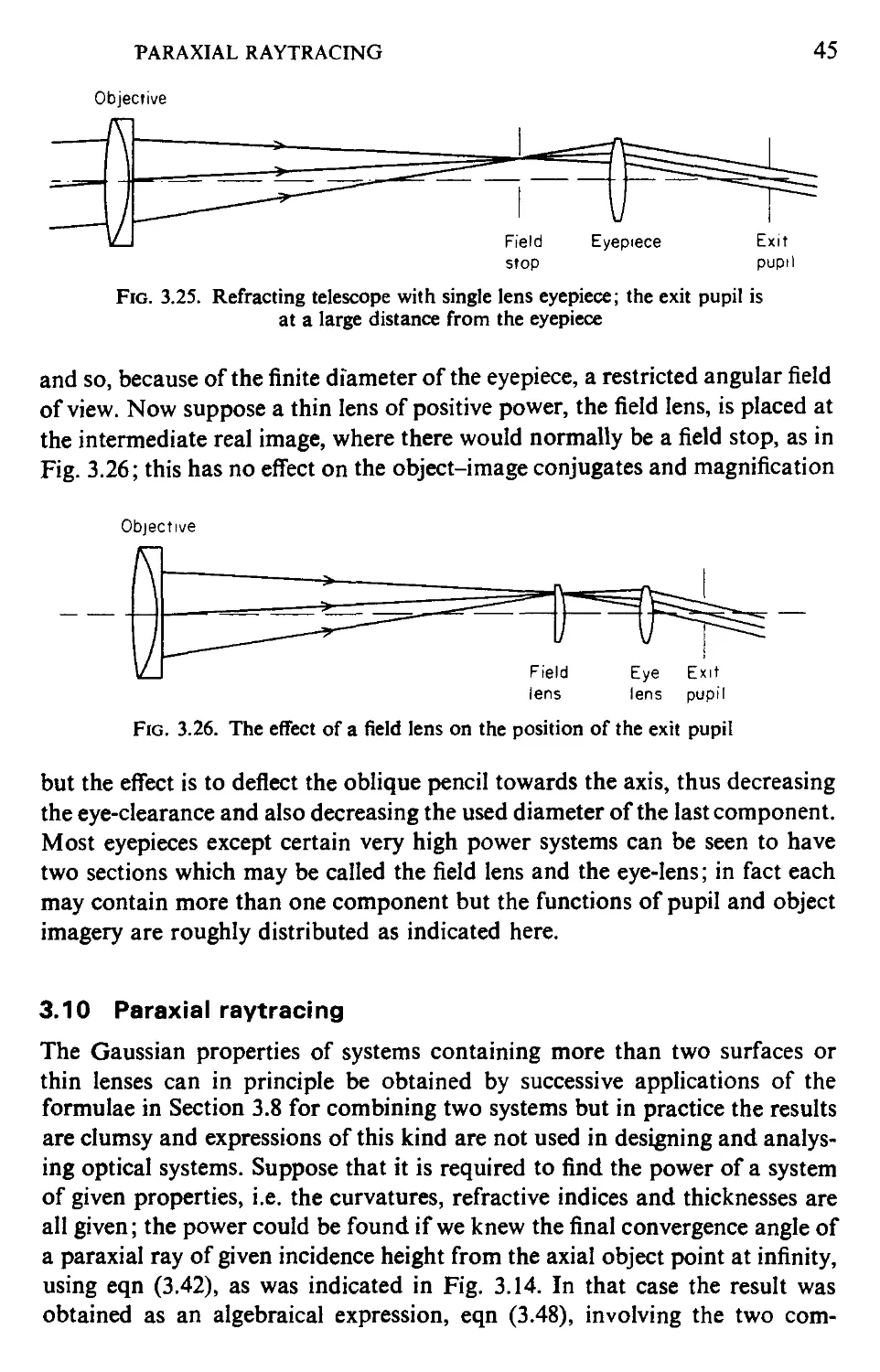
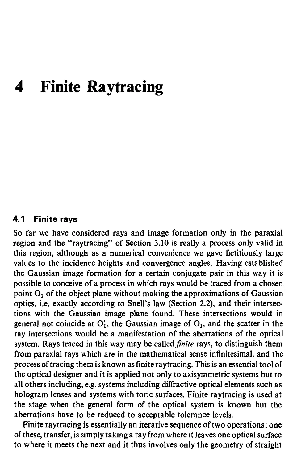
3.10 Paraxial ray tracing 45

VI CONTENTS
4 Finite raytracing
4.1 Finite rays 50
4.2 Snell's law for skew rays 51
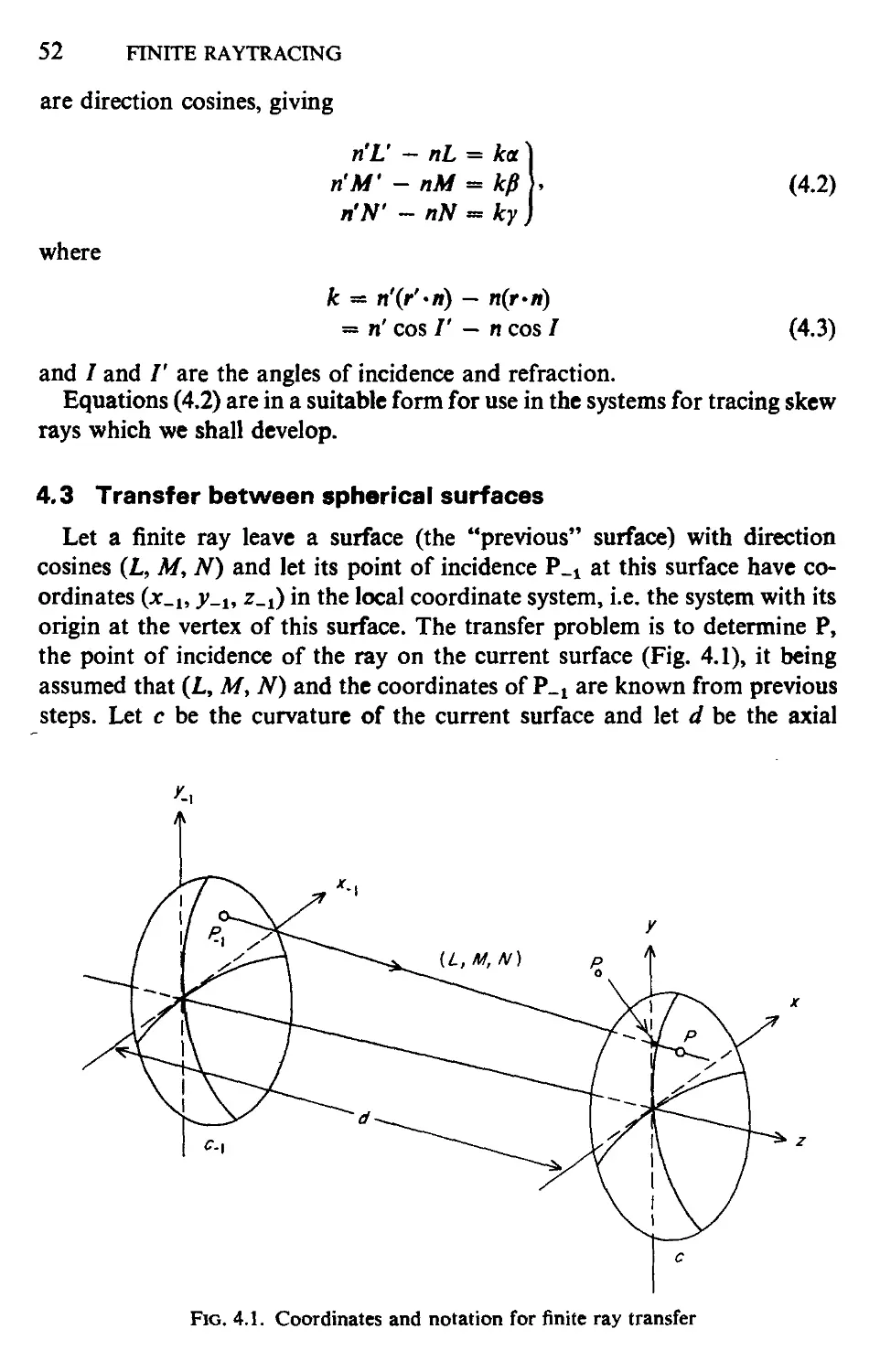
4.3 Transfer between spherical surfaces 52
4.4 Refraction through a spherical surface 54
4.5 Beginning and ending a raytrace 55
4.6 Non-spherical surfaces 57
4.7 Raytracing through quadrics of revolution 59
4.8 The general aspheric surface 61
4.9 Meridian rays by a trigonometrical method 63
4.10 Reflecting surfaces 65
4.11 Failures and special cases 65
5 Finite raytracing through non-symmetrical systems
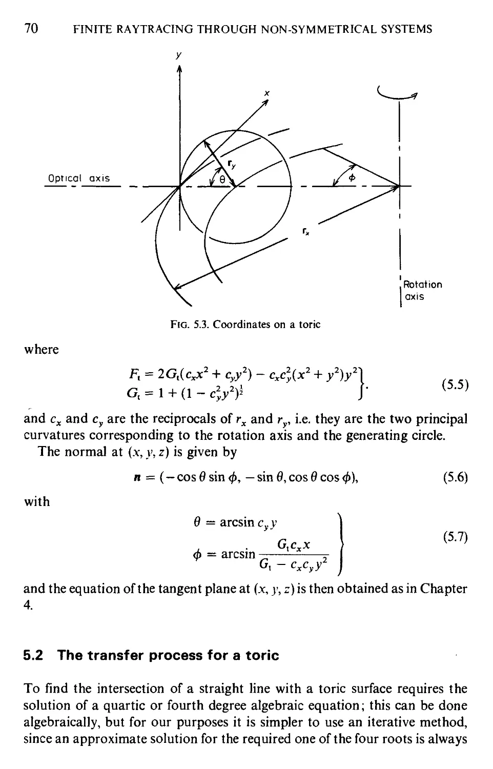
5.1 Specification of toric surfaces 67
5.2 The transfer process for a toric 70
5.3 Refraction through a toric 71
5.4 Raytracing through diffraction gratings 71
5.5 Raytracing through holograms 75
6 Optical invariants
6.1 Introduction 79
- 6.2 Alternative forms of the Lagrange invariant 79
6.3 The Seidel difference formulae 81
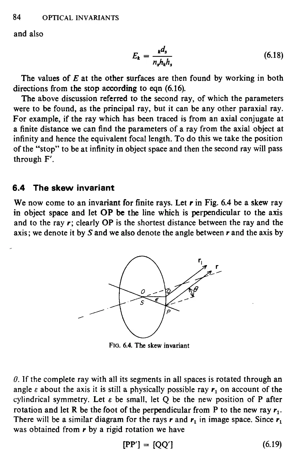
6.4 The skew invariant 84
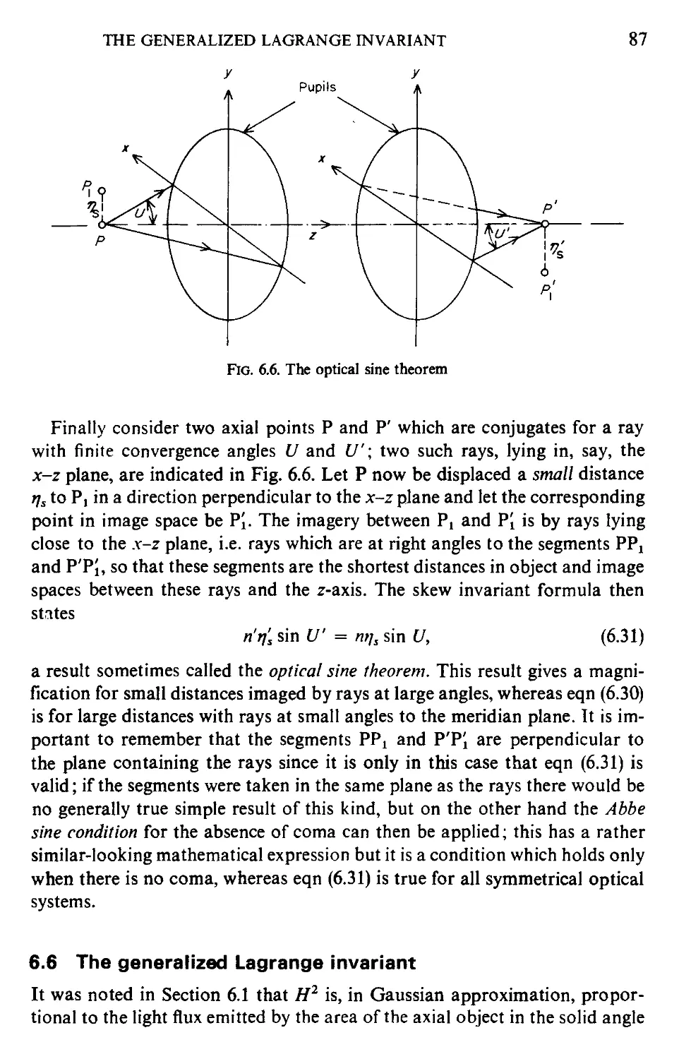
6.5 Some applications of the skew invariant 86
6.6 The generalized Lagrange invariant 87
7 Monochromatic aberrations
7.1 Introduction: definitions of aberration 92
7.2 Wavefront aberrations, transverse ray aberrations and
characteristic functions 93
7.3 The effect of a shift of the centre of the reference sphere on
the aberrations 98
7.4 Physical significance of the wavefront aberration 99
7.5 Other methods of computing the wavefront aberration 101
7.6 The theory of aberration types 105
7.7 The Seidel aberrations 109
7.8 Mixed and higher order aberrations 128
8 Calculation of the Seidel aberrations
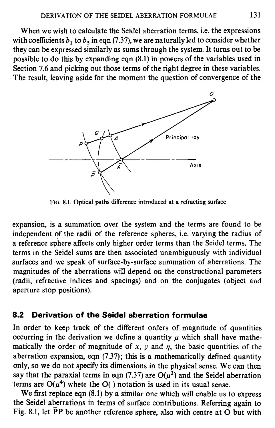
8.1 Addition of aberration contributions 130
8.2 Derivation of the Seidel aberration formulae 131
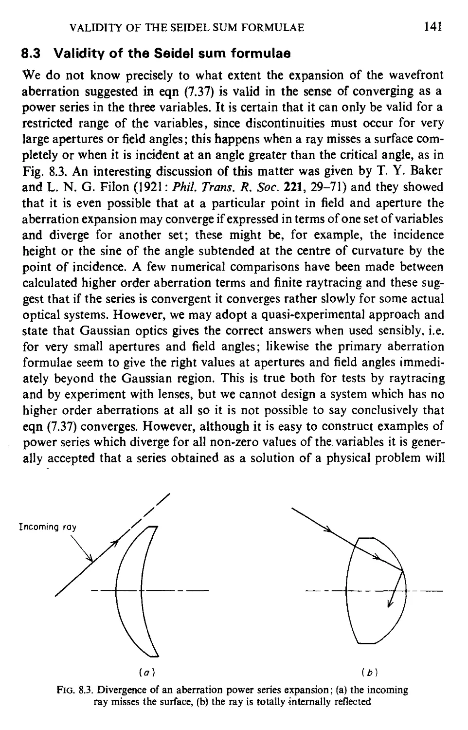
8.3 Validity of the Seidel sum formulae 141

CONTENTS Vll
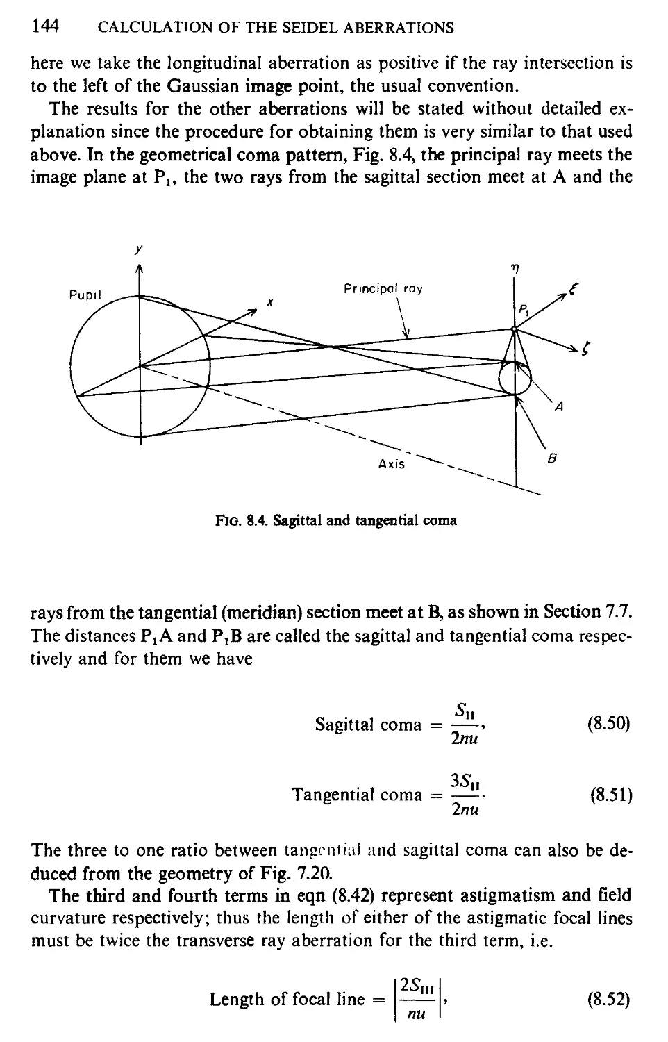
8.4 Ray aberration expressions for the Seidel sums 143
8.5 Computation of the Seidel sums; effect of stop shifts 148
8.6 Aspheric surfaces '• 152
8.7 Effect of change of conjugates on the primary aberrations 153
8.8 Aplanatic surfaces and other aberration-free cases 158
9 Finite aberration formulae
9.1 Introduction 162
9.2 The Aldis theorem for transverse ray aberrations 163
9.3 Expressions for total optical path aberration 165
9.4 Aplanatism and isoplanatism 171
9.5 Linear coma and offence against the sine condition 172
9.6 Isoplanatism in non-symmetric systems 176
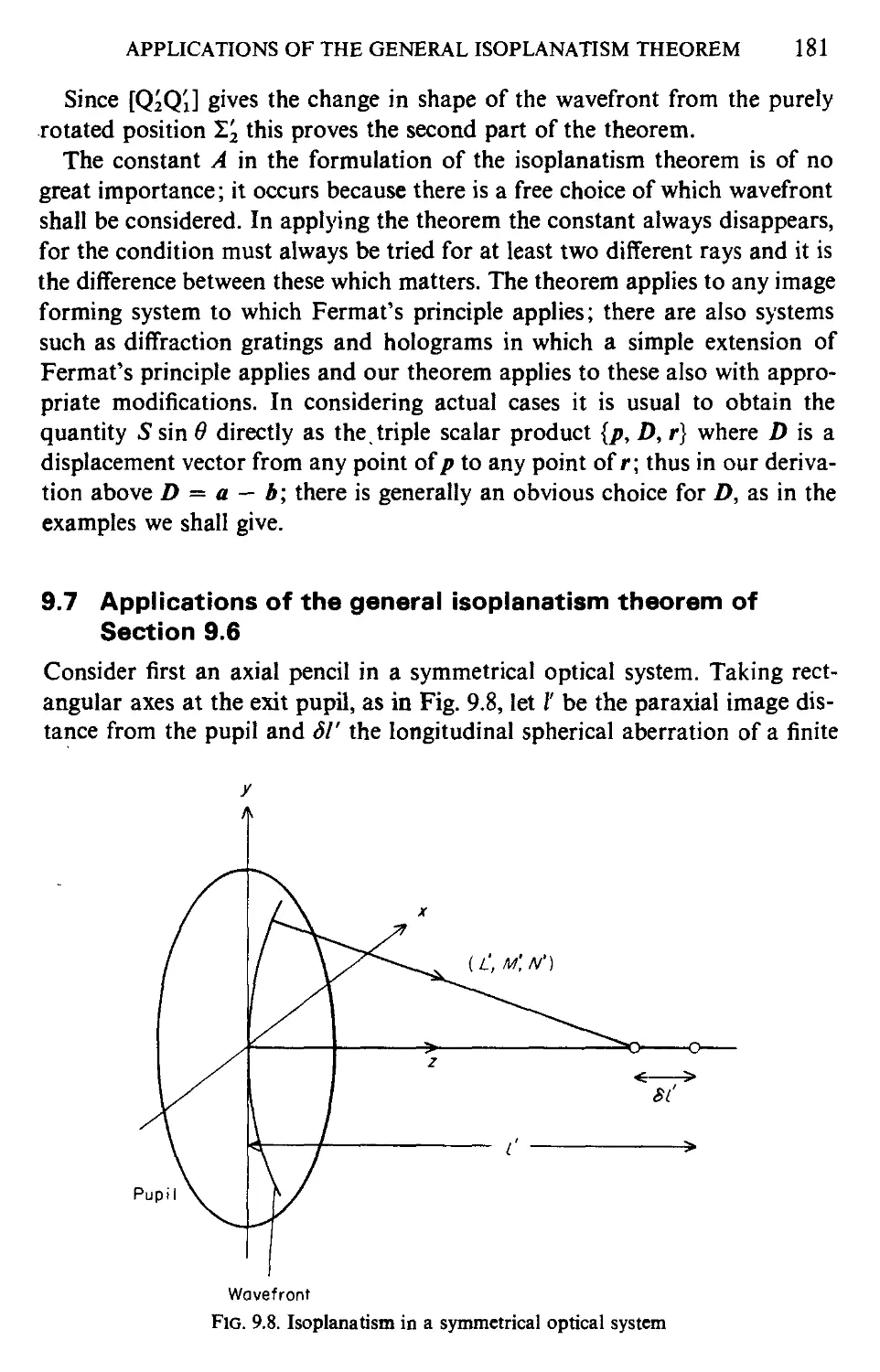
9.7 Applications of the general isoplanatism theorem of
Section 9.6 181
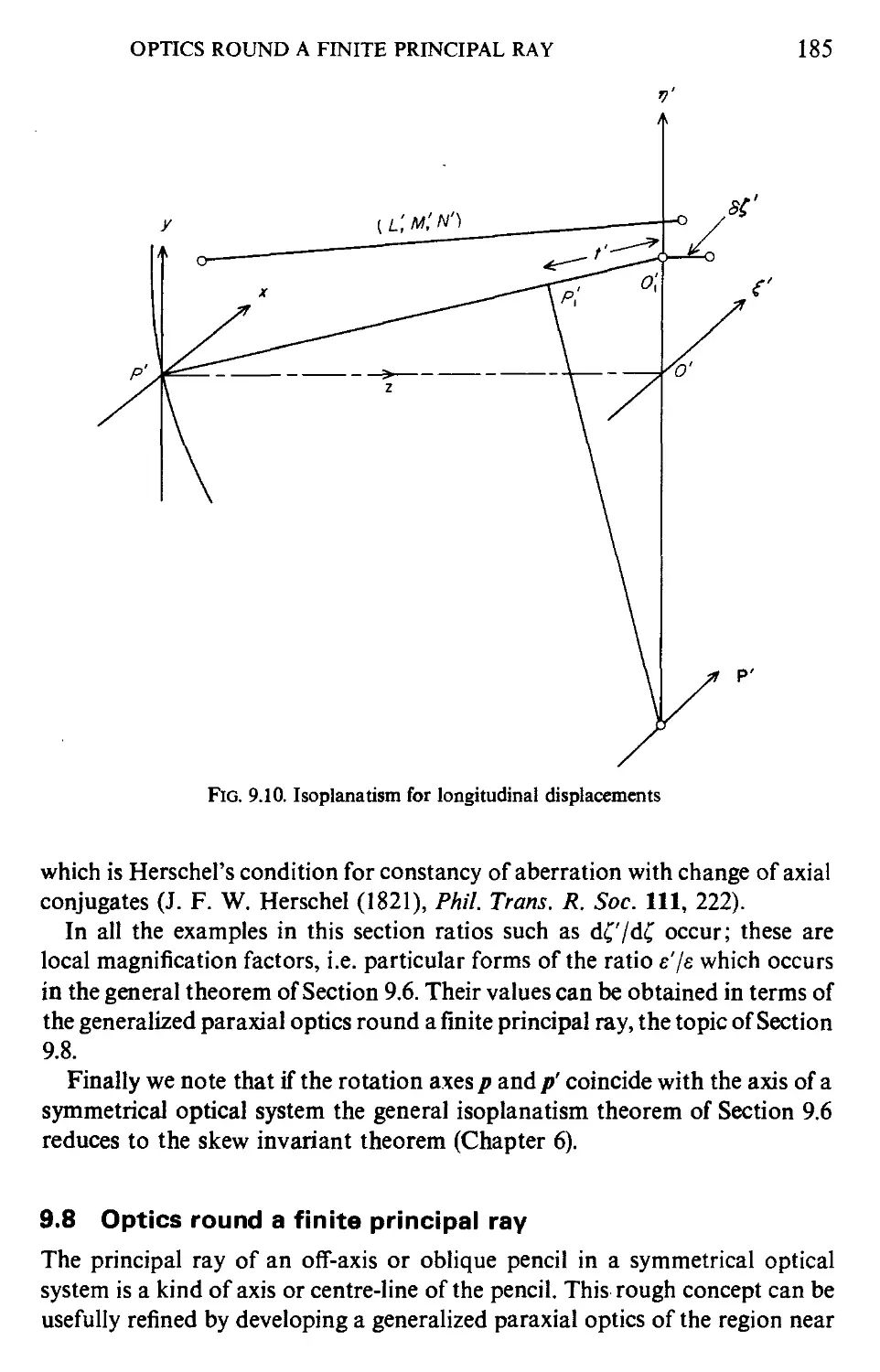
9.8 Optics round a finite principal ray 185
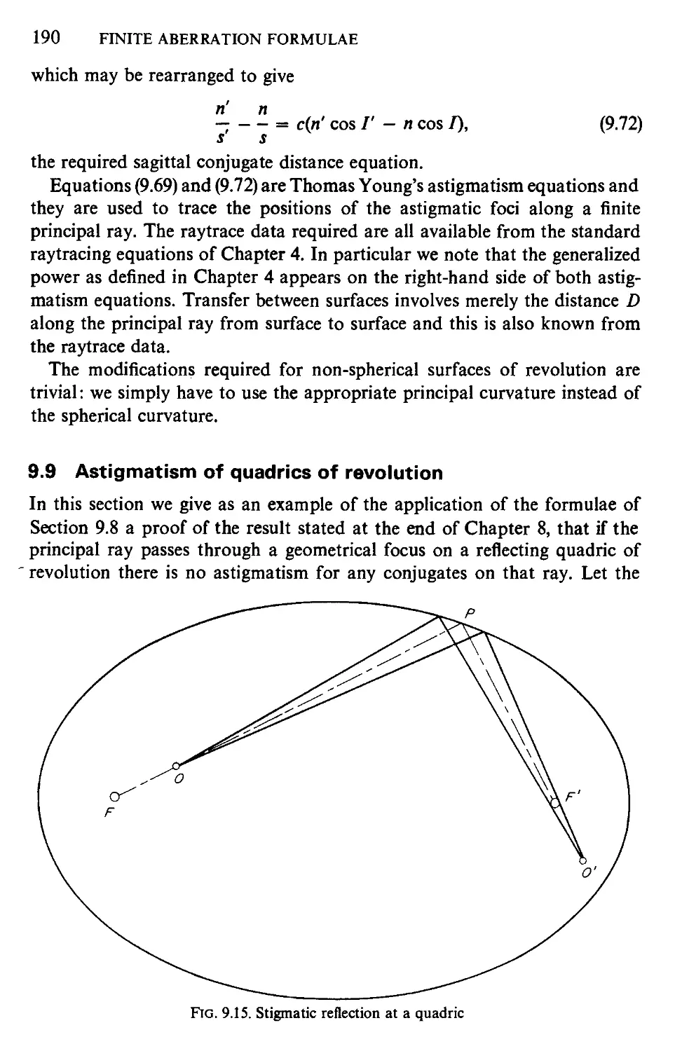
9.9 Astigmatism of quadrics of revolution 190
10 Chromatic aberration
10.1 Introduction: historical aspects , 192
10.2 Longitudinal chromatic aberration and the achromatic
doublet 193
10.3 Dispersion of optical materials 195
10.4 Chromatic aberration for finite rays; the Conrady formula 200
10.5 Expressions for the primary chromatic aberrations 202
10.6 Stop-shift effects 206
10.7 Ray aberration expressions for C\ and Cn 206
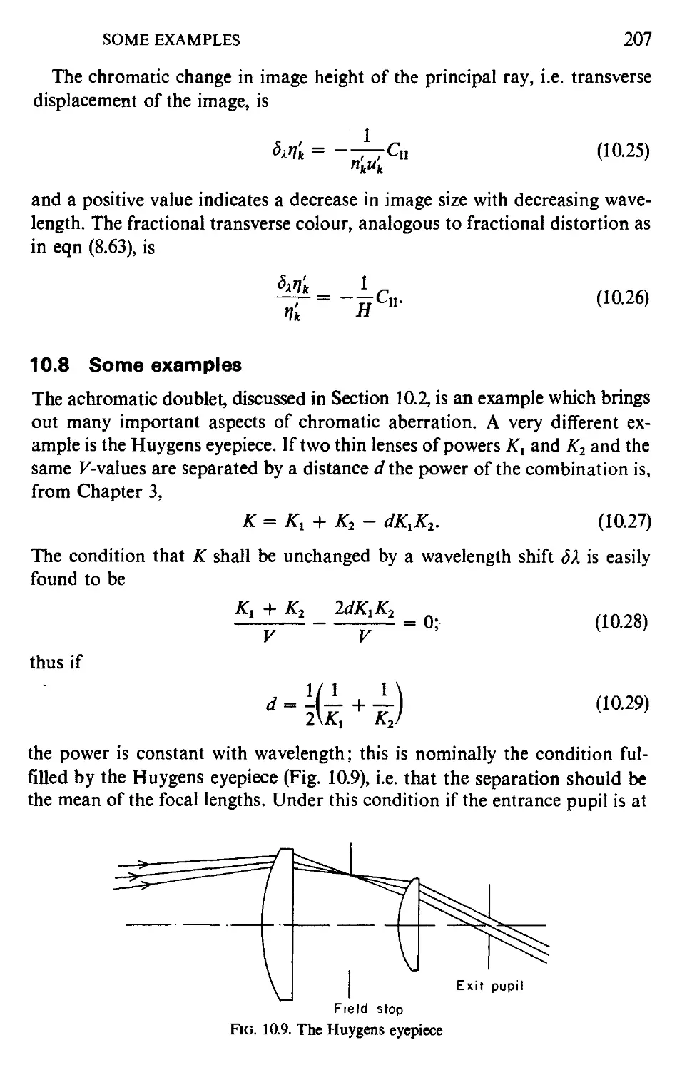
10.8 Some examples 207
11 Primary aberrations of unsymmetrical systems and of holographic
optical elements
11.1 Cylindrical systems 210
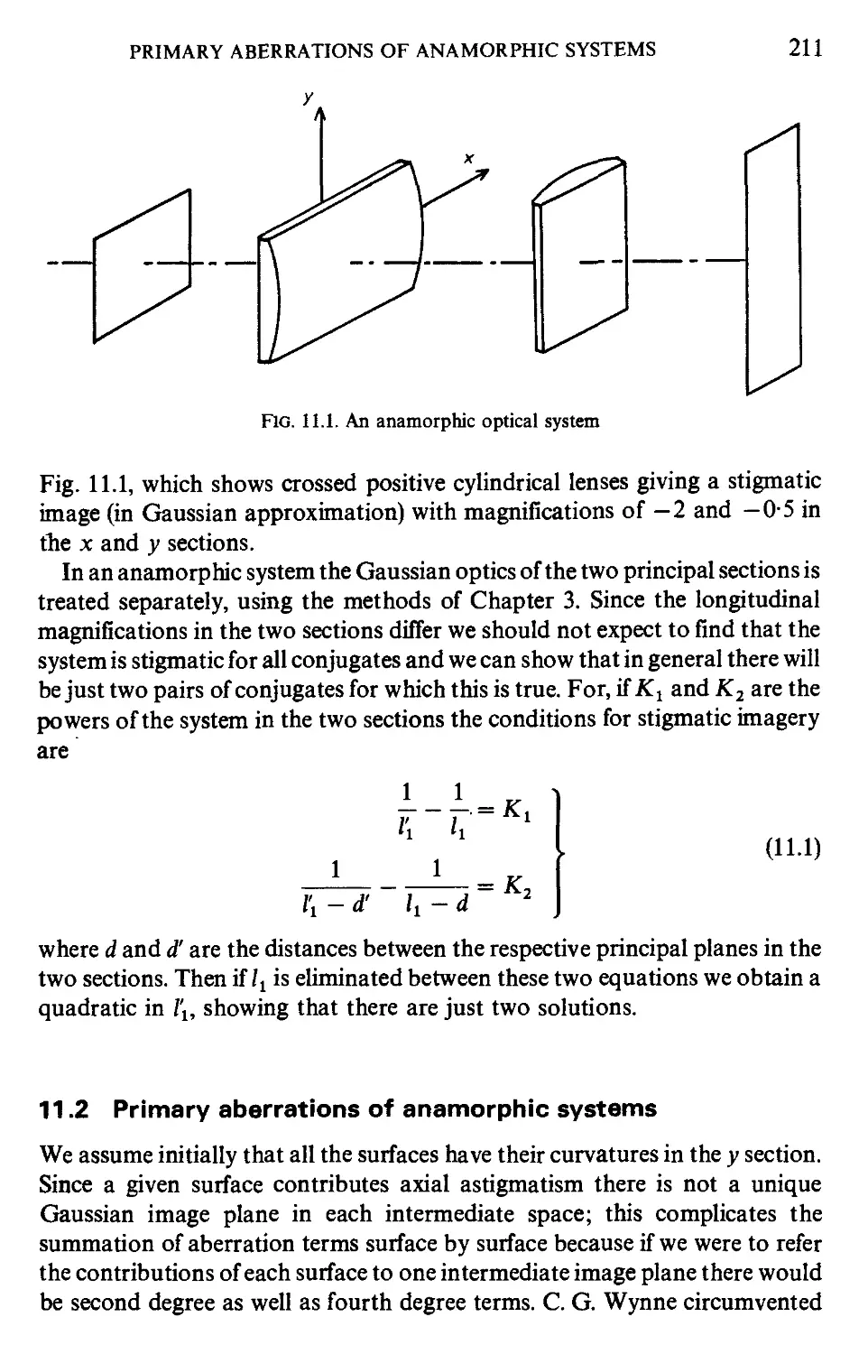
11.2 Primary aberrations of anamorphic systems 211
11.3 Aberrations of diffraction gratings 214
11.4 Aberrations of holographic optical elements 217
12 Thin lens aberrations
12.1 The thin lens variables 226
12.2 Primary aberrations of a thin lens with the pupil at the lens 228
12.3 Primary aberrations of a thin lens with remote stop 232
12.4 Aberrations of plane parallel plates 234
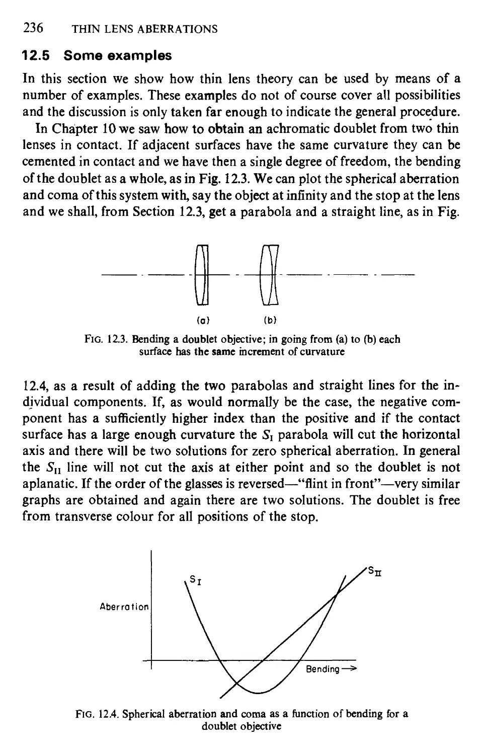
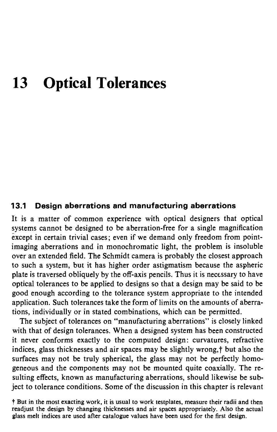
12.5 Some examples 236

vili CONTENTS
13 Optical tolerances
13.1 Design aberrations and manufacturing aberrations 240
13.2 Some systems of tolerances 241
13.3 Tolerances for diffraction-limited systems 241
13.4 Resolving power and resolution limits 246
13.5 Tolerances for non-diffraction-limited systems; definition
of the optical transfer function 249
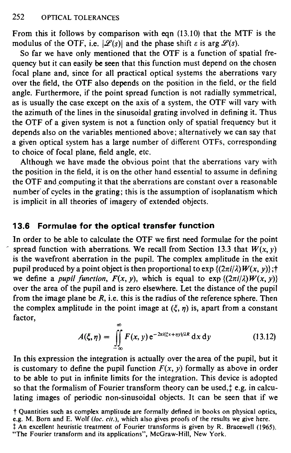
13.6 Formulae for the optical transfer function 252
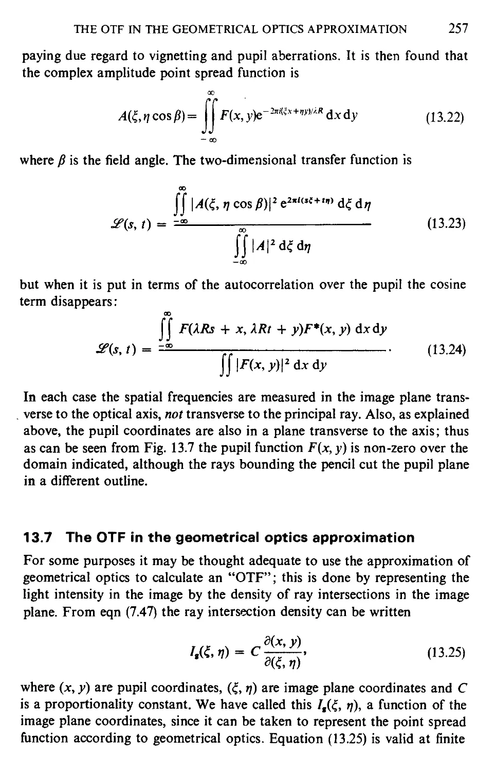
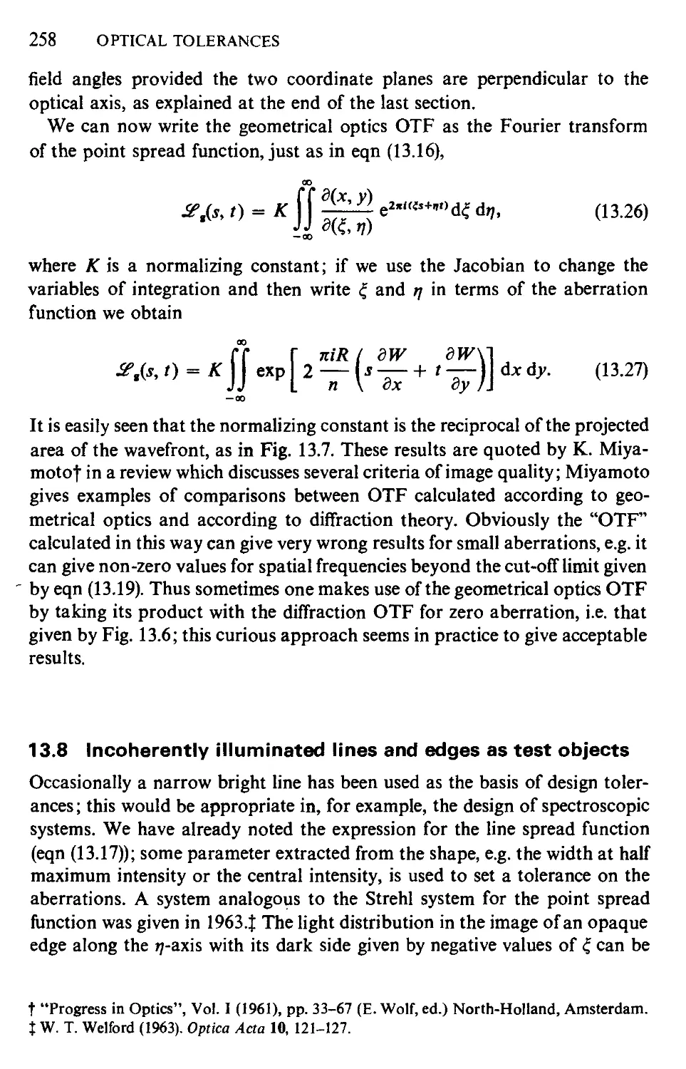
13.7 The OTF in the geometrical optics approximation 257
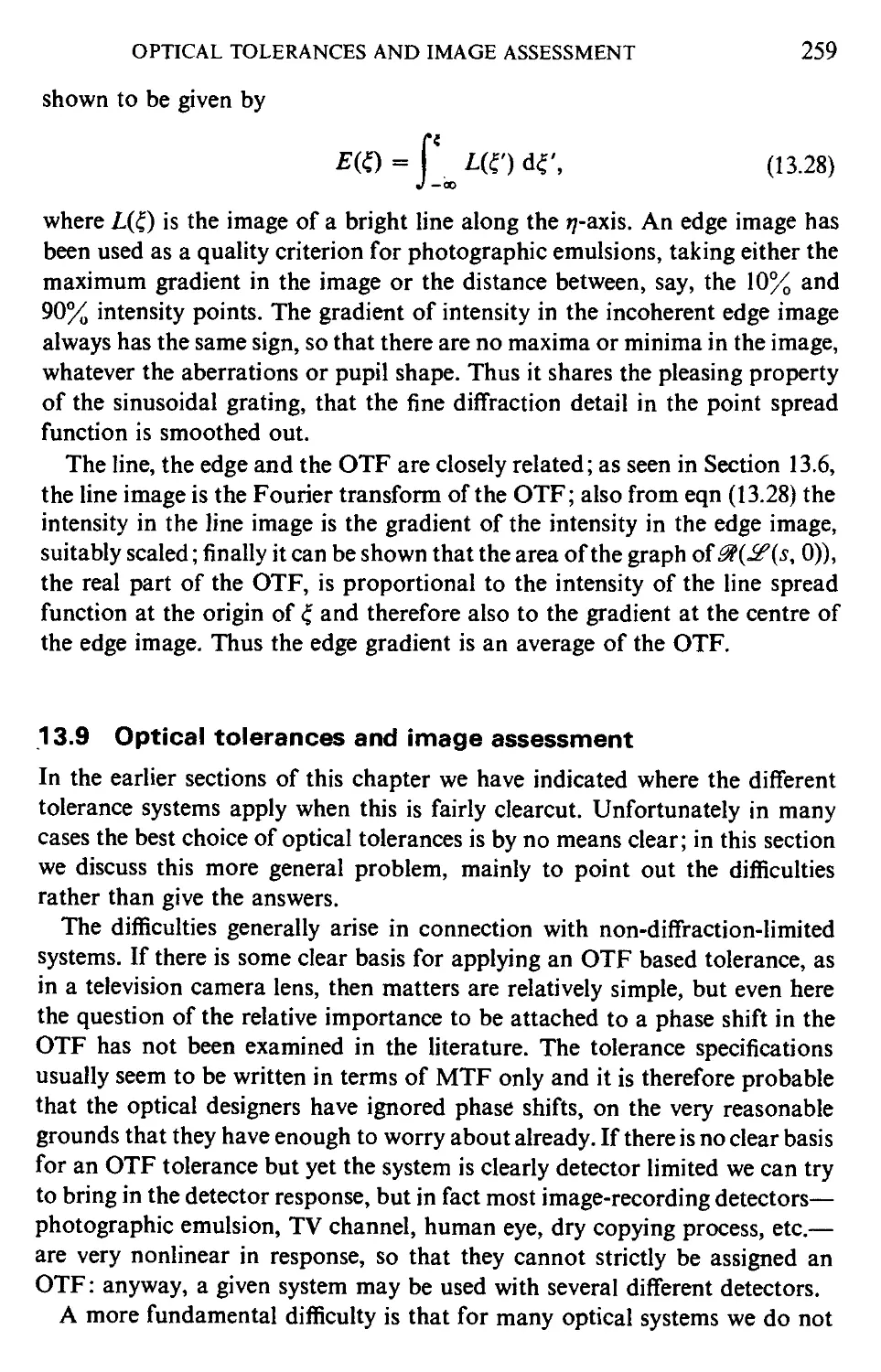
13.8 Incoherently illuminated lines and edges as test objects 258
13.9 Optical tolerances and image assessment 259
Appendix A
Summary of the main formulae 261
Appendix В
Symbols 271
Appendix С
Examples 273
Appendix D
Tracing Gaussian beams from lasers 277
Name index 279
Subject index 281

Series Editors' Preface
Optics has been a major field of pure and applied physics since the mid
1960s. Lasers have transformed the work of, for example, spectroscopists,
metrologists, communication engineers and instrument designers in addition
to leading to many detailed developments in the quantum theory of light.
Computers have revolutionised the subject of optical design and at the same
time new requirements such as laser scanners, very large telescopes and
diffractive optical systems have stimulated developments in aberration
theory. The increasing use of what were previously not very familiar regions
of the spectrum, e.g. the thermal infrared band, has led to the development
of new optical materials as well as new optical designs. New detectors have
led to better methods of extracting the information from the available
signals. These are only some of the reasons for having an Adam Hilger
Series on Optics and Optoelectronics.
The name Adam Hilger, in fact, is that of one of the most famous precision
optical instrument companies in the UK; the company existed as a separate
entity until the mid 1940s. As an optical instrument firm Adam Hilger had
always published books on optics, perhaps the most notable being Frank
Twyman's Prism and Lens Making.
Since the purchase of the book publishing company by The Institute of
Physics in 1976 their list has been expanded into all areas of physics and
related subjects. Books on optics and quantum optics have continued to
comprise a significant part of Adam Hilger's output, however, and the
present series has some twenty titles in print or to be published shortly.
These constitute an essential library for all who work in the optical field.

Preface and Acknowledgements
Aberration theory as used in optical design has changed considerably since
1974 when my book "Aberrations of the Symmetrical Optical System"
(Academic Press) appeared. Among these changes are the use of non-axially
symmetric systems and diffractive optical elements in quite complex designs
such as head-up displays and the increasing use of scanning systems with
laser illumination. The present book is based to a considerable extent on
that of 1974 and I acknowledge the use of much material from that book;
however, I have changed much and added material on the subjects men-
mentioned above and others suggested by colleagues. It is a pleasure to
acknowledge help and suggestions given by these friends, including
Prudence Wormell, Richard Bingham, Charles Wynne, Michael Kidger and
many others. I am grateful also to Jim Revill of IOP Publishing Ltd for his
advice and help in the preparation of the book.
W T Welford
Note added to the amended reprint
The Publishers wish to thank Dr Robin Smith of the Blackett Laboratory,
Imperial College, London for compiling the corrections and amendments
for this reprint from the notes of the late Professor Welford.
1991

1 Optical Systems and Ideal Optical
Images
The symmetrical optical system, i.e. a system with symmetry about an axis of
revolution, is the type of system most frequently met as a design problem; this
includes systems folded by means of plane mirrors or prisms, since it is trivial
to unfold them for optical design purposes. However, non-symmetrical
systems are not uncommon, e.g. some kinds of spectacle lens, spectrographic
systems, anamorphic projection systems and systems containing holographic
optical elements. In this book we shall be mainly concerned with symmetrical
systems but some discussion of non-symmetrical systems will be given, chiefly
in connection with raytracing.
1.1 Initial assumptions
The treatment will be based mainly on the geometrical optics model but there
will be occasional references to physical optics in the form of scalar wave
theory; this is needed for dealing with aberration tolerances. In geometrical
optics the essential concept is the ray of light; in this chapter we assume this as
an intuitive notion, deferring more precise definition to Chapter 2. It is then
possible to formulate definitions of ideal image formation using only the
concept of rays and the assumption that to one ray entering the system there
corresponds one and only one ray emerging. We do not at this stage invoke the
laws of reflection and refraction, and we make no assumptions about how the
transformation from object to image space is accomplished: i.e. there might be
non-spherical surfaces, media of continuously varying refractive index, etc., in

2 OPTICAL SYSTEMS AND IDEAL OPTICAL IMAGES
the system. However, it is convenient to assume that the entering and emerging
rays are straight line segments, or in physical terms that there are clearly
defined regions in the object and image spaces in which the respective
refractive indices are constant. Ideal image formation for a general system then
means that a pencil of rays from a point in object space becomes a pencil also
passing through a single point in image space and that this holds for some one-
or two-dimensional object surface. This does not get us very far but if we
assume a symmetrical system we can obtain many other properties of ideal
image formation to which the performance of a real well-corrected system
should approximate.
The first notions of ideal image formation through symmetrical systems are
due to A. F. Mobius A855). A few years later James Clerk Maxwell A856,1858)
formalized the concept of an ideal system without invoking any physical
image-forming mechanism. It is essentially Maxwell's concept which we
describe in this chapter.
1.2 Ideal image formation in the symmetrical optical system
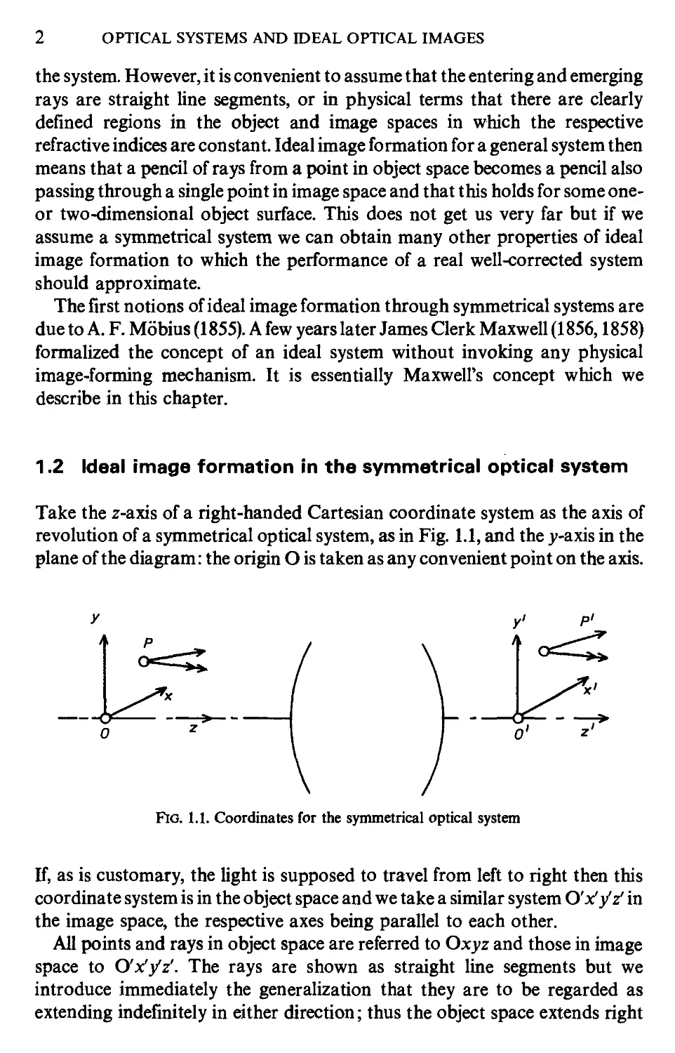
Take the r-axis of a right-handed Cartesian coordinate system as the axis of
revolution of a symmetrical optical system, as in Fig. 1.1, and the y-axis in the
plane of the diagram: the origin О is taken as any convenient point on the axis.
\
Fig. 1.1. Coordinates for the symmetrical optical system
If, as is customary, the light is supposed to travel from left to right then this
coordinate system is in the object space and we take a similar system O'xfy'z' in
the image space, the respective axes being parallel to each other.
All points and rays in object space are referred to Oxyz and those in image
space to O'xyz'. The rays are shown as straight line segments but we
introduce immediately the generalization that they are to be regarded as
extending indefinitely in either direction; thus the object space extends right

IDEAL IMAGE FORMATION IN THE SYMMETRICAL OPTICAL SYSTEM 3
through the optical system and through image space and similarly image space
is extended infinitely in both directions. This is an essential convention for
dealing with the details of image formation in the intermediate spaces of a
system, where the image from one optical element is the object for the next,
since this image-CMm-object is very frequently virtual.
Ideal image formation from the x-y plane to the x'-y' plane can then be
defined as follows. All rays through any point P on the x-y plane must pass
through one point P' on the x'-y' plane and the coordinates (x',y') are
proportional to (x, y); the constant of proportionality, which is, of course, the
magnification, depends on the nature of the optical system and on the axial
positions of the two planes. This can be summarized by saying that any figure
on the x-y plane is perfectly imaged as a geometrically similar figure on the x'-
y' plane. It will be shown that if there are two such pairs of conjugate planes
then any plane in object space is imaged ideally on another plane in image
space.
There is considerable interest in examining this Maxwellian ideal image
formation because, as will be seen in Chapter 3, the image formation in any real
symmetrical system approximates to the ideal in a narrow region sufficiently
close to the optical axis. We shall therefore study this ideal image formation in
more detail.
Let Oxy and OiXj^t be two planes in object space and let O'x'y' and
Oi^ij'i be the corresponding planes in image space. We suppose the image
formation to be perfect between these pairs of planes; thus, in Fig. 1.2, if a
mt
o\
Fig. 1.2. Ideal image formation
and ej are two-dimensional vectors in the planes Oxy and OjX^j from the
origins to points P and Pb the corresponding vectors in the image planes will
be given by
a' = ma \
I
a[ =
A.1)

4 OPTICAL SYSTEMS AND IDEAL OPTICAL IMAGES
where m and m^ are appropriate magnification factors between these planes.
These equations imply that all rays through P pass through P' and similarly
for P, and Pi, so that they express the assumption of perfect image formation
between the two planes.
Now we consider points P2 on a third plane O2x2y2; we enquire whether
all rays through P2 also pass through one point P2 in image space and, if so,
whether this point always lies on one plane perpendicular to the axis and is
related to P2 by an equation similar to eqn A.1). We have
a2 = (zj/zJia,. - a) + a A.2)
where zt and z2 are the coordinates of Ox and O2 with respect to O, this being
true for all points P and Pt which are on a ray through P2. If a point P2 with
the above properties exists, then we must also have
«2 - te/ziX-i - «') + «' A.3)
and
a'2 = w2e2. A.4)
Equations A.3) and A.2) can be rearranged as
a2 = (iHtzJ/zJK + m(l - z2 / z\)a A.3')
a2 = (z2/Zl)a, + A - z2/Zl)a A.2')
and these will be consistent with eqn A.4) if we can find z2 and m2 to satisfy
and m(l - z'2lz\) = w2(l - z2/z,); A.5)
clearly this can be done since we have two equations and two unknowns, and
the values will hold good for all points P2. Thus we have shown that ideal
image formation for two pairs of conjugate planes implies ideal imagery for
all other pairs.
1.3 Properties of an ideal system
We can now develop many properties of ideal systems which are to be used
in the paraxial approximation. For this purpose, we indicate the optical sys-
system schematically as in Fig. 1.3, but it must be understood that it may extend
for a considerable distance along the axis and the constructions to be ex-
explained may take place inside the physical system, i.e. with virtual parts of
rays.
In Fig. 1.3, let rx be a ray from the point at infinity on the axis in object
space, i.e. a ray parallel to the axis. It meets the axis in image space at some
point F'; this must be the image of the axial point at infinity in object space,
since two rays pass through both these points, namely the ray rt and the ray

PROPERTIES OF AN IDEAL SYSTEM
Axis
Fig. 1.3. Principal focus and principal point
along the axis, and we are assuming ideal image formation.! The point F' is
called the second principal focus or image-side principal focus.
Let the segment of ray rt in object space be produced until it meets the
segment in image space at PJ; a plane normal to the axis through P'x meets the
axis at P', the second or image-side principal point, the plane itself being the
second or image-side principal plane.
Similar constructions and definitions lead to the object-side principal focus
and principal point. These constructions can be made on the same diagram
with the rays rt and r2 parallel to the axis chosen to be at equal distances from
Fig. 1.4. Unity magnification between the principal points
the axis, as in Fig. 1.4, which shows all four points F, F', P, P'. The two seg-
segments of rj meet at P[ and those of r2 at Pt. Both rays г, and r2 pass through
Pj and Pi, so these points must be object and image; furthermore, using the
properties of ideal image formation, the planes normal to the axis through Pi
and PJ must be conjugates and since by construction PPt = P'Pi the magni-
magnification between these planes must be unity. For this reason, P and P' are
sometimes called unit points.
By their definitions, F and P are always in object space and F' and P' are
always in image space; however, it may very well happen, for example, that
F' and P' may physically lie to the left of the system, although they are still
t We defer until Section 3.4 the special case in which the ray rt emerges parallel to the axis.

OPTICAL SYSTEMS AND IDEAL OPTICAL IMAGES
Fig. 1.5. An optical system with P' and F' physically on the left of the system
in image space. Fig. 1.5 shows a system consisting of two components in
which this occurs.
The distance P'F' is the second or image-side focal length, denoted by/',
and PF = / is the object-side focal length. These magnitudes take signs
according to the order of the letters in the definition in relation to the positive
z direction, so that in Fig. 1.4/would be negative and/' positive.
The four points F, F', P, P', along the axis fix the properties of the ideal
optical system completely. We can use them in a construction to find the
position and size of the image of any object, as in Fig. 1.6 where the optical
system is represented merely by these four points and the principal planes.
Let the object be OOt and let the ray rt be drawn through C^ parallel to the
axis to meet the first principal plane in Pj; it must emerge through PJ at the
same distance from the axis, and pass through F'. In the same way, the ray r2
from Ot through F is drawn through P2 and P^. The point Oi in which the
image side segments of ry and r2 meet must be the image of Ou and O' must
therefore be on the perpendicular from Oi to the axis. This construction will
be recognized as a simple generalization of the elementary construction for
image formation by a thin lens.
Fig. 1.6. Geometrical construction for conjugates
Figure 1.6 also yields simple formulae relating the positions and sizes of the
object and image. Let tj and r\' be the object and image heights; these take
signs according to the j-axis in the coordinate system (Fig. 1.1), so that in
Fig. 1.6 r\ is positive and r\' negative. Let FO = z, F'O' = z', so that these
quantities specify the axial conjugate positions; they are taken as directed
segments with signs according to the z-axis, so that in Fig. 1.6 z is negative

PROPERTIES OF AN IDEAL SYSTEM 7
and z' is positive. From the similar triangles FOOi and FPP2 we have
Ч'М = ~flz A.6)
and likewise from F'O'O; and F'P'P;,
Ч'/Ч = -z'lf- 0.7)
Combining eqns A.6) and A.7), we have
zz'=ff; A.8)
this is known as a conjugate distance equation, since it relates z and z'; it is
generally called Newton's conjugate distance equation. Isaac Newton gave it
for a single surface ("Opticks", Book 1, Part 1, axiom 6, Dover 1952, based
on the 4th edition 1730).
At the same time, we have obtained important expressions for the magnifi-
magnification m = r\'\r\ in eqns A.6) and A.7); these are generally written
z = -flm, z' = -mf. A.9)
It is also useful to have a conjugate distance equation in terms of the dis-
distances of object and image from the respective principal planes. Let PO = /,
P'O' = /', again with signs implied by the fact that PO is a directed segment;
thus / is negative and /' positive in Fig. 1.6. We have
l = z+f, l'=*z'+f; A.10)
if the values of z and z' are substituted from eqn A.9) and m is eliminated, we
obtain
? L-
the required equation. We also have, analogous to eqn A.9),
and so
--l l'=f'{\-m) A.12)
ml
The considerable difference in form between the two conjugate distance
equations, eqns A.8) and A.11), is because in eqn A.11) the conjugates are
referred to origins in object and image space which are themselves conjugates,
namely the two principal points, whereas the principal foci are not conjugates.
This brings to light a slight inconsistency in notation; primed and unprimed
letters normally refer to conjugates or to some other quantities, e.g. angles of

8
OPTICAL SYSTEMS AND IDEAL OPTICAL IMAGES
incidence and refraction, which have the relationship "before and after going
through the optical system or one surface of it". The principal foci do not fit
into this scheme and they are therefore occasionally labelled Ft and F2, but
F and F' is the more usual notation.
A third useful pair of points on the axis can be defined, the nodal points N
and N'; these are such that a ray entering through N emerges from N'
parallel to its initial direction. We can find the positions of the nodal points
by starting with the usual skeleton system specified by F, F', P, P' as in Fig.
1.7; we construct any ray r, through F, meeting the principal planes in Pt
Flo. 1.7. Construction for the nodal points
and Pi and meeting the image-side focal plane at Fi; next we draw the ray r2
through F[ in image space and make it parallel to the segment of rt in object
space. Since rt and r2 meet at an image point F[ which is on the image-side
focal plane, they must come from an object point at infinity, i.e. they are
parallel in object space: thus, both segments of r2 are parallel to the segment
of rt in object space and so r2 must intersect the axis in the nodal points. It is
easily seen by similar triangles that
FN=/', F'N'=/.
0.14)
The six points F, F', P, P', N, N', are sometimes called the cardinal points.
If either of the quadruples F, F', P, P', or F, F', N, N', is known the properties
of the system are determined completely, since the conjugate distance equa-
equation and the magnification formulae are known. The points can occur in any
order and relative positions on the optical axis, subject only to the restrictions
implied by eqn A.14).
The relation between axial object and image points given by eqns A.8) and
A.11) is in effect a one-to-one correspondence between pairs of points on a
line, the optical axis; it is an involution, in the terminology of projective
geometry. Similarly, the transformation which expresses the image segment of
a ray in terms of the object segment is a one-to-one correspondence between
lines in the same three-dimensional space (a collineatiori) with axial symmetry.

PROPERTIES OF AN IDEAL SYSTEM 9
The more detailed theory of involutions and collineations is not important
in geometrical optics, but they are mentioned here to establish the point that
the most general one-to-one correspondences take this form; on the other
hand, it will be seen that in real optical image formation the relationship be-
between object and image>entities is more complex. For example, more than one
axial "image point" may correspond to a single object point, on account of
spherical aberration, and a point which is common to three rays in object
space may not be common to the corresponding three rays in image space.
Thus real optical image formation is essentially more complicated than the
ideal case we have been discussing.

2 Geometrical Optics
2.1 Rays and geometrical wavefronts
We obtained in Chapter 1 a simple model of image formation with axial
symmetry, and we pointed out there that this was based on assumptions about
optical systems which are only valid under certain restrictions. In this chapter
and the next we explain these restrictions and develop further the theory of
optical systems within them. In order to do this, we have to introduce a
further concept, the geometrical wavefront, in addition to the ray, already
used.
The concept of a geometrical wavefront appears in the work of Fermat
A667), Malus A808), Hamilton A820-30) and others, as a surface of constant
optical path from the source or a surface orthogonal to the rays from a source
point. More recently the shape of the geometrical wavefronts has been used
to characterize the aberrations of an optical system directly, rather than re-
regarding the ray patterns as fundamental; one of the earliest authors to do this
was G. Yvon ("Controle des surfaces optiques", Paris 1926). This usage of
the geometrical wavefronts provides a link with the physical concepts which
originated with C. Huygens A690) and A. Fresnel A866) and developed into
the Kirchhoff diffraction theory A891). A very full treatment of the early
history of these topics is given by E. T. Whittaker A951), "History of the
Theories of Aether and Electricity", Vol. I, revised edition, Nelson, London.
To an adequate approximation, we can regard rays as the paths along
which the radiation energy travels; this breaks down near foci and near the
edges of shadows, owing to diffraction effects, but it is essential to geometrical
optics that these are ignored. Now, let a point source of light be placed in

RAYS AND GEOMETRICAL WAVEFRONTS
11
Fig. 2.1. Geometrical wavefronts and rays
front of any optical system, not necessarily axially symmetric, and suppose
that the rays from this source О are traced through the system, as in Fig. 2.1,
using the law of refraction; the details of the law of refraction will be discussed
later (Section 2.2), but it is sufficient to know that we can calculate the ray
paths according to simple rules. Recalling that light is propagated with a
finite velocity, we can mark off on these rays sets of points which the light
disturbance reaches in given times and we can join up the sets to form sur-
surfaces Ib I2 and I3 in the figure, for example. We do this by noting that the
velocity of light in a medium of refractive index n is c/«,f and so light travels
from P2 to P3, say, in a time wP2P3/c, where n is the refractive index of the
medium between P2 and P3; more generally, light travels from A to В in the
time
1Г А
= - n ds,
cJa
B.1)
where the integration is taken along the ray path and ds is an element of this
path; thus the surfaces in Fig. 2.1 are simply surfaces of constant J n ds from
the source point O. In the diagram, it is implied that the refractive index is
constant along a ray segment and then changes discontinuously at a refracting
surface; in this case the integral becomes simply a summation.
The quantity j n ds (or ? n As for most systems) is called the optical path
t For many purposes, it is convenient to regard this as a definition of refractive index.

12 GEOMETRICAL OPTICS
length. The surfaces Zj, E2, ^з> • • •are called geometrical wavefronts or simply
wavefronts for brevity; they correspond approximately to surfaces of constant
phase or wave epoch in the wave model of light, i.e. phasefronts. The
approximation is good at large distances from foci or edges of shadow regions
but near such regions the geometrical wavefronts do not correspond at all to
true phasefronts. The most familiar example is a single mode tem00 or
Gaussian laser beam, where at the focus, or beam waist as it is usually called,
the phasefront is plane but the geometrical wavefront contracts to a single
point; see Appendix D for a discussion of the propagation of Gaussian beams.
The approximation may also be poor when the geometrical wavefronts are
almost plane, as explained in Section 13.3, but in most practical cases
geometrical wavefronts and phasefronts can be taken to coincide. In
geometrical optics the wavefronts are surfaces of constant optical path length
from the source point O. In a system such as in Fig. 2.1 we can imagine a
double infinity of rays from О and a single infinity of wavefronts; this ensemble
is sometimes referred to as a pencil and it is often convenient in discussing
aberrations to select various chosen rays and wavefronts from a hypothetical
complete pencil.
2.2 Snail's law of refraction
The wavefronts as defined in the preceding section are, with rays, the basic
concepts of geometrical optics, and optical path length is the basic physical
quantity. We next have to show how the rays and wavefronts are propagated
through lens surfaces, i.e. we have to investigate refraction.
In terms of rays we can express refraction by Snell's law; let / and /' be the
angles of incidence and refraction at an interface between media of refractive
indices n and ri, as in Fig. 2.2; then Snell's law states that the incident and
refracted rays are coplanar with the normal and that
ri sin /' = n sin /. B.2)
Snell's law can be put more compactly in vector form; if r and r' are unit
vectors along the incident and refracted rays and л is a unit vector along the
normal to the interface, then
ri(r' Л и) = n{r Л я), B.3)
for the absolute magnitudes of the two sides of this equation are equal to the
two sides of eqn B.2), and the vector equality ensures the coplanarity of the
rays and the normal. This form of the equation will be needed for tracing rays
in three dimensions.
According to E. T. Whittaker ("History of the Theories of Aether and

SNELL'S LAW OF REFRACTION 13
Refracting
surface
Fig. 2.2. Snell's law of refraction
Electricity", Vol. 1, 1951), W. Snell A591-1676) discovered the law experi-
experimentally about 1621; he did not publish it but communicated it privately to
several people including R. Descartes. The latter published it in 1637.
Snell's law can be verified experimentally by means of accurate gonio-
goniometers to a fraction of a second of arc. It also follows from the electromagnetic
wave theory of light, so we can regard it as given.
The quantities n and ri appear now merely as physical constants to be de-
determined for the media on either side of the interface and in fact refractive
index is almost invariably determined for optical instrumentation purposes
by methods based very directly on Snell's law. The proof that this quantity is
the same as that in the formula cjn for the speed of light in a material
medium again appears in the derivation of Snell's law from electromagnetic
theory. It should be remarked also that the refractive index varies with wave-
wavelength or frequency for all material media; this is called dispersion and it is
the source of chromatic aberrations in optical systems.
It is usual to include reflection as a special case in the formulation of Snell's
law by adopting the convention that ri is replaced by — n when the ray is
incident as in Fig. 2.2 and the interface is reflecting. This formal device yields
the correct result from the vectorial form, provided we accept the following
convention about ray directions. The directions of all rays are referred to a
right-handed coordinate system as in Fig. 2.3, and the direction cosines of the
line along the ray are used to specify its direction; these are, of course, the
same as the components of a unit vector which starts from the origin, is
parallel to the ray and has its termination to the right of the x-y plane. For
example, suppose we have a ray which passes through the origin and which
also lies in the octant with positive x, у and z, as in Fig. 2.3; then the corre-

14 GEOMETRICAL OPTICS
У
Fig. 2.3. Signs of ray components;, the coordinate system is right handed, so
that the дг-axis points into the paper
sponding unit vector has its three components all positive, and the ray direc-
direction is denoted in our convention by positive components irrespective of the
direction of travel of the light along it. If the light were travelling in the re-
reverse direction from that indicated by the double arrow, then this fact would
be indicated by there being a negative refractive index in the medium. With
this convention, eqns B.2) and B.3) include reflection when ri is taken as —и.
This is illustrated in Fig. 2.4, where r" is the unit vector along the reflected ray
direction as given by this convention and — nr" is the actual reflected ray; thus
(л)
n т l=-nr )
Fig. 2.4. Directions and signs of reflected rays

FERMATS PRINCIPLE
15
the geometrical line representing the reflected ray is correct and the factor
n" = -n gives the reversal.
If n' < n in eqn B.2) when sin / = n'/n we find sin /' = 1 and for greater
values of sin I the value of /' would be purely imaginary. In fact there is no
refracted ray when this happens and the light is completely reflected, an effect
known as total internal reflection. This has many applications in the design of
prisms.
2.3 Format's principle
An entirely different approach to refraction is provided by Fermat's principle,
which is a stationarity principle of the same kind as the principle of least
action of Maupertuis. It was originally proposed by Pierre de Fermat in 1657
as a principle of least time: the path taken by light travelling from A to В
through any optical system will be such that the time of travel is a minimum.
This can easily be put in terms of optical path lengths by means of eqn B.1):
of all possible paths (straight line segments or otherwise) between A and B,
that which has the shortest optical path length represents a physically possible
ray.
As stated in this form, the principle only applied to points A and В which
are close enough to ensure that there is no real focus between themf; if A
and В are general points, then the optical path length along the physically
possible ray is not necessarily a minimum, but it is stationary. The most
general explanation of the term stationary involves the calculus of variations,
and a good exposition is given by M. Born and E. Wolf ("Principles of
Optics", 3rd edition 1963, Pergamon Press, London); for the present pur-
purposes, it may be sufficiently explained in terms of paths from A to В consisting
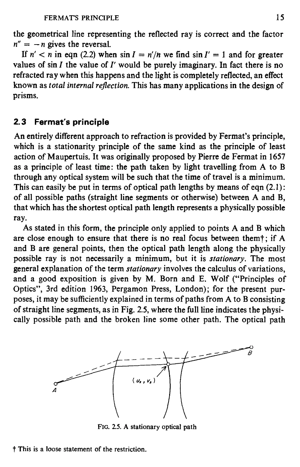
of straight line segments, as in Fig. 2.5, where the full line indicates the physi-
physically possible path and the broken line some other path. The optical path
\ / \
Fig. 2.5. A stationary optical path
t This is a loose statement of the restriction.

16
GEOMETRICAL OPTICS
length W from A to В is then a function of pairs of parameters uk, vk, {k =
1,2,...) which are generalized coordinates of the points where the line seg-
segments meet the refracting surface. Then stationarity of the optical path means
that for the physically possible ray these coordinates must be such that
dW
du'k
8fV
= 0 (*= 1,2,...).
B.4)
It should be emphasized that in this discussion A and В are not restricted
to be in any sense object and image—they are general points.
The straight line propagation of light, which we have already tacitly
assumed, is an immediate consequence of Fermat's principle. It is also easy
to obtain Snell's law, as in Fig. 2.6; let the y-z plane be the refracting surface,
(л)
Fig. 2.6. Derivation of SnelPs law from Fermat's principle
separating media of index n and ri, and let the points A and В have coordi-
coordinates (x0, y0) and (x1, 0). There is no loss of generality in taking a plane re-
refracting surface, since refraction according to either Snell's law or Fermat's
principle depends only on the local direction of the tangent plane at the point
of incidence C; also it is clear that С lies in the x-y plane by symmetry.
The optical path W from A to В is then
W = n{xl + (y - y0J}* + n'{x'2 + ?}\
The condition of stationarity with respect to changes in у is
B.5)
8W
п(У-Уо)
riy
= 0;
B.6)

THE LAWS OF GEOMETRICAL OPTICS 17
the coefficients of n and ri can be identified as the sines of the angles of
incidence and refraction, with suitable sign convention, and thus Snell's law
is obtained.
A direct verification of Fermat's principle by experiment is not, of course,
possible but, as in the case of Snell's law, it is possible to deduce Fermat's
principle from electromagnetic theory provided it is assumed that regions of
the electromagnetic field remote from foci, shadow edges and other places
where strong diffraction effects might occur are excluded; the whole concept of
rays breaks down in such regions. Treatments of this kind are given, for
example, by Born and Wolf ("Principles of Optics", 3rd edition 1963,
Pergamon Press, Oxford), by A. Sommerfeld ("Optics", English translation, O.
Laporte and P. A. Moldauer, Academic Press, New York, 1954) and by R. K.
Luneburg ("Mathematical Theory of Optics", Wiley-Interscience, New York,
1965); all these authors adopt different approaches which may be regarded
loosely as treatments of Maxwell's equations of the electromagnetic field in
which the wavelength of the light is allowed to tend to zero. In this way all the
usually accepted attributes of rays and geometrical wavefronts can be
obtained. A comprehensive survey of this question of the transition from
electromagnetic theory to geometrical optics with a discussion of the
limitations of each approach is given by M. Kline and I. W. Kay,
"Electromagnetic Theory and Geometrical Optics" (Wiley-Interscience, New
York, 1965).
2.4 The laws of geometrical optics
For our purposes it is convenient to regard both Snell's law and Fermat's
principle as basic postulates of geometrical optics, although, as we have
pointed out, they are both consequences of electromagnetic theory. It is con-
convenient also to mention explicitly the other properties of rays and wavefronts
in geometrical optics. These are rectilinear propagation in homogeneous
media, reversibility of ray paths, non-interference of intersecting ray paths
and the inverse square law of illumination for a point source.
We can immediately derive from Fermat's principle the important result
that rays are normals to wavefronts.f the theorem of Malus and Dupin. Let
S and S' in Fig. 2.7 be two wavefronts of a pencil from a point source; the
wavefronts are on either side of the kxh refracting surface 5 of an optical
system between media of refractive indices n and ri; let PQP' and P^Pi be
two rays and suppose that the theorem is true up to the medium of index n.
We have
[PQP'] = [РхОаРП, B.7)
t It is assumed here and everywhere else in this book that we are dealing only with isotropic
media.

18
GEOMETRICAL OPTICS
I
Fig. 2.7. The theorem of Malus and Dupin
where the square brackets denote optical path lengths, by the definition of
wavefronts. The path PiQPi, shown in broken line in the figure, is not a true
ray path, but, by Fermat's principle
[PiQiPi] = [PiQPl] + O(e2) B.8)
B.9)
B.10)
where e = QQt and the O( ) symbol has its usual significance. Thus
[PQP'l + O(e2)
But, since PQ and PiQt are normals to ? we have
[PiQ] = [PQ] + O(?2),
since PPt is of the same order of magnitude as QQi, and thus, by subtracting
eqn B.10) from eqn B.9), we have
[QP',] = [QP'] + O(e2),
B.11)
or QP' is normal to 2'. But, since the pencil originated at a point source, the
wavefronts in the object space must have been spherical and normal to the
rays; thus the theorem is proved by induction.
This theorem, that rays are normals to wavefronts, enables us conveniently
to develop the analogue for real optical systems of the ideal image formation
described in Chapter 1; this analogue is called Gaussian optics or paraxial
optics, the latter name implying that it is valid only in a region close to the
optical axis. The development is facilitated by the immediate deduction from
the theorem of Malus and Dupin that, if the rays of a pencil intersect in a
single point after refraction through an optical system, then the wavefronts
will be spherical,^ and vice versa. Thus we have two equivalent definitions of
t Here and elsewhere we use "spherical" to mean "portions of spheres".

THE LAWS OF GEOMETRICAL OPTICS 19
the formation of a perfect point image, that all the image-forming rays meet
in a single point or that the wavefronts are spherical. Departures from these
conditions imply the presence of aberrations and these will be defined in more
detail in Chapter 6.

3 Gaussian Optics
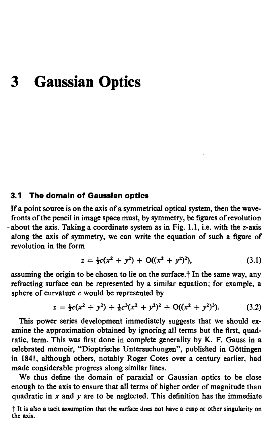
3.1 The domain of Gaussian optics
If a point source is on the axis of a symmetrical optical system, then the wave-
fronts of the pencil in image space must, by symmetry, be figures of revolution
about the axis. Taking a coordinate system as in Fig. 1.1, i.e. with the z-axis
along the axis of symmetry, we can write the equation of such a figure of
revolution in the form
г = Щх2 + f) + О((х> + у2J), C.1)
assuming the origin to be chosen to lie on the surface, f In the same way, any
refracting surface can be represented by a similar equation; for example, a
sphere of curvature с would be represented by
z = id*2 + У2) + ic3(*2 + ff + O((x2 + y2K). C.2)
This power series development immediately suggests that we should ex-
examine the approximation obtained by ignoring all terms but the first, quad-
quadratic, term. This was first done in complete generality by K. F. Gauss in a
celebrated memoir, "Dioptrische Untersuchungen", published in Gottingen
in 1841, although others, notably Roger Cotes over a century earlier, had
made considerable progress along similar lines.
We thus define the domain of paraxial or Gaussian optics to be close
enough to the axis to ensure that all terms of higher order of magnitude than
quadratic in x and у are to be neglected. This definition has the immediate
t It is also a tacit assumption that the surface does not have a cusp or other singularity on
the axis.

THE DOMAIN OF GAUSSIAN OPTICS 21
consequence that there is perfect image formation for object points on the
axis if we restrict the rays to the Gaussian region, since the equation of any
refracted wavefront must, to this approximation, be of the form
z = \c(x2 + f) C.3)
and this cannot be distinguished from a sphere of curvature c. In a similar
way, we can state that all reflecting or refracting surfaces are spherical, in
Gaussian approximation, since, by eqn C.2), other surfaces of the same axial
curvature such as paraboloids or ellipsoids of revolution differ from a sphere
only in the terms higher than quadratic.
We next have to define the extent of the Gaussian region for object points
which are not on the axis. Let О and O' be axial conjugates in Fig. 3.1, and
—*¦—о-
0
Fig. 3.1. Off-axis image formation
let Oj be an off-axis object point at a distance r\ from О in a plane perpendicu-
perpendicular to the optical axis. We wish to choose a restriction on the order of magni-
magnitude of г] which will similarly ensure perfect image formation for Qy. Let the
equation of a wavefront of the pencil converging to O' be
{2 2) A4)
where the origin is chosen arbitrarily at A and / is the distance АО'. The pencil
from Oj will travel through this region after refraction, and we can pick out
the wavefront which passes through A; let its equation be
z = ^(x* + f) + F{x,y,r,) C.5)
where the function F is to be determined. If we assume again that this wave-
wavefront has not a singularity at A then F can be written as a power series giving
Z = 2/(*2 + У^
+ t\2(dx2 + exy + fy2 + gx+ hy + j) + O(//3). C.6)

22 GAUSSIAN OPTICS
Now in the right-hand side of this equation we can set с and/ equal to zero,
since they do not contain x or у and we have postulated that the wavefront
passes through the origin A. Also the whole of Fig. 3.1 is symmetrical about
the y-z plane, since we assume Ot to lie in this plane, so that eqn C.6) must
contain only even terms in x, i.e. we set a, e and g equal to zero. It can be seen
by inspection of the remaining terms that, if only terms of order r\x and tjy
are retained, the resulting wavefront is still spherical, it has the same curva-
curvature as the axial wavefront and its centre is displaced from O' in a direction
perpendicular to the axis; the equation under this restriction is
z = j^ + f) + br,y, C.7)
which, in our approximation, represents a sphere of radius / and with centre
at a distance - lbr\ above O'. Clearly, this distance is proportional to r\ for a
given system and a given position of O; thus we have found restrictions under
which all object points have perfect point images and objects in a plane per-
perpendicular to the axis form geometrically similar images also in a plane
perpendicular to the axis.
The restrictions may be re-stated compactly in the form: terms in the wave-
wavefront shape depending on higher powers than the square of the aperture and
object coordinates are to be neglected. The paraxial or Gaussian region is so
-defined, and if we apply the reasoning of Section 1.2 to the result of the above
paragraph we see that within the Gaussian region there is ideal image forma-
formation with all the properties obtained in Section 1.3; the definitions of foci,
principal planes, focal lengths, etc., and the constructions and equations for
conjugates are all immediately applicable.
Thus, any axisymmetric optical system has ideal image formation in the
sense of Chapter 1 in the Gaussian region; however, at distances from the axis
at which the approximations of Gaussian optics are invalid this is no longer
true and the system will have aberrations. It seems to be true that no optical
system (with certain trivial exceptions such as plane mirrors) can have ideal
image formation in a finite region beyond the Gaussian region and only
certain restricted kinds of freedom from aberrations are possible. Optical
designers are therefore concerned with reducing aberrations to chosen
tolerance levels rather than to zero.
The choice of the particular powers of the aperture and object size to be
included as defining the Gaussian region may appear somewhat arbitrary at
this stage; in Chapter 7 it will be shown that the complete properties of a
symmetrical optical system can be expressed by a power series in three vari-
variables, representing coordinates in the aperture and the object size or field, and
that the lowest degree terms represent paraxial image formation while the
higher terms correspond to aberrations; in this way it will appear that the
definition of the paraxial region is natural and inevitable.

THE RELATIONSHIP BETWEEN THE TWO FOCAL LENGTHS 23
The above definition of the Gaussian region in terms of the degrees of
ter^ns in a power series which are to be neglected can be amplified by con-
considering the physical magnitudes of the terms neglected. Lord Rayleigh
suggested in 1880 that a pencil could be regarded as substantially aberration-
free if the wavefront were within a quarter of a wavelength of a true sphere,
since then the light disturbances arriving at the focus would all reinforce each
other in phase; this is the so-called Rayleigh quarter-wavelength rule. Thus,
we may say that physically the higher order terms which are neglected in the
Gaussian approximation ought to amount to less than a quarter of a wave-
wavelength, or, in other words, the Gaussian region is the region so close to the
axis that within it all deviations of wavefronts and refracting surfaces from
true spherical shape are less than a quarter wavelength. It is found that on the
basis of this definition the Gaussian region has quite a useful extent and it is
not merely a limiting concept.
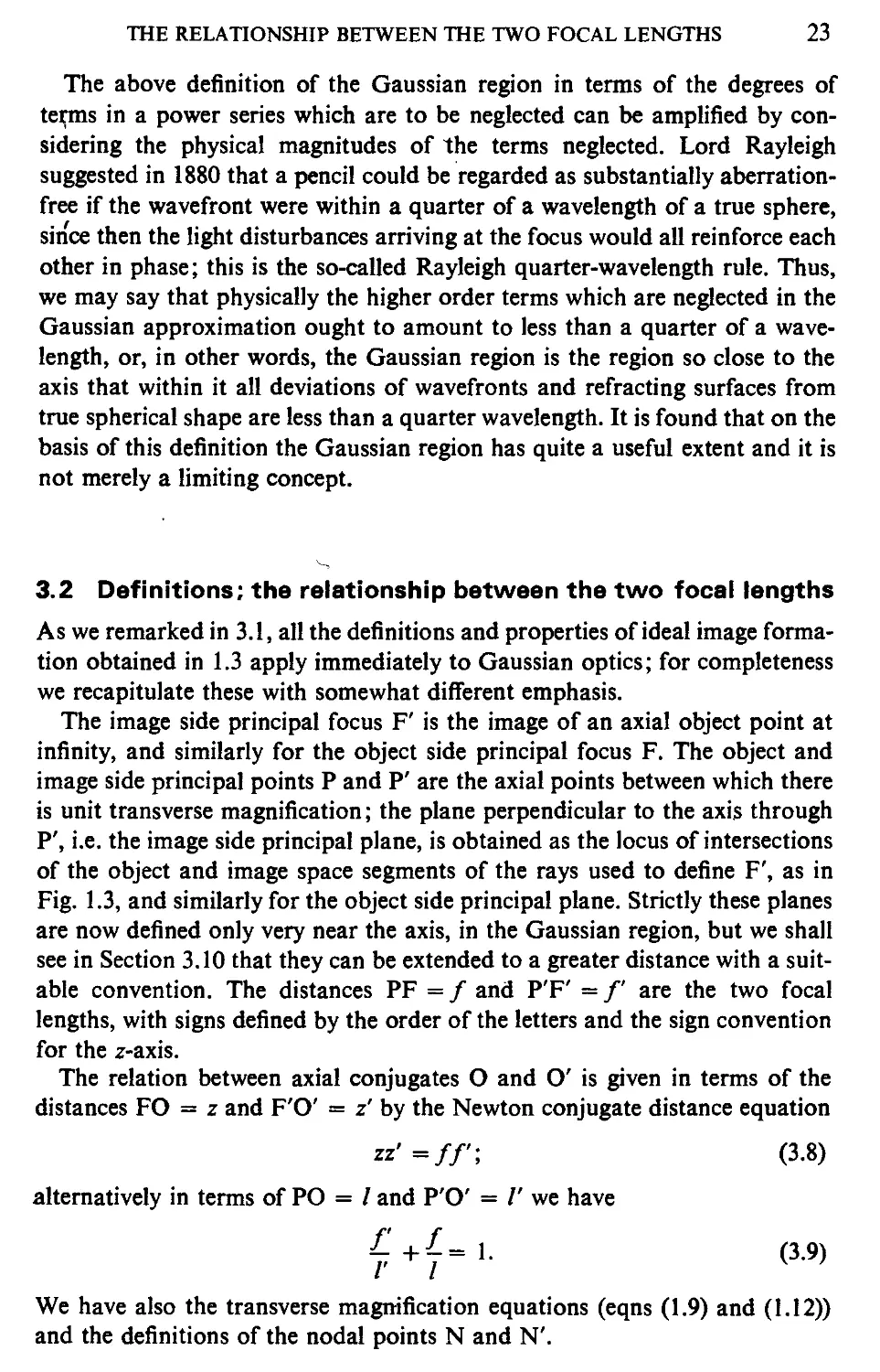
3.2 Definitions; the relationship between the two focal lengths
As we remarked in 3.1, all the definitions and properties of ideal image forma-
formation obtained in 1.3 apply immediately to Gaussian optics; for completeness
we recapitulate these with somewhat different emphasis.
The image side principal focus F' is the image of an axial object point at
infinity, and similarly for the object side principal focus F. The object and
image side principal points P and P' are the axial points between which there
is unit transverse magnification; the plane perpendicular to the axis through
P', i.e. the image side principal plane, is obtained as the locus of intersections
of the object and image space segments of the rays used to define F', as in
Fig. 1.3, and similarly for the object side principal plane. Strictly these planes
are now defined only very near the axis, in the Gaussian region, but we shall
see in Section 3.10 that they can be extended to a greater distance with a suit-
suitable convention. The distances PF = / and P'F' = /' are the two focal
lengths, with signs defined by the order of the letters and the sign convention
for the z-axis.
The relation between axial conjugates О and O' is given in terms of the
distances FO = z and F'O' = z' by the Newton conjugate distance equation
zz'=ff; C.8)
alternatively in terms of PO = / and P'O' = /' we have
We have also the transverse magnification equations (eqns A.9) and A.12))
and the definitions of the nodal points N and N'.

24
GAUSSIAN OPTICS
(л)
Fig. 3.2. The ratio between the two focal lengths
The first new result which we can obtain by the application of geometrical
optics is a relation between the two focal lengths. In Fig. 3.2 let F, P, P' and F'
be the principal foci and principal points of an optical system, and let a
paraxial ray r, through F meet the principal planes at Px and Pi and the
image side focal plane at F[. We can regard P'Pi and F'Fi as wavefronts of
the pencil from F and so we have
[FP.PiFI] = [FPP'F'], C.10)
or
n.FPl + [PtPn + n'f = -и/+ [PP'] + n'f. C.11)
Thus, if the distance PPX is denoted by ft, we have on expanding FP4 by the
binomial theorem
-nh2
2/
[PP'] - fP.P,'].
C-12)
Similarly by taking another ray r2 which enters the system parallel to the
axis and at the same height h, we obtain
^ = [pp'i - [p,p;]
C.13)
and comparing eqns C.12) and C.13) we obtain the required relationship:
ri —n
From eqn C.14) it is seen that if the refractive indices of the object space
and the image space are equal, then the two focal lengths are equal in magni-
magnitude and opposite in sign. This is, of course, the most frequent situation. The
quantity n'/f (= —n/f) is called the power of the optical system and it is de-
denoted by the symbol K; the power is frequently used as a measure of strength
of an optical system because, as will be seen, it occurs naturally in many
equations involving raytracing and the combination of optical systems; also,
its value is unchanged if the system, with terminating media, is reversed end

LAGRANGE INVARIANT AND TRANSVERSE MAGNIFICATION 25
to end. The reciprocal of K, which has the dimension of length, is called the
equivalent focal length, usually abbreviated to efl. It is in fact the image side
focal length which a system with airf on both sides would have if it had the
same power as the system in question. Thus for a system in air the image side
focal length is the efl, and it is the reciprocal of the power. It is easily shown
that, in terms of the power, eqn C.9) takes the form
ri n
J-J-K. C-15)
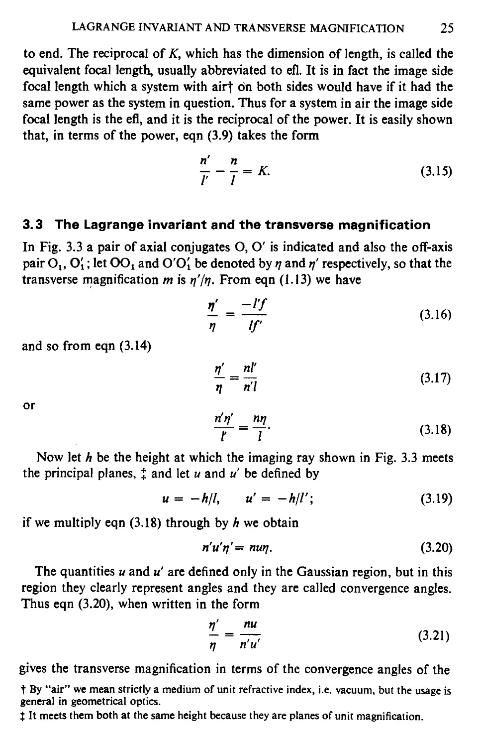
3.3 The Lagrange invariant and the transverse magnification
In Fig. 3.3 a pair of axial conjugates О, О' is indicated and also the off-axis
pair Oj, Oi; let ОО2 and O'OJ be denoted by n and rj' respectively, so that the
transverse magnification m is tj'/ij. From eqn A.13) we have
i. - --IL „.,«
4 If
and so from eqn C.14)
n' nl'
H'Vi (ЗЛ7)
or
rin'
rin' щ
~jr = T C-18)
Now let h be the height at which the imaging ray shown in Fig. 3.3 meets
the principal planes, % and let и and и be defined by
и = -h/l, u' = -A//'; C.19)
if we multiply eqn C.18) through by h we obtain
riu'r\'= nutj. C.20)
The quantities и and и are defined only in the Gaussian region, but in this
region they clearly represent angles and they are called convergence angles.
Thus eqn C.20), when written in the form
W nu
- = — C-21)
rj nu
gives the transverse magnification in terms of the convergence angles of the
t By "air" we mean strictly a medium of unit refractive index, i.e. vacuum, but the usage is
general in geometrical optics.
\ It meets them both at the same height because they are planes of unit magnification.

26
GAUSSIAN OPTICS
ray from the axial object point. The sign of the convergence angle is given by
its definition in terms of Л and / in eqn C.19), so that in Fig. 3.3 и is positive
and u' is negative; this convention is then extended to other paraxial angles,
and it agrees with the usual convention that an anti-clockwise rotation from
the axis is positive.
Equation C.20) has a much wider application than to the calculation of
transverse magnification. Let us suppose that the optical system of Fig. 3.3
\A
v Fig. 3.3. Transverse magnification
is to be followed by a further system; then the quantity n'u'ij' for the first
system will be the nurj for the second, for the refractive index is the same, the
image for the first system becomes the object for the second and the conver-
convergence angle is the same. Thus this quantity is an invariant through both sys-
systems and, therefore, it must be an invariant right from the object space
through all intermediate spaces of any symmetrical optical system. This in-
invariant was first given by Robert Smith in his "Compleat System of Opticks",
Book II, published in 1738. It was later given in various forms by Lagrange
and by Helmholtz. Following general usage we call it the Lagrange invariant
and denote it by the symbol H.
The Lagrange invariant enters into aberration calculations, as will be seen
in Chapter 8; it is significant in the photometry of optical instruments, since
it can be shown that the total flux collected by a system from a uniformly
radiating object is proportional to H2; also the Lagrange invariant divided
by the wavelength of the light is, in effect, the unit in the dimensionless co-
coordinates used in the diffraction theory of optical instruments. On account of
the importance of these varied applications, we now give a proof from first
principles of eqn C.20).
Let ООХ and O'Oi be conjugates of heights rj and r\' (Fig. 3.4) and let the
ray r, from О to O' have convergence angles и and и'. Rays r2 and r3 from Ot
to OJ are drawn respectively parallel to ray r1 and to the axis in object space
and OjP and OiP' are perpendiculars from Ot and O\ to ray rv Then
[OO']M = [OO']aIIS,
C.22)

LAGRANGE INVARIANT AND TRANSVERSE MAGNIFICATION 27
{n) r2
О P
Fig. 3.4. The Lagrange invariant
since О and O' are conjugates, and similarly
C.23)
We can now take ООХ to represent a wavefront of a pencil from the axial
object at infinity, so that ray r3 and the axis will be rays of this pencil; the
wavefront of this pencil which passes through O' will be spherical and tangent
to CO! at O' so that we have
C.24)
Combining eqns C.22), C.23) and C.24), we obtain
[О,О1]„ = [OO']ri
or
Oi],, = [°p] + PP'Im + [p'o'l + °(i2)-
C.25)
C-26)
Again we can regard OXP as a wavefront of a pencil of which rl and r2 are
rays and we have
[OiOi]r2 = [PP']M + 0(^2) C.27)
and subtracting from eqn C.26) we have
[OP] = [O'P'] + Ofa2). C.28)
Thus to the approximation of Gaussian optics we obtain again
nurj = n'u'rj'. C.20)
This proof is independent of previous results, except the general theorem
that imagery in the Gaussian region is perfect, and it shows the fundamental
nature of the Lagrange invariant.
It may happen that in one of the spaces of an optical system, not necessarily
the object space or the image space, the intermediate object/image is at

28
GAUSSIAN OPTICS
infinity; this is then said to be a star space.f The form of the Lagrange in-
invariant given in eqn C.20) becomes indeterminate in a star space, since .и
tends to zero and r\ tends to infinity, but the indeterminacy may be resolved
by writing и as —h/l, where A is the incidence height at a surface bounding the
space and / is the intersection length from this surface; also we put rj = pi,
where /? is afield angle defined with the same sign convention as for conver-
convergence angles. It is then seen that as / tends to infinity we have
#-> -nhfi.
C.29)
Any ghost surface in the star space can be used to determine A and / in the
above; for / tends to infinity, so the origin is unimportant, and the ray which
gives A becomes parallel to the axis. The field angle /? is defined here only for
a star space; the more general concept is that of the convergence angle of the
principal ray (Section 3.5) and it will be shown in Section 5.2 that this leads
to a simple alternative derivation of eqn C.29).
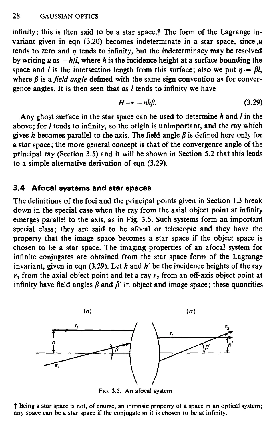
3.4 Afocal systems and star spaces
The definitions of the foci and the principal points given in Section 1.3 break
down in the special case when the ray from the axial object point at infinity
emerges parallel to the axis, as in Fig. 3.5. Such systems form an important
special class; they are said to be afocal or telescopic and they have the
property that the image space becomes a star space if the object space is
chosen to be a star space. The imaging properties of an afocal system for
infinite conjugates are obtained from the star space form of the Lagrange
invariant, given in eqn C.29). Let A and К be the incidence heights of the ray
r1 from the axial object point and let a ray r2 from an off-axis object point at
infinity have field angles /? and /?' in object and image space; these quantities
in)
Fig. 3.5. An afocal system
t Being a star space is not, of course, an intrinsic property of a space in an optical system;
any space can be a star space if the conjugate in it is chosen to be at infinity.

AFOCAL SYSTEMS AND STAR SPACES
29
are indicated in Fig. 3.5. Then we have immediately
n'h'p' = nhp
so that the angular magnification is
J
nh
C.30)
C.31)
If an afocal system is used with conjugates at a finite distance it can be seen
from Fig. 3.5 that the transverse magnification is constant, for it is equal to
h'/h. We cannot obtain conjugate distance relations analogous to eqn A.8)
or eqn (I.ll) for an afocal system since there are neither foci nor principal
planes to be used as origins for the measurement of conjugate distances.
Fig. 3.6. Conjugate distance equation for an afocal system
However, we can choose arbitrarily a pair of axial conjugates as origins, such
as О and O' in Fig. 3.6; we then construct another pair of conjugates OtB
and OiB' from the intersections of the rays through О and O' with a ray
parallel to the axis. If then OOX = /, O'Oi = /', we have from the figure
so that from eqn C.31)
/' AT?
Г n'h'2
I nh2
C.32)
C.33)
This is the required conjugate distance equation; it is clearly independent
of the particular pair of conjugates О and O' chosen as origins, a fact which
may be restated in slightly different form as, the longitudinal magnification is
constant and equal to the transverse magnification divided by the angular
magnification.
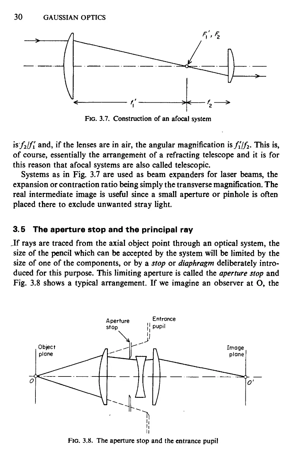
Figure 3.7 shows how an afocal system might be formed from two thin
lenses of equivalent focal lengths /i' and/2'; the lenses are placed so that the
foci FJ and F2 coincide and it may be seen that the transverse magnification

30
GAUSSIAN OPTICS
Fig. 3.7. Construction of an afocal system
is'/2//i and, if the lenses are in air, the angular magnification is////2. This is,
of course, essentially the arrangement of a refracting telescope and it is for
this reason that afocal systems are also called telescopic.
Systems as in Fig. 3.7 are used as beam expanders for laser beams, the
expansion or contraction ratio being simply the transverse magnification. The
real intermediate image is useful since a small aperture or pinhole is often
placed there to exclude unwanted stray light.
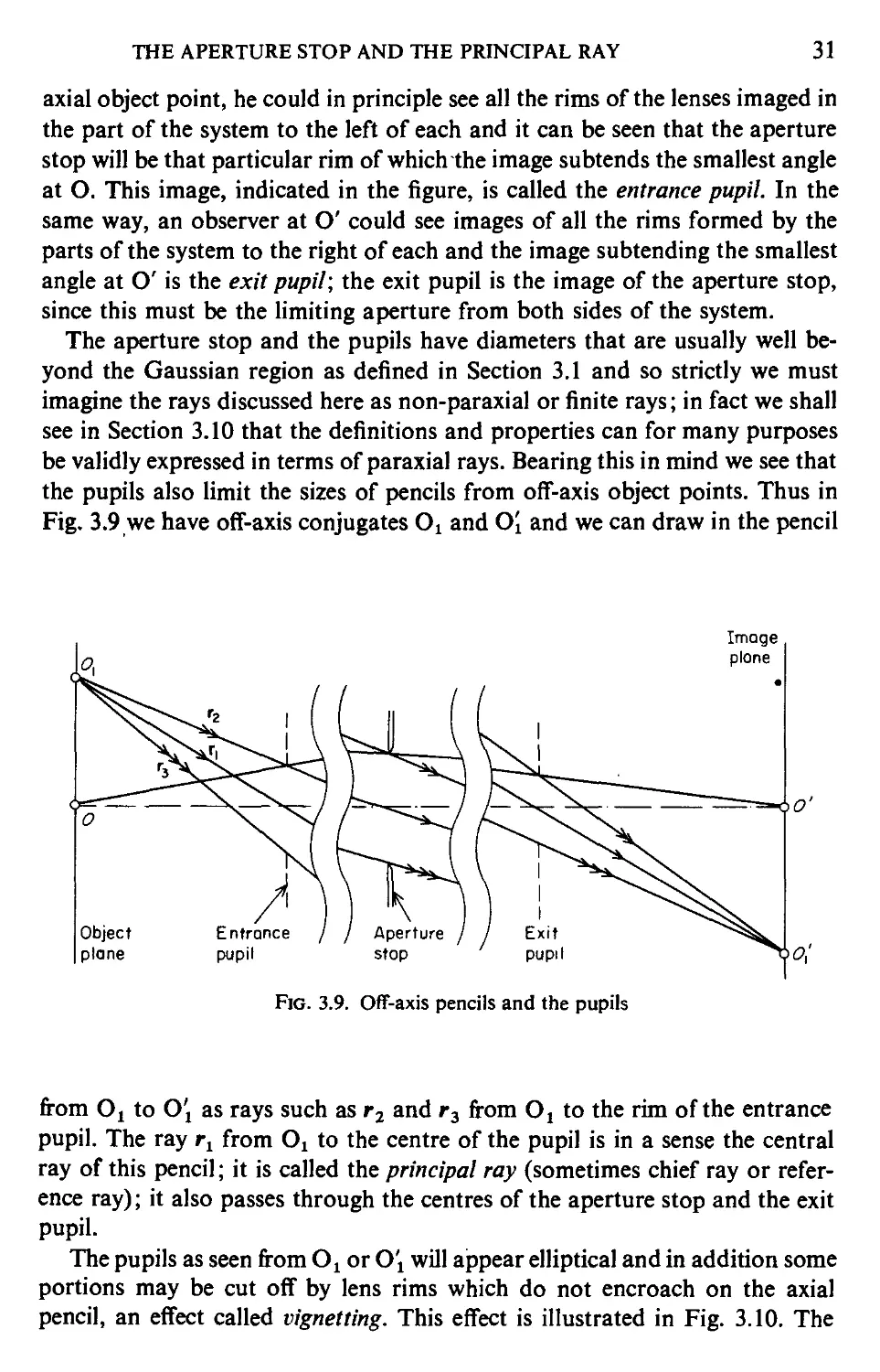
3.5 The aperture stop and the principal ray
Jf rays are traced from the axial object point through an optical system, the
size of the pencil which can be accepted by the system will be limited by the
size of one of the components, or by a stop or diaphragm deliberately intro-
introduced for this purpose. This limiting aperture is called the aperture stop and
Fig. 3.8 shows a typical arrangement. If we imagine an observer at O, the
Aperture
stop
Entrance
Fig. 3.8. The aperture stop and the entrance pupil

THE APERTURE STOP AND THE PRINCIPAL RAY
31
axial object point, he could in principle see all the rims of the lenses imaged in
the part of the system to the left of each and it can be seen that the aperture
stop will be that particular rim of which the image subtends the smallest angle
at O. This image, indicated in the figure, is called the entrance pupil. In the
same way, an observer at O' could see images of all the rims formed by the
parts of the system to the right of each and the image subtending the smallest
angle at O' is the exit pupil; the exit pupil is the image of the aperture stop,
since this must be the limiting aperture from both sides of the system.
The aperture stop and the pupils have diameters that are usually well be-
beyond the Gaussian region as defined in Section 3.1 and so strictly we must
imagine the rays discussed here as non-paraxial or finite rays; in fact we shall
see in Section 3.10 that the definitions and properties can for many purposes
be validly expressed in terms of paraxial rays. Bearing this in mind we see that
the pupils also limit the sizes of pencils from off-axis object points. Thus in
Fig. 3.9 we have off-axis conjugates O1 and O[ and we can draw in the pencil
Image
plane
Fig. 3.9. Off-axis pencils and the pupils
from Oj to Oi as rays such as r2 and r3 from O1 to the rim of the entrance
pupil. The ray rl from Ox to the centre of the pupil is in a sense the central
ray of this pencil; it is called the principal ray (sometimes chief ray or refer-
reference ray); it also passes through the centres of the aperture stop and the exit
pupil.
The pupils as seen from Ot or O\ will appear elliptical and in addition some
portions may be cut off by lens rims which do not encroach on the axial
pencil, an effect called vignetting. This effect is illustrated in Fig. 3.10. The

32
GAUSSIAN OPTICS
Fig. 3.10. Off-axis pupils and vignetting
choice of the ray of an off-axis pencil to be regarded as the principal ray is
somewhat arbitrary under such conditions, particularly as the pupil imagery,
i.e. the image formation from the entrance pupil to the exit pupil, may have
large aberrations; however, as suggested above, the essential points involve
only Gaussian considerations.
The aperture stop is usually physically inside an optical system; quite
frequently the pupils are near the principal planes, but this need not be the
case. The choice of the position of the stop depends sometimes in part on
mechanical considerations, as when it is incorporated as an iris diaphragm in
a photographic objective; however, the diameter and axial position of the
stop also affect the aberrations of the system to the extent that, as will be
shown in Chapter 8, an axial shift of the stop changes the relative proportions
of different aberrations. Another factor which sometimes affects the choice
of the position of the aperture stop is the inclination of the principal rays to the
axis in object space or image space. It may happen that it is desirable that the
principal rays in image space should all be parallel to the axis; this would in-
involve an exit pupil at infinity and this is achieved by putting the aperture stop
at the object side principal focus, as in Fig. 3.11; the aperture stop is then said
Image
plane
Fig. 3.11. Telecentric aperture stop

GAUSSIAN PROPERTIES OF A SINGLE SURFACE 33
to be telecentric. Of several possible reasons for requiring this we mention the
following two: (a) a measuring graticule may have to be put at the image
plane and then small errors of focus will have no effect on the size of the image
as measured on the graticule; (b) if a photograph is to be taken on film then
slight departures from flatness of the film will not produce apparent distor-
distortions of image size and shape, an application of importance in the photo-
photography of bubble chambers.
If a system is afocal it may happen that rays from infinity on the axis in
object space cross the axis in some intermediate space; then if the aperture stop
is placed at that position the pupils will be at infinity in both object and image
spaces, i.e. the system is telecentric on both sides.
3.6 Field stops
There may also be a stop in an optical system which limits the size of the field
and this, if it exists, will be at the object or image plane or some intermediate
real conjugate. For example, in a camera the field stop is a rectangular
diaphragm in contact with the film and in a slide projector it is a similar
diaphragm in contact with the slide; certain types of eyepiece usually have a
field stop at the position of a real image inside the eyepiece.
Field stops do not have the basic optical importance that the aperture stop
has since they do not control the aberration balance; this is, of course, be-
because the field stop can only be placed at the object conjugate in each space.
The field stop limits the field of view to that for which the optical system has
adequate aberration correction and it also provides a format of the required
shape. However, some optical systems do not have a definite field stop, for
example the human eye. The images of the field stop in object and image space
are sometimes called the entrance and exit windows, but little importance
attaches to this concept.
Other stops found in optical systems are for trapping unwanted light from
reflections and scatter off optical and non-optical surfaces and for preventing
light from travelling along inappropriate paths in reflecting systems.
3.7 Gaussian properties of a single surface
In order to carry the subject further we now have to consider how to find the
Gaussian properties of actual systems. Consider a single refracting (or re-
reflecting) surface of curvature с which separates two media of indices n and n',
as in Fig. 3.12. Clearly the principal planes coincide at the surface, since an
object at the surface will have its image there and of the same size; we are
then justified in measuring conjugate distances / and /' from the surface, as

34 GAUSSIAN OPTICS
0'
¦ Refracting
. / surface
Fig. 3.12. A single refracting surface
indicated. Let ? and ?' be two wavefronts of the axial pencil before and after
refraction, respectively, which both touch the refracting surface on the axis;
in our figure ?' happens to be a virtual wavefront, but this is of no significance.
Let the image-forming ray shown meet the wavefronts at P and P' and the
refracting surface at Q. Then since the distances between two wavefronts of
the same pencil along any two rays are equal we have
[PQP'] = 0 C.34)
or,
n'.P'Q = h.PQ. C.35)
This equation is correct without any restriction to the Gaussian region, but
within this region we have
PQ = ih2c - \h2\l, C.36)
where h is the incidence height of the ray, and similarly for P'Q. Substituting
in eqn C.34) we obtain on cancelling the factor A2,
C.37)
Rearranging this result in the form
- __ = („'_ ny C.38)
we recognize it as a conjugate distance equation of the form of eqn C.15)
and we identify the quantity (л' — ri)c as the power of the surface. Thus the

GAUSSIAN PROPERTIES OF TWO SYSTEMS
two focal lengths are respectively
—n , .. r,
n' - n)c
(n1 - n)c
35
C.39)
The nodal points (see Section 1.3) must coincide at the centre of curvature
of the surface, since a ray through the centre of curvature meets the surface
normally and is undeviated; this result also follows from eqn A.14).
For a mirror with light incident from the left we take и = — 1 and ri = 1 and
we find that the two focal lengths are both equal to l/2c and the power is 2c,
where с is again the curvature. As before the principal points are at the mirror
surface and the nodal points are at the centre of curvature.
3.8 Gaussian properties of two systems
Our next step is to consider the combination of two general systems of known
properties and with a given axial separation. It is convenient to do this by
determining the paths of certain paraxial rays through the combined system
and obtaining the Gaussian parameters from these paths. Consider first any
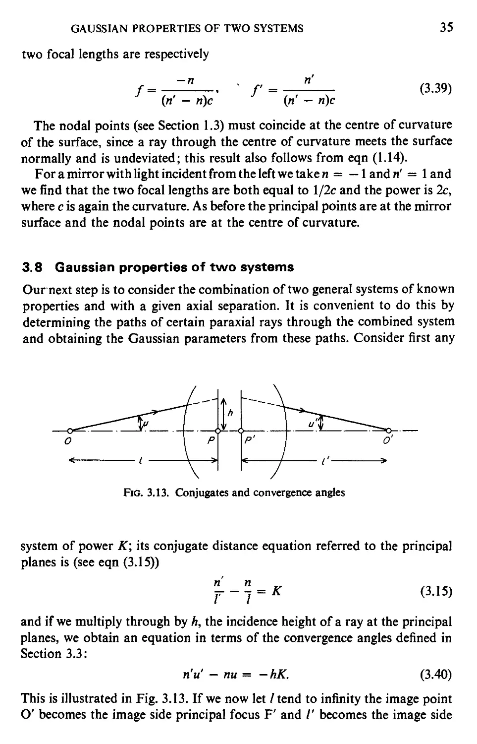
Fig. 3.13. Conjugates and convergence angles
system of power K; its conjugate distance equation referred to the principal
planes is (see eqn C.15))
" --
T 1
C.15)
and if we multiply through by h, the incidence height of a ray at the principal
planes, we obtain an equation in terms of the convergence angles defined in
Section 3.3:
n'u' - nu= -hK.
C.40)
This is illustrated in Fig. 3.13. If we now let / tend to infinity the image point
O' becomes the image side principal focus F' and /' becomes the image side

36 GAUSSIAN OPTICS
Fig. 3.14. Calculating/' from the path of a paraxial ray
focal length/', according to the definitions of Section 1.3. We have the situa-
situation shown in Fig. 3.14 and from eqn C.40) we have
or,
and
nV = -hK
K= -n'u'/h
f = -h/u'.
C.41)
C.42)
C.43)
The first focal length is easily obtained from the fundamental relationship
between the focal lengths, eqn C.14).
Returning now to the problem of combining two systems in series, let
their powers be Kt and K2 and let the separation between adjacent principal
planes Pi and P2 be d, as in Fig. 3.15; this quantity is taken positive if PJP2
is a positive distance, i.e. left-to-right; the refractive indices in the initial,
intermediate and final spaces are n, n[ and ri. We now take a ray from the
axial object point at infinity at distance ht from the axis. By applying eqn
C.40) we have, since и s 0 in this case,
n[u[ = -
By geometry in the intermediate space we have
h2 = ^ + du[
C.44)
C.45)
Fig. 3.15. Combining two systems in series; separation referred to the
principal points

GAUSSIAN PROPERTIES OF TWO SYSTEMS 37
and by a similar application of eqn C.40) to the second system,
n'u' - n[ui = -h2K2. C.46)
We can now eliminate h2 and u[ between eqns C.44), C.45), C.46), and we
obtain
d \
y + K2 KXK2 ; C.47)
n\ I
if we compare this with eqn C.41) we see that the quantity in the brackets on
the right-hand side of eqn C.47) must be K, the power of the combined
system, so we have
K= Kt + K2 K,K2. d C.48)
In order to specify the Gaussian properties completely we have to know
the positions of the principal planes P and P' as well as the power; let P^P' be
denoted by 3', positive in this sense, and let PjP be S. From the geometry of
the diagram we have
S' = -(A2 - kO/W, C.49)
= -du'Ju' C.50)
from eqn C.45); then substituting for u[ from eqn C.44) and for u' from
eqn C.42) we have
If we now reverse the whole procedure, i.e. take a ray which passes through
the object side principal focus, we obtain the result
n dK2
<* = -•— C.52)
n[ К
These results can now be applied to some cases of practical importance.
For the thick lens in air, as in Fig. 3.46, the powers of the individual surfaces
are given by the expression on the right of eqn C.38) and substituting in eqn
C.48) we have for the power
- c2
C.53)
where яа is the refractive index of air. This value is at ordinary temperatures
and pressures approximately 1-0003 but the universal practice in optical

38 GAUSSIAN OPTICS
f
8
<?—
P P'
С
-d —
\
8'
1
г
—=>
Fig. 3.16. A thick lens in air
design is to specify the indices of glasses as relative to air, not vacuum, so with
this convention we have for the thick lens,
К = (n - l)(c, - c2 + dcxcX
C.54)
where now the relative index is understood. Thus from Section 3.2 we see
that the reciprocal of К in eqn C.54), which is the equivalent focal length, is
also the image side focal length. As noted in Section 3.7, the principal planes
of a single surface coincide at the surface, so that the positions of the principal
planes of the complete lens are given by values of 8 and S' measured as indi-
indicated in the figure; here <5' happens to be negative. The explicit formulae are,
from eqns C.51) and C.52),
(и-
1)
dc2
K'
(л -
n
1)
A,
К
§_ (n-l)dc2
C.55)
If we allow the thickness d to tend to zero we obtain that very useful and
important abstraction, the thin lens in air; its power is given by
К - (n -
- c2)
C.56)
and its principal planes are at the lens. The concept of the thin lens finds many
applications in optical designing, in spite of the manifest impossibility of
realizing such a system; the thin lens approximation forms the first stage in
the design of many optical systems and the study of the aberrational properties
of thin lenses yields useful generalizations about what kinds of optical layout
are likely to lead to good designs.
By a further application of eqn C.48) we obtain the power of two separated
thin lenses in air (Fig. 3.17) as
Л = Ki + K2 — «AiA2 (y-J/)

GAUSSIAN PROPERTIES OF TWO SYSTEMS
39
h'iG. 3.17. Two separated thin lenses; the symbolic representation for a thin
lens as shown is frequently used in texts on optics
and the positions of the principal planes follow from obvious modifications
of eqns C.51) and C.52).
For two thin lenses in contact it can be seen from eqn C.57) that the re-
resultant power is the sum of the individual powers; this is one reason for the
use of power rather than focal length as a measure of strength in, for example,
ophthalmic optics.
It is sometimes useful to re-write some of the results of this section in terms
of the separation g between the adjacent foci of the two systems, instead of d,
the separation between adjacent principal planes. Paying due regard to signs
we have, from Fig. 3.18,
d = g +
* K
C.58)
Fig. 3.18. Combining two systems in series; separation referred to the foci
and substituting in eqn C.48) we obtain for the power of the resultant system
C.59)
—g
К = —'
In order to obtain compact expressions we find the positions of the principal
foci of the resultant system relative to the adjacent foci of the components;
referring again to Fig. 3.18 we put Л = FXF and A' = F^F' and we consider
a ray from the axial object point at infinity; as indicated, Fi and F' are
conjugates on this ray and we have from Newton's conjugate distance relation

40 GAUSSIAN OPTICS
(eqn A.8)), with appropriate signs,
or
n[n'
Similarly we obtain
A = -
n'K,
КгК
п[п пК2
KtK
C.60)
C.61)
C.62)
3.9 Thick lenses and combinations of thin lenses
In this section we obtain several interesting properties of lenses and lens
systems from the results of Section 3.8; these results will be by way of ex-
examples, rather than part of the systematic development of the subject.
If the same increment is added algebraically to the curvatures of a thin lens
its power remains the same, as can be seen from eqn^3.56), but its shape, i.e.
its cross-section by a plane through the axis, changes and, as will be seen in
later chapters, its aberrations change. Figure 3.19 shows how the shape
changes with the same increment of curvature at each surface; the process of
changing the shape in this way is called bending the lens. Since the aberrations
r\
л
V
/1
VJ
Fig. 3.19. Bending a "thin" lens; the shapes are (a) biconvex, (b) planoconvex,
(c) meniscus
change but the Gaussian properties remain constant the amount of bending
is a useful variable in balancing aberrations in a complex system. If the lens
is not thin in the technical sense it can still be bent by adding the same incre-
increment to both curvatures but then, as can be seen from eqns C.54) and C.55),
the power changes and the principal planes shift; however, if the thickness is
small compared to the focal length and the radii of curvature, the change in

THICK LENSES AND COMBINATIONS OF THIN LENSES
41
power is small and it is useful to see how the principal planes shift with
bending. The distance PP', sometimes called the interstitium, can easily be
found from eqn C.55) to be
( 1 In - l\2
PP'= </!--+
{ n \ n }
C.63)
and under the conditions mentioned above it can be seen that this is nearly
constant with bending at the value d(n — l)/n, i.e. one-third of the thickness
of the lens if the conventional approximate value of the refractive index of
glass is adopted. However, as can be seen also from eqn C.55), the principal
planes are displaced along the axis roughly proportionally to the increment in
curvature. Figure 3.20 shows how this occurs with positive and negative
lenses.
А
V7
Fig. 3.20. Dependence of the principal points on shape
For some purposes it is desirable to keep the Gaussian effect of a lens con-
constant as it is bent; it would then be necessary to displace the physical lens
along the axis in such a way as to keep the principal planes in the same
positions relative to the adjacent components. It might also be desirable to
add slightly different increments of curvature to the two surfaces so as to keep
the power precisely constant and even to allow for the slight change in the
interstitium; if this were done then the Gaussian properties of the rest of the
system would not be changed and, as will be seen in Chapter 8, the primary
aberrations of the rest of the system would also remain constant. However,
it is not usual to go to such refinements in bending a lens.

42 GAUSSIAN OPTICS
The value of the refractive index does not greatly affect the above discus-
discussion for lenses of moderate thickness, i.e. thickness small compared to either
radius of curvature and to the equivalent focal length. Very thick lenses are
occasionally of interest; for example a sphere of radius r has power 2(n — l)/nr
and its principal points coincide at the centre.f A concentric meniscus as in
Fig. 3.21 is also "very thick" in this sense; its power is —(л — X)dcxc2\n and
its principal points are at the centre of curvature. If the curvature of the second
surface is slightly decreased so that the radii are related by
r2 = r,-—rf C.64)
n
the power decreases to zero and the meniscus is afocal.
Fig. 3.21. A concentric meniscus lens; the principal points coincide at the
common centre of curvature of the surfaces
Two lenses with adjacent foci coincident form an afocal system, as in Fig.
3.7, with angular magnification -К21КЪ as can be seen from eqns C.59) and
C.31). A system of three thin lenses arranged as in Fig. 3.22 has unit angular,
transverse and longitudinal magnifications, by the formulae of Section 3.4;
thus it merely transports a real image a fixed distance along the axis, as indi-
indicated by the ray in the figure. A sequence of such systems is used for trans-
transporting laser beams without beam spreading and this is also the principle of
image transport in periscopes. The electron-optical lens system formed by a
uniform axial magnetic field (long solenoid) has essentially the same Gaussian
properties, apart from image rotation.
t In fact the principal points of any system with spherical symmetry and with object and
image spaces of the same refractive index coincide at the centre of symmetry; this can be
seen from the fact that the principal points in this case coincide with the nodal points and
the nodal points must be at the centre because a ray aimed at the centre is undeviated by the
system.

THICK LENSES AND COMBINATIONS OF THIN LENSES
к гк к
43
Fig. 3.22. An afocal system of magnification unity
The power and the equivalent focal length of an optical system are the
basic measures of its strength, ability to magnify, form bright images, etc.
However, for practical purposes it is also useful to define other quantities;
the back focal length is defined as the distance from the last surface of the
system to F' and the back vertex power is the reciprocal of this quantity. There
are similar definitions relative to F. These definitions are used chiefly in con-
connection with spectacle lenses and photographic objectives and so it is gener-
generally assumed that the medium on both sides of the optical system is air. An
interesting example in the Gaussian optics of lens systems is provided by the
theory of an instrument for measuring the vertex power of a lens, sometimes
called a vertometer. Referring to Fig. 3.23, a lens of known power К is set up
with a graticule or marker which can be moved axially in its object space; a
telescope adjusted for infinity is set up to view the movable graticule through
the lens; thus when the graticule appears in focus it must be at the object side
Movable
graticule
Lens of
power К
Telescope
(a)
Lens to
be tested
Movable
graticule
W
Ш
(b)
Fig. 3.23. Principle of vertometer (a) set for zero power; (b) measuring the
vertex power of a converging lens

44 GAUSSIAN OPTICS
principal focus F of the lens. There is a rounded contact at F' and the lens to
be measured is placed with its vertex touching the contact; the graticule must
then be displaced through a distance z, say, along the axis in order to bring
it into focus, as in the lower diagram. It can be seen that the graticule appears
at a distance z' from the vertex of the lens being measured which is the reci-
reciprocal of the vertex power, and by Newton's conjugate distance relation eqn
A.8) we have
zz1 = -l/K2, C.65)
thus the vertex power is obtained as — zK2, with due attention to signs.
A final example is provided by the field lens, a concept with a variety of
applications. One application is to the positioning cf the exit pupil in optical
systems which are to be used visually, e.g. microscopes; since all the principal
rays pass through the centres of the pupils it can be seen that the eye must be
placed with its entrance pupil at or near the exit pupil of the instrument, as in
Fig. 3.24, in order to see the whole field of view.f It is thus necessary to ensure
Eye clearance
Eyeball
Last refracting
surface Exit pupil of
optical system
Fig. 3.24. The exit pupil in a visual instrument
that the exit pupil is beyond the last surface of the system and that there is
adequate eye-clearance, usually between 10 mm and 20 mm. A field lens is
used to bring the exit pupil to a suitable position and also to produce a larger
angular field in such cases. Consider, for example, the refracting telescope as
in Fig. 3.7; we can re-draw this to show an off-axis or oblique pencil, as in
Fig. 3.25; usually the front lens or objective is itself the entrance pupil and
aperture stop, so that the exit pupil is formed near the second principal focus
of the eyepiece; a low-power eyepiece may thus produce a very remote pupil
t The same applies, of course, if two instruments are to be used in series.

PARAXIAL RAYTRACING
45
Fig. 3.25. Refracting telescope with single lens eyepiece; the exit pupil is
at a large distance from the eyepiece
and so, because of the finite diameter of the eyepiece, a restricted angular field
of view. Now suppose a thin lens of positive power, the field lens, is placed at
the intermediate real image, where there would normally be a field stop, as in
Fig. 3.26; this has no effect on the object-image conjugates and magnification
Objective
Fig. 3.26. The effect of a field lens on the position of the exit pupil
but the effect is to deflect the oblique pencil towards the axis, thus decreasing
the eye-clearance and also decreasing the used diameter of the last component.
Most eyepieces except certain very high power systems can be seen to have
two sections which may be called the field lens and the eye-lens; in fact each
may contain more than one component but the functions of pupil and object
imagery are roughly distributed as indicated here.
3.10 Paraxial ray tracing
The Gaussian properties of systems containing more than two surfaces or
thin lenses can in principle be obtained by successive applications of the
formulae in Section 3.8 for combining two systems but in practice the results
are clumsy and expressions of this kind are not used in designing and analys-
analysing optical systems. Suppose that it is required to find the power of a system
of given properties, i.e. the curvatures, refractive indices and thicknesses are
all given; the power could be found if we knew the final convergence angle of
a paraxial ray of given incidence height from the axial object point at infinity,
using eqn C.42), as was indicated in Fig. 3.14. In that case the result was
obtained as an algebraical expression, eqn C.48), involving the two com-

46 GAUSSIAN OPTICS
ponent systems or surfaces but in the present case there may be any number of
surfaces and so we track the path of the ray surface by surface, using numbers
instead of symbols. This process of finding a ray path in terms of the numeri-
numerical values of the incidence heights and convergence angles at each surface in
turn is called ray tracing and it is of fundamental importance in optical design;
this is because the results obtained are used in aberration calculations in
addition to yielding the Gaussian properties.
We have first to number the surfaces and spaces consistently. Suppose there
are к refracting or reflecting surfaces; we number them from the left, using
the number as a subscript, so that c} is the curvature of theyth surface; the
refractive indices of the media preceding and following c, are и, and n'j
respectively and the axial distance from c} to cJ+l is d'j, taken as positive if
cJ+l is to the right of Cj, as is usual; the symbol dj_t would denote the dis-
distance from Cj to c7_! and it would usually be negative, but this is not often
required. There is some redundancy of symbols, since n'j = nJ+i and d'} =
— rfj+i.f Figure 3.27 shows an optical system with ray segments numbered
according to this scheme.
It can be seen from Fig. 3.27 that a ray segment incident at surface j is
specified by its incidence height A, and its convergence angle uy, the refracted
ray is specified by h3 and u'j so that the incidence heights and convergence
angles are in a sense generalized co-ordinates of the ray as it passes through
the optical system. We then have from eqn C.40)
п)и] - njuj = -MO, C.66)
where
K, = (n'j - nj)cj; C.67)
also by analogy with eqn C.45)
hM = hj + d'ju'j. C.68)
The powers, refractive indices, etc., are, of course, given; thus if we start
from Uj and hs we can apply eqns C.66) and C.68) in succession to obtain
uJ+t and hJ+l, and so on through the system; eqn C.66) is called the refraction
equation and eqn C.68) is the transfer equation, both terms having obvious
derivations. These two are thus a set of recurrence or recursion formulae, to
be applied numerically. For example, if we begin with a ray from the axial
object point at infinity, for which ht is chosen at will and ut = 0, we obtain
hk and u'k at the final surface and we then, according to eqn C.42), obtain the
t It is also possible to number spaces rather than surfaces, in which case the surface between
spaces у and у + 1 would have some such symbol as cJtJ+l or perhaps simply cJ+l as de-
denoting rather arbitrarily the surface following space j. It is essential to have a consistent
notation but the choice is a matter for the individual and no special claim is made for that
described here.

PARAXIAL RAYTRACING
47
Cj-\
Fig. 3.27. A scheme of notation for paraxial raytracing
power:
C.69)
Similarly the equivalent focal length and the back focal length are given by
efl = -
bfl = -hk/u'k.
C.70)
Other applications of the raytracing process will be described later. We now
consider how the choice should be made of the initial value of ht to be used
in a raytrace to find the power. Since this whole process is based on results
which apply only to the Gaussian region it might at first be supposed that hx
should be chosen small enough to restrict all the incidence heights to the
Gaussian region. In fact we have not yet estimated the non-Gaussian terms
(i.e. the primary aberrations, see Chapters 7 and 8) and we therefore cannot do
this accurately, but suppose for the moment that a suitably small value of hx
has been chosen. The raytracing equations (eqns C.66) and C.68)) are linear
in the variables h and и and also the end results required, powers or focal
lengths, are of zero dimension in h and и jointly; thus if we multiply ht by a
large numerical factor, then all the succeeding hj and щ will merely be scaled
by the same factor and the powers and focal lengths will be unchanged. Thus
it can be seen that paraxial raytracing can be carried out with any arbitrarily
chosen incidence height of the incoming ray and the results are still valid for
the above purposes. The incidence height which is generally chosen is that
corresponding to the radius of the entrance pupil; when this is done the
primary aberrations, calculated as in Chapter 8, also have values appropriate
to the edge of the pupil.

48 GAUSSIAN OPTICS
The question of the choice of incidence heights for a paraxial raytrace can
also be considered in a different way. It may be said that what we are really
doing in tracing a ray from, say, the axial object at infinity to the second
principal focus is applying in succession the conjugate distance equation for
a single surface (eqn C.38)) and a simple transfer equation,
— — if I
Tj h~ J\ C.71)
and that the raytracing equations are really versions of these obtained by
multiplying through by the factors ht and Uj respectively. This point of view
gets round the question of the choice of a value of At within the paraxial
region but on the other hand, eqns C.71) only give the back focal length
directly and it is necessary to introduce incidence heights somewhere in order
to obtain the equivalent focal length or the power.
The raytracing equations may be written down at length as follows:
n\u[ - и,и, = -h^
h2 = ht + d[u[
n'2u'2 — n2u2 = —h2K2
h3 = h2 + d'2u2
C.72)
As stated at the beginning of this section, it is not usual to carry out an
algebraic elimination of the intermediate variables to obtain uk as a function
of hi and there is no situation which requires this in present-day optical design
techniques. This elimination has been done by means of continued fractions
and it is also possible to express eqns C.72) in matrix form and use a con-
continued matrix product, but this does not seem very useful. An equation which
is sometimes useful is obtained by simply adding together all the refraction
equations, giving
"X - riiUi = -{htKi + h2K2+--+ hkKk}; C.73)
this equation applies equally to thin lenses in air with powers Ku K2,...
provided the refractive indices are set equal to unity, and in this form it is used
in situations where the aberrations of thin lens systems are to be minimized.
A raytrace according to eqns C.72) from one axial object point specified
by hi and Ui to the conjugate in image space yields complete information
about the Gaussian image formation at these conjugates, since the transverse

PARAXIAL RAYTRACING 49
magnification is immediately given according to eqn C.21) by
Ik "r«i
- = — ¦ C.74)
It пЫ
If the object is at infinity, the form of the Lagrange invariant for star space
gives a relation between the angular subtense 0t of the object and the size rj'k
of the image,
n'M = -«AA C.75)
in terms of the raytrace results.
There is no need to trace further rays between these conjugates since accord-
according to Section 3.1 there is ideal image formation in the Gaussian region.
Many optical systems are designed for use with the object at infinity, e.g.
almost all photographic objectives. As a final example we note that eqn
C.75), together with eqn C.42) of Section 3.8, illustrates a method of measur-
measuring the power of such systems. By eliminating u'Jhy from these two equations
we have
C.76)
thus if the size of image rj'k corresponding to an object of angular subtense /^
is found, the power is obtained. This, the "focometer" method, is considered
to be one of the most accurate methods of measuring power or efi; it has even
been suggested as a way of defining efl for an industrial standard.

4 Finite Raytracing
4.1 Finite rays
So far we have considered rays and image formation only in the paraxial
region and the "raytracing" of Section 3.10 is really a process only valid in
this region, although as a numerical convenience we gave fictitiously large
values to the incidence heights and convergence angles. Having established
the Gaussian image formation for a certain conjugate pair in this way it is
possible to conceive of a process in which rays would be traced from a chosen
point Ot of the object plane without making the approximations of Gaussian
optics, i.e. exactly according to SnelPs law (Section 2.2), and their intersec-
intersections with the Gaussian image plane found. These intersections would in
general not coincide at Oi, the Gaussian image of Ob and the scatter in the
ray intersections would be a manifestation of the aberrations of the optical
system. Rays traced in this way may be called finite rays, to distinguish them
from paraxial rays which are in the mathematical sense infinitesimal, and the
process of tracing them is known as finite raytracing. This is an essential tool of
the optical designer and it is applied not only to axisymmetric systems but to
all others including, e.g. systems including diffractive optical elements such as
hologram lenses and systems with tone surfaces. Finite raytracing is used at
the stage when the general form of the optical system is known but the
aberrations have to be reduced to acceptable tolerance levels.
Finite raytracing is essentially an iterative sequence of two operations; one
of these, transfer, is simply taking a ray from where it leaves one optical surface
to where it meets the next and it thus involves only the geometry of straight

SNELL'S LAW FOR SKEW RAYS 51
lines and surfaces of appropriate shape. The other operation, usually called
refraction, is to find the direction of the ray after it has passed through or been
reflected or diffracted by the surface; the calculation involves either Snell's law
or a generalized form of it appropriate to diffractive optical elements. In this
chapter we shall deal only with refracting and reflecting surfaces of axial
symmetry; tone surfaces and diffractive components will be dealt with in
Chapter 5. The actual amount of numerical computation can, of course, be
quite considerable and this led in the past to the development of many systems
of formulae, each aimed at reducing the numerical work according to the
particular computing aids available, i.e. logarithmic and trigonometric tables
and various forms of desk calculating machine. It was also the case that most
work was done with rays lying in a plane through the optical axis (meridian
rays); rays skew to the axis were not often traced since much more work was
involved than in tracing meridian rays. The universal availability of electronic
computers has changed this situation completely since a skew raytrace can
now be carried through a complete system in a small fraction of a second. At
the time of writing the fastest machines will trace skew finite rays at the rate of
about 15000 ray-surfaces per second, whereas a skilled human took perhaps
20min for one ray-surface using log tables and perhaps 5min with a desk
calculator. We therefore describe first the universally used system for tracing
skew rays through spherical surfaces and we then discuss modifications
suitable for non-spherical surfaces; finally we shall give a method suitable for
tracing meridian rays through spherical surfaces by trigonometrical tables. In
all cases there are the two operations of refraction and transfer, applied
alternately, just as described in Section 3.10for paraxial raytracing. We deduce
and discuss the formulae in detail in the rest of this chapter; the equations are
collected for reference in Appendix A.
4.2 Snell's law for skew rays
It will be recalled from Chapter 2 that Snell's law can be written in the vector
form
n'(r' ля)- n{r A n), B.3)
where и is a unit vector along the normal at the point of incidence and r and r'
are unit vectors along the incident and refracted rays. If this equation is multi-
multiplied vectorially by n we obtain
ri(r' - я(г'.и)) = n(r - n(r-n)). D.1)
This can be expanded in scalar form by setting (L, M, N), (L', M', N') and
(a, P, y) as the components of r, r' and и respectively, so that these quantities

52 FINITE RAYTRACING
are direction cosines, giving
where
n'L - nL = ka"
n'M' - nM = kfi
n'N' - nN = ky \
- n'(r''n) — и(г-и)
n' cos /' - n cos /
D.2)
D.3)
and I and /' are the angles of incidence and refraction.
Equations D.2) are in a suitable form for use in the systems for tracing skew
rays which we shall develop.
4.3 Transfer between spherical surfaces
Let a finite ray leave a surface (the "previous" surface) with direction
cosines (L, M, N) and let its point of incidence P_t at this surface have co-
coordinates (*_!, y_u z_i) in the local coordinate system, i.e. the system with its
origin at the vertex of this surface. The transfer problem is to determine P,
the point of incidence of the ray on the current surface (Fig. 4.1), it being
assumed that (L, M, N) and the coordinates of P_! are known from previous
steps. Let с be the curvature of the current surface and let d be the axial
Fig. 4.1. Coordinates and notation for finite ray transfer

TRANSFER BETWEEN SPHERICAL SURFACES 53
separation. It is convenient to take the calculation in two steps, first finding
the coordinates of the point Po in which the ray meets the x-y plane for the
current surface. If the coordinates of Po лте (дг0, у0,0) we have
L
x0 = *-i +—(<*- z_
м 1" DA)
Уо = У-i +—(<*- z-i
Л'
by the standard properties of direction cosines.
Now let the coordinates of P be (x, y, z) and let the length of the segment
P0P be Л. We have
D.5)
The further condition, that P lies on a surface of curvature с which is
tangent to the x-y plane at the origin, can be put in the form
z = ^(x2 + у2 + z2). D.6)
We can eliminate x, у and z between eqns D.5) and D.6) to obtain a quadratic
in A:
ic{(x0 + LAJ + (y0 + MAJ + N2A2} = NA, D.7)
or
c2A2 - 2c{N - c(Lx0 + Myo)}A + c2(x2 + y2.) = 0. D.8)
Let
F = c(xl + у2) D.9)
and
G = N- c(Lx0 + My0), D.10)
then the solution of the quadratic is
cA = G ± VG2 - cF D.11)
By considering the special case when x0 and y0 tend to zero, i.e. the ray is
incident at the vertex of the refracting surface, we see that the negative sign
is to be taken in eqn D.11). Also it is generally the case that \cF\ is much less
than G2, since the latter is of order unity whereas cF is of the order of the
square of the angle subtended at the centre of curvature of the refracting sur-
surface by the arc joining the point of incidence to the vertex, and this angle is

54 FINITE RAYTRACING
usually less than 0-2 rad; in these circumstances a direct numerical evaluation
of eqn D.11) would give cA as the difference of two nearly equal numbers and
a loss of numerical precision would occur. This is avoided by multiplying and
dividing the right-hand side of eqn D.11) (with negative sign) by the quantity
G + VG2 - cF. The result is
A = D.12)
G + VG2 - cF
a form which involves no loss of significant figures when used numerically.
The value of A obtained from eqn D.12) can be substituted in eqn D.5) to
give (x, y, z), the coordinates of the point of incidence; this completes the
transfer process.
4.4 Refraction through a spherical surface
To obtain refraction formulae we need to know the components of the unit
normal at the point of incidence, in order to apply eqn D.2.). It can easily be
seen that for a spherical surface these are given by
(«,P, y) = (-ex, -cy, 1 - a), D.13)
where (x, y, z) is the point of incidence and с is the curvature. Substituting in
eqn D.2) we have as the refraction equations
n'L' = nL — Kx 1
n'M' = nM - Ky }, D.14)
n'N' = nN - Kz + n' cos Г - n cos /J
where
К = c(n' cos Г - n cos /). D.15)
We have, of course, to find cos /and cos /' before these can be applied. By
scalar multiplication we obtain
cos / = r-n
= N - c(Lx + My + Nz)
= N - c{L(x0 + LA) + M(y0 + MA) + N2A}
= N - cA - c(Lx0 + My0),
or
cos/= +{G2 - cF}*, D.16)
by eqns D.10) and D.11).

BEGINNING AND ENDING A RAYTRACE 55
Thus cos / has already been found in the transfer process.
We find cos /' by application of Snell's law in the form of eqn B.2):
ri cos /' = +{n'2 - n\\ - cos2 /)}+. D.17)
This completes the refraction process. The raytrace then proceeds as an
iterative sequence of transfers and refractions, using the equations of this and
the preceding sections alternately.
Numerical checks are sometimes useful, particularly when running a new
raytracing program. A check on the transfer process is provided by the
fact that the coordinates of the point of incidence must satisfy the equation of
the refracting surface, which is eqn D.6); the refraction process can be
checked by the requirement that the sum of the squares of the direction co-
cosines must equal unity:
L'2 + M'2 + N'2 = 1. D.18)
It is worth noting that the finite raytracing equations for transfer and re-
refraction (eqns D.4) and D.14)) reduce directly to the corresponding paraxial
forms (eqns C.72)) when the appropriate paraxializing approximations are
made; these are
7V->1, 2^0, A->0, cos/^1, cos/'-M. D.19)
The quantity AT of eqn D.15) then reduces to the Gaussian power, (n' — ri)c
for which we have intentionally used the same symbol; it is therefore called
the generalized power and it is a function of the angle of incidence at the sur-
surface.
4.5 Beginning and ending a raytrace
The procedures for starting a raytrace and finishing it depend very much on
the nature of the information required from the trace; we list first a few
possibilities in increasing order of complexity.
(a) We may wish to trace simply a principal ray at a given field angle, in
order to determine distortion by comparing the point at which it meets
the image plane with the Gaussian prediction.
(b) We may wish to trace a group of rays from an axial object point in order
to evaluate the aberration of the axial pencil (spherical aberration).
(c) A similar pencil from an off-axis object point may be required, in
which case skew rays have to be included.
(d) In both (b) and (c) above it may be required to trace enough rays to
enable a polynomial to be constructed to represent the ray aberrations;
this polynomial might be needed to facilitate some kind of deeper

56
FINITE RAYTRACING
evaluation of the system, e.g. a computation of the optical transfer
function (see Chapter 13).
These requirements and similar ones occurring on different occasions all
involve tracing a pencil of rays from a given object point, which will fre-
frequently be at infinity, through the system in such directions that they meet the
aperture stop or one of the pupils in a regular grid or mesh. Usually it is con-
convenient to put the regular grid at the entrance pupil and then the pattern of ray
intersections at the exit pupil will be distorted by pupil aberrations, but this
usually does not matter. Thus if the object point is at infinity the raytrace
starts with a set of parallel rays, direction cosines @. Mo. Л'о) leaving the
pupil, as in Fig. 4.2, with a grid spacing depending on the type of system, the
kinds of aberrations expected and the nature of the subsequent calculations.
Entrance
pupil
" \
First
Principal
ray
Fig. 4.2. Starting a raytrace from an object point at infinity in the direction
@, Mo, No)
It is convenient to treat the pupil as a plane ghost surface, i.e. a surface with
no refractive index change; the first step is then a transfer operation from the
pupil on to the first refracting surface at a distance d^; usually the entrance
pupil is physically inside the system, so that do is negative; but optically it is,
of course, in object space and it is on the object side of the first refracting sur-
surface.
The raytrace is completed by a final transfer from the last refracting surface
to the Gaussian image plane, or other chosen image surface, and the co-
coordinates of the ray intersections are compared with the Gaussian image
position to give the transverse ray aberrations; this is discussed in more detail
in Chapter 8. If the object is at a finite distance it is possible to start at the
object plane with a pencil of rays from a single object point having suitably

NON-SPHERICAL SURFACES
57
chosen direction cosines and to transfer direct to the first refracting surface.
However, if the object plane is at a considerable distance, this process leads to
loss of numerical accuracy and it is better to start at the entrance pupil with
a grid of rays having varying direction cosines. There is inevitably a loss of
significant figures in transferring over a long distance by eqn D.4) and it is
therefore usual to arrange that a raytrace starts at the longer conjugate, when
the transfer is avoided as above, even if this means reversing the system. Thus
for example projection lenses are designed by tracing rays from the projection
screen (usually assumed to be at infinity) to the plane of the object transparency
and microscope objectives are traced from the long conjugate to the short.
This reversal actually facilitates the interpretation of the aberration patterns.
When oblique pencils (i.e. pencils from an off-axis object point) are traced
it is usually necessary to allow for vignetting. In a raytracing program this
is done by checking at each surface and at the aperture stop whether the ray
falls inside the predetermined diameter of the lens or stop; for some purposes
it is necessary to determine, by interpolation, rays which just graze the
vignetted pupil. Thus the entrance and exit pupil grids might appear as in
Fig. 4.3, where the effect of pupil aberrations is seen as a distortion of the ray
grid. Even more complex effects can occur in reflecting systems; the axial
Entrance pupil
Exit pupil
Fig. 4.3. Vignetted and distorted pupils
pupil normally has a central obstruction in such systems and the oblique
pupil can appear as in Fig. 4.4. Clearly the ray grid must be chosen with some
care in such cases if it is to represent a point image reasonably well.
4.6 Non-spherical surfaces
Most optical surfaces are spherical (or plane) because a spherical surface is
the easiest to produce; it is formed when two surfaces wear together to a

58 FINITE RAYTRACING
Axial pupil Oblique pupil
Fig. 4.4. Vignetting in a reflecting system; the hatched areas are those obstructed by
reflections of mirrors
uniform contact and it is therefore obtained naturally by a uniform grinding
or polishing action.f However, non-spherical surfaces are necessary for some
purposes and in this section we show how rays are traced through them. There
is an immediate difficulty in specifying an aspheric: a sphere has only one
parameter, its curvature, but an aspheric of revolution can have an infinite
number of parameters, these being, say, the coefficients in the power series
specifying its meridian section. Alternatively we can choose a surface of a
definite shape, say a paraboloid of revolution; certain such surfaces, namely
the quadrics of revolution, appear as the solutions of particular optical
problems and in some cases methods have been developed for direct genera-
-tion, by linkages, of the surfaces. There is a further attraction to the special
case of quadrics, that the transfer and refraction operations are in terms of
simple closed formulae which are very similar in form to those obtained in
Sections 4.3 and 4.4 for spherical surfaces. On the other hand some form of
iterative calculation is necessary for transfer in the case of an aspheric ex-
expressed as a power series since this involves the solution of an equation of
degree equal to the power of the highest term in the series. The possibilities of
aspheric surfaces in optical design have not so far been fully explored, but
certainly surfaces expressed as quadrics and as general power series up to
about the tenth degree have both been found useful, so we shall deal with these
two cases.
It is necessary to have convenient expressions for the direction cosines of
the normal to a surface so that the general refraction equations can be used
(eqn D.2)), and we first give these expressions. Let the equation of the surface,
which need not for this purpose be of revolution symmetry, be
F(x,j,z) = 0; D.20)
t Unfortunately this is not strictly true; departures from true sphericity which are not
negligible on an optical scale usually occur and these have to be corrected by careful control
of the polishing process. These variations are not reproducible and cannot therefore be used
to generate chosen non-spherical shapes.

RAYTRACING THROUGH QUADRICS OF REVOLUTION 59
for a neighbouring point (x + Sx, у + ду, z + Sz) which is also on the sur-
surface we have
F(x + ёх, у + Sy, z + 5z) = 0 D.21)
or, by Taylor's theorem,
BE 8F 8F
F(x, y, z) + —ex + —3y + — & + ••• = 0 D.22)
8x by dz
Thus from eqn D.22) we see that the vector
IBF 8F 8F\
(_,_,_) D.23)
\8x By dz
By
is perpendicular to (Sx, Sy, Sz) and since the latter is restricted to lie in the
surface the expression D.23) must be a vector along the normal. Therefore the
direction cosines of the normal are
dF dF dFs
D.24)
This result will be used in the derivation of refraction*equations in the follow-
following sections.
4.7 Raytracing through quadrics of revolution
For raytracing purposes it is convenient to represent the general quadric of
revolution by the equation
z = \c(x2 + y2 + ez2). D.25)
It is easily seen that this is a surface of revolution about the z-axis, passing
through the origin and having curvature с at that point. The parameter ?
determines the asphericity as follows:
e > 1, oblate ellipsoid,
e = 1, sphere,
0 < e < 1, prolate ellipsoid,
e = 0, paraboloid,
e < 0, hyperboloid,
as may easily be determined by putting the equation into the appropriate
canonical form. In terms of the eccentricity e, which is the more usual

60 FINITE RAYTRACING
parameter, we have
e = Vl - e, ? > 0
D.26)
e = VI + g, e < Oj
For our purposes it is convenient to have a form such as eqn D.25) in which
one parameter varies continuously to give a range of asphericities while
keeping the paraxial curvature constant; the definition of the eccentricity
changes according to whether the surface is an ellipsoid or a hyperboloid, so
that it is an inconvenient parameter.
Sometimes yet another parameter is used which is equal to e — 1. This
would put eqn D.25) in the form of a sphere plus an extra aspheric term.
Equation D.25) does not include the cone although cones are degenerate
quadrics; for some purposes it would be possible to approximate to the effect
of a cone by using a hyperboloid with a very large value of e.
We can now obtain transfer equations for the quadric. Proceeding exactly
as in Section 4.3 we find the point P0(x0, y0, 0) at which the incoming ray
meets the x-y plane, i.e. the tangent plane to the surface where it meets the
optical axis. Then let P(x, y, z) be the point of incidence of the ray at the
surface and let the distance P0P be Л; as in Section 4.3 we have
D.27)
and A is found as the solution of the quadratic obtained by eliminating x. у
and z between these equations and eqn D.25). The procedure, including selec-
selection of the appropriate root, is as in Section 4.3 and the result is
A = G + {G2- cF(l + (e -
where as before
D'28)
G = N - c(LxQ + Myo)
It can easily be seen that the result for a sphere is recovered if s is put equal
to unity. The value of A is substituted in eqns D.27) to complete the transfer.
For the refraction calculation we again have first to find the cosine of the
angle of incidence of the ray; by applying eqns D.24) to the equation of the
quadric we obtain for the direction cosines of the normal
i о \ (-ex, -cy, 1 - cez)

THE GENERAL ASPHERIC SURFACE 61
By scalar multiplication with the direction cosines of the ray we have
}1 D31)
If eqns D.27) are used to put this expression in terms of x0 and y0 it is possible
to obtain an expression for cos / which is analogous to eqn D.16):
{G2 - cF(l + (? - l)N2)}i
COS ~ {l2(l)iVA + 2(iyV2A2}* ( '
However, this lacks the simplicity of eqn D.16) and it is probably just as easy
to use eqn D.31). The refraction calculation is completed by applying eqn
D.2).
4.8 The general aspheric surface
According to the argument in Section 4.6 we take as our general aspheric a
surface of revolution specified by an equation such as
z = ic(x2 + y2) + bt(x2 + y2J + bb(x2 + y2f +¦¦¦. D.33)
The number of terms taken will depend on the particular problem; coefficients
up to b12 have been used in some recent work and on the other hand it often
turns out that only a single aspheric coefficient is needed, i.e. 64, together with
the curvature term; for example it can happen that the aspheric plate of a
Schmidt camera of moderate size can be so represented with adequate pre-
precision, although it would be impossible to fit it with a quadric.
It will in general be impossible to find closed formulae for the transfer
operation for a general aspheric, since this would involve the solution of an
algebraic equation of degree higher than the fourth by closed expressions; it
is well known that this is not possible. The transfer process must therefore
be carried out by some system of iterative or recursive formulae. Many such
have been devised and we give an example here. The process is illustrated
by Fig. 4.5; let the incoming ray meet the x-y plane at P0(.v0, v0. 0); we find
the point Pi on the surface with the same x and у coordinates as Po and then
find P[, the intersection of the tangent plane at Pj with the ray. Next we find
P2, the point on the surface with the same x and у coordinates as Pi and then
find P2, the intersection of the tangent plane at P2 with the ray. The process
is repeated until the coordinates of Рл+1 are the same as those of Р„ to the

62
FINITE RAYTRACING
(L.M.N)
Refracting
s' surface
Fig. 4.5. Iterative process for transfer at non-spherical surface
desired number of significant figures. It is, of course, valid for skew rays and
it converges rapidly in almost all cases.f
The detailed formulae are as follows. The coordinates of Po are obtained
as for spherical surfaces by eqn D.4) and the z coordinate of Pt is obtained
by substituting x0 and y0 in the equation of the surface (eqn D.33)). Then
eqns D.24) are used to obtain the direction cosines (аь /?ь y^ of the normal
at P^Xq, y0, z^. The equations of the ray are:
х - х0 _ у - у о = ?
L M
and the equation of the tangent plane is
at(x - x0) + Pt(y - y0)
From these we find the coordinates of P[:
- zt) = 0.
+
+
D.34)
D.35)
D.36)
t It is possible to construct extreme cases which defeat the process, e.g. the incident ray
perpendicular to the z-axis, but such are unlikely to arise in practice.

MERIDIAN RAYS BY A TRIGONOMETRICAL METHOD 63
L
x2 ¦= — г\ + x0, D.37)
Л'
Уг = — Z'i + Уо- D-38>
N
By substituting x2 and y2 in eqn D.33) we find z2, the z-coordinate of P2, and
this completes a cycle of the iteration.
For the next cycle we find (a2, fl2, y2), the normal at P2, and then the co-
coordinates of P2, the intersection of the tangent plane at P2 with the ray, are
, - *o) + Р2(Уг - Уо) ,0
2 a2L + p2M + y2N
x3 = -z't + дго, D.40)
7з = — 4+у» D.41)
N
By substituting x3 and уг in eqn D.33), we obtain z3 and the second cycle is
completed. The equations are the same for further cycles, except that the
subscripts 2 and 3 are changed appropriately.
The process is continued until (х„, уп, zn) repeat to the required number of
significant digits; as with all iterative calculations, it has the agreeable pro-
property of being self-checking, and a numerical error at any stage only causes
some delay in reaching the correct result.
For the refraction calculation we use the final values of the direction cosines
of the normal to obtain cos /:
cos / = aL + 0M + yN D.42)
and it can be seen that this has already been obtained as the denominator of
the expression for z'n (eqn D.39)). Cos /' follows from eqn D.17) and then eqn
D.2) is used for the refraction calculation.
It should be emphasized that the above system is only one of many which
have been used; the choice is partly dependent on the general approach to
design, for example, it may be preferred to express the aspheric surface as a
true sphere plus a polynomial representing the aspherizing, or a different kind
of iterative process may be more suited to the computer available.
4.9 Meridian rays by a trigonometrical method
As mentioned in Section 4.1, many methods have been used for logarithmic

64
FINITE RAYTRACING
and desk calculator raytracing. For logarithmic calculations probably the
most efficient systems were developed by A. E. Conrady in "Applied Optics
and Optical Design" (Part I, 1929, Oxford; Part II, 1960, Dover). T. Smith
gave several elegant schemes suitable for use with desk calculating machines
Fig. 4.6. Meridian raytracing by trigonometrical formulae
and more or less abridged trigonometrical tables (Proc. phys. Soc. Lond. 27,
502-9 A915), 30, 221-33 A918), 32, 252-64 A920), 33, 174-78 A921), 57,
286-93 A945)). Many other authors have also given schemes and a complete
bibliography would contain dozens of items. These methods are mainly of
historical interest now but some of the basic formulae for meridian raytracing
are occasionally useful, sometimes in developing closed solutions, e.g. for
two-mirror aplanatic systems. We give the simplest system for meridian rays
below.
The notation is shown in Fig. 4.6, in agreement with Conrady except that
the convergence angle as shown is negative according to our sign convention.
The angle of incidence / and the intersection length L are positive as shown.
The ray coordinates are L and U. The scheme, which may easily be verified, is
as follows:
(L-r)
sin / =
r
ri sin /' = n sin /
Г - V = I - U
sin U
D.43)
sin V
There are certain situations with this simple scheme where significant figures

FAILURES AND SPECIAL CASES 65
can be lost, e.g. large L or large r; various modifications involving more
computation are used then. Equations D.43) can be computed with pocket
electronic calculators in less than a minute per ray surface, or in a few seconds
with programmable calculators.
4.10 Reflecting surfaces
The special case of reflection in finite raytracing is treated as explained in
Section 2.2 but for convenience we note here the necessary changes in the
principal equations.
Equation B.3) becomes
г' л л = — г а п. D.44)
Equation D.1) becomes
г' + г = 2и(г-и). D.45)
Equations D.2) become
L' + L = 2<x cos / \
M' + M = 20 cos I \ D.46)
N' + JV j
and eqns D.14) become
L + L = -fee
M' + M = -ky \ D.47)
N' + N = -kz + 2cos/
with
fc = 2ccos/. D.48)
4.11 Failures and special cases
The general raytrace method for spherical surfaces described in Sections 4.3
and 4.4 is numerically well behaved in the sense that no special cases can occur
of large losses of significant figures due to e.g. taking the difference between
two nearly equal numbers. However, it is worth noting when failures occur;
these are in the transfer operation when the ray misses the next surface

66 FINITE RAYTRACING
completely and in refraction when there is (unintended) total internal
reflection at the surface.
The first failure is signalled by a negative value of G2 — cF in eqn D.11) or
D.12), meaning that cos / from eqn D.16) would be imaginary; this should be
appropriately flagged in a raytracing program.
The second case, total internal reflection, is correspondingly signalled by a
negative value of the square root in eqn D.17), indicating that sin /' exceeds
unity. It could happen that the total internal reflection is intended; if this
applies to the whole used area of the surface it may simply be treated as a
reflecting surface in a medium of appropriate refractive index; in the unlikely
event that part of the surface is to transmit and part to reflect it is probably best
to determine the boundary and write a special subroutine for the surface.
(Certain prisms are used in this way but they can usually be dealt with by
developing them into plane parallel plates, as indicated in the introduction to
Chapter 1.)

5 Finite Raytracing through Non-
symmetrical Systems
Once we depart from axial symmetry the possibilities are endless.
Alternatively we might say that finite raytracing through any kind of surface is
covered in principle by Chapter 4, provided that appropriate modifications to
the algorithms for transfer and for finding the normal to the next surface are
made; this, however, is not strictly true since diffractive optical elements, e.g.
diffraction gratings and hologram lenses, are components through which rays
have to be traced and they require an extension of Snell's law to take a ray
through them. It may seem paradoxical that raytracing, which is a concept of
geometrical optics, can be applied to diffraction gratings, which depend on
physical optics for an explanation of their properties; it is found that the
direction of a diffracted ray can be predicted by the extension of Snell's law
mentioned above but the intensity of the radiation in the diffracted beam can
only be found from physical optics arguments. Of course, the same applies to
ordinary refraction, where the Fresnel formulae must be used to find the
reflected and transmitted intensities, but whereas for ordinary refraction these
effects can be neglected up to a certain stage in optical design because they are
easily predictable from common experience, diffracted intensities vary greatly
with the geometry and with the microstructure of the diffracting element; thus
raytracing through diffractive elements predicts where a ray will go but not
how intense it will be.
In this chapter we shall explain finite raytracing through toric surfaces,
diffraction gratings and hologram lenses and mirrors.
5.1 Specification of toric surfaces
For optical purposes a toric is a surface generated by rotating a circle about an

68 FINITE RAYTRACING THROUGH NON-SYMMETRICAL SYSTEMS
Optical axis
" A
Fig. 5.1. Generating a ring tone surface
axis in its plane but not passing through its centre; it has two principal
curvatures, corresponding to the radius of the generating circle and the
distance from the rotation axis to the furthest point of the generating circle.
Figure 5.1 shows a generating circle of radius rt and a rotation axis at a
distance r2 (which is greater than rt) from a point A which will be on the
equator of the tone. It can easily be seen that there is another way to
generate a toric with the same two principal radii of curvature. This is shown
in Fig. 5.2; the generating circle now has radius r2 and the axis is distant rt
from the point A on the equator.
If we take as the optical axis the axis of twofold symmetry formed by the line
through A perpendicular to the rotation axis it can be seen that these two
tones have the same paraxial properties (although as drawn one has the radius
rx in the plane of the diagram and the other has it in a plane perpendicular to
that of the diagram) but they differ away from the paraxial region. They are
called respectively ring and barrel torics for obvious reasons and one or other
might be used depending on the optical surfacing technology available; the
ring form is mostly used for spectacle lens generation since more blanks can be
blocked on a tool of given radius than for the barrel form.
To obtain the equation of the toric we set up the usual coordinate axes with
origin at the pole of the toric (the point A in Figs. 5.1 and 5.2) and we use
latitude and longitude angles в and ф as in Fig. 5.3; we now denote the two
radii of curvature by rx and ry as shown, and in what follows there will be no
need to distinguish between ring and barrel torics.

SPECIFICATION OF TORIC SURFACES
69
Optical
Rotation
axis
¦
Fig. 5.2. Generating a barrel toric surface
The parametric equations of the toric are easily seen to be
x = (rx - ry + rycosв)sinф
y = rj,sin0
z = rx — (rx — ry + ry cos в) cos ф
Eliminating в and ф and solving for z we obtain
z = rx ± [(r, -ry± (r2y - y2fJ - x
E.1)
E2)
The ambiguity signs correspond to four (possibly complex) values of z for given
x and y, since the toric is a quartic surface. For optical purposes the
appropriate solution is that for which z tends to zero with x and >>, i.e. the result
is
z = rr —
-ry+ (r2y -
E.3)
As in Section 4.3 this can be rearranged to conserve numerical precision in the
form
z =
Ft
Gt{Gt + (G2 -
E.4)

70
FINITE RAYTRACING THROUGH NON-SYMMETRICAL SYSTEMS
Optical axis
where
Fig. 5.3. Coordinates on a toric
Ft = 2Gt(Cxx2 + cyy2) - cxc2(x2 + y2)y
Gt = 1 + A - c2yy2f
\
E.5)
and cx and cy are the reciprocals of rx and ry, i.e. they are the two principal
curvatures corresponding to the rotation axis and the generating circle.
The normal at (x, y, z) is given by
with
л = (— cos в sin ф, — sin в, cos в cos ф),
в = arcsin cy у
ф = arcsin
Gxcxx
G, - cxcyy2
E.6)
E.7)
and the equation of the tangent plane at (x, y, z) is then obtained as in Chapter
4.
5.2 The transfer process for a toric
To find the intersection of a straight line with a toric surface requires the
solution of a quartic or fourth degree algebraic equation; this can be done
algebraically, but for our purposes it is simpler to use an iterative method,
since an approximate solution for the required one of the four roots is always

RAYTRACING THROUGH DIFFRACTION GRATINGS 71
known. The method is similar to that described for general aspherics in
Chapter 4. We start with the point Pt at which the incoming ray meets the
tangent plane at the axis, i.e. the plane z = 0, and find from eqn E.4) the z-
coordinate of the point Pi on the toric which has the same x and у coordinates
as Px. Next we find the tangent plane at Pi and take P2 as the intersection of
the ray with this plane. Then P'2 is the point on the toric with the same x and у
coordinates as P2 and so on until the coordinates of Р„ and Р'„ are the same to
the required precision.
5.3 Refraction through a toric
Since we have the direction cosines (L, M, JV) of the incident ray, the point of
incidence (from Section 5.2) and the normal at the point of incidence (from
Section 5.1), the refraction process is exactly as in Chapter 4.
5.4 Raytracing through diffraction gratings
It would be possible to treat the problem of raytracing through diffraction
gratings as a special case of raytracing through holographic optical elements,
particularly since many diffraction gratings are now made interferometrically,
i.e. as, in effect, holographic optical elements. On balance, it seems better to
treat diffraction gratings as a special case since they are generally thought of as
having been ruled with a specified number of rulings per millimetre, rather
than being a hologram. The main new thing to be taken account of is that there
can be several diffracted rays for one incident ray, corresponding to a certain
finite number of diffracted orders, and it is necessary to choose the appropriate
order of diffraction; this will be denoted by m in what we may now call the
diffraction algorithm, corresponding to refraction for lens surfaces.
A ruled concave grating has rulings corresponding to intersections of the
(spherical) grating surface with equally spaced parallel planes; this is because
of the method of manufacture but for no deeper reason. Thus in Fig. 5.4 with
the usual coordinate system we can take the grating rulings as the intersections
of the grating surface with the planes
У — 0, + a, + 2a,...
where a is known as the grating constant.
Consider a source point A of light of wavelength A, as in Fig. 5.5; if the
grating were a mirror a reflected wavefront X would be such that the optical
path length АРА' to a point A' on the wavefront would be constant as P

FINITE RAYTRACING THROUGH NON-SYMMETRICAL SYSTEMS
Fig. 5.4. Coordinate system for a concave diffraction grating
Fig. 5.5. Diffraction at a concave grating

RAYTRACING THROUGH DIFFRACTION GRATINGS
73
explored the mirror. However, if ? is actually a diffracted wavefront from the
grating and the order of diffraction is m, then the optical path length from A to
A' must change by mk each time P crosses a ruling on the grating. Thus a
quantity W must be constant as P explores the grating, where
W = AP + PA' + mky/a.
E.8)
The conditions that PA' shall be the diffracted ray of order m corresponding to
the incident ray AP are therefore
dW _ dW
dx 8y
= 0.
E.9)
These two conditions will be shown to determine the direction of PA', given
the point P and the direction of AP.
Let A, P, and A' have coordinates (?, r\, Q, (x, y, z) and (?,', r\\ ?') respectively.
Then we have
(APJ = (x -
{y- r,J + (z -
E.10)
with a similar result for PA'. Differentiating and substituting in eqns E.9) we
obtain
AP d PA' PA' d
АР АР dx PA' PA' dx
у—и z—t dz у—и' i
АР
dz mk_
E.11)
Now if the radius of curvature of the grating surface is R we have
dz x dz у
гх ~ R- z d~y ~ R- z
and also for the direction cosines of the rays,
E.12)
E.13)
{u,m;n-) = (С -x,tf -
Substituting from eqns E.12) and E.13) into eqns E.11) we obtain
(JV + JV')x
L + L +
R-z
= 0
R — z
E.14)

74 FINITE RAYTRACING THROUGH NON-SYMMETRICAL SYSTEMS
or, with a slight rearrangement,
L + L M + M' - mX/a N + N'
= = — = Q E.15)
x у z — R
where Q is to be determined. To find Q we rearrange eqns E.15) as follows:
L = xQ-L \
M'= yQ-M+ mX/(r\ E.16)
N' = (z-R)Q-N. J
Then squaring and adding we obtain the quadratic equation for Q:
{x2 + y2 + (z - RJ}Q2 - 2{Lx +y{M - mX/a) + N(z - R)}Q
-2MmX/a + т2Х2/ст2 = О. E.17)
To simplify this we note that the equation of the grating surface is
x2 + y2 + (z - RJ = R2 E.18)
so that the normal at P is
and therefore, if / is the angle of incidence of the ray AP, we have
Then substituting into eqn E.17) we have as the equation for Q
The appropriate root can be chosen by noting that if the grating were simply a
mirror Q would be given by — B cos I)/R; thus we have for Q
2X2
and this may be used in eqns E.16) for the diffraction algorithm, corresponding
to the refraction process of Chapter 4. Clearly Q corresponds to the
generalized power of eqn D.14) and it reduces to that quantity when m = 0.
The transfer operation is, of course, similar to that for refracting or reflecting
surfaces, although there may be some slight extra complications if the system
as a whole is not axisymmetric.

RAYTRACING THROUGH HOLOGRAMS 75
The diffraction algorithm can easly be modified for plane gratings by letting
R tend to infinity. Equations E.16) then take the following forms:
L = -L, M' = -M + ml/a,
, ) E-23)
N' = -N + cos I + {cos21 + IMmk/o - т2Х2/а2у.
5.5 Raytracing through holograms
Holographic optical elements are sometimes made on non-plane substrates;
the forming or writing beams may be deliberately aberrated and the readout
wavelength may be different from that used to write the hologram. We shall
give a diffraction algorithm of sufficient generality to deal with all these cases.
Just as for diffraction gratings, the raytracing process gives the directions of
diffracted rays of chosen orders but, as explained in the introduction to this
chapter, the process gives no information about the relative intensities of the
diffracted beams. In particular the diffracted intensity from "thick" or volume
holograms depends very strongly on fulfilment of the Bragg condition as well
as the raytracing equations (see, for example, L. Solymar and D. J. Cooke.
"Volume Holography and Volume Gratings", Academic Press 1981) but that
is beyond the scope of the present book. In fact, we shall assume that the
hologram can be represented by an indefinitely thin phase-changing layer of
appropriate shape, as was tacitly assumed for diffraction gratings.
In order to accommodate all the possibilities mentioned above we assume
that by means of suitable transfer algorithms rays from the forming beams and
the readout beam have been traced to a certain point P on the hologram; the
aim is then to determine the direction of the reconstructed or image beam at P.
In Fig. 5.6 let л be a unit vector normal to the hologram at P, let r0 and rr be
unit vectors along the two forming beams at P and let r? be a unit vector along
the readout beam at P. We assume the hologram was formed in wavelength A
and the readout is to take place in wavelength A'. Let rj, be the required
direction of the image beam at P. The principle of the method is as follows. All
four beams are assumed to have plane phasefronts over a small enough region
near P; the two forming beams then produce equi-spaced interference fringes
which intersect the hologram surface to give a fringe pattern with a certain
spacing and direction. The reconstructed beam must then be in a direction
such that together with the readout beam it forms a fringe pattern on the
hologram which either coincides with the first set or has a sub-multiple
spacing.
We begin by finding the direction and spacing of the fringe pattern formed
on the surface by the beams along r0 and rr. Let q be a unit vector parallel to

76 FINITE RAYTRACING THROUGH NON-SYMMETRICAL SYSTEMS
Fig. 5.6. Rays at a holographic optical element
these fringes; then q must be perpendicular to both n and (r0 — rr), so that we
must have
aq = n л (r0 - rr) E.24)
where a is a scalar. By squaring eqn E.24) and making use of elementary vector
identities we find that a is given by
a = {(r0 - rtJ - (n • (r0 - rt)J}i. E.25)
If P is displaced a small distance dr in the surface the optical path difference
between the two forming beams increases by Er«(r0 — rr); then if dr is a
displacement perpendicular to the direction of the fringes of magnitude one
fringe, say a, we must have
<5r«(r0 - rr) = Л
and also
dr = aq л я.
Substituting for dr in eqn E.26) we have
a(q л и)•(!•<) -rr) =
E.26)
E.27)
E.28)
and substituting for 9 from eqn E.24) and again using vector identities we find
for the fringe spacing
= Xja
E.29)

RAYTRACING THROUGH HOLOGRAMS 77
where a is given by eqn E.25). Thus the hologram fringes at P are defined in
direction by q from eqn E.24) and in spacing by a from eqn E.29) and this
completes the first half of the calculation.
On readout with wavelength X the vectors r^ and if must satisfy the
equation
я л ft - rf) = a'q E.30)
where q is the same unit vector as was defined in eqn E.24) but a' is a different
scalar. However, the fringes corresponding to rj, and if in wavelength X' must
either coincide with those already formed by r0 and r, in wavelength X or they
must be harmonics of the latter, so we must have
a' — mX'/o, m an integer E.31)
and thus
n л ft - if) = mX'q/c. E.32)
Now comparing this with eqn E.24) we have the vector raytracing equation for
holograms,
n л ft - if) = ^.и л ft - rr) E.33)
Л
where m is the order of diffraction; thus m = 0 gives the zero order or
undeviated ray and m = 1 gives the ordinary first order diffracted ray. If in eqn
E.33) we take components of the vectors in a coordinate system with its z-axis
along the local normal и, we obtain the two diffraction equations
—— (Lo —
E.34)
We notice that the direction and spacing of the local fringes do not appear
explicitly in the final result. For numerical work with curved hologram
substrates we can use eqns E.34) by making a suitable coordinate rotation
when the point of incidence has been found.
Alternatively we can avoid the coordinate transformation by a method due
to R. W. Smith (Optics Communications 1985 55 11-12). By multiplying
eqn E.33) vectorially by и we obtain
и л (и л Го) = и л (и л U) E.35)
where
U = r'r + ^(r0-rr) E.36)

78 FINITE RAYTRACING THROUGH NON-SYMMETRICAL SYSTEMS
is known; that is,
(и • r'0)n - r'o = n л U. E.37)
On squaring this equation and solving for (и • r'o) we obtain
n-r'0 = {l-U2 + (n-UJy/2 E.38)
since (и- U) = 0. Then substituting back in eqn E.37) we have as the
solution
r'0 = n{l- l/2}5 -ял1/. E.39)
Referring back to Section 5.5 it can be seen that the methods just described
could be used for raytracing through diffraction gratings, since the grating
rulings could be represented by holographic forming beams, both collimated
and intersecting at an angle 20 symmetrically about the normal, where the
grating constant is given by
a = л/2 sin 0. E.40)

6 Optical Invariants
6.1 Introduction
We introduced the Lagrange invariant H in Section 3.3 as part of the struc-
structure of Gaussian optics but, as indicated at that point, it has a much wider
significance; for example, H2 represents in Gaussian approximation the total
light flux through a given transverse section of an optical system and its in-
variance through a system is therefore a consequence of the conservation of
energy.f Other invariants in an optical system can be found, involving finite
rays, and, as with the Lagrange invariant, they have physical implications
beyond the immediate geometrical optics. It also turns out that they provide
neat and simple proofs of certain geometrical optics theorems which are
otherwise not so directly proven. In this chapter we examine these invariants
in detail.
6.2 Alternative forms of the Lagrange invariant
Figure 6.1 shows the configuration of an intermediate image, paraxial
principal ray, paraxial ray from the centre of the object, etc. in an inter-
intermediate space of an optical system. We denote quantities belonging to the
principal ray by a bar, so that its incidence height, convergence angle and
intersection length are h, п and / as shown. Let О be the axial object point,
P the axial point of the refracting surface, С the centre of curvature of the
refracting surface and Pt the point of incidence of the paraxial ray through О
which touches the rim of the pupil. Then in paraxial approximation he is equal
to the angle OCPj and thus in the triangle OCPi the external angle at Px is
f Reflection and absorption etc. are ignored.

80 OPTICAL INVARIANTS
Principal ray
Pupil
(n'l
Fig. 6.1. Derivation of paraxial invariants
given by he + u; this is the paraxial angle of incidence, which we denote by i,
so we have found that
i = he + u. F.1)
This equation serves to fix the sign convention for i, since that of и is fixed
by its definition in eqn C.19). Then from Snell's law we have
n\hc + «') = n(hc + u). F.2)
Either side of this equation is denoted by A and this quantity is called the
refraction invariant. It is essentially a paraxial quantity and it is, of course,
only an invariant before and after refraction at a given surface, i.e. it is not
true that A+l = A'. It can be seen that eqn F.2) could have been obtained by
multiplying eqn C.37) by h.
We define a refraction invariant A for the principal ray in the same way.
From Fig. 6.1 we have, with due attention to signs,
r, = (/ - l)u F.3)
and so
H = пщ = nuuQ - 1), F.4)
which is an alternative form of the Lagrange invariant.
Taking мм inside the bracket in eqn F.4) we have also
H = n(uh~ - uh). F.5)

THE SEIDEL DIFFERENCE FORMULAE 81
If we let и tend to zero in this result we recover the form of the Lagrange
invariant for a star space (eqn C.29)), since п is now the field angle.
Finally, using from eqn F.2) nu = A — nhc and nu = A - nhc, we have
from eqn F.5)
H = AE- Ah. F.6)
The forms of the Lagrange invariant given in eqns F.4-6.6) are used in
primary aberration theory; they also have the merit that they make explicit
the connection between the ray through the centre of the object and the ray
through the centre of the pupil (principal ray) by the symmetry of the ex-
expressions in the barred and unbarred quantities.
6.3 The Seidel difference formulae
It may reasonably be conjectured that if the path of one paraxial ray
through an optical system is known, then the path of any other ray can be
found from it without the need for a new paraxial raytrace. For if the first
ray is regarded as connecting a pair of axial conjugates, a second proposed ray
may be regarded as a paraxial principal ray connecting a pair of conjugates
at the edge of the field; if a segment of this second ray is given in any space,
the Lagrange invariant then supplies a relationship between the two in all
spaces, and this verifies the conjecture.
Several convenient formulae providing such a connection can be obtained
from the results of Section 6.2; they are known as the Seidel difference
formulae, after Ludwig Seidel, who gave them in a series of papers in the
Astronomische Nachrichten A856, Vol. 43) in which he obtained the formulae
for the primary aberrations (Chapter 8). The main application of the Seidel
difference formulae is in obtaining the data of a paraxial principal ray when
the paraxial ray between the axial conjugates has been traced; this is needed
for some forms of the primary aberration formulae.
Figure 6.2 shows the configuration of the two rays in an intermediate space;
to fix our ideas we assume the known ray to be from the axial object point to
the rim of the entrance pupil and the second to be the paraxial principal ray
from the edge of the field. However, this is not essential and the relationships
to be derived will apply to any pair of rays. The intermediate image and pupil
are both shown as real for clarity and the bar notation is used for the quanti-
quantities belonging to the principal ray, as in the previous section. Let
h~ = hHE, F.7)
where H is the Lagrange invariant and E is a parameter of which the Value is
to be found at each surface; E is sometimes called the eccentricity, since it is a
measure of h~/h, i.e. the relative displacement from the axis of the centre of the

82
OPTICAL INVARIANTS
Principal
ray
iectra_y u± v^
Current
surface
Fig. 6.2. Two rays in an intermediate space
image-forming pencil at the current refracting surface. If we suppose for the
moment that E can be found we can obtain all the other quantities relating to
the principal ray as follows. First from eqn F.6) we have:
or, substituting for fi/h,
Similarly from eqn F.5),
or,
Ah- H
J= --A - AhE).
h
пиЯ - Я
пи
пп = — — A — nuhE).
h
F.8)
F.9)
F.10)
F.П)
Thus provided the eccentricity E is known at each surface we can find all
the data of the principal ray from eqns F.7), F.9) and F.11). We have for any
two successive surfaces, from eqn F.7),
Л+1Л - Я
F.12)
F.13)

THE SEIDEL DIFFERENCE FORMULAE
83
Using the results h+l = -l+iu' = — (/' - d')u' and similarly for the barred
quantities we obtain:
(V - d')u' Л'и' - {Г - d'W Л'п'
h+lh
п'и'(Г - V)d'
F.14)
F.15)
Thus on using eqn F.4) we obtain
- E
-d'
F.16)
Thus the increment in the eccentricity on going from one surface to the next
is obtained from eqn F.16) in terms of the separation between the surfaces
and the incidence heights of the ray from the axial object point at the surfaces.
Now let the actual aperture stop be at a known position between surfaces к
and к + 1, as in Fig. 6.3. We can treat the stop plane as a ghost surface and
Aperture
stop
Fig. 6.3. Computing the eccentricity parameter
find the incidence height of the ray from the axial object point there, say hs.
From the definition in eqn F.7) it can be seen that the eccentricity is identically
zero at the stop, i.e. Es = 0. Then we have:
-А*
F.17)

84 OPTICAL INVARIANTS
and also
TT F18)
The values of E at the other surfaces are then found by working in both
directions from the stop according to eqn F.16).
The above discussion referred to the second ray, of which the parameters
were to be found, as the principal ray, but it can be any other paraxial ray.
For example, if the ray which has been traced is from an axial conjugate at
a finite distance we can find the parameters of a ray from the axial object at
infinity and hence the equivalent focal length. To do this we take the position
of the "stop" to be at infinity in object space and then the second ray will pass
through F'.
6.4 The skew invariant
We now come to an invariant for finite rays. Let r in Fig. 6.4 be a skew ray
in object space and let OP be the line which is perpendicular to the axis
and to the ray r; clearly OP is the shortest distance between the ray and the
axis; we denote it by S and we also denote the angle between r and the axis by
Fig. 6.4. The skew invariant
0. If the complete ray with all its segments in all spaces is rotated through an
angle e about the axis it is still a physically possible ray rt on account of the
cylindrical symmetry. Let e be small, let Q be the new position of P after
rotation and let R be the foot of the perpendicular from P to the new ray rv
There will be a similar diagram for the rays r and rt in image space. Since rt
was obtained from r by a rigid rotation we have
[PP'J = [QQ'] F.19)

THE SKEW INVARIANT 85
and since PR is perpendicular to both rays we have
[PP'] = [RR'J. F.20)
Therefore
[R'Q'] = [RQ], F.21)
or
(n'S' sin 0')e = (nS sin 0)e. F.22)
Thus we have the result that the quantity
Ж = nS sin в F.23)
is invariant through the system. It is not known who first discovered the skew
invariant but many authors have independently rediscovered it; it was given,
for example, by T. Smith in 1921. However, little use seems to have been made
of it in deriving general properties of optical systems until a note by the present
author (Optica Ada 15, 621-3 A968)).
It is useful to express the skew invariant in terms of the raytracing quanti-
quantities used in Chapter 4. Let (x, y, z) be any point on a skew ray of which the
direction cosines are (L, M, N); the equations of the ray are
L M
x' = x + -(z' - z), / = у + —(z' - z), F.24)
N N
(x', y', z') being the coordinates of the current point. The square of the per-
perpendicular distance of (x', y', z') from the z-axis, i.e. the optical axis, is there-
therefore
(^±ад._г)+^:(,_г), F,5)
This expression is stationary when the derivative with respect to z' is zero,
i.e. when
substituting this value in the expression E.25) we find
= M>* - TLMxy + LV
V + Мг
and therefore since sin в = Vl — N2 we have,
Ж = n{Mx - Ly). F.28)

86
OPTICAL INVARIANTS
This result could be used as an arithmetical check on skew raytraces when, for
example, x and у could be taken as coordinates of the point of incidence. In
fact it has much wider applications, as will be seen in the next section, since
x and у can refer to any point on the ray.
6.5 Some applications of the skew invariant
Off-axis object points are usually put in the y-z plane by convention, i.e. they
have zero x coordinates. Let a skew ray of a pencil from such an off-axis
object point P meet the y-z plane again in image space at P,; the point P! has
been called by M. Herzberger the diapoint corresponding to P via this ray.
It follows immediately from eqn F.28) that if r\ and r\' are the distances of P
and Pj from the axis then
n'L'ri' = nLtj. F.29)
This relation obviously applies also to all diapoints in the intermediate image
spaces.
Now suppose the skew ray to be very close to the y-z plane, as in Fig. 6.5,
and let a ray in the y-z plane be drawn from P to Pj having the same values of
Principal ray
Axis
Sagittal ray
Fig. 6.5. Close sagittal rays
N, the z-direction cosine; this latter ray can then be regarded as a principal
ray from P and the skew ray bears much the same relation to it as does a
paraxial ray to the optical axis. If then we denote the quasi-paraxial angle
between the skew ray and the principal ray by us the skew invariant formula
gives:
n'u'si's = nusrjs. F.30)
The skew ray lies in each space in a plane through the principal ray and at
right angles to the y-z plane; these planes are said to be sagittal planes, the
skew ray is a (close) sagittal ray and the foci P and P, are sagittal foci (see
Section 9.8).

THE GENERALIZED LAGRANGE INVARIANT
У У
Pupils
87
Fig. 6.6. The optical sine theorem
Finally consider two axial points P and P' which are conjugates for a ray
with finite convergence angles U and W; two such rays, lying in, say, the
x-z plane, are indicated in Fig. 6.6. Let P now be displaced a small distance
tjs to Pj in a direction perpendicular to the x-z plane and let the corresponding
point in image space be PJ. The imagery between Px and Pi is by rays lying
close to the x-z plane, i.e. rays which are at right angles to the segments PPx
and P'Pi, so that these segments are the shortest distances in object and image
spaces between these rays and the z-axis. The skew invariant formula then
stntes
n'r/'s sin V = nns sin U, F.31)
a result sometimes called the optical sine theorem. This result gives a magni-
magnification for small distances imaged by rays at large angles, whereas eqn F.30)
is for large distances with rays at small angles to the meridian plane. It is im-
important to remember that the segments PP, and P'PJ are perpendicular to
the plane containing the rays since it is only in this case that eqn F.31) is
valid; if the segments were taken in the same plane as the rays there would be
no generally true simple result of this kind, but on the other hand the Abbe
sine condition for the absence of coma can then be applied; this has a rather
similar-looking mathematical expression but it is a condition which holds only
when there is no coma, whereas eqn F.31) is true for all symmetrical optical
systems.
6.6 The generalized Lagrange invariant
It was noted in Section 6.1 that H2 is, in Gaussian approximation, propor-
proportional to the light flux emitted by the area of the axial object in the solid angle

88
OPTICAL INVARIANTS
collected by the entrance pupil; it corresponds to the etendue in spectroscopic
instrumentation. This suggests the question: is there a corresponding in-
invariant, not in Gaussian approximation, which represents the light flux
collected from an element at a finite distance from the axis ? Such an invariant
exists and although it has not so far been very important in optical design we
shall give it here because of its extreme generality.
The result is applicable to optical systems without any axis of symmetry;
the derivation we shall give depends on the point characteristic function К of
Hamilton, which is formally discussed in Section 7.2. This function is the
optical path length between any two points P and P', in object and image
space respectively, and its principal property, proved in Section 7.2, is that
its derivatives with respect to the coordinates of P or P' give the corresponding
In)
in')
Fig. 6.7. Coordinates for the generalized Lagrange invariant
direction cosines of the ray segment through these points. We take rectangular
axes arbitrarily oriented in object and image space as in Fig. 6.7 and we restrict
P and P' to lie on the x-y and x'-y' planes respectively. Then for the ray
through P and P' we have, from Section 7.2,
nL--r- n'L = —
дх дх'
dV dV
~ n'M' = —•
oy oy
F.32)
It is not supposed that P and P' are in any special object-image relationship.
Now consider small displacements dx and dy of P and small changes dZ.
and dM of the direction cosines of the ray through P. Then the generalized

THE GENERALIZED LAGRANGE INVARIANT
Lagrange invariant is the quantity n2 dx dy &L dM, so that we have
dx Ay dp dq = dx' dy' dp' dq',
F.33)
where we have put p = nL, q = nM, p = n'L', q' = n'M'.
The proof of this result is most easily carried out by making use of some
properties of matrices.
By differentiating eqns F.32) we have
dp = - Vxx. dx' - Vxy. dy' - Vxx dx - Vxydy '
dq = - Vyx. dx' - Vyy. dy' - Vyx dx - Vyy dy
dp' = Vx,x. dx' + Vxy d/ + Vx.xdx + Vx.ydy
dq' = Vy,x. dx' + Vy.y. dy' + Vy,x dx + Vy.y dy
where Vxx = 82V/8x2, Vxy = 82V/8x 8y, etc.
In matrix notation we can express eqns F.34) as
\ /dx'\ l-Vrt -V^ -1
F.34)
Vxy
Vyy
V V
i vyx- vyy
-1/
— V —V
-Vlx -1
yy
-vy.y
F.35)
Denoting the two matrices by A and В respectively and the column vectors
of differentials by M' and M, this equation may be written
AM' = BM,
so that
M' = A~lBM.
This matrix equation can be expanded to
8x' 8x' 8x' 8x'
dx' = — dx H dy H dp H d<7
dx dy 8p dq
F.36)
F.37)
and three similar equations, so that
det (A~lB) =
8(x',y',p\q')
F.38)
8(x, y, p, q)
But this is simply the Jacobian which transforms the differential hypervolume
element dx dy dp dq, i.e. we must have
dx' dy' dp' dq' = ^ ч dx dy dp dq, F.39)
8{x, y, p, q)

90 OPTICAL INVARIANTS
so that eqn F.33) will be proved if we can show that
det(A~1B) = l. F.40)
But
Kx- Ух,-
det(/() = = Q, say F.41)
"yx' Vyy'
and det (B) has the same value, remembering that Vxy. = Vy.x, etc. Also the
determinant of the product of two matrices is the product of their determin-
determinants, from which it follows that det (A'1) = Q'1. Thus eqn F.40) is proved
and so eqn F.33) is true.
This result has been given by several authorsf and it has been pointed out
that it is the geometrical optics analogue of Liouville's theorem in statistical
mechanics; in the present application the phase space is four-dimensional, the
optical direction cosines p and q are analogues of generalized momenta and
the spatial coordinates x and у are like generalized position coordinates. The
z-axis corresponds to the evolution of time. The analogy can be developed
from Fermat's principle; this would usually be expressed by saying that the
optical path length W between two fixed points is stationary along a physically
possible ray path and W is given by
W = \nAs. F.42)
However if W is written in the form
z F.43)
the integrand is of the form of the Lagrangian L of generalized mechanics, with
z as the time axis. This formulation is a convenient starting point for develop-
developing the geometrical optics of media of continuously varying refractive index,
e.g. graded index fibres. Also in this analogy the skew invariant of Section
6.4 corresponds to conservation of angular momentum with no frictional forces.
Returning to geometrical optics, the significance of the generalized
Lagrange invariant is that in the geometrical optics model the light flux
emitted by an element dx Ay of a Lambertian source in the x-y plane over a
range of solid angle specified by dLdM is constant through the optical system,
apart from reflection and absorption losses, assuming that all the rays of this
infinitesimal pencil do get through the system. Thus the volume element
dx Ay dp Aq in phase space which represents this pencil of rays changes in
shape as it travels through the system but its volume is constant. The analogy
t For example, G. Toraldo di Francia, J. Opt. Soc. Am. 40, 600 A950); O. N. Stavroudis, J. Res.
nat. Bur. Stand. 63B, 31-42 A959); and D. Marcuse, "Light Transmission Optics", Van Nostrand-
Reinhold, New York A972).

THE GENERALIZED LAGRANGE INVARIANT 91
dL
'.— dL
x
dx
-> L V- > L dx
-> L
dL dL
(A) (c) (d)
Fig. 6.8. The generalized Lagrange invariant traced in phase space
with the paraxial Lagrange invariant H of Section 3.3 is obvious but the
generalized Lagrange invariant applies to any optical system, symmetrical or
not and image-forming or not. The directions of the coordinate axes used in
defining the invariant can be chosen arbitrarily in the different spaces but in
any one space the direction cosine elements must be referred to the same axes
as the length elements dx and dy. It is, of course, assumed that the
differentiations carried out in eqns F.32) and F.34) are permissible; this is true
for optical systems with smooth surfaces provided singularities such as rays
being tangent to refracting surfaces or suffering total internal reflection are
avoided. It is also to be understood that if the characteristic function V is
multivalued between the points P and P' in Fig. 6.7 the invariant applies
separately along each ray between these points.
The meaning of the generalized Lagrange invariant can be illustrated by
considering a pencil of rays in one plane only, so that it becomes n dx dL, as in
Fig. 6.8a; the corresponding "volume" in phase space is as in Fig. 6.8b and after
propagating some distance in the same medium the rays will have spread and
the volume appears as in Fig. 6.8c. Finally after refraction the volume might
appear at the conjugate plane to the original element as in Fig. 6.8d; the area of
the figure multiplied by the refractive index of the medium is constant.
The ordinary Lagrange invariant H, the optical sine theorem (eqn F.31))
and other results could be deduced as special cases from the generalized
Lagrange invariant. However, it is a somewhat abstract concept for ordinary
glass optics, although the particle optics version is of great practical use; it
therefore seems more appropriate to use special derivations for these
theorems.

7 Monochromatic Aberrations
7.1 Introduction: definitions of aberration
We have already met the general concept of aberration in an optical system
as the failure of the system to conform to the mode of ideal image formation
described in Chapter 1. If P is any object point and P' is its Gaussian image
then all rays from P, i.e. all those transmitted by the aperture stop, should
pass through P'; alternatively the wavefronts from P should, in image space,
be portions of spheres centred on P'. These conditions are equivalent,
according to Chapter 2, and aberrations appear as non-fulfilment of either
condition. It is possible that the rays and wavefronts from P might all con-
converge to a point P" in image space which is not P', the Gaussian image of P,
but which is near P'. This leads to a very useful distinction between point-
imaging aberrations, in which the rays in image space are not concurrent, and
aberrations of image shape, where each object point forms a true image point
but there is not the correct similarity between object and image shapes. The
latter aberrations are, of course, field curvature and distortion while the
former are spherical aberration, coma, astigmatism and higher order com-
compounds of complex form.
The finite raytracing process described in Chapter 4 will clearly give un-
unlimited information about aberrations as ray deviations, provided enough
rays are traced, and this is a relatively simple matter if a fast computer is
available; it is also fairly simple to supplement the raytracing procedure to
obtain the wavefront shape errors directly, as will be shown in Section 7.2.
Thus in principle we have already solved the problem of determining the
aberrations of a given optical system. However, the inverse problem, that of

ABERRATIONS AND CHARACTERISTIC FUNCTIONS 93
obtaining a system to have given aberrations, i.e. zero aberrations to within
certain tolerances, is the basic problem of optical design and in order to
attempt to solve this we need to have some notions of how aberrations arise,
or what kinds of aberrations are produced by given kinds of optical elements.
This leads to a more detailed classification of aberrations and to systems of
formulae which give explicitly the more important aberrations in terms of the
structure of the system, the primary aberration formulae of Chapter 8.
In the present chapter we shall examine the relationship between the two
main definitions of aberration and we shall introduce a classification of
aberrations with formulae and nomenclature suitable for the purposes of
optical design. These relationships between the definitions are best obtained
by introducing the characteristic function of Hamilton, a remarkable concept
which can be used to obtain several useful theoretical results although in its
original form it does not have much direct application in optical design. We
restrict our discussion here to monochromatic aberrations, i.e. we do not yet
consider effects due to change of refractive index with wavelength. Hamilton's
work was published in the 1830s and can be found in Vol. 1 of his collected
papers ("The Mathematical Papers of Sir W. R. Hamilton" (A. W. Conway
and J. L. Synge, eds), Cambridge University Press, 1931).
7.2 Wavefront aberrations, transverse ray aberrations and
characteristic functions
Let P and P' be points in the object and image spaces of an optical system
which are not in general conjugates, so that usually only one ray can be found
to pass through P and P'. Hamilton's point characteristic function V is de-
defined as the optical path length along this unique ray from P to P'. Thus it is a
function of the coordinates of P and P' and may be written V(a, a') where a
and a' are position vectors of P and P'.f The functional form of V depends,
of course, on the optical system and it is only possible to compute it numeri-
numerically, i.e. it cannot be obtained by a closed formula, except in trivial cases.
Ignoring this difficulty, suppose that V is known for a given system. Let r' be
a unit vector on the ray through P' (Fig. 7.1) and let 1! be the wavefront from
P through P'. If P" is a neighbouring point with position vector a' + da' we
have, regarding V as a function of a' only for the moment
V{a' + da', a) - V(a', a) = Sa'-grad V. G.1)
But the left-hand side of this equation is equal to the optical path length be-
between the wavefronts I' and 57 through P' and P" respectively, i.e. it is
t If P' is near the Gaussian image of P it may happen that two or more rays from P pass
through P' and the optical paths may not be equal. The function V is then multivalued.

94
MONOCHROMATIC ABERRATIONS
Fig. 7.1. The characteristic function and the ray components
n' Sa'-r', where ri is the refractive index of the medium. Thus we have
n'Sa'-r' = da'-gradV G.2)
and, since da' is an arbitrary increment, we have n'r' = grad V or
n'V = dZ
8x'
8V
rt'M' = —
8y
8V
n'N' = —
dz'J
G.3)
where, as usual, L', M', N' are the direction cosines of the ray. In the same
way we obtain in the object space,
8V
nL =
dx
nM = --
8V
8V
"a7j
G.4)
Thus the point characteristic function would, if known, give completely the
object-image correspondence of rays. In fact it can only be obtained by
extensive numerical ray tracing so that this property is of no direct practical
value. Its value is as a foundation for the general theory.
Another, closely related, characteristic function is called the eikonal and is
denoted by E. This function was also defined and used by Hamilton, but it was
discovered independently and given the name eikonal by H. Bruns in 1895.

ABERRATIONS AND CHARACTERISTIC FUNCTIONS
(n)
95
0 x
Fig. 7.2. The eikonal
Let О and O' in Fig. 7.2 be origins in object and image space, not necessarily
conjugates, and let a ray meet the planes perpendicular to the axis through О
and O' in P and P'; let OP be the vector a and O'P' the vector a'; finally let
the perpendiculars from О and O' meet the ray at Q and Q'. The eikonal E is
defined as the optical path length from Q to Q', regarded as a function of the
direction cosines of the ray segments. Thus in terms of the characteristic
function we have
E(r, r') = V(a, a') - n'a'-r' + na-r.
By differentiating this equation with respect to V we have
G.5)
dE 8 У 8x' 8V8y'
8х'
- п'х' -n'L'— -nM —; G.6)
By'
on using the first two of eqns G.3) we have
BE
and similarly
8L'
дЕ
•= -п'х' G.7)
dM
7=-»У- G-8)
Again there are corresponding equations in object space and thus the eikonal
would also give completely the properties of the system if it could be com-
computed, since eqns G.7) and G.8) would yield the transverse ray aberrations
as defined below.
We can now define wavefront aberration and, through the characteristic
functions, relate it directly to ray aberration. Let О in Fig. 7.3 be the centre
of the exit pupil of a symmetrical optical system and let OPq be a finite
principal ray from an object point P, not shown; we take the usual x-, j-axes
in the pupil and ?,-, ^-axes in the image plane, but in the present case neither

96
MONOCHROMATIC ABERRATIONS
pupil nor image plane is necessarily the Gaussian plane, although it may be
convenient to suppose them to be so in the first instance. The point P is in
the plane containing the y- and z-axes; there is no loss of generality in this on
account of the axial symmetry of the system. Let Г' be the wavefront of the
pencil from P which passes through О and let S be a reference sphere with
centre Po and radius P0O. Let another ray r of the pencil from P meet S and
?' in Qo and Q respectively and let it meet the image plane at P'; the co-
coordinates of Qo, P' and Po will be (x, y, z), (?, n) and @, n0) respectively and
Fig. 7.3. Wavefront aberration and transverse ray aberration
the direction cosines of the ray r will be (L, M, N). The wavefront aberration
is then defined as the optical path length from Qo to Q, i.e. it is «Q0Q, where
n is the refractive index of the space in question. We use the symbol W for
wavefront aberration and in the present situation it is a function of the
position of Qo, a point on the reference sphere; thus we write it as W(x, y),
since z is determined by the condition that Qo lies on the reference sphere.
Clearly the function W(x, y) expresses the deformation of the wavefront
from the ideal spherical shape and it is therefore a suitable function to specify
the aberration according to the second mode described in Section 7.1.
We can also use Fig. 7.3 to frame a definition of ray aberration, according
to the first mode of 7.1. The fact that P' does not coincide with P'o constitutes
aberration and we can use the two components of the displacement P0P' to
specify the aberrations; these are ?,n — tj0 and they are called the compon-
components of transverse ray aberration. Again they are functions of x and y. We
denote them by <5? and 5n.

ABERRATIONS AND CHARACTERISTIC FUNCTIONS 97
Both wavefront aberration and transverse ray aberration also depend of
course on the position of the object point P, but we are not at present con-
concerned with this.
We can now use the characteristic function to obtain the connection be-
between wavefront aberration and transverse ray aberration. The optical path
length from P to Q is K(P, Q), where V is the point characteristic function as
defined above, so that
W(x,y)= F(P,Q)- K(P,Q0)
= F(P, O) - V(P, Qo), G.9)
since Q and О are on the same wavefront and are therefore at the same optical
distance from P. Differentiating this equation we have
8W
~8x~
8W
ly~ =
8V
~~8x
8V
~8y~
8V
~~8z
8V
~~dz
dz
'dx
8z
'Ту
G.10)
'r vz I
dz'FyJ
The equation of the reference sphere is
x2 + y2 + z2 — 2r/oy — 2zpZ = 0, G.11)
where zp is the distance of the image plane from the pupil. If we substitute the
values obtained from this for dz/дх and dz/ду into eqn G.10) and if we use eqn
G.3) we have:
\ 8W I Nx \ л
= -\L +
G.12)
But
and
и 8х
n 8y
(L, M, N) =
substituting these values in
dt\ —
Г ':,-:
/ A^f v
\ zp -
i» •
z)\
К - x, rj - y, zp - z)
QoP'
eqn G.12) we
Q0P'8W^
n 8x
Q0?'8W
n 8y _,
have
G.13)
G.14)
These equations relating the wavefront aberration to the transverse ray
aberrations are exact, but they contain the unknown distance Q0P'. For all

98 MONOCHROMATIC ABERRATIONS
practical purposes we can replace Q0P' by R, the radius of the reference
sphere, and we then have
n dx
RBW> GЛ5)
as the expressions for transverse ray aberration components in terms of the
wavefront aberration. It should be noted that the coordinates x and у are
those of Qo, the point of intersection of the ray with the reference sphere, not
the pupil plane; under this condition eqns G.14) are true for any field angle.
It happens more frequently that the transverse ray aberrations are known
from raytracing and we wish to calculate the wavefront aberration; thus we
know S? and Stj as functions of * and у for some locus across the reference
sphere from say A to B; then from eqns G.15) we have
- № -Wa)=- Г {SZ dx + Sr, dy}, G.16)
и Ja
where the path of integration is from A to B.
7.3 The effect of a shift of the centre of the reference sphere
on the aberrations
In Section 7.2 we discussed the relationship between transverse ray aberra-
aberrations and wavefront aberrations with a particular choice of the centre of the
reference sphere, namely the intersection of the principal ray with the image
plane. The choice was made in order to fix the ideas for the discussion in hand,
but other choices are sometimes desirable. More generally, we need to know
the effect on the aberrations of a small shift in the centre of the reference
sphere; this will enable us to choose as the nominal image point that centre
with respect to which the aberrations are minimal, according to some agreed
criterion.
Suppose that, in the notation of Section 7.2, the point P'o is shifted to Pi,
a position with coordinates (<5?0, tjo + Srj0, <5f0) and let the new reference
sphere still pass through O, the centre of the pupil. If the resulting increment
of wavefront aberration is 5W as in Fig. 7.4, then by differentiating the
equation of the reference sphere (eqn G.11)) we have
5W Ш
(xL + yM + zN) = -x <5?0 - у Stj0 + rj0 M
n n
5W
-z8t;0 + zpN G.17)

PHYSICAL SIGNIFICANCE OF THE WAVEFRONT ABERRATION
99
Fig. 7.4. The effect of shifting the centre of the reference sphere
since Sx — —L SW/n, etc.; for this differentiation it was necessary to put in
eqn G.11) a notional term -2?ox and to put ?0 = 0 after differentiation.
Thus we have
ySri0
Lx + M(y - Чо) + N(z - zp)
G.18)
Thus we have obtained the change in wavefront aberration due to the shift
in the centre of the reference sphere.
For the transverse ray aberrations the increments in 8% and Srj are obtained
by applying eqn G.15) to the increment 8W, remembering that x, у and z
relate to a point on the reference sphere, x2 + (y - щJ + (z - zpJ = R2.
We assume that this is essentially unaffected by the shift in the centre of
the reference sphere. We find that
z
8{o+8V
/
G.19)
7.4 Physical significance of the wavefront aberration
Following on the discussion of Section 7.3 it might be asked: What is the
effect on the wavefront aberration of a change in the radius R of the reference
sphere (but keeping its centre fixed)? It can be shown that if the change in R

100 MONOCHROMATIC ABERRATIONS
is SR then the change in W is of order в2 SR, where в is the small angle
P'oP'/R, i.e. the angular ray aberration. This quantity is generally very much
smaller than the actual wavefront aberration. Nevertheless it may be felt
that it is unsatisfactory to have defined a measure of aberration of which the
magnitude depends on the apparently arbitrary choice of the radius of'the
reference sphere, particularly since there is, of course, no such effect for the
transverse ray aberrations nor for the characteristic functions of Section 7.2.
This disadvantage of the wavefront aberration does not, however, seriously
affect its main utility, which is to provide a measure of aberration with direct
physical significance for the formation of an optical image. To see how this
comes about we have to refer to some concepts of physical optics, anticipating
the discussion in Chapter 13. The image of a point object formed by an
aberration-free system is not, of course, a point but a diffraction pattern of
which the scale depends on the wavelength and the convergence angle of the
image-forming pencil, the well-known Airy pattern. In the presence of
aberrations this pattern becomes less sharp and this effect can be regarded
as due to the fact that the light disturbances from different parts of the pupil
do not arrive at the geometrical image point (the centre of the reference sphere)
with the same phase; the phase of the disturbance from the point (x, y) in the
pupil is in fact Bл/Л) W(x, y) where W is the wavefront aberration as defined
in Section 7.2, and this quantity enters directly into the calculation of the
aberrated Airy pattern. It is thus found that tolerances for aberrations are
conveniently expressed in terms of W(дг, у) when the aberration correction of
the system is such that the point image is a good approximation to the Airy
pattern; it is therefore useful as a measure of aberration for high quality
systems.
It may be mentioned also that the wavefront aberration is obtained directly
from several interferometric methods of testing lenses, such as the Twyman
and Green interferometer; this provides a useful comparison with the results
of computation when the accurate construction of an optical system is in
doubt or when it is desired to carry out final correction of spacings or of the
figure of optical surfaces.
When the conditions of use do not require such high quality aberration
correction, e.g. when the resolution limit of the detector is much greater than
the Airy pattern, other measures of aberration quality may be more
appropriate. The transverse ray aberrations give a reasonably good
impression of a heavily aberrated point image and in later sections of this
chapter we show some different ways in which the aberrations can be
displayed for this purpose. Also, since the transverse ray aberrations are
obtained directly from raytracing they are often used in the detailed stages of
computer optimization of lens designs. Measures of image quality based on the

OTHER METHODS OF COMPUTING WAVEFRONT ABERRATION 101
diffraction image rather than geometrical optics are described briefly in
Chapter 13.
Clearly both methods of describing aberrations have important advantages
and it is therefore essential to be familiar with both. As explained in Chapter
2, the wavefronts with which we are dealing are strictly a geometrical optics
concept; nevertheless the wavefront aberrations yield information which can
be applied to the physical optics problems of diffraction image formation
and thus W(x, y) is the essential link between the two domains.
We may note finally how the eikonal as defined in Section 7.2 can be related
to the wavefront aberration. When the eikonal is used for basic theoretical
studies the origins О and O' (Fig. 7.2) from which perpendiculars are drawn
to the ray segments are usually on the optical axis and are either Gaussian
conjugates or, say, the principal foci. However, this need not be so and we
could, for example, take them to be the intersections of a finite principal ray
with the Gaussian object and image planes, Po and P'o (Fig. 7.3). Then it can
be shown (see Chapter 9) that if Q and Q' are the feet of the perpendiculars
from Po and Po to another finite ray of the pencil the quantity [P0P0] — [QQ]
is the wavefront aberration referred to a reference sphere of infinite radius of
curvature centred on P?. Since [QQ'] is the eikonal for origins Po and Po we
have related the two concepts directly.
7.5 Other methods of computing the wavefront aberration
Finite raytracing is the basic method for calculating the exact behaviour of an
optical system; from this we can obtain directly the transverse ray aberrations
and then, by numerical integration according to eqn G.16), the wavefront
aberration. All other techniques for computing the wavefront aberration or,
what is more or less equivalent, one of the characteristic functions defined in
Section 7.2, also depend essentially on finite raytracing. But there are several
variations, of which one or other may be more convenient, depending on the
aim of the computation and on the speed and capacity of the computer
available.
One method suggests itself immediately from the definition of wavefront
aberration given in Section 7.2. Referring to Fig. 7.3, W at the point Q0(x, y, z)
on the reference sphere is given as the difference between the optical paths
from the object point P to Qo and from P to O, the centre of the pupil, as in
eqn G.9). We can then trace finite rays from the object point through the
system, find their intersections with the reference sphere, sum the segments of
optical path length along the rays and use eqn G.9). To do this we have to
make a transfer to a decentred spherical surface, the reference sphere, and we
have to obtain the optical path lengths of the ray segments.

102 MONOCHROMATIC ABERRATIONS
Fig. 7.5. Calculating the intersection of a ray with the final reference sphere
Figure 7.5 illustrates the transfer to the reference sphere; the ray with
direction cosines (?.', M', N') leaves the final, kth, surface at P*, of which the
coordinates are (xk, yk, zk) in the system with origin at this surface. Let this
ray meet the reference sphere at Qo and the pupil plane at Qi and let the
pupil plane be at a distance / from the last surface. If the coordinates of Qx
are (xu yu 0) and those of Qo are (x, y, z) we have
and
U .
Xl = Xk + — (/ - Zk)
M' .
Л = Л + -jp (/ ~ Zk)
x =
G.20)
G.21)
where A,, = QiQ0. To obtain Ap we eliminate x, у and z between eqns G.21)
and the equation of the reference sphere, eqn G.11). The procedure including
the choice of sign of a square root is just as in the ordinary finite raytrace of
Chapter 4 and we can omit the details; the result is
^=177
i + y\ - 277О.У1
N'zr - Lxx - M\y, - i/o) + {(N'zp - L'x, - А/'(У, - По)J
- x\-y\
G.22)
which completes the transfer to the reference sphere.

OTHER METHODS OF COMPUTING WAVEFRONT ABERRATION 103
Let Dj be the length of the ray segment between surfaces/ — 1 and/; then
it is easily seen that:
Dj= J'i~Zj~l +А„ U= 1,2,...) G.23)
where the symbols refer to the usual raytracing quantities of Chapter 4 but
with the subscript/ to show explicitly the surface in question. In the same way
the length of the ray segment from the last (kth) surface to the reference
sphere is
A> = ^+Ap G-24)
and Dlt the segment from the object point to the first surface, is obtained by
an obvious modification of eqn G.23). Then from eqn G.9) we have
W{x,y) = 2<D- D) G.25)
where D refers to the principal ray and D to the ray meeting the reference
sphere in the point Qo with coordinates (x, y, z).
This result is in a form which shows directly the dependence of the wave-
front aberration on the parameters of the ray paths. However, as it stands it
is of limited practical use because each of the terms of the right-hand side is
of the order of magnitude of the overall length of the optical system, perhaps
several hundred millimetres, whereas the difference between them is to be
calculated to a fraction of a wavelength; this may make a heavy demand on
the computer when rounding-off errors are allowed for, since the computer
word length may correspond to only about six decimal digits. We can put eqn
G.25) into a form requiring less numerical precision in the following way.
Equation G.23) can be written as
d'j • — z,_i + z,
Dj = ^ -• G-26)
Then we have
G.27)
Now, making use of the properties of direction cosines we have, if N and

104 MONOCHROMATIC ABERRATIONS
N are any two z-direction cosines,
1 1 N- N
G.28)
NN(N + N)
_D + M2 - L2 - M2
= Nff(N + 17)
and since L and M are usually much smaller than JV this eliminates a loss of
precision. Next, substituting this expression in eqn G.27) we have
G.29)
In this expression we no longer have very large numbers subtracted from
each other to give a very small result; all the terms are of the order of magni-
magnitude of r, which is typically only a few millimetres, and so at the cost of a
slight increase in complexity in the expression the numerical precision is im-
improved to the point at which there is enough precision even for a six decimal
digit computer for an optical system of moderate size.
For many methods of image evaluation it is desirable to have either the
transverse ray aberration components or the wavefront aberration in the
form of a polynomial or a spline in л: and y, the pupil coordinates, rather than
as sets of values at isolated points. We shall not go into the details of this
polynomial fitting process here; the technique of fitting, usually by least
squares, is described in texts on numerical methods and subroutines are avail-
available on all computers. We assume that it is possible to fit polynomials to the
transverse ray aberrations and then to carry out the integration according to
eqn G.16) algebraically on these polynomials, i.e. to evaluate the indefinite
integral. An interesting point arises here concerning the integration; the two
transverse ray aberrations are in general functions of both variables .v and у
and they are connected by the property that they are proportional to the
partial derivatives of the wavefront aberration (see eqn G.15)). Thus the
integrand in eqn G.16) must be a total differential, i.e. we must have
д д
rSZ = — St,. G.30)
cy 8x
However, although this condition must be fulfilled for the actual functions 5?,
and 5r\ it does not follow that it will hold for fitted polynomials with terms of
any form, since these are approximations; if eqn G.30) is not fulfilled exactly it

THE THEORY OF ABERRATION TYPES 105
will not be possible to calculate W(x, y) as the indefinite integral of Sc dx +
drj Ay. Physically this means that different values of W would be obtained
according to the choice of the path of integration between the two points A
and В in the pupil in eqn G.16); this is an absurdity which could arise because
of the choice of inappropriate terms in the transverse ray aberration poly-
polynomials and it can be avoided by constraining these in advance to be of the
correct forms. For example, we know from symmetry that for an off-axis
pencil W is even in x (see Section 7.6) so that we have
W = ax2 + by2 + cx2y + dy3 + ¦¦¦; G.31)
it follows that 6? and Stj must be of the forms
8? = 2ax + 2cxy + • • •
Stj = Iby + ex2 + 3dy2 -\
apart from a constant factor; no other terms up to the third order are allowed
and the coefficients must be related as in eqn G.32).
Finally we note that for some purposes it may be useful to compute aberra-
aberration polynomials as functions of three variables, the two pupil coordinates
and a third coordinate which is a measure of field angle or image height,
rather than having separate polynomials for each field angle.
7.6 The theory of aberration types
So far in this chapter we have discussed aberrations by taking finite ray-
tracing as a starting point; thus we have seen how to compute the total
aberration through a system as a function of pupil position and field angle,
but we have not considered what kinds of aberration are likely to arise in a
system and we thus have no indication of the kinds of terms to be expected in
an aberration polynomial.
Sir William Hamilton developed a very elegant theory of aberration types,
(see the reference in Section 7.1), starting from his definition of the charac-
characteristic function and using the rotational symmetry of the optical system
to show that only certain terms could possibly occur. These terms correspond
to the spherical aberration, coma, etc. which are computed and measured for
optical systems. We can develop the theory by observing that the eikonal E
of Section 7.2 is nominally a function of four variables, L, M, L, M\ these
being the x- and ^-direction cosines of the object- and image-space segments
of a ray. However, the optical system is rotationally symmetric about the z-
axis, so that a rigid rotation of the ray about this axis cannot change the value
of E; alternatively, E must be independent of a rigid rotation of the x- and

106 MONOCHROMATIC ABERRATIONS
>-axes about the z-axis, so that it must be possible to write ? as a function
of variables which do not depend on the azimuth of the x- and y-axes. Such
variables are the inclination of the ray segments in object and image space to
the z-axis, and the angle between these segments, and it is easily seen that
these three variables are both necessary and sufficient to fix the ray configura-
configuration completely, apart from the rigid rotation. We can, of course, choose any
functions of these three angles as variables; Hamilton used quantities similar
to
L2 + M2, LU + MM', U2 + M'2, G.33)
and the first and third of these can be seen to be the squares of the sines of
the angles U and U' of the ray segments with the axis; the second is cos в -
cos f/cos U', where в is the angle between the segments. Hamilton wrote
E = E(L2 + M2, LU + MM', U2 + M'2) G.34)
and he then postulated that E could be expanded as a power series in the three
variables. It turned out that the first order terms corresponded to Gaussian
optics and the higher order terms to aberrations of different kinds.
For our purposes it is useful to carry out a similar expansion in terms of the
wavefront aberration W. We start by regarding W as a function of four
yariables, x, y, the exit (or entrance) pupil coordinates and ^, r\, the coordi-
coordinates of the object point. Note that for the moment we do not restrict the
object point to lie in the plane containing the y- and z-axes. Now on account
of the rotation symmetry Wmust not change if there is a rigid rotation of the
?,-, 77- and x-, j-axes around the z-axis, so that it must really be a function of
combinations of x, y, ?,, rj which are rotation invariant. Such combinations
are
x2 + y2, xi + yr,, e + ri2; G.35)
it can be verified by direct substitution according to the equations
x = x' cos в — у' sin в, у = у' cos в + х' sin в)
> G.36)
^ — i' cos в — t\' sin в, ч = rj' cos в + {,' sin в)
that these combinations are invariant under rotations, and all other rotation
invariant combinations must be functions of these since we could not get
more than three independent invariants from four variables. Thus W must
be a function of the three quantities in eqn G.35). We now make further use
of the symmetry by recalling that, as in Section 7.2, we need only consider
object points along the 77-axis; we therefore put с identically equal to zero and
write W as a function of x2 + y2, yr\ and r\2. Finally, following Hamilton,
we assume that Wc&n be expanded as a power series in these variables and we

THE THEORY OF ABERRATION TYPES 107
write
W(x,y,r,) = W(x2 + y2,yrj,rj2)
= av(x2 + у2) + аъуг\ + аъц2 + b^x2 + у1J + Ьгуц(х2 + у2)
+ b3y2r,2 + brf(x2 + у2) + b5yt}3 + brf + ••• G.37)
+ third and higher order terms.
The constant term is omitted because in the definition of wavefront
aberration we have assumed that both the wavefront and the reference sphere
are chosen to pass through the centre of the pupil (see Fig. 7.3), so that W
must be zero at the origin of the x, у coordinate system. This being so we note
that there can be no terms which are independent of .v and y, so that the co-
coefficients a3, bb, etc. of t]2, rf and higher powers must all be zero.
Of the remaining terms it can easily be shown that there are \n{n + 3) of
degree n in the three variables, excluding terms in r\2 alone, as noted above.
The two first degree terms (in x2 + y2 and yrj) have a special significance: it is
customary in the Hamiltonian theory to postulate that in the wavefront
aberration expansion the reference sphere for each field angle has its centre
at the Gaussian image point, i.e. the aberrations are measured taking the
Gaussian image point as the ideal image point; now if we refer to eqn G.18)
we see that a longitudinal shift of the centre of the reference sphere contributes
a term in z, i.e. in x2 + y2 to the aberration, so that the presence of such a
term indicates that the reference sphere is not correctly centred at the Gaussian
image plane. Similarly a non-zero yrj term would mean a transverse shift of
the centre of the reference sphere. Thus the two linear terms do not represent
proper aberrations and they are not normally included in the aberration
expansion.
The five second degree terms with coefficients b^ to b5 inclusive are thus the
first group of aberration terms. Their significance will be examined in detail
in the next section. The various groups of aberrations have been given several
different names; for example, it follows from eqn G.15) that the bx to b5
group will be of the third degree in the variables x, у and r\ if they are ex-
expressed as transverse ray aberrations, so they are sometimes called the third
order aberrations, and succeeding groups are fifth, seventh, etc. orders.
Alternatively the b^ to bs group may be called the primary aberrations and
succeeding groups secondary, tertiary, etc. Explicit formulae for computing
the third order aberrations were first given systematically by L. Seidel in 1856
so they are also called the Seidel aberrations. Seidel's full name was Philip
Ludwig von Seidel but he published his work on aberrations as L. Seidel, so it
seems best to continue to refer to him thus; some references give L. von Seidel
and others simply von Seidel. According to the Dictionary of Science
Biography (Putnam 1975) his father did not boast a "von" so perhaps Seidel

108 MONOCHROMATIC ABERRATIONS
assumed it at some time rather as Englishmen assumed an "Esquire" for
greater personal dignity.
In eqn G.37) x and у are understood to be the coordinates in the pupil
axes of the point Po in which the ray meets the reference sphere (Fig. 7.3);
with this proviso we have an unambiguous definition of all the groups of
higher order aberrations according to eqn G.37). However, it should be
pointed out that this is not the only possible way in which an aberration
expansion could be written down: we might, for example, take the coordinates
in the pupil system as those of the point at which the ray crosses the pupil
plane and then a given system would be found to have different coefficients
for the higher order aberration terms. The reason for this is that a change such
as that proposed would produce a change of order of magnitude a3 in x от у,
where a has the significance of a variable which is linear in x, у and tj, and
this substituted in any of the Seidel terms produces terms of the 6th degree,
i.e. secondary or 5th order aberration changes. By the same argument it can
be seen that the Seidel terms are not affected by details of the exact signifi-
significance of the coordinates. Thus the Seidel terms are unique and all of the many
systems for computing them lead to essentially the same quantities, apart
from constant numerical factors, but there is no such unanimity about higher
order aberration terms. However, this is not a serious matter, (a) because all
optical designs are finally checked by raytracing and (b) because it is not the
custom with present day design techniques to compute many higher order
aberrations explicitly as power series terms; the concept of higher order
aberrations is nevertheless very useful in discussing the possibilities and
limitations of an optical design.
It is relatively simple to compute numerically the values of the Seidel terms
for a given system; formulae for doing this will be derived in the next chapter.
These formulae, and likewise the discussion in the next section of the signifi-
significance of the aberration terms, will be developed in terms of both ray aberra-
aberrations and wavefront aberrations since both of these are useful in practice.
Similarly we shall use polar coordinates in the pupil instead of x and у when
this simplifies the discussion. It is desirable to stress that these alternative
descriptions all relate to the same physical things and none is more funda-
fundamental than any other. The Seidel aberration formulae in their various forms
are sufficiently simple in structure to permit the development of many general
theorems about the aberrations which can occur in optical systems and these
form a basis for the first approach to a corrected system. This is another
reason for the extended study of the Seidel aberrations, but on the other hand
all higher order formulae so far developed are relatively complicated and very
few general theorems have been found.

THE SEIDEL ABERRATIONS 109
7.7 The Seidet aberrations
In this section we shall examine in detail the forms of the five terms of eqn
G.37) in the 4th degree in x, у and r\ which were called the Seidel aberrations.
We shall suppose that the numerical values of the coefficients b± to b5 have
been found (by formulae to be given in Chapter 8) and we wish to find the
wavefront shapes and ray intersection patterns which result.
The first term, bt(x2 + y2J is called spherical aberration.^ The field variable
// does not appear in this term so that its effect is constant over the field of the
system.% In discussing this and the other aberrations it is sometimes conveni-
convenient to use p, ф, polar coordinates in the pupil, as alternatives to x, y, the
cartesian coordinates of Fig. 7.3. We have
p2 = x2 + f, tan ф = x/y,)
. . ,\ G.38)
x = p sin ф, у = p cos ф, I
and the basic variables of the aberration expansion (eqn G.37)) take the form
p2, pr\ cos ф, if. G.39)
Spherical aberration is therefore of the form byp* as a wavefront aberration.
The form of the deviation of the wavefront from the reference sphere is axially
symmetrical about the principal ray; the profile in the y-z section is indicated
in Fig. 7.6 and it can be seen that the reference sphere and the wavefront
have the same curvature in the centre of the pupil. The y-z section, which
contains the principal ray according to our convention in putting f = 0 for
the Gaussian image point, is called the meridian or tangential section. If we
suppose the pencil to be transferred to star space (by a notional aberration-
free system), the reference sphere becomes a plane and the meridian section
is as in Fig. 7.7. We can also imagine a view of this diagram in the direction
t This name has no significance in the present context; it came into use for historical reasons
which have since been shown to be wrong, but no confusion is caused by keeping to it. The
German equivalent Offnungsfehkr (aperture aberration) is less inappropriate.
+ Such statements as this recur throughout this section but they have meaning only within
the context of the aberration expansion theory. If the exact behaviour of a given optical
design is determined by raytracing, it is in general found that an aberration depending on
(x2 + y2J is present but that the magnitude of the coefficient varies with field angle; this
means that the varying part really ought to be written as another term of the form
ri2"(x2 + y2J, i.e. a higher order aberration. Also it might be found that the coefficient of
(x2 + y2J obtained from raytracing is not equal to the coefficient obtained from the formu-
formulae of Chapter 8. This is because the terms obtained by polynomial fitting to the raytrace
results are fitted to an arbitrarily chosen set of points in the x, y, r\ space, whereas the
aberration expansion is like a Taylor series with the paraxial region as origin, so that it is
fitted to the higher order derivatives at the origin.

110 MONOCHROMATIC ABERRATIONS
Image
plane
Exit pupil
Fig. 7.6. The wavefront shape in primary spherical aberration
S I
-*¦ Principal
ray
Fig. 7.7. A wavefront in star space with primary spherical aberration
of the arrow, plotting contours or levels of constant wavefront aberration.
This would appear as in Fig. 7.8; if each contour corresponds to, say, an in-
increase of one wavelength in wavefront aberration, the radii clearly increase as
JV*, where N is the number of wavelengths. Figure 7.8 corresponds to what
would be observed in an interferometer for measuring aberrations, such as
the Twyman-Green interferometer, the interference fringes corresponding to
levels at half wavelength increments.

THE SEIDEL ABERRATIONS
111
Fig. 7.8. Levels or contours of constant primary spherical aberration
If we now go to the transverse ray aberration representation we find from
eqn G.15) that the aberration components are
46, R
n
4b iR
n
x(x2 + y2)
y(x2 + y2)
G.40)
When, as in the present case, the aberration is symmetrical about the principal
ray it is sufficient to consider only one of these, say Л/7, and to deal only with
rays in the meridian section. We then can plot A77 as a function of y,
An = -^-y3 G.41)
and we obtain Fig. 7.9.
We can also draw the rays in the meridian section as normals to the wave-
front and we obtain the very useful representation of Fig. 7.10. The two halves
of this figure are not, of course, drawn to the same scale. The rays near the
Gaussian image point touch a surface of revolution, the caustic, of which the
equation of the meridian section can be found as follows. From eqn G.41) the
equation in rj, ? coordinates of a ray is
„3 (У-Су3)г
1 = Cy3 4, G.42)
R
where С = —4b, Я/и. In eqn G.42) у is a parameter which defines a particular
ray of the family of rays in the meridian section. We can find the envelope of
this family in the usual way by differentiating eqn G.42) with respect to у and
eliminating у between the result and eqn G.42). We obtain
ГЗ/2
4 = ~
(C(R +
G.43)

112 MONOCHROMATIC ABERRATIONS
У
* n
Fig. 7.9. Primary spherical aberration as transverse ray aberration at the
Gaussian image plane
or, if we assume ? is small compared to R,
2
1 = -
G.44)
a semi-cubical parabola. Only the upper branch is indicated in Fig. 7.10.f
Since all the rays touch the caustic we might expect a great intensity of light
in this region and this leads us to investigate the distribution of rays in image
planes other than that containing the paraxial focus. It is usual to assume
that the light intensity in an image is obtained according to the geometrical
optics approximation by tracing rays from the object point through a uniform
lattice of points in the entrance pupil and taking the light intensity to be pro-
proportional to the density of ray intersections in the chosen image plane. This
interpretation is obviously invalid on the evolute, where the ray intersection
density is infinite, but elsewhere in the image this provides a useful guide to
t This caustic surface is, of course, what is called in differential geometry the evolute surface
of the wavefront. The evolute of a surface is in general a surface of two sheets, the loci of
the centres of curvature of the principal sections or, what is the same thing, the envelope of
the normals. The evolute is thus common to all the wavefronts of a pencil, as is obvious
from the way in which it arises in Fig. 7.10. In the case of a surface of revolution, such as a
wavefront with spherical aberration, the second sheet of the evolute degenerates to a single line,
the axis of revolution, which passes through the cusp of the curve defined by eqn G.43) or G.44).

THE SEIDEL ABERRATIONS
113
Image
plane
Fig. 7.10. Ray paths in primary spherical aberration; the intersections with
the axis (principal ray) give the longitudinal ray aberration
image quality. We can sidestep the difficulty of the infinities by simply plotting
isolated points for the individual ray intersections, as in Fig. 7.11; the result
is called a spot diagram and it gives a very useful impression of the geometrical
image quality. The points can be drawn as squares, circles, etc., to indicate
the regions of the pupil from which the rays originate. Such diagrams can
easily be obtained from a computer graph-plotter programmed to operate
directly from the output of a raytracing programme.
The ray intersection density can be calculated by noting that a rectangle
йх.йу on the wavefront is delineated by the rays through it as a parallelogram
on the image plane and the ray density is inversely proportional to the area
of this parallelogram. The four vertices of the parallelogram have the
Fig. 7.11. A spot diagram for spherical aberration

114
MONOCHROMATIC ABERRATIONS
coordinates
RldW dW\
n\8x 8y )
82W
RldW d2W 8W
( 1 dx, 1
n\8x дх2 ду дхду
dx
RldW
~Л~8х
RldW
~~п\~дх~
82W 8W
82W
dx 8y
82W
IF
82W 8W d2W d2W
dx + dy, 1 dx + -7-rdy
8x8y 8y 8x8y 8y2 *
G.45)
so that the area of the parallelogram is
82W 82W
R ~dxT dxdy
d2W d2W
dxdy
dx dy.
G.46)
Thus the ray intersection density is proportional to the reciprocal of the
determinant
82 W
d2W
dxdy
82W
By dx dy2
d2W
G.47)
This function is plotted for spherical aberration in Fig. 7.12 at several
planes of focus near the paraxial focus. We can see from this figure that the
point image could hardly be said to be the "best" image at the paraxial focal
plane on almost any criterion, i.e. we improve the image by defocusing it. The
smallest image will be where the ray from the rim of the pupil meets the
caustic, as in Fig. 7.13. Let the pupil radius be a; from eqn G.42) the rim ray
meets the image plane at ц — — Ca3 + aC/R to a sufficient approximation,
so that from eqn G.44) the required defocus distance ? is given by the equation
3\/3C
G.48)
By factorizing or by trial a solution of this cubic in С is 3Ca2R/4. The point
at which the rim rays cross the principal ray is С — Ca2R, so that the smallest
image patch is found three-quarters of the way from the paraxial focus to the

THE SEIDEL ABERRATIONS
115
Fig. 7.12. Ray intersection densities for primary spherical aberration at
different planes of focus
rim or marginal focus and its radius is, from eqn G.44), Ca3/4. This image
patch is called the disc of least confusion.
The effect of the focal shift on the size of the image patch can be illustrated
in a slightly different way by noting that it is equivalent to adding a linear
term to eqn G.41) for the transverse ray aberration:
4biR
' R
G.49)
Thus Fig. 7.9 has a linear term added and the value of (, correspondmg to
the disc of least confusion is that for which the graph has equal positive and
negative excursions, as in Fig. 7.14. Clearly the addition of a suitably chosen
linear term considerably reduces the size of the image patch, by a factor 4 in
fact.

116
MONOCHROMATIC ABERRATIONS
Rim or
marginal focus
Disc of least
confusion
Fig. 7.13. The disc of least confusion for spherical aberration
Paraxiol focal
plane
Fig. 7.14. The transverse ray aberration at the disc of least confusion;
this is obtained from Fig. 7.9 by adding a linear term
Returning now to the wavefront aberration representation, we recall from
Sections 7.3 and 7.6 that a focal shift corresponds to the addition of a quadratic
term to the wavefront aberration; from eqn G.18) this term is seen to be
(n?/2R2)(x2 + y2), where ? is the focal shift, so that the wavefront aberration
with respect to the new reference sphere is
G.50)
2R2
and Fig. 7.7 would now appear as in Fig. 7.15. The effect of the shift of focus is
to decrease the departure of the wavefront from the reference sphere; this may
also be seen from Fig. 7.16, which shows the levels of wavefront aberration.
Figures 7.15 and 7.16 are drawn for the focal shift which gives the disc of least

THE SEIDEL ABERRATIONS
z s
117
Principal
ray
Fig. 7.15. Primary spherical aberration with defocus as a wavefront aberration
in star space; this is obtained from Fig. 7.7 by adding a quadratic term
Fig. 7.16. Contours of constant wavefront aberration for spherical aberration
with defocus

118 MONOCHROMATIC ABERRATIONS
confusion, so that the wavefront aberration is
W — Ьг(рА — |я2Р2)- G-51)
This amount of defocus completely reverses the sign of the aberration,
as can be seen by comparing Figs 7.15 and 7.7. It is not obvious, however,
that this is the optimum from a wave-aberration point of view; for example,
we might argue that the optimum defocus is that amount which minimizes
the mean square wave aberration over the pupil and in fact this is found to be
the correct choice according to one of the criteria in Chapter 13. The point
that wave and ray aberration criteria do not generally agree is worth making
here, although the extent of the disagreement will not be fully apparent until
Chapter 13.
The second term in the expansion of eqn G.37) which we have to consider
is coma, b2yr\(x2 + y2), or, in polar coordinates, Ъ2рът\ cos ф. On account of
the factor r\ this aberration is absent on the axis and it increases linearly with
the field angle or distance. If we consider the wavefront shape for a particular
point in the field only, the coordinate tj can be put together with b2 as a con-
constant coefficient and the variable part is y(x2 + y2). The cross-section of the
wavefront in star space across a diameter in azimuth ф has a cubic shape and
the wavefront therefore appears as in Fig. 7.17. The levels of constant
aberration can easily be found to be as in Fig. 7.18.
, The transverse ray aberration components are:
2R 1
A| = b2rixy
n
I; G.52)
Аи = b2ii(x2 + 3y2)
n
the ц component taken across the x and у directions appears as in Fig. 7.19.
Here we note that although the wavefront aberration is identically zero across
the x-section, or sagittal section, the transverse ray aberration does not
vanish because the wavefront has a finite gradient in the у direction across the
x-axis. It is more usual to write the transverse ray aberrations as functions of
polar coordinates in the pupil:
A? = b2tjp2 sin 2ф
R N G.53)
Arj = b2rjp2B + cos 2ф)
n J
if we consider for the moment only rays from a circle of radius p in the pupil
it can be seen that eqns G.53) are the parametric equations of a circle in the

THE SEIDEL ABERRATIONS
119
Wavefront
Fig. 7.17. The wavefront shape for primary coma
Fig. 7.18. Contours of wavefront aberration for primary coma

120
MONOCHROMATIC ABERRATIONS
Fig. 7.19. The ^-component of transverse ray aberration for primary coma,
plotted across the у and x sections of the pupil
image plane, the parameter being ф; the centre of the circle is at a distance
2Rb24p2/n from the Gaussian image point Oi and its radius is Rb2rip2/n as in
Fig. 7.20. Now if p is allowed to vary, a series of circles is taced out with
Fig. 720. The coma circle
varying radii and centres, each with the tangents from Oi enclosing an angle
of 60°, so that the whole appears as in Fig. 7.21. Each circle is traced out twice
for one traversal of the pupil, on account of the appearance of the double
angle in eqns G.53). This figure does not give a very good impression of the
ray density but nonetheless it indicates the reason for the name coma.
Figure 7.22 is a spot diagram for coma and it can be seen that there is a
very heavy concentration of light near the Gaussian image point but rela-
relatively little light in the largest circles. This also appears from the ray inter-

THE SEIDEL ABERRATIONS
121
Fig. 7.21. Transverse ray aberration for coma
section density (Fig. 7.23). The striking thing about a comatic image is the
marked asymmetry, in general a very undesirable characteristic, particularly
where position measurements have to be made, as in astrometry. The scale
of the whole coma pattern increases linearly with field angle and, from eqns
G.53), quadratically with the pupil radius.
In view of the improvement in image quality with spherical aberration
obtained by a shift of focus it is natural to ask whether the same applies to
coma. In terms of wavefront shape a focal shift corresponds to the addition
of a quadratic term but since the section of the wavefront in the y—z plane is
cubic in shape (Fig. 7.17), i.e. the wavefront aberration is an odd function of y,
it is clear that adding an even term (j2) can only make things worse for nega-
negative ^-values if it improves them for positive values. The ray picture is more
complicated but the same conclusion is usually accepted, that the comatic
image is not improved by a shift of focus. On the other hand it can be seen
that the ray intersections in the spot diagram are all on one side of the Gaussian
image point so that the "best" image centre on any criterion (centre of gravity
of the ray intersections, etc.) is shifted laterally, in the ц direction. This
corresponds to the addition of a linear term in у to the wavefront aberration
as in eqn G.18), so that the wavefront y-section in star space would appear

122
MONOCHROMATIC ABERRATIONS
(I О О О О О О
°°ООООООо
(о)
о
оОо
°о°
оо о оо
° о о
О о
о о ° о о
о о
о " о
О о
о
Fig. 7.22. Spot diagram for primary coma; (a) pupil, (b) image plane
as in Fig. 7.24 and the contours of wavefront aberration as in Fig. 7.25; the
effect of a suitable magnitude of linear term is clearly to decrease the general
departure of the wavefront from the reference sphere. This corresponds to
what is usually called the addition of tilt fringes in an interferometric test. Of
course, these lateral shifts do not really improve the image in the sense that a
focal shift gives an improvement; we are merely selecting a point other than the

THE SEIDEL ABERRATIONS
123
I 009
0-02
Fig. 7.23. The ray intersection density for coma; the scale of the contours is arbitrary
Fig. 7.24. Tangential section of the coma wavefront with linear term added
Gaussian image point to represent the best centre of light concentration in the
point image.
The third Seidel aberration, Ьъугцг in eqn G.37), is called astigmatism, again
a name which is not particularly appropriate. There is no wavefront aberra-
aberration in the x-section (sagittal section) but in the .y-section (meridian section)

124
MONOCHROMATIC ABERRATIONS
У
Fig. 7.25. Contours of coma wavefront with linear term
there is an increment of curvature, since the aberration depends quadratically
on y. Figure 7.26 shows the wavefront shape in star space in the representa-
representation we have already used. The increment in curvature in the _y-section de-
depends on the square of the field angle. The components of ray aberration are,
from eqn G.15),
= 0
2R
ЬзГ}2у\
n
G.54)
so that all rays pass through a line in the y-section of the image plane of
length 4Rb3r/2a/n, where a is the pupil radius. Since astigmatism is an even
function of the pupil variables we try the effect of a focal shift on the image;
as for spherical aberration, this is a term (nC/2R2)(x2 + y2) where ( is the
focal shift, and the ray aberration components become
С
G.55)

THE SEIDEL ABERRATIONS
125
Fig. 7.26. Contours of astigmatism wavefront
If ?, the amount of focal shift, is chosen so that
-
R
2R
n
G.56)
the coefficient of у in eqn G.55) vanishes and all the rays pass through a line
in the ^-section of the image plane of length 4/?/>3//2я/и. Thus the three-
dimensional distribution of rays in the image region is such that they all pass
through two lines at right angles, as in Fig. 7.27. The two lines are called the
astigmatic foci or astigmatic focal lines. The spacing between them increases
as the square of the field angle and so does the length of each line. The focal
lines are at the centres of curvature of the wavefront for the x- and y-sections,
Sagittal
Principal ray
Fig. 7.27. The sagittal and tangential focal lines

126 MONOCHROMATIC ABERRATIONS
i.e. they are portions of the evolute of the wavefront. We have defined the
primary aberrations as being of the 4th degree in the pupil and field variables
jointly so that, since we have rj1 in the aberration term, we can only have
quadratic terms in x and y. Thus there can be no higher degree terms to indi-
indicate more of the evolute shape within the limitations of the primary aberra-
aberration theory.
The best image is usually taken to be halfway between the astigmatic foci;
from eqns G.55) it is easily seen that the rays pass through a circular patch of
diameter 2Rb3rj2a/n, i.e. half the length of a focal line, and this is also some-
sometimes called the disc of least confusion. The spot diagram for this focal
position is a pattern of dots uniformly distributed over the circle. The vertical
line in Fig. 7.27 can be regarded as the focus for rays from the x-section of
the pupil, since A? is zero at this focus, and the horizontal line is the focus for
the j-section. Thus the vertical line is called the sagittal astigmatic focal line
and the horizontal line is called the meridian or tangential focal line; it is
necessary to guard against confusion here because the sagittal focal line is
actually in the meridian section and vice-versa.
The fourth primary aberration term, bxrj\x2 + y1), has the pupil depend-
dependence of a focal shift (p2) but it depends on the square of the field angle; in fact
the focus is easily seen to be at a distance 2R2b^r\2\n to the left of the Gaussian
image plane, so that the images are true point images on a curved image sur-
surface of curvature 4R2bJn as indicated in Fig. 7.28. Thus, this aberration is
called field curvature. Astigmatism and field curvature are often grouped to-
together since they both depend on the square of the field angle. If both b3 and
b4 coefficients are non-zero then the sagittal focal lines are formed on a curved
image surface instead of on the Gaussian image plane and the meridian focal
lines are formed on another surface of greater or less curvature, depending on
the signs and magnitudes of b3 and bA. Figure 7.29 indicates the effect in the
^-section of the image region. The surfaces on which the images are formed are
called the sagittal and tangential image surfaces. It can be seen that if an ob-
object consists of circles concentric with the axis and radial lines, the circles will
appear sharp on the tangential focal surface and the radial lines will appear
sharp on the sagittal focal surface, as in Fig. 7.30.
The last aberration term in eqn G.37) is b5yrj3 and from eqn G.18) it
follows that this has the effect of a shift of the centre of the reference sphere in
the ^-direction, i.e. the image point is displaced in the direction of the axis
by an amount
Ar, = --brf. G.57)
n
This is not simply a change in magnification since the shift is proportional to
r\b. The effect is that the shape of the image is distorted and consequently this

THE SEIDEL ABERRATIONS
127
Pupil
Gaussian
image plane
Fig. 7.28. Curvature of the field
Pupil
Gaussian
image plane
Fig. 7.29. Astigmatic curved fields

128 MONOCHROMATIC ABERRATIONS
Fig. 7.30. Images of a spoked wheel; (a) the object, (b) image on the tangential
focal surface, (c) image on the sagittal focal surface
{a)
Fig. 7.31. Distortion; (a) barrel, (b) pincushion
aberration is known as distortion. We can see the general effect by taking a
figure such as a square placed symmetrically with respect to the optical axis
and shifting each point radially by an amount proportional to the cube of its
distance from the centre as in Fig. 7.31; the original square is shown together
with the image, (a) when bs is positive, in which case the effect is called barrel
distortion, and (b) when b5 is negative, pincushion distortion.
7.8 Mixed and higher order aberrations
In Section 7.7 we considered the effects of each of the Seidel aberrations separ-
separately in order to see how they appear in the image; in practice, of course, they
occur in combination with each other and with higher order aberrations. The
proportions are determined by the relative magnitudes and signs of the
aberration coefficients, bu b2, ¦.., cu c2 The choice of sign for the co-
coefficients depends on our convention, implied by our definition in Section
7.2 of wavefront aberration as the optical path nQ0Q (Fig. 7.3), that wavefront
aberration is positive when the wavefront is in advance of the reference sphere

MIXED AND HIGHER ORDER ABERRATIONS 129
for positive у in the pupil. This is merely a convention and not all authors
adopt it; it has the advantage that the wavefront aberrations come out posi-
positive for a biconvex lens with conjugates and pupils in the more usual positions.
In agreement with tradition a system with such positive aberrations is said to
be undercorrected, whereas if one or other of the aberrations is negative the
system is said to be oiercorrected for this aberration.
The analysis into aberration terms appears naturally when the values of the
primary aberration coefficients are computed numerically for a given system,
as described in Chapter 8. On the other hand, if the properties of the system
are determined by raytracing the results appear as the combined effects of all
aberrations, including higher order terms; they can still be presented in any
of the ways described in Section 7.7, e.g. transverse ray aberration graphs
across the meridian and sagittal sections, wavefront aberration graphs for the
same sections, levels of wavefront aberration, spot diagrams, etc., but they
are not necessarily analysed in detail into simple aberration terms. It is fre-
frequently useful to use a broader analysis into general types; thus ignoring for
the moment variations with field angle, if the aberration has complete sym-
symmetry about the centre of the pupil it would be classed as spherical aberration-
like, if the wavefront or the ray congruence has two planes of symmetry, the
meridian and sagittal planes, it is astigmatic, and if there is only one plane of
symmetry, the meridian plane, the aberration is coma-like. The components
of these three degrees of symmetry can usually easily be seen on a graphical
representation and they can also be roughly sorted out as follows. Suppose
that the wavefront aberration for a given field angle is W{x, y) where the y-
axis is, as usual, in the meridian section; here the function W(x, y) may exist
only as isolated points computed as in Section 7.5, it may be in graphical
form or it may be a polynomial or other fitted function. Then clearly the
coma-like component of aberration is \{W{x, y) — W(x, —y)} and the re-
remainder is %{ W{x, y) + W(x, —y)} ,which is, say, W^x, y). Then Wr(x, y) —
W-^y/x2 + y2, 0) is the astigmatism-like component and W^x2 + y2, 0)
is the spherical aberration. It should be emphasized that this decomposition
is not rigorous; for example, the "spherical aberration" so found includes not
only all higher order spherical aberration terms but also simple defocus or field
curvature. However, some such procedure carried out on either ray or wave-
wavefront aberration is often adequate to characterize the state of correction of a
design for many purposes.

8 Calculation of the Seidel
Aberrations
8.1 Addition of aberration contributions
We saw in Section 7.5 that the total wavefront aberration could be written
as a sum of contributions from different parts of the system. Consider any
oblique pencil and let the principal ray in any chosen space meet the refracting
surface at P and the axis at A, as in Fig. 8.1; let О be the paraxial image point
in this space and let a reference sphere be drawn with radius OA; let any other
ray of the pencil meet the refracting surface at Q and the reference sphere at
A. Then the total wavefront aberration between this ray and the reference ray
can be written
W = Y. {"'(PA' - QA') - n(PA - QA)}, (8.1)
the summation being taken over all the refracting surfaces ;f this expression
can easily be seen to be equivalent to eqn G.25) but we have now put it in a
form which shows how an increment of aberration arises at each refraction;
thus, if a particular term were zero we should be able to say that the corre-
corresponding surface made no contribution to the aberration for the rays in
question. The terms in the sum in eqn (8.1) cannot, however, be regarded as
arising simply at the respective refracting surfaces because it can be seen that in
general a change in the radius of the reference sphere will slightly redistribute
the contributions from neighbouring terms, although there will be no net
change in the sum. Thus these terms may be regarded as partly due to the re-
refracting surfaces and partly due to the air or glass spaces.
t The primed points are omitted from the figure for clarity.

DERIVATION OF THE SEIDEL ABERRATION FORMULAE 131
When we wish to calculate the Seidel aberration terms, i.e. the expressions
with coefficients bt to b5 in eqn G.37), we are naturally led to consider whether
they can be expressed similarly as sums through the system. It turns out to be
possible to do this by expanding eqn (8.1) in powers of the variables used in
Section 7.6 and picking out those terms of the right degree in these variables.
The result, leaving aside for the moment the question of convergence of the
Axis
Fig. 8.1. Optical paths difference introduced at a refracting surface
expansion, is a summation over the system and the terms are found to be
independent of the radii of the reference spheres, i.e. varying the radius of
a reference sphere affects only higher order terms than the Seidel terms. The
terms in the Seidel sums are then associated unambiguously with individual
surfaces and we speak of surface-by-surface summation of aberrations. The
magnitudes of the aberrations will depend on the constructional parameters
(radii, refractive indices and spacings) and on the conjugates (object and
aperture stop positions).
8.2 Derivation of the Seidel aberration formulae
In order to keep track of the different orders of magnitude of quantities
occurring in the derivation we define a quantity ц which shall have mathe-
mathematically the order of magnitude of x, у and r\, the basic quantities of the
aberration expansion, eqn G.37); this is a mathematically defined quantity
only, so we do not specify its dimensions in the physical sense. We can then
say that the paraxial terms in eqn G.37) are O(/i2) and the Seidel aberration
terms are О(цА) whete the O() notation is used in its usual sense.
We first replace eqn (8.1) by a similar one which will enable us to express
the Seidel aberrations in terms of surface contributions. Referring again to
Fig. 8.1, let PP be another reference sphere, also with centre at О but with

132 CALCULATION OF THE SEIDEL ABERRATIONS
radius OP (and similarly for the primed space), and let s be the difference
between the radii of the two reference spheres; thus s = OP - OA; the
principal ray PS must pass close to O, the paraxial image point, and the
perpendicular distance from О to this ray is a transverse ray aberration and
is therefore of order fi3 (or perhaps of even higher order of magnitude). Thus
the angle between OP and the ray PS is O(ji3) and we have
PS - s = O(jfi). (8.2)
Similarly we can show that
PA - s = 0(^6) (8.3)
and thus for the second term in the summation in eqn (8.1) we have
PS - QA = PS - PA + PQ
PQ + O(jx<) f (84)
on using eqns (8.2) and (8.3); similarly for the primed symbols. Substituting
this result in eqn (8.1) we have
w= X ("'P'Q - "pQ) + °(^6) (8-5)
and by definition terms of order ft6 do not belong with the primary or Seidel
aberrations. We have now expressed the total primary aberration as a surface-
by-surface sum, since each term in the summation in eqn (8.5) belongs
clearly and unambiguously to the particular surface on which the point Q
lies. In other words, we have shown that the choice of the radius of the
reference sphere only affects higher order aberrations. This result is some-
sometimes called the summation theorem for primary aberrations.
We now have to develop this sum of surface contributions in terms of the
construction of the system and other relevant parameters; in what follows we
neglect terms of order higher than fi* without repeating the above justifica-
justification.! In order to carry out this development we draw the radii PO and PtO
of the reference sphere, where OPt passes through Q as in Fig. 8.2; we can
write eqn (8.5) in the form
, (8.6)
where A signifies the increment on refraction of the quantity which follows
A and so
W = I A{n(R + PQ - R)} + O(/*6) (8.7)
t At this point it may be worthwhile tc emphasize that the higher order aberrations are
usually not numerically negligible in real optical systems, although we are going to neglect
them in deriving the Seidel formulae. However, if we reduce the aperture and the field angle
sufficiently we can always make the higher order terms as small as we please compared to
the Seidel terms, just as by the same process the Seidel terms can be made negligible com-
compared to the Gaussian quantities.

DERIVATION OF THE SEIDEL ABERRATION FORMULAE
Finite rays
133
Gaussian image
__O pent
Axis
Fig. 8.2. Optical path difference to the approximation of the primary
aberrations
where R = PO = P,O; but we have
PQ = PXQ +
so that
W = I Д{п(РО - QO)} + O(/A
(8.8)
(8.9)
Equation (8.9) is to be used as the basis of the aberration expansion. We
set up our usual coordinate system with,origin at the pole of the refracting
surface; let (x, yt, z) be the coordinates of Q, let @, y, z) be P, let / be the
Gaussian conjugate distance and r\ the Gaussian image height. Then we have
PO - QO = {(/ - If + (, - Я2)* - {(/ - гJ + (r, - .v,J + **}*.
(8.10)
If the second square root is expanded by the binomial theorem up to and in-
including terms O(//4) we obtain
QO = / - z +
x2 + yj -
+ r,2
21
jp(*2 + yl - 1*1У\ +
But we have
z =
y\)
\J
y\)
(8.11)
(8.12)

134 CALCULATION OF THE SEIDEL ABERRATIONS
where с is the curvature of the refracting surface, and substituting this value
in eqn (8.11) we obtain
1 x2 + y\ - 2ny\ + tf2
QO = / - -c(x2 + y2) + 7' ътх -
1 1 с
\2 y\J + - - {x2 + y])(x2 + y\ - 2m\ + n2)
The corresponding expression for PO is clearly obtained from this by
putting .v equal to zero and changing y{ to y:
\^ Щ (8Л4)
Substituting from eqns (8.13) and (8.14) into eqn (8.9) we obtain for the
quadratic terms in ц,
^ ^J^4) (8.15)
^}]. (8Л6)
where /; is the incidence height of the paraxial ray from the axial object point.
The first difference term vanishes by eqn C.37) and the second vanishes since
nhrjlf is the Lagrange invariant. It is. of course, not surprising that the wave-
front aberration terms which are linear and quadratic in the pupil variables
should vanish identically because we are referring the surface aberration
contributions to reference spheres centred on the Guassian image points. We
are thus left with the O(/<4) terms, which must turn out to be primary aberra-
aberrations.
In order to obtain the fourth power terms in eqn (8.9) we shall make a
simple transformation of some of the expressions in eqns (8.13) and (8.14)
before substituting in eqn (8.9). The quantities such as x, yu у etc. which
appear in these fourth power terms can now be replaced by their paraxial
equivalents, since this change can only affect the 6th degree terms. We have
for the Lagrange invariant
Я = п{Гш - hu) (8.17)

DERIVATION OF THE SEIDEL ABERRATION FORMULAE 135
from eqn F.5), so that on division by h and writing у for h,
707> (818>
Also we put
У=Уг-У (8.19)
so that paraxially у corresponds to the quantity h, and we substitute from
eqns (8.18) and (8.19) to eliminate ц and yx in the expression
x2 + у2-Ъ,У1 + r,2 (g20)
which occurs several times in eqns (8.13) and (8.14); the result after some
reduction is
x2 + y2 - lt\yx + rj2 x2 + у2 2уу у2
ji - Y2 T + F' ( '
by a similar operation we find
x2 + y\ = x2 + y2 + 2yy + f. (8.22)
Substituting these expressions in eqn (8.13) we obtain for the 4th degree terms
in QO,
(8.23)
similarly for the 4th degree terms in PO we obtain, by substituting in eqn
(8.14), or, more simply, by putting x = у = 0 in eqn (8.23)
Finally the 4th power terms in PO - QO are obtained by subtracting eqn
(8.23) from (8.24); this gives simply the first five terms of eqn (8.23) with

136 CALCULATION OF THE SEIDEL ABERRATIONS
reversed sign. Thus reverting back to eqn (8.9) we have for the primary
aberration of the complete system,
By eqn (8.18) у at any one surface is proportional to the image height t\,
although with a different proportionality constant at each surface, so that у
can be regarded as a field variable; then the five terms in eqn (8.25) can be
identified with the five Seidel aberrations of Chapter 7, since they have
similar dependences on the pupil and field variables. We shall next take each
term in turn and rearrange it in a form corresponding to the expressions
usually used. The first term can be written as
where c2 is taken in front of the A symbol as it does not change at a
refraction. Furthermore, from eqn C.37), the quantity Д{и(с - 1//)} is
invariant on refraction and thus the first term in (8.25) becomes
In a similar way the second term can be written as
which reduces to

DERIVATION OF THE SEIDEL ABERRATION FORMULAE 137
Similarly the third term, written as
becomes
The fourth term is
As before the first term here is zero. We note that (c - l//)(c// - 1/ Г2) is
the same as (l//)(c - 1/ ГJ - c(l// - 1/ ГJ and so the fourth term becomes
(8.33)
as under refraction «A//-1/Г) is invariant because it is the same as
—n(c - 1/1) + n(c - 1/F), both terms of which are invariant.
The final term can be written as
As before the first term is zero. By substituting for (c/l - 1/ f2) using the
relation above we obtain
The total Seidel or primary aberration is the sum of the five terms given by
eqns (8.27), (8.29), (8.31), (8.33) and (8.35). However, these expressions are
still not in very convenient forms. We see that we have actually obtained the

138 CALCULATION OF THE SEIDEL ABERRATIONS
primary aberrations for the chosen conjugates as specified by values of/, /', я
etc. in each space, for the chosen pupil position as specified by the values of
/, /' in each space, and for a point in the exit pupil at which a particular ray
emerges; this is the ray given by x, у at each surface, and it is one ray of the
pencil from the off-axis object point at a distance tj0 from the axis in object
space. However, the primary aberrations have known simple forms, so that
if we obtain the aberration for one ray of the pencil we know it for all of the
rays; e.g. primary spherical aberration varies as (x2 + y2J so that if we
have one wavelength of aberration at half pupil radius we must have 16 wave-
wavelengths at the rim of the pupil; similarly distortion varies as the cube of the
field angle so that if there is 005 mm distortion at half the full field there will
be 0-4 mm at full field. Thus it is sufficient to write the formulae for one point
in the pupil and one field angle, suppressing the explicit dependence on pupil
and field variables. The values chosen are for the full aperture in the meridian
(y) section and the full field; these are respectively given by the values of h
obtained from a paraxial raytrace at full aperture from the axial object point
and the values of tj implied by the value of the Lagrange invariant H for full
aperture and field. Thus in eqn (8.27) we put x = 0 and у = h, take h2 with
n\c - I//J to give A2, take /; with \Jnl to give -и/л and we find for the
spherical aberration sum
' ~\ I W-l. (8.36)
surfaces
Similarly in eqn (8.29) the quantity у goes with n(c — l/l) to give A, the re-
refraction invariant of the principal ray, and we obtain for the coma sum
-i 2 ААИа(-\ (8.37)
2 .и W
surfaces
The third sum, eqn (8.31), gives in the same way
(8.38)
Putting и = -h/l and п = -h/T in eqn F.5) we obtain H = -nhhx
(l/l - \/T) and using this in eqn (8.33) gives
(8.39)

DERIVATION OF THE SEIDEL ABERRATION FORMULAE
and the fifth, eqn (8.35), gives
139
(8.40)
It is customary to denote these sums, with numerical factors omitted, and
with some redistribution between the third and fourth terms, by single
symbols, as follows:
5,--
su = -
= -2
(8.41)
These are the five Seidel sums. Now let Ap be the incidence height at the exit
pupil of the paraxial ray from the axial object point and let rjmax be the maxi-
maximum image height, i.e. that implied in the value of H. Then if xp and yp are
coordinates of any point in the exit pupil and r\ is any other image height it
follows from eqn (8.25) that the primary wavefront aberration for Xp, yp and ц
is
+
К
+isn
yP(xl +
Л
,??. ' (8.42)
Comparing these terms with those of eqn G.37) and the discussion which
follows, in Section 7.7, we see that they do in fact represent respectively
spherical aberration, coma, astigmatism, field curvature and distortion, since
they have the correct dependence on the aperture and field variables. We have
thus obtained the primary aberrations of the system in terms of the construe-

140 CALCULATION OF THE SEIDEL ABERRATIONS
tional parameters and of the data of two paraxial rays; these are the ray from
the axial object point through the rim of the pupil and the principal ray from
the extreme field point.
Equations (8.41) and (8.42) are substantially in the original form derived
by L. Seidel in 1856 although the derivation is different. Many different
versions have been given by different authors but they all yield essentially
the same quantities, the five Seidel sums, except that sometimes simple
numerical factors or powers of the Lagrange invariant occur; the different
formulae were derived for computing convenience. For most practical optical
design purposes it is sufficient to compute the Seidel sums (eqn (8.41)) and
we have included eqn (8.42) simply to make explicit their significance; in
practice one would always know how to obtain the aberration for fractional
aperture and field positions by applying the appropriate powers of the frac-
fractions to each Seidel sum and it would not be necessary to use eqn (8.42) by
calculating exit pupil coordinates.
We have grouped the terms in eqn (8.42) to correspond to those of eqn
G.37) so that the five primary aberrations can be identified. It can be seen
that, quite simply, when St, Sn or Sm vanish then there will be no primary
spherical aberration, coma or astigmatism respectively. Thus for zero SIU
the value of 5lv is a measure of field curvature; however, if S,,, is non-zero
both tangential and sagittal focal surfaces (see Section 7.7) have different
curvatures from that which would be given by Sjv a'one. We can see this more
clearly by regrouping the third and fourth terms of eqn (8.42) in the form
f + KS + S)
+ SIV) ;f ~ + KS,,, + S,v) —-ЗГ-; (8.43).
these could then be called tangential and sagittal field curvature terms; they
correspond to the focal shifts in the y- and .v-sections which produce the
astigmatic image surfaces indicated in Fig. 7.27. Their significance will be
seen more clearly in Section 8.4 when the ray formulae for the Seidel aberra-
aberrations are summarized.
The term S1V is called the Petzval sum, after J. Petzval who discovered in
1843 that SIV = 0 is the condition for a flat image field; however, it is not
clear whether he understood the need for a restriction to zero astigmatism.
The other four Seidel sums can be seen from eqn (8.41) to depend on the
Gaussian conjugates, since A, h and и occur in the formulae, and Slt, Sm and
Sv also depend on the stop position, since A occurs in the formulae; however,
it can be seen that S]y depends only on the curvatures and refractive indices.
Thus the Petzval sum can be regarded as intrinsic to an optical system, where-
whereas the other Seidel aberrations can vary, within limits, with conjugates and
stop position.

VALIDITY OF THE SEIDEL SUM FORMULAE
141
8.3 Validity of the Seidel sum formulae
We do not know precisely to what extent the expansion of the wavefront
aberration suggested in eqn G.37) is valid in the sense of converging as a
power series in the three variables. It is certain that it can only be valid for a
restricted range of the variables, since discontinuities must occur for very
large apertures or field angles; this happens when a ray misses a surface com-
completely or when it is incident at an angle greater than the critical angle, as in
Fig. 8.3. An interesting discussion of this matter was given by T. Y. Baker
and L. N. G. Filon A921: Phil. Trans. R. Soc. 221, 29-71) and they showed
that it is even possible that at a particular point in field and aperture the
aberration expansion may converge if expressed in terms of one set of variables
and diverge for another set; these might be, for example, the incidence
height or the sine of the angle subtended at the centre of curvature by the
point of incidence. A few numerical comparisons have been made between
calculated higher order aberration terms and finite raytracing and these sug-
suggest that if the series is convergent it converges rather slowly for some actual
optical systems. However, we may adopt a quasi-experimental approach and
state that Gaussian optics gives the correct answers when used sensibly, i.e.
for very small apertures and field angles; likewise the primary aberration
formulae seem to give the right values at apertures and field angles immedi-
immediately beyond the Gaussian region. This is true both for tests by raytracing
and by experiment with lenses, but we cannot design a system which has no
higher order aberrations at all so it is not possible to say conclusively that
eqn G.37) converges. However, although it is easy to construct examples of
power series which diverge for all non-zero values of the variables it is gener-
generally accepted that a series obtained as a solution of a physical problem will
Incoming ray
(a)
[b)
Fig. 8.3. Divergence of an aberration power series expansion; (a) the incoming
ray misses the surface, (b) the ray is totally internally reflected

142 CALCULATION OF THE SEIDEL ABERRATIONS
have at least a limited range of convergence; we therefore assume that the
aberration expansion is valid for ranges of the variables within the limits
suggested by Fig. 8.3. The best available justification for this assumption in
relation to the Seidel aberrations is, as implied above, that it seems to be
correct experimentally.
Many different derivations of the Seidel sum formulae are to be found in
the literature; of these the simplest to follow are perhaps those which start
by deriving the spherical aberration term alone by considering an axial pencil
and then use the concept of an "auxiliary axis" through the centre of curva-
curvature of the current surface to obtain the oblique aberration terms (see, for
example, L. С Martin and W. T. Welford, "Technical Optics", Vol. I, second
edition A966), Pitman, London). A derivation on these lines is shorter and
more direct than that given in Section 8.2 above but is open to the objection
that when the Gaussian object (or image) plane happens to lie at or near the
centre of curvature of a refracting surface the auxiliary axis is almost at right-
angles to the optical axis. The particular derivation used in Section 8.2 was
chosen because it avoids this and similar weaknesses for particular cases
(e.g. plane refracting surface, pupil at infinity, etc.). The formulae are of course
equally valid in all these cases—it is merely the derivations which become
suspect. In the derivation of Section 8.2 the main doubtful case is that of an
object (or image) in one of the spaces being at infinity; this can easily be dealt
with as a limiting case, for we have to take the difference between the expres-
expressions on the right-hand side of eqns (8.13) and (8.14), and if this be done
before I is allowed to tend to infinity there is no difficulty.
The remaining objection to the present derivation is concerned with the
expression for Sv in eqn (8.41). This or a very similar expression is almost
invariably given because it shows clearly the relationship of Sv to the other
four sums, but it can be seen that if the refraction invariant vanishes at one of
the surfaces, i.e. if the Gaussian image plane is at the centre of curvature, the
expression for Sv for that surface becomes indeterminate. This is not a very
serious matter because in deriving that form of Sv we had deliberately to
multiply and divide by A to get eqn (8.35). We can therefore obtain an alter-
alternative form which is never indeterminate by returning to the second term
of eqn (8.34), which gives the expression:
i ? ЛД(- /ш2 - h2cu) (8.44)
This could be used as it stands, removing the factor \ to get an expression for
Sy, or we can get several alternatives by expressing п and и in terms of A and
A by means of eqn F.2). The complete elimination leads to the form
-\ + KABhA - ЛА)са(-\; (8.45)

RAY ABERRATION EXPRESSIONS FROM THE SEIDEL SUMS 143
this can be used to substitute for any of the terms in Sv which becomes
indeterminate because the image falls at the centre of curvature.
The above discussion illustrates the fact that the Seidel sum formulae can
be put in many alternative forms, as mentioned in Section 8.2. As with finite
raytracing the main reason for the development of many alternatives was
computing convenience when electronic computers were not available;
nowadays it is appropriate to use the forms which show clearly the interrela-
interrelations between the aberrations and their dependence on the constructional data
etc. There seems little doubt that Seidel's original forms, i.e. eqn (8.42), do
this best.
8.4 Ray aberration expressions from the Seidel sums
As explained in Section 8.2 the Seidel sums represent, apart from simple
numerical factors, the wavefront aberration for each of the primary aberra-
aberration at full aperture and field. They arise naturally in this form because the
summation theorem for aberrations applies specifically to optical path terms.
However, it is also convenient to have ray aberration expressions and in this
section we apply eqns G.15) and related results to obtain such expressions.
Thus for spherical aberration we have, from the first term of eqn (8.42),
the expression
where rp is the radius in the exit pupil at which the aberration is to be found;
applying eqn G.15) the transverse ray aberration is
-f^r! (8.47,
and since hp/R = — u, the convergence angle, we have for the transverse ray
aberration at full aperture and at the Gaussian image plane
(8.48)
The longitudinal spherical aberration, i.e. the distance from the Gaussian
image point at which the ray from the edge of the pupil meets the axis, is
obtained by dividing this quantity by the convergence angle:

144
CALCULATION OF THE SEIDEL ABERRATIONS
here we take the longitudinal aberration as positive if the ray intersection is
to the left of the Gaussian image point, the usual convention.
The results for the other aberrations will be stated without detailed ex-
explanation since the procedure for obtaining them is very similar to that used
above. In the geometrical coma pattern, Fig. 8.4, the principal ray meets the
image plane at Pb the two rays from the sagittal section meet at A and the
Pupil
Fig. 8.4. Sagittal and tangential coma
rays from the tangential (meridian) section meet at B, as shown in Section 7.7.
The distances PtA and P^ are called the sagittal and tangential coma respec-
respectively and for them we have
Sagittal coma = —,
2nu
(8.50)
Tangential coma =
2nu
(8.51)
The three to one ratio between tangential and sagittal coma can also be de-
deduced from the geometry of Fig. 7.20.
The third and fourth terms in eqn (8.42) represent astigmatism and field
curvature respectively; thus the length of either of the astigmatic focal lines
must be twice the transverse ray aberration for the third term, i.e.
Length of focal line =
25,,
nu
(8.52)

which agrees with the result obtained in Section 7.7 if we make the correct
substitution for the aberration coefficient b3. Similarly we find the following:
"III
Distance between focal lines = —-• (8.53)
rnr
rnr
Distance from Gaussian image plane _ 35щ + 5[V
to tangential focal line Inu2
2
Distance from Gaussian image plane _ $m +
to sagittal focal line 2nu
The latter two are taken positive if the focal lines are to the left of the Gaussian
image plane, like similar quantities given below.
Distance from Gaussian image plane to the _ 25m + 51V
astigmatic disc of least confusion Inu2
The Petzval sum S,x only gives a realistic measure of field curvature if
there is no astigmatism but it is, as explained in Section 8.3, of fundamental
significance in aberration theory since it does not depend on conjugates or
stop position; it is therefore customary to speak of the "Petzval surface" as an
image surface near the Gaussian image plane even when there is astigmatism
in the system and we have,
O| V
Distance from Gaussian image surface to Petzval surface = -• (8.57)
2nu2
The four image surfaces implicitly defined by eqns (8.54) to (8.57) are, in
the approximation to which the Seidel aberrations are calculated, spherical
and they can be represented as in Fig. 8.5. It can be seen from the formulae
that in fact only two independent quantities are involved, say Slu and S\v;
from this it follows that the Petzval curvature and astigmatism can separately
have any given values, so that one could have astigmatism acting in effect as a
field-flattening influence, as in Fig. 8.6; however, the distance of the tan-
tangential image surface from the Petzval surface must always be three times the
distance of the sagittal image surface from the Petzval surface. The actual
curvatures of these surfaces can easily be obtained and they are occasionally
useful: nCSm + SIV)
Curvature of tangential image surface = — (8.58)
Ft
Curvature of sagittal image surface = (8.59)
Curvature of surface containing disc _ wB5ni + 51V)
of least confusion H2
ftS\\
Curvature of Petzval surface = —— • (8.61)

146
CALCULATION OF THE SEIDEL ABERRATIONS
Axis
DLC
s Ptz G
Fig. 8.5. The image surfaces; G—Gaussian, t—tangential, s—sagittal,
Ptz— Petzval, DLC—disc of least confusion
Axis
Ptz
I
s DLC, G
Fig. 8.6. Effect of negative astigmatism in flattening the field
Distortion is expressed as a ray aberration in several different ways. The
actual transverse ray aberration of the principal ray, i.e. the displacement of
the image point, is
Distortion = Srj' =
2nu
If this is written as a fraction of the ideal image height we obtain
<V Sv
Fractional distortion = — =
rj 2#
(8.62)
(8.63)

RAY ABERRATION EXPRESSIONS FROM THE SEIDEL SUMS 147
We can also calculate the rate of change of image height with respect to object
height, which is, in effect, the local magnification in the tangential (meridian)
section. We find
dtt' I 3SV\
Differential distortion = — = m\ 1 + -—
d»7 \ 2#/
(8.64)
In all the expressions in this section, it is, of course, implied that n and и
refer to the space in which the aberrations are to be computed, usually the
final image space. These expressions all break down if this happens to be a
star space, i.e. if и = 0 and in that case there are three alternatives: (a) to
keep to the wavefront aberrations, i.e. the Seidel sums themselves, which are
meaningful in star space as elsewhere; (b) to add a notional perfect optical
system with non-zero power, so that a finite conjugate is obtained; or (c) to
use angular ray aberrations. The third is sometimes useful and we give the
relevant expressions below, referred as usual to full field and aperture; they
are all obtained by applying eqns G.15) with both sides divided by R.
Angular spherical aberration = — = -— (8.65)
2лйр 2Н
where /? is the field angle in the star space.
35,, 3#S,,
Angular tangential coma = = —— (8.66)
2nhp 2H
S\i pS\i
Angular sagittal coma = = —— (8.67)
2//
Sv PSV
Angular distortion = = (8.68)
2лЛр 2Н
The concept of angular aberration is a trifle artificial when applied to
astigmatism and field curvature. We can incorporate these in the scheme by
using the angular aberration of the rays in the two sections with respect to
the Gaussian image point, so that we obtain two terms corresponding to the
terms in eqn (8.43), i.e. to eqns (8.54) and (8.55). We then have,
C5'" + 5iv)
a i • • i • • (
Angular tangential astigmatism =
Siv)
—• (8.69)
2tf
. . ... . (Sin + Siv)
Angular sagittal astigmatism =
'--^ (8.70)

148 CALCULATION OF THE SEIDEL ABERRATIONS
It should be noted that these angular aberration formulae are not very
suitable for use unless the image is in a star space because it is only in this case
that the values of /? and Ap which appear are actually independent of the loca-
location of the reference sphere. If the pupil were telecentric (which could not, of
course, happen in a star space since the pupil and image would coincide) the
angular aberration expressions would be quite meaningless.
The choice of the appropriate measure of aberration depends on the nature
of the problem. Wavefront aberrations arise naturally in the development of
the subject because of the summation theorem for primary aberrations but in
discussing distortion it is almost invariably thought of in terms of transverse
ray aberration and astigmatism is frequently considered as a longitudinal ray
aberration, as in eqns (8.53) to (8.56). Frequently the complete system of
Seidel aberration formulae is presented as surface-by-surface summations to
give longitudinal or transverse ray aberrations (e.g. A. E. Conrady A929),
"Applied Optics and Optical design", Part I, Oxford University Press) but
in fact these summations are really of wavefront aberration terms and the
conversion to ray aberrations is done after the summation by formulae
equivalent to those given here.
8.5 Computation of the Seidel sums; effect of stop shifts
As with finite raytracing, much work has been done in transforming the
Seidel sum formulae to obtain marginal gains in computing speed, but this
has lost its point with the availability of fast electronic computers and it is
necessary only to ensure that the formulae used are such that no losses in
significant figures occur for the required ranges of values of the input data.
It is easily shown that this is the case for all the expressions in eqn (8.41) with
the exception of Sv and this can easily be included by using eqn (8.44), eqn
(8.45) or many easily obtained alternatives. Thus the data required are, be-
besides the curvatures, indices and separations of the system, the incidence
heights, convergence angles and refraction invariants of the paraxial ray from
the axial object point through the rim of the aperture stop, together with the
refraction invariants of the paraxial principal ray from the edge of the field,
and, of course, the Lagrange invariant. The latter is, as mentioned in Chapter
6, a link between field and aperture, enabling either to be expressed in terms
of the other. The refraction invariants of the principal ray involve implicitly
the pupil position in every space and, through the Lagrange invariant, the
field angle. Thus all the data are available by simply tracing the above
mentioned two paraxial rays, and quite frequently this is all that is done.
However, there is an alternative approach to the computation in which
only the paraxial ray from the axial object point is traced and the refraction
invariants of the principal ray are obtained from these data together with a

COMPUTATION OF THE SEIDEL SUMS; EFFECT OF STOP SHIFTS 149
statement of the aperture stop position and the Lagrange invariant. This
offers no direct advantage as a numerical technique but the formulae ob-
obtained are of great importance because they show the dependence of the Seidel
aberrations on the stop position and they permit a simple numerical calcula-
calculation of these effects. The main results to be used, the Seidel difference formu-
formulae, were derived in Section 6.3; we defined the eccentricity parameter E =
hj{hH) and we showed that the increment in E from surface to surface is
given, with an extension of our present notation, by
A? = -=-j|- (8.71)
n hh+l
(cf. eqn F.16)). We can set a ghost surface at the aperture stop and E must be
identically zero there, so that eqn (8.71) enables us to compute E at all sur-
surfaces. Then eqn F.9) gives the values of A at each surface immediately and
we then have all that is needed for computing the Seidel sums. This method
has some slight advantage of speed for numerical work over the method of
simply tracing the two paraxial rays, but its real advantage is in the insight it
yields into the effects of changes of the axial position of the aperture stop, as
we shall now show.f
We know from the Seidel sum formulae that 5„, 5,„ and Sy depend on the
stop position, since the refraction invariant of the principal ray appears in
them; thus we may expect that changes in coma, astigmatism and distortion
can be made by moving the stop along the optical axis; clearly this could be a
useful design operation, so we investigate its possibilities. Suppose that the
stop is between surfaces к and к + 1 as in Fig. 8.7 and let it be moved a dis-
distance z to the right, changing its diameter at the same time in such a way that
t The Seidel difference formulae contravene a principle we have been applying, that all
expressions should be of uniform accuracy, i.e. they must not lose numerical precision or
become indeterminate for certain ranges of the variables. Clearly E tends to infinity at a
field surface, since h tends to zero, and under this condition F.9) for A is indeterminate.
This situation is very rare because there are important practical disadvantages in having
an image at or very near to a refracting surface, but for completeness we give some expres-
expressions which circumvent the difficulty. If surface k is the field surface then it is easily shown
from eqns F.16) and F.9) that
Як = НАкЕк_1--^-A +dL.lCt)
= HAkEk+l--^-(l -d'kck).
"k+l
The first equation yields Ak without indeterminacy and both together give a bridging rela-
relation between Як_, and Ek+1.

150 CALCULATION OF THE SEIDEL ABERRATIONS
Principal ray Stop
Fig. 8.7. Shifting the aperture stop
the size of the axial pencil is unchanged. It can be seen that the effect is to
increase the value of the eccentricity E at surface к + 1 by
Д(
Т7ТГV
where hs is the radius of the stop at its original position, us is the convergence
angle of the ray from the centre of the object and ws is the refractive index in
the stop space. But, as shown in Chapter 6, E is obtained by summing incre-
increments in E for each space, so that SE in eqn (8.72) is the increment in E at
- every surface of the system, corresponding to the shift z in the stop space.
It is therefore convenient to express the results of a shift of the stop in
terms of SE, rather than the actual value of the axial movement of the stop,
since SE refers equally to every space in the system whereas the axial move-
movement of the pupil varies according to the longitudinal magnification of the
pupil. In what follows we shall always use SE as the stop shift parameter and
it will be understood that the actual axial movement is found from eqn (8.72).
In order to find the changes in the Seidel sums due to a stop shift SE we
note first that from eqn F.9) the value of A at any surface becomes
A + SA = A + HSE.A; (8.73)
if this is substituted for A in eqn (8.41) we obtain for the aberration changes
ssu
ssm
SSv
- eS,
= 2?5M -
= eC5m
he2Sf
+ S1V)
(8.74)
3e2Su A
where we have put e for H SE. As noted above 5, and 5IV do not depend on
the stop position. These formulae, generally called the stop-shift formulae, are
of considerable importance in aberration theory and in practical optical
design.

COMPUTATION OF THE SEIDEL SUMS; EFFECT OF STOP SHIFTS 151
It is of interest to see in a graphical way how a movement of the stop can,
as it were, transform one aberration into another. Let ? in Fig. 8.8 be a wave-
front from an off-axis object point with, as indicated, spherical aberration;
if a small stop is placed so as to produce an exit pupil as indicated in the dia-
diagram the effect will be to select the central part only of the aberrated wave-
front, so producing a symmetrical image; if the stop is moved along the axis
the pupil will move, to the left, say, and the effect will be to select a different
Aperture selected by
stop shifted to left
Stop
Fig. 8.8. Effect of axial stop shift in converting spherical aberration to
coma and astigmatism
portion of the wavefront, as indicated; but if the original wavefront had
spherical aberration this selected region will be more strongly curved at the
upper half than in the lower half and it will thus be asymmetric in a coma-like
way. A deeper study shows also that astigmatism and distortion are intro-
introduced. The same thing can be seen algebraically: spherical aberration is
represented by
W = Ъх{х2 + у2J (8.75)
and from Fig. 8.7 a stop shift is equivalent to a change of origin to, say,
@, y0); the resultant expression for W becomes
W = bY\(x2 + у2J + 4y0y(x2 + у2) + 6y20y2 + 2y2x2 + Ayly]. (8.76)
The additional terms can be identified as corresponding to coma, tangential
field curvature, sagittal field curvature and distortion.
In the above discussion we spoke of a "small" stop and it can be shown
from the formulae that the most marked stop-shift effects occur with a small
stop and large field angles; again resorting to the graphical illustration, the
pupil in Fig. 8.8 could be so small that the spherical aberration of the wave-
front transmitted is quite negligible but yet when the stop is moved far enough
the displaced pupil can select a very asymmetric portion of the wavefront.

152 CALCULATION OF THE SEIDEL ABERRATIONS
Under these conditions of large field and small aperture the formulae suggest
that the stop position can be an important variable; for example, if S, is not
zero the stop position can be chosen by the first of eqns (8.74) to give zero
Sn and again by the second equation SIH can be made zero for non-zero Sn,
and so on. Conversely, Sn is independent of the stop position if St is zero,
5UI is independent of stop position if Su and St are zero and similarly for Sv.
There are, however, some important practical limitations to these elegant
theorems. First it should be noted that they apply only to the primary aberra-
aberrations ; higher order aberrations are also, of course, affected by stop shifts, but
in a much more complicated way, and it is in practice necessary to use ray-
tracing to determine such effects. Secondly it may happen that the amount of
stop shift required to produce a certain desired effect, as indicated by the
value of H 8E, may put the stop into a physically inconvenient or even un-
unrealizable position, say inside a piece of glass or in front of the object. Finally
the effect of the stop in controlling aberrations may be considerably modified
by vignetting at the rim of one or more elements; such vignetting is sometimes
deliberately allowed in order to eliminate badly aberrated parts of the extreme
off-axis wavefronts. With all these reservations it is still true that stop-shift
effects are of great importance in optical design.
8.6 Aspheric surfaces
To the approximation used in Seidel theory a spherical surface of curvature с
has the equation
z = \c(x2 + у2) + $с3(х2 + ff + ¦¦¦. (8.77)
The effect of aspherizing this surface in axisymmetric fashion, while keeping
the axial curvature unchanged, can clearly be specified by just one parameter,
the coefficient G of an additional fourth degree term G(x2 + y2I. Other
differences between possible aspherics and the sphere such as are discussed in
Sections 4.7 and 4.8 affect only the 6th and higher degree terms and so they
cannot affect the Seidel aberrations. It is therefore convenient to specify an
aspheric in Seidel approximation by the addition of a. figuring term, as it is
called, to the spherical shape:
z = ic(x2 + y2) + (ic3 + G)(x2 + y2J + ¦¦¦. (8.78)
The expression "figuring" derives from one process of manufacture in which
the surface is first polished to a spherical shape and then retouched or figured
to a shape a few wavelengths different from the sphere and it thus suggests
that the surface departs only slightly from the spherical shape, but we shall
call G the figuring coefficient or aspheric coefficient irrespective of the magni-
magnitude of the asphericity.
the *Л^н; of a">bi»nzin<» 'n the ori<Hn^l derivatipn

of the Seidel sums (Section 8.2) by using eqn (8.78) as the equation of the
refracting surface, but there would have been rather more complication in the
calculation; since in practice it is very unusual to have more than two aspheric
surfaces in any optical system it seems simpler to take account of aspherizing
by a special treatment, as follows.
The aspheric term affects only the fourth power of the aperture; thus it
can be seen that if the aperture stop or pupil is at an aspheric surface the only
effect of the aspherizing is to change the spherical aberration, since all other
Seidel aberrations depend on lower powers than the fourth in the aperture.
To be precise, the wavefront at (x, y) in the pupil is advanced relative to the
centre by (ri — n)G(x2 + y2J and so the effect of the figuring is to add to S,
a term
5? = 2 8G/i4A(n) (8.79)
where the summation is taken over all surfaces which are aspherized and the
appropriate figuring coefficient G is used at each.
If an aspherized surface is not at or conjugate to the aperture stop the
aspherizing will introduce coma, astigmatism and distortion, by the same
reasoning which was used in connection with Fig. 8.7 to show how a shift of
stop produces these aberrations at a surface where there is spherical aberra-
aberration. Thus at the aspheric surface there will be the following increments of the
oblique aberrations
5» = eSr )
STn^fSf). (8.80)
5$ = ?35,*j
These are increments to the aberrations at the aspheric surface only and they
are given in terms of the aspheric contribution S* at that particular surface.
If there is more than one aspheric each one has an aspheric contribution S*
and each of these gives rise to coma, astigmatism and distortion contributions
according to eqns (8.80) at its own surface.
8.7 Effect of change of conjugates on the primary
aberrations
The object and image conjugates appear in the Seidel sums through the
quantities u, h, etc. in eqns (8.41) and similarly in the other expressions for
primary aberrations given in this chapter, so that the dependence of the
aberrations on the conjugates is in a sense already given; equally the de-
dependence on the stop position is given through the value of A which appears in
these equations. However, we found in Section 8.5 that it is possible to obtain
relatively simple expressions for the effect of a change of the stop position on
"ft formoe laad-*Uo"-. hav° ""Tiero"c огрис?*'г""ъ in «o

154
CALCULATION OF THE SEIDEL ABERRATIONS
they are useful in the important thin lens stage of design (Chapter 12). It
turns out to be possible to obtain similar formulae for the effect of a change of
conjugates and we shall derive these in this section. The concept of a change of
conjugates is not of such basic importance in optical design proper as move-
movement of the aperture stop since optical systems are usually designed for
prescribed fixed conjugates, although many systems are in practice used over
a range of conjugates; also the formulae lead to several interesting results on
the questions of the possibility of complete correction of primary aberrations.
We follow mainly the derivation due to С G. Wynne.f
The principle of the method is to define aberrations of pupil imagery which
are analogous to the ordinary Seidel sums for object imagery and to apply to
these pupil aberrations formulae for "stop-shifts"; since the "pupil" for pupil
imagery is in fact the image plane we shall then obtain expressions for the
effects of conjugate shifts on the pupil aberrations. But the pupil aberrations
are, as it turns out, very simply related to the Seidel sums and so by substitu-
substitution we arrive at the effects of the conjugate shift on the Seidel sums. The
substitution and reductions are laborious, but not intrinsically difficult, and
we shall indicate the methods only briefly. We define first the pupil aberration
terms:
5, = А2ЯА
S --S
А
ш - J "
(-Э
(8.81)
Sy = —
A
These are defined exactly as for the Seidel aberration terms but with the
roles of pupil and image plane interchanged. We also define H= —H and
HE = h/h = (HE)'1 and we recall from Chapter 6 certain relations:
A = n(hc + u)
H = n(uh - uh)
Ah - Ah f • (8.82)
-^A + AhE)
h
fProc. phys. Soc. 65B, 429^37 A952).

EFFECT OF CHANGE OF CONJUGATES 155
We next derive the expressions for the pupil aberrations in terms of the Seidel
sums. We have
S, = A2h
_ She A\
= HE.A2hA\
\и л2/
(he +
Иа( - j + jHhcA{hc + п)
= He\— Ла(--) + —HcMjihc + h~u + hu- hu)\
\A \ n/ A )
I A3 I u\ A (hA H\\
= HE — ЛА — + -ЯсА •
\A \ n) A \n n)
Thus we have the result
S, = HeIsv + АЯНса(-\) (8.83)
Making similar substitutions in the expression for Sn in eqn (8.81) we obtain
S,, = 5V - #A(m2) (8.84)
and similar results can be obtained for Sul and Sv. Collecting them together
we have
'1
5, = HE{Sy + AhHcAl-
\n
?„ = Sv - ЯД(м2)
Sy = Slt - HA(u2)
(8.85)
It may be noted that S,, the spherical aberration of the pupil, is sometimes
denoted by 5VI and regarded as a sixth Seidel aberration; by symmetry S, is
then alternatively called SVi. The justification for this is that 5, actually

156
CALCULATION OF THE SEIDEL ABERRATIONS
appears in the characteristic function development of the aberrations as the
term in b6 in eqn G.37); for reasons explained in Section 7.6 it is not regarded
as an aberration in the strict sense but we shall find that when the effects of
conjugate shifts are worked out S, makes an important contribution.
The next stage is to note that a change in conjugates can be specified by.the
same increment to HE at all surfaces, HSE, say; here it is assumed that as the
image planes shift in the various spaces of the system the field sizes are adjusted
in such a way as to keep H, the Lagrange invariant, constant, just as for stop
shifts it was assumed that the new pupil diameters were adjusted to keep H
constant. We then have, by direct analogy with eqns (8.74),
?* — ?
ji — -ji
Sfi = §u
5m = Sm
Sy = Sv
гC5„
SIV)
(8.86)
where we have put e for H SE, the change in HE, and where, for example,
S* denotes the value of Su after the conjugate shift. It is implied that these
terms are to be summed over all surfaces as usual. There is one more result
needed to complete eqns (8.86), namely an expression for S^j or Sf. This is not
available from Section 8.5 because we did not compute the effects of stop shifts
on Syi- We have from Sections 8.1 and 6.3
so that
(8.87)
A* = A + EA
h* = h + lh
и
ей
IAY
\ п/ \ п/ \ п/
From eqn F.6) we have
-)} ¦ (8.88)
Я
R A H
(8.89)

EFFECT OF CHANGE OF CONJUGATES 157
and substituting in the last two terms in the second factor of eqn (8.88) we have
A
A
In this we put и = A/n — hc,u = Ajn — he in the last two terms on the right-
hand side and substituting back in eqn (8.88) we obtain
S* = (A + iIJ{hA(--\ + ?-W--)
I \ n/ \ n]
A 1 u\ A _ / п\ H2 1 \\\
+ i-hA\--) + i = hA{--) + ё — сА[-- .
A \ n) A \ n) AA \ n/f
When the terms in the product are collected and compared with the definitions
of the Seidel terms (eqns (8.41) and (8.81)) we obtain
S* = 5, + ёC5„ + Sv) + ejCS,,,
+ ?3CSn + Sv) + ?4S,.
35
,,,
2S,V)
(8.90)
That is the required equation to go with eqns (8.86), recalling that Бг is the same
as Svi-
The final step in calculating the effects ofconjugate shifts is to substitute the
values of Sn, Sm and Sv from eqns (8.85) into eqns (8.86) and (8.90); then, using
also the last of eqns (8.87) we obtain
(8.91)
S* = S, + H*Sn - HA(u2)) + ё2F5,„ - ЗЯД(иы) + 2SIV)
+ ?3D5V - ЗЯД(м2)) + i*Svl
S3 = Sn + eCSm + SIV - НА(ип)) + ?CSy - 2НА(п2)) + i
Si?i = Sm + eBSv - НА(п2)) + e2Sy1
Jy ^ Jy ~r CiJyi
These are the required conjugate-shift equations; they are more complex
than the stop-shift equations, mainly on account of the involvement of the
spherical aberration of the pupil St ( = 5Vi). As for the stop-shift equations,
it is understood that 5„ Sn etc. stand for the sums over all surfaces; terms like
Д(и2) need only be taken between the initial and final spaces since intermediate
terms cancel.

158 CALCULATION OF THE SEIDEL ABERRATIONS
C. G. Wynne in the reference quoted above pointed out several general
results which follow from eqns (8.91) and we give some here. Distortion does
not change with conjugate shift if the spherical aberration of the pupil is
zero. If also 2Sy — H А(м2) vanishes then the astigmatism is invariant and
since Syi = 0 the distortion must also be invariant. This distortion would
actually vanish if the pupils were at the nodal points sof that А(й2) = О.
Considering now the possibility of invariant coma, let the pupils be at the
nodal points and let the system have air in the object and image spaces; then
it follows that ЯА(мй) = H2K, where К is the power of the system, and from
the second of eqns (8.91) there are three conditions for the coma to be in-
invariant with conjugates; these are
3Sm + SIV - H2K = 0, 5V = 0, SVI = 0.
If the system has zero and invariant distortion and invariant astigmatism, the
second and third conditions are satisfied; if also the astigmatism is zero, the
first condition means equality of power and Petzval sum, so that the coma
cannot also be invariant if the system has a flat field and non-zero power.
Since 5, depends on the fourth power of e, the conjugate shift, there could
be four sets of conjugates for which the primary spherical aberration is zero.
Likewise there could be three sets of conjugates for zero coma, two for astig-
astigmatism and one for distortion. C. G. Wynne considers in detail the possibili-
possibilities of coincidences between these conjugates and shows that while it is im-
impossible to have a non-trivial system corrected for all aberrations at two
different conjugates, a result originally given by J. Clerk Maxwell, certain
combinations of aberrations can be corrected at two conjugates.
8.8 Aplanatic surfaces and other aberration-free cases
The aplanatism concept and certain generalizations are discussed in detail in
Section 9.4. In this section we shall apply the Seidel sum formula (eqns (8.41))
to show that spherical surfaces used at certain conjugates are aplanatic. The
results are frequently applied in a wide range of optical designs.
From eqns (8.41) if A(u/n) vanishes then the surface makes no contribution
to spherical aberration, coma or astigmatism. This condition is
i.e.
t An invariant Sv could also be zero if the pupils were at the points of magnification — 1,
so that п = —п', but this is an unlikely arrangement in an actual optical system.
и
n'
n'l
и
n
' = и/.

APLANATIC SURFACES AND OTHER ABERRATION-FREE CASES 159
If this is used to eliminate / or /' from the conjugate distance equation for a
single surface (eqn C.38)) we obtain
и + ri
n + ri
I = r
(8.92)
where r is the radius of curvature of the surface. The configuration of the
incident and refracted rays is shown in Fig. 8.9. It can easily be shown that if
the conjugates are as in eqn (8.92) the surface actually introduces no spherical
aberration at all, i.e. it is not merely primary spherical aberration which
vanishes. The transverse magnification of the system in Fig. 8.9(a) used in
reverse is easily found to be (n'/nJ; thus a system as in Fig. 8.10 forms a very
well corrected magnifier, a fact familiar to collectors of glass paperweights.
It is also used as the first stage in high power microscope objectives, where it
serves the useful purpose of reducing the divergence of the rays considerably
without introducing spherical aberration, astigmatism or coma.
From eqns (8.41) we note also the more obvious fact that Sb 5U and 5Ш
vanish if h = 0, i.e. if the image is formed at the surface, as in a field lens.
(b)
Fig. 8.9. Aplanatic refraction (a) ri > л, (b) ri < n

160
CALCULATION OF THE SEIDEL ABERRATIONS
Fig. 8.10. An aplanatic magnifier
Also Sj and ?п vanish if A = 0, i.e. if the rays from the axial object point are
incident normally on the refracting surface, so that object and image coincide
at the centre of curvature. This last property is made use of in aplanatic
components as in Fig. 8.11, where the refraction at the first surface is aplanatic
according to eqn (8.92) and the second surface has normal incidence. Such
components are useful in conjunction with that shown in Fig. 8.10 in micro-
„scope objectives; however, a limitation is that there is always one virtual
conjugate, so that a non-aplanatic component is needed if a system with a real
object and image is required.
The condition Д(м/и) = 0 for a mirror reduces to / = /' = 0, by eqn (8.92)
and recalling from Section 2.2 our convention about signs in reflection; thus
this case reduces to the object at the surface, or h = 0. The other case, A = 0,
corresponds to object and image at the centre of curvature and this has many
applications.
This last is a particular example of a general rule, that if an optical system
Fig. 8.11. Aplanatic component with normal incidence at the second surface

APLANATIC SURFACES AND OTHER ABERRATION-FREE CASES 161
has complete symmetry about a central plane perpendicular to the axis
(which will therefore be the stop plane) and if the magnification is — 1 then
all aberrations depending on odd powers of the field vanish identically, i.e.
coma, distortion and transverse chromatic aberration (Chapter 10) of all orders
are zero. This result can be proved by splitting the system into two mirror
image parts at the aperture stop and considering the aberration contributions
of each part separately with due regard to signs.
There are well-known examples of non-spherical surfaces which are free
from spherical aberration. The paraboloid of revolution with one infinite
conjugate and the ellipsoid of revolution with conjugates at the foci of the
generating ellipse have no spherical aberration, but they do have large coma
so they are not suitable for imagery of extended objects. Likewise the hyper-
boloid of revolution has no spherical aberration for conjugates at the geo-
geometrical foci, one of these being a virtual conjugate. A less well-known
property of these surfaces is that if the principal ray of an oblique pencil
passes through one of the-geometrical foci there is no astigmatism for conju-
conjugates at any position along the principal ray. The proof of this result depends
on the formulae for astigmatism round a finite principal ray given in Chapter
9, Section 9.8; it will be given in that chapter.

9 Finite Aberration Formulae
9.1 Introduction
By a finite aberration formula we mean first an expression for the whole of
the aberration for particular aperture and field coordinates, as opposed to the
primary aberration expressions with which we have dealt in the previous
chapter. Thus for example eqn G.25), which gives the total wavefront aberra-
aberration along a certain ray with respect to a reference sphere centred on the
intersection of the principal ray with the Gaussian image plane, is a finite
aberration expression; likewise eqn G.29) which was derived from eqn G.25).
Secondly we can extend this definition to include expressions which give the
total aberration of a certain kind or kinds; examples of these, which will be
derived in this chapter, are the astigmatism formulae of Thomas Young,
which give the astigmatism along a finite principal ray, and several expressions
akin to the sine condition of Ernst Abbe; these latter deal with the total of
coma terms which depend linearly on the field variable.
Finite aberration expressions, of which there is a considerable variety, were
developed for one or more of three different purposes: (a) to show the con-
contributions to the aberration from each surface; (b) to obtain, from considera-
considerations of symmetry, information about extra-axial aberrations from raytraces
of axial pencils; (c) to facilitate computation by reducing the number of
significant figures to be carried, just as the primary aberration formulae do.
The last point can still be important when computers are available, as noted
in Section 7.5, and it suggests a criterion for comparison of different ex-
expressions for the same aberration. Suppose that the terms in a certain ex-
expression are of degree Nin the aperture (and, if applicable, field) coordinates;

THE ALDIS THEOREM FOR TRANSVERSE RAY ABERRATIONS 163
then we shall say that we have an Mh-order finite aberration expression.
According to this eqn G.29) is a second order expression and eqn G.25), since
it contains actual distances in the axial direction, is a zero order expression.
Clearly no finite aberration expression can be of higher order than 4 if it is
for wavefront aberration or 3 if it is for transverse ray aberration, since the
primary aberrations are themselves of these orders.
The earliest expressions of this kind seem to have been for ray aberrations
of axial pencils and they were given by A. Kerber in 1895. Several years later
A. E. Conrady gave similar expressions for wavefront aberration of an axial
pencil. These and other formulae are collected with references in a paper by the
present author /f We do not reproduce them here because they are arranged for
logarithmic-trigonometric calculation and they are therefore of little value for
present-day computing methods. We give several more recent results which
are more appropriate for computer use, for both ray and wavefront
aberrations.
9.2 The Aldis theorem for transverse ray aberrations
One of the most remarkable examples of total aberration expressions is the
so-called Aldis theorem, which gives expressions for the transverse ray aber-
aberration components dc,'k and 5rj'k of a finite ray with respect to a paraxial
principal ray. As we shall define it the theorem relates to a system of к
spherical surfaces. Let H — njUjtij be the Lagrange invariant in the medium
preceding the yth surface, for the chosen paraxial field and aperture; let
(Lj, Mj, Nj) be the finite ray direction cosines and let (xj, y}, Zj) be the co-
coordinates of the point of incidence on surface у of this ray. Finally let A} be
the refraction invariant for the paraxial ray from the axial object point, i.e.
the ray to which the value of the Lagrange invariant applies. The Aldis theorem
states Ч AjXj )
- nXW S& = 2 AjZjALj + ; J АЩ + Mj)\ (9.1)
- nku'kNk' Sr,k = | [AjZjAMj + А'У'" А(Ц + Mj)\ ¦ (9.2)
The Aldis theorem was given, in a slightly different form, by A. Cox.J and
ascribed by him to H. L. Aldis. However, it was apparently never published
by Aldis. It can easily be seen that eqns (9.1) and (9.2) are third order ex-
expressions, according to the classification in Section 9.1. To prove these
formulae we note first that in any space we have
M
4 = y + -jjV-z), (9.3)
t W. T. Welford A972). Optica Ada 19, 719-727.
% A. Cox A964). "A System of Optical Design", Focal Press, London.

164 FINITE ABERRATION FORMULAE
where / is the Gaussian image distance and (?, rj) is the intersection of the
finite ray with the Gaussian image plane. Multiplying through by nuN we
have
nuNt] = (A - nhc)Ny - (A - nhc)Mz + nuMl. (9.4)
Also we have
nuNri0 = HN (9.5)
where tj0 refers to the paraxial principal ray involved in the Lagrange in-
invariant H. Then subtracting eqn (9.5) from eqn (9.4) we have
nuNSrj = A(yN - zM) - nhc(yN - zM) - nhM - HN. (9.6)
Thus the increment on refraction of the quantity on the left-hand side is
AnuNSr/ = (Ay - H) AN - Az AM
-hey AnN + (hcz - h) AnM. (9.7)
Now we recall from the finite raytrace equations for spherical surfaces
(Section 4.4) that
AnM = - cy(n' cos Г — n cos /),
AnN = A - cz)(n' cos Г - n cos /),
so that the third and fourth terms on the right-hand side of eqn (9.7) vanish
identically. Thus on summing through the system we obtain
ФкК Sn'k - nlulNl дщ = J {(Ajyj - H)ANj - AjZjAMj}- (9.8)
It was in essentially this form that Cox quoted the result, with the corre-
corresponding equation for 5c'k; it can be seen that on account of the expression
AN this is a first order formula. However, if we apply the method of trans-
transformation given in Section 7.5 (eqn G.28)), we can obtain
A(L2 + M2)
and we obtain eqn (9.2) above, which is a third order formula. The derivation
of eqn (9.1) follows exactly the same lines. In eqn (9.8) we have included on
the left the term «1м1УУ1<5^1 which occurs formally in the summation; this
would usually be zero, but it can be regarded as representing the aberration
in an incoming pencil from a preceding optical system.
Cox also gave a simple extension of the Aldis theorem to include aspheric
surfaces. Let the equation of an aspheric be given in the form
F(x, y, z) = 2z - c(x2 + y1 + z2) + f{x2 + y2) = 0; (9.9)
here с is the paraxial curvature and /is a term representing the aspherizing.

EXPRESSIONS FOR TOTAL OPTICAL PATH ABERRATION 165
The direction cosines of the normal are then
and we have from Chapter 4 that
An(L, M, N) = (a, P, y)An cos /.
If this result is used in eqn (9.7) we find that the terms corresponding to the
spherical part of the equation of the surface again vanish and we have finally
for the two components of aberration the expressions given in eqns (9.1) and
(9.2) with the following additional terms for the aspherizing at each aspheric
surface:
2hx(cz - 1)/' .
r An cos / (x component)
fpi + F2 + F2 P
y
2hy(cz - l)f
a ¦ P2 ¦ r2\i Д"cos ' (У component)
(9.11)
Since the aspherizing polynomial must be at least of order 2 in x2 + y2 these
contribute 3rd order terms to the transverse ray aberrations.
The terms in the Aldis theorem summation are dimensionally lengths. It is
possible to paraxialize these expressions and so arrive at an alternative deriva-
derivation, one of many, for the Seidel aberrations; this would, of course, lead to
transverse ray aberration expressions but the summations involved are
essentially the same as for wavefront aberrations in the Seidel domain so that
the Seidel sums would be obtained.
9.3 Expressions for total optical path aberration
Historically, expressions for total optical path aberration were developed
first for axial pencils, then for off-axis pencils in a meridian plane and finally
for skew rays. The derivation for skew rays is actually quite straightforward
and it is easy to derive the more specialized cases from the skew ray formula;
we therefore derive the expression for skew rays first.
Let r (Fig. 9.1) be a skew ray of an off-axis pencil and let f be the (finite)
principal ray of this pencil; let r and f meet the refracting surface in P and P
and the Gaussian image plane in Q and Q and'let the perpendicular from Q
to the ray r meet it in T. Let a and a be position vectors from the vertex of the
refracting surface to P and P and let r and r also denote, as usual, unit vectors
along the respective rays. The expression
A«(PQ - PT) (9.12)

166
FINITE ABERRATION FORMULAE
gives the difference in optical paths along the two rays measured respectively
from Q to Q' and from T to T; that is to say, it gives the wavefront aberration
for the skew ray path for foci, i.e. centres of reference spheres, at Q and Q'
provided the reference spheres are regarded as having infinite radii. (Alter-
(Alternatively this expression is the eikonal referred to Q and Q' as origins; how-
however, it is usual in formal aberration theory to refer the eikonal only to origins
Fig. 9.1. Notation for total optical path aberration
on the optical axis.) Thus the expression (9.12) if summed over all surfaces is
a total aberration formula for optical path aberration but, of course, it is only
a zero order formula.
We can convert (9.12) to a second order expression: let PQ = D and
PQ = D; the vector displacement QQ is easily seen to be equal to a + Dr —
a — Df, so that
PQ - PT = D - D + (a + Dr - a - Df)-r
= D{\ - f-r) + r-(a - a).
But
r-k
(9.13)
(9.14)
where / is the Gaussian image distance and A is a unit vector along the optical
axis, and also
1 - {f.rf
1 -r-r =
1 + f-r
[f Л r\2
1 + f-r
(9.15)

EXPRESSIONS FOR TOTAL OPTICAL PATH ABERRATION 167
If we substitute from eqns (9.14) and (9.15) into eqn (9.13) we have
Since \f a r|2 is the square of the sine of the angle between the two rays it
is a second order quantity; also r-a is second order and so (9.16) when
summed over all surfaces gives a second order aberration formula for skew
ray optical paths, referred to the intersection of the principal ray with the
Gaussian image plane. In terms of the more familiar cartesian components
used, for example, in Chapter 4, eqn (9.16) becomes
- z)
N(\ + LL + MM + NN)
+ L(x - x) + M(y - y) + N(z - z)\ (9.17)
So far no method of transforming this into a higher order expression has
been found. It is necessary to adopt a different approach to get a fourth order
expression suitable for skew rays. We recall first that the Aldis theorem gives
transverse ray aberration components with respect to the Gaussian image
point, a constant reference point for all rays; likewise eqn (9.16) gives the
optical path differences for all finite rays with respect to a constant reference
point, the intersection of the finite principal ray with the Gaussian image
plane. However, a common characteristic of all fourth order total aberration
expressions for optical path differences turns out to be that the reference point
or centre of the reference sphere is defined by the particular pair of rays be-
between which the optical path difference is being found and thus it is not a
constant point for a given pencil. Thus for an axial pencil the reference point
is the intersection of the finite ray and the axis and for two rays in a meridian
plane it is the intersection point of the two rays. Thus if several rays have been
traced and the optical path differences with respect to a common principal
ray are found a focal shift operation has to be carried out for each ray to get
to a common focal point for the whole pencil. For a skew ray and a principal
ray the question arises, what point should be chosen as the reference point,
since there is no intersection ? H. H. Hopkins suggested the mid-point of the
common perpendicular, or the shortest join, of the two rays and this led to a
very compact second order formula.! Let two rays r and г meet the refracting
surface at points with position vectors a and a (Fig. 9.2); the ray r may be
thought of as the principal ray but in fact the result to be proved holds if both
are skew rays. A general point on the ray r is a + Dr where D is the distance
t H. H. Hopkins A952). Proc. phys. Soc. LXVB, 934-942.

168
FINITE ABERRATION FORMULAE
Fig. 9.2. Optical path difference to the common perpendicular of two rays
of this point from the point of incidence, and similarly for the other ray. The
distance s between these two points is given by
s2 = \a + Dr - a - Df\2. (9.18)
The values of D and D corresponding to Q and Q, the feet of the common
perpendicular to the two rays, are obtained by differentiating s2 with respect
to D and D and setting the partial derivatives equal to zero. We obtain
-(r-
(г-(г
1
n -
(X'i
1 -
r)r)-
-(r
(r
)f)
(г-
(«
¦F)
+1
"(a -
rJ
-•)
2
»)•(« -
Й)
-
-a)
(9.19)
D =
and from these we have
We can now take [QQ'] — [QQ'] as a measure of the optical path difference
introduced on refraction through the current surface; this is, from eqn (9.20),
(r + f).(a - a)
AW= An
1 + r-f
(9.21)
and the total path difference between the rays is obtained by summing this
expression through the system. Equation (9.21) is Hopkins' result; he showed
that it gave the increment of wavefront aberration referred to reference
spheres centred at the midpoints of QQ and Q'Q' but in the present context

EXPRESSIONS FOR TOTAL OPTICAL PATH ABERRATION 169
it seems more appropriate to regard eqn (9.21) as expressing the difference
in optical paths along the two rays measured to the common perpendicular,
since the exact summation through the system can then be seen immediately.
The expression on the right-hand side of eqn (9.21) is still only a second
order expression, since the denominator is zero order and the terms such as
r -a in the numerator contain Lx and My, products of first order quantities,
and Nz, product of a zero and a second order quantity. It would reduce
identically to zero if paraxialized. It is a reasonable conjecture that it is
necessary to use Snell's law to obtain a fourth order expression for optical
path differences; certainly this is so for all known fourth order expressions
and we did not make use of Snell's law in deriving eqn (9.21).
We now transform (9.21) to 4th order form. We have first
1
1 +
1 1/ \-r-f\
= :1 + :
r-r 2\ 1 + f-rl
A + r-rJ
2\ A + r-r)'
Substituting in eqn (9.21) we have
к лг2
AW = ±Дя(г + r)-(a - S)jl + ' + j- (9.22)
We now consider only the quantity A(f, = $An(r + f)-(a — a), since the
rest of the expression in (9.22) is of 4th order. Let и and n be unit vectors along
the normals at the points of incidence in Fig. 9.2 and let A be a unit vector
along the optical axis. We have a = r(k — и) where r is the radius of curvature
of the refracting surface; thus on substituting for a and a,
AWi = \rAn{r + f)-(n -.n)
= Мй-й)-Ап(г +f). (9.23)
Now Snell's law in vector form gives (eqn D.1))
Anr = nAn(r-n) (9.24)
and substituting for Anr and Anr in eqn (9.23) we have
- n)-{nAn(r-n) + nAn(r-n)}
— n-n)An(r-n — f-n)
i 1ялЯ12л (к" л я|* - |г л я]2}
-4г : An (9 25)
Т 1 + п-Я f-H + г-п К '

170 FINITE ABERRATION FORMULAE
Since the denominators are of zero order this is a fourth order expression;
it is, however, slightly unsatisfactory still because the left-hand factor,
r\n л я|2/A + л-я) becomes indeterminate, in the form со х 0, as the radius
r tends to infinity. To put this right we recall that this term was obtained in
the last step in eqn (9.25) from the expression r(l — я«й); if we substitute for
the normals from a = r(k — n) we obtain
-^ = r(\ - n-n)
1 + n-n
a-a
= k-(a + a) - —. (9,26)
which is well behaved for all r. We can now use this in eqn (9.25) and bring back
the 4th order term from (9.22) which was temporarily discarded, to obtain the
final result:
AW = —~<k-(a + a) >An
2{ " ' r \ f-u + r-n
r) • (• - «ЮA|Г+ЛД2 (9-27)
This, a true fourth order result, was given by the present author (reference in
Section 9.1). On summing through the system it gives the total optical path
difference from the object point to the ends of the shortest join of the two rays
in image space; alternatively this is the wavefront aberration with respect to
a reference sphere centred on the midpoint of this shortest join. Equation
(9.27) can be paraxialized to give the Seidel sums; this is an involved opera-
operation since the expression obtained at first contains the quantities п and fi and
it is necessary to replace these by expressions involving A, the refraction in-
invariant of the principal ray, and H, the Lagrange invariant; the appropriate
substitutions are given in Chapter 6.
Equation (9.27) is, of course, valid also for meridian rays. Thus if we put
a = 0, f = n = k, we obtain an expression for the path difference along a ray
of an axial pencil:
Here the vector terms have been replaced by their scalar equivalents, the
coordinates, convergence angles, etc. of the finite meridian ray. Expressions
of this kind but adapted specifically for logarithmic computation are collected
in the reference in Section 9.1.

APLANATISM AND ISOPLANATISM 171
As noted above we might wish to refer the aberration as obtained from eqn
(9.27) or (9.28) in image space to another image point, e.g. the final Gaussian
image point. Then a term for longitudinal and transverse focal shift has to be
added to the summation of terms like eqn (9.27). Focal shifts are given by
second order expressions and since the shift concerned can be quite arbitrary,
i.e. not particularly related to the pair of rays to which eqn (9.27) refers, this
final term cannot be made higher than second order. Nevertheless the overall
saving in numerical precision from using a fourth order expression for the
main summation is considerable.
To get an expression suitable for use with eqn (9.27) let the new focus be T in
Fig. 9.2 and let its position vector be/», referred to the same origin as a and a.
Let Tj and Tt be the projections of T on the rays rand r. Then assuming as
before a reference sphere of infinite radius the required increment of aberration
is
SW = n'(QT, - QTJ (9.29)
where it is assumed also that we are in the final image space and that ri is the
refractive index in that space. But we have
so that
5W/ri = p-(f - r) + (d-f - a-r) - (PQ - PQ). (9.30)
The second term is clearly of second order; the third term is given by eqn (9.20)
and is also second order. The first term can be seen to be second order by
writing it in components as follows.
p-(r-r) = px(L - L) + Py(M -M) + pz(N - N)
This completes the expression of an arbitrary focal shift, transverse and
longitudinal, in second order terms.
9.4 Aplanatism and isoplanatism
The general concept of isoplanatism plays an important role in the theory of
the formation of images of extended objects, both according to physical
theory and in the geometrical optics approximation. An optical system is said
to be isoplanatic if a displacement of the object point produces no change in

172 FINITE ABERRATION FORMULAE
the aberrations of the corresponding pencil in image space, referred, of course,
to the appropriately shifted ideal image point. This concept would normally
apply to a limited region of the field and usually only a differential, i.e. an
infinitesimally small, object point displacement is considered. Aplanatism is
the corresponding stationarity condition when the pencil has actually zero
aberration at the original object point. The significance of the concept of iso-
planatism in the theory of image formation of extended objects is that if the
form of the point image (the so-called point spread function) is known for one
point of the object it is known everywhere, if the system is isoplanatic over
the relevant region of the field; then the image of the complete object can be
found by a relatively simple convolution integral, rather than having to allow
for a varying spread function.
The term aplanatism was used by early nineteenth century writers, e.g.
Coddington and Herschel, to mean simply freedom from spherical aberration.
The present day usage in the sense of stationarity of aberration as well as
freedom from spherical aberration was begun by Ernst Abbe. Abbe's first
paper concerned with aplanatism, among other things, appeared in 1873, in
Schultze's Archiv fur mikroskopische Anatomie IX, 413-468. In this he gave
the sine condition, which is the condition for axial aplanatism. The term iso-
planatism appeared in the literature in 1919 when F. Staeble and E. Lihotzky
simultaneously published conditions for zero linear coma in systems with
spherical aberration.
Axial symmetry in an optical system makes it possible to estimate departure
from isoplanatism near the axis by very simple formulae involving only rays
of the axial pencil; thus the concept of isoplanatism is important in optical
design. In addition to these simpler formulae we shall also give some more
general results relating to isoplanatism in systems with no symmetry; these
results have, apart from their intrinsic theoretical interest, applications to the
geometrical optics of holographic image formation.
9.5 Linear coma and offence against the sine condition
After Abbe published his sine condition in 1873 several other authors gave
different proofs, and then came variations and generalizations of the basic
theorem.
We shall give here a derivation of the most useful of these and show its
relationship to the other results. Abbe's result and all the others relate to
linear coma, i.e. coma varying linearly with the field coordinate. If we refer
to Section 7.7 we see that terms of the form yn'{x2 + y2f occur in the aberra-
aberration expansion; these are all like Seidel coma, for which m = 1, in that they
show the same degree of symmetry, the same azimuthal variation in the pupil

LINEAR COMA AND OFFENCE AGAINST THE SINE CONDITION 173
and the same, linear, dependence on field. The sum of terms of this type
Wcoma = 2 cm(x2 + у'Гл'у (9.32)
m
is therefore called the linear coma and it is this which is to be evaluated. We
suppose, as usual, that x and у are exit pupil coordinates and we assume a
circular pupil of radius a'. The j-component of transverse ray aberration due
to linear coma is (eqn G.15)).
R'n'
r
n
+ Bm +
(9.33)
where R is the radius of the reference sphere, and the value of this for the
point (a', 0) in the pupil is
R'rj'
5' 2'2"
= - -? ^cOm,@, a')
n a
(9.34)
from eqn (9.32). This above result can be used to compute Wcom!L from the
axial raytrace because 8rj'S4. can be found as follows. Let P be the axial point
of the Gaussian image plane (Fig. 9.3) and let Px be the axial focus of the rays
Fig. 9.3. Total linear coma calculated from the axial pencil

174 FINITE ABERRATION FORMULAE
from the rim of the pupil; thus PXP is the longitudinal spherical aberration
SI', taken positive as in the diagram, according to accepted convention. With
our usual notation we have /?' = /' — /' and then from the diagram
' - /' - Sl'\
) (9.35)
where r\' is the Gaussian image height and r/'sat. is the height above the axis at
which the sagittal pair of rays intersect in P2. But from the optical sine
theorem (eqn F.31)) we have
щ sin U = «Vsag. sin U', (9.36)
where U and U' are convergence angles of the axial pencil at full aperture.
Thus from eqns (9.34, 9.35, 9.36) we have
n'a'lntj sin U (I'-I-SI')
*_<0. a') = ~1F{V-F, ~ 1 v_v
or, since a'jR' = — sin U',
(/' — /' — SI'\
—FT7—)• (937)
If we take out the Lagrange invariant H = nutj as a factor on the right-hand
side we obtain
sin ?/'//' - /' - Sl'\ sin U)
() } (98)
Since as noted above all the components of linear coma have the same
azimuthal variation in the pupil, namely as cos ф, where tan ф = x/y, we can
write finally
„, ,,. . , ,, „ .fsinCT//' - /"' - Sl'\ sinU\
ffcoma(a sin ф, a cos ф) = -Яcos ^ —^—I—JT^Tp—j JTT
(9.39)
This remarkable expression gives the linear coma as a wavefront aberration
in terms of the properties of the axial pencil alone, together with a knowledge
of the position of the pupil. From our formulae for stop-shift effects (Section
8.5) we expect coma to be dependent on the stop position if there is spherical
aberration; conversely if 81' is zero eqn (9.39) shows that the linear coma does
not depend on the pupil position. Equation (9.39) refers strictly to the coma
at the radius in the pupil for which the finite ray of the axial pencil is traced;
other rays will behave differently according to the combinations of higher
order spherical aberration and coma present in the system. Also eqn (9.39)

LINEAR COMA AND OFFENCE AGAINST THE SINE CONDITION 175
refers only to the region near enough to the axis to justify neglecting effects
depending on higher powers than the first in tj. Non-linear coma-like aberra-
aberrations could be of the form (x2 + y2)mr]2''+ly where n is non-zero, and these
are not taken account of by eqn (9.39).
If the object plane tends to infinity, it can easily be seen that the second term
in the brackets on the right-hand side of eqn (9.39) tends to y/h where у is the
finite ray height in the entrance pupil and h is the paraxial ray height.
The ratio 5r}'Si>t 0/'sag. — <5>/'Saj.) >s a useful dimensionless measure of linear
coma; A. E. Conrady ("Applied Optics and Optical Design") called it the
offence against the sine condition (OSC) and gave the following expression
for it in 1929:
/' - /' .
(9.40)
(9.41)
и sin U' \l' - Г - 51'
When, as is usually the case, и = sin U this takes the simple form
sin U'\l' - Г - SI'
The above results are expressions for aberrations and they thus give
directly magnitudes which may be tested against tolerance figures. Microscope
objectives, telescope objectives and collimators are examples of systems with
small fields where all but the final stages of design can be carried out using
such expressions to control the off-axis aberrations. A different view is ob-
obtained by re-casting the expressions as conditions for zero coma. We then
obtain from eqn (9.39)
sin U'/Г - /' - Sl'\ sin U
—h-гт-) = — (942)
as the condition for isoplanatism for the zone of the pupil at which the finite
ray was traced. If we assume no spherical aberration eqn (9.42) reduces to the
form
sin U' sin U
(9.43)
this is the original sine condition of Abbe, the condition for aplanatism of a
symmetrical optical system. As before, it applies strictly to the aperture at
which the finite ray with convergence angles C/and U' is traced; there may be
longitudinal spherical aberration at other apertures and even if not, eqn (9.43)
may not be satisfied. Isoplanatism and aplanatism conditions of this kind
have applications in the synthesis of optical systems, i.e. design from closed
formulae rather than by raytracing and successive approximations. For

176
FINITE ABERRATION FORMULAE
example, there is a class of two-surface systems, i.e. two mirrors, a single
thick lens or two separated thin lenses, for which analytic solutions for exact
aplanatism exist if both elements are aspheric. Equation (9.42) can also be
used to solve for the position of the stop which will give zero coma, although
the cases in which this is of practical use are rather rare.
Equation (9.42) (or various rearrangements of it) is also known as the
Staeble-Lihotzky condition; it is given with variants by Berek,f who discusses
the variations and their significances in detail.
9.6 Isoplanatism in non-symmetric systems
The sine condition and its several generalizations discussed above are con-
concerned with the region near the axis of a symmetrical optical system. We may
also be interested in stationarity of aberrations at a finite distance from the
axis, i.e. we may ask under what conditions the shape of an off-axis pencil is
unchanged for a small change in the (finite) field angle. This leads to a more
general question in which no symmetry at all is assumed in the system and we
consider the effect on an emergent pencil of a small displacement of the inci-
incident pencil. Thus, referring to Fig. 9.4, the wavefront ? incident on an arbitrary
Non axisymmetric
system
Fig. 9.4. Isoplanatism in an optical system with no symmetry; X and X' are
incident and emergent wavefronts belonging to a single pencil
optical system, restricted only to having isotropic media, emerges as ?'; under
what conditions will a small rigid displacement of I result in a rigid displace-
displacement of I' without a change in shape ? Some attempts at solutions of this
problem under various restricted conditions have been made but it was not
until 1971 that the problem was stated and solved in complete generality, by
the present author (Optics Communications, 3, 1-6). It has considerable
t M. Berek A930). "Grundlagen der praktischen Optik", de Gruyter, Leipzig.

ISOPLANATISM IN NON-SYMMETRIC SYSTEMS 177
importance in the theory of holographic image formation and several special
cases can be deduced which are relevant to the symmetrical optical system.
The most general possible displacement of the wavefront I in Fig. 9.4 (to-
(together with the associated rays and the other wavefronts of the pencil) is an
infinitesimal rotation about an arbitrarily chosen axis; if the system is iso-
planatic with respect to this axis then such an infinitesimal rotation will pro-
produce an infinitesimal rotation of the emergent wavefront Z' about some axis
in image space without change of shape ofT. In order to obtain the required
condition, which in fact turns out to be remarkably simple, we need first an
auxiliary theorem on infinitesimal rotations of wavefronts.
Let V(a0, a) be the characteristic function (Section 7.2) of the part of the
optical system between the object space and some intermediate space; we
take a0 as the position vector of an object point Po and a as the position vector
of any point in the intermediate space. The equation of a wavefront I in this
intermediate space is
V(a0, a) = C, (9.44)
where С is the optical path length from Po to the wavefront and the coordi-
coordinates (x, y, z) in this implicit equation are, of course, the components of a.
Let/> be a unit vector along a proposed axis of rotation in the space in which
the wavefront E lies (Fig. 9.5) and suppose the wavefront (and the rest of the
pencil) to be rotated through a small angle ? about p to a new position Ix;
let b be the position vector of any point on the axis />.f To find the position
of Zj we note that a point with position vector ax on Et is obtained from the
point with position vector a on Z by adding the vector ер л (а — b), neglec-
neglecting squares of e. Thus the equation of Z can also be written
V(a0, ai - ер Л (a - b)) = С + О(ст2), (9.45)
where a is a quantity of order of magnitude e\a — b\. Now expanding the
left-hand side by Taylor's theorem as far as the linear term this becomes
V(a0, a,) - e(p A (a - A))-VF = С + O(a2), (9.46)
where the gradient is with respect to a. But VKis simply nr, where r is a unit
vector along the ray, by the basic property of the characteristic function
(Section 7.2); thus the rotated surface is given by the position vector au where
V(a0, a,) - en{p, (a - b), r} = С + О(<72); (9.47)
t The surface X, so defined is not necessarily a physically possible wavefront for this system,
in the sense that there may not be a single object point displaced from Po from which all the
rays of I, could have originated; however, since it is a surface of the same shape as I there
will be a congruence of rays normal to it and these rays when produced back to the object
space will be an aberrated pencil which could have been produced by a further optical
system of suitable properties. Thus it is reasonable to use a notation which implies that ?,
is a wavefront.

178
FINITE ABERRATION FORMULAE
Arbitrary origin
Fig. 9.5. A small rotation of a wavefront; the rotation is through the angle
e about the axis p
in this equation the brackets { } denote the triple scalar product of the three
vectors; this is equal to the volume of the parallelepiped with sides p, a — b
"and r and since p and r are unit vectors this volume is equal numerically to
the length S of the common perpendicular to p and r multiplied by the sine
of the angle в between p and r. Equation (9.47) can thus be written
V(a0, at) = С + enS sin в + О(ст2). (9.48)
This is the required auxiliary theorem. It means that the rotated wavefront
Sj can be obtained from the original wavefront I by marking off along each
ray the distance eS sin 0, as in Fig. 9.5, neglecting quantities of order a2. The
sign of ? must, of course, be chosen correctly to represent the direction of
rotation about the axis p. We note that the position vector a of a point on the
wavefront does not appear in eqn (9.48); this is as it should be since we should
not expect the choice of any particular wavefront of the pencil to affect the
result; in other words, we are really concerned with the change in optical
path along a particular ray, that to which the given values of S and sin в
refer. We now state the general isoplanatism theorem mentioned above.
Let p г.п&р' be unit vectors along rotation axes in object and image spaces,
let r and r' be unit vectors along segments of a ray of a pencil in object and
image space, let в and в' be the angles between r and p and between r' and
p' and let 5" and S' be the lengths of the common perpendiculars to or
shortest joins between r and p and r' and p'. Then the necessary and suffi-

ISOPLANATISM IN NON-SYMMETRIC SYSTEMS
179
Fig. 9.6. The most general isoplanatism theorem
cient condition that a small rotation e of the object pencil about p shall
produce a small rotation e' of the image pencil about p' is
e'n'S' sin в' = enS sin в + A + 0(<x2) (9.49)
for all rays of the pencil, where A is a constant. Furthermore if the con-
condition is not fulfilled the increment in optical path aberration due to the
rotation is
6W' = e'n'S' sin в' - enS sin 0 + 0(<x2). (9.50)
To prove this theorem, let Z and Z' be wavefronts of the pencil, as in Fig.
9.6 and let Z become Zx after a rotation e about the axis/». Let Zi be a wave-
front in image space of the pencil formed by the normals to the surface Zb
i.e. the rays of the pencil, and let rt.. .r[ be a ray of this new pencil. We choose
rt so that it meets St at the same point Q as r, as in the figure; also r meets
Z, Z' and Zi in P, P' and Qi while r1 meets these surfaces in Pl5 PJ and Q'.
We choose the wavefront Zi to be that one of the pencil from Zx which satis-
satisfies the condition
[QQ'L, =
(9.51)
Now
[QQ'L, = [PiPi],, + [P'iQ'J - [PiQ], (9.52)
these distances all being measured algebraically along the ray ru and since
the angle between the two rays is of order e in all spaces we have by Fermat's
principle
[PiPi],, = [PP'l, + O(a2),
[PiQ] = [PQ] + O(cr2),
[PiQ1 = [P'Q'J + 0(<t2).

180
FINITE ABERRATION FORMULAE
Combining these with eqns (9.51) and (9.52) we obtain
[P'Qi] = [PQ] + O(<72).
(9.53)
We have from the auxiliary theorem (eqn (9.48)), [PQ] = enS sin в and if Ii
is in fact a wavefront of a pencil which is obtained from ?' by a rigid rotation e'
about p' then, again from eqn (9.48),
[P'Qi] = e'n'S' sin в' + А;
(9.54)
the constant A occurs here because !.[ may be the wavefront obtained by
rotating a wavefront parallel to E' rather than I' itself. Thus the necessity of
the theorem is proved.
To prove that the condition is sufficient we note that if eqn (9.49) (the
theorem) is true for all rays then [P'Qi] must, by reversing the above reason-
reasoning, be given by an equation of the form of eqn (9.54) above; thus T,\ must be
parallel to a surface obtained by a rigid rotation of ?'. This completes the
proof that eqn (9.49) is a necessary and sufficient condition for isoplanatism.
To prove the second part of the theorem, suppose eqn (9.49) is not fulfilled;
let Si be, as before, a wavefront corresponding to the rotated incident pencil
?x as in Fig. 9.7. We can rotate ?' through e' about the assigned axis p' to
give a surface 1.'2 which would have been a wavefront parallel to Zi if the
condition had been satisfied. Let the ray r' meet Y.'2 in Q'2, the other points P'
and Qi being defined as before; then by the auxiliary theorem
[P'Qi] = e'n'S' sin в' + А
and we have also
[P'Qi] = [P'Qi] - [QiQ'x].
Thus from eqn (9.53)
[QiQil = [PQ] - [P'Qi]
= e'n'S' sin в' - enS sin в + А.
(9.55)
(9.56)
(9.57)
(9.58)
Fig. 9.7. Departure from isoplanatism in a system with no symmetry

APPLICATIONS OF THE GENERAL ISOPLANATISM THEOREM
181
Since [Q2Q1 ] gives the change in shape of the wavefront from the purely
rotated position Y.'2 this proves the second part of the theorem.
The constant A in the formulation of the isoplanatism theorem is of no
great importance; it occurs because there is a free choice of which wavefront
shall be considered. In applying the theorem the constant always disappears,
for the condition must always be tried for at least two different rays and it is
the difference between these which matters. The theorem applies to any image
forming system to which Fermat's principle applies; there are also systems
such as diffraction gratings and holograms in which a simple extension of
Fermat's principle applies and our theorem applies to these also with appro-
appropriate modifications. In considering actual cases it is usual to obtain the
quantity Ssin в directly as the triple scalar product {p, D, r) where D is a
displacement vector from any point of/» to any point of r; thus in our deriva-
derivation above D = a — b; there is generally an obvious choice for D, as in the
examples we shall give.
9.7 Applications of the general isoplanatism theorem of
Section 9.6
Consider first an axial pencil in a symmetrical optical system. Taking rect-
rectangular axes at the exit pupil, as in Fig. 9.8, let I' be the paraxial image dis-
distance from the pupil and SI' the longitudinal spherical aberration of a finite
Pupil
Wavefront
Fig. 9.8. Isoplanatism in a symmetrical optical system

182 FINITE ABERRATION FORMULAE
ray with direction cosines (I/, M', N'). For an off-axis object point in the
y-z plane we take the rotation axis along the x-axis and so we have
/'-A,0,0) ¦)
1У-@,0,/'-«W) |" (9.59)
r' = (?', M\ N') J
The scalar triple product {/>', D', r'} = S' sin в' is easily found to be
— M'(l' — 81') and correspondingly in object space. We take e = rj/l,
e' = rj'/Г where r\ and rj' are the (small) paraxial object and image heights.
Then the change in aberration as the object point moves from the axis to a
distance rj from the axis is
n'n' nn
Linear coma = f M\V - 81') + -j- Ml + С
The first expression strictly gives the change in aberration along the finite
ray and we have to subtract from this the change in aberration along some
standard ray; clearly this should be the axial ray, for which M' = M = 0 so
that on carrying out the subtraction the constant С disappears and the second
expression is obtained. It is easily seen that this is the same expression as in
eqn (9.39). From this follow immediately the Staeble-Lihotzky condition and
the Abbe sine condition as in Section 9.5.
A more sophisticated result is obtained if we consider the image formation
by a pencil which is a finite distance from the axis of a symmetrical optical
system. This is particularly relevant to the question mentioned in Section 9.4
of computing image formation of extended objects by convolution with the
point spread function.
Let P'O' be the axis of a symmetrical optical system in image space, P'
being the centre of the exit pupil and O' the Gaussian image point. Let tj' be
the (finite) coordinate of Oi, the intersection of the principal ray with the
Gaussian image plane, and let another ray, with direction cosines (Z/, M', N')
meet the Gaussian image plane with transverse ray aberration components
{S?,', 5t]')\ these points and rays are shown in Fig. 9.9. Now let the object
height increase by d/7; the principal ray from r\ + drj still passes through the
centre of the entrance pupil but since in general the pupil imagery is heavily
aberrated this new principal ray will in general intersect the original principal
ray at some point other than P', say P^.f The infinitesimal movement of the
pencil in image space which we have to consider is therefore that which moves
t This point P', is in fact the tangential image of the centre of the entrance pupil along the
principal ray; see Section 9.8.

APPLICATIONS OF THE GENERAL ISOPLANATISM THEOREM 183
p' V
Plane of
exit pupil
Fig. 9.9. Isoplanatism of an off-axis pencil
Oi along the //-axis and Pi along the principal ray. This axisp must therefore
be parallel to the x-axis and it must meet the y-z plane at the intersection of
the perpendicular to the principal ray at P[ and the perpendicular to the /7-
axis at Oi, as shown. The/>-axis in object space is defined in a similar way but
here Pi is at the centre of the entrance pupil. We put PJOJ = /' and we take
the vector D' from the point where the axis p' meets the y-z plane to the
point where the general ray meets the Gaussian image plane. Then we have
p' = A, 0, 0) _)
D' = (d?,',Sn',t'IN')
r- = (и, м; n1) J
(9.61)
where JV' is the third direction cosine of the principal ray. Thus
{p1, D', r'} = N' 5rj' - M't'/ff' (9.62)
and also e' = N' dtj'ft', so that the change in aberration along the ray
(L, M', N') is
-drjln' — (AT - N'N' Sij'lt') - nM) + С.
{ dtj )
In order to eliminate the constant we subtract the change in path along the
principal ray, giving finally for the aberration change corresponding to an
object shift drj,
dW = -d>7\n'~ (M' - M' - N'N' Sri'/t') - n(M - M)\-
I d^ )
(9.63)
In this expression the aberration change dWdoes not necessarily contain

184 FINITE ABERRATION FORMULAE
only coma-like terms; the unshifted off-axis pencil may have had aberrations
of many types, including coma, and d W is a measure of the change in all
these. The expression dn'/dn is merely the local magnification of the system
in the y-i section.
A rather different example is obtained by letting both axes p and p' move
to an infinite distance in the general theorem of Section 9.6; if the rotations
e and e' are made to decrease at the right rate we obtain in the limit infinitesi-
infinitesimal translations Ss and Ss' of the pencils. The theorem then gives as the
necessary and sufficient condition that the image side pencil is translated
through Ss' without distortion if the object side pencil is translated through
Ss,
n'Ss1-/ = nSs-r + C + O(a2). (9.64)
This result was given by T. Smith in 1922 (Transactions of the Optical
Society of London 24, 31 A922-23)); he called it the optical cosine law and he
deduced the Abbe sine condition from it. The optical cosine law appears at
first sight to be a very general law but it is in fact not even possible to deduce
Conrady's formula for offence against the sine condition (eqn (9.40)) from
it; this is because the infinitesimal translation is not the most general move-
movement possible for a pencil of rays: in effect it restricts us to the case where both
the entrance and the exit pupil are at infinity. The only situation where the
optical cosine law can be applied to derive results for pupils at a finite distance
is when the pencils have no aberration, since a rotation of a spherical wave-
front can always be replaced by a translation.
We next consider movement of the off-axis object point parallel to the axis,
i.e. a longitudinal displacement. The diagram (Fig. 9.10) is similar to Fig. 9.9,
but now we consider a displacement d?' of Oi; thus the axis/»' is obtained as
the intersection of the perpendicular to the tangential image PJ and the n axis.
We now have
p' = A, 0, 0)
D' = (8?, Sn' + t'lM', 0)
r' = (L\ M\ N')
e' = M' dC'/t'
and we find for the change in aberration
d W = - ddri Щй' - N' - ^- Sn) - n(N - N)\- (9.66)
[ d; \ t I i
If the pencil in this result is an axial pencil eqn (9.66) reduces to
dW= - ddri ^ (i - N') - «A - ло). (9.67)
(9.65)

OPTICS ROUND A FINITE PRINCIPAL RAY
185
p'
Fig. 9.10. Isoplanatism for longitudinal displacements
which is Herschel's condition for constancy of aberration with change of axial
conjugates (J. F. W. Herschel A821), Phil. Trans. R. Soc. Ill, 222).
In all the examples in this section ratios such as dC'/dC occur; these are
local magnification factors, i.e. particular forms of the ratio s'/e which occurs
in the general theorem of Section 9.6. Their values can be obtained in terms of
the generalized paraxial optics round a finite principal ray, the topic of Section
9.8.
Finally we note that if the rotation axes p and p' coincide with the axis of a
symmetrical optical system the general isoplanatism theorem of Section 9.6
reduces to the skew invariant theorem (Chapter 6).
9.8 Optics round a finite principal ray
The principal ray of an off-axis or oblique pencil in a symmetrical optical
system is a kind of axis or centre-line of the pencil. This rough concept can be
usefully refined by developing a generalized paraxial optics of the region near

186
FINITE ABERRATION FORMULAE
the principal ray. We neglect powers greater than the square of the distance
from the principal ray in expressing the shape of a wavefront of this pencil,
just as in Gaussian optics; since the configuration of a finite principal ray in a
symmetrical optical system has only a single plane of symmetry, the meridian
plane containing the ray, the pencil can be astigmatic; however, since higher
powers than squares are neglected aberrations such as coma and spherical
aberration, which depend on the cube or fourth power of the aperture, are
not taken account of. Thus we shall arrive at a method of calculating astig-
astigmatism along a finite principal ray.
The meridian plane containing the principal ray is also sometimes called
the tangential plane; rays near the principal ray and lying in this plane are
tangential rays and they produce a tangential focus. The plane through the
principal ray and orthogonal to the meridian plane in each space is the
sagittal plane but this in general changes at each refraction, as in Fig. 9.11;
sometimes the term sagittal section is used to denote the ensemble of sagittal
planes through the system which belong to a given principal ray. Rays near
the principal ray which start off in the sagittal section remain in this section
Fig. 9.11. The sagittal section; in each space it is a plane containing the
principal ray and perpendicular to the meridian section

OPTICS ROUND A FINITE PRINCIPAL RAY
187
right through the system, to the approximation used in this theory, and they
form the sagittal focus. These two foci are formed in every intermediate
space of the system, possibly as virtual foci, and they can be tracked along the
principal ray to the final image space. Thus we can obtain such diagrams as
Fig. 9.12 which show the position of the two foci relative to the Gaussian image
plane as a function of the image height; such a diagram is clearly an extension
To optical system
Optical axis
Fig. 9.12. Image surfaces showing higher order astigmatism
of, say, Fig. 7.29 to field angles beyond that for which the Seidel approxima-
approximation is valid.
The formulae to be derived are usually called s- and /-tracing formulae;
they are generally ascribed to Thomas Young as they were first given together
by him in 1801 (Phil. Trans. R. Soc. 102, 123-28) but special forms of the
individual formulae had been discovered and published many years before
that date.
In Fig. 9.13 r is a principal ray of an oblique pencil refracted through a
spherical surface of curvature с with refractive indices n and ri on either side.
Let T and 7" be the tangential foci before and after refraction and let these
be at distances / and t' from the point of incidence P. The angles of incidence
are / and /' and another ray of the pencil rx in the tangential section meets
the refracting surface at Q. Let PQ be denoted by ht; then if ht is small
enough to make h\ negligible the ray rt must meet r at Г and 7". Snell's law
gives
и sin / = 77' sin Г

188 FINITE ABERRATION FORMULAE
1+ SI
Centre of curvature
Fig. 9.13. Tangential foci
and differentiating this we have
ri cos Г.8Г = n cos I.ST.
(9.68)
If we wish this differentiation to apply to the shift from ray r to ray ry we have
to put
/ cos /\ / cos /'\
81 = ht\c - —J, 5Г = h,lc —j
and substituting in eqn (9.68) we have
/ cos/'\ / cos/\
П' COS I'\C ;—I = П COS I\c 1
or,
ri cos2 /' n cos2 /
/' t
= c{ri cos /' — n cos /).
(9.69)
This is a conjugate distance equation for the tangential foci; it has a close
resemblance to the paraxial conjugate distance equation (eqn C.38)), to which
it reduces if cos / and cos /' are put equal to unity.

OPTICS ROUND A FINITE PRINCIPAL RAY
189
We next obtain the corresponding relation for sagittal foci. In Fig. 9.14
let r again be the principal ray and let S be the sagittal focus in the incident
space. We join S to the centre of curvature and call this line the auxiliary axis
(it has, of course, nothing to do with the axis of symmetry of the complete
system). Let the auxiliary axis meet the refracted part of the ray r at S'; if the
three segments of ray shown are rotated about the auxiliary axis through any
(л)
Centre of curvature
- Auxiliary axis
Fig. 9.14. Sagittal foci
angle they will still represent a possible configuration of incident and refracted
ray at the surface, so that if this angle of rotation is small they will represent a
ray close to the principal ray in the sagittal section. Thus we see that S' is the
sagittal focus corresponding to S. To find an actual conjugate distance rela-
relation between PS = s and PS' = s' we note that
1
с sin (a — /)
1
sin a
s'
(9.70)
с sin (a — /') sin aj
If a is eliminated between these two equations we obtain
s sin / s' sin /'
1 — cs cos / 1 — cs' cos /'
(9.71)
or, from Snell's law,
n(l — cs cos /) n'{\ — cs' cos /')

190 FINITE ABERRATION FORMULAE
which may be rearranged to give
-,-- = c(n' cos Г - n cos /), (9.72)
s s
the required sagittal conjugate distance equation.
Equations (9.69) and (9.72) are Thomas Young's astigmatism equations and
they are used to trace the positions of the astigmatic foci along a finite
principal ray. The raytrace data required are all available from the standard
raytracing equations of Chapter 4. In particular we note that the generalized
power as defined in Chapter 4 appears on the right-hand side of both astig-
astigmatism equations. Transfer between surfaces involves merely the distance D
along the principal ray from surface to surface and this is also known from
the raytrace data.
The modifications required for non-spherical surfaces of revolution are
trivial: we simply have to use the appropriate principal curvature instead of
the spherical curvature.
9.9 Astigmatism of quadrics of revolution
In this section we give as an example of the application of the formulae of
Section 9.8 a proof of the result stated at the end of Chapter 8, that if the
principal ray passes through a geometrical focus on a reflecting quadric of
revolution there is no astigmatism for any conjugates on that ray. Let the
Fig. 9.15. Stigmatic reflection at a quadric

ASTIGMATISM OF QUADRICS OF REVOLUTION 191
principal ray be as in Fig. 9.15 with conjugates PO = / and PO' = /' and let
cs and ct be the curvatures of the quadric at P in the sagittal and tangential
sections.
Then from eqns (9.69) and (9.72) we must have
y+- = 2ctcos/
1 1 ic^
I + Г cos /
if there is no astigmatism for О and O' as conjugates. That is, we have
ct = cs cos2 /; (9.74)
but this condition is independent of the conjugates and so if it is true at one
pair of conjugates О and O', it is true for all conjugates. But it is true for the
conjugates F and F', since these are aberration-free, and therefore there is no
astigmatism at all conjugates.
At any non-singular point on a general reflecting surface, if the principal
curvatures cs and c, are of the same sign, an azimuth and an angle of incidence
can always be found to satisfy eqn (9.74) and thus there is always one principal
ray at any point for which there is no astigmatism at any conjugate.

10 Chromatic Aberration
10.1 Introduction: Historical aspects
The refractive index of any medium other than vacuum varies with wave-
wavelength. Thus the Gaussian and aberrational properties of any refracting optical
system are functions of wavelength, i.e. chromatic aberrations exist. It is
traditional to consider chromatic variations of Gaussian properties as aberra-
aberrations as well as chromatic variations of true aberrations. This usage, although
perhaps inaesthetic, has ample practical justification; in fact, many modern
refracting systems intended for use over an appreciable range of wavelengths
are ultimately limited in performance by chromatic effects, both Gaussian
and higher order, rather than by the monochromatic aberrations which we
have so far been considering. The history of astronomical telescope design
provides a useful example. Sir Isaac Newton invented the reflecting telescope
because he considered that it was impossible to correct the chromatic effects
in singlet lenses by combining two to form what we now call an achromatic
doublet; in effect he thought that the chromatic aberrations of all lenses were
proportional to their powers, with the same constant of proportionality even
for different glasses. Then, in the middle of the eighteenth century, John
Dollond and Chester Moore Hall showed that Newton had been wrong and
they made achromatic doublets. From this point larger and larger astronomical
telescope doublet objectives were made, the largest ever being the famous
Yerkes objective of 1 m diameter. However, as the objectives became larger
and the design techniques became subtler it was found that an "achromatic"
doublet was not quite free from chromatic aberration and a residual error,
known as "secondary spectrum", appeared. This led to the re-introduction of

CHROMATIC ABERRATION AND THE ACHROMATIC DOUBLET 193
reflecting objectives and these are now universally used for apertures exceed-
exceeding 1 m. There are in fact other reasons why reflecting objectives are used
exclusively for large telescopes but the secondary spectrum would be a
sufficient reason if the others did not exist.f
A natural reaction to the above brief history is to say, "Well, if a doublet is
limited by secondary spectrum why not try a more complex lens system, say
a triplet?" The answer brings out the essential difference between the chroma-
chromatic aberrations and the monochromatic aberrations; it is that adding more
components generally has the effect of increasing chromatic residuals, unless
we are content to accept a system with either unreasonably small relative
aperture or unreasonably large monochromatic aberrations. This is because
the variation of refractive index with wavelength, or dispersion, is a property
of the material which is not governed by a simple physical law; in fact it is
found necessary to use elaborate empirical formulae to represent the dis-
dispersion of optical glass with sufficient accuracy for optical design purposes
and the constants and functional forms of the formulae are still matters for
discussion. With monochromatic aberrations it seems possible, on the other
hand, to improve the correction indefinitely by adding enough refracting or
reflecting surfaces, although in practice we can reach a point where the com-
complexity of the optical design is such that it could not be made accurately
enough.
10.2 Longitudinal chromatic aberration and the achromatic
doublet
The ideas suggested in the introduction are best illustrated by the example of
the achromatic doublet. Suppose we place two thin lenses of powers A\ and
K2 in contact; then from the results of Chapter 3 the power of the combina-
combination is
K= Kx+ K2. A0.1)
This relationship is by implication true for a certain wavelength X at which
the refractive indices of the materials of the two lenses are, say, ny and n2.
If now the wavelength is changed to X + SX the refractive indices become
«t + <5«! and n2 + Sn2 and we find, recalling from Chapter 3 that the power
of a thin lens is (я — l)(c1 — c2).
SK = i- K, + 2— K2. A0.2)
«1-1 lt2 - \
t For more details of the history of the achromat see L. С Martin A962), J. R. microsc.
Soc. 80, 247-58.

194
CHROMATIC ABERRATION
Thus the condition for zero change in power for the wavelength change
E/1 is
Sn, 5n2
K, + K2 = 0.
«1- 1
n2-
A0.3)
If we postulate two different materials of known properties (n, Sn) it is
clearly possible to solve eqns A0.1) and A0.3) as a pair of simultaneous equa-
equations for the powers Kt and K2 of the components of an achromatic doublet
of power K.
The quantity (n - l)/Sn of which the reciprocal appears in eqns A0.2) and
A0.3) is usually denoted by V, or v in the German literature; it has been called
the reciprocal dispersive power and the constringence but is nowadays most
usually called the F-value. It can be seen that if the F-values Vx and V2 of the
glasses of the two components were equal then eqns A0.1) and A0.3) could only
be solved for К = 0. This was Newton's mistake, to suppose that the F-values
of all glasses were equal, although this quantity had not been explicitly defined
in his time. In fact the values for optical glasses in the visible spectrum vary
over a 4:1 range and achromatic doublets in this limited sense are easily
made.
All optical media have increasing refractive indices with decreasing wave-
wavelength, except in regions of anomalous dispersion, and in such regions the
Fig. 10.1. An achromatic doublet
absorption losses are high enough to make the materials useless for optical
design purposes. By convention the increment 81 is taken as negative so all
K-values are positive and thus any achromatic doublet designed according to
eqns A0.1) and A0.3) has one positive and one negative component, as in
Fig. 10.1.

DISPERSION OF OPTICAL MATERIALS 195
What we have done so far is to make the power of the doublet the same at
two different wavelengths X and X + SX; the change in power S'K at a third
wavelength X + 8'X is, by analogy with eqn A0.2),
A0.4)
S'n, S'n2
S'K = K, + —i- K2
О П^ Kt О П2 А2
Clearly if S'K is to vanish we must have
S'n, S'n2
These quantities are called relative partial dispersions and they are in fact not
equal for different glasses; thus there is a residual variation of power with
wavelength even with a so-called achromatic doublet, but the variation is
much less than with a singlet lens of either material and the same power. To
see the nature of this residual variation, the secondary spectrum mentioned in
Section 10.1, and its order of magnitude, it will be useful to examine the disper-
dispersion of optical materials in more detail and we do this in the next section.
10.3 Dispersion of optical materials
When we speak of optical materials in connection with aberration theory we
generally mean the optical glasses; these are the materials almost invariably
used in the visible spectrum and it is in this region that the most sophisticated
optical designs have been carried out; we shall therefore consider mainly
optical glasses. It follows from Section 10.2 that the F-values and the relative
partial dispersions are important parameters for chromatic correction and
clearly the refractive index itself at some mean wavelength is important for
Gaussian design and for monochromatic aberrations. The manufacturers of
optical glass list these data for their glasses and a catalogue of optical glasses
is therefore a prime source of numerical data for optical design. Refractive
indices are generally given to the fifth decimal and relative to air at normal
temperature and pressure and dispersions to an accuracy equivalent to about
the sixth decimal in index. To achieve this precision it is necessary to use
sharp spectral lines or laser lines for measurement and the index values are
given for about a dozen lines ranging from 0-365 um in the ultraviolet to
1-014 um in the infrared (both mercury lines). The mean wavelength is con-
conventionally taken as the helium d line @-5876 um) and the wavelength range
for specifying the F-value is, again by convention, usually from the hydrogen

196
CHROMATIC ABERRATION
С line @-6563 um) to the hydrogen F line @-4861 um). Thus the F-value as
normally given is defined by
V =
nd-
nr - nc
A0.6)
It should be stressed that the wavelengths used are conventionally chosen;
they correspond roughly to the middle of the visible spectrum (d) and the red
and blue extremes, С and F, beyond which the visual effect of the light is
usually insignificant. However, the actual wavelengths used to define the
F-values for a particular problem must depend on the nature of the light
source and detector to be used.
In order to display the main properties of glasses in graphical form the glass
catalogues use a graph in which V is plotted as abscissa and n as ordinate, the
n-Vdiagram; each optical glass appears as a point on the diagram and groups
of glasses in different regions are given generic names (hard crown, dense
flint, lanthanum crown, etc.), which are mostly of historical origin. Figure 10.2
shows the form of the n-V diagram with an indication of the regions where
points for actual glasses can be found. The available refractive indices range
from 1-45 to 1-95 and the K-values (C to F) from about 80 to 20.
- 1-5
80
30
Fig. 10.2. The glass chart; some points representing frequently melted glass types and also some of
the newer glasses with extreme properties, taken from the Schott catalogue

DISPERSION OF OPTICAL MATERIALS 197
Each glass type is denoted by the maker's abbreviation for the group,
followed by an arbitrary serial number. Thus the borosilicate crown made by
Schott with пй = 1-51680 and V = 64-29 is BK.7. Alternatively a more infor-
informative method is to use the six digit number of which the first three digits are
the first three decimal digits of the refractive index and the last three digits
are the three most significant digits of the V-values; according to this system
BK7 would be 517643.
The mathematical form of the dependence of refractive index on the wave-
wavelength (or frequency) of light is quite complicated when a precision of 0-00001
in index is in question. The Sellmeier type of dispersion formula,
has perhaps the best claim to represent a convincing physical theory, the
Ai being the wavelengths of absorption band maxima, but in fact it does not
represent the experimental data very well for optical glasses. Other formulae
which have been used are due to Cauchy,
» = A + 1 Tz' A°-8)
i Л j
Hartmann,
n = no + ——°Yyr2 A0.9)
and Conrady,
a b
« = «o + j+j375- A0.10)
However, none of these formulae fits the glasses now available over the full
wavelength range from near ultraviolet to near infrared to the accuracy of the
measurements. The best fit is obtained by a formula which was given in the
1967 Schott optical glass catalogue and which is now used by other
manufacturers as well. The formula is
the constants Ao to A5 are listed for each glass type and the formula seems to
be reliable for interpolation to better than 0-00001 in index. The values of the
six constants vary considerably between glasses and thus the general shapes
of all dispersion curves will be different, provided they are examined in enough
detail to see index variations of 0-00001. Thus we must expect that if an

198 CHROMATIC ABERRATION
achromat is made according to eqns A0.1) and A0.3) there will inevitably be a
residual mismatch of the dispersions, leading to secondary spectrum. From
eqns A0.4) and A0.5) it can be seen that in order to eliminate secondary spec-
spectrum we should need to find a pair of glasses with different F-values but the
same relative partial dispersions.
We define a general relative partial dispersion Pxt,x2 as
thus if this quantity were the same for two glasses, an achromat designed
for the range С to F would also have the same power for Ax as it had for X2.
We can seek for suitable pairs of glasses by plotting P against V, as in Fig.
10.3, which shows a selection of points from the Schott glass catalogue; the
values of Xt and X2 are for the hydrogen F line and the d line of helium
@-5876 um). We see that there is roughly a linear relation between P and V,
a fact first noted by Abbe; pairs of glasses of which the representative points
lie on a horizontal line would be needed to make an achromat with reduced
secondary spectrum but in order to keep the powers of the individual com-
components to reasonable values so as to reduce monochromatic aberrations the
F-values should be as different as possible.
-048
"f-"c
-0 47
-046
-
oFK52
FK5I D868I8)
D87845)
1
oO<*C
FK5
° D87704)
о"
о '' °
o°°° ¦ °°
E08612)
I
°&
n
о ° ^o °"
e°-i ° ° о KzFS5
1 ^ F53397)
°° $ r F13443)
kzFS6
E92485)
1 I l
-0 48
-047
-0 46
80 70 60 50 40 30
V
Fig. 10.3. The Abbe plot of relative partial dispersion against F-value. The points are for some
glasses in the Schott catalogue; some of the glasses lying apart from the general run have type
symbols (KzFS, ZKN) which do not appear in Fig. 10.2; these types are given a special designation
to indicate their different relative partial dispersions but their representative points do not fall in a
separate part of the glass chart

DISPERSION OF OPTICAL MATERIALS
199
Figure 10.4 shows the residual lack of achromatism (secondary spectrum)
in thin lens achromatic doublets. A typical pair of glasses would be K5
E22595) and KzFSN4, F13443); for this pair it can be seen that the residual
variation of power from С to F is about 0-03% and this is typical of what can
be expected of almost any pair of glasses chosen at random. If instead of K5
we choose FK51, D87845) the secondary spectrum is seen to be halved, as
10
°8
t 06
0 2
KzFSN4 +CaF2
KzFSN4 +FK5I
KZFSN4 +K5
1000 1001 1002 1003 1004 1005 1006 1007
Focal length
Fig. 10.4. The secondary spectrum of achromats; the KzFSN4 is the "flint", i.e. the material of
higher dispersion. The graphs are calculated for a doublet of unit power at С and F
would be expected from Fig. 10.3, where FK51 can be seen to lie well to the
left of the mean straight line. The designation FK. stands for fluor-crown,
meaning a glass having characteristics approaching those of fluorite (CaF2).
An achromat made with pure fluorite as the positive component would show
even smaller secondary spectrum, as in the third graph of Fig. 10.4; however
this material is expensive, unobtainable in large pieces and difficult to work
to a good polish, so that it is not often used; in fact the main use is in micro-
microscope objectives, which can be made to have the very high degree of achro-
achromatism known as apochromatism, and for ultraviolet transmitting achromats,
where it is generally used in combination with fused silica for the negative
element. The fluor-crowns are not often used in simple achromatic doublets
for various practical reasons concerned with cost, chemical stability and
homogeneity.
We can now see some justification for the statement in Section 10.1 that the
secondary spectrum cannot in practice be much reduced by adding more
components or by other means. To take the simplest possible case, the
achromatic doublet might be required as a collimator for a point source, e.g.
an illuminated pinhole, and then the only monochromatic aberration to be
corrected would be spherical aberration; if glasses with more nearly equal

200 CHROMATIC ABERRATION
relative partial dispersions are chosen from Fig. 10.3 their F-values will be
very close and consequently the individual powers of the elements would be
numerically large compared to the total power of the doublet. This sets an
upper limit to the relative aperture of the system if spherical aberration is to
be kept down.
We have discussed at some length in this section the effects of dispersion
on chromatic aberration in a purely numerical way. This discussion has
shown, as stated in Section 10.1, that it is not profitable to attempt to deal with
chromatic aberration by elaborate mathematical analysis since the dispersions
of glasses do not conform to reasonably simple mathematical forms. This,
and the resultant fact that no glasses with reasonably different K-values have
the same relative partial dispersions, are occasionally graphically summed up
as the "irrationality of dispersion": this phrase originally meant simply that
the relative partial dispersions, i.e. the ratios, differed between glasses but
nowadays it carries appropriate overtones suggesting the intransigence of
optical glass.
Sometimes systems are needed where the wavelength range to be used is
relatively small. For example, the light source may be a cathode ray tube with
a phosphor emitting a narrow wavelength range, or the detector may respond
only over a narrow wavelength range. In such cases a quadratic approximation
to the dispersion may be adequate and it may be possible to treat chromatic
aberration more analytically than is customary for wide-band systems. In
extreme cases, e.g. systems designed for use with lasers, no chromatic correc-
correction is needed.
10.4 Chromatic aberration for finite rays; the Conrady
formula
If we examine chromatic effects in detail we find, naturally, that all aberra-
aberrations vary with wavelength in a refracting system. Exact formulae for the
chromatic variations of even the Seidel aberration sums are very cumbersome,
excepting, of course, for S1V, the Petzval sum. It might be thought that one
could obtain formulae for chromatic variations of the aberrations simply by
differentiating the Seidel sum formulae with respect to refractive index, but
in fact the other quantities which appear, A, A, h and u, also have non-zero
first derivatives with respect to refractive index; thus the results would in
general be too unwieldy for general use.
It is, however, a trivial matter simply to trace more rays, both paraxial and
finite, in a selection of wavelengths, in order to obtain full details of the
behaviour of the system through the spectrum. The results, expressed either
as transverse ray chromatic aberration or as wavefront aberration in the new
wavelengths, provide full details of chromatic residuals. This method is
universally adopted when reasonably fast computers are available.

CHROMATIC ABERRATION FOR FINITE RAYS
201
Fig. 10.5. The Conrady formula for chromatic aberration of finite rays
There is in addition an interesting formulaf which can be applied to finite
rays to give an approximation to the chromatic aberration which is linear
with wavelength. In Fig. 10.5 a and b are two finite rays from a point О in
object space which intersect at O' in image space; the optical system is not
necessarily symmetrical. If we construct a reference sphere S centred on O' the
optical path difference between the two rays is
W = 2 «(A, - A.) A0.13)
where Da is a typical segment of ray a and the summation is taken over all
segments from О to the reference sphere S. Let the rays a and b as drawn be
for wavelength Я; if the wavelength is changed to к + <5Я then the ray a will
change its path after the first refraction to с as indicated and similarly for b.
The new optical path difference can be written
so that
-S Da)
SDb- Da- SDa)
- A,),
A0.14)
if we neglect second order terms like Sn 8Db. Now 2 и 3Db is the change in
optical path length from О to S in wavelength Я when instead of the physically
possible ray a we go to the neighbouring path c, which is not a physical ray
path;| but by Fermat's principle (Chapter 2) the optical path length along
ray a is stationary so that 2 n SDb is a second order small quantity and like-
likewise 2 n 8Da. Thus we have the result that the first order chromatic change in
optical path length is
Da).
A0.15)
t A. E. Conrady A904), Mon. Not. R. astr. Soc. 64,182-188; 458-560; R. A. Herman, "A Treatise
on Geometrical Optics", Cambridge University Press, 1900 (Article 169).
t The key point of this argument is that path с is a physically possible path in wavelength
X + SX but not in wavelength X.

202
CHROMATIC ABERRATION
In particular if О and O' are finite axial conjugates and one of the rays is the
axis we have for the chromatic aberration of the finite axial ray
- d)
A0.16)
where d is a typical axial component thickness. From the form of eqn A0.16)
the result of this section is usually called rather uneuphoniously "the Conrady
D minus d formula". It applies to the path difference between any pair of
intersecting finite rays if the reference sphere is taken to be centred at the
point of intersection in image space, f It is also possible to paraxialize the
formula and so obtain, for example, a very simple derivation for the chro-
chromatic aberration of a thin lens. Finally we note that in computing the terms
Db — Da in eqn A0.15) it is not necessary to take account of air spaces since 6n
is only non-zero in dispersive media.
10.5 Expressions for the primary chromatic aberrations
As noted in Section 10.1 it is usual to talk of the chromatic effects on Gaussian
properties as the primary or first order chromatic aberrations. We have al-
already seen in Section 10.2 how one of these arises, longitudinal chromatic
aberration, corresponding to a chromatic change in focusing distance or back
Fig. 10.6. Longitudinal chromatic aberration
t If the reference sphere is not centred at this point then the rays do not meet it normally
and the shift in ray paths produces a first order change in optical path. For small displace-
displacements of the centre of the reference sphere this error would probably be numerically small
even if mathematically significant.

EXPRESSIONS FOR THE PRIMARY CHROMATIC ABERRATIONS 203
Fig. 10.7. Transverse chromatic aberration
focal length of an optical system; clearly there must be another effect, chro-
chromatic change of magnification or transverse chromatic aberration, corre-
corresponding roughly to a chromatic change in equivalent focal length. In this
section we examine the latter in more detail and we derive surface-by-surface
expressions for both aberrations.
Let Hj in Fig. 10.6 be a paraxial wavefront from the axial object point in the
pupil in an intermediate space of an optical system. We suppose Хх to be
formed by light of wavelength A. Let ?2 be another wavefront from the same
object point but formed by light of wavelength A + <5A. If It and I2 converge
respectively to the intermediate image points Ot and O2 then the distance
0^2 is a measure of the longitudinal chromatic aberration. However, just as
for monochromatic aberrations, it turns out to be simpler to deal with optical
path differences, since effects can be summed through the system. We assume
Z, and I2 touch on the axis and we take points P, and P2 where the two wave-
fronts meet a ray from the edge of the pupil to Ot. Then the optical path
length [PiP2] is taken as a measure of the longitudinal chromatic aberration.f
We are in the Gaussian optics region here, so that both wavefronts are
portions of spheres and we are dealing with a chromatic shift of focus.
We can define transverse chromatic aberration as an optical path difference
similarly. In Fig. 10.7 let Zt be an off-axis paraxial wavefront converging to the
t The optical path is the geometrical distance multiplied by the refractive index, so the
question arises, which index to use, n or и + <5я? In fact, it is assumed that Sk is mathe-
mathematically small and then PiP2.<5n would be an order of magnitude smaller than P,P2.w.
Thus we ignore the difference and use the original refractive index.

204 CHROMATIC ABERRATION
intermediate off-axis image Oj formed in wavelength A. It may happen that
for wavelength A + 5k the image is formed at O2 by the wavefront Z2 and we
then use the optical path difference [PiP2] at the edge of the pupil as a measure
of transverse chromatic aberration. It is a chromatic change of magnification.
In practice there would generally be some longitudinal chromatic aberration
appearing at the same time but we have omitted this from the figure. We should
expect the longitudinal chromatic aberration to be constant over the field in
Gaussian approximation whereas the transverse chromatic aberration should
depend linearly on field angle or height. These predictions are verified by the
formulae obtained below.
In Chapter 3, Section 3.7, we obtained the conjugate distance equation for a
single surface by the condition that the difference between the optical paths
along the axis and along a ray should be zero. From eqns C.36) and C.37)
this path difference is
(c - y
W =* IA2 Лл(с - -I A0.17)
and the conjugate distance equation is obtained by equating the right-hand
side to zero. If we now differentiate eqn A0.17) with respect to wavelength we
obtain
(c - j
5JV = \h2 A Sn
= i Ah A —, A0.18)
n
recalling the definition of the refraction invariant A (eqn F.2)). Thus we have
a simple expression for the contribution of a single surface to the longitudinal
chromatic aberration as a wavefront aberration. It is usual to denote the sum
of the expressions AhA(Sn/n) by Ct by analogy with the Seidel sums and then
the total longitudinal colour as wavefront aberration is
A0.19)
The derivation of the surface contribution to transverse colour is even
simpler. Figure 10.8 shows a refracting surface with an off-axis pencil; the
(paraxial) principal ray is incident at P at angles i and i' before and after
refraction and the second ray of the pencil shown meets the surface at Q. Let
P and P' be points on this ray on the incident and refracted wavefronts which
pass through P. The path difference [PP'] is
W = n'.P'Q -7?.PQ A0.20)

EXPRESSIONS FOR THE PRIMARY CHROMATIC ABERRATIONS 205
p'
Normal
Fig. 10.8. Calculating the transverse colour
and this must vanish, by Fermat's principle, for physically possible rays.
The paraxial approximation eqn A0.20) becomes
W = Hn'i - ni)
A0.21)
where h is the incidence height of the second ray. Differentiating with respect
to wavelength we have immediately for the contribution to transverse colour
Xhb
G)
A0.22)
The sum of such expressions over the system is denoted by Cn. The sums C{
and С„ are usually coupled with the Seidel sums as constituting a group of
primary aberrations.
In the above derivations of the formulae for Cx and CM it will be noted that
when we differentiated with respect to wavelength we ignored variations of
A, h, i etc. with wavelength and considered only the effects of explicit changes
in n. In fact, of course, all the paraxial quantities must change with wave-
wavelength, but we can use the same argument as in Section 10.4 to show that these
effects are small and they can therefore be neglected in first approximation. In
fact it is possible to paraxialize the Conrady formula (eqn A0.15)) and arrive at
the same expressions for Q and Cn.
The increment en is the change in refractive index of each medium corre-
corresponding to a chosen wavelength change 51. The derivations above and the

206 CHROMATIC ABERRATION
discussions in the earlier sections of this chapter would suggest that 5k should
be small, but in practice it is usually taken as the full wavelength range over
which the system is to be used. This apparently inconsistent procedure can be
partly justified by arguments similar to those used to justify paraxial calcula-
calculations at full aperture and field (Section 3.10). Consider our previous example
of an achromatic collimator (Section 10.3). If 5k is taken as the wavelength
range from F to С then the achromatizing equations will ensure that, within
the thin lens approximation, the power of the doublet is precisely the same
for the F and С wavelengths; elsewhere it will vary, giving the secondary
spectrum already described. Similarly if the transverse colour is made zero
between the Fand С wavelengths there will be a residual secondary spectrum
of transverse colour and this will cause all wavelengths between F and С to
focus at a greater (or smaller) image height.
10.6 Stop-shift effects
In considering chromatic stop-shift effects we assume, as in Chapter 8, that
when the aperture stop is moved along the optical axis, its diameter is changed
so as to keep the size of the axial pencil constant. Thus again we can specify
the stop-shift in terms of the increment e = H 8E to the eccentricity parameter
HE(—R/h). As for S|, C\ is independent of the stop position, since the formula
(eqn 10.19)) contains only variables of the axial pencil. For Cn we use eqn (8.73)
for the change in A and we obtain immediately
6Cn = eC,. A0.23)
It follows that the transverse colour is independent of the stop position if there
is zero longitudinal colour.
10.7 Ray aberration expressions for C, and C,,
We can obtain ray aberration expressions for the primary chromatic
aberration sums Q and Cn by the same methods as were used in Section 8.4
for getting ray aberrations from the Seidel sums.
For longitudinal chromatic aberration the axial displacement of the focus,
i.e. the chromatic focal shift, is
ёЛ = ^-тг С„ A0.24)
nkuk
where n'k and u'k are the refractive index and convergence angle of the paraxial
ray in image space. A positive value of 6JI corresponds to a focal shift to the
left with increasing refractive index, i.e. shorter wavelengths.

SOME EXAMPLES
207
The chromatic change in image height of the principal ray, i.e. transverse
displacement of the image, is
A0.25)
and a positive value indicates a decrease in image size with decreasing wave-
wavelength. The fractional transverse colour, analogous to fractional distortion as
in eqn (8.63), is
A0.26)
10.8 Some examples
The achromatic doublet, discussed in Section 10.2, is an example which brings
out many important aspects of chromatic aberration. A very different ex-
example is the Huygens eyepiece. If two thin lenses of powers Ki and K2 and the
same K-values are separated by a distance d the power of the combination is,
from Chapter 3,
К = Kt + K2 - dKtK2. A0.27)
The condition that К shall be unchanged by a wavelength shift 5X is easily
found to be
K2
0;
thus if
гХк^ kJ
A0.28)
A0.29)
the power is constant with wavelength; this is nominally the condition ful-
fulfilled by the Huygens eyepiece (Fig. 10.9), i.e. that the separation should be
the mean of the focal lengths. Under this condition if the entrance pupil is at
Exit pupil
Field stop
Fig. 10.9. The Huygens eyepiece

208
CHROMATIC ABERRATION
О О'
Fig. 10.10. A system with complete symmetry about the plane of the aperture stop, including
magnification — 1; it has no transverse colour (also it has no coma or distortion)
infinity and if the image is at infinity, as indicated in the figure, there will be
no transverse chromatic aberration in the image. There will be longitudinal
chromatic aberration since the condition does not ensure that the positions
of the principal planes of the combination do not change with wavelength.
It is worth noting that although this result is very easily obtained in the above
way it is quite laborious to obtain it by calculating the transverse colour of the
system by means of eqn A0.22) or by means of the thin-lens equations in
Chapter 12; the reason is that it is necessary to put in explicitly the position
of the pupil to get the calculation to come out.
If a system is completely symmetrical about its aperture stop, including the
conjugates, as in Fig. 10.10, it has zero transverse colour; this is because trans-
transverse colour depends on an odd power of the field angle and the contributions
of the two halves of the system therefore cancel.f If the conjugates are not
completely symmetrical the residual transverse colour is usually small.
If it is necessary to control or vary the chromatic correction without
changing the monochromatic aberrations this may sometimes be done by
changing the glass of a component, keeping the same refractive index as the
original but selecting a different F-value. However, it may not always be
possible to get precisely the right change of K-value wanted for this purpose,
Fig. 10.11. Inserting a ghost contact surface to control colour without
affecting the monochromatic aberrations
t The same is true, by similar reasoning, for coma and distortion, as noted in Section 8.8

SOME EXAMPLES 209
since not many glasses lie accurately on the same horizontal lines in Fig. 10.2;
in this case we can get more flexibility by putting in a "ghost" contact surface,
as in Fig. 10.11, where the curvature can be varied continuously to control
chromatic aberration.
Allied to this is the concept of a doublet of given F-value. It may happen
that a thin-lens design calls for a lens in a certain position of power К and a
F-value not obtainable with known glasses. In this case we can make up this
thin lens as a doublet with individual components Kt and K2 and of glasses
with F-values Ft and F2. The total chromatic change of power is, as in Sec-
Section 10.2,
Kt K2
!K-v, + v,
and if SK is not zero we have a system of which the effective F-value is
F=^±^- A0.30)

11 Primary Aberrations of
Unsymmetrical Systems and of
Holographic Optical Elements
This chapter contains a sketch of the primary aberration theory of some lens
and mirror systems which are not axisymmetric, diffraction gratings and
holographic optical elements. The discussion of lenses and mirrors is restricted
to systems in which all the cylinder axes intersect a single line and are either
parallel or perpendicular to it. The discussion of holographic optical elements
is limited to holograms formed on surfaces which are either plane or are in the
form of quadrics (conicoids) of revolution, since these are at present the only
cases for which reasonably manageable results are available.
11.1 Cylindrical systems
This section is based on work by С G. Wynne (Proc. Phys. Soc. LXVIIB, 529,
1954); we give only an outline of Wynne's treatment, omitting details of the
algebra and of the justifications for neglecting terms of higher order.
11.1.1 Gaussian optics of cylindrical systems
A cylindrical surface, refracting or reflecting, has power in one section and
behaves like a plane surface in the perpendicular section. Thus in the systems
we are to consider a single surface has axial astigmatism. However, we could
have a system of crossed cylinders or cylinders combined with spherical
elements which is stigmatic on axis for a certain object position. Such a system
would in general have different magnifications in two perpendicular transverse
directions, i.e. it would be anamorphic. A simple illustration is given in

PRIMARY ABERRATIONS OF ANAMORPHIC SYSTEMS
211
Fig. 11.1. An anamorphic optical system
Fig. 11.1, which shows crossed positive cylindrical lenses giving a stigmatic
image (in Gaussian approximation) with magnifications of -2 and -0-5 in
the x and у sections.
In an anamorphic system the Gaussian optics of the two principal sections is
treated separately, using the methods of Chapter 3. Since the longitudinal
magnifications in the two sections differ we should not expect to find that the
system is stigmatic for all conjugates and we can show that in general there will
be just two pairs of conjugates for which this is true. For, ИКХ and K2 are the
powers of the system in the two sections the conditions for stigmatic imagery
are
1 l -к
ТГгГ l
l\ -d'
A1.1)
where d and d' are the distances between the respective principal planes in the
two sections. Then if lt is eliminated between these two equations we obtain a
quadratic in l\, showing that there are just two solutions.
11.2 Primary aberrations of anamorphic systems
We assume initially that all the surfaces have their curvatures in the у section.
Since a given surface contributes axial astigmatism there is not a unique
Gaussian image plane in each intermediate space; this complicates the
summation of aberration terms surface by surface because if we were to refer
the contributions of each surface to one intermediate image plane there would
be second degree as well as fourth degree terms. С G. Wynne circumvented

212 PRIMARY ABERRATIONS OF UNSYMMETRICAL SYSTEMS
У
Fig. 11.2. Notation for primary aberrations at a cylindrical surface
this difficulty by summing fourth degree contributions for the two sections
separately and allowing them to be combined only in a space, usually the final
image space, where the Gaussian image is stigmatic.
Figure 11.2 shows a single cylindrical surface of radius of curvature r in the у
section. The usual Gaussian optics holds in this section, with
A1.2)
A1.3)
Figure 11.2 shows a paraxial (skew) principal ray meeting the surface at С
and the other rays of the pencil meet the surface within the elliptical area
¦¦ 0, nuyr\y = Ну = const.
Also in the x section, since there is zero power,

PRIMARY ABERRATIONS OF ANAMORPHIC SYSTEMS 213
indicated. The distances lx and ly as computed from eqns A1.2) and A1.3) are
indicated and we mark on the principal ray the point Fx which is the
intersection of the principal ray with the plane z = lx. This point Fx is a
distance цх from the y-z plane. Similarly the principal ray meets the plane
z = ly at a distance tjy from the x-z plane. We take an outer ray of the pencil
which meets the surface at P and another ray, through Z, having the same x
coordinate as P and passing through the same cylinder generator as С Then to
the approximation needed the ray through Z meets the principal ray at Fx and
the ray through P meets the ray through Z at Fy, the intersection with the plane
z = lr Thus Fx and Fy are at intermediate astigmatic focal lines.
The optical path difference Wy introduced by the surface between the rays
through P and Z referred to the focus Fy is a fourth degree quantity and
consequently it may be summed surface-by-surface; the same applies to the
optical path difference Wx between the rays through Z and С referrred to the
focus Fx. Then in any space where Fx and Fy coincide, i.e. where there is axial
stigmatism, Wx and Wy may be added to give the total primary aberration of
the ray through P relative to the principal ray.
Wynne's results are expressed in terms of the data of two paraxial rays
traced through a system of spherical surfaces having the same curvatures, etc.,
as the cylinders; thus we have the usual h, h, etc. at all the surfaces. Also he
notes that the pupil is circular in a space where the axial image is stigmatic and
in such a space we can define ZP//i = sin ф0 (ZP/h is invariant through the
system although the azimuth of P changes) and Y\yjr\ = sin ф0, where r\ refers to
the paraxial principal ray mentioned above. Finally we can trace two paraxial
rays through a system of plane surfaces corresponding to the x-z section and
obtain Ux, Ux etc., and it follows that ux/Ux = cos ф0 and ux/Ux = cos \ji0.
Using all these definitions Wynne's method gives for Wy
Wy = {| sin4 ф0 Sly + \ sin3 ф0 sin \p0 Slly
+ | sin2 ф0 sin2 iA0C Vv + Vv)
+ lsin(/Hsin3i/'0SVy} + n2{Ux cos ф0 + Uxcos\l/0}2
x {sin2 ф0Ау + sin </>0[sin ф0Ау + A - sin фо)Ау]}А(—)
(П.4)
In the above expression S^, SIIv etc. are the Seidel aberration terms
corresponding to the paraxial rays traced in the у section through spherical
surfaces.

214 PRIMARY ABERRATIONS OF UNSYMMETRICAL SYSTEMS
For the second component of aberration, Wx, the result is
Wx = {icos4 0oSIx + \ cos3 ф0 cos i//0Sllx
+ |cos2</.0cos2iA0SIII;t
+ \ COS ф0 COS3 фо$Ух} + 4n'x^x COS Фо
x {Uxcos^H + 2Uxcos\l/0}
2^+
2 фо AL5)
where Sb, SIIx etc. are the Seidel aberration terms for the paraxial rays traced
through the system of plane surfaces and the other symbols have the same
meanings as before.
As explained above, Wx and Wy may be added in the final image space or
wherever the Gaussian imagery is stigmatic to give the total of fourth degree
aberration terms.
If there are crossed cylindrical surfaces there is an additional complication:
in the space in which the transition occurs it is necessary to add a transverse
focal shift to Wy in order to refer it to a point on the principal ray and the same
formulae can then be used after a suitable rotation of axes. However, Wynne
suggests that in practical anamorphic systems there is no advantage to using
- crossed cylinders: spherical surfaces combined with parallel axis cylinders give
adequate design freedom.
11.3 Aberrations of diffraction gratings
We noted in Chapter 5 the paradox that raytracing can be applied to
diffractive optical systems; it follows from this that aberration theory can be
developed for them also and in this section we sketch, again without detailed
algebra, the theory for conventionally ruled gratings on plane and concave
spherical surfaces. We follow the treatment in the review "Aberration Theory
of Gratings and Grating Mountings" (W. T. Welford, Progress in Optics, IV,
241-280, 1965).
Figure 11.3 shows a concave grating with radius of curvature R and grating
constant a, as in Fig. 5.4. Consider two points A and A'; the condition that the
ray from A to O, the centre of the grating, shall be diffracted to A' is
stationarity of the optical path length for small displacements of the point of
incidence from O, allowing for increments of a whole number of wavelengths
as we cross a ruling (see Section 5.4). Thus we have to write down the difference
between the optical path from A to A' via О and that from A to A' via another
point P on the grating and expand it in powers of the coordinates (x, y) of P.

ABERRATIONS OF DIFFRACTION GRATINGS
У
215
Fig. 11.3. A concave diffraction grating
The terms in different powers of x and у can then be picked out as different
aberrations. Figure 11.4 is a view in the y-z section to show the notation-
angles of incidence and diffraction, a, a'; distances О А, О A' and r, r'\ x-
coordinates of A and A', ?, ?' (not shown). The optical path length W from A to
Fig. 11.4. Angles of incidence and diffraction for a concave grating

216 PRIMARY ABERRATIONS OF UNSYMMETRICAL SYSTEMS
A' is easily found to be, as far as quadratic terms,
lJYl cosa\ /1 cos a
lj/cos2a cosa\ /cos2 a' cos a'
+ 2 (\~7 R~) + \? R~
+ ^sina + ^-sin a'U - - + ^- x + • • • A1.6)
Esina + ^-sin Ay - №¦ + ^
As was shown in Section 5.4 we require W to be stationary for small
displacements of P in the x direction and stationary apart from a linear term in
у for displacements in the у direction, i.e. we want
я - я =— AL7>
ox oy a
where m is the order of diffraction. The first of eqns A1.7) gives
and the second
sin a + sin a' = — A1.9)
a
This is known as the grating equation since it determines the directions of
diffracted rays for a given direction of incidence. If we now put
1 cos a cos2 a cos a
S = . Г = . etc. A1.10)
r R r R
and apply eqns A1.8) and A1.9) we find that eqn A1.6) takes the form
W = const. + i(T + T)y2 + i(S + S')x2 + i—^ry + ¦¦¦ A1.11)
2 <t г
We require a line focus parallel to the grating rulings in order to get
spectroscopic resolution and we ensure this by putting the coefficient of y2
equal to zero:
Г + Г = 0. A1.12)
This determines the locus of spectrum line foci. Of the remaining terms in eqn
A1.11), that in x2 corresponds to astigmatism and that in ?'2y to a curvature of
the spectrum line, since it is a displacement of the image point in the у direction
which is quadratic in <J'.

ABERRATIONS OF HOLOGRAPHIC OPTICAL ELEMENTS 217
In most arrangements of the concave grating the residual astigmatism is
very large compared to that allowed in ordinary image-forming systems; this
might be expected, since the grating is being used simultaneously for two very
different purposes, spectral dispersion and image formation, and at the large
angles of incidence and diffraction usually used we should expect large
astigmatism in an image-forming system.
The higher order terms up to the fourth degree are examined in the reference
given above; it is shown, for example, that types of coma and spherical
aberration occur which are not present in axisymmetric systems.
Plane gratings are an important special case; they are generally used in a
collimated beam with auxiliary collimating and focusing optics, usually
mirrors. If in eqn A1.6) we put ?/r = /?, ?'/r' = /?' and let 1/R, 1/r and 1/r' tend
to zero we obtain the properties of the plane grating in collimated light. Then
with the obvious condition /? + /?' = 0 the only non-zero term in eqn A1.6) is
sma.'W2y A1.13)
which corresponds as we have already noted to a curvature of the spectrum
line.
11.4 Aberrations of holographic optical elements
We recall from Section 5.6 that a holographic optical element may be formed
on a non-plane substrate with aberrated forming beams and that the readout
or reconstruction wavelength may be different from the recording wavelength;
in fact this last is probably the most usual situation. The equivalent of primary
aberration formulae for the most general geometry would be so involved as to
be useless for practical purposes. We shall give only some special cases which
illustrate the general method. First we give the primary aberration expressions
for plane holograms with no aberrations in the forming beams and with axial
symmetry (Section 11.4.1) and secondly we consider holograms on certain
curved substrates which have special finite aberration properties (Sections
11.4.2 and 11.4.3).
11.4.1 Plane hologram optical elements
Figure 11.5 shows the geometry for recording a hologram in wavelength к with
recording beams focused at Ar and Ao. These foci are at conjugates /r and /0 and
we take a typical point of incidence P with coordinate у from the origin O. We
assume that the readout beam of wavelength A' will be focused at A, and that
we are looking for an image point at AJ,, these two points being respectively at
conjugates l'r and /'„. Let the point P correspond to a certain whole number of

218 PRIMARY ABERRATIONS OF UNSYMMETRICAL SYSTEMS
Hologram
Fig. 11.5. Primary spherical aberration for a plane holographic optical element
fringes on the hologram from centre to edge. Then this number is
N = у {OA0 - PA0 - (OAr - PA,)}.
Then if A'o is to be an mth order image we require that
2k
7{OA'0 - PA'O - (oa; - pa;)} = n
A1.14)
A1.15)
and any deviations from this condition represent aberrations. The wavefront
aberration is therefore given by
A1.16)
w = Л'| — {oa0 - pa0 - (Оа; - pa;)}
- ^{OA0 - PA0 - (OA, - PA,)}
By Pythagoras' theorem we have, as far as the fourth degree terms in y,
i „2 i ,,4
and similarly for the other distances, so that
As
But the quadratic terms in у must vanish if A'o is to be a Gaussian image point,

ABERRATIONS OF HOLOGRAPHIC OPTICAL ELEMENTS
so that for the primary spherical aberration term we have
219
If m = 1, X' = X and /; = /r, then eqn A1.17) shows that there is no primary
spherical aberration for the image point at l'o, but, as is well known from the
elementary theory of holography, under these conditions the image point is
free from spherical aberration of all orders. The particular application of eqn
A1.17) is that it shows how to change the readout coordinates l'T and l'o to
eliminate the primary spherical aberration introduced when it is necessary to
have X' not equal to X (or, what is perhaps more useful, how to choose /r and /0
so that there will be no aberration at given l't and /'„).
To examine the off-axis aberrations of a holographic optical element
constructed as in Fig. 11.5 we refer to Fig. 11.6. Let the readout beam be
Fig. 11.6. Off-axis primary aberrations for a plane holographic optical element
focused at B| at a distance r\x from A,; we look for an image at B'o distant r\0
from A'o and to do this we examine the optical paths from points P(x, y) and О
on the hologram to B, and Wo. The appropriate difference of optical path
lengths expressed in units of phase is
2k
mX
7{ob'0-pb'0-(ob;-pb;)}
- — {OA0 - PA0 - (OAr - PAr)}. A1.18)
Again using Pythagoras' theorem and expanding as far as fourth powers in x

220 PRIMARY ABERRATIONS OF UNSYMMETRICAL SYSTEMS
and у we find
2) + 2fJ>
+ ^.V+/)-^,3y A1.19)
with a similar expression for OBq - PB'O. The linear and quadratic terms must
vanish if B'o is to be the Gaussian image point, so that njl't = no/l'o. Then
omitting the spherical aberration term we are left with the following
expression for the off-axis primary aberration:
у») + Ш-\,
A1.20)
The terms in this expression correspond respectively to coma and to
tangential and sagittal field curvature; since we have assumed the stop to be at
the hologram there is no distortion. As might be expected, the recording
geometry does not enter into eqn A1.20). We note that there is no term
corresponding to the Petzval sum and we see that the off-axis aberrations
vanish simultaneously if and only if l'o = l'r. Clearly coma would set a limit on
the performance of such an element, an inescapable limitation for single
holographic elements on plane substrates. Thus to get a corrected field of view
with a large convergence angle an axially symmetric plane hologram must be
combined with another or with reflecting or refracting components.
11.4.2 Hologram optical elements on curved substrates
We consider only substrates which have revolution symmetry and in this
section we calculate astigmatic effects along a principal ray, i.e. we seek the
analogues of the formulae of Thomas Young (Section 9.8). Figure 11.7 shows a
section of the hologram in a plane through the axis of symmetry; the local
principal curvatures at the point of incidence О are c, and cs. The principal rays
of the recording beam are OAr and OA0; the readout and image beams are not
shown but the same notation is used as in Section 11.4.1. If we set up a local
coordinate system as in the figure the equation of the surface as far as

ABERRATIONS OF HOLOGRAPHIC OPTICAL ELEMENTS
221
Fig. 11.7. Astigmatism produced by a holographic optical element on a non-plane substrate
quadratic terms is
The condition for imaging in the y-z section is as before
1
ml'
^ - PA'O - (oa; - pa;)}
1
Expanding OAr — PAr as far as quadratic terms we obtain
i y CQS j
OAr - PAr = у sin lt + \угсх cos It - Qk ' +
A1.21)
--{OA0-PA0-(OAr-PAr)}. A1.22)
A
A1.23)
with similar expressions for the other terms in eqn A1.22). Substituting all
these in eqn A1.22) we see that when the coefficient of у is equated to zero we
recover the raytracing formula, eqn E.33). Then the quadratic terms give the

222 PRIMARY ABERRATIONS OF UNSYMMETRICAL SYSTEMS
position of the focus A'o; putting OAr = tr etc., we find
1 f , cos2/'0 cos2/;]
—-<ct(cos I'o - cos /r) 1- —r '
mk I t0 t\
= 0. A1.24)
In the x-z section a similar calculation yields
—- <cs(cos Го - cos /;)- — + -
ml I s0 sr
- \\фоа Io - cos /,)-- + -} = 0. A1.25)
к I s0 srj
The correspondence with the results of Section 9.8 is obvious. Equations
A1.24) and A1.25) were first given by R. W. Smith (Optics Communications, 21,
106-109,1977). The same author showed also that they lead to a remarkable
set of special cases of hologram optical elements which are free from
astigmatism (Optics Communications, 19, 245-247, 1976 and 21, 102-105,
1977). These occur when the hologram is formed on a quadric of revolution
and the principal rays pass through the two foci of the quadric. For, put
cos /0 = cos /r = cos /'0 = cos /;
in eqns A1.24) and A1.25) and recall from eqn (9.74) that
ct = cs cos2 /
for a ray from one focus to the other. Then it follows that there is no
astigmatism for readout and image points along any principal ray. Figure 11.8
summarizes some typical geometries. The special case when the hologram is
formed on a plane is also shown, since this satisfies the two conditions above
although the foci are in this case both at infinity.
11.4.3 Aplanatic holographic optical elements
Our final special case is that of a hologram on a curved substrate which is
aplanatic—the analogue of the components described in Section 8.8. We first
recall from Chapter 9 that the Abbe sine condition for aplanatism becomes for
an object at infinity
y/h = sin l/'/sin и
so that if the optical system is "thin" it must look as in Fig. 11.9 (this is
sometimes expressed by the statement that the second principal "plane" must

ABERRATIONS OF HOLOGRAPHIC OPTICAL ELEMENTS
223
(a)
(b)
(d)
Fig. 11.8. Examples of stigmatic imagery by narrow pencils at holographic optical elements, (a)
Ellipsoid, (b) paraboloid, (c) hyperboloid and (d) plane. In the first three cases the pupils are at the
foci of the quadrics and in the last case the pupil magnification is — 1

224 PRIMARY ABERRATIONS OF UNSYMMETRICAL SYSTEMS
Fig. 11.9. Aplanatism for one inflnite conjugate with a holographic optical element on a spherical
substrate
be a spherical surface centred on the axial image point). Thus a hologram
optical element formed on a surface of radius of curvature r with recording
beams respectively parallel and normally incident will be aplanatic if used in
the same wavelength and with a collimated incident beam.
To generalize this consider a hologram on a spherical surface of radius of
curvature r recorded with beams converging to foci at distances / and /' and
read out with a beam of the same wavelength converging to /, as in Fig. 11.10.
_The sine condition requires
sin l/'/sin U = const. = ///'.
A1.26)
From the diagram,
sin2 U =
- (г - гJ
- zJ
-(r- zf
Fig. 11.10. Calculating the aplanatic conjugates for a hologram optical element on a spherical
substrate

ABERRATIONS OF HOLOGRAPHIC OPTICAL ELEMENTS 225
and substituting this and a similar expression for sin2 U' into eqn A1.26) we
obtain after some reduction the condition
-г
Thus the requirement for aplanatism is either
Г = 1 A1.28)
or
Equation A1.28) is trivial, since it is equivalent to normal incidence at a
spherical reflecting or refracting surface, but eqn A1.29) is a non-trivial result
giving a range of geometries for which aplanatism can be obtained. For a
discussion of the effects of using different recording and readout wavelengths
see W. T. Welford, Optics Communications, 15, 46-49 A975).

12 Thin Lens Aberrations
12.1 The thin lens variables
The notions of a thin lens and of combinations of thin lenses are essential in
setting out optical systems on the basis of their Gaussian properties, conjugate
positions, pupil positions, magnification, relative aperture, etc. Equally the
thin lens concept is useful in the early stages of aberrational design, i.e. where
the approximate powers, bendings and positions of lens elements are being
determined for the required aberration correction. Relatively simple formulae
are available for the primary aberrations, (including Ct and Cu), and these
can very often enable the designer to see if a proposed layout offers a reason-
reasonable chance of controlling the primary aberrations. In some cases the exact
solutions are available if suitable non-linear simultaneous equations are
solved; for example a thin lens solution for the celebrated Cooke triplet
objective invented by H. Dennis Taylor can be formulated in this way. The
thin lens aberration formulae also lead to several useful general rules about
the kinds of correction possible in certain cases; for example in Section 12.2
we shall see that a system of thin lenses in contact cannot have zero astig-
astigmatism unless the total power is zero.
In deriving the Seidel sums in Chapter 8 we added terms surface by surface
and these involved the parameters of the optical system (curvatures, refractive
indices, etc.) and the object-image conjugates. These were specified by
parameters and variables which appeared naturally in the derivations as the
formulae were tidied up and put into convenient forms for computing. We now
have to choose corresponding parameters and variables to be used in thin lens
theory. In this development we shall follow mainly an exposition by C. G.

THE THIN LENS VARIABLES
227
Wynnef in which many useful results are compactly collected. We shall,
following Wynne, generalize the notion of a thin lens slightly to mean a thin
component of refractive index n^n in a medium of index n0; this enables us to
include the case of a thin air gap with curved surfaces between glasses of
equal indices, a situation which sometimes occurs. Recalling the definition of
the power of a- system given in Section 3.2 we have for the power of this
generalized thin lens
К = гф - l)(cx - c2). A2.1)
Next we need to specify the shape or bending of the lens (Fig. 3.19) and the
conjugates. Here there are many possibilities but the choice which leads to
formulae which display most clearly the aberrational properties of thin lenses
goes back to Henry Coddington ;J he used symmetrical variables which,
apart from trivial factors, are defined as follows:
Shape or bending variable:
ПО(П - 1)(C! + C2) ~
В
C2
Conjugate or magnification variable:
и2) и, + и2
A2.2)
hK и, — и2
These are symmetrical in the curvatures and conjugates respectively and they
are dimensionless. Also they are normalized (division by K), so that the over-
overall scale is eliminated. Thus we find that for a lens of positive power, В = О
makes it equiconvex, В = 1 makes it planoconvex with the convex side to the
left and В = — 1 makes it planoconvex with the plane side to the left.- Simi-
Similarly С = 0 means equal conjugates, i.e. /=-/', С = 1 means the object
is at the first principal focus and С = -1 means the object is at infinity. The
following relations between the Coddington variables and the convergence
angles, etc. will be useful in Section 12.2.
2no(n -
К
2no(n - 1)
; (B + 1)
О»- О
hK
и, = —(C+ 1)
2n0
«-?(C-1)
t Optica Ada 8, 255-265 A961).
t "A treatise on the reflexion and refraction of light", London A829).
A2.3)

228 THIN LENS ABERRATIONS
Also for the transverse magnification m we have
Many different sets of variables for thin lens theory have been used, some
unsymmetrical and others symmetrical and more or less resembling the ori-
original Coddington variables as given above. For practical numerical work it is
possible to make a good case for other choices, in particular for variables
which are not dimensionless and normalized; however, our aim in this chap-
chapter is not so much to give the best system for practical computation but rather
to display as simply and clearly as possible the main aberrational properties
of thin lens systems. For this purpose the present choice seems best.
12.2 Primary aberrations of a thin lens with the pupil at the
lens
We can calculate the Seidel sums for a thin lens, i.e. a pair of surfaces, by
taking a symbolic raytrace through the lens, as was done in Section 3.8,
substituting in eqns (8.41) and then replacing и, с, A, etc. by their equivalents
in the thin lens variables as obtained from eqns A2.3). To simplify the algebra
it is best to consider first the case when the aperture stop is at the lens, i.e. at
both surfaces since it is thin, and then to allow for eccentric pupils by means
of the stop-shift formulae of Chapter 8. The calculation is lengthy but not
particularly difficult and we give here a brief outline.
The powers of the individual surfaces are no(n — l)ct and — no{n — l)c2;
the raytrace gives, for example, for the convergence angle inside the lens
{ux — (n — ljcj/ij/n and for the final convergence angle u'2 = "i — hK/n0.
Thus we obtain:
-Si =no(hcl + и,JА| u^
We next substitute from eqns A2.3) and it follows in the customary "few lines"
that
S,=
n(n - 1J\ n + 2
)' —"- 4 A15,
I n + 2 \

ABERRATIONS OF A THIN LENS WITH THE PUPIL AT THE LENS 229
Similarly we obtain for coma and astigmatism with central stop,
h2K2H\ и + 1 „ . Bn + l)
2ng Mn-ir
H2K
Sm = —3- A2.7)
«o
The Petzval sum is, as we already know, independent of the conjugates and
the stop position; we have
5IV = ~ A2.8)
If the principal ray meets the thin lens at the axis it is transmitted undeviated,
so the distortion vanishes:
Sv э 0 A2.9)
For longitudinal colour we obtain either by working through from eqn A0.19)
or more directly from eqn A0.2),
h2Kdn h2K
C,=-—p = —• A2.10)
Finally, the transverse colour must be zero by the same argument as for dis-
distortion :
C, s 0. A2.11)
We can immediately make several useful deductions from these results. We
already know that spherical aberration varies as the fourth power of the
aperture; from eqn A2.5) we see that if the other variables are fixed S, de-
depends on the cube of the power K. Likewise coma varies quadratically and
astigmatism linearly as K. From eqn A2.7) the astigmatism of a combination
of thin lenses in contact, with the stop at the lenses, is proportional to the sum
of their powers and since the total power is equal to the sum of the individual
powers we see that no thin system can have zero astigmatism unless it has zero
power, the result mentioned in Section 12.1. The same is not strictly true for
the Petzval sum (eqn A2.8)) since the factor 1/n can vary for the different
components, but in practice the available range is too small to be useful and
it is practically true that a thin system cannot have zero Petzval sum if its
power is non-zero.
We now return to eqn A2.5) and consider S, in more detail. If we keep the
conjugates the power fixed and vary the shape B, i.e. bend the lens, it can be

230 THIN LENS ABERRATIONS
seen that St depends quadratically on the bending. We can plot
as a function of В for given и and С (conjugate variable) and obtain a series
of parabolas; all parabolas for given n have the same curvature at the vertex,
2(и + 2)/и(и - IJ.
The vertex of each parabola, i.e. the minimum of 5,, occurs at
B = - 2i ~ ° С A2.12)
и + 2
and the value of the minimum is
A2.13)
From eqns A2.12) and A2.13) the locus of the minima is another parabola,
h*K3l/ n \2 n(n + 2)
Figure 12.1 shows the parabolas plotted with С = 0 for values of n of 1-5,
1-7, 1-9, 2-4 and 4-0; also the parabola represented by eqn A2.14), which
represents the locus of minima as С varies, is plotted in broken line for n = 1-5,
and values of С equal to 1,2 and 3 are marked on it. Thus to get the parabola
for Si for n = 1-5 and С = 2, say, the parabola shown for n = 1-5 is translated
without rotation until its vertex lies on the point marked 2 on the broken line
parabola.
It can be seen that the spherical aberration of a lens of positive power can-
cannot be made negative except for numerically large values of C, i.e. there must
be one virtual conjugate; at the same time numerically large values of В are
required, so the lens has to have a deep meniscus shape. From eqn A2.13) the
value of С required for zero SY is given by
n(n + 2)
cl <1215)
i.e. a value of \C\ between 4-5 and 2-5. From eqn A2.14) the value of В needed to
go with this is given by
, 4и(и + IJ
B2=— -, A2.16)
n + 2
i.e. between 3-3 and 8.
Figure 12.1 illustrates very clearly a general rule in optical design that, other
things being equal, higher refractive indices lead to smaller aberrations. The
effect is very marked in the infrared region, where materials with n ~ 4 are

ABERRATIONS OF A THIN LENS WITH THE PUPIL AT THE LENS 231
70-
60-
2 50-
40-
¦5 30-
20-
л = 1.5
.1.7
1
2
Fig. 12.1. Primary spherical aberration of thin lenses as a function of the shape variable B. The full
lines are for conjugate variable С = 0 and for the refractive indices indicated. For other values of С
the curves are translated as indicated in the text; for example, the curve for n = 1-5 is moved so
that its vertex stays on the broken line, the appropriate values of С being as labelled
available. In the visible, optical glasses with a range of dispersions and with
refractive indices in the order of 1-8 have become available only since about
1950 and these have had considerable effect in improving designs. A minor
further advantage of such glasses is that they can be anti-reflection coated
quite well with a single layer of magnesium fluoride; n = 1-9 gives the
theoretically perfect match but any index higher than 1-75 is close enough to
make it hardly worth bothering with a multilayer anti-reflection coating
unless very wide-band performance is wanted.
Equation A2.12) gives the best shape lens for given conjugates; thus for
equal conjugates (C = 0) the best shape is, not surprisingly, В = 0, or
equiconvex. For С = +1, object or image at infinity, the best shape is
approximately planoconvex with the convex side towards the infinity conju-
conjugate; however, the exact shape is usually slightly different, depending on the
refractive index; n = 1-69 gives exactly a planoconvex shape for minimum
aberration.
Equation A2.6) shows that Su is a linear function of bending when the stop is

232 THIN LENS ABERRATIONS
at the lens; thus the shape for zero linear coma is given by
(и - 1)B« + 1)^
ts = c;
и + 1
numerically this is close to the shape for minimum spherical aberration,
particularly for the higher values of refractive index.
12.3 Primary aberrations of a thin lens with remote stop
Thin lens aberration formulae for a remote pupil are, of course, essential for
design work involving off-axis aberrations. We can get these formulae very
easily by following the method used in Section 8.5 for stop-shift effects. We
can define an eccentricity parameter E for a thin lens in exactly the same way
as for a surface: HE is equal to R/h at the lens and it is computed for a thin
lens system in the same way, working outwards from the stop. We then have
for the collected Seidel aberrations of a thin lens
h*K>\( n у . n + 2 I t 2(И* - 1)
_ h2K2H [ n + 1 (In + 1)
_
"o
C
F
С = Я?С,
A2.17)
The monochromatic Seidel sums considered first as functions of B, the shape
variable, all have very similar quadratic forms, apart from 5IV, since they all
contain S|. If we plot Su Su, Sn, and Sv as functions of В we get a set of

PRIMARY ABERRATIONS OF A THIN LENS WITH REMOTE STOP 233
parabolas with vertical axes. The vertex curvatures are as follows:
n + 2 h*K3
S,:
Sa:
п(п - IJ 2nl
HE(n + 2) h*K3
n(n - IJ ' ~2nJ
n + 2 h*K3
Sm: (HEJ
5V: (HE)
n(n - IJ 2«2
(n + 2) h*K3
n(n - IJ 2n0 J
A2.18)
The abscissae of the vertices, i.e. of the axes of the parabolas, are
St: -
n + 2
(n2 -
n + 2
(n2 - 1)
': in + 2)
I C + Eh2K)
Sv:
2
Eh2K/J
A2.19)
Finally the ordinates of the vertices, i.e. the stationary values of the aberra-
aberrations with respect to varying shape, are
SIstat. ~
4n20 [\n-lj n + 2
S"stat. - HE ¦ SW ~
1 h2K2HC (n + IJ HK
2(n + 2) n20 n(n + 2) 2n\E
1 h2K2H2EC (n2 + 2n + 2)H2K
n + 2
n(n + 2) n20
3 h2K2H3E2C (Зи2 + An + 5)
stat- 2(и + 2) n20
2n(n + 2)
A2.20)
From eqn A2.18) the curvatures are successively multiplied by HE and from

234 THIN LENS ABERRATIONS
eqn A2.19) the axes are successively shifted by (n2 — l)/(n + 2)Eh2K. The
vertex ordinates do not have a regular progression unless the stop is very
remote, i.e. very large HE, when it can be seen that the first terms in eqn A2.20)
are dominant and successive values are multiplied by the factor HE.
These results cannot, of course, be used in the limiting case when E tends
to zero, i.e. the stop is at the lens, since then coma becomes a linear function
of bending, astigmatism is constant and distortion is zero, as in eqns A2.5)
to A2.9). Another special case is a field lens (Section 3.9), i.e. when an inter-
intermediate image is at the lens; the conjugate variable С then tends to infinity
and since h, the incidence height, tends to zero it can be seen that some in-
determinacies occur in the expressions for the Seidel sums. It is not difficult
to resolve these indeterminacies by examining the formulae or alternatively
we can return to the surface-by-surface forms of the Seidel sums given in
Chapter 8. Either way it is easily shown that all Seidel aberrations except Sw
vanish and likewise Ct and Cn vanish. The value of S|V is given simply by
eqn A2.8). Thus a thin field lens introduces no aberrations but field curvature.
It is sometimes useful to consider a thin lens as being aspherized; an im-
important example is a zero power system or aspheric plate. It is easily seen that
this can be incorporated into the thin lens scheme very easily by determining
its contribution to S, in the usual way and then adding the contributions to
the other aberrations if the stop is not at the aspheric plate by means of the
formulae in Section 8.6.
12.4 Aberrations of plane parallel plates
Plane parallel plates in the form of windows or prisms occur often in optical
systems and the Seidel sums take particularly simple forms. It is appropriate
to include these results in a chapter on thin lenses because it is often desirable
to include a prism in a design at the thin lens layout stage. Also it is of interest
that H. Dennis Taylorf used a method of calculating the Seidel aberrations
of a system with components of finite thicknesses by treating it as composed
of thin lenses and plane parallel plates.
We suppose the plate has thickness d and refractive index non and also it is
surrounded by a medium of index n0. Let the incident axial pencil have con-
convergence angle и and incidence height h on the first surface, as in Fig. 12.2.
t "A System of Applied Optics", Macmillan, London A906).

ABERRATIONS OF PLANE PARALLEL PLATES
235
Fig. 12.2. Seidel aberrations of a plane-parallel plate
Then by applying eqns (8.41) it is easily shown that
_ no(n2 - 1) 4
и
Slt = -S,
5IV = 0
A2.21)
Sn
—
where и is the convergence angle of the principal ray. It is easy to make a
substitution for п in terms of the Lagrange invariant but this then brings in
incidence heights explicitly; the forms given in eqns A2.21) show that the
Seidel aberrations introduced by a plane parallel plate are unchanged by
moving the plate along the optical axis, i.e. they are actually independent of
incidence heights. The same is in fact true for total aberrations of finite rays.
It can be seen also that a plane parallel plate introduces no aberrations if it is
in a star space and that the magnitudes of all the aberrations vary linearly with
the plate thickness.

236
THIN LENS ABERRATIONS
12.5 Some examples
In this section we show how thin lens theory can be used by means of a
number of examples. These examples do not of course cover all possibilities
and the discussion is only taken far enough to indicate the general procedure.
In Chapter 10 we saw how to obtain an achromatic doublet from two thin
lenses in contact. If adjacent surfaces have the same curvature they can be
cemented in contact and we have then a single degree of freedom, the bending
of the doublet as a whole, as in Fig. 12.3. We can plot the spherical aberration
and coma of this system with, say the object at infinity and the stop at the lens
and we shall, from Section 12.3, get a parabola and a straight line, as in Fig.
(o)
(b)
Fig. 12.3. Bending a doublet objective; in going from (a) to (b) each
surface has the same increment of curvature
12.4, as a result of adding the two parabolas and straight lines for the in-
individual components. If, as would normally be the case, the negative com-
component has a sufficiently higher index than the positive and if the contact
surface has a large enough curvature the Si parabola will cut the horizontal
axis and there will be two solutions for zero spherical aberration. In general
the Sn line will not cut the axis at either point and so the doublet is not
aplanatic. If the order of the glasses is reversed—"flint in front"—very similar
graphs are obtained and again there are two solutions. The doublet is free
from transverse colour for all positions of the stop.
Aberration
Bending -
Fig. 12.4. Spherical aberration and coma as a function of bending for a
doublet objective

SOME EXAMPLES 237
We can get an aplanatic thin lens doublet in either of two ways. First we
can choose the glasses in the cemented doublet carefully so that the 5,, line
crosses the axis at one of the crossing points of the parabola. The second
possibility is to break the contact and bend the two components separately;
clearly there are then enough degrees of freedom available to control S, and
Sh independently whatever the choice of glasses.
Similar reasoning would apply to the design of a doublet for any other
conjugates.
If the stop is remote from the lens we can control Sn by taking a non-zero
Si and making use of the stop-shift equations; this does not necessarily mean
that the system would have an objectionable amount of spherical aberration,
for if HE had a fairly large value, say, 3, at the lens it could happen that St
was below tolerance but HE. Si was large enough to control Sn usefully.
To make use of this notion properly we need the concept of aberration toler-
tolerances, discussed in Chapter 13. Similarly for a remote stop non-zero values of
Sj and S,, can be used to control Sm. However, these ideas are only of prac-
practical use for systems like microscope eyepieces which have very small apertures.
For a system of large aperture it is clear that St, 5n and Sm cannot all be
made to vanish unless either it contains thick lenses or it consists of separ-
separated thin lenses. The classical example is the Cooke triplet photographic
A
U
Fig. 12.5. A Cooke triplet photographic objective
objective, shown in Fig. 12.5; this contains precisely enough parameters to
enable all primary aberrations to be controlled, provided the glass types are
suitably chosen. The parameters may be divided into two groups, first the
three powers and the two separations and secondly the three bendings; four
parameters of the first group control the overall power, the two chromatic
aberrations and the Petzval sum; the remaining parameter of the first group
(the choice is not critical) and the three bendings together control Slt Su, Sm
and Sy. The actual solutions have been obtained by a variety of methods of
successive approximation. This simple design gives good correction as a
photographic objective of about 50 mm focal length up to relative aperture
//3-5 and field angle ±20°; beyond that more complex designs are needed to
control higher order aberrations.

238
THIN LENS ABERRATIONS
If two doublets have powers К and - Я and they are spaced d apart the
combination will have the non-zero power K2d; if both are separately
aplanatic the combination will have zero Sm and, if the glass pairs are the
same in both doublets, zero 5IV. The result with an infinite conjugate on the
negative side is an inverted telephoto system, as in Fig. 12.6, i.e. a system in
Fig. 12.6. An inverted telephoto system
which the efl is much less than the bfl; this is sometimes useful when access is
limited behind the lens.
A field-flattening lens is a lens at or near a field surface of which the object is
to correct field curvature; as we saw in Section 12.3 it cannot affect other
aberrations. Figure 12.7 shows the principle as used in large aperture
photographic objectives.
The Schmidt plate is the name given to the crucial element in the Schmidt
camera (Fig. 12.8); basically the Schmidt camera is a concave spherical mirror
with the aperture stop at its centre of curvature; under these conditions it is
Field
flottener
Fig. 12.7. A high aperture objective of which the last component is a
field flattener
Fig. 12.8. The Schmidt camera; the aspheric plate is at the centre of
curvature of the mirror and it forms the aperture stop

SOME EXAMPLES 239
easy to see from symmetry that only spherical aberration and field curvature
occur. The Schmidt plate is a thin aspheric plate at the stop; the aspherizing
is chosen to correct the spherical aberration and in order to improve the
higher order aberration correction a small Gaussian power is also given to
the plate. Occasionally a (convex) field flattening lens is used as indicated in
broken line.
Further examples on these lines can be found in the paper by С G. Wynne
quoted in Section 12.1 and in books on optical design.

13 Optical Tolerances
13.1 Design aberrations and manufacturing aberrations
It is a matter of common experience with optical designers that optical
systems cannot be designed to be aberration-free for a single magnification
except in certain trivial cases; even if we demand only freedom from point-
imaging aberrations and in monochromatic light, the problem is insoluble
over an extended field. The Schmidt camera is probably the closest approach
to such a system, but it has higher order astigmatism because the aspheric
plate is traversed obliquely by the off-axis pencils. Thus it is necessary to have
optical tolerances to be applied to designs so that a design may be said to be
good enough according to the tolerance system appropriate to the intended
application. Such tolerances take the form of limits on the amounts of aberra-
aberrations, individually or in stated combinations, which can be permitted.
The subject of tolerances on "manufacturing aberrations" is closely linked
with that of design tolerances. When a designed system has been constructed
it never conforms exactly to the computed design: curvatures, refractive
indices, glass thicknesses and air spaces may be slightly wrong,! but also the
surfaces may not be truly spherical, the glass may not be perfectly homo-
homogeneous and the components may not be mounted quite coaxially. The re-
resulting effects, known as manufacturing aberrations, should likewise be sub-
subject to tolerance conditions. Some of the discussion in this chapter is relevant
t But in the most exacting work, it is usual to work testplates, measure their radii and then
readjust the design by changing thicknesses and air spaces appropriately. Also the actual
glass melt indices are used after catalogue values have been used for the first design.

TOLERANCES FOR DIFFRACTION-LIMITED SYSTEMS 241
to such effects, but in general it is impracticable to develop systematic toler-
tolerances for, say, decentring and manufacturers have to be guided by experience.
13.2 Some systems of tolerances
Optical tolerances can be discussed in several different ways. On the most
elementary level we can take a geometrical optics approach and consider the
spread of the rays in the image of a point as indicating the degradation of the
image by aberrations. Thus the spot diagram or the ray intersection density
(Section 7.7) would be compared with the scale of structure to be imaged.
The geometrical optics approach is appropriate mainly to systems of moderate
performance and to the earlier stages of design of higher quality systems. If a
pencil from a point object were aberration-free, then geometrical optics would
suggest the system was capable of infinite resolving power, but it is well
known from physical optics that diffractien effects then limit the performance
and the aberration-free point image is actually a diffraction pattern of finite
width. More sophisticated systems are therefore based on the effect of aberra-
aberrations on the physical optics point image and these are applicable to systems
which are almost aberration-free.
Sometimes it is more appropriate to consider extended objects rather than
single points; these extended objects may be single lines, edges or periodic
structures; in each case the question of the nature of the illumination, i.e.
whether it is coherent or incoherent, has to be considered. It can be seen from
the above that the subject of optical tolerances is very extensive; it would be
inappropriate to treat it in detail in a book which is mainly concerned with
geometrical optics, but on the other hand, some discussion seems essential. In
what follows, we give an outline of the principal ideas and methods, but we
omit mathematical proofs.
13.3 Tolerances for diffraction-limited systems
If an optical system has no aberrations the image of a bright point object
against a dark background, the so-called point spread function, is a rather
complex diffraction figure of which the form depends on the shape of the exit
pupil of the system. It is customary to make certain approximations in
calculating the point spread function; these are that polarization effects are
ignored, that convergence angles are small and that the exit pupil is large in
diameter compared to the wavelength; these are usually known as the scalar
diffraction theory approximations and it is an experimental fact that the scalar
theory is very accurate under the conditions which usually hold in optics. If
we also assume that the light transmission of the optical system is the same all
over the pupil, i.e. that there is no varying absorption across the aperture,

242 OPTICAL TOLERANCES
0 5-
10"
Fig. 13.1. The Airy pattern or aberration-free point spread function for a circular pupil; (a) linear
scale of intensity, (b) logarithmic scale of intensity
then the point spread function for a circular pupil is the Airy pattern, shown in
Fig. 13.1, of which the light intensity distribution is
A3.1)
v=
Ъгпа
in this equation r\ is the radial distance from the centre of the pattern, a is the
radius of the pupil, R is the radius of the reference sphere, n is the refractive
index, and ^ is the vacuum wavelength of the light. There are no physical
units in this equation: it has been normalized so that the intensity of the centre

TOLERANCES FOR DIFFRACTION-LIMITED SYSTEMS 243
of the pattern is unity, as is customary in work of this kind. If now an aber-
aberrated system is considered, the point spread function changes and becomes
very complicated in form. However, if the aberrations are gradually intro-
introduced it is found that the initial effects on the point spread function are much
the same for any combination of aberration types; these effects are, that the
central intensity decreases, the halfwidth of the central maximum does not
change and more light appears in the outer rings. Thus we could set as a
tolerance level that amount of aberration which produces a just perceptible
change of this kind. The first systematic discussion on these lines was given
by K. Strehl.f A system conforming to the resulting tolerances is said to be
diffraction limited, corrected to the Strehl limit or Rayleigh limited corrected.%
Strehl considered the drop in intensity at the centre of the spread function
as a fraction of the central intensity in the unaberrated spread function and he
suggested a useful tolerance level for this ratio would be 0-8. He called the
ratio the Definitionshelligheit, usually rendered as Strehl ratio or Strehl in-
intensity ratio in English texts, and the value of 0-8 for the tolerance level is
generally accepted.
Let W(x, y) be the wavefront aberration as a function of coordinates (л:, у)
in the pupil; this is the function we have already defined in Chapter 7. Then
it can be shown§ that the Strehl ratio is given by
1
4я2 \^{W{x,y)fuxuy itf W(x, y) dx djf ]
" T [ A I A I J'
where A is the area of the pupil and the integrations are taken over the pupil.
The term in square brackets can be recognized as the variance of the wave-
front aberration, so that the Strehl tolerance level is reached when the
variance is Д2/197, or in round numbers when the r.m.s. wavefront aberration
is 1/14. The integrals in eqn A3.2) are easily evaluated for the Seidel aberra-
aberrations with circular pupil; it is best to express the aberrations in polar co-
coordinates (p, ф) in the pupil as in Section 7.7, but with the pupil radius scaled
so that p = 1 gives the edge of the pupil; the values of the coefficients then
give numerically the wavefront aberration at the edge of the pupil. For ex-
example, if we consider defocus as an aberration this can be written as at/>2 ||
and we find for the Strehl tolerance limit
a, = ±0-251. A3.3)
\Z. Instrumkde 22, 213 A903).
{.Lord Rayleigh, in 1878, obtained a tolerance of this kind for defocus considered as an
aberration.
§ M. Bom and E. Wolf A964), "Principles of Optics", 4th edition, Pergamon, Oxford.
II We shall use Greek letters for the coefficients to remind us that they are for unit radius
pupil; thus instead of au a2, blt ..., fc5,... etc. as in eqn G.37) we use a1; a2, plt ..., /!5, ... etc.

244
OPTICAL TOLERANCES
This was the case considered by Rayleigh and from it he extrapolated the
famous Rayleigh quarter-wavelength rule, that the optical system is sub-
substantially perfect if the wavefront can be included between two concentric
spherical surfaces Я/4 apart.
For primary spherical aberration, /?,/>4, the tolerance limit is
= +0-24/1.
A3.4)
However, we noted in Section 7.7 that a better image is obtained if the focus
is shifted from the paraxial focal plane and this suggests we should take
W{p, ф) as ai/>2 + PiP*; then o^ is chosen to minimize the variance of Wand
we find for the tolerance level
+ 0-95A if«! = -ft.
A3.5)
It is frequently the case that the optimum focal plane can be chosen and then
the tolerance for primary spherical aberration is almost quadrupled.
In the same way we could take a mixture of primary and secondary
spherical aberration and find a tolerance on secondary spherical aberration,
with defocus and primary spherical aberration as free parameters. For coma
we have a similar situation in that the position of maximum light intensity
in the comatic point spread function is displaced laterally from the Gaussian
image point; on the other hand, there is no gain from defocus. The results of
several calculations of this kind are collected in Table 13.1, which gives the
combination of aberrations and the aberration polynomial at the Strehl
tolerance limit.
Table 13.1 shows that the tolerances are symmetrical, i.e. the tolerance
Table 13.1
Strehl tolerances
Aberration
Aberration
polynomial
Coefficients at
tolerance limit
Defocus <xtp2
Primary spherical aberration (with choice of atp2 + ptp*
best focus)
Secondary spherical aberration (with choice atp2 + pxp*
of best primary and defocus) + yxpb
Primary coma (with choice of lateral shift) a2p cos ф
+ Pip3 cos ф
Primary astigmatism (with choice of defocus) ахр2 + /}3p2 cos2 ф
a, = + 0-25Л
A = ±0-95/1
a, = +0-95/
Yi = ±3-47;.
/?, = +5-62Я
a, = ±2-24Я
02 = +0-6Я
a2 = +0-4/1
Pi = + O-35/l
a, = +018/

TOLERANCES FOR DIFFRACTION-LIMITED SYSTEMS 245
limit is numerically the same for a change of sign of the aberration. It would
also be found that in all these cases, as in many others, the actual shape of the
wavefront conforms fairly well to the Rayleigh quarter-wavelength rule as
stated above.
In a given actual optical system the aberrations would occur in combina-
combinations, particularly off-axis, which depend in detail on the curvatures etc. and
to test for compliance with the Strehl limit it would strictly be necessary to
apply eqn A3.2) to the actual aberration polynomial, taking account of the
(possibly vignetted) pupil shape. In practice this is not often done; the orders
of magnitude of the tolerances in Table 13.1 are used as a general guide. If a
system has its aberrations within the Strehl tolerance over a certain field, this
does not necessarily mean that the point images appear to be perfect; many
graphs and photographs showing the light distribution in the point spread
function at the Strehl limit for various aberrations have been publishedf and
from these it can be seen that the effect of the aberrations is easily visible.
Thus occasions could arise when correction to better than the Strehl limit is
called for, but for many purposes it is taken to represent substantially perfect
correction. The Strehl tolerances can easily be put in terms of ray aberrations
and these are sometimes very useful. For example, it is found from Chapter 7
that the defocus tolerance corresponds to a longitudinal focal shift of
±0-5X/u2, where и is the convergence angle of the pencil; in other words
the focal range over which an aberration-free pencil appears to be sharply in
focus is Xfu2. This can be applied to get a tolerance on field curvature and also
on longitudinal colour; in the latter case, if all wavelengths are assumed to
have equal effects on the detector, the focal range gives the total permissible
spread. If an objective has a fixed aperture of diameter 2a and if its power is К
,then и = Ка; thus the focal range is proportional to the square of the focal
length, whereas the longitudinal colour varies linearly as the focal length
(Chapter 10). Therefore if a lens has given diameter and dispersion we can
always choose a large enough focal length to ensure that the longitudinal
colour spread is within the focal range. For a singlet lens (i.e. not achromatic)
of 20 mm diameter the required focal length is easily seen to be of order 1 m.
It is for this reason that early seventeenth-century astronomical refractors
were made with very long focal ratios, sometimes as much as//150.
The Strehl limit of primary spherical aberration with optimum defocus
corresponds to a choice of focal setting at a point halfway from the paraxial
focus to the focus of the rays from the edge of the pupil (marginal focus); this
contrasts with the purely geometrical optics result that the disc of least con-
confusion is three-quarters of the way from paraxial to marginal focus (Section
7.7). There is no real contradiction here, since the criteria are different, one
te.g. M. Francon, J. С Thrierr and M. Cagnet A962), "Atlas of Optical Phenomena",
Springer-Verlag, Berlin.

246 OPTICAL TOLERANCES
being based on maximum intensity and the other on the smallest image; also
the two criteria are based on different physical theories. Here we make the
point that the Strehl intensity calculation for any aberration or combination
of aberrations is only valid for small aberrations, i.e. aberrations not much
greater than Я/14 r.m.s.; this is partly because the mathematical approxima-
approximation involved in obtaining eqn A3.2) becomes invalid and partly because for
larger aberrations the form of the point spread function becomes so compli-
complicated that the change in intensity at a single point has no overall significance.
The expression given for the Strehl intensity (eqn 13.2) is completely
general but simplifications are possible for specific shapes of pupil; if the
aberration function W(x, y) is written not as a power series, as we have
normally assumed, but as a series of polynomials orthogonal over the pupil,
it becomes easier to pick out combinations of a given aberration with de-
focus, lateral shift and lower order aberrations to give the broadest tolerance,
as, for example, for secondary spherical aberration in Table 13.1; in fact, the
orthogonal polynomials themselves must represent such combinations. This
was done by F. Zernike for the circular pupil and the results are reproduced
by Born and Wolf {he. cit.). Again, these apply only to small aberrations and
for a pupil of different shape we have to go back to the original formulation
of eqn A3.2).
We noted at the beginning of this section the requirements of small
convergence angle and large pupil (compared to the wavelength) for the
validity of the theory. The case when the convergence angle is small and the
pupil is also small nowadays occurs frequently in optical systems used to
manipulate and focus laser beams. The parameter which matters is the Fresnel
number, a2/(Xz), where a is the pupil radius (or the corresponding laser
Gaussian beam parameter w) and z is the focusing distance. Then it is known
that for small Fresnel number the centre of curvature of the phasefront in the
pupil and the point of maximum intensity in the beam may be well separated
axially (see, e.g. H. Kogelnik and T. Li, Applied Optics, 5, 1550-1567 A966)).
The corresponding fact for hard-edged pupils, i.e. uniform amplitude over the
pupil, has been discussed more recently (see, e.g. Y. Li, J. Opt. Soc. America, 72,
770-774 A982)). In both cases care is necessary in using ray optics to predict
the position of maximum intensity along the principal ray for Fresnel numbers
less than, say, 10.
13.4 Resolving power and resolution limits
The concept of resolving power is frequently used in discussing the quality of
images formed by an optical system. In its simplest form the concept is con-
concerned with the capability of an optical system to produce an image of two

RESOLVING POWER AND RESOLUTION LIMITS 247
distinct bright object points which clearly indicates that the object points are
separate. Thus for an aberration-free system with a circular pupil if the two
points were of equal intensities and were monochromatic the image of each
would be an Airy pattern, as in Fig. 13.1 and eqn A3.1), and we should have
to consider how closely these images could approach and still be distinguish-
distinguishable as separate point images. To simplify the discussion, it is usual to assume
that the object points are incoherently illuminated, i.e. that there can be no
interference effects between light from the two points, so that the intensity
distribution in the combined image is the sum of two Airy patterns at a cer-
certain spacing.f Figure 13.2 shows the intensity across the line of centres for
some different spacings; it can be seen that the central dip in intensity dis-
disappears for spacings less than about 3 units between the centres of the two
Zero
intensity
Fig. 13.2. Intensity distribution across two equal Airy patterns added incoherently; the distances
between the centres of the pairs of patterns are 2-8, 3-2 and 3-8 diffraction units
t This assumption applies, for example, to two close stars as imaged by a telescope, but it is
not necessarily true for, say, pinholes in a metal film seen through a microscope; in this case
the illumination is usually partially coherent and for laser illumination there is almost com-
complete coherence. We shall consider only the incoherent case in this book. Likewise, we do not
discuss the precise meaning of "monochromatic illumination". These topics, which are
closely connected, are discussed by M. Born and E. Wolf A964), "Principles of Optics",
4th edition, Pergamon, Oxford.

248 OPTICAL TOLERANCES
patterns, so that a separation of approximately this value represents in some
sense the smallest distinguishable detail. For the moment we call this value к
in the units v defined in eqn A3.1); thus from this equation the least dis-
distinguishable separation between the geometrical image points is given by
kX,
A36)
There are no firm grounds on which a precise choice of & could be made since
even for very small separations the intensity distribution from two points
must be slightly different from that for a single point; thus if sufficiently
precise measurements could be made of the intensity distribution it would in
principle be possible to determine whether two points were being imaged.
Actually this approach is impracticable in all but a few special cases, since the
demands on the measuring system increase out of all proportion to the gain
in resolution and since various sources of random noise mask the very small
systematic effects. In practice the value of к generally taken is 3-83, corre-
corresponding to the radius of the first dark ring in-the Airy pattern, i.e. the first
zero of the Bessel function J^v); then eqn A3.6) becomes
(.3.7)
nu
where we have put и = a/R. It can be seen by comparing the definition of v
in eqn A3.1) with the formula for the Lagrange invariant (eqn C.20)) that a
given value of v represents geometrically conjugate distances in object and
image spaces, so that eqn A3.7) can be transferred back to the object space by
using the appropriate values of n and u. Also from the optical sine theorem
(eqn 6.31) we can write sin U for и in a space where there is a large con-
convergence angle, giving the familiar formula for "resolving power" in the
microscope.t
0-6 Uv
?7min = T^TJ' A3l8)
The resolving power or resolution limit so obtained will only apply if the
system is substantially perfectly corrected. If appreciable aberrations were
present, it would be necessary to use the aberrated point spread function in
Fig. 13.2.
Many other resolving power criteria in terms of arrays of bars, etc., have
been used, but mainly for experimental testing rather than design calculations.
t But, as noted earlier, microscopes are usually used in conditions where the illumination is
not completely incoherent.

TOLERANCES FOR NON-DIFFRACTION-LIMITED SYSTEMS 249
13.5 Tolerances for non-diffraction-limited systems;
definition of the optical transfer function
Many optical systems, e.g. most photographic objectives, do not have
anything approaching diffraction-limited aberration correction. The reason
may be explained by reference to photographic objectives as an example. A
fast objective, say an//1-2 50 mm lens for a 35 mm camera, could have a
theoretical resolution limit of less than 1 um on the photographic emulsion,
according to eqn A3.8); but no ordinary photographic emulsion such as
would be used in a 35 mm camera can resolve detail as fine as this and prob-
probably 10-20 (im would represent the practical limit. The point of the large
aperture is therefore to gain speed, i.e. to be able to use short exposures, not
to get high resolution. Such a system is limited in resolution by the detector
and there is clearly no point in improving the aberration correction beyond
what the detector will respond to. Another example of a detector limited
system is an objective for a television camera; the television pick-up tube has
between 400 and 1000 lines in its scanning frame, depending on the particular
system, and the bandwidth of the channel would normally be such that there
is approximately the same resolution along the scan lines as across them;
it is obvious then that no detail reproduced by the lens finer than the scan
line spacing will be transmitted.
For such detector limited systems it may be convenient simply to use
geometrical optics in the form of a spot diagram or some numerical abstract
of it, e.g. the r.m.s. distance of the ray intersections from the principal ray,
from the Gaussian image point or from some other chosen datum. Many such
systems are used in computer-aided optimization of optical design. They are
adequate if the aberrations are quite large, so that geometrical optics gives a
reasonable picture of the point image. However, there is an intermediate
region where the aberrations are above the diffraction-limited level, so that the
Strehl ratio system of tolerances cannot be used, but are not so large that
purely geometrical optics criteria are valid. The system of tolerances based on
the optical transfer function (OTF) is useful in this region.
The OTF concept originally developed by analogy with the electrical
communications concept of a transfer function for a network or an amplifier;
for example, an amplifier will amplify purely sinusoidal signals of different
frequencies by different gain factors; the amplification as a function of
frequency is the transfer function or response function. In optical systems we
introduce a notional sinusoidal test object, which can be thought of as a
grating with a sinusoidal transmission profile across the rulings, as in Fig.
13.3. If this is illuminated incoherently it can be shown that the image formed
of it by an optical system with any aberrations will be of sinusoidal form, as
in Fig. 13.4, but with reduced contrast, i.e. the dark parts of the image will

250
OPTICAL TOLERANCES
Zero
intensity
Fig. 13.3. A test-chart or "grating" with sinusoidal intensity variation
Zero intensity
Fig. 13.4. The image of a sinusoidal grating, showing reduction in contrast
not have zero intensity. The reduction in contrast will depend on the aberra-
aberrations of the optical system and on the spacing of the grating, i.e. on the spatial
frequency; this reduction in contrast as a function of spatial frequency is
given by the optical transfer function. The idea was first proposed and de-
developed in detail by Duffieux in 1946f although a few earlier authors, e.g.
R. K. Luneburg and W. D. Wright, had hinted at some of the concepts in-
involved. After Duffieux's book several authors took up the theme and image
assessment on the basis of the OTF, both by computation from designs and by
measurement of actual lens systems, rapidly became an accepted part of
t P. M. Duffieux A946). "L'integrale de Fourier et ses applications a l'optique" (published
by the author). A second edition, published by Masson et Cie., Paris, appeared in 1970; this
is completely rewritten.

TOLERANCES FOR NON-DIFFRACTION-LIMITED SYSTEMS 251
applied optics. A review of methods of measurement was given by K. Murata
(Progress in Optics, V, 199-245 A966)).
To formulate the OTF concept properly we take axes O?n in the image
plane of an optical system and similarly oriented axes O<^0>7o m the object
plane. However, any point Q with coordinates (?0, tj0) in the object plane is
given also a pair of coordinate numbers (m?,0, mrj0), where m is the transverse
magnification of the optical system, and all points in the object plane are
denoted by coordinate numbers in this system. This means that an object
point and its geometrical image point are denoted by the same "coordinates",
(<!;, rj), say, which are the actual coordinates of the image point. This conven-
convention, which we shall use throughout the rest of the chapter without further
comment, has advantages of clarity and simplification.
Now let the object have an intensity distribution (as before incoherently
illuminated) of the form
= a(\ + cos 2ns€) A3.9)
where a is a constant; in this expression s, which must have the dimensions
of a reciprocal length, is the spatial frequency of the sinusoidal grating.
Clearly if <J is measured in, say, millimetres, then j is the number of lines per
millimetre! m the grating. Then the result stated above in connection with
Figs. 13.3 and 13.4 is that the image of the grating will be of the form
O'(?) = a'(\ + b cos Bnsi + в)). A3.10)
Here b is a constant less than unity which gives the reduction in contrast in
the image and e is a phase shift which would be expected whenever the point
spread function is asymmetric, e.g. because of coma in the optical system. The
image takes the form in eqn A3.10) whatever the aberrations of the optical
system. The reduction in contrast b and the phase shift e are functions of the
spatial frequency s of the test object; they are expressed together by the OTF,
which is defined below. The function b(s) alone gives the drop in contrast or
modulation in the image and it is therefore called the modulation transfer
function, abbreviated to MTF. For systems in which the spread function is
symmetrical the MTF contains all the information about the image quality
but in general the phase shift e is an important factor in the imagery.
The OTF as defined formally is a complex function J?(s) of spatial fre-
frequency. It has the property that if the object is as in eqn A3.9) the image will be
of the form
O'(i) = a\\ + Щ&E) e2*1*)) A3.11)
where Щ ) denotes the real part of the complex quantity in the brackets.
t "Line-pairs" in television technology.

252 OPTICAL TOLERANCES
From this it follows by comparison with eqn A3.10) that the MTF is the
modulus of the OTF, i.e. |-2%s)| and the phase shift e is arg Jif(s).
So far we have only mentioned that the OTF is a function of spatial fre-
frequency but it can easily be seen that this function must depend on the chosen
focal plane and, since for all practical optical systems the aberrations vary
over the field, the OTF also depends on the position in the field, or the field
angle. Furthermore, if the point spread function is not radially symmetrical,
as is usually the case except on the axis of a system, the OTF will vary with
the azimuth of the lines in the sinusoidal grating involved in defining it. Thus
the OTF of a given system is not a function only of spatial frequency but it
depends also on the variables mentioned above; alternatively we can say that
a given optical system has a large number of different OTFs, corresponding
to choice of focal plane, field angle, etc.
Although we have made the obvious point that the aberrations vary with
the position in the field, it is on the other hand essential to assume in defining
the OTF and computing it that the aberrations are constant over a reasonable
number'of cycles in the grating; this is the assumption of isoplanatism which
is implicit in all theories of imagery of extended objects.
13.6 Formulae for the optical transfer function
In order to be able to calculate the OTF we first need formulae for the point
spread function with aberrations. We recall from Section 13.3 that W(x, y)
is the wavefront aberration in the pupil. The complex amplitude in the exit
pupil produced by a point object is then proportional to exp {Bni/X) W(x, y)} ;t
we define a pupil function, F(x,y), which is equal to exp {Bni/X)W(x, y)}
over the area of the pupil and is zero elsewhere. Let the distance of the pupil
from the image plane be R, i.e. this is the radius of the reference sphere. Then
the complex amplitude in the point image at (?, n) is, apart from a constant
factor,
n) = ("Г F(x, y) e-^+wVtt.dx Ay A3.12)
In this expression the integration is actually over the area of the pupil, but it
is customary to define the pupil function F(x, y) formally as above in order
to be able to put in infinite limits for the integration. This device is adopted
so that the formalism of Fourier transform theory can be used,* e.g. in calcu-
calculating images of periodic non-sinusoidal objects. It can be seen that if we
t Quantities such as complex amplitude are formally defined in books on physical optics,
e.g. M. Born and E. Wolf (he. cit.), which also gives proofs of the results we give here.
X An excellent heuristic treatment of Fourier transforms is given by R. Bracewell A965).
"The Fourier transform and its applications", McGraw-Hill, New York.

FORMULAE FOR THE OPTICAL TRANSFER FUNCTION
253
regard ?/XR and rj/XR as single variables eqn A3.12) does express A{?,,rj) as
the two-dimensional Fourier transform of F{?, if) except that the variables
?, and tj are to be re-scaled. This is true for any shape of pupil and any
aberrations; varying transmission over the pupil can be incorporated in
F(?, rj) and a shift of focus can be produced by adding a focal shift term to the
aberration function W(x, y).
The intensity point spread function, which is what is actually measured or
seen, is the squared modulus of the amplitude spread function:
l(t, tj) = \A((, rj)\\ A3.13)
In eqns A3.12-13) we have omitted constant factors which would give
appropriate dimensions to the physical quantities involved, since these will
disappear in the normalizing process we shall use. The appropriate factors
can be found in, for example, M. Born and E. Wolf (be. cit.).
We next define the two-dimensional optical transfer function as the
normalized inverse Fourier transform of the intensity point spread function
A3.14)
Here s and t are spatial frequency components in the ? and t] directions; they
have the dimensions of reciprocal length, i.e. "lines" per unit length. The
function JS?(s) defined in Section 13.4 by egn A3.11) is, in fact, this same func-
function with the second variable put equal to zero, i.e.
Sf(s) = Sf(s, 0).
A3.15)
The full two-dimensional function can be used to get the response of a system
to grating lines in any azimuth. If we are only interested in spatial frequencies
running in, say, the f direction, we can put t = 0 in eqn A3.14) and obtain
J?(s, 0) =
00
jj
00
J Щ)
A3.16)

254
where
OPTICAL TOLERANCES
00
Щ) = J /(?, 17) d*
A3.17)
The function L(<^) is the line spread function, i.e. the image of an infinitely
narrow incoherently illuminated line. Thus the one-dimensional OTF is the
Fourier transform of the line spread function; this result is the principle of
frequently used methods of measurement of the OTF. The denominator
JJ/(?, r])d^dr] in eqns A3.14) and A3.16) is the normalizing factor referred
to above. It ensures that J2?@, 0) = 1, which is obviously necessary, since
there should be no loss in contrast in the image of an object of uniform
intensity.
An alternative expression for the OTF can be obtained in terms of the auto-
autocorrelation of the pupil function:
CO
JJ F(lRs + x, XRt + y)F*(x, y) Ax Ay
&{s, t) = =2 5 A3.18)
\\\F(x,y)\2AxAy
Again, the denominator is a normalizing factor to make Л?@, 0) = 1. The
range of integration in the autocorrelation is only formally infinite; if the
pupil is drawn as in Fig. 13.5 it can be seen that the integral is only non-zero
over the area common to the pupil and its twin with origin shifted to (—XRs,
Fig. 13.5. The sheared pupils used to calculate the OTF as an autocorrelation; the spatial
frequency components are (s, t) if the components of shear are {IRs, XRt)

FORMULAE FOR THE OPTICAL TRANSFER FUNCTION 255
-XRt). This expression shows immediately that ?f{s, t) must vanish identi-
identically for spatial frequencies exceeding certain limits; these are given by the
values of XRs or XRt needed to shear the twin pupil completely clear of the
first one. Thus for a circular pupil of radius a this cut-off spatial frequency is
*«.„ tm = — • A3.19)
Alternatively, this can be put in the form that the limiting distinguishable
separation between the bars or lines in the sinusoidal grating is
0-5Д
(a/R)
A3.20)
which bears obvious similarities to eqn A3.6).
Both the approaches described above have been used for computing the
OTF of designed systems. An essential preliminary is to have adequate ray
tracing results to give the pupil function F(x, y) in enough detail, often with
W(x, y) as an aberration polynomial. Then in the first method the complex
amplitude point spread function is calculated (eqn A3.2)), it is squared to give
the intensity point spread function (eqn A3.13)) and Fourier transformed to
give the OTF (eqn A3.14)). In the second method the autocorrelation of the
pupil function is taken immediately (eqn A3.18)). The latter would seem to
be more direct, but in fact there is still at the time of writing no definite
agreement on the best technique. It clearly depends on the computing facili-
facilities available, both machines and programs.
From eqn A3.18) and the construction in Fig. 13.5 it can be shown that
the OTF for an aberration-free circular pupil of radius a is given by
2 xx
J?(s) = - arc cos
n 2a na
2
= - arc cos/1
n 2a na V 4a2
XRs XRs Г J^R
/1
2a na V 4a
A3.21)
This is written as a function of one variable, the spatial frequency s, since it is
obviously the same function for gratings in all azimuths. It is plotted in Fig.
13.6.
So far we have made the implicit assumptions that the convergence angle
and the field angle are both small. The first assumption is essential to scalar
diffraction theory; however, it is quite practicable to define the OTF at large
field angles. We have to define pupil coordinates in the pupil plane transverse
to the optical axis, as in Fig. 13.7, and image plane coordinates in a parallel
plane. The pupil function F(x, y) is defined in terms of these coordinates,

256 OPTICAL TOLERANCES
1-0
0-2 0 4 0-6 0-8 10
Fig. 13.6. The OTF for an aberration-free circular pupil; the transfer function is plotted against
the normalized spatial frequency, s/Ba/XR)
Image plane
Exit pupil
Fig. 13.7. Calculating the OTF for a pencil at a large field angle

THE OTF IN THE GEOMETRICAL OPTICS APPROXIMATION 257
paying due regard to vignetting and pupil aberrations. It is then found that
the complex amplitude point spread function is
А(?,ц cos/?)= F{x, у)е-*к*+чя* dxdy A3.22)
where fi is the field angle. The two-dimensional transfer function is
00
Ц \A((, r, cos /?)|2 е2«'«+ад d<f dn
&(', 0 = — 5 A3.23)
but when it is put in terms of the autocorrelation over the pupil the cosine
term disappears:
00
1^ F(XRs + x, XRt + y)F*(x, y) dxdy
&(s, t) = =2 _ A3.24)
\)\F(x,y)\*dxdy
In each case the spatial frequencies are measured in the image plane trans-
transverse to the optical axis, not transverse to the principal ray. Also, as explained
above, the pupil coordinates are also in a plane transverse to the axis; thus
as can be seen from Fig. 13.7 the pupil function F(x, y) is non-zero over the
domain indicated, although the rays bounding the pencil cut the pupil plane
in a different outline.
13.7 The OTF in the geometrical optics approximation
For some purposes it may be thought adequate to use the approximation of
geometrical optics to calculate an "OTF"; this is done by representing the
light intensity in the image by the density of ray intersections in the image
plane. From eqn G.47) the ray intersection density can be written
where {x, y) are pupil coordinates, (<J, if) are image plane coordinates and С
is a proportionality constant. We have called this /,(?, rf), a function of the
image plane coordinates, since it can be taken to represent the point spread
function according to geometrical optics. Equation A3.25) is valid at finite

258 OPTICAL TOLERANCES
field angles provided the two coordinate planes are perpendicular to the
optical axis, as explained at the end of the last section.
We can now write the geometrical optics OTF as the Fourier transform
of the point spread function, just as in eqn A3.16),
00
= К ff
Я Г niR I dW 8W
<42vbr+'-*r
, t) = К ff ^4 е2*"{*+"^ d* A3.26)
where К is a normalizing constant; if we use the Jacobian to change the
variables of integration and then write d; and rj in terms of the aberration
function we obtain
It is easily seen that the normalizing constant is the reciprocal of the projected
area of the wavefront, as in Fig. 13.7. These results are quoted by K. Miya-
motof in a review which discusses several criteria of image quality; Miyamoto
gives examples of comparisons between OTF calculated according to geo-
geometrical optics and according to diffraction theory. Obviously the "OTF"
calculated in this way can give very wrong results for small aberrations, e.g. it
can give non-zero values for spatial frequencies beyond the cut-off limit given
by eqn A3.19). Thus sometimes one makes use of the geometrical optics OTF
by taking its product with the diffraction OTF for zero aberration, i.e. that
given by Fig. 13.6; this curious approach seems in practice to give acceptable
results.
13.8 Incoherently illuminated lines and edges as test objects
Occasionally a narrow bright line has been used as the basis of design toler-
tolerances ; this would be appropriate in, for example, the design of spectroscopic
systems. We have already noted the expression for the line spread function
(eqn A3.17)); some parameter extracted from the shape, e.g. the width at half
maximum intensity or the central intensity, is used to set a tolerance on the
aberrations. A system analogous to the Strehl system for the point spread
function was given in 19634 The light distribution in the image of an opaque
edge along the ?/-axis with its dark side given by negative values of <f can be
t "Progress in Optics", Vol. I A961), pp. 33-67 (E. Wolf, ed.) North-Holland, Amsterdam.
% W. T. Welford A963). Optica Ada 10, 121-127.

OPTICAL TOLERANCES AND IMAGE ASSESSMENT 259
shown to be given by
?(?) = Г ЦОК', A3.28)
J -00
where L(?) is the image of a bright line along the ^-axis. An edge image has
been used as a quality criterion for photographic emulsions, taking either the
maximum gradient in the image or the distance between, say, the 10% and
90% intensity points. The gradient of intensity in the incoherent edge image
always has the same sign, so that there are no maxima or minima in the image,
whatever the aberrations or pupil shape. Thus it shares the pleasing property
of the sinusoidal grating, that the fine diffraction detail in the point spread
function is smoothed out.
The line, the edge and the OTF are closely related; as seen in Section 13.6,
the line image is the Fourier transform of the OTF; also from eqn A3.28) the
intensity in the line image is the gradient of the intensity in the edge image,
suitably scaled; finally it can be shown that the area of the graph of ^?(-S?(s, 0)),
the real part of the OTF, is proportional to the intensity of the line spread
function at the origin of f and therefore also to the gradient at the centre of
the edge image. Thus the edge gradient is an average of the OTF.
13.9 Optical tolerances and image assessment
In the earlier sections of this chapter we have indicated where the different
tolerance systems apply when this is fairly clearcut. Unfortunately in many
cases the best choice of optical tolerances is by no means clear; in this section
we discuss this more general problem, mainly to point out the difficulties
rather than give the answers.
The difficulties generally arise in connection with non-diffraction-limited
systems. If there is some clear basis for applying an OTF based tolerance, as
in a television camera lens, then matters are relatively simple, but even here
the question of the relative importance to be attached to a phase shift in the
OTF has not been examined in the literature. The tolerance specifications
usually seem to be written in terms of MTF only and it is therefore probable
that the optical designers have ignored phase shifts, on the very reasonable
grounds that they have enough to worry about already. If there is no clear basis
for an OTF tolerance but yet the system is clearly detector limited we can try
to bring in the detector response, but in fact most image-recording detectors—
photographic emulsion, TV channel, human eye, dry copying process, etc.—
are very nonlinear in response, so that they cannot strictly be assigned an
OTF: anyway, a given system may be used with several different detectors.
A more fundamental difficulty is that for many optical systems we do not

260 OPTICAL TOLERANCES
know what kind of images are to be formed and this is a severe limitation
in assigning optical tolerances. In certain cases the kind of image is known
and this information can be used in tolerancing; for instance spectrograph
objectives and cathode-ray tube relay lenses form line images, flying spot
relay lenses form point images, reflecting astronomical telescopes usually form
point images (refractors are usually used for low-contrast extended objects
such as planets). In these cases it is generally possible to put a sensible toler-
tolerance on the line or point spread function as a basis for optical design.
In the vast majority of cases the choice of tolerance system is made by the
optical designer on the basis of previous experience and since in so many
cases the ultimate test on the optical system will be the users' approval based
on subjective judgements this is probably the best that can be done.
When it comes to testing a manufactured system there are conflicting re-
requirements for the tolerance system. The tests which involve assessment of an
image, OTF, line spread function, etc. are attractive to the prospective user
for obvious reasons; however, it is not possible to calculate aberrations from
the results of such tests, so that they do not give a direct indication to the
designer of what may have gone wrong in the realization of his design. Also
these tests depend, sometimes very critically, on the mode of illumination, on
the spectral distribution of the illumination and on choice of focus (it is not
possible to calculate the OTF at a second focal setting from a knowledge of it
at one focal position). On the other hand a direct measurement of aberrations
tells the designer a lot more about how the real system and the design differ,
although the aberrations may mean little to the prospective user. Also if the
aberrations are known at a single focal position the effects of defocus can be
found and they can be used to compute image assessment data like the OTF.
From the above it will be seen that there is no single simple answer to the
problem of choosing tolerances; the designer should be flexible in his outlook
and should have programs available to cover all contingencies.

Appendix A Summary of the Main
Formulae
In this appendix the principal formulae are collected together with references
to the original equations in the book.
А.1 Gaussian optics
Newton's conjugate distance equation
Transverse magnification
m =
ri f
Tj Z
Conjugate distance equations referred to
Snell's law
Ratio of focal lengths
H-
ri n
J, ~ J =
ri sin /' = n
z'
f
principal
1,
K.
sin /,
ri(r' л я) = n(r A n).
ri n
7" ~?"
= K.
U
If'
points.
A.8)
A.6), A.7), A.13)
A.П)
C.15)
B.2)
B.3)
C.14)

262 SUMMARY OF THE MAIN FORMULAE
Lagrange invariant
n'u'f/' = пщ = -nhp = H. C.20), C.29)
Angular magnification of afocal systems
B' nh
рм' C-31)
Longitudinal magnification of afocal systems
/' n'h'2
J = ltf' C33)
A single refracting surface
1 - 1 = („' _ „)C . к, C.38)
Combination of two systems
A39)
К^Ъ + Кг--, К,К2, C.48)
"i
,-4^, «5'=-^ C.52), C.51)
Thick lens in medium и0
A" - (и - л,,)jc, - c2 + ^—p- rfc,c2j- C.53)
Thin lens
К = (и - l)(c, - c2). C.56)
Two thin lenses
К = ATj + Aj - rfA",*^. C.57)
Two systems referred to the interfocal distance
K= —КхКг, C.39)
_^ C.62) C.61)
K2K

FINITE RAYTRACING
Paraxial raytracing
n'u' — nu — —hK,
h+1 = h' + d'u'.
Refraction invariant
A = n(hc + u)
A. 2 Finite raytracing
Transfer between spherical surfaces
L ,,
M
yQ = y-! + —(d - z-j),
F = c(xl + yl),
G = N - c{Lx0 + My0),
F
Д =
x = xQ + LA
y = yo + MA}.
z = NA
Refraction through a spherical surface
cos / = + VG2 - cF,
n'cos Г = +{ri2 - n2(l - cos2 7)}i,
AT = с(и' cos Г — n cos /),
n'L' = nL - Kx )
n'M' = nM - Ky
n'N' = nN - Kz + ri cos /' - n cos /j
Meridian rays by trigonometrical formulae
(L - r)
sin / = sin U
r
ri sin /' = n sin /
Г - U' = I - U
r sin /'
L -r = -—--
sm U
263
C.66)
C.68)
F.2)
D.4)
D.9)
D.10)
D.12)
D.5)
D.16)
D.17)
D.15)
D.14)
D.43)

264 SUMMARY OF THE MAIN FORMULAE
A3 Primary monochromatic aberrations
Eccentricity parameter
n'hK
F.7)
F.16)
Parameters of the principal ray in terms of the eccentricity parameter (Seidel
difference formulae)
A = —-A - AhE),
n
H
Seidel sums
Sn = -
Total primary wavefront aberration
1^(^p, Ур, q) = IS,
К
hi '/max
F.9)
The Hamilton
W{x2 +
nu
к
expansion
f> У1,12) = «i
4
-f
= hHE.
[(jr2 4- j^2)
• b2yt}(x2 ¦
- nuhE),
+-^)н
h b3y2ri2 + b4t
F.11)
F.7)
{x2 + y2J
f{x2 + y2)
G.37)
(8.41)
:._^_ + isv--4— (8-42)

PRIMARY MONOCHROMATIC ABERRATIONS 265
Primary transverse ray aberrations
S,
Spherical aberration: -— (8.48)
2/jm
5,,
Sagittal coma: т—• (8.50)
35,,
Tangential coma: -— (8.51)
2nu
Length of astigmatic focal line:
25„
nu
2пи2
Gaussian image plane to astigmatic disc of least confusion:
2nu2
Gaussian image plane to Petzval surface:
(8.52)
Sy
Distortion: Stj' = -— (8.62)
2nu
Stj' Sy
Fractional distortion: —— = ——• (8.63)
n 2H
dw' / 3Sy\
Differential distortion: — = mil + —— )• (8.64)
an \ 2HI
Primary longitudinal ray aberrations
St
Spherical aberration: -—r- (8.49)
2nu2
Distance between t and s foci: —; • (8.53)
Gaussian image plane to /-focus:
35"' +/'V- (8.54)
2nu
Gaussian image plane to j-focus:
(8.55)
(8.56)
- 2 (8.57)
2nu2

266 SUMMARY OF THE MAIN FORMULAE
Image surface curvatures:
S,v)
(8.58)
(8.59)
(8.60)
(8.61)
(8.65)
(8.66)
(8.67)
(8.68)
SA = sA (8.73)
SS,n = 2eSu + e2S, }¦ (8.74)
i angciiuai
Sagittal
i^Cdbl L-UIHUblUll
Petzval
H2
mt( С _!_ С \
"Will "•" *JIV/
H2
H2
nSlv
H2
Primary angular ray aberrations:
Spherical aberration:
Tangential coma:
Sagittal coma:
Distortion
Stop shift effects
If e = H 8E, the change
гн
3fiSn
2H
2Я'
in HE, then
Thin lens primary aberrations
no(n — l)(ct + c2) с i + c2
Shape or bending variable; В = = A2.2)
/С С\ С_
Conjugate variable:
no{ul + u'2) ut + u'2
c hk ~W^72 A22)

TOTAL ABERRATIONS
Seidel sums, with remote stop
n
267
n-ll n(n-lJl n + 2
Bn
Siv —
H2K
"о 1Ф - 1)
H2KI 1
Sv = HE—- 3 +-
l
h2K
1 v
С = tf?. C,
Plane parallel plates
J -
Si,
Sin
Sv
no(n2 -
n3
п
= -Si
и
= (-T Si
Iй/
/й\3
= t 5'
1)
n + 2
A2.17)
A2.21)
A.4 Total aberrations
Transverse ray aberrations from the wavefront aberrations
R 8W~
R dW
Sri =
n dy
G.15)

268 SUMMARY OF THE MAIN FORMULAE
Wavefront aberration from transverse ray aberrations
ИЪ - Wa = I № dx + *7 <W. G.16)
Ja
Linear coma
1A'- I'- SI') sin U' sinU]
Wmma(a' sin tf>, a' cos <?) = H cos ф\ —— =- ; • (9.39)
\ (I - l) и и I
Offence against the sine condition
sin U и I V - V
Achromatic doublet
Conrady "D minus d"
~Vi
formula
Primary chromatic aberrations
c,=
c,,=
+ v2
2 Ah
2 Ah
eQ.
= 0.
(D-d)
'(*)¦
(9.40)
Abbe sine condition
и
snu \ i — i — oi i
sin U' sin U
и' и
Thomas Young's astigmatism formulae (s and / formulae)
ri cos
f
2 Г
n'
s'
n cos2 / ,
= с(л' cos /' — n cos /).
(9.43)
(9.69)
(9.72)
A.5 Chromatic aberrations
n - 1
Dispersion V = — A0.6)
A0.3)
A0.4)
A0.19)
A0.22)
A0.23)

HOLOGRAPHIC OPTICAL ELEMENTS AND GRATINGS 269
Chromatic focal shift
Ll- A0.24)
"*"
*"*
Chromatic change in image height
Chromatic aberration of thin lenses
A0.25)
h2K
С, = — A2.10)
С„ = 0 (stop at the lens) A2.11)
Cll = HE.Cl (remote stop) A2.17)
Plane parallel plates
я I A221)
Cn = uud.Sn
rr J
A.6 Holographic optical elements and gratings
Vector raytracing equation for holograms
ml' -.
л л ft — rr) = —г—я л (г0 — rr). E.33)
Я
Resolved parts of eqn E.33)
ml'
~T{
E.34)
The grating equation
sin a + sin a' = mXja. A1.9)
Aberration expansion for gratings
= const. + i(T+ Г)/ + i(S + S')x2 + -—^-y + • • ¦ A1.11)

270 SUMMARY OF THE MAIN FORMULAE
with
1 cos a „ cos2 a cos a ,„, „лч
S —r—R- T- — —T eta AU0)
Primary spherical aberration of a plane holographic lens
Off-axis primary aberrations of a plane holographic lens
1/1 1\ , . 2ч 3/1
0 >* ) + U
A1.20)
Astigmatism along a principal ray for a holographic optical element on a non-
plane substrate
1 Г cos2 /' cos2 /0
ml' { ' ° ' f0
- - jct(cos Io - cos /r) - ^-^ + ^-^ 1 = 0. A1.24)
—- ] cs(cos I'o - cos /;)- — + -
тЯ ( s0 sr
- |{cs(cos /0 - cos /r) - - + - j = 0. A1.25)
Condition for aplanatism for a holographic lens on a spherical substrate

Appendix B Symbols
The main symbols used are collected in this appendix with references to the
sections
A(i,ti)
ay-a3, b
В
bfl
С
с„ с„
с
D
d
E
E
efl
F,F
F,G
F(x,y)
f,f
G
g
H
Ж
h
I
where they are defined.
complex amplitude point spread function
x~b6, etc. coefficients in the Hamilton expansion
shape or bending variable for thin lenses
back focal length
conjugate variable for thin lenses
primary chromatic aberration sums
curvature
length of ray segment
axial thickness or separation
eccentricity parameter
the eikonal
equivalent focal length
principal foci
auxiliary quantities for raytracing
pupil function
principal focal lengths
aspheric coefficient
axial separation between foci
Lagrange invariant
skew invariant
paraxial incidence height
angle of incidence
13.6
7.6
12.1
3.9
12.1
10.5
3.1
7.5
3.8
5.3
7.2
3.2
1.3, 3.2
4.3
13.6
1.3, 3.2
8.6
3.8
3.3
6.4
3.3
2.2

Ill
Hi, ч)
к
к
L
(L,M,
mis \O j I 1
1,1'
m
N,N'
n
n
p
P,P'
R
r
r
S
S
Si, Su,
Syi
s
s,t
t
и
и
V
V
W
W
z,z'
(a, /?, y)
P
Д( )
A, A'
6,6'
?
e
f], T\'
в
P, Ф
I
SYMBOLS
Intensity point spread function
power
generalized power
finite intersection length
N) direction cosines of a ray
optical transfer function
conjugate distances from principal points
transverse magnification
nodal points
refractive index
unit normal vector
relative partial dispersion
principal points
radius of reference sphere
radius of curvature
unit vector along a ray
reference sphere
shortest distance between skew rays
..., Sv Seidel sums
spherical aberration of pupil imagery
sagittal intersection length
spatial frequency components
tangential intersection length
finite convergence angle
paraxial convergence angle
Hamilton's point characteristic function
reciprocal dispersive power
optical path length
wavefront aberration
conjugate distances from principal foci
I direction cosines of a normal
field angle
increment on refraction
coordinates of foci
coordinates of principal points
change in HE for a stop shift
asphericity parameter of a quadric of revolution
object or image height
angle between skew rays
polar coordinates in the pupil
geometrical wavefront
13.6
3.2
4.4
4.9
4.2
13.5
1.3, 3.2
1.2, 1.3
1.3, 3.2
2.1
2.2
10.3
1.3, 3.2
7.2
3.9
2.2
7.2
6.4
8.2
8.7
9.8
13.6
9.8
4.9
3.3
7.2
10.2
2.3
7.2
1.3, 3.2
4.2
3.3
8.2
3.8
3.8
8.5
4.8
1.3
6.4
7.7
2.1

Appendix C Examples
1 The cornea (front surface) of the human eye has a radius of curvature of
about 8 mm. Assuming as a crude approximation that the interior of the eye is
a uniform medium of refractive index 1 -34 calculate (a) the two focal lengths of
the eye, (b) its power and (c) the positions of the nodal points.
2 An afocal system is to be made of two thin lenses of focal lengths 100 mm
and 10 mm respectively. Find the positions of the image of an object placed at
the following distances from the 100mm lens: —1000mm, —200mm,
— 100 mm and 0 mm. Sketch ray diagrams showing how the images are
formed if the aperture stop is at the 100 mm lens.
3 A lens is to have an equivalent focal length of 100 mm and its centre
thickness is to be 10 mm. If the refractive index of the material is 1-523 calculate
the curvatures (a) for an equiconvex lens and (b) for a planoconvex lens. Find
the positions of the principal planes in each case.
4 A lens has the form of a complete sphere of radius r. Show that its power is
nr
For what refractive index will an object at infinity be imaged at the rear surface
of this lens?

274 EXAMPLES
5 The reflection factor for light polarized with the Zf-vector parallel to the
plane of incidence is
ri cos I — n cos Г
p ri cos I + n cos J'
Show that when the reflected intensity is zero the directions of reflection and
transmission are at right angles and
tan JB = n'/n.
(This angle /B is called Brewster's angle; the result is the basis of many
polarization devices.)
6 A ray meets a plane mirror at an angle of incidence 0; if the mirror is turned
through an angle a about an axis perpendicular to the plane of incidence, show
that the reflected ray is turned through 2a.
7 Two plane mirrors are fixed together with their normals intersecting at an
angle /?. Show that a ray in the plane containing the normals is turned through
a fixed angle 2/? after reflection at both mirrors, irrespective of its angle of
incidence on the first mirror.
^ A mirror has the shape of a conic section of revolution with the axis passing
through both foci. Show that a ray through one focus is reflected to pass
(possibly virtually) through the other focus.
9 Two positive thin lenses each of focal length / are spaced 2/ apart. Show
that this is an afocal system and calculate the longitudinal magnification.
Where must an aperture stop be placed to make the system telecentric?
10 Show that the distance between two real conjugates of a thin lens cannot be
less than four times the focal length (the pathological case when both
conjugates are at the lens is excluded).
11 An object of size ц is projected on to a screen at a fixed distance from the
object. Show that there are in general two possible positions for the projection
lens and that цг = r\\ri2 where riY and ri2 are the sizes of the images at these two
positions.
12 [Write a raytracing program for any computer that is available.] A singlet
lens has radii of curvature 50 mm and — 1000 mm, centre thickness 15 mm and
refractive index 1-523. Trace rays from the axial point at -1000 mm from the

EXAMPLES 275
first surface and find
(a) The transverse ray aberration at the paraxial focus for a ray incident at
у = 21 mm on the first surface A-55 mm).
(b) The incidence height on the first surface at which a ray from the same
object point has less than 0005 mm of transverse ray aberration referred to the
paraxial focus C mm).
13 The lens in example A2) has an aperture stop 20 mm in diameter in contact
with the second surface. If the object field at —1000 mm is 100 mm in diameter
calculate the Lagrange invariant H. How does the Lagrange invariant change
in magnitude if the stop is moved to the right a distance of 50 mm without
changing its diameter?
14 Given a paraxial ray traced between an object and an image, both at finite
distances, show how the Seidel difference formulae can be used to find the
positions of the principal foci. (Eqn F.16) should be used with an appropriate
approach to a limit.)
15 Use the optical sine theorem to calculate the transverse magnification for
the finite ray traced at an incidence height of 21 mm in example A2). Compare
this with the results of principal ray traces for object heights up to 50 mm,
taking the aperture stop at the first surface (the comparison should be made at
the paraxial image plane and at the image plane for the finite rays; the
differences in magnification are about 7% and 1% respectively).
16 Write down expressions in terms of the variables defined in eqn G.35) for
the fifth order or secondary aberrations. For 5th order spherical aberration
calculate the compensating amount of (a) primary spherical aberration to give
zero transverse ray aberration at the edge of the pupil and (b) the amount of
defocus needed for the same. Plot these in the style of Fig. 7.15.
17 Calculate the Seidel aberration contributions for the lens of example A2)
for an object height of 50 mm and for a 40 mm diameter stop in contact with
the first surface. (^ = 0-458 mm, Sn = -0-020 mm, SUI = 0-012 mm,
S,v = 0-007 mm, Sv = -0-0009 mm.)
:18 A meniscus lens of refractive index n has a positive first radius of curvature
rj and centre thickness d. Show that for zero Si and for infinite object distance
the second radius is given by
r2 =-j -(m-! - (n- Щ).
n — l

276 EXAMPLES
A meniscus has zero SIV. Show that for zero Si with an object at infinity the
following condition must hold:
r = n(n- \)d.
19 The material of a thin lens has refractive index n and thermal expansion
coefficient a. Show that the fractional change of power with temperature T is
given by
SK

Appendix D Tracing Gaussian
Beams from Lasers
In Section 2.1 it was remarked that the geometrical wavefronts do not exactly
coincide in curvature with the physical phasefronts near the focal region and a
Gaussian laser beam is a particularly simple example of this effect. The effect is
most marked in beams of small convergence angle and since such beams are
used extensively in optical systems we give without proof the method of
tracing them paraxially through refracting and reflecting surfaces.
A Gaussian beam such as is produced by a helium-neon laser has a position
along the axis where the phasefront is plane and the beam has the smallest
diameter; this is known as the beam waist and it corresponds to the focus in
geometrical optics. At this point the complex amplitude is given by
A=Aoe'r^\ (D.I)
where r is a radial coordinate, w0 is the radius of the beam waist and Ao is the
complex amplitude at the centre of the beam. Thus at the beam waist the
intensity decreases to 1/e2 of its central value at radius w0.
Figure D. 1 shows how the beam propagates beyond the waist; at a distance
z along the axis the phasefront has radius of curvature R and the intensity falls
to 1/e2 of its central value at radius w. However, the beam profile remains
Gaussian. The relations between these quantities are given by H. Kogelnik
and T. Li, Applied Optics, 5, 1550-1567 A966), and we reproduce them here.
Starting out from the beam waist we have, at a distance z,
w(z) = wo(z) jl + f-^-Yl' (D.2)

278
TRACING GAUSSIAN BEAMS FROM LASERS
Fig. D.I. Phasefronts in a Gaussian beam. The parameters w0, z, R and w are shown and it can be
seen that at any point along the beam the radius of curvature R of the phasefront is always greater
than the distance z to the beam waist
(D.3)
where Я is the wavelength in the medium.
Alternatively, to find the beam waist starting from another point along the
axis of given R and w,
Wn =
nw
m
nw
2") -1
(D.4)
(D.5)
The beam contour w{z) is a hyperbola of (small) angle в given by
в = k/nw0. (D.6)
To trace a Gaussian beam through a system we would usually start from the
beam waist (this is often at the output mirror of a laser) and find the phasefront
curvature at a distance z corresponding to the position of the first optical
element, say a thin lens, using eqns (D.2) and (D.3). Next we find the change in
this phasefront curvature by means of the ordinary Gaussian optics formulae
of Chapter 3. Then we use eqns (D.4) and (D.5) to find the position of the next
waist, and so on.
We notice from the equations and from Fig. D.I that, as mentioned in
Section 13.3, the centre of curvature of a phasefront does not lies at the beam
waist and the formulae show that the discrepancy is greatest for beams of small
convergence angle, i.e. small angle в of eqn (D.6).
There are, unfortunately, no corresponding simple formulae for dealing
with beams of small convergence angle (low Fresnel number) from hard-edged
pupils and it would be necessary to carry out a lengthy diffraction calculation
to find the difference between the centre of curvature of the phasefront and
whatever is taken to correspond to the beam waist.

Name Index
Abbe E., 1, 62, 172, 198
Aldis H. L., 163
Baker T. Y., 141, 176
Berek M., 176
Born M, 15, 17, 243, 247
Bracewell R., 252
Brans H., 94
Cagnet M., 245
Cauchy A. L., 197
Coddington H., 172, 227
Conrady A. E., 64, 148, 163, 175, 197,
200
Cooke D. J., 75
Cotes R., 20
Cox A., 163
Descartes R., 13
Dollond J., 192
Duffieux P. M., 250
Dupin C, 17
de Fermat P., 10, 15
Filon L. N. G, 141
Francon M, 245
Fresnel A., 10
Gauss K. F., 20
Hall С. М, 192
Hamilton W. R., 10, 93, 105
Hartmann J., 197
von Helmholtz H., 26
Herman R. A., 201
Herschel J. F. W., 172, 185
Herzberger M., 86
Hopkins H. H., 167
Huygens C, 10, 207
Kay W., 17
Kerber A., 163
Kirchhoff G, 10
Kline M., 17
Kogelnik H., 246, 277
Lagrange J. L., 26
Li Т., 246, 277
Lihotzky E., 172
Luneburg R. K., 17,250
Malus E.-L., 10, 17
Marcuse D., 90
Martin L. C, 142, 193
de Maupertuis P. L. M., 15
Maxwell J. C, 2, 158
Miyamoto K., 220
Mobius A. F., 2
Murata K., 250
Newton I., 1, 7, 192
Petzval J., 140
Rayleigh Lord, 23, 243
Seidel L., 81, 107, 140
Sellmeier W., 197
Smith R., 26
Smith R. W., 77, 222

280 INDEX
Smith Т., 64, 85, 184 Welford W. Т., 142, 163, 214, 225, 258
Snell W., 13 Whittaker E. Т., 10, 12
Solymar L., 75 Wolf E., 15, 17, 243, 247
Sommerfeld A., 17 Wright W. D., 250
Staeble F., 172 Wynne С G., 154, 158, 210, 227
Stavroudis O. N.. 90
StrehlK., 243 v „ 10_
Young Т., 187
_ . TT _ „, .,. Yvon G., 10
Taylor H. D., 226, 234
Thrierr J. C, 245
Toraldo di Francia G., 90 Zernike F., 246

Subject Index
Abbe sine condition, 87
aberration types, 105
aberrations,
chromatic, Ch 10, 192
definitions of, 92
higher order, 128
monochromatic, Ch 7, 92
of diffraction gratings, 214
of plane parallel plates, 234
of thin lenses, Ch 12, 226
achromatic doublet, 193
addition of aberrations, 130
afocal system, 28, 30, 43
Airy pattern, 100, 123
Aldis theorem, 163
anamorphic system, 211
angle of incidence, 12
paraxial, 80
angle of refraction, 12
angular magnification, 29
aperture stop, 30
aplanatic component, 160
aplanatic doublet, 237
aplanatic surface, 158
aplanatism, 171
apochromatism, 199
aspheric plate, 234
aspheric surface, 152
aspherics, 58, 61
astigmatism, 123
astigmatism formulae of T. Young, 187
auxiliary axis, 142
back focal length, 43
barrel toric, 68
beam expander, 30
bending, 40
cardinal points, 8
caustic, 111
characteristic function, 93
chromatic aberrations, Ch 10, 192
stop shift effects, 206
collineation, 8
coma, 118
concave grating, 72, 214
conjugate change, 153
conjugate variable, 227
Conrady formula for chromatic
aberration, 200
constringence, 194
convergence angle, 25
Cooke triplet, 237
curvature, 33
cylindrical system, 210
Deflnitionshelligkeit, 243
diapoint, 86
diffraction algorithm for hologram, 77
diffraction grating,
aberrations of, 214
raytracing, 71
diffraction-limited system, 241
disc of least confusion, 115
dispersion, 13, 193, 195
dispersion formulae, 197
dispersion, relative partial, 195
distortion, 128
eccentricity, 59

282
INDEX
eccentricity parameter, 81, 149
edge as test object, 258
eikonal, 94
ellipsoid, 59
entrance pupil, 31
equivalent focal length, 25
exit pupil, 31
failures of raytracing algorithm, 65
Fermat's principle, 15, 16, 90, 201
field angle, 28
field curvature, 126
field flattener, 238
Held lens, 144
field stop, 33
figuring, 152
finite aberrations, 162
finite rays, 50
focal length, 6
focal lengths, ratio between, 23
focal shift, 116
focometer, 49
focus, principal, 5
fourth-order formula, 170
Fresnel number, 246
Gaussian beam, 12, 277
Gaussian beam waist, 277
Gaussian optics, Ch 3, 20
Gaussian region, 21, 22
general isoplanatism theorem, 178
generalized Lagrange invariant, 87
geometrical optics, laws of, 17
geometrical wavefront, 17
ghost contact surface, 208
ghost surface, 56
grating equation, 216
Herschel condition, 185
holographic optical elements, 217
aplanatic, 222
on curved substrate, 220
Huygens eyepiece, 207
hyperbolid, 59
ideal image formation, 2
image space, 5
incoherent illumination, 247
interstitium, 41
invariant, Ch 6, 79
inverse square law, 17
involute, 112
involution, 8
isoplanatism, 171, 175
isoplanatism in non-symmetric systems,
176
Lagrange invariant, 25, 28, 79, 81, 134,
163
Lagrangian, 90
Lambertian source, 90
least time, principle of, 15
line as test object, 258
line spread function, 254
linear coma, 172, 182
Liouville's theorem, 90
longitudinal chromatic aberration, 193
magnification, 7
Malus and Dupin theorem, 17
modulation transfer function, 251
Newton's conjugate distance equation,
7,39
nodal point, 8
non-spherical surface, 57
non-symmetric systems, Ch 5, 67
normal (to a surface), 54
object space, 5
objective, 44
offense against the sine condition, 172,
175
optical cosine law of T. Smith, 184
optical glass, 196
optical path length, 11
optical transfer function, 249
order of diffraction, 73
overcorrection, 129

INDEX
283
paraboloid, 59
paraxial optics, 20
Petzval sum, 140
phase space, 90
phasefront, 12
plane grating, 12
plane parallel plate, aberrations of, 234
point spread function, 241, 253
polynomials for aberrations, 104
primary aberration, 138
principal plane, 5, 41
principal point, 5
pupil aberrations, 155
pupil autocorrelation, 254
pupil function, 252
pupil, sheared, 254
pupils, vignetted and distorted, 57, 58
quadric surface of revolution, 190
ray intersection density, 113
Rayleigh quarter-wavelength rule, 23
raytracing,
at reflecting surfaces, 45
finite, Ch 4, 50
iterative method, 61
paraxial, 45
through holograms, 59
through quadrics, 59
trigonometrical, 63
reciprocal dispersive power, 194
reference sphere, 96
reflection, 13
total internal, 15
refracting surface, 34
refraction algorithm, 54
refraction invariant, 80
refractive index, 11
resolving power, 246
ring toric, 68
rotation invariant coordinates, 106
sagittal focal line, 125
sagittal focus, 86, 190
sagittal plane, 86
sagittal ray, 86
sagittal section, 118
Schmidt camera, 238
second-order formula, 167
secondary spectrum, 195, 199
Seidel aberrations, Ch 8, 107, 109, 130,
136
Seidel difference formulae, 81
Seidel sums, 139
with aspherizing, 153
shape variable, 227
sine theorem, optical, 87
sinusoidal object, 249
skew invariant, 84
skew rays, Snell's law for, 51
Snell's law, 12, 16, 169
spatial frequency, 169
spectrum line curvature, 216
speed of light, 13
spherical aberration, 109
spot diagram, 113
Staeble-Lihotzky condition, 182
star space, 28, 109
stop shifts, 148
Strehl ratio, 243, 244
Strehl tolerance, 244
surface contributions to aberrations,
132
tangential focal line, 125
tangential focus, 188
tangential section, 123
telecentric pupil, 33
thick lens, 37
thin lens, 38
thin lens aberrations, Ch 12, 226
with remote stop, 232
thin lens variables, 227
tolerances, Ch 13, 240
toric, transfer algorithm for, 70
toric surface, 67
total aberration, 165
transfer algorithm, 52
transverse chromatic aberration, 203
transverse ray aberration, 93, 97, 143
two systems combined, 35

284 INDEX
Twyman and Green interferometer, 100, vignetting, 31, 57
110 volume hologram, 75
V-value, 194
under-correction, 129
vertex power, 43 Wavefront aberration, 93, 95
vertometer, 43 computing it, 101