/


Текст
The Principles of
Nonlinear Optics
Y. R. SHEN
University of California, Berkeley
A Wiley-Interscience Publication
JOHN WILEY & SONS
New York Chichester Brisbane Toronto Singapore
Preface
The laser is certainly one of the greatest inventions in the history of science. Its
arrival, a quarter of a century ago, created many fascinating new fields, among
which nonlinear optics undoubtedly has the broadest scope and the most
influential proponents. The field originated with the experimental work of
P. A. Franken and co-workers on optical second-harmonic generation in 1961
and the theoretical work of N. Bloembergen and co-workers on optical wave
mixing in 1962. Since that time the field has grown at such a prodigious rate
that today it has already found applications in nearly all areas of science.
The very broad expanse of nonlinear optics certainly is most exciting, but it
also makes the field difficult to comprehend. The vast amount of knowledge
generated over the years is scattered everywhere in the literature. Beginners in
nonlinear optics often have a hard time acquainting themselves with the many
facets of the field. Even workers in nonlinear optics may sometimes have
difficulty finding some rudimentary information about a subarea of the field
they are not familiar with. A book on nonlinear optics offering a fair introduc-
introduction to all branches of the field is clearly needed.
Actually, there already exist a number of books on the subject of nonlinear
optics. The most authoritative, by N. Bloembergen, lays the foundation for
nonlinear optics. However, since the book was written in 1965, it is clearly
outdated, as is the 1964 book by S. A. Akhmanov and R. V. Khokhlov
(English translation 1972). Among the remaining books found in most academic
libraries, some are elementary or narrow in scope and others tend to con-
concentrate on special topics of nonlinear optics. Conference proceedings may
provide a broader perspective but usually are very advanced and lack continu-
continuity. What one would like to have is a book that not only logically presents ihe
basic principles of nonlinear optics but also systematically describes the
subareas of the field. This book is meant to fulfill that need.
To write a book covering the entire field of nonlinear optics in depth is an
impossible task for a single author. This book falls short of the full details in
the description of some subject matter. Furthermore, to limit the size of the
book several areas were omitted. These include collision-induced nonlinear
optical excitations, optical multistabilities, bifurcations and chaos, quantum
statistics of nonlinear optics, and many highly nonlinear optical effects. In
writing the book, I chose to emphasize the fundamentals as well as the
interplay between theory and experiment. Physical concepts are stressed in the
theoretical presentation, although equations are usually unavoidable for a
careful account. In the illustration of a particular process, a brief description of
the experimental situation is given to provide the readers with a realistic
picture. References at the end of each chapter supplement the omitted details
in the text, but each list is purposely brief.
This book grows out of a graduate physics course on modern optics I taught
several times at Berkeley. The frustrating experience of selecting appropriate
materials for the course led me to write this book. It was therefore prepared at
a level intended for a physics graduate student. With some effort, students of
chemistry and engineering who are serious in learning about nonlinear optics
should also be able to appreciate the material without much difficulty. And the
book should be a useful reference for professionals in their review of the field.
The book begins with a general introduction, followed by a description of
the fundamentals in Chapters 2 and 3. Electrooptical and magnetooptical
effects are considered in Chapter 4 as special nonlinear optical phenomena,
and their inverse effects are discussed in Chapter 5. The more familiar
second-order nonlinear optical effects are discussed in Chapters 6 to 9, and the
third-order effects are considered in Chapters 10 to 17. In the discussion,
parametric conversion in Chapter 9 is treated as the inverse of a mixing
process. Stimulated light scattering is shown in Chapters 10 to 11 to behave
like a parametric process from the general coupled-wave point of view,
although it is often understood as a two-photon process resulting in material
excitation. While the first half of the book deals with the traditional type of
nonlinear optics, the second half is on special topics. Chapters 13, 15, and 18
to 28 are devoted to the discussion of various nonlinear optical effects and
applications which have fascinated researchers in recent years. In many of
these areas, new results and discoveries are still being reported frequently at
meetings and in journals. Some parts of the text are bound to become obsolete
sooner or later, but it is hoped that the principles should always remain
unchanged.
As a tribute to the twenty-fifth anniversary of the invention of lasers, this
book is written to manifest a part of the intellectual wealth lasers have created.
I am deeply indebted to Professor Bloembergen for introducing nonlinear
optics to me during its early development stage. His teaching and guidance
have led to the great satisfaction I have experienced in research in the past 20
years. I should like to express my gratitude to all my friends and colleagues
who have supported my effort in writing this book. Special thanks are due to
S. J. Gu, whose critical reading of the manuscript resulted in many changes
and corrections. I also thank T. F. Heinz, X. D. Zhu, M. Mate, Y. Twu, and
many others for their contribution in proofreading and improving the
manuscript. With respect to the preparation of the manuscript, I, am most
grateful to Rita Jones, who not only typed the entire manuscript but also
helped and supported the project in all possible ways. Without her devoted
effort, completion of this book would not have been possible. Finally, my wife,
Hsiao-Lin, deserves my warmest appreciation. It is her patience, understand-
understanding, encouragement, and help in many details that gave me faith and strength
in the course of writing this book.
Y. R. Shen
flertefry. California
April 1984
Contents
1 Introduction 1
2 Nonlinear Optical Susceptibilities 13
3 General Description of Wave Propagation in Nonlinear Media 42
4 Electrooptical and Magnetooptical Effects 53
5 Optical Rectification and Optical Field-Induced Magnetization 57
6 Sum-Frequency Generation 67
7 Harmonic Generation 86
8 Difference-Frequency Generation 108
9 Parametric Amplification and Oscillation 117
10 Stimulated Raman Scattering 141
Π Stimulated Light Scattering 187
12 Two-Photon Absorption 202
13 High-Resolution Nonlinear Optical Spectroscopy 211
14 Four-Wave Mixing 242
15 Four-Wave Mixing Spectroscopy 266
16 Optical-Field-Induced Birefringence 286
17 Self-Focusing 303
18 Multiphoton Spectroscopy 334
χϊϊ Contents
19 Detection of Rare Atoms and Molecules 349
20 Laser Manipulation of Particles 366
21 Transient Coherent Optical Effects 379
22 Strong Interaction of light with Atoms 413
23 Infrared Multiphoton Excitation and Dissociation of Molecules 437
24 Laser Isotope Separation 466
25 Surface Nonlinear Optics 479
26 Nonlinear Optics in Optical Waveguides 505
27 Optical Breakdown 528
28 Nonlinear Optical Effects in Plasmas 541
Index 555
1
Introduction
Physics would be dull and life most unfulfilling if all physical phenomena
around us were linear. Fortunately, we are living in a nonlinear world. While
linearization beautifies physics, nonlinearity provides excitement in physics.
This book is devoted to the study of nonlinear electromagnetic phenomena in
the optical region which normally occur with high-intensity laser beams.
Nonlinear effects in electricity and magnetism have been known since Maxwell's
time. Saturation of magnetization in a ferromagnet, electrical gas discharge,
rectification of radio waves, and electrical characteristics of p-n junctions are
just a few of the familiar examples. In the optical region, however, nonlinear
optics became a subject of great common interest only after the laser was
invented. It has since contributed a great deal to the rejuvenation of the old
science of optics.
1.1 HISTORICAL BACKGROUND
The second harmonic generation experiment of Franken et al.1 marked the
birth of the field of nonlinear optics. They propagated a ruby laser beam at
6942 A through a quartz crystal and observed ultraviolet radiation from the
crystal at 3471 Ä. Franken's idea was simple. Harmonic generation of electro-
electromagnetic waves at low frequencies had been known for a long time. Harmonic
generation of optical waves follows the same principle and should also be
observable. Yet an ordinary light source is much too weak for such an .
experiment. It generally takes a field of about 1 kV/cm to induce a nonlinear
response in a medium. This corresponds to a beam intensity of about 2.5
kW/cm2. A laser beam is therefore needed in the observation of optical
harmonic generation.
Second harmonic generation is the first nonlinear optical effect ever ob-
observed in which a coherent input generates a coherent output. But nonlinear
optics covers a much broader scope. It deals in general with nonlinear
interaction of light with matter and includes such problems as light-induced
changes of the optical properties of a medium. Second harmonic generation is
then not the first nonlinear optical effect ever observed. Optical pumping is
certainly a nonlinear optical phenomenon well known before the advent of
lasers. The resonant excitation of optical pumping induces a redistribution of
populations and changes the properties of the medium. Because of resonant
enhancement, even a weak light is sufficient to perturb the material system
strongly to make the effect easily detectable. Low-power CW atomic lamps
were used in the earlier optical pumping experiments on atomic systems.
Optical pumping is also one of the effective schemes for creating an inverted
population in a laser system.
In general, however, observation of nonlinear optical effects requires the
application of lasers. Numerous nonlinear optical phenomena have been
discovered since 1961. They have not only greatly enhanced our knowledge
about interaction of light with matter, but also created a revolutionary change
in optics technology. Each nonlinear optical process may consist of two parts.
The intense light first induces a nonlinear response in a medium, and then the
medium in reacting modifies the optical fields in a nonlinear way. The former
is governed by the constitutive equations, and the latter by the Maxwell's
equations.
At this point, one may raise a question: Are all media basically nonlinear?
The answer is yes. Even in the case of a vacuum, photons can interact through
vacuum polarization. The nonlinearity is, however, so small that with currently
available light sources, photon-photon scattering and other nonlinear effects in
vacuum are still difficult to observe.2 So, in a practical sense, a vacuum can be
regarded as linear. In the presence of a medium, the nonlinearity is greatly
enhanced through interaction of light with matter. Photons can now interact
much more effectively through polarization of the medium.
1.2 MAXWELL'S EQUATIONS IN NONLINEAR MEDIA
All electromagnetic phenomena are governed by the Maxwell's equations for
the electric and magnetic fields E<r, f) and B(r, r):
1 dB
νχΕ=-71Γ·
V Χ Β = —τ— + —— J, (ι ι!
c dt c U-l)
V ■ Ε = 4πρ,
V -B = 0
where J(r, /) and p(r, t) are the current and charge densities, respectively. They
Maxwell's Equations in Nonlinear Media
are related by the charge conservation law
We can often expand J and ρ into series of multipoles:3
A.2)
-^(V ■ Q)
= p0- V P- V(V
Here, P, M, Q,..., are respectively the electric polarization, the magnetization,
the electric quadrupole polarization, and so on. However, as pointed out by
Landau and Lifshitz,4 it is not really meaningful in the optical region to
express J and ρ in terms of multipoles because the usual definitions of
multipoles are unphysical. In many cases, for example in metals and semicon-
semiconductors, it is more convenient to use J and ρ directly as the source terms in the
Maxwell's equations, or to use a generalized electric polarization Ρ defined by
where Jdc is the dc current density- In other cases, the magnetic dipole and
higher-order multipoles can be neglected. Then, the generalized Ρ reduces to
the electric-dipole polarization P. The difference between Ρ and Ρ is that Ρ is a
nonlocal function of the field and Ρ is local. In this book, we assume electric
dipole approximation, Ρ = Ρ, unless specified. -*■
With A.2) and A.4), the Maxwell's equations appear in the form
1 dB
V Χ Ε- 3",
e at
V -(E + 4ttP) = 0,
V -B = 0
where Ρ is now the only time-varying source term. In general, Ρ is a function
of Ε that describes fully the response of the medium to the field, and it is often
known as the constitutive equation. If we could just write the constitutive
equation and find the solution for the resulting set of Maxwell's equations with
appropriate boundary conditions, then all optical phenomena would be pre-
predictable and easily understood. Unfortunately, this seldom is possible. Physi-
Physically reasonable approximations must be resoried to in order to make the
mathematical solution of the equations feasible. This is where physics comes
into play.
The polarization Ρ is usually a complicated nonlinear function of E. In the
linear case, however, Ρ takes a simple linearized form
P(r,0=/°° XA)(r-r'.'-'')-E(r\ t')dr'dt' A.6)
where χ is the linear susceptibility. If Ε is a monochromatic plane wave with
E(r, f) = E(k, ω) = ^(k, w)exp(ik-r — ϊωί), then Fourier transformation of
A.6) yields the familiar relation
P(x,t)-P(k,u)
)E(k)
with
XA)(k,«)= f" xA)(r, (Jexpi-ikT + iw/lrfnif. A.8)
The linear dielectric constant e(k, ω) is related to xA)(k, ω) by
e(k,«) = l + 4irxA>(k,w). A.9)
In the electric dipole approximation, x(IJ(r, r) is independent of r, and hence
both xA)(k, ω) and e(k,«) are independent of k.
In the nonlinear case, when £ is sufficiently weak, the polarization Ρ as a
function of Ε can be expanded into a power series of E:
P(r, () = /" XAV -r',f- f')-E(r,f')rfr'i*
+ /_" Xm(r - η, t - v.w -rltt~ ij):^, (J
χΕ^,ί^^Λ^Γ,Λ1
where χ(π) is the nth-order nonlinear susceptibility. If Ε can be expressed as a
group of monochromatic plane waves
Anharmonic Oscillator Model 5
then, as in (he linear case, Fourier transform of A.10) gives
P(k, ω) - P<»(k, ω) + PB)(k. ») + PC'(k, «) + · · ■ A.12)
with
PB|(k, ω) - x<2>(k - k,- + k}, u = ω,- + «,): E(k„ «,)E(kr «,),
PE>(k, ω) = x<3)(k = k,- + k, + k,, u = ω,- + ω, + ω,)
and
X<n)(k = k, + k2 + ■ ■ ■ + k„, u = c^ + w2 + ■■■«„)
Again, in the electric dipole approximation, x(n)(r, () is independent of r, or
X(ll)(k, ω) independent of k.
The linear and nonlinear susceptibilities characterize the optical properties
of a medium. If χ(β) is known for a given medium, then at least in principle,
the nth-order nonlinear optical effects in the medium can be predicted from
the Maxwell's equations in A.5). Physically, χ<π) is related to the microscopic
structure of the medium and can be properly evaluated only with a full
quantum-mechanical calculation. Simple models are, however, often used to
illustrate the origin of optical nonlinearity and some characteristic features of
χ1. We consider here the anharmonic oscillator model and the free electron
gas model.
U ANHARMONIC OSCILLATOR MODEL
In this model, a medium is composed of a set of Ν classical anharmonic
oscillators per unit volume. The oscillator describes physically an electron
bound to a core or an infrared-active molecular vibration. Its equation of
motion in the presence of a driving force is
A.15)
6 Introduction
We consider here the response of the oscillator to an applied field with Fourier
components at frequencies ±ωι and ±ω;:
F = ^ [E,(*--.' + «'">') + £,(«"'-.' + e-")I· A.16)
The anharmonic term ax2 in A.15) is assumed to be small so that it can be
treated as a perturbation in the successive approximation of finding a solution:
The induced electric polarization is simply
P = Nqx. A.18)
The first-order solution is obtained from the linearized equation of A.15):
) + c.c.
where c.c. is a complex conjugate. Then, the second-order solution is obtained
from A.15) by approximating ax7 by ax{1I:
(, 2) (,) B) + x«>@) + c.c
(ω ± ω ) = -2aDi/mJ£1£2
(Ug - Ιύ\ - iW,r)(tJo - td; Τ '«21")
VI-'(«l±"i)'
"o -(«ι ± ) - i("i ± "j)rj
A.20)
(ω2 - ω,2 - ίω,ΓJ(<4 - 4ω,2 - /2«,Γ)
/ ί \2 1 / 1 . 1
By successive iteration, higher-order solutions can also be obtained. As seen in
the second-order solution, new frequency components of the polarization at
<■>! ± ω3, 2«ι, 2ω2, and 0 have appeared through quadratic interaction of the
field with the oscillator via the anharmonic term. The oscillating polarization
components will radiate and generate new em waves at «ι ± «2> 2«i, and 2ω2-
Anharmonic Oscillator Mode] 7
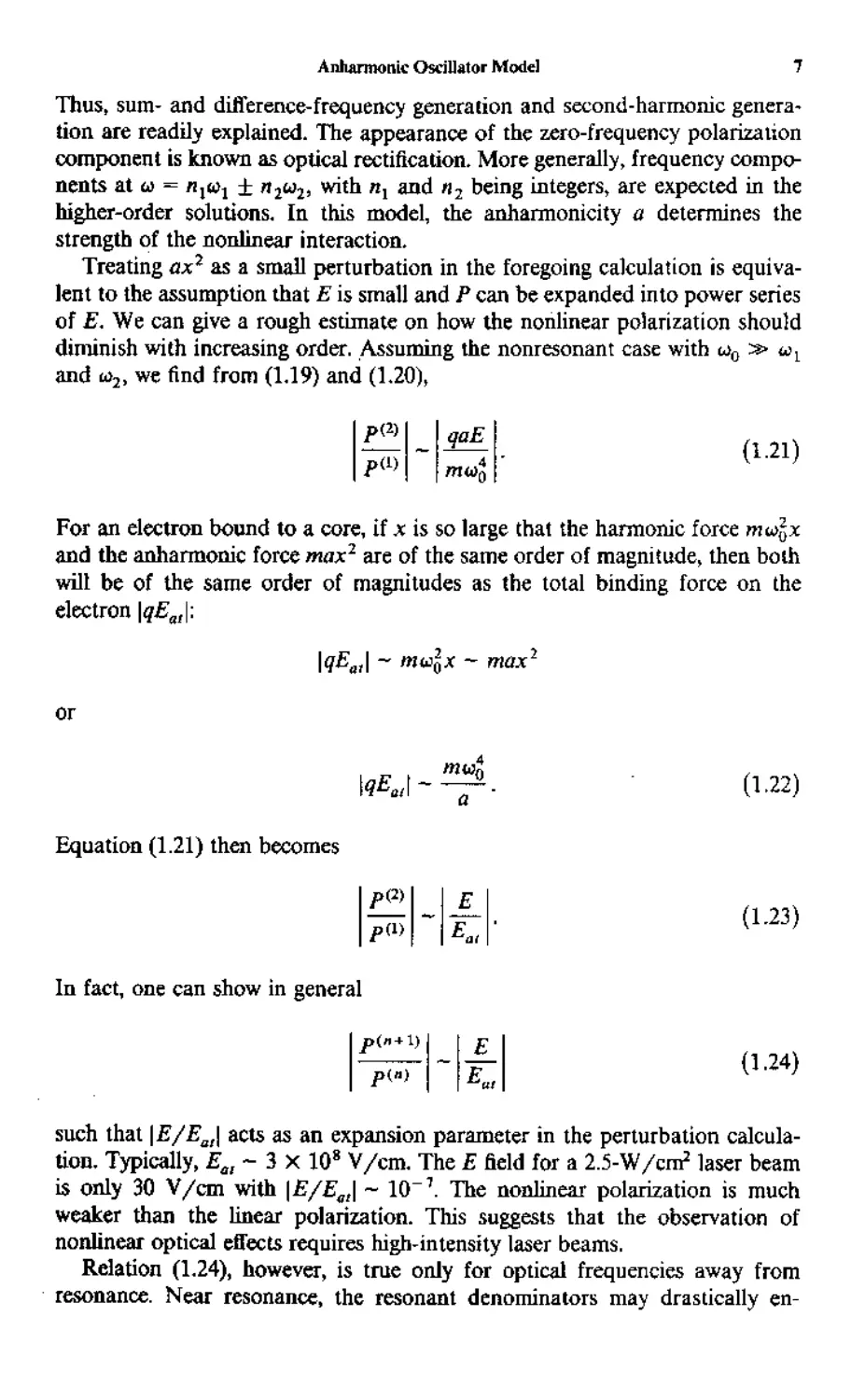
Thus, sum- and difference-frequency generation and second-harmonic genera-
generation are readily explained. The appearance of the zero-frequency polarization
component is known as optical rectification. More generally, frequency compo-
components at ω = η,«! ± η2ω2, with π, and n2 being integers, are expected in the
higher-order solutions. In this model, the anharmonicity a determines the
strength of the nonlinear interaction.
Treating ax2 as a small perturbation in the foregoing calculation is equiva-
equivalent to the assumption that Ε is small and Ρ can be expanded into power series
of E. We can give a rough estimate on how the nonlinear polarization should
diminish with increasing order. Assuming the nonresonani case with ω0 » ωι
and ω2, we find from A.19) and A.20),
ρω
qaE
A.21)
For an electron bound to a core, if χ is so large that the harmonic force muijj
and the anharmonic force max2 are of the same order of magnitude, then both
will be of the same order of magnitudes as the total binding force on the
electron \qEal\:
\qEa,\ - mu^x ~ max7
A.22)
Equation A.21) then becomes
ρφ
In fact, one can show in general
A.23)
A.24)
such that \E/Ea!\ acts as an expansion parameter in the perturbation calcula-
calculation. Typically, Εαι~3χ 108 V/cm. The Ε field for a 2.5-W/W laser beam
is only 30 V/cm with \E/Ea,\ ~ 10"'. The nonlinear polarization is much
weaker than the linear polarization. This suggests that the observation of
nonlinear optical effects requires high-in tensity laser beams.
Relation A.24), however, is true only for optical frequencies away from
resonance. Near resonance, the resonant denominators may drastically en-
hance the ratio |/>ι"+1)/Ρ(''Ί- Consequently, the nonlinear effects can be
detected with much weaker light intensity. Optical pumping is an example.
With resonant enhancement, it may even happen that \Pin+ V/pW\ > 1. When
this is the case, the perturbation expansion is no longer valid, and the full
nonlinear expression of Ρ as a function of Ε must be included in the
calculation. The problem then falls into the domain of strong interaction of
light with matter.
1.4 FREE ELECTRON GAS
A simple but realistic model to illustrate optical nonlinearity in a medium is
the free electron gas model. It properly describes the optical properties of an
electron plasma. The simplified version of the model starts with the equation of
motion for an electron
A.25)
Damping is neglected here for simplicity. Clearly, the only nonlinear term in
this equation is the Lorentz force term. Since υ ■* c in a plasma, the Lorentz
force is much weaker than the Coulomb force, and then (e/mc)v Χ Β in A.25)
can be treated as a perturbation in the successive approximation of the
solution. For Ε = £ie!k<'-'w*' + (f2elk''r"'"i'' + c.c, we obtain
, x(k2 X i2) + «?2 x(k, Χ <f,)
and so on. For a uniform plasma with an electronic charge density p, the
current density is given by
with, for example,
Free Electron Gas 9
and so on. This shows explicitly how an electron gas can respond nonlinearly
to the incoming light through the Lorentz term.
In a more rigorous treatment of an electron gas, we must also lake into
account the spatial variations of the electron density ρ and velocity v. Two
equations, the equation of motion and the continuity equation,5 are now
necessary to describe the electron plasma:
and A.28)
^+ V(pv) = 0
where ρ is the pressure and m is the electron mass. The pressure gradient term
in the equation of motion is responsible for the dispersion of plasma reso-
resonance, but in the following calculation we assume vp = 0 for simplicity. Then,
coupled with A.28), is the set of Maxwell's equations
1 dB
c dt
v XB_I^ = i^ = i5PI A.29)
c dt c c '
VE = 4w{p-p(m),
and
VB-O
We assume here that there is a fixed positive charge background in the plasma
to assure charge neutrality in the absence of external perturbation. Successive
approximation can be used to find J as a function of Ε from A.28) and A.29).
Let6
ρ - ρ«) + ρθ> + pW + . . . ,
V = T0) + f (D + . . . ,
and
j = j(i) + jP) + ... A.30)
with
j(') = pCV»
and A.31)
Introduction
We shall find the expression for jB)Btd) as an example assuming E
exp(ik-r - ίωί). Substitution of A.30) into A.28) and A.29) yields
= -ί,,,ν«» --^1
A-32)
M_ -/2ων<2)= -
»-— ϊA»ΧΒ.
me
The second-order current density is then given by
ip<°>\ e2
Γ(Ε-
2ω [mV m'wc
+ ·4 " (? E)E.
The last term in A.33) has the following equalities:
A.33)
Vp|0> ■ Ε
1 - ωl
A.34)
where ωρ = Dwp(O1e/m)i/! is the plasma resonance frequency. With A.34),
Β = (e/w)v X E, and the vector relation Ε X (V Χ Ε) + (Ε- ν)Ε =
i V(E · Ε), the current density in A.33) can be written as
Am V
4m V
V(E-E)
ie2 | ypl0>-E
1 - «>2
E.
A.35)
Equation A.33) shows exph'citly that aside from the Lorentz term, there are
also terms related to the spatial variation of E. They actually arise from the
nonuniformity of the plasma. In a uniform plasma, vp@) = 0 and hence
VE = 0 from A.34). This means that k is perpendicular to Ε and therefore
(Ε · ν )E also vanishes. The Lorentz term is then the only term in J|2lBu).
The induced current density JB)Bu) should now act as a source for second
harmonic generation in the plasma. In a uniform plasma with a single pump
beam, J<2)B«) α Ε χ Β is only along the direction of beam propagation.
Since an oscillating current cannot radiate longitudinally, no coherent second
harmonic generation along the axis of beam propagation is expected from the
bulk of a uniform plasma. In the bulk of a nonuniform plasma or at the
boundary surface of a uniform plasma, however, it is possible to find second
harmonic generation through the nonvanishing Vp@).
Equation A.35) shows that when vp@> Ψ 0, the nonlinear response of the
medium JB>B(d) is greatly enhanced if ω is near the plasma resonance. From
the general principle, the nonlinear response of a medium is resonantly
enhanced when the incoming field hits the resonance of the medium. One
should, of course, also expect a resonant enhancement in the second harmonic
generation when 2ω is at resonance. This actually does come in through the
response of the second harmonic field to JB)Bu). As 2ω -· ωρ, the current
density will excite the longitudinal field at 2ω resonantly.
As shown in A.33) or A.35), the current density JaBio) depends exclu-
exclusively on the spatial variation of E. In fact, using vector identities, the
expression of J<2)Bw) in A.33) or A.35) can be put into the form7 JB)Bij) =
cV X ( ) - fwv ■ ( ). Comparing it with A.3), we recognize that the two
terms in J<2)B«) represent the magnetic dipole and electric quadrupole
contributions, respectively. No induced electric dipole polarization exists in a
plasma. Also, the induced electric quadrupole polarization depends on the
gradient of the electric field, and therefore cannot show up in the bulk of a
uniform plasma.
The free electron model here is applicable to a number of real problems.
First, it can be used to describe the optical nonlinearities due to plasmas in
metals and semiconductors. Second harmonic generation from metal surfaces
is readily observable,6 Then, with some modification to take into account the
net charge distribution, the nonvanishing v/>, and so on, it can also be used to
describe the optical nonlinearities of a gas plasma. Various nonlinear optical
effects in gas plasmas have been observed. They will be discussed in some
detail in Chapter 28. The model has also been used to describe the observation
of nonlinear effect in a crystal in the X-ray region.3 The electron binding
energy is much weaker than the X-ray photon energy, and therefore the
electrons in the crystal will respond to the X-ray as if they were free.
REFERENCES
1 P. A. Franken, A. E. Hill, C. W. Peters, and G. Weinreich, Phys. Rev. Uli. 7, 118 A961).
2 See, for example, G. Rosen and F. C. WhiUnore, Phys. Rev. 1J7B, 1357 A965).
3 J. D. Jackson, Classical Electrodynamics (McGraw-Hill, New York 1975), 2nd ed., p. 739;
W. K. H. Panofsky and M. Phillips, Classical Electricity and Magnetism (Addison-Wesley,
Reading, Mass., 1962), p. 131.
12 Introduction
4 L. D. Landau and Ε. Μ. Lifshitz, Electrodynamics in Continuous Media (Pergamon Press, New
York, 1960), p. 252.
5 I. D. Jackson, Classical Electrodynamics (McGraw-Hill, New York, 1975), 2nd ed., p. 469.
6 N. Bloembergen, R. K. Chang, S. S. Jha, and C. H. Lee, Phys. Rev 174, 813 A96S).
7 P. S. Perehan, Phys. Rev- 130, 919 A963).
8 P. E. Eisenbergei and S. L. McCall, Phys. Rev. Lett. 26, 684 A971).
BIBLIOGRAPHY
Bloembergen, N., Nonlinear Optics (Benjamin, New Yoik, 1965).
Bloembergen, N., Reo. Mod. Phys. 54, 685 A982).
Nonlinear Optical
Susceptibilities
For tower-order nonlinear optical effects, nonlinear polarizations and nonlin-
nonlinear susceptibilities characterize the steady-state nonlinear optical response of a
medium and govern the nonlinear wave propagation in the medium. Chapter 1
showed how the nonlinear optical response can be calculated for two model
systems. Chapter 2 gives a more general discussion of nonlinear susceptibilities
starting from the microscopic theory.
2.1 DENSITY MATRIX FORMALISM
Nonlinear optical susceptibilities are characteristic properties of a medium and
depend on the detailed electronic and molecular structure of the medium.
Quantum mechanical calculation is needed to find the microscopic expressions
for nonlinear susceptibilities.1 Density matrix formalism is probably most
convenient for such calculation and is certainly more correct when relaxations
of excitations have to be dealt with.2
Let ψ be the wave function of the material system under the influence of the
electromagnetic field. Then the density matrix operator is defined as the
ensemble average over the product of the ket and bra state vectors
Ρ-ίΨΧΨ] B.1)
and the ensemble average of a physical quantity Ρ is given by
(Ρ>=(ψ|Ρ|ψ>
B.2)
= Tr(PP)
In our calculation here, Ρ corresponds to the electric polarization. From the
13
14 Nonlinear Optical Susceptibilities
definition of ρ in B.1) and from the Schrödinger equation for |ψ), we can
readily obtain the equation for motion for p,
known as the Liouville equation. The Hamiltonian Jfis composed of three
parts,
In the semicJassical approach, JPO is the Hamiltonian of the unperturbed
material system with eigenstates \n) and eigenenergies E„ so that &\n) =
EJn), jP^ is the interaction Hamiltonian describing the interaction of light
with matter, and 3ftaaäaa is a Hamiltonian describing the random perturbation
on the system by the thermal reservoir around the system. The interaction
Hamiltonian in the electric dipole approximation is given by
J?ml = er-E. B,5)
We consider here only the electronic contribution to the susceptibilities. For
the ionic contribution, we would have to replace er · Ε by - E^-R,- · Ε with g,
and R, being the charge and position of the ith ion, respectively. The
Hamiltoniao Ji^m, is responsible for the relaxations of material excitations,
or in other words, the relaxation of the perturbed ρ back to thermal equi-
equilibrium. We can then express BJ) as.3·*
■f^Jr^+^pl+i-^) B.6)
with
If the eigenstates \n) are now used as base vectors in the calculation, and |ψ) is
written as a linear combination of |n), that is, |ψ) = Σπαπ\η), then the
physical meaning of the matrix elements of ρ is clear. The diagonal matrix
element p„„ = (n|pln) = |aj represents the population of the system in state
|/i), while the off-diagonal matrix element pnn- = (n\p\n') = a „a*, indicates
that the state of the system has a coherent admixture of |n) and |n'). In the
latter case, if the relative phase of a„ and a„- is random (or incoherent), then
pnn. = 0 through the ensemble average. Thus at thermal equilibrium p<°> is
given by the thermal population distribution, for example, the Boltzmann
distribution in the case of atoms or molecules, and pJJ = 0 for η * η'.
Density Matrix Formalism 15
We can use a simple physical argument to find a more explicit expression
for (dp/dt)Kiai. The population relaxation is a result of transitions between
states induced by interaction with the thermal reservoir. Let W„_„- be the
thermally induced transition rate from \n) to Jn'). Then the relaxation rale of
an excess population in \n) should be
At thermal equilibrium we have
J!p. = Y\W, p<?>, - w „.pi0|l = 0 B.9)
Therefore, B.8) can also be written as
B,10}
The relaxation of the off-diagonal elements is more complicated.2 In simple
cases, however, we expect the phase coherence to decay exponentially to zero.
Then, we have, for η Φ π',
= -Γηπ-Ρηη- B.Π)
with T~J = Γ^1 = (Τ2)ππ- being a characteristic relaxation time between the
states |n) and |«'>. In magnetic resonance, the population relaxation is known
as the longitudinal relaxation, and the relaxation of the off-diagonal matrix
elements is known as the transverse relaxation. In some cases, the longitudinal
relaxation of a state can be approximated by
lift. - Λω - -(ΓΧ'ί«,. " P^). _ B.12)
Then 7Ί is called the longitudinal relaxation time. Correspondingly, T2 is called
the transverse relaxation time.
Thus, at least in principle, if Jf0, Jf^, and Cp/3i)relM are known, the
Liouville equations in B.6) together with B.2) fully describe the response of
the medium to the incoming field. It is, however, not possible in general to
combine B.6) and B.2) into a single equation of motion for {P). Only in
special cases can this be done. In this chapter we consider only the case of
steady-state response with (P) expandable into power series of E. The tran-
transient response is discussed in Chapter 21.
16 Nonlinear Optical Susceptibilities
To find nonlinear polarizations and nonlinear susceptibilities of various
orders, we use perturbation expansion in the calculation. Lei
and
<P) = (PA)) + <PB>) + ■·■ B.13)
with
(P<"<) = Tr(p'n>P) B.14}
where p|0) is the density matrix operator for ihe system at thermal equilibrium,
and we assume no permanent polarization in the medium so that (P101) = 0.
Inserting the series expansion of ρ into B.6) and collecting terms of the same
order with Jf^, treated as a first-order perturbation, we should obtain
B.15)
and so on. We are interested here in the response to a field that can be
decomposed into Fourier components, Ε = S^expf/k, · r — (to, t). Then, since
-^iDi = Σ.·*ΐοΐ(ωι) an^ ^mii«;)α <?,βχρ(-/ω,0' *e operator pM can also be
expanded into a Fourier series
pi») = Σ>">(ω)
With dp<n>(Uj)/3t = -iujp^^&j), B.15) can now be solved explicitly for
ρ("'(ω,) in successive orders. The first- and second-order solutions are
B.16)
We use here the notation Ann· = (n|^|n'). Higher-order solutions can be
Microscopic Expressions for Nonlinear Susceptibilities 17
obtained readily, although the derivation is long and tedious. Whenever
diagonal elements ρ£1@) appear in the derivation, further approximation on
(dPffim/tOreiin >n B.8) is often necessary in order to find a closed-form
solution. We also note that the expression for ρ$(ω; + ωΛ) in B.16) is valid
even for η = η' as long as «,- + «t * 0 since the term (dp$/di)relas can then
be neglected in the calculation.
2.2
MICROSCOPIC EXPRESSIONS FOR NONLINEAR
SUSCEPTIBILITIES
The full microscopic expressions for the nonlinear polarizations (P""> and the
nonlinear susceptibilities (x(ll)) follow immediately from the expressions of
p(">. With Jffc, = er · Ε and Ρ = - Nei in B.14) and B.16), the first- and
second-order susceptibilities due to electronic contribution are readily ob-
obtained. They are given here in explicit Cartesian tensor notation:
(ω - vng
(ω — ω
ι to + ω
V η
f tj + ω
(ω - ω
, + 'Τ-,Χ«
f +/Γ-ΐ)(«
η- + T„.)
,)fl-n('>)gD.
ι «B'f + ίΓ,,-j,)
i + w--g + 'TB.f)
! + o>n.g + iT„,s)
1
ω2 + ujt + ϊΤΛ
ι
1
ω, - w„s + /T„
1
(ω - ωππ. + ίΤππ.) \ ω2 - ω + /Γ ω, + ωπ.;
IS Nonlinear Optical Susceptibilities
There are two terms in χγ> and eight terms in χ$. The calculation can be
extended to third order to find x{-fk, (ω = ωι + «2 + ω,), which will have 48
terms. The complete expression for xf^, is given in the literature5 and is not
reproduced here. The resonant structure of xf^kh however, is discussed in
Chapter 14. In nonresonant cases, the damping constants in the denominators
in B.17) can be neglected. The second-order susceptibility can then be reduced
to a form with six terms, noting that the last two terms in the expression for
xf/k in B.17) become
(ωι ~ ω-ϊΗ«! + ««'») (ωι + "VsK^ ~ «Bf) '
With Λ' denoting the number of atoms or molecules per unit volume, the
expressions in B.17) are actually more appropriate for gases or molecular
liquids or solids, and p<0) is given by the Boltzmann distribution. For solids
whose electronic properties are described by band structure, the eigenstates are
the Bloch states, and p™ corresponds to the Fermi distribution. The expression
for χί}' and %f^k should then be properly modified. Since the band states form
essentially a continuum, the damping constants in the resonant denominators
can be ignored. In the electric dipole approximation with the photon wavevec-
tor dependence neglected, χ^\ for such solids has Ihe form3
fi2' \
}/r(q)
)
where q denotes the electron wavevector, v, c, and c' are the band indices, and
/„(q) is the Fermi distribution factor for the state |t\q).
For condensed matter, there should be a local field arising from the induced
dipole-dipole interaction. A local field correction factor L(n| should then
Diagrammatic Technique 19
appear as a multiplication factor in χ<π). We discuss the local field correction
in more detail in Section 2.4. For Bloch (band-state) electrons in solids with
wavefunclions extended over many unit cells, the local field tends to get
averaged out, and L("' may approach 1.
2.3 DIAGRAMMATIC TECHNIQUE
Perturbation calculations can be facilitated with the help of diagrams.
Feynman diagrams have been used in perturbation calculations on wavefunc-
tions. Here, since the density matrices involve products of two wavefunctions,
perturbation calculations require a kind of double-Feynman diagram. We
introduce in this section a technique devised by Yee and Gustafson.6 Only the
steady-state response is considered here.
The important aspects of any diagrammatic technique are that the diagrams
provide a simple picture to the corresponding physical process as well as
allowing one to write down immediately the corresponding mathematical
expression. It is essential to find the complete set of diagrams for a perturba-
perturbation process of a given order. The scheme we adopt for calculating p'"' involves
in each diagram a pair of Feynman diagrams with two lines of propagation,
one for the |ψ) side of ρ and the other for the (ψ| side. Figure 2.1 shows one of
Fig. 2.1 A representative double-Feynman
diagram describing one of the many terms
in ρ'"'(ω — «! + ii>2 + ■ - ■ + un).
20 Nonlinear Optical Susceptibilities
the many diagrams describing the various terms in p'n)(« = wj + ω2 + ■ ■ * +
ωη). The system starts initially from |g)(g| with a population p<°>. The ket state
propagates from |g) to |«') through interaction with the radiation field at
wP«2 «„. and the bra state propagates from (g\ to (n\ through interaction
with the field at ω3,...,ω,,_1. Then, the final interaction with the output field at
ω puts the system in |«){n|. Through permutation of the interaction vertices
and rearrangement of the positions of the vertices on the lines of propagation,
the other diagrams for p(n) can also be drawn.
The microscopic expression for a given diagram can now be obtained using
the following general rules describing the various multiplication factors:
1 The system starts with \g)p{^(g\.
2 The propagation of the ket state appears as multiplication factors on the
left, and that of the bra state on the right.
3 A vertex bringing \a) to \b) through absorption at ω; on the left (ket) side
of the diagram is described by the matrix element
with .#;„,(«,■) α e~'"'' denoted by J^ in Fig. 2.1
l*>
instead of absorption, the vertex should be described by
I")
(\/ih)(b\ .#£, {u,)\a). Because of the adjoint nature between the bra and
ket sides, an absorption process on the ket side appears as an emission
process on the bra side, and vice versa.· Therefore, on the right (bra) side
<b\'
of the diagram, the vertices for emission
If it is emission
are described by -
and absorption
and -(l//fi)<e|
•*mt (ω,-)Ι^)ι respectively.
4 Propagation from thejth vertex to the (j + l)th vertex along the \l)(k\
double lines is described by the propagator Π, = ±[ί(Σ/_!ω, - ulk +
iT(jt)]"' The frequency «, is taken as positive if absorption of ω, at the ith
vertex occurs on the left or emission of ω; on the right; it is taken as
negative if absorption of ω; occurs on the right or emission on the left.
5 The final state of the system is described by the product of the final ket and
bra states, for example, \n')(n\ after the nth vertex in Fig. 2.1 for p(n).
6 The product of all factors describes the propagation from |g)(g| to \n')(n\
through a particular set of states in the diagram. Summation of these
•If the field is also quantized, Jf:ai( ω,) operating on a ket state will annihilate a photon at ω,, while
if operating on a bra state it will create a photon.
\g> <ί
\g>
f/J
(g)
Fig. 2.2 The complete set of eight diagrams for the eight terms in ρί2){ω = ω,
3
2
1
l£> '
Fig· ϊ-3 The eight basic diagrams for p'"(« = W[ + ω2 + ω3).
Local FteW Coirectkm To χ"» "
products over all possible sets of states yields the final result with contribu-
contributions from all states.
By using these rules, the diagram in Fig. 2.1 leads to the expression
Ä"| _
J — 1 / \ ._l
B.19)
(ω, + öj + ω3 - ωήΓ + iTbc)(u1 + ω2 - ubg + iTig)(tj, - vag + iTa
which is just one term in the full expression for ρ(π) (ω = ω1 + ω2 + - - ■ + ωπ).
As a more concrete example, Fig. 2.2 gives the complete set of diagrams for
pB) (ω = ω! + tuj) that leads to χ$ (ω = ω, + u2) in B.17). The eight
diagrams (a)-(h) correspond in successive order to the eight terms in B.17).
Note that xgi (ω - wL + ω2) is derived from Ji(p(T'Pi)/EJ(wl)Ek(u2). There
are in fact only four basic diagrams, (a), (c), (e), and (g), in Fig. 2.2. The
others can be obtained by permutation of the i^ and ω2 vortices.
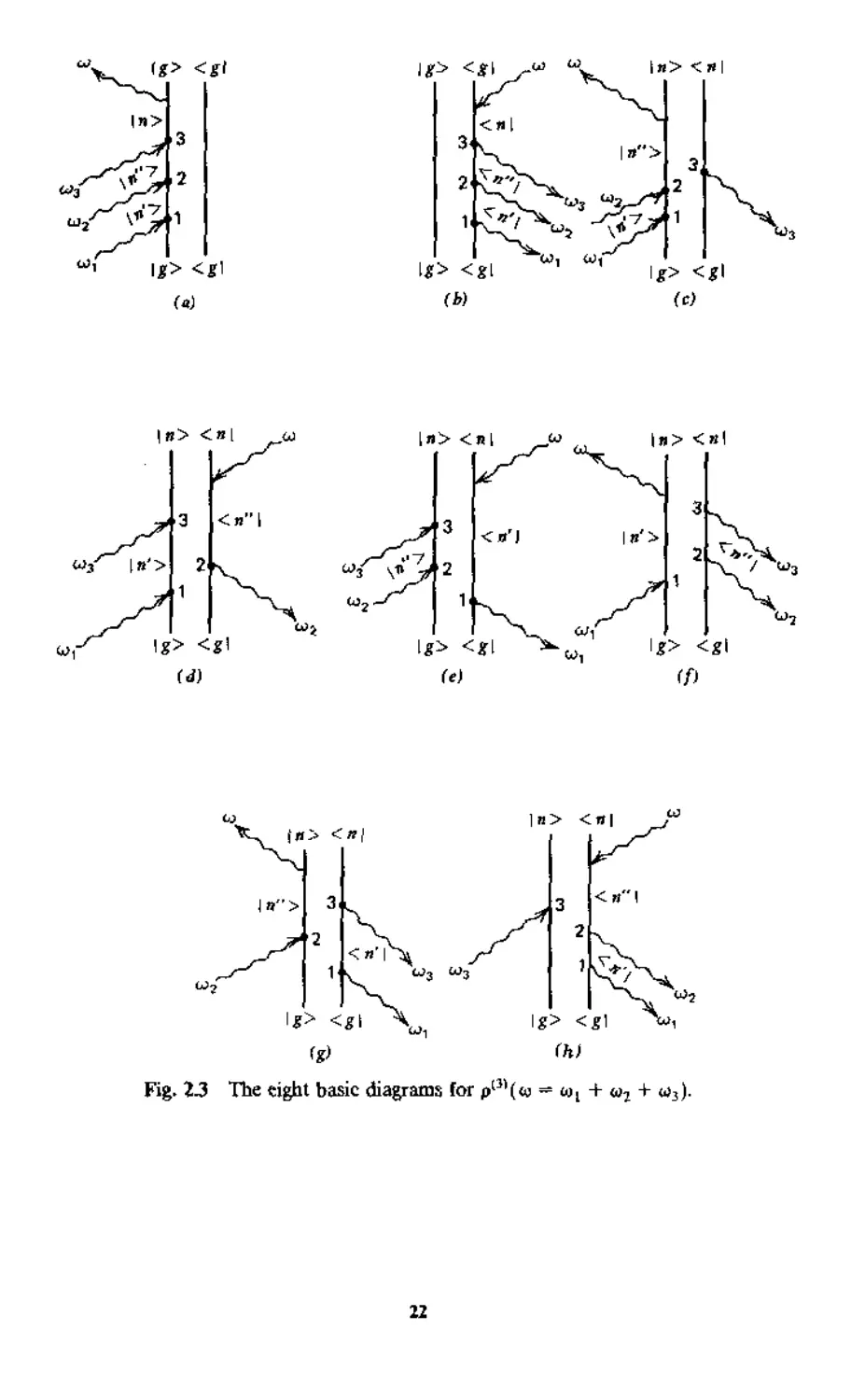
As another example. Fig. 2.3 presents eight basic diagrams for pC) (ω = ω1
+ ω2 + ω3) that lead to χ$; (ω = ut + ω2 + ω3). There should be 48 dia-
diagrams in the complete set corresponding to the 48 terms in χ(^,. The other 40
diagrams are obtained from permutations of the three vertices A,2,3) in the
eight basic diagrams in Fig. 2.3. The full expression of χ|^, can then be written
down from the diagrams according to the rules.
What happens if identical photons appear at a number of vertices? Dia-
Diagrams obtained from permutations of these vertices in a given diagram yield
identical terms in p<r". They should not be discarded, and should be taken into
account by a degeneracy factor attached to the terms in p(n). For example,
χ8?,Cω = ω + ω + «) has 48 diagrams, but 40 of them yield terms identical
to others. Thus χί?/,Cω = ω + ω + ω) has only eight terms, each having a
degeneracy factor of 6. It reduces further to four terms when the damping
constants in the denominators of the expression can be neglected.
2.4 LOCAL FIELD CORRECTION TO χ<π)
The expressions for χ(<ι> in the previous sections are strictly correct only for
dilute media. They can be written as χ<π) = JVa1"' with Ν being the number of
atoms or molecules per unit volume and aln) the nth-order nonlinear polariza-
24 Nonlinear Optical Susceptibilities
bilities. In condensed matter, however, the induced dipole-dipole interaction
becomes important and leads to the so-called local field correction. The
susceptibilities χ(η) are no longer simply proportional to α(π). The usual
derivation of local field correction applies to isotropic or cubic media with
well-localized bound electrons. The general theory applicable to media with
any symmetry or with more freely moving electrons is not yet available.
The local field at a local spatial point is the sum of the applied field Ε and
the field due to neighboring dipoles ΕΛρ,
Eioc-E + E^. B.20)
In the Lorentz model, Edjp is proportional to the polarization; for isotropic or
cubic media, it is given by7
The polarization can be expressed in terms of either microscopic polarizabili-
lies and local fields or macroscopic susceptibilities and applied fields:
With B.20) and B.21), the first expression in B.22) becomes
B.23)
}
If the contribution of P"° to E^ with η > 1 is neglected [which is usually an
excellent approximation since |Pl")|ll>1 ■« IP11*!], then the local field can be
written as
Then, from B.22) and B.23), we find
B.25)
Permutation Symmetry of Nonlinear Susceptibilities
and more generally
χ'π)(ω = «j + ω2 + ■ ■ ■ + ωπ)
ΐύτ+ --■ + w„)'
Since the linear dielectric constant eA) is related to χ'1' by
we can write
and B.26) becomes3
B.27)
with
B,8)
being the local field correction factor for the nth-order nonlinear susceptibili-
susceptibilities. In media with other symmetry, the expression B.27) is still valid, but LM
will be a complicated tensorial function of eA>(«), e'11^),..., and εο)(ωη).Β
IS PERMUTATION SYMMETRY OF NONLINEAR
SUSCEPTIBILITIES
There is inherent symmetry in the microscopic expressions of susceptibilities.
As can be readily seen from B.17), the linear susceptibility χ·]1 has the
symmetry
Χ!}>(ω) = χί}»·(-ω), B.29)
which is actually a special case of the Onsager relation. Similarly, the nonlinear
susceptibility χ$.(ω = ω1 + ωΙ) in B.17) or a similar expression for χ[^Bω
= ω + ω) has the following permutation symmetry when the damping con-
26 Nonlinear Optical Susceptibilities
stants in the frequency denominators can be neglected (i.e., the nonresonant
cases):1·9
X$*(« = "i + «2) = Χ%(ωι = -»ι + «)
-χ^(«ι-«-«,), B.30)
χί^(Ζω = ω + ω) = }χ$(« - 2« - ω) - *χ$(ω = -ω + 2«).
In Ihe permutation operation, the Cartesian indices are permutated together
with the frequencies with their signs properly chosen. More generally, one can
show that the nth-order nonlinear susceptibility also has the permutation
symmetry9
Xiilj...;.*(" = ωι + «1 + ■■■ «») = xi,"j-/./(«i = ~ui ■■· + ωη + ω)
B.31)
If the dispersion of x<fl) can also be neglected, then the permutation symmetry
in B.31) becomes independent of the frequencies. Consequently, a symmetry
relation now easts between different elements of the same χ<π) tensor, that is,
xi.1?,,. .1 remains unchanged when the Cartesian indices are permuted. This is
known" as Kleinman's conjecture,10 with which the number of independent
elements of χ(η> can be greatly reduced. For example, it reduces 27 elements of
Xt2> to only 10 independent elements. We should, however, note that since alt
media are dispersive, Kleinman's conjecture is good approximation only when
all frequencies involved are far from resonances such that dispersion of χ(η> is
relatively unimportant.
2.6 STRUCTURAL SYMMETRY OF NONLINEAR
SUSCEPTIBILITIES
As optical properties of a medium, the nonlinear susceptibility tensors should
have certain iorms of symmetry that reflect the structural symmetry of the
medium. Accordingly, some tensor elements are zero and others are related to
each other, greatly reducing the total number of independent elements. As an
illustration, we consider here the second-order nonlinear susceptibility tensor
Xln-
Each medium has a certain point symmetry with a group of symmetry
operations {S}, under which the medium is invariant, and therefore χ1
remains unchanged. In real manipulation, S is a second-rank three-dimen-
three-dimensional tensor Slm. Then, invariance of χ<2) under a symmetry operation is
Table 2.1
Independent Noimmishing Elements of χ(ίι(ω = ω, + ω2) for
Crystals of Certain Symmetry Classes
Symmetry Class
Independent Nonvanishing Elements
Triciinic
1
Monoclinic
2
Qrthorhombic
222
mm!
Tetragons!
4
422
4mm
32m
Cubic
432
43m
23
Trigonal
3
32
3m
Hexagonal
6
622
6 mm
All elements are independent and nonzero
xyz, xzy, xxy, xyx, yxx, yyy, yzz,yzx, yxz, zyz,
izy, ixy, zyx (two fold axis parallel to^)
xxx, xyy, xzz, xzx, xxz,yyz, yzy, yxy, yyx, zxx,
zyy, zzz, zzx, zxz (mirror plane perpendicular toy)
xyz, xzy, yzx, yxz, zxy, zyx
xzx, xxz, yyz, yzy, zxx, zyy, zzz
xyz ** -yxz, xzy = -yzx, xzx = yzy, xxz — yyz,
zxx = zyy, zzz, zxy = -zyx
xyz - yxz, xzy — yzx, xzx — -yzy, xxz = -yyz,
zxx — -zyy, zxy = zyx
xyz - -yxz, xzy = -yzx, zxy = -zyx
xzx — yzy, xxz = yyz, zxx = zyy, zzz
xyz — yxz, xzy = yzx, zxy = zyx
xyz - - xzy — yzx = -yxz — zxy = - zyx
xyz — xzy = yzx
= yxz — zxy — zyx
xxx - -xyy - -yyz = -yxy, xyz = -yxz, xzy = -yzx,
xzx =yzy,xxz =yyz,yyy = —yxx = -xxy = -xyx,
zxx = zyy, zzz, zxy — —zyx
xxx — -xyy - —yyx ™ -yxy, xyz = -yxz, xzy = -yzx,
zxy — —zyx
xzx =- yzy, xxz — yyz, zxx — zyy, zzz, yyy = -yxx =
- xxy — - xyx (minor plane perpendicular to it)
xyz — — yxz, xzy — — yzx, xzx = yxy, xxz = yyz,
zxx = zyy, zzz, zxy = -zyx
xxx - -xyy - -yxy - -yyx,yyy ~ -yxx — -xyx =
—xxy
xyz = — yxz, xzy = -yxz, zxy — -zyx
xzx = yzy, xxz = yyz, zxx = zyy, zzz
yyy — -yxx — -xxy = —xyx
IS Nonlinear Optical Susceptibilities
explicitly described by
B.32)
For a medium with a symmetry group that consists of η symmetry operations,
η such equations should exist. They yield many relations between various
elements of χ'2', although often only a few are independent. These relations
can then be used to reduce the 27 elements of χ(ϊ) to a small number of
independent ones.
An immediate consequence of B.32) is that χB) = 0 in the electric dipole
approximation for a medium with inversion symmetry: with S being the
inversion operation, S · i = -e, B.32) yields χ^ί = —xiyi = 0- This explains
why χ'2> for a free electron gas does not have an electric dipole contribution as
shown in Chapter 1. Among crystals without inversion symmetry, those with
the zincblende structure such as the III-V semiconductors have the simplest
form of xm. They belong to the class of TdD3m) cubic point symmetry.
Table 2.2
Independent Nonvanishing Elements of x^'iw = ut + ω2 + ι^) for
Crystals of Certain Symmetry Classes
Symmetry Class Independent Nonvanishing Elements
Tridinic All 81 elements are independent and nonzero
Tetragonal xxxx = yyyy, zzzz,
422,4mm, yyzz = zzyy, zzxx - xxzz, xxyy = yyxx,yzyz " zyzy,
4/mmm,42m zxzx = xzxz,xyxy = yxyx, yzzy — zyyz,zxxz = xzzx,
xyyx = yxxy
Cubic xxxx = yyyy = zzzz,yyzz - zzxx =- xxyy,
23, mi zzyy = yyxx = xxzz, zyzy - xzxz - yxyx,
yzyz = zxzx — xyxy, zyyz = xzzx - yxxy,
yzzy = zxxz = xyyx
432,43m, m3m xxxx — yyyy — zzzz
yyzz = zzyy - zzxx - xxzz - xxyy = yyxx
yzyz = zyzy — zxzx = xzxz = yxyx = xyxy
yzzy = zyyz = zxxz - xzzx = xyyx = yxxy
Hexagonal zzzz, xxxx = yyyy — xxyy + xyyx + xyxy
622,6mm, xxyy ■= yyxx, xyyx — yxxy, xyxy =* yxyx,
d/mmm, 6m2 yyzz - atjw;, izjy - zzxx, zyyz = ϊχχϊ,
yzzv — Ar/ix, >>zyi = λγγλζ, zyzy " zxzx
Isotropie xxxx — yyyy = zzzz,
yyzz — zzyy — zzxx — xxzz = xxyy = yyxx,
yzyz — zyzy = ζκχ — λϊλ^ — χκχκ *" yxyx,
yzzy — zyyz — zxxz — xzzx = xyyz = yxxy,
xxxx — xxyy + xyxy + xyyx
Practical Calculations of Nonlinear Susceptibilities 29
Although many symmetry operations are associated with 7^ D3m), only the
180° rotations about the three four-fold axes and the mirror reflections about
the diagonal planes are needed to reduce χ<2). The 180° rotations make
xffi = -xffl = 0, xjg = -x|g = 0, and χ$ = -χ$ = 0, where ί,;, and k
refer to the three principal axes of the crystal. The mirror reflections lead to the
invariance of xfyii Φ j Φ k) under permutation of the Cartesian indices.
Consequently, xjjj,(' * j * k) is the only independent elemen! in χB) for the
zincblende crystals.
For other classes of crystals, the forms of χB) can be similarly derived
through the corresponding symmetry operations. The symmetry consideration
here is the same as the one used to derive the electrooptical tensor [which is
actually a special case of χα'(« = w, + ω2) "witli ω2 = 0] and the piezoelectric
tensor.11 The forms of χ<2) for second-harmonic generation are in fact identical
to the latter.*3 We reproduce a part of χB>(ω = ω, + ω2) for various classes of
crystals in Table 2.1.
The above symmetry consideration for χB) can of course be extended to
higher-order nonlinear susceptibilities. In particular, symmetry forms for χC)
are most important in view of the many interesting third-order nonlinear
optical effects that can be observed readily in almost all media. Table 2.2 lists
the χC) tensors for the more commonly encountered classes of media.12
2.7 PRACTICAL CALCULATIONS OF NONLINEAR
SUSCEPTIBILITIES
Symmetry operations drastically reduce the number of independent elements
in a nonlinear susceptibility tensor, but then for a given medium, we would
also like to know the values of these independent elements. While they can
often be measured (see, for example, Section 7.5), it is also important that they
can be calculated from theory. A successful theoretical calculation can help in
predicting χ'"' for media not easily subject to measurements or for the design
of new nonlinear crystals. In principle, the microscopic expressions, such as the
one for χ^ in B.17), with appropriate local-field correction, can be used for
such calculations. However, in most practical cases these expressions are
useless because neither the transition frequencies nor the wavefunctions for the
material are sufficiently well known. This is especially true for large molecules
or solids. Simplifying models or approximations often are needed. If all
frequencies involved are far from resonances, one simplifying assumption often
used is to replace each frequency denominator in the microscopic expression of
χ<"> by an average one and bring all frequency denominators out of the
summation [see, for example, χB) in B.17)]. Then the summation over matrix
elements can be greatly simplified through the closure property of the eigen-
states and can be expressed in terms of moments of the ground-state charge
distribution. The problem reduces to finding the ground-state wavefunction of
the system.13
30 Nonlinear Optical Susceptibilities
The foregoing approximation, however, is too drastic to yield good results.
A more successful calculation of χ'π> can be done by the bond model. Such a
model was used in the early 1930s to calculate the linear polarizability of a
molecule or the linear dielectric constant of a crystal.14 The bond additivity
rule was assumed: the induced polarizations on a molecule (or a crystal) is the
vector sum of the polarizations induced on all bonds between atoms. In other
words, the bond-bond interaction is neglected. The same rule can be used in
the calculations of χ1. We can write
ΧΜ-Σ*Ρ B-33)
κ
where aj?' is the nth-order nonlinear polarizability of the K\h bond in the
crystal (or medium), and the summation is over all the bonds in a unit volume.
Thus, with known crystal structure, the calculation of χ* reduces to the
calculation of a^1' for different types of bonds.
We discuss here only the calculations of χ<2), using the zincblende crystals
as an example. The general procedure is as follows. The linear bond polariza-
polarizability a^' is first calculated as a function of the applied field using the recently
well developed bond theory.11 The second-order nonlinear bond polarizability
αψ is then obtained from the first derivative of ajj' with respect to the applied
field. Finally, the summation of B.33) over the bonds is performed to find χ'2'.
We assume here that a simple crystal can be constructed entirely out of the
same type of bonds, and the bonds are cylindrically symmetric. The linear
susceptibility χ<|> of the crystal can then be written as
+ G<V]> B.34)
where ajj1' and αψ are the polarizabilities parallel and perpendicular lo the
bond, μ = u^/a^K and Gjj1* and G^' are the respective geometric factors
arising from the vectorial summation over the bonds. Both Gjj" and G^' are
proportional to the number of unit cells per unit volume. For the zincblende
structure, G'11 = $G<P = 4JV/3, and B.34) becomes
χα>-<£A + 2μ)«ί». B.35)
The next step is to find an approximate expression for «j1' through χ£'. The
microscopic expression of χ'}' in B.17) away from resonance has the form
Practical Calculations of Nonlinear Susceptibilities 31
In the low-temperature limit, pf = 0 for all states except the ground state.
Then, following the approximation of replacing ωΠί in the denominator by an
average ω and the sum rule16
B.36) reduces to
with Ωρ = 4-nNe2/m being the electron plasma frequency. This simplified
expression for xj)> has actually been shown more rigorously by Penn for solids
in the limit of zero frequency.17 From B.34), we now have
B.39)
We are, however, interested in af1 as a function of applied field. The
polarizability should depend on the field through the field perturbation on the
transition frequencies and matrix elements. However, in the approximate form
of B.39), ajj" can depend on the field only through wjjr To find an repression
for ülg is where the bond theory comes in. Physically, hu„g = E? can be
regarded as an average energy gap between the filled and unfilled states. It can
be written as15
E,= [Ei + C>]1/2 B.40)
where EA and C are known as the homopolar and heteropolar gaps, respec-
respectively, and, in the bond theory, have the expressions
Ci1 * ad"
and B.41)
In these expressions, a, b, and s are constant coefficients, ZA and ZB are the
valences, and rA and rB are the covalenl radii of the A and Β atoms forming the
bond, d — rA + rBis the bond length, and exp(—k^d/2) is the Thomas-Fermi
screening factor. If A and Β are identical atoms, then C = 0. Equation B.40)
can be derived easily from molecular orbital theory.18 The bond electrons have
two eigenstates, a bonding state and an antibonding state. The energy dif-
32 Nonlinear Optical Susceptibilities
ference between the two states is Eg. For a homopolar bond {A = ß), the
bond electrons see a symmetric potential with respect to the bond center and
Eg = E„. For a heteropolar bond {Α Φ Β), the bond electrons see an anti-
syymmetric potential, and Eg = El + C1 with C proportional to the asymmet-
asymmetric part of the potential. The wavefunctions of the bonding and antibonding
States along the bond are shown in Fig- 2.4. It is seen that in the heteropolar
case, there is a charge transfer from the side of the less electronegative atom to
the side of the more electronegative atom. According to the molecular orbita)
theory, the amount of transferred charge Q is related to the heteropolar gap C
by
"-'f
B.42)
Figure 2.4 also shows that there is a bond charge cloud between the two atoms.
The magnitude of the bond charge derived from the bond theory is
2eE
11 +
B.43)
Fig. 2.4 Sketches of electronic wavefunctions of (u) the bonding stale and (b) the
antibonding state along the bond connecting the atoms A and B. The solid curves are
for the homopolar case and the dashed curves for the heteropolar case.
Practical Calculations of Nonlinear Susceptibilities 33
Levine1' suggests that the bond charge may be considered as a point charge
sitting at distances rA and rB, respectively, from atoms A and B.
We can now discuss how the bond polarizabih'ty changes when the bond is
subject to an external field. The change occurs through the field perturbation
on the charge distribution. In our description here, ajj1' depends on the applied
field Ε through the dependence of Ε on Ε
while EA and C depend on Ε through field-induced changes in the charge
transfer and bond charge. However, since the applied field is not expected to
change the bond length, we have SE^dEj = 0 from B.41). The second-order
nonlinear bond polarizability afj£ is obtained from da^/ΘΕ^.. If I and ή
denote the two directions parallel and perpendicular to the bond, respectively,
then from ihe symmetry argument, only affa and ot^1,, are nonvanishing. We
also neglect o^ by assuming that a field transverse to the bond will not
significantly perturb the charge distribution. Thus af^ is the only nonvanisliing
element of a™. Using B.39) and B.44), we find
dB(
-2h2ttjC gc
Now, either B.41) or B.42) can be used to calculate dC/d£k. The two,
however, correspond to two different physical pictures. In B.41), the applied
field changes rA and rB, but keeps rA + rB = d. In terms of the simple mode!
where the bond charge can be treated as a point charge sitting at distances rA
and rB away from the atoms A and B, the field then simply shifts the position
of the bond charge along the bond. This is known as the bond-charge model."
In B.42), on the other hand, it is the field perturbation on the charge transfer
Q that relates C lo the field. This is the charge-transfer model.20
The bond-charge model involves, with Ar = ArA = - irfi,
and since qbr= ajjl)(io')A£{(w') for ω' -* 0, we find from B.41), B.45),
34 Nonlinear Optical Susceptibilities
B.46), B.34), and B.38)
B.47)
The charge-transfer model following B.42) gives
It is assumed in this model that the field-induced charge transfer is from atom
Β to atom A, treating the atoms as points. Since a$\af)&Et(<ar) = t^Qd, we
have from B.45) and B.48)
B-49)
We should, however, keep in mind that the description of how an applied field
modifies the charge distribution in both models is still fairly crude. In reality,
the electronic charges are broadly distributed in the region between the two
atoms. The peak of the distribution is near the center of the bond. As an
example, a contour map of the valence electron distribution around a Ga-As
bond obtained by empirical pseudopotential calculation is shown in Fig. 2.5.21
In the presence of a dc external field along the bond, the charge distribution
becomes only slightly more asymmetric with its peak essentially unshifted. This
is shown in Fig. 2.6 for the charge distributions along the Si-Si and Ga-As
bonds.22 The field-induced shift of the bond charge in the bond-charge model
actually refers to the shift of the center of gravity of the valence electron
distribution, while the field-induced charge transfer in the charge-transfer
model refers to the redistribution of the valence charges around the bond from
one side of the bond center to the other.
Finally, we can obtain χ{^ of a given medium from «^ for various bonds,
where i,), and k denote the three orthogonal symmetry axes in the crystal:
Practical Calculations of Nonlinear Susceptibilities
Fig. 2.5 Coniour map of valence electron density distribution (in units of e per
primitive cell) forGaAsin the A, -1,0) plane. (From Ref. 21.)
where [G^)iJk is a geometric factor for the Λ-type bonds reflecting the
structure of the medium. We note that with («${)a expressed in terms of χ!,-1
rather than af1 in B.47) and B.49), even the total field correction has been
somehow taken into account in the above derivation.
We now use InSb as an example to illustrate the calculation of χ$. The
crystal has a zincblende structure; therefore, the only nonvanishing elements of
χB) are x<?j{ with i*j* k. There is only one type of bond in the crystal: those
connecting In and Sb. The geometric factor Gj$t is then given by 4^/3/3 and
the density of unit cells JV is related to the bond length d by Ν = 3vT/16i/3.
We also have Gj'> = \ΰψ = 4JV/3. From B.47), B.49), and B.50), the bond-
■(lill
-MID
Fig. 2.6 Sketches of the charge distribution along a bond in (a) Si and (t) GaAs.
Solid and dashed curves refer to cases with and without an external field along the
bond, respectively. (Courtesy of S. Louie.)
36 Nonlinear Optical Susceptibilities
charge model gives
, , _ 32«f'c[X<»(«)]W)] [g, g
and the charge-transfer model gives
(vß) \ = "Ί. li* 'ω^ '* '" '' ij S2\
We calculate here χψγι in the low-frequency limit ω ~ ω' - 0. For InSb,
d = 2.5 Ä, Es = 3.7 eV, £k = 3.1 eV, C = 2.1 eV, χA> - 1.17 esu, ΛΩ - 13
eV, ZA = 3, ZB = 5, /> = rfl = ti/2, ftexp(-M/2) = 0.12 e2, μ = {, and
« = 0.6 e,23 we obtain (x^)BC= 1.6 x Wesuandta^cT.« 2.3 Χ ΙΟ
esu. The results of both models are in fair agreement with the experimental
value of χ^; = C.3 ± 0.7) χ 10"* esu. This should be considered satisfactory
in view of the crude approximations in the models.
The calculations can also be extended to higher-order nonlinear susceptibili-
susceptibilities. However, because of the crude approximations involved, they become
much less reliable. Also, since we use the covalent bonding picture in the
models, the calculations are less suitable for ionic crystals. In nonlinear optics,
we are often interested in materials with high nonlinearity. This discussion
suggests that the materials should have high nonlinearity in bond polarizabili-
ties. For large χB), the crystal structure should also be as asymmetric as
possible so that there is a minimum of vectorial cancellation in summing over
αψ of all bonds.
The calculations here are good only in the low-frequency limit. The ap-
approximations in the models break down when the optical frequencies are close
to the absorption bands. Because of resonant enhancement, the transitions
with transition frequencies closer to the optical frequencies contribute much
more to the susceptibilities. In order to calculate χ'"* and its dispersion in
these cases, we must use the full microscopic expression of χ{ΐ" such as those
derived in Section 2.2. Then detailed information about the transition matrix
elements and frequencies of the material is necessary. Such calculations have
been carried out by several authors on χ<2)Bω) of zincblende semiconductors
with various degrees of approximation. In most cases, constant matrix ele-
elements are assumed. The more accurate calculations, however, are those with
wavefunctions and energies of the band states derived from the empirical
pseudopotentia! method,24 which has been extremely successful in reproducing
χA|(ω) for zincblende semiconductors; it should therefore also yield accurate
results for χB)Bω). An example is shown in Fig. 2.7 for InSb. The peaks and
shoulders in the spectrum generally correspond to resonances of ω or 2 ω with
the critical point transitions. The results also show that it is important to
Miller's Coefficient
Λ-Κ3-5)
■Γ{4-5)
A-LD-5) A-LC-5)
800
600
Fig. 2.7 Dispersion of χ^;Bω) of InSb calculated using the empirical pseudopoten-
tial method. The pealcs arise from inteiband transitions in the regions indicated. (From
Ref. 24.)
include the dispersive effects of both the matrix elements and the density of
states for transitions in the calculations.
Full quantum mechanical calculations of χB) of B.17) for molecular crystals
have also been carried out using semiempirical Hartree-Fock LCAO (linear
combination of atomic orbitals) methods by many researchers.25 They were
able to predict quite satisfactorily the measured values of χ<2). Highly asym-
asymmetric molecules with strong charge-transfer bands appear to yield large |χ<3)|
if the crystal structure is also highly asymmetric.
2.8 MILLER'S COEFFICIENT
Miller defined a coefficient26
B,53)
and found empirically that iijk has only weak dispersion and is almost a
constant for a wide range of crystals. This is known as Miller's rule. It suggests
that high refractory materials should have large nonlinear susceptibilities. The
weak dispersion of i,Jlt can be seen from either the bond-charge or the
38 Nonlinear Optical Susceptibilities
charge-transfer model. Equations B.51) and B.52) show that for ω' -» 0,
Δ,-yjt = constant independent of frequencies.
The constant is, however, proportional to the heteropolar gap C, and does
change, although only mildly, from crystal to crystal. That the measured Δ,^. is
indeed proportional to C for a large number of semiconductors has been
demonstrated by Levine." For a crystal with several different types of bonds, a
weighted average C must be used. The values of i,Jlt for most nonlinear
crystals are around few times 10 ~6 esu.
2.9 CONVENTIONS ON NONLINEAR SUSCEPTIBILITIES
The definitions of nonlinear susceptibilities in the literature vary and have
caused some confusion. This section clarifies the conventions used in this book.
The definition of nonlinear susceptibilities is governed by the following rela-
relation between the nonlinear polarization P1"' and the electric fields E;:
Ρ<">(ω) = χ(η)(ω = ux + ω2 + ■ ■ ■ + «„) :Ε1(ω1)Έ,2(ω2) ■ ■ ■ Επ(ωπ)
B.54)
with Ε,- and Ρ(π) expressed as complex quantities:
E, = <ffexp(ik;-r- iwji
P«0(w) . ^-O
assuming ω; and ω are both nonzero. Many authors have written the ampli-
amplitudes of E; and P(n) in somewhat different forms with
Ey = ii/exp(fk, · r - ίω,-ί)
B.56)
Ρ(π>(ω) - iä"<">exp(ik ■ r - lut)
and defined a nonlinear coefficient d<n) to connect the amplitudes
5"<") = d(n>:^i-·- *.' B.57)
or
pt-) = B)"d("): E!E2 - ■ ■ En. B.58)
Comparison of B.54) and B.58) gives
Conventions on Nonlinear Susceptibilities 39
and in particular d#l = hxfjk- Equation B.59), however, needs modification
when there are dc fields present. For ω, = 0, the corresponding dc field E,
should be related to < and £,' by E, = l€i = £[. Then, if s of the η fields,
namely, Ε^.,.,Ε^ are dc, we have, following B.54) and B.57) as definitions
for χ'"' and d(">,
p(») = x(»>:E1 ■■■ Ε,(^)""ν;+1 ■■■ ^exp[i(kJ+1 + ■■■ +kj-r
r , . ^ " B-60)
- id': E, ■ ■ ■ E, //+1 ■ ■ ■ <Jap[/(kI+l + ■ ■ ■ + kj · r
and hence
a<»)= B)-"+ι+!χ('·>, B.61)
More explicitly, B.54) takes the form
= Σ x'i"X..j,(u = ui + U2+ ■■■+«j
/„ /,...,;.
B.62)
Our Convention is that the term χί/"ί,..^(ω = wj + ι»2 + ■■■ + ωπ)
£ί](ω1)£1/ΐ(ω2) ■ ■ ■ £,,(«„) can be written with the fields arranged in any order
as long as the subiadices of χ<π) are arranged in the same order, but no
additional contribution to ?/"> should arise from permutation of the fields in
B.62). The conventional notation demands that the field arrangement should
always follow the ordering of the frequencies in the argument of χ'. This
leads to the question of what happens if two or more fields involved have the
same frequency. In our convention, permutation of the fields with the same
frequency should yield no additional contribution to /*"'. For example, we
have for second-harmonic generation.
B.631
Φ χ%Ε()Ε() £»Ε>)
In the convention using the d coefficients, however, all terms derived from
permutation of the fields with the same frequency must be included in the
expression of the nonlinear polarization. For example,
B.64)
40 Nonlinear Optio] Susceptibilities
In comparison with
lif'K - ω, + ω2) = rf«, (ω, = u, + «3 )£,(«,) E>;) B,65)
we notice that since the nonlinear response of the medium is not expected to
have a sudden change as ωλ approaches ω2, the coefficient ά^(ω3 = «j + «3>
should change smoothly to 2α®ζ(ω3 = 2ω,). The result that Κ$(ω3 = ωι +
ω3)]ω,-ω, = 2ΛΡ,[BωΙ) with j # k has caused a great deal of confusion. A
similar situation occurs when one or more fields have their frequencies ap-
approach zero, as we discussed earlier. Our convention here avoids such diffi-
difficulty: χ!;1(ω3 = ω, + ω2) changes continuously to χ^(ω3 = 2ΐύΎ) as ω! ap-
approaches ω3, or to X^C«! = 0 + 10!) as ω2 approaches zero. The continuous
variation of χ^ with frequencies can be explicitly seen in the microscopic
expression of xjyj, in B.17).
Another convention proposed by Maker and Terhune27 and often used for
third-order nonlinearity is to indicate explicitly the number of terms one can
obtain by permutation of different field components in the expression of the
nonlinear polarization. For example, we write
u3)
= Σ Djk
J.k.l
where D/kl is the degeneracy factor for the particular terms. If £,(ω[) Φ Ek(u2)
Φ £/(«3), then Djkl = 6, indicating that six terms can be obtained by permut-
permuting the three fields. For £,(«]) = Ek(u2) Φ E,(u}), we have DJk, = 3, and for
£,(«,) = E/t(«2) = E,(u3), we have Djkl = 1. This convention also has the
difficulty that the nonlinear coefficients C^.t{a - uL + ω2 + ω,) vary discon-
tinuously as the frequencies become degenerate.
Further discussions of nonlinear optical susceptibilities appear in later
chapters in connection with the specific nonlinear optical problems discussed.
REFERENCES
1 I. A. Annstrong, R Bloembergen. J. Duelling, and P. S. Peishaa, Phys. Rev. 127,1918 A962).
1 N. Bloembergen and Y. R. Shea, Phys. Rev. 133, A37 A964).
3 N. Bloembergen, Nonlinear Optics (Benjamin, New ΥοΛ, 1%5).
4 C. P. Slichter, Principles of Magnetic Resonance, 2nd ed. (Springer-Verlag, Berlin, 1978),
Chapter 5.
5 N. Bloembergen, H. Lotem, and R. T. LuDch, Indian J. Pure Λρρί. Phys. 16,151 A978).
6 T. K- Yee and T. K. Gusiafson, Phys. Rev. A18,1597 A978).
7 See, for example, C. Kind, Introduction to Solid State Physics, 5ih ed. (Wiley, Ne» York,
1976), p. 406.
8 D. Bedeaux and N. Bloembergen, Physica (Amsterdam) 69, 67 A973).
Bibliography 41
9 Υ. R Shen, Phys. Rev. 167, 818 A968).
10 D. A. KJeinman, Phys. Rev. 126,1977 A%2).
11 See, for example, J. F. Nye, Physical Properties ofCrystals (Oxford University Press. London,
1957).
12 P. N. Butcher, Nonlinear Optical Phenomena (Ohio Stale University Press, Columbus, 1965),
pp. 43^50.
13 F. Ν. Η. Robinson, Bell Syst. Tech. J. 46, 913 A967); J. Phys. C 1, 286 A968); S. S. Jha and
N. Bloembergen, Phys. Reu. 171, 891 {1968); C. Flytzaois and J. Duelling, Phi's. Rev. 178,
1218 A969).
14 K. G. Denbigh, Trans. Faraday Soc. 36, 936 A940).
15 See, for example, J. C. Phillips, Covalent Bonding in Crystals, Molecules, and Polymers
(University of Chicago Press, Chicago, 1969); Bonds and Bands in Semiconductors (Academic
Press, New York, 1973).
16 The relation is known as the Thomas-Reiche-Kubn sum rule in solid slate physics. See, for
example,.!. Ziman, Principles of the Theory of Solids (Cambridge University Press, Cambridge,
1965), p. 224.
17 D. R. Penn, Phys. Rev. 128, 2093 A%2).
18 See, for example, C. A. Coulscm, Valences (Oxford University Press, London, 1961).
19 B. F. Levine, Phys. Rev. Lett. 22, 787 A969); Phys. Reu. B7, 2591 A973); 2600 A973).
20 C. L. Tang and C. Flytzanis, Phys. Ren. B4,2520 A971); C. L. Tang, IEEEJ. Quant. Electron.
QE-9, 755 A973); F. Scholl and C. L. Tang, Phys. Ren. B8, 4607 A973).
21 J. P. Walter and M. I. Cohen, Phys. Rev. Lett. 26,17 A971).
22 S. Louie and M. L. Cohen, personal communication.
23 Values of the various quantities are obtained from J. C. Phillips and J. A. Van Vechien, Phys.
Rev. 183. 709 A969).
Μ C. Y. Fond and Y. R, Shen, Phys. Rev. B1I, 2325 A975).
25 See, for example, J. L Oudar and J. Zyss, Phys. Ret>. A26, 2106 A982); J. Zyss and I. L.
Oudar, Phys. Rev. AM, 2028 A982); C. C. Teng and A. F. Garito, Phys. Rev. Lett. 50, 350
A983); and references therein.
26 R. C Millet, Appl. Phys. Leu. 5,17 A964).
27 P. D. Maker and R. W. Terhune, Phys. Rev. 137, A801 A965).
BIBLIOGRAPHY
Bloembergen, K, Nonlinear Optics (Benjamin, New York, 1965).
Butcher, P. N., Nonlinear Optical Phenomenon (Ohio Slate University Press, Columbus, 1965).
Duelling, J., and C. Fiytzanis, in F. Abetes, ed.. Optical Properties of Solids (North-Holland
Publishing Co., Amsterdam, 1972), p. 859.
Flytianis, C in H. Rabin and C. L. Tang, eds., Quantum Electronics (Academic Press. New York,
1975).
Shen, Y. R., in N. Bloembergen, ed., Nonlinear Speclroscopy, Proceedings of Ihe International
School of Physics, Enrico Fermi, Course LXIV (North-Holland Publishing Co., Amsterdam,
1977), p. 17ft
General Description of
Wave Propagation in
Nonlinear Media
Waves can interact through nonlinear polarization in a medium. Propagation
of waves in the presence of wave interaction leads to various nonlinear optical
phenomena. The quantitative description of a lower-order nonlinear optical
effect usually starts with a set of coupled wave equations with the nonlinear
susceptibilities acting as the coupling coefficients. This coupled-wave approach
can also be generalized to include waves other than electromagnetic. This
chapter is devoted to a general discussion of coupled electromagnetic waves in
a medium and the solution of the coupled wave equations under certain
approximations. Applications of the analysis to specific nonlinear optical
phenomena appear in later chapters.
3.1 COUPLED WAVES IN A NONLINEAR MEDIUM
The wave equation that governs optical wave propagation in a medium is
0-1)
which follows directly from the Maxwell equations A.5). Wave interaction
gives rise to the nonlinear terms in P. We assume that both E(r, () and P(r, /)
Coupted Waves in a Nonlinear Medium
can be decomposed into a set of infinite plane waves:
E(r, t) = £E,(k„ «,)
-Σχ'Ή-,ϊ'Ε,Οί/.ωί). C.2)
and
where ^, is taken as essentially independent of time. With είω,) = 1
4ττχ<1|(ω,), C.1) becomes
[v X(V X) -^
C.3)
Suppose PNL(km, ω) = P(a>(km, ω) is a nonlinear polarization from the prod-
product of E;(k„ vj ■·■ E„(k„, «„). Then, for the η fields E,(kt, ω,), there should
be η corresponding wave equations similar to C.3). Together with C.3), they
form a set of (n + 1) coupled wave equations. Note that while um should be
equal to ω in PNL(km,tJm) because of photon energy conservation in the
steady-state case, km need not be exactly equal to k since wave momentum
conservation is not strictly required in a finite medium. Equation C.3) clearly
indicates that the various waves E,(k,,«,) arc nonlinearly coupled through the
nonlinear polarization Ptn-, and their propagations in the medium will conse-
consequently be very different from the linear case where PNL = 0. Through
nonlinear coupling, energy can now be transferred back and forth between
waves, and the larger PNL is, the more pronounced the effect should be. The
coupled wave approach was first used in the description of microwave para-
parametric amplification1 and later adopted by Armstrong et a!.3 for describing
wave interaction in nonlinear optics.
The simplest case of optical wave interaction deals with second-order
nonlinear optical effects. We use it here as an example to illustrate the coupled
44 Genera] Description of Wave Propagation in Nonlinear Media
wave formalism. Consider three waves Wku ut), E{k2, ω2), and E(k, ω = Wj +
ω2) interacting in a medium by second-order nonlinear polarization. Then, the
coupled wave equations from C.3) are
ω) : E£(k2, W;)E (k, «),
£»,B)/,, —,,_,. ^ ■ E'f'L *.\tr*/L· ** \
— ΙΧ' \^2 — W — ίύ-,) . ΕΊ,Κ, ίύ Jü^rtKi, tOi I
<r
and
I
V x(v
As seen here, the nonünear susceptibilities appear explicitly as the coupling
coefficients. They determine the rate of energy transfer among the three waves.
In the case of a dissipationless medium, the permutation relation χ$.*(ω = ω,
+ «j) = Χ%(ωι = ~ω2 + ω) = xi?j(«2 = ω — ω1) exists (see Section 2.5).
This is actually a necessary condition for the coupled wave equations to satisfy
the requirement that the total energy in the three waves is a constant, as we
shall see in Section 3.2. The photon energy and momentum conservations in
the present case are ω = ωλ + ω2 and k = kL + k2, respectively. For most
effective energy transfer among the waves, one naturally expects that both
photon energy and momentum conservations should be satisfied in the wave
interaction. Therefore, even though k = ^ + k2 is not required, as mentioned
earlier, satisfaction of the relation is preferred for the maximization of the
wave coupling. This photon momentum matching condition is known in
nonlinear optics as the phase matching condition, and it is one of the most
important considerations in many nonünear optical processes. Detailed solu-
solutions of C.4) appear in later chapters.
3.2 FIELD ENERGY IN A NONLINEAR MEDIUM
The Maxwell equations A.5) lead to the following familiar energy relation for
the fields:
Äv-(EXB)=-^|(£2 + ^)-E-f. C.5)
Field Energy in a Nonlinear Medium 45
With Ε Χ Β being the Poynling vector, it shows that the rate of electromag-
electromagnetic energy flowing out of a unit volume is equal to the reduction rate of the
stored electromagnetic energy density. If the dispersion of the medium can be
neglected, then the polarization Ρ can be written as
C.6)
and C.5) reduces to the form
with
U(r, ή = —(Ε1 + Β2) + ^Ε-χ(Ι)·Ε + |ε·χ<2>: ΕΕ + - ■ ■ C.8)
being the instantaneous electromagnetic energy density. This is clearly not
valid in a medium with dispersion, since the susceptibilities are defined only in
terms of the Fourier components of fields and polarizations. In reality, it is
more meaningful to consider the time-averaged energy relation. Let us il-
illustrate the problem by first assuming a linear medium.
We begin by assuming a quasi-monochromatic field
where 4f(l) is a slowly varying amplitude. Expressing &(t) as a Fourier
integral, we have
E(r, 0 = \d-qS{u + η)β<-»··--')-"i' + c.c. C.10)
Then the linear polarization takes the form
Pro(r, 0 = [αηχA){<ύ + η)·^(ω + η)ε'»-'-"^-'ψ + c.c. C.Π)
This leads to
, 0 = /</n(-/)(« + 1)|X(» + ^rn + ■ ■ - | -<?U + ij)
C.12)
"ω" + c.c.
4ΐ General Description of Wave Propagation in Nonlinear Media
With xg-'(w) - χ$'<-«)*, the time average of C.5) yields3
(£v(ExB))--!<i/m>-ß C.13)
where
ß = ^('W'-<?@. C.14)
and
e = e' + ίε"= 1 + 4ΐ7χA).
As may be inferred from the preceding equations, (Ua>) is the average field
energy density stored in the linear medium and Q is the average power density
dissipated into heat through absorption because e" Ψ 0. Equation C.13) is
therefore an energy conservation relation one should expect physically.
The above calculation can be extended to the nonlinear case.4 Additional
terms in the energy relation are expected from wave coupling. Consider, for
example, three waves with ω3 = ωι + ω2 and k3 = kL + k2 interacting in a
nonlinear medium via χ11'. One finds, with the help of the permutation
symmetry relation of xra, that the average field energy density has an
additional term
Xw(«i - -«! + «,): *ί(* W)
obtained from
/-I
Note that only when \umdxU)/d<jim\ « |χB)| can we write
(Um) = 2&* ■ Xra("i = ~ωι + «3> : ^2^3 + c-c- C-16)
The last equation, however, is frequently used in the literature5 to describe the
interaction free energy density for the wave coupling. One would write the free
energy density as Fm = - (UB)) using C.16) and derive the nonlinear polari-
polarization from PB)(lü„,) = — \dF{2)/d&*. From
Slowly Varying Amplitude Approximation 47
11· d<f3 = 3Ρ(ί>*(ω3)/3/ί W2*, the permutation symmetry rela-
relation of χ|2> immediately results. Although this is a practice one can indeed
follow, we must realize that it is actually the permutation symmetry of χ<3) that
leads to the expression of (Ua>) in C.15). Conversely, it is the existence of
(Um) that physically justifies the permutation symmetry of χ|2). Near reso-
resonances, when dissipation in the medium becomes important, the permutation
symmetry relation of χB) breaks down, and accordingly, C.15) is no longer
valid.
More generally, in a nonabsorbing medium, the time-averaged field energy
density should be4
(U) = £ (Vw) C.17)
where (t/1"') arises from nonlinear coupling of (η + 1) waves via then ih-order
nonlinearity in the medium, and is given by
' 3«, ' * 2
The time-averaged energy conservation relation takes the form
33 SLOWLY VARYING AMPLITUDE APPROXIMATION
In actually solving the coupled wave equations, several simplifying approxima-
approximations are often made.2· 6 Among them are the slowly varying amplitude
approximation, the infinite plane-wave approximation, and constant pump
intensity approximation. We discuss here only the slowly varying amplitude
approximation and leave the others to later chapters.
As mentioned earlier, wave coupling in a nonlinear medium results in
energy transfer among waves. Therefore, the wave amplitudes are expected to
change in propagation. We assume for illustration a plane wave propagating
along ί:
Since the energy transfer among waves is usually significant only after the
waves travel over a distance much longer than their wavelengths, we expect
"Ψ -hfl- <->
48 General Description of Wave Propagation in Nonlinear Media
The field Ε can generally be decomposed into a longitudinal component E||
parallel to k and a transverse component E± perpendicular to k. The wave
equation for E, following C.3), can similarly be sput into two equations:
and
We now have
and
JJ- dz
C.21a)
C.21b)
C.22)
C-23)
Then the approximation of C.20) reduces the second-order differential equa-
equation C.21a) to a simple first-order differential equation
C-24)
This is known as the slowly varying amplitude approximation.
The preceding description of the slowly varying amplitude approximation is
what is usually found in the literature. However, the real physical implication
of the approximation is in neglecting the oppositely propagating field compo-
component generated by PNL. Consider, for example, the wave propagation in an
isotropic medium,
C.25)
with plane boundaries at ζ =■ 0 and /. The equation can be solved by the Green
function method. Let G(z, z') be the Green function, which obeys the equation
C.26)
Then we find
ilk
'kU-!') forz>z'
'kU l) for ζ < ζ'
Slowly Varying Amplitude Approximation
with k = ω-ft/c. The solution of C.25) is given by
- Ε— =0
C.28)
If we write
Ε(ω, ζ) = £F{z)el<k'-"» + iXzJi'«-*1-"" C.29)
and impose the boundary conditions d£F/dz' = 0 and d£B/dz' = 0 at ζ = 0"
and /+, indicating that no amplitude change should occur outside the medium,
then we have
= [/,@)«'*+ *,(/)*-*<],-"' C.30)
o
Comparison of C.28) and C.29) yields
and
*.(*) = Μ') + i^-f^^'U^^dz'. C.31)
The corresponding differential equations for ιίρ and £B are
tfz kc2
and
^£ = _I-2H^pNi(fc)i z)e'<*—>. C.32)
dz Ac1
Comparing C.24) with C.32), we recognize that C.24) can be obtained by
neglecting SB in € (or neglecting $F if 6± is propagating with wavevector - k).
50 General Description of Wave Propagation in Nonlinear Media
3.4 BOUNDARY CONDITIONS
The usual boundary conditions for electromagnetic waves should be valid here;
for example, the tangential components of Ε and Β at a boundary surface must
be continuous for each Fourier component. In general, the solution of the wave
equation C.3) for E(k„ ω,) driven by PNL(km, um = ω,) α exp(ikm · r - ίω,ί)
has the form
where the £H and <fP terms correspond to the homogeneous and particular
solutions, respectively. At the boundary, an incoming wave E,(kH,km/, u,}
splits into a reflected wave ER(k,R,kmR, ω,) and a transmitted wave
Er(k/r, kmT> ω,). Let ζ = 0 be the boundary plane, and k-z be the plane of
incidence. Then it is easily seen that the continuity of the tangential compo-
components of Ε and Β leads to the following relations:1
and
with two similar equations for the y components, and
*f/,i = Kml.i ™ k/R.x = ^FFlfi.J = KlT.jt = *«7".jr· C.35)
The last equation relating the various tangential wavevectors is most inter-
interesting. It prescribes the directions of propagation for all waves (homogeneous
and particular) in the media when one of them is given. This is therefore
equivalent to Snell's law in linear optics.
3.5 TIME-DEPENDENT WAVE PROPAGATION
Propagating waves with time-varying amplitudes should of course obey the
time-dependent wave equation in C.1). Here again, the slowly varying ampli-
amplitude approximation is usually valid. We expect that both the second-order time
derivative and the second-order spatial derivative of the field amplitude can be
neglected in the wave equation. This is illustrated in the following by assuming
a quasi-monochromatic plane wave propagating along a symmetry axis, z, of
the medium. The wave equation takes the form
Time-Dependent Wave Propagation 51
with D(z, i) = EO:, f) + 4irPA)B, f), and Efz, /) = <?<z, r)exp(fc - ίωί).
Then, as shown in Section 3.3, the slowly varying amplitude approximation
gives
—Mz, t) = [ilk-l-*- fcVU«*1-"". C-37)
If E(z, i) is expressed in terms of the Fourier integral
then we have
D(z, f) = fe(u
ζ, 0 - ,-2Α^ £
where us = (dk/duy1 is the group velocity. Insertion of C.37) and C.38) in
C.36) with the approximation of 5iPNL/3fI 3 -ω:ΡΝ1- yields8
In faci, as we have shown in the time-independent case in Section 3.3, the field
amplitude £ in C.39) actually corresponds to SF for the forward propagating
wave. For the backward propagating wave, the corresponding equation is
Equations C.39) and C.40) should be used for short pulse propagation in a
nonlinear medium. The time-derivative term in the equations is negligible only
if the amplitude variation is insignificant during the time Τ = ijs/c it takes
for light to traverse the medium. We use C.39) and C.40) later in the
discussion of nonlinear optical effects with ultrashort pulses.
52 General Description of Wave Propagation in Nonlinear Media
REFERENCES
1 See, for example, W. H. Louiseil, Coupled Mode and Parametric Electronics (Wiley, New York,
1960).
1 J. Λ. Armstrong, N. Bloembergen, J. Ducuing, and P. S. Pershan, Phys. Ren. 127, 1918 A962).
3 L Landau and E. M. LifshiE, Electrodynamics in Continuous Media (Addi son-Wesley, Reading,
Mass., 1959). ρ 253.
A Y. R. Shen, Phys. Reu. 167, 818 A968).
5 P. S. Pershan, Phys. Rev. 130, 919 A963), and many books and review articles on nonlinear
optics.
6 See, for example, N. Bloembergen, Nonlinear Optics (Benjamin, New York, 1965).
7 N. Bloembergen and P. S. Pershan, Phys. Rev. 128, 606 A%2).
S S. A. Akhmanov, A. S. Chiikin, K. N. Dtabovich, A. I. Kovrigin, R. V. Khokhlov, and A. P.
Sukhorukov, IEEEJ. Quant. Electron. QE-4, 598 A94S).
BIBLIOGRAPHY
Akhmanov, S. Α., and R. V. Khokhlov, Problems of Nonlinear Optics (Gordon and Breath, New
York, 1972).
Bloembergen, N., Nonlinear Optics (Benjamin, New York, 1%5).
Dueuing, in R. Glauber, ed., Quantum Optics, Proceedings of the Inlemalson School of Physics
Enrico Fermi Course XUI (Academic Press, New York, 1969), p. 421.
Electrooptical and
Magnetooptical Effects
Optical properties of a material can be modified by an applied electric or
magnetic field. The refractive index changes as functions of the applied electric
and magnetic fields are responsible for many electrooptical and magnetooptical
effects. Although these effects were well known long before the advent of
lasers, they can be regarded as nonlinear optical mixing effects in the limit
where one of the field components is of zero or nearly zero frequency. This
chapter therefore offers a brief discussion on these effects.
4.1 ELECTROOPTICAL EFFECTS
In the presence of an applied dc or low-frequency field E0(Si - 0), the optical
dielectric constant ε{ω,Ε0) of a medium is a function of Eo. For sufficiently
small Eo, ε(ω,Εο) can be expanded into a power series of Eo:
β(ω,Ε0) = ΕA)(ω) + ε'3>(ω + Ο)·Ε0 + ε<3>{" + 20): Ε0Ε0 + ■ ■ ■ .
D.1)
SinceE + 4ffP = e-E, and Ρ = χA)·Ε + χρ>:ΕΕ + ■■■, we recognize that
ε'2>(ω + Ü) = 4πχ™(ω + Ω)
and
βC)(ω + 2Ω) = 4πχ<3>(ω + 2Ω). D.2)
Then, in a medium with no inversion symmetry, the electrooptical effect is
dominated by the i<2> term linear in Eo. This is known as Pockel's effect. The
symmetry forms of the nonvanishing eB) or χ|2) for (he 20 classes of crystals
54 Ekctrooptical and Magnetooptical Effects
are already given in Table 2.1 with, in addition, χ{^(ω = ω + 0) = Χ$\(ω =
ω + 0). In a medium with or without inversion symmetry, the quadratic
field-dependent term D.1) always exists and is known as the dc Kerr effect.
The symmetry forms of eC) or χ|3) for some classes of crystals are given in
Table 2.2 with, in addition, χ&,(ω = ω + 0 + 0) = χ%,(ω = ω + 0 + 0)
and ν<3! = ν<}>
The field-induced refractive indices give rise to linear birefringence or
double refraction. Traditionally, the electrooptical effect is defined through the
idex ellipsoid1
with ηι;' = (e ^V2 being the refractive index tensor. The power series expan-
expansion is carried out for all the coefficients n~.2(E0) of the index ellipsoid
The coefficient riJk often is called the linear electrooptical tensor, and pijk/ is
the quadratic electrooptical tensor. The values of rijk for many crystals are
tabulated in the literature.2
Physically, electrooptical effects result from both ionic or molecular move-
movement and distortion of electronic cloud induced by the applied electric field.
Even if the induced refractive index change is only around 10"s (typical values
of rjjk are around 10~10 to 10"8 cm/v), a medium 1 cm long can already
impose on a visible beam a phase retardation of more than ϊγ/2. Therefore,
electrooptical effects have been widely used as optical modulators.
4.2 MAGNETOOPTICAL EFFECTS
The optical dielectric tensor e of a medium is also a function of an applied dc
magnetic field, Ho. It has the symmetry relation 3
ef;(H0)-e,,(-H0). D.5)
Here, even in the absence of dissipation, efJ is a complex quantity but it has the
property of being Hermitian:
eo(H0) = e;,(H0) + «S(H0) - e*(H0). D.6)
Msgnetooptical Effects
Then, in a nondissipative medium, we have
D 71
Thus the real part of the tensor is symmetric and is an even function of Ho,
and the imaginary part is antisymmetric and odd in Ho. The dependence of ejj
on Ho leads to circular birefringence or the Faraday effect, while the depen-
dependence of ejy on Ho leads to linear birefringence or the Cotton-Mouton effect.3
This can be illustrated with a medium of uniaxial symmetry, having Ho
parallel to the axis. In this case, the only nonvanisliing elements of e are
t'IX = e'yy and t'ZI even in Ho, and e"y = — t'yx odd in Ho. Diagonalization of e
in the coordinate system with orthogonal unit vectors e ± = (x + iy)/^2 and;
yields the three diagonal elements e± and ejr, where ε±= t.'xx ± e"y are the
susceptibilities for right and left circularly polarized waves, respectively. Since
e" « t'IIt the wavevectors of the two circularly polarized waves can be written
D.8)
and the circular birefringence in a medium of length / is
D-9)
A linearly polarized beam propagating along ζ will have its polarization
rotated by an angle
♦ -ß^fJi D.10)
which is known as the Faraday rotation. On the other hand, since t'/x(H0) —
e'xx@) is generally different from e'tI(H0) - e'!r@), the linear birefringence in
the k-i plane is also altered by the presence of Ho, known as the
Cotton-Mouton effect.
For sufficiently weak Ho, the power series expansion of e(Hu) yields
ε'{ω,Η0) = «·°>(») + β^'ί« + 2Ω)·Η0Η0 + ■ ■ -
and
Ε"(ωΗ0) = ί"B>(ω + ί2).Η0+ .... D.11)
56 Electrooptical and Magnetooptical Effects
Again, eB|/4w, em/A,v, and so on, can be regarded as nonlinear susceptibili-
susceptibilities, although they now arise from the magnetic contribution.
Analogous to the electrooptical effects, the magnetooptical effects can also
be used for optical modulation. The Faraday effect or circular birefringence
causes the linear polarization of a beam traversing the medium to rotate. In the
low-field limit, the rotation is proportional to the applied magnetic field.
Again, the induced change in the dielectric constant or refractive index is
usually small (- 10"'/gauss for glass doped with a few percent of rare earth
ions), but the rotation resulting form the relative phase shift between the two
circular polarizations can be few tens of degrees in a 1-cm-long medium with a
field of several thousand gausses. The Cotton-Mouton effect, however, is much
weaker and has limited applications.
REFERENCES
1 Sec, for example, A. Yariv, Quantum Electronics, 2nd ed. (Wiley, New York, 1975), p. 327.
1 R. J. Pressley, ed., CRC Handbook of Lasers, (Chemical Rubber Co., Cleveland, Obio, 1971), p.
447
3 See, tor example, J. van den Handel, Encyclopedia of Physics, vol. IS, S. Flügge, ed. (Springer-
Verlag, Berlin, 1956), p. 15.
BIBLIOGRAPHY
Landau, L. D,, and Ε. Μ. LifshiE, Electrodynamics in Continuous Media (Pergamon Press, Oxford,
1960).
Nye, J. F., Physical Properties of Solids (Ojford University Press, London, 1964).
Pressley, R. J., ed.. Handbook of Lasers (Chemical Rubber Co., Cleveland, Ohio, 1971).
Wemple, S. H., in F. T. Arecchi and Ε. Ο. Schub-Dubois, eds.. Laser Handbook (North-Holland
Publishing Co., Amsterdam, !972), p. 975.
Optical Rectification and
Optical Field-Induced
Magnetization
Modulation and demodulation are commonly known processes at radio wave
and microwave frequencies. They form the basis of telecommunications. It is
natural to believe that these processes should also exist in the optical region.
Light modulation by electrooptical and magnetooptical effects has already
been discussed in Chapter 4. In this chapter, optical rectification producing dc
electric polarization and magnetization is considered.
5.1 OPTICAL RECTIFICATION
In the literature, optical rectification, which was among the first nonlinear
optical effects discovered,1 usually refers to the generation of a dc electric
polarization by an intense optical beam in a nonlinear medium. The effect can
be seen directly from the nonlinear polarization
P«),0) = xW(o = ω - ω) :Ε(ω)Ε·(ω) E.1)
with Ε(ω) = <fexp(ikT — ί'ωί). The nonlinear susceptibility χ|2ι@ = ω — ω)
here governs the magnitude of the effect. In a nonabsorbing medium, the
permutation relation of χB) relates χB|@ = ω - ω) to the electrooptical
coefficients
χ$@ = «-«) = χ%{ω = ω + 0) = χβ>,(« = 0 + ω)
58 Optical Rectification and Optical Field-Induced Magnetuation
in a principal-axis system. Thus, from the electrooptical coefficient rjjk, the
polarization generated in optical rectification can be predicted. In actual
experiments, the induced dc field or voltage, instead of Po>, is measured, bul
the two are linearly related. Bass et al.1 and Ward3 performed optical rectifica-
rectification experiments and measured *J2i@ = ω ~- ω) for a number of crystals. The
experimental arrangement can be simple. A slab of crystal is oriented with its ί
axis perpendicular to the two parallel faces of the slab. The faces are coated
with silver to form a set of condenser plates. An intense light beam is then
directed through (he crystal in a direction perpendicular to ΐ to generate I*-A){0)
according to E.1), and the induced dc voltage across the condenser plates is
measured. Let the dc dielectric constant of the crystal along / be e0 and assume
that the beam intensity can be approximated as uniform over a rectangular
cross section s X t in the crystal, as shown in Fig. 5.1. Then, following the
infinite plane approximation for condensers, the equations governing the dc
fields are
Eod~Ea(d-t) + Eht
and since there is no net charge on the plates
-£„<*.-*) = £„*. E.4)
The solution of these equations yields a dc voltage across the plates as
E-5)
In the experiments to find x'JJ,(O = ω — «), both the voltage V (in the
d Ec
Τ
1 1<
Fig. 5.1 Experimental geometry for measurement of optical rectification.
Effective Free Energy Density 59
mv/MW range) aod the laser intensity must be accurately measured. The
results of Bass et al.1 and Ward2 oe optical rectification show thai the identity
of E.2) indeed holds within experimental error.
S.2 EFFECTIVE FREE ENERGY DENSITY
The time-averaged field energy density (U) in a nonlinear medium was
derived in Section 3.2, where we saw that we can obtain the polarization
P(w)in the medium from the derivative of the effective free energy density
if the dispersions of susceptibilities are neglected. Thus the effective free energy
density corresponding to a not very intense quasi-monochromatic wave in a
nonabsorbing medium subject to a dc electric field Eo is·
F[E(w),E0]SF<°>(EQ)-£[xA(E0)£;{u)£/((tJ)+ ...]. E.7a)
If χ;1(Ε0) can also be expanded into power series of Eo, it becomes
E.7b)
t.j.k
The free energy density here governs both the electrooptical effect and the
optical rectification. From E.6), the polarization induced in optical rectifica-
rectification is given by
»)£*(«) E-8)
as is expected. The same xfj'k in E.7) and E.8) is clearly responsible for the
linear electrooptical effect.
The above description can be extended to the magnetic case.1·4 For a not
too intense light beam propagating in a nonabsorbing medium in the presence
of a magnetic field, the effective free energy density can be written as a power
•Note that Eo = lifflo^0lI(S2) + EJ(fl}].
60 Optical Rectification and Optical Field-Induced Magnetization
series of the optical field
E.9)
In analogy to the electric case, [χ,,(Η0) — χ^@)] here governs the magneto-
opiical effect. Then one also expects from M@) = - 3F/dH0 that there should
be a dc magnetization induced in the medium by the incoming light. Indeed,
this has been observed and is known as the inverse magnetooptical effect.5
For illustration, we assume a medium of uniaxial symmetry with light
propagating along the axis, say, the z-axis. It is well known that if the dc
magnetic field is also along z, the two circular polarizations are the eigenmodes
of propagation. The effective free energy density can therefore be written as
f-F0(H0)-x+(H0)|£+(«)|1-X_(H0)|£_(«)|1+ ■■■ E.10)
where χ+= χχχ + ϊχχγ and χ_= χχχ — ϊχχγ are, respectively, the linear sus-
susceptibilities for the right and left circularly polarized waves. Equation E.10)
can be rearranged into
F = F0(H0) - i[X+(ff0) - X.(«o)](|£+i3 " \E-\2)
with [χ+(/ϊ0) - x_(//0)l ^Ί [x+t^o) + X-Wo)) being odd and even func-
functions of Ho, respectively. The Faraday effect is now proportional to
~3Ü^ + ^ = X+(*o)~x4i/o)
()№
as discussed in Section 4.2. We can also show
Xxx{Xo)x„W E13)
x«() - x„(o) = *[x+(*o) + x-(ffo) - x+(o) - x-(o)].
This magnetic field-induced susceptibility change is connected to the
Cotton-Mouton effect. On the other hand, the optical field-induced magneti-
magnetization can also be derived from E.11). With the optical field on, the induced
Inverse Faradaj and Cotlon-Mouron Effects
magnetization change along ζ is given by
E.14)
and
The terra &MF even in HQ comes Γτοηι the term responsible for the Faraday
effect in F, and iA/CM odd in Ho from the Cotton-Mouton term in F. The
phenomena are therefore called the inverse Faraday effect and the inverse
Cotton-Mouton effect, respectively. As seen from E.14), even if Ho = 0, the
inverse Faraday effect is nonvanishing as long as j£+| * |£_|, and is a
maximum for circular polarization. The light beam with |£+|2 Φ t-E-l1 here
plays the role of a dc magnetic field and breaks the time-reversal symmetry of
the medium. The inverse Cotton-Mouton effect can, however, exist even with
linearly polarized light but vanishes for Ηϋ — 0 since d(x++ χ_)/ΘΗ0 is odd
in J/o.
The effective free energy density then allows us to predict the magnitudes of
the inverse Faraday and Cotton-Mouton effects from the measured Faraday
rotation and Cotton-Mouton effect in the medium. Physically, the Faraday
and Cotton-Mouton effects originate from circular and linear dichroism
induced by the dc magnetic field, but how do we describe the inverse effects?
This is the subject of the following section.
53 INVERSE FARADAY AND COTTON-MOUTON EFFECTS
Microscopically, the light-induced dc magnetization arises because the optical
field shifts the different magnetic states of the groiind manifold differently
(known as optical Stark shifts), and mixes into these ground states different
amounts of excited states. Let the interaction Hamiltonian be
From the time-dependent perturbation calculation, we find the perturbed
62 Optical Rectification and Optical Field-Induced Magnetization
eigenstate as
■I") - Σ l«')o
« + ω'
and the optical Stark shift for |n) as
E.16)
E.Π)
where kun.„ = E„. - E„. To demonstrate the inverse magnetooptical effect, we
assume here a simple paramagnetic ion with only two pairs of states as shown
in Fig. 5.2. The ground | + m) state is connected to the excited | - m') state
only by the matrix element { — m'\r_\m) and the 1 — m) state connected to
the I + m') state by { + m'|r+j - m), with r±= {x ± iy)/ fl. In an applied
magnetic field along ί, the Zeeman splittings for the two pairs are respectively
2gßmH0 and 2g'ßnt'H0, where β is the Bohr magneton. The energy separation
between the pairs of states is Αω0 ^> kT al Bo = 0. The dc magnelization of a
system of Ν ions per unit volume along ζ is given by
•ffgß(Jt)
•Ngß[<m\J,\m)f>„ + (- m\J,\-
E.18)
Here J: is the angular momentum operator and ρ ± m are the thermal popula-
Ffe. 5.2 Energy level diagram of an ideal
paramagnetic system with only two pans of
states connected by circularly polarized opti-
cal fields.
Int erst Faraday and Colton-Mouton Effects
lions ia\± m) described by the Boltzmann distribution
,-i±n/kT
E.19)
with E±m = ±gßmH0 + ΔΕ±ηι. Through its perturbation onE±m and \m),
the optical field induces a dc magnetization
E.20)
and
- AMP + AMD,
ΔΜ" - -Ngßm\{Pm - P_m) -(pi - p°_J],
ΔΜ" = -Ngß[(A(m\)j,(A\m))pl +(Δ{ -
where p°±m = (ρ±Β,)ΔΕ _0, and ΔΑί'and ΔΛί" come from induced changes
in the populations and matrix elements, respectively. From E.15) to E.20) with
|AE±J « fcrand|{m'|r+|- m)|2 = |( - m'|r_|m)|2, we readily find
Α(ω - ω0)
E.21)
+ g'm')ßH0
(U - ω0J -(gm + g'
(gm + g'm')ßH0
64 Optical Rectification and Optical Field-Induced Magnetization
and
(« - w0)
(« + «„)-(«m
g'm')ßHa]
(« + «ο) +(β» + «'«')№>] i E.22)
(« + **)-(gin
Since ΔΜΡ arises from the induced population change in the ground states due
to optical Stark shifts, ii vanishes in a diamagnetic system which has only a
singlet ground state that is populated at ordinary temperatures. It is therefore
designated as the paramagnetic part of AM. Because of the finiie relaxation
time for the population distribution to reach new equilibrium, &Me cannot
respond instantaneously to a short incoming light pulse. In fact, from the time
variation of &MF, one should be able to deduce the Tx relaxation time of
the ground states. "The &MD term arising from the wavefunciion mixing by the
optical field exists even in a diamagnetic system and is designated as the
diamagnetic part of ΔΜ. It responds almost instantaneously to the incoming
light. The paramagnetic part is proportional to 1/kT for |ΔΕ ± m| ·* W, and
the diamagnetic part is essentially independent of temperature. This is similar
to the temperature behavior of ordinary paramagnetism and diamagnetism.6
Both &MF in E.21) and ΔΜ° in E.22) have been explicitly decomposed into a
Inverse Faraday and Cotton-Moulon Effects 65
pan proportional to (|£+j2 - \E_\2) and a part proportional to (|£+|2 +
1£_|2). The former corresponds to the inverse Faraday effect, and the latter to
the inverse Cotton-Mouton effect. For light frequency far away from reso-
resonance, the inverse Cotton-Mouton effect is much smaller than the inverse
Faraday effect. As seen from E.21) and E.22), the ratio of iMCM to &MF is
about Kg'm' + grri)ßH0/h(u — ωο)| for the paramagnetic part, and is about
is'm' + gm)ßHu/h(u ~ «0)|or(p° - p°.m)/(pi + p°-m), whichever is larger,
for the diamagnetic part. It may become comparable to 1 when Λ(ω - ω0)
approaches the Zeeman splitting energy. However, close to resonance, the
induced dc magnetization due to optical pumping often becomes dominant.7 In
actual experiments, the inverse Cotton-Mouton effect is distinguishable from
the inverse Faraday effect by the fact that with a reversal of the magnetic field
Ho, AAiCM changes sign but AMF does not. Finally, we realize that E.21) and
E.22) can be derived from E.14) if the microscopic expressions of χ+ and χ_
for the system in Fig. 5.2, following B.17) for χ,7, are used. This is left as an
exercise to the readers. The above calculation for AM can of course be
generalized to a paramagnetic system with Ν ground states. In dense media, a
local field correction factor should also be included.
The experimental scheme for observing the light-induced dc magnetization
is seen in Fig. 5.3. The light pulse induces a pulsed ΔΛ/(ί) in the sample. The
time-derivative ά(ΔΜ)/ώ then induces a voltage across the terminals of a
pick-up coil around the sample. As an example, consider the case of
CaF2:3%Eu2+. The Faraday rotation at λ = 7000 Ä is 2 χ 10 rad/cm-Oe
at 4.2 K. From D.9) and D.10), we obtain [3(χ+- X-)/9H0]Hc_0 = 1.8 χ
100 esu/Oe. Then E.14) predicts that with a circularly polarized ruby laser
beam of 10 MW/cm2 in the sample, the induced dc magnetization is ΔΛί =
ΔΜ( = 7 x 10 erg/Oe-cm3. yhis is equivalent to that induced by a dc field
of about 0.01 Oe. If a ß-switched laser pulse with a 10-MW peak intensity and
Laser pulse
Polarizer 4 Bean) splitter
Oscilloscope
Fig. 53 Experimental arrangement for measurement of inverse magnetooptical effects.
66 Optical Rectification and Optical Field-Induced Magnetization
a rise time of 2 X 10~8 sec is used, and ΔΛ/(ί) is assumed to follow instanta-
instantaneously the intensity variation of the laser pulse, then the voltage induced
across the terminals of a 30-tuni pick-up coil wfll be 1.3 mv. This agrees with
the experimental observation of van der Ziel et al.,s who demonstrated that the
inverse relationship between the Faraday effect and the inverse Faraday effect
indeed holds for many paramagnetic and diamagnetic substances.
5.4 INDUCED MAGNETIZATION BY RESONANT
EXCITATION
The dc magnetization can of course also be induced by light through direct
optical pumping, and is generally much stronger than the inverse magnetoopti-
cal effect discussed in Section 5.3. Optical pumping by circularly polarized
light, for example, alters the population distribution in the magnetic sublevels
of both the ground and the excited states. A net angular momentum and hence
a magnetization result. Theoretically, rate equations can be used to calculate
the population redistribution and hence the magnetization induced by the
resonant optical excitation if transition probabilities and relaxation rates
between levels are known. Optical pumping in gases and solids has long been a
subject of extensive investigation. Polarized fluorescence is often a means for
detection of the induced orientation of the angular momentum in the medium.
With the setup in Fig. 5.3, however, it can also be studied by measuring the dc
magnetization generated in the medium by the laser pulse.7 This may be useful
in some cases for studying relaxation between magnetic sublevels in condensed
matter.
REFERENCES
1 M. Bass, P. A. Franken, J. F. Ward, and G. Weinreich, Phys. Rev. Leu. 9, 446 A962).
2 J. F. Waid, Phys. Rev. 143, 569 A966).
3 Y. R. Shen and N. Bloembergen, Bull. Am. Phys. Soc. 9, 292 A964).
4 P. S. Pershan, I. P. van der Ziel, and L. D. Malmstrom, Phys. Rev. 143, 574 A966).
5 1. P. van der Ziel, P. S. Pershan, and L. D. Malmstrom, Phys. Rev. Uli. 15,190 A965)
6 I. H. van Vleck and M. H. Hebb, Phys. Ren. 46, 17 A934).
7 J. F. Hokrichter, R. M. MacFarlane, and A. L. Schawlow, Phys. Rev. Leu. 26, 652 A971)
Sura-Frequency Generation
Wave interaction in a nonlinear medium leads to wave mixing. The result is the
generation of waves at sum and difference frequencies. Sum-frequency genera-
generation is one of the first three nonlinear optical effects discovered in the early
days.1 With the recent advances in tunable lasers, it has become one of the
most useful nonlinear optical effects in extending the tunable range to shorter
wavelengths. This chapter deals mainly with the basic principle of sum-
frequency generation.
6.1 PHYSICAL DESCRIPTION
Bass et al.1 in 1962 first observed optical sum-frequency generation in a crystal
of triglycine sulfate. In their experiment, two ruby lasers, with their operating
wavelengths 10 A apart, were used to provide the input beams. The output,
analyzed by a spectrograph, exhibited three lines around 3470 A, two side lines
arising from second harmonic generation and the middle one from sum-
frequency generation by the two laser beams.
The physical interpretation of sum-frequency generation is straightforward.
The laser beams at Wj and ω2 interact in a nonlinear crystal and generate a
nonlinear polarization Ρρ>(ω3 = wl + ω2)· The latter being a collection of
oscillating dipoles acts as a source of radiation at ω3 = ι^ + ω2. In general, the
radiation could appear in all directions; the radiation pattern depends on the
phase-correlated spatial distribution of PB)(«3). With appropriate arrange-
arrangement, however, the radiation pattern can be strongly peaked in a certain
direction. This can be determined by phase matching conditions. As discussed
in Section 3.1, for effective energy transfer from the pump waves at ωγ and ω2
to the generated waves at «j, in the sum-frequency generation (Fig. 6.1), both
energy and momentum conservation must be satisfied. The energy conserva-
conservation requires ω^ = ωλ + Wj, while the momentum conservation requires k3 =
k! + k2. The latter indicates that the sum-frequency radiation is most effec-
Sum-Frequency Generation
Fig. 6.1 Schematic description of sum-frequency generation.
tively generated in the so-called phase-matching direction defined by k3 = k,
+ k2.2 If the wave interaction length / is finite, momentum conservation needs
to be satisfied only to within the uncertainty range of l/l. The radiation
pattern should therefore be a finite phase-matching peak with an angular width
corresponding to Ak - l/l. Absorption in the medium, for instance, can limit
the interaction length and broaden the phase-matching peak. In general,
sum-frequency generation from the bulk, if allowed and phase-matched,
dominates over that from the surface. In reflection, however, because of lack of
phase matching, a surface layer ~ λ/2 it thick could contribute significantly to
the output. This description gives a qualitative picture of sum-frequency
generation, which needs to be substantiated with a more formal treatment.
6.2 FORMULATION
The coupled wave approach discussed in Section 3.1 finds a direct application
here.3 The three coupled waves are E(wt), E(«2), and the sum-frequency
output Ε(ω3). Each field can be decomposed into a longitudinal and a
transverse part Ε(ω() = Ε^ω,-) + Ε^ (ω,). They obey the wave equations
and
V -[Ε,ί«,) + 4πΡ<1>(ωί) + 4πΡ<2>(ω,)] - 0 F.1)
where !■(«,) = Ρ,,(ω,) + Ρ± Κ), ΡA)(«ι) - Xffl(«i = "«j + «j) : Ε*(ω2)
Ε<ω3), ρΡ>(ωϊ) - χ<2>(«2 = ω3 - «,): E(«,)E·^,), and Ρ^(ω3) = χα\ω3
= W[ + ω2): Ε(ωι)Ε(ωΐ). The general solution of F.1) with boundary condi-
conditions is extremely complicated. Fortunately, in real situations, reasonable
approximations often can be made to simplify the solution. To illustrate,
consider a simple case with the following assumptions: A) all waves are infinite
plane waves; B) depletion of energy from the pump waves can be neglected;
C) the nonlinear medium is semi-infinite with a plane boundary surface; D)
the nonlinear medium is cubic, or the beams are propagating along a symmetry
axis. These assumptions are of course not essential, and in the appropriate
circumstances can be relaxed, as we shall discuss later.
These assumptions drastically simplify the solution. Negligible depletion of
pump field energy means that the nonlinear polarization terms responsible for
wave coupling and energy transfer in the equations for E^) and Ε(ω2) can be
neglected. Thus the pump waves propagate essentially linearly in the nonlinear
medium with Ε(ω,) and Ε(ω2) governed by the linear wave equations. In the
infinite plane wave approximation we have in the nonlinear medium Ετ(ωχ) =
/lrexp[i(k17. ■ r — ω,ί)] and ΕΓ(ω2) = i2rexp['('tir " r ~ uil)\ Tne only
equations left to be solved are those for Ε(ω3) in F.1) with ΡB|(ω3) =
^3B)exp[i(k3j ■ r - w3/)l and k3l = k17- + k2r. The solution for E(w3) in the
medium is straightforward. It comprises a homogeneous solution (a free wave
with wavevector k3r) and a particular solution (a driven wave with wavevector
F.2)
where the amplitude A of the homogeneous solution is a coefficient to be
determined from the boundary conditions, and we assume ΕΓ||(ω3) +
We now give a more complete description of the problem including the
boundary conditions.4 Let ζ = 0 be the boundary plane separating the semi-
infinite nonlinear medium on the right and a linear medium on the left. All
waves are propagating in the x-z plane with wavevectors described in Fig. 6.2.
For each ω,, there exists in the linear medium an incoming field Ε,(ω,) from
theileft and a reflected field Efi(w;) to the left, and in the nonlinear medium a
transmitted field ΕΓ(ω;) to the right. They are related to one another by the
boundary conditions. An immediate consequence of matching of the field
components at the boundary is that at each ω(, all the wavevector components
parallel to the boundary surface must be equal. This leads to Snell's law of
reflection and refraction for the pump waves. For the sum-frequency wave, we
have
In terms of the propagation angles described in Fig. 6.2, this relation becomes
F.4)
k1Tunö2T
Equation F.4) can be regarded as the nonlinear Snell law. When the wavevec-
Fig. 6.2 Description of wavevectors of various waves involved in sum-frequency
generation in a semi-inflnite nonlinear medium with a boundary surface al ζ = 0.
tors of the incoming pump waves are known, it determines the propagation
directions of the nonlinearly generated output waves.4 To complete the solu-
solution, one must also find the amplitudes of the output waves.
In F.2), #,B>(ω3) = χ*2': SlT€lT. For a given nonlinear medium, χ12) is
prescribed, and &1T and £1T are related to the incoming pump field amplitudes
by the Fresnel coefficients. The only unknown in the expression of Ej-(w3) in
F.2) is the coefficient A. Then we should also consider the incoming and
reflected waves at «3, described by Ε,(ω3) and Es(w3), respectively, in the
linear medium
and
F.5)
The incoming field amplitude ^3/ is given, but the reflected field amplitude ^3H
is to be determined. Thus there are two unknown coefficients, A and SiR, to be
fixed by the boundary conditions. Clearly, the requirement that both electric
and magnetic field components parallel to the surface must be continuous
provides enough relations to solve for A and SiR. We postpone the solution to
a later section, considering first the case of sum-frequency generation in the
bulk.
Simple Solution of Bulk Sum-Frequency Generation 71
6.3 SIMPLE SOLUTION OF BULK SUM-FREQUENCY
GENERATION
We are interested here only in sum-frequency generation in the bulk of a
nonlinear medium, as described by the growth of ΕΓ(ω3) along ζ in Fig. 6.2.
Since the growth of the sum-frequency field is generally insignificant over a
distance of a wavelength, the slowly varying amplitude approximation dis-
discussed in Section 3.3 is applicable here. With ET(«3) = £iT(z)exp[i(kiT ■ τ -
«3 01, F.1) then takes the form
dZ W F.6)
where
Ak = ζ ΔΑ = kir + k27- - k3T F.7)
is the phase mismatch. Solution of F.6) yields
= 'jr., @) + ir^7^(e'"' " D
6.8)
As a further approximation, we may neglect the effect of nonlinear polarisation
on reflection and refraction at the boundary. Then, &3T(Q) is directly related to
the incoming field *?3/@) through the Fresnel coefficients.
The intensity of the generated sum-frequency wave at ζ is given by
/,(*)-^p-I^T-i.*)!1. F.9)
The corresponding output power is obtained from the integration of I3 over the
beam cross section. Here, the finite beam cross section seems to be in conflict
with the infinite plane wave assumption, but as is well known, if the beam
cross section is sufficiently large, then the ray approximation is valid, and each
ray can be treated as an infinite plane wave. Thus with /3 depending on the
transverse coordinate p, the total output power at «3 is
F.10)
72 Sum-Frequency Generation
A case of practical interest occurs in the absence of an input at ω3, that is,
^3/ = 0. In the present approximation, ί3Γ@) also vanishes. Then for |ίτ3/ΔΑ:|
» 1, we have |<fJ7.J ·*: |<?37U j,. and the intensity /3 following F.8) and F.9)
takes the form
2-αωϊ
F.11)
As shown in Fig. 6.3, /3 versus Aft;z given here peaks strongly at phase-match-
phase-matching ΔΙςζ = 0. The peak value is
F.12)
and the half-width between the first zeroes is
= 2ττ.
F.13)
Fig. 63 Sum-frequency output as a function of the phase mismatch Ak near &k - 0.
Solution with Boundary Reflection 73
For ζ = 1 cm, kJT ~ I05 cm in a typical example, we find (Δ^)ΐην/λ37- -
10~Λ which indicates that in terms of Ak, the phase-matching peak is often
extremely narrow.
The calculation of sum-frequency generation in anisotropic media requires
slight modification. First, since Pj2* in the second equation of F.1) is usually
negligible, ET№(ai)/ETi(ui)= tana, is a constant determined from linear
wave propagation, where a, is the angle between Ετ-(ω,) and ΕΓ± (ω,). With
the inflnte plane wave approximation, and the slowly varying amplitude
approximation, F.1) becomes
ζ 6ΊΤ\ζ)
02 k^^
where eJT is the unit vector along SlT. The solution of F.14) is
^-" F15)
Within the range of our approximation, F.15) is consistent with F.8) for the
isotropic medium.
6.4 SOLUTION WITH BOUNDARY REFLECTION
In the more general solution of F.2) and F.5), ΕΓ(ω3) can be rewritten in the
form
{kL ~ Mr) F.16)
with ^3Γ.ι @) = Α + 4*rw^3(i>A2(A:33J - Α32Γ) and *3Γ,|@) - -
e,(u3). We then notice immediately that if the approximation
is used, F.16) reduces to the simplified solution in F.8). The above approxima-
approximation is excellent when ΔΑ is small, or equivalently, when the output in the
backward direction with ΔΑ - Ä3rcan be neglected. As pointed out in Section
3.3, the latter is just what the slowly varying amplitude approximation means.
74 Sum-Frequency Generation
In finding ^3i-@), however, the more correct solution should include the
effect of nonlinear polarization on boundary reflection of the sum-frequency
. wave. By requiring the tangential components of electric and magnetic fields be
matched at the boundary ζ = 0 (see Fig. 6.4), we find"
1A,2 _
\K3t
k.cose.
_ ,,2
«3Γ
F.18)
Fig. 6.4 Schematic diagram describing the incoming and reflected sum-frequency
waves in the linear medium and the transmitted sum-frequency waves in the nonlinear
medium. The boundary surface between the two media is at ζ — 0-
Solution nilh Boundary Reflection 75
where the subscript k denotes components in the plane of incidence. This set of
four equations can then be used to find the four unknown coefficients Ay, Ah,
£2Κ y, and (£,„ h. The result is
2(lc2 - k2
\Kls K3T
A3Scos ΘΎ
X
F.19)
and
Ä:3iicosö3R
X (A:37-cosfl3J, -
With A and &2R known, the solution in F.2) and F.5) is then complete. It
shows that even in the absence of an input, &ir = 0, both &3R and &iT(Q) are
nonvanishing because of the nonlinear polarization effect on reflection and
refraction. In fact, the reflected sum-frequency wave is easily detectable.5 It can
be shown that &3T(Q) = 0 and (?3fl is about kz times smaller than SiT{z) at
76 Sum-Frequency Generation
phase matching. Thus the reflected sum-frequency wave is essentially generated
by the nonlinear polarization in a surface layer of the order of λ/2 π thick.
With some modification, the solution here for a cubic nonlinear medium can
be extended to anisotropic media.
6.5 PHASE-MATCHING CONSIDERATIONS
As shown in Fig. 6.3, the bulk sum-frequency generation is strong only when
\Akz\ < 1. The phase mismatch, Δλ, defines a coherent length, l^ = 1/Ak. If
the length of the medium / is below /^, the sum-frequency output increases
more or less quadraticaliy with /. If / > /^, the output tends to saturate and
may even decrease as / increases. For efficient sum-frequency generation, we
must therefore have l^ sufficiently long, of the order of at least a few
millimeters in practice.
In actual experiments, to avoid reduction of the effective beam interaction
length due to finite cross sections, collinear phase matching is required:
ΔΑ = kIT + k2T - jfcjj- = 0. F.20)
In terms of the refractive indices η(ω(), F.20) can be written as
Clearly, for isotropic or cubic materials with normal dispersion /i(w3) >
(nfi^), η(ω2)), this relation can never be satisfied. Therefore, collinear phase
matching can be achieved only with A) anomalous dispersion or B) birefrin-
gent crystals.2 In the latter case, the medium should be a negative uniaxial
crystal with «„(«,) < ηο(ω;). By choosing the wave at ui to be extraordinary,
it is possible to find [ι((ω3) - n(«[)] and Ιη,(ω3) — ι(ω2)] with opposite
signs so that F.21) can be satisfied. Two types of collinear phase matching are
commonly used. In Type I, both n(«i) and η(ω:) are ordinary or extraor-
extraordinary, while in Type II, either π(ω,) or π(ω,) is ordinary.
6.6 EFFECT OF ABSORPTION
Absorption is detrimental to sum-frequency generation since it limits the
effective interaction length to roughly the attenuation length. It also broadens
the phase-matching peak and lowers the peak value. This can be seen by
including absorption in the derivation in Section 6.4. With absorption, the
wavevectors become complex: k = k' + iß, where β is the attenuation coeffi-
coefficient. Equation F.14) changes into
clk'iT jCOS-Oj
Sum-Frequency Genention with High Conversion Efficiency
with
The resulting solution is
c2k;r^cos2a}[iMc' -{ß1T + ß1T - ßiT)\ F 23)
If the absorption at either the pump frequencies wL and ω2 or the output
frequency ω3 is appreciable so that
then the output intensity can be approximated by
2"*ft-«p' F.24)
where β = β,Γ + j8;r with &Γ - 0 or β = ftr with β1Γ + β2Γ - 0. The
phase-matching curve 13 versus Δλ now takes on a Lorentzian shape with a
half-width β. Compared with the zero absorption case, the peak value here is
independent of ζ and is reduced by a factor of Χ/β1!1. This shows that with
absorption, the effective interaction length is reduced to 1/β, which is just the
attenuation length. When both (ßlT+ ß1T) and ßiT are appreciable, the
output intensity even decreases exponentially with z.
6.7 SUM-FREQUENCY GENERATION WITH HIGH
CONVERSION EFFICIENCY
We saw in earlier sections that at perfect phase matching, the output power of
sum-frequency generation in a nonabsorbing bulk medium is proportional to
I1, the square of the length of the medium. Then as / -* 00, the output power
would increase without limit, in violation of energy conservation. This is the
consequence of the assumption of negligible pump power depletion, which is
not valid when the output becomes significant compared to the pump. The set
of three coupled equations in C.4) or F.1) must now be solved together to und
a complete solution.
For sum-frequency generation with high conversion efficiency, the following
conditions usually exist: A) the coupled waves are colhnearly phase matched;
B) the medium is nearly lossless; and C) the slowly varying amplitude
78 Sum-Frequency Generation
approximation is valid. The coupled equations can therefore be written as
[similar to F.14»
and
with
F-25)
= ω3 ~ ωι
and
.. lit
From the permutation symmetry of χ'21 in a lossless medium discussed in
Section 2.5, we find Kl = Κτ = K} = K. Equation F.25) can be solved exactly.3
First, we can easily show from F.25) that the total power flow W in the
medium,
2ιτ [ j 2 3
F.26)
is a constant independent of z. This is also known as the Manley-Rowe
relation.6 Then the number of photons created at ω3 must be equal to the
numbers of photons annihilated at ωι and u2:
F.27)
Sum-Frequency Generation wilh High Con*ersion Efficiency
In solving F.25), we define
j
F.28)
= κ
ml = h|@) + u32@) = u\ + u\
ml ~ Ul(fy + wf @) = Hj + U2
and
WI3 = «i@) - «i@) = ~ u\
Equation F.25) becomes
j = UjH2sni0,
and
-^r = -Hj^sini, F.29)
The last equation in F.29) can be integrated to yield
ulu2uicos6 = Γ
where Γ is a constant independent of z. Then by eliminating sin θ in F.29), we
find
80 Sum-Frequency Generation
The choice of sign " + " or " — " in F.30) depends on the initial value of Θ. The
general solution of F.30) is given in Ref. 3.
We consider here the frequently encountered case where the boundary
condition is <f3r@) = 0, or w3@) = 0, which leads to Γ = 0 and θ = π/2.
Equation F.30) becomes
The solution takes the form of a Jacobi elliptical integral
dy
■■γι,
F.32)
^<Ρ> [(!-/)(!-Τ V)]
1/!
assuming m2 = uf@) > ml = ul@) and γ = «2@)/u,@). From F.32) and
F.28), we find the intensities of the three waves as
and
The elliptical function sn^u^OJJ, γ] is periodic in f with a period
, _ 2 Γ" Φ
Physically, this indicates that as the interaction length increases, energy is
transferred back and forth between the wave at u2 and the waves at ω, and ω2
with a period L. While the process first pumps energy into the sum-frequency
field, it reverses the energy flow after photons in one of the pump waves are
depleted.
A simple case of physical interest is the up-conversion process used, for
example, to convert an infrared image to the visible. It often occurs with
UjfO) » u2@) and ü3@) = 0. Since γ « 1, the elliptical integral of F.32)
reduces to a simple form and we find
and
«?(» = «f@) - ^@)sin2E",(OK] = «i@).
Sum-Frequency Generation with High Conversion Efficiency SI
They are plotted in Fig. 6.5, which shows explicitly the periodic variation of
energy flow back and forth between the waves at ω2 and ω3. In this case, the
depletion of the pump field at ω1 is negligible. Therefore, the solution in F.35)
can also be obtained from F.25) by letting &lT be a constant.
Another case of interest is when Uj@) = h2@) so that γ = 1. The solution
becomes
It shows that the period of interaction L is infinite. As- ζ -* co, we have
u3(f) -» U[@) and b^J) = n2(f)-* 0. This applies to the case of second
harmonic generation, which we discuss in more detail in Chapter 7.
The foregoing discussion is based on the assumption of infinite plane waves.
In reality, the beam cross sections are finite with intensity variation over the
transverse profile. Accordingly, the results here have to be modified, using, for
example, the ray approximation. As a result, complete depletion of photons in
any beam is impossible. Focused beams are often used in actual experiments to
increase the laser intensity, and the theoretical treatment of the problem
Fig. 6.5 Relative numbers of photons, as a function of 2, in the three coupled waves
with perfect phase matching (ω3 — ι^ + ω2, ft3 - *:, + k2) in an up-conversion pro-
process. The initial distribution of the photons in the three waves is Hi - 100 n2 and
n3 - 0. (After Ref. 3.)
82 Sum-Frequency Generation
becomes more complicated. Boyd and Kleinman7 have worked out the case
with negligible depletion. Here we simply refer to their work and postpone our
discussion on focused beams to the next chapter.
6.8 A PRACTICAL EXAMPLE
In most applications, efficient sum-frequency generation is desired. A number
of rules should therefore be followed:
1 A nonlinear optical crystal with little absorption at wl5 ω2, and ω3 is first
chosen. It should have a sufficiently large nonlinear susceptibility χ12* and
should allow collinear phase matching.
2 The phase matching directions in the crystal, generally in the form of a
cone, are determined from the known refractive index tensor of the crystal.
3 The particular phase-matching direction with the appropriate set of polari-
polarizations for the three waves is selected to optimize the effective nonlinear
susceptibility χ<$ - e3 · χ·2': e$r.
4 The length of the crystal is finally chosen to give the desired conversion
efficiency.
We consider here a practical example of sum-frequency generation in a
KDP crystal with the pump beams at λ, = 5320 Ä and λ2 = 6200 Ä. The
sum-frequency generated is at λ3 = 2863 Ä. The ordinary refractive indices of
KDP at room temperature are ηο(ωι) = 1-5283, «0(w2) *= 1.5231, and no(w3)
= 1.5757. For a beam propagating in a direction at an angle {hJ away from
the optical axis, the extraordinary refractive index is given by
with «,„(«!) = 1.4822, nem(«2) = 1.4783, and nem(u3) = 1.5231. For type I
phase matching, we have from F.21)
nf f«j, (if) ) = ^^(«ι) + Y~"o(^2)
= 1.5258
from which we can find
iff)-sin "l 3)Ί °V " - 3j
76.6°.
Limiting Factors for High Conversion Efficiency 83
Let the waves be propagating in a plane al an angle Φ from the X-axis of the
crystal. In the X- Y-Z coordinates, the three polarization vectors are
>, -cos$,0)
and
e3 = ~cqs{HJ cosi>, -cos(/f) sin<£,sin(/f_) I.
The KDP crystal has a 4 2-m point group. Its nonvanishing χ12' elements are
χΨτζ - X&z = X&y = X%x - 2.6 Χ ΗΓ9 esu
and
xSn--xft*-2.82xlO-»«u.
The effective nonlinear susceptibility* for type I phase matching is
Xcff e3 X ■ ei
= -2.74 Χ 1
To optimize |χ§||, we must choose Φ = 45°. Finally, in the limit of negligible
depletion of pump power, the output power is, following F.12), given by
Ρ,Ρ,
where ^4 is the beam cross section in square centimeters, ζ in centimeters, and
we have used the approximation P, = ltA in megawatts.
6.9 LIMITING FACTORS FOR HIGH CONVERSION
EFFICIENCY
As a nonlinear effect, the output power of sum-frequency generation is
expected to increase with the pump intensity if the pump power is kept Ehe
same. This seems to suggest that a tighter focusing of the pump beams should
•The expressions of χ'$ for lype I and type II phase matching for the 13 umaxial crystal classes
can be found in Ref. 8.
84 Sum-Frequency Generation
be used to attain higher conversion efficiency, as long as the longitudinal focal
dimension (the confocal parameter) is longer than the effective interaction
length. There is, however, a limit to the focusing one can use. First, too high a
iaser intensity leads to optical damage in the crystal. Then, the reduced beam
cross section due to focusing may decrease the effective interaction length even
for collinearly propagating beams. This occurs in an anisotropic crystal. For
and extraordinary wave, the directions of wave propagation and ray (energy)
propagation are generally different. Therefore, although the waves are propa-
propagating collinearly, the rays are not. "Walk-off" of the rays effectively decreases
the interaction length.
The walk-off effect can of course be minimized if the beams are propagating
in a direction along which the waveveclor and ray vector are parallel This may
be achieved for sum-frequency generation in a uniaxial crystal in a plane
perpendicular to the optical axis, and is known as 90 " phase matching. Such
phase matching has been found possible in many crystals over a certain
frequency range by temperature tuning.
The poor beam quality also reduces the conversion efficiency. A multimode
laser beam can be considered crudely as a beam with hot spots. The small
dimension of these hot spots increases the walk-off effect and decreases the
interaction length. Therefore, for high conversion efficiency, beams with TEM^,
mode should be used.
Good crystal quality is also important for efficient sum-frequency genera-
generation. Inhomogeneity prevents perfect phase matching throughout the crystal.
Since {äkz\ < π/2 is needed for efficient energy conversion, the tolerable
fluctuation of the refractive index due to inhomogeneity is Δη < λ/4ζ = 2.5 Κ
10~5 for λ = 1 μΐη and ζ = 1 cm. This means that the requirement on the
crystal quality is stringent. For the same reason, temperature uniformity
throughout the crystal length is also important. For a typical case with
dn/dl = 5X 10"s, a temperature stability of ΔΓ< 0.5 Κ throughout the
crystal is necessary to achieve Δη < 2.5 X 10"s, This discussion generally
applies to all mixing processes.
REFERENCES
1 M. Bass, P. A. Franken, Α. Ε Hill, C. W. Peters, and G. Wcinreich, Phys. Rev, Leu. 8, 18
A962).
2 P. D. Maker, R. W. Tirbunc, M. Nisenhoff, and C. Μ Savage, Phys. Rev. Lett, s, 21 A962);
J. A. Giordmaine, Phys. Rev, Leu. 8,19 A962).
3 I. A Armstrong, N. Bloemtxrgeo, J. Duelling, and P. S. Pcisaao, Phys. Rev. 127, J918 A962).
4 N. Bloembcrgeo and P. S. Pershan, Phys. Rev. 128, 606 (iM2).
5 J. Ducuing and N. Bloembergen, Phys. Rev. Leu. 10, 474 A963)- R. K. Chang and N.
Bloembergen, Phys. Rw. 144, 775 A966).
6 I. M. Man)e> and Η. Ε. Rowe, Proc. IRE 47, 2115 A959).
Bibliography 85
7 G. D. Boyd and D. A. KJeinman, J. Appl. Phys. 39, 3597 A%8).
8 F. Zemike and J. Ε Midwinler, Applied Nonlinear Optics (Wiley, New York, 1973), pp. 64-65.
BIBLIOGRAPHY
Akhmanov, S. Α., and R. V Khokhlov, Problems of Nonlinear Optics (Gordon and Breach, New
York, 1972).
Bloembcrgen, N., Nonlinear Optics (Benjamin, New York, 1965).
Zernike, F., and J. E. Midwinrer, Applied Nonlinear Optics (Wiley, New York, 1973).
7
Harmonic Generation
In the history of nonlinear optics, the discovery of optical harmonic generation
marked the birth of the field.1 The effect has since found wide application as a
means to extend coherent light sources to shorter wavelengths. This chapter
summarizes the important aspects of harmonic generation. As it is a special
case of optical mixing, most of the discussion in Chapter 6 can be applied here
without much modification. The application of harmonic generation to the
measurements of nonlinear optical susceptibilities and to the characterization
of ultrashort pulses is also discussed.
7.1 SECOND HARMONIC GENERATION
The theory of second harmonic generation follows exactly that of sum-frequency
generation discussed in Chapter 7. With ωι = ω2 = ω and ω3 = 2ω, the
derivation and results in Sections 6.2 to 6.6 can be applied directly to the
present case. In particular, the plane wave approximation with negligible pump
depletion yields a second harmonic output power
For collinear phase matching in a crystal with normal dispersion, we must
have, following F.20), either
Μ2ω) = η0(<ο) (type I) G.2)
η,Bω) = Η«0(ω) + η£(ω)} (type II). G.3)
8«
Second Harmonic Generation 87
The calculation in the limit of high conversion efficiency requires slight
modification. Specifically, for type I collinear phase matching, the permutation
symmetiy of χB), following B.30), gives
I G-4)
~Τέ« ■ XB)(« = ~« + 2ω): ej2u.
The coupled equations of F.24) reduce to the form'
2« _ -ιBω)
The conservation of power flow and the conservation of the number of photons
in F.26) and F.27), respectively, become
2ω
G.6)
Using the definition of uu and ulu \μλ and u3 in F.28) with ut = ω2 = ω and
ω3 = 2a], we obtain
duu
~~jy~ = ~2οωι/2ω5ΐη0
and
1" = u:,sinö G.7)
dl
If we assume mIu@) = 0, then θ = π/2, and the solution takes the form
G.8)
The second harmonic output power is then given by
Pj-U) = P-@)tantf[c(P.,@)/J4I/1*] G.9)
SS Harmonie Generation
where C = £Bω/γι X2wc/i/ε I/2, assuming, for simplicity, k^t = ka
= i^2^> = i^Ju.i aad α« = aiw Following G.9), Fig. 7.1 shows how P2w(i)
increases with ζ at the expense of Ρω(ζ)-
As a practical example, we consider the use of KDP as a second-harmonic
generator for a Nd: YAG laser beam at 1.06 μπι. Using the same calculation
as in Section 6.8 with ηο(ω) = 1.4939 and ntmBw) = 1.470ό at room tempera-
temperature, we find that for type I collinear phase matching, the beams should be
propagating in a direction at an angle (β) = 40.5° away from the Z-axis of
the crystal. The pump field should be linearly polarized in a plane bisectingjhe
X-Z and Y-Z planes in order to yield an optimum χ$ = χψχγBω)$ϊη{Η)
= 1.5 X 10"9 esu. With the plane wave approximation, the efficiency of
second harmonic generation, following G.9), is
I
tanh2 4.7 X
1
Ρ @1
G.10)
(P.inMW).
As seen from G.10), the efficiency η reaches 58% when lPJU)/A]l/2z =
21\/MW, or Ραφ)/Α = 18 MW/crn2 for ζ = 5 cm. In an actual experiment, ij
is often less because of the finite dimension and transverse intensity variation
of the pump beam. An efficiency as high as 4056 with giant pulses or 85% with
ultrashort pulses has, however, been achieved.3 The foregoing calculation does
indicate that in order to have an appreciable conversion efficiency (tj > 10%)
in a crystal like KDP, a pump intensity of the order of 10 MW/cm2 is needed
UI
<
Q .5
1711VI
a.
ο
η
-—β^_^
/
-^^^^^
•■^ ^
1
^. ■—
. 2nd HARMONIC
1
Fig. 7.1 Decay and growth of the normalized fundamental and second harmonic
amplitudes, respectively, for the perfect phase-matching case. (After Ref. 1.)
Second Harmonic Generation by Focused Gaussian Beams 89
with a crystal length of a few centimeters. (A much longer crystal is seldom
practical.) In general, higher pump intensity leads to a larger η, except in the
limit of very high conversion efficiency.1 For a low-power pump beam,
therefore, focusing is generally used to increase η and hence the second
harmonic output.
Focusing, however, increases the walk-off effect, but as mentioned in Section
6.9, it also increases the spread of the beam propagation. The spread hurts the
conversion efficiency as a portion of the beam now deviates from the exact
phase matching direction. For type I collinear phase matching at the angle
\HJ , for example, it can be shown readily that a small deviation Δβ of the
beam propagation direction from [H) leads to a phase mismatch3
Ak S iA^gt») -Ύ~- - -^— \m2{h) Δϋ. GΛ1)
L»iB») »qB«)J W
With Δ/d = irbeing the half-width of the phase-matching peak, the acceptance
angle about \HJ one can allow for beam convergence is, from G.11),
G12)
For a KDP crystal with /= 1 cm and {η) = 45° at λω = 1.06 /im, the
acceptance angle ΜΛ is only 2.5 mrad. Equation G.12) shows that Δ0 diverges
as [Η) approaches 90°. This occurs because the higher order terms of ΔΟ
were neglected in G.11). The correct result for (//_) = 90° is, assuming
ηοBω)~ neBw),
For a 1-cm KDP crystal at λω = 1.06 /im, the acceptance angle is 36 mrad,
which is an order of magnitude larger than in the previous case. The large
acceptance angle for 90° phase matching is clearly advantageous if beam
focusing is used in second harmonic generation.
7.2 SECOND HARMONIC GENERATION BY FOCUSED
GAUSSIAN BEAMS
Single-mode laser beams usually are required for efficient second harmonic
generation. The conversion efficiency may be greatly enhanced by focusing of
the pump beam into the nonlinear crystal. At the focal waist a single-mode
90 Harmonic Generation
beam has a Gaussian intensity profile described by expt-p2/!^,2) with Wo
being the beam radius. The longitudinal dimension of the focal region is
defined by the confocal parameter b = kW£ as the distance between two
points on the focusing axis where the beam radii are /Σ times larger than that
at the waist. Within the focal region, the beam has approximately a plane wave
front, so that the plane wave approximation can be used.
We consider first the case of negligible double refraction or walk-off effect,
e.g., the 90° phase-matching case. Obviously, if the crystal length / is smaller
than the confocal parameter b, the conversion efficiency for second harmonic
generation can be described by the result of plane wave approximation in
G.10) with A = itWf,
Here, as long as b > I, tighter focusing should increase Pu@)/vWq and
improve the efficiency. If b < I, however, the approximation breaks down, and
tighter focusing tends to reduce the efficiency. Thus optimum focusing occurs
when the confocal parameter is about equal to the crystal length, b ~ I. Boyd
and Klemman" studied the focusing problem in detail with numerical calcula-
calculation. They introduced an efficiency reduction factor A0(i) with £ = l/b to take
into account the effect of focusing on the efficiency4'5 They find
G.15)
The function Ao(£) is plotted in Fig. 7.2. For ξ = l/b < 0.4, we have ha{ ΐ) = ΐ,
and ij in G.15) reduces to the form in G.14) as we expected. In the tight
focusing limit, ξ > 80, the function Ao(£) lakes the asymptotic form Α0(ξ) =
1.187wVi· ant' lne efficiency drops rapidly with increasing ξ. The maximum
value of Α0(ί) = 1.068 appears at f = 2.84, with fto(£) =1 in the range
1 < ί < 6. This shows that although optimum focusing occurs at b = //2.84
for given /, the efficiency will not decrease appreciably even if b — I.
With double refraction, the situation is more complicated. Boyd and Klein-
man showed that in the limit of low conversion efficiency, G.15) is still valid if
A0(i) is replaced by h(B, £) [*<Q. f) - A0(f)l or
V =
where δ = %p(kj)l/1 is a double refraction parameter, and
Ρ = tan S±L
Second Harmonic Generation by Focused Gaussian Beams
10
Fig. 7.2 Efficiency reduction factor h(B, |) versus ξ = i/b at various values of ihe
double refraction parameter B. (After Ref. 4.)
is the walk-off angle between the Poynting vectors of the collinearly propagat-
propagating fundamental and second harmonic waves along a direction at an angle {//)
away from the optical axis. The function h( B, £) for several values of Β is seen
in Fig. 7.2. Note that h(B, ζ) depends only weakly on ξ near its maximum
hM(B). The latter can be approximated to within 10% by the expression3
G.17)
with AM@) = 1.068. This equation together with G.16) indicate that the
efficiency reduction due to double refraction becomes appreciable when
DB2/v)hM@) ~ 1. We can define an effective length
Equation G.17) becomes
G.18)
G.19)
This shows explicitly that when 1^ — I in the presence of double refraction, the
efficiency for second harmonic generation with optimum focusing reduces by a
factor of 2 as compared to the case without double refraction. When lcB -e: /,
Harmonic Generation
this efficiency becomes
G.20)
The effect of double refraction on η,^, is insignificant only when / « 1^. These
results do not depend critically on focusing as long as h(B, ξ) = hM(B).
One can use a more physical argument to understand these results. Because
of double refraction, the phase-matched fundamental and second harmonic
beams can overlap only over roughly a distance, /„ = B^vV/p, often known as
the aperture length. For optimum focusing, we like to have / = b - kJVj, but
to avoid reduction of efficiency by double refraction, we must have / < /„
= \til/kup2, which leads to I < !&= "/Αωρ2, which is the same result
described in the preceding paragraph.
This discussion assumes that the laser intensity in the crystal is not limited
by optical damage. This is of course not always the case. As an example, let us
20 40 60 SO
TEMPERATURE 'C
Fig. 7-3 Fundamental wavelength versus crystal temperature at 90° phase matching
for some of the KDP isomorphs. (After Ref. 6.)
Harmonic Generation in Gases 93
assume a crystal with η = 1-5, / = 1 cm and ρ = 30 mrad at λ_ = 1.06 μτα.
Then, Β = 3.65, and from Fig. 7.2, h(B = 3.65, ξ) = hM(B) for 0.2 < £ < 10.
Since /eff = 0.04 cm is much less than /, we have ft M (Β) = letc/i, and according
to G.20) η cc l^. Comparing with the case of no walk-off and optimum
focusing b - /, we have ijp_0 cc /, and hence, vp-o/\ = l/Un = 2ηρ2Ι/λ =* 25.
This shows that it is of great advantage to use 90° phase matching to avoid the
walk-off effect. The 90° phase matching for second harmonic generation can be
achieved by temperature tuning in many crystals. In Fig. 7.3, the 90° phase-
matched wavelength as a function of temperature is shown for a number of
K.DP isomorphs.6
7.3 THIRD HARMONIC GENERATION IN CRYSTALS
In a crystal with inversion symmetry, second harmonic generation is forbidden
under the electric dipole approximation, although it can be induced by an
applied dc electric field.7 Third harmonic generation, on the other hand, is
always allowed. The theory for third harmonic generation in the limit of
negligible pump depletion is the same as that for second harmonic generation
with P|2)B«) replaced by ΡC)Cω) = χ<3)Cω = ω + α> + ω):Ε(«)Ε(«)Ε(ω).
Since |χ{3)| is usually small [- 10" n to ΙΟ"5 esu as compared to|x|2|| - 10"T
to 10"* esu typically], and the laser intensity is often limited by optical damage
in crystals, the conversion efficiency for this third-order nonlinear process is
small. In addition, phase matching is more difficult to achieve. It has therefore
found little practical application.
An efficient third harmonic generator can, however, be constructed by
having two nonlinear crystals in series.8 The first generates a second harmonic
beam. The transmitted fundamental beam and (he second harmonic output
beam are then combined in the second crystal to yield a third harmonic output
by sum-frequency generation. Both processes are phase-matched (either type I
or type 11). With a sufficiently intense fundamental beam, the overall efficiency
of third harmonic generation can be fairly high. Commercial units with
efficiency as high as 20% are available.
In principle, this type of two-step third harmonic generation can occur in a
single crystal. However, except in very special cases, it is not possible to have
both second harmonic generation and sum-frequency generation simulta-
simultaneously phase matched. Consequently, the overall conversion efficiency cannot
be very significant.
7.4 HARMONIC GENERATION IN GASES
Third harmonic generation can also occur in gases. One would think that
because of the much lower atomic or molecular density in gases than in liquids
or solids, the third-order nonlinear susceptibility |χ|3|| for a gas medium should
Μ Harmonie Generation
be much smaller than that for a liquid or solid, and the efficiency for third
harmonic generation in gases would be so low that it could never be significant.
This conjecture turns out to be incorrect, as pointed out by Miles and Harris.'
First, |χC>| can be resonantly enhanced. The much sharper transitions in gases
allow much stronger enhancement near resonances, especially those with
higher transition matrix elements. Then, the limiting laser intensity in gases is
orders of magnitude higher than in condensed matter (> few GW/cnr1 in
gases as compared to few hundred MW/cra2 in solids). As a result, although
|χC)| is small, the induced nonlinear polarization |PC)| by a high-intensity laser
field can be comparable to |PB)| induced in a solid with a moderately intense
beam.
Consider sodium vapor. The third-order nonlinear susceptibility for Na can
be fairly accurately estimated from the general expression of χ|3)Cω) derived
by the technique in Sections 2.2 and 2.3:
" g.a.b.c
where
G.21)
Here N is the number of atoms per unit volume, and we assume that the
frequencies are sufficiently far way from resonances so that the damping
constants in the denominators can be neglected. For alkali atoms, the transi-
transition frequencies and the major matrix elements are often known. Therefore,
|χC>C«)| can be calculated from G.21). This has been done by Miles and
Harris.9 The result for Na is seen in Fig. 7.4 along with the energy level
diagram for Na. It shows that even when 3ω is a few hundred cm away from
an s -* ρ resonance, the near-resonance enhancement can make the value of
\χα)[/Ν larger than ΗΓ33 esu. Then, with Ν = W atoms/cm3, and |£(ω)| -
2 Χ 103 esu corresponding to a beam intensity of 1 GW/cm2, the induced
nonlinear polarization \Pl>i\ = |χC)£££] can be larger than 10 esu. This is
compared with |P|2)B<ö)| = \χα)ΕΕ\ ~ ΚΓ5 esu induced in KDP with |χB'| -
10~9 esu and |£| - 102 esu B.5 MW/cra2). Therefore, third harmonic genera-
generation in sodium vapor should be easily observable with 3ω near resonance, e.g.,
with a Nd laser at 1.06 jim.
Harmonic Generation in Gases
1.064 ft- -
.2,6342
Ζ
Μ
Fig. 7.4 (a) Energy levels of sodium, (fe) Third-order nonlinear polarizabiliiy,
X(!)Cii))/tf, versus fundamental wavelength for sodium. (After Ref. 9.)
To have high conversion efficiency, aside from resonant enhancement and
sufficiently high pump intensity, the third harmonic generation process must be
collinearly phase-matched with n(«) = πCω). Since a gas medium is isotropic,
the usual method utilizing the birefringent property of a medium for phase
matching is not applicable here. Then, phase matching for third harmonic
generation (or optical mixing in general) is not always achievable in a gas
medium. When anomalous dispersion exists between ω and 3ω, however, it can
be achieved by using a buffer gas to compensate the difference of refractive
indices at « and 3ω. This is demonstrated in Fig. 7.5. With ω below and 3ω
above a strong s — ρ transition of the alkali atom, the anomalous dispersion
causes ηΑ(ω) > ηΑ(ΐω) in a pure alkali vapor. If a buffer gas (e.g., Xe) with
normal dispersion nfl(u) < nBCw) is mixed into the medium, then by adjust-
adjusting the buffer gas density, it is possible to achieve phase matching with
Μ") + «β(ω) = "^Cω) + ηΒCω).
Harmonie Generation
5p 6p
5t 4d
Μ Sp/
1.5 1.0 03 0.8 CU
INCIDENT WAVELENGTH (μ)
<»
Fig. 7.4 (Continued).
There are several important advantages of using a gas medium for nonlinear
optical mixing.
1 A homogeneous medium longer than 10 cm is easily available.
2 Since the medium is isotropic, the walk-off problem does not exist. Opti-
Optimum focusing can then be used to increase conversion efficiency.
3 Aside from the high optical damage threshold, a gas medium also has
self-healing capability. Except in special cases, no permanent change can be
afflicted in the medium by laser-induced ionization or dissociation.
4 Atomic vapor is transparent to radiation at almost all frequencies below the
ionization level except for a number of discrete absorption lines, and is the
only nonlinear medium one can use in the extreme uv or soft X-ray region.
A gas medium may then appear to be ideal for third harmonic generation,
especially for conversion to the uv range. High conversion efficiency could
presumably be obtained by using a high laser intensity with a reasonably long
gas cell. Unfortunately, there are also many factors that often limit the
Harmonic Generation in Gases
0.78 0.35
WAVELENGTH (μ)
Ι ,
INCIDENT WAVELENGTH (
Fig. 7.5 (α) Refractive indices of Rb and Xe versus wavelength. (i>) Required ratio of
Xe to alkali atoms versus fundamental wavelength for phase-tnatclied third harmonic
generation. (After Ref. 9.)
efficiency through limitation of the laser intensity:
1 Linear absorption at ω and 3ω suppresses the efficiency (Section 6.6).
Resonant enhancement of |χC)| also enhances the linear absorption, al-
although not proportionally.
2 Two-photon and multiphoton absorption may become important in limit-
limiting the efficiency when a high-intensity pump beam is used.
3 Population redistribution due to absorption can induce a phase mismatch
to the optical mixing process.
98 Harmonie Generation
4 A refractive index change caused by another laser-induced mechanism can
also give rise to a phase mismatch.
5 Laser-induced breakdown of the medium may cut off the mixing process.
All these factors become rapidly more important when ω or 3ω gets closer to
resonance. Usually, C) turns out to be the limiting process and E) may easily
occur with long laser pulses.
Third harmonic generation in gases has been experimentally demonstrated
in many cases.10 With 30-psec, 300-MW Nd:YAG laser pulses optimally
focused to a 10-cm2 spot in a 50-cm RbC torr): XeB000 torr) cell, Bloom et
al.u observed a phase-matched third harmonic output at 3547 A with a 10%
conversion efficiency. The same group also obtained phase-matched third
harmonic generation at 3547 Ä in Na: Mg with a 3.8% efficiency. Then, the uv
third harmonic generation Irom 5320 to 1773 Ä and from 3547 to 1182 A was
also observed in Cd: Ar and Xe: Ar gas mixtures by Kung et al." with a
maximum efficiency of 0.3%.
This discussion could be extended to higher-order harmonic generation in
gases, although the conversion efficiency is expected to be very low because of
the relatively small nonlinear optical susceptibilities. It was suggested by
Harris13 that coherent vacuum uv and soft X-ray radiation could be obtained
from fifth and seventh harmonic generation in atomic vapor. This was later
demonstrated by Reintjes et al.14
7.5 MEASUREMENT OF NONLINEAR OPTICAL
SUSCEPTIBILITIES
The well-established theory of sum-frequency and harmonic generation allows
us to deduce nonlinear optical susceptibilities χA)(ω = «L + w2)andxl"l(iiw)
from sum-frequency and harmonic generation. We discuss here the measure-
measurement of χA)Bω) as an example.
As shown in G.1), the absolute magnitude of \elw * χB): ejea\ can be
deduced from the measured second harmonic output power if Ρ(ω), A, ifc, z,
etc. in G.1) arc known. Then, by choosing the set of polarizations eu and e2w
properly aligned with the appropriate crystal orientation, the particular tensor
element of χΡ)Bω) can be found. For more accurate determination of
χί3)Bω), the second harmonic output PBw) as a function of &kz is measured,
and the effect of beam profile is taken into account in the calculation. An
absolute measurement is always difficult, however, as the laser beam character-
characteristics must be known to great accuracy, ft has only been attempted in a few
cases, mainly on ammonium dihydrogen phosphate (ADP).1S The nonlinear
susceptibilities of other crystals can then be measured in comparison with that
of ADP. In particular, careful comparison between KDP, quartz, and ADP has
been made,16 and these three crystals are now often used as reference materials
in the measurements of χ·2* of given materials.
Measurement of Nonlinear Optical Susceptibilities
Sample
BS\
\
PD
1ΡBω)
Reference F
crystal
Fig. 7.6 Experimental arrangement for measurement of the relative second harmonic
susceptibility of a sample.
In the relative experiment, the laser beam is split into two; one is used for
generating Ρ{2ω) in the sample and the other for generating PRBu) in the
reference crystal (Fig. 7.6). The ratio of the two is
ΡBω)
Ρ* B«)
2- · X<
2(\k 1/2)
sin2(AkR!R/2)
G.22)
assuming that two arms have equal laser intensities. Here, the subindex R
refers to the reference crystal. With other quantities known, the ratio \elu ·
Χίϊ>: *ω^υΙ/Ι*ΐω "X5?: ^«*bI can be determined from the measurement of
ΡBω)/ΡΛB«) versus Akl. As seen in G.22), the result is now independent of
the laser characteristics. This makes the measurement much easier since the
very difficult absolute measurement of the laser characteristics is no longer
necessary.
The result of ΡBω)/ΡΒBω) α sin3(AW/2) as a function of kkl appears as
a set of fringes, known as Maker fringes.17 It is usually obtained by rotation of
a plane-parallel slab of sample about an axis. The effective sample thickness is
then given by dcosff with d being the slab thickness and θ the angle between
the slab normal and the beam propagation direction. With ΡBω) α
sin2[(AA)i/cos 9/2], the Maker fringes arise through variation of β. In practice,
the crystal orientation is also chosen, if possible, to make Δ& independent of 6.
An example is seen in Fig. 7.7, where a slab of quartz is used with its c-axis
parallel to the face being the axis of rotation for variation of β.
The nonlinear susceptibility is in general a complex quantity. The phase
factor of x(ifk can be measured from the interference of second harmonic
generation in two slabs of crystals in series.18 Let the two crystals of thickness
äfj and d2, respectively, be separated by a distance s. Assume phase matching
in the first crystal. The second harmonic field generated from the first crystal in
Harmonie Generation
t t
theory
13.9/i
■40
30
40
20 JO 0 10 ZO
ANGULAR ROTATION IN DEGREES
Fig. 7.7 Relative second harmonic intensity as a function of the optical thickness of
the crystal, displaying the Maker fringes. Change of the optical thickness is achieved by
the angular rotation of the crystal. (After Ref, 17.)
the normal direction is
G.23)
The input fields at the entrance of the second crystal are
and
Ε2Λάι + J) = Elu(dl)e't-2a/c>°'>^^3 G.24)
where π 0 is the refractive index of the medium between the two crystals. Then
the second harmonic output from the second crystal is
PB«) cc 1£ϊω(Α
G.25)
Expression G.25) shows that ΡBω) depends on the relative phase of the
Measurement ol Nonlinear Optical Susceptibilities 101
effective nonlinear susceptibilities of the two crystals x£'eK and χ^. If the
crystals are mounted in an enclosed chamber filled with a known gas and
the gas pressure is varied, then because of the dispersion of the gas, ποBω) Φ
ηο(ω), the relative phase of the two terms in G.25) will vary, resulting in a set
of interference peaks. This observed interference in ΡBω) versus [noBw) —
πο(ω)]ί allows us to determine the relative phase of x^>ff and xf?cfr- Usually,
XzW of KDP is used as tnc reference. For a nonabsorbing crystal, xf>k is real,
either positive or negative. In Table 7.1, we list the values of χ^[ for a number
of commonly encountered nonlinear optical crystals.
Table 7.1
Selected Second Harmonic Nonlinear Susceptibilities of a Number of Crystals
Material
o-SiOj
(quartz)
Te
Ba2NaNb50,s
LiNbO3
BaTiO,
NHeH2PO4
(ADP)
KH2PO4
(KDP)
ZnO
U1O3
CdSe
GaAs
GaP
Symmetry
Class
32-O,
32-i>3
mml-C2l,
3m-C3„
4nvn-C4rl
A2m-D2d
Ä2m-D2d
6mm-Qa
6-Q
6mm-Qt
43m- Td
Um-Td
ml 3 ,„·· Υ
χ£,= 0.8 + 0.04
χ% - 0.018
X^j = 10*
χ™, = -29.1 ± 1.5
χ%- -29.1 + 2.9
xSi - -40 ± 2.9
Xfyy - 6.14 ± 0.56
X&- -11.6 ±1.7
χ® = 81.4 ± 21
χψζχ = -34.4 ±2.8
χ™χ = - 36 + 2.8
χ™ = -13.2 ± 1
χ«^ = 0.96 ± 0.05
X% - 0.97 ± 0.06
χ™ - 0.98 + 0.04
xg = 0.94
xg£ = 4.2 ± 0.4
xlSt = 4.6 ± 0.4
χ®. 14.0 ±0.4
χ*2Λ= -11.2 + 0.6
χ^Ι 8.4 + 2.8
xi2?, = 62 ± 15
X?L = 57 ± 13
χ® = 109 ± 25
χ% - 377 ± 38
X% - 70
Fundamental
Wavelength (μηι)
1.0582
10.6
1.0642
1.0582
1.0582
0.6943
1.0582
1.0582
1.0642
10.6
10.6
3.39
"The values of χ*11 are obtained from R. J. Pressley, ed.. Handbook of Lasers
(Chemical Rubber Co., Cleveland, Ohio, 1971), p. 497. In the convention we
have adopted, our χ121 here are two times larger than the d coefficients given in
the literature. Note that χ<2) (esu) here is related to χΙΤι (m/v) by χ (esu) -
3/4* X 10« χB> (m/v).
101 Harmonic Generation
For absorbing crystals, x[yi is complex, and Che measurement of second
harmonic reflection from the surface, with the help of the theory developed in
Section 6.4 is often used to find xijl-19 Again, the interference technique can be
adopted to measure the phase of χ{^.
The foregoing methods allow accurate relative or absolute measurement of
X·^, but the crystal to be studied must be of fair size and good quality. In
practice, however, special effort often is needed to grow a crystal of large
dimensions. It is therefore important that the nonlinear optical constants of the
crystal can somehow be estimated beforehand. The powder method developed
by Kurtz20 is most helpful in this respect,
Figure 7.S shows the experimental arrangement. Powder sample is packed
into a thin cell of a definite thickness, and (he second harmonic output from
the sample over the entire 4π solid angle is collected. The output is measured
relative to the second harmonic generation in a reference crystal. The desired
information can then be obtained by the measurement of the second harmonic
output as a function of the panicle size of the powder. For an average panicle
size f much smaller than the average coherent length, defused by lcob = w/Älc
= itc/«(jiB«) — π(ω)], the second harmonic output ΡBω) increases almost
linearly with r since essentially all the particles in the beam are effectively
phase matched while the number of particles in the light path decreases
inversely wilh f. As f becomes larger than "lail, the output PB«) can increase
further if the material is phase-matchable. This is because some particles in the
light path should have the correct orientation for phase matching. The output,
however, shows saturation as the corresponding decrease in the number of
POWDER SAMPLE
TRIGGER FOR SCOPE
Fig. 7.8 Schematic layout of the apparatus used in the powder measurement of the
second-order nonlinearity. [After S. K. Kurtz, IEEE J. Quant. Electron. QE-4, 578
A968).]
Second Harmonic Generation with Ullrashort Pulses
Κ
I
7/2,-RATIO OF JWG. PAHTICLE SIZE TO
ÄVG COHERENCE LENGTH (DIMENSI0NLE3S)
Fig. 7.9 Typical second harmonic output as a function of normalized particle size for
powders of phase- matchable and non-phase-matchable crystals. [After S. K. Kurtz,
IEEE J. Quant. Electron. QE-4, 578 A968).]
particles in the light path suppresses the gain of ΡBω) (Fig. 7.9). For
non-phase-matchable materials, the output from each particle saturates when
f > /„j,, and hence ΡBω) should decrease inversely with rasa result of
decrease in the number of particles in the light path as shown in Fig. 7.9. With
this technique, numerous materials have been surveyed. They can be divided
into five groups:20 centrosymmetric, phase-matchable, non-phase-matchable,
large nonlinear coefficient, and small nonlinear coefficient.
7.6 SECOND HARMONIC GENERATION WITH
ULTRASHORT PULSES
Second harmonic generation with ultrashort pulses requires some special
consideration. With the pulse length smaller than the length of the medium, the
nonlinear polarization varies drastically along the length at a given time. The
only simple case occurs when the group velocities of the forward propagating
fundamental and second harmonic waves are the same. Then the two pulses
will propagate together and interact with each other as if the problem were
stationary. This is the quasi-stationary case. The solution is identical to that of
the stationary case if ζ - \>ti replaces ζ where vg is the group velocity. If the
group velocity dispersion is nonnegtigible, then the solution becomes much
more complicated. Physically, the velocity mismatch causes the fundamental
pulse to displace against the second harmonic pulse as they propagate along.
This reduces the effective interaction length and decreases the conversion
efficiency.21·M
A rigorous mathematical treatment of the problem has been worked out by
Akhmanov et al.zl Infinite plane waves propagating along ζ with slowly
varying amplitudes are assumed. As shown in Section 3.5, the pulse propaga-
104 Harmonie Generation
tion of a wave, δ(ζ, t)exp[ikz — iut), in a nonlinear medium can be described
by
dz d. at kc1
G.26)
In the present case, the group velocities of the fundamental and second
harmonic waves are vig and u2g, respectively. If we use, as independent
variables, ζ and ij s / - z/olg instead of ζ and (, then the wave equations
governing the fundamental and second harmonic wave amplitudes &J_z, τι)
and £lu(z, η) under the phase-matching condition become
-J^ =Ο^ω^2ω-
dz
G.27)
where ν = v2g - o,^ and ο = Birui/klc1)e2a' χ12': &aeu assuming S2u{z =
0) = 0 The solution of G.27) is nontrivial. Akhmanov et al.21 showed that the
coupled nonlinear equations can be combined into a single second-order
differential equation
G.28)
where f(ij - vz) = α\&* + Sfj) + fsvd$2Jd-(\ is a function of (η - vz)
only, as can be shown by the vanishing Jacobian
dF/S-η,
dF/dz
= 0.
Equation G.28) is now a linear equation with a varying coefficient F. It can be
solved analytically for arbitrarily large conversion efficiency.
Let the fundamental pulse at ζ = 0 take the form
G.29)
Here, τ is the pulsewidth. In addition, we define a number of characteristic
lengths for the problem: L is the length of the medium; L^ = 1/oA is the
interaction length at which 75% of the fundamental power is converted into
Second Harmonic Generation with Utrashort Pulses 105
second harmonic power in the stationary case; Lr = τ/ν is the propagating
distance over which the overlapping fundamental and second harmonic pulses
of width τ are clearly separated. With a new set of variables η = η/τ,
ζ a z/L„ τα = vL^h,f= (τ2/τ£ - I)'/2 and £ = [τ2/τ^ - 1]1/2 X jtan"^
— tan(ij - ζ)], the solution of G.27) has the form
cosh i + -7SÜ1
G.30)
/[l+iü-fI].
When L, » i.NL (τ ~» τα), the group velocity dispersion is clearly negligible
so far as second harmonic generation is concerned. In this quasi-stationary
case, the solution in G.30) reduces lo
They are exactly the same as the stationary solution for second harmonic
generation given in G.8) if we replace €u(z = 0) there by A/(l + η2). In the
limit of negligible pump depletion, ζ « A + η2)ί-Νί, the second harmonic
field from G.31) is proportional to the square of the fundamental field
Then the second harmonic pulsewidth is approximately half of that of the
fundamental.
When Lv < i,NL, the group velocity mismatch becomes important, and the
general solution of G.30) must be used. There is a relative displacement
between the fundamental and the second harmonic pulses. Consequently, the
conversion efficiency drops, and the second harmonic pulse broadens. This has
been experimentally confirmed.23 On the other hand, one can also use the
group velocity mismatch to sharpen an input second harmonic pulse through
amplification. If the fundamental pulse is appreciably longer than the second
harmonic pulse, and if og2 > vgl, then the two pulses can be arranged in such a
way that the leading edge of the second harmonic pulse always sees the
undepleted part of the fundamental pulse and gets amplified more than the
lagging edge, resulting in a sharper output pulse.
106 Harmonie Generation
The group velocity mismatch is generally more appreciable at higher fre-
frequencies because of anomalous dispersion due to absorption bands in the uv
region. For a 1-psec pulse propagation in KDP, for example, /,„ s 3 cm at
λ = 1.06 μηι and L, = 0.3 cm at λ = 0.53 μΐη. Thus the effect of group
velocity mismatch is much more important for frequency doubling of picosec-
picosecond pulses into the uv.
REFERENCES
1 J. A. Armstrong, N. Bloembergen, J. Ducuing, and P. S. Pershan, Phys. Rev. 127,1918 A962);
N. Bloembergen, Nonlinear Optics (Benjamin, New York, 1963), p. 85.
2 J. Rrintjes and R. C. Eckardt, Appl. Phys. Lett. 30,91 A977).
3 R. L. Byer and R. L. Herbst, in Y. R. Shea, ed., Nonlinear Infrared Generation (Springer-Verlag,
Berlin, 1977), p. 81.
4 G. D. Boyd and D. A. Kieinmaa, J. Appl. Phys. 39, 3597 A968).
5 D. R. While, E. L. Dawes, and J. H. Marburger, IEEEJ. Quant. Electron. QE-6, 793 A970).
6 K. S. Adhav and R. W. Wallace, IEEE}. Quant. Electron. QE-9, 855 A973).
7 R. W. Terhune, Solid State Design 4, 38 A963).
8 See, for example, the review article by R_ Piston, Laser Focus 14G), 66 A978).
9 R. B. Miles and S, Ε Harris, Appl Phys. Lett. 19, 385 A971); IEEEJ. Quant. Electron. QE-9,
470 A973).
10 J. F. Young, G. C. Bjorklund, A, H. Kung, R. B. Miles, and S. E. Haitis, Phys. Rev. Lett. 17,
1551 A971).
11 D. M. Bloom, G. W. Betters, J. F. Young, and S. E. Harris, Appl. Phys. Leu. 26, 687 A975);
D. M. Bloom, J. F. Young, and S. E. Harris, Appl. Phys. Lett. 27, 390 A975).
12 A. H. Kung, I. F. Young, G. C. Bjorklund, and S. Ε Harris, Phys. Rev. Lett, 29, 985 A972);
A. H. Kung, J. F. Young, and S. Ε Harris, Appl. Phys. Lett- 22, 301 A973) [Erratum: 18, 239
A976I.
13 S E. Harris, Phys. Rev. Lett. 31, 341 A973).
14 I. Reintjes, C. Y. She, R. C. Eckardt, N. E. Karangelen, R. C. Elton, and R. A. Andrews,
Phys. Rev. Lett. 37,1540 A976); Appl. Phys. Lett. 30, 480 A977).
15 G. E. Francois, Phys. Rev. 143, 597 A966); J. E. Bjorkholm and A. B. Siegman, Phys. Rev.
154, 851 A967).
16 J. lerphagnon and S. K. Kurtz, Phys. Rev. Bl, X739 A970).
17 P. D. Mater, R. W. Terhune, M. Nisenoff, and C. M. Savage, Phys. Ree. Lett. 8, 21 A962).
IS J. I. Wynne and N. Bluembergen, Phys. Rev, 188, 1211 A969); R. C. Miller and W. A.
Nordland, Phys. Heu. B2, 4896 A970).
19 J. Ducuiog and N. Bloembergen, Phys. Rev. Lett. 10, 474 A963); R. K. Chang and N.
Bloembergen, Phys. Rev. 144, 775 A966).
20 S. K. Kurtz and T. T. Perry, J. Appl. Phys. 39, 3798 A968); S. K. Kurtz, IEEE J. Quant.
Electron. QE-4, 578 A968).
21 S. A. Akhmanov, A. S. Chirkin, K. N. Drabovich, A. I. Kovrigin, R. V. Khokhlov, and A. P.
Suthorakov, IEEEJ. Quant. Electron. QE-4, 598 A968).
22 J. Comly and Ε Oannire, Appl. Phys. Lett. 12,7 A968).
23 S. Shapiro, Appl. Phys. Lett. 13,19 A968).
Bibliography
BIBLIOGRAPHY
Akhmanov, S, Α., A. I. Kovrygin, and A. P. Sukhorukov, in H. Rabin and C. L. Tang, eds.,
Quantum Electronics (Academic Press, New York, 1972), Vol. 1, ρ 476.
Bloembergeu, N., Nonlinear Oplia {Benjamin, New York, 1965).
Kleinman, D. Α., in F. T. Arecchi and Ε. Ο. Schulz-Dubois, eds.. Laser Handbook (North-Holland
Publishing Co., Amsterdam, 1972), p. 1229.
Pressley, R. J., ed., Handbook of Lasers, (Chemical Rubber Co., Cleveland, Ohio, 1971), p. 489.
Zernike, F. and J. E. Midwinter, "Applied Nonlinear Optics" (Wiley, New York, 197})
8
Difference-Frequency
Generation
Difference-frequency generation is theoretically not very different from sum-
frequency generation, but the problem is of great technical importance in its
own right, as it provides a means for generating intense coherent tunable
radiation in the infrared. Traditionally, Wackbody radiation has been the only
practical infrared source. Yet, governed by the Planck distribution, it has weak
radiative power in the medium- and far-infrared range. A 1-cm2, 5000 Κ
blackbody radiates 3500 W over the 4π solid range, but its far-infrared content
in the spectral range of 50 ± 1 cm is only 3 Χ 10 W/cm2 ■ sterad.
Infrared lasers may seem to have all the desired properties as infrared sources
but their output frequencies generally are discrete with essentially zero tunabil-
ity. Tunable infrared radiation can, however, be generated by difference-
frequency generation. Being coherent with high average or peak intensity, it
may find many applications in the field of infrared sciences. This chapter deals
mainly with infrared generation by difference-frequency mixing. The diffrac-
diffraction effect is considered in the long wavelength limit. Far-infrared generation
by ultrashort pulses is also discussed.
8.1 PLANE-WAVE SOLUTION
In the infinite plane-wave approximation, the theory for difference-frequency
generation follows almost exactly that of sum-frequency generation if the
pump intensities can be approximated as constant. Then the output power at
ω2 = ω3 ~ ωι generated from the bulk is
8ir3 ,- mi ι ■ ■ ι25ίη2(Δ&ζ/2) ,
ί3Μ«ιΜ«ιΜ^Τ (Ata/2J
(8.1)
Plane-Wave Solution
With phase matching and in the presence of appreciable pump depletion, the
solution of Section 6.7 must be used. However, the usual initial boundary
condition is u2(z = 0) = 0 [i.e., ^@) = 0; the notations here follow those in
Section 6.7. ] in the present case. Theequation to be solved becomes(<? = — ir/2)
with m, = @) and m3 = h2@). The solution takes the form
uj(f) = -Ui(O)sa2[iu3{Q)S, γ],
«ϊ(ί) = »?(<>) - w,2@)sn2[;U3@)i, y], (8.3)
u^(f) = M^(o) + u12@)sn2[iu3@)i', γ]
where
dy
1 ' = /-'"i/".(t>>
U@),t] -Ό [(i_
In the particular simply case where u^(f) <κ u|@) or |γ2>>2| « 1, we have
sn[iw3(O)f] = /sinh|»3@)i'] and hence
(8.4)
= «Μ») - «?@)siiitf [
For [«3@)ίΊ « 1, this solution leads to (8.1) with ΔΑ - 0. The above results
can of course be obtained directly from the coupled wave equations of F.25)
by letting g% be a constant. The more general solution with S% = constant,
^@) Φ 0, &ι@) =* 0, and Ak Φ 0 can also be obtained, but this is postponed
to the next chapter in connection with a discussion of parametric amplification.
The plane-wave approximation adopted here is good as long as the output
wavelength is much smaller than the beam cross section. The foregoing results
should describe fairly well near-IR and mid-IR generation by difference-
frequency mixing. Experimental reports on the subject are numerous, and have
been summarized in recent review articles.1·2 An important fact to realize is
that the efficiency of infrared generation is expected to be low because of its
dependence on the square of the output frequency as seen in (8.1).
110 Difference-Frequency Generation
8.2 FAR-INFRARED GENERATION BY
DIFFERENCE-FREQUENCY MIXING
The infinite plane-wave approximation ceases to be valid for far-infrared
generation in the long-wavelength limil as diffraction becomes important when
the pump beam diameter appears comparable to the far-IR wavelength. We
must look for a belter solution of the wave equation
(8.5)
with P(I)(«j) « χ(ϊ>(«2 = ω3 - ω^: Ε(ω3)Ε*(ωι). Since the conversion
efficiency is expected to be small because of the small ω2, the depletion of the
pump fields can be neglected and the amplitude of Ρσ> can be regarded as
independent of propagation.
If we neglect the boundary reflections by assuming that the nonlinear crystal
is immersed in an infinite index-matched linear medium, the far-field solution
of (8.5) has the familiar expression1
where V is the volume of interaction of the pump fields in the nonlinear
medium. With P^'fr', ωζ) known, Bfj,u2) can be calculated. Consider, for
example, the case where the pump fields E(u,) = ^((r)exp(i7ciz — m^i) and
Ε(ω3) = 63(r)exp(ik3z — iu^t) can be approximated by rfj(r) and i3(r) being
consianl in a cylinder defined by (x2 + y1) < a2 and vanishing elsewhere. The
nonlinear polarization is assumed to have the form
A - ft).pw(r', uj) s ppy^'-«*') f0r (*i + /) s „i
= 0 for (λ2 + y1) > a1 (8.7)
k = It — k
With this expression of Pll), the integral in (8.6) can be readily evaluated. Let
r = ircos$ + ΧΓΟηφ (see Fig. 8,1),
r' = xp'cosff +>>p'sinö + zz',
and
Far-Infrared Generation by Difference-Frequency Mixing
for the far field. Equation (8.6) then becomes4·5
Ι α
with
k II Afc \
a =-%-\\ +-r οοβψΙ, β = k7asin4>, ΔΑ: = kls - k2,
and Jn being Bessel's function. We now have
Integration of c^e(u2)\E(r, (o2)|2/2w over the detector surface (Fig. 8.1) yields
the total far-infrared power Ρ(ω2) collected by the detector as
(8.10)
This result is physically understandable. The [2Jl{ß)/ß\2 term arises from
diffraction from a circular aperture as usual, and the (sin a/aI term describes
s Lineor M«dle ^
2o
Nonlinter
Crysiol
OetectoT
Fig. 8.1 Schematic for calculations of powet output. The laser beams produce a
nonlinear polarization in the crystal at ihe difference frequency; the polarization is then
treated as a source for the difference-frequency generation.
(tZ Difference-Frequency Generation
the phase-matching condition, (n the limit of k2a 3> 1 so that the diffraction
effect is expected to be negligible, 2Jx{ß)/ß is appreciable only for φ s l/fcjU,
and then (sin a/aJ reduces approximately to ihe usual phase-matching factor
[ sin (AW/2)/(i£//2)p. Also, for k2a s> 1, if the detector is large enough so
that φ^^ 3. l/kja, we have /0*m2Ji(ß)/^]Isini» d$ s l/k\a%. The output
power Ρ(ω2) calculated from (8.10) can then be shown to have an expression
exactly the same as that in (8.1) derived from the infinite plane-wave ap-
approximation.
The theory here properly takes into account the diffraction effect. Equations
(8.9) and (8.10) can in fact be used for an order-of-magnitude estimate of the
far-infrared output. In the Jong-wavelength limit, the output approaches toe ω£
dependence on the frequency as one would expect from the dipole radiation
theory. This suggests that the efficiency of difference-frequency generation
should decrease drastically toward longer wavelengths in the far-IR region.
Even so, with the commonly available lasers, the far-IR output from
difference-frequency generation still can be much more intense than a blackbody
radiation source.
A number of simplifying approximations have been employed in the deriva-
derivation leading to (8.9). It is possible to use a more realistic expression for
Pp>(r', w2) in (8.6) and evaluate the integral numerically to yield a better
result. However, the assumption that the nonlinear medium is immersed in an
index-matched linear medium is fairly ideal and is usually a poor approxima-
approximation. In practice, a nonlinear crystal in air has a very different refractive index
at far-IR wavelengths than that of the air. Consequently, reflections of far-IR
waves at the boundary surfaces are very important. In treating waves at the
boundaries of the nonlinear crystal, one cannot use the /ar-field approxima-
approximation. This makes the foregoing theoretical approach inappropriate for dealing
with the boundary effects. In order to properly take into account the boundary
effects, one should decompose the spatially dependent far-IR Held into spatial
Fourier components and impose the boundary conditions on each component
separately. The calculation naturally becomes much more complicated, and
numerical solution is often necessary for elucidation. We discuss here only
some of the physical results and refer the readers to the literature for the
details of the calculation.5·6
Since the far infrared refractive index of a solid is usually large (~ 5),
reflection at a solid-air boundary can be high. Even multiple reflections can be
significant, and in a crystal slab they give rise to a Fabry-Perot factor to each
Fourier component ia the output. The long wavelength of the far-IR field
makes the phase-matching angle less critical, so that phase matching can be
satisfied approximately by far-IR output over a fairly broad cone. This cone is
substantially broadened outside the crystal through refraction at the boundary.
Part of the far-IR radiation may not even be able to get out of the crystal
because of total reflection. Focusing of the pump beams generally helps, but
absorption hurts the far-IR output as expected. The output field in (8.6)
incorporated with an average transmission coefficient can in fact be a very
Far-Infrared Generation by Ultrasnort Pulses 113
good approximation if the realistic Pffl(r', ω2) is used in the calculation.
Equation (8.X) obtained from the infinite plane-wave approximation, however,
gives a poor description of the far-IR generation.
Experimentally, far-IR generation by difference-frequency mixing has been
observed in numerous cases,2·s with output frequencies ranging from 1 to
several hundred inverse centimeters. For example, in LiNbO3,x9r-y(w = ωι ~
ω2) = 4.5 X 10~8esu for «! ~ ω2 around the ruby laser frequency. If the
pump laser beams are of 1 MW each over an area of 0.2 cm2, a far-IR power of
— 3 mW at 10 cm is expected from (8.10) to be generated from a LiNbO3
crystal 0.05 cm thick under the phase-matching condition. In a real experi-
experiment, 1 mW at 8.1 cm was detected from a crystal of 0.047 cm.4 Discretely
tunable CW far-IR output of 10~7 W has also been observed from mixing of
two CO2 lasers B5 W) in GaAs.7 Tunable far-IR radiation can also be
generated by stimulated polariton scattering and by spin-flip Raman transi-
transitions. We postpone their discussion to Chapter 10.
83 FAR-INFRARED GENERATION BY ULTRASHORT
PULSES
The discussion in previous sections on infrared generation by optical mixing
applies to cases where the pump beams are quasi-monochromatic. The two
pump pulses are assumed to be sufficiently long, and the spectral purity of the
infrared output, generally correlated with the laser spectral widths, is limited
by the pulsewidth. Here, however, we consider the case of far-IR generation by
a single short laser pulse.6'9 If the laser pulsewidth is as short as 1 psec, the
corresponding spectral width should be at least 15 cm. Then, in a nonlinear
crystal, the various spectral components of the pulse can beat with one another
and generate far-IR radiation up to the submillimeter range. One might
consider this an optical rectification process in which a dc picosecond pulse is
generated. However, unlike the case discussed in Section 5.1, we are here
interested only in the radiative component of the rectified field. This generation
of the radiative output is subject to the influences of phase matching, diffrac-
diffraction, boundary reflection, radiation efficiency, and so on.10
Far-IR generation by ultrashort pulses is, as usual, governed by the wave
equation
(8Λΐ)
Given PB)(r, /), (8.11) with appropriate boundary conditions can, at least in
principle, be solved. The far-IR output and its power spectrum can then be
calculated. The solution of far-IR generation by a single short pulse in a thin
slab of nonlinear crystal has actually been obtained through the Fourier
ϊ Ί w ^ S 'S" § -
= _ " e <« 5 ε u α
ϊ "ο ο « * Ji **
ϊ ^ s us I si
»tnaimio ioii5S(is
Far-Infrared Generation by Ultrashort Pulses US
transform of E(r, () and PB)(r.'). neglecting the dispersion of ί and χ|2) in
PA)(r. I) = X{1> ■ E(r, /)E*(r, r).10 We present here a physical description of the
solution.
Figure 8.2a shows the calculated power spectrum of far-IR radiation
generated by a 2-psec Nd laser pulse from a 1-mm LiNbO, slab. First, the
Fabry-Perot geometry of the slab gives rise to the interference pattern under
the dotted envelope. Then the dotted envelope of the spectrum is basically the
product of three contributions seen in Fig. 8.2(j: curve a represents the power
spectrum of the rectified input pulse, curve b describes the ω2 dependence of
the radiation efficiency with a much sharper low-frequency cutoff as« ~* 0 due
. to diffraction; curve c is the phase-matching curve with its phase-matching
peak at ω = 0 for the particular crystal orientation with the c-axis along the
face of the slab. Thus, the calculated power spectrum in Fig. 8.2a can be
physically understood.
Such theoretical calculation actually gives a very good description of the
experimental observation. Figure 8.3a shows a comparison between theory and
experiment for far-IR generation from a 0.775-mm LiNbO3 with the c-axis in
the slab face by a train of normally incident mode-locked Nd/glass laser
pulses.8 The Fabry-Perot pattern is absent here because the spectrum has been
averaged over the actual instrument resolution. By orienting the crystal to
Fig. 83 (aj Far-infrared spectrum generated by mode-locked pulses in LiNbO3 phase
matched al zero frequency. Tie experimental points were obtained from the Michelson
interferogram and the solid curve from the theoretical calculation assuming Gaussian
laser pulses with a 1.8 psec pulsewidth. (b) Far-infrared spectrum generated by
mode-locked pulses in LiNbO3 oriented lo have forward and backward phase matching
at 13.5 and 6.7 cm, respectively. The experimental points were obtained from the
Michelson interferogram. The solid and dashed curves were calculated by assuming
Gaussian laser pulses with a pulse-width of 2.3 and 1.8 psec, respectively. (After Ref.
A)
116 Difference-Frequency Generation
achieve phase matching at finite ω, one expects, from the above discussion,
that a single phase-matching peak at ω * 0 may dominate the output spec-
spectrum. An example is seen in Fig. 8.3/>. Again, theory and experiment agree
well. The two peaks in the theoretical curves correspond to phase-matched
generation of the far-IR radiation in the forward and backward directions,
respectively. This figure suggests that we can have tunable far-JR output by
simply rotating the nonlinear crystal. As shown, the pulse still has a fairly
broad linewidth, indicating that it is also a pulse of picosecond duration.
Nevertheless, since the output hnewidth is appreciably narrower than the laser
linewidth, the output pulse must be appreciably longer than the input pulse.
That the output is still significant after the input has more or less decayed
away is an interesting fact considering that the medium response to the input
pulse is essentially instantaneous in this case. With an input peak power of 0.2
GW over a cross section of ] era2, a far-IR output of 200 W peak power has
been detected from a 0.78-mm LiNbO3 crystal.8
REFERENCES
1 R. L. Bycr, in Y. R. Shen, ed. Nonlinear Infrared Generation {Springer-Verlag, Berlin, 1977).
2 F. Zernike, inC. L. Tanked. Methods of Experimental Physics, Vol. XV: Quantum Electronics,
Part Β (Academic Press, New York, 1979), p. 143.
3 See, for example, I. D. Jackson, Classical Electrodynamics, 2nd ed. (Wiley, New York, 1975),
Chapter 9.
4 D. W. Faries, Κ. Λ. Gehring, P. L. Richards, and Y. R. Shen, Phys. Rev. 180. 363 A969).
5 Y. R Shen, Prog- Quant. Electron. 4, 207 A976).
6 J. R_ Morris and Y. R. Shen, Phys. Rev. A15,1143 A977).
7 B. Lax, R. L. Aggarwal, and G. Favrot, Appl. Phys. Lett. 23, 679 A973); B. Lax and R. L.
Aggarwal, J. Opt. Soc. Am. 64, 533 A974).
8 K. H. Yang, P. L. Richards, and Y. R. Shen, Appl. Phys. Lett. 19, 285 A971).
9 T. Yajima and N. Takeuchi, Jap. J. Appl. Phys. 10, 907 A971).
10 J. R. Morris and Y. R. Shen, Optics Comm. 3, 81 A971).
BIBLIOGRAPHY
Shen, Y. R., Prog. Quant. Electron. 4, 207 A976).
Shen, Y. R., ed.. Nonlinear Infrared Generation (Springer-Verlag, Berlin, 1977).
Warner, J., in H. Rabin and C. L. Tang, als. Quantum Electronics (Academic Press, New York,
1973), vol. 1, p. 703.
Parametric Amplification
and Oscillation
The three-wave interaction discussed in previous chapters is manifested by
energy flow from the two lower-frequency fields to the sum-frequency field or
vice-versa. The latter happens in difference-frequency generation, which, in
general, can be initiated with a single pump beam at the sum frequency.
Difference-frequency generation can then be considered as the inverse process
of sum-frequency generation, and is generally known as a parametric conver-
conversion process. Parametric amplification and oscillation in the radio frequency
and microwave range were developed before the laser was invented.1 The same
process was expected in the optical region, and was actually demonstrated in
1965.2 It has since become an important effect because it allows the construc-
construction of widely tunable coherent infrared sources through the controllable
decomposition of the pump frequency. In this chapter we explore the theory of
parametric fluorescence, amplification, and oscillation together with some
practical considerations.
9.1 PARAMETRIC AMPLIFICATION
As an inverse process of sum-frequency generation, the general theory of
parametric amplification is the same as that for difference-frequency genera-
generation. In fact, the only difference of the two processes is in the input conditions.
Even there, the difference is not clear-cut, but we normally consider parametric
amplification as a process initiated by a single pump beam while difference-
frequency generation is initiated by two pump beams of more or less compara-
comparable intensities. The difference disappears after a significant fraction of the
pump energy has been transferred to the two lower frequency fields. Thus the
theoretical description of parametric amplification with infinite plane waves
again starts from the set of three coupled wave equations C.4). In the slowly
118 Parametric Amplification and Oscillation
varying amplitude approximation with Ε(ω,) = <f,(;)exp[i(k,'r — ω,/ + ψ,)]
and a plane boundary at ζ = 0, they become (see Sections 3.3 and 6.7)
(9.1)
d
Tz1
where
*-4ί.
and hk —
and ö0 = φ3 - φ! - φ; is the initial phase difference of the fields at ζ = O.J We
assume here % = —τ/2. The solution of (9.1) with Δ£ = 0 has been discussed
in previous chapters in connection with sum- and difference-frequency genera-
generation. In parametric amplification, E(w3) is known as the pump wave, E(o)j) [or
Ε(ω2)] the signal wave, and E(w2) [or E^)] the idler wave. We consider here
first the case of negligible pump depletion with Afe Ψ 0.
The assumption of negligible pump depletion means that <f3 can be regarded
as a constant. Equation (9.1) then reduces to a set of two linearly coupled
equations between Sx and $£. Writing St = Cle''"z and S2 — C2e''n', we find
immediatdy γλ = ~γ? + Ak, and
~"ί
(9.2)
This leads to the solution
(9.3)
Parametric Amplification 119
This solution shows the following physical properties. If K$s is small so that
go < (&kJ, then g is purely imaginary. If K£3 is sufficiently large so that
go > (ΔΑ;J, then g is real and positive, and at large gz, both ifj and #2 grow
exponential with z. Thus g0 *= (Δ£) is the threshold for parametric amplifica-
amplification. The parametric gain is clearly a maximum with g = go at phase matching,
Δ/c = 0. Introduction of attenuation coefficients at «1 and ω2 in the above
formalism is straightforward. As expected, they increase the threshold and
decrease the gain.
As an example, consider parametric amplification in LiNbO3 with χ§| = 2.7
X 10~a esu at λ^ - λ2 = 1.06 fim with π} = «2 = 2.23. The maximum gain is
found to be g0 = 0.9 X 10" V3 cm. For a pump field of £, = 100 esu
corresponding to 2.5 MW/cm2, the gain is 0.9 cm. Thus the overall
exponential gain gl even in a crystal of length {= 5 cm is not very large. To
achieve an overall gain of g0/ ~ 40, we must either use a pump beam of much
higher intensity (which is attainable only with picosecond pulses if optical
damage to the crystal is to be avoided) or use an optical cavity to increase the
effective length. In the latter case, the system may become an osciJlaior, as wil]
be discussed later.
As noted in (9.3), the phase mismatch ΔΑ: suppresses the gain very effec-
effectively. Therefore, in the limit of high conversion efficiency, we need only
consider the phase-matching case although the general solution of (9.1) with
ΔΑ Φ 0 has been worked out by Armstrong et al.4 Following the notations and
derivation in Section 6.7, we find, assuming θ0 = —n-/2 in (9.1),
±ul-2[ul{ml-ul)(mi-ul)]1/1, (9.4)
which has the solution [assuming Wi@) < W;(OI
«ι@)
Y|,r
ιΚ(ο) - «1@)
2 =
«ϊ(ο)
In the case of u2@) = 0, this result can be shown to reduce to (8.3) derived for
difference-frequency generation.