Behaviours for Concurrency
Torben Amtoft
Flemming Nielson
Hanne Riis Nielson
Imperial College Press

Behaviours for Concurrency

p ill [(feet Systems
Behaviours for Concurrency
Torben Amtoft
Flemming Nielson
Hanne Riis Nielson
University of Aarhus, Denmark
jQ
Imperial College Press

Published by
Imperial College Press
203 Electrical Engineering Building
Imperial College
London SW7 2BT
Distributed by
World Scientific Publishing Co. Pte. Ltd.
P O Box 128, Farrer Road, Singapore 912805
USA office: Suite IB, 1060 Main Street, River Edge, NJ 07661
UK office: 57 Shelton Street, Covent Garden, London WC2H 9HE
British Library Cataloguing-in-Publication Data
A catalogue record for this book is available from the British Library.
TYPE AND EFFECT SYSTEMS: BEHAVIOURS FOR CONCURRENCY
Copyright © 1999 by Imperial College Press
All rights reserved. This book, or parts thereof, may not be reproduced in any form or by any means,
electronic or mechanical, including photocopying, recording or any information storage and retrieval
system now known or to be invented, without written permission from the Publisher.
For photocopying of material in this volume, please pay a copying fee through the Copyright
Clearance Center, Inc., 222 Rosewood Drive, Danvers, MA 01923, USA. In this case permission to
photocopy is not required from the publisher.
ISBN 1-86094-154-0
This book is printed on acid-free paper.
Printed in Singapore by Uto-Print

Contents
Preface xi
1 Introduction 1
1.1 Basic Concepts 1
1.2 Polymorphism 4
1.2.1 An Inference System ' 5
1.2.2 An Inference Algorithm 7
1.2.3 Implicit Treatments of Side Effects 10
1.3 An Inference System for Effects 13
1.3.1 Effects Controlling Polymorphism 15
1.3.2 Regions 15
1.3.3 Behaviours 18
1.3.4 Subeffecting 20
1.4 An Inference Algorithm for Effects 22
1.4.1 Effect Constraints 22
1.4.2 Solving Effect Constraints 24
1.4.3 Downwards Closure for Polymorphism 25
1.5 Shape Conformant Subtyping with Effects 28
1.5.1 Inference Systems for Atomic Subtyping 29
1.5.2 Algorithmic Techniques for Atomic Subtyping 32
1.5.3 Integrating Shape Conformant Subtyping 34
1.6 Overview of the Development 36

CONTENTS
1.6.1 The Main Ideas 36
1.6.2 A Prototype Implementation 38
1.6.3 Benchmarks 39
1.6.4 A Reader's Guide to the Book 40
2 The Type and Effect System 43
2.1 The Source Language 43
2.1.1 Concurrent Programming 45
2.2 Basic Notions 48
2.2.1 Regions 48
2.2.2 Behaviours 49
2.2.3 Types 49
2.2.4 Constraints 50
2.2.5 Miscellaneous 51
2.3 Shape Conformant Subtyping 52
2.3.1 The Ordering on Behaviours 53
2.3.2 The Ordering on Types 53
2.4 The Type Inference System 54
2.5 The Rule for Generalisation 59
2.5.1 Backwards Closure 60
2.5.2 The Arrow Relation 61
2.5.3 Well-formed Type Schemes 63
2.6 Pragmatics 64
2.7 Basic Results 67
2.7.1 Trace Inclusion 70
2.7.2 Normalisation of Inference Trees 71
2.8 Conservative Extension of Hindley-Milner 72
3 The Semantics 77
3.1 The Sequential Semantics 78

CONTENTS
3.2 The Concurrent Semantics 81
3.3 Reasoning about Inference Trees 82
3.4 Sequential Soundness 86
3.5 Erroneous Programs cannot be Typed 90
3.6 Concurrent Soundness 92
4 The Inference Algorithm 99
4.1 Algorithm W 101
4.2 Algorithm T 104
4.2.1 Termination and Soundness 109
4.3 Algorithm 11 110
4.3.1 Termination and Soundness 116
4.3.2 Confluence Properties 117
4.4 Syntactic Soundness of Algorithm W 119
4.4.1 The Relation to Hindley-Milner Typing 120
5 The Inference Algorithm: Completeness 121
5.1 The Completeness Result for Programs 121
5.1.1 Applicability of the Completeness Result 123
5.1.2 The Relation to Hindley-Milner Typing 123
5.2 Completeness of Algorithm T 124
5.3 Completeness of Algorithm K 125
5.4 Lazy Instance for Type Schemes 126
5.5 The Completeness Result for Expressions 128
5.5.1 The Proof: Lifting from W to W 129
5.5.2 The Proof: The Case for Type Schemes 130
5.5.3 The Proof: The Case for Types 134
6 Post-processing the Analysis 141
6.1 Solving Region Constraints 142

CONTENTS
6.2 A Catalogue of Behaviour Transformations 143
6.2.1 Simplification 144
6.2.2 Hiding 145
6.2.3 Unfolding 145
6.2.4 Collapsing 146
6.3 The Notion of Bisimulation 147
6.4 Correctness of the Transformations 151
6.4.1 Simplification 152
6.4.2 Hiding 153
6.4.3 Unfolding 154
6.4.4 Collapsing 156
6.5 A Subject Reduction Property 157
6.6 Semantic Soundness of a Post-processing W 164
7 A Case Study 165
7.1 The Production Cell 166
7.1.1 Safety Conditions for the Table 167
7.1.2 An Implementation of the Table 167
7.1.3 The Behaviour of the Table 169
7.2 Validating the Safety Conditions 170
7.2.1 Vertical Bounds for the Table 171
7.2.2 Horizontal Bounds for the Table 172
7.2.3 No Collisions on the Table 173
7.3 Discussion 174
A Proofs of Results in Chapter 2 177
A.l Proofs of Results in Section 2.5 177
A.2 Proofs of Results in Section 2.7 178
A.3 Proofs of Results in Section 2.8 183

CONTENTS
B Proofs of Results in Chapter 3 195
B.l Proofs of Results in Section 3.1 195
B.2 Proofs of Results in Section 3.3 197
B.3 Proofs of results in Section 3.6 202
C Proofs of Results in Chapter 4 213
C.l Proofs of Results in Section 4.3 213
C.2 Proofs of Results in Section 4.4 219
D Proofs of Results in Chapter 5 223
D.l Proofs of Results in Section 5.2 223
D.2 Proofs of Results in Section 5.4 226
D.3 The Proof of Theorem 5.12 227
E Proofs of Results in Chapter 6 233
F A Catalogue of Notation 237

List of Figures
1.1 The core of the Hindley-Milner type system 6
1.2 The core of Algorithm W 9
1.3 The pre-order C with equivalence = 21
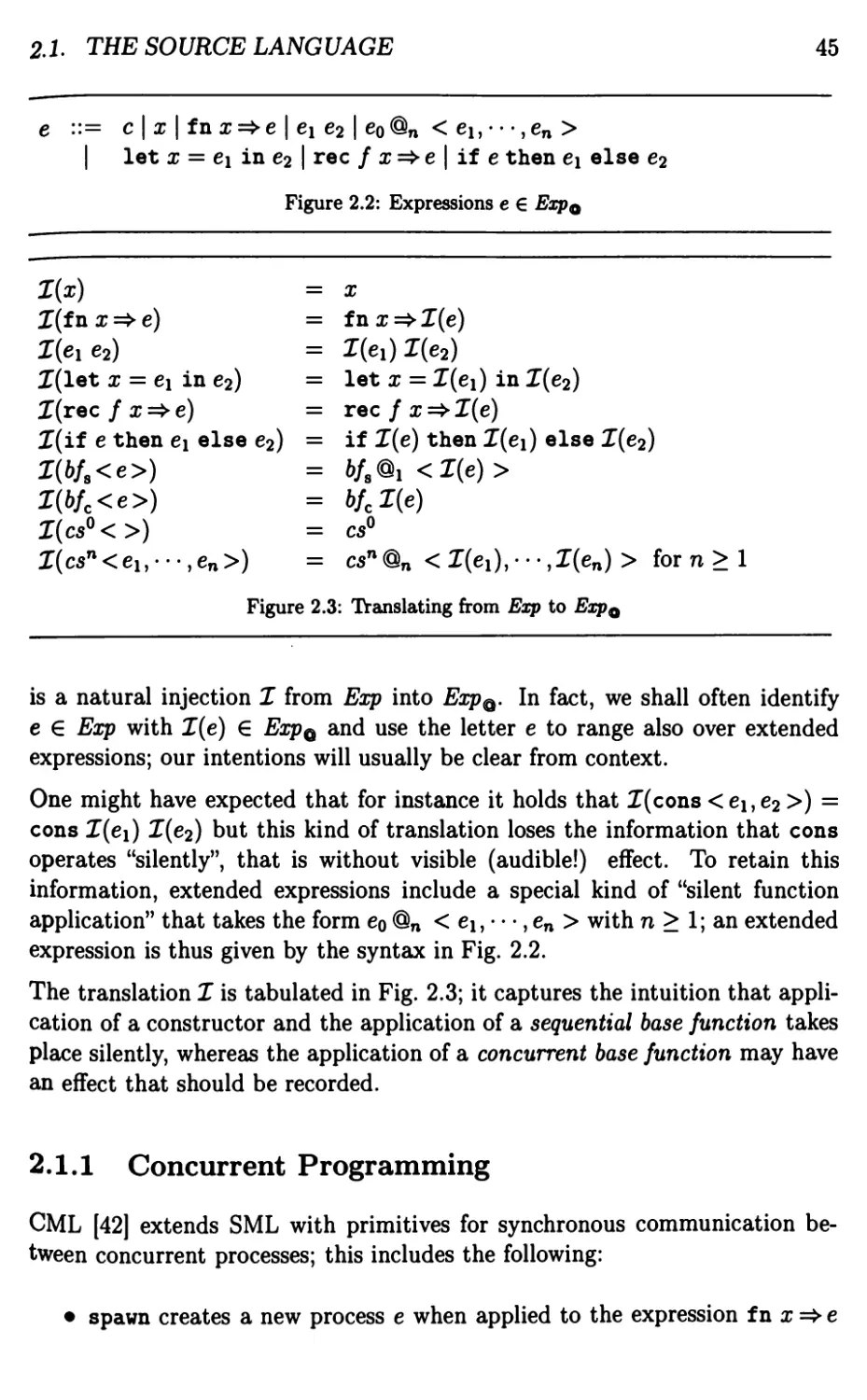
2.1 Expressions e £ Exp 44
2.2 Expressions e £ ExpQ 45
2.3 Translating from Exp to Exp® 45
2.4 The ordering on regions 52
2.5 The ordering on behaviours 54
2.6 The ordering on types 55
2.7 The types of constants 57
2.8 The type inference system 58
2.9 The possible traces of a behaviour 70
2.10 The core of the Hindley-Milner type system 74
3.1 The evaluation function S 79
3.2 The top-level sequential transition relation 79
3.3 The concurrent transition relation 82
4.1 Algorithm W: the overall structure 100
4.2 Syntax-directed constraint generation 102
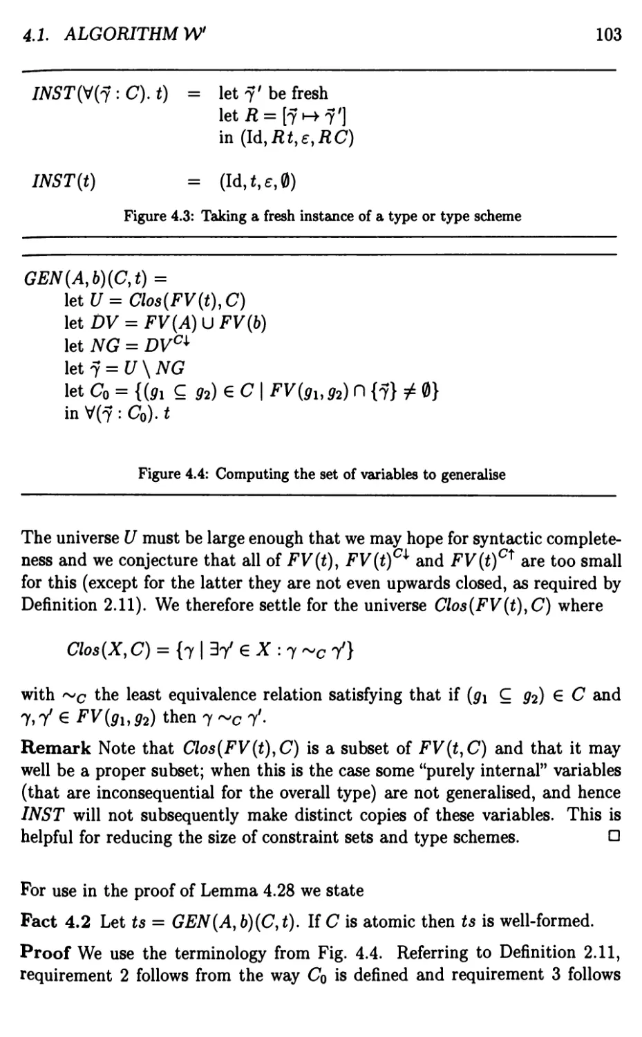
4.3 Taking a fresh instance of a type or type scheme 103
4.4 Computing the set of variables to generalise 103
4.5 Decomposition of constraints 105

LIST OF FIGURES
4.6 Rewriting rules for T 105
4.7 Forced matching 108
4.8 Eliminating constraints Ill
4.9 Monotonic and anti-monotonic variables 115
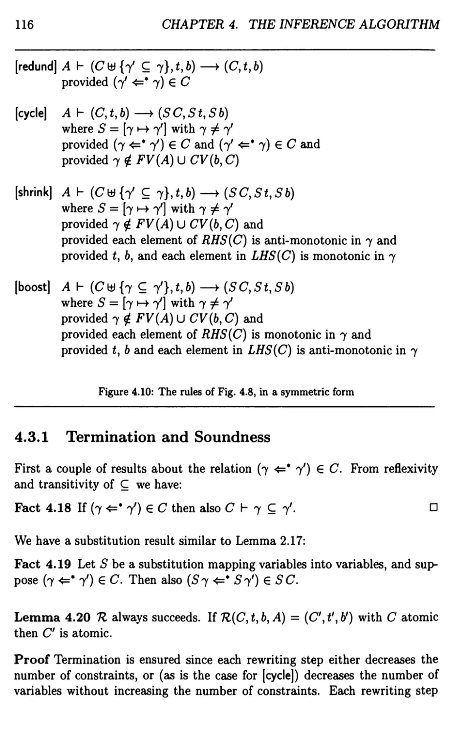
4.10 The rules of Fig. 4.8, in a symmetric form 116
6.1 The bisimulation relation ~ 147
6.2 The equivalence relation ~ on action configurations 148
6.3 The functionals Gp and Ga used for defining ~ and ~ 149
7.1 The Karlsruhe Production Cell 166
7.2 A CML program for the table 168
7.3 The behaviour for the table 170
7.4 Another CML program for the table 176

Preface
Program analysis and type systems have been recognised as important tools
in software development. By analysing a program before running it one may
catch a variety of errors in due time; this goes not only for obvious errors
such as adding an integer to a boolean, but also for "higher-level" errors such
as violating a given communication protocol. Even for programs that are
already correct, analysis is useful for reasons of efficiency: the result of the
analysis may guide the transformation into an equivalent program with better
performance; or it may guide the run-time system to improve the program's
execution profile, for example by giving directions for an optimal scheduling
of processors.
We firmly believe that for a given program analysis to be reliable, a solid
foundation must be established. This includes that the specification of the analysis
is faithful to a formal semantics for the source language, and that it is correctly
implemented. To demonstrate these issues involves stating and proving a bulk
of auxiliary results; and as analyses get more complex, it becomes increasingly
difficult to fit these bits together in a coherent way.
This book reports on a powerful type and effect analysis. Taking a type based
approach enables a succinct representation of program properties and
facilitates modular reasoning. The system meets the theoretical demands outlined
above and is useful for practical purposes, as witnessed by a prototype
implementation that is available on the world-wide web. Indeed, a main objective of
our research has been to advance the state of the art of effect system
technology, in particular by integrating polymorphism (essential for code reuse) with
a notion of subtyping (essential for the sake of precision).
The role of effects, or rather behaviours so as to emphasise that temporal
information is included, is to explicitly record the actions of interest that will
be performed at run-time. A variety of analyses on the language of behaviours
may be built on top of the system; one might even devise a tool (& la the
Mobility Workbench) for testing certain properties of behaviours.

PREFACE
Chapter 1 puts our development in perspective; prior knowledge of type
systems will be helpful but is not strictly assumed. Chapter 7 (which is based on
[39]) gives a case study illustrating the use of the system. Chapters 2-6 are
more technical and require some amount of "mathematical maturity" on part
of the reader.
The research documented in this book grew out of the ESPRIT project
LOMAPS (BRA 8130: Logical and Operational Methods in the Analysis of
Programs and Systems). For this reason our development is conducted for
a language (Concurrent ML) that integrates the functional and concurrent
paradigms, but most of the ideas can be immediately transferred to other
settings. Also, we have been partly supported by the DART project (funded by
the Danish Science Research Council).
We would like to thank our collaborators in the above projects for fruitful
discussions, in particular Pierre Jouvelot, Lone Leth, Jean-Pierre Talpin, Bent
Thomsen, and Mads Tofte; we also thank Hans Rischel for providing us with
the program used for the case study in Chapter 7.
Arhus, October 1998
Torben Amtoft Flemming Nielson Hanne Riis Nielson

Chapter 1
Introduction
1.1 Basic Concepts
Type inference. The notion of types dates long back into the history of
Computer Science. A main motivation is the desire to avoid certain kinds of
computations such as adding the boolean value true to the integer value 7;
this is permitted in untyped languages (perhaps yielding 8) but is regarded as
being meaningless by sensible programmers.
One approach (used e.g. in Scheme [58]) is to let the run-time system equip
all values with a "tyPe tag"; f°r eacn operation performed it must then be
checked that the type tags of the operands are appropriate. This "dynamic
typing" is potentially time consuming and often one prefers to do type checking
"statically", i.e. at compile-time, also so as to catch errors as early as possible.
The two approaches are not mutually exclusive and Java [13] is an interesting
mixture: it has static typing but the run-time system still has to compare tags
at some places, in particular when updating an array.
Another benefit of static typing is that it serves as a partial specification of the
program, for instance describing which kind of input a given function expects
and which kind of result it returns — if it expects an integer and returns a
boolean it will have type int -> bool. The programmer can thus check
whether this corresponds to what he had in mind.
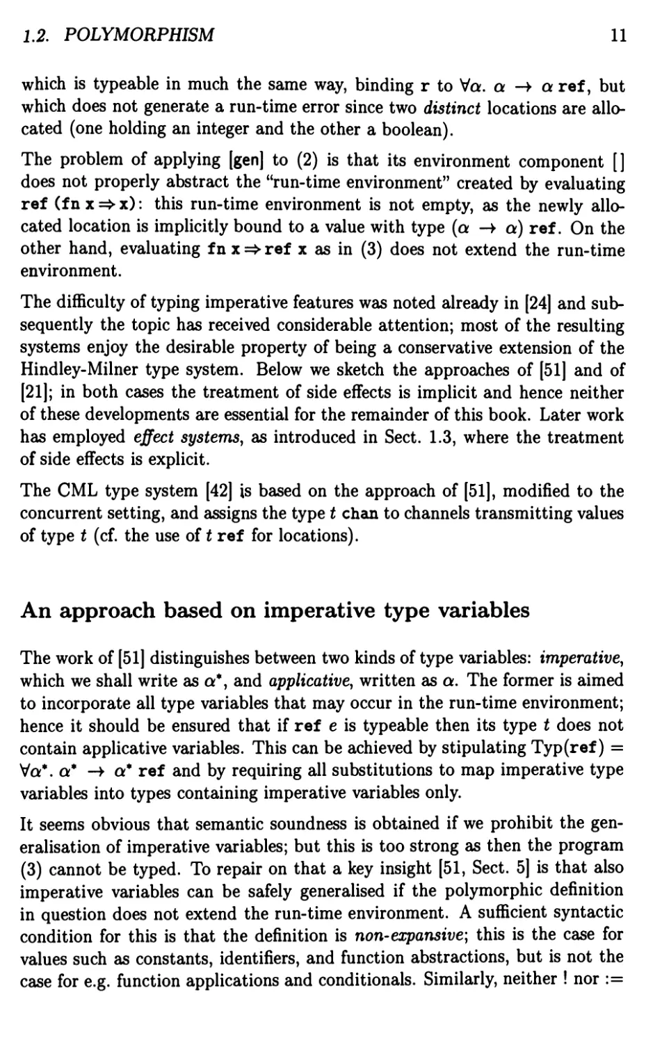
Static typing is usually specified in terms of an inference system consisting of
a number of axiom schemas and inference rules; simple examples of such are
h ei : int, h e2 : int
h n : int and
h e\ + e2 : int
1

2
CHAPTER 1. INTRODUCTION
The axiom schema on the left states that all natural numbers n have integer
type; and the inference rule on the right states that if it is possible to assign
the expressions e\ and e2 an integer type then also their sum has integer type.
We shall often want to compare a type system T for a language L to an
"extended" type system T for a language which is equal to or encompasses
L: we say that V is a conservative extension of T if for all //-expressions e it
holds that if e is typeable in T with type t then e is also typeable in V with
type t\ and t can be "obtained from" t'.
Semantic soundness. Of course a static type system must be faithful to
the semantics of the program: if h e : int is derivable and the program
expression e at run-time evaluates to a value then we certainly expect this
value to be an integer. The precise formulation of this semantic soundness
property depends on the kind of semantics [35] used; below we sketch some
approaches in their simplest form. In all cases, the statement of semantic
soundness contains h e : tasa premise.
One approach assumes that a set of "semantic values" v are given. Then one
has to define a relation v : t, to be read "the value v has type f\ and the
soundness requirements are
• for a denotational semantics: if h e : t and [e] = v then v : t\
• for a big-step (natural) semantics: if he:t and e —> v then v : t.
As languages grow in complexity and features, it becomes harder to come
up with a suitable set of "semantic values"; and hence the approach of using
a small-step semantics [41] has become increasingly popular. Writing => for
the transition relation, semantic soundness is then formulated as the subject
reduction property
• if h e : t and e => e' then also h e' : t.
Another advantage of this approach, compared to using a big-step semantics,
is that it also caters for non-terminating programs. To ensure that "well-
typed programs do not go wrong" [24] one must also establish that "error
configurations" (those which are "stuck") cannot be typed.
It should be noted that we cannot hope for a decidable type system that is
"completely" faithful to the semantics, e.g. in the sense that h e : int is
derivable if and only if e never evaluates to something which is not an integer.
To see this, consider the program

1.1. BASIC CONCEPTS
3
let p(x) = ••• in if p(3) then 7 else true.
This expression will evaluate to a boolean if and only if p(3) returns false; and
as is well-known from computation theory [18] this is in general undecidable
for "Turing-complete" languages such as the one studied here.
Syntactic soundness and completeness. Having defined a type inference
system, a natural goal is to devise an algorithm that automatically infers types
for expressions. Clearly such a "reconstruction algorithm" must be
syntactically sound; this property in its most simple form states that if the algorithm
assigns the expression e the type t then h e : t must be derivable in the
inference system — hence syntactic and semantic soundness can be combined
into a common soundness result which ensures that the output from the
reconstruction algorithm yields trustworthy information about the input program's
run-time behaviour.
A reconstruction algorithm should preferably be not only sound but also
syntactically complete, as then the algorithm does not reject valid programs. This
property in its simplest form states that if h e : t' is derivable in the type
system then the algorithm when applied to e returns a type t which has t' as an
"instance"; in other words the algorithm computes the "most general typing".
A reader's guide to Chapter 1. Our starting point (Sect. 1.2) is the
"Hindley-Milner type system" [24, 6], used as the basis for the statically typed
functional languages ML [12], Haskell [55] etc. A crucial feature of this system
is the ability to generalise over types so as to make functions polymorphic and
hence applicable to arguments of different types. The archetypical polymorphic
function is the identity function which just returns its argument; it has type
int -> int as well as bool -> bool and these types are instances of the type
scheme Va. a -> a (which is unambiguously parsed as Va. (a -> a)). In
particular, we do not consider system F [11] where generalisation may occur
inside types (allowing (Va. a) -> a), or the intersection type system [16].
An inference system for Hindley-Milner typing is presented in Sect. 1.2.1 and
Sect. 1.2.2 discusses the design of a reconstruction algorithm W.
In accord with the trend in programming languages towards integrating a
variety of features, the Hindley-Milner system has to be extended. Our focus
is on adding "non-applicative" features like "imperative" constructs, often
essential for efficient programming, or concurrency constructs. Research from
the beginning of the 1990'es indicates how to write semantically sound type
systems for the resulting languages; in Sect. 1.2.3 we mention the approaches

4
CHAPTER 1. INTRODUCTION
of [51, 21] which are "implicit" in that the types do not explicitly record the
"side effects" performed by the non-applicative constructs.
In Sect. 1.3 we give an introduction to effect systems, a formalism that allows
types to carry detailed information about run-time behaviour, and that also
facilitates writing semantically sound type systems [53, 49] for languages with
non-applicative features. In Sect. 1.4 we address the issues involved in writing
reconstruction algorithms for effect systems.
In Sect. 1.5 we shall see that in order to obtain more precision than provided
by the techniques of Sections 1.3 and 1.4, it is fruitful to combine with
techniques previously used [8, 9, 47] for adding subtyping to purely applicative
programming languages.
Sections 1.2-1.5 thus provide the background setting for the rest of this book,
which presents a rather precise type system for a functional language with
polymorphism and concurrency as outlined in Sect. 1.6. Moreover, the type
system yields temporal information about run-time behaviour; this is very
useful for validation purposes as demonstrated in Chap. 7 (based on [39]).
1.2 Polymorphism
In this section we shall introduce the basic concepts of Hindley-Milner
typing [24, 6] and consider a small purely applicative language that forms a core
fragment of ML. Expressions e in this language are built from identifiers x,
function abstractions fn x=>e, function applications e\ e<i, conditionals
if e0 then e\ else e2, recursive function definitions rec / x=>e (which
when applied to a value v evaluates e with x bound to v and with / bound
to the function itself), and let-expressions let x = e\ in e2 where e\ is a
polymorphic definition of x. We also include a selection of constants c,
encompassing the natural numbers and the standard arithmetic operators (which are
written in infix notation).
Much of the power of ML stems from the possibility of defining functions
which are higher-order and polymorphic, a simple example of this is the twice
function given by
twice = fn f => fn x =>f (f x).
It is higher-order in that it takes a function / as input and returns the function
/ of as output (functional composition); it is polymorphic in that it can be
applied to arguments having different types:

1.2. POLYMORPHISM
5
let tw = twice in • • • tw (f n x => x + 1) • • • tw (f n y => not y) • • •
When applied to the integer successor function, fnx=>x+ 1, twice returns
a function which increments its argument by 2; when applied to the boolean
negation function twice returns the identity function on booleans.
That twice is higher-order and polymorphic can be seen from its type scheme
Va. (a -> a) -> (a -> a)
which can be instantiated to yield (int -> int) -> (int -> int) which is
the type of twice when applied to the successor function.
1.2.1 An Inference System
An inference system for our core ML fragment is depicted in Fig. 1.1. Types
t can be variables (we use a to range over these), base types like int or bool,
or composite types like the function type t\ -> t2. A type scheme ts is of the
form Va. t with a a sequence of bound variables; accordingly its free variables
FV(ts) are given as FV(t) \ {3} where FV(t) are the variables occurring in
t. To cater for free identifiers (within the body of function definitions etc.) we
need an environment A mapping identifiers into types or type schemes; hence
judgements are of the form A h e : a where a is either a type or a type
scheme. A closed type or type scheme is one without free variables, and the
notion of free variables naturally extends to environments.
We shall also need the notion of substitutions; these map type variables into
types. A substitution gives rise to a mapping on types and the type resulting
from applying substitution S to type t is denoted S t. This operation binds
stronger than function arrow, so Si t\ -> t2 = (Si *i) -> t2. The domain of a
substitution S is the set of variables affected: Dom(S) = {a | Sa / a}. The
identity substitution is denoted Id and we write S2 Si for the substitution that
first applies Si and next S2, so (S2 Si)(a) = S2 (Si a). We say that S' is an
instance of S if there exists S" such that S' = S" S.
Note that in Fig. 1.1 there is one rule for each syntactic construct and two
specific rules for instantiation [ins] and generalisation [gen]; we use the term
structural for the former kind of rules. The rule [con] assumes the existence
of a function Typ that assigns a closed type or type scheme to each constant;
for example it holds that Typ(7) = int. The side condition for applying [ins]
says that an "instance substitution" must affect only the bound variables of a
type scheme. The side condition for applying [gen] is necessary for semantic

6
CHAPTER 1. INTRODUCTION
[con] A h c : Typ(c)
[id] A\- x : A(x)
A[x : ti] h e : t2
[abs]
[app]
[let]
[rec]
j4 h fnx=>e : ^ -> tf2
A h ei : t2 -+ h A h e2 : t2
A h ei e2 : ti
i4 h ei : tfsi i4[x : tfsi] h e2 : <2
j4 h let x = t\ in e2 : 22
A[/:t]hfnx=»e:t
i4 h rec f x=$>e : t
r.n ^4 h e0 : bool A h ei : t A h e2 : t
[if]
i4 h if eo then ei else e2 : 2
(.ns] A*-'■**■* if £,^(5) c {5}
l8enl /hCw^ if {3}nfF(>l)=0
i4 h e : Va. *
Figure 1.1: The core of the Hindley-Milner type system
soundness; indeed we shall show that otherwise the identity function fnx=>x
may have type int -> bool. If [gen] can be applied to [x : a] h x : a, in spite
of a being free in [x : a], we have [x : a] h x : Va. a; by [ins] we then get
[x : a] h x : bool and by [abs] also [] h fn x=^x : a -» bool; and by one
more application of [gen] we arrive at [] h fnx=>x : Va. a -> bool which
by [ins] yields the semantically incorrect [] h fnx=>x : int -> bool.
It is not difficult to prove the semantic soundness of the system in Fig. 1.1; for
a denotational semantics this can be done following the approach in [24].
Recursive functions and polymorphism. A key construct for defining
recursive functions in ML is let fun / x = e\ in e2 end which in our language
is expressible as let / = rec / x => e\ in e2. It is easy to see that the following
inference rule is derivable from Fig. 1.1:

1.2. POLYMORPHISM
7
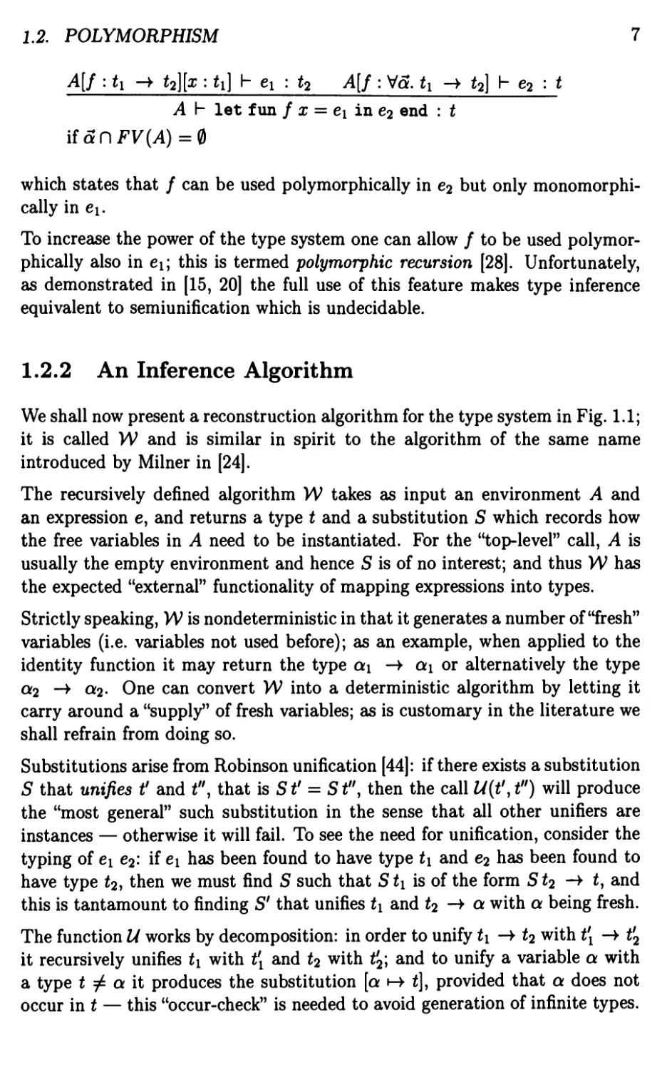
A[f : *i -» t2][x : U] h ei : t2 A[f : Vg. fr -> *2] h e2 : t
A h let fun / x = ei in e2 end : 2
iffinFVr(i4)=0
which states that / can be used polymorphically in e2 but only monomorphi-
cally in t\.
To increase the power of the type system one can allow / to be used
polymorphically also in ei; this is termed polymorphic recursion [28]. Unfortunately,
as demonstrated in [15, 20] the full use of this feature makes type inference
equivalent to semiunification which is undecidable.
1.2.2 An Inference Algorithm
We shall now present a reconstruction algorithm for the type system in Fig. 1.1;
it is called W and is similar in spirit to the algorithm of the same name
introduced by Milner in [24].
The recursively defined algorithm W takes as input an environment A and
an expression e, and returns a type t and a substitution S which records how
the free variables in A need to be instantiated. For the "top-level" call, A is
usually the empty environment and hence S is of no interest; and thus W has
the expected "external" functionality of mapping expressions into types.
Strictly speaking, W is nondeterministic in that it generates a number of "fresh"
variables (i.e. variables not used before); as an example, when applied to the
identity function it may return the type ai -> ai or alternatively the type
a2 -> a2. One can convert W into a deterministic algorithm by letting it
carry around a "supply" of fresh variables; as is customary in the literature we
shall refrain from doing so.
Substitutions arise from Robinson unification [44]: if there exists a substitution
S that unifies t' and *", that is St' = St", then the call U(t',t") will produce
the "most general" such substitution in the sense that all other unifiers are
instances — otherwise it will fail. To see the need for unification, consider the
typing of e\ e2: if e\ has been found to have type t\ and e2 has been found to
have type t2, then we must find S such that Sti is of the form St2 -> t, and
this is tantamount to finding S' that unifies t\ and t2 -> a with a being fresh.
The function U works by decomposition: in order to unify *i -> t2 with t[ -> t'2
it recursively unifies *i with t[ and t2 with t2\ and to unify a variable a with
a type t / a it produces the substitution [a 4 <], provided that a does not
occur in t — this "occur-check" is needed to avoid generation of infinite types.

8
CHAPTER 1. INTRODUCTION
We refer to [44] for the details.
Remark There exists type reconstruction algorithms with different "internal"
functionality. The algorithm T [7, p. 37] takes as input an expression only, and
returns a type together with an "assumption list", i.e. an environment where
there may be multiple assignments to each identifier. When closing the scope
of an identifier x (when typing fni=^e) all types assigned to x must then be
unified. Another algorithm is J [24, Sect. 4.3]; it is an optimised version of
W, in that the substitution component has been "globalised". □
The algorithm W is defined by the clauses in Fig. 1.2, where we have omitted
the clauses for recursion and conditional as these follow a similar pattern.
The placement of instantiation and generalisation reflects a standard result
ensuring that one can assume that an inference is normalised, i.e. that all uses
of rule [gen] take place after typing a polymorphic definition, and that all uses
of rule [ins] take place immediately after an application of [con] or [id]. To cope
with generalisation, the algorithm closely follows the inference system in that
it generalises over all type variables that are not free in the environment. To
cope with instantiation, the algorithm has to generate a fresh copy (so as to
be as general as possible) of the type scheme associated with a constant or an
identifier; this is done by the function INST which maps a type t into itself
and which maps a type scheme Va. t into [a »-► dt\ ] t with dt\ fresh variables.
Soundness and completeness. The syntactic soundness of W was
demonstrated already in [24]: if W([],e) = (S,t) then [] h e : t. This is a
consequence of a more general soundness result, admitting an inductive proof, which
states that if W{A,e) = (S,i) then S A h e : t.
W is also syntactically complete, as conjectured in [24] but first proved in
[6, 7]. For closed expressions this amounts to
if []he:f
then (i) the call W([],e) succeeds
(ii)ifW([],e) = (S,t)
there exists S' such that S't = t'.
This result, together with the standard result that inferences are "closed under
substitution", establishes that the system in Fig. 1.1 has a principal typing
property: if the set {t' \ [] h e : t'} is not empty then there exists a type t
such that the entire set is expressible as {S't \ S' is a substitution}.

1.2. POLYMORPHISM
9
W(A,c) = (Id, INST(Typ(c)))
W(A,x) =if x 6 Dom(A) then (Id, INST(A(x))) else/ai7i<tent
W04,fnx=*eo) =
let a be fresh
let (So,t0) = W(A[x:a},e0)
in (S0, So a ->• t0)
W(^,eie2) =
let(S1)t1)=W(>l,e1)
let (S2,t2) = WiStAei)
let a be fresh
let S=U(S2tut2 -*• a)
in (SS2Si,Sa)
W(A, let i = tx in e2) =
let(S1,t1) = W(^,ei)
let a = JV(ti) \ FV(SX A)
let tsi = Va. ti
let(S2)t2) = W((S1>l)[a;:ts1],e2)
in(S2Si,t2)
Figure 1.2: The core of Algorithm W
To admit an inductive proof of syntactic completeness, the above definition
must be extended so as to cater also for open expressions and this is a slightly
tricky matter. One formulation is
if A' h e : f and A' = S" A
then (i) the call W(A, e) succeeds
(ii)ifW(,4,e) = (S,*)
there exists S' such that S' t = t' and S" A = S' S A.
Also the notion of principal typing can be generalised to take environments
into account.

10
CHAPTER 1. INTRODUCTION
1.2.3 Implicit Treatments of Side Effects
It is necessary to modify and extend the system developed so far in order to
type languages that are not purely applicative, as will be the case if expressions
are allowed to have side effects, i.e. change a global "run-time environment".
In the remaining chapters of this book we study the incorporation of
concurrency; here the environment is "external" and consists of a set of communication
channels. In Concurrent ML (CML) [42, 40] the expression channel e
allocates a channel; the expression accept ch receives a value from the channel
ch; and the expression send (c/i, e) transmits the value of e over the channel
ch.
A prime example in the literature is the incorporation of imperative features;
here the environment is "internal" and consists of a set of locations. In
Standard ML (SML) [26, 59] the expression ref e allocates a location and initialises
it to the value of e; the expression ! / gets the content of location /; and the
expression / : = e assigns the value of e to the location /. As is well-known from
many imperative languages, the expression e\ ; e2 evaluates first e\ and then
e2.
To manage imperative features one may introduce [51] an additional type
construct t ref, with the intention that this is the type of a location holding a value
of type t. A naive approach is then to stipulate Typ(ref) = Va. a -> a ref
and Typ(!) = Va. a ref -> a (note that ref binds stronger than function
arrow), and similarly for the infix operator :=, whereas the rule for e\ ; e2 is
straightforward.
But without further modifications, the inference system from Fig. 1.1 is now
semantically unsound! This can be demonstrated by the program
let r = ref (f n x => x) in (r : = f n x =$► x + 1 ; ! r true) (1)
which generates a run-time type error, in that the function f n x => x + 1 is
applied to true, even though (1) is typeable: from the judgement
[] h ref (fnx=*x) : (a -* a) ref (2)
one can apply [gen] and then bind r to the type scheme Va. (a -> a) ref. By
applying [ins] twice, with an instance substitution which is first [a »->• int] and
next [a »->• bool], it is thus possible to type the body of the let-expression.
That the issue is rather subtle is illustrated by the program
let r = fnx=>ref x in (r 7 ; r true)
(3)

1.2. POLYMORPHISM
11
which is typeable in much the same way, binding r to Va. a -> a ref, but
which does not generate a run-time error since two distinct locations are
allocated (one holding an integer and the other a boolean).
The problem of applying [gen] to (2) is that its environment component []
does not properly abstract the "run-time environment" created by evaluating
ref (f n x => x): this run-time environment is not empty, as the newly
allocated location is implicitly bound to a value with type (a -> a) ref. On the
other hand, evaluating fnx=>ref x as in (3) does not extend the run-time
environment.
The difficulty of typing imperative features was noted already in [24] and
subsequently the topic has received considerable attention; most of the resulting
systems enjoy the desirable property of being a conservative extension of the
Hindley-Milner type system. Below we sketch the approaches of [51] and of
[21]; in both cases the treatment of side effects is implicit and hence neither
of these developments are essential for the remainder of this book. Later work
has employed effect systems, as introduced in Sect. 1.3, where the treatment
of side effects is explicit.
The CML type system [42] is based on the approach of [51], modified to the
concurrent setting, and assigns the type t chan to channels transmitting values
of type t (cf. the use of t ref for locations).
An approach based on imperative type variables
The work of [51] distinguishes between two kinds of type variables: imperative,
which we shall write as a*, and applicative, written as a. The former is aimed
to incorporate all type variables that may occur in the run-time environment;
hence it should be ensured that if ref e is typeable then its type t does not
contain applicative variables. This can be achieved by stipulating Typ(ref) =
Va*. a* -> a* ref and by requiring all substitutions to map imperative type
variables into types containing imperative variables only.
It seems obvious that semantic soundness is obtained if we prohibit the
generalisation of imperative variables; but this is too strong as then the program
(3) cannot be typed. To repair on that a key insight [51, Sect. 5] is that also
imperative variables can be safely generalised if the polymorphic definition
in question does not extend the run-time environment. A sufficient syntactic
condition for this is that the definition is non-expansive; this is the case for
values such as constants, identifiers, and function abstractions, but is not the
case for e.g. function applications and conditionals. Similarly, neither ! nor :=

12
CHAPTER 1. INTRODUCTION
extends the run-time environment; and hence we can allow Typ to map these
operators into type schemes where the type variables are applicative.
The semantic soundness of the resulting system is demonstrated in [51] with
respect to a big-step semantics; the correctness relation which states when a
value has a given type is defined coinductively so as to cope with cycles in the
run-time environment.
The type reconstruction algorithm presented in [51] is a modification of
algorithm W. The main extension is that when unifying an imperative variable a*
with a type t, all applicative variables in t are replaced by imperative variables
(due to the abovementioned requirement on substitutions).
Being non-expansive is not a necessary condition for not extending the
runtime environment, as illustrated by the expression
(f n x =$► f n y =$► ref (f n z => z)) 7. (4)
A more precise approximation is outlined in [4] where all imperative variables
are assigned a "weakness degree" n, 0 < n < oo. We cannot generalise over
imperative variables having weakness degree 0, as these may occur in the
runtime environment, but variables with weakness degree n > 0 occurring in the
type of an expression e are guaranteed not to occur in the run-time environment
as long as e is applied to at most n — 1 arguments.
This idea is employed in [60] which assigns the expression (4) the type a ->
(a*1 -> a*1) ref where also the imperative variable a*1 can be generalised.
On the other hand, the 1997 version of SML [59] returns to a simple but
somewhat crude generalisation strategy, in that the notion of imperative type
variables is eliminated but instead the "value restriction" is imposed: in order
to generalise over variables occurring in the type of a polymorphic definition,
the defining expression must be non-expansive (i.e. a syntactic value).
An approach based on tracking dangerous type variables
The work of [21] aims at a more direct way of estimating which type variables
that may occur in the run-time environment and hence must not be generalised:
these are decreed to be the variables that occur "dangerously" in the type of a
polymorphic definition.
To explain the idea, first consider the polymorphic definition in (1). Looking at
its type, (a -> a) ref, it is apparent that a occurs in the type of the location
created by the definition and thus also in the run-time environment. This

1.3. AN INFERENCE SYSTEM FOR EFFECTS
13
motivates the defining equation DV(t ref) = FV(t), where DV computes the
set of dangerous variables.
Next consider the polymorphic definition in (3). Looking at its type, a ->
a ref, it is apparent that the definition creates a "closure". Essentially, a
closure is an expression together with an environment recording the values
of the free identifiers. These values may contain locations themselves, and
therefore we define DV(ti -* ^2) to be the union of all DV(t) where t is the
type of an identifier free in the closure — in the example there are no such
identifiers and hence a is not dangerous.
As can be seen from [21, Fig. 3] the resulting system is able to type several
programs that are (i) composed from simple building blocks and thus not
contrived, and that are (it) not typeable by [51] nor by the "weakness degree"
approach described above. Unfortunately, it fails to be a conservative extension
of the Hindley-Milner type system: there exists a purely applicative program
[21, Sect. 3.6] which is Hindley-Milner typeable but not typeable by the system
as presented in [21].
1.3 An Inference System for Effects
In recent years effect systems have become increasingly popular; a major reason
is that they allow an explicit treatment of side effects and hence they are closer
to our intuition than the approaches sketched in Sect. 1.2.3. Judgements take
the form
Ah e : tkb
where the effect b describes the "visible effect" of evaluating e. This extra
component is used to gain concise information about certain aspects of the
program's run-time behaviour, possibly enabling a more efficient implementation.
An extra benefit is that the effects may be used to "control polymorphism", as
will be described in Sect. 1.3.1, so as to yield a semantically sound system for
languages with non-applicative features.
We use e for the effect denoting that no visible action takes place; for a call-
by-value language we thus have the axiom schema
A\- x : A{x)ke
In order to write a sensible rule for function application, we shall annotate
function types with an effect component describing what happens when the

14
CHAPTER 1. INTRODUCTION
function is applied. Accordingly, the rule for function abstraction records the
effect of evaluating the body in the type of the abstraction:
A[x:ti] h e : t2kb
A h f n x => e : tx ->6 t2 & e
When applying a function e\ to an argument e2, a call-by-value language first
evaluates t\ to a closure, next evaluates e2 to a value, and finally evaluates the
closure. This is reflected in the rule for function application
A h ei : t2 ->fr t\ fe &i Ah e2 : t2kb2
Ah exe2 : txk {bx SEQ b2 SEQ b)
where SEQ is an operator (in the meta language) for sequential composition
of effects. We shall assume that SEQ is associative with e as neutral element;
it will often be the case that SEQ is commutative but more precise analyses
will be obtained if it is not, cf. Sect. 1.3.3.
The rule for conditional expresses that while the test must always be evaluated,
we cannot in general statically determine which branch will be taken:
A h eo : bool&&o A h e\ : tkb\ A h e2 : tkb2
A h if e0 then tx else e2 : tkb0 SEQ (h OR b2)
where OR is an associative and commutative operator (still in the meta
language) for "nondeterministic" composition of effects.
A seminal paper in the field is [23] which treats the LISP dialect FX.
Corresponding to the imperative features NEW, GET and SET there are effects
ALLOC, READ and WRITE; the role of SEQ (and of OR) is played by the
commutative operator MAXEFF (that can be thought of as set union). Source
programs must be pre-annotated with type information, so for example
function abstractions are written as (LAMBDA (x : t) e), and also polymorphism
is explicit.
The theory of effect systems is further developed in [48]. Here types are not
explicitly present in the source program but inferred by a reconstruction
algorithm, and a simple kind of polymorphism is employed: a let-expression
let x = ei in e2 is considered a polymorphic definition of e\ (so that the type
of t\ can be generalised) if t\ is non-expansive, cf. the discussion of [51] in
Sect. 1.2.3.

1.3. AN INFERENCE SYSTEM FOR EFFECTS
15
1.3.1 Effects Controlling Polymorphism
We now describe how effect information can be used to decide which type
variables are generalised in a polymorphic definition; it should be clear from
the discussion in Sect. 1.2.3 that for this purpose effects must estimate the
set of variables that may occur in the run-time environment. (A type now
contains not only type variables but also effect variables and we use /? to range
over the latter.)
A minimalistic approach is taken in [53]. Here effects are just sets of type
and effect variables (so e is the empty set and SEQ as well as OR is union).
As in [51] the focus is on detecting the creation of locations so we stipulate
Typ(ref) = Va. a -»<*> a ref and Typ(!) = Va. a ref -»0 a. The rule
[gen] from Fig. 1.1 avoids generalising over variables that are free in the static
environment; it must be modified to also avoid generalising over variables that
are free in the run-time environment and as FV(b) is designed to be a superset
of the latter set, the rule now reads
A h e : tkb if{ap}n(FV(A)UFV(b)) = (I>
A h e : Vap.tkb
The semantic soundness of the resulting system is established using a small-
step semantics.
By adding more structure to the effects of [53] one can obtain more refined
systems; we shall mention some of these in the sequel. The task of integrating
side effects and polymorphism can thus be solved in several ways and [53,
Sect. 5] contains an insightful comparison between some of these, including
those outlined in Sect. 1.2.3. Some interesting benchmarks, illustrating the
strengths and limitations of various approaches, are given in [49, Sect. 11].
1.3.2 Regions
By incorporating regions, effect systems may yield highly informative output,
useful for e.g. program optimisation. A region r (we use p to range over region
variables) can be considered as an abstraction of the "place" where a side effect
occurs: for imperative languages one can think of a region as a set of locations;
for concurrent languages one can think of a region as a set of communication
channels. Regions are introduced already in [23] and we shall now elaborate
on their use in [49].
Here an effect is a set of atomic effects and thus SEQ and also OR is union;
an atomic effect is either init(r,t), indicating that a location holding a value

16
CHAPTER 1. INTRODUCTION
of type t is allocated in region r, or write (r, t), indicating that a location in
region r is assigned a value of appropriate type t, or read(r,t), indicating that
a value of type t is fetched from a location in region r. (Similarly the type
construct t ref is equipped with a region component, denoting where the
location represented by this type is allocated.)
Again effects are used to control polymorphism, in particular the rule for [gen]
is as in [53], and semantic soundness is established with respect to a big-step
semantics. Moreover, as we shall see below the presence of regions enables a
significant amount of "garbage collection" to be done statically.
To illustrate the issue, first consider the expression t\ given by
let v = ref 5 in ! v + 2 (5)
which returns 7 — afterwards it is clearly safe to deallocate the location
denoted by v. Next consider the expression t<i given by
let v = ref 3 in f n x =$► ! v + x (6)
which returns a closure — as the location denoted by v is referenced each time
this closure is applied, it cannot be safely deallocated.
The effect system in [49] can distinguish between those two cases. For (6) the
judgement
[] h e2 : int -»™*(^) int& mi*(r, int)
is derivable, and as r is present in the type it is not safe to discard this region.
On the other hand, for (5) the judgement
[] h d : int kinit(r, int) U read(r, int)
is derivable and here r does not occur in the type nor in the environment.
Hence r is not "observable" and we infer that it is safe to deallocate v\
additionally we can dispense with the unobservable effect and just get [] h t\ :
int&£.
"Filtering" of effects is called effect masking and dates back to [23]. As shown
in [49, Sect. 11] (by the example id4 id4) this enlarges the set of typeable
programs.

1.3. AN INFERENCE SYSTEM FOR EFFECTS
17
An application to region-based memory management
As demonstrated most impressively in [52], effect systems can be used also for
purely applicative languages! Still the purpose is to determine the lifetime of
"locations"; these are not explicit as for imperative languages but yet they do
occur implicitly in the underlying implementation. In the presence of higher-
order functions, this task is notoriously difficult.
To illustrate the problem, we can use programs similar to (5) and (6). First
consider the "block"
let v = 5 in v + 2
where the "region" holding 5 can be pushed onto the stack at block entry and
safely popped from the stack at block exit. To make this explicit, in [52] one
may write
letregion p in let v = 5 at p in • • • end
where • • • encodes v + 2 and is given by letregion p?. in (v 4- (2 at p2)) at px
(placing the result in the persisting region pi). Next consider the block
let v = 3infnx=>v + x
where the region holding 3 cannot be safely popped at block exit as it will be
referenced each time the generated closure is applied; usually such regions are
placed in the heap rather than on the stack. Alternatively, as in [52], the region
is still pushed onto the stack but "sufficiently early" (prior to being assigned
the value 3) so that it is not popped until the closure becomes inaccessible.
The effect system of [52] records when regions in the "underlying store model"
are referenced or assigned; simultaneously it transforms the source expression
into a target language where all operations on regions are explicit (as
indicated above). Thus the target language can be implemented using a stack
discipline well-known from block-structured languages [29], avoiding
expensive run-time garbage collection. (In general, however, some of the regions
may have unbounded size so the stack must contain a pointer to those regions
rather than their actual content.) This provides a main theoretical basis for
the ML Kit [56], a compiler for Standard ML.
In the target language of [52] functions are parametrised with respect to region
information. Consider for instance a function fib for computing the fibonacci
function; then f ibfp!,^] denotes a call where the argument is taken from pi

18
CHAPTER 1. INTRODUCTION
and the result is placed in P2. If fib is called elsewhere in the program then
these calls must be allowed to use different regions as otherwise the analysis
will be far too coarse; hence the effect system has to employ polymorphism
not only for type and effect variables but also for region variables and thus
type schemes take the form Va/?p. t.
Similarly, in order to get a fine-grained analysis [52] allows the two recursive
calls of fib to use different regions. Hence also the body of a function definition
is typed in an environment where the function being defined is given a type
scheme where region variables are bound. We thus have a limited form of
polymorphic recursion, cf. Sect. 1.2.1, but as this does not involve type variables
it is nevertheless possible [52, Sect. 10] to write a reconstruction algorithm that
is sound and that issues a warning message in the rare cases where it computes
a type that might not be principal.
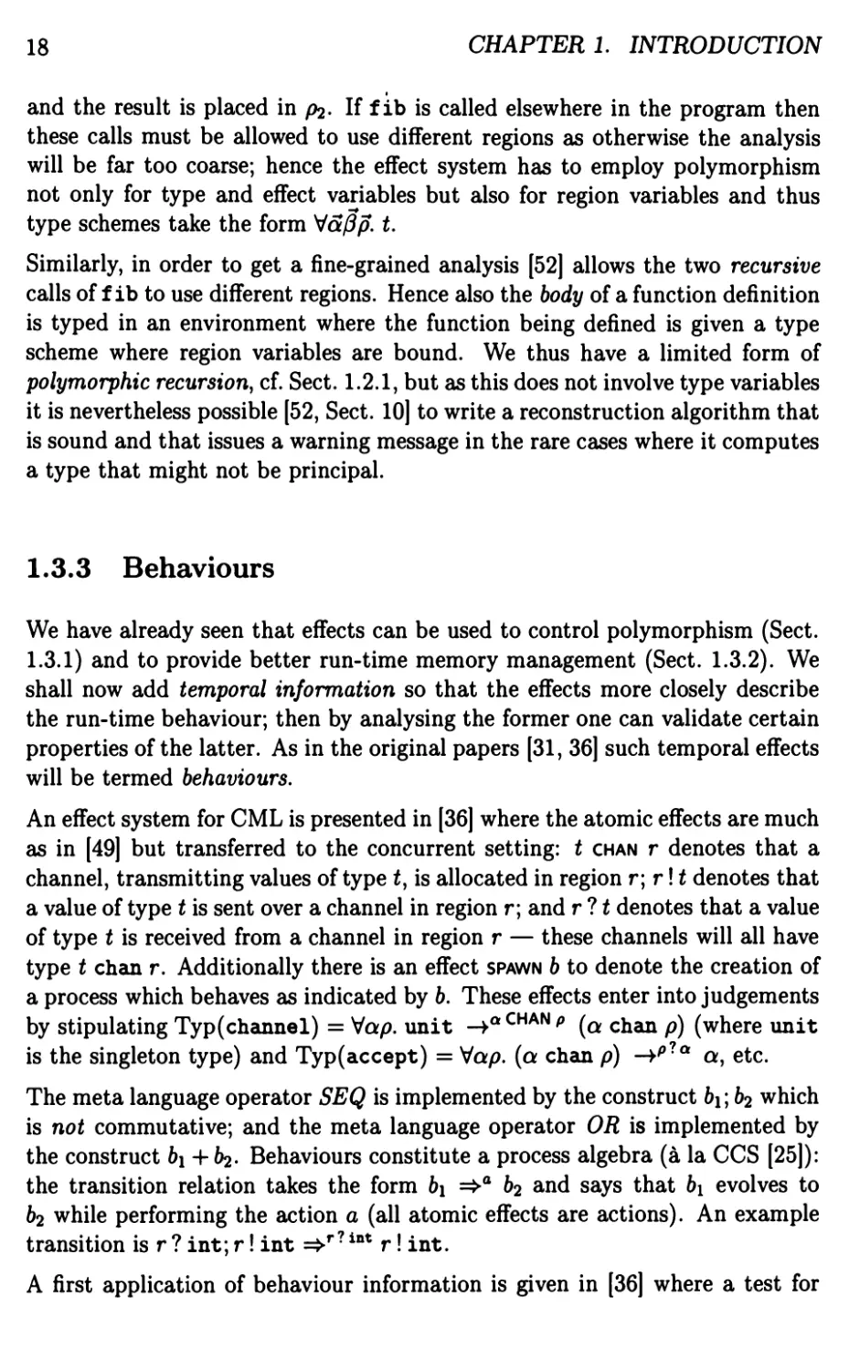
1.3.3 Behaviours
We have already seen that effects can be used to control polymorphism (Sect.
1.3.1) and to provide better run-time memory management (Sect. 1.3.2). We
shall now add temporal information so that the effects more closely describe
the run-time behaviour; then by analysing the former one can validate certain
properties of the latter. As in the original papers [31, 36] such temporal effects
will be termed behaviours.
An effect system for CML is presented in [36] where the atomic effects are much
as in [49] but transferred to the concurrent setting: t chan r denotes that a
channel, transmitting values of type t, is allocated in region r\r\t denotes that
a value of type t is sent over a channel in region r; and r ? t denotes that a value
of type t is received from a channel in region r — these channels will all have
type t chan r. Additionally there is an effect spawn b to denote the creation of
a process which behaves as indicated by b. These effects enter into judgements
by stipulating Typ(channel) = Vap. unit -4aCHANp (a chan p) (where unit
is the singleton type) and Typ(accept) = Vap. (a chan p) -V7** a, etc.
The meta language operator SEQ is implemented by the construct &i; 62 which
is not commutative; and the meta language operator OR is implemented by
the construct 61+62- Behaviours constitute a process algebra (a la CCS [25]):
the transition relation takes the form 61 =>a 62 and says that 61 evolves to
62 while performing the action a (all atomic effects are actions). An example
transition is r ? int; r! int =>r? int r! int.
A first application of behaviour information is given in [36] where a test for

1.3. AN INFERENCE SYSTEM FOR EFFECTS
19
finite communication topology is built on top of the effect system: given 6,
it computes upper bounds for the number of channels and processes that b
will create. As behaviours may be recursively defined, this is a non-trivial
task. The success of the analysis depends on the possibility of interpreting
behaviours as multisets of atomic effects; behaviours which are just sets (as in
e.g. [49]) would clearly not suffice.
To further illustrate how the temporal nature of behaviours may be used to
show (as done in [39]) the absence of certain bugs in concurrent systems,
consider the following safety criterion: a machine M must not be started until
the temperature has reached a certain level. This criterion may amount to
saying that a process P should never send a signal over a channel in region
start_M unless it has just received a signal over a channel in region temp.OK.
Now suppose we can show that P has some behaviour b: then it may be
immediately obvious that the above safety property holds, for instance if b is
defined recursively as b = • • •; temp_0K ? unit; start_M! unit; b.
In the system of [36] effects control the polymorphism: the rule for [gen] is as in
[53, 49]. Unlike [49] effects are not masked, as this might result in significant
loss of information and in particular invalidate the abovementioned test for
finite communication topology.
A new twist on semantic soundness
Below we shall briefly outline how to formulate semantic soundness in the
presence of temporal information (similar to what is done in [36]); we assume
a small-step semantics where the configurations are basically process pools PP
which map process identifiers into expressions.
To get a flavour of the subject reduction property, first consider the case where
PP evolves to PP' because process p allocates a fresh channel ch in region r
which is able to transmit values of type t'. If
A h PP(p) : tkb
holds then we must also have
A[ch : H chan r] h PP'(p) : tkV
where&=/CHANr&'.
Next consider the case where PP evolves to PP' because process p creates a
fresh process po, and suppose that

20
CHAPTER 1. INTRODUCTION
A h PP(p) : tkb
holds; then we must also have
A h PP'(p) : tkb' and A h PP'{p0) : unit&60
where&^SPAWN6o6'.
Thus the general picture is that Veil-typed programs communicate according
to their behaviour"; and that types are unchanged whereas the behaviours get
"smaller" and the environments are "extended".
1.3.4 Subeffecting
When designing an effect system for a language that already has a type system,
such as done in [36] for CML [42], one may reasonably expect the former to
be a conservative extension of the latter. To achieve this goal the inference
rules presented so far do not suffice as witnessed by the following example that
motivates the need for subeffecting.
Example 1.1 Suppose we want to type a conditional if eo then f\ else f2
occurring inside some function body e situated in the context
(fn/i^fn^^ejei e2
where t\ is of the form fn X\ =$>e\ and e2 is of the form fn x2 =>e2. Further
suppose that we have judgements
A[x\ : int] h e\ : int k &i and
A[x2 : int] h e2 : int & 62
with b\ / 62. We can thus assign t\ and hence f\ the type *i = int ->ftl int,
and we can assign e2 and hence /2 the type t2 = int ->62 int; but to use
the rule for conditional we must be able to assign f\ and /2 a common type
t = int -»612 int. D
One approach [53, 49, 36] is to find b\2 such that
A[x\ : int] h t\ : int & b\2 and
A[x2 : int] h e2 : int & b\2

1.3. AN INFERENCE SYSTEM FOR EFFECTS
21
(PI) b C 6 (P2)
6i C 62 62 C 63
61 C 63
. 61 C 62 63 C 64 61 C 62 63 C 64
( 6i;&3C&2;&4 61+63^62 + 64
61 C 62
(C3) -
SPAWN 61 C SPAWN 62
(SI) 61; (62; 63) = (61; 62); 63 (S2) (61; 63) + (62; 63) = (61 + 62); 63
(El) b = e\b (E2) &;<•=&
(Jl) 61 C 61+62, 62 C 61+62 (J2) 6 + 6 C 6
Figure 1.3: The pre-order C with equivalence =
for then e\ and e2, and hence also f\ and /2, can be assigned the type t =
int -+ftl2 int. The above judgements can be obtained provided that &i2
approximates b\ and 62, to be written 61 C 612 and 62 C 612, as we can then
apply the subeffecting rule
A\- e : tkb
Ah e : tkb'
if 6 C &'.
When effects are sets of atomic effects, as in [53, 49], the relation C is just
subset inclusion — hence OR (i.e. set union) is a least upper bound operator.
For behaviours as in [36] a more complex definition is needed. The aim is that
C should be a simulation in the sense that if 61 C 62 and 61 =>ai 6^ then also
62 =>°2 &2 for some a2 and 62, where 6^ C 62 and additionally a\ and a2 are
"suitably related". As shown in [37] the largest such simulation is undecidable,
but there exists a decidable relation C which is a simulation. This relation
can be syntactically defined as in Fig. 1.3; here 61 = 62 is a shorthand for
b\ C 62 and 62 C 61. We see that C is a pre-order (P1,P2) and a congruence
with respect to the various constructors (Cl,C2,C3); and that OR also in this
case is a least upper bound operator (J1,J2 using C2) — so in Example 1.1 we
can use &i2 = 61+ 62. As expected it holds (modulo =) that SEQ is associative
(Si) with e as neutral element (E1,E2).

22
CHAPTER 1. INTRODUCTION
1.4 An Inference Algorithm for Effects
In this section we discuss how to implement the type and effect systems
described in Sect. 1.3. Our starting point is algorithm W as defined in Fig. 1.2
and we shall see that W can be extended to infer not only types but also effects
(including those occurring within types).
Remark We shall use the name W for all algorithms that are "extensions"
of the algorithm W presented in [24], so as to emphasise their generic nature;
it should be clear from context which version we refer to and in Chap. 4 we
present the algorithm W of this book. Q
A first step is to modify the function U to operate on annotated types, and
this naturally raises the question of how to unify two effects. We can no longer
proceed by decomposition since this method is valid only for "free algebras".
To see this, consider the equation (on the effects of [49])
write(r, int) U write(r, int) = 0 U ft
Since 0 is the neutral element of U it is clearly possible to unify this equation,
even though the leftmost part of its "decomposition" is write(r, int) = 0 which
cannot be unified.
One may suggest to use results from unification theory, a survey of which is
given in [45], to solve equations such as
write(r, int) = ft U ft.
Unfortunately, for non-free algebras one cannot expect the existence of exactly
one most general unifier: in the example above, [ft »->• write(r, int), ft »->• 0]
and [ft !->• write (r, int), ft »->• 0] are both unifiers but there does not exist
a unifier having both as instances. Letting a call to U return a (potentially
infinite) tuple of unifiers does not seem attractive; instead we postpone the
unification of the effect equations. This motivates that W should accumulate
a set of effect constraints; in the following we therefore consider a version of
W returning a 4-tuple of the form (5, t, 6, C) where C is a constraint set.
1.4.1 Effect Constraints
The algorithm presented in [19], implementing what is basically the system of
[23], generates equational constraints of the form b\ = b2 where each k is a
union of effect constants and effect variables.

I A. AN INFERENCE ALGORITHM FOR EFFECTS 23
The system of [19] does not employ subeffecting and therefore many programs
are not typeable [48, p. 247]. The remedy [48] is to generate inclusion
constraints — in the future development we shall deal with this kind of constraints
only. The example in Sect. 1.3.4 suggests that to achieve the benefits of
subeffecting it is sufficient to use it immediately before applying the rule for function
abstraction; hence the key modification is to let the clause for function
abstraction generate a constraint expressing that the effect annotating the function
type approximates the effect of the body:
W(i4,f n x =* e0) =
let a be fresh
let (S0,t0,b0,Co) = W{A[x : a],e0)
let P be fresh
in (S0, So a -** *o,e,C0U{6o C /?})
An extra benefit of this modification is that the entities produced by the above
clause have a certain "simple" form in that they contain variables, rather than
more complex effects, at certain places: on the right hand side of the new
constraint, and in the top-level annotation of the type. In general we say that
a constraint set is simple if all its elements are of the form b C /?, and that
a type is simple if it does not contain effects that are not variables. When
writing the remaining clauses of W we shall maintain the invariant that all
types and constraints are simple — to do so we must additionally require that
also all substitutions are simple, that is they map type variables into simple
types and effect variables into effect variables, for then the application of a
simple substitution to a type or a constraint set will preserve the property of
being simple.
It is trivial to write a version of U that works on simple types and that returns
a simple substitution (or fails); a key clause is
W(*i V t2,t[ S t'2) =
let So = [/?' ^ p]
\etSl=U(S0tuS0t,l)
letS2 = W(SiSo*2,SiSo*'2)
in S2 Si So
With U properly defined, it is straightforward to modify most clauses of W to
deal with effects and constraints; for function application this results in
W(Aei e2) =

24
CHAPTER 1. INTRODUCTION
let(Si,til6ilCi) = W(illci)
let(52,^2,62,C2) = W(5M,e2)
let a and /? be fresh
let S = U(S2tut2 -V a)
let b = (SS2bx) SEQ (Sb2) SEQ (Sf3)
in (S S2SuSa,b,S S2CiU SC2)
The treatment of type schemes and polymorphism will be postponed until
Sect. 1.4.3 after we have addressed the issue of solving constraints.
1.4.2 Solving Effect Constraints
We say that a substitution 5 solves (or satisfies) C if Sb\ C Sb2 for all
(&i C b2) £ C. For simple constraints, finding a solution is particularly easy;
below we sketch the approach of [49] which is transferred to behaviours in [30].
The first step is to ensure that the same effect variable does not occur on more
than one right hand side. To obtain this goal we replace {(&i C /?), • • •, (bn C
/?)} (with n > 0) by (&i OR • • • ORbn C /?) and the validity of this
transformation follows from OR being a least upper bound operator (cf. Sect. 1.3.4).
The resulting constraint set C is then solved using the algorithm given below
(where the nondeterminism introduced in step 1 may be resolved e.g. by
imposing a linear order on effect variables). We use the symbol C to denote the
substitution that is returned.
1. if C is empty then return Id
else split C into C and (b C /?);
2. let recursively C be the result of solving C;, and let b' = C'ft;
3. if b' contains an effect with a type component where f3 is free
then abort
else let S0 = [/3t-+(pUb%
4. return S0 C7.
It turns out [49] that C is a principal solution to C in the sense that if S
also satisfies C then S = SC. Keep in mind, however, that in general C
is not a simple substitution and hence its only use within W is to control
polymorphism (as we shall see in Sect. 1.4.3) and effect masking.

1.4. AN INFERENCE ALGORITHM FOR EFFECTS
25
Remark To prove that C actually satisfies the constraints in C, first observe that
we can inductively assume that C" is satisfied by C and hence also by C = Sp C.
To show that C satisfies (b C 0) we perform the calculation (recall that b' = t?b)
Cb=[0^(0\Jb')]b' C 0Ub, = S00 = S0Ci0 = C0
where the inclusion follows since (due to 3) there exists b" with /3 £ FV(b") such
that either b' = b" or b' = /?U&", and where the second last equality is justified since
we can inductively assume that the domain of C is the set of right hand variables
of C and thus does not contain (3.
As can be seen from step 3, the system of [49] does not allow effects of "infinite
depth". The simplest known example of this phenomenon [49, p. 274] is where
the type tf of an input function / is forced (via a conditional) to match the
type of a function which (among other things) initialises a location to /. Hence
tf is given by int -*6/ int where bf contains the effect init(r, tf).
The system of [36] is able to cope with infinite depth as it has an explicit
construct REC/2.6 for recursion. This enables us to replace step 3 above by 3;
below, yielding an algorithm [30] that is able to solve an arbitrary set of simple
constraints. Unfortunately, due to the richer algebraic structure of behaviours,
we cannot expect the existence of a principal solution.
3' let S0 = [p i-> (RECp.b')]
Remark As above, the correctness of C boils down to the claim that Cb C C /?;
this now follows from the calculation (still with b' = C b)
Cb=[0^(REC0.b')}b' C REC0.b, = S0 0 = SpCi0 = C0
where the inclusion is a consequence of the axiomatisation of the construct REC/2.6.
1.4.3 Downwards Closure for Polymorphism
We shall next discuss how to reconstruct types and effects in the presence of
polymorphism. The first step is to allow constraints in type schemes which
thus take the form V(f : C). t where we use the letter 7 to range over a's and
/?'s and p's as appropriate. The clauses for constants and identifiers now read
W{A,c) =
\et(t1C) = INST(Ty?a(c))

26
CHAPTER 1. INTRODUCTION
in (Id,*,e,C)
W(A,x) =
let (t,C) = INST(A{x))
in (Id,*,e,C)
where the function Typa is as Typ except that it returns type schemes with
simple components: with effects as in [53] (cf. Sect. 1.3.1) we thus have e.g.
Typa(ref) = V(a/?: ({a} C /?)). a -V a ref.
Also the function INST is modified so that it returns not only a type but also
a constraint: it maps a type t into (t, 0); and it maps a type scheme V(7 : C). t
into (Rt,RC) where R = [7 *-¥ 71 ] with j[ fresh variables.
For a let-expression, we tentatively write the clause (with some holes to be
filled in later)
W(i4,let x = e\ in e2) =
let(Si,t1,61,C1) = W(>l,c1)
\etU = ---FV(tl)--
let DV = FV(Sl A) UFVih)
letNG=-DV-'
let 7 = U \ NG
let q = {(b C /?) € Ci I FV(6, /?) n {7} / 0}
let^! =V(^:C|). ii
let (52, t2,62, C2) = W((Si il)[x : t8X], e2)
in (S2 Sj, t2, (S261 5^(? 62), 52Ci U C2)
and make a sequence of remarks:
1. the set of bound variables 7 is taken from a universe U that must include
at least FV(ti) but typically also some subset of FV(C\)\
2. in the spirit of Sect. 1.3.1, we consider as dangerous (belonging to DV)
the variables free in the environment or in the effect;
3. the set of variables that cannot be generalised {NG) must clearly contain
DV but also some other variables may have to be included, as explained
below;
4. there is no point in letting ts\ contain constraints where no variables are
bound, since for such constraints INST will just make an identical copy;

14. AN INFERENCE ALGORITHM FOR EFFECTS
27
5. all constraints in C\ (rather than just C\ \C[) are returned by the clause,
in order to ensure that they are taken into account also if x does not occur
in e2-
To motivate a proper definition of NG, we again consider the program (1)
from Sect. 1.2.3 where the identifier r is defined as ref (fn x=>x) and thus
at run-time bound to a location holding values of type a -> a; recall that a
semantically sound inference system does not allow to generalise over a. It is
easy to verify that (for fresh type and effect variables) we have
W([],fnx=*x) = (Id,a ->*■ a,e,{e C &}) and
W([],ref) = (Id,a/ -V a'ref,£,{{a'} C /J1})
and hence the definition of r will be processed by W as follows:
W([],ref (fnx=*x)) =
([a; »-► (a -*A a), • • • ], (a -*"« a) ref, /?',
{eC/?ei{a,A} C /?'}).
We see that DV is the singleton set {/?'} and in particular does not contain a
which must be part of NG.
To understand what is going on, observe that for any solution S to the
constraint ({a, f3e) C /?') it will hold that S ff contains 5 a as a subpart. We can
therefore view a as a "sub-variable" of /?', so it seems right to demand that
if the latter is included in NG then also the former is included. One way of
formalising this intuition is to define NG as Z)VCl^, where in general the set
Xc^ — the downwards closure of X with respect to C — is the least set Y
that contains X and that has the property that if (b C /?) belongs to C and
0€Y then also FV{b) C Y.
Algorithms for effect reconstruction, able to deal with polymorphism, are
presented in [53, 49, 1]. Different as these approaches may be, in all cases the
way of computing (what corresponds to) NG essentially boils down to taking
the downwards closure of DV; an important insight is that with C as defined
in Sect. 1.4.2 we have that Xc^ = FV(C(X)). Moreover, in [53, 49] also the
universe is defined using downwards closure: U = FV(ti)ca.
The problem of lack of principality
When the effect constraints admit a principal solution (cf. Sect. 1.4.2), the
techniques outlined above are sufficient for the development of an algorithm

28
CHAPTER 1. INTRODUCTION
that is syntactically sound and complete [49]. When this is not the case, as for
behaviours, additional complications arise. To see this, consider an expression
e of the form
let / = co in (/ 0 ; /)
and assume that
W([],e0) = (---,int -V int,e,C)
where C "restrains" the value of /?. Since DV and hence also NG is empty,
we can wlog. assume that the body of e will be analysed in an environment
where / is bound to the type scheme V(7 : C). int -V int with f3 £ {7} =
FV(C); and for each occurrence of / a fresh copy of 7 will be created. We use
primed, respectively doubly primed, letters to denote entities created by the
first, respectively second, copy; it will then hold that
W([],e) = (•••,int -V" int,/?',CuC'UC"). (7)
Let S" and S" be arbitrary solutions to C. Then it is clearly possible to combine
them into a substitution S that solves (C U C U C") and where additionally
Sff = S'P and S/3" = S"/3 (stipulate S7' = S'7 and S7" = S"7 for each
7 £ {7}). If W is to be syntactically sound, we may therefore reasonably
expect from (7) that [] h e : int ->S0" int&S/?', that is
[]he: int -+s"^ intkS'P.
For this judgement to be derivable, S" (3 and S" f3 must both be instances of
a common behaviour (perhaps after applying a subeffecting step) and in the
absence of principality this will not always hold. The remedy of [1], which
improves on [30] in deriving a reconstruction algorithm for the type system
presented in [36], is to generate so-called "S-constraints"; in the example above
these constraints will record that the solution to C" as well as the solution
to C" must be an instance of the solution to C. The resulting algorithm is
syntactically sound and complete; unfortunately it is an open problem whether
there exists an algorithm for solving the generated S-constraints.
1.5 Shape Conformant Subtyping with Effects
It is actually possible to obtain a more precise analysis than the one provided
by the techniques from Sections 1.3 and 1.4. To justify this claim, we again

1,5. SHAPE CONFORMANT SUBTYPING WITH EFFECTS 29
consider Example 1.1 from Sect. 1.3.4. Without subeffecting this example
cannot be typed, but the price to pay for using only subeffecting is that then
all occurrences of f\ in e are indistinguishable from /2, and vice versa. This
might result in e being assigned a less precise type (or perhaps even inhibit
the typing of e), and is bad enough in itself if a "sticky" variant is used where
also the typings of subexpressions are of interest.
To increase the precision of the analysis we may use subtyping, cf. the
considerations in [50, Chap. 5]. This method allows f\ to be bound to t\ and f2 to be
bound to t2 when typing e; then *i and t2 are approximated to t immediately
before the rule for conditional is applied, using the subtyping rule
Ahe: t'kb
The subtype relation tx C t2 states that *i is a more precise type than t2 and
is naturally "induced" by the subeffecting relation via structural rules such as
t\ C h b C b' t2 C t'2
t\ -»6 t2 C t\ -»6' t'2
(note that C is contravariant in the argument position). For t\ C t2 to hold
it must thus be the case that these types are identical if their annotations are
removed; accordingly we shall use the term shape conformant subtyping for
this notion of subtyping.
In this section we shall extend the techniques from Sections 1.3 and 1.4 to
implement shape conformant subtyping rather than just subeffecting. It is
thus natural to see if we can reuse some of the ideas and techniques that were
originally developed for the purpose of adding subtyping to purely applicative
programming languages (not dealing with effects), as is done in [27, 9, 8] (only
briefly touching upon polymorphism) and in [47, 17] (treating polymorphism
in full generality). In Sections 1.5.1 and 1.5.2 we embark on outlining some of
the main insights of these papers.
1.5.1 Inference Systems for Atomic Subtyping
We shall restrict our attention to atomic subtyping, induced by a number of
inclusions between base types via structural rules (in particular saying that
*i -* t2 C t\ -> t'2 if and only if t\ C t\ and t2 C t'2). It is natural to specify
e.g. int C real; and a type system for object oriented languages must be able
to deal with inclusions such as K\ C K2 where K\ and K2 are class names.

30
CHAPTER 1. INTRODUCTION
A nice property of atomic subtyping is that if *i C t2 then *i "matches" t2 in
the sense that they have the same "tree structure", even though the leaves may
differ.
A main challenge is to formulate subtyping in a way that allows to state some
sort of principal typing property (cf. Sect. 1.2.2). A first naive attempt is to
conjecture that given typeable e there exists t such that [] h e : t' holds if
and only if S t C if for some S. To disprove this conjecture, assume that
int C real are the only base types and consider the twice function from
Sect. 1.2. It can be assigned the type tri = (real -> int) -> (real -> int)
which is in fact a minimal typing of twice: if *o is a type strictly less than t„ it is
not possible to derive [] h twice : t0l since *o will take the form (*i -> £2) -*
(real -> int) with t\ = int or t2 = real. Also ta = (int -> int) ->
(int -> int) and trr = (real -> real) -> (real -> real) are minimal
typings of twice. For a type t that is principal in the sense conjectured it
must thus be the case that tril ta, and trr are instances, but then clearly also
tir = (int -> real) -> (int -> real) will be an instance of t even though
fa/tce cannot be assigned the type tir.
The recipe for obtaining principality is to introduce type constraints of the form
t\ C t2\ in particular such constraints may occur in type schemes. Principal
typing of e now amounts to the existence of a type scheme ts such that t' is
a type of e if and only if t' is a "lazy instance" [8] of ts, where we say that a
type t' is a lazy instance of a type scheme V(a : C). t if there exists S with
Dom(S) C {a} such that S satisfies C and such that St C t'. We may expect
twice to have the principal type scheme
V(aa': {a' C a}), (a -» a') -» (a -» a'). (8)
Constraints in the inference system. To construct these extended type
schemes in the inference system, constraints must be present in judgements.
We shall write C, A h e : 2 to denote that the expression e (in environment
j4) has type t, provided that the type variables in t are related as indicated by
the constraints in C. Then the subtyping rule reads
C,A\- e : t
— if C h t C if
C,A\-e:t'
where the judgement C \- t\ C t2 formalises that *i C t2 is a consequence of
the assumptions in C. We write C h C to denote that C h *i C £2 for all

1.5. SHAPE CONFORMANT SUBTYPING WITH EFFECTS 31
(t\ Q t2) € C\ and we say that a type scheme V(a : Co). *o is solvable from C
by So if Dom{S0) C {5} and C h S0 C0.
It is trivial to incorporate constraints into the structural rules from Fig. 1.1;
and the rule for instantiation simply expresses that an instance substitution
must solve the constraints present in the type scheme:
C,A h e : V(a : C0). *0 if V(a : C0). *o is solvable from ,g*
C,A\-e:S0t0 C by S0 U
The rule for generalisation enables the construction of type schemes containing
constraints:
if{8}nFV(C,A) = Q
CuCq,A\- e : t0 an(j there exists So such that
C,i4 h e : V(a : C0). *o V(S : Co). *o is solvable from
CbySo
and we shall briefly explain the side conditions: first note that just as we
cannot allow to generalise over variables free in the environment, we cannot allow
to generalise over variables free in the "remaining" constraints — for
otherwise from {a C a'}, [] h fnx=>x : a -> ol we can derive {a C a;},[] h
fni=>i : V(aa;: 0). a -> ol which by the rule for instantiation yields the
unnatural {a C a;},[] h fni=>x : int -> bool. Next note that (as in
[47]) we only create type schemes that are solvable, so as to ensure that if
a let-expression let x = t\ in ti is typeable then t\ is typeable also in
the case where x does not occur in e2 (cf. remark 5 following the clause for
let-expressions outlined in Sect. 1.4.3).
That twice can be assigned the type scheme (8) is then a consequence of the
judgement
{a' C a},[] h twice : (a -* a') -* (a -» a;) (10)
which is a principal typing of twice in the sense that (i) the constraint set is
as weak as possible, and (ii) the type is as small as possible: if also C\ [] h
twice : t' then this judgement is a lazy instance [8] of (10) in that there exists
S such that (i) C h Sa' C Sa, and such that ft/ C; h (Sa -> Sa;) ->
(5a -* Sa') C f.

32
CHAPTER 1. INTRODUCTION
1.5.2 Algorithmic Techniques for Atomic Subtyping
To arrive at a reconstruction algorithm for subtyping one may, similar to what
is done in [8, 47], modify W from Fig. 1.2 so as to generate type constraints
at selected places, especially to record that the type of a function argument
must be a subtype of the argument type expected by the function:
W(^,e! e2) =
let(Sl,tl,Cl) = W(A,el)
\et(S2,t2,C2) = W(SlA1e2)
let a and a' be fresh
let S = U(S2tua' -» a)
letC = SS2CiUSC2U{S*2 Q Sa'}
in (SS2SuSa1C)
Unification is still used to ensure that the type of the operator is in fact a
function type; alternatively one could dispense with unification and instead
generate the constraint (S2t\ C t2 -> a).
Algorithm T. A type constraint relating large types is not very
informative, but we can repair on that since we have restricted ourselves to atomic
subtyping: it is possible to convert a set of type constraints into an equivalent
constraint set that is atomic, that is all constraints are of the form at\ C at2
where each ati is a base type or a type variable. A central technique is
decomposition: a constraint of the form (t\ -> t2 C t\ -> t'2) can be replaced by
the constraint set {t\ C t\,t2 C t'2}. On the other hand, if the constraint set
contains an element of the form (int C t\ -> t2) it is unsatisfiable (and may
thus be replaced by a special "fail" constraint). A consequence of this is that
for a constraint (a C tx -> t2) we know that a is forced to be a function type
and hence we can, without losing information, globally apply the substitution
[a \-¥ (ai -> a2)] with ai and a2 fresh — unless the occur-check fails, that is
a occurs in t\ or t2l in which case the constraint is unsatisfiable.
One can design an algorithm working along the lines sketched above; we shall
call it T as it does what [47] calls "forced instantiations" and it is similar in
spirit to algorithm MATCH in [9]. However, termination is not guaranteed
and in fact a naive implementation may loop (this is because some rules, like
the last one described above, introduce extra variables and additionally make
the constraints "larger"); to prevent this from happening one may adopt the
loop check mechanism, and the termination proof, from [9].

15. SHAPE CONFORMANT SUBTYPING WITH EFFECTS 33
An extensional view of T is that given C it first finds a matching
substitution, that is an S such that St\ matches St2 for all (*i C t2) € C, and then
decomposes the resulting constraints. Finding the most general matching
substitution bears certain similarities to unification and can actually be defined
in terms of unification. In [27, Sect. 8.2] one first computes the most general
unifier and then transforms it so it "maps into fresh variables". In [46, Fig. 3.7,
p. 92] it is first checked whether it is possible to unify a certain set of equations,
derived from the constraint set; if this is the case then the algorithm behaves
similar to the one presented above, except that the loop check mechanism is
no longer needed.
Algorithm 11. There is a large amount of freedom in determining when W
should call T\ one extreme is to do it after each subcall; another extreme
is to do it only after the whole program has been analysed. In any case
the resulting atomic constraint set may become rather unwieldy, as one will
quickly discover when implementing the algorithm. However, it turns out
that a substantial number of these constraints can be unified without losing
precision; this observation dates back to [8, 47]. Therefore W should be further
equipped with an algorithm 1Z, to be called at regular intervals, for doing
"constraint reduction".
The basic idea is that a variable can be (using the terminology of [47]) shrunk
into its "immediate predecessor" or it can be boosted into its "immediate
successor". To illustrate this, consider a constraint a\ C a2. Now suppose
that a2 does not occur on any other right hand side; then a2 can be shrunk,
i.e. replaced by a\ globally, provided a2 occurs "positively" in the type t
as is the case for t = a\ -> a2. (In this case one might alternatively
boost ai into a2, as ai occurs negatively.) This step is intuitively correct
as the type scheme "constructed from" the new type, V(c*i : 0). ai -> ai, has
the same lazy instances as the type scheme constructed from the old type,
V(a!a2 : {ai C a2}). ai -> a2 (namely all types t\ -> t2 with *i C t2).
The methods described in this section suffice for the derivation of
reconstruction algorithms W that are syntactically sound and complete [47, 8]. Syntactic
soundness simply states that if W(A,e) = (S,t,C) then C,SA h e : t. For
completeness, we may tentatively use the formulation (cf. the one given in
Sect. 1.2.2)
if C,A' h e : t' and A' = S" A
then (i) the call W(j4, e) succeeds
(ii)ifW(il,c) = (S,t,C)

34
CHAPTER 1. INTRODUCTION
there exists S" with C'hS'C
such that C h S't C *' and S'M = S'S4
the essential content of which is as in [8]. In the presence of polymorphism, as
in [47], a weaker premise is needed in order to conduct an inductive proof: we
only demand that A' is an instance of, rather than equals, S" A. (The reason
why the stronger premise cannot be preserved in the inductive proof is that
the rule for generalisation, used in the derivation of C, A' h e : t', allows to
generalise over a set of variables that may be smaller than the set constructed
by W.)
1.5.3 Integrating Shape Conformant Subtyping
The ideas from the preceding subsections can be combined with those from
Sections 1.3 and 1.4 to yield an effect system with polymorphism and shape
conformant subtyping. This is done (for a subset of CML) in [38, 2, 33] which
to the best of our knowledge is the first work integrating all these desirable
features.
Remark The algorithm reported in [50, Chap. 5] implements an effect
system with shape conformant subtyping, but without polymorphism. As the
effects are thus not used for controlling polymorphism, a two-stage approach
can be employed: first the Hindley-Milner types are reconstructed (e.g. using
the standard techniques from Fig. 1.2); next the effects are reconstructed, via
the generation of effect constraints. D
In Sect. 1.5.1 we saw that in the presence of atomic subtyping, a satisfactory
notion of principality is achieved by augmenting the inference system with type
constraints. This suggests that in the presence of subeffecting, a satisfactory
notion of principality — cf. the discussion in Sect. 1.4.3 — can be achieved by
augmenting the inference system with effect constraints. This also resolves the
discrepancy between having effect constraints in the reconstruction algorithm
(Sect. 1.4) but not in the inference system (Sect. 1.3).
The judgements in [38] are thus of the form C, A h e : t & 6, denoting that the
expression e has type t and effect 6, provided that the types (or type schemes)
of the free identifiers are given by A, and that the type and effect variables
are related as indicated by the type and effect constraints in C. To keep the
development as simple as possible, an effect is just a set of atomic effects of the
form t chan. This reflects that for effects to control polymorphism they must
record the creation, but not necessarily the use, of entities in the run-time

1,5. SHAPE CONFORMANT SUBTYPING WITH EFFECTS 35
environment (cf. Sect. 1.3.1).
We now address the crucial issue of providing suitable side conditions for the
rule for generalisation, which takes the form
C\JC0lA\- e : t0kb
C,A\-e: Vtf:C0).t0kb
Inspired by the theory of subtyping (Sect. 1.5.1) we demand that
tf}nFV(CyA) = 0 (12)
V(7 : Co). *o is solvable from C by some So- (13)
Inspired by the theory of effect systems (Sect. 1.3.1) we additionally demand
that
{j}DFV(b)=itl. (14)
To see the need for additional side conditions, consider the following example.
Example 1.2 Let the expression e be given by
let ch = channel () in spawn (fn d=> accept ch + 7) ; send (ch,true)
which is obviously not semantically sound. Nevertheless it might be typeable,
even from a satisfiable constraint set C; let
C = {{int chan} C /?, {bool chan} C /?} and C0 = {{a chan} C /?}
and observe that V(a : Co), a chan is solvable from C by either of the
substitutions [a !->• int] and [a *-¥ bool]. It is easy to see that by applying the
subeffecting rule one may get
CUC0,[] •" channel () : achan&/?
and if (12,13,14) are the only side conditions then the rule for generalisation
would give
C, [] h channel () : (V(a : C0). a chan)&/3
because a £ FV(C,/3). As the rule for instantiation (9) gives

36
CHAPTER 1. INTRODUCTION
C, [ch : V(a : Co), a chan] h ch : int chan&£ and
C, [ch : V(a : Co), a chan] h ch : bool chan & £
it is clearly possible to derive C, [ ] h e : 2 & 6 for suitable t and 6. D
The example is quite similar to the one given in Sect. 1.4.3 which motivated
the notion of downwards closure. Thus it seems natural to demand that also
in the inference system it holds that the set of variables not being generalised
is downwards closed; this observation was first made in [38]. To formalise
this notion, first define an "arrow relation" C h V <- 7 which will hold if
there is a type or effect constraint in C with 7' on the left hand side and
with 7 on the right hand side. Then we add the side condition to (11) that if
Co I" 7; <- 7 then 7 ^ {7} implies 7' ^ {7}. An equivalent formulation [38]
is that V(7 : Co). *o is "upwards closed" in the sense that if Co I- 7' <- 7 then
7; £ {7} implies 7 £ {7}. This is clearly not the case for the type scheme in
Example 1.2 (where Co I- a <- /?).
With the rule for generalisation properly defined, it is possible to demonstrate
semantic soundness [2]. A reconstruction algorithm is presented in [33]; it
is syntactically sound whereas the issue of completeness is still open. The
algorithm generates type constraints as well as effect constraints, combining
methods from the preceding sections in a relatively straightforward way. In
particular, it is possible to adapt the algorithm T from Sect. 1.5.2, since shape
conformant subtyping enjoys all the nice properties of atomic subtyping.
Moreover, the lack of inclusions between base types allows T to unify constraints
like (int C a); accordingly an atomic constraint is redefined as being one of
the form {cl\ C a2).
1.6 Overview of the Development
1.6.1 The Main Ideas
In the remaining chapters of this book we shall develop a semantically sound
effect system, together with a syntactically sound and complete
reconstruction algorithm, that encompasses polymorphism as well as shape conformant
subtyping. The source language is a fragment of CML; but the techniques are
immediately transferable to SML (by recording imperative effects rather than
concurrent effects). Our approach improves on [38, 2, 33] in that

1.6. OVERVIEW OF THE DEVELOPMENT 37
1. temporal information is added to the effects, which are therefore termed
behaviours;
2. behaviours are equipped with regions;
3. the reconstruction algorithm is not only syntactically sound but also
complete (with respect to so-called "atomic inferences").
The features 1 and 2 tremendously enhance the applicability of the
information produced by the system; the virtue of 3 is that then the reconstruction
algorithm does not reject valid programs.
Redefining downwards closure. Prom a technical point of view, it is
relatively straightforward to incorporate 1 and 2. To achieve 3 was a more
challenging task and involved a somewhat different notion of downwards
closure: the arrow relation from [38] (cf. Sect. 1.5.3) is redefined so that basically
only effect constraints are taken into account. In other words, we admit type
schemes of the form V(a : {a C a'}), t but not type schemes of the form
V(a : {a chan r C /?}). t. This reflects the following key insight: in the former
case all instances of a must be shape conformant subtypes of S a', where S is
the "global" substitution subsequently produced by W and applied to all free
variables, and hence they cannot have different shapes (like int and bool).
In the latter case, however, no such tight bounds on instances of a are
imposed by the behaviour constraint (which might be satisfied by mapping f3
into bool chan r + int chan r).
Types are simple. We have already argued (Sect. 1.4.1) that a
reconstruction algorithm should maintain the invariant that all types are simple. For
reasons of uniformity, and to facilitate certain correctness proofs, we shall also
demand that the inference system disallows types that are not simple. In fact
we define the syntax of types such that all types are inherently simple, by
stipulating that a function type is of the form t\ -V t2> and similarly for other
type constructs. We are thus no longer able to write e.g. int -y!lnt int
but need to "encode" it as the type int -»* int together with the constraint
plint C /?.
As types must be closed under substitution, we also demand that all
substitutions are inherently simple. We cannot in general expect behaviour constraints
to be satisfiable by such substitutions and hence we shall not attempt to solve
behaviour constraints; instead our goal will be to rewrite them into constraints
that are "more readable" but equivalent (in a sense to be defined).

38
CHAPTER 1. INTRODUCTION
Similar ideas occur elsewhere in the literature. In [53] a "direct" as well as
an "indirect" inference system is presented; the latter deals with simple types
only as it is geared towards the design of a reconstruction algorithm. In [52]
function types are annotated with pairs of the form e.<j> with c an effect variable
and with <j> an effect; one can think of this as an annotation with e together
with the constraint (</> C c).
Effect masking omitted. Another important design issue is whether the
system should employ effect masking as described in Sect. 1.3.2. In the
presence of effect masking, the behaviour returned by the algorithm will not "tell
the whole story" of the run-time behaviour, and we will for instance not be able
to conduct the test for finite communication topology mentioned in Sect. 1.3.3.
Therefore we have chosen to omit this feature.
Alternatively, so as to eat the cake and still have it, one might conceivably
carry around two kinds of effects: one that tells the whole story, and one that
is used to control polymorphism — then the latter can be subject to effect
masking.
1.6.2 A Prototype Implementation
The algorithm to be developed in this book has been used as the basis of a
prototype implementation, available for experimentation on the address:
http://www.daimi.au.dk/~bra8130/TBAcml/TBA_CML.html
A description of the system, illustrated by several examples, can be found in
[3] which also gives a brief account of the underlying theory (to be developed in
the rest of this book). It turns out [39] that the system is useful for validating
a number of safety properties for "realistic" concurrent systems; a worked-out
example is given in Chap. 7. We shall not attempt to estimate the complexity
of the algorithm nor of the implementation.
The system is written in Moscow ML [57] which is a variant of SML. This
language is convenient as it supports modular programming via separate
compilation, and as it contains support1 for a web interface: from Moscow ML code
one can create cgi scripts and there are functions for reading the contents of
html-forms.
1 ©Jonas Baxklund, Computing Science Dept., Uppsala University, 1996.

16. OVERVIEW OF THE DEVELOPMENT 39
1.6.3 Benchmarks
The abovementioned prototype assists us in comparing our approach to related
approaches; here the "measure" is the set of programs accepted and we shall
use the benchmarks given in [49, Sect. 11] and [21, Fig. 3]. To illustrate how
to perform the comparison, consider the SML program
let fun id y = y in
let fun make.ref x = ref x in , .
id make_ref
end end
which is typeable by the system in [21] but not by [60], as the top-level
expression id make.ref is assigned the type a*0 -> a*0 ref and as mentioned
in Sect. 1.2.3 one cannot generalise over imperative variables having weakness
degree 0. On the other hand, our prototype accepts the program
let fun id y = y in
let fun make.ref x =
let val ch = channel ()
in (send (ch,x);ch)
end in
let val id.ref = id make.ref in
id.ref 7; id.ref true
end end end
which is intended to be a faithful translation of (15): instead of allocating
a location, initialised to the value of x, make.ref now allocates a channel
and initially transmits the value of x over this channel. The calls id.ref 7
and id.ref true are appended to check that the system is indeed able to
generalise over the type variable occurring in the type of id.ref.
Concerning the classification in [21, Fig. 3], it turns out — if the benchmark
using exceptions is not taken into account — that all benchmarks accepted
by [60] are also accepted by our system, and that all benchmarks accepted
by our system are also accepted by the system of [21]. The benchmarks id
make.ref (mentioned above) and applicative.map make.ref are accepted
by our system but not by [60]; and the benchmark imperative.map id [] is
accepted by the system of [21] but not by our system.

40
CHAPTER 1. INTRODUCTION
Concerning the classification in [49, Sect. 11], it turns out that our system
accepts exactly the same benchmarks as does the system of [19] and the system
of [53]; this set is incomparable to the set of benchmarks accepted by [60], and
it is a proper subset of the benchmarks accepted by the system of [49].
The incorporation of effect masking into our system would significantly increase
its performance with respect to the above benchmarks, enabling e.g. the typing
of (idl idl) from [49, Sect. 11). Keep in mind, however, that our focus has
mainly been on providing detailed yet readable information about run-time
behaviour for "realistic" programs, as illustrated by the case study in Chap. 7.
1.6.4 A Reader's Guide to the Book
Chapter 2. We introduce our source language, which is a variant of CML,
and the language of behaviours. In Fig. 2.8 we present our effect system; much
emphasis is put on explaining and motivating the rule for generalisation which
depends on a carefully defined arrow relation. We show that the system is a
conservative extension of Hindley-Milner typing.
Chapter 3. Here the topic is the semantics of the source language. A small-
step semantics is defined, using evaluation contexts, in two stages: first we
consider the sequential aspects, and next we consider also the concurrent
aspects and here the configurations of the semantics are process pools.
We demonstrate that the inference system from Chap. 2 in semantically sound;
the proof of Lemma 3.25 is particularly interesting as it highlights how the
judicious choice of generalisation strategy allows type-safe extension of the
runtime environment. The soundness result (Theorem 3.29) is similar in spirit to
the one sketched in Sect. 1.3.3, stating that "well-typed programs communicate
according to their behaviour".
Chapter 4. A reconstruction algorithm W is presented; as can be seen from
Fig. 4.2 there is a clause for each syntactic construct in the source language. To
keep the constraint set manageable, W is equipped with auxiliary algorithms
T and 7£; the basic principles of these algorithms were sketched in Sect. 1.5.2
and in Sections 4.2 and 4.3 they will be explained in detail.
Using appropriate soundness results for T and H, we establish that W is
syntactically sound wrt. the inference system from Chap. 2.

1.6. OVERVIEW OF THE DEVELOPMENT
41
Chapter 5. We devote ourselves to the difficult task of proving, using
appropriate completeness results for T and 7£, that algorithm W from Chap. 4
is syntactically complete wrt. the inference system from Chap. 2. The
formulation of this property, as given in Theorem 5.1 (for closed expressions) and in
Theorem 5.12 (for arbitrary expressions), involves a suitable definition of "lazy
instance" and is similar in spirit to the one given in Sect. 1.5.2; it basically says
that if C", A' h e : t'kb', via an inference that fulfils certain criteria, then
the judgement will be a lazy instance of what is produced by W. In Sect. 5.1.1
we shall argue that the restrictions imposed by the side conditions are not too
severe.
Chapter 6. The algorithm W will produce a behaviour b and a set of
constraints C; the latter set may be quite large (in spite of the size reduction
performed by It). In this chapter we pave the way towards our prototype
implementation, by mentioning a selection of the techniques used by the system
for post-processing (6,C) so as to produce a "more readable" (6^,C^). We
show that the techniques are correct, in that (6^,C^) "bisimulates" (6, C). As
the semantic soundness result from Chap. 3 in essence says that (6, C)
simulates the source program, also (6^,C^) will simulate the source program —
this is made precise in Sect. 6.6, using the subject reduction property stated
as Theorem 6.13.
Chapter 7. In this concluding chapter we demonstrate that our prototype
facilitates the validation of certain safety conditions for reactive programs. As
in [39] this is done by means of a worked example, based on a case study used
as a benchmark in the literature [22].
Appendices. Some of the more tedious proofs are relegated from main text
and placed in the Appendices A-E. Appendix F provides a survey of the
symbols and naming conventions used throughout this book.

Chapter 2
The Type and Effect System
2.1 The Source Language
For illustrating our approach we have chosen a variant of CML [42, 40]. As
in Sect. 1.2, expressions e include identifiers, function abstractions, function
applications (to be evaluated using call-by-value), let-expressions, recursive
function definitions, and conditionals. We also include a selection of constants
for manipulating data structures.
Constants. There are two classes of constants: constructors for building
data structures, and base functions for inspecting and decomposing data
structures. A constant c is thus given by the syntax
c::=bf | cs° \ csl \ cs2 | • • •
where csn is the syntactic class of n-ary constructors (n > 0), and where bf
is the syntactic class of base functions (all unary). We further distinguish
between sequential and concurrent constants:
bf ::= bf8\bfc
csn ::= C58n | C5cn
The sequential constructors will at least include the unique element of the
unit type, the two booleans, numbers, pair for constructing pairs, and nil
and cons for constructing lists:
43

44
CHAPTER 2. THE TYPE AND EFFECT SYSTEM
e ::= x | fn x => e 11\ e2 | let x = ei in e2
| rec / x => e | if e then ei else e2
| 6/<e>| C5n<ei,---,en>
Figure 2.1: Expressions e € £tp
c^° ::= () | true | false | n | nil
css ::= pair | cons
The sequential base functions will at least include a selection of arithmetic
operators, fst and snd for decomposing a pair, and hd, tl and null for
decomposing and inspecting a list:
bfs ::= +1-1*1/1 = 1-
| f st | snd | hd | tl | null
The unique flavour of CML is due to the concurrent constants which we shall
introduce and motivate in Sect. 2.1.1.
Expressions. An expression (e € Exp) is given by the syntax in Fig. 2.1;
we use mostly x but also y and / to range over identifiers. A program is
an expression without free identifiers. The important thing to note is that
all constructors and base functions must be "fully applied"; this facilitates
the technical development in Chap. 3 and is no serious restriction as "partial
applications" can easily be encoded: instead of writing say cons 3 one writes
fn x=>cons<3,x>.
For readability, we shall allow to write cs° for cs° < >, to write (ei,e2) for
pair < ei,e2 >, to write [ ] for nil, and to write [ci,---,cn] for cons <
Ci, C e2, • • •, en ] >. Additionally we shall write e\ ; e2 for snd < (ci, e2) >; to
motivate this notice that since the language is call-by-value, evaluation of the
latter expression will give rise to evaluation of e\ followed by evaluation of e2,
the value of which will be the final result.
Extended expressions. For the purpose of writing a type inference system
and subsequently a type reconstruction algorithm, it is convenient that
constants are viewed as expressions and this is not the case in Fig. 2.1. To repair
on that, we introduce the syntactic class Exp@ of extended expressions where
constants are first-class objects; the term "extended" is justified since there

2.1. THE SOURCE LANGUAGE
45
e ::= c | x | fn x=>e \ ex e2 | e0@n < Ci, • • • ,en >
| let x = ei in e2 | rec / x => e | if e then ei else e2
Figure 2.2: Expressions e € ifcpo
X(x)
I(f n x => e)
X(e\ e2)
I(let x = e\ in e2)
I(rec / x => e)
X(if e then ei else e2)
I(V.<e>)
I(6/e<c>)
I(C5°<>)
I(c5n<e1,---,en>)
Figur
=
=
=
=
=
=
=
=
=
=
e2.2
X
fnx=*I(e)
I(ci) I(c2)
let x = X(ei) in X(e2)
rec / x => J(e)
if J(e) then X(ei) else X(e2)
6/.©! <J(e)>
VcIW
C5°
csn@n < I(ci), • • • ,I(en) > for n > 1
J: Translating from Exp to ^xpQ
is a natural injection J from Exp into £xp@. In fact, we shall often identify
e € £?xp with J(e) € £xpQ and use the letter e to range also over extended
expressions; our intentions will usually be clear from context.
One might have expected that for instance it holds that J(cons <ei,e2 >) =
cons X(ei) X(e2) but this kind of translation loses the information that cons
operates "silently", that is without visible (audible!) effect. To retain this
information, extended expressions include a special kind of "silent function
application" that takes the form eo @n < Ci, • • •, en > with n > 1; an extended
expression is thus given by the syntax in Fig. 2.2.
The translation I is tabulated in Fig. 2.3; it captures the intuition that
application of a constructor and the application of a sequential base function takes
place silently, whereas the application of a concurrent base function may have
an effect that should be recorded.
2.1.1 Concurrent Programming
CML [42] extends SML with primitives for synchronous communication
between concurrent processes; this includes the following:
• spawn creates a new process e when applied to the expression f n x => e

46 CHAPTER 2. THE TYPE AND EFFECT SYSTEM
and this process will then run concurrently with the other processes;
• channel allocates a new communication channel when applied to 0;
• send sends a value over a channel as soon as some other process is ready
to receive, and blocks until this is the case;
• accept receives a value from a channel as soon as some other process is
ready to send, and blocks until this is the case.
Consider now the scenario when a process wants to send data to two other
processes in a "first come first served" manner. This can be expressed by the
pseudo-code (in the style of [14])
if ready chl -> send (chl,datal); send (ch2,data2)
[] ready ch2 -» send (ch2,data2); send (chl,datal)
fi
We shall see that this can in fact be expressed in CML, using the notion of
events: one can think of an event as a communication possibility. Events
are "first class values", which means that they can be passed around just like
integers.
To create events, CML offers the primitive transmit that is a "non-committing"
version of send; in a similar way the primitive receive is a non-committing
version of accept. The CML primitive sync synchronises an event, i.e. turns
it into an actual communication. We thus have the equations send x =
sync (transmit x) and accept x = sync (receive x).
The CML primitive select is as sync except that it takes a list of events
and synchronises one of these; the choice is deferred until it can be ensured
that the selected communication will not block. The primitive choose is a
non-committing version of select.
An attempt to achieve part of the desired protocol is then to write
select [transmit (chl,datal),transmit (ch2,data2)]
but we must ensure that if select synchronises the first event then the
continuation will be to evaluate send (ch2,data2), and similarly if select chooses
the second event. We thus need a way of "inlining" a "continuation" into an
event, such that the event applies the continuation if synchronised. This is
taken care of by the CML primitive wrap; using this primitive the desired
protocol can be achieved by writing

2.1. THE SOURCE LANGUAGE
47
select [wrap( transmit (chl,datal),
fn d => send (ch2,data2)),
wrap( transmit (ch2,data2),
fn d => send (chl,datal))]
Our selection of concurrent constants. A number of concurrent
constants were introduced above, but not all of these will be present in our
development. We can easily dispense with send, accept, and select, as we have
seen that they are expressible in terms of other constants. We shall also omit
choose and wrap, thus reducing the expressive power; we do this to prevent
the semantic framework of Chap. 3 from being overly complicated, but see [37]
for a subject reduction result for a language that contains these features.
We thus settle upon the concurrent constructors and base functions given by
CS* ::= transmit | receive
bfc ::= sync | channel' | spawn
Note that each occurrence of channel is assigned a label I in order to keep
track of the "syntactic origin" of each channel allocated at run-time; we shall
elaborate on this in Sect. 2.2.1.
Example 2.1 Consider the program map2 that is defined below. It is a
version of the well-known map function (for mapping a function across a list)
except that a process is spawned for each tail while the spawning process itself
works on the head.
rec map2 f =>
f n xs =>
if null(xs) then []
else let ch = channel1 ()
in spawn (fn d =>
(sync (transmit (ch, map2 f (tl xs)))));
cons (f (hd xs))
(sync (receive ch))
That is, when applied to some function / and for example a three-element
list [v\, v2, V3], the initial process po will wait for a new process p\ to compute
[/ ^2, / vz] and send it over a new channel ch\, and in the meantime p0
computes / v\ so it can finally return [/ v\,f v2,f V3]. Similarly, p\ will do its job

48
CHAPTER 2. THE TYPE AND EFFECT SYSTEM
by waiting for a new process P2 to communicate the value of [/ v3] over a new
channel c/i2 and in the meantime p\ computes / v2; etc.
Suppose that / is a function which when applied to an argument of type ct\
performs the concurrent actions indicated by f3\ and at the end returns a value
of type a2. Then map2 applied to / will be a function which when applied to
a list will perform the following concurrent actions, to be denoted fo either
it performs no communication (if the list is empty) or it will first allocate in
region {1} a channel that transmits values of type a2 list; then it spawns a
process that first behaves like fa (to work "recursively" on the tail of the list)
and then outputs to region {1} a value of type a2 list; then it performs f3\
(when computing / on the head of the list); and finally it receives from region
{1} a value of type a2 list. O
In Sect. 2.6 we shall see how our inference system enables us to express the
information sketched above in a compact way by means of behaviours.
2.2 Basic Notions
In this section we prepare for the type inference system presented in Sect. 2.4,
in that we clarify the syntax and pragmatics of the various entities occurring
there. Most features have been motivated already in Chap. 1.
2.2.1 Regions
The notion of regions was introduced in Sect. 1.3.2 where we mentioned that
one can think of a region as a set of communication channels. Our intention
is that region information should enable us to distinguish between channels
allocated by different syntactic occurrences of channel, whereas we do not
aim at distinguishing between channels allocated by different invocations of
the same syntactic occurrence — see e.g. [5] for a methodology to achieve this
level of detail.
In other words, a region explicitly denotes a set of program points
corresponding to occurrences of channel, and implicitly denotes the set of channels
created from these points. We shall therefore think of a region as a set of channel
labels (recall from Sect. 2.1.1 that the constant for channel allocation is written
channel' with / a label); but this is only indirectly reflected in the syntax of a
region r that is given by

2.2. BASIC NOTIONS
49
r ::= p\{l)
with p ranging over region variables. The drawback of this minimalistic
approach is that one cannot directly represent a non-singleton set of channel
labels such as {2,7}; instead this set can be represented as a variable p
together with the region constraints {{2} C p, {7} C p}. In general, a region
constraint takes the form (r C p) (note that the right hand side must be
a variable); and in Sect. 6.1 we shall see how to solve such constraints, thus
removing this "level of indirection".
2.2.2 Behaviours
The notion of behaviours was introduced in Sect. 1.3.3 and we basically use
the same constructs: the syntax of behaviours b is given by
b ::= /?M6i;&2|61+62
| SPAWN b | t CHAN p | pit | pit | T
that is in addition to behaviour variables (/? ranges over such) we have the silent
behaviour e (no 'Visible" actions take place); a sequential composition b\\b2
(first &i is performed and then b2)\ a nondeterministic choice b\ + b2 (either b\
or 62 are performed); spawn b (a process with behaviour b is created); t chan p
(a channel able to transmit values of type t is allocated in region p); pit (a
value of type t is sent over a channel in region p); pit (a value of type t is
received over a channel in region p). For later use (Chap. 6) we also introduce
the behaviour r (denoting a communication over a "hidden" channel).
In contrast to [36], cf. Sect. 1.4.2, there is no explicit construct for recursion;
instead recursive behaviours are represented by "cyclic dependencies" in the
behaviour constraints (as we shall see in Sect. 2.6). In general, a behaviour
constraint takes the form (b C /?) and since the right hand side is a variable
it is "simple" in the sense of Sect. 1.4.1. We do not explicitly solve such
constraints (unlike what was the case for region constraints) but in Sect. 6.2
we shall present some techniques for simplifying behaviour constraints; we
may regard the resulting constraints as a representation of the "solution" to
the original constraints, cf. the methodological considerations in [45, p. 236].
2.2.3 Types
We shall augment the CML type structure [42, Sect. 7] with behaviour and
region components at certain places. Recall from Sect. 1.6.1 that a major

50
CHAPTER 2. THE TYPE AND EFFECT SYSTEM
design principle of our approach is to ensure that types are inherently "simple";
this amounts (cf. Sect. 1.4.1) to requiring that these components are variables
(and their actual "values" can be read from the constraints, cf. the remarks in
preceding subsections). Accordingly, the syntax of types t is given by:
t ::= a | unit | bool | int
I ti x t2 \t list | t chan p \ t event /?
In addition to type variables (ranged over by a) we have a selection of base
types and composite types. Base types include the the one-valued unit type,
the two-valued boolean type, and the integer type. Composite types include
the product type and the list type, where *i x t2 is the type of a pair whose first
component has type *i and whose second component has type t2, and where
t list is the type of a list where all components have type t\ the remaining
composite types are discussed below.
The function type *i ->^ t2 is the type of a function that when applied to
a value of type *i has the property that (i) it behaves as indicated by the
behaviour /?; and (ii) if it terminates then the resulting value will be of type
t2. If the function in question is a constructor or a sequential base function
we know that it operates in silence, cf. the remarks to Fig. 2.3; there is thus
no need to write down the annotation as it will "denote" the silent behaviour
e and instead we use a special "silent function type" *i -> t2.
The event type t event /? is the type of a communication possibility (cf.
Sect. 2.1.1) with the property that if it is synchronised then (i) it behaves as
indicated by /?, and (ii) it returns a value of type t. Finally, the channel type
t chan p is the type of a channel that (i) is allocated in region p, and (ii)
allows values of type t to be transmitted.
Concerning type constraints, their general form is (*i C t2) but the atomic
type constraints are of special interest (as we shall see in Chap. 4): they take
the form (ax C a2), cf. Sect. 1.5.3.
2.2.4 Constraints
A constraint set C is a finite set of type constraints, behaviour constraints,
and region constraints (as defined in the previous subsections). The set of
type constraints in C is written Cl\ the set of behaviour constraints in C is
written C6; and the set of region constraints in C is written Cr. We say that
a constraint set C is atomic if Cl is atomic (as defined above).

2.2. BASIC NOTIONS
51
2.2.5 Miscellaneous
Substitutions. A substitution is a mapping from type variables into types
and from behaviour variables into behaviour variables and from region
variables into region variables such that the domain is finite. Here the domain
of a substitution S is Dom(S) = {7 | 57 / 7} and the range is Ran(S) =
(J {FV(S7) I 7 £ Dom(S)}, where we use the letter 7 to range over a's and
/?'s and p's as appropriate and similarly we use g to range over Vs and 6's and
r's as appropriate. We mainly use the letter S to range over substitutions but
sometimes we shall also use the letter R, typically to emphasise that R is a
"special kind" of substitution (for example a "renaming").
We have defined substitutions such that they are inherently "simple" (as
defined in Sect. 1.4.1); accordingly it is easy to see that a substitution gives rise
to a well-defined mapping on types, behaviours, regions, and constraints (but
not necessarily preserving atomicity). The entity resulting from applying
substitution S to an entity g is denoted S g. The identity substitution is denoted
Id and we write S2 S\ for the substitution that first applies S\ and next 52, so
($2 Si) (7) = S2 (S\ 7). We write S+ [7 i-> g] for the substitution that maps 7
to g and that otherwise behaves as S.
Type schemes. A type scheme ts is given by
ts ::= Vtf:C).t
where 7 is a list of bound type and behaviour and region variables, C is a
constraint set, and t is a type; the set of free variables FV(ts) is given by
FV(t, C) \ {7} and a closed type scheme is one with FV(ts) = 0. We do not
distinguish between type schemes that are equivalent up to alpha-renaming
(i.e. renaming of bound variables). The result of applying a substitution S to
a type scheme V(-y : C). t is V(-y : SC). St, provided that Dom{S) U Ran(S)
is disjoint from {7} (which can be ensured by suitable alpha-renaming).
There is a natural injection from types into type schemes, taking the type t
into the type scheme V(() : 0). t. We shall distinguish rather sharply between
these two entities, even though Observation 2.14 suggests that (for the purpose
of the inference system) they may be identified. We use the letter a to range
over types t and type schemes ts as appropriate.
Environments. An environment A is a list [xi : a\, • • • ,xn : an] of typing
assumptions for identifiers; we write Dom(A) for {xi,--,xn} and we write

52
CHAPTER 2. THE TYPE AND EFFECT SYSTEM
ChrCp if(rCp)eC
ChrCr
C h ri C r2 Chr2Cr3
C h n C r3
Ch(t chan p) C (*' chan p')
ChpC//
Figure 2.4: The ordering on regions
A[x : a] for the list concatenation of A and [x : a]. An environment gives rise
to a mapping from identifiers into types or type schemes, in that we let A(x)
denote the rightmost entry for x in A.
2.3 Shape Conformant Subtyping
Our inference system employs shape conformant subtyping, as introduced in
Sect. 1.5; to formalise this notion we employ three kinds of judgements: the
relations C h r\ C r2 and C h &i C 62 and C \- t\ C t2 are defined by the
rules and axioms of Figs. 2.4-2.6 which are mutually recursive. In all cases we
write = for the equivalence induced by the orderings, that is C h g\ = g2 is a
shorthand for C h g\ C g2 and C \- g2 C gY. We shall also write C" h C to
mean that C \- g\ C. g2 for all (g\ C £2) in C.
We shall often need to "decompose" type constraints into type and behaviour
and region constraints; and therefore — unlike what is standard in the
literature — we employ explicit rules [bw] for "running the structural subtyping
rules backwards". (On the other hand it would not make sense to run the
structural behaviour rules backwards, since e.g. p?int;£ C £;p?int is valid
but p?int C e is not, cf. the initial remarks in Sect. 1.4.) If a judgement
C I- g\ C g2 is derivable from the rules in Figs. 2.4-2.6 without using the
rules labelled [bw], we shall write C \-fW g\ C g2 and say that the judgement
has a forward derivation.
[axiom]
[refl]
[trans]
IM

2.3. SHAPE CONFORMANT SUBTYPING
53
2.3.1 The Ordering on Behaviours
The relation C h bx C 62, defined by the rules in Fig. 2.5 which are much
as in Fig. 1.3, has the intended meaning (to be formalised in Sect. 2.7.1) that
given the assumptions in C, &i is a more precise approximation than 62 in the
sense that any sequence of actions performed by b\ can also be performed by
As is to be expected, the ordering is a congruence [cong] and + is a least upper
bound operator [ub],[lub]; and (modulo =) sequential composition is associative
[assoc] with e as neutral element [neut]. Compared to Fig. 1.3 we have omitted
the rule for left-distributivity as it is not essential for our purposes; using [cong],
[lub] and [ub] one can still establish C h (61; 63) + (62^3) Q (&i + &2);&3 but
not the converse relation.
Observe that we have no rules for relating say pit to pit' even if t = t'\ this
is due to technical reasons (in particular the desire that Lemma 2.10 should
hold).
2.3.2 The Ordering on Types
The relation C h t\ C t2, defined by the rules in Fig. 2.6, has the intended
meaning that given the assumptions in C, t\ is a more precise approximation
than 22- It is induced by the subeffecting relation via structural rules, one for
each type constructor; in particular, we do not have any ordering on base types
(such as int C real).
The structural rules are mainly as to be expected, in particular note the con-
travariance of the argument position in a (silent as well as non-silent) function
type. To motivate the rule [chan] for channel types, we assume that t' is a
"larger" type than t and reason as follows: if a channel permits one to send
values of type t' then it also permits one to send values of type t (just "convert"
them into values of type t' before sending); and if one receives values of type
t from a channel then in effect one also receives values of type t'. The former
observation suggests that t' chan C t chan; and the latter observation
suggests that t chan C t' chan. Thus the polarity of tin t chan p is both positive
(when used in receive) and negative (when used in transmit); on the other
hand the polarity of the region component p is only positive (if a channel is
contained in a region r then it is also contained in a region than encompasses
r). The proof of Lemma 3.28, used to establish semantic soundness, nicely
reflects the intuition presented above.

54
CHAPTER 2. THE TYPE AND EFFECT SYSTEM
[axiom] ChKjJ if (6 C 0) e C
[refl] C \- b C 6
C h 6i C 62 C h 62 C 63
[trans]
[cong]
C \- h Cb3
C h 6t C fr; C hli, C |/2
C 1-6,;62 C 6i;62
C h fri C 6j C h 62 C %
c 1- 61 + 62 c &; + i/2
c h 6 c y
C I- SPAWN 6 C SPAWN 6'
[assoc] C h 61; (62; 63) = (61; 62); t>3
[neut] Che;6 = 6 Ch6;e = 6
[ub] C I- 6, C 61 + 62 CI-62C61 + 62
.... C I- 61 C 6 C h 62 C &
[lub]
M
C 1- 61 + 62
C\- (t,
C 1- (*«
-^«a)
Ch)3
svent /?)
C 6
c (f,
C/3'
c(f
->"'
<'2)
event /?')
Figure 2.5: The ordering on behaviours
2.4 The Type Inference System
In Fig. 2.8 we present a type inference system with judgements of the form
C,A h e : akb
where C is a constraint set, A is an environment, e is an expression in Exp&1
a is a type or a type scheme, and 6 is a behaviour. This means that e has type

2.4. THE TYPE INFERENCE SYSTEM
55
[axiom] C h h C t2 if ft Ct2)eC
[refl] C \- t Ct
C \- h Ct2 C \- t2 C t3
[trans]
[list]
[chan]
C h U C t3
C \- t\ Cti C \- t2 Q t'2
C h ft -» *2) C ft -» fa)
CKjCti C\- t2Ct'2 C h /? C ff
C h ft -W *2) Q ft -V ^)
C \- h ct\ C \- t2 c t'2
c i- ft x *j) c ft x t'2)
C \- t Ct'
C \- (t list) C ft list)
C \- t = f C\- pC //
C \- (t chan p) C ft chan /J*)
Chtcf Ch/JC^
event
1 j Ch(< event /?) C ft' event ff)
[bw]
C K (^ -»* t2) c ft; ->* t'2) C h fa -» t2) c ft; -» f2)
c k (tt -»* t2) c ft; -V t'2) c h fa -»ta) c ft; -» f2)
C h t2 c t'2 Cht2c *'2
Chfex t2) C ft; x t'2) C h (^ x t2) C ft; x t2)
C \- tY ct\ C \- t2 c t'2
C h ft event /?) C ft' event /?') C h ft list) C ft; list)
C h t C t' C h K t'
C h ft chan p) C ft' chan p') C h ft chan p) C ft; chan pi)
C h t c f C h t' c <
Figure 2.6: The ordering on types

56
CHAPTER 2. THE TYPE AND EFFECT SYSTEM
or type scheme a, and that its evaluation will result in a behaviour described
by 6, assuming that free identifiers have types as specified by A and that all
variables are related as described by C.
The rule [con] employs a function Typc that is tabulated in Fig. 2.7 which
we shall motivate briefly. First notice that all function types are silent except
those occurring in concurrent base functions, cf. the remarks to Fig. 2.3. For
the sequential constants the constraint set is empty and the type is as in SML.
Turning to the concurrent constants, the type of sync interacts closely with
the types of transmit and receive: if ch is a channel of type t chan p,
the expression receive @i < ch > is going to have type t event f3 with
pit C /?, and the expression sync (receive@\ < ch >) is going to have
type t\ similarly for transmit. The type of channel* records the type of the
created channel as well as its syntactic origin / in the annotation of the function
type; finally the type of spawn records the behaviour of the spawned process.
(As discussed previously one might add wrap to the language; this constant
transforms communication possibilities of type t event /? into communication
possibilities of type t' event /?'.)
The overall structure of the type inference system of Fig. 2.8 is as in [38] which
was sketched in Sect. 1.5.3, and is thus close to those of [47, 17] with a few
components from [49, 36] thrown in. The novel ideas of our approach only
show up as carefully constructed side conditions for some of the rules.
The structural rules follow the pattern outlined in Sect. 1.3: as the language
is call-by-value, no actions take place when an identifier is retrieved from the
environment. As usual, the rule for function abstraction places the behaviour
of the body of a function abstraction on the arrow of the function type; but
in our setting this behaviour must be a variable — to achieve this one may
use subeffecting: if the body has behaviour b then /? can be placed on the
arrow, provided b C (3 can be deduced from C. One might suggest that if the
body has behaviour e then the function abstraction could be assigned a silent
function type; but to avoid ambiguity in representation we shall refrain from
doing so.
The rule(s) for function application is as one may expect for a call-by-value
language: first the function is evaluated, then its argument is evaluated, and
finally the function is applied. In case of a silent function application the
function type must be silent; this will be the case (as can be seen from Fig. 2.3
and Fig. 2.7) if the overall expression takes the form J(e) with e € Exp.
The rule for let is straightforward given that both the polymorphic
definition and the body needs to be evaluated. The rule for recursion makes use
of function abstraction to concisely represent the "fixed point requirement" of

2.4. THE TYPE INFERENCE SYSTEM
57
_£ Typc(c)
() unit
true,false bool
1,0,1,2-•• int
+, -,*, / int x int -> int
= int x int -> bool
pair V(aia2 : 0). oc\ -> a2 -> ai x a2
f st V(aia2 : 0). c*i x a2 -> ai
snd V(aia2 : 0). ai x a2 -> a2
nil V(a : 0). a list
cons V(a : 0). a -> a list -> a list
hd V(a : 0). a list -» a
tl V(a : 0). a list -> a list
null V(a : 0). a list -> bool
transmit V(a/?p : {p!a C /?}). (a chan p) x a -» (a event /?)
receive V(a/?p : {p?a C /?}). (a chan p) -» (a event fi)
sync V(a/? : 0). (a event ft) -*" a
channel' V(a/?p : {a chan pCft {/} C p}). unit -*" (a chan p)
spawn V(a/?/?0 : {spawn #> C /?}). (unit -**> a) -*" unit
Figure 2.7: The types of constants
typing recursive functions; note that we do not admit polymorphic recursion
(cf. Sect. 1.2.1) as this function abstraction is evaluated in an environment
where / is bound to a type rather than to a type scheme. The rule for
conditional is unable to keep track of which branch is chosen, therefore an upper
approximation of the branches is taken.
We have three non-structural rules: the rule [sub] caters for subtyping and
subeffecting as described in Sect. 2.3; the rule [gen] for generalisation employs
some complex side conditions that will be the topic of Sect. 2.5; and the rule
[ins] for instantiation uses the notion of solvability, introduced in Sect. 1.5.1:

58
CHAPTER 2. THE TYPE AND EFFECT SYSTEM
[con] C,Ah c : Typc(c)&£
[id] C,A h x : A{x)ke
C,A[x:tj\ h e : fafe/?
[abs]
[app]
[sapp]
[let]
[rec]
[if]
C,4 h fni=>e : (fa -V fa)&e
C,A h ei : (fa -»* fa)&6i C,4 h e2 : fafefr;
C,ith eie2 : fa&((6i;6a);/?)
C,4 h e0 : (fa -» ---fa -» fa)&6o'"C,i4 h e< : frfetj---
C, A h e0 @n < ci, • • •, en > : fa & (&o; &i; • • S bn)
C,A h e\ : tfsi & 61 C, j4[x : tfsi] h e2 : fa & ^
C, j4 h let x = ei in e2 : fa & (61; 62)
C,A[f:t] h fnx=^e : *fe6
C, j4 h rec / x => e : 2 & 6
C,4 h e0 : boolfeftp C,4 h ei : *fe&i C,4 h e2 : *fe62
C, A h if e0 then ei else e2 : * & (60; (&i + M)
[sub] C,i4h e : *&6 ifCh *C*'andCh 6C6'
C,A \- e :
C,A\- e\
C,A\-
Cl)C0,
: f &y
: V(7:C0).to&&
e : So to Sib
A \- e : to&cb
[ins] ' ^ — ^ ^ if V(7 : Co), fa is solvable from
C by So
[gen] ^,Q,.rC;t0o .f v(;? : Cq) ^ .s bQth we„_
C,i4 h c : V(7 : C0). fa&6 formed, solvable from C, and
{j}nFV{C1A1b)=H
Figure 2.8: The type inference system
a type scheme V(7 : Co), fa is solvable from C by the substitution S0 if
Dom(So) Q {7} and if C h SbCo; a type scheme 2s is solvable from C if
there exists a substitution 5 such that 2s is solvable from C by 5; and as
V(() : 0). t is trivially solvable from C, we stipulate that a type t is solvable
from C. An environment A is solvable from C if for all x in Dom(A) it holds
that A(x) is solvable from C. Finally, we say that Typc is solvable from C if

2.5. THE RULE FOR GENERALISATION
59
for all constants c it holds that Typc(c) is solvable from C; notice that Typc
is not solvable from 0 but it is easy to find C" such that Typc is solvable from
C'\ one could for instance let C" contain copies of the constraints mentioned
in Fig. 2.7, that is C" = {(/! a' C /?',-• •}.
Observation 2.2 As is to be expected, the premise of the rule [ins] can be
alpha-renamed without altering the conclusion: if V(7 : Co). *o and V(7; :
Cf0). t'0 are alpha-equivalent, and if the former type scheme is solvable from C
by some substitution So, then there exists S'Q such that the latter type scheme
is solvable from C by S'0 and such that So *o = S'Q t'Q.
Observation 2.3 Suppose that
C,A\- ex : tikbi andC,4 h e2 : fc&fc;
since C, A h pair : tx -> t2 -> ^i x t2 & e we clearly have
C,A h (ci,c2) : ^i x t2k.bi\\>2.
By similar reasoning we may arrive at other "derived rules", e.g.
C,A h et : ^i&6i C,>1 h e2 : ^2&&2
C,i4 h t\ ; e2 : t2 & 6i; 62
2.5 The Rule for Generalisation
We now take a close look at rule [gen] in Fig. 2.8. Already in Sect. 1.5.3
we motivated some of its side conditions, namely that V(7 : Co). *o must be
solvable from C and that {7} D FV(C,A,b) = 0; and we also argued that
these conditions alone are not sufficient for semantic soundness: one should
also ensure that the set of variables not being generalised is "downwards closed"
with respect to some "arrow relation". This last property is a key ingredient
in the definition of a well-formed type scheme, to be given in Sect. 2.5.3; the
arrow relation is defined in Sect. 2.5.2 and relies on the notion of backwards
closure that is defined in Sect. 2.5.1.

60
CHAPTER 2. THE TYPE AND EFFECT SYSTEM
2.5.1 Backwards Closure
As in Sect. 1.5.3 we shall in Sect. 2.5.2 introduce a judgement C h V <- 7;
the intended use of this judgement is to prevent the generalisation of V in the
case where 7 cannot be generalised. We demand — motivated by Sect. 1.4.3
— that if C contains a behaviour constraint (b C 0) then C h 7 <- 0 must
hold for all 7 £ FV(b), whereas one may argue — as done in Sect. 1.6.1 —
that a type constraint (a' C a) should not influence the arrow relation. We
cannot just disregard the type constraints, however, since these may implicitly
contain behaviour constraints: consider e.g. the type constraints {ct\ ->^1
ai C a, a C a2 ->^2 a2} from which (0\ C 02) is derivable.
For a given constraint set C we therefore wish to construct a constraint set
that explicitly contains all behaviour constraints "implicitly present" in C.
Below we define such a set; it is the least set containing C that is closed
under decomposition of type constraints and under transitive closure of the
type constraints.
Definition 2.4 The backwards closure of C, to be written C, is defined as
C = {(9x C g2)\C\-dc 9l C g2}
where h^ denotes a derivation that uses only the rules [axiom] and [bw] in
Figs. 2.4-2.6, and the rule [trans] in Fig. 2.6. □
We have to check that C is indeed a well-defined constraint set; to this end
first note that \i_C h^K i/ then b' will be a variable and similarly if C h^
r C r'. That C is finite follows from the observation that if (g\ C g2) £ C?
then g\ as well as g2 will be a syntactic subpart of C (this also implies that
FV(C) = FV(C)). Additionally, one should note that t=CiUCbUCr1 and
that C h g\ C g2 is derivable if and only if C h g\ C g2 is.
We say that a constraint set C is backwards closed if C = C and might
expect that for such constraint sets forward derivations are sufficient, that is
if C r- g\ C g2 holds then also C hfw g\ C g2, but to establish this result
we need an extra assumption. To see this, consider the backwards closed
constraint set
C = {a C a', int event 0 C a list, a' list C int event 0'}.
Since we have Cha list C a' list, transitivity on type constraints yields
C h int event 0 C int event 0', so by [bw] we get C h 0 C 0'\ but it is
clearly impossible to derive C hfw 0 C 0'.

2.5. THE RULE FOR GENERALISATION
61
The problem of the above constraint set C is that it is not consistent, according
to the following definition:
Definition 2.5 Let *i and t2 be types that are not variables; then we say that
there is a mismatch between t\ and t2 if their top-level type constructors are
different.
We say that a constraint set C is consistent if for all *i and t2 such that
C \~ t\ C t2 is derivable there is not a mismatch between *i and t2. D
The notion of consistency is what is needed in order to dispense with the
explicit decomposition rules:
Lemma 2.6 Consider the inference rules in Figs. 2.4-2.6, where we assume
that C is consistent and backwards closed. Then for all rules labelled [bw]
the following holds: if the premise has a forward derivation, then also the
conclusion has a forward derivation.
Proof See Appendix A.l. D
Proposition 2.7 Assume that C is consistent and that C h g\ C g2. Then
Proof Clearly C is consistent and backwards closed, so we can use Lemma 2.6
to establish the claim by induction in the inference C h g\ C g2. □
2.5.2 The Arrow Relation
After this short digression into forward derivations, we embark on defining the
arrow relation:
Definition 2.8 The judgement C h 7 «- 0 holds iff there exists (6 C f}) in
V such that 7 € FV(b).
Following conventional notation, we write C h 7 <-* 7' for the reflexive and
transitive closure of <-. a
Note that if C is atomic (cf. Sect. 2.2.4) then the above condition (b C 0) € C
is equivalent to (6 C 0) € C.
Remark In Chap. 1 we repeatedly make the point (e.g. in Sect. 1.3.1) that
for effects to control polymorphism they must record the creation, but not

62
CHAPTER 2. THE TYPE AND EFFECT SYSTEM
necessarily the use, of run-time entities. To reflect this intuition one might
alternatively stipulate that C h 7 <- /? holds iff there exists (b C /?) in C
such that 7 £ topchan(6), where topchan(6) are those variables which occur in
a part of b not inside some pit or p?t.
We conjecture that the future development will carry through using this revised
definition, with some modifications that are mostly obvious but may add to
the complexity of the exhibition. As it is not clear whether the power of the
type system will really be increased, we shall refrain from such an attempt. D
Definition 2.9 For a set X of variables the downwards closure Xc^ and the
upwards closure Xc^ is given by:
Xc± = {71 I 3-fc € X : C h 71 *-* 7*}
Xc* = {7i|372eX:Ch72+-*7l} D
It is instructive to think of C h 71 <- 72 as defining a directed graph
structure upon FV(C); then XCi is the reachability closure of X and Xct is the
reachability closure in the graph where all edges are reversed.
We now state a crucial result, used to establish the cases for [gen] in the
proofs of Lemma 3.25, essential for semantic soundness, and Theorem 5.12,
demonstrating the completeness of our reconstruction algorithm.
Lemma 2.10 Assume that C h b C b' with C consistent.
Then for all 7 € FV(b) there exists 7' € FV(V) such that C h 7 <-* y.
(That is, FV(b)Ci C FV(V)Ci.)
Proof By Proposition 2.7 we have C hfw b C &'; we perform induction in
this forward derivation. All cases are straightforward and we only list a few:
The case [axiom]. Suppose that C h/w b C /? because (b C /?) e C. Let
7 £ FV(b) be given: then the desired relation C h 7 <- /? holds by the
definition of <-.
The case [trans]. Suppose that C h/w 61 C 63 because C h/w 61 C 62 and
C •"/« &2 Q &3- Let 7! € irV(6i) be given: by applying the induction
hypothesis we find 72 £ FV(b2) such that C h 71 <-* 72, and by applying the
induction hypothesis once more we find 73 £ FV(b$) such that C h 72 f-* 73
— this establishes the desired relation C h 71 f-* 73.
The case [lub]. Suppose that C hfw b\ -f 62 Q b because C h/w 61 C 6 and
^ •"/«; f>2 C 6. Let 70 £ FV(&i + 62) be given: wlog. we can assume that

2.5. THE RULE FOR GENERALISATION
63
70 € FV(b\), so by applying the induction hypothesis we find 7 £ FV(b) such
that C h 70 «-* 7 and this establishes the desired relation. □
Remark As an important special case of Lemma 2.10, note that when C h
b C (J (by an arbitrary derivation) then C h 7 «-* /? for all 7 € FK(6).
This shows that for consistent C, a more liberal definition of h^ (permitting
a larger set of rules) would not affect the computation of downwards and
upwards closure. □
2.5.3 Well-formed Type Schemes
We are now ready to define the notion of well-formedness, used in the side
condition for the rule [gen] in Fig. 2.8.
Definition 2.11 A type scheme V(7 : C). t is well-formed if the following
conditions hold:
1. {7} is upwards closed wrt. C, i.e. {7} = {7}Ct;
2. all (gi C g2) in C contain at least one variable among {7};
3. the set of behaviour variables in FV{Cl) is disjoint from {7}.
A type t is trivially well-formed.
An environment A is well-formed if A(x) is for all x in Dom(A). □
Note that if C = 0 then V(7 : C). t is well-formed (this is the reason for
stipulating types to be well-formed). Requirement 2 reflects that there is no point in
having constraints where all variables are free (cf. remark 4 from Sect. 1.4.3).
Requirement 3 is needed in order for the following essential closedness
property:
Pact 2.12 If V(7 :C).t is well-formed then also S (V(f :C).t) is well-formed
(for all substitutions S).
Proof We can, without loss of generality, assume that (Dom(S) U Ran(S)) D
{7} = 0. Then S (V(7 : C).t)= V(7 :SC).St As Requirements 2 and 3 are
clearly fulfilled it suffices to show that {7} = {7>5Ct, i.e. that if 7 € {7} and
SC h 7 <-/? then^G {7}.

64
CHAPTER 2. THE TYPE AND EFFECT SYSTEM
The situation thus is that there exists b with 7 £ FV(b) such that (b C ft e
~SC\ that is either (6 C ft € JC1 or (b C 0) e SCb. But the former is
impossible: to see this, observe that all behaviour constraints in SCl are of
the form (ft C ft), where (by Requirement 3) {ft, ft} n {7} = 0.
So it must be the case that (b C ft e SCb; that is there exists b' with Sb' = b
and ft with 5ft = /? such that (&' C ft) e Cb. As Jton(S) n {7} = 0 we infer
that 7 € irV(6/), implying that C h 7 <- ft. From Requirement 1 we have
ft € {7}, so as Dom(S) D {7} = 0 we have 0 = 5ft = ft € {7} as desired. □
As was the case for Lemma 2.10, also the following lemma is needed to establish
the cases for [gen] in the proofs of Lemma 3.25, essential for semantic
soundness, and Theorem 5.12, demonstrating the completeness of our reconstruction
algorithm.
Lemma 2.13 Suppose the type scheme ts = V(7 : Co). *o is well-formed, and
that C is a constraint set with with {7} D FV(C) = 0. Then {<?}CuCot = {7}.
Proof Let C U C0 h 7 «- ft with 7 € {7}; our task is to show that 0 € {7}.
There exists b with 7 € FV(b) such that (6 C 0) € CuC0l leaving us with
three cases:
(b C ft € C6. This is impossible as {7} n FVr(C) = 0.
(6 C ft € Cp6. Then C0 h 7 <- i9 so as {7} = {7>Cot (since ts is well-formed)
we infer 0 £ {7} as desired.
(b C 0) £Cl\J C0l. Then b must be a behaviour variable so b = 7. As te is
well-formed 7 £ FV(Co') an(* by assumption 7 £ FV(C'); showing that also
this case is impossible. E
2.6 Pragmatics
We have completed the formal definition of the type inference system; yet the
reader may still wonder what a "typical" derivation looks like. To get a flavour
of the characteristic features of the system, we shall explain in some detail how
to type the program given in Example 2.1; in Chap. 4 we present an algorithm
that is able to find such typings automatically.
We thus consider the program map2 given by

2.6. PRAGMATICS
65
rec map2 f =>
fn xs =>
if null(xs) then []
else let ch = channel1 ()
in spawn (fn d =>
(sync (transmit (ch, map2 f (tl xs)))));
cons (f (hd xs))
(sync (receive ch))
and we shall see that by letting C contain the constraints
{1} £ p
e C ft
e + ft;ftsft;ft C ft
(a2 list) chan p C ft
SPAWN (3f C ftp
p!(a2list) C ft
p?(a2list) C ft
and with t = (ax -V1 a2) -**■ (c*i list -V2 a2 list) it holds that
C,[] h map2 : *&e. (1)
The behaviour constraints can be post-processed, using the techniques
described in Chap. 6, and as a result we end up with a single behaviour constraint
e + ((a2 list) chan p; spawn (ft;p!(a2 list));ft;p?(a2 list))
C ft
which shows that we can give ft the following "recursive interpretation" that
formalises the explanation in Example 2.1:
e
+ (a2 list) chan {1}; spawn (ft; {1} ! (a2 list)); ft; {1} ? (a2 list)
We are left with the task of proving (1). Let A0 be an environment where map2
is bound to t; then it will suffice to show
CyA0 h fnf =^fnxs=^--- : tke.

66
CHAPTER 2. THE TYPE AND EFFECT SYSTEM
Let A\ be an extension of A0 where f is bound to ai ->^1 a2; then it will
suffice to show
C, Ax h f n xs =^ • • • : ai list -V2 a2 list & ft.
Let ^2 be an extension of A\ where xs is bound to ai list; then it will suffice
to show (as C h e C ft) that
C, A2 h if null(xs) then • • • else • • • : a2 list & ft
and as C, A2 h null(xs) : bool&£ and C, ;42 I- [ ] : a2 list&£ it will
suffice to show
C,i42 K letch = ••• : a2 list &ft;ftsft;ft.
Observe that C, ;42 h channel1 : unit -Vc (a2 list) chanp&e and hence
C,i42 h channel1 0 : (a2 list) chanp&ft which by a trivial application
of [gen] yields C,A2 h channel1 () : V(() : 0). (a2 list) chan p&ft; with
i43 an extension of A2 where ch is bound to V(() : 0). (a2 list) chan p it will
thus suffice to show
C, Az h spawn • • • ; cons • • • : a2 list & ftr; ft; ft
which (cf. Observation 2.3) can be done by demonstrating
C,AZ h spawn ••• : unit&ftr (2)
C,AZ h cons ••• : a2list&ft;ft. (3)
To establish (2), it will suffice to show that
(since C,A$ h spawn : (unit ->^ a2 list) ->0F unit&e)
C,AZ h fnd=*-- : unit -V' a2list&6:
and with ;44 an extension of A$ where d is bound to unit it will suffice to show
C, j44 h sync (transmit • • •) : a2list&ft.
Observe that C, AA h sync : (a2 list) event ft -V* a2 list&e so it will
suffice to show (as C h ft; ft; ft C ft) that

2.7. BASIC RESULTS
67
CyA4 h transmit (ch, •••) : (a2 list) event /?,&&; (h-
Since the type ((a2 list) chan p) x a2 list -> (a2 list) event (58 can be
assigned to transmit (employing that C h p! (a2 list) C /?,), it will suffice
to show
C, Aj h (ch,map2 • • •) : ((a2 list) chan p) x a2 list &/?«;&
and (cf. Observation 2.3) this follows from
C,A4 h map2 f (tl xs) : a2 list&/?c;/?2
which is a consequence of the assumptions in Aj.
To establish (3) it will suffice to show
C,i43 h f (hdxs) : a2k/3l and
C, ;43 h sync (receive ch) : a2 list&^r.
The former is an easy consequence of the assumptions in j43; and the latter
follows since C,j43 h receive : (a2 list) chan p -> (a2 list) event f3T ke
and hence
C,j43 h receive ch : (a2 list) event fake.
2.7 Basic Results
In this section we list a few properties of the inference system to be used later;
we also introduce the notions of "trace inclusion" (Sect. 2.7.1) and "normalised
inference trees" (Sect. 2.7.2).
Observation 2.14 C,A\- e : tkb holds iff C,A h e : V(() : 0). tk b holds,
as [gen] or [ins] can be used to conclude one from the other. □
Among other things, the next fact states that constructors actually construct
something (that is, a composite non-functional type).
Pact 2.15 For all constants c the type (scheme) Typc(c) is closed, well-formed,
and satisfies that

68
CHAPTER 2. THE TYPE AND EFFECT SYSTEM
• if c is a sequential base function, then (the type part of) Typc(c) takes
the form t\ -> t'\
• if c is a constructor csn, then (the type part of) Typc(c) takes the form
A ~* '" t'n ""* *' w^tn *' not a variable and not a (silent or non-silent)
function type. D
Fact 2.16 If C,A h e : <r&6then
• if A is well-formed then a is well-formed;
• if A and Typc are solvable from C then a is solvable from C.
Proof A straightforward case analysis on the last rule applied. □
The next two lemmas, to be used heavily in the sequel (and often tacitly),
employ the notion of the shape of an inference tree: this is the result of replacing
all judgements with the (name of the) axiom or inference rule used to derive
them (and dispensing with side conditions).
Lemma 2.17 For all substitutions S:
(a) If C h Co then SC h 5Co (and has the same shape).
(b) If C,A h e : abb then SC,SA h e : SakSb (and has the same
shape).
Proof See Appendix A.2. □
Lemma 2.18 For all sets C of constraints satisfying C h C:
(a) IfC h Co then C h C0.
(b) If C, j4 h e : akb then C;, j4 h e : cr&6 (and has the same shape).
Proof See Appendix A.2. O
Fact 2.19 Let x and y be distinct: if C,^[x : a\][y : ^^ h e : cr&6
then C, A\[y : a2][x : ai]i42 K e : a&6 (and has the same shape).
Proof A straightforward induction in the inference tree.
D

2.7. BASIC RESULTS
69
Fact 2.20 Let x be an identifier not occurring in e and let t be an arbitrary
type; if C, A h e : akb then C, A[x : t] h e : a & 6 (and has the same
shape).
proof Let a be a fresh type variable. Then a straightforward induction in
the inference tree (using Fact 2.19) tells us that C,A[x : a] h e : akb (and
has the same shape). Now apply Lemma 2.17 with the substitution [a4<]. D
Next some results showing that the arrow relation is in some sense closed under
substitution and entailment:
Lemma 2.21 Suppose C h 7 <- /?. Let S be a substitution; then for all
i € FV(S-y) it holds that SC h Y <- 5/?.
Proof There exists 6 with 7 € FV(6) such that (6 C /?) e C; i.e. there is
a derivation C h^ (6 C /?). By Lemma 2.17 we infer that there also is a
derivation SC h^ (56 C S/?), implying that (Sb C Sp) e ~SC. For all
V € FK(57) we also have 7' € FK(56) and therefore SC h V f- 5)3 holds
as desired. Q
Lemma 2.22 Suppose C h 71 f-* 72. Let 5 be a substitution; then for all
7i ^ FV(57i) there exists 72 € ^^(572) such that SC h -y[ <-• 72.
Proof Induction in the length of the sequence C h 71 <-* 72; if the length
is zero then 7! = 72 and the claim is trivial. So assume that there exists
/? such that C h 7! <- /? and C h /? <-* 72 (by a shorter derivation).
Given 7; € FV(57i) we by Lemma 2.21 infer that SC h 7J f- 5/?; and
the induction hypothesis tells us that there exists 72 € ^(572) such that
SC h 5y3 f-* 72. This yields the claim. □
Lemma 2.23 Suppose C h 7 <- /? and that C \- C with C; consistent; then
C h 7 <-• /?.
Proof There exists 6 with 7 € FV(6) such that (b C f3) £ C\ thus it holds
that C h 6 C /3. The claim now follows from Lemma 2.10. □
Corollary 2.24 Suppose C h 7 «-* ^ and that C \- C with C" consistent;
then C; h 7 f-* 0.

70
CHAPTER 2. THE TYPE AND EFFECT SYSTEM
C/b>trii{bCfi)zC Ch/?>[/?]
C \- p > tr
C h bi > tr C h 62 > tr
C h 61 + 62 > tr C h bi+b2> tr
C h bi > tri C h 62 > tr2
C h 61; 62 > tri °tr2
C h b> tr
C h e >[] C h r > [r]
Ch t CHAN p > [t CHAN p]
C h spawn 6 > [spawn tr]
C h p\t> [pit] C h p?t > [pit]
Figure 2.9: The possible traces of a behaviour
2.7.1 Trace Inclusion
In Sect. 2.3.1 we introduced a syntactically defined ordering on behaviours,
with the intended meaning that if C h 61 C 62 then 62 can simulate 61 but
not necessarily vice versa. To formalise this property, we now introduce the
notion of traces and trace inclusion.
A trace tr is a finite (possibly empty) list of atomic traces, where an atomic
trace is either a variable /?, or of the form spawn tr, or of the form t chan p or pit
ox pit ox t. By including variables /?, we allow for a (partial) representation
of "infinite" traces.
We next introduce a relation C h 6 > tr, with the following intended
meaning: given the assumptions in C, the behaviour 6 has tr as one of its possible
traces — in the sense that tr can be derived from 6 by nondeterministically
picking among the alternatives, and by nondeterministically "unfolding"
behaviour variables. The judgement C h 6 > tr is defined by the inference rules
in Fig. 2.9 (where o denotes list concatenation); note that for given 6 there
exists at least one tr such that C h 6 > tr (thanks to the rule C h f3 > [/?]).
We are now ready to give a "semantic" ordering on behaviours: given a
constraint set C, we let Cc denote trace inclusion:
Definition 2.25 The relation 61 Cc 62 holds if and only if for all tr such
that C h 61 > tr we also have C h 62 > tr. □
As to be expected, the syntactic ordering on behaviours is a refinement of the

2.7. BASIC RESULTS
71
semantic ordering:
Proposition 2.26 Suppose C hfw b\ C 62. Then also 61 Cc b2.
Proof See Appendix A.2. D
2.7.2 Normalisation of Inference Trees
It turns out that the proof of semantic soundness (Chap. 3) as well as the
proof of completeness of an inference algorithm (Chap. 5) is complicated by
the presence of the non-structural rules [sub], [ins] and [gen] of Fig. 2.8. As is
customary in type systems, this motivates trying to normalise general inference
trees into a more manageable shape:
Definition 2.27 An inference tree for C, A h e : tkb is T-normalised if it
is created by:
• [con] or [id]; or
• [ins] applied to [con] or [id]; or
• [abs], [app], [sapp], [rec], [if] or [sub] applied to T-normalised inference
trees; or
• [let] applied to a TS-normalised inference tree and a T-normalised
inference tree.
An inference tree for C, A h e : ts & b is TS-normalised if it is created by:
• [gen] applied to a T-normalised inference tree.
We shall write C, A hn e : a & b if the inference tree is T-normalised (if a is
a type) or TS-normalised (if a is a type scheme). □
So if two inference trees have the same shape, and one of them is normalised,
then also the other tree is normalised. Notice that if jdg = C,A h e : a & 6
occurs in a normalised inference tree then we in fact have jdg = C,A hn e :
o & 6, unless jdg is created by [con] or [id] and a is a type scheme.
Some notation: we use [con, ins] for an application of [ins] to an inference tree
created by [con], and similarly for [id, ins]; and we use [sub]* for zero or more
applications of [sub].
The inference tree resulting from applying [ins] to a TS-normalised tree is not
normalised, but it can be converted into a tree that is:

72 CHAPTER 2. THE TYPE AND EFFECT SYSTEM
Lemma 2.28 Suppose that
jdg = C,A h e : St0kb
follows by an application of [ins] to the normalised inference tree
jdgf = C,A\-n e : Vtf:C0).t0kb
where Dom(S) C {7} and C h SC0. Then also jdg has a normalised inference
tree:
C,A hn e : St0kb.
Proof The TS-normalised inference tree of jdg' follows by an application of
[gen] to a T-normalised inference tree
CuC0lA hn e : t0kb
where {7} D FV(C, A, b) = 0. From Lemma 2.17 we therefore get
CuSC0lA hn e : St0kb
and using Lemma 2.18 we get C, A hn e : Sto&cb as desired. D
It is not a serious restriction to consider normalised inferences only:
Proposition 2.29 If A is well-formed, and if A and Typc is solvable from
C, then an inference tree C,A h e : akb can be transformed into one
C, j4 hn e : a & 6 that is normalised.
Proof See Appendix A.2. □
2.8 Conservative Extension of Hindley-Milner
In this section we show that our inference system is a conservative extension
of the Hindley-Milner type system. That is, if a pure expression is typeable
in the system of Fig. 1.1 then it is also typeable in the system of Fig. 2.8;
here a pure expression is an expression without the concurrent constructors
C5cn and without the concurrent base functions bfc. Actually, we also prove the

2.8. CONSERVATIVE EXTENSION OF HINDLEY-MILNER 73
converse property: if a pure expression is typeable in our system then it is also
Hindley-Milner typeable.
One should keep in mind that we do not prove that our system is a conservative
extension of the CML type system [42] and in fact this is not the case: in
Sect. 1.6.3 we mentioned that there are programs accepted by the SML type
system [60] not accepted by our system, and vice versa; and CML basically
borrows its type system from SML.
Hindley-Milner types were introduced in Sect. 1.2.1; in the present section they
will be termed "ML types" (to distinguish them from the types introduced in
Sect. 2.2.3 and used in the rest of this book) and similarly we shall use the
term "ML substitution" etc. In Fig. 2.10 we restate the Hindley-Milner typing
system given in Fig. 1.1; to avoid confusion we let u (rather than t) range over
ML types and let us (rather than ts) range over ML type schemes and let R
(rather than S) range over ML substitutions — additionally we shall use A'
rather than A to denote ML environments. Figure 2.10 contains (compared to
Fig. 1.1) an additional rule [sapp], similar to the one in Fig. 2.8.
Observe that we can only expect the conservative extension result to hold for
expressions in Exp: consider e.g. the expression cons 3 which is Hindley-Milner
typeable but not typeable in our system (since the function part of a function
application is expected to have a non-silent function type).
Also for the inference system of Fig. 2.10 we speak of normalised inferences,
denoted A' hJjfL e : u\ the definition is a straightforward modification of
Definition 2.27, bearing in mind that [sub] is not applicable.
Pure types. We may expect pure expressions to have pure types, where a
type is pure if it does not contain subtypes of the form t chan p or t event f3.
(But pure expressions may also have non-pure types: the identity function can
be assigned the type t chan p -V t chan p.) From a pure type t we can in a
natural way construct an ML type eft; it is convenient also to define eft for
non-pure types so we stipulate the total function e() as follows (where the last
clause is somewhat arbitrary): e(a) = a, e(unit) = unit, e(bool) = bool,
c(int) = int, eft ->*> t2) = eft -> t2) = eft) -» eft), eft x t2) =
cft) x eft), eft list) = eft) list, and e(t chan p) = e(t event /?) = eft.
We say that a type scheme ts = V(7 : C). t is pure if 7 contains type variables
only, if C is empty and if t is pure. From a pure type scheme ts = V(a : 0). t
we construct an ML type scheme e(ts) as follows: eft) = Va. eft.
Fact 2.30 For all sequential constants c it holds that Typc(c) is pure with
c(TyPcW)=Typ(c). D

74
CHAPTER 2. THE TYPE AND EFFECT SYSTEM
[con] A' hML c : Typ(c)
[id] A' hML x : A'(x)
A'[x : Ul] hML e : u2
[abs]
[app]
[sapp]
[let]
[rec]
i4' hML f n i =► e : m -*• u2
A' hML d : m2 -» Ul A* hML e2 : u2
A' hML e! e2 : ux
A' hML e0 : (ui -» •••«, -» uq)---^ I-ml fr : ur
A' hML e0@„ <e1)--,en > : u0
A* l-ML ei : usi A'[x : tt<i] l~ML e2 : u2
A' hML let i = ei in e2 : u2
A'[f:u] hML fnx=»e : u
A1 hML rec/x=>e : u
A' hML e0 : bool A' hML et : u A' hML e2 : u
A' hML if eo then ei else e2 : u
i- 1 ^ hML e : V5-" fn /m«-J-l
H A' ^ e : flu lf^^^a>
i4' hML e : Va. tz
Figure 2.10: The core of the Hindley-Milner type system
We may expect that a pure expression can be assigned a type where all
behaviour variables denote the silent behaviour e\ in fact a single variable will
suffice and this motivates the notion of being /3-pure: with /? a behaviour
variable, we say that a pure type t is /?-pure if no other behaviour variables than
P occur in t. We say that a pure type scheme V(a : 0). t is /?-pure if t is
/?-pure. To capture the intuition that the /? used in a /?-pure type denotes an
unbounded sequence of silent behaviours, we define Cp as the constraint set
{e C /?, /?;/? C /?}.
We are now ready for
Theorem 2.31 Let e be a pure program £ Exp.

2.8. CONSERVATIVE EXTENSION OF HINDLEY-MILNER 75
• If [ ] h^L e : u then there exists /?-pure type t with e(t) = u such that
C0,[] hn e : *&/?.
• If C, [ ] h e : ^ & 6 where C contains no type constraints then there
exists an ML type u with e(t) = u such that [] hML e : u.
Proof See Appendix A.3. D
So if e.g. [] hJjfL e : int x int then it is possible to derive
{e C /?, p\/3 C^},[]he: int x int&/?
(since int x int is the only pure type t satisfying e(t) = int x int).

Chapter 3
The Semantics
In Sect. 3.2 we define a small-step semantics for the source language presented
in Sect. 2.1; this involves defining a small-step semantics for the sequential
components as is done in Sect. 3.1. Running a source program may result in
the creation of a number of new processes, and in the allocation of a number
of new channels. To cater for the former, the configurations of the semantics
are process pools. To cater for the latter, one could introduce a special class
of constants, but we shall prefer that all constants are predefined and hence
we instead introduce a special class of identifiers called channel identifiers and
use ch to range over such identifiers.
Our goal is to establish a subject reduction property a la the one sketched
in Sect. 1.3.3. In Sect. 3.4 we prove a subject reduction property
(Proposition 3.21) for the sequential part of the language; this result states that the
sequential transition relation "preserves types and behaviours" and prepares
for the concurrent subject reduction property formulated as Theorem 3.29 in
Sect. 3.6. This theorem states that the actions performed by the system are
in a certain sense as "predicted" by the behaviours; these may thus "decrease"
whereas types are still preserved.
We shall restrict our attention to expressions that are essentially closed and
to environments that are channel environments. An expression is essentially
closed if all free identifiers are channel identifiers (created by previous channel
allocations); this will be the case for programs (in Sect. 2.1 defined as closed
expressions) and for all configurations that they may evolve into. An
environment is a channel environment if Dom(A) contains channel identifiers only, and
if for all ch € Dom(A) it holds that A(ch) takes the form t chan p. Thus the
key restriction is that we exclude a channel identifier from having a
polymorphic type, such as V(p : 0). int chan p which conflicts with the intuition that
77

78
CHAPTER 3. THE SEMANTICS
once a channel is allocated it remains in the same region, or V(a : 0). a chan p
which violates the implicit requirement that values of different types (such
as integers and booleans) cannot be transmitted over the same channel. Our
restriction thus seems necessary, and it is also benign in that (i) the empty
environment is a channel environment, and (it) we shall see that the subject
reduction result 3.29 guarantees that the assumption can be maintained.
The subject reduction result is not sufficient to claim that "well-typed programs
do not go wrong"; we must also demonstrate that it is not possible to assign a
type to the "error configurations" (that have been characterised in Proposition
3.8) and this is done in Sect. 3.5.
3.1 The Sequential Semantics
We are going to define a small-step semantics for the sequential part of the
language. Transitions take the form e —► e' where e and e' are essentially closed
expressions in Exp. The role of "terminal configurations" for this transition
system is played by the weakly evaluated expressions (we use w to range over
such expressions):
Definition 3.1 An expression w is a weakly evaluated expression provided
that either
• w is a channel identifier ch\ or
• w is a function abstraction fni=>e; or
• w is of the form csn < w\, • • •, wn > with n > 0, where w\,-- ,wn are
weakly evaluated expressions, and where csn is a n-ary constructor
(sequential or concurrent). D
To stipulate the semantics of the sequential base functions bf8 we employ an
"evaluation function" 6 that is (partially) defined by Fig. 3.1. The function S
is a partial mapping from expressions of the form bfa<e> into expressions,
and it preserves the property of being essentially closed. Note that we encode
certain "well-typed" run-time errors such as hd (nil) as loops, whereas e.g.
hd (7) is undefined.
At top-level there are five kinds of transitions, depicted in Fig. 3.2; note that
for "^-reduction" to take place [beta] the argument must be weakly evaluated,
and similarly for the rules [delta] and [let-beta]. This reflects that the language
is call-by-value; to further formalise this evaluation strategy we shall employ
the standard notion of evaluation context (used e.g. in [42]):

3.1. THE SEQUENTIAL SEMANTICS
79
bfs
fst
snd
hd
hd
tl
tl
null
null
+
/
e
pair<ei,e2>
pair<ei,e2>
cons<ei,e2>
nil
cons<ei,e2>
nil
nil
cons<ei,e2>
pair<ni,n2>
pair<n,0>
Ws<e>)
e\
e2
e\
hd<nil>
e2
tl<nil>
true
false
n where n = ri\ + n2
/<pair<n,0>>
Figure 3.1: The evaluation function 6
[beta]
[delta]
[let-beta]
[recur]
[branch]
(f n x => e) w
bfa<w>
let x = w in e
rec /x=>e
if iu then ei else
e2
-*
-
-
->
-
e[w/x]
e'iie' = 6(bfa<w>)
e[w/x]
(fnx=^e)[(rec/x=^e)//]
f e\ \iw = true
| e2 if w = false
Figure 3.2: The top-level sequential transition relation
Definition 3.2 Evaluation contexts E take the form
E ::= [}\Ee\wE
| let x = E in e | if E then ei else e2
I bf<E>\ csn<wxr • • ,Wi-i,E,ei+ir - ,en> □
Note that £ is a context with exactly one hole in it, and that this hole is not
inside the scope of any identifier. We write E[e] for the expression that has
the hole in E replaced by e, and similarly E[E'\ for the evalution context that
comes from replacing the hole in E by E'. The following (rather obvious) fact
is proved in Appendix B.l:
Fact 3.3 (El[E2])[e) = El[E2[e}).
D

80
CHAPTER 3. THE SEMANTICS
Now we are ready for:
Definition 3.4 The sequential transition relation -> is defined by
E[e] -» E[e'] provided e -* e' holds according to Fig. 3.2. D
Fact 3.5 If e -> e' with e essentially closed then e; is essentially closed. D
Observe that ex e2 -> e; holds iff either (i) ex e2 -1 e;, or fit,) there exists e\
such that ei -> t\ and e; = e'j e2, or fm^ there exists e'2 such that e2 -* e'2 and
e; = ei e2 (in which case ei is a weakly evaluated expression). Further observe
that let x = t\ in e2 -> e; holds iff either ^ let x = ei in e2 —^ e', or ftt^
there exists t\ such that t\ -> e^ and e; = let x = e^ in e2; and observe that
if eo then ei else e2 -> e; holds iff either (i) if eo then e\ else e2 —^ e;, or
(ii) there exists e(, such that eo -> e(> and e' = if e[, then e\ else e2. Finally
observe that bf < t\ >-> e; holds iff either (i) e' = (5(6/ < e >) (in which case
bf is sequential), or (ii) there exists e\ such that ei -> e\ and e' = bf < e\ >;
and observe that csn < ci, • • •, en >-> e; holds if there exists i £ {1 • • • n} and
cj such that e» -> cj and e; = csn <Ci, • • •, cj, • • •, en > (in which case t\ • • • e;_i
are weakly evaluated expressions).
As expected we have:
Fact 3.6 If w is a weakly evaluated expression then w -fa.
Proof It is easy to see that w -fa\ the result then follows by an easy induction
on w. D
We shall say that an essentially closed expression e is exhausted if it is not
weakly evaluated and yet e />. We shall say that an exhausted expression e is
top-level exhausted if it cannot be written on the form e = E[e'] with E ^ []
and with e' exhausted. It is easy to see (using Fact 3.3) that for any exhausted
expression e there exists E and top-level exhausted e; such that e = E[e'\.
Fact 3.7 A top-level exhausted expression e takes one of the following forms:
• if w then t\ else e2 with w £ {true, false}; or
• chw with ch a channel identifier; or
• (csn<Wi,- • -,wn>) w\ or
• bfc<w>\ or

3.2. THE CONCURRENT SEMANTICS
81
• bf8<w> with (5(e) undefined.
proof See Appendix B.l. □
Prom the preceding results we get:
Proposition 3.8 Suppose that e is essentially closed and that e -** e' -fa.
Then either
1. e; is a weakly evaluated expression; or
2. e' is of the form E[bfc < w >]; or
3. e' is of the form E[e"] with either
• e" = if w then t\ else e2 with w £ {true, false}; or
• e" = chw with ch a channel identifier; or
• e" = (csn<W\,- • -,u;n>) iu; or
• e" = bfa<w> with <S(e") undefined. D
The configurations listed in case 3 can be thought of as error configurations,
whereas in Sect. 3.2 we shall see that case 2 corresponds to a process that may
be able to perform a concurrent action.
As expected we have the following result, to be proved in Appendix B.l:
Pact 3.9 The transition relation -> is deterministic.
3.2 The Concurrent Semantics
Next we are going to define a small-step semantics for the concurrent part of
the language. Transitions take the form PP -^> PP', where PP as well as
PP* is a process pool and where sa is a label describing what kind of semantic
action is taken. A process pool is a finite mapping from process identifiers p
into essentially closed expressions in Exp. The transition relation is defined in
Fig. 3.3; note that the rule labelled p chan ch by / ensures that the channel
identifier ch is fresh; and similarly the rule labelled p spawn p' ensures that
the process identifier p' is fresh.

82
CHAPTER 3. THE SEMANTICS
PP\p : e] -=* PP\p : e']
if e -* e'
PP\p : ^[channel' <()>]] p ch^4 by' PP\p : E[ch}}
if the channel identifier ch is not in PP or E
PP\p : £[spavn<«>>]] p'^?p' PP\p : £[(>]]|j/ : u» ()]
if p' ^ £>om(PP)U{p}
ppfc;£fc<i;>ll ""--!V'"'' «*.=***»:***
if ei = transmit <pair <ch,w>> and e2 — receive <ch> and pi / #2
Figure 3.3: The concurrent transition relation
3.3 Reasoning about Inference Trees
In this section we present some auxiliary results that will eventually enable
us to show that if there is a typing for t\ and if there is a (sequential or
concurrent) transition from t\ into e2 then we can construct a typing for e2.
A common pattern will be that we have some judgement C, A h E[e] : akb,
but we want to reason about the typing of e rather than that of £[e]. To this
end we need to be precise about what it means for a judgement to occur "at
the address indicated by the hole in E"\ at the same time we shall record the
"depth" of the judgement so as to facilitate proofs by induction.
Definition 3.10 Consider judgements jdg' = (C',A' h e' : a' &6;) and
jdg = (C, A h e : a & b).
We say that jdg' occurs at E with depth 0 in the inference tree for jdg if
jdg' = jdg and E = [].
We say that jdg' occurs at E with depth 1 in the inference tree for jdg if
e = E[e'] and the last rule applied in the inference tree is either
• [sub], [ins], or [gen], with jdg' as premise and -£=[]; or
• [app], with jdg' as leftmost premise and E of the form [] e^\ or

3.3. REASONING ABOUT INFERENCE TREES
83
• [app], with jdg' as rightmost premise and E of the form W\ [] or of the
form &/c<[]>; or
• [sapp], with jdg' as rightmost premise and E of the form bf8 < [] >; or
• [sapp], with jdg' as premise no. i + 1 and E of the form
csn< Wi, • • •,Wi_i,[],ei+i,• • •,c„>; or
• [let], with jdg' as leftmost premise and E of the form let x = [] in e2;
or
• [if], with joy as leftmost premise and E of the form if [] then e\ else e2.
We say that jdg' occurs at E with depth n > 1 in the inference tree for jdg
if there exists ni,n2 < n with n\ + n2 = n, evaluation contexts E\,E2 with
iJ2[i?i] = £, and judgement jo^", such that joy occurs at E\ with depth r^
in the inference tree for joy;, and joy; occurs at E2 with depth n2 in the
inference tree for jdg. D
The clauses concerning [app] and [sapp] are motivated by the injection from
Exp to Exp0 given in Fig. 2.3. As expected we have the following results:
Fact 3.11 Suppose that C',A' h e' : a' kb' occurs at E with depth n in the
inference tree for C,A h e : <rk b\ then e = E[e'].
Proof Induction in n: if n = 0 the claim is obvious, and if n = 1 it holds
by definition. Next consider the case where n = n\ + n2 > 1: using the
terminology from Definition 3.10, with jdg" = (C",A" h e" : a"&6"), we can
inductively assume that e" = E\[e'] and e = i^fe"], so by Fact 3.3 we have the
desired relation e = £2[£i[e']] = (ft[£i])[e'] = E[e']. □
Fact 3.12 Given jdg = (C,A \- E[e] : akb)\ then there exists (at least one)
judgement jdg' of the form C',A' h e : a' kb' such that jdt/' occurs at E
in the inference tree for jdg. If jdg is normalised we can assume that joy is
normalised.
Proof See Appendix B.2. □
In the above result, note that if jdg is normalised we can even assume that a'
is a type.
It is easy to see that "equivalent" expressions may be substituted for each other:

84
CHAPTER 3. THE SEMANTICS
Fact 3.13 Suppose the judgement C',A' hn e : a' kb' occurs at E in the
inference tree of C,A hn E[e] : akb. If er is such that C',A' hn er : a'&&'
then also C,j4 hn E[er] : akb. D
It proves useful to know something about the relationship between the root of
an inference tree and the interior nodes of the tree:
Fact 3.14 Suppose the judgement C',A' h e' : a' kV occurs at E in the
inference tree of C, A h e : a k b. Then 4' = A\ and if C is consistent then
also C" is consistent.
Proof See Appendix B.2. D
The next two lemmas tell us something about the relationship between the
type of an expression c<ei, • • •, en >, the type of c, and the type of each e*.
Lemma 3.15 Suppose that with c £ csn, or c £ bf8 and n = 1, we have
C,j4 hn c<ci,---,c„> : *&&
and that Typc(c) is of the form (cf. Fact 2.15)
V(?:Cb).ti -+■■<-+ *'•
Then there exists 5, *i • • • tn, and &i • • • 6n, such that
Dom(S) C {7} and C h 5C0 and C h St' C *
for all * € {1 • • n}: C,4 hn e< : *<&&< and C \- U C Sf.
Ch 6i;---;6n C b.
Similarly, if Typc(c) = 1\ -► • • • t'n -> tf in which case {7} = 0 and C0 = 0
(so we have 5 = Id).
Proof The situation must be
C,A\-n c : ti -> --tn -+ tokbo--C,Ahn a : tjkbi-- f ,
C,A hn c<ci,--->cn> : *o&&o;&i;---*A r ,,,
sub
C,i4 hn c<ei,---,en> : *&& l J
with C h f0 U and C h 6o;6i; • * *;6»» £ &• The leftmost premise has a
derivation

3.3. REASONING ABOUT INFERENCE TREES
85
C,A\-c:Typc(c)be °"J
C,A hn c : St\ -» ■■■St; -» St'feg mS'
CM hn c : t! ->•••<„ -> *0&&o 'SU
where the instance substitution 5 satisfies Dom(S) C {7} and C \- SCq. All
the claims now follow immediately. D
Observation 3.16 Suppose that C,A hn csn<W\^ • • ,wn> : tkb. With
the type part of Typc(csn) taking the form t\ -> • • >tn -> if (cf. Fact 2.15),
Lemma 3.15 say that there exists 5 such that C h 51' C t. If C is consistent,
this has the a number of implications (as an examination of Fig. 2.7 will reveal):
if t = bool then csn £ {true, false} (and n = 0); if t is a product type then
csn = pair (and n = 2); and t cannot be a function type.
Lemma 3.17 Suppose that we have
C,A hn bfc<ex> : tkb
and that Typc(6/C) is of the form
V(7:CoMi ->"' H.
Then there exists 5, *i, and 61, such that
Dom(S) C {7} and C h SC0 and C h 5f C t
C,A hn ei : *i&6i and C h t, C S*; and C h &i;S/?' C 6.
Proof The situation must be
C,A hn 6/c : fr -»* ^ofefrp C,>1 Kn ei : *i&6i , ,
CM hn 6/c<ei> : t0&6d;6i;/? ill
[subj
CM hn bfc<ei> : tkb
withC ht0C JandC h b0\bi\P C 6. The leftmost premise has a derivation
CMh6/c:Typc(6/c)&e [j™1
CMhn ft/c : St\ ->*(* St'be
C,A hn bfc : t! ->' t0kb0 l J

86
CHAPTER 3. THE SEMANTICS
where the instance substitution S satisfies Dom(S) C {7} and C h 5 Co.
All the claims now follow immediately; in particular we have C h b\\S f3' =
e\bi\S? C bo;bi;P CI. D
The following two lemmas, both to be proved in Appendix B.2, show
• that we can replace variables by expressions of the same type, provided
these expressions have a silent behaviour; and
• that the latter condition can always be obtained for weakly evaluated
expressions.
Lemma 3.18 Suppose that C,A[x : a'] hn e : akb and that C, A hn e' :
a' ke\ then C, A hn e[e'/x] : akb.
Lemma 3.19 Suppose that C, A hn w : a k 6; then C h^C 6andC,i4 hn
tu : a&e.
3.4 Sequential Soundness
As a preparation for the proof of semantic soundness given in Sect. 3.6 we
shall establish a subject reduction property for sequential transitions; this
result (Proposition 3.21) is a direct consequence of the corresponding result
for top-level transitions:
Lemma 3.20 If e —* e' and
C,A hn e : akb
then also
C9A hn e' : akb.
Proof The proof is by induction in the normalised inference tree of C, A hn
e : akb. First we perform a case analysis on the last rule applied; observe
that the expression e is not a constant nor an identifier (since e —^ e;) and
hence it cannot be the case that [ins] has been applied.
The rule [gen] has been applied. Then the situation is

3.4. SEQUENTIAL SOUNDNESS 87
CuC0,A hn e : t0kb
C,A hn e : Vtf:C0).t0kb
[gen]
let
and the induction hypothesis yields CuC0,A hn e' : *0&& from which we
by [gen] arrive at the desired judgement C,A hn e' : V(f : C0). *o&&-
The rule [sub] has been applied. Then the situation is
C,A hn e : tkb , L1
sub
C,A hn e : t'kb' l J
and the induction hypothesis yields C,A \-n e' \ tkb from which we by [sub]
arrive at the desired judgement C, A hn e' : t' kb'.
Otherwise. Then a structural rule has been applied; we now perform case
analysis on the transition —^:
The transition [let-beta] has been applied. Then the situation is
C, A hn w : tskbi C,A[x:ts] hn e : tkfa
C, A h let x = w in e : 2&&i;&2
and using Lemma 3.19 we have
C h e C bi and C,4 hn w : Js&e
which by Lemma 3.18 can be combined with the second premise of the inference
to yield
C,A hn e[w/x] : tkb2
and since C h 62 C e; 62 C 6^ 62 we can apply [sub] to get the desired result.
The transition [recur] has been applied. Then the situation is
C,A[f :t] hn fnx=*e : tkb , ,
^ ■ kec
C,A h rec/x=*e : *&6
and using Lemma 3.19 we have
C,A[f:t] hn fni=>e : tke

88 CHAPTER 3. THE SEMANTICS
so by applying [rec] we get the judgement
C, A hn rec / x => e : t & e
which by Lemma 3.18 can be combined with the premise of the inference to
yield the desired
C,A hn (fnx=*e)[(rec/x=*e)//] : tkb.
The transition [branch] has been applied. Then the situation is
C,A hn w : bool&fto C,A hn t\ : tkb\ C,A hn e2 : *&62
C, j4 h if iu then t\ else e2 : th &oi (&i + M
and using Lemma 3.19 we have C h £ C 60- The claim now follows from the
fact that for i = 1,2 we have C h 6» C e\ (b\ + 62) C &oi (&i + M-
The transition [beta] has been applied. Then the situation is
CMfrrflh.ertY [abs][sub]'
C,A hn fnx^e : t2 -»* *fe6i [ n J CM hn w : *2fe62
C,i4 h (fnx=*e) w : tk{bi'M\(5)
where C h e C ij and also Ch^ ->^' *' C *2 -V * implying that
C h *2 C *'2 and C h /?' C /? and C h *' C t.
By Lemma 3.19 followed by an application of [sub] we get
C h e C 62 and C,A hn w : *'2&e
which by Lemma 3.18 can be combined with the upmost leftmost premise of
the inference to yield
C,A hn e[w/x] : *'&/?'
and since C h t' C t and C h ^' C /3 C e;f;/3 C ^fe^ we can apply
[sub] to get the desired result.
The transition [delta] has been applied. The claim then follows from an
examination of Fig. 3.1; below we shall list a typical case only. In all cases we
make use of Lemmas 3.15 and 3.19.
We consider the case where e = fst<pair<wi,u;2>> and (5(e) = w\. Then
the situation is that

3.4. SEQUENTIAL SOUNDNESS 89
C,A hn fst< pair < Wi, 102 >> : tkb
so since Typc(f st) = V(aia2 : 0). aixa2 -» ai, Lemma 3.15 tells us that
there exists to, bo and Sb such that
C, A hn pair <w\, w2 > : t0kbo and
ChSoaiCtandChtoCSo (c*i x a2) and C h b0 C b.
Since Typc(pair) = V(aia2 : 0). ai -> a2 -> ai x a2, Lemma 3.15 tells us
that there exists t\, &i, t2, 62 and 5 such that
C, j4 hn 1^ : t\ & 61 and C, j4 hn iu2 : t2 & 62
ChtjC 5ai and Ch<2C 5a2 and C h 6^62 C 60
ChSfoiX a2) C *0
and by Lemma 3.19 we infer that C \- e C b\ and C h e C 62. Since
ChtjX^C Sai x 5a2 C <0 C S0aiX 50a2
we deduce that C \- t\ C Sqoii C t, and we also have C \- b\ C b\\e C
61; &2 Q b0 C 6. FromC, i4 hn iuj : t\kb\ we thus get the desired judgement
C,A\-n w\ \ tkb.
This completes the proof. □
Proposition 3.21 If t\ -> e2 and
C,A hn ei : cr&6
then also
C,j4 hn e2 : akb.
Proof There exists E, e\ and e2 such that
ei = 2J[ei] and e2 = £[e2] and e^ -*> e2.

90
CHAPTER 3. THE SEMANTICS
By Fact 3.12 there exists C", A', a' and b' such that C',A' hn e\ : a'kb'
occurs at E in the inference tree of C, A hn E[e'x] : akb. Lemma 3.20 then
gives
C,A! hn e'2 : a'kb'
and by Fact 3.13 we get the desired judgement
C,A hn E[e'2] : akb.
This completes the proof. Q
3.5 Erroneous Programs cannot be Typed
One of the main purposes of types, cf. Sect. 1.1, is to detect certain kinds
of errors at analysis time rather than at run-time. To this end one usually,
cf. the methodical considerations in [54], wants a result that guarantees that
"error configurations are not typeable". In our setting, where the set of error
configurations is enumerated in case 3 of Proposition 3.8, we have
Proposition 3.22 Suppose that C, A hn e : akb, with C consistent and
with A a channel environment. Then e cannot be an error configuration. D
It is clearly necessary to demand consistency, as otherwise we would have
judgements like {int C bool},[] hn if 7 then 8 else 9 : int&£. Already
in the beginning of this chapter we argued why only channel environments
should be considered; for now notice that if for some ch we allow A(ch) to be
a function type then the error configuration ch w would be typeable.
Remark Proposition 3.22 would still hold even if A were allowed to assign
polymorphic channel types to channel identifiers; but then concurrent subject
reduction would fail as demonstrated by the expression
spawn (fn d=> accept ch + 7) ; send (ch,true)
(cf. Example 1.2 from Sect. 1.5.3). It is typeable under the assumption that
;4(ch) = V(a : 0). a chan p; but it spawns a process that evolves into the error
configuration true + 7. (It is Lemma 3.28 that breaks down.) □

3.5. ERRONEOUS PROGRAMS CANNOT BE TYPED
91
We shall now see that Proposition 3.22 follows from Lemma 3.23 given below:
for the sake of arriving at a contradiction, assume that jdg = C,A hn e : akb
with C consistent, with A a channel environment, and with e an error
configuration. We can write e as E[e'] where e' takes one of the forms enumerated
in Lemma 3.23. Fact 3.12 (and the subsequent remark) then tells us that
a judgement of the form C\A' hn e' : t'kb' occurs at E in the inference
tree for jdg. By Fact 3.14 we infer that C" is consistent and that A' is a
channel environment; as demonstrated by Lemma 3.23 this yields the desired
contradiction.
Lemma 3.23 Suppose that C,A hn e : tkb, with C consistent and with A
a channel environment. Then e cannot take one of the following forms:
• if w then t\ else e2 with w £ {true, false};
• ch w\
• (csn<wu-',wn>) w\
• bf3<w> with S(bf3<w>) undefined.
Proof We perform a case analysis: if e takes the form if w then t\ else e2,
there must exist a judgement C, A hn w : bool k b'. As C is consistent we
infer that w cannot be a channel identifier (as A is a channel environment)
and that w cannot be a function abstraction. Hence w is of the form csn <
Wi> • • •, wn >; now use Observation 3.16 to deduce that csn £ {true, false}.
If e takes the form ch w, there must exist a judgement of the form C, A hn
ch : t\ -V t2&>b'\ as A(ch) takes the form t chan p this conflicts with C
being consistent.
If e takes the form (csn < W\, • • •, wn >) w, there must exist a judgement of the
form C,A hn csn<W\, • • -,wn> : t\ -V t2kb'\ by Observation 3.16 this is
impossible.
We finally assume that e takes the form bf8<w> with S(bfa<w>) undefined.
There are many cases to consider and we shall list a typical case only. Let
bfB = f st and note that by Lemma 3.15 there must exist a judgement of the
form C, A hn w : t\Xt2kb'. As C is consistent we infer that w cannot be
a channel identifier (as A is a channel environment) and that w cannot be a
function abstraction. Hence w is of the form csn <iui, • • •, wn >; so by
Observation 3.16 we deduce that csn = pair. Thus w is of the form pair < tui, w2 >,
but then 6(fst<w>) is not undefined. E

92
CHAPTER 3. THE SEMANTICS
3.6 Concurrent Soundness
In this section we shall establish a subject reduction property for the semantics
given in Sect. 3.2; it will be similar in spirit to the one outlined in Sect. 1.3.3
but in our setting the transition relation on behaviours is defined modulo a
constraint set:
Definition 3.24 We write C h b =*a V if C h a; V C b. □
The intuition, supported by Proposition 2.26, is that if C h a; V C b then
one of the "options" of b is to first perform the action a and then become b'.
We can think of actions as "atomic behaviours"; their syntax is given by
a ::= spawn b | ca | r
ca ::= t chan p \ pit \ pit
so an action a is either a spawn action spawn 6, a channel action ca, or a hidden
action r (to be used in Chap. 6).
The subject reduction result is formulated as Theorem 3.29 and its proof
employs the Lemmas 3.26-3.28; there is one for each kind of concurrent transition.
But first we state a key result that generalises Fact 3.13 in two ways:
• We allow the behaviour b' of the "old" expression e to evolve into the
behaviour b'r of the "new" expression er, via the action a. Then also the
behaviour b of E[e] will evolve into the behaviour br of E[er]\ this reflects
that e is the subexpression of E[e] that is evaluated first.
• We allow for the new expression er to be typed in an environment Ar
that is an extension of the environment A in which the old expression
e is typed. For this to be sound, the action a must estimate the set of
"new" environment variables, cf. the discussion in Sect. 1.3.1.
Lemma 3.25 Suppose the judgement jdg' = (C',A h e : a' kb') occurs
at E in the normalised inference jdg = (C,A hn E[e] : akb) where C is
consistent.
Let a be an action and let Ar be of the form A[x\ : ax][•••:• • ][xm : am] with
m > 0, where x\ • • • xm do not occur in E[e] and where FV(ai)\J- • 'UFV(am) C
FV(a).
Let er be an expression and b'r a behaviour such that

3.6. CONCURRENT SOUNDNESS
93
C;, Ar hn er : a' & b'r and
c i- &' =*a &;.
Then there exists br such that
C,4r hn E[er] : akbr and
ChUa 6r.
Moreover, there exists 5 with Dom(S) D FV(A,a) = 0 such that C h SC
Proof First note that also C is consistent (Fact 3.14). The full proof is given
in Appendix B.3; here we only consider the crucial case where jdg follows from
jdg' by an application of [gen]. The situation is
jdg' = CuC0lA h e : t0kb f ,
[gen]
jdg = C,A h e : V(f: C0). t0kb
where V(7 : Co), ^o is well-formed and where {7} D FV(C, i4,6) = 0 and where
there exists So with Dom(So) C {7} such that C h 5oCo. Our assumptions
are
CuC0,Ar hn er : ^o&&; (1)
CUC0 h a;6; C 6 (2)
and we must show that there exists br and 5 such that the following holds:
C,Ar hner : V(7:C0).*o&&r (3)
C h a;6r C b (4)
J9om(5) 0 FV(A, a) = 0 and C h 5 (C U C0).
We choose 6r = Vr and S = So and then it will suffice to prove
{7}n*T(a,&;) = 0 (5)
for then (2) and Lemma 2.17 give that CuS C0 h a; 6J. C 6 which (by Lemma
2.18) implies (4); and since FV(Ar) \ FV(A) C FV(a) holds by assumption
we will be able to use [gen] to arrive at (3) from (1).
So we are left with the task of proving (5). By the assumption FV(b)C\{j} = 0
this can be done by showing

94
CHAPTER 3. THE SEMANTICS
Vy € FV(a, Vr) 37 € FV(b) : C U C0 h 7' +-* 7 (6)
Vy € {7} : C U Co h 7; <-* 7 implies 7 € {7}. (7)
(6) follows from (2) by Lemma 2.10, since C U Co is consistent. (7) follows
from Lemma 2.13. □
Lemma 3.26 Let C be consistent, and suppose that
C,A hn ^[channel'<()>] : akb.
Let ch be a channel identifier not occurring in ^channel'< 0 >]; then there
exists action a = t chan pa with C h {/} C pa, and behaviour 6r, such that
ChUa6r and
C, A[ch : * chan pa] hn E[ch] : a&6r.
Proof Using Facts 3.12 and 3.14, we infer that a judgement of the form
C,A hn channel'<()> : HkV
occurs at E in the inference tree of the premise. Typc(channel') is given by
V(a/?p : {a chan pC/3, {/} C p}). unit ->^ (a chan p)
and hence we infer, using Lemma 3.17, that there exists S such that
C h 5a chan Sp C Sp and C h {/} C 5p
C; h 5a chan Sp C *' and C; h 5/? C V.
Now define t = Sa and pa = Sp and a = 2 chan pa; thus C'haC &'. As
C',A[ch : * chan pa] hn c/i : *'&£ and C hi)'^ae
Lemma 3.25, which can be applied since FV(t chan pa) C FV(a), gives us a
br such that
C, 4[c/i: * chan pa] hn £[c/i] : a k br and C h b =*a 6r
and additionally S' with Dom(S') n FV(a) = 0 such that C h 5;C;. Using
Lemmas 2.17 and 2.18 on C h {/} C pa we therefore get C h {/} C pa and
this completes the proof. □

3.6. CONCURRENT SOUNDNESS 95
Lemma 3.27 Let C be consistent, and suppose that
C,A hn £[spawn<w>] : akb.
Then there exists action a = spawn 6", behaviour 6r, and type t", such that
(a) C h 6 =*a 6r
(b) C,4 hn £[()] : a&6r
(c) C,4 hntii(): t"kb"
Proof Using Facts 3.12 and 3.14, we infer that a judgement of the form
C\A hn spawn<w> : t'kb'
occurs at E in the inference tree of the premise. Typc(spawn) is given by
V(a/?/?o : {spawn fa C /?}). (unit -V° a) -V unit
and hence we infer, using Lemma 3.17, that there exists t\, b\ and 5 such that
C" h spawn (S fa) C Sp
C h unit C *' and C" h ^jS/? C b'
C\A \-n w : tikbx and C h tj C unit ->5A> 5a (8)
and by Lemma 3.19 we infer that
C" h e C &! and C",4 hn w : ij&e. (9)
Now define b" = S fa and a = spawn 6"; then C" h a\e C e;a C &i;S/J C 6'
so we get
C\A hn () : t'ke and C" h 6' =*a e.
We can thus apply Lemma 3.25 (with m = 0) to find br such that
C,A hn E[0] : a&6randC h b =*a 6r
which yields the claims (a) and (b), and in addition an S" such that

96
CHAPTER 3. THE SEMANTICS
Dom(S') 0 FV(A,a) = 0 and C h ffC.
From (8) and (9) we infer that
C',A \-nwO: Sakb"
so using (10), in particular exploiting that Dom(S') D FV(b")
Lemmas 2.17 and 2.18) arrive at
C,A hn w () : S'SakW
which yields the claim (c) (with t" = S' Sa).
Lemma 3.28 Let C be consistent, and suppose that
C,A hn E\[sync<transmit<pair<ch,w>>>] : a\kb\
and that
C, A hn E2[sync < receive <ch>>] : a2&&2-
Further suppose that A is a channel environment, with A(ch) = t chan po-
Then there exists actions a8 = p8\t8 and ar = pr^tri and behaviours 6, and
6r, such that
(a) C,A hn ^[w] : GXkb8 and
C h &i =^a* b8 and C h t8 C ^ and C h po C p5;
(b) C,4 hn 11; : tke;
(c) C,>1 hn ^[w] : a2&&r and
C h 62 =*ar 6r and C h t C ^r and ChpoC pr.
Proof The proof is given in Appendix B.3. It follows basically the same lines
as the proofs of Lemmas 3.26 and 3.27, with an interesting twist that relates
to the discussion in Sect. 2.3.2: when dealing with the transmitting expression
E\[- - -] we exploit that the type component of a channel type occurs contravari-
antly (from t chan p C t' chan pf we can deduce if C t); and when dealing
with the receiving expression E2I • •] we exploit that the type component of a
channel type occurs covariantly (from t chan p C if chan pf we can deduce
(10)
= 0, we (by

3.6. CONCURRENT SOUNDNESS
97
t C f). D
After these long preparations, we are able to state that our type system is se-
mantically sound, in the sense that "well-typed programs communicate
according to their behaviour". To formulate the soundness theorem in a succinct way
we introduce some notation: with PT a mapping from process identifiers into
types and with PB a mapping from process identifiers into behaviours, we write
C,A h PP : PThPB to denote that Dom(PP) = Dom(PT) = Dom(PB)
and that for all p € Dom(PP) we have C,Ah PP(p) : PT(p) & PB(p).
Theorem 3.29 Let C be consistent, let A be a channel environment, and
suppose that
C,A hn PP : PTkPB.
If PP -^> PP' there exists PT', PB' and a channel environment A' such that
C,A' hn PP' : PT'hPB'
and such that if ch occurs in PP then A'(ch) = A(ch) and such that if p is in
the domain of PP then (i) PT'(p) = PT(p) and (ii) if p is not mentioned in
sa then PB'{p) = PB{p).
Furthermore we have the following properties:
• If sa = po chan c/io by / then 3po> *o:
C h PB(p0) ^ PB'(p0) with a0 = *o chan po
and A'(ch0) = to chan po; additionally we have C h {/} C p0.
• If 5a = po spawn p' then
C h PB(p0) =>a' PB'(p0) with a' = spawn PB'(p').
• If sa = pi comm p2 via ch0 then 3p„ t„ pr, ^r:
C h PJ5(pi) =*a* PB'{pi) with a5 = p,! ^5 and
C h PB(P2) =^ar PP,(P2) with ar = pr ?^r.
The relation between these entities and A(ch0) = t0 chan p0 is given by
C h t, C t0 C <r and C h po C p5 and C h p0 C pr.

98
CHAPTER 3. THE SEMANTICS
Proof We perform case analysis on the semantic action sa:
sa = seq. It follows from Proposition 3.21 that we can use PV = PT, PB' =
PB and A' = A.
sa = po chan ch0 by /. It follows from Lemma 3.26 that there exists 2o>A> and
br such that the claim follows with PV = PT, PB' = PB\p0 : br] and A' =
A[ch0 :t0 chan po]. (For p in the domain of PP with p / p0 we must show that
C,A hn PP(p) : PT{p)kPB(p) implies C,A' hn PP(p) : PT(p)kPB(p)1
but this follows from Fact 2.20.)
sa = po spawn p'. It follows from Lemma 3.27 that there exists t", b" and br
such that we can use PV = PT\p': *"], PB' = PB\p0 : br]\p': V] and A' = A.
sa = p\ comm py via c/ip. It follows from Lemma 3.28 that there exists b8 and
br such that we can use PV = PT, PB' = PB\px : b8]\p2 : br] and 4; = A. □
Remark Theorem 3.29 makes it explicit that the type of a channel does not
change after it has been allocated. This should be compared with the subject
reduction result in [54, Lemma 5.2], the formulation of which allows one the
possibility of assigning different types to the same location at various stages
(although apparently it is always possible to choose the same type). □

Chapter 4
The Inference Algorithm
We now present a reconstruction algorithm W for the type system from Chap. 2.
The algorithm is an extension of Milner's algorithm of the same name [24] and
its design is basically as in [33] (sketched in Sect. 1.5.3): to reconstruct
behaviours we proceed along the lines of Sect. 1.4; and to incorporate shape
conformant subtyping we use techniques from Sect. 1.5.2 — our approach is
thus heavily inspired by [47, 9, 8]. Below we shall briefly describe the
ingredients of W.
Algorithm W. One ingredient, to be called W, is presented in Sect. 4.1.
Its task is to perform a syntax-directed traversal of the input expression (taken
from Exp®) in order to determine its type and behaviour; this involves
collecting a constraint set for expressing the required relationship between the type,
behaviour and region variables.
Algorithm T. The second ingredient, to be presented in Sect. 4.2, is based
on the algorithm T sketched in Sect. 1.5.2 and therefore inherits its name.
The task of T is to transform the constraints generated by W into constraints
that are atomic (i.e. with all type constraints of the form ai C a2)\ this may
not be possible for constraints such as (t\ x t2 C t\ -*^ t'2) and in this case T
will fail — this feature ensures, as made precise in Sect. 4.4.1, that if a (pure)
program is not Hindley-Milner typeable then W fails on this program, rather
than producing an unsolvable constraint set.
The algorithm T returns not only the transformed constraint set, but also a
substitution which is subsequently applied to the other entities produced by
W. This is due to the way T operates on constraints like (a C int) or

100
CHAPTER 4. THE INFERENCE ALGORITHM
W(A,e) = let (SutubuCl) = W(A1e)
let(52,C2) = JF(C1)
let (C3, t3, *s) = ^(ft, & tb S2 &!, S2 5! jl)
in (525i,^3,63,C3)
Figure 4.1: Algorithm W: the overall structure
(t\ x t2 C a), where a is forced to be replaced by a type that "matches" the
opposite side of the constraint.
Algorithm 7£. The third ingredient, to be presented in Sect. 4.3, is based on
the algorithm 1Z sketched in Sect. 1.5.2 and therefore inherits its name. The
task of TZ is to reduce the size of the constraint set, primarily by eliminating
variables that are not strictly needed. There is a trade-off between the desire
that TZ should execute quickly and that it should produce a substantial size
reduction; at one end lies the trivial version that does nothing, but in Sect. 4.3
we shall consider a more powerful version.
Algorithm W. Figure 4.1 shows how our reconstruction algorithm W
collects the abovementioned pieces together; the definitions of W and W are
mutually recursive as we shall see (Fig. 4.2) that W calls W in a number of
places. In Sect. 4.4 we demonstrate that W is syntactically sound; much as
in Sect. 1.5.2 this amounts to the property that if W(i4,e) = (5,^,6, C) then
C, S A\- e : tkb — this judgement is actually the "best correct" typing of e
relative to an environment that is derived from A, in a sense to be specified in
Chap. 5.
Example 4.1 To further clarify the intentions, suppose that W(A, e) =
(Si,*i,&i,Ci) so that C\,S\A h e : t\kbi is the "best correct" typing of
e. If
C\ = {ai x a2 C a3, a4 C int, a5 chan p\e C (5)
then (52,C2) = T{CX) should give
C2 = {<*i C a3i, a2 C a32, a5 chan p\e C f3)
S2 = [a3 ►-► a3i x a32, a4 \-> int]

4.1. ALGORITHM W
101
We expand a3 to a3i x a32 so the resulting constraint {ct\ xa2C a3i x a32)
can be "decomposed" into the atomic constraints (a\ C a31) and (a2 C a32).
Furthermore we have expanded a4 to int as it follows from Fig. 2.6 that
0 h t C int necessitates that t equals int. Clearly the intention is that also
C2,52 Si A h e : 52 *i & 52 &i is the "best correct" typing of e and additionally
it has an atomic constraint set (unlike what is the case for C\). □
4.1 Algorithm W
Algorithm W is defined by the clauses in Fig. 4.2 and its main task is to collect
a number of constraints; recall that the purpose of the algorithms T and 11 is
to simplify these constraints. Note that the unification algorithm U (sketched
in Sect. 1.4.1) is never applied: we generate type inclusions also in places
where type equations would yield sufficient precision (cf. the remark following
the version of the clause for function application given in Sect. 1.5.2) and thus
rely on T only. This yields a more uniform approach, cf. the remarks on [9,
p. 161]; the price to pay is that some superfluous constraints are generated (we
may reasonably expect 7£ to eliminate those).
The clause for function abstraction is as in Sect. 1.4.1; again note the use
of a constraint to record the "meaning" of the fresh behaviour variable. The
clause for function application is defined much as in Sections 1.4.1 and 1.5.2;
the desired connection between the types of the function and its argument
is recorded by means of a (non-atomic) constraint. The clauses for silent
function application, recursion and conditional follow the same pattern as the
abovementioned clauses.
Concerning the polymorphic aspects, the clauses for constants and identifiers
both make use of the auxiliary function INST defined in Fig. 4.3, in order to
produce a fresh instance of the relevant type or type scheme as determined by
the function Typc or by the environment A.
We are left with the clause for let-expressions which merits a more elaborate
treatment. The clause follows the schema given in Sect. 1.4.3 and employs a
special function GEN to construct the type scheme ts\\ this function is defined
in Fig. 4.4 and some of the items will be explained below.
As in Sect. 1.4.3 we only include constraints containing at least one bound
variable, consider as dangerous the variables DV free in the environment or in
the effect, and compute the set NG of non-generalisable variables by taking
the downwards closure of DV (as defined in Definition 2.9).

102 CHAPTER 4. THE INFERENCE ALGORITHM
W(A,c) = INST(Typc(c))
W(A, x) = if x € Dom(A) then INST(A(x)) else /o«ideBt
W(A,fnx=i>eo) =
let a be fresh
let (So, tQ, ft0, C0) = W(A[x : a],e0)
let /? be fresh
in (50,50a -»" t0,e,C0U{fto C /?})
W(yl,e1e2) =
\et(S1,t1,b1,C1) = W(A,e1)
let(ft,*2,6a>Q) = W(5ii4,e2)
let a, /? be fresh
in(ft5i,a,(Sa6i;62;^),SaCfiUCiU{S2*i £ t2 -W a})
W(i4,eoO„ <e1)---,en>) =
let • • • ($, ti, ft,, CO = W(S<_i • • • 5i S0 /I, eO • • •
let a be fresh
in (Sn ■ ■ • Si So, a. (S„ • • • Si fto; S„ • • • S2 fti; • • •; ftn),
S„---SiC0U---uCnU
{S„--Sit0 C Sn--S2ti -♦ •••*„ -»• a})
W(A, let x = ei in e2) =
let(5,,ti,6i,C,) = W(A,e,)
let tst = GEN(S1A,bx)(C1,ti)
let (S2) *j, ft,, C2) = W((Si A)[* : **,], e2)
in(S2Si)t2,(S26i;ft2),S2CiUC2)
W'(i4,rec /i=*-e0) =
let ai,/?,a2 be fresh
let (S0, to, 60, Co) = W(A\f : a, -►" a2][i: ai],e0)
in (S0, S0 (ai -»" a2),e,C0U{fto C S0£, t0 C S0a2})
W(A, if eo then e\ else e2) =
let (So,to,bo,C0) = W(A,e0)
let(Si,ti,6i,C,) = W(S0yl,ei)
let (S2,t2,ft2,C2) = W(Sx So A, e2)
let a be fresh
in (S2 Si So, a, (S2 5, fto; (S2 fti + ft,)),
S2SiC0US2CiUC2U{S2Sit0 C bool, S2*i C a, t2 C a})
Figure 4.2: Syntax-directed constraint generation

4.1. ALGORITHM W
103
INST(Vtf:C).t) = let 7' be fresh
let R= [7^7']
in (Id,Rt,e,RC)
INST{t) = (ld,*,e,0)
Figure 4.3: Taking a fresh instance of a type or type scheme
GEN(A,b)(C1t) =
\etU=Clos(FV(t),C)
let DV = FV{A) U FV(b)
let NG = DVCi
let 7 = U \ NG
let Co = {((/i C (/2) e C | FV^, (fe) D {7} / 0}
in V(7 : C0). ^
Figure 4.4: Computing the set of variables to generalise
The universe U must be large enough that we may hope for syntactic
completeness and we conjecture that all of FV(t), FV(t)Ci and FV(t)ct are too small
for this (except for the latter they are not even upwards closed, as required by
Definition 2.11). We therefore settle for the universe Clos(FV(t)yC) where
cios(x,c) = {71 ay € x •. 7 ~c i)
with ~c the least equivalence relation satisfying that if (g\ C g2) £ C and
7,Y € FV(0i,02) then 7 ~C V-
Remark Note that Clos(FV(t),C) is a subset of FV(t,C) and that it may
well be a proper subset; when this is the case some "purely internal" variables
(that are inconsequential for the overall type) are not generalised, and hence
INST will not subsequently make distinct copies of these variables. This is
helpful for reducing the size of constraint sets and type schemes. O
For use in the proof of Lemma 4.28 we state
Pact 4.2 Let ts = GEN {A, b)(C,t). If C is atomic then ts is well-formed.
Proof We use the terminology from Fig. 4.4. Referring to Definition 2.11,
requirement 2 follows from the way Co is defined and requirement 3 follows

104
CHAPTER 4. THE INFERENCE ALGORITHM
from C being atomic (as then there are no behaviour variables in FV{Cl))\
thus the only non-trivial task is to show that requirement 1 is fulfilled and this
can be done by establishing {7}Cot C {7}.
So assume Co h 7 <- /? with 7 £ {7}; we must show that /? £ {7}. There
exists b with 7 € FV(b) such that (6 C j3) € Co and as Co is atomic we can
even assume that (b C /?) e C0 C C, implying C h 7 <- /? and 7 ~c /?• From
7 € CMFV(*),C) and 7 £ FVr(i4,6)Ci we thus infer /? € CMFV(t),C)
and /? £ FV(i4,6)c* so 0 € {7} as desired. □
4.2 Algorithm ^
We are now going to define the algorithm T which 'forces type constraints to
match" by transforming them into atomic constraints; the algorithm closely
resembles [9, Algorithm MATCH].
The algorithm may be described as a nondeterministic rewriting process. It
operates over triples of the form (5, C, ~) where 5 is a substitution, C is a
constraint set, and ~ is an equivalence relation among the finite set of type
variables in C; we shall write Idc for the identity relation over type variables
in C. We then define T by
T(C) = let (S',C',~') be given by (Id,C,Idc) —>• (S',C',~')^
in if all type constraints in C are of the form ai C a2
then (S',C) else failforcing
The rewriting relation is defined by the rules of Fig. 4.6 and will be explained
below; it makes use of an auxiliary rewriting relation, defined in Fig. 4.5, that
operates over constraint sets. A small notational point: in these figures we
write C W C for C U C in case C D C = 0.
The rules of Fig. 4.5 are rather straightforward, implementing the rules [bw]
from Figs. 2.4-2.6. We now turn to Fig. 4.6. The rule [dc] decomposes the
constraint set but does not modify the substitution nor the equivalence
relation among type variables. The rules [mr] and [ml] both force left and right
hand sides of type constraints to match and produces a new substitution as a
result; additionally it may modify the equivalence relation among type
variables. The details require the predicate M (which performs an "occur-check"),
to be defined shortly. Before presenting the formal definition we consider a
motivating example.

4.2. ALGORITHM?
105
Ct±){unit C unit} 1
[base] C U {bool C bool} \ -^ C
Ct±){int C int} J
[-»] cy{tx ->12 c *; -> *2}-^cu{*i ^ M2 c a2)
Cu{h V *2 c ti V *'2}
^cu{t; c tup c /?',*2 c f2}
[x] Ct±){*i x*2 C t\ xt2}-±C\J{ti C ^,^2 C *'2}
[list] Cy{t list C H list} ^CU{< C *'}
[chan] Cv{t chan pCf chan p'}^Cu{t C *',*' Ct,pC p'}
[event] Cy{t event ^Cf event /?'}^Cu{t C *',/? C /?'}
Figure 4.5: Decomposition of constraints
[dc] ^^
[mr] (S, Ct±){* Ca},-)-)(itS,flCu{flK #a}>~')
provided A1(a, 2, ~, J£, ~')
[ml](5,Cw{a Ct},-)-)(itS,flCu{flaC #*}>~')
provided M(a, t, ~, J£, ~')
Figure 4.6: Rewriting rules for T
Example 4.3 With *i = (an x a\2) event ft, consider the constraint (*i C
a0). Forcing the left and right hand sides to match means finding a substitution
R such that Rt\ and Ra0 have the same shape. A natural way to achieve this
is by creating new type variables a2i and a22 and a new behaviour variable ft
and by defining
R = [a0 i-)- (a2i x a22) event ft].

106
CHAPTER 4. THE INFERENCE ALGORITHM
Then Rt\ = t\ = (an x ai2) event ft and Ra0 = (a2i x a22) event ft and
these types have the same shape. Returning to Fig. 4.6 we would thus expect
M(oto,tu~,R,~).
If instead we had considered the constraint (a event /? C a) then the above
procedure would not lead to a matching constraint. We would get
R = [a \-> a' event ft]
and the constraint (R (a event /?) C R a) then is
(a; event ft) event /? C a' event ft
which does not match; indeed it would seem that matching could go on
forever. To detect this situation we have an occur-check: when M(a, t, ~, J£, ~')
holds no variable in Dom(R) must occur in t. This condition fails when
t = a event ft
However, there are more subtle ways in which termination may fail. Consider
the constraint set
{ai event ft C a0) a0 C aj
where only the first constraint does not match. Attempting a match we get
R\ = [a0 »->• a2 event ft]
and note that the occur-check succeeds. The resulting constraint set is
{ai event ft C a2 event ft, a2 event ft C ai}
which may be reduced to
{ai C a2, ft C ft, a2 event ft C ai}.
The type part is isomorphic to the initial constraints, so this process may
continue forever: we perform a second match and produce a second substitution
R2l etc.
To detect this situation we follow [9] in making use of the equivalence relation
~ and extend it with ai ~ a2 after the first match that produced R\\ the
intuition is that ai and a2 must eventually be bound to types having the same

4.2. ALGORITHM?
107
shape. When performing the second match we then require R2 to expand not
only ai but also all a' satisfying ol ~ ol\\ this means that R2 must expand also
a2. Consequently the "extended occur-check" Dom(R2)OFV(a2 event fa) = 0
fails. D
To formalise the intuition gained from the example we need to be more precise
about the shape of a type.
Definition 4.4 A shape sh is a type with holes in it for all (type, behaviour
or region) variables; it may be formally defined by:
sh ::= [] | unit | bool | int | sh\ -> sh2 \ sh\ -*" sh2
| sh\ x sh2 | sh list | sh chan [] | sh event []
We write sh[t, fl, p] for the type obtained by replacing all type holes with the
relevant type in the list t and replacing all behaviour holes with the relevant
behaviour variable in the list p and replacing all region holes with the relevant
region variable in the list p; we assume throughout that the lengths of the lists
equal the number of holes and shall dispense with a formal definition. D
For each type t there clearly exists unique sh, a, /?, and p such that
sh[aj,p] =t.
Example 4.5 If sh = ([] x []) event [] then sh[t,f3yp] = (ti x t2) event fa
if and only if t = t\t2 and (3 = fa and p = (). □
As already mentioned, the rules [mr] and [ml] from Fig. 4.6 force a type t to
match a type variable a and make use of the predicate M defined in Fig. 4.7.
This predicate may also be considered a partial function with its first three
parameters being input and the last two being output; the "call" A<(a,2,~,
Ry ~;) produces the substitution R and modifies the equivalence relation ~
(over the free type variables of a constraint set C") to another equivalence
relation ~' (over the free type variables of the constraint set RC). In rules [mr]
and [ml] the newly produced substitution R is composed with the previously
produced substitution. Also note that the extended occur-check in Fig. 4.7
ensures that Rt = t.
Fact 4.6 Suppose (S,C,~) —> (S",C",~')- Then there exists R such that
S' = RS and such that RC-±*C. °

108
CHAPTER 4. THE INFERENCE ALGORITHM
M(a,t,^,R,^) holds
if {al,~-,an}nFV(t) = 9
and R = [ai ^ sh[eti ,(jx,px],-•-, an ^ sh[an,0n,&]]
and rJ is the least equivalence relation containing the pairs
{(a', a") | a' ~ a" A {a', a"} n {alf. • •, an} = 0} U
{(a0j, ay) | 1 < i < n, 1 < j < m}
where {ai, • • •, an} = {a' | a' ~ a}
and t can be written sh[do, /?o, Po ] with do having length m
and a*i, • • •, c£ are vectors of fresh variables, each of length m
and di = a»i • • • ajm (0 < z < n)
and /?i, • • •, Ai are vectors of fresh variables of the same length as /?o
and pi, • • •, pn are vectors of fresh variables of the same length as po
Figure 4.7: Forced matching
Remark The Hindley-Milner framework does not allow infinite types; hence
occur-checks are needed. Also recall from Sect. 1.4.2 that the system of [49]
does not allow effects of infinite depth. On the other hand, in our system a
constraint set such as
C = {int ->0 int C a, a chan p C /?}
can be viewed as a specification of an infinite type a and an infinite behaviour
/?. It is interesting to see, as done below, how C is handled by T.
As the rule [mr] in Fig. 4.6 is enabled, the substitution [a »->• int -*& int]
(with f3' fresh) is applied to C; this results in
{int ->0 int C int -*? int, (int -+? int) chan pC/5}
and after applying [dc] twice we end up with the constraint set
C = {P C /?', (int -+? int) chan pC/3}
which cannot be rewritten further. The set C" is atomic so Algorithm T
succeeds on C; and note that C" can be viewed as a specification of a behaviour
with infinite depth, whereas there are no infinite types left. □

4.2. ALGORITHM?
109
4.2.1 Termination and Soundness
Having completed the definition of T, we can state:
Lemma 4.7 T{C) always terminates (possibly with failure). If T{C) =
(S;, C") then C" is atomic.
Proof Much as in [9], we define an ordering on triples (S,C,~) as follows:
(S;, C", ~') is less than (5, C, ~) if either the number of equivalence classes in
FV(C) wrt. ~' is less than the number of equivalence classes in FV(C) wrt.
~ or these numbers are equal but C is less than C according to the following
definition:
for all i > 0 let s» be the number of constraints in C containing i symbols
and let s[ be the number of constraints in C" containing i symbols; then
C" is less than C if there exists n such that s'n < sn and such that s[ = Sj
for all i > n.
This relation on constraint sets is clearly transitive and it is easy to see (as
constraint sets are finite) that it is also well-founded, hence the
(lexicographically defined) ordering on triples is well-founded. Thus it suffices to show that
if (S,C,~) —> (5,,C,,-/) then (5,,C,,-/) is less than (S,C,~). If the rule
[dc] has been applied then C" is less than C (as n in the above definition we
can use the number of symbols in the constraint being decomposed), and the
number of equivalence classes remains the same. If the rule [mr] or [ml] has
been applied then the number of equivalence classes wrt. ~ will decrease as
can be seen from the definition of M in Fig. 4.7: the equivalence class
containing a is removed (as this class equals Dom(R) and C = RC) and no new
classes are added (as all type variables in Ran(R) are put into some existing
equivalence class).
That C" is atomic follows from the definition of T. E
Lemma 4.8 Suppose that T{C) succeeds with result (5;,C;). Then C" h
S' C. Moreover, it holds that C" is determined from S" C in the sense that
S'C^C A
Proof From ?{C) = (5;, C") we infer that C" 7^; and the soundness result
C h S'C will clearly follow if we can prove that S" C -** C. So our task can
be accomplished by demonstrating that if
(Id,C,IdC)—>*(Sn,Cn,~n)

110
CHAPTER 4. THE INFERENCE ALGORITHM
then SnC —^ Cn. We do this by induction on the length of the derivation,
where the base case is trivial. For the inductive step, assume that
(Id,C,Idc) ►* (Sn,Cn,~n) > (Sn+i,Cn+i,~n+i)
where the induction hypothesis ensures that Sn C —^ Cn. By Fact 4.6 there
exists R such that Sn+i = RSn and such that RCn -^ Cn+i- As it is easy to
see that the relation —^ is closed under substitution it holds that RSnC ->>*
RCni hence the claim. Q
Confluence Properties
The rewriting relation -* is confluent; to see this observe that each rewriting
rule operates on a single element only, and that for each element there is only
one possible rewriting. This property does not carry directly over to —► or T\
the constraint ol\ C a2 may yield ([a\ »->• a0], {a0 C a2}) as well as ([a2 *->
ao],{ai Q <*o})- However, Lemma 4.8 tells us that T(C) = (S',C) ensures
that C is determined from S" C; and we conjecture that S" is determined, up
to some notion of renaming, from C.
4.3 Algorithm U
The purpose of algorithm Tl is to reduce the size of a constraint set that is
already atomic. The techniques used are basically those of [47] and [8], adapted
to our framework.
The algorithm H may be described as a nondeterministic rewriting process,
operating over triples of the form (C, t, b) with C atomic, and with respect to
a fixed environment A. We then define 11 by:
ft(C,t,M) = let (C, *',&') be given by
A h (C,t,6)—»*(C, *',&')-A
in (C,,r,6/)
and are left with designing the rewriting relation —>. As mentioned earlier
this is a rather open-ended affair, with a trade-off between the desires that (i)
Tl should execute quickly, and that (it) it should produce a substantial size
reduction. The goal (i) may be achieved by defining —> as the empty relation

4.3. ALGORITHM TZ
111
[redund] A\- (C\0{1 C 7},t,6) —> (C,t,6)
provided (V «=* 7) € C
[cycle] A h (C, t, 6) —> (5 C, 51,5 6)
where 5 = [7 »->• y] with 7/7'
provided (7 «=* y) € C and (y «=* 7) € C and
provided 7 £ FV(i4) U (77(6, C)
[shrink] 4 h (Cw{y C 7},*, 6) —> (SC,St,Sb)
where 5 = [7 »->• y] with 7/7'
provided 7 £ FV(iMr5(C), j1) and
provided 2, 6, and each element in LHS(C) is monotonic in 7
[boost] A h (CW{7 C y},t,6) —> (SC,S*,S6)
where 5 = [7 »->• 7'] with 7/7'
provided 7 ^ FV(j4) and
provided 2, 6 and each element in LHS(C) is anti-monotonic in 7
Figure 4.8: Eliminating constraints
so that 7£(C,2,6, A) = (C,2, 6); experiments suggest that this cheap version
should indeed be used most of the times Tl is invoked, deferring the use of
more expensive versions until the constraint set is sufficiently large.
In this section we describe a rewriting relation that meets the demand (it): it
is defined by the rules in Fig. 4.8, to be explained in subsequent paragraphs.
Recall that t±) means disjoint union; additionally we employ some notation for
the right hand sides and left hand sides of a constraint set:
RHS(C) = {7 | 3g : (9 C 7) 6 C)
LHS(C) = {9 | 37 : (9 C 7) € C}.
To understand the rules, it is helpful to view the constraints as a directed
graph where each source node of an arrow is a (type, behaviour or region)
variable. With this in mind we define:
Definition 4.9 We write (7 <=* 7') € C if there is a path from y to 7;
that is if there exists 70 • • • 7n (n > 0) such that 70 = 7 and jn = y and
(7i C 7i+1) € C for all i € {0- • n - 1}.
(Notice that (7 ^=* 7) € C holds also if 7 $ FV(C).)

112
CHAPTER 4. THE INFERENCE ALGORITHM
We say that C is cyclic if there exists 71,72 € FV(C) with 71 / 72 such that
(7i «=* 72) € C and (72 <=* 71) € C. D
We now explain the rules: [redund] removes constraints that are redundant
due to the ordering C being reflexive and transitive; applying this rule
repeatedly is called "transitive reduction" in [47] and is essential for a compact
representation of the constraints.
All of the remaining rules replace some variable 7 by another variable 7', always
under the provision that 7 ^ FV(A). This demand will be motivated in the
remark following Example 4.12; observe that it follows that with S = [7 »->• Y]
we have S A = A and therefore it is unnecessary for 11 to return a substitution.
The rule [cycle] collapses cycles in the graph. It is not possible, however,
to eliminate a cycle that involves two elements of FV(A) U CV(b,C), where
CV(- • •) (an acronym for channel variables) is the set of variables occurring
in some channel action (cf. Sect. 3.6), i.e. inside some (sub)behaviour of the
form t' chan p, pit', or pit'. The requirement 7 ^ CV(b,C) might seem quite
unnatural and if only soundness is of interest we may dispense with it (and
the output from the algorithm will become simpler); but we need it for the
completeness proof (cf. Sect. 5.3) because Fig. 2.5 has no rules for relating say
pit to pit' even if t = t' (this in turn is due to the desire that Lemma 2.10
should hold).
The intuition behind the rule [shrink] is that a variable 7 (under certain
circumstances) can be replaced by its "immediate predecessor" 7', that is a variable
with the property that (f C 7) 6 C and that if also (7" C 7) £ C then
(7" <=* y) g C. Observe that by doing transitive reductions, an
"immediate predecessor" can be converted into an "only predecessor"; hence we can
use the simpler side condition 7 ^ FV(RHS(C)) where C are the remaining
constraints. We can allow 7 to belong to t or b or LHS(C), as long as we do
not "lose lazy instances" (cf. Sect. 1.5.2), that is we must have that St C t,
Sb C 6, and S g C g for each g € LHS(C). This will be the case provided
t and b and each element of LHS(C) is monotonic in 7, where for example
t = a\ -¥01 ol<i -^ ai is monotonic in 7 for all 7 ^ {ai,c*2}- A more formal
treatment of the concept of monotonicity will be given shortly, for now note
that if 7 ^ FV(g) or if g = 7 then g is monotonic in 7.
The rule [boost] expresses that a variable 7 can be replaced by its "immediate
successor" 7', and as for [shrink] this can be strengthened to the requirement
that 7; is the "only successor" of 7. In addition we must demand that we do not
"lose lazy instances", that is we must have that St C t, Sb C 6, and Sg C g
for each g £ LHS(C). This will be the case provided t and b and each element

4.3. ALGORITHM Tl
113
of LHS(C) is anti-monotonic in 7, where for example t = a\ -¥01 a2 -¥/3x a\
is anti-monotonic in 7 for all 7 ^ {c*i,/?i}. Observe that if each element of
LHS(C) is anti-monotonic in 7 then V is in fact the only successor of 7, so no
explicit condition is needed to ensure this.
Remark One may consider even more powerful variants of Tl where the set
of rewritings presented in Fig. 4.8 is augmented with other rules; for instance
it will be natural to allow the replacement of 6 by a "smaller" behaviour b'
provided that 0 h b = V holds (so e.g. £;/?; e can be replaced by /?).
Such rules can be added rather freely; of course they must be "correct" and
for that purpose it is sufficient to check that Lemmas 4.20, 4.22 and 5.6 still
hold. This amounts to checking that Tl terminates successfully and preserves
atomicity (Lemma 4.20); and to check that if A h (C, t, b) —> (C, t', b') (with
C atomic) then (i) C>A \-n e : tkb implies that also C",A hn e : t'&V
(Lemma 4.22); and (ii) C h C", C h if C t, and C h b' C 6 (Lemma 5.6).
It is easy to see that adding the above rule for behaviour simplification does
not destroy the conditions (i) and (ii) (which vacuously hold for —> being the
empty relation), and with the notion of "smaller behaviour" suitably defined
also termination will be preserved. □
Example 4.10 Let C and t be given by C = {a2 C aj and t = a\ -¥0 a2.
Then neither [shrink] nor [boost] is applicable, as t is not monotonic in ai nor
anti-monotonic in a2.
Example 4.11 Let C and t be given by
C = {<*i C a2} and t = ax ->p a2. (1)
As t is monotonic in a2 and anti-monotonic in c*i, the rules [shrink] and [boost]
are both applicable: by applying [shrink] we get
C = 0 and if = ax -►" a! (2)
and by applying [boost] we get
C" = 0 and if = a2 V a2
which modulo renaming is equal to (2).
As in Sect. 1.5.2, we may informally argue for the correctness of this rewriting
by pointing out that (1) and (2) has the same "lazy instances", namely the
types in {tx V t2 \ 0 h *i C t2). □

114
CHAPTER 4. THE INFERENCE ALGORITHM
Example 4.12 Consider the expression
(f n /i => f n /2 => • • • if eo then f\ else /2 • • •) t\ e2
from Example 1.1 (Sect. 1.3.4). We can assume that if eo then f\ else /2
will be analysed in an environment A binding f\ and /2 to type variables ot\
and a2, and (cf. the clause for conditional in Fig. 4.2) that
W(A, if e0 then }\ else /2) = (•••, a, •••,{•••, ai C a, a2 C a}).
Here neither [shrink] nor [boost] is applicable: a cannot be shrunk as it has two
immediate predecessors; and neither ai nor a2 can be boosted as they both
occur in FV(A). □
Remark Suppose that we drop the requirement that the variable being
replaced must not belong to FV(A). Then reconsider Example 4.12: it is now
possible to boost first ot\ and next a2 into a, causing the rest of the function
body to be analysed in an environment where f\ as well as /2 is bound to
a. Thus all occurrences of f\ will be indistinguishable from /2, resulting in
a significant loss of precision (cf. the discussion in the beginning of Sect. 1.5). □
Monotonicity: a formal treatment
First a couple of basic definitions, designed with the aim that Lemma 4.16
should hold.
Definition 4.13 Given a constraint set C. We say that a substitution S is
increasing (respectively decreasing) wrt. C if for all 7 we have C h 7 C S 7
(respectively C h S7 C 7).
We say that a substitution S increases (respectively decreases) g wrt. C
whenever C h g C S g (respectively C h S g C g). D
Definition 4.14 We say that g is monotonic in 7 if 7 £ M(g)\ and we say
that g is anti-monotonic in 7 if 7 £ A(g).
Here the sets M(g) and A(g) are recursively defined in Fig. 4.9, where V
denotes the "universe" of variables. O

4.3. ALGORITHM K
115
J
7
unit, bool, int, £, r,
*i -> *2
ti V *2
*1 X *2
* list
2chan p
t event /?
61562, 61+62
SPAWN 6
t chan p, p! *,
p?t
Figun
{i}
e4.9
M(g)
V
V
A(h)nM(t2)
A(h) n M(t2)
M(U) n Af(ta)
M(t)
V\FV(t)
M(t)
M(h) D M(62)
M(b)
V\{{p}UFV(t))
Mg)
V\{7}
V
M(ti) n A(t2)
(M(tl)nA(t2))\{0}
A(h) n Afo)
A(t)
V\({p}uFV(t))
A(t)\m
A(ii)nA(ba)
Mb)
V\({p}UFV(t))
: Monotonic and anti-monotonic variables
Fact 4.15 For all types/behaviours/regions g, it holds that M(g) D A(g) =
V \ FV(g)\ and for behaviours 6 we have even A(b) = V \ FV(b). (So if (7 is
monotonic as well as anti-monotonic in 7, then 7 ^ FV(0).)
Further observe that if 7 € CV(g) then 7 £ (M(g) U i4(#)). D
Lemma 4.16 Suppose that g is monotonic in all 7 £ Dom{S)\ then if 5
is increasing (respectively decreasing) wrt. C then 5 increases (respectively
decreases) g wrt. C.
Suppose that g is anti-monotonic in all 7 £ Dom{S)\ then if 5 is increasing
(respectively decreasing) wrt. C then 5 decreases (respectively increases) g
wrt. C.
Proof See Appendix C.l.
Observation 4.17 Figure 4.10 depicts a version of Fig. 4.8 where the rules
take a more symmetric look. The two figures denote the same rewriting
relation; to see this notice that the extra line in the rule for [boost] is void,
and that in the rules [shrink] and [boost] the requirement 7 ^ CV(6, C) follows
from the other requirements, exploiting Fact 4.15.

116
CHAPTER 4. THE INFERENCE ALGORITHM
[redund] A h (Cw{V C 7}, *,&) —> (C,*,6)
provided (7' ^=* 7) 6 C
[cycle] ,4 h (C, t, 6) —> (5 C, 51,5 6)
where 5 = [7 »->• 7'] with 7/7'
provided (7 «=* 7') € C and (V «=* 7) € C and
provided 7 £ FV(i4) U CV(b, C)
[shrink] ih(Cy{yc 7},*, 6) —> (SC,St,Sb)
where 5 = [7 »->• 7'] with 7/7'
provided 7 £ FvU) U (77(6, C) and
provided each element of RHS(C) is anti-monotonic in 7 and
provided t, 6, and each element in LHS(C) is monotonic in 7
[boost] ,4 h (CW{7 C y},t,6) —> {SC,St,Sb)
where 5 = [7 »->• 7'] with 7/7'
provided 7 £ F^U) U CT (&, C) and
provided each element of RHS(C) is monotonic in 7 and
provided 2, 6 and each element in LHS(C) is anti-monotonic in 7
Figure 4.10: The rules of Fig. 4.8, in a symmetric form
4.3.1 Termination and Soundness
First a couple of results about the relation (7 <=* 7') £ C. From reflexivity
and transitivity of C we have:
Fact 4.18 If (7 «=* i) e C then also C h 7 C 7'. D
We have a substitution result similar to Lemma 2.17:
Fact 4.19 Let 5 be a substitution mapping variables into variables, and
suppose (7 <=* i) € C. Then also (5 7 <=* S 7') eSC.
Lemma 4.20 11 always succeeds. If K(C, t, 6, A) = (CV,&;) with C atomic
then C is atomic.
Proof Termination is ensured since each rewriting step either decreases the
number of constraints, or (as is the case for [cycle]) decreases the number of
variables without increasing the number of constraints. Each rewriting step

4.3. ALGORITHM 11
117
trivially preserves atomicity. D
Turning to soundness, we first prove an auxiliary result about the rewriting
relation:
Lemma 4.21 Suppose A h (C, t, b) —> (C, t', V) with C atomic. Then there
exists S such that C" h SC, t' = St, V = 56, and A = SA.
Proof For [redund] we can use S = Id and the claim follows from Fact 4.18.
For [cycle] the claim is trivial; and for [shrink] and [boost] the claim follows
from the fact that with (7! C 72) the "discarded" constraint it holds that
(*?7i Q 572) is an instance of reflexivity. D
Using Lemmas 2.17 and 2.18 we then get:
Lemma 4.22 Suppose A h (C,t,b) —> (C',t',b') with C atomic.
IfC,,4 hn e : tkb then C, A hn e : t'kV. □
By repeated application of this lemma we get the desired soundness result:
Lemma 4.23 Suppose that ft(C, t, 6,4) = (C',^,6') with C atomic.
IfC,4 hn e : tkb then C, A hn e : t'kb'.
4,3.2 Confluence Properties
For % as defined by Fig. 4.8 (or equivalently by Fig. 4.10), we have the following
result showing that no new paths are introduced in the graph:
Lemma 4.24 Suppose A h (C, *',&') —> (C",*",&") and 7l,72 € FV(C").
Then (7! «=* 72) € C" holds if and only if (7! «=* 72) € C" holds.
Proof See Appendix C.l. D
It is easy to see (by considering Fig. 4.10) that if A h (C,t,b) —> (C',^,6')
then CV{b,C) = CV(b',C')\ from the previous lemma we therefore make
Observation 4.25 Suppose A h (C,t,b) —> {C',t',b') where the rule [cycle]
is not applicable from the configuration (C,2, b). Then the rule [cycle] is not
applicable from the configuration (C',^,6') either. O
This suggests that an implementation could begin by collapsing all cycles once
and for all, without having to worry about cycles again. On the other hand, it
is not possible to perform transitive reduction in a separate phase as [redund]
may become enabled after applying [shrink] or [boost]: as an example consider
the situation where C contains the constraints

118
CHAPTER 4. THE INFERENCE ALGORITHM
7o C 7, 7 C 71,
7o C V, V C 7!
so [redund] is not applicable. By applying [shrink] with the substitution [7 \-t
70] we end up with the constraints
7o C 7i, 70 C y, y C 7!
of which the former can be eliminated by [redund].
Concerning confluency, one would like to show a "diamond property" but this
cannot be done in the presence of cycles in the constraint set (especially if these
contain multiple elements of FV(A)): as an example consider the constraints
70 c 7,70 c y, 7 c y, y c 7
with 7,7; € FV(A); here we can apply [redund] to eliminate either the first
or the second constraint but then we are stuck as [cycle] is not applicable and
therefore we cannot complete the diamond. As another example, consider the
case where we have a cycle containing 70, 71 and 72 with 70,7i € FV(A).
Then we can apply [cycle] to map 72 into either 70 or 71 but then we are stuck
and the graphs will be different (due to the arrows to or from 72) unless we
devise some notion of graph equivalence.
On the other hand, we have the following result (where Example 4.11 shows
that we cannot drop the qualification "up to renaming"):
Proposition 4.26 Suppose that
A h (C,i,6) —► (Cutubi) and
Ah- (C,t,6) —> (C2,*2,&2)
where C is acyclic and atomic. Then there exists {C[,t\,b\) and (C^,^,^),
equal up to renaming, such that
Ah (Cutubx)—^(CJ, r^) and
Ah {C*MM)—>^1 {C2,t2,b2).
(Here "—»^" denotes "=" or "—»".)
Proof See Appendix C.l. □

4.4. SYNTACTIC SOUNDNESS OF ALGORITHM W
119
4.4 Syntactic Soundness of Algorithm W
Proposition 4.27 W(j4, e) and W(A, e) always terminate (possibly with
failure); and if W(j4, e) = (5, t, 6, C) then C is atomic.
Proof That the constraint set produced by W is atomic follows from Lemmas
4.7 and 4.20. To prove termination we proceed by structural induction in e:
using the induction hypothesis it is now immediate that a call W(A, e)
terminates, and using Lemmas 4.7 and 4.20 we then infer that also a call W(j4, e)
terminates. □
Note that if e is a program, i.e. a closed expression, then the only possible
form for failure is due to T.
As a final preparation for establishing syntactic soundness we establish a result
about our formula for generalisation.
Lemma 4.28 Let C be atomic; then
C,i4hne: tkb implies C,A hn e : GEN(A,b)(C,t)kb.
Proof Write
tf} = (Clos(FV(t),C))\(FV(A,b)Ci)
Co = {(9i Cg2)eC\ FV(9u g2) n {7} / 0}
so that GEN(A,b)(C,t) = V(f : C0). t; this is well-formed by Fact 4.2.
Next let R rename {7} into fresh variables. It is immediate that V(7 : Co), t
is solvable from (C\ C0) URC0 by some 50; simply take S0 = R. Finally note
that {7} D FV((C \ Co) U RC0) = 0 by construction of C0 and R, and that
{7} D FV(A, b) = 0 by construction of {7}.
We then have (using Lemma 2.18 on the assumption) that
((C\C0)URCo)UCo,A hn e : tkb
and from the above it follows that [gen] is applicable, yielding
(C\Co)URC0lA hn e : V(7:C0).*&6
and finally Lemma 2.17 (on the "inverse" of R) gives the desired result:
(C\Co)UC0,,4 hn e : Vtf:C0).tkb.

120
CHAPTER 4. THE INFERENCE ALGORITHM
This completes the proof. □
Theorem 4.29 If W(A, e) = (5, t, 6, C) or W(A, e) = (5, t, 6, C)
thenC,S,4 hn e : tkb.
Proof This is a fairly straightforward induction in e; to cope with let x =
t\ in e2 we use Lemma 4.28 and to "lift" the result from W to W we make
use of Lemmas 4.8 and 4.23. See Appendix C.2 for the details. D
Remark From the above results it can be seen that the "specifications" of the
algorithms W and W are identical, except that W must return a constraint
set that is atomic; from the proofs of the above results it can be seen that this
"extra feature" is exploited only when treating the call of GEN in the clause
for let.
This suggests that W could call itself recursively, rather than calling W, in
all but one place: the call W(i4,ei) in the clause for let. This is exactly the
place where the algorithm of [47] makes use of constraint simplification, in the
"close" function.
In Sect. 5.5 we shall see that also with regards to completeness, the
specifications of W and W are identical except for the abovementioned place. D
4.4.1 The Relation to Hindley-Milner Typing
We shall now see that if W succeeds on some pure program e £ Exp then e is
Hindley-Milner typeable, i.e. typeable in the inference system of Fig. 2.10.
So assume that W([],e) = (S,t,6,C). By Theorem 4.29 it holds that
C,[] Kn e : tkb
and C is atomic (Proposition 4.27). Let S' unify all type variables in C (for
instance by mapping them into the same type variable); then there clearly
exists C" containing no type constraints such that C" h S" C. By Lemmas
2.17 and 2.18 we then obtain
C",[] hn e : S'tkS'b
and from Theorem 2.31 we infer that there exists an ML type tz, with e(S' t) =
tz, such that [] hML e : u.

Chapter 5
The Inference Algorithm:
Completeness
In this chapter we address the syntactic completeness of algorithm W. For
programs (i.e. closed expressions), the relevant completeness result is stated
as Theorem 5.1 in Sect. 5.1. This result intuitively says that W computes a
typing that is principal; and as in Sect. 1.5.1 the notion of lazy instance [8] is
the key to achieve principality in the presence of subtyping. As a preparation
for the proof of Theorem 5.1, to be conducted in Sect. 5.5 by means of a
corresponding result for expressions (so as to admit a proof by induction), we
therefore adapt to our framework the notion of lazy instance for type schemes
(Sect. 5.4); additionally we must address the completeness of T (Sect. 5.2) and
of H (Sect. 5.3).
Remark In this chapter it is often convenient to be able to clearly distinguish
entities occurring in judgements from entities occurring in the algorithm, to
do so the former will often be given "*" as a superscript. □
5.1 The Completeness Result for Programs
In the completeness result given below, {C*,A* hjj* e : a*kb*) denotes a
normalised inference that is also atomic, that is for each application of the rule
[gen] the following demand is put on the type scheme V(7 : C0). t0 occurring
in the conclusion: Co must be atomic.
121

122 CHAPTER 5. THE INFERENCE ALGORITHM: COMPLETENESS
Theorem 5.1
If CM] h* e : t* kb* with C* atomic
then for all executions of W([],e) there exists 5, £, 6, C, 5' such that
this call of W([], e) succeeds with result (5, t, 6, C)
C* h S'C
C* h S'b C 6*
C* h S't cf n
Theorem 5.1, with side conditions to be discussed in Sect. 5.1.1, in essence
says that the algorithm W produces a judgement jdg = (C, [] h e : tkb)
such that if jdg* = (C*, [] h e : t* kb*) is another judgement for e then jdg*
is a lazy instance of jdg in the following sense: jdg can be instantiated to
yield a constraint set that is weaker, and a type and behaviour than is smaller,
than what is present in jdg* (so jdg* can be derived from jdg, using Lemmas
2.17 and 2.18). This notion of lazy instance is much as in [8, Definition 1], cf.
Sect. 1.5.1.
Recall that the definition of W contains a certain amount of nondeterminism,
in that T and 1Z may select between various rewriting rules and additionally
the "fresh" variables may be chosen in different ways. This nondeterminism
is reflected in the formulation of Theorem 5.1: if the conditions are fulfilled
then W([],e) will succeed each time it is called; on the other hand its output
(5, t, 6, C) may vary from invocation to invocation but it will always be possible
to find an 5' with the listed properties.
The proof of Theorem 5.1. The theorem is a special case, with A = A* =
[], of Theorem 5.12 (stated and proved in Sect. 5.5) which admits a proof
by induction. As the substitution 5 produced by a call W(j4, e) records how
the free variables in A must be instantiated, we may expect such a general
completeness result to state that 5 is "principal"; a tentative definition of
principality is that if also 5" is a "solution" then there exists 5' such that
5" = 5' 5. But if a is one of the fresh variables generated by W, it will in
general not be the case that S" a = S' Sa (as a may be in the domain of
a substitution produced by F). This motivates that we settle for a slightly
weaker notion of principality, saying that 5" 7 = 5' S 7 should hold for all 7
that are not fresh; this property clearly implies S" A = S1 S A (cf. the standard
completeness result formulated in Sect. 1.2.2) and may be expressed succinctly
as 5" „„,, v 5' S. Here we have introduced two notational shorthands: Si = S?
NF(A,e) X
denotes that V7 € X : Si 7 = S2 7, and NF(A, e) is the complement of the set
of freshly generated variables during the call W(i4,e).

5.1. THE COMPLETENESS RESULT FOR PROGRAMS
123
5.1.1 Applicability of the Completeness Result
To investigate the severeness of the side conditions of Theorem 5.1, we consider
an arbitrary derivation C*, [] h e : t* kb* with e closed. It is clearly possible
to find atomic constraints Q such that Typc is solvable from Q; thus we can
in fact assume (by Lemma 2.18 and Proposition 2.29) that C*UQ,[] hn e :
t* k b* — but to apply the theorem, we still need to ensure that C* as well as
the inference is atomic.
We believe that this will be the case for most inferences that occur in practice.
Nevertheless it would be desirable to come up with side conditions for Theorem
5.1 that are somewhat less restrictive, but so far this has eluded us. However,
we will not be able to avoid the demand that C* is consistent; to see this note
that with e = if 7 then 8 else 9 it holds that {int C bool},[] hn e :
int k e whereas W fails on e.
5.1.2 The Relation to Hindley-Milner Typing
In Sect. 2.8 we demonstrated that pure programs that are typeable in the
Hindley-Milner type system are also typeable in our system; we shall now
elaborate on this and show that such programs are in fact also accepted by
our algorithm W.
Let e be a closed pure expression belonging to Exp, and suppose that
[] h** e : ti.
Then Theorem 2.31 tells us that there exists t* with e(t*) = u such that
Cft,[] \~ne : fkP
where Cp = {e C /?, /?;/? C 0}. By examining the proof of Theorem 2.31,
we easily see that we can assume that the above inference is atomic. Hence we
can apply Theorem 5.1 to infer that
W([],e) succeeds with result (5,t,6,C)
and that there exists S' such that
Cfi h S't C t*.
Prom this we infer e(S')e(t) = c(t*) = u (by Fact A.6), so e{t) is the "most
general Hindley-Milner typing" of e.

124 CHAPTER 5. THE INFERENCE ALGORITHM: COMPLETENESS
5.2 Completeness of Algorithm T
Recall from Sect. 4.2 that the purpose of T is to "force type constraints to
match"; accordingly a main ingredient in formulating completeness for T (as
done in Lemma 5.5) will be to state that T produces the most general
"matching substitution" (cf. Sect. 1.5.2). We now formally define these concepts, using
the notion of shapes from Definition 4.4.
Definition 5.2 The types t\ and t2jnatch, written tx « t2, if and only if their
unique decompositions U = shi[di, $, ft ] satisfy that shx = sh2.
We say that R is a matching substitution for a constraint set C whenever
Rtx « Rt2 for all fa C t2) eC. □
All type variables match each other, as a = sh[a, (), ()] with sh = [].
Fact 5.3 The relation « is a congruence on types. O
Moreover, the relation « is an "inverse congruence" in the sense that if e.g.
fa event fix) « t2 then t2 = fa event fa) where t\ « t2.
Lemma 5.4 Suppose that for all constraints (t C t') in C it holds that t « t'.
For all tut2 such that C h tx C t2 it will then hold that tx « t2. □
Notice that the premise of the lemma will hold if C is atomic, and that the
conclusion of the lemma implies that C is consistent.
Proof We perform induction on the inference C h t\ C t2 (Fig. 2.6). For the
case [axiom] the claim follows directly from the lemma assumption; and the
cases of [refl] and [trans] are immediate because « is an equivalence relation.
The remaining cases are straightforward applications of the induction
hypothesis, using Fact 5.3 and the subsequent remark. D
If T{C) succeeds with result (5', C") then C \- S'C (Lemma 4.8) with C
atomic (Lemma 4.7); from Lemma 5.4 we hence deduce that 5' is a matching
substitution for C. In fact, 5' is the most general matching substitution:
Lemma 5.5 Suppose that R is a matching substitution for C. Then T(C)
will always succeed, and whenever F(C) = (5', C) there exists R! such that
RC \- R'C and such that R == R!S', where NF(C) is the complement of
the set of fresh variables generated in the call T(C).
Proof See Appendix D.l.
D

5.3. COMPLETENESS OF ALGORITHM K
125
5.3 Completeness of Algorithm K
Completeness of K (Lemma 5.7) amounts to stating that it does not
introduce unnecessarily large types or behaviours, and that it does not introduce
superfluous constraints; for a single rewriting step —> this is expressed as
Lemma 5.6 Suppose A h (C, t, 6) —> (C, *', b') with C atomic.
Then ChC.ChfCt, and C h V C b.
Proof We use the terminology of Fig. 4.8; for [redund] the claim is trivial. For
[shrink], we first show that CU {V C 7} h SC: let (g C 70) e C\ then the
desired relation C U {7' C 7} h Sg C 570 follows from the calculation
CU{Y C 7} h Sg C g C 70 = 57o
where the first inclusion follows from Lemma 4.16 which can be applied since
by assumption each element in LHS(C) is monotonic in 7, and where the
equality follows from the assumption that 7 ^ FV(RHS(C)).
Next we must show C U {7' C 7} h St C t and C U {V C 7} h 56 C 6,
but this follows from Lemma 4.16 since by assumption it holds that t and b
are monotonic in 7.
For [boost], we first show that CU {7 C 7'} h SC: let {g C 7o) € C\ then
the desired relation CU {7 C 7'} h Sg C 570 follows from the calculation
CU{7 C 7'} h S(/ C (/ C 70 C S70
where the first inclusion follows from Lemma 4.16 which can be applied since
by assumption each element in LHS(C) is anti-monotonic in 7.
Next we must show C U {7 C 7'} h St C t and C U {7 C 7'} h 56 C 6,
but this follows from Lemma 4.16 since by assumption it holds that t and 6
are anti-monotonic in 7.
For [cycle], the result will follow if we can show that for all subcomponents g
of (t, 6,C) we have C h g = Sg (to see that C h SC will then hold, observe
that for (g\ C g2) e C we have C h S g\ = g\ C g2 = Sg2). This claim can
be proved by induction in p: if p equals 7, the claim is C h 7 = 7' and follows
from the assumptions (using Fact 4.18). If g is a variable ^ 7, the claim is
trivial. If g is of the form t chan p or p! t or p ? t, we from the assumption
7 i CV{b,C) deduce that 7 £ FK(p) and hence C \- g = Sg trivially holds.
Otherwise, an examination of Figs. 2.4-2.6 shows that the task can be
accomplished by showing C h # = 5 & for all immediate subcomponents # of g\

126 CHAPTER 5. THE INFERENCE ALGORITHM: COMPLETENESS
but this follows from the induction hypothesis. D
Remark The side condition for [cycle], exploited above, is rather awkward (as
we admitted in Sect. 4.3); but if the condition is dropped then Lemma 5.6 will
not hold. To see this, assume that C and b are given by {a C a', a' C a}
and (p! a; p! a'). If the cycle in C is eliminated, in spite of the fact that a and
a' both belong to CV(b), we end up with a behaviour V given by (p!a;p!a)
and it is not possible to show C h V C 6, due to the lack of rules for _ ! _ in
Fig. 2.5. □
Lemma 5.7 Suppose U(C,t,b,A) = (C',t',b') with C atomic.
Then C h C, C h f C t, and C h 6' C 6.
Proof We perform induction in the length of the derivation A h (C, t, 6) —►*
{C',t',b'). The case for zero is trivial; so assume that
A h (C,t,6) —►• (C",t",6") —► (C',t',6').
Inductively we can assume that C h C", C h t" C t, and C h b" C 6.
Lemma 5.6 tells us that C" h C, C" h f C t", and C" h i>' C 6". The
claim now follows by combining these results (using Lemma 2.18). □
5.4 Lazy Instance for Type Schemes
Definition 5.8 The type t is a lazy instance (with respect to C) of the type
scheme V(7 : C0). t0, written t <c V(f : C0). t0, if and only if there exists a
substitution 5 such that Dom(S) C {<?}, C h 5C0, and C h St0 C t. D
The set of types "represented" by a type scheme is thus Upwards closed" wrt.
the subtyping relation. Note that t <c V(f : C0). t0 holds iff there exists So
such that V(7 : C0). t0 is solvable from C by S0 and C \- S0t0 C t.
We lift the notion of lazy instance so that it can be used also to compare two
type schemes:
Definition 5.9 The type scheme ts\ is a lazy instance (with respect to C)'
of the type scheme ts2, written ts\ <c ts2, ^ anc* on^y ^ f°r a^ C" anc^ ^:
whenever C'hC and t <C' ts\ then also t <o' ts2. D

5.4. LAZY INSTANCE FOR TYPE SCHEMES
127
Remark The relation <c is defined in a way such that it might be viewed as
a logical relation, and in fact as a /fripfce-logical relation: we allow to replace
C by any C such that C" h C.
We believe this extra "Kripke" property to be essential for ensuring that the
instance relation is closed under substitution and entailment, as stated in Lemma
5.11 which is employed in the case for [gen] in the proof of Theorem 5.12. We
thus avoid the problem identified in [47] about enlarging the constraint set. □
We write C\ <c o2 also in the case where o\ or o2 are types, exploiting
the natural injection from types into type schemes: thus ts <c t means
ts <c V(() : 0). t and t <c o means V(() : 0). t <c o. For environments A\
and A2 with Dom(A\) = Dom(A2) we write Ai <c A2 if and only if for all
entries o\ in A\ it holds for the corresponding entry a2 in A2 that (i) o2 is a
type scheme iff o\ is a type scheme, and (ii) o\ <c o2.
Fact 5.10 (i) t <c V(() : 0). t0 if and only if C h t0 C t\ and
(ii) V(() : 0). t <c ts if and only if t <c ts.
Proof Only the "if" part of case (ii) is non-trivial. So let t' <c> V(() : 0). t
with C h C, our task is to prove t' <& ts where we write ts = V(Gi :C\).t\.
From t <c ts we get a substitution 5 with Dom(S) C G\ such that C \- SC\
and C h 5 tx C t. From t' <c> V(() : 0). t and (a) it follows that C'htC t'.
It follows (using Lemma 2.18) that C \- SCX and C h Stx Cf and hence
f <a ts. O
So if G\ is a type *i and a2 is a type t2, then the condition (Ti <c o2 amounts
toC h t2 C ti.
Lemma 5.11 For all constraint sets C:
(a) <c is reflexive and transitive.
(b) If <j\ <c o2 and 5 is a substitution then So\ <sc Sa2.
(c) If G\ <c cr2 and C \- C then ox <c> o2.
Proof See Appendix D.2.
D

128 CHAPTER 5. THE INFERENCE ALGORITHM: COMPLETENESS
5.5 The Completeness Result for Expressions
We now state a completeness result that admits a proof by induction (and that
trivially implies Theorem 5.1); the formulation is much as in Sect. 1.5.2. Again
note that as in [47] our hypothesis cannot simply be A* = S" A but has to be
A* <c* S" A\ this is necessary for the inductive proof due to the fact that
the occurrences of rule [gen] in C*, A* h e : a* kb* allow to generalise over a
smaller set of variables than is forced by the use of GEN in Algorithm W.
Theorem 5.12
If C*,A* h* e : a*kb* with C* atomic, and
A* <c- S"A
then for all executions of W(A, e) there exists 5, t, 6, C, 5' such that
this call of W(j4, e) succeeds with result (5, t, 6, C)
S"===S'S
NF(A,e)
C* h S'C
C* h S'b C 6*
if a* is a type t*
thenC* h S't C t*
else a* <c- S'{GEN{SA,b){C,t)) D
The rest of this chapter is devoted to the proof of this theorem. Our
assumptions are
C\A* hf? e : a*kb* with C* atomic (AJ)
i4* <c- 5M (AA)
(so in particular, A*(x) is a type scheme iff A(x) is a type scheme). We
proceed by induction on the structure of the normalised inference tree of (AJ),
cf. Definition 2.27. In all cases we consider an arbitrary execution of W(j4, e)
and must show that there exists 5, t, 6, C, 5' such that
this call of W(i4, e) succeeds with result (5, t, 6, C)
S"WaT)S'S
C* h S'C
C* h S'b C 6*
and if <r* is a type scheme we must further establish
(CW)
(CS)
(cc)
(CB)

5.5. THE COMPLETENESS RESULT FOR EXPRESSIONS 129
<r* <c- S'{GEN{SA,b){C,t)) (CTS)
whereas if a* is a type t* we must further establish
C* h S't C f. (CT)
Our proof strategy. When a* is a type t* we must establish (CW), (CS),
(CC), (CB) and (CT), but when treating the various cases (as will be done
in Sect. 5.5.3) we do not want to reason about T and 71 repeatedly. This
motivates that in these cases we instead establish the property below, to be
included in the induction hypothesis:
Given an arbitrary execution of W(j4,e), there exists 5, t, 6, C, 5' such that
this call of W(A, e) succeeds with result (5, t, 6, C)
qil ^^^^ qi q
C* h S'C
C* h ffb C 6*
C* h 5't C t*
where NF'(A,e) is the complement of the set of freshly generated variables
during the call W(j4, e). In Sect. 5.5.1 we demonstrate that the above property
is sufficient to establish the desired property for W, thanks to the completeness
of T and %.
When a* is a type scheme we shall prove (CW), (CS), (CC), (CB) and (CTS)
directly; this is carried out in Sect. 5.5.2 and is the most intricate part of the
proof of Theorem 5.12.
5.5.1 The Proof: Lifting from W to W
In this section we shall justify the proof strategy explained above. Our basic
assumptions are that (AJ) and (AA) hold; our task is then to show that the
completeness property for W can be derived from the completeness property
for W.
So we must consider an arbitrary execution of W{A, e) (using the algorithm of
Fig. 4.1). This involves a call W(A,e), and using the completeness property
for W we find 5lf tlf 6lf Cx and S[ such that (CW, CS', CC, CB', CT')
(CW)
(CS')
(CC)
(CB')
(CT')

130 CHAPTER 5. THE INFERENCE ALGORITHM: COMPLETENESS
this call of W(A,e) succeeds with result {S\,t\,b\,C\)
[ s[ti c r.
Since C* is atomic (AJ), Lemma 5.4 enables us to deduce that S[ is a matching
substitution for C\\ when considering the call T{C\) we therefore by Lemma
5.5 find 1S2, C2 and 5' such that
^(C,) = (52,C2)
s'iWms'S2
S}C\ \~ S C2
where C2 is atomic by Lemma 4.7.
The final step of the execution of W(A, e) is then to perform the call
K{C2,S2tl, S2buS2SlA).
This call will succeed (Lemma 4.20) with a result of the form (C,t,6); by
Lemma 5.7 we infer that
C2 h C and C2 h t C 52ti and C2 h 6 C 526i-
Now define 5 = 525i; this establishes (CW) (cf. Fig. 4.1). Concerning (CS),
observe that if 7 € NF{A,e) then 7 € NF'{A,e) and FV{Sxj) C NF{Ci),
and hence 5'57 = S'S2Sij = S[ Si 7 = S"7. Concerning (CC), (CB) and
(CT), we from C* h 5'C2 get the desired relations (as FK(6i,*i) C NF{d))
[ S'C
C* \- I S'b C 5,5261 = 5;61 C b*
[ S't C 5,52t1=5Jt1 C f.
5.5.2 The Proof: The Case for Type Schemes
The TS-normalised inference tree for (AJ) must have the form

5.5. THE COMPLETENESS RESULT FOR EXPRESSIONS 131
G*, 4* h* e : a* = V(G* : Q). f &6* lg6n|
where a* is well-formed and solvable from G*, that is there exists 5* with
£om(S*) C G* such that G* h 5* Q; additionally G* n FK(G*, 4*, 6*) = 0.
The proof will be conducted in three phases. We employ a substitution R that
renames the variables in G* into variables that are fresh, in particular not used
in the call of W(j4, e) nor in the inference for (AJ) nor in Dom(S") U Ran(S")\
additionally we stipulate that R{Rj) for 7 € G* and that R is the identity
otherwise. It thus holds that RR = Id and that Dom{R)r\FV{C\ A*, b*) = 0.
Remark The need for R arises since apparently we cannot be sure that G*
is disjoint from FV(S" A), in spite of our assumptions FV(A*) n G* = 0
and A* <c* S" A. For in general it does not hold that ts <c ts' implies
FV{ts') C FV{ts), as witnessed by the fact that clearly V(() : 0). bool <0
V(a : {a C a'}), bool. D
Phase 1: From (AA) we have A* <c* S" A; so by applying Lemma 5.11
twice we get first A* <c* RS" A and then
A* <c-uc0- RS"A.
From (AJ) we see that
C* U Gq is atomic
and therefore we can apply the induction hypothesis to find 5, t, 6, C and 5'
such that
W(>l,e) = (5,t,6,G)
RS"wms's
( S'C
G*UG0* h \ S'b C 6* (1)
[ S't C t\
Let ts = GEN(SA,b){C,t)i our goal (to be accomplished in Phase 2 and 3)
will be to show that

132 CHAPTER 5. THE INFERENCE ALGORITHM: COMPLETENESS
<7*=V(G*:Q).f <c-uc0- S'ts (2)
for then the substitution 5* defined by
jeRG*
(7 if'
"\ RS*S'j otl
/ ^ ^ n* n, otherwise
can be used to obtain (CS), (CC), (CB) and (CTS), as we shall see below:
Since C* h flS*(C*UCJ) (as C* = RC* h RS'CS), we get from (1) and
(2) (using Lemma 5.11) that
J RS*S'C = &C
\ Sn = RS*S'b C b*
a* <c- RS*S'ts = SUs
where we exploit that RG* n FK(C,M$) = 0 and that FK(6*,<r*) is disjoint
from Dom{R) and Dom{S*). This establishes (CC) and (CB) and (CTS); we
are left with showing S" 7 = 5f 57 for 7 € JVF(i4, e). But if 7 belongs to RG*
we have 5"7 = 7 = S* 7 = S* 57; and otherwise we have S"j = RRS"j =
RS*RS"-y = RS* S'S-r = S* 57 where we exploit that FV{RS"j)nG* = 0
andFK(57)nflG* = 0.
Phase 2: We have an obligation to prove (2). For this we write
ts = V(Gi : Ci). t
and with R\ a renaming of G\ into fresh variables, not used in the call of
W(i4,e) and not in Dom{S') U Ran(S'), it holds that
S'ts = V(#! d : S,Rl d). S'Rl t.
We must show a* <c*uc^ S'ts, so consider t+ and G+ such that
C+ h C* U G0* and *+ <c+ a* = V(G* : Q). f
where the latter amounts to the existence of S+ such that
£oro(S+) C G*, C+ h S+G0*, C+ hS+t*C t+.

5.5. THE COMPLETENESS RESULT FOR EXPRESSIONS 133
We then have C+ h S+ (C* U Q), so from (1) we get
Our task is to show that t+ <c+ S'ts, and for that purpose we define S+ by
S+ = / 5+ 5'71 if 7 = Rl 7l With 7l e °l
\ 7 otherwise
and our goal (to be accomplished in Phase 3) will be to show
7 e FV{t, CO \ d implies FV{S'j) n G* = 0 (4)
for this will enable us to show the equation
S+ S'Rn = S+ 5' 7 for 7 € FV{t, Cx) (5)
which trivially holds for 7 € Gi, and for 7 € FV(t, Ci) \ Gi we have (as
FV{S' 7) n Ri Gx = 0) that Sf S' fli 7 = Sf S' 7 = S' 7 = S+ S' 7. Using (5)
on (3) we arrive at
c+h, „+„,_,+
SfffRit C
which shows the desired relation t+ <c+ S'ts.
Phase 3: We have an obligation to prove (4); as an aside note that a larger G\
(more polymorphism in the algorithm) and a smaller G* (less polymorphism in
the inference system) makes it easier to show this equation. Let 7 € FV(t, C\)\
G\ and 7' e FV(S'j) be given; our task is to show V ^ G*. Recall that
Gx = Clos{FV{t),C) \ FV{SA,b)Ci
Gi = {(9l Cg2)eC\ FV(gug2)nGl ? 0}
and note that
7€ Clos{FV{t),C):

134 CHAPTER 5. THE INFERENCE ALGORITHM: COMPLETENESS
if 7 e FV(t) this is obvious; and if 7 € FV(C\) there exists (gi C g2) e C and
70 with 7,70 € FV(gug2) such that 70 € Gi C Clos(FV(t),C) and therefore
also 7 € Clos(FV{t),C).
As 7 i Gx we infer that 7 € FK(5 4,6)Ci; that is there exists 71 € FV{S A, b)
such that C h 7 <-* 71. Lemma 2.22 then tells us that there exists t{ €
FK(S'7!) such that S'G h Y *-* iv
In Phase 1 we saw that C* U Cq is atomic and hence consistent (by Lemma
5.4), and that
G* U Q hS'C and G* UCJhS'K 6*.
Therefore by Corollary 2.24 we deduce that
C* U Q h V *-• t{
and we also deduce that there exists 72 € FV(fl5,M,6*) such that
C*UCSh7l4-*y2;
for if 7! e FV{b) and hence 7; e FV{S'b) this follows from Lemma 2.10; and
if 7! e FV{SA) and hence 7J e FV(S'SA) this follows (with 7J = 7J) since
we in Phase 1 saw that RS"A = S'S A.
Lemma 2.13, applied to G* (satisfying FV(C*) n G* = 0) and a* (which is
well-formed), tells us that
G*(cuc0')t = G*
and as G* n FV{R S" A, 6*) = 0 we infer that
y2 £ g*<c*ucw
from which we deduce that neither 7J nor V belongs to G*(c*uCo)t and in
particular that V ^ G*. This concludes the proof of (4). (In the last lines we
saw the need for fl, cf. the initial remark.)
5.5.3 The Proof: The Case for Types
We perform case analysis on the structure of the T-normalised inference tree
for (AJ). In each case we assume (AJ) and (AA), and consider an arbitrary
execution of the call W(j4,e); our task is then to find 5, t, 6, G, 5' that
establish (CW), (CS'), {CO), (CB') and (OF).

5.5. THE COMPLETENESS RESULT FOR EXPRESSIONS 135
The case [con]. The inference tree for (AJ) has the form
[con]
C\A* h c : t*ke l J
where f = Typc(c). The claims (CW), (CS'), (CC), and (CB') can clearly
be established by setting
5 = Id, t = Typc(c), b = e, C = 0, 5' = 5"
and also (CT') follows since t = t* is closed (Fact 2.15).
The case [id]. The inference tree for (AJ) has the form
[id]
where t* = A*(x); using (AA) we infer (by Fact 5.10) that A(x) is a type with
C* h S"A{x) C A*{x).
The claims (CW), (CS'), (CC), (CB') and (CT') can thus be established by
setting
5 = Id, t = A{x), b = e, C = 0, 5' = S".
The case [con, ins]. The inference tree for (AJ) must have the form
C\ A* he: Typc(c) = V(G : C0). tQke j00"1
C\A* h c : SU0ke l'nS|
where Dom(S*) C G and C* h S*C0. Let R be the renaming of G performed
by the call of INST; we then define
5 = Id, t = Rt0, b = e, C = RC0
so as to establish (CW) and trivially also (CB'). Now define S' by stipulating
, = f 5* i if 7 = flV with V eG
7 ~ 1 5" 7 otherwise

136 CHAPTER 5. THE INFERENCE ALGORITHM: COMPLETENESS
and this obviously establishes (CS'). Since Typc(c) is closed (Fact 2.15) it
holds that
S'R = S* on FV{t0,C0)CG
and therefore also (CC) and (CT) can be established:
= S'C
•-,* , I S*Cq — S'RCo = S'C
I u t = D RtQ = S tg.
The case [id, ins]. The inference tree for (AJ) must have the form
C\A* h x : 4*(:r)=V(G*:C0*).tSfeg |d'
C\A* h x : SHlke l'nS|
where Dom{S*) C G* and G* h 5*GJ. By (AA) we infer that A(x) is a type
scheme V(G : G0). t0 and that
V(G* : G0*). t; <c. 5" (V(G : G0). t0). (6)
Let R be the renaming of G performed by the call of INST; we then define
5 = Id, t = Rt0, b = e, C = RCQ
so as to establish (CW) and trivially also (CB'). Defining a suitable 5' involves
a little preparation.
From (6) we infer that
5* *S <c- S" (V(G : Go). t0) = V(fl' G : S" R!G0). 5" R! t0.
where R! renames G into variables not in Dom(S") U Ran(S") U FK(t0,G0).
Hence there exists S'0 with Dom(S'Q) C R! G such that
/^♦l I S'qS" R'Cq
\ S'QS"R'tQ C S*t*0.
We are now able to define 5':
57~\5"7 ot
7 = flf with y € G
otherwise

5.5. THE COMPLETENESS RESULT FOR EXPRESSIONS 137
and this obviously establishes (CS'). It holds that
S'R = S'0S"Ron FV{t0yC0)
since for 7 e G we have S'Ry = SqR'j = S'0S"R!^ (exploiting that
Dom{S") DR'G = 0); and for 7 e FV{t0,C0) \ G we have S'R-y = 5'7 =
S"7 = SJS"7 = S'0S"R!^ (the second last equality exploits that Ran{S") n
#'G = 0). Therefore also (CO) and (CT') can be established:
n+ \- J S'RC0 = S'C
I S t = S Rto = SoS R to C o £q .
The case [abs]. The inference tree for (AJ) must have the form
C\A*[x-.t\]^ e0 :*;&/?* , , ,
C\A* h? fnz=*e0 : Q -^ Q&e l J
With a the fresh variable chosen by the call of W, we must consider the
subcall W(j4[rr : a],e0). In order to reestablish the condition (AA) we define
S£ = S"+[a !-► t[]\ we can then apply the induction hypothesis to find 50, t0,
60, Co and S'Q such that
W{A[x : a],eo) = {So,to,b0,Co)
S*NF(A[x:aUo)S'<>So
ISq Co
S'0bo C /?•
S'0to C tj
With /? the fresh variable subsequently chosen by the call of W, we define
5 = So, * = S0a ->* t0, b = e% C = C0 U {60 C /?}
and this establishes (CW) and trivially (CB'); we further define

138 CHAPTER 5. THE INFERENCE ALGORITHM: COMPLETENESS
and this establishes (CS') since for 7 € NF'(A,fn x=>e0) we have S' Sj =
5J507 = ^7 = 5" 7 (exploiting that 7 ? a and 0 £ FV{Sy)). The
remaining items (CC) and (CT) follow from the calculations below, where we
exploit that S'S0a = S'0S0a = S£a = t{.
[ S'C0
C* V- { S'bQ C f3' = S'/3
{ S'(SQa -^ t0) = t\ -f S't0 C t\ ->f f0.
The case [app]. The inference tree for (AJ) must have the form
C*,A* h«« ei : tj -W t'&cbl C*,A* h«« e2 : Qfeh*. . .
CM* K* «i C2 = **&b\;b*2J* [aPPl
We first consider the subcall W(A,e\). The induction hypothesis gives 5i, ti,
61, C\ and S[ such that
W(i4,e1) = (51,*,,61,C1)
s"mmr)s'iSi
C\- I S[h C6J (7)
I 5J tj C tj -►"' t\
We next consider the subcall W(Si 4, e2); since A* <c> S" A = S[ Si A we
can apply the induction hypothesis once more to find 52) t2) &2, C2 and 52 such
that
W(51Ae2) = (52,t2,&2)C2)
5i^T^5^2 (8)
f 52C2
C* h j 5^6, C 6J (9)
^ *52 ^2 C tj
Given (8), and noticing that FV{tubuC\) C iVF(5i A,e2), we may replace 5}
in (7) by S'2 S2 so that we have

5.5. THE COMPLETENESS RESULT FOR EXPRESSIONS
f S'2(S2Cl)
C* V- { S'2{S2bx) C b\
{ s2(S2tx) c q ->r e.
139
(10)
With a and /? the fresh variables chosen by the call W(A, e\ e2), we now define
5 = 52 S\, t = a, b = S2 b\; 62; fi
C = S2CiUC2U{S2tl C t2 ->* a}
S'= SJ+[a »-► f, /?»-►/?•].
This clearly establishes (CW); and also (CS') follows since for 7 € NF'(A, e\ e2)
we have FK(57) n {a,/?} = 0 and FK(5i7) Q NF{SiA,e2) and therefore
S'S7 = 52525! 7 = SJ Si 7 = S"7.
The remaining items (CC), (CB') and (CT') follow from the calculations
below, exploiting (9) and (10) where S£ can be replaced by 5' (we also use that
the function type is contravariant in the argument position).
C* h
f ff{S2Cl)
S'C2
S,{S2t\) C Q -^ t* C S'(t2 -^ a)
S'b = S,S2bl;S'b2;S'f3 C 6J;65;^
Sft = f
The case [let]. The inference tree for (AJ) must have the form
C*,A* h«« ei : fajfebj C*,i4*[a?: fa?] hff e2 : tjkbj
C\A* h* letx = ci ine2 : t*2kb\\b*2
[let]
We first consider the subcall W(A,e\). The induction hypothesis gives Si, ti,
61, Ci and 5J such that
W(A,ei) = (Si,ti,buCi)
S" NF(A,ei) 5i 5l
n* i_ / ^Ci
° 15(6, C6J
and such that also (CTS) holds, that is
(11)

140 CHAPTER 5. THE INFERENCE ALGORITHM: COMPLETENESS
ts\ <c S[tsi withtsi = GEN(SiA,bi)(Ci,ti).
(12)
We next consider the subcall W((S\ A)[x : tsi],e2); thanks to (12) and (AA)
we have
A'[x : tej] <c- (5J Si A)[x : S[ t«,] = S[ ((Si A)[x : tSl))
so we can apply the induction hypothesis once more to find 52, h, h, Ci and
S2 such that
W((Si A)[* : ts,],e2) = (Sa.fe.k.Ca)
5lWF(S,yl[..t.,l«)5a52
f S2C2
C* h ^ 526j C 6J
V «^2 ^2 Q ^2 •
(13)
(14)
Given (13), and noticing that FV{buC\) C JVF(5ij4[jc : tei],e2), we may
replace 5} in (11) by S2 S2 so that we have
1 S'2S2bl C 6J.
(15)
We now define
S = S2 5i, t = t2, b = S2b\]62) C = «?2Ci U C2, S = S2
so as to establish (CW); and also (CS') follows since for 7 € NF'(A, let a; =
e! ine2) we have S'S7 = S'2S2Sn = S[ Sx 7 = S"r
The remaining items (CC), (CB') and (CT') follow from the calculations
below, exploiting (15) and (14):
C* h I
[ S'{S2Cl)
S'C2
S'b = S'S2buS'b2 C b\-b*2
\ S t = S2t2 C t2.
The remaining cases. See Appendix D.3.

Chapter 6
Post-processing the Analysis
In Chap. 4 we saw that our reconstruction algoritm W when applied
successfully to a given program returns a quadruple (5, t, 6, C); here S is often of no
interest (since the top-level environment [] contains no free variables), and t
will in many cases be unit. What we are really interested in is the behaviour
6, and the relation between the variables occurring there, as given by C; this
constraint set is atomic (Proposition 4.27) but may be quite large in spite of
the size reduction performed by 71 (Sect. 4.3). In this chapter we describe how
to transform the constraints, and at the same time simplify 6, so as to improve
readability.
In Sect. 6.1 we shall see how to find a solution RTC to the region constraints
Cr (which may thus be completely eliminated). The user will typically, as
illustrated in Chap. 7 and in [3, 39], restrict his attention to a few selected
channel labels; writing HL for the remaining "hidden" labels we shall use the
special behaviour r to denote creation of, or communication over, a channel
whose label belongs to HL.
With RTC and HL given, Sect. 6.2 lists a number of basic techniques that can
be used to manipulate the behaviour b and the behaviour constraints Cb. In
Sect. 6.4 we shall see that these transformations are in fact correct, using a
correctness criterion expressed using bisimulations as is well-known from other
process algebras [25] (Sect. 6.3).
Example 6.1 Suppose W returns the behaviour /?0; A; (spawn /?2); &> together
with the region constraints
{0} C po, {1} C Pl, pi C />2
and the behaviour constraints
141

142
CHAPTER 6. POST-PROCESSING THE ANALYSIS
unit chan p0 Q A)> unit chan p\ C ft,
P2 ! unit; p0?unit C ft, P2 ? unit; p0! unit C ft.
The mapping flrc given by RTC{p0) = {0} and flrc(pi) = flrc(p2) = {1} is
the least solution to the region constraints, and it is possible to eliminate all
behaviour constraints by "unfolding" ft, ft, ft, ft: in the case where HL = {1}
the overall behaviour is transformed into
unit chan {0}; r; spawn (t; {0} ?unit); r; {0} ! unit.
(To improve readability, we replace a region p by the value of RTC{p) \ HL.) D
Soundness and completeness issues. Let (5, t, 6, C) be the output from
the call W([],e), and suppose that (6,C6) has been transformed into (6^,C~),
modulo a solution RTC to Cr.
We do not aim at a "syntactic" correctness criterion k la Theorem 4.29 which
states that the result of algorithm W corresponds to a valid inference (i.e.
C, [] hn e : t&6), since apparently this theorem cannot be extended to state
that also the result of post-processing corresponds to a valid inference in the
system of Fig. 2.8.
On the other hand, the semantic soundness result from Chap. 3 can be
extended: Theorem 3.29 in essence says that the source program is simulated
by (6,C6), and in Sect. 6.4 we shall see that (6,C6) is simulated by (6^,0.).
This suggests that we can compose the results, as is formally done in Sect. 6.5
and Sect. 6.6; thus "well-typed programs communicate according to their
behaviour" also when this behaviour is b^ rather than b.
Concerning completeness, we from Theorem 5.1 know that 6 is a "small" (and
general) behaviour, in that for any other typing involving C* and 6* there exists
5' such that C* \- S'b C b*. In Sect. 6.4 we shall see that (6,C6) simulates
(6^,C), indicating that also b„ is a "small" behaviour. In Sect. 6.1 we shall
argue that RTC is in some sense "minimal" and hence we might be tempted
to say that the algorithm W, augmented with post-processing, is complete
wrt. the inference system; it seems hard, however, to formalise this claim in a
meaningful way, and hence we shall refrain from such an attempt.
6.1 Solving Region Constraints
Recall from Sect. 2.2.1 that region constraints are of the form ({/} C p) or
{p' Q p)\ the algorithm W will produce the former kind when meeting a

6.2. A CATALOGUE OF BEHAVIOUR TRANSFORMATIONS 143
constant channel', and the latter kind when T decomposes a channel type.
We want to solve region constraints: the considerations in Sect. 2.2.1 suggest
that a solution R to a set of region constraints C should map each region
variable into a set of channel labels, of course satisfying that R(r) C R(p)
for all (r C p) e C (where R{{1}) = {/}), but to cope with "open systems"
we also have to allow for "external" channel labels. To see this, consider the
program
rec f ch => if • • • then ch else channel0 0
for which W will infer the type
a chan p ->b a chan p
and also generate the constraint {0} C p. The result produced by f may
be a channel allocated by channel0 but it may also be a channel given as
input to the program, through ch that has type a chan p. It therefore seems
reasonable to implicitly add the constraint rp C p where rp is an "input region"
corresponding to the variable p; in general such a constraint must be added
for each region variable occurring negatively in the overall type.
Clearly there exists a least solution to these augmented constraints; and it
is computable using standard iteration techniques. In the example above, it
maps p into {0} U rp and this corresponds to our intuition.
6.2 A Catalogue of Behaviour Transformations
In this section we list a selection of basic transformation steps (assuming a
fixed mapping RTC and a set of hidden labels HL), operating on process
configurations: pairs of the form (6, C) where C contains behaviour constraints only.
In Sect. 6.4 we shall see that if (6, C) in a number of such steps is transformed
into (b',C), then (6,C) and (6',C") are bisimilar (modulo RTC and HL), as
defined in Sect. 6.3. The catalogue is not exhaustive, and the inclusion of other
techniques may be beneficial to further enhance readability.
A transformation step typically involves replacing a behaviour variable f3 by
a behaviour 6; if f3 occurs inside some channel action such as p! t we must
demand that 6 is a variable (to get a well-defined type) but otherwise we can
allow b to be arbitrary (unlike what is the case for substitutions). As already
mentioned we shall also want to replace a channel action such as pit by r,
provided that RTC{p) C HL\ in general we shall use the term col to denote the

144
CHAPTER 6. POST-PROCESSING THE ANALYSIS
region part p of a channel action. (Recall from Sect. 3.6 that a channel action
ca takes the form t chan p or p! t or p ? t.)
These considerations motivate the following definition of homomorphism, a
concept that enables us to express transformations in a succinct way.
Definition 6.2 Suppose that F map channel actions into channel actions or
r, and that F maps behaviour variables into arbitrary behaviours. The homo-
morphism induced by F, to be denoted SF, is the mapping from behaviours
into behaviours given by
Sf(P)
SF(e)
SFih'M)
Sp(b\ +62)
SF (spawn b)
SF(ca)
Sf(t)
=
=
=
=
=
=
=
m
e
SF(h);
SrQn)
\SF(h)
+ 5f(&2)
SPAWN Sp(b)
F(ca)
T
Note that if SF(b) is a variable then also 6 is a variable. On the other hand,
Sp applied to a variable (3 is not necessarily a variable in which case (• • • C
Sf((3)) is not a behaviour constraint (cf. the definition in Sect. 2.2.2); therefore
the natural extension of Sp to sets of behaviour constraints is only a partial
operator:
Definition 6.3 Let Sp be the homomorphism induced by F, let C be a set
of behaviour constraints, and suppose that for all (b C fj) e C it holds that
Sf{P) is either a variable or equals <Sf(&). Then we define Sp{C) as follows:
SF(C) = {{SF{b) C SF(fi)) I {b C /?) e C and SF{/3) is a variable}. D
Note that SF{C) may be well-defined even if C contains a constraint (6 C /?)
where SF((3) is not a variable, as long as SF "applied to" such a constraint
is an instance of reflexivity. We now embark on listing the basic tools for
post-processing.
6.2.1 Simplification
A behaviour or a constraint set may be simplified into something equivalent:
(6, C) can be transformed into (6', C"), provided

6.2. A CATALOGUE OF BEHAVIOUR TRANSFORMATIONS 145
C h C and C h C and C h 6 = 6'.
A very frequent application is to replace (6; e) or (e; b) by 6.
6.2.2 Hiding
Channel actions, not affecting the channels of interest, may be replaced by
r (this step needs to be done only once): (6o>C0) can be transformed into
(<H(6o),'W(Co)), where H is the homomorphism induced by Fh given below.
F(ca) = l T ifflrC(car)^
^ ' \ca otherwise
Fh(P) = P
HL
(as % maps variables into variables, H(Co) will always be well-defined).
6.2.3 Unfolding
Suppose that C0 contains one and only one constraint with f30 on the right hand
side, namely (60 C /?0); and further suppose that (i) fa does not occur in 60,
and (ii) (30 does not belong to CV(b0, Co) (as defined in Sect. 4.3). Then /?0 may
be unfolded into 60, that is (60, Co) can be transformed into (W/j0(M>^9o(Co))>
where W^ is the homomorphism induced by Fu given below.
W-\/J if/?^/?0
^ii(cfl) = «*•
We must show that W/j0(Co) is in fact well-defined: but if (b C /?) £ C0 and
W/Jq (/?) is not a variable then the assumptions ensure that (3 = (30 and b = b'0
and that W/j0(&) = 60 = W/j0(/?)> as required.
The requirement /?0 £ CV(60,C0) is needed in order to make sure that all
occurrences of f30 are in fact replaced by b'0 (a behaviour variable in CV()
occurs inside some channel action and hence cannot be replaced by a non-
variable behaviour).
To prevent "code explosion", unfolding should be performed only if either (i)
there is at most one occurrence of A) in 60 and LHS{C0), or (ii) b'0 is very small
(for example e).

146
CHAPTER 6. POST-PROCESSING THE ANALYSIS
To prepare for unfolding, it may be necessary to replace two constraints {b\ C
A)> h C fa} by a single constraint (6i + b2 C /?0); this is clearly a valid
simplification step (cf. Sect. 6.2.1).
6.2.4 Collapsing
Suppose that f3'Q and /%' are in some sense (to be specified soon) "equivalent"
wrt. C0; then /% may be collapsed into /%': (60, C0) can be transformed into
8' 8' 8'
(Cp(M>C/j/°/(C0)), where Cfi, is the homomorphism induced by Fc given below.
Fc replaces all occurrences of /% by /%'.
8' 8'
(As Cq?, maps variables into variables, Cp, will always be well-defined.) Below
we list two conditions, each of which is sufficient for this step to be valid:
Cycles: C0 h ft = /%' holds.
Sharing code: the only constraints in Co with f3'Q or /%' on the right hand
sides are (60 C /3'0) and (6J C /^), where 60' = cj|(60).
Note that also cycles where two or more elements belong to CV(b0,Co) may
be collapsed, something 71 does not allow (cf. Sect. 4.3); the reason why we
can be more liberal here is that we consider a correctness criterion based on
the notion of bisimulation, rather than on the inference system from Fig. 2.8.
It turns out that the ability to detect shared code is crucial for an efficient
implementation [3] of the algorithm; otherwise the size of the output will often
come close to the size of the source program (this should be contrasted with
the concise output reported in Chap. 7).
Example 6.4 Suppose that C0 is given by
{(p!int;fl C ft), 0»!int;/38f C fl)}UCJ
where C'0 does not contain /% or /%' on the right hand side; then the "code"
of (3'0 and /%' may be shared: the first constraint is eliminated, and in C'Q all
occurrences of f3'0 are replaced by /%'. O

6.3. THE NOTION OF BISIMULATION
147
(61,C\) ~ {b2,C2)
if C\ h 61 =>01 b'x implies 3a2,b2:
C2\-b2 =►•» 62 A (o„C,) ~ (a2)C2) A (6i,d) ~ (62,C2)
and C2 \- 62 =s>°2 62 implies 3a!, 6i:
Ci h 6, =►•> 6; A (o,,Ci) ~ {a2,C2) A (6',,Cx) ~ (62,C2)
Figure 6.1: The bisimulation relation ~
6.3 The Notion of Bisimulation
In this section we formally define the notion of (strong) bisimulation, much
as in [25]; the intention is that two process configurations are bisimilar if any
sequence of actions performed by the first can be "simulated" by the second,
and vice versa. Recall from Sect. 3.6 that actions are either spawn actions
or channel actions or hidden actions; notice that a homomorphism Sp maps
actions into actions. The transition relation on process configurations has been
given by Definition 3.24: C \- b =>a V amounts to C h a; V C b.
We shall introduce a relation ~ on process configurations and another
relation ~ on action configurations, i.e. pairs (a, C) with a an action and C a
set of behaviour constraints; these relations are implicitly parametrised with
respect to the given RTC and HL. Our aim is that ~ and ^ should be
equivalence relations that enjoy the properties stated in Figs. 6.1 and 6.2,
expressing their mutual dependency; these properties seem fairly natural. For
example, if (A,Ci) ~Xfk*C2) then it holds that (p!(int ->* int),Ci) ^
(p! (int ->02 int),C2), due to the last clause in Fig. 6.2.
We shall view Figs. 6.1 and 6.2 as coinductive definitions of ~ and ^. In fact
Figs. 6.1 and 6.2 give rise to a monotonic functional Q on a complete lattice C.
To be more specific: the elements Q of C are of the form (Qp, Qa) with Qp an
equivalence relation on process configurations and Qa an equivalence relation
on action configurations. We order the elements of C by pointwise subset
inclusion: (Qp,Qa) Q {Qp,Q'a) &Qp Q Qp and Qa C Q'a (recall that a relation
on a set A is an element of V{A x A)). That C is really a complete lattice
follows since the intersection of an arbitrary set of equivalence relations is also
an equivalence relation. We next define a mapping g = (gp, ga) that maps
a pair (Qp,Qa), where Qp is an arbitrary relation on process configurations
and Qa is an arbitrary relation on action configurations, into [gp{QP), ga{Qa)),

148
CHAPTER 6. POST-PROCESSING THE ANALYSIS
(spawn h,Ci) ~ (spawn 62,02)
if faCi) ~ fad)
{r,Cx) ~ {t,C2)
(oo,C1)~(t,C2)
if RK(caT) C HL
(oo,Ci) ~ (R(ca),Ca)
if R is a substitution with only behaviour variables in Dom(R)
and V0 € FK(ca) : (ftCi) ~ (fl/?,C2)
Figure 6.2: The equivalence relation ~ on action configurations
where gp(Qp) is the least equivalence relation containing Qp and similarly for
Qa(Qa)- The upper closure operator g enables us to write down the least upper
bound operator in £ explicitly: \Ji((Qp)i, (Qa)i) is given as g(Ui(Qp)i, Ui(Qa)i)-
Next we define a functional Q on C by stipulating
Q(Q) = g(Gp(Q),Ga(Q)) = (gP(Gp(Q)),ga(Gtt(Q)))
where Gp is the mapping "induced" by Fig. 6.1 and Ga is the mapping induced
by Fig. 6.2; these mappings are spelt out in Fig. 6.3. Clearly Gp and Ga are
monotonic, hence also Q is monotonic and we can define (~,~) as its greatest
fixed point (guaranteed to exist by Tarsia's theorem). That is,
~ = Qp(GP{~, ~)) and ~ = ga{Ga{~, ~)). (1)
It is easy to see that the relations ~ and ~ thus defined indeed "satisfy" Figs.
6.1 and 6.2: if for example (6i,Ci) ~ (62, C2) then (spawn b\, C\) Ga(~,~)
(spawn 62, C2) and hence (spawn 61, Ci) £a(Ga(~,~)) (SPAWN ^2^2) which by
(1) amounts to (spawn 61, Ci) ~ (spawn 62,^2).
In Fig. 6.1 we can actually read "iff" instead of just "if:
Fact 6.5 Suppose that
(&!,<?!) ~(62,C2).
Then Cx h 61 =>ai b[ implies 3a2,62'.

6.3. THE NOTION OF BISIMULATION
149
(buCx) Gp(Qp,Qa) (62,C2)
iff Ci h 61 =>ai b[ implies 3a2,&'2:
C2 h b2 =**> 6'2 A K d) Qa (02, C2) A (61, Ci) Qp (62, C2)
and C2 h ^ =>a* b2 implies 3au b[:
d h 61 =** 6i A (aud) Qa (a2,C2) A (b'^C,) Qp (62,C2)
(ai.CO Ga(Qp,Qa) (a2,C2)iff
ax = spawn 61 and a2 = spawn 62 and (61, Ci) Qp (62,C2)
or a\ = a2 = r
or ai = ca and a2 = r and flrc(car) C j/Z,
or a\ = ca and a2 = R (ca), where
fl is a substitution with only behaviour variables in Dom(R)
such that V/? € FV(ca) : (/?,Ci) Qp {R/3,C2)
Figure 6.3: The functional <7P and Ga used for defining ~ and ~
C2 h &2 =>•» 62 A (and) ~ (a2,C2) A (&'„<?,) ~ (62,C2)
and C2 I- 62 =>a2 62 implies 3a,\,b\:
C, I- 6, =*°l 6i A (oi.d) ~ (a2,C2) A (fc'pd) ~ (6&,C2).
Proof By (1) it holds that
(fci.COft-CGpK-))^^).
It is easy to see, exploiting that ~ and ~ are equivalence relations, that also
Gp(~,~) is an equivalence relation. Therefore we even have
(6i,C1)GPK-)(62,C2)
which yields the claim. D
Also Fig. 6.2 can in certain cases be read "backwards", as witnessed by the
following two results:

150
CHAPTER 6. POST-PROCESSING THE ANALYSIS
Fact 6.6 Suppose that (spawn 6,C) ~ (a',C'). Then there exists b' with
(6,C) ~ (6',C) such that a' = spawn V.
Proof By (1) it holds that (spawn 6,C) Qa{Ga(~,~)) (a',C) so there
exists n > 0, a0- --an with a0 = spawn b and an = a', and Co • • • Cn with
Co = C and C„ = C, such that for all i e {0- • n - 1} it holds that
either (dud) Ga(~,~) (ai+1,Ci+i) or (ai+i,Ci+i) Ga(~,~) (ai,Ci). Starting
with 60 = &> we infer from Fig. 6.3 that there exists b0- • -bn such that for
all i e {0- • n} it holds that a» = spawn 6»; and we also infer that for all
i e {0 • • • n - 1} it holds that (6», C») ~ (6j+i, C»+i). With 6' = 6„, we thus have
the desired relations a' = spawn V and (6, C) = (b0, Co) ~ (6n> C„) = (6', C). D
Fact 6.7 Suppose that {a,C) ~ (a',C') with a = p?t, and that RTC{p) is not
a subset of HL. Then there exists t' such that a' = p?t'\ moreover t' equals £
except that behaviour variables may differ.
Similarly if a = p! t or if a = t chan p.
Proof We only consider the case a = p?£, as the other are similar. By (1)
it holds that {a,C) Qa{Ga{~,~)) (a',C) so there exists n > 0, a0 • • -an with
a0 = p?t and an = a', and C0 • • • C„ with C0 = C and C„ = C, such that
for all i € {0---n- 1} it holds that either {di,Ci) Ga(~,~) (ai+1,Ci+i) or
(aj+ijCj+i) Ga(~,~) (aj,Ci). Starting with t0 = £, we infer from Fig. 6.3 that
there exists t0 • • • tn (equal except that behaviour variables may differ) such
that for all i € {0 • • • n} it holds that a» = p? £». This yields the claim. □
On the other hand, we cannot in general read "iff" instead of "if" in Fig. 6.2,
as Ga(~,~) is not an equivalence relation. In particular, (ca^Ci) ~ (ca2,C2)
may hold even if cax takes the form pi \t\ and ca2 takes the form P2?*2, ^
long as flrc(pi) C HL and RTC{p2) C HL (for then (cauCx) ~ (r,Ci) and
(ca2,C2)-(r,d)).
The following proof principle is most useful for reasoning about ~ and ~:
Observation 6.8 Suppose we want to check that for some relations Qp and
Qa it holds that
Qp C ~ and Qa C ~. (2)
Then it is sufficient to show
QP C Gp(Qp,Qa) and Qa C Ga{Qp,Qa).
(3)

6.4. CORRECTNESS OF THE TRANSFORMATIONS 151
For then (by monotonicity of Gv and Ga) we have
Qp Q eP(GP(g(QP,Qa))) and Qa C ea(Ga(g(Qp, Q«)))
from which we infer
Q(QP,Qa) Q (QP(GMQp^QamQa(Ga(g(QpiQa)))) = g(g(Qp,Qa))
which (again employing Tarski's theorem) is enough to establish Q{Qv,Qa) E
(~,~) and hence (2). □
6.4 Correctness of the Transformations
In Sect. 6.2 we have listed a number of techniques for transforming one process
configuration (6,C) into another (b',C')\ we shall now demonstrate that all
these techniques are "correct" in the sense that (6,C) ~ {b',C). As ~ is
reflexive and transitive, this shows that if (b0,Co) is transformed into (6n,C„)
via a sequence of such steps, then {b0,Co) ~ {bn,Cn).
Before examining the techniques in turn, we establish some general results
about homomorphisms:
Lemma 6.9 Let C be a set of behaviour constraints, and let Sp be a homo-
morphism such that Sp{C) is well-defined. If C h 6i C 62 then also
1. SF{C) h SF{bi) C SF{b2)
2. CV{bx)C CV{b2,C).
Proof As C is consistent (Lemma 5.4), Proposition 2.7 tells us that C \-/w
bi C 62 and we perform induction in this derivation. First consider the case
[axiom], where C h b C f} because (b C /}) e C: if Sf{0) is a variable then
{SF(b) C SF{fi)) e SF{C) so SF{C) h SF{b) C SF{0) holds by [axiom]; and
if SF{/3) is not a variable then (since SF{C) is well-defined) it must hold that
SF{/3) = SF{b) and then SF{C) h 5F(6) C SF{P) holds by [refl].
For the other cases, the claims are straightforward consequences of the
induction hypothesis and the homomorphism properties. □
Applying the lemma on judgements of the form C h a; bx C b yields

152
CHAPTER 6. POST-PROCESSING THE ANALYSIS
Corollary 6.10 Let C be a set of behaviour constraints, and let Sf be a
homomorphism such that Sf{C) is well-defined. If C h b =>a b\ then
1. SF{C) h SF{b) =>sfW 5f(6i)
2. CV{aM)Q CV{b,C). D
Lemma 6.11 Let C be a set of behaviour constraints, let Sf be a
homomorphism induced by F such that Sf{C) is well-defined, and suppose that SF has
the following properties:
1. if for some V and /? it holds that (V C £*■(/?)) € 5F(C), then there
exists 6 with SF(b) = 6' such that C h 6 C /?;
2. if for some ft it holds that F((5) is not a variable, then
C h F(/?) C /? and 5F(F(/?)) = F(/?).
We then have the following implications (recall that a ranges over actions):
1. if SF{C) h b\ C 5F(b2) there exists 6i with 5F(6i) = b\ such that
C h 6i C 62;
2. if SF(C) h 5^(62) =>a' % there exists a, 60 with SF(a) = a' and <Sf(M =
b'0 such that C h b2 =>a b0.
Proof See Appendix E. D
6.4.1 Simplification
We define relations Qp and Qa by stipulating
(&i.d) QP (62,C2) if d h C2 and d h d and d h ^ = h
(a,d) Qa (a,d) if d h d and d H d
(where all behaviours, actions and constraints are universally quantified). The
correctness of simplification (Sect. 6.2.1) can be demonstrated by proving Qp C
~; by Observation 6.8 it is sufficient to establish
Qp C Gp(Qp,Qa) and Qa C Ga(QP,Qa).

6.4. CORRECTNESS OF THE TRANSFORMATIONS
153
It is straightforward to establish the latter inclusion (by case analysis on a);
for the former inclusion consider (b\, C\) Qp (62, C2).
First assume C\ h 61 =>ai b[, that is C\ h a\\Vx C 6i = 62, so we also have
C2 h ai;6i C 62, that is C2 h 62 =>ai &i.
Next assume C2 h 62 =>°2 b'2, that is C2 h a2;62 Q 62, so we also have
C\ \~ a2\b'2 C b2 = bu that is Cx h 61 =>a2 62-
This shows that (61, Ci) Gp{Qp,Qa) (62,^2), as desired.
6.4.2 Hiding
In order to show the correctness of transforming (b0,Co) into (<W(6o)J<W(C0)),
cf. Sect. 6.2.2, we define relations Qp and Qa by stipulating
V6:(6lCo)Q,(«(6)l«(Co))
Va:(a>Co)gfl(W(a)>W(C0))
(keep in mind that 60 and Co are fixed). Then correctness can be demonstrated
by proving Qp C ~; by Observation 6.8 it is sufficient to establish Qp C
Gp(Qp,Qa) and Qa CGa(Qp,Qa).
First consider (a,C0) Qa (W(a), W(Co)), our aim is to show
M) Ga(Qp,Qa) {H{a),H{C0)). (4)
If a is a channel action ca with p = caT, we distinguish between two cases:
• if RTC{p) C #L then W(a) = r, so clearly (4) holds;
• if RTC{p) \HL^Q then H(a) = a, to establish (4) observe that for all fi
we have «(/?) = 0 and hence (/?,C0) QP (j9,W(C0)).
If a is a spawn action spawn 6 then W(a) = spawn H(b) from which we infer
(4).
The remaining possibility is that a is a hidden action r, then Hia) = r and
(4) trivially holds.
Next consider (6,C0) QP (W(&), W(Cb))> our aim is to show
(6,Co)Gp(Qp,Qa)(«(6),'W(Co)). (5)

154
CHAPTER 6. POST-PROCESSING THE ANALYSIS
By Corollary 6.10 it holds that
Co h b =>a bi implies Wo) h U{b) =>w(a) U{bx)
which provides the "one half' of (5); for the "other half" assume that
Wo) h H{b) =>*' b[
and we would like to find a and 6i with H(a) = a' and H{bi) = ftj such that
C0 h 6=>a 6i.
Lemma 6.11 will provide these a and 6i so we must check that the conditions
for applying this lemma are fulfilled: Condition 2 is vacuously true so we only
need to consider Condition 1 as done below.
Let (6' C Hi/3)) belong to W(Co), that is there exists ft and b such that
(6 C ft) e C0 and H(ft) = H{fi) and H{b) = V. As U is the identity
on variables we deduce that ft = ft hence we have the desired judgement
Co h 6 C ft
6.4.3 Unfolding
In order to show the correctness of transforming (60, C0) into (£//*> (M> W/jb(Co))>
cf. Sect. 6.2.3, we define relations Qp and Qa by stipulating
V6 with ft * CV(6): (6,Co) Qp (U0o(b)MCo))
Va with ft i CV(a): (a>C0) Qa (U0o(a)yU0o(Co))
(keep in mind that 60> C0 and ft are fixed). Then correctness can be
demonstrated by proving Qp C ~; by Observation 6.8 it is sufficient to establish
QP C Gp(Qp,Qa) and Qa C Ga(Qp,Qa).
First consider (a,C0) Qa (^(a^W^Co)), our aim is to show
(a,Co) Ga(Qp,Qa) (U0o(a),U0o(Co)). (6)
If a is a channel action then Up0(a) = a, to establish (6) observe that for all
0 e FV{a) we have (as then 0 e CV{a)) 0 ^ ft, implying U0O{0) = 0 and
hence (ftCo)Qp (ft^(Co)).

6.4. CORRECTNESS OF THE TRANSFORMATIONS
155
If a is a spawn action spawn b then Up0{a) = spawn Up0(b) from which we infer
(6) since fa $ CV{b) and hence (6,Co) Qp {U0o{b)yU0o{Co)). If a is a hidden
action r then W/?0(a) = r and (6) trivially holds.
Next consider (6,C0) Qp (^(^^(Co)), our aim is to show
(6,Co) Gp(Qp,Qa) {UkWMCo)). (7)
By Corollary 6.10 it holds (as fa i CV(C0)) that
C0hUfl bx implies U0O{CO) h W^0(6) =*w*<fl> W^0(6i)
with ft £ CV(aM)
which provides the "one half" of (7); for the "other half" assume that
and we would like to find a and 6i with W/j0(a) = a' and W/j0(M = &i such that
C0 h 6=>a 6i.
(Corollary 6.10 will then ensure fa £ CV(a,6i), hence {a,C0) Qa {d Mp0(Co))
and(61,Co)Qp(6,1,W^0(C0)).)
Lemma 6.11 will provide these a and 6i but we must check that the conditions
for applying this lemma are fulfilled; let (b'Q C ft) be the unique constraint in
C0 with ft on the right hand side.
Concerning Condition 2, our task can be accomplished by showing Co H 60 C
ft and W/j0(&0) = VQJ but this follows directly from the side conditions for
unfolding.
We are left with validating Condition 1: let (b' C Up0(/3)) belong to W/?0(C0),
that is there exists ft and b such that (b C ft) € Co and U^{b) = V and
Up0(fa) = Ufoi/3), we must then show C0 h b C fa
If /? ^ ft and fa ^ fa then A = W/j0(ft) = Up0{l3) = fi and the claim is trivial.
Next assume that /} = fa and ft ^ ft; then
Co \~bC fa=U0o(fa)=Upo(l3)=UM) = b'o C ft = ft
Finally assume that ft = fa. Then the uniqueness assumption on b'0 ensures
that b = b'0 = Up0(fa) = U0o(fa) = W/fc(/?). If P = fa then
Co \-b = U0o(/}) = f>'o C ft = /?
and otherwise C0 H 6 = UfoiP) = ft

156 CHAPTER 6. POST-PROCESSING THE ANALYSIS
6.4.4 Collapsing
Ql Ql
In order to show the correctness of transforming (60, Co) into (C£° (60)> Cft (C0)),
cf. Sect. 6.2.4, we define relations Qp and Qa by stipulating
V6:(6,Co)Qp(C(6),C(Co))
Va:(a,Co)Qa(C(a),C(Co))
Ql
where we for readability write C instead of 0$, (keep in mind that 60> C0, /%
and /%' are fixed). Then correctness can be demonstrated by proving Qp C ~;
by Observation 6.8 it is sufficient to establish Qp C Gp(Qp,Qa) and Qa C
Ga(QP,Qa).
First consider (a, Co) Qa (C(a),C(C0)), our aim is to show
(a,C0) Ga(Qp,Qa) (C(a),C(C0)). (8)
If a is a channel action then observe that C is a substitution with only behaviour
variables in the domain; hence (8) can be established as we for all f3 have
(/?,Co)Qp(C(/?),C(Co)).
If a is a spawn action spawn b then C(a) = spawn C(b) from which we infer (8).
If a is a hidden action r then C(a) = r and (8) trivially holds.
Next consider (6,C0) Qp (C(&),C(C0)), our aim is to show
(6,Co)Gp(Qp,Qa)(C(6),C(C0)). (9)
By Corollary 6.10 it holds that
Co h b =>a h implies C{C0) h C(6) =>c(a) C(60
which provides the "one half" of (9); for the "other half" assume that
C(C0) H C(b) =>*' b[
and we would like to find a and 6i with C(a) = a' and C(6i) = b\ such that
C0 h b=>abx.

6.5. A SUBJECT REDUCTION PROPERTY
157
Lemma 6.11 will provide these a and fti so we must check that the conditions
for applying this lemma are fulfilled: Condition 2 is vacuously true, so we only
need to consider Condition 1 as done below.
Let b' C C{(3) belong to C(C0), that is there exists fa and b" such that
(&" C fa) e Co and C(fa) = C{/3) and C{b") = V.
If /? = fa we define b = b" and obtain the desired relations: C(b) = ft' and
C0\- bC fa=fa
If fi ^ fa we infer that {fa fa} = {#,$'}. In the case of Cycles, that is
Co \- /3q = /%', we define b = b" and obtain the desired relations C(b) = b' and
Co h 6 C ft = /?. In the case of Sharing code, let (ft'0 C /%) and (ft0' C /%')
be the unique constraints in C0 with (3'0 or /%' on the right hand sides; we
consider two cases (and exploit that C is idempotent and that b'0' = C(b'0)):
• fa = f3'Q and /} = f3'0': then (by uniqueness of 60) b" = b0 and we define
6 = C(6"), yielding C(6) = C{C{b")) = C{b") = V and also
C0hb = C(b")=C(b0) = b'0' C0S = P.
• fa = /%' an(l P = Pb: ^en (by uniqueness of 60') ft" = ft0' and we define
ft = ft0, yielding C(b) = C(C(ft0)) = C(ft0/) = C{b") = V and also
C0hft = ft0 C /3'0 = fa
6.5 A Subject Reduction Property
So far in this chapter we have exhibited various techniques for manipulating the
output from W; in Sect. 6.6 we shall demonstrate that the resulting behaviour,
together with the resulting constraints, still "simulates" the source program in
question. As a preparation for this we introduce a judgement C~,A \-(THL e :
tkb^ (Definition 6.12) that loosely speaking says that (ft^,C) is bisimular
to the (ft, C) occurring in a valid inference C, A hn e : t & ft, and we show
(Theorem 6.13) that a subject reduction property holds for this judgement.
Definition 6.12 Let C~ be a set of behaviour constraints, let A be an
environment, let RTC be a mapping from region variables into sets of labels, let
HL be a set of labels, let PP be a process pool, let PT map process
identifiers into types, and let PB^ map process identifiers into behaviours (with
Dom{PP) = Dom{PT) = Dom{PB„).) Then we write

158
CHAPTER 6. POST-PROCESSING THE ANALYSIS
C^A \-*c»<< PP : PTkPB^
if there exists atomic constraint set C, and a mapping PB from process
identifiers into behaviours (with Dom(PB) = Dom(PP)), such that
RTC solves Cr
C,A \-n PP : PTkPB
(PB,Cb)~(PB„,CJ)
where ~ and ~ are the bisimulation relations implicitly induced by RTC and
HL (cf. Sect. 6.3). Here (PB,Cb) ~ {PB„,C„) denotes that (PB(p),Cb) ~
(PB„{p),CJ) for all p e Dom{PB). D
Theorem 6.13 Let j4 be a channel environment, and suppose that
C^A hfc^ PP : PTkPB^
If PP -^> PP' there exists PV, PB'„ and channel environment A' such that
C^A! hjf™ PP' : PT'kPB^
and such that if cA occurs in PP then j4'(cA) = A(ch) and such that if p is in
the domain of PP then ft/ PT'(p) = PT(p) and ftt^ if p is not mentioned in
sa then P£^(p) = PB„{p).
Furthermore we have the following specific properties:
• If sa = p0 chan ch by / then there exists t0 and p0 with / € #rc(po) such
that
i4,(cA) = to chan po
and there also exists action a with
(t0 chan p0,C6) ~ (a,CJ)
(for some C6) such that
O, h P^(po) =>a P^(po).
• If sa = po spawn p' then

6.5. A SUBJECT REDUCTION PROPERTY
159
C„ h PBM =>a PB'M
where a = spawn PB'^(p').
• If 5a = pi comm p2 via cA then, with A(ch) = t chan p, there exists
ts and tr with ts « £ « tr and
p5 and pr with #rc(p) C #rc(p5) and RTC{p) C #rc(pr)
and there exists actions a1} a2 with
{p,\ta,Cb)~(auC„)*Dd
(pr?*r,C6)~(a2,0.)
(for some C6) such that
0. h P^(pi) =>ai PBL(pi) and
0. h PB„{p2) =>a> PBi{p2).
Proof By the definition of C„,A h*rc^ PP : PTkPB^ there exists P£
and atomic C such that
RTC solves Cr
C,i4 hn PP : PTkPB
{PB,Cb)~{PB^CJ.
First a couple of observations regarding such atomic C:
1. IfC \~ ti C t2 then ti « t2 (by Lemma 5.4); in particular C is consistent.
2. If C h i>! C b2 then (by Proposition 2.7) C \-fw bx C b2 which
clearly amounts to {C)b \-fw bx C 62 so as {C)b = Cb we even have
Cb \-fW bx C b2. In particular this shows that C \- b =>a V will hold if
and only if Cb h 6=>a6' holds.
3. If C h ri C r2 then (by Proposition 2.7) C \-/w rx C r2 and as
(C)r = Cr we even have Cr \-/w rx C r2; a trivial induction in this
derivation shows that flrc(ri) C RTC(r2).

160
CHAPTER 6. POST-PROCESSING THE ANALYSIS
Back on track: we can apply Theorem 3.29 on C,A hn PP : PTkPB and
PP -^> PP', yielding PT, PB' and channel environment A' with C, 4' hn
PP' : PT' & P£' and with certain specified properties to be exploited in the
sequel. In particular, these specific properties often mention the existence of
6, a and b' such that C h b =>a b'\ thanks to the above observation (item 2)
this amounts to Cb h b =>a b'.
Below we shall embark on defining PB'^(p) for p mentioned in sa, in a way such
that (PB'(p),Cb) ~ (PB'„(p),C„)i for p not mentioned in sa we in all cases
define PB'„{p) = PB„(p) and also for these p it holds that {PB'{p),Cb) ~
{PBL(p),C„), since (PB'(p),Cb) = (PB(p),Cb) ~ (Pfl.(p)fO,).
This will therefore establish C„,A' \-*c"L PP' • PT'kPB'^ and the
"general" claims of Theorem 6.13 (about A', PT' and PB'„ being "extensions" of A,
PT and PB^) follow from the corresponding results in Theorem 3.29 (and the
way PB'^ is defined). In the case analysis performed below (where we make
use of Fact 6.5), we thus only need to establish the case specific claims.
sa = seq. The claim is void.
sa = po chan ch by /. We know that there exists p0 and t0 with A'(ch) =
t0 chan p0 such that C h {/} C p0 which by the above observation (item
3) implies / € <Rrc(po); and we know that
Cb h PB{Po) z^oCHANpo PB'{p0)
which as (PB(p0), Cb) ~ (P£^(p0), C~) implies the existence of a, b' such that
0. h PBM =>a V
(t0CHANp0,C6) ~ {a,CJ)
(PB'(p0),Cb)~(b',C„).
We can thus define PB'^(p0) = 6' to obtain the desired properties.
sa = po spawn p;. We know that
Cb h P5(po) z^spawn pb>') p^,(po)
which as (P£(p0),C6) ~ (P-B~(po)>C~) implies the existence of a and 60 such
that
0. h PB„(po) =>a b0

6.5. A SUBJECT REDUCTION PROPERTY 161
(spawn PB'tf),Cb) ~ (a,CJ
(PB'(po),C6)~(&o,C~).
By Fact 6.6 there exists V such that a = spawn V and such that
(PB'(p'),Cb)~(b\C„).
We can thus define PB^(p0) = 60 and PB'^(p') = V to obtain the desired
properties.
sa = p\ comm p2 via ch. We know that there exists ps and pr with C h p C p5
and C h p C pr which by the above observation (item 3) implies RTC(p) C
R^ips) and flrc(p) C RTC(pr)\ we know that there exists ts and tr with C h
f, C t C fr which by the above observation (item 1) implies ts « £ « tr; and
we know that
C6 h PBfo) =*>•"• P^fa)
C6 h PB{p2)=>p'u' PB'{p2)
which as (P5(p1),C6) - (P^(p1),C.) and (P£(p2),C6) - (P^p^O.)
implies the existence of a\y a2 and ftj, 62 such that
a. h p^(pi) =*ai &; a. h p^(p2) =>a* b'2
{PsUs,Cb) ~ (ai>C^) {Pr^tr,Cb) ~ (02, C^)
(P^(Pl),C6) - (fti.CL) (P£'(p2),C>) - (6'2,0.).
We can thus define PB^(pi) = b\ and PB^(p2) = 6'2 to obtain the desired
properties. D
Remark The action a mentioned in the case for channel allocation may seem
a bit unspecified. Keep in mind, however, that Fact 6.6 tells us that a cannot
be a spawn action; and if additionally / ^ HL then Fact 6.7 tells us that there
exists t such that a = t chan p0, where t equals t0 except that behaviour
variables may differ (so if t0 is a base type like int or unit then t = to).
Similar considerations apply for the actions a\ and a2 mentioned in the case
for communication. D
Theorem 6.13 often mentions the existence of an action a such that C^ h
PB^(p) =>a PB'„(p) for some process identifier p; thanks to the notion of
traces (Sect. 2.7.1) it is often possible to "read" the value of a from PB„(p):

162
CHAPTER 6. POST-PROCESSING THE ANALYSIS
Fact 6.14 Let C be a set of behaviour constraints, let 6o be a behaviour, and
suppose that there exists oi • • • an and b\--bn (n>l) such that
Vi€{l---n}:C h b^ =>ai b{.
Let tr\ - - - trn and trbn be traces with the property that
Vie {l---n} :C h Oi > tr{
C\- bn> trbn
where it should be noted that such traces exist, and that each of tr\-- trn will
have length one. Then
C h 60 > triO'--otrnotrbn.
Proof The assumptions yield C h ai,'-\an\bn C 60> so as C is consistent
(Lemma 5.4) we infer (by Proposition 2.7) that C h
which by Proposition 2.26 implies
This gives the claim, since C h a\, • • •; an; 6n > tri o • • • o trn o trbn is derivable
from the assumptions. D
The next example illustrates that if C, [] H*""1, e : tkb then 6 simulates e
very closely indeed:
Example 6.15 Suppose we have established C, [] Hjre|fL e : tkb0, with C a
set of behaviour constraints and with
60 = int chan p; spawn (p! int); (e + p? int)
where flrc(p) 2 #£• Let p be the name of the initial process so that the initial
process pool PPo is given by PPo(p) = e, and suppose that
pPo _^*J^ PPl _^*J^ Pp2 _^*i^ pPs
where the semantic actions sa\, sa2 and 503 are not seq — we shall now see
that they are "as one would expect" from 60-
Let PB0{p) = b0 and PT0{p) = t so that C,[] \-^HL PP0 : PT0kPB0;
by repeated applications of Theorem 6.13 we for i e {1,2,3} find PTi, PBi

6.5. A SUBJECT REDUCTION PROPERTY
163
and Ai with C, A{ \-%TChl PP{ : PTikPB{ and with certain properties to be
exploited in the sequel.
First observe that there exists a\ such that C \- b0 =>01 PBi(p). For all trx
such that C \- ai > trx we deduce by Fact 6.14 that tri = [int chan p]; hence
we infer a\ = int chan p. From Theorem 6.13 we therefore deduce that there
exists ch and / such that
sa\ = p chan ch by /
and that there exists t\ and pi with / € Rxc(p\) such that Ai(ch) = t\ chan px
and such that (for some C) it holds that {tx chan Pi,C") ~ (int chan p,C).
As <Rrc(p) 2 HL we infer from Fact 6.7 that pi = p and that t\ = int, so
;4i(cA) = int chan p.
Next observe that there exists a2 such that C h PBx(p) =>°2 PB2{p). For all
£r2 such that C h a2 > tr2 we deduce by Fact 6.14 that tr2 = [spawn [p! int]];
hence we infer that there exists V such that a2 = spawn V and such that if
C \- V > tr' then tr' = [p!int]. From Theorem 6.13 we therefore deduce,
using Fact 6.6, that there exists p' such that
sa2 = p spawn p'
and that PB2{p') = V.
Finally we consider sa3, and note that at least one of the two claims below is
true: (i) there exists a3 such that C h PB2(p) =>°3 PB$(p)\ (ii) there exists
a' such that C h P£2(p') =>a' PB3{p'). If (i) holds then Fact 6.14 tells us
that for all tr3 such that C h a3 > tr3 we have tr3 = [p?int]; hence we
infer a3 = p?int. If (ii) holds then Fact 6.14, combined with the property
of PB2(p') = V shown above, tells us that for all tr' such that C \- a' > tr'
we have tr' = [p!int]; hence we infer a' = p!int. From Theorem 6.13 we
therefore deduce, using Fact 6.7, that (i) and (ii) both holds, and that
sa3 = p' comm p via ch. O
On the other hand, C, [] HjrC|fL e : tkb does not imply that e "simulates" 6,
as witnessed by the following example:
Example 6.16 It is easy to see that with
e = (rec f x => f x) 7 ; channel0 ()

164
CHAPTER 6. POST-PROCESSING THE ANALYSIS
and with C = {e C (3, {0} C p, int chan p C /?'} we have
C,[] h„ e : int chan p &(#/?').
Since (int chan p, 0) is derivable from ((/?; /?'), C6) by unfolding (cf. Sect. 6.2.3),
and since RTC defined by RTC{p) = {0} solves Cr, it holds that
0, [] h£rc* e : int chan p& int chan p.
Nevertheless, with PP defined by PP{p) = e it holds for all transitions PP -^>
• • • -^ PPn that 5ai = • • • = san = seq; in particular there exists no i such
that sdi takes the form p chan ch by /. D
6.6 Semantic Soundness of a Post-processing W
We now consider the soundness of a system, based on the inference algorithm
W described in Chap. 4 and extended with the methods described in the
present chapter. The prototype, mentioned in Sect. 1.6.2 and used for the case
study in Chap. 7, is basically such a system.
Let e be a program, and suppose that W([], e) succeeds with result (5, t, 6, C).
By Theorem 4.29 it holds that
C,[] hn e : tkb
where C is atomic by Proposition 4.27. Next suppose that the methods from
Sect. 6.1 are applied to find RTC that solves Cr. Finally suppose that (6, Cb) is
transformed, using the methods from Sect. 6.2 and modulo this RTC and some
HL, into (b^,CrJ)\ from Sect. 6.4 we know that (6,C6) ~ (6~,C). Therefore
it holds that
C~,[] \-FHL * :'&&~
and we are thus in position to apply Theorem 6.13, ensuring that the well-
typed program e "communicates according to its behaviour".
Remark Concerning the type constraints in C, a system may optionally apply
some substitution 5 on type variables (yielding 5C,[] hn e : StkSb) and
subsequently manipulate (Sb,SCb) rather than (6,C6). It would be natural
(and is in fact done by the prototype) to let 5 collaps all cycles, that is unify
all ai,c*2 with C h c*i = a2. E

Chapter 7
A Case Study
In the previous chapters we have presented a system for extracting the
communication topology from concurrent programs. In this chapter, which is based
on [39], we shall report on an interesting use of a prototype implementation
of our system: the validation of a CML program, developed outside our group
[43], for controlling the well-known "Production Cell" [22] that is developed by
FZI in Karlsruhe as a benchmark for the construction of verified software for
embedded systems.
The prototype implementation. As described in [3], we have implemented
a prototype that is available for experimentation on the WWW at
http://www.daimi.au.dk/~ bra8130/TBAcml/TBA_CML.html
The prototype accepts programs written in a fairly large subset of CML;
compared to the CML system built on top of [60] the main restriction is the lack
of user-defined constructors, imperative features, and modules. The front end
translates such programs into the CML variant presented in Sect. 2.1,
augmented with extra constants1 such as choose and wrap. The prototype then
applies the algorithm W from Chap. 4, and subsequently simplifies the output
using the methods described in Chap 6.
Overview of this chapter. In Sect. 7.1 we describe the Karlsruhe
Production Cell. Three of the relevant safety conditions are presented in Sect. 7.1.1;
*As mentioned in Sect. 2.1.1, the inclusion of choose and wrap necessitates a
reformulation of the concurrent semantics (Sect. 3.2 and the proof of subject reduction given in
Sect. 3.6); see [37] for a subject reduction result for a language that contains these features.
165

166
CHAPTER 7. A CASE STUDY
;Message:
r #
| CRANE
1 J
1 "^
Mil-
_v PROOUCTION CEU:$WyjLATJpN
ELEVATING
ROTARY TABLE
'—" — -
<*::— *'*i
"V. „ :■".- .*■ , 7'
PRESS
§b
FZI
,'. i i
Figure 7.1: The Karlsruhe Production Cell
the CML implementation is listed in Sect. 7.1.2 and its behaviour is given in
Sect. 7.1.3.
In Sect. 7.2 we demonstrate how the prototype can be used to validate the
safety conditions; it turns out that one of the conditions is in fact not fulfilled
by the program. In Sect. 7.3 we discuss some further enhancements of our
techniques, and argue that the program analysis paradigm presented in this
book is an important and perhaps even indispensable tool for the validation
of non-trivial embedded systems.
7.1 The Production Cell
The Production Cell is designed to process metal blanks in a press [22]; its
various components are shown from above on Fig. 7.1 which is a picture from
the FZI simulator. At the bottom of the figure a supply of work pieces (metal
blanks) is depicted; these enter the system on the feed belt depicted just above
and are then transferred one at a time to a rotating table. The table is then
elevated and rotated such that one of the two robot arms can take the work
piece and place it in the press. After the work piece has been forged by the

7.1. THE PRODUCTION CELL
167
press, the other robot arm will take it out and deliver it to a deposit belt (the
top one on Fig. 7.1). For testing purposes a crane has been added to move the
work pieces from the deposit belt back to the feed belt.
We shall concentrate on just one of these entities, namely the rotating table.
7.1.1 Safety Conditions for the Table
The table can be in one of two vertical positions, and it can be rotated clockwise
as well as counterclockwise. In [22, Sect. 2.3.1] the following safety conditions
have been supplied:
1: The table must not be moved downward if it is in its lower position, and
it must not be moved upward if it is in its upper position.
2: The table must not be rotated clockwise if it is in the position required
for transferring work pieces to the robot, and it must not be rotated
counterclockwise if it is in the position to receive work pieces from the
feed belt.
3: There can only be one work piece at the table at any time.
7.1.2 An Implementation of the Table
We have been supplied with a CML program for the production cell; it
communicates with the FZI simulator via 63 channels. Internally, it consists of 7
processes that communicate with each other using 16 channels. The part of
the program controlling the movements of the table is shown in Fig. 7.2; for
testing the position of the table it uses the channels
val table.is.bottom
val table_is_not_bottom
val table_is_top
val table_is_not_top
val table.angle
val nev.table.angle
= channel
= channel
= channel
= channel
= channel
= channel
0:
():
0:
0:
0:
0:
unit
unit
unit
unit
int
unit
chan
chan
chan
chan
chan
chan
and for moving the table horizontally or vertically it uses the channels
val table.left = channel (): unit chan
val table.stop.h = channel (): unit chan

168
CHAPTER 7. A CASE STUDY
fun table () =
let
fun clockwise (a) = (*rotate clockwise until degree a*)
let val x = accept(table.angle)
in (send(table_right,());
while (accept(new.table.angle); accept(table.angle)) < a
do ();
send(table.stop.h,()) )
end;
fun counterclockwise (a) =
let val x = accept(table.angle)
in (send(table_left,());
while (accept(new.table.angle); accept(table.angle)) > a
do ();
send(table_stop_h,0) )
end;
fun main 0 =
(accept(beltl.transmit.ready); accept(beltl.transmit.done);
clockwise(50);
send(table_upward,());
accept(table.is.top);
send(table_stop_v,());
send(table.transmit.ready,()); send(table.transmit.done,());
send(table.downward,());
accept(table.is.bottom);
send(table_stop_v,());
counterclockwise(0);
mainO)
in
spawn(fn 0 => mainO)
end;
Figure 7.2: A CML program for the table
val table.right = channel (): unit chan
val table.upward = channel (): unit chan
val table.stop.v = channel (): unit chan
val table.downward = channel (): unit chan

7.1. THE PRODUCTION CELL
169
Internally, the table synchronises its movements with the feed belt and the
robot and for this it uses the channels
val belt 1 .transmit.ready = channeK): unit chan
val beltl.transmit.done = channeK): unit chan
val table.transmit.ready = channeK): unit chan
val table .transmit .done = channeK): unit chan
We shall not explain the program in detail here; some of the points will
naturally be dealt with when we come to discussing aspects of its behaviour.
7.1.3 The Behaviour of the Table
For the part of the CML program corresponding to Fig. 7.2, the prototype will
determine2 the type unit ->B unit where the value of B is given by Fig. 7.3.
Note that the prototype presents its output using a number of notational
conventions: it writes B{ for a behaviour variable #, and it writes "Bi = - •"
if there is a constraint (• • • C #). Moreover, it writes {chname} instead of
p if the region denoted by p consists of the defining occurrence3 of {chname}
(cf. [3, Sect. 6.1]).
In Fig. 7.3 we first take a closer look at the "code" for Bx, which is the
behaviour of the while-loop in the function clockwise (and also the while-loop
in counterclockwise has behaviour B\). As is to be expected, B\ is
recursive: first the while-loop receives a signal over the channel new_table_angle
(as soon as the angle has changed); subsequently it performs a communication
over the channel table_angle (to obtain the new angle); and after that it may
exit (the angle has the required value) or it may repeat the behaviour of Bx
(still waiting for the angle to get the required value).
We next explain the code for JB0- the first line corresponds to the first line in
the body of main; the second line corresponds to the call of clockwise; the
second last line corresponds to the call of counterclockwise; and the last line
corresponds to the recursive call of main.
We see that the behaviour retains the overall control structure of the source
code, whereas those details of tests that determine which branch is taken in
2Actually, for values received from external channels it cannot infer unit but only a.
3That is, there exists a construct val chname * channel 0; •••in the CML
program. The front end of our system translates this into an expression let chname =
channel' () in •••. Let RTC be the least solution to the region constraints (cf. Sect. 6.1);
then any variable p with RTC(p) = {/} may be replaced by {chname}.

170
CHAPTER 7. A CASE STUDY
B = spawn Bo
Bo = {beltl_transmit_ready} ?unit; {beltl_transmit_done} ?unit;
{table_angle} ? int; {table_right} ! unit; B\\ {table_stop_h} ! unit;
{table_upward} ! unit; {table_is_top} ?unit; {table_stop_v} ! unit;
{table_transmit_ready} ! unit;{table_transmit_done} ! unit;
{table_downward} ! unit; {table_is_bottom} ?unit;
{table_stop_v} ! unit;
{table_angle} ? int; {table_lef t} ! unit; B\\ {table_stop_h} ! unit;
B0
B\ = {new_table_angle} ?unit; {table_angle} ? int; (e + B\)
Figure 73: The behaviour for the table
conditionals are lost.
7.2 Validating the Safety Conditions
Most safety conditions of the Production Cell [22] are concerned about the
interplay between communications of only a few channels. Based on the
behaviours given in Fig. 7.3, we can easily attempt validating the three safety
conditions mentioned, but it is convenient to be able to ignore those channels
that are not relevant for validating the condition at hand. This is where the
notion of "hiding", cf. Chap. 6, comes to good use: we may direct the prototype
to replace communication over these channels by the "hidden" action r; and to
further improve readability we tell the system to replace the sequential
composition of n hidden actions (n > 1) by the symbol "• • •". (Also a "potentially
infinite" sequence of hidden actions is replaced by "• • •", using techniques not
mentioned in Chap. 6.)
We now briefly discuss some methodological issues. The theoretical foundation
of validation is Theorem 6.13 which states that the communications performed
by a CML program are safely approximated by the associated behaviour, in
the sense that whenever the CML program performs a sequence of steps then
also the behaviour can perform similar steps. One the other hand, a behaviour
may contain branches (&i or 62 in a behaviour 61+62) that are not chosen
at run-time; and even in the case where the behaviour contains no branching

7.2. VALIDATING THE SAFETY CONDITIONS
171
we cannot be sure that all communications mentioned are in fact performed
at run-time: the program may loop, or enter a deadlock, before reaching the
corresponding point (as is the case in Example 6.16).
To be more explicit about these issues, let us assume that one of the processes
in a CML program has a behaviour that contains the sequence
{table_is_not_top} ?unit; {table_upward} ?unit
where the channels table.is_not.top and table .upward do not occur
elsewhere in the behaviour. Then we can infer two things. First, if the CML
program engages in a communication on table.upward then it will already
have communicated on table_is_not_top. Second, after having engaged in a
communication on table_is_not_top then it will eventually perform a
communication on table.upward — unless it enters a looping computation or a
deadlock between the two communications.
We shall now go through the three safety conditions of the rotating table and
discuss to what extent they can be validated using the behaviours. Based
on the informal description of the condition and some overall assumptions
about the environment we shall decide which channels are of relevance for the
condition and extract that part of the behaviour. It turns out that this will
be a fairly simple behaviour so we can immediately judge whether or not the
safety condition is fulfilled; clearly also a more formal approach is possible
(following the pattern outlined in Example 6.15).
7.2.1 Vertical Bounds for the Table
We shall validate Condition 1 which reads:
The table must not be moved downward if it is in its lower position, and
it must not be moved upward if it is in its upper position.
Validation of this condition relies on the following assumptions about the
environment. One is that the vertical movement of the table can only be initiated
by communicating on the two channels table.upward and table.downward.
The other is that information about the vertical position of the table can only
be obtained from the four channels table_is_bottom, table_is_not_bottom,
table_is_top and table.is.not.top.
We therefore select these six channels as the channels of interest and obtain
the following behaviour:
Bq = • •; {table_upward} ! unit; {table_is_top} ?unit;

172
CHAPTER 7. A CASE STUDY
• • •; {table_downward} ! unit; {table_is_bottom} ?unit;
• • •; Bq
Thus we see that all communications on table .downward are preceeded by a
communication on table_is_top. It is also easy to see that, except for the
initial case, all communications on table.upward are preceeded by a
communication on table_is_bottom.
However, this is not the case for the initial communication on table.upward.
The behaviour will never allow a communication on any of the four channels
giving information about the vertical position of the table before the initial
communication on the channel table.upward. It follows that the CML
program will never be able to do that either. Hence the analysis has shown that
the CML program does not fulfil Condition 1.
7.2.2 Horizontal Bounds for the Table
We shall next validate Condition 2 which reads:
The table must not be rotated clockwise if it is in the position required
for transferring work pieces to the robot, and it must not be rotated
counterclockwise if it is in the position to receive work pieces from the feed
belt.
Again we have to rely on some assumptions about the environment. One
is that the rotation of the table can only be initiated by communication on
one of the two channels table.right and table.lef t and it is stopped by
communication on the channel table_stop_h. The other is that the horizontal
position of the table can be obtained from the channel table.angle.
We therefore select these four channels and obtain the following behaviour:
Bo = •••;{table_angle}?int;
{table_right} ! unit; B\\ {table_stop_h} ! unit;
• • •; {table_angle} ? int;
{table_left} ! unit;i?i; {table_stop_h} ! unit;
B\ = •••;{table_angle}?int;(e + £i)
Thus we have validated the following version of the safety condition:
The table is alternating between being rotated clockwise and
counterclockwise.

7.2. VALIDATING THE SAFETY CONDITIONS
173
However, there is no information in the behaviours ensuring that the clockwise
rotation stops when the angle is 50 (as required for the robot) or that the
counterclockwise rotation stops when the angle is 0 (as required for the feed
belt). More powerful analysis techniques will be needed to capture this kind
of information; we shall return to this in Sect. 7.3.
7.2.3 No Collisions on the Table
We shall validate Condition 3 which reads:
There can only be one work piece at the table at any time.
This condition is concerned about the synchronisation between the
individual processes of the system and hence its validation will depend on properties
of the other processes, in particular those for the feed belt and the robot.
The table is the passive part in both of these synchronisations. The
channels belt 1 .transmit.ready and beltl_transmit_done are used to
synchronise with the feed belt; between these two communications it is the
responsibility of the feed belt to place a work piece on the table. The channels
table_transmit_ready and table_transmit_done are used to synchronise
with the robot; between these two communications it is the responsibility of
the robot to remove a work piece from the table.
The analysis of the table will therefore need to make some assumptions about
the feed belt and the robot. These assumptions will later have to be
validated by analysing the behaviour of the program fragments for the respective
processes. The assumptions are:
1. Whenever the feed belt leaves the critical region specified by the two
channels beltl_transmit_ready and beltl_transmit_done it will have
moved one (and only one) work piece to the table.
2. Whenever the robot leaves the critical region specified by the two
channels table_transmit_ready and table_transmit_done it will have
emptied the table.
Under these assumptions we can now validate Condition 3; we select the four
channels specifying the critical regions as the channels of interest and obtain:
B0 = {belt l_transmit_ready} ? unit; {beltl_transmit_done} ?unit; • • •;
{table_transmit_ready} ! unit; {table_transmit_done} ! unit; • • •;
#0

174
CHAPTER 7. A CASE STUDY
Clearly this shows that the two pairs of communications alternate. Also it
shows that the synchronisation with the feed belt happens first and by
assumption 1 a work piece is placed on the table; subsequently there will be a
synchronisation with the robot and by assumption 2 the work piece will be
removed from the table. Hence Condition 3 has been validated with respect
to the assumptions.
7.3 Discussion
The results obtained from the analysis depend to a large extent on the
programming style. As an example, an alternative program for the Production
Cell uses the following function instead of the two functions clockwise and
counterclockwise:
fun turn.to(a) =
let val x = accept(table.angle) in
if x < a then
(send(table_right,());
while (accept(new.table.angle); accept(table.angle)) < a
do ();
send(table_stop_h,()) )
else if x > a then
(send(table_left,0);
while (accept(new.table.angle); accept(table.angle)) > a
do ();
send(table_stop_h,()) )
else ()
end;
In the setting provided by Condition 2 we now get the following behaviour:
Bo = ••\B\\-\Bi;Bo
B\ = {table_angle} ? int;
(e + {table_lef t} ! unit; B2\ {table_stop_h} ! unit
-I- {table_right} ! unit; B2\ {table_stop_h} ! unit)
B2 = •••;{table_angle}?int;(e + £2)
As expected we cannot validate Condition 2 from this. But even worse, we
cannot even validate that the table is alternating between being rotated clockwise
and counterclockwise; only that it is rotated an even number of times. The

7.3. DISCUSSION
175
reason is that our technology does not incorporate any information about
values of variables and the entities communicated, and therefore we cannot prune
the behaviour for turn_to to take the branch of interest for a given value of the
parameter. The integration of techniques from Control Flow Analysis [10, 34]
are likely to be useful when further developing our technology.
The CML program for the Production Cell is basically a first-order program
and hence it does not exploit the higher-order constructs of CML. Our
technique has no problems handling higher-order functions nor communication of
channels. To illustrate this, consider the following polymorphic function
fun move start action stop =
(send(start,()); actionO; send(stop, ()))
that takes a channel, a function and yet another channel as arguments. Let
us rewrite the program to use this function, as done in Fig. 7.4. It turns out
that the behaviour of this version of the program is exactly as in Fig. 7.3;
in particular the techniques easily distinguish between the different sets of
parameters supplied to the four calls of the move function.
On the construction of reliable software
There are several approaches for how to close the gap between the specification
of a system and its actual realisation as a program in some programming
language. Different procedures for systematic design have been developed with
the goal of reducing the likelihood of introducing errors, and concise notations
have been introduced for documenting and reasoning about systems.
Unfortunately, a system may have been developed using formal methods but
still have bugs. Advanced proof techniques may have been used to show that
the specification fulfils certain safety and liveness properties, but there is
always the risk that the formalisation does not fully correspond to the informal
description (or even a formal description in another framework) and that the
code written does not fully correspond to the specification. Clearly the risk of
such unfortunate scenarios gets smaller the more care is taken in the
development of the system but we believe that it is not feasible to completely eliminate
the risk. Indeed there always is the risk of human mistake (like using a
previous and incorrect version of the system instead of the current correct version)
and of malicious behaviour (a subcontractor cutting corners to increase profit).
While formal methods clearly are very useful for increasing our confidence in
the system, it would seem that more is needed. In this chapter we have
demonstrated that technology from program analysis can be invaluable in spotting

176
CHAPTER 7. A CASE STUDY
fun table () =
let
fun clockwise (a) =
let val x = accept(table.angle)
in move table.right
(fn () => while (accept(new.table.angle);
accept(table.angle)) < a do ())
table.stop.h
end;
fun counterclockwise (a) =
let val x = accept(table.angle)
in move table.left
(fn () => while (accept(new.table.angle);
accept(table.angle)) > a do ())
table.stop.h
end;
fun main () =
(accept(beltl.transmit.ready); accept(beltl.transmit.done);
clockwise(50);
move table.upward
(fn () => accept(table.is.top))
table.stop.v;
send(table_transmit_ready,()); send(table.transmit.done, 0);
move table.downward
(fn () => accept(table.is.bottom))
table.stop.v;
counterclockwise(0);
mainO)
in
spawn (fn 0 => mainO)
end;
Figure 7.4: Another CML program for the table
some of the subtle bugs that may have survived the careful use of formal
methods. In other words, program analysis has an important role to play in program
validation.

Appendix A
Proofs of Results in Chapter 2
A.l Proofs of Results in Section 2.5
Lemma 2.6 Consider the inference rules in Figs. 2.4-2.6, where we assume
that C is consistent and backwards closed. Then for all rules labelled [bw]
the following holds: if the premise has a forward derivation, then also the
conclusion has a forward derivation.
Proof We will show that if C \-fw t event f3 C f event f¥ then C \-fw t C t'
and C \-fw f3 C /?'; the other cases are similar.
It is easy to see that there exists n > 0 and t'0 • • • t!n with t'0 = t event f3 and
t'n = t' event /?', such that for all t € {0 • • • n - 1} we have C \-/w t\ C t(+1
where the last rule applied is neither [refl] nor [trans].
As C is consistent by assumption, each t'{ must be either a variable or an event
type. We shall enumerate the latter kind of indices: let m be the number of
z's in {0 • • n} with t\ an event type; then m > 1 and there exists a strictly
monotone sequence i\'-im (with i\ = 0 and im = n), types t\ • • tm, and
behaviour variables A • • /?m, such that for all j e {1 • • m} we have i!{. =
tj event fy. As t\ = t, fi\ = (J, tm = t' and (3m = ft, our task can be
accomplished by showing that for all j € {1 • • m - 1} it holds that C \-/w
tj C tHl and C \-fw 0j C ^+1.
For a given j we distinguish between two cases:
tj-+1 = jj -f 1. The situation is that C \-jw tj event (ij C tJ+i event /?J+1
where the last rule applied is neither [refl] nor [trans]; as the rules labelled [bw]
are not permitted the last rule applied must be either [event] or [axiom]. In
177

178
APPENDIX A. PROOFS OF RESULTS IN CHAPTER 2
the former case the claim follows directly; in the latter case the claim follows
from C being backwards closed.
Otherwise. The situation is that there exists ot\ • • • ap with p > 1 such that
C \-/w tj event fa C <*i, C \-/w a* C a/fe+i for all A; € {1 • • p - 1}, and
C \-fw ap C tj+i event fa+u where the last rule applied in all these
inferences is neither [refl] nor [trans]. As the rules labelled [bw] are not permitted
we infer that the last rule applied in all those inferences is [axiom]. The claim
now follows from C being backwards closed. D
A.2 Proofs of Results in Section 2.7
Lemma 2.17 For all substitutions 5:
(a) If C h Co then SC h SC0 (and has the same shape).
(b) If C,A h e : akb then SC,SA h e : SakSb (and has the same
shape).
Proof To establish (a), we prove that C h g\ C g2 entails 5 C h S g\ C S g2
(with the same shape); this is straightforward by induction. For the claim (b)
we proceed by induction on the inference.
For the cases [con] and [id] the claim is immediate (in the former case exploiting
that Typc is closed), and for the cases [abs], [app], [sapp], [let], [rec], [if] it follows
directly using the induction hypothesis. For the case [sub] we use (a) together
with the induction hypothesis.
The case [ins]. Then C,A h e : S0t0kb because with C h S0C0 and
Dom(So) C {7} we have C,A h e : V(f: C0). t0kb, and wlog. (cf.
Observation 2.2) we can assume that {7} is disjoint from (Dom(S) U Ran(S)).
The induction hypothesis gives
SC,SA h e : V(f : SC0). St0kSb. (1)
From (a) we get SC h SS0C0. Let S'0 = [7 *-> SS0% then on FV{t0,C0) it
holds that S'0S = SS0. Therefore SC h S0SC0, so we can apply [ins] on (1)
with S'0 as the instance substitution to get 5 C, 5 A h e : S'0StokS b. Since
S'0 S t0 = S So t0 this is the required result.

A.2. PROOFS OF RESULTS IN SECTION 2.7
179
The case [gen]. Then C, A h e : V(7 : C0). t0 k b holds because
CUC0,A h e : t0kb
V(7 : Co). t0 is well-formed (2)
there exists S0 with Dom(S0) C {7} such that ChS0C0 (3)
{7}nFK(C,>l,6) = 0. (4)
Define R = [7 !-► 7'] with {7'} fresh. We then apply the induction hypothesis
(with 5 R) and due to (4) this gives us
SCUSRC0,SA h e : SRt0kSb. (5)
Note that 5(V(7 : C0). t0) =V{y' :SRC0). SRt0. Below we prove
V(7' :SRCo).SRt0\s well-formed (6)
there exists 5' with Dom{S') C {7'} such that SC h S'SRC0 (7)
{7,}HFK(5C,5>1,56) = 0. (8)
We can thus apply [gen] to (5) in order to get the required judgement SC,S A h
e : 5(V(7 : Co). to)kSb (which clearly has the same shape).
First we observe that (6) follows from (2) and Fact 2.12. For (7) define
S' = [7' \-> SSo(t)]; from (3) and (a) we get SC h SS0C0 and since
S'SR = SS0 on FV{C0) the result follows. Finally (8) holds trivially by
choice of 7'. D
Lemma 2.18 For all sets C of constraints satisfying C h C:
(a) If C h C0 then C h C0.
(b) If C,i4 h e : okb then C\A \- e : akb (and has the same shape).
Proof To establish (a), we prove that C h g\ C g2 entails C \- g\ Q g2\ this
is straightforward by induction. For the claim (b) we proceed by induction on
the inference.
For the cases [con] and [id] the claim is immediate, and for the cases [abs],
[app], [sapp], [let], [rec], [if] it follows directly using the induction hypothesis.
For the cases [sub] and [ins] we use (a) together with the induction hypothesis.
The case [gen]. Then C, A h e : V(f : C0). t0 k b because

180
APPENDIX A. PROOFS OF RESULTS IN CHAPTER 2
CUC0,>1 h e : t0kb
V(7 : Co). t0 is well-formed
there exists 5 with Dom(S) C {<?} such that C h SC0 (9)
{7}nFK(C,>l,6) = 0. (10)
We now use a small trick: let R map the variables of {7} C\ FV(C) into fresh
variables. Prom C'hC and Lemma 2.17(a) we get RC h RC and using
(10) we get RC = C so RC h C. Clearly #C'UC0 h CuC0 so the induction
hypothesis gives AC U C0,i4 h e : t0&6. Below we verify that
there exists 5' with Dom{S') C {7} such that RC \- S'C0 (11)
tf}nFV{RC,A,b) = fb (12)
and using [gen] we then have RC,A \- e : V(7 : C0). t0&6. Now define
the substitution R' such that Dom(R') = Ran(R) and R' y' = 7 if #7 = 7'
and 7' € Dom(R'). Using Lemma 2.17(b) with the substitution fl' we get
C,A h e : V(7 : C0). t0&6 as required. Clearly the inference has the same
shape.
To prove (11) define 5' = 5. Above we showed that RC h C so using (9)
and (a) we get RC h S'C0 as required. Finally (12) follows trivially from
(lO)and{7}nFK(#C') = 0. □
Proposition 2.26 Suppose C \-jw b\ C 62- Then also 61 Cc 62-
Proof Induction in the derivation of C h^ b\ C 62, where we use the
terminology of Fig. 2.5.
The case [axiom]. The claim follows directly from Fig. 2.9, as C h b > tr
implies C h f3 > tr.
The cases [refl] and [trans]. Straightforward.
The cases [cong]. First assume that C h 61; 62 > tr. An examination of Fig. 2.9
reveals that there must exist tr\ and tr2 with tr\ o tr2 = tr such that C h
61 > tr\ and C h fe > tr2; inductively we can assume that also C h b\ > tn
and C h 62 > tr2 which enables us to infer the desired relation C h b[\ b2 > tr.
Next assume that C h 61 -f 62 > tr. An examination of Fig. 2.9 reveals that
either C h 61 > tr or C h 62 > <r; the induction hypothesis then tells us
that either C h b\ > tr or C h 62 > tr so in both cases we have the desired
relation C h b\ -f b2 > tr.

A.2. PROOFS OF RESULTS IN SECTION 2.7
181
Finally assume that C h spawn b > tr. An examination of Fig. 2.9 reveals
that there exists tr' with tr = [spawn tr'] such that C h b > tr'\ the induction
hypothesis then tells us that C h b' > tr' which implies the desired relation
C h spawn b' > [spawn tr'].
The case [assoc]. This is really two rules (as b = V amounts to b C b' and
6' C 6), we shall consider only one of them as the other is similar. Assume
that C h 6i; (62; 63) > fr; an examination of Fig. 2.9 reveals that there exists
tru tr2 and tr3 with tr\ o (tr2 o tr3) = tr such that C \- bx > trY and C h
62 > *r2 and C h 63 > tr3. This shows that we have the desired relation
C h (fei;&2);&3 > fr, since (tr\ otr2) otr3 = tr.
The case [neut]. It is enough to consider the rule for e; 6, as the rule for 6; e
can be treated in an analogous way. For the direction (b C e;6), assume that
C \- b > tr. But then C h e; 6 > [] o tr, and as [] otr = tr this is as desired.
For the direction (e;6 C 6), assume that C h e\ b > tr. An examination of
Fig. 2.9 first reveals that there exists tre and trb with tre o trb = tr such that
C \- e > tre and C h b > tr6, and next reveals that tre = [] so that trb = tr
which yields the claim.
The case [ub]. From C h b\ > tr we can clearly deduce C h 61 + 62 > fr;
similarly for the other rule.
The case [lub]. Assume that C h bx -f 62 > tr\ an examination of Fig. 2.9
reveals that either C h 61 > tr or C h 62 > *r. In both cases the induction
hypothesis yields the desired relation C h b > tr. D
Proposition 2.29 If j4 is well-formed, and if j4 and Typc is solvable from
C, then an inference tree C,A h e : cr&6 can be transformed into one
C,j4 hn e : a & 6 that is normalised.
Proof We proceed by induction on the inference.
The case [con]. If Typc(c) is a type then we already have a T-normalised
inference. So assume Typc(c) = V(7 : C0). t0 and let R map 7 into fresh variables
7'; note that V(7; : RC0). Rt0 is alpha-equivalent to V(7 : C0). t0. We can
then construct the following TS-normalised inference tree:
CuRCp.A h c : V(7:Co).t0feg
CuRCp.A h c : Rtpke
C,A h c : V(7; :RC0).Rt0ke

182
APPENDIX A. PROOFS OF RESULTS IN CHAPTER 2
The rule [ins] is applicable since Dom(R) C {7} and C U RC0 h RC0. The
rule [gen] is applicable because V(7 : C0). t0 is well-formed (by Fact 2.15) and
solvable from C (by assumption), and furthermore {7'} n FV(C,A,e) = 0
holds by choice of 7'.
The case [id]. If A(x) is a type then we already have a T-normalised inference.
So assume A(x) = V(7 : C0). to and let R map 7 into fresh variables 7';
note that V(7' : RC0). Rt0 is alpha-equivalent to V(7 : C0). t0. We can then
construct the following TS-normalised inference tree:
CuRCp.A h x : V(7:Co).t0fcg . J
CuRCp.A h x : Rtpke j
C,A h x : V(7;: flC0). Rt0ke [g^
The rule [ins] is applicable since Dom(R) C {7} and C U flC0 h flC0. The
rule [gen] is applicable because V(7 : C0). t0 by assumption is well-formed and
solvable from C, and furthermore {7'} n FV(C,A,e) = 0 holds by choice of
r.
The case [abs]. Then we have C,A h fnx=^e : tx ^ t2ke because
C,A[x :t\] \- e : t2 k /}. Since ti is trivially well-formed and solvable from C
we can apply the induction hypothesis and get C, A[x :ti]\-ne:t2k/3 from
which we infer C, A \-n fn x=>e : *i -^ t2&£.
The case [app]. Then we have C,A \- exe2 \ t\ k (bi,b2\ (5) because C,A h
ei : t2 ->P t\kb\ and C,i4 h e2 : t2kb2. The induction hypothesis gives
C,>1 hn ci : t2 ^ *!&&! and C,>1 hn e2 : t2kb2. We can thus infer the
desired C,A \-n ex e2 : tik{bi\b2;/3).
The case [let]. Then we have C, A h let a; = ei in e2 : t2 & (61; 62) because
C,A\-e\ : tSi&fei and C,i4[x : tsx] h e2 : t2H- The induction
hypothesis, applied to the first premise, gives C,A hn ex : tsikbi. From Fact 2.16
we infer that ts\ is well-formed and solvable from C, so we can apply the
induction hypothesis to the second premise and get C, A[x : tsi] hn e2 : t2k 62-
This enables us to infer the desired C, A hn let x = t\ in e2 : t2 k {b\\ b2).
The cases [sapp], [rec], [if], [sub]. Analogous to the above cases.
The case [ins]. Then C,A h e : St0kb because with Dom(S) C {7} and
C h 5 Co we have C,A h e : V(7 : C0). t0&6. By applying the induction
hypothesis we get

A.3. PROOFS OF RESULTS IN SECTION 2.8
183
C,A hn e : V(7:CoMo&6
so by Lemma 2.28 we get C, A hn e : St0 k b as desired.
The case [gen]. Then we have C,A h e V(7:C0).t0&6 because
CuCoyA h e : t0&6 where V(7 : C0). to is well-formed, solvable from
C and satisfies {7} n FV(C,A,b) = 0. Now A and Typc is solvable from
C U C0 (Lemma 2.18) so the induction hypothesis gives C\JC0,A hn e :
tokb. Therefore we have the TS-normalised inference tree C,A \-n e :
V(7:CoMo&&. °
A.3 Proofs of Results in Section 2.8
Theorem 2.31 Let e be a pure program e Exp.
• If [] hJjfL e : u then there exists /?-pure type t with e(t) = u such that
Q,[] hn e : *&/?.
• If C, [ ] h e : t & b where C contains no type constraints then there
exists an ML type u with e(t) = u such that [] hML e : u. D
Before embarking on the proof we need to extend e() to work on substitutions:
from a substitution 5 we construct an ML substitution R = e(S) by stipulating
Ra = e{Sa).
Fact A.l For all substitutions 5 and types t, we have e(St) = e(S) e(t).
Proof Induction in t. If t = a, the equation follows from the definition of
e(S). If t is a base type like int, the equation is trivial. If t is a composite
type like t\ -^ £2, the equation reads
e{Sh) -► e{St2) = e{S)e{tl) -► e(S)e(t2)
and follows from the induction hypothesis. If t is a non-pure type like t' chan p,
the equation reads e(St') = e(S) e(t') and follows from the induction
hypothesis. O

184
APPENDIX A. PROOFS OF RESULTS IN CHAPTER 2
Auxiliary notions I.
Theorem 2.31 consists of two parts and so does its proof; for the first part we
need to develop some extra machinery (used in this part only). For even though
attention is restricted to expressions in Exp, the typing of such expressions
(such as tl< e >) may involve the typing of something not in Sep (such as tl),
and hence a proof by induction must be able to deal with certain expressions
not in Exp.
Intermediate expressions. We say that e € ExpQ is an intermediate
expression expecting m arguments if either
• e is a constructor cs8m (ra > 0); or
• e is a sequential base function 6/8, and m = 1; or
• e € l(Exp), and m = 0.
Recall that X is stipulated in Fig. 2.3, and note that if e is an intermediate
expression expecting m arguments then this m is unique.
Silence-free types. We say that a type is silence-free if it does not contain
any subtypes of the form t\ -¥ t2 (but it may contain subtypes of the form
h -+* h).
We say that a type is ra-order silence-free if it is of the form t\ ->• • • • tm -> to
with t0, ti, • • •, tm all silence-free (so to be 0-order silence-free amounts to being
silence-free).
We say that a type scheme is ra-order silence-free if its type is.
Fact A.2 Given ML type u, there exists a unique silence-free /?-pure type t
such that e(i) = u.
Proof Induction in u: if u = a then we can use t = a; and there clearly exists
no other pure t with e(t) = a.
Now consider the case where u is a composite type like U\ ->• u2. By
induction there exists silence-free /?-pure types t\ and t2 such that e(t\) = u\ and
e(t2) = u2. Let t = t\ -^ t2\ then t is silence-free and /?-pure and moreover
e(i) = u. Concerning uniqueness, suppose that also t' is silence-free and /?-pure
with e(t') = u. From t' being silence-free and pure we deduce that t' takes the
form t\ -¥? t'2, as e(t[) = u\ and e(t'2) = u2 we from the induction hypothesis

A.3. PROOFS OF RESULTS IN SECTION 2.8
185
deduce that t\ = t\ and t'2 = t2\ and from t' being /?-pure we deduce that
/}' = /}. Hence t' = t as desired. D
Proof of the first part of Theorem 2.31
The first part of the theorem clearly follows from the following proposition
which admits a proof by induction:
Proposition A.3 Let e be pure and also an intermediate expression expecting
ra arguments (ra > 0). Suppose that A' hJjfL e : u with e(A) = A', where for
all y e Dom(A) it holds that A(y) is silence-free and /?-pure.
Then there exists ra-order silence-free and /?-pure t with e(t) = u such that
C0,A \-n e : tk(3.
Similarly with us and ts instead of u and t. D
The proof is by induction on the structure of the normalised inference tree
(cf. Definition 2.27) for A' hJjfL e : u (where the clauses for recursion and
conditional are omitted, as they present no further complications). We assume
that the last rule applied in this inference borrows its naming conventions from
the corresponding rule in Fig. 2.10.
The case [con]. Here u = Typ(c) and we can use t = Typc(c): then
{e C /?, /?;/? C p),A hn c: ttc/3
will follow using [con] and [sub]; and Fact 2.30 tells us that e(t) = u. That t is
ra-order silence-free and /?-pure follows from an inspection of Fig. 2.7 (recall
that c is sequential).
The case [con, ins]. Here A' hJ^L c : Ru holds because Typ(c) = VS. u and
Dom(R) C {a}. Using Fact 2.30 we infer that Typc(c) takes the form V(5 :
0). t with e(t) = u. It is clearly possible (using Fact A.2) to find a substitution
5 with Dom(S) C {3} such that e(S) = R and such that for all a e {a} it
holds that 5 a is silence-free and /?-pure. We can then use [con], [ins], and [sub]
to arrive at the judgement
{e C /?, fc/3C /3},A\-n c: Stk/3

186
APPENDIX A. PROOFS OF RESULTS IN CHAPTER 2
which is as desired since by Fact A.l we have e(St) = Ru. Moreover, an
inspection of Fig. 2.7 reveals that t is ra-order silence-free and /?-pure, from
which we deduce that also S t is ra-order silence-free and /?-pure.
The case [id]. Here u = A'(x) and we can use t = A{x)\ then e(i) = u and
{e C /?, /?;/? C 0),A hn x : tic/3
will follow using [id] and [sub]. The assumptions about A tell us that t is silence-
free and /?-pure, and is thus of the desired form since x is an intermediate
expression expecting 0 arguments.
The case [id, ins]. Here A' \-™L x : Ru holds because A'(x) = VS. u and
Dom(R) C {&}. From e(A) = A' with A pure we infer that A(x) takes the
form V(5 : 0). t with e(t) = u. It is clearly possible (using Fact A.2) to find
a substitution 5 with Dom(S) C {5} such that e(S) = R and such that for
all a € {5} it holds that 5 a is silence-free and /?-pure. We can thus use [id],
[ins], and [sub] to arrive at the judgement
{e C /?, /?;/? C /?},i4 hn rr : St&/?
which is as desired since by Fact A.l we have e(St) = Ru. The assumptions
about A tell us that t is silence-free and /?-pure, from which we deduce that
also 51 is silence-free and /?-pure and is thus of the desired form since x is an
intermediate expression expecting 0 arguments.
The case [abs]. As fn x=>e e I(Exp) we deduce that also e € I(Exp). By
Fact A.2 there exists silence-free /?-pure t\ such that e(t\) = u\y implying that
e(A[x : t\]) = A'[x : u\]. We are thus able to apply the induction hypothesis on
the inference A'[x : u\] hJjfL e : u2; and we infer that there exists silence-free
and /?-pure t2 with e(£2) = u2 such that
{e C /?, /?;/? C /?},i4[«:*i] ^n e : fefc/?.
By using [abs] and [sub] we get
{e C )8, ^^ C P},A hn fna:=>e : tx ->* t2k/3
which is as desired since t\ ->& t2 is silence-free and )8-pure and since e(t\ ->^
t2) = u\ ->• u2.

A.3. PROOFS OF RESULTS IN SECTION 2.8
187
The case [app]. As t\ e2 € I(Exp) we deduce that also ei, e2 € I(Exp), since ei
is pure and hence cannot be of the form bfc. We can thus apply the induction
hypothesis to find silence-free and /?-pure t\ and t'2 with e^) = u2 -> Ui and
e(t2) = u2 such that
C/j,^ hn d : ti&^andQ,^ hn e2 : t'2&/?.
Clearly ^ takes the form t2 -^ ti, implying e(ti) = ui and e(t2) = u2; and as
t2 and t2 are silence-free and /?-pure we can use Fact A.2 to infer that t2 = t2.
Hence we can apply [app] to get
{e C /?, /?;/? C /?},i4 hn eie2 : tx k {ft 0); 0
so by [sub] we arrive at the desired judgement
{e C /?, /?;/? C /?},i4 hn exe2 : «!&/?
and we have already seen that t\ is of the desired form.
The case [sapp]. As e0@n < ei,---,en >€ I(Exp) we deduce that e0 is an
intermediate expression expecting n arguments and that e1}• • • ,en € X(Exp).
We can thus apply the induction hypothesis to find silence-free and /?-pure
*i>*i> •••>*»»>4)*o such that
Cp,A hn e0 : t\ -> ••< -> t0&/?and •••C>,i4 hn e» : Uk/3--
and such that e(*i) = ui, • • • ,e(tn) = un and such that e(ti -> • • • tj> -> t0)
= Ui -> • • -un -> uo, implying e(*i) = u1} • • • ,e(^) = un,e(t0) = u0. Prom
Fact A.2 we infer that t\ = tu • • •, t'n = tn. Hence we can apply [sapp] to get
{e C /?, /?;/? C 0},A \~n e0@„ <c1>---,cn> : t0kfc--"J
so by [sub] we arrive at the desired judgement
{e C ft /?;/? C fi),A \-n e0@n <c1>---,cn> : t0k/3
and we have already seen that t0 has the desired properties.
The case [let]. As let x = ex in e2 e I{Exp) we deduce that also eue2 €
I{Exp). We can apply the induction hypothesis to find silence-free and /?-pure
ts\ with e(ts\) = us\ such that

188
APPENDIX A. PROOFS OF RESULTS IN CHAPTER 2
{eC /?, /?;/? c 0},A\-n d : tejfc/J.
Since c(i4[x : tsi]) = j4'[a; : usi] (and tsi is silence-free and /?-pure) we can
apply the induction hypothesis once more to find silence-free and /?-pure t2
with e(t2) = u2 such that
{e C /?, /?;/? C /?},i4[*: **] hn e2 : t2&/?.
We can now apply [let] and [sub] to get the desired judgement
{e C /?, /?;/? C /?},i4 hn letx = c1 ine2 : t2k/3.
The case [gen]. We can apply the induction hypothesis to find ra-order silence-
free and /?-pure t with e(t) =u such that
CfaA \~n e : tkfi.
The conclusion we want to arrive at is
Cfi,A \~n e : \/(S:9).tkfi
which follows by using [gen] provided that (i) V(<5 : 0). t is well-formed and
solvable from C/j, and (ii) {3} C\ FV(C)g, A, f3) = 0. Here (i) is trivial; and (ii)
follows from {3} fl FV(A') = 0 since a type variable that is free in A will also
be free in A'.
Auxiliary notions II.
We next develop the extra machinery needed for the proof of the second part
of Theorem 2.31.
ML type equations. ML type equations are of the form u\ —u2. With Ct
a set of ML type equations and with R an ML substitution, we say that R
satisfies (or unifies) Ct iff for all (u\ = u2) € Ct we have Ru\ = Ru2.
The following fact is well-known from unification theory:
Fact A.4 Let Ct be a set of ML type equations. If there exists an ML
substitution that satisfies Cu then Ct has a "most general unifier": that is, an
idempotent substitution R that satisfies Ct such that if R' also satisfies Ct
then there exists R" such that R' = R" R.

A.3. PROOFS OF RESULTS IN SECTION 2.8
189
Lemma A.5 Suppose Ro with Dom(Ro) C G satisfies a set of ML type
equations Ct. Then Ct has a most general unifier R with Dom(R) C G.
Proof Prom Fact A.4 we know that Ct has a most general unifier RXy and
hence there exists R2 such that Ro = R2RX. Let G\ = Dom(Ri) \ Dom(Ro);
for a € G\ we have R2 R\ a = Ro a = a and hence R\ maps the variables in
G\ into distinct variables G2 which by R2 are mapped back again. Since R\ is
idempotent we have G2 n Dom(Ri) = 0, so i?o equals #2 on G2 showing that
G2 C Dom{Ro). Moreover, Gx n G2 = 0.
Let 0 map a € Gi into #i a and map a e G2 into R2 a and behave as the
identity otherwise. Then <j> is its own inverse so that <\><\> = Id. Now define
R = <t>R\\ clearly R unifies Ct and if R' also unifies Gt then (since Rx is most
general unifier) there exists R" such that R' = R"Rx =R"(j>(j>Rl = (R"<f>) R.
We are left with showing (%) that R is idempotent and (ii) that Dom(R) C G.
For (i), first observe that i2x 0 equals Id except on Dom(Ri). Since Rx is
idempotent we have FV(R\ a) n Dom(Ri) = 0 (for all a) and hence
RR = <f> R\ <j> R\ = 0 Id i?i = R.
For (n/ observe that R equals Id on Gi so it will be sufficient to show that
fla = aifa^ (GU G\). But then a ^ Dom(Ro) and hence a £ G2 and
a ^ Dom(Ri) so Ra = <t>a = a. □
From a constraint set G we construct a set of ML type equations e(G) as
follows:
c(C) = {(c(ti)=c(t2))|(*i £ t2)€G}.
Fact A.6 Suppose C \- tx C t2. If R satisfies e(G) then fle(ti) = Re{t2).
So if G h C' and R satisfies e(G) then R satisfies e(G').
Proof Induction in the inference tree. If (*i C t2) e G, the claim follows from
the assumptions. The cases for reflexivity and transitivity are straightforward.
For the structural rules with the "pure" type constructors, assume e.g. that
G h tx -^ t2 C t[ -+0' t2 because (among other things) G h t\ C tY and
C \- t2 C t'2. By using the induction hypothesis we get the desired equality
Re{tx -^ h) = R€{tx) -► Re{t2) = Re{t[) -► fle(t2)
= «c(ti ^ t2).

190
APPENDIX A. PROOFS OF RESULTS IN CHAPTER 2
For the structural rules with the non-pure type constructors, assume e.g. that
C h t event 0 C f event f¥ because of C h t C t'. Then the desired
equality reads Re(t) = Re(t') and follows from the induction hypothesis.
For the backwards rules, assume e.g. that C h t\ C ti holds because of
C h ti -^ t2 C t'j -^ tj. By using the induction hypothesis we have
Re(ti) -> Re{t2) = Re(tx ->* t2) = Re{t'x -^' t'2)
= Re{t'x) -> fle(t2)
from which the desired relation Re(t\) = -Re(t,1) follows. □
Relating type schemes. For a type scheme ts = V(f : C). t we shall not
in general (when C ^ 0) define any entity e(ts)\ this is because one natural
attempt, namely V(a : e(C)). e(t), is not an ML type scheme and another
natural attempt, V5. e(t), causes loss of the information in e(C). Rather we
shall define some relations between ML types, types, ML type schemes and
type schemes:
Definition A.7 Let R be an ML substitution, let ts = V(7 : Co), to where
7 = 3)8p, and let u be an ML type. We then write u -<f ts iff there exists Rq
which equals R on all variables except a such that Rq satisfies c(Cq) and such
that u = Roe(to). Q
Notice that instead of demanding Rq to equal R on all variables but 3, it is
sufficient to demand that Rq equals R on FV(ts). (We have the expected
property that if u -<f ts and ts is alpha-equivalent to ts' then also u -<f ts'.)
Definition A.8 We write u -< us, where us = VS. uo, iff there exists Rq with
Dom(RQ) C a such that u = Rq uq.
Definition A.9 We write us =f ts to mean that (for all u) u •< us iff
u -<f ts.
Fact A. 10 Suppose us = e(ts), where ts = V(a : 0). t is pure. Then us =Jd
ts.
Proof We have us = VS. e(t), so for any u it holds that u -< us & 3 R with
Dom{R) C 5 such that u = fle(t) & u -<™ ts. □
Notice that V(). u *? V(() : 0). t holds iffu = Re{t). We can thus consistently
extend ^f to relate not only type schemes but also types:

A.3. PROOFS OF RESULTS IN SECTION 2.8 191
Definition A.ll We write u *f tiff u = Re(t).
Definition A.12 We write A' *? A iff Dom(A') = Dom{A) and A'{x) *f
A(x) for all x e Dom(A).
Fact A.13 Let R and 5 be such that e{S) = R. Then the relation u -<f ts
holds iff the relation u -<Jd Sts holds.
Consequently, us ** ts holds iff us ^*d Sts holds.
Proof Let ts = V(7 : C). t with 7 = aft p. Due to the remark after Definition
A.7 we can assume that 7 is disjoint from Dom(S) U Ran(S), so Sts = V(7 :
SC). St.
First we prove "if. For this suppose that R' equals Id except on a and that
R! satisfies e(SC) and that u = R! t{St), which by straightforward extensions
of Fact A.l amounts to saying that R' satisfies Re(C) and that u = R' Re(t).
Since {5} fl Ran(R) = 0 we conclude that R' R equals R except on 5, so we
can use R' R to show that u -<f ts.
Next we prove "only if. For this suppose that R! equals R except on a and that
R! satisfies e(C) and that u = R! e(t). Let R" behave as R' on a and behave as
the identity otherwise. Our task is to show that R" satisfies e(SC) and that
u = R"e(St), which as we saw above amounts to showing that R" satisfies
R e{C) and that u = R" R e{t). This will follow if we can show that R' = R" R.
But if a € a we have R"Ra = R"a = R'a since Dom(R) fl {5} = 0, and if
a $. a we have R" R a = R a = R' a where the first equality sign follows from
Ran{R) n {5} = 0 and Dom{R") CS. D
Fact A.14 If us ^d ts then FV{us) C FK(ts).
Proof We assume us =Jd ts where us = Va. u and ts = V(7 : C). t. Let ai
be given such that c*i ^ FV(ts), our task is to show that c*i ^ FV(us).
Clearly u ^ us so u -<l* ts, that is there exists R with Dom(R) C 7 such
that R satisfies e(C) and such that u = Re(t). Now define a substitution R\
that maps c*i into a fresh variable and is the identity otherwise. Due to our
assumption about c*i it is easy to see that Ri R equals Id on FV(ts), and as
#1R clearly satisfies e(C) it holds that Rlu = RlR e(t) -<™ ts and hence also
Ri u ^ us. As c*i £ FV(RX u) we can infer the desired c*i £ FV(us). □

192 APPENDIX A. PROOFS OF RESULTS IN CHAPTER 2
Proof of the second part of Theorem 2.31
The second part of the theorem follows (by letting R = Id) from the following
proposition, which admits a proof by induction.
Proposition A. 15 Let e € ExpQ be pure, suppose C, A h e : ts & 6, suppose
R satisfies e(C), and suppose A' =f A\ then there exists a us with us =f ts
such that A' hML e : us.
Similarly with t and u instead of ts and us (in which case u = Re(t)). D
The proof is by induction in the shape of the inference tree for C, A h e :
ts&6, using the terminology from Fig. 2.8 (the clauses for silent function
application, recursion, and conditional are omitted, as they present no further
complications):
The case [con]. From Fact A. 10, using Fact 2.30, we infer that Typ(c) =*d
Typc(c); and as Typc(c) is closed this amounts to Typ(c) =f Typc(c) which
is as desired.
The cage [id]. We have A' hML x : A'{x) with A'{x) ** A{x).
The case [abs]. Suppose R satisfies e(C) and that A' ^f A. Then also
A'[x : Rt{t\)\ =f A[x : *i], so the induction hypothesis can be applied to
find u2 such that u2 = Re(t2) and such that A'[x : Re{t\)\ hML e : u2. By
using [abs] we get the judgement
A' hML fnrr=>e : Re(tx) -> u2
which is as desired since fle(ti) -> u2 = fle(ti ->^ t2).
The case [app]. Suppose R satisfies e(C) and that A' =f i4. The induction
hypothesis can be applied to infer that
A' hML Cl : fle(t2 ^ t0 and 4' hML e2 : Rc(t2)
and since fle(t2 ->^ ti) = fle(t2) ->• -Re(ti) we can apply [app] to arrive at
the desired judgement A' hML ex e2 : Re(ti).
The case [let]. Suppose R satisfies e(C) and that A' =f i4. We can apply
the induction hypothesis to find usi such that us\ =f ts\ and such that
A' hML e\ : usi; and since A'[x : usi] =f i4[x : tsi] we can apply the

A.3. PROOFS OF RESULTS IN SECTION 2.8
193
induction hypothesis once more to infer that A'[x : us\] hML e2 : Re(t2). Now
use [let] to arrive at the desired judgement A' hML let x = e\ in e2 : Re(t2).
The case [sub]. Suppose R satisfies e(C) and that A' =f A. By applying the
induction hypothesis we infer that A' hML e : Re(t) and since by Fact A.6
we have Re(t) = Re(t') this is as desired.
The case [ins]. Suppose that R satisfies e(C) and that A' =f A. The induction
hypothesis tells us that there exists us with us =f V(7 : C0). t0 such that
A' hML e : us. Let 7 = 5/3p.
Since C h 50 C0 and fl satisfies e(C), Fact A.6 tells us that fl satisfies e(S0 C0)
which by Fact A.l equals e(S0)e(C0), thus fle(50) satisfies e(C0). As fle(50)
equals R except on 5, it holds that Re(So)e(t0) -<f V(7 : C0). t0 and since
us =f V(f : Co). t0 we have fle(50)e(t0) -< us. But this shows that we can
use [ins] to arrive at the judgement A' hML e : Re(S0) e(t0) which is as desired
since e(S0)e(t0) = e(S0t0) by Fact A.l.
The case [gen]. Suppose that R satisfies e(C) and that A' 2* A. Our task
is to find us such that us 2* V(7 : C0). t0 and such that A' hML e : us.
Let 7 = 5)8p; below we will argue that we can assume that {3} n (Dom(R) U
ifcm(#)) = 0.
Let R* be a substitution mapping a into fresh variables a'. By applying
Lemma 2.17, by exploiting that FV(C,A,b) n {7} = 0, and by using
[gen] we can construct an inference tree whose last nodes are
C\JR*Cq,A h e : RUpkb
CAY- e : V(c?£/7: R*C0). R*t0kb
the conclusion of which is alpha-equivalent to the conclusion of the
original inference tree, and the shape of which (by Lemma 2.17) is equal to
the shape of the original inference tree.
There exists 50 with Dom(S0) C {7} such that Ch50 C0. Fact A.6 then tells
us that R satisfies e(S0C0) which by Fact A.l equals e(S0)e(C0).
Now define /^ to be a substitution with Dom(R^) C {5} that maps each a in
a into Rc(Sq) a. It is easy to see (since a is disjoint from Dom(R) U Ran(R))
that R!qR = Re(S0), implying that R!q satisfies Re(C0).
By Lemma A.5 there exists Rq with Dom(Ro) C {5} that is a most general
unifier of R e(C0). Hence with R! = Rq R it holds not only that R' satisfies e(C)

194
APPENDIX A. PROOFS OF RESULTS IN CHAPTER 2
but also that R' satisfies e(Co), so in order to apply the induction hypothesis
on R' we just need to show that A' =f A. This can be done by showing
that R equals R' on FV(A), but this follows since our assumptions tell us that
Dom{RQ)nFV{RA) = $.
The induction hypothesis thus tells us that A' hML e : R' e(t0). We can clearly
find 5 such that e(5) = R and Dom(S) = Dom{R) and Ran(S) n 0p) = 0;
since {3} fl Ran(R) = 0 we can also obtain {3} fl Ran(S) = 0. By Fact A. 13
and Fact A.14 we infer that FV(A') C FV(SA), so since {3} n FV(A) = 0
we infer {3} 0 FV(A') = 0. We can thus use [gen] to arrive at the judgement
A' hML e : V3.Re{tQ).
We are left with showing that V3. R'efo) =f V(7 : C0). t0 but this follows
from the following calculation (explained below):
u -<? V(7 : Co). t0
<*u ^ V(7:5C0).5t0
<* 3Ri with Dom{Rl) C {3}
such that R\ satisfies Re(C0) and u = R\ Re(t0)
& 3fli with Dom{Rx) C {3}
such that 3fl2 • R\ = R2R0 and u = #1 #e(t0)
«* 3fl2 with Dom(R2) C {3} such that u = fl2 i?o #e(t0)
«*u^V3. #'e(t0).
The first «=> follows from Fact A. 13 where we have exploited that {7} is disjoint
from Dom(S) U Ran(S)\ the second & follows from the definition of -<Jd
together with Fact A.l; the third & is a consequence of Rq being the most
general unifier of Re(C0)\ and the fourth & is a consequence of Dom(Ro) C
{3} since then from R\ = R2Rq we conclude that if d £ {3} then R\ d =
R2d and hence Dom(R{) C {3} iff Dom{R2) C {3}.

Appendix B
Proofs of Results in Chapter 3
B.l Proofs of Results in Section 3.1
Fact 3.3 (El[E2])[e] = El[E2[e}}.
Proof The proof is by induction in E\. If E\ = [] the equation reads E2[e] =
E2[e], so assume that E\ is a composite context and let us consider the case
E\ = E e2 (the other cases are similar). By using the induction hypothesis for
E we get the desired equation
£i[£2][e] = (E e2)[E2][e] = (E[E2) e2)[e) = E[E2)[e) e2
= E[E2[e]]e2 = El[E2[e]].
This completes the proof. D
Fact 3.7 A top-level exhausted expression e takes one of the following forms:
• if w then t\ else e2 with w £ {true, false}; or
• chw with ch a channel identifier; or
• (csn<wi,- • -,K;n>) w; or
• bfc<w>\ or
• bfa<w> with 6(e) undefined.
Proof We perform a case analysis on the essentially closed expression e. If e
is a channel identifier or a function abstraction then e is weakly evaluated and
195

196
APPENDIX B. PROOFS OF RESULTS IN CHAPTER 3
hence not exhausted. If e is of the form rec / x => e, then e -* • • • and hence
e is not exhausted.
If e is of the form let x = e\ in e2 then e\ is essentially closed and e\ -ft (as
otherwise e ->) but e\ is not exhausted (as e is top-level exhausted). Hence
we conclude that t\ is weakly evaluated, but this is a contradiction since then
e -^ • • •.
If e is of the form if e0 then e\ else e2 then e0 is essentially closed and
e0 /> (as otherwise e ->) but e0 is not exhausted (as e is top-level exhausted).
Hence we conclude that e0 is weakly evaluated; and this yields the claim since
if e0 = true or e0 = false then e -* • •
If e is of the form e\ e2 we infer (using the same technique as in the above
two cases) that e\ is a weakly evaluated expression w\ and subsequently that
e2 is a weakly evaluated expression w2. This yields the claim since if w\ is a
function abstraction then e -* • •
If e is of the form bf <e\> we infer (as above) that e\ is a weakly evaluated
expression w\, this yields the claim since if F is sequential and 5(bJ<w\>) is
defined then e -* • •
If e is of the form csn < ei, • • • ,en > we infer (by subsequent applications of
the by now familiar reasoning technique) that ei, • • •, en are weakly evaluated
expressions; thus also e is weakly evaluated and hence not exhausted. D
Fact 3.9 The transition relation -> is deterministic.
Proof We perform induction on e to show that if e ->• e' and e ->• e" then
e' = e". If e is an identifier or a function abstraction then e /> and if e is of
the form rec / x => e determinism is obvious.
If e is of the form let x = w in e2 the claim follows from w -ft. If e is of the
form let x = e\ in e2 with ei not a weakly evaluated expression then e' takes
the form let x = e\ in e2 where ei ->• e\ and by the induction hypothesis this
e\ is unique.
If e is of the form if w then ei else e2 the claim follows from w -ft. If e is of
the form if eo then e\ else e2 with eo not a weakly evaluated expression then
e' takes the form if e'0 then ei else e2 where eo —► e0 and by the induction
hypothesis this e0 is unique.
If e is of the form bf <w> the claim follows from w -ft and from 6 being a
function. If e is of the form bf <e\> with ei not a weakly evaluated expression
then e' takes the form bf < e\ > where e\ -¥ e[ and by the induction hypothesis

B.2. PROOFS OF RESULTS IN SECTION 3.3
197
this e\ is unique.
If e is of the form csn < wu • • • ,wn > the claim follows from e -ft. If e is
of the form csn < wu • • •, Wi-i, e», • • •, e„ > (i < n) then e' takes the form
csn < wu • • •, u/i-i, e •,•••, en > where e» -► e- and by the induction hypothesis
this e'{ is unique.
We are left with the case e = ei e2. First suppose that e\ is not weakly
evaluated. Then e 7^ so we infer that e' takes the form e\ e2 where e\ -> e\
and by the induction hypothesis this e\ is unique.
Next suppose that e = W\ e2 with e2 not weakly evaluated. Then e ft so as
k/i 7^ we infer that e' takes the form w\ e2 where e<i ->• e2 and by the induction
hypothesis this e2 is unique.
Finally assume that e = w\ w2. Then w\ -ft and k;2 7^ so it must hold that
e -* e'. Thus k;i is a function abstraction and then e' is clearly unique. D
B.2 Proofs of Results in Section 3.3
Fact 3.12 Given jdg = (C,A h E[e] : akb)\ then there exists (at least
one) judgement jdg' of the form C", A' h e : a' & b' such that jdp' occurs at
E in the inference tree for jdg. If jdp is normalised we can assume that jdg'
is normalised.
Proof The proof is by induction in the inference tree for jdg. If E = [] we can
use jdg' = jdg, so assume E ^ []. Hence the last rule applied in the inference
tree for jdg is none of the following: [con], [id], [abs], or [rec].
First assume that [sub], [ins] or [gen] has been applied: the premise jdg" takes
the form C",A" h E[e] : a"kb" and we can apply the induction hypothesis
to find jdg' such that jdg' occurs at E in the inference tree of jdg"\ as jdg"
occurs at [ ] in the inference tree of jdg this shows that jdg' occurs at E in the
inference tree of jdg. If jdg is normalised it cannot be the case, since E[e] is
neither a constant nor an identifier, that [ins] has been applied; hence jdg" is
normalised so the induction hypothesis ensures that also jdg' is normalised.
Next assume that a structural rule [app], [sapp], [let] or [if] has been applied;
we only consider [app] as the other cases are similar. Then E takes either the
form Ei e2 or the form wx E2 or the form bfc <E\>\ we consider the former
only as the latter are similar.

198
APPENDIX B. PROOFS OF RESULTS IN CHAPTER 3
The situation thus is that E[e] = E\[e] e2 so the left premise of jdg is of the
formC,,,i4,/ h Ex[e] : a" k b" (abbreviated jdg"). Inductively we can assume
that there exists jdg' occurring at E\ in the inference tree for jdg"; but as
jdg" occurs at [ ] e2 in the inference tree for jdg this shows that jdg' occurs at
E in the inference tree for jdg. If jdg is normalised then jdg" is normalised
so inductively we can assume that also jdg' is normalised. D
Fact 3.14 Suppose the judgement jdg' = C\Al h e' : a' kb' occurs at E
with depth n in the inference tree of jdg = C,A h e : akb. Then A' = A;
and if C is consistent then also C is consistent.
Proof We perform induction in n: if n = 0 then C = C and A = A' and the
claim is obvious.
If n > 1 there exists judgement jdg" = (C", A" h e" : a" & 6") and evaluation
contexts E\ and £"2 such that jdg' occurs at £"i with depth < n in the inference
tree for jdg"\ and jdg" occurs at E2 with depth < n in the inference tree for jdg.
We can thus apply the induction hypothesis twice to infer that A' = A" = A,
and that if C is consistent then C" and in turn also C is consistent.
So we are left with the case n = 1, where the inference rule applied is either
[app], [sapp], [let] with jdg' as leftmost premise, [if], [sub], [ins] or [gen]. In all
cases we have A = A'\ and in all cases but the latter we have C = C. So we
only need to consider [gen] where the situation is
jdg' = CUCp,A h e : t0kb
jdg = C, A h e : V(7 : C0). t0kb
where {7} n FV(C,A,b) = 0 and where there exists S with Dom(S) C {7}
such that C h 5 C0, implying that C h 5(CuC0). We need to show that if C
is consistent then CUC0 is consistent: butifCuC0 \~ t\ C t2 where there is a
mismatch between t\ and t2 then (by Lemmas 2.17 and 2.18) C h St\ C 5t2
where there is clearly a mismatch between St\ and St2\ this conflicts with our
assumption about C being consistent. Q
Lemma 3.18 Suppose that C,A[x : a'] \-n e : akb and that C,A hn e' :
a'ke\ then C,j4 hn e[e'/x] : akb.
Proof Induction in the shape of the inference tree for C, A[x : a'] hn e : a k 6;
we perform case analysis on the way it is constructed (cf. Definition 2.27).
[con] or [con, ins] has been applied. Then e is a constant; and as e[e'/x] = e

B.2. PROOFS OF RESULTS IN SECTION 3.3
199
the claim is clear.
[id] or [id, ins] has been applied. Then e is an identifier y. If y ^ x then
e[e'/x] = e and the claim is clear since A[x : <j'](y) = A(y). We next
assume that y = x.
If [id] has been applied, the inference takes the form C,A[x : a'] h x : a' ke
and therefore we must show C,A hn e' : o' ke, but this is exactly the second
part of the lemma assumption.
If [id, ins] has been applied, the inference takes the form
C,A[x:a'\ h x : a'ke
C,A[x:<j'\ h x :tke ^
and therefore we must show C, A hn e' : tke. But clearly C, A h e' : tke is
derivable by [ins] from the second part of the lemma assumption; and Lemma
2.28 tells us that there also exists a normalised inference tree.
[abs] has been applied. Here the inference takes the form
C>;4[g:<7/][y:t1] hn e : t2k/3
C,A[x:o'\ hn fny=>e : tx ->* t2ke
where we can assume (by suitable alpha-renaming) that y ^ x and that y does
not occur in e'. Hence we can apply Fact 2.19 and Fact 2.20 to get
C, A[y : t\][x : a'] hn e : t2 k f3 with the same shape as the premise
C,A[y:tx] \-n e' : a'ke.
We can thus apply the induction hypothesis to construct an inference tree
whose last inference is
C,A\y:tx] \-n e[e'/x] : t2k/3
C,A hn fny=>e[e'/x] : tx -^ t2ke
which is as desired since (fn y=>e)[e'/x] = (fn y=>e[e'/x]).
[app] has been applied. Here the inference takes the form
C,A[x : a'] hn eY : t2 ->* txkbi C,A[x : a'] \~n e2 : hkh
C,A[x:a'] hn ex e2 : h k (bvM', P)

200
APPENDIX B. PROOFS OF RESULTS IN CHAPTER 3
where we can apply the induction hypothesis twice to construct an inference
tree whose last inference is
C,A hn ei[ef/x] : t2 ->* txkbx C,A hn e2[e'/x] : t2&&2 , ,
C, A \-n ex[e>/x] e2[e'/x] : tx k (6l5 62; /?) l3PPl
which is as desired since (ei e2)[e'/z] = e\[e'/x] e2[e'/x].
[sapp], [let], [rec] or [if] has been applied. Similar to the above two cases,
exploiting Fact 2.19 and Fact 2.20 and we only spell the case [rec] out in detail.
Here the inference takes the form
C,A[x:g'][j :t] hn fny=»e : tkb
C, A[x : a'] hn rec f y=>e : tkb
where we can assume that y ^ x, f ^ x and that neither y nor / occurs in e'.
Hence we can apply Fact 2.19 and Fact 2.20 to get
C,A[J :i\[x:o'\ hn fn?/=>e : tkb
C,A[f:t] \~n e' : a'ke.
and as the former inference has the same shape as the premise we can apply
the induction hypothesis to infer
C,A[f:t] \-n {fny=>e)[e'/x] : tkb
which since y ^ x and y does not occur in e' amounts to
C,A[f:t] \-n fny=>e[e'/x] : tkb.
By applying [rec] we get
C,A hn rec fy=>e[e!/x] : tkb
which is as desired since (rec / y=>e)[e'/x] = (rec / y=>e[e'/x]).
[sub] has been applied. Here the inference takes the form
C,A[x:o'] hn e : tkb
C,A[x:o'} hn e : t'kb'

B.2. PROOFS OF RESULTS IN SECTION 3.3
201
with C h t C t' and C h 6 C 6', so we can apply the induction hypothesis
to construct an inference tree whose last inference is
C,A hn e[e'/x] : tkb , L1
—-—- sub
C,A hn e[e'/x] :t'kb'[ J
[gen] has been applied. Here the inference takes the form
C U Cp, A[x : a'] hn e : tpfcb
C,A[x : a'] hn e : tskb
where ts = V(7 : C0). t0 is well-formed, solvable from C, and satisfies {7} D
FV(C,A[x : <r'],6) = 0. By applying Lemma 2.18 on the second part of the
lemma assumption we get
C\JC0,A \~n e' : a'ke
so we can apply the induction hypothesis to get
CuC0,A hn e[e'/x] : t0kb.
We can then apply [gen] (since {7} D FV(C, A, b) = 0) to arrive at the desired
judgement C,A hn e[e'/x] : tskb. D
Lemma 3.19 Suppose that C,A \-n w : akb; then C h e C b and
C,A hn w : ake.
Proof It is enough to consider the case where a is a type t, for if the inference
CuC0yA h w : t0kb
C,A h w : V(?:C0). t0kb
[gen]
is valid it remains valid when b is replaced by e. We now prove the claim by
induction in the size of w, and the only interesting case is where w = csn <
Wir • • ,wn> with n > 1.
The normalised inference takes the form
C, A hn C5n : tj -> • • • tn -> tokbo-'C,A \-n Wj : fr fe fr • • • , ,
C,>1 hn csn<u;i,---,ii;n> : t0&60;&i;- • S&n , J
sub
C,i4 hn csn<wu-',wn> : tkb l J

202
APPENDIX B. PROOFS OF RESULTS IN CHAPTER 3
where C h t0 C t and C h 60; 61; • • •; bn C b. We now infer, making use of
the induction hypothesis for w\ • • • wn, (i) that C h e C 6» for i € {0 • • • n},
implying C h e C £;£;•••;£ C 6o;&i;---;&n £ &; and ^ that we can
construct the inference tree
C,A \-n csn : ti -> • • • tn -> t0&5• • • C,A hn ^ : Uke-
C,A hn C5n<n;i,-•-,!(;„> : t0&e;---;^
C,i4 hn csn<wi,'-,wn> : t&e
This concludes the proof.
[sapp]
[sub]
B.3 Proofs of results in Section 3.6
Lemma 3.25 Suppose the judgement jdg' = (C, A h e : a' k V) occurs
at E with depth n in the normalised inference jdg = (C, A \-n E[e] : akb)
where C is consistent.
Let a be an action and let Ar be of the form A[x\ : <j\][- • • : • • -][rrm : am] with
m > 0, where rri • • • xm do not occur in E[e] and where FK((7i)U- • •UFV(crm) C
FV{a).
Let er be an expression and b'r a behaviour such that
C',Ar hn er : a' k b'r and
C" h a\b'T C 6'.
Then there exists 6r such that
C,>lr hn E[er] : a&6r and
C h a; 6r C 6.
Moreover, there exists 5 with Dom{S) n FK(i4,a) = 0 such that C h SC.
Proof We perform induction in n: if n = 0 then E = [], C = C, a = a',
b = b' and the claim is trivial as we can choose br = b'r and 5 = Id.
If n > 1 there exists evaluation contexts E\ and E2 with E = E2[E\] and
judgement jdg" such that

B.3. PROOFS OF RESULTS IN SECTION 3.6
203
jdg' occurs at Ex with depth < n in the inference tree for jdg"\ and
jdg" occurs at E2 with depth < n in the inference tree for jdg.
The inference tree for jdg" is normalised (as it is a subtree of the normalised
tree for jdg and has jdg' as a proper subtree); we can thus write jdg" =
C'\A hn Ex[e] : a"kb". By Fact 3.14 C" is consistent, so if C',Ar hn er :
a'kb'r and C \- a;b'r C b' we can apply the induction hypothesis (with jdg'
and jdg") to infer that there exists b" and Si such that C",Ar hn Ei[er] :
a"kb'; and C" h ajfej.' C 6" and Dom{Sx) n FK(>l,a) = 0 and C" h ^ C.
We can then apply the induction hypothesis once more (with jdg" and jdg)
to infer that there exists br and S2 such that C,i4r hn ^[E'lfer]] : akbr
and C \- a\br C b and Dom{S2) n FK(>l,a) = 0 and C h S2C". This is
as desired, since with S = S2SX we have Dom(S) n FV(i4,a) = 0 and (by
Lemmas 2.17 and 2.18) C \- SC.
So we are left with the case n = 1. We perform case analysis on E:
E = E\ e2. Here E\ = [] and the situation is:
jdg' = C,A hn ex : {t2 -^ tQfcfci C,>1 hn e2 : t2fcb2 , ,
jdg = C,A\- exe2 : txk{bx;b2;/})
and our assumptions are
C,Ar \-n er : t2 -** txkb'r
C h a;6; C 6i
and we must show that there exists br and 5 such that
C,Ar \-n ere2 : txkbr (1)
C\~ a-X C bx,b2\P (2)
Dom(5) n FV(A,a) = 0 and C h SC.
We can choose br = b'/M'iP and 5 = Id: then (2) is a trivial consequence of
the assumptions and of C being a congruence; and (1) will follow provided
we can show that
C,Ar hn e2 : t2kb2
but this follows from Fact 2.20.
E = w E2. Here E2 = [] and the situation is:

204 APPENDIX B. PROOFS OF RESULTS IN CHAPTER 3
C,A hn w : {t2 -^ ti)kbx jdg' = C,A hn e2 : hkh , .
jdg = C,A h we2 : *i & (61; &2; /3)
and our assumptions are
C,Ar \-n er : t2kb'r
C h a; 6; C 62
and we must show that there exists 6r and 5 such that
C, >lr \-n w er : t\ k br
C h a;6r C 61;62;^
£oro(S) n FV(i4,o) = 0 and C h SC.
By Lemma 3.19 and Fact 2.20 we infer that
C h e C 61 and C,i4r hn w : (t2 ->* t{)ke
which shows than we can use br = b'r\/3 and trivially 5 = Id.
E = let x = E\ in e2. Here i?i = [] and the situation is:
jdg' = C,A \-n ei : tgt fc 6t C,A[x : tei] hn e2 : t2fc&2 ,. ,
jdg = C, i4 h let a; = ei in e2 : t2 & (6r, 62)
and our assumptions are
C,Ar \-n er : tsiktfr
C h a; 6; C 61
and we must show that there exists br and 5 such that
C, >lr hn let x = er in e2 : t2 & 6r (3)
C h a;6r C 6i;62 (4)
£oro(S) n FK(>l,a) = 0 and C h SC.
We can choose 6r = b'r\ b2 and 5 = Id: then (4) is a trivial consequence of the
assumptions; and (3) will follow provided we can show that
C,Ar[x : ts\] hn e2 : t2kb2.

B.3. PROOFS OF RESULTS IN SECTION 3.6 205
But this follows from Fact 2.20 and Fact 2.19 since all of X\ • • • xm are ^ x and
do not occur in e2.
E = if E0 then ex else e2. Here #o = [ ] and the situation is:
jdg' = C,A hn e0 : bool&60 Vz € {1,2} :C,ihnei: t&6. ..n
[if]
jdg = C, A h if e0 then ei else e2 : tkb0\ (b\ + 62)
and our assumptions are
C,Ar hn er : bool&6;
C h a;6; C 60
and we must show that there exists 6r and 5 such that
C,Ar hn if er then ex else e2 : £&6r
C h a\br C 60;(&i + &2)
£oro(S) n FV(i4,o) = 0 and C h SC.
We can choose br = 6J.; (6i -f 62) and 5 = Id; then the claims will follow since
by Fact 2.20 we have
C,Ar hn e\ : tkb\ and C,Ar hn e2 : t&i^.
E = bf8<E\>. Here £"i = [] and the situation is:
C,A \-n bf8 : (tx -» t0)kb0 jdg' = C,A hn ei : txkbx
jdg = C,A h 6/8<e!> : t0k{b0\bx)
and our assumptions are
C,Ar \-n er : txkb'r
C h a;6; C bx
and we must show that there exists br and 5 such that
C,Ar hn bf8<er> : t0&6r
Cha;i>r C 60;6i
Dom{S) n FV(i4,o) = 0 and C h SC.

206
APPENDIX B. PROOFS OF RESULTS IN CHAPTER 3
We clearly have
C h e C 60 and C,Ar hn bf8 : (^ -> t0)&e
which shows than we can use br = b'r and trivially 5 = Id.
E = bfc<Ei>. This case is much similar to the case E = w E2.
E = csn<- •,Wj.1,E'j,ei+i,->. Here E{ = [] and the situation is that
C,A hn can<u;i,---,u;i_i,Ci,Ci+i,- •-,€„> : t0&60;&i;- • S&n
because
C,A hn C5n : (ti -> •••*„ -> t0)&60 and
C, 4 hn ^ : tj k bj for all j e {1 • • • i - 1} and
C, j4 hn ej : tj k bj for all j e {i • • • n}.
Our assumptions are
C,Ar hn er : ti&yr
C h a;6; C 6i
and we must show that there exists br and 5 such that
C,Ar hn C5n<^i,---,w;i_i,er,ei+i,- -,en> : t0kbr
C \- a\bT C bQ\b\\- -\bn
Dom{S) n FK(>l,a) = 0 and C h SC.
We infer (making use of Lemma 3.19) that
C \- e C 6,-for all je {0-2-1}
and using Fact 2.20 and Lemma 3.19 we infer that
C,Ar hn csn : (h -> --tn -> to)ice
C, Ar \-n Wj : tjke for all j e {1 • • • i - 1}
C, Ar \~n ej : tjk bj for all j € {» + 1 • • • n}

B.3. PROOFS OF RESULTS IN SECTION 3.6
207
which shows that we can use br = b'T\ 6i+i; • • •; bn and trivially 5 = Id.
E = []. In this case jdg follows from jdg' by one application of either [sub],
[ins] or [gen].
[sub] has been applied. The situation is
jdg' = C,A hn e : tkb
jdg = C,A h e : t'kb'
where C h t C t' and C h 6 C 6'. Our assumptions are
C,Ar \-n er : tkVT
C h a;6; C b
and we must show that there exists br and 5 such that
C,Ar hn er : i'&6r
C h a; 6r C 6'
Dom{S) n FV(i4,o) = 0 and C h 5C.
But we can clearly choose 6r = b'r and 5 = Id.
[ins] has been applied. The situation is
jdg' = C,A h e : Vtf:Co).t0kb
jdg = C,A h e : S0t0kb
where V(7 : Co). £o is solvable from C by So (and where the premise is
constructed by [con] or [id]). Our assumptions are
C,Ar\-ner : V(7:Co).*o&&;
C h a\b'r C 6
and we must show that there exists br and 5 such that
C, >lr hn er : Sot0kbr
C \- a\bT Cb
Dom{S) n FV(i4,a) = 0 and C h SC.

208
APPENDIX B. PROOFS OF RESULTS IN CHAPTER 3
But we can clearly choose br = b'r and S = Id, using Lemma 2.28.
[gen] has been applied. This case has been covered in the main text. D
Lemma 3.28 Let C be consistent, and suppose that
C,A hn E\[sync<transmit<pair<ch,w>>>] : <7i&6i (5)
and that
C, A hn £,2[sync<receive<ch>>] : <t2&62- (6)
Further suppose that A is a channel environment, with A(ch) = t chan p0.
Then there exists actions as = ps\ts and ar = pr?tr, and behaviours bs and
6r, such that
(a) C,A hn Ex[w] : <Jikbs and
C h bi =>a* i>, and C h t, C t and C h po C ps;
(b) C,A\-nw : tke\
(c) C,>1 hn E2[w] : a2kbr and
C h 63 =>a' 6r and C h t C tr and C h p0 £ Pr-
Proof Using Facts 3.12 and 3.14, we infer that a judgement of the form
C\,A hn sync<transmit<pair<ch,w>>> : t\kb\ (7)
occurs at E\ in the inference tree of (5); and that a judgement of the form
C2,j4 hn sync<receive<ch>> : £2&&2 (8)
occurs at E2 in the inference tree of (6).
We first consider (7): since Typc(sync) is given by
V(a/?: 0). (a event 0) ->* a
we infer, using Lemmas 3.17 and 3.19, that there exists £3 and 53 such that

B.3. PROOFS OF RESULTS IN SECTION 3.6
209
C\,A hn transmit <pair < cA, w > > : t3&ce
Cx h S3/3 C 61
Cih53aCt!
Ci\~ t3 C (S3a) event (S3/?).
As Typc (transmit) = V(a/?p : {p!a C /?}). (a chan p)xa4 (a event /?),
Lemma 3.15 (together with Lemma 3.19) tells us that there exists U and S4
such that
C\,A hn pair<cA,w> : Uke
Cx h (S4p)\(SAa) C S4/?
Ci h (S4 a) event (S4 /?) C *3
Ci h *4 Q ((54a) chan (S4p)) x (S4a).
Since Typc(pair) = V(c*ia2 : 0). &\ -> a2 -> c*i x a2, Lemma 3.15 (together
with Lemma 3.19) tells us that there exists £5, t6, and S5 such that
CUA \-n ch : t5ke (9)
CUA hn w : t6ke (10)
Ci h 55 c*i x 55 a2 C U
C\\- t5 C 55a! and Ci h t6 C S5a2.
Since j4(cA) = £ chan po we infer from (9) that
C\ \~ t chan po £ ^5-
Define ps = S4 p and £s = S4 a and as = ps! ts. We now repeatedly apply the
rules labelled [bw] from Figs. 2.4-2.6: from
Cx h ts event (S4/?) Ct3C (S3a) event (S3/?)
Ci h t5 x t6 C 55 a! xS5a2Ct4C (£s chan ps) x ts
we deduce that
Cj h t, C S3a C *!
Ci h * chan p0 £ *5 Q ts chan ps (11)

210
APPENDIX B. PROOFS OF RESULTS IN CHAPTER 3
Cx\- t6 c ts
Cx h S4/3 c Sz/3
C\\~ po C
pausing (10) and the calculation Cx \- as C S4 (3 C S$ f3 C b'x, we get
CX,A hn w : txke and Cx h 6^ =>a* e
so Lemma 3.25 (with m = 0) applied to (5), (7) gives 6S and Sx such that
C4 hi ^iH : (T1&63 and C h 61 =►"• 6, (12)
Dom{Si) n FV(i4, a,) = 0 and C h Si Cx. (13)
By exploiting that the type component of a channel type occurs contravari-
antly, cf. Sect. 2.3.2, we get from (11)
Cx\- t6 Cts Ct
and from (10) therefore
C\,A \-n w : tke.
Using (13), and recalling that FV(t,p0) C FV(A) and FV(ts,ps) C FV(a,),
we from the preceding lines get
C \- ts C t and C,j4 hn k; : tke and Chpo.C ps.
Together with (12) this yields the claims (a) and (b).
To show the claim (c) we consider (8): since Typc(sync) is given by
V(a/?: 0). (a event /?) ->* a
we infer, using Lemmas 3.17 and 3.19, that there exists t7 and 57 such that
C2,A hn receive<ch> : t7ke
C2 \- S7(3 C 6'2
C2\- S7a C t2
C2 \- t7 C (S7 a) event (S7/?).

B.3. PROOFS OF RESULTS IN SECTION 3.6
211
Since Typc(receive) = V(a/?p : {p?a C /?}). (a chan p) -> (a event /?),
Lemma 3.15 tells us that there exists ts and S8 such that
C2,A \-n ch : t8ke (14)
C2 h (58p)?(58a) C S8/?
C2 h (58 a) event (58 /?) C t7
C2\~ t8 C (S8a)chan(S8p).
Since A(ch) = t chan p0 we infer from (14) that
C2 h £ chan po £ ^8-
Define pT = S%p and £r = 58 a and ar = pr?tr. We then repeatedly apply the
rules labelled [bw] from Figs. 2.4-2.6, and now exploit that the type component
of a channel type occurs covariantly, cf. Sect. 2.3.2: from
C2 h tr event (Ssfi) C t7 C (S7a) event (S7 0)
C2 \~ t chan Po C tg C tr chan pr
we deduce that
C2\~ t C tr C S7a C t2 and C2 h p0 C pr (15)
C2 h ar C S8/? C S7/? C 62.
Clearly C C C2 so by Lemma 2.18 we can deduce from claim (b) that
C2,A \-n w : tke.
We thus have
C2,A hn w : t2ke and C2 h 62 =»flr £
so Lemma 3.25 (with m = 0) applied to (6), (8) gives br and 52 such that
C,A \~n E2[w] : a2kbr and C \- b2 =>a' br (16)
£>om(S2) n FV(A,ar) = 0 and C h S2C2. (17)
Using (17), and recalling that FV{t,p0) C FV(A) and FK ft. ,/>,.) C FV{ar),
we get from (15)

212 APPENDIX B. PROOFS OF RESULTS IN CHAPTER 3
C h t C tr and C h p0 C pr
which together with (16) yields the claim (c).
This completes the proof. □

Appendix C
Proofs of Results in Chapter 4
C.l Proofs of Results in Section 4.3
Lemma 4.16 Suppose that g is monotonic in all 7 G Dom(S)\ then if S
is increasing (respectively decreasing) wrt. C then S increases (respectively
decreases) g wrt. C.
Suppose that g is anti-monotonic in all 7 G Dom{S); then if S is increasing
(respectively decreasing) wrt. C then S decreases (respectively increases) g
wrt. C.
Proof Induction on g, we list some typical cases:
g is a variable. The key observation is that if g is anti-monotonic in all 7 G
Dom(S), then g £ Dom(S).
g is a type t\ —>p t2. First consider the sub-case where g is monotonic in all
7 G Dom(S) and where S is increasing wrt. C. Then 7 G Dom(S) gives
7 G M(£i —^ t2), and we infer that 7 G ^4(ti) and 7 G M(£2), so that £1
is anti-monotonic in 7 whereas t2 is monotonic in 7. We can thus apply the
induction hypothesis to infer that S decreases t\ wrt. C and that S increases
t2 wrt. C. But then it is straightforward (as C h /? C S/?) that 5 increases
<7 wrt. C
The other sub-cases are rather similar.
g is a behaviour 6t; b2. First consider the sub-case where g is anti-monotonic
in all 7 G Dom(S) and where 5 is increasing wrt. C. Then 7 G Dom(S) gives
7 G i4(6i;62), and we infer that 7 G ^4(6i) and 7 G i4(62), so that 61 and b2
213

214
APPENDIX C. PROOFS OF RESULTS IN CHAPTER 4
are both anti-monotonic in 7. We can thus apply the induction hypothesis to
infer that S decreases 61 as well as 62 wrt. C. But then it is straightforward
that S decreases g wrt. C.
The other sub-cases are similar.
g is a behaviour t chan p. First consider the sub-case where g is monotonic in
all 7 G Dom(S). Then 7 G Dom(S) gives 7 G M(t chan p), that is 7 £ FV(0
and 7 7^ p. Thus St = t and S p = p, so clearly 5 increases as well as decreases
<7 wrt. C
The other sub-case is similar. □
Lemma 4.24 Suppose A h (C",*',6') —► (CV,6") and let 71,72 G
Fl^C"1). Then (71 <=* 72) G C" holds if and only if (71 <=* 72) G C holds.
Proof (We use the terminology from the relevant clauses in Fig. 4.8, which
does not conflict with the one used in the formulation of the lemma.) For
[redund] this is a straightforward consequence of the assumptions. For [cycle],
[shrink] and [boost] the "if'-part follows from Fact 4.19: if (71 «=* 72) G C then
(S7l «=* 572) G SC and as 71,72 i Dom{S) (since 71,72 G FV{C")) this
amounts to (71 <f=* 72) G SC which is clearly equivalent to (71 «=* 72) G C".
We are left with proving the "only if-part for [cycle], [shrink] and [boost]; to
do so it suffices to show that
(7', C i2) e C" implies (7; <=' V2) € C.
As C" = SC we can assume that there exists (71 C 72) G C such that
7i = 57i and j'2 = S 72; then (since C C C') our task can be accomplished by
showing that
(57i «=* 7i) € C" and (72 «=* S 72) G C".
This is trivial except if 71 =7 or 72 = 7. The former is impossible in the
case [boost], since LHS(C) is anti-monotonic in 7, and otherwise the claim
follows from the assumptions; the latter is impossible in the case [shrink], since
7 ^ RHS(C), and otherwise the claim follows from the assumptions. D
Lemma C.l Let S = [7 »-» 7'].
1. If 71 G M(g) then 71 G M(S g), provided that 7 G M(g) or 71 ^ 7'.

C. 1. PROOFS OF RESULTS IN SECTION 4.3
215
2. If 71 G i4(p) then ji e A(Sg), provided that 7 G A(g) or 71 ^ 7'.
Proof Induction in g. First consider the case where g is a variable: then also
S g is a variable so (1) follows vacuously; for (2) we must show that if 71 ^ g
then 71 ^ S g, but this follows from the side condition which reads 7 ^ g or
7i 7^ 7'-
Next consider the case where g is a function type t\ —^ t2. Let 71 G M(g)
(the case 71 G A(g) is rather similar) and let 7 G M(p) or 71 ^ 7', then
7i € ^(*i) H M(£2) and we also have 7 G A(ti) C\ M(t2) or 71 ^ 7'. Thus we
can apply the induction hypothesis to infer (by 2) that 71 G A(St\) and to
infer (by 1) that 71 G M(St2); hence 71 G Af (S*i ->5/? S*2) = Af (Sp) as
desired.
Next consider the case where g is a behaviour p\t. Let 71 G M(p) (the case
71 G i4(p) is similar), then 71 £ FV(g). If 7 G M(p) then 7 £ FV^p) so
Sg = g and the claim is trivial; if 71 ^ 7' then 71 ^ FV(Sg) so 71 G M(Sg).
The other cases are similar. □
Proposition 4.26 Suppose that
A h (C,*,6) —>(Ci,*i,&i) and
A h (C,«,6)—►(C2,«2,62)
where C is acyclic and atomic. Then there exists (CJ,^,^) and {C2,t'2,b2),
equal up to renaming, such that
Ah (Ci^i.M—►^1(C{,«/1>fti)and
A\- (C2,t2M) ^'(C'2,t2,b2).
Proof As [cycle] is not applicable, each of the two rewriting steps in the
assumption can be of three kinds yielding six different combinations:
[redund] and [redund]. Let (7} C 7^ and (72 C 72) be the constraints
eliminated; if these are equal then the claim is trivial so assume that either j[ ^ j'2
or 71 7^ 72. The situation thus is
A h (Cy{7; C 7i}w{72 C 72>,M)—►(Cw{72 Q 72},M)
A h (Cy{7; C 7i}W{72 C 72},M)^(CW{71 C 71}, M)
where

216
APPENDIX C. PROOFS OF RESULTS IN CHAPTER 4
(7l<=*7i)eCw{72 C 72} and (1)
(72 «=* 72) €CW hi C 71}. (2)
It will suffice to show that
either (7J <=* 7l) G C or {j'2 <=* j2) e C (3)
for if e.g. (7J <f=* 71) G C holds then by (2) also (72 <=* 72) £ C holds and we
can apply [redund] twice to complete the diamond.
For the sake of arriving at a contradiction we now assume that (3) does not
hold. Using (1) and (2) we see that the situation is that
(7l «=* 72) € c and (72 <=* 7i) € C and
(72 <=* 7'i) e C and (71 <=* 72) e C
and this conflicts with the assumption about the graph being cycle-free.
[redund] and [shrink]. Assume that (7J C 71) is eliminated by [redund], and
that 72 is shrunk into y'2. First notice that it cannot be the case that (7} C
7i) = (72 £ 72)) f°r tnen we would have (7J «=* 71) G C as well as 72 ^
RHS(C) (with C the remaining constraints). The situation thus is
A h (Cy{7; C 7i}w{72 C 72},^)^
(CW{72 C 72},t, 6)
A h (CW{7; C 7i}w{72 C 72},M) —►
(5CU{57; C 57i},St,Sb)
where 5 = [72 »-> 72] and where
(7,i^=*7i)^Cu{72 C 72} and
72 £ FV{RHS{C),A) and 72 ^ 7i and
t, 6, LHS(C) is monotonic in 72.
Applying Fact 4.19 we get (Sj[ <=* Sj\) e SC which shows that
A h (5CU{57; C S7l},S*,S6) —>^ {SC,St,Sb)
(if (57j C 571) G SC we have "=" otherwise "—►"); it is also easy to see
that the conditions are fulfilled for applying [shrink] to get
A\- (CW{72 C <>*},*,&)—>(SC, St, S6)

C.L PROOFS OF RESULTS IN SECTION 4.3
217
thus completing the diamond.
[redund] and [boost]. Assume that (71 C 7J) is eliminated by [redund], and that
72 is boosted into j2. First notice that it cannot be the case that (71 C 7O =
(72 £ 72)) f°r then we would have (71 «=* 7J) G C (with C the remaining
constraints) showing that 71 G LHS(C), whereas a side condition for [boost]
is that each element in LHS(C) is anti-monotonic in 72.
Now we can proceed as in the case [redund],[shrink].
[shrink] and [shrink]. Assume that 71 is shrunk into j[ and that 72 is shrunk
into 72, where we can assume that either j[ ^ 72 or 71 7^ 72 as otherwise the
claim is trivial. The situation thus is
A h (Cy{7; c 7i}w{72 Q l2},t,b) —►
(Si CU {Si 72 £ Si 72}, Si*, Si 6)
A h (CW{7; C 7i}w{72 C 72},*,6)^
(S2CU{S27; C S27i},52i,S26)
where Si = [71 k> j[] and S2 = [72 »-> 72]- Due to the side conditions for
[shrink] we have 71 ^ 72 and 71,72 i RHS{C) so RHS{SiC) = RHS{C) =
RHS{S2C) implying 71,72 i RHS{SlC) and 71,72 i RHS{S2C), thus the
"U" on the right hand sides is really "l±J". Our goal then is to find S[ and S2
such that
S2 Si = S[ S2 and
A h (SiCw{Si72 £ -fthSittSib) —►
{S'2 Si C, S'2 Si t, S'2 Si 6) and
A h (52Cy{527; C 7i},52i,S26) —►
(s;s2c,s;s2i,s;s26).
We naturally define S[ = [71 »-> S2 tJ] and S2 = [72 »-> Si y2] with the purpose
of using [shrink], and our proof obligations are:
s2Si = s;s2 (4)
S27i 7^ 7i and Si 72 ^72 (5)
S21, S2 6, LHS(S2 C) is monotonic in 71 (6)
Si t, Si 6, LHS{Si C) is monotonic in 72. (7)
Here (4) and (5) amounts to proving that
S'2j[ = S27i and Si72 = 5} 72 and S27'i ± 7i and Si i2 ± 72 (8)

218
APPENDIX C. PROOFS OF RESULTS IN CHAPTER 4
which is trivial if 7} ^ 72 and 72 ^ 71. If e.g. 7J = 72 then we from our
assumption about the graph being cycle-free infer that 72 ^71, from which
(8) easily follows.
Using Lemma C.l, the claims (6) and (7) are easy consequences of the fact
that t, b and LHS(C) are monotonic in 71 as well as in 72.
[boost] and [boost]. We proceed, mutatis mutandis, as in "[shrink] and [shrink]".
[shrink] and [boost]. Assume that 71 is shrunk into j[ and that 72 is boosted
into 72. Let S\ — [71 »-> j[] and S2 = [72 »-> 72]. Four cases:
(i) jx = j2 (to be denoted 7). Then our assumption about the graph being
cycle-free tells us that 7J ^ 7J, and the situation is
A h (Cy{7; C 7}W{7 C y2},«,6)—►(5iCu{7i C y2},5i«,5i6)
A h (Cy{7; C 7}W{7 C 72},i,6)^(52Cu{7,1 C 72}^2^526)
where (according to the side conditions for [shrink] and [boost]) it holds that
7 £ RHS(C) and that t, b and each element in LHS(C) is monotonic as well
as anti-monotonic in 7. By Fact 4.15 we infer that 7 ^ FV(C, £,6), thus the
right hand sides of the above two transitions are identical.
(ii) 71 = 72- By the side condition for [shrink] we then have 72 = 7}. The
situation thus is
A h (CW{72 C 7i},M)—►(SiC,Sit,Si&)
A h (CW{72 C 7i},M)—►(S2C7,S2t,S2&)
where the right hand sides are equal modulo renaming.
(Hi) 72 = 7}. By the side condition for [boost] we then have 71 = 72 so we can
proceed as in (ii).
(iv) 71 £ {72,72>7i} and 72 £ {7i>7i>72} wi^ hold in the remaining case. The
situation thus is
A h (Cy{7; C 7i}^{72 C V2},t,&)—►
(5iCu{72 C y2},5i«,5i6)
A h (CW{7; C 7i}^{72 C V2},t,&)—►
(S2CU{7; C 7i},52i,526)
where 71 ^ FVr(ii/f5(C),i4), where £ and 6 and each element in LHS(C) is
monotonic in 71, where 72 £ FV(A), and where t and 6 and each element in
LHS(C) is anti-monotonic in 72.

C.2. PROOFS OF RESULTS IN SECTION 4.4
219
As 71 ^ 72 it is easy to see (using Lemma C.l) that 71 ^ FV(RHS(S2C),A)
and that S21, S2 b and LHS(S2 C) is monotonic in 71; and as 72 ^ 7{ it is easy
to see (using Lemma C.l) that Si t, S\ b and LHS(Si C) is anti-monotonic in
72. Hence the "U" on the right hand sides is really "l±J", and we can apply
[boost] and [shrink] to get
A h (SiCi±J{72 S 72}>Si*,Si6)—>(525iC,525ii,525i6)
A h (52Ci±){7l C 7l},s2*,S26)—>(5i52C,5i52i,5i526)
which is as desired since clearly S2 Si = S1S2. Q
C.2 Proofs of Results in Section 4.4
Theorem 4.29 If W(A,e) = (S,*,6,C) or W(A,e) = (S,*,6,C) then
C,SA hn e : tkb.
Proof We proceed by structural induction on e; we first prove the result for
W (using the notation introduced in Fig. 4.2) and then in a joint final case
extend the result to W.
The case e = c. If Typc(c) is a type t then the claim is that
0,A hn c : tke
but this follows by [con].
Otherwise write Typc(c) = V(7 : C0). t0. The claim is that
RC0,A \-n c : Rt0ke
where R maps 7 into fresh variables 7'. But this follows from the inference
RC0)A h c : V(7:C0).^fcg j
RC0,A \-n c : Rt0ke l'nS|
where the application of [ins] is justified since RCq \~ RCq.
The case e = x. If A(x) is a type t then the claim is that Mhnx:tk but
this follows by [id].

220 APPENDIX C. PROOFS OF RESULTS IN CHAPTER 4
Otherwise write A(x) = V(7 : C0). *o- The claim is that RC0,A hn x :
Rt0ke where R maps 7 into fresh variables 7'. But this follows from the
inference
RCp.A h x : V(7:Co)^0fc£ [|^
it!C0,A \-n x : Rt0ke l'nS|
where the application of [ins] is justified since RC0 h i?C0.
The case e = f n x =» ep. The induction hypothesis gives
Co,S0(j4[x : <*]) H„ e0 : £0&fy)
so using C = C0 U {60 Q P) and 5 = S0 we can construct the inference tree
C,S{A[x:a]) \~n e0 : t0kb0
C,(SA)[x:Sa] hn e0 : t0k/3 S"
[absj
C,SA \-n fnx=>e0 : 5a -^ *0&£
which yields the desired judgement.
The case e = e\ e2. Concerning ei the induction hypothesis gives
CuSiA \-n ei : Ukbi.
Using Lemmas 2.17 and 2.18 and then [sub] we get
C,SA \-n ex : S2*i&S26i
C,SA \-n ex : t2 ->fi akS2b1.
Turning to e2 the induction hypothesis and then Lemma 2.18 gives
C2,52 5i A \-n e2 : t2 & b2
C,5A hn e2 : *2&62.
Using [app] we get the desired result
C,SA \-n ex e2 : akS2bub2;P>
The case e = e0 @n < ei, • • •, en >. For e0 the induction hypothesis gives

C.2. PROOFS OF RESULTS IN SECTION 4.4 221
Co, So A \-n eo : tok b0.
Using Lemmas 2.17 and 2.18 and then [sub] we get
C, S A \-n e0 : Sn • • • S\ t0 k Sn • • • Si 60
C,SA \-n e0 : Sn---S2tl -> ...tn -> a&5n---5i60.
For i G {1 • • • n} the induction hypothesis gives
Ci, Si - - - S\ So A \-n ei : Uk, bi
and using Lemmas 2.17 and 2.18 we get
C,S A \-n e» : Sn • • • Si+i ^ & 5n • • • S^+i bi.
Using [sapp] we get
C,SA \-n e0@n < ei,---,en > : akSn- • -Si 60; • • -;Sn • • -5i+i 6,; • • •
which is the desired result.
The case e = let x = e\ in e2« Concerning ei the induction hypothesis gives
CuSiA \-n ex : tikbi
and note that by Proposition 4.27 it holds that C\ is atomic. Next let ts\ =
GENiSx A,bi){Cuti) so that Lemmas 4.28, 2.17 and 2.18 give
CuSiA \-n ei : tsikbi
C,SA \-n ei : 52^i&526i.
Turning to e2 the induction hypothesis and then Lemma 2.18 gives
C2,{S2S1A)[x:S2ts1] \-n e2 : t2kb2
C,{SA)[x:S2tsi] \-n e2 : t2kb2.
Using [let] we get the desired result
C,SA \-n let x = e\ in e2 : t2kS2b\\b2.

222 APPENDIX C. PROOFS OF RESULTS IN CHAPTER 4
The case e = rec / x =» en. Concerning en the induction hypothesis gives
Co,(5oA)[/:50ai ->5o/? S0a2][x : S0 ax] hn e0 : t0 &60
so with S = So and C = C0 U {60 £ S (3, t0 C Sa2} we can construct the
inference tree
C,{SA)[f:Soti ->5/? Sa2][x:Sa1] hn e0 : tpkbp f
C,(Si4)[/:Sai ^5/? Sa2][x:Sai] hn e0 : Sa2kS/3 S"
C,(Si4)[/:Sai ->5/? Sa2] ^n fns=»e0 : Son ->5/? Sa2ke * S|
C,SA \-n recfx=>e0 : Sax -+S0 Sa2ke ^
which yields the desired judgement.
The case e = if en then e\ else e2. The induction hypothesis, Lemmas 2.17
and 2.18 and rule [sub] give:
C,SA \-n e0 : bool&S2Si60
C,SA \-n ei : akS2b1
C,SA \-n e2 : akb2
and rule [if] then gives the desired result
C, S A \-n if e0 then ei else e2 : akS2Sib0\(S2bi +b2).
Lifting the result from VV to W. We use the notation introduced in
Fig. 4.1. Prom W(A,e) = {Si,tubuC\) we infer, using what we established
above, that
CuSiA \-n e : Ukb^
From (S2,C2) = T{C\) we infer by Lemmas 4.7 and 4.8 that C2 is atomic and
that C2 h S2C\\ so using Lemmas 2.17 and 2.18 we get
C2,S2SlA hn e : 52*i&526i.
From (C3, *3,63) = K{C2) S2 tuS2 buS2 Si A) we infer by Lemma 4.23 that
CZ)S2S1A \-n e : t3kbz
which is the desired result. □

Appendix D
Proofs of Results in Chapter 5
D.l Proofs of Results in Section 5.2
The proof of Lemma 5.5 requires some intermediate results; first a fact that
reflects that we do not have infinite types:
Fact D.l If *«sA[-••*••-,/3,p] then sh is [].
Proof There exists unique decompositions such that t = sh\[ai ,/?i ,pl ] and
sh[ ••£•••,/?, p] — sh,2\oL2, fc , P2 ], and by definition of t « sh[- ••£•••,/?, p]
we have sAi = sh2. That is, sft[- • • shi[a!, fa , pi ] • • •, (3, p] = sAi [cT2, ^2, P2 ]•
Clearly (say by counting the number of symbols that are not variables) this is
only possible if sh is []. D
The next result, among other things, highlights the intended use of the
equivalence relation: two type variables related by ~ will eventually be bound to
types that match.
Lemma D.2 Suppose that R is a matching substitution for C, that a' ~ a"
implies Ro/ « Ro/\ and that (S,C,~) —► (S",C",~')-
Then there exists R' and Rq with S' = RoS and it! = R!Rq such that RC h
i?C, and such that a' ~' a" implies R! a' « il'a" (where iVF is the
complement of the set F of fresh variables generated).
Proof We perform case analysis on Fig. 4.6.
The case [dc]. Here S' = S and ~'=~ and F = 0; we choose Ro = Id and
R' = R. Clearly RC h RC can be derives using the rules labelled [bw]; and
the remaining claims are trivial.
223

224
APPENDIX D. PROOFS OF RESULTS IN CHAPTER 5
The cases [mr] and [ml]. They are quite similar and we only consider [ml] in
detail. Here M{a,t,~,i2o,~') holds and C = RqC. Considering the
definition of M in Fig. 4.7 (where Rq plays the role of R), our assumptions
ensure that Rati « Ra (for all i e {1 • • • n}) and Ra « Rt. Since Rt =
sh[Ra0,RPo,Rpo] this gives
Rcti « sA[i?cTo,.R/3o,.Rp3] (for all i G {1 • • n}).
We can clearly find U and f}[ and pj such that Rcti = sA [£,#,/?£ ] (for all
i e {1 • • • n}). We now define R' by
#7:
(ty if7 = Oy (i>0)
% if7 = fly(i>0)
#7 otherwise
so that R'Roai = R! {sh[a{,$,/*]) = sA[£,#,pj] = Ra{ (for 2 > 0). Since
F consists of the variables in di, $ and pj (t > 0), it follows easily that
R,R°WR'
Now RC = R'RoC = R'C, so we are left with showing that a' ~' a" implies
R' a' « il'a". Since « is an equivalence relation it suffices to consider the
two base cases in the construction of ~'. One is when a' ~ a" and {a', a"} D
{<*i, -,an} = 0; here R'a' = Ra' « it!a" = it!'a". The other is when
a0j ~' ctij (for i > 0); we have
« it! a, = 5h [U , ^, Pi ] = sh [R' a{, R' &, R! pj ]
and from the remark after Fact 5.3 we conclude R! a0j « iPofy- (for i > 0).
This completes the proof of Lemma D.2. □
Lemma D.3 Suppose that R is a matching substitution for C, that a! ~ a"
implies Ra' « i?a", and that (S,C,~)-/->. Then C is atomic.
Proof Our task is to show that C cannot contain constraints of the form
£1 Q ^2» with £1 and t<i non-variables, and that C cannot contain constraints
of the form a C t or t C a, with t a non-variable.
For the former claim observe that Rt\ « #£2, with t\ and £2 non-variables,
forces t\ and £2 to have the same top-level type constructor and this contradicts
our assumption that (S, C, ~)-/*.

D.J. PROOFS OF RESULTS IN SECTION 5.2
225
For the latter claim it suffices to demonstrate that if Ra « Rt with t a non-
variable type then the "call" M(a, t, ~) succeeds, that is there exists R' and
~' such that M(a,t,~,R',~') holds. Let sh[a,/3,p] be the unique
decomposition of t. Assume for the sake of arriving at a contradiction that a' is
such that a' ~ a and a' G FV(t) (i.e. a' G a); then Ra' & Ra & Rt
= sh[Ra,R0,Rp] = sh[- • Ra'- • ;R/3,Rp]. By Fact D.l we infer sh = []
and hence t is a variable, yielding the desired contradiction. D
Lemma 5.5 Suppose that R is a matching substitution for C. Then F(C)
will always succeed, and whenever T{C) = (S', C) there exists R' such that
RC h R'C and such that R == R!S', where NF(C) is the complement of
the set of fresh variables generated in the call F(C).
Proof We know by Lemma 4.7 that T will terminate. It will be sufficient to
prove that for all sequences
(Id,C,Idc) = (So,Co,~o) ^* (si>ci>~i)
there exists R{ such that
RC h RiCi
(so R{ is a matching substitution for C» by Lemma 5.4) and
R = RiSi^nd
a' ~i a" implies R{ a' « iZt a"
(where iVF» is the complement of the set F» of fresh variables generated in the
first % steps), for then Lemma D.3 will ensure that if (5», C», ~i)-fr then C{ is
atomic and hence T will succeed (with the desired properties).
The claim above will be proved by induction in 2, where the base case is
immediate when we take Rq = R.
For the inductive step we make use of Lemma D.2 and find i^+i and R" with
Si+i = R"Si and Ri = Ri+iR" such that Rid h ft+iCi+i, and such that
a' ~»+i a" implies i^+1 a' « #,+1 a" (where NF is the complement of the set
F of fresh variables generated during the induction step). The only non-trivial
claim is then that R == #t+i S»+i; to show this notice that if 7 £ Fi+1 then
7 £ F» and Si7nF = 0,+so i^+1Si+17 = #»+i J?'$ 7 = ft £ 7 = Rj. D

226
APPENDIX D. PROOFS OF RESULTS IN CHAPTER 5
D.2 Proofs of Results in Section 5.4
Lemma 5.11
(a) ^c is reflexive and transitive.
(b) If <7i <c 02 and S is a substitution then S C\ <sc Sa2.
(c) If <7i <c 02 and C \- C then o\ <a o2>
Proof Concerning (a), reflexivity of <c is immediate. For transitivity
assume that ts\ <c ts2 and that £$2 <c ^35 then C h C and t' <c> ts\
gives first t' <c' ts2 and secondly t' <c tsz\ this shows that ts\ <c ts$.
The entailment property (c) is an immediate consequence of Lemma 2.18 (a),
thanks to <c being defined as a "Kripke-logical relation". This leaves us with
the substitution property (b).
We can, without loss of generality, assume that Oi = V(7» : C»). U and that 7J
does not occur elsewhere (i = 1,2). Then S<Ji = V(tJ : SC{). SU.
Now consider t <c> Sax where C \- SC\ our goal is to prove t <a S a2.
We have
C'hSiSd (1)
C h SiStx C t (2)
for some Si with Dom(Si) C {j[}. Clearly tx <cuCi <J\ so using ax <c o2
we get tx <cuCi ^2; again we have employed that <c is defined as a "Kripke-
logical relation". Therefore
CUd \- S0C2 (3)
CuCi h S0*2 C tx (4)
for some S0 with Dom(S0) C {72}. Since {7I} does not occur in C nor in
Ran{S) we from C \- SC get C" h SiSC. Using (1) we therefore have
C h 5i 5 (C U Ci), and Lemmas 2.18 and 2.17 applied to (3) and (4) give
C'\-SlSS0C2 (5)
C 1 S\ S Sq t2 C Si S t\.
Using (2) the latter yields

D.3. THE PROOF OF THEOREM 5.12 227
C h SlSS0t2 C t. (6)
Now define S2 = [72 *-* Si SS072]. Below we show that
S2S7 = 5i 5507 for 7 € FK(*2,C2) (7)
so (5) and (6) can be rewritten as
C 1 02 S (J2
c v- s2st2 c t
showing the desired relation t <c> Sg2-
To prove (7), first assume that 7 G FV{t2,C2) n {f2}. Then 7 £ Dom{S) so
52 5 7 = 52 7 = 5i 5 50 7.
Next assume 7 G FVr(i2,C2) \ {^}. Then 7 £ {7I} and we infer FV(Sj) n
{7172 } = 8- Therefore
5257 = 57 = 5157 = 515507.
This completes the proof. Q
D.3 The Proof of Theorem 5.12
Below we list the cases that were omitted in main text (Sect. 5.5.3).
The case [sapp]. For n = 1 this is similar to [app] except that we dispense
with /} and /?*. Generalising this result to arbitrary n (in particular n = 2)
is conceptually straightforward; but we refrain from spelling out the details as
the notation may become somewhat unwieldy.
The case [rec]. The normalised inference tree for (AJ) must have the form

228
APPENDIX D. PROOFS OF RESULTS IN CHAPTER 5
jdg0:
C*,A*
C*
= C\A
[/:**]
,*V
V
' n
t'\
. f][x : t{]
f n x => eo
|_Ot
' n
:t;
h* fnx=>e0
eo
->
: t*
*S&/?*
"' Q&e
kb*
C*,A* \-%l recfx^eo : <*&6*
[abs]
[sub]'
[rec]
where
C* h *J -^' Q C r and C* h e C 6*.
With ai, a2 and /? the fresh variable chosen by the call of W, we consider the
call W(i40,e0) where A0 = A[f : c*i ->& a2][x : a\]. In order to reestablish
the condition (AA) we define
S% = 5/;+[oi h> t*v a2 h> Q, /? h> pr]
so that t\ — SqAo{x)> and since
C* h S0' (oi -^ o2) = Q -^ Q C r
we also have £* <c* Sq A0(f). We can therefore apply the induction
hypothesis on jdgo to find So, £o> &o> Co and 50 such that
W(i40,co) = (5o,«o,6b,C,o)
5?
■S0So
0 WF(A0,eo) °'
506o C 0'
50<o C <j-
We now define
S = S0, t = S0(al S oj), 6 = e,
C = C0 U {60 C 50 /?, to C 50a2}, 5' = S0
and this establishes (CW) and (CS'). The remaining items (CC), (CB') and
(CT') follow from the calculations below:
f S' Co
S'b0 C p = SZ0 = S'{So0)
C* h { 5'to C Q = 50'a2 = 5'(50a2)
5'6 = e C 6'
[ S't = S0' (a! -►' as) = t\ ->"* Q C f.

D.3. THE PROOF OF THEOREM 5.12
229
The case [if]. The immediate premises of the inference (AJ) have the form
C\A* h* e0 : bool&6S
C*,A* h* ei : t*kb\
C\A* hj* e2 : fkb'2.
We first consider the subcall W(A, e0). The induction hypothesis gives So, t0,
b0, C0 and S0 such that
W(i4leo) = (Sblt0lJb,Co)
S" NF(A,eo)S'oS°
(S0Oo
SQ bo C 6S
50t0 C bo<
C* h { S0b0 C 6; (8)
bool.
We next consider the subcall W(S0A,ei); since j4* <<?• S"A = SqSo^ we
can apply the induction hypothesis once more to find Si, tu bu C\ and S[ such
that
W(S0i4,c1) = (Si,«i,61>Ci)
SS^S^SISi (9)
rsjCi
C* h j Sifti C b\ (10)
We next consider the subcall W(Si S0 A, e2); since 4* <c* S" A = S0 (S0 j4) =
51 (Si So A) we can apply the induction hypothesis for the third time to find
S2, t2, 62, C2 and S£ such that
W(SlS0A)e2) = (S2,t2,b2,C2)
S\==S'iS2 (11)
1 NF(SiS0Aye2) 2 2 V '
I s2c2
C* h ^ S262 C 6J (12)
(S2C2
S262 C b*2
S2*2 c **.
Given (9), and noticing that FV(t0, b0) C0) C NF(S0 A, ei), we may replace Sq
in (8) by S[ Si so that we have

230
APPENDIX D. PROOFS OF RESULTS IN CHAPTER 5
(S[ Si Co
S[Sibo C b*0
S[ Si t0 C bool.
(13)
Given (11), and noticing that FV{tu bu d) as well as FV(SX t0, Si 60, Sx C0)
are subsets of NF(S\ S0 A, e2), we may replace S[ in (10) and (13) by S'2 S2 so
that we have
(S2 S2 Ci
S'2S2bi C 6J
S'2S2ti C f
(S2 S2 Si Co
^ St Si bo C b'0
S2 S2 Si t0 C bool.
(14)
(15)
With a the fresh variable chosen by the call of W, we now define
S = S2 Si So, t = a, 6 = S2 *5i 6o> {S2 bi + 62)
C = S2 Si Co U S2 Ci U C2 U {52 5i *0 £ bool, S2 tx C a, t2 C a}
so as to establish (CW); by defining
S' = S'2+[a k> f]
we trivially get (CT') and also (CS') follows since for 7 not fresh in the call of
W we have S'S-y = S'2S2Sl S07 = S[SlS0j = 50507 = S" 7-
The remaining items (CC) and (CB') follow from the calculations below,
exploiting (15) and (14) and (12) where S2 can be replaced by S'.
C* h
f S' {S2 Si Co U S2 Ci U C2)
S'S2Slt0 C bool
S'S2*i C 5'a
S'*2 £ 5'a
5' 6 = 5' 52 5i 60; (S' S2 61 + 5' b2) C 65; (6J + 6J).
The case [sub]. The inference tree for (AJ) has the form
jdg- = C\A* l-ff e : f-fe6*-
jdg = C%A* h* e : **&6*
[sub]

D.3. THE PROOF OF THEOREM 5.12
231
where C* h t*~ C f and C* h 6*~ C 6*. We can apply the induction
hypothesis on jdg~ to find 5, t, b, C and S' satisfying (CW), (CS'), (CC),
(CB') and (CT'), that is
W(A,e) = (S,t,b,C)
S" NF'(A,e)S'S
( S'C
C \- I S'b C 6-
l S't C f".
These 5, t, 6, C and 5' can thus also be used to establish (CW), (CS') and
(CC) for jdg; and also (CB') and (CT') follows since
C* V- S'b C 6- C 6* and C* h S't C t'~ C t*.

Appendix E
Proofs of Results in Chapter 6
Lemma 6.11 Let C be a set of behaviour constraints, let Sp be a homomor-
phism induced by F such that Sf{C) is well-defined, and suppose that Sp has
the following properties:
1. if for some V and fi it holds that {V C SF(P)) € <SF(C), then there
exists 6 with Sp{b) = b' such that C h 6 C f}\
2. if for some /3 it holds that F(/3) is not a variable, then
C h F(P) C /? and 5F(F(/3)) = F(/3).
We then have the following implications:
1. if Sp{C) h 6i C 5^(62) there exists 61 with Sp{bi) = 6^ such that
C h 61 C 62;
2. if Sf(C) I" ^(62) =^a' 6J) there exists a, 60 with SF{a) = a' and SF{b0) =
b'0 such that C h 62 =>a 60 •
Proqf We first prove 1.
As SF{C) is consistent (Lemma 5.4), Proposition 2.7 tells us that Sp{C) \-fW
b\ C 5^(62); we shall perform induction in this derivation (in the various cases,
61 and b\ and 62 always retain their meaning from the lemma formulation).
The case [axiom]. Then Spih) is a variable so also 62 must be a variable; the
claim now follows from Property 1.
The case [refl]. As 61 we can choose 62-
233

234
APPENDIX E. PROOFS OF RESULTS IN CHAPTER 6
The case [trans]. Suppose Sp{C) h 6^ C <Sf(62) because Sf{C) h b[ C 6'3
and Sf{C) h 6'3 C Sf^)- By applying the induction hypothesis on the latter
inference we find 63 with <Sf(&3) = ^3 such that C h 63 C 62; by applying the
induction hypothesis on the former inference we next find 61 with Sp{b\) = b\
such that C \- b\ C 63; as then C h 61 C 62 this yields the claim.
The cases [cong]. Suppose Sf{C) h b\ = fenjfe^ £ ^21^22 = ^(M because
5F(C) h 6'n C 621 and SF(C) h 6'12 C 622. (1)
First assume that 62 takes the form (621; 622), then <Sf(&2i) = &21 anc^ ^(^22) =
622. We can thus apply the induction hypothesis twice to find 611 and 612 with
<Sf(&h) = b'n and <Sf(&i2) = &12 such tnat C h 6n C 621 and C h 612 C 622.
Now define 61 = 6n; 612 and it is easy to verify that <Sf(M = b\ and C \- b\ C
62.
Next assume that 62 is not of the form (_;_), then it must be the case that 62 is
a variable and that F(b2) = 621; 6'22. As Property 2 holds we have C h F(62) Q
62 and SF{b'2l]b22) = &2i;fe22> implying 5F(621) = 621 and 5F(622) = &22. We
can thus apply the induction hypothesis twice on (1) to find 611 and 612 with
<Sf(&h) = b'n and <Sf(&i2) = b'l2 such that C h bn C 621 and C h 612 C 622.
Now define 61 = 6n; 612 and it is easy to verify that <Sf(M = &i; moreover we
have
C \~ bx C 621;622 = F(62) C h
as desired.
The rules for + and spawn are treated in a similar way.
The case [assoc]. This is really two rules (as b = b' amounts to b C b' and
b' C 6), we shall consider only one of them as the other is similar. So suppose
b[ = &'3; (6i; b'5) and SF(fc) = (&'3; 6»; &'5.
First assume that there exists 63, 64 and 65 such that 62 = ((foMj&s), tnen
5^(63) = &3 and <Sf(M = 64 and Sp{h) = b'5\ this shows that we can use
b\ = b3;(b4)b5).
Next assume that there exists b6 and 65 such that ^ = (65; 65) but be is not of
the form (_; _), then we infer that F(66) = 63; 64 with 66 a variable and that
SF{b5) = b'b. As Property 2 holds we have C h tJ;i/4 C d6 and <SF(F(66)) =
F(66), implying Sf^) = &3 and SF(b'4) = b\. By defining 61 as 63; (64; 65) we
obtain the desired relations: Sp{b\) = ftj, and

235
Ch&i = (&'3;&4);&5 C b6;b5 = b2.
Finally assume that b2 is not of the form (_; _), then we infer that F(b2) =
(63; 64); 65 with 62 a variable. As Property 2 holds we have C h F(b2) C 62>
together with SF{b'z) = b'z and SF{VA) = 64 and <Sf(&5) = b'b. By defining 61 as
6'3; (64; 65) we obtain the desired relations: Sp{b\) = b'v and C h 61 = F(62) Q
62.
The case [neut]. It is enough to consider the rules for (e; _), as the rules for
(_;e) can be treated in an analogous way. For one direction (e; b C 6), suppose
that b\ = e\ Sp{b2)\ then we can use 61 = e\ b2 as Sp{b\) = b\ and C h 61 = b2.
For the other direction (b C e;6), suppose that <Sf(M = £;&i-
First assume that there exists 61 such that 62 = (e;M- As desired we then
have Sp{b\) = 6^ and C h 61 = 62-
Next assume that there exists 60 and 61 such that b2 = (60; &i) but 60 # £> then
^(M = e with 60 a variable and <Sf(M = &i. As Property 2 holds we have
C h £ C 60, enabling us to show the desired
C h 61 = e\b\ C feoj^i = b2.
Finally assume that b2 is not of the form (_; _) and hence a variable; as
Property 2 holds we have C h e\ b\ C b2 and Sf^'i) = b\. By defining 61 = b\
we therefore obtain the desired relations: Sp{b\) = 6'i and C \- b\=e\ b\ C 62-
The case [ub]. Suppose Sp{b2) = {b\ + _) (the case where SF{b2) = (_ + b[) is
similar).
First assume that there exists 61 such that b2 takes the form (&i + _). As
desired we then have Sp{b\) = b\ and C \- b\ C b2.
Next assume that* b2 is not of the form (_ + _) and hence a variable; as
Property 2 holds we have C h SF{b2) Q b2 and SF{b[) = b[. By defining
bx = b[ we therefore obtain the desired relations: SF(b\) = b\ and C \- b\ C
SF(b2) Q b2.
The cage [lub]. Suppose SF{C) h ftj = &'n + 6i2 Q 5f(^) because SF(C) H
&ii C SF(b2) and SF{C) h 6'12 C <Sf(M- We can apply the induction
hypothesis twice to find 6n and 612 with <Sf(&h) = b'n and <Sf(&i2) = b\2 such
that C h bn C 62 and C h 612 C 62. Now define 61 = 611 + 612 and it is easy
to verify that SF{bx) = b\ and C h 61 C 62.

236
APPENDIX E. PROOFS OF RESULTS IN CHAPTER 6
This concludes the proof of 1. We next prove 2. Suppose Sp(C) h Spfa) =»0'
60, that is Sp{C) h a';60 C 5^(62), then by 1 there exists 61 with Sp{b\) =
a';60 such that C \- b\ C b2.
First assume that 61 does not take the form (_; _) and is thus a variable; as
Property 2 holds we have C h a';60 C b\ and Sf{o!) = a' and <Sf(&o) = bo-
Define a = a! and 60 = &o> tnen we nave the desired relations Sf{cl) = a' and
SF{b0) = 60 and C h a; 60 C 6i C 63, that is C h 62 =>a fro-
Next assume that 61 takes the form (a; b0). As desired we then have Sf{o) = a!
and SF{b0) = 60 and C h a; 60 C 63, that is C h 62 =>a &o-
Finally assume that 61 takes the form (6; 60) with b not an action, as Sp{b) = a'
we deduce that b must be a variable. As Property 2 holds we have C \- a! C b
and Sp{o!) = a', so by letting a = a' we obtain the desired relations Sf{cl) = a!
and SF{b0) = b'0 and Cho;l>o C ii;i)0 C 62, that is C h 62 =>a &o- D

Appendix F
A Catalogue of Notation
Table F.l Naming conventions.
Table F.2 Symbol dictionary.
Table F.3 Judgements.
Table F.4 Transitions and rewritings.
Table F.5 Relations.
Table F.6 Operations on constraints.
Table F.7 Miscellaneous.
Table F.8 Notation used in Chap. 1.
237

APPENDIX F. A CATALOGUE OF NOTATION
A
a
a
b
0
bf
C
c
ca
ch
csn
E
e
G
9
7
HL
jdg
I
P
PB
PP
PT
Q
R
RTC
r
P
S
a
sa
sh
t
tr
ts
u
us
w
X
environment
action
type variable
behaviour, effect
behaviour variable
base function
constraint set
constant
channel action
channel identifier
constructor (n-ary)
evaluation context
expression in Exp or ExpQ
set of bound variables
type/behaviour/region
type/behaviour/region variable
set of hidden channel labels
judgement
channel label
process identifier
mapping from process identifiers to behaviours
process pool
mapping from process identifiers to types
relation on process/action configurations
ML substitution or special kind of substitution, e.g.
matching substitution or "renaming" substitution
solution to a set of region constraints
region
region variable
substitution
type or type scheme
semantic action
shape (of type)
type
trace
type scheme
ML type
ML type scheme
weakly evaluated expression
identifier (also y and / are used)
Table F.l: Naming conventions.

M)
c0
4
channel'
Clos{X,C)
CV{)
8
Dom
Dom{S)
DV
<()
Exp
ExpQ
T
FVQ
Gp, Ga
GEN
n
I
Id
Idc
INST
LHS(C)
M
M()
NF(A,e)
NF(C)
NF'{A,e)
NG
n
Ran{S)
RHS(C)
sF
T
Typ
Typc
W/f
V
w
w
Figure 4.9
{e C /?, /?;/? C ,8}
Section 6.2.4
Section 2.1.1
after Figure 4.4
the variables occurring inside some channel action
Figure 3.1
for mappings: the domain of definition
{7|S7^7}
the set of "dangerous variables"
Section 2.8
Figure 2.1
Figure 2.2
Section 4.2
the free variables
Figure 6.3
Figure 4.4
Section 6.2.2
Figure 2.3
the identity substitution: Id (7) = 7
Vai, a2 € FV(C) : a\ \Ac <*2 iff <*i = a2
Figure 4.3
{9 I 37: (9 c 7) e C}
Figure 4.7
Figure 4.9
variables not freshly generated during call W(j4, e)
variables not freshly generated during call T(C)
variables not freshly generated during call W(A,e)
the variables that must not be generalised
Section 4.3
\J{FV{Sj)\yeDom{S)}
{7 1 3(7: (9 £ 7) e C}
Definition 6.2
the hidden action
assigns a ML type to each sequential constant
Figure 2.7
Section 6.2.3
the universe of variables
Figure 4.1
Figure 4.2
Table F.2: Symbol dictionary.

240
APPENDIX F. A CATALOGUE OF NOTATION
judgement explanation
ChtiCtj Figure 2.6
C h bx C 63 Figure 2.5
C h n C r2 Figure 2.4
C H Pi = 92 C \- gx C g2a,ndC \- g2 C 9i
C \-dc g\ C g2 Definition 2.4
C \~fW 9\ £ 92 C \- g\ C g2 via forward derivation
C h 7 4- 0 Definition 2.8
C h b> tr Figure 2.9
C,A h e : akb Figure 2.8
C,A \-n e : akb Definition 2.27
C, A hjj* e : a & 6 atomic and normalised inference
CsoJl h*™ PP : PTkPB^ Definition 6.12
A' hML e : u Figure 2.10
A' hJ*L e : u As Definition 2.27
Table F.3: Judgements.

transition
explanation
e-e'
e -> e'
PP -^> PP'
C \- b=>aV
Figure 3.2
Definition 3.4
Figure 3.3
Definition 3.24
C -* C Figure 4.5
(5, C, ~) —► (5', C", ~') Figure 4.6
(C,*,6)—►(<?', *', 6') Figure 4.8
Table F.4: Transitions and rewritings.
relation explanation
b\ Qc 62 Definition 2.25
(6,C)~(6',C) Figure 6.1
(a,C) ~ (a!,C) Figure 6.2
*1 «*2
£ <c ts
&\ ^C ^"2
u -<f ts
U^sUS
US *? ts
U *? t
Definition 5.2
Definition 5.8
Definition 5.9
Definition A.7
Definition A.8
Definition A.9
Definition A. 11
Table F.5: Relations.

242 APPENDIX F. A CATALOGUE OF NOTATION
operation explanation
Cb behaviour constraints in C
Cr region constraints in C
Cl type constraints in C
C Definition 2.4
XCi Definition 2.9
Xct Definition 2.9
CVC' C U C in case C n C = 0
Table F.6: Operations on constraints.
symbol explanation
e[e'/x] replacing free occurrences of x in e by e'
E[e] filling e into the hole in the evaluation context E
sh[t, (i, p ] filling t,/? ,p into the holes in the shape sh
car the region part of the channel action ca
Si=S2 V7€X:5l7 = 527
(7 <=* V) e C Definition 4.9
o List concatenation
Table F.7: Miscellaneous.

notation explanation
Ah e : t
A h e : tkb
C,A\- e :t
U
tref
SEQ
OR
init(r,t)
write(r,t)
read(r,t)
Figure 1.1
kb Section 1.3
: t Section 1.5.1
Section 1.2.2
Section 1.2.3
Section 1.3
Section 1.3
Section 1.3.2
Section 1.3.2
Section 1.3.2
Table F.8: Notation used in Chap. 1.

Index
action, 18, 92, 147
configuration, 147
alpha-equivalent, 51, 59
Ammann, J, 34-36
Amtoft, T, 4, 19, 27, 28, 34-38, 41,
56, 99, 141, 146, 165
annotated type, 13, 22
anti-monotonic, 113, 114
Appel, A.W, 12
arrow relation, 36, 37, 60-63
atomic
constraints, 32, 36, 50, 99, 104,
109, 110, 119, 141
inference, 37, 121
subtyping, 29-34, 36
/?-pure, 74
backwards closure, 60-61
base function, 43
behaviour, 18, 37, 49
constraints, 49, 143
variable, 49
benchmarks, 15, 39-40
bisimulation, 143, 147-151
bound variables, 5, 51
call-by-value, 13, 14, 43, 44, 56, 78
channel, 10, 15, 48
action, 92, 143
allocation, 10,18,19, 39, 46, 47,
49, 77, 94, 97, 98, 158
environment, 77, 90, 96, 97, 158
identifier, 77
label, 47, 48, 56, 143
type, 50
polarity, 53, 96, 210, 211
CML, 10, 20, 36, 43, 45, 165
type system, 11, 20, 49, 73
Colby, C, 48
communication
channel, see channel
possibility, see event
completeness, 3, 8, 33-34, 37, 41,
103, 112, 121-140, 142
concurrent
base function, 45, 47, 85
constant, 43
constructor, 47
conservative extension, 2,11, 20, 72-
75
consistent, 61, 62, 85, 90, 97, 123
constant, 43-44, 165
constraint set, 50, 99
constructor, 43, 68, 84
cycles in constraints, 112, 117, 118,
126, 146, 164
Damas, L, 3, 4, 8
dangerous variables, 12, 26, 101
decreasing substitution, 114
depth, see occurs at E with depth
domain of substitution, 5, 51
downwards closure, 27, 36-37, 62,
101
effect, 13, 15, 34
atomic, 15, 18, 34
constraints, 22-23, 34
245

246
INDEX
controlling polymorphism, 15-
16, 19, 34, 38, 61
masking, 16, 19, 38, 40
of infinite depth, 25, 108
system, 13-18, 34
variable, 15
environment, 5, 51
error configuration, 2, 78, 81, 90
essentially closed, 77
evaluation context, 78
evaluation function, 78
event, 46-47
type, 50
exhausted, 80
expression, 4, 43-45, 78
extended, 44-45, 54, 99
Felleisen, M, 90, 98
forward derivation, 52, 61
free algebra, 22
free variables, 5, 51
fresh variables, 7, 8, 122
Fuh, Y-C, 4, 29-34, 99, 101, 104-
110, 121, 122
Gasser, K.L.S, 175
generalisation, 3, 5, 8, 15, 19, 26-
27, 31, 35-36, 59, 101-103,
128
Gifford, D.K, 14-16, 22, 23, 40
Girard, J-Y, 3
Gordon, M, 3
Gosling, J, 1
Gries, D, 46
Hankin, C, 175
Harper, R, 10
Haskell, 3
Henglein, F, 7
hidden
action, 92, 143, 170
channel labels, 141
Hindley, J.R, 3
Hindley-Milner typing, 3-6, 72-73,
99, 120, 123
homomorphism, 144, 151
identifier, 4
imperative features, 3, 10, 11, 14
increasing substitution, 114
instance, 3, 5
substitution, 5, 31
instantiation, 5, 8, 26, 31, 57, 101
intermediate expression, 184
Java, 1
Jones, M.P, 29, 56
Jones, N.D, 3
Jouvelot, P, 4, 14-16, 18-25, 27, 28,
39-40, 56, 108
Joy, B, 1
judgement, 5, 13, 30, 34, 54
Karlsruhe Production Cell, 165-167
Kfoury, A.J, 7
Kripke-logical relation, 127, 226
Lafont, Y, 3
lazy instance, 30, 31, 33, 112, 121,
122, 126-127
Leroy, X, 4, 11-13, 39-40
Lewerentz, C, 41, 165-174
Lindner, T, 41, 165-174
Lucassen, J.M, 14-16, 22
MacQueen, D, 10, 12
matching, 30, 104, 124, 223
substitution, 33, 124, 223, 224
Milner, R, 2-4, 6-8, 10, 11, 18, 22,
99, 141, 147
Mishra, P, 4, 29-34, 99, 101, 104-
110, 121, 122
mismatch, 61
Mitchell, J.C, 29, 33

INDEX
ML, 3, 4
kit, 17
substitution, 73
type, 73
type scheme, 73
monotonic, 112, 114
Morris, L, 3
Moscow ML, 38
Mycroft, A, 7
Naur, P, 17
Newey, M, 3
Nielson, F, 2, 4, 18-21, 24, 25, 27,
28, 34-38, 41, 47, 49, 56, 99,
141, 146, 165, 175
Nielson, H.R, 2, 4,18-21, 24, 25, 27,
28, 34-38, 41, 47, 49, 56, 99,
141, 146, 165, 175
non-expansive, 11, 12, 14
normalised inference, 8, 71-73, 121
occur-check, 7, 32, 104, 106-108
occurs at E with depth, 82
Panangaden, P, 10, 43
Plotkin, G.D, 2
polymorphic definition, 4
polymorphic recursion, 7, 18, 57
polymorphism, 3-5, 14, 34, 36
post-processing, 41, 65, 141-165
principality, 8,18, 24, 25, 27, 30-31,
34, 121, 122
process
algebra, 18, 141
configuration, 143, 147
identifier, 81
pool, 19, 81
program, 44
prototype implementation, 38, 165,
169
pure
expression, 72
247
type, 73
type scheme, 73
reconstruction algorithm, 3, 7-8,12,
18, 22-27, 32-33, 99-120
recursive behaviour, 19, 49, 65, 169
region, 15-18, 37, 48-49
constraints, 49, 142-143
variable, 15, 49
Reppy, J.H, 10, 11, 20, 43, 45, 49,
73,78
Rischel, H, 165
Robinson, J.A, 7, 8
run-time
behaviour, 3, 13, 18, 38, 40, 170
environment, 10-12, 15
extending the, 11, 12, 34, 40,
61,98
error, 1, 10, 78, 90
Scheme, 1
semantic action, 81
semantic soundness, see soundness,
semantic
sequential
base function, 44, 45, 68, 78, 84
constant, 43, 73
constructor, 43
sequential composition, 14, 18, 49,
53
shape
of inference, 68
of type, 107
shape conformant subtyping, 29, 34,
36, 52, 53
sharing code, 146
side effect, 4, 10, 13
Siekmann, J.H, 22, 49
silence-free type, 184
silent
behaviour, 49, 86

248
INDEX
function application, 45, 56
function type, 50, 56
simple types, constraints etc., 23,
37-38, 50, 51
simulation, 21, 41, 53, 70, 142, 162-
164, 170
Smith, G.S, 4, 29, 31-34, 56, 99,
110, 112, 120, 127, 128
SML, 10, 12, 36, 39, 45
of New Jersey, 12, 39, 40, 73,
165
solvable, 31, 57-59, 68, 72, 126
solving constraints, 24-25, 37, 49,
141-143
soundness, 3, 142
semantic, 2, 6, 10, 12, 15, 16,
19-20, 36, 97, 142, 158, 164
syntactic, 3, 8, 28, 33, 100,119-
120, 142
spawn action, 92
Steele, G, 1
structural rules, 5, 29, 53, 56
subeffecting, 20-21, 23, 29
subject reduction, 2, 19-20, 47, 89,
97, 98, 158-159
substitution, 5, 7, 23, 37, 51
subtyping, 29
atomic, see atomic subtyping
shape conformant, see shape
conformant subtyping
Sun, H, 165
syntactic completeness, see
completeness
syntactic soundness, see soundness,
syntactic
T-normalised, see normalised
Talpin, J-P, 4, 14-25, 27, 28, 38-40,
56, 108
Tang, Y-M, 29, 34
Taylor, P, 3
temporal information, 18-19, 37
Tiuryn, J, 7
Tofte, M, 4, 10-15, 17-18, 38
top-level exhausted, 80
trace, 70, 161
inclusion, 70
transitive reduction, 112
TS-normalised, see normalised
type, 1, 5, 37, 49-50
constraints, 30, 32, 34, 50
variable, 5, 50
type scheme, 3, 5, 25, 31, 51
unification, 7-8, 22-23, 32, 33, 101
upwards closure, 36, 62, 63
Urzyczyn, P, 7
validation of software, 19, 38, 170-
174
Wadsworth, C, 3
weakly evaluated expression, 78, 80,
86
Weis, P, 4, 11-13, 39-40
well-formed type scheme, 63
well-typed programs
communicate according to their
behaviour, 20, 97, 142, 164
do not go wrong, 2, 78
Wright, A.K, 4, 15, 16, 19-21, 26,
27, 38, 40, 90, 98

Bibliography
[1] Torben Amtoft and Flemming Nielson and Hanne Riis Nielson: Type and
behaviour reconstruction for higher-order concurrent programs. Journal
of Functional Programming, 7(3):321-347, May 1997.
[2] Torben Amtoft and Flemming Nielson and Hanne Riis Nielson and Jtirgen
Ammann: Polymorphic subtypes for effect analysis: the dynamic
semantics. In Analysis and Verification of Multiple-Agent Languages, pages
172-206, SLNCS 1192, 1997.
[3] Torben Amtoft and Hanne Riis Nielson and Flemming Nielson: Behaviour
analysis for validating communication patterns. Springer International
Journal on Software Tools for Technology Transfer, vol. 2, 1998.
[4] Andrew W. Appel and David B. MacQueen: Standard ML of New Jersey.
In Proc. PLILP'91, pages 1-13, SLNCS 528, 1991.
[5] Christopher Colby: Determining storage properties of sequential and
concurrent programs with assignment and structured data. In Proc. SAS'95,
pages 64-81, SLNCS 983, 1995.
[6] Luis Damas and Robin Milner: Principal type-schemes for functional
programs. In Proc. POPL'82, pages 207-212. ACM Press, 1982.
[7] Luis Manuel Martins Damas: Type assignment in programming
languages. Ph.D thesis, University of Edinburgh, Department of Computer
Science, 1985.
[8] You-Chin Fuh and Prateek Mishra: Polymorphic subtype inference:
Closing the theory-practice gap. In Proc. TAPSOFT89, pages 167-183,
SLNCS 352, 1989.
[9] You-Chin Fuh and Prateek Mishra: Type inference with subtypes.
Theoretical Computer Science 73, pages 155-175, 1990.
249

250 BIBLIOGRAPHY
[10] Kirsten L. Solberg Gasser and Flemming Nielson and Hanne Riis Nielson:
Systematic realisation of control flow analyses for CML. In Proc. ICFP'97,
pages 38-51. ACM Press, 1997.
[11] Jean-Yves Girard and Yves Lafont and Paul Taylor: Proofs and Types.
Cambridge University Press, 1989.
[12] M. Gordon and Robin Milner and L. Morris and M. Newey and C.
Wadsworth: A metalanguage for interactive proof in LCF. In Proc.
POPU18, pages 119-130. ACM Press, 1978.
[13] James Gosling and Bill Joy and Guy Steele: The Java Language
Specification. Addison-Wesley.
[14] David Gries: The Science of Programming. Springer Verlag, 1981.
[15] Fritz Henglein: Type inference with polymorphic recursion. ACM
Transactions on Programming Languages and Systems, 15(2):253-289, April
1993.
[16] J. Roger Hindley: Types with intersection: an introduction. Formal
Aspects of Computing, 4:470-486, 1992.
[17] Mark P. Jones: A theory of qualified types. In Proc. ESOP'92, pages
287-306, SLNCS 582, 1992.
[18] Neil D. Jones: Computability and Complexity from a Programming
Perspective. MIT Press, 1997.
[19] Pierre Jouvelot and David K. Gifford: Algebraic reconstruction of types
and effects. In Proc. POPU91, pages 303-310. ACM Press, 1991.
[20] A.J. Kfoury and J. Tiuryn and P. Urzyczyn: Type reconstruction in the
presence of polymorphic recursion. ACM Transactions on Programming
Languages and Systems, 15(2):290-311, April 1993.
[21] Xavier Leroy and Pierre Weis: Polymorphic type inference and
assignment. In Proc. POPU91, pages 291-302. ACM Press, 1991.
[22] Claus Lewerentz and Thomas Lindner (editors): Formal Development of
Reactive Systems; Case Study Production Cell. SLNCS 891, 1995.
[23] John M. Lucassen and David K. Gifford: Polymorphic effect systems. In
Proc. POPL'88, pages 47-57. ACM Press, 1988.

BIBLIOGRAPHY
251
[24] Robin Milner: A theory of type polymorphism in programming. Journal
of Computer and System Sciences, 17:348-375, 1978.
Robin Milner: Communication and Concurrency. Prentice Hall, 1989.
Robin Milner and Mads Tofte and Robert Harper and David MacQueen:
The Definition of Standard ML (revised). MIT Press, 1997.
John C. Mitchell: Type inference with simple subtypes. Journal of
Functional Programming, l(3):245-285, 1991.
Alan Mycroft: Polymorphic type schemes and recursive definitions.
In Proc. 6th International Conference on Programming, pages 217-228,
SLNCS 167, 1984.
Peter Naur (editor): Revised report on the algorithmic language Algol
60. Communications of the ACM, 6(1):1-17, 1963.
Flemming Nielson and Hanne Riis Nielson: Constraints for polymorphic
behaviours of Concurrent ML. In Proc. CCL'94, pages 73-88, SLNCS
845, 1994.
Flemming Nielson and Hanne Riis Nielson: From CML to process
algebras. In Proc. CONCUR'93, pages 493-508, SLNCS 715, 1993. Full
version in Theoretical Computer Science, 155:179-219, 1996.
Flemming Nielson (editor): ML with Concurrency: Design, Analysis,
Implementation and Application. Springer Monographs in Computer Science,
1997.
Flemming Nielson and Hanne Riis Nielson and Torben Amtoft:
Polymorphic subtypes for effect analysis: the algorithm. In Analysis and
Verification of Multiple-Agent Languages, pages 207-243, SLNCS 1192,
1997.
Flemming Nielson and Hanne Riis Nielson and Chris Hankin: Principles
of Program Analysis: Flows and Effects. To appear, 1999. The home page
of the book is http: //www. daimi. au. dk/~hrn/PPA/ppa. html.
Hanne Riis Nielson and Flemming Nielson: Semantics with Applications:
a Formal Introduction. John Wiley & Sons, 1992.
Hanne Riis Nielson and Flemming Nielson: Higher-order concurrent
programs with finite communication topology. In Proc. POPL'94, pages 84-
97. ACM Press, 1994.

252
BIBLIOGRAPHY
[37] Hanne Riis Nielson and Flemming Nielson: Communication analysis for
Concurrent ML. In [32].
[38] Hanne Riis Nielson and Flemming Nielson and Torben Amtoft:
Polymorphic subtypes for effect analysis: the static semantics. In Analysis and
Verification of Multiple-Agent Languages, pages 141-171, SLNCS 1192,
1997.
[39] Hanne Riis Nielson and Torben Amtoft and Flemming Nielson: Behaviour
analysis and safety conditions: a case study in CML. In Proc. FASE'98
(part of ETAPS'98), pages 255-269, SLNCS 1382, 1998.
[40] Prakash Panangaden and John H. Reppy: The essence of Concurrent ML.
In [32].
[41] Gordon D. Plotkin: A structural approach to operational semantics.
Report DAIMI FN-19, Aarhus University, Denmark, 1981.
[42] John H. Reppy: Concurrent ML: design, application and semantics. In
Functional Programming, Concurrency, Simulation and Automated
Reasoning, pages 165-198, SLNCS 693, 1993.
[43] Hans Rischel and Hongyan Sun: Design and prototyping of real-time
systems using CSP and CML. In Proc. 9th Euromicro Workshop on Real-
Time Systems, Toledo, Spain, pages 121-127. IEEE Computer Society
Press, 1997.
[44] J.A. Robinson: A machine-oriented logic based on the resolution principle.
Journal of the ACM, 12(1):23-41, 1965.
[45] Jorg H. Siekmann: Unification theory. J. Symbolic Computation, 7:207-
274, 1989.
[46] Geoffrey S. Smith: Polymorphic type inference for languages with
overloading and subtyping. Ph.D thesis from Cornell, 1991.
[47] Geoffrey S. Smith: Polymorphic type inference with overloading and
subtyping. In Proc. TAPSOFT93, pages 671-685, SLNCS 668,1993. Also
see: Principal type schemes for functional programs with overloading and
subtyping; Science of Computer Programming 23, pages 197-226, 1994.
[48] Jean-Pierre Talpin and Pierre Jouvelot: Polymorphic type, region and
effect inference. Journal of Functional Programming, 2(3):245-271, 1992.

BIBLIOGRAPHY 253
Jean-Pierre Talpin and Pierre Jouvelot: The type and effect discipline.
Information and Computation, 111:245-296,1994. (A preliminary version
appeared in Proc. LICS'92.)
Yan-Mei Tang: Syst£mes d'effet et interpretation abstraite pour Tanalyse
de flots de contr6le (in English). These de Doctorat, Ecoles des Mines de
Paris, 1994.
Mads Tofte: Type inference for polymorphic references. Information and
Computation, 89:1-34, 1990.
Mads Tofte and Jean-Pierre Talpin: Region-based memory management.
Information and Computation, 132, pages 109-176,1997. An early version
appeared as: Implementation of the typed call-by-value A-calculus using
a stack of regions; Proc. POPL'94, pages 188-201, ACM Press, 1994.
Andrew K. Wright: Typing references by effect inference. In Proc.
ESOP'92, pages 473-491, SLNCS 582, 1992.
Andrew K. Wright and Matthias Felleisen: A syntactic approach to type
soundness. Information and Computation, 115, pages 38-94, 1994.
The Haskell home page is http://haskell.org.
The ML kit home page is
www.diku.dk/research-groups/topps/activities/kit2/index.html.
The Moscow ML home page is
http://www.dina.kvl.dk/~sestoft/mosml.html.
The Scheme home page is
http://www-swiss.ai.mit.edu/scheme-home.html.
The Standard ML home page is
http://cm.bell-labs.com/cm/cs/what/smlnj/index.html.
Standard ML of New Jersey, Version 0.93, February 15, 1993.
The home page for our system is
http://www.daimi.au.dk/~bra8130/TBAcml/TBA_CML.html.