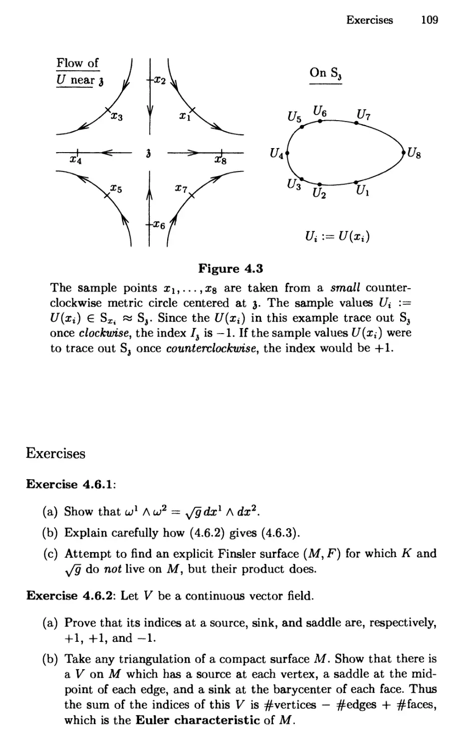
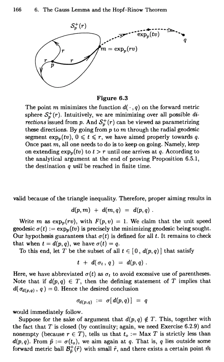
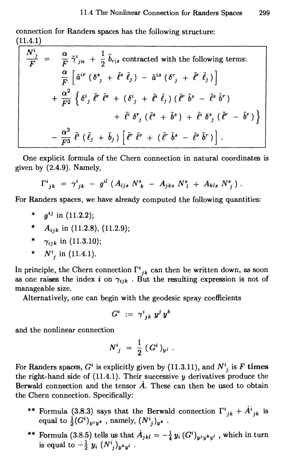
/


Автор: Bao D. Chern S.-S. Shen Z.
Теги: mathematics geometry higher mathematics history of mathematics
ISBN: 0-387-98948-X
Год: 2000


Текст
Graduate Texts in Mathematics
200
Editorial Board
S.Axler F.W. Gehring KA. Ribet
Springer
New York
Berlin
Heidelberg
Barcelona
Hong Kong
London
Milan
Paris
Singapore
Tokyo
Graduate Texts in Mathematics
1 Takeuti/Zaring. Introduction to
Axiomatic Set Theory. 2nd ed.
2 Oxtoby. Measure and Category. 2nd ed.
3 Schaefer. Topological Vector Spaces.
2nded.
4 Hilton/Stammbach. A Course in
Homological Algebra. 2nd ed.
5 Mac Lane. Categories for the Working
Mathematician. 2nd ed.
6 Hughes/Piper. Projective Planes.
7 Serre. A Course in Arithmetic.
8 Takeuti/Zaring. Axiomatic Set Theory.
9 Humphreys. Introduction to Lie Algebras
and Representation Theory.
10 Cohen. A Course in Simple Homotopy
Theory.
11 Conway. Functions of One Complex
Variable I. 2nd ed.
12 Beals. Advanced Mathematical Analysis.
13 Anderson/Fuller. Rings and Categories
of Modules. 2nd ed.
14 Golubitsky/Guillemin. Stable Mappings
and Their Singularities.
15 Berberian. Lectures in Functional
Analysis and Operator Theory.
16 Winter. The Structure of Fields.
17 Rosenblatt. Random Processes. 2nd ed.
18 Halmos. Measure Theory.
19 Halmos. A Hilbert Space Problem Book.
2nded.
20 Husemoller. Fibre Bundles. 3rd ed.
21 Humphreys. Linear Algebraic Groups.
22 Barnes/Mack. An Algebraic Introduction
to Mathematical Logic.
23 Greub. Linear Algebra. 4th ed.
24 Holmes. Geometric Functional Analysis
and Its Applications.
25 Hewitt/Stromberg. Real and Abstract
Analysis.
26 Manes. Algebraic Theories.
27 Kelley. General Topology.
28 Zariskj/Samuel. Commutative Algebra.
Vol.1.
29 Zariskj/Samuel. Commutative Algebra.
Vol.11.
30 Jacobson. Lectures in Abstract Algebra I.
Basic Concepts.
31 Jacobson. Lectures in Abstract Algebra II.
Linear Algebra.
32 Jacobson Lectures in Abstract Algebra
III. Theory of Fields and Galois Theory.
33 Hirsch. Differential Topology.
34 Spitzer. Principles of Random Walk.
2nd ed.
35 Alexander/Wermer. Several Complex
Variables and Banach Algebras. 3rd ed.
36 Kelley/Namioka et al. Linear Topological
Spaces.
37 Monk. Mathematical Logic.
38 Grauert/Fritzsche. Several Complex
Variables.
39 Arveson. An Invitation to C*-Algebras.
40 Kemeny/Snell/Knapp. Denumerable
Markov Chains. 2nd ed.
41 Apostol. Modular Functions and Dirichlet
Series in Number Theory.
2nd ed.
42 Serre. Linear Representations of Finite
Groups.
43 Gillman/Jerison. Rings of Continuous
Functions.
44 Kendig. Elementary Algebraic Geometry.
45 Loeve. Probability Theory I. 4th ed.
46 Loeve. Probability Theory II. 4th ed.
47 Moise. Geometric Topology in
Dimensions 2 and 3.
48 Sachs/Wu. General Relativity for
Mathematicians.
49 Gruenberg/Weir. Linear Geometry.
2nd ed.
50 Edwards. Fermafs Last Theorem.
51 Klingenberg. A Course in Differential
Geometry.
52 Hartshorne. Algebraic Geometry.
53 Manin. A Course in Mathematical Logic.
54 Graver/Watkins. Combinatorics with
Emphasis on the Theory of Graphs.
55 Brown/Pearcy. Introduction to Operator
Theory I: Elements of Functional
Analysis.
56 Massey. Algebraic Topology: An
Introduction.
57 Crowell/Fox. Introduction to Knot
Theory.
58 Koblitz. p-adic Numbers, p-adic Analysis,
and Zeta-Functions. 2nd ed.
59 Lang. Cyclotomic Fields.
60 Arnold. Mathematical Methods in
Classical Mechanics. 2nd ed.
61 Whitehead. Elements of Homotopy
(continued after index)
D.Bao
S.-S. Chern
Z. Shen
An Introduction to
Riemann-Finsler Geometry
With 20 Illustrations
Springer
D. Bao
S.-S. Chern
Department of Mathematics Department of
University of Houston
University Park
Houston, TX 77204
USA
bao@math.uh.edu
Mathematics
University of California
at Berkeley
Berkeley, CA 94720
USA
Z. Shen
Department of
Mathematical Sciences
Indiana University-Purdue
University Indianapolis
Indianapolis, IN 46202
USA
zshen@ math. iupui.edu
Editorial Board
S. Axler
Mathematics Department
San Francisco State University
San Francisco, CA 94132
USA
F.W. Gehring
Mathematics Department
East Hall
University of Michigan
Ann Arbor, MI 48109
USA
K.A. Ribet
Mathematics Department
University of California at
Berkeley
Berkeley, CA 94720-3840
USA
Back cover illustration: Courtesy of Mrs. Chern.
Mathematics Subject Classification (1991): 53C60, 58B20
Library of Congress Cataloging-in-Publicauon Data
Bao, David Dai-Wai.
An introduction to Riemann-Finsler geometry/D. Bao, S.-S. Chern, Z. Shen.
p. cm. — (Graduate texts in mathematics; 200)
Includes bibliographical references and index.
ISBN 0-387-98948-X (alk. paper)
1. Geometry, Riemannian. 2. Finsler spaces. I. Chern, Shiing-Shen,
1911- II. Shen, Zhongmin, 1963- III. Tide. IV. Series.
QA649.B358 2000
516.37S-<ic21 99-049808
© 2000 Springer-Verlag New York, Inc.
All rights reserved. This work may not be translated or copied in whole or in part without the
written permission of the publisher (Springer-Verlag New York, Inc., 175 Fifth Avenue, New
York, NY 10010, USA), except for brief excerpts in connection with reviews or scholarly
analysis. Use in connection with any form of information storage and retrieval, electronic
adaptation, computer software, or by similar or dissimilar methodology now known or heraf-
ter developed is forbidden.
The use of general descriptive names, trade names, trademarks, etc., in this publication, even
if the former are not especially identified, is not to be taken as a sign that such names, as
understood by the Trade Marks and Merchandise Marks Act, may accordingly be used freely
by anyone.
This reprint has been authorized by Spnnger-Verlag (Berlin/Heidelberg/New York) for sale in
the People's Republic of China only and not for export therefrom
987654321
ISBN 0-387-98948-X Springer-Verlag New York Berlin Heidelberg SPIN 10524454
To Our Teachers
in £ife ant) in SPtat^ematics
Preface
A historical perspective
The subject matter of this book had its genesis in Riemann's 1854 "habil-
itation" address: "Uber die Hypothesen, welche der Geometrie zu Grunde
liegen" (On the Hypotheses, which lie at the Foundations of Geometry).
Volume II of Spivak's Differential Geometry contains an English translation
of this influential lecture, with a commentary by Spivak himself.
Riemann, undoubtedly the greatest mathematician of the 19th century,
aimed at introducing the notion of a manifold and its structures. The
problem involved great difficulties. But, with hypotheses on the smoothness of
the functions in question, the issues can be settled satisfactorily and there
is now a complete treatment.
Traditionally, the structure being focused on is the Riemannian metric,
which is a quadratic differential form. Put another way, it is a smoothly
varying family of inner products, one on each tangent space. The resulting
geometry — Riemannian geometry — has undergone tremendous
development in this century. Areas in which it has had significant impact include
Einstein's theory of general relativity, and global differential geometry.
In the context of Riemann's lecture, this restriction to a quadratic
differential form constitutes only a special case. Nevertheless, Riemann saw
the great merit of this special case, so much so that he introduced for it
the curvature tensor and the notion of sectional curvature. Such was done
through a Taylor expansion of the Riemannian metric.
The Riemann curvature tensor plays a major role in a fundamental
problem. Namely: how does one decide, in principle, whether two given
Riemannian structures differ only by a coordinate transformation? This was
solved in 1870, independently by Christoffel and Lipschitz, using different
methods and without the benefit of tensor calculus. It was almost 50 years
later, in 1917, that Levi-Civita introduced his notion of parallelism
(equivalent to a connection), thereby giving the solution a simple geometrical
interpretation.
Riemann saw the difference between the quadratic case and the general
case. However, the latter had no choice but to lay dormant when he
remarked that "The study of the metric which is the fourth root of a quartic
differential form is quite time-consuming and does not throw new light to
the problem." Happily, interest in the general case was revived in 1918
viii Preface
by Paul Finsler's thesis, written under the direction of Caratheodory. For
this reason, we refer to the general case as Riemann-Finsler geometry, or
Finsler geometry for short.
Finsler geometry is closely related to the calculus of variations. See §1.0.
As such its deeper study went back at least to Jacobi and Adolf Kneser. In
his Paris address in 1900, Hilbert formulated 23 unsolved problems. The
last one was devoted to the geometry of the calculus of variations. It is the
only problem for which he did not formulate a specific question/conjecture.
Hilbert gave praise to Kneser's book, then new. He provided an account of
the invariant integral, and emphasized the importance of the problem of
multiple integrals. The Hilbert invariant integral plays an important role
in all modern treatments of the subject.
The geometrical data in Finsler geometry consists of a smoothly
varying family of Minkowski norms (one on each tangent* space), rather than
a family of inner products. This family of Minkowski norms is known as a
Finsler structure. Just like Riemannian geometry, there is the equivalence
problem: how can one decide (in principle) whether two given Finsler
structures differ only by a transformation induced from a coordinate change? It
is not unreasonable to expect that the solution of the equivalence problem
will again involve a connection and its curvature, together with the proper
space on which these objects live.
In Riemannian geometry, the connection of choice was that constructed
by Levi-Civita, using the Christoffel symbols. It has two remarkable
attributes: metric-compatibility and torsion-freeness. Although we now know
that in Finsler geometry proper, these cannot both be present in the same
connection, such was perhaps not common knowledge during the turn of
the century. Even after reaching this realization, one still faces the daunting
task of writing down viable structural equations for the connection.
Furthermore, the Levi-Civita (Christoffel) connection operates on the tangent
bundle TM of our underlying manifold M. But the same cannot be said of
its Finslerian counterpart.
It was not until 1926 that significant progress was made by Ludwig
Berwald (1883-1942), from an analytical perspective. See the poignant and
informative obituary by Max Pinl in Scripta Math. 27 (1965), 193-203.
Berwald's work stemmed from the study of systems of differential
equations, and was very much rooted in the calculus of variations. He introduced
a connection and two curvature tensors, all rightfully bearing his name. See
Matsumoto's appendix ("A History of Finsler Geometry") in Proceedings
of the 33rd Symposium on Finsler Geometry (ed. Okubo), 1998, Lake Ya-
manaka. (A revised version is scheduled to appear in Tensor.) The Berwald
connection is torsion-free, but is (necessarily) not metric-compatible. The
Berwald curvature tensors are of two types: an hh- one not unlike the Rie-
mann curvature tensor, and an hv- one which automatically vanishes in
the Riemannian setting. Berwald's constructions have, since their
inception, been indispensable to the geometry of path spaces.
Preface ix
Enthusiasts of metric-compatibility were not to be outdone. It is an
amusing irony that although Finsler geometry starts with only a norm in any
given tangent space, it regains an entire family (!) of inner products, one for
each direction in that tangent space. This is why one can still make sense
of metric-compatibility in the Finsler setting. In 1934, Elie Cartan
introduced a connection that is metric-compatible but has torsion. The Cartan
connection remains, to this day, immensely popular with the Matsumoto
and the Miron schools of Finsler geometry. Besides the curvature tensors
of hh- and hv- type, there is a third curvature tensor associated with the
Cartan connection. It is of vv- type. Curiously, this last tensor is
numerically identical to the curvature of a canonical (albeit singular) Riemannian
metric on each tangent space.
Back in the torsion-free camp, the next progress came in 1948, when the
Chern connection was discovered. Its formula differs from that of Berwald's
by an A term. In natural coordinates on the slit tangent bundle TM \ 0,
the Chern connection coefficients are given by
^1 ( ^fi _ *M + ^ihl \
2 V tek tes sxj J
To get those for the Berwald connection, one simply adds on the tensor
Aljk. More importantly, replacing the operator ^ by ^ gives the familiar
Levi-Civita (Christoffel) connection of Riemannian metrics.
The connections of Berwald and Chern are both torsion-free. They also
fail, slightly but expectedly, to be metric-compatible. Of the two, the Chern
connection is simpler in form, while the Berwald connection effects a leaner
/i/i-curvature for spaces of constant flag curvature. These connections
coincide when the underlying Finsler structure is of Landsberg type. They
further reduce to a linear connection on M, one which operates on TM,
when the Finsler structure is of Berwald type.
In the generic Finslerian case, none of the connections we mentioned
operates directly on the tangent bundle TM over M. Chern realized in his
solution of the equivalence problem that, by pulling back TM so that it
sits over the manifold of rays SM rather than M, one provides a natural
vector bundle on which these connections may operate. It is within this
geometrized setting that the equivalence problem and its solution admit a
sound conceptual interpretation.
The layout of the book
The Riemann-Finsler manifolds form a much larger class than the
Riemannian manifolds. Correspondingly, the former has a much more extensive
literature, connected with the names Synge, Berwald, E. Cartan, Buse-
mann, Rund, and many of our contemporaries. It is not the objective of
this book to provide a comprehensive survey. Rather, following the general
x Preface
outline of Riemann and Hilbert, our aim is to develop the subject
somewhat independently, with Riemannian geometry as a special case. We hope
our attempt at least reflects some of the spirits of those two pioneers.
This book is comprised of three parts:
* Finsler Manifolds and Their Curvature: four chapters.
* Calculus of Variations and Comparison Theorems: five chapters.
* Special Finsler Spaces over the Reals: five chapters.
The key points of each chapter are detailed in our table of contents. Given
that, we refrain from discussing here the specific topics covered.
There are fourteen chapters with an average of 30 pages each. The
chapters are intentionally kept short. It seems that psychologically, one's
progress through the Finsler landscape is more easily monitored this way.
Every chapter is devoted to (only) one or two major results. This
constraint allows us to base each chapter on a single theme, thereby rendering
the book more teachable.
Regarding classroom use, the students we have in mind are advanced
undergraduates or first-year graduate students. They are assumed to have
had at least a small amount of tensor analysis, to the extent that they
are comfortable with the gymnastics of raising and lowering indices. It
would also help if they have had some exposure to manifolds in the
abstract, so that pull-backs and push-forwards are familiar operations. Some
computational experience with the Gaussian curvature of Riemannian
surfaces would provide adequate motivation and intuition. This book contains
enough material for roughly three semester courses.
We have adopted a candid style of writing. If something is deemed simple
or straightforward, then it really is. If an omitted calculation is long, we say
so. Details, annotations, and remarks are provided for the harder or subtler
topics. Perhaps these gestures will help encourage the newly initiated to
stay the course and not give up too easily.
At the end of every chapter, one finds a list of references. Other than
a few books, these consist primarily of research papers mentioned in that
chapter. We have chosen to list them there for a reason. It is helpful to be
able to tell, at a glance, the research territories and boundaries with which
the chapter in question has made contact. We hope this feature helps foster
the book's image as an invitation to ongoing research. Incidentally, a master
bibliography also appears at the end of the book.
We have compiled 393 exercises. Among those, there are 80 that prompt
the reader to fill in some of the steps that we have omitted. Nothing was left
out due to laziness on our part. Instead, the omissions are to be thought of
as casualties of the editorial process. Their inclusion would either prove to
be too distracting, or add unnecessarily to the size of the book. Those 80
problems aside, the remaining 313 exercises explore examples, touch upon
new frontiers, and prepare for developments in later chapters.
Preface xi
If the purpose of the reader is to gain a nodding acquaintance of Finsler
geometry, then the exercises can be skipped without harm, until some
specific ones are referred to later. If the reader plans to do research in Finsler
geometry, then practically all the exercises need to be carefully worked
out. And, to assist those in the second group, we have provided detailed
step-by-step guidance on the more challenging problems. The adventurous
reader can always restore as much challenge as he or she wants by blocking
out some of our suggestions. We simply want to ensure that no one feels
demoralized by any of the exercises.
A good number of explicit examples are presented in this book. Those
discussed in the sections proper include:
* Minkowski spaces: §1.3A, §14.1.
* Riemannian spaces: §13.3, especially §13.3B, §13.3C.
* Berwald spaces: §10.3, §11.6B.
* Randers spaces: §1.3C, §11.0, §11.6B, §12.6.
* Spaces of scalar curvature: §3.9B.
* Spaces of constant flag curvature: §12.6, §12.7.
Many more can be found among the exercises.
The above examples all involve y-global Finsler structures F, with the
exception of the Berwald-Rund example treated in §10.3. By ^/-global, we
mean that F is smooth and strongly convex on TM \ 0. The said example
does not meet this stringent criterion, but is nevertheless included because
it illustrates some computation well. It also provides excellent motivation
for the rest of Chapter 10 and all of Chapter 11.
By no means have we exhausted the realm of interesting examples, y-
global or not. For instance, it is with great reluctance that we have omitted
Antonelli's Ecological Models, Matsumoto's Slope of a Mountain Metric,
and Models of Physiological Optics discussed by Ingarden. The interested
reader can consult the book The Theory of Sprays and Finsler Spaces with
Applications in Physics and Biology written by these three authors.
It is true that Finsler geometry has not been nearly as popular as its
progeny—Riemannian geometry. One reason is that deceptively simple
formulas can quickly give rise to complicated expressions and mind-boggling
computations. With the effort of many dedicated practitioners, this
situation is slowly being turned around. Nonetheless, some intrinsic aspects of
the subject are suggesting bounds on what one can do with mere pencil
and paper.
Fortunately, we are in a technological age. Symbolic computations and
large-scale computations on the computer are readily accessible. We took
the first step in that direction by writing Maple codes for the Finslerian
analogue of the Gaussian curvature. Then we implemented those codes
on some explicit examples in Chapter 12. We hope this modest attempt
represents the start of a trend. This could also be the venue by which a
geometry-minded computer scientist helps advance the field significantly.
xii Preface
As we mentioned earlier, this book is not intended to be a comprehensive
survey. Furthermore, our choice of topics and examples is guided by an eye
towards the global geometry. The picture we paint can possibly be rather
idiosyncratic. In spite of that, the material covered here is fundamental
enough to be considered essential to all branches of Finsler geometry.
To our colleagues
In earlier versions of the manuscript, our definitions of the nonlinear
connection and related objects on TM \ 0 differed from those of our fellow
researchers by factors involving the Finsler function F. In this final
version, we have decided to match their notations exactly. It is hoped that by
removing an unnecessary accent, we have enhanced the book's suitability
as a textbook or as a basic desk reference. Here are the specifics:
n^ -.= 7lJfc yk - ^f i\s yrys = -fik yk - Cjk -ykrs yrys,
We have not changed our philosophy of working, as much as possible, with
objects that are homogeneous of degree zero in y. Our reason for doing so
is that they make intrinsic sense on the manifold of rays SM. For instance,
we prefer to work with Nlj/F rather than just Nlr But, unlike our earlier
notation, the Nl here is identical to the Nl used by others.
Next, our convention on the wedge product does not contain the
normalization factors ^i, ^r, etc. For example, if 0, £, and £ are 1-forms, then:
0AC := 0<8>C ~ C®0 i
0ACAf := 0<g>C®f - 0®£®C
+ £<8>0<8>C - f ®C®0 •
Our placement of indices and sign convention on the curvature tensor
are adequately illustrated by what we do in the Riemannian case:
y* - g-
7 Jk 2
3 kl "~ !h* " ~dxT 7**7J< ~ ^ hi! 3h •
Finally, our G{ := 7* -fc y3yh is twice the Gl of Matsumoto.
Houston, Texas D. Bao
Berkeley, California S.-S. Chern
Indianapolis, Indiana Z. Shen
/ djhi _ dgjk dgks \
V dxk dxs 8x3 J '
Acknowledgments
This book project began as an attempt to sort through the literature on
Finsler geometry. It was our intention to write a systematic account about
that part of the material which is both elementary and indispensable. We
want to thank many fellow geometers for their encouragement, for
answering our email calls for help, and for steering us towards the pertinent
references. Some of these colleagues also helped us by proof-reading parts
of the manuscript.
We are grateful to Peter Kabal (Electrical Engineering, McGill
University) and Brad Lackey for the roles they played in our 20 pictorial
illustrations. Brad spent countless hours researching the various software for
drawing pictures. It was he who introduced us to Peter Kabal's very user-
friendly TfejXdraw. Brad then provided a number of examples, one of which
we retained as Figure 2.1. After Brad initiated us into TJgXdraw, Peter
supplied us with a copy of the manual. Incidentally, Brad also alerted us to a
theoretical blunder. Happily, it was something that we were able to fix.
One of us (Bao) would like to thank the University of Houston for a
Limited-Grant-In-Aid (LGIA) which partially funded Brad's efforts.
There are several cherished monographs on Finsler geometry that we
have not directly referenced in this book, although it is certain that we
have benefited from them in many ways. We are referring to the books by
Abate and Patrizio [AP], Bejancu [Bej], Miron and Anastasiei [MA].
Our book does not discuss the applications of Finsler geometry to
biology, engineering, and physics. For this reason, we are especially thankful
for the monographs [Asan] by Asanov, [AB] by Antonelli and Bradbury,
[AIM] by Antonelli, Ingarden, and Matsumoto, and [AZas] by Antonelli
and Zastawniak. We have also gained much insight from the four
expository essays by Antonelli [Ant], Ingarden [Ing], Gardner and Wilkens [GW],
and Beil [Bl] in the Seattle proceedings volume [BCS2].
The details for all the references cited here can be found in the master
bibliography at the end of the book.
We would like to acknowledge the always enthusiastic support of Ina
Lindemann (Mathematics Editor), the TfeK-nical expertise of Fred Bartlett
(Supervising Developer), Kanitra Fletcher and Yong-Soon Hwang for help
with miscellaneous issues, and Frank McGuckin (Production Editor) for
xiv Acknowledgments
his editorial guidance. Finally, we want to thank Valerie Greco, who copy-
edited the manuscript, for a splendidly accurate and constructive job.
Houston, Texas D. Bao
Berkeley, California S.-S. Chern
Indianapolis, Indiana Z. Shen
Contents
Preface vii
Acknowledgments xiii
PART ONE
Finsler Manifolds and Their Curvature 1
CHAPTER 1
Finsler Manifolds and
the Fundamentals of Minkowski Norms 1
1.0 Physical Motivations 1
1.1 Finsler Structures: Definitions and Conventions 2
1.2 Two Basic Properties of Minkowski Norms 5
1.2 A. Euler's Theorem 5
1.2 B. A Fundamental Inequality 6
1.2 C. Interpretations of the Fundamental Inequality 9
1.3 Explicit Examples of Finsler Manifolds 14
1.3 A. Minkowski and Locally Minkowski Spaces 14
1.3 B. Riemannian Manifolds 15
1.3 C. Randers Spaces 17
1.3 D. Berwald Spaces 18
1.3 E. Finsler Spaces of Constant Flag Curvature 20
1.4 The Fundamental Tensor and the Cartan Tensor 22
* References for Chapter 1 25
CHAPTER 2
The Chern Connection 27
2.0 Prologue 27
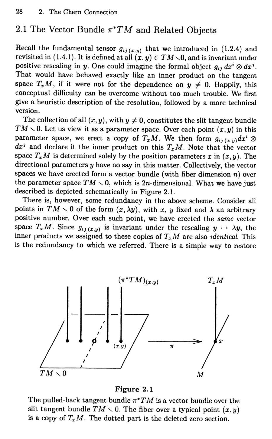
2.1 The Vector Bundle n*TM and Related Objects 28
2.2 Coordinate Bases Versus Special Orthonormal Bases 31
2.3 The Nonlinear Connection on the Manifold TM \ 0 33
2.4 The Chern Connection on tt*TM 37
xvi Contents
2.5 Index Gymnastics 44
2.5 A. The Slash (...)is and the Semicolon (...);s 44
2.5 B. Covariant Derivatives of the Fundamental Tensor g 45
2.5 C. Covariant Derivatives of the Distinguished £ 46
* References for Chapter 2 48
CHAPTER 3
Curvature and Schur's Lemma 49
3.1 Conventions and the hh-, hv-, vv-curvatures 49
3.2 First Bianchi Identities from Torsion Freeness 50
3.3 Formulas for R and P in Natural Coordinates 52
3.4 First Bianchi Identities from "Almost" ^-compatibility 54
3.4 A. Consequences from the dxk A dxl Terms 55
3.4 B. Consequences from the dxk A y8yl Terms 55
3.4 C. Consequences from the j;6yk A ^6yl Terms 56
3.5 Second Bianchi Identities 58
3.6 Interchange Formulas or Ricci Identities 61
3.7 Lie Brackets among the ^ and the F^- 62
3.8 Derivatives of the Geodesic Spray Coefficients Gl 65
3.9 The Flag Curvature 67
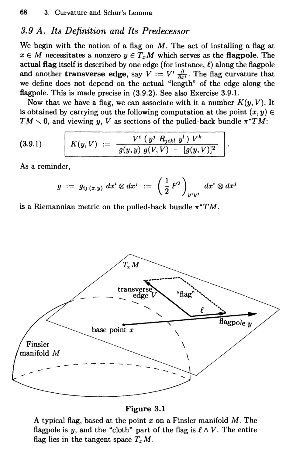
3.9 A. Its Definition and Its Predecessor 68
3.9 B. An Interesting Family of Examples of Numata Type — 70
3.10 Schur's Lemma 75
* References for Chapter 3 80
CHAPTER 4
Finsler Surfaces and
a Generalized Gauss-Bonnet Theorem 81
4.0 Prologue 81
4.1 Minkowski Planes and a Useful Basis 82
4.1 A. Rund's Differential Equation and Its Consequence 83
4.1 B. A Criterion for Checking Strong Convexity 86
4.2 The Equivalence Problem for Minkowski Planes 90
4.3 The Berwald Frame and Our Geometrical Setup on SM 92
4.4 The Chern Connection and the Invariants I, J, K 95
4.5 The Riemannian Arc Length of the Indicatrix 101
4.6 A Gauss-Bonnet Theorem for Landsberg Surfaces 105
* References for Chapter 4 110
Contents xvii
PART TWO
Calculus of Variations and Comparison Theorems Ill
CHAPTER 5
Variations of Arc Length,
Jacobi Fields, the Effect of Curvature Ill
5.1 The First Variation of Arc Length Ill
5.2 The Second Variation of Arc Length 119
5.3 Geodesies and the Exponential Map 125
5.4 Jacobi Fields 129
5.5 How the Flag Curvature's Sign Influences Geodesic Rays 135
* References for Chapter 5 138
CHAPTER 6
The Gauss Lemma and the Hopf-Rinow Theorem 139
6.1 The Gauss Lemma 139
6.1 A. The Gauss Lemma Proper 140
6.1 B. An Alternative Form of the Lemma 142
6.1 C. Is the Exponential Map Ever a Local Isometry? 143
6.2 Finsler Manifolds and Metric Spaces 145
6.2 A. A Useful Technical Lemma 146
6.2 B. Forward Metric Balls and Metric Spheres 148
6.2 C. The Manifold Topology Versus the Metric Topology ... 149
6.2 D. Forward Cauchy Sequences, Forward Completeness ... 151
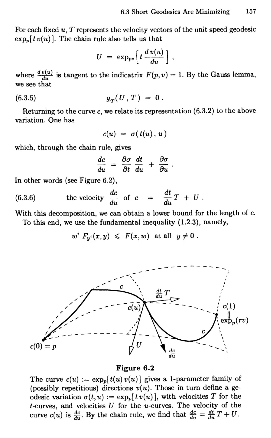
6.3 Short Geodesies Are Minimizing 155
6.4 The Smoothness of Distance Functions 161
6.4 A. On Minkowski Spaces 161
6.4 B. On Finsler Manifolds 162
6.5 Long Minimizing Geodesies 164
6.6 The Hopf-Rinow Theorem 168
* References for Chapter 6 172
CHAPTER 7
The Index Form and the Bonnet-Myers Theorem 173
7.1 Conjugate Points 173
7.2 The Index Form 176
7.3 What Happens in the Absence of Conjugate Points? 179
7.3 A. Geodesies Are Shortest Among "Nearby" Curves 179
7.3 B. A Basic Index Lemma 182
7.4 What Happens If Conjugate Points Are Present? 184
7.5 The Cut Point Versus the First Conjugate Point 186
xviii Contents
7.6 Ricci Curvatures 190
7.6 A. The Ricci Scalar Ric and the Ricci Tensor Ricij 191
7.6 B. The Interplay between Ric and Ric^ 192
7.7 The Bonnet-Myers Theorem 194
* References for Chapter 7 198
CHAPTER 8
The Cut and Conjugate Loci, and Synge's Theorem 199
8.1 Definitions 199
8.2 The Cut Point and the First Conjugate Point 201
8.3 Some Consequences of the Inverse Function Theorem 204
8.4 The Manner in Which Cy and iy Depend on y 206
8.5 Generic Properties of the Cut Locus Cutx 208
8.6 Additional Properties of Cutx When M Is Compact 211
8.7 Shortest Geodesies within Homotopy Classes 213
8.8 Synge's Theorem 221
* References for Chapter 8 224
CHAPTER 9
The Cartan-Hadamard Theorem and
Rauch's First Theorem 225
9.1 Estimating the Growth of Jacobi Fields 225
9.2 When Do Local Diffeomorphisms Become Covering Maps? ... 231
9.3 Some Consequences of the Covering Homotopy Theorem 235
9.4 The Cartan-Hadamard Theorem 238
9.5 Prelude to Rauch's Theorem 240
9.5 A. Transplanting Vector Fields 240
9.5 B. A Second Basic Property of the Index Form 241
9.5 C. Flag Curvature Versus Conjugate Points 243
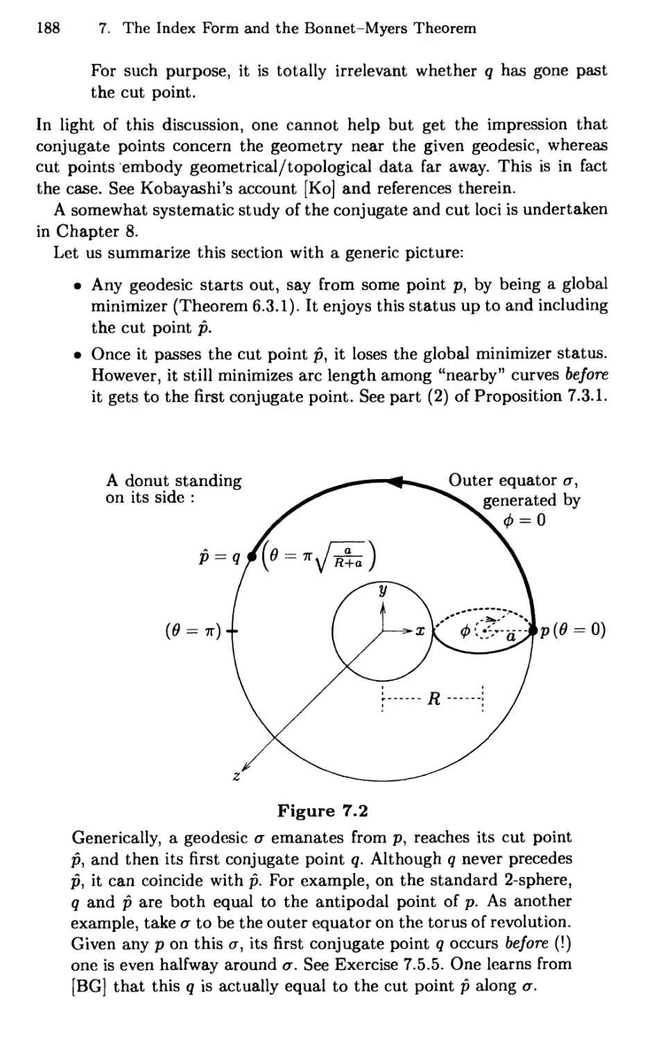
9.6 Rauch's First Comparison Theorem 244
9.7 Jacobi Fields on Space Forms 251
9.8 Applications of Rauch's Theorem 253
* References for Chapter 9 256
Contents xix
PART THREE
Special Finsler Spaces over the Reals 257
CHAPTER 10
Berwald Spaces and
Szabo's Theorem for Berwald Surfaces 257
10.0 Prologue 257
10.1 Berwald Spaces 258
10.2 Various Characterizations of Berwald Spaces 263
10.3 Examples of Berwald Spaces 266
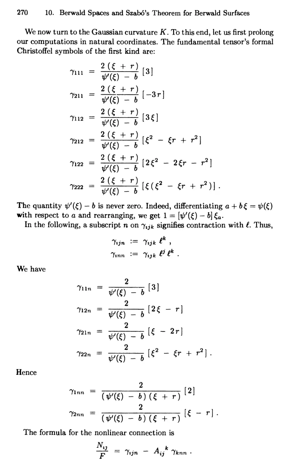
10.4 A Fact about Flat Linear Connections 272
10.5 Characterizing Locally Minkowski Spaces by Curvature 275
10.6 Szabo's Rigidity Theorem for Berwald Surfaces 276
10.6 A. The Theorem and Its Proof 276
10.6 B. Distinguishing between t/-local and t/-global 279
* References for Chapter 10 280
CHAPTER 11
Randers Spaces and an Elegant Theorem 281
11.0 The Importance of Randers Spaces 281
11.1 Randers Spaces, Positivity, and Strong Convexity 283
11.2 A Matrix Result and Its Consequences 287
11.3 The Geodesic Spray Coefficients of a Randers Metric 293
11.4 The Nonlinear Connection for Randers Spaces 298
11.5 A Useful and Elegant Theorem 301
11.6 The Construction of y-global Berwald Spaces 304
11.6 A. The Algorithm 304
11.6 B. An Explicit Example in Three Dimensions 306
* References for Chapter 11 309
CHAPTER 12
Constant Flag Curvature Spaces and
Akbar-Zadeh's Theorem 311
12.0 Prologue 311
12.1 Characterizations of Constant Flag Curvature 312
12.2 Useful Interpretations of E and E 314
12.3 Growth Rates of Solutions of E + A E = 0 320
12.4 Akbar-Zadeh's Rigidity Theorem 325
12.5 Formulas for Machine Computations of K 329
12.5 A. The Geodesic Spray Coefficients 329
12.5 B. The Predecessor of the Flag Curvature 330
xx Contents
12.5 C. Maple Codes for the Gaussian Curvature 331
12.6 A Poincare Disc That Is Only Forward Complete 333
12.6 A. The Example and Its Yasuda-Shimada Pedigree 334
12.6 B. The Finsler Function and Its Gaussian Curvature 335
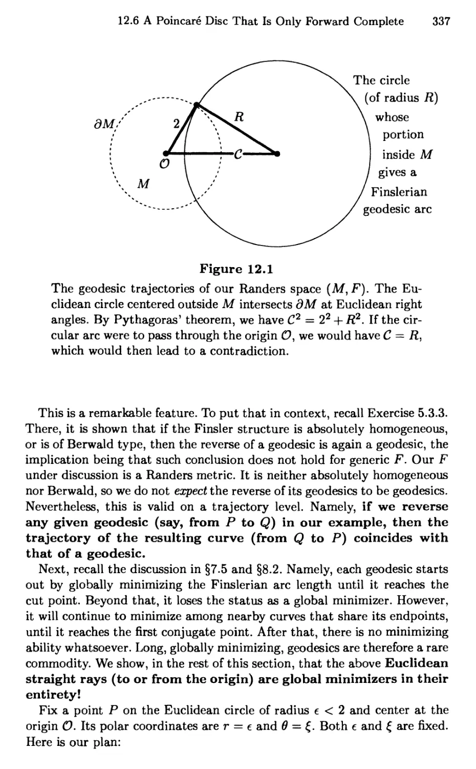
12.6 C. Geodesies; Forward and Backward Metric Discs 336
12.6 D. Consistency with Akbar-Zadeh's Rigidity Theorem ... 341
12.7 Non-Riemannian Projectively Flat S2 with K = 1 343
12.7 A. Bryant's 2-parameter Family of Finsler Structures ... 343
12.7 B. A Specific Finsler Metric from That Family 345
* References for Chapter 12 350
CHAPTER 13
Riemannian Manifolds and Two of Hopf's Theorems 351
13.1 The Levi-Civita (Christoffel) Connection 351
13.2 Curvature 354
13.2 A. Symmetries, Bianchi Identities, the Ricci Identity 354
13.2 B. Sectional Curvature 355
13.2 C. Ricci Curvature and Einstein Metrics 357
13.3 Warped Products and Riemannian Space Forms 361
13.3 A. One Special Class of Warped Products 361
13.3 B. Spheres and Spaces of Constant Curvature 364
13.3 C. Standard Models of Riemannian Space Forms 366
13.4 Hopf's Classification of Riemannian Space Forms 369
13.5 The Divergence Lemma and Hopf's Theorem 376
13.6 The Weitzenbock Formula and the Bochner Technique 378
* References for Chapter 13 382
CHAPTER 14
Minkowski Spaces, the Theorems of Deicke and Brickell 383
14.1 Generalities and Examples 383
14.2 The Riemannian Curvature of Each Minkowski Space 387
14.3 The Riemannian Laplacian in Spherical Coordinates 390
14.4 Deicke's Theorem 393
14.5 The Extrinsic Curvature of the Level Spheres of F 397
14.6 The Gauss Equations 399
14.7 The Blaschke-Santalo Inequality 403
14.8 The Legendre Transformation 406
14.9 A Mixed-Volume Inequality, and BrickeH's Theorem 412
* References for Chapter 14 418
Bibliography 419
Index 427
Chapter 1
Finsler Manifolds and the
Fundamentals of Minkowski Norms
1.0 Physical Motivations
1.1 Finsler Structures: Definitions and Conventions
1.2 Two Basic Properties of Minkowski Norms
1.2 A. Euler's Theorem
1.2 B. A Fundamental Inequality
1.2 C. Interpretations of the Fundamental Inequality
1.3 Explicit Examples of Finsler Manifolds
1.3 A. Minkowski and Locally Minkowski Spaces
1.3 B. Riemannian Manifolds
1.3 C. Randers Spaces
1.3 D. Berwald Spaces
1.3 E. Finsler Spaces of Constant Flag Curvature
1.4 The Fundamental Tensor and the Cartan Tensor
* References for Chapter 1
1.0 Physical Motivations
Finsler geometry has its genesis in integrals of the form
/
J a
bF(xl xn.^ ^l)dt
The function F(xl,..., xn ; yl,..., yn) is positive unless all the yl are zero.
It is also homogeneous of degree one in y. Let us single out some contexts
in which this integral arises.
* In certain physical examples, x stands for position, y for velocity.
Then F would have the meaning of speed, and t would play the
2 1. Finsler Manifolds and the Fundamentals of Minkowski Norms
role of time. In these cases, the above integral measures distance
traveled. However, other interpretations are possible.
* Take optics for instance. Keep in mind that in an anisotropic
medium, the speed of light depends on its direction of travel. At
each location x, visualize y as an arrow that emanates from x. Now
measure the amount of time it takes light to travel from x to the
tip of j/, and call the result F(x,y). The hypothesized homogeneity
allows us to rewrite the displayed integral as Ja F(x,dx). This then
represents the total time it takes light to traverse a given (possibly
curved) path in this medium. See Ingarden's exposition in [AIM].
* There are many variations on the theme we just described. A
particularly interesting one concerns the time it takes to negotiate any
given path on a hillside. It was originally mentioned by Finsler to
Matsumoto [Ml]. The premise here is that one's walking speed
depends heavily on the slope of the terrain, and hence on one's
direction of travel. See Matsumoto's account in [AIM].
* Mathematical ecology provides more esoteric examples. For
instance, x could stand for the state of a coral reef, and y the
displacement vector from the state x to a new state. The quantity F(x, dx)
represents the energy one needs in order to evolve from the state x
to the neighboring state x + dx. Hence the integral Ja F(x, dx) is
the total energy cost of a given path of evolution. See Antonelli's
treatment in [AIM], as well as the book by Antonelli and Bradbury
[AB].
For explicit mathematical examples, see §1.3.
1.1 Finsler Structures: Definitions and Conventions
Let M be an n-dimensional C°° manifold. Denote by TXM the tangent
space at x G M, and by TM := Ux6m TxM the tangent bundle of M. Each
element of TM has the form (x, j/), where x € M and y eTxM. The natural
projection 7r : TM —> M is given by 7r(x, y) := x. The dual space of TXM
is T*M, called the cotangent space at x. The union T*M := UxEm T*M
is the cotangent bundle of M.
A (globally defined) Finsler structure of M is a function
F : TM -> [0,oo)
with the following properties:
(i) Regularity: F is C°° on the entire slit tangent bundle TM \ 0.
(ii) Positive homogeneity: F( x , A y) = A F(x, y) for all A > 0 .
1.1 Finsler Structures: Definitions and Conventions 3
(iii) Strong convexity: The n x n Hessian matrix
"rl
(9ij) :=
L2f!
vV J
is positive-definite at every point of TM \ 0 .
• In some situations, the Finsler structure F satisfies the criterion
F(x, -y) = F(x, y). In that case we have absolute
homogeneity instead: F(x, A y) = |A| F(x,y) for all A € R. In general, we
find this property to be too restrictive, because it would
immediately exclude some interesting examples such as Randers spaces (see
§1.3C).
• Let us make sense of the y% in criterion (iii). Fix any basis {&*}
for TXM. Out of habit, one can take 6* to be gfr , although this
restriction is unnecessary. Express y as yl 6* . The Finsler structure
F is then a function of (x\t/1), and the partial derivatives of \ F2
are taken with respect to the yl. It can be checked that the positive-
definiteness stipulated in (iii) is independent of our choice of {bi}.
Given a manifold M and a Finsler structure F on TM, the pair (M, F)
is known as a Finsler manifold. See §1.3 for explicit examples of some
important Finsler manifolds.
Throughout the book, the rules that govern our index gymnastics are as
follows:
• Lower case Latin indices (except the alphabet n) run from 1 ton.
• Lower case Greek indices run from 1 to n — 1 .
• Vector indices are up; covector indices are down.
• Any repeated pair of indices—provided that one is up and the other
is down—is automatically summed.
• The lowering and raising of indices are carried out by the gij defined
above, and its matrix inverse gx*.
Let (x1,---,^71) = {xl) : U —► Rn be a local coordinate system on
an open subset U C M. As usual, {^fr} and {dx1} are, respectively, the
induced coordinate bases for TXM and T*M. The said xx give rise to local
coordinates (xi,yi) on ty~1U C TM through the mechanism
i 9
y = y d*'
The yj are fiberwise global. Whenever possible, let us make no distinction
between (x,t/) and its coordinate representation (x\yl). Functions F that
are defined on TM can be locally expressed as
F(x\...,xn;y1,...,yn).
4 1. Finsler Manifolds and the Fundamentals of Minkowski Norms
We continue a convention employed in criterion (iii) above; namely, denote
by Fyt, Fyiyj, ..., etc. the partial derivative(s) of F with respect to the
coordinates yl. Adopt a similar notation for the partial derivatives with
respect to the coordinates xl.
We close this section with some cautionary remarks about our notation.
For the sake of concreteness, we focus our attention on the various objects
that the symbol ^fr comes to represent throughout this book.
* When evaluated at the point x £ M, ^fr refers to a coordinate
vector on M.
* When evaluated at the point (x, y) G TM, the same notation ^
stands for a coordinate vector on TM. As such, it would be on the
same footing as the ^7, which are also coordinate vectors on the
tangent bundle TM.
* Later on, we use the restricted projection n : TM \ 0 —► M to pull
the tangent bundle TM back, producing a vector bundle tt*TM
that sits over TM \ 0 . In that case, when -£^ is evaluated at the
point (x, y) £ TM \ 0 , it will take on yet another meaning, namely,
as (the value of) a basis section of the bundle tt*TM.
In short, we are using the same symbol ^7 to denote objects that belong
to three different spaces. Furthermore, they do not obey the same
transformation law. Indeed, let
X = X ( X , . . . , X )
be a local change of coordinates on M. Correspondingly, the chain rule
gives
(!■") *'%*■
One can apply the chain rule carefully to deduce that:
* As coordinate vector fields on M, or as basis sections of 7r*TM, the
t^t transform like
ox1
(112) A.^IA
v " ■ ' dxP dxP dxl
* On the other hand, as coordinate vector fields on TM, the ^
transform like
ma) _L = «El A + _£fl«. A
K ' ' J dxP dxP dxl dxPdx* dyl '
Nevertheless, we have decided that the inherent risks of this practice
do not outweigh its virtue, which is simplicity. We feel (or hope!) that it
is easier for the reader to ferret out the proper meaning of ^§7 from the
context of our discussion or computation, than to create a different symbol
for each of the three objects described.
1.2 Two Basic Properties of Minkowski Norms 5
Exercises
Exercise 1.1.1: Recall that the definition of the g^ involves a choice of
basis for each TXM. Explain why the positive-definiteness of the matrix
(gij) is a basis-free concept.
Exercise 1.1.2: Derive the induced transformation laws (1.1.1)—(1.1.3).
1.2 Two Basic Properties of Minkowski Norms
The restriction of a Finsler structure F to any specific tangent space TXM
gives what is known as a Minkowski norm on TXM. Thus a Finsler structure
of M may be viewed as a smoothly varying family of Minkowski norms.
Generically, this family has rather limited (to be precise, no more than C1)
differentiability along the zero section of the tangent bundle TM. Such
regularity issues are dealt with later. Here, let us concern ourselves with
certain geometrical aspects of Minkowski norms.
Every n-dimensional vector space is linearly isomorphic to Rn, whose
elements y have the form (t/1,... ,t/n). Thus there is no loss of generality
in confining our discussion to Minkowski norms on W1.
1.2 A. Euler's Theorem
First, let us dispense with a technical ingredient that manifests itself
repeatedly in our arguments. It is known as Euler's theorem for homogeneous
functions.
Theorem 1.2.1. Suppose a real-valued function H on W1 is differen-
tiable away from the origin ofW1. Then the following two statements are
equivalent:
• H is positively homogeneous of degree r. That is,
H(\y) = \r H(y) for all A >0 .
• The radial directional derivative of H is r times H. Namely,
I yl Hyi(y) = rH{y) I.
Proof.
* Suppose H satisfies H(\y) = Xr H(y) for all positive A. Fix y.
Differentiating this equation with respect to the parameter A gives
y'H^Xy) = rX'-1 H(y) .
Setting A equal to 1 gives the criterion sought.
6 1. Finsler Manifolds and the Fundamentals of Minkowski Norms
* Conversely, suppose yl Hyt(y) = rH(y). Fix y and consider the
function H(X y) with A > 0. By the chain rule, we have
^ H(Xy) = yl Hy,(\y) = A (Ay)' tfw«(Ay) .
Using our supposition, we see that the last term equals \ r H(Xy).
Since we have not assumed that H is nonzero away from the origin,
we cannot read the above as ^ log H(X y) = j = j^ log Ar. Instead,
we rewrite it as the ODE
^H(Xy) - ^H(Xy) = 0.
The integrating factor -^ then gives H(Xy) = CAr, where C is
some constant that depends on our fixed y. Setting A equal to 1
shows that C = H{y). D
In particular, if F is positively homogeneous of degree 1, then
(1.2.1) y* Fyr(y) = F{y) , equivalent^ ^ Fy. = 1 ,
(1.2.2) yJ ^y^(y) = o.
1.2 B. A Fundamental Inequality
The next theorem tells us that positivity and the triangle inequality are
actually consequences of the defining properties of Minkowski norms. It also
calls our attention to a multifaceted fundamental inequality.
Theorem 1.2.2. Let F be a nonncgative real-valued function on Rn with
the properties:
* F is C°° on the punctured space Rn \ 0 .
* F(Xy) = XF(y) for all A > 0.
* The n x n matrix (gij), where gl3 (y) := [ ^ F2 J^j (j/) , is positive-
definite at aii y ^ 0.
Then we have the following conclusions:
* (Positivity)
F(y) > 0 whenever y ^ 0 .
* (Triangle inequality)
F(yi+V2) < F(Vl) + F(y2) ,
where equaiity holds if and oniy ify2 = oty\ or y\ = a j/2 for some
a^0.
1.2 Two Basic Properties of Minkowski Norms
• (Fundamental inequality)
(1.2.3)
wl Fr(y) < F(w) at all y^Q
and equality holds if and only ifw = ay for some a > 0.
Remarks:
** The hypotheses of the above theorem define what one means by a
Minkowski norm on W1. According to this theorem, there is no
need to hypothesize that F be positive at y ^ 0; it is necessarily so.
** If the Minkowski norm satisfies F(-y) — F(y), then one has the
absolute homogeneity F( A y) = |A| F(y). The simplest example of
an absolutely homogeneous Minkowski norm on Kn is
F(y) := VVV »
where • denotes the canonical inner product tz • i; := 5^ ul vJ. This
F is called the standard Euclidean norm of Rn.
** In view of the first two conclusions of this theorem, every absolutely
homogeneous Minkowski norm is a norm in the sense of functional
analysis.
In preparation for the proof of Theorem 1.2.2, we observe the following:
• One can check that
(1.2.4) gij{y) := (| **) ; . (») = [f Fy,yi + Fy, Fyl](y) .
The gi3 are C°° functions on IRn \ 0 and, in typical examples (that
are not Riemannian), they cannot even be extended continuously to
all of Rn.
• Applying the consequences (1.2.1), (1.2.2) of Euler's theorem to the
above formula for g^ gives
(1.2.5) gijly) ylyJ - F2(y) , equivalently gXJ - — = 1 .
We now give a proof, adapted from Rund [R], of Theorem 1.2.2.
Proof of the theorem.
(i) Positivity:
Consider (1.2.5); namely, ^(y) V1 Vj = F2(y) • Tne hypothesized strong
convexity of F says that the left-hand side is positive whenever y ^ 0, thus
F is strictly positive on IRn \ 0 .
8 1. Finsler Manifolds and the Fundamentals of Minkowski Norms
(ii) The triangle inequality:
At each point y G W1 \ 0 , the matrix (gij) defines an inner product. So
we have the Cauchy-Schwarz type inequality
(1.2.6) [ 9ij ly) Crff < [ 9ii {y) V ? ] 19ki (V) Vk rf ] V £, r, 6 Rn ,
where equality holds if and only if £ = (£*), 77 = (77*) are collinear. Setting
rf = yl and using (1.2.5), we obtain
(1.2.7) [9rHV)Vv']2 < F2{y)[gij(y)e?) V^R",
where equality holds if and only if £ and y are collinear. On the other hand,
the formula (1.2.4) for gij leads us to
(1.2.8) Fryi(y) Ce = j±fi {F2(y) [9iHv) ??) ~ lfc,<y) V*??}
which, in conjunction with (1.2.7), gives
(1.2.9) FytyJ(y)Ce > 0 V^Rn.
Here, equality holds if and only if £ and y are collinear.
Next we prove that
(1.2.10) 2F(y) ^ F(y + 0 + F(y - 0 V y, <f G R" ,
and equality holds if and only if £ = A y for some |A| ^ 1.
Let us begin by analyzing all the linearly dependent cases:
* If f = A y for some |A| ^ 1, the (positive) homogeneity of F implies
that both sides of (1.2.10) are equal to 2F(y).
* If £ = A y with |A| > 1, the right-hand side of (1.2.10) reduces to the
form (2 + a)F(y) + /?, where a, (3 are positive. Hence the inequality
in question is strict as claimed.
* The case of £ = 0 is covered by the above. The only scenario left
is when £ ^ 0 but y = 0, for which the inequality is strict by the
positivity we just established.
Now suppose t/, £ are linearly independent. Consider F(y + t£), which is
a C°° function in the real variable t. By the second mean-value theorem,
we have
(1.2.11) F(y±0 = F(y) ± Fy,(y) ? + \ Fytyl(y±eO Cij
for some 0 < e < 1. Since y ± e£ and £ are linearly independent, (1.2.9)
tells us that the quadratic term in (1.2.11) is positive. Thus
(1.2.12) F(y + 0 > F{y) + Fy,(y) ? ,
(1.2.13) F(y-0 > F(y) - Fy,(y) V ■
These add to yield the strict inequality part of (1.2.10).
1.2 Two Basic Properties of Minkowski Norms 9
By setting y := \ (yx -f-2/2) and £ := \ (yi - y2) in (1.2.10), we obtain the
triangle inequality stated in the theorem. The fact that (1.2.10) becomes an
equality only when £ = Xy for some |A| ^ 1 now implies that the triangle
inequality is strict except when j/i = a j/2 or j/2 = ol V\ for some a ^ 0.
Let us note in passing the following. We have seen that (1.2.10) implies
the triangle inequality. The converse is quite straightforward. So the two
are actually equivalent.
(Hi) The fundamental inequality:
Finally, we ascertain (1.2.3):
wi Fy*{y) ^ F{w) at all y^O,
where equality is supposed to hold if and only if w = ay for some a ^ 0.
The consequences of Euler's theorem, as described in (1.2.1) and (1.2.2), are
used repeatedly without mention. As before, we enumerate all possibilities:
* When w = ay for some a ^ 0, both sides equal aF(y).
* When it; is a negative multiple of y, the inequality is strict because
its left-hand side becomes a negative multiple of F(y).
* The case w ^ 0 but y = 0 is disallowed.
* Lastly, suppose y,w are linearly independent; then so are y and
£ := y - w. Inequality (1.2.13) now reads
(1.2.14) F(w) > F(y) - Fyi(y) (y* - «;') ,
which readily reduces to the strict part of (1.2.3).
We have completely proved Theorem 1.2.2. □
1.2 C. Interpretations of the Fundamental Inequality
In this subsection, let us explore the many different faces of the fundamental
inequality (1.2.3).
* At face value, (1.2.3) says that
I wl Fyi(y) ^ F(w)~\.
And, the latter becomes an equality if and only if w = ay for some
a ^ 0. Note that the said equality, after cancelling off a (if > 0),
is none other than Euler's theorem (1.2.1): yl Fyi(y) = F(y). Hence
(1.2.3) may be viewed as an extension of Euler's theorem, from an
equation to an inequality.
* Adding the equation F(y) — yl Fyi(y) = 0 to (1.2.3) gives
(1.2.15)
F(V) + Fyi(y)(w-yY < F(w)
5
10 1. Finsler Manifolds and the Fundamentals of Minkowski Norms
where equality holds only when w = ay with a > 0. Think of y
as fixed and w as the independent variable. The left-hand side is
then the linear approximation of the value F(w). So, at any fixed
(y,F(y)) on the graph of F, the tangent hyperplane touches the
graph only along the ray (ay, aF(y)), a ^ 0. Everywhere else, the
tangent hyperplane lies below the graph of F. This is depicted in
Figure 1.1. In this way, (1.2.3) tells us that the graph of F is a
convex cone with its vertex at the origin of our Minkowski space.
Since F(y) > 0 for y ^ 0, we can multiply (1.2.3) by F(y) to
get wiF(y)Fyi(y) < F(y)F(w). Now, (1.2.4), (1.2.2), and (1.2.1)
together give yj gij = FFyx. Thus (1.2.3) is equivalent to
(1.2.16) ftj(y)ti/V ^ F(w)F{y)
Consider first the case in which F is the norm associated with an
inner product on Rn. Here, F(y) = y/gij yiyj1 where the g^ are
constants. Almost by inspection, we see that the fundamental
tensor 9ij(y) := (\F2)yiyj is simply given by the inner product g^.
Also in this case, F(—y) = F(y). These observations allow us to
deduce that (1.2.16) is equivalent to \QijUixy^\ ^ F(w) F(y), which
is the standard Cauchy-Schwarz inequality. So, in the general case,
we may view (1.2.16) [equivalently (1.2.3)] as a generalization of
the Cauchy-Schwarz inequality, from inner products to Minkowski
norms. Note however that, when spelled out, (1.2.16) implies that
[ftj(»)ttfVf < [9pq(w) wpwq] [grs{y) yrys] .
We emphasize that in the first term on the right, it is gpq(w) and
not gpq(y)> As such, this last inequality is distinctly different from,
and much more subtle than, the Cauchy-Schwarz type inequality
(1.2.6) encountered during the proof of Theorem 1.2.2.
• Finally, the fundamental inequality (1.2.3) plays a pivotal role in the
proof (Theorem 6.3.1) that short Finslerian geodesies are minimal.
Upon this edifice rests the Hopf-Rinow theorem (see §6.6) and the
enterprise of cut versus conjugate loci (treated systematically in
Chapter 8). As we show, the fundamental inequality comes to the
rescue when the Riemannian proof of Theorem 6.3.1 breaks down
in the generic Finsler case. The same technique saves the day again
in Proposition 9.2.2, when we prove that for (forward geodesically)
complete connected Finsler manifolds of nonpositive flag curvature,
the exponential map is a covering projection.
We have interpreted the fundamental inequality (1.2.3) in several
contexts. In each case, something interesting and important emerges. This is
a testimonial to the inequality's depth and significance.
Exercises 11
Figure 1.1
The graph of a Minkowski norm is a convex cone with its vertex
at the origin. The one shown here "tilts to the right."
Exercises
Exercise 1.2.1: Let F be positively homogeneous of degree 1 on IRn. Use
Euler's theorem to show that
(a) y'Fy^F.
(b) y> FyiyJ = 0 .
(c) ykFy*y>yk = ~ Fy^ •
(d) yl Fyiyjykyl = ~ 2 FyryJyk .
Here, all formulas are supposed to be evaluated at y.
Exercise 1.2.2: Let F be the standard Euclidean norm on W1. Show that
its gij is simply the Kronecker delta 6ij .
Exercise 1.2.3: Derive (1.2.5).
Exercise 1.2.4: A Minkowski norm F on W1 is said to be Euclidean if it
arises from an inner product ( , ) through F(y) = y/(y, y). Prove that
the following three criteria are equivalent:
(a) The Minkowski norm F is Euclidean.
(b) The functions g^ defined in (1.2.4) are constant.
(c) The functions Aijk^ := ~ (F2 )yiyjyk are all zero.
Exercise 1.2.5: Let F be a Minkowski norm on Rn.
(a) Explain why its Hessian matrix (Fyiyj ) is positive sermdefinite.
(b) Prove that its rank is n — 1 .
12 1. Finsler Manifolds and the Fundamentals of Minkowski Norms
(c) Verify that its 1-dimensional null space at any point y ^ 0 is spanned
by the vector yl ^ .
Hint: you may want to review the discussions that center around (1.2.9).
Exercise 1.2.6: A domain D in Rn is said to be strictly convex if it
contains the interior of every line segment joining any two points of the
topological closure D. Let F be a Minkowski norm. Given any r > 0,
define the ball Bn(r) and the sphere Sn_1(r) of radius r (centered at the
origin) as follows:
Bn(r) := {y£Rn: F(y)<r},
Sn~l(r) := {y£Rn: F(y) = r}.
Show that:
(a) Each Bn(r) is a strictly convex domain with C°° boundary Sn_1(r).
(b) Explain what it means to say that strong convexity implies strict
convexity.
Exercise 1.2.7: Suppose B is a strictly convex open domain "centered" at
the origin, with smooth boundary S := dB. Define a nonnegative function
F on Rn as follows:
F(y) := - , where t > 0 is such that ty € S .
(a) Check that F(y) > 0 for all y ^ 0 .
(b) Verify that F( Xy) = A F(y) for all positive numbers A. Also,
ascertain that if the domain B satisfies y € B <=> -y £ B, then we have
F{Xy) = \X\F(y) for all A <E R.
(c) Show that
F(y) is
< 1 if and only if y £ B
= 1 if and only if y € S
> 1 if and only if y £ B
(d) Prove that F satisfies the triangle inequality.
(e) Then check that
F(V + H) + F(y-ta - 2F(y) > 0.
(f) Explain why F is C°° on Rn \ 0, but is typically not differentiable
at the origin.
(g) Fix y ^ 0 and divide the inequality in part (e) by t2. Then take the
limit as t —► 0+. Show that the result is
Fy.y,{v)eS> > 0.
Exercises 13
In other words, the Hessian of F is positive-semidefinite. Hint:
expand the terms F( y ± t£) using the second mean-value theorem,
(h) Use formula (1.2.4) and part (g) to help you deduce that the Hessian
9ij := [ \ F2 ]y V ls typically only positive-semidefinite. Can you
exhibit a nonzero £ such that g^ f * £J = 0? Hint: see Exercise 1.2.9.
The moral here is that:
There are homogeneous functions F with strictly convex
unit balls but fail (just barely) to be strongly convex.
Hence they do not define Minkowski norms.
Exercise 1.2.8:
(a) Let S be some smooth hypersurface in IRn that is defined by an
equation P(v) = 0. Suppose we want to find a function F on Rn that
has the constant value 1 on 5. Explain why F(y) is characterized
by the equation
p[-M =o.
L F(y) J
Occasionally, such an equation can be solved to give an explicit
formula for F(y). The method we have just described is known
affectionately as Okubo's technique.
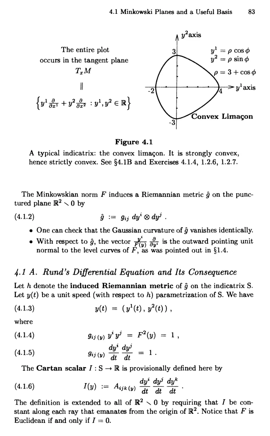
(b) As a concrete example, let S be the convex limagon in IR2. In polar
coordinates, it has the description
p = 3 + cos0 , 0 ^ 4> ^ 2?r .
Sketch S and check that its Cartesian description is
(y1)2 + (y2)2 = 3V(j/')2 + (y2)2 + y1 ■
(c) Apply Okubo's technique to show that the function F which has
constant value 1 on S is
(y1)2 + (y2)2
F(y) =
Zy/iv1)2 + (y2)2 + y1
(d) Can you prove that this F has all the defining properties (especially
strong convexity) of a Minkowski norm?
Exercise 1.2.9: Let
B := {(yV)€R2: (y1)4 + (y2)4 < !}•
(a) Check that B is strictly convex (as defined in Exercise 1.2.6) and
has a smooth boundary.
(b) Consider the F defined in Exercise 1.2.7. Use Okubo's technique to
deduce that here, it has the explicit formula
F(y) = [(y1)4 + (y2)4]1/4-
14 1. Finsler Manifolds and the Fundamentals of Minkowski Norms
(c) Calculate the matrix (gij) and check that it is singular (that is, not
invertible) on the yl and y2 axes. As a result, it cannot possibly be
positive-definite at these points. Show that these are the only points
at which it fails to be positive-definite.
(d) Explain what it means to say that strict convexity does not imply
strong convexity
Exercise 1.2.10: In R2, abbreviate j/1, y2 as p, q, respectively. Define
F(p,q) := a(p2+q2)1/2 + /? (p4+<?4 )1/4 ,
where a > 0, (3 ^ 0 are constants.
(a) Calculate the functions gij and check that they are homogeneous of
degree zero.
(b) Identify all constants a and (3 for which F defines a Minkowski norm
onR2.
Exercise 1.2.11: Let F be a Minkowski norm on Rn.
(a) Show that if two vectors y and w satisfy g^ (y) yJ = g{j (w) w3, then
y = w.
(b) Decide whether anything can be concluded if those two vectors
satisfy the following identity instead: Fyx(y) = Fwt(w).
1.3 Explicit Examples of Finsler Manifolds
1.3 A. Minkowski and Locally Minkowski Spaces
A Finsler manifold (M, F) is said to be locally Minkowskian if, at every
point igM, there is a local coordinate system (xl), with induced tangent
space coordinates yl, such that F has no dependence on the x\
In order to construct locally Minkowskian manifolds, one might
intuitively begin with a smooth manifold M and try to put the "same"
Minkowski norm on each of its tangent spaces. However, a good amount of
caution should be exercised, because there are topological obstruction(s)
that one must overcome. For example, if M is compact and boundaryless,
then having a locally Minkowskian structure will force its Euler
characteristic to vanish. See [BC2].
The simplest locally Minkowskian manifolds are of the following type:
* We start with a Minkowski norm F on Rn.
* We change our perspective and regard Rn as a manifold, albeit a
linear one.
* Given any tangent vector v based at y 6 IRn, we slide it (without
twisting) until it emanates from the origin "o" instead. Then we
evaluate F at the tip of this translated vector.
1.3 Explicit Examples of Finsler Manifolds 15
* In terms of a formula, we have
One is certainly justified in saying that the locally Minkowskian examples
we just cited are actually Minkowski norms in trivial disguise! Yet, this
does not detract from the fact that such examples are among the most
important ones in practice.
For numerical explorations, a particularly instructive family of
Minkowski norms is the following. Here, A can be any nonnegative constant.
F(t/l,t/2) := y/ y/{v1)4 + (v2)4 + A[(v1)2 + (v2)2}
This may be viewed as a perturbation of the quartic metric. See
also Exercise 1.2.11. Let us demonstrate that the perturbation serves to
regularize the singularity in the quartic metric. To this end, we first relabel
vl as p and v2 as q in order to avoid clutter. Straightforward computations
then give
fgn 212 \ = ( '
\ 921 922 J y
Hence
, P2(p4 + 3q4)
1 (p4+ ,4)3/2
-2 p3 ,3 ,
(p* + ,4)3/2 A
2 , , (P2 + I')"
(p4 + g4)3/2
, , (P2 + 92)3
3 „3
-2P: . ,
q2 (94 +3p4)
(p4+g4)3/2
3p:
2 „2
det(9ij) = x* + x ;^ ; ;4^/2 +
trace(^) = 2 A + (p4 + g4)3/2 .
Note that
• If A = 0, then det(^j) vanishes on the p and q axes in each
tangent plane. In that case, the Finsler function F, whose fundamental
tensor is called the quartic metric, fails to be a Minkowski norm
because strong convexity is violated at some nonzero y.
• If A > 0, then both the determinant and the trace of {gij) are
positive away from the origin in each tangent plane. In that case,
gij is positive-definite because both its eigenvalues are positive. The
Finsler structure F is then a Minkowski norm. In this sense, the
perturbation has regularized the quartic metric.
1.3 B. Riemannian Manifolds
Let M be an n-dimensional C°° (smooth) manifold. A smooth Riemannian
metric g on M is a family {gx}x£M of inner products, one for each tangent
space TXM, such that the functions g^ (x) := gx( -^ , ^fj ) are C°°. Since
16 1. Finsler Manifolds and the Fundamentals of Minkowski Norms
each gx is an inner product, the matrix (g^) is positive-definite at every
iGM. We can write
9 = 9ij (x) dxl ® dx3 .
This g defines a symmetric Finsler structure F on TM by the mechanism
F(z,y) := y/gx{y,y) .
Every Riemannian manifold (M,(j) is therefore a Finsler manifold. A
Finsler structure F is said to be Riemannian if it arises from a
Riemannian metric g in the manner we just described. In practice, one ascertains
this by showing that the fundamental tensor computed from F via (1.2.4)
has no y dependence. As a matter of fact,
'■■-&%„ =
9ij (*)
Let us describe some fundamental Riemannian metrics. To this end, let
S\(t) be the unique solution to the ODE
*" + AsA = 0, with initial data sA(0) = 0 , s'A(0) = 1 .
Here, A is an arbitrary but fixed real number. Explicitly, we have
sin( \f\t)
(1.3.1)
sx{t)
yTx
t
sinh( y/—\t)
if A > 0
if A = 0
if A < 0
Let (xl) denote the natural coordinates of Rn. At any point x € Rn,
introduce the abbreviations
to avoid clutter. Define
X3
and ip :=
«a(M)
(1.3.2)
{6ikxk) {Sjix1)
gij{x) := (1-^) 1^ + tfiSij
One can verify that:
* These g^ can be extended smoothly to the origin x = 0.
* g := gi3 (x) dx1 <8> dx3 is a Riemannian metric on W1 if A ^ 0.
* If A > 0, our g is a Riemannian metric on the open ball
{,€R»:|x| <-==}.
1.3 Explicit Examples of Finsler Manifolds 17
As we show in §13.3, these Riemannian metrics have constant sectional
curvature A. They are the Riemannian space forms.
1.3 C. Randers Spaces
In 1941, G. Randers [Ra] studied a very interesting class of Finsler
manifolds. Let M be an n-dimensional manifold. A Randers metric is a Finsler
structure F on TM that has the form
(1.3.3) F(xlV) := a(xlV) + 0(xlV) ,
where
(1-3.4) ot{x,y) := yjaij{x) ylyi ,
(1.3.5) (3(x,y) := bi(x) y{ .
* The tiij are the components of a Riemannian metric and the hi are
those of a 1-form. Both objects live on M, and are understood to
be fixed throughout the discussion.
* Due to the presence of the /? term, Rander's metrics do not
satisfy F(x1—y) = F(x,y) when b ^ 0. In fact, the Finsler function
of a Randers space is absolutely homogeneous if and only if it is
Riemannian.
The indices on certain objects are lowered and raised by
(a>ij) and its inverse matrix (alJ). Such objects are
decorated with a tilde.
Since (3(x,y) is linear in j/, it cannot possibly have a fixed sign. Thus, in
order for F to be positive on TM \ 0 , the size of the components 6* must
be suitably controlled. It can be shown (see §11.1) that the said positivity
holds if and only if
(1.3.6) || b || := sfl~^ < 1,
where
(1.3.7) V := aij bj .
We also need to address the issue of strong convexity. The Qij associated
with F can be computed according to formula (1.2.4). One finds that
(1.3.8) gij = ~ (aij - liij) + (ti + bi) [lj + bj) ,
where
(1.3.9) tt := ayi = M- .
18 1. Finsler Manifolds and the Fundamentals of Minkowski Norms
Equivalent ly,
F 3 ~ ~
(1.3.10) gl3 = - ai3 - - iiij + iibj + *, b% + ^ 67 .
It turns out (see §11.1) that the criterion || 6 || < 1, which guarantees the
positivity of F, also ensures strong convexity. And the crux of the argument
involves the following computational fact:
(1.3.11) det(^) = ( —)n+ det(al3) .
Its derivation can be found in [M2], albeit in the more general context of
(a, 0) metrics. A direct and expository account of (1.3.11) is given in
§11.2.
Let us borrow an explicit example of a Randers metric from [AIM]. Set
M := IR2 \ 0 . At each x € M, the indicatrix is to have the following
properties:
* It is an ellipse with eccentricity e, possibly depending on x, in the
tangent plane TXM.
* One of its foci is located at the orgin y = 0 of TXM.
* The directrix (corresponding to the above focus) passes through the
deleted point 0 of M, and is perpendicular to the line segment from
0 to x.
Using Okubo's technique (see Exercise 1.2.8), it can be shown that the
formula for F is
Fix1 x2-vl v2) - l 1 ly|2 X#2/
*(x ,x ,y ,y ) - e y |x|2 |i|2
(1.3.12)
Here, we have introduced some temporary abbreviations
,| := V(v1)2 + (y2)2
in order to avoid clutter.
X9y := x1 yl + x2 y2
1.3 D. Berwald Spaces
Berwald spaces are just a bit more general than Riemannian and locally
Minkowskian spaces. They provide examples that are more properly Fins-
lerian, but only slightly so. The most easily described characteristic of a
Berwald space is that all its tangent spaces are linearly isometric to a
common Minkowski space. One might say that the Berwald space in
question is modeled on a single Minkowski space. For a precise definition of
Berwald spaces, see Chapter 10.
1.3 Explicit Examples of Finsler Manifolds 19
We shall focus on Finsler structures F that are smooth and strongly
convex on all of TM \ 0. Let us refer to these F as j/-global for emphasis. As
we show, it takes some work to explicitly locate a j/-global Berwald space
that is neither Riemannian nor locally Minkowskian. In fact, according to
a rigidity result (see §10.6) of Szabo's, these do not even exist in dimension
two. Fortunately, examples of the desired vintage can be found in dimension
three or higher. The ones we know had their genesis in a result of Mat-
sumoto [M4], Hashiguchi-Ichijyo [HI], Shibata-Shimada-Azuma-Yasuda
[SSAY], and Kikuchi [Ki]. By contrast, y-local Berwald surfaces do exist,
and an explicit example of such is analyzed in §10.3.
Let us quote (from §11.6) an example of a 3-dimensional y-global
Berwald space that is neither Riemannian nor locally
Minkowskian. It is given by a Randers metric constructed with the following data:
• The underlying manifold is the Cartesian product
M := S2 x Sl .
It is compact and boundaryless. As local coordinates, one can use
the usual spherical 0, <j) on S2, and t for Sl. For concreteness,
we measure </> from the positive z axis down. Also, t is such that
(cos t, sin 2,0) parametrizes Sl.
• The Riemannian metric a is the product metric on S2 x S1. Here,
S2 and S1 are given the standard Riemannian metrics that they
inherited as submanifolds of Euclidean R3. Explicitly, one finds that
a := (sin20 dO <g) dO + d<j)®d<t)) + dt®dt.
This metric is not flat because it has nonzero curvature tensor.
• The 1-form we need is
b := edt,
where e is any (fixed) positive constant less than 1. This b is
globally defined on M, even though the coordinate t is not. It is non-
vanishing by inspection, and has Riemannian norm || b \\ = e < 1. A
straightforward calculation shows that it is parallel with respect to
the Levi-Civita (Christoffel) connection of a.
We now write down the resulting Randers metric. Let x be any point on
M, with coordinates (0, <f>, t). Let the arbitrary tangent vector y 6 TXM be
expanded as ye de -I- y* d<j> + yldt . Then
(1.3.13)
F{x,y) := ^sin2^*)2 + (l/*)2 + (l/*)2 + c y*
Since this F is of Randers type, its fundamental tensor is in principle given
by (1.3.8) or (1.3.10), although a direct computation is probably more
efficient. The reader is asked to do this calculation in Exercise 1.3.6.
20 1. Finsler Manifolds and the Fundamentals of Minkowski Norms
1.3 E. Finsler Spaces of Constant Flag Curvature
An extensive discussion of Finsler spaces with constant (flag) curvature
is given in Chapter 12.
There are non-Riemannian Finsler structures on IR2 with negative
constant Gaussian curvature. These are discussed in [Br3]. In §12.6, we
construct one (known to Okada [Ok]) using the Yasuda-Shimada theorem [YS]
as an inspiration (because we do not prove that theorem in this book). We
then directly verify that it has constant negative Gaussian curvature
K — — |. The explicit formula for the Finsler function is
(1.3.14)
F{x,y) := -^ v^JT + (1 _ ^ + ri) dr{y)
Here, r2 := (x1)2 4- (x2)2, where x = (xx,x2) is any point on the Poincare
disc M :— {x e R2 : r < 2}. And y is an arbitrary vector in the tangent
plane TXM.
This is a very special Randers metric:
* It has constant negative (Finslerian) Gaussian curvature — \.
* It violates some completeness assumption in Akbar-Zadeh's [AZ]
rigidity theorem.
* The Finslerian metric distance from the origin to the rim of the disc
is infinite. But that coming back from the rim to the origin has the
finite value log 2!
* Its geodesies are, trajectorywise, the same as the geodesies of the
Riemannian Poincare disc.
For these reasons, we would like to view it as the Finslerian analogue of
the Poincare disc.
Next, we turn to positive flag curvatures. In two dimensions, we have
explicit non-Riemannian examples with constant positive Gaussian
curvature K = 1, due to Bryant [Brl, Br2]. Here, we focus on a 2-parameter
family from [Br2]. Each Finsler structure in this family has K = 1 and is
projectively flat. In [Br2], it is explained how these are related to some of
Funk's earlier works [Fl, F2].
Let V be a 3-dimensional real vector space with basis {61,62,63}. Let p,
7 be two fixed angles satisfying
(*) l7l < P < \ ■
Define a p and 7 dependent, complex-valued quadratic form Q on V by
Q{u,v) := eip ulvl + e^ u2 v2 + e~ip u3 v3 .
In the above exponentials, i means >/--T . Also, u = ul bi ; v = vl bt.
Let S2 denote the set of rays in V. Equivalently, we are identifying X
and X* in V whenever X* = XX for some A > 0. Each point of S2 can
Exercises 21
thus be denoted as an equivalence class [X], with 0 ^ X 6 V. A moment's
thought shows that every tangent vector at the point [X] on S2 is the initial
velocity to a curve of the form [AT + ty], for some Y € V. Each such curve is
half of a great circle on S2. And it makes sense to denote the said tangent
vector by [X, Y). Note that [X', Y'] = [X, Y] if and only if X' = A X and
Y' = X Y + /xX, for some A > 0 and \x e R .
The Finsler function F : TS2 —> [0, oo) for Bryant's family of metrics,
indexed by p and 7, is
(1.3.15)
F{[X,Y\) := Re
/Q(y,F)Q(X,X)--Q2(X,r) _ .0(^10
Q2(X,X) %Q{X,X)
where "Re" means taking the real part. The complex square root function
is taken to be branched along the negative real axis, and to satisfy y/T = 1.
In other words,
Re y/a + ib := +
a + y/a2 + b2
It is not difficult to check that when p = 0 = 7, the above F is Riemannian.
It is also instructive to work out a manifestly real formula of F for specific
choices of p and 7. See §12.7 for a sample.
Bryant assures us that his methods in [Br2] give the following:
* The above F is indeed a Finsler structure in the sense of §1.1. Unless
p = 0 = 7, this Finsler function is non-Riemannian and is only
positively homogeneous.
* Each great semicircle [X + tY] is a geodesic of the Finsler structure.
(Incidentally, such curves are not yet parametrized to have constant
speed. Nevertheless, the Finslerian length of each great circle is 2ty.)
* The Gaussian curvature of the Finsler surface (S2,F) has the
constant positive value 1.
Exercises
Exercise 1.3.1: Show that the Minkowski spaces arising from the
Minkowski norms
F(y) :-
\
1=1
are all nonisometric for different values of A > 0.
Exercise 1.3.2: Recall the g^ defined in (1.3.2). Prove that they can be
smoothly extended to the origin x — 0 of Rn.
22 1. Finsler Manifolds and the Fundamentals of Minkowski Norms
Exercise 1.3.3: This again concerns (1.3.2). Show that
(a) For A < 0, the matrix (gij) is positive-definite at every x eRn.
(b) For A > 0, the matrix (gi3) is positive-definite if M < ~7r •
Exercise 1.3.4: Verify formula (1.3.8) for the gi3 of Randers metrics.
Exercise 1.3.5: (Borrowed from [AIM].) Let M := R2 \ 0. Suppose at
each x € M, we want the indicatrix to have the following properties:
* It is an ellipse with eccentricity e in the tangent plane TXM.
* One of its foci is located at the origin y = 0 of TXM.
* The directrix (corresponding to the above focus) passes through the
deleted point 0 of M, and is perpendicular to the line segment from
0 to x.
(a) Draw a picture of what we have just described.
(b) Use Okubo's technique to derive formula (1.3.12) for F.
(c) For this Randers metric, identify a^ and &*.
(d) Directly compute the fundamental tensor and its determinant.
Exercise 1.3.6: For the 3-dimensional Berwald space given in (1.3.13),
compute directly the fundamental tensor and its determinant.
Exercise 1.3.7: Show that the Finsler function F, given in (1.3.15), is well
defined on TS2. In other words, that expression for F remains unchanged
upon replacing X by AX and Y by XY + /iX, where A > 0 and /i € R .
1.4 The Fundamental Tensor and the Cartan Tensor
Let F be a Minkowski norm on W1. We have seen the utility of the functions
(1.4.1)
** := (lF2)., = FFyy + Fy,F*
\ Z ' ylyJ
in §1.2. Next define
(1.4.2)
2 dyk 4
Atjk(y) '•- 0 o *. - i (^ )ylyiyk
which are manifestly symmetric in the three indices i, j, k. All these
functions are homogeneous of degree zero. In other words, they are invariant
under the rescaling y »-» Xy. In a context that we postpone describing
until Chapter 2, the gi3 and the A^ are, respectively, the components of
two important tensors, called the fundamental tensor and the Cartan
tensor. Incidentally, some authors have chosen to call
CtJk := -p Aijk
1.4 The Fundamental Tensor and the Cartan Tensor 23
the Cartan tensor instead.
Exercise 1.2.1 enumerated some specific consequences of Euler's theorem.
Using these, one gets the following identities:
(1.4.3)
9ij
V
y,
(1.4.4)
(1.4.5)
n y y - ,
*i F F "
*&-"
y
dyk
0, yk
dyk
0 .
The last one can be re-expressed as
(1.4.6) V* Aijk{y) = V3 Aijk{y) = yk Aijk(y) = 0.
The gij define a natural Riemannian metric
9ii (y) dyl <8> dy3
on the punctured linear manifold Rn \ 0 . Here, we use dyx <g) dy3 instead
of dxl (g) dx3 because, throughout our discussions of Minkowski norms, the
natural coordinates on Rn have been denoted by yx and not xl. Some
features of this punctured Riemannian manifold are worth noting. We list
them here and refer the details to the exercises at the end of this section.
• Its volume form is chosen to be y/g dy1 A • • • Adj/n, where y/g stands
for y/det(gij).
• It admits the hypersurfaces S(r) := {y £ Rn : F(y) = r} as smooth
Riemannian submanifolds.
• Each S(r) is the boundary of a strictly convex domain and, with
respect to g^ dy1 <g> dy3, its outward-pointing unit normal [Y] is
£ A
F dy* '
(1.4.7)
flout := -f;
The volume form of the Riemannian submanifold S(r) is
(1.4.8) y/g Y, (-ly-ydy'A-.-Adtf-'Ady3
r+i
A • • •A dyn .
The significance of the A^ lies in the fact that their vanishing
characterizes Euclidean norms among Minkowski norms.
Theorem 1.4.1 (Deicke) [D]. Let F be a Minkowski norm on W1. The
following three statements are equivalent:
(a) F is Euclidean. That is, it arises from an inner product.
24 1. Finsler Manifolds and the Fundamentals of Minkowski Norms
(b) Aljk =0 for alii, j, k.
(c) Ak := g%3 Aijk = 0 for all k. Here, (glJ) denotes the inverse matrix
of(9ij)-
Remarks:
* The equivalence between the first two statements comes directly
from (1.4.2). Namely, Atjk is proportional to the vertical derivative
of gtj. Thus this derivative vanishes if and only if gi3 has no y-
dependence (which means that F comes from an inner product).
This equivalence between (a) and (b) constitutes the easy part of
Theorem 1.4.1, and is used without mention.
* It is clear that (b) implies (c). Thus it remains to prove the converse
or, equivalently, that (c) implies (a). Such is a result of Deicke's.
However, the proof that we give for (c) => (a) is due to Brickell
[Bl]. It involves tools that we have yet to learn. For this reason,
the proof is postponed until Chapter 14, which studies Minkowski
spaces. Needless to say, the implication (c) => (a) is never used
before that proof.
Exercises
Exercise 1.4.1: Let F be a Minkowski norm on IRn. Show that under a
change of coordinates of the special type yp = cpl y\ where the cpl are
constants, the gXJ and A^k transform like:
9iJ = ^i C j 9pq »
Atjk — C\ C j C k Apqr .
Exercise 1.4.2: On S(r), the function F has the constant value r.
(a) Take the directional derivative of the above statement along an
arbitrary vector vl A which is tangent to S(r).
(b) Re-express your answer with the help of the identity (1.4.3).
(c) Interpret what you obtain in order to conclude (1.4.7). Be sure to
explain why that nout has unit length.
Exercise 1.4.3: Suppose we have an ambient Riemannian manifold (M,g)
with volume form dV, and a submanifold S with outward-pointing unit
normal field nout. By simply restricting g to vectors tangent to 5, one
induces a Riemannian metric on 5, whose volume form can be obtained
by contracting nout into the first slot of dV. Use this procedure to derive
formula (1.4.8).
References 25
Exercise 1.4.4: Refer to Exercise 1.3.1, where we introduced a family of
Minkowski norms, indexed by a parameter A. At each y € Rn \ 0 , define
II 4 II A WWUk
Also, set || A || := supy_£0 || A \\y . Show that there is a constant c, depending
only on the dimension n, such that
Mil ^ c(A-l).
References
[AB] P. L. Antonelli and R H. Bradbury, Volterra-Hamilton Models in the
Ecology and Evolution of Colonial Organisms, World Scientific, 1996.
[AIM] P. L. Antonelli, R S. Ingarden, and M. Matsumoto, The Theory of
Sprays and Finsler Spaces with Applications in Physics and Biology,
FTPH 58, Kluwer Academic Publishers, 1993.
[AZ] H. Akbar-Zadeh, Sur les espaces de Finsler a courbures sectionnelles
constantes, Acad. Roy. Belg. Bull. CI. Sci. (5) 74 (1988), 281-322.
[Bl] F. Brickell, A new proof of Deiche's theorem on homogeneous functions,
Proc. AMS 16 (1965), 190-191.
[BC2] D. Bao and S.S. Chern, A note on the Gauss-Bonnet theorem for Finsler
spaces, Ann. Math. 143 (1996), 233-252.
[Brl] R. Bryant, Finsler structures on the 2-sphere satisfying K = 1, Cont.
Math. 196 (1996), 27-42.
[Br2] R. Bryant, Protectively flat Finsler 2-spheres of constant curvature, Se-
lecta Mathematica, New Series 3 (1997), 161-203.
[Br3] R. Bryant, Finsler surfaces with prescribed curvature conditions, Aisen-
stadt Lectures, in preparation.
[D] A. Deicke, Uber die Finsler-Raume mit Ai = 0, Arch. Math. 4 (1953),
45-51.
[Fl] P. Funk, Uber zweidimensionale Finslersche Raume, insbesondere uber
solche mit geradlinigen Extremalen und positiver konstanter Kriimm-
ung, Math. Zeitschr. 40 (1936), 86-93.
[F2] P. Funk, Eine Kennzeichnung der zweidimensionalen elliptischen
Geometric, Osterreichische Akad. der Wiss. Math., Sitzungsberichte Ab-
teilung II 172 (1963), 251-269.
[HI] M. Hashiguchi and Y. Ichijyo, On some special (a, /3)-metrics, Rep. Fac.
Sci. Kagoshima Univ. 8 (1975), 39-46.
[Ki] S. Kikuchi, On the condition that a space with (a, (3)-metric be locally
Minkowskian, Tensor, N.S. 33 (1979), 242-246.
[Ml] M. Matsumoto, A slope of a mountain is a Finsler surface with respect
to a time measure, J. Math. Kyoto Univ. (Kyoto Daigaku J. Math.)
29-1 (1989), 17-25.
26 1. Finsler Manifolds and the Fundamentals of Minkowski Norms
[M2J M. Matsumoto, Foundations of Finsler Geometry and Special Finsler
Spaces, Kaiseisha Press, Japan, 1986.
[M4] M. Matsumoto, On Finsler spaces with Randers' metric and special
forms of important tensors, J. Math. Kyoto Univ. (Kyoto Daigaku J.
Math.) 14 (1974), 477-498.
[Ok] T. Okada, On models of protectively flat Finsler spaces of constant
negative curvature, Tensor, N.S. 40 (1983), 117-124.
[RJ H. Rund, The Differential Geometry of Finsler Spaces, Springer-Verlag,
1959.
[Ra] G. Randers, On an asymmetric metric in the four-space of general
relativity, Phys. Rev. 59 (1941), 195-199.
[SSAY] C. Shibata, H. Shimada, M. Azuma, and H. Yasuda, On Finsler spaces
tvith Randers' metric, Tensor, N.S. 31 (1977), 219-226.
[Y] H. Yasuda, On the indicatrices of a Finsler space, Tensor, N.S. 33
(1979), 213-221.
[YS] H. Yasuda and H. Shimada, On Randers spaces of scalar curvature, Rep.
on Math. Phys. 11 (1977), 347-360.
Chapter 2
The Chern Connection
2.0 Prologue
2.1 The Vector Bundle tt'TM and Related Objects
2.2 Coordinate Bases Versus Special Orthonormal Bases
2.3 The Nonlinear Connection on the Manifold TM \ 0
2.4 The Chern Connection on ?r*TM
2.5 Index Gymnastics
2.5 A. The Slash (...)|s and the Semicolon (...);s
2.5 B. Covariant Derivatives of the Fundamental Tensor g
2.5 C. Covariant Derivatives of the Distinguished I
* References for Chapter 2
2.0 Prologue
The Chern connection that we construct is a linear connection that acts
on a distinguished vector bundle 7r*TM, sitting over the manifold TM x 0
or SM. It is not a connection on the bundle TM over M. Nevertheless,
it serves Finsler geometry in a manner that parallels what the Levi-Civita
(Christoffel) connection does for Riemannian geometry. This connection is
on equal footing with, but is different from, those due to Cartan, Berwald,
and Hashiguchi (to name just a few).
In the exercise portion of §5.2, we use this linear connection to induce
nonlinear covariant derivatives on M. These derivatives involve
"correction" terms highlighted by certain connection coeflScients. Our covariant
derivatives are nonlinear in the generic Finsler setting because the said
connection coefficients have a dependence on either the direction of
differentiation or the vector that is being differentiated. Such connection
coefficients reduce to the usual Christoffel symbols when the Finsler structure
is Riemannian. In that case, the corresponding covariant derivative on M
becomes the familiar one due to Levi-Civita (Christoffel).
28 2. The Chern Connection
2.1 The Vector Bundle tt*TM and Related Objects
Recall the fundamental tensor 9ij(x.y) that we introduced in (1.2.4) and
revisited in (1.4.1). It is defined at all (x, y) 6 TM\0, and is invariant under
positive rescaling in y. One could imagine the formal object gi3 dxl (8> dxJ.
That would have behaved exactly like an inner product on the tangent
space TXM, if it were not for the dependence on y ^ 0. Happily, this
conceptual difficulty can be overcome without too much trouble. We first
give a heuristic description of the resolution, followed by a more technical
version.
The collection of all (x, t/), with 2/^0, constitutes the slit tangent bundle
TM \ 0. Let us view it as a parameter space. Over each point (x, y) in this
parameter space, we erect a copy of TXM. We then form gi3{x,y)dxl ®
dx3 and declare it the inner product on this TXM. Note that the vector
space TXM is determined solely by the position parameters x in (x,t/). The
directional parameters y have no say in this matter. Collectively, the vector
spaces we have erected form a vector bundle (with fiber dimension n) over
the parameter space TM \ 0, which is 2n-dimensional. What we have just
described is depicted schematically in Figure 2.1.
There is, however, some redundancy in the above scheme. Consider all
points in TM \ 0 of the form (x, At/), with x, y fixed and A an arbitrary
positive number. Over each such point, we have erected the same vector
space TXM. Since g%2{x,y) is invariant under the rescaling y »—> At/, the
inner products we assigned to these copies of TXM are also identical. This
is the redundancy to which we referred. There is a simple way to restore
(n*TM){x,y)
TTM
i*,y)
TM\0
Figure 2.1
The pulled-back tangent bundle n*TM is a vector bundle over the
slit tangent bundle TM \ 0. The fiber over a typical point (x,y)
is a copy of TXM. The dotted part is the deleted zero section.
2.1 The Vector Bundle n*TM and Related Objects 29
economy. First, we can treat the ray {(x,Aj/) : A > 0} as a single point in
the projective sphere bundle SM. Then over that point, we erect a single
copy of TXM and endow it with the inner product gi3 (x?2/)dxl ® dx3. The
resulting vector bundle has fiber dimension n as before, but now it sits over
the 2n — 1 dimensional sphere bundle SM. In case the Finsler structure
is absolutely homogeneous rather than positively homogeneous, we can
economize further by replacing SM with the projectivized tangent bundle
PTM. The latter treats each line {(x, Xy) : X € R} as a single point.
Now we give the technical equivalent of what has just been said. Over
M, we have the tangent bundle TM and the cotangent bundle T*M. Much
of Finsler geometry's tensor calculus can be handled in any one of the
following two environments.
• For analytical and global purposes, it is often advantageous to
work with a compact parameter space. In that case, the base
manifold of choice is the sphere bundle SM, or PTM when F happens
to be absolutely homogeneous (of degree one). Let p : SM —* M
be the canonical projection map. A good number of our geometrical
objects are sections of the pulled-back bundle p*TM or its dual
p*T*M, or their tensor products. These bundles sit over SM and
not M.
• For ease of local computations, it is to our advantage to work
on an affine parameter space, where natural coordinates are readily
available. In that case, the preferred base manifold is the slit
tangent bundle TM \ 0. A good number of our geometrical objects are
sections of the pulled-back bundle n*TM or its dual 7r*T*M, or
their tensor products. These sit over TM \ 0 and not M.
There is no consensus among Finsler geometers as to which approach one
should take in a book. And picking one instead of the other will inevitably
render the book less useful to some. Happily, there is a way to retain the
essence of both approaches.
We work on TM \ 0. But, unlike other authors who prefer the
slit tangent bundle, we rigidly use only objects that are
invariant under positive rescaling in all our important computations.
For example, we use yNlj and yby% instead of AT1- and 6yl by
themselves. This way, all calculations can be done in natural
coordinates. And, since all the steps are manifestly invariant under
positive rescaling in y, one can correctly view them as having been
carried out on the sphere bundle SM (or PTM) using
homogeneous coordinates.
Local coordinates (xl) on M produce the basis sections {^fr} and {dx1},
respectively, for TM and T*M. Now, over each point (x, y) on the manifold
TM\0, the fiber of n*TM is the vector space TxM while that of tt*T*M is
the covector space T*M. Thus, the ^fr and dx1 give rise to sections of the
30 2. The Chern Connection
pulled-back bundles, in a rather simple-minded way. These transplanted
sections are defined locally in x and globally in y. This global nature in
y is automatic because once x is fixed, the transplanted sections do not
change as we vary y.
In order to keep the notation simple, we also use the
symbols ^ and dx1 to denote the transplanted sections.
We hope this does not cause too much confusion.
There is a distinguished section £ of tt*TM. It is defined by
(2.1.1)
Its natural dual is the Hilbert form a;, which is a section of tc*T*M. We
have
*- ~ *•(*,!/)
F(y) dx*
_ y' 9
F dx'
dx'
(2.1.2)
UJ
^(s.y) := Fyi(x,y) dx1 = Fyi dx1
Both I and uj are globally defined on the manifold TM \ 0. The asserted
duality means that
w(l) = VjFyt = 1,
which is a consequence of Euler's theorem. See (1.2.1).
The pulled-back vector bundle tc*TM admits a natural Riemannian
metric
(2.1.3) g = gtJ dx1 <8> dx3 .
This is the fundamental tensor that we have alluded to before. It is
a symmetric section of tc*T*M (g> 7r*T*M. Likewise, there is the Cartan
tensor
(2.1.4) A = Aijk dx1 ® dx3 <8> dxk ,
which is a symmetric section of ®37r*T*M. In these formulas, we have
suppressed the point of evaluation (x, y) in order to avoid clutter. The
components gtJ and A^k have already been defined in (1.4.1) and (1.4.2).
We reproduce them here for convenience:
(2.1.5)
9tj
G"L
F Fyly, + Fy, Fyl
(2.1.6)
Aljk — 2 dyk
\r )yxy3yk
As we mentioned before, the object
Cijk *— AtJk
2.2 Coordinate Bases Versus Special Orthonormal Bases 31
is called the Cartan tensor in the literature at large. But we prefer to work
with quantities that are homogeneous of degree 0 because they make sense
on the (projective) sphere bundle SM.
By another consequence [see (1.2.5)] of Euler's theorem, we find that our
distinguished section £ has norm 1 with respect to the said Riemannian
metric:
(2.L7) 9(1,1) = gijt;t; = 1.
Exercises
Exercise 2.1.1: Consider the components P := ^ of our distinguished
section t. Show that
[~l~:= 9ij V = F~\.
Thus the Hilbert form is expressible as w = ^ dxl.
Exercise 2.1.2: Let a : [a, b] —► M be a piecewise C°° curve. Its integral
length is defined as L(a) := Ja F(a, jfc)dt . Prove that this length can
be re-expressed as the line integral of the Hilbert form along a. Namely:
L(a) = f uj .
Jo
The right-hand side is sometimes called Hilbert's invariant integral.
Exercise 2.1.3:
(a) Check that A^ is totally symmetric on all its indices.
(b) Show that P Aijk = 0 .
Exercise 2.1.4: Show that f££ = - | Aijk .
2.2 Coordinate Bases Versus Special Orthonormal Bases
We have described how the coordinate bases {^r} and {dx1}, respectively,
for TM and T*M, can be transplanted from M to the manifold TM \ 0.
These transplants form basis sections of the bundles %*TM and 7r*T*M.
We have also decided, in the name of keeping things simple, not to create
new symbols for these sections.
Occasionally, the exposition can benefit from the use of (/-orthonormal
basis sections. The ones we use are defined as follows:
• For n*TM, the special (/-orthonormal basis {ea} must satisfy
0(ea, eb) = 6ab
en = £ , the distinguished section.
32 2. The Chern Connection
• For 7r*T*M, the special basis {a;6} is dual to {ea}, thus
ubM = 6»a
ujn = u) , the Hilbert form.
Note that:
• The special p-orthonormal bases we have just introduced make sense
only on the manifold TM \ 0; in general they have no analogues on
M. This is because the natural Riemannian metric g lives on tt*TM
and not TM, unless F is Riemannian.
• Furthermore, we have unequivocally specified only the last member
in each such basis. The residual "gauge" freedom is equal to the
orthogonal group 0(n— 1).
The bases {^f?} and {ea} can be expressed in terms of each other. The
same can be said of {dx1} and {uja}. That is,
(2.2-1) ea = < £-
(2-2-2) ^ = A ea
(2.2.3) wa = i/°, dx1
(2.2.4) dx1 = uj uja .
• A basic relationship between (ua*) and (v^) is that they are matrix
inverses of each other. Namely,
< < = 6\ ,
• Since we have already specified that
6n "" l tl dx* '
ujn := uj = Fyt dx1 = ^ dx1 ,
we see that u^ = £l and v* = £i .
These, together with other identities of interest, are addressed in the
exercises below.
Exercises
Exercise 2.2.1: Verify the following statements:
(a) <V = «V
2.3 The Nonlinear Connection on the Manifold TM \0 33
(b) ua> vaj = 6^ .
(c) ^^ = 0.
(d) uJFy> = 0.
Exercise 2.2.2: Show that
(a) uj gij ub3 = 6ab .
(b) vai g*> vbj = 6ab .
(c) g^ = v\ 6ab vbJ .
(d) j^tt.'^u/.
Exercise 2.2.3: Deduce the following identities.
(a) uj = 6ab vbj g^ .
(b) v% = 6°bub> 9ji.
(c) v° vp3 6aP = F Fv*y, .
-(d) m^m/ FFyiyj =6a0 .
Hint: you may need to use the results of the above exercises.
2.3 The Nonlinear Connection on the Manifold TM \ 0
The components g^ [see (2.1.5)] of the fundamental tensor are functions
on TM \ 0, and are invariant under positive rescaling in y. We use them
to define the formal Christoffel symbols of the second kind
(2.3.1) | Yjk == ST'
and also the quantities
(2.3.2a)
1 ( dgsj dgjk
1 / Q9sj
2 V dxk
dgks
dxs dxi
Wj := lljkVk - C*jklkrsyry*
Our preference for objects invariant under y ■-► Ay dictates that we work
with
(2.3.2b)
ATV
:~~ 7 jk
tk - Aijk-rkrsres
instead.
The transformation law for ^ AT* • is quite elegant. Let
X — JL [ JO j...juL I
be a local change of coordinates on M. Correspondingly, the chain rule
gives
dx{ _
y
dxP
tr
34 2. The Chern Connection
It can be shown, albeit with some tedium, that
1 ~ D dxp dx> Nl, dxp
— Np = —— -f-
F q dxl dx* F
d2a
dx{ dx<*dxs
Transformation laws of various geometrical objects are treated
systematically elsewhere.
We show momentarily why the above Nl are known in the trade as the
nonlinear connection on TM \ 0.
In order to set the stage for this realization, observe that:
* The tangent bundle of the manifold TM has a local coordinate basis
that consists of the ^~ and the ^l . However, under the
transformation on TM induced by a coordinate change on M, the vectors
^|j transform in a somewhat complicated manner, as exhibited in
(1.1.3). On the other hand, the -jfj do not have this "problem."
* The cotangent bundle of TM has a local coordinate basis {dx\dy1}.
Here, under the said transformation, the dxl behave simply while
the dy1 do not. See Exercise 2.3.1.
The remedy lies in replacing -£^ by
(2.3.3)
and dy' by
(2.3.4a)
As before, we
(2.3.4b)
prefer
tc
6xJ dxJ J dy1
1 6yl := dy1 + N1, dxJ 1 .
) work with
% = j{dy' + N*,dx>)
which is invariant under rescaling in y. Note that
(2.3.5)
6x3
natural
dual
natural
dual
dxj ,
F '
• These objects typically only make sense on TM\0. With the
exception of the dx\ the rest are nonholonomic. That is, they are neither
coordinate vector fields nor coordinate 1-forms.
• They indeed have simple behavior under transformations induced
by coordinate changes on M. The verification of this claim though,
is quite tedious. It is not pursued in the current book.
Exercises 35
It turns out that the manifold TM \ 0 has a natural Riemannian metric
, i , i by1 8y3
gxj dx1 <g> dx3 + 9i3 — <g> -y ,
known as a Sasaki (type) metric. With respect to this metric, the
horizontal subspace spanned by the ^|j is orthogonal to the vertical sub-
space spanned by the F-^j . The manifold TM \ 0 therefore admits
an Ehresmann connection through this splitting, and the latter owes its
existence directly to the quantities Nly This is why the Nlj are collectively
known as the nonlinear connection.
We have just introduced two new natural (local) bases that are dual to
each other:
* { ^ ' Fa^ } for the tangent bundle of TM \ 0,
* { dx1, ^ } for the cotangent bundle of TM \ 0.
Since TM \ 0 is a Riemannian manifold with the Sasaki (type) metric, the
above bases have orthonormal analogues:
* {ea ,en+a } forT(TMxO),
* {u/\u;n+a} forT*(TM\0).
The relationship between the natural bases and the orthonormal ones can
be readily written down, thanks to the "n-beins" ual and vai we
encountered at the end of §2.2 :
(2.3.6)
(2.3.7)
(2.3.8)
(2.3.9) _ _t p
Recall that the n-beins were originally introduced to relate the natural and
the ^-orthonormal bases of the pulled-back bundle 7r*TM, which sits over
the manifold TM \ 0. Surprisingly, they also serve as a go-between for the
"natural" versus the Sasaki-orthonormal bases on TM \ 0.
Exercises
Exercise 2.3.1: Consider local coordinate changes on M, say
JL> — XIX ,...,tXs I,
and their inverses xp = xp(xl,..., xn ). They induce transformations on
the manifold TM, as described at the end of §1.1. Show that, as differential
ea
€n+a
u)a
o;n+a
=
=
=
<
<
<
va.
6
Sxi
dy'
dxi
6y>_
36
2. The Chern Connection
forms on TM, the dx1 and dyx behave as follows:
dx*
'dx1
dxp
dxp
dyp
dx1 ,
d2xp i ; .
„ dy + tt—t^— yJ dx1 .
&rl y dx*dxJ y
Exercise 2.3.2: Define the quantity
gx := 9iS r)k y3 yk — 7^ </J y* •
Show that
1 dGt
2 dyJ lljk V
Exercise 2.3.3: Let
Gl
7 ik y y
rj«*
This is Jiwce the Gl in [AIM]. By combining the above exercise with the
conclusion of Exercise 2.1.4, prove that
1 d&_
2 dyJ
Nl,
We later show that Finslerian geodesies are curves in M which obey the
equation xl + Gl = 0, where in Gl we set yl := ±\ Thus, if the geodesic
equation is somehow known (say, through a shortcut), the nonlinear
connection Nl- can be computed without having to first calculate the Cartan
tensor A1 jk and the formal Christoffel symbols Yjk.
Exercise 2.3.4: Directly rewrite the Sasaki type metric on TM \ 0 as
6abuja®ujb + 6abujn+a®ujn+b .
Exercise 2.3.5:
(a) Recall the fact l% = Fyx . Prove that
li F
rf(logF) = w"
(b) A curve in TM \ 0 is said to be horizontal if all its velocity vectors
are horizontal, in the sense denned near the end of this section.
Explain why F is constant along all horizontal curves. Namely,
^=0
6xl
for all i
2.4 The Chern Connection on ir*TM 37
2.4 The Chern Connection on tt*TM
The distinguished section
F dx* dx1
and the fundamental tensor
9 := (F Fyryj + Fyi FyJ ) dx{ <g> dxJ = ^ dxl <g> dxJ
are both sections of tensor bundles that sit over the manifold TM \ 0. As
one moves around on TM \ 0, not only do the components £l and gzj vary,
the basis sections -J^ and dxl change as well. Thus, when measuring the
rate of change VVE of any tensor field F, along a given direction v at the
point p, we must invoke the product rule. For example:
* Vv g = (dgij)(v) dxl ® dxj + g{j (Vv dxl) ® dxj + 9ij dxl ® (Vv dxJ") .
The terms on the right-hand sides of these formulas split into two groups:
(1) The first group consists of (d£j)(v) -~j and (dg^^dx1 ® dxj.
They come from taking the ordinary directional derivative of the
components, which are scalars, but leaving the basis sections alone.
(2) In the second group, the components are left untouched, but we have
yet to make sense of the quantities Vv -J~ and Vv dx\ Intuitively,
this is done by tabulating the values of the basis section ^|j or dxl
as we move away from p in the direction v. These are then compared
to its value at p in order to produce the requisite rate of change.
However, before a meaningful comparison can be carried out, the
tabulated values must first be transported back to p. In general, on a manifold
there is no canonical way to carry out this transport. The best we can
hope for is to specify one that does not run afoul of any a priori
geometrical or topological constraint. These specifications are usually spelled out
in the form of so-called structural equations. One then solves these
equations to obtain the connection 1-forms a;/, using which the covariant
— a - — - • -
1 dx>
derivatives Vv A- and Vv dxl can be explicitly written down:
(2.4.1)
v. A := Wi<(t,) J^
(2.4.2) Vv dxl := - uMv) dxJ
See Exercise 2.4.1 for an explanation of the minus sign.
Suppose the structural equations have been proposed, and the connection
forms have been solved for. (We carry out these steps momentarily, in the
proof of Theorem 2.4.1 below.) Let us substitute (2.4.1), (2.4.2) into our
38 2. The Chern Connection
formulas for Vv £ and Vv g, relabel some summation indices, and suppress
v. The results read:
(2.4.3)
(2.4.4)
ve = {dp + £J uj/)i
dx*
^9 = {dgi3 - 9k3 uk - glku3k)®dxl ®dxJ .
The operator V, or the ujf collectively, defines what is called a
linear connection on n*TM and its associated tensor products. Each linear
connection, for example, the Chern connection that we introduce, is fully
characterized by its structural equations. Nevertheless, there is a general
set of axioms that all linear connections must satisfy. They are:
* Vv(fE) = W){v)E + fVvEt
* VV(E1+E2) - VVEX+VVE2 ,
* Vav E = X Vv E for all constants A ,
* VVl+V2E = VVlE + VV2E .
Theorem 2.4.1 (Chern) [Chi]. Let (Af,F) be a Finsler manifold. The
pulled-back bundle ty*TM admits a unique linear connection, called the
Chern connection. Its connection forms are characterized by the
structural equations:
* Torsion freeness:
d(dxi) - dxj Au/ = - dx3 A
(2.4.5)
* Almost (/-compatibility
(2.4.6)
cj„
= 0 .
dgij - gkj ^i
gik uk = 2 Aijs -j-
In fact:
• Torsion freeness is equivalent to the absence of dyk terms in ujj1;
namely.
(2.4.7)
<*>,
rv dxk
together with the symmetry
(2.4.8)
pi _ pi
1 kj — L jk
• Almost metric-compatibility then implies that
(2.4.9)
2.4 The Chern Connection on n*TM 39
Equivalently,
(2.4.10)
Here:
*
g is the fiber Riemannian metric of n*TM. See §2.1. It is not to be
confused with the Sasaki (type) metric that we encountered in §2.3.
6ys was defined in (2.3.4a), and ^~ in (2.3.3). Namely,
6y°
S
6xs
:~
:-
dy°
d
dxa
+
-
Nsj
N\
dx1
d
• The 7Zjfc, defined in in (2.3.1), are the formal ChristofFel symbols of
the second kind, associated with the fundamental tensor.
• The N*j were defined in (2.3.2a). They represent the nonlinear
Ehresmann connection on the tangent bundle of TM \ 0 .
Remarks. Formula (2.4.10) is the raison d'etre of the Chern connection.
Note its structural similarity to the ChristofFel symbols in (2.3.1). However,
there are three famous connections in the literature, each with its own
merit. We express them in terms of the Chern connection.
• The Cartan connection is given by uj-1 + Aijk^r. It is metric-
compatible but has torsion. One of its merits is that it makes readily
accessible a specific Bianchi identity for Landsberg spaces. See [M2]
or [BCS1].
• The Hashiguchi connection is given by ujf + Aljk^r- + Aljkdxk.
Here, A = SJ^A is the horizontal covariant derivative of the Cartan
tensor A along the distinguished (horizontal) direction £ := £lj^i>
See Exercise 2.5.5.
• The Berwald connection is given by ujf+A1 jkdxk. Like the Chern
connection, it has no torsion. The Berwald connection is particularly
convenient when dealing with Finsler spaces of constant flag
curvature. It is most directly related to the nonlinear connection N1^ and
most amenable to the study of the geometry of paths. See Exercises
2.3.3, 3.8.3, 3.8.4, 3.8.5, and 3.10.7.
For a systematic treatment of these connections, see [M2] and [AIM].
Practitioners of Finsler geometry may wonder why the Rund connection is
conspicuously absent from the above. The reason is that it coincides with
the Chern connection, as pointed out by Anastasiei [A].
40 2. The Chern Connection
Proof of Theorem 2.4.1.
(A) The consequences of torsion freeness:
A priori, we have Ujl = P fc dxk + Zl-k dyk. Substituting this expression
into the torsion freeness criterion, namely, dx^ A ujf = 0, we immediately
get
P^ dxJ A dxk + Z^-fc dxJ A dy* = 0 .
Thus the Zl . must vanish. The same applies to the antisymmetric part
(in the lower indices j and k) of Tl -fc. That is,
(B) The explicit formula for T% k:
Let us substitute (2.4.7) and the formula (2.3.4a) for 6ys into the criterion
(2.4.6). Equating the coefficients of the dxk terms, we get
*^i- - n Vs 4- a Ts 4-2 4 ^Js.
dxk ~ J ik 9ts jk JS F '
In other words,
(2.4.11)
rw + r„k = gf - 2A„, ^
Now we use the so-called Christoffel's trick. Namely, apply (2.4.11) to
the combination
( rrJfc + Tjrk ) - ( Tjkr + Tkjr ) + ( ^krj + ^rkj ) ,
and impose the symmetry (2.4.8). After much cancellation, this will result
in a formula for IY,*. Raising the index r will give (2.4.9) as desired.
Finally, using the operators ^ defined in (2.3.3), we can re-express the
Chern connection coefficients in the elegant form (2.4.10). □
Let us describe the Chern connection for two important families of Finsler
spaces:
• Riemannian manifolds. These are characterized by F2 having only
an explicit quadratic dependence on y. As a result, y dependence
will be absent from the fundamental tensor, which then coincides
with the Riemannian metric on the underlying manifold M. See §1.3.
Since the Cartan tensor A vanishes in this case, formula (2.4.9)
reduces to Tljk = Yjk. Thus, on Riemannian manifolds, the Chern
connection coefficients Tljk are simply the Riemannian metric's
Christoffel symbols of the second kind.
• Locally Minkowski spaces. These are characterized by F having no x
dependence in some privileged coordinate charts. Consequently the
fundamental tensor vanishes and so do its formal Christoffel
symbols. A quick glance at (2.3.2) shows that the nonlinear connection
Exercises 41
Nlj is zero too. These reduce formula (2.4.9) to read Tljk = 0. So,
for locally Minkowski spaces, the Chern connection coefficients
completely vanish in certain natural coordinates. Exercise 2.4.8 assures
us that in arbitrary natural coordinates, these connection
coefficients can have at most an x (but no y) dependence.
Exercises
Exercise 2.4.1:
(a) Let E := El -^ be an arbitrary section of 7r*TM. Show that
V£ - (dE% + E3 u; >)«>•£ .
3 dxl
(b) Given any section 0 := 0{dxx of 7r*T*M, the quantity 0(E) is a
scalar. Insist that the following Leibniz rule holds:
V[0(£)] = (V0)(E) + 0(VE) .
Prove that the above can be manipulated to yield the statement
V0 = (dOi - 0j uj^tedx1 .
(c) Explain how you would deduce (2.4.2) from part (b).
Exercise 2.4.2: Recall that torsion freeness forces the ujj% to have the
structure Tljk dxk. In other words, there are no dyk terms.
(a) As in the proof of Theorem 2.4.1, substitute the above and (2.3.4a)
(the formula for 6ys) into the almost ^-compatibility criterion
(2.4.6). Show that equating the coefficients of dy terms simply
recovers the definition of the Cartan tensor.
(b) Suppose, in the compatibility criterion (2.4.6), we replace the AijS
on the right-hand side by some other functions. Explain why the
resulting structural equations have no solutions.
(c) A connection is said to be ^-compatible if
d9ij ~ 9kj ^ik ~ 9ik uf = 0 .
Prove that the following two statements are equivalent:
• There exists a torsion free (/-compatible linear connection on the
pulled-back bundle tc*TM.
• The Finsler structure F is Riemannian.
Exercise 2.4.3: The proof of Theorem 2.4.1 spelled out Christoffers trick,
but did not exhibit all the interesting cancellations that eventually led to
(2.4.9). Supply the missing details of that computation.
42 2. The Chern Connection
Exercise 2.4.4: If we had discussed the connection V using the special
g-orthonormal bases, we would have
Vv eb := uba{v) ea
Vvujq := -ujba(v)ujb
instead of (2.4.1) and (2.4.2). Recall the n-beins ual and va{ of §2.2.
(a) Apply V to both sides of eb = ubk ^ . Show that after relabeling
a summation index, we have
ujba ea = (dubk + ubl ujtk)
dxk
(b) In that equation, check that expanding out the ea and equating
coefficients of jj^ then leads to
<V Ua = dubk + Ubl U)tk .
(c) Invert away that uk to obtain
u)ha = (d<)< + V<<
This expresses the connection forms for the orthonormal basis in
terms of those for the natural basis.
(d) Likewise, prove that
u>> = (^)V + v^ujfu.
It expresses the connection forms for the natural basis in terms of
those for the orthonormal basis.
Exercise 2.4.5: Use the last formula in the above exercise, together with
suitable items from §2.2 and §2.3, to re-express the structural equations of
the Chern connection.
(a) Check that torsion freeness (2.4.5) now reads
duja
ujbAu)ha = 0
(b) Show that the "almost (/-compatibility" criterion (2.4.6) becomes
UJab + Uba = - 2 Aabc UJ
n+c
where uba abbreviates uJbc 6ca
(c) Explain why
Un
0 = u;"
Exercises 43
in a special g-orthonormal basis. Caution: this is not a statement
about ujn+n.
Exercise 2.4.6:
(a) Deduce from (2.4.9) that
(b) Use this to rewrite ^- as
3k J
= rfci* =
N\
F
{vey + r d(iogF)
where V£ = d£l + £j uj/.
(c) Show that part (b) leads us to
u
n+a
u>a(Vl) + 6an d(logF) .
Equivalently,
a;
n-fa
,ett = V* + MlogF)
(d) Contract the formula in part (b) with £{ . With the help of Exercise
2.3.5, show that £i {V£)x = 0. In coordinate free notation:
g(i,W) = 0
Exercise 2.4.7:
(a) Check that V£ = u;na ea .
(b) Use part (d) of Exercise 2.4.6 to reduce this to W = u;nQ ea .
(c) Substitute the above into part (c) of Exercise 2.4.6. Show that one
obtains
uj° = u;n+a
in a special g-orthonormal basis.
(d) Explain why
"n * «
n+n
Exercise 2.4.8: Consider local coordinate changes on M, say
JO —— X I X j • ■ • ) X I ,
and their inverses xp = xp( x1,..., xn ). Denote the Chern connection
coefficients in the natural coordinates (xl, yl) by PjA., and their counterparts
in the natural coordinates (xp,j/p) by Tpqr.
(a) Imitate the technique in Exercise 2.4.4 to show that
rp
qr
dx*> d2xi dxp { dxi dxk
&? 9x9dxr + dxl jk dx* dxr
44 2. The Chern Connection
(b) As explained at the end of this section, the Chern connection
coefficients of a locally Minkowski space vanish in certain privileged
natural coordinates. Explain why, in arbitrary natural coordinates,
they can have at most an x (but no y) dependence.
Exercise 2.4.9:
(a) Derive formula (2.4.11) for the Chern connection coefficients.
(b) Prove that dlog y/g = | gij dgi3 , where yfg := \/det{gtJ).
(c) Show that rkl = rik = \g* ^ = ^ log Jg .
Exercise 2.4.10: Derive formula (2.4.10) in detail.
2.5 Index Gymnastics
Let T := T\ -J^ ® dxl be an arbitrary smooth local section of n*TM ®
tt*T*M. It is a tensor field of rank (J) on the manifold TM \ 0. Its
covariant differential is
VT := (VTft ^-®<*x* ,
where
(2.5.1) (VT)J, := dT\ + 7* u;^ - TJfc w,* .
2.5 A TTie Slash (...)|5 fl^rf iAe Semicolon (...)•,*
The (VT)^ are 1-forms on TM \ 0. They can therefore be expanded in
terms of the natural basis { dxs, ^jr }:
(2.5.2) (VT)\ = T* dxs + T\.s %- .
In order to obtain formulas for the coefficients, we evaluate equation (2.5.2)
on each individual member of the dual basis { —^ , F-^ }. We also use the
fact that the Chern connection forms for the natural basis have no -|r-
terms, and are given by a;.1 = rijs dxs. The results are:
(2.5.3)
(2.5.4)
T3
1 i\s
- (v* T)\ - s-£+ T*r'-
'•s V FW ) i dys
- n r*»s
2.5 Index Gymnastics 45
As a reminder:
(2.5.5)
8T\
6xs
dxs
- Nr
dyr
F -— is the homogenized usual partial derivative.
oys
(2.5.6)
Note that with respect to the natural basis:
• The horizontal covariant derivative T3t> is comprised of a hor-
izontal directional derivative -^ and correction terms.
• The vertical covariant derivative T3i.s consists merely of a
homogenized partial derivative. There are no correction terms.
The treatment for tensor fields of higher rank is similar. There will
simply be more correction terms because of the additional indices. We ask
the reader to provide the details. Instead, let us now illustrate the above
formalism with two basic examples.
2.5 B. Covariant Derivatives of the Fundamental Tensor g
Criterion (2.4.6) says that the Chern connection is almost (/-compatible:
(2.5.7) (S7g)ij = dgij - gkj u;tk
This immediately gives:
9ik Uj = 2 Aijs — .
(2.5.8)
(2.5.9)
Next, it can be shown (s
(2.5.10)
Thus (gijgjk)\s =
9ij\s = 0
9ij\s — ^ **ijs
ee Exercise 2.5.2) t
hat
Vl. = 0 and V;s = 0
0 and ((;
(2.5.11)
(2.5.12) [
)ij9jk);s=0
9\ = 0
These the
9ij;s = -2A«S
The above statements say that the fundamental tensor (with all possible
index configurations) is covariantly constant along horizontal directions. Its
vertical derivatives are, as expected, proportional to the Cartan tensor.
46 2. The Chern Connection
2.5 C. Covariant Derivatives of the Distinguished £
Part (b) of Exercise 2.4.6 says that
(vey
Sy'
- tdOogF).
According to part (a) of Exercise 2.3.5, the d(log F) term can be rewritten
as ts $£. Thus
(2.5.13)
Hence
(2.5.14)
(2.5.15)
(wr = (*',- et.)
6y°
?.. = «*.
te.
These, together with (2.5.8) and (2.5.9), can then be used to deduce that
(2.5.16)
Zi\a
0
(2.5.17)
ti.
£i ts
Our formulas show that the distinguished section £ and the Hilbert form
u) are both covariantly constant along horizontal directions. Their vertical
derivatives are equal to suitable configurations of the angular metric.
Exercises
Exercise 2.5.1: Instead of writing T :— T\ -^ <g> dx\ let us expand it in
terms of a special (j-orthonormal basis. Namely: T := Tba e\> ® u;a. Thus
VT = (VT)ba eb <S> a;a, and the analogue of (2.5.2) is
(VT)ba - **
n«c ^ + Tba;c "^
Show that:
• nk = < < «ck T\lk.
. I* .c = ^ uj uck T\.k .
In particular, the formula for Tba.c is practically as simple as (2.5.4). This
simplicity is unexpected because, according to part (c) of Exercise 2.4.4,
the Chern connection forms uJha for our orthonormal basis do contain u;n+c
terms.
Exercise 2.5.2:
(a) To what is dS^ - 6kj uf + SfuJ equal?
Exercises 47
(b) Explain why 6^ = 0 and 6^., = 0 .
Exercise 2.5.3: Derive (2.5.16) and (2.5.17).
Exercise 2.5.4: The covariant differential of the Cartan tensor A is
VA = (dAijk - Aljk ujtl - Auk uj/ - Aiji uk) dxi <g) dxJ <g) dxk .
The quantity inside the parentheses is {VA)ijk. It can be expanded as
6ys
(VA)ijk = Aijkls dxs + Aijk.a — .
(a) Explain why Aijk\s and Aijk;s are both symmetric in the first three
indices i, j, k.
(b) Show that Aijk]s £k = 0 .
(c) Show that Aijk;s £k = - AijS .
Exercise 2.5.5: Define the quantities
Aijk .*= Aijk\s £ ,
and set A := Aijk dx% ® dxj <g> dxk.
(a) Show that A = V/4 , where £ := ^ ^ .
(b) Check that Aijk £k = 0 .
(c) Explain why the quantities Aijfc;s £5 are uninteresting.
Exercise 2.5.6: With the help of (2.5.3) and part (a) of Exercise 2.4.6,
show that:
I 6T^ _ _6_( >, ,T]N^ I
| 6x» ~ 6x° \ 0 ' F 1"
Exercise 2.5.7: Here is one practical use of Exercise 2.5.6. We learn from
Exercise 3.3.4 that the expression
£J(±_Nj_ _ jj^N
y6xk F 8xi F J
describes something of paramount importance. It is numerically equal to
the predecessor Rlk of the flag curvature. Let us now use some material
developed in §2.3 to rewrite that expression into a more computationally
friendly form.
(a) Manipulate the first term I? -^~yL as follows. Use Exercise 2.5.6 to
move t past ^. This introduces a "correction" term (N^ N\)/F2
which, through Exercise 2.3.3, can be expressed as y derivatives of
G\ Next, (2.3.2b) shows that V {N^/F) = G^F2. Use part (b) of
Exercise 2.3.5 to move the \/F2 outside the ^ derivative. Finally,
48 2. The Chern Connection
6
spell out j^ with (2.3.3). These maneuvers should produce
_1_
(&)* - -(G*)yJ(Gi)yk
(b) Now work on the second term -& 3^7-7^- As in part (a), move the
\/F past £. Then spell out £ and "use P Nsj = Gs/F. Check that
one obtains
^(ff)y^ + l&iG^y^
In short, the expression we stated at the beginning is equal to
1
F2
where
The utility of this result is shown in §3.9B.
References
[A] M. Anastasiei, A historical remark on the connections of Chern and
Rund, Cont. Math. 196 (1996), 171-176.
[AIM] P. L. Antonelli, R. S. Ingarden, and M. Matsumoto, The Theory of
Sprays and Finsler Spaces with Applications in Physics and Biology,
FTPH 58, Kluwer Academic Publishers, 1993.
[BCSl] D. Bao, S. S. Chern, and Z. Shen, On the Gauss-Bonnet integrand for
4-dimensional Landsberg spaces, Cont. Math. 196 (1996), 15-25.
Chi] S. S. Chern, Local equivalence and Euclidean connections in Finsler
spaces, Sci. Rep. Nat. Tsing Hua Univ. Ser. A 5 (1948), 95-121; or Selected
Papers, vol. II, 194-212, Springer 1989.
M2] M. Matsumoto, Foundations of Finsler Geometry and Special Finsler
Spaces, Kaiseisha Press, Japan, 1986.
Chapter 3
Curvature and Schur's Lemma
3.1 Conventions and the /1/1-, hv-, vu-curvatures
3.2 First Bianchi Identities from Torsion Preeness
3.3 Formulas for R and P in Natural Coordinates
3.4 First Bianchi Identities from "Almost" (/-compatibility
3.4 A. Consequences from the dxk A dxl Terms
3.4 B. Consequences from the dxk A ~>8yl Terms
3.4 C. Consequences from the j^Syk A y8yl Terms
3.5 Second Bianchi Identities
3.6 Interchange Formulas or Ricci Identities
3.7 Lie Brackets among the ^ and the F-—
3.8 Derivatives of the Geodesic Spray Coefficients Gx
3.9 The Flag Curvature
3.9 A. Its Definition and Its Predecessor
3.9 B. An Interesting Family of Examples of Numata Type
3.10 Schur's Lemma
* References for Chapter 3
3.1 Conventions and the /i/i-, hv-, tw-curvatures
The curvature 2-forms of the Chern connection are
(3.1.1)
fl/ := dwf - w/AWfc*
Our convention on the wedge product does not include any normalization
Tactor. Thus, for example, the wedge product of two 1-forms is
(3.1.2) 0AC:=0®C-C®0,
vuithout the factor of \.
50 3. Curvature and Schur's Lemma
Since the Q,/ are 2-forms on the manifold TM\0, they can be generically
expanded as
A/ := \ R/kl dxk A dx' + P/kl dxk A *± + \ Q/kl *£ A ^ .
The objects R, P, Q are respectively the hh-, hv-, uu-curvature tensors
of the Chern connection. There is no loss in generality in supposing that
(3.1.3)
Rjik — ~Rjlki
(3-1.4) Q;lk = -Q/kl.
As we soon show, the w-curvature Q actually vanishes for the Chern
connection.
Exercises
Exercise 3.1.1: Explain why it does not make sense to put a factor of |
in front of the term PJ*W dxk A &- .
Exercise 3.1.2: Why is (3.1.3) an assumption instead of a consequence?
3.2 First Bianchi Identities from Torsion Freeness
The Chern
then gives
The Chern connection is torsion free: dx3 Auf = 0. Exterior differentiation
dx3 A duJ3l = 0 .
Since the term dx3 A oj* A uJkl vanishes by torsion freeness, it can be
subtracted from the left-hand side of the above equation without affecting
anything. Thus
(3.2.1) dx3 AQ/ = 0.
Into this we substitute our expansion for fi l, and obtain:
0 = I R/kt dx3 Adxk Adx1
(*) +P/u<ii'Adi*A^-
The three terms on the right are of completely different types. Therefore
each must vanish. Let us discuss them in turn.
Exercises 51
• One important consequence comes from the vanishing of the third
term on the right. It says that Q must be symmetric in the indices
k and /. Yet (3.1.4) tells us that there is antisymmetry in those two
indices. So
Qi
kl
0
This simplifies the curvature 2-forms to
(3.2.2)
fi/ = \ Rjkl dxkAdxl + P/kl dxkA6-f
• The vanishing of the second term on the right of (*) uncovers a
symmetry
(3.2.3)
k jl
Pj %kl
of P, between its first and third indices.
• Finally, the vanishing of the first term on the right of (*) gives the
first Bianchi identity for R:
(3.2.4)
Rj\i + Rkij + Riljk - °
Exercises
Exercise 3.2.1: Consider the connection forms u;ba for our (j-orthonormal
basis sections. According to Exercise 2.4.5, in that situation the criterion
for vanishing torsion reads dwa = ujb A uba.
(a) Show that the analogue of (3.2.1) is
J> A (V = 0 ,
where Slha := du)ba - uJbc A uJca.
(b) Check that flba has the structure
<V = |Vc^C^d 4- PbacdujcAu;
n+d
Exercise 3.2.2:
(a) Is the uu-curvature Q always zero for torsion-free connections?
(b) Can it vanish for connections that have torsion?
52 3. Curvature and Schur's Lemma
3.3 Formulas for R and P in Natural Coordinates
The left-hand side of (3.2.2) is fi^1. We replace it by the denning expression
given in (3.1.1):
(3.3.1) du>> - u3h AuV = l- R;kl dxkAdxl + P3lkl dxk A jj- .
* Note that du)> — dTl 7 Adx1. Since the differential dTtjl is a 1-form
on TM \ 0, it can be expanded in terms of dxk and -^. Carrying
that out, we get
dxk /\dxl + F
"^A*-
9t/fc F
Relabeling the second term on the right then gives:
3 bxk
3- dxk A dxl - F-^r- dxk A-^r ■
dyl ~~ " F
* Also, - <j3h A u^ = o/fc£ A w/ = T\k rhjt dxk A dx'.
Substituting these into (3.3.1), we see that the expression
6P
OP
-K A _?..
^ Sxk + r^r^j dSAdx* - F-^dSAf
is supposed to be equal to
l-RjikldxkAdxl + P;kldxkA^ .
Hence the antisymmetric part (which involves a factor of \) of (• • •) must
1 pt
2 nj kl'
equal \ Rlkl. In other words,
(3.3.2)
Also,
(3.3.3)
Lj kl
6xk
<5P
jk { pi p/i pi p/i
"^T + * Ml 3l ~ l hi1 jk
p l
r3 kl
dyl
Note that (3.3.3) implies (3.2.3). As a reminder:
i d
N
6 = d
bxk ~ dxk iV k dy{
See §2.3.
We conclude by discussing the curvatures R and P of two important
classes of Finsler spaces. This is a follow-up of the discussion we gave, at
the end of §2.4, of their Chern connections.
Exercises 53
Riemannian manifolds. In natural coordinates, the Chern
connection coefficients Tljk of Riemannian manifolds simply equal the
underlying Riemannian metric's Christoffel symbols 7* -k of the second
kind. The latter do not have any y dependence. Therefore P — 0 by
(3.3.3), and those ^ in (3.3.2) reduce to 3^. In other words,
i kl " ~&rT ~ ~dxr 7^7^ ~ ^hil jk •
Locally Minkowski spaces. In certain natural coordinates, the Chern
connection coefficients Tl k vanish identically. Thus (3.3.2) and
(3.3.3) tell us that both R and P must be zero in these privileged
natural coordinates. But curvatures are tensorial objects, so they
remain zero in all natural coordinates (and actually, in ail bases).
Exercises
Exercise 3.3.1: Review part (b) of Exercise 3.2.1. Show that
(a) R£cd = uj v% uck uj R/kl .
(b) Pbacd =, V < *ck uj P/w .
Exercise 3.3.2: Explain how Euler's theorem can be used to deduce the
statement
Pj\i ? = 0
Exercise 3.3.3: Let (M, F) be a locally Minkowski space, as defined in
§1.3. Show that its Rjlki and Pjlki are both identically zero in all natural
coordinates.
Exercise 3.3.4: The quantities (see §3.9)
R\ := V R.lkl £
are of paramount importance in Finsler geometry. Prove that
A viable strategy is as follows:
* Start with the formula (3.3.2) for RjXkl in natural coordinates.
* Use Exercise 2.5.6 to move V and £l past the appropriate ^.
* Then refer to part (a) of Exercise 2.4.6.
Exercise 3.3.5: Recall from Exercise 2.4.6 that
% = dP + t> u>f + t d(logF).
r
54 3. Curvature and Schur's Lemma
Prove that its exterior differential is given by the formula
,(«).!. 0,' + ^A(^-«J«)
Exercise 3.3.6: For our orthonormal frame, recall from Exercises 2.4.7,
2.3.5, and 2.4.5 that:
* u;n+n = d(log F) ,
* wn»=0.
Without doing any computation, explain why one immediately has:
(a) dcjn+Q = f2nQ + u)nb A ujba = QnQ + u;n+fe A (u;bQ - £b a;n+a) .
(b) <L;n+n = 0 .
3.4 First Bianchi Identities from "Almost" ^-compatibility
The Chern connection is almost metric-compatible, in the sense that
6ys
dgij ~ 9kj u* - gik u)jk = 2 Aijs —> .
After exterior differentiation and some manipulations, we get
ntj + ajt = -2(VA)ijkAS-jr - 2Aijk[d(^r) + "i" A^r] •
The expansion of (VA)i3k was considered in Exercise 2.5.4, and d(-%r)
was computed in Exercise 3.3.5. These turn the above into the following
fundamental identity:
= j (^« + RJiU ) dx* A d*' + (Piifci + PjM ) dxk A
(3.4.1) = - (AHu R\i) dxk A dx'
- 2(Ai,uP% + Amk)dxkA6-jr
+ 2{Aijki,-Aijkl,) ^A^.
Here, we have introduced the abbreviations
(3.4.2)
Syl
R'fci :— & Rj\i
(3.4.3)
P\i ■■= P Pj'u
3.4 First Bianchi Identities from "Almost" ^-compatibility 55
in order to reduce clutter.
There is a wealth of information that one can uncover from this
fundamental identity. We carry that out systematically below.
3.4 A. Consequences from the dxk A dxl Terms
In (3.4.1), the coefficients of the dxk A dxl terms tell us that
(3.4.4)
Rijki + Rjiki = 2 (- AijU Rukl) =: 2 Bijki
where we have introduced a temporary abbreviation
Bijkl •" =
xiju
Rui
kl
It is symmetric in z, j but skew-symmetric in fc, /. Thus Rjiki is in general
not skew on its first two indices. Formula (3.4.4), together with the first
Bianchi identity for R [namely (3.2.4)] and (3.1.3), can be used to deduce
the following:
(3-4.5)
Rkiji — R3iki = (Bkiji - Bjiki) + (Bkiij + B^ki) + (Bujk + Bjku)
The procedure is spelled out in Exercise 3.4.2.
In Exercise 3.3.4, we encountered the quantities
(3.4.6)
Rtk := (? Rjiki I
Using (3.4.4) and (3.4.5), we see that
ll Rtkij £j = *' Rkiji P = V Rjm ll
In other words,
(3.4.7)
Rki = Rik
This symmetry was not apparent from the said exercise.
3.4 B. Consequences from the dxk A y8yl Terms
The coefficients of the dxk A ^- terms in our fundamental identity tell us
that
(3.4.8)
Bijkl + Pjikl
9 4 Pu
kl
2 A
ijl\k
Let us use this to derive a constitutive relation for Pjiki :
• Apply (3.4.8) three times to the combination
( Pijkl 4- Pjikl ) — ( Pjkil + Pkjil ) 4- ( Pkijl + Pikjl ) •
With the help of a temporary abbreviation
Eiiki '•=
4 Pu
56 3. Curvature and Schur's Lemma
the result takes the form
Pjiki = — (Aiji\k - Ajkl\i -f Akil\j ) + (Eijki - Ejku + Ekiji) •
• Contract this with t? and Vlk:, respectively, and use (2.5.14) (which
says that the horizontal covariant derivative of £ is zero). One can
check that the second contraction gives Pjlki I? £k = 0, which then
reduces the first contraction to the important statement
(3.4.9)
ikl
lj Pii
jikl
Ukl
Here,
(3.4.10)
Ai
ijk
ijfc|s
It follows that E^ki = A^u Auki . This updates the above
intermediate formula for Pjiki to the constitutive relation
(3.4.11)
Pjiki = - {Aiji\k — Ajki\i 4- Aku\j)
+ AtJ AUki — Ajk Auu -f Aki AUJi
Therefore:
The second Chern curvature tensor P is a functional of
the Cartan tensor Aijk and its horizontal covariant
derivatives Aijk{s.
Formula (3.4.9) can be used to re-express (3.4.8) as
(3.4.12)
1
Aiji\k = Ai3u Aukt - - (Pijki -I- P^ki)
which is a converse to the constitutive relation (3.4.11). In particular, we
now see that
if and only if A{
0.
(3.4.13) Pjiki = 0 ir ana oniy n siijk\t
3.4 C. Consequences from the j?Syk A j>6yl Terms
Finally, the coefficients of the ^jjr- A ^- terms in (3.4.1) tell us that
(3.4.14) I Aljk;l - Ai3l.k = Aijk lx - Ai3i lk
Exercises
Exercise 3.4.1: Supply all the details that are involved in the derivation
of our fundamental identity (3.4.1).
Exercises 57
Exercise 3.4.2: Derive (3.4.5) as follows.
(a) Cyclicly permute the first, third, and fourth indices of Rjiki- We
simply get the first Bianchi identity Rjtki 4- RkUj + Rujk = 0. Next
do the same to Rikij, and likewise to Rkiji and to Rijik-
(b) Add the four resulting equations together; then use (3.1.3) and
(3.4.4). Check that after some appropriate relabeling, one gets
formula (3.4.5) as claimed.
Exercise 3.4.3: Derive the constitutive relation (3.4.11) by following the
guidelines given in this section.
Exercise 3.4.4:
(a) Explain why Piki := V Pjiki is totally symmetric in all its indices.
Also, explain why P{k\ £l = 0.
(b) Recall the statement P^^ £l = 0 from Exercise 3.3.2. There, it was
derived from first principles. Check that it is also a consequence of
the constitutive relation (3.4.11). Does Piki£l = 0 follow
immediately from the said statement?
(c) Use (3.4.4) to help show that £j t Rjikl = 0 = Rjikl £k £l. In
particular, deduce that
1 l* R%k = 0 = Rjk £ I •
Exercise 3.4.5:
(a) Contract the fundamental identity (3.4.1) with £\ With the help of
part (c) of Exercise 2.5.4, show that one gets
(b) Explain whv the above carries no more information than (3.4.4) and
(3.4.8).
Exercise 3.4.6: Consider the following two statements:
(1) The Chern connection coefficients Tl -k have no t/-dependence, in
which case the Finsler structure is said to be of Berwald type.
(2) o^(yj^jk) - o.
We surely have (1) => (2), and it would be intuitively appealing to have
the converse as well. This is indeed the case. To demonstrate that, adopt
the following strategy:
(a) First show that
Hint: use (3.3.3) and perhaps (3.4.11).
58 3. Curvature and Schur's Lemma
(b) Show that ~Pplkq and Alkp.q each produces a copy of — Akpq if we
contract them with lx.
(c) Now explain in detail why (2) => (1).
3.5 Second Bianchi Identities
Exterior differentiation of (3.1.1) gives the second Bianchi identity
(3.5.1) dCt/ - ufASlj + <All/ = 0.
Into this we substitute the expression (3.2.2) of Qjl in terms of R and P.
• In the computation of dQj\ let us use
^)-'H'^»(i'-^)
whenever we encounter d(-^-). See Exercise 3.3.5.
• The combination
dR3lkl - Rtlkl uf + fl/w ujtl - R3ltl u)k - Rj\t (jt
will show up. Being a 1-form on TM \ 0, it can be re-expressed as
R3\i\t dxt + R3ki\t ~y •
• Likewise, we replace the 1-form
dP3 \t - Pt \t a// + P} \t uS-P, \t uj - P, \t Ul l
with the expression
Fj kl\t aX + rj kl-t p •
The result is
0 = \{ R}\i\t ~ P3 *. RUU ) dxk A dxl A dx*
(3.5.2) +\(Rjiklit ~ 2P/M|I + 2P/ku A\)dxkAdxlA6-^-
+ (P/W;t - P]'kl£t)dxkA6-^A6-^.
This is a useful restatement of the master second Bianchi identity. It is
equivalent to the following three identities:
(3.5.3)
R/kl\t + Rj lt\k + Rj\k\l ~ R3%ku & It + Pj\u & tk + Pj\u & kl »
Exercises 59
(3.5.4)
Rj\l]t — Pj%kt\l ~ Pj\t\k ~ {Pj%ku AUit - Pj\u Aukt)
(3.5.5)
Pj%kl\t ~ Pjlkt\l — Pj%kl &t — Pj%kt ^l
It can be shown that (3.5.4) embodies a constitutive relation for the
first Chern curvature tensor R. Namely, Rjlki is a functional of the tensor
Wk and its first and second vertical covariant derivatives, together with
A and its first horizontal covariant derivatives. The tensor Rik becomes
known in §3.9 as the predecessor of flag curvatures. Explicitly, the said
constitutive relation reads:
(3.5.6)
The derivation of this is somewhat tedious. It is carried out systematically
in Exercises 3.5.5-3.5.7.
r;
W
~ 3 (****
+ f(**
- (A%jl\k '
3
ll -
- A1
R%i;k;j
- tfitf
jk\l +
+
tk
A{
ij
+
uk
R\;l "
R\ 9jl
Au
- ij Rli\k)
- R'lQjk)
A ui A jk) .
Exercises
Exercise 3.5.1: Note that of the four indices on R/m, i and j are bundle
(that is, n*TM) indices while fc, I are manifold (namely, TM \ 0) indices.
The combination
dRfki ~ Rt\i Vj + Rj ki <V - Rjti uk - Rj\t ^i
we encountered above suggests that all four indices have been treated as
bundle indices, not by us willfully but by the exterior calculus. How does
the bundle connection ujj1 even know what to do with the manifold indices
on R?
Exercise 3.5.2: Use identity (3.5.3) to derive the following:
R\i\t + R\t\k + R\k\i — ~ a\u Ruu
A /,. R fu — A t.L R i
lu
kl
Exercise 3.5.3:
(a) By contracting (3.5.5) with #', prove that
Pj%kl ~~ Pl\
A kj;l ~~ A ki-j
60
3. Curvature and Schur's Lemma
(b) Using this and the constitutive relation (3.4.11), derive the
intriguing formula
A kj\l
— A{
A klj
— Ai A{
- A kj\l A kl\3
+ (A jU Aukl -f A JU A kl)
~~ (A iu Aukj + Allu A kj) .
Exercise 3.5.4: Prove that the following three statements are equivalent:
• Aijk = 0 (this is the definition of a Landsberg space).
• Aijk\i is totally symmetric in all four of its indices.
• Pjikl = ~AJlk\i .
Hint: you will need to use (3.4.11) and Exercise 3.5.3.
Exercise 3.5.5:
(a) Show that £j R
j kl;t
R1
kl:t
Rt\l + *t R\l •
(b) By contracting (3.5.4) with £J and relabeling, prove that
Rjlki - Rlki,j + ^j Rlki
~ (A1 ji\k ~ Aljk\i 4- Aluk A jl — A ul Aujk ) .
Note that the quantity inside the parentheses is like a curvature!
Exercise 3.5.6:
(a) Show that /« #fctt;| = R\tl + R\ £t - Wkl .
(b) Contract part (b) of Exercise 3.5.5 with £l to obtain
R3lki t = R\-j + ^^k £3 + Rljk + ^j\\i * -
(c) Without doing any more computation, explain how one could get
ol
Rkij <-
Exercise 3.5.7:
= - Rl
3\k
2Rlj £k + Rljk - Ak j(/ £
(a) How would one obtain RJ kl £l + Rk h £l + ftjk = 0 ?
(b) Into this, substitute parts (b) and (c) of Exercise 3.5.6. Show that
one gets
R\l - n ( R\;l ~ R\-k ) + « ( R\ t-l ~ ft I Ik )
(c) Using this and part (b) of Exercise 3.5.5, derive the constitutive
relation (3.5.6) for Rf kV
Exercises
61
3.6 Interchange Formulas or Ricci Identities
Let
be a smooth section of tc*TM ® ir*T*M. Its covariant differential VT can
be written out two ways:
dl» + T\ «/
n "i = nudxj + n, t-
By taking the exterior derivative of this equation, one can deduce the
following Ricci identities or interchange formulas:
(3.6.1)
(3.6.2)
(3.6.3)
rpP rpp rpS O P rpp p S rpp r*S
q\j\i q\i\j - * q nsij J a nq ij * q;s ** ij
rpP rpp _ rpS p p rpp p S , rpp \s
J q\j\i q\i\j q s ij s ^q ij "T" q;s -"■ ij |
rpP rpp rpp p rpp p
A q\3\i ± q\i\j ± q\j Cl * q]i CJ
The exercises provide some minimal guidance, should the reader decide to
fill in the details.
These are versatile formulas. In the Riemannian case, only (3.6.1) is non-
vacuous, and its right-hand side reduces to two terms.
Exercises
Exercise 3.6.1:
(a) Explain why, when we encounter dTl\. , we can replace it by the
expression
- nw »? + T% < + Km <V + Km & + nii, T ■
(b) Likewise, explain why dTpq.j can be replaced by
- T>rJ u* + T% < + 7*V «/ + T9.,, dx* + 2»rJii ^ .
Exercise 3.6.2: Deduce the interchange formula^ (3.6.1)-(3.6.3).
62 3. Curvature and Schur's Lemma
3.7 Lie Brackets among the ^ and the F^j-
Given any local vector fields X, Y on TM \ 0, and any 1-form u>, the
Cartan formula says that
(3.7.1) (dw)(X,Y) = d[uj(Y)](X) - d[u;(X)}(Y) - u{[X,Y])
Let W := W° ^|j be any local section of 7r*TM. Using the Cartan formula,
one can prove that
(3.7.2)
W3
W*>*) d* = (V*V* ~ V*V* ~ V[*.*l)
W
Here, the covariant derivative operator V is the one we encountered in §2.4
and §2.5.
Recall from §2.3 that the ^ span the horizontal distribution, and
that the F~- span the vertical distribution. These notions make sense
with respect to the Sasaki (type) metric on TM \ 0. Their Lie brackets can
be computed with the help of the Cartan formula.
• Formula (3.7.2), together with the fact that £ and F are both co-
variantly constant along all horizontal directions, will show that
(3.7.3)
See Exercise 3.7.3. Since the Lie bracket of the horizontal vector
fields ^, ^r is strictly vertical, the horizontal distribution is not
involutive, hence not integrable.
Next, (3.7.2) and primarily (3.4.10) can be used to deduce that
s s '
Sxk ' Sxl
= -eJ *A< Fl$
(3.7.4)
This one involves considerable detail. See Exercise 3.7.4.
• Finally, (3.7.2) and an appropriate interchange formula from §3.6
will lead to
(3.7.5)
See Exercise 3.7.5. This, together with the identity
[fX,gY] = fg[X,Y] + f (dg)(X) Y - g (df)(Y) X ,
will show that the vertical distribution is involutive, hence
integrable.
Exercises
Exercises 63
Exercise 3.7.1: Verify the Cartan formula (3.7.1).
Exercise 3.7.2: Derive (3.7.2) in detail.
Exercise 3.7.3: Let X, Y be ^, ^r, respectively.
(a) In (3.7.2), set W equal to £. Show that one obtains
Formula (2.5.14) says that £ is covariantly constant in all horizontal
directions. So the Lie bracket here cannot possibly be horizontal,
unless it vanishes.
(b) With the help of Exercise 2.3.5, check that F is constant along
i 6 6 ]
I6xk » Jx** *
(c) Using the above, together with ^ = (V£)i-\-£i d(log F) , show that
(^)i
8xk ' 6xl
kl
(d) In the Cartan formula, set uj := dxl. Check that it gives
(W
6 _6_
6xk ' 6xl
0.
We can now conclude that
6 J_
6xk ' Sxl
= -ej */« fw ■
In particular, the Lie bracket of -^ with -^ is strictly vertical!
Exercise 3.7.4: Return to (3.7.2). This time, set
and
Y := F-
X := —r and Y := t — .
oxK oyl
(a) Show that the curvature formula (3.7.2), together with (3.4.10),
gives
d
V^
^'F^"]
— A1
~ A " dx>
kl
(b) With the help of
* |f = 0 (Exercise 2.3.5) and £l]k = 0 (2.5.16),
* the relationship (2.5.3) between -^£\ and £t\k ,
* formulas (2.4.9), (2.3.2) twice, (2.3.1), (1.4.1) for T, JV, 7, g,
* Euler's theorem (Theorem 1.2.1) applied to (\F2)yk ,
64 3. Curvature and Schur's Lemma
show that:
d(logF)|
— ,F±
Sxk ' dyl
1 (FP \ Nkl
(c) Using the above, together with ^- = (V£)* +? d{\og F) , show that
(£)'
6xk J dyl
= A\t + j{Ftk)a
F
(d) Deduce from the Cartan formula that
(dx*)
6xk dyl
= 0
Now conclude that
— ,F±
8xk ' dyl
= {yi'„ + j(Fek)x,
So, the Lie bracket of ^fr with F—y is vertical.
Exercise 3.7.5: In (3.7.2), let us set
d
Nki
Nki 1
F J
9t/1
X := F
%
,k '
y -
^
We now complement Exercises 3.7.3 and 3.7.4 by computing the remaining
Lie brackets.
(a) With the help of an interchange formula on £\ show that
d
1 dy* ' dy<
~M' = «**•«-*««%) «=;
(b) By applying an interchange formula to log F, check that it is
constant along [F^, F^r] .
(c) Use the Cartan formula to verify that
(<**')(
dyk ' c?t/
0.
Imitate the trend of thought in Exercise 3.7.4 to conclude that
dyk ' dyl
{tk8\ - £i6\)F^
Thus the Lie bracket of F —^ with FA is vertical.
dyK dyl
3.8 Derivatives of the Geodesic Spray Coefficients G% 65
3.8 Derivatives of the Geodesic Spray Coefficients G%
In Exercise 2.3.3, we introduced certain quantities
(3.8.1)
G% := 7'^yV
where the 7' -fc are the formal ChristofFel symbols of the fundamental tensor.
(Our G' is twice that in [AIM].) In that exercise, it was shown that
(3.8.2)
1 d£_
2 dyi
»li
where Nlj is the nonlinear connection [see (2.3.2)].
Constant speed Finslerian geodesies are (see §5.3) curves in M that obey
the coupled system of quasilinear second order ODEs xl + Gx = 0, where
in Gi we set yl := xl (that is, ^£). The vector field
6xk
= „* (.
\ dxk
*>£?)
dxi
- Gl
dyi
on TM \ 0 is called the geodesic spray (see [AIM], [AB]). In the second
equality, we have used the fact that Gl is homogeneous of degree two in y,
and Euler's theorem (1.2.1): yj 0- = 2G\
As we have seen, the first t/-derivative of \G% gives the nonlinear
connection Nly We show in the following exercises that successive ^-derivatives
continue to yield quantities which are both interesting and geometrically
significant. The following is a quick summary. We have
(3.8.3)
^(G^yjyk ~ Tljk + Aljk
The quantity on the right is known as the Berwald connection bTl -k. It
has two a priori nonzero curvature tensors just like the Chern connection
does. The "/iv" one is given by
(3.8.4)
fep i
rj kl
— Pj kl ~~ A jk.l — — — (G )y3ykyl
This has the consequence [part (c) of Exercise 3.8.5]:
(3.8.5)
A*
jkl
J Vi {G%)y3ykyl
Finally, the "/i/i" quantities Rlk := t? Rf^?1 are intimately related to
the flag curvature. We make precise the relation in §3.9. Exercise 3.3.4
66 3. Curvature and Schur's Lemma
demonstrates that Rlk can be expressed rather simply in terms of the
nonlinear connection TV1-. Namely,
(3.8.6)
where -^ •= ^ ~ N\ ^- Through (3.8.2), the curvatures R\ can then
be expressed entirely in terms of the x and y derivatives of the geodesic
spray coefficients Gl. This was carried out in Exercise 2.5.7. The result
reads:
(3.8.7)
where
F2 R\ = 2(Gi)I* - (&)y,(&)vt
Gs :=
Exercises
Exercise 3.8.1:
(a) Check that
Gi = (gij)xk y3yk - 2 (9j*)x* Vyk
(b) Then show that
G, = \y> (F*)x]y,
\(F>),
Exercise 3.8.2: Verify that Gl = P^ yj yk, where the Pifc are the Chern
connection coefficients.
Exercise 3.8.3:
(a) With the help of Exercise 2.3.3, prove that
7i{G JyJyk = rljk + Aljk .
Hint: review the derivation of (3.3.3) and (3.4.9).
(b) Why is this statement potentially very useful?
Exercise 3.8.4: Revisit part (a) of Exercise 3.8.3. There, the left-hand side
of the equation defines another torsion-free linear connection on 7T*TM.
3.9 The Flag Curvature 67
This connection is known as the Berwald connection. Its connection
coefficients are
Note that it differs from the Chern connection by a simple A term.
(a) Express the curvature tensors of the Berwald connection in terms
of the R, P, Q of the Chern connection, together with suitable
derivatives of the Cartan tensor. Show that one has:
Rjlki — Rj\i +
A%ji\k + A1 sk Asjl
bp i _ p i \i
rj kl — rj kl ~ A jk;l »
v/fci — Qjki — o •
(b) Prove that
fib™
bp i _ r?° L jk
_ p i Ai
' — rj kl — ** jk-l
(?r0
F i
Hint: you may want to borrow the strategy in §3.3.
(c) Why is the Berwald connection torsion-free?
Exercise 3.8.5: So far, we have seen that taking
* one y derivative of \GX yields the nonlinear connection,
* two y derivatives gives the Berwald connection, and
* three y derivatives produces ^ times the Berwald /iv-curvature bP.
(a) Verify that Vi := 9ij y> = FU = F Fyi .
(b) Use (3.4.8) to show that t Pjiki = - & Pijki •
(c) Using part (b) of Exercise 3.8.4, together with the Bianchi identity
(3.4.9), and (2.5.17), prove that
Ajkl = "J Vi {Gl)yjykyl .
3.9 The Flag Curvature
We now illustrate the usefulness of some of our Bianchi identities in the
study of the flag curvature. This is a geometrical invariant that generalizes
the sectional curvature of Riemannian geometry. Furthermore, the flag
curvature is insensitive to whether one is using the Chern-, Cartan-, Berwald-,
or Hashiguchi-connection.
68 3. Curvature and Schur's Lemma
3.9 A. Its Definition and Its Predecessor
We begin with the notion of a flag on M. The act of installing a flag at
x £ M necessitates a nonzero y € TXM which serves as the flagpole. The
actual flag itself is described by one edge (for instance, £) along the flagpole
and another transverse edge, say V := V1 jj^. The flag curvature that
we define does not depend on the actual "length" of the edge along the
flagpole. This is made precise in (3.9.2). See also Exercise 3.9.1.
Now that we have a flag, we can associate with it a number K(y, V). It
is obtained by carrying out the following computation at the point (x, y) £
TM \ 0, and viewing t/, V as sections of the pulled-back bundle n*TM:
(3.9.1)
K(y,V) :=
V'JV1 R,iUlt)Vk
g(y,y)g(v,v) - [9(y,v)^
As a reminder,
9 := 9i3 (x,y) dxl ® dxj := ( - F2 ) dxl <g) dxj
is a Riemannian metric on the pulled-back bundle tc*TM.
TXM
base point
Finsler
^manifold M
Figure 3.1
A typical flag, based at the point x on a Finsler manifold M. The
flagpole is t/, and the "cloth" part of the flag is £ A V. The entire
flag lies in the tangent space TXM.
3.9 The Flag Curvature 69
The right-hand side of (3.9.1) is unchanged if we divide both numerator
and denominator by F2(x,t/). Thus
(3.9.2) K(y,V) = K(l,V) ,
where
K{e,v)
(3.9.3)
y'(gRJikle)vk
g{ej)g{V,V) - W,V)f
V Rik Vk
g(v,v) - \g(itv)]* •
Here, we have used the fact (2.1.7) that g(£, £) = 1. The number we have
just defined is called the flag curvature for the flag y A V or £ A V.
There is no loss of generality in choosing only those transverse edges V
that are (/-orthogonal to the flagpole y. Indeed, any arbitrary V can be
decomposed as V = W + ££, where g(£, W) = 0 and £ is a scalar multiple.
Part (c) of Exercise 3.4.4 tells us that
£l R%k = 0 = Rtk £ •
Hence
* VtRikV* = WiRikWk.
* 9{VtV)-\g{t,V)]2 = g(W,W).
There is no need for the [g(£, W)]2 term because it is zero. Consequently
K(e,V) = K{t,W).
Although the above calculation was carried out on 7r*TM, it admits an
interpretation on TXM as follows. The flagpole y €TXM singles out an inner
product g as defined immediately after (3.9.1). That inner product may be
viewed as living on TXM, and lets us make sense of the (n - l)-dimensional
(/-orthogonal complement of y. It is from this subspace in TXM that we
should pick our transverse edges V. For further discussions, see Exercises
3.9.4 and 3.9.5.
The following object is algebraically a predecessor of the flag
curvature:
K(ttVtW)- ^«'W)W*
(394) 9(V,W) - g{t,V)g{l,W)
V' RlkWk
g(V,W) - g(t,V)g{t,W)
• It is clear that K(t, V, V) = K(t, V).
• The fact (3.4.7) that R^k is symmetric tells us that
(3.9.5)
K(e, w, v) = K{e, v, w).
70 3. Curvature and Schur's Lemma
• One can derive the polarization identity
(3.9.6) K{l,V,W) = -K(£,V + W) - ^K{t,V-W).
3.9 B. An Interesting Family of Examples of Numata Type
We now calculate the flag curvature for a family of examples that are
valid in ail dimensions. These examples are interesting because their flag
curvatures do not depend on the transverse edges V at all. Moreover, the
flag curvatures in question have a simple nonconstant dependence on the
basepoint x and the flagpole y.
To describe our family, begin with a smooth function / = f(x) defined
on an open subset of Rn. We either require that / has at least one critical
point, or scale it down so that the open subset
M := {x£Rn: y/WJ~JZ~ < 1}
is nonempty. In other words, M is the open set on which the gradient of /
has Euclidean length strictly less than 1. On TM, define
(3.9.7)
F(x,y) := >j8l3ylyi + U yl =: a + (df)(y)
This is a Randers metric. Its underlying Riemannian metric is the Euclidean
one on Rn, and its drift 1-form is df. As stated in §1.3C, and proven in
§11.1, the fact that || df \\ < 1 on M enables F to satisfy all the axioms of
a Finsler structure.
With the help of
(3.9.8) U := | = Fyl = **-£ + /x. ,
r a
one can check that
(3.9.9) d := njky3yk - ti /*,** y>yk .
Hence
(3.9.10) (P := Y^yiy" = ^ f^ v> ^ .
As always, our Gl is twice that of [AIM]'s. Formula (3.9.10) says that
(3.9.11) G1 = y*p,
where
(3-9.12) p := jf^tfif.
Let us digress to point out something. Note that the analogous Gl of the
Euclidean metric is zero. We may ([AIM], §3.3) thus interpret (3.9.11) as
Gl - Gl = p y{ .
3.9 The Flag Curvature 71
This says that the Finsler structure F is projectively related to the
Euclidean structure. The function p is our projective factor.
We turn to the calculation of F2 R\. Let us begin with formula (3.8.7).
It reads:
F2 R\ = 2(G*)xk - {&)y3 {&)yu
where Gs := ^. Into this formula we substitute (3.9.11). Since p is
positively homogeneous of degree 1 in t/, Euler's theorem (Theorem 1.2.1) says
that
These simplify the result to
F2 R\ = (p2 - ^pxJ) 8\ + y* (2px* -ppyfc - y*"pxJyfc) ,
where p is the projective factor that [AIM] would have used:
(3.9.13)
1 1 * ik
2 P := 2F fx3xk V V
We are now ready to compute the flag curvature. Formula (3.9.3) implies
that
g{v,v) - W,v)f ■
In §3.9A, we explained why one only needs to use transverse edges V that
are (/-orthogonal to the flagpole y. Consequently, the g(£, V) term drops
out, and we have
F* K{i V) = Vi(F*Xk)V
(' ' g(v,v)
Into this we substitute our formula for F2 Rlk, and use
S\ ViVk = Vi V* = g(V,V) , y'Vi = g(y,V) = 0 .
These maneuvers give
1 ',2
* = p2 (P2 ~ ^'Pxi)
Inputting formula (3.9.13) for p and computing briefly, we get
(3.9.14)
K = K{x,y) = -— (fxix, t/V)2 - ;r™ (/*•**** yVyfc)
4F* \Jx*xj if y ) 2jf3
Here, the second- and third-order partials on / are functions of x only. As
promised, the flag curvatures have no dependence on the transverse edges
72 3. Curvature and Schur's Lemma
V. Furthermore, they have an explicit simple dependence on the basepoint
x and the flagpole y. That dependence on y is quite obviously variable.
As a concrete example, take / to be a quadratic polynomial Ci3xxx3\
where the c%3 are constants. Formula (3.9.14) then simplifies to
K = 4^4 («JVV)2-
In this case, the flag curvatures K are strictly positive if and only if the
matrix (ci3) is positive-definite.
Let us put our family of examples into the proper perspective. It is a
theorem of Numata's [Nu] that the flag curvatures of
(*) (*■ y) » yj<iij(y)yiyj + k(x) yl,
where b is a closed 1-form, depend only on the basepoint x and the flagpole
y G TXM, but not on the transverse edges V. See Matsumoto's account in
[AIM]. We hasten to point out that the dominant term here is a Minkowski
norm of a special type, rather than the norm of a Riemannian metric. The
latter would look like y/ai3{x)yiy3 instead. Thus, the above [namely, those
given by (*)] Finsler metrics of Numata type are in general not Randers
metrics. However, the ones we considered in our calculations are of both
Numata and Randers type because their qi3 are constants. For a companion
investigation that focuses on Randers metrics rather than those of Numata
type, see Exercise 3.9.8.
Exercises
Exercise 3.9.1: Show that as far as the flag curvature is concerned, the
actual dimensions of the flag are irrelevant. In other words, neither the size
of the edge along the flagpole, nor that of the transverse edge, matters.
Mathematically, this means that
K(ay,l3V) = K(y,V)
for all constants a and (3.
Exercise 3.9.2: Derive the polarization identity (3.9.6).
Exercise 3.9.3: Check that
(a) ftt =(gu-liti) K(l,&).
(b) R%k = {9ik-lilk)K{l, g|r, s|f).
Exercise 3.9.4: Fix a flagpole 0 ^ y G TXM. There are n— 1 linearly
independent transverse edges. Using the Riemannian metric gi3 (x y) dxx <8> dx3,
we can normalize these transverse edges and require them to be
perpendicular to each other, as well as to the flagpole. Denote the resulting collection
Exercises 73
by {eQ}. Adding en := £ to this collection produces a special 9(x,y) or-
thonormal basis {ea} for TXM, exactly the type discussed in §2.2. Show
that with respect to this basis:
(a) RaQ = K(t, eQ ).
(b) Rnn = 0.
Here, Rac equals ual Rik ucfc, a consequence of Exercise 3.3.1.
Exercise 3.9.5: The Ricci scalar is defined as
Ric := gik Rxk .
(a) Show that it is a sum of n — 1 appropriate flag cuvatures.
(b) Identify the flags behind these flag curvatures.
(c) Explain why Ric can actually be obtained from Rj\t without ever
using the fundamental tensor or its inverse.
We would like to remark that:
• In two dimensions, the Ricci scalar is the same as (the Finslerian
analogue of) the Gaussian curvature. See §4.4 and especially
Exercises 4.4.7, 4.4.8.
• The Ricci scalar plays a central role in the concept of Finsler-
Einstein structures. An elementary discussion of this scalar is given
in §7.6.
Exercise 3.9.6: Using (3.5.6), one can express Rjiki in terms of R%k, -A-ijk
and their derivatives. In this exercise, let us derive an alternative formula
in which the dependence on derivatives is eliminated. The price we pay is
that the algebraic dependence on R^k, Mjk is made much more complicated
than before.
In Riemannian geometry, the full curvature tensor is expressible as a sum
of sectional curvatures (each multiplied by the area of the corresponding
parallelogram or "flag"). An explicit formula can be found in Cheeger-Ebin
[CE]. It is the goal of this exercise to generalize such a statement to Finsler
geometry, and to correct two typographical errors in the above reference.
Let W, V, X, Y be local sections of n*TM over TM \ 0. Define the
quantities
(W,V,X,Y) := W'ViXkYlRjikll
(y,X) := (Y,X,X,Y) = Y^XiXkYlRjiki.
(a) Let R(X, Y) W := Wj Xk Yl Rfkl ^. Check that
(W,V,X,Y) = g(R(X,Y)W,V),
(Y,X) = g(R(X,Y)Y,X).
Hence Rik = g(R(bk,l)€,«*) = (/,fc,bk,£).
74 3. Curvature and Schur's Lemma
(b) In order to avoid clutter, let us introduce the abbreviation
B{WVXY) := - A(W,V, R{X,Y)t) .
This B is symmetric in its first two arguments, and skew-symmetric
on the last two. It vanishes when the Finsler structure is
Riemannian, or when one of its first two arguments is proportional to
the canonical global section £. Show that the symmetry properties
(3.2.4), (3.1.3), (3.4.4), (3.4.5) of Rjiki can be re-expressed as
(W,V,X,Y) + (X,V,Y,W) + (Y,V,W,X) = 0,
(W,V,Y,X) = -(W,V,X,Y),
(V,W,X,Y) + (W,V,X,Y) = 2B(WVXY),
{X,Y,W,V) - (W,V,X,Y) = [B(XYWV) - B{WVXY)]
+ [B(XVYW) + B(YWXV)}
+ [B(VYWX) + B(WXVY)} .
(c) Verify that
(X,Y) - (Y,X) = -2B{YXXY).
Thus when the Finsler structure is of Riemannian type, we have
(X, Y) — (Y, X). Nevertheless, for Finsler geometry in general, we
still have {X,£) = (t,X).
(d) Lastly, prove that 6 (W, V, X, Y) is equal to
(X + V,Y + W) - (X + W,Y + V)
+ (X + W,Y) + (X + W,V) + (X,Y + V) + {W,Y + V)
-(X + V,Y) - (X + V,W) - (X,Y + W) - (V,Y + W)
+ (X,W) + (V,Y) + (V,W)
-(W,Y) - (X,V) - (W,V)
+ 6 B{WVXY)
+ 4[B(YWVX) - B{YVWX)}
- 2 [B(XYWV) + B(XWVY) + B(XVYW)] .
When the space is Riemannian, all B terms vanish and (X, Y) is
symmetric. Then the above reduces to the formula intended by
Cheeger-Ebin. Their typographical mistakes consist of the
following: instead of {X + W, Y) and -(X, V), they had (V + W, Y) and
~{X,Y).
(e) Rewrite that last formula as Rjiki = ... .
3.10 Schur's Lemma 75
Exercise 3.9.7: Consider
F(x,y) := yj6i:i tfyi + 6, y* =: a + b(y) ,
where b is a closed 1-form. Restrict to an open subset M of Mn, so that
on M we have
y/s^hk < 1 .
(a) Show that the flag curvatures of this F are given by
K(x,y) = ^ ((M-iWV)2 - ^3 ((fcWvW) •
(b) We insist that the F considered here is not more general than that
studied in the section proper. Why?
Exercise 3.9.8: Finsler metrics of Numata type were discussed at the end
of §3.9. Let us now consider Randers metrics
F{x,y) := yjdijix) y* y* + e b^x) yi ,
where 0 < e < 1 is a constant. We assume that:
* The Riemannian metric a has constant sectional curvature.
* The 1-form b has Riemannian norm < 1 everywhere, and is closed.
(a) Explain why, for sufficiently small e, the flag curvatures of F have
the same sign as the sectional curvatures of d.
(b) Show that the flag curvatures of F do not depend on the transverse
edges V of the flags.
(c) Now suppose a has constant positive sectional curvature, and b is
not identically zero. For small enough e, and in dimension ^ 3, is it
true that the flag curvatures of F are positive numbers that must
depend on the flagpole?
3.10 Schur's Lemma
If rotation of the transverse edge V about the flagpole y leaves the flag
curvature unchanged, we say that our Finsler space has scalar flag
curvature. In [M2] and [AIM], such spaces are said to be "of scalar curvature"
Denote this scalar by A = A(x, y). For instance, every Finsler surface has
scalar flag curvature. We have also seen (§3.9B) examples of this vintage in
higher dimensions. In those examples, the dependence of A on the flagpole
y is explicit and nonconstant
To effect a less cluttered presentation below, let us introduce two
abbreviations:
(3.10.1)
ilij '— 9ij ^i ^j
76 3. Curvature and Schur's Lemma
the so-called angular metric, and
(3.10.2) hijk := 9ij 4 - 9ik tj
Proposition 3.10.1. Let (M,F) be a Finsler manifold and let R be the
hh-curvature tensor of the Chern connection. The following four statements
are equivalent:
(a) Ru = A(xy) hu ; that is, (M,F) has scalar Hag curvature \(x,y).
(b) Rik = \x,y) hue •
(<0 Rikl = \x,y) hikl + 3 (hik \-L - hu X-k) •
(d) The full curvature tensor Rjiki has the formula
\x,y) (9ik 9jl ~ 9il 9jk)
- {Aiji\k - Aijk\i + Aisk Asjt - Aisi Asjk)
+ \-,j hiki + - [X;k (ti hji + hiji) - X-i {£i hjk + hijk)]
+ o ( hik A;fj - /ijj A;Jfc;j ) .
And, given any of them, we have
(3.10.3) Aljk + A(x>y) i4ijA: + - (A;t /ijfc + A;J hfci 4- A;fc h»j ) = 0 i
where
(3.10.4) A^jfc := i4ijfc|5 £s = (Aijk\r £r )\s £s = Aijfc|r|5 ^r^5 .
Remark: In case the above A has no dependence on either x or z/, the
Finsler manifold in question is said to have constant flag curvature. We
study such manifolds in Chapter 12.
Proof.
• The equivalence between (a) and (b) is a consequence of the
polarization identity (3.9.6).
• Given the Rik in (b), we can reconstruct Rlkl using the formula in
Exercise 3.5.7, and then lower the index i to get (c). Conversely, (c)
and the fact that A;s la = 0 (see Exercise 3.10.2) gives (b).
• Given (c), we use (3.5.6) to reconstruct R3iki, thereby obtaining
(d). The converse follows readily with the help of A;5^5 = 0 and
A;r;s £s = 0 (Exercise 3.10.2 again).
As for (3.10.3), first compute RjUd + R%3ki two ways, once using (3.4.4)
and the other using formula (d) here. Then we compare the two answers
3.10 Schur's Lemma 77
to deduce that
Aijl\k ~ ^ijk\l
= Aijk (A;/ + Xti) - Ai:ii (\.k + A4)
Finally, we contract this with ^z to get (3.10.3). □
For n-dimensional Finsler manifolds of scalar flag curvature:
* Let us contract the second Bianchi identity (3.5.3) with t? and I1,
and lower the index i. We get
Riki\t t> + Rn\k ~ R%k\i — — Aiks Rsi + Aus Rsk •
* Into this we substitute formulas (b), (c) of the above proposition,
and then use the fact that both hij and h^ have zero horizontal
covariant derivatives (see Exercise 3.10.3).
* Contract with glh and relabel. The result is:
(3.10.5) (n-2) (A 4 - A,, + \ A;i|rf) = 0,
where
(3.10.6) A := A,r C .
Within the class of Finsler manifolds whose flag curvature has no
dependence on the transverse edge, we now consider those for which there is no
dependence on the flagpole y either. In that case, the flag curvature is
simply a function \(x) of x only. All Riemannian surfaces have this property,
where X(x) is simply the Gaussian curvature function. It turns out that the
situation in higher dimensions is constrained by a good amount of rigidity,
as described in the following Schur's lemma. Its proof is adapted from
the one given in Matsumoto [M2]. We have also been informed by Lilia del
Riego that this was proved in her thesis [delR].
Lemma 3.10.2. Suppose:
• (M,F) is a connected Finsler manifold.
• Its dimension n is at least 3.
• Its flag curvature depends neither on the transverse edge nor on the
flagpole; in other words, it is a function A of x only.
Then A must in fact be constant.
78 3. Curvature and Schur's Lemma
Remarks:
* In dimension two, the Gaussian curvature of every Riemannian
metric is a function K(x) of the position x only. And there are many
Riemannian metrics for which this function is nonconstant. Thus,
the second hypothesis in Schur's lemma is sharp.
* In §3.9B, we have encountered a particular family of examples of
Numata type, for all dimensions. In those examples, the flag
curvatures have no dependence on the transverse edges, but they do
manifest a variable dependence on the flagpole. For this reason, the
third hypothesis in Schur's lemma cannot be weakened.
Proof. The key hypotheses here are A;i = 0 (namely, A has no dependence
on y) and n ^ 3. They reduce (3.10.5) to
(**) \i = A it ,
which implies that
A|t;j = A;j q + A h{j .
Since A is a scalar, and is independent of y, we see from (2.5.3), (2.5.5) that
£A_ _ 0A
li ~ 6xi ~ dx* '
which is yet another function of x alone. Thus
dyj
So the above becomes
(***) A;J ti 4- A hij = 0 .
Since M is higher than 1-dimensional, in each fiber of n*TM there is at
least one nonzero U which is ^-orthogonal to I. Contracting (***) with Ul
gives A Uj = 0. That is, A U = 0. Hence
A = 0,
which by (**) gives A^ = 0. Since A = A(x), the vanishing of its horizontal
derivatives is synonymous with
So A is constant on the connected M. □
Exercises
X^ := Fd^ A|i = °
Exercise 3.10.1: Explain why every Finsler surface has scalar flag
curvature.
Exercises 79
Exercise 3.10.2: Suppose (M, F) has scalar flag curvature A(x,z/).
(a) Check that A;s £s = 0.
(b) Apply vertical covariant differentiation to the above statement; then
use a Ricci identity (§3.6). Show that A;r;5 £s = 0. Explain why this
conclusion can also be obtained through a much simpler way.
Exercise 3.10.3: Verify the following statements:
(a)
(b)
(c)
(d)
(e)
(f)
(g)
his I* = 0 .
h P$ = h ■■
9ijhik=6jk-tUk.
gij h^ =n-l .
9ijhljk = (n~l)£k.
hij\k = 0 .
hijk\i = 0 .
Exercise 3.10.4: We merely outlined the proof of Proposition 3.10.1. Give
the details of the omitted computations.
Exercise 3.10.5: For Finsler manifolds of scalar flag curvature, derive the
important equation (3.10.5) by following the given guidelines.
Exercise 3.10.6: In the proof of Lemma 3.10.2, we saw that if A depends
only on x, then A|i;j = 0. Now suppose A is a function of y only, does the
quantity A.^ have to vanish ?
Exercise 3.10.7:
(a) Show that the concept of flag curvature does not depend on whether
one is using the Berwald or the Chern connection. (Nor does it
depend on the Cartan and Hashiguchi connections mentioned in §2.4.
Furthermore, it can be obtained through a Jacobi endomorphism
in Foulon's [Fou] dynamical systems approach to Finsler geometry.)
(b) In part (a) of Exercise 3.8.4, we encountered the /i/i-curvature bR
of the Berwald connection. With the help of part (d) in
Proposition 3.10.1, prove that whenever a Finsler space has constant flag
curvature A, the Berwald curvature bR must have the form
Rjiki — A (gik g3i - gu gjk) .
For this reason, the Berwald connection is particularly suited for the study
of Finsler spaces of constant flag curvature.
Exercise 3.10.8:
(a) Show that for a Riemannian manifold, the Berwald and Chern
connections both reduce to the Christoffel symbols of the Riemannian
metric.
80 3. Curvature and Schur's Lemma
(b) A Riemannian manifold is said to have constant sectional curvature
A if, as a Finsler space, it has constant flag curvature A. Explain
why, in that case, the curvature tensor Rjiki (see the end of §3.3) of
the Christoffel symbols Yjk has the form
Rjiki = A (gik gji - gu gjk ) .
Exercise 3.10.9: Here is an interesting result given in [AIM].
Suppose M is connected, F is of scalar curvature A(x,z/), and
\\i = 0. Then A must in fact be constant.
We may assume that A is not identically zero; otherwise there is nothing
to prove. Note also that there is no restriction on the dimension of M.
(a) Use the Ricci identity (3.6.1) to check that A;5 RS{J = 0.
(b) Prove, from part (a) here and part (c) of Proposition 3.10.1, that
\i (\\o + A'j) - \j (\k + A*) =0.
(c) Part (b) implies that two particular sections of ir*T*M are linearly
dependent at every point (x,y). Explain why there is a scalar field
£ such that A;i = £ (^A;* + A^), and why contracting with t gives
£A = 0.
(d) On the interior of the support of A, use part (c) to show that A
has no dependence on y. Then use A]* = 0 to show that it has no
dependence on x either. Finally, invoke the continuity of A.
References
[AB] P. L. Antonelli and R. H. Bradbury, Volterra-Hamilton Models in the
Ecology and Evolution of Colonial Organisms, World Scientific, 1996.
[AIM] P. L. Antonelli, R. S. Ingarden, and M. Matsumoto, The Theory of
Sprays and Finsler Spaces with Applications in Physics and Biology,
FTPH 58, Kluwer Academic Publishers, 1993.
[CE] J. Cheeger and D. Ebin, Comparison Theorems in Riemannian
Geometry, North Holland/American Elsevier, 1975.
[delR] L. del Riego, Tenseurs de Weyl d'un spray de directions, Theses, Uni-
versite Scientifique et Medicale de Grenoble, 1973.
[Fou] P. Foulon, Geometrie des equations differentielles du second ordre, Ann.
Inst. Henri Poincare 45(1) (1986), 1-28.
[M2] M. Matsumoto, Foundations of Finsler Geometry and Special Finsler
Spaces, Kaiseisha Press, Japan, 1986.
[Nu] S. Numata, On the torsion tensors R3hk o.nd Phjk of Finsler spaces with
a metric ds = (gij(dx)dxldxJ)1/2 + bi(x)dxl, Tensor, N.S. 32 (1978),
27-31.
Chapter 4
Finsler Surfaces and a Generalized
Gauss-Bonnet Theorem
4.0 Prologue
4.1 Minkowski Planes and a Useful Basis
4.1 A. Rund's Differential Equation and Its Consequence
4.1 B. A Criterion for Checking Strong Convexity
4.2 The Equivalence Problem for Minkowski Planes
4.3 The Berwald Frame and Our Geometrical Setup on SM
4.4 The Chern Connection and the Invariants J, J, K
4.5 The Riemannian Arc Length of the Indicatrix
4.6 A Gauss-Bonnet Theorem for Landsberg Surfaces
* References for Chapter 4
4.0 Prologue
So far, our treatment has emphasized the use of natural coordinates. At
the beginning of Chapter 2, we stated our policy that in important
computations, we only use objects which are invariant under positive rescaling
in y. Consequently, our treatment using natural coordinates on TM \ 0
can be regarded as occurring on the (projective) sphere bundle SM, in the
context of homogeneous coordinates.
Nevertheless, it is also useful to learn to compute with orthonormal
frames on SM. We would like to illustrate how that can be carried out
for Finsler surfaces. In this relatively simple setting, all the important
geometrical invariants manifest themselves as two pseudo-scalars and one
scalar rather than tensors.
Dealing exclusively with surfaces and not higher-dimensional manifolds
has freed us from the sometimes cumbersome tensor calculus. Recall the
orthonormal frame {uja, ujn+a} for T*(TM \ 0). We encountered that in
§2.3. For T*(SM), we delete the last member un+n := d(\ogF). In the
82 4. Finsler Surfaces and a Generalized Gauss-Bonnet Theorem
case where M is a surface, its sphere bundle SM is 3-dimensional, and the
frame in question consists simply of three 1-forms uj1 , a;2, a;3. We explicitly
write down their formulas in a later section.
The geometry of Finsler surfaces is completely controlled by two pseudo-
scalars (whose sign changes if we reverse the orientation of a certain basis)
and one scalar, all living on SM. Specifically:
• The Cartan (or Main) "scalar" I. This is the only a priori nonvan-
ishing component of the Cartan tensor, when the latter is expressed
in terms of a special orthonormal basis. It is a pseudo-scalar.
• The Landsberg "scalar" J. This is also a pseudo-scalar. We derive
a Bianchi identity which says that J is simply the directional
derivative of I along a distinguished horizontal direction on SM.
• The Gaussian curvature K. Like I and J, this function a priori lives
on SM. But unlike those two, K is a true scalar. It has a familiar
analogue that goes by the same name in elementary differential
geometry ([doCl], [On]). The main difference between the two is that
the K here does not live on M in general.
In order to simplify our prose, let us refer to all three as scalars. These
appear prominently in the structural equations
dwl = -7 a;1 A a;3 + J1 A a;3
duj2 = -a;1 A a;3
<Lj3 = KulAu2 - Ju/Aa;3.
We carry out a systematic review of these structural equations, together
with their associated Bianchi identities and interchange formulas. The
vanishing of 7, J, K, respectively, characterizes Riemannian surfaces,
Landsberg surfaces, and flat surfaces (in the Finslerian sense).
4.1 Minkowski Planes and a Useful Basis
A Minkowski plane is the number space R2 equipped with a Minkowski
norm F (§1.2). The strong convexity assumption, which says that
\2 J yXyJ
is positive-definite at all 0 ^ y 6 M2, is included in our definition of
Minkowski norms. As a result, the indicatrix
(4.1.1) S := {yeH*2: F(y) = l}
is a closed, strictly convex, smooth curve that surrounds but never passes
through the origin. Here, y1, y2 are the canonical coordinates on R2. See
Figure 4.1.
4.1 Minkowski Planes and a Useful Basis 83
A y axis
The entire plot
occurs in the tangent plane
TXM
{s/^ + y2^
y\y2 e
r}
y1 = p cos 4>
y2 = p sin <t>
- 3 + cos <t>
yxaxis
Convex Limagon
Figure 4.1
A typical indicatrix: the convex limagon. It is strongly convex,
hence strictly convex. See §4.1B and Exercises 4.1.4, 1.2.6, 1.2.7.
The Minkowskian norm F induces a Riemannian metric g on the
punctured plane R2 \ 0 by
(4.1.2) g := 9ij dyl ® dtf .
• One can check that the Gaussian curvature of g vanishes identically.
• With respect to g, the vector -^-y A is the outward pointing unit
normal to the level curves of F, as was pointed out in §1.4.
4-1 A. Rund's Differential Equation and Its Consequence
Let h denote the induced Riemannian metric of g on the indicatrix S.
Let y(t) be a unit speed (with respect to h) parametrization of S. We have
(4.1.3)
where
(4.1.4)
(4.1.5)
y(t) = (»*(*), »"(*)).
ft;(j,)yV = F2(y) = ]
dyi dyi
9ii^-dJ-dT = l-
The Cartan scalar I: S —► R is provisionally
(4.1.6)
Hy) :=
dy* dyj dyk
ijk{y) dt dt dt '
The definition is extended to all of R2 \ 0 by requiring that I be
constant along each ray that emanates from the origin of R2. Notice that F is
Euclidean if and only if I = 0.
84 4. Finsler Surfaces and a Generalized Gauss-Bonnet Theorem
Proposition 4.1.1 (Rund) [R]. Every unit speed parametrization y(t)
of the indicatrix (S, ft) must satisfy the following ODE:
(4.1.7a) I y + I y + y = 0
That is,
(4.1.7b) y{ + I yl + z/ = 0 for i = 1,2.
Here, the abbreviations y = ^ and y = ^r are used in order to avoid
clutter.
Remark: The quantity ^pf is totally symmetric on all three indices. Recall
from (1.4.5) that as a consequence of Euler's theorem, one has
dyk
We use this basic fact without explicit mention.
^3 = ».
\*
iF*
y3 y y% ■
yky1y°
Proof. Differentiating (4.1.4) once with respect to t yields
(4.1.8) 9ij(y)yly3 = 0,
which says that the position vector y and the velocity vector y are g-
orthogonal. Note that in (4.1.4), differentiating gi3 produces the term
yk y{ yj =
\yly3yk L
This vanishes by Euler's theorem and the fact that [\F2]ykyx is
homogeneous of degree zero.
Next, differentiation of (4.1.8), followed by the unit speed condition
[namely (4.1.5)], gives
(4.1.9) fti(y)lFV = "I-
Likewise, differentiating (4.1.5) and using the definition (4.1.6) of/ yields
(4.1.10) 9i}(y)yly3 = -/•
To make sure there is no misunderstanding: the right-hand side of (4.1.9)
is minus one, whereas that of (4.1.10) is the negative of the Cartan scalar.
Let us use the above to resolve the acceleration y into two y-orthogonal
components:
y = a y + 0 y .
* To determine a, we take the g inner product of this equation with
y. With the help of (4.1.9), (4.1.4), and (4.1.8), we get a = -1.
* Similarly, taking the g inner product with y and using (4.1.10),
(4.1.5) yields 0 = -/.
4.1 Minkowski Planes and a Useful Basis 85
Thus y = (-1) y + (-/) y , which is the desired (4.1.7). □
The following corollary invokes the concept of the Riemannian arc
length L of the indicatrix S. Recall that S is a submanifold of the punctured
Riemannian manifold (R2 \ 0, g), and has inherited a Riemannian metric
h from the simple restriction of g. The said length of the simple closed
curve S is measured with respect to this h. As mentioned in (1.4.8), an
element of arc along S has length
(4.1.11) ds = ^(y1*2 - y2yl)dt.
Here, y/g := y/det(gij) and we have left the factor of F in the denominator
for conceptual purpose only. Also, along S there is no distinction between
the above ds and the form
M := ^(l/W - y2dyl).
Historically, the parameter 0 is called the Landsberg angle.
Formula (4.1.11) is valid as long as the parametrization (4.1.3) traces S
out in a direction deemed positive by ds. For a unit speed parametrization,
(4.1.11) reduces simply to ds = dt because, in that case, we are supposed
to have ^f = 1. Anyway, the Riemannian arc length of the indicatrix is
(4.1.12) L := / ds ,
Js
and it is typically not equal to 2n. See §4.5.
* In [BS], a 1-parameter family of absolutely homogeneous Minkowski
norms was considered. The Riemannian arc length of the
corresponding indicatrices was found to decrease from 2n down to about
5.4414.
* In [BL1], a 1-parameter family of positively homogeneous Minkowski
norms was considered. Those were not absolutely homogeneous.
Interestingly, the Riemannian arc length of the corresponding
indicatrices was found to increase from 2tt to oo.
See also the paper [M3] by Matsumoto.
Corollary 4.1.2. Let F be a Minkowski norm on R2. (It is smooth and
strongly convex on R2 \0.J Then the average value of the Cartan scalar, over
the indicatrix S, is zero. In particular, for any unit speed parametrization
of S, we have
(4.1.13)
/ I(t) dt = 0
Jo
where I(t) := I[y(t)] and L is the length of (S, h).
86 4. Finsler Surfaces and a Generalized Gauss-Bonnet Theorem
Proof. As before, let y(t) — (yl(t), y2{t)), 0 ^ t ^ L be a unit speed
parametrization of S. Since the indicatrix is a closed curve in R2 \ 0 , the
functions yl(t) are periodic with period L.
In components, (4.1.7) reads yl + Iyl + yx =0. Using this, one checks
that the //-periodic quantity
x := y1 y2 - y2 yl
satisfies the ODE
X + *X = 0.
Here, 7(i) is continuous because F is (by hypothesis) smooth (hence at
least C3) away from the origin. Thus
X(t) = x(0)e^'/(T)dr|.
Since our parametrization has unit speed, (4.1.11) tells us that
^(y'y2 - yV) = 1.
In particular, \{p) ls nowhere zero. Therefore the condition x(L) = x(®)
implies (4.1.13). D
4-1 B. A Criterion for Checking Strong Convexity
In the previous subsection, we have seen the efficacy of the basis {t/,2/}.
Here, we further explore its versatility. We use it to help us derive an
elegant criterion for checking the strong convexity, or the lack of such, of
any given candidate F.
So, let us be given a nonconstant F, defined on K2. The associated
indicatrix S is the level curve on which F has constant value 1. We begin by
parametrizing the indicatrix S as
y(t) = (j/^),^)) •
Here:
• The parametrization does not have to have unit speed.
• Also, it does not have to be counterclockwise.
Since y(i) lies on the indicatrix, we have F(y) — 1. Equivalently,
(*) 9ij wtfy3 = i •
Differentiating this with respect to t gives (4.1.8), which we reproduce here
for convenience:
(**) ftj(»)»V = o.
As explained before, the term containing a derivative on gij is absent
because of Euler's theorem. Yet another differentiation gives the analogue
4.1 Minkowski Planes and a Useful Basis 87
of (4.1.9) for parametrizations that are not necessarily of unit speed. The
result reads:
(4.1.14) 9ij(y) y{ y3 = - 9ij(y) y{ iP •
Again, the derivative on g^ does not contribute on account of Euler's
theorem.
Let us turn to the main issue, which is the strong convexity, or the lack of
such, of F. Being strongly convex means that at any y ^ 0 (not necessarily
on the indicatrix), we must have 9ij(y) wxw^ > 0 whenever w is nonzero.
Keep in mind that w is a tangent vector on the linear space R2, and that
gtj (y) is invariant under positive rescaling in y. A moment's thought then
convinces us that nothing is missed by checking strong convexity only at
points y which lie on the indicatrix.
With this realization, we can make good use of the basis {y,y}, just
as we did in the proof of Proposition 4.1.1. In view of (**), this basis is
p-orthogonal. Let us express w as a linear combination of y and y,
w = a y + (3 y .
Using this and (*), (**), (4.1.14), we get
(4.1.15) gij(y) wlnP = a2 - 02 gij{y) y1 yj .
By applying Euler's theorem to the quantity [\F2]yi, which is
homogeneous of degree 1, we have
9ij(y) y> ■■
Thus, at y on the indicatrix
\"
- F{y) Fyi = Fyi .
nay) y* v* = Fv y1 = fy v1 + fy f ■
Now,
y1 Fyi + y2 Fy2 = 1
because F is homogeneous of degree one, and F(y) = 1. Also, one gets
yl Fyi + y2 Fy2 = 0
by applying the chain rule to the statement F(yx,y2) — 1. Solving these
two equations for Fyi, Fy2 gives
Fl = z£ F2 = y1
y yl y2 - yl y2 ' y y1 y2 - y1 y2
These then lead to
(4.1.16) - giny)yW
y1 y2 - y1 y2
y1 y2 - y1 y2
Note that according to (4.1.14), the right-hand side of (4.1.16) gives
an explicit formula for the g{j (y) length-squared of the velocity y of our
88 4. Finsler Surfaces and a Generalized Gauss-Bonnet Theorem
parametrization of S. We show below that the positive-definiteness of gij(y)
is equivalent to y having a positive length-squared. In other words, it is
neither null nor time-like, in the language of Lorentzian geometry.
Substituting (4.1.16) into (4.1.15), we see that at any y € S,
(4.1.17)
amy)*?*? = «2 + /?2 VI *lX
*) yl yl _ yl y2
where w = ay + (3y. It is now immediate that the following two statements
are equivalent at any point y on the indicatrix of F:
* 9ij(y) wlwJ > 0 for every nonzero w.
ylyZ -yly'
9ij (y) V1 V3 is positive at y.
In particular, given any parametrization (yl(t),y2(t)) of the indicatrix:
(4.1.18) ______^___
••1 -1 • 1 -2
v y — y y
F is strongly convex <=> —.— t—ttt > 0 everywhere on S
yl y2 _ yl yl
This is the criterion we seek. We emphasize that it is applicable to an
arbitrary parametrization of the indicatrix S. See Exercise 4.1.4 for a concrete
illustration.
Exercises
Exercise 4.1.1: In (4.1.2), we defined a Riemannian metric g on the
punctured plane R2 \ 0. It induces the metric h on the indicatrix S.
(a) Show that the Gaussian curvature of g is identically zero.
(b) Suppose R2 \ 0 is identified with (0, oo) x S by
*-(™-m)-
Verify that g admits the block decomposition
g = dr <g) dr 4- r2 h .
Exercise 4.1.2: Suppose the indicatrix is not parametrized to have speed
(relative to h) 1 but some nowhere zero function v = v(t). Show that the
analogue of (4.1.7) is
y + ylv ) y + v2 y = 0 .
Exercise 4.1.3: Suppose the Minkowski norm is given by
F(y\ y2) := Viv1)2 + (l/2)2 + By1 ,
Exercises 89
where 0 ^ B < 1 is a constant parameter. Introduce polar coordinates on
R2, so that yl = rcos<j) and y2 = rsin</>.
(a) Check that the polar equation of the indicatrix S is r = ^g^, .
(b) This indicatrix is an ellipse of eccentricity B. Identify its center, the
two foci, as well as the semimajor and semiminor axes.
(c) Check that the differential dO of the Landsberg angle is given by
dO = -—i 5T d<t>.
y/l + BcOS<j> ^
(d) With the substitution 0 = 2/x, prove that the Riemannian arc length
of S is given by
4
7f
4 r* d»
TB J0 Vl-*2sin2/i '
where k := J ^b- Note that the above involves a complete elliptic
integral of the first kind.
(e) Get numerical answers of L for the following values of the parameter
B: 0.0, 0.3, 0.9, 0.999, 0.999999. As B -* 1~, what becomes of the
value of L ?
Exercise 4.1.4: This exercise uses criterion (4.1.18) to verify the strong
convexity of the Finsler function, whose indicatrix is the convex limagon.
In polar coordinates for R2, the convex limagon is given by
p = 3 -f cos <(> , 0 ^ 4> ^ 2n .
The explicit formula for F has been recovered using Okubo's technique;
see Exercise 1.2.8. The power of criterion (4.1.18), however, is that what F
explicitly looks like is totally irrelevant. All we need is some parametrization
of the indicatrix.
(a) Check that a parametrization at hand is
(y!(*)>y2W) = ( [3 +cos*] cos* , [3 + cos*] sin*)
= - ( 6 cos*-f cos2*-f 1 , 6 sin*-f sin2* ) .
(b) Show that
/ 11 + 9 cos* \
V 19 + 12cos* + cos2* J
yl y2 - y1 y2
yl yl _ y\ y2
(c) Explain why the above ratio is positive everywhere on the convex
limagon.
90 4. Finsler Surfaces and a Generalized Gauss-Bonnet Theorem
4.2 The Equivalence Problem for Minkowski Planes
Consider two Minkowskian planes (R2,F) and (R2,F), with their
corresponding indicatrices S, S. Let y(t) and y(t) be unit speed parametrizations
of the indicatrices S and S, respectively. As in (4.1.6), we have the Cartan
scalars I and 7. When restricted to the respective indicatrices, they give
rise to functions I(t) and I(t) of the parameter t. The following result gives
a criterion for the global equivalence between two Minkowski planes.
Proposition 4.2.1. Suppose the unit speed parametrizations y(t), y(t)
trace out the indicatrices S, S in a positive manner with respect to
the canonical orientation ofR2. Then the following two statements are
equivalent:
• The two Minkowski planes are equivalent; that is, there exists a
linear orientation-preserving map L : R2 —► R2 such that
(a) F o L = F .
• The Cartan scalars restricted to the corresponding indicatrices
satisfy
(b) I(t +10) = I(t) for some t0 .
Proof.
That (a) =► (b) :
Suppose the two Minkowski planes are equivalent in the sense (a). Then
L maps S into S and therefore L[y(t) ] parametrizes the indicatrix S. Next,
at all v := (y\y2) € M2, differentiating F2[L(v)] = F2{v) twice with
respect to the natural coordinates yl gives
32F2 dLa dLb d2F2
dyadyb dy{ dy] dyldyJ '
where we have dropped the term proportional to q\^.* $ because the
components of L are (by hypothesis) linear functions of the yl. The above
equation is equivalent to
(AOU - dL° ^
(4.^.1 J 9ab[L(v)) -Q-; -g^j - 9i3(v) •
We deduce from what has been said that L[y(t)} is, just like y(t), a unit
speed parametrization of the indicatrix S. Moreover, both of them have the
same orientation. Hence
(4.2.2) L[y(t)} = y(t + t0) for some t0 , and
(4.2.3) L.[y(t)] = j(t + t0).
4.2 The Equivalence Problem for Minkowski Planes 91
Differentiating (4.2.1) and using again the linearity of L, we obtain
r dLa 8Lb 8LC
Contracting both sides with y®y<8>y and using (4.2.2), (4.2.3) on the left,
we get
I(t + to) = I(t),
which is (b).
That (b) =► (a) :
Suppose (b) holds. Recall from (4.1.8) that the nonzero vectors y and
y are g orthogonal at all times. In particular, they form a basis for R2 at
time t = 0. We construct a linear map L : R2 —* R2 by stipulating that
(4.2.4) L[y(0)} := y(t0) , L[y(0)\ ■= KQ ,
where tQ is the "phase" promised by statement (b). Since the curves y(£),
y(t) are both traced out in a positive manner, the canonical orientations
of the domain R2 and the range R2 coincide, respectively, with those given
by the ordered bases { y, y } and { y, y }. Thus L is orientation preserving
by construction.
By Proposition 4.1.1, y(t) satisfies the ODE y + ly + y = 0. Apply L to
both sides of this equation and use the following:
* L(0) = 0
* L[y] = £(Loy)
* L[y] = ^(Loy)
* I(t + t0) = I(t) for some t0 .
Here, the first three are due to the linearity of L, while the last one is our
hypothesis (b). Consequently, L o y satisfies
^(Loy)(t) + i(t + t0)jt{Loy){t) + (Loy)(t) = 0,
with initial data (4.2.4). But Proposition 4.1.1 tells us that this initial value
problem already has a solution, namely, the map t «-> y(t + t0). Thus by
uniqueness we must have
L[y(t)\ = y(t + t0).
We have just shown that our linear L maps the indicatrix S into the
indicatrix S. In particular, F[L(y) ] = F(y) for all y(t) € S. Multiplying this
by positive A, and using the fact that F, F are both positively homogeneous
of degree one, we conclude that
F[L(v)} = F(v)
92 4. Finsler Surfaces and a Generalized Gauss-Bonnet Theorem
for all nonzero i; G K2. Of course such statement also holds at v = 0. We
have therefore obtained (a). □
4.3 The Berwald Frame and Our Geometrical Setup on SM
Having studied Minkowski planes, we turn our attention to orientable
Finsler surfaces. A Finsler structure on a surface M is a function F :
TM -* [0, oo) that is C°° on TM \ 0 and whose restriction to each tangent
plane TXM is a Minkowskian norm.
Let SM be the quotient of TM \ 0 under the following equivalence
relation: (x, y) ~ (x, y) if and only if y, y are positive multiples of each
other. In other words, SM is the bundle of all directions or rays, and is
called the (projective) sphere bundle. A moment's thought shows that it
is diffeomorphic to the indicatrix bundle {(x,y) € TM : F(x,y) = 1},
which is a subbundle of TM \ 0 . They are in fact isometric to each other;
see [BS]. So, no real harm is done even if one inadvertently confuses the
two.
Local coordinates x1, x2 on M induce global coordinates y1, y2 on each
fiber TXM, through the expansion y = yl ^L . Thus (x1; y1) is a coordinate
system on SM, with the yl regarded as homogeneous coordinates (in the
projective space sense).
• The base manifold here is the sphere bundle SM.
• Using the canonical projection p : SM —► M, we pull the tangent
bundle TM back so that it sits over SM. This pulled-back bundle,
denoted p*TM, is a vector bundle (of fiber dimension 2) over the
3-manifold SM.
The vector bundle p*TM has a global section £ := jSC^ -£^ . It also has
a natural Riemannian metric
9 '•=■ 9ij dxl ® dx3 .
By Euler's theorem, £ has norm 1. One can complete £ into a positively
oriented y-orthonormal frame {ei,e2} for p*TM, with ei := £. Explicitly,
(4.3.1)
(4.3.2)
Here,
I *£ _d_
y/g dx1
y1 d
62 F dx1
y/g dx2
, y2 d
F dx2
, d 2 9
=: m a^ + m dx~2
dx1 dx2
4.3 The Berwald Frame and Our Geometrical Setup on SM 93
and, as usual, Fyi abbreviates the partial derivative ^ . It is a peculiarity
of the 2-dimensional case that the Berwald frame {61,62} is a globally
defined y-orthonormal frame field for p*TM. Our to* in (4.3.1) are opposite
in sign to those in [AIM] and [M2]. However, they list our 62 as their first
vector in the basis. Consequently, our Berwald frame and theirs have the
same orientation.
The natural dual of £ is the Hilbert form uj := Fyx dx%, which is a global
section of p*T*M. The coframe corresponding to {ei, 62} is {a;1, a;2}, where
(4.3.3)
(4.3.4)
Recall that the formal Christoffel symbols of the fundamental tensor are
lj1 = ¥=- (y2dxl - yldx2) =: midx1 + m2dx2
F
J2 = Fyx dxl + Fy2 dx2 = £xdxl + £2dx2
v*
I ali ( ^- - dgjk -4- ^i
2 * \dxk dx*
Let us also recall the nonlinear connection
dxi
)•
7V
A1
jk 7:
ee
and
_6_
6xi
_9_
ax*
TV'
{j|r,Fg|T} is a local field of bases for T(TM \ 0); it is naturally dual to
{dx\&-}, where
($yi := dy* + N\ dxs .
The sphere bundle SM is a 3-dimensional Riemannian manifold equipped
with the Sasaki (type) metric
(4.3.5)
where
(4.3.6)
uj1 (g> uj1 +w20w2 + a;3 <g> a;3 ,
a;
/ 2 dy i oy \ <>y
(y t" -y -7-) = ^iy
-1 6y2
Here, we are exercising a slight abuse of notation by regarding a;1, a;2 as
sections of p*T*M as well as 1-forms on SM.
The collection {a;1,a;2,a;3} is a globally defined orthonormal basis for
T*(SM). Its natural dual is {ci,62,63}, where
(4.3.7)
ei
F
6_
>/5 ^
y/g 6x2
1 * 2 *
94 4. Finsler Surfaces and a Generalized Gauss-Bonnet Theorem
(4.3.8)
(4.3.9)
2 F 6xl F 6x2 6xl 6x2
Fy2 d Fyx „ d ! „ d 2 _ d
V^ #y ^ dy2 dy1 ay1
These three vector fields on SM form a global orthonormal frame for
T(SM). The first two are horizontal while the third one is vertical.
• The objects a;1, a;2, a;3 and i\, e^, e$ are defined in terms of objects
that live on the slit tangent bundle TM \ 0 . But the definitions are
invariant under positive rescaling in y. Therefore they give bonafide
objects on the sphere bundle SM.
• Conversely, any object on SM can be viewed as objects on TM \ 0.
They are then necessarily invariant under the rescaling y »-*• Ay,
with A > 0.
Exercise
Exercise 4.3.1: Show that {a;1,a;2,a;3} and {ei,£2,63} consist of well
defined objects on SM, and that they are indeed naturally dual as claimed.
Exercise 4.3.2: Use Exercise 2.3.5 to review why (dF){e\) = 0 = (dF)(e2).
(a) Check that (dF)(e3) = 0.
(b) Explain why £3 must be tangent to each indicatrix.
(c) In (4.1.11), we used the arc length form /x := (y/g/fF)(yl dy2 -
y2 dy1) to obtain ds and its companion dO, where 0 is the Landsberg
angle. Show that ii(e^) = — 1. This means that £3 points opposite
to the direction which is deemed 'positive' by the arc length form.
Exercise 4.3.3: Directly verify the following formulas.
(a) ml = gij mP and £{ = gi3 V .
(b) ra{ ml = 1 = £t P .
(c) mi £ = 0 .
(d) £ £k +mimk= 6\ .
Exercise 4.3.4:
(a) Let hij := g^ — £i£j be the components of the angular metric h.
Explain why g = uj1 <g> a;1 + a;2 <g) a;2, /i = a;1 <g> a;1.
(b) How can one deduce that F Fyt y3 = rrii utj ?
4.4 The Chern Connection and the Invariants /, J, K
(c) Verify that
95
det(
9ij
gi3
9ij)
=
=
=
tit,
e p
+
+
{t\ m2
rrii rrtj ,
ml m? ,
- t2 mi
?■
4.4 The Chern Connection and the Invariants /, J, K
With respect to the special y-orthonormal basis {ea} for p*TM, the Cartan
tensor takes the form
A = Aabc ua ® ujb ® ujc .
We know that when A is contracted in any slot with the distinguished
global section £, the answer is zero. Here, this means that the component
Aabc vanishes whenever any of its three indices equals n, which is 2 in the
case of surfaces. Thus the only a priori nonvanishing component of A is
Am. Let us call
(4.4.1)
I := Am = i4(ci, ex , ex)
the Cartan scalar. Here, ei has the formula (4.3.1).
• A provisional definition of / was given in (4.1.6). Although the two
definitions are readily shown to be equivalent, the definition here is
the preferred one.
• The vanishing of / is equivalent to our Finsler structure being Rie-
mannian; that is, F(x, y) = y/gij(x)yiy^ in some local coordinate
system.
• It was pointed out to us, in particular by Antonelli and Lackey,
that / is not a true scalar. The reason is that if the orientation of
the Berwald frame {ci,e2} were reversed, our e\ would have to be
replaced by —e\. And (4.4.1) tells us that / would then undergo
a sign change. Nevertheless, in order to simplify our prose, let us
continue to call / a scalar.
The Chern connection forms for the special y-orthonormal basis were
considered in Exercise 2.4.5. In particular, the "almost" ^-compatibility
criterion (one of the structural equations) was re-expressed as
Uab + Uba = - 2 Aabc Un+° .
Now, our base manifold is the 3-dimensional sphere bundle SM rather
than the 4-dimensional TM \ 0 . So conceptually we need to delete the
form u)4 := d(logF). Pragmatically, that term cannot contribute anyway
because its coefficient — 2Aab2 vanishes. No matter which viewpoint we
96 4. Finsler Surfaces and a Generalized Gauss-Bonnet Theorem
take, the above statement reduces to
Uab + Uha = - 2 Aabl UJ3 .
We see immediately that:
* ^n = -Iw3 •
* a>22 = 0 .
Also, Exercise 2.4.7, which secretly invokes the Chern connection's torsion
freeness, says that
* U)2\ = ^21 = <*>3 »
where a;3 is given by (4.3.6). Thus the Chern connection matrix has
been completely determined, and it has the rather simple structure:
(4.4.2a)
Explicitly,
(4.4.2b)
\U)i\ UJ22J \U2l UJ22 J \ UJ3
2 y/9 ( 1 V 2 & \
Wl = ~F\V ~F ~V -F)
»
-w3\
0 y
where 6yl = dyl -f N*j dxJ.
More information can be extracted from the torsion-freeness criterion
among the structural equations. According to Exercise 2.4.5, it says that
dwa = ujb A ujba .
This and (4.4.2) then implies that
(4.4.3)
dul = -/a;1 A a;3 + a;2 A a;3
(4.4.4) J da;2 = -a;1 A a;3
Since {a;1,a;2,a;3} is an orthonormal basis for T*{SM), let us complete the
above by taking the exterior differential of a;3. We get, a priori,
duj3 = K lj1 Alj2 - J lj1 Alj3 + L lj2 A a;3 .
Now, applying d to (4.4.4) gives 0 = Lou1 A a;2 Aw3. Thus L vanishes and
(4.4.5)
<Lj3 = K lj1 Auj2 - J ujl Auj3
The choice of a minus sign in front of J is strictly cultural. It is done here
in order to agree with a convention in [Ch2].
The scalar K is called the Gaussian curvature of the Finsler surface.
If our F happens to be Riemannian, K will reduce to the usual Gaussian
Exercises 97
curvature (for example, that defined in [doCl]). We say a bit more about
the Landsberg scalar J after we set up the following notation.
Given any function / on SM, we can expand its differential in terms of
its directional derivatives along ci, e2, £3, getting:
(4.4.6) df = fxujl + f2 J1 + f3 uj3 .
Let us now give the Bianchi identities that exhibit the relationships
among the three scalars /, J, K. We remind ourselves that these are all
functions on SM, not M.
• Differentiating (4.4.3) yields
0 = - (dl) A a;1 A a;3 - J uj1 A J2 A a;3
= (J2 - J) uj1 A J2 A a;3 .
Thus
(4.4.7)
1 / 1 6I 2 6I \
As observed at the beginning of this section, / changes sign under a
change of orientation of p*TM. In view of (4.4.7), the same applies
to J. Thus J is not a true scalar either, although we continue to
refer to it as such.
Differentiating (4.4.5) gives
0 = ( K3 + KI + J2 ) a;1 A J2 A uj3 .
So
(4.4.8) K3 + KI + J2 = 0
Exercises
Exercise 4.4.1: Show that the two definitions of the Cartan scalar, given
respectively in (4.1.6) and (4.4.1), are indeed equivalent.
Exercise 4.4.2: Supply the details in the derivation of (4.4.5), (4.4.7), and
(4.4.8).
Exercise 4.4.3: Suppose ^3 = 0 at all points of a particular indicatrix
Sx := {yeTxM: F(x,y) = l}.
(a) Explain why / must then be constant on that Sx.
(b) Use Corollary 4.1.2 to show that / must in fact vanish identically
on that Sx.
98 4. Finsler Surfaces and a Generalized Gauss-Bonnet Theorem
Exercise 4.4.4: Show that exterior differentiation of (4.4.6) yields
0 = (-/u + /m + lf/3)w1Au2
+ (-/13-//1-/2 + /31- Jfz)wl Au?
+ (/i-/23+/32)w2Aw3 .
This then gives rise to the following Ricci identities:
/21-
/32 "
/31 "
-hi --
~ /23 =
-/l3 =
= ~Kh,
= -/l,
= Ifl + h + Jh-
In these identities, all indicated derivatives are directional derivatives. For
example, /i2 means first differentiate / along e\ to get a new function /i,
whose directional derivative along e<i is /12. See [BCS3] for applications.
Exercise 4.4.5: The Cartan formula was given in (3.7.1). Using it and
(4.4.5), show that
1 K = ^([ei,ea]) |.
Exercise 4.4.6: In our orthonormal coframe {a;1,a;2,a;3}, the curvature
2-forms are
*V - lRbacd0JcAujd + PbacducAun+d .
According to Exercise 3.3.1, Rbacd is related to the curvature R/ki in the
natural basis via
Rbacd = V < uck uj R;kl.
The same relation holds between Pbacd and Pjlki . Now restrict to the case
of Finsler surfaces.
(a) With the help of Exercise 3.3.2, show that
*V = Rbai2 ^A^2 + Pbacl uc Ao;3 .
What happened to the factor of ^?
(b) Using the symmetry (3.2.3) of P and the Bianchi identity (3.4.9),
reduce the above further to
^V = iCl2^lA^2 + Pfc*!! W1 AW3 " AablLJ2ALJ^.
(c) Check that in the surface case,
nba = ckjba.
In other words, the quadratic term ubc Auca drops out.
Exercises 99
Therefore:
d"ba = Vw^Aw2 + PbanujlAuj3 - Aablu2Auj3.
Exercise 4.4.7: All statements in this exercise are made with
respect to the orthonormal frame {ei,e2,e3} and its dual {u;1,^2,^3}.
(a) Explain why, up to a sign, there are only two a priori nonvanishing
components in Rbacd> They are i?m2 and i?i2i2-
(b) Explain why, up to a sign, there are only two a priori nonvanishing
components in Pbac\> They are P2111 (which is —Am) and Pun-
Hint: you will need to use (3.4.8) and Exercise 3.3.2.
(c) Is Am the only a priori nonzero component of A ?
(d) Specialize the conclusion of Exercise 4.4.6 to du2l. By comparing
with (4.4.5), show that
K — ^2 12 = — ^1212 ,
J — - P2 u — A n = Am .
(e) Specialize Exercise 4.4.6 to dwxl and apply exterior differentiation.
Prove that
R\\\2 — —IK,
I Pun = / J - h ■ 1
Hence we have expressed all the components of R and P in terms of /, J,
K and a directional derivative (namely, that along e\) of /. Also, let us
not forget that, according to the Bianchi identity (4.4.7), J itself is equal
to the directional derivative I2.
Exercise 4.4.8: Part (d) of Exercise 4.4.7 demonstrates that, with respect
to the orthonormal frame {ei, e2, £3}, one has K — R^w ^ can De checked
that in this orthonormal frame, #2^2 ls actua^y ^V tne predecessor of
the flag curvature. In particular, K = Rlx. Also, the same trend of thought
gives R22 — 0 (and Rl2 = 0 = #\)- For the rest of this exercise, we
turn our attention to the components R1 k in natural coordinates.
(a) The Ricci scalar Ric is defined as the trace Rlt. With our automatic
summation convention, there is an implied sum on the natural
coordinate index i. We first encountered Ric in Exercise 3.9.5, in the
equivalent form glk R^k- Check that
I K = Ric = R\ + fl22 |.
(b) Show that R\ yk —0 and R\ y{ — 0. Here, y{ := gij yj.
100 4. Finsler Surfaces and a Generalized Gauss-Bonnet Theorem
(c) Where do the following five equations come from?
R\ + R2
K
R\ y1 + R\ y2 = o
R\ y1 + R\ y2 = o
R\ yi + R\ y2 = o
R\ yi + R22 m = 0 .
(i)
(2)
(3)
(4)
(5)
(d) Use (1) to express R}x in terms of R22, substitute that into (2), and
pair the resulting equation with (5). This gives two equations for the
two "unknowns" Rl2 and R22. Likewise, we can use (1) to express
R22 in terms of Rlx, substitute that into (3), and pair the resulting
equation with (4). That gives two equations for the two "unknowns"
i?1! and R2X. Derive the following formulas for the components R\
in natural coordinates:
(R\ R\\ _ K_ ( y2y2 -yly2\
{r\ R\) ~ f* \~y2yi ylyx)
(e) Using C := kF2, re-express your conclusions in part (d) as
R\ R}2\ _ K_ ( y2£yi -j'£^\
R\ R\) ~ F* \~y2Cyl ylCy.)
Use Euler's theorem (Theorem 1.2.1) to verify that y1 Cy\ + y2Ly2 =
F2, so that the diagonal entries are indeed consistent with part (a).
Part (a), along with (d) or (e), offers five different formulas for machine
computations of the Gaussian curvature K. For instance,
F2
K =
yl A,i
R22 wherever y1 ^ 0 .
The one in (a), namely, K = R11 -{- R22, may appear to be more efficient
because it involves less symbolic division. Strangely, our actual experience
indicates otherwise. In any case, these formulas are useful because each
specific component of Rlk is fairly accessible through the following sequence
of objects:
9ij :~ ^!/*i/J-
lijk '-— 2 \9ij,xk
7 jk ''— 9 Isjk-
9jk,x* + 9ki.x3 )•
Gl :-
il3k yjyk-
3 \ (Gl )y3, derived in Exercise 2.3.3.
R\ = V ( 6x^ ^ ~ 'eh ^ )» derived in Exercise 3.3.4.
4.5 The Riemannian Arc Length of the Indicatrix 101
Here, —*- := —^ - N\ -^. See §12.5 for more on this matter.
Exercise 4.4.9: (Suggested by Brad Lackey)
(a) Show that (d ]ogy/g)(e3) = \glj{dgij )(e3) = /.
(b) Use this to give a new proof of the fact that / has zero average on
each indicatrix (Corollary 4.1.2).
4.5 The Riemannian Arc Length of the Indicatrix
Let (R2,F) be a Minkowski plane. We saw in §4.1 that F endows the
punctured plane R2 \ 0 with a natural Riemannian metric g^ dyx <g> dyK
We encountered the indicatrix
S := {y€R2: F(y) = l]
in §4.1. It is a submanifold of the punctured plane. It was pointed out in
§4.1 that the Riemannian arc length of the indicatrix S is
(4.5.1) L = J ^-(y'dy2 - y2dyl),
and the factor of F is left there for conceptual purpose.
As we can see, the domain of integration depends on F. Out of
curiosity, one might wonder whether the integration can be carried out on the
standard unit circle
:= {yen2: (ylf + (y2)2 = 1}
instead, say at the expense of having to use a more complicated integrand.
This can indeed be done and, happily, the new integrand is almost as simple
as the original. Here are the steps involved:
Since F — 1 on S, we can divide the integrand in (4.5.1) by an
additional factor of F without affecting the outcome. Thus
(4.5.2)
= f ^iv1*? - y2V)
Note that the revised integrand
^(j/'dy2 -y2dy>)
is constant along any ray that emanates from the origin. In other
words, it is invariant under positive rescaling in y. Given that, we
might expect its integrals over S and S1 to give the same answer.
Our intuition is borne out by the fact that the new integrand is
a closed 1-form on R2 \ 0, together with an application of Stokes'
theorem. See Exercise 4.5.2 for more elaborations.
102 4. Finsler Surfaces and a Generalized Gauss-Bonnet Theorem
• This remarkable integrand is sometimes denoted by d0. As we
mentioned in §4.1, the quantity 0 is known as the Landsberg angle.
Therefore
(4.5.3)
L = L i*iyldy2 ~y2dyl)
Each tangent plane TXM of a Finsler surface (M,F) is a Minkowski
plane. The coordinates y1, y2 come from local coordinates x1, x2, through
the expansion y = y1 ^ . At each x E M, we can calculate the Riemannian
arc length L(x) of the indicatrix
S* := {yeTxM: F(x,y) = l},
using formula (4.5.3). A quick glance at (4.4.2b) (remember: 6yl = dy1 +
NXjdxi) tells us that the integrand in (4.5.3) is none other than the dy
terms of uj2 . Thus,
(4.5.4)
L(x) = / the pure dy part of u2
If the Finsler surface (M, F) is Riemannian, L(x) has the constant value
2x on M. In general, L(x) is nonconstant. With the help of an unexpected
but useful technical formula (see Exercise 4.5.6), and the fact that duj2 =
ilx2 (Exercise 4.4.6), .we find that
— = Jsj the pure dy part of {^( — , •) }.
We simplify the above integrand to the pure dy part of Pi\i uc{-g~)u?,
which can then be further reduced to
-J^(^)^{yldy2-y2dyl)-
This is done with the help of parts (b) and (d) of Exercise 4.4.7. Hence
(4.5.5)
On a locally Minkowskian surface, J vanishes because both R and P
do. (Again, see Exercise 4.4.7.) Thus on such a surface, the Riemannian
arc length function L(x) is constant. However, unlike Riemannian surfaces,
the value of that constant is typically not 27r. We remarked about that
right after (4.1.12), and referenced examples which are testimonial to this
phenomenon. See Matsumoto [M2], [M3], and [BS], [BL1] for further
discussions.
dL
dx1
dL
dx2
-L
-jC
J tfy/9)
JtfVg)
£(y>
gv
dy2 -
dy2 -
- V2 dy1) ,
- y2dyl).
Exercises 103
Exercises
Exercise 4.5.1: Suppose the Minkowski norm F on R2 is derived from
an inner product (, ), in the sense that F(y) = \J (y, y). Prove that the
Riemannian arc length L [defined in (4.5.1)] of the indicatrix must have
the value 27r.
Exercise 4.5.2:
(a) Prove that
dy/g = g \/9 9ij dgij
In particular, %$ = 5 y/g gij ^t -
(b) Introduce the abbreviation Ak := <7lJ -4^^ • Check that
dy/g _ y/g ,
dyk ~ F k '
(c) Show that $ (y1 dy2 - y2 dyl) is a c/osed 1-form on R2 \ 0.
(d) Use Stokes' theorem to demonstrate that integrating this 1-form
over S and S1 give the same answer. Explain why the same
conclusion holds if the standard unit circle S1 is replaced by some simple
closed curve with winding number 1 around the origin.
Exercise 4.5.3: Suppose, instead of the indicatrix S, we want to compute
the Riemannian arc length of an arbitrary level curve of F, say
S(r) := {yeR2: F(y)=r}.
(a) By beginning with (1.4.8), show that the answer is
dy2 - y2 dy1) .
££"'
(b) Is the Riemannian arc length of S(r) simply r times that of the
indicatrix? If so, is there a more elementary reason for that?
Exercise 4.5.4: In this exercise, let us use the temporary abbreviations
P '•= V1 , Q '•= V2 •
Parametrize the indicatrix S as t »-> (p(t), q(t)). Abbreviate the
components of the velocity vector as p = yl and q = y2.
(a) Explain why p Fp + q Fq = 0. Then conclude that
p = -a Fq , q = +a Fp
for some function a{t).
104
4. Finsler Surfaces and a Generalized Gauss-Bonnet Theorem
(b) With the help of det( Fyiy3 ) = 0, show that
det(fti) = F [ Fpp (Fq)2 - 2Fpq Fp Fq + Fqq (Fp)2 ] .
(c) With the help of Euler's theorem (§1.2) and (a), check that
(d) By a direct computation and part (a), prove that
9ij(y) tfv3 = det(ftj-) a2 •
Thus
F2
*£(yly2 - yV)
yl
9ij (V) y* yj
This again explains why (4.5.3) is measuring the Riemannian arc length
of the indicatrix.
Exercise 4.5.5: The Finslerian arc length of the indicatrix S is given
by the integral
J \] 9ij{y) y*yj dt.
Here, the indicatrix is treated as a parametric curve, and y is the
instantaneous velocity vector. Note that unlike Exercise 4.5.4, the gij here is
evaluated at y, not at y.
(a) As a contrast, explain why its Riemannian arc length is given by
Is y/9ij(y)ylyj dt instead.
(b) Show that the indicatrix's Finslerian arc length can be re-expressed
asJsF(y)dt.
(c) What condition must be imposed on the Minkowski norm F in order
for the Riemannian and Finslerian arc lengths to coincide?
Exercise 4.5.6: Suppose
• u) is any 1-form on SM,
• br are functions of x only; that is, they live on M.
Then:
""5— / tne Pure dy part of u
°xr J yes1
/ the pure dy part of < (du))( 6r^-j: , * ) } -
The proof amounts to a careful scrutiny of two cases:
4.6. A Gauss-Bonnet Theorem for Landsberg Surfaces 105
(a) Let a; be a 1-form on SM that is of the type u;t dyl. Check that both
sides of our assertion reduce to / eS1 br |^ dy\
(b) Next, let u) be of the special type uji dx\ The left-hand side of the
asserted statement is of course zero. Show that its right-hand side
equals
Jyesi dys
Verify that the integrand is an exact differential in the y variable.
Then explain why the displayed integral vanishes.
Exercise 4.5.7: Fill in the details in the derivation of (4.5.5).
4.6. A Gauss-Bonnet Theorem for Landsberg Surfaces
A Finsler surface (M, F) is said to be of Landsberg type if J = 0. Both
Riemannian and locally Minkowskian surfaces belong to this category. The
reason is as follows. We observed at the end of §3.3 that PjXkl = 0 (in
natural coordinates) for these spaces. Since P is a tensor, we must have
Pbacd — 0 (in any ^-orthonormal basis) as well. By part (d) of Exercise
4.4.7, J must therefore vanish.
On a Landsberg surface, we see from (4.5.5) that the Riemannian arc
lengths of its indicatrices are all equal to a constant value L.
The theorem that we present below is the generalization of the
classical Gauss—Bonnet theorem to Landsberg surfaces. Matsumoto informs
us that a result of this vintage was first anticipated by Berwald [Berl].
However, our method of proof is through Chern's transgression, which is
an intrinsic argument. See [Ch2] and [BC2]. It has the advantage that the
Gauss-Bonnet theorem and the Poincare-Hopf index theorem are
established simultaneously.
The proof of this Gauss-Bonnet theorem involves the concept of metric
distance. We give a cursory definition of that here. A detailed study is
undertaken in §6.2. Let a : [a, b] —> M be a piecewise C°° curve with
velocity | = ^^G Ta{t)M. Its integral length L(cr) is defined as
For p, x E M, denote by T(p, x) the collection of all piecewise C°° curves
a : [a, 6] —> M with c(a) = p and c(b) = x. Define the metric distance from
p to x by
d(p, x) := inf L{cr) .
r(p,x)
Note that since F is typically positively homogeneous (of degree 1) but not
absolutely homogeneous, d(p, x) is possibly not equal to d(x,p).
106 4. Finsler Surfaces and a Generalized Gauss-Bonnet Theorem
Theorem 4.6.1 (Gauss-Bonnet). Let (M,F) be a compact connected
Landsberg surface without boundary. Denote the common value of the
Riemannian arc lengths of all its indicatrices by L. Then:
j f K y/gdxl Adx2 = *(M)
Here:
The product Kyjg depends only on x, even though K and y/g
individually may have y dependences.
X(M) is the Euler characteristic of M.
Proof.
Fix any arbitrary continuous vector field V on M, and suppose its zeroes
are all isolated. Since M is compact, the number of zeroes of such a V must
be finite, possibly none. Denote each of its zeroes by a generic symbol 3.
For each small e > 0, we remove the metric discs
{x € M : d{i,x) < c }
from M. The resulting compact connected manifold with boundary is
denoted by Me. Its boundary consists of circles
o\(-t) , 0^*^2tt
of metric radius c. Each of them is centered at 3 and is parametrized in
a clockwise manner (that's why we put that minus sign in front of t).
Normalizing our vector field V produces a lift (Figure 4.2) of Me into SM:
u V(x)
F(V(x)) '
For a Landsberg surface, (4.4.5) tells us that
(4.6.1) - K lj1 Alj2 = cLu? ,
where all quantities involved are globally defined on SM. Equivalently (see
Exercise 4.6.1),
(4.6.2) - K yfi dx1 A dx2 = dwx2 .
Exterior differentiation on SM (but treating yly y2 as homogeneous
coordinates) then gives
(4-6.3) |»(*VS)=0.
So the product Kyjg depends only on x. In other words, the left-hand sides
of (4.6.1) and (4.6.2) live on M whenever (M, F) is of Landsberg type.
4.6. A Gauss-Bonnet Theorem for Landsberg Surfaces 107
' U{Me)
u(x) ;
/
Both "discs" have their interiors deleted
/
Mf
Figure 4.2
U( M€) is a codimension 1 submanifold of SM. The form u2 is
globally defined on SM, but only makes sense locally on M. This
is so because its definition requires an orthonormal frame, which
may fail to be continuously extendible past certain points of M.
Let us integrate (4.6.2) over the 2-dimensional submanifold U( M€) of
SM, apply Stokes' theorem, and take the limit as e —► 0. The result is:
/ - Ky/gdx1 Adx2 = Y" lim /
Jm V Y e~*° M*H-t
In other words,
(4.6.4)
/ K y/g dx1 A dx2 = Y* lim / uj2
Jm j c—° Ju[*i(t)]
Here, the circles
a\(t) , 0^^2?r
are manifestly traced out in a counterclockwise manner. Also, recall from
(4.4.2b) that
*,* = f (,.£-•£).
where 6y* = dyl + Nlj dxK
Focus on a fixed zero j:
* Consider its corresponding integral
sjL«, *('*-'*)
lvWi(t)]
108 4. Finsler Surfaces and a Generalized Gauss-Bonnet Theorem
on the right-hand side of (4.6.4). As we traverse the small circle
cr* (in a counterclockwise way), the dx terms in this integral keep
track of our spatial displacements, while the terms (y1 dy2 — y2 dyl)
measure the net change in directions of the unit vector field U.
* We are continually shrinking the metric radius of the circle centered
at 3. So the dx terms in the above integrand do not contribute in
the long run. Hence the integral is the same as
limn / 4(yldv2 - y2dv1)-
Here, we have again used the fact that 6yl = dy1 + Nl3 dx3.
* As we walk once around an arbitrarily small counterclockwise circle
cr*, we note that the direction field U traces out the indicatrix S3 (in
the tangent plane ^M) a number of times, counted algebraically.
Namely, +1 for each counterclockwise tracing of S3, and —1 for each
clockwise tracing. This number Ih is called the index of V at the
zero 3. See Figure 4.3. With this understanding, we realize that the
above limit is equal to
/, / ^(y'dj/2 - y2dy>).
By (4.5.2), this is simply 73 L.
Repeating the described procedure at every zero of V converts (4.6.4) to
(4.6.5) y / Ky/gdxlAdx2 = V /3 .
L Jm T
Formula (4.6.5) is interesting:
• It says that the sum of the indices of V gives a number which is
independent of V. A creative choice of V reveals that this sum is
simply the Euler characteristic of M. See Exercise 4.6.2. Thus, the
Poincare-Hopf index theorem is a corollary of (4.6.5)! It says
that on a compact manifold without boundary, the total index of any
vector field with isolated zeroes is equal to a topological invariant,
namely, the Euler characteristic.
• Updating (4.6.5) with the above realization, it reads
j f Ky/gdx1 Adx2 = x(M) ,
which is the Gauss-Bonnet theorem we seek. □
Exercises 109
Flow of
OnS,
%3 ^7
U2 UX
Ui := U(xi)
Figure 4.3
The sample points 2i,...,x8 are taken from a small
counterclockwise metric circle centered at 3. The sample values Ui :=
U(xi) G S^ « S3. Since the U(xi) in this example trace out S3
once clockwse, the index 73 is -1. If the sample values U(x{) were
to trace out Si once counterclockwise, the index would be -hi.
Exercises
Exercise 4.6.1:
(a) Show that a;1 A a;2 = y/gdx1 A dx2.
(b) Explain carefully how (4.6.2) gives (4.6.3).
(c) Attempt to find an explicit Finsler surface (M, F) for which K and
y/g do not live on M, but their product does.
Exercise 4.6.2: Let V be a continuous vector field.
(a) Prove that its indices at a source, sink, and saddle are, respectively,
+1, -hi, and -1.
(b) Take any triangulation of a compact surface M. Show that there is
a V on M which has a source at each vertex, a saddle at the
midpoint of each edge, and a sink at the barycenter of each face. Thus
the sum of the indices of this V is # vert ices — #edges + # faces,
which is the Euler characteristic of M.
110 4. Finsler Surfaces and a Generalized Gauss-Bonnet Theorem
References
[AIM] P. L. Antonelli, R. S. Ingarden, and M. Matsumoto, The Theory of
Sprays and Finsler Spaces with Applications in Physics and Biology,
FTPH 58, Kluwer Academic Publishers, 1993.
[BC2] D. Bao and S. S. Chern, A note on the Gauss-Bonnet theorem for
Finsler spaces, Ann. Math. 143 (1996), 233-252.
[BCS3] D. Bao, S. S. Chern, and Z. Shen, Rigidity issues on Finsler surfaces,
Rev. Roumaine Math. Pures Appl. 42 (1997), 707-735.
[BL1] D. Bao and B. Lackey, Randers surfaces whose Laplacians have
completely positive symbol, Nonlinear Analysis 38 (1999), 27-40.
[BS] D. Bao and Z. Shen, On the volume of unit tangent spheres in a Finsler
manifold, Results in Math. 26 (1994), 1-17.
[Berl] L. Berwald, Atti Congresso Internal dei Mate., Bologna 3-10, Sept
(1928).
[Ch2] S. S. Chern, Historical remarks on Gauss-Bonnet, Analysis et Cetera,
volume dedicated to Jiirgen Moser, Academic Press, 1990, pp. 209-217.
[doCl] M. P. do Carmo, Differential Forms and Applications, Springer-Verlag,
1994.
[M2] M. Matsumoto, Foundations of Finsler Geometry and Special Finsler
Spaces, Kaiseisha Press, Japan, 1986.
[M3] M. Matsumoto, Theory of curves in tangent planes of two-dimensional
Finsler spaces, Tensor, N.S. 37 (1982), 35-42.
[On] B. O'Neill, Elementary Differential Geometry, 2nd ed., Academic Press,
1997.
[R] H. Rund, The Differential Geometry of Finsler Spaces, Springer-Verlag,
1959.
Chapter 5
Variations of Arc Length, Jacobi
Fields, the Effect of Curvature
5.1 The First Variation of Arc Length
5.2 The Second Variation of Arc Length
5.3 Geodesies and the Exponential Map
5.4 Jacobi Fields
5.5 How the Flag Curvature's Sign Influences Geodesic Rays
* References for Chapter 5
5.1 The First Variation of Arc Length
In this section, we use the method of differential forms to describe the first
variation. There is another approach which uses vector fields and covariant
differentiation. That is explored in a series of guided exercises at the end of
§5.2. (Those exercises involve the second variation as well.) A systematic
self-contained account can also be found in [BC1].
Let a{t), 0 ^ K r be a regular piecewise C°° curve in M. Let 0 =: tQ <
t\ < - - - < tk := r be a partition of [0, r] such that a is C°° on each closed
subinterval [£5-i, ts]. The integral length of a is defined as
Consider the rectangle
□ := { (£, u) : O^t^r , -e < u < + e } .
A piecewise C°° variation of cr(t) is a continuous map a(t,u) from □
into M which is smooth on each [£5-i,£5] x (—e,c), and such that cr(t,0)
reduces to the given "base" curve a(i). The object a(t, u — constant) is
112 5. Variations of Arc Length, Jacobi Fields, the Effect of Curvature
known as a i-curve, while a(t — constant, u) is called a u-curve. Their
velocity fields give rise, respectively, to two vector fields:
(5.1.1)
8_ _ da JL - ^
*" °*dt "at1 a*du ~ du '
The quantity U is called the variation vector field, and is defined over
all of □. On the other hand, note that at each (£s, u), we have two velocities
T(t;,ti) := limTftti), T(t+,u):= lim T(t,u) ,
t-^tj t-+tf
and these may not coincide. Thus T is possibly not defined at the points
ts X (-6,6) Of D.
The map a(t,u) admits a canonical lift a : D —► TM \ 0, defined by
(5.1.2)
&(t,u) := (a(t,u),T(t,u))
The map b is possibly undefined at the points ts x (—6, e) of D. In order
that o be well defined everywhere else, we assume from now on that all the
f-curves in the variation cr(t, u) are regular; that is, they have nowhere zero
velocity fields.
Corresponding to a, one gets the following vector fields that are defined
over □, except perhaps at the points (tsyu):
(5.1.3) T := ,._ = - , U :=a,- = -^.
a(tQ,u)
i-curves are solid
u-curves are dotted
a(t,ui)
a(t2,u)
Figure 5.1
A piecewise C°° variation: its ^-curves, u-curves, together with
the vector fields T and U. Note that the kinks (3 large solid dots)
all occur at the same parameter value t = t\. Also, at the kinks,
U is defined but T only has left and right limits.
5.1 The First Variation of Arc Length 113
Each f or U is a tangent vector of TM \ 0, based at the point cr. On
the other hand, each T or U is a tangent vector of M\ as such, they are
elements of TaM, Without being unreasonable, we can also regard T and
U as elements in the fiber of it*TM over the point a. In other words,
the vectors Tk ^fr. , Uk ^fr. on M can be identified with the elements
Tk df*>> Uk af^la of n*™- In particular, note that
(5.1.4) TW = F(T) / .
Take a special j-orthonormal frame field {e^} for 7r*TM, namely, one
with en := £. Its coframe {u/} then has un equal to the Hilbert form. Let
us digress to explain what it means to express T and U in terms of {e{}.
* T aaad U are elements. a£ the tm&eat space T0M. At the point a
on TM \ 0, we have the g-orthonormal basis {ei(cr)} for the fiber
of tt*TM over that point. But the fiber in question is simply a
transplanted copy of TaM, to which the e* (evaluated at a) belong.
So we may regard {^(a)} as living on M and expand T and U in
terms of it.
* Alternatively, think of T and U as belonging to the fiber of n*TM
over the point a. That fiber has the (7-orthonormal basis {^(a)}.
We use this basis to expand T and U.
These two equivalent interpretations allow us to write, for later use,
T = T a , U = W e{ .
With respect to the coframe {a/}, we obtain the Chern connection 1-
forms Ujl, which are differential forms on TM \ 0. By our usual abuse of
notation, the forms u)1 can also be regarded as differential forms on TM\0.
Strictly speaking, they are sections of n*T*M.
These 1-forms can be pulled back to D by a*. We write
(5.1.5)
(5.1.6)
Since u>1 has no dy terms,
d
<r*u/ = a{ dt + tf du
G*u3l = a> dt + b> du .
(*V)(-) = ^(f) = o/'CT) = a/[F(T)/] = F{T)6\.
Hence
(5.1.7)
Similarly,
(5.1.8)
(5.1.9)
| aa = 0 , an = F(T)
U* = tf* l>
a/ = a//(f) , 6/ = u,/(£>)
114 5. Variations of Arc Length, Jacobi Fields, the Effect of Curvature
In order to avoid confusion with a, a. and 6, 6. , we
are temporarily using i, j, fc, etc. to denote indices with
respect to our special £-orthonormal frame. Previously,
these midrange lower case Latin indices were exclusively
reserved for natural coordinate bases. Here, they are
shared by both types of bases. For instance, we write
{e^} instead of {ea}, and continue to write {^fr}«
Next:
The almost metric-compatibility of the Chern connection [part (b)
of Exercise 2.4.5] implies that ujni = -u)in, hence
u;nn = 0 and u;Qn = -6a0ujn0 ,
where we remind ourselves that lower case Greek indices run from
1 to n — 1. These are equivalent to the statements
(5.1.10)
< = 0 , 6nn
0
(5.1.11)
<C = - 6a0 a/ , C = - 6«p tf
Using a* to pull back the torsion-free criterion [part (a) of Exercise
2.4.5] and plugging in (5.1.5), (5.1.6) give
d<li , ^ 3 U i U «
- &7 + -m = a3 b> ~ v a*
ar, we have
dba
du dt + ° a°
(5.1.12)
(5.1.13)
and
(5.1.14)
The length L(u) of any t-curve in the variation cr(t, u) is given by
k rt* _±_ fts
(5.1.15) L(u) = E /S F(T) dt = £ f °n
dt
Differentiate this with respect to the parameter u and input (5.1.14). We
get:
(5.1.16)
l'(u) = H - £ H + £ / 6° <C
5=1 ' 8=1 Jts~l
dt
5.1 The First Variation of Arc Length 115
This is the formula for the first variation of arc length in Finsler
geometry. See also Exercise 5.2.4.
* The use of tj and tf is necessary in dealing with piecewise smooth
paths.
* Since bl = Ul (the components of the variation vector field E/), we
see that bn vanishes at both 0 and r if the variation of a(t) keeps
its endpoints fixed.
* It is also helpful to realize that
(5-1.17) bn = gT ( U , -^ ) ,
where
(5.1.18)
9T '•= 9ij (a,T) dxl <g> dx3
is an inner product induced on the tangent space Ta^t^M by the
fundamental tensor. Consequently, the second group of terms on the
right-hand side of (5.1.16) is now better understood:
(5.1.19) bn f = gT(u(ta),
!r =g*{
F(T)
The difference J(£+) - ^(tj) represents a sudden change in
direction at ts . In other words, it is a "kink" along the £-curve in
question. Curves that are C1 do not have kinks.
Proposition 5.1.1. Let cr(t)} 0 ^ t ^ r be a regular piecewise C°° curve
in a Finsler manifold (M, F). The following two statements are equivalent:
(a) Z/(0) = 0 for all piecewise C°° variations of a that keep its end-
points fixed. Any curve a with this property is called a Finslerian
geodesic.
(b) a is Cl (that is, has no kinks) on the entire [0, r] and satisfies
aQn(£,0) = 0; equivalent^ anQ(i,0) = 0.
Remarks:
• This proposition reaffirms the intuition that a curve (with fixed
endpoints) cannot be critical in arc length unless all its kinks are
eliminated.
• There are other characterizations of geodesies besides part (b) of
the above proposition. In the Exercise section of §5.2, we develop
the concept of covariant differentiation, and deduce in Exercise 5.2.4
116 5. Variations of Arc Length, Jacobi Fields, the Effect of Curvature
the geodesic equation
T
DT
[F(T)
= 0 with reference vector T := —
at
For those interested in a a description using only ODEs, see Exercise
5.3.1. There, we find that Finslerian geodesies are solutions of
dV da* dak , i x dM _//ml dai
i^ + irir^^ = it^F{T)]-dF-
None of the descriptions mentioned ever assumes that the parametri-
zation gives constant Finslerian speed. In other words, the quantity
F(T) := F(%) need not be constant.
Proof of Proposition 5.1.1. Consider only variations in which all the
t-curves share the same endpoints. For these, the variation vector field
vanishes at tQ — 0 and tk = r. After restricting (5.1.16) to the base curve,
we get:
n w--1>r("<«•>• ^ I* )+££."-'*■
That (b) =» (a) :
This is immediate from the remarks we just made about kinks, together
with formula (*) above.
That (a) =► (b) :
Suppose (a) holds. Construct a variation that has variation vector field
Ua(t) = f(t)a^ and Un(t) = 0 along the base curve a{t). Here, f(t) is
chosen to be zero at t0,...,tk and positive on each (£s_i,£5). Since by
hypothesis 1/(0) = 0, formula (*) becomes
0 = - E T f(t) 6a0 aQ" a?
8=1 Jt*-1
dt
Thus aQn = 0 on each open subinterval (ts-\,ts).
Given that, formula (*) reduces to
fc-i /
3 = 1 \
U(ts) , T
F(T)
This time, construct a variation of a with endpoints fixed, and such that
the variation vector field satisfies
T
U(ts) =
F(T)
Exercises 117
for s — 1,..., k - 1. Again, Z/(0) = 0 by hypothesis and we have
n = _ V ( J- f _X_ f \
h9T\ FV) It." ' F(T) k" ) ■
Thus the kinks must all vanish, and a is C1 on the entire interval [0,r].
This implies that the coefficients aQn are well defined at each ts, and vanish
there too. □
Exercises
Exercise 5.1.1: The tangent space Ta^tu)M has an induced inner product
9T '•= 9ij (a,r) dxl ® dxj .
(a) Check that gT(T,T) = F2(T).
(b) With the help of the fundamental inequality (1.2.3), show that
gT(U,U) < F2(U) + (FFyiyi){atT)WW .
(c) Explain why that second term on the right is positive. Hint: try to
obtain that through a careful Cauchy-Schwarz type argument on
the inner product gT. Consult (1.2.9) only as a last resort.
Exercise 5.1.2: Let u) be any section of ir*T*M. Regarding T and U as
7r*TM-valued, the pairings oj(T) and oj(U) make sense. On the other hand,
uj can be viewed as a l-form of TM\ 0, in which case uj(T) and u(U) make
sense. Explain why
uj(T) = u(f) and lj(U) = lj(U) .
Hint: find out how f differs from T in natural coordinates, and keep in
mind that uj has no dy components.
Exercise 5.1.3:
(a) Give the details in the derivation of (5.1.12).
(b) Establish the first variation formula (5.1.16), following the guidelines
stated in the section proper.
Exercise 5.1.4: Let a(t,u) be any piecewise C°° variation of a geodesic
cr(£), 0 ^ t ^ r, with velocity T. However, do not assume that the variation
leaves the endpoints of a(t) fixed. Show that
£'(0)=,T(^,^)
0
Exercise 5.1.5: Let a(t) be a C1 regular curve in M, with velocity T. Let
a := (cr, T) denote its canonical lift into TM \ 0. Prove that the following
three statements are mutually equivalent.
118 5. Variations of Arc Length, Jacobi Fields, the Effect of Curvature
(a) The curve a(t) is a geodesic.
(b) Its canonical lift satisfies the exterior differential system:
u/>(f)
un(f)
"nit)
= W*(T)
= F(T) ,
= 0.
= o,
(c) The velocity f of its canonical lift is given by the formula
f = F(T)
M 6
6xl
+
>gF<n
("£)
Hint: review part (a) of Exercise 2.3.5, and part (c) of Exercise 2.4.7.
Exercise 5.1.6: As a continuation of Exercise 5.1.5, show that the following
two statements are equivalent.
(a) a(t) is a geodesic parametrized to have constant speed.
(b) Its canonical lift a := (a,T) is an integral curve of Ft.
Here, £ abbreviates tl ^L. Can you now explain why constant speed
geodesies are necessarily C°°?
Exercise 5.1.7: The previous exercise shows that every constant speed
geodesic of M generates, through the canonical lift, an integral curve of
Ft. It does not claim that every integral curve of Ft must arise this way.
Nevertheless, such is indeed the case.
(a) Show that if {xt,yt) is an integral curve of Ft, then it is equal to
the canonical lift of its projection xt. Hint: compute the velocity
field of xt.
(b) Use Exercise 5.1.6 to explain why the curve xt must be a constant
speed geodesic.
Exercise 5.1.8: Instead of using the route proposed in Exercise 5.1.7, there
is a more direct way. Again, let (xt,yt), now abbreviated simply as (x,z/),
be an integral curve of the vector field F t.
(a) Where do the equations x? — y* and yi = — N\ come from? Here,
N is the nonlinear connection introduced in §2.3. Hint: list the
components of t in terms of ^ and ^-.
(b) Use part (a) of Exercise 2.4.6 to help show that x? — —F\kylyk,
where the Pjk are the components of the Chern connection in
natural coordinates. Check that the right-hand side further reduces to
-y,ikytykJ where the Yjk are the fundamental tensor's Christoffel
symbols of the second kind.
5.2 The Second Variation of Arc Length 119
Therefore, the projected curve xt satisfies & + 7^ x{ xk = 0. As we show in
§5.3, this second order system of ODEs describes the component functions
of constant speed Finslerian geodesies.
5.2 The Second Variation of Arc Length
The setup is just like what we had in §5.1, except now the base curve
cr(t) — <r(t, 0) in our piecewise C°° variation
a(tyu) , with [t,u) E □ := [0,r] x (-e,e) ,
is a geodesic. As before, the continuous map a(t, u) is smooth on each
[£s_i,£s] x (-e,e), and 0 =: t0 < ti < • • • < tk := r. Also, all the i-curves
in the variation are assumed to have nowhere zero velocity fields T(t,u).
Thus the canonical lift a := (<x,T), a map from □ into TM \ 0, is well
defined.
Exercise 3.2.1 says that
1
cL//
<A(Jfcl
2R;klujkAujl + p;^fcA^
n+a _
With the help of Pjlkn = 0 (Exercise 3.3.2) and the relations u)
u;nn = 0 (see Exercise 2.4.7), the above becomes
Use cr to pull this back to □. After some simplifications, we obtain
= oj
96/
~dt '
da/
du
= a/ 6t« - 6/ a^
+ «/m a" bl
+ P/n/3 a" 6/ - P/w 6* a/ .
(5.2.1)
As always, n is not a summation index. Now specialize j to a and i to n.
We also use the fact that PQnn/3 = —Pnanp = ^an/3 = 0, which comes from
some of the Bianchi identities in §3.4. The result is:
daan _
du
dban
dt
- aak bkn + bak akn
- Ra\i *n bl
+ Pa\0 bk a/ .
(5.2.2)
We are ready to compute the second variation of arc length. Begin with
S=l Jts-l
ts d2an
~duT
dt
120 5. Variations of Arc Length, Jacobi Fields, the Effect of Curvature
Recall that
dan dbn
du ~ at +b°<-
To calculate 7^, we use (5.2.2), followed by
dt dt( a ' dt a '
and get the intermediate formula
d2an 8/dbn ,„,„\ fdb'
Fa" _ d(db" N (dba hn , hankhn\
- an ba bl R»nl .
Our work in §5.1 tell us that
~ (?r 6°n + b° a° K) = ~ °°n 6"60a b? ~ a" b°K
= - aan bn 6a0 bf + an Sn 6n< bj ,
and
ba ban = - 6a V bj .
Also, the R term can be rewritten: R™nl = Ranni = Rnain = #az-
Consequently,
&" bl RaUnl = &" flnQ,n &< - V ^ V = V Ri3 V .
These maneuvers improve the intermediate formula to:
(5.2.3)
82an
du2
d(dhn x vhA
+ aQn(S" +^^° " ^ W "
- bn 6a0 b0n") .
Now:
* Evaluate (5.2.3) at u = 0,
* Use the fact that the base curve cr(t) is a geodesic, so aan(£,0) = 0.
* Being a geodesic, a(t) has no kinks (Proposition 5.1.1), thus the
quantity ^- - 6ij bl b^ has no jump discontinuity at any ts.
Exercises 121
These observations give
(5.2.4)
+ [ *n(&aK K - biRijv)dt.
Jo
This is the formula for the second variation of arc length in Finsler
geometry.
• One should keep in mind that the base curve is a geodesic here.
• According to (3.9.3), the term bl Rtj & is proportional to a flag
curvature. The flagpole in question is the velocity T, and the transverse
edge of the flag is the variation vector field U.
• Note that the second Chern curvature P is conspicuously absent.
For the second variation of the energy functional in Finsler geometry, see
Dazord [Daz] and Matsumoto [M2].
Exercises
In these exercises, we explore the variational calculus using vector fields
and covariant derivatives, instead of differential forms. We show that the
covariant derivative approach has its merits too.
Let a(t) be a smooth regular curve in M, with velocity field T. Let
W(t) := W%(i) ^fr be a vector field along a. The expression
dWi
dt
+ wj rk r
jk
8xl \tr{t)
would have defined the covariant derivative DtW', had T not had a
directional y-dependence. This dilemma is resolved by defining two versions of
the said covariant derivative:
• If T is plugged into the direction slot y, we get
dWi
dt
+ w> rk (rjk){aiT)
dx{\a{t) '
We call it DtW with reference vector T.
If W is plugged into the direction slot y, we get
dWi
dt
+ W> Tk (rjk)laiW)
dxl \a(t)
We call it DtW with reference vector W.
122 5. Variations of Arc Length, Jacobi Fields, the Effect of Curvature
Exercise 5.2.1: Let T and U be the vector fields defined in (5.1.1). They
are associated with any piecewise C°° variation. Prove that
DtU — DuT , both with reference vector T .
Exercise 5.2.2: Let a(i) be a smooth regular curve in M, with velocity
field T. Let T denote the velocity field of its canonical lift a := (cr,T).
Recall the almost ^-compatibility criterion (2.4.6) of the Chern connection.
By evaluating this criterion on T, show that
^9T(V,W) = gT(DTV,W) + gT(V,DTW)
I +2A(V,W1anaea). |
This is an important formula. Embodied in it are the special circumstances
under which the derivative of gT(Vy W) obeys a "product rule." Those are
enumerated in Exercise 5.2.3. In the displayed formula:
* 9T := 9i3 (a,T) dxl <8> dx3\ see (5.1.18).
* V and W are two arbitrary vector fields along a.
* Both DtV and DtW are defined with reference vector T.
* A is the Cartan tensor, evaluated at (cr, T).
* an":=<*(f), as in (5.1.9).
Exercise 5.2.3: As a continuation of Exercise 5.2.2, show that
~ 9T(V, W) = gT(DTV, W) + gT(V, DTW)
whenever one of the following three conditions is met:
* V or W is proportional to T.
* cr is a geodesic.
* A vanishes along our curve a.
In other words, the coveted product rule holds under these circumstances.
Exercise 5.2.4:
(a) Exploit the relationship between Arfwjnl and VfL Do that in
natural coordinates.
(b) Write out Vj, I in our special y-orthonormal frame for ir*TM. Check
that it equals anQeQ (automatically summed on a from 1 to n — 1).
In particular, there is no en := £ component. With this information
Exercises 123
at hand, rewrite the first variation (5.1.16) as
(c) Recall that Finslerian geodesies are characterized by the
conditions anQ = 0. Show that they are equally well described by the
following equation:
DT
' T '
.F(T).
= 0 , with reference vector T
(d) Show that the constant speed geodesies are precisely the
solutions of
DTT = 0 , with reference vector T
Exercise 5.2.5: Establish the following correspondence for the terms that
appear in the second variation of arc length:
dbn
du
2
gT{DTU,DTU) - (^P)'
an Sa bj bj = —^-r
ij un un F(T)
Here:
-crb'R.jV = -j^ gT( R(U,T)T, U ) .
All covariant derivatives have T as reference vector.
Exercise 5.2.1 is needed for the second statement.
R(U,T)T := (T^/fcJTi){7fc A
Exercise 5.2.6: Consider the component of U that is (jT-orthogonal to the
velocity T. Namely,
U^U-'r(ut^)
F(T)
--: U - A / .
The abbreviations A and I are temporarily used to reduce clutter.
(a) With the help of Exercises 5.2.3, 5.2.4, and 5.2.1, show that DTX is
actually equal to --§^F{T).
124 5. Variations of Arc Length, Jacobi Fields, the Effect of Curvature
(b) Next, show that
9T(DTU±,DTU±) = gT{DTU,DTU) - (DTX)2 .
Thus
gT{DTU,DTU) - (j^~\ = gT{DTUL,DTUL).
(c) Use the properties of Rjlkl to check that
gT(R(U±,T)TyU±) = gT(R(U,T)T,U).
Exercise 5.2.7:
(a) Show that the second variation can be expressed as
and
L"(0) = I(U,U) + gT (Dull, j^ )
r i (dF(T)\2
- L W) {-air) *'
where
I(V,W) := £ j^ [ gT(DTV,DTW)
-gT(R(V,T)T,W) }dt
is the index form. All covariant derivatives here use T as the
reference vector.
(b) In case the variation does keep the endpoints of a fixed, explain why
the formula for L"(0) reduces to
L"(0) = I{UuUi.)
and
(c) Is the index form symmetric? Namely, is it true that
I(W, V) = I{V, W) ?
5.3 Geodesies and the Exponential Map 125
5.3 Geodesies and the Exponential Map
We assume that all our geodesies a(t) have been parametrized to have
constant Finslerian speed. That is, the length F(T) is constant, where
T is the velocity field. According to Exercise 5.2.4, these geodesies are
characterized by the equation
DtT = 0 , with reference vector T .
Namely, they are autoparallels. Since
T = f^i a
dt dxl '
this equation says that
/■.„,* d2^ d^ fok /« .
The second term on the left can be reduced, using the explicit formula
(2.4.9) of the Chern connection coefficients P ,k. It turns out that only
the formal ChristofFel symbols jljk [see (2.3.1)] contribute to that double
contraction. Thus the differential equations that describe constant speed
geodesies are:
(5.3.2)
dV dai dak . i x
It turns out that the system of ODEs is equally elegant when the geodesic
has variable speed. In that case, one begins with
T
DT
[F(T)
= 0 , with reference vector T
See Exercise 5.3.1.
Let us now mention two analytical properties of constant speed geodesies:
• At each point of M, we have a precompact coordinate neighborhood
U and an 6 > 0 such that, given any x £ U and y € TXM with
0 < F(x,y) < e, there exists a unique geodesic crX)y(£), — 2 < t < 2
which passes through x at t = 0 with velocity y. Furthermore, crXjy(t)
is C°° in £, and in its initial data x, y ^ 0.
The existence aspect can be seen as follows. Take any
coordinate neighborhood U that has compact closure. For each x in the
closure [/, consider the finite-dimensional vector space TXM. The
coordinate basis {^7} induces an x-dependent Euclidean norm
\y\ := y/6ijy{yj. The quotient F(y)/\y\ is constant along rays that
emanate from the origin of TXM. It defines a continuous positive
function on the compact set given by the portion of the indicatrix
bundle over U. Its absolute minimum m and absolute maximum M.
are both positive. Choose c > 1 such that one has \ < m ^ M < c.
126 5. .Variations of Arc Length, Jacobi Fields, the Effect of Curvature
Then i|y | ^ F(y) ^ c \ y | for all y = y{ & € TXM and x€U.
The asserted existence can now be obtained from standard ODE
theory.
• Suppose we are given the above crx,y(t) and any positive constant A.
The chain rule tells us that the curve crXiy(Xt), ^ < t < | is also a
geodesic which passes through x at time 0, but the velocity at that
moment is Ay. By uniqueness, the said curve must be crx Ay(i). We
express this as
(5.3.3) cr(£,x,Ay) = cr(A*,x,y)
Define the exponential map as follows:
■ V)
(5.3.4)
(cr(l,x,i
exp(x,y) := <
A>0 .
y = 0.
The above properties have the following to say about the exponential map:
• exp is defined on an open neighborhood of the zero section
of TM, and is C°° away from the zero section.
• Statement (5.3.3) implies that
(5.3.5)
exp(x,Ay) = cr(A,x,y) , A>0
The derivative of exp exists at the zero section of TM, and is
the identity map. In other words,
(5.3.6)
dexp1
dyi
(*,0)
<5\
This follows from the following two facts:
* limA.
* UmA.
exp1 (i, At;) — x1
A
V\
exp*(x,Av) -
.o+ j^-
For the first one, we have
.. expl(x,Ai>) — xl
hm
a-*o- A
= +
lim
A—o+
lim
A-0+
expl(x, A[-i>]) - xl
^A
cr'(A,x, -v) - cr{(0,X, -v)
= -^(0,x,
v)
(~v)1 = vl .
The second limit can be established similarly.
We would also like to show that the exponential map is C1 at the
zero section of TM. To this end:
5.3 Geodesies and the Exponential Map 127
* Relabel y as v in (5.3.5) and differentiate with respect to v. The
chain rule gives
^("■AiOA**,
d&
dy.
jj(A,x,v) •
That is,
^r(x-Ai;) ^ JW{x'XtVh A>0
* Note that <t(0,x,i>) = x for all i>, hence §^(0,x,i>) = 0. Thus the
above can be rewritten as
dy^
&«>•> - \
*j(x>x>v) - -£j{0'x>v)
dy
dyi
* Letting A —> 0+, the right-hand side becomes Qtg $ (Q,x,?;), which
equals P 3^t(Q,x,?;). The latter, upon the use of |^ = y, gives 6^.
Therefore
lim ^Pl(XjAv) = **, .
a-o+ dyi v ' ' 3
* Since the indicatrix F(x, v) — 1 is compact, it can be shown that the
above limit is uniform in all v which have norm 1. In other words,
for each e > 0, there exists a 6 > 0 independent of v [as long as
F(v) = 1] such that
dexp1
0< X<6
We have just demonstrated that
(5.3.7)
dyi
- (x, Xv) — 6*j
< t
^~airix'y) = j = ~W(x']
This, together with the fact that exp is already C°° at all x, gives the
asserted C1 smoothness.
Let us summarize what we have accomplished in this section:
• We have shown that for Finsler manifolds in general, the
exponential map exp is (only) C1 at the zero section of TM (and
C°° away from it). Its derivative at the zero section is the
identity map. This is a result of Whitehead's [W].
• In Exercise 5.3.5, the analysis here is extended to derive a result of
Akbar-Zadeh's [AZ]. It says that exp is C2 at the zero section
if and only if the Finsler structure is of Berwald type (as
defined in Exercise 5.3.3). In that case, the exponential map exp is
actually C°° throughout TM.
128 5. Variations of Arc Length, Jacobi Fields, the Effect of Curvature
Exercises
Exercise 5.3.1:
(a) Show that the system of differential equations which describes
geodesies (not necessarily of constant speed) is:
dV daj dak . t x dr. „/rml da1
Hint: begin with part (c) of Exercise 5.2.4.
(b) Using the theory of ordinary differential equations, show that
geodesies (hence C1, according to Proposition 5.1.1) must in fact be
C°° in t, in x, and in y ^ 0. Here, cr(0) = x and ^(0) = y are the
initial data of the geodesic.
The formula in part (a) is useful because it is not always to our advantage to
parametrize geodesies to have constant Finslerian speed. For example, we
show in §11.3 that when a Randers space is of Douglas type, a parametriza-
tion with constant Riemannian speed is much more telling.
Exercise 5.3.2: Let cr(£), 0 ^ t ^ r be a geodesic in a Finsler manifold.
Define £(s) := a(as 4- /?), where a, /3 are constants.
(a) If a > 0, show that £ is again a geodesic.
(b) If (Tljk )(x,-y) = (r* * )(x,y)» show that £ is a geodesic for all values
of a and /3.
Exercise 5.3.3: Let cr(£),0^£^rbea geodesic. Its reverse is the curve
C(s) := cr(r - s). Show that the reverse of o is again a geodesic if one of
the following conditions is satisfied:
• The Finsler structure F is absolutely homogeneous. For example,
this is the case on Riemannian manifolds.
• In natural coordinates, the Chern connection coefficients Tljk
depend only on x. Manifolds of this type are called Berwald spaces.
Exercise 5.3.4: In a locally Minkowskian space, let a(t) be a geodesic that
passes through the point x at t = 0 with velocity v. Prove that in some
local coordinate system, our geodesic has the description al(t) = xl -f- tvx .
Exercise 5.3.5: This exercise characterizes the situation in which exp is
C2 at the zero section of TM. It addresses a result of Akbar-Zadeh's [AZ].
(a) Suppose the exponential map is C2 at the zero section. Differentiate
(5.3.5) with respect to t twice. Show that one gets
vv Ww{xM = -w{Kx'vh A>0-
5.4 Jacobi Fields 129
(b) Substitute this into the geodesic equation (5.3.1) and take the limit
as A —► 0+. With the help of the C2 hypothesis, show that
y3yk [!S(*'0) + ^ ><•■»>
0.
(c) Note that since exp is C2 at (x, 0), the first term inside the brackets
is, like the Chern connection coefficients, symmetric in j, k.
Differentiate the above with respect to yl to get
2^
_e.(x,o)+ <!",, )(,.,>
fir1
(d) Use (3.3.3) and (3.4.9) to help you show that yj yk ^f*- is in fact
zero. Thus
which says that the left-hand side depends only linearly on y.
(e) Now use Exercise 3.4.6 to show that P -k does not depend on y.
That is, the Finsler structure is of Berwald type.
(f) Conversely, check that if P -k has no y-dependence, then the
exponential map is C°° (and in particular, C2) at the zero section of
TM.
5.4 Jacobi Fields
Let cr(£), 0 ^ t ^ r be a geodesic with velocity field T. To keep things
simple, let us assume that a has been parametrized to have constant speed
F(T) = c. The defining equation for a is then
DTT = 0,
the criterion for being an autoparallel.
For the rest of this chapter, all covariant differentiations
DT and D\j are to be carried out with reference vector T.
In Exercise 5.2.7, we have encountered the index form /(V, W), whose
arguments V and W are piecewise C°° vector fields along a. Let 0 =: t0 <
ti < - • • < tk '•— t be a partition of [0, r] such that V, W are both C°°
on each closed subinterval [ts-i,ts}. Using integration by parts, one can
130 5. Variations of Arc Length, Jacobi Fields, the Effect of Curvature
re-express the index form as
I(V,W) := -gT(DTV,W)
c x
k-1
-- J2gT(DTV,W)f
- i ^ yT( DTDTV + R(V,T)T , W )
A vector field J along a is said to be a Jacobi field if it satisfies the
equation
(5.4.1) DTDTJ + R(J,T)T = 0
The following abbreviation is customary:
J" := DTDTJ .
Standard ODE theory tells us that given the initial data
J(t0) and J'(t0) := [DTJ)(t0) ,
there exists a unique C°° solution J(t) along the geodesic a(t).
Jacobi fields naturally arise through geodesic variations. Namely:
Given any piecewise C°° variation (not necessarily with
fixed endpoints) in which all the £-curves are geodesies,
the variation vector field U is necessarily a Jacobi field.
A sketch of the proof is as follows:
• In (5.2.1), set j = n. With the help of aj^(t,u) — 0, we obtain
(*) ^ + Kk a£ - - a" R\ bk .
• The left-hand side, when summed with e* , gives Dt( bnl &i )• Now,
6nl t{ = 6na ea , and it is straightforward to show that
K e° = F(T) [DuT d^T) ■
• On the other hand,
(-anR'kbk)et = - ^i_ R{U,T)T .
• Substitute these into (*), and use the fact that
* DTF(T) = 0 (constant speed),
* DtT = 0 (all ^-curves are geodesies),
* DuT = DTU (Exercise 5.2.1).
5.4 Jaeobi Fields 131
We obtain
DTDTU + R(U,T)T = 0,
which says that the variation vector field satisfies the Jaeobi
equation.
Let us now consider the case of "wedge-shaped" geodesic variations.
• Restrict the exponential map exp to a fixed tangent space TXM, and
denote it by expx . Take expx(£T), 0 ^ t ^ r as our base geodesic,
where T € TXM. This geodesic emanates from the point x with
initial velocity T.
• Let Wx -A; be a tangent vector emanating from the point tT along
the straight ray. Since TXM is a linear manifold, we can slide that
tangent vector to the origin, thereby getting an element W1-^ of
TXM. Let us, by a slight abuse of notation, refer to both as W.
• For conceptual clarity, we only think about those W that are
transverse to T. In the Minkowski space TXM, we have the variation
t (T + u W) of the straight ray t T. If the parameter u is kept small,
say — e < u < +e, and if r is made smaller if necessary, the definition
(5.4.2) <r(t,u) := expx[ t (T + uW))
makes sense. It gives a variation by geodesies of our base curve
expx(£T), O^t^r.
• For each value of u, the corresponding geodesic emanates from x at
time t = 0, and has constant speed F(x, T + uW).
The variation vector field U(t) of this cr(i, u) is, through the chain rule,
given by
(5.4.3) U{t) = expxHtT)(tW)
For Finsler geometry in general, we learned in §5.3 that expx is only C1 at
the origin of TXM. Thus the U(t) here is a priori only continuous from the
right at t — 0 and C°° on 0 < K r. Because it arises from a variation by
geodesies, U(t) is a Jaeobi field. Strictly speaking though, it is only one on
(0, r], since Jaeobi fields are supposed to be C°° after all.
In the following lemma, we contend that U(t) is actually C°° at t — 0.
And its initial data are U(0) = 0, U'(0) = W. Keep in mind that by ODE
theory, our base geodesic expx(£T), 0 < t ^ r always admits an extension
to a (slightly) larger time interval.
Lemma 5.4.1. Suppose
* (M, F) is a Finsler manifold, where F is C°° on TM \ 0 but not
necessarily symmetric. That is, F is positively (but perhaps not
absolutely) homogeneous of degree one.
132 5. Variations of Arc Length, Jacobi Fields, the Effect of Curvature
On TXM A On M
— < ^w
Figure 5.2
The straight ray t T and its variation in TXM. Exponentiating this
gives the variation a(t,u)y whose variation vector field is U(t) =
expx*(tT)(tW). The straight ray, under expx, becomes the base
geodesic cr(£,0).
* 7(i), -6 < t < r + 6 (with 6 > 0) is any extension of the base
geodesic expx(tT), 0 < t < r.
* W is a fixed (but arbitrary) element ofTxM.
Then:
* The Jacobi field U(t) — expx+,tT)(tW), 0 < t < r extends uniquely
to a C°° Jacobi field J(t), -6 <t <r + 6 (along 7J.
* J has initial data J(0) = 0 and J'(0) := (DTJ){0) = W.
Proof.
Fix an arbitrary t0 G (0, r) and compute U(t0), U'(t0). Let J(f), -<5 <
£ < r + <5 be the unique C°° Jacobi field along the extended geodesic 7(2),
satisfying the initial data J(t0) — U(t0), J'(t0) — U'(t0).
Since U(t) is C°° for 0 < t < r, the uniqueness theorem in ODE theory
tells us that J must agree with £/ on (0, r]. This agreement also holds at
£ = 0 because
J(0) = lim J(Q = lim £/(*) = (7(0) = 0 .
t—o+ t—0+
Thus J(£) is the unique C°° extension of U(t) to 7.
Exercises 133
Abbreviate the velocity field T(t) of 7 as T. Prom the fact that J(0) = 0
and J' := [ ^ + Ji T* (P .fc)(7;T) ]^,we see that
™ - %«»1
However,
—-(0) = hm —— — = hm —— = hm —— .
ctt t—0+ £ t—0+ £ t—0+ £
Using (5.4.3), followed by the continuity of expx* at the origin o of TXM,
and the fact that it is the identity map there, we have
So
lim —— = lim expx+(tT)W = expx*MW = W .
t—0+ t t—0+ k ; v '
J'(0) = W . D.
In view of this lemma, we can say that:
• The U(t) given by (5.4.3), namely, expx*(tT)(fW), is truly a C°
Jacobi field on 0 ^ t < r.
• It has initial data
(5.4.4) U(0) = 0 , U'(0) = W
Exercises
Exercise 5.4.1:
(a) We gave an outline for the proof that geodesic variations give rise
to Jacobi fields. Fill in all the details.
(b) Does the converse hold?
Exercise 5.4.2: Consider the geodesic ray expx(£T), t € [0,r] that
emanates from x with initial velocity T. ODE theory tells us that there exists
a C°° extension j(t), -6 < t < r + 6 (for some 6 > 0) of our geodesic ray.
(a) Use the fact that expx is at least C1 at the origin olTxM to conclude
that -y(t) = expx(tT) on [0, r + S) .
(b) For negative £, show that expx(£T), — S < t < 0 is the reverse of a
certain geodesic. Identify the initial velocity of that geodesic. Hint:
consider the expression expx[(—t)(—T)].
(c) Explain why, if the Finsler structure F is absolutely homogeneous
(which includes the Riemannian case) or of Berwald type, then
j(t) = expx(£T) on the interval (—5,0) .
134 5. Variations of Arc Length, Jacobi Fields, the Effect of Curvature
(d) Explain why expx(-iT), 0 < t ^ r is a geodesic for some r. What
is its initial velocity?
Exercise 5.4.3: Suppose J is a Jacobi field along the geodesic a(t) with
velocity T.
(a) Use Exercise 5.2.3 to show that [gT(J,T)}n = gT{J" ,T) = 0.
(b) Explain why gT(J',T) is constant.
(c) Fix any t0 in the domain of a(t). Show that
gT(J,T) = gT(J(to),T{t0)) + {t-t0)gT{J\t0),T(t0))
(d) Deduce that J is ^-orthogonal to a at two points if and only if it
is ^-orthogonal to o everywhere.
Exercise 5.4.4: Let a(t), 0 $ t ^ r be a geodesic with velocity Tina
Finsler manifold (M,F). Let J be a Jacobi field along a. Prove that if any
one of the following conditions holds,
J(0) = 0 = J(r)
J'(0) = 0 = J(r)
J(0) = 0 = J'{r)
then J and J' — DtJ must both be ^T-orthogonal to T at all times.
Exercise 5.4.5: Let J be a Jacobi field along the geodesic a(t) with velocity
T. Let c denote the constant speed of a. Define
T
J\\ := gT(J'T) ^2 ' J± '= J - J\\ •
(a) Prove that Jy and J± are both Jacobi fields along a.
(b) If (M,F) has scalar flag curvature \(x,y) (see §3.10), prove that
J" 4- A c2 J± = 0
Hint: calculate ^T( V, R(J±,T)T) for arbitrary V. In this equation
and henceforth, we use A to abbreviate A(cr, T).
(c) Suppose Jj_ happens to have a special form, say, a function /
multiplying a parallel (see definition below) vector field E which is gT-
orthogonal to a. Demonstrate how the equation in (b) can be
reduced to a scalar Jacobi equation
/ + A c2 / = 0 .
Here, E is obtained by parallel translation along cr, with reference
vector T. It satisfies the equation DTE — 0 with reference T.
(d) Let {Ei : i — 1,... ,n} be a moving basis of parallel vector fields
(again, with reference vector T) along a. Then J± can always be
5.5 How the Flag Curvature's Sign Influences Geodesic Rays 135
expressed as J± = fl E{ (with automatic summation on i). Suppose
(M, F) has scalar flag curvature A(x, y). Explain why each of the
component functions /* must satisfy the scalar Jacobi equation.
Namely,
f +Ac2f =0
for i = 1,
Exercise 5.4.6: Let U, W be Jacobi fields along a geodesic a(t) with
velocity T. Prove that
g (*/', W) - gT(U, W) = some constant
This is known as the Lagrange identity.
5.5 How the Flag Curvature's Sign Influences Geodesic Rays
The purpose of this section is simple. Imagine a family of geodesic rays
emanating from the point x. We would like to show that:
• If the flag curvature is positive at x, then these geodesic
rays will appear to "bunch together."
• If the flag curvature at x is negative, then these geodesic
rays will appear to "disperse."
But in order to prove these statements, we must first make precise what
we mean by "bunching together" and "dispersing."
Let us begin with the setup discussed in the last section. Take T, W €
TXM, where W is transverse to T. In order to simplify things, let us choose
T e TXM to have Finsler norm F(T) = 1, and use ^ (Xit) dxl(^dx^ to ferret
out those W € TXM that have length one and are orthogonal to T. Any
such W would be a legitimate choice. Using T and W, we generate a family
of geodesies that emanate from x at time t = 0. This family is indexed by
a parameter u £ (—e,+e), and the "tith" member is expx[t(T + uW)]y
t € [0, r]. These curves are viewed as variations of the base geodesic a(t) :=
expx(£T), whose velocity field we abbreviate as T.
The length squared
(5.5.1)
\U(t)f := gT(U(t),U(t))
of the variation vector field U(t) = expx*(tT)(tW) measures the rate (in
units of length squared per unit change in u) with which the "tzth" geodesic
is deviating from cr(t). If this function of t climbs to a maximum and then
decreases, the geodesies in question must be showing a focusing behavior.
On the other hand, if this function is monotonically increasing, then the
geodesies must be diverging. This type of detailed information, however,
is beyond the technical reach of the present chapter. What we do in this
section is the next best thing.
136 5. Variations of Arc Length, Jacobi Fields, the Effect of Curvature
Consider the situation in the tangent space TXM. There, the ray tT is
the analogue of our base geodesic a. The map (t,u) »-* t(T ~\-uW), with
u € (-e,+e) and t € [0,r], is the variation of the ray tT. One can see by
inspection that the corresponding variation vector field has the value tW at
time t along the said ray. With respect to the inner product gi3 (X)t) dxl ®
dxJ on TXM, the length squared of this variation vector field is simply t2
because the length of W was stipulated to be 1. This t2 describes a rate
with which the "tzth" ray is deviating from the base ray t T.
We now have two variation vector fields at hand. The one on TXM is tW,
and the one on M is U(t). Let us compare the Riemannian length squared
[ U(t) ||2 with that of tW, which is t2.
* If || U(t) ||2 < t2, we say that the geodesic rays emanating from x
on M are bunching together.
* If || U(t) ||2 > £2, we say that the geodesic rays emanating from x
on M are dispersing.
This comparison need only be made for small ty which means that we can
get by with the first few terms in the power series expansion of || U(t) ||2.
Information which is valid on long time intervals can also be obtained, but
that requires a more delicate comparison technique. See Chapter 9.
Let us calculate (as in [CE]) the first four t derivatives of the
function || U(t) ||2. To reduce clutter, we abbreviate that as f(t) and suppress
(whenever possible) the t dependence on U(t) and its successive covariant
derivatives. Since the base curve cr(i) along which U(t) is defined is a
geodesic with velocity T, and since the inner product in question is gT, we
can apply Exercise 5.2.3 repeatedly to get
fM(t) = 2gT(U,uW),
/<2> (t) = 2 gT( tf<l>, UW ) + 2 gT{ U, U™ ) ,
/<3) (t) = 6 gT( UW , UW ) + 2 gT( U, U™ ) ,
/W (t) = 8 gT( U& ,UW) + 6gT( U™ , U& )
+ 2gT(U,UW),
where
£/(1) := DTU ,
U{2) := DTDTU = - R(U,T)T ,
£/(3) := DTDTDTU = - [DTR](U,T)T - R(U',T)T ,
£/(4) := DTDTDTDTU .
All covariant derivatives here are taken with reference vector T.
Now evaluate the derivatives of / at t = 0 with the help of (5.4.4). Note
that we do not need f/(4)(0) because, in /(4)(0), it is paired with U(0) which
5.5 How the Flag Curvature's Sign Influences Geodesic Rays 137
happens to be zero. Anyway:
£/(0) = 0 ,
*/(1)(0) = U'(0) = W &TXM ,
C/(2)(0) = 0 ,
f/(3)(0) = - R(W,T)T .
Therefore
/(0) = 0 ,
/(1)(0) - 0 ,
/<2>(0) = 2gT(W,W),
/(3)(0) = 0 ,
/<4>(0) - -8gT(R(W,T)T,W).
So we have the following power series expansion in t:
1
3
(5.5.2) \\U(t)\\2 = gT(W,W)t2 - - gT(R(W,T)T, W) t4 + 0(t5) .
The curvature operator was introduced in Exercise 5.2.5. Definition chasing
tells us that gT(R(W,T)T,W)\s equal to
K{T,W) { gT{T,T) gT{W,W) - [gT{T, W)]2 } ,
where K(T, W) is a flag curvature. Recall that at the outset, we have
normalized T € TXM to have Finsler norm F(T) = 1, and have used
9ij (x,r) dxl<g>dxj to choose only those W €TXM that have length one and
are orthogonal to T. Therefore (5.5.2) simplifies to
| U(t) ||2 = t2 - \ K(T, W) tA + 0(t5)
(5.5.3)
Note that:
* If the flag curvature at x is positive, then || U(i) ||2 < t2 for small
t. Thus geodesic rays emanating from x are spreading apart more
slowly than the corresponding rays in TXM. In other words, the said
geodesic rays are bunching together.
* If the flag curvature at x is negative, then || U(t) \\2 > t2 for small
t. Thus geodesic rays emanating from x are spreading apart more
quickly than the corresponding rays in TXM. In other words, the
said geodesic rays are dispersing.
These conclusions are illustrated in Figure 5.3.
138 5. Variations of Arc Length, Jacobi Fields, the Effect of Curvature
On TXM On M, for t « 0+
Figure 5.3
The straight ray tT and its variation t(T + u W) in TXM.
Exponentiating this gives the geodesic ray a(t) := expx(tT) and its
variation expx[t(T + uff)] on M. The two are compared by
examining the length squared of the respective variation vector
fields. If the flag curvature at x is positive, then geodesic rays
emanating from x appear to bunch together. If the flag curvature
at x is negative, then geodesic rays emanating from x appear to
disperse. This "appearance" is gauged by comparing the variation
vector field U(t) with its generator tW. Their Riemannian lengths
squared are, respectively, || U(i) ||2 and t2.
References
[AZ] H. Akbar-Zadeh, Sur les espaces de Finsler a courbures sectionnelles
constantes, Acad. Roy. Belg. Bull. CI. Sci. (5) 74 (1988), 281-322.
[BCl] D. Bao and S. S. Chern, On a notable connection in Finsler geometry,
Houston J. Math. 19 (1993), 135-180.
[CE] J. Cheeger and D. Ebin, Comparison Theorems in Riemannian
Geometry, North Holland/American Elsevier, 1975.
[Daz] P. Dazord, Proprietes globales des geodesiques des Espaces de Finsler,
Theses, Universite de Lyon, 1969.
[M2] M. Matsumoto, Foundations of Finsler Geometry and Special Finsler
Spaces, Kaiseisha Press, Japan, 1986.
JW] J. H. C. Whitehead, Convex regions in the geometry of paths. Quarterly
J. Math. Oxford, Ser. 3 (1932), 33-42.
Chapter 6
The Gauss Lemma and the
Hopf-Rinow Theorem
6.1 The Gauss Lemma
6.1 A. The Gauss Lemma Proper
6.1 B. An Alternative Form of the Lemma
6.1 C. Is the Exponential Map Ever a Local Isometry?
6.2 Finsler Manifolds and Metric Spaces
6.2 A. A Useful Technical Lemma
6.2 B. Forward Metric Balls and Metric Spheres
6.2 C. The Manifold Topology Versus the Metric Topology
6.2 D. Forward Cauchy Sequences, Forward Completeness
6.3 Short Geodesies Are Minimizing
6.4 The Smoothness of Distance Functions
6.4 A. On Minkowski Spaces
6.4 B. On Finsler Manifolds
6.5 Long Minimizing Geodesies
6.6 The Hopf-Rinow Theorem
* References for Chapter 6
6.1 The Gauss Lemma
Fix x € M. In TxMy we define the tangent spheres
(6.1.1) Sx(r) := {y£TxM: F(x,y) = r}
and open tangent balls
(6.1.2) Bx(r) := {y£TxM: F(x,y)<r}
of radii r. The exponential map expx is a local diffeomorphism at the origin
of TXM because its derivative there is the identity; see §5.3. Thus, for r
140 6. The Gauss Lemma and the Hopf-Rinow Theorem
small enough, not only does expx[Sx(r)] makes sense, it is also diffeomor-
phic to Sx(r). The image set
expx[Sx(r) ]
is called a geodesic sphere in M centered at x. We later show why it can
be said to have radius equal to r.
The punctured tangent space TXM \ 0 is a Riemannian manifold with
metric
9x := 9ij(x.y) dyl ®dy3 .
Fix y G TXM \ 0; say F(x, y) = r.
• Since F is constant on Sx(r), we have
0 = wi Fyi = w{ 9ij ^
for any w1-^ tangent to Sx(r). In particular, any constant multiple
of yx A- is gx-orthogonal to Sx (r).
• Consider the ray ty, t ^ 0. What we have just said, together with
a moment's thought, implies that at any instant t > 0, the (ray's)
velocity yx -^ is always yx-orthogonal to the tangent sphere Sx(tr)
that the ray has just pierced. We record that symbolically as
ty _L Sx(tr) with respect to gx
6.1 A. The Gauss Lemma Proper
Apply expx to the above setup. Namely, for r small, we take y G Sx(r) and
exponentiate the ray segment ty, 0 ^ t ^ 1. The resulting radial geodesic
expx(£y), 0 ^ t ^ 1 has velocity field T(£), with T(0) = y. It intersects all
geodesic spheres of radii not exceeding r and centered at x. The fact that
T is <7T-orthogonal to all the geodesic spheres that expx(ty) pierces is the
essence of the following lemma.
Lemma 6.1.1 (The Gauss Lemma).
• Fix y e TXM \ 0 and set r := F(x, y). Suppose expxy is defined.
• Let T denote the velocity field of the geodesic expx(ty), 0 < t ^ 1
emanating from x. Call this a radial geodesic.
Technical statement: Fix any instant t G [0,1]. Take any vector
V in the tangent space ofSx(tr). Then, at the time t location of our
radial geodesic, we have the orthogonality relation:
gT{expx*V,T) = 0
6.1 The Gauss Lemma 141
Figure 6.1
For r small, take y e Sx(r). With respect to the "punctured"
Riemannian metric gx, the ray ty intersects the tangent sphere
Sx(tr) at right angles. Next, exponentiate the ray segment ty,
0 ^ £ < 1. The resulting radial geodesic expx(£z/), 0 ^ t ^ 1 has
velocity field T(£), with T(0) = y. It is ^T-orthogonal to all the
geodesic spheres of radii not exceeding r and centered at x.
Geometric statement: Suppose y is short enough that it
belongs to some open tangent ball on which the exponential map is
a difFeomorphism. Then, at each instant t, our radial geodesic (or
more precisely its velocity) is gT-orthogonal to the geodesic sphere
expx[Sx(tr)] that it is piercing. Symbolically:
expx(ty) _L expx[Sx(tr)] with respect to gT .
Remarks:
* Recall that along any curve a with velocity field T,
9T := 9i3 (a,T) dxl <g> dx3 .
* In the tangent space, we have deduced that the ray ty is always gx-
orthogonal to the tangent spheres Sx(tr). According to this lemma,
the exponential image of this ray is ^-orthogonal to the geodesic
spheres expx[Sx(£r) ]. This phenomenon is a bit of a surprise because
the exponential map is not known to be a local isometry, even in
the Riemannian setting.
Proof.
142 6. The Gauss Lemma and the Hopf-Rinow Theorem
For the technical statement:
Fix an instant r e [0,1]. Then ry e Sx(rr). Let c(tz), —c < u < +e be
any curve on Sx(rr) that passes through the point ry at u — 0. Denote its
velocity at that moment by V. Consider the rectangle {(t, u) : 0 ^ t ^
1, —e < u < +e }. Define a variation of the geodesic a(t) := expx(£ry),
(K i ^ 1 by
cr(t,u) := expx[ £c(u) ] .
* Every i-curve in this variation is a geodesic which emanates from
x and has constant speed rr. Thus their lengths are equal and we
have 1/(0) = 0.
* The variation vector field U has U(Q) = 0, U(l) = expx*V, and the
latter is tangent to the geodesic sphere expx[Sx(rr)].
* Since the velocity of expx(£y) is T, that of a(t) := expx(try) must
berT.
Exercise 5.1.4 deals with a special case of the first variation of arc length.
The variation we have just described is of that type. Inputting the above
observations leads to 0 = <7T(expx*V, rT), where we have used the fact
that g(<T,TT) — 9(o,T)- Hence T is ^T-orthogonal to expx*V, as asserted.
Fbr the geometric statement:
When r is sufficiently small as described, expx is a diffeomorphism from
each Sx(tr) onto its image. Thus, every tangent vector on the geodesic
sphere expx[Sx(£r) ] can be expressed as expx*V for some V that is tangent
to Sx(tr). The conclusion now follows from the technical statement we have
just established. D
6.1 B. An Alternative Form of the Lemma
The Gauss lemma can be recast into a form that appears more general.
As before, fix y G TXM \ 0 and suppose expxy is defined. Fix any instant
t € [0,1]. Take any vector W in the tangent space Tty{TxM \ 0). Note that
the velocity of the ray ty is y, which also belongs to Tty(TxM \ 0). Then:
(6.1.3)
0T((exPlO(*y)»^T(O) = 9x{ty)(W,y)
Both expx* and gx are evaluated at the point ty. But we suppress this
dependence whenever possible, in order to reduce clutter.
To derive (6.1.3), resolve W into V + ay, where V belongs to the tangent
space of Sx(£r), and ay is along the straight ray. Since T is the velocity
field of expx(£y), we have (expx*)((y)y = T(t) and T(0) = y. Thus
(/T(expx*ay,T) = a gT(T(t), T(t))
(6.1.4) = a0T(T(O),T(O)) = gx(^y) •
6.1 The Gauss Lemma 143
Also, the Gauss lemma says that
gT(expx*V,T) = 0 = gx(V,y) .
Adding the last two statements produces (6.1.3).
Let us digress to point out a subtlety in the last step of (6.1.4).
* In gT(T(0), T(0)), that T(0) refers to the initial velocity y of
our geodesic expx(ty). This y is a point in the punctured manifold
TXM \ 0. Thus gT = g{j (Xil/) dx{ ® dxj and y = y'afr-
* In 9x{y,y), that y refers to the time £ velocity of the straight ray
ty. As such, it is given by the tangent vector yl ^ which emanates
from the point ty. On the other hand, gx means gtj (x,ty) dyx ® dy3,
which is numerically the same as g{j (x>y) dyx ® dy*, and the y here
denotes the point yl^f? of TXM \ 0.
6.1 C. Is the Exponential Map Ever a Local Isometry?
Now take any two vectors, say W\ and W2, from the same tangent space
Tty(TxM \ 0). One might wonder whether, for 0 < * ^ 1,
(6.1.5) gT((expx,)(ty)W1A^Px.hy)W2) = gx{ty)(WllW2) ??
To analyze this, decompose W\ as Vi+ aiy, and W2 as V2+a2y, where Ki, V^
are tangent to Sx(tr). With the help of the Gauss lemma and a calculation
very much like (6.1.4), it can be checked that (6.1.5) is equivalent to the
following question: for 0 < £ < 1,
(6.1.6) 0T((expx*)(ty)Vi, (expx*)(ty)V2) = gx(ty)(Vi,V2) ??
The more general (in appearance only) statement of the Gauss lemma,
namely (6.1.3), evidently prompted these questions. One can check that:
* In the Riemannian setting: (6.1.5) makes sense and holds at t — 0;
if it also holds for 0 < t ^ 1 and all y, then the exponential map is
a local isometry between TXM and M.
* In the non-Riemannian case, even if (6.1.5) were to hold at all y
and all 0 < t $ 1, the exponential map would still fail to be a local
isometry between TXM \ 0 and M \ x. See Exercise 6.1.4.
It turns out that for Finsler manifolds of constant flag curvature A, and
tangent vectors Vi, V2 which are ^-orthogonal to the straight ray ty in
TXM \ 0, one has, for 0 < t ^ 1:
(6.1.7)
t2 9T({exPx*){ty)Vi, {expx*){ty)V2^) = s^2(0 gx(ty)(VuV2) \.
144 6. The Gauss Lemma and the Hopf-Rinow Theorem
Here, r := F(x,y) is the constant speed of the geodesic ray expx(£y), 0 <
£ ^ 1, and
1
*Ar*(0 := {
y/Xi
Xr
sin( V\ r t)
t
sinh( y/--Xrt)
( A>0)
> resp., for <
A = 0
L A < 0 J
In particular, for the A = 0 case, (6.1.6) holds. The derivation of (6.1.7) is
carried out in the guided Exercises 6.1.5 and 6.1.6.
Exercises
Exercise 6.1.1:
(a) Explain why for small r, expp is a C^-diffeomorphism from Bp(r)
onto expp[Bp(r)].
(b) What can you say about the Finsler structure if the said diffeomor-
phism is of class Ck>ll
Exercise 6.1.2: Suppose F(x,y) = r and the exponential map expx is a
diffeomorphism on some open tangent ball containing y. Let V £ Ty(TxM).
Explain why the following two statements are equivalent:
(a) V is tangent to Sx(r).
(b) expx*V is tangent to the geodesic sphere expx[Sx(r) ].
Exercise 6.1.3: Use the Gauss lemma to help show that (6.1.5) and (6.1.6)
are equivalent questions.
Exercise 6.1.4:
(a) Suppose our Finsler structure is Riemannian. Explain why, if (6.1.5)
holds, then the exponential map expx is a local isometry.
(b) Suppose our Finsler structure is non-Riemannian. Explain why, even
if (6.1.5) holds, the exponential map expx is still typically not a local
Finslerian isometry between TXM \ 0 and M \ x. Hint: is the norm
induced by gT the same as the Finslerian norm?
Exercise 6.1.5: Fix a nonzero y € TXM at which expxy is defined. Set
r := F(x, y). This fixed y singles out an inner product gl3 (x>3/) dxl ®dx3 on
TXM. Use it to choose and fix any V := V'1^— that is orthogonal to y.
(a) At any instant t along the straight ray ty, construct the tangent
vector V%-§~i and denote it also as V. For any t ^ 0, check that V
is ^-orthogonal to the straight ray. What are the initial data of the
Jacobi field exp^^^V)?
6.2 Finsler Manifolds and Metric Spaces 145
(b) Let T denote the velocity field of the geodesic ray expx(£y), 0 $
t ^ 1. It has constant speed r := F(x,y). Use Exercise 5.4.3 to help
show that our Jacobi field is everywhere ^-orthogonal to the said
geodesic ray.
(c) Now suppose that our Finsler manifold has constant flag curvature
A. Parallel transport V :— V1—-, with direction vector T, to
generate a vector field V(t) along expx(ty). Use Exercise 5.2.3 to check
that V(t) is everywhere ^-orthogonal to the geodesic ray. Then use
part (b) of Exercise 5.4.5 to show that S\r2(t) V(t) is a Jacobi field.
Identify its initial data.
(d) Explain why the two Jacobi fields discussed in parts (a) and (c) are
equal. That is, on a Finsler manifold of constant flag curvature A,
we have
| expx,(ty)(£VQ = sXr*(t)V(t)\'
Here, V is orthogonal to y in the sense that g^ (x y) Vlyj = 0.
Exercise 6.1.6: We now derive (6.1.7) for Finsler spaces of constant flag
curvature A. In Exercise 6.1.5, choose and fix any two V, say V\ and V^.
Using part (d) of Exercise 6.1.5, and then Exercise 5.2.3, show that
i2^T((expx,)(ty)^,(expx,)(ty)^2) = s2Xr2(t) 3r(vi(0),%(())) .
Now check that
Sr(Vi(0),V2(0)) = 9m*,y)Vivi = gxity)(VuV2) .
In the term involving gx, V\ means V? A and likewise for V2.
6.2 Finsler Manifolds and Metric Spaces
Let (M, F) be a Finsler manifold, where F is positively homogeneous of
degree 1. Let a : [a, b] —> M be a piecewise C°° curve with velocity ^ =
^ ^fr € Ta(t)M. Its integral length L(a) is defined as
For xQ,x\ £ M, denote by r(x0,xi) the collection of all piecewise C°°
curves o : [a,b] —► M with c(a) = x0 and c(b) = x\. Define a map d :
M x M -> [0,oo) by
d(x0,Xi) := inf L(a) .
r(x0,x!)
It can be shown that (M,d) satisfies the first two axioms of a metric
space. Namely:
146 6. The Gauss Lemma and the Hopf-Rinow Theorem
(1) d(xOTxi) ^ 0 , where equality holds if and only if Xq — X\ •
(2) d(x0,x2) ^ d(x0,xi)+d(xi,x2) .
If the Finsler structure F is absolutely homogeneous, then one also has
(3) d(x0,xi) =d(xi,x0) .
In that case, (M, d) is a genuine metric space. We emphasize that gener-
ically, the distance function dona Finsler manifold does not have the
symmetry property (3).
6.2 A. A Useful Technical Lemma
In order to establish (1), we need the following technical lemma.
Lemma 6.2.1. Let (M, F) be a Finsler manifold. At every point p € M,
there exists a local coordinate system tp : U —► Rn that has the following
properties:
• The closure of U is compact, ip(p) = 0, and <p maps U diffeomor-
phically onto an open ball ofRn.
• There is a constant c > 1 such that
\y\ ^ F(y) ^ c\y\
and
F(-y) ^ c2 F(y)
for all y = yl ^ e TXM and xeU. Here, \y\:= y/6l3 ylyi .
• Given any xOJ xi € U, we have
\<p(xi)-<p(x0)\ ^ d(x0)xi) ^ c\<p(xi)-<p(x0)\
• For every pair of points xOJ X\ E U, we have
1
d(xi,x0) ^ d(x0,X!) ^ c2rf(xi,x0)
Proof. Take any local coordinate system ip : W —► W1 at p with <p(p) = 0.
Let Bn(r) denote the standard open ball {{vl) e Rn : y/Si3 vj vi < r}.
Take any r > 0 such that Bn(r) C ^>{W). Its corresponding inverse image
y?_1[Bn(r)] is a precompact U that satisfies the first claim of our lemma.
For each x in the closure (in the manifold topology) U, consider the
tangent space TXM. On this finite-dimensional vector space, we have the
Minkowski norm y h-» F(x,y). It is positive-definite, continuous, and
positively homogeneous of degree one. Using the coordinate basis {-^}, we
also obtain an x-dependent Euclidean norm y »-* \y\. The quotient F(y)/\y\
is well defined for y ^ 0, and is invariant under positive rescaling.
6.2 Finsler Manifolds and Metric Spaces 147
Consider the portion of the indicatrix bundle over U. It is a compact set
because U and the indicatrix {y E TXM : F(x,y) = 1} are both compact.
The said quotient is a positive continuous function on this compact set.
So its absolute minimum m and absolute maximum M. exist and are both
positive. Now choose c > 1 such that £ < m ^ M < c. In particular,
for nonzero elements y in TXM, with x E U, one has £ < ^^- < c.
Equivalently, for all y E TXM, x E U, we have
(*)
C
which immediately gives F(—y) ^ c2 F(y). The second conclusion of our
lemma has thus been established.
Before tackling the third statement, we digress to make two technical
observations.
* Observation (I):
For any xQ,X\ E U, one has d(x0,x\) < c\ip(xi) —ip(x0)\ .
Indeed, let 7 be the path in U whose image under ip is the line
segment joining <p(x0) and <p(xi). Abbreviate the velocity field of 7
as 7'. Then
d(x0lxx) ^ LF(7) = / F{i)dt
Jo
^ c / \i\dt = c \<p{xi) -<p(x0)\ ,
Jo
where the second inequality follows from (*).
* Observation (II):
Let r0 := ^, e0 := £, and f/0 := <p-l[Mn{r0)] C U. Take
any two points x0,xi E UQ . Let 7 : [0,1] —► M be a
piecewise C°° curve with 7(0) = x0, 7(1) = x\. Suppose
Lf(i) ^ d(xQ,x\) + e0; then the curve 7 is necessarily
contained in U.
This can be deduced as follows. Note that by Observation (I),
d(x0,xi) ^ |^ for all x0, Xi E E/0 • Thus the described curve 7 must
satisfy
(**) Mt) < I •
Suppose 7 is not contained in U. Let 0 < t0 < 1 be the first instant
7 reaches the boundary dU, say, at the point q := 7(^0 )• Observe
148 6. The Gauss Lemma and the Hopf-Rinow Theorem
that \<p(q)\ = r. Then:
LF(7) ^ M7|[o,to)) = f°F{i)dt
Jo
1 fto
> ~ / IVI dt
c Jo
> ~ \<P(Q) -<P(zo)\
c
1 /
S* - (r - r0) ,
c
where the second inequality follows from (*). But this lower bound
equals 5~^r which, since c > 1, is ^ |£. A comparison with (**)
produces a contradiction. So 7 must in fact be contained in U.
We are now ready to examine the third assertion of the lemma. In view
of the first technical observation, we only need to derive the lower bound
on d(x0jx\), where x0, x\ € UQ. This is because the first two conclusions
of our lemma remain valid when restricted to the smaller open subset U0-
So, at the end, we simply replace the old U by this U0.
By the definition of metric distance, given any 0 < € < e0, the two points
x0, xi can be joined by a piecewise C°° curve 7 : [0,1] —► M with integral
length
Lf(i) ^ d(x0,xi) + c •
Our second technical observation assures us that this 7 must lie in U. A
calculation similar to the one above then yields
LF{l) > - \<p(x\)-<p{x0)\ .
c
Hence
- \<p{x\) -<p(x0)\ ^ d(xoyxi) +c.
c
Letting e —> 0 gives the desired estimate.
The final assertion now follows from what we have just shown, through
the symmetry of the Euclidean norm. Specifically,
\<p(xl)-<p(x0)\ = MXo)-<p(Xi)| • □
One of the consequences of this lemma is that the topology defined by
the distance d is equivalent to the original manifold topology of M. See
§6.2C.
6.2 B. Forward Metric Balls and Metric Spheres
We defined the notion of a tangent ball Bp(r) and a tangent sphere Sp(r)
in the beginning of §6.1. These objects have radii r and center p, and live in
6.2 Finsler Manifolds and Metric Spaces 149
the tangent space TXM. Their counterparts on M are the forward metric
balls B+(r) and the forward metric spheres S+(r):
(6.2.1) B+(r) := {x E M : d(p,x) < r},
(6.2.2) S+(r) := {x E M : d(p,x) = r}.
They are said to have center p. As we show in §6.3, if r is small, B^{r) and
<S+(r) have metric radii r.
* The metric distance function is in general not symmetric in its two
arguments. This mirrors the fact that generic Finsler structures F
do not satisfy F(x,—y) = F(x,y). For example, non-Riemannian
Randers spaces are positively homogeneous but not absolutely
homogeneous.
* Since the distances in the above definitions are always measured
from p, we tagged on "forward" as an adjective.
6,2 C. The Manifold Topology Versus the Metric Topology
Our goal here is to show that the manifold topology coincides with that
generated by the forward metric balls. For this purpose, the second last
inequality of Lemma 6.2.1 is of direct relevance. It says that:
* Given any p E M, there is a coordinate map ip defined on the closure
of some precornpact open subset U containing p.
* ip maps U diffeomorphically onto the open Euclidean ball Bn(r),
and sends p to the origin.
* Furthermore, there is a constant c> 1, depending only on p and C/,
such that
(6.2.3)
- \<p(x0) - <p(xi)\ ^ d(x0,xi) ^ c\<p(x0) - y?(xi)|
c
for any x0, xi in U. Here, | | denotes the Euclidean norm on En.
The right half of (6.2.3) says that points which are close to each
other in the manifold topology are also close in the metric
topology. Equivalently, the metric topology is contained in the manifold
topology. The technical argument is given below, and is entirely
straightforward.
The left half of (6.2.3) seems to say that points deemed close by
the metric topology are also close in the manifold topology. We
are sounding a bit tentative here because, in order to use (6.2.3),
one must ascertain that the points in question actually lie inside
the (possibly) small coordinate neighborhood U. This is indeed the
case. But as we demonstrate next, the requisite technical argument
is less straightforward than the other inclusion described above.
150 6. The Gauss Lemma and the Hopf-Rinow Theorem
Every forward metric ball is an open set:
Take any point p in the forward metric ball B*(s). The number e given
by s — d{x,p) is therefore positive. Associated with p is an open set U, a
coordinate map tp, an open Euclidean ball Bn(r), and a constant c > 1 with
the properties described in (6.2.3). By passing to a larger c if necessary, we
may assume without any loss of generality that -c ^ r. This, together with
the fact that ip is a diffeomorphism, implies that
is a well-defined open set in the manifold topology. It contains the point p.
For each q € O, the right half of (6.2.3) implies that
d(p, q) ^ c | <p(q) | < c - = e .
c
Thus
d(x,q) ^ d(x,p) + d(p,q) < (s - e) + e = 5 .
In other words, (9 is contained in B+(s).
Carrying out the above procedure for every point p in the forward metric
ball B+(s) shows that the latter is expressible as a union of manifold open
sets. This is the straightforward half.
Every open set is a union of forward metric balls:
Now the less straightforward half. Let O be any open set in the manifold
topology of M. Take any p G O. Associated with p is a coordinate
neighborhood U, a coordinate map <p, an open Euclidean ball Bn(r), and a constant
c > 1 with the properties described in (6.2.3). Shrink r, if necessary, so
that U is contained in O. Let us demonstrate that
Since we have already arranged to have [/CO, the said metric ball will
then be contained in O. Carrying out such a process for each p € O would
imply that the latter is a union of forward metric balls.
So, it suffices to establish (***). Suppose there is a point q in the said
metric ball that lies outside U. We derive a contradiction by reasoning as
follows:
* Since d(p,q) < ^, there is a continuous piecewise smooth curve
7(£), 0 ^ t ^ 1 that goes from p to q, and which is shorter than ;-.
In particular, the entire curve 7 must lie in the forward metric ball
* Now, 7 starts at p but its destination q is outside U. Let 7(£0) be
the point at which it first leaves U. Note that for 0 < t < t0, ^(t)
lies in U and S+(£). Hence the left half of (6.2.3) is applicable. It
6.2 Finsler Manifolds and Metric Spaces 151
tells us that
That is,
-c |^(7(0)l < d(p,<y(t)) < ±
\vh(t))\ < \
for 0 < t < t0.
• On the other hand, since j(t0) is at the boundary of U\ we have
lv(7(*o))l = r.
These last two conclusions violate the continuity of the composite map
<£ o 7. This is the contradiction we seek.
Let us summarize:
The topology generated by the forward metric balls
coincides with the underlying manifold topology.
6.2 D. Forward Cauchy Sequences, Forward Completeness
• A sequence {xi} in M is said to converge to x G M if, given any
open set O containing x, there exists a positive integer N (depending
on O) such that
i ^ N ==> Xi € O .
• A sequence {x^ in M is called a forward (resp., backward)
Cauchy sequence if, for all e > 0, there exists a positive
integer N (depending on the e) such that
N^i<j =$> d(xi,Xj) < e [resp., d(xj,Xi) < c] .
Consider the last inequality in Lemma 6.2.1. It says that for each fixed p,
there is a coordinate neighborhood U containing p, together with a constant
c> 1 depending only on p and f/, such that
(6.2.4)
-r d(xi,x0) ^ d(xQ,xi) ^ c2 d(xi,xQ)
for all xOJ x\ in U.
Using (6.2.4), together with what we have just said about the manifold
topology and the metric topology, one can show that the following three
statements
Xi —> x , d(x,Xj)—►(), d(xi,x) —>0
are equivalent. This is the subject of Exercise 6.2.5.
152 6. The Gauss Lemma and the Hopf-Rinow Theorem
One can also use (6.2.4) to check that among the convergent Cauchy
sequences, there is no distinction between forward Cauchy and backward
Cauchy. See Exercises 6.2.6.
A Finsler manifold (M, F) is said to be forward complete with respect
to its metric distance function d if every forward Cauchy sequence converges
in M. It is backward complete with respect to d if every backward
Cauchy sequence converges. See our example in §12.6, especially §12.6D.
• Exercise 6.2.11 shows that a compact Finsler manifold is at the same
time both forward and backward complete, whether d is symmetric
or not.
• If the Finsler structure F is absolutely homogeneous of degree one,
then d is symmetric. In which case, forward completeness is
equivalent to backward completeness. Thus, for example, one only needs
to speak of completeness when dealing with Riemannian manifolds.
• Absolute homogeneity of F (equivalently, symmetry of d) is not a
prerequisite for having both forward and backward completeness.
For instance, the Finsler functions of Minkowski spaces are in
general only positively homogeneous of degree one. Yet, these spaces
are always forward and backward complete. This issue is addressed
more leisurely in Exercise 14.1.1.
Exercises
Exercise 6.2.1:
(a) Suppose the Finsler structure F is absolutely homogeneous; explain
why we must then have d(x0,X\) = d(x\,x0).
(b) Which fact about F correlates with the triangle inequality satisfied
by the distance function d ? Is absolute homogeneity needed?
Exercise 6.2.2:
(a) In the proof of Lemma 6.2.1, we sketched the arguments for deriving
the second and the third [namely (6.2.3)] conclusions. Fill in the
details.
(b) Use (6.2.3) to deduce inequality (6.2.4).
(c) Show that d{x0,X\) is positive unless x0 = X\.
Exercise 6.2.3: Given a closed subset of Euclidean En, we know from
topology that it is compact if and only if it is bounded. Explain why Lemma
6.2.1 does not imply this property for the "metric" space (M, d).
Exercise 6.2.4: Suppose expp is defined on all of Bp(r).
(a) Explain why expp[Bp(r)] C B+(r).
(b) At this moment, can you tell whether the same relationship holds
between expp[Sp(r)] and «S+(r)?
Exercises 153
Exercise 6.2.5: Let {x^} be any sequence in a Finsler manifold (M,F).
Prove that the following three statements are equivalent.
(a) {xi} converges to x under the manifold topology of M.
(b) d(x, Xi) —► 0.
(c) d{xi,x) —► 0.
Exercise 6.2.6: Use (6.2.4) to prove the following statements.
(a) A convergent sequence is at the same time both forward Cauchy
and backward Cauchy.
(b) {xi} is a convergent backward Cauchy sequence if and only if it is
a convergent forward Cauchy sequence.
Exercise 6.2.7: Let M be a C°° manifold equipped with a metric distance
function d. Suppose there is a map F : TM —> [0, oo) such that, given any
two C1 curves cri, a2 which emanate from x with initial velocities z/i, y2,
we have
d(ox(t), o2{fy) = \t\F(x,yx-y2) + o(t).
Show that this F must have the following properties:
(a) F(x , Ay) = |A| F(x, y) for all real numbers A.
(b) F(x , yi + y2) ^ F(x, yx) + F(x , y2).
(c) For any C1 curve cr that emanates from x with initial velocity z/,
one has
F(X|y) = 1^ .
This is in essence the Busemann—Mayer theorem [BuMa] for absolutely
homogeneous F. For its counterpart in the positively homogeneous (but not
absolutely homogeneous) case, see Exercise 6.3.4.
Exercise 6.2.8: In this exercise, we illustrate another application of the
inequality (6.2.4). To this end, let c> 1 and U (a coordinate neighborhood
centered at p) be as described in Lemma 6.2.1. Let e > 0 be such that the
forward metric ball B+( [1 4- c2] e) is contained in U. Prove that:
If 7 is any minimal geodesic that emanates from a point (say,
z) in the small ball B+(e) and terminates at p, then it must be
contained entirely in the larger ball 0+( [1 4- c2]e). In case the
distance function is symmetric, the said geodesic 7 must actually
lie entirely in B+(e).
Here, a geodesic from x0 to xi is said to be minimal if its length equals the
metric distance d(x0, xi). Also, whenever the distance function is symmetric
(equivalently, when the Finsler function is absolutely homogeneous), the
decoration + on Z3+ will be superfluous.
154 6. The Gauss Lemma and the Hopf-Rinow Theorem
Suppose there was a minimal geodesic 7 from some z E S+(e) to p that
violated our claim. Derive a contradiction as follows:
(a) When the distance function is possibly nonsymmetric.
Since 7 started inside S+(e) and was supposed to have wandered
out of the larger metric ball 0+( [1 -f- c2]e), it must first cross the
boundary of B£(e) at some point A, and then the boundary of
B+ ([1+ c2] e) at some point B. Give the portion of 7 from A to B a
name, say a. By using a triangle inequality on d(p, 5), explain why
the length of the segment a must be at least c2e. Hence the length
of 7 must exceed c2e. On the other hand, the length of 7 equals
d(z,p). Use (6.2.4) to show that this is in turn < c2e.
(b) When the distance function is symmetric. Show that if 7
wandered outside S+(e), its length would have to exceed e. On the
other hand, this length equals d(z,p); explain why it must therefore
be < e.
Exercise 6.2.9: Let us give yet another application of (6.2.4). As usual,
the Finsler structure F is only assumed to be positively homogeneous of
degree one. We want to show that:
Each of the following two families of functions
{ d( •, q) : q€ M } and { d( q , •) : q € M }
is equicontinuous at every p G M.
To this end, let e > 0 be given.
(a) Consider any p E M. Take the coordinate neighborhood U and
the constant c > 1 guaranteed by Lemma 6.2.1. Explain why, by
passing to a larger c if necessary, one may assume without any loss of
generality that the forward metric ball S+ := B^(j~^) is contained
in U. Hint: review §6.2C.
(b) For iG8+, use a straightforward triangle inequality to deduce that
d(p,q) < e 4- d(x,q). Also, using an appropriate triangle inequality,
together with part (a) and (6.2.4), show that d(x,q) < e -f d(p,q).
Thus, given any e > 0, there exists a S+ (depending on e and p but
not on q) such that
x € B+ => I d(x, q) - d{p, q) | < c .
(c) For ieB+, use an appropriate triangle inequality, together with
part (a) and (6.2.4), to deduce that d{q,p) < d(q,x) + e. Next, using
a straightforward triangle inequality, show that d(q,x) < d(q,p)+e.
So, given any e > 0, there exists a 5+ (depending on e and p but
not on q) such that
xeB+ => \d(q,x) - d(q,p)\ < e.
6.3 Short Geodesies Are Minimizing 155
Since we have seen in §6.2C that forward metric balls are open sets, we are
done. We see that the "equi-" part of the continuity is directly attributable
to the triangle inequality and the remarkable property (6.2.4).
Exercise 6.2.10: Suppose (M,F) is a Finsler manifold, where F is
positively (but perhaps not absolutely) homogeneous of degree one. Let us
define the backward metric balls as
B~ := {x € M : d(x,p) < r} .
(a) Show that every backward metric ball is an open set of M.
(b) Prove that every open set of M is a union of backward metric balls.
In other words, the topology generated by the backward metric
balls is precisely the underlying manifold topology.
Exercise 6.2.11: Let d be the possibly nonsymmetric metric distance
function of a Finsler manifold. Prove that:
If M is compact, then all forward and backward Cauchy sequences
(with respect to d) must converge in M. In other words,
compact Finsler spaces are automatically both forward complete and
backward complete. This holds whether the Finsler structure is
absolutely homogeneous or only positively homogeneous.
6.3 Short Geodesies Are Minimizing
We now give a substantive application of the Gauss lemma. Recall that
geodesies are defined as critical points of the arc length functional. It is
then a natural question to wonder whether any such critical point is an
absolute minimum. As we show, the affirmative answer for short geodesies
is a consequence of the Gauss lemma and a fundamental inequality [namely
(1.2.3)] in Finsler geometry. So, every short geodesic indeed minimizes the
arc length functional, among all piecewise C°° curves that share its end-
points. The precise statement carries much more information than that,
and is given in the following theorem.
Theorem 6.3.1.
* Fix a point p in a Finsler manifold (M,F), where F is positively
(but perhaps not absolutely) homogeneous of degree one in y.
* Suppose for some r and e, both positive, expp is a Cl-diffeomorph-
ism from the tangent ball Bp(r + e) onto its image.
Then:
(a) Each radiai geodesic expp(tv), 0 < £ ^ r, F(p,v) — 1, will minimize
distance (which is r) among all piecewise C°° curves in M that share
its endpoints.
156 6. The Gauss Lemma and the Hopf-Rinow Theorem
(b) Any piecewise C°° curve in M that has the same arc length and
endpoints as the geodesic expp(tv), 0 ^ £ ^ r, F(p, v) = 1, must lie
inside expp[Bp(r) U Sp(r) ] and is in fact a reparametrization of that
geodesic.
(c) The following hold:
expp[Bp(r)} = 0+(r),
exPp[Sp(r)] = S+(r).
(6.3.1)
Remarks:
• The hypothesis is satisfied by small positive r and e, in view of the
Inverse Function theorem and (5.3.6).
• The statement expp[Sp(r)] = S+ (r) justifies our calling the object
expp[Sp(r) ] a geodesic sphere of radius r.
Proof.
A special case of (a):
Let us first prove that,
If c(it), 0 ^ u ^ 1 is a piecewise C°° curve with endpoints c(0) = p
and c(l) = expp(ru), and if c lies inside expp[Bp(r)uSp(r)], then
its arc length is at least r.
Note that r is the arc length of the unit speed geodesic expp(£i>), 0 ^ t ^ r,
F(p,v) — 1. The argument we present is directly fashioned after the one
given by Bao and Chern in [BCl].
Since c lies inside expp[Bp(r) U Sp(r)], we can express it as
(6.3.2) c{u) = expp[t(u)v(u)] , with F(p, v(u)) = 1 .
The endpoints of c are c(0) = p and c(l) = expp(rv), thus
(6.3.3) t(0) - 0 , t(l) = r ,
(6.3.4) v(l) = v .
For the moment, digress to consider the following variation of our
geodesic expp(tv) :
a(t,u) := expp[£v(u)] ,
where O^i^r, O^u^l. As usual, employ the abbreviations
ou
6.3 Short Geodesies Are Minimizing 157
For each fixed u, T represents the velocity vectors of the unit speed geodesic
expp[t v(u) ]. The chain rule also tells us that
dv(u)
where vj£* is tangent to the indicatrix F(p,v) = 1. By the Gauss lemma,
we see that
(6.3.5) gT(U,T) = 0.
Returning to the curve c, we relate its representation (6.3.2) to the above
variation. One has
c(u) = a(t(u), it)
which, through the chain rule, gives
dc da dt da
du dt du du
In other words (see Figure 6.2),
(6.3.6) the velocity — of c = —T + U.
du du
With this decomposition, we can obtain a lower bound for the length of c.
To this end, we use the fundamental inequality (1.2.3), namely,
w% Fyi(x,y) ^ F(x,w) at all y ^ 0 .
c(0)=P fiU \^ -~^\
du
Figure 6.2
The curve c(u) := expp[t(u)v(u)] gives a 1-parameter family of
(possibly repetitious) directions v(u). Those in turn define a
geodesic variation cr(t,u) := expp[tu(u)], with velocities T for the
i-curves, and velocities U for the u-curves. The velocity of the
curve c(u) is ^. By the chain rule, we find that jt = ^T + U.
158 6. The Gauss Lemma and the Hopf-Rinow Theorem
It is an equality if and only if it; = a y for some a ^ 0. Recall from the
discussion in §1.2.C that this can be interpreted as a kind of Cauchy-
Schwarz inequality for normed vector spaces. Anyway, into this inequality
we substitute c(u) for x, ^ for wy and T for y. In conjunction with (6.3.6),
we obtain
(6.3.7) F(x, ^) > Fy,(c,T) £ T + Fy,(c,T) Ul .
By (1.4.3) and (6.3.5), we have
Fy,(c,T)U> = jgmc-nT'W = 0.
Using Euler's theorem together with the fact that for fixed it, each geodesic
expp[tv(u)] has (constant) unit speed and initial velocity v(u)y we get
,-, , ^x r^i dt „, m. dt „. , x x dt dt
Fy'(c,T)T-=F(c,T)- = F(P,v(u))- = -.
Inputting these last two statements into (6.3.7), we see that
dc \ dt
V du 7 ^ du
Hence,
(•) L(c) = f f(x, ¥-) du > I ~ du = t(l)-t(0) = r.
J0 \ du J J0 du
Thus we have shown that if c lies in expp[Bp(r) U Sp(r)] and shares the
same endpoints with the geodesic expp(£i>) [0 $ t ^ r, F(p,v) = 1], then it
cannot be shorter than the geodesic in question.
The rest of (a) and the first half of (b):
What if c wanders outside expp[Bp(r) U Sp(r)]? Well, in that case, let
u0 < 1 be the first instant it intersects the geodesic sphere expp[Sp(r)].
The argument presented above shows that the portion c(u)y 0 ^ u ^ u0
already has arc length at least r, hence that of c must exceed r. Thus part
(a) is completely proved, and so is the first half of part (b).
The second half of (b):
Since we now know that any c which has the same arc length and end-
points as the unit speed geodesic expp(£i>), 0 ^ t ^ r must lie inside
expp[Bp(r) U Sp(r) J, the representation (6.3.2)-(6.3.4) holds. Also, by
hypothesis we have L(c) = r. Thus (*) becomes an equality. A bit of argument-
chasing shows that this can happen if and only if the fundamental inequality
is actually an equality. Such is in turn valid if and only if
dc _ r
— = aT for some a ^ 0 .
du
6.3 Short Geodesies Are Minimizing 159
Comparing this with (6.3.6), we conclude that the "transverse" component
U of ^ must vanish. In view of our formula for t/, this means that
«*.[*0^]-o.
But expp is by assumption nonsingular on Bp(r) U Sp(r), so this last
statement is equivalent to
dv(u)
du
In other words,
v(u) — v(l) = v
and
c(u) = expp[t(u)v] , 0 < it < 1 ,
with
t(0) = 0 and t(l) = r .
This is manifestly a reparametrization of the geodesic expp(ta), 0 ^ t ^ r.
Part (b) is now completely proved.
The first half of (c):
By Exercise 6.2.4, we have expp[Bp(r)] C B+(r).
Suppose for the sake of argument that expp[Bp(r)] is a proper
subset of the forward metric ball B£(r).
Then there exists a piecewise C°° curve c(tz), 0 ^ u ^ 1 such that c(0) = p,
c(l) = q, L(c) < r, and q £ expp[Bp(r)]. Since the destination of c lies
outside expp[Bp(r)], it must intersect expp[Sp(r)] at least once during its
journey. Let u0 ^ 1 be the first instant that happens. By part (a), we
conclude that the portion c(u), 0 ^ u ^ uQ must have arc length at least
r, which contradicts the statement L(c) < r. Thus the above supposition
is false and we have
expp[Bp(r)] = B+(r)
instead.
The second half of (c):
What we have just deduced says that expp[Bp(r + 6)] = B£(r + 6) for
small 6. In particular, every point on «S+(r) can be reached from p through a
unit speed radial geodesic expp(tv), 0 < t ^ r. Thus S+ (r) C expp[Sp(r)].
A moment's thought shows that the inclusion in the other direction is a
consequence of part (a). So
expp[Sp(r)] = S+(r). D
160 6. The Gauss Lemma and the Hopf-Rinow Theorem
Exercises
Consider a piecewise C°° curve 7 : [a, b] —> M. We say that short pieces
of 7 are minimizing if, for every t0 G [a, 6], there exists a subinterval
[01,61] := [t0-e,t0 + e] H [a, 6]
such that
£(711^]) < L(c)
for a// piecewise C°° curves c which share the same endpoints with 7|[ai.61|-
Exercise 6.3.1: Show that short pieces of a geodesic are indeed minimizing,
as the title of this section asserts.
Exercise 6.3.2: Show that if short pieces of a piecewise C°° curve 7 are
minimizing, then 7 can in fact be reparametrized as a constant speed
geodesic. Hint: your argument may depend on the smooth extension of curves
that satisfy second order ODEs.
Exercise 6.3.3: Analogous to the "forward" metric balls, we have also
defined the "backward" metric balls
B~ := {xeM: d(x,p) < r} .
See Exercise 6.2.10. Here, our goal is to show that:
For every point p in a Finsler manifold (M, F), there exists a small
r > 0 such that every pair of points q0i q\ in B+(r) n B~(r) can
be joined by a unique minimizing geodesic from q0 to q\.
Note that it is the intersection that we want here, not the union.
(a) First apply the Inverse Function theorem to the map
(q,v) h-> ( q, expqv) .
Conclude that at every p € M, there exists an r > 0 (depending
only on p) such that for all q close to p, the map expq is a C1-
diffeomorphism from Bq(2r) onto B+(2r).
(b) By shrinking r if necessary, we assume without loss of generality
that all points q in B+(r) n B~(r) may be considered close enough
to p so that the aforementioned property of expq holds. Show that
this neighborhood of p has the feature we are supposed to establish.
(c) Also, check that the resulting minimizing geodesies all lie in B^"(3r).
Exercise 6.3.4: Let (M, F) be a Finsler manifold, where F is positively
(but perhaps not absolutely) homogeneous of degree one. Let a(t), 0 ^ t < e
be any short (hence e must be small) C1 curve that emanates from p with
initial velocity v := vl -^.
(a) Show that a admits the representation a(t) — expp(yt) , where yt is
a curve in TPM that emanates from the origin with initial velocity
6.4 The Smoothness of Distance Functions 161
v. Strictly speaking, the local coordinates xl on M induce global
coordinates yx on TpM. Therefore, we should have asserted that the
initial velocity of yt is vl A rather than vx -^. However, this is a
forgivable confusion on linear spaces, of which TpM is one.
(b) Use Theorem 6.3.1 to explain why d(p, a(t)) = F(p, yt).
(c) Check that v = limt_*0+ \ yt .
(d) Finally, use the continuity of F to help you deduce that
F(PtV) = um d(P'g(<)) .
This is the Busemann-Mayer theorem [BuMa] for positively
homogeneous functions F.
Exercise 6.3.5: The following argument seems to have bypassed the use
of the fundamental inequality (1.2.3) in proving part (a) of Theorem 6.3.1.
Begin with (6.3.6): fa = £T + U. By the Gauss lemma, gT{U,T) = 0.
So
/ dc
M
dc dc \ _
du ' du )
\ —
\du
gT(T,T) + gT(U,U) Z
du
Here, T is the velocity field of the unit speed geodesies expp[£i>(tz)], and
we have used the fact that gT(T,T) — 1. Thus
dc
du
II / / dc dc
>
eft
Upon integration, we get
/ II?II *i > f 1^1 du ^ | I* ^- du\ = |t(l) - i(0)| = r .
JQ II dull J0 \du\ IJQ du I
Therefore L(c) ^ r.
(a) Can you identify the flaw in this argument?
(b) Explain why the above argument is valid in the Riemannian case.
6.4 The Smoothness of Distance Functions
6.4 A. On Minkowski Spaces
We begin with a Minkowski space (Rn,F). The distance from the origin
of any y € Rn is simply F(y). Recall that the Minkowski norm F is by
hypothesis C°° on Rn \0. As a matter of fact, its square F2 is differentiate
and C1 at y = 0, and the derivative there is zero. Indeed:
* Note that
F2(tv) = t2 F2{v) , t > 0 ,
F2(tv) = t2 F2(-v) , t < 0 .
162 6. The Gauss Lemma and the Hopf-Rinow Theorem
So all directional (hence partial) derivatives of F2 are zero at y — 0.
By contrast, those of F do not exist at the origin, even if F is
absolutely homogeneous of degree one.
* One can derive the identity
dF2
-g-(y) = 2yJ 9v(y), for all 2/^0.
Since the gi3 are constant along rays, we conclude that (g^) is a
bounded positive matrix. Therefore Q£r (y) —* 0 as y —» 0.
In the Riemannian setting, F2(y) = g{j yl y3, where the gij are constants.
Thus F2 is C2 (in fact, C°°) at y = 0. It turns out that the Riemannian
case is the only scenario in which F2 can be C2 or smoother at the origin.
To see this, suppose F2 is C2 at y = 0, which then enables us to do a
second-order Taylor expansion. Since F2 and its derivative both vanish at
y = 0, we have
i ca pi
But F2(v) is homogeneous of degree 2 in i>, so all the higher-order terms
must vanish, and our claim follows.
Let us summarize:
Lemma 6.4.1. Let (Rn,F) be a Minkowski space, where F is positively
(but perhaps not absolutely) homogeneous of degree one. The square F2
of the distance function is:
(a) C°° away from the origin.
(b) C1 at the origin and has a zero derivative there.
(c) C2 at tie origin if and only if F is Riemannian.
6.4 B. On Finsler Manifolds
Fix a point p e M. Let dp := d(p, •) be the distance function as measured
from p, using the Finsler structure and integrating along curves. See the
beginning of §6.2.
* Note that for x close to p, we can write x = expp(i>). The
correspondence x <-♦ v is only Cl at p, although it is C°° away from p.
We learned that in §5.3.
* In view of Theorem 6.3.1, the geodesic expp(ti>), 0 < t ^ 1 is
minimizing. It also has constant speed F(v). Hence
dp(x) = d(p,x) = F(v) .
Exercises 163
These, together with Lemma 6.4.1, now imply that d2 is C°° in a punctured
neighborhood of p, is C1 at p, and its derivative there is zero.
If F happens to be Riemannian, then the correspondence x <-► v is C°°
even at p. In that case, the function d£ is C°° (in particular, C2) at p.
Conversely, suppose d2 is C2 at p. We perform a second-order Taylor
expansion of d% in an arbitrary (C°°) coordinate chart tp : U C M —» Rn
with v?(p) = 0. Since d2 vanishes at p and has a zero derivative there,
1 d2d?
Given any y — y% ^f? € TPM, we can use the components yx to define
a useful curve a(t) := <p~~1[t(y1)] in the coordinate patch U. This curve
passes through the point p with initial velocity y. By Exercise 6.3.4,
F(Pjy) = tUm ^<*P(<7(*)).
Using our Taylor expansion, we have
4iieu-W^«***<w
Therefore
/ l a2d2
2 ax^xJ
which says that F is Riemannian in TPM.
We have just derived the exact analogue of Lemma 6.4.1:
Proposition 6.4.2. Let (M, F) be a Finsler manifold, where F is C°° on
TM \ 0, and is positively (but perhaps not absolutely) homogeneous of
degree one. Fix any p € M. The function d?v that measures metric distance
squared from p is:
(a) C°° in a punctured neighborhood of p.
(b) C1 at p and has a zero derivative there.
(c) C2 at p if and only if F is Riemannian in TpM.
Exercises
Exercise 6.4.1: Let (lRn,F) be a Minkowski space. This exercise concerns
the strict convexity of the open balls
B(r) := {yeRn: F(y)<r}.
Namely, every line segment with endpoints in B(r) must be completely
contained in B(r).
164
6. The Gauss Lemma and the Hopf-Rinow Theorem
(a) Parametrize the line segment in question as j(t) = y + ££, a ^ t ^
b. If 7 passes through the origin, deduce the conclusion from the
homogeneity of F.
(b) Suppose 7 does not pass through the origin; that is, y ^ 0 and £
is not collinear with y. Consider the function h(t) := F(y + ££),
a ^ t ^ 6. By hypothesis, /i(a) and /i(6) are both less than r. Use
the chain rule (which is applicable because t/-f t£ never goes through
the origin) to show that
A"(!,-^w'?''
Then explain, with the help of (1.2.9), why the graph of h(t) is
concave up throughout [a, 6]. Why is that relevant to the problem
at hand?
Exercise 6.4.2: Let p be any point in a Minkowski space (Rn,F). Define
B(p,r) := {yeRn: F(y-p) < r} .
Show that B(p, r) is strictly convex.
Exercise 6.4.3: The above statements extend from Minkowski spaces to
Finsler manifolds, and are results of Whitehead's [W]:
Let K be a compact subset of a Finsler manifold (M, F). Then
there exists a positive number e such that every B+(r) with p G K
and r ^ € is strictly convex. Namely, given any geodesic segment
with endpoints in B^(r), it must stay entirely in B+(r).
Would you attempt to give a proof of this theorem?
Exercise 6.4.4: Let (M, F) be a Finsler manifold. Suppose F is C°° on
TM\0, and is possibly only positively homogeneous of degree 1. Fix q e M.
Do the conclusions of Proposition 6.4.2 hold for the function d2( •, q) that
measures metric distance squared towards q?
6.5 Long Minimizing Geodesies
In this section and the next, we study various characterizations of forward
complete Finsler manifolds (M, F) through the Hopf-Rinow theorem. Two
rather striking features emerge.
• We find that the behavior of geodesies controls, and is controlled
by, the metric space structure.
• It is shown that on a metrically forward complete Finsler manifold,
any two points can be joined by a minimizing geodesic. The fact
that a connecting geodesic exists at all, let alone a (possibly "long")
minimizing one, is itself a surprising phenomenon.
6.5 Long Minimizing Geodesies 165
The following proposition is the driving force behind what we just
discussed. Since our Finsler structure is only assumed to be positively
homogeneous of degree 1, the metric distance function d may not be symmetric.
This introduces a subtle twist (which is happily resolved by Exercise 6.2.9)
in the standard proof. Nevertheless, we owe our style of presentation to
O'Neill [ON].
Proposition 6.5.1. Let p be any point in a Finsler manifold (M,F),
where F is positively (but perhaps not absolutely) homogeneous of degree
one. Suppose
* M is connected, and
* expp is defined on all ofTpM.
Then:
• For any q £ M, there exists a minimizing unit speed geodesic
expp(tv) from p to q.
• The direction of the unit initial velocity v is chosen in the following
way. Among all points on a sufficiently small metric sphere S+(r)
centered at p, the point expp(rv) is closest, although perhaps not
uniquely so, to the point q.
Remark: We soon show that the hypothesis of "expp being defined on all
of TPM" is equivalent to the forward completeness of M, whether regarded
as a "metric" space or as a topological space.
Proof. Fix a sufficiently small r. Then (6.3.1) assures us that
expp[Bp(r)] = B+(r) and expp[Sp(r)] = 5p+(r) .
Here, Sp and Bp are specified by F = r and F < r in TPM, while S+ and
B+ are defined by d(p,-) —r and d(p,-) < r. If q G B+ (r), then Theorem
6.3.1 ensures the desired conclusion.
So suppose q £ B+(r). We seek the minimizing geodesic by learning how
to aim properly from p towards q. The insight here is that the geodesic in
question must cross the metric sphere S+ (r) at a point m that is closest
to q. See Figure 6.3. The existence of this m follows from the continuity of
d( •, q) (see Exercise 6.2.9) and the compactness of S+(r).
Since q lies outside B+(r), any curve c from p to q can be broken up
into two segments c\ and C?., where C\ ends on S+(r) and c<i emanates from
«S+ (r). By part (a) of Theorem 6.4.1, the length of c\ will be at least r,
which is d(p,m). Also, the definition of m implies that the length of C2 is
at least d(m, q). Thus L(c) ^ d(p, m)+d{m, q), from which we deduce that
^(P> <l) ^ d(P> m) + d(m, q). On the other hand, the "^" statement is always
166 6. The Gauss Lemma and the Hopf-Rinow Theorem
*expp(^)
'm = exp (rv)
Figure 6.3
The point m minimizes the function d{ •, q) on the forward metric
sphere S+{r). Intuitively, we are minimizing over all possible
directions issued from p. And S+(r) can be viewed as parametrizing
these directions. By going from p to m through the radial geodesic
segment expp(ta), 0 ^ t ^ r, we have aimed properly towards q.
Once past m, all one needs to do is to keep on going. Namely, keep
on extending expp(tv) to t > r until one arrives at q. According to
the analytical argument at the end of proving Proposition 6.5.1,
the destination q will be reached in finite time.
valid because of the triangle inequality. Therefore, proper aiming results in
d{p, m) + d(m, q) = d(p, q) .
Write m as expp(rt>), with F(p,v) — 1. We claim that the unit speed
geodesic a(t) := expp(tv) is precisely the minimizing geodesic being sought.
Our hypothesis guarantees that a(t) is defined for all t. It remains to check
that when t = d(p, q), we have a{t) — q.
To this end, let T be the subset of all t e [0, d(p, q) ] that satisfy
t + d((Tt,q) = d(p, q) .
Here, we have abbreviated a(t) as at to avoid excessive use of parentheses.
Note that if d(p, q) € T, then the defining statement of T implies that
d( Qd(p,9)» Q) — 0. Hence the desired conclusion
Vdfaq) '•- <*[d(p,q)] = q
would immediately follow.
Suppose for the sake of argument that d(p, q) £ T. This, together with
the fact that T is closed (by continuity; again, we need Exercise 6.2.9) and
nonempty (because r € T), tells us that t0 := Max T is strictly less than
d(p,q). From p := o~(t0), we aim again at q. That is, q lies outside some
forward metric ball B^(r) with small f, and there exists a certain point m
Exercises 167
on Sp(r) such that
d(p, m) + rf(m, q) = d(p, q) .
Since tQ € T, adding it to this equation yields
(*) t0 + d{p,rh) + d(m,g) = d(p,g) .
Let a be the geodesic from p to m; it has length d(p, m). Using this and
d{p,q) ^ d(p,fh) + d(ih,q), equation (*) can be transformed to read
£(<7|[0,*o|) + L(a) ^ d(p,rh) .
But the union of 0"|[o.to] with <j is itself a curve from p to rh. This means
that
d(p,rh) ^ L(al[Qito]) -f L(a) .
So we actually have
The said union is therefore minimizing. By Proposition 5.1.1, it must be
C1. Thus the two curves are joined together without kinks to form a single
geodesic; namely, a(£),0^£^£o-ff. Equation (*) now reads
(t0 + r) + d(ato+^ q) ■= d(p,q) ,
which says that (tQ + f) G T, a contradiction. This means that d(p, q) G T
after all, and we are done. □
Exercises
Exercise 6.5.1: Consider the conclusion of the proposition we just
established. It is evident that we need connectedness. But where exactly did that
hypothesis get used in the proof?
Exercise 6.5.2: Proposition 6.5.1 asserts that there is a minimizing
geodesic from p to q\ but it never claims that there is only one such geodesic.
(a) Give an example on the 2-sphere for which there are at least two
minimizing geodesies joining p and q.
(b) Can you think of another example, but not on the 2-sphere?
(c) Is there an example in which that minimizing geodesic is always
unique?
Exercise 6.5.3: Consider the following statement:
If M is connected and if expp is defined on all of TPM for some
p € M, then any two arbitrary points q\, q<i in M can be connected
by a minimizing geodesic.
168 6. The Gauss Lemma and the Hopf-Rinow Theorem
Do you think it is true? Do keep in mind that the reverse of any geodesic
from p to <7i may not be a geodesic at all! This rather pathological issue
was addressed in Exercise 5.3.3.
6.6 The Hopf-Rinow Theorem
A Finsler manifold (M, F) is said to be forward geodesically complete
if every geodesic 7(£), a ^ t < b, parametrized to have constant Finslerian
speed, can be extended to a geodesic defined on a ^ t < oo. The Hopf-
Rinow theorem gives several characterizations of this completeness. For its
proof, we again borrow the streamlined arguments from [ON]. However, we
do have to exercise care because the metric distance in question may not be
symmetric. Compare our exposition here with that given by Dazord [Daz].
Theorem 6.6.1 (Hopf-Rinow). Let (M,F) be any connected Finsler
manifold, where F is positively (but perhaps not absolutely) homogeneous
of degree one. The following five criteria are equivalent:
(a) The "metric" space (M, d) is forward complete.
(b) The Finsler manifold (M, F) is forward geodesically complete.
(c) At every point p € M, expp is defined on all ofTpM.
(d) At some point p G M, expp is defined on all ofTpM.
(e) Every closed and forward bounded subset of (M, d) is compact.
Furthermore, if any of the above holds, then every pair of points in M can
be joined by a minimizing geodesic. More details about that geodesic are
given in Proposition 6.5.1.
Remarks: The following subtleties arise because the Finsler structure is
generically only positively homogeneous of degree 1, hence its associated
metric distance d is typically nonsymmetric.
* Forward completeness as a metric space means that every forward
Cauchy sequence (§6.2D) is convergent. Exercise 6.2.5 explains why
there is no need to attach the adjective "forward" to the notion of
convergence. Exercise 6.2.11 shows that compact Finsler
manifolds are always forward complete (and backward complete).
* The Hopf-Rinow theorem only involves forward geodesic
completeness. There are other theorems (see, for instance, §12.4) that also
require the notion of backward geodesic completeness. Namely,
every geodesic y(t), a < t ^ b, parametrized to have constant
Finslerian speed, should be extendible to a geodesic defined on
-oo < t ^ b. In the Finslerian realm, these two notions are not
equivalent, unlike Riemannian geometry. See §12.6 for an explicit
example.
6.6 The Hopf-Rinow Theorem 169
* If F is absolutely homogeneous of degree one, then
forward and backward geodesic completeness either both hold
or both fail. This is the case for Riemannian metrics.
However, the converse is false! Namely, forward and backward
geodesic completeness can both hold without F having to be
absolutely homogeneous. Such a phenomenon is illustrated by locally
Minkowskian spaces. There, the geodesies with constant Finslerian
speed are affinely parametrized straight lines in some suitable
coordinate systems (see Exercise 5.3.4). A moment's thought shows that
these geodesies are indeed both forward and backward infinitely
extendible.
* A subset is said to be forward bounded if it is contained in some
forward metric ball Bp(r), defined in (6.2.1). That subset is
backward bounded if it is contained in some backward metric ball,
defined in Exercise 6.2.10. In the Finsler setting, forward bounded-
ness and backward boundedness are two distinct concepts. This is
also explicitly illustrated in §12.6.
* The concept of a closed subset is best defined in terms of the
underlying manifold topology of M. According to §6.2C, the manifold
topology coincides with that given by the forward metric balls.
Proof.
• Suppose (a) holds. Let 7(2), a ^ t < b be a maximally forward
extended geodesic. Without loss of generality, let us assume that
it has unit speed. If b ^ 00, take an increasing sequence {U} in
[a, b) converging to b. The corresponding sequence {liU)} is forward
Cauchy because, having unit speed implies that for i ^ j, we have
<*(7(*i),7(*j)) < tj-U.
Hence by (a) it converges to some q G M. Define 7(6) as q. Now ODE
theory tells us that 7(2) must in fact be defined on a neighborhood
of t — 6, which is a contradiction. Thus b = 00 after all, and we have
forward geodesic completeness.
• Suppose (b) holds. Criterion (c) is then automatic. And of course
(c) implies (d).
• Suppose (d) holds. Let A be a closed and forward bounded subset
of (M,d). For each q e A, Proposition 6.5.1 ensures that there
exists a minimizing geodesic expp(tvq), 0 < £ < 1 from p to q. The
collection of all vq is a subset A of TPM. This subset is bounded
because F(p,vq) = d(p, q) which, by the forward boundedness of A,
is ^ some r independent of q. In other words, A is contained in the
compact set Bp(r) U Sp(r) and exppA = A. By being closed and
170 6. The Gauss Lemma and the Hopf-Rinow Theorem
sitting inside the compact set
expp[Bp(r)USp(r)] ,
A must itself be compact. This establishes (e).
• Finally, suppose (e) holds. Let {p^ be a forward Cauchy sequence
in M. By the triangle inequality (see §6.2), it must be forward
bounded. The closure of its point set, with respect to the
manifold topology, is again forward bounded; see Exercise 6.6.2. This
closure, denoted A, must then be compact, in view of the Heine-
Borel hypothesis (e).
We claim that the sequence {pi} therefore contains a convergent
subsequence. To see this, suppose it has no convergent subsequence.
Then at each p 6 A, there exists a small forward metric ball
(centered at p) that contains no point of {pi} except perhaps at its
center. By §6.2C, these forward metric balls are open in the
manifold topology. Since they form an open cover for the compact A, we
can extract a finite subcover. By construction, each forward ball in
this finite subcover can contain at most one point of our sequence.
Consequently, the point set of the said sequence is finite. In which
case there surely is at least one convergent subsequence, and that is
the contradiction we seek.
In order to avoid subscripts upon subscripts, let us denote the
convergent subsequence as {pQ}- Say it converges to some q 6 A C
M. We now check that {p^ must converge to q as well. To this
end, let e > 0 be given. Since the sequence {pz} is forward Cauchy,
there is an N\ such that if N\ ^ i < j, then d(pi,pj) < §. Also, the
subsequence {pQ } converges to q. Thus there exists an iV2 such that
if a ^ N2, then d(q,pQ) < §.
Let iV be the larger of Ni and N2. By further increasing N if
necessary, we may assume without loss of generality that it actually
equals some index in the convergent subsequence. And, since N is
at least as large as iV2, one sees that d{q,pN) < §. Thus, whenever
i ^ iV, we have
d(q,Pi) ^ d{q,pN) + d{pN,pi) < - 4- - = e .
Given (e), we have just demonstrated that every forward Cauchy
sequence is convergent. Hence (M, d) is forward complete.
This finishes the proof of the theorem. □
Compare our treatment of completeness with that in Udriste [Ul], [U2].
Keep in mind that, for generic Finsler metrics, there is a distinction between
forward and backward completeness.
Exercises 171
Exercises
Exercise 6.6.1: This concerns the beginning of our proof of the Hopf-
Rinow theorem.
(a) Suppose, instead of an increasing sequence, {^} is any sequence
in [a,b) that converges to b. Explain why d(i(ti), 7(£j)) is not
necessarily bounded above by \U — tj\.
(b) Is the definition of 7(6) in the proof independent of our choice of
the convergent sequence?
(c) Also, provide the precise ODE statements to which we alluded.
Exercise 6.6.2: Let A be any subset of a Finsler manifold M, with distance
function d induced by the Finsler structure F. A point x G M is said to be
in the closure of A if there is a sequence {x{} in A that, under the manifold
topology of M, converges to x.
(a) Suppose x is in the closure of A. Prove that for each e > 0, there
exists an X{ € A such that d(x{,x) < e. Hint: you may need to
consult Exercise 6.2.5.
(b) Use part (a) and the triangle inequality (see §6.2) to show that the
closure of a forward bounded subset is again forward bounded.
Exercise 6.6.3:
(a) Show that any two points p, q of a forward complete connected
Finsler manifold can be joined by a minimizing geodesic.
(b) Revisit Exercise 6.5.3 and make a better-informed decision.
Exercise 6.6.4: Prove that:
A compact Finsler manifold (M, F) is both forward and backward
geodesically complete, whether F is absolutely homogeneous or
only positively homogeneous.
Hint: Exercise 6.2.11 may be helpful.
Exercise 6.6.5: Let F be a Finsler structure that is positively (but perhaps
not absolutely) homogeneous of degree one. Define
F(x,y) := F{x, -y) .
(a) Verify that F satisfies all the axioms (§1.1) of a Finsler structure.
(b) Suppose a is a geodesic of the Finsler structure F. Prove that the
reverse of a is a geodesic of the Finsler structure F.
Exercise 6.6.6: Let (M, F) be a connected Finsler manifold, where F is
positively (but perhaps not absolutely) homogeneous of degree one.
Suppose the exponential map of F (as described in Exercise 6.6.5) is defined on
all of some tangent space TPM. Can you formulate and prove a companion
version of Proposition 6.5.1?
172 6. The Gauss Lemma and the Hopf-Rinow Theorem
Exercise 6.6.7: Can you prove the following companion of the Hopf-Rinow
theorem? (Again, see Exercise 6.6.5 for the definition of F in terms of F.)
Let (M, F) be any connected Finsler manifold, where F is positively
(but perhaps not absolutely) homogeneous of degree one. The following
five criteria are equivalent:
(a) The "metric" space (M, d) is backward complete.
(b) The Finsler manifold (M, F) is backward geodesically complete.
(c) At every p £ M, the exponential map of F is defined on all of TPM.
(d) At some p £ M, the exponential map of F is defined on all of TpM.
(e) Every closed and backward bounded subset of (M,d) is compact.
References
-BCl] D. Bao and S. S. Chern, On a notable connection in Finsler geometry,
Houston J. Math. 19 (1993), 135-180.
[BuMa] H. Busemann and W. Mayer, On the foundations of the calculus of
variations, Trans. AMS 49 (1941), 173-198.
Daz] P. Dazord, Proprietes globales des geodesiques des Espaces de Finsler,
Theses, Universite de Lyon, 1969.
'ON] B. O'Neill, Semi-Riemannian Geometry, unth Applications to Relativity,
Academic Press, 1983.
[Ul. C. Udriste, Appendix 4- Completeness and convexity on Finsler
manifolds, Convex Functions and Optimization Methods on Riemannian
Manifolds, MAIA 297, Kluwer Academic Publishers, 1994, pp. 318-330.
U2j C. Udriste, Completeness of Finsler manifolds, Publ. Math. Debrecen
42 (1993), 45-50.
W] J. H. C. Whitehead, Convex regions in the geometry of paths, Quarterly
J. Math. Oxford, Ser. 3 (1932), 33-42.
Chapter 7
The Index Form and the
Bonnet-Myers Theorem
7.1 Conjugate Points
7.2 The Index Form
7.3 What Happens in the Absence of Conjugate Points?
7.3 A. Geodesies Are Shortest Among "Nearby" Curves
7.3 B. A Basic Index Lemma
7.4 What Happens If Conjugate Points Are Present?
7.5 The Cut Point Versus the First Conjugate Point
7.6 Ricci Curvatures
7.6 A. The Ricci Scalar Ric and the Ricci Tensor Ricij
7.6 B. The Interplay between Ric and Ricij
7.7 The Bonnet-Myers Theorem
* References for Chapter 7
7.1 Conjugate Points
Let (M, F) be a Finsler manifold, where F is C°° on TM \ 0 and is
positively (but perhaps not absolutely) homogeneous of degree 1. Fix T € TPM.
Consider the constant speed geodesic a(t) = expp(£T), 0 < £ < r that
emanates from p = a(0) and terminates at q = a(r). If there is no confusion,
label its velocity field by T also. Let Dt denote covariant differentiation
along cr, with reference vector T. This concept was introduced in the
Exercise portion of §5.2.
• Recall from §5.4 that a vector field J along a is said to be a Jacobi
field if it satisfies the equation
DTDTJ + R(J,T)T = 0.
174 7. The Index Form and the Bonnet-Myers Theorem
• We say that q is conjugate to p along a if there exists a nonzero
Jacobi field J along a which vanishes at p and q. More precisely,
J(t) vanishes at t = 0 and t = r. For such a Jacobi field J, Exercise
5.4.6 tells us that J and J' = Dr J must both be #T-orthogonal to
T at all times.
Proposition 7.1.1. Let a(t) — expp(tT), 0 ^ K r be a constant speed
geodesic from p = <j(0) to q = a(r). The following five statements are
mutually equivalent:
(a) The point q is not conjugate to p along a.
(b) Any Jacobi field that vanishes at both points p and q must be
identically zero along o.
(c) Take the variation field of any variation of a by geodesies. If it
vanishes at p and q, then it must be identically zero along o.
(d) Given any v £ TPM and w e TqM, there exists a unique Jacobi
Geld J along a that equals v at p and w at q.
(e) The derivative expp+ of the exponential map expp is nonsingular at
the location rT in TpM.
Proof. By definition, (b) and (a) are equivalent.
That (b) and (c) are equivalent:
Suppose (b) holds. Consider any variation whose ^-curves are all
geodesies. According to §5.4, its variation vector field U is a Jacobi field. Thus,
if U is zero at p and q, (b) will force it to vanish identically. This gives (c).
Conversely, suppose (c) holds. Every Jacobi field J along a is the
variation vector field of some variation of a by geodesies. (This fact was hinted
at in Exercise 5.4.1. We now provide guidance for proving it in Exercise
7.1.1.) Thus, if J is zero at p and q, (c) will guarantee that it is identically
zero along a. (Incidentally, the vanishing of the variation field at p and q
does not imply that the variation keeps the endpoints fixed.)
That (b) and (d) are equivalent:
It is quite transparent that (d) implies (b). So, let us concentrate on the
converse. Suppose (b) holds.
Take Jacobi fields {Vl} along a such that V5(0) = 0 and {V/(0)} are
linearly independent. These are nonzero by ODE theory. We claim that
{K(r)} must be linearly independent. Otherwise we have a Jacobi field
cl Vi (for some constants c\ not all zero) that vanishes at both p, q and is
nonzero because clV/(0) ^ 0, thereby violating (b). Since K(0) = 0 and
{K(r)} are linearly independent, we see that given any w € TqM, there
exists a unique Jacobi field J (built out of a linear combination of the V^)
along a such that J(0) = 0 and J(r) = w.
Exercises 175
The above conclusion has a "symmetrical" counterpart: given any v G
TpM, there exists a unique Jacobi field J along a such that J(0) = v and
J(r) = 0. This, however, does not follow from considering the reverse of a
because it may not even be a geodesic. Instead, take nonzero Jacobi fields
{Vi} along a such that Vi(r) = 0 and {V?(r)} are linearly independent;
then {K(0)} must be linearly independent by an argument that parallels
the one above. Since {K(0)} are linearly independent and Vi(r) = 0, we
see that given any v G TPM, there exists a unique Jacobi field J (again, a
linear combination of the Vi) along a such that J(0) = v and J(r) = 0.
Adding the results of these two paragraphs tells us that there is a Jacobi
field J along a such that J(0) = v and J(r) = w. The uniqueness of this J
follows from yet another application of (b). We have just obtained (d).
That (b) and (e) are equivalent:
Suppose (b) holds. Let W be any element in the null space of expp*,rT).
Consider the Jacobi field U(t) := expp+,tTJtW) discussed in §5.4. Since
this U vanishes at both t — 0 and t = r, it must be identically zero by
(b). Now, (5.4.4) tells us that U has initial data U(0) = 0 and [/'(0) = W.
Hence W must be zero, or else U(t) could not vanish identically. This gives
criterion (e).
Conversely, suppose (e) holds. Take any Jacobi field J along a that
vanishes at both p and q. Let W := J'(0). In view of (5.4.3), (5.4.4), we know
that U(t) := expp+,tTJtW) has the same initial data as J(t). Thus they
must be equal by uniqueness. In particular,
0 = J(r) = U(r) = expPHrT)(rW) .
This shows that rW is in the null space of expp„,rT). By (e), we have
W = 0. Therefore U vanishes identically and so must J. □
Exercises
Exercise 7.1.1: Prove that every Jacobi field J along a geodesic a(t) is
the variation vector field of a variation by geodesies. Consider the following
suggestions.
(a) Find a curve u »-> ^{u) with velocity V(u) such that V\u=0 = J\t=o>
(b) Explain why there are vectors Y(u) along 7 such that Y\u=0 = Tjt=0
and (DyY)\u=0 = Ju=0- Here, J' := DtJ is, as usual, covariant
differentiation along a with reference vector T. On the other hand,
DyY is covariant differentiation along 7 with reference vector Y,
not V.
(c) Define the variation as o~(t,u) := exp7(u)[£ Y(tz)]. Draw a schematic
picture of the ^-curves in this variation.
(d) Check that the variation vector field U satisfies C/|i=o = ^|<=o and
(DTU)(o,o) = (£>t/T)(0fo) = (£V^)|u=o = J\t=o'
176 7. The Index Form and the Bonnet-Myers Theorem
(e) Why can you conclude that J is in fact equal to U ?
Exercise 7.1.2: State the contrapositive of Proposition 7.1.1. What does
criterion (d) become?
Exercise 7.1.3: We proved Proposition 7.1.1 by checking that statements
(a), (c), (d), (e) are individually equivalent to statement (b). Are you able
to restructure the thinking to result in (b) => (c) => (d) => (e) => (b)
instead?
Exercise 7.1.4: Consider a geodesic o that goes from p to q. According
to Proposition 7.1.1, the conjugacy of q to p is equivalent to:
Whenever the variation field—of any variation of a by geodesies—
vanishes at p and q, it must be identically zero.
(a) How does the existence of conjugate points relate to the focusing of
geodesies issued from p?
(b) Explain why geodesies in spaces with negative flag curvature do not
admit conjugate points.
(c) Do geodesies in spaces with positive flag curvature have to have
conjugate points?
(d) What about geodesies in spaces with non-positive flag curvature?
Hint: for parts (b) and (c), review §5.5.
7.2 The Index Form
Suppose the geodesic a(t) — expp(£T), 0 ^ t ^ r has constant speed c.
As before, let T denote its velocity field as well as its initial velocity. The
index form was first introduced in Exercise 5.2.7. In the present setting,
it reads:
(7.2.1)
I(V,W) := - f [ gT{DTV,DTW)
c Jo
-gT{R{V,T)T,W) }dt
The vector fields V, W are assumed to be continuous and piecewise C°°
along a. As always, all Dt are calculated with reference vector T, and the
curvature in
d
R{V,T)T := (T* R,ikiTi)Vk1r-i
dxi
is evaluated at the point (<7,T).
It is a consequence of (3.4.6), (3.4.7) that the object yJ RJtki yl is
symmetric in the indices i and k. That is,
yJ R3kii yl = yJ R3iki yl •
Exercises 177
Using this, it is almost immediate that
(7.2.2)
I(W,V) = I{V,W)
So the index form is a symmetric bilinear form.
Let 0 =: tQ < h < - - - < tk := r be a partition of [0,r] such that V,
W are both C°° on each closed subinterval [£i_i,£*]. Integration by parts,
which is made possible by Exercise 5.2.3, tells us that
I(V,W) := -gT(DTV,W)
c i=\ *
- - / <?T( DT£>TV + R(V,T)T , w) dt .
The sum X^f_/ collapses to zero if V is C1 on the entire interval [0,r]. So
(7.2.3)
In particular
(7.2.4)
I(J,W) =
I(J,J) =
-c9T(J',W)
r
if J is a Jacobi field
o |
-C9T(J',J)
r
for all Jacobi fields J
0 J
Here, J' := DTJ, where T is the velocity field of our constant speed
geodesic a. This covariant derivative is computed with reference vector T. See
the exercises of §5.2.
Exercises
Exercise 7.2.1: Let a(t), 0 ^ t ^ r be a geodesic. In this exercise, all
vector fields V(t), W(t) are a priori continuous and piecewise C°° along
a. Suppose V vanishes at the endpoints of a. Show that the following two
statements are equivalent:
(a) V is a Jacobi field.
(b) /(V, W) — 0 for all fields W that vanish at the endpoints of a.
Hint: imitate the spirit of Proposition 5.1.1's proof.
Exercise 7.2.2: Restrict the index form I(V, W) to continuous piecewise
C°° vector fields V, W that vanish at the endpoints of the geodesic a(t),
0 ^ t ^ r. Consider the space of continuous piecewise C°° fields V such
that /(V, W) vanishes for every W. Explain why:
(a) This space is finite-dimensional.
178 7. The Index Form and the Bonnet-Myers Theorem
(b) Its elements are globally C°° on [0,r].
(c) Does the dimension of this space have any geometrical significance?
Exercise 7.2.3: Let J be a Jacobi field along the constant speed geodesic
a(t), 0 ^ t ^ r with speed c. Suppose J(0) = 0. Use Exercise 5.2.3 to
explain why formula (7.2.4) can then be rewritten as
'<•«>- 5 L.«rV"'>
This says that /(J, J) controls a certain growth rate of the Jacobi field J,
provided that the latter starts out with zero length.
Exercise 7.2.4: Let W be any piecewise C°° vector field along a geodesic
<j(£), 0 ^ t ^ r. Suppose J is a Jacobi field along a that happens to have
the same boundary values as W. Namely,
J(0) = W(0) and J{r) = W{r) .
Use (7.2.3) to show that
I{J,W) = I{J,J).
Exercise 7.2.5: Let a(t), 0 ^ t ^ r be a constant speed geodesic with
velocity T and speed c. Suppose W is a continuous piecewise C°° vector
field that is <7T-orthogonal to a. Show that
I(W,W) :=
Jjf>
<7T(DTW,DTW)
tf(T,W)c2<UW,W) ]dt
where K(T, W) is the flag curvature of the flag with flagpole T and
transverse edge W.
Exercise 7.2.6: Assume throughout this exercise that (M, F) has scalar
flag curvature A(x, y). This holds, for example, whenever the flag curvature
is constant, or if we are working with a Finsler surface. Let a{i), 0 ^ t ^ r
be a constant speed geodesic with velocity T and speed c. Let E be a
parallel vector field (constructed using reference vector T) along a such
that gT{E,T) = 0 and gT{E,E) = 1.
(a) Suppose J is a Jacobi field that is <7T-orthogonal to a and has the
form T E. Recall from Exercise 5.4.5 that the function T satisfies
the scalar Jacobi equation
T" + Ac2 T
0 .
Show that
/(J, J)
1
C L
F(r) T{r) - f'(0) T(0)
7.3 What Happens in the Absence of Conjugate Points? 179
(b) Let W be a continuous piecewise C°° vector field that is gT-
orthogonal to a and has the form / E. Show that
I(W,W) = - fr[(f')2 - Xc2f2}dt.
c JO
7.3 What Happens in the Absence of Conjugate Points?
Consider the following technical setup:
* Let <j(£), 0 ^ t ^ r be a geodesic that emanates from p. Denote its
velocity field by T. Suppose this geodesic contains no point that is
conjugate to p.
* Let {Ji}"=i be Jacobi fields along a such that J{(0) = 0 and {Jt'(0)}
are linearly independent. Then {Ji(t)} must be linearly independent
for each t £ (0,r). Otherwise, there would exist constants cl (not
all zero) and tQ G (0,r] such that cl Ji(t0) — 0. The Jacobi field
J(t) := c1 Ji(t) would then vanish at both 0 and t0, but is nonzero
because J'(0) = cl J[{G) ^ 0. This would violate (see Proposition
7.1.1) the hypothesis that a(t0) is not conjugate to p.
* Let W be any piecewise C°° vector field along a.
Our plan in this section is as follows:
* Let us first work with the simpler situation in which W(0) = 0 so
that we can enlist the help of the above {J^}. There is an
important payoff. It says that among all piecewise C°° curves that share
the same endpoints, geodesies (without conjugate points) are in a
certain sense the "local" minima of the arc length functional.
* After that, we bootstrap our way back up to the case of a general W.
There, it is shown that among all piecewise C°° vector fields along
a which share the same boundary values, Jacobi fields minimize the
quadratic form of the index form.
7.3 A. Geodesies Are Shortest Among "Nearby" Curves
* Suppose W(0) = 0. Expand W as
^(0 = fWMt),
where the component functions fl(t) are continuous and piecewise
C°°, and f(0) = 0. As in Cheeger-Ebin [CE], introduce the
temporary abbreviations A, B:
W := DTW = P'Ji + PJ[ =: A + B .
180 7. The Index Form and the Bonnet-Myers Theorem
Note that
gT{W\W) = 9T(A,A) + gT(B,B)
+ gT{A,B) + gT{B,A).
* The Lagrange identity studied in Exercise 5.4.6 assures us that
gT{ J'i,J3) - gT{ Ji, J'j ) = constant .
Evaluating at t = 0 shows that the constant in question is zero. So
9T(J'n Jj) = 9T{Ji, J'3) •
This will be needed in the second last step of the calculation we are
about to perform.
Using the defining equation of Jacobi fields, Exercise 5.2.3, and the
Lagrange identity we just discussed, we have
gT(B,B) - gT(R(W,T)T,W)
= PP \gT{J[,J]) + gT(J?,J,)]
= rrjt9Tui,j3)
\fpgT{Ji,jj)] ~ r'f39t(j:,j3) - ff 9T(j;,Jj)
~dtV
= jt[rf3 gT{Jl,J,)] - fl'fj9T{Jr,J'j) - Pf3'9T(JLJj)
= Jtirfj gT{J^J^} - 9T(^B) - gT(B,A).
In the present notation,
I(W,W) = - /P [9T(W',W) - gT(R(W,T)T,W)} dt .
c Jo
The above deliberations and computation therefore imply that
I(W,W) = \p{r)P{r)gT{Jl{r),J3{r))
(7.3.1) +- f gT{A,A)dt,
c Jo 2
where A := p' J%.
In particular, if W vanishes at t — r as well, so that p{r) = 0, then
c Jo
I(W,W) = - / gT{A,A)dt > 0.
Note that in this case I(W, W) can equal zero only when P'{i) — 0, that
is, when each P(t) is constant. But /2(0) = 0 = /*(r), so every P(t) must
7.3 What Happens in the Absence of Conjugate Points? 181
vanish and hence W = 0. We have just established the first part of the
following proposition.
Proposition 7.3.1.
• Let a(t), 0 ^ t ^ r be a constant speed geodesic that emanates from
some point p in a Finsler manifold (M,F). Denote its constant speed
by c.
• Suppose no point a(t), 0 < t ^ r is conjugate to p.
Then:
(1) For all piecewise C°° vector fields W(t) along a such that W(0) =
0 = W(r), we have I(W, W) > 0. Equality holds if and only if W is
identically zero.
(2) The geodesic a is a minimum among all "nearby" piecewise C00
curves from p to q := <r(r).
Remarks: Being a geodesic, a is a critical curve of the length functional L.
An obvious question is whether this critical a is a minimum or a maximum
of L among "nearby" piecewise C°° curves from p to q. The comparison
with "nearby" curves renders this notion of maximas and minimas a "local"
one. Quantifying the meaning of "nearby" requires more work than what
we are prepared to do here.
Proof. It remains to prove the second assertion.
Using the index form, the second variation of arc length is succinctly
expressed as
L"(0) = I(U±,UX) + -gT(DuU,T)\r ,
c L lo
with U±:=U - -±z gT{U, T) T. This was carried out in Exercise 5.2.7.
Consider only piecewise C°° variations in which the ^-curves begin at p
and end at q. In that case, the variation vector field U satisfies: C/(0, u) =
0 = U(r,u) for all u. Hence DjjU vanishes at all (0,u) and (r, u), and the
boundary term in L"(0) drops out. In other words,
L"(0) = I(U±,U±) if the variation has fixed endpoints.
Let us work only with variations in which no two ^-curves have the same
trajectory. By reparametrizing these variations if necessary, we can ensure
that U± is not identically zero. In view of the first conclusion of our
proposition, the index I(U±iU±) must then be positive. Consequently, the above
formula implies that Z/'(0) > 0.
By the second derivative test, the function L(u) has a local minimum
at the critical u = 0. This means that for small iz, the length L(u) of the
corresponding £-curve is larger than that of a . □
182 7. The Index Form and the Bonnet-Myers Theorem
7.3 B. A Basic Index Lemma
Return to formula (7.3.1). Since q := a(r) is not conjugate to p, it can
be checked that J(t) := /*(r) Jj(^), 0 ^ t ^ r is the unique Jacobi field
along a which has the same boundary values as W. That is, J(0) = 0 and
J(r) = W(r). Also, (7.2.4) helps us realize that
J/lW/J(r)^(j;(r), J,(r)) = /(J, J) .
Thus (7.3.1) can be summarized as follows:
• Suppose no point along a is conjugate to p.
• Let W(i) = PitfJiit) be any piecewise C°° vector field along a
that vanishes at t = 0.
• Let J(£) be the unique Jacobi field along a that has the same
boundary values as W(t).
Then:
(7.3.2) I(W,W) = I(J,J) + - (* gT(r'Ji>f3'J,)dt.
c Jo l
In particular,
(*) I(W,W) > I(J,J).
We now generalize (*) to the case in which W(0) does not necessarily
vanish. Of course, J still stands for the unique Jacobi field along a that
has the same boundary values as W. The following is known as a "basic
index lemma."
Lemma 7.3.2.
• Let <r(t), 0 ^ t ^ r be a geodesic in a Finsler manifold (M,F).
Suppose no point cr(t), 0 < t ^ r is conjugate to p :— <r(0).
• Let W be any piecewise C°° vector Geld along a.
• Let J denote the unique Jacobi field along a that has the same
boundary values as W. That is, J(0) = W(0) and J(r) = W(r).
Then
(7.3.3) I(W,W) > I(J,J)
Equality holds if and only ifW is actually a Jacobi field, in which case the
said J coincides with W.
Proof. Since q := <r(r) is not conjugate to p along <r, Proposition 7.1.1
guarantees the existence of the said J. Apply the first part of Proposition
7.3.1 to the piecewise C°° vector field W - J. This requires the hypothesis
Exercises 183
that no point along a is conjugate to p. We conclude that
I(W- J, W - J) > 0,
and I(W - J, W - J) = 0 if and only if W - J = 0.
To finish the proof, it suffices to note that
I(W-J,W-J) = I(W% W) - 7(J, J) .
Indeed, I(W-J, W-J) = /(W, WP)-2/(J, W)-f/(J, J); but (7.2.3) and
the defining properties of J tell us that 7( J, W) is numerically the same as
7(J,J). D
Exercises
Exercise 7.3.1: The computation leading up to (7.3.1) could benefit from
a few more details. Fill those in.
Exercise 7.3.2: Consider formula (7.3.1). It was derived under the
assumption that no point <r(£), 0 < t ^ r is conjugate to p.
(a) Explain why J(t) := fl(r) Ji(t), 0 ^ t ^ r is the unique Jacobi field
along a that has the same boundary values as W. That is, J(0) = 0
and J(r) = W{r).
(b) With the help of (7.2.4), show that for this Jacobi field,
7(J,J) = \nr)P(r)gT{<Jlir),Jj(r)).
Exercise 7.3.3: Let a(t), 0 ^ t ^ r be a constant speed geodesic with
velocity T and speed c. Suppose it contains no conjugate points.
(a) Let W be any continuous piecewise C°° vector field that is gT-
orthogonal to o. Let J be the unique Jacobi field J that has the same
boundary values as W. Explain why J must also be pT-orthogonal
to a.
(b) Now suppose {M,F) has scalar flag curvature \(x,y). Restrict the
basic index lemma to vector fields W that are ^T-orthogonal to a. In
conjunction with Exercise 7.2.6, deduce the following comparison
result for functions:
Let / be any continuous piecewise C°° function on [0,r]. Let T
be the unique solution of T" -I- A c2 T — 0 [here, A(<r, T) is a function
of t], subject to the boundary data
JT(0) := /(0) , T{r) := f(r) •
Then
|>(r)JF(r) - JT'(0)^(0)] < f\W? ~ Ac2/
dt
184 7. The Index Form and the Bonnet-Myers Theorem
with equality if and only if / is identical to T.
(c) Suppose, in part (b), we further demand that A be constant and
/(0) = 0. Check that the comparison function T is given as follows:
A>0: T = ^ sm{y/\ct)
sin( vAcr)
r
f(r) j
A<0: T = J-±=L sinh(VcAcO.
sinh( v—Acr)
7.4 What Happens If Conjugate Points Are Present?
The previous section provides us with a fairly good understanding of the
quantity I(W, W) and its ramifications when no point cr(i), 0 < t ^ r is
conjugate to p. We now investigate what happens when some point a{t0),
0 < tQ < r is conjugate to p. Note that we have specifically excluded the
borderline case in which q := a(r) is the first point conjugate to p along
a. This special case is addressed in §7.5 and some of its accompanying
exercises.
Proposition 7.4.1.
• Let a(t), 0 ^ t ^ r be a constant speed geodesic in a Finsler mani-
fold (M, F). Denote its constant speed by c.
• Suppose some point a(t0), 0 < t0 < r is conjugate to p := <r(0).
Then:
(1) There exists a continuous piecewise C°° vector field U(t) along <r,
with U{0) =0 = U(r), such that I(U,U) < 0.
(2) Among the piecewise C°° curves from p toq := cr(r), there are some
that are "near" a but have shorter lengths.
Remark: The proof here mimics that in Cheeger-Ebin [CE].
Proof.
The first assertion:
Since a(t0) is conjugate to p, there exists a nonzero Jacobi field J(t)1
0 ^ t ^ t0 along (a portion of) a such that J(0) = 0 = J{t0). Extend J
to a piecewise C°° vector field V(t), 0 ^ t < r by assigning V(t) = 0 on
[t0, r]. We have /(V, V) = 0. This is seen by using (7.2.4) on [0, t0] and
inspection on [t0 , r]. We perturb V appropriately to give the desired vector
field U.
Exercises 185
Choose a small positive S such that there are no conjugate pairs on
[t0-8, t0 + 6]. By Proposition 7.1.1, there exists a unique Jacobi field K(t),
t0-6 < t ^ t0+8 with the prescribed values K(t0-6) = V(t0-6) = J(t0-S)
and K(t0 + 6) = V(£0 + 6) = 0 at the endpoints. Since V is not smooth at
t0l we know that K has to be different from V.
Define a continuous piecewise C°° vector field U{t), 0 ^ £ ^ r as follows.
* On [0, tQ - <5], set U(t) := V(t) = J(t).
* On [t0 — 6, t0 + 6], set U(t) := K(t)\ thus on this portion, U is a
Jacobi field having the same endpoint values as V.
* On the remainder of the interval, namely, [t0 + 6, r], we simply
prescribe U(t) := V(t) = 0.
This piecewise smooth U is the sought perturbation of V. See Figure 7.1.
Note that:
* On[0,to-6\,I(U,U)=I(V,V).
* On [to — 6, t0 + 6], in view of our basic index Lemma 7.3.2, we have
the strict inequality I(U, U) < J(V, V).
* Lastly, both 7(C/, U) and I{V, V) are trivially equal to zero on the
subinterval [t0 -f 6 , g].
Hence I(U,U) < I(V, V) = 0 on [0,r], which proves the first part of this
proposition.
The second assertion:
Construct a piecewise C°° variation a(t1 u) of the geodesic <r(£), such
that the latter's endpoints are kept fixed and that the variation vector field
is precisely the U we have just described.
According to Exercise 5.2.7, the second variation simplifies in the present
setting to
l»{o) = wu) - I [ [If(T)}2 dt < o.
This means that if the parameter u in o~(t,u) is kept sufficiently small,
then among the family of ^-curves considered by that variation, our base
geodesic o~(t) is actually the longest* □
Exercises
Exercise 7.4.1: In the above proof, Z/'(0) was shown to be negative for
some variation, not for all variations. Yet, when establishing part (2) of
Proposition 7.3.1, we checked that Z/'(0) was positive for all variations
with U± not identically zero. Can you explain why the strategies were so
different for the two propositions?
186 7. The Index Form and the Bonnet-Myers Theorem
*_ » 4*. 4 »
0 t0 - 6 t0 t0 + 6 r
Figure 7.1
A nonzero Jacobi field J{t), 0 ^ t ^ tQ that has zero boundary
data. It is graphed here as a thickened dotted arch. The vector
field V (its graph is the entire thickened dotted pattern) extends
J by prolongating the zero data from time tQ to time r. Its index
I(V, V) is 0, essentially because of (7.2.4). A clever perturbation of
V around the "kink," namely, on [t0~6, tQ 4-6], gives a piecewise
smooth U (the entire thickened solid pattern). The basic index
lemma is then used to check that /([/, U) < 0.
Exercise 7.4.2: Use the standard 2-sphere to illustrate the message of
Proposition 7.4.1.
7.5 The Cut Point Versus the First Conjugate Point
Using the index form as a tool, we have arrived at a reasonable answer to
the question posed in §7.3.A. Namely:
Any geodesic a from p to q is a critical curve of the length
functional L. How can one tell whether this critical a is a minimum
or a maximum of L among "nearby" piecewise C°° curves from p
toq?
The essence of Propositions 7.3.1 and 7.4.1 answers this question as follows:
Theorem 7.5.1. Let a(t), 0 ^ t ^ r be a geodesic from p := <r(0) to
q :— a(r) in a Finsler manifold (M, F).
• If no point &(t), 0 < t ^ r is conjugate to p, then a minimizes arc
length among unearby" piecewise C°° curves from p to q.
• If some point a{t0)y 0 < t0 < r is conjugate to p, then among the
piecewise C°° curves from p to q} there are some that are "near" a
but have shorter lengths. In particular, a no longer minimizes arc
length among all, nearby or not, piecewise C°° curves from p to q.
7.5 The Cut Point Versus the First Conjugate Point 187
Remarks: If q := a(r) is the first point conjugate to p along <r, then the
conclusion can lean either way. In other words, the above "conjugate point
test" is inconclusive.
• There are many examples in which the geodesic a from p to q still
minimizes arc length among nearby piecewise C°° curves from p
to q. We readily see that on a sphere or on an ellipsoid with two
equal semi-axes. These situations are easy to visualize because they
possess a lot of symmetry.
• However, it is much harder to come up with examples in which
a geodesic a connecting the conjugate pair p, q fails to minimize
arc length among nearby curves from p to q. Ellipsoids (preferably
those with distinct semi-axes) and the torus of revolution seem to
be promising places to look for this phenomenon.
Theorem 7.5.1 is about "long" geodesies whereas Theorem 6.3.1 is about
"short" geodesies. Let us compare their messages. Let a{t) := expp(£F),
0 ^ t ^ r be a geodesic that emanates from p with initial velocity T.
Generically, expp will map only small tangent Finsler balls centered at the
origin of TVM diffeomorphically onto their images. The latter are aptly
called "small" geodesic balls on M centered at p. Our geodesic is "short" if
it is contained in one of these small geodesic balls centered at x. Otherwise
it is said to be "long."
• Theorem 6.3.1 says, without qualifications, that a "short" geodesic
from p to q is always the shortest curve among all piecewise C°°
curves from p to q. Suppose our Finsler manifold is forward geodesi-
cally complete, then the geodesic a can be continued forward
indefinitely. Eventually it will no longer be short, although it may still
be minimizing. If a is minimal from p to a certain point p but not
beyond, then p is called the cut point of p along the said geodesic.
We emphasize that the concept of minimality here is a global one.
Namely, our geodesic from p to its cut point p must minimize arc
length among all piecewise C°° curves from p to p.
• Theorem 7.5.1 has two parts. The second part tells us that the cut
point of p along our geodesic must occur either before or at the first
conjugate point of p, but not beyond. The reason is that beyond the
first conjugate point, our geodesic cannot even minimize arc length
among "nearby" curves that share its endpoints, so naturally it is
no longer a global minimizer.
• Now we come to the first part of Theorem 7.5.1. It concerns a "long"
geodesic a from p to q. If q is before the first conjugate point of p,
then <r is definitely shortest among "nearby piecewise C°° curves
from p to q. This notion of minimality involves comparison with
nearby curves only, and is local in a tubular neighborhood sense.
188 7. The Index Form and the Bonnet-Myers Theorem
For such purpose, it is totally irrelevant whether q has gone past
the cut point.
In light of this discussion, one cannot help but get the impression that
conjugate points concern the geometry near the given geodesic, whereas
cut points embody geometrical/topological data far away. This is in fact
the case. See Kobayashi's account [Ko] and references therein.
A somewhat systematic study of the conjugate and cut loci is undertaken
in Chapter 8.
Let us summarize this section with a generic picture:
• Any geodesic starts out, say from some point p, by being a global
minimizer (Theorem 6.3.1). It enjoys this status up to and including
the cut point p.
• Once it passes the cut point p, it loses the global minimizer status.
However, it still minimizes arc length among "nearby" curves before
it gets to the first conjugate point. See part (2) of Proposition 7.3.1.
A donut standing ^0t0t ^ ^^Outer equator cr,
on its side : ^^^ >w generated by
(* = *)+ y^xK <P^-a-XP(° = °)
Figure 7.2
Generically, a geodesic a emanates from p, reaches its cut point
p, and then its first conjugate point q. Although q never precedes
p, it can coincide with p. For example, on the standard 2-sphere,
q and p are both equal to the antipodal point of p. As another
example, take a to be the outer equator on the torus of revolution.
Given any p on this cr, its first conjugate point q occurs before (!)
one is even halfway around a. See Exercise 7.5.5. One learns from
[BG] that this q is actually equal to the cut point p along a.
Exercises 189
• At the first conjugate point, it may or may not minimize among
"nearby" curves that share its endpoints. See Exercises 7.5.1 and
7.5.3.
• Beyond its first conjugate point, our geodesic definitely cannot
minimize, even among "nearby" curves. See part (2) of Proposition 7.4.1.
Exercises
Exercise 7.5.1:
(a) Fix any point p on the standard 2-sphere. Let a be any geodesic
that emanates from p and terminates exactly at its first conjugate
point q (which is antipodal to p). Show that a minimizes arc length
among all (hence "nearby") piecewise C°° curves from p to q.
(b) Formulate an analogous statement on an ellipsoid with two equal
semi-axes.
Exercise 7.5.2: In R3, take a profile curve in the right zz-plane and revolve
it around the z-axis. This generates a surface of revolution.
(a) At any given moment during the revolution, the rotated profile curve
is called a meridian. Show that all meridians are geodesies.
(b) Under the revolution, any given point on the profile curve traces out
a circle. Each such circle is called a parallel. Single out the ones
whose arc lengths are critical when compared to "nearby" parallels.
Show that among all parallels, only these are geodesies.
Exercise 7.5.3: Consider ellipsoids with two unequal semi-axes. Decide if
there are points p and q on such ellipsoids, and a geodesic a connecting
them, with the following property:
The point q is the first conjugate point of p along a. Yet, a fails
to minimize arc length among "nearby" curves from p to q.
Suggestion: as a first step, consult Spivak [Sp4] and doCarmo [doC2] for
pictures of conjugate loci on ellipsoids.
Exercise 7.5.4: Circular cylinders and cones are surfaces of revolution.
(a) Identify all the geodesies and check that none contains any conjugate
point. Hence every geodesic minimizes arc length among "nearby"
curves that share its endpoints.
(b) Produce a geodesic that is not a shortest curve joining its endpoints.
(c) Which geodesies do not contain cut points?
Exercise 7.5.5: Consider the torus of revolution. As in Figure 7.2, it is
generated by revolving a specific circle around the z-axis. That circle is
190 7. The Index Form and the Bonnet-Myers Theorem
located in the xz-plane, has radius a, and center (/?, 0,0), with R> a. The
following parametrization, with 0 ^ 6 ^ 27r, 0 ^ 0 ^ 27T, is natural:
(0,0) h-> ([i?-f-a cos 0] cos 0, [/? + a cos 0] sin 6, a sin 0) .
(a) By working with (4.4.2b) and (4.4.5), or by consulting [On], show
that the Gaussian curvature is
COS0
K
a (R + a cos 0)
(b) The outside equator corresponds to 0 = 0. Give it the
defining parametrization a(6) := ([R + a] cos 6 , [R 4- a] sin 0 , 0). Check
that a is a geodesic with constant speed R + a. Show that the vector
field 0$ is parallel along a.
(c) Let J(6) be any nontrivial Jacobi field along a, with J(0) = 0 =
J(r). Use Exercise 5.4.4 to explain why J(0) = f(6)d<p, where
/(0) = 0 = /(r) but / is not identically zero.
(d) With the help of part (c) of Exercise 5.4.5, show that / satisfies the
scalar Jacobi equation
R + a ,
fee + / = 0 .
a
(e) Carefully prove that the first conjugate point q of p := (R + a, 0,0)
along a occurs at
'"/
Explain why this is before one reaches the halfway point around a.
(f) Let p, q be as described in (e). Consider the geodesic segment from
p to q. Can you explain why it does minimize arc length among
nearby piecewise C°° curves from p to ql
7.6 Ricci Curvatures
There are two notions of Ricci curvature with equivalent mathematical
content. We have the Ricci scalar Ric which is a real-valued function on
TM \ 0. Then there is the Ricci tensor which is a symmetric covariant
2-tensor on the vector bundle tt*TM that sits over TM \ 0. We give a
cursory treatment of these objects here.
The single most important ingredient that enters into the definition of
these two objects is the flag curvature, which we quickly review. In order
to erect a flag at any given point x £ M, we need a flagpole y that is a
nonzero element of the tangent space TXM. This y singles out a particular
inner product, namely,
9(x,y) :=r 9ij (x,y) dxl ® dx3 ,
7.6 Ricci Curvatures 191
which we use to measure lengths and angles in TXM. To reduce clutter,
suppose the actual "cloth" part of the flag is described by the unit vector
£ := F(xy) al°ng the flagpole, together with another unit vector V (called
the transverse edge) which is perpendicular to the flagpole. The flag
curvature is then given as
(7.6.1a) K(x,y,tAV) := V{ (£j Rjikl£l )Vk =: V* Rik Vk .
If the transverse edge V is orthogonal to the flagpole but not necessarily
of unit length, then
(7.6.1b) 9(x,y)(V,V) K(x,y,lAV) = ViRikVk .
The case in which V is neither unit length nor orthogonal to £ was treated
in §3.9.
7.6 A. The Ricci Scalar Ric and the Ricci Tensor Ricij
We next rotate V about our fixed flagpole. This generates n— 1 orthonormal
transverse edges, say {eQ : a = l,...,n — 1}. Augmenting these eQ by
en := £, we get a ^-orthonormal basis for the fiber of 7r*TM over the
point (x,y) € TM \ 0. With respect to this orthonormal basis, one has
K(x,y,£ A eQ) = RQa (no sum). If we add up these n — 1 flag curvatures,
the resulting quantity is a well-defined scalar on TM \ 0. It is positively
homogeneous of degree zero (that is, invariant under positive rescaling)
in y. If our Finsler structure F happens to be absolutely homogeneous,
F(x, cy) = \c\ F(x, y), then so is the scalar in question.
The quantity we have just described is called the Ricci scalar. Let us
denote it by Ric. So
n—1 n—1
(7.6.2a) Ric := J]lf(a;,y,<Aea) = ^ Ract •
To put it simply, Ric is a sum of n— 1 appropriately chosen flag curvatures.
It is therefore n — 1 times the average of these flag curvatures. If the n —
1 linearly independent transverse edges, say {Va}, are orthogonal to the
flagpole but are not necessarily of unit length, then
(7.6.2b) Ric := £ K(x,y,£Aea) = £ *™ .
For computational purposes, it is desirable to have a formula for Ric that
is valid in any basis. Indeed,
(7.6.3) ( Ric = gikRlk = Rss \.
This comes readily from (7.6.2a) if we note that Rnn = 0. Thus the Ricci
scalar is simply the trace of the predecessor of our flag curvature.
192 7. The Index Form and the Bonnet-Myers Theorem
In the general Finslerian setting, the notion of a Ricci tensor was first
introduced by Akbar-Zadeh [AZ]:
(7.6.4)
d2{\F2Ric) rl.,, i
dyldyk 12 Jy«y*
which is manifestly symmetric and covariant. Compare this with the
definition of the fundamental tensor, namely, gik :— [ \ F2 ]yiyk.
Let us summarize:
• We begin with Rlk, the predecessor of the flag curvature.
• Taking the trace of Rik gives the Ricci scalar Ric.
• The transformation h h-» (^ F2 h)ylyk generates the Ricci
tensor Ricik from the Ricci scalar.
?. 6 B. The Interplay between Ric and RiCij
We would like to express Ric in terms of Ricij. To this end, let us compute
the double contraction P- £k Ricn^.
* First, use the fact that [ ^ F2 Ric\yi is homogeneous of degree one
in t/, together with Euler's theorem (1.1.5), to calculate the quantity
yk[±F2Ric]ytyk .
* Next, use the fact that ^ F2 Ric is homogeneous of degree two in t/,
and again (1.1.5), to calculate yl [ \ F2 Ric\yi .
These maneuvers yield the identity
(7.6.5a)
Equivalent ly,
(7.6.5b)
RiCfx y
Ric -
) = 1
=. elekRiclk
^—Avlyk
In Riemannian geometry, the Ricci tensor is defined as Ric3i := RjSsi »
and Ric(U, V) : = U3 RiCji V1. For the Riemannian case, a bit of definition-
chasing shows that
(*) The Ricci scalar Ric = Ric I ---r , rr—T
V llyll \\y\\ )
Here, ||?/|| := y/g{y,y), where g is the Riemannian metric. Note that the
Ricci scalar depends on y even in the Riemannian setting. The above
realization puts (7.6.5) in a favorable light, because it now stands out as the
natural generalization of (*) to the Finslerian context.
Exercises 193
Formula (7.6.5) expresses the Ricci scalar Ric in terms of the Ricci tensor
Ricik- Conversely, one already has (7.6.4). But we can make the dependence
more explicit.
* Expand the two y derivatives in the defining formula, using the
product rule and the notation ;i := F -^j. This will produce a useful
(albeit not so esthetically pleasant) relation:
(7.6.6) RiCtk = - Ric-k-i + r U Ric-k + 4 Ric;i + gik Ric .
* Next, decompose \ Ric^i into its symmetric and skew-symmetric
parts. Then apply the Ricci identity or interchange formula (3.6.2)
to the skew-symmetric part.
This computation ultimately gives the explicit formula
(7.6.7)
Ricik = - (Ric;i;k + Rie-k;i)
3
+ - {£iRic.k+ekRic;i)
+ gik Ric .
Exercises
Exercise 7.6.1:
(a) Verify (7.6.3) and the asserted homogeneity of Ric.
(b) Check that Ric has actually been obtained from the /i/i-curvature
Rjlki without the use of the fundamental tensor gik.
(c) Explain why the same Ric is obtained whether one is using the
Chern, Cartan, or Berwald connection.
Exercise 7.6.2: Show that if the Finsler structure is Riemannian, the Ricci
tensor defined in (7.6.4) coincides with the Ricci tensor in Riemannian
geometry. Hint: review the short discussion just before (*).
Exercise 7.6.3: Show that if (M,F) is a Finsler manifold with constant
flag curvature c, then:
Ric = (n
RiCxk = (n
l)c,
l)cgik
Compare the second statement with the predecessor Rik of the flag
curvature, which in this case is R^ = c{gtk — £ih), according to Proposition
3.10.1.
194 7. The Index Form and the Bonnet-Myers Theorem
7.7 The Bonnet-Myers theorem
Let (Af, F) be a Finsler manifold, where F is positively (but perhaps not
absolutely) homogeneous of degree one. Recall from §6.6 that (Af, F) is said
to be forward geodesically complete if every geodesic, when parametrized
to have constant Finslerian speed, is indefinitely forward extendible. Also,
recall from §6.2D that (Af, F) is said to be forward complete if every
forward Cauchy sequence converges. According to the Hopf-Rinow theorem
(Theorem 6.6.1), these two notions of completeness are equivalent. As we
show in the proof below, geodesic completeness is more appropriate for us
to use in the following theorem.
Theorem 7.7.1 (Bonnet-Myers). Let (Af, F) be a forward geodesically
complete connected Finsler manifold of dimension n. Suppose its Ricci
scalar has the following uniform positive lower bound
Ric ^ (n- 1) A > 0 .
Equivalently, suppose its Ricci tensor satisfies
yx y3 RiCij (xy) ^ (n - 1) A F2(x,y) , with A > 0 .
Then:
(1) Along every geodesic, the distance between any two successive
conjugate points is at most -j=. In other words, every geodesic with
length -?= or longer must contain conjugate points.
(2) The diameter of M is at most -j=.
(3) Af is in fact compact.
(4) The fundamental group 7r(Af, x) is finite.
Remarks:
(a) The equivalence between the hypothesis on Ric and that on Ricl3
is a consequence of (7.6.5b).
(b) Conceptually, it is more illuminating to rewrite our inequality on
the Ricci scalar as
Ric
n- 1
^ A > 0 .
The reason is that Ric(xy) is obtained by summing the flag
curvatures of n — 1 mutually y(xy)-orthogonal "unit" flags, all based at
x 6 Af and sharing a common flagpole y eTxM. This was discussed
in detail at the beginning of §7.6. The above inequality says that
the average flag curvature, corresponding to each selection of base
point and flagpole, has a uniform positive lower bound.
7.7 The Bonnet-Myers theorem 195
(c) The curvature hypothesis is satisfied if the flag curvatures are
bounded below uniformly by the positive constant A. In that case,
the result is known as Bonnet's theorem whenever dimM = 2.
(d) The essence of our proof comes from that given in Cheeger-Ebin
[CE] for the Riemannian case. Compare our treatment here with
the ones given by Auslander [Au], Dazord [Daz], and Matsumoto
[M2].
Proof.
• Every geodesic of length ^ -7= must contain conjugate points:
Consider any unit speed geodesic <j{t), 0 ^ t < L with velocity field
T = T(t). As usual, abbreviate <7(<t,t) by gT. Use parallel transport (with
reference vector T) and Exercise 5.2.3 to generate a moving frame {ei(t)}
along a such that:
* Each ti is a parallel vector field along a.
* {e^} is a 0T-orthonormal basis.
* en := T.
Let
Sx(t) := -±= sin(VAt)
and define
Wa(t) := Sx(t)ea(t) , a=l,...,n-l.
Fix a positive r ^ L and consider the index form for a{t), 0 ^ t ^ r.
Since each WQ is <7T-orthogonal to T, we can use the formula depicted in
Exercise 7.2.5 to compute I(Wa , Wa):
/(WQ,Wa) = yr{||<||2 - H Waf K(T,Wa)}dt.
Here, we are using the temporary abbreviation
\\Vf := gT(V,V)
in order to reduce clutter.
Referring to the properties of ea, we see that
* l|W£(t)||2 = [S'x(t)\* - coB2(VAt).
* l|WQ(0H2 = S*(t) = i sin2(VAO-
* K(T, WQ) = K{T, eQ) (see Exercise 3.9.1) .
Substituting these into the formula for I(Wa , Wa) and then summing over
the index a, we get
£ I(Wa,Wa) = fr{(n-l)[S'x(t))2 - S2x(t) ]T K(T,ea)\dt.
196 7. The Index Form and the Bonnet-Myers Theorem
That sum of flag curvatures is precisely the Ricci scalar Ric (see §7.6).
And we have hypothesized here that Ric ^ (n— 1) A . So the above becomes
£ I(Wa,Wa) < (n-1) f{[S'x(t)}2 - \Sl(t)}dt.
cr=l ^°
Evaluating that integral explicitly, we get
(7.7.1) nfnwa,Wa)^(n-l)^^l.
a=l V
Now suppose the length L of our unit speed geodesic is at least -7= . In
which case we choose our r to be -7=, and (7.7.1) becomes
-1
Y. 1(<w«»w«) < °
a=l
Hence some I(Wa , Wa) must be nonpositive. Relabel this Wa as W to
reduce clutter.
Suppose for the sake of argument that <r(£), 0 ^ £ ^ r := -?= contains no
conjugate points. Then Proposition 7.1.1 tells us that our vector field W,
being nowhere zero except at t = 0 and t = r, cannot possibly be a Jacobi
field. The same proposition also tells us that the unique Jacobi field J(t)
wnich vanishes at the endpoints of &(t), 0 ^ t ^ r is none other than the
identically zero field. So 7( J, J) = 0. By the basic index lemma (Lemma
7.3.2), we must then have
0 - I{J,J) < I(W,W) ^ 0 ,
which is a contradiction. Therefore <r(£), 0 < t ^ r := -7= must contain
conjugate points.
• The fact that diam(M) ^ ^ :
Fix a point x 6 M and consider all y in the indicatrix Sx- For each such
y, issue the unit speed geodesic from x with initial unit velocity y. Since
[M, F) is forward geodesically complete, the said geodesic is defined on
0 ^ t < 00.
Let cy denote the moment this geodesic reaches the first conjugate point
of x, and iy the moment it reaches the cut point of x. According to the
discussion in §7.5, one has
ly $ Cy
because the first conjugate point can never come before the cut point.
Furthermore, what we have shown in the previous part may be paraphrased
as
TV
r < —
7.7 The Bonnet-Myers theorem 197
for all y. Thus
7T
SUP ly ^ SUP Cy ^ —p= .
yesx yes* VA
Since (M, F) is connected and forward geodesically complete, the Hopf-
Rinow theorem says that the exponential map is defined on all of TXM.
Proposition 6.5.1 then tells us that every point can be reached from x by
a unit speed minimizing geodesic. Based on this fact, a moment's thought
shows that
diam(M) ^ sup iy
y£Sx
which, in conjunction with the above, gives
7T
diam(M) ^ —= .
vA
• The compactness of M:
The manifold M is always closed in its own topology. Also, we have just
shown that it is forwardly bounded from the above (arbitrarily) fixed x.
Since (M, F) is by hypothesis forward geodesically complete, its
compactness therefore follows from the Hopf-Rinow theorem (Theorem 6.6.1).
• About the fundamental group of M:
Let M be a simply connected covering space (that is, a universal cover)
of M, with smooth projection p : M —+ M. Using the smooth map p, we pull
the Finsler structure F back to M. The resulting F is smooth and strongly
convex on TM \ 0 . Since (M, F) is locally isometric to (M, F), the Ricci
scalar of F inherits the same uniform positive lower bound (n — 1) A .
Our universal cover (M,F) is forward geodesically complete because
(M, F) is. To see this, let a(t) be any geodesic emanating from some point
x € M at t = 0. Its projection on Af, denoted o~(t), is a geodesic because
(M, F) and (M, F) are locally isometric. This a(i) emanates from some
x € M at t = 0. By the hypothesized forward geodesic completeness on
(M,F), cr(t) is extendible to all t € [0,oo). The said local isometry now
implies the same for &(t). Hence the universal cover (M, F) is forward
geodesically complete, as claimed.
We now know that {M,F) is forward geodesically complete, and that
its Ricci scalar has the uniform positive lower bound (n — 1) A. Also, its
connectedness is part of the definition of being simply connected. Therefore
we can apply part (3) of the present theorem to (M, F) to conclude that
it is compact.
By hypothesis, M is connected, so all its fundamental groups 7r(M, x),
where the x denotes base points, are isomorphic. Since M is a universal
cover, any specific 7r(M, x) is bijective with the collection of isolated points
p~l(x). See [ST] for a review. Finally, the compactness of M implies that
the closed subset p~l{x) is also compact, hence finite. □
198 7. The Index Form and the Bonnet-Myers Theorem
Exercises
Exercise 7.7.1: Verify (7.7.1).
Exercise 7.7.2:
(a) Explain in detail when and why diam(M) ^ supyGSi iy is valid.
(b) Does this fail to hold if (M, F) is not assumed to be forward geodesi-
cally complete?
Exercise 7.7.3: Suppose (M, F) is forward complete. Can you deduce the
forward completeness of its universal cover (M, F) directly, using forward
Cauchy sequences?
References
[AZ] H. Akbar-Zadeh, Sur les espaces de Finsler a courbures sectionnelles
constantes, Acad. Roy. Beig. Bull. CL Sci. (5) 74 (1988), 281-322.
[Au] L. Auslander, On curvature in Finsler geometry, Trans. AMS 79 (1955),
378-388.
[BG] M. Berger and B. Gostiaux, Differential Geometry: Manifolds, Curves,
and Surfaces, Graduate Texts in Mathematics 115, Springer-Veriag,
1988.
[CE] J. Cheeger and D. Ebin, Comparison Theorems in Riemannian
Geometry, North Holland/American Elsevier, 1975.
[Daz] P. Dazord, Proprietes globales des geodesiques des Espaces de Finsler,
Theses, University de Lyon, 1969.
[doC2] M. P. do Carmo, Differential Geometry of Curves and Surfaces,
Prentice-Hail, 1976.
[Koj S. Kobayashi, On conjugate and cut loci, Global Differential Geometry,
S. S. Chern, ed., Math. Assoc. America, 1989, pp. 140-169.
[M2] M. Matsumoto, Foundations of Finsler Geometry and Special Finsler
Spaces, Kaiseisha Press, Japan, 1986.
[On] B. O'Neill, Elementary Differential Geometry, 2nd ed., Academic Press,
1997.
[ST] I. M. Singer and J. A. Thorpe, Lecture Notes on Elementary Topology
and Geometry, Undergraduate Texts in Mathematics, Springer-Veriag,
1976.
[Sp4]
M. Spivak, Differential Geometry, vol. IV, Publish or Perish, 1975.
Chapter 8
The Cut and Conjugate Loci, and
Synge's Theorem
8.1 Definitions
8.2 The Cut Point and the First Conjugate Point
8.3 Some Consequences of the Inverse Function Theorem
8.4 The Manner in Which Cy and iy Depend on y
8.5 Generic Properties of the Cut Locus Cutx
8.6 Additional Properties of Cutx When M Is Compact
8.7 Shortest Geodesies within Homotopy Classes
8.8 Synge's Theorem
* References for Chapter 8
8.1 Definitions
In this chapter, the following assumptions are made throughout:
• The Finsler structure F is positively (but perhaps not absolutely)
homogeneous of degree one. Consequently, the associated metric
distance function d may not be symmetric.
• The Finsler manifold (M, F) is forward geodesically
complete. That is, all geodesies, parametrized to have constant Finsle-
rian speed, are indefinitely forward extendible. By the Hopf-Rinow
theorem, this is equivalent to saying that all forward Cauchy
sequences are convergent. See Theorem 6.6.1 and §6.2D. Also,
according to Exercise 6.6.4, the completeness hypothesis is automatically
satisfied whenever M is compact.
• Unless we specify otherwise, all geodesies are parametrized to
have unit Finslerian speed.
200 8. The Cut and Conjugate Loci, and Synge's Theorem
Fix a point x in the Finsler manifold (M,F). Let ay{t) be a unit speed
geodesic that passes through x at time t = 0, with initial velocity y. Here,
F(x,y) — 1, so y is an element of the unit tangent Finsler sphere in TXM.
In other words, y € Sx, the indicatrix at x.
• Define the conjugate value cy of y by
cy := sup { r : no point <?y(t), 0 ^ t ^ r is conjugate to x } .
Note that the positive number cy can equal oo. If cy < oo, the
point oy (cy) is known as the first conjugate point of x along ay.
Otherwise, x is said to have no conjugate point along ay.
* The conjugate radius at x is defined as
cx := inf cv ,
yes*
while the conjugate locus of x is
Conx := { oy (cy) : y e Sx with Cy < oo } .
• Likewise, define the cut value iy of y by
iy := sup{r : the segment <7y|[o,r] is globally minimizing} .
The positive number iy can equal oo, in which case the cut point of
x does not exist in the direction y. If iy < oo, the point ay (iy) is
called the cut point of x along ay.
* The injectivity radius at x is defined as
xx := inf i
yeSx
whereas the cut locus of x is
y '
Cutx := { Oy (iy) : y G Sx with iy < oo } .
Explicit examples of Corix and Cutx are scarce. See Spivak [Sp4] for
those on the ellipsoid, and Berger-Gostiaux [BG] for those on the torus of
revolution.
Exercises
Exercise 8.1.1: Given a geodesic expx(ty), 0 ^ t ^ r, show that the
following two statements are equivalent:
• The point expx(ry) is the first conjugate point of x along this
geodesic.
• The derivative expx* of the exponential map expx is nonsingular at
all ty, t £ [0,r), and singular at the point ry.
Hint: consult the proof of Proposition 7.1.1.
8.2 The Cut Point and the First Conjugate Point 201
Exercise 8.1.2:
(a) Why are cy and iy always positive?
(b) Suppose M is compact; explain why cy and iy are both finite, for
every unit speed geodesic ay.
8.2 The Cut Point and the First Conjugate Point
As we discussed in §7.5, every geodesic a from x starts out by being "short"
and therefore minimizing among all piecewise C°° curves that share its
endpoints. However, the moment it gets past the first conjugate point of x,
we see from Theorem 7.5.1 that it won't even minimize arc length among
"nearby" piecewise C°° curves. So the cut point of x along a must occur
either before, or exactly at, the first conjugate point.
Also, we saw that even though a can no longer globally minimize arc
length beyond the cut point of x, it can still continue to do so "locally" (that
is, among "nearby" piecewise C°° curves) until it hits the first conjugate
point of x.
Let us now demonstrate another important property of the cut point.
The first two parts of Theorem 6.3.1 assert that given any "short" unit
speed geodesic ay from x, it is in fact the unique minimizer (up to repara-
metrization) of arc length among all piecewise C°° curves that share its
endpoints.
We show that the distinction of being the unique minimizer is
actually sustained until, but perhaps not including, the moment
ay hits the cut point of x.
To this end, we sketch an argument presented in [Ko]. Let the geodesic
in question be &y(t), 0 ^ t ^ r. It goes from x to a point x := o~y{r) that
is strictly before the cut point x := ay(iy).
Suppose there exists another curve 7 from x to x, having the same
arc length as cry|[0.rj. Suppose for the sake of argument that 7 is
genuinely different from (that is, not a reparametrization of) ay.
* By first traveling along 7 from x to x, and then along oy j[r ,»„] from
x to x, we trace out a curve c from x to its cut point x. The defining
property of 7 implies that it must be a minimal geodesic. Thus c is
piecewise C°°, and has arc length equal to the distance from x to
x, which is iy. However, c is not a geodesic because it has a "kink"
(perhaps an extremely slight one) at x.
* Fix a point V on 7 that is slightly before x, and a point Q on o~y that
is slightly beyond x. If V and Q are close enough, there is always a
minimal geodesic connecting them, whether our manifold is forward
geodesically complete or not. The triangle inequality for the distance
202 8. The Cut and Conjugate Loci, and Synge's Theorem
function can be used to check that this geodesic is shorter than the
arc along 7 from Ptox, followed by that along oy from x to Q.
* Therefore c can be replaced by another curve, also going from x to
x, but which has shorter length. This is a contradiction because, as
we have seen, the length of c is iy, which is the distance from x to
the cut point x.
This demonstrates that the supposed scenario is impossible. In other words,
every geodesic from x retains its status as the unique minimizer of arc
length, as long as it does not reach the cut point x.
An immediate question is: what happens to its unique minimizer status
if our geodesic ay goes from x to the cut point x? The following proposition
claims that:
* If the cut point x comes before the first conjugate point, then the
unique minimizer status will definitely be lost when ay reaches x.
* If the cut point x occurs right at the first conjugate point, then in
general there is no definite conclusion when ay reaches x.
Proposition 8.2.1. Let x be any point in a forward geodesically complete
Finsler manifold (M,F), and y an arbitrary element in the indicatrix Sx.
Let <jy be a unit speed geodesic that passes through x with initial velocity
y. Then:
(1) iy ^ cy ; hence ix ^ cx .
(2) The cut point of x along o~y occurs either before, or exactly at, the
first conjugate point.
(3) For any r < iy, the geodesic ay |[0,r] *s, up to reparametrization, the
unique minimizer of arc length among all piecewise C°° curves that
share its endpoints.
(4) This "unique minimizer property" will definitely fail at the cut point
if the latter occurs before the first conjugate point. Namely,
whenever iy < cy, there exists a geodesic that is distinct from (that is, not
a reparametrization of) but has the same endpoints and arc length
Proof. Items (1) and (2) have been known since §7.5. And we have just
deduced (3). It remains to establish (4).
The portion of oy that concerns us has the description expx(ty), 0 ^ t ^
iy. Take a sequence of points {xk} along oy that are beyond the cut point
x and converging to x. For concreteness, set
xk := o-y([iy + e*]) = expx([iy + ek]y) ,
where the Ck are positive numbers that decrease monotonically to zero.
8.2 The Cut Point and the First Conjugate Point 203
For each A:, Proposition 6.5.1 gives a minimizing unit speed geodesic
expx(tyk), 0 ^ t ^ Lk of length Lk, from x to ifc. Since xk is beyond the
cut point x, we must have yk ^ y. The continuity of the distance function
d(x, •) assures us that Lk —> iy.
By construction,
(8.2.1) expx(Lkyk) = x k -> x = expx(iyy).
The sequence {t/^} is contained in the indicatrix Sx, which is a compact
set. Thus, by passing to a subsequence if necessary, we may assume that it
converges to some Y 6 Sx. In particular,
(8.2.2) Lkyk -> iyr.
Applying expx to this and comparing the result with (8.2.1) gives
(8.2.3) expx(iyY) = x = expx(iyy) .
Thus expx(£Y), 0 ^ t ^ iy and our original <7y|[o,i ] are both geodesies
from x to £, and they have the same arc length.
Now we impose the hypothesis that the cut point comes strictly before
the first conjugate point. It remains to be checked that under such
circumstance, we must have Y ^ y.
An almond standing
on its side:
^ 1
v___^
exp^K) \
~• ^ expx(ty) y
Figure 8.1
An illustration of property (4) in Proposition 8.2.1. Consider for
instance the ellipsoid analyzed in Spivak [Sp4]. Its semi-axes are
all unequal, so the surface looks roughly like that of an almond.
We take x to be the East Pole, and expx(ty) (much thickened) to
be the equator traversed clockwise. The cut point x is the West
Pole. But the first conjugate point q is, somewhat surprisingly,
"beyond" x rather than at x. Note that the equator traversed
counterclockwise (slightly thickened) gives the "other" geodesic
expx(tY) encountered in the proof of Proposition 8.2.1. Namely,
for this example, an appropriate Y just happens to be —y.
204 8. The Cut and Conjugate Loci, and Synge's Theorem
Indeed, iy < cy implies (see Exercise 8.1.1) that expx* is nonsingular at
iy y. The Inverse Function theorem then guarantees that expx is injective
on a ball B centered at iy y. The element iy Y cannot be inside B, or else
we would have Lk yk £ B for sufficiently large A:, which would contradict
the said injectivity because
(8.2.4) expx(Lkyk) = xk = expx([iy + ek] y)
and Uk 7^ V- Since iy Y lies outside B (with center iy y), we see in particular
that Y cannot possibly be the same as y. □
Corollary 8.2.2. Let x be any point in a forward geodesically complete
Finsler manifold (M,F), and y an arbitrary element in the indicatrix Sx.
Let <jy be a unit speed geodesic that passes through x with initial velocity
y. Assume that iy is finite and abbreviate the cut point <Jy(iyy) as xy.
Then at least one of the following two scenarios must hold:
• xy is equal to the Brst conjugate point of x along oy.
• There exist two distinct geodesies of the same length from x to xy.
Exercises
Exercise 8.2.1: Fill in the details in the proof of part (3) of Proposition
8.2.1.
Exercise 8.2.2:
(a) Suppose the Finsler structure is either absolutely homogeneous
(which includes the Ftiemannian case) or is of Berwald type. Use
Corollary 8.2.2 to deduce that: x is the cut point of x along a if and only
if x is the cut point of x along the reverse of a.
(b) Why doesn't this statement hold in the general Finsler setting? Can
you provide a counterexample?
8.3 Some Consequences of the Inverse Function Theorem
This section consists of four guided exercises. We use them to explore the
fact that nonconjugate points are "stable" under suitable
perturbations.
Exercises
Exercise 8.3.1: Suppose expx* is nonsingular at the point tQy G TXM,
where F(x, y) = 1 and t0 ^ 0. Show that one can find a neighborhood U
Exercises 205
of (x, y) in the indicatrix bundle S and a small e > 0 (both depending only
on x, y, and tQ) with the following properties:
(a) Whenever (x,y) £ U and i £ [t0 — e, £0 4- e], the derivative map
expx* is nonsingular at the points iy ETXM.
(b) In a local trivialization of S, the neighborhood U is the Cartesian
product of an open ball (for the positions x) in Rn with an open
"disc" (for the directions y) on the standard unit sphere Sn_1.
Hint: by hypothesis, (expx*)^oI/) has nonzero determinant or, equivalently,
it has rank n.
Exercise 8.3.2: This exercise uses the above but involves a bit more
subtlety. Let (x, y) £ S and fix an r such that 0 < r < Cy. Then expx* is
nonsingular at all points along the ray ty, 0 ^ t ^ r. Show that there is a
neighborhood U of {x, y) in S and a small e > 0 (depending only on x, y,
and r) with the following properties:
(a) Whenever (£, y) £ U, the derivative map exp^* is nonsingular at all
points along the ray ty, 0 ^ t ^ r + e. Hence eg > r + e.
(b) limr_+Cy e = 0.
Try the following strategy:
• For each fixed t £ [0,r], get a neighborhood W4 and an interval
It := [t — et, t + €<] with the properties stated in Exercise 8.3.1.
Here, both Ut and et also depend on the suppressed (x, 2/).
• Explain why a finite number of the intervals, say Itl, ... , Itk, cover
[0,r]. Order the t{ so that £i < ••• < £*. Include 0 and r among
the U, so that t\ — 0 and £* = r. What is the advantage of this
ordering? Is there a real need for having tk = r?
• Construct U as the intersection of W*1?... ,W*fc, and perhaps set e
equal to etk (that is, er). Keep in mind that we have to produce
property (b). Do you see why U must shrink as r approaches Cy?
Exercise 8.3.3: Here, we begin with the same hypothesis as that in
Exercise 8.3.1, namely, expx* is nonsingular at the point t0y £ TXM, where
F(x, y) = 1 and t0 > 0, but we extract information from a different
perspective.
Consider the map EXP : TM —► M x M given by (x, v) •-> (x, expx[t;]).
Show that its derivative matrix EXP* at the point (x, v) £ TM has the
following structure: the two diagonal blocks are, respectively, the n x n
identity matrix and (exp^)^), while the upper off-diagonal block is zero.
If expx* is nonsingular at the point t0y €TXM, demonstrate that:
(a) The matrix (EXP*)(X toV) is nonsingular.
(b) There exists a neighborhood V of (x, t0y) in TM on which EXP is
a diffeomorphism.
206 8. The Cut and Conjugate Loci, and Synge's Theorem
Exercise 8.3.4: Formulate and prove the statement that an
accumulation point of conjugate points is a conjugate point.
8.4 The Manner in Which Cy and iy Depend on y
Let us now turn to the analytical properties of the conjugate and cut value
maps. In the following, let S denote the indicatrix bundle; namely,
S := {(*,</) ETM: F(x,y) = 1}.
Proposition 8.4.1. Let (M, F) be a forward geodesically complete Finsler
manifold. Let S be the indicatrix bundle.
(1) The function (x, y) *-> Cy is lower semicontinuous from S into (0, oo].
That is,
(8.4.1) liminf Cy ^ Cy .
(x,y)-> (x,y)
(2) The function (x, y) »—► iy from S into (0, oo] is continuous.
Remarks:
• We have to use (0, oo] instead of (0, oo) because in some directions
2/, the quantities iy and cy are both equal to oo. For instance, this
is so for all y in Minkowski spaces.
• Whenever Cy is finite, statement (1) means the following:
Given any p > 0, we can find a neighborhood of (x, y) in
which all the points (x, y) satisfy
Cy > Cy - p .
Proof.
The lower semicontinuity of (x,y) »-+ Cy :
According to Exercise 8.3.2, for (x,y) close to (x, y) and any fixed r in
(0, Cy), we have cq ^ r +1 for some positive e. In particular,
lim inf Cy ^ r + c .
(x,i/)-»(x,y)
As r —► cy, we were told that e —► 0. So
liminf Cy ^ cy ,
(x,2/)-»(x,y)
which is part (1).
8.4 The Manner in Which Cy and iy Depend on y 207
The continuity of (x, y) »-+ iy :
Let {(xk.yk)} he any sequence in S that converges to (x,y) € S. Hence
(8.4.2) lim expXk(tyk) = expx(ty) for all t^O.
fc—♦oo
The same holds for any subsequence of {(xk,yh)}-
We want to show that lim^oo iyk exists and equals iy. It suffices to check
the following statement:
(8.4.3) iy $ i0 := liminf iyk < lim sup iyk ^ iy .
First consider the purported inequality on the far right. Without loss of
generality, let iy < oo (if iy = oo, there is nothing to prove). Given any
e > 0, the number of iyk that exceed iy + e must be finite. Otherwise, for
those t/fc in question, relabeled as a subsequence {{xj,y0)}, we have
d{ Xj , expXj {[iy +e]yj}) = iy + e .
Upon letting j —> oo, this says that the distance from x to expx([zy + e] y) is
iy + e. (Taking that limit needs Exercise 6.2.9. Try to supply the steps.) In
other words, the geodesic expx(ty) continues to minimize arc length beyond
the cut point of x, which is a contradiction. Thus, for all but finitely many
2/jt, we must have iyk ^ iy + e. Hence limsup^.^^ iyk ^ iy.
Next, we establish iy ^ i0. Suppose the contrary; then we have i0 < iy ^
Cy because the cut point never occurs beyond the first conjugate point.
Since expx* is nonsingular at the point i0y € TXM, we see from Exercise
8.3.3 that there exists a neighborhood V of (x, i0 y) in TM on which the
map EXP, namely, (x,v) ^-> (x, expx[v]), is a diffeomorphism.
By the definition of i0, there is a subsequence {(xj,yj)} such that iVj
converges to i0 from above. Also, (8.4.1) tells us that Cy $ liminf^—oo Cyk-
We can therefore choose our subsequence so that each (xj , iVj yj) is in V
and
(8.4.4) i0 ^ iyj < iy ^ Cy ^ Cy3 .
Since iVj < Cy3, the last part of Proposition 8.2.1 guarantees a unit vector
Yj t£ yj such that
(8.4.5) expXj{iyjYj) = expx.{iVj yj) .
Given what was said about EXP, we see that (xj , iy. Yj) cannot be in V.
Since Xj —> x, the points Xj are in some compact subset of M. Hence the
sequence {(xj,Yj)} is contained in a compact subset of S, even though S
itself is not compact unless M is. By passing to a subsequence if necessary,
we may assume that (xj,Yj) —► some {x,Y) € S. Using this and iVj —> iQ
in (8.4.5), we get
(8.4.6) expx(zoy) = expx(i0y) .
Since all the (xj , iy. Yj) are outside V, so is their limit (x, i0Y). But
{x ,i0y)e V. Therefore Y ^ y.
208 8. The Cut and Conjugate Loci, and Synge's Theorem
Beginning with the assumption i0 < zy, we arrived at (8.4.6). It says
that there are two distinct unit speed geodesies expx(ty) and expx(tY),
which emanate from x and meet at time t — i0. This contradicts part (3) of
Proposition 8.2.1, which assures us that since i0 < iy, the geodesic expx(ty),
0 ^ t ^ io is the unique minimizer of arc length among all piecewise C°°
curves which share its endpoints. Thus we must have iy ^ i0 in the first
place, and the proof of (2) is complete. □
Exercises
Exercise 8.4.1: Using the fact that an accumulation point of conjugate
points is again a conjugate point, give an alternate argument for the
statement iy ^ i0 in Proposition 8.4.1.
Exercise 8.4.2:
(a) Explain intuitively why the map (x, y) »—» Cy is typically not (fully)
continuous.
(b) Can it ever be (fully) continuous?
8.5 Generic Properties of the Cut Locus Cutx
In this section, we enumerate some generic features of the cut locus. These
are valid without having to assume that M is compact. Forward geodesic
completeness, however, is presumed.
First we list those that follow from our work in §8.2.
Lemma 8.5.1. Fix a point x in a forward geodesically complete, connected
Finsler manifold (M, F). Let x be any point that is not in the cut locus of
x. Then there is exactly one minimizing geodesic from x to x.
Define the following star-shaped "domain" in TXM:
(8.5.1) Dx := {ty : F(x,y) = 1 and 0 ^ t < iy } .
Keep in mind that iy can equal oo. Correspondingly, in M we define
(8.5.2) Vx := expx(Dx) .
It is reasonable to expect that Vx is also star-shaped. This would certainly
be the case if the exponential map expx, when restricted to Dx, is a diffeo-
morphism. Such is the thesis of the following proposition.
Proposition 8.5.2. Fix a point x in a forward geodesically complete
Finsler manifold {M,F) and let Dx, Vx be as defined above. Let Cutx
denote the cut locus ofx. Then:
8.5 Generic Properties of the Cut Locus Cutx 209
(1) expx maps the connected open set Dx diSeomorphically onto the
connected open set Vx. Both Dx and Vx are star-shaped.
(2) The boundary of Vx is Cutx.
(3) Whenever M is connected, it is the disjoint union of Vx with Cutx.
Proof.
For (1), it suffices to check that expx is injective on Dx. Suppose not;
then we have
(8.5.3a) expx(£i2/i) = expx(t2y2) =: some x , say,
for certain unit vectors 2/1, 2/2 and t\ < iyi , t2 < iy2 • I*1 fact> we must have
(8.5.3b) tx = t2 = dist(x,z) .
This is because, of the two geodesies expx(tyi), expx(ty2) in question,
neither has reached its cut point when they meet at x, and hence must
still be minimizing at that moment. Nevertheless, according to part (3)
of Proposition 8.2.1, the situation we have just depicted in (8.5.3) is a
contradiction. Thus expx is a difFeomorphism from Dx onto Vx. Since Dx
is connected and star-shaped, so is Vx.
For (2), first note that Cutx C dVx. Indeed, any neighborhood about a
cut point xy := expx(2y y) intersects both Vx (say at expx[(iy — c) y]) and
its complement (say at xy).
Conversely, take any x G dVx\ it must lie in the connected component
of M that contains Vx. Proposition 6.5.1 says that there exists a minimal
unit speed geodesic, say expx(ty), 0 ^ t ^ r, from x to x. Neither iy — 00
nor r < iy is possible; for otherwise x and hence a neighborhood of x lies
entirely inside the open set Vx. Also, since the said unit speed geodesic is
minimizing, we cannot have r > iy either. Thus r = iy , and x is a cut
point of x.
For (3), suppose M is connected. Given any x 6 M, take as before a
minimal unit speed geodesic expx(ty), 0 ^ t ^ r from itoi If iy = 00,
then of course r < iy and x must be in Vx. If iy is finite, then r ^ iy
because our geodesic is minimizing; hence x is either in Vx (if r < iy) or
in Cutx (if r — iy). □
Since the boundary of Vx is Cutx, it follows from general point set
topology that the cut locus is a closed subset of M. In this trend of thought, the
hard work is buried in Proposition 6.5.1. As an alternative, we can invoke
the continuity of the function y h-> iy instead. Such is carried out in
Exercise 8.5.3. Of course, hard work is also implicit in this second approach,
as we can see from the proof of Proposition 8.4.1. Let us now state some
consequences of that proposition. The proofs are relegated to the exercises
at the end of this section.
210 8. The Cut and Conjugate Loci, and Synge's Theorem
Corollary 8.5.3. Let (M,F) be a forward geodesically complete Finsler
manifold. Fix x G M. Let Sx denote the indicatrix at x. For any y E Sx
with iy < oo, use xy to abbreviate the cut point expx(iy y).
(1) The function y —► dist(x, xy), with its value set equal to oo
whenever iy is infinite, is continuous from Sx into (0,oo).
(2) The map y+->xy from Sx onto the cut locus Cutx ofx is continuous
wherever it is defined.
Lemma 8.5.4. Let (M, F) be a forward geodesically complete Finsler
manifold. For each x G M:
• The cut locus Cutx is a closed subset of M.
• Cutx has null Lebesgue (hence null Hausdorff) measure.
Exercises
Exercise 8.5.1: Prove Lemma 8.5.1. Hints: you will need to use
Proposition 6.5.1, the definition of cut points, and part (3) of Proposition 8.2.1.
Exercise 8.5.2: Establish Corollary 8.5.3. For part (2) in that corollary,
recall that in order to define the cut point of x in the direction y, one must
have iy < oo.
Exercise 8.5.3: Prove Lemma 8.5.4. Here are some suggestions.
(a) For the part about the Lebesgue measure, use the fact that given
any continuous function into the one point compactified interval
[0,oo], its graph must have null measure.
(b) As for the closure of the cut locus, fill in the details of the following
two arguments.
* One way is to use Cutx — dVx to represent Cutx as the intersection
of two closed subsets of M. This was the point set topology argument
we alluded to before.
* Alternatively, one can use the sequential compactness of the
indicatrix Sx, the fact that every point in the cut locus has the form
expx(iy y) for some yGSx, together with the continuity of the
function yy-*iy.
Exercise 8.5.4: Let (M, F) be a forward geodesically complete Finsler
manifold.
(a) Show that the function which sends x to the injectivity radius at x,
namely,
x •-> ix := inf i
8.6 Additional Properties of Cutx When M Is Compact 211
is lower semicontinuous from M into (0, oo]. Explain why this
function measures the metric distance from x to its cut locus Cutx.
(b) Show that given any compact subset K C M, there is a point x € K
such that
0 < ix = inf ix =: \k .
(c) Using this i#, Proposition 6.5.1, and part (3) of Proposition 8.2.1,
conclude that:
Given any two points p, q in a compact subset K
such that d(p,q) < i#, there is one and only one
globally minimizing geodesic that connects them.
(d) Must that special geodesic lie entirely in the compact set Kl
Exercise 8.5.5: Let x be any point in a forward geodesically complete
Finsler manifold (M,F). Show that:
• Bx(ix) := {ty : F(x, y) = 1 and 0 ^ t < xx} is the largest open ball
on which the exponential map expx is injective.
• expx maps Bx(ix) difFeomorphically onto the forward metric ball
B^ix) := {x : d{x,x) < ix}.
8.6 Additional Properties of Cutx When M Is Compact
We begin this section with a simple but interesting statement from do-
Carmo [doC3].
Lemma 8.6.1. Let (M,F) be a forward geodesically complete Finsler
manifold.
(1) If M is compact, every geodesic contains a cut point.
(2) If M is connected and if every geodesic emanating from some
particular x contains a cut point, then M is compact.
Proof. Actually, (1) has already been addressed in Exercise 8.1.2. If M is
compact, it must have finite diameter D. No geodesic longer than D can
remain minimizing. Thus (1) holds.
Consider (2). Our special x here guarantees that each iy is finite, hence
Vx [see (8.5.2)] is forward bounded and so is M (because all points can
be reached from x). Of course M is closed in its own topology. The Hopf-
Rinow theorem (Theorem 6.6.1) now tells us that M is compact. D
When M is compact, the significance of any specific cut locus Cutx is
encapsulated in the following proposition.
212 8. The Cut and Conjugate Loci, and Synge's Theorem
Proposition 8.6.2. Fix a point x in a compact Finsler manifold (M, F).
Let Cutx denote its cut locus. Then:
(1) Cutx is a compact and connected subset of M.
(2) The distance d(x, Cutx) is attained at some expx(iy y) in Cutx.
(3) Whenever M is connected, Cutx is a deformation retract of the
punctured space M \ x.
Proof. Let xy abbreviate the cut point expx(iyy) of x in the direction
of y. Since M is compact, the map y »—> xy is defined everywhere on the
indicatrix Sx. This map is continuous in view of Corollary 8.5.3. Since
Sx is both compact and connected, (1) follows. The continuity (again, see
Corollary 8.5.3) of the function y h-» d(x , xy) gives (2).
Now suppose M is connected. Given any point x in M \ x, we express
it as expx(tx y) and define r(x) := expx(iy y). The map r : M \ x —> Cutx
is a retraction because it is the identity on Cutx.
Let i : Cutx —► M \ x be the inclusion. The map ior: M\x-> M\a;
is homotopic to the identity through
h(x,e) := expx([*i + c(iy-t£)]y),
with 0 ^ e < 1. So r is a deformation retraction of M \ x onto the cut
locus Cutx. D
This proposition implies that Cutx has the same homotopy type, hence
the same cohomology, as the punctured space M \ x.
Exercises
Exercise 8.6.1: Suppose M is compact, connected, and has dimension n
at least 3.
(a) Use a Mayer-Vietoris sequence [Spl] to relate the cohomology of
Cutx with that of M.
(b) Consult Kobayashi [Ko] for the argument that relates the homotopy
groups of Cutx to that of M.
Specifically, one has:
Hl{Cutx) ^ H\M) for z^n-2,
7Ti( Cutx ) ^ *Ki{M) for i ^ n - 2 ,
together with a homomorphism of 7rn^\(Cutx ) onto 7rn_i(M).
Exercise 8.6.2: For the example depicted in Figure 8.2, draw the
retraction from M \ x onto the cut locus Cutx.
8.7 Shortest Geodesies within Homotopy Classes 213
A donut standing ^^"" ^^-^Outer equator
on its side:
-v
R+a
R
\6 = 27r-7r<Aj
R+a
Figure 8.2
Whenever M is connected, Cutx is a deformation retract of the
punctured space M \ x . Take for example the situation on the
torus of revolution, as discussed in Berger-Gostiaux [BG]. Here,
x is a point on the outer equator. The cut locus Cutx is comprised
of one arc (endpoints included) and two circles, all thickened.
8.7 Shortest Geodesies within Homotopy Classes
In this section, we present a theorem whose proof contains some ideas
borrowed from the exposition in Spivak [Sp4], The underlying trend of
thought was, according to Spivak, first used by Hilbert to answer existence
questions posed by some calculus of variations problems. The proof also
relies on the notion of the injectivity radius of a compact set. This was
treated in detail by Exercise 8.5.4.
Theorem 8.7.1. Let (M, F) be a connected Finsler manifold.
(1) Suppose (M,F) is forward geodesically complete.
• Fix any two points p and q in M. Then every homotopy class of
paths from p to q contains a shortest (hut perhaps not uniquely so)
smooth geodesic within that class.
• In particular, fix any p G M. Then every homotopy class of loops
based at p contains a shortest (but perhaps not uniquely so) smooth
closed geodesic within that class.
214 8. The Cut and Conjugate Loci, and Synge's Theorem
(2) Suppose M is compact. Then, in addition to the above, every free
homotopy class of loops in M contains a shortest smooth closed
geodesic within that class.
Remarks:
* Free homotopy classes of loops are elements of the space [S1;M],
which is a groupoid. Homotopy classes of loops based at a fixed
p are elements of the fundamental group 7r(M,p), which is a
bonafide group. Only for some very special manifolds M are the
two collections of homotopy classes bijective to each other. This
is the case, for example, when M is a path-connected topological
group.
* In Chapter 9, we show that when the flag curvature of (M, F) is
nonpositive, then those shortest smooth geodesies with designated
endpoints are actually unique. So, within each homotopy class of
paths from p to q, there is a unique shortest smooth geodesic. And,
every homotopy class of loops based at p contains a unique shortest
smooth closed geodesic within that class.
* It is also interesting to compare Theorem 8.7.1, with or without the
refinement afforded by nonpositive curvature, with the Hodge
decomposition theorem. This concerns Finsler manifolds that are
smooth, compact, boundaryless, and orientable. One of the
conclusions of the Hodge theorem [BL2] says that each cohomology class of
M contains a unique harmonic representative. Note also that, just
as geodesies are extremals of the arc length functional on the space
of paths, harmonic forms are extremals of certain energy functionals
on the space of differential forms. The Euler-Lagrange equation for
geodesies is a system of second-order quasilinear ODEs, while that
for harmonic forms is a system of second-order linear elliptic PDEs.
In this light, Theorem 8.7.1 may be viewed as a key component in
the homotopy analogue of Hodge theory.
Proof.
Consider a specific homotopy class, say a, of piecewise smooth curves.
[In case (1), these would be piecewise smooth curves from the fixed p to
the fixed q.] The geometric length of this class is defined as
|q| := inf L(c) ,
where the infimum is taken over all piecewise smooth curves c in the class.
A piecewise smooth path cr in the homotopy class a is said to be shortest
among curves in a if L(o~) = |a|. The existence of such a a is demonstrated
momentarily. Let us now digress to check that if it exists, it must be a
smooth geodesic.
8.7 Shortest Geodesies within Homotopy Classes 215
• Regularity:
Without loss of generality, let us suppose that a(t), 0 < t ^ r has
been parametrized to have unit speed. Denote its velocity field by T(t).
A priori, a is only piecewise smooth, so there is an associated partition
0 =: t0 < t\ < -•• < tk := r such that a is smooth on each closed
subinterval [ti-\, U].
Let DtT be defined with reference vector T. We construct a variation
of a with variation vector field U(t) = f(t) DTT, where /(£) is zero at
t0,...,tk and is positive on each {U-\ , U). The ^-curves of this variation
are then necessarily homotopic to a. Substituting this U(t) into the first
variation (see Exercise 5.2.4) and using the fact that cr is a shortest curve
in the class a, we have
- f f{t)gT{DTT,DTT)dt = L'(0) = 0.
JO
So DtT (with reference vector T) must vanish identically. Therefore a is
a unit speed geodesic.
Given this, the first variation (Exercise 5.2.4 again) reads
Ar-l
L'(0) = - Y, 9T( U(ti) , T(tt)-T(t-) )
for any variation of a. Next, construct a variation such that the variation
vector field satisfies Ufa) = T(t+)-T(t~) for i = 1,..., it-1. The ^-curves
here are again homotopic to a. Since a is shortest, we see that
- E 9T( U{U) , T(i+)-T(t-) ) = 2/(0) = 0 .
1=1
This implies that the "jumps" T{tf) - T(t~) must all vanish. Hence the
geodesic cr is C1. By the discussion in Exercise 5.3.1, it must in fact be C°°
(provided that our Finsler structure is C°° away from the zero section in
TM).
• Existence:
We next turn to the existence of a shortest a in the given homotopy class
q. Let q bea sequence of paths in the class a such that L(c{) —> |q|. Let
us enumerate some information about these paths:
(a) The number L := sup L(c^) is finite because the lengths Lfa) form
a convergent sequence.
(b) In the case that M is forward geodesically complete, the paths
Ci must all lie inside some sufficiently large "forward" metric ball
B+(R). Otherwise, some C{ always wanders outside any given B+(r),
no matter how large r may be; but then the lengths L(c{) won't even
be uniformly bounded, let alone convergent. The closure of B+(R)
216 8. The Cut and Conjugate Loci, and Synge's Theorem
is forward bounded, hence a compact set by the Hopf-Rinow
theorem (Theorem 6.6.1). Call that compact set K. Thus, the fact that
the paths in question have fixed endpoints enables us to confine the
dynamics to a compact ball K.
(c) In the case that M is compact, the analogue of the above K is simply
M itself. Note that in this case, the homotopy classes in question
are not assumed to have a fixed base point. Since free loops are
not pinned down, there is a priori no builtin mechanism to prevent
them from escaping to infinity. For instance, on the bugle surface
(which is complete), the circular parallels are all homotopic to each
other, and there is always a shorter one farther out. Replacing
completeness by the considerably more stringent compactness rules out
this phenomenon, and restores our analytical control of the
situation. This is why compactness is needed when dealing with free
homotopy groups.
Exercise 8.5.4 assures us that
xK := inf ix > 0 .
xeK
Part (c) of the same exercise says that:
Given any two points in (the compact) K that are less than Xk
units apart (as measured by the metric distance function), there
is one (by completeness) and only one [by part (3) of Proposition
8.2.1] globally minimizing geodesic connecting them.
Getting things set up:
Using this observation, we cut up every cx into arcs (say Ni of them)
with lengths less than ^\k- In particular, the metric distance between the
endpoints of each arc is less than \\>k> (That factor of | was introduced
for technical reasons which later become clear.) A single large enough N
can be used for all the cz. Indeed, any integer N that satisfies
N (\xk\ > L
(N
will do.
Replace each arc, say c\ (s = 1,..., N), by the corresponding globally
minimizing geodesic discussed above. This move is not absolutely necessary.
It is undertaken to streamline arguments at and after (*) below. Denote
the resulting modified version of cx as cr*. By construction, L(a*) ^ L(cf)
for each s, so
Lfo) ^ L{Cl) .
Each of the newly constructed Oi is a piecewise smooth curve made up
of N geodesic segments of, s = 1,..., N. Let x*-1 and x\ denote the two
8.7 Shortest Geodesies within Homotopy Classes 217
For each fixed s e {1,..., N}:
Xs'1 * s * Xs
Figure 8.3
A sequence of paths c* in the homotopy class a. They lie inside
some common compact set K, and L(ci) —> \a\. We cut each c% up
into a large number N of short arcs, each with length < \\r- Each
short arc cf (s = 1,..., N) is nomotopic to a minimizing geodesic
erf. The homotopy exists because cf and af both lie inside some
small forward metric ball, which is in turn diffeomorphic to a
simply connected tangent Finsler ball. For each 5, the endpoints
of the arcs converge to a pair of points xs~l and xs. These are
joined by a minimizing geodesic as.
endpoints of each such segment. We digress to check that erf and C* are
homotopic, through a homotopy that keeps their common endpoints fixed.
This would tell us that Oi can be deformed to c* by a piecewise smooth
homotopy.
Indeed, the statement
L{ai) < L(c$) < \xK < \K
implies that for any point z along cf or erf, we have d(x\~x,z) < i/f. In
order to avoid clutter, let us temporarily abbreviate x\~l as x. Thus the
two segments cf and erf are both contained in the forward metric ball
B+(\K). Using \k <: ix, together with the first part of Proposition 8.5.2,
we conclude that expx maps Bx(xK) := {ty : F(x,y) = 1 and 0 < t < \k}
diffeomorphically onto the above metric ball. The sought homotopy now
follows readily from the fact that the tangent Finsler ball Bx(\k) is simply
connected.
Since Oi is homotopic to c*, the two belong to the same homotopy class
q. In particular, \a\ ^ L(<Ji). Combining this with our previous observation
L(vi) ^ L(ci), we get
|a| ^ L(<7i) ^ L{*) .
218 8. The Cut and Conjugate Loci, and Synge's Theorem
Given that L(c{) —► |a|, one must have
L(at) - \a\
as well.
The construction of a shortest geodesic:
Let us resume the discussion proper. For each fixed s, the sequence of
points {xf : i — 1,... ,00} lies in the compact set K, and hence contains
a convergent subsequence. There are only finitely many values for the
superscript s on i-. Namely, 0,..., N. So, by passing to a subsequence (in
the index z) if necessary, we can assume without loss of generality that for
every value s, there exists some point xs G K such that
lim d(xs, x\) = 0 .
2—» OO
Also,
d(xrl , x?) - d(xs~l, xs) = { d(x°-1, x?) - d(x°-1, x') ]
+ [d(xf-\x') - d(xs-\x5)].
Thus the equicontinuity of the distance function, detailed in Exercise 6.2.9,
can be used to deduce that
lim «f(x?-1,xf) - ^(x5-1,**) .
i—»oo
Now
d«~\xj) < - i*
which, upon taking the limit, gives
d(xs~l, xs) $ - i/c < i#c .
Therefore there exists a (unique) globally minimizing geodesic segment as
from xs_1 to xs. Denote by a the union of the segments cr1, ... , aN. It is
a priori a broken geodesic. Note however that
N N
L{a) = £ L(<r5) - ]T d^1, Xs)
TV N
= Y" lim d(xs~l, xj) = V lim L(<r2s)
s=l s=l
= lim L(cr2)
i—*oo
(*) = M •
(We will soon show that a belongs to the class a.) Hence o is shortest and,
by the established regularity, it is actually a smooth geodesic.
8.7 Shortest Geodesies within Homotopy Classes 219
Showing that our minimizer is indeed in the homotopy class a:
We must check that this a really lies in the homotopy class a. It suffices
to show that a is homotopic to ai (for some sufficiently large i) because we
already know that ai is homotopic to c^
To this end, fix a large i such that for every s — 0,..., Af, we have
d{xs,x\) < \\k> This is possible because for every 5 (and there are only
finitely many 5), the sequence {xf : i = 1,... ,00} converges to xs. Since
the exponential map at xs is a diffeomorphism from the tangent Finsler
ball Bxs(^iK) onto the forward metric ball Bj^i/c), we can connect xs
to xf by a unique globally minimizing radial geodesic 7* that lies entirely
inside Sj, (^ !/<:)• We construct our deformation of a to a^ by "sliding" along
these "guideposts" 75.
Fix a large i.
For each fixed 5 G {1,..., N}:
Figure 8.4
Our shortest geodesic a indeed belongs to the same homotopy
class a as the intermediate ai} each of which is comprised of
geodesic arcs. This is so because a is homotopic to some ai, for i
sufficiently large. The intuition behind this fact is fairly simple. In
the forward metric ball S^~a_!(i/c), we have a curvilinear
rectangle with geodesic edges. Here, the latter are drawn as "straight"
segments to emphasize geodecity. The top and bottom edges are,
respectively, given by a\ and as. The left and the right edges
are, respectively, the "guideposts" 75"1 and 7*. The latter are
minimizing geodesies that join x\~l and x\ to x5-1 and xs,
respectively. A homotopy (see those dotted lines) between a\ and
as is obtained by "sliding" the endpoints xs~l and xs along the
said guideposts. This is made possible by the fact that the forward
metric ball Z?*s-i(i/<:) is small, and is therefore diffeomorphic to a
simply connected tangent Finsler ball.
220 8. The Cut and Conjugate Loci, and Synge's Theorem
Take any point x along of, which has left endpoint xs{~1 and right end-
point xf. The triangle inequality tells us that
d(xs~l,x) ^ d(x*-\x\-1) + d(x\-\x) < y + y = i* ■
Also, d(xs~l , xs) ^ \%k implies that every point x along as satisfies the
criterion d(xs~l, x) ^ \\k- Thus both segments a* and as are contained
in the forward metric ball 6^,-1 (!/<-).
The left endpoints of as and of, namely, x5-1 and a:*"1, are connected
by the path 7s""1 which lies in S*s_i (^ii<)- Likewise, their right endpoints
xs and xf are connected by 7s, which lies in B*s(\\k)- Note that
#.(y) C B+_I(i#f).
Indeed, let x be any point in S+S(|ij<); then d(xs_1,x) ^ d(xs_1,xs) -f
d(xs,x), which is < \k because the first term on the right is at most \}k,
while the second is strictly less than \\k-
Thus, in the forward metric ball B*s-1(\k), we have the two segments
as and of, together with the geodesic 7s-1 which connects their left end-
points, and the geodesic 7s connecting their right endpoints. Since this
metric ball is diffeomorphic to the (simply connected) tangent Finsler ball
BX3-i(ii<), a homotopy hs between as and of can be constructed, with the
prescribed "boundary data" 7s-1 and 7s. All the intermediate curves in
this deformation are contained in B+5_i(iK).
We digress to elaborate on case (1), wherein (M,F) is forward
geodesically complete and the homotopy classes concern paths
with fixed endpoints p and q. In that case, the xf are equal to
p and the xtN are equal to q, for i = 1,..., 00. So, the very first
guidepost 70 and the very last guidepost 7N are both constant
curves; they are equal to p and c/, respectively.
Let's return to the proof proper. The homotopies hs, with s = 1,..., AT,
collectively produce a piecewise smooth homotopy from our (possibly non-
unique!) shortest geodesic a to the broken geodesic cr*. Furthermore, ox is
by construction homotopic to the path ct, which belongs to the homotopy
class q. This shows that our shortest smooth geodesic a indeed belongs to
the class a, and completes the proof of the theorem. □
Exercises
Exercise 8.7.1: In the proof of Theorem 8.7.1, we have the sequence of
broken geodesies {crt}, together with the geodesic a which is a shortest
curve in the homotopy class a. Without loss of generality, let us suppose
that the curves a, and a, have all been parametrized to have constant
8.8 Synge's Theorem 221
speed and time domain [0,1]. By passing to a subsequence if necessary,
show that as maps from [0,1] into the compact set if, the <7; converge
uniformly point wise to a.
Exercise 8.7.2: When setting things up to prove existence, we cut up each
path a,, into N pieces of length < \}k> We mentioned that our use of that |
was due to a technical reason. Pinpoint exactly where and how that factor
of | was needed in the proof of Theorem 8.7.1.
Exercise 8.7.3: Would the conclusions of Theorem 8.7.1 remain the same
if (M, F) were backward geodesically complete (see §6.6) instead?
8.8 Synge's Theorem
Here's a result that makes pivotal use of part (2) of Theorem 8.7.1. It was
first derived for Finsler manifolds by Auslander [Au]. See also [Daz].
Theorem 8.8.1 (Synge). Let (M,F) be a Finsler manifold. Suppose:
• M is even-dimensional, oriented, and connected.
• (M, F) is forward geodesically complete.
• All flag curvatures are bounded below uniformly by some positive
constant X.
Then:
(a) Every free homotopy class of loops in M is trivial. That is, every
loop is freely homotopic in M to a point.
(b) M is simply connected. That is, for any fixed x € M, every loop
based at x can be deformed to the point x through a family of loops
that are all based at x.
Proof.
Checking that conclusions (a) and (b) are equivalent:
• Suppose (a) holds. Take any loop c(t), 1 ^ t < 2 based at x. By
ignoring the base point x, we use (a) to obtain a free homotopy
from c to a single point, say p. This free homotopy consists of a
1-parameter family of loops cK(t), 1 < £ < 2. Here, n £ [0,1] and,
co(t) =c(£), cx{t) =p .
As k increases from 0 to 1, cK(l) [equivalently c*(2)] traces out
an arc from x to the point p. This arc will help us define a family
of loops that are all based at x, and which serves as a deformation
of c to the point x.
222 8. The Cut and Conjugate Loci, and Synge's Theorem
To this end, for each k € [0,1], define
{ctK(l) for 0 < i ^ 1
cK(t) for l^t^2
c3«-t/c(2) for 2^t^3.
This hK heads from x to the starting point of c«, goes around the
loop cK once, and then returns from the final point of cK back to x.
When k = 0, hK is a reparametrized form of c. When « = 1, hK goes
from x to p along some arc during the first second, sits at p for a
full second, and then returns from p back to x using the reverse of
the said arc. Call this loop 7. A reparametrized version of c is thus
homotopic to 7 through loops that are all based at x.
It is straightforward to deform 7 to x using loops that are all
based at x. Therefore we have demonstrated that (a) implies (b).
* Suppose (b) holds. Take any loop c(t) and declare its starting point
as our base point x. Then (a) immediately follows.
Deducing (a) from the hypotheses of the theorem:
It therefore suffices to establish (a). In view of the second and the third
hypotheses, we see from the Bonnet-Myers theorem (Theorem 7.7.1) that
M must be compact.
Suppose, for the sake of argument, that there is a nontrivial free homo-
topy class a. We derive a contradiction.
By part (2) of Theorem 8.7.1, a contains a shortest smooth closed
geodesic <r. Without loss of generality, we may assume that <r(£), 0 ^ t ^ L
has already been parametrized to have unit speed. Since the loops in a are,
by the above supposition, not homotopic to a point, a cannot have zero
length. In other words, L must be positive.
Abbreviate a(0) as x, and the initial velocity of a as T. The unit velocity
field T(t) of a is occasionally abbreviated as T also, when there is no danger
of confusion.
Parallel transport once around the geodesic loop <r, with reference vector
T(£), is an orientation preserving isomorphism Pa : TXM —* TXM. Let T1-
denote the <?T-orthogonal complement of the unit vector T in the tangent
space TXM. Recall that gT refers to the inner product g(a,T)- By Exercise
5.2.3, the map Pa preserves gT lengths and gT angles. So its restriction to
T-1, say Va : TL -+ Tx, is well defined. We know that:
* TL is odd-dimensional because M has even dimension.
* Va is an orthogonal transformation with positive determinant (equal
to 1) because its predecessor Pa is orientation preserving, and
Pa(T)=T.
Observe that:
Exercises 223
* The characteristic polynomial of Va has real coefficients. So its
complex eigenvalues must come in complex conjugate pairs.
* That polynomial also has odd degree; hence there is necessarily an
odd number of real eigenvalues. One of those real eigenvalues must
be positive because detVa = 1.
* Since Va preserves lengths of vectors, all its eigenvalues have norm
one. Hence that real positive eigenvalue must be equal to 1.
Consequently, there is a vector u G TXM that is <7T-orthogonal to T and
kept invariant by Pa. By rescaling u if necessary, we may assume that it
has gT length one.
Follow the evolution of u as it gets parallel transported (with reference
vector T) once around a. It generates a parallel vector field U(t) along a
before returning to itself. Produce a variation of a by piecewise smooth
loops such that the resulting variation vector field is this U(t). Keep in
mind that:
* The base geodesic o in this variation is a closed curve of unit speed.
* The variation vector field U(t) is <7T-orthogonal to a at all times.
* DtU — 0 all along a.
* gT{U(t),U(t)) = 1 foralWe [0,L].
Here, the second and the fourth items follow from Exercise 5.2.3. These
observations reduce the second variation of arc length (see Exercises 5.2.7
and 5.2.6) to
L"(0) = / -K{T,U) dt.
Jo
By hypothesis, all flag curvatures of (M, F) are bounded below by the
positive constant A. Thus
£"(0) ^ -AL < 0.
This implies that many loops (near a) in this variation are strictly shorter
than cr, contradicting the defining property of a as a shortest loop. So our
original supposition must be wrong; there is no nontrivial free homotopy
class after all. □
Similar ideas are involved in the proof of an estimate (due to Klingen-
berg) on the injectivity radius of certain Riemannian manifolds. See [CE].
Exercises
Exercise 8.8.1: For Synge's theorem, verify that
224 8. The Cut and Conjugate Loci, and Synge's Theorem
(a) Real projective space of dimension two is a counterexample if we
drop the orientability hypothesis.
(b) Real projective space of dimension three is a counterexample if we
drop the hypothesis that M is even-dimensional.
See [Sp4] for more discussions.
Exercise 8.8.2: Contemplate the following questions which complement
Synge's theorem. See [Sp4], [GHL], and also [Daz] for insights.
Let (M, F) be a forward geodesically complete Finsler manifold
whose flag curvatures are uniformly bounded below by a positive
constant.
• If M is even-dimensional and nonorientable, must its
fundamental group be Z2?
• If M is odd-dimensional, must it be orientable?
References
jAu] L. Auslander, On curvature in Finsler geometry, Trans. AMS 79 (1955),
378-388.
[BG] M. Berger and B. Gostiaux, Differential Geometry: Manifolds, Curves,
and Surfaces, Graduate Texts in Mathematics 115, Springer-Verlag,
1988.
[BL2] D. Bao and B. Lackey, A Hodge decomposition theorem for Finsler
spaces, C.R. Acad. Sci. Paris 323 (1996), 51-56.
CE] J. Cheeger and D. Ebin, Comparison Theorems in Riemannian
Geometry, North Holland/American Elsevier, 1975.
[Daz] P. Dazord, Proprietes globales des geodesiques des Espaces de Finsler,
Theses, Universite de Lyon, 1969.
[doC3] M. P. do Carmo, Riemannian Geometry, Mathematics: Theory and
Applications, Birkhauser, 1992.
[GHL] S. Gallot, D. Hulin and J. Lafontaine, Riemannian Geometry, Univer-
sitext, 2nd ed., Springer-Verlag, 1990.
[Ko] S. Kobayashi, On conjugate and cut loci, Global Differential Geometry,
S. S. Chern, ed., Math. Assoc. America, 1989, pp. 140-169.
[Spl] M. Spivak, Differential Geometry, vol. I, Publish or Perish, 1975.
[Sp4] M. Spivak, Differential Geometry, vol. IV, Publish or Perish, 1975.
Chapter 9
The Cartan-Hadamard Theorem
and Rauch's First Theorem
9.1 Estimating the Growth of Jacobi Fields
9.2 When Do Local Diffeomorphisms Become Covering Maps?
9.3 Some Consequences of the Covering Homotopy Theorem
9.4 The Cartan-Hadamard Theorem
9.5 Prelude to Rauch's Theorem
9.5 A. Transplanting Vector Fields
9.5 B. A Second Basic Property of the Index Form
9.5 C. Flag Curvature Versus Conjugate Points
9.6 Rauch's First Comparison Theorem
9.7 Jacobi Fields on Space Forms
9.8 Applications of Rauch's Theorem
* References for Chapter 9
9.1 Estimating the Growth of Jacobi Fields
In §5.5, we estimated the growth of certain Jacobi fields using the first few
terms of a power series. That was valid only for a short time interval. In the
present section, we use a more delicate approach—known as a comparison
argument. The resulting estimate holds for long time intervals.
The hypotheses here are as follows:
• o~(t), 0 ^ £ ^ L is a unit speed geodesic with velocity field T.
• J is a nonzero Jacobi field along a such that J(0) = 0.
We do not assume a priori that our Finsler manifold is forward geodesically
complete.
Our goal is to estimate the growth of
226 9. The Cartan-Hadamard Theorem and Rauch's First Theorem
We seek a lower bound on ||J(£)|| when the flag curvature K(T, J) is
uniformly bounded above by a constant A. The result is used to help deduce
the Cartan-Hadamard theorem in §9.4. It turns out that in order to derive
this lower bound on || J(t)\\, we need to first estimate the index 7( J, J) from
below.
The case wherein K is uniformly bounded below is not treated
in the section proper. Instead, we relegate it to a much guided
Exercise 9.1.3. In this case, we seek an upper bound (rather than
a lower bound) on || J(t)\\. As we show in part (b) of Exercise 9.1.3,
a key step calls for an upper bound on the index /(J, J). Thus
the basic index lemma is happily relevant, thereby simplifying a
technical portion of the argument.
Note that J can be resolved into two components, one tangential to a and
one which is <7T-orthogonal to it. In view of Exercises 5.4.3 and 5.4.5, the
growth rate of the tangential component is well understood. As a matter of
fact, it is linear in t. For this reason, there is no conceptual loss in assuming
that:
* J is everywhere <7T-orthogonal to a.
We first dispense with two technical issues:
* Since J vanishes at t — 0 but is nonzero, there must exist a positive
/ ^ L such that J is nowhere zero on (0, /]. Our analysis is carried out
on [0, /]. Such caution is necessary because some of the intermediate
formulas below involve division by ||J||. Later on, we explain why
the estimate actually holds on [0,L], provided that
7T . . .
L ^ —r= in the case of positive A .
vA
* For each fixed r in (0,i], let Ir denote the index form in which the
integration is carried out from 0 to r.
Estimating the index form:
According to Exercise 7.2.3,
\ j gT(J,J) = Ir(J,J).
I at\t-r l
Let us estimate Ir(J, J) under the curvature assumption
K{T,J) ^ A.
As a preliminary step, we have:
Ir(J,J) = f [gT(J',J') - K(T,J)\\J\\2} dt
Jo
> f {{\\J\\')2 - A||J||2] dt.
Jo
9.1 Estimating the Growth of Jacobi Fields 227
Here, J' abbreviates the covariant derivative DtJ, taken with reference
vector T. Also, a Schwarz inequality has been applied without mention:
{\\j\yy =
9T(J',J)
< 9T(J',J').
Anyway, we have just shown that
(9-1.1) \(\\J\\2y(r) > jf [(IW)2 - XWJf] dt.
A comparison argument on functions:
In order to estimate that integral, we appeal to Exercise 7.3.3. Define
T
\\J(r)
sin(\/Ar)
\U(r)\\
sm
(y/Xt)
\\J(r)\\
smh(y/^\t)
> .
V sinh(\/^Ar)
Since our fixed r can be any number in (0, /], we must impose the constraint:
7T
0 < r ^ I < —j=z in the case of A > 0 .
vA
The exercise in question says that:
(9.1.2) f [ (||J||')2 - A ||J||2 ] dt > T'{r) F{r) .
Jo
Some calculus:
Let us combine (9.1.1) with (9.1.2), and divide the resulting statement
by || J(r)||2. Since T(r) = || J(r)\\ by construction, we have
1
2 ||J(r)||=
(\\J\\2Y(r) >
f'(r) = s>x(r)
T{r) sx(r) '
where
(9.1.3)
Thus
*x(t) := i
(I r- \
—= sin( v A t)
vA
t
sinh( v^-A t)
< v—A j
> resp., for <
r a > o i
A = 0
cA<0 ,
>
( log||J|| )'(r) > (logsA)'(r) at all r G (0,1)
228 9. The Cartan-Hadamard Theorem and Rauch's First Theorem
Equivalently:
(log7^) > 0 on (0,1] .
In particular, the quotient || J\\/s\ is nondecreasing and
ta(t, > „m iaw.
SA r-0+ SA
It turns out that the limit of ||J||2/sa 1S considerably easier to compute
than that of || J||/sa- Carrying out that calculation using L'Hopital's rule
(see Exercise 9.1.1), we update the above inequality to
(9.1.4) \\J(t)\\ > Sx(t) ||J'(0)|| .
Since J(0) = 0, we must have J'(0) ^ 0, otherwise our Jacobi field J would
have to vanish identically.
Showing that our estimate is actually valid on [0, L]:
As of now, (9.1.4) is valid on all intervals [0,/] such that J(t),0 < t ^ l
is nowhere zero.
* Because of (9.1.4), the first positive zero of J(t) cannot possibly
come before the first positive zero of S\(t). (Prove it.)
* For the A < 0 and A = 0 cases, S\(t) has no positive zero. Therefore
neither does J(t). This means we could have chosen / to be L. That
is, (9.1.4) holds on [0,L],
* For the A > 0 case, the first positive zero of S\(t) occurs at
7T
t = ~= .
In this case, let us impose the restriction
Our proof tells us that (9.1.4) is valid on [0, L] if L < n/y/X . An
inspection assures us that the validity persists even if L = tt/v/A .
Let us summarize:
Theorem 9.1.1. Suppose:
• (M, F) is a Finsler manifold whose Hag curvature is bounded above
by a constant A.
• cr(£), 0 ^ t ^ L is a unit speed geodesic with velocity Held T, and
L ^ -7= in the case of positive A.
• J is a Jacobi field that is gT-orthogonal to a, and we have J(0) = 0,
J'(0) ,* 0.
Exercises 229
Then the norm \\J\\ := JgT{J, J) satisfies the inequality
\\J(t)\\ 2 sx(t) \\J'(0)\\ on [0,L\.
Remarks:
* Here, S\ is given explicitly by (9.1.3).
* The said norm || || is induced by gT, which is an inner product. It
is not the Finsler norm F. Put another way, gT{V, V) and F2(V)
are typically different, unless V is a positive multiple of T. For this
reason, the Jacobi field estimate is lamentably not a sharp one.
Nevertheless, it is still useful. This echoes similar sentiments expressed
by Egloff [E].
* Exercise 9.1.3 deals with an analogue of this theorem when the flag
curvature is bounded below. In that case, we seek an upper bound
on ||J(0l|. It reads:
\\J(t)\\ < *x(t)\\J'(0)\\ on (0,/).
The number / is made precise in that exercise.
Proposition 9.1.2. On any Finsler manifold (M, F) of nonpositive Hag
curvature, no geodesic can contain any conjugate points.
Proof. This follows from Theorem 9.1.1 by setting A = 0 there. Indeed,
let o~(t), 0 ^ t ^ L be any geodesic with velocity T. Suppose there is a
nonzero Jacobi field J along a such that J(0) = 0 = J(r), with r £ [0, L].
According to Exercise 5.4.4, J must be <7T-orthogonal to a at all times.
Furthermore, since J(0) = 0 but J is nonzero, we must have J'(0) ^ 0. By
Theorem 9.1.1, the following inequality holds on [0, L]\
W)\\ > t ||j'(o)||.
In particular, J(r) cannot possibly be zero. Thus we have arrived at a
contradiction, and there are no conjugate points after all. □
Exercises
Exercise 9.1.1: Apply L'Hopital's rule twice to deduce that
,.m w . lim h^Jl , ,lm >J£J1
r-+0+ SZX r-*0+ S\ S'x r—0+ S\
v 9T(j",j) + 9T(j;j')
= lim — ;—
= 9T(j'(0),J'(0))
230 9. The Cartan-Hadamard Theorem and Rauch's First Theorem
Try to compute lim JLJ1 (namely, without first squaring) using L'Hopital's
rule and see what happens.
Exercise 9.1.2: Deduce the following conclusion from Theorem 9.1.1.
Suppose the flag curvature of our Finsler manifold is bounded above by a
positive constant A. Then, given any unit speed geodesic <r(£), the first
conjugate point of a(0) cannot occur before t = -?=. Put another way:
Given a constant positive upper bound A on the flag
curvature, successive conjugate points along a geodesic must
be at least -?= units apart.
Exercise 9.1.3: Suppose
• (M, F) is a Finsler manifold whose flag curvature is bounded below
by a constant A.
• <j(£), 0 ^ t ^ c is a unit speed geodesic with velocity field T. Here,
c is chosen such that a(c) is the first conjugate point of <r(0). If
no conjugate point exists, set c equal to -foo. In that case, replace
O^t^cbyO^Koo.
• J is a Jacobi field that is <7T-orthogonal to <r, and J(0) = 0,
J'(0) ^ 0. This J is not identically zero. By the definition of
conjugate points, J must be nowhere zero on the open interval (0,c).
Our exercise deals with an estimate of \\J\\ := JgT(J, J) from above. It is
the other side of the coin, so to speak, of Theorem 9.1.1.
(a) Fix any r € (0, c). Explain why there exists a parallel vector field E
along o such that E(r) = J(r).
(b) Set
{muM c, —= \ for A > 0 ,
c for A ^ 0 .
Fix r € (0,/). Consider the vector field
W(t) := ^ E(t)
along a(t), 0 ^ t ^ r. Check that
\(\\J\\2)'(r) = Ir(J,J) < Ir(W,W).
(c) Explain why \\E(t)\\ = \\E(r)\\ = \\J(r)\\ .
(d) Prove that under the said curvature assumption, we have
Ir(W,W) < ||J(r)||2(logsA)'(r).
9.2 When Do Local Diffeomorphisms Become Covering Maps? 231
(e) Put parts (b) and (d) together, and manipulate the result into the
form
(logPif) ^ ° on (0,°-
(f) Carry out a computation much like that in Exercise 9.1.1. Then
show that
| ||J(Q|| ^ sx(t) \\J'(0)\\ on (0,Q~|-
(g) Explain how you would deduce from this inequality that c ^ -?= in
the case of positive A. Note: somewhere in the arguments, one needs
to acknowledge the conclusion of Exercise 5.4.4.
So:
Whenever the flag curvature has a constant positive lower
bound, conjugate points must exist along every geodesic,
and these are spaced at most ~= units apart.
We have therefore derived, from a different perspective, conclusion (1) of
the Bonnet-Myers theorem (Theorem 7.7.1). See also [M2]. No definite
conclusion can be made however, if the uniform lower bound is either zero
or negative.
9.2 When Do Local Diffeomorphisms Become Covering Maps?
Fix any point p in a Finsler manifold (M, F).
• In Proposition 9.1.2, we saw that if (M, F) has nonpositive flag
curvature, then no geodesic can contain any conjugate points. In
that case, Proposition 7.1.1 assures us that the exponential map
expp is a local diffeomorphism wherever it is defined.
• Now suppose that, in addition to being nonpositively curved, our
Finsler manifold is also connected and forward geodesically complete
(see §6.6). Proposition 6.5.1 then assures us that we can go from
p to any point q e M by way of a globally minimizing geodesic
a(t) := expp(tv). In other words, expp maps TpM onto M.
Thus, for any p in a forward geodesically complete, connected Finsler
manifold of nonpositive flag curvature, the exponential map expp :TpM —>
M is a globally defined surjective local diffeomorphism. It is Cl at the
origin and C°° elsewhere. Our goal in this section is to show that, under
the stated circumstances, expp is also a covering projection.
A map <p : M —> M is said to be a covering projection if the following
holds. Take any fixed x e M together with the points xa in its inverse
image (p~l(x). We must find a neighborhood O of x such that:
232 9. The Cartan-Hadamard Theorem and Rauch's First Theorem
• <p~10 is a disjoint union of open neighborhoods Oa, one for each
point xa € (p~1(x). This O is then said to be evenly covered.
• ip is a homeomorphism from each Oq onto O.
Our basic tool is the following elegant result in doCarmo [doC2]:
Let us be given a local homeomorphism tp : M —* M that lifts
continuous arcs. Suppose M is locally arcwise connected and M
is locally simply connected. Then tp is a covering projection.
Manifolds are locally both arcwise and simply connected. Our manifolds
are smooth, and the ip that we consider are at least C1. A study of the
proof in [doC2] shows that the following variant holds:
Proposition 9.2.0.
• Let (p : M —> M be a local C1 diffeomorphism between manifolds.
• Suppose every piecewise C1 curve in M, defined on a closed interval
[a, 6], can be lifted to one in M.
Then ip must be a covering projection.
This proposition lets us generalize a theorem in [KN1] to the Finslerian
category. Its original Riemannian version is useful in §13.4, when we discuss
Hopf's classification of Riemannian space forms.
Theorem 9.2.1. Let (M, F) and (M, F) be two Finsler manifolds of the
same dimension. Here, the Finsler structures are positively (but perhaps
not absolutely) homogeneous of degree one. Suppose:
• Both Finsler manifolds are connected, and the domain (M,F) is
forward geodesically complete.
• <p : (M, F) —> (M, F) is a smooth local isometry That is, ip is a
smooth local diffeomorphism and F = F o ip+ = ip*F.
Then:
• {M,F) must in fact be forward geodesically complete as well
• ip must necessarily be surjective.
• ip is a covering projection.
The above Finsler structures are presumed smooth and strongly convex
away from the zero section in the respective tangent bundles.
Remarks:
• According to the first conclusion, the forward geodesic
completeness of the domain (M, F) automatically implies that of the target
(M, F). A certain converse [KN1] holds, but it is not as elegant.
9.2 When Do Local Diffeomorphisms Become Covering Maps? 233
* Suppose we do not care whether (M, F) is complete or not, and
we hypothesize that ip is onto. Then the assumption on ip being
a smooth local isometry can be weakened, and it would still be a
covering projection. See [doC3] and Exercise 9.2.2.
Proof. The completeness of the target and the surjectivity of tp both follow
from a precise understanding of how short geodesies in the two spaces are
related to each other. We relegate the proof to Exercise 9.2.1.
It remains to deduce that ip is a covering projection. We accomplish this
by checking that ip lifts piecewise C1 curves. Proposition 9.2.0 then delivers
the said conclusion.
Take a piecewise C1 curve in M. A typical C1 segment of it can be
reparametrized as c(u), 0 < tx < 1. At the endpoints, it has the one-sided
velocities c(0+) and c(l~). We want to show that c, together with the
one-sided velocities, admits a Cl lift c(u), 0 < tx < 1.
Whenever the lift c exists, it must satisfy ip o c = c. Since ip is a local
diffeomorphism and both it and c are at least C1, so is the lift.
Furthermore, the derivative <£* is continuous and c = (<^*)-1 c . So c has one-sided
endpoint velocities, and they correspond properly to those of c.
It suffices to show that the lift exists. Since ip is a surjective local
diffeomorphism, we can at least lift a small beginning portion of c. Take the
maximal subinterval C (containing 0) on which c can be lifted. A priori,
there are three possibilities for C It is either [0, /x] or [0, /i), with 0 < fi < 1,
or [0,1]. The first is not viable because the local diffeomorphism at c(/i)
always enables the lift to be extended past u = /z, so [0,/z] cannot be
maximal. The third is what we want. Let us rule out the second scenario.
Let {u{} be a positive increasing sequence that converges to /i. Note that
we have
d(c(0),c(ui)) ^ L(c|[0,Ui]) = L(c|[0,Ui]) ^ L(c) < oo ,
where the equality comes from F=Fo^ . Thus the sequence of points
{c(ui)} is forward bounded in some forward d metric ball of M. By the
Hopf-Rinow theorem (§6.6), the closure of this ball is compact because F
is assumed to be forward geodesically complete. Hence our sequence {c(ut)}
has an accumulation point x.
By passing to a subsequence if necessary, we may suppose that c(ui) —► x.
Applying cp to this statement, we see that c{ui) —* x —: <p(x). On the other
hand, c(ui) —> c(/jl). So x = c(fji).
Since (p is a local diffeomorphism, it maps an open neighborhood U of x
diffeomorphically onto an open neighborhood U of ip(x) =: x — c(fi). Also,
the lifted portion on [0,/i) "heads towards" x because c(u{) —► x. It is now
apparent that c can be lifted on an interval larger than [0,/i). Thus the
latter cannot be maximal, thereby leaving [0,1] as the only possibility for
£, as desired. □
234 9. The Cartan-Hadamard Theorem and Rauch's First Theorem
Proposition 9.2.2. Let (M, F) be any forward geodesically complete,
connected Finsler manifold of nonpositive flag curvature. For any p € M,
the exponential map expp :TpM —> M is a covering projection.
Proof. Given the hypotheses, our expp : TpM —► M is a surjective Cl local
diffeomorphism. If we had set M := TPM, ip := expp, F:=(/?*F = Fo^,
and then tried to apply Theorem 9.2.1, we would be wrong. Finsler metrics
are supposed to be smooth at all positions and in all nonzero directions.
This F is typically only continuous at the origin (which is a position!) of
M because ip is generically only C1 (hence <^» is only C°) there.
What saves the day is the following general fact. Let
c(u) := expp[t(u)v(u)] , with Fp[v(u)} = 1 ,
be a curve of the "liftable" form, defined on 0 ^ u ^ u0. The scalar t and
the unit vector v are both C1 in the parameter u. The endpoints of c are
c(0) = expp[t(0)v(0)} and c(u0) = expp[t(u0)v(u0)} .
We claim that the length of c satisfies the estimate
| L(c) ^ t{uo)-t{0) = Fp[t(uo)v{u0)} - Fp[t(0)v(0)] |.
The proof uses the Gauss Lemma (§6.1) and the fundamental inequality
(1.2.3). It begins with the paragraph after (6.3.4) and is word-for-word the
same, up to and including the quantity t(l) - t(0) in the statement (*) in
our proof of Theorem 6.3.1. After that we simply replace t(l) by t(u0).
In view of Proposition 9.2.0, our local C1 difFeomorphism expp is a
covering projection if it lifts piecewise C1 curves. We explained in the proof of
Theorem 9.2.1 why one only needs to show that each C1 segment can be
lifted. The issue of one-sided end point velocities always resolves itself.
A typical Cl segment can be reparametrized as c(u), 0 < tx < 1. The sur-
jectivity of our local Cl difFeomorphism expp implies that a small beginning
portion of c admits a lifting. Take the maximal subinterval C (containing
0) on which c can be lifted. Namely, there exists a C1 curve in TPM, given
by the "position vectors"
c(u) := t(u)v(u) , u £ C , with Fp[v(u)] = 1 ,
such that expp[c(iz)] = c(u). As in the proof of Theorem 9.2.1, £ is a priori
either [0,/i), with 0 < p, < 1, or [0,1]. We now rule out the former.
Let {m} be a positive increasing sequence that converges to p.. The
general estimate stated above helps us conclude that
Fp[c{ui)\ - Fp[c(0)\ ^ L(cl[0,Ul]) ^ L{c) < oo .
Therefore the sequence of points {c(ui)} in TPM must be bounded in the
Minkowski norm Fp, or else we would have a contradiction.
By choosing a basis for the vector space TpM, it inherits the usual
Euclidean norm | | of Rn. The second conclusion of Lemma 6.2.1 says that Fp
9.3 Some Consequences of the Covering Homotopy Theorem 235
and | | are equivalent. The completeness of Euclidean space then implies
that our bounded sequence {c(u{)} has an accumulation point x e TPM.
This occurs in the topology defined (by | |, hence that defined) by Fp, which
is what we use to make sense of "local" on TPM. The rest of the argument
is identical to the last two paragraphs in our proof of Theorem 9.2.1. □
Exercises
Exercise 9.2.1: Let ip : (M,F) —> (M,F) be a local isometry between
Finsler manifolds. Short geodesies in M and M then correspond to each
other. This fact can be stated as a commutation relation:
ip o exp = exp o ip* .
Now suppose (M, F) is forward geodesically complete. Use that
commutation relation to help in the following tasks. (See [KN1] only if necessary.)
(a) Show that the target (M, F) must necessarily be forward
geodesically complete.
(b) Suppose, in addition to (M, F) being complete, we also assume that
M is connected. Prove that ip must necessarily be surjective.
Exercise 9.2.2: Use Proposition 9.2.0 to help prove a result in [doC3].
Let ip be a local C1 difFeomorphism from the Finsler manifold
(M,F) onto the Finsler manifold (M,F). If (M,F) is forward
geodesically complete, and Fo<^* ^ F, then ip is a covering map.
Exercise 9.2.3: If (M, F) is a Berwald space, can Proposition 9.2.2 be
deduced from Theorem 9.2.1? Hint: see §5.3.
Exercise 9.2.4: Unlike [KNl], our proof of Theorem 9.2.1 does not begin
with a geometrically chosen O. Study the Riemannian case in [KNl], then
reprove Theorem 9.2.1 for absolutely homogeneous Finsler manifolds.
After that, modify (using Lemma 6.2.1) your proof to handle the positively
homogeneous case. In both cases, make clear where completeness gets used.
9.3 Some Consequences of the Covering Homotopy Theorem
Fix any point p in a forward geodesically complete Finsler manifold (M, F).
Recall from Theorem 8.7.1 that for each homotopy class of paths on M from
our p to another fixed q, there is a shortest smooth geodesic within the same
class.
Now suppose that in addition to being forward geodesically complete,
the Finsler manifold is also connected and has nonpositive flag curvature.
Our goal in this section is to show that under these circumstances, there
236 9. The Cartan-Hadamard Theorem and Rauch's First Theorem
is only one shortest smooth geodesic within each homotopy class of paths
from p to q.
We saw in §9.1 and §9.2 that given the hypotheses on (M, F), especially
the fact that its flag curvature is nonpositive, the exponential map expp :
TPM —► M is a covering projection. A rather useful fact about any covering
projection ip : M —> M is the Covering Homotopy theorem described
below. It is precisely the tool we need to accomplish the stated goal.
Theorem 9.3.1.
* Let if : M —> M be a covering projection.
* Let a(t), t £ [a, b] be a curve in M. Let a(t), t £ [a, b] be a lift of a.
That iSj ip o b = a.
* Suppose h : [a, b] x [0,1] —> M is a homotopy with h(t, 0) = a(t) for
allte [a,6].
Then:
* There exists a unique lift h : [a, 6] x [0,1] —> M of h such that
h(t, 0) = &{t). Here, ip o h = h.
* Furthermore, if for some t0 € [a, 6], h(t0,u) happens to be constant
for all u, then h(t0,u) will also be constant in u.
Remarks: There are two immediate corollaries of this theorem.
* Let 7 be any curve in M that emanates from p. By performing a
reparametrization and a relabeling if necessary, we may write 7 as
7(11), with u € [0,1]. View 7 as a homotopy h(t,u) := 7(1*) in which
all the intermediate i-curves are constant curves. Fix any p £ M
such that ip(p) = p. Then the first conclusion of Theorem 9.3.1
ensures that 7 admits a unique lift 7 into M with 7(0) = p.
* Let h : [a, b] x [0,1] —► M be a homotopy among paths with fixed
endpoints p and q. That is, h(a,u) = p and h{b,u) — q for all
iz € [0,1]. Then the second conclusion of Theorem 9.3.1 tells us that
its lift h will also be a homotopy among paths with fixed endpoints.
For a more general statement of the Covering Homotopy theorem and a
detailed proof, see [ST].
We are ready to establish the following interesting fact.
Lemma 9.3.2. Let (M, F) be a Finsler manifold.
* Suppose that at somep £ M, the exponential map expp : TPM —► M
is a covering projection.
* Let ao{t) := expp(tTQ) and 0\(t) := expp(tT\), 0 ^ t ^ L be any
two (smooth) geodesies emanating from p and terminating at some
common q £ M.
9.3 Some Consequences of the Covering Homotopy Theorem 237
The following conclusions hold:
* If <7o is homotopic to <j\ through a homotopy with fixed endpoints
p and q} then T0 = T\ (equivalently, a0 = a\).
* In particular, if gq and <j\ are not reparametrizations of each other,
then they cannot be deformed to each other through a homotopy
with fixed endpoints p and q.
Proof. The contrapositive of the first conclusion encompasses the second
conclusion. So it suffices to establish the first one.
Suppose <7o is homotopic to <7i, through a homotopy h(t,u), 0 ^ t ^ L,
0 ^ u ^ 1 with fixed endpoints p and q. Using Theorem 9.3.1, we lift this
/itoa homotopy h : [0, L] x [0,1] -+ TpM with h(t, 0) = tT0.
By hypothesis, every t-curve of the homotopy h begins at p and ends at
q. Theorem 9.3.1 assures us that correspondingly, every £-curve of the lifted
homotopy h begins at the origin of TPM and ends at the tip of LTq € TpM.
Note that both h(t, 1) and tT\ are lifts of a\ which emanate from the
origin of TPM. So, by a corollary of Theorem 9.3.1, they must be the same.
Consequently, h is a homotopy between the rays tT0 and tT\, and all the
intermediate ^-curves share the same endpoints. However, the only way for
the two rays tTo and tT\, 0 ^ t ^ L, to have the same endpoints would be
T0 = T\. This is equivalent to saying that ao is actually identical to a\. □
Let us now fulfill the goal stated at the beginning of this section.
Theorem 9.3.3. Let (M, F) be any forward geodesically complete,
connected Finsler manifold of nonpositive flag curvature.
• Fix p, q € M. Then, within each homotopy class of paths from p to
q, there exists a unique shortest smooth geodesic within that class.
• In particular, fixp £ M. Then, within every homotopy class of loops
based at p, there exists a unique shortest smooth closed geodesic
within that class.
Proof. The existence has been ascertained in Theorem 8.7.1; it only
requires forward geodesic completeness and connectedness.
We establish uniqueness here. Since (M,F) has, by hypothesis, non-
positive flag curvature, the exponential map expp : TPM —> M is a covering
projection. This was what we found in §9.2.
Let a be any homotopy class of paths from p to q. Suppose <7o(£) :—
expp(JTo) and cr\(t) := expp(£Ti), 0 ^ t ^ L are any two shortest geodesies
in the class a. Being members of the same homotopy class, they are homo-
topic to each other through intermediate paths with endpoints p and q. By
Lemma 9.3.2, we must have <tq = <j\. □
238 9. The Cartan-Hadamard Theorem and Rauch's First Theorem
Exercises
Exercise 9.3.1:
(a) Give a proof of the Covering Homotopy theorem (Theorem 9.3.1).
This is a standard result covered in every algebraic topology text.
It is also treated in some geometry texts; see, for example, [ST].
However, consult an external reference only if absolutely necessary.
(b) What is the intuitive message behind that theorem?
Exercise 9.3.2:
(a) In case the flag curvature of our compact connected Finsler manifold
is nonpositive, do you suppose that every free homotopy class of
loops in M contains a unique shortest geodesic loop?
(b) Also, are there any compact, simply connected Finsler manifolds
with nonpositive flag curvature?
9.4 The Cartan-Hadamard Theorem
Let us give another application of the Covering Homotopy theorem
discussed in §9.3.
Theorem 9.4.1 (Cartan-Hadamard). Let (M, F) be any forward geo-
desically complete, connected Finsler manifold of nonpositive flag
curvature. Then:
(1) Geodesies in (M, F) do not contain conjugate points.
(2) For any fixed p G M, the exponential map expp : TVM —► M is a
globally defined C1 local diffeomorphism from TpM onto M.
Furthermore, this surjection is in fact a covering projection.
(3) In case M happens to be simply connected, that exponential map
expp is actually a C1 diffeomorphism from the tangent space TVM
onto the manifold M.
Remark: Recall from §5.3 that, in the general Finsler setting, the
exponential map is only C1 at the origin of TPM, although it is smooth away
from the origin. Exercise 5.3.5 tells us that the exponential map is smooth
on the entire TPM if and only if the Finsler structure is of Berwald type.
Proof. The first two conclusions have already been established in
Propositions 9.1.2 and 9.2.2.
It remains to check that the covering projection expp is injective
whenever the manifold M is simply connected. We give two separate and
independent arguments. The first one depends on the Covering Homotopy
Exercise 239
theorem discussed in §9.3. The second argument completely avoids the
material in that section, but uses the concept of deck transformations instead.
* Suppose expp(t>o) — q — expp(v\). Then ao(t) := expp(£t>o) and
(T\(t) := expp(tv\), 0 ^ t ^ 1 are two geodesies in M from p to q.
Since M is simply connected, it can be shown that a$ is homotopic to
<7i through a homotopy with fixed endpoints. See Exercise 9.4.1. By
Lemma 9.3.2, which follows from the Covering Homotopy theorem,
we must have t>0 = v\. Thus expp is injective.
* Alternatively, we can apply a standard result about covering
projections to expp. Note that its domain TpM is simply connected
and, its range M, being a manifold, is always locally simply
connected. Therefore the group of deck transformations at any x € M
is isomorphic to the fundamental group 7r(M,x). However, M is
by hypothesis simply connected. Thus 7r(M, x) contains only one
element and consequently there is only one deck. That means
every x has exactly one preimage under expp. This again proves the
injectivity of expp. □
Compare the treatment here with those in [Au] and [Daz].
Exercise
Exercise 9.4.1: Let D and C be any two curves from p to q, in a simply
connected manifold. Prove that they are homotopic, through a homotopy
with fixed endpoints p and q. Hints: visualize the following intuition.
* Go from p to q along D, then back to p along the reverse of C This
defines a loop based at p. Call it O-
* Since M is simply connected, O can be shrunken down to the point
p, using a 1-parameter family (indexed by u € [0,1]) of loops Qu in
M based at p. Here, Oo = O and Oi ls tne constant curve at p.
* During this shrinking, the point q gives rise to a curve f = £(u),
where f (0) = q and f (1) = p.
* Each intermediate loop On can be described in a convenient way
as follows. Go from p to £(u) along some Du, then back to p along
the reverse of some Cu-
* For each u, we travel along Du from p to £(u), then to q along the
reverse of a portion of f. This defines a curve from p to q. The
resulting iz-indexed family of curves from p to q represents a homotopy,
with fixed endpoints, between D and the reverse of f. Likewise, the
use of Cu gives a homotopy, again with fixed endpoints, between C
and the reverse of £.
240 9. The Cartan-Hadamard Theorem and Rauch's First Theorem
* Combine the two homotopies described above.
Exercise 9.4.2: In the proof of the Cartan-Hadamard theorem, we gave
two arguments for the injectivity of expp when M is simply connected.
The second one invokes the fact that the group of deck transformations is
isomorphic to 7r(M, x). Prove this fact without consulting [ST].
9.5 Prelude to Rauch's Theorem
We now prepare to extend the comparison arguments in §9.1 and Exercise
9.1.3 to a broader setting. The preparation involves two technical
ingredients that are interesting and important in their own right.
9.5 A. Transplanting Vector Fields
Begin with an n-dimensional Finsler manifold (M,F). Denote the induced
inner product on n*TM by g. Let <r(£), a ^ t ^ b be a unit speed geodesic
in M, with velocity field T(t).
We compare (M, F) with a Finsler space (M0 , FQ) of dimension ^ n, say
= n + k. Denote the induced inner product on 7r*TM0 by g0 . Let a0{t),
a ^ t ^ b be a unit speed geodesic in M0, with velocity field T0(t).
Let W(t) be a piecewise C°° vector field along a(t). In order to compare
W with something in M0, we construct its transplant W(t), which is a
certain piecewise C°° vector field along the geodesic aQ{t). To avoid clutter,
introduce the abbreviations
W := DTW , W' := DTW ;
9T '•= 9{<y,T) j 9Tq '= 9o{a0,T0) •
We would like our W to have the following properties:
(1) W'(t) and W(t) have discontinuities (if any) at the same t values.
(2) gTo(W,W) = gT(W,W).
(3) gTo(W,T0) = gT(W,T).
(4) gTo(W',W')=gT(W',W).
(5) If W(b) is nonzero and <7T-orthogonal to T(b), then W(b) can be
arranged to be equal to C times yJgT( W(b), W(b)), where C is any
unit vector that is g^ -orthogonal to T0(b).
1 o
Remark: Admittedly, that bit of freedom in (5) is unmotivated; but it
becomes useful in §9.6, during the proof of the Rauch comparison theorem.
9.5 Prelude to Rauch's Theorem 241
To construct the W described, we proceed as in Spivak [Sp4].
Choose a <7T-orthonormal basis {2% : i = l,...,n} for Ta^M, with
En := T(a). Parallel transport (with reference vector field T) the basis
{Ei} along o to obtain {Ei(t)}. In view of Exercise 5.2.3, {Ei(t)} is a gT-
orthonormal frame field along a. Being a geodesic with constant speed, a
is an autoparallel, therefore
En(t) = T(t) .
Likewise, we carry out parallel transport (with reference vector field T0)
along <t0 to find {Fj(t) : I = 1,..., n, n+ 1,..., n -f A:}, a gT -orthonormal
frame field with
Fn(t) = To(0 .
Whenever W(b) is nonzero and <7T-orthogonal to T(6), let us choose the
initial data for E\(t) appropriately in order to effect
This is always possible because parallel transport (with reference vector T)
along a generates an isomorphism from Ta^a)M onto T^^M. By the same
token, we can arrange to have
Fi(b) = C ,
for any (freely specifiable) unit vector £ [by that we mean gT (£, Q = 1]
which is gT -orthogonal to T0(b).
In any case, expand W(t) as
W(t) = ^(0 Ei(t)
and then use the coefficients ip1 to define
(9.5.1) W(t) := <pl{t)Fi{t) +0Fn+i(0 + --- + 0Fn+fc(0-
It can be checked that this "transplant" W has the five desired properties
mentioned earlier.
9.5 B. A Second Basic Property of the Index Form
Tor (M,F), the index form was defined in (7.2.1):
I(V,W) := ^ -J^[gT(DrV, DTW) - gT(R(V,T)T, W)\dt.
Here, our geodesies are unit speed, so F(T) — 1. Furthermore, we are
concerned with the associated quadratic form
(9.5.2) I(W,W) := / [gT(DTW,DTW)- gT(R(W,T)T,W)]dt.
Ja
242 9. The Cartan-Hadamard Theorem and Rauch's First Theorem
All Dt are calculated with reference vector T, and R is evaluated along
the canonical lift (<r, T).
The flag curvature K(T, W) was described in §3.9. It is related to the
quantity gT( R{W, T)T, W ) as follows:
gJR(W,T)T, W)
Substituting (9.5.3) into (9.5.2) gives
I(W, W) = f [ gT(DTW, DTW)
(9.5.4) - (gT(W,W) - \gT{W,T)\2) K{T,W) ] dt
A similar discussion holds for the unit speed geodesic oQ (with velocity
field T0) in the comparison Finsler space (M0 , F0). The quadratic form
associated with the index form is
I(W0,W0) = J [ gTo(DToW0,DToW0)
(9-5.5) - (gTo(W0,W0) - [gTo(W0,T0)}2) K(T0,W0) ] dt ,
where Dt0 is calculated with reference vector T0.
One important property of the index form is given in Lemma 7.3.2, also
known as the basic index lemma. It says that:
In the absence of conjugate points, the index is typically
decreased if we replace our vector field by the Jacobi field
that shares its endpoint values.
The following lemma (Lemma 9.5.1) brings out a second basic property:
The index is typically decreased whenever we transplant
our vector field into a space of higher flag curvature.
This is quite evident if we compare the integrand of (9.5.4) with its
counterpart in (9.5.5). The following lemma makes precise that intuitive statement.
Lemma 9.5.1. Let (M, F) be an n-dimensional Finsler manifold. Let <r(t),
a ^ t ^ b be a unit speed geodesic in M, with velocity field T(t). Similarly,
let (M0, F0) be a comparison Finsler space of dimension n + k, and let
<?o{t), a ^ t ^ b be a unit speed geodesic in M0, with velocity field T0(t).
Take any piecewise C°° vector field W along o. Construct its "transplant"
W onto <j0, in such a way that:
(1) W'(t) and W'(t) have discontinuities (if any) at the same t values.
(2) gTo(W,W) = gT(W,W) .
(3) gT(W,T0) = gT(W,T).
9.5 Prelude to Rauch's Theorem 243
(4) gTo(W',W) = gT(W,W), with W := DTW, W' := DToW.
If K(T,W) < K(T0,W0) for any WeTa(t)M and W0 GTao(t)M0,
then
I{W,W) > /(W^W)
P. 5 C. F/ap Curvature Versus Conjugate Points
Let us give some applications of this new property.
Theorem 9.5.2. Let a(t), a ^ t ^ b be a unit speed geodesic, with
velocity field T, in a Finsler manifold of dimension n. Let K abbreviate the
collection of Rag curvatures { K(T, W) : W e Ta{t)M, a ^ t ^ b }.
(1) If K ^ 0, then cr(t), a ^ t < b contains no conjugate point of <r(a).
(2) If-ftT ^ 4f and L(a) < nr, then a(t), a ^ t < b contains no conjugate
point of a (a).
(3) If K ^ ^ and L(<j) > nr, then a(t), a < t ^ b contains at least
one point that is conjugate to a(d).
Remarks: According to [Sp4],
* In the Riemannian case, items (2) and (3) are collectively known as
the Morse—Schoenberg theorem.
* However, when dimM = 2, they are considered parts of Bonnet's
theorem.
Proof. In the following proof, when we speak of piecewise C°° vector
fields along a geodesic, we mean those that vanish at the endpoints of
that geodesic. This omission effects a less cumbersome prose. Note that W
vanishes at the endpoints of a if and only if its transplant W vanishes at
the endpoints of oQ. This is due to the second property of W.
For (1), let M be the given Finsler manifold and let M0 be Euclidean Kn.
The flatness of M0 implies that its index quadratic form is nonnegative.
This, together with Lemma 9.5.1, tell us that I(W, W) ^ 0 for all piecewise
C°° vector fields along a. Thus, in view of Proposition 7.4.1, a cannot
contain any conjugate point in its "interior."
Next consider (2). As above, let M be the Finsler manifold in question.
We choose M0 to be the Euclidean rc-sphere Sn(r) of radius r in Rn+1, and
specify a0(t), a ^ t ^ b to be a unit speed arc along (but strictly less than
half of) some great circle. Since aQ has length b - a < 7rr, it contains no
conjugate points. By Proposition 7.3.1, we must then have I(W, W) ^ 0.
244 9. The Cartan-Hadamard Theorem and Rauch's First Theorem
Our hypothesis says that K is bounded above by 4p, which is the constant
flag (sectional) curvature of M0. Substituting this and the conclusion of
the above paragraph into Lemma 9.5.1, we see that I(W, W) ^ 0 for all
piecewise C°° vector fields along a. Therefore (2) follows from Proposition
7.4.1.
As for (3), we let the M in Lemma 9.5.1 be the standard §n(r). Our
given Finsler manifold now plays the role of M0 (!) in that lemma. The
hypothesis K > ^ says that the flag curvatures of MQ dominate those
of M. Hence Lemma 9.5.1 assures us that the index quadratic form (with
argument W) of M0 is bounded above by that (with argument W) of M.
On our given Finsler manifold M0, we rename the geodesic (denoted by
or in the statement of the theorem) as a0. On M := Sn(r), let us take a
unit speed arc a(t), a ^ t ^6 along (and covering definitely more than half
of) some great circle. Since a has length b — a > 7rr, it must contain an
"interior" point conjugate to a(a). As a result, by Proposition 7.4.1, there
exists a piecewise C°° vector field W along a satisfying J(W, W) < 0.
Putting these last two paragraphs together, we get I{W, W) < 0 for
some piecewise C°° vector field W [albeit one transplanted from Sn(r)]. By
Proposition 7.3.1, the geodesic on our given Finsler manifold must contain
some point that is conjugate to <r(a). □
Exercises
Exercise 9.5.1:
(a) Verify that the constructed W in (9.5.1) does indeed satisfy the five
intended properties.
(b) Deduce Lemma 9.5.1.
Exercise 9.5.2:
(a) Compare the third conclusion of Theorem 9.5.2 with the Bonnet-
Myers theorem (Theorem 7.7.1).
(b) What is the common ingredient in the proofs of these two results?
9.6 Rauch's First Comparison Theorem
We are now ready to extend and unify the comparison arguments used
in §9.1 and Exercise 9.1.3. Our goal here is the very basic first Rauch
theorem. It relates the growth of Jacobi fields to flag curvature bounds.
The geometrical setup is exactly as in Lemma 9.5.1. But instead of stopping
at the conclusion I(W,W) ^ I(W,W), we probe deeper with a bit of
9.6 Rauch's First Comparison Theorem 245
calculus. Loosely speaking, we find that:
Raising (more positive or less negative) the flag curvature
slows down the growth of Jacobi fields. In particular, Ja-
cobi fields grow fastest on negatively curved spaces, less
so on flat spaces, and considerably slower on positively
curved spaces.
This is consistent with what we learned in §5.5. The method we use borrows
from that in Spivak [Sp4] and Cheeger-Ebin [CE].
Theorem 9.6.1 (Rauch).
• Geometrical setup. Let (M, F) be an n-dimensional Finsler
manifold. Let o(t), 0 ^ t ^ L be a unit speed geodesic in M, with velocity
field T(t). Similarly, let (M0 , F0) be a comparison Finsler space of
dimension n + k, and let aQ(t), 0 ^ t ^ L be a unit speed geodesic
in M0, with velocity Geld T0(t).
• Bound on curvature. Suppose the flag curvatures of M and M0
satisfy
(9.6.1) K(T,W) ^ K(T0,W0)
for any W e Ta{t)M and W0 G Tao{i)M0 .
• Data on Jacobi fields. Let J := (at + 0)T + JL and J0 :=
(at -f (3) T0 -f J^ be two Jacobi fields, respectively, along a and oQ.
Note that it is the same a, (3 for J and J0. These Jacobi fields are
to satisfy
(9.6.2) Jx(0) = 0 , Jox(0) = 0
and
(9.6.3a) gT(j'{0), J'(0)) = STo(4(0), J'o(0)) .
Equivalently,
(9.6.3b) gT((J±)'(0)AJ±Y(0)) = 9To((JoY(0),(Jo)'(0))-
Statement proper. Assume the above setup, bound, and data.
If <t0(£), 0 ^t ^ L contains no conjugate point of <7o(0),
then:
(1) .T(p'(.),^w) .rMrn.xw) forall te( L]
(2) Hence gT(J(t),J(t)) > 9To(J0{t),Jo{t)) for O^t^L.
That is, the Jacobi Geld J grows no slower than J0.
246 9. The Cartan-Hadamard Theorem and Rauch's First Theorem
(3) In particular, o~(t), 0 ^ t ^ L will not contain any conjugate points
either.
Notations: We have continued to use ( )' to abbreviate Dt or Dt0,
depending on whether one is dealing with vector fields on M or M0. Other
abbreviations include gT := g^^r) and gT :— g0 (ao.T0), as well as tne
following that are used:
|| W\\ := y/gT(W,W) for W eTa{t)M ,
\\W0\\0 := y/gTo(W0,W0) for W0eTaoWM0.
Remarks:
• It is somewhat lamentable that the norms || J(t) || and || J0(t) \\0
involved in (2) are typically not equal to the squares of the Finsler
norms F(J) and F0(J0).
• Quite often one is given a Jacobi field J := {at + 0)T + J1- on
the Finsler space we are trying to study. In order to apply Rauch's
theorem, we must build a Jacobi field J0 on the comparison space
such that hypotheses (9.6.2), (9.6.3) are both satisfied. This can
always be done. In fact, one first constructs J^ and then adds on
(at + P)T0. See Exercise 9.6.2.
Proof of Rauch's theorem.
(A) Some technical concerns:
Since
(9.6.4a) || J ||2 = (at + 0)2 + || J1-1|2 ,
(9.6.4b) ||J0||» = (at + 0)2 + WJj-Wl,
the inequality
(9.6.5) IUX(t)||2 > \\JHt)\\l on[0,L}
is equivalent to (2). Thus we work with J1, Jj1 instead of J, J0 .
If (9.6.3b) reads 0 = 0, then in view of (9.6.2) both Jacobi fields J1, J^
are identically zero. In that case (9.6.5) is trivially true. So let us assume
that neither (JL)'(f)) nor (J^)'(0) vanishes; then J1- and J^ are nonzero
Jacobi fields.
Since oQ contains no conjugate points by assumption, and since J^
already vanishes at <ro(0), we know that J^(t) must be nowhere zero on (0, L].
The same cannot yet be said about JL{t) on (0,L). A priori, this nowhere
vanishing criterion is needed in order to make sense of (1). Nevertheless,
since one must travel along a at least for a short while before encountering
the first conjugate point, and since Jx already vanished once [namely, at
9.6 Rauch's First Comparison Theorem 247
the initial point <r(0)], we are sure that there exists a positive I ^ L such
that J±(0 is nowhere zero on (0,/].
Our next two steps are carried out on [0, /]. After that, we use a continuity
argument to extend our conclusions from [0,/] to [0, L\.
«T((^)'(t).^(o) > 9TA^)'W.JJW) .
(B) Proving that pi^ ^ px^
For each fixed e in (0,/], let Ie denote the index form in which the
integration is carried out from 0 to e. That is,
£i
It(W,W) := / 9t(DtW,DtW)
- (gT(W,W) - [gT(W,T)f) K(T,W)
dt
and
h{W0,W0) := j*[ gTo(DToW0, DToW0)
- (gTo(Wo,W0) - [gTo(W0,T0)}2) K(T0,W0) ] dt .
Let J1- denote the transplant of JL, with the five properties listed in
§9.5.A. For the case at hand, these read:
• J±(0 is as smooth as J±(0 .
. ^(J1, J1) = 0T(J-L,JJ-).
. gTo{T\T0) = gT(Jx,T).
• 5To((^1)'. (J1)') = flT((«/-L)'. (J±)') •
. jl(e) = || JHe) II fffifa ■ Namely, set C := jffifc; ■
For the last property, recall that one has the freedom to specify Jx(e)
to be || J±{e) || times any unit vector £ € TGo^M0 , as long as the latter is
g„ -orthogonal to a0. Here, we have chosen that £ as indicated.
The following calculation holds:
JjhW w±'J±)
>
J-^e)
W7'(jx«jx)
i , ( \\JHt)\\ 7x
L(e)ll2 ^IUoX(e)|U ° '
> i ,• f ii^-^h tj. il Jx(e) II 7x
" '\JH€)\\* n ||J0x(e)||0J° ' \\JHe)\\o ° .
\3tmi W^J^
248 9. The Cartan-Hadamard Theorem and Rauch's First Theorem
The first inequality comes from Lemma 9.5.1, which is a second important
(albeit straightforward) fact about the index form. Its validity requires the
assumed curvature bound and the first four properties of the transplant J1-.
The second inequality is our so-called basic index lemma (Lemma 7.3.2).
Here, we have used again the hypothesis that the geodesic a0 contains no
conjugate points. Also, we have invoked the fifth property of the transplant.
It says that on the interval [0, e], the vector field J1- has the same endpoint
values as the Jacobi field
1^(01
UoMOl
Since JL and J^ are Jacobi fields, formula (7.2.4) applies and we get
I((JL,JX) = 9T((J±)'(e),J±(e)),
h(J^J^) = 0To((JoX)'(e),^)) .
The hypothesis that a and a0 are unit speed geodesies, as well as (9.6.2),
have all been used without mention.
Putting the last two paragraphs together, and relabeling e as t, we see
that
5T((jx)'w, JHt)) gT U^nt), j0Ht))
(9-6-6) V iijw * 'iwrni on M'
as desired.
(C) Deducing || J(t) \\2 > \\ J0(t) \\20 on [0,/]:
Multiplying (9.6.6) by 2, we can re-express it as
I [loglU^Of] » i- [log||^(()|g] on(0,!|.
That is,
<9-6-7) ft
\]nrf \\JHt)\\2 \]
L g\ \\J0Ht)\\2o )\
^ 0 on (0,1] .
This implies that on (0,1], the function j jtfcj L is nondecreasing. In
particular,
(9-6-8) for 0<<^' iwoiif > A* wwlif
We calculate that limit by using Taylor's formula.
Since J±(0) = 0 = ^(0), our remark right after the proof of Lemma
5.4.1 tells us that
J^{t) = (expx)MtT(0)1 {tiJ^'iO)} , with x:=v(0) ,
J^(t) = (expXo), [tTo(0)] { t {Jt-)'(Q) } , with x0 := ao(0) .
9.6 Rauch's First Comparison Theorem 249
With the help of these representations, formula (5.5.2) reduces to
lU-W = IK^mil2 [t2 - ^(txomj^'co))
II^WII2 = II (^/(O) 112 [t2 ~ jK(To(0),(Jt-Y(0))
Only the t2 terms matter in evaluating limt_>0+ \\j±[t) * • By hypothesis
we have
||(JX)'(0)||2 = ||G/Ox)'(0)||2,
+ 0(t5) ,
+ 0(t5) .
so
(9.6.9)
Thus (9.6.8) says that,
(9.6.10) for 0 < t < /
Hm IUW = !
1UXWI12 > ,
II4M*)II2 " '
II uo \ ) Wo
Rearranging and using (9.6.2), followed by (9.6.4), we get
(9.6.11) ||./(t) ||2 > ||J0(*)||2 on [0,1].
(D) Passing (bootstrapping) from [0,/] to [0,L]:
Here, we could use an argument similar to the one we gave just before
stating Theorem 9.1.1. But, for fun, let us try a totally abstract perspective.
Consider the following subset of (0, L],
£ := {Ze(0,L]: J±(*) is nowhere zero on (0,/]}.
What we said in (A) shows that £ contains an interval of the form (0,/],
for some positive /. In particular, £ is nonempty. Next, if Z E £, then the
continuity of J^it) implies that numbers near / again belong to £. In other
words, £ is an open set.
It is also closed. To see this, let {/*} be a sequence in £, converging to
some / E [0,L]. Inequality (9.6.10) tells us that
\\JHh)\\2 > \\JoHh)\\2o-
Letting U —► /, we get
\\JL{i)\? > II #(0112 > o.
where the strict inequality follows from the assumption that aQ contains
no conjugate points [see the discussion in (A)]. By continuity, || J±(/) ||2
must remain positive in a neighborhood of Z, which in turn must capture
some U. It is now clear that J±(t) is nowhere zero on (0,/]; hence / E £.
We have demonstrated that our £ is a nonempty subset which is both
open and closed in the connected (0,L]. Thus £ = (0, L], Consequently,
250 9. The Cartan-Hadamard Theorem and Rauch's First Theorem
(9.6.6) and (9.6.11) are in fact respectively valid on (0, L] and [0, L]. These
are precisely the first two conclusions in the statement of the theorem.
(E) Why a cannot contain any conjugate points either:
Assume the contrary. Equivalently (see Proposition 7.1.1), suppose there
exists some nonzero Jacobi field along the unit speed geodesic <j(£), 0 ^
t ^ L that vanishes at t equals 0 and again at some positive I ^ L. We
derive a contradiction.
According to Exercise 5.4.4, this nonzero Jacobi field and its derivative
must both be <7T-orthogonal to a at all times. So, let us denote it by J1-.
By Exercise 9.6.2, one can construct a Jacobi field J^ along a0 such that:
(i) j£- is g„ -orthogonal to a0 at all times.
(ii) JoJ-(0) = 0.
(iii) ||(JX)'(0)||2 = ||(^)'(0)||2.
(iv) J^ is nonzero.
The Jacobi fields JL and 3^ satisfy all the hypotheses of the Rauch
theorem; hence
\\jHt)f > U^WHo on [0,L).
Since a0 contains no conjugate points, the nonzero Jacobi field 3^ (which
vanishes at t = 0) must be nowhere zero on (0, L]. At the beginning of this
discussion, we assumed that Jx vanishes at t equals 0 and again at some
positive I ^ L. But this contradicts the above inequality. So our supposition
was wrong and a contains no conjugate points after all. This proves the
third and last conclusion of the theorem. □
Exercises
Exercise 9.6.1: Show that (9.6.3a) and (9.6.3b) are equivalent by first
establishing the following formulas:
3' = aT + (JL)' ,
II j' ||2 = a2 + IKJ^'II2;
J'Q = aT0 + (J±y ,
Ufa - «2 + iic^-rii2 -
Exercise 9.6.2: This exercise concerns our proposed data on the Jacobi
fields J1- and JjK Let the geometrical setup be as stated in Rauch's
theorem. Given any Jacobi field JL that is <7T-orthogonal to a, we claim that
a Jacobi field 3^ along o0 can always be constructed such that:
(i) 3^ is gT -orthogonal to a0 .
(ii) 11^(0) ||2 = II #(0)112-
9.7 Jacobi Fields on Space Forms 251
(iii) ||(J-L)'(0)||a = ||(JoJ-)'(0)||».
(iv)f j£- is nonzero if and only if JL is nonzero.
Use th^ following guidelines. Choose a pT-orthonormal basis {Ei : i =
1,. ,n}-tfor Ta(0)M, with En := T(0). Parallel transport (with reference
vector field T) the basis {Ei} along a to obtain {Ei(t)}. In view of Exercise
5.2.3, {Ei(t)} is a 0T-orthonormal frame field along a. Since a is an auto-
parallel, we get En(t) = T(t).
(a) Show that
J^t) = <p"(t) Ea(t) ,
(J^)'(O = (<PQ)'(t) Ea(t) ,
11^(0 II2 = ««/JV°(t)^),
where the Greek summation indices a, /? run from 1 to n — 1.
(b) Analogous to the definition of Ei(t), carry out parallel transport
(with reference vector TQ) along a0 to get a pT -orthonormal frame
field {Fi(t) : I = 1,..., n, n -f 1,..., n + £}, with F„(i) = T0(i).
By ODE theory, there exists a unique Jacobi field J^ along <70
with the initial data
■/oX(0) := Va(0) FQ(0) ,
(^)'(O) := (^)'(O) FQ(0) .
The summation only runs from 1 to n — 1, so neither Jo(0) nor
J^(0) has any component/along Fn(0) [which is To(0)], Fn+1(0),
... , Fn+fc(0). Use Exercise 5.4.3 to conclude that the Jacobi field
j£- is indeed g^ -orthogonal to a0 at all times. This justifies the
superscript x and gives property (i).
(c) Check that
II «/0x(o) 112 = *«/» va(o) ^(0),
IK#)'(o)ll2 = to* (<pa)'(o) (^)'(o).
Do these imply properties (ii) and (iii)? How about (iv)?
9.7 Jacobi Fields on Space Forms
Let (Af, F) be a Finsler manifold of constant flag curvature A. Let cr(£),
0 ^ t < L be a unit speed geodesic in (M, F), with velocity field T. We
learned from Exercises 5.4.3 and 5.4.5 that every Jacobi field J along a
splits into two individual Jacobi fields Jjj and Jx, respectively, tangent to
and <7T-orthogonal to a. As before, gT abbreviates 9(a,T), and {J^Y means
DTJL.
252 9. The Cartan-Hadamard Theorem and Rauch's First Theorem
The structure of Jjj is well understood. Indeed, Exercise 5.4.3 says that
if J||(0) = 0, then Jjj(t) must be a constant multiple of tT An this section,
let us focus our attention on the g -orthogonal piece Jx, which we suppose
is nonzero. Exercise 5.4.5 tells us that Jx satisfies the ODE
{J1-)" + XJ1- = 0.
In order to solve this equation, we let {Ei(t)} be a basis of parallel vector
fields along a. This is obtained through parallel transport along <r, with
reference vector T. Carry out the expansion
Jx(t) = f{t)Ei(t).
Exercise 5.4.5 assures us that the coefficient functions must satisfy the
scalar Jacobi equation
(/*)" + A/1 = 0.
Suppose J_L(0) = 0. Since J1- is not identically zero, we must have
(J-L)/(0) ^ 0. Let us arrange to have
£n(0) = (Jx)'(0) = (f)'(0) £<(()).
Then the initial data for the coefficients fl are:
rw = o,
(D'(o) = o,
where a runs from 1 to n — 1, and
/"(0) = 0 ,
(D'(o) = l.
Thus the first n— 1 coefficient functions fl(t),
zero. The expansion J-1 = f* E{ now reduces to
, fn * (t) are all identically
(9.7.1)
Jx(0 - BX(t) E(t)
where we have relabeled fn as S\ and En as E. Here,
• Jx(0)=0.
• E(t) is the parallel transport along a (with reference vector T) of
the nonzero vector (J-1)'(()).
• S\(t) is the solution of the ODE s" 4- \s\ = 0, subject to the initial
dataSA(O) = 0, s'A(0) = 1. It has been explicitly displayed in (9.1.3).
We reproduce it here for convenience and for emphasis:
—j= sin(y/\t)
vA
*a(0 := <
> resp., for
sinh( v—A^)
Exercises
9.8 Applications of Rauch's Theorem 253
Exercise 9.7.1: This concerns formula (9.7.1).
(a) Explain why || E(t) ||2 := gT( E(t), E(t)) is a positive constant
(b) By identifying that constant, check that
||^(t)||2 := gT{JHt),J*-{t)) = HJ'-YWfslit).
Is this formula consistent with the Taylor expansion (5.5.3)?
Exercise 9.7.2: For any t at which S\(t) ^ 0, demonstrate that
gT((j1-y(t),jHt))
\\JHt)\\2
where
*j§- = VXcot(^Xt),
«a(0 _ J
\it^j^ = W)>
7T
0<t<—=
v/A
*'a(0
«a(«)
0< t
= v711^ coth( yf^X t) , 0 < t
> resp., for <
f A>0
A = 0
I A<0
Exercise 9.7.3: Fix any point x in a Finsler manifold of constant flag
curvature A. Let a(t) be any unit speed geodesic that emanates from x
with initial velocity T. Show that:
• If A > 0, then the conjugate value in the direction T is -5= . In other
words, cT = -?- .
• If A ^ 0, then a contains no conjugate point. That is, ct = oo.
9.8 Applications of Rauch's Theorem
In this section, we specialize the Rauch theorem to the case in which one
of the two spaces (M,F), (M0 , FQ) has constant flag curvature A.
Using information we have just gathered about Jacobi fields on space
forms, one can recover (not surprisingly!) the estimates obtained in
Theorem 9.1.1 and Exercise 9.1.3. However, this time they are obtained much
more systematically.
In order to state the results in question, let us use (as before)
9T
( Y
WWW2
to abbreviate
9{<r,T)
DT (with reference vector T)
9T(W,W)
254 9. The Cartan-Hadamard Theorem and Rauch's First Theorem
Also as before, let
( 1 s- }
I —= sin(vAt) I
vA
s\(t) := <
I s/=\
sinhiV^Xt)
A>0 1
} resp., for { X — 0 > ,
A<0 J
so that
^1 = y/\ cot(vOu), 0<t<4= )
*\(t) VX '
£aW
•A«)
•aW
•a(«)
7- °<«
yf^X coth( V^A t), 0 < t
A>0
^ resp., for \ A = 0
A<0 .
Judicious use of Rauch's theorem (Theorem 9.6.1) and the discussion in
§9.7 give the following two results.
Corollary 9.8.1. Let (M,F) be an n-dimensional Finsler manifold. Let
a(t), 0 ^ t < L be a unit speed geodesic in M, with velocity field T(t).
Suppose:
• The flag curvature K{T, W)^\ for any W € Ta{t)M.
• Jx is a Jacobi field along a that is gT-orthogonal to a.
• J-L(0) = 0.
• For simplicity, L ^ -?- in case A is positive.
Then:
gT((J±)'(t),JHt)) S'x(t)
IUXMII2
•a(0
for
{0<t<^= if A > 0
v/A
0 < t < L if A < 0
II^WII2 > IK^mf^W for
0 < t < -7= if A > 0
vA
0 < t < L if A < 0 .
Corollary 9.8.2. Let (M, F) be an n-dimensional Finsler manifold. Let
a(t), 0 < t < L be a unit speed geodesic in M, with velocity field T(t).
Suppose:
• The Hag curvature K(T, W) > A for any W <E ra(t)M.
• JL is a Jacobi field along o that is gT-orthogonal to a.
• Jx(0)=0.
Exercises 255
For simplicity, L > ct, where <j(ct) is the first conjugate point of
<t(0) along a.
Then:
gT(W(t),JHt)) 5>x{t) , n
UW < t® for0<
t < cT •
11^(0 If < II (^)'(O) II2 *!W fcrO^Ucr
Exercises
Exercise 9.8.1: Establish Corollaries 9.8.1 and 9.8.2 using the Rauch
comparison theorem (Theorem 9.6.1), together with §9.7.
(a) For Corollary 9.8.1: Let the comparison space (M0, F0) be an n-
dimensional complete Riemannian manifold of constant sectional
curvature A. Fix any unit speed geodesic a0(t), t ^ 0 in that M0.
If 0 < A = ^, let (M0, F0) be the standard n-sphere of radius
r, whose geodesies are great circles. In this case, a0(t) contains no
conjugate points as long as 0 ^ t < n r = -3- . If A < 0, let (M0 , F0)
be either Euclidean IRn or hyperbolic space; hence aQ contains no
conjugate points.
(b) For Corollary 9.8.2: Let (M0, F0) be an n-dimensional complete
Riemannian manifold of constant sectional curvature A. Fix any
unit speed geodesic a0(t), t ^ 0 in M0 . When we apply the Rauch
theorem, be sure to let our given Finsler manifold (M, F) play the
role of the "(M0, F0)" in the statement of Rauch's theorem. This
means the space form we just defined now takes the place of the
"(M, F)n in that theorem. One final hypothesis needs to be satisfied.
Namely, our present geodesic a should contain no conjugate points.
This explains the appearance of the parameter value cT.
In both cases, one also needs to use Exercise 9.6.2 to construct a Jacobi
field Jj- along a0 such that J^ is gT -orthogonal to a0, J^~(0) — 0, and
liax)'(o)ll2 = llW(o)Ha.
Exercise 9.8.2: Derive the following consequence of Corollaries 9.8.1 and
9.8.2. Let (Af, F) be an n-dimensional Finsler manifold. Let <r(£), 0 < t < L
be a unit speed geodesic in M, with velocity field T{t). Suppose the flag
curvature has the following uniform bounds
0 < A < K(T,W) < A
256 9. The Cartan-Hadamard Theorem and Rauch's First Theorem
for any W G Ta^M. For simplicity, suppose L > Max{ ct, -7^ }, where
(t(ct) is the first conjugate point of a(0) along a. Then
7T 7T
7x * CT * Tx ■
In other words, the distance between any two consecutive conjugate points
along a is at least -7= but no more than -7=. (For a simpler statement, one
can set A = 00.) How does this result compare with Theorem 9.5.2?
References
Au] L. Auslander, On curvature in Finsler geometry, Trans. AMS 79 (1955),
378-388.
[CE] J. Cheeger and D. Ebin, Comparison Theorems in Riemannian
Geometry, North Holland/American Elsevier, 1975.
[Daz] P. Dazord, Proprietes globales des geodesiques des fjJspaces de Finsler,
Theses, Universite de Lyon, 1969.
[doC2] M.P. do Carmo, Differential Geometry of Curves and Surfaces, Prentice-
Hall, 1976.
[doC3] M.P. do Carmo, Riemannian Geometry, Mathematics: Theory and
Applications, Birkhauser, 1992.
[E] D. Egloff, Uniform Finsler Hadamard manifolds, Ann. Inst. Henri
Poincare 66 (1997), 323-357.
[KN1] S. Kobayashi and K. Nomizu, Foundations of Differential Geometry,
vol. I, Wiley-Interscience, 1963 (1996).
[M2] M. Matsumoto, Foundations of Finsler Geometry and Special Finsler
Spaces, Kaiseisha Press, Japan, 1986.
[ST] I. M. Singer and J. A. Thorpe, Lecture Notes on Elementary Topology
and Geometry, Undergraduate Texts in Mathematics, Springer-Verlag,
1976.
[Sp4] M. Spivak, Differential Geometry, vol. IV, Publish or Perish, 1975.
Chapter 10
Berwald Spaces and Szabo's
Theorem for Berwald Surfaces
10.0 Prologue
10.1 Berwald Spaces
10.2 Various Characterizations of Berwald Spaces
10.3 Examples of Berwald Spaces
10.4 A Fact about Flat Linear Connections
10.5 Characterizing Locally Minkowski Spaces by Curvature
10.6 Szabo's Rigidity Theorem for Berwald Surfaces
10.6 A. The Theorem and Its Proof
10.6 B. Distinguishing between y-local and y-global
* References for Chapter 10
10.0 Prologue
In this chapter, we study Berwald spaces in some detail. Here are several
reasons why such spaces are so important. These reasons are elaborated
upon as the chapter unfolds.
*
Berwald spaces are just a bit more general than Riemannian and
locally Minkowskian spaces. They provide examples that are more
properly Finslerian, but only slightly so.
For Berwald spaces, the Chern connection (in natural coordinates)
actually defines a linear connection directly on the underlying
manifold M. (For that matter, so does the Berwald connection.) A
theorem of Szabo's tells us that this linear connection also happens to be
the Levi-Civita (Christoffel) connection of a (nonunique)
Riemannian metric on M.
258 10. Berwald Spaces and Szabo's Theorem for Berwald Surfaces
* Given a Berwald space, ail its tangent spaces are linearly isometric
to a common Minkowski space. One might say that the Berwald
space in question is modeled on a single Minkowski space.
Since we have an eye toward global theorems, we focus on Finsler
structures F that are smooth and strongly convex on TM \ 0. These F are
y-global. Surprisingly, it takes some work to explicitly locate a y-global
Berwald space that is neither Riemannian nor locally Minkowskian. In fact,
according to a rigidity result (see §10.6) of Szabo's, such a creature does
not even exist in dimension two. Happily, examples of the desired vintage
do exist in dimension three or higher. But they won't materialize until we
reach §11.6, after an excursion into the territory of Randers spaces.
10.1 Berwald Spaces
A Finsler structure F is said to be of Berwald type if the Chern connection
coefficients Fl -k in natural coordinates have no y dependence. We see from
part (a) of Exercise 2.4.8 that this is a well-defined concept. For a Berwald
space, the coefficients Fl k define a linear covariant derivative D directly
on the underlying manifold M.
** The derivative of a vector field W := W^gfr in the direction of
v:==yk^ is
W~ * (?£ + w'r»)
_d_
dx>
Let a{t) be any curve in M with velocity field T(i) := ^. Suppose
W{t) := W'(t)jp is a vector field along a. The covariant derivative
of W along a is
DTW :=
dWx
+ W3TkT\
dxx \a{i)
dt T rr x >k_
The vector field W(£) is said to be parallel along a if DTW = 0.
Since we are dealing with a Finsler metric of Berwald type, there is by
assumption no y dependence in ri -k. For this reason, the concept of a
reference vector, first introduced amidst the exercises of §5.2 and used
thereafter, is happily irrelevant here.
Recall that each tangent space TXM of a Finsler manifold is a Minkowski
normed linear space (TXM, Fx). In this context, a result of Ichijyo's [I] says
the following.
Proposition 10.1.1 (Ichijyo). Let (M, F) be a Berwald space. Then:
• Given any parallel vector field W along a curve cr in M, its Finslerian
norm F(W) is necessarily constant along a.
10.1 Berwald Spaces 259
• Whenever M is connected, its Minkowski normed linear spaces,
namely, (TXM,FX), are all linearly isometric to each other.
Proof. By (1.2.5), we can express the Finslerian norm of W as
nw) = y/gw(w,w),
where gw := 9ij((T)w)dxl <g> dxj . Note that even though Tljk has no y
dependence, the same cannot be said of g^.
Proving the first assertion:
We proceed analogous to Exercise 5.2.2. There, one worked with the
canonical lift (a, T), where T is the velocity field of a. But here let us use
the lift (<j, W) instead. The almost ^-compatibility criterion (2.4.6) of the
Chern connection reads
dgij - 9kj u>i - 9ik ujj = 2 Aijs — ,
where uj-% = Y% -k dxk. Restrict it to the lift (a, W)(t). Then contract with
Wl and WK The A term promptly drops out because of (1.4.6). So we are
left with
VTWi [dgtj - gkj Tkisdxs - gik Tkjsdxs] = 0 .
Next, contract this 1-form equation with the velocity of the lift-(er, W). The
result is
W'W* (^ - gkj rkis T* - gik Tkjs T°) = 0 .
Here, we have used the fact that in natural coordinates, the Chern
connection forms ujj1 contain only dx terms. After some straightforward
manipulations and relabeling, the above becomes
jtgw(W,W) = 2gw{DTW,W).
The first assertion of the proposition is now immediate.
Proving the second assertion:
To that end, we take any two points p, q in the connected M and a curve
o (with velocity field T) joining them. In an arbitrary Finsler space, the
differential equation DtW = 0 is linear in W if the reference vector is T,
and typically nonlinear in W if the reference vector is W. But presently
we are dealing with a Berwald space, so reference vectors are irrelevant,
and that ODE is always linear in W. It can therefore be used to define a
linear map from TPM into TqM. Furthermore, we have ascertained above
that this parallel transport preserves the Finsler norm of the vector being
transported. Hence it must be an isomorphism as well. □
260 10. Berwald Spaces and Szabo's Theorem for Berwald Surfaces
Each tangent space TXM of an rc-dimensional Riemannian manifold M
is linearly isometric to Rn equipped with the dot product. This can be
seen by taking an orthonormal basis for TXM. In this sense, one says that
all rc-dimensional Riemannian manifolds are modeled on a canonical inner
product space, namely, Euclidean W1. By contrast, the tangent Minkowski
spaces (TXM, Fx) of an arbitrary Finsler manifold (M, F) are typically not
isometric to each other. So, generic Finsler manifolds are not modeled on
any single Minkowski space, let alone a canonical one.
The result of Ichijyo's that we have just described puts Berwald spaces
somewhere in between Riemannian manifolds and generic Finsler
manifolds. In essence, it says that each connected Berwald space is modeled on
precisely one Minkowski space, although the exact identity of the latter
does vary from one Berwald space to another. So, while Euclidean Rn gives
rise to the entire category of Riemannian manifolds, every single Minkowski
norm (among an inexhaustible supply!) gives rise to a whole family of
connected Berwald spaces. Of course, when the Minkowski norm in question
happens to be the norm associated with the usual dot product, the family
it generates is comprised of all Riemannian manifolds. Viewed from this
perspective, the category of Berwald spaces extends and unquestionably
dwarfs that of Riemannian manifolds.
Exercises
Exercise 10.1.1: Let (M, F) be a Berwald space. Let a be a curve in M
with velocity field T. Suppose V and W are vector fields defined along a.
(a) Imitate the proof of Proposition 10.1.1 to show that
^9W(V,W) = gw(DTV,W) + gw(V,DTW).
(b) How does this result compare with that in Exercise 5.2.3?
Exercise 10.1.2: Let us now work in the setting of an arbitrary Finsler
manifold. Then the Chern connection coefficients in natural coordinates
do (generically) have a directional {/-dependence. By extrapolating slightly
from the exercise portion of §5.2, one could define DtV and DtW, both
with reference vector W. Explicitly:
DTW :=
DTV :=
dWl
dt
dVl
~df
+ w>Tk(rJk)latW)
+ WTk(rJk){e
,W)
_d_
0x{ \a(t)
_d_
3xl \a(t)
(a) Show that we again have
-r, 9W(V'W) = 9W(DTV, W) + gw(V, DTW) .
dt
'w
Exercises 261
Compare your arguments with that in Exercise 5.2.3.
(b) Explain why the quantity DtW, with reference vector W, is
nonlinear m W.
(c) Define a nonlinear notion of parallel transport by solving DtW = 0
(with reference vector W). Check that this process, though
nonlinear, still preserves the Finsler norm F(W) of the vector being
transported.
Exercise 10.1.3: Given any Finsler manifold (M, F), one computes as
usual the components gtj := {\F2)ytyj of the fundamental tensor
9 := 9ij(x,y) dxl <g>dxj .
This tensor is a section of the pulled-back tensor bundle 7r*T*M (g>7r*T*M,
which sits over the slit tangent bundle TM \ 0.
On the other hand, we can also define the object
9 := 9ij{x,y) dyl ®dyJ .
For each fixed x E M, this represents a Riemannian metric gx on the
punctured space TXM \0 . The indicatrix SXM therefore inherits a Riemannian
metric, say gx. We briefly pursued this type of thinking in §1.4, and then
revisited it in §4.1, 4.5.
(a) Suppose a is a curve in M from p to q. The nonlinear parallel
transport (along a) discussed in part (c) of Exercise 10.1.2 uses, as
reference vector, the one that's being transported. Explain why it
gives rise to a map from (TPM, gp) to (TqM, gq), and also one from
(SpAf, gp) to (SqM, gq).
(b) Prove that these maps are actually diffeomorphisms. Hints: let's say
that a tangent vector Wp (at p) got parallel transported along a to
a tangent vector Wq (at q). Explain why parallel transporting Wq
along the reverse of a should give us back Wp. Equivalently, suppose
W(t) is parallel along a(t), 0 < t < r. (Keep in mind that W is also
the reference vector here !) Check that W(r — i) is parallel along
the reverse of a, namely, cr(r — t).
(c) In case (M, F) is a Berwald space, the said diffeomorphisms come
from restricting the linear isometry between the Minkowski spaces
(TpM,Fp) and (TqM,Fq). Prove that in this case, the
diffeomorphisms in question are also isometries between Riemannian
manifolds. A map <f>: (M,g) —* (N, h) between Riemannian manifolds is
a Riemannian isometry if h(<f>*u, <f)*v) = g(u,v).
(d) Other than the Berwald case, can you think of any other setting in
which the above diffeomorphisms are Riemannian isometries? How
about Finsler spaces for which Aijk = 0?
Exercise 10.1.4: Let (M, F) be a Berwald space. The Chern connection
coefficients Pjfc in natural coordinates are then functions on M. They are
262 10. Berwald Spaces and Szabo's Theorem for Berwald Surfaces
always symmetric in j and k. It is therefore natural to wonder whether they
coincide with some (nonunique) Riemannian metric's Christoffel symbols of
the second kind. As Szabo [Sz] demonstrated, this is indeed the case. Note
that one's obvious guess—the fundamental tensor—does not work. This is
because the gtj for Berwald spaces typically depend on t/, and hence do not
live on M.
Recall the covariant derivative D that we discussed in this section.
Relative to a coordinate basis {^fr}, it is described by the Chern connection
coefficients P .fc, which have the symmetry T%k = Pjfc. As a result, the
operator D is torsion-free:
DXY - DYX = [X,Y].
To effect Szabo's claim, it suffices to construct a Riemannian metric h on
M that satisfies
Dh = 0 .
In other words, D is compatible with h. We can then "deduce" from
Theorem 2.4.1 (or quote directly from §13.1) that D is the unique torsion-
free connection which is compatible with the constructed h. So, in natural
coordinates, its connection coefficients must coincide with the Christoffel
symbols (of the second kind) of h.
Let us go through Szabo's construction below. Fix any x0 e M. Denote
by G the group of all linear isomorphisms of TXo M that preserve the in-
dicatrix SXoM. Since the indicatrix is compact, this G is a compact Lie
group. The strategy here is to define an appropriate inner product at x0 by
G-averaging, and then use parallel translation to propagate it to all points
of M that lie in the same connected component as xQ.
(a) Begin with any inner product, say J, on TXoM. Since G acts on this
tangent space, each g E G induces a new inner product which we
denote by g* X. Define
**• := Vofe) i 9*T "G '
where /i^ denotes the Haar measure on the compact group G. Verify
that the inner product hXo is G-invariant. That is,
g*hXo = hXo
for all g eG.
(b) Consider any x £ M that is in the same connected component as x0.
Connect x to x0 by a curve a. Let Pa denote the parallel translation
operator from TXM to TXoM, along a. Define
hx := P;hXo := fiXo(Pa,Pa-).
It must be checked that if a different path a from x to x0 were
chosen, one would still get the same answer for hx. To this end, let
10.2 Various Characterizations of Berwald Spaces 263
<r_ denote the reverse of a. By considering the loop a o a_ based at
x0, check that
p;hXo = p;hXo.
(c) Show that h satisfies all the axioms of a Riemannian metric. How
does its differentiability class depend on that of D?
(d) It remains to show that D is compatible with h. Take any tangent
vector v £TXM; it suffices to check that
(Dvh)(Wl(x),Wj(x)) = 0,
where {Wi(rc)} is a basis for TXM. Let us realize v as the initial
velocity of a curve 7(£) and parallel translate {Wi(a:)} along 7 to
form a field of bases {W{}. Explain why the formula
(D%h)(U,V) = jt[h(U,V)}
- h(D^U,v\ - h(u,D^v)
reduces in our setting to
(A,fc)(Wi(x),Wj(z)) = ^ [h{Wi,Wj)].
at\t=o
Calculate h(Wi, Wj) using a curve that runs from the point *y(t) to
x, and then from x to x0. Conclude that our h(Wi,Wj) does not
depend on t. Thus Dh = 0.
With the conclusion of this exercise, one can deduce a Gauss-Bonnet-
Chern theorem for Berwald spaces of arbitrary dimension. This was
first observed by Shen. For more details, see the last section of [BCSl], and
then [Ch3], [Ch4].
10.2 Various Characterizations of Berwald Spaces
In this section, we produce several characterizations of Berwald spaces.
Some of these are particularly useful to us later.
Proposition 10.2.1. Let (M, F) be a Finsler manifold. Then the following
five criteria are equivalent:
(a) The hv-part of the Chern curvature vanishes identically. Pjlkl — 0.
(b) The Cartan tensor is covariantly constant along all horizontal
directions on the slit tangent bundle TM \ 0. Namely. Aijk\i — 0.
(c) The Chern connection coefficients F fc in natural coordinates do
not depend on the directional variable y. In other words, the Finsler
structure F is of Berwald type.
264 10. Berwald Spaces and Szabo's Theorem for Berwald Surfaces
(d) The quantities (Tljk yjyk)ypyq do not depend on y.
(e) The quantities (G*)^pyq, with Gl := 7* fcyJyfc, do not depend on y.
Proof. Let us make a few preliminary observations:
• The equivalence between (a) and (b) was established near the end
of §3.4. See (3.4.13). The key consists of constitutive formulas that
come from first Bianchi identities. These formulas express the
curvature P entirely in terms of the horizontal covariant derivatives of
A, and vice versa.
• Formula (3.3.3) says that in natural coordinates,
dr\k
j kl ~ ~b ~W'
This immediately gives the equivalence between (a) and (c).
• In (e), the Yjk are the fundamental tensor's formal Christoffel
symbols of the second kind. See (2.3.1). Using the explicit formula (2.4.9)
of the Chern connection T, one can check that P -k yiyk reduces to
ll3k y3yk- The equivalence between (d) and (e) is now transparent.
• Given (c), straightforward differentiation shows that (Tl k yJyk)ypy<i
is equal to 2Pp(? . Thus (c) indeed implies (d).
In view of these remarks, it remains to prove that (d) =» (c). To this end,
the first step is to establish that
This is accomplished by applying (3.3.3) and (3.4.9) twice, and (3.2.3) once.
More detailed guidance can be found in Exercise 10.2.1.
Suppose (d) holds. Namely, the quantities (r* -fc y3yk)ypy<t do not depend
on y. The above identity then implies that, in natural coordinates, the
Berwald connection Alpq + Tlpq is independent of y. So
A1 4- rl = o
™ pq;s ' x pq;s w >
where each semicolon abbreviates the operation F^- . The use of (3.3.3)
converts this to
2 Atjl\k
(•)
Formulas (3.
Thus
4.8), (3.4
Pijkl +
pi —A
.9) together say
*jikl = " A{ju
i
pq;s '
that
Au
A kl
P Prjkl = ~ f Pjikl = A,H .
Exercises 265
In view of this, contraction of (*) with lx gives
A — p. A} _ _ p. ki
-n-pqs — ii si pq;s — ci;s /l pq .
But (2.5.17) tells us that U,s = gls - £i£s . The above then simplifies to
2 Apqs = 0 ,
showing that the Berwald and Chern connections in fact coincide. We
already know that the Berwald connection in natural coordinates is
independent of y, so the same holds for the Chern connection. □
We close by highlighting a few facts:
• For a Berwald space, the Chern connection coefficients in natural
coordinates have no y-dependence. This is the definition of a Berwald
space.
• Equivalent to this definition is the vanishing of the hv Chern
curvature. Namely, Pjlki — 0. Also equivalent is the vanishing of the hv
Berwald curvature bPjXki introduced in Exercise 3.8.4. This can be
seen by putting part (b) of that exercise together with criteria (a)
and (e) of Proposition 10.2.1.
• The /i/i-Chern curvature of a Berwald space is given by
R
dP
ar
i kl dxk
jk
dxl
"+" X hk l jl ~ L hi L jk
Note that these are ordinary partial derivatives with respect to x.
Exercises
Exercise 10.2.1: Let Tl-k be the Chern connection of an arbitrary Finsler
manifold. In this exercise, compute with P -fc yjyh as is. That is, do not
reduce it first to Yjk yjyk.
(a) Show that in spite of the fact that P -k generically depends on t/,
one always has
(rittfW = 2rpkyk
You will need to use, the fact that (P -fc )yi = (-1/F) Pfkl , namely
(3.3.3). You will also need the Bianchi identity (3.4.9), which says
that V Pjxkl = -Al
ki
(b) In the same spirit, deduce the statement
(r^yVW = 2M'M + r\q)
266 10. Berwald Spaces and Szabo's Theorem for Berwald Surges
Note that the right-hand side is twice the Berwald connection. As
in part (a), you will need to use (3.3.3). But the symmetry property
pi _ p t
rj kl — rk jl >
namely (3.2.3), will have to be invoked before (3.4.9) is relevant
again.
(c) Now suppose Tljk has no y dependence. The computational steps in
parts (a) and (b) then simplify considerably. Check that they lead
directly to the statement (TljkyJyk)ypyq = 2rip<? instead.
Exercise 10.2.2: Show that for a Berwald space, the hh part of the Chern
curvature has the simple formula
dr., dr., . . .
j kl ~ lh* dxr hk jl ~ hl jk'
Hint: you may want to review (3.3.2). Note that the right-hand side consists
entirely of quantities defined on the underlying manifold M. This formula
is symbolically the same as that for the curvature tensor of a Riemannian
manifold.
Exercise 10.2.3: Verify that on a Berwald space, the Chern connection
Txjk and the Berwald connection Tljk + A1 -k are identical.
10.3 Examples of Berwald Spaces
At the end of §2.4, we determined the Chern connection, in natural
coordinates, for Riemannian manifolds and locally Minkowski spaces. Let us
review our findings:
• Riemannian manifolds. In natural coordinates, the Chern
connection coefficients Pjk coincide with the underlying Riemannian
metric's Christoffel symbols of the second kind. In particular, they
are independent of y.
• Locally Minkowski spaces. In certain natural coordinate charts, the
Chern connection coefficients Tljk vanish identically. Hence, in
arbitrary natural coordinates, they can have at most an x dependence.
Thus all Riemannian manifolds and locally Minkowski spaces are examples
of Berwald spaces.
The rest of this section concerns an example described in Rund's book
[R]. This example had its genesis in a work of Berwald's. We refer to it as
the Berwald-Rund example. It is a Finsler surface with:
• constant Cartan scalar / = -4=,
• vanishing Landsberg scalar J = 0, but
• nonconstant Gaussian curvature K.
10.3 Examples of Berwald Spaces 267
As we show below, this is indeed a Berwald space that is neither Riemann-
ian nor locally Minkowskian, albeit one with a lamentable fault. Namely,
its Finsler function F is only positive and strongly convex on the upper
half (and with a ray excluded) of each tangent plane TXM.
In general, if F is only smooth and strongly convex on a proper subset of
TM \0, it is said to be y-local. For example, the interesting 3-dimensional
conformally flat Berwald spaces given by Matsumoto [M9] are t/-local
because they do not have strong convexity on all of TM \ 0.
We digress to recall something. Let (M, F) be an orientable Finsler
surface. Its sphere bundle SM was introduced in §4.3. When equipped with the
Sasaki (type) metric, SM is a 3-dimensional Riemannian manifold. In §4.3,
a globally defined orthonormal frame field {61,62,63} was constructed on
the sphere bundle SM. The first two vectors are horizontal, and the third
one is vertical. Given any scalar / on SM, the quantities /1, /b, h denote,
respectively, its directional derivatives along i\, 62, £3.
Lemma 10.3.1. Given any Finsler surface (M, F) which is either y-local
or y-global, the following two statements are equivalent:
(a) The Finsler structure F is of Berwald type.
(b) Its Cartan scalar I is horizontally constant; that is, I\ = 0 = I2.
Proof. In Exercise 4.4.7, we enumerated the only two a priori
nonvanishing components of the /w-curvature P, relative to the Berwald frame
{61,62} of the pulled-back bundle p*TM (which sits over SM). They are
P2111 and Pi in. The same exercise, together with the Bianchi identity
(4.4.7), also shows that
P2111 = — h ,
Pi 111 = 112 — I\ •
Thus P = 0 (so that F is Berwald by Proposition 10.2.1) if and only if
h = 0 = J2. □
Remarks:
* In the Berwald-Rund example that we present, I is equal to the
constant 3/\/2. Thus the Finsler surface in question is a Berwald
space. Its Finsler structure is non-Riemannian since 7^0. And it
is not locally Minkowskian because we show that K, one of the two
surviving components of R (see Exercise 4.4.7), is nonzero.
* The y-local feature that we lamented about is inevitable whenever
I is a nonzero constant. The reason for that is Corollary 4.1.2. It
says that if the Finsler function is smooth and strongly convex on
any given TxM \ 0, then I must have zero average on the indicatrix
in that TXM. Hence, for Finsler structures that are smooth and
268 10. Berwald Spaces and Szabo's Theorem for Berwald Surfaces
X1,
v1,
6
Q
~2
:= x
:=y2,
r
p
q
strongly convex on TM \ 0 (that is, y-global), the only way / can
stay constant is by vanishing.
* As we show in §10.6, Szabo's rigidity theorem says that every
connected y-global Berwald surface is necessarily Riemannian or locally
Minkowskian. Such a theorem puts the mandatory y-locality of the
Berwald-Rund example in a broader context. In contradistinction to
this, we show in §11.6 that for higher dimensions, there are indeed
y-global Berwald spaces that are neither Riemannian nor locally
Minkowskian.
We now give some details on the Berwald-Rund example. The underlying
manifold is M := E2, with coordinates (xl,x2). As usual, the coordinate
basis {^fr} induces global coordinates (yl,y2) in each tangent plane of M.
To avoid clutter, let us adopt the following abbreviations:
a :=
p :=
The Finsler metric he gave involves a function
t = t(a,b)
which is a noraconstant solution of the PDE
€* - * =0.
q da db
Berwald [Ber2] found (and one can verify) that the solutions f of this PDE
are implicitly given by
a + Kb = rP(0 ,
where V is an arbitrary analytic function with
r * o.
With this background, the Finsler function in question is defined as
F(x,y) := q(S + rf .
Note that F < 0 if q < 0. Also, in the open upper half (where q > 0) plane,
F = 0 along the ray r = —f . By Theorem 1.2.2, this F can only be y-local.
Straightforward calculations give
? = r
U + ry •
1
U + r)2
and
*, = 2U + r),
U - r)U + r).
10.3 Examples of Berwald Spaces 269
Hence
(Fpp Fpq\ _ 2 / 1 -r\
\Fqp FqJ q {-r r2 ) '
(9u 9n\ = (, r)2 ( 6 2[* - 2r] \
9 = 2U + rf , Vff - v^Ce + r)3,
(9U 9l2\ _ 1 /2r2 + [£-r]2 -2[£-2rA
U21 S2V " 2(* + r)« V -2[C-2r] 6 J '
The Cart an tensor Aijk has the following components:
Am = 6U + r)3
A112 = (-r)6(f + r)3
A122 = (r2)6(£ + r)3
A222 = (~r3)6(£ + r)3.
So far, all the formulas are in natural coordinates. But the scalars of
interest, namely, /, J, K, are more readily obtained through orthonormal
frames. Specifically:
* For / we only need the Berwald frame {ei,e2} for the pulled-back
tangent bundle p*TM, and the formula / = A(e\,e\,e\).
For the remaining invariants, we need to work with {ci,C2>63}. This is
a vector basis (orthonormal with respect to a Sasaki type metric) on the
sphere bundle SM, over which the pulled-back tangent bundle sits.
* In that context, J = I2.
* And K can be obtained by exterior differentiation of a;3, the dual
1-form of e3.
This formalism was detailed in §4.3.
We find that the e\ [see (4.3.1)] in the Berwald frame is given by
1
Cl
«-"£-»!
>/2tf + r)2
Using this, a straightforward computation gives
"*
as claimed. In particular,
270 10. Berwald Spaces and Szabo's Theorem for Berwald Surfaces
We now turn to the Gaussian curvature K. To this end, let us first prolong
our computations in natural coordinates. The fundamental tensor's formal
Christoffel symbols of the first kind are:
7111 - ntr^[3]
_ 2 U + r)
*" - no _ b [H]
The quantity ip'{£) — b is never zero. Indeed, differentiating a + b£ = ip(£)
with respect to a and rearranging, we get 1 = [V>'(f) - b] fa.
In the following, a subscript n on 7^ signifies contraction with I. Thus,
Ifijn '•:= Ifijk " j
Ifmn '•== Ifijk " "
We have
Hence
?»» = n0 - 6 I3]
**»* = ^ _ b [2€ - r]
^" = ^ _ 6 IS - 2r]
7ln" " W0 -6)(« + r)[2]
2
72nn = (no -b)(t + r) u - r] ■
The formula for the nonlinear connection is
F
10.3 Examples of Berwald Spaces 271
It requires us to first calculate
Anl = 3(f - r)
V = - 6
V = 3(€ - r)(-r)
V = -6(-r)
V = 3(€ - r)(r2)
A222 = -6(r2).
Using these, one finds that
Consequently,
F
*\
F
N\
F
N\
NtJ
F ~ ">»jn •
1 1
(^(0 - 6) U + rf
1 r
(V(0 - b) (£ + r)2
= 0
1 2
*" (V(0 - b) U + r)2 •
The above computations lead to
I = q{s1+rydp+ mo-b)TrTTy[da + rdb]
At the beginning of this section, we recalled (from §4.3) the global or-
thonormal frame field {e\,e2,e^} for the Sasaki (type) metric on SM. The
corresponding coframe {a;1,^2,^3} has also been given explicit formulas
in that section. In particular,
a;3
*(<■£-'£)
For the example at hand, and with p := y1, q := t/2, we find that
.3 _ V^
u
(dp - r dq) + (da — r db)
In general, (4.4.5) says that da;3 = Ka;1 A a;2 - J a;1 A a;3. But J = 72 is
zero here because our / is constant. Thus
dw3 = Ku^Au;2 = Ky/gdaAdb.
272 10. Berwald Spaces and Szabo's Theorem for Berwald Surfaces
A somewhat tedious calculation indeed gives
This and our formula for y/g then imply that
no
K =
By hypothesis, tl>"(£) ^ 0, hence K is nonzero.
Exercises
Exercise 10.3.1: Denote partial differentiation by subscripts.
(a) Verify that all functions f defined implicitly by the relation a + b^ =
tp(£) are indeed solutions of £fa - & = 0.
(b) Prove that every solution of the above PDE can be characterized
that way.
(c) Check that the functions ^'(f) — b and £a are never zero. Hint: apply
^ to the implicit relation.
(d) Explain why the zeroes of f and &> must coincide. Hint: apply J^ to
that relation.
Exercise 10.3.2: For the Berwald-Rund example, derive the stated
formula of the Gaussian curvature K.
10.4 A Fact about Flat Linear Connections
In this section, let us describe a result about flat linear connections D on
finite-dimensional manifolds M. It so happens that for the present purpose,
the formalism based on differential forms is less intuitive than that which
uses vector fields and covariant differentiation. Thus we adopt the latter
approach. In that case, the torsion and curvature of D are, respectively,
given by the operators
T(X,Y) := DXY - DYX - [X, Y] ,
R(X,Y)Z := [dxDy - DYDX - D[XY])z .
Proposition 10.4.1. Let D be a torsion-free linear connection on a finite
dimensional manifold M. Let p be any point in M. If the curvature of D
vanishes in a neighborhood of p, then there is a local coordinate system
(il) about p in which all the connection coefficients Tljk are zero.
10.4 A Fact about Flat Linear Connections 273
Proof. We sketch an argument from Volume II of Spivak's book [Sp2].
Specifically, we focus on his "Test Case III".
Let (ul) be any local coordinate system defined on some open set U that
contains our point p. Without loss of generality, we may assume that
(a) the coordinates of p are all zero,
(b) the open set U is path-connected, and
(c) the curvature of D vanishes on U.
In order to avoid cumbersome prose, let us not distinguish the points in U
from their coordinate representation (ul).
Our first step is to demonstrate that any vector X(p) e TPM can be
extended to a covariantly constant vector field X (that is, DX = 0) on U.
Let 7(u1) := (ul, 0,..., 0) be the ^-coordinate curve that passes through p.
Parallel translate X(p) along 7. At each point along 7, we now have a vector
X(ul,Q, .. ,0) and a ^-coordinate curve a. Parallel translate this vector
along a. We have thus extended X(p) to a vector field X(u1,u2,0,... ,0)
on the u ^-coordinate surface E that passes through p.
Since the curvature of D vanishes on U and hence on E, we have
(*) DdDoX-DaDdX = 0 on E.
0U1 0u2 3u2 du1
But by construction, D a X = 0 on E. So (*) reduces to a statement which
says that the vector field D a X is parallel along the u2-coordinate curve
a passing through the point 7(u1). By construction, the said vector field
vanishes at i(ul). Therefore the linearity of parallel transport (which comes
from the linearity of D) implies that it must be identically zero along a.
This holds for every u2-coordinate curve that traverses 7; thus D aX = 0
on E. This process of extension can be continued until one obtains a vector
field X on U satisfying D_a_rX = 0 for all i. And this last property is
equivalent to
DYX = 0 for all vector fields Y .
Next, take any basis {Xl(p)} of TPM and, through the above procedure,
extend it to a collection of covariantly constant vector fields {Xi} on U. It
is a consequence of the linearity of parallel transport by D that these vector
fields form a basis at every tangent space in U. Also, the torsion-freeness
of D implies that
[Xi,X3] = 0.
Using this information, one can construct local coordinates (xl) on U such
that
274 10. Berwald Spaces and Szabo's Theorem for Berwald Surfaces
On the surface E:
- / X{p) curvature /
is zero
Figure 10.1
Start with a single vector X(p). We parallel translate it along
the ua-coordinate curve 7 through p. At each point 7(u1) along
7, we now have a vector X. Parallel translate that along the
incoordinate curve a through 7(1^). This procedure generates a
vector field X (solid arrows) defined on the u1 ^-coordinate
surface E through p. As we explained in the proof of Proposition
10.4.1, the vanishing of the curvature implies that this X is co-
variantly constant on the entire coordinate surface E. Now, we
could have first parallel translated X(p) along the u2-coordinate
curve a through p, and then along the u1 -coordinate curve 7. The
vanishing of the curvature would again imply that the resulting
vector field X (dotted arrows) is covariantly constant on E.
Actually, X is identical to X! Note that their difference is covariantly
constant on E, and is zero at p. A moment's thought shows that
it must remain zero everywhere.
The statement DxkXj — 0 then implies that
0 = De ( 9
\ = r —
a** \ dxi ) Jk dxl
Therefore Pjk = 0. □
Exercises
Exercise 10.4.1:
(a) Continue the process of extension mentioned in the proof, until one
obtains a vector field on U satisfying D_a_X — 0 for all i.
(b) Explain why the above property is equivalent to DyX — 0 for all
vector fields Y.
10.5 Characterizing Locally Minkowski Spaces by Curvature 275
Exercise 10.4.2:
(a) Show that it is a consequence of the linearity of parallel transport
by D that the vector fields {X%} form a basis at every tangent space
inU.
(b) Deduce from the torsion-freeness of D that [Xt, X3; ] = 0.
(c) Explain why there must exist local coordinates (xl) on U such that
10.5 Characterizing Locally Minkowski Spaces by Curvature
Let us review our nomenclature. A Finsler manifold (M,F) is called a
locally Minkowski space if there exist certain privileged local
coordinates (xl) on M which, together with coordinates on TM induced by
V = yl 3F > render F dependent only on y and not on x. On the other
hand, a Minkowski space consists of a vector space V and a Minkowski
norm F (see §1.2), the latter inducing a Finsler structure on V by
translation (see §1.3). A very little amount of definition-chasing will show that
Minkowski spaces are always locally Minkowskian.
Proposition 10.5.1. Let {M,F) be a Finsler manifold. Let Rfkl and
Pjlki bej respectively, the hh- and hv-curvatures of the Chern connection.
Then the following three conditions are equivalent:
(a) (M, F) is locally Minkowskian.
(b) R/kl=0 and P/fcl = 0.
(c) Rik := P Rjlkl £l = 0 and Pjikl = 0.
Remark: In view of Proposition 10.2.1 and §3.10, criterion (c) describes
Berwald spaces with zero flag curvature.
Proof. Let us make some preliminary observations.
* Our discussions at the end of §2.4 and §3.3 show that (a) => (b).
* It is apparent that (b) =» (c).
Thus it remains to check that (c) => (a).
Suppose (c) holds. By Proposition 10.2.1, the vanishing of P implies that
in natural coordinates, the Chern connection coefficients P -k have no y-
dependence. As described in §10.1, they then define a linear connection D
directly on the underlying manifold M. These rijk are the components of
De-£j with respect to {^}.
Since P vanishes, so does A. This follows from the first Bianchi identity
(3.4.9). Using A = 0 and Rlk = 0 in the constitutive relation (3.5.6), which
276 10. Berwald Spaces and Szabo's Theorem for Berwald Surfaces
in turn comes from a second Bianchi identity, we see that
Rj'ki = o •
For the left-hand side of this equation, we substitute (3.3.2) for R, but with
one important simplification. Namely, we use J^ instead of ^ because the
P k here have no ^-dependence. The end result is
It says that the torsion-free connection D on M is flat.
Proposition 10.4.1 now tells us that, by changing to a different coordinate
system (on M) if necessary, we may assume without any loss of generality
that the Tl k are zero. Hence N\ — 0 by part (a) of Exercise 2.4.6. These
then give
d9ij = Q
dxk
by (2.4.10). So the gij have no rc-dependence and, by (1.2.5), neither does
the Finsler function F. We have finally obtained criterion (a). □
The above theorem shows that the definition of locally Minkowski spaces
translates into a curvature criterion. Typically, there are topological
obstructions to the fulfillment of any curvature condition. Here, one such
obstruction is the vanishing of the Euler characteristic of the underlying
manifold M. A derivation of this fact is through the use of a generalized
Gauss-Bonnet Theorem; see [BC2].
Exercises
Exercise 10.5.1: Verify that Minkowski spaces are locally Minkowskian.
Exercise 10.5.2: Give all the details in our proof of Proposition 10.5.1.
10.6 Szabo's Rigidity Theorem for Berwald Surfaces
10.6 A. The Theorem and Its Proof
The Berwald-Rund example (of a Berwald surface) was discussed in §10.3.
It has the merit of being neither Riemannian nor locally Minkowskian.
Unfortunately, it also has a fairly serious fault. Namely, its Finsler structure
F is only strongly convex on part of each punctured tangent plane.
One might wonder if there is a Berwald surface in which the Finsler
structure is smooth and strongly convex on TM \ 0. Szabo [Sz] addressed this
question and found a surprisingly rigid picture. Namely, any such surface
must necessarily be of the Riemannian or locally Minkowskian variety.
10.6 Szabo's Rigidity Theorem for Berwald Surfaces 277
Given this fact, if we want an example of a Berwald space (M, F) that
is neither Riemannian nor locally Minkowskian, and such that F is smooth
and strongly convex on all of TM \ 0, we must search for it in dimension
three or higher. Our chapter on Randers metrics shows that this goal can
be realized by searching instead for Riemannian manifolds which admit
globally defined parallel vector fields. This is so thanks to the works of
Matsumoto [M4]; Hashiguchi and Ichijyo [HI]; Shibata, Shimada, Azuma,
and Yasuda [SSAY]; and Kikuchi [Ki]. See §11.5 and then §11.6.
We now give a proof of Szabo's rigidity theorem. To this end, let us first
establish a fact about the Gaussian curvature K of Landsberg surfaces.
These are the ones for which the Landsberg scalar J = h vanishes. We
considered them in §4.6. The Landsberg family includes Riemannian
surfaces, locally Minkowskian surfaces, and more generally, Berwald surfaces.
The reason is that Berwald spaces have P = 0. This holds in natural
coordinates and, since P is a tensor, remains so in the Berwald frame {ei,e2}.
By part (d) of Exercise 4.4.7, J must therefore vanish.
Consider any fixed indicatrix SXM, which is a simple closed convex curve
in our formalism.
• As we discussed in §4.1, this curve has Riemannian arc length L.
Give it a unit speed parametrization y(£), 0 ^ t < L such that the
velocity field is precisely the £3 defined in (4.3.9). This is done in
order to effect
My(t)} = p[y(t)\ =: /
for any function /. Part (c) of Exercise 4.3.2 is of interest here,
though not directly relevant.
• To avoid clutter, let us also adopt the abbreviations
/(*) := I[y(t)}, K(t) := K{y(t)\ .
Proposition 10.6.1. Let (M,F) be a Landsberg surface for which the
Finsler structure F is smooth on TM \ 0. Then the value of K at any
point y(t) of the indicatrix SXM is determined by the Cartan scalar I
according to the following formula
(10.6.1) K(t) = K(0)e ifonr)dr]
Remarks:
* As a consistency check, set t = L in (10.6.1). Since K(L) = K(Q),
we get /0 I(t) dt — 0 whenever K(0) ^ 0. This is consistent with
(4.1.13), which says that the average of / over any indicatrix is
unconditionally zero.
* Formula (10.6.1) says that for a Landsberg surface, the way in which
K varies on any given indicatrix is completely controlled by the
278 10. Berwald Spaces and Szabo's Theorem for Berwald Surfaces
Cartan scalar in an explicit manner. In particular, on any SXM, K
is either nowhere zero or vanishes identically.
Proof. Since J = 0 on a Landsberg surface, (4.4.8) reduces to
K3 + IK = 0.
Restricting this to SXM gives K(t) + I(t) K(t) = 0. Our hypothesis on F
implies that I{t) is continuous; hence the solution is as claimed. D
As an application of Proposition 10.6.1, we now give a short proof of
Szabo's rigidity theorem about Berwald surfaces. Recall from Lemma 10.3.1
that a Berwald surface is one for which I\ = 0 = I2. That is, its Cartan
scalar / does not vary in the horizontal directions. Since J = h, we see
that Berwald surfaces are of Landsberg type.
Theorem 10.6.2 (Szabo) [Sz]. Let (M, F) be a connected Berwald
surface for which the Finsler structure F is smooth and strongly convex on all
ofTM\0.
• If K vanishes identically, then F is locally Minkowskian everywhere.
• If K is not identically zero, then F is Riemannian everywhere.
Proof. According to Exercise 4.4.7, K vanishing identically implies the
same of the /i/i-Chern curvature R3l kl • And being Berwald is synonymous
with Plkl = 0. Proposition 10.5.1 now tells us that (M, F) must be locally
Minkowskian. This takes care of the first scenario.
Next, suppose K is not identically zero on SM. Then there exists an
indicatrix SpM on which K is nonzero at some point, and hence at all
points (of that SpM) on account of Proposition 10.6.1. Applying a Ricci
identity (from Exercise 4.4.4) to the Cartan scalar /, we get
f\2 — h\ — — K I3 .
Since our Finsler structure is of Berwald type, namely, I\ = h = 0, the
left-hand side of this Ricci identity vanishes. The resulting equation, when
restricted to SPM, reads
K I = 0.
But K is nowhere vanishing on the connected set SPM, so / = 0. This
means that / must be constant along the indicatrix SpM. That constant
is necessarily zero because / has zero average (see Corollary 4.1.2) on the
indicatrix SPM.
Since / vanishes on SPM, F(p,y) must have the form
F{p,y) = yj 9ij{p) y{yj
Exercises 279
for all y in TPM. Now, on a connected Berwald surface, every Minkowskian
plane (TXM,FX) is linearly isometric to (TPM, Fp). This is the essence of
Proposition 10.1.1. Thus F{x,y) is equal to F(p,y), where y is related to
y by a linear transformation that depends only on x and a path from x to
p. It is then straightforward to check that F(x, •) inherits from F(p, •) the
form
F(*,V) = y/9ij(x) V{yJ •
In other words, the Finsler structure is Riemannian everywhere. □
10.6 B. Distinguishing between y-local and y-global
We hasten to point out that the above theorem applies only to Finsler
structures which are y-global. That is, those which are smooth and strongly
convex on TM \ 0 . It is perfectly consistent with the local treatment of
Finsler surfaces by Matsumoto in the references [M2] and [AIM].
* In [M2] and [AIM], one reads that Berwald surfaces which are
not locally Minkowskian are characterized by / being constant. In
these references, the Finsler functions are typically only smooth and
strongly convex on some open cone in each tangent plane. Thus the
indicatrices are not necessarily closed curves, and our Corollary 4.1.2
cannot be recklessly applied to conclude that the J in question is
zero. As a result, the y-local Finsler structures in question are spared
the fate of having to be Riemannian.
* The same references also give Berwald's classification of y-local
Finsler surfaces whose / is a function of the position x alone.
Exercises
In the two exercises below, we consider the Okubo metrics [Oku]
F(x,y) = {[A(y1)2 + n(y2)2 } [ niy1)2 + A(y2)2]}1/4 ,
where A and /i are positive functions of position x = (xl,x2) G M := R2.
Exercise 10.6.1: Prove that the ratio A//i has the uniform bounds
l—^ = 3-2\/2 < — < 3 + 2\/2
3 + 2V2 /i
if and only if F is smooth and strongly convex on TR2 \ 0.
Exercise 10.6.2: Can A and /x be chosen to produce a y-global Berwald
structure (on any connected open domain of R2) that is neither Riemannian
nor locally Minkowskian? Make a theoretical decision, then give some direct
computational verifications. For the latter, recall the quantities Gx, i = 1,2
280 10. Berwald Spaces and Szabo's Theorem for Berwald Surfaces
given by (3.8.1). Formulas for their machine computation are given in §12.5.
According to (3.8.4), taking three y derivatives of Gl yields a multiple of
the Berwald /iv-curvature bP. As remarked after the proof of Proposition
10.2.1, the vanishing of bP also characterizes Berwald spaces.
References
[AIM] P. L. Antonelli, R. S. Ingarden, and M. Matsumoto, The Theory of
Sprays and Finsler Spaces with Applications in Physics and Biology,
FTPH 58, Kluwer Academic Publishers, 1993.
»BC2] D. Bao and S. S. Chern, A note on the Gauss-Bonnet theorem for
Finsler spaces, Ann. Math. 143 (1996), 233-252.
'BCS1] D. Bao, S. S. Chern, and Z. Shen, On the Gauss-Bonnet integrand for
4-dimensional Landsberg spaces, Cont. Math. 196 (1996), 15-25.
[Ber2] L. Berwald, Two-dimensional Finsler spaces with rectilinear extremals,
Ann. Math. 42 (1941), 84-112.
JCh3] S. S. Chern, A simple intrinsic proof of the Gauss-Bonnet formula for
closed Riemannian manifolds, Ann. Math. 45(4) (1944), 747-752.
iCh4] S. S. Chern, On the curvatura integra in a Riemannian manifold, Ann.
Math. 46(4) (1945), 674-684.
[HI] M. Hashiguchi and Y. Ichijyo, On some special (a, j3)-metrics, Rep. Fac.
Sci. Kagoshima Univ. 8 (1975), 39-46.
[I] Y. Ichijyo, Finsler manifolds modeled on a Minkowski space, J. Math.
Kyoto Univ. (Kyoto Daigaku J. Math.) 16-3 (1976), 63^-652.
[Ki] S. Kikuchi, On the condition that a space with (a,0)-metric be locally
Minkowskian, Tensor, N.S. 33 (1979), 242-246.
|M2] M. Matsumoto, Foundations of Finsler Geometry and Special Finsler
Spaces, Kaiseisha Press, Japan, 1986.
[M4] M. Matsumoto, On Finsler spaces with Randers' metric and special
forms of important tensors, J. Math. Kyoto Univ. (Kyoto Daigaku J.
Math.) 14 (1974), 477-498.
rM9] M. Matsumoto, Theory of Finsler spaces with m-th root metric II, Publ.
Math. Debr. 49 (1996), 135-155.
rOku] K. Okubo, Lecture at the Symposium on Finsler Geometry, 1977,
unpublished (communicated to us by M. Matsumoto).
;Rj H. Rund, The Differential Geometry of Finsler Spaces, Springer-Verlag,
1959.
ISSAY] C. Shibata, H. Shimada, M. Azuma, and H. Yasuda, On Finsler spaces
with Randers' metric, Tensor, N.S. 31 (1977), 219-226.
»Sp2] M. Spivak, Differential Geometry, vol. II, Publish or Perish, 1970.
.Sz] Z. Szabo, Positive definite Berwald spaces (structure theorems on
Berwald spaces), Tensor, N.S. 35 (1981), 25-39.
Chapter 11
Randers Spaces and an Elegant
Theorem
11.0 The Importance of Randers Spaces
11.1 Randers Spaces, Positivity, and Strong Convexity
11.2 A Matrix Result and Its Consequences
11.3 The Geodesic Spray Coefficients of a Randers Metric
11.4 The Nonlinear Connection for Randers Spaces
11.5 A Useful and Elegant Theorem
11.6 The Construction of y-global Berwald Spaces
11.6 A. The Algorithm
11.6 B. An Explicit Example in Three Dimensions
* References for Chapter 11
11.0 The Importance of Randers Spaces
In 1941, G. Randers [Ra] studied a very interesting type of Finsler
structures. These are called Randers metrics, and we first encountered them
in §1.3. Randers metrics are important for six reasons.
• They occur naturally in physical applications, most notably in
electron optics. According to Ingarden's account in [AIM], the La-
grangian of relativistic electrons gives rise to the following Finsler
function F(x,y) of Randers type:
/
*(x) + \&(x) Vd/1)2 + (y2)2 + (y3)2 + Mx) y*.
Here, $ and A are respectively normalized versions of the electric
("scalar") and magnetic ("vector") potentials. The normalization
involves the physical constants of the theory.
282 11. Randers Spaces and an Elegant Theorem
• They provide a rich source of y-global Berwald spaces, particularly
those that are neither Riemannian nor locally Minkowskian.
Recall (from §10.6) that in dimension two, every y-global (smooth and
strongly convex on TM \ 0) Berwald structure is necessarily
Riemannian or locally Minkowskian. This is Szabo's theorem. Thus, to
locate the examples described, we must look in dimensions three or
higher. As we show in §11.5 and §11.6, an elegant result
demonstrates that Randers metrics are most relevant to our quest.
• Thanks to the Yasuda-Shimada theorem [YS], Randers metrics
provide intriguing examples of non-Riemannian Finsler spaces with
constant negative flag curvature. See §12.6 for the construction and
the detailed analysis of one such example—the Finslerian Poincare
disc. Also, we explain carefully in §12.6 why the said example is
perfectly consistent with Akbar-Zadeh's rigidity theorem (Theorem
12.4.1). Since we do not prove the Yasuda-Shimada theorem in this
book, all assertions about that example are verified explicitly, either
by hand or by symbolic computation on the computer.
• More generally, Randers spaces represent a medium in which
Riemannian geometry interfaces with Finsler geometry proper.
Studying them induces a mind set that opens up many new possibilities. A
bewildering plethora of Finsler spaces can be constructed with
Riemannian metrics satisfying certain Ricci curvature criteria, together
with 1-forms of geometrical or topological significance. For instance,
using parallel 1-forms gives Berwald spaces (see §11.5, §11.6), while
using closed 1-forms gives Douglas spaces (see Exercise 11.5.4 and
especially Exercise 11.3.4).
• Many new geometrical invariants are first explicitly computed for
Randers spaces. This is the case for the geometric ratio introduced
by Bao-Lackey [BL1], and for the 5-curvature given by Shen [Sh].
Also, Randers spaces (with drift term strictly less than 1) are in
some sense invariant under the £-duality proposed by Miron. This
involves the Legendre transformation that we study in §14.8. See
Hrimiuc-Shimada ([HS1], [HS2]) and Sabau-Shimada [SaS] for
detailed treatments.
• Finally, from an axiomatic standpoint, Randers spaces form a self-
contained category. We say this because of the following. Every
submanifold of a Randers space is itself a Randers space. This is
explicitly illustrated in Exercise 11.1.4; see also Exercise 11.1.5.
Furthermore, any properly weighted Cartesian product of two Randers
spaces is again a Randers space. This is made precise in Exercise
11.1.6. Loosely speaking, the alleged self-containment comes about
because Riemannian metrics and 1-forms, the data that constitute
Randers spaces, are both well behaved under pull-backs and direct
sums.
11.1 Randers Spaces, Positivity, and Strong Convexity 283
11.1 Randers Spaces, Positivity, and Strong Convexity
The given data of a Randers space consist of:
• a Riemannian metric a := a^ dx'-Qdxi on a smooth n-dimensional
manifold M, and
• a 1-form b:=bi dxl on M.
Together they define a Finsler structure F in a deceptively simple way:
F(x,y) := a(x,y) + /3(x,y)
where
<*(*,y) := yj^ij(x) y{yJ
/3(x, y) := bi {x) y{
For some explicit mathematical examples, see §1.3 and §11.6.
By inspection, one sees that a Randers metric F is absolutely
homogeneous of degree 1 [that is, F(x, Ay) = |A| F(x, y) for all real A] if and only if
the 1-form b vanishes identically. This in turn is equivalent to F being
Riemannian. Therefore, by excluding the case b = 0, the remaining Randers
metrics are non-Riemannian and only positively homogeneous in y.
As in §1.3, the convention described below solves a good amount of
bookkeeping problems:
The indices on certain objects are lowered and raised by
(dij) and its inverse matrix (atJ). Such objects are
decorated with a tilde.
Since /3(x, y) is linear in y, it cannot possibly have a fixed sign. Exercise
11.1.1 explains how the size of b should be controlled, in order for F to be
positive on TM \ 0. Namely, the said positivity holds if and only if
:= V^
ti < 1
where
Let
(11.1.1)
One can check that
(11.1.2)
bl := a13 bj .
U ~ OLyi
Qjj y5
a
£i '.= Fyi — £{ -f b{
284 11. Randers Spaces and an Elegant Theorem
The fundamental tensor can then be expressed as
F 8 ~ ~
(11.1.3) gtj = - al3 - - ttej + tibj + tjbi + bib,
Equivalently,
(11.1.4)
F
9lj = - {at3 - elej) + iitj
a
The issue of strong convexity needs to be addressed. This pertains to the
positive-definiteness of the fundamental tensor gi3. It turns out that the
criterion \\b\\ < 1, which guarantees the positivity of F, also ensures strong
convexity! The crux of the argument involves the following computational
fact:
/ F \n+1
(*) det(^) = ( — ) det(d^) .
Its derivation can be found in [M2], albeit in the more general context of
(a, /?) metrics. A self-contained exposition is given in §11.2.
Anyway, here's how we can establish strong convexity. Consider
Fc := yjai3 ylyi + e k yl ,
where || b \\ < 1 and 0 < e < 1. Note that:
* Fc is positive on TM \ 0. Let ge abbreviate the fundamental tensor
of F£. Its determinant is given by the right-hand side of (*), with
F replaced by Fc. So det(#c) is positive. In particular, none of the
eigenvalues of ge can vanish.
* The eigenvalues of ge depend continuously on e. At e = 0, they are
simply those of (di;), and hence are all positive. As e changes from 0
to 1, none of these eigenvalues can become negative. This is because
doing so would necessitate crossing zero first, which is forbidden.
Thus they stay positive.
Setting 6 equal to 1 tells us that the fundamental tensor (gio ) of F is
positive-definite whenever |(6|| < 1. This is the conclusion we seek. See
Exercise 11.1.4 for an explicit example, to which is applied what we have
just established.
We conclude now with two more formulas. A simple one for the angular
metric
riij '~ 9ij ^t \7 i
amd a preliminary one for the Cartan tensor
F
li3k := — (F2)y>
yjyk
Exercises 285
They read:
(11.1.5)
(11.1.6)
Ajk = -
Exercises
F ~ - F -
h^ = — (hij - U lj) = — h^
a a
hi3(hk -^4) + hJk(bi -^u) +
0
Exercise 11.1.1: Fix x e M. The positivity of the Randers metric F on
TXM \ 0 means that
(**) y/aij y{yj > -bitf for ail y £ 0 .
(a) Suppose positivity holds. If b ^ 0, substitute
yl = - bl := - a13 bj
into (**). Show that one obtains the criterion \\b\\ < 1. Of course,
this same criterion is also trivially satisfied by the case 6 = 0.
(b) Conversely, suppose || b || < 1 holds. Use a Cauchy-Schwarz
inequality to show that if y ^ 0, then
iWl < yj&ij y{Vj •
Hence (**) follows.
Exercise 11.1.2: Explain why the positive-definiteness of (g^) is obvious
if the pointwise Riemannian norm || b \\ is much smaller than 1.
Exercise 11.1.3: Derive (11.1.6).
Exercise 11.1.4: Let M be the manifold R3, with Cartesian coordinates
X , X , X . Denote arbitrary tangent vectors by yldxx. Define
F(x,y) := v/(yM2 + (y2)2 + (y3)2 + Ay3,
where A < 1 is some positive constant. (M, F) is a Randers space with
Riemannian metric
d := 6ij dx{ ® dxj = dxl ® dxl + dx2®dx2 + dx3®dx3
and 1-form
b := A dx3 .
The assumption A < 1 is equivalent to \\b\\ < 1.
Now consider a surface of the form x3 = /(x1,i2) inM :== M3. Call
that surface M, and parametrize it by
(u, v) »-+ (u, v, /(u, v)j .
286 11. Randers Spaces and an Elegant Theorem
Denote partial derivatives of / by fu and fv.
(a) Since u, v are local coordinates for M, arbitrary tangent vectors of
M have the form pdu + qdv. Check that
du = dxi 4- fu dx3 , dv = dx2 + fv dx3 .
Hence
v = p dxi + q dx2 -f (p fu + q fv) #x3 •
(b) Show that when d is pulled back to the surface M, it yields a
Riemannian metric d whose explicit formula is
[1 + (/u)2] du®du
+ fu fv {du®dv 4- dv (gidu)
+ [l + (/J2] dv®dv .
Call this Riemannian metric d. Likewise, show that the pull-back of
b to M gives the 1-form
b := X (fu du -f fv dv) .
(c) Prove that the square of the Riemannian length of b with respect to
d is
1 + (fu)2 + (fv)2 "
Explain why we have || b || < 1 everywhere on M.
(d) On each tangent plane of M, the Finsler norm F induces a function
F. Check that F sends the tangent vector pdu + qdv to the number
y/p2 + q2 4- (pfu + 9 A)2 + A (p /u + 9 A,) .
Verify that F is positive homogeneous of degree one.
(e) Using parts (b), (c), and what we discussed in the section proper,
explain why F is positive and strongly convex. Equivalently,
verify that (M, F) is a Randers surface whose underlying Riemannian
metric and 1-form are, respectively, a and 6.
Exercise 11.1.5: Let (M, F) be a Randers space, with Riemannian metric
d and 1-form b such that \\b\\ < 1. Let M be any submanifold of M.
(a) Let d denote the pull-back of d, from M to M. Check that d is a
Riemannian metric on the submanifold M.
(b) Let b denote the pull-back of 6, from M to M. Prove that the
Riemannian length of b with respect to d is strictly less than 1.
(c) On each tangent space of M, F induces a function F. Check that
F is positive homogeneous of degree one. Express F in terms of d
11.2 A Matrix Result and Its Consequences 287
and b. Then use part (b) and the discussion proper of this section
to explain why F must be positive and strongly convex.
(d) Conclude that (M, F) is a Randers space with underlying
Riemannian metric a and l-form b.
Thus, every submanifold of a Randers space is itself a Randers space.
Exercise 11.1.6: Let us be given two Randers spaces (M, F) and (M, F):
one with Riemannian metric a and l-form 6; the other with Riemannian
metric a and l-form 6. Recall that we must have ||6|| < 1 and ||6|| < 1.
This is to ensure that F and F are both positive and strongly convex.
(a) Check that a © a is a Riemannian metric on the Cartesian product
M x M.
(b) Check that (l/\/2) {b ® b) is a l-form on M x M. Prove that its
pointwise norm with respect to a(ba is strictly less than lonMxM.
(c) On each tangent space of M x M, show that \J F2 ® F2 is always
positively homogeneous of degree one, positive, and strongly convex.
On the other hand, explain why F® F may not be strongly convex.
(d) There is no canonical way of inducing a Finsler structure on the
Cartesian product M x M. Justify this statement.
(e) Show that on M x M, if we declare the underlying Riemannian
metric and l-form to be
a®>a and —= (b ® b) ,
V2
respectively, then it is indeed a Randers space. Express its Finsler
function T explicitly in terms of F and F. How does T2 differ from
F2 ® F2?
11.2 A Matrix Result and Its Consequences
Our goal in this section is to present formulas for the determinant and
the inverse of the fundamental tensor. To that end, the following standard
matrix identity plays a central role.
Proposition 11.2.1. Suppose:
* (Qij) is a nonsingular n x n complex matrix with inverse (Qu).
* Cj, with j = 1,..., n, are n complex numbers.
Let us define Cs := Q*jCj. Then:
* det( Qij + CiCj ) = (1 + CSCS) det(Qij) .
288 11. Randers Spaces and an Elegant Theorem
* Whenever 1 + CSCS ^ 0, the matrix (Q{j 4 dCj ) is invertible. In
that case, its inverse is
I QlJ Cl Cj | .
\W 1 4 C*CS J
Remarks:
* In [M2], the above proposition was stated for symmetric nonsingular
matrices (Qij). This symmetry hypothesis on Q is removable.
* Q certainly need not be positive-definite.
Proof. The asserted formula for the inverse is correct, because multiplying
that on the right by (Q3k + C0Ck) indeed gives 6\. Thus it remains to
compute the determinant of {Qij + CiC3).
Let C (resp., Cl) stand for the column (resp., row) vector whose entries
are Cs, s — 1,..., n. Then
(Ql3 + CiC,) = Q + CCl .
Hence
det{Q 4- CC1}
= det{Q[J 4 (Q-'OC1}}
= detQ det{7 + (Q-lC)C1} .
Now we invoke a matrix fact which is perhaps better known. It says that
if v and w are column vectors, then
(**) det{ I + wvl } = 1 4- vlw .
Suppose neither v nor w is identically zero, or else there is nothing to check.
Given that, there are two cases to be analyzed.
* vlw ^ 0 : One can find n — 1 linearly independent complex column
vectors wa such that vlwa = 0. The vectors wQ, together with w,
form a basis for Cn. Consider the matrix I 4 wvl. It has the wa as
eigenvectors, of eigenvalue 1. The vector w is also an eigenvector,
but with eigenvalue 1 -\-vtw. This observation gives (**).
* ylw = 0 : As agreed, we can suppose that both v and w are nonzero.
Thus there is a complex column vector u such that ulw ^ 0.
Abbreviate v 4 eu as ve. Note that v[w = eulw ^ 0 for all nonzero e. And
in that case, we already know that det{7 -\-wvle} = 1 -\-vlew. Letting
e —> 0 gives (**).
Let us substitute, into the above, Q~lC for w and C for v. The said
matrix fact then tells us that
det{/ 4 {Q-lC)C1} = 1 + Cl(Q-lC) - 1 4 CSCS ,
11.2 A Matrix Result and Its Consequences 289
which finishes the proof. □
Two applications of Proposition 11.2.1 will produce formulas for det(^)
and gtJ. These read:
(11.2.1)
(11
.2.2)
9ij =
( F \n+l
det( gij) = [ —) det(ay)
>
a &ij + c?_ fi + aW w _ * (* y + & *,
Here:
(~aij) = (%)"
6' = aij bj and ||6||2
Vbi,
e = *-.
a
Recall from (11.1.4) that
9ij — V Q>ij Z>iZ>j ) ~r %iZj •
However, this is not amenable for Proposition 11.2.1 because the matrix
(dij — £i£j) is singular. In fact, its null space is the line generated by V.
Happily, the rearrangement
Qij = I d{j -j- t{ tj J cj tj
J \ a J J J a J
remedies the problem. Also, do keep in mind that we must work on the slit
tangent bundle TM \ 0, or else the g^ would not make sense.
In the first application, we set
_ F _
Uiij •== O-ij j
L>i '.— £t .
Note that
CSCS
a
{Is + bs)(L + 6,) > 0
because both F and a are positive-definite. In particular, the quantity 1 +
CSCS is strictly positive. Further manipulations give
(11.2.3)
0 < 1 + CSCS = 2 +
/? + a||6||:
290 11. Randers Spaces and an Elegant Theorem
Proposition 11.2.1 then assures us that
(11.2.4)
and
det i — en-, + £i £j J
f — J det( aij )
0 + afbW
(11.2.5)
- ( - ai} = ^ It + b* 1 [P' + V 1 \ .
Now we apply Proposition 11.2.1 again. This time, set
F -
a J J
The inverse {QtJ) of (Qij) exists, and is given by the right-hand side of
formula (11.2.5). Using that, one can compute
C := Qij C3 and 1 + Cs Cs .
The answers are:
(11.2.6) C = v^ J£ -* L- ,
y J y F 2 4- A**"6"2
F
(11.2.7) 1 + C5CS = (^)
2 -f ^
F
In view of (11.2.3), the quantity 1 -f CSCS here is strictly positive on
TM \ 0. Thus Proposition 11.2.1 can indeed be applied. Straightforward
calculations, with intermediate steps involving (11.2.4) and (11.2.5), will
then give (11.2.1) and (11.2.2).
The formulas for the determinant of (gtJ) and its inverse (gtJ) are rather
useful.
• Having formula (11.2.1) for det(gtJ), an argument given in §11.1
tells us that Randers metrics satisfying ||b|| < 1 are strongly convex.
More precisely, if
\J ali bibj < 1
at x e M, then F(x,y) is positive and (#ij(x.y)) is positive-definite
at each nonzero y in TXM.
Exercises 291
• Using (11.2.2) for (gij), one can check that
(11.2.8) Ak := g* Aijk = ^±1 (fc - £ 4)
This converts the preliminary formula (11.1.6) to
(11.2.9)
A?fc = ^T~[ (htf A* + hJ* ^* + hki A3)
In the language of [M2], every Randers space thus has
reducible Cartan tensor. For n > 2, only Randers and Kropina
spaces (the latter not treated in our book) have this property. See
[M7H]. Incidentally, every Finsler surface, whether it is of Randers
type or not, has reducible Cartan tensor. See Exercise 11.2.4.
Exercises
Exercise 11.2.1: Deduce (11.2.3)-(l 1.2.5) from Proposition 11.2.1.
Exercise 11.2.2: Verify (11.2.6) and (11.2.7). Then use them, together
with Proposition 11.2.1, to deduce (11.2.1) and (11.2.2).
Exercise 11.2.3: Verify (11.2.8), which enables us to say that every
Randers space has reducible Cartan tensor.
Exercise 11.2.4:
(a) Prove that every Finsler surface has reducible Cartan tensor,
Aijk = ^ ( hi3 Ak + hJk Ai + hki Aj ) ,
whether it is of Randers type or not. Here, hi3 := gij — U £j is the
angular metric.
(b) Explain in detail how the j4j, AJ} Ak in the above formula are related
to the Cartan scalar /.
Suggestion: what does the above equation look like in the Berwald frame
we studied in §4.3?
Exercise 11.2.5: This exercise concerns the Cartan scalar I of a Randers
surface. Our goal is to derive a specific formula in [AIM].
(a) Recall the definition of I from (4.4.1). Verify that it can be re-
expressed as Ak (ei)fc, where ei is one of the vectors in the Berwald
frame, introduced in (4.3.1).
(b) With the help of formulas (11.2.8) and (11.2.1), show that
i®1 * <*.*-*.'.>■
292 11. Randers Spaces and an Elegant Theorem
(c) Square what we have just derived. For now, focus on the resulting
1/d and just one factor of (61^2 — &2^i)- Express the £{ here as dijP.
Show that these maneuvers lead to
a
62 M = (b1 r - b2 e1).
(d) Prove that
*-;©(■"'-5)
Exercise 11.2.6: (Suggested by Brad Lackey)
(a) Consider part (d) of Exercise 11.2.5. Using the Riemannian metric
hij, we can introduce an angle ip between the arbitrary y and the
fixed b (converted to a vector). Show that this gives
I2 = -
\\b\\2 sin2^
1 + || b || cos^>
(b) As the continuous and periodic I2 varies over the compact interval
0 ^ (p < 27T, it attains its absolute maximum. Use calculus to verify
that the value of this absolute maximum is
9
2
(1 - yji - 11* 112) •
(c) Conclude that at any point xona Randers surface, one must have
l(x,y)
<
Tif7^
I b II2
for all y e TXM \ 0. Is this upper bound sharp?
(d) Explain why
3
l(x..y) I
^
y/2
at all (rr, y) e TM \ 0.
Exercise 11.2.7: Let {M,F) be an arbitrary Finsler manifold. Let A
denote its Cartan tensor. At each x £ M, define
|| A \\x := max y/Aaia2a3 Aa*a*a* .
y€Sx
(a) Consider an arbitrary Finsler surface. Use the Berwald frame of §4.3
to express A. Check that
\\A\\X = max|/|.
y€Sx
11.3 The Geodesic Spray Coefficients of a Randers Metric 293
(b) Identify \\A\\X explicitly for every Randers surface.
(c) Make precise the statement that:
For every Randers surface, the norm of the Cartan tensor
has iasa universal uniform upper bound.
(d) In that regard, what can you say about the Cartan tensor of higher-
dimensional Randers spaces?
11.3 The Geodesic Spray Coefficients of a Randers Metric
In §5.3, we first encountered the equation for a Finslerian geodesic a, when
it is parametrized to have constant speed. The equation reads DtT = 0,
where T is the velocity field of a. In local coordinates, this translates into
the system of equations
Here, the 7ljA. are the formal ChristofFel symbols (of the second kind) of
the fundamental tensor gij.
The main goal of this section is to write down the geodesic spray
coefficients Gl of a Randers metric. We accomplish this by computing the
following quantities in succession:
* lijk := \ (9i3,xk ~ 9jk,xi + 9ki,xi ) J
* HjkPlk\
* 7V'"'fc;
* Gl := Yjk yJyfc, which is twice that in [AIM].
Before the task proper, here are two preliminaries:
* The Riemannian metric a^ has its own ChristofFel symbols of the
first and second kind. These are respectively denoted by 7^ and
lljk. In order to minimize clutter, let us use the following
abbreviation scheme in the ensuing calculations.
Whenever an index on 7^ is contracted with the
quantity Is := ^- (not to be confused with £s, which
is ^), we replace it by the letter n.
For example:
7njfc :== " lijki
link '•— *- lijki
etc.
294 11. Randers Spaces and an Elegant Theorem
• We use formula (11.1.4) for g^. Namely,
F
9ij = - ( Ciij ~ li (-J ) + U (-3 •
However, from time to time it would be advantageous to re-express
the factor ^ as
a a
Begin with the fact that the Riemannian metric ai3 is covariantly
constant with respect to its Levi-Civita (Christoffel) connection. Equivalently,
(11-3.1) aljiXk = %k + Ijik ,
where
1 /- ~ ~ ^
7ijfc := ^ \aij,xk ~ ajk,x* + flfci,xJ ) •
Substituting this into the last step of the following computation
Qxfc = dx* ^hpq yPy<1 = 2a hpq'xk yPy<I = 2 hpq'xk ^^ '
we get
(11.3.2) axk = a %nk .
Also,
(11.3.3) 0xk = a bPiXk lp .
These two statements then imply that
(H-3.4) (-) t = h,*** ~ ~W-
\ a / xh y a
Similarly, from
f _ CLipVP
a
we obtain
(H-3.5) £iyXk = 7inA: + 7mfc ~ 4 7nnA: -
That and (11.1.2) then gives
(11.3.6) £ixk = 7mfc 4- %ik - li %nk + bixk .
Throughout, the subscript xk signifies partial differentiation. On tensors,
it is preceded by a comma for clarity.
Using what we have just established, it is straightforward to deduce the
formulas for &Jxfc and 7^. For the sake of reducing clutter, we introduce
the abbreviation
(11-3.7) & := 6. - - /, =/.--£.
a a \
11.3 The Geodesic Spray Coefficients of a Randers Metric 295
Using £l = ft, we can check that
(11.3.8) f&=0 = f{i.
The said formulas now read:
9ij,xk ~ aij,xk
+ &i,xfc £j + 6j>a:fc ^i
+ & (7jnfc + 7nj* ) + £j (7infc + 7nifc )
(H.3.9) - & ^ 7nnfc " & £ 7nnfc .
And
lijk — ~ 7ij'fc
ty I ^p,x* *- 7nni J hjk
(11.3.10) +i (*ijfc + *ifcj),
where
♦ijfc := hij \bpxk £P — — 7nnfc J
+ & (7jnfc + 7njfc) - £j (%ni + 7nJfei ) + ffc (7inj t" 7ntj )
St "j 7nnfc "T sj *-fc 7nni sfc *-i Ifnnj •
With the help of (11.3.8) and (11.3.10), we find that
7ijfc I I =z ~ ^inn ~r "j^ si 7nnn
+ 4 6,-,**'** + (6i|jr; - 6J>xi)P .
The index i is now raised using formula (11.2.2) for g**. After a
straightforward computation and some relabeling, one gets
Yjk e ek = j£ (?„„ + [6jilt - 6kilJ ] a« /*)
3
+ ^3 ^ (*il* ^ l" + [^ " **.*' ] # 6* ) •
Here,
bj|fc := fy,** ~ bs Yjk
296 11. Randers Spaces and an Elegant Theorem
is the covariant derivative of the 1-form b with respect to the Levi-Civita
(Christoffel) connection 7 of the Riemannian metric a. By inspection,
bj,xk - fyt.xJ = bj\k — bk\3 •
Thus the above, after some manipulation, becomes
F2
— VJ^fc = V
a2 ' jk c c 1 nn
+ bjlk (aijek - aikij)
-hbj^t (ijek + ljlk - Ikv).
In other words, our Gl (twice that of [AIM]'s) is given by:
(11.3.11)
Sometimes the following equivalent version (given in [M10]) is more useful:
Gi
■= Yjk yj yk
= i\k y3 yk
+ 'bjlk[a^yh - a'V]a
+ bj\ktl {y3yk + [s/^fc -
ykh>}a).
Gl
~ 7*,fc y3 yk
= {fjk + SbM)uiyk
+ (a» - eV)(~bjlk-bklJ)ayk .
(11.3.12)
That t is not to be mistaken as t. Also, as a reminder,
-i -is " / - — - \
7 jk '•= a Isjk = -y {Q>sj,xk - <*>jk,x* + ak3tX3 ) .
By contrast,
is 9is
ll3k '•= 9ls Isjk = -y (9sj,xk ~ 9jk,xs + 9ha,x>) ■
Formula (11.3.12) immediately leads to the equation a1 + Gl = 0 for au-
toparallels in a Randers space. Namely, a curve (<Jl(t)) in M is a constant
Finslerian speed geodesic of the Randers metric F :— a + /? if
where T := ~. Unlike its counterpart in [AIM], our geodesic equation gives
rise to curves that are parametrized to have constant Finslerian (rather
Exercises 297
than Riemannian) speed. Put another way, F(4jL) is constant while ct(^)
is typically not. For a treatment in which the Riemannian speed is kept
constant, see the guided Exercises 11.3.3 and 11.3.4.
Exercises
Exercise 11.3.1: Verify (11.3.8).
Exercise 11.3.2:
(a) Derive (11.3.11) in detail.
(b) Re-express (11.3.11) as (11.3.12).
Exercise 11.3.3: Let us suppose that the geodesies of Randers spaces were
reparametrized to have constant Riemannian speed instead. Namely,
a(T) is constant, where T := ^. It is the objective of this exercise to
show that the geodesic equation would then read
£+**££ + *<c«».-^-m£-o
Dn
= 0 with reference vector T
In order to facilitate some later discussions in this exercise, let us abbreviate
the left-hand side of this equation as it1.
Recall from Exercise 5.2.4 that Finslerian geodesies, without any
assumption about their speed, are described by the equation
r t i
I F{T) J
In Exercise 5.3.1, we showed that this represents the following system of
differential equations:
,*\ d2(ji d(jj d(jk / i \ rfM „/rml dcr1
() Ifi + W ~aT W<-.i = Jt[losF{T)] It ■
Note that on the left-hand side, it is *yljk (tne Renders metric's formal
Christoffel symbols of the second kind) rather than 71 -fc (that of the
underlying Riemannian metric).
(a) Suppose a(t) has been parametrized to have constant Riemannian
speed. Show that
dr, „,_, 1
d,[logF(T)] = F(T)
bj'xk dt dt + bj dt*
(b) Substitute part (a) into the right-hand side of (*), and use (11.3.12)
on the left-hand side. After a cancellation, check that (*) can be
rearranged to read
*. = JL £i 1 +*
F(T) dt
298 11. Randers Spaces and an Elegant Theorem
(c) By contracting part (b) with &*, show that one obtains the statement
a(T) 6.*-=0.
(d) How will part (c) lead to the desired geodesic equation?
Exercise 11.3.4: Let (M, F) be a Randers space, where F is determined
by a Riemannian metric a and a 1-form 6, both globally defined on M.
(a) Show that
If b is a closed 1-form, then the Finslerian geodesies
have the same trajectories as the geodesies of the
underlying Riemannian metric a.
Hints: see Exercise 11.3.3; also, how are the quantities bjXk - bkjXJ
and bj\k — bk\j related to each other?
(b) Is the converse to part (a) true? If not, can you provide a
counterexample?
Exercise 11.3.5: Recall the Randers spaces (M, F) and (M,F) that we
studied in Exercise 11.1.4. Briefly:
* M := R3, with Cartesian coordinates x1, x2, x3. Its underlying
Riemannian metric a is the Euclidean inner product, and the 1-
form in question is b := Xdx3. Here, A < 1 is a positive constant.
* M is the graph of a function f{xl, x2). The data a and b for (M, F)
are simply the pull-backs of a and b.
(a) Explain why the geodesies of (M, F) have the same trajectories as
those of its underlying Riemannian metric a.
(b) Explain why the geodesies of (M,F) have the same trajectories as
those of its underlying Riemannian metric a.
(c) What do the geodesies of a in M look like?
(d) Write down the system of two coupled ODEs that describe the
geodesies of a on M. Can you solve this system explicitly? Can
you reduce it to one single equation?
11.4 The Nonlinear Connection for Randers Spaces
The nonlinear connection Nlj was first defined in (2.3.2). But we found
in Exercise 2.3.3 that it can be computed through Nl- — \ (Gl)yj . In
(11.3.11), we have successfully obtained the formula for the geodesic spray
coefficients Gl of Randers spaces. Using it, one can show that the nonlinear
11.4 The Nonlinear Connection for Randers Spaces 299
connection for Randers spaces has the following structure:
(H-4.1)
N'. a , 1 -
—=r = -p 7 jn + - 6r|s contracted with the following terms:
£ [a? (6% +rt3) - 5is(^ + ^4)]
+ J2 {6ii "e ~e + (*** + ^ ij)(^bs - £s'br)
+ t 6rj (i3 + bs) + e 6sj (t - br)}
a3
F31 (ij + ij )[t t + (tbs - Is ~v)].
One explicit formula of the Chern connection in natural coordinates is
given by (2.4.9). Namely,
T{jk = jljk - ga (Aljs N*k - Ajks N^ + Akls N%) .
For Randers spaces, we have already computed the following quantities:
* <^ in (11.2.2);
* Aijk in (11.2.8), (11.2.9);
* lijk in (11.3.10);
* N^ in (11.4.1).
In principle, the Chern connection Tljk can then be written down, as soon
as one raises the index i on 7^ . But the resulting expression is not of
manageable size.
Alternatively, one can begin with the geodesic spray coefficients
G* := 7VvV
and the nonlinear connection
For Randers spaces, Gl is explicitly given by (11.3.11), and Nlj is F times
the right-hand side of (11.4.1). Their successive y derivatives produce the
Berwald connection and the tensor A. These can then be used to obtain
the Chern connection. Specifically:
** Formula (3.8.3) says that the Berwald connection rijk + Aljk is
equal to ^(G%Jyfc , namely, (JVV),,* .
** Formula (3.8.5) tells us that Ajki = -\ yi {G^yjykyi , which in turn
is equal to -5 y{ {Nlj)ykyi .
300 11. Randers Spaces and an Elegant Theorem
Raise an index on A and subtract that from the Berwald connection. The
resulting formula gives the Chern connection:
(11.4.2) rjk = (#',)„* + \ gu ys (N*t)y3yk .
Now we turn to the curvatures. The hv-Chem curvature is given by
(3.3.3), which says that
pj\i = - F (^ljk)yl •
This is computationally reasonable. On the other hand, the full hh-Chevn
curvature Rjlkl, though given by (3.3.2), that is,
D t J1 JK i pi r/i pt pft
H> kl ~ ~Jx^ " "foT + l m*1 Ji - l w1 Jfc '
does not have a manageable expression in terms of the data a^ and 6j.
In view of this, one might want to concentrate on the predecessor (see
§3.9)
r\ := ti r;h t
of the flag curvature. After all, there is a constitutive relation (3.5.6) that
expresses R*kl in terms of R\, Ai3k, and their covariant derivatives.
Furthermore, Exercise 3.3.4 gives an elegant statement:
* - P d-^ii _ ±^\
k \6xk F 6xJ F J '
The following references are also useful: Yasuda and Shimada [YS]; Mat-
sumoto [M5]; Shibata and Kitayama [SK]. See especially formula (1.10) in
[M5] and formula (1.9) in [YS].
In this section, we have not been able to write down anything explicit,
except for the nonlinear connection. This is because the requisite calculations
are quite formidable. The references cited above have made substantial
strides in detecting useful structure among tedium. It is a worthwhile
endeavor to understand them. Incidentally, Miron has also openly lamented
about the computational hurdles presented by Randers metrics. See his
treatment in [Mirl].
Exercises
Exercise 11.4.1: Derive formula (11.4.1) for the nonlinear connection of
Randers spaces.
Exercise 11.4.2: Let (M, F) be a Randers space. Suppose the 1-form b
on M is parallel (or covariantly constant) with respect to the Riemannian
metric a. That is, bj\k = 0.
11.5 A Useful and Elegant Theorem 301
(a) Prove that bj\k — 0 implies Tljk = ^l-k. In other words, whenever
b is parallel with respect to d, the Chern connection of F and the
Levi-Civita connection of a share the same ChristofFel symbols of
the second kind. Hint: use (11.3.11) and the discussion in the second
half of this section.
(b) Explain carefully why the same does not hold for ChristofFel symbols
of the first kind.
Exercise 11.4.3:
(a) Verify that
r*.. ek = — n1-
Jk F 3
holds for every Finsler space.
(b) Now suppose we have a Randers space with bj\k — 0. Part (a) here,
together with that of Exercise 11.4.2, would then imply that
p j i jk c
We emphasize that it is £k and not lk . On the other hand, our
formula (11.4.1) says that
p o p ' 3n
How are these two conclusions in agreement with each other?
11.5 A Useful and Elegant Theorem
In this section, we describe a simple criterion that characterizes Berwald
spaces among Randers spaces. This is later used in §11.6 to construct a 3-
dimensional y-global Berwald space that is neither Riemannian nor locally
Minkowskian.
Theorem 11.5.1. Let (M, F) be a Randers space. Denote
* the underlying Riemannian metric by d := atJ dxl (8) dxj ,
* the Levi-Civita (ChristofFel) connection of a by 7ljfc ,
* the underlying I-form by b := bi dxl, with \\ b \\ < 1 everywhere.
Abbreviate the covariant derivative ofb with respect to d as
* [ bj\k =0asa sufficient condition] If bj\k = 0 , namely, the
I-form b is parallel with respect to a, then our Randers space (M, F)
is of Berwald type.
302 11. Randers Spaces and an Elegant Theorem
* [ bj\k = 0 as a necessary condition] Conversely, if our Randers
space is of Berwald type, then we must have b3\k — 0.
Remarks: Let us mention some history behind this elegant result.
* In a 1974 paper [M4], Matsumoto showed that a Randers space is of
Landsberg type (that is, Aidk = 0) if and only if bj\k = 0- We recall
from (11.2.9) that the Cartan tensor of a Randers space is reducible.
Whenever one has such reducibility in dimensions n ^ 3, the Finsler
structure is of Landsberg type if and only if it is of Berwald type.
See [M7H], then [M6]. A more recent account is given in [M10].
* In a 1975 paper [HI], Hashiguchi and Ichijyo gave direct arguments
to show that if bj\k = 0, then the Randers space in question will be
of Berwald type.
* In a 1977 paper [SSAY], Shibata, Shimada, Azuma, and Yasuda
provided more concrete formulas for the connection coefficients and
the curvatures in [M4]. They again proved the fact that a Randers
space is of Landsberg type if and only if bj\k = 0. Also, they
acknowledged that for Randers spaces of all dimensions, the notions
of being Landsberg and being Berwald are equivalent.
* Finally, in a 1979 paper [Ki], Kikuchi proved directly that given a
Randers space of Berwald type, one must have b3\k = 0.
Proof of the theorem.
• ftjjfc — 0 as a sufficient condition:
Given that b is parallel with respect to a, formula (11.3.11) reduces to
G1 = Jljkyjyk- Taking two y derivatives of Gl then gives 2Yjk, which
comes from a alone and therefore has no y-dependence. As a result, Ajki =
-{{Gl)yjykyi [see (3.8.5)] vanishes. In that case, (3.8.3) implies that the
Chern connection Tljk in natural coordinates is given by \{Gl)y3yk , which
is simply 7* fc. So the coefficients P fc have no y-dependence, and thus the
Randers space in question is by definition a Berwald space.
• bj\k = 0 as a necessary condition:
Suppose our Randers metric is of Berwald type. Proposition 10.2.1 gives
several characterizations of Berwald spaces. The one most useful to us says
that the y-Hessian {Gl)y3yk of Gl must be independent of y. In (11.3.11),
we have explicitly calculated the quantity Gl for Randers metrics. It has
the structure
Gl = i\syrys + 6r|s^irs,
where
Virs := \aiTy° - aisyr]a + t (yrys + [yr'bs - ysbr}<*).
Exercises 303
This gives
(G%y* = yjk + 6rjs (4>irs)yV .
Thus, in order for (Gl)yJyk to be independent of y, one of the following two
scenarios must hold:
* either (iptrs)yjyk is independent of y,
* or 6r)s = 0.
We show that the first scenario is impossible unless b is identically zero (in
which case certainly br\s = 0). Thus both scenarios effect the conclusion
sought; namely, the 1-form b is parallel with respect to the Riemannian
metric a .
So, let us suppose that {^trs)y3yk is independent of y, and b is not
identically zero on M. We reach a contradiction momentarily.
Since ars and bk depend only on x, our supposition implies that the
function bk (iptrsars)yjyk has no y-dependence. A straightforward computation
gives
bk (rrs drs)yjyk = (1+n)^ [(a + 20)0 - a2 fb\\2]
=: (1 + n)*.
By our supposition, there exists some iGMat which b is nonzero. Fix one
such x. Within this TXM, the above A supposedly has no y-dependence. It
is then equal to some constant C (which varies with our choice of the fixed
x). That is,
^ [(" + 2/3)/3 - a2||6||2] = C.
Algebraic manipulations give the equation
(C-2)02 + (2C-l)a0 + (C+||6||2)a2 = 0.
After considering the two cases C ^= 2 and C = 2 separately in the above
equation, we find that they lead to similar conclusions. Namely, 0 = A a,
where the proportionality factor A depends not on y but possibly on x.
Hence F — a -\- 0 = (A -f I) a is Riemannian at our fixed x G M. This
surely cannot be, since the 1-form b is by assumption nonzero at this x.
Thus we have finally reached a contradiction. □
Exercises
Exercise 11.5.1: Derive the defining equation for the quantity £. Namely,
6fc(^r"oP.W = (l + n)-l [(a + 20) (3 - a2||6||2].
304 11. Randers Spaces and an Elegant Theorem
Exercise 11.5.2: We asserted that the C ^ 2 and C — 2 cases both lead to
the conclusion /3 = A a, where A has no y-dependence. Fill in the algebraic
details that we omitted.
Exercise 11.5.3: Suppose we want to use Theorem 11.5.1 to construct a y-
global Berwald space that is neither Riemannian nor locally Minkowskian.
Attempt to answer the following questions without consulting §11.6.
(a) In order to guarantee success in this endeavor, what criteria must
one impose on the Riemannian metric a and the 1-form 6?
(b) Wouldn't your success in part (a) contradict Szabo's rigidity
theorem (see §10.6) about Berwald surfaces?
Exercise 11.5.4:
(a) Show that bjxk - bkx3 = bj\k - bk\3 .
(b) Explain why parallel 1-forms are automatically closed.
(c) Are closed 1-forms necessarily parallel?
When the given b is a closed 1-form, the resulting Randers space is known
as a Douglas space. See [BM]. Also, recall from Exercises 11.3.4, 11.3.5
that for any Randers space of Douglas type, the Finslerian geodesies have
the same trajectories as the geodesies of the underlying Riemannian metric
a. More precisely, when the Finslerian geodesies are parametrized to have
constant Riemannian speed, their defining equation is exactly the geodesic
equation of a.
11.6 The Construction of ?/-global Berwald Spaces
11.6 A. The Algorithm
Let us take stock of the situation regarding explicit examples of Berwald
spaces. Naturally, we would like to focus on those that are neither
Riemannian nor locally Minkowskian.
In §10.3, one such example in dimension two was discussed. However, its
Finsler structure F is not strongly convex on all of TM \ 0 . Surprisingly,
this y-local feature turns out to be unavoidable among Berwald surfaces
that are neither Riemannian nor locally Minkowskian. That is the message
of Szabo's rigidity theorem, which we proved in §10.6.
So, y-global (F being smooth and strongly convex on TM \ 0) Berwald
spaces that are neither Riemannian nor Minkowskian can only be found in
dimension three or higher. This is where the sufficiency part of Theorem
11.5.1 becomes quite useful. Namely, if 6^^ — 0, then the Randers space in
question is of Berwald type. Here's how we deduce the algorithm:
* One constructs Randers metrics using Riemannian metrics a on M
that admit globally defined parallel 1-forms b which are not identi-
11.6 The Construction of y-global Berwald Spaces 305
cally zero. See also the article [Fult]. We must work only with those
1-forms b whose Riemannian norm || b \\ is uniformly bounded. That
way they can be normalized (if necessary) to satisfy ||6|| < 1, as
per §11.1. Using these 6, the resulting Randers spaces will
automatically be of Berwald type, thanks to Theorem 11.5.1. They will also
be y-global, a much desired feature.
* Since we are using nonzero 1-forms 6, the said Berwald spaces are
definitely not Riemannian. This is so because the Finsler structures
formed using such b are positively homogeneous but not absolutely
homogeneous. Incidentally, since the b in question here is parallel, it
is nonzero (that is, not identically zero) if and only if it is nowhere
zero.
* Among these Berwald spaces, we need to ferret out those that are
not locally Minkowskian. One way is to check whether there is no
coordinate system in which the components of a and b are
simultaneously constant. In principle, such nonexistence claims are difficult
to establish.
* A more direct route is through curvature. Since the spaces in
question are of Berwald type, the hv-Chem curvature P already vanishes
(Proposition 10.2.1). A characterization of locally Minkowski spaces
by curvature is given in Proposition 10.5.1. It tells us that among
our Berwald spaces, the ones that are not locally Minkowskian will
be singled out by having nonzero /i/i-Chern curvature tensors R.
* Recall the first half of Theorem 11.5.rs proof. It says that for a
Randers space with bj\k = 0, the Chern connection coefficients Tljk
are equal to 7**.- The latter are the ChristofFel symbols of the second
kind of the underlying Riemannian metric a. Since these have no y-
dependence, formula (3.3.2) for R simplifies to
The right-hand side is none other than the curvature tensor of a.
Therefore, among the Berwald spaces obtained above, the ones that
are not locally Minkowskian arise precisely from nonflat Riemannian
metrics a.
Let us summarize the algorithm we have just discussed, before using it
in an explicit construction.
Proposition 11.6.1. Let (M, F) be a Randers space constructed from
a Riemannian metric a and a I-form 6, both globally defined on M. The
following two statements are then equivalent:
* The Riemannian metric a is not flat, and b is a nonzero (hence
nowhere zero) parallel I-form with \\b\\ < 1 everywhere.
306 11. Randers Spaces and an Elegant Theorem
• The Randers space (M, F) is a y-global Berwald space, and it is
neither Riemannian nor locally Minkowskian.
Remark:
There is at least one topological obstruction involved when one
tries to put this proposition to practical use. It can be seen by
raising the index of that nonvanishing parallel b to form a nowhere
zero vector field on M. If M is compact and boundary less, or if
this vector field should happen to be everywhere transversal to the
boundary 9M, then the Euler characteristic x{M) must vanish in
the first place. This is a consequence of the Poincare-Hopf index
theorem.
Incidentally, what does Theorem 11.5.1 produce when we apply it to
surfaces? Let us restrict to compact oriented Riemannian surfaces without
boundary. The only such surface that admits globally defined
nonvanishing parallel 1-forms is the flat torus. (See Exercise 11.6.3.) Furthermore,
although the resulting Randers metrics are indeed of Berwald type, they
are at the same time all locally Minkowskian. (Exercise 11.6.3 again.) Thus
there is no conflict with what's being predicted by Szabo's rigidity theorem.
11.6 B. An Explicit Example in Three Dimensions
Let us conclude this section with an example of a 3-dimensional y-global
Berwald space that is neither Riemannian nor locally Minkowskian. It is
given by a Randers metric constructed with the following data:
• The underlying manifold is the Cartesian product
M := S2 x S1 .
It is compact and boundaryless. As local coordinates, one can use
the usual spherical 0, (j) on S2, and t for S1. For concreteness,
we measure 0 from the positive z axis down. Also, t is such that
(cos£,sin£,0) parametrizes S1.
• The Riemannian metric a is the product metric on S2 x S1. Here,
S2 and S1 are given the standard Riemannian metrics that they
inherited as submanifolds of Euclidean R3. Explicitly, one finds that
a := (sin2<t> dO ® dO + d<t>®d<t>) + dt®dt .
This metric is not flat because it has nonzero curvature tensor.
• The parallel 1-form is
b := e dt ,
where e is any (fixed) positive constant less than 1. This 1-form is
globally defined on M, even though the coordinate t is not. It is non-
vanishing by inspection, and has Riemannian norm \\b\\ — t < 1.
Exercises 307
A straightforward calculation shows that it is indeed parallel with
respect to the Levi-Civita (Christoffel) connection of a.
We now write down the resulting Randers metric. Let x be any point on
M, with coordinates (0,0, t). Let y e TXM be expanded as
V = y° de + y* d* + y% dt •
Then
F(x,y) = y/sm2<t>(yey + (y*)2 + (t/<)2 -f e y«
According to Proposition 11.6.1, (M, F) is a t/-global Berwald space, and
it is neither Riemannian nor locally Minkowskian.
* In Exercise 11.6.6, we show that this example can be generalized to
all higher dimensions. Specifically, we consider the Cartesian
products Sn x S1, where n ^ 2. It is to be endowed with the product
Riemannian metric. The 1-form in question again comes from the
dt on S1.
* There is a deeper reason why these examples work. It is through the
theory of harmonic forms and the Bochner technique, for
Riemannian manifolds with nonnegative Ricci curvature. That is explained
in a later chapter on Riemannian manifolds. See the second part of
Theorem 13.6.1 and Exercise 13.6.5.
As remarked in §10.3, the 3-dimensional conformally flat Berwald examples
given by Matsumoto [M9] are t/-local. This is because they only have strong
convexity on proper subsets of TM \ 0 .
Exercises
Exercise 11.6.1:
(a) Let a be a Riemannian metric on M. Suppose it admits a parallel
1-form 6. Show that || 61| must be constant.
(b) Explain why a parallel 1-form is not identically zero if and only if
it is nowhere zero.
Exercise 11.6.2: Let a be a Riemannian metric on M.
(a) Show that a admits a parallel 1-form b if and only if it admits a
parallel vector field £r.
(b) Check that b is nonvanishing if and only if 6tt is nowhere zero.
(c) Suppose £r is nowhere zero. Explain why if M is compact and bound-
aryless, or if 6tt is everywhere transversal to the boundary 9M, then
the Euler characteristic x(M) must vanish.
308 11. Randers Spaces and an Elegant Theorem
Exercise 11.6.3: Let us ponder the implications of Theorem 11.5.1 for
Finsler surfaces.
(a) Focus on compact oriented Riemannian surfaces without boundary.
Explain why among such, only the torus (together with whatever
Riemannian metrics we are able to put on it) can possibly admit
globally defined nonvanishing parallel 1-forms.
(b) Prove that, whenever a Riemannian surface (M, a) admits a globally
defined nonvanishing parallel 1-form b, its Gaussian curvature must
be identically zero. Here are some hints (from Exercise 6 on p. 333
of [On]): raise the index on b to form a nowhere zero vector field W
on M, and use that as one of the vectors in an orthonormal frame
field. The covariant derivative of tfi is zero in every direction. What
does that tell us about the connection forms?
(c) Explain why the tori discussed in part (b) are all isometric to the
so-called "flat torus."
(d) In view of parts (a)-(c), the "flat torus" is the only Riemannian
surface that admits globally defined nonvanishing parallel 1-forms
b. Check that there exists (suggestion: see §10.4) a coordinate system
in which the components of the metric are simply 6{j, and those of
b are constants. Then explain why the resulting Randers metric is
locally Minkowskian.
Exercise 11.6.4: This exercise concerns the example we produced in
§11.6B.
(a) Write down the matrix (a^) in the described coordinates. Show that
the product metric a has the formula we asserted.
(b) Explain why the 1-form dt and the vector field ^ are globally
defined on M. Check that they each have Riemannian norm 1.
(c) Show that J^ is parallel with respect to the Levi-Civita (Christoffel)
connection of a. Explain why the same can then be said of dt.
(d) Compute the curvature tensor of a.
Exercise 11.6.5: This again concerns that example encountered in §11.6B.
(a) Proposition 11.5.1 tells us that the example we described is a
Berwald space. Double check this by directly computing the
/incurvature P of the given Finsler structure F.
(b) Proposition 11.6.1 assures us that this Berwald space is not locally
Minkowskian. Verify this by a brute force computation of the
/incurvature R of F.
(c) Does our M satisfy the topological constraint x(M) = 0? (We
mentioned that immediately after the statement of Proposition 11.6.1.)
(d) Within each tangent space of M, the indicatrix is a simple closed
surface. Identify this surface with a detailed sketch.
References 309
Exercise 11.6.6: This exercise demonstrates that the example studied in
§11.6B is actually part of a hierarchy. To this end, fix any n ^ 2, and
prescribe the following data:
• The underlying manifold is the Cartesian product M :— §n x S1. It
is compact and boundaryless. As local coordinates, one can use the
usual spherical 6l,... ,6n on Sn, and the parameter t for S1. Let us
agree that (cos t, sin t, 0,..., 0) parametrizes S1, as a submanifold of
Euclidean M71*1.
• The Riemannian metric d is the product metric on Sn x S1. Here,
§n and S1 are given the standard Riemannian metrics that they
inherited as submanifolds of Euclidean Mn4"l.
• The 1-form we have in mind is b := tdt, where e is any (fixed)
positive constant less than 1. This 1-form is globally defined on M,
even though the coordinate t is not.
(a) Write down an explicit formula for the Riemannian metric a, in
terms of the spherical coordinates 01,..., 6n, and t.
(b) Calculate the Riemann curvature tensor of a. Your answer should
be nonzero!
(c) Check that our 1-form b has Riemannian norm || b || = e < 1
everywhere. Is it nowhere zero on M?
(d) Show that b is parallel with respect to the Levi-Civita (Christoffel)
connection of d.
(e) Verify directly that the Euler characteristic of §n x S1 is zero by
tabulating its cohomology. Explain how this also follows from the
fact that the 1-form b is nowhere zero.
(f) Write down the Finsler function F for the Randers space defined
by a and b. Explain why this F is of Berwald type, but is neither
Riemannian nor locally Minkowskian.
References
[AIM] P. L. Antonelli, R. S. Ingarden, and M. Matsumoto, The Theory of
Sprays and Finsler Spaces with Applications in Physics and Biology,
FTPH 58, Kluwer Academic Publishers, 1993.
[BL1] D. Bao and B. Lackey, Randers surfaces whose Laplacians have
completely positive symbol, Nonlinear Analysis 38 (1999), 27-40.
[BM] S. Bacso and M. Matsumoto, On Finsler spaces of Douglas type, a
generalization of the notion of Berwald space, Publ. Math. Debrecen 51
(1997), 385-406.
[Fult] C. M. Fulton, Parallel vector fields, Proc. Amer. Math. Soc. 16 (1965),
136-137.
310 11. Randers Spaces and an Elegant Theorem
[HI] M. Hashiguchi and Y. Ichijyo, On some special (a, (3)-metrics, Rep. Fac.
Sci. Kagoshima Univ. 8 (1975), 39-46.
[HSl] D. Hrimiuc and H. Shimada, On the C-duality between Lagrange and
Hamilton manifolds, Nonlinear World 3 (1996), 613-641.
[HS2] D. Hrimiuc and H. Shimada, On some special problems concerning the
C-duality between Finsler and Cartan spaces, Tensor, N.S. 58 (1996),
48-61.
[Ki] S. Kikuchi, On the condition that a space with (a, 0) -metric be locally
Minkowskian, Tensor, N.S. 33 (1979), 242-246.
[M2] M. Matsumoto, Foundations of Finsler Geometry and Special Finsler
Spaces, Kaiseisha Press, Japan, 1986.
[M4] M. Matsumoto, On Finsler spaces with Randers* metric and special
forms of important tensors, J. Math. Kyoto Univ. (Kyoto Daigaku J.
Math.) 14 (1974), 477-498.
[M5] M. Matsumoto, Randers spaces of constant curvature, Rep. on Math.
Phys. 28 (1989), 249-261.
[M6] M. Matsumoto, Remarks on Berwald and Landsberg spaces, Cont. Math.
196 (1996), 79-82.
[M7H] M. Matsumoto and Hojo, A conclusive theorem on C-reducible Finsler
spaces, Tensor, N.S. 32 (1978), 225-230.
[M9] M. Matsumoto, Theory of Finsler spaces with m-th root metric II, Publ.
Math. Debr. 49 (1996), 135-155.
[M10] M. Matsumoto, Berwald connection of a Finsler space with an (ct,/3)-
metnc, Tensor, N.S. 50 (1991), 18-21.
'Mirl] R. Miron, General Randers spaces, Lagrange and Finsler Geometry, P.
L. Antonelli and R. Miron (eds.), Kluwer Academic Publishers, 1996,
pp. 123-140.
[On] B. O'Neill, Elementary Differential Geometry, 2nd ed., Academic Press,
1997.
[Ra] G. Randers, On an asymmetric metric in the four-space of general
relativity, Phys. Rev. 59 (1941), 195-199.
[SK] C. Shibata and M. Kitayama, On Finsler spaces of constant positive
curvature, Proceedings of the Romanian-Japanese Colloquium on Finsler
Geometry, Bra§ov, 1984, pp. 139-156.
[SSAY] C. Shibata, H. Shimada, M. Azuma, and H. Yasuda, On Finsler spaces
with Randers' metric, Tensor, N.S. 31 (1977), 219-226.
[SaS] S. Sabau and H. Shimada, Classes of Finsler spaces with (a, (3)-metrics,
1999 preprint.
Sh] Z. Shen, Curvature, distance and volume in Finsler geometry,
unpublished.
[YS] H. Yasuda and H. Shimada, On Randers spaces of scalar curvature, Rep.
on Math. Phys. 11 (1977), 347-360.
Chapter 12
Constant Flag Curvature Spaces
and Akbar-Zadeh's Theorem
12.0 Prologue
12.1 Characterizations of Constant Flag Curvature
12.2 Useful Interpretations of E and E
12.3 Growth Rates of Solutions of E + A E = 0
12.4 Akbar-Zadeh's Rigidity Theorem
12.5 Formulas for Machine Computations of K
12.5 A. The Geodesic Spray Coefficients
12.5 B. The Predecessor of the Flag Curvature
12.5 C. Maple Codes for the Gaussian Curvature
12.6 A Poincare Disc That Is Only Forward Complete
12.6 A. The Example and Its Yasuda-Shimada Pedigree
12.6 B. The Finsler Function and Its Gaussian Curvature
12.6 C. Geodesies; Forward and Backward Metric Discs
12.6 D. Consistency with Akbar-Zadeh's Rigidity Theorem
12.7 Non-Riemannian Projectively Flat S2 with K = 1
12.7 A. Bryant's 2-parameter Family of Finsler Structures
12.7 B. A Specific Finsler Metric from That Family
* References for Chapter 12
12.0 Prologue
In §3.9, we encountered the flag curvature. As the name suggests, this
quantity (denoted K) involves a location x E M, a flagpole £ := j^-\ with
y € TXM, and a transverse edge V E TXM. The precise formula is quite
elegantly given by (3.9.3):
Kit v\ •= vi(tjRnkie')vk = v* Rik vk
K' ; • 9(e,e)g(v,v) - w,v)\* 9(v,v) - [9(£,vw '
312 12. Constant Flag Curvature Spaces and Akbar-Zadeh's Theorem
Here, the tensor Rik is known as the predecessor of the flag curvature.
In §3.10, we proved Schur's theorem about flag curvatures. It concerns
connected Finsler manifolds of dimension at least three, and deals with the
scenario in which K depends neither on the flagpole nor on the transverse
edge. In other words, K is supposed to be a function of x only. In that case,
the theorem asserts that K must actually be constant.
The present chapter is, in its entirety, about Finsler manifolds with
constant flag curvature A. We take the somewhat arrogant attitude that these
spaces are self-evidently important. As we show:
• The forward geodesically complete A = 0 spaces are necessarily
locally Minkowskian. The A < 0 spaces that are both forward and
backward geodesically complete must be Riemannian. These
results are established under growth constraints imposed on
the Cart an tensor, and are due to Akbar-Zadeh [AZ]. They are
treated in §12.3 and §12.4.
• Tampering with the completeness hypothesis or the growth
constraint revives many interesting examples. For instance, the
classification theorem of Yasuda-Shimada [YS] predicts the existence
of a non-Riemannian Poincare disc with K = ~\. This fascinating
Randers surface, known to Okada [Ok], is studied in §12.6. There is
no contradiction with Akbar-Zadeh's result because, as we
demonstrate, this example fails to be geodesically backward complete.
• The A > 0 case is the least understood. Bryant has produced many
interesting non-Riemannian examples on 52 with K = 1. In §12.7,
we present one from [Br2]. It is projectively flat (Exercise 12.7.3),
and all its geodesies are the familiar great circles. They even have
Finslerian length 2tt.
The existence of so many esoteric non-Riemannian examples renders the
"space form problem" rather complicated in Finsler geometry. By contrast,
the Riemannian situation is considerably simpler, thanks to HopPs
classification theorem. That result is given a detailed treatment in §13.4.
12.1 Characterizations of Constant Flag Curvature
As in §3.10, let us use two abbreviations in order to reduce clutter. They
are:
hij ~ 9ij ~ *,% *j )
the so-called angular metric, and
Kjk := 9i3 4 - 9ik £j •
To regain a feel for these quantities, one could verify the following
properties:
12.1 Characterizations of Constant Flag Curvature 313
*
*
*
*
*
*
*
hts £s = 0 .
i^ijs ^ == ^ij •
9tjhlk = 6jk-eUk.
gij h^ = n-l .
gijhijk = (n-l)£k.
Kj\k = o.
Kjk\i = o.
We first encountered that list in Exercise 3.10.3.
Specializing Proposition 3.10.1 to the case of constant flag curvature A,
we get:
Proposition 12.1.1. Let (M,F) be a Finsler manifold. Let R be the hh-
curvature of the Chern connection, for the portion of7r*TM over TM \ 0.
The five statements listed below are mutually equivalent:
• (M, F) has constant Rag curvature A .
• Rn — A (gu — £i £{) =: A hn .
• Rik = A (gik - U 4 ) =: A hik .
• Riki = X(gik?i - gu 4) =: A hiki .
• The full hh-curvature tensor has the formula
Rjiki — X(9ikgji - giigjk)
- {Aijt\k - Aijk\i + AiskAsjl - AislAsjk)
= A (gik9ji - gugjk)
-XiAijkd- Aijt£k) - (AiskAsjl - AislAsjk).
And, given any of them, we have
(12.1.1)
Mjk "f" A Aijk
where
Aijk := i4jj/tjs £ — [Aijk\r £ )\s i =■ Aijk\r\s t i .
The above two formulas for Rjiki are equivalent because, when the flag
curvature is a constant A, we have
Aiji\k - Aijk\i = A (Aijk £i - Aiji 4) •
See the second half of the proof of Proposition 3.10.1.
We conclude with some remarks about Finsler manifolds that satisfy the
condition A — 0. These are known as Landsberg spaces. They include
locally Minkowski spaces (R = 0 = P), Riemannian spaces (A — 0), and
more generally, Berwald spaces (P = 0).
314 12. Constant Flag Curvature Spaces and Akbar-Zadeh's Theorem
* For Landsberg spaces, formula (12.1.1) reduces to
A Aijk = 0 .
Thus A must vanish whenever A ^ 0. Consequently,
All Landsberg spaces of nonzero constant flag
curvature must be Riemannian.
This is a special case of Numata's theorem [Num].
* The statement of Proposition 12.1.1 implies that for Landsberg
spaces of constant flag curvature A, the full /i/i-Chern curvature
has the formula
Rjiki = A (gik9ji - 9ii9jk) •
In contradistinction to that, the full /i/i-Berwaid curvature bR3iki
has that form for every Finsler space of constant flag curvature A.
See Exercise 12.1.1 below.
Exercises
Exercise 12.1.1: In Exercise 3.2.2, we related the Berwald's /i/i-curvature
bRjlkl to that of Chern's. Using that relationship, explain why the following
two statements are equivalent:
• (M, F) has constant flag curvature A.
• bRjiki = A (gik g3i - 9ii gjk )•
This shows that the Berwald connection is particularly suited for studying
generic Finsler manifolds of constant flag curvature.
Exercise 12.1.2:
(a) Suppose (-M, F) is a Finsler manifold of nonzero constant flag
curvature with A — 0. Show that it must be Riemannian.
(b) We explained why Landsberg spaces of nonzero constant flag
curvature are necessarily Riemannian. Must Landsberg spaces of zero
flag curvature be locally Minkowskian?
12.2 Useful Interpretations of E and E
On a Finsler manifold of constant flag curvature A, the equation
A + XA = 0 ,
namely, (12.1.1), is one whose usefulness was noted by Akbar-Zadeh [AZ].
It would be a Jacobi equation if those dots on A were time derivatives
along some curve. Since the solutions of Jacobi-type equations can usually
12.2 Useful Interpretations of E and E 315
be written down explicitly, we might expect to obtain substantial
information about the Cartan tensor A. As it stands though, the dots on A have
nothing to do with time derivatives. Happily, there is a simple construction
of Akbar-Zadeh's that will bring fruition to the above trend of thought.
In retrospect, it is even necessary to consider tensor fields more general
than the Cartan tensor A. So, let us consider
E := Ei dx1 ,
a section of the p-fold tensor product of the pulled-back bundle 7r*T*M.
Here, / is a multi-index i\ • • • ip , with
dx1 := dxil (8) • • • (8) dxip .
We work out the proper context in which the equation
E + A E = 0
makes sense as a Jacobi differential equation.
We digress to discuss the issue of invariance under positive rescaling in
y. This has meaning for objects of the type
• jq. And
H
The J here is, like the /,
A typical
1
:= Hjj dx
also a multi-
v =- £
H that we have in mind is
V vert-A I
= Aijk-t dxi
'®jrq6yJ.
index, namely,
r
(8) dxj (8) dxk (8)
ii-
6yl
F
All H under consideration are presumed invariant under y *-* Ay, with
A > 0. Since the forms dx and ^f already have the said invariance, the same
must also hold for the components of H. In other words, its components are
positively homogeneous of degree 0 in y. Euler's theorem (Theorem 1.2.1)
then tells us that
Using the index gymnastics notation of §2.5, specifically (2.5.6), this reads
(12.2.1) HIJ;s £s = 0 .
Examples of such H include:
* The fundamental tensor g^ dx1 ® dx-7'.
* The Cartan tensor Aijk dx1 (8) dxj ® dxk.
* The ubiquitous A^k dx1 (8) dxj (8) dxfc, where A^k := Aijk\t £l.
* The horizontal covariant derivative A^m dx1 <S> dxj <g) dxk <g) dx1.
316 12. Constant Flag Curvature Spaces and Akbar-Zadeh's Theorem
* The vertical covariant derivative Atjk-i dx1 (g> dxJ ® dxk ® -Jr.
Exercises 12.2.1 and 12.2.2 explain why the last three have the asserted
invar iance.
Let us now return to the tensor E :— Ej dx1, which we presume to be
invariant under positive rescaling in y. By imitating the definition (Exercise
2.5.5) of A := V^4, in which £ := £s £, we define
(12.2.2) E := VfE = Ei dx1 ,
(12.2.3) E := V^ = £/ dx1 .
The components £7 and E\ are given explicitly by
(12.2.4) E, = £„s t ,
(12.2.5) E, - (EIlrer)lse° = £/,r|./*■/*,
where in the second line we have made use of (2.5.14). It can be checked
that both E and E are, like E, again invariant under positive rescaling in
y. See Exercises 12.2.1 and 12.2.2.
In order to interpret E and E as time derivatives of sorts, we must at
the very least restrict them to curves. Globally defined on TM \ 0 is the
distinguished horizontal vector field £ := £s ^~. Its integral curves (xtlyt)
are all horizontal and, as we show, suit our purpose. Here, our notation is
such that {xuyt) denotes the integral curve which passes through the point
(x, y) at time t — 0.
Choose any y-orthonormal basis for tt*TM at (x, y) and parallel-translate
it along (xuyt). Call the resulting field of bases {ha(t)}. The almost g-
compatibility criterion (2.4.6) of the Chern connection reads
dgi3 - 9kj vtk - gik u)k = 2 AlJS — ,
where
Fjk dxk
Restrict it to the integral curve (xt,yt), which has velocity i. The A term
promptly drops out because ^-, when evaluated on the horizontal £, gives
zero. The said criterion then becomes
~Jt 9kj r ls £ - 9ik r JS
gk3 T\s £s - glk TkJS £s = 0 .
Contract this equation with the components of two of our basis vectors,
say ha and /i&. The result can be manipulated into the form
^ dtg<<ha'hb^ = 9(Vtha'hb) + 9(ha,Vihb) .
But the right-hand side vanishes because ha, hb were obtained through
parallel transport along (xt,yt). Therefore the entire field of bases {ha(t)}
remains orthonormal at every point along the integral curve {xt,yt).
Exercise 317
Let us suppress the ^-dependence of {ha(t)} to minimize clutter. Form
the components of E with respect to this new basis:
(12.2.6) Eai...ap(t) := E(hai,...,hap).
Using the chain rule, the Leibniz rule, and the fact that each ha is parallel
along (xt,yt), it can be shown that
(12.2.7) l^-apW = E(hai,...,hap),
(12.2.8) ^Eai...ap(t) = E(hai,...,hap).
Suppose E satisfies an equation of the type
(12.2.9) £ + AJS = 0
for some constant A. For instance, when dealing with Finsler manifolds of
constant flag curvature A, Proposition 12.1.1 assures us that the Cartan
tensor A always satisfies such an equation. Now take the tensors E, E in
the said equation and evaluate them on the parallel #-orthonormal frame
field {ha} we have just constructed. With the help of (12.2.6) and (12.2.8),
we obtain
(12.2.10) (^ + A) £«>-»p(*) = °-
This is indeed a differential equation of the Jacobi type. So the goal of this
section has been accomplished. However, two issues are worth
recapitulating:
• In order to obtain the Jacobi equation (12.2.10), we have restricted
E -f XE = 0 to an (arbitrary) integral curve {xt,yt) of the vector
field £ on TM \ 0.
• The unknowns Eai...ap in that Jacobi equation are typically not
the components of E in natural coordinates. Rather, they are the
components of E relative to a parallel g-orthonormal frame field
along {xt,yt).
Exercise
Exercise 12.2.1: In this exercise, we ascertain that if E := E{dxl is
invariant under positive rescaling in t/, then so are Vhoriz^ and Vvert^-
As we mentioned in the section, the said invariance is equivalent to
Ei-S t = 0 ,
and one should expect to have to use this repeatedly.
318 12. Constant Flag Curvature Spaces and Akbar-Zadeh's Theorem
(a) The tensor field Vhoriz^ is defined as Ei\j dxx <8) dxj. Select an
appropriate Ricci identity from Exercise 3.5.8 and use it to show that
Ei\j;s £S — Ei;s\j ^ •
Then compute the right-hand side with the help of (2.5.14).
(b) The tensor field Vvert£ is defined as E^j dx1®^-. Select an
appropriate Ricci identity from Exercise 3.5.8 and use it to show that
Then compute the right-hand side with the help of (2.5.15).
Exercise 12.2.2: Generalize Exercise 12.2.1 to the case of E := E\ dx1.
Ebcercise 12.2.3: Although the flow of I does not project onto M, any
specific integral curve {xt,yt) does. Denote its projection to M by xt.
(a) Show that the velocity field of xt is £\(Xt,yt) — ffe)• Hence it has
constant unit speed.
(b) Is the canonical lift of xt equal to (xt,yt)?
(c) Explain why the distance d(xa,Xb) (with b > a) from xa to x& is no
more than b — a.
(d) Prove that xt is a geodesic by using the following approach.
Abbreviate (xt,yt) simply as (x, y). List the components of £ with respect
to ^ and #. Use that to write down the equations
xJ = £j (note: not y>) , yj = - yl - N{ .
r
Then derive the statement
xj + yt.fc x'x* = o.
Hint: imitate Exercise 5.1.8.
Ebcercise 12.2.4: Derive equation (*) in detail.
Exercise 12.2.5: As in the section, denote V^E by E, and V^VjE) by
E, where V is the Chern connection. Let h\ = h\(t), ..., hp = hp(t) be
any p parallel sections of 7r*TM. Define
Prove that
In particular,
one
Et
Et
Et
Et
=
:= E(hu...
:= E(hu...
:= E(hu...
d
JtEt ' Et '-
obtains (12.2.7) and (12
,/ip) ,
,M >
,/iP) •
- d2E
2.8).
Exercise 319
Exercise 12.2.6: In this exercise, we use first principles to establish the
following fact.
Suppose M is forward complete with respect to the metric
distance d induced by F, in the sense that every forward Cauchy
sequence converges. (For example, this is so if M is compact.)
Also, suppose our M is boundary less as always. Then every
integral curve (xtl yt) of the horizontal vector field £ on TM \ 0 must
be indefinitely forward extendible.
Adopt the following guidelines.
(a) Use the fact that £ is defined at every point in TM \0, together with
an existence theorem for first order ODEs, to show that if (xt,yt)
is defined at t = r, then it is defined on an open time interval
containing r. This is where the fact that M is boundaryless gets
used. Thus every maximally extended integral curve is defined on a
maximal time interval a < t < /?.
(b) Suppose /? 7^ oo. Take a Cauchy sequence {U} in K such that U / /?.
Check that {xti} is a forward Cauchy sequence (see §6.2D). By the
hypothesized forward completeness, it converges to some x E M.
Show that
lim xt = x .
Hence we can define xp to be x.
(c) Next, recall from Exercise 2.3.5 that F(yt) has constant value (say c)
for all t because (re*, yt) is a horizontal curve. Consider the collection
of tangent Finsler spheres
{SXt(c): /?-€<*</?},
where e > 0 is small. They form a compact subset of TM \ 0 (but
with respect to which topology?), and contain all ytt for sufficiently
large i. Show that the latter admits a subsequence that converges
to some y E SX0 (c). Explain why one must then have
lim yt = y .
So we can define yp to be y.
(d) There exists an integral curve of £ that passes through the point
(xp, yp). Again, the fact that M is boundaryless has been used here.
Explain why this integral curve's velocity field matches with that of
our supposedly maximal curve (xt, yt), thereby furnishing a smooth
extension of the latter to t = /? and beyond. This then contradicts
the assumed maximality of the time interval a <t < /?.
320 12. Constant Flag Curvature Spaces and Akbar-Zadeh's Theorem
Exercise 12.2.7: Reformulate the result in Exercise 12.2.6 for the case in
which (M, F) is backward complete (see §6.2D). Then prove it using first
principles.
Exercise 12.2.8: In this section, we have worked exclusively with the
integral curves of the distinguished horizontal vector field £. Equally important
is the horizontal vector field F £. Indeed, according to Exercise 5.1.6, the
constant speed Finslerian geodesies on M are, through the canonical lift
procedure, bijective with the integral curves of Ft.
Let us now rederive the results of Exercises 12.2.6 and 12.2.7 from
another perspective. Show that the following statements are equivalent:
(a) The integral curves of £ are indefinitely forward (resp., backward)
extendible.
(b) The integral curves of F£ are indefinitely forward (resp., backward)
extendible.
(c) (M,F) is forward (resp., backward) geodesically complete.
(d) Every forward (resp., backward) Cauchy sequence in (M, F) is
convergent.
Hints: recall the Hopf-Rinow theorem (Theorem 6.6.1); also, how are the
integral curves of FI related to those of £ ?
12.3 Growth Rates of Solutions of E + A E = 0
In order to measure the growth rate of our tensor E, we need a norm. And
to put that growth rate in perspective, we must stipulate the size of the
domain on which that is being measured.
First, recall from §6.2 that the positively homogeneous Finsler function
F induces a metric distance d(p, q) on M which is positive-definite, satisfies
the triangle inequality, but which may not be symmetric. In fact, it has the
property d(q,p) = d(p,q) only when F(x,y) is absolutely homogeneous of
degree one in y.
Given any point p E M and a radius r > 0, we have defined in §6.2B the
notion of forward metric balls:
Bp(r) := {x£M: d(p,x) < r}.
Likewise, one also defines (Exercise 6.2.10) the backward metric balls:
#p(r) := {xeM: d(x,p) < r}.
Let
Bp(r) := fi+(r) U B"(r) .
The three sets described above are neighborhoods in M containing the
point p. They are not to be confused with the tangent Finsler balls Bp(r)
12.3 Growth Rates of Solutions of E + A E = 0 321
introduced in §6.1. The latter are neighborhoods in the tangent space TPM
instead of M.
The neighborhoods Bp(r) serve as domains on which we measure the
growth rate (in terms of r) of certain tensors. In the definition of Sp(r), it
is the union and not the intersection that we want. Let us indicate why.
Take any integral curve {xt,yt) of the vector field £ on TM \ 0. According
to Exercise 12.2.3, the projection of that integral curve onto M, denoted
xt, is a unit speed geodesic. It passes through the point x at time t = 0.
Define
rQ := max{ d(Q,x), d(x,Q) } ,
which measures how far the point x is from a certain designated "origin"
0. Let r be any positive number such that the curve xt is defined on the
time interval —r < t ^ 0. Then it can be shown (Exercise 12.3.2) that
(12.3.1) {xt: -r<*<0} C Bx{r) C fie(r0 + r).
Likewise, if xt is defined on 0 < t < r, then
(12.3.2) {xt: 0^t<r} C Bx{r) C Be(r0 + r).
Therefore, neighborhoods of the form Bq{t) do contain the important
curves along which we measure the growth rates of the tensor field E.
Next, we turn to norms. The pointwise norm of E on TM \ 0 is simply
y/Eai...ap E**~"P .
This norm is independent of the choice of coframe, be it natural or g-
orthonormal. Given any punctured tangent space TXM \ 0, our hypothesis
on E says that it is constant along each ray which emanates from the
origin. Thus maximizing the pointwise norm over TXM \ 0 is the same as
maximizing it over the indicatrix Sx. Let us then define
\\E\\X := max y/Eai...ap E<*~** .
Since Sx is compact, || E \\x is well defined.
* There is an advantage in using a ^-orthonormal coframe to express
E, for then its components satisfy the following inequality:
(12.3.3) |£ai...a>,y)| ^ \\E\\X.
See Exercise 12.3.3.
* Fix a point Q £ M once and for all. It will serve as a reference
origin. We say that
sup ||£?|U = o[/(r)l
i€Be(r)
if that supremum grows more slowly than /(r) as r —► oo. Note that
this is the little *>oh" notation.
322 12. Constant Flag Curvature Spaces and Akbar-Zadeh's Theorem
We are now ready to prove a result of Akbar-Zadeh's [AZ]:
Proposition 12.3.1 (Akbar-Zadeh). Let (M, F) be a connected
boundary less Finsler manifold. Let 0 be any designated "origin" in M. Let E be
any section of the tensor products of the portion of 7r*T*M over TM \ 0.
Let's suppose that E is invariant under positive rescaling in y and obeys
the equation
E -f A E = 0 , where A is a constant .
(a) Suppose A = 0 and (M, F) is forward geodesically complete.
If sup \\E\\q = o[r] , then E = 0 .
qeBG(r)
(b) Suppose A < 0 and (M, F) is both forward and backward
geodesically complete.
If sup ||EorJ5?||, = o[ey/ZJr}1 then E = 0 .
qeBG(r)
Remark: Forward (resp., backward) geodesic completeness is equivalent
to the hypothesis that every forward (resp., backward) Cauchy sequence
converges. See §6.6 or Exercise 12.2.8.
Proof.
Fix an arbitrary (re, y) E TM \ 0. We show that the conclusions hold at
that point.
Recall the distinguished horizontal vector field £ discussed in §12.2. Let
(xt,yt) be the integral curve of I that passes through the point (x,y) at
t = 0. According to Exercise 12.2.8:
• When (M, F) is forward geodesically complete, this integral curve
on TM \ 0 is defined at all t e [0, oo).
• When (M, F) is backward geodesically complete, this integral curve
on TM \ 0 is defined at all t G (-oo,0].
In §12.2, we constructed a field of bases {ha(t)} along the said integral
curve. For each t, this is a y-orthonormal basis for the fiber of tt*TM over
the point {xuyt). Furthermore, each ha(t) is parallel with respect to the
Chern connection on n*TM. Using this field of bases, we defined in (12.2.6)
the components of E:
Eai...ap(t) := E(hai,...,hap).
Then we showed that the equation E + A E — 0, where E means V^(V^--E),
is equivalent to
n (^ + a)^...8,(o = o.
12.3 Growth Rates of Solutions of E + A E = 0 323
Let r0 := max{d(e,:r), d(x,Q) }. We see from (12.3.1), (12.3.2) that
{xt: -r<t^0} C Be(ro+T),
{xt: 0^t<r} C Be(r0+r) .
Together with (12.3.3), these give
(**) sup \Eai...ap(t)\ < sup \\E\\Xt < sup \\E\\q
-r<t^O -r<t^O qeBG(r0+T)
and
(***) sup \Eai...ap(t)\ < sup \\E\\Xt < sup \\E\\q .
Case (a) A = 0 :
The solutions of the Jacobi type equation (*) are
Eai-ap(t) = a + 0t.
Using this and the hypothesis
sup ||E||, = o[r) ,
qeBQ(r)
we infer from (***) that
sup I a + 0t\ < o[r0 + r] .
(K t <t
Since our integral curve is defined for all t e [0,oo), we can let r —* oo.
Now, o[r0-t-r) means slower than linear growth in r, thus 0 must vanish. So
Eai-ap{t) is constant. According to (12.2.8), the components of E := V' $E
equal ^Eai...ap(t), which are then zero. We have therefore deduced that
E — 0 all along (xt,yt). In particular, E vanishes at our fixed (x,y), as
desired.
Case (b) A < 0 :
In this case, the solutions of the Jacobi type equation (*) are
Eai...ap(t) = ae^1 + Z^e"^1* .
By (12.2.8), the components of E are given by -^Eai...ap{t). So,
Eai...ap(t) = ^ae^1 - V^A/J
-y/^Xt
•
Suppose
sup \\E\\q = o[e
q€BG(r)
y/=\l
Then (**) and (***) together tell us that
sup |ae^< + /Je"^' \ < o[e^(r°+r)]
-T <t<T
324 12. Constant Flag Curvature Spaces and Akbar-Zadeh's Theorem
Note that ey/r~^t exhibits exponential growth for t > 0 and e-v^*
undergoes the same for t < 0. In the above growth constraint, the
hypothesized forward and backward geodesic completeness allows
us to let r —* oo and r —► — oo. Since o[ev/^^r°+r^ ] means slower
than exponential growth in r, we must have a = 0 = /3. Thus E — 0
all along (xt,yt), and at {x,y) in particular.
Suppose
sup \\E\\q = o[e^r]«
Applying (**) and (***) to the tensor E := V^-E, we have
sup
-r < * < t
-Aae^ - v/^A/Je-^M < o[e^~x{r°+T)\
Again, letting r —* ±oo forces a and /? to vanish. Thus E = 0 all
along (x^t/t), and at (x,y) in particular. □
Exercises
Exercise 12.3.1:
(a) Produce an example in which the forward metric ball B+(r) and the
backward metric ball B~[r) are different.
(b) Draw a typical pair of forward and backward bails.
Hint: consult §12.6 only if absolutely necessary.
Exercise 12.3.2: Let {xuyt) be any integral curve of the vector field £.
Let xt be its projection onto M. Review Exercise 12.2.3.
(a) Let r0 be as defined in the section. Check that
Bx{r) C Be(r0 + r)
for every positive number r.
(b) Let r be any positive number such that xt is defined on the time
interval — r < t ^ 0. Show that
{art : -r < t^ 0 } C Bx{r) .
(c) Let r be any positive number such that xt is defined on the time
interval 0 ^ t < r. Show that
{xt: 0^t<r} C Bx(t) .
Exercise 12.3.3:
(a) Show that with respect to any #-orthonormal coframe, the
components of E satisfy the inequality
\Eai .ap(x,y)\ < \\E\\X
12.4 Akbar-Zadeh's Rigidity Theorem 325
(b) Exemplify how such an inequality might fail in the natural
coordinate coframe {dx1}.
Exercise 12.3.4: Let (M, F) be a complete Finsler manifold of constant
flag curvature 1. Let a(t) be a unit speed geodesic with velocity field T.
Denote by a the canonical lift (a, T) of o. Suppose U = U{t), V = V{t),
W = W(i) are parallel sections of tt*TM along the canonical lift a. Define
At := A(U,V,W) , At := A(U,V,W) .
Show that
At = Aq cost -f A0 sin£ ,
At = — A0 smt -h Aq cost .
12.4 Akbar-Zadeh's Rigidity Theorem
When the flag curvature is a nonpositive constant, one has rigidity under
additional analytical hypotheses. §12.6 describes an example which shows
that one of the said hypotheses is sharp. Also, for the case of constant
positive flag curvature, there is no rigidity (see §12.7) unless one imposes
additional curvature criteria [such as the one mentioned after (12.1.1)].
Theorem 12.4.1 (Akbar-Zadeh) [AZ]. Let (M, F) be a connected bo-
undaryless Finsler manifold of constant flag curvature A. Let V be the
Chern connection on the portion of tt*TM over TM \ 0. Let 0 be any
designated "origin" in M.
(a) Suppose A < 0 and (M, F) is both forward and backward geodesi-
cally complete. If
sup || A or A\\x = o[ev/==Tr] ,
x£BG(r)
then (M, F) must be Riemannian.
(b) Suppose A = 0 and (M, F) is forward geodesically complete. If
sup ||i4||x - o[r] ,
xeBo(r)
then A = 0 and hence F is of Landsberg type. If, in addition,
sup ||VvertA||x = o[r] ,
xeBG(r)
then (M, F) is locally Minkowskian.
Remark: Forward (resp., backward) geodesic completeness is equivalent
to the hypothesis that every forward (resp., backward) Cauchy sequence
converges. See §6.6 or Exercise 12.2.8.
326 12. Constant Flag Curvature Spaces and Akbar-Zadeh's Theorem
Proof.
According to Proposition 12.1.1, given a Finsler manifold of constant flag
curvature A, the Cartan tensor A always satisfies the equation
(*) A + A A = 0 .
• Suppose A < 0. Imposing the said growth constraint on A or A, and
using Proposition 12.3.1, we see that A = 0. In other words, (M, F)
must be Riemannian.
• Next, suppose A = 0. The first constraint
sup \\A\\X = o[r]
x€BQ(r)
says that A has slower than linear growth. So Proposition 12.3.1
tells us that A must vanish. That is, F is of Landsberg type.
It remains to ascertain the following:
Let us be given a Landsberg space (M, F) with zero flag
curvature. If the tensor Vvert^4 has slower than linear
growth, then (M, F) must be locally Minkowskian.
This is the companion of a statement we made near the end of §12.1:
All Landsberg spaces of nonzero constant flag curvature must be
Riemannian.
Note that for Landsberg spaces with A = 0, equation (*) reduces to
0 = 0, which gives no information. Remarkably, Akbar-Zadeh has found a
new pair of equations that saves the day.
A useful'identity for Landsberg spaces:
On any Landsberg space, we have the identity
(12.4.1)
Ujk\l\s iS — — Aijk\i
This can be derived as follows:
* Apply the Ricci identity or interchange formula (3.6.2) to Ai3k and
impose the Landsberg criterion A — 0. The resulting formula reads
Aijk-l\s — ^ijk\s;l = - AVJk P{Vsl - Aivk PjVsi - AlJV PkVsl .
* Contract the above with £s. Note that by the symmetry condition
(3.2.3) and the Bianchi identity (3.4.9), we have
es Pivsi = zsP8\i = -Ki = o.
Thus we get
With the help of (2.5.15), and the criterion A — 0, the right-hand
side is found to be equal to —Ai^i-
12.4 Akbar-Zadeh's Rigidity Theorem 327
Thus (12.4.1) is valid on Landsberg spaces, as claimed.
Akbar-Zadeh's technique:
For ease of exposition, let us introduce the temporary abbreviations
(12.4.2) H := Vhoriz^ ~ Aljk]l ,
(12.4.3) V := VvertA ~ Aijk;l .
Then the identity (12.4.1) looks like
(12.4.4) V = -H.
Observe that
Jiijki = Aijk\i\s Is .
By Proposition 12.1.1, the curvature Rjiki vanishes on a Landsberg space
with zero flag curvature. Using this and the Ricci identity (3.6.1), we see
that
Aijk\l\s tS = ^ijk\s\l tS •
But the right-hand side is zero because of (2.5.14) and A — 0. So, in the
present setting one has
H = 0 .
Formula (12.4.4) then yields
(12.4.5) V = 0 .
Our next step is to "integrate" (12.4.5). Note that V is invariant under
positive rescaling in y. Also:
* Condition (12.4.5) is a Jacobi-type equation concerning V.
* The abbreviation (12.4.3), together with our hypothesis about the
quantity Vvert^j gives us a growth constraint on V.
* Finally, we have the assumed forward completeness of M.
Therefore all the hypotheses in Proposition 12.3.1 are met, and we can
conclude that
V = 0.
In view of (12.4.4), H vanishes as well. This means that
Aijk\i = 0 .
Through the constitutive relation (3.4.11), which expresses the curvature
P in terms of Aijk\i, we see that P must vanish. (So our flat Landsberg
space is actually of Berwald type.)
328 12. Constant Flag Curvature Spaces and Akbar-Zadeh's Theorem
We have just shown that the hv-Chem curvature P is zero. It has been
remarked above that A = 0 effects the vanishing of the /i/i-Chern
curvature R (Proposition 12.1.1) as well. Therefore, by Proposition 10.5.1, the
Landsberg space in question must be locally Minkowskian. □
Suppose M is compact with respect to its manifold topology. By
Exercises 6.2.11 and 6.6.4, (M, F) is then both forward and backward geodesi-
cally complete. Furthermore, given compactness, the stated asymptotic
growth constraints are automatically satisfied. In view of this, Theorem
12.4.1 has a most elegant corollary.
Corollary 12.4.2 (Akbar-Zadeh) [AZ]. Let (M,F) be a compact
connected boundaryless Finsler manifold of constant Bag curvature A.
(a) If A < 0, then (M, F) is Riemannian.
(b) If A = 0, then (M,F) is locally Minkowskian.
Exercises
Exercise 12.4.1: Prove in detail that on a Landsberg space, the identity
Ai3k\i\s is = - ^ijk\i
holds. It was used crucially in the proof of Akbar-Zadeh's theorem
(Theorem 12.4.1).
Exercise 12.4.2: Let (M, F) be a boundaryless simply connected Finsler
manifold of zero flag curvature. Suppose it is forward complete with respect
to the metric distance function d induced by F. Let 0 be some designated
"origin" in M. Prove that if
lim sup ||A||X = 0 ,
r-°° x€M\Se(r)
then the Finsler structure F is Riemannian.
Exercise 12.4.3:
(a) Check that Finsler manifolds with Rjl kl = 0 necessarily have zero
flag curvature. Explain why the converse is false. That is, having
zero flag curvature does not imply that the /i/i-Chern curvature has
to vanish.
(b) Recall the constitutive formula (3.5.6) for the /i/i-Chern curvature
R, and Exercise 3.8.4 about the /i/i-Berwald curvature bR. Show that
a Finsler manifold has zero flag curvature if and only if bR3lkl — 0.
(c) In view of the Akbar-Zadeh theorem, is it difficult to find a Finsler
manifold with R = 0 but P / 0? Do such examples exist?
12.5 Formulas for Machine Computations of K
12.5 Formulas for Machine Computations of K
12.5 A. The Geodesic Spray Coefficients
The quantities
Gi = irjk y3yk = 2 (9ij,x" - 93h,x* + 9ki,x>) y3 yk
have been introduced in Exercise 2.3.2. Define
329
(12.5.1)
c~\r
Note that the fundamental tensor is given by
9ij ~ *-"y%y3 -
Since Lyx is positively homogeneous of degree 1 in y, Euler's theorem
(Theorem 1.2.1) gives
(12.5.2) 9ij y> = Cy* .
With this, one can check that
(12.5.3) Gt = Cy,x3 yj - Cx* .
Raising the index i gives
(12.5.4)
G8
9si Gi .
Now we specialize to Finsler surfaces. In order to reduce clutter, let us
relabel the natural coordinates x1, x2 as re, y. The induced global coordinates
j/1, y2 on each tangent plane are relabeled as u, v. That is:
(12.5.5)
X
y
u
V
«—►
4-»
*-+
«—►
X1
x2 1
y1
y2
Strategic uses of Euler's theorem, together with
J-sxu 1L — ^ *^x *~>xv u
*yv
£t *~"y JLsyu U
(which are themselves consequences of Euler's theorem), lead to explicit
formulas for our G1 and G2 (twice those in [AIM]). These read:
G1 -
\*^vv *-'X J^vx *"v) \*^uv *-*y
"uy
A,)
det(ff)
*^uy *~*u) \*-'vu *^x *^vx *^u)
r
uu *-^y
det(ff)
330 12. Constant Flag Curvature Spaces and Akbar-Zadeh's Theorem
Here,
(12.5.6)
det(g) := Cuu Cvv - (£uu)2
It turns out that some curvature-related quantities look slightly simpler if
expressed in terms of \Gl rather than G%. Thus we introduce
(12.5.7a, 12.5.7b)
G :--
H :--
\*"VV *~X
\*~uu *"y
- Cvx Cv) - (£ uv *^y
2 det(ff)
vu *^x
2 det(ff)
*^uy *^v)
i
~ L,vx L,u)
12.5 B. The Predecessor of the Flag Curvature
In Exercise 3.3.4, we gave a strategy for deriving the elegant formula
(12.5.8)
R\ = tJ
6xk F
8xi F
The Nls are the coefficients of the nonlinear connection (see §2.3).
Let us manipulate the first term P -^-p^ on the right-hand side as
follows:
* We use Exercise 2.5.6 to move £ past ^, thereby gaining a
"correction" term
— TV*- NJ
This correction term can be expressed in terms of y derivatives of
the geodesic spray coefficients G\ using Exercise 2.3.3.
* It can be seen from (2.3.2b) that
— P AT*
p 3
1
J2
Gl .
Since part (b) of Exercise 2.3.5 tells us that F is horizontally
constant, the factor 1/F2 can be moved outside the ^ derivative.
* Finally, we use (2.3.3) to spell out the operator ^.
These maneuvers give
6 N*,
P
6xk F
_1_
F2
(Gl)x*
-{(?)„ {G>)y>
Less work is required on the second term —P j^^-^'-
* We use the horizontal constancy of F to move the 1/F past the ^-.
* Then we spell out £ and use P Nsj = Gs/F.
12.5 Formulas for Machine Computations of AT 331
The result is
6xi F
F2
-^(C)^ + ^(G'W
Together, they tell us that:
(12.5.9)
where
F2 R\ =
= 2{&)xk - (&)y, {&)y>
-y* (G*)v*xi + 2& {&)yky]
Gs :=
G*
Specializing to two dimensions, and using the relabeling that we have
introduced above, (12.5.9) gives:
(12.5.10)
F R j = (Gxv ~ Gyu) v + 2GGuu 4- 2HGUV — Gu Gu — GVHU ,
(12.5.11)
F R 2 = \HyU — Hxv) u -\-2 HHVV -f- 2 GHVU — HVHV — HUGV ,
(12.5.12)
F R 2 — \GyU — Gxv) u -f 2 HGVV -\-2GGuv — GVHV — Gv Gu ,
(12.5.13)
F R i — {Hxv — Hyu) v -f 2 GHUU -t~ 2 HHVU — HUGU — HUHV .
12.5 C. Maple Codes for the Gaussian Curvature
Part (e) of Exercise 4.4.8 shows that, in natural coordinates, one has:
VF2^ F»#J - K \-y2£y> yl£y>) '
These, together with (12.5.10)-(12.5.13), lead to the following
computational formulas for the Gaussian curvature K:
(12.5.14)
K =
(Gxv ~ Gyu) v 4- 2 G Guu + 2 HGUV — Gu Gu — G^ Hu
v Cv
(12.5.15)
K
(Hyu — Hxv) u + 2 HHVV + 2 GHVU — HVHV — HUGV
u Cu
(12.5.16)
K
{Gyu ~ Gxv) u -f- 2 HGVV -\-2G GUv ~~ GVHV — Gv Gu
—_
332 12. Constant Flag Curvature Spaces and Akbar-Zadeh's Theorem
(12.5.17)
K — (ffirtt ~ Hyu) v + 2 GHUU 4- 2 HHVU — HUGU — HUHV
- v £„
Since
u Cu 4- v Cv = 2 C = F2
by Euler's theorem, we also have
F2 K = (Gxu - Gyu) v + (tfytt - ffxw) u
(12.5.18) +2(GGUU + MW) + 2(HGUV + GHVU)
— (Gu Gu + HVHV) — (GVHU 4- HUGV) .
This is a rather symmetric looking formula for K. However, it turns out to
be not as computationally friendly as we thought it would be.
We conclude this section with the Maple code for implementing (12.5.14).
For concreteness, we also include a specific example. Review (12.5.5).
> K:-proc(F)
> local L,Lx,Ly,Lu,Lv,Lxv,Lyu,Luu,Luv,Lvv,D,
G,H,Gu,Gv,Guu,Guv,Gxv,Gyu,Hu,K;
> L:=F~2/2;
> Lx:=difF(L,x);
> Ly:=diff(L,y);
> Lu:=difF(L,u);
> Lv:=diff(L,v);
> Lxv:=difF(Lx,v);
> Lyu:=difF(Ly,u);
> Luu:=difF(Lu,u);
> Luv:=difF(Lu,v);
> Lvv:=diff(Lv,v);
> D:=simplify(2*(Luu*Lvv-Luv*Luv));
> G:=simplify(((Lx*Lvv-Ly*Luv)+(Lyu-Lxv)*Lv)/D);
> H:=simplify(((Ly*Luu-Lx*Luv)4-(Lxv-Lyu)*Lu)/D);
> Gu:=difF(G,u);
> Gv:=difF(G,v);
> Guu:=difF(Gu,u);
> Guv:=diff(Gu,v);
> Gxv:=diff(Gv,x);
> Gyu:=difF(Gu,y);
> Hu:=difF(H,u);
> K:=((Gxv-Gyu)*v+2*G*Guu4-2*H*Guv-Gu*Gu-Gv*Hu)/(v*Lv);
> simplify(K);
> end:
> F:=sqrt(u~24^inh(x)~2*v~2)4-tanh(x)*u:
> K(F);
12.6 A Poincare Disc That Is Only Forward Complete 333
-1/4
bytes used=129197548, alloc= 11139080, time=125.06
In the above code, the Finsler function is in arbitrary coordinates! See
the abbreviation chart (12.5.5). At the end, the specific example entered is
(12.5.19) F(x,y\u,v) := yju2 + sinh2(x) v2 + u tanh(x) .
Its Gaussian curvature happens to be a negative constant, with value — |.
We explain the origin of this example in §12.6.
For further information about machine computations in differential
geometry, see Oprea [Op] (which uses Maple) and Gray [Gr] (which uses
Mathematica).
Exercises
Exercise 12.5.1: Derive formulas (12.5.7a,b) in detail.
Exercise 12.5.2:
(a) We sketched a derivation of (12.5.9). Fill in the details.
(b) By specializing (12.5.9) to specific values of i and A;, establish
formulas (12.5.10)-(12.5.13).
Exercise 12.5.3:
(a) Modify the given Maple code to implement (12.5.15), (12.5.16), and
(12.5.17). Rerun your code with example (12.5.19) in each case. How
do the four formulas (12.5.14)-(12.5.17) compare with each other in
terms of computational efficiency?
(b) Investigate what happens if you try to carry out the same program
with formula (12.5.18).
(c) For the Finsler function F given in (12.5.19), are you able to
calculate its Gaussian curvature K by hand?
(d) Convert the given Maple code into a Mathematica code.
12.6 A Poincare Disc That Is Only Forward Complete
Our story begins with a theorem entitled "On Randers spaces of scalar
curvature" by Yasuda and Shimada [YS], published in 1977. This theorem is
stated for Randers spaces of dimension n ^ 2. A 1989 paper by Matsumoto
[M5] corroborates the results of [YS] for n > 2. Shimada has assured us
that the theorem remains valid for n = 2, as originally stated. See also the
treatment in [SK].
334 12. Constant Flag Curvature Spaces and Akbar-Zadeh's Theorem
The proof of the Yasuda-Shimada theorem is difficult, and we do not
give it in this book. However, we are free to use its conclusions as
inspirations for constructing examples. This attitude is logically fine, as long
as one explicitly verifies that the constructed examples have the properties
expected of them. We do just that.
12.6 A. The Example and Its Yasuda-Shimada Pedigree
The example we are going to construct is of Randers type (Chapter 11),
and is also known to Okada [Ok]. It resides on the Euclidean open disc with
radius 2 and center (0,0) in R2. Denote the canonical Cartesian coordinates
by X, Y. And introduce polar coordinates via
X = r cos0 ,
Then our underlying manifold is
M ~ {(X,r)€R2
r sin0 .
r2 = X2 + r2<4}.
In order to stipulate a Randers space, we need two other pieces of data
besides M: a Riemannian metric a and a 1-form 6, both globally defined
on M. For our example, a is the usual Poincare disc model of the
hyperbolic metric with constant Gaussian curvature —1. See [On] for detailed
discussions about this Riemannian metric. Explicitly,
(12.6.1)
The 1-form b
(12.6.2)
in
a := 5- \dr®dr + r2d6®d6]
question is
6 := d(log
" 4 + r2 '
4 - r2
) " (l + f)r(l-f)dr
Note that b is exact, hence closed in particular. The relevance of this feature
is shown later in this section.
We digress to describe the genesis of this 1-form 6. The Yasuda-
Shimada theorem says, among other conclusions, that:
A Randers space has constant negative flag curvature ——
if and only if
The underlying Riemannian metric a has constant negative sectional
curvature (see Exercise 3.10.8) —A2.
The drift 1-form b is exact (that is, has the form df) and satisfies
the system of PDEs
Kx> ~ h 7*; ■
A (a, j - bi bj ) .
12.6 A Poincare Disc That Is Only Forward Complete 335
In our example, A = 1. By limiting our choice of / to those with only an r
dependence, we reduced the above PDE system to two ODEs. They are:
16 r
fr =
/n
2r
(4 + r2)(4-r2) '
16
4_r2
Solving the first one gives
(4 - r2)2
frfr
(12.6.3)
/(r) = log
44-r2
-f an arbitrary constant .
It is then checked that this / satisfies the second ODE identically. The drift
1-form b is the exterior differential of this /, as stipulated in (12.6.2).
12.6 B. The Finsler Function and Its Gaussian Curvature
Let V be any tangent vector to M. The value of the Finsler function F on
V is, in the abstract,
F(V) - >Ja{V,V) +b{V).
In §11.1, we explained why a Randers F is positive and strongly convex
(that is, has positive-definite fundamental tensor) on TM \ 0 if and only if
the Riemannian norm of b is uniformly less than 1 on M. For the example
in question, one finds that
(12.6.4)
1611 =
4r
4 + rl
Straightforward calculus shows that since 0 < r < 2 here, we indeed have
|| 61| < 1.
Thus our F is a y-global Finsler metric. It has also been obtained by Okada
[Ok] through his study of Funk and Hilbert metrics.
At any point in M, with polar coordinates (r, 0), our arbitrary tangent
vector V can be expanded as
(12.6.5) V
The value of the Finsler function on this tangent vector is
Pd~r +Qd6
F(V) :=
1
1
4
\/?2
+
r2 q2
+
(1-
p r
ri)
(12.6.6)
The Yasuda-Shimada theorem says that this F should have constant
negative Gaussian curvature -|. Since we have not proved the said theorem
in this book, we verify their conclusion by direct calculation.
336 12. Constant Flag Curvature Spaces and Akbar-Zadeh's Theorem
Let us convert the right-hand side into a form that is friendlier towards
machine computations. To this end, define
m
(12.6.7) s := log
~ 2 -
Since 0 ^ r < 2, we see that G ^ s < oo. One can check that:
ds
1 _ zL '
(12.6.8) 4
d ' -2>
= (i--)-.
\ A) dr
ds
And
sinh(s) = T± ,
(12.8.9) r "
tanh(s)
Our arbitrary tangent vector V then has the expansion
4
where p is p normalized as shown. And the Finsler function becomes
(12.6.11)
F(s,0;p,q) := yp2 -h sinh2(s) q2 4- p tanh(s)
According to the Maple calculation just before (12.5.19), this Finsler
structure does have constant negative Gaussian curvature — |.
We have therefore explicitly verified, for the example under discussion, the
prediction of the Yasuda-Shimada theorem.
12.6 C. Geodesies; Forward and Backward Metric Discs
The drift 1-form b in our example is exact, hence closed. In that case,
Exercises 11.3.3 and 11.3.4 tell us that the geodesies of our Randers space
are trajectorywise the same as the geodesies of the underlying Riemann-
ian metric a. Those exercises demonstrate this fact by simply
parametrizing the Finslerian geodesies to have constant Riemannian speed. Now,
the geodesies of a are well understood. See, for instance, [On]. So, the
geodesies of our example have the following trajectories:
• Euclidean circular arcs that intersect the boundary of the Poincare
disc at Euclidean right angles. In view of the Pythagoras theorem,
none of these can pass through the origin. See Figure 12.1.
• Euclidean straight rays that emanate from the origin.
• Euclidean straight rays that aim towards the origin.
12.6 A Poincare Disc That Is Only Forward Complete 337
The circle
\ (of radius R)
\ whose
\ portion
inside M
J gives a
/ Finslerian
' geodesic arc
Figure 12.1
The geodesic trajectories of our Randers space (M,F). The
Euclidean circle centered outside M intersects dM at Euclidean right
angles. By Pythagoras' theorem, we have C2 = 22 -f R2. If the
circular arc were to pass through the origin Q, we would have C — #,
which would then lead to a contradiction.
This is a remarkable feature. To put that in context, recall Exercise 5.3.3.
There, it is shown that if the Finsler structure is absolutely homogeneous,
or is of Berwald type, then the reverse of a geodesic is again a geodesic, the
implication being that such conclusion does not hold for generic F. Our F
under discussion is a Randers metric. It is neither absolutely homogeneous
nor Berwald, so we do not expect the reverse of its geodesies to be geodesies.
Nevertheless, this is valid on a trajectory level. Namely, if we reverse
any given geodesic (say, from P to Q) in our example, then the
trajectory of the resulting curve (from Q to P) coincides with
that of a geodesic.
Next, recall the discussion in §7.5 and §8.2. Namely, each geodesic starts
out by globally minimizing the Finslerian arc length until it reaches the
cut point. Beyond that, it loses the status as a global minimizer. However,
it will continue to minimize among nearby curves that share its endpoints,
until it reaches the first conjugate point. After that, there is no minimizing
ability whatsoever. Long, globally minimizing, geodesies are therefore a rare
commodity. We show, in the rest of this section, that the above Euclidean
straight rays (to or from the origin) are global minimizers in their
entirety!
Fix a point P on the Euclidean circle of radius e < 2 and center at the
origin O. Its polar coordinates are r = e and 0 — £. Both e and £ are fixed.
Here is our plan:
dM/
\ M
338 12. Constant Flag Curvature Spaces and Akbar-Zadeh's Theorem
* Take an arbitrary curve
c(t) := ( r(t) cos 0(0 , r(t) sin0(0 ) , O^t^e
from O to P. Here, r(0) = 0, r(e) = e, and 0(e) = f. We show that
its Finslerian arc length is bounded below by that of the straight
ray
a(t) := ( t cosf, t sin£ ) , O^t^e
from O to P.
* Take an arbitrary curve
c(t) := ( r(t) cos 0(0 , r(t) sin0(0 ) , 0 ^ t < e
from P to O. Here, r(0) = e, r(e) = 0, and 0(0) = £. We show that
its Finslerian arc length is bounded below by that of the straight
ray
G(t) := ( [e - t] cosf, [c - t] sinf ) , 0 ^ t < e
from P to O.
Note that
^ - (cos0,sin0) = — ,
9c , . . . . d
dc dr dc dO
+
Thus the chain rule
dc _
~dt ~ dr dt ' 86 dt
yields the following decomposition of the velocity:
dc . d • d
c := — = r — + 0 — .
* dr 86
Hence, by (12.6.6), we have
F^ = ttit v
r2 + r2 02 +
r r
(i-f)0 + f)
(12.6.12)
>
1
1 -
r +
4
± 1
(1-?)(1 + ^)
l-l1
+
0-¥)(i + ^)
Integrating this inequality, and realizing that r dt — dr, gives:
(12.6.13)
r=r(e)
re rr=r{e)
/ F(d)dt > /
JO Jr=r(0)
± 1
i-S
+
0-f)(i + f) J
dr .
12.6 A Poincare Disc That Is Only Forward Complete 339
The case of going from the origin O to P:
In the ±1 on the right-hand side of (12.6.13), we take the plus sign. Also,
since the curve c goes from O to P, we have r(0) = 0 and r(c) = e. Thus
LF(c) := f F(c)
Jo
Jr=0
dt
>
4
(1-?)(! + '?)
dr.
Now, the velocity of the Euclidean straight ray a from O to P is ^
Using (12.6.6) to calculate its speed, we see that its Finslerian length is
dr'
LF(a)
J
Jt=o
1
+
t
dt
i-T (i-S)(i + S)
This integral is identical to the lower bound of Lp{c). Therefore
LF(c) > LF(a) ,
which shows that the straight ray a is globally shortest among all curves
from O to P. Furthermore, the method of partial fractions can be used to
compute the said integral, leading to
4 + f2
d(0,P) = LF{a) = log
(2-e)2j
d(0,dM) = lim log
e-»2-
4 + e2
(2-e)2
-foo
(12.6.14)
In particular,
(12.6.15)
That is:
The Finslerian metric distance from the origin to the rim
of the Poincare disc is infinite.
Using calculus, one checks that the above logarithm is a monotonically
increasing (hence one-to-one) function of c, for 0 < e < 2. Based on this
information, a moment's thought convinces us that
(12.6.16)
>(e)
- #(
log
4 + e
2 1
Here, B0(e) is the Euclidean open disc of radius e and center O. Also,
S+ denotes forward metric discs centered at (9, as defined in §6.2B. In
particular,
(12.6.17)
M
B0(2) = S+(oo)
This finishes our analysis of the "outward bound" situation.
340 12. Constant Flag Curvature Spaces and Akbar-Zadeh's Theorem
The case of going from P towards the origin O:
In the ±1 on the right-hand side of (12.6.13), we take the minus sign
this time. Also, since the curve c goes from P to O, we have r(0) = e and
r(e) = 0, Thus
LF(c) := f F(c)
Jo
> I
Jr=e
dt
- 1
+
Equivalent ly,
LF(c) > re
Jr=0
1
(1-£)(! + ¥)
(i-SHi*2?)
dr.
dr.
The velocity of the Euclidean straight ray a from P towards O is - ^.
Using (12.6.6) to calculate its speed, we see that its Finslerian length is
rt=e
M
o - /
Jt=0
1
e-t
1-
(€-02
(i-^)(i + ^) J
dt .
Either by a change-of-variable or a graphical argument, one sees that
/ f(e -t)dt = f f(t) dt .
Jo Jo
Thus
LF(
- - s: [t^
t
dt .
This integral is identical to the lower bound of LF(c). Therefore
LF(c) ^ LF(o) ,
which shows that the straight ray o is globally shortest among all curves
from P to O. Now, the method of partial fractions can be used to calculate
the said integral, giving
(2 + e)2
(12.6.18)
In particular,
(12.6.19)
d(P,0) = LF(a) = log
4 + e2
d(dMtO) = lim log
€->2-
(2 + e)2
4 + e2
log 2
That is:
Coming in from the rim of the Poincare disc to the center,
the Finslerian metric distance has the finite value log 2!
12.6 A Poincare Disc That Is Only Forward Complete 341
It can be verified that the above logarithm is a monotonically increasing
(hence one-to-one) function of e, for 0 < e < 2. This information, together
with a moment's thought, tells us that
(12.6.20)
B0(e) = B~ log
<>
(2 + e)2l
4 + e2
Again, M0(e) is the Euclidean open disc of radius e and center O. Also,
B~ denotes the backward metric discs centered at O, as defined in Exercise
6.2.10. In particular,
(12.6.21) M = B0(2) = B-(iog2)
This finishes our analysis of the "inward bound" situation.
Let us propose a model to help visualize the fact that
d{0,dM) = oo, while d{dM,0) = log2.
* Suppose water in a kitchen sink is draining towards a sink-hole
located at O. Let's say that the walls of the kitchen sink are situated
at dM. To complete the picture, imagine a tiny bug swimming either
from O to dM, or from dM to O, along the straight rays that we
called a.
* Let F(&) dt = F(da) denote the physical time (which is distinctly
different from the parameter increment dt) it takes the bug to
traverse a short portion da of its journey. Then the mathematical Fins-
lerian "arc length" / F{da) is actually measuring the total physical
time of the journey. Revisit similar discussions in §1.0.
* It is now conceivable that, swimming against a current, the bug
might need an eternity to reach dM. On the other hand, aided by
a current, it can easily reach O in finite physical time.
12.6 D. Consistency with Akbar-Zadeh's Rigidity Theorem
By construction, our example is of Randers type, and is manifestly non-
Riemannian. It has also been verified explicitly to have constant negative
Gaussian curvature — |. Is this then somehow a counterexample to Akbar-
Zadeh's rigidity theorem (Theorem 12.4.1)?
Happily the answer is no. There are two crucial hypotheses in that
theorem:
* The Cartan scalar I is supposed to have slower than exponential
growth.
* The Finsler surface is supposed to be both forward and backward
geodesically complete.
Let's examine them in turn. (Study Okada [Ok] in the same spirit.)
342 12. Constant Flag Curvature Spaces and Akbar-Zadeh's Theorem
The Cartan scalar:
We see from Exercise 11.2.6 that for Randers surfaces, the Cartan
scalar has the uniform universal bound A=. Hence our / certainly
grows more slowly than exponentially!
Forward geodesic completeness:
Take any unit speed Finslerian geodesic a(t) that passes through the
origin O, say at time t = 0. In view of the discussion at the beginning
of §12.6C, the trajectory of a must be part of a Euclidean straight line
through the origin. Extend a(t) maximally forward, so that it is denned on
an interval 0 ^ t < b. Since the Euclidean line reaches the boundary dM,
we must have
lim ait) e dM .
If b were finite, the Finslerian length of the unit speed geodesic a(t),
0 ^ t < b would be finite. The metric distance from O to dM would
then be finite as well, contradicting (12.6.15). Therefore b has to be oo.
This means that (M,F) is forward geodesically complete at O. By
the Hopf-Rinow theorem (Theorem 6.6.1), it is so everywhere.
Backward geodesic completeness:
We now demonstrate that our Randers metric is not backward
geodesically complete. To this end, extend the above a(t) maximally backward, so
that it is defined on an interval a < t < 0. Since the trajectory of a is part
of a Euclidean line that reaches the boundary dM, we must have
lim a(t) e dM .
If a were equal to —oo, the Finslerian length of the unit speed o~(t),
a < t ^ 0 would be infinite. The metric distance from dM to O would then
be infinite as well, contradicting (12.6.19). This means that a cannot equal
—oo. Hence (M, F) is not backward geodesically complete. Given that,
the negative curvature case in Akbar-Zadeh's theorem cannot be applied
to our example. So all is well.
Exercises
Exercise 12.6.1:
(a) Derive the ODEs that characterize the potential function /.
(b) Solve one of them to obtain (12.6.3).
Exercise 12.6.2:
(a) Show that the Riemannian norm of the drift 1-form is indeed given
by formula (12.6.4).
12.7 Non-Riemannian Projectively Flat S2 with K = 1 343
(b) Prove that this norm is uniformly less than 1 on the Poincare disc.
Exercise 12.6.3:
(a) Start with (12.6.7). Derive the transformation formulas (12.6.8) and
(12.6.9).
(b) Check that our Finsler function F has the two equivalent
descriptions (12.6.6) and (12.6.11).
Exercise 12.6.4: In (12.6.6), take the difference instead of the sum of the
two terms. Does this destroy forward completeness and restore backward
completeness? Can you physically interpret this new Finsler metric?
12.7 Non-Riemannian Projectively Flat S2 with K —\
Let us turn to the case of positive flag curvatures. In [AZ], Akbar-Zadeh
showed that if an n-dimensional Finsler manifold (M, F) has constant
positive flag curvature, then its universal cover must be diffeomorphic to the
standard sphere Sn. Through the works of Bryant, we now know that
(M,F) need not be isometric to Sn. He has informed us that this holds
for surfaces as well as for higher dimensions.
12.7 A. Bryant's 2-parameter Family of Finsler Structures
In two dimensions, Bryant [Brl, Br2] has published explicit non-Riemann-
ian examples with constant positive Gaussian curvature K = 1. Here, we
focus on a 2-parameter family from [Br2]. Each Finsler structure in this
family has K = 1. In [Br2], it is explained in detail how these are related
to some earlier works of Funk's [Fl, F2]. See also [Br3].
To describe that 2-parameter family, let V be a 3-dimensional real vector
space with basis {6i,62,63}. Let p, 7 be two fixed angles satisfying
(12.7.1) |7| < p < \ .
Define a p and 7 dependent, complex-valued quadratic form Q on V by
(12.7.2) Q{u,v) := eip ul vl + e27 u2 v2 + e~lp u3 v3 .
In the above exponentials,
i := y/^ ,
and
u = ul bi , v = vx bi .
Let S2 denote the set of rays in V. Equivalently, we are identifying X
and X* in V whenever X* = A X for some A > 0. Each point of S2 can thus
be denoted as an equivalence class [X], with 0 ^ X G V. As a manifold,
344 12. Constant Flag Curvature Spaces and Akbar-Zadeh's Theorem
S2 is a projective sphere. A moment's thought shows that every tangent
vector at the point [X] on S2 is the initial velocity to a curve of the form
[X + tY], for some Y 6 V. Each such curve is half of a great circle on
S2. It makes sense to denote the said tangent vector by [X, Y). Note that
[X'X] = \X,Y) if and only if X' = AX and Y' = XY + /iX, for some
A > 0 and /x G R.
For each choice of p and 7 satisfying (12.7.1), Bryant gives an explicit
formula for the corresponding Finsler function F : TS2 —> [0,00). It reads:
(12.7.3)
F{[X,Y]) := Re
/Q(y,y)Q(x,x)-Q2(Jr>r) _ .Q(x,r)
Q2(X,X) 'Q(X,X)
where "Re" means taking the real part. The complex square root function
is taken to be branched along the negative real axis, and to satisfy y/l = 1.
In other words,
Re Va + ib := +
+ Va2 + 62
For each F defined by (12.7.3), with p and 7 constrained by (12.7.1),
the method of exterior differential systems in [Br2] effects some interesting
properties. We quote but do not attempt to prove them in this book.
* The F given by (12.7.3) is indeed a Finsler structure in the sense
of §1.1. Unless p = 0 = 7, this Finsler function is non-Riemannian
and is only positively homogeneous.
* Each great semicircle [X + tY] is a geodesic of the Finsler structure.
(Incidentally, such curves are not parametrized yet to have constant
speed.) Furthermore, every Finslerian geodesic is part of a great
circle, and hence traces out a curve of the form [X + tY].
* More technically, there exists a privileged coordinate system in
which the Finslerian geodesies are defined by linear equations. In
other words, the Finsler surfaces (52,F) described by (12.7.3) are
projectively flat. (See also Exercise 12.7.3.)
* The Finslerian length of each great circle is 27r. The calculation for
a special case, namely, p = \ = 7, is not too difficult. The reader is
asked to undertake a portion o/that task in Exercise 12.7.2.
* The Gaussian curvature K of each such Finsler surface (52,F) has
the constant positive value 1.
* The 2-parameter (p and 7) family presented in (12.7.3) encompasses
all projectively flat Finsler structures on S2 with K = 1. The 2-
dimensional moduli space is non-compact.
We invite the reader to read Bryant's papers, especially [Br2], and to try
to verify his first few claims.
12.7 Non-Riemannian Projectively Flat S2 with K = 1 345
12.7 B. A Specific Finsler Metric from That Family
We next work out the manifestly real formula for one of the Finsler
functions described in (12.7.3). The case we are concerned with is
I 7T I
| p = \ = 11-
As in (12.5.5), we use
x <-*• xl ,
y <-> x2 ,
u <-> t/1 ,
v <-» y2 .
Take the 3-dimensional vector space to be M3, with Cartesian coordinates
x, y, z. For concreteness, we realize S2 as the unit sphere defined by the
equation x2 + y2 + 22 = 1. As a graph, it admits a parametrization
<p : {(x,y): x2 + </2 < 1 } - S2
given by
(x,3f) »-> X := ( x , 1/, s \/1 — x2 — y2 J with s := ±1 .
We have omitted the equator, where x2 +1/2 = 1, because some subsequent
quantities involve division by positive powers of 1 - x2 — y2. Here, 5 = ±1
corresponds to the upper and lower hemispheres, respectively. It turns out
that only s2 (which is 1) enters the crucial steps leading to the formula
for F. Thus the Finsler structure on the upper hemisphere is the same
as that on the lower hemisphere. We later see—from the "2C term" in
(12.7.4)—that F is positively but not absolutely homogeneous.
With the present graph parametrization, one finds that
(— x s \
Thus an arbitrary tangent vector to S2 at X is
v * , x ( - s[xu + yv)\
Y:=udx+vdy= ^tWf___J .
Note that by construction, our X lies on S2 and Y is tangent to S2. So
there is no need to projectivize.
dx := <p,
dx
d» := *•&
346 12. Constant Flag Curvature Spaces and Akbar-Zadeh's Theorem
To minimize clutter, let us also introduce the following abbreviations:
1 r2 := x2 + y2 ,
pi
B
R2
C
a
b
= l-r2,
= 2r2-l ,
= u2 + v2 ,
— xu + yv ,
= (l + B2)[(P2R2+C2) + B(P2R2-C2)} + 8(l + B)C2Pi ,
= (l + B2)[(P2R2-C2)-B(P2R2 + C2)]-8(0 + B)C2P2 .
We emphasize that in 6, the very last term contains C2 P2 and not C2 P4.
Straightforward computations yield:
Q(X,X) = ~(1 + iB),
Q(X,Y) = -L(i2C),
Q(Y,Y)
V2 P2
[(P2R2 + C2) + i(P2R2-C2)]
And
Re
Q(Y,Y)
— I
Q(X,Y)
Q(x,x)
Q(X,Y)
Q(X,X) [Q(X,X)
2C
n2
1 + B2 '
a -f i b
P2 (1 + B2)2 '
Consequently, the formula for the Finsler function is
(12.7.4)
Note that the quantity a is a quadratic, and that a2 -I- b2 is a quarticl Let
us contrast (12.7.4) with the Riemannian metric induced on the graph S2
by the Euclidean metric (dot product) of R3. The corresponding norm is
(12.7.5)
F(X,Y) = i \/P2R2 + C2
We tried to use Maple to demonstrate symbolically that the Gaussian
curvature of the Finsler metric in (12.7.4) is 1, but failed. However, we have
succeeded in obtaining numerical evidence of K = 1 by plugging (randomly
selected) specific positions X (with x2 + y2 <gi 1) and tangent vectors Y
into the Maple expression for K. The answer is, up to many decimal places
of accuracy, always 1. Here is a sample documentation:
12.7 Non-Riemannian Projectively Fiat S2 with K = 1 347
> r:=sqrt(x~2+y~2):
> P:=sqrt(l-r~2):
> B:=2V2-1:
> R:=sqrt(u~2+v~2):
> C:=x*u+y*v:
> a:=(l+B~2)*((P~2*R~2+C~2) +B*(P~2*R~2-C~2))
+8*(1+B)*C~2*P~4:
> b:=(l+B~2)*((P*2*R~2-CT2) -B*(P-2*R~2+C~2))
-8*(0+B)*C~2*P~2:
> rt:=sqrt((a+sqrt(a~2+b~2))/2):
> F:=(rt/P+2*C)/(1+B*2):
> L:=F~2/2:
> Lx:=difF(L,x):
> Ly:=difF(L,y):
> Lu:==difF(L,u):
> Lv:=difF(L,v):
> Lxv:=difF(Lx,v):
> Lyu:=difF(Ly,u):
> Luu:=diff(Lu,u):
> Luv:=difF(Lu,v):
> Lvv:=difF(Lv,v):
> DN:=2*(Luu*Lvv-Luv*Luv):
> G:=((Lx*Lvv-Ly*Luv)-f(Lyu-Lxv)*Lv)/DN:
> H:=((Ly*Luu-Lx*Luv)+(Lxv-Lyu)*Lu)/DN:
> Gu:=difF(G,u):
> Gv:=difF(G,v):
> Guu:=diff(Gu,u):
> Guv:=difF(Gu,v):
> Gvx:=diff(Gv,x):
> Guy:=difF(Gu,y):
> Hu:=difF(H,u):
> K:=((Gvx-Guy)*v>h2*G*Guu-f2*H*Guv-Gu*Gu-Gv*Hu)/(v*Lv):
> x:=0.2:
> y:=0.2:
> u:=0.0:
> v:=0.5:
> K;
1.000000089
This Maple computation took almost 20 minutes!
For choices of x, y such that x2 -f y2 is close to the limiting value 1 (that
is, for positions X near the equator), the computation time needed is
considerably longer. And the accuracy drops off sharply too.
A much more efficient program can be had by changing to polar
coordinates r, 0 in parameter space. In that case, x = rcosfl, y = rsinfl,
348 12. Constant Flag Curvature Spaces and Akbar-Zadeh's Theorem
and
d d 8 3
Udi +Vd-y=PFr +qd6-
One can check that
(12.7.6) u = p cos# - qrsinO, v = psinfl -f q r cosO .
Hence
(12.7.7) u2 + v2 = p2 + r2 $2 ,
(12.7.8) xu + yv = rp.
These are used to re-express the quantities R and C that enter into the
definition of F, so that F(x,y\u,v) = F(r,0;p,q).
Now comes a simple but conceptually important point. Recall formula
(12.5.14), upon which our Maple code for K is built. In the code, beginning
with the line "Lx:= ..." and ending with the line "K:= ...," the x and y are
merely abbreviations of arbitrary coordinates xl and x2 on S2, while u and
v abbreviate the corresponding coordinates y1 and y2 on the tangent planes.
The point is, r and 6 are legitimate choices for x1 and x2. Consequently, p
and q are perfectly fine as yl and y2. This freedom comes about because
K is intrinsic. It does not depend on the coordinates used to calculate it.
Furthermore, the economy in using these new coordinates, as opposed to
the Cartesian ones, is that our example has no ^-dependence whatsoever.
Hence lines of code concerning 6 derivatives can be dropped. The new and
simplified Maple code, together with a sample run, reads:
> P:=sqrt(l-r~2):
> B:=2V2-1:
> R:=sqrt(p~2+r*2*q~2):
> C:-r*p:
> a:=(l+B~2)*((P~2*R~2+C~2) + B*(P~2*R~2-C~2))
+8*(1+B)*C~2*P~4:
> b:=(l+B~2)*((P~2*R~2-C~2) -B*(P~2*R~2+C~2))
-8*(0+B)*C~2*P~2:
> rt:=sqrt((a+sqrt(a~2+b~2))/2):
> F:=(rt/P+2*C)/(1+B~2):
> L:=F~2/2:
> Lr:=diff(L,r):
> Lp:=diff(L,p):
> Lq:=diff(L,q):
> Lrq:=diff(Lr,q):
> Lpp:=difF(Lp,p):
> Lpq:=difF(Lp,q):
> Lqq:=difF(Lq,q):
> DN:-2*(Lpp*Lqq-Lpq*Lpq):
Exercises 349
> G:=(Lr*Lqq-Lq*Lrq)/DN:
> H:=(Lp*Lrq-Lr*Lpq)/DN:
> Gp:=diff(G,p):
> Gq:=diff(G,q):
> Gpp:=diff(Gp,p):
> Gpq:=diff(Gp,q):
> Gqr:=diff(Gq,r):
> Hp:=difF(H,p):
> K:=(Gqr*q-f2*G*Gpp+2*H*Gpq-Gp*Gp-Gq*Hp)/(q*Lq):
> r:=0.5:
> p:=0.0:
> q:=1.0:
> K;
.9999991812
bytes used=89659664, alloc=80463472, time=48.15
The runtime and accuracy begin to suffer only when r exceeds 0.95.
Exercises
Exercise 12.7.1:
(a) Check that corresponding to the choice p = 0 = 7, Bryant's metric
(12.7.3) is indeed Riemannian.
(b) Deduce the formula for the Riemannian F of (12.7.5). How does it
compare with that in part (a)?
Exercise 12.7.2: Provide all the details in the derivation of (12.7.4). Then
use it to show that every great circle which passes through the North Pole
on Bryant's 2-sphere has Finslerian length 2n.
Exercise 12.7.3: Recall formulas of G := \G\ H := \G2 from (12.5.7).
(a) Calculate the quantities G and H for the Riemannian structure F
on S2, as described by (12.7.5). It gives the standard 2-sphere.
(b) Compare these with the G and H for the Bryant metric depicted
in (12.7.4). Specifically, use Maple to demonstrate symbolically that
(G - G)/u = (H - H)/v .
Two Finsler metrics (on a given surface) that satisfy the above criterion are
said to be projectively related. The function common to the left-hand
and right-hand sides is \ times our projective factor. Part (b) shows
that the Bryant metric defined by (12.7.4) is projectively related to the
standard Riemannian metric, both living on the 2-sphere.
Exercise 12.7.4: Consider the parametrization
350 12. Constant Flag Curvature Spaces and Akbar-Zadeh's Theorem
Use -hi (resp. —1) when parametrizing the upper (resp. lower) hemisphere.
(a) Draw a picture to bring out the geometry behind this map. Show
that it parametrizes each of the hemispheres (excluding the equator)
with the entire plane R2. Explain why the equator corresponds to
points at infinity in R2.
(b) Carry out the analysis and Maple computations, as in §12.7B, for
this parametrization.
References
[AZ] H. Akbar-Zadeh, Sur les espaces de Finsler a courbures sectionnelles
constantes, Acad. Roy. Belg. Bull. CI. Sci. (5) 74 (1988), 281-322.
[Brl] R. Bryant, Finsler structures on the 2-sphere satisfying K — 1, Cont.
Math. 196 (1996), 27-42.
[Br2] R. Bryant, Projectively flat Finsler 2-spheres of constant curvature, Se-
lecta Mathematica, N.S. 3 (1997), 161-203.
[Br3] R. Bryant, Finsler surfaces with prescribed curvature conditions, Aisen-
stadt Lectures, in preparation.
[Fl] P. Funk, Uber zweidimensionale Finslersche Raume, insbesondere uber
solche mit geradlinigen Extremalen und positiver konstanter Krumm-
ung, Math. Zeitschr. 40 (1936), 86-93.
[F2] P. Funk, Eine Kennzeichnung der zweidimensionalen elliptischen
Geometric, Osterreichische Akad. der Wiss. Math., Sitzungsberichte Ab-
teilung II 172 (1963), 251-269.
[Gr] A. Gray, Modern Differential Geometry of Curves and Surfaces vnth
Mathematica, 2nd ed., CRC Press, 1998.
[M5] M. Matsumoto, Randers spaces of constant curvature, Rep. on Math.
Phys. 28 (1989), 249-261.
[Num] S. Numata, On Landsberg spaces of scalar curvature, J. Korean Math.
Soc. 12 (1975), 97-100.
[Ok] T. Okada, On models of projectively flat Finsler spaces of constant
negative curvature, Tensor, N.S. 40 (1983), 117-124.
[On] B. O'Neill, Elementary Differential Geometry, 2nd ed., Academic Press,
1997.
[Op] J. Oprea, Differential Geometry and its Applications, Prentice-Hall,
1997.
[SK] C. Shibata and M. Kitayama, On Finsler spaces of constant positive
curvature, Proceedings of the Romanian-Japanese Colloquium on Finsler
Geometry, Bra§ov, 1984, pp. 139-156.
[YS] H. Yasuda and H. Shimada, On Randers spaces of scalar curvature, Rep.
on Math. Phys. 11 (1977), 347-360.
Chapter 13
Riemannian Manifolds and Two of
Hopf 's Theorems
13.1 The Levi-Civita (Christoffel) Connection
13.2 Curvature
13.2 A. Symmetries, Bianchi Identities, the Ricci Identity
13.2 B. Sectional Curvature
13.2 C. Ricci Curvature and Einstein Metrics
13.3 Warped Products and Riemannian Space Forms
13.3 A. One Special Class of Warped Products
13.3 B. Spheres and Spaces of Constant Curvature
13.3 C. Standard Models of Riemannian Space Forms
13.4 Hopf's Classification of Riemannian Space Forms
13.5 The Divergence Lemma and Hopf's Theorem
13.6 The Weitzenbock Formula and the Bochner Technique
* References for Chapter 13
13.1 The Levi-Civita (Christoffel) Connection
A Riemannian metric g on a manifold M is a family of inner products
{9x}x€M such that the quantities
toil*) :- 9\dxi> dxj
are smooth in local coordinates. The Finsler function F(x, y) of a
Riemannian manifold has the characteristic structure
F(*>V) = \J 9ij{x) ylVj •
In that case, the fundamental tensor {\F2)yiyj is simply <7ij(x), which is
independent of y.
352 13. Riemannian Manifolds and Two of Hopf's Theorems
Let us recall a construction in the generic Finsler case, from §2.1. For
each fixed x £ M, we erected a copy of TXM over every point (x, y) in the
parameter space TM\0. Then we assigned the inner product gi3(xy) dxl®
dxJ to each such TXM, If we were to insist on this setup for the Riemannian
case, the amount of redundancy would be embarrassing because all these
inner product spaces corresponding to a fixed x are identical. For this
reason, we work with one single copy of TXM over the point x, and endow
it with the inner product 9i3{x) dxx ®dxJ. Consequently, the vector bundle
of relevance is the tangent bundle TM over M, rather than the pulled-back
bundle tt*TM over TM \ 0.
Under this simplification, the Chern connection of §2.4 reduces to the
usual Levi-Civita (Christoffel) connection, described below. Take an
arbitrary local frame {b{ : i = 1,..., n} of TM. Denote the corresponding
(naturally dual) coframe of T*M by {a/}. The structural equations of the
Levi-Civita (Christoffel) connection uj> are:
* Torsion-freeness:
du/ - ujj A uf = 0 .
* Metric-compatibility:
dgij - 9kj uS ~ 9ik uf = 0 .
Here,
9ij := 9{bi,bj) .
If the local frame happens to be orthonormal, then gat> equals the Kronecker
delta 6abi and the metric-compatibility criterion reads ujab+Uba = 0. In that
case, the connection forms, with both indices down, are skew-symmetric in
those two indices.
There are two other ways to describe these structural equations. The first
one is coordinate-free, while the second one is not. In any case, we begin
by defining the covariant directional derivative of b3 along 6^:
Vbkb3 := w/(6fc) bx =: Vjk bt .
Extending this by linearity and the product rule, one can define the
covariant derivative of any tensor field on M. As an example, for the rank (J
tensor T := Tl3 bt 0 ujj , we have
VbkT = (dT) + T'.o;/ - T\u3s){bk)bi^^
=: T^bitouP ,
where
Tjik := (dr,-)(*fc) + Ts} T\k - T\ rjk .
Exercises 353
Using V, the coordinate-free description of the structural equations is:
VXF - VyX = [X,Y] for all vector fields X,Y ,
Vg = 0.
On the other hand, the description in terms of natural coordinates is
k3
jk »
This has its merits. To uncover that, rewrite metric-compatibility as
(*)
r , r - ^ii
1 ijk * L jik —
dxk
and use the so-called ChristofFel's trick. Namely, apply (*) to the
combination
(Frjk + Fjrk) - (Tjfcr + Tkjr) + (^krj + ^rkj) ,
and impose the symmetry
* sqp = 1 sp<? •
After much cancellation and raising the index r, one finds that
(13.1.1)
Compare with formula (2.4.10). The right-hand side of (13.1.1) consists of
the Riemannian metric's ChristofFel symbols of the second kind.
Exercises
Exercise 13.1.1:
(a) Use metric-compatibility to show directly that the following is
always valid on a Riemannian manifold. Let V and W be vector fields
along any smooth curve a(t) with velocity T, then:
dt
g(V,W) = g(DTV,W) + g(V,DTW)
(b) Explain how this could also have followed from Exercise 5.2.3.
Exercise 13.1.2: Carry out the ChristofFel trick to derive (13.1.1) in detail.
354 13. Riemannian Manifolds and Two of Hopf's Theorems
13.2 Curvature
The curvature 2-forms of the Levi-Civita (ChristofFel) connection are
(13.2.1)
A/ := du)> - ujjk Auk{
Our convention on the wedge product does not include any normalization
factor. Thus, for example, the wedge product of two 1-forms is
6 A£ := 0<g>C ~ t®6 ,
without the factor of ^.
Since the Slf are 2-forms on the manifold M, we can expand them as
n.
-R/klukAujl.
The quantities Rj*kl are the components of the curvature tensor. In
natural coordinates, it has the formula
(13.2.2)
R * - ^
7 hi 7 jk
Compare with formula (3.3.2).
13.2 A. Symmetries, Bianchi Identities, the Ricci Identity
Lowering the index i on R gives the Riemann tensor:
Rjikl •= Qis R/kl '
The Riemann tensor has beautiful symmetry properties:
(13.2.3-5)
These are obtained by specializing (3.1.3), (3.4.4), and (3.4.5) to the
Riemannian setting.
Next, we turn to the Bianchi identities. The first Bianchi identity is
algebraic:
Rjilk
Rijkl
Rklji
=
=
=
— Rjikl »
— Rjikl ,
+ Rjikl •
(13.2.6)
Rjki + Rk'ij + Ri'jk = °
The second Bianchi identity involves covariant differentiation:
(13.2.7)
Rj kl\m + Rj lm\k + Rjmk\l
0
13.2 Curvature 355
Here, the covariant differentiation j is as defined in §13.1. For example, in
natural coordinates, we have
dR p
R P •= q rs — R P *vv + R v ^P ~ RP *vv — R P >\v
^q rs\t ' flxt v rs J Qt 2Lq rs I vt 1Lq vs l rt *Lq rv J st '
The above Bianchi identities are the Riemannian versions of (3.2.4) and
(3.5.3).
The Ricci identity measures the difference between the double
covariant differentiation j^ and its interchanged version, namely, ^y. For this
reason, it is sometimes known as the interchange formula. The formula
below comes from restricting (3.6.1) to Riemannian manifolds. When
applied to a tensor field T of rank (j), it reads:
(13.2.8)
npP _ nrP hps p P _ nnp p s
q\j\i q\i\j ~ * 9 ns ij 2 s ^q ij
The above index correction pattern extends to tensors with any number of
up and down indices.
13.2 B. Sectional Curvature
Restricting the concept of flag curvatures (§3.9) to Riemannian geometry,
one gets sectional curvatures. As a review, let us begin with the notion of
a flag on M. The act of installing a flag at x € M necessitates a nonzero
U G TXM which serves as the flagpole. The actual flag itself is described
by one edge along the flagpole and another transverse edge, say V :—
V% -fig. It is denoted by U A V. As we show, the actual "length" of the edge
along the flagpole plays no role in the sectional curvature.
Now that we have a flag, we can associate with it a number K(U, V). It
is obtained by carrying out the following computation at the point x £ M:
(13.2.9)
K(U,V) := VWBW^V
9{U,U)g(V,V) - [g(U,V)f
The quantity K(U, V) is called the sectional curvature of the flag U A V
at the point x. It has certain basic properties:
• K(U,V) = K(y,U).
• K(U, V) remains unchanged if we multiply U or V by any nonzero
number.
• More generally, if U := aU + (3 V and V := jU -h 6 V, where
a 6 - /?7 ^ 0, then K(U, V) = K{U, V).
In the Riemannian case, the quantities Rjiki and g depend only on x.
This is unlike the generic Finslerian case, in which they depend on both
the position x and the direction y € TXM. Consequently, the sectional
curvature K(U, V) is a function of the position x and the flag U A V, but
has no separate dependence on the flagpole U.
356 13. Riemannian Manifolds and Two of Hopf's Theorems
* For Riemannian surfaces, there is only one sectional curvature
K — K(x) at each point x. This function K is called the
Gaussian curvature function. It is computed as follows (see [On]). Take
a (7-orthonormal frame field a;1, J2. The Levi-Civita (Christoffel)
connection is comprised of a single 1-form because u^1 = 0 = u;22
and ujx2 — —u^1. Finally,
duj2l = K ul Au2 .
Compare this with our treatment of Finsler surfaces in Chapter 4,
especially (4.4.5).
* In dimensions n ^ 3, there are many different 2-planes within each
tangent space. Thus the sectional curvature typically depends on
both the position x and the choice of the 2-plane. Nevertheless, one
might wonder whether there are situations in which K has no
dependence whatsoever on the 2-planes chosen. By specializing Schur's
lemma (Lemma 3.10.2) to the Riemannian setting, we see that:
The sectional curvature K has no dependence on the 2-
planes defining the flags if and only if it is a constant on
each connected component of our Riemannian manifold.
Sectional curvatures completely determine the full curvature
tensor. If K has the constant value A, such is apparent from Proposition
3.10.1, which says that
(13.2.10) Rjlkl = \{gik9ji - 9u9jk) •
See also Exercise 3.10.7. As for the general case, we need an abbreviation
to minimize clutter. Set
(U,V) := V*{W RjikiUl)Vk ,
so that (13.2.9) reads
(U,V) = K(U,V){g(U,U)g(V,V) - \g(U,V)]2} .
In other words, the symbol ({/, V) abbreviates the sectional curvature times
the area squared of the flag in question. According to Exercise 3.9.6,
6 Wj V Rjiki Xk Yl
is equal to
{X + V,Y + W) - {X + W,Y + V)
+ (X + W,Y) + (X + W, V) + (X,Y + V) + (W, Y + V)
-(X + V,Y) - (X + V,W) - (X,Y + W) - (V,Y + W)
+ (X,W) + (V,Y) - (W,Y) - (X,V).
This expression corrects two typographical errors in [CE], and agrees with
the one given in [J].
13.2 Curvature 357
13.2 C. Ricci Curvature and Einstein Metrics
The Ricci tensor is defined as
(13.2.11) Ric%j := R^ .
By (13.2.3)-( 13.2.5), Ricij is symmetric in the indices i, j. Its trace is the
scalar curvature 5:
(13.2.12) 5 := gij Rici3 .
Do not confuse the scalar curvature with the Ricci scalar Ric defined in
Exercise 3.9.5. The Ricci scalar is a scaling invariant function on the tangent
bundle TM. Equivalently, it is a function on the unit tangent bundle. At
any unit vector £/, the value of Ric is Ul RiSsj UK Note that this is precisely
a double contraction Ul Uj Rici3, and is manifestly different from the trace
gtJ Ricij.
A Riemannian metric g is said to be an Einstein metric if
Ri^j = c g^ for some constant c .
The manifold (M,g) is then called an Einstein manifold. By tracing on
the i and k indices in (13.2.10), we see that:
If (M,g) is an n-dimensional Riemannian manifold of constant
sectional curvature A, then it is also an Einstein manifold with
constant c = (n - 1)A.
Conversely:
• If (M,g) is an Einstein surface with constant c, then it must have
constant Gaussian curvature c. This follows from the fact that
RtCtj — Kg^. See Exercise 13.2.1.
• If (M, g) is a 3-dimensional Einstein manifold with constant c, then
it must have constant sectional curvature A = |. According to
[KN1], this is a result of Schouten and Struik [SS]. Its proof
uses only the hypothesized dimension and the symmetry
properties of the Riemann tensor. The details are relegated to the guided
Exercises 13.2.6 and 13.2.7.
• Such a converse fails in higher dimensions. For example, in
dimension four there are infinitely many (complete) Einstein metrics that
do not have constant sectional curvature. See Exercise 13.2.8.
We conclude with a Schur-type result. Suppose, instead of the above
definition for Einstein metrics, we merely require the Ricci tensor to be
& function multiple of g. Namely, Ric^ = c(x)gij. Then all Riemannian
surfaces satisfy this criterion. For higher dimensions, it turns out that the
function c(x) must be constant on a connected Riemannian manifold. The
derivation involves computations that center around the second Bianchi
identity (13.2.7). See Exercise 13.2.9 for details.
358 13. Riemannian Manifolds and Two of Hopf's Theorems
Exercises
Ebcercise 13.2.1: Let (M,g) be a Riemannian surface with Riemann
curvature tensor Rjiki- Denote its Gaussian, Ricci, and scalar curvatures by
K, Ricij, and 5, respectively.
(a) Explain why there is only one sectional curvature, and it is equal to
the Gaussian curvature K.
(b) Prove directly that Rjikl = K(gik gjt - gu gjk ).
(c) Show that Ricji = K gji.
(d) Explain why (M,g) is an Einstein surface with constant c if and
only if it has constant Gaussian curvature c.
(e) Deduce that S = 2K.
Exercise 13.2.2:
(a) Explain why a Riemannian manifold is 1-dimensional if and only if
its metric has the form dO ® d6 for some choice of coordinate 6.
(b) Show that the Gaussian curvature of the metric
dr®dr + r2 dO <g> dO
is identically zero. Here, r > 0.
(c) Let A be a positive constant. Consider the metric
ds®ds + - sin2(\/Xs) d6®d6 , 0 < s < —= .
A v A
Show that this metric is Riemannian and has constant positive
Gaussian curvature A.
(d) Let A be a negative constant. Consider the metric
ds®ds - - sinh2( V^A s) dO <8> d0 ,
A
where s > 0. Show that this metric is Riemannian and has constant
negative Gaussian curvature A.
These describe model Riemannian surfaces. We will understand their
geometry better by the end of §13.3.
Ebcercise 13.2.3: On M \— (0,7r) x S1, let us define a family of Riemannian
metrics as follows:
g := d<t><8>d<f> + A sin2(0) d6®d0 .
This family is indexed by a positive constant A. Show that (M,g) has
constant Gaussian curvature 1 for all A > 0.
Exercises 359
Exercise 13.2.4: At each point x in R4, introduce the abbreviation p :=
\x\. On K4 \ 0, define the following global 1-forms:
01 := 4 {'^dxl - x3dx2 + x2dx3 + x'dx4) ,
02 := -L (+x3dx! - x4dx2 - xldx3 + x2dx4) ,
P2
03 := -L (-x2dx1 + a^dx2 - x4dx3 + x3dx4) .
(a) Explain why these 8l can be regarded as differential forms on the
unit sphere §3.
(b) Verify that
d0l = 2 62 A 03 ,
d02 = 2 03 A 61 ,
d03 = 2 6l A62 .
(c) Use part (b) to directly check that the metric £f=1 0* ® 5* on S3
has constant sectional curvature 1.
(d) Show that the standard flat metric on E4 can be re-expressed as
3
dp® dp + p2 ]P 0* <8> 0i .
Exercise 13.2.5:
(a) Show that K{U, V) = K(V, U).
(b) Suppose U:=aU + /3V and V := 7f/ + <5V, where afi- /?7 ^ 0.
Check that #(#, V) = K(U, V).
Exercise 13.2.6:
(a) At any unit vector U, the value of the Ricci scalar Ric := Ul RiSSj Uj
is precisely the double contraction Ul W Ricij. Use this fact to help
show that:
Given any fixed unit vector U on an n-dimensional Rie-
mannian manifold, the quantity Ul Uj Ricij is the sum of
(n — 1) sectional curvatures.
Hint: consider U as a member in an orthonormal basis.
(b) Let Ric^ be the components of the Ricci tensor, relative to an
arbitrary orthonormal basis {e* : i = 1,..., n} at x. For any fixed index
z0, explain why
RiCioio = Yl K(ei<>, ei) •
i&0
360 13. Riemannian Manifolds and Two of Hopf's Theorems
Exercise 13.2.7: Let (M,g) be an Einstein manifold. Express the Ricci
tensor with respect to an orthonormal basis. Write out Ricu,..., Ricnn
using part (b) of Exercise 13.2.6.
(a) Suppose dimM = 3. Explain how the following equations come
about:
c = K(el,e2) + K(eue3) ,
c = K(e2,el) + K(e2,e3) ,
c = K(e3,ei) + K{e^e2) .
In view of part (a) of Exercise 13.2.5, these equations involve only
three unknowns. Solve them to show that the sectional curvatures
are all equal to |.
(b) Suppose dimM ^ 4. In what way does the method in part (a) break
down?
Exercise 13.2.8: Let S2(3r) be the standard 2-sphere of radius 3r. Set
M := S2(3r) x S2(3r) .
(a) Define what should be meant by the product metric g on M.
(b) Show that g is an Einstein metric with constant ^.
Exercise 13.2.9: Let (M, g) be an n-dimensional connected Riemannian
manifold. In this exercise, we prove the Schur-type theorem discussed at the
end of the section. Let us begin with the second Bianchi identity (13.2.7),
namely,
Rj' kl\m + Rj\rn\k + Rj mk\l = 0 •
(a) Contract with gjm, lower the index z, and then contract with glk.
Demonstrate that the resulting equation is
2 *^i. = 5" = a? •
Here, S is the scalar curvature defined in (13.2.12).
(b) Suppose Ricij = c(x)glJ. Check that one must have c(x) = ^ .
(c) Substitute Ric^j = ~ gij into the equation we obtained in part (a).
Show that the result can be manipulated into the form
(n - 2) S|Z = 0 .
(d) Explain why, if n > 3 and Rici3 = t{x)gi3, then the function c(x)
must in fact be constant.
13.3 Warped Products and Riemannian Space Forms 361
13.3 Warped Products and Riemannian Space Forms
In this section, we discuss some special Riemannian manifolds. One of the
most basic properties of Riemannian metrics, which general Finsler
metrics do not have, is the splitting property. This feature is illustrated by
examples here, under the guise of warped products.
Let us be given two Riemannian manifolds (Mi,pi) and (M2,<72)- Form
the Cartesian product M = Mx x M2. The tangent space TXM at x =
(xi,X2) has the natural decomposition
TXM = TXlMi 0 TX2M2 .
The canonical product metric g = g\ 0 g2 on M = M\ x M2 is defined
by
g(u,v) := gi(ui,vi) + g2(u2,v2) ,
where u = ui 0 u2, v = vi 0 v2 are elements in TXM. More generally,
suppose (j> and ^ are two real-valued C°° positive functions on M. Then
0 := <t>2gi © ^2P2
is a Riemannian metric on M. It is called a warped product metric.
13.3 A. One Special Class of Warped Products
Many standard Riemannian metrics can be realized as warped products.
Let us illustrate this phenomenon. Consider the Cartesian product M =
(a, b) x M, where M is a smooth (n— l)-dimensional manifold. Let g be any
Riemannian metric on M, and let tp : (a, b) —► (0, oo) be any C°° positive
function. Define the following warped product:
(13.3.1) g := dt®dt + <p2(t) g .
Let us express the geometry of g in terms of that of g and the first two
derivatives of the function (p.
To this end:
* Let {uQ : a = 2,... ,ra} be an arbitrary coframe on the (n — 1)-
dimensionai M. Set
cj1 := eft , cjq := u;Q (a = 2,..., n) .
Then {cja : a = l,...,n} is an adapted coframe on M. In this
section, the lower case Greek indices run from 2 to n instead of the
usual 1 to n — 1. Note that
V0al 9a(3j V° V29(*(3) '
UQl if*) " Vo ^^V '
362 13. Riemannian Manifolds and Two of Hopf's Theorems
In particular, if we begin with an orthonormal coframe on M, then
the corresponding adapted coframe on M will only be orthogonal,
but typically no longer orthonormal.
* Denote the Levi-Civita (ChristofFel) connection forms on M by
{#0°}, and those on M by {uba}. They are characterized by torsion-
freeness and metric compatibility. Review §13.1.
* The curvature forms of (M, g) are defined as
ftf := duf - u>£ A u)7Q ,
and those on (M,g) are defined as
Qba := dwha - ubc A ujca .
We first compute the connection forms of M. This is most easily done
by calculating the ChristofFel symbols in natural coordinates. Set
a;1 := dt , ua := u)a = dxa (a = 2,...ln)l
where the xQ are local coordinates on M. Together with x1 := t, they
provide local coordinates on M. Straightforward computations give the
connection forms:
w,1 = 0
(13.3.2a-d)
LJ0l =
uf =
10-,
u>0a = u>0a + 2- 60a dt .
Upon exterior differentiation, we get the curvature 2-forms:
fij1 = 0
(13.3.3a-d)
*V =
(lxa =
- - v ^a
w"
= -Z— dt A u)a
f
ft/ = fy- + 5 (-^)2 (*„ «°c - a* «°7)^a
The components of the curvature tensors are contained in the above
2-forms.
i
"* cd
fi„a - -Rha^ucAwd
2
13.3 Warped Products and Riemannian Space Forms
In view of (13.3.3a-d), we find that:
Rilcd = o
363
(13.3.4a-d)
Ricd = ^-(90cSld-g0d6lc)
RlQcd -
(6ac6ld-6Qd6lc)
/ \2
Vc- = *A« 61c ^ + {*r) (90c 6ad ~ 90d 6*e)
Recall that the Ricci tensors are defined by
RiCa/3 := Ra a(3 » RtCab := RJsb »
in which the two automatic summations (one in a and one in 5) are
understood. They are symmetric tensors. Formulas (13.3.4a-d) imply that:
Ricn — — (n - 1)
(13.3.5a-c) Ricai = 0 = /Hc^
RiCa/3 ~ RiCafi —
9a(3 ■
Finally, the scalar curvature is the trace of the Ricci tensor:
$ := ga0 Rica0 , S := gab Ricab .
Using (13.3.5a-c), one gets:
(13.3.6)
V'
(n-1)
^+ <-»(-*-)'
Formulas (13.3.3)-(13.3.6) are tensorial. They are valid in any coframe
on M, and in the corresponding adapted coframe on M. By specializing
them to the case of
<P(t)
*a(0 := <
1
—j=z sin( \/A t)
vA
, sinh(v^At)
I V-A
> resp., for <
f A>0
A = 0
LA<0
one can deduce the following proposition.
Proposition 13.3.1.
* Let (M,g) be a Riemannian manifold of dimension n — 1.
* Set M := (0, r) x M, wiere r := 00 if A < 0 and r := ^ if A > 0.
364 13. Riemannian Manifolds and Two of Hopf's Theorems
* On the n-dimensional M, consider the warped product metric
g := dt®dt + s2x(t) g .
* Let K, Rica0, S be the sectional, Ricci, and scalar curvatures of
(M, §). Denote their counterparts on (M,g) by K, Ricab, and S.
Suppose dim M = 1. That is, n = 2.
Then the warped product (M,g) is a Riemannian surface with
constant Gaussian curvature K = A. Equivalently, Ricab — Xgab
orS=2X.
Suppose dimM ^ 2. That is, n ^ 3.
(1) If (M,g) has constant sectional curvature K = 1, then (M,g) has
constant sectional curvature K — X.
(2) If Rica(3 = (n - 2) §Q/3, then ^zca6 = A (n - 1) #ab.
(3) IfS= (n- l)(n-2), then5 = n(n- 1) A.
Remarks:
* In the n = 2 case, the statements about if, Ricab, and 5 are
equivalent because of Exercise 13.2.1. The conclusion K — A comes from
Exercise 13.2.2.
* As for the rest of the proposition, its proof involves direct
applications of (13.3.4)-(13.3.6) and a keen awareness of gQi3 = <£2 gap. We
omit the straightforward but tedious details.
* For the n ^ 3 cases, conclusion (1) is most relevant to us. It shows us
how to use induction to construct Riemannian space forms. And, for
some special Riemannian metrics, it offers an elegant indirect way
of getting the sectional curvature. We illustrate these techniques
below.
13.3 B. Spheres and Spaces of Constant Curvature
Here are two applications of Proposition 13.3.1. The first one concerns the
sectional curvature of the standard unit sphere §n.
* Fix a pair of antipodal points on Sn and call them the north and
south poles. Orient the Cartesian axes of Rn+1 such that the north
pole has coordinates (0, ...,0,1). In other words, it is along the
positive xn+1 axis.
* For each fixed choice of 0 < 4> < n, the n-dimensional hyperplane
xn+1 = cos0 intersects §n at a standard (n - l)-sphere with radius
sin 0. In this light, the parameter
(f> := cos"1^1)
13.3 Warped Products and Riemannian Space Forms 365
gives the colatitude of the said (n - l)-sphere.
* This is the perspective of spherical coordinates. It gives a diffeo-
morphism p from Sn \ {the two poles} onto (0, it) x Sn_1. One then
finds that
(13.3.7) gsn = p*[d(t>®d<t> + sin2(</>) g^ }
except at the two poles. The metric, however, is smoothly defined
(hence continuous) at these poles. The singularities are only of
coordinate nature.
For n = 2, either Proposition 13.3.1 or Exercise 13.2.2 tells us that S2
has Gaussian curvature 1 away from its two poles. By continuity, S2 must
have K = 1 everywhere. Now apply Proposition 13.3.1 inductively to the
recursion relation (13.3.7). We see that for n > 3, §n \ {the two poles} has
constant sectional curvature 1. By continuity again, the same holds for the
entire unit sphere §n.
As a second application of Proposition 13.3.1, we compute the curvature
of some standard Riemannian metrics. In order to reduce clutter, let us
introduce two abbreviations. At any point x = (x1,..., xn) € Rn, set
\x\ := V(*1)2 + ••• + (xn)2 ,
X{ '.z= Oik X
For each constant A, the metric we are interested in is g := g^ ^ dxl<S>dx^
where
(13.3.8) gij(x) := -±J- +
«a(|»|)
1*1
(* " 1^)
These gij can be extended smoothly to the origin x = 0. And, g is a
Riemannian metric
the entire Rn : \x\ < oo
on V := { « ,, , , * } resP-' for
the open ball: |rr| < —=.
|A^0 1
\A>0J '
It is not difficult to deduce from (13.3.8) that, according to g, all points
a: at a fixed positive distance p(= |x|) from the origin collectively take on
the geometry of a standard sphere. But that sphere only has radius p if
A = 0. For A ^ 0, the radius in question is S\{p). To make this precise,
consider the difFeomorphism
„(*):= (|x|,-iL)
from V n 0 onto (0, oo) x Sn_1. One can check that
(13.3.9) g = p*[dp®dp + sl(p) « _, ]
366 13. Riemannian Manifolds and Two of Hopf's Theorems
except at the origin. Note that the origin is only a coordinate singularity
because the metric g is smoothly (hence continuously) defined there.
For n = 2, either Proposition 13.3.1 or Exercise 13.2.2 tells us that g has
Gaussian curvature A away from the origin. By continuity, it must have
K ~ X everywhere. Since we have shown that the standard unit spheres
have constant sectional curvature 1, Proposition 13.3.1 immediately implies
that, when n ^ 3, our Riemannian metric g has constant sectional curvature
A away from the origin. By continuity, this must hold at the origin as well.
13.3 C. Standard Models of Riemannian Space Forms
Let us discuss the three cases A = 0, A > 0, and A < 0 in some detail. As
in (13.3.9), p means \x\. However, pull-back maps are suppressed.
• For zero sectional curvature, the manifold in question is W1. It is
simply connected. The Riemannian metric at any point x away from
the origin has the description
dp® dp + p2 gsn_l , 0 < p < oo .
This is none other than the usual Euclidean metric Sij dxl (g> dxj
expressed in spherical coordinates (which has the origin as a
coordinate singularity). The resulting Riemannian manifold is complete,
and is known as the flat or Euclidean model.
• For constant positive sectional curvature A > 0, the manifold is
technically the open ball of radius -3-, centered at the origin of
Euclidean Rn, n > 2. It is simply connected. The Riemannian metric
is
dp® dp + - sin2(\/\p) g^, , 0 < p < -^= .
It can be extended smoothly to the origin, where p = 0.
The above Riemannian metric is not complete. To find its
completion, let us consider the standard n-sphere of radius -7=, centered
at the origin of Euclidean Rn+1. As in the discussions leading up
to (13.3.7), we introduce the colatitude 0 which ranges from 0 to
71*. These two values correspond to the north and the south poles,
respectively. The ambient Euclidean structure induces a
Riemannian metric on this sphere. Parametrizing the sphere with spherical
coordinates (of which 0 is one), one finds that the induced metric
looks like
-d<t>®d<t> + - sin2(0) g%n_x , 0 < <j) < n .
Note that <f> = 0, n are coordinate singularities.
Instead of the angular variable 0, let us use s :~ -4= <t> instead.
The quantity s measures arc length along a longitude, from the
13.3 Warped Products and Riemannian Space Forms 367
north pole down to the point with colatitude <j>. The induced metric
on our sphere then has the description
ds<8>ds + - sin2(\/As) gsn_x , 0 < 5 < —=
away from the two poles. This is identical in form to the one on the
open ball.
Therefore the completion we seek is the n-sphere of radius -4«,
together with its Riemannian structure induced by the Euclidean
ambient space. Since n > 2, this standard sphere is simply
connected. It has constant positive sectional curvature A, and is known
as a spherical or an elliptical model.
* For constant negative sectional curvature A < 0, the manifold in
question is again Rn, which is simply connected. The Riemannian
metric in this case is
dp® dp - - sinh2( \f^\p) g x , 0 < p < oo .
A s
It can be smoothly extended to the origin (where p = 0). The
resulting Riemannian manifold is complete.
The above Riemannian manifold is isometric to the Poincare
model of hyperbolic space. For simplicity, let us only
demonstrate this for a special case: n = 2 and A = — 1.
The underlying manifold of the Poincare disc is the open disc of
radius 2, centered at the origin of R2. See [On]. (For higher
dimensions and arbitrary negative constant A, see [KN1].) Its Riemannian
metric in polar coordinates r, 6 is
^-^ {dr®dr + r2 dQ®dO) , 0 < r < 2 .
The origin (where r = 0) is only a coordinate singularity. Set
Straightforward calculations show that this converts the metric to
ds®ds + sinh2(s) d0®d0 , 0 < s < oo ,
as claimed.
Any complete, simply connected Riemannian manifold of constant
sectional curvature A is called a Riemannian space form. We have examined
three specific models of Riemannian space forms:
* Euclidean space En.
* The standard spheres. For A = 1, the standard sphere we need is
simply the unit sphere §n.
368 13. Riemannian Manifolds and Two of Hopf's Theorems
* Hyperbolic spaces. For A = — 1, the usual notation for the hyperbolic
space in question is Hn.
It is shown in the next section that every Riemannian space form is
necessarily isometric to one of these models.
Exercises
Exercise 13.3.1: Transform (13.3.2) from the adapted coordinate coframe
into an arbitrary adapted coframe. Do the formulas remain unchanged in
form?
Exercise 13.3.2: Fill in the details in the derivation of (13.3.3)-(13.3.6).
Exercise 13.3.3: Use (13.3.4)-(13.3.6) to prove Proposition 13.3.1.
Exercise 13.3.4:
(a) Show that the analogue of (13.3.7) for a sphere of radius c is
ds®ds + c2 sin2f — J gsn_1 .
Here, s equals c times the colatitude <f> introduced in (13.3.7).
(b) Establish (13.3.9).
Exercise 13.3.5: We claimed that the metric defined by (13.3.8) extends
smoothly to the origin o of IRn. For each of the three cases A = 0, A < 0,
A > 0, identify explicitly the inner product on the tangent space T0Rn.
Exercise 13.3.6: Let (M, g) be a Riemannian manifold.
(a) Let c be a positive constant. Define a new Riemannian metric g :=
c g on M. Show that:
9ij = c g(
ij ,
r
v*
Rjki
Rjikl
K{U,V)
RiCij
S
=
=
=
=
=
=
=
;»•'•
I'jk ,
Rj kl »
c Rjiki ,
\k(U,V),
Ricij ,
is.
C
13.4 Hopf's Classification of Riemannian Space Forms 369
(b) Suppose the positive constant c is replaced by a positive smooth
function c(x) on M. What happens to the above transformation
formulas? Hint: see pp. 183-184 of [SY] if necessary.
13.4 Hopf's Classification of Riemannian Space Forms
There are three technical ingredients that we need for proving Hopf's
classification theorem. One holds only for complete Riemannian manifolds of
constant sectional curvature, while the other two are valid on arbitrary
Riemannian manifolds. Let us describe them in turn.
Let (M, g) be a complete Riemannian manifold of constant sectional
curvature A. Fix p £ M and consider the exponential map expp : TpM —►
M. Since we have hypothesized completeness, (6.1.7) is valid for all y.
Namely, for all y and for all 0 < 6 < 1, we have
(*) t2 0((expp«.)(ty)Vi, (expp,)(ty)V2) = s2Xr2(t) gp(ty)(Vi,V2) ,
where r denotes \/g(y,y). Here, Vi, V2 are tangent vectors on the linear
manifold TpM that emanate from the point ty and are </p-orthogonal to
the straight ray in question. And
s\r*(t) := <
Vxi
1
sin
.(y/Xrt)
sinh(\/-Ar£)
> resp., for <
(A>0 ]
A = 0
L A < 0 J
Let us simplify (*) a bit.
* On the right-hand side, gp(ty) is simply gij(p)dyl (g> dyj because
i 6
dyi
the gij depend only on p. Each tangent vector V := VlA; of the
linear manifold TPM can be regarded as a "point" (again denoted
V) V^ofTpAf.Tokeep pace with this change of perspective, we
replace g^ (p) dyx ® dyj by g^ (p) dxl ® dxj, which is gp. Thus
9P(ty){VuV2) = 9P(VUV2).
* Express y as rY, where Y has unit length, and abbreviate rt as r.
Note that S\r2(t) = ~i8\(t). Then (*) becomes
r2 g((expp.)(rY)Vi, (expp*)(rY)V2 J = b\[t) gP{VuV2) ,
where 0 < r < 00.
Now relabel Y as y and r as t. We have just demonstrated that on a
complete Riemannian manifold of constant sectional curvature A, the following
370 13. Riemannian Manifolds and Two of Hopf's Theorems
holds:
(13.4.1)
0((«pp.)(ty)Vi, (expp.)(ty)V2) = -~2"- 9p(VuV2)
for all (unit) directions y e TpM, all V\, V2 that are gp-orthogonal to y,
and all positive t. Here,
1 VA
«aW := {
sinh( v7—A £)
> resp., for <
( \>0]
A = 0 }
U<0 J
As £ —» 0+, the left-hand side becomes <7p(Vi,V^). L'Hopital's rule shows
that on the right, -**& approaches 1. Therefore we may say that (13.4.1)
is valid at t = 0 as well.
Two more ingredients are needed in the proof of Hopf's classification
theorem. Given an arbitrary Riemannian manifold:
• The Gauss lemma (Lemma 6.1.1) tells us that
(13.4.2)
^((expp*)(ty)V, (expp,)(ty)at/J = 0 = gP(V,ay)
for all constants a, and for all V that are gp-orthogonal to y.
• Also, observe that T(t) := (expp*)(ty)t/ is the velocity field of the
autoparallel expp(ty), and T(0) = y. Thus, by Exercise 5.2.3 or
Exercise 13.1.1, we see that
(13.4.3)
y((expp*)(ty)at/, (expp,)(ty)/fy) = gP(ay,Py)
for all constants a and /?.
Theorem 13.4.1 (Hopf). Let (M, y) be a complete connected
Riemannian manifold of constant sectional curvature A. Denote by (M,g) the
standard model of a simply connected complete Riemannian space with
constant sectional curvature A. It is hyperbolic space for X < 0, Euclidean
space for A = 0, and the standard sphere of radius -4= for A > 0. Then:
(1) There exists a smooth local isometry <p : (M,g) —► (M,g). It is an
onto map and a covering projection.
(2) If M is also simply connected, that surjection (p must necessarily
be infective, hence a smooth diffeomorphism. In that case, (M,g) is
isometric to (M,g).
Remark: The essence of our proof comes from that given in Gallot-Hulin-
Lafontaine [GHL]. But our exposition is quite a bit more leisurely.
13.4 Hopf's Classification of Riemanniari Space Forms 371
Proof. Here, both M and M are complete and connected. So, according
to Theorem 9.2.1, every smooth local isometry <p : M —* M must be an
onto map and a covering projection.
Also, (2) follows from (1). Indeed, M is simply connected and M,
being a manifold, is always locally simply connected. Therefore at
any point p £ M, the group of deck transformations is isomorphic
to the fundamental group 7r(Af,p). If M is hypothesized to be
simply connected as well, then 7r(M,p) is trivial and consequently
there is only one deck. So the surjection <p is injective, and is thus
a difFeomorphism. By (1), this difFeomorphism ip is presumed to
be a smooth local isometry; therefore it is a smooth isometry.
It suffices to construct the smooth local isometry (p. As we show, there
are three levels of subtlety. The A = 0 case is the simplest. It is followed by
the A < 0 case, in which we have to come to terms with a conformal factor,
albeit straightforwardly. The same issue of a conformal factor resurfaces in
the A > 0 case, but this time the peripheral arguments are complicated by
a topological feature of the sphere.
The A = 0 case:
Fix any point p € M and consider the exponential map expp. It is smooth
because we are in the Riemannian category.
Since A = 0, we have sx(t) = t in (13.4.1). This, together with (13.4.2)
and (13.4.3), tells us that expp is a local isometry between (TPM, gp) and
(M,g). The domain (TPM, gp), being a finite-dimensional inner product
space, is complete. Also, both the domain and the target space are
connected. By Theorem 9.2.1, the map expp must in fact be surjective, and
is a covering projection. (Note: This last conclusion also follows from the
Cartan-Hadamard theorem.)
Now (TPM, gp) is, upon the choice of an orthonormal basis, isometric
to Euclidean Kn, which is the {M,g) in the A = 0 case. Call this linear
isometry / : (M, g) -► (TpM, gp).
Finally, define tp := expp o / and we are done.
The A < 0 case:
Again, fix p £ M. We have the smooth exponential map expp : TpM —►
M. Since the sectional curvatures are negative, Proposition 9.1.2 tells us
that no geodesic can contain any conjugate points. Thus, by Proposition
7.1.1, the exponential map expp is a local difFeomorphism. (As a matter of
fact, the Cartan-Hadamard theorem says that in this case, the exponential
map is a covering projection. But that is considerably more than what is
relevant.)
Let p be any point in hyperbolic space (M,g). Since M is simply
connected, the Cartan-Hadamard theorem (Theorem 9.4.1) assures us that
the exponential map exp^ : TpM —> M is a smooth difFeomorphism. Hence
its inverse makes sense.
372 13. Riemannian Manifolds and Two of Hopf's Theorems
Choose an orthonormal basis for TPM and one for TPM. This gives rise
to an isometry / : (TpM, gp) -* (TPM, gp).
Consider the composition
eSpJ1 f expp
ip : (M,g) —♦ (TpM,gp) —> (TpM,0p) —> (M,<?) .
Observe that at the point p € M, the derivative <p* is /*, which is a
linear isometry. So, it is the behavior of <p* away from p that we need to
understand.
* Take any point x € M different from p. Completeness implies (see
Proposition 6.5.1) that there is a unit speed geodesic expp(ty) from
p which reaches x when, say, t — r > 0. Take any two tangent
vectors at x that are ^-orthogonal to this geodesic. Since exp^
is invertible, we can express these vectors as (exp^J^^Vi and
(SxPp*)(ry)^2- The Gauss lemma (Lemma 6.1.1) then implies that
Vi and V2 are both (jp-orthogonal to y in TpM. Now use the fact
that (exp^1)* = (exp^)-1, together with (13.4.1) applied to (M,g).
After a slight rearrangement, we get
~ ~ (v7—Ar)2 / - - \
9p(Vi,V2) = 2 v^Tah" s[(^Pp*)(ry)Vi , (exp^)(r^)V2 j .
This shows that on tangent vectors at x which are ^-orthogonal to
the said geodesic, the action of (exp^~ )* is conformal, with confor-
mal factor . ^/~J^ —.
sinh( V-Ar)
* The map / : (TpM, gp) —♦ (TPM, gp) is a linear isometry between
inner product spaces. Since / is linear, its derivative /* may be
identified with / itself. Under the linear isometry /, the straight
ray ty gets transformed to one, say ty, in TpM. The vectors Vi, V2
that are (jp-orthogonal to y become vectors Vi, V2 in TpM that are
Pp-orthogonal to y. Furthermore,
9P(Vi,V2) = gp(Vi,V2).
This last statement holds because / is an isometry. It remains valid
even if the vectors V are not orthogonal to the straight rays in
question.
* Since the vectors Vi, V2 in TpM are yp-orthogonal to y, (13.4.1) says
that
g( (expp*)(ry)Vi, (expp*)(ry) V2 ) - Sm^— J gp{Vu VT).
In other words, on vectors that are <7p-orthogonal to the straight
ray ty in TpM, the action of the derivative map expp* is conformal,
with conformal factor (v- r) ^
V —A r
13.4 Hopf's Classification of Riemannian Space Forms 373
These three observations together establish that, on tangent vectors at x
which are ^-orthogonal to the geodesic expp(ty), the derivative of <p is con-
formal, with conformal factor 1. It turns out that </?* also has conformal
factor 1 along other directions, primarily because of the Gauss lemma. Such
can be deduced by decomposing arbitrary tangent vectors into components
along and orthogonal to the geodesic in question, then following with
judicious applications of (13.4.2), (13.4.3) to (M, #) and (M,g). Therefore y>
is a smooth local isometry.
The A > 0 case:
As before, fix p € M and consider the smooth exponential map expp.
Parts (2) and (3) of Theorem 9.5.2 say that the first conjugate point of
p, in any direction y, occurs exactly at a distance of -?- units along the
geodesic expp(ty) emanating from p. Proposition 7.1.1, together with the
Inverse Function theorem, then tells us that the map
expp : Bp
is a local diffeomorphism.
Now fix p on the sphere M. The antipodal point -p is the cut locus
of p. So the injectivity radius at p is -3=. This means that we have a
diffeomorphism
Sq3p : Bpf-^J -* M\-p.
Thus, onM\ —p, the inverse exp^ makes sense.
Choose an orthonormal basis for TpM and one for TPM. This gives rise
to an isometry / : (TpM, gp) —* (TPM, gp). In particular, the linear
transformation / restricts to an isometry between the open tangent balls
Bp(7r/\/A)andBp(7r/VA).
Consider the composition
At the point p € M, the derivative ip* is simply /♦, which is a linear
isometry. So, let us study instead the behavior of <p* away from p. On
arguments that are similar to those of the negative curvature case, we shall
be brief.
* Take any point x € M \ —p that is different from p. Completeness
implies that there is a unit speed geodesic expp(ty) from p which
reaches x when t = r > 0. Take any two tangent vectors at x that
are ^-orthogonal to this geodesic. Since exp^ maps diffeomorphically
onto M\—p, we can express these vectors uniquely as (expp*)(ry)V\
and (exp^)(ry)V2- The Gauss lemma then assures us that both V\
*-"
374 13. Riemannian Manifolds and Two of Hopf's Theorems
and V2 are (^-orthogonal to y in TPM. Now apply (13.4.1) to (M, #).
It leads to
9p(Vi, V2) = g( (exppJM)Vi, (exp^)^^ ) •
sin ( v Ar) x 7
Thus, on tangent vectors at x that are ^-orthogonal to the said
geodesic, the action of (exp^ )* is conformal, with factor . j\£
* The map / : (TpM, gp) —► (TpM, gp) is a linear isometry
between two inner product spaces. It transforms the straight ray ty of
Bp(Tr/y/\) into the straight ray ty of Bp(7r/\/A). The vectors Vi,
V2 in TpM that are (^-orthogonal to y become, under the derivative
map /* (= /), vectors Vi, V2 in TPM that are (jp-orthogonal to y.
Furthermore,
9p{VuV2) = gp{VuV2).
This last statement remains valid even if the vectors V are replaced
by vectors not necessarily orthogonal to the straight rays.
* Since the vectors Vi, V2 in TPM are <7p-orthogonal to y, (13.4.1) says
that
9[(e*Pp*)(ry)Vi , (expp*)(ry)V2j = 1Rr- I 9P(Vi,V2).
In other words, on vectors that are yp-orthogonal to the straight ray
ty, the action of expp* is conformal, with factor smV r' •
The two nonunit conformal factors are reciprocals of each other. So, on
tangent vectors at x that are ^-orthogonal to the geodesic &cpp(ty), the
derivative of <p is conformal, with conformal factor 1. As in the negative
curvature case, judicious applications of (13.4.2), (13.4.3) to {M,g) and
(M, £) will show that <p* also has conformal factor 1 along other directions.
Therefore ip is a smooth local isometry from the punctured sphere M \ —p
into M.
We now extend the domain of definition of this <p, so that it becomes a
local isometry from the entire sphere M into M. To this end:
* First express the local isometry as a commutation relation:
ip o exp = exp o ^ .
This statement is valid everywhere on the punctured sphere M\ — p.
So we evaluate it at some fixed q that is not -p, and get
<p o exp- = exp^) o ^ .
It is now ready to accept elements of TqM as inputs.
Exercises 375
• Restrict the above to the open tangent ball B^(7r/\/A) in TqM.
Then the inverse of exp^ exists, has domain M \ -q, and
V = eXP*>(<?) ° V*q ° expj1 •
In order for both sides to make sense, the domain of this equation
technically should not include the points —q and —p.
• This is an interesting formula for (p. It says that for every fixed
choice of q which is different from —p, our map (p has the said
representation onM\{-g, ~P}- Let us now agree to choose q so
that it is different from p as well. Then the right-hand side of our
formula actually makes sense at the point —p \
• We have just discovered that the singularity -p in the original
definition of if is removable. And, we can extend <p to — p by
<p{-p) := [expvW) o y+q o Scp^Jf-p).
Since the extension was carried out solely with the commutation
relation, one can check that the extended <p retains its status as a
local isometry.
We have finally obtained a smooth local isometry from the standard sphere
{M,g) into (M, g). This completes the proof of (1). Since we have already
explained at the beginning how (2) follows from (1), the proof of Hopf's
classification theorem is complete. □
Exercises
Exercise 13.4.1: Revisit the proof of Hopf's classification theorem for the
A < 0 and A > 0 cases. There, we claimed that what was said, together
with (13.4.2) and (13.4.3), implied that the constructed map tp was a local
isometry. Fill in the details.
Exercise 13.4.2: Recall our hyperbolic metric
dp® dp - - sinh2( V^Xp) g _. , 0 < p < oo
A s
on Rn. Here p means |x| and, as pointed out before, this metric can be
smoothly extended to the origin (where p — 0).
(a) Write down the metric for the Poincare model, in dimension n, with
constant negative sectional curvature A < 0. Without doing any
computation, explain why it is necessarily isometric to the above
hyperbolic space.
(b) Now calculate an explicit formula for this isometry. Hint: you might
want to consult §13.3C.
376 13. Riemannian Manifolds and Two of Hopf's Theorems
13.5 The Divergence Lemma and Hopf's Theorem
We begin with the fact that dyfg = \ y/g glJ dgij. Equivalently,
(13.5.1)
dy/g
1
dxk
= oV9 9
,ij d9ij
dxk
For the purposes of this section, we rephrase this as
(13.5.2)
1 ik
d
1 ki
dxk
logv/P
Using (13.5.2), a straightforward computation shows that
(13.5.3)
d
V\y/g =: {Vi\r)y/g = ^(VvS)
Here,
V\
\i
diV1 + Vk Yki
is the divergence of the vector field V.
We have the following divergence lemma:
Lemma 13.5.1. Let V be any globally defined vector field on a compact
Riemannian manifold (M,g) without boundary Denote the volume form
in natural coordinates by y/g dx. Then
/
JM
(ViVl)y/gdx = 0.
Proof. Because M is compact, we can decompose it as a finite union of
closed subsets UQ whose interiors UQ are mutually disjoint from each other.
Furthermore, we may assume that each UQ lies inside some coordinate
neighborhood.
Over each C/Q, we integrate (13.5.3) and get:
(*) J_ {W^Jgdx = J_ JL{V*Jg)dx.
To the right-hand side of (*), we apply the standard divergence theorem in
Euclidean space. This converts (*) to the statement
(**) / (V2Kl) yfg dx = the outward flux of V through dUQ .
Sum (**) over a.
• Adding the left-hand sides produces fM (V^V1 )yfg dx. This is
because the closed subsets have union equal to M, and their mutual
intersections are either empty or have measure zero.
13.5 The Divergence Lemma and Hopf's Theorem 377
• Adding the right-hand sides gives zero. This is so because M is
boundary less, hence the oriented boundaries of the Ua must cancel
each other out algebraically. □
Let us apply the divergence lemma to deduce a theorem of Hopf's. Given
any C2 function / on (M,(j), define its Laplacian as
(13.5.4)
Equivalently:
(13.5.5)
A/ := gij fliU =: V% f
v-^hi*'!*)
The function / is said to be harmonic if A/ = 0.
• Our definition of the Laplacian follows the tradition in analysis and
geometry. There is no minus sign in front. However, when analysts
and geometers speak about eigenvalues of the Laplacian, they use
the equation (-A)/ = Xf instead. This switch from A to —A
ensures that the eigenvalues A are always nonnegative. See [SY].
• There is also the Laplace-Belt rami operator on differential forms,
introduced in the next section. When that is applied to functions (0-
forms), one gets 6(df). Here, the codifferential 6 turns out to be the
negative of the divergence. See (13.6.2). So, the Laplace-Beltrami
operator and the Laplacian do differ by a sign.
• In the literature, the above distinction is not so fastidiously
maintained. Some may use the word "Laplacian" to abbreviate the phrase
"Laplace-Beltrami operator." See, for instance, [BL1]. Others may
use the symbol A to denote the Laplace-Beltrami operator. See, for
example, [J].
Theorem 13.5.2 (Hopf). Let (M,#) be a compact connected Riemann-
ian manifold without boundary. Then every globally defined function f,
with A/ ^ 0 everywhere or A/ ^ 0 everywhere^ must be constant. In
particular, there are no nonconstasit globally defined harmonic functions on
such M.
Proof. By replacing / with —/if necessary, we may assume without loss
of generality that A/ ^ 0 everywhere.
In view of the divergence lemma and (13.5.4), we have
Jm
A/ y/g dx = 0 .
This integral makes sense because M is compact. Since A/ ^ 0 by
assumption, and / is C2, we conclude that A/ = 0 everywhere on M.
378 13. Riemannian Manifolds and Two of Hopf's Theorems
We now know that the said / is actually harmonic. In particular,
f Af y/gdx = 0 .
/
JM
Integrating by parts and using the divergence lemma again, we obtain
- / 9ij f\if\j yfgdx = 0.
JM
Hence dif = f\{ vanishes identically on M. Since M is connected, / must
be constant. □
Exercises
Exercise 13.5.1:
(a) In the proof of the divergence lemma, explain in detail why the
outward fluxes cancel out each other.
(b) In the proof of Hopf's theorem, explain what is meant by
"integrating by parts and using the divergence lemma."
Exercise 13.5.2: Derive (13.5.5) from (13.5.4).
Exercise 13.5.3: Suppose (M,g) is a compact Riemannian manifold
without boundary. Let / and ip be twice different iable functions on M. Check
that
/ (/ Aip - ip A/) yfgdx = 0.
JM
This is a special case of Green's second identity. It shows that the
Laplacian is a formally self-adjoint operator.
13.6 The Weitzenbock Formula and the Bochner Technique
In §13.5, we defined the Laplacian on functions. It is manifestly in
divergence form. Here, we extend that definition to differential A;-forms. We show
that the result can be manipulated into a divergence form plus corrections
terms involving the curvature. Such is known as a Weitzenbock formula.
Let (M, g) be an n-dimensional Riemannian manifold with volume
element dVg. A canonical one can be specified uniquely if M is orientable.
* In natural coordinates x1,..., xn, the volume element is taken to be
y/g dxl A • • • A dxn.
* More generally, in an arbitrary coframe {u/}, naturally dual to a
frame {fy}, our dVg is given by y/det[g(bi,bj)] u;1 A • • • A u;n.
13.6 The Weitzenbock Formula and the Bochner Technique 379
Let us write generic fc-forms 0 on M as
(*) 0 = ^^^A-AwS
where each coefficient function 0i1...ik is totally skew-symmetric in all its
indices. Our convention for the wedge product is as stipulated in §13.2.
Thus, as a covariant tensor of rank k, the object 0 can be re-expressed
as 0 = 9ilm..ik u)tl (g) • • • (8> u/fc without the ^. That factor is present in (*)
because the spanning set {ujtl A • • -Aw**} for k- forms is fc!-fold redundant.
The metric g defines an inner product on the fc-forms and on the covariant
tensors of rank k. These inner products are
ifc dv9 .
(9, Inform := ~ I 0i1...ik9iljl--9ikjkrpjl..
Kl JM
(0, ^tensor := / 0h...ik Qilh ' ' ' 9^ *»...» dVg .
JM
They make sense, for example, on all objects with compact support. Not
distinguishing these two inner products can lead to all sorts of paradoxes.
Using the skew-symmetry of 0i1...ik, one can rewrite dJ0 covariantly as
(13.6.1) d0 = ——— {Vs0h...ik + cyclic perms.) us Auil,
(k + 1).
Here:
• Au/1 A---AW
,**
• Covariant differentiation of tensor components is denoted by Vs
instead of |s. This choice of notation will bring out, in the simplest
way, the nature of the combinatorics at hand.
• Those additional terms inside the parentheses are all generated from
the first by cyclic permutations on s, iXi..., ik. These terms all have
plus signs when k is even, and alternating signs when k is odd. For
example,
*=1: M = | (V^-V^Ju^Ao/,
fc = 2: <W = ^(V.^ + Vi^ + Vj-^Jw'A^A^.
Define the codifferential 6 [which converts a fc-form into a (k — 1)-
form] to be the formal adjoint of d with respect to (, )f0rm, not (, )tensor-
Suppose 0 is a A:-form and </> is a (A: — l)-form, both compactly supported
in the interior of M; then 60 is implicitly given by
(<50,0)fOrm = (0, d<j>)(orm .
Using (13.6.1) and integration-by-parts, we get the explicit formula
(13.6.2) 69 = ^I)T (~yil ft.«»-u ) wfa A • • • A «'* .
380 13. Riemannian Manifolds and Two of Hopf's Theorems
* In this covariantized formula, V1 means glj Vj.
* Traditionally, the codifferential is defined as 6 := (-l)w(fc+1)+1 *d *,
where * is the Hodge star operator. See, for example, [Wa].
On differential A;-forms 0, the analogue of the Laplacian is the Laplace-
Beltrami operator d6 + Sd. The zeroes of this operator are known as
the harmonic fc-forms. Using (13.6.1) and (13.6.2) judiciously, one finds
that (d6 + 8d) 0 has the preliminary expression
It is understood that the coefficients have to be explicitly antisymmetrized
in the indices i\,..., ik>
Applying the Ricci identity (13.2.8), followed by the first Bianchi
identity (13.2.6), that preliminary expression can be converted to the following
Weitzenbock formula:
(13.6.3)
(d6 + 6d)0 = LlIA-Au;lfc
[-VsV50tl...tfc
+ k RiCi* 6sl2...ik + g RrSni2 °rsis...ik J •
We hasten to point out that:
* The coefficients on the right-hand side must be explicitly
antisymmetrized in the indices i\ through z^.
* Our Rqprs is written as Rpqrs by some authors.
As an application, consider the Weitzenbock formula for 1-forms. The
message in this case is particularly elegant, and reads:
(13.6.4) {d6 + 6d)0 = (-VSVS^ + RicSO,)^.
Our application exemplifies the so-called Bochner technique.
Theorem 13.6.1 (Bochner). Let 0 be a globally defined 1-form on a
compact boundaryless Riemannian manifold (M,g).
* Suppose the quadratic form defined by the Ricci tensor of g is
positive-definite. That is, Ricij V1 Vj > 0 at x whenever V ^ 0
at x. Then: 0 is harmonic if and only if it is identically zero.
* Suppose the quadratic form defined by the Ricci tensor of g is non-
negative. That is, Ric^ V1 Vj ^ 0 for all V. Then: 0 is harmonic if
and only if it is parallel; that is, V0 = 0.
Exercises 381
Proof. Take the inner product of (13.6.4) with 0. All the integrals make
sense because M is compact and 6 is globally defined. Carry out an
integration-by-parts on the term involving the double covariant derivative.
Since M is boundaryless, there is no subsequent boundary integral because
of the divergence lemma (Lemma 13.5.1). The result reads:
(13.6.5) {6,{d6 + 6d)0)iorm = f {Vs6iVs0l + Riczj 0l 03 ) dV9 .
Jm
Suppose the Ricci tensor is positive-definite:
If 6 = 0, then it is trivially harmonic. Conversely, suppose (d6+6 d) 6 — 0.
Then the left-hand side of (13.6.5) is zero. This means that two non-
negative integrals have a vanishing sum. Hence each must vanish. In
particular, the integral of Ric(0,8) := RiCij6l6J is zero. Since Ric(0,0) is a
continuous nonnegative function, it must vanish at each x. The
hypothesized positive-definiteness of Ricij now implies that 6 must be identically
zero on M.
Suppose the Ricci tensor is nonnegative:
If V0 = 0, then according to (13.6.1) and (13.6.2), 6 must be closed
and coclosed, hence harmonic. Incidentally, if one had concentrated on
(13.6.4) instead, then V0 = 0 would seem to only imply that (d 6 + 6 d) 6 =
Ric{s 6S u)1. But that term on the right is actually expressible (see Exercise
13.6.4) as a commutator of covariant derivatives on 0. Thus it is zero after
all, and we can again conclude that 6 is harmonic.
Conversely, suppose (d6 + 6d) 6 = 0. Then the left-hand side of (13.6.5)
is zero. Again, each integral must vanish. In particular, the integral of
||Ve||2 := Vs0i Vs 0l is zero. This implies that ||V0|| vanishes pointwise.
Thus 6 is parallel. □
For matters such as Weitzenbock formulas in the Finslerian realm, see
[BL3] and related articles in the monograph [AL].
Exercises
Exercise 13.6.1: Derive the covariantized formulas (13.6.1) and (13.6.2).
Exercise 13.6.2:
(a) Let 6 be a globally defined fc-form on a compact Riemannian
manifold without boundary. Prove that it is harmonic if and only if it is
closed and coclosed.
(b) Show that the Laplace-Beltrami operator is formally self-adjoint.
Exercise 13.6.3: Establish the Weitzenbock formula (13.6.3) for the two
simplest cases, namely, for 1-forms and 2-forms.
382 13. Riemannian Manifolds and Two of Hopf's Theorems
Exercise 13.6.4:
(a) Produce the origin of the formula
Op\j\i - Op\i\j = - 0S Rpsi3 .
(b) What do Ric^Os and (VPV2 - ViVp)0p have in common?
Exercise 13.6.5: Consider the Cartesian product SnxS1,n>2, endowed
with the product metric g.
(a) Use (13.3.5) to help show that the Ricci tensor of g is nonnegative.
Specifically, along directions tangent to Sn, it agrees with that of
Sn. And, along the direction tangent to S1, it's zero.
(b) Let t denote the coordinate along S1. Is dt is a harmonic 1-form of
the metric g? Is there any other harmonic 1-form of g that is not a
constant multiple of dt?
References
^AL] P. L. Antonelli and B. Lackey (eds.), The Theory of Finslerian Lapla-
cians and Applications, MAIA 459, Kluwer Academic Publishers, 1998.
[BL1] D. Bao and B. Lackey, Randers surfaces whose Laplacians have
completely positive symbol, Nonlinear Analysis 38 (1999), 27-40.
[BL3] D. Bao and B. Lackey, A geometric inequality and a Weitzenhock
formula for Finsler surfaces, The Theory of Finslerian Laplacians and
Applications, P. Antonelli and B. Lackey (eds.), MAIA 459, Kluwer
Academic Publishers, 1998, pp. 245-275.
[CE] J. Cheeger and D. Ebin, Comparison Theorems in Riemannian
Geometry, North Holland/American Elsevier, 1975.
[GHL] S. Gallot, D. Hulin, and J. Lafontaine, Riemannian Geometry, Univer-
sitext, 2nd ed., Springer-Verlag, 1990.
[J] J. Jost, Riemannian Geometry and Geometric Analysis, Universitext,
Springer-Verlag, 1995.
[KNlJ S. Kobayashi and K. Nomizu, Foundations of Differential Geometry,
vol. I, Wiley-Interscience, 1963 (1996).
[On] B. O'Neill, Elementary Differential Geometry, 2nd ed., Academic Press,
1997.
[SS] J. Schouten and D. Struik, On some properties of general manifolds
relating to Einstein's theory of gravitation, Amer. J. Math. 43 (1921),
213-216.
[SY] R. Schoen and S. T. Yau, Lectures on Differential Geometry,
Conference Proceedings and Lecture Notes in Geometry and Topology, vol. I,
International Press, 1994.
[Wa] F. Warner, Foundations of Differentiate Manifolds and Lie Groups,
Scott-Foresman, 1971.
Chapter 14
Minkowski Spaces, the Theorems of
Deicke and Brickell
14.1 Generalities and Examples
14.2 The Riemannian Curvature of Each Minkowski Space
14.3 The Riemannian Laplacian in Spherical Coordinates
14.4 Deicke's Theorem
14.5 The Extrinsic Curvature of the Level Spheres of F
14.6 The Gauss Equations
14.7 The Blaschke-Santalo Inequality
14.8 The Legendre Transformation
14.9 A Mixed-Volume Inequality, and Brickell's Theorem
* References for Chapter 14
14.1 Generalities and Examples
Let y »—► F(y) be a Minkowski norm on Rn. It is nonnegative and has the
following denning properties.
* Regularity: F is smooth at all y ^ 0.
* Positive homogeneity: F(\y) = A F(y) for all A > 0.
* Strong convexity: The fundamental tensor
9ij(y) :=
I*
}y*y3
is defined and positive-definite at all y ^ 0.
Given these, it follows from Theorem 1.2.2 that F(y) must be positive for
all nonzero y. More important, review the fundamental inequality (1.2.3)
and its myriad interpretations (§1.2C).
384 14. Minkowski Spaces, the Theorems of Deicke and Brickell
The restriction of a Finsler structure F to any specific tangent space TXM
gives a Minkowski norm Fx. Thus, any Finsler manifold may be viewed as
a smoothly varying family of Minkowski spaces { (TXM, Fx) : x € M }.
Every Minkowski space (En,F) is at the same time a Finsler manifold,
albeit a rather simple one. This is realized by assigning the same F to every
tangent space of IRn (which is identifiable with IRn itself). Review §1.3A for
explicit details. The resulting Finsler manifold is an example of a locally
Minkowskian space.
* As such, both the Chern curvatures R and P must vanish (see the
end of §3.3). Therefore the only geometrical invariant is the Cartan
tensor and its "vertical" derivatives. For instance, Minkowski planes
are classified by the Cartan scalar alone (Proposition 4.2.1).
* According to Exercise 5.3.4, all geodesies in locally Minkowskian
spaces are straight lines. Hence these spaces are geodesically both
forward and backward complete. This is true in spite of the fact
that F may only be positively homogeneous of degree 1. See also
Exercise 14.1.1.
Let us list some important examples of Minkowski planes (IR2,F). In
order to reduce clutter, we use the following abbreviations:
P := V1 , q '•= V2 •
* Minkowski planes of Randers type. Here, the Minkowski norm
has the form
F{y) := ^fdjy'y3 + fc yl,
where bi and dj are constants, and
clJ bib3 < 1 .
This last criterion is needed to ensure strong convexity and positiv-
ity at all nonzero y; see §11.1. These Minkowski norms can be put
into normal form as follows. Choose an orthonormal basis for the
inner product defined by Cij. Moreover, align the first vector of this
basis with the vector whose components are bl := cx3b3, so that they
point in the same direction. In terms of the global linear coordinates
defined by this carefully chosen basis, we have the normal form
(14.1.1) F(y) = vV + Q2 + Bp%
where B < 1 is a positive constant. A moment's thought tells us that
B is the length, with respect to c^, of the covector bt. Compare the
above with Matsumoto's treatment in [M8J. See Exercise 14.1.2 for
details about the indicatrix, and [BL1] for a further restriction on
B (namely B £ 0.9139497) which has an analytical origin.
14.1 Generalities and Examples 385
• Regularized quartic metrics. We encountered this family in
§1.3A. The Minkowski norms in question have the formula
(14.1.2) F{y) := yjy/p* + tf + e [p2 +(?2] ,
where e is a constant. This may be viewed as a perturbation of
the quartic metric. As explained in §1.3A, strong convexity is
violated at some nonzero y if e = 0. See also Exercise 14.1.3. If
e > 0, our treatment in §1.3A shows that the fundamental
tensor g^ is positive-definite because both its eigenvalues are positive
everywhere on R2 \ 0. The function F is then a bonafide Minkowski
norm for each choice of the positive constant e. In this sense, the
perturbation has regularized the quartic metric. We believe that
the regularized quartic metric has considerable potential in physical
applications.
• Regularized quartics with drift term. The simplest one we have
in mind is
(14.1.3) F(y) = yf\/p4 + <Z4 + c [P2 + Q2} + Bp,
where e and B are both positive constants. It would be an interesting
calculation (Exercise 14.1.4) to determine the restrictions (if any)
on the positive constants e and B, so that the resulting F has all the
defining attributes of a Minkowski norm. More generally, Bryant's
example (§12.7) inspires us to consider
F(y) = y/y/Ptfaq) + eQ2(p1q) + (6iP + b2q) .
Here, P4 is a fourth order polynomial, Q2 is a quadratic, and e is a
positive constant. However, the constants b\, b2 need not be positive.
They represent the components of the drift covector, in a Randers
sense. There is much mathematics to be learned from this family.
We conclude this section with two useful tools:
• The Okubo technique. This was first introduced in Exercise 1.2.8,
and is applicable to all dimensions. It is useful when the indicatrix
S is specified by physical or geometrical concerns, and one wants to
recover the candidate Minkowski norm F from the specified S. We
say "candidate" because it is not guaranteed that the F obtained
indeed satisfies the defining properties of Minkowski norms. For
instance, in Exercise 1.2.8, the indicatrix was a priori stipulated to be
the convex limagon p = 3 + cos0. The Okubo technique produced,
rather effortlessly, the explicit formula of the candidate F, which
turns out to be a bonafide Minkowski norm (see Exercise 4.1.4). On
the other hand, in Exercise 1.2.9, the technique (trivially) produced
the unregularized quartic metric, which fails to be strongly convex
along the coordinate axes.
386 14. Minkowski Spaces, the Theorems of Deicke and Brickell
* An elegant criterion for checking strong convexity. This was
derived in §4.IB, and is applicable only to candidate Minkowski
norms on IR2. The exact criterion is spelled out in (4.1.18). It is
precisely the method used to ascertain that the candidate F
corresponding to the convex limagon is indeed a Minkowski norm. See
Exercise 4.1.4. Its power lies in the fact that any parametrization of
the indicatrix will suffice. Its drawback is that in some cases, such
as the families of examples described above, there is no obvious way
to parametrize the indicatrices in question.
Exercises
Ebcercise 14.1.1: Let (Mn,F) be a Minkowski space, where F is positively
(but perhaps not absolutely) homogeneous of degree one.
(a) Show that there exists a constant c > 1, depending only on F and
a choice of basis for Rn, such that
-c \y\ ^ F(y) ^ c\y\
at every y. Hint: examine the proof of Lemma 6.2.1.
(b) The distance from y to z is F(z - y), whereas that from z to y is
F{y—z). Review §6.4A. Explain why these two numbers are typically
different.
(c) Check that every forward Cauchy sequence (see §6.2D) with respect
to F is an ordinary Cauchy sequence with respect to | |. And, every
convergent sequence in | | is a convergent sequence in F. Show that
all forward Cauchy sequences in (lRn,F) are convergent.
(d) Repeat part (c) for backward Cauchy sequences.
Thus, Minkowski spaces are both forward and backward complete,
even though F may only be positively homogeneous of degree 1.
Exercise 14.1.2: By passing to polar coordinates p, <f>, show that the
normal form (14.1.1) can be re-expressed as
F = p (1 + B cos0) .
Verify that the indicatrix is an ellipse with the following features:
* Its eccentricity is B.
* Its center is at the point (p,q) — (- 1_^,0).
* The semimajor axis is horizontal and has length x^Bt-
* Its right focus is at the origin (p, q) — (0,0).
* Its left focus is at the point {p,q) = f- ir§?>0j.
14.2 The Riemannian Curvature of Each Minkowski Space 387
* The semiminor axis is vertical and has length —-
rv-W
Exercise 14.1.3: This exercise concerns the perturbed quartic metric that
we defined in (14.1.2). Is there any value of e < 0 for which the stated F is
smooth and strongly convex at every nonzero y?
Exercise 14.1.4: Consider the 2-parameter family of F defined by (14.1.3).
Determine all the positive values of e and B such that F is smooth and
strongly convex on K2 \ 0.
Exercise 14.1.5: Consider the following family of candidate Minkowski
norms,
F(y) := [P4 + 6ApV + g4]1/4,
where A is a constant. Show that F is smooth and strongly convex away
from the origin if and only if 0 < A < 1.
14.2 The Riemannian Curvature of Each Minkowski Space
Let (Rn, F) be a Minkowski space. Since the manifold in question is actually
the vector space IRn, each choice of basis gives rise to a set of globally
defined coordinates (y1,..., yn) on Rn. Every change of basis is equivalent
to a linear change of coordinates
y' - ^ y>,
where (cl3) is a constant invertible matrix. Also, at each point y of IRn, the
tangent space TyRn and the cotangent space T*Rn have the bases {A}
and {dy1}, respectively.
We define a Riemannian metric on the punctured space En \ 0, and
compute its Levi-Civita (ChristofFel) connection and curvature. In the
treatment here, we define and calculate the said objects in the global
coordinates yl mentioned above. The metric and the curvature are then required
to transform tensorially when we change from these privileged coordinates
to arbitrary (possibly local) coordinates yp, such as spherical coordinates.
Likewise, the connection is required to transform like a connection under
such coordinate changes.
Let us begin with the Riemannian metric. The Minkowski norm F gives
rise to the fundamental tensor
0"L
9ij(y) := ( o F2 ) = F F2/V + Fv* Fi
y3 j
which in turn defines a Riemannian metric
(14.2.1) g := 9ij{y) dyl ® dy>
Typically, the gij are not even continuous at y = 0. For this reason, the
Riemannian metric g lives on the punctured space Rn \ 0.
388 14. Minkowski Spaces, the Theorems of Deicke and Brickell
Let Yjk De this metric's Christoffel symbols of the second kind. Using
the definition (1.4.2) of the Cartan tensor, we see that
(14.2.2)
** - 9i (
dyk
Aft
dy
'jk_ + d9<
d9ks \ _ 1 Ai
W J " F Jk
Denote the corresponding Levi-Civita (Christoffel) connection by V, then
A = -» A
ifc dyi 7 jk dy*
(14.2.3)
——it Q. .1 ' jfc Q. .»
The curvature operator of V is
R(U,V)W := (WW - WW - V[t/,K])
W
(14.2.4)
W3 Uk Vl Rj
j kl
dy* '
where J7, V, W are vector fields on Rn \ 0. That curvature tensor has
components
(14.2.5)
S7l
fly*
i + 7 /ifc 7 jj 1 hil 3k -
A simple expression for ^,lfc/ can be obtained as follows. Substitute (14.2.2)
into (14.2.5). Now use the fact that
dy\F qr J
1 8A",
= A ?L Av +
F2 dys qr F dy
qr
F2
( ^ qr\s A qr £s) ,
followed by (2.5.12) and the Bianchi identity (3.4.14). After all that has
been carried out, we get, as in Kikuchi [Kik],
(14.2.6)
R/kl ~ ~pi (A/k ^sl ~~ ^// As k)
This expression always reduces to zero whenever our Minkowski space is 2-
dimensional! Exercise 14.2.3 uses an indirect way to deduce this somewhat
surprising fact.
The expressions given for gtj, 7'jk, and R*kl retain their forms if we
decide to use a different basis for Rn. This is not difficult to verify. Now
suppose, instead of a linear change of coordinates, we change from the
global yl to arbitrary (and typically local) coordinates yp. The components
of the Riemannian metric g, the Levi-Civita (Christoffel) connection 7, and
Exercises 389
the curvature R in these new coordinates are defined to be:
dyl dyi
9pq *~ dyP dp 9l3
.p .= 5yP dy>_ dy^ ^ fly* d2ys
7 «r ' dyl dp dyr 7 jk dys dpdyr '
>p .= d^ dp dy^_ <V ~2
9 rs * dy« dy{ dyr dys j kl
We conclude with the sectional curvatures of (W1 \ 0 , g). Take any two
linearly independent tangent vectors £/, V in T^R71 \ 0). They define a
2-plane in that tangent space. The sectional curvature corresponding to
this 2-plane is
(14.2.7) &(U,V):=Tr, ^V^U ^
g(U,U)g(V,V)-\g(U,V)]2 '
The sectional curvature depends only on the 2-plane in question. See
Exercise 14.2.4. Intuitively, it is the Gaussian curvature of the surface obtained
by "exponentiating" the 2-plane.
Exercises
Exercise 14.2.1:
(a) What does it mean to say that under a linear change of coordinates
yl —► zl := clj yi, an expression remains unchanged in form?
(b) Show that the expressions for y^, 71 .fc, and Rf ki share this property.
Exercise 14.2.2:
(a) Derive formula (14.2.2) for 7* .fc.
(b) Derive formula (14.2.6) for R}kl.
Exercise 14.2.3: In this exercise, we show that for every Minkowski
plane, the metric g is flat. Fix any y0 6 K2 \ 0, let us check that R is
zero at y0.
(a) In the tangent plane TyJH2, consider the right-handed g(y0) or-
thonormal basis {ei,^} with
i •= _«LA ,i_A
2 • F(y0) dy\yo + F(Vo) fly»|y/
Write down e\ explicitly without first consulting the Berwald frame
of §4.3.
(b) Show that R{U, V)W vanishes whenever U or V or W is
proportional to £2.
390 14. Minkowski Spaces, the Theorems of Deicke and Brickell
(c) Explain why there exists a linear change of coordinates on K2, say
from y% to zl := cl3 y3, such that at the point y0 we have j^-j. = e^.
(d) At the point y0, demonstrate that the components of R with respect
to the global coordinates zx are all zero.
Exercise 14.2.4:
(a) Show that K(U,V) = K(V,U).
(b) Check that if U := a U+/3 V and V := 7 U+6 V, where a 6-07 ^ 0,
then K(U,V) = K(U,V).
14.3 The Riemannian Laplacian in Spherical Coordinates
We now get a technical ingredient ready for §14.4, when we prove Deicke's
theorem. This concerns the Laplacian of g, expressed in spherical
coordinates. Recall from §14.2 that g is the Riemannian metric on the punctured
Minkowski space W1 \ 0. Its components are those of the fundamental
tensor $r
Consider the difFeomorphism
$(r, u) := r u
from (0,00) x S onto W1 \ 0. Here, the indicatrix S is regarded as a subset
of Rn \ 0. Let:
* y\ i = 1,..., n be global coordinates on Rn, from a choice of basis;
* 0Q, a = 1,..., n — 1 be local coordinates that are intrinsic to S.
Some amount of definition-chasing will show that, at the image point ru in
Rn \ 0, we have
(14.3.1)
(14.3.2)
Our interpretation of the right-hand sides is as follows:
* Take the "position vector" of the point u and slide it along the ray
tu until the base reaches the point ru. The resulting tangent vector
is u1-^, which is an element of TruRn.
* The quantity ^ is a vector tangent to S. And is none other than
the realization in IRn of the tangent vector ^ intrinsic to S. We
slide it along the ray tu until its base point is at ru. The resulting
vector is tangent to r S. Multiplying that by r gives the right-hand
side of (14.3.2).
«A
*0r
* 86°
= ui ir '
du
~~ r dlF '
14.3 The Riemannian Laplacian in Spherical Coordinates 391
In view of the discussion that immediately precedes §6.1 A, we know that
(14.3.3) $* — J. <£>* —j- with respect to g .
or oua
Let g denote the Riemannian metric induced by g on the indicatrix S,
regarded as a submanifold of Kn \ 0. Our understanding of (14.3.1) and
(14.3.2), together with (14.3.3), is enough to effect the statement
(14.3.4) $* g = dr®dr -f r2 g .
Equivalently, define the diffeomorphism ^ : Rn \ 0 —> (0, oo) x S by
This is the inverse of $, and we have
(14.3.5) g = V*(dr®dr + r2 g) .
The message behind (14.3.4) or (14.3.5) is useful. It says that when
expressed in terms of the spherical coordinates r, 0a, the metric g takes on
the form of a warped product (see §13.3), with warping factor <p := r.
Denote the Christoffel symbols (of the second kind) of g by 7ljfc, and
those of g as 7^. Now use (13.3.2) and keep in mind that
The results are as follows:
9a(3
7Jn
l\
-1
1 0K
7 11
7 0i
=
r=
=
=
=
=
r2 ga0 •
0
0
- r g/3K
0
r"1 S*0
(14.3.6a-f)
I 0k ~ 1 (3k •
Do not confuse the Greek k with the Latin k.
As in (13.5.4), we define the Laplacian of (Rn \ 0, g) by
More explicitly,
(14.3.7) A§f = JUW ~ 1***/).
Likewise, the Laplacian of (S,<?) is given by
(14.3.8) Aj/ = pf* (dad0f - r0a dKf) .
The definition of A$ / is independent of the coordinate system we use. Let
us then expand it out in terms of spherical coordinates, and use (14.3.6).
392 14. Minkowski Spaces, the Theorems of Deicke and Brickell
This straightforward calculation yields the formula
(14.3.9)
Agf = \ [^ frr + r(n-l)/r] + 1 Ag f
Here, fr and /rr abbreviate partial differentiation with respect to r. In
particular,
(14.3.10) Ag f = — Ag f whenever / is constant along rays.
r2.
Exercises
Exercise 14.3.1: Derive (14.3.4).
Exercise 14.3.2:
(a) Supply all the details leading to (14.3.9).
(b) Is that formula consistent with what one finds in vector calculus
texts?
Exercise 14.3.3:
(a) Deduce from (14.3.7) and (14.2.2) that
Agf = gVdidjf - jAkdkf
Here, Ak := gij Aljk and Ak := gks As.
(b) The definition of A$ is independent of coordinates. Using this fact,
show that if Ak — 0, then the natural coordinate functions yl are
all g harmonic.
Exercise 14.3.4: This exercise relates formula (14.3.9) with the subject of
spherical harmonics.
(a) Each y £ Rn \ 0 can be expressed as ru, where r := F(y) and u e S,
the indicatrix. Explain why
dyl = yi
dr r
(b) Suppose / is a positively homogeneous function of degree m in the
natural coordinates y1,...,yn. Use the chain rule, part (a), and
Euler theorem (Theorem 1.2.1) to show that
fr = - m f ,
r
frr = — m (m - 1) / .
14.4 Deicke's Theorem 393
(c) Now, suppose in addition to being homogeneous of degree m in the
coordinates yl, our function / is also g harmonic. Restrict this / to
the indicatrix S and call the resulting function y. Use (14.3.9) to
help prove that y is an eigenfunction of A^. Specifically,
A<,y = - m (m + n-2) y , or
(-Ag)y = +m(m + n-2);y .
These eigenfunctions y are known as spherical harmonics.
14.4 Deicke's Theorem
We now give Brickeirs proof [Bl] of a theorem of Deicke's [D]. Recall that
a Minkowski norm F is induced by an inner product on Rn if and only if
the Cart an tensor A^ vanishes. Define
Ak := gij Aijk ,
where gtj is the inverse of the fundamental tensor of F. Then Deicke's
theorem states that F comes from an inner product if and only if Ak = 0.
Theorem 14.4.1 (Deicke). Let F be a Minkowski norm on En, smooth
and strongly convex at all y ^ 0. Let
m := O2) , Alik := f (V)
be its fundamental tensor and Cartan tensor, respectively. Then the
following statements are equivalent:
(1) The components g^ are constant.
(2) Aijfc = 0.
(3) The determinant det(^) is constant.
(4) Ak=0.
Proof.
* Statements (1) and (2) are equivalent, and is local. This can
be seen directly from the definition of the Cartan tensor.
* Statements (3) and (4) are equivalent, and is local. Note that
det(gij) is constant if and only if y/g is constant. And, we have
(v^)yfc = 2 y/9 9ij (9ij)yk = jV9Ak'
Since (2) => (4) is clear, it suffices to demonstrate that (4) implies (1). This
is where we use the y-global assumption on F, through the application of
Hopf 's theorem to a certain Laplacian on the indicatrix.
394 14. Minkowski Spaces, the Theorems of Deicke and Brickell
Some linear algebra preliminaries:
Denote by g(y) the matrix (gij) evaluated at arbitrary y in Mn \ 0.
Denote by g~l(y0) the inverse matrix (gli) evaluated at any fixed nonzero
y0. Consider the matrix product g~l(yQ) g(y)> Our primary goal here is to
show that all its eigenvalues are real and positive.
Note that
det[ g-l(y0) g(y) - A / ] = det[ g'l{y0) ] det[ g(y) - A g(y0) ] ,
and that the inverse matrix g~1(y0) is positive-definite because g{y0) is.
Therefore the eigenvalues of our special matrix product are precisely the
solutions of the equation
(*) det[ g(y) - A g(y0) } = 0 .
Let A be any solution of (*). Then there exists a (possibly complex)
nonzero column vector v such that [g(y) — Xg(y0) ]v — 0. That is,
g(y) v = A g(yQ) v .
Taking the complex conjugate of this statement and using the fact that
9(y), 9(yo) are real, we have
g{y) v = A g(y0) v .
So
^ vT g(y0) v
= vT[g(y) v]
= [g{y) v]Tv
= vT 9(y) v
= vT A g(y0) v
= *{vT9(yo)v}T
= A vT g(yQ) v .
In this calculation, the fact that g{y), g(y0) are symmetric has been used
without mention. Also, the symmetry of g(y0) implies that
vT g(y0) v = Re(v)T g(y0) Re(v) + lm(v)T g(yQ) lm(v) .
Since v is nonzero and g(y0) is positive-definite, we must have
A = A.
Hence the solutions of (*) are indeed real. Furthermore, observe that the
matrix g(y) — Xg(y0) would be positive-definite, and consequently would
have to have a positive determinant, if A were ^ 0. Therefore, in order for
it to have a zero determinant, the real A must necessarily be positive.
We have just ascertained that the eigenvalues of
V := g-l(yo)9(y)
14.4 Deicke's Theorem 395
are real and positive. Its trace and determinant are, in view of its Jordan
canonical form, respectively, the sum and the product of these positive
eigenvalues. Thus the arithmetic-geometric mean inequality tells us that
(**) - trP > (det^)n .
n
Proving that (4) implies (1):
Let us now suppose that
Ak = 0.
We want to demonstrate that the quantities gij are constant functions.
• As a function of the variable y, the quantity trP takes on its
absolute minimum value n at the point y = yQ. Indeed, since
Ak = 0, the determinant of (g^) (and hence of its inverse) is
independent of the point of evaluation. This is so because (4) <=> (3).
Consequently detT5 = 1 and, in view of (**), n is a lower bound of
trP. Moreover, the value of trT5 at y = y0 is precisely n.
• Let A$ denote the covariant Laplacian gl* V* V, of the metric
9 := 9ij(y) dy* ®dy>
on Rn \0. Then the matrix (A$ gpq ) is positive-semidefinite at
every point of Rn \ 0. As we show below, this follows from the fact
that trT5 has its absolute minimum at y = yQ. For then its Hessian
matrix at y — yQ must be positive-semidefinite. Indeed,
[txV]yPyq
= [9ij(yo) 9ji(y))yPy<
>>
= 9*](yo)
\yly3yPy<i
= 9i3(yo)dyidyJgpq(y) .
According to Exercise 14.3.3, the difference between the operator
9lj (j/o) dyi dyj and the covariant Laplacian A$ is a term proportional
to Ak(y0), which is by hypothesis zero here. Therefore
[trV ]ypy<,(y0) = [&g9Pq](yo).
Our criterion on the Hessian of trP is tantamount to saying that
the matrix (A$ gpq ) is positive-semidefinite at every fixed y0 ^ 0.
Since (A§ gvq ) is positive-semidefinite, each of its diagonal entries A$ gpp
must be > 0. Now each gpp is constant along rays through the origin of
Rn, so it can be regarded as living on the indicatrix S. Formula (14.3.10)
then implies that A^ gpp ^ 0, where A^ is the Laplacian on S. By Hopf's
theorem (Theorem 13.5.2), g^ must be constant on S, and hence on Kn \0.
396 14. Minkowski Spaces, the Theorems of Deicke and Brickell
Using (14.3.7), we then have Ag gpp = 0. This says that the diagonal entries
of our matrix (Aq gpq ) are all zero. In particular, its trace vanishes.
The matrix ( A$ gpq ) is real and symmetric, hence it can be diagonalized
at every fixed t/G- Since it is positive-semidefinite, all the resulting diagonal
entries are nonnegative. But we have just seen that it has vanishing trace,
which is a basis independent criterion. So all the diagonal entries are in fact
zero. This means that the matrix (A$ gpq ) must have been identically zero
in the first place, at every y0. In other words, each gpq is a Ag harmonic
function. By scale-invariance, each gpq is Ag harmonic as a function on the
indicatrix S. The constancy of gpq on S again follows from Hopf's Theorem.
Scale-invariance then gives its constancy on Rn \ 0. □
Remark: Instead of using the covariant Laplacian and Hopf's theorem,
Brickell [Bl] originally worked with the elliptic operator glj dyidyj and the
strong maximum principle ([GT], [Smo]), which is also due to Hopf.
Exercises
Exercise 14.4.1: The arithmetic-geometric mean inequality states
that given any n positive numbers Ci,..., cn, we have
- ( Ci + • ■ ■ + Cn ) ^ ( Ci • • • Cn ) «
n
Furthermore, equality holds if and only if ci = • • • = Cn.
(a) The n = 2 case says that
C\ + C2 ^ 2 yfc[ y/ci ,
with equality if and only if c\ = c2. Demonstrate this algebraically.
(b) Now consider the function
( Ci C2 X )3
on the half interval (0,oo), with positive constants c\ and c2. Using
calculus and part (a), establish the n = 3 case of the inequality.
(c) Use part (a), calculus, and mathematical induction to prove the
general case.
Exercise 14.4.2: The strong maximum principle for our operator
gtJ didj says the following.
Suppose glJ did3 / ^ 0 (resp., < 0) on a domain (not necessarily
bounded) Q of IRn. If / takes on its absolute maximum (resp.,
absolute minimum) at an interior point of fi, then it must in fact
be constant.
14.5 The Extrinsic Curvature of the Level Spheres of F 397
For an arbitrary elliptic operator, the boundedness of the domain is needed.
We do not need that here because each gli is constant along rays emanating
from the origin, and hence our operator satisfies the criterion of uniform
ellipticity. See [GT] for details.
(a) Instead of Theorem 13.5.2, use the strong maximum principle to
prove Deicke's theorem. Does we still need F to be t/-global ?
(b) Can you give a proof of the strong maximum principle for our special
operator gli dtdj ?
14.5 The Extrinsic Curvature of the Level Spheres of F
Let us now turn our attention to a family of submanifolds of Rn \ 0. These
are the hypersurfaces
S(r) := {y£Rn: F(y)=r}
that we first introduced in §1.4. This family of level spheres is indexed by
the radius r > 0.
The metric g of the ambient space restricts (or pulls back) to a Riemann-
ian metric g on S(r), whose Levi-Civita (ChristofFel) connection
(characterized by torsion-freeness and ^-compatibility) we denote by V. The resulting
curvature tensor and sectional curvatures are, respectively, i?, K. They are
defined just like R and K.
For our purposes, it is advantageous to give an extrinsic description of
V. This would eventually allow us to see, in §14.6, how R, K are related to
R, K. First recall from §1.4 that at each point y € S(r), the radial vector
(14.5.1) v := -A A = t *
K } F(x,y) dy* r dt
is the outward-pointing unit normal with respect to the metric g. It is also
the (/-gradient of F. In other words,
(14.5.2) v% = Fyi .
Since S(r) has codimension 1, this v spans its normal bundle. Thus we have
the following ^-orthogonal direct sum decomposition:
(14.5.3) Ty(Rn\0) = TyS(r) 0 Ri/.
Given any two locally defined vector fields U, V of S(r), we can extend
them to vector fields (also locally defined) on Rn \ 0. In order to keep the
notation simple, we continue to denote the extended objects by U, V. In
view of (14.5.3), we can decompose the covariant derivative Vc/V into two
pieces:
S7VV - (Vt/VOu + (VuV)1- .
398 14. Minkowski Spaces, the Theorems of Deicke and Brickell
The two terms on the right-hand side are, respectively, tangential and g-
perpendicular to S(r).
• By going through some definition-chasing, one can show that the
tangential piece {VuV)\\ defines a connection on S(r) which is
torsion-free and ^-compatible. Therefore, by the uniqueness of the Levi-
Civita (Christoffel) connection, it must actually be V. Put another
way, we have an extrinsic formula for V:
(14.5.4) VVV = (Vt/VOll •
• As for the piece that is ^-orthogonal to Sn_1(r), it is traditionally
called (the value of) the second fundamental form II of S(r). In
general, the second fundamental form of a Riemannian submanifold
S takes values in the normal bundle of S. However, the normal
bundle in our case is 1-dimensional, and is being spanned by v.
Thus we can write
(14.5.5) (Vc/K)-1 =: U(U,V) = W{U,V)v .
This FT is a symmetric bilinear form on S(r).
Let us calculate an explicit formula for the HU{U, V) of S(r). To begin,
HV(U,V) = g(VuV, v) which, by the ^-compatibility of V and the fact
that v is p-orthogonal to V, becomes — g( V, Vjy i/). For a general U, we
have
V[/i/
<
yis
F2
)<">&
vkUk +
+ Tu ^kaJ
1 V3 t A\k
-=ul + ^-uk —£
F F F
Note that the last of the three terms (on the right-hand side) vanishes
because yJ Aljk(x,y) = 0. Now, let us restrict our U to those that are
tangential to S(r), so that vkUk = 0. The above computation then says
that
(14.5.6)
r r
for U tangent to S(r) .
Put another way,
S(r) is umbilic with principal curvatures all equal to £.
Therefore
(14.5.7)
r r
on S(r) .
We digress to mention an interesting observation by Xinyue Chen (and
possibly others as well). He pointed out to us that in Minkowski spaces:
14.6 The Gauss Equations 399
* The level spheres S(r) do not look "round" intrinsically. Their
volumes can be computed using the induced volume form (1.4.8). See
§4.1 for some cited references about the n — 2 (Minkowski plane),
r — \ (indicatrix) case. One finds that, unlike the level spheres of
Euclidean norms, these volumes are not equal to rn~l multiplying
universal constants which depend only on the dimension n.
* However, extrinsically these S(r) do look "round." Indeed, as we
have established above, they are umbilic with constant principal
curvature, and hence constant mean curvature, equal to £ .
Exercises
Exercise 14.5.1: Prove that the tangential piece fiuV)\\ defines a
connection on S(r) that is torsion-free and p-compatible.
Exercise 14.5.2: Show, without reference to (14.5.7), that the IF defined
in (14.5.5) is a symmetric bilinear form on S(r).
Exercise 14.5.3: Fill in the details leading to (14.5.6).
Exercise 14.5.4: With the help of the volume form (1.4.8) and a rescaling,
prove that in any n-dimensional Minkowski space, we have
vol[S(r)] = rn~l vol[S(l)] .
Note that S(l) is the indicatrix S.
Exercise 14.5.5:
(a) Consider any two norms F and F that arise from inner products on
Rn. Prove that the volumes of their level spheres S(r), S(r) are the
same for each value of r. Hint: what does an inner product look like
in an orthonormal basis?
(b) Suppose F(y) = y/(yl )2 + • • • + (yn )2. Then the level sphere S(l)
is the standard unit sphere Sn_1 in Euclidean n-space. Show that
2tt"/2
. (^ - IV
volfS"-1) = l{2 h
K ' 1 2(n+l)/2 ^{n-l)/2
1-3- --(71-2)"
for n even ,
for n odd .
14.6 The Gauss Equations
For each fixed r, (S(r), V) is a Riemannian submanifold of the punctured
Riemannian manifold (Rn \ 0, g). Let U, V be locally defined vector fields
of S(r). Denote their extensions to Rn \ 0 by the same symbols. Let V be
400 14. Minkowski Spaces, the Theorems of Deicke and Brickell
the Levi-Civita (Christoffel) connection of g, and V the one of g. One of
the main points of §14.5 is the ^-orthogonal decomposition
(14.6.1a) VVV = VuV + I1(U,V) ,
where II is the second fundamental form of S(r). Equivalently,
(14.6.1b) VVV = VVV - Ii(U,V) ,
which expresses the Levi-Civita (Christoffel) connection on S(r) in terms
of that for the ambient space, and the second fundamental form.
Repeated use of (14.6.1a) in
V(/ W W - W Vc/ W - V[u.v] W
gives the Gauss curvature equation
(14.6.2a)
[R(u,v)\v}l{ = h{u,v)w + [Vc/ii(v;wo]|, - \?vn(u,w)]n.
Here, U, V, W are tangent to S(r). A rearrangement gives
(14.6.2b)
k(u,v)w = [R(u,v)w){l + [wn(p)]| - [%n(v,w)]\{.
Note that (14.6.2) carries information only when the dimension n of the
ambient manifold is at least 3. If n = 2, the submanifold S(r) is 1-dimensional.
In that case, (14.6.2) reduces to 0 = 0.
For Z tangent to S(r), note that
g(l--h,z) = g([-],z).
This fact, together with (14.6.2b) and
will lead to
g(R(U,V)W,Z) = g(R(U,V)W,Z)
(14.6.3) + g( n(K, W), 11(17, Z)) - g{ U(U, W), U(V, Z)) .
For n > 3, (14.6.3) immediately yields
k(u,v) = k(u,v)
niR^ 9(n(u,u),n(v,v)) - 9(n(u,v),n(u,v))
1 ; j(u,u)j(KT)-mnF
Let us also refer to these as the Gauss equations.
Formulas (14.6.1)-(14.6.4) are perfectly general. They could have been
derived for any submanifold of an ambient Riemannian manifold. It is only
now that we specialize them to the case at hand.
14.6 The Gauss Equations 401
* The ambient curvature R(U, V)W in our case study is, according to
(14.2.6), a very special vector:
WiPV^s (A/kA;t - a/iAs\) A.
A moment's reflection shows that it is always ^-orthogonal to the
outward unit normal v of S(r). Hence
\R{V,V)W\\ = R(U,V)W
= ± [A(V, A(W,U)) - A(U, A(W,V))] .
r
* Next, (14.5.6) implies that
[VcII(V;W0]|| = =^g(V,W)U .
Therefore (14.6.2) becomes
(14.6.5) R{U,V)W = R(
Also, it follows from (14.6.4) and (14.5.6) that
(14.6.5) R(U,V)W = R(U,V)W + -1 [^(V.WJt/ - g(U,W)V] .
rz
(14.6.6)
K(U,V) = W,V) + ^
Just like (14.6.4), this makes sense only when n ^ 3. Compare the
treatment here with that by A. Kawaguchi [Kawa].
We are ready to deduce the following:
Proposition 14.6.1. Let (W1, F) be any Minkowski space of dimension
n ^ 3. Here, F is typically only positively homogeneous of degree one.
Then the following statements are equivalent:
(a) The metric g := g^y) dy{ ® dyj on Rn \ 0 is flat.
(b) Every level sphere (S(r), g) has constant sectional curvature p.
(c) Some level sphere (S(r0), g) has constant sectional curvature p.
Remarks:
• For n ^ 3, whenever the level sphere (S(r), g) has constant
sectional curvature p, it is necessarily isometric to the standard sphere
of radius r in Euclidean space W1. This follows from HopPs
classification of Riemannian space forms, discussed in §13.4.
• In that case, one might wonder if the Minkowski norm F arises from
an inner product on IRn, for then the ambient Minkowski space is
actually Euclidean. For those F that are absolutely homogeneous
402 14. Minkowski Spaces, the Theorems of Deicke and Brickell
of degree one, the answer is surprisingly yes! This is the theorem of
Brickell's that we prove in §14.9.
Proof. The Gauss equation (14.6.6) holds only when n ^ 3. It tells us
that (a) => (b). Also, (b) => (c) is logically immediate.
It remains to show that (c) => (a).
* Given (c), we conclude from (14.6.6) that all sectional curvatures K
must vanish on the level sphere S(r0). It is not difficult to deduce
from (14.2.6) and (14.2.7) that K is homogeneous of degree -2 in
y. Therefore it vanishes everywhere in W1 \ 0.
* Now specialize Exercise 3.9.6 to the Riemannian setting (or see
§13.2B). It says that every value of the full curvature tensor R is
expressible as a sum of sectional curvatures K (each multiplied by
the area of the corresponding "flag").
Combining these two observations gives (a). □
Exercises
Exercise 14.6.1: In (14.6.1), we have
VVV = (Vc/V)„ and n(C7, V) = (Vt/K)± .
The U and V on the left-hand sides are local vector fields tangent to the
level spheres S(r). Those on the right-hand sides are local extensions of the
said U, V to Rn \ 0.
(a) Show that the value of VyV along S(r) does not depend on the
extensions we just described.
(b) Explain why VjyK and Il([/, V) are independent of the way by which
one extends U, V from S(r) to lRn \ 0.
Exercise 14.6.2:
(a) Derive the Gauss equation (14.6.2), as well as (14.6.3).
(b) Explain why, when n = 2, (14.6.2) reduces to 0 = 0.
(c) Why can't one derive (14.6.4) when n — 2?
Exercise 14.6.3: Show that on S(r), we have
[Vc/nwwoiii = - \g{v,w)u.
r
Exercise 14.6.4: Let (S,g) be a submanifold of an ambient Riemannian
manifold (M,g).
14.7 The Blaschke-Santalo Inequality 403
(a) Let v be any smooth local section of the normal bundle NS. Let U
be tangent to 5. Define
Vuv := (Vc/i/)-1- .
Verify that V satisfies all the axioms for a connection on a vector
bundle (see §2.4).
(b) The normal bundle NS has an induced metric h obtained by
restricting g. Is the normal connection V torsion-free in any appropriate
sense? Is it ft-compatible?
(c) For U, V, W all tangent to 5, the Gauss equation addresses the
part of R(U, V)W tangential to S. Show that the part which is
p-orthogonal to S is
[R{U,V)Wf = (VuYL)(V,W) - {Vvn){U,W),
where the quantity (T>u II)(V, W) abbreviates
Vu[ii(v,w)] - n(Vc,v; w) - n(v, vvw).
This is the Codazzi-Mainardi equation.
In view of the Gauss and Codazzi-Mainardi equations, one expects that
the most interesting Riemannian submanifolds are to be found inside
geometrically simple ambient spaces.
14.7 The Blaschke-Santalo Inequality
Let K be a subset of Rn.
* K is said to be convex if, given any 2/1, 2/2 in K, the line segment
(1 — t) t/i + ty2, 0 < t < 1 joining them also lies in K.
* K is said to be centrally symmetric if, for each y £ K, —y also
belongs to K.
* Let • denote the usual dot product on W1. The polar body K° of
K is defined as follows:
K° := {zeRn: z*y < 1 for all y <E #} •
As an example, the closed unit ball
(14.7.1) B := {yeRn: yy ^ 1}
is convex and centrally symmetric. It is also equal to its polar body.
Let yl,...,yn denote Cartesian coordinates of Rn. Namely, these are
globally defined coordinates induced by an orthonormal basis with respect
to the dot product. Given any closed subset K, we define its Euclidean
volume by
(14.7.2) vo\(K) := f dyl---dyn .
JK
404 14. Minkowski Spaces, the Theorems of Deicke and Brickell
Here, dyl • • dyn is the usual Lebesgue measure on W1. See Royden [Roy]
for a review of measure-theoretic issues.
Let K be a closed, convex, centrally symmetric subset of
Euclidean space W1. Then
vo\(K) vo\(K°) < vol(B) vol(B°) = [vol(B)]2
Equality holds if and only if K is an ellipsoid.
This is known as the Blaschke-Santalo inequality. It was proved by
Blaschke [Bla] in dimensions 2 and 3. Santalo [San] established the
inequality for higher dimensions. We defer to Schneider [Sch2] for a detailed
methodical exposition, and to Meyer-Pajor [MP] for a short proof.
For application to Finsler geometry, take K to be the indicatrix S
together with the interior region of which it is the boundary. Namely,
(14.7.3)
B := {yeW1: Ffo) < 1 }
where F is the Minkowski norm under study. Although the polar body B
still makes sense as defined above, it is nevertheless desirable to replace it
by an object that is more akin to F than to the dot product •.
To this end, let us define, as in functional analysis, the norm F* on the
dual space Rn*. As we justify in the next section, it is appropriate to denote
generic points in the dual space by p. Then F* is defined as follows:
(14.7.4)
F*(p) := sup p(v) — sup p
y
[F(y)\ '
Take any nonzero element p £ W1*. It is a nonzero linear functional on IRn,
so its level sets are parallel hyperplanes in lRn. Since S is the boundary of a
(strictly) convex set, the above supremum is actually achieved at a unique
v on the indicatrix S. That is,
(14.7.5) F*(p) = P(v) f°r some unique v € S .
More geometrically, the hyperplane on which p has the constant value F*(p)
is tangent to S at v. And this v depends implicitly on the nonzero linear
functional p.
The F* we have defined turns out to have all three properties (see §1.1)
of Minkowski norms, but on Rn* rather than on Rn. Of these properties,
positive homogeneity is the most apparent; see Exercise 14.7.3. The
remaining two, namely, smoothness away from p = 0 and strong convexity, are
discussed at the end of §14.8. Anyway, using F*, we introduce the following
subset of Rn*:
(14.7.6)
Then we have the bijection
B* := {p<EMn* : F*(p) < 1}
B°
B
Exercises 405
Indeed, definition-chasing shows that the map
z »—► z • ( • )
is a diffeomorphism from B onto B . See Exercise 14.7.4.
Let us digress to describe what is meant by vol(B ). Suppose t/1,..., yn
are Cartesian coordinates induced by some basis {e;} for Kn. Let pi,... ,pn
be the coordinates induced by the corresponding dual basis {e1} on Rn*.
Then
(14.7.7) voKB*) := / dPl...dpn.
Jb*
Now, the above diffeomorphism z »—► z • ( • ) from B onto B has Jacobian
determinant equal to 1. Hence by the change-of-variables theorem, we have
vol(lT) = vol(B°) .
To conclude this section, we apply the Blaschke-Santalo inequality
to K := B. Let F be an absolutely homogeneous Minkowski norm, so
that B is closed, convex, and most important, centrally symmetric. Then
(14.7.8) vol(B) vol(B*) < [vol(l)]2
where equality holds if and only if B is an ellipsoid. Equivalently, equality
holds if and only if F is the norm induced by an inner product on Rn.
Exercises
Exercise 14.7.1: Let B denote the closed unit ball in W1. Show that:
(a) It is convex and centrally symmetric.
(b) The polar body of B is itself.
Exercise 14.7.2: In the section, we have explained why given any nonzero
p € Rn*, there exists a unique v £ S such that p(v) ~ F*(p).
(a) Along the ray A v, A ^ 0 generated by this v, explain why one has
p(y) = F(y) F'{p) .
(b) Prove that corresponding to the given nonzero p, there is a unique
nonzero y € Rn such that
p(y) = F(y) F*(p) and F(y) = F'(p) .
(c) Equivalently, prove that there is a unique nonzero y € Mn at which
one has
p(y) = F2(y) and F*{p) = F(y)
406 14. Minkowski Spaces, the Theorems of Deicke and Brickell
Exercise 14.7.3:
(a) Show that F* (p) is positively homogeneous of degree 1 in p.
(b) Prove that F*(p) is absolutely homogeneous in p if and only if F(y)
is absolutely homogeneous in y.
Exercise 14.7.4:
(a) Show that if z E B°, then the linear functional z • ( • ) is in B .
(b) Conversely, suppose p € B is given. Explain why it must be of the
form z • ( • ) for some z € Rn. Then show that such z must be in
B°.
(c) Check that the map znzi(.) has derivative matrix given by the
Kronecker delta; hence its Jacobian determinant is equal to 1.
14.8 The Legendre Transformation
Given y € Rn \ 0, define the element t/b € Rn* \ 0 by
(14.8.1) y\v) := 9ij(y) y{ v* =: Vj xP
So, with each nonzero y, we have associated a nonzero linear functional t/\
Note, however, that the map y *-* yb is typically nonlinear because of the
presence oft/ in gi3.
Let us motivate the above definition. See also Miron [Mir2], [Mir3].
* Start with the given Minkowski norm F. As in classical mechanics,
we form the Lagrangian function
C(y) := \ F2(y)
on the velocity phase space lRn. The coordinates yx are our velocity
variables.
* Next, we switch from the velocities-Lagrangian description to the
momenta-Hamiltonian description. To this end, define the
conjugate (or canonical) momenta pj by
dC
* := a? = y>'
The last equality comes from {\F2)y3 — FFy3 = F£j = yj. So the
conjugate momenta of any nonzero y3 is simply the y3 in (14.8.1).
* The corresponding Hamiltonian 7i is a function on the momentum
phase space Rn*. Its value at p = yb is given (via Euler's theorem)
by
n{p) := Pjyt-Ciy) = 2C-C = \F2(y),
14.8 The Legendre Transformation 407
which is numerically the same as C(y)\
What we have just described is known as the Legendre transformation.
Although it is true that the process y »-> y9 maps Rn \ 0 onto Rn* \ 0, we
have not established the said surjectivity yet. How then would one define
the Hamiltonian H on all of Rn*? For that purpose, let us recall the dual
norm F* defined in §14.7. By definition, we have
F*(yb) = sup yb(v) .
ves
For each v in the indicatrix S, the fundamental inequality (1.2.16) says that
y\v) = giMtfv* < F(y)F(v) = F(y) .
Thus F(y) is an upper bound of {y*(v) : v € S}. This upper bound is
actually attained at v := -^h)- Therefore,
(14.8.2)
F*(yb) = F(y)
Consequently, we can define the Hamiltonian on all of Rn* as
W(P) := I F'2iP) .
and that would be consistent with what we obtained through the Legendre
transformation.
Let us also set
(14.8.3)
9ij(p) "
\ F*\P)
ptPj
Note that since [\F*2{p))p. is homogeneous of degree 1 in p, Euler's theorem
(Theorem 1.2.1) implies that
(14.8.4)
9ij(p)Pj
F*<(p)
We are now ready to state the following useful proposition. Some of our
arguments are based on insights from the treatment in Rund [R].
Proposition 14.8.1. Let F be a Minkowski norm on Rn that is possibly
only positively homogeneous. Let F* denote the dual norm, in the
functional analysis sense, on Rn*. Then:
• The Legendre transformation yt-^y9, namely,
y3 >-+ Vj := 9ij(y) yl,
is a smooth diffeomorphism from Rn \ 0 onto Rn* \ 0.
• It is norm preserving. That is,
F*(y>) = F(y).
408 14. Minkowski Spaces, the Theorems of Deicke and Brickell
• The inverse of the Legendre transformation is given by
p »-> p* , namely, pi >-> pl := gv(p) Pj .
• At p = t/b, we have
glj(p) = gi3(y).
where glJ(y) denotes the matrix inverse of gi3{y).
• The dual norm F* in the functional analysis sense is actually a
bonafide Minkowski norm on Rn*.
Proof.
• The Minkowski norm is by hypothesis smooth at all nonzero y.
Hence the same holds for the fundamental tensor gi3{y). This now
gives the smoothness of the map yJ >-> y3 := gij(y) yl.
• According to (14.8.2), the said map is also norm preserving. That
is, F*(yb) = F(y).
We now turn our attention to the remaining assertions of the proposition.
Establishing injectivity:
Suppose y\ = p = y\ for nonzero yXl y2 in Rn. In particular,
p(Vi) = F2(Vi) and pfo) = F2(y2) .
The elements
2/i 2/2
belong to the indicatrix S; they re-express the above equalities as
(*) p{vi) = F(yi) and p(v2) = F(y2) .
As remarked at the beginning of the proof, the map y »—► yb is norm
preserving. So F(s/i) = F*(p) = F(y2), thereby converting (*) to read:
(**) PM = F'(p) = p(v2) .
The element p is nonzero. This is made manifestly so through (*).
Statement (14.7.5) then guarantees a unique v in the indicatrix S such that
p(v) = F*(p). This uniqueness forces v\ and v2 to be equal, which
implies that y2 — \y\ for some positive A. Substituting such conclusion into
yJ = y\, we get
9u(yi) V\ = 0ij(A3/i) A yl .
But yij(y) is invariant under positive rescaling in $/, thus the above becomes
9ij(yi) y\ = 9ij(y\) Ayl.
14.8 The Legendre Transformation 409
In other words,
(1 - A) y\ = (1 - A) p = 0 .
Since p ^ 0, we must have A = 1. That is, 2/2 = 2/1-
Establishing surjectivity:
Let us be given any nonzero p € Rn*. By (14.7.5), there exists a unique
v in the indicatrix S such that p(v) = F*(p). Define
y := F*(p) v .
Then
(***) F(y) = F'(p) .
We want to show that t/b = p. To this end, fix any w € Mn. In view of
(14.7.4) and (14.7.5), we have
'(?£t=>)< *•>-"•«■
Therefore the function
f(t) := p(y + tw) - F(t/ + to)F*(p)
is nonpositive for all £, and achieves its absolute maximum value of zero
at t — 0. In particular, /'(0) = 0. Using the fact that p is linear, together
with (***) above and formula (1.4.3) for Fy», we have
/'(0) = p(w) - A w* F*(p) = p(«,) - S(w) .
This holds for any fixed w. Therefore p = t/b as claimed.
We have shown that:
The Legendre transformation y >-► yb is a smooth, norm preserving
diffeomorphism from (Rn \ 0, F) onto (Rn* \ 0, F* ).
The inverse of the Legendre transformation:
We wish to demonstrate that
glJ(p)pj = yl at p = yb .
The computation consists of the following steps, all to be carried out at
P = yb.
* With the help of (14.8.4) and then (14.8.2), we have
9ij(p)Pj •-
\ F*2(P)
\ F2{y)
Pi
* Since the Legendre transformation is a smooth diffeomorphism, the
relation p = yb can be inverted, albeit only implicitly at the moment,
410 14. Minkowski Spaces, the Theorems of Deicke and Brickell
to give y as a smooth function of p. In particular, the chain rule is
applicable to the last term in the above. The result reads
9lJ(p)Pj
F2{y)
F\y)
= 9Ay) y
J y3yk
kdvL
dpi
dyJ_
dpi
Here, the second last equality follows from Euler's theorem
(Theorem 1.2.1) and the fact that [\F2(y)]yJ is homogeneous of degree 1
in y.
* Differentiate the statement pi = gij(y) y3 with respect to pk'.
Sfk = ^M §£ yl + gijiy) djL
dys dpk
F2(y)
yly3y3
dpk
y ^r + sijiv) ^r
opk opk
= 9ij(y)
dyJ
dpk
The last equality comes from a direct application of Euler's theorem
(Theorem 1.2.1) to the quantity {\F2{y)]yxyS, which is homogeneous
of degree zero in y. Hence
dpk
= 93k(y) := the inverse of &j(y) .
* Putting all these ingredients together, we have:
9i3(p) Pj = 9Jk(y) yh g»(y) = «fc* v" = v* ,
as desired.
This proves that the map p •—► p\ namely, pi »-► gl3{p)p3, is the inverse of
the Legendre transformation.
Showing that at p = yb, we have glJ(p) = glJ{y)m*
* We have just shown that
1
yl = glJ(p)Pj =
F^(p)
Differentiating with respect to yk and using the chain rule, we get:
6\ =
\ F^
Pipj
& - ™
dpj
dyk
Exercises 411
* On the other hand, differentiating the relation pj — QjS (y) ys with
respect to yk gives
w = 9jk{y) ■
The computation is similar to (but simpler than) that for |^, which
we carried out in detail a moment ago.
* Therefore,
s\ = gij{p) gjk(y) ■
We have just shown that at p = yb, the matrix (glj(p)) is the inverse of
the matrix (gjk(y) )• In other words, y1J(p) = glj(y)-
That F*(p) is a Minkowski norm on W1*:
At any nonzero p, we have p = t/b.
* The inverse p »—> y of the Legendre transformation is a smooth
diffeomorphism from Rn* \ 0 onto Rn \ 0. Also, F*(p) = F(y) and
F is smooth at any nonzero y. Therefore, the chain rule tells us that
F* is smooth at every nonzero p.
* It can be checked from its definition (14.7.4) that F*(p) is positively
homogeneous of degree 1 in p. See Exercise 14.7.3.
* We have seen that
\ F"(P)
= 9ij(p) = 9ij(y)
Pipj
Since F is strongly convex, gij (y) is positive-definite. Thus so is its
inverse gtj(y). It follows that [^Fm2(p)]PiPj is positive-definite.
We now know that F* is regular, positively homogeneous of degree 1, and
strongly convex. Therefore it is a Minkowski norm on Rn*. Note that given
these three properties, its positivity is automatic, by Theorem 1.2.2. Such
is also apparent from the statement F*(p) = F(y). □
Exercises
Exercise 14.8.1: Show that the Jacobian determinant of the Legendre
transformation is simply det(gij(y)).
Exercise 14.8.2: By differentiating the relation Pj = gjS{y) ys with respect
to yk, show that
412 14. Minkowski Spaces, the Theorems of Deicke and Brickell
14.9 A Mixed-Volume Inequality, and Brickell's Theorem
This section has two goals:
* We first illustrate how the Blaschke—Santalo inequality and the Le-
gendre transformation can join forces to produce a beautiful mixed-
volume inequality.
* This mixed-volume inequality is then used, in conjunction with
Hopf's classification of Riemannian space forms, to give an elegant
proof of Brickell's theorem.
The plan we have just outlined is due to Schneider [Schl].
We begin with some preliminaries. Let F be any Minkowski norm on
Rn. Recall from §14.2 the Riemannian metric g := gij{y)dyl <8> dyj that it
induces on the punctured space Rn \ 0. Worth emphasizing is the fact that
these yl are global linear coordinates, discussed in detail in §14.2. This g,
in turn, induces a Riemannian metric g on the indicatrix S.
Those global linear coordinates, like Cartesian coordinates in Euclidean
space, are sometimes not the most convenient to use. Such is the case in
these preliminaries. So, as in §14.3, let us introduce the radial variable
r := F(y). The coordinates 8a (a — 1,... ,n - 1) on S are then our
angular variables. Formula (14.3.5) tells us that, in terms of the spherical
coordinates just described, the metric g takes the form
dr <8> dr + r2 g .
In matrix language:
(14.9.1) (tr *") = (I 2° ) .
Formula (14.9.1) immediately gives
det£ = (r2)n~l detg ,
which can equivalent ly be re-expressed as
Consequently, we have the following relationship between volume forms:
yfg dr Ad6 = rn_1 dr A (yjl dO ) .
Here, dO := dO1 A • • • A dO71'1. In other words,
(14.9.2) dV§ = rn"1 dr A dV§ .
We now use (14.9.2) to calculate the g Riemannian volume of
B(r) := {yeRn: F(y)^r} .
14.9 A Mixed-Volume Inequality, and BrickelPs Theorem 413
This is to be distinguished from its Euclidean volume. See Exercise 14.9.1.
Anyway, we have
vol5[B»] = / dV§ = lim / ( /V"1 dp) dVd .
JO<F(y)^r <-,07s \Je /
It is necessary to have improper integrals here because g is typically singular
at the origin of Rn. But the singularity is mild, and simple calculus gives
(14.9.3)
vol*[B(r)]
volg(S)
where S is the indicatrix, not S(r). In particular, for r = 1, we have
(14.9.4)
1
vol^(B) = - vol^(S)
There is a way to derive (14.9.4) without using spherical coordinates. See
Exercise 14.9.3. Also, combining (14.9.3) with Exercise 14.5.4 gives
something worth noting: vol[B(r)] = ^ vol[S(r)].
We have finished the requisite preliminaries. Now we turn to the first
goal of this section, namely, the mixed-volume inequality.
Proposition 14.9.1. Let (Kn, F) be a Minkowski space. Suppose the
Minkowski norm F is absolutely homogeneous of degree one. Then
vol§(B) ^ vol(B)
Equlvalently,
VOlg(S) ^ VOi(S)
In either case, equality holds if and only if F is the norm induced by an
inner product on Rn.
Remarks:
* For emphasis, we reiterate that
B := {yeRn: F(y) ^ 1}
5 := {yeRn: yy < 1}
S := {yeRn: F{y) = 1}
S := {yeRn: yy = 1},
where • denotes the dot product.
* The closed balls are n-dimensional, but the spheres are (n — 1)-
dimensional.
* The upper bounds vol( B) and vol( §) are Euclidean volumes. See
Exercise 14.5.5 for explicit formulas of vol(S).
414 14. Minkowski Spaces, the Theorems of Deicke and Brickell
* By contrast, the quantities they are bounding, namely, vol$( B) and
voly(S), are (typically non-Euclidean) Riemannian volumes. Hence
the name "mixed-volume" inequality.
Proof. Formula (14.9.4) says that vol$(B) = ~vol$(S). Specializing it
to Euclidean space gives vol(B) = £ vol(S). The two asserted inequalities
are thus equivalent.
We prove the inequality for the closed balls. In order to reduce clutter,
let us introduce the abbreviation
dy := dyl A • • • A dyn .
We first write out the definition of vol^(B) and apply the standard
Cauchy-Schwarz inequality to it:
volj(B) = lim / Jdet[gij(y)] dy
(*) < lin* \ det[0O-(i/)]dy / dy
= lim / det[9ij(y)} dy
€->0 Je<F<l
1/2
[vol(B)]1/2
1/2
Note that vol( B) is the Euclidean volume of the subset B of Rn.
Next, recall from Proposition 14.8.1 that the Legendre transformation
y >-+ t/b is a norm preserving diffeomorphism from Rn \ 0 onto Rn* \
0. Hence it takes the subset c < F(y) ^ 1 diffeomorphically onto the
subset 6 ^ F*(p) ^ 1. Also, Exercise 14.8.1 tells us that this map has
Jacobian determinant equal to det[^(t/)]. Therefore, by the change-of-
variables theorem, we can re-express the Euclidean volume of the dual
closed unit ball B* [see (14.7.6)] as follows:
]( B* ) = lim / dpi A • • • A dpn
= lim / det[gij(y)} dy .
c"*° Je<F<l
Consequently, we can rewrite (*) simply as
(**) vol$(B) ^ [vol(B*)l* [vol(B)]4 .
By hypothesis, the Minkowski norm F is absolutely homogeneous of
degree 1. Thus the closed convex subset B is centrally symmetric. As a result,
the Blaschke-Santalo inequality (14.7.8) is applicable to the right-hand side
of (**). It refines (**) to read:
(***) vols(B) ^ [vol(IT)]* [vol(B)]* ^ vol(I) .
14.9 A Mixed-Volume Inequality, and Brickell's Theorem 415
This is the inequality we wanted to deduce.
Finally:
• Suppose vol$( B) is equal to vol( B). This implies that in (***), the
Blaschke-Santalo inequality becomes an equality. As stated at the
end of §14.7, such forces B to be an ellipsoid, and hence F must be
the norm induced by an inner product on Rn.
• Conversely, suppose our Minkowski norm arises from an inner
product on Rn. Say, F = y/cijyiy^, where the Ci3 are constants. The
fundamental tensor is then c^, and
vol^(B) = / Jdet(cij) dy1 A--- Adyn .
Choose an orthonormal basis for this inner product and use the
resulting global linear coordinates za. Then F = y/6abZazb — y/z • z.
Express the y coordinates in terms of the z coordinates:
v* = K za ■
This means that the y basis vectors are equal to the inverse matrix
P~~l acting on the z basis vectors. Linear algebra then gives c —
(P~lY IP~l because the fundamental tensor in the z coordinates
is simply the identity matrix. In particular, y/detc = (det P)~l.
On the other hand, dy1 A • • • A dyn = (det P) dzl A • • • A dzn. These
maneuvers transform the above integral to
/ dzl A•• • A dzn ,
which is vol(B). We have thus shown that when the Minkowski
norm comes from an inner product, (***) reduces to an equality.
The proof of the proposition is therefore complete. □
We are now fully prepared to state and prove Brickell's theorem [B2].
The proof we give is due to Schneider [Schl].
Theorem 14.9.2 (Brickell). Suppose:
• (W1, F) is a Minkowski space, with F smooth and strongly convex
on all of Rn \ 0 .
• n>3 .
• F is absolutely homogeneous of degree one.
• The curvature tensor of g := gtj(y) dy1 ® dyj is zero on Rn \ 0 .
Then F must be the norm of some inner product on Rn.
416 14. Minkowski Spaces, the Theorems of Deicke and Brickell
Remarks:
(a) The hypothesis n ^ 3 is essential, because the conclusion blatantly
fails for Minkowski surfaces. As we can see from the 2-D examples
given in §14.1, none of the Minkowski norms there is induced by
any inner product. Yet, given any Minkowski norm F on R2 \ 0,
the curvature of g is always zero. This can be verified as in Exercise
14.2.3. Or one can use part (b) of Exercise 4.1.1, followed by the
same of Exercise 13.2.2.
(b) There has been some speculation by a number of researchers (for
example, Matsumoto) that perhaps the absolute homogeneity
hypothesis can be weakened to positive homogeneity. This issue has yet to
be settled. We feel that Brickell's original proof is more amenable to
this purpose. However, a certain reference to Cartan in that proof
needs to be closely scrutinized.
Proof. The argument we describe involves three major ingredients:
* The Gauss equation (14.6.6).
* Hopf's classification of Riemannian space forms (Theorem 13.4.1).
* The mixed-volume inequality (Proposition 14.9.1). This in turn
comes from the Blaschke-Santalo inequality (14.7.8) and a detailed
understanding of the Legendre transformation (Proposition 14.8.1).
The Riemannian metric g is defined by the fundamental tensor gij(y) of
F. It induces a Riemannian metric g on the indicatrix S. In view of
Proposition 14.6.1, the hypothesized flatness of g is equivalent to the statement
that (S,<?) has constant sectional curvature 1. This is a direct consequence
of the Gauss equation (14.6.6).
Since n ^ 3, the indicatrix S has dimension at least two. It is therefore
simply connected. It is also compact, hence complete. By Hopf's
classification theorem of Riemannian space forms (Theorem 13.4.1), (S, <?) must be
isometric to the standard sphere of radius 1 in Euclidean Rn.
Because of the said isometry, the Riemannian volume of (S, g) is equal to
the Euclidean value vol(S). This means that our mixed-volume inequality
becomes an equality for the case in question. According to Proposition
14.9.1, this can only happen when the Minkowski norm F is induced by an
inner product on Rn. □
Exercises
Exercise 14.9.1: The difference between the Riemannian and the
Euclidean volume of B(r) is most easily seen in terms of global linear
coordinates yl (i = 1,... ,ra).
Exercises 417
(a) Let y/g denote y/det( gij), where g^ is the fundamental tensor of
the Minkowski norm F, in the said global linear coordinates. Check
that the g Riemannian volume of B(r) is
/ y/g dyl A • • • A dyn .
JF(y)^r
Hint: see §14.2.
(b) On the other hand, explain why the Euclidean volume of B(r) is
simply
/ dyl A•••A dyn .
JF(y)^r
Hint: see §14.7.
Exercise 14.9.2: Prove that
(V5)yfc = o y/9 9ij (9ij)y* = -z y/9 Ak
Exercise 14.9.3: Define
S(r) := {y€Rn: F(y) = r}.
Recall from (1.4.8) or Exercise 1.4.3 that the volume form of the
Riemannian manifold S(r) is
n j
\/9 J2(~iy~l jdy1A.-.Adyi-lAdyi+lA-..Adyn,
j=i
where that F is actually equal to the constant value r. Introduce, for the
sake of this exercise, the following (n — l)-form:
n
<|> := ,/g JT (-1)J_1 y3 dyl A • • • A dyJ~l A dyJ+l A • • • A dyn .
3 = 1
(a) Show that the integral of <$ over S(€) is en times its integral over
S = S(1).
(b) Prove that
d$ = n y/g dyl A • • • A dyn = n dV§ .
Hint: use Exercise 14.9.2.
(c) Identify the origin of the statement
f <p - [ $ = n [ dV§ .
JS{1) JS{e) Je^F^l
(d) Let 6 —► 0 in part (c). Check that (14.9.4) results.
How would you modify the above strategy to deduce (14.9.3)?
418 14. Minkowski Spaces, the Theorems of Deicke and Brickell
References
[Bl] F. Brickell, A new proof of Deicke's theorem on homogeneous functions,
Proc. AMS 16 (1965), 190-191.
[B2] F. Brickell, A theorem on homogeneous functions, J. London Math. Soc.
42 (1967), 325-329.
[BL1] D. Bao and B. Lackey, Randers surfaces whose Laplacians have
completely positive symbol, Nonlinear Analysis 38 (1999), 27-40.
[Bla] W. Blaschke, Vorlesungen uber Differentialgeometrie, vol. II, Springer,
1923.
[D] A. Deicke, Uber die Finsler-Raume mit Ai = 0, Arch. Math. 4 (1953),
45-51.
[GT] D. Gilbarg and N. S. Trudinger, Elliptic Partial Differential Equations
of Second Order, Grundlehren der Mathematischen Wissenschaften, vol.
224, Springer-Verlag, 1983.
[Kawa] A. Kawaguchi, On the theory of non-linear connections II. Theory of
Minkowski spaces and of non-linear connections in a Finsler space,
Tensor, N.S. 6 (1956), 165-199.
[Kik] S. Kikuchi, Theory of Minkowski space and of non-linear connections in
Finsler space, Tensor, N.S. 12 (1962), 47-60.
[M8] M. Matsumoto, The main scalar of a two-dimensional Finsler space with
special metric, J. Math. Kyoto Univ. (Kyoto Daigaku J. Math.) 32(4)
(1992), 88S-898.
[MP] M. Meyer and A. Pajor, On Santalo's inequality, Geometric Aspects
of Functional Analysis, Lecture Notes in Mathematics, vol. 1376, J.
Lindenstrauss and V. D. Milman, eds., Springer-Verlag, 1989.
[Mir2] R. Miron, Cartan spaces in a new point of view by considering them as
duals of Finsler spaces, Tensor, N.S. 46 (1987), 330-334.
[Mir3] R. Miron, Hamilton geometry, Ann. §t. Univ. Al.I.Cuza, Ia§i 35 (1989),
33-67.
[R] H. Rund, The Differential Geometry of Finsler Spaces, Springer-Verlag,
1959.
[Roy] H. L. Royden, Real Analysis, Macmillan, 1963.
[San] L. A. Santalo, Un invariante afin para los cuerpos convexos del espacio
de n dimensiones, Portugal Math. 8 (1949), 155-161.
[Schl] R. Schneider, Uber die Finslerraume mit StJki = 0, Arch. Math. 19
(1968), 656-658.
[Sch2] R. Schneider, Convex Bodies: The Brunn-Minkowski Theory,
Encyclopedia of Mathematics and its Applications, vol. 44, Cambridge
University Press, 1993.
[Smo] J. Smoller, Shock Waves and Reaction-Diffusion Equations,
Grundlehren der Mathematischen Wissenschaften, vol. 258, 2nd ed., Springer-
Verlag, 1994.
Bibliography
Here, we consolidate all the cited references into one place. This is intended
to give a sense of the book's scope. We ask that our readers not feel offended
by any omission.
References
[A] M. Anastasiei, A historical remark on the connections of Chern and
Rund, Cont. Math. 196 (1996), 171-176.
[AB] P. L. Antonelli and R. H. Bradbury, Volterra-Hamilton Models in the
Ecology and Evolution of Colonial Organisms, World Scientific, 1996.
[AIM] P. L. Antonelli, R. S. Ingaxden, and M. Matsumoto, The Theory of
Sprays and Finsler Spaces with Applications in Physics and Biology,
FTPH 58, Kluwer Academic Publishers, 1993.
[AL] P. L. Antonelli and B. Lackey (eds.), The Theory of Finslerian Lapla-
cians and Applications, MAI A 459, Kluwer Academic Publishers, 1998.
[AP] M. Abate and G. Patrizio, Finsler Metrics — A Global Approach, with
applications to geometric function theory, Lecture Notes in
Mathematics, vol. 1591, Springer-Verlag, 1994.
[AZ] H. Akbar-Zadeh, Sur les espaces de Finsler a courbures sectiohnelles
constantes, Acad. Roy. Belg. Bull. CI. Sci. (5) 74 (1988), 281-32^.
[AZas] P. L. Antonelli and T. J. Zastawniak, Fundamentals of Finslerian
Diffusion with Applications, FTPH 101, Kluwer Academic Publishers, 1999.
[Ant] P. L. Antonelli, Preface for Applications of Finsler Differential
Geometry to Biology, Engineering, and Physics, Cont. Math. 196 (1996), 199-
202.
[Asan] G. S. Asanov, Finsler Geometry, Relativity and Gauge Theories, FTPH
12, D. Reidel and Kluwer Academic Publishers, 1985.
[Au] L. Auslander, On curvature in Finsler geometry, Trans. AMS 79 (1955),
378-388.
[Bl] F. Brickell, A new proof of Deicke's theorem on homogeneous functions,
Proc. AMS 16 (1965), 190-191.
[B2] F. Brickell, A theorem on homogeneous functions, J. London Math. Soc.
42 (1967), 325-329.
[BCl] D. Bao and S. S. Chern, On a notable connection in Finsler geometry,
Houston J. Math. 19 (1993), 135-180.
420 Bibliography
[BC2] D. Bao and S. S. Chern, A note on the Gauss-Bonnet theorem for
Finsler spaces, Ann. Math. 143 (1996), 233-252.
[BCS1] D. Bao, S. S. Chern, and Z. Shen, On the Gauss-Bonnet integrand for
A-dimensional Landsberg spaces, Cont. Math. 196 (1996), 15-25.
[BCS2] D. Bao, S. S. Chern, and Z. Shen (eds.), Finsler Geometry, Joint
Summer Research Conference on Finsler Geometry, July 16-20, 1995,
Seattle, Washington, AMS, Cont. Math. 196, 1996.
[BCS3] D. Bao, S. S. Chern, and Z. Shen, Rigidity issues on Finsler surfaces,
Rev. Roumaine Math. Pures Appl. 42 (1997), 707-735.
[BG] M. Berger and B. Gostiaux, Differential Geometry: Manifolds, Curves,
and Surfaces, Graduate Texts in Mathematics 115, Springer-Verlag,
1988.
[BL1] D. Bao and B. Lackey, Randers surfaces whose Laplacians have
completely positive symbol, Nonlinear Analysis 38 (1999), 27-40.
[BL2] D. Bao and B. Lackey, A Hodge decomposition theorem for Finsler
spaces, C.R. Acad. Sci. Paris 323 (1996), 51-56.
[BL3] D. Bao and B. Lackey, A geometric inequality and a Weitzenbock
formula for Finsler surfaces, The Theory of Finslerian Laplacians and
Applications, P. L. Antonelli and B. Lackey (eds.), MAI A 459, Kluwer
Academic Publishers, 1998, pp. 245-275.
[BM] S. Bacso and M. Matsumoto, On Finsler spaces of Douglas type, a
generalization of the notion of Berwald space, Publ. Math. Debrecen 51
(1997), 385-406.
JBS] D. Bao and Z. Shen, On the volume of unit tangent spheres in a Finsler
manifold, Results in Math. 26 (1994), 1-17.
<Bej] A. Bejancu, Finsler Geometry and Applications, Ellis Harwood, 1990.
[Berlj L. Berwald, Atti Congresso Internal dei Mate., Bologna 3-10, Sept.
(1928).
[Ber2] L. Berwald, Two-dimensional Finsler spaces with rectilinear extremals,
Ann. Math. 42 (1941), 84-112.
[Bl] R. G. Beil, Preface for Applications of Finsler Geometry to Relativistic
Field Theory, Cont. Math. 196 (1996), 261-263.
[Bla] W. Blaschke, Vorlesungen uber Differentialgeometrie, vol.11, Springer,
1923.
[BrlJ R. Bryant, Finsler structures on the 2-sphere satisfying K — 1, Cont.
Math. 196 (1996), 27-42.
[Br2] R. Bryant, Projectively flat Finsler 2-spheres of constant curvature, Se-
lecta Mathematica, New Series 3 (1997), 161-203.
|Br3] R. Bryant, Finsler surfaces with prescribed curvature conditions, Aisen-
stadt Lectures, in preparation.
puMa] H. Busemann and W. Mayer, On the foundations of the calculus of
variations, Trans. AMS 49 (1941), 173-198.
References 421
[CE] J. Cheeger and D. Ebin, Comparison Theorems in Riemannian
Geometry, North Holland/American Elsevier, 1975.
[Chi] S. S. Chern, Local equivalence and Euclidean connections in Finsler
spaces, Sci. Rep. Nat. Tsing Hua Univ. Ser. A 5 (1948), 95-121; or Selected
Papers, vol. II, 194-212, Springer 1989.
[Ch2] S. S. Chern, Historical remarks on Gauss-Bonnet, Analysis et Cetera,
volume dedicated to Jurgen Moser, Academic Press, 1990, pp. 209-217.
[Ch3] S. S. Chern, A simple intrinsic proof of the Gauss-Bonnet formula for
closed Riemannian manifolds, Ann. Math. 45(4) (1944), 747-752.
[Ch4] S. S. Chern, On the curvatura integra in a Riemannian manifold, Ann.
Math. 46(4) (1945), 674-684.
[D] A. Deicke, Uber die Finsler-Raume mit At = 0, Arch. Math. 4 (1953),
45-51.
[Daz] P. Dazord, Proprietes globales des geodesiques des Espaces de Finsler,
Theses, Universite de Lyon, 1969.
[delR] L. del Riego, Tenseurs de Weyl dfun spray de directions, Theses,
Universite Scientifique et Medicale de Grenoble, 1973.
[doCl] M. P. do Carmo, Differential Forms and Applications, Springer-Verlag,
1994.
[doC2] M. P. do Carmo, Differential Geometry of Curves and Surfaces,
Prentice-Hall, 1976.
[doC3] M. P. do Carmo, Riemannian Geometry, Mathematics: Theory and
Applications, Birkhauser, 1992.
[E] D. Egloff, Uniform Finsler Hadamard manifolds, Ann. Inst. Henri
Poincare* 66 (1997), 323-357.
[Fl] P. Funk, Uber zweidimensionale Finslersche Raume, insbesondere uber
solche mit geradlinigen Extremalen und positiver konstanter Krumm-
ung, Math. Zeitschr. 40 (1936), 86-93.
[F2] P. Funk, Eine Kennzeichnung der zweidimensionalen elliptischen Ge-
ometrie, Osterreichische Akad. der Wiss. Math., Sitzungsberichte Ab-
teilung II 172 (1963), 251-269.
[Fou] P. Foulon, Giometrie des equations differentielles du second ordre, Ann.
Inst. Henri Poincare 45(1) (1986), 1-28.
[Fult] C. M. Fulton, Parallel vector fields, Proc. Amer. Math. Soc. 16 (1965),
136-137.
[GHL] S. Gallot, D. Hulin, and J. Lafontaine, Riemannian Geometry, Univer-
sitext, 2nd ed., Springer-Verlag, 1990.
[GT] D. Gilbarg and N. S. Trudinger, Elliptic Partial Differential Equations
of Second Order, Grundlehren der Mathematischen Wissenschaften, vol.
224, Springer-Verlag, 1983.
[GW] R. Gardner and G. Wilkens, Preface for Applications of Finsler
Geometry to Control Theory, Cont. Math. 196 (1996), 227-229.
422 Bibliography
[Gr] A. Gray, Modern Differential Geometry of Curves and Surfaces with
Mathematica, 2nd ed., CRC Press, 1998.
[HI] M. Hashiguchi and Y. Ichijyo, On some special (a, (3)-metrics, Rep. Fac.
Sci. Kagoshima Univ. 8 (1975), 39-46.
[HSl] D. Hrimiuc and H. Shimada, On the C-duality between Lagrange and
Hamilton manifolds, Nonlinear World 3 (1996), 613-641.
[HS2] D. Hrimiuc and H. Shimada, On some special problems concerning the
C-duality between Finsler and Cartan spaces, Tensor, N.S. 58 (1996),
48-61.
[I] Y. Ichijyo, Finsler manifolds modeled on a Minkowski space, J. Math.
Kyoto Univ. (Kyoto Daigaku J. Math.) 16-3 (1976), 639-652.
[Ing] R. S. Ingarden, On physical applications of Finsler geometry, Cont.
Math. 196 (1996), 213-223.
[J] J. Jost, Riemannian Geometry and Geometric Analysis, Universitext,
Springer-Verlag, 1995.
[KN1] S. Kobayashi and K. Nomizu, Foundations of Differential Geometry,
vol. I, Wiley-Interscience, 1963 (1996).
[Kawa] A. Kawaguchi, On the theory of non-linear connections II. Theory of
Minkowski spaces and of non-linear connections in a Finsler space,
Tensor, N.S. 6 (1956), 165-199.
[Ki] S. Kikuchi, On the condition that a space with (a, /?)-metric be locally
Minkowskian, Tensor, N.S. 33 (1979), 242-246.
[Kik] S. Kikuchi, Theory of Minkowski space and of non-linear connections in
Finsler space, Tensor, N.S. 12 (1962), 47-60.
[Ko] S. Kobayashi, On conjugate and cut loci, Global Differential Geometry,
S. S. Chern, ed., Math. Assoc. America, 1989, pp. 140-169.
JM1] M. Matsumoto, A slope of a mountain is a Finsler surface with respect
to a time measure, J. Math. Kyoto Univ. (Kyoto Daigaku J. Math.)
29-1 (1989), 17-25.
|M2] M. Matsumoto, Foundations of Finsler Geometry and Special Finsler
Spaces, Kaiseisha Press, Japan, 1986.
[M3j M. Matsumoto, Theory of curves in tangent planes of two-dimensional
Finsler spaces, Tensor, N.S. 37 (1982), 35-42.
[M4] M. Matsumoto, On Finsler spaces with Randersy metric and special
forms of important tensors, J. Math. Kyoto Univ. (Kyoto Daigaku J.
Math.) 14 (1974), 477-498.
[M5] M. Matsumoto, Randers spaces of constant curvature, Rep. on Math.
Phys. 28 (1989), 24&-261.
[M6] M. Matsumoto, Remarks on Berwald and Landsberg spaces, Cont. Math.
196 (1996), 79-82.
[M7H] M. Matsumoto and Hojo, A conclusive theorem on C-reducible Finsler
spaces, Tensor, N.S. 32 (1978), 225-230.
References 423
[M8] M. Matsumoto, The main scalar of a two-dimensional Finsler space with
special metric, J. Math. Kyoto Univ. (Kyoto Daigaku J. Math.) 32(4)
(1992), 889-898.
[M9] M. Matsumoto, Theory of Finsler spaces with m-th root metric II, Publ.
Math. Debr. 49 (1996), 135-155.
[M10] M. Matsumoto, Berwald connection of a Finsler space with an (a, /?)-
metric, Tensor, N.S. 50 (1991), 18-21.
[Mil] M. Matsumoto, A History of Finsler Geometry, Proc. of the 33rd Symp.
on Finsler Geometry (ed. Okubo), Lake Yamanaka, 1998, pp. 71-97.
[MA] R. Miron and M. Anastasiei, The Geometry of Lagrange Spaces: Theory
and Applications, FTPH 59, Kluwer Academic Publishers, 1994.
[MP] M. Meyer and A. Pajor, On Sant aid's inequality, Geometric Aspects
of Functional Analysis, Lecture Notes in Mathematics, vol. 1376, J.
Lindenstrauss and V. D. Milman, eds., Springer-Verlag, 1989.
[Mirl] R. Miron, General Randers spaces, Lagrange and Finsler Geometry, P.
L. Antonelli and R. Miron (eds.), Kluwer Academic Publishers, 1996,
pp. 123-140.
[Mir2] R. Miron, Cartan spaces in a new point of view by considering them as
duals of Finsler spaces, Tensor, N.S. 46 (1987), 330-334.
[Mir3] R. Miron, Hamilton geometry, Ann. §t. Univ. Al.I.Cuza, Ia§i 35 (1989),
33-67.
[Nu] S. Numata, On the torsion tensors Rjhk and Phjk of Finsler spaces with
a metric ds = {gij{dx)dxidxj)1/2 + bi(x)dx\ Tensor, N.S. 32 (1978),
27-31.
[Num] S. Numata, On Landsberg spaces of scalar curvature, J. Korean Math.
Soc. 12 (1975), 97-100.
[ON] B. O'Neill, Semi-Riemannian Geometry, with Applications to Relativity,
Academic Press, 1983.
[Ok] T. Okada, On models of projectively flat Finsler spaces of constant
negative curvature, Tensor, N.S. 40 (1983), 117-124.
[Oku] K. Okubo, Lecture at the Symposium on Finsler Geometry, 1977,
unpublished (communicated to us by M. Matsumoto).
[On] B. O'Neill, Elementary Differential Geometry, 2nd ed., Academic Press,
1997.
[Op] J. Oprea, Differential Geometry and its Applications, Prentice-Hall,
1997.
[P] M. Pinl, In memory of Ludwig Berwald, translated by P. Bergmann and
M. Grumet, Scripta Math. 27 (1965), 193-203.
[R] H. Rund, The Differential Geometry of Finsler Spaces, Springer-Verlag,
1959.
[Ra] G. Randers, On an asymmetric metric in the four-space of general
relativity, Phys. Rev. 59 (1941), 195-199.
[Roy] H. L. Royden, Real Analysis, Macmillan, 1963.
424 Bibliography
[SK] C. Shibata and M. Kitayama, On Finsler spaces of constant positive
curvature, Proceedings of the Romanian-Japanese Colloquium on Finsler
Geometry, Bra§ov, 1984, pp. 139-156.
[SS] J. Schouten and D. Struik, On some properties of general manifolds
relating to Einstein's theory of gravitation, Amer. J. Math. 43 (1921),
213-216.
[SSAY] C. Shibata, H. Shimada, M. Azuma, and H. Yasuda, On Finsler spaces
with Randers' metric, Tensor, N.S. 31 (1977), 219-226.
[ST] I. M. Singer and J. A. Thorpe, Lecture Notes on Elementary Topology
and Geometry, Undergraduate Texts in Mathematics, Springer-Verlag,
1976.
[SY] R. Schoen and S. T. Yau, Lectures on Differential Geometry,
Conference Proceedings and Lecture Notes in Geometry and Topology, vol. I,
International Press, 1994.
[SaS] S. Sabau and H. Shimada, Classes of Finsler spaces with (a, 0) -metrics,
1999 preprint.
[San] L. A. Santalo, Un invariante aftn para los cuerpos convexos del espacio
de n dimensiones, Portugal Math. 8 (1949), 155-161.
[Schl] R. Schneider, Uber die Finslerraume mit Stjki — 0, Arch. Math. 19
(1968), 656-658.
[Sch2] R. Schneider, Convex Bodies: The Brunn-Minkowski Theory,
Encyclopedia of Mathematics and its Applications, vol. 44, Cambridge
University Press, 1993.
[Sh] Z. Shen, Curvature, distance and volume in Finsler geometry,
unpublished.
[Smo] J. Smoller, Shock Waves and Reaction-Diffusion Equations, Grundleh-
ren der Mathematischen Wissenschaften, vol. 258, 2nd ed., Springer-
Verlag, 1994.
;Spl] M. Spivak, Differential Geometry, vol. I, Publish or Perish, 1975.
;Sp2) M. Spivak, Differential Geometry, vol. II, Publish or Perish, 1970.
tSp4] M. Spivak, Differential Geometry, vol. IV, Publish or Perish, 1975.
[Sz] Z. Szabo, Positive definite Berwald spaces (structure theorems on Ber-
wald spaces), Tensor, N.S. 35 (1981), 25-39.
[Ul] C. Udriste, Appendix 4- Completeness and convexity on Finsler
manifolds, Convex Functions and Optimization Methods on Riemannian
Manifolds, MAIA 297, Kluwer Academic Publishers, 1994, pp. 318-330.
[U2] C. Udriste, Completeness of Finsler manifolds, Publ. Math. Debrecen
42 (1993), 45-50.
JW] J. H. C. Whitehead, Convex regions in the geometry of paths, Quarterly
J. Math. Oxford, Ser. 3 (1932), 33-42.
JWa] F. Warner, Foundations of Differentiate Manifolds and Lie Groups,
Scott-Foresman, 1971.
References 425
[Y] H. Yasuda, On the indicatrices of a Finsler space, Tensor, N.S. 33
(1979), 213-221.
[YS] H. Yasuda and H. Shimada, On Randers spaces of scalar curvature, Rep.
on Math. Phys. 11 (1977), 347-360.
Index
Aijk , 22, 30
Aijk , 47
Aijk\s , 44, 45, 47
Aijk-s , 44, 45, 47
A^k , 313
Akbar-Zadeh's theorem, 325, 328
almost ^-compatibility, 38
angular metric hi3 , 75, 76, 284, 312
arith.-geom. mean inequality, 396
autoparallel, 125
Base curve, 111
base manifold, 29
basic index lemma, 182
basic property of index (2nd), 242
n-beins, 35
Berwald frame {ei,e2}, 93
Berwald space, 18, 128, 258
explicit j/-global example, 304,
306, 309
Berwald-Rund example, 266
Bianchi identities for J, J, K, 97
Bianchi identity/identities,
first, 51
for Riemannian spaces, 354
second, 58
for Riemannian spaces, 354
Big "Oh" notation, 137
Blaschke-Santalo inequality, 404
Bochner
result of, 380
technique, 380
Bonnet-Myers theorem, 194
Bonnet's theorem, 195, 243
bootstrapping, 249
bounded,
backward, 169
forward, 169
BrickelPs theorem, 415
Bryant's family of metrics, 21, 343
specific member of, 346
Busemann-Mayer theorem,
absolutely homogeneous, 153
positively homogeneous, 161
C>ijk » 22
canonical lift, 112
canonical momenta, 406
canonical (Cartesian) product, 361
Cartan formula, 62
Cartan scalar J, 82, 83, 95
Cartan tensor, 22, 30
Cartan-Hadamard theorem, 238
Cauchy sequence,
428 Index
Cauchy (continued)
forward, 151
backward, 151
centrally symmetric, 403
Chern connection matrix, 96
Christoffel connection, 352
Christoffel symbols,
of the 1st kind (7^*), 36, 270
Yjk > of the 2nd kind, 33, 353
Christoffel's trick, 40, 353
Codazzi-Mainardi equation, 403
codifFerential, 379
commutation relation, 235
comparison result for functions, 183
^-compatible, 41
complete,
forward, 152, 333
backward, 152
conjugate,
locus, 200
point, 174, 200
radius, 200
value, 200
conjugate momenta, 406
connection,
1-forms u)* , 37
Berwald, 39, 65, 67
Cartan, 39
Chern Tljk , 38
Hashiguchi, 39
nonlinear, 34
Rund, 39
constant flag curvature,
Finsler spaces of, 20, 76, 313
const, sectional curvature, 364, 365
constitutive relation, 56, 59
co variant,
derivatives, 37
horizontal (.. .)|5 , 44, 45
vertical (.. .);5 , 44, 45
differential, 44
convergence of sequences, 151
convex limagon, 83
convex subset, 403
convexity,
strict, 12, 13
strong, 3, 383
criterion for, 88, 386
covering homotopy theorem, 236
covering projection, 231
curvature,
P of type hv- , 50, 67
Q of type w- , 50, 67
R of type hh- , 50, 67
curvature 2-forms 0/ , 49, 354
curvature tensor(s) of,
Berwald spaces, 263, 265
locally Minkowskian spaces, 53
Riemannian manifolds, 53, 354
cut,
locus, 200
point, 187, 200
value, 200
W , 34
6?>34
Deicke's theorem, 393
distinguished section £ , 30
distribution,
horizontal, 35, 62
vertical, 35, 62
divergence lemma, 376
divergence of vector fields, 376
Douglas space, 304
cii £2, £3, 93, 94
£, 30
£\ 30
it, 31
Einstein metric/manifold, 357
equicontinuous families, 154
Euclidean volume, 403
Euler characteristic x(A*)> 108> 109
Euler's theorem, 5
evenly covered, 232
exponential map, 126
Finsler structure, 2
flag, 68
transverse edge of, 68
flag curvature, 68, 69, 311
predecessor of, 69, 312, 330
flagpole, 68
flat linear connections, 272
fundamental group, 214
fundamental identity, 54
fundamental inequality, 7, 9, 10
fundamental tensor gi3 , 22, 30
Index 429
0,30
p,83
g , 397, 412
9T , H5, 141
Gauss curvature equation, 400
Gauss lemma, 140
Gauss-Bonnet theorem, 105
Gaussian curvature K, 96, 336
Maple codes for, 331, 332, 347,
348
of Riemannian surfaces, 356
geodesic,
constant Finslerian speed, 123,
125, 296
const. Riemannian speed, 297
Finslerian, 115, 123, 336, 337
minimal, 153
radial, 140, 155
short pieces, 155, 160
geodesic completeness,
backward, 168, 342
forward, 168, 342
geodesic sphere, 140
geodesic spray, 65
coefficients G\ 36, 47, 48, 65, 70,
264, 293, 296, 298, 299, 329,
330, 331
geodesies,
bunching together, 136, 138
dispersing, 136, 138
global equivalence, 90
Green's second identity, 378
Hamiltonian, 406
harmonic
forms, 380
functions, 377
Hilbert form u) , 30
Hilbert's invariant integral, 31
Hodge decomposition theorem, 214
Hodge star, 380
homogeneity,
absolute, 3, 405
positive, 2, 383
Hopf-Rinow theorem, 168
Hopf's classification theorem, 370
Hopf's result on A/, 377
horizontal subspace, 35
Ichijyo's result, 258
index form, 176
index of vector fields, 108, 109
indicatrix, 82, 101
Finslerian arc length of, 104
Riemannian arc length L of, 85,
101, 104
indicatrix bundle, 92
induced Riemannian metric
9 , 397, 412
h ,83
injectivity radius, 200
integral length of curves, 105, 111,
145
interchange formulas, 61
for Riemannian spaces, 355
isometry,
Finslerian, 197, 232
of Minkowski spaces, 259, 260
Riemannian, 261, 370
Jacobi endomorphism, 79
Jacobi equation, 130
scalar, 134
Jacobi field, 130, 173
Jacobi-type equation, 320, 322
Lagrange identity, 135
Lagrangian, 406
Landsberg angle, 85, 102
Landsberg scalar J, 97
Landsberg space, 60, 105, 313
useful identity for, 326
Laplace-Beltrami operator, 380
on 0-forms, 377, 380
Laplacian, 377
eigenvalues of, 377
Legendre transformation, 407
Leibniz rule, 41
Levi-Civita connection, 352, 353
Lie brackets, 62
linear connection, 38
little "oh" notation, 321
locally Minkowskian, 14, 275
lower semicontinuity, 206
Main scalar J, 82, 83, 95
meridian, 189
metric ball,
430 Index
metric (continued)
backward, 155, 320
forward, 149, 320
metric distance d, 145, 146
metric sphere,
forward, 149
metric-compatibility, 352
metrics of Numata type, 72
Minkowski
norms of Randers type, 384
normal form, 384
plane, 82
space, 275
mixed-volume inequality, 413
Morse-Schoenberg theorem, 243
Nonconjugate points, 204
nonlinear connection N*, , 34, 271
norm,
Euclidean, 7, 11
Minkowski, 7
Numata type metrics, 72
o;\u;2,a;3, 93
Okubo metrics, 279
Okubo's technique, 13, 385
Parallel (noun), 189
parallel translation/transport, 134,
258
parallel vector field, 134, 258
piecewise C°° variation, 111
Poincare disc,
Finslerian analogue of, 20, 333,
339, 340
Poincare-Hopf index theorem, 108
polar body K° , 403
polarization identity, 70
product metric
canonical, 361
warped, 361
projective factor, 71, 349
projectively flat, 344
projectively related, 71, 349
pulled-back bundle, 28, 29, 92
Quartic metric, 15
perturbation of, 15
Randers metric, 17, 281
Rauch theorem (first), 244, 245
reducible Cart an tensor, 291
reference origin, 321
reference vector, 121
regularity, 2, 383
regularized quart ics, 385
with drift term, 385
generalized, 385
reverse of curves, 128
Ricci identities, 61, 98
for Riemannian spaces, 355
Ricci scalar, 73, 191
for Riemannian metrics, 357
Ricci tensor, 192, 193
for Riemannian metrics, 357
Riemann curvature tensor, 354
Riemannian metric, 351
Riemannian space forms, 17, 366,
367
Rund's ODE, 84
Sasaki (type) metric, 35, 93
scalar curvature (of), 75
scalar flag curvature (has), 75
Schouten and Struik (result of),
357
Schur-type result, 357
Schur's lemma, 77
for Riemannian spaces, 356
second fundamental form, 398
sectional curvature, 355
underlying flag of, 355
underlying flagpole of, 355
underlying transverse edge of,
355
slit tangent bundle TM \ 0, 2, 29
special p-orthonormal basis, 31
sphere bundle SM, 29, 92
spherical harmonics, 393
splitting property, 361
standard unit circle S1, 101
std. models of Riem. space forms,
elliptical/spherical model, 367
flat/Euclidean model, 366
hyperbolic/Poincare mdl., 367
strictly convex domain, 12
strong convexity, 3, 88, 383, 386
strong maximum principle, 396
Index 431
Synge's theorem, 221
Szabo's rigidity theorem, 278
Tangent,
ball, 139
sphere, 139
tensor field of type (}), 44, 352
torsion-freeness, 38, 352
transplant of vector fields, 240
transverse edge, 68
Uniform ellipticity, 397
unique minimizer, 202
variation vector field, 112
velocity variables, 406
vertical subspace, 35
Warped products, 361
wedge-shaped variation, 131
Weitzenbock formula, 378, 380
y-global, 19, 258, 279, 304
j/-local, 19, 267, 279
Yasuda-Shimada theorem, 334
Variation of arc length,
first, 115
second, 121
Graduate Texts in Mathematics
(continued from page ii)
62 Kargapolov/Merlzjakov. Fundamentals
of the Theory of Groups.
63 Bollobas. Graph Theory.
64 Edwards. Fourier Series. Vol. 12nd ed.
65 Wells. Differential Analysis on Complex
Manifolds. 2nd ed.
66 Waterhouse. Introduction to Affine
Group Schemes.
67 Serre. Local Fields.
68 Weidmann. Linear Operators in Hilbert
Spaces.
69 Lang. Cyclotomic Fields II.
70 Massey. Singular Homology Theory.
71 Farkas/Kra. Riemann Surfaces. 2nd ed.
72 Still well. Classical Topology and
Combinatorial Group Theory. 2nd ed.
73 Hungerford. Algebra.
74 Davenport. Multiplicative Number
Theory. 2nd ed.
5 Hochschild. Basic Theory of Algebraic
Groups and Lie Algebras.
76 Iitaka. Algebraic Geometry.
77 Hecke. Lectures on the Theory of
Algebraic Numbers.
78 Burrjs/Sankappanavar. A Course in
Universal Algebra.
79 Walters. An Introduction to Ergodic
Theory.
80 Robinson. A Course in the Theory of
Groups. 2nd ed.
81 Forster. Lectures on Riemann Surfaces.
82 Bott/Tu. Differential Forms in Algebraic
Topology.
83 Washington. Introduction to Cyclotomic
Fields. 2nd ed.
84 Ireland/Rosen. A Classical Introduction
to Modern Number Theory. 2nd ed.
85 Edwards. Fourier Series. Vol. II. 2nd ed.
86 van Lint. Introduction to Coding Theory.
2nd ed.
87 Brown. Cohomology of Groups.
88 Pierce. Associative Algebras.
89 Lang. Introduction to Algebraic and
Abelian Functions. 2nd ed.
90 Brondsted. An Introduction to Convex
Polytopes.
91 Beardon. On the Geometry of Discrete
Groups.
92 Diestel. Sequences and Series in Banach
Spaces.
93 Dubrovin/Fomenko/Novikov. Modem
Geometry—Methods and Applications.
Part I. 2nd ed.
94 Warner. Foundations of Differentiable
Manifolds and Lie Groups.
95 Shiryaev. Probability. 2nd ed.
96 Conway. A Course in Functional
Analysis. 2nd ed.
97 Koblitz. Introduction to Elliptic Curves
and Modular Forms. 2nd ed.
98 Brocker/Tom Dieck. Representations of
Compact Lie Groups.
99 Grove/Benson. Finite Reflection Groups.
2nd ed.
100 Berg/Christensen/Ressel. Harmonic
Analysis on Semigroups: Theory of
Positive Definite and Related Functions.
101 Edwards. Galois Theory.
102 Varadarajan. Lie Groups, Lie Algebras
and Their Representations.
103 Lang. Complex Analysis. 3rd ed.
104 Dubrovin/Fomenko/Novikov. Modem
Geometry—Methods and Applications.
Part II.
105 Lang. SL2(R).
106 Silverman. The Arithmetic of Elliptic
Curves.
107 Olver. Applications of Lie Groups to
Differential Equations. 2nd ed.
108 Range. Holomorphic Functions and
Integral Representations in Several
Complex Variables.
109 Lehto. Univalent Functions and
Teichmuller Spaces.
110 Lang. Algebraic Number Theory.
111 Husemoller. Elliptic Curves.
112 Lang. Elliptic Functions.
113 Karatzas/Shreve. Brownian Motion and
Stochastic Calculus. 2nd ed.
114 Koblitz. A Course in Number Theory and
Cryptography. 2nd ed.
115 Berger/Gostiaux. Differential Geometry:
Manifolds, Curves, and Surfaces.
116 Kelley/Srinivasan. Measure and Integral.
Vol. I.
117 Serre. Algebraic Groups and Class Fields.
118 Pedersen. Analysis Now.
119 Rotman. An Introduction to Algebraic
Topology.
120 Ziemer. Weakly Differentiable Functions:
Sobolev Spaces and Functions of Bounded
Variation.
121 Lang. Cyclotomic Fields I and II.
Combined 2nd ed.
122 Remmert. Theory of Complex Functions.
Readings in Mathematics
123 Ebbinghaus/Hermes et al. Numbers.
Readings in Mathematics
124 Dubrovin/Fomenko/Novikov. Modern
Geometry—Methods and Applications.
Part III.
125 Berenstein/Gay. Complex Variables: An
Introduction.
126 Borel. Linear Algebraic Groups. 2nd ed.
127 Massey. A Basic Course in Algebraic
Topology.
128 Rauch. Partial Differential Equations.
129 Fulton/Harris. Representation Theory: A
First Course.
Readings in Mathematics
130 Dodson/Poston. Tensor Geometry.
131 Lam. A First Course in Noncommutative
Rings.
132 Beardon. Iteration of Rational Functions.
133 Harris. Algebraic Geometry: A First
Course.
134 Roman. Coding and Information Theory.
135 Roman. Advanced Linear Algebra.
136 Adkins/Weintraub. Algebra: An
Approach via Module Theory.
137 Axler/Bourdon/Ramey. Harmonic
Function Theory.
138 Cohen. A Course in Computational
Algebraic Number Theory.
139 Bredon. Topology and Geometry.
140 AUBrN. Optima and Equilibria. An
Introduction to Nonlinear Analysis.
141 Becker/Weispfenning/Kredel. Grobner
Bases. A Computational Approach to
Commutative Algebra.
142 Lang. Real and Functional Analysis.
3rd ed.
143 DOOB. Measure Theory.
144 DENNIS/FARB. Noncommutative
Algebra.
145 VlCK. Homology Theory. An
Introduction to Algebraic Topology.
2nd ed.
146 BRIDGES. Computability: A
Mathematical Sketchbook.
147 ROSENBERG. Algebraic /T-Theory
and Its Applications.
148 ROTMAN. An Introduction to the
Theory of Groups. 4th ed.
149 RATCLIFFE. Foundations of
Hyperbolic Manifolds.
150 ElSENBUD. Commutative Algebra
with a View Toward Algebraic
Geometry.
151 SILVERMAN. Advanced Topics in
the Arithmetic of Elliptic Curves.
152 ZlEGLER. Lectures on Polytopes.
153 FULTON. Algebraic Topology: A
First Course.
154 BROWN/PeaRCY. An Introduction to
Analysis.
155 KASSEL. Quantum Groups.
156 KECHRlS. Classical Descriptive Set
Theory.
157 Malliavin. Integration and
Probability.
158 ROMAN. Field Theory.
159 CONWAY. Functions of One
Complex Variable II.
160 LANG. Differential and Riemannian
Manifolds.
161 BORWErN/ERDELYI. Polynomials and
Polynomial Inequalities.
162 Alperin/Bell. Groups and
Representations.
163 DlXON/MORTIMER. Permutation
Groups.
164 NATHANSON. Additive Number Theory:
The Classical Bases.
165 NATHANSON. Additive Number Theory:
Inverse Problems and the Geometry of
Sumsets.
166 SHARPE. Differential Geometry: Cartan's
Generalization of Klein's Erlangen
Program.
167 MORANDI. Field and Galois Theory.
168 Ewald. Combinatorial Convexity and
Algebraic Geometry.
169 BHaTIA. Matrix Analysis.
170 BREDON. Sheaf Theory. 2nd ed.
171 PETERSEN. Riemannian Geometry.
172 REMMERT. Classical Topics in Complex
Function Theory.
173 DlESTEL. Graph Theory. 2nd ed.
174 BRIDGES. Foundations of Real and
Abstract Analysis.
175 LlCKORlSH. An Introduction to Knot
Theory.
176 LEE. Riemannian Manifolds.
177 Newman. Analytic Number Theory.
178 Clarke/Ledyaev/Stern/Wolenski.
Nonsmooth Analysis and Control
Theory.
179 DOUGLAS. Banach Algebra Techniques in
Operator Theory. 2nd ed.
180 Srivastava. A Course on Borel Sets.
181 KRESS. Numerical Analysis.
182 WALTER. Ordinary Differential
Equations.
183 MEGGINSON. An Introduction to Banach
Space Theory.
184 BOLLOBAS. Modern Graph Theory.
185 COX/LITTLE/0'SHEA. Using Algebraic
Geometry.
186 Ramakrishnan/Valenza. Fourier
Analysis on Number Fields.
187 Harris/Morrison. Moduli of Curves.
188 GOLDBLATT. Lectures on the Hyperreals:
An Introduction to Nonstandard Analysis.
189 Lam. Lectures on Modules and Rings.
190 ESMONDE/MURTY. Problems in Algebraic
Number Theory.
191 Lang. Fundamentals of Differential
Geometry.
192 HirSCH/LaCOMBE. Elements of Functional
Analysis.
193 COHEN. Advanced Topics in
Computational Number Theory.
194 ENGEL/NAGEL. One-Parameter Semigroups
for Linear Evolution Equations.
195 NATHANSON. Elementary Methods in
Number Theory.
196 OSBORNE. Basic Homological Algebra.
197 ElSENBUD/ HARRJS. The Geometry of
Schemes.
198 ROBERT. A Course in p-adic Analysis.
199 HEDENMALM/KORENBLUM/ZHU. Theory
of Bergman Spaces.
200 BAO/CHERN/SHEN. An Introduction to
Riemann-Finsler Geometry.
201 HlNDRY/SlLVERMAN. Diophantine
Geometry.