Modern Geometric
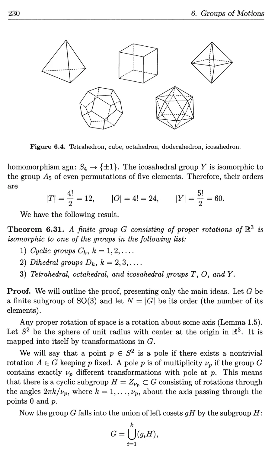
Structures and Fields
S. P. Novikov
I.A.Taimanov
Graduate Studies
in Mathematics
Volume 71
erican Mathematical Society

Modern Geometric
Structures and Fields

Modern Geometric
Structures and Fields
S. P. Novikov
I.A.Taimanov
Translated by
Dmitry Chibisov
Graduate Studies
in Mathematics
Volume 71
^l^^fySI American Mathematical Society
Providence, Rhode Island

Editorial Board
David Cox
Walter Craig
Nikolai Ivanov
Steven G. Krantz
David Saltman (Chair)
C. II. Hobhkob, VL. A. TaiiMaHOB
COBPEMEHHblE TEOMETPMHECKME CTPYKTYPbl H IIOJLH
MIIHMO, MocKBa, 2005
This work was originally published in Russian by MIIHMO under the title
"CoBpeMeHHbie TeoMeTpH^ecKHe CTpyrcrypbi h IIojiji" ©2005. The present
translation was created under license for the American Mathematical Society
and is published by permission.
Translated from the Russian by Dmitry Chibisov
2000 Mathematics Subject Classification. Primary 53-01; Secondary 57-01.
For additional information and updates on this book, visit
www.ams.org/bookpages/gsm-71
Library of Congress Cataloging-in-Publication Data
Novikov, Sergei Petrovich.
[Sovremennye geometricheskie struktury i polia. English]
Modern geometric structures and fields / S.P. Novikov, LA. Taimanov.
p. cm. — (Graduate studies in mathematics, ISSN 1065-7339 ; v. 71)
Includes bibliographical references and index.
ISBN-13: 978-0-8218-3929-4 (alk. paper)
ISBN-10: 0-8218-3929-2 (alk. paper)
1. Geometry, Riemannian. 2. Differentiable manifolds. I. Taimanov, I. A. (Iskander Asanovich),
1961- II. Title. III. Series.
QA685.N6813 2006
516.3'73—dc22 2006047704
Copying and reprinting. Individual readers of this publication, and nonprofit libraries
acting for them, are permitted to make fair use of the material, such as to copy a chapter for use
in teaching or research. Permission is granted to quote brief passages from this publication in
reviews, provided the customary acknowledgment of the source is given.
Republication, systematic copying, or multiple reproduction of any material in this publication
is permitted only under license from the American Mathematical Society. Requests for such
permission should be addressed to the Acquisitions Department, American Mathematical Society,
201 Charles Street, Providence, Rhode Island 02904-2294, USA. Requests can also be made by
e-mail to reprint-permissioiiQams.org.
© 2006 by the American Mathematical Society. All rights reserved.
The American Mathematical Society retains all rights
except those granted to the United States Government.
Printed in the United States of America.
@) The paper used in this book is acid-free and falls within the guidelines
established to ensure permanence and durability.
Visit the AMS home page at http: //www. ams. org/
9 8 7 6 5 4 3 2 1 11 10 09 08 07 06

Contents
Preface to the English Edition
Preface
Chapter 1. Cartesian Spaces
and Euclidean Geometry
1.1. Coordinates. Space-time
1.1.1. Cartesian coordinates
1.1.2. Change of coordinates
1.2. Euclidean geometry and linear algebra
1.2.1. Vector spaces and scalar products
1.2.2. The length of a curve
1.3. AfRne transformations
1.3.1. Matrix formalism. Orientation
1.3.2. Affine group
1.3.3. Motions of Euclidean spaces
1.4. Curves in Euclidean space
1.4.1. The natural parameter and curvature
1.4.2. Curves on the plane
1.4.3. Curvature and torsion of curves in R3
Exercises to Chapter 1
Chapter 2. Symplectic and Pseudo-Euclidean Spaces
2.1. Geometric structures in linear spaces
2.1.1. Pseudo-Euclidean and symplectic spaces
2.1.2. Symplectic transformations
2.2. The Minkowski space

vi
Contents
2.2.1. The event space of the special relativity theory 43
2.2.2. The Poincare group 46
2.2.3. Lorentz transformations 48
Exercises to Chapter 2 50
Chapter 3. Geometry of Two-Dimensional Manifolds 53
3.1. Surfaces in three-dimensional space 53
3.1.1. Regular surfaces 53
3.1.2. Local coordinates 56
3.1.3. Tangent space 58
3.1.4. Surfaces as two-dimensional manifolds 59
3.2. Riemannian metric on a surface 62
3.2.1. The length of a curve on a surface 62
3.2.2. Surface area 65
3.3. Curvature of a surface 67
3.3.1. On the notion of the surface curvature 67
3.3.2. Curvature of lines on a surface 68
3.3.3. Eigenvalues of a pair of scalar products 70
3.3.4. Principal curvatures and the Gaussian curvature 73
3.4. Basic equations of the theory of surfaces 75
3.4.1. Derivational equations as the "zero curvature"
condition. Gauge fields 75
3.4.2. The Codazzi and sine-Gordon equations 78
3.4.3. The Gauss theorem 80
Exercises to Chapter 3 81
Chapter 4. Complex Analysis in the Theory of Surfaces 85
4.1. Complex spaces and analytic functions 85
4.1.1. Complex vector spaces 85
4.1.2. The Hermitian scalar product 87
4.1.3. Unitary and linear-fractional transformations 88
4.1.4. Holomorphic functions and the Cauchy-
Riemann equations 90
4.1.5. Complex-analytic coordinate changes 92
4.2. Geometry of the sphere 94
4.2.1. The metric of the sphere 94
4.2.2. The group of motions of a sphere 96
4.3. Geometry of the pseudosphere 100
4.3.1. Space-like surfaces in pseudo-Euclidean spaces 100
4.3.2. The metric and the group of motions of the
pseudosphere 102

Contents
vii
4.3.3. Models of hyperbolic geometry 104
4.3.4. Hilbert's theorem on impossibility of imbedding the
pseudosphere into M3 106
4.4. The theory of surfaces in terms of a conformal parameter 107
4.4.1. Existence of a conformal parameter 107
4.4.2. The basic equations in terms of a conformal parameter 110
4.4.3. Hopf differential and its applications 112
4.4.4. Surfaces of constant Gaussian curvature. The Liouville
equation 113
4.4.5. Surfaces of constant mean curvature. The sinh-Gordon
equation 115
4.5. Minimal surfaces 117
4.5.1. The Weierstrass-Enneper formulas for minimal surfaces 117
4.5.2. Examples of minimal surfaces 120
Exercises to Chapter 4 122
Chapter 5. Smooth Manifolds 125
5.1. Smooth manifolds 125
5.1.1. Topological and metric spaces 125
5.1.2. On the notion of smooth manifold 129
5.1.3. Smooth mappings and tangent spaces 133
5.1.4. Multidimensional surfaces in Rn. Manifolds with
boundary 137
5.1.5. Partition of unity. Manifolds as multidimensional
surfaces in Euclidean spaces 141
5.1.6. Discrete actions and quotient manifolds 143
5.1.7. Complex manifolds 145
5.2. Groups of transformations as manifolds 156
5.2.1. Groups of motions as multidimensional surfaces 156
5.2.2. Complex surfaces and subgroups of GL(n, C) 163
5.2.3. Groups of affine transformations and the Heisenberg
group 165
5.2.4. Exponential mapping 166
5.3. Quaternions and groups of motions 170
5.3.1. Algebra of quaternions 170
5.3.2. The groups SO(3) and SO(4) 171
5.3.3. Quaternion-linear transformations 173
Exercises to Chapter 5 175
Chapter 6. Groups of Motions 177
6.1. Lie groups and algebras 177

viii
Contents
6.1.1. Lie groups 177
6.1.2. Lie algebras 179
6.1.3. Main matrix groups and Lie algebras 187
6.1.4. Invariant metrics on Lie groups 193
6.1.5. Homogeneous spaces 197
6.1.6. Complex Lie groups 204
6.1.7. Classification of Lie algebras 206
6.1.8. Two-dimensional and three-dimensional Lie algebras 209
6.1.9. Poisson structures 212
6.1.10. Graded algebras and Lie superalgebras 217
6.2. Crystallographic groups and their generalizations 221
6.2.1. Crystallographic groups in Euclidean spaces 221
6.2.2. Quasi-crystallographic groups 232
Exercises to Chapter 6 242
Chapter 7. Tensor Algebra 245
7.1. Tensors of rank 1 and 2 245
7.1.1. Tangent space and tensors of rank 1 245
7.1.2. Tensors of rank 2 249
7.1.3. Transformations of tensors of rank at most 2 250
7.2. Tensors of arbitrary rank 251
7.2.1. Transformation of components 251
7.2.2. Algebraic operations on tensors 253
7.2.3. Differential notation for tensors 256
7.2.4. Invariant tensors 258
7.2.5. A mechanical example: strain and stress tensors 259
7.3. Exterior forms 261
7.3.1. Symmetrization and alternation 261
7.3.2. Skew-symmetric tensors of type (0, k) 262
7.3.3. Exterior algebra. Symmetric algebra 264
7.4. Tensors in the space with scalar product 266
7.4.1. Raising and lowering indices 266
7.4.2. Eigenvalues of scalar products 268
7.4.3. Hodge duality operator 270
7.4.4. Fermions and bosons. Spaces of symmetric and skew-
symmetric tensors as Fock spaces 271
7.5. Poly vectors and the integral of anticommuting variables 278
7.5.1. Anticommuting variables and superalgebras 278
7.5.2. Integral of anticommuting variables 281
Exercises to Chapter 7 283
Chapter 8. Tensor Fields in Analysis
285

Contents
ix
8.1. Tensors of rank 2 in pseudo-Euclidean space 285
8.1.1. Electromagnetic field 285
8.1.2. Reduction of skew-symmetric tensors to canonical form 287
8.1.3. Symmetric tensors 289
8.2. Behavior of tensors under mappings 291
8.2.1. Action of mappings on tensors with superscripts 291
8.2.2. Restriction of tensors with subscripts 292
8.2.3. The Gauss map 294
8.3. Vector fields 296
8.3.1. Integral curves 296
8.3.2. Lie algebras of vector fields 299
8.3.3. Linear vector fields 301
8.3.4. Exponential function of a vector field 303
8.3.5. Invariant fields on Lie groups 304
8.3.6. The Lie derivative 306
8.3.7. Central extensions of Lie algebras 309
Exercises to Chapter 8 312
Chapter 9. Analysis of Differential Forms 315
9.1. Differential forms 315
9.1.1. Skew-symmetric tensors and their differentiation 315
9.1.2. Exterior differential 318
9.1.3. Maxwell equations 321
9.2. Integration of differential forms 322
9.2.1. Definition of the integral 322
9.2.2. Integral of a form over a manifold 327
9.2.3. Integrals of differential forms in R3 329
9.2.4. Stokes theorem 331
9.2.5. The proof of the Stokes theorem for a cube 335
9.2.6. Integration over a superspace 337
9.3. Cohomology 339
9.3.1. De Rham cohomology 339
9.3.2. Homotopy invariance of cohomology 341
9.3.3. Examples of cohomology groups 343
Exercises to Chapter 9 349
Chapter 10. Connections and Curvature 351
10.1. Covariant differentiation 351
10.1.1. Covariant differentiation of vector fields 351
10.1.2. Covariant differentiation of tensors 357
10.1.3. Gauge fields 359

X
Contents
10.1.4. Cartan connections 362
10.1.5. Parallel translation 363
10.1.6. Connections compatible with a metric 365
10.2. Curvature tensor 369
10.2.1. Definition of the curvature tensor 369
10.2.2. Symmetries of the curvature tensor 372
10.2.3. The Riemann tensors in small dimensions, the Ricci
tensor, scalar and sectional curvatures 374
10.2.4. Tensor of conformal curvature 377
10.2.5. Tetrad formalism 380
10.2.6. The curvature of invariant metrics of Lie groups 381
10.3. Geodesic lines 383
10.3.1. Geodesic flow 383
10.3.2. Geodesic lines as shortest paths 386
10.3.3. The Gauss-Bonnet formula 389
Exercises to Chapter 10 392
Chapter 11. Conformal and Complex Geometries 397
11.1. Conformal geometry 397
11.1.1. Conformal transformations 397
11.1.2. Liouville's theorem on conformal mappings 400
11.1.3. Lie algebra of a conformal group 402
11.2. Complex structures on manifolds 404
11.2.1. Complex differential forms 404
11.2.2. Kahler metrics 407
11.2.3. Topology of Kahler manifolds 411
11.2.4. Almost complex structures 414
11.2.5. Abelian tori 417
Exercises to Chapter 11 421
Chapter 12. Morse Theory and Hamiltonian Formalism 423
12.1. Elements of Morse theory 423
12.1.1. Critical points of smooth functions 423
12.1.2. Morse lemma and transversality theorems 427
12.1.3. Degree of a mapping 436
12.1.4. Gradient systems and Morse surgeries 439
12.1.5. Topology of two-dimensional manifolds 448
12.2. One-dimensional problems: Principle of least action 453
12.2.1. Examples of functionals (geometry and mechanics).
Variational derivative 453
12.2.2. Equations of motion (examples) 457

Contents
xi
12.3. Groups of symmetries and conservation laws 460
12.3.1. Conservation laws of energy and momentum 460
12.3.2. Fields of symmetries 461
12.3.3. Conservation laws in relativistic mechanics 463
12.3.4. Conservation laws in classical mechanics 466
12.3.5. Systems of relativistic particles and scattering 470
12.4. Hamilton's variational principle 472
12.4.1. Hamilton's theorem 472
12.4.2. Lagrangians and time-dependent changes of
coordinates 474
12.4.3. Variational principles of Fermat type 477
Exercises to Chapter 12 479
Chapter 13. Poisson and Lagrange Manifolds 481
13.1. Symplectic and Poisson manifolds 481
13.1.1. ^-gradient systems and symplectic manifolds 481
13.1.2. Examples of phase spaces 484
13.1.3. Extended phase space 491
13.1.4. Poisson manifolds and Poisson algebras 492
13.1.5. Reduction of Poisson algebras 497
13.1.6. Examples of Poisson algebras 498
13.1.7. Canonical transformations 504
13.2. Lagrangian submanifolds and their applications 507
13.2.1. The Hamilton-Jacobi equation and bundles of
trajectories 507
13.2.2. Representation of canonical transformations 512
13.2.3. Conical Lagrangian surfaces 514
13.2.4. The "action-angle" variables 516
13.3. Local minimality condition 521
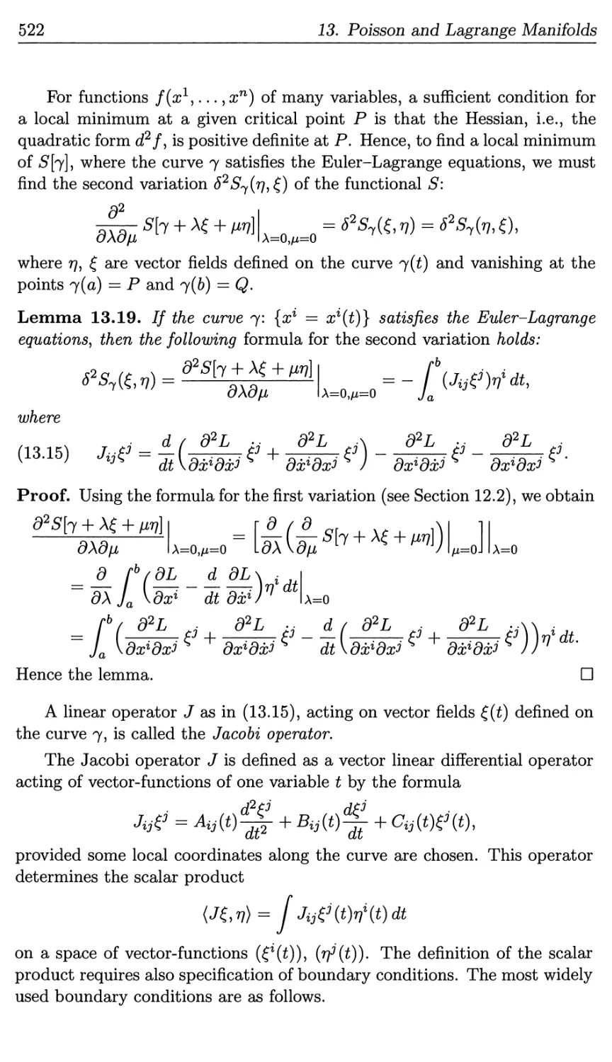
13.3.1. The second-variation formula and the Jacobi operator 521
13.3.2. Conjugate points 527
Exercises to Chapter 13 528
Chapter 14. Multidimensional Variational Problems 531
14.1. Calculus of variations 531
14.1.1. Introduction. Variational derivatives 531
14.1.2. Energy-momentum tensor and conservation laws 535
14.2. Examples of multidimensional variational problems 542
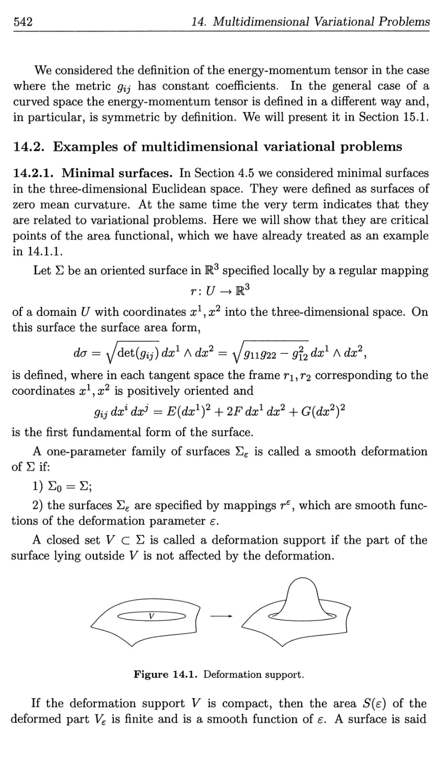
14.2.1. Minimal surfaces 542
14.2.2. Electromagnetic field equations 544
14.2.3. Einstein equations. Hilbert functional 548

xii
Contents
14.2.4. Harmonic functions and the Hodge expansion 553
14.2.5. The Dirichlet functional and harmonic mappings 558
14.2.6. Massive scalar and vector fields 563
Exercises to Chapter 14 566
Chapter 15. Geometric Fields in Physics 569
15.1. Elements of Einstein's relativity theory 569
15.1.1. Principles of special relativity 569
15.1.2. Gravitation field as a metric 573
15.1.3. The action functional of a gravitational field 576
15.1.4. The Schwarzschild and Kerr metrics 578
15.1.5. Interaction of matter with gravitational field 581
15.1.6. On the concept of mass in general relativity theory 584
15.2. Spinors and the Dirac equation 587
15.2.1. Automorphisms of matrix algebras 587
15.2.2. Spinor representation of the group SO(3) 589
15.2.3. Spinor representation of the group 0(1,3) 591
15.2.4. Dirac equation 594
15.2.5. Clifford algebras 597
15.3. Yang-Mills fields 598
15.3.1. Gauge-invariant Lagrangians 598
15.3.2. Covariant differentiation of spinors 603
15.3.3. Curvature of a connection 605
15.3.4. The Yang-Mills equations 606
15.3.5. Characteristic classes 609
15.3.6. Instantons 612
Exercises to Chapter 15 616
Bibliography 621
Index
625

Preface to the English
Edition
The book presents basics of Riemannian geometry in its modern form as the
geometry of differentiable manifolds and the most important structures on
them. Let us recall that Riemannian geometry is built on the following
fundamental idea: The source of all geometric constructions is not the length
but the inner product of two vectors. This inner product can be symmetric
and positive definite (classical Riemannian geometry) or symmetric
indefinite (pseudo-Riemannian geometry and, in particular, the Lorentz geometry,
important in physics). Moreover, this inner product can be complex Her-
mitian and even skew-symmetric (symplectic geometry). The modern point
of view to any geometry also includes global topological aspects related to
the corresponding structures. Therefore, in the book we pay attention to
necessary basics of topology.
With this approach, Riemannian geometry has great influence on a
number of fundamental areas of modern mathematics and its applications.
1. Geometry is a bridge between pure mathematics and natural sciences,
first of all physics. Fundamental laws of nature are expressed as relations
between geometric fields describing physical quantities.
2. The study of global properties of geometric objects leads to the far-
reaching developments in topology, including topology and geometry of fiber
bundles.
3. Geometric theory of Hamiltonian systems, which describe many
physical phenomena, leads to the development of symplectic and Poisson
geometry.
xiii

xiv Preface to the English Edition
4. Geometry of complex and algebraic manifolds unifies Riemannian
geometry with the modern complex analysis, as well as with algebra and
number theory.
We tried, as much as possible, to present these ideas in our book. On
the other hand, combinatorial geometry, which is based on a completely
different set of ideas, remains beyond the scope of this book.
Now we briefly describe the contents of the book.
Chapters 1 and 2 are devoted to basics of various geometries in linear
spaces: Euclidean, pseudo-Euclidean, and symplectic. Special attention is
paid to the geometry of the Minkowski space, which is a necessary ingredient
of relativity.
Chapters 3 and 4 are devoted to the geometry of two-dimensional
manifolds; here we also present necessary facts of complex analysis. Some famous
completely integrable systems of modern mathematical physics also appear
in these chapters.
Basics of topology of smooth manifolds are presented in Chapter 5.
Some material about Lie groups is included in Chapter 6. In addition to
classical theory of Lie groups and Lie algebras, here we pay attention to the
theory of crystallographic groups and their modern generalizations related
to the discovery of so-called quasicrystals.
Chapter 7 and 8 are devoted to classical tensor algebra and tensor
calculus, whereas in Chapter 9 the theory of differential forms (antisymmetric
tensors) is presented. It should be noted that already in Chapters 7 and 9
we encounter the so-called Grassmann (anticommuting) variables and the
corresponding integration.
Chapter 10 contains the Riemannian theory of connections and
curvature. The idea of a general connection in a bundle (Yang-Mills fields) also
appears here.
Conformal geometry and complex geometry are the main subjects of
Chapter 11.
In Chapter 12, we present elements of finite-dimensional Morse theory,
the calculus of variations, and the theory of Hamiltonian systems. Geometric
aspects of the theory of Hamiltonian systems are developed in Chapter 13,
where the theory of Lagrangian and Poisson manifolds is introduced.
Chapter 14 contains elements of multidimensional calculus of variations.
We should emphasize that, contrary to the majority of existing textbooks,
the mathematical language of our exposition is compatible with the language
of modern theoretical physics. In particular, we believe that such notions as
the energy-momentum tensor, conservation laws, and the Noether theorem
are an integral part of the exposition of this subject. Here we also touch

Preface to the English Edition xv
upon simplest topological aspects of the theory, such as the Morse index and
harmonic forms on compact Riemannian manifolds from the point of view
of Hodge theory.
In Chapter 15 we present the basic theory of the most important fields in
physics such as the Einstein gravitation field, the Dirac spinor field, and the
Yang-Mills fields associated to vector bundles. Here we also encounter
topological phenomena such as the Chern and Pontryagin characteristic classes,
and instantons.
Each chapter is supplemented by exercises that allow the reader to get
a deeper understanding of the subject.

Preface
As far back as in the late 1960s one of the authors of this book started
preparations to writing a series of textbooks which would enable a modern
young mathematician to learn geometry and topology. By that time, quite a
number of problems of training nature were collected from teaching
experience. These problems (mostly topological) were included into the textbooks
[DNF1]-[NF] or published as a separate collection [NMSF]. The program
mentioned above was substantially extended after we had looked at
textbooks in theoretical physics (especially, the outstanding series by Landau
and Lifshits, considerable part of which, e.g., the books [LL1, LL2], involve
geometry in its modern sense), as well as from discussions with
specialists in theoretical mechanics, especially L. I. Sedov and V. P. Myasnikov,
in the Mechanics Division of the Mechanics and Mathematics Department
of Moscow State University, who were extremely interested in
establishing courses in modern geometry needed first of all in elasticity and other
branches of mechanics. Remarkably, designing a modern course in geometry
began in 1971 within the Mechanics, rather than the Mathematics Division
of the department because this was where this knowledge was really needed.
Mathematicians conceded to it later. Teaching these courses resulted in
publication of lecture notes (in duplicated form):
S. P. Novikov, Riemannian geometry and tensor analysis. Parts I and
II, Moscow State University, 1972/73.
Subsequently these courses were developed and extended, including, in
particular, elements of topology, and were published as:
S. P. Novikov and A. T. Fomenko, Riemannian geometry and tensor
analysis. Part III, Moscow State University, 1974.
xvii

xviii
Preface
After that, S. P. Novikov wrote the program of a course in the
fundamentals of modern geometry and topology. It was realized in a series of books
[DNF1]-[NF], written jointly with B. A. Dubrovin and A. T. Fomenko.
Afterwards the topological part was completed by the book [Nl], which
contained a presentation of the basic ideas of classical topology as they have
formed by the late 1960s-early 1970s. The later publication [N2] also
included some recent advances in topology, but quite a number of deep new
areas (such as, e.g., modern symplectic and contact topology, as well as new
developments in the topology of 4-dimensional manifolds) were not covered
yet. We recommend the book [AN]. We can definitely say that even now
there is no comprehensible textbook that would cover the main
achievements in the classical topology of the 1950s-1970s, to say nothing of the
later period. Part II of the book [1] and the book [2] are insufficient; other
books are sometimes unduly abstract; as a rule, they are devoted to
special subjects and provide no systematic presentation of the progress made
during this period, very important in the history of topology. Some well-
written books (e.g., [M1]-[MS]) cover only particular areas of the theory.
The book [BT] is a good supplement to [DNF1, DNF2], but its coverage
is still insufficient.
Nevertheless, among our books, Part II of [DNF1] is a relatively good
textbook containing a wide range of basic theory of differential topology in
its interaction with physics. Nowadays this book could be modernized by
essentially improving the technical level of presentation, but as a whole this
book fulfills its task, together with the books [DNF2] and [Nl], intended
for a more sophisticated reader.
As for Part I, i.e., the basics of Riemannian geometry, it has become
clear during the past 20 years that this book must be substantially revised,
as far as the exposition of basics and more complete presentation of modern
ideas are concerned. To this end, the courses [T] given by the second author,
I. A. Taimanov, at Novosibirsk University proved to be useful. We joined
our efforts in writing a new course using all the material mentioned above.
We believe that the time has come when a wide community of
mathematicians working in geometry, analysis, and related fields will finally turn
to the deep study of the contribution to mathematics made by theoretical
physics of the 20th century. This turn was anticipated already 25 years ago,
but its necessity was not realized then by a broad mathematical community.
The advancements in this direction made in our books such as [DNF1] had
not elicited a proper response among mathematicians for a long time. In
our view, the situation is different nowadays. Mathematicians understand
much better the necessity of studying mathematical tools used by physicists.
Moreover, it appears that the state of the art in theoretical physics itself is

Preface
xix
such that the deep mathematical methods created by physicists in the 20th
century may be preserved for future mankind only by the mathematical
community; we are concerned that the remarkable fusion of the strictly rational
approach to the exploration of the real world with outstanding mathematical
techniques may be lost.
Anyhow, we wrote this book for a broad readership of mathematicians
and theoretical physicists. As before (see the Prefaces to the books [DNFl,
DNF2]), we followed the principles that the book must be as comprehensible
as possible and written with the minimal possible level of abstraction. A
clear grasp of the natural essence of the subject must be achieved before
starting its formalization. There is no sense to justify a theory which has
not been perceived yet. The formal language disconnects rather than unites
mathematics, and complicates rather than facilitates its understanding.
We hope that our ideas will be met with understanding by the
mathematical community.
The authors
Bibliography
[DNFl] B. A. Dubrovin, S. P. Novikov, and A. T. Fomenko, Modern geometry: Methods and
applications. Part I. Geometry of surfaces, groups of transformations, and fields. Part II.
Geometry and topology of manifolds. 2nd ed., Nauka, Moscow, 1986; English transl. of
1st ed., Modern geometry—Methods and applications. Parts I and II, Graduate Texts in
Mathematics, vols. 93 and 104, Springer-Verlag, New York, 1992.
[DNF2] B. A. Dubrovin, S. P. Novikov, and A. T. Fomenko, Modern geometry: Methods of the
homology theory, Nauka, Moscow, 1984; English transl. Modern geometry—Methods and
applications. Part III, Graduate Texts in Mathematics, vol. 124, Springer-Verlag, New
York, 1990.
[NF] S. P. Novikov and A. T. Fomenko, Elements of differential geometry and topology, Nauka,
Moscow, 1987; English transl., Math, and Applications (Soviet series), vol. 60, Kluwer,
Dordrecht, 1990.
[NMSF] S. P. Novikov, A. S. Mishchenko, Yu. P. Solov'ev, and A. T. Fomenko, Problems in
geometry: Differential geometry and topology, Moscow State University Press, Moscow,
1978. (Russian)
[LL1] L. D. Landau and E. M. Lifshits, Mechanics, 3rd ed., Nauka, Moscow, 1973; English transl.
of 1st ed., Pergamon Press, Oxford, and Addison-Wesley, Reading, MA, 1960.
[LL2] L. D. Landau and E. M. Lifshits, The field theory, 6th ed., Nauka, Moscow, 1973; English
transl., Pergamon Press, Oxford-New York-Toronto, 1975.
[Nl] S. P. Novikov, Topology-!, Current Problems in Mathematics. Fundamental Directions,
VINITI, Moscow, 1986, vol. 12, pp. 5-252. (Russian)
[N2] S. P. Novikov, Topology. I, Encyclopaedia of Math. Sciences, Springer-Verlag, Berlin, 1996.
(English transl. of [Nl].)
[AN] V. I. Arnol'd and S. P. Novikov, eds., Dynamical systems, Current Problems in
Mathematics. Fundamental Directions, VINITI, Moscow, 1985, vol. 4; English transl., Encyclopaedia
of Math. Sciences, vol. 4, Springer-Verlag, Berlin, 2001.
[Ml] J. W. Milnor, Morse theory, Ann. of Math. Studies, no. 51, Princeton Univ. Press,
Princeton, NJ, 1963.

XX
Preface
[M2] J. W. Milnor, Lectures on the h-cobordism theorem, Princeton Univ. Press, Princeton, NJ,
1965.
[A] M. F. Atiyah, K-Theory, Benjamin, New York, 1967.
[MS] D. McDuff and D. Salamon, Introduction to symplectic topology, Clarendon Press, Oxford,
1995.
[BT] R. Bott and L. W. Tu, Differential forms in algebraic topology, Springer-Verlag, New York-
Heidelberg-Berlin, 1982.
[T] I. A. Taimanov, Lectures on differential geometry, Inst. Comp. Research, Moscow-Izhevsk,
2002. (Russian)

Chapter 1
Cartesian Spaces
and Euclidean
Geometry
1.1. Coordinates. Space-time
1.1.1. Cartesian coordinates. Geometry describes events in a space
consisting of points P, Q,... . We say that Cartesian coordinates are introduced
in this space if each point of the space is associated with an ordered n-tuple
(re1,... , ren) of real numbers, called the coordinates of the point, in such a
way that the following conditions are satisfied:
1) every n-tuple (re1,... , ren) of real numbers corresponds to a point of
the space, being the coordinates of this point;
2) the correspondence between the points of the space and the n-tuples
of coordinates is one-to-one, i.e., the points with coordinates (re1,... ,xn)
and (y1,..., yn) coincide if and only if x% = y% for i = 1,..., n.
A space where Cartesian coordinates (re1, ..., xn) are introduced is called
an n-dimensional Cartesian space and denoted by W1.
The number n is called the dimension of the space.
Our physical space is of dimension n = 3, while time has dimension
n = 1. According to the concepts of modern physics, space and time are
inseparable, and one must consider the 4-dimensional space-time continuum
whose points are instant events. This space is 4-dimensional, with
coordinates the ordered quadruples (t • 00 • 00 • 00 6), where t is the "time instant"
when the event occurs, and re1, re2, re3 are the coordinates of the "spacial
1

1. Cartesian Spaces and Euclidean Geometry
location" of the event. The 3-dimensional space of classical geometry is
then the level surface t = const, and the "life" of an object which may be
regarded at any instant of time as a point (a so-called "point-particle") is
identified with the world line of the point-particle xa(t)y a = 1,2,3.
x(t0) x(ti)
Figure 1.1. The world line of a particle.
We will often refer to the n-tuples x = (re1,..., xn) as the points of the
Cartesian space
>n
1.1.2. Change of coordinates. A real-valued function f(x) defined on
an n-dimensional Cartesian space can be regarded as a function of n real
variables, f(x) = /(x1,..., xn) for x = (jc1, ..., xn).
In what follows we will also consider functions which will not be denned
on the entire space Mn, but rather on a part of Mn, namely, on a domain of
the space.
A domain (without boundary), or an open set in the space W1 is a set
U of points in Rn such that, together with a point x belonging to U, all the
points sufficiently close to x also belong to U. More precisely, U is a domain
in W1 if for each point x$ = (rcj,.. •, Xq) in U there exists e > 0 such that
all the points x = (re1,..., xn) satisfying the inequalities
lie in U. Any domain containing the point x is said to be a neighborhood of
this point.
A set V C Rn is closed if its complement U = Rn \ V, i.e., the set
consisting of all the points that do not lie in V, is open.
A function / defined on the entire space Rn or on a domain in Rn is
called continuous if it is continuous as a function of n real variables that are
Cartesian coordinates in W1. In a similar way, continuously differentiable
(smooth) functions are defined.

1.1. Coordinates. Space-time
Figure 1.2. Examples of domains in a plane (a triangle bounded by
straight lines, interior of a parabola, a bounded domain with smooth
boundary).
Example. Let /i,..., fm: Rn —> R be continuous real-valued functions
on the space Rn. Then the set U of the points x satisfying the inequalities
/i(rc)<0, ..., fm{x)<0
is a domain in Rn.
We prove this assertion. Let xq = (zj,... ,#o) ne m U' Since the
functions /i,..., fm are continuous, one can find positive numbers ei,..., em
such that for each j the inequalities \xl — xl0\ < Ej, i = 1,... , n, imply the
inequality fj(xl,... ,xn) < 0. Putting e = mmjEj we see that the set U
contains all the points such that \x% — Xq\ < e, i = 1,..., n. Therefore U is
a domain.
A domain U is bounded if there is R > 0 such that all the points of U
satisfy the inequality
n
^(^)2<i?2, {x\...,xn)eU.
Let {/ and V be domains in Rn and let F: U —*■ V be a mapping specified
coordinatewise by smooth functions
y% =yx(xl,...,xn), i = l,...,n
(we denote the coordinates in C/ and V by and y3, j =
1,..., n, respectively). The matrix
A{x0) = (aj) = (^C)
is called the Jacobi matrix of the mapping F at the point xq = (xq, ..., #o)
and is denoted by (§|) • The determinant of this matrix is referred to as
the Jacobian of the mapping F and is denoted by J,

1. Cartesian Spaces and Euclidean Geometry
A point xo = (#o> • • • > xo) *s sa^ *° De nonsingular for the mapping F if the
Jacobian at this point does not vanish.
The following inverse function theorem is a version of the implicit
function theorem and is familiar to the reader from a calculus course.
Theorem 1.1. // the mapping F has a nonzero Jacobian at a point xo =
(#o,..., Xq ) then in a sufficiently small neighborhood of the point F(xo) =
(t/q, ...,2/J), where y^ = yx(x\,...,Xq), the coordinates (x1,...,xn) are
uniquely determined by y1}..., yn\
X = X \JJ ,...,?/ J, 1 = 1,. . . , 77,,
and the Jacobi matrix \%) of the inverse mapping F~l is the inverse of
the matrix ( ^ ):
dx% dyi _ i _ J 1 for i = k,
dy^'dx1*- k~[0 fori + k.
Here and elsewhere we apply the convention of summation over repeated
indices, i.e., the presence of an index repeated once as a subscript and once
as a superscript means summation over this index (over j in the above
expression).
This theorem implies that in a neighborhood of a nonsingular point the
functions y1i... yyn specify new coordinates, which are connected with the
coordinates n by smooth one-to-one transformations,
yi = yi(x11...txn)y xj =xj(y1,...,yn), 1 <ij <n.
In general, whenever there exists such a mapping between the domains U
and V in Rn, we say that a change of coordinates is given.
The simplest example of a change of coordinates is provided by a linear
transformation
yx = djX3, i = 1,... ,n.
In this case the Jacobi matrix is constant and equal to (ap, while the inverse
mapping has the form
x% = bjy3, i = 1,... ,n,
where &*• a?k = 8\.
However, in the plane and in three-dimensional space there are systems
of coordinates, useful for applications, which are related to the Cartesian
coordinates by transition functions y% = yl{x1y... ,#n) nonlinear in x3.
1. Polar coordinates r,cp in the plane with Cartesian coordinates re1, a;2:
x1=rcos(p, x2 = rsm(p,

1.1. Coordinates. Space-time
5
where r > 0. For an integer k, the pairs (r, </?) and (r, y? + 27r/c) represent the
same point; therefore, in order to make the coordinate ip single-valued, we
will impose the restriction 0 < (p < 2ir. The Jacobi matrix of the mapping
(r,y>) —> (re1, re2) is
~W ~&y \ _ /cosy? — rsin</?
&c2 &r2 I I siny> rcosy>
and its determinant (Jacobian) equals
J = r > 0.
The Jacobian vanishes only for r = 0. Hence in the domain r > 0, 0 <
Figure 1.3. Polar coordinates.
(p < 27r, i.e., in the plane R2 with deleted half-line x1 > 0, x2 = 0, the
coordinates r, y? are uniquely determined and have no singular points.
2. Cylindrical coordinates r, y>,2 in R3:
1 O 9
re =r cosy?, re =rsin</?, re = z,
where re1, re2, re3 are Cartesian coordinates in M3. The Jacobian of the change
of coordinates (r,(p}z) —► (re1, re2, re3) vanishes only for r = 0; therefore, this
mapping has no singular points in the domain r > 0. As before, these
coordinates are uniquely determined if 0 < (p < 2tt.
3. Spherical coordinates r, 9,(p in R3:
"1 O 9
re =r cosy? sin #, re =rsiny?sin0, re =rcos#,
where r > 0, 0 < 0 < 7r, 0 < </? < 27r. The Jacobian equals J = r2 s'mO and
does not vanish in the domain r > 0, 0 ^ 0, ir. In the domain r > 0, 0 <
0 < 7r, 0 < y? < 27r, the spherical coordinates are uniquely determined and
the transition mapping (r, #,</?) —> (re1, re2, re3) has no singular points.
•

6 1. Cartesian Spaces and Euclidean Geometry
Zk
2<r
r
Figure 1.4. Cylindrical coordinates.
Figure 1.5. Spherical coordinates.
1.2. Euclidean geometry and linear algebra
1.2.1. Vector spaces and scalar products. The Cartesian space W1 is
associated in a natural way with an n-dimensional vector space.
Namely, to each point P — (a?1,..., xn) corresponds the "radius-vector"
of its coordinates, which is the n-tuple (x1}..., xn) regarded as a vector £ in
n-dimensional vector space. We will denote points and their radius-vectors
by the same symbols: x = (x1,..., xn).
The vectors may be added and multiplied by real numbers: if £ =
(f\ • • • >£n) and 7] = (n1,... ,nn), then
The vectors e% = (0,..., 1,..., 0) (with 1 on the ith. place) for i = 1,..., n
form a basis of the vector space.
Let L be a subset of M.n specified by a system of linear equations
djXj + 6l = 0, i = l,...,n- k

1.2. Euclidean geometry and linear algebra
(with summation over repeated indices), or
a\xl + a\x2 H + a\xn + bl =0,
aj~ V + a^z2 + • • • + a^~kxn + bn~k = 0,
and let the (n — k) x n matrix (a!) be of maximal rank n — k < n. Then,
for x\ and X2 running over L, the vectors x\ — X2 form a ft-dimensional
vector space. For this reason, L is called a A;-dimensional plane in En, and
a hyperplane for k = n — 1.
In order to define the length of a straight line segment in Mn, we must
introduce a symmetric positive Euclidean scalar product on the n-dimensional
vector space, i.e., a real-valued function (£, rj) of a pair of vectors such that:
a) (Aifi+A2&,f7)=Ai(£i,77)+A2(&,»7), (£,Ai»n + A2^2> = ^i{^m) +
A2(£>772) for Ai,A2 Gl (bilinearity);
b) (€>V) = foO (symmetry);
c) (^,0>0if^0(positivity).
A Cartesian space endowed with a Euclidean scalar product is referred to
as a Euclidean space. The squared length of the vector £ equals |£|2 = (£,£),
and the angle (p between vectors £ and rj is denned by the formula
cos„= «!"> = j3>
y^l)xA^?> KIM
The validity of this definition, i.e., the inequality
—1 < cosy? < 1,
is provided by the well-known inequality
(t,v)2 = (E^)2 ^ (£#)(£*?) = ^o(v,v),
which holds since
(£<) (£ tf) - (£6«)2 = \ £«*« - ^)2 * °-
If re and y are two points in Mn, then the distance p{xyy) between them
is defined as the length of the vector x — y:
p(x,y) = \x-y\.
The distance so defined fulfills the following requirements:
1) pfav) = p(y,x)',
2) p(x,z) < p{x,y) + p(y,z) (the triangle inequality);
3) p(x, y) > 0 for all #, y, and p(x, y) = 0 if and only if x = y.

8 1. Cartesian Spaces and Euclidean Geometry
x p(x, z) z
Figure 1.6. A triangle.
These definitions of length and angle are based on the Pythagorean
theorem. Indeed, by linearity of the scalar product in both arguments,
where £ = £le;, rj = rfiej. The matrix (g%j) with gij = (ei,ej) is referred
to as the Gram matrix of the scalar product. In case this is the identity
matrix,
Jl fori =,7,
10 otherwise,
the coordinates in W1 are called Euclidean^ and the basis e\,..., en is said
to be orthonormal. When the coordinates are Euclidean, the line segments
joining the points O = (0,..., 0), P = (a, 0,..., 0), and Q = (0,6,0,..., 0)
form a right-angle triangle OPQ. The lengths of its catheti OP and OQ
equal |a| and |6|. By the Pythagorean theorem, the length of the side PQ
equals \/a2 + 62, which is the length of the difference of radius-vectors of the
points P and Q. In general, bilinearity and symmetry of the scalar product
imply that
«- v,t -v) = (U) + {v,v) -2«,i/>,
and if £ and rj are radius-vectors of the points P and Q, this identity becomes
the cosine theorem for the triangle OPQ.
Theorem 1.2. In any finite-dimensional vector space V with a symmetric
positive scalar product there exists an orthonormal basis.
Proof. Take a nonzero vector £i and put e\ = £i/|£i|. Denote by V\ the one-
dimensional subspace spanned by £i, and by Vf1, its orthogonal complement.
The subspace Vf1 is a hyperplane specified by the linear equation
(?7,ei) =0,
and its dimension is by one less than that of V. Now we perform the same
operation with Vj1: take £2 £ VfS where £2 7^ 0, put 62 = &/I&I) etc.

1.2. Euclidean geometry and linear algebra 9
Since the space V is finite-dimensional, after finitely many steps we will
construct an orthonormal basis ei,..., en. D
Corollary 1.1. In any Euclidean space there exist Euclidean coordinates.
In view of this corollary, for any given n we may speak about a single
Euclidean space of dimension n because the choice of Euclidean coordinates
makes the spaces of the same dimension indistinguishable.
In what follows, when speaking about a Euclidean space, we will assume
that the coordinates in this space are Euclidean.
If we are already given some basis e?i,... ,en in the space V, then an
orthonormal basis can be constructed in a canonical way (by means of the
procedure known as the Gram-Schmidt orthogonalization). Namely, put
ei = ei/|ei|. In the subspace spanned by the vectors e\ and e2, construct
an orthogonal basis consisting of ei and the vector
£ = e2 - (ei,e2)ei
(which is orthogonal to e\ by construction) and then normalize £ by setting
e2 = £/|£|- Applying this operation successively, for each A; we arrive at an
orthonormal system of vectors ei,..., e& such that their linear span coincides
with that of the vectors e?i,..., e&. Then we put
k ~ f
Continuing this way, we end up with an orthonormal basis c\,..., en such
that for each k the linear span of the vectors ei,..., e& coincides with the
linear span of e?i,..., e&.
This canonical procedure can be used, e.g., for constructing bases in the
following spaces of polynomials.
Let p be a piecewise continuous nonnegative function on an interval [a, 6],
and let p be positive at least on some subinterval of [a, b]. Consider the space
formed by polynomials y?, ip,... of degree at most n with scalar product
<^V,)p= / <p{x)i/>(x)p(x)dx.
J a
The function p is called the weight function. Two polynomials <p and tp are
orthogonal if (y?, ip)p = 0.
Taking the family e{ = xl~l, i = l,...,n + 1, for the initial basis,
the canonical orthogonalization procedure results in an orthonormal basis
ei,..., en+i such that e^ for each i is a polynomial of degree i — 1. Here are
the best-known examples of such systems of orthogonal polynomials.

10 1. Cartesian Spaces and Euclidean Geometry
Example 1. Let [a,6] = [—1,1] and p(x) = 1. In this case ek+i(x) =
Pk(x), k > 0. The polynomials
Pk(x) = \j ^y Pk(x), (PhPk) = Sik,
are called the Legendre polynomials,
P0(x) = 1, Pi(z) = x, P2(x) = i (3x2 - 1),...,
Example 2. Again, let [a, 6] = [—1,1], but this time take the weight
function to be p(x) = 1/Vl — x2. Then
11 [2
ei(x) = —=Tq{x) = -7=, ek+i(x) = \ -Tk(x), k>l,
where Tjt(a;) = cos(A; arccosrc). The Tjt are called the Chebyshev polynomials.
If the weight function p(x) is denned on the entire real line and decreases
at infinity fast enough for the integral
/oo
(p(x)ip(x)p{x) dx
-oo
to converge for any pair of polynomials, then this function specifies a scalar
product on the space of polynomials on the real line.
Example 3. Let p(x) = e~x2/2. Then (setting k\ = 1 for k = 0)
where the polynomials Hk(x) are uniquely determined by the recurrence
relations
H0{x) = 1, Hk+i(x) = xHk(x) - — Hk{x).
They are called the Hermite polynomials.
1.2.2. The length of a curve. Now we turn from linear to more
complicated objects.
A smooth parametrized curve in W1 is a line in Rn specified by smooth
functions of a univariate parameter t:
r(t) = (x\t),...,xn(t)).

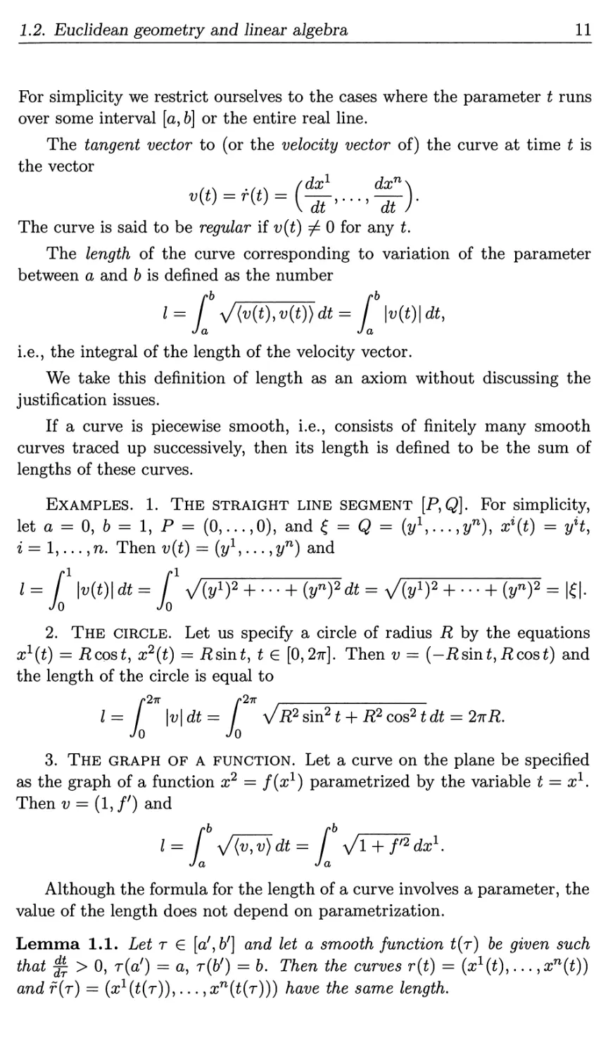
1.2. Euclidean geometry and linear algebra 11
For simplicity we restrict ourselves to the cases where the parameter t runs
over some interval [a, b] or the entire real line.
The tangent vector to (or the velocity vector of) the curve at time t is
the vector
(dx dxn \
The curve is said to be regular if v(t) ^ 0 for any t.
The length of the curve corresponding to variation of the parameter
between a and b is defined as the number
rb rb
1= / ^/(v(t),v(t))dt = / \v(t)\dtt
J a J a
i.e., the integral of the length of the velocity vector.
We take this definition of length as an axiom without discussing the
justification issues.
If a curve is piecewise smooth, i.e., consists of finitely many smooth
curves traced up successively, then its length is defined to be the sum of
lengths of these curves.
Examples. 1. The straight line segment [P,Q]. For simplicity,
let a = 0, b = 1, P = (0, ...,0), and f = Q = (j/1,... ,yn), x^t) = yHt
i = 1,... ,n. Then v(t) = (y1,... ,yn) and
/= / \v(t)\dt= f VQ/1)2 + • • • + (yn)2dt = Vfo1)2 + • • • + (yn)2 = l£|.
Jo Jo
2. The circle. Let us specify a circle of radius R by the equations
x1^) = Rcost, x2(t) = Rsint, t G [0,2ir]. Then v = (—Rsmt,Rcost) and
the length of the circle is equal to
/*27r p2ir
/= / \v\dt= VR2 sin21 + R2 cos21 dt = 2irR.
Jo Jo
3. The graph of a function. Let a curve on the plane be specified
as the graph of a function x2 = fix1) parametrized by the variable t = x1.
Thenv = (l}f) and
/= f y/(Viv)dt= j Vl + f,2dx\
J a J a
Although the formula for the length of a curve involves a parameter, the
value of the length does not depend on parametrization.
Lemma 1.1. Let r 6 [a ,6] and let a smooth function t(r) be given such
dr
that £ > 0, r(af) = a, r{b') = b. Then the curves r(t) = (x1^),... }xn(t))
and r(r) = (ar(£(r)),... }xn(t(r))) have the same length.

12 1. Cartesian Spaces and Euclidean Geometry
Proof. Indeed,
«'>-jfi/<yjJ>*
,(f) , f JKf)ir - I" J/****)*
Ja> V W dr/ Ja, V \dt dr dt drI
=L "l(%di)frdT=L v/(^S)di=/(r)-
The proof is completed. □
1.3. Affine transformations
1.3.1. Matrix formalism. Orientation. An affine transformation of W1
is an invertible transformation of Rn into itself which in Cartesian
coordinates is given by the formula
xl\ fxl
(ii) I ; l-H ; 1 + h =
xn) \xn) \bn) \a^xi + bn/
where the n x n matrix A = (a*) and the vector b = (b1) do not depend on
jc1, ... ,rcn. In what follows we will briefly write formulas like this as
x —> Ax + b or y = Ax + b.
We have already used in 1.1.2 the following rule of summation over repeated
indices, which will be used throughout, unless otherwise stated.
If a formula involves an index repeated once as a superscript and once
as a subscript, then this means that the expression is summed up over all
possible values of this index.
For instance, formula (1.1) involves a repeated index i} which means
summation over alH = 1,..., n.
Each affine transformation is associated with a linear transformation of
the vectors of the Cartesian space, which is specified by the matrix A:
C-+At or ? = At.
This transformation has a simple geometric structure. Let the affine
transformation map the points x\ and x^ into the points x[ and x'2. The difference
£' = x[ — x'2 depends only on the difference £ = x\ — x^ and we have £' = A£.
Any two bases ei,..., en and ei,..., en of the Cartesian space are related
to each other by mutually inverse transition matrices,
(1.2) ei = a\ej, ij = a^e^ a\akj = <Sj.

1.3. Affine transformations
13
The bases are said to have the same orientation if det A > 0. Obviously all
bases fall into two classes such that:
1) two bases have the same orientation if and only if they belong to the
same class;
2) if two bases belong to different classes and A is the transition matrix,
then det A < 0.
In order to specify the orientation of the space W1 we have to choose
one of these classes as the class of positively oriented bases. The bases of
the alternative class are then negatively oriented.
An affine transformation x —> Ax + b of an oriented Cartesian space
is said to be proper if the transformation A: (ei,..., en) —> (Aei,..., Aen)
maps positively oriented bases of this space again into positively oriented
bases. Obviously, a transformation is proper if and only if det A > 0.
Suppose we are given two systems of Cartesian coordinates (a?1,..., xn)
and (sc1,... ,xn) in W1. Assume for simplicity that they have a common
origin. Then the coordinates are related by the formula
Putting (1.2) into this relation we obtain
and therefore
x3 = a\x%.
In a similar way it can be shown that
(1.3) xi = a)xj.
In the coordinates (a;1,..., xn) the affine transformation
x —> Bx = y
is given by another matrix, which can be easily found. The radius-vector of
the point Bx is expanded in the basis \^\ j • • • j ^7T, Cw^ Bx = b\xkei. Therefore,
its expansion in the basis e\,..., en is
y = b\xkei = (b)exk)a?ieji
and substituting (1.3) we obtain
y={bia*nxm4)ej.
Since the matrices A = (a*) and A = (aj) are mutually inverse, we have
Vm = dUkakm, B = ABA-1.

14 1. Cartesian Spaces and Euclidean Geometry
Now the formula for the transformation x —> Bx in the new coordinates
takes its final form
£-► Bx, B = ABA~l.
Usually we will tacitly assume that a coordinate system is given. In
this case we will identify transformations with matrices which specify them.
These are always nonsingular square matrices.
If we dispense with these properties and consider arbitrary matrices, we
obtain linear mappings from one space into another, with possibly different
dimensions of the spaces.
A mapping A: V —► W of vector spaces is said to be linear if
1) Afa + &) = Mi + M2 for any pair of vectors £1, £2 € V\
2) A(\() = \A£ for any f G V and A G R.
If ei,..., en is a basis in V and ei,..., em a basis in W, then a linear
mapping is uniquely determined by the matrix a!- such that
A£ = aJ£J'e?t, where £ = £J'ej.
If V = W and the mapping A is invertible, we obtain a linear transformation.
1.3.2. Affine group. Recall that a group is a set G endowed with two
operations on its elements: multiplication associating with each ordered
pair of elements g, h their product gh G G, and inversion associating with
each element g its inverse g~l G G.
Moreover, there is the unit element 1 G G (the identity of G), and all
the elements f,g,h G G satisfy the following conditions:
!) f(9h) = (fg)h (associativity);
2)gg-1=g-1g = l;
3) 9 -1 = 1 • 9 = g.
The composition of mappings <p: X —> Y and ip: Y —> Z is the mapping
such that
#>(s) = ip{<p{x))
for every x £ X. The composition operation is associative,
The composition of affine transformations y?: x —► Ax+c and -0: # —► Bx-\-d
is
tp(p: x ^ BAx + (Be + d),

1.3. Affine transformations
15
or, in more detail,
bl^xi + b\ci + dl\
b?a)x> + bfc1 + dnj
The composition of affine transformations is obviously invertible and
Therefore, the composition of affine transformations is again an affine
transformation.
Theorem 1.3. Affine transformations with composition and inversion
operations form a group with the identity transformation as the unit element.
The group of affine transformations is called the affine group and is
denoted by A(n).
Proof of the theorem. Since the affine transformation g: x —> Ax + b is
invertible, we have Ax-\-b ^ Ay+b for x ^ yy hence A(x—y) ^ 0. Therefore,
the matrix A is invertible, so the transformation
g~x\ x —> A~lx- A~lb
is also affine. The proof is completed. □
Affine transformations of the form
x —> x + 6
are called translations. A translation x —> x + a is a shift along the vector a.
The product of translations along vectors a and b is the translation along
the vector a + 6, and the inverse of the translation along the vector a is
the translation by (—a). Hence we conclude that translations form a group,
which is isomorphic to the additive group of vectors of the space. This
group is commutative, i.e., the order of factors does not affect the value of
the product, gh = hg.
Another example of affine transformations is provided by linear
transformations, which are written in Cartesian coordinates as
x —> Ax.
The composition of linear transformations x —*■ Ax and x —> Bx is again a
linear transformation
x —► BAx.
The inverse transformation to x —> Ax = y is y —> A~xy = x.
x
x
n

16 1. Cartesian Spaces and Euclidean Geometry
The linear transformations of M.n form a (complete) linear group, which
coincides with the group of nonsingular n x n matrices denoted by GL(n).
For n > 1 this group is noncommutative.
A special class of linear transformations is formed by dilatations or ho-
motheties determined by the matrices A that are multiples of the identity
matrix,
x —> Xx = y.
A motion of the space Rn is a smooth mapping (p: Rn —► Rn preserving
distances between points,
\x-y\ = p(xty) = p((p(x)t<p(y)) = \tp(x) - <p(y)\
for any pair of points x and y.
It is easily seen that translations preserve distances between points, so
that they are a particular case of motions.
Theorem 1.4. Any motion of the Euclidean space is an affine
transformation.
Proof. It can be easily shown that any motion ip maps straight lines into
straight lines. We will present this geometric argument, although it will not
be needed in the proof.
Let xy yy z be three points lying consecutively on a straight line.
Construct the triangle with vertices at <p(x), <p{y)> <p(z). By the triangle
inequality,
(1.4) p((p(x),(p(y)) + p(ip(y),ip(z)) > p(<p(x)y <p(z)).
The equality is attained only when the angle at the vertex cp(y) equals 7r,
i.e., all the three vertices lie on the same straight line (see Figure 1.7).
Figure 1.7. The extreme case in inequality (1.4).
Since
p(x,y) + p{y,z) = p{x,z)
and (p is a motion, we see that (1.4) is also an equality. The point y inside
the interval xz was chosen arbitrarily. Therefore, cp maps the entire straight
line segment again into a straight line segment, hence it maps straight lines
into straight lines.

1.3. Affine transformations
17
Let (p(0) = 6, where 0 = (0,..., 0). The composition of the
transformation (p and the translation x —► x — b is a motion
tp: x —> ip(x) — b
such that ip(0) = 0. We will prove that the motion tp is linear.
First of all, observe that if a motion a maps the zero point into itself,
then
(x,y) = (a{x),a{y))
for any vectors x and y. Indeed, the condition that a preserves the distance
between x and y can be written as
{x - y, x - y) = (a{x) - a(y),a{x) - a(y)),
and for y = 0 the equality a(0) = 0 implies
(xyx) = (a(x),a(x)).
Generally, we have
(x - y,x- y) = (xtx) - 2(x,y) + (y,y)
= {a(x), a(x)) - 2(a(rc), a(y)) + (a(y)t a(y))
= (a{x) - a(y)t a(x) - a(y)),
which implies that (x,y) = (a(x)ya(y)).
Now, let jci, ..., xn be the points with radius-vectors e\ = (1,0,...,0),
..., en = (0,... ,0,1). Denote by ei the radius-vector of the point ip{xi).
Since ip is a motion and -0(0) = 0, we have
\€iiei) = \ei)ei) = 1)
(e», ej) = (e», ej) = 0 for i ^ j.
Therefore, the vectors ei,..., en form an orthonormal basis.
Denote by A the matrix specifying the linear transformation which maps
ei into ei. Since this transformation maps an orthonormal basis again into
an orthonormal basis, it determines a motion x: x —> Ax. Obviously, the
composition xi> is also a motion, and
x<0(o) = o, x^M = et-
We expand the vectors x and x^(^) m the basis ei,..., en:
n n
x = ^(z, e»)ei, X^(x) = ^(xV(^), ei)e».
Since
(X?l>(x),ei) = (x^{x),Xip{ei)) = (s,e<),
we have
x = xi>{x)

18 1. Cartesian Spaces and Euclidean Geometry
for any vector x. Hence the motion x^ 1S the identity, and therefore the
transformation ip is linear,
ip: x —> A~lx.
This implies that the transformation (p is linear as well,
tp(x) = A~lx + b.
Hence the theorem. □
It is easily seen that the motions of the space W1 form a group. This
group is denoted by E(n).
Recall that a subgroup F of a group G is a set of elements of G which
is closed with respect to the multiplication and inversion operations. In
this case F is itself a group relative to these operations. The groups of
translations, linear transformations, and motions are subgroups of the affine
group A(n) and are denoted by Mn, GL(n), and E(n), respectively.
A mapping tp of a group G into a group if,
(p: G^H,
is a homomorphism of groups if it preserves the operations: (p(ab) = (p(a)ip(b)
and <^(a_1) = (y>(a))-1. Obviously, it must map the unit element into the
unit element: <p(1g) = ^(a)^(a_1) — Iff •
The elements of G that are mapped into 1# by the homomorphism <p
form a subgroup Kenp, which is called the kernel of the homomorphism.
If, for a subgroup F C G, there is a homomorphism ip: G —> H into
a group H such that Kercp = F, then the subgroup F is called a normal
subgroup (or a normal divisor). In such a case, if the homomorphism ip
maps the group G onto the entire group Hy then H is called the quotient
group of the group G by the subgroup F> H = G/F. Obviously, to any
normal subgroup F corresponds the quotient group G/F = (p(G).
If for a homomorphism <p: G —> H there is a homomorphism </?_1: H —>
G such that the mappings </?_1</?: G —► G and (p<p~x: H —> H are the
identities, then the homomorphism (p is called an isomorphism, and the groups G
and if are said to be isomorphic.
The simplest normal subgroup of the group GL(n) is the special linear
group SL(n) consisting ofnxn matrices with determinant 1. The subgroup
SL(n) is the kernel of the homomorphism which associates with each matrix
in GL(n) its determinant,
det: GL(ra) -> R*,

1.3. Affine transformations
19
where R* denotes the multiplicative group of nonzero real numbers. The
groups GL(n) and SL(n) are also denoted by GL(n, E) and SL(n, R),
respectively.
Theorem 1.5. The mapping that associates with each affine transformation
x —> Ax -r b
the linear transformation
x —> Ax
is a homomorphism of the affine group G = A(n) onto the group of linear
transformations H = GL(n). The kernel of this homomorphism coincides
with the group of translations of the space Rn.
Proof. The composition of transformations x —► A\x + b\ and x —► ^2^ + 62
is x —> i42i4ia;+(A26i+62)) hence it is mapped into the linear transformation
x —► A2A1X. The inverse transformation to x —> .Aa; + b is
re —> A_1a; - A~lb,
which is mapped into the linear transformation
Therefore, this mapping of the affine group into the group of linear
transformations is a homomorphism of groups. It is obvious that the kernel of
this homomorphism consists precisely of translations. □
Corollary 1.2. The group of translations of the space M.n is a normal divisor
of the affine group A(n). Hence it is a normal divisor of the group of motions
E(n).
1.3.3. Motions of Euclidean spaces. By Theorem 1.4, any motion of
the affine space W1 is an affine transformation. Consider the restriction of
the homomorphism in Theorem 1.5 to the group of motions. The image of
the group of motions under this homomorphism is the group of orthogonal
transformations.
The orthogonality conditions can be written down algebraically. Choose
some Euclidean coordinates in the space. Then the transformation x —*■
Ax + b is a motion of the space Rn if and only if
for each vector £. Indeed, the distance between the points x\ and X2 equals
the length of the vector £ = x\ — X2, while the distance between the images
of the points x\ and X2 equals the length of the vector A£. Therefore, the

20 1. Cartesian Spaces and Euclidean Geometry
distance between x\ and x<i is preserved under an affine transformation if
and only if |A£| = |£|, or, equivalently,
We can write down this equality in the matrix form as
?atm=et,
where £ is written as a column vector and T means transposition (in
particular, {aTYj = cil). Since this equality is fulfilled for all £, we obtain
(1.5) ATA = 1,
where 1 is the n x n identity matrix.
A square matrix A satisfying equation (1.5) is said to be orthogonal.
Orthogonal nxn matrices form the orthogonal group 0(n). Since det AT =
det .A, equality (1.5) implies that det A = ±1 for A G O(n). The
matrices in O(n) with determinant equal to 1 form the subgroup of orthogonal
transformations preserving orientation. This subgroup is denoted by SO(n).
Thus we have proved the following assertion.
Lemma 1.2. An affine transformation written in Euclidean coordinates as
x —> Ax + b
is a motion if and only if the matrix A is orthogonal.
Suppose we are given a family of orthogonal matrices B(t), which are
smooth functions of a parameter t.
Theorem 1.6. We have
dB
(t) = A{t)B{t\
dt
where A(t) is a skew-symmetric matrix depending on t.
Proof. Let B(0) = Bo. We write down the Taylor expansion of B(t) about
the point t = 0:
B(t) = (1 + At + O(t2))B0.
Substituting this expansion into (1.5) we obtain
Bj{AT + A)B0t + O{t2) = 0,
hence AT + A = 0, so that the matrix A = ^ B~l is skew-symmetric. □
Consider the motions of two- and three-dimensional Euclidean spaces in
more detail. We assume that our coordinates are Euclidean.
Let n = 2. The orthogonality condition for a matrix A = (achd) becomes
a2 + c2 = b2 + d2 = 1, ab + cd = 0.

1.3. AfRne transformations
21
The solutions to this system fall into one of two classes:
cosy? sinyA , /l 0\ / cosy? siny?"
siny? cosy?/ \0 —l) \— sirup cosy?y
The first class consists of rotations (through an angle y>) about the origin.
Lemma 1.3. A linear transformation x —> Ax with
. _ (\ 0\ / cosy? siny?'
\0 —l) \— sirup cosy?^
is a reflection in a straight line. In suitably chosen Euclidean coordinates
this transformation can be written as
V\ (I 0\ (xr
x2) ^\0 -l) [x2
Proof. For cos y? = 1 this transformation is the reflection in the line x2 = 0,
and for cosy? = — 1 this is the reflection in the line x1 = 0.
Let cos ip 7^ ±1. The roots of the equation det(A — A • 1) = 0 are A = ±1,
and one can easily construct a basis of mutually orthogonal eigenvectors:
ei = (siny?, 1 — cosy?)T, e~2 = (siny?, —(1 + cosy?)) ,
Ae\ = ei, Ae-2 = —e2>
Therefore, A is the reflection in the line \te\: t E R}. D
Thus, if an orthogonal transformation of the plane is proper, i.e., det A =
1, then it is a rotation; otherwise it is the reflection in a straight line.
The following theorem provides a classification of motions of the plane.
Theorem 1.7. 1. Any proper motion of the plane is either a rotation about
a fixed point or a translation.
2. Any nonproper motion of the plane M2 is a "glide-reflection", i.e., a
composition of the reflection in a straight line and a translation along this
line.
Proof. Let detA = 1. If A is the identity matrix, A = 1, then the motion
is a translation. Otherwise, if
, / cosy? siny?\ , .
A=[ . * * , cosy? ^1,
y—siny? cosy?y
the equation
Ax + b = x
has a solution because the matrix (1 — A) is invertible, and the solution xo
has the form xq = (1 — A)~1b. Shifting the origin into the point xq we

22 1. Cartesian Spaces and Euclidean Geometry
obtain that in the new coordinates the motion is specified as x —> Ax, and
therefore, it is a rotation about the point xq.
Now let det A = — 1. Using Lemma 1.3 we represent the motion as
x2) ~* (o -lj \x2) + [tf
Now we shift the origin into the point (0, y). Then in the new coordinates
x1 = x1, x2 = x2 — %■ the motion takes the form
—x*
which shows that it is a glide-reflection. The proof is completed. D
Now let n = 3.
Lemma 1.4. Any linear transformation of the space R6 has a nonzero
eigenvector, i.e., a vector £ such that
A£ = A£ and £ ^ 0.
Proof. Any eigenvector £ is a solution to the equation (A — A • 1)£ = 0.
This equation has nonzero solutions if and only if det(A — A • 1) = 0. Since
p(A) = det (A — A • 1) is a polynomial of odd degree, it has a real root Ao-
Now take for £ a nonzero solution to the equation
(A - A0 • 1)$ = 0.
The proof is completed. D
Let £ be an eigenvector of an orthogonal transformation x —> Ax. Then
A = ±1 because the transformation preserves the length of the vector £, i.e.,
1^1 = l*|.
If (£,77) = 0, then (A£,An) = (£,77) = 0 and (^,Ar}} = 0 because
(A£,Ar)) = ±(£,.At7). Therefore, the transformation A maps the plane
(£,??) =0 orthogonal to the vector £ into itself.
Take a new orthonormal basis such that e\ = £/|£| and the vectors
e2 and e% are orthogonal to £. In appropriate Euclidean coordinates this
transformation has the form
(±1 0\
x ~* v ° A')x'
where the plane transformation a/ —► A'x' is also orthogonal.
It follows from the classification of orthogonal transformations of a plane
that A' is either a rotation about the origin or a reflection in a straight line.
Hence we obtain two statements.

1.3. Affine transformations
23
1 0
0 1
0 0
0
0
-1
1. If det A = 1, then the matrix A can be reduced to the form
'1 0 0 \ /-l 0 0N
0 cosy? sirup I or [01 0
^0 — sirup coscpj \ 0 0 —ly
In the former case this is the rotation through the angle </? about the a^-axis,
and in the latter case the rotation through the angle ir about the #2-axis.
2. If det A = — 1, then the matrix A can be reduced to the form
'-1 0 0 \
0 cosy? simp I or
0 — sin <p cos (pj
In the former case this is a rotatory reflection, i.e., the composition of a
rotation (through the angle (p) about some axis (presently the a^-axis) and
the reflection in a plane orthogonal to this axis. The latter case is also
a rotatory reflection, namely, the one about the #3-axis through the angle
(p = 0.
Thus we have proved the following assertion.
Lemma 1.5. 1. If an orthogonal transformation x —*■ Ax ofM3 is proper
(i.e., det A = 1), then it is a rotation about some axis through some angle.
2. // an orthogonal transformation of R3 is not proper {i.e., det A =
—1), then it is a rotatory reflection.
Now we turn to general (not necessarily origin-preserving) motions of R3.
The preceding lemma implies that a proper motion reduces to the form
1 ° ° \ (Xl\ fbl
0 cos(p sirup I I x2 1 + I b2
x?J \0 — sirup cosy?/ \x31 \63
Prom the classification of motions in the plane we see that if cos cp = 1, then
the motion is a translation; otherwise, if costp ^ 1, then the mapping
coscp sinyA fx2\ (b2
siny? cosipj \x3J \b3
has a fixed point in the plane x1 = 0. Shifting the origin to this point
reduces the motion of M3 to the form
+
Such motions are referred to as screw-displacements; they include, as
particular cases, translations (for ip = 0) and rotations about an axis (for 6 = 0).

24 1. Cartesian Spaces and Euclidean Geometry
Now we apply similar reasoning to nonproper motions, which in general
reduce to the form
x2 ) —> [ 0 cosy? siny? ) I x2 1 + I b2
0 — siny? cosy?/ yE3/ \63,
For cosy? = 1 this is a glide-reflection, i.e., the composition of a reflection in
the plane x1 = b1/2 and a translation in the direction parallel to this plane.
For cosy? ^ 1 we can reduce this motion (possibly, shifting the origin) to
the form
•lx '-1 0 0\ /aA (bv
0 cosy? siny? ) I x2 ] + I 0
Kx3J \ 0 —siny? cosy?/ \^3/ \0
Shifting the origin into the point (61/2,0,0), we obtain that any nonproper
motion of M3 can be reduced to the form
.i\ /-i o
0 cosy?
0 — sin y?
i.e., such a motion is a rotatory reflection.
Thus we have proved the following theorem.
Theorem 1.8. Any proper motion of the space M3 is a screw-displacement,
and any nonproper motion is either a rotatory reflection or a glide-reflection.
1.4. Curves in Euclidean space
1.4.1. The natural parameter and curvature. We have defined smooth
parametrized curves in Mn as smooth mappings of intervals or the entire real
line into Rn. In what follows, we treat parametrized curves obtainable by
tracing out the same line with different velocities as one and the same curve.
Namely, let ri(t) and ^(r) be smooth parametrized curves, and let there
exist a function r(t) such that ri(t) = t*2(t(£)) for all t. We assume that
dr/dt > 0 and r(t) takes all possible values of r when t varies. In this case we
will treat r\(t) and ^(r) as the same curve with different parameters t and r.
A parameter / of a curve r(l) is said to be natural if the length of the
arc of the curve corresponding to variation of / from /' to I" equals /" — V
for any pair /' and /":
/
dl = I" - I'.
dl
This formula implies that / is natural if and only if

1.4. Curves in Euclidean space
25
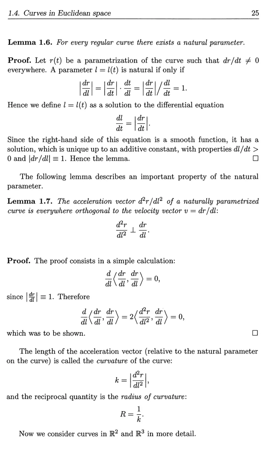
Lemma 1.6. For every regular curve there exists a natural parameter.
Proof. Let r(t) be a parametrization of the curve such that dr/dt ^ 0
everywhere. A parameter I = l(t) is natural if only if
'<U _
dt ~
Hence we define I = l(t) as a solution to the differential equation
\dr
~dl
=
dr
~dt
dt
"dl~
dr
~dt\
cU
dt
dr
~dt
Since the right-hand side of this equation is a smooth function, it has a
solution, which is unique up to an additive constant, with properties dl/dt >
0 and \dr/dl\ = 1. Hence the lemma. □
The following lemma describes an important property of the natural
parameter.
Lemma 1.7. The acceleration vector d2r/dl2 of a naturally parametrized
curve is everywhere orthogonal to the velocity vector v = dr/dl:
d2r dr
~dP ~dl'
Proof. The proof consists in a simple calculation:
d / dr dr\
~dl\~dV~dl/= '
since
dr
dl
= 1. Therefore
d /dr dr\ _ /d2r dr\ _
Jl\~dV~dl/= \dP'~dl/= '
which was to be shown.
□
The length of the acceleration vector (relative to the natural parameter
on the curve) is called the curvature of the curve:
d2r
k =
dl2
and the reciprocal quantity is the radius of curvature:
«4
Now we consider curves in M2 and R3 in more detail.

26 1. Cartesian Spaces and Euclidean Geometry
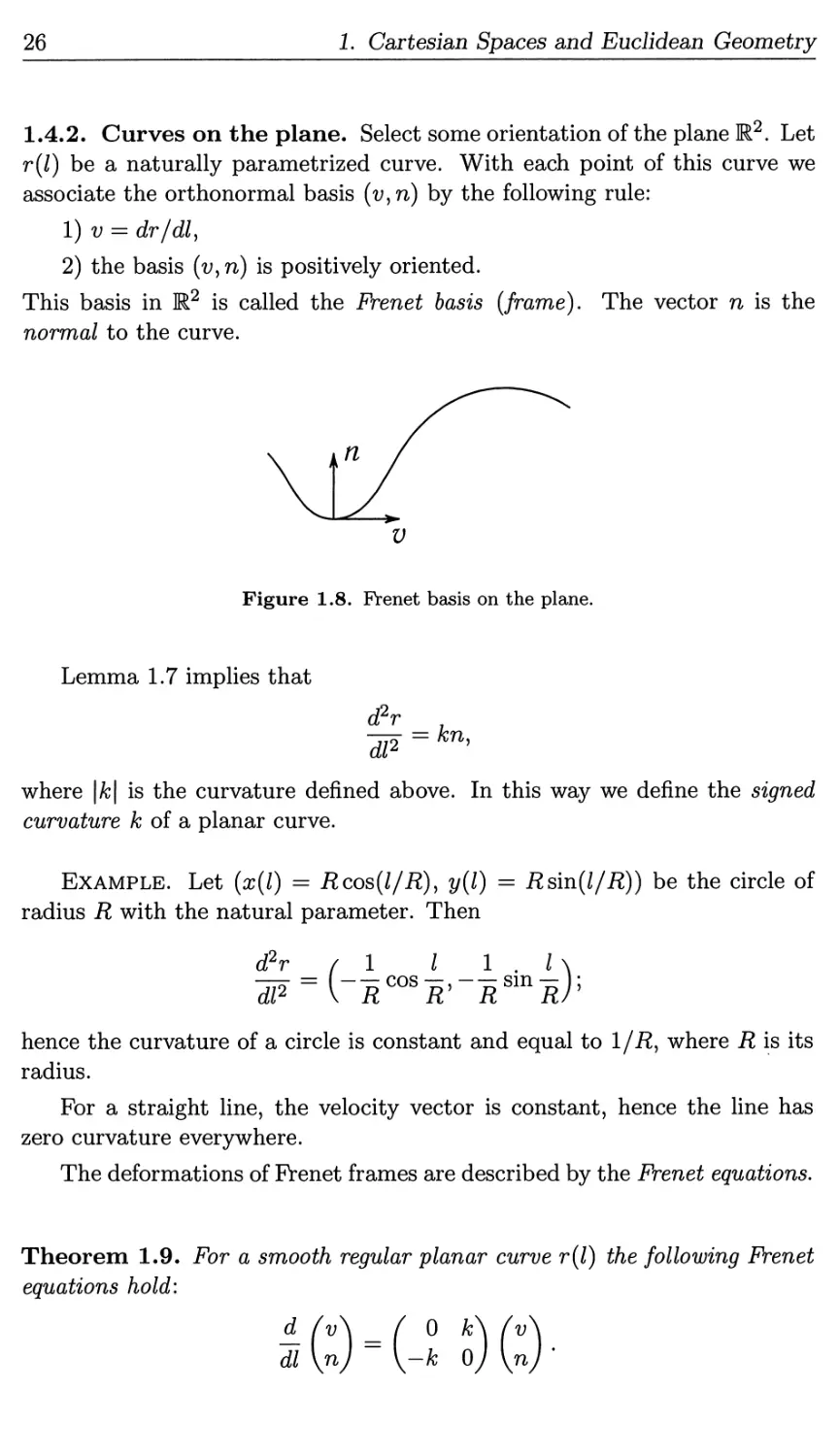
1.4.2. Curves on the plane. Select some orientation of the plane R2. Let
r(l) be a naturally parametrized curve. With each point of this curve we
associate the orthonormal basis (v,n) by the following rule:
1) v = dr/dly
2) the basis {vyn) is positively oriented.
This basis in M? is called the Frenet basis (frame). The vector n is the
normal to the curve.
Figure 1.8. Frenet basis on the plane.
Lemma 1.7 implies that
dp - kn>
where \k\ is the curvature defined above. In this way we define the signed
curvature A; of a planar curve.
Example. Let (x(l) = Rcos(l/R)} y(l) = Rsin(l/R)) be the circle of
radius R with the natural parameter. Then
d2r ( 1 I 1 . l\
^ = {-RC0SR>-RSmR>
hence the curvature of a circle is constant and equal to 1/i?, where R is its
radius.
For a straight line, the velocity vector is constant, hence the line has
zero curvature everywhere.
The deformations of Prenet frames are described by the Frenet equations.
Theorem 1.9. For a smooth regular planar curve r(l) the following Frenet
equations hold:
dl \n) ~ \-k OJ \n) '

1.4. Curves in Euclidean space 27
Proof. Since (v>v) = (n,n) = 1, (v,n) = 0, we have the following relations:
d / v n/dv \ n d . . n/dn \
-{v,v) = 2(-,v) = 0, -(„,„) = 2(-,n)=0,
d . . I dv \ I dn\
d&'n) = \-di'n) + \v'Ti) = Q-
But the vectors v and n form an orthonormal basis. Hence the first two
equalities imply
dv dn
_ = «,, -=0v,
while the third yields
(an, n) + (^, /ft;) = a + /? = 0.
By definition, a = /c, hence (3 = —k. The proof is completed. □
There is a one-to-one correspondence between smooth curvatures k(l)
and curves considered up to proper motions.
Theorem 1.10. 1. For any sufficiently smooth function k: [0, /] —► R there
exists a smooth naturally parametrized curve r: [0, /] —> M2 m£/& curvature
equal to k(l). This curve can be found from the Frenet equations.
2. // the curvatures of naturally parametrized planar curves ri(l) and
r2{l) are equal, then there exists a proper motion (p: R2 —*■ M? which maps
one curve into the other, r2{l) = (p(ri(l)).
Proof. 1. Take an orthonormal positively oriented basis ei, e<i and consider
a solution to the Frenet equations with initial conditions v(0) = ei, n(0) =
e2- Such a solution exists and is unique because the Frenet equations may
be viewed as an ordinary differential equation in E4 = R2 0 R2.
At the same time the scalar products of v(I) and n(l) satisfy another
system of differential equations,
-^ = 2k(v,n), -^- = -2k(v,n), -±±-*- = /c(n,n> - k(v,v).
This system with initial conditions (vyv) = (n, n) = 1, (v,n) = 0 has a
unique solution. It is easily seen that this solution is a constant, hence for
any / the vectors v(l) and n(l) form an orthonormal basis in R2.
Define the curve by the formula
r(l) = / v(t)dt.
Jo
By construction, \v(l)\ = 1; therefore, / is a natural parameter, v is the
velocity vector, and (v, n) is the Frenet frame.
Since dv/dl = kn, we see that &(/) is the curvature of the planar curve
r(l).

28 1. Cartesian Spaces and Euclidean Geometry
2. Let (vi,rii) be the Prenet frame of the curve r*, i = 1,2. We may
assume for definiteness that 0 < I < L. Define </? as the composition of
the shift by a = r2(0) — ri(0) and the linear transformation A that maps
(vi(0),ni(0))into(v2(0),n2(0)),
(p(x) = A(x) + a.
The Prenet frame of the curve ip{r\) is {Av\, An\). It satisfies the equation
d_ (AvA _ ( 0 k\ (Avx
dl \Am) ~ \-k OJ \Am
and so does the frame (t>2>^2)- Moreover, these two frames coincide for
/ = 0. Since the Frenet equations with given initial conditions have a unique
solution, the equalities Av\ = t>2, An\ = ri2 hold everywhere.
By the choice of the shift we have
r2(l) = r2(0) + / v2(t)dt = tp(ri(l)).
Jo
The proof is completed. D
For planar curves the Frenet equations can be easily integrated. Let
a(l) = J0 k(t) dt. Then the curvature of the curve
r(l) = I / cosa(t)dt, / sina(t)dt
wo Jo
is k(l). For curves in E3 the Frenet equations cannot be integrated explicitly.
1.4.3. Curvature and torsion of curves in M3. In the oriented
Euclidean space M3 there is one more binary operation besides the scalar
product, namely, the vector (or cross) product. In Euclidean coordinates it has
the form
(ei e2 e3\
f1 £2 £3 J > i-e-> [ei>e2] = e3, [e2,e3] = ei, [e3,ei] = e2,
rj1 rj2 r}3/
where (ei,e2,e3) is a positively oriented orthonormal basis, £ = ^e^, rj =
rfejy and the determinant is calculated by the formal algebraic rules:
[(,*] = «Y - «V)ei + (fl1 - SW)e2 + «V - tW)e3.
This product is linear in both factors,
[Aifi + A2&,»/] = AiKi,»7] + A2 [&,»/],
K, Ai»7i + A2772] = AiK,77i] + A2[£,772]
for Ai, A2 € R, and anticommutative,
K,»?] = -kC]-

1.4. Curves in Euclidean space
29
Moreover, it can be easily checked that
These equations determine [£, 77] up to a sign. Indeed, if the vectors £ and 77
are proportional to each other, then [£, 77] = 0 by anticommutativity.
Otherwise |[£, 77]! 7^ 0, the vector [£, 77] is orthogonal to £ and 77, and we know its
length. The sign is chosen so that ($,77, [£,77]) be a positively oriented basis
inM3.
Figure 1.9. Vector product.
In addition, the vector product satisfies another important identity,
called the Jacobi identity,
fc.fo,x]] + [»?,[x,0] + [x,K,»?]] = o
for any £, 77, x- To prove this identity, it suffices, using linearity and
anticommutativity, to reduce it to the case £ = ei, 77 = e2, X — e3- But then it
is obvious because
[ei,e2] = e3, [e2,e3] = ei, [e3,ei]=e2.
In what follows, unless otherwise stated, we will always assume that the
space Rn is oriented so that the basis (ei,..., en) has the positive orientation.
A vector space endowed with a bilinear anticommutative operation
satisfying the Jacobi identity is called a Lie algebra. The space R3 with vector
product gives us the first example of a Lie algebra.
For the Prenet frame of a curve in R3 to exist, it is not enough to assume
that the curve is regular. We have to require the curve r(l) to be biregular,
i.e., such that its acceleration vector does not vanish anywhere.
Then the Prenet frame (t>, ti, b) is
v =
dr
~dly
n =
<Pr_
dl2
<Pr_
dl2
b = [v,n\.

30
1. Cartesian Spaces and Euclidean Geometry
Figure 1.10. The Prenet frame for a curve in
The vector n is called the principal normal to the curve, and b is called the
binormal.
By definition,
dv ,
-irkn
and A; > 0.
The Prenet frame is orthonormal and positively oriented. The quantity k is
called the curvature of a curve in M3. It may be equal to zero, so it is defined
not only for biregular curves. It has a simple physical meaning: if we view
our curve as the trajectory of a point-particle and take time for the natural
parameter, then the curvature equals the length of the acceleration vector.
The reciprocal quantity R = £ is the radius of curvature for the curve. The
deformations of Prenet frames are described by the Frenet equations for a
curve in R3.
Theorem 1.11. The Frenet frame of a biregular curve in M3 satisfies the
Frenet equations for a space curve:
(1.6)
Proof. As in the proof of Theorem 1.9, observe that (v(l),n(l),b(l)) for
any I form an orthonormal basis. In particular, the lengths of these vectors
are kept constant, hence the derivative of each of these vectors is orthogonal
to the vector itself:
0 a12 ai3\ (v
Q>2\ 0 a23 J \n
«31 «32 0 J \b
It remains to note that
d(v, n)
dl
= ai2-t-a2i =0,
d(ny b)
dl
= «23 -H ^32 = 0,
d(vtb)
dl
= ai3 + a3i = 0.

1.4. Curves in Euclidean space
31
By the definition of curvature, we have a\2 = k and a\s = 0. Putting
k = a23) we obtain equations (1.6). □
In fact, we restated the proof of Theorem 1.6 for n = 3. Namely, let
B(l) be a one-parameter family of orthogonal matrices specifying the
transformations such that B{l)e\ = v(l), B(l)e2 = n{l), B(l)ez = 6(/), where
(ei,e2,e3) is a fixed orthonormal positively oriented basis.
By Theorem 1.6 we have
^-(l) = A(l)B(l),
where the matrix A is skew-symmetric and by its construction
v
v
ai;j""l;
Figure 1.11. A spiral with the Frenet frame.
The quantity k, involved in the Frenet equations is called the torsion of
the curve.
We can state the following analog of Theorem 1.10.
Theorem 1.12. 1. Let k and k be smooth functions on an interval [0,L]
with k > 0 everywhere on this interval. Then there exists a smooth naturally
parametrized curve r: [0, L] —*• M3 with curvature k(l) and torsion k(1). This
curve may be found from the Frenet equations.
2. // two naturally parametrized curves r\(l) and r2{l) in M3 have the
same curvatures and torsions, then there exists a proper motion <p: M? —> M3
that maps one of the curves into the other: (p(r\(l)) = T2(0-
Since the proof of this theorem is quite similar to that of Theorem 1.10,
we omit it.
If we consider a curve lying entirely in the plane R2 C M3, then the
binormal to this curve will coincide with the binormal to the plane, so that

32 1. Cartesian Spaces and Euclidean Geometry
it will be constant. It follows from the Frenet equations that in this case
« = 0.
The converse is also true. If a curve r(l) has torsion k, = 0, then by
Theorem 1.12, for a given A;, we can construct a planar curve r(l) with
curvature k. Since the curves r(l) and f (I) have the same curvatures and
torsions, they can be mapped into one another by a proper motion of E3.
Therefore r(l) is a planar curve.
The equations k = k(l) and k = «(/), where A; and k are the curvature
and torsion regarded as functions of the natural parameter /, are called the
natural equations of the curve. By the previous theorem, they determine
the curve uniquely up to motions of the entire space.
Exercises to Chapter 1
1. Prove that the Jacobi matrix of the composition of two smooth
mappings is the product of the Jacobi matrices of these mappings.
2. Prove that the rank of a Jacobi matrix does not depend on the choice
of local coordinates.
3. Write down the Laplace operators on the plane,
A d2 d2
dx2 dy2'
and in the 3-dimensional space,
A d2 d2 d2
dx2 dy2 dz2'
in polar, spherical, and cylindrical coordinates.
4. Determine the functions r = r(<p) that specify straight lines in polar
coordinates.
5. Show that the length of a curve equals the limit of the lengths of
polygonal lines consisting of segments that consecutively join finitely many
points of the curve as the maximal length of the segments tends to zero.
6. Prove the following formula for the curvature of a planar curve r(t)
(with arbitrary parameter t):
\[r,f}\
1*1 =
7. Suppose a half-line OA revolves about the point O with constant
angular velocity u. Derive the equation for the trajectory of the point P
that
a) moves away from the point O along the line with constant velocity
{spiral of Archimedes);

Exercises to Chapter 1
33
b) moves along the line with velocity proportional to the distance \OP\
(logarithmic spiral).
Find the curvatures of the corresponding curves.
8. Prove that for any tangent to the curve #2/3+y2/3 = a2/3, the segment
lying between the Euclidean coordinate axes has the constant length a.
9. Prove that for any tangent to the curve
a. a -h y/a2 - x2 r^ r
^ a — Vfl — #
the segment between the y-axis and the point of tangency has length a.
10. Let a circle of radius a be rolling along a straight line without
gliding. Derive the equation for the trajectory of a point fixed to the circle
at a distance d from its center. Find the curvatures of these curves.
11. Let a circle of radius r be rolling without gliding over a circle of
radius R staying outside the circle. Derive the equation for the trajectory
of a point of the rolling circle and find its curvature.
2 2
12. Find the curvature of the ellipse ^ + |j = 1 at its apexes.
13. Find the curvature of the curve specified by the equation F(x, y) = 0.
14. Find the curvature of the curve satisfying the differential equation
P(x, y) dx + Q(xy y) dy = 0.
15. Suppose a curve on a sphere intersects all the meridians at a given
angle (loxodrome). Derive its equation and find the curvature and torsion.
16. Prove that if all the normal planes to a curve in E3 contain a fixed
vector £, then the curve lies in a plane.
17. Prove that if all the normal planes to a curve pass through a fixed
point P, then the curve lies on a sphere with center at this point.
18. Prove that a curve of identically zero curvature k(l) = 0 is a straight
line.
19. Prove that a curve with identically zero torsion k(1) = 0 lies in a
plane and find this plane.
20. The mixed product of three vectors in R3 is defined as (tt, vyw) =
([u, v],w), i.e., as the scalar product of [tt, v] and w. Prove that a curve r(t)
is planar if and only if the mixed product of the vectors ryr\ and 'r is equal
to zero:
(r,r, 'f) = 0.
21. Prove that the torsion of a curve r(t) in E3 is equal to
\
r,r,r)
K IMP •

34 1. Cartesian Spaces and Euclidean Geometry
22. Denote by S the area between a planar curve and its secant passing
parallel to a tangent at a distance h from it. Express
lim T-5-
h^o h6
in terms of the curvature of the curve.
23. Prove that for any smooth closed curve r = r(t) in E3 the following
equality holds:
(rdk + Kbdl) = 0.
/■
24. Solve the equation rf = [w,r], u> = const.
25. Prove that a curve lies on a sphere of radius r if and only if
k2\^(Kk)2)
(with the derivative taken with respect to the natural parameter).
26. Prove that if a curve lies on a sphere and has a constant curvature,
then this is a circle.
27. For a smooth curve r = r(Z), let n(l) be the curve formed by the
tips of the normal vectors. Let /* be the natural parameter on this curve.
Prove that
dl

Chapter 2
Symplectic and
Pseudo-Euclidean
Spaces
2.1. Geometric structures in linear spaces
2.1.1. Pseudo-Euclidean and symplectic spaces. In many
applications we need a more general notion of scalar product than the Euclidean
scalar product.
A scalar product on a finite-dimensional vector space V is a function
(£,77) of a pair of vectors £,77 G V satisfying the following bilinearity
condition:
<Ai£i + A2&,»7) = Ai(£i,77) + A2 (&,*/),
faAifi + A2&) = Ai (77, £1) + A2<77,£2)
for any Ai, A2 G R and £1, £2,77 G V. This product is said to be nondegenerate
if for each vector £ ^ 0 there exists a vector 77 such that (£,77) ^ 0.
If ei,..., en is a basis in V, then bilinearity implies that
n
where £ = ^e^, 77 = if ej. Therefore, the product is specified by the Gram
matrix G = (#f?), where
9ij = \ei? ej/'
Lemma 2.1. A scalar product is nondegenerate if and only if detG ^ 0.

36
2. Symplectic and Pseudo-Euclidean Spaces
Proof. A scalar product is degenerate if there exists a nonzero vector £
such that (£,77) = Cv^Qij = 0 for all r\. In this case g^1 = 0 for any j.
This system of equalities may be rewritten as a matrix equation which has
a nonzero solution if and only if det G = 0. □
Of particular interest are the following two types of nondegenerate scalar
products, namely, pseudo-Euclidean and symplectic.
a) A nondegenerate scalar product is said to be pseudo-Euclidean if it
is symmetric,
<t,v) = (0,$ foralU,»?eV,
but not positive definite.
b) A nondegenerate scalar product is called symplectic if it is skew-
symmetric,
«.»?> = -(v,C) faralU.ijeV.
Symmetric scalar products are also called quadratic forms. In linear
algebra and number theory, by quadratic forms are also meant functions
q(x) = (xyx)y where (£,77) is a symmetric scalar product.
Symmetric and skew-symmetric scalar products can be reduced to a
canonical form in special bases.
Theorem 2.1. 1. If (•, •) is a symmetric scalar product on Vy then there
exists a basis e\,..., en inV such that
(2.1)
1 fori = j,l<i<p,
(e», ej) = { -1 for i = j} p + 1 < i < p + q < n,
0 otherwise.
2. If {•} •) is a skew-symmetric scalar product on V, then there exists a
basis e\,..., en inV such that
(2.2)
(e2»-i, e2i) = -(e2i, e2i-i) = 1 for i = 1,... ,p, p < [n/2],
{eiyej) =0
otherwise.
Remark. In the basis (2.2) the Gram matrix has the form
/ 0 1 0\
-1 0
J =
Vo
0 1
-1 0
0
0/

2.1. Geometric structures in linear spaces 37
In the symplectic case with dim V = 2p we can introduce the following
basis ei,... ,e2p:
(2.3) ei = ei, e2 = ep+i, ..., e2j-i = ej, e^j = ep+j, j = 1,... ,p.
This basis is called symplectic, and in this basis the Gram matrix becomes
where 1 denotes the p x p identity matrix.
Proof of Theorem 2.1. 1. If (£,£) = 0 for all vectors £eV, then
(Z + V,Z + V) = «,0 + <^> + «,*/) + <t|,0 = 2«,i/> + <£,£) + <^> = 0.
Combined with condition (£, £) = (17,77) =0 this implies the equality (£,77) =
0. Therefore, the form ($,77) is identically zero, p = q = 0, and the basis
ei,..., en may be chosen arbitrarily.
If (£>£) 7^ 0 f°r some vector £, then we set e\ = £/>/!(£>£) I anc^ de-
note by Vi and Vf1 the one-dimensional subspace spanned by e\ and its
orthogonal complement. Since V±- is determined by the nontrivial equation
<{,x)=0 forzeVf1,
we see that V^- is a hyperplane in V. Now we restrict (•, •) to Vf1 and
repeat the same argument. Then after finitely many steps we construct the
required basis ei,e2,... ,en (apart from ordering its vectors). This proves
part 1 of the theorem.
2. If (£,77) = 0 for any pair of vectors £,77, then the form (•, •) is
identically zero, and the basis be chosen arbitrarily.
Otherwise, take £ and 77 such that (£, 77) ^ 0. Set
Denote by V\ the subspace spanned by e\ and e2, and by V^- its orthogonal
complement. The pair of linearly independent equations
(^x) = (V,x)=0
determines VJ1; hence the subspace V^- has codimension 2 in V, i.e., dim V—
dim Vf1 = 2.
Restrict (•, •) to Vf1- and apply the same arguments. In this way, after
finitely many steps, we construct a collection of vectors ei,..., C2P such that
the form is identically zero on the orthogonal complement to them, say, Vo.
Now we supplement the collection ei,...,e2P with an arbitrary basis
in Vq to become a basis in V. This yields the required basis. □

38 2. Symplectic and Pseudo-Euclidean Spaces
In the case of a symmetric scalar product (quadratic form), the tuple
{p,q,n — (p + q)) is invariant, i.e., it depends on the form but not on the
choice of the basis e\,..., en in which the Gram matrix takes the diagonal
form. The sum p + q is called the rank of the quadratic form, and the
difference p — q, its signature.
If p -t- q = n and p > 0, q > 0, the scalar product is called pseudo-
Euclidean. A Cartesian space with such a scalar product is referred to as
pseudo-Euclidean and is denoted by WyQ. The coordinates in which the
scalar product has the form (2.1) are called pseudo-Euclidean.
A Cartesian space with a symplectic scalar product is called symplectic,
and the coordinates in which the scalar product has the form (2.4) are called
symplectic.
Theorem 2.1 implies the following statement.
Corollary 2.1. A symplectic space has an even dimension.
In what follows, when speaking about pseudo-Euclidean or
symplectic spaces, we will assume that the coordinates chosen in these spaces are
pseudo-Euclidean or symplectic, respectively.
Lemma 2.2. A linear transformation A: V —*■ V preserves a nondegenerate
scalar product with Gram matrix G if and only if
ATGA = G.
Proof. Write down the equality (£,77) = {A£y An) in the coordinate form:
9ijCrt =gkiakiCaljrf.
This equality is fulfilled for all £ and rj if and only if
k I
9ij = ai9kia>j,
i.e., for G = ATGA. D
Since detG 7^ 0 for any nondegenerate scalar product, the equality
det AT = detA implies the following result.
Corollary 2.2. If a linear transformation A preserves a nondegenerate
scalar product, then it is invertible and detA = ±1.
Indeed, det G = det AT det G det A = det2 A det G, which implies the
equality det2 A = 1.
Theorem 2.2. Linear transformations A: V —> V preserving a
nondegenerate scalar product form a group.

2.1. Geometric structures in linear spaces 39
Proof. Obviously, the composition of such transformations preserves the
scalar product. Let a transformation A preserve the scalar product. As
we have just shown, it is invertible. Multiplying both sides of the equality
ATGA = Gby A-1 on the right and by (-A_1)T on the left we obtain
G = (A~1)TGA-1.
Hence the linear transformation A-1 also preserves the scalar product. □
The group of linear transformations of the space W,q preserving the
pseudo-Euclidean scalar product is denoted by 0(p, q). Specifying pseudo-
Euclidean coordinates we obtain that this group is a group of matrices
preserving the scalar product
a, n)=zW + • • •+w - e+v+1 e«tr«.
The subgroup of 0(p, q) formed by the matrices with determinant equal to 1
is denoted by SO(p, q).
In the next section we will consider these groups and pseudo-Euclidean
spaces in more detail.
2.1.2. Symplectic transformations. The group of linear
transformations of the space R2n preserving a symplectic scalar product is denoted by
Sp(n, R) and is called a symplectic group. This is the group of matrices
preserving the scalar product in the basis (2.3):
«, v) = £ V+1 + • • •+eV - e+W z2nvn.
Examples. 1. Let n = 1. A matrix A = (acbd) belongs to Sp(l,E) if
and only if
(a c\ ( 0 1\ (a b\ ( 0 l\
\b d) \-l OJ \c d) ~ \-l OJ '
The left-hand side of this equation equals
/ 0 ad- bc\
\-{ad-bc) 0 Jm
Therefore, Sp(l,E) consists exactly of (2 x 2) matrices with determinant
equal to 1,
Sp(l,R) = SL(2).
2. Consider a symplectic basis ei,..., C2n (i-e., a basis with Gram
matrix (2.4)). Then any linear transformation B of the n-dimensional space
with basis e\,..., en induces the following symplectic transformation of the
2n-dimensional space:
(2.5) A=(* (jBT0ri). SeGL(n).

40 2. Symplectic and Pseudo-Euclidean Spaces
Lemma 2.3. Let V be a 2n-dimensional symplectic space, let A G Sp(n, M),
and let \i be a real eigenvalue of A. Then the characteristic polynomial
p(\) = det(A — A • 1) of the transformation A has the form
p(A) = (A-M)(A-±)j/(A),
where p'{\) is the characteristic polynomial of a matrix A' G Sp(n — 1,
Proof. It is seen from the proof of Theorem 2.1 that in the construction of
a basis with property (2.2) the vector e\ can be chosen arbitrarily. Let us
construct a basis as in the proof of Theorem 2.1, with e\ such that Ae\ = \xe\.
It is easily seen that
since (Aei, Ae<i) = 1 = (ei,e2). Hence the transformation A is given by the
matrix
(/j, * * \
0 J ° >
0 * A'J
where A' specifies the symplectic transformation. Therefore, we have p(\) =
det{A - A • 1) = (A - fj)(\ - i) det(A' - A • 1). D
Now we can prove the following statement.
Lemma 2.4. If A € Sp(n,E), then det A = 1.
Proof. The determinant of a matrix A is equal to the product of the roots
of its characteristic polynomial p(A) = det (A — A • 1). Lemma 2.3 implies
that
det(A - A • 1) = (A - mi) (A --)..- (A - fik) (\ - — )p(A),
where the polynomial p(\) is either identically equal to one or has no real
roots. In the former case det A = Mi^j-1 • • -//fcM^1 = 1. In the latter case
the roots of the real polynomial p(X) are of the form i/i, z/i,..., vi, &i, so that
det(A) =p(0) = (fiwj1) x (X[vj
Vj ) > 0.
Since det A = ±1, this implies that det A = 1. □
Now that we know that det A = 1, we will show that the characteristic
polynomial of a symplectic matrix has a stronger property.

2.1. Geometric structures in linear spaces
41
Lemma 2.5. If A € Sp(n,R), then the characteristic polynomial p(X) =
det(A — A • 1) is reciprocal to itself:
p(A) = A2"p(i)
Proof. Denote by J € Sp(n, R) the Gram matrix,
/ 0 1 0\
-1 0
J =
0 1
\0 -10/
Observe that J2 = — 1 and det J = 1. The symplecticity condition is
AT J A = J.
This implies that
p(X) = det(A - A • 1) = det J det (A - A • 1) = det( J A - A J)
= det( J A - XATJA) = det(l - XAT) det J A
= det(l - XAT) = A2n det(A~1 • 1 - A)T
= X2ndet(X~l'l-A).
But since A is a 2n x 2n matrix, we conclude that det(A_1 • 1 — A) =
(-l)2ndet(A - A"1 • 1); hence
p(X) = A2ndet(A - A"1 • 1) = A2npQ).
D
These lemmas entail an important property of the spectrum of a
symplectic matrix, i.e., the set of the roots of its characteristic polynomial.
Corollary 2.3. The spectrum of a matrix A G Sp(n, R) is symmetric about
the real axis and the circle \X\ = 1. It falls into:
1) J^-tuples A, A, A-1, A-1, where \X\ ^ 1 and ImA ^ 0;
2) pairs A, A-1 lying on the real axis (A = A);
3) pairs A, A-1 lying on the circle \X\ = 1 (so that A-1 = A).
A specific feature of a symplectic space is dissimilarity between hyper-
planes. For example, in R4 no symplectic transformation maps the plane
x2 = x4 = 0 into the plane a;3 = x4 = 0. Indeed, any two vectors £ and rj
of the plane x3 = x4 = 0 satisfy the equality (^n) = 0, whereas for the
vectors £ = (1,0,0,0) and n = (0,0,1,0) of the plane x2 = x4 = 0 we have

42 2. Symplectic and Pseudo-Euclidean Spaces
•Xi
= 1
x2
•x,
Figure 2.1. Roots of the characteristic polynomial of a symplectic matrix.
A subspace V of a 2n-dimensional symplectic space is said to be
Lagrangian if it is n-dimensional and
for any two vectors £,77 6 V.
All coordinate Lagrangian subspaces have the form
(2.6) xh = • • • = xin = 0,
where {eipeik) = 0.
Two subspaces L\ and L^ in RN are transversal to each other if their
vectors span the entire space RN. If dimLi + dimZ/2 = N = dimM^, then
transversality implies that L\ and L^ intersect only at the origin.
To each coordinate Lagrangian subspace L of the form (2.6) corresponds
the transversal coordinate Lagrangian subspace V'. It is specified by the
equations
xjl = • • • = xjn = 0,
where ji ^ %k for all /, k = 1,..., n.
Lemma 2.6. Let L be a Lagrangian subspace in R2n. Then there exists a
coordinate Lagrangian subspace L transversal to L.
Proof. Making use of transformation (2.5), we construct a new symplectic
basis such that its first k vectors e~\,..., e^ span the entire intersection of L
with the subspace (xn+1 = 0,..., x2n = 0).
Define the subspace L transversal to L as the one spanned by the vectors
^/c+i) • • •) cn, en-|_i,..., en_|_fc.

2.2. The Minkowski space
43
Obviously, this subspace is Lagrangian. Consider the vector r\ G Lf)L. Since
(77, L) = (77, L) = 0, we have
(V>ej) =°> j = l,...,n.
Therefore, 77 = ]Cj=i ^^ and hence 77 = 0. □
This lemma implies that each Lagrangian plane is representable as the
graph of a mapping of a coordinate Lagrangian subspace. Namely, the
following theorem holds.
Theorem 2.3. For any pair of transversal Lagrangian subspaces (L,L), one
can construct a symplectic basis of the form (2.3) such that
Ci,..., en G L/y en_|_i,..., e2n G Li,
and the Gram matrix has the form
ei > en+j / = *ij > * > ,7 = -I- > • • • > ^
(with all other elements equal to zero).
The proof is obvious.
2.2. The Minkowski space
2.2.1. The event space of the special relativity theory. The most
important class of pseudo-Euclidean spaces is the class of spaces R1,n. In
this case the scalar product in pseudo-Euclidean coordinates 00 • 00 » • • • » 00
becomes
(t,r,)= «V-*Y CV"-
It specifies the Minkowski metric.
For n = 3 we obtain the Minkowski space, which is the 4-dimensional
space-time of the special relativity theory. In this case x° = ct, where c is
the velocity of light in vacuum and t is time, while x1yx2yx3 are coordinates
in the three-dimensional physical space. The points of the space M1,3 are
instantaneous events, and the quantity
y/(x - y, x - y)
for xy y G M1'3 is the space-time interval between the points (events) x and y.
The squared length of a vector may be positive, negative, or zero. A
vector £ is a light-like vector if (£,£) = 0. If (£,£) > 0, the vector £ is said
to be time-like, and when (£,£) < 0, it is called space-like.
This terminology has physical grounds. Namely, the special relativity
theory relies on the following postulates:
1) A material point-particle cannot move in the space at a velocity
greater than the velocity of light. For a particle with mass, the velocity

44
2. Symplectic and Pseudo-Euclidean Spaces
Figure 2.2. Light-, time- and space-like vectors; light cone.
is always less than the velocity of light, while the velocity of a zero-mass
particle equals the velocity of light.
2) In all the inertial frames the velocity of light has a constant value
c « 2.998 • 10iU cm/sec
The curves r(r) in M1'3 with velocity vectors of zero length, i.e.,
.... dr
VTifr) = 0) where rT = —,
dr
are the world lines of zero-mass particles, e.g., photons. Therefore, the light
rays propagate along these lines.
If the velocity vector rT = (x^x^x^yX^.) of a curve r(r) is everywhere
time-like, then r(r) is a world line of a particle with mass. Consider such a
world line r(r). Its length in the Minkowski metric is
1 =
f \rT\ dr = f J(x°T)2 - ^>?)2 dr > 0.
The quantity l/c is called the proper time elapsed for the particle. For a
particle at rest {x\ = x\ = x\ = 0), it is equal to the interval of world time
between the events r(a) and r(b), °(b)-x°(a).
Example. For a particle at rest described by the world line
a<x°<b, xa = 0, a = 1,2,3,
the time elapsed is x°(b) — x°(a). Let the life of another particle be described
by a world line (#°(t), xa(r))} where r = t = x°/c, a < x° < 6, with the
same initial and end points. Assume that this second particle moves during

2.2. The Minkowski space
45
this period of time: xa(r) ^ 0, a = 1,2,3. Then its proper time is
V fb 1 /~I ^/dx°>? ,
Obviously, we have
I'/c <b-a = l/c.
Thus we see that time contracts at movement.
The physical principle of constant velocity of light is expressed by the
requirement that the change from one inertial frame to another is determined
by a motion of the Minkowski space, i.e., by a transformation </?: R1'3 —► R1,3
preserving space-time intervals. This means that
((p(x) - (p{y),ip{x) - ip{y)) = (x-ytx-y)
for each pair of points x and y in R1'3.
Theorem 2.4. Any motion of the space R1'71 is an affine transformation.
Proof. The proof differs very little from that of Theorem 1.4 for the
Euclidean space. Let ip be a motion of the space R1'71 and (p(0) = b. Since the
shift x —*■ x — b is a motion, define ip as the composition of (p and this shift,
ip: x —> ip(x) — b. This is a motion with -0(0) = 0.
Preservation of space-time intervals means that
(2.7) (tp(x) - ip{y),ip{x) - ip{y)) = (x-y,x-y)
for i,|/G R1'™. In particular, for y = 0 we have
(2.8) (iP{x),iP{x)) = (x,x).
Rewriting (2.7) as
(ip{x)yip(x)) - 2{*i>(x)iii>{v)) + {*l>{v)Mv)) = ix>x) - 2ix>y) + <s/>s/)>
and taking (2.8) into account, we obtain that
(tp{x),ip{y)) = (x,y)
for dl\x,yeRhn.
Let eo,..., en be the orthonormal basis in R1'71 that corresponds to the
pseudo-Euclidean coordinates, and let xoy...yxn be the points for which
the basis vectors are radius-vectors. Denote by e?i the radius-vector of the
point ip(xi). The basis eo,..., en is orthonormal. Consider the linear
transformation x: x —*■ Ax which maps e~i into e^, i = 0,... ,n. Obviously, this
transformation is a motion.

46
2. Symplectic and Pseudo-Euclidean Spaces
Therefore, the composition x*P is a motion that leaves the origin fixed
and satisfies the equalities xV;(ei) = e» for i = 0,1,... ,n. Any vector x is
expanded in this basis as
n
X
= {x,e0)e0 -^2(x,ei)ei
t=i
For any point x G K1,n we have
(x,ei) = {xtp{x),ei), i = 0, ...,n.
Therefore, xi>{x) = %•> i-e-> this 1S the identity transformation; hence ip =
A-1, which is a linear transformation, and
(p(x) = A~lx + b.
The proof is completed.
□
The definition of a motion and the proof of the theorem can be extended
to arbitrary spaces Rp'q with obvious changes. A similar result for Euclidean
spaces was obtained in Theorem 1.4.
Corollary 2.4. Every motion of the space R1,n is uniquely representable in
pseudo-Euclidean coordinates as
x —► Ax + 6,
where
(2.9)
A
T
A
^o
0\
-1
A =
-v
/I
\o
0\
-1
-v
2.2.2. The Poincare group. The group of motions of R1,3 is called the
Poincare group.
Consider the subgroup of all motions of the subspace R1,1 in more detail.
Let
a 6'
A =
c d '
The equation (2.9) becomes
a c\ (I 0\ (a bs
b d V0 -1 [c d
1 0N
o -iy
which can be rewritten as the system of equations
a2 - c2 = d2 - b2 = 1, ab-cd = 0.

2.2. The Minkowski space 47
The solutions of this system fall into four families:
f cosh. ij) sinh?A /—cosh^ — sinh-0
ysinh^ coshi/ij ' y—sinh-0 — cosh^
cosh-0 — sinn^M ( —cosh ijj sinh^
sinn^ — cosh tp J ' y—sinh^ cosh^
where ip is an arbitrary real parameter. The top two families consist of
unimodular transformations (det A = 1), and the bottom two, of
transformations with det A = — 1. This implies the following result.
Theorem 2.5. The group 0(1, n) consists of four components.
If A 6 0(1, n), then (Aeo,eo) ^ 0. Indeed, otherwise the vector Aeo
would be a linear combination of ei,..., en, implying that (Aeo, Aeo) < 0.
But this contradicts the fact that (Aeo, Aeo) — (^O)^o) = 1-
Let Z2 be the group formed by the numbers ±1 with the multiplication
operation. Define the mapping ip: 0(1,n) —► Z2 x Z2 by
(p(A) = (detA,sgn(Ae0,e0>),
where
(1 for A > 0,
0 for A = 0,
-1 for A < 0.
Consider the group Z2 x Z2 with componentwise multiplication
{a)b)'{a',b') = (aa\bb').
Lemma 2.7. The mapping cp is a homomorphism of the group 0(1, n) on
the group Z2 x Z2.
Proof. The transformations in 0(1, n) preserve the light cone
which is the boundary of the domain formed by the vectors £ with (£, £) > 0.
This domain consists of two components, which are the interior parts of the
cone. If sgn(Aeo,eo) = 1, each component is mapped into itself, and if
sgn(Aeo,eo) = — 1, they interchange. This implies that cp is a
homomorphism.
Now we list the values of ip for the families in (2.10): (1,1), (1,-1),
(—1,1), (—1, —1). Hence for n = 1 the image of ip coincides with Z2 x Z2.
For n > 1 any transformation in 0(1,1) may be extended in a trivial way
(Ae2 = e2, • • •, Aen = en) to a transformation in 0(1, n). Therefore, <p is a
homomorphism on the entire group Z2 x Z2 for any n. □

48
2. Symplectic and Pseudo-Euclidean Spaces
If sgn(Aeo,eo) = 1, then the transformation A is called orthochronous,
meaning that it does not change the direction of time. In pseudo-Euclidean
geometry a transformation A is said to be proper if <p(A) = (1,1), i.e., it
preserves the orientation of the space M1'3 and the direction of time.
2.2.3. Lorentz transformations. The transformations forming the group
0(1,3) appeared initially in the special relativity theory as Lorentz
transformations. They describe the change from one inertial reference frame to
another. Consider them in more detail.
In this subsection we will denote the space coordinates by x,y,z as is
customary in physics.
Denote by ct,x,y,z the coordinates in a frame K and by ct', x'', yf, z\
the coordinates in a frame K'.
Figure 2.3. Different reference frames moving relative to each other.
Suppose that the origin of the frame K'} moving along the re-axis with
constant velocity v, coincides with the origin of the frame K at time t = 0.
The transition formulas have the form
fct\
X
y i
W
i |
'
fa b 0 0\
c d 0 0
0 0 10
\0 0 0 l)
f 1
(ct'\
x'
y'\
w
and are specified by a matrix of the group 0(1,3) because this
transformation must preserve space-time intervals in R1'3. Naturally, this
transformation must continuously depend on v and become the identity transformation
for v = 0. Hence it must belong to the identity component of the group
0(1,3) and have the form
b\ _ /coshV' sinn?/'
d) \smh.ij) cosh-0^

2.2. The Minkowski space 49
The point with x' = y' = z' = 0 corresponds to the origin of the frame K',
for which x/t = v, and we obtain
sinh ip x v
tanh?/> =
cosh ip ct c
cosh ip = — =, sinh ip =
y/1 - v2/c2' y/l - v2/c2'
The formulas of the Lorentz transformation become
_ t' + x'v/c2
, , l~ Jl-v2/^
vt + x , ,
x = —. =. y = y, z = z.
y/1 ~ V2/C2 y U
As v/c —> 0, the Lorentz transformations turn into the Galilean
transformations
t = t', x = vt' + x\
which approximate the former with high accuracy if the velocity v is much
less than the velocity of light c, v <C c.
Here we point out some physical phenomena which follow from the
Lorentz transformations.
1. Contraction of length. Suppose we have a rod that is fixed
relative to the frame Ky is parallel to the re-axis, and has a length / in this
frame. The rr-coordinates of its endpoints are xq and xq + 1. The difference
between the coordinates of its endpoints in the frame K' is
I' = l^l-v2/c2.
Therefore, the length of the rod contracts in a moving reference frame.
2. Addition of velocities. Let r(r) be the world line of a particle
with mass. Then the tangent vector at each point of this line is time-like.
We normalize it to be of unit length. Such a vector is called the velocity
A-vector. It is equal to
/ 1 v
(2.12) u = . —,
Wl-(v/c)*' cy/l-(v/c)2
where v = (^-, ^-, ^-) is the usual three-dimensional velocity vector.
When changing from one inertial frame to another the velocity 4-vector,
like any vector in E1,3, transforms by the Lorentz formulas. Let us consider
the consequences of this.
Let the frame K' move relative to the frame K at a constant
velocity w along the rc-axis. Denote the three-dimensional velocity vectors of the

50 2. Symplectic and Pseudo-Euclidean Spaces
particle with mass by v = {vx,vy,vz) and v' = {vx>vy,vz) as measured in
the frames K and K' respectively, and similarly the velocity 4-vectors by u
and v!.
The Lorentz transformation (2.11) for 4-vectors u = (w°,w1,u2yu3)
becomes
ti1 = -_=L==(r^ti/°+u/iy ^=^/2, ^3=u/3.
Vl - {w/c)2 V c /'
Substituting here the expressions (2.12) for the components of the 4-vectors
we derive the following formulas known as the relativistic law of addition of
velocities:
v'x + w _ v'y\/l - {w/c)2 v'z^/l - {w/c)2
x 1 . v'w "> V n v'w ' z 1 . v'w
If the particle itself moves along the a;-axis, these formulas take a particularly
simple form:
_ v'x + w
x 1 , vLw '
l + JbtL
with all other components of the three-dimensional vectors v and v' equal
to zero.
If we substitute here v'x = c, then for any w we obtain vx = c, which tells
us in mathematical terms that the velocity of light is the same in all inertial
frames. This fact was first observed in the Michelson-Morley experiment.
One more well-known physical phenomenon is contraction of the proper
time of a moving particle, which was already stated in 2.2.1.
Exercises to Chapter 2
1. Prove that the type (i.e., the pair p, q) of the pseudo-Euclidean scalar
product does not depend on the choice of the basis.
2. Let gij = —gji be a nonsingular skew-symmetric matrix specifying a
symplectic product in R2n. Prove that a linear subspace of E2n such that
the symplectic product restricted to this subspace is identically zero is of
dimension at most n.
3. Define the "vector product" of vectors £ = (^°,^1,^2) and 77 =
(^y0)7?1)7?2) m the space 1R1'2 by the formula
«x v=(tv - ev\t%2 - ev°,ev° - «y >,

Exercises to Chapter 2 51
where (eo,eo) = 1 and (ei,ei) = (e2,e2) = —1. Prove that
eo x ei = —e2, eo x ^2 = ei, ei x e2 = eo,
the Jacobi identity holds,
& x (& x 6) +& x (ft x &) +& x (& x 6) = 0,
and this vector product is invariant with respect to SO (1,2).
4. Let r = r(l) be a time-like curve in R1,2 with natural parameter I
(i.e., r2 = (r0)2 - (r1)2 - (r2)2 = 1) such that r° > 0. Set v = r, i) = A;n,
b = nxv. Prove the "Prenet formulas":
v = kn, h = kv — Kb, b = ku.
5. Solve the following equation in E1'2:
r = u x r, oj = const.

Chapter 3
Geometry of
Two-Dimensional
Manifolds
3.1. Surfaces in three-dimensional space
3.1.1. Regular surfaces. The existence of a natural parameter on a curve
implies that each part of the curve can be mapped into the real line
preserving the distances between the points. In contrast, two-dimensional surfaces
in 3-dimensional space possess intrinsic geometry. In general, no
neighborhood of a point on a surface may be mapped onto a domain of the Euclidean
plane so as to preserve the distances between the points.
Before considering the geometry of surfaces, we will discuss how they
can be specified. Following the tradition, we will denote coordinates in M3
by x, y, z.
The most usual way is to specify a surface as the graph of a function
* = ffay).
However, if we consider the unit sphere,
x2 + y2 + z2 = 1,
it can be described by the graph of a function /(#,?/) in a neighborhood
of any of its points except for those with z = 0. If we take a point of the
sphere with z = 0, then one of the remaining coordinates, say, x, does not
vanish at this point, so that in a neighborhood where x ^ 0 the sphere can

54 3. Geometry of Two-Dimensional Manifolds
be represented by the graph
x = f(y, z) = ±^l-y2 - z2.
The sign in the right-hand side is taken to coincide with that of x. Similarly,
in general a surface in R3 is defined as follows.
A set of points, 5 C I3, is a regular surface if, in a neighborhood of
each of its points, it can be represented as the graph of a smooth function
z = f(x,y) in appropriate Cartesian coordinates x, y, z. The functions /
may be different for different points of S.
The graph representation of a surface is a particular case of the two
other ways of specifying it:
a) as the set of zeros of a smooth function;
b) parametrically, 1.6.) 3S the image of a mapping r: U —* R3 of a domain
U cR2.
Indeed, if a surface S is the graph of a function z = f(x, y) in a
neighborhood of a point (^o>2/o>^o) £ #> then it is representable in the same
neighborhood as the set of zeros of the function
F(x,y,z) = z- f(x,y)
and as the image of the following mapping of a neighborhood of the point
(x0,yo)eR2:
(x,y) -► r(x, y) = {x,y, f(x, y)).
All these ways of specifying a surface are equivalent. Before proving this,
we recall the implicit function theorem.
Theorem 3.1. Let F: U —> Mn be a smooth mapping of a domain U of the
space Rn+k with coordinates (x1,..., xn+k) into Rn,
F = (Fi,...,Fn), FiiU^R, i = l,...,n.
Let F(xo) = 0, where xo = (xq, ..., x$+ ) G U, and suppose that the matrix
\dxk+J Jl<i,j<n
is invertible at the point xq. Then there exist a neighborhood V of the
point xq and a neighborhood W of the point (rrj,..., Xq) G Rk such that:
1) there are smooth functions
/i,...,/n: W->»
defined on W;
2) ifx = (x\...,xn+k) € V, then (x\ ..., xk) eW;
3) F(x) = 0 if and only if
X /1 \X ,...,# y, ...,# — Jn yX , . . . , X ).

3.1. Surfaces in three-dimensional space 55
The condition on the point xq means that it is nonsingular. Namely, a
point x G U C Rn is a nonsingular or a regular point of a smooth mapping
F: U ->Rm,
\*£ ,•••,# J * ^2/ v*^ )•••># J,. • •, 2/ v^ ,•••,# J J,
if at this point the rank of the matrix of the first-order derivatives (Jjj£)
equals m. Otherwise the point x is said to be singular or critical point of
the mapping F.
For instance, let /: U —► R be a smooth function. Then a point :r is
nonsingular if the gradient of / at this point does not vanish, grad / ^ 0.
Lemma 3.1. A set of points S Cl3 is a regular surface if and only if for
every point x £ S there exists a neighborhood U C R3 of this point such that
in this neighborhood the set S is representable as the set of zeros of a smooth
function F: U —> R, and all the points of S are nonsingular points of F.
Proof. As we pointed out, if a surface in U is the graph of a function
z = /(#, y), then we can take F to be
F(x,ytz) = z- f{x,y).
Assume now that there is a function F: U —*■ R, defined in a
neighborhood of a point (xo,yo,zo), such that the set of its zeros {F = 0} consists
of nonsingular points. Without loss of generality we may assume that
dF(xo,yo,zo)
dz ^
Then by the implicit function theorem there exists a function / defined
in a neighborhood of the point (#o,2/o) and & domain U' C U such that
F(x, y, z) = 0 for (#, 2/, z) € t/7 if and only if z = /(#, y). Therefore, the set
of zeros {F = 0} in a neighborhood of every point of S can be represented
as the graph of a function. □
Lemma 3.2. A set of points S C R3 is a regular surface if and only if, in
a sufficiently small neighborhood U C R3 of every point, S can be specified
as the image of a smooth mapping
r: (u,v) -► (x(uyv)iy(u,v)yz(uiv))
from a domain V CM2 into U, and the vectors ru = dr/du and rv = dr/dv
are linearly independent at every point ofV.
Proof. The graph of a function is a particular case of the parametric
representation. Therefore, it suffices to show that for a mapping r: V —> R3 of
the form
(utv) -► (x(u,v),y(u,v),z(u,v))

56
3. Geometry of Two-Dimensional Manifolds
Figure 3.1. Surface as the graph of a function.
such that all the points (it, v) G V are nonsingular, the image of V, in a
neighborhood of every point of this image, is the graph of a function.
Let (uq,vo) G V. The vectors ru and rv are linearly independent
everywhere. We may assume without loss of generality that the matrix (J" J")
is invertible at the point (uo,vq). By the inverse function theorem, there
exists the inverse mapping
(x,y) -► (u(xiy)iv(xiy))
defined in some neighborhood of the point (x(uo,vo),y(uo,vo)). Therefore,
in a sufficiently small neighborhood of the point r(ito,vo)» *ne surface can
be specified as the graph of the function
z = z(u(x, y), v(x, y)) = z(x, y),
which completes the proof.
□
So far we have not introduced any scalar product in R3, but it is easily
seen that in the definition of a surface one may consider the Euclidean
coordinates x, y, z if the space K3 is endowed with Euclidean scalar product.
By a domain on a regular surface S we mean the intersection of S with
a domain in K3. Accordingly, for a point of 5, any domain on S containing
this point is said to be a neighborhood of this point.
3.1.2. Local coordinates. Parametrization of a surface is particularly
convenient in that it introduces local coordinates. Namely, if a mapping
r: V —*■ M3 specifies a regular surface, then the coordinates u and v become
coordinates in the domain r(V) on the surface: the tuples (u,v) G V are
in one-to-one correspondence with the points of the plane. The mapping
r: V —*■ S is called a local map covering the domain r(V).
A function on the surface
/: S-^R

3.1. Surfaces in three-dimensional space 57
is said to be continuous or smooth if, in a neighborhood of each point, it
can be represented by a continuous or smooth function of local coordinates.
To be well defined, the properties of continuity and smoothness must
be independent of the choice of coordinates. Namely, let two domains r(V)
and f(V) have a nonempty intersection. Then in this intersection we obtain
two different systems of local coordinates, (u, v) and (u, v). By the inverse
function theorem, there exist smooth one-to-one mappings
(u,v) —> (u(u,v),v(it,i>)), (u, v) —*■ (u(u,v),v(u,v))
defined on r~l{r{V) D r{V)) and r~l{r(V) n f(V)). Therefore, if, say,
f(u,v) = f(u(u,v),v(u,v)),
then
df _ df du df dv
du du du dv du1
Since the Jacobian
/du
1 du
I dv
\du
d£__
dv
du\
dv \
dv J
dv/
df du df dv
du dv dv dv
does not vanish and is also a smooth function, the notion of smoothness, and
a fortiori of continuity, does not depend on the choice of coordinates. We
may also speak about the degree of smoothness of a function, which makes
sense, however, only when the smoothness of the function is less than that
of the changes of local coordinates, since otherwise this property is no longer
invariant. Usually we deal with infinitely smooth surfaces (of class C°°), in
which case this question does not arise. However, analytic functions can be
defined only under additional restrictions on the changes of coordinates.
A mapping from one surface to another, F: Si —> $2) is said to be smooth
if it is everywhere specified by smooth functions of local coordinates:
(xty) -► {u(x,y),v{x,y)),
where (x,y) are local coordinates on 5i, and (u, t>), on 62 • This notion is
well defined for the same reasons as that of a smooth function on a surface.
Continuity of a mapping between surfaces is defined in a similar way.
Note that we have discussed only regular surfaces so far. However,
sometimes it is convenient to deal with more general surfaces, which are locally
or globally specified by an equation F(x, 2/, z) = 0. In this case the points
where grad F = 0 are said to be singular points of the surface.
Examples. 1. Consider a sphere or, more generally, an ellipsoid
x2 y2 z2
\- -—I = 1.
a2 b2 c2

58 3. Geometry of Two-Dimensional Manifolds
This is a regular surface which cannot be globally parametrized or globally
represented as the graph of a function.
2. A HYPERBOLOID OF ONE SHEET,
a2 b2 c2
is not globally a graph of a function, but admits a global parametric
representation
z I z
x = a\ll + ~2 -cosy?, y = by 1 + -^ • sin(p, z = z,
where z and the angle (p (in the polar coordinates on the plane xy) specify
coordinates on the entire hyperboloid.
3. A CONE,
x2 y2 z2
1- = 0.
a2 b2 c2
This surface has a single singular point (0,0,0). If we delete it, the cone
falls into two parts (with z > 0 and z < 0), which are the graphs of the
functions
lx2 y2
4. Surfaces of revolution. Let r(t) be a regular curve in the
half-plane y > 0, z = 0. Revolving it about the rr-axis yields a surface
of revolution. For example, if this curve is the graph of the function y =
VR2 — x2, — R < x < i?, we obtain the sphere x2 + y2 + z2 = R2. In
general, a surface of revolution obtained from a function y = f(x) can be
parametrized as
r(tt, v) = (it, f(u)cosv,f(u)sm.v).
A torus of revolution is obtained by rotation of a circle (x — a)2 +
(y - b)2 = R2 with b > R.
3.1.3. Tangent space. Consider a smooth curve on a surface. If the
surface is parametrized, then the curve can be represented as the composition
of mappings
t -^ (u(t),v(t)) ^ r(u(t),v(t)).
The velocity vector is
dr(u(t),v(t))
dt
= ruu + rvv.

3.1. Surfaces in three-dimensional space
59
Furthermore, any vector of the form £ = ^^(ito, vo) + £27"v(^o>fo) is the
velocity vector of some curve on the surface. For example, we can take the
curve written in local coordinates as
u = uq + £*£, v = vo + £2£.
The vectors £ as above form a two-dimensional vector space, which is called
the tangent space at the point r(u, v). The vectors ru and rv are a basis of
this space.
Examples. 1. Let the surface be specified by the equation F(x, y, z) =
0. Then a curve j(t) = (x(i),y(t), z(t)) on the surface satisfies the equation
f(t) = F(x(t)7y(t),z(t)) = 0, and so df/dt = 0. Therefore, the tangent
space at a point (#o, 2/0 > ^0) consists of the vectors (£, y, z) such that
df I AT?d^\ dF dF dF.
Jt = \gmdF>Tt/ = ^x + ^y + ^z-z = 0'
2. Let a surface be the graph of a function z = f(x,y). Then the vectors
(1,0, fx) and (0,1, fy) form a basis in the tangent space at a given point.
Figure 3.2. Basis in a tangent space.
3.1.4. Surfaces as two-dimensional manifolds. We now summarize the
above constructions. A regular surface S in R3 is covered by a finite or
countable collection of domains Ua-
S = \JUa
a
such that:
1) in each domain Ua we can define local coovdinates xa^xa'y
2) the local coordinates (x^x^) run over some domain yQ C I2, and
each point of Va is associated with exactly one point of the domain Ua on
the surface;
3) in the intersection of two domains Ua C\ Up the local coordinates
(x^x^) and (#Lar|) are related by mutually inverse smooth mappings

60
3. Geometry of Two-Dimensional Manifolds
(changes of coordinates):
xa = xa\xfii x/3)i xp = xp\x00 xa)i *>.? = 1->A
with nonzero Jacobians
Figure 3.3. Overlapping charts.
The collection of domains UQ is called an atlas of the surface, and the
domains Ua are called charts.
Now we can carry over many notions of the classical calculus to regular
surfaces.
a) A domain on a surface S is a set U C S such that the coordinates
(#^,0^) of the points in the intersection of U with any chart Ua form a
domain in R2.
b) Any domain U containing a point x € S is said to be a neighborhood
of the point re.
c) A function /: S —► R is said to be smooth if in each chart Ua it may
be written as a smooth function of local coordinates x^x"^.
d) A mapping r: (a, 6) —> S specifies a continuous curve if for every
point r(£o) lying in a chart C/a, the points of the interval \t — to\ < e for
some e > 0 are carried by r also into Ua, and in local coordinates x^^x"^
this mapping is given by continuous functions
Moreover, if xla(t), x2a(t) are smooth functions of t, then the curve r(t) is
said to be smooth.
Note that the regular surfaces in M3 additionally possess the following
"Hausdorff" property.
4) For any two different points x, y on the surface, there exist nonover-
lapping neighborhoods U and V,
[/ n V = 0, a € U, y e V.

3.1. Surfaces in three-dimensional space 61
Any set of points for which there is an atlas satisfying conditions l)-4)
is called a two-dimensional smooth manifold.
A tangent vector £ at a point a; of a two-dimensional manifold is the
velocity vector of a smooth curve r(t) at the point x:
^ = ~dt' r(to)=x.
It is written differently in different local coordinates. If the point x lies in
the intersection of two charts Ua and Up, we have
in the coordinates #«,#«• Then by the chain rule (for differentiation of a
composite function) the same tangent vector in the coordinates #L#| is
written as
_ (dxl{xj(t),xl{t)) <fajS(a&(0,a£(t))^ (dx\,. 9x|..x
if>~\ dt ' dt )~\dx*,x°"dxi,Xa)-
Therefore, a tangent vector at a point x may be defined as an entity £ =
(^jC2) whose representations £a and £/? in different local coordinates are
related as
All tangent vectors of a two-dimensional manifold S at a point x form a
vector space called the tangent space at the point x and denoted by TXS.
The above definitions are rather general, and, as can be shown, by no
means every two-dimensional smooth manifold can be realized as a regular
surface in K3. By realization we mean the existence of a smooth embedding,
1.6.) Qt smooth mapping
F: S->R3
such that F has maximal rank at each point,
rank) —- ) = 2;
^dx3J
different points of the surface are mapped into different points of the
Euclidean space,
F(x)j±F(y) if x + y;
and whenever a sequence of points F(xi) converges to a point F(xoo), the
sequence X{ converges to the point x^.
To be more precise, we say that a sequence of points yi converges to a
point 2/00 if the points yi lie in a coordinate neighborhood of yoo for all i
large enough, and in this neighborhood they converge to y^ in the usual
sense (as on the plane).

62 3. Geometry of Two-Dimensional Manifolds
If there exists such an embedding, its image is called a smooth subman-
ifold of the Euclidean space R3 or a regular surface in M3.
3.2. Riemannian metric on a surface
3.2.1. The length of a curve on a surface. Let x, y, z be the Euclidean
coordinates in M3.
It is natural to define the length of a curve (u(t), v(t)) on a surface r(u, v)
as its length in M3. In this case the metric on the surface is said to be induced
by the metric of the space M3 containing the surface.
The velocity vector is
(z,y,i) = ruu + rvv,
where
x = xuu + xvv, y = yuu + yvv, z = zuu + zvv,
and the length of the curve is
/ =
= J y/x2 + y2 + z2 dt.
Substituting the formulas for £, y, and z into the integrand, we obtain
x2 + y2 + z2 = Eu2 + 2Fuv + Gv2,
where
E = (rUlru) =x2u + yl + z2w
G = (rv,rv) =xl + y2 + z2.
In order to present these formulas in a tensor form, we will write the
coordinates u and v as x1 and x2. Then
E F\ = (9n 9l2
F G) \92\ 921,
where
_ / dr dr \
Thus we have proved the following lemma.
Lemma 3.3. The length of a curve (x1 (t), x2(t)) on a surface is equal to
I = / \lgijX%& dt.

3.2. Riemannian metric on a surface
63
The expression
dl2 = gij dxi dxj = Edu2 + 2F dudv + G dv2
is called the first fundamental form or the Riemannian metric on the surface.
Here E, F, and G are functions of the coordinates u and v.
For each point of the surface, this form specifies a Euclidean scalar
product on the tangent space at this point:
• dr ■ dr ■ ■
By means of this scalar product, the angle (p between the tangent vectors £
and rj is defined by the usual formula:
cosy? =
\(M'
Examples. 1. Let the surface be the graph of a function z = f(x,y).
Then
rx = (1,0, fx), ry = (0,1,/y),
E = (rx, rx) = l + fl F = (rX7 ry) = fxfy, G = (r„, ry) = 1 + f2.
2. Let the surface by given by the equation F(x> y,z) = 0 and let Fz ^
0 in a neighborhood of a point (xo,yo,zo). Take x and y for the local
coordinates, u = x, v = y. The condition F = 0 implies the identity
Fxx + Fyy + Fzz = 0
for the tangent vectors (£, y, i) to the surface, which implies
z = —zr(FxX + Fyy).
Hence we derive that
J.
x2 + y2 + z2=x2 + y2 + -, (F2x2 + 2FxFyxy + F2y2)
Thus we obtain the following formulas for the metric:
F2 FxF F2
011 = l+j5l> #12 = -^, P22 = l + ^|-
2
2; ■* z z
Suppose that in some domain on the surface there are two different
coordinate systems (x1ix2) and (51,52) related by the transition formulas.

64 3. Geometry of Two-Dimensional Manifolds
Then the same tangent vector may be expanded in different bases:
• dr ~- dr
dx1 d&
Since its length does not depend on the choice of the basis, we have
This equality can be rewritten as gij dx1 dx3 = gki dxk dx1. Putting into the
right-hand side of this equality the expressions dxk = ^- dxz, we obtain
dx dx
gij dx1 dx3 = gki -TTj -TT-j dx1 dx3.
The equality between the forms implies the equality of the corresponding
coefficients. Thus we have proved the following fact.
Lemma 3.4. The coefficients of the first fundamental form
gij dx1 dx3 = gki dx dx
written in different coordinate systems are related by the formula
_ „ dxk dx1
9ij = 9kl~dx^dx^'
A smooth mapping of one surface to another is called an isometry if it
preserves the lengths of all curves. This property can be written in local
coordinates as follows. Let the mapping be
(xVj-foV.iO.vV,*2)).
The isometry condition is equivalent to the equality
dyl dy3
(3.1) 9ij(y(x)) dy1 dy3 = 9ij(y(x))-Q-j--^-j dxK dx1 = gkl dxK dx
where gki dxk dx1 and gij dy1 dy3 are the first fundamental forms of the
surfaces.
Indeed, let r(t) = (x1 (t), x2(t)) be a curve and let r(t) be its image,
a < t <b. They have the same length if
/ V'9kl{r{t))xkxl dt = [ JgijiritytfyJdt
J a J a
= japMt))d£k%^dt.
Under an isometry this equality holds for any curve r(t), which is equivalent
to relations (3.1).

3.2. Riemannian metric on a surface
65
3.2.2. Surface area. The area of a domain [Zona surface r = r(u, v) is
defined as
G(U) = II y/gdudv.
Here the domain U is parametrized by coordinates u and v, and
g = det(gij) = gug22 - gh = EF - G2.
We take this definition, and that of the length of a curve, as an axiom, but
we will present some arguments to justify it.
Let e?i, e<i be a basis in M2 and gij = (e^, ij). Determine the area of the
parallelogram with sides e\ and e<i. Let ei, e<i be an orthonormal basis such
that
e\ = ae\, ei = be\ + ce<i.
Then the area of the parallelogram is \ac\. It is easily seen that
a2c2 = (ei,ei)(e2,e2) - (ei,e2>2 = g.
Let U be a domain on a surface
z = f(x,y)
and let V be its projection on the plane xy. The area of the
parallelogram spanned by the tangent vectors rx and ry at a point (re, y) is equal to
V9fay). Herer(z,2/) = (x,y, f(x,y)).
The tangent plane to a surface at a point r(#o,2/o) is the plane in M3
which passes through the point r(xo, yo) and consists of the tangent vectors
to the surface. It is given by the equation
z = z0 + fx(x - x0) + fy(y - y0)7
where zo = f{xo,yo) and the partial derivatives of / are taken at the point
(#o>2/o)- Using the Taylor expansion of /, we can write the equation of the
surface as
z = z0 + fx(x - xo) + fy(y - yo) + 0(p2),
where p = ^(x — xo)2 + (y — yo)2. Therefore, the tangent plane
approximates the surface within 0(p2) as p —> 0.
The area of a domain V on the plane is defined as
//
dxdy,
v
the integral of the function f(x,y) = 1 over the domain V. For
an arbitrary function f(x,y), the integral over V is defined as the limit
(provided it exists) of the sums
^2f(xa,ya)AxaAya
OL

66
3. Geometry of Two-Dimensional Manifolds
over partitions of subdomains V C V into rectangles. Here (xa,ya) is the
center of a generic rectangle of the partition, the sides of the rectangles tend
to zero, Ax a, Aya —► 0, and in the limit, the domains V exhaust V. The
parallelograms in the tangent planes at the points (#a, ya) with sides rxAxai
ryAya approximate the surface within (Axa)2 + (Aya)2, and their areas are
y/g(xaiya). Hence it is natural to define the area of the domain U on the
surface as the integral
li
y/gdxdy.
Examples. 1. If a surface is the graph of a function z = f(x,y), and V
is the projection of a surface domain U on the plane (#,?/), then
m = J J 4
1 + % + ftdxdy.
gradF
F = 0
Figure 3.4. Gradient of a function and the tangent plane.
2. Let a surface be specified by the equation F(x7y7z) = 0, and let
Fz ^ 0 in a domain U, which projects to a domain V on the plane (x,y).
Then
gradF |
°{U) = ffy
\FZ
dxdy.
3. If a surface is given in a parametric form r = r(tt, v), and V is the
domain on the plane (u> v) such that r(V) = U, then
a(U) = // \[ru,rv]\dudv.
Here [rn,rv] is the vector product in M3, which was defined so that the
absolute value \[£,r}]\ be equal to the area of the parallelogram spanned by
the vectors £ and 77.

3.3. Curvature of a surface
67
3.3. Curvature of a surface
3.3.1. On the notion of the surface curvature. The idea of the
curvature of a surface is most transparent in the case when the surface is the
graph of a function and the point where we want to determine the curvature
is a critical point of this function.
Consider the Euclidean coordinates in R3 such that the point x = y =
z = 0 lies on the surface, the surface is the graph of a function z = f(x,y)
in a neighborhood of this point, and the z-axis is orthogonal to the surface
at this point. The last condition means that the point x = y = 0 is a critical
point of the function /, i.e., fx = fy = 0 for x = y = 0.
Figure 3.5. Special local coordinates.
At the point x = y = 0 the first fundamental form is dx2 + dy2 (i.e.,
9ij = fiij)> and the second fundamental form is defined to be the quadratic
term of the Taylor expansion of /:
bij dx1 dxj = fxx dx2 + 2fxy dx dy + fyy dy2
for x = x1 = 0, y = x2 = 0. The curvature is defined in terms of this form:
the Gaussian curvature of the surface at the point x = y = z = 0 is the
determinant,
-K = Jxxjyy ~ JXyi
and the mean curvature is the half-trace,
■" = ~^\Jxx + Jyy)'
This definition gives a clear intuitive notion of the geometric meaning of
positive or negative Gaussian curvature.
1) If K > 0, then the point x = y = 0 is either a (local) minimum point
of the function f(x,y) (for H < 0) or a (local) maximum point (for H > 0),
and in a neighborhood of this point the surface lies entirely on one and the

68 3. Geometry of Two-Dimensional Manifolds
same side of the tangent plane, i.e., is convex or concave (looking like a cup
or a cap); see Figure 3.6.
Figure 3.6. A cup (&i, fo < 0) and a cap (fci, fo > 0).
2) If K < 0, the point x = y = 0 is a saddle-point: in any arbitrarily
small neighborhood of this point there are points of the surface lying on
either side of the tangent plane, and the surface looks like a saddle
(Figure 3.7).
Figure 3.7. A saddle (K < 0).
To clarify how the curvature of a surface is related to the curvature of
curves lying on this surface, we will invoke Euler's classical approach.
3.3.2. Curvature of lines on a surface. Consider a parametrized surface
r = r(u,v). At each point of the surface, we define the normal n by the
formula
From this definition it follows that the vector n is orthogonal to ru and rVy
\n\ = 1, and the basis (rUlrVln) has positive orientation.
The second fundamental form is defined as
L du2 + 2Mdudv + N dv2,
where
L = {ruu,n), M = (rUVln)7 N = (rw,n).
Setting x1 = it, x2 = v, we will write it also in the form
bij dx% dxJ, where L = 6n, M = 612, N = byi-

3.3. Curvature of a surface
69
Lemma 3.5. If r = r(u(t),v(t)) is a smooth curve on the surface, then the
projection of the acceleration vector on the normal is equal to
(r, n) = Lu2 + 2Miiv + Nv2,
i.e., to the second fundamental form in the components of the velocity vector.
Proof. The vector of acceleration equals
r = ruuu2 + 2ruvuv + rvvv2 + ruu + rvv.
Taking the scalar product of r and n, we obtain
(r,n) = (ruu,n)u2 + 2(ruv,n)uv + (rvv,n)v2,
since (ru,n) = (rv,n) = 0 by definition. □
Let I = l(t) be a natural parameter on the curve. Then by definition
dt _
Jl =
The curvature k of a curve r in K3 and the principal normal to r are defined
by the equality
dl2 ~ r'
where \nr\ = 1 (see Section 1.4.3). Lemma 3.5 implies that
72
\dr
\~dl
=
dr\
~di\
I d v \
l—^,n)dl2 = Ldu2 + 2Mdudv + Ndv2 = bij dxldxj,
i.e.,
But
/d2r \ T/du^ nlt,dudv *r/dv^
dl2 = \r\2dt2,
and we conclude that
k(nr,n) = (-jj?,n) =
d2r \ Lv? + 2Muv + Nv2 bikx^xk
_ WJ
dl2' I Eu2 + 2Fuv + Gi)2 gjkxjxk'
where
0ii = E, gn = F, #22 = G,
6n = L, 612 = M, 622 = N,
•1 • -2
X = U, X = V.
The product (nr,n) is the cosine of the angle between nr and n:
(nr,n) = cosO.
Thus we have proved the following theorem.

70 3. Geometry of Two-Dimensional Manifolds
Theorem 3.2. // a curve lies on a surface in M3, then the product of its
curvature and the cosine of the angle between the normal to the surface and
the principal normal to the curve is equal to the ratio of the second and the
first fundamental forms in the components of the velocity vector of the curve.
Figure 3.8. The normal to a curve and the normal to the surface.
Let r(tto,fo) be a point on the surface. Consider the plane passing
through this point with the space of its vectors spanned by the normal n
and a tangent vector £ = £}ru + £,2rv. This plane intersects the surface in
a curve in M3, which is called a normal section. For this curve cos# = ±1,
where the sign depends on the side of the tangent plane at the point r (i^o, ^o)
where the curve lies. The quantity
is called the normal section curvature at the point r(wo, ^o)> and its absolute
value is equal to the curvature of this section as a curve in R3 (recall that
the curvature of a curve in M3 is nonnegative by definition).
3.3.3. Eigenvalues of a pair of scalar products. Consider a general
setting where two scalar products G = (gij) and B = (bij) on a vector space
are given and G is nondegenerate (the determinant of this matrix does not
vanish). We say that the scalar product G determines the geometry of
the space (Euclidean, pseudo-Euclidean, symplectic, etc). For our present
purpose, i.e., for the theory of surfaces in Euclidean space, we only need the
case where both scalar products are symmetric and gijC^ > 0 for £ 7^ 0.
However, other cases are also very important for applications.
Lemma 3.6. When changing the basis from (ei,..., en) to (e?i,..., en) the
Gram matrix of the scalar product, Q = ((e^e^)), transforms by the formula
Q-^Q = ATQA,
where Ae{ = e\ for i = 1,..., n.

3.3. Curvature of a surface
71
Proof. Consider the expansions of an arbitrary vector in the two bases:
^=ca=etj.
Since ej = a^ei, we obtain
Cei = ea)ei and f = a}f>.
The scalar product can be written in the matrix form as
where A = (a!-) and the vectors are written as (n x 1) matrices (columns).
Therefore,
Q = ATQA,
which proves the lemma. □
Let g%i be the inverse matrix to gij, i.e., gtkgkj = $)• Consider the
operator determined by the matrix 6J = glkbkj. Its eigenvalues are called the
spectrum of the pair of scalar products specified by the matrices G = (gij)
and B = (6y). In other words, we arrive at the following definition: the
roots of the equation
det(£ - AG) = 0
are called the eigenvalues of the pair of scalar products.
Lemma 3.7. The eigenvalues of a pair of scalar products do not depend on
the choice of the basis of the vector space.
Proof. In another basis the Gram matrices have the form ATBA = B
and ATGA = G, hence
det(B - AG) = det(ATBA - A,4TG.A)
= det AT det(£ - AG) det A = det2Adet(£ - AG).
Since det A ^ 0, the polynomials det(£ — AG) and det(£ — AG) have the
same roots. □
Lemma 3.8. Let G and B be two quadratic forms, i.e., the corresponding
matrices are symmetric, and let the form G be positive definite. Then there
exists a basis of the vector space in which G = (gij) is the identity matrix
and B = (6^) ^s a diagonal matrix.

72 3. Geometry of Two-Dimensional Manifolds
Proof. We regard G as a scalar product, (£, rf) = gijCrf - Then there exists
an orthonormal basis in which G is specified by the identity matrix, The
form B in this basis is given by a symmetric matrix. It is well known from a
course of linear algebra that any quadratic form can be reduced by a rotation
to a diagonal form. Hence the lemma. □
For the two-dimensional space we will construct this basis in an explicit
form. Let B = (g bc). The eigenvectors £1, £2 satisfy the equations B& =
\i£i, where Ai, A2 are the roots of the equation
det(£ - A • 1) = 0.
It can be easily shown that these roots are real and equal to
. a + c± y/(a-c)2 + 462
Ai,2 = g '
If Ai = A2, then a = c, b = 0, so B is already the identity matrix up to a
scalar factor. If Ai ^ A2, then
and, since the form is symmetric, we have
Ai«i,6> = <£&,&) = <&,£&> = A2(&,&>.
The equality (Ai — A2)(£i,£2) = 0 implies that (£1,^2) = 0. Therefore, the
vectors £1 and £2 are orthogonal, and in the basis e\ = £i/|£i|, e^ = 62/I62I
the form G is specified by the identity matrix, while B, by a diagonal matrix.
Obviously, in the basis stated in Lemma 3.8 the following equality holds:
\0 An/
where Ai,..., An are the eigenvalues of the two forms. The directions of the
vectors e\,..., en are called the principal directions.
The following lemma has been just proved in the two-dimensional case.
Lemma 3.9. If the eigenvalues of a pair of quadratic forms are different,
then the corresponding principal directions are orthogonal (relative to the
form G).
Proof. Let Ai ^ A2. Then
Ai«i,&> = <££i,&) = «!,£&> = A2(fi,6>,
hence (£1,62) = °-
□

3.3. Curvature of a surface
73
3.3.4. Principal curvatures and the Gaussian curvature. Now we
return to our geometric setting, where G and B are the first and the second
fundamental forms of a surface at a point r(uo,vo). Then the previous
algebraic lemmas imply the following result.
Theorem 3.3. For any point on a surface there exist coordinates x1 and x2
in a neighborhood of this point such that the first and the second fundamental
forms at this point become
gij dx1 dxj = (dx1)2 + (dx2)2,
bij dx1 dxj = ki(dx1)2 + k2(dx2)2.
In fact, we constructed such coordinates already in Section 3.3.1, before
starting the systematic theory, by specifying the surface as the graph of a
function z = /(re, y), where fx = fy = 0 at the point of interest x = x1,
y = x2.
Note that even the first fundamental form alone cannot in general be
reduced to such a form in an entire neighborhood.
The eigenvalues k\ and hi are called the principal curvatures of the
surface at a given point. Their product
K = jfeife
is called the Gaussian curvature, and their half-sum,
rj h+k2
is called the mean curvature of the surface.
Consider the equation det(B — XG) = 0, whose roots are k\ and k2:
det(B - XG) = X2 det G - A(#n&22 + #22&n - #12^21 - #21612) + det B = 0.
Applying the Vieta theorem we obtain the following assertion.
Theorem 3.4. The Gaussian curvature is equal to the ratio of the first and
the second fundamental forms:
detff = 611622 - b\2
det (7 911922-912'
and the mean curvature is
rj 1 #ll622 + #226ll - #12621 - #2l6l2
"■ = O 2 '
2 #11#22 - #12
If £ — Crxi 1S a tangent vector at some point, then the curvature of the
corresponding normal section equals
hit1)2 + hi?)2
k =
K1)2 + «2)2

74 3. Geometry of Two-Dimensional Manifolds
Denote by a the angle between £ and the direction of the vector dr/dx1.
Then
(^)2 ^2. (C2)2
cos2oj = , „ '" #, „»xft, sin"o; =
(fl)2 + ({2)2> K'P + K2)2"
Thus we have proved the following Euler's formula.
Theorem 3.5. The curvature of the normal section determined by a tangent
vector £ is equal to
k = k\ cos2 a + &2 sin2 oj,
w//iere fci, &2 are the principal curvatures and a is the angle between £ and
the principal direction corresponding to the vector -^.
For definiteness, let k\ < fo. Then k\ and &2 are the minimal and
maximal curvatures of normal sections.
Example. Let the surface be the graph of a function z = f(x, y). Then
rx = (1,0, fx), ry = (0,1,/y), [rXiry] = (-/*, -/„, 1),
^xx = (0, U, /xccjj ^xy = (.0,1), /xyjj fyy = (0j0,/yyj,
_ iTa;> ^j/J _ \JXi ~Jy> 1/
n =
Jxx a /T l l /a?!/
L = &n = = M = &12 = 621 =
Jl + fZ + ff ^/l + Zl + Zy2'
TV = 622 =
/yy
^i+/1+/,
Since
9 = 911S22 - Si22 = (1 + /')(1 + 42) - /2/y2 = ! + /' + /y2,
we obtain the following result.
Corollary 3.1. // the surface is the graph of a function z = f(x,y), then
its Gaussian curvature is
/o o\ K — ^xx^yy ~ ^xy
(1 + /I + /,2)2 ■
We have already stated this formula in Section 3.3.1 for the case fx =
fy = 0-

3.4. Basic equations of the theory of surfaces 75
3.4. Basic equations of the theory of surfaces
3.4.1. Derivational equations as the "zero curvature" condition.
Gauge fields. For any point of the surface r = r(x11 re2), the vectors
dr dr
form a basis of the three-dimensional space. Consider the expansions of the
partial derivatives r^ = d®jQxk m this basis:
r\2 = r-21 = rj2n + rf2r2 + 6i2n,
r22 = r^2n + r|2r2 + &22n.
These equations can be written briefly as
rjk = ^)kri + bjkn>
Since the vectors r\ and r2 are orthogonal to n, we obtain
Oij = v y, n),
so these are the coefficients of the second fundamental form.
The quantities
■pi pi
jk -1 fcj
are called the Christoffel symbols.
By the definition of the vector n we have
(n,n) = 1, (n,ri> = (n,r2) = 0,
hence
for all i,j = 1,2. Similarly to deriving the Prenet equations, we obtain from
the first equality that
therefore, dn/dx1 is a linear combination of the vectors r\ and r2:
a? =a^-
In order to find the coefficients a;-, we will use the other equalities:
d , 4 I dn
i(n>rj) = {^vri) + <n'ri^ = °>
which can be rewritten as
(3.3) ak(rk, rj) + 6y = a*^- + kj = 0.

76
3. Geometry of Two-Dimensional Manifolds
The Gram matrix (gij) is invertible since the scalar product is nondegener-
ate. The inverse to the Gram matrix is denoted by (g^):
9ik9kj = 4
On multiplying the left-hand side of (3.3) by (gli) and summing over j we
obtain
9jlakgkj + 9jlbij = a\ + gjlbi:j = 0.
These equations yield the coefficients (a:-):
<4 = -hkgkj.
The systems of equations
d
dxi
= Ai
where
i4i =
r1
1 ii
1 12
kl
-W" -
A2 =
r1
1 21
r1
x22
M
r2
x21
r2
x22
-t>2k9 ~hk9
k2
are called the derivational equations. According to their geometric meaning,
they must be compatible:
d d
dx1 dx2
which is equivalent to the equations
dx2 dx1
r d
ldx]
Ao-
d
dx2
Ai - (AiA2 - A2Ai)
= 0.
Since ri, r2i n form a basis, we obtain
(3.4)
9M dM-\A A\
where [^1,^2] is the commutator of the matrices A\ and A2, i.e., [Ai, ^2] =
A\A2- A2Ai.
We will call (3.4) the zero curvature equations; in the theory of surfaces
they are called the Codazzi equations. It is worth noting here that in this
case we are faced with the following very general situation.
Suppose we are given a family of square matrices Afa1,... ,#fe), i =
1,..., A;, called the gauge field, and we are to find a family of matrices

3.4. Basic equations of the theory of surfaces 77
tp(x11..., xk) satisfying the equations
dip
dx{
— jTx^ip^ o — JLj • • • • AC.
In our case k = 2 and ip is the transition matrix from the initial or-
thonormal basis in R3 to the basis r*i,r2,n depending on the point on the
surface.
It follows from commutativity of mixed derivatives that the problem of
finding such a family of matrices ip has a solution if and only if the zero
curvature equations hold.
Under a change ip(x) —> Q(x)ip(x) = (p(x) the new matrix satisfies the
system of equations
where the new component of the gauge field A% is related to the old
component by the gauge transformation of the form
Ai = -Q-1^i+Q-1AiQ(x).
The family of matrices
„._dAi_d_Ai_ ,
indexed by iyj = 1,..., k is called the curvature of the gauge field. Under
gauge transformations, the curvature transforms by the rule
Rij = Q-lRijQ(x),
as can be shown by a simple calculation.
One can observe that the components of the curvature treated as
operators are representable as commutators of the covariant derivatives,
[VhVj]=Rij, Vi=di-Ai.
We will return to the gauge fields later. They are of fundamental
importance in modern mathematics and physics.
The following lemma shows that the coefficients of the matrices A\
and A2 are completely determined by the first and the second fundamental
forms.
Lemma 3.10. The following equalities hold:
ij 2y \dxi dxi dxl)

78 3. Geometry of Two-Dimensional Manifolds
Proof. It follows from the definition of the ChristofTel symbols that
Hence we obtain
2\dxJ'tdxi dxl) ij9sl'
To complete the proof, it suffices to multiply both sides of this equality
by gkl and sum over I. □
3.4.2. The Codazzi and sine-Gordon equations. The Codazzi
equations are the necessary and sufficient conditions for the form (bij) to be the
second fundamental form of a surface with metric (gij). If they are fulfilled
in a neighborhood U of a point (ajj, Xq)1 then the derivational equations with
initial conditions at (rrj, Xq)
(r» rj) = 9ij(xh xl), (n, n) = 0, (n, n) = 1
can be shown to have a solution. The last two relations are included into
initial conditions, but it is seen from the form of the equations that they
will be satisfied everywhere. Then the surface is locally constructed by the
formula
r(x1,x2) = r(x\, Xq) + / (n dy1 + r2 dy2),
Jxo
where the integration is along any path between the points (x^x2)) and
(x1y x2) in a sufficiently small neighborhood V of (zj, Xq) (actually it suffices
to require that the neighborhood V be simply connected; we will discuss this
in detail in Section 4.5.1 when dealing with minimal surfaces). Similarly to
the proof of Theorem 1.10, it can be shown that the (gij) and (6^) determine
the surface up to motions of R3.
The following lemma is proved by direct calculations.
Lemma 3.11. The Codazzi equations have the form
^'^ ~dx^^ij ~ ~dxi^ik + r^'rfcs ~ r^r^'s = biJbk ~ bikbP
(3-6) ^-^=rsb._rs.
dxk dxi ikJS ij
where b\ = bikg^k.
The equations (3.5) are called the Gauss equations.
The left- and right-hand sides of (3.5) and (3.6) change signs when j
and k interchange. In fact, these equations may be reduced to three
independent equations. One of them is obtained as follows. Multiply both
sides of (3.5) by gmi and sum over / to obtain an equivalent system of
equations indexed by i, jt k, m. It can be shown that their left- and right-hand

3.4. Basic equations of the theory of surfaces 79
sides change signs when i and m interchange. Therefore, equations (3.5) are
equivalent in fact to a single equation, which is obtained, e.g., for i = j = 1,
k = m = 2. The two other equations are obtained by putting i = j = 1,
k = 2 into (3.6).
Example. Surfaces of constant negative curvature K = -1.
Prom a course of analytic geometry we know that a quadratic form Q in
two variables with detQ < 0 factorizes into the product of linear forms.
Therefore, the second fundamental form of a surface of negative curvature
(K < 0) can be written as
bijdxidxj = (Adx1 + B dx2)(C dxl + D dx2),
where the linear forms can be chosen to be smooth in a small neighborhood
of a given point. The direction of the tangent vector £ = (£\£2) is said to
be asymptotic (at the point) if bij^1^ = 0. In our setting these directions
are found from the equations
A? + B? = 0, C^1 + D£2 = 0.
Figure 3.9. Asymptotic directions.
Their solutions can be taken to be the directions of the vectors (£, —A)
and (D,—C). Since
det (d -i) = det (c d) * °>
in a neighborhood of any point one can find coordinates u and v such
that (B, —^4) and (Z), —C) are the tangent vectors to the curves u = const
and v = const. In these coordinates
bij dx1 dx3 = 26 du dv.
Let
_ LN-M2 _ -b2
~ EG-F2 ~ EG-F2=~ '
Then b2 = EG — F2, and the equations (3.6) imply that

80 3. Geometry of Two-Dimensional Manifolds
where E, F, and G are the coefficients of the first fundamental form. Now
we change the coordinates by setting
pu rv
x = / \/~Edu, y = VGdv.
Juo Jvo
In these coordinates
(3.7) gij dxl dxi = dx2 + 2 cos codxdy + dy2, bij dxl dx^ = 2 sin u> dx dy,
where lj is the angle between the asymptotic directions. Equations (3.5) for
this metric reduce to the equation
wxy + sin a> = 0,
which is referred to as the sine-Gordon equation. Introducing the variables
£ = x +1/, r = x — y, it becomes
d2u d2u
_____ = sma,
The sine-Gordon equation is one of the exactly integrable nonlinear
equations, which are called soliton or KdV-like equations (i.e., similar to the
Korteweg-de Vries (KdV) equation). Any nonzero solution of this equation
determines the first and the second fundamental forms (3.7), which enable
us to construct a surface of constant curvature K = — 1. The fact that
the sine-Gordon equation does not have everywhere-geometric (0 < u < n)
solutions played a fundamental role in Hilbert's theorem on nonexistence of
globally regular embeddings of the Lobachevsky plane into R3 (see Section
4.3.4). In the 19th century Bianchi and Lie found substitutions (named
"Backlund transformations" later on) that allowed for obtaining new
solutions of this equation from those given in advance. The presence of such
transformations is a characteristic feature of the famous integrable systems
(the Korteweg-de Vries equation, Schrodinger's nonlinear equation (NLS),
the sine-Gordon (SG) equation, the Kadomtsev-Petviashvili equation, etc.)
and enables one to construct their simplest solutions. General rapidly
decreasing (soliton-like) solutions are constructed by the methods of the
inverse scattering problem, while solutions periodic in x are obtained by the
methods of analysis on Riemann surfaces (finite-zone integration).
3.4.3. The Gauss theorem. We set i = j = 1, k = 2 in equations (3.5),
multiply both sides by g2u and sum over /. Then in the right-hand side
we obtain the determinant of the second fundamental form and in the left-
hand side, an expression involving the gij and the Christoffel symbols, which
also are representable in terms of the metric. Putting this expression into
the formula for the Gaussian curvature, we obtain the Gauss theorem, which
says that the Gaussian curvature can be expressed in terms of the coefficients
of the first fundamental form and their derivatives.

Exercises to Chapter 3 81
However, this can be proved by a direct calculation. It follows from the
derivational equations that
(rii,r22> - (ri2,ri2> = 611622 - 6?2 + ^n^229ki - ^i2^i29kh
At the same time,
d2gn 1 d2gn 1 d2#22
(ni,r-22> - (n2,r-i2> =
dxldx2 2dx2dx2 2dx1dx1'
which follows from the relation
dJ^? = dx*dxl = (r>ifc'rj7) + ^'^ + ^T3kl) + (nkhTj).
It remains to compare the two formulas for (rn, r22) — (^12>^12) to complete
the proof of the following theorem.
Theorem 3.6. The following equality holds:
K _ 611622 - b\2 _ g2i fdVln dV[2 . . \
^ ~ 2~ — 2~ I ~ET~9 o~l ■" L ll1 2s ~ L 121 Is J»
911922-912 911922 - 012v ®x2 dx1 J
so the Gaussian curvature is completely determined by the metric.
Theorem 3.6 implies that isometric surfaces have the same Gaussian
curvature. In particular, the following statement holds.
Corollary 3.2. Suppose a domain U on a surface can be mapped isometri-
cally to a domain of the plane. Then the Gaussian curvature at each point
of U is equal to zero.
Proof. Take the Euclidean coordinates x and y to be the coordinates on
the surface. Since the mapping is isometric, the metric of the surface has
the same form dx2 + dy2 as the metric of the plane. Hence the Gaussian
curvature of the surface, being equal to that of the plane, is equal to zero. □
Exercises to Chapter 3
1. Consider a surface of revolution given by
r(u,(p) = (u, f(u) coscp, f(u) simp).
Find the first and the second fundamental forms and show that the
meridians {ip = const} and the parallels {u = const} are mutually orthogonal.
Consider, in particular, the cases of a torus and an ellipsoid of revolution.
2. Derive the parametric equation of the cylindrical surface formed by all
the straight lines that are parallel to a vector £ and pass through a directrix
curve r = r(t).

82 3. Geometry of Two-Dimensional Manifolds
3. Derive the parametric equation of the conic surface formed by all
the straight lines which pass through a directrix curve r = r(t) and a given
point P lying outside this curve.
4. A surface consisting of tangents to a curve is said to be developable.
Derive the parametric equation of such a surface corresponding to a curve
r = r(t).
5. Derive the first and the second fundamental forms for the surface of
revolution of the curve y = a cosh | about the axis Ox (a catenoid) and find
its principal curvatures.
6. A ruled surface is given parametrically by an equation of the form
r = r(u, v) = p(u) + va(u). Derive the equations of the ruled surface whose
elements are straight lines parallel to the plane y = z and intersecting the
parabolas y2 = 2px, z = 0 and z2 = —2px, y = 0.
7. Show that the sum of angles of a triangle formed by arcs of great
circles on a standard two-dimensional sphere in R3 is greater than 7r, and
express the sum of angles in terms of the area of the triangle.
8. Derive the first and the second fundamental forms of the helicoid
r{u,v) = (ucosv,usinv7av).
Prove that this surface is minimal (i.e., its mean curvature is identically
zero) and find its principal curvatures.
9. Show that the surface of revolution
r(uycp) = (f (u),u cos <p,u sin (p),
where
f(u) = ±(a\og ya2 — u2\ a > 0,
has constant Gaussian curvature K = — 1 (this surface is referred to as the
Beltrami surface).
10. Describe the surfaces all of whose normals intersect at the same
point.
11. Find the Gaussian and the mean curvatures of the graph of a function
* = f(z)+9(y).
12. Show that a surface whose Gaussian and mean curvatures vanish
everywhere is a plane.
13. Show that the mean curvature of the graph of a function z = /(#, y)
equals
tf=div(%=ei£=
V^l + |grad/P

Exercises to Chapter 3 83
14. Show that if the first fundamental form of a surface is equal to
dl2 = A2 du2 + B2 dv2, A = A(u, v), B = B(u, v),
then the Gaussian curvature has the form
ab\\b)v \a)u\'
15. Prove that two surfaces with the same constant Gaussian curvature
are locally isometric.
16. Prove that cylindrical and conic surfaces are locally isometric to the
plane.
17. Show that the metric on a surface of revolution has the form dl2 =
du2 + G(u) dv2 in appropriate coordinates. Find these coordinates for a
sphere, torus, catenoid, and Beltrami surface.
18. For a surface S formed by the tangent lines to a curve 7, express
the Gaussian and mean curvatures of this surface in terms of the curvature
and torsion of the curve 7.
19. Find the asymptotic lines on the following surfaces:
*)* = (! + !);
b) z = xy.
20. Prove that there exist orthogonal asymptotic directions at a point
of a surface if and only if the mean curvature at this point is equal to zero.
21. Prove that a two-dimensional pseudo-Riemannian metric of type
(1,1) with analytic coefficients can be reduced by a change of coordinates
to the form dl2 = \(x,y)(dx2 - dy2).

Chapter 4
Complex Analysis in
the Theory of Surfaces
4.1. Complex spaces and analytic functions
4.1.1. Complex vector spaces. A vector space of dimension n over the
field of complex numbers C consists of all vectors of the form
£ = zkeki zk = xk + iyk,
where zK are complex coordinates, basis of the space, and i
is the imaginary unit (i2 = — 1). As in the real case, these vectors can be
added,
fl = *ie*, 6 = 4^k -> fl + & = (*i + *2)e*>
and multiplied by numbers, this time including complex numbers,
A£ = (Xzk)eki A € C.
This space can also be regarded as a 2n-dimensional vector space over the
field of real numbers, with basis
The passage from a complex to a real vector space is called realization.
Linear transformations of a complex vector space are mappings specified
by matrices A = (aj), a^ G C and det.A ^ 0, which act by the formula
This definition mimics the one for real vector spaces, and linear mappings
of one space into another are defined similarly.
85

86 4. Complex Analysis
It follows from the definition that the linear transformations of the n-
dimensional space form the group GL(n, C). This is the group of complex
(n x n) matrices with nonzero determinant. The matrices in GL(n, C) with
determinant equal to one form the group SL(n, C).
The vectors £ = zkek are radius-vectors of points in the Cartesian
space Cn. The realization turns linear transformations of Cn into linear
transformations of K2n. Thus we obtain the group homomorphism
r: GL(n,C)-+GL(2n,K),
which is called the realization chart. In order to distinguish between the
real and complex cases, we write GL(A;,R) for the group GL(fc) of linear
transformations of the space Rk (this group was introduced in Section 1.3.2).
Let us write down a matrix A G GL(n, C) as the sum of its real and
imaginary parts,
A = AR + iAIt
where Ar, Aj are real (n x n) matrices. Upon realization, the matrix A
becomes
«*>-$ ~zy
For example, the group GL(1,C) is formed by nonzero complex numbers
with multiplication. Let z = x + iy be the coordinate of an element of C
and let A = a + ib G GL(1, C). Then
'<*>=(; 1) •
The image of the mapping r: GL(n, C) —♦ GL(2n,M) is described by the
following condition. Upon realization, multiplication by i takes the form
i(ek) = iek, i(iek) = -ek.
Hence it is specified by the matrix
-«> - (i -i") ■
where ln is the identity matrix in GL(n,R). Since multiplication by i
commutes with any transformation A G GL(n, C),
iM = A(iO,
we obtain
r(i)r(A) = r(A)r(i).
Therefore, the matrices r(A) commute with r(i). It can be verified by a
simple calculation that the matrices which commute with r(i) have the block
structure (^ ~%), i-e., they exactly coincide with the image of the
transformation r.

4.1. Complex spaces 87
4.1.2. The Hermitian scalar product. Choose a scalar product such
that the coordinates a;1,..., xn, y11..., yn are Euclidean. The length of a
curve specified in complex coordinates as zk(t) = xk(t)+iyk(t), k = 1,..., n,
is equal to
jJi:(^)2+(yj)2)dt=jJ^zk-zk
dt
(with the bar indicating the complex conjugate). Thus, trying to define the
length of a vector in complex coordinates, we arrive at the complex-valued
scalar product in Cn:
n
(4.1) «i,6> = £#&
k=\
It has the following properties:
1) <Af,t|> = A<g,T?>> (t,\t)) = \{Z,n);
2) tt.ij) = (i?,{>;
3) «i+6,»?> = <&,»?>+ <&,»/>;
4)«,0>Ofar^O.
Any scalar product with properties l)-3) is said to be Hermitian. If,
in addition, property 4) holds, then the scalar product is called positive
definite.
One can prove, in a quite similar manner to the Euclidean case, that for
any positive definite Hermitian scalar product there exists a basis in which
it has the form (4.1).
We write down the Hermitian scalar product (4.1) in terms of real
coordinates a?7', yk, where £« = a? + iy\ a = 1,2, j = 1,..., n:
n n n
(&,&> = Xfc* + iyk){4 -W2) = $3(*]>2 + 2/12/2) + * $3(^2 -^12/2)-
fc=l fc=l fc=l
Thus we have proved the following lemma.
Lemma 4.1. A positive definite Hermitian scalar product in Cn has the
form
<fi,&> = <£i,6)R + MCi>6),
where (•, «)r is a real symmetric (Euclidean) scalar product mM2n, andu(-, •)
is a symplectic scalar product in R2n. In particular, the Hermitian and real
squared lengths of vectors coincide:
Remark. A similar result holds for all Hermitian scalar products, not
necessarily positive definite.

88 4. Complex Analysis
Observe that
(*f i,6> =*(&,&) = t({i,6>R-w(fi,&),
and, on the other hand,
(*&,&) = (»&, &)r+ «*>(»&,&)•
Comparing these two expressions, we obtain
(4.2) (fi,6>K = w(<fi,6).
Therefore, the Hermitian scalar product is completely determined by its
imaginary part, by the symplectic form a;, or by its real part, which is a
symmetric scalar product.
4.1.3. Unitary and linear-fractional transformations. A linear
transformation A 6 GL(n,C) is said to be unitary if it preserves the positive
definite scalar product (4.1):
for all vectors fi, &•
Choose the coordinates relative to which the Hermitian scalar product
has the form (4.1). Then the condition for A to be unitary is written as
n
or, in the matrix notation,
(4.3) ATA = 1.
The matrices satisfying relation (4.3) constitute the unitary group denoted
by U(n). Equality (4.3) implies that
iT
det(A' A) = det AdetA=\dekA\z = l.
The subgroup consisting of unitary matrices with determinant equal to 1 is
denoted by SU(n).
The group U(l) C GL(1,C) consists of complex numbers A such that
|A| = 1. This means that A = exlp = cosip + i sirup for an appropriate angle
<£>, and the transformation
r(X) = (C0S(p _sin<^
^ ' ysin<£> cos<^
is a rotation. This shows that the group U(l) is isomorphic to SO(2):
realization turns ellp G U(l) into rotation through the angle (p.

4.1. Complex spaces 89
The Hermitian scalar product is completely determined by its real part
via formula (4.2). Therefore, a transformation A G GL(n, C) is unitary if
and only if the transformation r(A) is orthogonal,
r(U(n)) = 0(2n) nr(GL(n,C)).
The spaces C™q are defined analogously to the pseudo-Euclidean ones:
in these spaces the squared length of a vector £ with coordinates (£*,..., £n)
(u) = \e\2+---+\e\2-\e+1\2 — iff,
where n=p + q. The linear transformations preserving this form constitute
the group U(p, q). The subgroup of U(p, q) consisting of all matrices with
unit determinant is denoted by SU(p, q).
Now we will give more examples of transformation groups. A matrix
(J 5) belongs to U(2) if and only if
|a|2 + |c|2 = |&|2 + |d|2 = 1, ob + cd = 0.
The subgroup SU(2) is specified by the additional condition ad — be = 1;
hence it consists of matrices of the form
a t>\ \ \2 x |l|2 -1
-6 a)' |a| +W =L
In its turn, the group SU(1,1) consists of the matrices
Define the mapping SU(1,1) —> SL(2,R) by the formula
°L b\ _^ ( aR + h ai + 6^'
b a) \-ai + bR aR + bi
where a = aR + ia/, b = bR + ibj. It determines a group isomorphism
SU(1,1)~SL(2,R).
Now, there is a homomorphism of the group SL(2, C) onto the group L of
linear-fractional transformations of the extended complex plane C = CUoo,
i.e., the complex plane completed by the point at infinity. Namely, with each
matrix (ac J), ad — bc= 1, we associate the linear-fractional transformation
, az + b
Z —► Z = ;.
CZ + d
The composition of two linear-fractional transformations has the form
„ _ a'z' + b' _ (aa' + b'c)z + (a'b + b'd)
Z~*Z ~ c'z' + d'~ (c'a + d'c)z + (c'b + d'd)'
Hence the mapping
SL(2,C)^L

90 4. Complex Analysis
constructed above is a homomorphism. It can be easily seen that its image
is the entire group L, while the kernel consists of two matrices 1 and — 1.
Thus we have proved the following theorem.
Theorem 4.1. The group L of linear-fractional transformations of the
extended complex plane C = C U oo is isomorphic to the group SL(2, C)/ ± 1,
L~SL(2,C)/±1.
4.1.4. Holomorphic functions and the Cauchy-Riemann equations.
The passage to complex coordinates gives rise to partial derivatives
d _±(_d__ . d \
dzk 2 V dxk dyk )'
d i/0 . d
a _ i / a .a \
>i* ~ 2V^ + *d^J'
dzk 2 V dxk dyh
which satisfy the natural conditions
dzi dzi 3' dzi dzJ
Obviously,
_d___d_ _d_ A--i(A ^J\
dxk dzk dzk' dyk V dzk dzk)
These formulas imply that the differential of a complex-valued function
f{z,z) = /(a;1,... ,xn,2/1,... ,yn) has the form
aj dz*az + + dz*az + dz*az + + dznaz -
where
dzk = dxk + i dyk, dzk = dxk - i dyk.
The operators A and A are linear combinations with constant
coefficients of the operators A and A; hence they satisfy the Leibniz formula
JL(f„\- ®Ln+ f dg
dzkU9)~ 8zk9 J 0zk'
dzk {J9) dzk9 J dzk'
A function f(x1i...,xn,y1,...,yn) is said to be complex-analytic or
holomorphic if
cs-k = u, k = 1,..., n.
The simplest example of a complex-analytic function is a polynomial P(z).

4.1. Complex spaces 91
A polynomial P(z, z) of two variables can be written as a polynomial
of z alone if and only if
8P
dz
= 0.
Indeed, let P{z,z) = aozm + • • • + am-\z + am, where OjQ j • • • j 0^777, 9/16
constants. Since
§=[zm} = 0, ^[zm] = mzm-\
we obtain that dP/dz = 0. Conversely, any nonzero polynomial P(z, z) can
be written as
P(z, z) = aozm H h am-iz + am,
where polynomials in z and the leading coefficient ao is not
identically zero. If m ^ 0, then
dP -m-l
— = a0 • mzm H
and ao 7^ 0 implies ff ^ 0.
This fact holds also for convergent power series.
For n = 1 the analyticity condition becomes
df
1/0/ .0/\ „
cte 2\dx dy
Decomposing / into the real and imaginary parts, f{x, y) = u(x, y)+iv(x, y),
we can rewrite these conditions in the form of the Cauchy-Riemann
equations:
du dv du dv
dx dy' dy dx
These equations imply that
Au = Av = 0,
where
A = 7-^ + 7^ =4-
dx2 dy2 dzdz
is the Laplace operator. The functions <p satisfying the Laplace equation
A(p = 0 are called harmonic.
As we have shown, the real and imaginary parts of a complex-analytic
function are harmonic functions.

92 4. Complex Analysis
4.1.5. Complex-analytic coordinate changes. A set U in Cn is called
a domain in Cn if it is a domain in the realized space R2n. Suppose that
there are two complex coordinate systems in the domain U:
z1 = x1 + iy1,..., zn = xn + iyn7
w1 = u1 + iv1,..., wn = un + ivn.
This means that there are smooth functions
(4.4) wk = wk(x1,...,xn,y11...,yn)1 fc = l,...,n,
such that the mapping (x, y) —» (u, v) is invert ible and the inverse mapping
is also smooth.
The change of coordinates (4.4) is called complex-analytic (holomorphic)
if
ozl
The complex Jacobi matrix for such a change of coordinates is defined as
k_ dwk
ai " 0?'
and its determinant is called the complex Jacobian:
Jc = det(af).
The change (4.4) determines at the same time a change of coordinates in
the realized space:
u — u \x ,...,# ,2/ > • • • iV />
V ^— X) [X ) . . . ) X ) y ,...,?/ J} K ^— 1, . . . , 77-.
Denote its Jacobian by Jr:
JK = det ' .
d(x,y)
Lemma 4.2. For a complex-analytic change of coordinates,
Jr = \Jc\ •
Proof. Since
~dz*=<Xk' ~dz*=ak7 ~dz* = ~dz* = '
the Jacobi matrix of transition from the coordinates z1,..., zn, z1,... ,z
to the coordinates tu1,..., wn, it)1,..., wn equals
'A 0
0 A
~n

4.1. Complex spaces 93
Its determinant is
detA-detA = |detA|2 = |JC|2-
The transition from the coordinates jc1, ..., xn, y1,..., yn to the coordinates
21,... , zn, z1,..., zn or from w1,... ,wn, v1,..., vn tow1,..., tun, 1D1,... ,wn
is a linear mapping specified by the matrix
where ln is the (n x n) identity matrix.
Now we consider the composition of the coordinate changes (#, y) —►
(2:, z) —► (u>, w) —* (it, v) to obtain
Jk = det(B->^ i)s)=l^c|2.
This proves the lemma. □
The proof of Lemma 4.2 and the inverse function theorem entail the
following assertion.
Lemma 4.3. If the Jacobian of a complex-analytic change
wk = wk(z1,...,zn), & = 1, ...,n,
does not vanish, then this change is locally (in a neighborhood of each point)
invertible:
zk = zk(w1,...,wn), & = 1, ...,n,
with complex-analytic functions zk(w).
Proof. The existence of the functions zk(w,w) follows from the inverse
function theorem. The Jacobi matrix of the change (w,w) —*■ (z,z) has the
form
(V -■) ■
Therefore, dz^ /dwk = 0 for j, k = 1,..., n, which proves the lemma. □
Let U be a domain on a surface with coordinates x and y. Then z = x+iy
determines a complex coordinate (or complex parameter) on the surface.
This parameter is said to be conformal if the first fundamental form writes
as
(4.5) g(x, y)(dx2 + dy2) = g(z, z) dz dz.
In this case the coordinates x and y are also called conformal or isothermal.

94 4. Complex Analysis
Lemma 4.4. The property (4.5) of a metric to be conformal is invariant
with respect to the class of complex-analytic changes of coordinates and their
compositions with complex conjugation.
Proof. Let z = z(w) and dz/dw = 0. Then
-z— I dw dw.
dw
dz = ( -— ) dw, dz = (-r- ) dw
\dw/ \dw/
and
g(z, z) dz dz = g(w, w) I
The proof for dz/dw = 0 is similar.
Therefore the transformations stated in the lemma preserve the
conformal metric.
Now let z = z(w,w), dz/dw ^ 0, and dz/dw ^ 0 in some domain U.
Then
g(z, z) dz dz = g(w, w) I 7— dw + 7— dw) I 7— dw + 7— dw)
\dw dw / \dw dw /
, _,/ dz dz , 0 {dz dz dz dz\ . ._ dz dz 2\
= g(wy w)( — —dw + — — + — — ) dw dw + — — diu I
Vou; au> \au> au> aw; aw;/ aw aw /
= £du2 + 2Fdudv + Gdv2,
where w =u+iv and the coefficient of dw2 does not vanish in the domain U.
The proof is completed. □
4.2. Geometry of the sphere
4.2.1. The metric of the sphere. The sphere S2 C R3 of radius R with
center at the origin is specified by the equation
(4.6) x2 + y2 + z2 = R2.
In spherical coordinates r, 0, (p this equation takes a particularly simple
form
r = R.
Hence 9 and cp parametrize the sphere except for two points, the "North
and South Poles". At these points 6 = 0 and 0 = 7r, respectively.
In spherical coordinates the Euclidean metric in M3 has the form
dx2 + dy2 + dz2 = dr2 + r2{d62 + sin2 6 dy2).
On a level surface r = R the differential dr vanishes, and the metric of the
sphere of radius R becomes
dl2 = R2(d02+sin2 9 d<p2),
where 0 < ip < 2ir, 0 < 6 < n.

4.2. Geometry of the sphere 95
The distance between two points P and Q on a surface is denned as the
infimum
p(P,Q) = mil(r)
of the lengths of the curves r on the surface joining the points P and Q.
Let P+ be the "North Pole" (i.e., 0 = 0) and Q = (60,<po). Consider a
curve r: [a, b] —*■ S2 joining these points: r(a) = P+ and r(b) = Q. Then we
have
l(r) = f Ry/e2 + sin2 6<p2 dt > f rV¥dt > f ° Rd6 = R60.
Ja J a «/0
A great circle on a sphere S2 is obtained by intersecting the sphere with a
plane passing through the origin. It is easily seen that the curve of minimal
length among those joining P+ and Q is the smaller part of the great circle.
Indeed, since l(r) = ROq only for </? = 0, the length of any other curve is
greater than R6q.
Figure 4.1. Great circles: geodesies on a sphere.
Thus we have proved the following lemma.
Lemma 4.5. The distance p(P+,Q) from the "North Pole" P+ = (0,0, R)
to a point Q = (#o, <^o) is equal to ROq and is attained exactly on the smaller
part of the corresponding great circle.
Denote by Be the circle of radius e with center P+ on the sphere, i.e.,
the set of points Q such that p(P+,Q) < e. In spherical coordinates it is
specified by the inequality
and its boundary (the circumference) is given by the equation

96 4. Complex Analysis
The length of this circumference is equal to
f2n e e
le = R sin — d(p = 2ttR sin —,
Jo R R
and the area of the circle B£ is equal to
r2n re/R , £.
<je = dip R2 sin a da = 2irR2 (1 — cos — J.
The length l£ attains its maximum at the equator 0 = 7r/2, where it is equal
to 2irR, i.e., to the length of the great circle. For e = ttR the circle Be covers
the entire sphere, and we see that the area of the sphere is 4irR2.
As e —► 0, we have the following expansions:
(4.7) lc = 2*e - ^ e3 + 0(e% <re = ire2 - ^ e4 + 0(£6).
Observe that the normal sections of the sphere are great circles. They have
a constant curvature equal to R~1. Therefore, the Gaussian and mean
curvatures of the sphere are
K=W H=R-
Then the expansions (4.7) can be restated as
(4.8) l£ = 2ne-^ ire3 + 0(e5), a£ = ire2 - ^- ire* + 0(e6).
The leading terms of these expansions are the length of the circumference
and the area of the circle of radius e on the Euclidean plane. The departures
from the Euclidean case are estimated in terms of the curvature:
K 3 K 4
Al£ ^ ~Tn£ > A<7e ~ ~ 12
as e —► 0.
4.2.2. The group of motions of a sphere. Consider motions of a sphere
52, i.e., transformations ip\ S2 —> S2 that preserve the lengths of curves:
l(r) = l(i>(r))
for any curve r. It follows from the definition of the distance that the motions
preserve the distances between points:
KP,Q) = Ki>(P)MQ))
for any points P,Q G S2.
An orthogonal transformation x —> Ax, where A G 0(3), maps the
sphere (4.6) into itself and preserves the Euclidean metric in M3. Hence any
orthogonal transformation is a motion of the sphere.

4.2. Geometry of the sphere 97
For any pair of points P and Q on the sphere, there exists an orthogonal
transformation A such that A(Q) = P. In particular, any point can be
carried into the "North Pole" P+ = (0,0, R). Therefore, roughly speaking, the
sphere has the same form in a neighborhood of any of its points. Moreover,
orthogonal transformations map great circles again into great circles. Thus
we have proved the following lemma.
Lemma 4.6. The asymptotic formulas (4.8) for the length of the
circumference and the area of a circle of radius e hold in a neighborhood of any
point of the sphere.
The distance between any two points P, Q £ S2 is equal to the length of
the smaller part of the great circle on which these points lie. If p(P, Q) < irR,
then there is a unique great circle which passes through the points P and Q.
Before completing the description of the group of motions of a sphere
we will prove the following assertion, which is a corollary of Lemma 4.5.
Lemma 4.7. // the point P+ = (0,0, R) stays fixed under a motion of
the sphere (4.6), then this motion is either a rotation about the z-axis or
a composition of such rotation with reflection in the plane xz: (#, t/, z) —>
(x,-y,z).
Proof. Since a motion preserves distances between points, by Lemma 4.5 it
maps the circles 9 = const into themselves. It acts on them by the formula
where e(9) = ±1. The motion maps the shorter part of the line (p = const
passing through P+ again into the shorter part of such a line. Therefore,
e(9) and (po(9) do not depend on 9, and the motion has the form
which proves the lemma. □
Theorem 4.2. Any motion of the sphere (4.6) is induced by an orthogonal
transformation of the space M3.
Proof. Let tp: S2 —> S2 be a motion and let tp(P+) = P. Consider an
orthogonal transformation that maps P into P+. Then x^P is a motion
keeping the point P+ fixed. By Lemma 4.7 this motion is an orthogonal
transformation. Therefore, ip = x_1(xV0 is an orthogonal transformation.
□
Corollary 4.1. The motions of the sphere S2 form a group that is
isomorphic to 0(3).

98 4. Complex Analysis
Let P+ = (0,0, R) and P_ = (0,0, -R) be the "North and South Poles"
of the sphere S2. We construct the stereographic projections from these
points onto the plane xy.
Let Q G S2 \ P+ be a point of the sphere different from P+. Draw a
straight line through Q and P+ and denote by tt+(Q) the intersection point
of this line with the plane xy. The mapping
Q -* t+(<3)
is called the stereographic projection from P+. In polar coordinates (r, <£>)
on the plane xy it is written as
/ 9 \
(6,(p) -► (#cot-,</?).
This mapping is invertible, hence (#, y) may be taken for coordinates on
the sphere S2 with deleted "North Pole" P+. The metric d/2 = R2(d92 +
sin2 9 dcp2) on the sphere is given in these coordinates by the formula
AT>A
dl2 = (B? + x* + y2)2 (da;2 + ^2)-
Define a complex parameter
x + iy
z+ = —
on S2\P+. The metric on the sphere in terms of this parameter becomes
.772 4#2 , ^_
«' = T-i rxdz+dz+.
(1 + Z+Z+)2
We see that the parameter z+ is conformal.
The stereographic projection 7r_ from the "South Pole" P_ is defined in
a similar manner. It is given by the formula
/ 9 \
(9,cp) -> (fltan-,y>J.
On 52 \ P_ we can introduce the parameter
x — iy
z- = -lT'
where (x,y) = 7r_(Q). It is also conformal:
.772 4#2 , ^_
dl = — rx dz- dz-.
(1 + Z-Z-)2
If Q G S2 \ {P+,P_}, i.e., Q is a point on the sphere different from P+
and P_, then its coordinates z+ and z_ are related as
1
z+ = —.

4.2. Geometry of the sphere 99
Hence the change of coordinates z+ —► z- is complex-analytic. Thus we
have proved the following theorem.
Theorem 4.3. The sphere (4.6) is covered by the domains U+ and C/_,
where U± = S2\P±, S2 = U+UU-. In these domains we have the conformal
parameters z+ and z- related by the formula
Z+Z- = 1
in the intersection U+ 0 U- of the domains. On U± the metric of the sphere
has the form
AR2
(i + \z±\zy
It is natural to assign to the points P+ and P_ the values z+ = oo
and z- = oo of the corresponding parameters. For this reason in complex
geometry the sphere S2 is identified with the extended complex plane C.
On C the linear-fractional transformations
z —> w = :, ad — be = 1,
cz + a
are defined. Since
we have
dw ad — be
dz (cz + d)2 (cz + d)2'
. ._ dzdz
dwaw =
\cz + d\4'
Thus we obtain that linear-fractional transformations preserve the conformal
form of the Euclidean metric.
Take z equal to z+ or Z-. Then any linear-fractional transformation
maps the sphere S2 onto itself. Let us find motions of the sphere among
these transformations. They must satisfy the equality
dw dw dz dz
(1 + ww)2 = (l + zz)2'
Rewrite the left-hand side as
1 dz dz dz dz
A , Jo£+6p\2 \cz + d\4 (\cz + d\2 + \az + b\2)2
dzdz
((\a\2 + \c\2)zz + {ah + cd)z + (ab + cd)z + (|6|2 + \d\2))2'
Therefore, a linear-fractional transformation is a motion if
|a|2 + |c|2 = l, |6|2 + |d|2 = l, a6 + cJ=0, ad-bc=l.

100
4. Complex Analysis
These equalities hold if and only if the matrix (J J) belongs to SU(2), i.e.,
(?^) = (4a)andH2 + l6|2 = 1-
Thus we obtain a homomorphism
SU(2) -► 0(3)
with kernel ±1. Indeed, since all motions of the sphere S2 are induced by
orthogonal transformations of R3 (Theorem 4.2), the identical
transformation in 0(3) keeps all the points of the sphere fixed; hence it may result only
from the identical linear-fractional transformation z —> z, i.e., ±1 € SU(2).
A motion of the sphere S2 is called proper if it is induced by a proper
orthogonal transformation x —> Ax. For a = 1, b = 0 we get the identical
transformation, which is proper. Since det A is a continuous function of a
and b and it can take only two values 1 and —1, linear-fractional
transformations can produce only proper motions. Thus we conclude that the
linear-fractional motions form a subgroup of the group of all proper motions
of the sphere. The following theorem shows that this is actually the entire
group.
Theorem 4.4. The group SU(2)/±1 of linear-fractional motions of the
sphere (4.6) is isomorphic to the group SO(3) of proper orthogonal
transformations of the space IR3.
Proof. It is easily seen that different elements of SU(2)/ ± 1 determine
different linear-fractional motions. Hence it suffices to show that any motion
in SO (3) is given by a linear-fractional transformation.
The projection 7r+ maps the point P- into the point z = 0. All linear-
fractional motions of the sphere C are given by the formula
*-> t ,-> M + m =i.
—bz + a
For b = 0 we obtain all rotations of the sphere leaving the point P_ fixed.
Let ip G SO(3), tp(P-) = -P, and Tr+(P) = z$. Linear-fractional motions
can move the point z = 0 £ C into any point of C. Take a linear-fractional
motion x such that x(zo) = 0. The motion x^ is proper and leaves the point
P- fixed. By Lemma 4.7 the mapping x*l> is a rotation keeping the point P-
fixed. Therefore, the motions xty and hence ip are given by linear-fractional
transformations. The proof is completed. □
4.3. Geometry of the pseudosphere
4.3.1. Space-like surfaces in pseudo-Euclidean spaces. Let R1,2 be
the pseudo-Euclidean space with coordinates (£, x, y) and metric
(4.9) ^,;^HEnf";""' dl2 = dt2-dx2-dy2.

4.3. Geometry of the pseudosphere
101
In the domain t2 — x2 — y2 > 0 we introduce pseudospherical coordinates
t = p cosh x, x = p sinh x cos <^, 2/ = P sinh x sin y>,
where —oo</?<oo,0<x<°°> and 0 < </? < 27r. In these coordinates the
metric becomes
dl2 = dp2 - p2(dX2 + sinh2 x dcp2).
2 , „.2 42 D2
ti x'+yz = t'-R
Figure 4.2. Pseudosphere.
A pseudosphere of radius R is given by the equation
(4.10) t2-x2 -y2 = R2
(see Figure 4.2). It is a two-sheeted hyperboloid, and its upper and lower
parts are specified in pseudospherical coordinates by the equations
p = R and p = —R.
We will restrict our attention to the upper part, where p = R.
The pseudosphere is an example of a space-like surface in R1,2, which
means that all tangent vectors to this surface are space-like. Hence, in order
to make the induced metric positive definite, we must reverse its sign: by
definition, the first fundamental form on such a surface is — dl2.
There are two ways to define the Gaussian curvature of space-like
surfaces in M1'2.
First, take a unit time-like normal vector n to the surface and specify
the second fundamental form by the equality
_ / °^2"r
bin =
13 \ dxidxi
r»n)» M = l,2,
where r = r(xl,x ) is a parametrization of the surface. Now we let
K =
detb
V
det gij

102 4. Complex Analysis
For example, for a surface given as the graph of a function t = f(x,y) we
have
9ij dx1 dxi = -dl2 = (1 - fl) dx2 - 2fxfy dx dy + (l- f2) dy2,
where x1 = x, x2 = y. The normal vector is
(1) Jx-> Jy)
n =
V 1 ~ fx ~ fy
and by definition the Gaussian curvature equals
(a -i -i \ K _ Jxy ~ Jxxjyy
( ' (i-ZI-42)2'
Secondly, the Gaussian curvature may be obtained from the metric using
the formulas in Lemma 3.10 and Theorem 3.6.
By using analogs of the Codazzi equations for space-like surfaces in K1,2
one can show that both ways lead to the same result.
Recall that for surfaces in R3 we had a similar formula (3.2),
rs _ Jxxjyy ~ JXy
(i + /l + /|)2'
but with different signs.
The upper part of the pseudosphere is given by the equation
t = f(x,y) = y/R2 + x2 + y2.
Substituting this function into the formula for the Gaussian curvature in
R1,2, we obtain
Ks~w
Thus we have shown that the pseudosphere has a constant negative
curvature.
4.3.2. The metric and the group of motions of the pseudosphere.
On the pseudosphere p = Rwe have dp = 0, so the induced metric is
-dl2 = R2(dX2 + sinh2 X dip2).
This metric is called the Lobachevsky metric or the hyperbolic metric. For
R = 1 the pseudosphere with this metric is called the Lobachevsky plane or
hyperbolic plane.
The pseudoorthogonal transformations (elements of 0(1,2)) map the
pseudosphere into itself and, more specifically, they are its motions. Any
point of the pseudosphere may be sent into any other point of the pseudo-
sphere by such a transformation. Therefore, when evaluating the area and

4.3. Geometry of the pseudosphere 103
the circumference of a circle of radius r with center at a point P, we can
take for P the "North Pole" P+ = (R, 0,0).
The proofs of the following assertions are similar to those of Lemmas 4.5,
4.7, and Theorem 4.2.
Lemma 4.8. The distance between the point P+ = (R, 0,0) and a point Q of
the upper part of the pseudosphere is Rxo, where (xo> <£o) are the coordinates
of the point Q. It is attained exactly on the part of the "straight line"
<p = const from P+ to Q.
Lemma 4.9. If a motion of the pseudosphere (4.10) leaves the point P+ =
(i?, 0,0) fixed, then it is either a rotation about the y-axis or the composition
of such a rotation with the reflection in the plane xy: (t,x,y) —» (—t,x,y).
Theorem 4.5. The class of motions of the pseudosphere (4.10) coincides
with the class of pseudoorthogonal transformations of R1,2, i.e., of linear
transformations preserving the metric (4.9).
The circumference of a circle of radius e is equal to
f2n e e
le = R sinh — d<p = 2irR sinh —
J0 R R
and the area of this circle is
-2tt re/R
cr£ = / dip R2 sinh a da = 2irR2 ( cosh — — 1J
As e —> 0, we have the following expansions:
(4.12) k = 27re+^£3 + 0(£5), fft = .lre* + -L-e* + 0(ee).
The expansions (4.12) can be rewritten as
le = 27re-j ire3 + 0(e% a£ = ™2-f- ^ + 0(e6).
These formulas coincide with their analogs (4.8) for the sphere (4.6). As in
that case, the leading terms of these expansions are the circumference and
the area of a circle of radius e on the Euclidean plane, and deviations from
the planar case are estimated in terms of the Gaussian curvature:
K 3 K 4
AL ~ —— ire , Aa£ ~ — — ire
6 3 12
as e —> 0. Since K = 0 in the planar case, we conclude that these formulas
hold for all curvatures.

104
4. Complex Analysis
4.3.3. Models of hyperbolic geometry. Let us construct the stereo-
graphic projection ir of the upper part of the pseudosphere from the "South
Pole" P- = (-R, 0,0) onto the plane xy. Let Q be a point on the pseudo-
sphere. We draw a line segment joining Q with P_. Denote by tt(Q) the
intersection point of this segment with the plane xy (see Figure 4.3). In
polar coordinates on the plane this projection has the form
R sinh x
/ itsinnx \
+ cosh x
This mapping is invertible, its image is the interior of the circle x2-\-y2 < R2,
and hence (#, y) can be taken for coordinates on the pseudosphere.
Figure 4.3. Stereographic projection on the pseudosphere.
In these coordinates the metric of the sphere, R2(dx2 + sinh2 xd<p2),
becomes
Denning a conformal parameter
x + iy
z =
R
on the pseudosphere, we can write the metric of the pseudosphere as
m2
-dV =
dzdz,
(l-\z\2)2
where \z\ < 1. This representation of the Lobachevsky metric on the
pseudosphere for R = 1 is called Poincare's model of the Lobachevsky plane.
Next, we perform the following one-to-one mapping of the circle {\z\ < 1}
onto the half-plane {(x,y) \ y > 0}:
.l-z
z —► w = i- , w = x + iy.
1 + * ^

4.3. Geometry of the pseudosphere 105
The coordinates (#, y) on the half-plane can again be taken for coordinates
on the pseudosphere. In these coordinates the Lobachevsky metric becomes
R
2 dx2 + dy2
yZ
The half-plane y > 0 with this metric provides another model of the
Lobachevsky plane.
The curvature of the Lobachevsky plane is K = —1 everywhere (see
Section 4.3.1).
A linear-fractional transformation
/a -io\ az -\-b
(4.13) z —► w = ;, ad — be = 1,
v J cz + d
determines a motion of the Lobachevsky plane, (in Poincare's model) if
, v dwdw dzdz
( } (1-|^|2)2 = (1-H2)2'
and it maps the circle \z\ < 1 into the circle \w\ < 1. We write (4.14) in
more detail:
dw dw dz dz
(1-M2)2 = (\cz + d\2 - \az + b\2)
dzdz
= ((|c|2 - \a\2)zz + (cd- ab)z + (cd - ab)z + {\d\2 - \b\2))2'
This implies that equation (4.14) holds whenever
\a\2 - \c\2 = \d\2 - \b\2 = ±1, ab-cd = 0.
Condition \w\ < 1 implies the equalities
|a|2-|c|2 = l, \d\2 - \b\2 = -1.
Therefore, the matrix (ac Jj) G SL(2, C) of a linear-fractional transformation
which is a motion of the Lobachevsky plane belongs to the group SU(1,1).
The proper transformations (orthochrone and preserving orientation) in
0(1,2) form a group isomorphic to SU(1,1)/±1.
If the linear-fractional transformation (4.13) maps the upper half-plane
y > 0 into itself, then a, 6, c, and d are real numbers. Such a
transformation is an orientation-preserving motion of the half-plane with hyperbolic
metric. The calculations justifying this statement and the fact that such
transformations determine all the proper motions are similar to the
previous arguments, and we omit them. These transformations form the group
SL(2,K)/±1.
Thus we have deduced the following corollary.

106 4. Complex Analysis
Corollary 4.2. The groups SU(1,1)/±1, SL(2)/±1 and the subgroup 0(1,2)
formed by proper transformations are isomorphic to each other.
A detailed proof of this corollary repeats almost verbatim the proof of
Theorem 4.4 with Lemma 4.9 used instead of Lemma 4.7.
Each of these groups determines all the proper motions of the Lobachev-
sky plane in one of the three models (Poincare, half-plane, pseudosphere).
The complete groups of motions are obtained by supplementing these groups
with the motion that reverses orientation and with all its compositions with
the proper motions. In the half-plane model this motion is the mapping
z —> —2, and in Poincare's model, it is the conjugation z —> z.
4.3.4. Hilbert's theorem on impossibility of imbedding the
pseudosphere into M3. In Section 3.4.2 we have shown that the Codazzi
equations for a surface of constant negative curvature reduce to the sine-Gordon
equation
wXy + sin a; = 0,
where x,y are the asymptotic coordinates on the plane in which the first
and the second fundamental forms are
(4.15) gij dx% dxi = dx2 + 2 cos udxdy + dy2, bij dxl dx^ = 2 sin to dx dy,
where x1 = x,x2 = y, and u) is the angle between the asymptotic directions.
Therefore, if we have a solution to of the sine-Gordon equation which satisfies
the geometric condition
0 <UJ < TT
and is defined in some domain U, then this solution enables us to construct
an imbedding of U C M2 into M3 for which the first and the second
fundamental forms are given by (4.15).
As was shown by Hilbert, there is no such solution defined on the entire
plane. This implies the following theorem.
Theorem 4.6. The Lobachevsky plane cannot be imbedded into R3.
This theorem says that there is no metric imbedding for which the metric
induced on the two-dimensional plane is the Lobachevsky metric.
Proof. We present an outline of the proof using the fact that if such an
imbedding existed, then the asymptotic coordinates could be introduced
globally. We do not prove this fact, which follows from the theory of ordinary
differential equations.
Suppose that such an imbedding does exist. Its area form is
y/g dx dy = sin u dx dy.

4.4. Con formal parameter on a surface
107
Figure 4.4. A "parallelogram" on the Lobachevsky plane.
Consider a "parallelogram" na5 defined by the conditions —a<x<a
and —b<y<b (see Figure 4.4). Its area is f* f_b sinudx dy, and according
to the sine-Gordon equation this integral is equal to
/a rb pa rb
/ sin u) dx dy = — / / ujxy dx dy = ot\ + ol<i + 0:3 + 0:4 — 2n,
-a J —b J—a J—b
where the oti are the inner angles of the "parallelogram" Ua,b- We have
0 < ol{ < 7r, i = 1,..., 4, which implies that the area of na>ft is bounded from
above by 2ir for all a, 6. As a, 6 —* 00, these "parallelograms" asymptotically
cover the entire plane, whereas we know that the area of the pseudosphere is
infinite. Thus we arrived at a contradiction, which proves the theorem. □
4.4. The theory of surfaces in terms of a conformal
parameter
4.4.1. Existence of a conformal parameter. Consider a smooth
parametrized surface r = r(u,v) in K3. Let
dl2 = Edu2 + 2Fdudv + Gdv2
be its first fundamental form.
Theorem 4.7. In a neighborhood of any point of a smooth surface one can
introduce conformal coordinates x and y, i.e., the coordinates such that
dl2 = g(x, y)(dx2 + dy2).
For the proof we need some auxiliary results. First, we derive equations
for the transition functions to the new coordinates,
(u,v) -> (x(u,v),y(u,v)).

108
4. Complex Analysis
Lemma 4.10. Ifx,y are conformal coordinates, then
(4.16)
I
(4.17)
dx
du
dx
dv
dy_
du
dy
1
y/EG - F2 V dv
(**-'£)•
1
dy „dy
VEG - F2
1
VEG - F2
1
dv
-G
dJ'
dv y/EG - F2
dx
dv
dx
dv
+ F
+ G
dx
du
dx
du
The systems (4.16) and (4.17) are equivalent.
Proof. The equality
g(dx2 + dy2)=E du2 + 2Fdudv + G dv2
can be transformed as follows:
g((^du+^.dv>f+(^Ldu + ^.duyf) =Edu2 + 2Fdudv + Gdv2.
\\du dv / \du dv / /
Therefore, it is equivalent to the system
/^\2 + fdy* = 1
\du/ \du) g
dx dx dy dy 1
du dv dudv g
which can be rewritten as two linear systems
_ 1
9
(4.18)
'Es
F
1
9
'r
where A is the Jacobi matrix of the change of coordinates: A = (»" |/«)
Actually we only restated the transition formulas for the Gram matrix:
,T
9 0
0 9.
A =
'E F"
F G
Now we extract the square roots from the determinants of the left- and
right-hand sides of this equality to obtain
VEG - F2
9 =
detA
Substituting this expression for g into equations (4.18) and solving these
systems formally we obtain the systems (4.16) and (4.17). □
/

4.4. Conformal parameter on a surface 109
To every metric g^ dxi dxk corresponds the Laplace-Beltrami operator
acting on a function <p (on the surface) by the formula
^ = js W (^™jk &)
V9
Solutions to the Beltrami equation
A<p = 0
are called harmonic functions (on the surface). For the Euclidean metric
9jk = fijk the Laplace-Beltrami operator becomes the Laplace operator
d2 32
A=T7—TT77 + --- +
= 0
{dx1)2 (dxn)2'
and in what follows, by A we mean this operator unless otherwise stated.
Lemma 4.11. If smooth functions x(u,v) and y(u,v) satisfy equations
(4.16) and (4.17), then they are harmonic:
Ax = Ay = 0.
Proof. Substitute relations (4.16) into the obvious equation
d2x d2x
dudv dvdu
to obtain
8 ( 1 (pdy Cdy^ d( 1 (fM-f^-W =n
du \y/EG-F2\ dv duJJ dv\^EG-F2\ dv du))
Setting E = gn, F = #12, and G = #22» this equation can be rewritten as
Ay = 0. In a similar way we prove that Ax = 0. □
Next, we show by a direct substitution that if x(u, v) and y(u, v) satisfy
equations (4.16) and (4.17), then the Jacobian of the mapping (it, v) —> (x, y)
equals
(4 19) ^ - ^ = * (V V)
{ } dudv dvdu y/EG-F2[ ' ;'
where V = (dx/dv, —dx/du) and the scalar product is specified by the
metric of the surface. Indeed,
dx dy dx dy
du dv dv du
= ?1 l (-F — + G—)-— 1 (__E <^+F®l\
du y/EG - F2 \ dv du) dv y/EG - F2 \ dv du)
- l (r (^ -9F— — +F (—^\
~ VEG - F2 V \du) du dv* \dv) )'
For the proof of Theorem 4.7 we also need the following lemma.

110 4. Complex Analysis
Lemma 4.12. In a neighborhood of any point (uo,vo) of the surface there
exist
1) a harmonic function x(u, v) such that in this neighborhood
«*» (1/+(IJ -«
2) a function y(u,v) satisfying equations (4.17).
We state this lemma without proof. Note only that when the mapping
r(u, v) is analytic, the solutions x(u, v) and y(u,v) can be constructed in
the form of convergent series.
Proof of Theorem 4.7. Take a harmonic function x(u, v) satisfying
condition (4.20) in a neighborhood of a point and, based on this function,
construct a solution y(u,v) to equations (4.17). Formulas (4.19) and (4.20)
imply that the Jacobian of the mapping (it, v) —> (x,y) does not vanish
anywhere. Hence, by the inverse function theorem, the functions x and y
specify local coordinates in a small neighborhood of the point (uo,vo).
Formulas (4.16) and (4.17) imply that these coordinates are conformal, which
completes the proof. □
4.4.2. The basic equations in terms of a conformal parameter. Let
x1 = x, x2 = y be conformal coordinates:
gjk dx^ dx = g(dx2 + dy2).
Then substituting gjk into the formula
ri = * n*(d9ji | d9ik dgjk\
ik 2y \dxk dxi dx1)
we find the Christoffel symbols:
ri - p2 _ p2 _ ri _ 1 dlo&9
1 11 — L 12 — L 21 — -i 22 — o ^1 '
(4.21) 2 0*1
P2 _ rl _ rl _ r2 _ 1 diogff
I22-J-I2-I2I--I ll-^-^--
By Theorem 3.6 we obtain the formula for the Gaussian curvature,
1 / d2 d2\,
K = -29{dx-2 + dy-2r°gg'
Another way to obtain this formula is to derive it as a consequence of the
Codazzi equations written in terms of the conformal parameter
z = x + iy.

4.4. Con formal parameter on a surface
111
Denote by rz and rz the derivatives of r with respect to z and z. Extend
the scalar product in M3,
&v) = (W + tW + ?v\
to complex vectors £ = £?ej and 77 = ry^e^, where £J, 77^ € C, j, k = 1,2,3.
Lemma 4.13. X7ie parameter z = x + iy on a surface r = r(x,y) is con-
formal if and only if
(rz,rz) = 0.
Proof. The left-hand side can be written as
1 (a _ o _ 1 f,
and it vanishes if and only if E = G, F = 0. □
Using formulas (4.21), rewrite the derivational equations in the form
(4.22)
where
£(;iH(;:"
ft I ' Z \ I ' Z
u =
(§-z\ogg 0 A\
0
IB
\
0 B
_M 0
9
0 0 B\
d
I
V= I 0 felogg A
_2A _2B_ q /
0 0 /
-4= (rZz,n), B = {rzz,n),
with n being the normal vector to the surface.
Let us write down the second fundamental form
bjk dxi dx = (rjk, n) dx^ dx
in terms of A and B. Since
d2r (d <9\2
rn =
<9#2
( o o \*
= yjr + ^zj r = rzz + 2rzz + rzz,
T\2 =
r*22 =
d2r
dxdy
&r_
dy2
3
d\/ d
d
.(a a \( a a \ .. N
d
<9\12
" V\dz dz)
r = -rzz + 2rzz - rzz,
we have
hi 612
&21 &22.
M N
'2B + A + A i(A -A)_
i(A -A) 2B-(A + A)

112 4. Complex Analysis
Hence we immediately obtain the formulas for the mean and Gaussian
curvature:
(4.23) H=™, K=«B2-JAf\
g r
The Codazzi equations provide a condition for the derivational
equations (4.22) to be compatible. They have the form
dU dV [TTTn n
One can check by a direct calculation that they reduce to two equations:
d2 , __ , 2/o2 2, n dA dB dlogg
- log <? + -(Bz - \A\') = 0, — - — + -^-B = 0.
dzdz g dz dz dz
Substituting the formulas (4.23) for the curvatures into these equations, we
reduce the Codazzi equations to the form
2 & i dA g 8H
The latter equation falls into two real equations for the real and imaginary
parts of the expressions. In this way we obtain three real Codazzi equations
(see Section 3.4.2).
4.4.3. Hopf differential and its applications. The expression Adz2,
where A = (rzz,n), is called the Hopf differential of the surface. Under a
complex-analytic change of coordinates z —> w (when changing to another
conformal parameter) it transforms by the rule
i.e.,
dw\t
(4,5, , . *(=)
Differentials A dz2 = A dw2 satisfying (4.25) are called quadratic
differentials.
Analytic properties of the Hopf differential are related to certain
geometric properties of the surface.
Theorem 4.8. 1. The quadratic Hopf differential Adz2 vanishes at a point
(A = 0) if and only if the principal curvatures at this point are equal to each
other: k\ = k<i.
2. The Hopf differential Adz2 is holomorphic (i.e., dA/dz = 0) in some
domain if and only if the mean curvature takes a constant value in this
domain: H = const.

4.4. Conforms,! parameter on a surface 113
Proof. The principal curvatures are equal if and only if the discriminant of
the equation
p(X) = det (^ _ XF N_XG)=0
is equal to zero. But in our case the discriminant vanishes exactly when
(A + A)2 -(A- A)2 = 4(Re A)2 + 4(Im A)2 = 0,
which is equivalent to A = 0.
The equality dH/dz = 0 can be rewritten as
dH _l(dH__ .dH\
and since H is a real function, this equality is equivalent to gradif = 0.
Now the theorem follows from the Codazzi equations (4.24). □
A surface point where the principal curvatures are equal to each other
is said to be umbilical.
The following assertion known as the Darboux theorem is deduced from
Theorem 4.8.
Theorem 4.9. If all the points of a domain on a surface are umbilical, then
this domain lies either on a plane in K3 or on a sphere of radius R.
Proof. Condition A = 0 implies that H = const. Hence, integrating the
derivational equation nz = —Hrz with respect to z, we obtain
n = —Hr + ro-
If H = 0, then the normal n is constant, and the surface coincides with a
domain on the plane orthogonal to n. If H ^ 0, we shift the surface by
ro/H: r —> f = r — ro/H. Then we have
(Hr, Hr) = (n, n) = 1
and (r,r) = 1/H2. Hence the shifted surface lies on the sphere of radius
1/H. □
New we present some applications of the Codazzi equations in complex
form.
4.4.4. Surfaces of constant Gaussian curvature. The Liouville
equation. Let g(z,z)dzdz be a metric on a surface and let g = e^. The
Gaussian curvature equals
(4.26) K = -*-*%&■

114 4. Complex Analysis
If it is constant, then the function (p satisfies the Liouville equation
Aip = -IKe*.
Like the sine-Gordon equation, this equation is also used in the theory of
solitons; it is integrable by simpler methods. The general solution was found
by Liouville and, say, for K = —1 it has the form
?(*.»)= tog [(ilW + B(g))2.
where A(u>), B{uj) are arbitrary complex-analytic functions and z = x + iy.
Prom this formula one can derive general solutions for other K ^ 0.
Theorem 4.10. // the Gaussian curvature is constant, then the surface is
locally isometric to:
1) a sphere for K > 0;
2) a plane for K = 0;
3) a pseudosphere for K < 0.
Proof. The equality (4.26) implies that
dz\ 2/ dz\ dzdzJ
= -»( dV dtp d2<p\= -(pd_(d^p_l(^p\2\
e \dz2dz dzdzdz) e dz\dz2 2\dz))'
Thus the function
is holomorphic.
Find a conformal parameter w on the surface such that
*->-g-i(gr-»
To this end observe that the change of coordinates z = f(w) transforms the
metric by the formulas
e$(w,w) __ e(p(z,z)
df\2 ~i x / x i df , df
<p(w, w) = <p(z, z) + log — + log —
dw
The function ip(w) equals
*->-8-3(£r-"xt ♦£-!(#•
where /' = ^. The expression
f 2\f)

4.4. Conformal parameter on a surface 115
is called the Schwarz derivative. It can be shown that the equation
(4-27) fT-Kfd =-*(/W)(/')2
is locally solvable for /. Indeed, the function ip(z) is holomorphic and
represent able in a neighborhood of any point by a convergent series in powers of z.
Substituting this series into equation (4.27), one can find a local solution in
the form of a convergent series in powers of w.
We will use the solution to this equation for the change of coordinates.
We obtain
d2e~&2
dw2
Since e~$l2 is a real function, we have
d2e~&2
2 \dw2 2\dw))
= 0.
dw2
This implies that
g-VV 2 _ aWyj _|_ fay _|_ foyj _|_ ^
where a, c are real constants and 6 is a complex constant. The metric of the
surface becomes
(4.28) g(zt z) dz dz = - ,
(aww + ow + ow + c)^
and its curvature is equal to
K = A(ac-bb).
The form (4.28) is reduced by linear-fractional transformations to one of the
following forms:
±R2dzdz 1
_____ for * = ^>0,
dz dz for iif = 0,
4R2dzdz £ 1
_____ te * = -^<0.
These are metrics of the sphere, plane, and pseudosphere. □
4.4.5. Surfaces of constant mean curvature. The sinh-Gordon
equation. It is not hard to show that the holomorphic differential on a
sphere is identically equal to zero. Hence Theorem 4.9 implies that if a
sphere imbedded into M3 has a constant mean curvature iJ, then it is
specified by the equation
2,2,2 1
x +y +z =jp

116 4. Complex Analysis
(in appropriate Euclidean coordinates). The imbedding of a torus is specified
by a doubly periodic mapping into R3:
r: R2 -> R3, r(x + A) = r(x),
where A G A and A is a lattice in R2, i.e., the set of vectors of the form
pe\ + #e2, where the vectors ei, e<i are linearly independent and p, q G Z.
The uniformization theorem, which is a deep and important fact of
complex analysis, states, in particular, that the conformal parameter on the
imbedded torus can be chosen globally. This means that the torus is
specified by an imbedding
r: C->R3,
which is periodic relative to a lattice A (possibly different from A),
r(z + \)=r(z), AG A,
and the first fundamental form is
ert*& dz dz.
The lattice A is uniquely defined up to affine transformations of the complex
plane z —> az + /3 and determines the conformal class of a metric on the
torus. Therefore, we take a global conformal parameter z on the torus.
The Hopf differential on a torus has the form A dz2 = f(z, z) dz2, where
the function / is doubly periodic relative to shifts by A G A. If H = const,
then / is a holomorphic function. But any doubly periodic holomorphic
function is a constant, hence A = const. If A = 0, then all the points are
umbilic, and by Theorem 4.9 the imbedded torus must lie either on a plane,
or on a sphere, which is, obviously, impossible. Set y> = logg and rewrite
the first of the Codazzi equations in the form
(4.29) d5<p + 2e~lp(B2 - \A\2) = 0.
A homothety r —> Xr changes the mean curvature by the formula H —>
JjTA-1; hence we can take H = 1/2. In a similar way, changing the conformal
parameter z to /iz with \i = const, we can reduce A to A = 1/4. Now,
substituting the expressions for A and B = He*?/2 into (4.29), we obtain
the equation
A(p + sinh</? = 0.
Like the sine-Gordon equation, this equation belongs to the class of
integrable (soliton) equations. However, it differs from the former by the
following two features.
1. In contrast to the sine-Gordon equation, this equation is elliptic.
Consequently, every doubly periodic solution of it without singularities is
determined by a Riemann surface of finite type. This property does not
hold in the hyperbolic case typical for the theory of solitons; it is only

4.5. Minimal surfaces
117
known that similar so-called "finite-zone" solutions are everywhere dense in
some cases. There are also various classes of Riemann surfaces of infinite
type, which have been explored only in some particular settings.
2. Based on any doubly periodic smooth solution of this equation, one
can construct an imbedding of the complex plane C into M3 such that the
mean curvature is constant, H = ^, and the bases (rx,ry,n) are periodic
relative to the lattice A. However the resulting surface need not roll up into
a torus, but it may remain an imbedded plane or roll up into a cylinder.
It turned out that among such surfaces, indeed, there exist tori of constant
mean curvature, but to describe the situations that give rise to a torus is a
separate problem, which is solved in terms of analysis on Riemann surfaces
(see [6, 53]).
4.5. Minimal surfaces
4.5.1. The Weierstrass—Enneper formulas for minimal surfaces.
There is an elegant application of the conformal parameter that provides
a general method for constructing minimal surfaces from a pair of complex-
analytic functions. We present this method in this section.
The derivational equations (4.22) imply that
where n is the normal vector and gdzdz is a metric on the surface r(z,z).
The surface is said to be minimal if its mean curvature vanishes
everywhere, H = 0. Formula (4.30) implies that a minimal surface satisfies the
equality
d2r n
^ = 0,
dzdz
i.e., the coordinate functions x^(z1z)1 j = 1,2,3, are harmonic relative to
the conformal coordinates:
• / d2 d2 \ ■
where z = x + iy. This property can be taken for the definition of a minimal
surface.
We see that the functions
da?
dz'
j = 1,2,3,

118
4. Complex Analysis
are complex-analytic. Since the parameter z is conformal, Lemma 4.13
implies that
Since the surface is regular and its metric is
the vector-function (dx1 /dz,dx2/dz,dx3/dz) has no zeros.
It turns out that from any vector-function ip = (<^i,<£2><^3) satisfying
these conditions one can locally construct a minimal surface. And what is
more, this is true for any such vector-function defined in a simply connected
domain on C.
A domain U C C is said to be simply connected if each continuous
mapping /: S1 —> U of the unit circle {\z\ = 1} C C into U can be
extended to a continuous mapping of the entire unit disk {\z\ < 1} into U.
The disks {\z\ < R} provide immediate examples of simply connected
domains. The Stokes theorem to be proved in Chapter 9 implies that for any
complex-analytic function f(z) in a simply connected domain U the
integrals J f(z)dz and J f(z)dz are completely determined by the initial and
terminal points of the integration path. In the forthcoming theorem this
fact will be needed to make sure that the notion of minimal surface is well
defined.
Theorem 4.11. Let U be a simply connected domain on the complex plane
C. Let
tp:U-^C3
be a vector-function defined in this domain and satisfying the following
conditions:
1) (p is a complex-analytic function (i.e., each of its components ip\, y>2,
and (ps is complex-analytic);
2) (p has no zeros in U;
3) y>? + <& + <fl = 0.
Then there exists a regular minimal surface r(z,z) such that
_ dr _ /dx1 dx2 dx3\
(p = Yz = \~dz~'~dz~'~dz~)'
and z is a conformal parameter on this surface.

4.5. Minimal surfaces
119
Proof. We know from the theory of analytic functions that if / is complex-
analytic, then the value of the integral
JZC\
(f(w)dw + f(w)dw)
zo
does not depend on the choice of the integration path joining the points zq
and z in the simply connected domain U. Therefore, the functions
(4.31) x\z, z) = I (<Pj(w) dw + (pj(w) dw)
J zo
are well defined. They specify a mapping
r:U -^R3, r = {xl,x2,xz),
and it is obvious that
dr fdx1 dx2 dx3\ ,
Since the vector-function ip has no zeros, we have {rz,rz) ^ 0 everywhere.
But
(rz,rz) = ^({rx,rx) + (ry,ry))
and
H>\ + <P2 + vl = (rz, rz) = - ((rXl rx) - {ry, ry)) - - (rx, ry) = 0.
This implies that the functions rx and ry are linearly independent
everywhere and the parameter z is conformal.
It remains to note that rzz = 0. Relation (4.30) implies that the mean
curvature is equal to zero everywhere, i.e., the surface is minimal. □
The general solution of the equation
<f\ + vl + Vz = 0
has the form
(4.32) ^1 = 2 (*i ~ *2)> ¥>2 = g (Xi + xi)» ^3 = X1X2,
and two such pairs, (xi>X2) and (—Xi>—X2)> correspond to any nonzero
solution. Therefore, if we are given two complex-analytic functions xi and X2
that do not vanish simultaneously in a simply connected domain £/, then
these formulas enable us to construct the vector-function (p. This function
satisfies all the conditions of Theorem 4.11, and using this function we can
construct the minimal surface. The metric on this surface is
(4.33) 2(rZirz)dzdz = (\Xi\2 + \X2\2)2dzdz.

X3'
120 4. Complex Analysis
Usually the formulas specifying a surface by a pair of complex-analytic
functions are written in terms of functions / and g that satisfy the relations
(4.34) / = xl 92f = Xl
Substituting the equalities (4.32) and (4.34) into (4.31), we obtain the
following Weierstrass-Enneper formulas:
x1(z,z) = ±J((l-g2)fdw + (l-gi)fdw),
(4.35) x2(z, z)=%-J{{\ + g2)f dw-(l + g2)f dw),
The integration is along any path from zq to z in the domain U. Obviously,
we can add any constants specifying r(zo) in the right-hand side. It is clear
from the construction that these formulas locally give any minimal surface.
4.5.2. Examples of minimal surfaces.
Example 1. A plane. In this case / = z2, g = 1 (or xi = Xi = z
and zGC).
A plane may be specified as the graph of a function z = /(#, y) by taking
for / a trivial function / = const on the entire plane xy.
In general, a surface that locally is the graph of a function z = /(#, y)
is minimal if
tt _ 1 v ~^~ Jy)Jxx + (1 + JxJJyy ~ ^Jxjyjxy _
2 i+a+% -u
(which follows from Theorem 3.4). For this reason the equation
(4.36) (1 + ft)f„ + (1 + fl)fm - 2fxfyfxy = 0
is referred to as the equation of minimal surfaces in M3.
A plane turns out to be the only regular minimal surface which is the
graph of a function defined on the entire plane xy. This is a consequence
of the fact that linear functions f(x,y) = ax + by + c are the only regular
solutions to equation (4.36) denned on the entire plane. This is Bernstein's
classical theorem.
Example 2. A catenoid. If we write down the minimality condition
for surfaces of revolution, then the resulting equation is solvable and its
general solution has the form
<p{x) = a cosh ( —h 6 J,

4.5. Minimal surfaces
121
Figure 4.5. Catenoid.
with a nonzero constant a. These surfaces are obtained by rotation of the
graph of the function cp about the #-axis and are called catenoids. In the
Weierstrass-Enneper representation they are specified by the functions / =
a/2, g = 1/z (or xi = Va/V2, X2 = y/a/(y/2z))t where z <E C\ {0}. The
function z is defined on the plane with a deleted point, but the integrals
involved in the Weierstrass-Enneper formulas do not depend on the choice
of the integration path. The explicit formulas are
x = a cosh 14 cos i>, x = — a cosh it sin t>, x = au,
where z = eu+w.
Figure 4.6. Helicoid.
Example 3. A helicoid. This surface is described by a straight line I
that rotates at a constant angular velocity around a fixed axis, intersects the
axis at the right angle, with the intersection point uniformly moving along
the axis.
The helicoids are specified by the functions / = m/2, g = 1/z (or xi =
y/ai/\/2y X2 = \/(ri/{\f2z)), where a / 0 is a constant. Here z € C \ {0},
but now the integrals in equation (4.35) depend on the integration path. To
achieve uniqueness, we remove from C the negative real half-line M_ given
by the formulas x < 0, y = 0. Then we obtain a single turn of the helicoid
corresponding to one rotation of I through the angle n. The entire helicoid
is obtained by analytic continuation: we must glue the upper boundary of

122 4. Complex Analysis
one copy of C\R_ to the lower boundary of the other copy, etc. The explicit
formulas for the helicoid are
x1 = a sinh v sin u, x2 = — a sinh v cos u, x3 = au,
where z = e-z(u+zv) = ev~m. This implies that the helicoid is specified by
the equation
x3 x1
tan — = —^.
a xl
Note that the functions xi and X2 for the catenoid and helicoid (with
the same value of a) differ by the factor yfi. In general, if minimal surfaces r
and r are such that
dr Qv
__ = p%oc __
dz dz'
where a is a real constant, then they are said to be associated.
Formula (4.33) implies that associated surfaces are locally isometric. For the
catenoid and helicoid we have a = 7r/2, and the local isometry is given by the
mapping (u, v) —> (v,u). However, globally they are different: the catenoid
is an imbedded cylinder, whereas the helicoid is an imbedded plane. The
latter statement follows from the fact that the helicoid may be specified by
another pair of functions, / = ie~z, g = z, which are defined on the entire
complex plane.
Figure 4.7. Enneper's surface.
Example 4. Enneper's surface. Although this surface can be
specified very simply: / = 1, g = z (or xi = 1> X2 = 2), it is self-intersecting,
and so it is immersed but not imbedded.
Exercises to Chapter 4
1. Show that the only minimal surfaces of revolution are the plane and
catenoids.

Exercises to Chapter 4 123
2. Let dl2 = du2 + G(u) dv2 be the first fundamental form of a surface.
Find its Gaussian curvature and construct explicitly a conformal parameter
on this surface.
3. Show that the stereographic projection of a two-dimensional sphere
onto the plane maps each planar section of the sphere (i.e., the circle in the
intersection of the sphere with a plane) either into a circle or into a straight
line.
4. Find the Riemannian metric on the one-sheeted hyperboloid induced
by its imbedding into R1,2 as a pseudosphere of real radius.
5. Show that any surface (not necessarily minimal) may be represented
by the Weierstrass-Enneper formulas (4.34). The functions xi, X2 must then
satisfy the equation
_p") ft) ■ °'
where xi = \/^/;i>X2 = Viip2i the metric has the form
(IV'iI2 + \fh\2)2dzdz = e2adzdz,
and the real potential U is expressed in terms of the metric and mean
curvature H by the formula
Hea
2
For H = 0 this representation turns into the Weierstrass-Enneper formulas
for minimal surfaces.

Chapter 5
Smooth Manifolds
5.1. Smooth manifolds
5.1.1. Topological and metric spaces. For completeness, we state here
basic definitions and facts of the theory of topological and metric spaces.
A set X is said to be equipped with a topology if there is a family of its
subsets, which are called open sets, satisfying the following requirements:
1) the union of any family of open sets is open;
2) the intersection of finitely many open sets is open;
3) the set X and its empty subset, i.e., the set containing no points of X,
are open.
The set X equipped with a topology is called a topological space. Any
open set containing a point xGXis called a neighborhood of this point.
A set V C X is said to be closed if its complement, i.e., the set U = X\V,
is open. It follows from the properties of open sets that:
1) the intersection of any family of closed sets is closed;
2) the union of finitely many closed sets is closed;
3) the space X and its empty subset are closed.
Any subset Y of a topological space X is equipped in a natural way with
the induced topology: a set V C Y is said to be open if it is the intersection
of Y with an open set U C X, V = U n Y (see Figure 5.1). The set Y with
this topology is called a subspace of the topological space X.
Moreover, for each subset Y C X its closure Y is defined. It consists of
points x € X such that any neighborhood of x has a nonempty intersection
with y. Obviously, Y <zY and the set Y is closed.
125

126
5. Smooth Manifolds
Figure 5.1. Induced topology.
Let X and Y be two topological spaces. A mapping /: X —* Y is said
to be continuous if the inverse image f~l(U) of any open set U C Y is an
open set in X. For mappings of Euclidean spaces W1 —> Rm this definition
coincides with the classical definition.
If a mapping of topological spaces /: X —» Y is continuous, one-to-
one, and its inverse /-1: Y —> X is also continuous, then / is called a
homeomorphism and the spaces X and Y are said to be homeomorphic or
topologically equivalent. Prom the topological point of view such spaces are
indistinguishable and have the same properties, unless they are endowed
with other structures besides topology.
A set X is a metric space if for any two points (elements of X) a distance
between them, or a metric, is defined. This means that there is a nonnegative
function
p: X xX ^R, p>0,
that associates with each pair of points a;,j/Gl the distance p(x, y) between
them satisfying the following conditions:
1) pfay) = p(y,x)\
2) the triangle inequality holds:
p(x, z) < p(x, y) + p(y, z) for any x,y,ze X\
3) p(x, y) = 0 if and only if x = y.
The open ball B(x,e) of radius e with center at x G X is the set of all
points of X at distance less than e from x:
B(x,e) = {y eX: p(x,y) < e}.
A subset U C X is said to be open if together with any point xo G X it
contains a sufficiently small open ball centered at xq (of radius depending
on xo). The open sets so defined specify a topology on the metric space X.
When we say that a topological space is a metric space, we mean that
the topology is specified by a metric.

5.1. Smooth manifolds
127
Example. Euclidean spaces Rn are metric spaces with distance
determined by the formula p(x,y) = y/Y27=i(xi ~~ 2/*)2> where x = (x1,... ,xn)
and y = (2/1,..., yn) are points of Kn.
A metric px on X induces the metric py (#, y) = px(x> y) for x,j/GFon
every subset Fcl, thus making it a metric space. The topology specified
by the metric py is induced by the topology of X.
A mapping /: X —> Y of metric spaces is called an isometry if it
preserves the distances between points, i.e., px{x,y) = py(f(x),f(y)), and
there exists the inverse mapping f~l: Y —> X. In this case the spaces X
and Y are said to be isometric or metrically equivalent. Obviously, such
spaces are homeomorphic.
The following definitions restate the definitions known from a course of
calculus:
1) A sequence of points {xn} in a metric space is a Cauchy sequence if
for any positive number e > 0 there exists a positive integer N = N(e) such
that p(xm,xn) < e for ra,n > N(e).
2) A point #oo is called the limit of a sequence {xn}, limn_>oo xn = Xqo,
if limn^oo p(xoo, xn) = 0.
If every Cauchy sequence in a metric space X converges to a point in X,
then the space is said to be complete.
A mapping of metric spaces /: X —> Y is continuous at a point x G X if
limn-^oo xn = x implies that limn_,oo f(xn) = f(x). A mapping / of metric
spaces is called continuous if it is continuous at every point.
A topological space X is said to be compact if each covering {Ua} of it
by open sets, X = \Ja Ua, contains a finite subcovering, X = U*=i kW
A subset Y c X of a topological space is said to be compact if it is
compact as a topological space with induced topology.
The following lemma will enable us to establish compactness of many
spaces.
Lemma 5.1. Let X be a compact topological space. Then:
1) If f: X —> Y* is a continuous mapping on the entire space Y, then the
space Y is compact.
2) If Z c X is a closed subset o/X, then it is compact as a topological
space with induced topology.
Proof. 1. Let {Ua} be a covering of Y by open sets. Since the mapping / is
continuous, the sets /_1(C/a) are open and cover the space X. Compactness
of X implies that this covering contains a finite subcovering /-1(/77), j =
1,..., k. Now it remains to note that the sets £/,-, j = 1,..., &, cover the

128
5. Smooth Manifolds
image of /, which is the space f(X) = Y. Therefore, any open covering of Y
contains a finite subcovering. Hence the image of a compact space under a
compact mapping is also compact.
2. Let {Ua} be a covering of Z by sets that are open in the induced
topology. This means that they have the form Ua = Z nVa, where Va
is an open set in X. The complement of Z is the open set X \ Z. The
sets {Va} together with this complement form an open covering of X. Now
we select a finite subcovering X \ Z, V\,..., Vk and observe that the sets
U\ = Z n Vi,..., Uk = Z fl Vk form a finite covering of Z. Hence each open
covering of Z contains a finite subcovering, which completes the proof. □
Corollary 5.1. Let X be a compact topological space and f: X —> R a
continuous function. Then for any c G R the level set /_1(c) = {x G X:
f(x) = c} is compact.
It is well known from a course of calculus that a subset X C Rn is
compact if and only if X is closed and bounded in Rn.
Another fact from calculus holds for all compact spaces.
Theorem 5.1. Every continuous function on a compact space attains its
minimum and maximum.
A continuous mapping /: X —> Y is said to be proper if for any compact
set K C Y the inverse image f~l(K) is also compact.
Figure 5.2. Disjoint neighborhoods.
If any two different points x and y of a topological space X possess
disjoint neighborhoods U and V,
UnV = 0, xeU, y G V,
then X is called a Hausdorff space (see Figure 5.2).
Theorem 5.2. Every metric space is a Hausdorff space.
Indeed, if p(x,y) = r > 0, then the open balls B(x,r/3) and B(y,r/3)
with centers at these points are disjoint.
The existence of a metric is the most effective way to prove that a
topological space is Hausdorff. In what follows we will consider only such spaces,
usually without special mention.

5.1. Smooth manifolds
129
A topological space X is connected if it cannot be represented as a union
of two nonempty disjoint subsets that are open and closed at the same time.
A topological space X is arcwise connected if any two of its points
x\>X2 £ X can be joined by a continuous line, i.e., there exists a
continuous mapping /: [0,1] —> X such that /(0) = x\ and /(l) = #2-
A connected space X is simply connected if each continuous mapping
/: 51 —> X of the unit circle {\z\ = 1} c C into X may be extended to a
continuous mapping of the unit disk {\z\ < 1} into X.
Another way to define simple connectedness uses the notion of homotopy.
Continuous mappings /o: X —> Y and f\: X —> Y are homotopic if there
exists a continuous mapping F: X x [0,1] —> Y that coincides with /o for
< = 0 and with /i for * = 1, i.e., /0(a;) = F(rc,0), /i(z) = F(rc,l). This
mapping is called a homotopy between the mappings /o and /i.
Similarly, two paths r*o: [0,1] —> X and ri: [0,1] —> X from #o to x\
are said to be homotopic if there exists a homotopy between these paths
F: [0,1] x [0,1] -> X (i.e., F(*,0) = r0(t) and F(t, 1) = ri(*)) such that
for any fixed s € [0,1] the mapping F(-, 5): [0,1] —> X specifies a path from
x0 = F(0,s) to a* = F(lis).
It is easily seen that if we divide the circle S1 = {|z| = 1} into the upper
and lower arcs specifying the paths from /(l) to /(e"1"), then the homotopy
between these paths specifies an extension of the mapping /': S1 —> X onto
the entire disk {\z\ < 1}. Therefore, we have the following lemma.
Lemma 5.2. A space X is simply connected if and only if for any two of
its points xo and x\, all paths from xo to x\ are homotopic to each other.
5.1.2. On the notion of smooth manifold. Topological spaces that have
the structure of a Euclidean space in a neighborhood of each point are called
manifolds. Now we will give a formal definition.
Let M be a set of points. We say that M carries a smooth atlas if
there is a finite or countable family {Ua} of subsets of M with the following
properties:
1) These sets form a covering, i.e., M lies in their union, M C |Ja ^*-
2) The points of each set Ua are in a one-to-one correspondence, Ua <->
Vai with the points of a domain Va C Mn. Therefore, one can introduce
local coordinates (x^,..., x£) in Ua by assigning to a point x € Ua the
coordinates of the corresponding point in Va.
3) In the intersection Ua C\ Up, the local coordinates (xla,... ,#2) and
(rcL... jXq) are related to each other by mutually inverse smooth changes
of coordinates,
(5.1) xa = xa{xp,... ,Xp), Xp = Xp\xa,... ,#a), i, j = 1,... ,n,

130
5. Smooth Manifolds
with nonzero Jacobians,
(5.2) det(g)^0, det(g)^0.
Figure 5.3. A chart.
The sets Ua that constitute a smooth atlas are called charts. An atlas
specifies a topology: a set U C M is open if the coordinates of the points
in its intersection U D Ua with any chart Ua of the atlas form an open set
inMn.
Figure 5.4. Overlapping charts.
In particular, all charts are open sets. Moreover, the above definition
implies that each coordinate correspondence Ua <-► Va is a continuous
mapping, and hence a homeomorphism.
If the topology on M is specified by a smooth atlas and one of the
following two conditions holds:
1) M is a metric space,
2) M is a Hausdorff space,
then M is called a smooth manifold.
The number n is called the dimension of the manifold M, dim M = n.
It can be shown that the two conditions in the definition of a smooth
manifold are equivalent. Note that we specify an atlas first, and then specify
the topology by means of this atlas.

5.1. Smooth manifolds
131
For smooth manifolds the notions of connectedness and arcwise
connectedness are equivalent.
As is shown by the following example, the condition that the space is
Hausdorff is essential.
Example. Straight line with a double point. Consider two
copies of a straight line, R+ and M_, with coordinates x+ and X-. Let
us glue them along the complements of the points x+ = 0 and X- = 0,
identifying the points with coordinates x+ = y and X- = y for any |/Gl,
2/^0. The resulting set X is covered by two charts, U+ and U-, with
coordinates x+ and X-. The chart U+ covers the whole set X, except for
the point which was initially on the line M_ and had the coordinate X- = 0.
The chart U- is defined similarly, changing the signs ± <-> =p everywhere. We
see that any two neighborhoods of the points x+ = 0 and X- = 0 intersect.
Hence X is not a Hausdorff space.
Now we will give the simplest examples of smooth manifolds.
Examples. 1. Euclidean spaces Rn and their domains. When
speaking about a Euclidean space or of a domain of this space, we mean
that it is covered by a single chart with Euclidean coordinates.
Figure 5.5. Stereographic projections.
2. Spheres Sn. Consider the unit sphere Sn in Rn+1; it consists of
all the points at unit distance from the origin. Take two opposite points
on it: the "North Pole" P+ = (0,...,0,1) and the "South Pole" P_ =
(0,..., 0, -1). On the sphere Sn \ P+ with deleted "North Pole", the
stereographic projection ir+ is defined, which maps each point x into the
intersection point of the plane xn+1 = 0 with the straight line passing through
the points P+ and jc,
7r+(x1,...,a:n+1) = (3/i,...> j#,0), (yl,...,y1)= 1_1xn+1(x\...,xn).
In a similar way the stereographic projection 7r_ of the sphere with deleted
"South Pole" is defined:
7r_(^,...,^+1) = (2/i,..., j£,0), (yl,...,yn_) = —^(x\...,xn).

132
5. Smooth Manifolds
Thus we obtain an atlas consisting of two charts, U+ = Sn \ P+ with
coordinates (y+) and U- = Sn\P- with coordinates (y~). In the intersection
of these charts the coordinates are related by smooth transition formulas:
for any point x they are inverse proportional and
\v+\\v-\ = i-
The smooth manifold Sn with such an atlas is called the n-dimensional
sphere.
3. Projective spaces RPn. Denote by RPn the set of all straight lines
passing through the origin in Rn+1. Each line intersects the unit sphere in
two points, which can be interchanged by reflection a: x —> —x. Let us
construct an atlas on RPn. To this end, take the atlas {£/+,£/_} on the
sphere and construct a collection of open subsets of U± covering Sn such
that none of them overlaps with its image under the reflection a. This can
be done, for example, as follows:
u±,i,+ = u±n{xl > o}, u±,i- = u±n{xl < o}, % = l,...,n + i.
In these charts we retain the same coordinates y±. Thus we obtain charts
on RPn: each subset U parametrizes the straight lines crossing the sphere
at the points of U. These charts cover the entire space MPn, and there exist
smooth changes of coordinates on their intersections. Hence we obtain a
smooth atlas on the manifold RPn) which is called the n-dimensional real
projective space.
4. Products of manifolds. Tori. Suppose we have two manifolds,
Mn with atlas {Ua} and Nk with atlas {Vp}. Consider their direct product
Mn x Nk, which is the set of all pairs (#, ?/), where x € Mn and y € Nk. On
this set we introduce the atlas consisting of all products of charts {C/Q x 1^}
with local coordinates (xla,..., x™, yL ..., yS). Thus we obtain a smooth
manifold Mn x Nk of dimension (n + k) called the product of the manifolds
Mn and Nk. This procedure may be applied repeatedly. In this way one
obtains, e.g., the n-dimensional torus Tn = S1 x • • • x 51, which is the
product of n copies of the circle 51.
5. Connected sums of manifolds. Let Mi and Mi be smooth
manifolds of the same dimension n. In each of them take a point, x\ G M\
and X2 G M2, and a coordinate neighborhood of this point. We may assume
that xi = 0 and X2 = 0 and that the neighborhoods contain balls \xj\ < 2r,
j = 1,2. Now we delete the open ball la^l < r from the corresponding
manifold and glue the boundaries of the remaining manifolds along the boundary
spheres |jci| = r and \x2\ = r, identifying the points with the same
coordinates xi and X2. The boundary spheres have neighborhoods whose closures
are diffeomorphic to cylinders, say, 5n_1 x [—1,0] and Sn~1 x [0,1]. Gluing

5.1. Smooth manifolds
133
the boundaries joins them into the cylinder 5n l x [— 1,1], to which smooth
coordinates from the initial neighborhoods are extended (see Figure 5.6).
Mi#M2
Figure 5.6. Connected sum of manifolds.
Thus we obtain a new manifold, which is denoted by
Mi#M2
and is called the connected sum of the manifolds M\ and M<i.
6. Tangent bundles. Let Mn be a smooth manifold. Then the pairs
(x,v), where x G Mn and v is a tangent vector at the point x, form a
smooth manifold TMn of dimension 2n. Indeed, to each chart Ua with
coordinates x^,... ,x™ on the manifold Mn corresponds the chart Ua with
coordinates x^ ..., #™, £^,..., £2, where £ = x is the tangent vector at x to
some curve (recall that all tangent vectors to Mn are specified in this way).
The transition functions between the charts have the form
i i j ®xJp i
The manifold TMn is called the tangent bundle to M
n
5.1.3. Smooth mappings and tangent spaces. Having introduced a
smooth atlas, we can define the notion of a smooth function on a manifold.
A function /: Mn ->iona manifold is smooth if in a neighborhood
of each point of the smooth manifold Mn it is a smooth function of local
coordinates, / = f(xla,... ,#2). Since there are smooth invertible changes
of coordinates (5.1) in the intersections of charts, a smooth function relative
to some coordinates is smooth relative to others. Furthermore, by the chain
rule,
(5.3)
d^=di_dxi
dx^ dx{ dxlp
Hence a smooth function is well defined.

134
5. Smooth Manifolds
Obviously, continuous functions on manifolds can also be defined by the
condition that, written in local coordinates, they are continuous functions
of these coordinates.
If Mn and Nk are smooth manifolds, then a mapping F: Mn —> Nk is
said to be smooth if, written in local coordinates on Mn and Nk, it is a
smooth mapping of a domain in Rn into a domain in Mfc,
yl = F\x\...,xn), ..., yk = Fk(x\...,xn).
Two smooth manifolds Mn and Nk are said to be diffeomorphic if there
exist mutually inverse smooth mappings /: Mn^Nk and f~l: Nk -► Mn
(in which case, obviously, n = k). Such mappings are called diffeomor-
phisms. We will not distinguish between diffeomorphic manifolds.
Suppose there are two different smooth atlases on the same topological
space Mn. These atlases are equivalent or specify the same smooth structure
if the sets of smooth functions relative to each of the atlases coincide. This
means that the identity mappings Mf —> M^ and MJ —> Mf are smooth.
Here the subscript indicates the number of the atlas specifying the smooth
structure on Mn. The manifolds with equivalent atlases are diffeomorphic
as smooth manifolds.
Let r(t) be a smooth curve on a manifold Mn. In local coordinates xla
it is specified by smooth functions,
r(t) = (x1a(t),...,x2(t)).
Suppose that it passes through a point x £ Mn at time t = 0. Its velocity
vector £ = r(0) at this point is called a tangent vector to the manifold Mn
at the point x. In the coordinates xza it is specified by an n-tuple of the form
dxi(o) d*2(o)
* \ dt '*•*' dt J
In another coordinate system xJq the same vector is specified by another
n-tuple,
Z sdxftO) dsg(0h
4 V dt '*"' dt )'
These representations are related by the transition formulas
(5-4) f = -|?,
OXa
which, like (5.3), are obtained by the chain rule. By conditions (5.2), the
transformation £ —> £ is invertible. We consider two tangent vectors £ and rj
at the point x to be equal if they are specified by the same n-tuple in
some coordinate system. The above arguments show that this notion is well
defined.

5.1. Smooth manifolds
135
All the tangent vectors at the point x form a vector space with the usual
operations of componentwise addition,
and multiplication by a real number,
A£ = (A£\...,An-
This space is called the tangent space to the manifold at the point x and
is denoted by TxMn. Obviously, its dimension is equal to the dimension of
the manifold.
In order to specify a scalar product
on the tangent space, we must assign the coefficients g^ (which are functions
of coordinates) so that the value of the scalar product be invariant with
respect to coordinate changes,
To satisfy this requirement, g^ must transform under the coordinate changes
by the rule
dxlQ dx^
9kl = ~9ijdxjdxl'
If at every point of a manifold Mn there is a positive definite scalar
product, then the manifold is said to be equipped with a Riemannian metric gij.
Such a manifold is called Riemannian.
By means of the Riemannian metric we assign to each smooth curve
r(t), a < t < 6, its length
*6 rb
no no
l(r)= / v^(r, r) dt = / \r\dt.
J a J a
Let the Riemannian manifold Mn be connected. The Riemannian metric
determines a metric on Mn in the usual sense, i.e., as the distance between
points,
r: [a,6]—►M71,
r(a)=x,r(b)=y
where the infimum is taken over all smooth curves joining x and y. The
space Mn with such a distance p is a metric space.
Every smooth mapping of manifolds F: Mn —> Nk determines a linear
mapping of tangent spaces called the differential F*. Namely, if r(t) is a
smooth curve on Mn and r(t) is its tangent vector at a point r(t), then

136
5. Smooth Manifolds
the mapping takes r(t) into the tangent vector s(t) at the point s(£), where
s(t) = F(r(t)) is a smooth curve in the coordinates of Nk.
If (xl,....,xn) and (y1,... ,yk) are local coordinates on Mn and Nk,
respectively, then we have
r(t) = {x\t),...,xn{t)), r = {x\t),...,xn{t)),
and setting
r \x ,..., x ) = [y {x ,..., x ),..., y \x ,..., x )j,
we obtain
s(t) = (yl(x1(t),...,xn(t)),...,yk(xl(t),...,xn(t)))-
Therefore, the differential F*, which assigns the vector s to the vector r, has
the form
(X\t),...,Xn(t))^(^jX^t),...,^X^(t)),
and so it is specified by the Jacobi matrix
MS)-
Let F: Mn —> Nk be a smooth mapping of manifolds. If at every point
x G Mn the differential F* is an imbedding of the tangent space TxMn into
the space TF(x)Nk, then the mapping F is called an immersion.
If an immersion F: Mn —► TV^
a) maps different points of Mn into different points of Nk (i.e., F(x) /
F(y) for x ^ y) and
b) is a proper mapping (i.e., the image of any compact set is also
compact),
then F is called an imbedding and its image F(MP) is called a submanifold
of the manifold Nq.
Example. Let Tn = S1 x • • • x 51 be the n-dimensional torus. On
each factor there is an angular coordinate <pi defined modulo 2n. Consider a
mapping F: R —> Tn of the form F(t) = (ait,..., ant). It is an immersion
and takes different points into different points, F(x) ^ F(y) for % ^ V>
Suppose that the numbers c^, * = l,...,n, are linearly independent over
the field of rational numbers Q (for example, for n = 2 this means that the
ratio 0Li/ot2 is irrational). Then the "winding" F(R) is everywhere dense on
the torus, i.e., the closure of the image of the mapping F coincides with the
entire torus, F(R) = Tn. This mapping is not proper, although it has all
the other properties of an imbedding.

5.1. Smooth manifolds
137
If a mapping Mn is compact, then any sequence of points {xi} in Mn
has an accumulation point. This means that it contains a subsequence
{xik} converging in some chart to a point Xqq G Mn, which is called an
accumulation point. This implies that if Mn is a compact manifold, then
any imbedding of it is proper.
In each tangent space one can introduce an orientation. If the
orientations are compatible, then the manifold is said to be oriented. Let us
give a formal definition: we say that a manifold Mn is oriented (or that an
orientation is given on Mn) if Mn is covered by an atlas such that all the
Jacobians of the transition functions are positive,
det(H)>0.
Then, by definition, the basis of tangent vectors written in these coordinates
as ei = (1,0,..., 0),..., en = (0,..., 0,1) is positively oriented at each point.
If a manifold can be oriented, it is said to be orientable.
5.1.4. Multidimensional surfaces in Rn. Manifolds with
boundary. As a particular case of smooth manifolds, we will consider regular
multidimensional surfaces in Euclidean spaces.
A set Mk C ln is a k-dimensional surface (or a A:-dimensional sub-
manifold) in W1 if for any point x G Mk there is a neighborhood U of this
point such that in this neighborhood, Mk is specified as the set of zeros of
a smooth mapping F: U —> Rn~k (a collection of n — k functions),
{X , . . . , X ) > {riyX , . . . , X j, . . . , rn—k\X , . . . , X )).
A surface is said to be nonsingular or regular if all its points are nonsingular,
i.e., the rank of the matrix (§§) at any point is (n — k).
Let x G Mk. We may assume without loss of generality that in a
neighborhood of this point the minor
r\ 771
det(^j)- fe + 1^^n>
does not vanish. By the implicit function theorem there are smooth functions
/1,..., fn-k defined in a neighborhood of x such that
Fi(x) = •• • = Fn.k(x) = 0
if and only if
x*+1 = f1(x1,...,xk),
(5-5) ^

138
5. Smooth Manifolds
Therefore, in a small neighborhood of x the surface Mk is the graph of the
smooth mapping
[X , . . . , X ) —> (/i, . . . , Jn—k)'
Let us introduce new variables in a neighborhood of x,
yl /y»l yk ^K
A/ *JU , • • • , A/ JU ,
Z = X J\\X ,... yX ),...) Z = X Jn—kyX , . . . , X ).
The determinant of the matrix (^7) is identically equal to one; hence by
the inverse function theorem, 21,..., zn are coordinates in a neighborhood
of the point x in Rn. Then the A;-dimensional surface Mk is specified in this
neighborhood by the equations
zk+1 = • • • = zn = 0.
In this C8W36 Z ) • • • ) Z 811*6 local coordinates on the surface (in a neighborhood
of a given point).
Let r(t) = (x1^),..., xn(t)) be a smooth curve on the surface Mk. Then
relations (5.5) imply that its velocity vector r(t) at a point of the surface
has the form
r(t) = x1ei + hAfe,
where
p = (\ n n M d/n-fc\
1 V1'u'-"'u'^i'"-' da;1 /'
p _ /n n * #A %-fc\
efc ^u,u,...,i,^fc,..., dxk J.
The vectors ei,..., e& are linearly independent and form a basis in the k-
dimensional tangent plane to the surface at this point. In the basis ei,...,e*,
the velocity vector has coordinates (2c1,..., xk).
If
■T\\X ,...,# J = ' ' * = J^n—k\% ,•••,# j = U
are equations specifying the surface, then the coordinates £ = (^1,... ,£n)
of any tangent vector at a point a; G Mfc satisfy the equations
It is easily seen that any vector satisfying these equations is a tangent vector
to the surface at the point x.
The following statement is obvious.

5.1. Smooth manifolds
139
Lemma 5.3. A point x is a nonsingular point of the surface F\(x) =
• •• = Fn-k(x) = 0 if and only if equation (5.6) for the tangent vectors
£ = (£*,... ,£n) specifies a k-dimensional vector subspace. If a point x is
singular, then these equations specify a subspace of dimension greater than k.
Indeed, the dimension of the space of solutions to the linear system (5.6)
is n — rank (^1), and the matrix ( q^ ) has maximal rank (= n — k) at
nonsingular points and only them.
Thus we have proved the following theorem.
Theorem 5.3. For any regular smooth k-dimensional surface Mk in W1
there is a smooth atlas such that all coordinate functions xl,...,xn are
smooth functions on the surface.
This smooth structure on the surface is canonical: all atlases for which
the coordinate functions are smooth yield diffeomorphic manifolds. Indeed,
let Mi and M| be the same regular surface with two different atlases. If for
both atlases the coordinate functions are smooth, then the identity mappings
Mi —> M* and M$ —> Mf are diffeomorphisms. In what follows we will
always assume that a regular surface is equipped with this smooth structure.
Examples. 1. Unit spheres Sn are regular surfaces in Rn+1 specified
by the equations
(s1)2 + --- + (xn+1)2 = l.
2. Consider regular surfaces in M10 = C5 specified by the equations
o/c—1 i 3 i 2 i 2 i 2 s\ ii2ii i2 i i i2 i i i2 i i i2 -i
z\K + z\ + £3 + z% + 25 = 0, \z\Y + \Z2\ + \zz\ + \za\ + F5T = !
for k = 1,... ,28. Here complex linear coordinates in C5. The
first equation is complex-valued and consists of two real-valued equations
(for real and imaginary parts of the polynomial). It can be shown that all
these regular surfaces are pairwise nondiffeomorphic, but all of them are
homeomorphic to the (7-dimensional) sphere S7. Furthermore, any smooth
manifold homeomorphic to S7 is diffeomorphic to one of these surfaces. The
proofs of these results (due to Milnor) require deep methods of classical
topology.
In connection with Example 2, we will state another surprising fact. If
a manifold Mn is homeomorphic to the Euclidean space Rn for n ^ 4, then
it is diffeomorphic to this space. This is also a result of classical topology.
Using the methods of the calculus of variations on manifolds discovered in
theoretical physics (the so-called instanton phenomenon due to Polyakov-
Belavin-Schwarz-Tyupkin), it was proved that this result does not hold for
n = 4 (Donaldson): there are infinitely many pairwise nondiffeomorphic
manifolds homeomorphic to M4.

140
5. Smooth Manifolds
Theorem 5.4. Let Mk dW1 be a k-dimensional regular surface specified
everywhere by the equations
F!(x) = • • • = Fn.k(x) = 0.
Then it is orientable.
Proof. At any point x G Mfc, the vectors
(dFi dFx\ (dFn_k dFn-k\
are linearly independent and orthogonal to the tangent plane to Mk. We can
specify orientation in the tangent planes to Mk as follows: a basis ei,..., ek
is positively oriented if the vectors ei,..., ek,gradFi,...,gradFn-k form a
positively oriented basis in the Euclidean space Rn. This proves the
theorem. □
Corollary 5.2. The spheres Sn are orientable for alln > 1.
Similarly to surfaces in Mn, one can define surfaces in arbitrary smooth
manifolds. For example, let /: Mn -^Ibea smooth function and suppose
that its gradient (gjr, • • •, ^r) does not vanish anywhere on the set of its
zeros. Since the gradients of a function in different coordinate systems are
related by formula (5.3), this condition holds regardless of the choice of
coordinates. Denote by Qn~l the set of zeros of /. In a neighborhood of
each point of Qn~l the manifold Mn has the structure of a Euclidean space;
hence we can choose a smooth atlas on Qn~l such that all the coordinate
functions 00 • • • • • 00 3JTG smooth functions on Qn .
0
Figure 5.7. Manifold with a boundary.
The closed set Wn C Mn specified by the inequality f(x) > 0 is called
a smooth manifold with a boundary Qn~l = dWn.
In a neighborhood of any boundary point x, it is similar to the half-space
xk > 0 with the point x lying on the hyperplane xk = 0.
If a manifold Mn is compact and has no boundary, it is called closed.

5.1. Smooth manifolds
141
5.1.5. Partition of unity. Manifolds as multidimensional surfaces
in Euclidean spaces. For some purposes it is convenient to use atlases of
a special form. Namely, one says that on a compact manifold Mn there is
an atlas "with thick boundary" consisting of charts Ua, a = 1,..., k, if
1) in each chart the local coordinates xa, i = 1,..., n, run over the unit
ball Ei(4)2 < 1;
2) the balls Wa C Ua of radius 1/2, J2i(xi)2 < V2. also form a
covering of Mn, i.e., the charts Ua,a = 1,..., k, cover the manifold Mn "with
excess"
Obviously, an atlas of charts "with thick boundary" can be chosen for
any compact manifold.
We say that we have a partition of unity on Mn if there is a family
of smooth functions cpa and a covering of the manifold by coordinate
domains Ua such that
1) each function (pa is concentrated in Ua, i.e., <pa(%) = 0 for x G Mn\Ua;
2) 0 < (pa < 1 for all a;
3) at any point x there are only finitely many nonzero functions cpa and
^2<pa(x) = 1.
a
For compact manifolds a partition of unity consists of finitely many
domains Ua and corresponding functions <pa.
Theorem 5.5. Let Mn be a compact smooth manifold. Then on Mn there
is a partition of unity.
Proof. Take a smooth function ip(r) defined on the half-line r > 0 such
that:
1) ip(r) = 1 for r < 1/2;
2) 7p(r) = 0 for r > 1;
3) 0<ip < 1 for 1/2 <r < 1.
Cover Mn by an atlas of charts "with thick boundary". For each chart
Ua, a = 1,..., k, define the function
0„(a£,...,*2)=tf(r) for r = V(4)2 + • • • + (x»)».
The functions
<Pa(x) = —k —~
and the coordinate domains Ua form a partition of unity. D

142
5. Smooth Manifolds
By means of an atlas of charts "with thick boundary" one can easily
construct an imbedding of any compact manifold into a Euclidean space of
sufficiently large dimension.
Theorem 5.6. Let Mn be a compact smooth manifold without boundary.
Then there exists its imbedding
f: Mn^RN
into a Euclidean space of sufficiently large dimension.
Proof. As in the proof of the previous theorem, take an atlas of charts
"with thick boundary" Uaj a = 1,..., &, and construct the corresponding
functions <pa such that (pa(x) = 0 outside C/a, <pa(x) = 1 for r < 1/2,
and 0 < (pa(x) < 1 for 1/2 < r < 1, where r = \xa\.
Define the smooth mappings
fa: Mn^Rn+1, a = l,...,fc,
by the rule
fa(x) = ((pa(x)x1a, . . . , (pa(x)Xa, <fa(x)) for X € Ua
and fa(x) = 0iorxeMn\ Ua.
Each of these mappings specifies an imbedding of the ball Wa into Rn+1
(see the definition of an atlas "with thick boundary"); therefore, at the
points of this domain it has maximal rank equal to n + 1. Hence the direct
product of these mappings
/(») = (AW.-mAW)
is an immersion of Mn into Rk(n+1\ In fact, it is an imbedding. Indeed,
a) if two points x\ and X2 lie in the same domain Wai then their images
under the mapping fa are different because they have different coordinates
in this domain;
b) if x\ lies in a domain Wa and #2 is outside this domain, then the
(n + l)th coordinate of fa is equal to one for x\ and is less than one for #2-
This proves the theorem. □
The ideology of transversality developed by Whitney makes it possible to
obtain imbeddings into spaces of smaller dimension by means of projections
onto linear subspaces in RN. He has shown that:
An imbedding of an n-dimensional manifold into RN remains an
imbedding under almost all projections RN —> RN_1 for N > 2n+ 1, and becomes
an immersion for N > 2n.
This is clear for curves in E3. The following result is a corollary.

5.1. Smooth manifolds
143
Theorem 5.7. Any compact smooth n-dimensional manifold Mn can be
immersed into M?n and imbedded (realized as an n-dimensional surface)
in R2n+1.
Actually the theorem is valid also for noncompact manifolds; it is
essential for the proof that the topology on Mn is specified by a smooth atlas
containing at most countably many charts, and Mn is a Hausdorff space.
Under an imbedding, the space Mn inherits the metric of RN and becomes
a metric space. This implies that the two definitions of a smooth manifold
— by means of an atlas (Section 5.1.2) and as a multidimensional surface
in RN (Section 5.1.2) — are equivalent.
5.1.6. Discrete actions and quotient manifolds. Here we point out
one more method of constructing manifolds.
Let X be a set and G a group. The group G acts (from the left) on
the set X if to each element g G G corresponds a one-to-one invertible
transformation a(g): X —> X satisfying, for all elements g,h G G, the
following conditions:
1) a(gh) = a(g)a(h);
2) a(g-1) = (a(g))-1;
3) a(l) is the identity transformation (where 1 is the unity element of G).
The action is right (the group acts from the right) if, instead of 1),
10 a(gh) = a(h)a(g).
The action is said to be free if no transformation g: X —> X, except for
the identity ce(l), has fixed elements.
To simplify the notation, we will write g for a(g) and gx for a(g)(x).
Let xGl. Then the set of all elements of the form gx, where g G G, is
called the orbit of the element x.
Example. Let G be a group and H its subgroup. Then H acts on G
by left and right translations:
9 ~~* hg (left action), g —> gh (right action), g G (7, h G H.
These actions are free. Orbits are the cosets (left and right, respectively) of
G by the subgroup H.
Let X be a topological space, and let a group G act on it by homo-
morphisms g: X —> X. The action is said to be discrete if it satisfies the
following two conditions:
1) For any pair of points x and y with different orbits there are
neighborhoods U and V of these points such that the orbits of these
neighborhoods are disjoint.

144
5. Smooth Manifolds
2) For every point x there is a neighborhood U such that the
domains U and gU have a nonempty intersection only for gx = x.
For Hausdorff spaces discreteness is provided by the following
requirement: any two different points x and y have neighborhoods U and V such
that the domains gU and V have a nonempty intersection only for finitely
many elements g G G. This property is often taken for definition.
Theorem 5.8. Let a group G act on an n-dimensional manifold Mn by
diffeomorphisms g: Mn —> Mn, which are free and discrete. Then one can
introduce a smooth atlas on the set of orbits Mn/G such that:
1) Mn/G is a smooth n-dimensional manifold;
2) the projection
7T: Mn ^ Mn/G
that associates with each point of Mn its orbit is a smooth mapping.
Proof. Let x G Mn and let U be a neighborhood of x such that the
domains gU are pairwise disjoint for g G G. We may assume that in the
domain U there are coordinates JU « • • • ^ *Aj • To each point of this domain
corresponds exactly one orbit of action of the group G. In this case we say
that U is a chart on Mn/G with coordinates JU • • • • • JU • It is specified as a
projection of a domain in Mn. Such charts cover the entire set Mn/G.
Let an orbit Gx lie in the intersection of two such charts, Gx G UaC\Up.
If these charts are obtained from neighborhoods of the point gx, then the
change of coordinates on their intersection is given by the same functions as
on the manifold Mn. Let Ua be the projection of a neighborhood of the point
gax, and Up the projection of a neighborhood of gpx. Then the formulas
of the coordinate change are given by the diffeomorphism gpg^1 '• Ua —> Up
written in local coordinates as x\ = gp9Zl(.x'a'> • • • > #2)* * = 1> • • • >n- Thus
we obtain a smooth atlas on the space Mn/G. Condition 1) in the definition
of discrete action implies that Mn/G is a Hausdorff space. The proof is
completed. □
Example 1. On the spheres Sn the group Z2 acts by interchanging
opposite points, x —> —x. The quotient spaces are real projective spaces
Rpn = Sn/Z2.
Theorem 5.9. If the quotient manifold Mn/G is orientable, then the
manifold Mn is also orientable and the action of the group G preserves the
orientation on Mn.
Proof. Let an orientation of the manifold Mn/G be chosen. We will assign
positive orientation to a basis ei,..., en in the tangent space TxMn at a point

5.1. Smooth manifolds
145
x € Mn if the basis 7r*(ei),... ,7r*(en) is positively oriented. Obviously, this
way we specify an orientation on Mn, which is preserved under the action
of the group G. □
Corollary 5.3. A projective space RPn is orientable if its dimension is odd,
and it is not orientable if its dimension is even.
Proof. Let Sn be the unit sphere in Mn+1. It can be easily verified that
the reflection x —> —x preserves orientation if and only if the dimension
of the sphere is odd. This reflection induces the action of the group Z2,
and RPn = 5n/^2- Therefore, for even n the manifold RPn is not orientable.
For odd n we will regard a basis in the tangent space at a point of RPn as
positively oriented if it is the image of a positively oriented basis under the
mapping 7r*. This orientation is well defined because in this case orientation
is preserved under the reflection x —> — x. □
Example 2. For any Euclidean space Mn, the group of translations Zn
acts on this space:
IX , . . . , X ) ^ l X ~\~ K ,...,3? "1 AC ), [K , . . . , kn) e zn.
The quotient space Tn = Rn/Zn is the n-dimensional torus.
5.1.7. Complex manifolds. Suppose that a smooth manifold M2n of
even dimension is covered by an atlas of charts {Ua} with coordinates
(a£> • • • > #2> 2/a> • • • > Va) and transition functions
Xa — Xa\Xp, . . . , Xpt yp, . . . ,
Va = l£(x0> • • •»x% vh • •'' 2$)> A; = 1,..., n,
on all intersections UanUp. Let these transition functions be written as
xa "I" Wa = za = za\z0i ' ' ' ' z0/'
We assume that for all intersections UaDUp, the transition functions are
complex-analytic (holomorphic) functions of complex coordinates si,..., zfi,
— =0, j,fc = l,...,n,
with nonzero Jacobians
jc = det(g)^0
In this case we say that this atlas specifies a complex (or, in other words,
complex-analytic) structure on the manifold M2n, and the manifold is then

146
5. Smooth Manifolds
said to be complex. Locally it has the structure of the space Cn; hence we
say that its complex dimension dime is n,
dime M2n = n.
Introduction of a complex-analytic structure enables us to define the
notion of a complex-analytic (holomorphic) function on the manifold and,
in general, the notion of a holomorphic mapping. Namely, a smooth mapping
/: M2n —> N2k of smooth manifolds is said to be holomorphic if in local
complex coordinates it is specified by holomorphic functions
In particular, a mapping /: M2n —> C1 is a holomorphic function on the
complex manifold M2n.
A holomorphic mapping /: M —> TV of complex manifolds is said to be
biholomorphic if it is a diffeomorphism and the inverse mapping f~l: N —>
M is also a holomorphic mapping. If there exists such a mapping between
manifolds M and iV, then these manifolds are said to be biholomorphically
equivalent or complex-diffeomorphic.
It is seen from the definition of a complex manifold that it must have an
even dimension. This condition is not sufficient, however, for the existence
of a complex structure on a manifold, as the following theorem shows.
Theorem 5.10. Complex manifolds are orientable.
Proof. Let zJa = xJa + iyJa, j = 1,..., n, be complex coordinates on a
manifold M2n. In each domain Ua these local coordinates (x1^ ..., rcJJ, 2/i, • • •, 2/2)
specify an orientation. We will show that on the intersections of charts
Ua n Up these orientations coincide. Indeed, by Lemma 4.2 the Jacobians of
real and complex changes of coordinates are related by the formula
dXg
det I !1 ";: I = Jk = IJcf > 0,
dzi
where Jc = det (§^r). Hence the theorem. □
This theorem and Corollary 5.3 imply the following result.
Corollary 5.4. For any n, it is impossible to introduce a complex structure
on a real projective space RP2n of even dimension.
Note that for a manifold of an even dimension, its orientability is still
insufficient for the presence of a complex structure. At the same time, there
are many examples of complex manifolds.

5.1. Smooth manifolds
147
Example 1. Two-dimensional sphere S2. By Theorem 4.3 the two-
dimensional unit sphere (x1)2 + (x2)2 + (x3)2 = 1 in R3 is covered by the
domains U+ and £/_, which admit diffeomorphic mappings onto the plane
x3 = 0 by projections from the "North" and "South Poles", (0,0,1) and
(0,0,-1), respectively. These mappings associate complex coordinates z±
in U± with complex parameters z = x1 ± i#2 on the plane x3 = 0. On the
intersection of the domains £/+ fl U- these coordinates are related by the
complex-analytic mapping
1
z+ = —.
Z-
Thus the atlas {(U±,z±)} specifies a complex structure on the
two-dimensional sphere 52. In this way we obtain the Riemann sphere, which is the
complex plane C completed with the point at infinity z = oo with local
parameter w = \ in its neighborhood. Note that there are no complex
structures on the even-dimensional spheres S4 and S2n for 2n > 8, and
the question whether there exits a complex structure on the 6-dimensional
sphere S6 remains open.
Example 2. Complex projective spaces CPn. A one-dimensional
complex linear subspace L C Cn+1 is specified by the formulas
w1 = z\t, ..., wn+1 = Zn+it,
where (it;1,... >wn+1) are complex linear coordinates in Cn+1, t is a
parameter running over C, and z— (21,..., zn+i) is the "directing vector" defined
up to a constant factor. One-dimensional subspaces L C Cn+1 form a
manifold, which is the n-dimensional complex projective space CPn. This
manifold can be defined by covering it by an atlas in the following way. Let Lz
be the subspace specified by a vector z = (21,... ,2n+i) and let Zk =fi 0.
Since this vector is determined by the subspace up to a nonzero factor, we
normalize it by the condition Zk = 1. In the set Uk of such subspaces we
can introduce local complex coordinates
Uk = Z\,...,Uk~ = Zk-lyUk = 2fc+i,...,ttjJ = Zn+i.
We take these sets £/&, k = 1,..., n + 1, to be the charts with local
coordinates u3k. It is easily seen that the changes of coordinates on the intersections
of charts Uk H Ui are given by complex-analytic functions. For example, for
n = 1 we obtain the complex projective straight line CP1, and u\ = £-.
Thus we have proved the following fact.
Lemma 5.4. The complex projective line CP1 and the Riemann sphere S2
are biholomorphically equivalent.
By analogy with the real case, the space CP2 is called the complex
projective plane. The coordinates (21,..., zn+\) are called the homogeneous

148
5. Smooth Manifolds
coordinates on the projective space, and they are written as
z = (z! :---:zn+i)GCPn
to express the fact that proportional vectors specify the same point of the
projective space.
In a similar way the homogeneous coordinates are introduced on real
projective spaces.
Example 3. Multidimensional complex surfaces (submani-
folds) IN Cn. Let /i,..., fn-k be holomorphic (complex-analytic)
functions of n complex variables z1,..., zn. Suppose that everywhere on the set
of points M specified by the equations
fi(z\...,zn) = ... = fn..k(z11...,zn) = 0
the matrix {-^k) has the maximal rank equal to n — k. Then the complex
version of the implicit function theorem (see Lemma 4.3) implies that M is
a fc-dimensional complex manifold which, in a neighborhood of each of its
points, is the graph of a holomorphic mapping. For example, if we assume
without loss of generality that
detfTr^-Wo for 1 < I < n - k, k+1 < m < n,
\ozm J
at some point, then in a neighborhood of this point the surface M is specified
by
/C + 1 k + lf 1 k\ Tl yU(y^ yk\
A/ As l/£ •••••/£ J • •••• A/ A/ l/^ • • • • • /O J •
In the complex case there is no analog of Whitney's theorem:
multidimensional complex surfaces in complex linear spaces do not exhaust all possible
complex manifolds. This is a corollary of the following theorem.
Theorem 5.11. Let f:M-^C be a holomorphic function on a connected
compact complex manifold M. Then f = const.
The proof of this theorem will consist of several steps. First, we prove
the following maximum principle.
Lemma 5.5. Let f:U—>C be a holomorphic function defined on a
connected domain in Cn. Then if its modulus \f\ attains its maximal value at
an interior point ofU, then f is a constant. In particular, if the domain U
is bounded, then \f\ attains its maximum on the boundary ofU.
Proof. Let zq be a local maximum point of |/| interior to U. If we restrict
the function |/| to any complex straight line passing through z$, then the
point zq will also be a local maximum point for the restriction. Hence we
may prove the lemma for the case n = 1. Without loss of generality let

5.1. Smooth manifolds
149
zq = 0. We normalize the function / so that its value at zero be real and
nonnegative,
/(0) > 0, /(0) € JR.
Cauchy's integral formula, which is one of the corollaries of the Stokes
theorem (see Chapter 9), says that
/(0) = i/7
/(*) dz
where 7 is a contour enclosing the origin. Take for 7 the circle z = re%* of
a small radius r. Then
1 f /(re**) dire**)
™-hL
•2tt
^ Jq
2m J0 re1* 2tt Jo
This formula implies that
/ Re(/(0)-/(re^))^ = 0,
Jo
and, since /(0) = |/(0)| > \f(re**)\ > Kef [re**) by the local maximum
condition, this equality is possible only for /(0) = f{re1*) = Re f(rel(p).
This holds for all sufficiently small r. Therefore, the holomorphic function
f(z) is constant in a neighborhood of the local maximum point z = 0, and
hence it is constant in any connected domain containing this point. □
Proof of Theorem 5.11. Let /: M —* C be a holomorphic function on a
connected compact manifold. Due to compactness, |/| attains its maximum
at some point zq G M. The manifold M is locally like Cn; hence in some
coordinate neighborhood of zq the function / equals a constant C.
Obviously, the set N specified by the equation / = C is closed. Any point of it
is a maximum point of |/|; hence it is contained in N together with some
neighborhood. Therefore, the set N is open and nonempty. It remains to
note that a nonempty open and closed subset N of a connected topological
space M coincides with the entire M. □
Corollary 5.5. Multidimensional complex surfaces in Cn are not compact.
The proof is simple: each coordinate z-7', j = 1,... ,n, on the space Cn
is a holomorphic function on a connected surface, and if the surface were
compact, then by the preceding theorem the coordinate z^ would have to be
constant.

150
5. Smooth Manifolds
Example 4. Riemann surfaces. Consider a one-dimensional complex
submanifold in C2 specified by an equation
f(ztw) = 0.
We assume that the complex gradient does not vanish at any point of the
surface,
Therefore, in a neighborhood of each point the equation f(z, w) = 0 can be
solved for one of the variables. For example, if ^ ^ 0 at a given point, we
obtain that the surface is the graph of a function w = w(z). By analytic
continuation of this relation to the entire complex plane C we obtain a
representation of the submanifold as the graph of a function which may be
multivalued. Let us give some examples.
a) If /(z, w) = z—ew, we obtain the graph of the multivalued logarithmic
function,
w = logz = log \z\ + iaxgz + 2irik> k = 1,2,...,
defined for z / 0. In a sufficiently small neighborhood of each point of the
surface, the projection (z,w) —*■ z onto the z-plane is a diffeomorphism of
this neighborhood onto its image.
b) If f(zyw) = w2 — F(z), where the function F and its derivative Fz
with respect to z do not simultaneously vanish at the same point, we have
a hyperelliptic surface specified by the formula
W=yf¥(z).
The projection (z, w) —> z is a diffeomorphism in a neighborhood of any
point such that w ^ 0.
A surface in C2 specified by an equation f(z,w) = 0, where / is a
complex-analytic function, is called a Riemann surface. It is represented
as the graph of a multivalued complex-analytic function
w = w(z).
The points of a Riemann surface at which the Jacobian of the projection
(z, w) —> z vanishes, are called the branch points of the surface. This
condition is equivalent to
— = 0.
dw
In some cases a Riemann surface may be made a compact complex
manifold by adding finitely many points. Consider a hyperelliptic Riemann
surface
w = y/(z-zi)-"(z-Zn)
branching at finitely many points z\,..., zn.

5.1. Smooth manifolds
151
Assume first that the number of these points is even, n = 2g + 2, g > 0.
In this case we delete from the z-plane the pairwise disjoint segments 7^,
j = 1,..., # + 1, which are curves joining the consecutive pairs of branch
points, z\ and ^2, 23 and 24, ..., Z2g+i and ^2^+2- Let T be the z-plane with
deleted segments 7^, j = 1,..., g + 1. On the plane V the function
™= \/(z ~ *l) " ' (* ~ z2g+2)
is two-valued, and its graph falls into two copies T+ and T_ of a surface
that is complex-diffeomorphic to T. These surfaces are called the branches
of the multivalued function w = w(z).
Note that T may be supplemented by the point at infinity to become
the Riemann sphere S2 = CP1 with deleted segments 7^, j = 1,... ,g + 1.
Denote this complex manifold also by V. The graph of the function w is also
completed to two copies, T±, of T. In a neighborhood of the point at infinity
z = 00, we will have then two different branches of w with asymptotics
w = ±z9+1(l + 0(-^
on T±. The projection r+ur_ —> T of the graph of u> onto the 2-plane given
by (z, tu) —> 2 is a holomorphic mapping. In this way we have completed a C-
valued holomorphic function to a holomorphic mapping into the Riemann
sphere CP1.
If a curve 7 intersects the segment 7^, then its image ^(7) will be cut
by the intersection point into two pieces lying near this point on different
branches of the function w(z). A segment deleted from T may be approached
from opposite directions, let us say, from the left and from the right.
Riemann constructed a new surface by identifying for each j = 1,..., g + 1 the
left-hand side of the curve jj on T+ with its right-hand side on T_ and the
right-hand side of jj on r+ with its left-hand side on T_. The result, the
Riemann surface of the function w(z), is a complex surface on which the
holomorphic mapping w into CP1 is single-valued.
This surface has the following topological structure. Recall that T± are
two copies of the sphere S2 with g + 1 deleted segments. Such a sphere is
homeomorphic to the sphere S2 with g + 1 closed disks deleted. Identifying
different sides of the segments 7^ on the two spheres is equivalent, from
the point of view of topology, to the following operation: on each of the
two spheres we take the boundary of the deleted disk and glue the cylinder
Sl x [0,1] to these two circles. We leave it as an exercise for the reader to
show that the Riemann surface of the function w = y/(z — z\) • • • (z — zig+z)
is homeomorphic to the connected sum of g tori, which is a sphere with g
handles.

152
5. Smooth Manifolds
Figure 5.8. A sphere with three handles.
The function
w = ]/(z ~ zi) " ' (z ~ z2g+i)
with an odd number of finite branch points does not allow for exactly the
same construction. In this case one of the segments 7p+i must join Z29+i with
the point at infinity. On the Riemann sphere, there is no difference between
finite points and the point oo, hence such an analog is well defined. Then,
identifying the left- and right-hand sides of boundary segments of different
branches, we construct the Riemann surface on which w(z) is single-valued.
It may be proved similarly to the previous case that
The Riemann surface of the function w = y/(z — z\) • • • (z — Z29+i) is
homeomorphic to the connected sum of g tori, which is a sphere with g
handles.
A compact Riemann surface may be constructed for any surface of the
form f(z,w) = 0, where / is a polynomial. The added points correspond
to different asymptotics of the multivalued function w = w(z) at infinity.
Any compact Riemann surface E is diffeomorphic to the connected sum
of finitely many tori. The number of these tori is called the genus of the
Riemann surface S.
The Riemann surfaces corresponding to polynomials f(z, w) admit the
following immersion into CP2. Making the substitution
z\ z2
z = —, w = —
zz z3
in the polynomial f{z,w) and multiplying it by z^, where D is its degree,
we obtain an equation of the form
^(21,^2,23) = 0
written in homogeneous coordinates (z\ : z2 : £3) in CP2. The points at
infinity correspond to the solutions of this equation with z% = 0. They may
glue to each other, and the "finite" part of the Riemann surface /(z, w) = 0
defined by the condition zs ^ 0 will be imbedded into CP2.
For example, the equation
w2 = z3 - 1,

5.1. Smooth manifolds
153
with the corresponding equation
^2^3 = Z\ - *3
in homogeneous coordinates, specifies a surface of genus one. The projection
CP1 —> CP1, as shown above, has three (finite) branch points on the z-plane,
which are the roots of the equation z3 — 1 = 0. The point z% = 0 is a double
point, at which two compactified branches of the function y/z3 — 1 intersect
under the immersion into CP2.
Example 5. Algebraic manifolds. We say that M is a complex
submanifold of a complex manifold N if it can be imbedded into AT as a
smooth submanifold,
f:M^N,
and the imbedding is specified by holomorphic (complex-analytic) functions.
Like all smooth manifolds, M is locally determined by equations
/i(*V...*") = ••• = AC*1,.••,*") = <>,
but in this case f\,..., /& are holomorphic functions of complex coordinates
in TV.
The complex submanifolds of complex projective spaces are called
algebraic manifolds.
By the Chow theorem, if M is a complex submanifold of the space CPn
and dime M = k, then M is the set of zeros of a family of homogeneous
polynomials of homogeneous coordinates (z\ : • • • : zn+i) in CPn,
Pl(zi, . . . , Zn+i) = • • • = Pn_k(zii . . . , Zn+i) = 0.
This is the reason that such manifolds are called algebraic. Recall that a
function /(21,..., zn+\) is said to be homogeneous if for any constant A,
/(A21,..., \zn+i) = A /(21,..., Zn+i),
where the constant D is the degree of homogeneity. The sets of zeros of
homogeneous functions are invariant relative to homotheties z —> Xz.
In contrast to complex submanifolds in Cn, we have the following
Theorem 5.12. Algebraic manifolds are compact.
Proof. First of all we will prove that complex projective spaces CPn are
compact. The equation
(5.7) |^|2 + ... + |2:n+i|2 = l
specifies the (2n+ l)-dimensional sphere in Cn+1 = R2n+2. The continuous
mapping
/: S2n+1 -» CP", f(Zl,..., 2n+i) = («!:••■: z^+i) e CPn,

154
5. Smooth Manifolds
assigns to each point of the sphere a point in CPn. The homogeneous
coordinates of any point in CPn may be multiplied by a constant to make
them satisfy (5.7). Thus /(S2n+1) = CPn, and Lemma 5.1 implies that
the space CPn is also compact being the image of a compact set under a
continuous mapping.
Algebraic manifolds are closed subspaces in CPn and by Lemma 5.1 are
also compact. □
Example. Quadrics in CP2 and CP3. The equation
zi + z2 + z3 = °
specifies the Riemann sphere imbedded into CP2. Indeed, let z = I1, w =
i^-. Then for z$ ^ 0 this equation becomes
■2-3
2 2 i
Z = W — 1.
The points (1:1:0) and (1 : —1 : 0) for which z% = 0 complete this surface
in C2 to the Riemann sphere in CP2.
Consider now the equation
(5.8) z\ + zl + zi + zl = Q
specifying a complex surface in CP3.
Let us introduce new homogeneous coordinates
A = z\+ iz2, z'2 = z\ - iz2, z'z = i(z3 + iz4), z'A = i(z3 - iz^).
In terms of these coordinates the equation (5.8) becomes
(5.9) z[z2 = z'zz'A.
Take two copies of the Riemann sphere CP1 with homogeneous coordinates
(ri : T2) and (s\ : 52) and define a mapping CP1 x CP1 —> CP3 by the
formula
[(n. : r2), (si : s2)] -> (z[ \z2\z'z\ z'A) = (nsi : r2s2 : ns2 : r2si).
We leave it to the reader as a simple exercise to verify that this mapping is
an imbedding and its image is the surface specified by equation (5.9). Thus
we have proved the following assertion.
Theorem 5.13. The equation
A. + '' • + *l = 0
specifies the Riemann sphere CP1 C CP2 for n = 3 and the direct product
of two spheres, CP1 x CP1 C CP3, for n = 4.

5.1. Smooth manifolds
155
Example 6. Complex tori are quotient spaces of Cn by the action
of the discrete subgroup A ~ Z2n of the additive group Cn. The quotient
space Cn/Z2n is diffeomorphic to the 2n-dimensional real torus T2n, and
in a small neighborhood of each point, linear coordinates in Cn determine
the complex coordinates on the torus. Therefore, the quotient space is a
complex manifold. It is called the n-dimensional complex torus.
Theorem 5.14. Each one-dimensional complex torus is
complex-diffeomorphic to a torus of the form ET = C/{m-\-nr: m, n G Z}, where Im r > 0; two
tori ET and Er> are complex-diffeomorphic if and only if the parameters r
and r' are related by a linear-fractional transformation,
, _ ar -\-b
CT + of
where a,b,c,d G Z and ad — bc = det (ac hd) = 1.
Proof. Let T = C/A be a one-dimensional complex torus, and let e\, e<i be
a basis of the lattice A. Replacing possibly e2 by —e2, we reduce the basis
to the form where Im^ > 0 and let r = e^jex- Take the vector e\ as the
basis of the complex linear space C with coordinate z. We see that in these
coordinates the torus has the form T = C/{m + nr: m,n G Z}.
The linear transformation of the real space M.2 = C specified by a matrix
C 5)eSLftZ>
maps the subgroup A into itself. This implies that the subgroups generated
by the vectors (l,r) and (cr + d,ar + b) coincide. Therefore, the tori ET
and Eri coincide if r and r' are related by the corresponding linear-fractional
transformation. We omit the proof of the converse statement. □
Corollary 5.6. There exist compact complex manifolds that are
diffeomorphic, but not complex-diffeomorphic.
If a complex torus is an algebraic manifold, then it is said to be Abelian.
The following is the well-known Riemann theorem.
A complex torus Cn/A is Abelian if and only if, in appropriate linear
coordinates in Cn, it reduces to the form
Cn/{AM + BN: M, N G Cn},
where A is a diagonal matrix with positive integer diagonal elements, and B
is a symmetric matrix such that its imaginary part is positive definite,
Bjk = Bkj, Im Bikrj>rik > 0 for n G Rn, r) ^ 0.

156
5. Smooth Manifolds
Corollary 5.7. 1. All tori of complex dimension 1 are Abelian.
2. For n>2, almost all n-dimensional complex tori are non-Abelian.
The meaning of this statement is as follows. For a given basis ei,..., e^n
in R2n = Cn, a subgroup A isomorphic to Z2n is specified by the coordinates
of the vectors 77i,...,?72n generating the subgroup A. These coordinates
rfc, where rjj = rfce^, lie in a domain in R4n , and "almost all" points of
this domain correspond to non-Abelian tori. "Almost all" means that the
intersection of the complement of the set of these points with any ball in R4n
has zero measure.
If A is the identity matrix, then one says that the Abelian torus has
principal polarization. In this case the famous Riemann theta-function
e{zu...)zn)= ]T expi(-BjkMjMk + ZjMj^
Mezn
is defined as an entire function of n complex variables zi,..., zn.
5.2. Groups of transformations as manifolds
5.2.1. Groups of motions as multidimensional surfaces. Denote by
M(n, R) the space of all n x n matrices (or matrices of the nth order) with
real elements. This is a linear space of dimension n2, and the matrix entries
a1, are the Cartesian coordinates in M(n, R) = Rn .
If A = (aj), B = (b1,) are two matrices in M(n,R), then their product
C = (cj), where
(5.10) c}=a£&},
also belongs to M(n,R). Hence the multiplication law (5.10) specifies a
smooth mapping of the direct product M(n,R) x M(n,R) into M(n,R),
M(n,R) x M(n,R) -> M(n,R),
with (A, B) -> AB.
The radius-vectors of points in M(n, R) are defined in a natural way as
nx n matrices. On the corresponding vector space we define the Euclidean
scalar product
n
It is clear that the matrix elements specify Euclidean coordinates in R'
The scalar product determines the matrix norm by the formula
n2

5.2. Groups of transformations as manifolds 157
Obviously,
(5.11) \A + B\ < \A\ + \B\.
Moreover, this norm satisfies the inequality
(5.12) \AB\ < \A\\B\,
which is written in the coordinate form as
The latter inequality is a consequence of the inequality (see 2.1.1)
(£**0N (£*?)(£*?)•
Lemma 5.6. If \X\ < 1, then the matrix A = 1 + X is invertible.
Proof. Write down the series
(5.13) £ = l-X + X2-X3 + .-. + (-l)nXn + • • • .
It follows from inequalities (5.11) and (5.12) that for any k, Z,
\Xk - Xk+1 + • • • + (-l)1"1!^1!
< \x\k(i + \x\ +. • • + m1-1) < l*lfc^p^ < Y^Yy
This implies that the partial sums of the series (5.13) form a Cauchy
sequence for \X\ < 1; hence this series converges. Multiplying i by 5, we
obtain
AB = (1 + X)(l - X + X2 - X3 + •••) = 1.
ThusB = A-1. □
This lemma implies that the group GL(n, R) contains a neighborhood of
the identity matrix in M(n, R). In fact, this property holds for any matrix
in GL(n,R). Indeed, let A G GL(n, R). Then the matrices of the form
A{1 + X), where \X\ < 1, constitute a neighborhood of A in M(n,R) and
all of them are invertible,
[A(1 + X)]-1 = (1 + X)-1A-1.
Therefore, this neighborhood lies in GL(n,R), and the elements of the
matrix X specify local coordinates in a neighborhood of the matrix A G
GL(n, R). Thus we have proved that the group GL(n,R) is a domain
inM(n,R).
The tangent space to the group GL(n, R) at its unit element is the space
of all matrices of order n. The dimension of this group is n2.

158
5. Smooth Manifolds
The following lemma shows that if G is a subgroup of GL(ri, R) specified
by a system of equations F = 0, then it suffices to verify its regularity as a
2
surface in Rn only in a neighborhood of the identity.
Lemma 5.7. Let G C GL(n, R) be a subgroup specified in a neighborhood
U of the unit element as the set of zeros of a smooth mapping
F:U^Rk
(i.e., by the set of common zeros for k functions Fi,... , i^ = 0), and all
the points of G are nonsingular. Then G is an (n2 — k)-dimensional regular
surface in M(n, R).
Proof. Let A £ G. Consider the neighborhood AU of the matrix A
consisting of the matrices AX, where X e U. Define on AU a smooth mapping Fa'-
FA(AX)=F(X).
The equation Fa = 0 determines the elements of G in a neighborhood of A,
and all the points of G are nonsingular. Since A G G is an arbitrary matrix,
G is a regular surface of dimension (n2 — k). □
The subgroup SL(n, R) of GL(n, R) is specified by the equation
(5.14) detA = l.
Theorem 5.15. SL(n,R) is an (n2 — 1)-dimensional nonsingular surface
in Rn . The tangent space to SL(n, R) at the unit element is the space of all
matrices with zero trace, Tr X = 0.
Proof. Let A(t) be a smooth curve in SL(n, R) passing through the identity,
A(0) = 1. Write down the Taylor expansion of A(t),
A{t) = l + Xt + 0{t2),
and substitute this expansion into (5.14):
det A = 1 + ^TrX + 0(t2) = 1.
Hence the tangent vectors to SL(n, R) at the identity are the zero-trace
matrices,
n
TrX = J£xi = °> X = W)-
t=i
Lemma 5.3 implies that the unit element of the group and the points of
SL(n, R) lying close enough to it are nonsingular. By Lemma 5.7 the entire
group SL(n, R) is a nonsingular surface. □

5.2. Groups of transformations as manifolds 159
2
The group of orthogonal matrices 0(n) is specified in Rn by the equation
(5.15) ATA = 1,
which can be written as
n
^2alka3k = SlJ, i,j = l,...,n.
k=i
Interchanging of i and j yields the same equation. Hence there are n2 —
n(n + l)/2 = n(n — l)/2 equations which correspond to the pairs i = j
and i < j.
Theorem 5.16. The group 0(n) is a nonsingular surface of dimension
n^n2~ '. The tangent space to O(n) at the identity consists of all skew-
symmetric matrices.
Proof. Let A(t) be a curve in O(n) such that A(0) = 1. We have the Taylor
expansion
A{t) = l + Xt + 0{t2).
Substituting it into the equation (5.15) yields
(1 + XTt + 0(t2))(l +Xt + 0(t2)) = 1 + (XT + X)t + 0(t2) = 1.
Therefore, the equations (5.6) for the surface O(n) specify an n(n — l)/2-
dimensional space consisting of all skew-symmetric matrices,
XT = -X, x) = -x{, X = (x)).
Now the theorem follows from Lemmas 5.3 and 5.7. □
This argument can be extended to the group of linear transformations
preserving any nondegenerate scalar products in M71. Namely, if G is the
Gram matrix of a scalar product, then it is preserved by a transformation
AeGL(n,l) if and only if
ATGA = 67,
which implies that
(1 + XTt + 0(t2))G(l + Xt + 0(t2)) = G + {XTG + GX)t + 0(t2) = G.
Hence we obtain the following equation for tangent vectors:
(5.16) XTG + GX = 0.
If the scalar product is symmetric (e.g., pseudo-Euclidean), then GT = G
and relation (5.16) means that the matrix GX is skew-symmetric. For
a nondegenerate scalar product (detG ^ 0) this condition specifies an
n(n — l)/2-dimensional subspace. This implies the following result.

160
5. Smooth Manifolds
2
Theorem 5.17. The groups are nonsingular surfaces in M.n of dimension
-^2—> where n = p + q. Their tangent spaces at the identity consist of all
matrices satisfying the equation
(GX)T + GX = 0,
where G is a diagonal n x n matrix of the form
G = diag (1,..., 1, —1,..., —1).
P Q
If the scalar product is skew-symmetric (e.g., symplectic), then GT =
—G and the equality (5.16) implies that the matrix GX is symmetric.
Recall that symplectic transformations of the space R2n form the group
Sp(ra,R). This group consists of matrices (c d)> where A, B, C, and D are
n x n matrices satisfying the equation
'AT CT\ ( 0 l\(A B\ f 0 Is
BT DT) \-l OJ \C DJ \-l 0
In particular, as we have shown before, Sp(l,M) = SL(2,
Similarly to the above one can prove the following assertion.
Theorem 5.18. The group Sp(n, R) is a (2n2+n)-dimensional nonsingular
surface in M.4n .
The subgroups SO(n) and SO(p, q) of the groups O(n) and 0(p, q) are
also nonsingular surfaces of the same dimension as the corresponding groups.
The groups O(n) and 0(p, q) are not connected. This follows from the
fact that the smooth function det can take the values ±1, and matrices with
determinants of opposite signs cannot by joined by a curve in the group.
A submanifold Nk C Mk is called a connected component of the
manifold Mk if it is connected and the manifold Mk is a union Mk = Nk U Lk
of two disjoined submanifolds which are closed and open at the same time
as subsets of Mk.
Before proving that SO(n) is a connected component of the group O(n)
we will prove the following statement.
Lemma 5.8. Let A G SO(n). Then the n-dimensional Euclidean vector
space Rn is the direct sum Rn = Vo 0 V\ 0 • • • 0 Vm of subspaces Vj, j > 0,
such that
1) the Vj are pairwise orthogonal;
2) A is the identity transformation on Vo;
3) the Vj are two-dimensional for j > 1, and A acts on each of them as
rotation through an angle <pj.

5.2. Groups of transformations as manifolds 161
Proof. We will prove the lemma by induction on n. For n = 1 the assertion
is trivial, since A = 1. Assume that it holds for k < n. Let A G SO(n).
Write down the characteristic equation
det(i4 - A • 1) = 0.
If /x is a complex root of this equation, then there exists a complex
vector n = £i + i£2> where £1,^2 € Mn, such that An = fin. Obviously,
A(£i — {&) = A(£i ~ *&) and the vectors £1,^2 generate a two-dimensional
invariant subspace W = R • £1 + R • £2- Since the operator A preserves the
lengths of vectors, we obtain that |/x| = 1, /x = cosy? — zsiny?, and
Ai'€i\ _( cosy? sin<^ f£{
fyj \-smcp costpj \£2/
This implies that |£i| = |^| and (£1,^2) = 0. Hence we can assume that
Now we decompose the vector space Rn into the direct sum of the sub-
space W and its orthogonal complement W1-. This decomposition is
invariant with respect to the action of the operator A: AW = W and AW1- = W1.
It remains to apply the induction assumption to the restriction of A to W1-.
If all the roots of the equation det(A — A • 1) = 0 are real, then they
are equal to ±1, and since det A = 1, the number of the roots equal to —1
is even. If all the roots are equal to +1, we set Rn = Vq. Otherwise, we
take two orthogonal vectors £1 and £2 such that A£; = — £;, i = 1,2. On the
subspace W spanned by them, A acts as rotation through the angle 7r. The
decomposition W1 = W + W1- is invariant, and for W1- the lemma holds by
the induction assumption. □
Now we deduce connectedness of the space SO(n) from this lemma.
Theorem 5.19. The space SO(n) is a connected component of the group
0(n).
Proof. In order to show that SO(n) is connected, it suffices to show that
any transformation A G SO(ra) can be continuously reduced inside SO(n) to
the identity of the group. As we have shown, any element A G O(n) may be
represented in an appropriate basis by a block-diagonal matrix
/l 0\
(5.17)
A
1
\0 Ak)
where the matrices Aj specify rotations through angles cpj. By varying the cpj
continuously, we can transform each matrix Aj into the identity matrix. □

162
5. Smooth Manifolds
Thus we have shown that SO(3) is a connected three-dimensional
surface in R9 = M(3,R). A system of local coordinates on SO(3) provided
by Euler's angles is well known from analytic geometry. A rotation which
transforms a coordinate system (#,?/,z) into (x'yy'yz') can be represented
as the composition of the following three rotations.
1. Rotation through the angle <p about the z-axis. The #-axis turns into
the line of nodes.
2. Rotation through the angle 0 about the line of nodes. The z-axis
turns into the z'-axis.
3. Rotation through the angle ip about the ^'-axis. The line of nodes
turns into the z-axis.
Figure 5.9. Euler's angles (the dotted line is the line of nodes).
Prom the classification of motions of R3 given in Section 1.3.3 we know
that any transformation in SO (3) is representable as a rotation about some
axis. Let us assign to such a rotation a point of the sphere \x\ < ir. The
radius-vector of this point specifies the axis of rotation, and |jc|, the
rotation angle. To a given x corresponds the counterclockwise rotation through
the angle <^, where \<p\ = \x\. This parametrization is almost unique: two
different points of the sphere specify the same rotation only if these are x
and —x with \x\ = n (since rotations through the angles ir and —7r provide
the same motion). Therefore, SO(3) is obtained from the sphere \x\ < it by
gluing every two opposite points of the boundary into a single point. Thus
we have shown that SO(3) « RP3 (i.e., these manifolds are diffeomorphic).
The groups SO(p, q) for nonzero p and q are not connected surfaces
in M(p + g, R). For example, for p = 1 they contain orthochronous and
nonortho-
chronous transformations, which cannot be joined by curves in SO(l,g).

5.2. Groups of transformations as manifolds 163
5.2.2. Complex surfaces and subgroups of GL(n, C). Now we turn to
the complex case. Denote by M(n, C) the space of all n x n matrices with
elements in C. The group GL(n, C) of invertible matrices is the domain
in M(n, C) = Cn2 specified by the condition det A^O.
A surface M in Cn is said to be complex if, in a neighborhood of each
of its points, it is determined by the equations
(5.18) Fx{z\ ..., zn) = • • • = Fn-k(z\ ...,zn) = 0
with complex-analytic functions Fi,...,Fn_fc. A point of the surface is
called nonsingular if the rank of the matrix (-^f) at this point is maximal
and equal to n — k. The number k is then called the complex dimension
of M, dime M = k. By the implicit function theorem for complex-analytic
functions, if a minor, say,
\ dzl Jj=l,...,n-k, l=k+l,...,n
does not vanish at x G M, then the surface can be locally specified as the
graph of a mapping
Z = Jl\Z )'••■>% )•> •••> % = Jn—k\z )'''iz )■>
where f\,..., fn-k are complex-analytic functions.
We may also consider the corresponding real space M2n, in which
equations (5.18) specify a (2fc)-dimensional surface M with dimM = 2 dime M.
In this case a point x e M is nonsingular if and only if it is nonsingular as
a point of the complex surface. The only distinctive feature of this surface
Mik c M2n is that
we can introduce complex coordinates on it and hence
define complex-analytic functions.
An example of a complex surface in Cn is given by the group SL(n, C)
formed by all matrices with determinant one. It is specified by the equation
detA = 1,
where the determinant is a polynomial, and hence, a complex-analytic
function of matrix elements. This equation consists of two real equations,
Re det A = 1 and Imdet A = 0. The group SL(n, C) is of complex
dimension n2 — 1, and the tangent space to it at the identity consists of zero-trace
matrices. These facts are proved along the same lines as their analogs for
SL(n,M).

164
5. Smooth Manifolds
The group U(n) C M(n, C) is described as the set of zeros of complex-
valued, but not complex-analytic functions:
fjk(A) - 5jk = 0, j,A; = l,...,n, or AT A - 1 = 0,
(5'19) A = (a}), fjk(A) = J24«t
i=i
Therefore, U(n) is not a complex surface. Each of the equations fjk(A) =
Sjk determines two real equations:
Re fjk = Sjk> Im fjk = 0.
Since fjk = fkj and Imfjj = 0, we have n2 = n + 2 n 2 ^ different
equations. Let A(i) be a curve in U(n) such that A(0) = 1. Consider its Taylor
expansion at £ = 0:
A(t) = l + X£ + 0(*2).
Prom (5.19) we have
ATA = (1 + XT* + 0(t2))(l + Xt + 0(t2)) = 1 + (XT + X)* + 0{t2) = 1.
Therefore, equations (5.6) for the group U(n) specify the space of all skew-
Hermit ian matrices,
sp3 — ™k
xk — j,j .
The dimension of this space equals n2 = n + 2 n 2 '. Now Lemmas 5.3
and 5.7 imply the following result.
Theorem 5.20. The group U(n) is an n2-dimensional nonsingular surface
in M(n, C) = Cn . The tangent space to U(n) at the identity consists of all
skew-Hermitian matrices.
It can be proved in a similar way that SU(n) is an (n2 — l)-dimensional
nonsingular surface and its tangent space coincides with the space of skew-
Hermitian zero-trace matrices.
Example. The group SU(2) consists of matrices
|a|2 + |6|2 = l.
a ^ ' 12 , |l|2
-b a) '
Let a = x + iy, b = u + iv. The equation \a\2 + \b\2 = 1 specifies a sphere of
radius 1 in M4 with coordinates x, y, it, v. Recall that SO(3) = SU(2)/±1
(Theorem 4.4).

5.2. Groups of transformations as manifolds 165
5.2.3. Groups of afRne transformations and the Heisenberg group.
The Lie subgroups of the group GL(n, R) may have a very simple structure.
We will indicate here an important example, namely, the Heisenberg group
consisting of all matrices of the form
x,y,z G R,
with usual multiplication operation. It is diffeomorphic to the Euclidean
space R3, but the group operation is not commutative:
(x,y,z) -(x'yy'yz') = {x + x\y + y',z + z' + xy').
Another example of a matrix group which is not a group of motions
is provided by the group of affine transformations A(n). Let a;1,... ,scn be
coordinates in the Cartesian space Rn. AfRne transformations have the form
(5.20) (A,b):x^Ax + b, A e GL(n), b e Rn.
Consider the Cartesian space Rn+1 of larger dimension with coordinates
a;1,..., xn+1 and imbed Rn into it as a hyperplane xn+1 = 1:
To each afhne transformation (A, 6) we assign the linear transformation C
specified by the (n + 1) x (n + 1) matrix:
(5.21) M,&)-C=({J ^
The afRne transformation (5.20) is obtained as the restriction of this
transformation to the hyperplane Rn = {xn+1 = 1}. It can be verified by a direct
calculation that the mapping A(n) —> GL(n + 1) constructed in this way is
a homomorphism of groups. Thus we have proved the following theorem.
Theorem 5.21. The mapping (5.21) specifies a homomorphic imbedding of
the group of affine transformations A(n) into the group GL(n + 1).
If the matrix A in (5.20) is orthogonal, then the afRne transformation
preserves the distance between points defined by the formula
n
P(x,y) = <r£(xi-yi)2,
i=l
_ <„\ „n\ „, _ (n,\
where x = (ar,..., xn), y = (y ,..., yn) G Rn. The subgroup E(n) formed
by afRne transformations (5.20) with orthogonal matrices A is the group of
motions of the Euclidean space.
Taking Theorem 5.16 into account we obtain the following result.

166
5. Smooth Manifolds
Corollary 5.8. The affine group A(n) is an (n2 + n) -dimensional regular
surface in M(ra + 1,R) = R(n+1) . The group of motions E(n) of the
Euclidean space Rn is an ( 2~ ^ + n) -dimensional regular surface in W.(n+1) .
5.2.4. Exponential mapping. The tangent spaces to the group GL(n, C)
and its subgroups enable one to recover the groups, at least locally, and
introduce convenient local coordinates on them. This can be done with the
aid of the exponential mapping,
exp: T -► GL(n, C), exp(O) = 1,
where T = M(n, C) is the tangent space to GL(n, C) at the identity. This
mapping is determined by the formal series
X X2
(5.22) expX = l + - + — + ...
and is also denoted by ex = exp X.
Lemma 5.9. 1. The series (5.22) converges for all X € M(n, C).
2. If the matrices X and Y commute, i.e., XY = YX, then
(5.23) exp (X + Y) = exp X exp Y = exp Y exp X.
3. For any matrix X € M(n,C),
(5.24) expX-exp(-X) = l,
(5.25) exp(XT) = (expX)T.
4. For any X <E M(n,C) and A € GL(n,C),
(5.26) exviAXA'1) = A(expX)A_1.
5. For any X e M(n,C),
(5.27) detex = eTrX.
Proof. Since
vk v-fc+1 vk+l
+ „ . „xt +••• +
k\ (fc + 1)! (k + l)\\ ~ k\ (k + l)V
convergence of the series (5.22) follows from convergence of the series for
el*'. UXY = YX, then
m! ,V kill
m=0 \ k+l=m
oo 1
m=0

5.2. Groups of transformations as manifolds 167
Since X and —X commute, equalities (5.23) imply (5.24). The
formulas (5.25) and (5.26) are obvious. To prove (5.27), we reduce the matrix X
to the Jordan form X:
X = AXA~l.
Obviously, TrX = TrX and (5.26) implies that
dete* = detex.
The matrix X is upper triangular with coefficients Ai,..., An on the
diagonal. We have
det e* = eXl • • • eXn = eXl+'"+Xn = e1**,
which implies (5.27). □
Theorem 5.22. 1. If X e M(n,R) (or X € M(n,C)) and Tr X = 0, then
expX € SL(n,R) (or X G SL(n,C), respectively).
2. If X £ M(n,R) is a skew-symmetric matrix, i.e., XT = —X, then
expX € O(n).
3. If X £ M(n, C) is a skew-Hermitian matrix, i.e., XT = —X, t/ien
expX € U(n).
Proof. 1. Let TrX = 0 and A(t) = exp(Xt). Since t\X and t^X commute
for all £i, £2 € R» we nave
Setting /(£) = det A(t), we obtain
f(ti+t2) = f(t1)f(t2)) /(0) = 1.
This implies that
*fi> = Um /(«+*)-/(«) = m. lim /Mzi = cm,
dt At^o At 'w At^o At J w'
where the constant C equals
C- Um !Mzl= lim det(l + XAt + 0(A^))-l
At^O At At^O At
= UmivxAt + o(At!)=TVX = 0
A*^0 At
We obtain that ^ = 0 everywhere and /(0) = 1. Therefore, det A(t) = 1.
2. Since X is skew-symmetric, i.e., XT = —X, the matrices X and XT
commute. Hence
ATA = expXTexpX = exp(XT + X) = 1, A € O(n).
3. Since X is skew-Hermitian, XT = —X, we have
ATA = expXTexpX = exp(XT + X) = 1, Ae U(n).

168
5. Smooth Manifolds
The proof is completed. □
Lemma 5.10. If A = 1 + Y G GL(n,C) and \Y\ < 1, then
A = exp X,
X = \ogA = Y- — + — + ••• + (-I)""1— + • • • .
Proof. The series for log A converges if the series
in+!rr+...+!r!:+...,
2 n
which is the Taylor series for log(l — z), z = |Y|, is convergent. It is well
known that the Taylor series for log(l — z) converges for \z\ < 1. Therefore,
for \Y\ < 1, the series for X = log A converges. Substituting it into expX
we obtain A = expX. □
Corollary 5.9. In a neighborhood of the unit element of GL(n,lR) the
mapping exp is one-to-one and the entries x1a = a*- — 8j determine local
coordinates.
A smooth curve r(£), t G R, in the group GL(n, C) (or in its subgroup)
is called a one-parameter subgroup of the group GL(n, C) if
r(t1+t2)=r(ti)r(t2)
for all ti,t2 G R. Obviously, r(0) = 1 G GL(n,C).
Lemma 5.11. If r(t) is a one-parameter subgroup of the group GL(n, C),
then r(t) = ext for some matrix X G M(n,C).
Proof. We have
dr(t)
dt
where
But
Therefore,
equation
= lim
At^O
r(t +
the functions
At)-
At
X
r(t),
~ r(t) _
= lim
At->0
dext _
dt
and ext
d£_
dt
-- r(t) ( lim
r{At) - 1
= extX.
satisfy the
--fx
r(At)
At
same <
--1)
= r(t)X,
ordinary differential
in R2™2 = C2 = M(n, C) with the same initial condition
/(0) = 1.

5.2. Groups of transformations as manifolds
169
By the theorem on the existence and uniqueness of solutions of ordinary
differential equations we obtain
r(t) = ext
for all t e
□
Lemma 5.12. Let F: G —> H be a smooth homomorphism of groups that
are nonsingular surfaces in M(n, R),
F(x-1) = [F(x)]-\ F(xy) = F(x)F(y), x,y€G.
Then F maps one-parameter subgroups into one-parameter subgroups,
F(ext) = eYt,
where Y = F*X and F* is the differential of the mapping F at the identity.
Proof. Obviously, r(t) = F(ext) is a one-parameter subgroup.
r(t) = eYt. The tangent vector to the curve r(t) at t = 0 is
Hence
dr ,n. ^ /dext
t=oJ
F*X.
D
expo-
For some (but not all) subgroups in GL(n,R), the image of the ex
nential mapping covers the entire group. We will deduce this property
SO(n) from Lemma 5.8.
Lemma 5.13. Any element of the group SO(n) is representable as expX
for some skew-symmetric matrix X.
Proof. Let A G SO(n). By Lemma 5.8, we can find in V an orthonormal
basis in which the transformation A: V —► V is specified by a matrix A of
the form (5.17). We have
A = BAB~1,
One can easily calculate that
exp
<P
0 1
-1 0
Hence
A = exp X = exp
/0 0
0 ipiJ
\o o
B e SO(n).
cos (f sin <p
— sin cp cos tp
0
0
where J =
0 1
-1 0

170
5. Smooth Manifolds
The matrix X is skew-symmetric. Let us show that X — B 1XB is also
skew-symmetric. Indeed, since BT = B~l, we have
(B~1XB)T = BTXT(B-1)T = B~lXTB = -B~lXB.
It remains to note that
A = B~l{ey^>X)B = expiB^XB) = expX
D
5.3. Quaternions and groups of motions
5.3.1. Algebra of quaternions. Let H be the four-dimensional real
vector space consisting of vectors
q = a 4- bi 4- cj 4- dk,
where a, 6, c, d e R are the coordinates of the vectors. Define an associative
bilinear multiplication on this space by the following rules:
1) (Atfi)(/^2) = (AM)tfitf2, A,/z € R, gi,^2 € H;
2) (tfitf2)?3 = qi{q2qz) (associativity);
3) for the basis vectors,
ij = —ji = k, jk = —kj = i, ki — —ik = j,
e=f = k2 = -i.
The space H with multiplication so defined is called the algebra of
quaternions. It can be realized in M(2,C) by setting
, = a + bi + cj + dk ^ A(q) = (_^ -*-£) .
One can easily verify that
A(qiq2) = A(q1)A(q2)i A(qx + q2) = Afa) 4- A(q2).
The matrices
ao = A(l) = U J » o-i = *^W = h 0) '
are called the Pauli matrices. They satisfy the equalities
1 2 2 2 1
00 = 1, cfx = cr2 = <j3 = 1,
0"10"2 = —<J2o\ = ia3, o~2o~z = —asa2 = io~i, o^ai = —<ji<J3 = ia2.
On the algebra of quaternions, we define the conjugation operation
q = a-\-bi + cj 4- dk —> q = a — bi — cj — dk

5.3. Quaternions and groups of motions 171
and the corresponding norm
\q\2 = qq = a2 + 62 + c2 + d2.
Since
A(5) = Mq)T,
we have
9i + 92 = 9i + 92, 9i ' 92 = 92 * 9i-
Note also that
\q\2 = det A(q).
Therefore
(5.28) |9!tf2| = |9i||92|.
Since this norm is generated by the scalar product
(qu 92) = ai«2 + hb2 + C1C2 4- dicfe,
it has the usual properties
I91 + 92I < |9i| + l92|, |Ag| = |A||g| forAeM, \q\ > 0 for <j ^ 0.
Therefore, H is a normed algebra (the formal definitions of abstract and
normed algebras will be given in 6.1.10). In H, the division operation is also
defined: to each nonzero element q G H corresponds a unique inverse,
—1 9 —i —1
9 =M2> W =9 9=1-
A finite-dimensional vector space with bilinear multiplication such that
the equality xy = 0 implies that at least one of the factors is equal to zero
is called a division algebra. This condition (that there are no divisors
of zero) implies that for each a ^ 0, the mappings x —> ax and x —> xa
are invertible linear transformations. Real division algebras exist only in
dimensions 1,2,4, and 8 (which is a complicated topological theorem).
If a division algebra contains a unity (an element multiplication by which
is the identity transformation) and the multiplication is associative, then it
can be proved that there are only three such algebras over the field of real
numbers R, namely, the field of real numbers R itself, the field of complex
numbers C, and the algebra of quaternions H.
5.3.2. The groups SO(3) and SO(4). Let x = a - id, y = -c - ib. Then
A(q) = (_* I) , \q\2 = \x\2 + \y\2.
The equality (5.28) implies that the quaternions for which |g| = 1 form the
multiplicative group of unit quaternions Hi. It is easily seen that this group
is isomorphic to SU(2).

172
5. Smooth Manifolds
Denote by Ho the space of imaginary quaternions:
q = —q, q = xi + yj + zk.
The metric in Ho is defined by the formula
I |2 2 2,2,2
\q\ = -q = x* + y + z .
Therefore, Ho can be identified with the three-dimensional Euclidean vector
space.
Lemma 5.14. // \q\ = 1, then the transformation
aq:x^qxq, zGH0 = M3, q G Hi = SU(2),
is a rotation of the Euclidean space M3, and the quaternions ±q determine
the same rotation.
Proof. We have x = —x, hence
aq(x) = qxq = qxq = —qxq.
Therefore, qxq € Ho. The mapping aq is linear and osq(0) = 0. Moreover,
we have
k^l = \q\\x\\q\ = W,
hence aq is a motion and is determined by a matrix aq G 0(3). The function
f(q) = detaq is a continuous function of q and takes only two values ±1.
But /(l) = 1 and SU(2) « S3 is a connected surface. Therefore, detag = 1
and aq G SO(3) for q G Hi. □
The group SU(2) x SU(2) consists of all pairs (#i,#2)> where gi,g2 €
SU(2), with multiplication operation
{9U92J' (hi,h2) = (gihi,g2h2).
Obviously, this group is isomorphic to Hi x Hi.
The space H with the norm \q\ is identified in a natural way with the
space of radius-vectors of points of the Euclidean space M4.
Lemma 5.15. If\p\ = \q\ = 1, then the transformation
ap,q\ x -> pxq, x€l = R4, p,q G Hi = SU(2),
is a rotation of the Euclidean space M4.
The proof of this lemma is similar to that of Lemma 5.14.
Thus we have constructed smooth mappings
(5.29) q G SU(2) -► aq G SO(3),
(5.30) (p,q) G SU(2) x SU(2) -> ap>q G SO(4),
which are at the same time homomorphisms of groups.

5.3. Quaternions and groups of motions 173
It can be proved by simple calculations that these mappings have
maximal rank at the identity elements of the groups, and hence determine
isomorphisms of tangent spaces at the identities.
Therefore, any vector Y tangent to SO(3) or SO(4) at the identity has
the form F*X, where F is a mapping given by (5.29) or (5.30), and X is a
tangent vector to SU(2) or SU(2) x SU(2) at the identity. The image of the
one-parameter group eXt is the group eYt. Since the exponential mapping
covers the entire SO(n), the images of the mappings (5.29) and (5.30) cover
the entire groups SO(3) and SO(4).
It is easily seen that
1) Op = 1 if and only if p = ±1 € Hi = SU(2);
2) ap,q = 1 if and only if p = q = ±1 <E Mi x Mi = SU(2) x SU(2).
Thus we have proved the following theorem.
Theorem 5.23. 1. The mapping (5.29) is a smooth homomorphism of the
group SU(2) onto SO(3) with kernel ±1. Therefore,
SO(3) ~ SU(2)/±1.
2. The mapping (5.30) is a smooth homomorphism of the group SU(2) x
SU(2) onto SO(4) with kernel ±1 = (±1,±1). Therefore,
SO(4) ~ (SU(2) x SU(2))/±1,
SO(4)/±l ~ SO(3) xSO(3).
The group SU(2) is diffeomorphic (as a smooth manifold) to the three-
dimensional sphere. Since the projective spaces RPn are quotient manifolds
of spheres by Z2-actions, we obtain the following result.
Corollary 5.10. The group SO(3) is diffeomorphic to the three-dimensional
real projective space:
SO(3)«MP3.
5.3.3. Quaternion-linear transformations. Quaternions are closely
related also to the groups Sp(n) (not to be confused with symplectic groups
Sp(n,M.) defined in Section 2.1.2).
Let Mn be the n-dimensional quaternion space with basis ei,..., en and
coordinates (#l, ..., qn) taking values in EL Since a quaternion
q = a + bi + cj + dk
can be represented as
q = x + yj = x + jy, where x = a + bi, y = c + di,

174
5. Smooth Manifolds
Hn may be regarded as the space C2n with basis ei,..., en, jei,..., jen and
complex coordinates 2c1,..., xn, y1,..., 2/n.
A quaternion-linear transformation is an invertible transformation A:
Hn —> Hn specified by a matrix A = (A*) by the formula
qk - A* = 9*
(since the coordinates gfc and the entries Xf belong to H and
multiplication in H is noncommutative, the order of the factors is essential). This
transformation is linear in the following sense:
AKi + 6) = A& + A&, A(<?0 = <7(A0 for <? G H.
Note that in general
A(ft)?MAfl and A(&) ^ (A*)?.
Note also that a matrix A = j • 1 corresponds to right multiplication of
the coordinates of a point £ by j. Identifying HP with C2n we obtain the
complex form of the transformation A:
(5.31) xk^xkaf-y'bf, yk -» A* + 2/'«f- A? = of + &fc.
Quaternion-linear transformations form a group GL(n,H), and formulas
(5.31) specify the complexification homomorphism
(5.32) c: GL(n, H) -► GL(2n, C)
with
As in the case of the realization homomorphism r, the image of this
homomorphism in GL(2n, C) is specified by the condition of commuting with
(right) multiplication by the imaginary unit j:
Ac(j) = c(j)K, c(j)=(j ~JV AeC(Sp(n))cGL(2n,C).
Define the Hermitian scalar product on quaternion-valued vectors in Hn,
n
«1,6>H = J>*& & = «?), & = «})•
The group Sp(n) consists of all quaternion-linear transformations preserving
this form,
(A£i,A&>H = (fi,6>H for AeSp(n).

Exercises to Chapter 5
175
In complex coordinates ar, y , where £fc = xk + ykji k = 1,..., n, the form
(•, ')h is written as
n n
(£l,6>H = X^2 + 2/l27a) + 5^(2/1^2 - *l2/2)J-
fc=l fc=l
Therefore, a transformation A belongs to Sp(n) if it preserves both the
Hermitian form (£1,62)0 — Yfk=i(xi%2 + 2/12/2) and the symplectic form
E/c=i (2/1^2 ~ ^12/2)- Hence we conclude that
c(Sp(n)) C U(2n).
It is easily seen that the mapping (5.32) establishes the isomorphism
Sp(l) = SU(2).
Exercises to Chapter 5
1. Show that there is no atlas on the sphere consisting of a single chart.
2. Construct a smooth one-to-one mapping of two smooth manifolds
which is not a diffeomorphism.
3. Show that the set of all straight lines on the plane forms a smooth
manifold which is homeomorphic to the Mobius strip.
4. Construct the imbeddings:
a) of the torus Tn = S1 x • • • x S1 into Rn+1;
b) of the product of spheres Sk and Sn into Mfc+n+1.
5. Show that a pair of intersecting straight lines on the plane is not a
manifold.
6. Show that any smooth manifold has an atlas with each chart
homeomorphic to a Euclidean space.
7. If the Mobius strip is cut along its middle line, will the resulting
manifold be orientable? connected? What will happen if this procedure is
repeated several times?
8. Construct an atlas of four charts on the torus T2.

Chapter 6
Groups of Motions
6.1. Lie groups and algebras
6.1.1. Lie groups. A smooth manifold G is called a Lie group if it is a
group such that the group operations, i.e., multiplication
GxG^G:(g,h)^gheG
and inversion
G^G-.g^g-1,
are smooth mappings.
A homomorphism of Lie groups G and if is a smooth mapping (p: G —*■
H that at the same time is a homomorphism of groups. Two Lie groups are
said to be isomorphic if there exists a homomorphism of these groups that
at the same time is a dirTeomorphism.
A simple example of a Lie group is provided by a vector space Rn with
the usual addition operation
(x1,... ,xn) ■ (y\. ..,yn) = (x1 + y\... ,xn + yn).
If A is a subgroup in Rn isomorphic to Zn, then the quotient space, which is
the n-dimensional torus Tn = Rn/Zn, is a compact Lie group with respect
to the same operation. The groups Rn and Tn are commutative.
If a Lie group H is imbedded into a Lie group G and this imbedding of
smooth manifolds is at the same time a homomorphism of groups, then H
is said to be a Lie subgroup of the Lie group G.
Lie subgroups of the Lie groups GL(n, R) are called matrix Lie groups.
These are, e.g., the groups GL(n,R), SL(n,R) and the groups of motions
O(n) and U(n).
177

178
6. Groups of Motions
The following example shows that Lie groups are not exhausted by
matrix groups.
Consider the group of the following transformations of the real line:
1 — zetx
(6.1)
x —> x + 2irt + i log
1 — ze zx
where t € R, z G C with \z\ < 1, and log is the continuous branch of the
logarithmic function for which logl = 0. This group, to be denoted by
SL(2,R), is a three-dimensional Lie group with coordinates t,Rez,Imz.
Theorem 6.1. The group SL(2, R) cannot be imbedded into any group
GL(n, R), and so it is not a matrix Lie group.
Proof. Suppose that the group SL(2, R) is a matrix Lie group and is
imbedded into GL(n, R) C GL(n, C). The equation z = 0 determines a one-
parameter group with parameter £, which is isomorphic to R. By Lemma 5.11
any such group has the form eXt, where X € M(n, C). Recall that for a
group (7, the subgroup H of elements that commute with all elements of G
is called the center of G. One can easily verify that the center Z of the group
SL(2, R) consists of the elements such that z = 0 and t € Z. Therefore, this
group must admit imbedding into the one-parameter subgroup ext.
Take a basis in Cn in which the matrix X has the Jordan form. Combine
all the Jordan boxes with the same eigenvalues into blocks X\,..., X^, where
each block has the form
A ax 0 0\
Xi =
0
0
ax
0
a>2
0
0
0 0 0
\0 0 0
with ai,..., ai equal to 0 or 1. Then
/l axt \ axa2t2
0 1 a2t
gXit _ g\it
nai
ait1 \
0 0
(7=I)T a2' •• Q>lt
l-i
0 0 0
\0 0 0
ait
1
/
Select an element A € SL(2, R) c GL(n, C) that does not commute with
at least one element of the group ext. Since for t = 1 the matrices ex and A
commute, i.e., ex A = Aex, the subspaces corresponding to the blocks X{
are invariant relative to A. Indeed, the vectors £ of such a subspace are

6.1. Lie groups and algebras 179
characterized by the condition that (ex — eXi)m£ = 0 for some ra, but
since ex and A commute, we obtain (ex — eXi)mA£ = 0. Therefore, the
matrices ext and A reduce to the same block-diagonal form
0 0 \ Mi 0
0 1 , A= 0 ...
0 eXktJ \ 0 0
The conditions for them to commute are
[eXli, Ax) = e^Ai - Axex^ = 0, ..., [eXk\ Ak] = eXktAk - AkeXkt = 0,
and it is seen from the explicit form of these matrices that this is a system of
polynomial equations for t. The system is nontrivial because the matrices A
and ext do not commute for some t by the choice of A. Therefore, the
system must have finitely many solutions. But this contradicts the fact that
it is satisfied for all integers t. This contradiction proves that the group
SL(2,R) cannot be imbedded into any group GL(n,R) and hence is not a
matrix group. □
Consider the center Z of the group SL(2,R). It acts on the Lie group
SL(2,R) by right translations g —► gh, and this action is discrete. Consider
the quotient manifold SL(2,R)/Z.
In order to describe this quotient manifold, rewrite the action (6.1) in
the form
w^e2«it^±t w = eix.
1 — zw
Thus we obtain a homomorphism of the group SL(2, R) onto the group of all
linear-fractional transformations of the disk \w\ < 1. It was shown in Section
4.3.3 that the latter group is isomorphic to SL(2,R)/±1. The kernel of this
homomorphism is the subgroup Z that corresponds to the transformations
such that z = 0, t € Z, and is isomorphic to Z; a homomorphism is a smooth
mapping. Thus we have proved the following result.
Theorem 6.2. The quotient manifolds SL(2,R)/Z and SL(2,R)/±1 are
diffeomorphic, and this diffeomorphism is determined by the smooth
homomorphism SL(2,R) —> SL(2,R)/±1. The kernel of this homomorphism is
the subgroup Z , which is the center of the group SL(2,R) and is isomorphic
toZ.
6.1.2. Lie algebras. Let G be a Lie group, and let x1i...ixn be local
coordinates in a neighborhood of the identity element 1 of the group G with
1 = (0,..., 0). For brevity we denote by V = T\G the tangent space at the
identity.

180
6. Groups of Motions
In the coordinates (x%), multiplication is written in terms of smooth
functions y>*, i = 1,... ,n, as follows:
x-y = ((p1(xyy),...,ipn(x,y)),
where x = (x1,..., xn), y = (y1,..., yn), and
yl(x, y) = x% + y% + bljkxjyk + (terms of order > 3).
Let £ and 77 be tangent vectors at the identity of the group, and let £ =
(£*> • • • >£n)> V = (v1)- • )Vn) De their coordinates in the coordinate system
(xz). Define the commutator [£,77] G V of these vectors by the formula
(6.2) £,»;]'= (&-&kKV.
Lemma 6.1. The commutator
[;■}■ VxV^V, tt,^)-»K,»j],
is a linear mapping in both arguments, is shew-symmetric, i.e.,
k, »>] = -[»?, a
and satisfies the Jacobi identity
(6.3) K,b.x]] + [»».[x,a] + bc.K.»7]]=o.
Proof. We must prove only the Jacobi identity because the rest is obvious
from the definition of the commutator. The group multiplication is
associative,
(xy)z = x(yz).
Let us write down the Taylor expansions for all components of the left-
and right-hand sides of this equality about the point x = y = z = 1. The
coefficients oix^ykzl in these expansions for the ith. component, i = 1,..., n,
coincide,
u% urn _ iA urn
°ml°jk — °jm°kl-
Using this equality, the Jacobi identity can be verified by direct substitution
of (6.2) into (6.3). D
Consider a simple example. Let G = GL(n, R). Each matrix in GL(n, R)
is represent able as 1 + ^4, where the entries of A may be taken for local
coordinates in a neighborhood of the identity. The Taylor formula for
multiplication reduces to a quadratic polynomial,
(1 + A)(l + B) = 1 + A + B + AB.
Therefore, the commutator in the tangent space at the identity to the group
GL(n, R) has a very simple form:
(6.4) [A,B] =AB-BA,

6.1. Lie groups and algebras 181
where A, B are matrices of the nth order. In this case the Jacobi identity
can be verified very easily.
Lemma 6.2. The commutation operation on the space M(n, M) of all
matrices of order n satisfies the Jacobi identity,
(6.5) [A, [B, C]] + [B, [C, A}} + [C, [A, B}} = 0.
Proof. Let us write down the terms in the left-hand side of (6.5) in detail:
[A, [By C]] = A[B, C] - [By C]A = ABC - ACB - BCA + CBA,
[C, [A, B}} = CAB - CBA - ABC + BAC,
[Bt [C, A]] = BCA - BAC - CAB + ACB.
These expressions sum up to zero. □
Now we come to the following important notion.
A vector space V with a binary operation
(6.6) VxV^V, «,?)-» K,»7],
is called a Lie algebra if this operation is bilinear (i.e., linear in each variable),
skew-symmetric, i.e.,
\£,v] =-fat],
and satisfies the Jacobi identity
(6.7) K,fo,C]] + [»?,[C.fl] + [C,K,»?]] = o.
The operation (6.6) is referred to as the commutator in the Lie algebra.
Corollary 6.1. The tangent space of a Lie group at the identity is a Lie
algebra with respect to the operation (6.2).
In particular, the matrix algebra M(n, R) is a Lie algebra (over the field R
of real numbers) with respect to the operation of matrix commutation (6.4).
The tangent space at the identity of a Lie group G with operation (6.2)
is called the Lie algebra of the Lie group.
For a Lie algebra V there is a mapping which associates with each
element of it a linear operator on the algebra V. Namely, let £ G V. Define
the linear mapping
ad£: V -> V
by the formula
edHn) = [tv].
A linear operator A: V —»■ V on a Lie algebra is referred to as a
differentiation of the algebra V if it satisfies the Leibniz identity
m,v]) = [A(0,r)] + [l;,A(r,)].

182 6. Groups of Motions
The Jacobi identity (6.7) is equivalent to the following assertion: for any
element £ € V, the mapping ad £ is a differentiation of the Lie algebra V.
If ei,..., en is a basis in a finite-dimensional Lie algebra, then the
multiplication in this basis is specified by the structural constants c\y
(as usual, the rule of summation over repeated indices is used). The
condition that the commutator is skew-symmetric implies that the structural
constants c\a are skew-symmetric with regard to subscripts:
(6.8) 4 = ~4 for all t,,;,fc.
The Jacobi identity (6.7) can be rewritten as a system of quadratic equations
for structural constants. Indeed, it suffices to check this assertion for the
basis vectors. In this case the equation
[e*> [ejy ek]\ + [ejy [eky ej] + [ek, [eu ej]] = 0
rewrites as the system of equations
(6-9) cfc'jk + cflClH + c^c\i = 0
for m = 1,... , dimF.
The simplest solution to equations (6.8) and (6.9) is trivial: c^ = 0.
It corresponds to the trivial commutator [£, rj] = 0 for all £, ij € V. A Lie
algebra with such a commutator is said to be commutative.
As we pointed out in Section 1.4.3, the three-dimensional Euclidean
space R3 is a Lie algebra relative to the vector product operation. This
algebra is noncommutative. The multiplication in it is specified by the
formulas
[ei, e2] = e3, [e2,63] = ei, [e3, e\] = e2.
Important examples of Lie algebras are provided by tangent spaces at
the identity to the groups of motions with usual operation of matrix
commutation (6.4). We considered them in Section 5.2.1 and will give a detailed
list of such algebras in Section 3. They are Lie subalgebras of the algebra
M(n,R). This means the following.
Let V C V be a linear subspace of a Lie algebra V, which is closed with
respect to the commutation operation (commutator)
[vy](iv'.
Then V' itself is a Lie algebra with respect to this operation. This algebra
is said to be a Lie subalgebra of the Lie algebra V.
There is also a converse relationship, which enables one to recover Lie
groups from Lie algebras.

6.1. Lie groups and algebras 183
We say that we are given an n-dimensional local Lie group if there are
smooth mappings
defined in a neighborhood U of the origin 0 = (0,..., 0) G Rn such that the
following relations hold:
l)<p{xi0) = <p{Qix) = xt V(0) = 0,
2) (p(x,il>(x)) = <p(ip{x),x) = 0,
3) <p(<p(x, y),z) = (p(x, <p(y, z))>
provided that the terms involved in these relations are well defined (if ip(x) G
U in relation 2) and if <p(x,y) and <p(y,z) belong to U in relation 3)).
Relation 1) and continuity of the mappings cp and ip imply that there
exists a neighborhood of the origin W C U such that <p(x,y),(p(y,z) G U
and ip(x) G U for x,y,z G W. In this case all the terms involved in relations
l)-3) are well defined.
We see that the operations xy = y>(jc, y) and x~l = ip(x) satisfy the same
requirements as multiplication and inversion in a group with the identity
element 1 = (0,... ,0).
A mapping tp: U —*■ V of local Lie groups U and V such that <p(xy) =
(p(x)<p(y) is called a homomorphism of these groups. Two local groups are
said to be isomorphic if for some neighborhoods U and V of their identities
there exists a one-to-one homomorphism cp: U —»■ V of local groups: <p(U) =
V, and (p(x) = ip(y) in V if and only if x = y in U.
The following theorem is due to Lie.
Theorem 6.3. For any finite-dimensional Lie algebra V over the field of
real numbers, one can construct (uniquely up to isomorphism) a local Lie
group for which this algebra is the tangent algebra at the identity with
commutator (6.2).
For a Lie group (7, any sufficiently small neighborhood U of the identity
element is a local Lie group. Two Lie groups G and H are said to be locally
isomorphic if there are neighborhoods U and V of their identities such that
they are isomorphic as local Lie groups.
Corollary 6.2. Two Lie algebras are isomorphic if and only if the
corresponding local Lie groups are isomorphic.
For any Lie algebra there may be a family of pairwise nonisomorphic Lie
groups for which it is the tangent algebra. Theorem 6.2 presents an example
of this situation: groups SL(2,R) and SL(2,R). Therefore, the Lie algebras
provide a classification of Lie groups up to a local isomorphism.

184 6. Groups of Motions
In fact, the following result holds.
For any Lie algebra g there exists a unique simply connected (as a
topological space) Lie group G for which the Lie algebra g is the tangent algebra.
All other Lie groups locally isomorphic to G have the form G/T, where T is
a discrete normal subgroup of the group G.
A subgroup F = {x(t)} of a Lie group is a one-parameter subgroup if it
is parametrized by the points of the real line and
x(s)x(t) = x(s + t)
for all s,t€K. In particular, x(0) = 1 G G. Note that we do not require
that x(t) 7^ x(s) for t ^ s.
Theorem 6.4. All the one-parameter subgroups x(t) in a Lie group G are
solutions to the ordinary differential equation
x = x£
with a constant vector £ € T\G and initial condition x(0) = 1.
Here and afterwards, the product of a group element x and a vector £
means the action of the differential of left multiplication by x on the tangent
vector £:
g-^xg, { € TiG -> x£ e TXG.
Proof. First of all we observe that in a neighborhood of each point x € G
the Lie group has the structure of a Euclidean space. Therefore, to prove
the existence and uniqueness of the solution to such an equation in the
Lie group we can invoke the corresponding fact for ordinary differential
equations x = v(x) in Euclidean spaces.
If x(t) is a one-parameter subgroup in (7, then
xW = ^^| =«W^| =x(0*(0);
dS le=0 a£ le=0
hence the one-parameter subgroup satisfies the ordinary differential equation
x~lx = f, f = x(0) € TiG,
on the Lie group.
If V is the tangent space to the group G at the identity, then to each
vector £ G V corresponds the curve sc(£), which is the solution to the ordinary
differential equation
-l • /■
x x = £
with initial condition x(0) = 1 in the Lie group G. Fix some s ^0 and
consider the curve y(t) = x(s)x(t). It satisfies the differential equation
-l • &
y y = t>

6.1. Lie groups and algebras 185
with 2/(0) = x(s). Note that the curve z(t) = x(s + t) satisfies the same
equation with the same initial condition. Therefore, these curves coincide,
and we have x(s + t) = x(s)x(t). Since s may be chosen arbitrarily, this
relation holds for all s and t. Hence we conclude that x(t) is a one-parameter
subgroup. □
Example. The one-parameter subgroups for the matrix group GL(n, R)
have the form e^* = exp(££). Therefore, for arbitrary Lie groups they also
have this form, and the mapping
f->exp(f),
which assigns to an element £ G T\G of the Lie algebra the element e& with
t = 1 of the one-parameter subgroup, is called the exponential mapping.
By means of the exponential mapping one can introduce two different
types of local coordinates in a neighborhood of the identity. Let ei,..., en
be a basis of the Lie algebra. Then each point g in a sufficiently small
neighborhood of the identity is uniquely representable as the image of the
exponential mapping,
g = exp(x%ei).
This follows from the fact that the Jacobian of the exponential mapping at
zero is equal to the identity matrix, which can be easily verified. We take
(a;1,..., xn) for the coordinates of the point g. These are the coordinates of
the first kind.
At the same time each point in a small neighborhood of the identity is
representable as
g = exp(iiei) • • -exp(£nen).
The n-tuple (£i,..., tn) specifies coordinates of the point g. They are called
the coordinates of the second kind.
By means of the exponential mapping we can give another definition
of the commutator in a Lie group. Let £,77 G T\G = g. Take the Taylor
expansion in t of the product e^e^e^e-77* about the point t = 0.
Lemma 6.3. In local coordinates in a neighborhood of the identity 1 =
(0,..., 0) of the Lie group, the following equality holds:
e^e^e-^e-^ = [^r)]t2 + 0{t3).
Proof. For brevity, we restrict ourselves to the case where G is the matrix

eXteYte-Xte-Yt
186 6. Groups of Motions
group. The general case is treated similarly. For ( = lG M(n, R), 77 = F G
M(n, R) we have
= (1 + xt + i x2*2 + o(*3)) (1 + yt + i F2t2 + o(t3))
x (1 _ X* + i X2*2 + 0(*3)) (l - Ft + i Y2t2 + 0(*3))
= 1 + (XY - YX)t2 + 0(t3).
This proves the lemma. □
Corollary 6.3. Let F: G —> iJ 6e a smooth homomorphism of matrix
groups. Then the differential F* of this mapping at the identity of the group
is a homomorphism of Lie algebras:
F.{\X,Y\) = [F.{X),F,{Y)\.
Proof. The homomorphism F of Lie groups maps one-parameter subgroups
ext into one-parameter subgroups ex *, where X' = F*(X). This was proved
for matrix groups in Lemma 5.12. This implies that
F(exteYte-xte-Yt) = e*VV*Vy'« = 1 + [X\Y'}t2 + 0(t%
where exteYte~xte~Yt = 1 + [X, Y]t2 + 0(t3). Hence we conclude that
F.([X,Y]) = [Fm(X),F.(Y)].
This proves the corollary. D
There is an explicit formula, written in terms of the exponential
mapping, for construction of the local Lie group for a Lie algebra. We state this
Campbell-Hausdorff formula without proof.
Theorem 6.5. Let V be a Lie algebra. Let the mapping V x V —> V be
specified by the formula
00
\xy V) * z = / 'j zn-> zn = / j \zp,q * Zp,q)i
n=0 p+q=n
where
1
zp,q
X
£
p + q
(_l)m+i ad(x)Pi ad(?/)91 • • • ad(rc)Pm-1(2/) ad(a;)*»-1(x) a,d(x)Pm(y)
m Pl\qi\'-Pm-llqm-ll'Pml
(with summation over m > 1, pi + • • • + pm = P-, qi + * • • + qm-i = q — 1>
Pi + qi > 1 /or i = 1,..., m — 1, and pm > 1) and
1 v-^ (-l)m+1 a,d(x)Pl &d{y)qi • • • ^(y)^-1 (x) adfo)*"*-1^)
z'L =
E
PA p+g^ m Pl]. qi\ - ' Pm-ll qm-11-

6.1. Lie groups and algebras 187
(with summation over m > 1, p\ -\ 1- pm-i = p — 1, q\ H \- qm-\ = q,
Pi + Qi > 1 for i = 1,..., m). The mapping
ex • ey -> e*
specifies multiplication in the local Lie group, and the series for z converge
in a sufficiently small neighborhood of zero.
If there exists TV such that
Ki,[&,[.--,KN,fiv+i]...]]] = o
for any elements £i,... ,£/v+i of the Lie algebra V, then V is said to be
a nilpotent Lie algebra of class (degree) TV. In this case the series for z
is a polynomial of degree TV, and we obtain a polynomial multiplication
rule z = P(x, y) in the Lie group. For example, the Heisenberg group is a
nilpotent Lie group of degree two with multiplication rule
(z, 2/, z) • (a/,y'', ^) = (x + a/,2/ + 2/, 2 + z' + z?/)-
Note that, unlike Lie groups, all Lie algebras are matrix algebras. This
is established by the following Ado theorem.
Theorem 6.6. If V is a finite-dimensional algebra over the field of real or
complex numbers, then there exists its linear imbedding
<p:V ->M(n,R) or M(n,C)
into the algebra of square matrices over the same field, which is a homomor-
phism of Lie algebras:
<p([A, B]) = <p(A)<p(B) - V(B)V(A).
6.1.3. Main matrix groups and Lie algebras. Here we list the most
important examples of matrix Lie groups (subgroups of the Lie group GL(n, M))
and their Lie algebras.
We denote the groups by capital letters and their tangent spaces at the
identity (tangent algebras) by the corresponding small German letters.
1. The special linear group SL(n,M) (or SL(n, C)) consists of all real
(complex) matrices of order n with determinant equal to 1. The tangent
space $l(n, R) (or $i(n, C)) at the identity is the space of zero-trace matrices
(Theorem 5.15).
2. The group of rotations SO(n,R) (or SO(n, C)) consists of all real
(complex) orthogonal matrices with determinant 1:
ATA=1, deti4 = l, A<ESO(n,M), SO(n,C).

188 6. Groups of Motions
By Theorem 5.16 the tangent algebra so(n, R) (so(n, C)) is the algebra of
skew-symmetric real (complex) matrices of order n:
(6.10) XT = -X, X <E so(n, R), so(n, C).
3. Pseudoorthogonal groups SO(p, q). If G = (g%j) is a pseudo-Euclidean
metric in the space R£g, p + g = n, then the group SO(p, q) consists of all
real matrices A with determinant 1 preserving the form G = (gij):
ATGA = G, detA = l, AeSO(p,q).
The tangent algebra $o(p, q) is the algebra of matrices X = (a£) such that
(6.11) GX + XTG = 0
(Theorem 5.17). This equality implies that GX is a skew-symmetric matrix.
Therefore, the mapping
X^GX
specifies an isomorphism of linear spaces so (p, #) and so(p+q). This
isomorphism does not preserve the commutator, and hence is not an isomorphism
of Lie algebras.
4. The symplectic group Sp(n, R) consists of matrices of order 2n
preserving a nondegenerate skew-symmetric scalar product on R2n. By
Theorem 2.1 such a scalar product is specified in an appropriate basis by the
matrix
G =
/0 1
-1 0
V
\
0 1
-i o/
hence we have
ATGA = G, AeSp(n,
The algebra jsp(n,R) consists of all matrices X of order 2n satisfying the
condition
XTG + GX = 0.
Since GT = —G, this means that the matrix GX is symmetric.
The group Sp(n, C) is defined as the group of linear transformations
of C2n preserving the symplectic form specified by the matrix G.
5. The unitary group U(n) consists of matrices of order n with the
unitary property
ATA = li Ae\J(n).
Its tangent algebra u(n) consists of skew-Hermitian matrices
(6.12) XT = -Xy X € u(n)
(Theorem 5.20).

6.1. Lie groups and algebras 189
6. The special unitary group SU(n) is the group of unitary matrices
with determinant 1. Its tangent algebra su(n) is the intersection of the
algebras sl(n, C) and u(n), and so $u(n) consists of zero-trace skew-Hermitian
matrices
XT = -X, TrX = 0, Xesu(n).
7. The pseudounitary group U(p, q) consists of linear transformations of
<ry+q preserving the pseudo-Hermitian scalar product
p n
(6.i3) <& n) = J2 xiy{ - E xi$=«**v,
i=l i=p+l
£ = (re1,..., xn), rj = (y1,..., yn)} n = p + q.
If the matrix G = (gij) specifies the form (6.13), then the matrix A G U(p, q)
satisfies the equation
ATGA = G, Ae\J(p,q).
The algebra u(p, q) consists of matrices X such that
(6.14) GX + XTG = 0.
Similarly to the real case the mapping X —> GX determines an isomorphism
of the linear space u(p, q) onto the space of skew-Hermitian matrices.
8. The group SU(p, q) is the subgroup of the group U(p, q) consisting of
matrices with determinant 1, and the algebra su(p, q) is the subalgebra of
u(p, q) formed by the zero-trace matrices, TrX = 0.
9. The group of quaternion-linear transformations Sp(n) preserving the
Hermitian scalar product on HP is imbedded into GL(2n, C) as the
intersection
Sp(n) = Sp(n,C)HU(2n)
(see Section 5.3.3).
10. The affine group A(n) of all affine transformations
x^Ax + b, A G GL(n), b G Mn,
of the n-dimensional Cartesian space and its subgroup E(n) formed by all
motions of this space and specified in A(n) by the condition A G O(n) C
GL(n).
We will show that the tangent algebras of the matrix groups listed above
are Lie subalgebras of the Lie algebras M(n,R) or M(n, C).
Theorem 6.7. The linear spaces sl(n,R), sl(n,C), so(n,R), so(n>C),
jso(p, q), sp(ra,R), sp(n,C), u(n), su(n), u(p, q), su(p>q)> sp(n), a(ra), and
e(n) are L^e algebras relative to the matrix commutation (6.4).

190 6. Groups of Motions
Proof. Since TrXY = TrYX, we obtain Tr[X,r] = 0; hence the spaces
$i(nyR) and sl(n, C) are closed with respect to commutation and are Lie
algebras.
Let us show that whenever matrices X and Y satisfy condition (6.14) for
a real symmetric matrix G, the commutator of these matrices also satisfies
this condition. For real matrices condition (6.14) takes the form (6.11). For
G = 1 we obtain condition (6.10) for real matrices and condition (6.12) for
complex matrices.
Suppose matrices X, Y satisfy condition (6.11):
XTG = -GX, YTG = -GY.
Then
[X, Y]TG = YTXTG - XTYTG = -YTGX + XTGY
= GYX - GXY = -G[Xt y],
which proves the theorem. □
Now we arrive at the following important notion. Let G be one of
the matrix transformation groups listed in 1-10. The tangent space at its
identity endowed with the operation of matrix commutation is called the
Lie algebra of the group G and is denoted by g.
Examples. 1. The Lie algebra so(3,R) of the group of rotations of
the three-dimensional space consists of skew-symmetric 3x3 matrices. We
introduce the following basis ei, e2,e3 in this space:
(6.15)
/0 0 0\ / 0 0 1\
ei = I 0 0 -1 1 , e2 = [ 0 0 0 J , e3 =
\0 1 0/ \-l 0 0/
The commutator is specified by the formulas
[ei, e2] = e3, [e2, e3] = ei, [e3, ei] = e2.
Corollary 6.4. The Lie algebra so (3, R) is isomorphic to the algebra of
vectors of the three-dimensional Euclidean space with vector product operation.
2. The Lie algebra su(2). Take the following basis si,S2,s3 in this
algebra:
(6-16) Sl = (o -i)> S2=(-°i o)- S3={i 0
The commutation relations are
[sus2] = 2s3, [s2,s3] = 2si, [s3,5i] = 2s2.

6.1. Lie groups and algebras 191
Theorem 6.8. There is a Lie algebra isomorphism
5u(2) ^>so(3,M).
Proof. This isomorphism has a particularly simple form in the bases (6.15)
and (6.16) for the algebras so(3,M) and su(2):
It is specified as the isomorphism of tangent spaces at the identity induced
by the smooth isomorphism of the matrix groups
SU(2)/±1 -> SO(3)
given by (5.29). D
In a similar way, Theorem 6.8 and the existence of the smooth
isomorphism of the groups (SU(2) x SU(2))/±1 and SO(4) given by (5.30) imply
the following result.
Theorem 6.9. There is a Lie algebra isomorphism
*o(3,]R) X5o(3,M) ^>$o(4,M).
3. The Lie algebra sl(2,R). In the basis lb, Yi, Y2 defined by
the commutators become
(6.18) [y0,Yi] = -2F2, \Y0iY2] = 2Yu [YUY2]=2Y0.
Theorem 6.10. There is a Lie algebra isomorphism
«r(2,R) ^50(1,2).
Proof. Define the quadratic form
(6.19) (y,y> = detr
on the linear space sl(2,R). This is a pseudo-Euclidean form of signature
(1,2), since
detF = 3/0—2/1 -2/2
for Y = y0Y0 + y{Yi + y2Y2.
With each transformation A 6 SL(2, R) we associate the linear
transformation
Y -► AY A'1
of the space sl(2,R). It preserves the linear form (6.19), since detF =
det AY A-1] hence it specifies a smooth homomorphism of matrix groups
F: SL(2,R)->SO(l,2)

192 6. Groups of Motions
similar to homomorphisms (5.29) and (5.30). The mapping F induces a
linear mapping of tangent spaces at the identity:
F*:*l(2,]R)->*o(l,2).
By definition, this mapping assigns to each matrix in sl(2,M) the linear
operator on ${(2, R) that acts by the formula
F.(X)(X) = i\ (extYe-Xt)
dt
d_
~dt
t=o
[(1 + Xt + o(t))Y(l -Xt + o(t))] = [X, Y] = adX(y).
it=o
Thus we have shown that
F*(X) = a,dX.
Since
(F(ext)(Y),F(ext)(Y)) = (Y,Y),
by differentiating both sides of this equality with respect to t at t = 0 we
obtain
(ad(x)(r),r) = -(y,ad(x)(y)),
i.e., the operators adX are skew-symmetric relative to the metric (6.19).
The commutation relations (6.18) imply that there is no nonzero
matrix X such that ad X = 0. Therefore, the mapping F* has zero kernel and,
since the groups SL(2, R) and SO(l,2) have the same dimension, is a Lie
algebra homomorphism. This completes the proof. □
4. The Lie algebra a(n) of the affine group A(n) consists of nxn matrices
of the form
X Fl Xegl(n), YeR7
i /% t— n 11 7#. i. r t— m
0 0
The commutator is
[(Xx, Yx), (X2,Y2)] = (XiX2 - X2XUX1Y2 - X2YX)
= ([XUX2],(X1Y2-X2Y1)).
Here [Xl,X2] is the usual matrix commutator of order n, and XY denotes
the vector obtained by the action of the matrix X on the vector Y.
The Lie algebra e(n) of the group of motions E(n) is the subalgebra
in a(n) specified by the condition X G so (n).
For example, the Lie algebra of the group E(3) of motions of the three-
dimensional Euclidean space is generated by the matrices ei, e2} es in (6.15)
and the vectors /i = (1,0,0)T, f2 = (0, l,0)T,/3 = (0,0,1)T. The
commutation relations are
[eiiej\ = £ijkeki [eiy Jj\ = ^ijkjki [jii Jj\ = 0, I, J = 1,Z,0,

6.1. Lie groups and algebras 193
where
!1 if (\ "j l) is an even permutation,
—1 if (\ 2j I) is an odd permutation,
0 if i,j, k are not all different,
and summation over k is assumed.
5. The Lie algebra g of the Heisenberg group of matrices of the form
1 x z\
0 12/1, x,yyzeR,
fi 0 l)
with usual multiplication. This Lie algebra is generated by the matrices
e2 = u u i , e3 =
with commutation relations
[ei, e2] = e3, [ei, e3] = [e2, e3] = 0.
These relations imply that [£, [77, ("]] = 0 for any triple £, 77, £ G 0. This means
that the Lie algebra of the Heisenberg group is a nilpotent Lie algebra of
degree 2.
6.1.4. Invariant metrics on Lie groups. Let G be a Lie group or, for
simplicity, one of the matrix transformation groups listed above. For any
element g G (2, left and right multiplications by g specify smooth invertible
mappings G —> G (with multiplication by g~l being the inverse mapping):
h —> gh, h —> hg.
These mappings are called the left and right translations by an element
g G G. Obviously, the left translations commute with the right translations.
Being smooth invertible mappings, translations induce isomorphisms of
tangent spaces,
ThG —> TghG, ThG —*■ ThgG.
For matrix groups these isomorphisms have a very simple form: if X G
M(n,R) and AeG, then
X —> AX (left translation), X —> XA (right translation).
For simplicity, we will use this notation for translations in all groups.
The composition of the left translation by g and the right translation by
g~l determines an automorphism of the tangent Lie algebra g = T\G:
k&g:g^g, Ad g(£) = g^g'1.

194 6. Groups of Motions
Recall that a finite-dimensional representation of an arbitrary group G
is a homomorphism p of this group into the linear group GL(n, R):
p: G->GL(n,R).
A representation is said to be exact if this homomorphism is injective: p(g) ^
p(h) for any pair of different elements g,h G G. A representation is said to
be irreducible if it has no nontrivial invariant subspaces. This means that if
V C Rn is a linear subspace and p(G)V C V, then either V = 0 or V = Rn.
We see that the mapping
Ad: G -> GL(ra,R), n = dimg,
is a representation of the Lie group G. It is called the adjoined representation
of the group G.
Theorem 6.11. The differential of the mapping Ad: G —> GL(n, R) at the
identity of the Lie group is the mapping
ad: 5 -► flI(n,R), sd(X)(A) = [X, A],
w/iere X,ieg and the operator ad(X) acts linearly on the space Rn, which
is isomorphic as a linear space to the Lie algebra g.
Proof. We will use the Taylor expansion of multiplication in the Lie group
and for simplicity present the proof for matrix groups. It suffices to consider
GL(7V, R). We have Ad 1 = 1 and
Ad etx(A) = etxAe~tx = (l + tX + 0(t2))A(l -tX + 0{t2))
= A + (XA - AX)t + Oit2) = A + [X, A]t + 0(t2).
This proves the theorem. □
Let (v)o De a scalar product in the Lie algebra g = T\G of the Lie
group G. It generates the metrics on the entire group G defined by the
formulas
(6.21) ({,T7>L = (g-^g-'vh, (t,v)n = «P_1, W_1>o
for {, r) € TgG.
The metric (•, -)l is invariant with respect to left translations (is left-
invariant):
Indeed, we have
(hi, huh = {(hgr'hZAhgr'hvh = {g-H.g^vh = {Z,v)l
for all £,rj G TgG. It can be shown in a similar way that (^rj)ji is a right-
invariant metric: (£,17)^ = (€9,7)9)r>

6.1. Lie groups and algebras 195
Theorem 6.12. Any invariant metric on a Lie group G is determined by
the scalar product on the Lie algebra g according to (6.21).
Proof. For definiteness, let (•, •) be a left-invariant metric. Consider its
restriction to the tangent space at the identity:
It follows from the left invariance that
i.e., this metric satisfies (6.21). □
A metric in a group G is said to be bilaterally invariant if it is invariant
relative to both left and right translations.
Theorem 6.13. Let a bilaterally invariant metric in a Lie group be specified
at the identity of the group by a scalar product (Y, Z). Then the operators
ad X are skew-symmetric with respect to this scalar product,
(6.22) (adX(Y)tZ) = - (Y, a,d X (Z)).
Proof. Obviously, a bilaterally invariant metric satisfies the equation
{AdetX{Y),Adetx{Z)) = (Y,Z)
for all t. We write down the series expansion in t of the left-hand side of
this equality:
{Adetx{Y),Adetx{Z)) = (Y,Z) + «adX(Y),Z) + (Y^dX(Z)))t + 0(t2).
Comparing these two equalities we see that
(adX(Y),Z) + (YtadX(Z)) = 0,
which proves the theorem. □
Now we arrive at the following important definition. A symmetric scalar
product (Euclidean or pseudo-Euclidean) in a Lie algebra g is called a Killing
metric if the operators ad X are skew-symmetric with respect to this scalar
product for all leg, i.e., equality (6.22) holds for any vectors X,Y,Ze Q.
If the scalar product (X, Y)o in the Lie algebra g of a group G is a
Killing metric, then the left-invariant metric in the group G constructed by
formula (6.21) is called the Killing metric in the group G.
Examples. 1. The usual scalar product
3
(Y, Z) = Y, yizi
t=i

196 6. Groups of Motions
in R3 is a Killing metric if we regard the space R3 as a Lie algebra with
vector product operation (this Lie algebra is isomorphic to $u(2)).
2. The scalar product (Y, Y) = det Y in the algebra 51(2, R) is a pseudo-
Euclidean Killing metric.
These two metrics exemplify the general construction, which is given by
the following theorem.
Theorem 6.14. Let g be a Lie algebra. Then the scalar product
(6.23) (X,y) = -Tr(adX-adF), X,F<E0,
is a Killing metric in the algebra g.
Proof. Note that the trace does not depend on the choice of a basis in the
Lie algebra: this well-known fact of linear algebra is valid for operators on
an arbitrary vector space V. Moreover, it is well known that
Tr(AB) = Tr(BA)
for arbitrary operators A, B: V —> V. Hence the scalar product (6.23) is
symmetric and well defined regardless of the choice of a basis in g.
The Jacobi identity can be rewritten as
ad[X,F] = adXadr-adFadX.
Using this equality we obtain
-(adX(F), Z) = Tr(ad[X,y] adZ) = Tr(adXadFadZ - adFadXadZ)
= Tr(ad Y ad ZadX - ad Y adX ad Z) = Tr(ad Y ad[Z, X})
= -Tr(adFad[X,Z]) = (y,adX(Z)>.
Hence the theorem. □
Theorem 6.13 also provides elegant examples of Killing metrics.
Lemma 6.4. 1. The metric induced by the imbedding SO(n, R) C M(n, R) =
2
Rn is bilaterally invariant
2. The metric induced by the imbedding U(n) C M(n, C) = R2n is
bilaterally invariant.
2
Proof. The Euclidean metric in the space Rn ofnxn matrices has the
form
(X,Y) = Tr(XYT).
Let X,Y € 5o(n,R) and A € SO(n,R). Since the metric in SO(n,R) is
induced by the imbedding, we have
(AX, AY) = Tr{AX{AY)T) = Tr(AXYTAT).

6.1. Lie groups and algebras 197
Interchanging the factors does not affect the trace and ATA = 1; hence
Tr(AXYTAT) = Tr(ATAXYT) = Tr(XYT) = (X,Y).
Therefore, the induced metric is left-invariant. Moreover,
{XAyYA) = Tr(X A(YA)T) = Tr(X AATY) = Tr(XY) = (X,Y).
This shows that the induced metric in SO(n, R) is right-invariant as well.
The proof for the metric in U(n) is similar. Note only that the Euclidean
metric in M(n, C) is
(X,Y) = ReTr(XYT);
hence the induced metric in the Lie algebra has the form
{X, Y) = Re Tr(XYT) = - Re Tr XY.
The proof is completed. □
Corollary 6.5. The metrics of the groups SO(ra,R) and U(n) induced by
their imbeddings into M(n,R) and M(n, C) are Killing's metrics.
6.1.5. Homogeneous spaces. Here we point out an important class of
spaces related to Lie groups.
Theorem 6.15. Let G be a Lie group, and H a closed Lie subgroup of it.
Then on the space G/H of left cosets by the subgroup H, one can introduce
a structure of smooth manifold of dimension
dim G/H = dim G - dim H
such that the projection
tt:G^G/H
is a smooth mapping.
Proof. The closed subgroup H acts on G by translations
g^gh~\ geG, heH.
If this action is discrete, then dimH = 0 and H is said to be a discrete
subgroup. For this case we have constructed the required smooth structure
on the quotient space G/H in Theorem 5.8.
Suppose that dimH > 1. Decompose the Lie algebra g into the direct
sum
where f) is the Lie algebra of the group H and t is the linear complement
of f) in g. Take a basis ei,..., em, em+i,..., en in g such that ei,..., em
form a basis in t and em+i,... ,en a basis in f). In a neighborhood U of

198 6. Groups of Motions
the identity of the group G we construct the coordinates of the second kind
corresponding to this basis,
Next, we find a neighborhood V C U of 1 G G such that V • V C U.
If gi = (n,..., rm, 0,..., 0) and #2 = («i, • • •, sm, 0,..., 0) belong to V,
then the left cosets #i# and #2# coincide if and only if T{ — s^, i = 1,..., m.
Indeed, if g\ = gih, where h G H, then h = g^lgi G C/ and we have
where h = etiem+1 • • • etn-men. But by the definition of coordinates of the
second kind, this is possible only for t\ = • • • = tn-m = 0, r% = Si, i =
1,... ,ra.
Hence for a given V we can construct a domain V' in G/H by assigning
a point y G G/H to F; if it is the orbit of a point x G M with coordinates
(ail,..., #m, 0,..., 0), and we take the tuple (#i,...,#m) for the coordinates
of the point y G G/i7. In this way we construct smooth neighborhoods of a
coset H G G/H (the orbit of the unit of action of the group H).
Let gH G G/H and let V be a neighborhood of H in G/#. Then we
regard the totality of cosets of the form gV' as a neighborhood of gH and
we take for smooth coordinates in this neighborhood the coordinates which
come from V':
(gg')H = (xii...,xm) <-> g'H = (xu ... ,zm), g' G V'.
As in the proof of Theorem 5.8, we now prove that the transition functions
which relate different coordinate systems on the intersections of coordinate
domains are smooth. Obviously, the projection G —> G/H is smooth relative
to this smooth structure. The proof is completed. □
There is also another definition of such spaces G/H.
We say that Mn is a homogeneous space if on this space there is a smooth
(left or right) action of a Lie group G and this action is transitive, i.e., for
each pair of points x and y in Mn there exists an element g of the group G
which carries x into y.
The group G acts on itself by left translations, and such a space is called
the left principal homogeneous space of the group G. In a similar way the
right principal homogeneous space is defined.
For definiteness, we consider the left actions of the group. All the proofs
for the right actions are similar.
To each point x G Mn corresponds its isotropy group Hx (or the
stationary group) that consists of all elements leaving the point x fixed.

6.1. Lie groups and algebras 199
Lemma 6.5. All the stationary groups of points of a homogeneous space
are pairwise isomorphic.
Proof. Let x,y G Mn and let g{x) = y. Then Hy = gHxg~l, which proves
the lemma. □
Corollary 6.6. There is a one-to-one correspondence between the points
of a homogeneous space Mn and left cosets G/H, where H is the isotropy
group.
We see that the homogeneous space Mn and the space of left cosets G/H
constructed in Theorem 6.15 are diffeomorphic.
A scalar product (e.g., a Riemannian metric or a symplectic product) in
a homogeneous space Mn = G/H is said to be invariant if it is preserved
under the action of the group G:
for all £, n G TxMn,g G G. It is called left-invariant or right-invariant
depending on the type of the action.
Examples of homogeneous spaces. 1. The sphere Sn is specified in
the Euclidean space Rn+1 by the equation
(a;1)2 + ... + (a;n+1)2 = l,
which is fulfilled for vectors of unit length. Linear actions of the groups
0(n+ 1) and SO(n+ 1) on Rn+1 generate transitive actions of these groups
on the sphere Sn: x —> Ax, where x G Sn and A G 0(n + 1) or SO(n + 1).
The isotropy group of the point (1,0,..., 0) consists of all block matrices of
the form
AeO(n + l) or SO(n+l).
Hence we conclude that
Sn = 0(n + l)/0(n) = SO(n + l)/SO(n).
If the sphere is of odd dimension 2n + 1, then it may be specified as the
set of vectors of unit length in the space Cn+1:
|2l|2 + ... + |2n+l|2 = L
In this case the groups U(n + 1) and SU(n +1) act linearly on the sphere.
Similarly to the real case, the isotropy groups of the point (1,0,..., 0) consist
of block matrices and are isomorphic to U(n) and SU(n). Therefore
52n+i = n(n + x)/u(n) = SU(n + l)/SU(n).
2. The real projective space RPn consists of all straight lines in Rn+1
passing through the origin. Similarly to the case of the sphere, the group

200 6. Groups of Motions
0(n+l) acts on this space linearly and transitively: an element A G 0(n+l)
carries the line with direction vector £ into the line with direction vector A£.
The isotropy group of the line with direction (1,0,..., 0) consists of matrices
of the form
and we conclude that
RPn = 0(n + 1)/(0(1) x O(n)).
3. The complex projective space CPn parametrizes the subspaces of
complex dimension one in Cn+1. Such subspaces are specified by the direction
vector £ and consist of all vectors of the form A£, where A G C. We may
assume that the direction vector £ is normalized so that |£| = 1. On the space
of unit direction vectors, the group U(n + 1) acts linearly and transitively.
The isotropy group of the complex line with direction vector f = (1,0,...,0)
consists of all matrices of the form
'expUtp) 0\ ^ . TT/ x
0 A) ' ^ e M' A e U(n)*
We see that
CPn = U(n + 1)/(U(1) x U(n)).
When normalizing the direction vectors to make them of unit length, we in
fact consider the unit sphere in Cn+1. The unit vectors £i and £2 specify the
same point in CPn if and only if they are proportional, £1 = exp(i<^)£2- We
see that the group U(l) = {exp(i<p)} acts on the sphere 52n+1 by
multiplications: £ —> exp(i(p)£. This action is not transitive, and its space of orbits
is the smooth manifold CPn:
£pn = ^+1/11(1).
Since CP1 = S2 and U(l) = <S'1, we have a remarkable projection
of the three-dimensional sphere onto the two-dimensional sphere, where each
layer (the inverse image of a point) is a circle. This mapping is called the
Hopf fibration.
4. The Stiefel manifold Vnjk consists of all orthonormal collections x =
(/l) • • • > fk) of k vectors in En. Each of these collections is an orthonormal
basis in a fc-dimensional subspace. The group O(n) acts on Vn^ linearly:
(/1, • • •, fk) -> (Afu..., A/fc), A € O(n),
and it is easily seen that this action is transitive. Let ei,..., en be a fixed
orthonormal basis in W1. Consider the point x = (ei,..., e^) G Vn>k. It is

6.1. Lie groups and algebras 201
obvious that its isotropy group consists of all matrices of the form
( n A ) ' ^ ^ ^(n — ^)> 1 *s tne uinty of the group O(fc).
Therefore
Vn,k = 0(n)/0(n - Aj), dim Vn>k = nk —-.
For each point x = (/i,..., fk) G V^, let us expand the vectors fa in the
given basis ei,..., en:
n
Ji == / J %ji&ji 1 = 1) • • • > nJ-
Then we obtain the mapping
(6.24) Vnyk -*Rnk: (/i,...,/fc) -> (xn,... ,zni,... ,xik,... ,»„*).
The images of points of Vntk satisfy the orthonormality equations (/$, /j) =
5ij, which can be rewritten in the coordinate form as
n
\b.Zu) / v %mi%mj — Viji 1">3 — 1,... , ft, I Si 3'
Lemma 6.6. The Stiefel manifold is a regular surface in Rnk specified by
equations (6.25).
Proof. It is obvious that each point of the surface (6.25) corresponds to a
point of the Stiefel manifold under the mapping (6.24). Since the Stiefel
manifold is homogeneous, it suffices to verify regularity of this surface at
the point Xij = 8%j. The system (6.25) consists of ^ £ equations, and the
tangent space to the surface at the point x%j = 8%j consists of the vectors
£ij = ^ij satisfying the equation
d - n
U — j,l / ^ %mi%mj
<m=l
n
— / j Ksmi^mj H~ dmi^mj) — y?i > si? — 0.
lt=0 m=l
This condition specifies a subspace of dimension nk ^ £ m the tangent
space to Rnk. Therefore, the surface given by equations (6.25) is regular. □
Many manifolds considered above are Stiefel manifolds:
14,n = 0(fl), Vn.n-1 = SO(n), K„,i = 5""1.
If k < n, then the group SO(n) acts transitively on a Stiefel manifold, and
we have
Vn,k = SO(n)/SO(n-k).

202 6. Groups of Motions
5. The Grassmann manifold (or the Grassmannian) Gn>k
parametrizes all fc-dimensional linear subspaces in Rn. On GHyk the group O(n) acts
transitively, and the stationary group of the subspace xn~k+1 = • • • = xn = 0
consists of all matrices of the form
q lY A€0(k),BeO(n-k).
Hence
Gnjk = 0(n)/(0(k) x 0(n - k)), dimGnyk = nk - k2.
On the Stiefel space Vn^ define the action of the group O(k)
transforming the frames (/i,..., fk) G Vn>k by the rule
(/i> • • • > fk) —> (Afi>..., Afk) = {a\fi, • • •, a^/n),
where A = (ap is an orthogonal matrix, A G O(fc). This action preserves
the subspace spanned by the vectors /i,..., fk- The space of orbits of this
action is the Grassmann manifold Gn>k, and we obtain the projection
To each fc-dimensional subspace in Rn uniquely corresponds its orthogonal
complement, and this correspondence determines a diffeomorphism
^Uyk = ^rifU—k'
For k = 1 we, obviously, have
Gn,i=RPn-x.
If we consider the oriented ^-dimensional subspaces in Rn, we will obtain
the Grassmann manifold of oriented subspaces. It is denoted by Gn>k, and
we have
Gn>k = SO(n)/(SO(fc) x SO(n - *)).
There is the mapping of "forgetting orientation"
under which every point of Gn>k has exactly two inverse images. For n = 1,
k = 2 we have the mapping that glues two antipodal points of the two-
dimensional sphere,
^3,2 = S —> Gs}2 = S /Z2 = MP •
The general description of the spaces (5n>2 is given by the following theorem.
Theorem 6.16. The manifold Gn>2 is complex diffeomorphic to the quadric
defined in CPn_1 by the equation
4 + *'' + 4 = 0.

6.1. Lie groups and algebras 203
Proof. In each two-dimensional subspace, we take a positively oriented or-
thonormal basis 771 = J2kakek, V2 = J2k^e^^ wnere ei,...,en is an or-
thonormal basis in ]Rn. We put z\ = a\ + «6i,... ,zn = an + ibn. The
orthonormality condition for the basis 771, 772 can be written as
zi + ••• + *£ = toil2- M2 + «faii*fc) = °-
To each nonzero solution {z\ : • • - : zn) of this equation corresponds the
oriented plane in Rn spanned by the vectors 171,772, and to each plane
corresponds a solution of this equation determined up to multiplication by a
nonzero constant A 6 C The proof is completed. D
6. The complex Stiefel manifold V^k consists of all orthonormal systems
of k vectors in Cn with Hermitian scalar product. It can be proved similarly
to the real case that
*& = U(n)/U(n - *), dim V%k = Ink - k2,
and for k < n we have
V& = SU(n)/SU(n - *).
The simplest examples of such manifolds are
V£n = U(n), V& = S2"-1.
7. The complex Grassmann manifold G^ k is formed by all fc-dimensional
linear subspaces in Cn. Again, similarly to the real case, it can be easily
shown that
(%,k = Gn,n-k = U(n)/(U(fc) x U(n - *)), dimGfo = 2(n - *)*,
and by the definition of the complex projective space,
8. The Stiefel and Grassmann manifolds can also be defined for vector
spaces Hn, where EI is the quaternion algebra. In this case
V^k = Sp(n)/Sp(n-fc), v£B = Sp(n), G«, = Sp(n)/(Sp(*)xSp(n-*)).
The manifold GrJJi is called the quaternion projective space HLPn_1.
9. Let the vector space Cn = E2n be equipped with a Hermitian
positive definite scalar product (u,v). Take an orthonormal basis ei,...,en
and denote by zk = xk + iyk, xk,yk e R, k = 1,... ,n, the corresponding
coordinates. The scalar product of two vectors has the form
(z, z') = £(*V* + ykV'k) - i f>Vfc - x'kyk),
fe=l k=l

204 6. Groups of Motions
i.e., its real and imaginary parts specify the Euclidean and symplectic scalar
products on R2n, respectively.
Recall that an n-dimensional subspace in R2n is called a Lagrange plane
if the restriction of the symplectic product to it is identically zero. Take
vectors e[,..., e'n in the Lagrange plane (relative to the scalar product Im(-, •))
such that Re(e'-,e^) = 6jk. Since the plane is Lagrangian, this implies that
(e'j,e'k) = 8jk and the linear transformation A: e& —> e'fc, k = l,...,n, is
unitary: A G U(n). Therefore, any Lagrange plane in Cn can be obtained
from the plane y1 = • • • = yn = 0 by a unitary transformation. Obviously,
this transformation is defined up to orthogonal transformations of the plane
y1 = • • • = yn = 0. Thus we conclude that the Lagrange planes in Cn are
uniquely parametrized by the points of the homogeneous space
A(n) = U(n)/0(n),
which is called a Lagrangian Grassmann manifold or Lagrangian Grass-
mannian.
6.1.6. Complex Lie groups. A Lie group G is called a complex Lie group
if it is a complex manifold and the group operations, i.e., multiplication
(#> h) —> gh and inversion g —> #_1, are given by complex-analytic functions.
Some examples of complex Lie groups were given in Section 3.
1. The group GL(n,C), which is the domain in Cn = M(n, C) specified
by the condition det A ^ 0.
2. The group SL(n, C) is the complex manifold in Cn defined by the
equation det A = 1.
3. The group 0(n, C) is defined in M(n, C) = Cn2 by the equation
ATA = 1.
It is formed by complex matrices that preserve the scalar product in Cn,
«,»?> = *Y + - + {V, { = tt1,.■.,«"). v=(v\---,vn)ecn.
By the basis change
61,..., 6/- > ei,..., e/j, e/j-j-i,..., en > 2e/j_|_i,..., ien
in Cn this scalar product is reduced to the form
«,»?> = * Y + • • • + £ V - £*+Y+1 fV-
Hence the group 0(fc, n — k, C) of complex matrices that preserve this scalar
product is isomorphic to 0(n, C) for any k = 0,..., n.

6.1. Lie groups and algebras
205
4. The group Sp(n, C) consists of complex matrices of order 2n
preserving the symplectic form in C2n specified by the matrix
/ 0 1
-1 0
G =
\
\
0 1
■1 0/
Arguing as in Section 3 we can prove the following fact.
Lemma 6.7. Each of the complex Lie groups G = GL(n, C), SL(n, C),
0(n, C), or Sp(n, C) contains as a subgroup the real Lie group H = GL(n, R),
SL(n, R), 0(n,R), or Sp(n, R), respectively, consisting of real matrices that
satisfy the conditions which determine the corresponding group.
The real tangent algebra f) to a subgroup H generates over the field of
complex numbers the tangent algebra g to the group G.
In the context of this lemma, the complex Lie algebra g is called the
complexification of the Lie algebra J) because it is generated by basis
vectors with the same commutation relations but considered over the field of
complex numbers. This is denoted by g = f)c = f) <g) C.
As a rule, complex Lie groups are not compact. This is stated by the
following theorem.
Theorem 6.17. Any compact connected complex Lie group is commutative
and diffeomorphic to the complex torus.
Proof. Consider the homomorphism Ad of the Lie group G into the group
GL(2n,R), where dimcG = n and GL(2n,R) is regarded as a matrix group
of automorphisms of the tangent Lie algebra g. It is specified by the formula
-l
(see Section 4).
The matrix coefficients Ad# are holomorphic functions on a compact
connected Lie group, hence they are constant (by Theorem 5.11). Since
the group G is connected and Adl = 1, we obtain that AdG = 1. We
conclude that Ad(p)£ = f. Let g = etv. As t —> 0, the equality Ad(#)£ = f
in the limit turns into the equality [77, £] = 0. Therefore, the Lie algebra g
is commutative and the group itself is diffeomorphic to the quotient group
of the group R2n with addition operation. Thus the group G is complex
diffeomorphic to the complex torus Cn/A. This completes the proof. □

206 6. Groups of Motions
6.1.7. Classification of Lie algebras. Here we present without proof
important results on classification of Lie algebras. We will assume that the
Lie algebras are denned either over R or over C.
The Killing form
{X,Y) = -Tr(ad(X)ad(Y))
plays an important role in classification of Lie algebras.
A Lie algebra g is said to be nilpotent of degree N if
[£i, [&,... &v,6v+i]...]]=0
for any £i,..., (n+i £ 0> or, equivalently,
ad(£i)...adfev) = 0
for all £i,..., £/v 6 g. The following Engel theorem establishes a relationship
between these concepts.
Theorem 6.18. A Lie algebra is nilpotent if and only if its Killing form is
identically zero.
A subalgebra f) of a Lie algebra g is called an ideal if [g, J)] C f). The
simplest example of an ideal is the commutator subalgebra, denoted by [0,0],
which is the subalgebra linearly generated by the elements of the form [£, 77],
where £,77 G g.
A Lie algebra g is said to be solvable if the sequence Dxg = [Dz~1g, D%~1g]
vanishes after finitely many steps:
0 = DNS = [D^'b, D^-'g) C D"-^ C • • • C D^ = [0,0] C 0.
It is easily seen that every nilpotent Lie algebra is solvable, but the converse
is not true, as the following example shows.
Example. Consider the three-dimensional Lie algebra formed by all
matrices
'ez 0 x
0 e~z y , x,y,zeR,
0 0 1/
with usual matrix multiplication. In these coordinates the multiplication
becomes
(x, y, z) • (x'y y', z') = (eV + x, e~zy' + y,z + z').
The Lie algebra of this group is generated by the matrices
/0 0 1\ /0 0 0\ /l 0 0'
ei = 0 0 0 , e2 = 0 0 1 , e3 = I 0 -1 0
\0 0 0/ \0 0 0/ \0 0 0,

6.1. Lie groups and algebras 207
which satisfy the commutation relations
[ei, e2] = 0, [e3, e\] = ei, [e3, e2] = -e2.
It can be easily verified that this Lie algebra is solvable but not nilpotent
(e.g., [e3,[e3,...[e3,ei]...]] = e{).
The following theorem gives a condition for solvability of a Lie algebra
in terms of the Killing form.
Theorem 6.19. A Lie algebra g is solvable if and only if
{X,Y)=0 for all lG5) Ye[g,g\.
This theorem is a consequence of the following Lie theorem.
Theorem 6.20. A Lie algebra g over the field of complex numbers C is
solvable if and only if there is a basis in g in which all operators ad X: 0 —> 0
are specified by upper triangular matrices.
A Lie group is said to be nilpotent or solvable if its Lie algebra is nilpotent
or solvable, respectively.
Let H be a discrete subgroup of a group G and let the manifold G/H
be compact. Then such a manifold is called a nilmanifold if the group G is
nilpotent, and a solvmanifold if the group G is solvable.
We see that the Killing forms on solvable and, in particular, nilpotent
Lie algebras are degenerate.
If the Killing form on a Lie algebra g is nondegenerate, then the algebra g
is said to be semisimple. This is equivalent to the property that g does not
contain nonzero commutative ideals (Cartan's criterion).
A Lie algebra g is said to be simple if it does not contain nontrivial ideals
different from zero and g. If a semisimple Lie algebra contains an ideal €,
then it decomposes into a direct sum
where I1- is the orthogonal complement of t relative to the nondegenerate
Killing form (and t1- is also an ideal). Therefore, any semisimple Lie algebra
is a direct sum of simple Lie algebras:
0 = 0i©---©0*, [fliiflj]=0 fori^j,
and the classification of semisimple Lie algebras reduces to that of simple
Lie algebras.
It turns out that the classification of simple Lie algebras simplifies if we
consider algebras over the field of complex numbers C

208 6. Groups of Motions
Recall that the complexification g <8> C of a real Lie algebra g is the Lie
algebra over C determined by the same basis ei,..., en and the same
commutation relations [e^e^] = c^e^ as the algebra g. The complexifications
of two nonisomorphic real Lie algebras may be isomorphic as Lie algebras
over C, which is demonstrated by the following example.
Example: s((2) <g> C = so(3) <g> C. Let ei,e2,e3 be the basis (6.15) in
the algebra so(3), and Yb> Yi, ^2 the basis (6.17) in the algebra sl(2,R). We
have the following commutation relations:
[ei,e2] = e3, [e2,e3] = ei, [e3,ei] = e2,
[F0,n] = -2F2, [Ko.Ya] = 2YU [YUY2] = 2Y0.
The isomorphism of the complex algebras sl(2) ® C and so(3) ® C is given
by the mapping
1 i i
2*b->ei, ->i^e2, --Y2^e3.
This is only a particular example of such an isomorphism: it was proved
above that s\{2) = so(l, 2), and the algebra so(p, q)®C for any p, q is the Lie
algebra of a group of matrices in M(n, C), n = p + q, that preserve the scalar
product (w, v) = v}vl H (-unvn in Cn. If we restrict this scalar product to
different n-dimensional real subspaces in R2n = Cn, we will obtain different
Euclidean and pseudo-Euclidean scalar products in Rn. The Lie algebras
of the groups of motions related to these scalar products are different and
equal to so(p, #), whereas their complexifications are isomorphic.
We say that g is the real form of a Lie algebra gc over the field C if
g 0 C = gc. We see that the algebras so(k, n — k) for k = 0,..., n are the
real forms of the same complex algebra.
The following Killing-Cartan theorem provides a complete classification
of simple complex Lie algebras.
Theorem 6.21. Let g be a simple Lie algebra over the field of complex
numbers.
If it is commutative, then g = C.
If the algebra g is noncommutative, then it belongs to the following list
of pairwise nonisomorphic algebras:
1) An = su(n + 1) ® C for n > 1;
2) Bn = so(2n + 1) (8) C for n > 2;
3) Cn = $p(n) ® C for n > 3;
4) Dn = $o(2n) (g)C/orn>4;
5) the special simple Lie algebras Eq^Ej^E^^F^ and G2.

6.1. Lie groups and algebras 209
The dimensions of the special algebras are: dim Eq = 78, dim £7 = 133,
dim #8 = 248, dimF4 = 52, and dimG2 = 14.
The subscript in the notation of these algebras has a special meaning:
it indicates the dimension of the maximal commutative subalgebra of the
algebra g.
A Lie group is said to be simple if its Lie algebra is simple. In a similar
way, a Lie group is semisimple if its Lie algebra is semisimple.
A real Lie algebra is said to be compact if it is the tangent algebra of a
compact Lie group. It turns out that:
1) For semisimple Lie algebras, compactness is equivalent to positive
definiteness of the Killing form.
2) Any simple complex Lie algebra has exactly one compact real form.
3) Any compact Lie group is locally isomorphic to the direct product of
simple compact Lie groups and a torus Tn.
6.1.8. Two-dimensional and three-dimensional Lie algebras. For
small dimensions there is a complete classification of Lie algebras up to
isomorphism. We will present this classification for two-dimensional and
three-dimensional Lie algebras.
1. Let g be a two-dimensional Lie algebra with basis ei,e2. Then
multiplication in this algebra is specified by a single relation
[ei,e2] =aei + be2,
since [ei,ei] = [e2,e2] = 0 and [e2,ei] = — [ei,e2] by the definition of Lie
algebras.
If a = b = 0, then the Lie algebra is commutative.
Suppose that multiplication in the algebra g is nontrivial. Without loss
of generality, assume that a^O and select the new basis
,1 , b
e1 = —e2, e2 = ei + -e2.
a a
Then the commutation relation becomes
(6.26) [ei,e2] = e2.
Lemma 6.8. The real two-dimensional Lie algebra with commutation
relation (6.26) is isomorphic to the Lie algebra of the group of affine
transformations of the real line R.
Proof. The group A(l) of affine transformations of the real line consists of
transformations of the form x —> Xx + fi.

210 6. Groups of Motions
Consider the imbedding
x —*■ (x, 1)
of R into R2. The group A(l) can be realized by the matrices (J ?)• Indeed,
we have
A fj\ fx\ _ (\x + \x
,o ij W " I i
The tangent algebra to this group is generated by the matrices
Yl = \o o)' y2=(o o,
which satisfy the relation
[Yi,Y2) = YlY2-Y2Yl = Y2,
which proves the lemma. □
This lemma implies the following result.
Theorem 6.22. If g is a two-dimensional Lie algebra, then it has a basis
ei,e2 such that one of the following two relations holds:
[ei,e2]=0 or [ei,e2] = e2.
In the former case the algebra g is commutative, while in the latter it is
isomorphic to the Lie algebra of the group of affine transformations of the
real line.
2. Let g be a three-dimensional Lie algebra with basis ei,e2,e3 and
commutation relations [e», ej] = c^e*,, where ckj = — c&. The Jacobi identity
is equivalent to the system of equations (6.9) on the structural constants c^-:
ml i ml , ml _ n
cil cjk + cjlcki + cklcij — u-
Since the constants c&, i,j,k = l, 2,3, are skew-symmetric in subscripts i,j,
c\a = —A, they can easily be represented in the form
where the symbol e^ is defined by (6.20) (and is equal to ±1 depending on
whether (] 2 f) is an even or odd permutation, and to zero if some of the
i,j, k coincide).
Let us single out the symmetric and skew-symmetric parts of the
matrix tlk:
blk = 1 (tlk + tkl^ dlk = I ^ik _ tkl^
tlk = blk + dlk, blk = bkl, dlk = -dkl.

6.1. Lie groups and algebras 211
The space of skew-symmetric 3x3 matrices X = (xlk) is three-dimensional
and contains the three-dimensional subspace of matrices of the form
x
Ik
= eijl(5kOi - 5kdj), a = (ai, a2, as).
Therefore, any matrix, including the matrix d!k, is representable in this
form. Thus we have shown that the structural constants cji- of the three-
dimensional Lie algebra are representable in the form
ckj = €ijiblk + €ijidlk = eijtblk + 8k<n - Skajy
where the matrix blk is skew-symmetric and a = (ai,a2,a3) is a three-
dimensional vector.
Now let ei,..., en and e?i,..., en be two bases in the Lie algebra g related
by the transition formulas
Then the corresponding structural constants c& and crpq are related by
(6.27) 4 = o*6f6j5,.
This formula is derived by simple calculations:
[ei,ej] = 6f6j[Sp,eg] = tfb)cTvqeT = (&?&?c£ga*)efc = c£-e*.
Now let cfL- be structural constants of a three-dimensional Lie algebra 0.
The above lemmas imply that by a change of the basis, the c& can be reduced
to the form
ckj = eijib^5lk + 8kOi - Sfcij,
i.e., the matrix blk becomes diagonal, blk = b®6lk.
The Jacobi identity (system (6.9)) implies that
blkak = 0.
Since blk is a diagonal matrix, we can assume without loss of generality that
a = (a, 0,0). Then the commutation relations become
[ei, e2] = ae2 + 6(3)e3, [e2, e3] = 6(1)ei, [e3, e\] = 6(2)e2 - ae3,
where
a&W = 0.
Normalizing the vectors ei, e2, e3 we obtain the following classification of
the three-dimensional Lie algebras up to isomorphism, known as the Bianchi
classification.

212 6. Groups of Motions
Type
[2pt] I
II
VII0
VIo
IX
VIII
a
0
0
0
0
0
0
~Wf
0
i
i
i
i
i
~Wf
0
0
i
-l
i
i
~W]
0
0
0
0
1
-jj
|Type
V
IV
VIIa, a > 0
III
VIa, 0 < \a\ < 1
a
1
1
a
1
a
~^T
0
0
0
0
0
~w^
0
0
1
1
1
~ph
0
1
1
-1
-1
The algebras of type I and III are decomposable into direct sums: the
algebra of type I is commutative and the algebra of type III is isomorphic
to the direct sum a(l) 0 R.
The other algebras are indecomposable; in particular, the Lie algebra of
the Heisenberg group is of type II, e(2) is of type VIIo, $1(2, R) = 00 (1,2) is
of type VIII, and so (3, R) is of type IX.
6.1.9. Poisson structures. There are important examples of
infinite-dimensional Lie algebras. Some of them, to be discussed now, are specified
by Poisson structures on spaces of smooth functions; others, Lie algebras of
vector fields, will be considered in the next chapter.
A vector space L is called a Poisson algebra if it is a Lie algebra, i.e.,
K. v] = - to, & K, to. C]] + Iv, K, Q] + [C, K, v]] = o,
and, in addition, a multiplication operation is defined on this space,
which is commutative, associative, linear in both arguments, and satisfies
the Leibniz identity
K»?,C] = «['7,C1+»?K,C]-
The most important example of such an operation is given by the Poisson
bracket on the space of smooth functions.
Let M be an n-dimensional manifold or a domain in En. Denote by
C°°(M) the space of all smooth functions on M. Then M is said to be
endowed with a Poisson structure if on the space C°°(M) there is a bilinear
operation
(6.28) f,g->{f,g)
such that the space C°°(M) is a Lie algebra relative this operation, i.e.,
{/.»} = -{g, /}. {/. {9, h}} + {9, {h, /}} + {h, {/, <?}} = 0,
and the Lie algebra C°°(M) is a Poisson algebra relative to ordinary
multiplication of functions, i.e., the Leibniz identity
{f9, h} = /{<?, h} + g{f, h}, f,g,h€ C°°(M),

6.1. Lie groups and algebras 213
holds. In this case the operation (6.28) is called the Poisson bracket.
A smooth manifold endowed with a Poisson structure is called a Poisson
manifold.
Let / be the product of powers of coordinate variables, /(a;1,..., xn) =
(z1)°1---(a:n)0n. Then it can be written as / = (xl)aih{x2,... ,xn). It
follows from the Leibniz identity that
{/,<?} = h{{xl)a\g) + (x'n^g} = /MM^r" V>S} + {xX)ai{h,9}
= £L{x\g} + (xir{h,g}.
Applying these arguments to the variables X j ... j X j WG obtain
This relation can be extended by linearity to all polynomials, and more
generally to all real-analytic functions /. Thus we have proved the following
lemma.
Lemma 6.9. If f,g are real-analytic functions of Jb « • • • « Jb bib Lb domain
M C W1, and the Poisson bracket is defined in this domain, then this bracket
°f /? 9 is given by the formula
(6.29) {f,g} = ^L^lh»(x), where {as*,**} = h»(x) = -#*(*).
In what follows we will simply require the Poisson bracket to have the
form (6.29). Of course, the quantities h%i must satisfy certain conditions.
Lemma 6.10. Suppose that on the space of smooth functions on M a skew-
symmetric bilinear operation is defined, which in local coordinates x1,... ,xn
has the form (6.29).
Then this operation satisfies the Leibniz identity and in arbitrary local
coordinates y1,..., yn has the form
df ®9_ r.jfe „.j-
dyk dyl
{/.«> = SS{iM-
Proof. The proof of the Leibniz identity is simple:
ff u\ d(fd) dh r x j\ (td9 . df\dhfi j,
{f9'h} = Vdxl{x>x} = V^+9dx-OM{x'x}
= f{9,h} + g{f,h}.

214 6. Groups of Motions
If we are given a change of coordinates y% = yt(x1J..., xn)y i = 1,..., n,
then
r, \_^L^9_ri j\_ df_dy^dg_d^_c i jx
u'9* ~ dx* dxj{x ,x j" dyk dx> dyldxi{x ,x '
dld^sdy^dl t • x df_ dg_ k ,
dyk dyl \0xi dxi ^ >x *) dyk dyl W yV *'
The proof is completed. □
The condition that the bilinear operation (6.29) satisfies the Jacobi
identity implies additional restrictions on the functions h^(x). The following
lemma provides a simple criterion for fulfillment of this identity.
Lemma 6.11. An operation {/, g} defined by (6.29) satisfies the identity
{f,{9,h}} + {g,{h,f}} + {h,{f,9}}
({**, {x>',xk}} + {x>, {xk,x1}} + {xk, {x\x*}});
dxi dx^ dxk
therefore, the Jacobi identity is fulfilled if and only if it holds for linear
functions,
(6.30) {x\ {x\xk}} + {at, {x^x*}} + {xky {x\aP}} = 0.
In terms ofh%i(x) = {xz,xi}, relation (6.30) is written as
(6-31) -Wh + ~dxTh +~d^h - °-
Proof. We have
_ df dg dh . i . j fcu df d / dg dh\, i Zu j k,
~^dxldx^{X'{X 'x n + ^M\^dx^){X'XnX'X *'
We sum this equality with its analogs for {g, {h, /}} and {/i, {/,#}} and
write down the left-hand side of the Jacobi identity for the functions /, p, h
in the form
{f,{9,h}} + {g,{h,f}} + {h,{f,9}}
= ^i^^{{xi,{xi,xk}} + {x^{xk,xi}} + {xk>{x\x?}}) + Q,
where Q = Qf + Qg + Qh is the term containing the second-order
derivatives of /, p, h. Let us demonstrate, for example, the term Qf containing

6.1. Lie groups and algebras 215
the second-order derivatives of /. They arise from the terms {/i, {/, g}}
and {#, {/i, /}}, and so we have
Q (Mj^_d9_ dg_dh_ _lL\{xi xi]{xj xk}
Wf Kdx* dxldxi dxk + dxi dri dxldxk)x ' n ' *
_(dhLdg__dhLdg_\ d2f i i , k
\dxi dxk dxk dxiJdxtdxJx ' n ' ''
Of course, summation over repeated indices is assumed in this formula, and
since permutations of indices of the type i «-> k, j <-> / reverse the signs of
the corresponding terms, their sum is equal to zero, Qf = 0. In a similar
way, Qg = Qh = 0.
It remains to note that
{x\ {x>,xk}} + {x>, {**,*'}} + {xk, {*V}}
= {x*. ft**} + {*>, A"} + {**, A«} = ^ ft" + ^ ft* + |£ ft".
The proof is completed. □
Now we point out some important examples.
Theorem 6.23. If the matrix h%^ is constant in the domain M C Rm, then
formula (6.29) determines the Poisson bracket.
Proof. For a constant matrix /iy", equations (6.31) obviously hold. D
Of particular interest is the case where the rank of the constant
matrix hli equals the dimension of the space. Then by Theorem 2.1 the Poisson
bracket in suitable coordinates g1,..., qn,pi,... ,pn> m — 2n, becomes
^ydpi dql dq{ dpi
In this case the Poisson bracket is said to be determined by the symplectic
structure.
This is the form in which the Poisson bracket first appeared in analytic
mechanics.
The Lie-Poisson bracket on the space of smooth functions on Rn has the
form (6.29) with elements of the matrix h%i = {x%yaP} depending linearly
on coordinates,
where
{x\xj} = hij(x) = c^xk.

216 6. Groups of Motions
Theorem 6.24. Formula (6.32) determines the Poisson bracket if and only
if the quantities ckJ are the structural constants of a Lie algebra, i.e., there
is a Lie algebra g with basis e1,..., en such that
Proof. We have
{x\ {x?,xk}} + {*>, {xk, x*}} + {xk, {x\ xJ}} = (c* cf* + cgcf* + <£<? )xm,
and in view of equation (6.9) the condition that this expression vanishes is
equivalent to the fact that the ck3 are the structural constants of some Lie
algebra. D
Note that if the matrix h%i is nonsingular, then the equations (6.31)
are linear in terms of the inverse matrix. Namely, introduce the matrix hki
uniquely determined by the equations
hikhkj =SJiy ij = l,...,n.
Since the matrix h%i is skew-symmetric, hki is also skew-symmetric, i.e., hki =
—hik, and we have
hikhkj = -hikhjk = 5{, i, j = 1,..., n.
Theorem 6.25. A skew-symmetric matrix hli nonsingular in a domain
l/cRn determines the Poisson bracket in this domain if and only if the
inverse matrix hki satisfies the "Maxwell equations"
(stirs Otlgn Otlpr /-> .,
-s-^ + ~^-y + -^t = 0> p, r, s = 1,..., n.
ox? oxr oxs
Proof. Note first of all that
djhjkh*) . dhkidhikhkj
OX1 OX1 OX1
By Lemma 6.11, the matrix h%i determines the Poisson bracket if and only
if
dh?k ,u dhki uil dW uia n . . , 1
(recall that we assume summation over repeated subscripts and superscripts,
in this case over / = 1,... ,n). Multiply these equations by hPihrjhsk and
sum over repeated indices iiji k:
(6.33) hpihrjhsk (|J fc« + |£ h? + f£ h") = 0.
Consider, for example, one of the terms,
dhPk j dhik dh?k
hpihrjhsk ^ h = dphrjhsk ^ j = hrjhsk ~ .

6.1. Lie groups and algebras 217
Taking into account that hrj^p- = —•$$- h?k, rewrite this term as
_hsAh* = A = dh
rs
dxP s dxP dxP '
By applying the same arguments to the other terms, equations (6.33) become
Uflrs Oflgp Oflpr _
dxP dxr dxs
This completes the proof. □
6.1.10. Graded algebras and Lie superalgebras. The general
definition of an algebra is as follows: an algebra L is a vector space over a given
field F with a multiplication operation
L x L —► L: (a, 6) —> a&,
which is bilinear in both factors, i.e.,
(x\a\ + x^a^b = x\(a\b) + #2(a2&)>
a{x\b\ + X262) = x\(abi) + ^2(062)
for all ai, a2,61,62 G L and #1,#2 € F.
The algebra is commutative if
a& = ba
for all a, b G L, and associative if
(a6)c = a(6c)
for all a,b,c G L.
An important example of a nonassociative and a noncommutative
algebra is provided by a Lie algebra with commutation operation [£,77].
An algebra L is called graded if it decomposes into a family of subspaces
L = ^y La
aeG
parametrized by elements of a commutative semigroup G, such that
La - Lj3 C La+p
for this family. The elements lying in the same subspace La are called
homogeneous.
The most important are the cases when G is the group of integers Z,
the semigroup of nonnegative integers Z+ = {0,1,2,... }, or the group Z2.
However, the Z+-graded algebras may be regarded as a particular case of
Z-graded algebras with Li = 0 for i < 0.

218 6. Groups of Motions
Examples. 1. With every finite-dimensional Lie algebra g one can
associate the graded Lie algebra g[t, t~l] of Laurent polynomials in t with
coefficients in g:
f= Y, &*> &G^' * = 0,1,2,..., 0<d = d(O<oo.
-d<i<d
The commutator is defined by termwise commutation of coefficients:
(6.34) r j2 &, E *A =Y,(Y,^ ^i) **•
Li j J A; \i+j=k /
The coefficient of each power of t is a finite sum of commutators of the form
[&> Vj] and hence is well defined. Such algebras are called affine Lie algebras.
They may be extended to the algebra g((t)) of Laurent series with
coefficients in g:
«= E &**•
i>io>—oo
In this case the commutator on the Lie algebra g({t)) is again well defined
by formula (6.34) because the coefficients of powers of t in the right-hand
side again are defined by finite sums of commutators.
This algebra contains the subalgebra g[[t]] consisting of formal series in
nonnegative powers of t with coefficients in g.
2. An algebra L over a normed field F (e.g., over R or C) is called
normed if there is a nonnegative function
L-R:f7-|M|
satisfying the following conditions:
1) ||At7|| = IA|||77|| for all 77 e L and X e F;
2) \\m +7721| < ||*7i II + Ml for all 771,772 € L\
3) IMI = 0 if and only if 77 = 0;
4)||r7-Cll<IMI||CI|forall77,CGL.
If g is a normed Lie algebra, then the algebra g((t)) may be extended to
the algebra of currents (current algebra) gy consisting of series
with rapidly decreasing norms of coefficients ||&|| as \i\ —*■ 00. In this case
the sums Xyi+j=fc life'7?.?] II converge for all such series £ and 77, hence the
commutators of the elements of this current algebra are well defined by
formula (6.34).
For the one-dimensional commutative Lie algebra g = C, the current
algebra coincides with the algebra L2(S1) of 27r-periodic complex-valued

6.1. Lie groups and algebras 219
square-integrable functions /(#), i.e., such that f0* \f(x)\2dx < oo. The
isomorphism is established by the mapping t —► e2ntx, which takes a series
in 0 into the Fourier series of the corresponding function in L2(S1).
The algebras in Examples 1 and 2 are Z-graded in powers of t.
3. A Lie algebra 0 and its subalgebra t form a symmetric pair (0, t) if
there exists a Z2-grading of 0 such that go = t:
0 = 00 ©01, 00=*, [0a,0/?] C 0(<*+/?)mod2-
This condition appeared first in the theory of symmetric spaces. It implies
that the linear involution
u\ I £ for ^G 0o,
[-£ for £<E 0i
is an automorphism (an isomorphism onto itself) of the Lie algebra 0.
In the 1940s, a generalization of Lie algebras appeared in algebraic
topology, namely, Lie superalgebras; later, they proved useful in quantum field
theory. By definition, a Lie superalgebra 0 is a Z2-graded algebra
0 = 0o © 01
with supercommutation operation satisfying the following graded analogs of
skew-symmetry and the Jacobi identity:
[t,v] = -(-Va0fat] for «€fla, ^€fl/9,
K,['?.C]] = [K.'/].C] + (-i)'^['7.K,C]] for t e ga, v € aP.
The subspace 0o of a Lie superalgebra is closed with respect to the super-
commutation operation, i.e., [0o,0o] C 0o, and it is easily seen to be the
ordinary Lie algebra relative to this operation.
Example. Let L be a Z2-graded algebra with associative multiplication
(£> v) ~^ £'V- Define a supercommutator [,]: LxL->LonL. By definition,
it is linear in both factors, hence it suffices to define it for homogeneous
elements. Set
(6.35) [t,v] = t • V - (-1)"** ■ t for teLcveLf,.
It can be easily verified that the algebra L with supercommutation operation
is a Lie superalgebra.
An important class of graded algebras is formed by graded-commutative
(or skew-commutative, or supercommutative) algebras. These are Z-graded
algebras L with multiplication that satisfies the identity
£ • f? = (-l)aV £ for teLatVeL0ta,0eZ.

220 6. Groups of Motions
On every Z-graded algebra there is a natural Z2-grading:
L = Lo0Li, Lo = QL2k, Li = @L2k+i-
k k
The elements of Lq are called even, and those of Li, odd. The supercom-
mutator (6.35) on L is trivial, [£,rj\ = 0 for all £,77 G L. As usual, Lie
superalgebras with trivial commutator are called commutative.
Example. Let Fbea vector space with basis ei,..., en. Consider the
vector space AV of all linear combinations of the form
e%x A • • • A e*fc.
Set
(6.36) eh A • • • A eik = sgn(a)ea^ A • • • A ea(k)
and
(6.37) e^ A • • • A e»fc = 0 if ii = im for / ^ m.
No other relations are assumed. Define the bilinear multiplication operation
on AV specifying it for the generators by the rule
(6.38) (e*! A • • • A eik) A {eix A • • • A eit) = eh A • • • A eik A e^ A • • • A eir
Relations (6.36) and (6.37) imply that the space AV is finite-dimensional
with basis formed by the elements
e^ A •• • A e»fc, i\ < • • • < %k-
On the algebra AV there is a natural grading
eh A • • • A eik G AkV
Relations (6.36) and (6.38) immediately imply that the algebra AV is graded-
commutative. It suffices to verify this statement for the generators. Since
sgn \k +1 k + l 1 k J { } '
we obtain
eix A • • • A eik A e^ A • • • A ei{ = (-1)*^ A • • • A eit A eix A • • • A eik.
The graded-commutative algebra AV is called the exterior algebra or Grass-
mann algebra of the space V.
If the space V is a Lie algebra, then one can define in a natural way the
structure of a Lie superalgebra on its exterior algebra, where the
multiplication is determined by the Schouten bracket (see 7.3.3).

6.2. Crystallographic groups 221
6.2. Crystallographic groups and their generalizations
6.2.1. Crystallographic groups in Euclidean spaces. In physics, the
concept of infinitely extended solid body, adopted before the appearance of
quantum mechanics, was that the body is formed by atoms that take rigid
positions in space, cannot be infinitely close to each other, and at the same
time fill out the entire space.
Mathematically this means that the atoms are considered to be point-
particles that form a lattice in space.
This notion is defined as follows: a set T of points in space is called
a lattice if there are positive constants R > r > 0 such that the distance
between any two points of T is at least r and each ball of radius R contains
at least one point of T.
Recall that if G is a subgroup of the group of motions of the space,
then the orbit Gx of a point x is the set of points obtained from x by the
transformations in G.
A crystal is a regular lattice in space. Namely, it is required that the
lattice be invariant with respect to the action of some group G formed by
motions of the space, and the entire lattice be a union of finitely many orbits
of this action:
A;
r = (J Gxt.
i=l
Such a group G is called a crystallographic group.
We will refer to this definition as the classical definition.
Example. In Rn consider the subgroup
T = {kiai H h knan: &i,..., kn e Z},
where basis in W1. This is a lattice isomorphic to Zn, and for
this reason, it is called an Abelian lattice in Rn. The group T acts on this
lattice by translations x ^ x -\- g, # G T. Therefore, the group Zn = T is a
crystallographic group for any n = 1,2,... .
The above definitions are very general and work, for example, in the case
of Lobachevsky space. We will consider the case where the ambient space
is the Euclidean space W1. This is the only case that arises (so far) in the
real-world physics in the description of crystals.
Crystallographic groups in Euclidean spaces may be defined as follows.
A subgroup G of the group of motions of the n-dimensional Euclidean
space is called an n-dimensional crystallographic group if its intersection with
the group of translations Rn C E(n) is an Abelian lattice T « Zn in Rn.

222 6. Groups of Motions
This definition is more convenient because its modification leads to a
natural definition of quasi-crystallographic groups.
A subgroup G of the group of motions of the space Rn is an n-dimensional
quasi-crystallographic group in the sense of Novikov-Veselov if its
intersection with the group of translations of Rn is a finitely generated subgroup T
that generates Rn as a vector space. When the group T has the minimal
possible rank equal to n, we obtain a crystallographic group.
We will show that in Euclidean spaces the two definitions of
crystallographic groups are equivalent.
First we prove a general lemma on subgroups of the group E(n) of
motions of the Euclidean space Rn. Recall that every motion g G E(n) is
specified in Euclidean coordinates as
g = (A, b): x -► Ax + 6, Ae O(n), b G Kn.
Lemma 6.12. Let G be a subgroup of the group E(n).
1. The mapping
p: G —> O(n), where g = (A,b) —> p(g) = A,
is a homomorphism of groups. Its kernel is the normal subgroup T C G
consisting of all translations that belong to G.
2. If Ae p{G) and ceT, then Ac G T.
Proof. The first statement is obvious. We prove the second. If A G p(G),
then there exists a transformation g: x —> Ax + b that belongs to G. The
inverse transformation g~x: x —> A~xx — A~xb also belongs to G. Consider
the composition grg~x, where r: x —> x + c is the translation by vector c:
x -> ^(^_1a; - A~lb + c) + b = x + j4c.
It is the translation by vector Ac, and it belongs to the group T. □
Corollary 6.7. Le£ G be a subgroup of the group E(n) and suppose that its
intersection T with the group of translations is an Abelian lattice. Then the
quotient group G/T is finite.
Proof. Let a\,..., an be the generators of the lattice T. They lie in a
ball D of finite radius with center 0 G Mn, which contains only finitely many
points of T. Each transformation A G p(G) C O(n) is uniquely defined by
the images A(ai),..., A(an), which also belong to DDT. Hence if the group
G/T = p(G) were infinite, the set D D T would consist of infinitely many
points. But this contradicts the fact that T is a lattice. Thus we conclude
that the group G/T is finite. D

6.2. Crystallographic groups 223
If G is a crystallographic group corresponding to a crystal T, then the
image of the homomorphism p is called the group of symmetries of the crystal
or the point group of the crystal and is denoted by S(T). Two point groups
of n-dimensional crystals are equivalent if they are conjugate in O(n), i.e.,
there exists a transformation g G 0(n) such that gS\g~l = S2- The kernel of
the homomorphism p is called the crystal translation group and is denoted
by T(r). For simplicity we will identify the elements of this group with
translation vectors.
For Euclidean spaces the following theorem holds.
Theorem 6.26. Let G be a crystallographic group (according to the classical
definition). Then its subgroup of translations T is an Abelian lattice in Rn
and has a finite index in the group G.
Proof. We restrict ourselves to the case n = 2. By the following lemma, it
suffices to prove the theorem for the case where the entire group G consists
of proper motions.
Lemma 6.13. If G is a crystallographic group in Rn, then its normal
subgroup Go formed by proper (preserving orientation) motions is
crystallographic as well.
Proof. If G consists entirely of proper motions, then the lemma is obviously
true. Let g' be an improper motion in G. Then any improper motion g G G
has the form g = hg'', where h G Go. The group Go preserves the lattice T,
which can be represented as
r= \^(jGoxi)umGo(g,xi)Y
Therefore Go is also a crystallographic group. D
Recall that any proper motion of the plane is either a translation x —>
x + a or a rotation about some point (Theorem 1.7).
A crystallographic group cannot contain rotations through arbitrarily
small angles. Indeed, let G contain a rotation through an angle (p with
center xo. There exists a point of the crystal lying at a distance p < R from xo.
Under rotation it turns into a point x" lying at a distance 2psin(<^>/2) from
x'. By assumption, the distance between different points of the lattice is at
least r, which implies the inequality sin(^) > ^ for the rotation angle (p
(see Figure 6.1).
Suppose that the group G contains no translations. Then this group is
isomorphic to the point group 5(r), which cannot contain arbitrarily small
rotations and hence is finite. But since the lattice T is infinite, the group G

224 6. Groups of Motions
/y ]_
Xo x'
Figure 6.1. The rotation angle.
is also infinite, and we arrive at a contradiction. Therefore, the group G
contains at least one translation x —> x + fa.
If the group G does not contain rotations through angles other than
multiples of 7r, then it necessarily contains a translation by a vector fa
linearly independent of fa. Otherwise the orbit of every point of the crystal
would lie on a straight line with direction vector fa, and so the crystal
could not be a union of finitely many orbits. Now, let the group G contain a
rotation A with center at a point xq through an angle ip that is not a multiple
of 7r. The vector fa = A fa is not proportional to fa and by Lemma 6.12
liesinT(r).
Thus we have shown that the group of translations T(T) contains
translations by linearly independent vectors Pi and fa.
Now we will show that there exist two linearly independent vectors a\
and a2 whose linear combinations with integer coefficients form the
translation lattice,
(6.39) T(r) = {fciai + k2a2, h,k2e Z}.
First we choose in T(T) a nonzero vector a\ of minimal length. Since
T(r) is imbedded in a lattice, such a vector does exist. Draw the straight
line £ = ta\,t G K, in the direction of a\ and find a translation vector 0:2?
not proportional to ai, such that the point a2 G M2 lies at the shortest
distance to this line. Such a vector also exists. To prove this, introduce a
basis ei, e2 in R2 such that e\ = ai and e2 is orthogonal to e\. Any vector
of the lattice is representable as x\e\ + x2e2. We look for a vector in T(T)
with the least value of \x2\ > 0. Any vector of T(T) can be translated by a
vector ka\ with k € Z so that it will have 0 < x\ < 1 with x2 unchanged.
Hence we search for a translation vector with minimum value of \x2\ in a
bounded domain containing finitely many points of the lattice. Therefore,
such a vector a2 does exist.
Now we will show that the vectors ai and a2 generate the lattice of
translations. Let r G T(T). Since the vectors a\ and a2 form a basis in R2,

6.2. Crystallographic groups 225
we have r = x\a\ + #20:2. Consider the fractional parts {x\} and {#2}
of the numbers x\ and #2, so that 0 < {xi} < 1, i = 1,2. The vector
t' = {x\}a\ + {#2)0:2 also belongs to T(T). If {#2} > 0, then r' does not
lie on the line tax, but is closer to it than 02? which contradicts the choice
of QJ2. Therefore, {#2} = 0. Now if {xi} > 0, then the vector {xi}o;i belongs
to T(r), but is of smaller length than a\. This contradicts the choice of a\.
Therefore, £i,£2 € Z. Thus we have proved equality (6.39).
It remains to prove that the point group of the crystal 5(r) = G/T(T)
is finite. This follows from Corollary 6.7.
The proof of Theorem 6.26 for two-dimensional crystals is completed. □
This theorem implies that in case of Euclidean spaces the two definitions
of crystallographic groups given above are equivalent.
Although a crystal consists of points, it is expedient to associate with it
a partition of the space into identical parallelepipeds. Namely, if ai,..., an
are the generators of the group of translations of a crystal in Rn, then
the parallelepiped spanned by these vectors is called a primitive cell of the
crystal (see Figure 6.2). Each cell contains finitely many points of the
crystal. Take a vertex of some cell for the origin and denote by £1,..., & the
radius-vectors of the points of the lattice lying inside the primitive cell, i.e.,
satisfying the inequalities
£i = ai\a.\ H V ain&n, 0 < o^ < 1, i = 1,..., k, j = 1,..., n.
Obviously, the translation lattice and the vectors £1,..., f& completely
specify the lattice.
Figure 6.2. A primitive cell.
In the simplest case, where k = 1 and £1 = 0, all the points of the crystal
lie at the points of the translation lattice kioti + • • • + knan. Such crystals
are called the Bravais lattices.
Prom the affine point of view, all the Bravais lattices in Rn are equivalent
to each other because any two of them can be superposed by an affine
transformation. However, they may have different symmetry groups, which
is connected with arithmetic properties of their generators.
There is another partition of the space into cells (of possibly different
shape), which is used in physics. Namely, to each point of the lattice (atom)

226 6. Groups of Motions
Figure 6.3. A Wigner-Seitz cell.
one assigns the set of points which lie closer to this atom than to any other
one (see Figure 6.3). These cells are called the Wigner-Seitz cells (in number
theory, they are called the Dirichlet domains).
Now we proceed to the classification of crystallographic groups in the
two-dimensional space. First we prove the following general theorem.
Theorem 6.27. The point groups of crystals in W1 are exactly the groups
of (orthogonal) symmetries of Abelian lattices T in Rn.
Proof. By Lemma 6.12, if A e S(T) and c e T(T), then Ac € T{T). Hence
each element of the point group of the crystal determines a symmetry of the
translation lattice T(T). Conversely, if S' C O(n) is the group of symmetries
of some n-dimensional lattice T' in the translation group of Rn, then the
group G generated by translations by the vectors in T' and by elements of
5', is a crystallographic group. One may take the lattice T' for the crystal;
then the point group of the crystal will be the group S'. □
The point groups of n-dimensional crystals are called crystallographic
classes. It is assumed that the conjugate groups in O(n) (i.e., equivalent
groups) determine the same class. By Theorem 6.26, they are finite
subgroups of O(n), but not every such subgroup can be realized as a point
group of some lattice.
The complete classification of two-dimensional crystallographic classes
is given by the following theorem.
Theorem 6.28. If S C 0(2) is the point group of a crystal in R2, then it
is one of the following groups:
1. The cyclic group Ck = %ki where k = 1,2,3,4,6, generated by
rotations through the angle 2ir/k.
2. The dihedral group Dk, where k = 1,2,3,4,6, generated by rotations
in Ck and reflections in a straight line.

6.2. Crystallographic groups 227
In case 1 the crystallographic group G contains only proper motions; in
case 2 it contains improper motions as well.
Recall that the dihedral group Dk is the group of motions of the plane
which take the regular k-gon into itself, i.e., the group of symmetries of this
k-gon. The group Dk C 0(2) is generated by rotation through the angle ^
about the center of symmetry and by reflection in a symmetry axis of the
k-gon. Therefore, Dk contains, as a normal subgroup of index 2, the cyclic
group Ck generated by rotation through the angle ^. The subgroup Ck is
the kernel of the homomorphism det: Dk —> {±1}-
Proof of Theorem 6.28. Assume that the group G consists only of proper
transformations. By Theorem 6.26, the point group S(T) of the crystal
is a finite subgroup of the group SO(2) of rotations of the plane. The
group SO (2) is isomorphic to the group of complex numbers of modulus
one, SO(2) ~ {ezv?}, where rotation through an angle </? corresponds to
multiplication by e%<p. This group is commutative and its finite subgroups
are cyclic and generated by rotations through the angle ^, k = 1,2,... .
In the translation group T(r), select a basis ai, oli such that ol\ has the
minimum length among nonzero vectors of T(T).
Let gk denote the rotation through the angle ^, which is the generator of
the group C^ = Z^. If k > 6, then it can easily be verified that |ai— gk(&i)\ <
|ai|, which contradicts the choice of a\. Therefore, if S(T) = C^, then
1 < k < 6.
A rotation through the angle ir is always a symmetry of the of translation
group T(r). If the group C5 = Z5 is the point group of the lattice, then,
combined with rotation through the angle 7r, it generates the group C\q of
rotations through the angles t£, specifying symmetries of the lattice T(T).
But this contradicts the fact that Ck may be imbedded into the point group
of a crystal only for k < 6. Therefore, the group C5 cannot be realized as
the point group of a two-dimensional crystal.
We leave it as an exercise for the reader to show that the remaining
groups Ck-, where k = 1,2,3,4,6, can be realized as point groups of crystals
inE2.
It remains to consider the case where the group G contains improper
motions. In this case the point group S contains the subgroup Sq of index
two formed by proper symmetries, which, according to the above, is Ck with
k equal to 1, 2, 3, 4, or 6.
Any improper orthogonal transformation of the plane is the reflection a
in some straight line (this can easily be proved or deduced from
Theorem 1.7). It is easily seen that a and the elements of Sq = Ck generate

228 6. Groups of Motions
the dihedral group Dk> We again leave it as an exercise to prove that any-
dihedral group Dk for k = 1,2,3,4,6 can be realized as a point group of a
crystal in R2. □
This theorem does not say how dihedral groups are realized as groups of
automorphisms (linear invertible mappings) of translation lattices. The
automorphisms of the Abelian lattice TcKn are in one-to-one correspondence
with matrices of the group GL(n, Z), i.e., invertible nx n matrices with
integer coefficients. Indeed, if a\,..., an is a basis of the lattice T, which is
mapped by the automorphism f:T^>T into f{ai) = &\olj, i = 1,... ,n,
then the matrix (a?) lies in GL(n, Z) and uniquely determines the
automorphism /. Each element g G S of the point group S specifies an automorphism
T —> T, and we obtain a homomorphic imbedding
5^GL(n,Z).
Two point groups (groups of symmetries) of a lattice are said to be
equivalent if they are conjugate as subgroups of GL(n, Z). It turns out that the
groups D\, r>2) and D$ admit two nonequivalent imbeddings each. Hence
we have the following result.
Theorem 6.29. There are 13 pairwise nonequivalent point groups of two-
dimensional lattices, five of which consist of proper transformations only,
while the remaining eight contain also improper transformations.
Now, in order to obtain the classification of crystallographic groups
in R2, we must find all groups G such that G contains the normal subgroup
T = Z2 and the quotient S = G/T is a two-dimensional crystallographic
class. Each such group is imbedded in a natural way into the group E(2) of
motions of the plane: any element of G is represent able as g = t • 5, where
t € T and s G S C 0(2), and it corresponds to the motion t • s in E(2).
Note that the elements of S themselves need not belong to G arising only
in combinations g = t • s with nontrivial translations t ^ 0.
Two crystallographic groups G\ and G<i are equivalent if there exists a
proper affine transformation h: R2 —> R2 such that hGih'1 = G<i-
For two-dimensional crystallographic groups, equivalence coincides with
the existence of a usual algebraic isomorphism G\ —> G<i>
We state the following theorem for the sake of completeness, omitting
the proof.
Theorem 6.30. There are 17 pairwise nonequivalent two-dimensional
crystallographic groups, five of which contain only proper transformations, and
12 contain also improper transformations.

6.2. Crystallographic groups 229
Thus we conclude that there are three levels of classification of planar
crystals, which we list in the order of increasing accuracy:
1) By equivalence classes (conjugacy in O(n)) of point groups, i.e., by
crystallographic classes, — 10 types.
2) By conjugacy classes of point groups in GL(2, Z) — 13 types.
3) By equivalence classes (conjugacy in E(n)) of crystallographic groups
— 17 types.
Two-dimensional crystallographic groups are equivalent if and only if
they are isomorphic as groups. For three-dimensional groups this is not the
case.
In dimensions 2 and 3 the classification of all crystallographic groups
was obtained independently by Fedorov and Schoenflies; hence two- and
three-dimensional crystallographic groups are also called Fedorov's groups.
Now we proceed to classification of three-dimensional crystallographic
groups.
Recall that any proper orthogonal transformation A of M3 is a rotation
about some axis (Lemma 1.5).
All cyclic groups Ck = ^k are realized as groups of rotations through
the angles 2irl/k, / = 1,..., k, about some axis in M3.
The action of the dihedral group Dk in the coordinate plane x3 = 0
can be extended to a proper action in E3: the cyclic subgroup Ck acts by
rotations about the axis Ox3, and the reflection in the line x2 = 0 in the
plane x3 = 0 is extended to rotation of R3 through the angle tt about this
line.
Note that the group D\ acts as the group C2.
Besides the groups Ck and Dk we must introduce the groups of proper
symmetries of regular polyhedra. Namely, a polyhedron is said to be regular
if for each pair of tuples (Pi, Q\) and (P2, Q2), where Pi is a vertex of the
polyhedron and Qi is an edge with one of the end-points at Pi, there exists a
proper rotation, which is a symmetry of the polyhedron and takes (P\,Qi)
into (P2)Q2)- There are five regular polyhedra: tetrahedron, cube,
octahedron, dodecahedron, and icosahedron (see Figure 6.4). Denote their proper
groups of symmetries by T (for tetrahedron), O (for cube and octahedron;
these groups are the same), and Y (for dodecahedron and icosahedron; their
groups of symmetries also coincide).
The tetrahedral group T is isomorphic to the group A4 formed by even
permutations of four elements. The octahedral group O is isomorphic to
the symmetric group S4 formed by all permutations of four elements. Hence
it contains T as a normal subgroup of index 2, which is the kernel of the

230 6. Groups of Motions
Figure 6.4. Tetrahedron, cube, octahedron, dodecahedron, icosahedron.
homomorphism sgn: 54 —> {±1}. The icosahedral group Y is isomorphic to
the group A§ of even permutations of five elements. Therefore, their orders
are
\T\ = ^ = 12, \0\ = 4! = 24, |F| = | = 60.
We have the following result.
Theorem 6.31. A finite group G consisting of proper rotations of R3 is
isomorphic to one of the groups in the following list:
1) Cyclic groups C^, k = 1,2,
2) Dihedral groups Dk, k = 2,3,
3) Tetrahedral, octahedral, and icosahedral groups T, O, and Y.
Proof. We will outline the proof, presenting only the main ideas. Let G be
a finite subgroup of SO(3) and let TV = |G| be its order (the number of its
elements).
Any proper rotation of space is a rotation about some axis (Lemma 1.5).
Let S2 be the sphere of unit radius with center at the origin in M3. It is
mapped into itself by transformations in G.
We will say that a point p G S2 is a pole if there exists a nontrivial
rotation A E G keeping p fixed. A pole p is of multiplicity vv if the group G
contains exactly vv different transformations with pole at p. This means
that there is a cyclic subgroup H = ZVp C G consisting of rotations through
the angles 27rfc/^p, where k = 1,..., vp, about the axis passing through the
points 0 and p.
Now the group G falls into the union of left cosets gH by the subgroup H:
k
G=\J(9iH)y

6.2. Crystallographic groups 231
where giH is the set of elements of G represent able as g{h, h € H'. The cosets
are disjoint, giH D gjH = 0 for i ^ j. Hence TV = k\H\ = kvv. Therefore,
the multiplicity of each pole is a divisor of the order TV of the group G.
The number kp = N/vp is equal to the number of points in the orbit of p.
Each point gp of the orbit is a pole of the transformation gAg~l GG. It is
easily seen that this pole is of the same multiplicity as the pole p, since the
point gp stays fixed under transformations in the group gAg~l.
Let us count the number of pairs (Ayp), where A is a nontrivial rotation
in G and p is a pole of A. Since each rotation has two poles, the number
of such pairs is 2(TV — 1). On the other hand, the contribution of each pole
into this sum is {yv — 1). Thus we obtain
(6.40) 2(TV-l) = ^/cp(^-l),
where the sum in the right-hand side is extended over different orbits of
poles (rather than over all poles). Since TV = kvvv for each pole p, dividing
both sides of this relation by TV we obtain
'-h-n-$-
The subsequent proof of the theorem consists in analyzing this relation.
If TV > 1, all the solutions to this relation are exhausted by the following
list:
1) v\ = 1/2 = TV and TV is arbitrary (two orbits);
2) v\ — v<i = 2,v$ = n, TV = 2n and n is arbitrary (three orbits);
3) i/i = 2, u2 = 3, vz = 3,TV = 12 (three orbits);
4) i/i = 2, i/2 = 3, v$ = 4, TV = 24 (three orbits);
5) v\ = 2, v<i = 3, i>z = 5, TV = 60 (three orbits).
All these cases can be realized and correspond to the following groups: 1)
cyclic groups CW; 2) dihedral groups Dn; 3) tetrahedral group T;
4) octahedral group O; 5) icosahedral group Y.
We omit the cumbersome arguments leading to this conclusion and stop
here the proof of the theorem. □
Reflection in three-dimensional space is specified by the matrix — 1; it
changes orientation and commutes with any rotation. Therefore, the group
0(3) is the direct product:
0(3) = SO(3) x {±1}.
Any group G of proper rotations may be extended to the group G x {±1}
by adding the elements —g, where g G G. There is another method of

232
6. Groups of Motions
constructing subgroups of 0(3) from subgroups of SO(3): let a group G C
SO(3) contain a subgroup Go of index two. Denote by GGq the group of
elements g and — g', where g 6 Go and g' € G\G$.
The classification of three-dimensional crystallographic classes is given
by the following theorem.
Theorem 6.32. 1. It the point group of a three-dimensional crystal contains
only proper rotations, then it belongs to the following list:
cyclic groups C&, k = 1,2,3,4,6;
dihedral groups £>&, fc = 2,3,4,6;
tetrahedral and octahedral groups T and O.
2. // the point group of a three-dimensional crystal contains improper
motions, then it belongs to the following list:
Ck x {±1}, where k = 1,2,3,4,6;
Dk x {±1}, where k = 2,3,4,6;
G2C1, C4C2, CeC3, D4D2, DqDs, -D2C2, D3C3, D^C^, DqCq;
OT, T x {±1}, O x {±1}.
All the groups of these lists are realized as three-dimensional
crystallographic classes.
Therefore, there are 32 different 3-dimensional crystallographic classes.
The following theorem shows how complicated is a finer classification of
3-dimensional crystals.
Theorem 6.33. There are 72 pairwise nonequivalent point groups of 3-
dimensional lattices and 230 different 3-dimensional crystallographic groups,
65 of which contain only proper motions and 165 also contain improper
motions.
We may weaken the notion of equivalence and regard two
crystallographic groups as equivalent if they are conjugate to an affine (not
necessarily proper) transformation. In these terms there are 219 different three-
dimensional crystallographic groups. In the two-dimensional case this
difference in definitions has no influence, and the crystallographic groups are
equivalent if they are simply isomorphic.
6.2.2. Quasi-crystallographic groups. At present, the science and
technology deal with many substances taken from nature or produced artificially
for technical purposes. Some of them closely resemble a solid body, i.e., they
fit well the definition of a lattice (see above), which, however, is not
regular. This means that their properties are not periodic with (free Abelian)

6.2. Crystallographic groups 233
group Zn, which generates an Abelian lattice in Euclidean space Rn (in
reality, modern physics deals with the cases n = 1,2,3).
At the same time, according to the presently adopted conceptions, some
of these substances, discovered in the 1980s, seem to have a continuous
long-range correlation between positions of atoms and a symmetry which is
impossible for crystals. The properties of the most important substances of
this kind are similar to those of crystalline solid bodies; they are described
by so-called "quasi-periodic functions" in Rn.
A function /(x1,... ,xn) is called quasi-periodic relative to the dual
quasi-lattice generated by vectors lji ,..., con+k G Rn* if it can be expanded
in a trigonometric series
/ n+k \
f{xl,...,xn) = ^2 flmexp i^mj^.x) J,
m€Zn+k \ 3 = 1 /
where
x = (xl,...,xn), m = (mi,...,mn+fc),
n
q=\
The lattice of points ya G Rn is called quasi-periodic if the function
a
n
is quasi-periodic for each smooth function (p(x) with compact support in R
A quasi-periodic function can always be represented as a function of TV
variables, N = n + k, that is periodic relative to a regular lattice in RN with
periods Tv G RN, p = l,...,iV, restricted to an irrational n-dimensional
direction, /(x1,..., xn) = ^(y1,..., yN), where
y3 =yl + aJqxq, y = {y1,.. .yyN),
Quasi-periodic lattices suitable to our purposes are constructed as
follows: suppose we are given a regular crystallographic lattice of points in RN,
a subspace Rn C RN, a vector a G Rn, and a bounded convex body Y in RN.
Consider the tubular domain
Sa = {a + Rn + Y}cRN.
We will project all the points of the lattice lying inside Sa to the subspace Rn
along some direction R-1, where

234 6. Groups of Motions
Usually the lattice is taken to consist of all integer-valued vectors of RN in
some basis (ei,..., e^v), while Rn is taken to be an irrational subspace. In
this way we obtain a set of points in W1 which form a quasi-lattice. It is
pointed out in the survey [58] that the equivalence of this definition to the
initial definition was carefully verified by V. I. Arnold. We will not prove it
here.
However, the simplest and most interesting quasi-periodic point lattices
are constructed by means of so-called tilings of the space En with finitely
many polyhedra K\,..., Kl, which adjoin each other in the right way (i.e.,
by a complete face of some dimension) and cover the entire space Rn so that
their interiors are disjoint. The famous Penrose tiling of R2 is specified by
two rhombs K\> K<i with acute angles 72° and 36° and sides of equal length.
We will describe it below. As pointed out by de Bruijn in 1981, this tiling
is quasi-periodic, i.e., the set of vertices forms a quasi-periodic lattice. This
pair of rhombs enable one to construct a large family of Penrose-type tilings
following certain local rules (see below), by which only quasi-periodic tilings
are obtained.
Taking into account the discovery in the 1980s of substances which are
apparently the quasi-crystals in this sense, the idea of local rules that impose
quasi-periodicity, may be regarded as an explanation (to some extent) of
this form of long-range regularity in atom positioning. This subject was
elaborated in depth by a number of physicists (L. Levitov, A. Katz, and
others), and taken also by geometers (see [58]).
We present here only the simplest example of a tiling generated by the
two Penrose rhombs mentioned above. We introduce the "colored rhombs"
according to Figures 6.5 and 6.6. We will require the vertices in a tiling to
be of one of the six types shown in Figure 6.7. (These are our local rules.)
ej-o a-a
Figure 6.5. Colored rhombs K\.
Figure 6.6. Colored rhombs Ki.
The tilings will be composed of colored rhombs (see above) and of the
same rhombs turned through multiples of 72° = 2-7r/5. In this way the

6.2. Crystallographic groups 235
>f X >-
(all angles are 72°) (one angle is 144°) (two angles are 144°)
>f >f >f
(all angles are 72°) (two angles are 36°) (two angles are 36°)
Figure 6.7. Local rules.
initial four colored rhombs give rise to 20 figures. We will allow only parallel
translations of these 20 colored rhombs. We state without proof the following
important fact.
Theorem 6.34. Any tiling of the plane by colored rhombs satisfying the
local rules (the choice of six admissible vertices) is quasi-periodic.
When gluing the rhombs to each other, they must adjoin along sides of
the same color. Let us emphasize once more that the positions in E2 of the
colored rhombs (ifi), (K2) are shown in Figures 6.5 and 6.6 up to parallel
translations and rotations through multiples of 72°.
A certain lack of uniqueness, the possibility to sometimes make a choice
in combining the rhombs, is the reason that we have a continuum of different
tilings. However, this arbitrariness in gluing is so limited that it restricts
us to only quasi-periodic tilings. This reflects the long-range order in atom
positioning.
Now we turn to the group-theoretic aspect of quasi-crystallographic
tilings dealing with their symmetries. The above example shows that,
besides the group of translations, there is a cyclic group of order 5 of rotations
of the plane, built in the structure of all these tilings, which did not
appear in crystallographic groups of the plane. Let us construct these tilings
following de Bruijn's scheme. Consider the Euclidean space R5 with or-
thonormal basis (ei, e<i, e^ e^ e$) and the action of the group of order 5 by
the formula T(ej) = e^+i, where j = 1,2,3,4,5 and the number j is treated
as the residue modulo 5. The space R5 decomposes into the direct sum of

236 6. Groups of Motions
orthogonal spaces
r5 = r? ©Ri©R\
where R1 is generated by the vector
e = ei H +e5,
Rf is generated by the vectors e±,
5 5
E/2-7rn\ v^ . /27rn\
cos(^—Jen, e_ = 2^sin(^—Jen,
n=l n=l
and R| is generated by the vectors a±,
5 5
E/47rn\ v^ • /47rn\
cos(^—-Jen, a- = 2^sm{~r~)en'
n=\ n=l
It is easily seen that, over the field of complex numbers, the vectors
e+ ± ie- and a+ ± m_ are the eigenvectors of the operator T: R5 —> R5
with eigenvalues exp(±27ri/5) and exp(±47ri/5), respectively. Therefore,
the transformation T acts in the planes Rf and R2 as rotation through the
angles 72° and 144°, respectively. These subspaces are orthogonal to each
other. Consider the 5-dimensional unit cube 75 generated by the vectors
ei> ^2, e3, e4, e5 in the space R5. Denote by Sa the body in R5 swept out by
all shifts of this cube by the vectors 7 € R^ + a:
Sa = {J{I*+y}.
7
Suppose that the vector a is regular, i.e., the boundary of Sa does not
contain integer-valued vectors (points of the cubic lattice in R5).
The projections of two-dimensional faces of the cube I5 on the plane
Rf give the required Penrose's rhombs. The projections of all 2-faces of I5
on Rf (along R2 © R) in their totality produce just the Penrose-de Bruijn
tilings dependent on the vector a. Quasi-periodicity of this construction is
obvious.
This is the general "method of projections" for constructing tilings: we
take the Euclidean space R^ with orthonormal basis (ei,..., eyv) and the
cubic lattice generated by these vectors. Suppose we are given a subspace
Rn C R^ and a vector a G RN~n, where RN~n is orthogonal to Rn. Define
the body Sa as the union
Sa = (J(/w+7 + a),
7
where 7 runs over Rn. The projections of the n-dimensional faces of the
cube IN on the subspace Rn provide the elements that form the tiling.

6.2. Crystallographic groups 237
If the vector a is regular, as above, then the set of all n-dimensional faces
of integer-valued cubes IN in Sa, projected to Rn, provides the required
tiling, which is quasi-periodic by construction.
In examples of this type it is natural to associate with this construction
the subgroups of the multidimensional (cubic) crystallographic group in RN
related somehow to the subspace Rn C RN, although these groups do not
translate the points of the lattice into one another.
We follow the definition of quasi-crystallographic groups given in the
previous section, which relied on geometry of the initial "physical" Euclidean
space: a quasi-crystallographic group G is an arbitrary subgroup of the
group of isometries (motions) of the Euclidean space En,
G C E(Rn),
for which the intersection with the group of translations, GnRn = ZN, is a
finitely generated Abelian group generating the entire subspace Rn over R.
Thus N > n. We have shown in the previous section that for TV = n
this yields an equivalent definition of ordinary crystallographic groups. For
N > n we arrive at a new type of groups describing the symmetry of crystals.
These groups of symmetries cannot be seen directly from the positioning of
atoms in Rn; it is an extension G of the group of frequency vectors Uj,
ZN = {^rrijUjjX C Rn\ m, e Z,
as a subgroup of dual translations ljj G Rn* in the space of wave vectors.
We require the equality G D Rn* = ZN to hold, i.e., we assume that the
extension does not increase the amount of translations.
The simplest example is the group discussed above, where n = 2 and
the basis frequencies are shown in Figure 6.8 with ojj+i = e2m^u>j.
Figure 6.8
We have Y2j=iCJj = 0. Hence the vectors ojj generate the subgroup
Z4 c R2*. The group G has two generators T, w0> where T5 = 1, TujjT'1 =
Wj+i) and wq, wi, u;2, w% commute with each other. The quotient group

238 6. Groups of Motions
G/(GnRn) by the subgroup of translations is a subgroup of the orthogonal
group
G/(Gflln)cOn(t).
In the above example this group is isomorphic to the group Z/5Z, i.e., to the
cyclic group of order 5. A more general class of examples obtained from the
above construction of quasi-crystallographic groups in multidimensional
Euclidean spaces RN, which preserve an irrational direction Rn C RN, always
lead to quasi-crystallographic groups G such that the quotient group
G/{GC)Rn*)cOn(R)
is finite. Note that the Novikov-Veselov definition (see the previous section)
does not necessarily imply this property: already for n = 2 there are fairly
simple examples where this quotient group in infinite, i.e., there appear
rotations through irrational angles. The classification theory of such groups
is developed in [58]. We will present here the simplest facts about them.
Consider the case n = 2.
Theorem 6.35. An angle <p determines a rotation in a two-dimensional
quasi-crystallographic group if and only if the number zq = ex<p is an algebraic
integer, i.e., there is a polynomial P(z) = zN + E?=i flj^~J'> aN = 1?
aj = a^-j, aj G Z, i = 1,..., n, such that P(zq) = 0.
Proof. Sufficiency. Define the group G with generators t = 1 G C = R2
and z$ = eZ(p G U\. Consider an irreducible polynomial P(z) with integer
coefficients such that P{zq) = 0. Let
P(z) = zN + aizN~l + • • • + aN, aj G Z.
Then all powers Zq^, M > N, can be expressed in terms of the basis ui — 1,
tt>2 = 2o> • • • i&N = zN_1. We know that P(zq) = P(zq1) = 0. At the same
time
20"P(1) = P(zo) = 0.
Hence we conclude that a^ = a/v-fc and
Zq1 = -(zq-1 + aN-iZQ~2 -\ h a2z0 + a\).
Therefore, the element z$ = Zq1 is also expressible in terms of the same
basis with integer coefficients. Thus we see that G is a quasi-crystallographic
group.
Necessity. Let (p be a rotation in a quasi-crystallographic group G.
Consider the subgroup generated by zq = et(p and translation t G C. The
vectors z§t, k G Z, are translations that belong to our subgroup. The
existence of a finite Z-basis in G implies that there is a number M such that
the vectors zkt with \k\ < M generate the Abelian group generated by all
the vectors {zqt, q G Z}. Therefore, the number zq is a root of a polynomial

6.2. Crystallographic groups 239
P(zo,Zq1) = 0 with integer coefficients and the leading coefficient equal
to one. Multiplying by a suitable power of the variable z, we obtain the
polynomial P(zq) = z$ + ^cljZq ~3 = 0. The proof is completed. □
Theorem 6.36. There is no nontrivial 2-dimensional quasi-crystallographic
group with translation subgroup Z3.
Proof. We will use the previous theorem. Let zq = etip be a rotation in
such a group, and let P{zq) = 0 be a polynomial of degree 3:
Zq + tuzq + uzq + p = 0, m,n,p G Z.
Since p = 1, we have
P(z) = (z-z0)(z-z0)(z-l).
Hence the polynomial P(z)/(z — 1) has integer coefficients. Therefore, zq
is an algebraic integer of degree 2 and \zo\ = 1. This implies that Zq = 1
or Zq = 1. Thus we arrive at the case of ordinary crystallographic groups,
which proves the theorem. □
Consider now the important case where the group G has an Abelian
(translation) part isomorphic to Z4. Assume that
zq + zq = 2 cos (p = — (m + ny/d)/2, m,n,d G Z,
with (m2 — n2d)/A G Z. The polynomial P(^) has the form
i'W = (* 2 2 + ) ( 2 * + *)
= ^4 - m^3 + f 2 + \z -mz + ly
P(zo) = 0, P(z0) = P(z^) = 0.
Then the following two cases are possible:
a) \m - n\fd\/2 < 2, \m + n\fd\j2 < 2;
b) \m - ny/d\/2 > 2, \m + ny/d\/2 < 2.
Theorem 6.37. The case a) /io/ds i/ and only if the number zq = etlp is a
root of one.
Corollary 6.8. In case b) the number z$ = e%{p cannot be a root of one.
Thus we arrive at irrational rotation angles.
Proof. If zq is a root of one, then the corresponding irreducible polynomial
with integer coefficients is such that all the other roots are also roots of one.
Hence for any other root wq = e*^ we also have
|wo + wo| = |(wi — n\fd)/2\ = |2cos^| < 2.

240 6. Groups of Motions
If \wo + u>o| > 2, then wq surely cannot be a root of one; moreover, zq = eZ(p
is not a root of one either. □
Example. For even numbers (m,n) the condition (m2 — n2d)/A G Z is
fulfilled. Let — m = n = 2, d = 2. We see that
|-2 + 2\/2| < 4, |-2 - 2\/2| > 4.
Thus the rotation here is irrational. We can easily deduce an infinite
series of similar cases from the conditions stated above. The reader can find
classification results and very interesting examples for n = 2 in [58].
For instance, in the case where n — 2 and G fl 1R2 = Z4, which was
discussed above, it is not hard to prove the following general statement.
An element zq = ezlp is a rotation in a quasi-crystallographic group if
and only if there exist integers m, k € Z, m2 > 4/c, such that
. ra+ y/m2 — Ah . .
A+ = Zq + Zq = , 120 + 201 < 2
(for some sign of y/m2 — 4k). In this case we have
P(z) = (z2 - A+z + l)(z2 - A-z + 1), A=m-Vrn*-4k
If u>o is another root of the polynomial, then
wo + wq = A-.
Thus we conclude that the condition
|j4+|<2, \A-\ < 2
implies that zq is a root of one, zl0 = 1. Then it is easily seen that the only
possibilities are
1 = 5,8,10,12,oo
(apart from the "crystallographic" / = 4,6 and "trivial" / = 1,2,3).
Whenever the reverse inequalities hold,
i a i i^ i a m±vm?^4k
\A+\<2, |A_|>2, A± = ,
we have \zq\ = 1, but zl0 ^ 1 for any / ^ 1.
It turns out that all these cases,
1 = 5,8,10,12, co,
are compatible with the local rules (see [58]. Thus quasi-crystals with
rotational symmetry of infinite order inevitably arise from physical
considerations as well.

6.2. Crystallographic groups 241
Now we present a construction demonstrating the geometric (rather than
number-theoretic) nature of this phenomenon. Consider the space R4 with
basis (ei,e2,e3,e4) and integer lattice J2mieii mi € ^- Suppose that in
this space there is a Minkowski metric of signature (1,3) and an irrational
space-like direction R2 C R4 such that the group 0(1,3) flSL(4,Z) contains
a nontrivial transformation preserving the Minkowski metric, the lattice Z4,
and this direction,
T: R4 -► R4, T(Z4) C Z4, T(R2) C R2.
This immediately gives rise to a quasi-crystallographic group Gt- R2 —> R2,
which is defined as follows: let R1 be the "orthogonal" subspace,
R1- 0 R2 = R4, (R^R2) =0.
All the basis vectors ej determine translations R2 —> R2, so that
ej(v) = P±(v + ej)i 3 = 1,2,3,4,
and P±: R4 —> R2 is the projection in the direction of R-1. Moreover, we
have the rotation
T: R2^R2.
Altogether they specify a quasi-crystallographic group Gt C E(R2) on the
(Euclidean) plane, where \Gt/(Gt PI R2)| = oo. Thus, following the above
scheme, we obtain the corresponding quasi-lattices as well. Obviously, this
construction can be extended to all dimensions. Hence we conclude that
For a description of the symmetry of real crystals in ordinary Euclidean
spaces of dimension n > 2, one must invoke hyperbolic geometry and the
corresponding number-theoretical methods.
Example. Here n = 2. As above, let
m± y/m2 — 4k ... rt ...
A± = y— , |,4+| < 2, |A_|>2.
Consider 4 vectors ei, e2, e3, e4 G R4, the integer lattice Z4, and the subspace
R2 c R4 spanned by the vectors
771=61+63-^-621 _9
\ € M2.
m = e2 + e4 - A-es)
The integer-valued operator T: Z4 —► Z4 will be specified in the basis
(ei, e2, e3,64) by the formula
/o 0 0 -1 \
10 0 m
I 0 1 0 -2-k
\0 0 1 m )

242 6. Groups of Motions
In the plane R2 the transformation T acts as the rotation through the angle (p
(such that 2cos</? = A+). In the plane R-1 it acts as the hyperbolic rotation
with eigenvalues u>i, u>2 (wj G R), which together with (20,20)5 where zq =
et</?, are the roots of the polynomial
P(z) = z4 - mx3 + (2 + k)z2 -mx + 1.
In this way, the Minkowski metric is naturally introduced, where T G
0(1,3).
Exercises to Chapter 6
1. Show that the group 0(p, q) is diffeomorphic to the manifold 0(p) x
0(q) x RP9.
2. Show that the projective spaces RPn, CPn, and MPn are compact.
3. Construct an atlas of n+1 charts on the n-dimensional real projective
space RPn.
4. Show that the Stiefel and Grassmann manifolds Vn>k and Gn>k are
compact.
5. Show that the quaternion projective space HPn parametrizes the
classes of nonzero vectors in Hn+1 up to left multiplication by nonzero
quaternions.
6. Construct diffeomorphisms CP1 w S2 and MP1 « 54.
7. Construct the mappings
analogous to the mappings S2n+1 —> CPn and find the inverse images of
points under these mappings.
8. Show that the theta-function satisfies the following periodicity
conditions:
0(z + ea) = 0{z), 0{z + Bea) = e-2^z^B^^6(z),
where ei,..., en is a basis in Cn and z = ^2k z^e^, and that it is an even
function,
0(z) = 0(-z).
9. Show that the groups GL(n,C), SL(n,C), U(n), and Sp(n) are
connected.
10. Show that the group GL(n, R) consists of two connected components.
11. Let G be a connected Lie group. Show that:
a) G is generated by an arbitrarily small neighborhood of the identity;
b) the connected component of the identity is a normal subgroup in G.

Exercises to Chapter 6 243
12. Show that every Lie group is orientable.
13. Find all the one-parameter subgroups in SL(2,R) and prove that
the image of the exponential mapping does not cover the entire group.
14. Prove the following isomorphisms of Lie algebras:
*u(l, 1) ~ «r(2,R), 50(1,3) ~ *[(2,C).
15. Show that the Lie algebra so (1,2) is isomorphic to the algebra of
vectors in E1'2 relative to the "vector product".
16. Show that Killing's metric on a compact matrix Lie group has the
form
dl2(g) = -Tr(g-1dg-g-1dg).
17. For Killing's metric gij on a Lie algebra, show that the tensor
Ckij = 9klCij
is skew-symmetric in all the three subscripts (here the c& are structural
constants, [e», e^] = Ae*.).
18. Show that Killing's metric for the group SO(p, q) is obtained as a
restriction of a pseudo-Euclidean metric (X, Y) = Tr(GXGYT), where G is
the Gram matrix of type (p, q).
19. Show that Euler's angles are coordinates of the second type in the
Lie group SO(3).
20. Let m = (mi,..., rrik) be a partition of a number n, i.e.,
mi + rri2 H \-rrik = n.
A family of linear subspaces of Rn,
0 = 7T0 C 7Tl C ' ' ' C 7Tfc = Rn,
is called an m-flag if
dim7Ti — dim7T;_i = m».
On the set of all ra-flags F(nt m), introduce the structure of a homogeneous
space (flag space) of the group O(n) and find the isotropy group of this
space.

Chapter 7
Tensor Algebra
7.1. Tensors of rank 1 and 2
7.1.1. Tangent space and tensors of rank 1. If 00 ) • • • « 00 3>I*6 local
coordinates in a domain [Zona manifold, then a tangent vector £ is specified
by a (2n)-tuple of real numbers: the coordinates (a;1,... ,xn) of the initial
point and the coordinates (^1,...,^n) in the space of vectors originating
from this point. The tangent space at a point x is denoted by TXM.
Figure 7.1. Tangent vector.
Any such tangent vector can be realized as the velocity vector of a curve
on the manifold. Namely, consider the curve written in local coordinates as
x(t) = x0 + £t,
where (xj,..., Xq) are the coordinates of the initial point x of the vector £
(or, in other words, the point where £ is tangent to the manifold). Then
dx(t)
*(0) =
dt
«=<■
Due to the physical meaning of the velocity vector, it is a definite entity
independent of the choice of the coordinate system. However, it is written
245

246 7. Tensor Algebra
differently in different coordinates. Indeed, let us introduce new coordinates
and write the curve x(t) in terms of these new coordinates:
z(t) = (zl(xl{t),..., xn(t)),..., zn(x1(t),..., xn{t))).
By the chain rule, the velocity vector at t = 0 equals
dz(x(t)) I fdz1 dxi(t) dzn dx^(t)
-((\\ - az\x\t)) I _ (0z dxJ{t) Oz" dxJ{t)\
Z( >~ It L=o~ Vda7 dt ''"'dxi dt )
t=o
Here the partial derivatives ^j are taken at x = x(0) and summation over
the repeated subscript and superscript j is assumed. Hence we conclude
that the tangent vector to the curve x(t) in coordinates (z) is written as
dz1
? dx> q '
We have already encountered this phenomenon in a simpler setting. Let
ei,..., en and ei,..., en be two bases in the Cartesian space Rn, related by
the formula
Then the same vector £ is written differently in these bases:
We have ^e^ — ^'(ajefi) = (£* — aj^')ei = 0, which implies the formula
relating these two representations:
e = #*.
Since the change of coordinates is linear, the elements of the matrix at = Jj£
are constant (independent of the point x).
Thus we have proved the following theorem.
Theorem 7.1. The velocity vectors £ = x and £ = z of a moving point
written in coordinate systems (a;1,..., xn) and (z1,..., zn) are related by the
formula
dz1
Henceforth we always assume summation over repeated subscripts and
superscripts unless otherwise stated.
In mechanics and physics the state of a system is described by a point of
an n-dimensional space. This space, which comprises all possible
configurations of the system, is called the configuration space. If the point x(t) moves
(the system changes in time), then the state of x is described by the (2n)-
tuple that consists of its coordinates (a;1,..., xn) and the components of the

7.1. Tensors of rank 1 and 2
247
velocity vector ^ = (a;1,... ,xn). These tuples (x(t),x(t)) are specified by
points of the 2n-dimensional phase space.
In applications it may be expedient to use different coordinate systems.
For example, we already encountered cylindrical and spherical coordinates
in 1R3, which are related to affine coordinates by nonlinear transformations
of the form
A/ A/ I Jb « • • • « Jb 1 % v JL««« ••/£'•
Furthermore, if the configuration space has a complicated geometry (e.g.,
it is a two-dimensional sphere), then it is impossible to introduce a single
coordinate system on the entire space, and we must cover it by charts with
coordinates related by transition formulas on the intersections of charts. In
any case, the velocity vectors z and x in different coordinates are related by
formula (7.1).
The quantities which remain unchanged under coordinate changes are
called scalars. Real-valued functions f(x11... ,xn) are an example.
Theorem 7.1 shows that such functions are insufficient for describing physical
systems of interest. We need a new type of quantities, which are called
tensors.
If the expression for (£*,..., £n) changes under a change of coordinates
by formula (7.1), it is called a vector. A vector is the simplest example of a
tensor. We now give other natural examples of tensors.
The expression
At (9f 9f\
determines the gradient of a function.
Theorem 7.2. The value of the gradient depends on the choice of the
coordinate system. Under a change of coordinates the quantities
^ = (6,...,^)=(^T,...,^)and|=(li,...,ln)=(^r,...,^)
are related by the formula
dxi
(7-2) 6 = 1TT&-
Proof. By the chain rule, for a composite function f(x) = f(z(x)), we have
df _ df dx>
dzi dxi dzi'
The proof is completed. □

248 7. Tensor Algebra
Observe that formula (7.1) is different from (7.2), and so the
gradient of a function is not a vector. It exemplifies another type of tensor: a
quantity (£i,... ,£n)> which under the change of coordinates transforms by
formula (7.2), is called a covector.
Recall that the Jacobi matrix J of a mapping (coordinate change) (x) —>
(z) is the matrix
Its transpose is JT = (&*•), where a*; = b3i. Thus formulas (7.1) and (7.2)
become
£ = J£ (velocity vector), £ = JT£ (gradient).
The changes of coordinates are invert ible, hence we can rewrite the formula
for gradient as
We come to an important conclusion: the vectors and covectors are
transformed in the same manner if J = (JT)~1. This condition means
that J JT = 1, i.e., the Jacobi matrix specifies an orthogonal
transformation. Therefore, in the case of orthonormal coordinates in Euclidean space,
we sometimes speak about a gradient as a vector and do not distinguish
between subscripts and superscripts because the vectors and covectors are
transformed identically when changing to other orthonormal coordinates.
Lemma 7.1. Let (z) —> (x) be the change of coordinates inverse to the
change (x) —> (z). Then
dx% dzi _ {
d^ds?~ k'
Proof. We apply the chain rule to the identity mapping x = x(z(x)). Then
the left- and right-hand sides of (7.3) are equal to Jjj-J, which proves the
lemma. D
This lemma implies the following important theorem.
Theorem 7.3. Covectors are linear functions of vectors: ifn = (771,... yrjn)
is a covector at a point x, then it specifies a linear function 77: V —> R on
the space V of vectors at this point by the formula
v(0 = vie.
Proof. Linearity of this function is obvious. It remains to prove that its
value does not depend on the choice of coordinates. When changing to
(7.3)

7.1. Tensors of rank 1 and 2
249
new coordinates z = z(x), we have, by formulas (7.1) and (7.2), £* = ^j f7
and fji = ^r}k, whence
*M§^)(I^')=#*'='**-
The proof is completed. D
If a covector 77 = grad / is the gradient of a function /, then the
corresponding linear function
is known in calculus as the directional derivative of / in the direction of £.
The scalars have no indices, hence they are said to be tensors of rank 0.
The vectors and covectors involve one index (a subscript or superscript), so
they are tensors of rank 1. The vectors are said to be of type (1,0) (one
superscript), and covectors are of type (0,1) (one subscript).
7.1.2. Tensors of rank 2. An example of a tensor of rank 2 is given by
the Riemannian metric g%j(x).
Theorem 7.4. Under coordinate changes z = z(x) the Riemannian metric
gij dx% dxi = %i dzk dzl is transformed by the formula
dx% dxi
(7.4) gki = g^
dzk dzl'
Proof. The Riemannian metric assigns to each pair of vectors £ and rj that
are tangent at a point x their scalar product
Since the length of the curve x(t), a < t <b, equals Ja yj{x, x) dt and does
not depend on the choice of coordinates, the scalar product (£, rj) does not
depend on the choice of coordinates either. Under the change of coordinates
we have £* = |^ £k and rf = ^J- fjl. Hence
„i a dx% ~kdxi . / dx% dxj\~k, „ ~k,
9vCrf = m^ejjft = {9a W W)tW = 9UtW.
Since £ and r) are arbitrary vectors, the last equality implies (7.4). □
Covectors form a linear space relative to the ordinary coordinatewise
addition,
£ + V= (£i +m>-••>£»» H-^n)-
Moreover, we can define the scalar product for covectors by the formula

250 7. Tensor Algebra
An example of a skew-symmetric scalar product is given by the Poisson
structure. In this case g%i = {x*, a?7'}, where {•, •} is the Poisson bracket in
the domain. By the definition of this bracket,
~ij — f i j\ — ^_ ®*L f k l\ _ ®^_ ^_ kl
Thus we obtain the transformation formula for the symbols g^ that specifies
the Poisson structure:
(7-5) 9 =g,ww
(note that this formula differs from the transformation formula of the Rie-
mannian metric).
The linear operators acting on vectors are specified by matrices with
entries having one subscript and one superscript:
Under the coordinate changes |* = J-*£ £fc, rf = ffr V the equality £* = cfyfp
becomes
Multiplying both sides by ^- and summing over z, we obtain, taking
Lemma 7.1 into account,
This implies the following result.
Theorem 7.5. The elements of the matrix A = (aj) of a linear operator
are transformed under coordinate changes by the rule
tt-, n\ ~4 &Z OX u
(7-6) ^a?^-
Formulas (7.4)-(7.6) specify the transformation rules for all tensors of
rank 2, although we derived them in special settings (e.g., tensors
specifying the Riemannian metric are always symmetric, g^ = gji, whereas those
specifying the Poisson structures are skew-symmetric, g%i = —gi%).
7.1.3. Transformations of tensors of rank at most 2. Here we give
a list of transformation rules T —> T derived so far for tensors of rank at
most 2 under the coordinate changes
IcX/ ) • • • ) Jb ) * \A/ ) • • • ) A/ J) A/ At It// ) • • • ) Jb yj b JL j • • • ) /£•
1. Tensors of rank 0 (scalars) do not change:
f = T.

7.2. Tensors of arbitrary rank 251
2. Tensors of rank 1:
2a) vectors (type (1,0), e.g., the velocity vectors):
dzl
T% — —— TO •
~ dxJ '
2b) covectors (type (0,1), e.g., the gradients of functions):
dxi
T--——T-
3. Tensors of rank 2:
3a) tensors of type (0,2) (e.g., Riemannian metrics):
~ _ dxk dxl m
ij ~ dz* dzi ±kh
3b) tensors of type (2,0) (e.g., Poisson structures):
fii = d*1 d*j Tki.
dxk dxl
3c) linear operators on vectors (type (1,1)):
ft = dzi dxl Tk
j dxk dzj l'
7.2. Tensors of arbitrary rank
7.2.1. Transformation of components. The above transformation rules
under coordinate changes for tensors of small rank lead us to the general
definition of tensor.
A tensor (or a tensor field) is an object specified in every coordinate
system (x1,... ,xn) by an array of numbers ^l\"!p which transform under
a coordinate change (x) —> (z): x% = x%(z1i... ,2n), z^ = ^'(a;1,... ,a;n),
i,j = 1,... , n, z(x(z)) = z, by the rule
(77) fh...ip=dz^_ 8z^dx^_ dxl< fci...fcp
^ ' Ol-k faki ' ' ' Qxkp Qzh ' ' ' Qzh h...lq >
where T*1 '"]p is the tensor written in coordinates (z) and T, 1",' p is the same
tensor in coordinates (x). A tensor T with p superscripts and q subscripts
is said to be of type (p, q) and rank p-\- q.
Recall that the superscripts and subscripts in (7.7) run over l,...,n,
where n is the dimension of the space, and summation over repeated
superscripts and subscripts is assumed.
We can deduce from (7.7) the formula for the inverse transformation. To
this end, multiply both sides of (7.7) by f£ ... gg. J^ ... *$L and sum

252 7. Tensor Algebra
over repeated indices ii,...iiPijii...ijq. Taking into account Lemma 7.1,
which states that ^ J-^- = 6%ki we obtain
dxri dxr* dz* dzh ^...ip
Qzh ' ' ' Qzip Qxsi ' ' ' Qxsq h-jq
dxri dxr? dz'1 dz'* dzh dz1* dxh dxl* -^...^
dzix dzlp dxSl dxs<i dxkl dxkp dz^1 dzfo h-iq
=**;•■■ slp/s\ ■ ■ ■ &A\£=*£#•
As a result, we obtain the following inversion formula for transformation
(7.7):
Tn...rp = dx^_ dx^_ dz^_ dzh_ fh...ip
Sl-"Sq dz^ ''' dz{p dxsi ''' dxs* jl-j«'
This formula determines the inverse transformation of tensors under the
inverse transformation of coordinates (z) —> (x) and is obtained from (7.7)
by replacement (x) «-► (z). The above calculation may be regarded as a
verification of the fact that the transition formulas do not depend on the
choice of coordinates (x) or (z).
Theorem 7.6. At any point of the n-dimensional space, the tensors of type
Cp> q) form a linear space relative to the operations of addition
trp _j_ Q\*1"-*P rp^l'-^p _j_ qll-.-lp
^ ' 3\---3q 3l---3q 3l---3q
and multiplication by scalars
The dimension of this space is np+q.
Proof. The fact that tensors form a linear space follows from (7.7). By this
formula, the expressions T + S and AT also transform as tensors.
Let V = M.n be the space of vectors at a given point and let e\,..., en
be its basis. The covectors constitute the dual vector space V*, the dual
basis of which, e1,..., en, is determined by the formulas
e%(ej) = 8), i,j = l,...,n.
Indeed, covectors are linear functions of vectors (Theorem 7.3), and the value
of any linear function £ on the vector rj = rfei is equal to £(77) = rf^{ei).
The expansion of the function £ in the dual basis has the form
f = &e*, 6 = €fe)-
Denote by
(7.8) eh ® • • • ® a ® ejl <g> • • • <g> ej\

7.2. Tensors of arbitrary rank 253
where 1 < ii,... ,ip,,7i,... ,jq < n, the tensor 5 of type (p, g) with all
components equal to zero, except for one component S^1'"*? = 1. Such
tensors form a basis in the space of tensors of type (p, q) at a given point,
since any tensor T is uniquely representable as a linear combination
T = T^;Xeh ® • • • ® eip <g> ejl <g> • • • (8) e*«.
The operations of addition and multiplication by a scalar in this formula are
defined coordinate wise.
The order of indices i\y... ,ip and ji,..., jq in (7.8) is essential: their
permutation yields a different basis tensor. Therefore, this basis contains
np+q elements. □
Note that the addition operation is defined only for tensors "attached"
to one and the same point.
7.2.2. Algebraic operations on tensors. Here we define the basic
algebraic operations on tensors.
In order to introduce the operation of index permutation, recall the
definition of the permutation group Sn (also called the symmetric group).
Consider the integers from 1 ton and reorder them in some way. Such
a permutation is determined by a one-to-one mapping <j : X —> X of the set
X = {1,..., n} onto itself:
" = Ul) Jin)) ■
The symmetric group Sn contains all such permutations with composition
as the group operation. The unit element of this group is the identity
permutation, a(k) = fc, k = 1,..., n.
Each permutation a may be obtained as composition of transpositions
of two elements:
A k I n\
\1 ... / k ... n) '
A permutation a is said to be even, sgn(cr) = 1, if it is representable as the
composition of an even number of transpositions. Otherwise the
permutation is called odd, sgn(<r) = — 1.
Let Aa: Rn —> Rn be a linear mapping defined by the formula Aa{ei) =
ea{i)y i = 1, •.., ft. We will denote the matrix specifying this mapping in the

ei\...in
254 7. Tensor Algebra
basis ei,..., en also by A<j, and we have det Aa = sgn(<r). This
representation implies that
1) The group of permutations is a subgroup of the group O(n) C GL(n);
the mapping
(7.9) <r^Aa
determines an imbedding of Sn into O(n).
2) The mapping
sgn: Sn -> {±1}
is a homomorphism, and its kernel is the group of even permutations An C
3) Under the mapping (7.9) the group of even permutations is imbedded
into SO(n).
For each permutation a of the form a(k) = i^, k = 1,... , n, we define
the symbol
1 if (j is even,
—1 if a is odd.
For n = 3, this symbol was given by formula (6.19).
Now we introduce algebraic operations on tensors.
1. Permutation of indices. Let T = T^'"l-P be a tensor of type (p, q)>
and a 6 Sq a permutation of the numbers (1,..., q).
Define the tensor cr(T) by formula
°V hl-3q ~ J<7(l)-Ja(q)'
This tensor is obtained from T by the permutation of subscripts specified
by a. Permutation of superscripts is defined in a similar way. It can be
easily deduced from (7.7) that the operations of permutation of superscripts
and subscripts are not invariant relative to coordinate changes.
2. Contraction (trace). For any pair consisting of a superscript and
a subscript we can produce the contraction of the tensor. This operation
results in the trace of the tensor. It is defined as follows.
Let Tj*'"jP be a tensor of type (p,q), and (ik,ji) a pair of indices. The
tensor S of type (p — 1, q — 1) is defined as
qii...ip-i /riii...ifc-iiifc...ip-i
jl-jq-l ~ jl-jl-lijl-jq-l
and is called the trace of T. Recall that in this formula summation over the
repeated index i is assumed.

7.2. Tensors of arbitrary rank 255
In the simplest case where T is the tensor specifying a linear operator,
J
its trace
we already encountered this operation, which associates with the matrix T\
S = TrT = Tf.
%
3. Tensor multiplication (product). Let T and S be tensors of
types (p, q) and (k,l). The tensor product of T and S is defined as the
tensor R = T <g) S of type (p + k, q + /) given by the formula
jl---jq+l ~ 31—jq 3q+l---3q+l '
Theorem 7.7. 1. The operations of permutation of indices, contraction,
and tensor multiplication result again in tensors.
2. The operation of permutation of indices is linear:
cr(T + S) = <r(T) + a(T), a(XT) = Xa(T).
3. Tensor multiplication is linear, associative, but not commutative:
(Ti + T2) <8> S = Ti (8) S + T2 <g> S, (XT) ® S = X(T ® S),
r®(5i + 52) =T(8)5i+T(8)52, T<8> (AS) = A(T<8>5),
T <8> (5 <8> fl) = (T <8> 5) ® fl.
Proof. Statements 2 and 3 follow directly from definitions. Only
statement 1 needs a detailed proof.
We will denote by T and S the tensors written in coordinates (x), and
by T and S the same tensors in coordinates (z).
a) Since any permutation is a product of transpositions, it suffices to
prove that interchanging a single pair of indices results in a tensor. Let
_ /l r ... s ... q
a ~ \l s ... r qj
Then the tensor S = <r{T) has the form
°Jl • • -3r• • -js • ■ -jq ~ jl--3s ■ • -jr•..jq '
On changing to coordinates (z1,..., zn) we obtain
Q%\...%p rj-fillp
jl-jq ~ jl-js-jr-jq
(7-10) +k1...kpdxh dx{p dzh dzlr dzls dzl<>
— J_ _ _ • • • ■— • • • ■— • • • — • • • ■—
ll...lq Qzk\ Qzkp Qxji Qxjs Qxjr fix3?

256 7. Tensor Algebra
Because of summation over lr and Zs, their interchanging does not affect the
right-hand side of (7.10), which becomes
qh...ip _ rpki...kp dxh dx^ dzh dzls dzlr dzl"
jl-jq ~ h...ls...lr...lq Qzkl ' ' ' Qzkv Qxh ' ' ' dX3s ' ' ' dX3r ' ' ' QX3q
_ ^...kpdx11 dx{p dzh dzlr dzls dz1*
~ h...lq Qzki ' ' ' Qzkp Qxji ' ' ' Qxjr ' ' ' Qxjs ' ' ' dX3q '
Hence cr(T) = S is a tensor of type (p, q).
b) Let S be the tensor obtained from T by contraction over ir and js:
sn...ir...ip = fkl...kp dx* dx** 8zh dzl«
h...lq Qzkx Qzkp Qxh Qxjq
lr Js 1
_ rf,ki...kpAs dx11 dxir dxxp dzlx dzls dzlq
~ h.-lq K QzkX ' ' ' Qzkr ' ' ' Qzkp QXJX ' ' ' fajs ' ' ' QxJq
c,ki...k7...kp dx%1 dxir dxzp dzLl dzls dzl(*
h...is...iq dzkl dzkr dzkp dx^1 dx3s dxJi
In this formula the notation a means that the expression a is skipped.
Moreover, we used the equality -^— ^- = 8ks. Thus we have proved that
the contraction of a tensor T over the indices ir and js is also a tensor.
c) It is obvious that the tensor product of tensors is again a tensor. □
In the space of tensors of type (p, q) at a given point, we introduced the
basis (7.8) of the form e^ <g) • • • ® eip ® e?x ® • • • <g) e^q. All these basis tensors
can be obtained as tensor products of vectors and covectors. Therefore, the
space of tensors (at a point x) of type (p, q) is a tensor product of linear
spaces and has the form
v™ = v®--®v®v*®---®v*,
N v ' v v '
v q
where V is the space of vectors (at the point x) and V* is the space of
covectors dual to V. This form means that the space is linearly generated by
tensor products of the basis tensors of their factors. Recall that dim Vp,q =
np+9, where n = dim V.
Permutations of superscripts and subscripts of the basis vectors can be
linearly extended to the entire space of tensors. This determines the homo-
morphism of groups of permutations in GL(np+q):
Sp -► GL(np+q), Sq -. GL(np+q).
7.2.3. Differential notation for tensors. The transformation (7.7) of a
tensor field under a change of coordinates may be regarded as a change of

7.2. Tensors of arbitrary rank 257
basis,
Zkx ® • • • ® ekp® ^ ® * * * ® e
Q
dxn dxtp dzlx dzlq , ,•
in the space of tensors. Observe that we know from calculus two other
expressions that change by the same rule, namely, the operators of
partial differentiation with respect to one of the variables and the
differentials da;1,..., dxn.
Indeed, by the chain rule, for any smooth function /,
df _ dxi df
dzk dzk dx1'
and hence
d dxl d
dzk dzk dxv
Thus we see that the operator of partial differentiation with respect to x%
behaves under coordinate changes as the basis vector e% in the tangent space.
Therefore, we may identify them and write the vector fields as
The differentials dx^ are transformed by the rule
dzl = dzHx1, ...,xn) = 7—t dxj,
v ' ' J dxo
the basis covectors e?. Therefore, a covector field is written in the
basis e1 = dx1i..., en = dxn as
r]{x) = r)i(x)dx%.
The simplest example of a covector is the gradient grad / of a function /.
We know that covectors are linear functions on vector spaces acting by the
rule
vii) = mC-
Let 77 = grad / and let £ be a vector field. Then
at any point x is the directional derivative of / at this point in the direction
of the vector £(x).
Another example of a tensor written in the differential form is the Rie-
mannian metric gij dx% dx^. This is nothing but the expansion of a metric
tensor of type (0,2) in the basis e% ® eJ = dx% (8) dxK

258 7. Tensor Algebra
7.2.4. Invariant tensors. Under a change of coordinates, tensors
transform by formula (7.7). A tensor is said to be invariant if it has the same
form in all coordinate systems. This means that
jl--jq ~ jl—jq
for any change of coordinates (x) —► (z).
Let (£,77) be a scalar product in the vector space V, and let G be the
matrix group of linear transformations preserving this scalar product. For
example, this may be O(n) or 0(p, q). In this case we may consider a
weaker invariance property: a tensor is said to be invariant relative to the
transformations in G if its components do not change under the coordinate
changes with Jacobi matrices in G. Then the tensor is invariant if it is
invariant relative to transformations in the group G = GL(n).
A tensor that is invariant relative to orthogonal transformations of V is
said to be isotropic.
Theorem 7.8. 1. There are no nonzero isotropic tensors of rank 1.
2. Among the tensors of type (0,2) only those of the form X5ij are
isotropic.
3. There are no nonzero isotropic tensors of rank 3.
4. The isotropic tensors of type (0,4) form a three-parameter family
Tijki = XSijSki + I^SikSji + v6u8jk.
Proof. Statement 1 is obvious because it says that there are no vectors and
covectors which remain unchanged under rotations.
We prove statement 2. Suppose the tensor T%j is isotropic. The
transformation z% = —xl, zi = xi, i y£ jt changes only the component T^:
iij = —Tij. Hence an isotropic tensor must be of the form ^ A^-. Under
the change z% = 2^, z^ = x%, zk = xk, where k ^ i,j, we have Tu = Tjj,
Tjj = Tu. Therefore, all the constants Aj coincide, and we conclude that an
isotropic tensor must have the form T^ = XSij.
It remains to prove that the tensor 5%j is isotropic. But the matrix
A = (§§) is orthogonal if and only if A-1 = AT, and this condition is
written as
dxk dxl
Therefore, the tensor 6{j is isotropic, which proves statement 2.
The proofs of statements 3 and 4 are similar to those of 1 and 2, but are
more tedious. D
Lemma 7.2. If T is an invariant tensor, then its type is of the form (p,p)
and, in particular, the tensor has an even rank.

7.2. Tensors of arbitrary rank
259
Proof. Under a dilatation z = \x the tensor T of type (p, q) transforms
into \p~qT. Hence it may be invariant only if p = q. □
The invariant tensors of small dimension are described by the following
analog of Theorem 7.8.
Theorem 7.9. 1. Invariant tensors of rank 2 have the form T* = XSj.
2. Invariant tensors of rank 4 compose a two-parameter family
7.2.5. A mechanical example: strain and stress tensors. Suppose
we have a domain in Euclidean space filled with some continuum, which
may be a solid body or a fluid. Consider a situation where exterior forces
deform the continuum, which was initially in the equilibrium state.
Figure 7.2. Deformation of a continuum.
In mathematical terms this deformation is described by the displacement
vector ul = x'% — x%, which specifies the displacement of the point with initial
coordinates (xl,x2>x3) into the point (a/1, a/2,a/3). The coordinates x'% are
functions of the coordinates x%. Hence the displacement vector is also a
function of the initial coordinates of the point, u% = ul{xl,x2, a;3), i = 1,2,3.
The deformation is nontrivial if the distances between points change,
which gives rise to forces tending to restore the initial equilibrium state.
Since in the new coordinates x'% the distance between points of the deformed
body is also measured in the Euclidean metric
ds12 = {dx'1)2 + {dx12)2 + {dx'3)2,
we have
ds'2 = (dx1 + du1)2 + (dx2 + du2)2 + {dx3 + dv?)2
= (dx1 +
dul dafl + (dx2 + ^ dx^ + (^3 + g dx^
dxi ~~ J ' V~~ ' dx1 ) ' V ' dx1
= {dJ)2 + {dx2)2 + {dx*)2 + 2J2d£idxkdx> + J:d^d1^dxUx>.
k=l k=l

260 7. Tensor Algebra
This expression is written in Euclidean coordinates, and, as is usually done
in physics and mechanics (and will be justified below), we will not distinguish
between superscripts and subscripts. Then the formula for ds'2 is rewritten
as
ds* = (dXr + (cfc2)2 + (d*3)2 + (g + gf) dx* dxk + ^^k dx' <fc*
(assuming summation over repeated superscripts and subscripts i, &, /). The
tensor
2 V dxk dxi dx* dxk J
is called the strain tensor.
In the linear approximation, which corresponds to small deformations,
this tensor becomes
- \(®0i. _l ^Uk\
Uik~ 2\dxk + dx*)'
If the continuum is out of the equilibrium state, there arise forces that
tend to return it to the equilibrium. It follows from physical considerations
that these forces act on the given domain through its boundary surface, and
the pressure acting on a small area orthogonal to a vector n has the form
P{n) dS, where P = (Pik) is a linear operator,
P(n) = XIPikUk
k
(recall that all elements are written with subscripts because a single
Euclidean coordinate system is fixed). The tensor Pik is called the stress tensor.
If the continuum satisfies Pascal's law, which says that pressure in the
continuum is the same in all directions and depends only on the point, then
the stress tensor is diagonal,
Pik =p8ik,
where p is the pressure at a point of the continuum.
According to Hooke's law, for small deformations of a continuum, the
stress depends on deformation linearly. This is expressed by the following
formula for the stress tensor:
Pik = 2_^ TikimUi
m,'
l,m
The tensor T has 81 components, but for an isotropic continuum it must have
the same form in all orthonormal coordinates. The hypothesis of isotropy

7.3. Exterior forms
261
holds for fluids, but not always for solid bodies. Under the isotropy condition
we can apply Theorem 7.8 for a description of the tensor T. We obtain
22 TiklrnUlm = OLUik + (3uki + jSik TV It,
l,m
where Tru = J2iuu- Since uik = uku we may combine the first two terms
to obtain the following form of Hooke's law:
Pik = 2fj,Uik + XSik TV u.
The quantities A and \x involved in Hooke's law are called the Lame
coefficients.
We can conclude that in an isotropic continuum, a linear relationship
between two symmetric tensors of rank two is specified by a tensor of rank 4,
which is determined at each point by two constants (by the Lame coefficients
in the case of Hooke's law).
7.3. Exterior forms
7.3.1. Symmetrization and alternation. Two operations, symmetriza-
tion and alternation, are related to the operation of permuting indices.
Let V* <g> V* be the space of tensors of type (0,2). These tensors are
bilinear functions on V:
T^,r,) = Tijerf.
Now, we have the group of permutations S2 acting on the space of such
tensors. This group consists of two elements, the identity permutation,
preserving all tensors, and the permutation a = (21) transforming the
tensor Ty into cr(T)ij = Tj{. The space V* <S> V* decomposes then into the
direct sum
v* <g> v* = wsym e wal\
and every permutation a G S2 acts on these subspaces as multiplication by
the following constants:
Indeed, each tensor can be represented in the form
i (Ttj + Tji) + \
and the tensor
■ij — o v ^ "^ iv ~^~ o (-H7 -*j*/j
??/m = \ Va + Tji)
is obtained from T^- by means of symmetrization, while the tensor
rpalt (rp rp \

262 7. Tensor Algebra
by means of alternation. It remains to note that the tensor Tsym is
symmetric, i.e., it does not change under permutations of indices (so that Tsym G
Wsym), and the tensor Talt is specified by a skew-symmetric matrix, Tff =
Let e1,..., en be a basis in V*; then all the possible products e%®eJ, i, j =
1,..., n, form a basis in V*®V*. Applying the operations of symmetrization
and alternation to this basis, we conclude that the basis in the space of
symmetric tensors of type (0,2) is
e% <g> eJ + e3 <g) e\ i < j>
while the basis in the space of skew-symmetric tensors is
e% A ej = e% ® e3 - e3 <g> e\ i < j.
Indeed, a symmetric tensor T%j is decomposed as
t^ = J2 Tuei ®ei+Y, Ti^ei ®ej+ej ®ei)'
i i<j
while a skew-symmetric tensor T^- as
J- ij —— / J-ij^ A 6 .
i<j
These bases are written in the differential form as
e* <S> e3 -\- e3 (& e*
dx% dx3 = , dx% A dxJ = e% A e3.
2
7.3.2. Skew-symmetric tensors of type (0, k). The definition of skew-
symmetry is extended to the case of arbitrary tensors of type (0, k) as follows:
a tensor T^...^ is said to be skew-symmetric if for each permutation a G 5&,
This means that the tensor changes its sign under odd permutations and
remains unchanged under even permutations. This interpretation shows
that the definition does not depend on the choice of coordinates.
Theorem 7.10. 1. If the rank of a skew-symmetric tensor T^...^ is greater
than the dimension of the vector space V, i.e., k > dimF, then the tensor T
is identically equal to zero.
2. // n is the dimension of the space, then there exists a single (up to
proportionality) skew-symmetric tensor of type (0,n).
Proof. If at least two indices of a component of a skew-symmetric tensor
Tix...ik coincide, ip = iq, p ^ g, then this component is equal to zero. To
show this, take the transposition a that interchanges p and q. We know that
sgn(o-) = -1, hence Til...ip...iq...in = -T^...^...^...^ = 0.

7.3. Exterior forms
263
If the rank of T is greater than the dimension of the space, then each
component has at least two equal indices; hence this tensor is equal to zero.
If the rank of T is equal to the dimension of the space, then only for the
components of the form Ta^ a^ are all indices different. But
Ti...n = sgn(o-)T(T(1)...(T(n),
hence the tensor is completely determined by the component Ti...n. □
We introduce the tensor e^...^ in n-dimensional space by the formula
(I n
eh...in = sgn i
y&l • • • i'n/
It is skew-symmetric and specifies a basis in the space of skew-symmetric
tensors of maximal rank: any such tensor T has the form
J-ii...in = £i\...in-L\...n'
For n = 3 we already introduced this tensor.
Theorem 7.11. Let T be a skew-symmetric tensor of rank n in
n-dimensional space with coordinates x1i...,xn, and let z% = z%(x1,...,xn)> i =
1,... ,n, be a change of coordinates. Then in the new coordinate system the
tensor T is written as T, where
Ti...ndetJ = Ti...n
and J = (|pj) is the Jacobi matrix of the change of coordinates.
Proof. By formula (7.7) of tensor transformation we have
_ ~ dzil dzin ~ ( dzh dzin\ ~
Ti...n = Tii...in^"-^=Ti...n{eil..^
Hence the theorem. □
A basis in the space of skew-symmetric tensors of type (0, k) is given by
the elements
eh A • • • A eik = dxil A • • • A dxik, i\ < • • • < i^
where
dxil A • • • A dxik = J2 sgn((J) dx<T{il) ® '' * ® dx^ik).
Obviously, each expression dx%1 A • • • A dx%k is skew-symmetric relative to
permutations of indices,
dxa(<l) A • • • A dxaM = sgn(<T) dxh A • • • A dxik,
and skew-symmetric tensors are expanded in this basis as follows:
Ti^..^ dxil <g> • • • <8> dxik = ^ Tilm..ik dxh A • • • A dxik.
h<-<ik

264 7. Tensor Algebra
The expressions
h<--<ik
are also called exterior or differential forms. The rank of the skew-symmetric
tensor is referred to as the degree of the differential form: degu; = k.
There are also objects which behave as skew-symmetric tensors only
under coordinate changes with positive Jacobian, det J > 0. We will
demonstrate here an important example.
Let gij dx% dx^ be a Riemannian metric in the space. Consider the
expression
y/gdx1 A ••• Adxn,
where g = det(gij). It is called the volume element determined by the metric
gijdx1 dxK
Theorem 7.12. The volume element y/gdx1 A • • • A dxn changes as a
tensor under coordinate changes such that det J = det(|^-) > 0> ^.e., under
coordinate changes with positive Jacobian.
Proof. On changing to new coordinates (z) the metric becomes % dz% dz^
where
_ _ dxk dxl
In matrix terms this means that the matrix G = (<)ki) has the form
G = ATGAy
where A = J~l = (^f) and AT is its transpose. This implies that det G =
det G (det A)2, whence
| det J\y/§= y/g.
□
7.3.3. Exterior algebra. Symmetric algebra. It is easily seen that the
tensor product of skew-symmetric tensors is not skew-symmetric. For such
tensors there is another operation resulting in a skew-symmetric tensor.
Let Rix...%p and Sj1,„jq be skew-symmetric tensors. They are associated
with differential forms
u\ = ^^ Ri^.ipdx*1 A--Adx%p, W2= ]P Sji...jqdxjl A--- Adxjq.
i\<—<ip ji<—<jq
Define their exterior product as the form
uj1Au2= J2 T*i-*p+« dxkl A • • • A <&*p+*>

7.3. Exterior forms
265
where the tensor T is denned by
(7.11) Tkl..mkp+q = — J2 S&n(^)Ra(k1)...a(kp)S^(kP+i)...<7(kP+q)'
Actually, we have already introduced the exterior product of basis forms dxl
when we defined the forms dx%l A • • • A dx%k.
Theorem 7.13. The exterior product of differential forms is associative,
{u\ A C02) A cos = ^1 A (uj2 A cos),
bilinear in both arguments, and skew-commutative, i.e.,
(7.12) wiAw2 = (~1)PV2 A coi,
where p = degu;i, q = degu;2-
Proof. Bilinearity and associativity follow in an obvious way from (7.11).
To prove (7.12), it suffices to note that the sign of the permutation
/ 1 q q + 1 P + q\
\p-\-l p + q 1 p )
is (-1)**. □
Corollary 7.1. 1. The skew-symmetric tensors in a domain U C W1 or
on a regular surface M form a graded-commutative algebra relative to the
operation of exterior product.
2. Let V be the tangent space at a point. Then the exterior product
determines in the space of forms at this point the structure of exterior algebra
(or Grassmann's algebra, or complete exterior power of the space V*).
Since every vector space L can be represented as the space of covectors at
a point, one can formally introduce the exterior product on this space. The
algebra generated by vectors of the space L (for example, L = V*) relative
to the exterior product is denoted by A*L. It is graded by the degrees of
forms:
n
A*L = 0AfcL, n = dimL,
k=0
where AkL is the subspace consisting of all forms of degree k.
Let L be a Lie algebra. We introduce the bilinear operation { ,} on its
exterior power A*L by the following rule:
1) if v,w € L, then {v,w} = [v,w] (this operation coincides with the
commutator in the Lie algebra);

266 7. Tensor Algebra
2) if a G L, v G AkL, w G AmL, then
{aAv,w} = aA {v, w} + (—l)kv A {a, w},
{t>, w A a} = {v,w} A a + (—l)m{v> a} A w.
These conditions uniquely determine the operation which is specified on
homogeneous vectors in A*L by the following formula:
{vi A • • • A Vkt w\ A • • • A wm}
= y^(—iy+^[vi,Wj] Av\- •- Avl A--- AVk Aw\ A- •- AWj A- " A wm,
where the "hat", as usual, means that this symbol is skipped. We see that
{w, w} G A*+m-1L for v G AfcL, w G AmL.
Decompose the algebra A*L into the direct sum Lq 0 Li, where Lo is
the linear span of all the vectors in A2fc+1L, and L\ is the linear span of all
the vectors in A2kL, k = 0,1,... . Set degu = a for u G La. We leave it as
an exercise to prove that the operation thus obtained specifies the structure
of Lie superalgebra on A*L:
{lL,v} G £(<*+/?) mod 2>
{u,t;} = (-l)^+1{t;>ti}>
(-l)^K {t;, w}} + (-^{t;, {«;, n}} + (-l)^(ti;, {ti, v}} = 0,
where deg u = a, deg v = (3, deg w = 7.
For polyvector fields (skew-symmetric tensors with superscripts; see
Section 7.5.1) this operation is called the Schouten bracket, for vector fields it
becomes the usual commutator.
7.4. Tensors in the space with scalar product
7.4.1. Raising and lowering indices. Let gij be a tensor of type (0,2)
that defines a nondegenerate scalar product of vectors,
If the tensor gij is symmetric, then it specifies a Riemannian or a pseudo-
Riemannian metric, whereas a skew-symmetric tensor specifies a symplectic
scalar product. Since the scalar product is nondegenerate, the matrix (gij)
has a nonzero determinant. Therefore, there exists the inverse tensor gkl of
type (2,0) defined by the condition
9ik9kj = 9jk9ki = SI •

7.4. Tensors in the space with scalar product 267
It defines the scalar product of covectors:
Having a scalar product gij, we can define the operation of lowering the
index. It associates with each tensor T*1 '"*p of type (p, q) the tensor Tif2'"Zp-
Jl---3q J * V^>*/ HJl---Jq
of type (p — 1, q + 1) by the following rule:
(7-!3) T&t, = 9n^tt-
Lemma 7.3. The operation (7.13) results again in a tensor.
Proof. This operation can be represented as a composition of two
operations, which have already been shown to transform tensors into tensors.
Namely, consider first the tensor product S = g®T\
qli2-..ip rpH2---ip
Dhl'h...jq ~ 9iil'1j1...jq >
and then take the contraction of this tensor in the superscript / and the
subscript I'. As a result, we obtain the tensor T. □
The passage from the tensor T]1'"*? to T*2'-"tp- is called lowering the in-
° Jl---Jq HJl---Jq u
dex i\ by means of the scalar product g^. Usually, the case of a metric gij
is considered, but in the framework of the Hamiltonian formalism it is
expedient to use this operation in the case of skew-symmetric scalar products.
Example. If £* is a vector, then lowering the index yields a covector
Therefore, lowering an index specifies a linear mapping of the space of vectors
into the space of covectors. With a vector £ it associates the covector £
such that for any vector 77 the scalar product (£, 77) equals the value of the
functional £ on the vector 77:
In a similar way the inverse tensor g%3 specifies the operation of raising
the index by the rule
rpjlh—ip _ Qj\krpi\...ip
32-j q * kj2...jq'
Lemma 7.4. // we lower an index and then raise it, we obtain the initial
tensor, f = T.
Proof. This follows from the formula
„illrpl2---1p r,ill r, rpfi%2• • •t'p r%\ rpk%2 • •-^p rp^X'-^p
9 1ljl...jq-9 9lkJ-jx...jq -°k1j1...jq -1jl...jq'
□

268 7. Tensor Algebra
The matrix g^ specifies a scalar product on the space of covectors. The
following lemma shows that lowering an index of a vector preserves scalar
products.
Lemma 7.5. Let £ = (£*) and rj = {rf) be vectors, and let £ = (&) = (gij£J)
and rj = (fji) = (gijrf) be the covectors obtained from £ and r\ by lowering
the index. Then their scalar products specified by the tensors g^ and g%i
satisfy the relation
In particular, they coincide for a symmetric scalar product
Proof. The scalar product of covectors can be written as
{lv) = 9iJiiVj = 9ij9ik£k9jirf = <*/WV = fane? = (v,0-
Hence the lemma. □
Consider the case where g^ is a metric in Euclidean space. In Euclidean
coordinates it has the form g^ = 8%j. Therefore, lowering (or raising) an
index does not change the components of any tensor (relative to Euclidean
coordinates),
1hh-3q ~ °ililh...jq — ±h-3q '
Hence there is no difference between superscripts and subscripts in Euclidean
coordinates. For this reason all tensors are usually written with subscripts.
This form is invariant with respect to transformations that preserve the
Euclidean metric (orthogonal transformations). For example, the gradient
behaves like a vector under such transformations.
7.4.2. Eigenvalues of scalar products. Suppose in a vector space there
is a scalar product specified by a tensor Tij and a metric specified by a
tensor g^. The eigenvalues of the scalar product Ty in the metric gij are
defined as the solutions to the equation
P{\) = det{Tij - \gij) = 0.
This definition of eigenvalues is invariant with respect to the choice of
coordinates.
Example. Let bij be the second fundamental form of a surface and gij
the first fundamental form of the same surface. Then the principal
curvatures k\ and fo are the eigenvalues of the second fundamental form in the
metric g^.
Without a metric, it makes no sense to speak about symmetry or skew-
symmetry of linear operators (tensors of type (1,1)). Given a metric (/#, a

7.4. Tensors in the space with scalar product 269
linear operator T%- in the space with this metric is said to be symmetric (or
skew-symmetric) if the bilinear form
is symmetric (T^- = Tji) or skew-symmetric (Tji = —Ty).
The definition of the quadratic form T^ implies the following result.
Lemma 7.6. A linear operator T = (T*) in the space with metric gij
(possibly, pseudo-Euclidean) is symmetric or skew-symmetric if and only if for
all vectors £ and rj the following identities hold:
(Tf, 77) = (£, Trj) (symmetry)
or
(T£,r)) = —(£,Trj) (skew-symmetry).
Suppose the following equalities hold:
Z#J' = A£*, * = l,...,n,
i.e., £ is an eigenvector of the operator Tj with eigenvalue A. Then
Tiktk = 9ijTUk = x9ik£k, * = 1,..., n,
i.e., we have
fa - \gik)Zk = Qt i = l,...,n.
The trace
TrTJ = Tt = gikTki
and the determinant det T- of the linear operator Tj = gzkTkj are invariant
under the coordinate changes preserving the metric, but, in general, they
depend on the metric.
Example. For a regular surface in R3, the Gaussian curvature K and
the mean curvature H are defined by the formulas
det(6g) H_lbi_lijb,,
K~det(9ijy "-2»'-29 »v>
where g^ and by are the first and the second fundamental forms of the
surface. Hence
K = (det(^))"1 det(6y) = det(gikbkj) = det(6}).
Thus we see that K and 2H, being the determinant and the trace of the
operator &!•, are metric invariants of the second fundamental form.

270 7. Tensor Algebra
7.4.3. Hodge duality operator. In the n-dimensional space with metric,
there is a certain duality operator (the Hodge duality operator, also called
the Hodge star-operator) that assigns to a skew-symmetric tensor T of type
(0, k) a skew-symmetric tensor *T of type (0, n — k) by the formula
(*■* )*fc+i-*n = ~j7\ V \9\£i\...inT '" ,
where
rpii...ik _ hji nik3kT-
1 —y y -Lji--jk-
Since y \g\£h...in 1S a tensor relative to coordinate changes with positive
Jacobian (see Section 7.3.2), *T is also a tensor relative to such coordinate
changes. Obviously, *T is skew-symmetric.
Note that the duality operator is linear,
*(S + T) = *5 + *T, *(/T) = / * T,
where / is a function on a manifold.
Example. Let gij be a Riemannian (positive definite) metric that has
the Euclidean form g^ = 5ij at any point #o, and let the basis of tangent
vectors (^fr, • • • > ^f*r) is positively oriented. Then, at this point,
*(/(x) dx1 A • • • A dxk) = f(x) dxk+1 A • • • A dxn.
In particular, for three-dimensional Euclidean space with coordinates x,y,
and z, we have
*dx = dy A dz, *dy = —dx A dz, *dz = dx A dy,
and by linearity
*u> = Pdy Adz -\-Qdz Adx + Rdx Ady
for an arbitrary 1-form u = P dx + Q dy + Rdz. Note also that
*(*u;) = lu,
and if / is a scalar (function), then */ = / dx A dy Adz is a form of rank 3.
The proof of the following formula is left as an exercise for the reader:
(7.14) *(*T) = (-!)*("-*) sgn(0)T.

7.4. Tensors in the space with scalar product 271
7.4.4. Fermions and bosons. Spaces of symmetric and
skew-symmetric tensors as Fock spaces. Consider a space with metric gij = const.
In this section we assume that this metric is Euclidean, i.e., symmetric and
positive. For convenience, we also assume that the metric is given in an
orthonormal basis ei,..., en G Mn, where g^ = (e;, ej) = 8ij.
According to physics conceptions of the 20th century, quantum particles
are associated with operators, and the particles fall into two types: fermions
and bosons. We will describe here a very simple algebra lying behind these
concepts, which is sometimes also very useful within geometry itself.
We introduce the associative algebra generated by elements
ai '• • •' ak ' l ' * * *' I
and relations
(Lidj + ajdi = 0, afaf + a+af = 0,
CLid^ + Oj~ai = gij = 5ij,
fabA = [ahb+] = [bi,bj] = [&+,&+] = 0,
[bi,bf] = gij = 5ij,
where [a, b] = ab — ba.
The most fundamental representation (due to Dirac), where this algebra
is realized as an operator algebra, is constructed as follows. We introduce the
so-called vacuum (or generating) vector |0) =770 and require the following
relations to hold:
aiVo = bjTjQ = 0, i = 1,..., fc, j = 1, — , Z.
We will call the operators ai and bj the annihilation operators of particles,
specifically, of fermions for ai and bosons for bj. Now we assume that no
more relations are given: all relations must follow from the commutation
relations in the algebra and the properties of the vacuum vector 770 = |0). In
other words, this means that all the basis vectors must be obtained from the
vacuum 770 = |0) by successive application of creation operators of fermions
at and bosons 6~J~:
The space generated by the action of the algebra of operators a^, af',
bj, &~|~ on the vector 770 will be called the Fock space Fkj.
We introduce a scalar product in the Fock space subject to the following
requirements:
i) |>»| = 1.

272 7. Tensor Algebra
2) The vectors
Kr-K+r(i!r-(Vr*
(see above) form an orthogonal basis in the Fock space for all tuples (a, m)
such that ctj = 0,1, rrij = 0,1,2,3,... .
3) The annihilation operators 6^, a* are dual to frt, af.
These requirements completely determine the scalar product. We will
construct the Fock space successively, based on the relations a{\0) = bj\0) =
0. Using the commutation relations we obtain the following assertion.
Lemma 7.7. Any vector obtained from the vacuum rjo by application of
operators a^ af, bj, b^ can be reduced to a linear combination of vectors
that involve no symbols ai and bj.
Proof. Any operator a^ commutes with bj and 6~|~ for all j and anticommutes
with all aq (i.e., aiaq = —aqai) and all a+ forp^i (i.e., cua* = —a+ai). For
p = iwe have apa+ = l—a+ap. Moreover, from the same relations we obtain
ai = (at)2 = 0* Consider any vector of the form rj = (... )a»(... )|0), where
the parentheses embrace words consisting of the letters a9, ap , bj,b+.
Applying the above commutation relations, we move ai to the right, "closer to the
beginning" |0). Performing this operation repeatedly, a* either arrives at the
beginning, in which case we use the relation (... )ai|0) = 0, or ai meets the
element af. In the latter case we use the relation aia^ = —a^ai + 1, which
represents our element as a linear combination of two words in which ai
either comes closer to the beginning (left) or disappears (right). Thus we
finally arrive at a linear combination of words which do not contain a*. In
the same way we obtain a linear combination of words containing no
symbols bj. □
Next, all the words can be reduced to the form where the letters are
written in the natural order:
(ofr-(a+)«»(6+r'..-(6+rio>.
Obviously, a* = 0,1, since (af)2 = 0. The rrij may be any numbers, rrij > 0.
This set of vectors is linearly independent.
Now we define the scalar product in the Fock space Fkj.
Lemma 7.8. Suppose that in the Fock space there is a scalar product such
that (770,770) = 1 and the pairs of operators (ai,af), (b^bf) are formally
conjugate. Then the basis constructed above is orthogonal and
(77,77) = mil-"mi\y
where rj = a***1 • • • a^"a&6jl"mi • • • bj~mir}o.

7.4. Tensors in the space with scalar product 273
Proof. We proceed to construction of the Fock space. For the action of a+
we have
(a+770,770) = (770,^770) = 0,
(a>tvo>a?Vo) = {no><H*tvo) = (770,770) - (770,^+^770) = (770,770) = 1.
In a similar way, for the action of operators 6+ we have
(6+770,770) = (770, Mo) =0,
(Kvoibfrjo) = (rfQ.bibfrfo) = (770,770) + (770,6^6^770) = (770,770) = 1,
<(6,+)277o, (6+)277o) = (6+770,6i(6+)27?0) = (6+770,6+770) + (6+770,6+770) = 2,
<(6,+r77o,(6+r77o)=m!.
If we continue by induction to calculate the scalar product, we obtain the
formulas stated above. □
Now we have the following theorem.
Theorem 7.14. The Fock space F^j is well defined as a direct sum of
finite-dimensional Euclidean spaces with basis consisting of vectors of the
form 77 = a+Q:i • • • a+afc6+mi • • • 6+m/77o, where olj = 0,1 and rrij = 0,1,2,...
are nonnegative integers.
This basis is orthogonal, and the squared norm of a basis vector as stated
above equals rai! • • • ra/!. The annihilation operators ai are dual to a+, the
operators bi are dual to 6+, and ^770 = 6^770 = 0 for all i, j. We introduce
the following grading on the vectors 77 of the form stated above:
^^ \^2a3^mj) = (a>m)-
Lemma 7.9. The set of vectors with a given pair of numbers (a, m)
generates a Euclidean vector space isomorphic to the tensor product
KaRk <g> SmRl = F$m\
where A^R^ is the exterior power of the space Rk (i.e., the set of all skew-
symmetric tensors of rank a inRk), and SmRl is the symmetric power of the
space Rl (i.e., the set of all symmetric tensors of rank m onR1). Moreover,
we have
(a,m)
where a = 0,1,..., k, and m = 0,1,2,... .

274 7. Tensor Algebra
The proof of the lemma follows from the commutation relations in an
obvious way.
Recall that all the symbols af anticommute with each other, while the
symbols 6~J~ commute.
Example. Let 770 = ce~x /2, x el, where the constant c is chosen so
that
c2e~x dx = 1.
fa>>*to) = / Vodx =
Then c2 = ±.
Next, let -V2bi = d/dx + x, V%bf = d/dx - x. Then
Md = 0, 616+= 1 + 6+6i.
The basis of the space Fo,i consists of the vectors
(b+)nvo = cPn(x)e-*2'\
where the Pn(x) are the Hermite polynomials. This is the well-known
realization of the simplest boson Fock space in analysis.
The fermion Fock space is naturally realized in geometry as the space of
exterior forms at a given point of a manifold.
Now we give the simplest examples of important operators acting in the
Fock spaces of bosons and fermions.
1) The operators of the number of particles of a given kind i:
nf = afa,i (fermions)
or
nf = b^bj (bosons).
2) The operator of the total number of particles, n = J2i nf + J2j nf •
We have the following simple lemma.
Lemma 7.10. The eigenvalues of the operators nf and nf acting on the
Fock spaces are nonnegative integers, which for the operators nf are equal
to 0 or 1. By definition, these numbers are equal to the number of fermions
{respectively, bosons) in the given state.
The eigenvectors are exactly the iterations of the creation operators
applied to the vacuum vector |0) =770.
All the operators nf and nf commute with each other. Their sum h =
J2i nf + J2j nf has the same eigenvectors and is called the "number-of-
particles operator".

7.4. Tensors in the space with scalar product 275
Proof. The proof of this lemma is almost obvious. For example, applying
the operator nf = afai to any vector of the form 77 = 6+ • • • b~\ af • • • a^~|0),
we obtain
a* aw = nfn = 0
if a,iq y£ a,i for all iq, since the operator ai commutes with all the operators
&+, anticommutes with all the operators af for iq ^ i and, by definition,
Oi|0) = 0. Next, if one of the numbers coincides with i (i.e., iq = z), then we
have ciidf = —a^ai + 1. Hence in this case nf77 = afain = rj. This proves
the lemma for fermions.
The situation for bosons when j = jq is similar. The vector 77 has
the form (b~^)mJ(... )|0), where m^ > 0 and the part in the parentheses
does not contain 6+. Applying the operator nf = b^bj to the vector 77 =
(6t)m^(...)|0), we obtain
W(#)m'(. • • )|0> = m#;)m'(. • • )|0> = mjV9
since bj\0) = 0 and fy commutes with all operators frjj" for k ^ j. The proof
is completed. □
Thus the Fock space is a graded vector space, where the corresponding
subspace of grade n is exactly the eigenspace of the number-of-particles
operator h with eigenvalue n, where n = 0,1,2,... .
The simplest class of important operators acting in the Fock space is the
class of quadratic forms, which are operators with quadratic expressions in
terms of annihilation and creation operators af, a*, frt, bj. For example,
the number-of-particles operator n introduced above is an operator of this
kind.
We define a real fermion or boson quadratic form as a selfadjoint
operator that is a quadratic form of the operators of annihilation and creation
of fermions or bosons, respectively, with real coefficients.
By definition such an operator has the form (with real coefficients)
A = ^2(uijafa+ + 2vijalaj + WijOidj) + C
(for fermions), where u%j = —Uji, v%j = Vji> and w%j = — ity, since A+ = A
(the operator A is selfadjoint), or
B = Yl^btbt + 2viJhtb3 + wHbibj) + C
i,3
(for bosons), where u%j = Uji, v%j = Vji, and w%j = u%j, since B+ = B.

276 7. Tensor Algebra
To satisfy the requirements of quantum theory and geometry, we must
be able to reduce the fermion and boson quadratic forms to a diagonal form
by means of the Bogolyubov transformations:
a% = lijQjj ~r Lgijaj) 0{ = irijO- ~~r ^ij^jt
a+ = Qijaf + Pija'j, b+ = Q^ + P^
(where summation over j is implied). We will require that the coefficients
of the Bogolyubov transformation be real and that the new operators a^1", a\
satisfy the same commutation relations as the ones we had before for
creation and annihilation operators, with operators o!^ and o^ being mutually
conjugate:
K* > a'k\+ = fyk, W*, afc1+ = K> a'k\+ = °> where [a> b] + = ab + ba-
The only difference in commutation relations for bosons is the use of [a, 6]_ =
ab — ba instead of [*,*]+.
The following lemma is obvious.
Lemma 7.11. The real fermion and boson quadratic forms can be written
in the following "standard" real form:
A = Rij{at + a{)(a-f - a,) + C- Tr R,
B = Sij(bf + bi)(b+ + bj) + Ti:j(bt - bi)(b+ - bj) + C - TrS + TrT,
where
Rij = uij + Vij (fermions),
Stj + Tij = u^, Stj - Tij = v^ (bosons).
In the case of bosons, this form has a natural meaning in terms of the
operator realization of the Fock space. As before, we set
bi = -=[
770 = exp
vs(a?+4 bt = v=2^-xi)> bim = 0-
b+ + bi = V2 —7, bf -b{ = V2x\
Then the operators bf + bi and bf — bi are exactly the operators
d_
dxv
Therefore, Sli(bf + bi)(b+ + bj) = K is the kinetic (differential) part of the
Schrodinger operator B, whereas Tij(bf — bi)(bf—bj) is a quadratic potential
of the form
U{x) = 2Y^Tijxix\ K = 2j2Sij d °
dxl dxi

7.4. Tensors in the space with scalar product 277
Thus we obtained the standard quantum oscillator B. This operator is
diagonalized by a single linear transformation of the #-space, which
determines dual transformations in the spaces (J^) and (x). We must reduce to
the diagonal form a pair of quadratic forms one of which is a form on the
space Rn, and the other, on the dual space. As we know, two forms may be
diagonalized by a linear transformation if one of these forms is positive, and
the more so if both forms are positive. As a result, we may assume that
o ► Oij = O , l%j > t^ 0%j = ±ij.
Let us see what this problem looks like in terms of the Bogolyubov
transformations.
Lemma 7.12. Under the real Bogolyubov transformation
h = Pijb'f + Qijb'j
the coefficients 5y" and Tij of the standard real form transform so that in
the new variables b[+, bf they become
S = DS'DT, T = D-lT'{D-l)T,
where
D = P + Q, D-1 = (P-Q)T.
The proof of this lemma consists in a direct verification based on the
canonical relations:
[bf,bt} = hM = [b?,b'+] = [b'^j = 0,
[b$,bk] = lb'}+,b'k}=Sjk-
This lemma shows that the language of Bogolyubov transformations is
equivalent in this case to the usual reduction of quadratic forms by a linear
transformation.
Now we turn to fermions. In this case there is no classical analog, and
diagonalization of quadratic forms was done in 1986 (S. P. Novikov) with
the aim of constructing analogs of the Morse inequalities for critical points
of vector fields.
Lemma 7.13. Under real Bogolyubov transformations, the coefficients of
the standard real representation of a fermion form are transformed by the
rules
R = O+R'O-, A = Rij(af + ai)(af + a^),
where R = (%), R! = {R!^) with
Rij = Uij + Vij, 0± = P±Q,
0± being orthogonal transformations, 0± 6 O(n).

278 7. Tensor Algebra
Conversely, by these rules any pair of orthogonal matrices 0± G 0(n)
determines a real Bogolyubov transformation of the fermion form.
This lemma is also proved by an elementary direct substitution.
CONCLUSION. A real fermion quadratic form A can always be diagonal-
ized by a real Bogolyubov transformation (even such that 0± G SO(n)). In
this case the matrix R is diagonalized by a pair of orthogonal
transformations 0±:
R' -*R = 0+R'0-.
The only invariants are the eigenvalues A| of the matrix RRT ("s-numbers").
The eigenvalues of the fermion form
A = Y,(uijatat + 2vijafaj - Uijaiaj) + y~]u
i,j i=l
n
on a complete Fock space of fermions isomorphic to the complete exterior
power
n
n
3=0
have the form (±Ai ± A2 ± • • • ± An).
7.5. Poly vectors and the integral of anticommuting variables
7.5.1. Anticommuting variables and superalgebras. Let 6^,...,6+
be the boson creation operators, and let &i,...,6n be the dual to them
annihilation operators introduced in Section 7.4.4. Consider their realization
by operators acting on polynomials in n-dimensional Euclidean space with
coordinates (this realization is different from the one given in
Section 7.4.4):
b+(f(x))=x>f(x)t bk(f(x)) = y&, j,* = l,...,n.
In this case the function / = 1 is the vacuum vector.
The creation operators for fermions cannot be realized in a similar
manner, since they anticommute: a^ = —a^Oi. For their realization we must
use the anticommuting variables. They are introduced as follows.
A superspace is defined to be any Z2-graded vector space
V = Vo®V1.

7.5. Polyvectors 279
The elements of Vq are called even, and those of V\ odd. This is indicated
by the function a (a) defined on the elements of Vo and V\ as
. f 0 for a e V0t
a(a) = <
V ' \\ for a € Vi.
If an associative multiplication is given on a superspace such that
ab=(-l)a^a^ba
on even and odd elements, then the superspace is called a superalgebra. This
implies, in particular, that the multiplication is anticommutative on the odd
elements.
Examples. 1. The Grassmann algebra A*Rn = A0 © Ai in Rn.
It consists of all exterior forms, which are skew-symmetric tensors of type
(0, k), with exterior product operation
The space Ao consists of all tensors of even rank, and the space Ai consists
of all tensors of odd rank.
2. The algebra of polyvectors in En. A polyvector is a skew-
symmetric tensor with superscripts only. The theory of polyvectors is similar
to the theory of exterior forms.
1) The exterior product of polyvectors is specified as follows: if R1^-1p
and 5-7'1 ••••?« are polyvectors of types (p, 0) and (g, 0), then
rpki...kp+q _ -1 Y^ Sgji((J)Jl^(ki)-CT(kp)^a(kp+i)...a(kp+q)
Cr^Op+q
2) If basis of vectors at a point, then the polyvectors
eix A • • • A e;fc, h < - - < ik,
constitute a basis of polyvectors of type (&, 0) at the point, and their
contraction with the basis forms is
(7.15) (e,,A-AeijIe*A-Ae'») = ^-^,
where ji < • - • < jk and e% = dx%.
3) At each point the polyvectors compose an exterior algebra A*V
generated by the symbols e\ = ^|r,..., en = ^r? i-e-> by the basis vectors of
the tangent space V at this point.
4) The following analog of Theorem 7.11 holds.

280 7. Tensor Algebra
Theorem 7.15. Under the changes of coordinates in the n-dimensional
vector space, the polyvectors transform by the formula
(7.16) Tl-n = J-1f1-nt
where T = Tl-n^ A • • • A gg_ = f1-"-^ A • • • A ^ is a polyvector of type
(n, 0) and J = det(dyl/dx^) is the Jacobian of the coordinate change.
An example of a polyvector of type (2,0) is given by the tensor of the
Poisson structure h^k-£^ A ^.
We see that, relative to the exterior product, the Grassmann algebra of
exterior forms at a point is generated by basis covectors dx1,..., dxn, while
the algebra of polyvectors is generated by the basis vectors -^,..., -^.
Obviously, the algebra of polyvectors is a superalgebra relative to the exterior
product.
Let V = Vo © V\ be a superalgebra. Consider the linear space Vp\q by
all formal sums
p q
3=1 k=l
where ei,..., ep+q are basis vectors in Vp\q. We regard the vectors ei,..., ep
as even basis vectors, and ep+i,..., ep+q as odd basis vectors. The condition
Xj e Vb, j = l,...,p, £k e Vu k= l,...,g,
specifies in Vp\q a subspace M endowed with two types of coordinates: the
coordinates xi,... ,xp commute relative to multiplication, while the
coordinates £i,..., £q anticommute:
Example. The space Rp\q. Take the superalgebra V to be the
Grassmann algebra over the field R with q generators. Then the space M with p
even and q odd coordinates is denoted by W\q. By definition, smooth
functions on this space are the functions
h<--<ik
where /*i...*fc(ici> • • • > xp) are real smooth functions of variables x\,..., xp.
In the basis (ei,..., ep+q), linear transformations of the space Vp\q are
specified by matrices of the form
(7.17) T=(cd)-

7.5. Polyvectors 281
We will only consider linear transformations satisfying the condition
T(M) c M,
i.e., those that generate linear transformations of the space M. This means
that the elements of the p x p matrix A and q x q matrix D are even, and
those of the matrices B and C are odd.
The invertible matrices of this form constitute the group GL(p|g, V). We
will give an important example of a subgroup of this group.
Example. The group OSp(m|2n). Consider the following nondegen-
erate bilinear scalar product on the space Vm\2n:
m 2n
(V,t/) = J2XJX'j + ]C(&fib+n " &+»&)'
j=l k=l
which is Euclidean in commuting coordinates and symplectic in anticom-
muting ones. The group of all transformations in GL(ra|2n, V) preserving
this scalar product is called the orthogonal-symplectic group and denoted by
OSp(m|2n,y).
The groups GL(p|g, V) and OSp(p|g, V) are denoted by GL(p\q) and
OSp(m|2n), respectively, when V is a Grassmann algebra with 2n
generators.
The trace of a transformation T (supertrace) is defined by the formula
stvT = TrA-TrD
and takes values in the subalgebra Vq. In physics it is also denoted by
Tr((-1)FT).
7.5.2. Integral of anticommuting variables. Let £i,..., £n be anticom-
muting variables and let /(£i,..., £n) be a polynomial in the exterior algebra
with generators £i,..., £n.
Following modern literature on quantum field theory, define the "integral
of anticommuting variables",
/ ••• / /({l,...,fn)dfl A-'-Adfn,
J JR°ln
by the following rules:
1) The integration is extended over the entire space, hence the integral
is a functional on polynomials /(£i,... ,£n) m the exterior algebra.
2)
f <,<*& = 1, / d& = 0.

282 7. Tensor Algebra
3) The multiple integral is taken by iterated integration, e.g.,
// /(6)a<?(6KiA^2=(7 /KiKiW/ 0(6)de2Y
J J E0I2 \7r0|i / VlR0!1 /
4) Under linear changes of variables in the £-space, the expression
d£i A • • • A d£n is transformed by the rule
d£i A • • • A d£n = J'1 dfi A • • • A d&,
where J = det(0&/0^.).
Formulas (7.15) and (7.16) imply that integration so defined is the
contraction of tensors in the Cartan formalism of exterior algebras for forms
and poly vectors. Indeed, on associating d£j —> ejy £j —> e7, the expression
d£i A • • • A d£n reduces to the basis polyvector, which is a tensor of type
(n, 0), the leading term of the coefficient /(£i,..., £n) reduces to a tensor of
type (0,n), and the "integral" becomes their ordinary contraction.
Example. The Gaussian integral of anticommuting variables.
Let /(£i,..., £n) = exp^a*-7'^ A £/), where aJ* = —ay". Then
(7.18) /... / /(&,...,fn)dfi A • • • A dfn = Jdet(aV).
We can consider more general, not necessarily linear, changes of
coordinates in the £-space requiring that they be Z2-graded. This means that
they must take odd elements into odd elements. The partial derivatives of a
function /(£i,...,£n) of °dd variables £i,..., £n with values in the exterior
algebra generated by these variables are defined by the formula
df
where
= hy
/(si) • • • > snj = &i(sl> • • • > si> • • • »snj ~r si A 0i(4"l> . . . ,^j, . . . , £n)«
Under Z2-graded changes of variables (£i> • • •> £n) ~~* (£i> • • • > £n) the partial
derivatives ^ff are even elements of the exterior algebra; they commute
with each other under multiplication, hence the Jacobian det(^lf) is well
defined.
Example. Consider the nonlinear change of coordinates:

Exercises to Chapter 7 283
The Jacobi matrix of this change is
<|)" f1
0 1 0
0 0 1
whence
J = det(H)=l + &A& rx = \-&h&.
The formula for the change of variables holds also for nonlinear
coordinate changes:
(7.19) / /«(0)J~¥i A • • • A & = [ /(0&A-A&,,
where J = det(<%/<9^).
The derivation of formulas (7.18) and (7.19) is left as an exercise for the
reader.
Exercises to Chapter 7
1. Find the expression for the Euclidean metric on the plane in terms
of polar coordinates.
2. Write down the metric tensor in M3 in cylindrical and spherical
coordinates.
3. Show that if an invertible matrix gij specifies a tensor of type (0,2),
the inverse matrix (#u), where g^gjk = #j.> determines a tensor of type (2,0).
4. What is the type of a tensor specifying a linear operator from the
space of tensors of type (&, s) into the space of tensors of type (p, q)l
5. Write down the gradient of a function, which is the vector field
obtained as a composition of partial differentiation and raising indices, in
polar, cylindrical, and spherical coordinates.
6. Let uji = a\ dx1. Show that
(J1 A • • • A uik = j£;;;V; dxjl A • • • A dxjk,
where «/?'"!* is the minor of the matrix (a^) placed in the intersection of the
rows ii,..., ik and columns ji,..., jfe. For k = n we have
lj1 A • • • A un = det(a{) dx1 A • • • A dxn.
7. Prove the formula
2^aifc£*l---*fc-lj*k+l-"*n = £il...in ^*A0*)>
k
where Tr(a^) = a\ is the trace of the matrix.

284 7. Tensor Algebra
8. Express the vector product in R3 in terms of algebraic operations on
tensors and operator *.
9. Give the classification of tensors of rank at most 4 relative to rotations
in R2 (in R3) leaving the unit square (respectively, the unit cube in R3)
unchanged.
10. Show that in Euclidean space Rn there are no tensors of odd rank
invariant under rotations.
11. Prove formula (7.14):
*2 = (_i)fc(n-fc)
for the squared Hodge star-operator.
12. Show that the linear transformation of the superspace Vp\q specified
by the matrix (7.17) is invertible if and only if the matrices A and D are
invertible.
13. Prove formula (7.18) for the Gaussian integral of anticommuting
variables.
14. Prove formula (7.19) for the change of variables in the integral of
anticommuting variables.

Chapter 8
Tensor Fields in
Analysis
8.1. Tensors of rank 2 in pseudo-Euclidean space
8.1.1. Electromagnetic field. The electromagnetic field F^ is specified
by the electric and magnetic fields E and H by the formula
(8.1)
F = (Fik) =
/ 0 E\ E2 E^\
—E\ 0 — Hs H2
—E2 H% 0 —H\
\-E3 -H2 #1 0/
Under rotations of three-dimensional Euclidean space M3, E and H are
transformed as vectors (which allows us to write their components with
subscripts). Under the Lorentz transformations
xl =
x + vt
2 _ ~2
Jb Jb «
Jb Jb «
t =
V^'
where x° = ct, x° = ci, the electric and magnetic fields are transformed by
the following formulas:
Ei = Ei, E2 = —, c _ , E3 =
E3 — ^ H2
\Ar?' 0T?'
Hi = Hi, H2 =
H2 — 7 Es
i-S
#3 =
#3 + ? F,2
l/
i-4
285

286 8. Tensor Fields in Analysis
This implies that the electromagnetic field Fjk is a skew-symmetric
tensor of rank 2 in the 4-dimensional Minkowski space M1'3. In terms of
differential forms this statement is written as
F = J2 Fjk dxj A dxk
(8.2) j<k
= Ej dx° A dxj - Hi dx2 A dx3 - H2 dx3 A dx1 - H3 dx1 A dx2.
The invariants of the field Fjk are defined to be the coefficients of the
characteristic polynomial
P(A) = det(Fjk - \gjk).
Substituting formula (8.1) and the Minkowski metric gjk into this expression,
we obtain
P(A) = -A4 + (E2 - H2)A2 + (E,H)2.
At each point, the skew-symmetric tensors of rank 2 form a 6-dimensional
linear space, on which the operator * acts.
Lemma 8.1. The operator * acts on the field (8.2) by the formula
(8.3) *F = -Hi dx° A dxi - Ex dx2 A dx3 - E2 dx3 A dx1 - Es dx1 A dx2,
i.e., *(E,H) = (-H,E).
Proof. By definition, the operator * acts by the formula
V*-^ )jk = ~Z^jklm^ >
where Flm = glpgmqFpq and gjk is the Minkowski metric. Hence
Fok = -Fok = -Eki Fik = Fjk for J,* = 1,2,3.
Substituting this expression for F^k into the formula for the action of * , we
obtain the lemma. □
Corollary 8.1. The operator * applied twice {squared) is — 1, i.e., *2 = — 1.
If on a linear space, we have an operator such that its square equals —1,
we can introduce complex coordinates in this space. Indeed, we identify this
operator with multiplication by the imaginary unit i = <\/^T and let
(a + bi)F = aF + b*F.
Since i2F = **.F = — F} this correspondence is well defined.
In the space C3 formed by all skew-symmetric tensors of rank 2, the
field F is written as
F = E + zH.
Indeed, *F = —H -f tE = %F. Therefore, we will regard the fields E and H
as the real and imaginary parts of the field F.

8.1. Tensors of rank 2 in pseudo-Euclidean space 287
The operator * is invariant under the action of the group SO (1,3),
which preserves the Minkowski metric. Furthermore, the transformations
in SO(l,3) preserve the characteristic polynomial of the field. This is due
to the fact that they preserve the quadratic form
(F, F) = -*(F A *F + iF A F) = ~ (FjkFki + iejklmFjkFlm),
which in coordinates zk = Ek-\- iHk, k = 1,2,3, is written as
3
(F,F) = (E + zH)2 = 5>fc)2.
fe=i
Hence we see that the transformations in SO(l, 3) determine the linear
transformations of C3 that preserve the scalar squares of complex vectors.
The group of complex-linear transformations of Cn that preserve the
complex-valued scalar product (z,w) = X)/c=i zkvjk 1S denoted by 0(n, C),
not to be confused with the group U(n), which consists of transformations
that preserve the Hermitian product (z, w) = 2Z=i zkwk-
Thus we obtained the homomorphism
(8.4) SO(l,3)->0(3,C),
which is realized by action of Lorentz transformations on the complex space
of fields Fjk. The invariants of Lorentz transformations are the real and
imaginary parts of the scalar square of the field, Re(F, F) = E2 — H2
andIm(F,F) = (E,H).
Both groups SO(l,3) and 0(3, C) have real dimension 6. It can be
proved that the mapping (8.4) is an isomorphism of Lie groups, S0(l,3) ~
0(3, C).
8.1.2. Reduction of skew-symmetric tensors to canonical form. We
have shown in 2.1.1 that any skew-symmetric form in a linear space can be
reduced to the canonical form. But, of course, this fails to hold if we require
that the reduction be done by a Lorentz transformation. In this case there
are several "canonical" forms, which are described by the following theorem.
Theorem 8.1. 1. Let (F,F) = E2 - H2 + 2i(E,H) ^ 0. In this case the
field Fjk is reduced by a Lorentz transformation to the form
(8.5)
where E2 - H2 = E2
F =
/ 0 E 0 0\
-E 0 0 0
0 0 0 -H\
\ 0 0 H 0/
H2 ar
idEH= (E,H).

288 8. Tensor Fields in Analysis
Here the following two cases are possible:
a) if (E, H) ^ 0, then EH ^ 0;
b) if (E,H) = 0 and E2 - H2 ^ 0, then £ ^ 0, # = 0 /or E2 - H2 > 0
and E = 0, H + 0 for E2 - H2 < 0.
2. Let (F,F) = 0, i.e., E2 - H2 = (E,H) = 0. Then the field Fjk is
reduced by a Lorentz transformation to the form
I 0 E 0 0\
-E 0 -E 0
0 E 0 0
\ 0 0 0 0/
(8.6) F =
Proof. 1. Let (F, F) ^ 0. The vector F = E-MH can be written as F = en,
where c = y/{F\F) and (n,n) = 1. Transform the vector n into the basis
vector e\ directed along the a^-axis by a Lorentz transformation belonging
to 0(3, C) = SO(1,3). The vectors E and H are transformed then into
E' = (£',0,0), H' = (JI',0,0),
where E'H' = (E,H). The field F takes the form (8.5). If (E,H) / 0, then
the vectors E' and H7 are parallel and both of them are not equal to zero.
If (E, H) = 0, then either E' = 0 or H' = 0 depending on the sign of the
second invariant E2 - H2 = E'2 - H'2.
2. If E2—H2 = (E, H) = 0, then we transform the vector E into a vector
parallel the x1-axis by a real rotation in 0(3, R) C 0(3, C). The vector H
goes then into a vector lying in the plane x1 = 0, and it can be taken into
a vector parallel the x3-axis by a rotation of this plane. □
The physical meaning of this theorem is as follows: by transition to
a new inertial coordinate system in the Minkowski space the electric and
magnetic fields E and H may be reduced at any given point to one of the
canonical forms (8.5) or (8.6).
Let Fjk be a skew-symmetric (electromagnetic field) tensor in the
Minkowski space R1'3. We construct a symmetric tensor Tjk corresponding
to Fjk by setting
1 1
Tjk = y~ \9 ""'FjiFkm + t FimF mgjkj •
It is called the energy-momentum tensor of the electromagnetic field.
Its components have the form
T°0 = —8^—' T°a = ~4^ 'E'H'a'
*1 *1
Tap = j- \-EaEp - HaHp + - 5ap(E + H ) j,

8.1. Tensors of rank 2 in pseudo-Euclidean space
289
where a, /3 = 1,2,3. All of them have their own physical meaning: Too = W
is called the density of the energy of the electromagnetic field, the vector
Sa = —cToa is called the Poynting vector (here c is the velocity of light in
vacuum), and the tensor Ta^, a, /3 = 1,2,3, is the Maxwell stress tensor.
We apply Theorem 8.1 to the tensor Tjk-
In the case of (8.5), where E = (E, 0,0) and H = (H, 0,0), we have
(W 0\
(Tjk) =
-W
W
W=±(E2 + H%
\o w)
i.e., the tensor Tjk is diagonal.
In the case of (8.6), where E = (£, 0,0), H = (0,0, H)t and E = H, the
tensor Tjk is not reduced to the diagonal form and is equal to
/
(Tjk) =
\
w
0
-w
0
0
0
0
0
-w
0
w
0
0^i
0
0
0/
E2 H:
W = — =
47T 47T
Note that by definition, the trace of the energy-momentum tensor is
always equal to zero:
T = g>%k = 0.
8.1.3. Symmetric tensors. In Euclidean space any symmetric matrix is
reduced to the diagonal form by orthogonal transformations. Contrary to
this, we have seen that in some cases the energy-momentum tensor of
electromagnetic field cannot be diagonalized by means of Lorentz transformations.
Now we explore to which canonical form one can reduce a symmetric
tensor of type (0,2) in pseudo-Euclidean space, taking as an example the
two-dimensional space E1,1 with metric gjk = (J -?) •
The eigenvalues of a (symmetric) tensor Tjk in a space with metric gjk
are the solutions to the characteristic equation
P(X) = det(Tjk - Xgjk) = 0.
Raising the subscripts, we see that they are eigenvalues of the operator
Tl = gjlTlk. Indeed,
detpTj - \SJk) = det[gjl(Tlk - \glk)} = detgjl det(Tlk - \glk).
The eigenvectors related to the eigenvalue A are the solutions to the equation
4e = \e,

290 8. Tensor Fields in Analysis
which, upon lowering superscripts, becomes
Theorem 8.2. 1. // the eigenvalues Ao and \\ of the tensor Tjk are real
and distinct, then the tensor can be reduced by a Lorentz transformation to
the diagonal form
(8.7)
2. If the eigenvalues are equal (Ao = Ai = A) and hence real, then the
tensor can be reduced by a Lorentz transformation to the form
'A + \i -jjl
-fi -A + fj>/
where \x does not, in general, vanish and is not an invariant of the tensor.
3. If the eigenvalues are not real, then they are complex conjugate (Ao,i =
a ± i/3) and the tensor is reduced to the form
Proof. 1. Let Te^ = A^e^, k = 0,1. Then the vectors eo and e\ are
orthogonal. Indeed,
Ao(eo,ei) = (Te0,ei) = Tjke30e1{ = (e0,Tei) = Ai(e0,ei),
and since Ao ^ Ai, we have (eo, e\) = 0. Take the coordinate axes directed
along eo and e\. Then the matrix Tjk takes the form (8.7).
2. If there are two linearly independent eigenvectors corresponding to
the same eigenvalue A, then T3k = XSJk and the matrix Tjk is reduced to the
diagonal form. Suppose that there is a single eigenvector £, and let L be
the corresponding eigenspace. The orthogonal complement LL is invariant
under the operator T: (L,TLL) = {TL,LL) = A(L,LX) = 0. Therefore,
if L1 7^ L, then LL contains another eigenvector. Hence L = L1, which
means that the vector £ is isotropic, (£,£) = 0. Hence £ = (a, ±a). We can
normalize it by setting a = 1 and, applying a reflection if necessary, reduce £
to the form £ = (1,1). Then the condition (Tjk — Xgjk)£k = 0 becomes
^bo + ^bi = A, Tio + Tn = -A,
which, taking into account symmetry of Tjk, implies
T00 = A + m, Th = -A + m, Toi=T10 = -fi.
3. Let eo,] = u ± iv be (complex) eigenvectors with eigenvalues Ao,i-
Since the eigenvalues are different, these eigenvectors are orthogonal,

8.2. Behavior of tensors under mappings 291
(u + iv,u — iv) = 0 (see part 1 of the proof). We normalize them by the
conditions
(u + iv, u + iv) = (u — iv,u — iv) = 2.
Hence we see that
(w,i>)=0, (ti, u) = — (i>,i>), (u, u) — (v, v) = 2.
Therefore, the vectors u and v form an orthonormal basis,
(u,u) = -(v,v) = 1, (u,v) = 0,
and the matrix Tjk in this basis has the form (8.8). □
8.2. Behavior of tensors under mappings
8.2.1. Action of mappings on tensors with superscripts. Suppose
is a smooth mapping.
If £ is a tangent vector to Mn at a point x G Mn, then it is the velocity
vector at x of some curve 7(2), 7(0) = £, 7(0) = x.
Consider the image of this smooth curve under the mapping F. The
velocity vector of the curve F(7(£)) at t = 0 is tangent to the manifold TV'2
at the point F(x). Thus we obtain a mapping of tangent spaces,
F*:TxMn^TF{x)Nk,
which by the chain rule is written in local coordinates as
F p = dyl(x)dxj = dylix)ti
^ dxi dt dxi * '
where x1,..., xn are local coordinates on the manifold Mn and y1,..., yk
are local coordinates on Nk. It is seen from the representation in local
coordinates that this mapping is linear and is specified by the Jacobi matrix
of the mapping F. We have already mentioned it before; this mapping is
called the differential of the mapping F at the point x.
Figure 8.1. Differential of a smooth mapping.
In classical analysis we have a smooth function /: Rn -^R, and its
differential is a linear mapping to the real line, /* : Rn —> R, which determines

292 8. Tensor Fields in Analysis
the mapping of tangent spaces specified by the gradient (the Jacobi matrix
for a mapping into R).
The tensor products of the basis vectors e^ ® • • • ® e^ form a basis in
the space of tensors of type (k, 0); the differential is extended to these basis
vectors in a natural way:
F*(eh <g> • • • <g> ei{) = (F*eh) <g> • • • <g> (F*eit).
Thus we obtain the following result.
Theorem 8.3. A smooth mapping F: Mn —> Nk generates a linear
mapping of tensors of type (/,0) at a point x G Mn into tensors of the same
type at the point F(x). This mapping is specified by the Jacobi matrix at the
point x by the formula:
(8.9) (ft^SF(x)) = ^...^^H*),
F(x) = (y1(x),...,yk(x))i
and for vector fields (tensors of type (1,0)) coincides with the differential.
If the manifolds Mn and Nk have the same dimension and the Jacobi
matrix at a point x G Mn is invertible, then by the inverse function theorem
the mapping F is a local diffeomorphism in a neighborhood of this point,
the mapping i*1* is invertible, and hence the inverse mapping F~x is defined
for tensors of type (/, 0) with any I >1.
8.2.2. Restriction of tensors with subscripts. Now we consider the
action of a smooth mapping F: Mn —> Nk on tensors of type (0,1), i.e.,
tensors with subscripts.
Let a;1,..., xn be local coordinates in a neighborhood of a point x G Mn
and y1,... ,yk local coordinates in a neighborhood of the point F(x) G Nk.
Any tensor of type (0,1) at the point F(x) is decomposed into a sum of the
form
T = Til.mAldyil®--®dyil.
We restrict this tensor to the image of the mapping F. Then, setting y% =
y%(x), i = 1,..., k, we obtain a tensor at the point xy
Ti^Fixfidy^ix) <g> • • • <g> dyil(x)
Thus we have proved the following theorem.

8.2. Behavior of tensors under mappings 293
Theorem 8.4. A smooth mapping F: Mn -> Nk generates a linear
mapping of tensors of type (0, /) at the point F(x) G Nk into tensors of the same
type at the point x. This mapping is given by the formula
(8.10)
{F*T)n...iM = !£••• ^Th...ii(F(x)), F(x) = {y\x\ .. .,/(*)).
The operation F* is called the restriction of a tensor (to the image of
the mapping F).
Examples. 1. Covectors. First of all, we point out that a smooth
mapping F: Mn —> Nk acts on tensors with subscripts and superscripts
in opposite directions. For example, for vectors and covectors we have,
respectively,
F*: TxMn -> TF(x)Nk, F*: T}.{x)Nk -> T*Mn.
Formulas (8.9) and (8.10) imply that these mappings are specified by
conjugate matrices and preserve the action of covectors on vectors.
Corollary 8.2. Let £ be a vector at a point x G Mn, and rj a covector at
the point F(x) G Nk. Then'
(F*r,,t) = {o,Fmt).
2. Riemannian metric. Let gij be a Riemannian metric in the space
Nk with local coordinates y1i..., yk, and let F: Mn —> Nk be an imbedding
of an n-dimensional surface with local coordinates
yi = yi(x1,...,xn), i = l,...,fe.
By means of restriction operation we obtain the metric gij on the imbedded
surface Mn,
dyk dyl
9ij = 9kl'd?'dx~y
This metric is called the induced metric (it is induced by the imbedding F).
When M2 is a regular surface in Nk = R3, it is also called the first
fundamental form of the surface (see 3.2.1).
3. Skew-symmetric TENSORS. Consider the restriction of an n-form
to a submanifold of dimension n.
Theorem 8.5. Let Mn be an n-dimensional submanifold of Nk specified by
functions y% = y%(x1i..., xn), i = 1,..., &, and let
= £ Th...in dy* A • • • A dy*
ii<-"<i
n

294 8. Tensor Fields in Analysis
be an n-form on Nk. The restriction of the n-form u to the n-dimensional
submanifold Mn is
J2 ^i-in dyh A . •. A dyin =(J2 jil"'inTh-in) dxl A • • • A dxny
i\<--<in \ii<--<in /
where Jll-ln is the n x n minor of the matrix (^j) that is composed from
the (iiy..., in)th columns.
Proof. Since
and the tensor T is skew-symmetric, we have
0y^_ dy^ _ ^ / ^ 0yM*> cfyM")
ii<--<in \<j£Sn
\ ^ rn jii---in
— j/_^ ■Ll\...lnJ
h<---<in
Hence the theorem. □
8.2.3. The Gauss map. As an example, we consider the action of the
Gauss map on the forms.
Let Nk be a submanifold in Euclidean space Rn. At each point x G Nk
consider the tangent space, which is realized as a ^-dimensional plane in Rn.
To this plane corresponds a point of the Grassmann manifold Gn^- Define
the mapping
V>: Nk -> Gn^ 1>(x) = TxNk e Gn,k.
It is referred to as the Gauss map. If the submanifold Nk is oriented, then
to each of its points we can assign the oriented tangent space to obtain the
mapping
i,:Nk^Gn,k.
Consider the case of a hypersurface Mn_1 C Rn in more detail. The
hypersurface is locally specified as the set of zeros of a smooth function,
F(xl,...,xn) = Oy gradF^O,
where oo «• • •«oo ctro Euclidean coordinates.
On the hypersurface the "curvature form"
K da = Ky/gdy1 A • • • A dy71'1
is defined, where K is the curvature, which for n = 2 is the curvature of the
curve on the plane, and for n = 3, the Gaussian curvature. We do not give
the definition in the general case.

8.2. Behavior of tensors under mappings 295
The Grassmann manifold (5n,n-i is diffeomorphic to the sphere S'n_1
in Rn (see 6.1.5). Indeed, to each oriented (n — 1)-dimensional plane the
Gauss map assigns a unique unit normal vector n to the plane which together
with a positively oriented basis £i,... ,£n-i of the plane forms a positively
oriented basis (£i,..., £n-i> n) in I&n-
On the sphere S'n_1 specified by the equation J2(xk)2 = 1 we have the
volume element On_i, which is rotationally invariant and which for n = 2,3
has the form
f^i = d(p for n = 2,
O2 = sin 6 dO dip for n = 3.
Theorem 8.6. The Gauss map of the hypersurface,
i):Mn~l ^Sn-\
acts on the volume form by the formula
Kda = iP*(nn-1),
where da = y/gdy1 A- • -/\dyn~l is the element of (n—1)-dimensional volume
in local coordinates y1,... ,2/n_1 on the hypersurface Mn_1.
For n = 2,3 we have
Kdl = i/>*(dtp) forn = %
Ky/gdyl A dy2 = ^*(£22), ^2 = sin 6 d6 dip, for n = 3.
Figure 8.2. The Gauss map of a hypersurface.
Proof. We will give the proof for n = 3. The proof for the other cases is
similar. In R3, take Euclidean coordinates with origin at a point P G M2
such that the 2-axis is orthogonal to the surface at the point P, while the
x- and y-ax.es are tangent to the surface. Then in a neighborhood of P the
surface is specified by an equation z = f(x>y)y where df \p = 0.
Moreover, on the sphere S2 we take coordinates of the same kind relative
to the point ip(P) = Q, namely, with i-axis orthogonal to the sphere and x-
and ?/-axes tangent to it at the point Q.

296 8. Tensor Fields in Analysis
In these coordinates, at the point P, we have
ft = fy=0, K = tet(fxX {'A, <?y=5y.
\Jyx JyyJ
In a neighborhood of the point Q the sphere is specified by the equation
z = \/l - x2 - 2/2,
and the volume form at the point Q is
Q2 = dx A dy.
The coordinates of the normal vector at a point of the surface lying near
the point P are
Jx Jy ~ 1
n =
71 + /' + 42' yfi+fTn? Jl + fZ + f^'
and n = (0,0, —1) at the point P. Therefore, in a neighborhood of P the
Gauss map ip has the form
(x,y)^>(x,y): x= f y= y
^/l + /,2 + /y2' ^ + ft + Py
Hence
where J is the Jacobian of the mapping i/> at the point P.
Since fx = fy = 0a,t P, we have |#| = 1 and J = /zx/yy - fxyfyx = K
at this point.
Thus we conclude that in the chosen coordinate system the following
formula holds at the point P:
Ky/\i\dxAdy = i)*(n2).
Since both sides of this equality are tensors, they coincide in all coordinate
systems. Hence the theorem. □
8.3. Vector fields
8.3.1. Integral curves. We recall that an ordinary differential equation
(ODE) is an equation of the form
(8.11) x = v(x),
specified in a domain U C Kn by a vector field v{x). In the coordinate form,
xx = vz(x), i = 1,... ,n.

8.3. Vector fields
297
More precisely, this formula specifies an autonomous ODE (i.e., such that
the right-hand side does not depend on time). But any nonautonomous
ODE
x = v(x,t), telcR,
can be reduced to the autonomous form in the extended space U x I with
coordinates y = (x,t):
y = {x}i) = (v{x}t),l).
The solutions x(t) = {x1^),... ,xn(t)) to the equation (8.11) are called
its integral curves.
Figure 8.3. An integral curve.
By the theorem on the existence and uniqueness of the solution to an
ODE we have the following statement.
If v{x) is a smooth vector field, then for any point x$ G U there exists a
neighborhood V of this point and a positive e {depending on xq) such that for
all x' G V and t G [—£,£] there exists a unique solution to equation (8.11)
with initial conditions
x(0) = x' e V.
This solution is a smooth function of the initial condition x'.
It follows from this theorem that there exists (locally) the translation
mapping along integral curves,
which associates with a point x its translation along the integral curve for
time t. To this end, consider the solution <p(s) of the ODE
dip
ds
= v&is))
with initial condition <^(0) = x, and set

298 8. Tensor Fields in Analysis
Let v be a smooth vector field, which in any coordinate neighborhood
of a smooth manifold Mn specifies an equation of the form (8.11). Then we
obtain an ODE on the smooth manifold Mn. The theorem on the existence
and uniqueness of a solution is of local nature and therefore holds also in
this case. The existence of a global solution is provided by the following
lemma.
Lemma 8.2. If v is a smooth vector field on a compact smooth manifold Mn,
then for any point xo 6 Mn there exists a unique solution to equation (8.11)
with initial condition x(0) = xq for all tGM, which is a smooth function of
the initial condition xq.
Proof. For any point x G Mn, find a neighborhood Vx such that for t 6
[—ex,ex] there exists a unique solution to equation (8.11) with initial
conditions in Vx. Prom the open covering {Vx} we can select a finite subcovering
{Vi = VXi}y since the manifold Mn is compact. Let e = mm.ieXi. We see
that for any point x there is a unique translation ipu for u 6 [—£,£]. Define
the translation (ft as the iteration
<ft = <Pe ° ' ' ' ° <fe ° <£s> t = US + S, 0 < S < €.
n
Then it is uniquely defined and determines a smooth mapping (pt • Mn —>
Mn. Hence the lemma. □
This proof carries over almost unchanged to the case where v is a smooth
vector field on a manifold Mn and the closure of its support (the set of points
where v ^ 0) is compact. For Mn = Rn this means that the vector field
vanishes outside a bounded domain.
To each vector field corresponds a one-parameter local group of diffeo-
morphisms ipt. This means that for small t (possibly dependent on domains
of the space) there are diffeomorphisms (ft satisfying the axioms of group
theory,
<Ps+t = <fs° <Pt, {<Pt)~l = <P-t
whenever both sides of these equalities are (locally) defined. The
diffeomorphisms (ft are translations in time t along the integral curves of the vector
field.
The Taylor expansion of the solution to ODE yields
ipl(x) =xi + tvi(x)+o(t), x = (x1i...ixn).
Therefore, the Jacobi matrix of the mapping (ft equals
%
<»■"> gM-£-«>■

8.3. Vector fields
299
Obviously, there exists also the converse correspondence: to each
local one-parameter group of diffeomorphisms (ft corresponds a vector field v
tangent to its trajectory,
d<pt{x)
v{x) = ~dT-
It is called the field of velocities.
Example. On the plane with coordinates (#,2/), consider the linear
vector field
€(x,y) = (~y,x).
The group (ft consists of rotations of the plane about the origin clockwise
through the angle t:
_ (cost —sinA
\sint cosy '
If the vector field is given on a compact manifold, then Lemma 8.2
implies the global correspondence:
To each smooth vector field on a compact manifold Mn corresponds a
one-parameter group of diffeomorphisms ipt> t 6l, defining a smooth action
of the group M.
When the group of diffeomorphisms corresponding to the vector field on
a manifold Mn is isomorphic to E, one says that there is a smooth flow on
the manifold,
tpt: Mn -* Mn, <p8+t = ipso(pu te R,
with ipo being the identity mapping.
8.3.2. Lie algebras of vector fields. Let (ft be a one-parameter group
of diffeomorphisms of the manifold Mn generated by the vector field £.
We restrict a smooth function /: Mn —> R to the integral curve of the
field £ passing through the point xq at time t = 0. Then we obtain a
function of t on the integral curve and consider its derivative with respect
to t at t = 0. As a result, we obtain the directional derivative of f at the
point xq in the direction of the field £:
4ffo(so))| dfjxp + tgxp) + o(t)) 1 {df
*/(*o) = ^ \t=0 = Jt L „ = £
dt
t=o dxt
In this way, to each vector field corresponds a first-order differential operator,
It can be easily verified that this operator defines differentiation of the
algebra of smooth functions, i.e., it is linear and satisfies the Leibniz identity
Mfg) = (d(f)g + f(deg).

300 8. Tensor Fields in Analysis
Theorem 8.7. Let £ and rj be smooth vector fields. Then the commutator
of the operators d% and d^ is the first-order differential operator
%*?] = [<%, drjl = d^dv - dvd^
where the vector field [£, rj] has the form
(8.13) fc^J^J..
Proof. This is shown by a direct calculation:
dddnf) -dv(d,f) = ^(Vg) -dv(e^)
-(*
dxi dx1 dxidx^ dxi dx% dxidx^
jdrf__ jd?\dl_
dxi V dxi ) dxl'
□
The vector field [£,77] of the form (8.13) is called the commutator of the
vector fields £ and 77.
Since operators of the form 8$, obviously, satisfy the Jacobi identity
[[%, ft,], dT] + [[dr,, dT], <%] + [[<9T, <%], C^] = 0
relative to the usual commutator [d^ dv] = d^d^ — d^d^, Theorem 8.7 implies
the following result.
Corollary 8.3. Smooth vector fields satisfy the Jacobi identity
[[t;,ri),T} + Hv,T},<;} + [{T,tU] = o,
and hence they form a Lie algebra relative to the commutator.
The Lie algebra of smooth vector fields is, obviously, infinite-dimensional
and contains many subalgebras originating in geometry. In particular, the
following theorem holds.
Theorem 8.8. // Nk is a submanifold of the manifold Mn, then smooth
vector fields tangent to Nk form a Lie subalgebra in the Lie algebra of smooth
vector fields on Mn.
Proof. Since the statement is of local nature, it suffices to prove it for
a domain where the submanifold is specified by the equations x1 = • • • =
xn-k = o in appropriate local coordinates. The condition that £ is a tangent
field is £x = • • • = £,n~k = 0. Let £ and rj be vector fields tangent to Nk.
This means, in particular, that
dC drf
dxi dxi
= 0, i = 1,... , n — &, j = n — k + 1,... ,n,

8.3. Vector fields
301
at the points of Nk, since xn k+1>..., xn are local coordinates in Nk.
Therefore, at a point of Nk, for i = 1,..., n — k, we have
[^m * 8xJ V Oxi ^V dxi V dxJJ'
and the right-hand side is equal to zero, since f * = rf = 0 for i = 1,..., n — k
on the submanifold Nk. Thus we conclude that [^rj]1 = • • • = [£,rj\n~k = 0
on Nk. This means that the commutator of tangent vector fields is also
tangent to the submanifold. □
Corollary 8.4. If nonzero vector fields £i,...,£n in a domain of Rn are
tangent to the coordinate lines Jb « • • • « Jb • £/&en £/&eir commutators have the
form
(£/ie n//e of summation over repeated indices does not apply here).
Proof. Any pair of vector fields & and ^ at any point (xj,..., Xq) is tangent
to a manifold of the form fc ^= i,j. Therefore, their commutator
must also be tangent to this manifold. Hence the corollary. □
8.3.3. Linear vector fields. Let A = (a*) be an n x n matrix. It
determines a vector field Ta in En by the formula
x = Ta{x) = -Ax,
or, in the coordinate form,
JU (Jj q Jb •
Such a field Ta is called a linear vector field, since it depends linearly on the
coordinates %Jb • • • • • vLf •
Theorem 8.9. The commutator of linear vector fields Ta and Tb is equal
to
[Ta,Tb] =T[AyB].
Therefore, the linear vector fields form a finite-dimensional Lie subalgebra of
the Lie algebra of smooth vector fields in Rn. This subalgebra is isomorphic
to the algebra gl(ri) formed by all n x n matrices.
Proof. This is shown by a direct calculation:
rm m „• , j k.d(-b)xl) , ,,- k.d(-a)xl)
[TA,TBf = (-4z<=)-^-U - (_^)^-p
= «***«$ - tya) = -{a% - 6K)** = ?(W
Hence the theorem. □

302 8. Tensor Fields in Analysis
The following theorem shows that the integral curves of linear vector
fields are found very easily.
Theorem 8.10. The integral curve of a linear vector field Ta that passes
through a point xq at time t = 0 has the form
x(t) = e~tAXQ.
Proof. Recall that the exponential function of a matrix A is defined as the
convergent series
1 1
eA = 1 + A + -A2 + • • • + — An + • • •
2 n!
Differentiating the series for e~tA with respect to t termwise, we obtain the
series converging to — Ae~tA. This implies that
|(e-Mz0) = -A(etAxQ);
hence the vector-function F(t) = e~tAxo satisfies the differential equation
x = —Ax and F(0) = xq. As is well known, the solution to this equation
with a given initial condition is unique. Hence the theorem. □
We see that the one-parameter group of diffeomorphisms (ft generated
by a linear vector field Ta acts on Rn linearly and coincides with the one-
parameter subgroup of the group GL(n) generated by the tangent
matrix —A e gi(n).
Theorem 8.9 implies the following result.
Corollary 8.5. Any matrix Lie algebra q C Ql(n) generates a Lie subalgebra
of the algebra of smooth vector fields by the correspondence
A^TA, A eg.
Let G C GL(n) be a matrix Lie group and q its Lie algebra with a
basis ei,..., e/fe, and let Tei,..., Ten be the corresponding linear vector fields
in Rn. Then the differentiation operators in the direction of these fields are
called the generators of the (matrix) group G. For example, consider the
group SO(3); its Lie algebra has a basis
with commutation relations [e», ej] = e%jk^k- The vector fields corresponding
to this basis are
Lx = (0, z, -2/), Ly = (-z, 0, x), Lz = (y, -x, 0).

8.3. Vector fields
303
They generate rotations about the #-, y-y and £-axes, respectively. The
generators of the group of rotations SO(3) are denoted by the same letters:
d 0 d 0 d 0
Lx = %~y^ Ly = xJz~zdx-> Lz = yTx-xyy'
8.3.4. Exponential function of a vector field. The generators of a
matrix group generate its regular representation by means of the exponential
mapping. We explain what it means.
Suppose we are given the action of a group G on a space X. Consider
the linear space C(X) of functions on this space. The action of the group G
generates a regular representation of G in the linear space C(X) by the
formula
f**9f, gf(x) = f(gx), g€G, f€C(X), x€X.
Let G be a one-parameter group of diffeomorphisms (ft: Rn —> M.n. If it
is generated by a constant vector field £, then
<Ptf{x) = f(x + tQ.
If this group is generated by a linear vector field T^, then
Ptf(x) = f(e~tAx).
Similarly to the case of matrix groups acting on finite-dimensional linear
spaces, we represent (ft as an exponential function of the "tangent vector"
at the identity to the group of all diffeomorphisms. This group is infinite-
dimensional, and the "tangent vectors" are vector fields on a manifold. Thus
we arrive at the formal definition of the exponential function of the vector
field £ on W1 as the operator specified by the series
exp(^) = l + tdi + -(%)2 + • • • = X) 3 (%)"•
n=0
Its action on smooth functions also is specified by the formal series
exp(^)/(x) = f(x) + tdsfix) + ^(dsffix) + ■■■.
Example. Let £ = ^ be a constant vector field on the line R. It
generates the group of translations
<Ptf(x) = f(x + t) = f(x) + tf + |/" + • • • ,
and its exponential function is
6XPV dx) ~ 2~*n\dxn'
71=0

304 8. Tensor Fields in Analysis
The Taylor series is not always convergent, hence the exponential
function specified by a formal series need not determine the action of a one-
parameter group of diffeomorphisms. When the functions and the vector
fields are specified by convergent Taylor series, the exponential mapping
becomes well defined, as the following theorem shows.
Theorem 8.11. If the vector field ^(x) is real-analytic, i.e., all its
components £* are given by real-analytic functions of coordinates then
the action of the exponential function exp(td^) on real-analytic functions
f(x) coincides with the action (regular representation) of (ft for small t:
exp(tdt)f(x) = (ptf{x) = f(<Pt(x))'
Proof. If £(xo) = 0, then exp(td^) = 1 and (ft(xo) = xq at this point.
Consider a point xo such that £(#o) ¥" 0- Then in a small neighborhood of
this point the vector field is linearized in new coordinates y = y(x):
Moreover, if the field £ is real-analytic, then the change of coordinates may
be chosen real-analytic. In the new coordinates
•ptfto) = f(y + *fl, exp(t$) = 23 -[ gpp
and the equality exp(£c^)/(a;) = (ft o f(x) holds for small t (i.e., in a domain
where the coordinates (y) are defined and the Taylor series for / converges
to /). Hence the theorem. □
Thus we conclude that if we know the generators of a matrix group, then
with the aid of the exponential mapping we can recover the (regular) action
of the group on real-analytic functions:
exp(tdTA)f{x) = f(exp(-tA)x).
This holds for infinite-dimensional groups of diffeomorphisms as well, which
in many applications are specified by means of their generators.
8.3.5. Invariant fields on Lie groups. Let G be a matrix Lie group
realized by n x n matrices. Consider the imbedding G C GL(n) of this
group into the linear space Qt(n) = Rn formed by all matrices of order n.
For each matrix X G Jjl(n) we can construct the linear field Rx taking
the value
RX(A) = XA
2
at a point A € Mn . Theorem 8.9 implies that
(8.14) [Rx,Ry] = -R\x,Y\-

8.3. Vector fields
305
By Theorem 8.10 the integral curves of this field have the form
A(t) = exp(tX)A0, -4(0) = A0.
The field Rx is right-invariant. This means that the field Rx is invariant
relative to the the actions of the group G by right multiplications on the
space gl(n) = Rn ,
RX{A)B = RX(AB), AeRn\ BeG.
In a similar way one shows that the vector field
LX(A) = AX
is left-invariant, i.e., BLx{A) = Lx(BA). Its integral curves have the form
Aoexp(tX), and
(8.15) [LxyLy] = L[x,Y]-
Let a matrix X belong to the Lie algebra of the Lie group G, X 6 g.
Then, as was shown in 5.2.4 (Lemma 5.11), any matrix etx belongs to the
group G. The vector Rx = XA is tangent to the curve etx A at the point
t = 0, and the vector Lx = AX is tangent to Aetx at t = 0. Hence if A G G,
then the vectors Rx{A) and Lx(A) are tangent to the submanifold G at
the point A. Thus we have proved the following.
Theorem 8.12. Let l€fl. Then the vector fields Lx and Rx are tangent
to the submanifold G, i.e., they specify vector fields on this submanifold.
This implies that these vector fields are obtained by translations of Lie
groups, which were introduced in 6.1.4,
lA*X = Lx, rA*X = RX, AeG, X eg.
Since the translations are isomorphisms of tangent spaces, we, obviously,
have the following result.
Corollary 8.6. Let X\,..., Xn be a basis in g. Then Lxx {A),..., Lxn (A)
and Rxx (A),..., Rxn{A) are bases in the tangent space TAG to the
submanifold G at the point A. In particular, at each point of the group G the left-
(or right-) invariant vector fields form the entire tangent space to the group
at this point.
The formulas (8.14) and (8.15) imply the following result.
Theorem 8.13. The left-invariant vector fields on the group G with
commutation operation form a Lie algebra isomorphic to the Lie algebra g of
this group.
The right-invariant vector fields on the group G with "commutation"
operation
Rx,Ry - -[Rx,Ry]
also form a Lie algebra isomorphic to the Lie algebra g.

306 8. Tensor Fields in Analysis
8.3.6. The Lie derivative. Let £ be a smooth vector field on a
manifold Mn, and let (ft be the one-parameter local group of diffeomorphisms
formed by translations along the integral curves of the field £.
To each point x G Mn corresponds the differential of the mapping
<pt*:TxMn-*TMx)Mny
which defines a linear mapping of tangent vectors by the formula
Since (ft is a diffeomorphism, this differential is an isomorphism of tangent
spaces at the points x and <ft{%)- The linear mapping conjugate to it also
is an isomorphism, but in this case, of cotangent spaces,
V*t:T;t(x)Mn^T*Mn.
We introduced this mapping in a more general setup in 8.2.2.
Define the "translation" of tensors along the integral curves from the
point ipt{x) into the point x as follows. If T is a tensor of zero rank, i.e., a
function, then it is natural to set
ipt(T(x))=T(<pt(x))-
If we have a tensor
T = e$ = eix <g> • • • <g> eik <g> ejl <g> • • • <g> ejl
of type (&,/) at the point <£>*(#), then its translation (in time t) along the
integral curve is the tensor of the same type,
at the point x. This mapping is extended by linearity to all tensors.
According to this definition the translation commutes with the operation of
tensor contraction.
As a result we obtain a smooth family of tensors iptT at the point x.
The Lie derivative of the tensor field ^i1 "jfc in the direction of the vector
field £ is defined by the formula
It determines the rate of variation of T under deformations of the space
produced by the mappings ipt. In applications (e.g., in continuum
mechanics), the tensor field depends explicitly on time as well, T = T(t,x). The
expression
dT &T
lt=^t+L*T

8.3. Vector fields
307
is called the total derivative of the tensor T in the direction of the field of
velocities £.
The definition of the Lie derivative entails the following lemma.
Lemma 8.3. 1. The Lie derivative does not affect the type of the tensor:
if T is a tensor of type (k, I), then L^T is also a tensor of type (k, I).
2. The Lie derivative commutes with contraction of tensors.
3. For the Lie derivative, the Leibniz formula holds:
L^(R®S) = (L^R) ®S + R® (L^S).
4. If ui and U2 are differential forms, then
Lf (cc>i A U2) = {L^oji) A U2 + tt>i A (LfCc>2).
Proof. Statements 1 to 3 follow directly from the definition. Statement 4
follows from the Leibniz formula, since the exterior product is by definition
the alternating sum of tensor products. □
For small t the points x and (ft(x) lie in the same domain with
coordinates x1,... ,xn. Hence the tensors attached to different points will be
written in the same coordinates.
According to (8.12) the mapping ip^ = (p-t* has the form
*• - (4 - * dlw^+°v)tj=w - « d4?+°^y-
Therefore, the mapping of covectors has the form
ton = (H+1%^-+ow)2>
Now we can easily obtain the formula for translation of an arbitrary tensor:
*(*-'££)-(*-«i£)
• • / • • d£m ■ ■ d£m
rpl\...lr . ,1 rpll...lr ^> i ,rpl\...lr >
~~ ji-js ~ri\1mj2...js Qxjx A h ji...ja-imQxj8
ji...js Qxm h-3s Qxm) ^ V h
Here the tensor in the right-hand side is evaluated at the point <pt{x).
Differentiating this equality with respect to t at t = 0, we obtain the formula

308 8. Tensor Fields in Analysis
for the Lie derivative of the tensor field T:
Qrpil...ir ^m ^
J1--JS i mll...Zr US , , mll...lr ^S
(8.16)
m
fj rp\l\...lr _ cm Jl~'3s i rpli...lr _L_ I . . . I ^l ••• V
jl-js Qxm " Jl-js Qx
m
Examples. 1. Functions (tensors of rank 0). The Lie derivative
for functions coincides with the directional derivative in the direction of the
vector field:
The function / is constant along the flow (ft if and only if L^f = 0. In
this case / is called the integral of the field £ or the integral of the equation
x = £{x). If the equation x = £(x) has the first integral /, then its order
can by reduced by one in the following sense. The integral curves lie on the
level surfaces f{xl,...,xn) = const, and the field £ is, obviously, tangent
to these surfaces. The level surfaces are of dimension (n — 1), and the
restriction of the equation x = £(x) to them yields an equation involving
fewer variables x%.
2. Vectors. The equality (8.16) implies that
i.e., Lgq coincides with the commutator of the vector fields £ and 77.
3. COVECTORS. It follows from (8.16) that
Corollary 8.7. For functions, the differential commutes with the Lie
derivative, L^(df) = d(L^f).
Proof. Let r\i = -^ be the gradient of the function /. Then
• d2f dC df d
{L^)j = Cdx^J + Md? = dxld*f-
Hence the corollary. □
4. Tensors of type (0, &) and, in particular, differential
forms. The Lie derivative for them is written as
LcT = -^*t| .
6 &Vl U=o
For example, for bilinear forms we have
(8.17) (£#)« = {*|| + |Cffly + dA-.gik = Uij.

8.3. Vector fields
309
For a metric gij the tensor L^g is called the small-deformation tensor. It
describes the variation of the metric under the deformation of the space
specified by the flow (pt. For the Euclidean metric g^ = 5{j (in which case
the superscripts and subscripts are undistinguishable) this tensor takes the
standard form for elasticity theory,
** ~ da* + dx*'
5. The volume element. Consider the volume element >/Meu-*n>
where g = det g^ which transforms as a tensor only under coordinate
changes with positive Jacobian. Formula (8.16) determines its Lie
derivative, which equals
.Mil
dxk
/uP _ *k0y\9\r
~ dxk h-in "*" v '*' dx* 1"'%n
- /u\r ^fcaio6vlgl , df\
Note that the expression in parentheses is the trace of the deformation tensor
Tr(v,ij) = g^Uij specified by (8.17). As a result, we obtain
LdV\9\£ii...in) = 5^^VM^i...in-
For the Euclidean metric the right-hand side simplifies:
Ldv\9\£ii...in) = ~Q~i£ii-in-
8.3.7. Central extensions of Lie algebras. Important for physical
applications are not only Lie algebras of vector fields, but also their central
extensions. The most widely known among them is the Virasoro algebra.
A Lie algebra L+ is said to be a central extension of an algebra L if it
is obtained from L by adding the space V generated by elements t\,..., tn
with commutation relations
[G,v]+ = [G,v] + fi(t>v)ti + '~ + fn(t,v)tn, [L+,U]+ = 0, z = 1,... ,n,
where £, n G L, [•,•] is the commutator in the algebra L, and [*,*]+ is the
commutator in the algebra L+. Thus we see that the subspace V consists
of central elements of L+ (i.e., commuting with all others).

310 8. Tensor Fields in Analysis
Obviously, any (finite-dimensional) central extension can be obtained
by successive one-dimensional central extensions (with dimF = 1), each
specified by a function
f:LxL-+F,
where
K.»?]+ = K.»?]+ /«.»?)*
and F is the field of coefficients of the Lie algebra. The function / must
be bilinear and skew-symmetric to provide for anticommutativity [£,77]+ =
— [77,$]+. It can be easily verified that the following condition is necessary
and sufficient for the Jacobi identity to hold:
(8.18) f([t,v],r) + f([ri,T],t) + f([r,t],ri) = 0, (,r,,T e L.
This condition is satisfied, e.g., for functions of the form
(8.19) f(C,v)=9([t,ri\),
where g is any linear function on L.
A bilinear skew-symmetric function ffarj) satisfying condition (8.18)
is called a (two-dimensional) cocycle on the Lie algebra. A cocycle of the
form (8.19) is called a coboundary.
Obviously, the cocycles form an additive group Z(L), and the cobound-
aries comprise its subgroup B(L) C Z(L).
Each coboundary specifies a trivial central extension of the Lie algebra.
Indeed, if L+ is a central extension determined by a coboundary #, then
there exists an isomorphism
L+^L@Ft: {-►£+ p(f)*, t-*t, (eL.
It can be shown in a similar way that if two cocycles fa and fa differ by a
coboundary g = fa — fa, then they specify isomorphic extensions, and that
a one-dimensional central extension is isomorphic to a trivial extension if
and only if the cocycle that specifies this extension is a coboundary. As a
conclusion, we state the following theorem.
Theorem 8.14. One-dimensional central extensions of a Lie algebra L are
in one-to-one correspondence (up to isomorphism) with the commutative
group H2(L)y which is the quotient group of the group of cocycles by the
subgroup of coboundaries,
H2(L) = Z(L)/B(L).
The group H2(L) is called the (two-dimensional) cohomology group of
the Lie algebra L.
Smooth vector fields on the circle have the form

8.3. Vector fields
311
The function £(x) can be expanded in a Fourier series in sinnx and cosnx,
n = 0,1,..., hence the vector fields
d d . d . n
—, cosnx—, smnx—, n = l,2,...,
ax ax ax
compose a formal basis in the Lie algebra V(S1) of smooth vector fields on
the circle.
In order to simplify the commutation relations, it is expedient to consider
the complexification V(Sl) <g> C of the algebra V(S1)i which is formally
generated by the basis elements
en = einx4-, neZ,
dx
with commutation relations
[em, en] =i(n- m)em+ny m,n eZ.
The Lie algebra V^1) is generated over the field of real numbers by the
fields en + e_n and i(en — e_n), n > 0.
Lemma 8.4. The bilinear skew-symmetric function
(8.20) f((,v)= Cr)dx
Jo
is a cocycle on the Lie algebra V(S1) and on its complexification V(S1)<S>C.
Here the prime denotes the derivative with respect to x.
Proof. The function f(£,r)) takes the following values on the elements of
the basis {en}:
We have
/([ejk, ej], em) + /([ej, em], ek) + /([em, efc], ej)
= 27T&+i+m|0((/ - fc)(fc + /)3 + (m - /)(/ + m)3 + (A; - m)(fc + m)3)
= 0.
Hence (8.20) specifies a cocycle on the algebra V{Sl) <S> C. Since it is real-
valued on the subalgebra V(Sl), it specifies a cocycle on the algebra V^1)
as well. □
The cocycle (8.20) is referred to as the Gelfand-Fuchs cocycle. The
following theorem due to I. Gelfand and D. Puchs is stated without proof.
Theorem 8.15. The cohomology group i^2(y(51)) is one-dimensional,
if2(F(S'1)) = R, and its generator is the cocycle (8.20).

312 8. Tensor Fields in Analysis
For the Lie algebra of vector fields on the circle, the one-dimensional
central extension Vc of the form
L dx} dxl
I = «*/ - ?v) ^ + 2nc ^ CV dx^j t,
d_
L dxy .
= 0,
is called the Virasoro algebra. The constant c is called the central charge
of the extension Vc.
Exercises to Chapter 8
1. Find the action of the operator * on skew-symmetric tensors in the
4-dimensional Minkowski space.
2. Prove that the action (8.4) of the Lorentz group on the space of skew-
symmetric tensors of rank 2 in the Minkowski space specifies a Lie group
isomorphism, SO(l,3) = 0(3, C).
3. Show that the electromagnetic field in the Minkowski space is
determined by a pair of tensors consisting of a vector in R3 and a tensor that
is skew-symmetric relative to changes of spacial coordinates (which do not
affect time).
4. Prove the following formula:
F*(u>i A u2) = F*(u>i) A F*(cj2).
5. Prove that for diffeomorphisms F: U —> V the mappings F* take
commutators of vector fields again into commutators,
6. Prove that one-parameter groups commute if and only if the vector
fields £ and 77 generating them commute,
7. Prove that if linearly independent vector fields X\,..., Xn in a domain
in En commute, i.e., pQjXj] = 0, then there are coordinates x1y...yxn
in this domain such that each field X% is everywhere tangent to the ith.
coordinate axis, dx^x^) = 8j.
8. Compute the operator exp[(ax + b)-£-\.
9. Write down the generators of the group of affine transformations
of Rn and the group of motions of the space E1,n.
10. Prove that the vector fields Lx, Ly, Lz in R3, which generate the
group SO(3,R), are tangent to any sphere with center at the origin and find
the form of the corresponding differential operators of first order on the unit
sphere in spherical coordinates.

Exercises to Chapter 8 313
11. Prove that left-invariant vector fields Lx on a Lie group commute
with right-invariant vector fields Ry:
[LXyRY} = 0.
12. Let Z/£ and Lv be the Lie derivatives in the direction of vector fields £
and 77. Prove the formula
13. A vector field £ on a Riemannian manifold with metric g^ is called
a Killing field if the Lie derivative of the metric in the direction of this field
vanishes,
L^gik = 0.
Prove that:
a) If (ft is a one-parameter group of isometries acting on the manifold,
then the field £(x) = (ft(x)\t=0 tangent to it is a Killing field.
b) A linear combination of two Killing fields with constant coefficients
is a Killing field.
c) The commutator of two Killing fields is a Killing field.

Chapter 9
Analysis of Differential
Forms
9.1. Differential forms
9.1.1. Skew-symmetric tensors and their differentiation. Physical
laws (at least, most of them) are expressed as differential relations between
physical quantities represent able as tensor fields. This is due to the fact
that physical laws are independent of the choice of coordinates and hence
are of tensor nature. Differential operations involved in them must also be
independent of the choice of a particular coordinate system, hence any such
operation applied to a tensor must result again in a tensor.
For example, let T(x1,... ,xn,o;) be a tensor field depending on a
parameter a. Then the derivative dT/da with respect to this parameter is a
tensor of the same type as T. This is because differentiation is performed
at each particular point and is unrelated to the geometry of the space. In
classical mechanics, the role of parameter a is played by time, a = t.
Taking the gradient of a smooth function,
/(x1,...)^)-grad/=(g>...,|^),
carries the function (scalar) / into the covector grad/, which transforms
under coordinate changes z = z(x) by the rule
Of _ Of dxi
dzl dxi dzl'
This operation is not connected with the metric (geometry) of the space
either.
315

316 9. Analysis of Differential Forms
In physics of the 19th century two more operations arose on vector fields
in three-dimensional space with Euclidean coordinates x1, x2, x3 (we will not
distinguish between superscripts and subscripts of coordinates in Euclidean
space). With a vector field T = (Ti,T2,Ts) one associates its curl
curlT= /dl3_dT2 dT\_m dT2_^\\
\dx2 dx3' dx3 dx1' dx1 dx2)
and divergence
divT=^- + ^ + ^.
dx1 dx2 dx3
Under transitions to other Euclidean coordinates, the curl transforms as a
vector field, while divergence behaves as a scalar. Since we do not distinguish
between vectors and covectors in Euclidean space, we may assume these
operations to be defined on covectors as well. Note that they fulfill the
following identities:
curl grad / = 0, div curl T = 0.
These operations admit the extension to general skew-symmetric tensors
of type (0, k) as follows.
Let Tjlt„jk be a skew-symmetric tensor of type (0, &) in n-dimensional
space with coordinates 2c1,..., #n, jm = 1,..., n. The gradient of the tensor
T is the skew-symmetric tensor of type (0, k + 1) with components
fc+! dT. -r-
/J/TP\ \ A/ 1 \m+l jl---jm---jk+l
Kal )jl...jk+l - Z^ l) dxjm
m=l
(as usual, the "hat" over the subscript jm means that this subscript is
skipped).
First of all, we explain why this operation generalizes the above
examples.
1) If T is a scalar (function), then (dT)i = J-£ and we see that dT =
gradT.
2) To each covector field T in E3 corresponds the vector field dT of type
(0,2). In three-dimensional Euclidean space, the curl of the field T has the
form
curlT = *dT,
where * is the Hodge star-operator.
3) For a tensor T of type (0, 2) in three-dimensional space we have
/,0x ##12 &Sl3 . ##23
(ds)123 = -^r-^2+^r>
which implies that in Euclidean space E3 the divergence of the field T is
divT=*_1d(*T).

9.1. Differential forms
317
We verify that the notion of gradient of a tensor is well defined.
Theorem 9.1. The gradient dT of a skew-symmetric tensor of type (0,k)
is a skew-symmetric tensor of type (0, k + 1).
Proof. For k = 0 this theorem was proved in 7.1.1.
To avoid cumbersome calculations, we restrict ourselves to the case of
k = 1. An analysis of this proof makes it clear how to proceed in the general
case.
Consider a change of coordinates
Jb Jb I A/ • ••••/£ J« t JL • • • • « tv»
Let Tjj...^ and T^...^ be the components of the tensor in coordinates (x)
and (z), respectively. By definition,
~ dx%1 dxifc
(9-1) Tjlmmmjk = Tilm.mik -Q-fx'" -Q-fk-
Consider the gradients of the tensor in these coordinate systems:
^ df. ^ .
(9.2) (dT)h...jk+1 = E(~1)m+1 ^rJfc+1>
m
„ dT. <• .
(9.3) (rfrji,..^, = xx-ir1 •^"•+i.
To prove the theorem, we must substitute formulas (9.2) and (9.3) into
formula (9.1) of tensor transformation, in order to see that the gradient
(dT)(j) is expressed in terms of (dT)^ by the tensor rule. Let k = 1 and let
Ti be a covector. Then
(trr\ -VR_?lL t -rdA
[ )ij~ dx* dx*' °~ Udzi'
We have
{ )lk ~ dz* dzk " dzl \udzk) dzk \ 3 dzl)
dT4 dx{ m d2xi dT. dxi m dV
dzl dzk %dzldzk dzk dzl 3 dzkdzl
_ /dT\ dtf_\ dx^ _ /dTj_ dx^\ dx^
~ Vfo? ~dzJ)'dzk~ \~dx1 dzk) dzl
_/^_07}\^_^_ dxl dxi
~ \dxi dxOdz* 0zl ~ ( )jidzk dzl'
which proves the theorem for k = 1. □

318 9. Analysis of Differential Forms
9.1.2. Exterior differential. Let T^...^ be a skew-symmetric tensor of
type (0, k). It was shown in 7.2.3 that one can associate with it the
differential form
u= Y Til..Akdxil A-- Adxik.
ii<--<ik
The exterior differential of the form u is the form du of degree k +1 defined
by the formula
FfT-
(9.4) dw = Y q'C dxi°A dxh A'"Adxik-
io, h<---<ik
If u = f is a scalar, then du = -qL dxl is the differential of the function /.
Theorem 9.2. If u = E»i<••.<** ^h-ik dx%1 A • • • A dxZk> then
du = Y, {dT)h...jk+l dx» A ... A dx^.
ji<--<jk+i
Proof. By the definition of dT we have
jl<-'-<jk+l ryj, ^
= y Z)(-l)m+1 jl'diZ'jk+1 dxhA'"Adxjk+1 •
jl<--<jk+l m
Since dxjl A • • • A dx^1 = (-l)m+1 dxjm A dxjl A • • • A dx^ A • • • A dx^1,
by setting io = jmy i\ = ji,..., ifc = jk+i m the mth term the right-hand
side is reduced to the form (9.4). □
The identities curlgrad/ = 0 and divcurlT = 0 are generalized as
follows.
Theorem 9.3. The squared exterior differential of a form is identically
equal to zero,
d2u = d(du) = 0.
Proof. For a differential form
0J= Yl Tii...ikdxh A'" Adxh
ii<--<ik
we have
d2u = didw) = V ^r<1'"ifc dxq A dxp A dxh A • • • A dxik.
p,q, ti<---<tk

9.1. Differential forms
319
d2T
The expression Qxq1Qxpk is symmetric in q and p, whereas dxq A dxp is skew-
symmetric, dxp A dxq = — dxq A dxp. This implies that their contraction
vanishes. □
Definition. A form u is said to be closed if du = 0, and it is said to
be exact if u = drj for some form rj.
Theorem 9.3 asserts that all exact forms are closed.
The following theorem shows how the exterior differential acts on the
exterior product of differential forms.
Theorem 9.4. Ifu)\ andu2 are differential forms of degree p andq,
respectively, then
d(uj\ A UJ2) = dw\ A u>2 + (—l)pk>i A du2>
Proof. Let
u\ = f dx%1 A • • • A dxzp, U2 = g dxjl A • • • A dxjq.
We have
wiAo/2 = fgdx%l A • • • A dx%v A dxjl A • • • A dxjq,
d(ui A u2) = -7TT9 dxk A dxh A • • • A dxjq + f^r dxk A dxh A • • • A dxjq
OXK OXK
= (-^j dxk A dxh A • • • A dxlA A (#dxjl A • • • A ote^)
+ (-l)p(/ dxil A • • • A da^) A (-|^ dxk A da^'1 A • • • A da?M
= duj\ A CJ2 + (—l)p^i A dw2,
since
da;'2 A dxh A • • • A da;ip A ofo^'1 A • • • A dxjq
= (-l)p dxh A • • • A dxip A otefc A da:-7'1 A • • • A dxjq.
The proof is extended to general differential forms by linearity of d. □
We will give another expression for the differential of a form, which is
useful in applications.
Theorem 9.5. Let u be a differential k-form, and X\,..., X^+i smooth
vector fields. Then
dw(Xi,...,Xk+i)
= VA-l)*-1dxM^i> • • •, Xi,..., Xk+i)
(9.5) i
+ 2_^{-i)%+J u{[Xi, Xj), X\,... ,Xi,.. .,Xjy.. .,Xk+i).
i<j

320 9. Analysis of Differential Forms
Here the expression dxiW{Xi,..., Xi,..., Xk+i) means the directional
derivative of the smooth function o;(Xi,..., X^ ..., Xk+\) in the direction
of the field Xi.
Proof. Let Ti dx% = u; then
du = y(^l.^\)dxiAdxj
^ V dx% dxi)
Kj
and the form du on the vector fields X and Y is equal to
(9.6) MX,Y) = £(§ - §)(*^ - XV) = X*Y>Q - §),
Kj
where the summation over repeated indices i and j is assumed in the right-
hand side. For k = 1 formula (9.5) becomes
du{X, Y) = dxu{Y) - dyuj{X) - u>([X, Y])
(9.7) = dx(TiY<) - <V(T**) " Ti(xk—k - Y*—,)
\dx{ dxiJ'
We see that the right-hand sides of (9.6) and (9.7) coincide. This proves
the theorem for k = 1. The general case is left to the reader. □
In the presence of a metric we can define one more operation on forms,
which lowers the degree of the form by one, in contrast to the exterior
differential, which increases it by one. This is the divergence S of a skew-
symmetric tensor. Its action on fc-forms on an n-dimensional manifold is
defined by the formula
8 = (-1)**"1*** = (-l)nfc+n+1*d*.
Theorem 9.3 implies that
S2 = (*-1d*)(*"1d*) = *"1(i2* = 0.
Example. We derive once more the formulas for curl and divergence in
R3 with Euclidean coordinates x. Let u = T\ dx1 + T<i dx2 + T3 dx3. Then
*-=(§-§) <^2+(§-S) ^*3+(S-§) ^
is a 2-form, and
tfa = (HO. - ^1) dx1 + (^ - ^) dx2 +(?*l-?Ii\ dx3
\dx2 dx3/ \dx3 dx1 / xdx1 dx2/
On identifying vectors and covectors we obtain
curl T = *dT.

9.1. Differential forms
321
Now we write down the form 8u = — * d*u. This is a form of degree zero:
lj = Ti dx1 + T2 dx2 + T3 dx3
-^ T\ dx2 A dx3 + T2 dx3 A dx1 + T3 dx1 A dx2
d f&rx , #r2 ar3\ ! 2 3 - /OTi <9T2 #r3\
Therefore
ff...,.,.-*r.-®+g+g).
In non-Euclidean coordinates, divergence is determined by a different
formula (see (10.31) below).
9.1.3. Maxwell equations. As an example of a physical law involving
differential relations of curl and divergence type we present the Maxwell
equations for electromagnetic field.
Consider the four-dimensional Minkowski space (space-time) with
coordinates x° = ct, x1, #2, x3 (where c is the velocity of light) and pseudo-
Euclidean metric
dl2 = (dx0)2 - (dx1)2 - (dx2)2 - (dx3)2.
The electromagnetic field is a skew-symmetric tensor F^ of rank 2, where
i,j = 0,1,2,3 (see 8.1.1). It is determined by the electric and magnetic
fields E and H according to the formula
/ 0 E\ E2 E$\
—Ei 0 — H3 Hi
—E2 H% 0 —Hi
\-E3 -H2 Hx 0/
(Fa) =
The tensor Fij of electromagnetic field satisfies the Maxwell equations,
which fall into two pairs of equations.
The first pair is
m (^ = B-g + gf + g = 0.
In terms of the fields E = (Foi,Fo2,Fo3) and H = (F32, F13, F21) equation
(9.8) with (iyjik) = (1,2,3) becomes
while the other equations in (9.8) mean that
(9.10) curlE=-i^5.
c at

322 9. Analysis of Differential Forms
Thus we see that the system (9.8), or, equivalently,
can be rewritten as a system consisting of the scalar equation (9.9) and the
vector equation (9.10).
In contrast to the first pair, the second pair of Maxwell's equations is
related to the presence of the pseudo-Euclidean metric and has the form
—4n
(9.11) 6F = *d*F = j(4),
where j^ is the four-dimensional (co)vector of current, j^ = (pc, —/w1,
—pv2, —pv3) = (p, — j), p is the density of the electric charge in the three-
dimensional space, and v = (v1, i>2, i>3) is the usual velocity of charges in the
three-dimensional space.
Using formula (8.3) for the operator * in pseudo-Euclidean coordinates,
equation (9.11) can be rewritten as a pair of equations: the scalar equation
div E = 4irp
and the vector equation
IdE 47r
curlH--— = —J.
c ot c
9.2. Integration of differential forms
9.2.1. Definition of the integral. In the classical calculus, for each
continuous function f(x1,...,xn), we have its integral over a bounded domain
U of Euclidean space Rn,
/... / f{x)dx1---dxn= j... / f{x)dx1 A---Adxn.
If we are given a change of variables
y = 2/0*0, yeV,
with positive Jacobian
'-*•(£)>*
then the following formula for the change of variables in the integral holds:
(9.12) j ... j f(y(x)) dy1 A • • • A dyn = f ... f f{x)Jdx1 A • • • A dxn.
The sign A means that dx% A dxi = —dx^ A dx%1 hence under the change
of variables x = x(y) we have dy1 = ^j dx^ dy1 A dyi = —dyi A dy1 and

9.2. Integration of differential forms 323
finally, as a consequence of these formulas,
dyh A • • • A dyik = ^ Jh-'t dxh A " * A dx^'
h<-<jk
where j\.1 is the minor of the Jacobi matrix |^-. For k = n we obtain
dy1 A--Adyn = Jdx1 A--A dxn,
where J is the Jacobian (the determinant of the Jacobi matrix).
Recall that the expression Tdx1 A • • • A dxn specifies a skew-symmetric
tensor of type (0,n), since under coordinate changes it transforms by the
rule
Tdx1 A"-Adxn = Tdet(^L) dyl A • • • A dyn = TJ~l dyl A • • • A dyn.
Another integral considered in classical analysis is the integral of a
function over a surface in space. Let r: U —> M3 be a regular imbedding of a
surface with coordinates x1i x2 running over a domain U CM2 and let f(x1yx2)
be a function on the surface. Then the integral of this function over the
surface is defined as the iterated integral
(9.13) ff f(x\x2)y/gdx1 Adx2y
where g = det(gij) and gijdxzdx^ is the first fundamental form on the
surface.
Note that if an n-dimensional manifold is endowed with a Riemann-
ian metric gijdx1dx>, then the metric tensor transforms under coordinate
changes y = y(x) by the formula
dyl dyj
,k j J, _ „,. j^fc j J,
gij dy% dy3 = g{j —j —j dxk dxl = gki dx dx ,
so that
g = det(gki) = det(^) det^^J det^^-j = gJ2.
Therefore, under coordinate changes with positive Jacobian, the quantity
y/g behaves like a tensor of type (0, n).
We can draw the following conclusions from (9.12) and (9.13).
1) Let U be a bounded domain in n-dimensional space, and let T be a
scalar function of a point in U which behaves like a skew-symmetric tensor
of type (0, n) with positive Jacobian. Then the integral
l-l
is well defined.

324 9. Analysis of Differential Forms
2) A skew-symmetric tensor T of type (0, n) is written in coordinates as
T = T1„.ndx1 A---AGten,
and under a change of coordinates y = y(x) (with positive Jacobian) we
have
A .. / Tlm..n(y{x)) dy1 A • • • A dyn = f...j TL..n(x) J dx1 A • • • A
dx
n
3) In order to integrate a function f(x) over some domain, we must
specify a skew-symmetric tensor T of type (0, n) in this domain (if Ti...n
is everywhere positive, then this tensor is called a volume element, or a
measure) and the integral of the function f(x) over the domain U is defined
as the integral of the tensor f(x)T:
[...[ f(x)T1...n(x)dx1A"-A
4) If there is a Riemannian metric g%j in the domain U, then one can
choose for the measure the tensor
T = da = yfgdx1 A--- Adxn,
which in Euclidean coordinates has the form dx1 A • • • A dxn.
Thus we obtain the definition of the integral of the first kind, which
requires specification of the volume element. In this case we must integrate
the function multiplied by this element. If we restrict ourselves to coordinate
changes with positive Jacobian, then this integral reduces to an integral of
a tensor.
The integral of the first kind of a function f(x) over an n-dimensional
domain U with Riemannian metric gij dx1 dx^ is the iterated integral
f...ff(x\...,xn)^/gdx1A'"A
The integral of the second kind is defined regardless of the choice of a
metric, and it is an integral of a skew-symmetric tensor. To each skew-
symmetric tensor of type (0, k) corresponds a unique differential fc-form.
The very notion of the differential form is related to the fact that a /c-form
can be integrated over any fc-dimensional surface.
Let T be a skew-symmetric tensor of type (0, k) in an n-dimensional
domain U, let
Y2 Th...ikdxil A--Adxik
ii<-<ik
be the differential form corresponding to this tensor, and let Mk be a regular
^-dimensional surface in U (i.e., a submanifold) with coordinates z1i..., zk.

9.2. Integration of differential forms 325
Then the integral of the skew-symmetric tensor T of type (0, k) over the
A;-dimensional surface in U {integral of the second kind) is defined as
/ T= [...[t[ kdz1A---Adzk,
JMk J J
where the right-hand side is the usual iterated integral of the restriction of
the tensor T to the surface (see 8.2.2):
Y^ Th...ikdxil A--Adxik
h<--<ik
i^ n...%kdzn dzJk
t\<--<ik
= T[^dzl A--Adzk.
For k = n we obtain the definition of the integral of T over a domain U.
Lemma 9.1. The value of the integral of the second kind of T over a k-
dimensional surface in a domain U is not affected by a change of coordinates
on the surface {provided that the Jacobian of the transition matrix is
positive) and does not depend on the choice of coordinates in U.
Proof. If u1,..., uk are new coordinates on the surface, then the restriction
of T to the surface is again a tensor of type (0, &),
T[...k du1 A--Aduk = f{ kJdxx A--Adxk = T[_k dx1 A • • • A dxk,
where J = det(|^-) > 0, and we have
/ T = / T[ k dx1 A • • • A dxk = [ f{ kdv} A--A duk.
Jm Jm Jm
The restriction of T to the surface is not affected by changes of coordinates
in the domain U. Indeed, if y = y{x), then
53 Th..Ak dxh A • • • A dxik
%\<—<%k
= T t- • dx%l • • • dx%k dvjl A • • • A dvjk
*i<-<*jb * *
= £ fh...jkdy»A-..Adyik,
h<-<jk

326 9. Analysis of Differential Forms
and we have
1-k £-J %1-%k f)?3l ftrlk
*!<—<**;
v^ m ( dx%1 dymi \ ( dxlk dymk \ J ,
= > Th ile I ^- ) • • • ( - £— ) dzn A • • • A dzJk
t-J %l-%k\dvrn^ dzK J \dymk dz»° J
h<-<ik
Edvmi dvmk
Tmi mk ^~- ^— dz?1 A • • • A dz3k,
mi...mk qzJi QzJk ,
h<-<3k
which proves the lemma. □
Example. Let x(t) = (x1(t)i...ixn(t))i t e [a,6], be a smooth curve,
and T = Ti dx% a covector field in the space. The integral (of the first kind)
of the field T over the curve x(t) is
/ Tidx*= fbTi(x(t))^-dt.
Jx(t) Ja at
To find the integral over the curve of a scalar function f(t) defined on this
curve (e.g., of its curvature), we must introduce the length (volume) element
on the curve as \x\ dt = y/gndt = dl, where / is the natural parameter, and
then calculate the integral (of the second kind)
/ f(t)\x\dt= I f(t(l))dl,
Ja JO
where L is the length of the curve.
Remark on the most general integral. The natural question to
ask is which integrals do not depend on coordinates, similarly to the integrals
of differential forms.
It is not hard to answer this question. Suppose we are given an arbitrary
function F(x, P), where re is a point, P is an arbitrary A;-dimensional tangent
plane at this point, and in this plane an oriented /c-measure is chosen, i.e.,
an element of the kth exterior power of this plane. When this measure is
multiplied by a number, P —> XP, we require that F —> XF or F —*■ \X\F.
Such a quantity may be integrated over any oriented /^-dimensional surface
like a differential form. Briefly, the restriction of this quantity to the surface
is a standard object of integration of the same kind as before. The simplest
example for any curve is the length element generated by a Riemannian
metric g%j{x) (in this case, P is the tangent vector and F is its length).
In the same way the Riemannian metric generates the A;-area of any k-
dimensional surface. All objects of this kind admit invariant integration.

9.2. Integration of differential forms 327
The differential forms are singled out by the property that for them,
besides integrals, the differentials are defined, which together with integrals
possess remarkable topological properties expressed by Stokes-type formulas.
This is what determines the special role of skew-symmetric tensors. Of
particular interest is the extension of the theory of integration to superman-
ifolds.
9.2.2. Integral of a form over a manifold. When defining integrals of
the first and second kind in 9.2.1, we used coordinates in the domain over
which the integral was taken. At the same time we pointed out that the
value of the integral does not depend on the choice of these coordinates
(Lemma 9.1). Moreover, the integral is additive:
1) If Ui and U2 are two disjoint domains in which the form T is defined,
then
/ T= [ T+ [ T.
Juxyju2 JUx Ju2
2) If T\ and T2 are skew-symmetric tensors restricted to the surface M,
then
/ (T1+T2)= [ Ti+ / T2.
Jm Jm Jm
We will use these properties to define the integral of a form over a
manifold on which there are no global coordinates. The simplest example of such
a manifold is a sphere, which may be represented as a union of two pieces
with global coordinates.
In the classical calculus, the iterated integral does not depend on the
order in which integration is performed:
dx dyf(x,y) = dy dxf(x,y).
At the same time, interchanging the coordinates x <-> y takes a skew-
symmetric tensor / dxAdy into —fdyAdx, since the Jacobian of this change
is negative. Therefore, in the local definition of the integral of a form as an
iterated integral, we actually choose an orientation on the manifold: we set
// f{x,y)dxAdy= dx dy f(x,y)
when the frames (J^, ■$-) are positively oriented in the domain U (see 5.1.3).
Since the statement of Lemma 9.1 that the integral is not affected by
coordinate changes is valid only for orientation-preserving changes, to define
integration over a manifold Mn we must require this manifold to be oriented.

328 9. Analysis of Differential Forms
Let Mn be an oriented smooth manifold of dimension n on which a
differential n-form u and a partition of unity (see 5.1.5) are defined. Recall
that by a partition of unity we mean a covering of the manifold Mn by
coordinate domains Ua and a collection of smooth functions (pa with the
following properties:
1) Each function (pa is identically equal to zero outside the domain Ua
and takes values in the interval [0,1], 0 < y>a(sc) < 1.
2) At each point x 6 Mn there are only finitely many nonzero functions
(pa and
J2<Pa(x) = 1.
a
For simplicity we will consider the case where the partition of unity
consists of finitely many domains Ua. Such a partition always exists if the
manifold is compact.
The integral (of the second kind) of a form T = Ti...n dx1 A • • • A dxn over
the manifold Mn is the quantity
JMn a JU,
PaT,
where the summands Jv (paT are integrals (of the second kind), defined as
iterated integrals, of the forms <paT over the domains Ua- This means that
/ <paT = / (paTi...ndx1a--dXay
where the bases consisting of tangent vectors (^fr,.. •, ^pr) are positively
oriented in the corresponding domains Ua.
The following simple argument shows that this definition does not
depend on the choice of the partition of unity. Let x be a point lying together
with its neighborhood U in the intersection of domains Z7i,..., Uk> Since
the value of the integral over a coordinate domain does not depend on the
choice of coordinates, we obviously have
k „ „ / k
E/„^X(S>> = Xr.
Therefore
/ u>= [ T+ [ T.
JMn JMn\U JU
The value of the second integral does not depend on the choice of the
partition of unity, thus the value of the second kind integral taken over a
neighborhood of any point does not depend on the choice of the partition of unity.
Hence it is clear that the integral over the entire manifold is also well defined.

9.2. Integration of differential forms 329
The integral (of the first kind) of a function f(x) on an oriented manifold
Mn with Riemannian metric g^ is defined to be
/ fda= J fy/gdx1 A--Adxn,
JMn JMn
where the integral of / da is defined with the aid of a partition of unity as
the integral of a skew-symmetric tensor.
We point out one more possibility to define the integral over a manifold
without using a partition of unity. On some manifolds one can introduce
global coordinates with singularities lying in a set of smaller dimension, such
as, e.g., spherical coordinates on spheres (for a two-dimensional sphere they
were defined in 1.1.2) or polar coordinates on the plane. The integrals of
forms of maximal degree over the sets of singular points vanish, and such
coordinates are often used in the theory of integration.
9.2.3. Integrals of differential forms in M3. Consider integrals of
differential forms over submanifolds in Euclidean space R3 with Euclidean
coordinates a;1,^2,^3.
1) The integral of a tensor of rank zero, i.e., of a scalar /(#), over a
O-dimensional submanifold (a point P) is simply the value of the function
f(x) at the point P, i.e., the integral equals f(P).
2) The integral of a tensor of rank 1, i.e., of a covector field Ti dx% over
a curve T specified as x(t) = (a;1^),^2^),^3^)), a < t < 6, is
f Tidx1 = [ Tifrityx*dt.
Jr Ja
If the curve is closed, x(a) = x(6), this integral,
<t Tidx*,
is called the circulation of the field T along the curve I\ Since vectors
and covectors are not distinguished in Euclidean coordinates, this integral
is usually referred to as the circulation of the vector field T = (Ti,T2,T3).
3) In general, the integral of a tensor field (T^) = ^2iKj Tij dxx Adx^ over
a two-dimensional surface T in En specified by equations x% = xz(z1,z2)1
% JL) • • • ) lb) lo
/ET««fa<A«te>=/Er«(*w)(Sdz*)A(S<te')
(9.14) i<j r iKi . .
dx% dx3 dx3 dxx\
lteT»t
dzl dz2 dz1 dz2/
dz1 A dz2.

330 9. Analysis of Differential Forms
At each point of the surface, the tangent vectors
dx% \ ( dxl \
. (OX"\ /OX"\
constitute a basis in the tangent space at this point. In three-dimensional
Euclidean space the vector product of these vectors
(e\ e2 e%
e e e
is orthogonal to the surface (here ei,e2,e3 are an orthonormal basis in R3).
The length of the vector [£,77] is equal to y/g, where g = det (gij) is the
determinant of the first fundamental form of the surface (see 3.2.1),
£$ i
gij dz% dzj = ^(ote*)2, dxl = 7—r dzj.
i=l
To a skew-symmetric tensor T of rank 2 there corresponds the covector field
*T, which will be denoted by T and which in Euclidean coordinates may be
regarded as the vector field
f=(f\f\f3) = (T23,-Ti3,T12).
Substituting the expressions for T and [£,77] into (9.14) we obtain
(9.15) f ^Ti:jdx{ Adxj = f(f,[^n])dz1Adz2= f (f^njy/gdz1 Adz2,
t<3
M. - M
where n is the unit normal vector to the surface, n = ^Ar = %=^.
Thus we have proved the following theorem.
Theorem 9.6. In the three-dimensional space R6 the integral of a 2-form
T over a surface coincides with the integral of the first kind of the function
(T, n), where n is the normal to the surface and T = *T.
In spaces of dimension greater than 3, the integrals of 2-forms cannot
be reduced to operations only on vector fields, since the operator * does not
take 2-forms into covector fields.
If the surface T is closed (is the boundary of some domain), then the
integral
/ J2 Tij dxl A dxj
is called the total flux of the field T over the surface T.

9.2. Integration of differentia,! forms 331
9.2.4. Stokes theorem. In the classical calculus there are a number of
results that relate integrals over a domain and its boundary (the Green,
Gauss-Ostrogradskii, and Stokes formulas). All of them are special cases of
the Stokes theorem.
The simplest connection between integrals over a domain and its
boundary is established by the Newton-Leibniz formula: if f(x) is a smooth
function on a curve M specified by the equation x = x(t), a <t < 6, then
[ df= f p-xidt = f(x(b))-f(x(a)).
Jm Jm vx
Here the pair of endpoints P = x(a) and Q = x(b) may be regarded as the
boundary of the one-dimensional manifold M with orientation determined
by the direction of the curve (parameter t varies from a to 6). We will
formally write the boundary of M as
dM = Q-P.
Then the Newton-Leibniz formula becomes
/ df = [ /,
JM JdM
where / is a 0-form (a scalar function).
Consider now the general case.
Let Mn be an oriented smooth manifold with smooth boundary dMn
(possibly, empty). Define the orientation on the boundary by the following
rule: a basis ei,..., en_i of tangent vectors to the boundary at a point x 6
dMn is positively oriented if the basis v, ei,..., en_i is positively oriented,
where w = —v is an inward normal to dMn at the point x (the vector v is
called an outward normal).
As an example of such a manifold we may consider a domain U in Rn
with smooth boundary T.
Theorem 9.7 (Stokes). Let T be an (n — l)-form on an oriented compact
smooth manifold of dimension n with smooth or piecewise-smooth boundary
dMn. Then
(9.16) / T= [ dT.
JdMn JMn
In particular, if the manifold Mn is closed (has no boundary), then the
integral of any form dT over this manifold is equal to zero.
The boundary is said to be piecewise-smooth if it consists of finitely
many smooth pieces which mutual boundaries of smaller dimension. For
example, the Cartesian cube
In = {(x\...,xn): 0<x{ < 1, t = l,...,n}

332 9. Analysis of Differential Forms
in Rn is piecewise smooth. By definition, the integral over a piecewise-
smooth boundary is the sum of the integrals over its smooth pieces.
Consider some particular cases of the general Stokes formula (9.16)
familiar to the reader from a course of calculus.
Figure 9.1. Orientation of the boundary of a domain.
Examples. 1) Green's formula. Consider a closed contour T that
bounds a domain U on the plane with coordinates x}y (Figure 9.1). Then,
for a smooth covector field T = T\ dx -\-T2 dy, the following Green formula
(a particular case of (9.16) with M2 = U) holds:
(9.17) jjTldx + T2dy)=Jfm-^)dx^y.
Here integration over T goes counterclockwise.
2) Cauchy's formula. We apply the Green formula to a smooth
complex-valued function f(z) = /(x, y) = u(x, y)+iv(xy y), where z = x+iy.
We have
i f(z) dz = (p (u + iv)(dx + idy) = (t (udx — v dy) +i (p (vdx -\-udy)
du dv\ . . . f f (du dv\ ,
lv\d^ + Tx) dx A dy + lllvKYx ~ d-y) dx A dy-
Therefore, if f(z) is complex-analytic in U, or, equivalently, if it satisfies the
Cauchy-Riemann conditions (see 4.1.4),
du _ dv dv _ du
dy dx' dy dx'
then frf(z)dz = 0 and the form f(z) dz is closed in U.
If f(z) is complex-analytic in U, then the integral of f(z)/(z — a) over
T, where a is an interior point of U, is equal to
2-7™ Jp z — a

9.2. Integration of differential forms 333
This is the residue formula or Cauchy's formula. To prove it, we delete from
U a ball B of radius e with center at a. Let V be the boundary of this ball.
Then (9.16) implies that
Jrz-a Jrz-a Ju\B \z-aJ
The integral over V is taken with the opposite sign to make the orientation
of this boundary contour compatible with that of U. Let us write down the
Taylor series expansion of f(z) about z = a:
/(*) = /(a) + £cfc(*-a)fc.
fc>i
For the circle V = {a + eezt} we obtain by a direct calculation that
0 ifn^-1,
I
{z-a)ndz= ,
r' I 2m if n = — 1.
Substituting now the Taylor series for f(z) into the integral j^, j^ dz, we
obtain
/ -M. dz=I l^L dz = 27rt/(a),
Jr z-a Jr, z-a
which proves Cauchy's formula.
For a Laurent series f(z) = ^2k>k0>-oo ck(z~a)k m the domain U (which
for ko > 0 turns into the Taylor series for a complex-analytic function),
Cauchy's formula enables us to compute all the coefficients of the expansion:
i
(z — a) kf{z) dz = 2irick-i-
T
3) The Gauss-Ostrogradskii formula. Let U be a domain in R3
with Euclidean coordinates a;1, a;2, a;3, and let T be its piecewise-smooth
boundary. For a tensor field T = ^2iKj Tij dx1 A dx^, formula (9.16) implies
that
We rewrite this formula in terms of the vector field T = (T23, — T13, T12). By
(9.15) we obtain
// Yl Tii dxi A dxJ = [[ <T> n> ^ dzl A d^2 = [[ <T'n> dc7'
where z1, 22 are coordinates on the surface and da = y/g dz1 A dz2 is the
area element. Note that
^12_^3+^3=^= divT
dx3 dx2 dx1 dx1

334 9. Analysis of Differential Forms
Substituting these expressions into (9.18), we obtain the Gauss-Ostrogradskii
(or divergence) formula:
(9.19) if (T, n) da = III (div T) dx1 A dx2 A dx3.
4) The Stokes formula. Let U be a domain on a surface xl =
xz(zl, z2), i = 1,2,3, in E3, and let V be the boundary of this domain. For
a covector field T, dx1 we have
£
T4«fe«= /Y (Yg - g) dz1 A <te2
r JJu
+(§-SK^M§-g)^4
Now (9.15) implies the Stokes formula
(9.20) / Ta dxa = 11 (curlT, n)y/gdzl A <te2.
Note that in expressions such as JM(T, n) dz1 A <£z2, the choice of the
sign (orientation of the boundary) is determined by the direction of the
normal n.
Now we indicate some important physical applications of the general
Stokes formula (9.16).
Recall that the Maxwell equations of electromagnetic field break up
into two pairs of equations for the vectors E = (EiiE21Es) and H =
(#i, H2,Hz) of electric and magnetic fields in three-dimensional Euclidian
space (see 9.1.3).
The first pair of equations is
(9.21) divH=^- = 0,
1 <9H
(9.22) curlE+-— = 0,
v ; c dt
where c is the velocity of light in vacuum.
From (9.21) and the Gauss-Ostrogradskii formula (9.19) we obtain
III divH dx1 A dx2 A dx3 = 11 (H, n) da = 0,
J JJU JJdU
which implies that:
The flux of a magnetic field through a closed surface is equal to zero.
Equation (9.22) and the Stokes formula (9.20) imply that
1 ff /dU
c .1 Ju \ ot
/ / (curl E, n) da = i> Ea dxa}
JJu JdU

9.2. Integration of differential forms 335
which says that
The derivative with respect to time of the flux of a magnetic field through
a closed surface is equal, up to the factor —\, to the circulation of the electric
field over the boundary of the surface.
The second pair of the Maxwell equations in the three-dimensional case
is written as
(9.23) div E = 47170,
9.24 curiH--—= —j,
c at c
where p is the density of charge and j is the vector of current.
Now (9.23) and the Gauss-Ostrogradskii formula (9.19) imply that
/// 47rpdxx Adx2 Adx3 = // (E,n) da.
JJJu JJdu
This means that
The flux of an electric field through the boundary of a domain in space
is equal, up to 4tt, to the total charge in this domain.
Prom the Stokes formula (9.20) and (9.24) we obtain
c // (W n) d<7 + 7" // <j'n> d<7 = If <curlH' ri)d(T= j> H<* dxa.
The physical meaning of this equality is as follows:
The circulation of the magnetic field along the boundary of a surface is
equal to the sum of the net current through this surface and the derivative
with respect to time of the flux of the electric field through this surface.
9.2.5. The proof of the Stokes theorem for a cube. We will prove
the Stokes theorem only for a cube. The idea of the proof (reduction to the
Newton-Leibniz formula) will be clear. In fact, the general case is obtained
from the proof for a cube by additivity.
A singular k-dimensional cube a in Rn is a smooth mapping a: Ik —> En,
where Ik is the ^-dimensional Cartesian unit cube,
lk = {(x\...,xk):0<xa <l}.
The equations x^ = 0 and xl = 1 determine two (k — 1)-faces l~ and d",
respectively.
According to the convention about orientation of the boundary adopted
in 9.2.4, we endow the faces IJ and /t with the signs (—l)-7 and (—1)J'+1,
respectively (i.e., the orientation is determined by the outward normal).
Let (p be a (k — l)-form in Rn, and dip its exterior differential.

336
9. Analysis of Differential Forms
^
\
y^\
o
Figure 9.2. Singular cube.
Theorem 9.8. For a singular k-dimensional cube Ik in
/ ip= / d(p.
J<j(dlk) Ja(Ik)
m
Proof. Let u> = o~*((p). Since the operations a and d commute, we have
duj = a* (d(p). By definition,
/ dip= / a*{dtp), / tp= <t*(<p);
J<j(Ik) JIk Ja(dlk) Jdlk
hence we must prove that
Jdik Ji
= I du>.
jk
The form u is written as a sum
v = ]PTi(xl> • • • >xk) dx1 A ''' A dxi A * * * A °^fc,
where T^rc1,. • • > xk) are smooth functions. By the definition of the exterior
differential, we have
du = Y^dxiAdx1A'-AdxiA--<Adxk = ^(-l)^1 ^4 dkx,
where dkx = dx1 A • • • A dxk.

9.2. Integration of differential forms 337
By a direct calculation we obtain
/*./(B-i)"§)A
dx1 A • • • A dx* A • • • A dxk
=yf ■[ ■( \f — dx*
i Jix1) 7(x*) J(xk) Uixi) dx%
= > / ... I ... I {Ti(x , . . . , X ) \xi=l
iJix1) J{xi) J(xk)
- Ti(xl,..., xk)\xi=Q) dx1 A • • • A dx* A • • • A dxk
= u.
Jdik
Hence the theorem. □
9.2.6. Integration over a superspace. Modern physics considers
transformations that mix bosons and fermions (supersymmetries). To deal with
them, we need differential and integral calculus on the space Mmln.
In Rmln there are natural real-valued coordinates xly... yxm and anti-
commuting coordinates £*,... ,£n, which generate the exterior algebra ARn.
Multiplication in Rm'n satisfies the following commutation relations:
xixj=xjxi, x%=^x\ # = 0, && = -&& for i^j.
Smooth functions on Rmln have the form of polynomials in anticommut-
ing variables,
n
k=l ii<---<ik
where the coefficients /o and fix...ik are smooth functions of 2c1,..., xm.
Functions and variables are said to be even if they commute with any
other functions (in which case fa...^ = 0 for odd k). Otherwise they are
called odd.
The derivatives of / are defined by the rules
d£=dfo A y. dfix...ik
0xj dxi 2— *-" dx* ^ ^k'
k=lii<---<ik
df
-p— = /l(#,£i,. . . ,£j,. . . , £n)>
where

338 9. Analysis of Differential Forms
(the "hat" means that the expansion of g into a polynomial in
anticommuting variables does not contain ^).
Consider nonlinear changes of coordinates
Each function xn itself is represented as a polynomial of anticommuting
variables,
where the last dots denote the nilpotent part, i.e., the terms which vanish
on raising them to some power. In order to define, for any smooth function
/(a;1,..., xm), the result of the substitution
J\X , . . . , X J,
we write down the formal Taylor series for / about the point (a/1,..., x,m)
and consider the nilpotent part (xf — Xq) as the increment Ax. Since the
increment is nilpotent, the Taylor series will be a polynomial in anticommuting
variables. For example,
sin(# + (iA £2) = sin x + cos x £1 A £2-
The above rules are enough for developing differential calculus on Mmln.
Now we proceed to integration.
The definition of integral over anticommuting variables presented in 7.5.2
is extended to integration over the entire space Mm'n by the formula
/ f(x,$>)dx1A--AdxmAdt1A--Ad£n = [ fi...n{x)dxl A • • • Adxm.
Now, let x' = a/(x,£), f; = £'(x,£) be a change of variables. Its Jacobi
matrix is
(Qx> Qxi \
Since the variables x' are even and £' odd, the differentiation rules imply
that the matrices A and D consist of even elements, while B and C consist
of odd elements.
In Chapter 7 we proposed a problem to prove that such a matrix is
invertible if and only if the matrices A and D are invertible. Therefore, A has
an inverse A~l and det Adet-A-1 = 1. Hence we see that the determinant
of A has a nonzero numerical part, i.e.,
det A = 00 + 0(£2), det A-1 = d^1 + 0(£2).

9.3. Cohomology 339
By definition, we let
sgndetA = sgnao-
A formal calculation of the determinant of A encounters difficulties, since
matrix entries have odd components (and so we must take into account
the order of variables when multiplying them). A natural analog of the
determinant for matrices containing anticommuting variables is defined only
in the case where the matrix D is invertible:
„ T det(A - BD~lC)
Ber J = —-—— .
detZ)
It is called the Berezinian. Since all the components of A and BD~1C are
even (commute with all variables), a formal calculation of this determinant
presents no difficulties.
Now integration with respect to any coordinates is reduced to integration
with respect to x1,..., #m, £1,..., £n by the formula
/
m\n
dx'
= sgndet(^-) / f{x'{x,Z)^(x,Z))BexJdmxhdnZ.
\ OX / Jmm\n
9.3. Cohomology
9.3.1. De Rham cohomology. Let Mn be a smooth manifold of
dimension n. Denote by Cp(Mn) the linear space of all smooth p-forms on Mn.
The exterior differentiation determines homomorphisms
d:Cp(Mn)-+Cp+1(Mn),
which form a sequence
C°(Mn) -i Cl(Mn) -i • • • -i Cp{Mn) -i Cp+1(Mn) -i • • • -i Cn(Mn),
with the following important property:
(9.25) d2 = 0.
A linear mapping d: C —> C of an arbitrary linear space C into itself (in our
case C = @CP{M)) is called a differential if it satisfies condition (9.25).
The pair (C, d) is called a complex.
In any space Cp(Mn) one can single out the following two subspaces:
1) the subspace Zp(Mn) of all closed p-forms (which are called cocycles);
2) the subspace Bp(Mn) of all exact p-forms, i.e., the exterior derivatives
of (p — l)-forms (they are called coboundaries).

340 9. Analysis of Differential Forms
By definition we have
Zp(Mn) = KerdnCp{Mn), Bp(Mn) = Imdn Cp(Mn).
Formula (9.25) implies that
Im d C Ker d,
i.e., all coboundaries are cocycles. The quotient space
H*(Mn;R) = Kevd/lmd
is called the de Rham cohomology space.
This is a particular case of the following general construction: if we
are given a linear space C on which a differential d: C —*■ C acts, then
the quotient space H = Ker d/ Im d is called the cohomology space of the
complex (C, d).
De Rham cohomology is graded, i.e., it breaks up into the direct sum of
p-dimensional cohomology spaces Hp(Mn\R):
H*(Mn;R) = 0tfp(Mn;R), Hp(Mn;R) = Zp(Mn)/Bp(Mn).
The following result is an immediate consequence of definitions.
Corollary 9.1. If Mn is an n-dimensional manifold, then Hp(Mn;R) = 0
for p > n.
Lemma 9.2. The 0-dimensional cohomology space H°(Mn'}R) is generated
by connected components of the manifold Mn.
Proof. The 0-dimensional smooth forms are smooth functions on Mn. By
definition B°(Mn) = 0. A 0-dimensional form / is closed if its gradient
vanishes everywhere, i.e., the function / is constant on each connected
component of Mn. Therefore, the 0-dimensional cohomology class [/] is uniquely
determined by the values of / on connected components of the manifold.
Hence the lemma. □
Corollary 9.2. Let X = pt be a point. Then H°(X;R) = R and HP(X;R)
= 0 for p > 0.
The elements of the cohomology space are the equivalence classes [u] of
closed modulo coboundaries:
[lji] = [ct>2] if and only if oji — U2 = dip.
If closed forms u and u>' belong to the same cohomology class, then they are
said to be cohomological to each other.
The cohomology space is, obviously, an Abelian group with addition
[ui] + [uj2} = ki +^2].

9.3. Cohomology
341
This group contains p-dimensional cohomology subgroups Hp(Mn,R).
The following lemma shows that this group is endowed also with a
multiplication operation.
Lemma 9.3. The operation of multiplication of smooth forms generates
multiplication in cohomology,
[uji] ^ [u2] = [ui Au2],
which is associative and has the following properties:
Hp - Hq c Hp+q, a^b= (-l)pqb - a foraeHp, be Hq.
Proof. We will show that the equivalence class [ui] ^ [u2] does not depend
on the choice of the smooth forms ui and u2. Then the algebraic properties
follow from the properties of multiplication of smooth forms. Let uj\ 6
Cp(Mn); then
(oji + d(fi) A (u2 + dif2) = tt>i A u2 + cji A d(p2 + dipi Au2 + dip\ A d<p2
= oji A u2 + d{{—l)p(jj\ A <p2 + (pi A u2 + (pi A d(p2) = oji A u2 + d-0.
Therefore
[(wi + d(pi) A (a;2 + dip2)\ = [u\ A ^2].
Hence the lemma. □
Corollary 9.3. The cohomology class H*(Mn'}M) with the above addition
and multiplication is a ring (real cohomology ring).
9.3.2. Homotopy invariance of cohomology. Let /: Mn —> Nk be a
smooth mapping. Then it generates a mapping of smooth forms
f*:Cp(Nk)^Cp{Mn), p>0.
Since df* = /*d, the mapping /* carries closed forms into closed forms and
exact forms into exact forms. Therefore, it generates a linear mapping of
cohomology rings by the formula
/*: H*(Nk;R) -+ #*(Mn;R), f*[u] = [f*u].
Furthermore, since f*(u\ Au2) = f*(wi) A f*{u2)} this mapping is a homo-
morphism of cohomology rings:
f*(a - 6) = f*a - /*&, a,be H*(Nk;R).
In this case /* is referred to as the homomorphism induced by the mapping f.
Recall that two smooth mappings /o: Mn —> Nk and f\: Mn —> Nk are
called (smoothly) homotopic if there is a smooth mapping F: Mn x [0,1] —>
Nk such that it coincides with the mappings /o and f\ on the boundaries of
the cylinder Mn x [0,1]:
F(x,k) = fk(x), A; = 0,1.

342 9. Analysis of Differential Forms
This mapping F is called a homotopy between the mappings /o and f\.
Theorem 9.9. // smooth mappings f0: Mn -► Nk and /i: Mn -* N* are
homotopic, then the homomorphisms of cohomology rings induced by them,
fS:H*{Nk;R)^H*(Mn;R) and ff:H*(Nk;R)^H*(Mn;R),
coincide:
fS = A* •
First we will prove a technical lemma.
Any p-form O on the cylinder Mn x [0,1] breaks up into the sum
Q = uJp-i Adt + upi
where
Up-i = ]T au...ip_! (x, t) dxil A • • • A dx**-1,
ii<--<ip-i
up = ^^ bfr ...jp (xy t) dx^1 A • • • A ds?*,
3\<-<3p
and local coordinates on the manifold Mn. We introduce the
operator D that associates with a p-form Q the following (p — l)-form DO,
onMn:
DCt= up-idt= J2 ( / ah ip_1(x,t)dt)dxh A--Adx^-1.
Lemma 9.4. T/ie following identity holds:
dDQ - DdQ, = (-l)p+1(^l*=i - n\t=o).
Proof. The statement is obtained by a direct calculation:
dDn= Y, Ylij daildTl dt)dxJ Adxil A'"Adxip~l>
DdQ. = D(dup) + D(dup-i A dt)
= d( Yl Y^^dxkAdxJ1A'-'AdxJp
\ft<—<Jp k
+ Y hfi"JP dt A ^ A'"A ^
jl<-<jP
+d( y E a%"t"1 dxjAdxilA'"Adxip~lAdt
\1<--<ip-i j
= (-!)P( E (bjlMx^)-bhMxMdxJlA'-'AdxJp) + dDn'
Hence the lemma. □

9.3. Cohomology 343
Proof of Theorem 9.9. Let F: Mn x [0,1] be the homotopy between the
mappings /o and /i, and let wbea smooth p-form on Nk. Let Q, = F*lj.
Lemma 9.4 implies that
A» - /o» = (-l)p+1(^» " DdF*(w)).
But dF*(ui) = F*(du>) = 0, and we see that
l/i»] - l/o»] = (-l)p+1[d(DF*(c))] = 0,
which implies the equality /q = /jf of the homomorphisms of the cohomology
rings. □
Two manifolds, Mn and Nkt are said to be homotopically equivalent if
there exist (smooth) mappings /: Mn —> Nk and g: Nk —> Mn such that
the mappings fg: Nk —> JVfc and #/: Mn —> Mn are homotopic to the
identity.
Example. Euclidean space Rn, the n-dimensional disk {\x\ < 1}, and
a point pt are homotopically equivalent. Indeed, let f(x) = pt and #(pt) =
0, where f:Mn -* pt and Mn is either Rn or the disk {\x\ < 1}. The
mapping fg is the identity, and the mapping gf is homotopic to the identity
by means of the homotopy F(x,t) = (1 — t)x.
It is obvious from the definition of the de Rahm cohomology that a
diffeomorphism / gives rise to a cohomology isomorphism. Theorem 9.9
implies a stronger property, namely, the homotopy invariance of the de Rahm
cohomology.
Theorem 9.10. For homotopically equivalent manifolds, the corresponding
cohomology groups are isomorphic.
Proof. Let /: Mn —> Nk and g: Nk —> Mn establish the homotopic
equivalence. Then by Theorem 9.9 the mappings f*g*: H*{Mk;R) -* H*(Mk;R)
and g*f*: H*{Nn;R) -> H*{Nn;R) are isomorphisms. Therefore, the
mappings /* and g* are mutually inverse and establish an isomorphism of the
groups H*{Mn\R) and H*(Nk;R). Hence the theorem. □
Corollary 9.4 (Poincare lemma). The cohomology groups of the
n-dimensional disk, the n-dimensional Euclidean space Rn, and a point coincide.
In particular, any closed p-form on the disk or Euclidean space is exact for
p>0.
9.3.3. Examples of cohomology groups. By a (geometric) cycle on a
manifold Mn we will mean a pair (Nk, f) consisting of a closed manifold Nk
and a smooth mapping /: Nk —> Mn. If there is an orientation on the
manifold Nk> then such a cycle will be said to be oriented.

344 9. Analysis of Differential Forms
A cycle {Nk, /) is called a boundary cycle or simply a boundary if there
is a smooth mapping F: Pk+1 —> Mn of a manifold Pk+1 with boundary
Nk = dpk+i such that the
mapping F coincides on the boundary with the
mapping /,
(Nk,f)=d(Pk+1,F).
In what follows we will assume all the cycles to be oriented, unless
otherwise stated.
Any closed fc-form wona manifold Mn specifies a function on the set of
all A;-dimensional cycles z = (Nk,f) by the formula
(u,z) = / f*u.
JNk
Theorem 9.11. 1. The value of the function (w,z) depends only on the
cohomology class of the form u:
([u], z) = (uj + dip, z) = (u, z).
In particular, if the form u is exact, then
(u, z)=0
for all k-dimensional cycles.
2. The value of the function u(z) on a boundary cycle equals zero for
any closed form u:
([u],z) = 0 if z = d(Pk+\F).
In particular, if a cycle z' = (Nk,f) is homotopic to z, i.e., the mappings f
and f are smoothly homotopic, then
(u,z) = (u,z')
for any closed form u).
Proof. Both statements follow from the Stokes formula. We have
(u + dip, z) = [ f*(u> + dip) = f f*u>+ [ fdip
JNk JNk JNk
= / r<»+[ «*(/v)= / /*«+/ /v=/ /•« = <«,*>.
JNk JNk JNk JdNk JNk
This proves the first statement.
For the proof of the second, note that
/ f*Lj= f F*oj = f d(F*oj) = f F*(du) = 0.
JNk JdPk+l Jpk+l Jpk+1

9.3. Cohomology
345
If two cycles are homotopic via the mapping F: Nk x [0,1] -* Mn and
F(x,0) = /(*), F(x, 1) = f(x), then the cycle (d(Nk x [0, l]),^b(^x[o,i]))
is a boundary and
/ F*oj = [ f'*w - [ f*w = (H,z') - (H, z) = 0.
Jd(Nkx[0,l]) JNk JNk
Hence the theorem. □
Corollary 9.5. If Mn is a closed oriented manifold of dimension n, then
Hn{Mn;R)^0.
Proof. On a compact manifold one can construct a Riemannian metric g^-,
and using it, construct the n-dimensional volume form u = y/gdx1 A •••
A dxn. This form is closed, since it has the maximal degree. At the same
time, the integral of this form over the n-dimensional cycle specified by the
manifold Mn itself (with the identity mapping /: Mn —> Mn) does not
vanish,
/ y/gdx1 A--- Adxn > 0.
Therefore, [u] ^ 0 in Hn{Mn;R). Hence the corollary. □
We state the following theorem without proof.
Theorem 9.12. // the integral of a closed k-form u over any k-dimensional
cycle is equal to zero, then this form is exact, i.e., [u] = 0.
Corollary 9.6. The p-dimensional cohomology groups of the n-dimensional
sphere Sn vanish for 1 < p < n — 1:
Hp(Sn;R) = 0, p=l,...,n-l.
Proof. For p < n — 1 the image of a p-dimensional cycle z does not cover
the entire n-dimensional sphere and hence lies in the complement of some
point. This sphere with a point removed is diffeomorphic to the Euclidean
space Rn; hence any closed form u restricted to the punctured sphere is exact
for p > 1 (see Lemma 9.4). Therefore, the integral of any closed p-form u
over any p-dimensional cycle is equal to zero for 1 < p < n — 1. □
Another way to determine the cohomology groups of the sphere (as well
as cohomology of homogeneous spaces) is provided by the averaging method
we now present.
Let Mn be a manifold on which a connected compact Lie group G acts,
Tg:Mn-*Mn, Tgh = TgTh.
If e is the unit element of the group G, then the mapping Te is the identity.
Since the group G is connected, for any element g G G there is a path

346 9. Analysis of Differential Forms
g(t) joining it to the unit element, #(0) = e, #(1) = g. The mapping Tg^
specifies a homotopy between the mapping Tg and the identity mapping Te.
Let w be a closed form on Mn and let T*u be its image under the
mapping Tg. Since Tg is homotopic to the identity mapping, Theorem 9.9
implies that
u = T*uj - dipg,
where ipg is a smooth form on Mn.
Recall that a form u is said to be invariant if T*u = u for all g 6 G.
Let dfi be an invariant volume form on the group G normalized by the
condition JqcL/jl = 1.
Theorem 9.13. Let u be a closed form. Then the averaging formula
u>= T*u dfj,
specifies an invariant form that is closed and homological to the form u.
Proof. The form Cj is invariant by construction, being the integral of all
possible translations of the form u.
We have
u = / (u + dipg) d(i = u dfi + dI / ipg d/j, J = u + d I / ipg d\x
Jg jg \Jg / \Jg /
Therefore, the forms u> and to are cohomological. □
Corollary 9.7. The cohomology ring of the n-dimensional torus is generated
by one-dimensional classes ri,...,rn satisfying only the relations T{Tj =
—TjTi for i, j = 1,..., n. Therefore
n'
dimffl(Tn;R)= ' .
p\(n — p)\
Proof. We represent the torus as the direct product of n circles with
coordinates (pij..., (pn defined modulo 2n. The torus acts on itself by translations
((fly... ,y>n) —> (<fi +tii...i(pn + tn).
Obviously, the invariant forms are precisely the forms with constant
coefficients, hence any invariant form is closed.
The forms dip^ A • • • A d(fik with i\ < • • • < ik constitute a basis in the
space of invariant fc-forms. Let us define a A:-dimensional cycle Zj1,ijlc, where
ji < - • - < jk, by the equations (pi = 0 for i ^ ji,..., jk- We have
f , A A , f(27r)* for (t1,...,ifc) = (ji,...,jfc),
/ diph A • • • A dtpik = < .
JZjl ...jk \y otherwise.

9.3. Cohomology 347
Therefore, all the forms d(p^ A • • • A d(pik are pairwise noncohomological and
specify nontrivial cohomology classes. It remains to note that the
cohomology space as a ring is generated by the classes t\ = [d(pi],... ,rn = [d(pn].
This proves the corollary. □
For n = 1 we obtain the cohomology group of the circle
H°(S1;R)=H1{Sl;R)=R, Hk{Sl;R) = 0 for k > 1,
and conclude that a periodic 1-form u = f(ip) d<p on the circle specifies a
nontrivial cohomology class if and only if JQ * f(<p) d(p ^ 0.
We have shown in 6.1.5 that the n-dimensional sphere is a homogeneous
space of the form
Sn = SO(n+l)/SO(n).
Any closed form is cohomological to an invariant form, and there is a unique,
up to a constant factor, n-dimensional form on the sphere Sn (which is
uniquely determined by its value Cdx1 A • • • A dxn at an arbitrary point).
Therefore Hn(Sn;R)=R.
Lemma 9.5. In the space Rn there are no nonzero skew-symmetric tensors
of rank p < n that are invariant with respect to the group SO(n).
Proof. Let T be a tensor of rank k that is invariant with respect to the
group SO(n). Let x and y be a pair of coordinates from among the
orthogonal coordinates The tensor T can be written as
T = dx A a + dy A b + dx A dy A c,
where the forms a, 6, and c written in the orthogonal coordinates do not
contain dx and dy. Consider the rotation
x\ /cos (p -
y) ^\sin<£>
It acts on the forms as follows:
dx —> cos (pdx — sin <p dy, dy —*■ sin (pdx + cos <p dy, a —> o, 6 —> 6, c^> c,
and consequently,
T —> dx A (cos (pa + sin (pb) + dy A (— sin (pa + cos (pb) + dx A dy A c.
Hence we see that the tensor T is invariant under rotations through any
angle (p if and only if a = b = 0, i.e., T = dx A dy A c. Since the pair of
orthogonal coordinates was chosen arbitrarily, the invariant tensor T has the
form f(x) dx1 A • • • A dxn, i.e., has the maximal rank n and is proportional
to the volume form. Hence the lemma. □
Corollary 9.8. There are no invariant forms of rank p = 1,... ,n — 1 on
the sphere Sn = SO(n + l)/SO(n).

348 9. Analysis of Differential Forms
Proof. Each invariant form is specified by its value at a single point of the
sphere, and it must be invariant with respect to the action of the stationary
subgroup SO(n). But we know that on Rn there are no skew-symmetric
tensors of rank p = 1,..., n — 1. Hence the statement. □
Corollary 9.9. The cohomology groups of the n-dimensional sphere Sn are
fl*(S»;R) = (R f°rP = 0andn'
10 otherwise.
Now we state, for reference, some useful facts.
It is not true that if the integral of any closed p-form over a p-dimensional
cycle (iVp, /) vanishes, then this cycle is a boundary. For example, if Np is
a closed manifold which is not a boundary of any other manifold (and such
manifolds do exist) and /: Np —> Mn maps it into a point, then the integral
of any form over this cycle equals zero, but it is not a boundary cycle.
The quotient space of all oriented p-cycles by the boundary cycles is
called the group of oriented bordisms Clp°(Mn). It is nontrivial already for
points. If we consider also the mappings of nonoriented manifolds 7VP, then
the quotient group of such cycles by the boundary cycles is called the group
of bordisms ft°(Mn).
Let Cp(Mn) be the space generated by all oriented p-cycles over the
field R. For each element z of this space we can define the integral of a
closed p-form u over z. Namely, \et z = \\Z\-\ 1- A^, where A* 6 R and
the z% = (Nf, fi) are ordinary cycles, i = 1,..., k. Then
i i Jn*
Let Bp(Mn) C Cp(Mn) be the subspace consisting of the cycles such
that the integrals of all closed p-forms over these cycles vanish. The quotient
space
Hp(Mn;R) = Cp{Mn)/Bp(Mn)
is called the real p-dimensional homology group of the manifold Mn. Since
all the integrals over boundary cycles vanish, we obtain a homomorphism
nl°(Mn) (g)R -► Hp{Mn;R).
A cycle lying in the kernel of this homomorphism is said to be homological
to zero.
The image of this homomorphism coincides with the entire homology
group. This is a deep result of algebraic topology.

Exercises to Chapter 9 349
The homology space is dual to the cohomology group Hp(Mn;R), and
for any nonzero element [u] € Hp(Mn;R) the linear functional
<["],[*]> = (",*>, [z]eHp(Mn;R),
is nondegenerate. Furthermore, any smooth mapping
g: Mn-+Vk
induces homomorphisms (for all p) of cohomology and homology groups:
g*: Hf(Vk;R) - fl»(Jlf;R), <?>] = \g'u],
g,: Hp(Mn;R) -» ffp(V*;R), <7*[(JV,/)] = Wgf)],
and by construction these homomorphisms are dual to each other,
For compact manifolds all the cohomology groups are finite-dimensional
and their dimensions are called the Betti numbers:
bp{Mn) = dimHp(Mn;R) = dimHp(Mn;R).
The alternating sum of the Betti numbers,
x(Mn) = b0(Mn) - h(Mn) + b2(Mn) - • • • + (-l)kbk(Mn) + • • • ,
is called the Euler characteristic of the manifold Mn.
Given an n-dimensional oriented connected compact manifold Mn
without boundary, its cohomology groups meet the Poincare duality:
Hn-k(Mn. R) = Hk(Mn. R^ fc = 0, 1, . . . , n
(see Problem 14.10), and therefore, for such an odd-dimensional manifold,
the Euler characteristic vanishes: x(M2n+1) = 0.
Exercises to Chapter 9
1. Prove that the mapping F* induced by a smooth mapping F
commutes with the exterior differential,
F*(du) = dF*(«>).
Using this fact, prove that the exterior differential commutes with the Lie
derivative,
Lx{duj) = d(Lxw).
2. Let us associate with each vector field X the following linear operator
i(X) on the forms:
li(xMji...jk-i = x3(Jm-3k-i-
Prove that

350 9. Analysis of Differential Forms
a) i{X) is antidifferentiation:
i(X)(vi A u2) = (i(X)u!) Aw2 + (-l)*wi A i(X)u2,
where u)\ is a fc-form;
b) the following formula holds:
i{X)d + di(X) = Lx,
where Lx is the Lie derivative in the direction of the field X.
3. Let X be a vector field in K4. The flux of the field X over a hyper-
surface is the integral of the differential form uj = X% dSi, where
1 ^ —; - • k a jJL
dSi = -y/\g\ £jku dx3 A dxK A dx
Prove that if a hypersurface T is the boundary of a domain [/, then
/ XM5< = f ^d4x.
Jdu=v Ju ox1
4. Let the charge density p be equal to zero, and let the vector potential
of the electromagnetic field Ai have the form Ai(x — ct), i = 0,1,2,3
(electromagnetic wave propagating along the a;-axis). Prove that all the eigenvalues
of the electromagnetic field are identically equal to zero.
5. Prove that the Berezinian and supertrace satisfy the relation
Ber(l + eA) = 1 +estrA + 0(s2).
6. Determine the value of the Gaussian integral over the superspace:
exp(aijXlx3 + 2bijX%ij + (Hj^j) dmx A dn£.
j
£m|n
Here the summation rule over repeated indices is applied, the quantities o^
and c^ are even and bij are odd, and the following conditions are satisfied:
0>ij ^ Qtjii ®ij ^ ^ji") Cij ^ Cji'
7. Prove that the cohomology groups of the space CPn are
^(CP»;R) = JR top = »<2B,
10 otherwise,
and the cohomology ring is multiplicatively generated by the cohomology
class of the Kahler form [u] satisfying the only condition [cj]n+1 =0.
8. Prove that the cohomology groups of the direct product of
manifolds M and N are given by
Hp{MxN;R)= ^ #fc(M;R) <g> Hl(N\.
k+l=p

Chapter 10
Connections and
Curvature
10.1. Covariant differentiation
10.1.1. Covariant differentiation of vector fields. In order to
construct differential calculus for tensors, we need to define the gradient of a
tensor so that the resulting object will again be a tensor. The usual
definition of gradient does not meet this requirement because, in general, the
gradient transforms as a tensor only under afflne transformations.
Theorem 10.1. Let T^'"x-P be a tensor field of type {p,q) in the space with
coordinates and let
z% = aljxi + &*, i, j = 1,..., n,
where at = const, be an affine transformation specifying the transition to
new coordinates z1,..., zn. Then under this change of coordinates the
gradient
transforms as a tensor of type (p, q + 1).
Proof. For brevity, we restrict ourselves to the case of a vector field because
the general case is treated similarly. The equality
• dz{
rpl _ rp3 U*
dxi
351

352
10. Connections and Curvature
implies that
nn. fi _ &r _ dxl d ( dzS = dxl dz* j dxl . av
{ } 'fc dzk 8zkdxl\ dxi) dzkdxi >l dzk dxidx1'
A transformation is amne if and only if
d2zl
(10,3) dx^dx~l=0' *».?>* = 1>--->n>
at each point. This equality implies that amne changes of coordinates satisfy
the equality
fi = dxl d^ T3
'fc dzk dxi *'
In a similar way one proves that the gradient of any tensor field transforms
as a tensor provided equality (10.3) holds everywhere. □
Given any nonaffine change of coordinates, one can always find a vector
field Tl such that the second term in formula (10.2) does not vanish. This
means that the gradient of the field T is not a tensor.
Hence we conclude that the operation of taking gradient must be
generalized to account for the geometry of the space, and in the case of Euclidean
geometry, this operation should coincide with the usual gradient (10.1). The
result of this operation must be a tensor.
Consider two examples which will lead us to the required formula for
such an extension.
Examples. 1. Euclidean connection. Suppose that a generalized
gradient operation V is defined on vector fields in such a way that V maps
vector fields into tensors of type (1,1):
dz1 dxq
(10.4) T!..=T^^.
Moreover, suppose that in some coordinate system (x1,..., xn) this
operation is represented as the usual gradient,
ST1
3 ,3 dxi
Let (z1,... ,zn) be another system of coordinates. How is the operation V
written in this coordinate system?
Since Tfq = ^£, formula (10.4) becomes
~ i dTP dxq dz1 dTP dz1
'j ~ 'dx^'dz^'dxP ~ 'dzT'dxP'

10.1. Covariant differentiation
353
Since Tl = Tp^y this equality takes the form
- _OTP_dz^_ df^_Tp_d_(^_\ _ dfl d2zl dx*
]j ~ dzi dxP ~ dzJ dzi \dxPJ ~ dzi dx^dx* dzo
Substituting Tp = Tk |^ into this relation, we obtain
j* =dfi fk°xP ^^ dxQ
]J dzi dzk dxPdx* dz*'
Using the notation
{ } kj dzk dzi dxvdx^
we arrive at the equality
Thus we come to the following conclusion.
(10.6) 2rf = -5T + TLT*.
Theorem 10.2. Suppose that the "generalized gradient" of a vector field
(Tl) transforms as a tensor under any change of coordinates, and in
coordinates (x) it is calculated by the usual formula
rpl KJJ-
]j ~ dxi'
Then in any other coordinate system (z) this gradient has the form
rjni U± I pi rpk
>j ~ dzi kj '
where the coefficients r* • are given by formula (10.5).
2. Covariant differentiation on a surface. Let r(xl,x2) be
a surface imbedded into three-dimensional Euclidean space K3 with basis
ei,e2,e3- Denote by r\ = dr/dx1 and r<i = dr/dx2 the basis vectors in the
tangent spaces, and by n the field of unit normal vectors to the surface.
Recall the derivational equations
rij = dx^dxl = F«rk + bijU'
Suppose we are given a vector field T = T%ri on the surface. We differentiate
it at some point in the direction of the vector v = v^ry.
dvT=VJMn+^aii=vjd^ri+^(^+b^-
For an "observer" living on the surface, the vector n is unobservable because
it is not a tangent vector. Trying to build the intrinsic geometry of the
surface, we must forget about this vector, since it does not exist for such an

354
10. Connections and Curvature
"observer". Hence we define the "generalized derivative" V of the field T in
the direction v as the projection of dvT to the tangent space to the surface:
VVT = v> —^n + viTT%rk = T^n.
In particular,
(io.7) vTjn = r&r*.
Thus we arrive at the following definition of the generalized gradient of a
vector field on a surface:
(10.8) t.;. = vr .r = — + rkjTk.
This quantity is a tensor since its definition is invariant and does not depend
on coordinates. Indeed, the field T can be expanded in the basis of R3:
r = r1ei+r2e2 + T3e3,
where the Tl are functions of a;1, a;2, i = 1,2,3. Then dvT = ^v^ei and
this vector as well as its projection to the tangent space do not depend on
the choice of coordinates on the surface. Therefore, T*- is a tensor field(of
type (1,1) on the surface.
If the surface is a Euclidean plane in K3 with linear coordinates x1
and a;2, then all the Yl-k vanish and the generalized gradient coincides with
the ordinary gradient.
Theorem 10.3. The "generalized derivative" VVT of a vector field T on
a surface in K3 defined as the projection of dvT to the tangent space to the
surface by formula (10.8) is linear in v and T,
VVT = T.*y,
and T%a is a tensor of type (1,1).
Formula (10.6) is the same as (10.8). We will take this formula for the
definition of the "generalized gradient" in the general case. Now we will find
conditions on the symbols P-fc which ensure that the gradient T*- is a tensor.
Theorem 10.4. Suppose that the "generalized gradient" T*- of a vector field
T is a tensor that, in coordinate systems (x) and (z), is given by the rules
n = ^J+r^ and 3* = _ + fj?T«.
Then the symbols TL and T^q are related by the equation
~ dx{ dzq dzs dxl d2zp
(10.9) nf = l»|L*L|£E + <*B
kj sq dzP dxi dxk dzP dxkdx)

10.1. Covariant differentiation
355
Proof. Since T% and X!*- are tensors, they satisfy the equalities
rpl rpp rpp rpK rpS rph
+
]J dzvdxi ;<?' dxk' dxk'
and we have
'* dzp dxi 'q dzp dxi \ dz* sq J
= dxi dzq / d / k 8zP \ ~p k dzs \
dzp dxi \ dz* \ dxk) sq dxk J
= dx^dzq_/dr^df_ .TkJL(^\ . fvTk^\
dzP dxi V dz« dxk dz* \dxk) sq dxk J
_ / dxl dzP \ dTk dzq
~ \'dzP'dxk)'dz^'dxi
/dxi/dzqdxm\ d2zP ~p dxl dzq dzs\ k
\dzP \dxi dz* ) dxkdxm + sq~dzP dxi dxk)
Since f^ffj = Slk and ffj^r = 6™, the last formula becomes
, = &T_d_^_ /dx* d2zP ~p to^d*_d*\Tk
]j dz<i Oxi "*" V dzP dxkdxi sq dzP dxi dxk ) '
Comparing this expression with the formula
,J Qxj kJ
and taking into account that T is an arbitrary vector field, we conclude that
the symbols rjL and T^q must satisfy relation (10.9). □
Now we are prepared to define the generalized gradient of vector fields.
We say that the operation of covariant differentiation (taking the
gradient) is specified if in any system of coordinates x1,..., xn there is an array
of functions FlkAx) that transforms under coordinate changes z = z(x) by
the formula
f1()in) ri _>f* =Vi dzPdxidxk dzP 0V
^iu.iu; kj sq kj ^ dzq ^ -t- ^ dz$dzq.
The covariant derivative of a vector field (71*) is the following tensor of type
(1.1):
(10.11) VjT = rj = -^J+ T%Tk.
The quantities TL are called the Christoffel symbols.

356
10. Connections and Curvature
We denote the covariant gradient by X!*- to distinguish it from the
Euclidean gradient Tj = |^-:
dTl
VjT1 = T.I-, ^-r = T).
The operation of covariant differentiation is also referred to as a linear
connection on tangent vector fields. A linear connection is said to be
Euclidean if there are coordinates JU ) • • • • Jb 111 which Y\'a = 0, or, equivalent ly,
ST1
rpl _ <-/-1-
; j ~ dxi '
Such coordinates are called Euclidean.
In the general case, take some basis of vector fields ei,..., en and
consider their covariant derivatives. Relation (10.11) implies the following
formula, which explains the meaning of the Christoffel symbols:
For covariant differentiation on surfaces in K3 this formula turns into
relation (10.7).
Before defining the covariant differentiation of an arbitrary tensor field,
we point out some properties of Christoffel symbols. It is seen directly
from (10.10) that due to the presence of the second term fff dz8dz« ^e
Christoffel symbols do not form a tensor. However, under affine
transformations of coordinates this term vanishes. It also vanishes in the transformation
formulas for the difference of the Christoffel symbols of two connections and
for the alternating Christoffel symbol (because of its symmetry in q and s).
Thus we have proved the following lemma.
Lemma 10.1. 1. The Christoffel symbols TjL transform as a tensor only
under linear or affine transformations of coordinates zl = zl(x1,..., xn). In
this case d^kzdxi = 0 for all i, k,j.
2. The variation (difference) of Christoffel symbols of two different
connections
is a tensor of type (1,2).
3. The alternated expression
(10.12) Tfcj = vlkj - rjfe = rffc:7-]
forms a tensor, which is called the torsion tensor.
A connection TjL is said to be symmetric if its torsion tensor TL = rj.-i
is identically equal to zero, TL = nfc.

10.1. Covariant differentiation
357
For example, for a Euclidean connection, TL =0 in Euclidean
coordinates. In these coordinates T%-k = 0, and, since the Tx-k form a tensor, they
vanish in any coordinates. Therefore, a Euclidean connection is symmetric.
A symmetric connection has the following property.
Lemma 10.2. If a connection is symmetric, then in a neighborhood of any
point xo G Mn there are coordinates (zl,...,zn) in which the Christoffel
symbols at this point vanish,
rjk(Xo) = o.
Proof. Recall the transformation rule for Christoffel symbols TL —> 1%
under transitions from coordinates (x) to coordinates (z):
ri vp - r* dz" dxJ dx" j. dzP 9V
kj SQ kj dxi dzq dzs T Qxi dzsdzq '
We must find a change of coordinates such that rfg(#o) = 0, i.e., such that
at the point xo G Mn the following relations hold:
noiox Fi ^ ^j ^ , ^ ^ = n
{ } kjdxi dz* dzs dxi dz*dz<i
We may assume that the coordinates of the point xq are equal to zero in
both coordinate systems. Define the functions z1,..., zn in a neighborhood
of zero by the formulas
X = Z — 1 jkZJZ .
By the implicit function theorem this mapping is invertible in a
neighborhood of zero, since its Jacobian at zero is the identity matrix. Obviously,
relation (10.13) is fulfilled under this change of coordinates, hence (z1,..., zn)
are the required coordinates. □
10.1.2. Covariant differentiation of tensors. We will extend covariant
differentiation to arbitrary tensors with the aid of the following rules:
1) The operation of covariant differentiation is linear,
Vi(r + 5') = ViT + Vi5
for any tensor fields T and S.
2) The covariant derivative of a scalar tensor field (a function) coincides
with the ordinary gradient,
(10.14) Vif = U = 9f
UJb~
f-v»r* r\\"\ rvv^ r\\- \-r\"r\ cyr^K+cy ^
™0) (?)
dx%
3) The covariant derivative of the contraction of tensors T^j.^S™^' with
respect to the index m is calculated by the Leibniz formula,
(10.15) VitAtf) = (ViT« )5"\<p> + Til(ViSTf).
■mWrte) l~yy%-LrnU))"(q) ^*m(j)\ v^'(«)

358
10. Connections and Curvature
4) The covariant derivative of a vector field is given by (10.11).
These rules uniquely define covariant differentiation for all tensors.
Indeed, we first derive the formula for the covariant derivative of a covector
field.
Let Ti be a covector field. For any vector field S the contraction TiS% is
a scalar, hence formula (10.14) implies that
The Leibniz formula (see (10.15)) implies that
Comparing these two expressions for Vj(TiSl) we obtain
(T«-S+r^)5i=o-
Since 5 is an arbitrary vector, the expression in parentheses vanishes. Thus
we have proved the following fact.
Theorem 10.5. The covariant derivative of a vector field is given by the
formula
dT-
(10.16) ?& = T,tj = ^-l - J*Tk.
Now we can derive the general formula by induction. Assume that it
has been derived for tensors of rank at most d and let T be a tensor of type
(ra-f-1, n) or (m, n-\-1), where m-\-n = d. Assume without loss of generality
that the type is (m, n + 1). We already know the formulas for V'j{T^?\Sl)
and for VjS1. Using the Leibniz formula (10.15) in the same manner as
when deriving (10.16), we obtain the formula for V-/T.
We omit the cumbersome calculations and state only the final result.
Theorem 10.6. The covariant derivative of a tensor T^ of type (ra, n),
V7 rp{i) _ (fc) _ rp(i) -pk _ _ rp{l) -pk
(10.17) V^(fc)_ Qxj 1kk2...knLklJ '" 1k1...kLknj
i ji^2--impii i ... i /T»ii...ipim
(k) tj (fc) tj

10.1. Covariant differentiation
359
In particular, the covariant derivatives of tensors of rank two are
amik
v,Tifc = -z-T- + rhTlk + rkr*,
V7 rpi k _i_ T*i rpl W rpi
3k ~ ~dxJ lj k~ kj li
Vrp U lk -p/ qn -p/ qn
3 ik ~dxT ~ i3 lk ~ T^Til'
Now we will state two corollaries from formula (10.17) for the covariant
derivative. Their proofs are left as an exercise for the reader.
Corollary 10.1. Covariant differentiation satisfies the Leibniz rule
Vi(<) ® S$) = (V,J$) ® 5$ + R% ® (V,S$),
which expresses the derivative of the tensor product in terms of the
derivatives of the factors.
Assume now that the tensor field TjS is defined only on a curve x(t), and
let v = x be the velocity vector of the curve. We can define the covariant
derivative along the curve:
dT rp{i) -rk „j rp(i) -rk
(10.18) 'v dt kk2-k*'
V*T = ^ " TkLAvJ TZ.kq-Av
+ r^-^rgV + • • • + t^-^v3 .
Corollary 10.2. The covariant derivative VVT of the field T along the
curve is well defined, and its value depends only on the values of T on this
curve.
10.1.3. Gauge fields. Let G C GL(ra, K) be a matrix group acting on Rk.
Let D be an n-dimensional domain with coordinates a;1,...,^71. A
vector-function in D is simply a function
with values in the A;-dimensional vector space. We do not require that n = k.
Define the covariant derivative of ip by the familiar formula
(10.19) Vai> = -^ + Aai>,
where Aa is a k x k matrix depending on the point a;6D,a = lr..,n. For
the definition to be independent of the choice of coordinates in D, we will
require that the matrix-valued functions Aa form a tensor and the covariant
derivative be written in coordinates y = (y1(x)i... ,yn(x)) as
dib ~ ~ dxa
v^ = &^+A^' where A"= &^ Aa-

360
10. Connections and Curvature
However, the field A may vary not only under coordinate changes in D,
but also under basis changes in Rk depending on x (which is the main point
of our construction here).
We say that Aa form a gauge field for the group G if the matrices Aa lie
in the Lie algebra g of the group G and covariant differentiation commutes
with basis change transformations (smooth in x) belonging to the group G:
(10.20) ${x)^g{x)1){x),
i.e., for any smooth function g\ D —► G the following identity holds:
Va{9(x)il>(x)) = g(x)(Vail>(x)).
Transformation (10.20) is called a gauge transformation of the field i/j.
In the physical literature gauge fields are sometimes called compensating
fields.
In geometry the construction just described is the general definition of
a linear connection.
Theorem 10.7. Covariant differentiation (10.19) commutes with
transformations (10.20) if and only if the coefficients Aa change under these
transformations by the formula
Aa(x) = g-\x)A'a(x)g(x) + g~\x) 2g>,
(10.21) n ( \
A'a(x) = g(x)Aa(x)g-1(x) - M g~\x).
Proof. We have
Va(#) = ^ + A'a(#) and g(VBd>) = g(^ + Aa*).
Equating these two expressions we obtain (10.21). □
A connection Aa is said to be trivial if there is a function go: D —» G
such that
Aa{x)=g-0\x)d-^.
In this case the gauge transformation go(x), common for all fields ip(x),
reduces covariant differentiation to the form
„ , dip
Consider the simplest examples of gauge fields.
Example 1. Linear connection on tangent vector fields. In
this case G = GL(n,M), where n is the dimension of D. The coordinates
x11..., xn specify, at each point of D, the basis ^r,..., -£^ in the space

10.1. Covariant differentiation
361
of tangent vectors. Hence tangent vector fields may be regarded as vector-
functions £ = (£*,..., £n) with values in Kn. The gauge transformations are
induced by local changes of coordinates x —> y(x):
? "*ik = w ?=9(^-
where
<?(x)=(^^)eGL(n,R).
The Lie algebra of the group GL(n, R) consists of all n x n matrices. Hence
the connection coefficients Aj(x) themselves are nxn matrices. Denote their
entries by {Aj)k = Yk-. The covariant derivative of the vector function £ (i.e.,
of the tangent vector field) has the form
A change of coordinates generates a transformation of connection coefficients
r£. by formula (10.21):
rk _♦ vu = ®£- vk — 4- ***L — (—\
ij \i dxk ij dyX ^ dxl dxj \0yXj'
Taking into account that Aj is a covector, i.e., A^ = ^iAjy we obtain
-v _w_dri_Tkdrf_.dir d2xi
AAi dxk dy» ij dyx dxl dyxdyfx'
Thus we have derived once more formula (10.10) for transformation of
Christoffel symbols under coordinate changes.
Example 2. Electromagnetic field. Let G = U(l) = SO(2) be the
one-dimensional commutative group, and let G act on R2 = C by rotations:
e^(£) = e^£, where £ e C and e^ e U(l), <p e R. The Lie algebra g
consists of purely imaginary numbers, so the connection has the form
d
~ dxa + a'
where the Aa are real-valued (they form the potential of the electromagnetic
field) and e is a physical quantity (charge). This is how the vector potential
of electromagnetic field enters into the quantum mechanics equations —
similarly to covariant derivatives in geometry, as observed by H. Weyl. The
gauge transformation ip —* etip^ip generates the following transformation of
the connection:
A ^A +^-
What makes the gauge fields so popular, is their important role in physics
of elementary particles.

362
10. Connections and Curvature
Let a vector-function tp describe some physical field with interior
degrees of freedom (their number equals the number of components of the
vector-function). Suppose that such fields describe physical states not in
one-to-one way, but up to a gauge transformation, i.e., vector-functions ip(x)
and g(x)ip(x) describe the same physical state. Then, when trying to build
a mathematical theory of such fields, one must define differentiation so as to
preserve this invariance. This gives rise to connections Aai which themselves
describe fields interacting with the "material fields" tp (see 15.3.4) and
provide a natural extension of the electromagnetic field. These fields describe
some fundamental particles, and they are called the Yang-Mills fields.
10.1.4. Cartan connections. Recall that the group of all affine
transformations of the Cartesian space Rk is denoted by A(fc,M). An affine
transformation of Rk is uniquely specified as £ —> A£ + 6, where A G GL(/c,M),
b G Kfc, and any transformation of this form is affine. This group is also a
matrix group, being imbedded into GL(k + 1,R):
(10.22) C = (A, &)-»(£ f
We fix a hyperplane £fc+1 = 1 in Rk+1 and assign to each vector £ G Rk the
point on this hyperplane by the following rule: £ = (f1,... ,£fc) —> (£, 1) =
(£\...,£fc,l). Then
Let D be a domain in Rn with coordinates x ,... ,xn. Let Aa(x) be
an array of functions with values in the Lie algebra of the group A(fc, R)
specifying in the domain D covariant differentiation of Mfc-valued vector-
functions ip:
We will require that the functions Aa form a covector relative to changes
of coordinates in D (i.e., that Aa dxa specify a matrix-valued 1-form on D)
and that covariant differentiation be invariant with respect to gauge
transformations
tp(x) ->• g(x)ip(x)
with values in a group G C A(fc,K). This means that
g(x)(Varl>(x)) = Va(g(x)ip(x)), g(x) G G C A(fc, R).
Such an array of functions Aa(x) is called an affine connection.
Here we make an important remark: since multiplication of a vector by
a number or summation of two vectors are not invariant with respect to
affine transformations, the covariant differentiation Va is not linear in ip.

10.1. Covariant differentiation
363
There is a simple construction, introduced by Cartan, that associates
with each linear connection Aa an affine connection on the same space of
vector-functions. This construction uses the imbedding (10.22). Define the
affine connection as the restriction of the linear connection on Kfc+1-valued
functions to vector-functions of the form (-0,1):
VQ(V>, 1) = (^ + A^ + (pa, l),
where (pa(x) G Rk. Set the vectors (pa to be
Thus we obtain the affine connection
(10.23) (V^f = (Va4>r + %
where Va is the given linear connection. The affine connection (10.23) is
called the Cartan connection.
The gauge transformations i/j(x) —> g(x)ip(x)+b(x), where g G GL(/c,
b G Kfc, do not preserve the equality y>a = 8a'. the connection transforms by
the rules
, A _i dg _i db ( . _i dg _i\,
Aa^gAag - — g , ipa -. Wo - — - ^p - — p J 6.
10.1.5. Parallel translation. The notion of parallel lines in Euclidean
geometry is based on the fifth of Euclid's postulates:
Given a straight line in the Euclidean plane, for any point P there is a
unique line passing through P and parallel to the given line.
Here the parallel line either coincides with the given line (when P lies
on it) or does not intersect it. In Euclidean coordinates this manifests itself
in that one can choose tangent vectors to these lines so that they coincide as
vectors of two-dimensional space; these vectors (originating from different
points) are called parallel. This approach allows us to extend the notion of
parallelism to multidimensional Euclidean spaces.
In general we cannot introduce global coordinates on the entire space
(e.g., on a sphere) and reduce parallelism to arithmetic equality between
coordinates of vectors. In order to define parallelism we will employ another
property of parallel vectors in Euclidean spaces.
Let P and Q be two points on the plane, and let x(t) be a smooth curve
going from #(0) = P to x(l) = Q. Consider the equation for tangent vectors
to the curve x(t):
,+ r, ~ „\ dv
(10.24) - = 0

364
10. Connections and Curvature
with initial condition v(0) = vq. This is a first-order ordinary
differential equation which has a unique solution. In Euclidean coordinates
equation (10.24) takes the simple form
hence the vectors v(t) tangent to the curve at the points x(t) will be parallel
to vo. In particular, the vector v(1) at the point Q is parallel to the vector vo
at the point P. In curvilinear coordinates equation (10.24) rewrites as
V±v = 0,
and, since covariant differentiation takes tensors into tensors, it has the same
solutions as (10.24).
This approach underlies the definition of parallel translation in arbitrary
spaces with connection V. Namely, we will introduce connections also on
manifolds different from domains in Euclidean space. To this end we cover
a manifold by an atlas, and in each of its charts introduce a connection
as in a domain of the Euclidean space. We only have to require that the
connections on intersections of the charts be compatible. This means that
the symbols TV taken relative to different coordinates (x) and (z) must be
related by formulas (10.10). Then the covariant derivatives of tensors are
well defined on the entire manifold.
A tensor field T is said to be parallel along a curve x(t), a < t < 6, if it
satisfies the equation
(10.25) V±T = x{ViT = 0.
The tensor T(b) at the point x(b) is called the parallel translation of the
tensor T(a) from the point x(a) along the curve x(t).
In particular, for vector fields equation (10.25) takes a simple form
V*r = — + xkVjkTi = 0, * = l,...,n.
Equation (10.25) is of first order and linear in T. By the theorem on the
existence and uniqueness of solutions of differential equations we obtain the
following fact.
Theorem 10.8. Let x(t), a < t < 6, be a smooth curve in a space with
connection V. Then the parallel translation of a tensor T along the curve
x(t) is well defined, and its outcome is uniquely defined by the initial value
T(a) and depends on it linearly.
In Euclidean geometry the outcome of parallel translation of a tensor
from a point P to a point Q does not depend on the curve joining these

10.1. Covariant differentiation
365
points. This property singles out this geometry, since in general, parallel
translation depends on the curve.
Figure 10.1. Parallel translation on the sphere.
Example. Let S2 be the unit sphere in Euclidean space with coordinates
00 « 00 « 00 . Define covariant differentiation on it by formula (10.8) (as on an
imbedded surface). Take the points P = (0,0,1), Q = (1,0,0), and Z =
(0,1,0) on the sphere. Join these points by the arcs of great circles:
xi(t)= (^0,siny,cosyJ, x2(t) = (sin —, cos —, 0J,
. N / . irt ^ irt\
xs{t) = (sin- ,0,cos— ), 0 <t<l.
Then 1) rci(0) = P, xi(l) = Z; 2) x2(0) = Z, x2(l) = Q\ 3) x3(0) = P,
£3(1) = Q. At the point P take the tangent vector vq = (0,1,0). By a
parallel translation we carry it along x\(t) into the point Z to obtain the
vector w, next we carry the vector w along x2{t) to obtain the vector v\ at
the point Q. Then we define the vector v2 at the point Q by the parallel
translation of v$ along x$(t). As a result, we obtain
V!=W = (0,0,-1), V2 = (0,1,0),
and we see that v\ ^ v2 (Figure 10.1).
The difference between parallel translations along different curves is due
to curvature of the space, which will be considered in Section 10.2.
10.1.6. Connections compatible with a metric. The concepts of a
connection and a Riemannian metric are unrelated to each other. At the
same time we actually use two different definitions of Euclidean coordinates:
1) coordinates in which the metric has the form gij = 5ij, and
2) coordinates in which the connection is trivial: H-fc = 0.
In fact, these are different notions, but there is a canonical
correspondence between metrics and connections such that the Euclidean metric

366
10. Connections and Curvature
9ij = &ij corresponds to the Euclidean connection Y%-k = 0. Now we will
explain how this correspondence is established.
First of all we note that for Euclidean coordinates the operator of parallel
translation is an isometry. This means the following.
Let x(t), a < t < 6, be a curve in the space. To each t corresponds the
linear operator Lt that associates with the tangent vector at a; (a) the result
of its parallel translation to the point x(t) along this curve. In Euclidean
space this operator preserves the scalar product:
(10.26) {t,n) = {Ltt,Ltti).
In the general case, if the parallel translation of vectors is an isometry
for any curve, i.e., (10.26) holds, the connection is said to be compatible with
the metric.
Now we will find analytic conditions describing such connections. Let
£(£), rj(t) be a pair of parallel vector fields along a curve x(t). Suppose that
the connection is compatible with the metric:
We rewrite this relation in terms of covariant derivatives:
jt{9iMt))€(t) VW) = (Vi^Y +9ij(Vif )rf + 9ijC (V4V) = 0.
Since the fields £ and n are parallel, we conclude that at each point
(10.27) {Vx9ij)Crf = 0.
Note that any vector x is a velocity vector of some curve, and any vector £
or r\ can be extended to a parallel vector field along this curve. Hence (10.27)
implies that
(10.28) ^7k9ij = 0, i, j, k = 1,..., n.
Thus we arrive at an equivalent definition: a connection 1^- is said to
be compatible with the metric gij if the covariant derivative of the metric
tensor is identically equal to zero, i.e., equalities (10.28) hold.
We do not require the metric to be Riemannian, since this definition is
suitable also for pseudo-Riemannian and degenerate metrics.
Lemma 10.3. Let V be a connection compatible with a metric gij. Then:
1. For £(t) andrj(t) vector fields along the curve x(t),
2. Lowering of any tensor superscript commutes with covariant
differentiation.

10.1. Covariant differentiation
367
Proof. 1. It follows from the Leibniz formula for covariant differentiation
that
2. In a similar way, we have
Vfete^W) = (v^m)r™(i)) + sav*r™w) = ^(v^').
Hence the lemma. □
The Euclidean connection (10.5) and the connection on an imbedded
surface (10.7), which started our discussion, have an additional property of
symmetry. Namely, a connection r*.fc is said to be symmetric if
jk = ^ kji i">3-> & = *■>''•) ^>
or, equivalently, if the torsion tensor vanishes, T-fc = rjfc — TjL = 0.
Now we state an important theorem.
Theorem 10.9. Let gij be a nondegenerate metric (i.e., g = det(gij) ^ 0).
Then there exists a unique symmetric connection compatible with this
metric gij. In any coordinate system (a;1,..., xn) this connection is specified by
the Christoffel formulas
no 29) r* - -oH(^li + ^iL- ?M\
Proof. Since the connection is compatible with the metric, we have
(10.30) Vk9ij = |& - T\k9lj - Vljkga = 0.
Let us solve this system of equations for Tkj. On lowering the superscript,
J- kij = 9hi*- %ji
equations (10.30) become
-L iik i J- iik =
ijk "t- -L jik - Qxk
Since the connection is symmetric, Y^ = r^- for all i,j, k. By cyclic
permutations of indices i,j, k we obtain the equations
r a-r - Obi v j-r _ ^9kj r r _ %fc
i ijk -r J- jik — q k > J- jki -r J- fej't — q i * l ikj -I- J- fcij — ^ •
Let (1), (2), (3) be the left-hand sides of these formulas. Then symmetry of
the connection implies that (2) + (3) — (1) = 2Tkij. Therefore
r _ 1 (dgkj_ dgik _ %A _ n vi
kij ~ 2\0xi + da* dxk ) ~ 9kl ij'
Now we raise the subscript k to obtain (10.29). The proof is completed. □

368
10. Connections and Curvature
Corollary 10.3. If in some coordinates all the first order derivatives of gij
vanish at some point, then the Christoffel symbols of the symmetric
connection T^j compatible with the metric vanish at this point.
The covariant divergence of a vector field v is denned as
diW = Vw* = v^.
Corollary 10.4. // the connection is symmetric and compatible with a non-
degenerate metric g^, then the covariant divergence of the vector field is
(io.3i) vy = -i=A(vm
where g = det (g^).
In order to obtain (10.31), substitute the expression
ki ~ 2 9 \dx* + dxk dxl) ~ 2 9 dxk ~ 2a 8xk ~ 0xk gl V m
dv* i -pi n,k
into the equality VjV* = jfr + rjLir. We obtain
_ ,• dv% 1 dg k 1 d , rr—. is
™ = W + TgdZV = 7J£( &? ^ >'
In Euclidean space the meaning of divergence is as follows. Let
xi^xi-\- vH
be a small displacement of points of the space. Then the volume element of
a domain transforms under this displacement by the formula
dx1 A • • • A dxn -» (1 + v\-t + o(t)) dx1 A<-A dxn.
In a space with Riemannian metric the volume element is equal to y/gdx1 A
---A dxn, and under the displacement it becomes
(y/9 + (^= ^ + <i^y + °W) dx'A---A dxn,
i.e., as in the Euclidean case, the increment of the volume, up to quantities
of order o(t)> equals
&\vv(y/gdxl A • • • A dxn)t.
We conclude that the divergence has its usual form div v = v\ only if the
volume element in the given coordinates coincides with the Euclidean element,
i.e., g = 1.

10.2. Curvature tensor
369
10.2. Curvature tensor
10.2.1. Definition of the curvature tensor. In 10.1.5 we have already
given an example where the result of parallel translation of a vector on the
unit sphere depends on the path rather than only on the endpoints. In
particular, parallel translation of a vector along a closed path may result in
a vector different from the initial vector.
This is not the case in Euclidean geometry: parallel translation is
specified by the equation
and its result depends only on the endpoints. This is due to the fact that in
Euclidean geometry the covariant derivatives commute:
VjC = -Qg, (VjV* - VkVj)i = 0.
However, this property fails for a general connection. Recall that the
parallel translation of a vector field £ along a path x(t) is determined by the
equation
f+1^=0.
We have
v'v^=v'(S+r^)
T "7T~T -L lb "T 1 mo* "7T~r — -1
dx3dxk dxi lk mj dxk kj dx
fir*
•■I lk I -ni "nwi A T^m T~*i A
m
~dx~J~ ° k ~ j
This implies that the commutator of covariant derivatives in the
directions of basis vector fields equals
/•nm -nm\-ni A
~ \L jk ~ L kj)-Q-^ ~ KL jk ~ l kj)1 lm$ •
Thus we have proved the following theorem.
Theorem 10.10. In arbitrary coordinates x1,...1xn the commutator of
covariant differentiations equals
(10.32) (V*V, - V;Vfc)f = Ri/ + T%Vme,

370
10. Connections and Curvature
where
pi \j_ _ Ik I pi pm _ pi pra
i ~ &Xk dxJ mk y LmjLlki
rpi y\i y\i
1 jk *- jk *- kj'
As will be shown below, the quantities R\jk constitute a tensor, which is
called the curvature tensor, or the Riemann tensor. We have already shown
in 10.1.1 that T^k is a tensor, called the torsion tensor (Lemma 10.1).
Recall that a connection is said to be symmetric if its torsion tensor
vanishes,
rpi y\i y\i r\
jk ~ L jk L kj u*
Since
^jek = rjye*,
where basis vector fields, symmetry of a connection is
equivalent to
V^efc = Vfcej for j, k = 1,..., n.
Thus we obtain the following result.
Corollary 10.5. // a connection is symmetric, then
(VkVj-VjVk)? = Rlki?.
Recall that by Lemma 10.2, for a symmetric connection, in a
neighborhood of any given point, one can introduce coordinates in which all the
Christoffel symbols at this point vanish. In this case the Riemann tensor at
this point has also a simple form:
(10-33) Rlv = ^i~~d£-
The following lemma implies that Rhk is a tensor.
Lemma 10.4. For arbitrary vector fields £, rj, £,
(10.34) (V4i? - V„€ - K, rft)' = Tjkrfe = -T^V,
(10.35) (V„Ve< - V$V„< + Vk.,,0* = BtiyeW.
where [£, 77] is the commutator of vector fields and the left-hand sides are the
ith. components of the fields in parentheses. In particular, the values of the
left-hand sides of these formulas at a point are determined only by the values
of the vector fields £, rj, and £ at this point.
For basis vector fields £ = ej and 77 = e^, their commutator vanishes and
formula (10.35) coincides with (10.32).

10.2. Curvature tensor
371
Proof. Denote, for brevity,
r& v) = v^ - v„£ - k, ij], i?(£, J?)c = v,v€c - v?v,c + vK,„,<.
These expressions are linear with respect to the fields £,77, and £. Therefore,
in order to reduce the proof of the identities (10.34) and (10.35) to their
verification for basis vector fields, we must prove that T(£,77) and R(^rj)(
are linear not only under multiplication of the fields by constants, but also
under their multiplication by smooth functions.
Let / be a smooth function. We will denote by d^f the directional
derivative of / in the direction of the vector field £.
We have
= /[v^ - v„£ - k, 17]] - (dnm + (dvm = /t«, *?)•
In a similar manner one shows that T(£, frj) = /T(£, rj).
For i2(£, ry)C we show by a direct calculation that
R(ft,v)C = (v„v/€ - v,^ + v^K
= (/v„ve + (<v)ve - /v^v, + vmvMdvmK = fR&vK,
and, since R(^vK = -#(*?> £)C we have R(^ fv) = /#(£,??)•
Let us show that #(£,*?)(/£) = fR(£,r))£. This is also done by a direct
calculation:
««,»»)(/C) = v„v{(/<) - v€v,(/o + vK,„,(/c)
= v„ [($/)< + /v€ci - v{ [($,/)< + /v„c]
+ (%„]/)< + /vK,„,C
= OWK + (V)v„c + («j/)v«C + /v,v$c
- (a^/)c - (V)v€C - (%/)v„c - /v«v„c
+ (%<v - a&fx + /vBlfli<
Now it remains to prove equalities (10.34) and (10.35) for basis vector
fields £ = ejfc, r\ = ei, and£ = ej. By the definition of the Christoffel symbols,
This implies the relation
Vejek ~ Vete.,- - [ej, ek] = (r^ - V)k)eh
which is equivalent to the equality
T(evek) = Ve,efc - Vekej.

372
10. Connections and Curvature
Now we write
VefcVeie, - Ve.Vefce, + V[ejMet = Ve^rj^) - V^-OV*)
n
dT\- dTl
= ~dxk + ^ T%rnk ~ ~dx^ ~ ^^%mj = R%lkiei = R(ei' 6k^ei'
This proves the lemma. □
Corollary 10.6. A necessary condition for a connection to be reducible to
the form
Tljk = ° f°r M,A: = l,...,n,
in the entire domain of an n-dimensional manifold is that the Riemann
tensor in this domain vanishes:
R\kj=0 for t,j,fc = l,...,n.
Corollary 10.7 (Bianchi identity). For a symmetric connection the
following equality holds:
(10.36) V,B*^ + VjKmik + VkR-mjl = 0
for all i,j, fc,Z = 1,... ,n.
Proof. In a neighborhood of an arbitrary point xq £ Mn, we introduce
coordinates in which all the Christoffel symbols at this point vanish (Lemma
10.2). In these coordinates
lkj dxk dxi '
and covariant differentiation at this point coincides with the ordinary
differentiation. Now we rewrite the left-hand side of (10.36) as
/ <92P • fl2r* \ / ffiv1 ff-v1 \ / fl2r* <92P • \
( U ™3 _ ° lmk\ _|_ fOLmk _ ° Lml \ + f ° l ml _ U L rnj \ _ Q
\dxkdxl dx^dx1/ \dxldxi dxkdxi J \dx^dxk dxldxk)
Hence the corollary. □
The Bianchi identity for arbitrary connections will be treated in 15.3.3.
10.2.2. Symmetries of the curvature tensor. It follows from the very
definition of the curvature tensor that it is skew-symmetric in the last two
indices. When the connection is symmetric or compatible with metric, the
curvature tensor possesses additional symmetries to be listed in the following
theorem.
Before doing that, for the case of a manifold equipped with a metric #f/,
we define the tensor Rujk obtained by lowering the superscript from the
curvature tensor:
■*hnlkj = 9mi-^lkj'

10.2. Curvature tensor
373
Obviously, we have
(R(X,Y)Z,W) = RmlkjWmZlYkXK
Theorem 10.11. Let R\k, be the curvature tensor of an affine connection
on a manifold. Then:
1) The following equality holds:
(10.37) Rijk = -Rfkj, or R(X,Y)Z =-R(Y,X)Z.
2) If the connection is symmetric, then
(10.38) R\jk + R)ki + Riij = °>
or
R{X, Y)Z + R(Y, Z)X + R(Z, X)Y = 0.
3) If the connection is compatible with the metric gij, then
(10.39) Rnjk = -Rlijk, or (R(X, Y)Z, W) = -(R(X, Y)Wt Z).
4) // the connection is symmetric and compatible with the metric gij {not
necessarily positive definite), then
(10.40) Riljk = Rjkil, or (R(X, Y)Z, W)) = (R(Z, W)X, Y).
Proof. Statement 1) is obvious.
To prove statement 2), it suffices to show that
[Vj, Vk]et + [Vfc, Vi]ej + [V/, Vj]ek = 0.
Since the connection is symmetric, Vie^ = V^ for any pair of basis vector
fields ei and e^, and the left-hand side becomes
(V^Vfce/ - VfcV/e^) + (VfcV/e^ - V/V^e*) + (V/V^e* - VjVkei) = 0.
Statement 3) is equivalent to
(R(X,Y)Z,Z)=0
for any vector fields X, Y, and Z. Since Rx-kl is a tensor, for the proof of this
fact we may restrict ourselves to the case where X and Y are basis fields.
We have
(R(eJ9ek)Z,Z) = <[Vfc, Vj]Z,Z) = -<[V,-, V*]Z,Z>.
Since the connection is compatible with the metric, on differentiating the
function (Z, Z) we obtain
\ W&?{z'z) = {ViVhZ'z) + <VfcZ'VjZ)'
\ dW{z'z) = <VfcV^'z) + {VjZ'VkZ)-

374
10. Connections and Curvature
Subtract the second equality from the first to obtain
([Vi,Vib]ZlZ>=0,
which was to be proved.
Now we prove statement 4). In terms of the tensor Rijki relation (10.37)
becomes
Hi jkl = Hijlki
and (10.38) can be rewritten as
Riljk + Rijkl + Riklj = Ri[jkl] = 0>
where the notation [jkl] means summation over all cyclic permutations of
these indices. Taking into account (10.37), (10.38), and (10.39), we obtain
Ri[jlk] + Rl[ijk] - Rj[ikl] - Rk[ilj] = 2(Rlijk ~ Rjkli) = 0>
which implies statement 4). The proof is completed. □
10.2.3. The Riemann tensors in small dimensions, the Ricci
tensor, scalar and sectionaKcurvatures. We consider a connection which
is symmetric and compatible with the metric. Recall that the metric need
not be positive definite.
Theorem 10.11 implies that the Riemann tensor Rijki is skew-symmetric
in the first and second pairs of indices,
±Hjkl = ~Hjikl = ~*Hjlk)
symmetric relative to permutations of these pairs of indices,
■K>ijkl = ■tlklij)
and satisfies the relation
Ri[jkl] = Rijkl + Riklj + Riljk = 0.
Since the Riemann tensor satisfies quite a number of relations, in small
dimensions it is completely determined by the parameters involved in the
Ricci tensor Rm, which is the contraction of the curvature tensor:
Rki = Rkii-
In coordinates, the Ricci tensor is given by the formula
8Vi BY1
r> ^ kl ki i y*i pra _ pi pra
_ dx{ dxl im il'
Relations (10.37) to (10.40) imply that the Ricci tensor is symmetric,
■tiik = ^ki-
It may also be defined as the trace of the linear mapping $x,y-
*x,y(Z) = R(X, Y)Z, RikX'Y* = Tr($ v Y).

10.2. Curvature tensor
375
The trace of the Ricci tensor
R = R\ = gijRij
is called the scalar curvature.
When speaking about the Ricci curvature or the scalar curvature of a
manifold with a metric, we presume that the unique symmetric connection
compatible with the metric has been chosen on the manifold.
Now we examine how many independent components the Riemann
tensor may have in case of manifolds of a small dimension.
1. Two-dimensional case: dimM = 2. It follows from the
symmetries of the Riemann tensor that the entire tensor is determined by a single
component P1212 = — ^2112- All the other components either vanish, or can
be obtained from this one by permutations. It is easy to compute that
(10.41) Rki = Rgki, R = 2Rl2U 2 .
#11022 - 012
The following theorem establishes a relationship between the scalar and
Gaussian curvatures in the two-dimensional case.
Theorem 10.12. Let M2 be a two-dimensional surface in K3 (with induced
metric). Then its scalar curvature R is twice the Gaussian curvature:
R = 2K.
Proof. Take some point P G M2 and represent the surface in a
neighborhood of this point as the graph of a function z = f(x,y), assuming that
the z-axis is directed along the normal to the surface at the point P. The
metric on the surface is
011 = ! + /», 9l2 = fxfy, 022 = l + /y,
and, since the z-axis is orthogonal to the surface at P, grad/(P) = 0. We
see that all the derivatives of the form -^ at P vanish, hence the Christoffel
symbols at this point also vanish, T^ = 0. Therefore, at the point P we
have (see (10.33))
dll- dT
I
» _ ij ULik
Rlkj dxk dxi '
1 / fPa*
Ri
= 1 / d2ga d2gjk d2gik d2gjt \
13 2\dvPduk d^du1 du^du1 di^di^/
where u1 = x, u2 = y. Substituting the expressions for the metric gij into
this formula, we obtain
]yy ~ Jxy
R\212 — fxxfyy ~ fXv — &•

376
10. Connections and Curvature
In this coordinate system, det(gij) =0 = 1, hence
R = = 2i?i2i2 — 2K.
9
Since the scalar curvature R and the Gaussian curvature K are scalars, the
equality R = 2K derived in some coordinate system is valid regardless of
the choice of coordinates. Hence the theorem. □
Formula (10.41) can be rewritten as
K = — = (jR(ei»e2)ei,e2)
2 (ei,ei)(e2,e2) - (ei,e2)2'
where ei,e2 is a basis in the tangent space. We see that this expression
yields the Gaussian curvature, hence it does not depend on the choice of
basis ei,e2.
In general, it follows from the symmetries of the curvature tensor that
if, at some point of an n-dimensional Riemannian manifold, we consider the
two-dimensional plane a spanned by tangent vectors X and Y in the tangent
space, then the expression
(R(X,Y)X,Y)
{ } (X,X)(Y,Y)-(X,Y)2
depends only on the plane a, but not on the choice of vectors X and Y. It
is called the sectional curvature of the Riemannian manifold along the plane
(two-dimensional direction) a.
As we see, in the two-dimensional case the sectional curvature coincides
with the Gaussian curvature.
For a metric of the form
dx2 + G{x, y) dy2
the sectional curvature equals
1 d2VG
VG dx* ■
With the aid of this formula we can easily construct metrics of constant
sectional curvature.
1) The metric of zero curvature corresponds to the Euclidean plane,
dl2 = dx2 + dy2, K = 0.
2) The metric of positive curvature K corresponds to the sphere of radius
dl2 = dx2 + sin2 (VKx) dy'

10.2. Curvature tensor
377
3) The metric of negative curvature K corresponds to the pseudosphere,
dl2 = dx2 + smh2(VZKx) dy2.
The examples of coordinates in which the metrics on the sphere and
pseudosphere take this form were given in Chapter 4. These are spherical
and pseudospherical coordinates.
2. Three-dimensional case: dimM = 3. In n-dimensional space,
consider all skew-symmetric tensors of type (2,0). They form a linear
space V of dimension n^n2~ ' generated by the tensors
eA = e» A ej, A = [ij], 1 < i < j < n.
It follows from the symmetries of the curvature tensor that the latter
determines a quadratic form on the space of all such tensors in the tangent space
at each point, by the rule
(e» A ej, ek A et) = Rijki = RAb, A = [ij], B = [hi],
which by bilinearity yields the general formula
(t,v)=RABtA»lB.
The space is said to have a positive curvature operator if at each point of
this space the quadratic form Rab is positive definite on the space of skew-
symmetric tensors of type (2,0).
For n = 3, the space V of skew-symmetric tensors of type (2,0) is
three-dimensional and a quadratic form on such a space is specified by six
parameters. The Ricci tensor also has six independent components, being a
quadratic form on a three-dimensional vector space. It turns out that in the
three-dimensional case the Ricci tensor completely determines the Riemann
tensor by the formula
(10.42) Rijki = Rik9ji + RjWik - RiWjk - Rjk9u + -^ (9u9jk ~ 9ik9ji)-
10.2.4. Tensor of conformal curvature. In the 4-dimensional case the
Ricci tensor has 10 independent components, the space of skew-symmetric
tensors of type (2,0) is 6-dimensional, and a quadratic form on such a space is
determined by 21 parameters. In this well as for higher dimensions,
the Ricci tensor does not determine the Riemann tensor.
The following formula generalizes (10.42):
Rijkl = ——^ (Rik9jl + RjWik ~ Ril9jk ~ Rjk9il)
(10.43) n R
+ (n_i)(n_2) ^9il9ik ~ 9ik9^ + Wyfcf'

378
10. Connections and Curvature
where n is the dimension of the space. The tensor Wijki has zero trace,
wL = o-
Hence it may be regarded as the skew-symmetric part of the Riemann tensor,
i.e., the part that makes no contribution into the Ricci tensor. This tensor
is called the Weyl tensor of the tensor of conformal curvature.
Let us explain the last term.
A positive definite (Riemannian) metric gij dx% dx? is said to be confor-
mally flat if in a neighborhood of any point it can be reduced by a change
of coordinates to the form
U c
Qij — e Oij,
or, equivalently, if upon multiplying by the positive function e~u, the metric
reduces to the planar form, i.e., becomes Euclidean in some coordinates.
In 4.4.1 we have shown that in the two-dimensional case any metric is
conformally flat. For higher dimensions this is not the case.
The Schouten tensor is the tensor
One can define a symmetric multiplication on the space of quadratic forms
resulting in tensors of type (0,4), by the formula
(fog)ijkl=det(ffil f*)+det(£* 9A .
\Jjl 9jkJ \Jik 9ilJ
In terms of this multiplication the formula for the Weyl tensor simplifies to
1 1R
Wijki = Rijki - —- (R o g)ijld + _1wyi_2x (9 ° 9)ijkl
= Rijkl - {S og)ijki.
The tensor
Tijk = (ViS)jk - (VjS)ik
is called the Weyl-Schouten tensor.
In the three-dimensional case the Weyl tensor always vanishes, which
follows from (10.42). In general, one can verify by an easy calculation that
the Weyl tensor always vanishes for a conformally flat metric. Hence it
can be viewed as an obstruction to reducing the metric to the conformally
Euclidean form gij = eu8ij in a domain of the space (obviously, this can
always be done at a single point). We state the following theorem without
proof.
Theorem 10.13. 1. A three-dimensional Riemannian manifold M3 is
conformally flat if and only if its Weyl-Schouten tensor vanishes:
{ViS)jk = (Vj5)ifc, i,jtk = 1,2,3.

10.2. Curvature tensor
379
2. A Riemannian manifold Mn of dimension n > 4 is conformally flat
if and only if its Weyl tensor vanishes:
Wijki = 0, ij,k,l = l,...,n.
Thus we conclude that starting from dimension 4, the Riemann tensor
cannot be recovered from the Ricci tensor.
However, the case of dimension 4 with indefinite metric gij of signature
(H ) provides the setup where the Ricci tensor plays an important role
in physics.
The basic conception of Einstein's general relativity theory is that the
gravitational field is a metric gij of signature (H ) (at each point, it
reduces, by a change of coordinates, to the Minkowski metric c2 dt2 — dx2 —
dy2 — dz2). The material fields (i.e., all the fields except for the gravitational
one) occur in Einstein's equations
Rki - -w9ki = —j-Tki
via the energy-momentum tensor ^p-T^, where G is the gravitational
constant and c is the velocity of light in vacuum. If there are no material fields,
then Einstein's equations become
R
Rkl - -W9kl = 0.
We find the trace of the tensor in the left-hand side of this formula:
R%-^6jl = R-2R=-R = 0,
which implies that without material fields, Einstein's equations are
equivalent to the condition that the Ricci tensor vanishes,
Rki = 0.
Manifolds with zero Ricci tensor and the corresponding metrics (of any
signature) are said to be Ricci flat. Therefore, the Ricci flat manifolds with
indefinite metrics of signature (-1 ) exactly correspond to solutions of
Einstein's equations in vacuum.
In modern differential geometry, a manifold for which the Ricci tensor
is proportional to the metric,
Rki = ^9kh A = const,
is called Einstein's manifold irrespective of the signature of the metric. A
metric proportional to its Ricci tensor is called Einstein's metric.

380
10. Connections and Curvature
10.2.5. Tetrad formalism. There is one more formalism for dealing with
curvature, which was developed by physicists to study Einstein's equations.
It was called tetrad to emphasize the four-dimensional nature of the physical
space, although we will present it for a general dimension.
Let gij be a metric of fixed signature in n-dimensional space Mn. In this
space, we introduce a constant metric hij of the same signature. At each
point of Mn the metric gij can be reduced to the form hij by choosing basis
vectors e\,..., en in the tangent space at this point such that
\^i) 67/ = flij.
Furthermore, we can achieve locally a smooth dependence of these basis
vectors on the point. Thus we obtain a collection of smooth vector fields
ei,..., en satisfying the equalities (e^, ej) = hij. For example, in the general
relativity theory it is expedient to choose a tetrad, i.e., a quadruple of vector
fields eo,..., e3 such that
(eo,e0) = (ei>ei) = °> (eo,ei) = 1, (e2,e2) = (e3,e3) = -1,
with all other scalar products of the basis vectors being equal to zero. Here eo
and e\ are light vectors, while e2, es are space-like.
Note that if the space is not flat, then these vector fields do not commute.
Indeed, otherwise we could find local coordinates for which these vector fields
would be basis fields and then to reduce the metric to a constant form in
the entire domain of the space.
Consider the pairwise commutators [e*, ej] of the fields and expand them
in the same basis:
[ei, ej\ = c^ek.
Define the Christoffel symbols by the usual formula,
Ve^-Ci = J- ij^k-
Lemma 10.5. // the connection is symmetric, then
(10.44) c% = T% - V%.
Proof. The symmetry implies that for any vector field the torsion tensor is
equal to zero, T{^,rj) = 0 (Lemma 10.4). In particular, we have
T(eiy ej) = Veiej - V^ei - [e», ej] = (T^ - Tkj - c^)ek = 0.
Hence the lemma. D
With the aid of this lemma one can easily find the Christoffel symbols
of the symmetric connection compatible with the metric.

10.2. Curvature tensor
381
Theorem 10.14. // the connection is symmetric and compatible with the
metric, then
1
r)k = 2 h% (cJlk + CW ~ cw),
where c^ = hucljk.
Proof. Since the connection is compatible with the metric, we have
0 = Vefc(ei5 ej) = (Vefee;, ej) + (e*, Vekej) = Y\khij + rljkhu.
Denote T^k = huYl-k and write down the last relation for all cyclic
permutations of i, j, k; we obtain a system of three equations:
1 i,kj ~r l k,ij = 1 kji ~r -L ^',fci = 1 j,ifc + -L ijfc == U.
This system is solved taking into account (10.44) to yield the formulas for
the coefficients of the connection. □
Using the formulas for the ChristofFel symbols thus obtained, the
curvature tensor (and hence the Einstein equations) can be written in terms of
the functions c\a and their first-order derivatives, which is often helpful for
computations.
10.2.6. The curvature of invariant metrics of Lie groups. Consider
left-invariant metrics on Lie groups specified from the outset by means of
"tetrads".
Let G be a Lie group, and let 0 be its Lie algebra identified with the
tangent space to G at the identity. Take some basis e\,..., en in g and define
the scalar products of these vectors:
\ei> ej) — 9ij-
These scalar products uniquely determine a metric on the entire group G
by the following rule. To each element g G G corresponds a diffeomorphism,
which is the left translation
h —> gh.
It smoothly depends on g and induces an isomorphism of tangent spaces
T\G —> TgG. Denote by Lx the left-invariant vector field on the group G
obtained by translations of the vector X G 0 = T\G.
The collection of vector fields Lei,..., Len determines bases in the
tangent spaces at the points g £ G (see 8.3.5). The formula
(LeiiLej) = gij, ij = l,...,n, g G G,
uniquely specifies a metric on the group. This metric is left-invariant, i.e.,
satisfies the equality
(X,Y) = (Lx,LY)

382
10. Connections and Curvature
for all X,Y e TgG, g € G. It is obvious that all the left-invariant metrics
can be specified in this way.
Theorem 10.14 implies that the curvature of these metrics is determined
by the scalar product g^ and commutation relations in the Lie algebra g of
the group G:
[Lei,Lej] = L[e.>e.] = cijLek>
Consider the simplest case where the Lie algebra is endowed with a
Killing metric, 1.6.) 81 metric for which all the operators aAX are skew-
symmetric,
(ad X(Y)tZ) = -(YtadX(Z))t
where X,Y,Z € g.
Theorem 10.15. The connection
1 1
^LXLY = 2 L[x,Y] = 2 \.l*>ly]
is symmetric and compatible with the Killing metric on the group G.
Proof. We write down the torsion tensor of this connection:
T(LXlLY) = VLx^y-V'lyLx-[Lx,Ly] = -^L{x,y)-2L[y,x)-L[x,y) = 0.
It suffices to verify the compatibility condition only for left-invariant vector
fields that determine the basis in the tangent space at each point:
VLx(LY,Lz) = (VLxLY,Lz) + (LY,VLxLz).
The equality (LY,LX) = const implies that
VLx (LYt Lz) = dLx (LYi Lz) = 0.
Since all the operators ad X: Y —> [X, Y] are skew-symmetric relative to the
Killing metric, we have
{VLxLYyLz) + (LY,VLxLz) = - ((L[xxhLz) + (LYlL[XtZ]))
= i(([X,y],Z) + (F,[X,Z]» = 0.
Hence the theorem. □
Corollary 10.8. The curvature of a symmetric connection compatible with
the Killing metric is equal to
R(LX,LY)LZ = \l[[xx],z], {R(Lx,Ly)Lz,Lw) = i ([X,Y],[Z,W]}.
Proof. We have
R(LX,LY)LZ = VLyVLxLz - VLxVLyLz + V[Z/X)Ly]Lz
= \ [LY, [LX, Lz}} - i [LX, [Ly, Lz}} + \ [[Lx, LY}7 Lz],

10.3. Geodesic lines
383
and taking into account the Jacobi identity we obtain
R(Lx,Ly)Lz = \i[Lx,Ly],Lz].
For the Killing metric the operator ad Z is skew-symmetric, hence
(R(Lx,LY)Lz,Lw) =1-{[{X,Y\,Z],W) = 1-{[X,Y},{Z,W\).
The proof is completed. □
10.3. Geodesic lines
10.3.1. Geodesic flow. In spaces with connection there are analogs of
straight lines called geodesies and defined again by analogy with Euclidean
geometry.
A curve x(t) is called a geodesic if its velocity vector is parallel along the
curve:
(10.45) V±x = 0.
By the definition of the covariant derivative along a curve (see (10.18))
equation (10.45) can be rewritten in coordinates as
(Vi&y = xl + T)kx3xk = 0, % = 1,..., n.
The equation thus obtained,
(10.46) — + r]k— — = 0, , = !,...,„,
is called the geodesic equation.
If rj^ = 0, the solutions to this equation are ordinary straight lines, in
accordance with Euclidean geometry.
For an arbitrary connection, (10.46) is a system of differential equations
of second order. In a neighborhood of a point (zj,... >Xq) there exists a
unique solution to this equation with initial conditions
A I j QjJU
t=0
— *£()' 3 — 1, . . . , Ti,
for any x30 and x30 (by the theorem on the existence and uniqueness of
solutions). Hence we obtain the following lemma.
Lemma 10.6. Given a connection (Hfc), for any point x and any vector v
at this point there exists a unique geodesic of this connection starting from x
with initial velocity vector v.

384
10. Connections and Curvature
Remark. It is seen from (10.46) that the geodesies of a connection
depend only on its "symmetric part" rj .fex = Hfc + rjL-.
If the connection is symmetric and compatible with the metric (Rie-
mannian or pseudo-Riemannian), then the flow (10.46) on the tangent
bundle is referred to as the geodesic flow of this metric.
Lemma 10.7. The quantity
E = (x,x) = gijX%x3
is preserved along the geodesic flow of the metric gij.
Proof. The lemma is obtained by a direct calculation: we have
jt9i3^^j = ^xgijtfxi = (V&gij) + Pij [(Vi*)^' + x\V±xy] = 0,
since V±x = 0 by definition of the geodesic flow, while the property that the
connection is compatible with the metric implies that V±9ij = 0. □
A geodesic flow has the form of an ordinary differential equation on the
tangent bundle TMn to the manifold:
x1 = £*, vl = -Ttjk(x)vjvk1 i = 1,..., n.
Moreover, we will state the following simple lemma.
Lemma 10.8. If x{t) is a trajectory of the geodesic flow and C is a nonzero
constant, then the curve y(t) = x(Ct) is also a trajectory of the geodesic flow.
Proof. Indeed,
V^ = Vcx(Cx) = C2V±x = 0.
Hence the lemma. □
Henceforth we restrict ourselves to geodesic flows of Riemannian metrics.
For the geodesic flow of a metric gij the tangent bundle fibers into
submanifolds of the form {E = const} invariant with respect to the flow.
Lemma 10.8 implies that the restrictions of the geodesic flow to various
levels {E = Ci} and {E = C2} are equivalent in the sense of trajectories, i.e.,
they have the same trajectories if we regard them as curves. Indeed, we
have the one-to-one correspondence
x(t) c{E = Ci] <—> y(t) = x(Xt) c{E = C2}, where A = JQ.
For E = 0 each trajectory consists of a single point (which is not the case
for a pseudo-Riemannian metric). For this reason, by the geodesic flow of a
Riemannian metric is usually meant the restriction of the geodesic flow to
the level hypersurface {E = \x\2 = 1}.

10.3. Geodesic lines
385
The hypersurface LMn = {\x\ = 1} consisting of unit tangent vectors
to Mn is called the manifold of unit elements on Mn. If the manifold Mn
is compact, then LMn is also compact. As the following theorem shows, in
this case we obtain a stronger property than the local existence of a solution.
Theorem 10.16. Let x = v(x) be an ordinary differential equation with
smooth right-hand side v(x) on a compact manifold Mn without boundary.
Then for any point xq G Mn there exists a solution x(t) to this equation
with initial condition x(0) = xq, which is defined for any time teR and is
a smooth function of the initial condition.
Proof. By the local theorem on the existence and uniqueness of the solution
to an ordinary differential equation, for any point xq there is a neighborhood
U = U(xq) of this point and a constant T = T(U) > 0 such that for any
x' G U there exists a unique solution x(t), t G [0, T], of the equation with
initial data x(0) = x'. Such domains U(xq) form an open covering of Mn,
and due to compactness of Mn, this covering contains a finite subcovering Ui,
i = 1,..., N. Set T = mint/. T(Ui).
We will show that there exists a unique solution for any tEK and any
initial condition x(0) = xq. Denote by (ft: Mn —> Mn the translation along
the solution of the equation. These mappings are defined for t G [0,T]. Take
an arbitrary value t = kT +1\ t' G [0, T), k G Z, and set
x(t) = <Pt'{<PT)k{xo).
It is obvious that the curve x(t) is defined for all t > 0 and determines
a unique solution to the equation. Due to smooth dependence of the
mapping (ft on the initial data, the value x(t) for each time t > 0 is also a smooth
function of the initial data. Applying the same reasoning to the reversed
flow x = —v{x), we come to similar conclusions for t < 0. □
Applying this theorem to the geodesic flow restricted to the manifold of
linear elements on a compact manifold, we obtain the following result.
Corollary 10.9. On a closed Riemannian manifold, each geodesic x(t) can
be extended unboundedly (it is defined for all t€lR).
Riemannian manifolds on which all geodesies are extended unboundedly
are said to be complete or geodesically complete. Such manifolds possess an
important property to be stated without proof.
Theorem 10.17. On a complete Riemannian manifold any two points can
be joined by a geodesic.
By means of geodesies one can construct special coordinate systems in
a Riemannian manifold that are useful for computations and applications.

386
10. Connections and Curvature
Let x G Mn and let v be a tangent vector at x. Draw a geodesic x(t)
starting from x = x(0) with initial velocity vector x(0) = v. If the point
x(l) is denned, denote it by expx(v). The mapping
exp: TxMn -> Mn
is called the exponential mapping. Here we indicated the entire tangent
space as the domain of its definition, which is true for complete manifolds.
In general, it follows from the local existence of geodesies that this mapping
is defined at least for vectors of small length \v\ < e.
Lemma 10.9. There is a ball B = {\v\ < rj} in the tangent space at a point
x € Mn such that
expx: B^Mn
maps this ball diffeomorphically onto a neighborhood of x G Mn.
Proof. Since ££* = £), the Jacobian is invertible, and by the inverse
function theorem, the mapping exp^ is invertible on the image of a
sufficiently small ball B = {\v\ < rj}. D
One can introduce new coordinates in the neighborhood U onto which
the ball B is mapped diffeomorphically, by letting
P = (y\...,yn) if P = expx(y).
Such coordinates are called geodesic. In physics they are also called inertial,
since they possess an important property to be stated in the following lemma.
Lemma 10.10. Let a;1,..., xn be geodesic coordinates in a neighborhood of
a point P constructed by the mapping expp. Then at the point P,
Proof. In geodesic coordinates the geodesies with initial point P and initial
velocity vector v have the form x(t) = vt. Substituting this formula into the
geodesic equation we obtain Yl-kv^vk = 0. Since the direction of the vector v
at the point P can be chosen arbitrarily, all the Christoffel symbols vanish.
Hence the lemma. □
10.3.2. Geodesic lines as shortest paths. Coordinates
called semigeodesic if the metric tensor in these coordinates has the form
(10.47) gij dxl dxj = ^2 9ij dxi dxJ + {dxn)2.
l<ij<n— 1
For example, the spherical and pseudospherical coordinates are semi-
geodesic (see Sections 4.2 and 4.3).
Semigeodesic coordinates have the following property.

10.3. Geodesic lines
387
Lemma 10.11. In semigeodesic coordinates jc1, ... ,xn any "straight line'''
of the form (x1,... ,xn~l) = const is a geodesic with natural parameter
t = xn.
Proof. By the formulas for Christoffel symbols we have
r* = - n^(o^ihl _ ®iEL\ = n rn = * dgij
nn 2y \ dxn dxi ) ' ij 2 dxn'
The "straight lines" (x1,... ,xn_1) = const, xn = t obviously satisfy the
geodesic equations:
S*+ £ T)k#xk + 2 Y, T*ina*xn + Timxni»
l<j,k<n-l l<j<n-l
l<j,fc<n-l l<?'<n-l
Hence the lemma. D
The following lemma will be needed for the proof of the existence of
semigeodesic coordinates.
Lemma 10.12. Let x G Mn, and let SX,T be spheres of the form {\v\ = r}
in the tangent space at the point x. Then the geodesies expx(tv) are
orthogonal to the submanifolds expx(Sx>T) (for small r such that the exponential
mapping is defined).
Proof. Let v(s) be a smooth curve on the sphere SX}T. It suffices to show
that the tangent vector fields Ft = dF/dt and Fs = dF/ds to the surface
F(s,t) = expx(tv(s)) are everywhere orthogonal.
First, we prove that
Since the connection is compatible with metric, we have
§t(Ft,Fs) = (§tFt,Fs) + (f(i|fs) = (§-tFs,Ft).
Here we have used the fact that for all fixed 5 the curves F(s, t) are geodesic
and DFt/dt = 0. The following identity can be easily verified to hold for
imbedded surfaces (e.g., by expanding both sides in a basis):
d~ts ~ d~sFt'
Thus we obtain
since \v\2 = r = const. But Fs = 0 for t = 0. Therefore, (Fs,Ft) = 0 for
t = 0, and hence for alH. □

388
10. Connections and Curvature
Corollary 10.10. For any geodesic x(t) and any of its points P, there are
semigeodesic coordinates *Xj ) • • • ) Jb Lib (Jb neighborhood of P in which the
geodesic x(t) is specified by the equations x1 = • • • = xn~l = 0, xn(t) = t.
Proof. On the geodesic x(t) take a point Q close enough to P for the
mapping expg to be defined in the ball {\v\ < 277}, and let expqw = P, where
\w\ = 77. We take a;1,..., xn~l to be the coordinates on the sphere {\v\ = rj}
in TqMu such that the point w has the coordinates x1 = • • • = xn~l. Take
for xn the natural parameter on geodesies going from the point Q. By
Lemma 10.12 these coordinates satisfy (10.47), i.e., they are semigeodesic.
All the other properties required for these coordinates are fulfilled by
construction. □
Semigeodesic coordinates allow for a simple proof of the fact that locally,
geodesies are the shortest paths.
Theorem 10.18. Let x(t) be a geodesic, and P a point on it. Then for any
point of x(t) sufficiently close to P, the geodesic between P and this point
has the smallest length among all curves joining these points.
If a curve x(t) joining two points P and Q has the shortest length among
the curves joining these points, then this curve is a geodesic.
Proof. In a neighborhood of P, take semigeodesic coordinates given by
Corollary 10.10. Suppose that they are defined in a domain U. Denote by S
the distance from P to the boundary of U. Let a point Q lie on a geodesic
x(t) at a distance p < S from P, and let 7 be a curve joining the points P
and Q. If it goes somewhere outside the domain U, then its length is greater
than S > p. Suppose that the curve lies entirely in U. Then its length L
satisfies the following inequalities:
L =
= f / ^ gij&xi + (xn)2 dt > f y/{xn)2 dt = f dxn = p,
and the equality is attained only for x1 = • • • = xn~l — 0, i.e., for an interval
of the geodesic x(t).
Now we show that the second statement is a consequence of the first.
Any two sufficiently close points on the shortest curve can be joined by a
geodesic, which must coincide with a part of the shortest curve. Since this
holds in a neighborhood of any point on the curve, the entire shortest curve
is a geodesic. The proof is completed. □
Globally geodesies are not the shortest paths. For example, as was shown
in Section 4.2, the geodesies on the unit sphere in K3 are great circles. Any

10.3. Geodesic lines
389
two nonantipodal points split the great circle into two geodesic curves, one
of which is the shortest path between these points, whereas the other is not.
10.3.3. The Gauss—Bonnet formula. Let M2 be an oriented
two-dimensional Riemannian manifold, and let r(t) be a curve on this manifold.
Suppose that the curve is regular, i.e., r ^ 0 everywhere. The notion of curvature
of a planar curve is extended to curves in M2 in the following way.
Introduce the natural parameter on the curve, which will again be
denoted by t, \r\ = 1, and take the Prenet frames on the curve, i.e., the
orthonormal positively oriented frames (r, n) in the tangent spaces at each
point of the curve. The geodesic curvature is the quantity
k9 = (Vrr,n).
When M2 is the Euclidean plane, the geodesic curvature coincides with the
curvature of the planar curve. Since \r\ = 1, it can be proved as in the planar
case that Vf r -L r. This implies that a curve has zero geodesic curvature if
and only if this curve is a geodesic.
Theorem 10.19 (Gauss-Bonnet formula). Let V C M2 be a closed domain
homeomorphic to a disk, and let its boundary dV consist of successively
traversed regular curves r\,... ,rn {the initial point of the curve ri+\ is the
terminal point of ri(t), and we set rn+i = ri). Let be
the angle (taken inside V) between the curves ri and ri+\ at their common
endpoint. Then
(10.48) / kgdt = 2ir- YVtt -oh)- f K
JdV r"f JV
da,
where the integral over the boundary contour is taken counterclockwise, t is
the natural parameter on the curve dV, and da = a/#ii<?22 — 9u du1 A du2
is the oriented area form on the surface.
Proof. Assume that the entire domain V lies in a neighborhood where
semigeodesic coordinates (x,y) are introduced, ds2 = dx2 -\-Gdy2. We leave
it as an exercise for the reader to derive the following formulas by direct
calculations:
pi _ l>o r2 _ p2 _ 1 ri t-»2 _ 1 r<
J-22 — — o £' 12 — 21 — 2(7 22 — 2G
while all the other Christoffel symbols are equal to zero. Here we let u1 = x,
v? = y. Hence we obtain the formula for the sectional curvature:

390
10. Connections and Curvature
d_
dt
Let ei, e2 be bases in the tangent spaces corresponding to the coordinates
x, y. The normal to the curve has the form
n= -j=(-Gyei +xe2).
Substitute these expressions into the formula for the geodesic curvature to
obtain
kg = VG^-xy + xy+- Gxy3 + — Gxx2y + — Gyxy2J.
Recall that \r\2 = x2 + Gy2 = 1, whence we derive that
arctan(—r-J = VGy-xy + xy + — Gxx2y + — Gyxy2j,
(VG)xy = (x2 + Gy2) ^ = Vg(\ Gxy* + i G,x2y).
Thus we see that kg dt can be written as
kg dt = (yG)xy dt-\- d arctan ( —:— ].
By Green's formula (9.17) (which is a particular case of the general Stokes
formula), the integral of (VG) ydt over the boundary is equal to
/ (^G)jdt = / (VG)x dy= j (VG)xx dx A dy.
Jav Jdv Jv
Using here the expression (10.49) for the Gaussian curvature we obtain
/ (VG)xydt = - [ Kdtr.
Jdv Jv
Figure 10.2. Geodesic polygon.

10.3. Geodesic lines
391
The angle arctan(^r^) equals (up to ir) the angle ip between r and e\.
If dV is a smooth curve, then Jdv dip = 2ir. In the general case we have
/.
n
dv i=i
dip = 2tt — y~A7r — ai).
Finally, we obtain
I kgdt= [ (d<p+(VG)jdt)=2n-y2(7r-ai)- [
Jdv Jdv ~\ Jv
— &i) — / K da.
*=1 "V
For a large domain V, the formula is proved as follows. Divide V into
small domains V% in which semigeodesic coordinates can be introduced, and
sum up formulas (10.48) for fgv hg dt over these domains. The boundary
contours of these domains lying inside V will occur in the sum twice with
opposite signs, hence Jdv kg dt = J2i Jav kg dt. Summing up the right-hand
sides of formulas (10.48) over 1^, we obtain the right-hand side of (10.48)
for the domain V, and this completes the proof. □
A geodesic triangle on a surface M2 is a domain homeomorphic to the
interior of a triangle and bounded by three geodesic intervals. The sum of
angles a% between these intervals with vertices at their common endpoints
is called, as in Euclidean geometry, the sum of angles of the triangle. For a
geodesic triangle we have kg = 0 on the boundary, and (10.48) implies the
following formula.
Corollary 10.11. The sum of angles cl\,ol<2., and as of a geodesic triangle A
on a surface equals
oc\ + ol<i + 0:3 = 7r + / K da.
Ja
If the curvature of the surface is positive, then the sum of angles is greater
than 7r, and if it is negative, the sum of angles is less than n.
ai 4- 0L2 + 0(3 > n
Figure 10.3. Geodesic triangle on a sphere.

392
10. Connections and Curvature
Exercises to Chapter 10
1. Prove that infinitesimal parallel translation of a vector £* by Sxk
transforms it by the formula
{*-»?- e^kSx" + o(\Sx\).
2. Write down the deformation tensor in terms of covariant derivatives.
3. Prove that the trajectories of a point charge moving in the field of a
magnetic pole determined by the equation
r — a i iQ > a = const,
IT" I
are geodesies of a circular cone.
4. A two-dimensional metric is said to be a Liouville metric if it has
the form dl2 = (/(u) + g(v))(du2 + dv2) in some coordinates. Prove that the
level curves of the function
du f dv
J \/f(u) - a J
^/f{u) - a J y/g(v) + a
are geodesies of such a metric.
5. Prove that the meridians of a surface of revolution (the lines cp =
const) are geodesic lines, while a parallel of such a surface is geodesic if and
only if the tangents to the meridians at its points are parallel to the axis of
revolution.
6. Show that the geodesic lines of the metric dl2 = v(du2 + dv2) are
parabolas on the plane (u,v).
7. Prove that for a metric specified in polar coordinates by the
formula dl2 = Adr2 + r2 d(p2, the straight lines passing through the center are
geodesies.
8. For a connected manifold, prove that:
a) a motion (isometry) which preserves a point and acts as the identity
on the tangent space at this point is the identity;
b) the isometries of the manifold form a Lie group.
9. Prove that the isometries of a Killing metric on SO(n;M) that keep
the unit element fixed are precisely the inner automorphisms X —* AXA~l,
whereX,^GSO(3,M).
10. Prove that a field £ = (£*) is a Killing field if and only if
Vi& + Vfc& = 0
for alH, k, where & = gik£k-
11. Let r(t) be a geodesic and £ a Killing field. Prove that the scalar
product (r, £) is constant along the geodesic.

Exercises to Chapter 10 393
12. Find all the Killing fields on the unit sphere in Kn, n > 3.
13. Prove the following identities for a symmetric connection Yx-k
compatible with a metric gij\
kl-ni ( A—T ik\ -ni ®9
14. For n-dimensional space with metric (pij), prove the formula
/ X* dSi = [ ViXi^\dx1 A • • • A dxny
JdV JV
where
1
dSi = (n_1\\y\9~\£h...in-iidxh A • • • A dxin~\
15. Prove the following formula for three-dimensional manifolds:
Rijkl = Rik9jl + RjWik - RiWjk - Rjk9il + -^(9il9jk - 9ik9jl)-
16. Let £e be a vector obtained by parallel translation of a vector £ = (£fc)
counterclockwise along the boundary of the square with side e spanned by
the coordinate 81X6S X ) X • Prove that
?k ck
lim^—S- = Rk.£l.
17. Derive from the Bianchi identity the following identity for the
divergence of the Ricci tensor:
,i 1 dR
"m 2 dxm
VjflL = =
18. Let the sectional curvature K at each point of the space be the same
along all the two-dimensional directions. Prove that the curvature tensor
has then the form
Rijkl = K(9ik9jl - 9il9jk),
and, using the Bianchi identity, deduce from this equality that the space has
a constant sectional curvature.
19. Prove that the Weyl tensor Wijk is invariant under conformal
transformations of the metric gik{x) —> \{x)gik{x).
20. Let Xi,... ,Xn be vector fields that form a basis in the tangent
space at each point of an n-dimensional manifold. Introduce the dual basis
of 1-forms u>i,... ,u;n specified by the condition u)i(Xj) = Sij. Prove that
duk = -- ckjUi A ujt where [Xu Xj] = ckjXk
(here and in the next problem summation over repeated indices is assumed).

394
10. Connections and Curvature
21. In the context of the previous problem, consider an affine connection
specified by its values on the basis fields:
Vx,Xi = TijXk.
Define 1-forms Uj as
.k
Wj — 1 jk(J .
These forms uniquely determine the connection V. Let Ty and R\jk be the
torsion and curvature tensors of this connection. Using formula (9.5), show
that the following Cartan's structural equations hold:
1 1
duJi = -Uij A cjj - - TjkUj A Uk, duij = —Uik A u>kj + r R)ik^l A ^k-
If the curvature equals zero, then the last equation becomes the Maurer-
Cartan equation
dO + QAn = 0, Cl = (u^).
22. Let x1,...,^71 be a geodesic coordinate system with center at a
point P. Prove that the following equalities hold at P:
&9ij _
dxk
— Uj Z j j j K — JL ^ • • • j Tl»
23. In the space M2 with coordinates x, y take the half-plane y > 0 and
define the metric on it by the formula
2 dx2 + dy2
dsz =
V
This gives us the Lobachevsky plane.
a) Prove that the sectional curvature of the Lobachevsky plane is
everywhere equal to K = — 1.
b) Prove that the geodesies of this metric in Euclidean coordinates x, y
are the rays orthogonal to the line y = 0 and the semicircles with centers on
the line y = 0.
Figure 10.4. Geodesies on the Lobachevsky plane.

Exercises to Chapter 10 395
c) Prove that the Lobachevsky plane is geodesically complete and every
two different points on it are joined by a unique geodesic segment, which is
the shortest line between these points.
d) A geodesic will be said to be a "straight line" if it is unbounded in
both directions (i.e., defined for all t). Prove that if a point x does not belong
to a "straight line" 7, then there are infinitely many different "straight lines"
passing through x, which do not intersect 7 (Lobachevsky's axiom).
e) Prove that the action of the group SL(2, K)/{±1} on the Lobachevsky
plane determined by the formula
az -\-b fa b\ ^T trx ^
preserves the lengths of all curves (is isometric).
f) Prove that for a geodesic triangle ABC on the Lobachevsky plane
with sides BC, AC, and AB of length a, 6, and c, respectively, and the
angles at A, B, and C equal to a, /?, and 7, the following equalities hold:
. cos a + cos (3 cos 7 . , cos B + cos 7 cos a
cosha= :—— , cosho= : : ,
sin p sin 7 sin 7 sin a
cos 7 + cos a cos j3
coshc = : —- .
sin a sin p
g) Prove the following "law of sines" for the Lobachevsky plane:
sinha sinhfr sinhc y/Q
sin a sin/9 sin7 sin a sin ^ sin 7'
where Q = cos2 a + cos2 0 + cos2 7 + 2 cos a cos p cos 7 — 1.
h) Find the length of a circle on the Lobachevsky plane as a function of
its radius.
24. In the half-space {xn > 0} in Mn, define the metric by the formula
,i ,< _ (dXy + ■ ■ ■ + (dx«r
gtjax ax — 2
(the n-dimensional Lobachevsky or hyperbolic space). Prove that the
sectional curvature of this metric at each point and in each two-dimensional
direction is K = — 1.
25. Prove that the geodesies of a Killing metric on a Lie group which pass
through the identity are precisely the one-parameter subgroups exp(X£).
26. Prove that if the covariant derivatives of a differential form wona
Riemannian manifold vanish everywhere, V^cj = 0, then this form is closed,
duj = 0.

Chapter 11
Conformal and
Complex Geometries
11.1. Conformal geometry
11.1.1. Conformal transformations. Let gij and g^ be two metrics
defined in the same domain U or, more generally, on the same manifold M.
These metrics are said to be conformally equivalent if the angles between
vectors in both metrics are the same. This is expressed simply as
proportionality of the metrics:
gij(x) = A(x)p^(x), X(x) > 0.
Here \(x) is a scalar function depending on a point of the manifold, and
the metrics are proportional with the same coefficient \(x) in any other
coordinate system.
A mapping /: M —> N of a manifold M with coordinates x1i...ixn and
metric gij dx% dxJ into a manifold N with coordinates j/1,..., yn and metric
g'{A dy% dy3 is said to be conformal if for any pair of vectors £, r\ tangent to M
at the same point the angle between them is equal to the angle between
their images df(^) and df(rj) under the action of the differential. In tensor
terms, it is obviously written as
dyl dy3
9ij(y(x)) dy1 dy3 = sfi5{y(x)) -^ -^ dxk dxL = \(x)gkl(x) dxk dxl
i.e.,
dij1 dvp
&MX)) ~^k -fai = X(x)9ki(x)
for some positive scalar function X(x) on M.
397

398 11. Conformal and Complex Geometries
Example. Stereographic projection. Let Sn be the unit sphere
in Rn+1 specified by the equation
(z1)2 + -.. + (o;n+1)2 = l.
We construct the stereographic projection of the sphere onto the space Kn
specified by the equation xn+1 = 0. To this end we take the North Pole of
the sphere P+ = (0,..., 0,1) and join it to each point x G Sn different from
P+ by a straight line lx. Let 7r(a;) be the intersection point of lx with the
plane xn+1 = 0. Thus we obtain the mapping
tt: Sn \ {P+} -» Kn,
which maps the sphere with point P+ removed onto the entire space Kn. It
is easily seen that this mapping is conformal. For n = 2 we already used it
in 4.2.2 to construct complex coordinates on the two-dimensional sphere.
What are other conformal mappings known to us?
Obviously, for n = 1 any mapping is conformal.
For n = 2 any complex-analytic function f:U—*C specifies a conformal
mapping of a small neighborhood V of a nonsingular point zq G U, fz{zo) /
0, onto the domain f(V).
For n > 3 we indicate the following conformal mappings of the Euclidean
space:
1) translations: x —> x + a, where a G Rn;
2) rotations: x —> Ax, where A e SO(n);
3) dilatations: x —► A#, where A is a nonzero constant;
4) inversions (with center at xq G Mn):
x — xq
x —> xq +
\x — xq\2
Note that an inversion takes the point xq (the center of inversion) into
the "point at infinity". The precise meaning of this is as follows. Each
mapping / of the form 1) to 4) can be extended to a conformal mapping of
the sphere Sn into itself by the rule:
yeSn^ir-1fw(y).
Therefore, by a conformal mapping of Rn we mean a conformal mapping
of the extended Euclidean space Kn = Sn into itself.
For n = 2 we considered two models of the Lobachevsky plane L2
(see 4.2.2):
1) Poincare's model, which is the circle \z\ < 1 on the complex plane
with metric (14_^p^;

11.1. Conformal geometry 399
2) the upper half-plane y > 0 with metric dx \dy .
For n > 3, an analog of the upper half-plane with hyperbolic metric is
the half-space xn > 0 with metric
(dx1)2 + • • • + {dxn)2
(xn)
n\2
xn>0,
while an analog of Poincare's model is the ball |jc| < 1 in Rn with metric
4/i_?j\i)i' These models of the n-dimensional Lobachevsky space (or
hyperbolic space) Ln are related by an isometry that continues to the boundary, on
which this isometry is conformal. The sectional curvatures of these metrics
are equal to —1 in any two-dimensional direction.
In Section 4.3 we used one more representation of the Lobachevsky plane
as a pseudosphere (a;0)2 — Y^i=i{x%)2 = 1 w^n induced metric from RliU
(n = 2). A similar representation (as a sheet of a hyperboloid in R1,n)
is valid for any hyperbolic space Ln, and one can prove, by means of this
representation, that the group of orientation-preserving isometries of Ln is
the connected component of the group SO(l, n) that contains the identity. In
this case the action of the group SO(l,n) on the hyperboloid is a restriction
of the linear action of the group on R1,n.
The proof of all these facts for n = 2 given in Section 4.3 can be easily
extended to an arbitrary n.
Lemma 11.1. Translations, dilatations, rotations, and inversions of the
space W1 regarded as the n-dimensional boundary plane of the (n + 1)-
dimensional half-space Ln+1 with hyperbolic metric are extendable to
isometries of the space
Proof. We will indicate these isometries explicitly. Let x = (x',y), where
x' = (x1,..., xn), and let the metric in Ln+1 be
tf^W^, y>0.
yZ
Then the isometries are given by the following formulas:
1) translation: (x',y) —> (x' -\- a,y)\
2) rotation: (x',y) —> (Ax1,y);
3) dilatation: x —> Xx;
4) inversion (with center at xo): x —► x§ -\- i*Zx°\*• ^
Any geodesic of the Lobachevsky metric (with a given direction of the
curve) tends asymptotically to some point of the boundary. Let ip be an
isometry of the Lobachevsky space Ln+1. If a geodesic 7 tends to a point

400 11. Conformal and Complex Geometries
P e Sn = Kn_1, and the geodesic ^(7) to a point Q G Sn, we set
Thus with each isometry of the space Ln+1 we associate a mapping
ip: Sn —> S^. All conformal transformations of the sphere Sn indicated in
Lemma 11.1 are obtained in this way.
Let us roughly calculate the number of parameters: the dimension of
the group SO(l, n + 1) is 1 + • • • + (n + 1) = (n + l)(n + 2)/2. The number
of parameters specifying a group generated by conformal transformations of
the form 1) to 4) is n+n(n—l)/2+l+n = (n+l)(n+2)/2, where the first and
the last terms correspond to translations (n-dimensional translation vector)
and inversions (n coordinates of the center of inversion), respectively. We
have compared the dimensions of the corresponding Lie algebras, and now
it can be easily shown that in fact these groups coincide.
Theorem 11.1. Each isometry of the (n+1) - dimensional Lobachevsky space
Ln+1 induces a conformal mapping of the n-dimensional "boundary" sphere
Sn = Rn, which mapping is a composition of translations, rotations,
dilatations, and inversions. This correspondence is one-to-one.
11.1.2. Liouville's theorem on conformal mappings. It turns out that
for n > 3 all the conformal transformations of the sphere Sn are generated
by isometries of Ln+1 as described above. This is a consequence of the
following theorem.
Theorem 11.2 (Liouville). Let f-.U^-Vbea smooth conformal mapping
of domains U and V in Euclidean space Rn, where n > 3. Then f is a
composition of a motion, dilatation, and inversion.
Corollary 11.1. The group of conformal transformations of the sphere Sn
for n > 3 coincides with the group of isometries of the Lobachevsky space
Ln+1.
It can be proved by similar methods that the group of conformal
transformations of the pseudo-Euclidean space W,q is 0(p + 1, q + 1), p + q > 3.
In particular, for the Minkowski space M1,3 we obtain 0(2,4) as the group
of conformal transformations.
The following lemma will be needed for the proof of the theorem.
Lemma 11.2. Suppose that a metric X(x)((dx1)2-\ \-{dxn)2) in a domain
U C W1, n > 3, is Euclidean in some coordinates. Then either A = const,
or
1 n
(11.1) A = ~2, where p = 2Z(ax% + M2> a ¥" 0*

11.1. Con formal geometry 401
Proof. Since the metric is Euclidean, its Riemann tensor Rhk is identically
equal to zero,
^pi. flyi
^Ikj — Qxk Qxj "r LmkLlj LmjLlk _ u>
where the Christoffel symbols are calculated by the formula
Vk = \nki(?9ii 4.^9u_ d9ij\
ij 29 \dxi dxi 8xl)'
Substituting the metric
1
9ij — ™ij = T2^*J
into these formulas, we obtain
y*i Px% pi y*i __ PxJ pj PxJ pfc r\
ii ^ ' ij ji ^ ' ii ^ ' ij '
p J J p p J
where i, j, k are pairwise different indices running over 1,..., n. Here and in
the sequel, a subscript such as x^ means differentiation with respect to xK
For the components of the Riemann tensor we have
where the indices i,^, k are different and no summation over the repeated
index k is assumed (it is the derivation of this equality where the condition
n > 3 is important). We have proved that
pxiX3 = 0, 1 < % < j < n.
In a similar way, for R\ -, we obtain
■^iji ~ Z\Pxixi + PxJxJ) ~ ~o /,\Pxk) — 0>
where i ^ j. This implies the equalities
P(Px*x* + Pxixi) = (Pxi)2 + ' ' ' + (Px*)2, l<i<j <U.
Since the right-hand side of the last equality does not depend on i,j, we
have
Pxxxx = - ' = pxnxn>
These equalities, which hold in a domain of Mn, imply that the function p
has the form
p(xx, ...,zn) = a{x1)2 + • • • + a(xn)2 + bxxl + • • • + bnxn + 60,
where
Aap = 2ppxixi = (2axl + bi)2 + h (2axn + bn)2.
If a = 0, then p = bo = const. If a ^ 0, then p2 = A-1 has the
form (11.1). The proof is completed. □

402 11. Conformal and Complex Geometries
Proof of Theorem 11.2. Let /: U —> V be a conformal mapping of
domains in En, n > 3, with coordinates x1i...ixn and yl,...,yn,
respectively. Since this mapping is invertible in a small neighborhood of any point
y G /(C/) (by the inverse function theorem), we can take xx,...,xn for
the coordinates of the point y = y(xl,... ,xn) in this neighborhood. The
Euclidean metric (dy1)2 + • • • + {dyn)2 in these coordinates becomes
dyl dy3
wwSii= x(x)5kl
(due to the fact that the mapping is conformal). Since this metric is
Euclidean, we can apply Lemma 11.2, which implies that either
1) A = c2 = const, or
2) A = p~2 with p(x) = YZ=i(axi + &<)2» a ± 0-
Such conformal factors X(x) arise, respectively, when the mapping is either
1) the dilatation y(x) = (ex1,..., cxn), or
2) the composition of the inversion centered at the point (— ^,..., —^-)
and the dilatation with coefficient a-1.
Denote these conformal mappings by g: Rn —> Mn, and let W be the
domain W = g(U).
We see that the mapping fg~x = h: W —* V is a motion, hence f = hg
is a composition of the motion h and the mapping #, the latter being a
composition of inversion and dilatation or simply a dilatation. Hence the
theorem. □
11.1.3. Lie algebra of a conformal group. In 8.3.4 we realized Lie
algebras by means of vector fields, or, equivalently, by means of first-order
differential operators. Here we present such realizations for the Lie algebras
of conformal groups.
Let us introduce the following fields written as first-order differential
operators:
&ij = 9ikXk -7T-J - 9jkXk -77-r (pseudorotation),
Pi = 7T—r (translation),
ox1
D = x1-^^ (dilatation),
ox%
Ki = 2gikxkxJ-r—j - gjkxJxk-Q-r (inversion),
where i,j = 1,... ,n.
For the Euclidean metric gij = Sij, the transformation exp(tClij) specifies
a rotation in the plane (x%,xi). For a pseudo-Euclidean metric gij = XiSij,

11.1. Conformal geometry 403
A» = ±1, the transformation exp(tQ{j) specifies either a rotation (if \i = Xj),
or an elementary Lorentz transformation (if A; = —Xj) in the plane (x%tx^).
The transformations exp(£^-) are translations along the xl-axis, and the
transformation exp(txl-£^) is a dilatation D(x) = tx. The fields K% are
nonlinear, but it can be proved that the group exp(tfQ) specifies dilatations
with centers on the a^-axis.
Any conformal transformation on Rp,q close to the identity is repre-
sentable as exp(L4), where
A = WSUj + fjfPi + jD + PKi.
The vector fields fiy,Pi,D,Ki, i,j = 1,...,n, form a Lie algebra L with
commutation relations
[Qij, Qkl] = Qikfyl - 9jk^il + gifokj - gjfoki,
[ttij, Pk] = gikPj - gjkPi, [SlijjKi] = guKj - gjiKit
[QijiD] = [PuPj\ = [KiiKj]=0i
[Pi, Kj] = 2(9ijD + %), [Ph D] = Pu [Ku D] = -Ki.
The following theorem can be verified directly.
Theorem 11.3. If gab = $ab {Euclidean metric), then there is an
isomorphism between the Lie algebra L and the Lie algebra of the group 0(n + l, 1),
L = o(n+1,1).
It is established by the relations
i lij > i l^v, /Z = 2 = 1, . . . , 71, Z/ = ^ = 1, . . . , 71,
p. -O' — (Y
D —♦ "n+i>n+2)
where the vector fields Cl' are generators of pseudorotations in the planes
(x",^) inR"*1'1.
For n = 2 there are many local conformal transformations, and of
particular interest among them is the subgroup of linear-fractional transformations
of the sphere S2 —> 52,
az + b
Z —> :.
cz + a
This subgroup is important for the study of motions of the Lobachevsky
plane L2 (see Section 4.3). It is isomorphic to SL(2,C)/±1 and is
generated (after transition to the stereographic projection) by rotations,
translations, dilatations, and inversions in M2. The isomorphism (11.2) specifies
an isomorphism between the Lie algebra sl(2, C) consisting of all zero-trace

404 11. Conformal and Complex Geometries
complex 2x2 matrices and the Lie algebra of the Lorentz group SO(3,1)
realized as the group of pseudorotations (of the form exp(L4)). The latter
isomorphism is called the semispinor representation of the Lorentz group
SO(3,1) by complex 2x2 matrices (see Section 15.2).
11.2. Complex structures on manifolds
11.2.1. Complex differential forms. If a manifold is endowed with
complex coordinates (see 5.1.7 for examples of complex manifolds), then it is
natural to consider complex-valued differential forms on such spaces and to
study them by methods of complex analysis.
Let U be a 2n-dimensional domain with complex coordinates z1,..., zn.
Consider the corresponding real coordinates jc1, ..., #n, y1,..., yn, where
zk = xk + iyk, k = 1,..., n.
In the tangent space Tx at any point x € £/, there is a natural basis of
tangent vectors:
8 _d_ _8_ _d_
dx1''''' dxn' dy1''''' dyn
Over the field of complex numbers, these vectors generate a complexified
tangent space TjF, in which there is another natural basis over the field C:
d ltd . d \ d If d . d
= - -^—r -I-
dzk 2 V dxk dyk /' dzk 2 V dxk dy1
To each of these bases corresponds the dual basis in the space of complex-
valued 1-forms:
dx1,..., dxn, dy1,..., dyn,
and
dzk = dxk -\-i dyk, dzk = dxk - i dyk7 k = 1,..., n,
respectively.
Note that multiplication of complex-valued forms by the imaginary unit
i = y/—l corresponds to the linear mapping on the space of real forms:
dzk = dxk + i dyk -^idzk = i dxk - dyk: J(dxk) = -dyk, J(dyk) = dxk,
and this mapping satisfies the equality
j2 = -i.
Since in arbitrary coordinates the transformation J is determined at each
point by a matrix J = (JJ), it specifies also an automorphism of tangent
spaces
(n.3) (Jzy = Jie, j2 = -i.
The operator J (which is a field of tensors of type (1,1)) is said to specify
the complex structure on the manifold.

11.2. Complex structures on manifolds 405
Any complex-valued p-form u is representable as a linear combination
of forms
dzh A • • • A dzir A dzjl A • • • A dz3\ r-\-s = p,
i.e., the following decomposition holds:
(11.4) U = Y, Til...irjV..js dzh A'"A ^ A dZ~Jl A'"A d*JS>
ii<---<ir
jl<-<js
where the components of the tensor Tix irj j are skew-symmetric
separately in the subscripts ii,..., ir and ji,..., js.
Here and after, when writing coordinates of tensors, we mark by a bar
the indices related to the coordinates zk.
We see that each p-form u admits a natural decomposition into a sum
of forms av)S, which are linear combinations of products of r forms of type
dz3 and s forms of type dzk:
(11.5) u = uPto + tUp-i,i H h oJi,p-i + cjo.p-
The form urtS is said to be a form of type (r, s).
Since under holomorphic changes of coordinates vP = wi(z), w^ =
wJ(z), the forms dzk go into linear combinations of forms dufl > and the forms
dzk go into linear combinations of forms dw^ the decomposition (11.5) is
independent of the choice of complex coordinates on the manifold. Therefore,
this decomposition generates a decomposition of the exterior differentiation
operator.
Lemma 11.3. The operator d of exterior differentiation decomposes into
the sum
d = d + d .
If to is a form of type (r, s), then d'u) is a form of type (r + 1, s) and d"u
is a form of type (r, 5 + 1). This decomposition is invariant with respect to
complex-analytic changes of coordinates.
Proof. If the form u is given by (11.4), then we set
dT • - -
d'u = J2 Yl tl^rfc1""?s dzk A dzh A -.. A dzir A dzJ1 A • • • A dzJ%
k i\<---<ir
ji<-<js
dT • - -
d"u = J2 Yl %1"*:j1"-3' dzl A dzh A .•. A dzir A dz31 A • • • A dz3s.
I ii<---<ir
jl<-<js
We see that du = d'w+d"u), hence we obtain a decomposition of the form du
into the sum of an (r +1, s)-form d'u and an (r, s + l)-form d"u. Uniqueness

406 11. Conformal and Complex Geometries
of this decomposition implies that the decomposition d = d' + d" is invariant
under complex-analytic changes of coordinates. Hence the lemma. □
Since
d2 = {d! + d")2 = d'2 + d"2 + {d'd" + d"d!) = 0,
and for an (r, s)-form uj the forms d'2u>, d"2uj, and {d'd" + d"d')uj are of the
types (r + 2, s), (r, 5 + 2), and (r +1,5 +1), respectively, we see that all these
terms in the decomposition for d2uj vanish, and so we obtain the following
result.
Corollary 11.2. The operators d' and d" satisfy the relations
{d')2 = {d")2 = 0, d"d' = -d'd".
Thus we see that on the space C{M) of smooth forms on a complex
manifold M, one can introduce two more differentials
d':Cp-+ Cp+\ d": Cp -♦ Cp+1
and define the cohomology groups for the pair (C, d) as was done in 9.3.1.
We restrict our attention to the differential d". The forms of type (r, 0)
that are closed relative to this differential, i.e., satisfy the relation
d"uj = 0,
are called holomorphic forms.
In the case r = 0, the holomorphic (0,0)-forms are exactly the complex-
analytic functions on the manifold M. In the general case, these are (r, 0)-
forms
oj= ^2 Th...irdzl A--- Adzir,
h<--<ir
with coefficients T^...^ that are complex-analytic functions.
The cohomology groups
Kerd":Cp{M)^Cp+1{M)
°{ } Imd": Cp~1{M) -► Cp{M)
are called the Dolbeault cohomology.
These groups have one more grading related to the presence of the
complex structure:
flg(Jlf) = ^ flJ'(M),
r+s=p
where
= Kerd":Cr>s{M)-.Cr>s+1{M)
9{ } lmd"'.Cr>s-l{M)^Cr>s{M)
and Cr,s{M) is the space of (r, 5)-forms on the manifold M.

11.2. Complex structures on manifolds 407
Unlike the de Rham cohomology, the Dolbeault cohomology groups may
be quite large even for simple manifolds. For example, in the case of Cn,
the group ii/J(Cn) is the space of all holomorphic functions on Cn.
11.2.2. Kahler metrics. In the complexified tangent space at a point,
each vector £ can be expanded in the basis d/dzk, d/dzl, k, I = 1,..., n:
The real tangent vectors are singled out by the condition
which shows that any real tangent vector is uniquely determined by its
complex coordinates £*,..., £n.
A Hermitian metric in a domain U C M with complex coordinates
zl,...,zn is specified by the functions g^ that determine the Hermitian
scalar product of real tangent vectors by the rule
The Hermitian condition
(H-6) «,»»> = fol)
implies the following condition on the functions g^:
9jk = 9kj-
Henceforth we will consider only positive definite scalar products. This
means that
«,0=ty&^*>O for £/0.
For a Hermitian scalar product to be invariant with respect to complex-
analytic changes of variables, we must require that the functions g^
constitute a tensor and transform under the changes z? = zPiz1,... ,zn) by the
rule
_ dz? dzk
9^k'dzJdz^=gifh'
Decompose the Hermitian scalar product into the real and imaginary
parts:
(£,77)=Re(£,77)+iIm(£,77).
The Hermitian condition (11.6) implies that
(r?, {) = Refa, 0 + i Imfa, 0 = Re(£, rj) - i Im(£, rj) = (^).
Hence we make two conclusions.
1) The real part of a Hermitian scalar product specifies a Riemannian
metric (£,77) = Re(£, rj) on the tangent space.

408 11. Conformal and Complex Geometries
2) The imaginary part of a Hermitian scalar product is a skew-symmetric
2-form Im(£, 77) = —ft(£, 77) on tangent vectors.
It is easily verified that the form Cl can be written as
(11.7) {l=l9j-kdz?Adzk.
One can always find coordinates in which the Hermitian metric at a given
point is reduced to the diagonal form: g^ = Sjk. In this case the Riemannian
metric is
(11.8) ds2 = J2 \dz"\2 = E((^fc)2 + (V)2)
fc=i fc=i
and the form Cl equals
n n
(11.9) Q = %- Y, dzk A dzk = Y, dxk A dyk,
k=l k=l
where zk = xk + iyk, k = 1,..., n.
It follows from (11.7) that the imaginary part of a Hermitian product
specifies a 2-form on the entire manifold. Formulas (11.8) and (11.9) imply
that in these coordinates
(11.10) (£,»?) = n(£,j7?),
where J is the complex structure operator (11.3). Since this relation is of
tensor nature, it holds in any coordinates.
A Hermitian metric g •£ on a complex manifold M is called a Kdhler
metric if the form Q as in (11.7) is closed:
<2Q = 0.
When speaking about the curvature of a Kahler metric, we will mean the
curvature of the Riemannian metric Re(£, rj). Naturally, a complex manifold M
with a Kahler metric is called a Kahler manifold, and the corresponding
form f2, the Kahler form.
Example 1. Let M2 be a two-dimensional Riemannian manifold. Then
one can introduce on it a conformal parameter z = x + iy such that the
metric becomes g dz dz (see 4.4.1). The corresponding 2-form O is written as
O = ^gdzAdz. It is closed, as is any 2-form on a two-dimensional manifold.
Therefore, any Riemannian metric on a surface determines a Kahler metric.
Theorem 11.4. Let gdzdz be a conformally Euclidean metric on a two-
dimensional manifold. Then the (1, l)-form
u = —id'd" log g

11.2. Complex structures on manifolds 409
is well defined and satisfies the equality
(11.11) u = KQt
where K is the Gaussian curvature of the surface (or the sectional curvature
of the two-dimensional manifold) and O = | g dz A dz is the Kdhler form.
Proof. Note that log g is not a (0,0)-form, and it transforms under a change
z = f(z) of the conformal parameter by the rule
logg -> log £ = los(#0j *j) = log^ + logF + log F,
where F = df/dz is the complex Jacobian of the parameter change. This
change is holomorphic, i.e., §f = 0. Therefore, d"F = d'F = 0, and taking
into account the relation d"d' = —d'd", we obtain
d'd" (log g + log F + log F) = d'd" log g + d'd" log F - d"d'F = d'd" log g.
Therefore u is well denned as (1, l)-form.
Now to complete the proof it remains to note that in conformally
Euclidean coordinates the Gaussian curvature is given by the formula
K= 2d2\ogg
g dzdz
(see 4.4.2) and
d2
d'd" log g = -rr^rz log g dz A dz.
Hence the theorem. □
Example 2. Let M = Cn/A be a complex torus, obtained as the
quotient space of Cn by the action of the translation group A with 2n generators.
We choose the planar metric on the torus:
ds2 = Y,\dzk\\
k
where z1i..., zn are linear coordinates defined modulo the lattice A C Cn.
The following theorem shows that locally Kahler metrics look like a
planar Kahler metric up to infinitesimal terms of second order.
Theorem 11.5. Let M be a manifold of complex dimension n with Her-
mitian metric (£,77), let V be a symmetric connection compatible with the
Riemannian metric (£,r)) = Re(£, 77), and let J be the complex-structure
operator (11.3).

410 11. Conformal and Complex Geometries
Then M is a Kdhler manifold if and only if at least one of the following
three conditions is fulfilled:
1) in a neighborhood of each point P £ M one can introduce complex
coordinates z1,..., zn such that the Hermitian metric at the point P becomes
(H-12) 9fk = Sjk + [2],
where [2] are the second-order terms in the Taylor expansion of the metric;
2) V^O = 0;
3) Ve J = 0.
Remark. Property 2) means that parallel translations are not only
orthogonal (preserve the Riemannian metric), but also unitary (preserve
the Hermitian structure, i.e., both the metric and the form Cl).
Proof of Theorem 11.5. 1. If the metric reduces to the form (11.12) in a
neighborhood of a point P, this immediately implies that the differential of
the form Cl = |g ^ dz^ A dzk vanishes at this point, dtt(P) = 0.
Assume now that g^ is a Kahler metric and write down its Taylor
expansion about the point P:
9jk = SJk + a>jkiJ + afkl*1 + PI.
where z*(P) = 0, j = 1,... ,n. Since the metric is Hermitian, we have
akjl = ajkb ak~jl = ajkl-
The condition dCl = 0 implies that
ajkl = alkj> ajkl = ajlk-
We leave it as an exercise to prove by a direct calculation that a change of
coordinates
wk = zk + _ bkizjziy bkjt = 6fc = af^ fc = 1,..., n,
reduces the Hermitian metric at the point P to the form (11.12).
2. Now we will prove that conditions 1) and 2) are equivalent. Let
a Hermitian metric be of the form (11.12). Then at the point P all the
Christoffel symbols Y3kl of the Riemannian metric (£,77) = Kegj^fjk vanish.
Now formula (11.12) implies that
V^ft = <%ft = 0,
where 8% is the directional derivative in the direction of the vector £. Since
the point P and the vector £ G TpM were chosen arbitrarily, we conclude
that V^Cl = 0 everywhere.

11.2. Complex structures on manifolds 411
Assume now that condition 2) holds. Take the geodesic coordinates
x1,..., xn, y1,..., yn with center at the point P. Since again all the Christof-
fel symbols T3kl at the point P vanish, we obtain that at this point
V^O = <%ft.
By assumption, we have Vf ft = 0, which implies that
dCl(P) = 0.
Since the point P is arbitrary, dCl = 0, which, as was shown before, is
equivalent to condition 1).
3. The formula (£,77) = ft(£, Jrj) (see (11.10)) immediately implies the
equivalence of conditions 2) and 3). Indeed, if hki is the Riemannian
metric, then Clji = hjiJlk. It remains to apply the Leibniz rule for covariant
differentiation
(V<ft)i« = (Vefc)j*jf + fc^(V€J)f
and remember that the connection is compatible with the metric, V^hji = 0.
The proof is completed. □
The fact that condition 1) of Theorem 11.5 is equivalent to the property
that the manifold is Kahlerian, implies the following statement.
Corollary 11.3. An identity on a Kdhler manifold that involves only the
metric and its first-order derivatives is valid if and only if it holds for the
planar metric g^ = Sjk on Cn.
11.2.3. Topology of Kahler manifolds. First of all we state a theorem
that will enable us to construct new examples of Kahler manifolds from
previously known.
Theorem 11.6. 1. If Mi and M^ are Kdhler manifolds with Kahler
metrics gi and #2> then M = Mi x M^ with metric g = gi + g<i is a Kdhler
manifold.
2. Let M be a Kahler manifold with metric g, and let <p: N —> M be a
complex-analytic imbedding of a manifold N into M. Then the manifold N
with induced metric is also a Kahler manifold.
Proof. Assertion 1 is obvious. To prove assertion 2, note that if O is a
Kahler form on M, then the imaginary part of the induced metric on N
is the form (p*Cl. Since the differential commutes with the operation of
restriction of the tensor y>*, we obtain
Therefore, the induced metric on the submanifold N is also Kahlerian.
Hence the theorem. □

412 11. Con formal and Complex Geometries
Now we give some important examples of Kahler manifolds.
Consider the complex projective space CPn with homogeneous
coordinates (z1 : • • • : zn+1). It can be represented as the quotient space of the
sphere S2n+1 C Cn+1 (specified by the equation J2k \zk\2 = 1) by the action
of the group S1: (z1,..., zn+1) -> (e^1,..., ei(^zn+1), <peR. The
projection 7r: S2n+1 —* CPn has the maximal rank, equal to the dimension of the
space CPn. Therefore, if 7r*u> = 0 for some form u on CPn, then u = 0.
Consider the metric
ds2 = J2 dzkdzk
k
on the sphere, which is invariant with respect to the action of S1 and
therefore generates a metric on the quotient space CPn = S2n+1 /S1 called the
Fubini-Study metric.
Let O be the imaginary part of this metric on CPn. On the sphere S2n+1
we have
tt*Q = UY1 dzk A dz*
^ k
Obviously, this form is closed on the sphere 52n+1 (and even exact: ^2k dzkA
dzk = d(Y^,kzkdzk))- Therefore, d(7r*Cl) = 7r*(dCl) = 0, and we conclude
that dQ = 0. Thus we have proved the following theorem.
Theorem 11.7. Complex projective spaces CPn with Fubini-Study metric
are Kahlerian.
In what follows we will assume that the Kahler form corresponding to the
Fubini-Study metric is normalized so that its integral over the submanifold
CP1 = {(21 : 22 : 0 : • • • : 0)} equals one.
In 5.1.7 we defined algebraic manifolds as complex-analytic submanifolds
in CPn, n > 1. Theorems 11.6 and 11.7 imply the following result.
Corollary 11.4. Algebraic manifolds {with metrics induced by the
imbedding into CPn) are Kahlerian.
Let M be a compact Kahler manifold. As any complex manifold, it is
oriented. At each point, the Kahler form Cl can be written in appropriate
coordinates as Q = X)fc=i dxk A dyk\ therefore,
—%Sln = (dx1 A dy1) A • • • A (dxn A dyn).
n\
We see that the form ^ fin is the volume form on the manifold, hence
Qn>0.
n!
/
JM

11.2. Complex structures on manifolds 413
Thus the form Cl is not exact and realizes a nontrivial cohomology class
[n»] = [ny + o;
otherwise, by the Stokes theorem, we would have JM fin = fdM a = 0, where
da = Cln. We have thereby proved the following theorem.
Theorem 11.8. The Kdhler form Cl on a compact Kdhler manifold of
complex dimension n is not cohomological to zero, neither are its first n powers,
[ft]fc/0, k = l,...,n.
In particular, the Betti numbers &2p — dimiJ2p(M;R) of even degree are
positive.
Corollary 11.5. Complex-analytic submanifolds of Kdhler manifolds are
not homological to zero.
Proof. Let ip: N —> M be an imbedding, and let O be a Kahler form on M.
Denote by k the complex dimension of the submanifold N. We know that
/ Qk = f <p*Qk > 0.
J<p(N) JN
If a cycle (N, cp) is homological to zero, then the integrals over it of all closed
forms vanish (see Theorem 9.11). Hence the corollary. □
Corollary 11.6. There exist compact complex manifolds that have no
Kahler structure. This is true, e.g., for S1 x S3.
Proof. On the space C2 \ {0}, consider the complex-analytic action of the
group Z generated by the mapping (z\,z<i) —> (2^1,2^2). The quotient
space M4 is a complex manifold diffeomorphic to the Cartesian product
of the spheres 51 x S3. Since these spheres are Lie groups, S1 = U(l)
and 53 = SU(2), any cohomology class of the homogeneous space 51 x 53 is
realized by an invariant form, which is expressed in terms of invariant forms
on the spheres S1 and S3. Therefore, any cohomology class of M4 is repre-
sentable as a sum of products of cohomology classes of the spheres 51 and S3.
Since H^S3) = H2(S3) = H^S1) = H2(S3) = 0, we have H2{Sl x S3) = 0,
hence there is no Kahler form on the manifold S1 x S3. □
With the aid of Hodge theory for compact Kahler manifolds, one can
prove a number of strong results, which we state for reference without proof.
1) dimc HPB{M) < 00, p = 1,..., 2n, dimc M = n.
2) The Dolbeault cohomology groups coincide with quotient spaces of
closed forms modulo exact forms, i.e., with the de Rham cohomology for
complex-valued forms:
HPJM) = Hp(M; C) = HP(M; R) <g> C

414 11. Con formal and Complex Geometries
(the last equality means that the group HP(M;C) is generated over the
field C by the generators of the de Rham cohomology group HP(M;R) over
the field R), which implies the following decomposition of the Betti numbers
bp = dim HP (M;R):
(11.13) bp= Yl ^,s, hr,8 = dime Hr/(M).
r+s=p
3) The complex conjugation of forms u —> u generates isomorphisms of
cohomology groups
which implies the equality hr)S = hs,r.
4) The Betti numbers &2fc+i of °dd degree are always even (which follows
from the decomposition (11.13) and the equality hrtS = hS}T).
11.2.4. Almost complex structures. Let M be a smooth manifold, and
suppose that in the tangent space at each point of M there is an isomorphism
J: TXM ^TXM
such that J2 = —1. Moreover, assume that the tensor field J = (ak) is
smooth.
In this case the manifold is said to be equipped with an almost complex
structure, and the manifold itself is said to be almost complex.
Lemma 11.4. Any almost complex manifold is of even dimension.
Proof. Let J: MP —> MP be a linear transformation of a finite-dimensional
vector space such that J2 = —1. We have det J2 = (—l)p, and, on the other
hand, det J2 = (det J)2 > 0. Therefore, det J2 = 1 and p = 2n. Hence the
lemma. D
As an example of almost complex manifolds we may consider complex
manifolds. On these manifolds, complex-valued forms of type (1,0) are
generated at each point, over the field of real numbers R, by the forms
ak = dxk +iJ(dxk), fc = l,...,2n,
whereas the forms
Pk = dxk - U(dxk), k = 1,..., 2n,
constitute a basis of forms of type (0,1).
An almost complex structure is said to be integrable if there are complex
coordinates on the manifold for which it is a complex structure.

11.2. Complex structures on manifolds 415
Theorem 11.9. An almost complex structure J is integrable if and only if
the tensor
(11.14) Nkl - ak {dxj dxl j - aj^_ _ _),
where J = (aj[.), vanishes everywhere:
Kl = 0-
Proof. We will prove only the necessity of the condition Nfa = 0, i,kj =
1,..., n, since the converse statement requires a complicated analytic proof.
If the structure J is integrable, then the forms afc, k = 1,... , 2n, are
linear combinations of the forms dz^ i dz\ j = 1,..., n\ hence their
differentials dak can be written as
dak = ^V Aa1.
Note that for any vector 77,
ock(rj — iJrj) = 0, k = 1,..., 2n.
Therefore, if the structure is integrable, then for any pair of vectors £ and 77
the following equalities hold:
dak(£-iJ£,r)-iJr}) = ^w1 A al(£ - iJ^rj - iJrj) = 0, k = l,...,2n.
We write them down in more detail:
da* = d(dxk + iakdx<) = iJ2(^ - ^) dxl A dx™,
l<m
l<m
We leave it as a simple exercise to show by a simple calculation that these
equalities are equivalent to Nfa = 0 for all i, A;, I. Thus the necessity of
the condition iV = 0 for integrability of an almost complex structure is
proved. D
The tensor N specified by formula (11.14) is called the Nijenhuis tensor.
Example. We will give an example of a nonintegrable almost complex
structure on the 6-dimensional sphere 56. To this end we introduce the
algebra of octonions (= octaves) (or the Cayley algebra) O. It is constructed
from the algebra of quaternions as follows.
We set O = H2 and define multiplication by the formula
x-y= (xi,x2) • (2/1,2/2) = (xiyi - V2X2, x2yi+ y 2X1).
We specify conjugation on the algebra O by the rule {xi,x2) = (#i, —X2).

416 11. Con formal and Complex Geometries
Note that by this rule we can successively introduce, starting with R,
the algebras C = R2 and M = C2.
The algebra of octaves is a division algebra: to each nonzero element
uniquely corresponds its inverse (we will not verify this). Multiplication in
this algebra is not associative, i.e., the identity a(bc) = (ab)c does not always
hold. However, it holds in any subalgebra generated by any two elements
of O.
On the algebra of octaves O = R8, we define the Euclidean scalar product
as
(x,y) = Rexy.
The imaginary octaves (i.e., those satisfying the relation x = —x) form a
7-dimensional subspace, in which we consider the unit sphere 56. We see
that in © this sphere is given by the equations
(11.15) x = -x, (xix) = -x2 = li zeO = R8.
Now we will construct an almost complex structure on this sphere. Each
tangent vector to the sphere is represented by an imaginary octave £, i.e.,
by a vector in R7.
Lemma 11.5. The formula
(11.16) J(Z)=Zx, £eTxS\
specifies an almost complex structure on the ^-dimensional sphere (11.15).
Proof. Since J£ = £,x = —£# and the tangency condition is (£,x) = Re£x
= 0, we see that J(GlmO = R7. We have
(J£, a;) = Re(J£)x = - Re(J£)x = - Re(£x)x = - Re £(x2) = Re f = 0.
Therefore, J(TXS6) C Tx56, and since J2£ = (£x)x = £(x2) = -£, we
conclude that J is an almost complex structure on 56. D
One can verify that the Nijenhuis tensor of this structure is not equal to
zero, hence it is not integrable (see problems below).
It can be proved by topological methods that among even-dimensional
spheres, only S2 and S6 have almost complex structures. The
two-dimensional sphere is a complex manifold, S2 = CP1. The question whether there
exists a complex structure on S6 is open so far.
Moreover, it was proved, also by topological methods, that only for
dimensions 1, 2, 4, and 8 there exist (real) division algebras. These possibilities
are realized by the algebras R, C, H, and O, respectively. As a consequence,
only for the spheres of dimension n = 1,3,7 the tangent bundle TSn is
homeomorphic to the Cartesian product Sn xW1.

11.2. Complex structures on manifolds 417
Note that a manifold Mn is said to be parallelizable if its tangent bundle
is trivial, i.e., homeomorphic to the Cartesian product: TMn = Mn x Rn.
11.2.5. Abelian tori. In 5.1.7 we defined Abelian tori as complex tori
Cn/r that can be imbedded complex-analytically into a complex projective
space CPN of sufficiently large dimension. Under such an imbedding, the
Pubini-Study metric induces a Kahler metric on the torus.
Lemma 11.6. Let /: M —► CPn be a complex-analytic imbedding, and
let ft = /*fto be the Kahler form on M induced by the Fubini-Study form on
CPn under this imbedding. Then the integrals of ft over all two-dimensional
cycles in M are integer-valued.
Proof. Let (z\ : • • • : zn+i) be homogeneous coordinates in CPn (they are
defined up to multiplication by nonzero constants A G C). The subspace
CPn_1 is specified in CPn by the equation zn+i = 0, and its complement
is diffeomorphic to Cn, since its points are uniquely parametrized by tuples
(z\ : - • • : zn : 1).
If g: N2 —*■ CPn, n > 1, is a smooth mapping, then it may be homo-
topically deformed into a mapping g': N2 —* CPn_1. Indeed, by the Sard
theorem (see Section 12.1), the image of the manifold N2 does not cover the
entire complement CPn \ CPn_1 = Cn. Then we can choose a point P that
does not lie in the image g{N2), and deform Cn \ P along the rays passing
through P into "infinity", i.e., into CPn_1.
Repeating this procedure successively, we see that any two-dimensional
cycle (TV2, g) in CPn deforms into a cycle (TV2, g') whose image lies in CP1 =
{{z\ : Z2 : 0 : • • • : 0)}. Since the integral of the Fubini-Study form over CP1
is equal to one, for any two-dimensional cycle (iV2, h) in M we deform the
composition fh into a mapping g: N2 —> CP1 to obtain
/ h*n = ([ft], (TV2, h)) = flfto], (iV2, fh))
Jn2
= / h*f*Q0 = degg ft0 = degp,
Jn2 Jcp1
where deg# is the degree of the mapping g (see Section 12.1). Hence the
lemma. □
Thus we arrive at an important definition: a compact Kahler manifold
is said to be a Hodge manifold if the integral of the Kahler form over any
two-dimensional cycle is integer-valued.
The above lemma says that all the algebraic manifolds are Hodge
manifolds. The converse is also true: this is a difficult Kodaira's theorem.

418
11. Conformal and Complex Geometries
Theorem 11.10 (Riemann's criterion). A complex torus M2n = Cn/T is
Abelian (i.e., it is an algebraic or a Hodge manifold) if and only if, in an
appropriate basis, the lattice of periods of V reduces to the form
T = A7VX + BN2, NuN2e Zn,
where the matrix A is diagonal with positive integer diagonal elements,
\0 SJ
and the matrix B is symmetric with a positive definite imaginary part,
Bjk = Bfcj, Im5 > 0.
Proof. By Lemma 11.6 we can prove the theorem for a Hodge torus.
Let fl = %hjk dzi A dzk be a Kahler form. We may assume that it has
constant coefficients (otherwise we achieve this by averaging, which does not
affect the cohomology class of the Kahler form; see Theorem 9.13).
The form Q with constant coefficients specifies a skew-symmetric form
on the lattice:
ft: TxT-^Z, (v,w) ->Q(vtw).
Its value on a pair of vectors v,w is, obviously, equal to the value of the
integral of the form ft over the torus generated by the vectors v and w (the
order of the vectors determines orientation on the two-dimensional torus).
Since Qn is the volume form on the torus, the form O on the lattice T is
nondegenerate.
Now we prove a technical lemma.
Lemma 11.7. Any nondegenerate skew-symmetric form Q on the integer-
valued lattice r « Z2n is specified in an appropriate basis by a matrix
(-A o)>
where the matrix A = diag(<$i,..., 6n) is diagonal with positive integer
diagonal elements 5k > 0, k = 1,..., n.
Proof. Choose the vectors ei, en+i of the lattice Z2n so that Q(ei, en+i) =
8\ is minimal among all positive values of Q(u,v).
Note that the quantities Q(e\,v) and Q(en+i,v) for any v are divisible
by Si. Indeed, assume the contrary, i.e., assume that Q(e\,v) = A > 0
(making the change v —> — v if necessary), Si > 1, and the greatest common
divisor of A and Si equals one. Then, according to Euclid's algorithm, there
exist integers r and s such that
1 = rSi + s\ = Q(ei,ren+i + sv) < Si,
in contradiction with the choice of Si.

11.2. Complex structures on manifolds 419
Each vector vGTis uniquely representable as
Q(ei,v) Q(en+i,v) . /
v = —-z en+i - ei + v ,
where v' belongs to the orthogonal complement V of e\ and en+\. Thus we
have obtained the orthogonal decomposition
r = Z(ei,en+i)+r/.
Now we restrict the form Q to V and repeat this process. After several
repetitions we construct the required basis. □
Applying this lemma to our setting, we construct a basis ei,..., e2n for
the lattice T in which the form Q becomes as stated in the lemma.
Now we carry through the Gram-Schmidt orthogonalization of the
vectors ei,... ,en relative to the metric (v,w) = Re(t>,iu), where {v>w) is the
Kahler metric:
Re(vi,ei) ^Re(u,-,efc)
vi = ei, t»2 = e2 -. r— vi, ..., Vk = ek~y~/ r~vi> ••••
\ui>vi/ .<fc \vj>vj)
Since ft(vj>vfc) = — Im(^-,ffc) = 0 for all j, A; = 1,... ,n, and Re(vj,Vfe) =
8jk, we see that
hence the vectors v\,..., vn so constructed form a basis in Cn over the
field C.
We will write ei,..., en for the vectors t>i,..., vn. Note that the Gram-
Schmidt transformation preserves the form Q.
The vectors e\/8\y... ,en/#n,en+i,... , e2n constitute a real basis in
J£2n = Cn with coordinates xi,..., #2n> in which the form fi becomes
n
fi = 2J dxk A oten+fc>
fc=l
and the lattice of periods Y is written as
r = AiVi + BN2, NuN2e Zn.
What can we say about the matrix Bl It is involved in the formula for
the change of coordinates,

420 11. Conformal and Complex Geometries
Consider the following chain of equalities:
n
Q = 2J o hjk dZj A dzk
j,k=l,...,n
= 5Z 0 hjk ( dXj + S ^ dXn+l ) A(dxk + ^2 ^km dxm
j,k ^ I ' ^ m
= 2J ^fc A Gten+fc
(all summations are over l,...,n). We examine the left- and right-hand
sides of this chain.
1. We have
- 2Z hjk dxj A dxk = 0,
which implies that hjk — hkj = hjk — hkj = 0. Hence the matrix hjk is
symmetric and real:
n>jk = rikji ft'jk = iijk'
2. The following relation holds:
0 zZ hkj(Bil ~ BJl) dxk A dxn+l = 22dxqA dxn+qi
j,kj Q
which implies that the matrices H and Im B are mutually inverse,
2J hkj Im Bji = Skh
3
3. We have
/ „ hjkBjiBkm = Tim = Tmi = 0.
3,k
Substituting the identity Bkm = Bkm — 2ilm.Bkm into this equality, we
obtain
Tim = X, hjkBji(Bkm - %i Im Bkm)
= 2^ hjkBjiBkm - 2z 2_^ Bji ( 2_^ hjk Im £?fcm J
j,k j ^ k '
= 2_^ hjkBjiBkm — 2i 2^ BjiSjm = 2_^ hjkBjiBkm — 2s 2^ £mz-
Since the last expression is symmetric in Z,ra, we conclude that the
matrix Bki is symmetric. Its imaginary part is inverse to the matrix hjk, which

Exercises to Chapter 11 421
is real and specifies a positive definite scalar product. Hence the matrix
Im B specifies such a product as well. Thus we conclude that
Bjk = Bkj, j, k = 1,..., n, ImB > 0.
This shows that Hodge's tori have the form stated in the theorem.
To prove the converse statement, it suffices to construct the metric
(hjk) = (ImB)-1 corresponding to the matrix B and, inverting the above
arguments, to see that the Kahler metric hjk dz^ A dzk specifies the Hodge
form. This completes the proof. □
As a corollary, it can easily be shown that for n > 2 almost all complex
tori are non-Abelian (the property of being an Abelian torus is violated by
a small perturbation of the lattice of periods).
Note that Lemma 11.7 in fact establishes a stronger property (which is
easily deduced from the above proof): for any fc = 1,..., n—1, the coefficient
Sk+i is divisible by Sk. Furthermore, it is obvious from the construction
that #i,...,<5n are invariants (of the Kahler form). They are called the
polarization divisors.
If 6i = - - - = Sn = 1, then the Abelian torus is said to be principally
polarized. It is imbedded in CP^ by means of the theta-function constructed
for this torus (see 5.1.7).
Exercises to Chapter 11
1. Prove that all conformal transformations of a connected Riemannian
manifold form a Lie group.
2. Construct a complex structure on the product of spheres of odd
dimension 52fc+1 x S2l+\ kj>0.
3. Let M be a Kahler manifold of complex dimension n with operator
J = (JJ) of complex structure (J2 = —1), let Q, be the Kahler form, and Rjk
the Ricci tensor of the Kahler metric. Define the function / by the formula
nn = f • ^ ; n — dz1 A • • • A dzn A dz1 A • • • A dzn.
J 2n
Prove that the tensor pjk = JlRik specifies a closed (1, l)-form, which is
equal to
p = -id'd" log /.
For n = 1 we obtain formula (11.11).
4. Let M be an almost complex manifold, and N the Nijenhuis
tensor (11.14). Prove that for vector fields £, r\ on the manifold, the vector field

422 11. Conformal and Complex Geometries
■W(£> tj) — Nlt^rf is expressed in terms of various commutators as
ff(t, v) = J(IJ(, v) + K, H) + K,»»] - [ J€, ^1
(this operation is called the Nijenhuis bracket).
5. Prove that the Nijenhuis tensor of an almost complex structure (11.16)
on the 6-dimensional sphere is not equal to zero.
6. Prove that all the Lie groups are parallelizable.
7. Prove that all the one-dimensional complex tori are Abelian, while
forn > 2 almost all n-dimensional complex tori are non-Abelian. Construct
an explicit example of a non-Abelian two-dimensional torus.

Chapter 12
Morse Theory and
Hamiltonian Formalism
12.1. Elements of Morse theory
12.1.1. Critical points of smooth functions. A variational problem
consists in finding the points where a given function /: X —> R on a space X
takes its extremal (maximal or minimal) values.
In the simplest case where /: Mn —► R is a smooth function on a smooth
manifold Mn, this problem extends to finding critical points of the
function /. Recall that a critical point of a smooth function / is a point xq G Mn
where the gradient of this function vanishes,
-a«*>-(4^ ^)-o.
Since the gradient of a function is a covector, it vanishes simultaneously in
all coordinates systems; hence the definition of a critical point is independent
of the choice of coordinates. The value c = f(xo) of / at a critical point is
called a critical value of the function /.
Lemma 12.1. Let f: Mn —► R be a smooth function on a smooth
manifold Mn. Then the points at which f attains its maximum and minimum
values are its critical points.
Proof. Let x$ be a point at which / takes its maximum value. Expand /
into Taylor series about this point:
/(z) = /(x0) + |^-4) + O(r2),
423

424 12. Morse Theory and Hamiltonian Formalism
where r = ^Y!j=i(xj ~ xo)2- Suppose grad/ = (J£,..., J^) ^ 0 at x0.
Then we can find a point x = (a;1,... ,xn) sufficiently close to xq and such
that f(x) > f(xo). Indeed, if, for example, ^jr ¥" 0 at xo, we may set
# = #o + (e, 0,..., 0) with some positive and sufficiently small e. This
contradicts the assumption that / attains its maximum at xq. Hence a
maximum point is a critical point of the function.
The proof for a minimum point is similar. □
Now we give other examples of critical points.
Examples. 1. A saddle. Consider a smooth function f(x,y) =
x2 — y2 on the plane with coordinates x and y. The only critical point is
the point x = y = 0. The level curves corresponding to noncritical values
are hyperbolas x2 — y2 = const ^ 0, while the critical level curve consists of
two straight lines x = ±y that intersect at the critical point. The graph of
this function in a neighborhood of the critical point looks like a saddle (see
Figure 12.1).
Figure 12.1. Saddle.
2. Monkey saddle. Consider the function f(x,y) = Re(x + iy)k on
the plane. For k = 2 this is the function of the previous example. The only
critical point is x = y = 0, and the critical level curve consists of k straight
lines intersecting at the critical point. These lines divide the plane into 2k
sectors. The sectors where / takes positive and negative values alternate
upon traversing the plane around the point x = y = 0, and the level curves
corresponding to noncritical values break up into k curves lying in sectors
with a given sign of /. For k = 3 the graph of this function has the shape
of a "monkey saddle" (with three directions of descent for two legs and the
tail; see Figure 12.2).
3. Consider the smooth function f(x,y) = x2 on the plane with
coordinates x, y. The critical points are not isolated and form a submanifold
in R2, namely, the line x = 0. If we multiply f(x,y) by y2, then the set of

12.1. Elements of Morse theory 425
Figure 12.2. Monkey saddle.
critical points of the function thus obtained is not a manifold and consists
of two intersecting lines x = 0 and y = 0.
4. Critical points of the restriction of a function to a
submanifold. Examples 1-3 may also be regarded as examples of critical
points of the height function h(x, y,z) = z restricted to submanifolds in R3
specified as the graphs of functions z = f(x,y). In the general case the
critical points of restrictions of smooth functions to manifolds are described
by the following lemma.
Lemma 12.2. Let Mn be a smooth submanifold in a domain U C Rn+fc
specified by equations F\(xl,..., xn+k) = • • • = jFa^jc1, ..., xn+k) = 0. Let
/:£/—> R 6e a smooth function defined in U, and let g: Mn —> R be the
restriction of f to the submanifold Mn. A point xq G Mn is a critical point
of the function g if and only i/grad / at this point admits a linear expression
in terms of grad F\,..., grad i^.
Proof. This lemma follows from the Lagrange theorem on conditional ex-
tremum, familiar from a course of calculus. The Lagrange theorem says
that xq is a critical point of the function / restricted to Mn if and only if
there exist constants Aj,..., A^ (Lagrange multipliers) such that the point
(xq, ..., Xq+ , Aj,..., Aji!) is a critical point of the function
k
F(x^...,xn+^A1,...,Afc)=/(x^...,^+fc)+x;AiFi(xl,...,^+fc).
3=1
Indeed, in this case the point x$ lies in the manifold Mn, since
|£- = F1 = 0, ..., |f = Fk = 0,

426 12. Morse Theory and Hamiltonian Formalism
and grad / is expressed linearly in terms of grad F\,..., grad F^:
k
OF Of v^x dFi
+E*B = °
dxJ dxi f-f dxi
i=i
for j = 1,..., n + k. Hence the lemma. □
As an example of application of the Lagrange theorem, we prove the
following assertion.
Theorem 12.1. Each symmetric matrix A in M.n has an eigenvector with
eigenvalue
A = mm(Ax,x).
1*1=1
Proof. Consider the smooth function
f(x) = (Ax,x)
and its restriction to the unit sphere 5'n_1 = {\x\ = 1}.
Any smooth function on a compact manifold has a minimum point x G
Rn. Since the point x is critical, there is a constant A such that, at this
point,
B i
= 0
((Ax,x) — \(x,x))
x=x
dxi
for alH = 1,..., n. It follows from symmetry of A that
(Ax, x) = y ^ Aj^x x , Ajk = Afy, — = 2 / ^ Aj^Xk,
j,k=i OXi k=i
and we obtain
n
/ J AikXk AXi =^ U, I = 1, . . . , 77-,
k=l
i.e.,
Ax = Ax, A = (Ax, x) = min A(x, x).
\x\=l
Hence the theorem. □
Corollary 12.1. Any symmetric matrix in Rn is diagonalized in some
orthogonal basis.
Proof. We will prove this assertion by induction on the dimension of the
space. For n = 1 it holds trivially. Assume that the corollary is proved for
n < k.
Let ei be an eigenvector of the symmetric matrix A in Rfc (which exists
by Theorem 12.1). Then the space e^ C Rk of vectors orthogonal to e\ is
invariant under the transformation A. Indeed, if x £ e^, then
(Ax, e\) = (x, Ae\) = X(x, e{) = 0.

12.1. Elements of Morse theory 427
We have obtained an orthogonal decomposition that is invariant under the
transformation A:
Mfc = Re1+e]L,
and since dime]1- = k — 1, by the induction assumption the restriction of
the linear transformation A to ej- is diagonalized in some orthogonal basis
e2,..., efc. Then ei,..., e^ is the required basis in Rfc. □
The following theorem follows from the diagonalization process of a
symmetric matrix.
Theorem 12.2 (Rayleigh's principle). Let Ai < A2 < • • • be the eigenvalues
of a quadratic form A. Then the kth eigenvalue of the quadratic form equals
. (Ax, x)
Xk = mm max r-,
dimL=fc xeL,x^0 [X, X)
where the minimum is taken over all k- dimensional sub spaces L inW1.
12.1.2. Morse lemma and transversality theorems. The examples
show that there is a wide diversity of critical points, but only for some
of them, the geometric form of the graph of the function in a neighborhood
of the critical point is stable under small perturbations. For example, if we
add to the function of Example 1 a sufficiently small function g such that
the point x = y = 0 is a critical point of / + g, then the graph of this new
function will still look like a saddle, whereas if we add the function ey2 to
f(x,y) = x2, then the graph of the new function in a neighborhood of the
critical point x = y = 0 will look as a saddle for arbitrarily small negative
£, but for positive € the point x = y = 0 will be a minimum point.
Thus we arrive at an important definition.
A critical point xq of a function /: Mn —> R is said to be nondegenerate
(in the sense of Morse) if the matrix of its second-order partial derivatives
is nonsingular at this point:
This matrix is called the Hessian.
The Hessian of a function at a critical point is symmetric, hence it can
be diagonalized. The number of negative eigenvalues of the diagonalized
matrix is referred to as the index of the function / at the critical point (the
Morse index).
The following lemma shows that the notions of nondegeneracy and
index of a critical point do not depend on the choice of local coordinates
I Jb • • • • • JU J •

428 12. Morse Theory and Hamiltonian Formalism
Lemma 12.3. At a critical point of a smooth function (and only at such
points) the Hessian defines a quadratic form on the tangent space at this
point.
Proof. Let (x1,..., xn) and (y1i..., yn) be two local coordinate systems in
a neighborhood of a point xq. Using the chain rule, we obtain
d2f = _?_(WL) = JL(^L?]£\= d2f 9y^9^_+dl d2yk
dxxdxi dxi\dx^J dxi\dyk dxi) dykdyl dxi dxl dyk dxxdxi
This formula shows that the Hessian transforms as a tensor that specifies a
quadratic form only if the second term in the last expression vanishes. For
arbitrary local changes of coordinates, the Hessian always vanishes only at
the critical points of /. Hence the lemma. □
This lemma clarifies the use of the term "index": in linear algebra the
index of a quadratic form (£, rf) on a vector space V means the maximum
dimension of subspaces V on which the quadratic form is negative definite,
(£>£) < 0 f°r £ £ V \ {0}- Obviously, this quantity equals the number of
negative eigenvalues of the diagonalized matrix of the quadratic form.
We have the following important theorem.
Theorem 12.3 (Morse). Letxo be a nondegenerate critical point of a
function f. Then in a neighborhood of this point, there are local coordinates
(jc1, ..., xn) such that xq = (0,..., 0) and
f(x) = /(*„) - (x1)2 (xk)2 + (xk+1)2 + ■■■ + {xnf
(and the index of this critical point equals k).
In the proof of this theorem we will use summation signs in a usual
manner, as in calculus.
First we will prove the following lemma.
Lemma 12.4. Let f be a smooth function in a convex neighborhood V of the
point 0Gln and /(0) = 0. Then, in this neighborhood, f is representable
as
n
j\x y...yx ) — y x gj[x ,...,# J,
t=l
where pi,..., gn are smooth functions and g%(0) = ■$£. (0), i = 1,..., n.
Proof. Write / as
f(x1,...,xn)= [df{tXl'dt"tXn)dt= rg^^.-.-.teVft

12.1. Elements of Morse theory 429
and set
Qi\X , . . . , X ) — / _ ^ [tX , . . . , tX ) at.
□
Proof of Theorem 12.3. We will assume for simplicity that f(xo) = 0
(which is achieved by subtracting the constant f(xo) from f(x)) and the
point xo is the origin of the coordinate system (y1,..., yn). By Lemma 12.4
in some neighborhood of xq we have
n
Since xq is a critical point of /,
*(°) = |jj(°)=o,
and applying Lemma 12.4 to the functions #i,... ,gn we obtain
n
/(v1,...,vn) = $>VMv1 vn\
i=l
where
n
9j(y\ • • • ,2/n) = X^M^1* - • • >2/n)'
Replacing if necessary the smooth functions hij by ^ (/i^- + hji), we can
assume them to be symmetric in i,j.
We will construct the required coordinates by induction. Assume that
we have already constructed coordinates zly...,zn in a neighborhood U
of xo in which
/ = ±(z1)2 ± • • • ± (z1-1)2 + £ Mhtjiz1, ...,zn),
where the matrices {hij{zl,... ,zn)) are symmetric. By a linear change of
the last n — l + 1 coordinates we can achieve that hu(0) ^ 0. Set
g(zl ,...,zn) = y/\hu(z\...yzn)\.
In a neighborhood U' C U of #o, where the smooth function g does not
vanish, we introduce the functions uii...iun by the formulas
u% = z\ i^ I,
ul(z\...,zn) = g(z\...,zn)
i , y^ % hu{z ,...,zn)
J£ hu(z\ ..., z")\

430 12. Morse Theory and Hamiltonian Formalism
In view of the implicit function theorem, in a sufficiently small neighborhood
U" of xq these functions specify local coordinates in which
Applying this procedure successively, we obtain the required coordinates.
The proof of Theorem 12.3 is completed. □
Corollary 12.2. A nondegenerate critical point of a smooth function is
isolated, i.e., in a sufficiently small neighborhood of this point there are no
other critical points of this function.
Example 1. Let Mn_1 be a hypersurface in Mn, and let F: Mn~l -> R
be the coordinate function xn, which is called the height function (over the
hyperplane xn = 0). On Mn_1 the Gauss map is defined, which assigns to
each point of the surface the tangent plane to it:
Recall that the Grassmann manifold GUii is diffeomorphic to the projective
space MPn_1 and this diffeomorphism associates with each hyperplane the
unit normal vector to it (taken up to its direction).
Theorem 12.4. 1. A point po G Mn_1 is a critical point of the height
function f(p) = xn if and only if the xn-axis is directed along the normal to
the surface at the point po.
2. A critical point of the height function is nondegenerate if and only if
it is a regular point of the Gauss map.
Proof. The first statement follows from Lemma 12.2. To prove the second,
we represent the hypersurface in a neighborhood of the critical point po as
the graph of the function
JU — / I JU • • • • • *Xj j •
In this neighborhood, X ) • . • ) X C£LH be taken for local coordinates on
the surface. Since the normal vector is directed along the #n-axis, the
point po is a critical point of /: grad/(po) = 0. A small neighborhood
of the point (0,..., 0,1) G Gn>i is identified with a neighborhood of the
vector (0,... ,0,1) on the unit sphere 6'n-1, which near this point is specified
as the graph of the function
yn = \A - (v1)2 (y"-1)2-
We take y1,... ,yn~l for local coordinates on Gn,\.

12.1. Elements of Morse theory 431
The Gauss map in these coordinates has the form
(Xl «»-!)_» 1 (&f JUL.)
Since grad f(po) = 0, the Jacobi matrix J of the Gauss map at this point
coincides up to a sign with the Hessian of the height function f(p) = x1
,n.
V dx%dxi )
Hence the theorem. □
Recalling the interpretation of the Gaussian curvature given in 3.3.1, we
obtain the following result.
Corollary 12.3. Let M2 be a smooth surface in R3. The critical points
of the Gauss map M2 —► G^i = RP2 are precisely the points where the
Gaussian curvature equals zero.
Example 2. Let Mk be a smooth submanifold in Rn. Consider all
smooth functions Lp: Mk —> R of the form
Lp(x) = \x-p\2.
To treat critical points of these functions, we need some notions.
The normal bundle N(Mk) to a submanifold Mk is the smooth manifold
consisting of all the pairs (x,£), where a; is a point of Mk and £ is a vector
in Rn orthogonal to Mk at this point. This is an n-dimensional smooth
manifold on which the smooth mapping
(12.1) F:N(Mk)->Rn, F(xt€)=x + £i
is denned. A point q G Rn is called a focal point if q = x + £, where (x, £) is
a critical point of the mapping F.
Theorem 12.5. 1. A point xo 6 Mk is a critical point of the function Lp
if and only if the vector £ = p — x§ is orthogonal to the manifold Mk at the
point xq.
2. A critical point xq of the function Lp is degenerate if and only if the
point p = xo + £o is a focal point, the mapping F of the form (12.1) has
a singularity at the point (#o,£o); and ^e index of the point x$ is equal to
the degeneracy degree of the Jacobi matrix of the mapping F at the point
(xo,Go)€N.
Recall that the degeneracy degree of a symmetric matrix is the
multiplicity of the zero root of its characteristic polynomial.

432 12. Morse Theory and Hamiltonian Formalism
Proof. It is a modification of the proof of the previous theorem.
1. Let^1,... ,uk) be local coordinates on Mk. We obtain simply by
differentiation that
^ = 2^<(.(«)-^«)-p) = 2(^,,(«)-p).
The vectors J^, i = 1,..., A;, form a basis in the tangent space to Mk at
the point x{u). Therefore, x(u) is a critical point of the function Lp if and
only if the vector £ = x — p is orthogonal to all these vectors and hence is
orthogonal to the submanifold Mk at the point x(u).
2. Let (#o,£o) be a critical point of the mapping Lp. By
differentiating Lp once more we obtain the following expression for the Hessian:
dLp „/ i d2x ^ \ . I dx dx
j = K-(a^h^o) +
dtfdtP V XdutduJ / \duvdu>/)'
Now we will find the Jacobi matrix of the mapping F at the point (xq, &)•
Let us introduce orthonormal coordinates in Rn such that in a neighborhood
of the critical point xq the submanifold Mk is the graph of a mapping
x = tpiyX ,...,# J,. ..,# = (pn—k\X ,...,x J,
xo is a point with coordinates (0, ...,0), the basis vectors
tangent to Mk at #o, and the vectors e^+i,..., en are orthogonal to Mk at
this point. This implies, in particular, that the point x1 = • • • = xk = 0 is
critical for functions </?i,..., (pn-k-
Since the surface is specified by the equations
Gi{xl,..., xn) = xk+1 - <p!(x\ ..., xk) = 0,
the vectors grad <7i,..., grad Gn-k are orthogonal to the submanifold at
each of its points. Hence we can take local coordinates on the manifold N
to be u1 = x1,... ,uk = xk, t1,... ytn~k, where (x,rj) G N, x is the point
of the submanifold with coordinates (x1,... ,xk), and r\ = tl gra,dGi is the
vector orthogonal to Mk at the point x.
We have
d(Pi ..k A&£l
duk
and the Jacobi matrix of this mapping is
FKt)=(u1-t^,...,^-t/|^,^i+t\...,^_fc + tn-^
, _ fdF/du\ _ (^3 t duidlj dJ
J ~ \dF/dt) ~

12.1. Elements of Morse theory 433
At the point (#o,£o) we have
and the Jacobi matrix becomes
dx_ dx\ _ I d*x c\ Q\ /l 32LP nN
l) \ * 1
This formula directly implies the second statement, which completes the
proof. □
A smooth function /: Mn —> R for which all critical points are non-
degenerate is called a Morse function. It turns out that on each smooth
manifold there exists a Morse function, and, what is more, Morse functions
are dense among all smooth functions.
In case of a compact manifold Mn the fact that Morse functions are dense
means that for a given finite covering Ua of Mn and a given function /, for
any arbitrarily small s > 0 and any positive integer N, there exists a Morse
function g: Mn —> R that approximates / and its derivatives up to the iVth
order within e:
8kf dkg
\f-9\<e,
<s
dxla - - • dx%£ dxa • • • dx%£
for all tuples (ii,..., ik) with k < N and all charts Ua.
The proof of this theorem relies on the Sard theorem, which is an
important technical result having numerous applications. Before stating this
theorem, we recall the definition of a critical point of a mapping of manifolds
F: Mn -► Nk, which was given in Chapter 3.
A point x G Mn is said to be a critical point of a smooth mapping
F: Mn -^Nk if the image of the differential
F*:TxMn-+TF{x)Nk
does not cover the entire tangent space to Nk at the point F(x). In
particular, if the dimension of the manifold Mn is less than that of Nk, then all
the points of such a mapping are critical. The image F(x) of a critical point
is called the critical value of the mapping F.
Theorem 12.6 (Sard). The set of critical values of an (infinitely) smooth
mapping F: Mn-^Nk has zero measure in Nk.
Corollary 12.4. On any smooth submanifold Mk C Kn there exists a Morse
function.

434 12. Morse Theory and Hamiltonian Formalism
Proof of the corollary. By Theorem 12.5, if a point p G Mn is not a focal
point of the submanifold Mk, then the function
Lp(x) = \x-p\2
has no degenerate critical points and hence is a Morse function on Mk. But
the focal points are exactly the critical values of the mapping N{Mk) —> W1
specified by (12.1). By Theorem 12.6, such points form a set of zero measure
in Rn, hence for almost all points p G W1 the function Lp is a Morse function.
This proves the corollary. □
Note that by Theorem 5.6 any compact closed manifold can be imbedded
into Euclidean space of sufficiently large dimension, and so on this manifold
there exist Morse functions. We will not prove that Morse functions are
dense.
Corollary 12.5. Let F: Mn —> Nk be a smooth mapping. Then for almost
all points y of Nk (i.e., lying in the complement of a set of zero measure),
their inverse image F~1(y) is a smooth submanifold in Mn.
Proof. Suppose yo = (y^,... ,7/q) € Nk is not a critical value of the
mapping F. Then the inverse image of yo is given in a neighborhood of any of
its points by the equations
y1(x\...,xn)=y0v, ..., yk(x\...,xn) = yk].
Since the rank of the mapping F at the points of F~1(yo) is equal to ft,
by the implicit function theorem these equations specify a smooth manifold
of dimension n — k in a neighborhood of any point of F~1(yo). Hence the
corollary. □
This corollary states, in particular, that by an arbitrarily small
perturbation of an arbitrary point y G Nk we can obtain a point y' in general
position whose inverse image F~1(yf) is a smooth submanifold in Mn.
There is another, more general setting, where analogs of these results
hold.
Let Pl C Nk be a submanifold in Nk. A smooth mapping F: Mn —> Nk
is said to be transversally regular (or t-regular) along Pl if for any point x
that is mapped into Pl, the following equality holds:
TF(x)Nk = ft(TxMn)+TF(x)Pl,
i.e., the tangent space at the point F(x) G Pl is generated by tangent vectors
to Nk and the images of tangent vectors to Mn under the mapping F*.
When Pl is a O-dimensional submanifold (a point), this means that it is not
a critical value of the mapping F.
The following assertion is proved similarly to Corollary 12.5.

12.1. Elements of Morse theory 435
Lemma 12.5. Let F: Mn —> Nk be a smooth mapping transversally regular
along a submanifold Pl. Then the inverse image F~1(Pl) of Pl is a smooth
submanifold in Mn of dimension n — k + l.
The following assertion is also proved with the aid of the Sard theorem.
Lemma 12.6. The mappings F: Mn -> Nk that are transversally regular
along a submanifold Pl are dense among smooth mappings from Mn into Nk.
We will not give a formal definition of the notion of density here. This is
a natural generalization of the corresponding notion for smooth functions,
and the definition says that each mapping is specified in coordinates by
smooth functions which are approximated, together with arbitrarily many
derivatives, by functions that define transversally regular mappings.
We know that on each smooth manifold there is a metric p specifying
its topology. In particular, Lemma 12.6 says that for any smooth mapping
F: Mn —► Nk and any e > 0 there exists a smooth mapping G: Mn —> Nk
such that
(12.2) p(F(x),G(x))<e for all x e Mn
and G is transversally regular along Pl.
It turns out that two mappings sufficiently close to each other are
nomotopic, as the following lemma shows.
Lemma 12.7. Let Nk be a closed manifold. Then there exists a constant
€o > 0 such that whenever any two mappings F,G: Mn —> Nk satisfy
inequality (12.2) for e < £o> they are homotopic.
Proof. Choose a Riemannian metric on Nk. Since the manifold Nk is
compact, there exists a constant eo such that any two points x, y at distance
less than £q from each other can be joined by a unique shortest geodesic
Jx,y(t), where jx,y(0) = x, Jx,y(d(x,y)) = yy and d(x,y) is the length of
this geodesic. This family of shortest geodesies is also smoothly dependent
on x and y (see Chapter 10). We will construct the homotopy between the
mappings F and G by the following formula:
H(t,x) = lF{x),G{x){td), where d = d(F(x),G(x)).
The mapping H: [0, l]xM^ Nk is smooth, H(0,x) = F(x), and H(ltx)
= G(x). Hence the lemma. □
A mapping G that is homotopic to F and close to it, is often called a
small perturbation of the mapping F.
Lemma 12.6 is most often applied in the setting where the mapping
F: Mn^Nk is an imbedding. We may also assume that Mn is a
submanifold in Nk.

436 12. Morse Theory and Hamiltonian Formalism
Two submanifolds Mn,Pl c Nk are said to intersect transversally if the
imbedding of one of them, e.g., F: Mn —> Nk, is transversally regular along
the other manifold Pl. Since a sufficiently small perturbation of an
imbedding is, obviously, also an imbedding, Lemma 12.6 says that any setting may
be reduced by an arbitrarily small perturbation of the imbedding F to the
case where the manifolds Mn and Pl intersect transversally.
Figure 12.3
If d\mNk = dimMn + dimP*, then the tangent spaces to Nk at the
points y 6 Nk of transversal intersection break up into the Cartesian sum
of the tangent spaces to the manifolds:
TyNk =TyMn®TyPl.
Transversal intersections (see Figure 12.3, a)) are stable relative to small
perturbations in contrast to nontransversal intersections. For example,
tangent submanifolds may become disjoint under a small perturbation as shown
in Figure 12.3, b).
Thus, the reduction of mappings to the transversally regular form is
called the reduction to the general position.
12.1.3. Degree of a mapping. Here we present briefly the notion of the
degree of a mapping. Its formal justification relies on the facts given in the
previous subsection 12.1.2.
Let /: M —> iV be a smooth mapping of oriented closed manifolds of
the same dimension. Let yo be a regular value of this mapping. Then the
degree of the mapping f is defined by the formula
(12.3) deg/= Yl sSndet(^(a;i))-
Zi€/-1(yo)
In other words, it is the sum of the signs of the Jacobian J(f) taken over all
points of the inverse image of yo. The number of such points is finite, since
they form a "O-dimensional" submanifold of the compact manifold M.
Lemma 12.8. 1. The value of the degree of a mapping does not depend on
the choice of the regular value yo.

12.1. Elements of Morse theory 437
2. // two mappings /: M —> AT and g: M —> N are smoothly homotopic,
then these mappings have the same degrees .
Figure 12.4
Proof. 1. Let yo and y\ be two different regular values of the mapping /.
As in Lemma 12.6, using Sard's theorem (Theorem 12.6) one can show that
the points yo and y\ may be joined by a path 7 along which the mapping / is
transversally regular (such a path may be obtained by a small perturbation
from an arbitrary path 7' joining these points). The inverse image T =
/_1(7) of this path is a smooth one-dimensional submanifold in M with
boundary consisting of the sets f~1(yo) and f~1(yi). If the points Po and Pi
of /_1(2/o) (or f~1(yi)) are the boundary points of the same connected
component of V C T, then continuing the function det J along the path T;,
we see that det J has opposite signs at these points (in Figure 12.4 these
are X2 and £3). If the points Po £ /_1(2/o) and Pi G f~l{y\) are the
boundary points of the same component of T, then det J has the same sign
at these points (in Figure 12.4 these are xo and x\). Therefore
^2 detJ= Y^ detJ-
f-Hvo) f-Hvi)
2. For the proof of homotopic invariance of the degree it suffices to
repeat the same argument in a somewhat different situation. Take a smooth
homotopy F: M x [0,1] -> JV, where F(x, 0) = f(x) and F(x, 1) = g(x), and
choose a point yo 6 N that is a regular value of the mapping F. The inverse
image of this point is a one-dimensional manifold T in the cylinder M x [0,1]
with boundary consisting of the subsets /-1(2/o) for t = 0 and g~1(yo) for
t = 1. As in the proof of part 1, we see that if two points Po and Pi are
the boundary points of a component of T and lie on the same base of the
cylinder, then they contribute opposite signs into the expressions for the
degree of the mappings / or g, whereas if they lie on the opposite bases of

438 12. Morse Theory and Hamiltonian Formalism
the cylinder, they contribute the same sign (see Figure 12.5). This implies
that deg/ = degg. Hence the lemma. □
c :>
7o
Figure 12.5
Example. The fundamental theorem of algebra. Let S2 be
the two-dimensional sphere specified as the complex plane with parameter
z completed with the "point at infinity" (see 4.2.1). Polynomials P(z) =
zn + a\zn~^ H h an-\z + an determine smooth mappings S2 —> S2 taking
the "point at infinity" into itself. Indeed, in a neighborhood of this point
we can take w = z_1 for a local parameter, and in terms of this parameter
this mapping is written as
, 1 w
w =
n
P(z) 1 + aiw + • • • + an-±wn-1 + anwn'
Obviously, it is smooth in a neighborhood of the point w = 0.
Lemma 12.9. The degree of the mapping S2 —> S2 specified by the
polynomial P(z) = zn + a\zn~l H h an-\z + an is equal to n, i.e., to the degree
of the polynomial.
Proof. Let P(z) = zn. Then the point z = 1 is regular and has n inverse
images. Since the mapping is complex-analytic, it preserves orientation, so
that at each point of P_1(l) (at each nth root of one) the Jacobian of the
mapping is positive. Hence deg zn = n.
Now it remains to note that there exists a homotopy F(z,t) = zn +
t(ai2;n_1 H h an-\z + an) between the mappings zn and P(z). Hence the
lemma. □
Corollary 12.6 (Gauss theorem). Each polynomial P(z) = zn + a\zn~x +
h an-\z + an has a root in the complex plane.
Proof. We will prove this by contradiction. Suppose the polynomial has
no roots. Then the point w = 0 lies in the image of the mapping S2 —> S2
specified by this polynomial, and hence it is regular. Applying formula (12.3)
to this point we obtain that deg P = 0. Thus we arrive at a contradiction,
which proves the corollary. D

12.1. Elements of Morse theory 439
Note that all the proofs of this theorem known so far are based on
this topological argument. No purely algebraic proof of the "fundamental
theorem of algebra" has been given yet.
The following theorem is useful in applications.
Theorem 12.7. For a smooth mapping f:M—*Nof manifolds of the
same dimension,
[ f*n = degf [ n.
JM JN
Proof. The set C of critical values of / has zero measure in N, and the
Jacobian is degenerate on its inverse image. Therefore
/ f*Q = f O = 0.
Jf-HQ Jc
Let 2/0 be a regular value of the mapping /, and let U be its neighborhood
such that its inverse image breaks up into the union of domains Uj, j =
1,..., ra, on which the mapping / acts as a diffeomorphism on U: f~l(U) —
U\ U • • • U Uk (the existence of such a neighborhood follows from the inverse
function theorem). By the theorem on the change of variable in the integral
we have
/ u(y(x))det(^}dx1A'--Adxn = sgndet(^^) / u(y)dyl A- • -Adyn.
Therefore
/ rn = deg/ /n.
Jf-Hu) Ju
Since the set of regular values of the mapping / is exhausted by unions of
such domains U, the theorem follows by additivity of the integral. □
Remark. The degree may also be defined for mappings of nonorientable
manifolds. In this case the degree is the number of points in the inverse
image of the regular value taken modulo 2. It is well defined, takes values
in Z2 = {0,1}, and is homotopically invariant (the above proofs are even
simplified in this case).
12.1.4. Gradient systems and Morse surgeries. For Euclidean spaces,
there is not much difference between vectors and covectors, since the index
raising is done by means of the constant Euclidean metric gij = Sij. In this
case, by the gradient, one often means the vector pointed in the direction of
the maximal growth of the function. Indeed, let £ be a tangent vector at a
point xGln. The directional derivative of a function / in the direction of
the vector £ is given by the formula
dtf = ^-e = <grad/(*U> < |grad/(*)|K|,

440 12. Morse Theory and Hamiltonian Formalism
where grad / is the gradient vector field:
(grad/)« = a«|£, i = l,...,n.
For vectors of unit length (i.e., |£| = 1) the directional derivative d% in
the direction of £ takes its maximum value on the vector collinear to the
gradient,
= grad/
*"|grad/r
Accordingly, the reverse direction is the one of steepest descent of /.
For manifolds with Riemannian metric gij one can also introduce the
notion of the gradient vector field grad / for a function / by the formula
(grad/r^gj.
It can be easily verified that the directional derivative of / in the direction
of £ is given by the formula
%f = (grad/,0,
where the scalar product is specified by the Riemannian metric gij.
Suppose a manifold Mn is endowed with a scalar product of covectors
(which need not be positive definite and nondegenerate)
The equation
dxi
is referred to as the gradient system. If the scalar product is specified by a
smooth tensor h%i (which will be assumed throughout) and the manifold Mn
is compact, then by Theorem 10.16, for any point xq 6 Mn there exists a
unique trajectory x(t) of this system with initial condition x(0) = xq. This
solution is defined for any positive time t6i. Compactness of the manifold
is required to guarantee that no trajectory will go "into infinity" in finite
time.
The simplest example of a gradient system for a given function / is
specified by a Riemannian metric g^ and has the form
df
x% = -g*>
dxi
As the following lemma shows, such gradient systems can be used for
finding critical points of /.
Lemma 12.10. Let f: Mn —> M be a smooth function on a closed (compact
and borderless) manifold Mn, and let xq 6 Mn and grad/(#o) ^ 0. Then

12.1. Elements of Morse theory 441
any accumulation point of the trajectory x(t) with initial point xq = x(0) is
a critical point of f.
Proof. Since
the function / is strictly decreasing along the trajectory. Compactness of
the set {/ < f{xo)} implies that there exists an accumulation point Xqq
and f(xoo) < f(x(t)) for all t. If gra,df(x00) ^ 0, then the trajectory could
be extended beyond this point, which would contradict its choice. Therefore,
grad f(xoo) = 0. Hence the lemma. □
For a smooth function /: Mn —> R denned on a smooth manifold Mn,
we will denote by Ma the set of points of Mn where / is no greater than a:
xeMacMn if f(x) < a.
If Ma is nonempty and a is a regular value of /, thenMa is a smooth manifold
with boundary f~1(a).
If the function has no critical points with values in [a, 6], then the inverse
image /-1([a, b]) of this interval has a fairly simple structure.
Lemma 12.11. Let f: Mn —> R be a smooth function on a closed manifold.
Suppose that the set /_1([a, b]) contains no critical points of f. Then there
exists a diffeomorphism
/-1(fr)x[a,6]=r1([a,6])
with the layers of this Cartesian product for various fixed t 6 [a, b] being the
level surfaces:
f{x,t)=t, xtf-\b), te[atb].
In particular, any level surfaces /-1(£i) and /-1(^2)> where t\,t2 € [a,6],
are pairwise diffeomorphic.
Proof. We introduce the covector field £ = grad f/\ grad f\2 on /_1[a, b]
and construct the corresponding gradient system
(12.4) # = -9% = -^ g.
On /-1(6) we define the mappings
x —> (p(x,t),
where <p(x,t) is the trajectory of this gradient system with initial data
<p{x,0) = x. Since
df(<p{x,t))
dt
= -1,

442 12. Morse Theory and Hamiltonian Formalism
the mapping (p(xy t) is well defined for 0 < t < b — a, and (p(x, t) G f~l(b—t).
Moreover, backward translation along the trajectories shows that any point
y G f~l{b — t) is representable as ip(x,t) for a single point x G /-1(6). Hence
the mapping
f-^b) x [a,b] -» r^M): (»,*) -> ¥>(*,*-*)
specifies the required diffeomorphism. For a < c < 6, each level surface
/_1(c) is obtained from /_1(6) by translation along the trajectories of the
gradient system (12.4) in time (b—c) (see Figure 12.6). Hence the lemma. □
x = - grad /
Figure 12.6
Theorem 12.8. // on a closed manifold Mn there exists a smooth function
f: Mn —> R with only two critical points, then this manifold is homeomor-
phic to the sphere Sn.
Proof. We will prove this theorem assuming additionally that both critical
points are nondegenerate (in the general case the statement remains true,
but the proof is more complicated). A continuous function on a compact
manifold attains its maximum and minimum, and the maximum and
minimum points are critical points. Since there are two critical points, these
are precisely the maximum point x+ and the minimum point x-. By
Theorem 12.3, in small neighborhoods of these points there exist coordinates
2/j_,..., 2/J in which / is representable as
/(») = /(*±) t (fei)2 + • • • + (vl)2)
and the critical points have coordinates y±(x±) = (0,..., 0). Hence, for
sufficiently small £, the submanifolds Mf(x_)+£ and {/ > f(x+) —e} are disjoint
and homeomorphic to n-dimensional disks. Their boundaries are homeo-
morphic to the (n — l)-dimensional sphere S'71-1. The set f~1([f(x-) + £,
f(x+) — e]) joining them contains no critical points and is diffeomorphic to
the Cartesian product S*1-1 x [0,1]. Thus the manifold Mn is homeomorphic
to the sphere 5n, which is obtained by gluing together two n-dimensional
disks along a homeomorphism of the boundary. Hence the theorem. □

12.1. Elements of Morse theory 443
Note that this theorem does not say that the manifold Mn is diffeomor-
phic to the standard n-dimensional sphere. In fact, this is not true. For
example, as was shown by Milnor, on some 7-dimensional smooth manifolds
there exist smooth functions with only two (nondegenerate) critical points;
these manifolds are homeomorphic, but not diffeomorphic to the sphere S7.
If a level surface /_1 (c) contains a critical point of /, then, as a rule, close
level surfaces f~1{c — e) and f~l(c + e) are not diffeomorphic to each other.
If the critical points of / are nondegenerate, then the difference between
their topologies may be described explicitly.
Before doing this, we introduce two important definitions.
Let Mn be a closed manifold with a fc-dimensional sphere Sk imbedded
into it. Suppose this sphere has a closed tubular neighborhood W
diffeomorphic to the Cartesian product of the sphere and (n — fc)-dimensional disks,
W = Sk x Dn~k. The boundary of this neighborhood is diffeomorphic to
the Cartesian product of the spheres Sk x Sn~k~1. In turn, this Cartesian
product is also the boundary of another manifold with a boundary, namely,
W\ = Dk+1 x 5n_fc_1. Now we delete from Mn the interior of the
manifold W and glue the manifold W\ to the boundary arisen. Thus we obtain
a new closed manifold Mf. This transformation Mn —> Mf is called Morse
surgery or spherical surgery over a fc-dimensional sphere.
Examples. 1. Let M2 = S2 be a two-dimensional sphere with imbedded
O-dimensional sphere 5°, which is a pair of points. Let W be a tubular
neighborhood of the latter sphere. Now we apply Morse surgery: we delete
from the two-dimensional sphere the pair of disks, which constitute Wy and
glue the cylinder W\ = D1 x S1 to the boundary arisen (see Figure 12.7).
Figure 12.7
As a result, we obtain a two-dimensional torus T2. Repeating this
transformation successively, after n steps we will obtain a sphere with n handles.
Thus we have proved the following lemma.
Lemma 12.12. A sphere withn handles is obtained from a two-dimensional
sphere by means of n Morse surgeries over ^-dimensional spheres. In
particular, for n = 1 we obtain a two-dimensional torus T2.

444 12. Morse Theory and Hamiltonian Formalism
2. Let M2 = T2 be a two-dimensional torus with imbedded
one-dimensional sphere 51, which is a closed curve such that the torus cut along
this curve becomes the cylinder Z = S1 x [0,1]. We remove a tubular
neighborhood of this curve and glue a tubular neighborhood S° x D2 of
the 0-dimensional sphere instead. As a result, we obtain a two-dimensional
sphere, i.e., a cylinder Z each side of which is glued up with a disk (see
Figure 12.8). Thus we have proved the following lemma.
Figure 12.8
Lemma 12.13. A two-dimensional sphere S2 is obtained from the torus T2
by means of Morse surgery over a one-dimensional sphere.
Let Pn+1 be a manifold with boundary Mn, and let 5fc_1 be a (k - 1)-
dimensional sphere imbedded into Mn along with a tubular neighborhood
W = 6,fc_:L x Dn'k+1. If we glue a handle Dk x Dn~k+1 along this tubular
neighborhood, we obtain a new manifold P™+1 with a boundary. The
transformation Pn+1 —> P™+1 is called the attachment of a handle of index k.
In this case the boundary dP™+1 = Mf is obtained from the boundary of
the initial manifold as a result of Morse surgery over a (k — l)-dimensional
sphere.
Example. Let P3 be a three-dimensional disk. If we attach to it a
handle of index 1, we obtain the handlebody D2 x S1.
Theorem 12.9. Let f: Mn —> R be a smooth function on a closed
manifold Mn. Suppose that the set /-1([c — e,c + e\) contains a single critical
point xq of /, f(xo) = c, and this critical point is nondegenerate and has
index k. Then:
1) The manifold {with a boundary) Mc+e is obtained from the manifold
Mc-£ by attachment of a handle of index k.
2) The level surface f~1{c-\-e) is obtained from the level surface f~1(c—e)
by Morse surgery over a (k — 1)-dimensional sphere.
Proof. By Theorem 12.3 there exists a neighborhood U of the point xq with
coordinates such that xq = (0,..., 0) and
f{x) = c - (x1)2 (xk)2 + (xk+1)2 + • • • + (xn)2

12.1. Elements of Morse theory
445
in this neighborhood. Take a Riemannian metric gij on Mn that is Euclidean
in U, gij = 5ijy and take a constant 8 > 0 such that 8 < e and all the points
with \x\ = ^/(x1)2 H h (xn)2 < 8 lie in U. Since the Riemannian metric
in U is chosen to be Euclidean, the gradient field of / in this domain is
^ — (^—Zx ,. . . , — Lx , Zx ,. . . , X ) ~— \ — ZJi. ,2i ).
Note that by Lemma 12.11 the following diffeomorphisms hold:
f-\c±s) « f-\c±8/2), Mc±£ « M,
[c±(J/2-
Consider the spheres T± cU specified by the equations
Y = (xk+1t...,xn) = Oi \x\2=6- for xGL,
r
X = (x1,...,xk) = 0, |x|2 = - for xeT+.
Obviously, dimT_ = k - 1, dimT+ = n - k - 1, and T± C /_1(c ± 5/2).
The trajectories of the gradient system x = grad/ (see Figure 12.9)
originating from the points of T_ fill out the fc-dimensional disk D- =
{Y = 0, \x\2 < 6/2} with point x = 0 removed, and they converge to the
critical point xo as t —> oo; the trajectories that end at the points of T+
fill out the (n — ft)-dimensional disk D+ = {X = 0, \x\2 < 8/2} with point
x = 0 removed, and they converge to xq as £ —> — oo.
Figure 12.9
The complement of the disks D+ and D_ in /_1([c — £/2,c + 5/2]) is
filled by the trajectories of the gradient system
(12,5) A = ^idTp-
Let V be a sufficiently small tubular neighborhood of the sphere T_ in the
level surface f~1(c—8/2). Then translation along the trajectories of the
system (12.5) establishes a diffeomorphism between the complement of V in the
level surface and the complement of a tubular neighborhood V of the sphere

446 12. Morse Theory and Hamiltonian Formalism
T+ in the level surface f~1(c + 5/2). Hence the level surface f~1{c-\-5/2) is
obtained from the surface f~l(c — 8/2) by removing a tubular neighborhood
of a (A; — l)-dimensional sphere and attaching a tubular neighborhood of an
(n — k — l)-dimensional sphere instead, i.e., by means of Morse surgery over
a (k — l)-dimensional sphere. This proves statement 2).
Let H be the set of points specified by the equations
(^+1)2 + .. . + {xnf < *, f{x) > c _ *.
It is homeomorphic to the n-dimensional disk and borders the submanifold
Mc-$/2 along a tubular neighborhood of a (k — l)-dimensional sphere T_
(see Figure 12.10).
T-y/Z/ytiV/AV-
Figure 12.10
The set
S = Mc_6/2 U H C Mc+6/2
is bounded by the surface dS, which has angles at the bordering points
of H with Mc_<5/2 and hence is not smooth. It can be easily verified by a
simple calculation that the gradient vector field of the function / is nowhere
tangent to the surface OS. On the set
{/<c + 5/2}\5
the gradient system (12.5) is well defined. With each point y G dS we
associate the time T(y) < 8 for which it moves along the trajectories of
system (12.5) to the surface f~1(c + 5/2). Now we construct the homeomor-
phism
dS ^/-^(c + 5/2): y ^(y,T(j/)),
where <p(z,t) is the solution to system (12.5) with initial data <p(z, 0) = z.
The translations y —> <^(?/, —f+ t) establish an analog of Lemma 12.11: the
closure of the set Mc+§/2 \ S is homeomorphic to the Cartesian product
OS x [0,5]. This implies a weakened statement 1): the manifold (with a
boundary) Mc+(j/2 is homeomorphic to the manifold Mc_§/2 with attached
handle H of index k.

12.1. Elements of Morse theory 447
In order to prove the diffeomorphism in statement 1), we construct a
smooth surface dS' by smoothing the angles of the boundary dS. Then the
function T(y) becomes smooth. It is not hard to carry this construction
through, so we omit the details. □
It is seen from the proof of this theorem that all surgeries of level surfaces
and submanifolds Ma take place locally (in arbitrarily small neighborhoods
of nondegenerate critical points). Since such points are isolated, a Morse
function on a compact manifold may have only finitely many critical points,
and the theorem carries over in an obvious way to the case where a critical
level /_1(c) contains several critical points.
Corollary 12.7. Let f: Mn —> R be a smooth function on a smooth
manifold Mn. Suppose that the set [c — £, c + e] contains a single critical value c.
Assume that all the critical points x\,... ,#/ lying on this critical level are
nondegenerate and have indexes &i,..., fc/. Then:
1) The manifold Mc+£ is obtained from the manifold Mc-e by attachment
of I handles of indexes &!,...,&/.
2) The level surface f~1(c-\-€) is obtained from the level surface f~1{c—e)
by means of Morse surgeries along I spheres of dimension k\ — 1,..., ki — 1,
and these surgeries are carried out over disjoint domains.
Furthermore, note that we formally described Morse surgeries and
handle attachments without showing how a smooth structure is introduced on
the space thus constructed. Theorem 12.9 demonstrates this by examples
where surgery is related to the passage of the critical level of the Morse
function (in fact, Morse surgery can always be described in this way). Although
statement 2) of Theorem 12.9 follows from statement 1), we have given an
independent proof, which demonstrates the connection of these surgeries
with the behavior of dynamic systems in a neighborhood of a saddle critical
point.
There is an extension of the Morse function, for which the surgeries of
the level surfaces and submanifolds Ma may be described by means of the
same ideas. Namely, a function /: Mn —> R is called a Morse-Bott function
(or simply a Morse function) if the following two conditions hold:
1) The critical points of the function form smooth closed submanifolds
inMn.
2) The critical submanifolds are nondegenerate.
Condition 2) means that for any connected critical submanifold JV*, there
exists an integer k > 0 such that for any point x 6 Nl and any imbedded

448 12. Morse Theory and Hamiltonian Formalism
disk D intersecting Nl transversally at the point #, this point a; is a nonde-
generate critical point of index k for the restriction of / to the disk D (this
number k is referred to as the index of the critical submanifold).
If all the critical submanifolds are O-dimensional, i.e., each of them is a
point, we obtain the definition of the Morse function.
Example. On the Lie group M3 = SO(3) of all 3-dimensional
orthogonal matrices, consider the function
f(A) = a\, A = (oJ), AAT = 1.
This function has two critical levels, / = — 1 and / = 1, diffeomorphic to
the circle S1 = SO(2):
^K"! -a)' '"«=(o a)' A€S0{2)-
The function / has no other critical values, for small positive values £
the submanifolds M\-e and M-\+e are diffeomorphic to the handlebodies
S1 xD2, and by Lemma 12.11 the manifold SO(3) is homeomorphic to two
handlebodies glued together along their boundaries.
In a similar way, the Morse-Bott functions can be constructed for matrix
representations of other classical compact Lie groups. These examples are
due to L. S. Pontryagin who was the first to use the Morse theory for the
study of topology of particular smooth manifolds.
12.1.5. Topology of two-dimensional manifolds. As an example of
application of Morse theory in topology, we will describe all closed two-
dimensional manifolds up to homeomorphism.
Attachment of a handle to a two-dimensional manifold with boundary
consists in the following.
1) If we attach a handle of index two, this means that we glue a two-
dimensional disk to the manifold M2 over the boundary component that is
a hole homeomorphic to a circle (roughly speaking, we glue up this hole).
2) If we attach a handle of index one, this means, up to homeomorphism,
that we take the square [0,1] x [0,1] and glue it along the opposite sides
0 x [0,1] and 1 x [0,1] to various parts of the boundary dM2.
There are two different ways to attach a handle of index one even to a
two-dimensional disk. The disk is homeomorphic to the square D specified
on the Euclidean plane by the inequalities 0 < x,y < 1. Attachment of
a handle of index one consists in gluing another such square to it. Up to

12.1. Elements of Morse theory 449
homeomorphism, there are two possibilities:
1) We glue together the squares D and D' identifying points on the parts
of their boundaries by the rule
(0,2/)-(0,2/0, (i,y) ~(W),
which yields the cylinder S1 x [0,1].
2) We glue together the squares D and D' by the rule
(0,3/) ~ (0,j/), (l,j/) ~ (1,1 -y').
This results in a two-dimensional manifold with boundary, which is called a
Mobius strip. It also arises if we identify the opposite sides of the square by
the rule
(12.6) (0,2/) -(1,1 -y).
Figure 12.11. Cylinder and a Mobius strip.
Obviously, the cylinder and the Mobius strip are not homeomorphic,
since the boundary of the former consists of two circles, whereas the
boundary of the latter is a single circle.
There is an even more important difference, stated in the following
lemma.
Lemma 12.14. The Mobius strip is not orientable .
Proof. Suppose it is orientable. Without loss of generality we may assume
that the basis e\ = (1,0), e<i = (0,1) in the tangent space at the point
x = 0, y = 1/2 is positively oriented. By continuous variation of the point
(x, y) we obtain positively oriented bases at various points of the square. In
particular, the basis at the point x = 1,2/ = 1/2 must be positively oriented
as well. But as a result of gluing (12.6) of the points (0,1/2) and (1,1/2)
the basis (ei, e^ at the point (0,1/2) is identified with the basis (ei, — e<i) at
the point (1,1/2). Thus we obtain that at the point (0,1/2) of the tangent
space both bases (ei, e<2) and (ei, — e<i) must be positively oriented, whereas
they have in fact opposite orientation. Hence the lemma. □
It is easily seen that the cylinder is orientable.
In general, the following simple observation holds.

450 12. Morse Theory and Hamiltonian Formalism
If a two-dimensional manifold is not orientable, then imbedded in the
manifold is a smooth path along which the orientation reverses, and a
neighborhood of this path is homeomorphic to the Mobius strip.
In 5.1.6 we have shown that the two-dimensional projective space RP2
is homeomorphic to the quotient space of the unit sphere S2 C R3 modulo
the reflection x —> — x. Since in this case the upper hemisphere x3 > 0 is
identified with the lower hemisphere, RP2 is homeomorphic to the space
obtainable from the closed hemisphere {\x\ = 1,£3 < 0} by gluing the
boundary points according to the rule x ~ — x.
Lemma 12.15. The projective plane RP2 is obtained from a Mobius strip
by attachment of a handle of index 2.
Proof. Let I\ and 1% be two intervals on the boundary of the hemisphere
specified in polar coordinates by the inequalities —7r/4 < (p < 7r/4 and
37r/4 < (p < 57r/4. Upon identifying the boundary points by the rule
x —> — x, these intervals will be glued into one, and one can find their
neighborhoods U\ and U2 in the lower hemisphere which will glue together
into an open two-dimensional disk D. The complement of D is
homeomorphic to the closed lower hemisphere with opposite points of two centrally
symmetric intervals of the boundary glued together. But this is a Mobius
strip. Therefore, having attached to its boundary the disk D (a disk of index
2), we obtain the real projective plane. Hence the lemma. □
The projective plane admits the following elegant description in terms
of Morse functions.
Theorem 12.10. Let M2 be a closed two-dimensional manifold on which
there exists a Morse function with three critical points. Then this manifold
is homeomorphic to RP2.
Proof. Let F: Mn —>• R be such a Morse function, and let x+ and X- be
its maximum and minimum points. They have indices 2 and 0, respectively.
The third critical point must have index 1. We prove this by contradiction.
Suppose xo has index 0. Then it is a local minimum point, and by
Lemma 12.11, for e > 0 small enough, the manifold Mf(Xo)+e is a pair of
disks, each containing a single critical point of index 0, while the manifold
{/ > /(#+) — £} is homeomorphic to the disk. Since there are no other
critical points, their boundaries f~1(f(xo) + e) and f~1(f(x+) — e) must
be diffeomorphic by Lemma 12.11, but they consist of different numbers of
circles, and so we arrive at a contradiction. The same argument with /
replaced by — / shows that the index of xq is not equal to 2.
Therefore, xq is a critical point of index 1 and f{x-) < f(xo) < f(x+).

12.1. Elements of Morse theory 451
Theorem 12.9 implies that M2 is obtained from the two-dimensional disk
Mf(x_)+e by successive attachment of handles of indexes 1 and 2. Since the
manifold M2 has no boundary, having attached a handle of index 1 to the
disk we must obtain a manifold N2 with connected boundary, which will
be glued up by a disk (a handle of index 2). We have already considered
two possible ways of attaching handles of index 1 to the two-dimensional
disk, and we see that N2 must be homeomorphic to the Mobius strip rather
than to the cylinder. It remains to use Lemma 12.15 to show that M2 is
homeomorphic to RP2. Hence the theorem. □
Note that, unlike Theorem 12.8, the requirement in the above
theorem that all the critical points be nondegenerate is essential: on the two-
dimensional torus T2 there exists a smooth function with three critical points
that is not a Morse function.
Recall that the connected sum of g copies of two-dimensional tori is
called a sphere with g handles. If we delete from such a sphere the interiors
of k pairwise disjoint imbedded disks, we obtain a sphere with g handles
and k holes. A disk is a sphere with one hole.
The following lemma is now intuitively obvious.
Lemma 12.16. Let M be an orientable two-dimensional manifold which is
the union of finitely many spheres with holes and handles, M = |JM;, and
let M' be the oriented manifold obtained from M by attaching a handle of
index 1. Then:
1) The number of connected components of the manifold M' is no greater
than that of M.
2) // the resulting number of connected components decreases, then M' is
obtained from M by gluing together a sphere S\ with g\ handles and ki holes
and a sphere S2 with g<z handles and &2 holes into a sphere S with g\ + g<i
handles and k\ + k<i — 1 holes.
3) If the resulting number of connected components remains unchanged
and the handle is attached to a single component of the boundary of M, then
M' is obtained from M by a transformation of the sphere with g handles
and k holes into a sphere with g handles and k + l holes.
4) // the resulting number of connected components remains unchanged
and the handle is attached to different components of the boundary of M,
then M' is obtained from M by a transformation of the sphere with g handles
and k holes into a sphere with g handles and k — 1 holes.
Corollary 12.8. Attachment of a handle of index 1 or 2 to a union of
spheres with handles and holes yields again a union of spheres with handles
and holes.

452 12. Morse Theory and Hamiltonian Formalism
Note that transformations 3) and 4) do not involve imbedding Mobi-
us strips, for which reason the numbers of handles and holes stated in the
lemma are obtained.
The complete classification of oriented closed two-dimensional manifolds
is given now by the following theorem.
Theorem 12.11. Each orientable connected closed two-dimensional
manifold is homeomorphic to a sphere with handles.
Proof. Let M2 be such a manifold. Take a Morse function / on it and
consider surgeries of the sets Ma when a varies from the minimum value
of / to its maximum.
Since nondegenerate critical points are isolated and the manifold M2 is
compact, the function / has only finitely many critical points.
If c_ is the minimum value of / and the interval [c_, c_ + e] contains
no other critical points, then the submanifold Mc_+£ is diffeomorphic to
the union of finitely many disks corresponding to the critical points for
which f = C-. When a crosses other critical levels, we see that either two-
dimensional disks corresponding to local minima of / are attached to Ma
or handles of indexes 1 or 2 are glued. By Corollary 12.8, in either case we
obtain a union of spheres with handles and holes. Since the manifold M2 is
connected and has no boundary, we conclude that it is homeomorphic to a
sphere with handles. Hence the theorem. □
In order to complete this classification, we have to prove that spheres
with different number of handles are not homeomorphic. This can be shown
as follows. Let M2 be a sphere with g handles, and let 7 be a contour
on it which has no self-intersections and does not encircle a domain on the
surface. Then, on cutting the surface along this contour and gluing up the
boundary with a pair of disks, we obtain a sphere with (g — 1) handles. By
such operations we can pass from any sphere with g handles to a sphere
with k handles, where k < g, but not conversely. Therefore, these surfaces
are not homeomorphic.
Moreover, it is known that in the two-dimensional case homeomorphic
smooth manifolds are always diffeomorphic.
The classification of nonorientable closed two-dimensional manifolds is
a little more difficult to obtain, although the reasoning is similar. We only
formulate the main result.
Theorem 12.12. Any nonorientable connected closed two-dimensional
manifold is homeomorphic to a connected sum of finitely many projective
planes:
M2 = RP2#--#RP2.

12.2. One-dimensional problems: Principle of least action 453
Connected sums of different numbers of projective planes are not homeomor-
phic.
12.2. One-dimensional problems: Principle of least action
12.2.1. Examples of functionals (geometry and mechanics).
Variational derivative. Already in the 17th century, before the laws of
mechanics were formulated, arose the idea that acoustic and light signals propagate
in media with variable parameters in such a way that the signal reaches
its destination in minimal possible time. This fundamental principle, put
forward by Fermat, which explained the law of refraction at interface, was
not adopted by Newton.
Nevertheless, in the long run this approach proved to be correct.
Following the ideas of Maupertuis and Euler, Lagrange finally formulated the
variational "principle of least action". This approach became known as the
"Lagrangian formalism". It involves a number of important constraints on
the forces which can in principle act on physical systems provided their
description is sufficiently complete. The further development of this approach
gave rise to new kinds of geometry (symplectic and Poisson). The
modern conceptions of natural laws are impossible without this geometry: for
example, the laws of quantum mechanics refining upon classical mechanics
cannot in principle (so far) be formulated without recourse to it.
Consider the following example. According to our conceptions, geodesies
are trajectories of free motion of a particle over a surface under the constraint
that the particle must stay on the surface. In Section 10.3 we defined
geodesic lines x% = xl(t) by the equation
V±x = 0,
where x = (^-,..., ^-) is the velocity vector of the curve. This equation
can be rewritten as
x1 + Tljkxjxk = 0, i = 1,..., n.
For a symmetric connection Tl-k compatible with the Riemannian metric gij,
geodesies are locally the shortest paths: the length of a geodesic joining two
sufficiently close points is minimal among all curves joining them (see 10.3.2).
Therefore, geodesies are solutions to a variational problem. Consider this
question from a general point of view.
Let L(x, £, t) be a function of a point x = (a;1,..., xn) and the tangent
vector £ = (£*,... ,£n) at this point. For a fixed pair of points P and Q,
consider all possible smooth curves 7: x = x(t), a < t < 6, joining these

454 12. Morse Theory and Hamiltonian Formalism
points, x(a) = P, x(b) = Q. The quantity
S[j\ = f L(x(t),x(t),t)dt
Jy
specifies a functional on the space of all such curves. It is referred to as the
action.
Here and in what follows we denote by a dot differentiation with respect
to time t.
For which curve 7 does the action 5(7] take the minimum value?
Consider examples of such problems.
Examples. 1. Let the metric be Euclidean, and let
m
|2
L(x, x, t) = — bijXxx? — U(x)
be the difference between the kinetic energy y \x\ and the potential
energy U(x) (the function U(x) is called the potential). The parametrized
curves minimizing the action S are the trajectories of the motion of a
Newtonian particle in the potential field /{ = — ^7, where the parameter t on
the curve is the physical time.
2. Let gijix) dx% dxi be a Riemannian metric. The function
generalizes the kinetic energy of the motion of a particle in an arbitrary
Riemannian manifold. The value of the action depends on the choice of the
parameter on the curve.
3. For a Riemannian metric gij(x) dx% dx\ set
L(x,0 = yj9ij(x)ZiSj = \t\,
which is the length of the tangent vector £. Then the action S[y] = f Ldt
is the length of the curve 7, and its value does not depend on the choice of
the parameter on the curve.
4. A light particle (photon) moves in a medium with velocity c(x) at a
point xeRn. Set
_ , .. dl
L{x'° = 7(x)=dt'
where t is the actual time. The extremal curves for the functional S are
described by Fermat's principle, which states that
Light follows the path of least time.

12.2. One-dimensional problems: Principle of least action 455
At the same time the geometric meaning of the functional S = J L dt is
the length in the new Riemannian metric cUf = dl/c(x), which has in general
a nonzero curvature. Prom the point of view of geometry, this example is a
particular case of Example 3.
We have the following theorem.
Theorem 12.13. If on a curve 7: x% = xl(t) the value of the action S[j] =
J L(x, x, t) dt is critical (e.g., it is minimal among all smooth curves from P
to Q), then the Euler-Lagrange equations
where
OL dL(x,^t)\ dfdL\ ( d2L , d2L , d2L
dx{ di{
i=x
k=&' dtKdxt) \d?d& dpdxi dgdtJ
are fulfilled along this curve (the derivatives of L are taken with respect to
the independent variables x, £, and t, and then their values along the curve 7
are plugged in).
Proof. Let rf = rf(t), a <t < 6, be any smooth function such that rf(a) = 0
and r}l(b) = 0. For the proof, it will suffice to consider only strongly local
variations 77, i.e., infinitely differentiable and vanishing identically outside a
small neighborhood of the time instant to.
Consider the curves 7+677 of the form xx(t) +£rf(t), which also go from P
to Q. They are close to 7 for small e. We restrict the action functional 5
to this family and find its derivative at e = 0 (at the "point" 7):
,. S[y + erj\ - S[y] d ar ,
hm -^ 4 Ui = S 7 + erj\
e-*o e ae
e=0
By definition, the curve 7 is a critical point of the functional S[y] (e.g.,
a minimum) if for any smooth strongly local vector-function rj(t),
e-^o e de l n
= 0.
e=0
We have
(12.8) |*[7 + eV]lo = f{^(t) + g^)} dt = 0,
where the integral is taken along the curve 7: x% = xx(t), £* = xx(t).
Integrating by parts we obtain
-6

456 12. Morse Theory and Hamiltonian Formalism
since rf{o) = rf(b) = 0. We substitute this expression into (12.8) to see
that if 7 is a critical point of the functional, then for any strongly local
vector-function rf(t),
(12.9) -^[7+ £*7] I = Al^"##W = 0-
v J ds u n\e=o JaWxl dtdxl\'
This implies that
,,-/fv dL d dL ,
Indeed, if ipx{t) ^ 0 for some values i and t = to, where a < to < 6,
then we take a strongly local function rfit) such that the integral (12.9)
does not vanish (e.g., rf{t) = ip%f(t), where f(t) is a nonnegative function
vanishing outside a small neighborhood of to and such that f(to) > 0). This
contradicts condition (12.9). Thus the proof is completed. □
Now we introduce the basic terminology.
1. The integrand
L = L(x, £, t) = L(x, x, t)
is referred to as the Lagrange function or Lagrangian. This is a scalar
function which remains unchanged under changes of coordinates.
2. Equations (12.7) as in Theorem 12.13,
d /dL\ _ dL .
are called the Euler-Lagrange equations.
3. The trajectories satisfying the Euler-Lagrange equations are called
the extremals of the functional S.
4. The (scalar) quantity
(12.10) E = E(x,x,t) = E{x,Z,t) =?—i-L = xijgS-L
is called the energy.
5. The momentum is a covector in the x-space defined as
_ dL _ dL
6. The covector

12.2. One-dimensional problems: Principle of least action 457
is called the force. In terms of the momentum and force the Euler-Lagrange
equations become
Pi = fi-
7. The expression
SS _ dL d PL
Sx^t) ~ dxl dtdx1
is called the variational derivative of the functional S [7]. If the functional is
a function on an infinite-dimensional manifold, then the variational
derivative is a functional analog of the usual partial derivative in the "direction"
of xx{t) (for fixed i and t) in the space of smooth curves.
Here we make two remarks.
1. For a given system, the Lagrangian is not uniquely defined; rather, it
is defined up to addition of a total derivative. In this case the energy and
momentum change along with the Lagrangian:
rl r df(x,t) . „ df , Of
2. If the Lagrangian L(x, x) is a homogeneous function of velocities
£ = x of degree one, i.e., L(x, Af) = AL(:r,£), A > 0 (e.g., it is the length of
a vector), then the energy E vanishes identically and the parameter on the
extremal may be chosen arbitrarily.
12.2.2. Equations of motion (examples). Consider the Euler-Lagrange
equations (equations of motion) for the functionals in the examples given
in 12.2.1.
1. For the Lagrangian
777.
L(x, x, t) = —5ijX%xJ — U{x))
the Euler-Lagrange equations are Newton's equations of the motion of a
point body of mass m in the potential field U(x):
..i dU
mx = —7—^.
ox%
The energy of this system is the sum of the kinetic and potential energies,
E = ^\x\* + U(x).
2. For the Lagrangian L(x,x) = \ gijXlx^ the equations of motion have
the form
(12.11) pk = - —^ xlx3, where pk = gkjxJ.

458 12. Morse Theory and Hamiltonian Formalism
We write them down in more detail:
dx
.. 7 . &9kj . i . 7
Pk = 9kjXJ + ^-f x xJ,
Since gmkgkj = SJ1, we have
V dx1 2 dec*
Here we sum over i and j, hence
^ §a ^ = J $##<» (dJhi + d-m.
dx1 2 V dx' dx1 J
On substituting this identity into the previous equation we obtain
xm + T^xixj = 0,
where T1^ = \ gkm 1jgjjjf- + -£&- — -J^fc ] is a symmetric connection compatible
with the metric gij.
Hence we have proved the following theorem.
Theorem 12.14. The Euler-Lagrange equation for the Lagrangian
1 • • 1 1
coincides with the equation for geodesies of the metric gij dx1 dxK
3. Consider the length-of-curve functional with Lagrangian L(x,x) =
\Jgij&xi = \x\. The length of the curve 5 [7] = LLdt does not depend on
the parametrization of the curve. The Euler-Lagrange equations are
df 9k^ \= ggW
dt\^~¥¥j 2yJgijXiXJ'
and if we take the natural parameter on the curve, for which y/gijXlxi =
const, they become
d / * j\ 1 C^i? .i . j
Jt {9kjX } ~ 2 &?* * *
This is the equation of geodesies (12.11) obtained for naturally parametrized
curves.
Thus we have proved the following theorem.
Theorem 12.15. The Euler-Lagrange equations for the length-of-curve
functional (i.e., L(a;,£) = y/g%j£%&) coincide with the equation of geodesies
if the curve is parametrized by the natural parameter.
Corollary 12.9. A smooth curve that is the shortest path joining two points
P and Q satisfies the equation of geodesies relative to the natural parameter.

12.2. One-dimensional problems: Principle of least action 459
Now we indicate two extensions of the functionals considered above.
A Finsler metric is a function L(x,£) specifying, at each point x, a norm
in the tangent space at this point. This means that L(x^) is homogeneous
of first degree as a function of the tangent vector £,
(12.12) L(z,AO = AL(x,0 for A > 0,
nonnegative, L(x, £) > 0, equals zero only for £ = 0, and satisfies the triangle
inequality
£(*,&+&) < £(*>&) + £(*,&)•
The length of a curve 7 in the Finsler metric equals
J<y
Geometrically we may think of a convex body Kx containing the point
O = £, in the tangent space of vectors {£} at the point x e JRn. The
function !/(#,£) equals 1 if £ lies on the boundary of Kx\ then homogeneity
condition (12.12) defines the Lagrangian uniquely.
Such metrics are induced, e.g., on a surface by its imbedding into a
Banach space of any dimension, in the same way as the Euclidean metric
generates the Riemannian metric on a surface in Rn.
The homogeneity condition (12.12) is fulfilled also for the Lagrangian
L(x,x) = ygijW&xJ + /j,Ai(x)x\
which in general does not satisfy the condition of positivity (it always fails
for sufficiently large /j,) and the triangle inequality.
For this Lagrangian, the naturally parametrized trajectories satisfy the
equation
xm + VKtfxi + g^fiFikX1 = 0,
where
P dAk dA
dxl dxk
These are equations of the motion of a charged particle with kinetic
energy \x\2/2 in the magnetic field F = Yli<k^kd^% A dxk (for more details
see 12.3.3).
According to Maxwell's equations the magnetic field is specified by a
closed form F (dF = 0). There are situations when on some topologically
nontrivial manifolds (e.g., on U = M3 \ {0}) this form is not exact and its
vector-potential Ak dxk is defined only locally:
F = ^ Fi3 ^ A dxJ = d(Ak dxk)'
We will refer to this setting as the Dime monopole and discuss it later on.

460 12. Morse Theory and Hamiltonian Formalism
12.3. Groups of symmetries and conservation laws
12.3.1. Conservation laws of energy and momentum. It follows from
the Euler-Lagrange equations that if the Lagrangian L(x, x) does not
depend on time t explicitly, then the energy conservation law holds: the total
derivative of the energy E along an extremal is equal to zero, i.e.,
dE d (.A dL T\ ... dL . .; d (8L\ dL .{_dL_ ..<
dt dt\ d±i ) dxl dtKdx1) dx^ d&
(d dL dL\ _
= xl[^-
\dt dx{ dxl
If the Lagrangian !/(#,£, t) does not depend on the coordinate x*, then the
corresponding momentum is conserved (the momentum conservation law):
dpi = dL =
dt dxl
In this case the coordinate x% is said to be cyclic.
For example, in the case of geodesies, the Lagrangian L = \\x\2 does
not depend on time explicitly, coincides with the energy E, and is
preserved along the trajectories. Therefore, all the geodesies are naturally
parametrized.
The knowledge of conservation laws enables us to simplify the equations
of motion and sometimes integrate them completely.
Example. Geodesic flow on a surface of revolution. Let a
surface in three-dimensional space be specified in cylindrical coordinates
r, </?, z by the equation
r = r(z).
Take z and (p to be local coordinates on the surface. Since the Euclidean
metric in cylindrical coordinates is given by
dl2 = dz2 + dr2 + r2d(p2,
the first fundamental form of the surface is
dl2 = gzz dz2 + r2{z) dip2, gzz = l + r2z.
The Lagrangian for the equation of geodesies is equal to
L = \ (gzzz2 + r\z)<p2) = \ (grrr2 + rV),
with energy E equal to L and the momentum corresponding to the cyclic
coordinate <p equal to
dL 2.
Both quantities E and p^ are preserved along the trajectories.

12.3. Groups of symmetries and conservation laws 461
Denote by a the angle between the velocity vector v of the geodesic and
the tangent vector e<p. Then
cos a: =
(v,e«>)
_ ry _ iy
y/(v,v)(e(p,eip) y/2Er V2Er'
This implies that the quantity rcosa = -fe (Clairaut's integral) is
preserved along the trajectories.
I = r cos ip
Figure 12.12. Clairaut's integral.
Theorem 12.16. The angular component r cos a: of the momentum is
preserved along a geodesic on a surface of revolution in R3.
Now that we know two independent variables E and p^ that remain
unchanged, we can completely integrate the equations of geodesies on a
surface of revolution:
dr = t \2E-pl/r2 dip _ Vjf_
dt ~ '
jrr
dt
(here grr is locally a function of r).
12.3.2. Fields of symmetries. Consider the conservation law of
momentum from a more general point of view.
We say that a local one-parameter group of transformations Sr, — oo <
r < oo, is given in Rn if for any point of Rn there is a number To > 0 and
a neighborhood U of this point where the transformation Sr is defined and
smooth for |r| < ro:
ST: U-^Rn.
Moreover, ^o = 1 is the identity transformation, and the local group
properties
*-Vl+T2 _ &Ti ° bT2) &—T — &r
-1
hold whenever these mappings are defined.
A local one-parameter group is generated by translations along
trajectories of a vector field by time r:
* = £*(«)
T=0

462 12. Morse Theory and Hamiltonian Formalism
By the theorem on the existence and uniqueness of solution to an ordinary
differential equation, any smooth vector field determines a group of
translations along the integral curves of the field ST (see 8.3.1). Moreover, in a
small neighborhood of any point a;eln where the vector X is not equal to
zero, the vector field can be linearized, namely, there exist special local
coordinates y1,..., yn in which X = (1,0,..., 0), and hence the transformation
Sr is a translation along the first coordinate:
^r(2/1,...,2/n) = (2/1+r,y2,...,yn).
A local one-parameter group of transformations ST preserves the La-
grangian L(x,£,t) if this Lagrangian is preserved under translations along
the trajectories of the group:
jj:L(Sr(x),Sr*e,t) = 0,
where ST* is the mapping of the tangent spaces (see 8.2.1). In the special
coordinates in which the group is the translation along the first coordinate,
this coordinate is cyclic, i.e., the Lagrangian does not depend on it.
This condition is equivalent to the property that the Lie derivative of
the function L(x,£,t) along the field X% vanishes:
dL
r=o dx{ dxi q dp
dr
(the field X is a symmetry field).
Theorem 12.17. For a one-parameter group of transformations ST
preserving the Lagrangian L, the momentum component along the field X =
^t^T(x)\r=0 is conserved:
i(*S)-i<*»>-*
In the special coordinates this is the first component of the momentum.
Proof. Suppose the field X is nonzero at the point x G Rn. Choose special
coordinates (y1,..., yn) near x in which the transformation ST is the
translation by r along the first coordinate. By the Euler-Lagrange equations,
dt\dyl) dy1 '
dL _ Yi dL
and by the construction of special coordinates, J^ = ^ J^i- Hence the
theorem. D

12.3. Groups of symmetries and conservation laws 463
12.3.3. Conservation laws in relativistic mechanics. The motion of
a relativistic free particle of nonzero mass m > 0 in the Minkowski space
with coordinates (ar « 00 j 00 • 00 3), x° = ct, is determined by one of the two
functionals (actions), which are considered only for time-like curves:
r 3
According to the relativistic principle of least action, the world lines of free
particles with mass are extremals of the functionals S\ or S2.
Similarly to the case of Riemannian metric (see Section 12.2) it is proved
that the extremals of these functionals coincide and are time-like curves. The
action 62 is better suited for comparison with classical mechanics, which is
obtained in the relativistic limit as v/c —> 0.
Since the value of the functional S2 does not depend on parametrization
of the curve, the parameter may be taken arbitrarily. Usually one takes it
to be r = t = x°/c. For this parametrization,
52 = — met = —mcz I \l 1 — ( - ) dt,
If1®
where v is the three-dimensional velocity and l/c is the proper time of the
particle. Note that the Lagrangian
is written in the three-dimensional form. According to the general rules
(see 12.2.1), the energy and momentum of such a Lagrangian have the form
_ _ .a dL mc2 mva
E = pv-L = xa 7— -L= . pa =
As v/c —> 0, we have
E = mc2 (l + ^ + * * *), Pa = mva(l + •••),
first approximation for the momentum we obtain the classical
expression
pa « mva1
and for the energy, the classical expression up to the constant mc2:
111:1'
E « mcz +
2 mv

464 12. Morse Theory and Hamiltonian Formalism
Moreover, the following identity holds:
E2 - c2p2 = m2c4, E = c^/p2 + ra2c2.
For E > 0, the points (E, cp) run over a three-dimensional Lobachevsky
space (the mass surface) in the (Minkowski) space of 4-momenta R1,3 with
coordinates (E, cp\, cp2, cps).
For particles of zero mass (ra = 0), the mass surface degenerates into a
cone, with positive part of the form E = c\p\. This relation determines the
law of motion of photons by means of the Hamilton equations.
In terms of this formalism the time is a special coordinate. So far, special
relativity looks simply like usual mechanics with somewhat different kinetic
energy.
These conceptions are appropriate if we consider the motion of a
particle in an exterior field provided the particle does not affect the field (the
influence is negligible).
Given an electromagnetic field F^, v,fj, = 0,1,2,3, the Lagrangian for
a particle with mass m > 0 and charge e is
L2 dt = -mc2Jl - (-} dt+- Aa(x(t)) dxa - eA0 dt.
Here dxa/dt = va, a = 1,2,3, c is the velocity of light in vacuum, and Aa
is the vector-potential of the electromagnetic field,
F =^L-^Hi A0 = U.
* dx» dxv'
Recall that Foa = Ea is the electric field, and Fap is the magnetic field,
a,/3 = 1,2,3 (see 9.1.3).
Now we state the fundamental principle of inclusion of the
electromagnetic field.
Both in classical mechanics and special or general relativity, inclusion of
the electromagnetic field is done as follows.
Suppose we know the Lagrangian L(x,x) of a particle with charge e
when there is no field. Then the action of the particle in the presence of the
field is
S= JL(x,x)dt+- f Aadxa,

12.3. Groups of symmetries and conservation laws 465
where the integral is taken along the trajectory. Here Aa dxa is the 1-form
(4-covector) called the vector-potential of the electromagnetic field, and so
d(Aa dxa) = Y, Fnu dx^ A dxu,
X° = Ct.
The vector-potential is defined up to addition of the gradient,
Aadxa^(Aa + ^)dxa,
which does not affect the equation of extremals.
The vector-potential is often "calibrated" (fixed) by the requirement
A0 = 0.
Then
_ dAp dAa ...
a(!f = ~dx~^ ~ ~dx~0 (magnetlc field)'
dA
Foa = Ea= —^ (electric field).
Now we return to the functional
_, mc f/dx dx\ .
S' = ^I\Tr'Tr)dT
in order to clarify the 4-dimensional meaning of relativistic mechanics. For
a free particle with mass (m > 0) the extremal is naturally parametrized
(by the conservation law of the formal "energy"). Define the 4-dimensional
momentum vector pi = (i?o>Pa)> ot = 1,2,3, as
dL .«.,«« , /,• dx%
P0=da?' l = 0»1»2»3» where x =~JZ'
We obtain
Po = -j^o = ™,cx'°, pa = —— = -mcx/a, a = 1,2,3.
Upon raising the index in the Minkowski metric we obtain the vector
f = mcx'\ i = 0,l,2,3.

466 12. Morse Theory and Hamiltonian Formalism
Since the parameter on the extremals of the functional Si is natural, we
have
f = mcxl0 = J™' =E,
-a ,a Cte" 1 m^0'
p = mcx = mc— 7= = —, = cp .
dt /i iu2 /i v2
C v c"
Therefore, the 4-vecfor of energy-momentum (or the momentum 4-vector) p
is related to the three-dimensional momentum and energy by the equalities
f = E, pa = cpa.
We see that the energy-momentum vector (E,cp) transforms as a 4-
vector under Lorentz transformations, and the 4-dimensional momentum
vectors of particles with mass lie on the mass surface endowed with Loba-
chevsky geometry:
E2 - c2p2 = (p0)2 - X>")2 = m2c4.
a=l
For example, under transition to a coordinate system moving uniformly with
velocity v along the x1-axis, we have
{E,cp)^{E',cp'),
where
V\ = i > P2 = P2, Pz = P3-
i_^- - yrr^'
7*
12.3.4. Conservation laws in classical mechanics. Consider a system
of n classical particles in R3 with pairwise interaction. It is described by a
Lagrangian in M3n of the form
n . 2
^r--\ T(X{X^ , v / 1 2 3\
L = y ^ - u[xi,..., xn), xi = [x^,x^, x^ j,
where the the coordinates of the particles, the ra; are their masses,
and U = \ ^2i^j V(xi,Xj) is the interaction potential.
We will require that the system be translation invariant, i.e., that the
Lagrangian remain unchanged under translations by vectors £ e R3:

12.3. Groups of symmetries and conservation laws 467
This holds, e.g., if the potential of pairwise interaction depends only on the
difference of the arguments:
V(xi,Xj) = V(xi - Xj).
Theorem 12.18. For a translation invariant system of particles with pair-
wise interaction, the total momentum is conserved:
n dP
P = ^mixi) -jr = Q-
Proof. There are three groups of symmetries acting in R3n:
S?: xf^xf + r, xf^4 for 0 ? a,
where a,/? = 1,2,3. By Theorem 12.17, corresponding to these groups are
three quantities Pi,P2,P3, the components of the total momentum, which
are conserved. Hence the theorem. □
Example. System of two particles. Let n = 2 and let
L = rai|£i|2 + m2|^2|2 - 2V{x\ - #2)-
We pass to a uniformly moving coordinate system in which P = 0. Then
m\X\ + 7712^2 = 0.
We place the origin at the center of mass. Then
m\X\ + 7712^2 = 0, V(xi - X2) = V\X\ H Xi).
V 7712 /
Set m* = ^k and U(xd = ^(l1 + ^)Xl)' Then the Newton equations
..a dV(xi -x2) n 0 Q
mix% = — , a = 1,2,3,
reduce to the equations
*..<* dU{x{)
Hence we obtain the following theorem.
Theorem 12.19. The problem concerning the motion of two particles with
translation-invariant interaction potential in the coordinate system with
origin at the mass center is equivalent to the problem of the motion of a
single particle with reduced mass m* = ™ll%l in the field with potential
U(x\) = V(x\ — #2), where m\X\ + m^xi = 0.
Now we consider systems that are invariant relative to the group of
rotations SO (3).

468 12. Morse Theory and Hamiltonian Formalism
If the Lagrangian of a particle in R3 is invariant under all rotations,
it is said to be spherically symmetric. To the one-parameter subgroups of
rotations about the #-, y-, and z-axes correspond their generators Lx,LyiLz:
Lx = (0,-2,?/), Ly = (2,0,-x), Lz = (-s/,x,0)
(see 8.3.3). They give rise to the conservation laws for spherically symmetric
Lagrangians:
Mx = L£pa, My = L^pa, Mz = Lazpa,
d », d _ , d
dtM* = JtMy = dtM* = 0'
which can be rewritten as
(12.13) Mx = ypz - zpy, My = zpx - xpZy Mz = xpy - ypx.
Thus we have proved the following theorem.
Theorem 12.20. The motion of a particle in R3 with a spherically
symmetric Lagrangian conserves the vector
M = (Mx,My,Mz) = [x,pl
where x = (x,y,z) and p is the momentum of the particle.
This vector M = [x,p] is called the angular momentum.
In Rn the angular momentum has the form
M = (Mij) = xlpi - xjpj = x A p
(exterior product); hence it is in fact a skew-symmetric 2-tensor rather than
a vector.
Example. Complete solution of the two-particle problem.
Let
L = mi\xi\2 + m2\x2\2 — U(\xi —X2\).
Since the potential depends on the distance between the particles, r =
\x\ — X2I, this system is invariant relative to the entire group of motions
of R3. Using Theorem 12.19 (invariance relative to translations), we pass
to the problem for a single particle of mass m in the field U(r). For such
a particle, the conservation laws of the angular momentum M = [x,p] and
the energy
_ _ mv2 TT, N
E = pv- L = ——- + U(r), v = x,
hold, since the Lagrangian does not depend on time.
Lemma 12.17. The particle moves in the plane spanned by the vectors x
and p.

12.3. Groups of symmetries and conservation laws 469
Proof. Since the angular momentum M is conserved and x = p/m, the
vector [xjx] = M/m has constant direction, which is orthogonal to the
plane (x,p). Hence the lemma. □
We pass to cylindrical coordinates (2, r, (p) with 2-axis in the direction
of the vector M. We obtain
L =
•2 '1 ■ 2 • 2
mxz (rz + rV
U(r)=m(r +^)-U(r),
where
2. 9L . M
p = M = mr (p = -— = const, <p = —^,
dip mrz
„ m / .9 M2 \ Tr/ N mr2 rT , .
The problem on the motion of the particle reduces to the one-dimensional
problem (in r) with potential Ueg(r), which is solved explicitly by the
formulas
r2 = - (E - UeS),
m
f Mdt
mrz
Excluding t, one can obtain the equation of the orbit (p = cp(r) or r = r{<p).
In the two important well-known cases, U = a/r (Newton's potential of
the gravitation field) and U = ar2, there are entire domains in the (x,x)-
space filled out by closed orbits:
ct
the domain E < 0 for U = — and a < 0,
r
the domain E > 0 for U = ar2 and a > 0.
The domain E < 0 in the case U = a/r is the domain of Kepler's ellipses.
For the orbit to be closed, the following nontrivial equality is required:
(12.14) r(ip + 2iTn) =r((p),
where n is an integer.
For analytic spherically symmetric potentials U(r) ^ a/r, ar2,
equality (12.14) cannot be fulfilled in an entire domain of the phase space, and
in general the closed orbits fill out only a set of measure zero.

470 12. Morse Theory and Hamiltonian Formalism
Therefore, Newton's potential U{r) = f has a deep latent symmetry,
which disappears under any small perturbation. This is a fact of
fundamental significance.
12.3.5. Systems of relativistic particles and scattering. Let L(x,x),
where x = (x" j 00 j 00 } 00 ), be a Lagrangian in the Minkowski space M '
invariant relative to the group 0(1,3). Linear vector fields that determine
one-parameter subgroups have the form
X\x) = xkAki = gklxlAk\
where gki is the Minkowski metric and Akl is an arbitrary skew-symmetric
matrix (see 8.3.3). To any such vector field X corresponds the conservation
law of the X-component of the 4-momentum,
PiXz = PiXkAkz = const,
where Pi = §§[- Because of skew-symmetry of the matrix Akl we have
PiXkAki = - (Pixk - pkXi)Aki = - MikAki = const.
Since the matrix Ak% may be chosen arbitrarily, all the components of the
tensor
Mik = Xipk - xkpu
which is called the momentum 4-tensor, are conserved.
For the corresponding tensor M%k with superscripts, the spacial
components Ma/?, a, p = 1,2,3, are
M^ = (// - xV),
and hence they are equal to the components of the three-dimensional
momentum vector
M23 = MX) M31 = Mv, M12 = Mz.
M=[x,p],
y
The components M01, M02, M03 form a three-dimensional vector
(12.15) dp --x = (M01, M02, M03).
c
Consider now a system of n relativistic particles #i,...,a;n with
Lagrangian L(#i,..., xn, jci,..., xn), which is invariant relative to the Poincare
group, i.e., the group of motions of the Minkowski space M1'3. We will require

12.3. Groups of symmetries and conservation laws 471
the motion to act on all the particles X{. We have the following conservation
laws:
n E n \
2_. —> 2^Pi) = const (conservation of the total momentum 4-vector),
n
2J M^1 = const (conservation of the total momentum tensor),
i=l
where Mfl is the momentum tensor of the ith particle. Now formula (12.15)
implies that
J^EiXi Y) c2pi
T^ = iT^+const'
Therefore, the point
(12.16) x=E^i
which is the relativistic analog of the mass center, moves with constant
velocity
Ec2pj
In the limit, as the velocities of particles are small relative to c, we have
Ei « rriiC2 and formula (12.16) turns into the classical formula for the mass
center
^rriiXi
x = -= .
22 mi
Note that the relativistic mass center is not invariant with respect to the
choice of coordinate system.
In the physics of real elementary particles and high energies, the
classical treatment without recourse to quantum theory is possible only when the
particles are already far away from each other. We assume that as t —> —00,
there were m incoming particles, and as t —► +00, there are n outgoing
product-particles. Nevertheless, the total conservation laws corresponding
to the Poincare group are considered unquestionable whatever the
interaction in the interim, provided all the incoming and outgoing particles as
t —*■ ±00 are taken into account.
For example, we point out that it is impossible for a process to have two
particles of mass m% > 0 as t —> —00 to become a single particle of mass
m = 0 as t —> +00. We leave it as a problem for the reader to prove that
this would contradict the conservation laws stated above.
Consider an elastic process with two massive particles, i.e., a process
where the masses remain unchanged and no new particles appear. The

472 12. Morse Theory and Hamiltonian Formalism
physical assumptions about the process are stated relative to the mass
center system: the total 4-momentum is equal to zero. Therefore, for the
3-momenta we have p± = —p± as t —> ±00, as well as \p±\ = \p±\,
with all of them lying in the same plane. Consequently, the vector py is
obtained from p_ by a planar rotation through an angle (p.
Experimental measurements are performed in another frame where one of the particles
(heavy) stays at rest (the 4-momentum is P = (Mc2,0,0,0)), while the light
particle hits it with 4-momentum p = (e,pi,£>2,P3), e2 — c2J2pf = m2c4.
Applying the Lorentz transformation first from the experimental frame as
t —> —00 and then conversely as t —► +00, when the process is completed,
one can find the result of elastic scattering as a function of the angle <p. We
also leave it as a problem.
12.4. Hamilton's variational principle
12.4.1. Hamilton's theorem. A Lagrangian L(xtx) is said to be
nondegenerate if
By the inverse function theorem, for a nondegenerate Lagrangian the
mapping
dL
X^V=Tx
of tangent vectors to covectors at a given point x is locally invertible. A
Lagrangian is said to be strongly nondegenerate if this mapping is invertible
globally, i.e., there exist smooth functions x% = vx(x,p) for all x,x.
For example, the Lagrangian L = gijX%xJ, where gij is a Riemannian
metric, is strongly nondegenerate, and the velocities are related to the
momenta by linear transformations
Pi =9ijx\ x% = gl3Pj.
Assume that the Lagrangian is strongly nondegenerate. Let us introduce
the basic definitions.
The energy E = xaL& — L expressed as a function of x and p = L± is
called the Hamilton function or Hamiltonian.
The transformation
dL .
dv*
L(x,v) —> H(x,p) = v%
is called the Legendre transformation.
The space Rn of all possible states x € Rn of a system is called the
configuration space, and the space R2n with coordinates (x,p) is called the
phase space.

12.4. Hamilton's variational principle 473
The variational problem was initially posed for trajectories in the
tangent bundle TMn = TRn to the configuration space. Under the Legendre
transformation, the Euler-Lagrange equations go into the Hamilton
equations.
Theorem 12.21 (Hamilton). Let L(x,x) be a nondegenerate Lagrangian,
and let H(x,p) be the corresponding Hamiltonian, where p = —j^rp- andx =
v(xip) is the local inversion of the mapping x —> p. The Euler-Lagrange
equations
dL d (dL\ _
dx dt\dx)
are locally equivalent to the Hamilton equations in which x and p are treated
as independent variables:
(m7) *=a>> p = ~^
in any domain of the phase space (x,p) where the Legendre transformation
is one-to-one.
Proof. Let v = x and
H(x,p) = pv — L(x,v(x,p)).
Since p = ^, the Euler-Lagrange equations imply the equalities
dH _ d ( . _ dv dL dv _
dp dp dp dv dp '
dH d t TX dv dL dL dv .
(pv -L) = -p-z- + -F- + ^- tt = p,
dx dx dx dx dv dx
which constitute the Hamilton equations (12.17). Hence the theorem. □
Rewrite the action S = J L dt in terms of the phase space:
S= J Ldt= f(px-H(x,p))dt
and consider it for all curves in the phase space without assuming that
x = v(x1p). This action is related to the variational problem for the curves
(#(£),£>(£)) in R2n; the following fundamental theorem (from the viewpoint
of modern symplectic geometry) holds for this problem.
Theorem 12.22 (Hamilton's variational principle). The equations of
extremals for the functional
(12.18) S = f(px - H(x,p)) dt
in the 2n-dimensional phase space with coordinates (x,p) coincide with the
Hamilton equations and do not have any new solutions. This functional has
no nontrivial minima.

474 12. Morse Theory and Hamiltonian Formalism
Proof. Let (z1i..., z2n) be the coordinates (2c1,..., #n,Pi,... ,pn) in
and let L(z,z) = px — H{x)p). The Euler-Lagrange equations for this
Lagrangian have the form
Pi ~ dt \'dx~i) ~ dxi ~ dx '
d_ /dl\ _dl__ .j dH
dt\dpiJ dpi dpi
Hence the theorem. □
12.4.2. Lagrangians and time-dependent changes of coordinates.
Consider Lagrangians L(x, x, t) of the most general form, which explicitly
depend on time.
Under a change of coordinates x = x(x',t) that explicitly depends on
time, the action S = J Ldt remains unchanged. Hence the Lagrangian L
may change only by a total derivative:
L{x,x>t) - L{x{x',t),x,t) + ^^-
If the change of coordinates does not explicitly depend on time, x =
x(x'), then
x{ = ^', L{x',x',t) = L(x{x%^x',t),
,, _ dl_ _ dL_ dx<_ _ dvi_
Pi~'dxTi~'dx1dx1F ~Pi dxv
i.e., the velocity is a vector, the momentum is a covector, and the Lagrangian
is a scalar. In this case, the energy remains unchanged,
E = PiX1 -L = p'^ -L = E'.
Now we proceed to coordinate changes depending on time:
Having fixed a time instant to, we assume that the change is "instantaneous".
This means that at time t = to we have x' = x, i.e., at t = to, the coordinate
systems x and x' coincide.
There is a general formula
.i dx% ../ dx1 dx% .j/ if , iX
which in the case of instantaneous change at t = to becomes
xl = x'i + ai(x',t).

12.4. Hamilton's variational principle 475
Now we pass to a moving coordinate system x'\
L-^ll = L, L(x, v, t) = L(x', v' + a, t)\
v —> v' = v — a(x',t);
, . dL 8L'
P^p=p, since ^ = ^7;
E-+&= p'v' -L'=pi(vi-ai)-L = E-p^V,t).
We see that for t = to the momentum does not change and the Hamiltonians
undergo translation:
H(x,p) -» H(x',p') -pfcV.*) = H'(x',p',t), a = J
Since x' = x and p' = p for t = to, we obtain
., dH' 8H . .. dH' OH .
Thus we have proved the following theorem.
Theorem 12.23. Under the transition to a moving coordinate system x'
that coincides with x = x(x',t) at the initial time t = to, the coordinate and
momentum remain unchanged (for t = to), and the Hamiltonian (energy)
changes by — (p, a), where
dx 1
H^H' = H-(p,a), a = a(x',t).
t=t0
a =
dt
t=t0
Now we will give examples of application of this theorem.
Examples. 1. Translational movement of the coordinate
system. In this case a = a(t) does not depend on the space point x'. Let
T m±2 TT( \
L = — - U(x).
Then
p = mv, p' = p = mv = m(v' + a) = mv' + ma,
H' = H-(p',a).
The Newton equations become
mv = f = mv' + ma, mv' = f — ma = /'.
The force / gets the additional inertial term —ma.
2. Rotation of the coordinate system in R3. Let a = [Cl,x'],
where Q is the angular velocity (a constant vector). We have
H' = H-(p',a) = H-(p',[a,x'}),
p' = p, x' = x for t = to.

476 12. Morse Theory and Hamiltonian Formalism
. 2
For the Lagrangian L = ^— U(x) at t = to we obtain
p = p' = mx = m(x' + [ft, x'}) = mx' + ma,
and the Hamilton equations for H' imply that
p' = mx' + m\Q,x'l = — — h [(mx' + ma),ftl
ox
(here we take into account that ft = 0). Using the equality a = [ft,a/], we
rewrite the last equation as
mx' = f + 2m[x'y ft] + m[[ft, a/], ft],
where / = — ^ (the "old" force in the coordinate system #). If \x'\ is small
or simply bounded, then the last term is of order |ft|2 as ft —> 0. The force
2m[x/, ft] is called the Coriolis force. Finally we obtain
mx' = f + 2m[x'y ft] + 0(ft2).
3. Again let L = 22y—U(x). Then the transition to a moving coordinate
system has the form
H -> H - pia\ pi = mv% =p'i = m(vn + az),
where
Therefore, in the moving coordinate system the relationship between the
momentum and velocity changes:
mv' = p' — ma,
2
and the potential gets the additional term —m^-.
4. Inclusion of electromagnetic field. Let L(x,x) be a
Lagrangian. Define a new Lagrangian by the formula
Li == Li -p —-rliX ,
C
where Ai is the vector-potential of the electromagnetic field and e is the
charge. Then the action becomes
S= f(Ldt+-Aidxi).
The operation of adding the term -c A{X% to the Lagrangian is called
"inclusion of the field", as was already pointed out in 12.3.3.
If H(x,p) = pv — L and H(x,p) = pv — L, where p = ^, then
Pt =P» + -Ai, iJ(x,p) = H[x,p- -Ay

12.4. Hamilton's variational principle 477
Thus inclusion of the field is equivalent to a translated momentum in the
Hamiltonian and is similar in that to the transition to a moving coordinate
system.
It is worthwhile to point out that in the framework of Hamiltonian
formalism this operation is applicable also to particles of zero mass (although
no charged particles of this kind are known):
I e I
H(x,p) = c\p A(x) \.
\ c I
12.4.3. Variational principles of Fermat type. Hamilton's variational
principle (Theorem 12.22) allows us to obtain the following result.
Theorem 12.24. Let H(x,p) be a Hamiltonian independent of time. Fix
an energy level H = E = const and define the truncated action
dx
(12.19) S0 = J pxdt= I p
for curves (x(t),p(t)) lying on this level. Then the trajectories of the
Hamiltonian system with energy E are precisely the extremals of the functional Sq
on the space of all curves (x(t),p(t)) with given energy H(x(t),p(t)) = E.
Proof. By Theorem 12.22, the initial functional S = f(pdx — H dt) attains
an extremum on the surface H(x,p) = E on all initial extremals (solutions
to the Hamiltonian system). Now we consider the extremal problem on the
narrower class of curves such that H(x,p) = E. Since
S= (pdx-Edt)= (pdx-d(Et)),
the Lagrangians px = L(z,z) and L(z,z) — ^ (Et) in coordinates z1,...,
z2n~l on the surface H(x,p) = E (of dimension 2n — 1) are equivalent.
Therefore, all the extremals of the initial functional in the (#,p)-space are
the extremals of the new (truncated) action 5o = J pdx on the surface
H = E. Hence the theorem. □
Making use of the truncated action we can prove the following theorem.
Theorem 12.25 (Maupertuis-Fermat-J acobi principle). If (x(t),p(t)) is a
solution to a Hamiltonian system with Hamiltonian H = p2/2m-\-U(x) = E
with fixed energy E, then the curve x(t) is a geodesic of the new metric
gij = 2m(E - U(x))5ij,
but the parameter t on this curve is not natural relative to this metric.
Proof. Let
L=^f-U(x), H{x,p) = £ + U(x).

478 12. Morse Theory and Hamiltonian Formalism
The following equation holds along the extremals:
. _ dH _ p
dp m
We introduce an even smaller class of curves on the surface H = E by
requiring the relation x = p/m to hold on them, and restrict the truncated
action Sq = / p dx to this class. Then the equality H = E implies that
lx\
|p| = y/2m{E - U(x)),
and since x = p/m, we have
fax) =paxa = \p\\x\.
Hence
So= pdx = (p,x)dt= / \p\\x\ dt= \p\ \d:
= f y/2m(E-U(x))\dx\.
This completes the proof. □
Note that this theorem continues to hold in a more general case where
L= 2 9ijX%x3 -U(x).
In this case the extremals specify geodesies of the metric 2m(E — U{x))gij
(the proof is similar).
Consider now the natural Hamiltonian with included electromagnetic
field
where A(x) = (^1,^2, A3) is the vector-potential of the magnetic field
Repeating word for word the above argument, we arrive at the following
extension of the preceding theorem: The trajectories of the motion of a
particle in the magnetic field Bap on the energy level E specify the extremals
of the functional
SE = f yj2m{E - U(x)) JY^(dxa)2 + - f Aa(x)dxa.
As usual, the integral is taken here along the trajectory.
It is worth pointing out that it is only the magnetic field tensor Bap that
has a direct physical meaning. The vector-potential Aa dxa is in general
defined only locally by the condition d~lB = A, and still not uniquely. We
will discuss the invariant meaning of such variational principles later on.

Exercises to Chapter 12
479
Consider now the Hamiltonian
H = c(x) ■ \p\
describing the trajectories of light in an isotropic medium with light variable
velocity c(x). Restrict the truncated action So = f pdx to the set of curves
such that H(x,p) = E and
. 9H p
X = -^ = C{%\
(obviously, \x\ = c(x)). Since \p\ = H/c{x) = E/c{x) and (p,dx) = \p\ • \dx\,
we have
The integral J j^t is, obviously, equal to the time of motion of light along
the path 7. Thus we have proved the following theorem.
Theorem 12.26 (Fermat's principle). Light moves along the curve for
which the time of motion has extremum among all smooth curves joining
given points. For an isotropic medium these curves are geodesies of the
metric
1 s
9ij~ c2(x) ij'
Exercises to Chapter 12
1. Prove that for the mappings /: SO(n) -> S71'1 and g: U(n) -> S271'1
which assign to a matrix its first column, all points are regular. Find the
inverse images of points under these mappings.
2. Prove that the mappings f:Sn^>Sn and g: Sn —► Sn are homotopic
if and only if they have the same degree, deg / = degg.
3. Prove that if we glue a Mobius strip to a two-dimensional disk along
the identity diffeomorphism of their boundaries, then we obtain the
projective plane RP2.
4. Prove that the connected sum of the torus and the projective plane
is isomorphic to the connected sum of three projective planes:
T2#RP2 = RP2#RP2#RP2.
5. Consider the square 0 < x,y < 1 on the plane and identify the
boundary intervals by the rule
(0,2/) ~ (1,1-2/), (x,0)~ (as,!).

480 12. Morse Theory and Hamiltonian Formalism
The surface thus obtained is called the Klein bottle. Prove that it is home-
omorphic to the connected sum of two projective planes RP2#RP2.
6. Prove that if L contains higher order derivatives,
Jlj — jL/IZ/j Ct/j ju) %J0j • • • ) dj J)
then the Euler-Lagrange equation for the functional S[7] = f Ldt has the
form
S_S__dLL_dLdIi d?_^L kdk dL
Sx~ dx dt dx + dt? <9£ + ' " + ( ' dtk dxW ~ '
7. Prove that the trajectories of a particle moving in a central force field
U = U(r) in M3 are planar curves.

Chapter 13
Poisson and Lagrange
Manifolds
13.1. Symplectic and Poisson manifolds
13.1.1. ^-gradient systems and symplectic manifolds. We begin with
local theory, having in mind a large class of manifolds. In any domain of
the space Rm with coordinates (y1,... ,ym) the most important geometric
structures can be specified by means of a scalar product of vectors or cov-
ectors gij or gxK We do not impose any symmetry on them at the moment.
In the nondegenerate case it is assumed that
9jk9ki = 9ik9kj = fy
i.e., these matrices are mutually inverse. To begin with, suppose that this
condition if fulfilled.
In this structure, the gradient V/ of a function /Q/1,... ,ym) is defined
as the vector
(13.1) (V/)* = 0«|£,
without assuming that the tensor g%i is symmetric. To the vector field V/
there corresponds the gradient dynamic system, i.e., the system of equations
(see 8.3.1)
(13.2) yl = (V/)\
A system of the form (13.2) is called a g-gradient system, with the function /
being its generator. In general, generators of Hamiltonian systems are also
called Hamiltonians. We have the following simple lemma.
481

482 13. Poisson and Lagrange Manifolds
Lemma 13.1. For any function h{y), its derivative V/(/i) has the form
fc = V/(fc) = (Vfc,V/)=^0^.
Here and subsequently we denote by V/(/i) the directional derivative
of h in the direction of the field V/ of the form (13.1).
Proof. By definition,
h=dh_.i_d^{vf)i_dlL ijdl
n dtV " dyi[Vf) <V dyi'
Hence the lemma. □
Of particular interest for us will be nondegenerate skew-symmetric
"metrics" gij = —gji specified by 2-forms
tt = Y2gijdyi AdyJ,
i<j
for which the inverse matrix g%* is defined, so that g%j<pk = 5*, g1* = —gi%,
and det gij = g ^ 0. Obviously, the space in this case has an even dimension,
i,j = 1,... ,2n (see 2.1.1).
This interest has fundamental grounds: the generator of any such system
is a conservation law, since
f = <v/,v/> = o
by the skew-symmetry condition g^ = —gi% {energy conservation law).
Lemma 13.2. The following formula holds:
(13.3) — Q A • • • A ft = y/gdy1 A • • • A dy2n.
n
In particular, y/g is a polynomial function of gij (called a Pfaffian).
Proof. It suffices to prove (13.3) for each separate point. Hence without loss
of generality we may assume that g^ = const. Introduce new coordinates
[x ,..., x , p\,..., pn) = yz ,..., z )
in which gij = (J ~J) (here 1 is the identity n x n-matrix). In this case
Cl = S^dpi Adx%,
i
ft A • • • A ft = n! ob1 A • • • A dz2n.
In these coordinates the lemma is proved, since y/g = 1. In view of invariance
of formula (13.3), the lemma holds in any coordinate system. D

13.1. Symplectic and Poisson manifolds 483
Thus the nondegeneracy condition g ^ 0 is equivalent to the condition
A manifold is said to be endowed with a symplectic structure if on
this manifold a nondegenerate 2-form (a nondegenerate skew-symmetric
scalar product gij of tangent vectors at each point x) is specified, such
that for any point x there exists its neighborhood U with local coordinates
(y1,..., 2/n, 2/n+1, • • •, y2n) in which the scalar product can be written as
w = (J "J). 9ij = [_\ J),
or the form is given by the "canonical" expression
(13.4) J2 9ij dVl Adyj = Cl = J2 dVoc A dx",
i<j
where pa = yn+a, xa = ya, a = 1,..., n.
The form Q, is called a symplectic structure or a symplectic form on the
manifold.
The next lemma, obviously, follows directly from the definition.
Lemma 13.3. If a manifold M2n is endowed with a symplectic structure Cl,
then the form Q, is closed, dfl = 0.
The converse statement is also true.
Theorem 13.1 (Darboux). Any closed nondegenerate 2-form can be reduced
locally to the canonical form (13.4), and so any closed nondegenerate 2-form
specifies a symplectic structure.
We postpone the proof of this theorem.
A symplectic manifold, i.e., a space with a skew-symmetric metric gij,
which admits, in a neighborhood of any of its points, local coordinates (x,p)
such that
9ij =yx 0J ,
is also called a phase space.
The coordinates (x,p) in which the form Cl = X)i<j 9ij dyl/\dyi is written
as in (13.4) are called canonical.
^-gradient systems on symplectic manifolds are called Hamiltonian
systems.
Hamiltonian systems have the form
y^iVHf, * = l,...,2n,

484 13. Poisson and Lagrange Manifolds
or, in canonical coordinates,
(l3-5) x = to> Pi = -te> *=l.-.«-
Lemma 13.1 entails the following lemma.
Lemma 13.4. For a Hamiltonian system (13.5) the derivative of any
function f(x,p,t) equals
where, in canonical coordinates,
(vfvm = ^di^ = ^fdf_dH_dHdi\
K J' ' y dv1 dvi ^\dxi dv, dx* dm)'
dyl dyi ^\dx% dpi dx% dpi
In particular, if f = H = H(x,p, t), then
r, rr ^H
E = H = l>t>
since (VH,VH) = ~{VH,VH) = 0.
A function f(x,p) on the phase space (which does not explicitly depend
on time) is said to be a first integral or simply an integral (of motion) of the
Hamiltonian system if it is preserved along the trajectories of the system:
/ = o.
Since the system is Hamiltonian, this is equivalent to the identity
/ = (V/, VH) = 0.
If the Hamiltonian H of the system does not explicitly depend on time, then,
as the preceding lemma shows, it is an integral of this system.
The importance of the class of Hamiltonian systems is due to the theorem
on equivalence of the Euler-Lagrange equations (for strongly nondegenerate
Lagrangians) and the Hamilton equations in the phase space (see 12.4.1).
13.1.2. Examples of phase spaces. The most common example of a
phase space in modern mechanics and physics is the space T*M of all cov-
ectors on some n-dimensional manifold M. Its points y eT*M are pairs
2/= (£,£)>
where x £ M and £ is a covector at the point x. The dimension of this space
is 2n. Local coordinates (y1,... ,y2n) about a point y G T*M are specified
as (x1,... ,#n,£i,... ,£n), where x% are local coordinates on M about the
point x G M, and (£i,... ,£n) are the coordinates of the covector £ in this
system.

13.1. Symplectic and Poisson manifolds 485
These local coordinates (#,£) on T*M are canonical: the 2-form
n
n = ^2d£aAdxa
a=l
is invariant (i.e., does not depend on local coordinates x1,... ,xn). It
specifies the standard symplectic structure on T*M. The manifold M is the
"configuration space".
Examples. 1. For the problem of m interacting points xi in R3, i =
1,..., m, we have M = R3m and T*M = R6m with coordinates
(»l,«l,«l,---,«m»a;m»a;m»Pll»Pl2»Pl3,---,Pml,Pm2,Pm3)
and the standard 2-form Q = ^ dpa A ote".
2. For the motion of a solid body about a fixed point, we have
M = SO(3), T*M = SO(3) x R3,
since the position of the solid body is uniquely determined by some orthonor-
mal frame fixed to the body.
3. For the motion of a solid body in space, we have
M = SO(3) x R3, T*M = SO(3) x R3 x R6.
Later on, we will say more about the natural Lagrangians describing the
motion of a solid body. In the case of free motion of a body in space, it
can be easily shown that the mass center of the body moves at a constant
velocity. In the coordinate system moving together with the body (i.e., when
the mass center is fixed) this reduces to the previous case, where the fixed
point lies in the mass center (Euler's motion). Consider this case of a "free
gyroscope". The motion is described by a curve in the group SO(3):
g(t) € SO(3).
On the Lie algebra of skew-symmetric matrices the tensor of inertia is
specified, which is a positive quadratic form (,)/ determined by the distribution
of mass in the body. The Lagrangian has the form
L(g,g) = (A(t),A(t))I,
where A(t) is the "angular velocity",
regarded as a skew-symmetric matrix (an element of the Lie algebra of the
group SO(3)).
We see that this Lagrangian possesses the symmetry
L(gog,gog) = L{g,g)

486 13. Poisson and Lagrange Manifolds
(left-invariance). Indeed,
(OOO)'1 jt (909) = 9~19q1909 = 9~l9 = A.
Therefore, (A, A)j stays unchanged.
Thus we arrive at the following conclusion.
Lemma 13.5. Any left-invariant Lagrangian L(gog,gog) = L(g,g) on the
group G = SO(3) is determined by a single real-valued function e(A) on the
Lie algebra, where A = g~lg is a skew-symmetric matrix.
Actually, we have already proved this for L = (A, A)j.
Now we present an important nonstandard symplectic structure on T*M
constructed for a magnetic field on the manifold M.
Consider a charged particle with charge e in R3, with Lagrangian L${x, x)
and Hamiltonian Ho(x,p), when there is no magnetic field. After inclusion
of a stationary magnetic field specified by a 2-form
B= Y^Bapdxa Adx?, a,0= 1,2,3,
we can locally introduce the vector-potential (independent of time)
dA = B
and write down the Lagrangian and the action as
L = Lo(x, x) + - Aa(x)xai
S = Lq(x,x) + - / Aa(x) dxa.
However, this formula is of local nature. What is the global meaning of this?
We will return to this question later, but one of the answers is as follows.
Theorem 13.2. Introduce the new symplectic form
e
c
CI = ]P dpa A dxa + - B
a
on the space T*R3. Then the same Hamiltonian Hq(x,p) as before in the new
symplectic structure specifies the equation of motion of the charged particle
in the magnetic field.
Remark. As is usually stated in physics textbooks, inclusion of the
magnetic field does not affect energy. This principle in the present geometric
form has apparently been formulated for the first time by one of the authors
of this book.

13.1. Symplectic and Poisson manifolds 487
Proof. The proof consists in elementary verification.
In the absence of magnetic field we have
dt\dxa) ~ dxa'
After inclusion of the magnetic field we obtain
^/d£o\ = dLo erdA^ 0 _ dAa .p]= dLo e p
dt \dx«) dx« ^ c Ldx* dxP \ dx« "*" c ap '
where Ba(3 = %£ - §^.
The inverse matrix g^ to the new symplectic form Cl is
gV = {-l lBa0(x))>
where i,j = 1,2, ...,6, a,P = 1,2,3. Now we find the ^-gradient of the
Hamiltonian Ho(x,p) (see (13.5)). As before, we have
dpa dyi
(yWiy3!!/4,!/5,*/6) = (x1,x2,x3,pi,p2,P3).
For the second part of equations (13.5) we obtain
dH0 _,_ e dH0
Combined with the first part, this provides the equation of the motion in
the magnetic field. The proof is completed. □
Prom this point of view, the introduction (locally) of the vector-potential
B = d(Aa(x) dxa) = J2 B<*P dx<X A dxP
is simply introduction of new canonical coordinates.
Lemma 13.6. Let
Pa — Pa H Aa,
C
where d(Aadxa) = B. Then the form Cl coincides with the standard form
Clo = 2^ dpa A dxa.
Proof. By definition, we have
- dAa) A dxa = > dpa A dxa + -
c *-^ c
y~] dpa A dxa = y2(dpa + - dAa) A dxa = ^ dpa A dxa + - dAa A dxa.

488 13. Poisson and Lagrange Manifolds
At the same time,
d(Aa dxa) = J2 B<*P dxa A dxP.
Hence the lemma. □
If [£l] = ^[B] is a nonzero cohomology class, then the global reduction to
the canonical form is impossible. However, expressions of the form d_1(fi)
are locally well defined if the form Q is closed. This follows from the Poincare
lemma (see 9.3.2).
Expressions of the form d_1(r2) arise in the formulation of the following
global variational Hamilton's principle on an arbitrary symplectic manifold
(phase space), i.e., on a manifold M with a symplectic form Ct which is
locally reducible to the form Cl = ^ dpa A dxa in special local canonical
coordinates y = (x,p) in a neighborhood of any point (y) G M.
Lemma 13.7. Choose locally a l-form uj such that du = Cl. Then the
expression (integral along the curve)
S= f(u-Hdt) = f(d-l(Q)-Hdt)
has an extremum on any curve where the Hamilton equations are fulfilled
(i.e., the curve is a trajectory of a Hamiltonian system) with Hamilton-
ian H and symplectic form Cl. In particular, this holds for all strongly local
variations of the curve concentrated in a small neighborhood of the point
under consideration where the l-form u is defined.
Proof. The Euler-Lagrange equations remain unchanged if we make a
gradient change uj —> u + dip, i.e., add a total derivative. Hence we may
assume without loss of generality that the l-form u is locally chosen as
^2aPadxa = uj. For this choice of the l-form the lemma has already been
proved before as Hamilton's variational principle (Theorem 12.22). This
implies also the proof in the general case. □
Later on, we will return to the question about the meaning of the
invariant expression
S= [(d-^ty-Hdt)
on a symplectic manifold. It is worthwhile to note that, as the above example
shows, expressions of the form d-1(fi) arise in real physical applications.
Now we introduce the notion of a closed l-form on an arbitrary
topological space X. Suppose we are given an arbitrary covering of the space X by
open sets,
x = \Jv„.

13.1. Symplectic and Poisson manifolds 489
A collection of continuous functions ipq: Vq —> R will be referred to as the
antiderivative of a closed 1-form on X that is exact in each domain Vq, if in
the intersections Vq H Vs the differences ipq — (ps are locally constant functions
(constant on each connected component).
Consider some examples.
1. Let N = X be a manifold and u a 1-form on it. Consider a covering
N = {JVq
fine enough so that on each domain Vqi
u = d(pq(x), x £ Vq.
For example, if the domains Vq are disk-shaped convex domains in Mn, then
we simply take one point xq in each Vq and set
px
<pq(x) = / w,
Jxq
where the integration path lies entirely in Vq. Then for the differences in
the intersections Vq n Vs we obtain
d[(pq(x) - (fs(x)] = 0.
Hence these differences are locally constant.
2. Consider now the space X whose points are all smooth mappings of
the circle S1 with coordinate t (mod 2w) into the manifold M under
consideration with a closed 2-form 17, dfl = 0. This is the space of loops L(M) = X.
Lemma 13.8. For any smooth curve j' G L(M) = X there is an open
domain Vy in the space of curves X such that the expression
J'Y
7-1,
cT1(ft)=9y(7)
'7
is well defined as a functional on the domain Vy of the space of curves X.
Proof. By the transversality theorems, the image of the circle S1 under
an infinitely differentiate mapping 7': S1 —> M covers a one-dimensional
set 7(51) C M. We will use the following fact without proof: for any
one-dimensional compact closed set in a smooth manifold M, there is a
sufficiently small open neighborhood Uy D 7(£1) such that the restriction
of the 2-form Q, to it is exact:
ft = dujy (in the domain Uy).
This is obviously true for a polygonal mapping of the circle into a domain
of Euclidean space. Denote by Vy <Z X the open domain in the space

490 13. Poisson and Lagrange Manifolds
X = L(M) consisting of all smooth mappings 7: S1 —> Uy. For any curve
7 € Ky/ we set by definition
Sy (7) = f uy.
The proof (though somewhat informal) is completed. □
The domains Vy cover the space X, since the curve 7' may be chosen
arbitrarily. They form a set of continuum cardinality.
Theorem 13.3. The expression J d_1(rj) determines a well-defined closed
1-form on the space X = L(M) of smooth closed curves in the manifold M.
Proof. Using the lemma we construct a continual covering
x = \Jvq,
where q = 7' € X = L(M), i.e., for each curve 7' we construct a covering
domain with the required property.
Consider the intersection 7 6 Vq D V8i where q = 71, 5 = 72 are two
curves. Then there exist two forms cj7i = lui and u;72 = U2 such that
cL>i = du>2 = £1.
Consider the difference ip\ — y?2*
<Pi-<P2= ui - I u2 = / (wi - o>2).
77' y7' j7'
Since the form u>i — U2 is closed, the integral over a closed path
/
(wi - o;2)
remains unchanged under a small deformation of this path. Therefore, the
functional (function) <pi — cp2 on the intersection Vlx n V^2 of the domains
in the space of curves is locally constant. Hence the theorem. □
Remark. We see that the antiderivative of a closed form on the space
of curves is well defined by the expression J,d_1(Q). In a naive way, this
can be stated as follows: as we know, the variation SS of a functional is well
defined. It is a closed form. It determines the Euler-Lagrange and Hamilton
equations, but the functional itself is not, in general, defined globally. We
will deal with topological consequences of this phenomenon later on.

13.1. Symplectic and Poisson manifolds
491
13.1.3. Extended phase space. Let H = H(x,p,t) be a Hamiltonian
that explicitly depends on time t. It determines a Hamiltonian system on a
phase space M with local coordinates xz,pj, i,j = 1,2,..., n.
Prom the Hamilton equations
x =
dp '
p = -
dJL
dx '
we obtain the equations
E =
dH_
8ty
t = l.
It is expedient to introduce the so-called extended phase space with local
coordinates (#,p, E, t), where xn+1 = E, pn+i = t, and with skew-symmetric
metric
/0 -1 0\
9ij =
1 0
v>
to which corresponds the form
n
0
1
Adx1 -
-1
0
0 -1
1 0/
- d£7 A dt.
t=l
Consider the Hamiltonian H(x,pyy,E) = H{x,p,t) — E and the
corresponding Hamiltonian system
dH
x =
p =
OH
dp ' dx '
This implies the following theorem.
t =
E =
Of
Theorem 13.4. In the extended phase space (x,p,t,E) with metric gij (or
form Cl) the Hamilton equations with Hamiltonian H = H(x,p,t) — E on
the surface H = 0 coincide with the initial Hamilton equations in the space
(x,p) supplemented with the relations t = 1, E = dH/dt. *.
Now the energy conservation law is also explained by symmetry. If the
initial Hamiltonian H does not explicitly depend on time, then the time
t = xn+1 is a cyclic coordinate and the corresponding momentum pn+i — E
is conserved.

492 13. Poisson and Lagrange Manifolds
13.1.4. Poisson manifolds and Poisson algebras. To construct Hamil-
tonian systems, we need only a skew-symmetric scalar product g%i = —g>%
with superscripts. If a manifold M is endowed with a skew-symmetric tensor
field gV = —gi%, then the ^-gradient system
X=93M
is called a Hamiltonian system, and the function H is called the Hamiltonian.
In this setting the scalar product of covectors (gli) may be degenerate: we
only assume that det(g^) ^ 0, admitting the possibility of det(g^) = 0.
A pair (M, g1*) consisting of a manifold M and a skew-symmetric tensor
field (gzi = —g^1) is called a Poisson manifold or a Poisson structure on the
manifold M if for any pair of smooth real functions /, h on M, their Poisson
bracket (g-scalar product of their gradients) is defined,
df dg
{f,9) = 9l3{x)
dyl dyi'
where (y11..., ym) are local coordinates and any triple of real smooth
functions f,g,h on M satisfies the Jacobi identity
0 = {{/,</},/>} + {{h,f},g} + {{g,h},f}.
The Poisson brackets possess the following important properties:
{/i 9} = -{9, /} (skew-symmetry),
{/#>h} = f{g,h} + g{f, h} (Leibniz identity).
Now we introduce the general concept of the Poisson algebra over an
arbitrary field.
A linear space C over an arbitrary field is called a Poisson algebra if it
is equipped with two additional operations:
a) multiplication of elements ab, a G C, b G C, which makes C a
commutative associative algebra over this field, with the identity IgC;
b) a bilinear "Poisson bracket" {a, 6}, which is skew-symmetric,
{a, b} = -{6, a},
related to the above multiplication by the Leibniz identity,
{a&, c} = a{6, c} + 6{a, c},
and satisfies the Jacobi identity for any triple of elements,
£{{a,6},c} = 0
cyclic
(where the summation is over all cyclic permutations of the elements a, 6,
and c).

13.1. Symplectic and Poisson manifolds 493
First we consider pre-Poisson algebras C, which have all the properties
except for the Jacobi identity.
Moreover, we will assume that the algebra C is generated over the field K
by a set of elements xl,x2,... G C, i.e., any element x G C is expressed as
a polynomial in jc1, #2,... .
Lemma 13.9. For any polynomial in n variables $(ai,... ,an), aj G C,
and any element b G C, £/ie general Leibniz identity holds:
{$(ai,..., an), 6} = 2^ — {a,, 6}.
da,
3 J
Proof. This fact for arbitrary polynomials $(ai,..., an) is proved similarly
to the usual derivation of this identity for partial derivatives
{aj,b}
<—>
dxo
using the property
9 (fn\ df nM f dg
dxl{f9) = dxl9 + fdxl
from elementary calculus. The operators {a^, 6} possess the same properties
as A. Hence the lemma. □
The following lemma states a condition for an algebra C to be a Poisson
algebra.
Lemma 13.10. If the Jacobi identity is fulfilled for any triple of generators,
£{{*V},a*} = 0,
cyclic
then it holds for any triple of elements f,g,h G C that are polynomials in
ry*l- rp"
Proof. Lemma 13.9 implies that
cyclic xyclic
(see the proof of Lemma 6.11 in 6.1.9). Hence the lemma. □
Now we proceed to algebras of functions in which the Poisson bracket
operation is specified by a smooth tensor field (glJ) on a manifold Mn.
Similarly to usual differentiation, smooth analogs of Lemmas 13.9 and 13.10
are valid. We state without proof that Lemma 13.9 holds for any smooth
functions of coordinates:

494 13. Poisson and Lagrange Manifolds
We have already introduced Poisson manifolds in 6.1.9 when discussing
examples of infinite-dimensional Lie algebras, without any connection with
the Hamiltonian formalism. Therefore, we will sometimes recall some facts
with references to the previous proofs.
Instead of Lemma 13.10 we have the following theorem (it was proved
in 6.1.9; see Lemma 6.11).
Theorem 13.5. A Poisson structure is well defined by a tensor field (gli)
on a manifold M if and only if the following identity holds:
cyclic
(ijk)
Corollary 13.1. Let the Poisson tensor g^ be a constant matrix in
coordinates (y). Then the Poisson brackets
satisfy the Jacobi identity for any two functions f,g G C°°(M, M).
Example. Let a symplectic structure be specified in canonical
coordinates (xa,pa), a = 1,..., n, ft = ^ dpa A dxa, by the formula
>« - (11-
Then the Poisson bracket becomes
It satisfies the Jacobi identity.
Theorem 13.6. A Poisson structure on a manifold M2n, i,j = 1,... ,2n,
is well defined by a nondegenerate skew-symmetric scalar product g%3',
det((jy') 7^ 0, if and only if the corresponding nondegenerate form ft =
J2i<j 9ij dyl A dyj is closed,
dQ = 0.
Proof. We proved in 6.1.9 that a nondegenerate skew-symmetric scalar
product g%i defines a Poisson structure if and only if
dgrs . dgsp dgw
dyP dyr dys
where index raising and lowering are done by means of a skew-symmetric
metric, gzjgjk = 8%k.

13.1. Symplectic and Poisson manifolds 495
Obviously, these relations are equivalent to the equation
dCl = 0
for the 2-form £1 = J2i<j 9ij &V% A dyK Hence the theorem. □
Recall an important operation: the commutator of vector fields on a
manifold M (see 8.3.2).
To a vector field 77 corresponds a first-order operator acting on functions
(the directional derivative):
in local coordinates (y1,... ,ym). The commutator of two operators is also
a first-order operator:
The vector field [77, f ] is called the commutator of the fields 77 and (onM.
The field [77, £] has the form
fat¥ = v'Tr4-t
Theorem 13.7. The Poisson brackets possess the following property:
V{/,5} = -[V/,V5],
where [, ] is the commutator of vector fields and (Wh)1 = gli ^j is the
Hamiltonian vector field corresponding to the Hamiltonian h.
Proof. By the definition of the Hamiltonian vector field and Poisson
brackets we have
V/(3) = {S, /} = -{/, <?}•
Hence
V{f,g}(h) = -{{f,g},h}.
The Jacobi identity for this triple implies that
V{/,g}(h) - {{h, /}, g} - {{g, h},f} = 0.
Using skew-symmetry, we obtain
V{f,9}(h) = Vg({h,f}) -Vf({h,g}
= VgVf(h) - VfVg(h) = [Vg, Vf](h).
The proof is completed. □

496 13. Poisson and Lagrange Manifolds
Now we introduce an important notion. The center %c of a Poisson
algebra C is the set of elements z such that
{z,C} = 0.
The center %c is also called the annihilator of the Poisson algebra, and its
elements z E Zc are called Casimir functions.
Suppose in some phase space we have a Hamiltonian system with
Hamiltonian H. Then the derivative of any function / = f(x,p) along this system
has the form
(13.6) f = {f,H}.
In particular,
xl = {x\H}, pi = {puH}.
Therefore, a function f(x,p) is an integral of the Hamiltonian system
(integral of motion) if it commutes with the Hamiltonian H:
if, H} = 0.
The set of integrals of a Hamiltonian system is a Lie algebra, which is also
closed relative to multiplication of functions. Hence we obtain the following
lemma.
Lemma 13.11. The integrals of motion of a Hamiltonian system form a
Poisson algebra.
The algebra of integrals of motion is also denoted by Zh and called the
centralizer of H. It follows from the Jacobi identity that the centralizer
Zh itself is a Poisson algebra because the Poisson bracket of integrals of
motion is also an integral of motion. Casimir functions are integrals for any
Hamiltonian system (with any Hamiltonian).
Example. Let L(x,x) be a spherically symmetric Lagrangian. As was
shown in 12.3.4, to the three one-parameter subgroups of SO(3) correspond
three moment integrals MX1 My, Mz, where
_ _ ri dL _ _ ri dL _ _ ri dL
with Lx, Ly, Lz being the corresponding linear vector fields. The
commutators of these fields are (see 8.3.3)
[LX,Ly] = LZ, [LyyLZ] = La;, [L^jL^J = Ly.
Theorem 13.7 implies that the Poisson brackets of the components of a
moment are given by the formulas:
{MXlMy} = MZt {My,Mz} = Mx, {Mz,Mx} = My.
Therefore, the functions MX) Myy and Mz on the phase space of a spherically
symmetric system form a Lie algebra relative to Poisson brackets, which is

13.1. Symplectic and Poisson manifolds 497
isomorphic to the Lie algebra so (3). Polynomials in these functions form a
nontrivial Poisson algebra.
13.1.5. Reduction of Poisson algebras. Let H be a Hamiltonian on a
Poisson manifold M, and suppose that H does not explicitly depend on
time, jtL = 0. Then the energy is conserved and all the trajectories of the
Hamiltonian system with Hamiltonian H lie on a level surface H = E.
Let / be an integral of this system, {/, H} = 0. Then {/i, /} = 0 as
well, i.e., the function H is constant along the trajectories of the ^-gradient
system V/. Therefore, the vector field V/ is tangent to the level surface
H = E. Since vector fields tangent to a given surface form a subalgebra
of the Lie algebra of all vector fields (see 8.3.2), one can speak about the
Lie algebra of integrals of the Hamiltonian system on a given energy level
H = E.
Example. In Kepler's problem the Hamiltonian H(x,p) in R6 has the
form
H(x,p) = |- + t^t, a < 0.
2ra \x\
In view of spherical symmetry there are three moment integrals:
M = (Mi, M2, M3) = [x,p] = const.
Besides, in this problem there are three more integrals:
W={WUW2,W3) =
ax
+ -;—r = const,
\x\
Am
m
which form the co-called Laplace-Runge-Lenz vector. Let us find the Poisson
brackets of these integrals. First we check that
{Pi, Mj} = eijkMk, {Mu Mj} = eijkMk.
Taking into account these relations and the Leibniz rule, we obtain by direct
calculations that
{MhWj} = eijkWk.
It can be shown by some more tedious calculations that
o 171
{WhWj} = Mk.
m
Therefore, on the space of the first integrals generated by the functions
Mi,Wj, i,j = 1,2,3, we have the Poisson algebra structure that depends on
the energy E.
Consider this situation more closely from the point of view of Poisson
algebras.

498 13. Poisson and Lagrange Manifolds
Even if the initial Poisson structure on the manifold M was nondegener-
ate, the centralizer Zh of an element if, being a Poisson algebra, certainly
has a nontrivial Casimir function, since
{H, ZH} = 0
by definition. Now we define the reduction of Poisson algebras.
In the algebra Zh the function H G Zh behaves as a constant. If we
simply set H = E, this will give rise to the quotient Poisson algebra Ze,
where E is a number:
RE: ZH -► ZE, %H C C°°{M,R).
We will call the homomorphism Re the reduction homomorphism of the
initial system with Hamiltonian H on an arbitrary Poisson manifold M.
Now we make the following assumptions:
a) The Poisson structure on the n-dimensional manifold M is nondegen-
erate, det(g^) ^ 0, i.e, (M,g) is a symplectic manifold, n = 21.
b) The system is topologically integrable about a point y G M, or, more
precisely, about the trajectory of the system with Hamiltonian H passing
through this point. Formally, this means that there exist C°°-functions
2i,..., zn-2 such that
1) {*,,.»} =0;
2) the equations Zj = 0, j = 1,..., n — 2, H = E determine a nondegen-
erate trajectory of the initial system with Hamiltonian H.
The system is said to be factorizable globally on the level H = E if
condition b) if fulfilled everywhere on this level, i.e., the system is topologically
integrable about any point y G Me-
We define the ring of functions of the quotient space (i.e., of the
reduced phase space) to be the Poisson algebra Ze = C°°(MYied'y K) of smooth
functions on the quotient space MRed-
Local coordinates about a point of the quotient space
{H = E} = ME -► MRed, y-+y,
are constructed as follows: these are functions 21,..., 2n-2 in condition b),
which specify the trajectory passing through the point y G Me C M. Their
images (zj) in the quotient ring Ze are taken for the local coordinates of
the point y G MRed.
13.1.6. Examples of Poisson algebras. Here we give the fundamental
examples of Poisson algebras.

13.1. Symplectic and Poisson manifolds 499
1. The Poisson structure generated by the standard 2-form
Cl = V^ dpa A dxa
on the co-tangent manifold T*M with the Poisson bracket indicated above.
For local canonical coordinates y = (xa,pa) we have
{xa, x?} = {pa, pe} = 0, {xa, p0} = 6%.
For a given Hamiltonian H(x,p) = H(y) the equations of motion take the
classical Hamiltonian form
x« = {x«,H} = ?-y
dpa
P* = {Pa,H} = - —
in view of the properties of the Poisson brackets. For any smooth function /,
its directional derivative in the direction of the Hamiltonian field satisfies
the Liouville equation
J U' ' dx« dpa dPadx<*'
Lemma 13.12. To any vector field £(x) on a configuration space N
corresponds a unique Hamiltonian system on T*N with Hamiltonian H =
£a(x)pa and the standard symplectic structure.
Proof. This follows trivially from the Hamilton equations
dpa
. __dH__ &T_
Pa~ dx«~Pldx«'
□
2. Now we consider the nonstandard symplectic (Poisson) structure on
T*N = M specified by a magnetic field B = (Bap(x)) by means of the
2-form
Ct = \^dpa Adxa - -B,
*—' c
a.
where e is the charge of the particle and c the velocity of light in vacuum.
For the corresponding Poisson brackets we obtain
{xa,*"} = 0, {xa,p0} = 5%,
g
{Pa,Pp} = -Bap(x).
C
The equations of motion of a particle with Hamiltonian H(x,p) have the
form
xa = {xa,H}, pa = {Pa,H}

500 13. Poisson and Lagrange Manifolds
and coincide with the equations in which a magnetic field independent of
time is additionally included. This has been already discussed above.
Before we proceed to the next example, we will prove the generalized
Darboux theorem. Its particular case for nondegenerate brackets has been
already stated without proof.
Theorem 13.8. For any Poisson structure g%i on a manifold M having
a constant rank in a neighborhood of a point yo G M, there exist local
coordinates neighborhood of this point such
that
{x\xj} = {pi,Pj} = 0, {phxj} = 8), {zqJ} = 0
for all smooth functions f on M.
Proof. As the first step, we construct a pair of functions x1, p\ defined in a
neighborhood of yo and such that {pi^x1} = 1. The Poisson tensor g%i does
not vanish near the point yo; hence there exists a function x1 generating a
Hamiltonian vector field that does not vanish at yo. We take the function p\
to be the time coordinate of this Hamiltonian system with reversed sign.
By definition, we have {pi^x1} = —1, since (— p\) is the time and x1 the
Hamiltonian:
pi = {p11xi} = -l.
At the second step we consider the local action of the group R2
generated by the Hamiltonians x1 and p\. The vector fields Vx1 and Vpi
commute with each other since the commutator of these fields is generated
by the Poisson bracket of the functions {pi,^1}, which is equal to one, so
that the commutator is equal to zero. We choose the local coordinates
x11piiw1i... ,wm_2, m = dimM, by the existence theorem for a pair of
commuting ordinary differential equations. Here the vP by definition are
integrals of action of R2. Therefore, we have
{wi,x1} = {uji\pi} = 0, j = 1,... ,ra — 2.
At the third step we apply this procedure to coordinates w and repeat
it until the remaining Poisson brackets {w%, w^} become equal to zero at yo.
This completes the proof for brackets of locally constant rank. □
This theorem immediately implies the following result.
Corollary 13.2. For Poisson brackets of locally constant rank, the set of
Casimir functions is locally well defined: their levels generate a symplec-
tic foliation for which the restrictions of the Poisson brackets to leaves are
nondegenerate.

13.1. Symplectic and Poisson manifolds 501
This corollary follows directly from the theorem by taking the set of
local Casimir functions to be the local coordinates z*.
3. Now we consider the case where the configuration space AT is a Lie
group G = N. For example, as we pointed out before, G = SO(3) is the
configuration space for the motion of a solid body about a fixed point. The
tangent manifold (#, g) G TN is represented as the Cartesian product
TN = G x En
for N = G, dim G = n. This isomorphism is established by left translation
from the point 1 G G to any point go G G:
Lgo: G->G, Lgo(g) = g0g,
where the differential dLgo establishes an isomorphism between the tangent
space at the point g = go and the Lie algebra realized as the tangent space
at the point 1. In particular, for a curve g(t) G G, the vector g~l{t)g(t)
lies in the Lie algebra (realized as the tangent space at go = 1). Any
Lagrangian L(gyg) on the group G can be conveniently written in variables
{g,g~lg) = (g,A), where A is an element of the Lie algebra g.
Let the Lagrangian be written in these variables as L(g, g~xg) = L(g, A).
Then it is said to be left-invariant if L = L(A).
Let ei,..., en be a basis of the Lie algebra 0; thus any of its elements can
be written as xaea. In a neighborhood of the identity leG, the exponential
mapping determines the coordinates
g = exp(xaea) <-> g = (a;1,... ,zn),
where exp(^4) = J2n>o An/n\ for matrix groups, and A is the tangent matrix
(these are coordinates of the first kind; see 6.1.2).
The expression g~lg is the generic symbol for all left-invariant fields on
the group G: indeed,
where #o = const. Hence we have
{909)~l{909)' = 9'19^909 = 9~l9-
We assume that the elements ea £ g are extended to left-invariant fields on
the group G (to be denoted by the same symbols) and the Ma are Hamilto-
nians in T*G = GxRn corresponding to these fields (see Lemma 13.12). By
the definition of the Ma, their pairwise Poisson brackets are linear functions
of them:
{McnMp}=Cl0M1.
For the variables xa we obviously have
{xa,xf3} = 0.

502 13. Poisson and Lagrange Manifolds
If we regard
dxi
as left-invariant fields on the group G, then in canonical coordinates (#,p)
on T*G about the point g = 1, where g = exp(xaea), we have by definition
{xa,afi} = {patpf,} = 0t {xa,pfi} = S$,
Ma = tpl{x)p1.
The Poisson brackets have the form
{Ma,x0} = {^(*K.^} = -1>l{x)% = -l£(x).
By the definition of the fields ea, the normalizing condition
^(0) = %
holds at # = 1.
Taking into account the type of coordinates x&, where g = exip(xaea),
we see that the matrix functions ipa(x) are determined by the group G and
the Poisson tensor is
For left-invariant Lagrangian (Hamiltonian) systems the Hamiltonian
has the form
H = H(Mu...tMn).
Hence we obtain a closed equation
The quantity dH/dMp is called the angular velocity O^ = dH/dMp:
Ma = ^MyC}a.
For compact Lie groups there is a unique (up to proportionality) Killing
metric. This is a Riemannian (i.e., positive definite) metric that is invariant
under left and right translations. Using index raising and lowering in this
metric, we can write the Hamilton equation as
Ma = O^M7C7/3a.
For compact Lie groups one can find a basis in the Lie algebra g such that
the Killing metric will be Sap. In this case one can show that the tensor
C1p0l is skew-symmetric relative to permutations of subscripts (a,/?, 7) (e.g.,
for SO (3) this is the tensor C%jk = £ijk, and the proof in the general case
reduces to this one by imbedding the compact group into SO(n)). In the

13.1. Symplectic and Poisson manifolds 503
particular case under consideration, the right-hand side of the Hamilton
equation becomes the commutator in the Lie algebra:
m = [u,m], n = f§.
This is a generalization of Euler's equations for a free solid body.
For the group G = SO(n) the Hamiltonian is
j Qi + Qj
where i,j = 1,2,... ,n, i < j, qj > 0. The group G = E(3) of motions of
the space R3 arises in connection with Kirchhoff equations for the motion
of a solid body in a fluid.
Our discussion leads us to an important example of Poisson algebras.
Consider the manifold M = g* = Mn, which is the linear space dual to
the Lie algebra g = Mn, and let Mi,..., Mn be a basis in the space of linear
functions on M (i.e., in the Lie algebra g) with Poisson bracket
{MonM0} = Cll3M1
(here C7g are structural constants of the algebra g). This bracket can be
extended to the Poisson bracket on the space of all smooth functions on
M = g*. It is called the Lie-Poisson bracket, and its restriction to symplectic
leaves is called the Kirillov form.
This bracket has Casimir functions. Consider the universal enveloping
algebra U(g) of the Lie algebra g. This is the algebra with addition and
associative multiplication generated by the elements 1, Mi,..., Mn with
relations
MaMp - MpMa = ClpM7.
Casimir functions of this algebra are defined to be polynomials K in
generators Mi,..., Mn such that
[if,Ma] = 0, a=l,...,n.
Although the algebra is not commutative, any element K e U(g) can be
written as a linear combination of monomials of the form M™"1 • • • M™k,
where i\ < %2 < • • • < ik- The quantity m = mi + • • • + ra& is called the
degree of such an ordered monomial. For the element K we have
where the degree of Kj is j.
Lemma 13.13. // [K,Ma] = 0 for all a = 1,... ,n in the algebra U(g),
then the following equalities hold in the Poisson algebra:
{Km,Ma} = 0, a = l,...,n.

504 13. Poisson and Lagrange Manifolds
Proof. The Poisson bracket of any homogeneous polynomial of degree q
with elements Ma is again a polynomial of degree q,
deg{Kq,Ma} = q,
by the definition of a linear bracket
{McnMp} = Cll}M1
and the Leibniz identity.
The commutator of any ordered homogeneous polynomial with Ma is
{Kq,Ma] = {Kq,Ma} + K'q_1,
where the remainder Kq-\ is of lower degree. Therefore, the condition
[if, Ma] = 0 implies that {Km, Ma} = 0. Hence the lemma. □
Conclusion. The set of Casimir functions of the Lie-Poisson brackets
for any Lie algebra q is a ring generated by homogeneous polynomials. If in
the enveloping algebra U(q) we choose a basis consisting of Casimir functions
relative to the commutator that are homogeneous polynomials, then there is
a one-to-one correspondence between the Casimir functions of the enveloping
algebra U(q) and those of the Poisson algebra on q. We will not prove here
the possibility of the choice of a homogeneous basis of Casimir functions
in 17(fl).
13.1.7. Canonical transformations. Consider an arbitrary symplectic
manifold. It will be convenient to write Hamiltonian systems in canonical
coordinates.
Theorem 13.9. If the Hamilton function H(x,p) does not depend explicitly
on time, then the form O = J27=i dxzAdpi is preserved along the Hamiltonian
system:
O = 0.
Proof. We will use the following facts (see 8.3.6):
(13.7) -(Oi A 02) = -Oi A 02 + Oi A -02,
at at at
|(<te) = -<g) = -&§£<& - ^7 dPi,
Zt{dx} = dWJ = d^idx + d^df, dv>-

13.1. Symplectic and Poisson manifolds 505
Therefore
hj
it H it H ^\
+ dPi A WZ ^ + dPi A d^ dV>\ = °'
since the exterior product is skew-symmetric. Hence the theorem. □
Corollary 13.3 (Liouville's theorem). A Hamiltonian system preserves the
phase volume of any domain in the (x,p)-space.
Proof. By Lemma 13.2, the volume element of a 2n-dimensional symplectic
manifold is On = Q, A • • • A O. Since O = 0, formula (13.7) implies that
(fi A • • • A (])• =0. Hence the corollary. □
A transformation $: R2n —» R2n of the phase space (xtp) (or, more
generally, of a symplectic manifold) is said to be canonical if it preserves
the skew-symmetric scalar product (i.e., if the form Q, transforms into itself).
In other words, canonical transformations are "motions" of the skew-
symmetric "metric". By Theorem 13.9, translations along the trajectories
of the Hamiltonian system with Hamiltonian H(x,p) give rise to a one-
parameter group of canonical transformations. We may assume here that
the Hamiltonian is defined only locally, i.e., only the closed 1-form dH is
well defined globally on the manifold M. The converse is also true.
Theorem 13.10. Let $t{%,p) = (#W>pW) &e a local one-parameter group
of canonical transformations and X = ^\t=0 the corresponding vector field.
Then there is a locally single-valued smooth Hamilton function H(x,p)
(i.e., a closed 1-form dH) relative to which X is a Hamiltonian vector field,
(dH dH
X
_ rati ati\
V dv ' dx )'
dp
Proof. Let X = (Al,Bi), i = 1,... ,n, in coordinates (x,p). Consider the
translation by a small time At. We have
xi^xi + Ai(x,p)At + 0(At2) = x\
Pi->Pi + Bi{x,p)At + 0{At2) = pi.
The skew-symmetric metric is preserved:
Y^ dpi A dx% = Y^ dpi A dx%.

506 13. Poisson and Lagrange Manifolds
Therefore, we have
dpi A dxl = (dpi + (d.Bi)At) A (dxi + {dAl)At)
= dpi A dxl + At -p—- dp< A dx{ + tt^ dxj A ofo*
L apj arc-?
+ -^-r dpi A da^ + ^— dp* A dp,- + 0(At2).
OXl OPj J
Hence
dA* , , „ &4* £#'
^— dp; A dpj = 0 4=> -5— = -£—,
_^A^+ dp.A^ = 0^_ = -^-2.
These equalities are equivalent to the property that the form
u; = A1 dpi - Bi dx%
is closed, du> = 0. But locally each closed form is exact:
Hence the theorem. D
If a Hamiltonian H(x,p, t) explicitly depends on time, then it specifies a
one-parameter family of canonical transformations ipt, which are translations
by time t along the trajectories, but this family is not a group: (pti+t2 ¥"
<Pti ° <Pt2 •
For n = 1 the canonical transformations are precisely the ones that
preserve the area, i.e., the form ft = dx A dp.
For n > 1 there are more volume-preserving than canonical
transformations.
This can be seen already for linear transformations. In canonical
coordinates (jc1, ..., xnipii... ,pn)> the volume-preserving transformations
constitute the group SL(2n), whereas the linear canonical transformations are
precisely the symplectic transformations, which form the group Sp(n,R).
Note that the Lie algebra of the group Sp(n, R) is isomorphic to the Lie
algebra of quadratic potentials relative to the Poisson bracket. Indeed, let
the Hamiltonian H(x,p) be a quadratic form:
^=2^ (oysV + 2bijX%pj + (kjPiPj) = ^(x P) (bt c) LJ '

13.2. Lagrangian submanifolds and their applications 507
where a^- = a^, Cij = Cj{. For example, so is the potential of a harmonic
oscillator
H(x,p) = -^—P2 + muj2x2,
where u is the frequency. For a quadratic Hamiltonian, the Hamilton
equations become
(13.8) y = Ky, K = (f _£V
where y = {x,p). The Lie algebra of the group Sp(n, E) consists of matrices
(13.8), and the Lie algebra of such matrices is isomorphic to the Lie algebra
of quadratic potentials relative to the Poisson bracket.
13.2. Lagrangian submanifolds and their applications
13.2.1. The Hamilton—Jacobi equation and bundles of trajectories.
Let M be a phase space with coordinates pi, x%, i = 1,..., n, i.e., a symplectic
manifold with a closed form O = ^ dpi A dx%.
A submanifold T C M of dimension n is said to be Lagrangian or an
n-dimensional Lagrangian surface if the restriction to it of the symplectic
form ft is equal to zero:
O|r = 0.
This is equivalent to the property that at each point x £ T the tangent
n-plane to V is Lagrangian in the tangent space to M (see 2.1.2).
Example. Any Lagrangian subspace in R2n with symplectic product
specified by the form J2i^Pi A dxl (see 2.1.2) is Lagrangian. This is true,
e.g., for the n-planes
x1 = - - = xn = 0 or p\ = • • • = pn = 0.
Now we will give other (equivalent) definitions of Lagrangian surfaces
(submanifolds) in the phase space and extended phase space.
A submanifold Tn of the phase space with canonical coordinates (x,p)
is said to be Lagrangian if in a small neighborhood U of any point of Tn,
the truncated action (12.19)
So = pdx
does not depend on the path 7 C U in Tn, being a function of its endpoints.
A submanifold rn+1 of the extended phase space with canonical
coordinates (#,p, Ey t) is said to be Lagrangian if locally in a neighborhood of any

508 13. Poisson and Lagrange Manifolds
point of Tn+1, the action (12.18)
50= (pdx-Edt)
J<y
is a function of the endpoints of the path.
The equivalence of these definitions obviously follows from the Stokes
formula. Indeed, the actions are functions of the endpoints if the integrands
are closed forms on T, which means that
(X)^*Ada;i) =0 or (^dpiAdx*-dEAdt)
= 0.
Lemma 13.14. 1. A submanifold Tn specified in the phase space as the
graph of a mapping pi = fi(x), i = 1,... ,n, is Lagrangian if and only if it
can be written locally (in a neighborhood of each of its points) as
(13.9) ft = S' S0 = S0(x\...,xn).
2. A submanifold Tn+1 specified in the extended phase space as the graph
of a mapping pi = /i(x,t), i = 1,... ,n, E = E(x,t), is Lagrangian if and
only if it is locally given by the formulas
W = |§, £ = -^> S = S(x\...,xn,t).
Proof. If the submanifold Tn is Lagrangian, then we can take for So the
truncated action with a;1,... ,#n treated as coordinates on P\ Conversely,
if Tn is as in (13.9), then
and d2S0 = (^ dPi A dxl) |pn = 0.
A similar proof works for submanifolds rn+1 in the extended phase
space. D
The relation E = H(x,p,t) implies that in the extended phase space,
the action function satisfies the equation
dS „ / dS
dt
which is called the Hamilton-Jacobi equation.
Lemma 13.15. Under canonical transformations, Lagrangian submanifolds
map into Lagrangian submanifolds.

13.2. Lagrangian submanifolds and their applications 509
Proof. If F: M —> M is a canonical transformation and T C M is a
Lagrangian submanifold, then
0(F*£, F.ri) = F*Q(£, 77) = ft(£, 77) = 0.
Hence the lemma. D
Now we turn to the most important example of Lagrangian surfaces.
Let r be a Lagrangian surface in the phase space R2n. Consider a
Hamiltonian system with Hamiltonian H(x,p,t) and denote by T the bundle of
trajectories, i.e., the submanifold in the extended phase space R2n+2
consisting of all trajectories intersecting I\ We may assume that they intersect T
As.
for t = 0. Any section of the surface T at time t = const is the translation I\
of the initial surface T by time t along the trajectories of the flow.
Lemma 13.16. The submanifold T is Lagrangian.
Proof. It suffices to show that the restriction of the form J2i pi dx% — E dt to
this submanifold is closed. Since T is a bundle of trajectories, E = H(x,p, t)
onf.
Consider the symplectic form Cl = J^ dpi A dx% — dE A dt in the extended
phase space. For t = to the tangent space at the point (x,p,E,to) G T is
generated by the vectors
OH ^ dH
dpi
(the tuples of vectors (£, 77) are not arbitrary) and the vector
- (-1 •« • - ®*L A
W — [X ,...,# ,£>!,...,pn, ,11
tangent to the trajectory. Obviously, for any two such vectors v, v' we have
Q(v,v) = 0, since the submanifold T is Lagrangian in the phase space.
By virtue of the Hamilton equations, £l(v,w) = 0 for any tangent vector v
As.
(which is verified by a direct substitution). Therefore, Q\p = 0 at the points
of T.
A symplectic form Q, is preserved by the Hamiltonian flow. The proof of
this fact is similar to that of Theorem 13.9, differing in that one has to
consider the extended phase space with form O and Hamiltonian H(x,p, t, E) =
H(x,pst)-E.
Since the form O is conserved by the flow and its restriction to T equals
zero for t = 0, it vanishes everywhere. Hence the lemma. D
As an example of such a Lagrangian submanifold, consider the bundle
of trajectories originating at the surface T = (#o,£>) (the point xq of the
configuration space is fixed, while the momenta p are arbitrary). For t = 0

510 13. Poisson and Lagrange Manifolds
the surface T cannot be specified as the graph of a mapping p = ^, but for
any small t > 0, its translation by time t can. We will consider such bundles
in Section 13.2.3.
Now we indicate an important consequence of the above results. Suppose
a Hamilton-Jacobi equation
dS / OS \
is given and we look for a solution to this equation with initial condition
We construct the bundle of trajectories starting at t = 0 from the Lagrangian
surface in M2n specified as the graph of the function
Pi = ~q^% \x '• • • 'x )•
Suppose for small times t the surfaces Tt are diffeomorphically projected to
the rc-plane in Rn. Then with each point x of W1 we can associate its inverse
image P(x,t) and set
pP(x,t)
S(x, t) = f(x) + / (pi dxl -Hdt).
JP(x,0)
The function S(x, i) provides the required solution to the Hamilton-Jacobi
equation.
Suppose the Hamiltonian H = H(x,p) does not explicitly depend on
time. Then the following theorem holds.
Theorem 13.11. 1. The vector Vif = (^-fj) = (x,p) is tangent to
the surface H = Eq = const and its {skew-symmetric) scalar product with
any tangent vector to this surface equals zero.
2. At any point of an n-dimensional Lagrangian surface Y lying on the
energy level H{x,p) = Eq, the vector VH is a tangent vector; in particular,
if a trajectory of the Hamiltonian system with Hamiltonian H is tangent to
the surface T, then it entirely belongs to this surface.
Proof. 1. A vector £ is tangent to the surface H = Eq if and only if
:dH
dyi
€B=°,y=(x>P)' We have
c)¥f c)¥f
2. A symplectic product is nondegenerate, and if the symplectic scalar
product of some vector with any vector of a Lagrangian plane is zero, then
this vector lies in this plane. Since (Vif, &) = 0 for all basis vectors £i,..., £n
in the tangent plane at any point of T, the vector VH itself is tangent to T.

13.2. Lagrangian submanifolds and their applications 511
The integral curves of the field VH tangent to T at least at one point lie
entirely in T. The proof is completed. □
Figure 13.1. Bundle of trajectories on a level surface.
Corollary 13.4. Let 5n_1 be an (n — 1)-dimensional surface on the level
H(x,p) = Eo and let the restriction of the form Cl to it be equal to zero.
Draw the trajectories of the Hamiltonian system in (x^p)-space through the
points of this surface. Suppose that the resulting surface is n-dimensional.
Then this n-dimensional surface Tn is Lagrangian and lies on the energy
level Eo. If the surface Fn is specified (locally) by the equation
pi = /i(«) = §.
then the function So(x) satisfies the truncated Hamilton-Jacobi equation
* = *(*• lr).
and the function S(x,t) = Jpdx — Hdt is written as
S(x,t) = So(x) - Eot, ^+h(x,^-)=Q.
Note that the 1-form a = pi dxl — Edt restricted to the surface of energy
level H(x,p) = E in the extended phase space R2n+2 is not closed and
satisfies everywhere the relation
a A (da)n ^ 0.
Manifolds of dimension (2n + 1) endowed with a 1-form a satisfying such a
relation are said to be contact, and the form a is called a contact form or a
contact structure.
For contact structures, which locally are always obtained as restrictions
of the form pdx — Edt to an energy level surface, the following analog

512 13. Poisson and Lagrange Manifolds
of the Darboux theorem holds (and is proved using this very theorem):
Any contact structure can be locally reduced in appropriate coordinates
(x1,... ,xn,p\,... ,pn,t) to the form
a = 2_\Pidxz — dt.
i
13.2.2. Representation of canonical transformations. Transitions to
other canonical coordinates (i.e., canonical transformations) play a very
important role in many analytic studies in the theory of Hamiltonian systems,
as well as in applied computations, especially in celestial mechanics. There,
one must consider not only one-parameter families specified by Hamiltoni-
ans H, but also finite canonical transformations. We will give a convenient
form of their representation in canonical coordinates {x,p) assuming that
the transformation is sufficiently close to the identity.
Suppose we are given a mapping of symplectic manifolds,
$: M ->M',
written locally as
y' = y'(y), y'= {y'\...,y'2n), y = (y\...,y2m).
Consider the Cartesian product
MxM'
with local coordinates (y, y') and 2-form O — Q,' = £1,
« = X>(y)dyi Adyj~ Hd'kiiv') dy'k a dy".
i<j k<l
Theorem 13.12. The mapping $ is symplectic, i.e., $*Cl' = ft, if and only
if the restriction of O to the graph of this mapping,
M* = {(j/,#(j/))}cMxM',
is equal to zero. For m = n this means that M$ is a Lagrangian submanifold
in M x M'.
Proof. We may assume that m < n, since for m > n the form $*fl' is
degenerate.
Let the mapping be symplectic. This simply means that the scalar
product of vectors is preserved. If £i, £2 are tangent vectors to M at the
point y, and £J = d<I>(£i), £2 = d$(&) are the corresponding vectors at the
point $(y) = y', then
«!.6> = «i.6>-
Any tangent vector to the graph M$ C M x M' has the form (£,£')> where
£' = d$(£) at the point {y, $(y)) 6 M$.

13.2. Lagrangian submanifolds and their applications 513
By the definition of the form O = Cl — O', for a pair of vectors, we have
«((&,£). (&.£)) = «(&.&) - &(&,&),
where Q = d$(&). Hence the theorem. □
Consider now the important case m = n in canonical coordinates.
Suppose we are given a canonical transformation $:
x' = x'(x,p), p' = p'(x,p),
H = dp A cfo, ft' = dp' A da/, and $*£l' = ft. Let M$ be the graph of the
transformation $. By the above theorem, this is a Lagrangian submanifold
in M x M' D M$.
Suppose that M = M' and the transformation $ is close to the identity.
In this case the graph M$ is close to the diagonal (y,y). The Lagrangian
submanifold M$ is projected (locally) to Lagrangian subspaces of the
variables (xyj/) or (p, x') with ft = dp Adx — dp' A da/.
Case 1: (x,pf). Since the manifold M$ is Lagrangian, it can be locally
specified as a graph: there is a function S\(x,p') such that M$ has the form
_ds1 ,a_dSi
Pa~dxai x ~ dp'a
Case 2: (p,x') (the "dual choice"). There is a function 62(2?, a/) such
that M$ has the form
a_dS2 , _ os2
x <W Pa dx'«'
In view of the properties of the Legendre transformation
(x,j/) -> (p,a/),
which has already been used in deriving the Hamilton equations from the
Euler-Lagrange equations, we have
xaPa + x'ap'a - Si(x,p?) = S'2(p,x').
Recall that for the form drj A d£ we started with the function Si (rj) and
the submanifold
* Or) '
The same submanifold may be written (locally) as
where 77^ — 61(77) = 52(£) and the equation £ = Si(rj) is (locally) solvable.
In our case ft = dp A dx — dp' A dx', £ = (x,p'), and 77 = (p, a/).

514 13. Poisson and Lagrange Manifolds
In some cases it is expedient to choose other Lagrangian projections,
e.g., when the mapping $ is not close to the identity.
13.2.3. Conical Lagrangian surfaces. Consider separately Hamiltoni-
ans H(x,p) that are first-order homogeneous functions with respect to the
momentum,
H(x, Xp) = XH(x,p), X > 0.
Such is, e.g., the Hamiltonian for rays of light in isotropic medium:
H(x,p) =c(x)\p\.
For such a Hamiltonian is suffices to know its trajectories on a single nonzero
energy level H = Eq (for example, Eq = 1). All other trajectories are
obtained from these by dilatation p —> Xp, H —> XH.
Example. Geodesics. The Hamiltonian for geodesies of a metric
gij(x) is H = g^PiPj, but they can also be obtained from the Hamiltonian
H' = y/H = y/gVpiPj. The corresponding Hamilton equations on each
energy level H = const are proportional with a constant factor.
Theorem 13.13. Let a (local) one-parameter group of transformations $t
correspond to a Hamiltonian H(x,p) such that H(x,Xp) = XH(x,p) for
X > 0. Then all the transformations $t preserve the form pdx = pi dx%.
Proof. Consider the transformations $t for t close to some to. Without loss
of generality we may assume that to = 0. Then we have
Pi -> Pi = Pi ~ -Q~i*, xl ^ x'1 = xt + —t,
dx{ -> dxH = dxl +1 d(^-).
\opi/
All these equalities hold within 0(t2), since
&t(p%) =Pi=Pi+Pit + -' ,
<f>t(xi) = x'i = xi + xit+-- .
The form pdx transforms into
^M«-4f)(d*i+tO+0(i2)
r f)M / f)H\ i
Since Pi dM) = d{Pi »)-» fa, we have
dpi/ \Fl dpi/ dp.
p'i dxH = pi dx{ +1 [-dH + d(j>i —)] + 0(t2).

13.2. Lagrangian submanifolds and their applications 515
In view of H(x> Xp) = \H(x,p)>
8H _ dH(x, Xp) _
and we finally obtain
p' dx' =pdx + 0(t2).
This implies that the Lie derivative ^ (pdx) vanishes, i.e., pdx does not
change with time. Hence the theorem. □
A surface T in the phase space is called a conic Lagrangian surface if
the restriction of the form p dx to the surface T is identically equal to zero.
Theorem 13.13 implies the following result.
Corollary 13.5. Hamiltonian systems such that H(x,\p) = \H(x,p) for
A > 0 preserve the class of conic Lagrangian surfaces.
Example. The Lagrangian surface TXo (x = xq with arbitrary
momenta) is conic, since pdx = 0 on it. On the contrary, the surface Tpo
(p = Po 7^ 0 with arbitrary coordinates) is not conic (pdx ^ 0).
For any Hamiltonian which is first-order homogeneous in momentum, the
surface TXQ is associated with an important bundle of trajectories emanating
from the point x$. Denote by S^~l the surface of dimension n — 1 obtained
as the intersection of TXo with an energy level surface H = E$. Consider
all the trajectories starting from the points of S™~1. At any time t > 0 we
obtain the surface S^~l(i). The projection of S^~l(t) into the x-space is
called the wave front at time t.
This is a surface of dimension n — 1 in rc-space depending on time t.
Obviously, for t = 0 the projection of the surface 5J0_1(0) into the rc-space
is a single point xq.
For wave front surfaces the following Huygens principle holds:
To obtain the wave front surface for t\ > to > 0 from that at to, one
must consider all the wave fronts for time t\ — to centered at the points of
the wave front surface at time to. Then their envelope will be the wave front
for time t\.
Lemma 13.17. The projection of an n-dimensional conic Lagrangian
surface rn to the x-space has dimension at most n — 1.
Proof. Since the z-components £* of tangent vectors to V are subject to the
linear relation p^1 = 0, the dimension of the tangent space to the projection
is no greater than n — 1. Hence the lemma. □

516 13. Poisson and Lagrange Manifolds
Figure 13.2. Wave front and the Huygens principle.
We see that a conic Lagrangian surface Tn cannot be specified as a graph
Pi = fi(%) even locally, and no function S(x) can be assigned to it.
Consider the intersection of Tn with the level surface H(x,p) = Eo and
denote it by 5n_1. According to Corollary 13.4, the bundle of trajectories
starting from 5n_1 yields a Lagrangian surface Tn = U-oo<t<oo^n_1(0
on the level surface H{x,p) = Eo, which consists entirely of trajectories.
Unlike P\ the surface fn may have (locally) the form pt = ^&. The
function Sq(x) (truncated action) satisfies the Hamilton-Jacobi equation
(recall that the Hamiltonian does not depend on time).
Since the surface Tn is conic, the form p dx vanishes on 5n_1. Hence this
form vanishes also on each surface 5n_1(£) (by Theorem 13.13). Therefore,
the function
So(P)= f Pdx,
JPo
specifying the Lagrangian surface rn, is constant on 5n_1(£) for any t.
Moreover, fn lies on the energy level H = Eo. Therefore, Eq = Hlx, ^J, and
the level surfaces So(x) = const are precisely the projections of the surfaces
5n_1(£) into the rc-space. Thus we have proved the following theorem.
Theorem 13.14. The wave front surfaces are precisely the level surfaces
So(x) = const of the truncated action So>
13.2.4. The "action-angle" variables. In the examples of integrable
problems given above (geodesies on surfaces of revolution, the two-particle
problem in a field with translation-invariant potential) the solution was
obtained with the aid of additional (apart from the Hamiltonian) integrals
of motion. By restricting the system to their invariant level surfaces we
reduced the number of variables and hence the complexity of the system.
Now we present the Liouville integration method, which provides a
rather general procedure for integrating Hamiltonian systems.

13.2. Lagrangian submanifolds and their applications 517
Let M2n be a symplectic manifold of dimension 2n, and let H be a
smooth function on Mn specifying a Hamiltonian system. By formula (13.6)
the variation of any smooth function / on the manifold M2n along the
trajectories of the system is governed by the Liouville equation
/ = {/,#},
where the Poisson bracket corresponds to the symplectic structure.
A Hamiltonian system with Hamiltonian H on Mn is said to be totally
integrable or Liouville integrable if, apart from the Hamiltonian H = H\,
there are n — 1 integrals of motion (first integrals) H<i,..., Hn satisfying the
following conditions.
1) These integrals are functionally independent almost everywhere, i.e.,
the Jacobian of the mapping
F:M2n^Rn, F(y) = (H1(y),...,Hn(y))
has maximal rank n outside a set of points of zero measure (the mapping F
is called the momentum map).
2) The first integrals Hi,..., Hn are in involution, i.e., they commute
pairwise in terms of Poisson brackets,
{HiyHj} = 0, ij = l,...,n.
Since we have a symplectic structure, condition 1) implies that the
vectors VHi,..., VHn are linearly independent almost everywhere. Now we
recall that by Theorem 13.7
V{#i, Hj} = -[Vifi5 Viy, ij = 1,..., n.
Condition 2) now implies that if we consider n Hamiltonian systems with
Hamiltonians Hi,... ,Hn, then translations along the trajectories of these
systems are pairwise commuting, since
[ViJi,V^] = 0, i,j = l,...,n.
The image of the momentum map has positive measure, since it has
maximal rank almost everywhere. By the Sard theorem, the set of critical
values of the momentum map has zero measure. Therefore, for almost all
values c = (ci,... ,Cn) of the momentum map, the inverse image F_1(c) is
a smooth submanifold in M2n.
Consider now the setting where these submanifolds are compact. This
holds, e.g., for Hamiltonian systems with Hamiltonian
H(x,p) = - gij(x)piPj + U(x)
on T*N if the potential is bounded and the manifold N is compact. In this
case any level surface H = const is compact.

518 13. Poisson and Lagrange Manifolds
Lemma 13.18. Let Xn be a connected compact submanifold in M2n lying in
the intersection of level surfaces Hi = c\,..., Hn = cn of the first integrals
Hi,... ,i/n, and these first integrals are functionally independent at all the
points of Xn. Then Xn is an n-dimensional torus.
Proof. Since Xn is specified (locally) by n equations H\ = c\,..., Hn = cn
in a 2n-dimensional manifold and these equations are independent, by the
implicit function theorem Xn is of dimension n.
On Xn we have the action of the group Rn generated by translations
along the trajectories of Hamiltonian flows with Hamiltonians H\,... ,Hn.
The orbit of any point has dimension n and is a submanifold in Xn, since
at any point of Xn the vectors VHi,..., V#n are linearly independent.
Therefore, this orbit coincides with Xn.
All the translations in En which map a point x G Xn into itself form a
subgroup T C Mn, which is, obviously, a lattice and Xn is the quotient space
Xn = Mn/r. Since the manifold Xn is compact, this lattice has maximal
rank (is isomorphic to Zn), and we have
Xn = Rn/r « Mn/Zn = Tn.
Hence the lemma. □
Consider now a neighborhood of such a torus Xn, e.g., the inverse
image U of an open set FcEn under the momentum map: U = F~l(V).
Theorem 13.15. Suppose that the domain U in M2n is filled out by n-
dimensional invariant tori X(c) of the form Hi = ci,... ,Hn = Cn, c =
(ci,..., cn), and the first integrals H\,..., Hn are functionally independent
at the points of U.
Then for any torus X(c') there is a neighborhood U filled out by tori with
values F = c close to d, in which one can introduce coordinates ii,..., 7n,
V^i) • • •) fn such that:
1) i/j = ifc(ci,..., cnj, k = 1,..., n.
2) The coordinates cpi,..., cpn are defined modulo 2ir, and for any fixed
I = (ii,..., In) the points y = (I\,..., 7n, <^i,..., (pn) fill out the
n-dimensional torus X(c),I = 1(c) (i.e., the variables <pk, k = l,...,n, are cyclic
coordinates on the tori X(c)).
3) In these coordinates the symplectic form becomes
n
(13.10) tt = Y^dh Adipk.
k=l

13.2. Lagrangian submanifolds and their applications 519
4) The Hamilton equations for the Hamiltonian H = H\(Ii,..., In) in
these coordinates have the form
(13.11) 4 = 0, y>fc = o;fc(/i,...,ifc), fc = l, ...,n.
The variables Ik,V>h ktl = l,...,n, satisfying the conditions of this
theorem are called the "action-angle" variables. Equations (13.11) follow
from equality (13.10) and the fact that the Hamiltonian depends only on
the action variables I\,..., In and is independent of the angular variables
^l* • • • j <£n- We see that the motion on invariant tori is linear in these
variables.
Construction of "action-angle" variables enables one to integrate the
problem, since equations (13.11) can be integrated explicitly: for initial
conditions i" = V, (p = (p' at t = 0, the solution is
h(t) =I'k> WW =¥>J+wj(Ji>--->iJi)*> fc,/ = l,...,n.
Note that equality (13.10) implies that the invariant tori X(c) are
Lagrangian.
Proof of Theorem 13.15. Take an n-dimensional surface Y that
intersects each torus X(c) close to X(c') at a single point x(c). We may assume
that these tori fill out a domain U = F_1(V), where V = F(Y) C Rn is the
spherical domain of values of the momentum map.
Each point y £ X(c) is obtained from the point x(c) by a combination
of translations for times tk along the Hamiltonian flows with Hamiltonians
Hk (their ordering is immaterial because these flows commute). Take the
tuple (ti,..., tk) for the coordinates of y.
Thus we obtain the coordinates (ti,..., tn, Hi,..., Hn) satisfying the
relations
{ti,Hj} = Sijy {Hi,Hj} = 0, ij = l,...,n
(the first equality is a consequence of the fact that the U are the times along
the trajectories of the flows). Then the symplectic form is
O = Y^ dHi A dti + Y^ Cij dHi A dHj.
i
On each torus, take a basis ei,..., en in the lattice of periods V. This may
be done continuously by shrinking the domain U if necessary. Now in each
torus we make a linear change of coordinates
(*i,... ,*n) —► (^lj- • • »V>n)
such that the basis vectors of the lattice take a simple form
ei = (0,..., 0,27r, 0,..., 0), i = 1,..., n

520 13. Poisson and Lagrange Manifolds
(with 27r at the ith place and zeros otherwise). These are angular coordinates
(up to a translation). When the ith coordinate varies from 0 to 2ir (with
the rest fixed), the point on the torus runs through a closed contour a;.
Since the change t —» cp depends on the values H\,..., Hn, the symplectic
structure in the new coordinates becomes
(13.12) O = ^ fl«W <P) dHk AdHt + J2M#) dHk A <fy>j.
This implies that all the invariant tori H\ = c\,..., Hn = cn are Lagrangian,
and shrinking the neighborhood U homotopically to the torus (by shrinking
the domain V into the point c'), we deduce from the homotopic invariance of
the de Rham cohomology (see 9.3.2) that [O] = 0 in H2(U;R), since [ft] = 0
in H*(X(c');M). Therefore, the form ft is exact in the domain (7, and we
can choose the form a = d~lQ, to be well defined in the entire domain U.
Define the-action variables by the formula
(18.13) h = ±j
CK, J 1, . . . , 7T.,
where the basis contours a,j are taken on the torus X(H\,... ,Hn). The
functions Ji,..., In do not depend on y>i,..., (pn. This is shown as follows.
If we take any other contour a'-, which together with a,j encloses a
surface T on the torus, then by the Stokes theorem we obtain
/ a- / a= da= / ft = 0,
Jan Ja', JT JT
since the restriction of the form O to the torus is equal to zero. This implies
that the integrals of a over all contours homotopic to a,j are equal. In fact
the value of the integral depends only on the cohomology class realized by
the contour a,j.
Formula (13.12) implies that
a = YL[ /52bkl dHk )d(Pi + Y2 ?k dHk + ^°'
i ^ k ' k
and the result of integration over the cycles a,j is determined solely by the
first term,
(13.14) dh = Y,bkldHk
k
(the integral formulas determine the coordinates Ik up to constants). Hence
dHk
= hi(Hiy... >Hn),

13.3. Local minimality condition 521
and since the form O is nondegenerate, the matrix bki is invertible.
Therefore, by the inverse function theorem there exists locally a change of
coordinates
x3i, . . . , -tin > ii, . . . , in, lk = JkyrL\, . . . , Hn)i
which does not affect the other coordinates ipi,..., ipn.
The form ft in the new variables becomes
ft = ^2a^(7' VO dIk AdIi + ^2 bki dI* A dW'
AC jfc AC jfc
Applying to ft the above argument, we obtain from (13.13) an analog of
(13.14):
dli = Y]b'kldlk.
I
Since the variables ii,..., In are independent, we have b'kl = 5ki, and ft takes
the almost canonical form
ft = \J a^ d/fc A dli + /J c^/fc A d<pk.
The form ft is closed, which means that the coefficients a'kl do not depend
on the variables ipi and the form j3 = J2 a'kl dIkAdIi is closed. We have locally
/3 = d(y/gk(I)dlX
rC
It remains to shift the angular variables,
H>k -^<Pk+9k(I),
to reduce ft to the canonical form
ft = 2_\dlk A d(pk.
k
Thus the proof of Theorem 13.15 is completed. □
13.3. Local minimality condition
13.3.1. The second-variation formula and the Jacobi operator. The
Euler-Lagrange equations
SS dL d / dL
)=0, i = 1,... ,n,
5xi dx* dtydx1
for a functional
S[j\ = J L(x, x) dt
are only a necessary condition for 5(7] to have a minimum along some curve 7
among, e.g., all curves joining some points P and Q.

522
13. Poisson and Lagrange Manifolds
For functions /(a;1,..., xn) of many variables, a sufficient condition for
a local minimum at a given critical point P is that the Hessian, i.e., the
quadratic form d2/, is positive definite at P. Hence, to find a local minimum
of 5[7], where the curve 7 satisfies the Euler-Lagrange equations, we must
find the second variation 82S1{r),£>) of the functional S:
msb+H+m] U=o=^v)=s2s->iv' «•
where 77, £ are vector fields defined on the curve ^(t) and vanishing at the
points 7(a) = P and 7(6) = Q.
Lemma 13.19. // the curve 7: {x% = xz(t)} satisfies the Euler-Lagrange
equations, then the following formula for the second variation holds:
FSy(t,V) =
dXd/ji
x n = ~ [ (JiJ?W dt,
A=0,/z=0 Ja
where
(13.15)
j,e = 4:(XLe +
d2L
«0-
d2L
13 _
d2L
dt \dxldxi * ' dxldxi " J dxidxi s dx^xJ '
Proof. Using the formula for the first variation (see Section 12.2), we obtain
d2S[1 + A£ + H
dXdfi
d
A=0,/ii=0
d / d
(-5[7 + A^H)
dWd^x
/i=0J
A=0
b
b'dL__±dL\ i .,
./a x
A=0
-y(
d2L
dxldxi
7? +
d2L
u d / <92L •
dxidxi ~ ~dt \d¥dxl * + dx
d2L
W*))^
Hence the lemma.
D
A linear operator J as in (13.15), acting on vector fields £(t) defined on
the curve 7, is called the Jacobi operator.
The Jacobi operator J is defined as a vector linear differential operator
acting of vector-functions of one variable t by the formula
d2£J dP
Ja? = Mt)-jp- + JM*)-^- + cv(t)?(t),
provided some local coordinates along the curve are chosen. This operator
determines the scalar product
{Jt,rj)= I' Ji£W{t)dt
on a space of vector-functions (£*(£)), (jp(fii). The definition of the scalar
product requires also specification of boundary conditions. The most widely
used boundary conditions are as follows.

13.3. Local minimality condition 523
1. Dirichlet condition. In this case the vector-functions £*(£), rf(t) are
assumed to vanish at the endpoints t = to and t = t±. These values
correspond to two points on the extremal 7,
7(to) = P, 7(*i) = Q-
Thus we explore our variational problem in the class of curves starting at
the point P and ending at the point Q.
2. Periodic problem. Here the coefficients of the operator J are periodic
with some period T in the variable t £ R. However, we study the operator J
not only on periodic vector-functions. Such problems are connected with
investigation of a neighborhood of periodic extremals. We will not discuss
them in detail here.
3. General separated boundary conditions. The vector fields £(£), rj(t)
for t = to and t = t± must satisfy the conditions
t = t0: uo£ + voi = 0,
t = h: ui£ + vii = 0,
where wo»wo>^i>wi are n x n matrices, and the curve 7 belongs to an n-
dimensional manifold TV, i,ji = l,...,n.
The Lagrangian L is said to be nondegenerate if at any point x G N
detf n..n. ■ ) 7^0.
Recall that the Lagrangians for which the Legendre transform p = ^ is
globally invertible,
(x,x)~(x,p),
were called strongly nondegenerate.
Separated boundary conditions are specified as follows. It is convenient
to treat extremal curves as lying in the space
M x J = T*N x J,
where I = [to,*i] is a chosen time interval, TV is the configuration space
of the problem with Lagrangian L(#,#,£), and T*(N) is the corresponding
phase space. We assume the Lagrangian to be strongly nondegenerate, and
so the Euler-Lagrange equations are equivalent to the Hamilton equations.
Then for two given n-dimensional Lagrangian submanifolds,
L0CT*(iV)xto,
LiCT*(W)x*i,
the extremal is required to start in Lq and end in L\\
7(t0) = P € L0, 7(ti) = QeLx.

524 13. Poisson and Lagrange Manifolds
The following problems provide the simplest examples of the above
settings.
1. The Dirichlet problem where both manifolds L$ and L\ are
momentum p-spaces at the points P = 7(io) and Q = 7(*i). This is the problem
with fixed endpoints.
2. The Neumann problem where the manifolds L$ and L\ are specified as
(ri—1)-dimensional surfaces in the configuration #-space N and the extremal
curves are required to be normal to them. The surface Lq in coordinates
(re1,... ,a;n,pi,... ,pn) is locally, in a neighborhood of the point P = 7(^0)>
representable as
L0 = {xn = 0,pi = • • • = pn_i = 0}.
Such local coordinates for the Neumann problem may be chosen in TV
and T*(iV), and similarly for L\.
Thus a problem with separated boundary conditions is a generalization
of the Dirichlet and Neumann problems.
For nondegenerate Lagrangians, the Jacobi equation
J£ = 0 or Jijtf = 0, i = 1,..., 71,
has a nondegenerate leading term and is equivalent to a linear Hamilton
equation in the variables
where the Hamiltonian is quadratic in (x,p) and depends on £,
H(x,p, t) = - AijpiPj + B)piXj + CyxV,
with Ay'Ajfe(t) = Sxk. All the other coefficients can be easily obtained from
the formulas
A Lagrangian is said to be regular if the quadratic form
rfrf
dfrdxi
is positive for rj ^ 0. The following fact is known from the theory of
differential equations. If the Lagrangian is regular for all tGt, then for any
t G R there exists e > 0 such that the Jacobi quadratic form
[*"
(J77,77) = / Jyr/V dt
Jt'
is negative ((J77,77) < 0) on the space of nonzero vector-functions r/(t) such
that
v(i!) = ntf') = o, \i!-f\<e, t'<t<t".

13.3. Local minimality condition 525
Hence we arrive at the following conclusion.
Suppose N is a compact manifold and
— rfrf > 0 for rf^O.
d&dxi
Then for any extremal curve j(t) {i.e., any solution to the Euler-Lagrange
equations) and any pair of its points sufficiently close to each other, P =
7(^o)> Q = l(h), 1^0 ~ h\ < £> the extremal is an isolated local minimum
among all smooth curves joining the points P and Q.
Now we turn to the theory of geodesies.
As an example we point out that for the Lagrangian L = y/gij(x)xix3
(i.e., for the length functional S = /), the corresponding matrix is such that
/ 82L \_
yd&dxJ /
Hence the corresponding Jacobi form is not strictly positive. This was to
be expected: our functional remains unchanged under reparametrizations,
which implies that there are zero eigenvalues of the Jacobi quadratic form.
For geodesies, it is expedient to consider the action
fb 1
S = / 9 9ijXlx3 dt.
Ja &
Theorem 13.16. The bilinear form
!a=o,/x=o
= S2S^rj)
dXdfj,
for the action S = f \gijXxx? dt, any geodesic 7: xl = xl{t), and smooth
vector fields £(t),r}(t) along the geodesic that vanish at its endpoints, can be
written as
PSyfor,) = - f <V&+ «(*,{)*, 17)<tt,
Ja
or
(13.16) 52S1(^r)) = - / (Jt,r,)dt,
Ja
where t is the natural parameter along the geodesic 7 and
with Kjkl being the curvature tensor.
Proof. For the Lagrangian L = \ g%jXxx?', the first variation is given by the
formula (see Section 12.2)
^ % + AC]IA=Q = -[ (xk + I%atel)gu? dt = - j (Vi*,f>
dt.

526 13. Poisson and Lagrange Manifolds
Hence
d2
dXdfi
d
S[l + K + H
rb I no
/ (Vii, 77) d* = - / {(V^Vii, rj) + (Vii, V^»
•/a I A=0 J a*
d\
A=0,/x=0
dt.
IA=0
The second term in the integrand vanishes on 7 in view of the equation for
geodesies: V±x = 0. We transform the first term. We have
by symmetry of the connection. Finally, we obtain
which implies the theorem. □
Example. Consider the two-dimensional case. Near the geodesic 7(4)
we introduce a special system of coordinates (x,y), x = 2c1, y = x2 (semi-
geodesic coordinates; see 10.3.2) in which:
a) the line (a?, 0) is the geodesic 7 itself, and x is the natural parameter;
b) the coordinate y is orthogonal to the geodesic and g%j(x, 0) = Sij.
In this case the bilinear form 52S^(^ri) for the pair of fields £(£), rj{t)
normal to j(t) can be written as
52Sy(S, V) = -f (§2 C + AWT)* *,
where K is the Gaussian curvature. Note that 5257(£, rj) = 0 if at least one of
these fields is proportional to the tangent vector field x(t) with a constant
factor. However, this variation does not satisfy the boundary conditions
because it does not vanish at the endpoints.
It is not hard to show that for piecewise smooth vector fields £(£) the
bilinear form 52Sy(^rj) is
52Sy(S,V) = - £>, APi(V40> - / {JS,v)dt,
p J a
where the summation extends over all the discontinuity points Pi of Vx£,
and Ap(Vx£) *s the jump of the covariant derivative at the discontinuity
point P.
The proof of this formula follows the lines of that of Theorem 13.16
taking into account the discontinuity points when integrating by parts.

13.3. Local minimality condition 527
13.3.2. Conjugate points. Now, let us find out under which conditions
the bilinear form £257(£, 77) is nondegenerate. For simplicity, we will consider
only geodesies, although this is not crucial.
A vector field £ along an extremal 7 going from P to Q is said to be
a Jacobi field if it satisfies the Jacobi equation J£ = 0 and vanishes at the
endpoints P and Q.
For S = J(x, x) dt we have
Points P and Q are said to be conjugate along the extremal—the
geodesic 7 joining P and Q—if there is a nonzero Jacobi field £ along 7.
Lemma 13.20. The bilinear form £257(£, 77) is nondegenerate on the space
of smooth fields vanishing at the endpoints if and only if the endpoints P
and Q of the extremal 7 are not conjugate along 7.
Proof. Actually this lemma says that any bilinear form on a space with
nondegenerate scalar product is specified by the Jacobi operator, and the
"zeros" of this operator (the vectors in its kernel), if any, make the
bilinear form degenerate. Thus this lemma restates a well-known fact of linear
algebra. □
This lemma remains valid also on the space of piecewise smooth vector
fields.
Theorem 13.17. For a positive Riemannian metric, if a geodesic 7 joining
some points P and Q contains a pair of conjugate points P', Q'', then this
geodesic 7 is not minimal.
Proof. We may assume that the points P and Q are not conjugate along 7
(otherwise, we can move inside the curve and take the resulting geodesic
7' C 7). We will consider the form extended to all piecewise smooth curves,
which is also nondegenerate. Then the bilinear form £257(£, 77) is
nondegenerate. Therefore, the quadratic form £257(£,£) for a minimal geodesic must
be nonnegative, £257(£,£) > 0. We will show that this requirement fails in
the presence of conjugate points.
Let £' be the Jacobi field corresponding to the points P', Q'. First, we
construct a piecewise smooth field £ between P and Q which is equal to
£' betweenP' and Q' and zero outside the interval P'Q' (see Figure 13.3).
Then we have
However, the form 52S1 is nondegenerate. Therefore, £257(£,£) takes also
negative values. Hence the theorem. □

528
13. Poisson and Lagrange Manifolds
Figure 13.3. Conjugate points and the field £.
Theorem 13.18. For a sufficiently small length interval, the geodesies of a
Riemannian metric afford the global minimum of the action functional S[j]
among all smooth curves joining the same points. Therefore, any sufficiently
short geodesic locally realizes the shortest path between the points.
Proof. A sufficient condition for local minimality of a geodesic j(t) is that
the quadratic form £257(£, £) is positive for all vector fields £ vanishing at
the endpoints. By formula (13.16) we obtain
J a
dt
J a
(integrating by parts and using the equalities £(a) = £(b) = 0). For a
sufficiently small length interval Al we have the inequality
/ {R(x,0x,0dt\<c(Al) f <Vif,V*0A,
J a I J a
where the factor c(A/) depends on the metric gij and the length A/ and
tends to zero as Al —> 0. Since
/
J a
(Vif, V*0 dt > 0,
this implies the theorem.
□
Exercises to Chapter 13
1. Let X be a vector field on a configuration space. Consider the function
Fx = PiX1 on the phase space. Prove that:
a) {Fx,FY} = -F[XyY];
b) if a function / = f(x) does not depend on momentap, then {/, Fx} =
dxf.

Exercises to Chapter 13 529
2. Prove that in the Kepler problem the Lie algebra of integrals W», Mj
for a fixed energy E is isomorphic to:
a) so(4) for E < 0;
b)$o(l,3) for £>0;
c) the Lie algebra of the group of motions of E3 for E = 0.
3. Let ft = gik dy% A dyk be a symplectic form, and X = (Xk) a vector
field. Prove that the form i(X)(u) = gikXk dy% is closed if and only if the
Lie derivative of the form O along the field X vanishes, Lx$l = 0.
4. Let a; be a symplectic form on a manifold Mn. Prove that there exists
an almost complex structure J on Mn such that the expression cj(w, Jv) =
(u, v) specifies a Riemannian metric on the manifold.
5. Let MX1 My, Mz be the moment integrals (12.13). Prove that:
a) The function M2 = M% + My2 + M2 is a Casimir function of the
Poisson algebra generated by the moment integrals:
{M2, Mx} = {M2, My} = {M2, MJ = 0.
b) Together with the functions Px,Py,Pz> these integrals form a Lie
algebra relative to the Poisson bracket, which is isomorphic to the Lie algebra
of the group of motions of E3.
6. Prove that:
a) The formulas
{x, y} = xy, {x, z) = xz, {x, u} = 2yz,
{y, z) = 0, {y, u} = yu, {z, u} = zu
specify a Poisson structure in the space E4 with coordinates x,y,z,u.
b) The function f(x,y,z,u) = xu — yz is a Casimir function of these
Poisson brackets, which are quadratic in coordinates, and restriction of the
Poisson structure to the surface xu — yz = 1 yields the invariant Poisson
bracket on the Lie group
SL(2) = \[ y):xu-yz
4
7. In a phase space with canonical coordinates a?1,..., scn, pi,... ,pn, we
introduce new coordinates X1,..., Xn, Pi,..., Pn such that
_ dS{x, X) 3S(x,X)
Pi~ dxi ' l~ dX* '
i = 1,... ,n, where S(x,X) is a smooth function of variables x, X with a
nondegenerate Hessian. Prove that the new coordinates are canonical. The
function S(x, X) is called the generating function of the canonical
transformation (x,p) —> (X, P).

530 13. Poisson and Lagrange Manifolds
8. Prove that on a manifold of negative sectional curvature geodesies
contain no conjugate points.
9. a) Prove that for a manifold of positive sectional curvature K >
const > 0 there exists a constant T such that any geodesic of length at
least T contains a pair of points conjugate along this geodesic.
b) Prove that under the condition that the Ricci curvature is nonneg-
ative, RikC€k > Cgikdk, the statement a) holds for T = (n - l)n/C,
where n is the dimension of the manifold.

Chapter 14
Multidimensional
Variational Problems
14.1. Calculus of variations
14.1.1. Introduction. Variational derivatives. Here we use the
approach to exposition of the basics of field geometry developed by theoretical
physicists of the 20th century—the golden age of this science. In our
opinion, this is the approach closest to geometry in its spirit and most suitable
for further development of many applications both in natural sciences and
geometry; it is indispensable, e.g., for understanding the field quantization.
By the word "analysis" we mean approximately the same as "calculus",
that is, a collection of convenient tools for working formally with analytic
quantities, deriving and writing formulas, and reading and understanding
them in an easiest way based on analogies with elementary classical
calculus of finite-dimensional objects. The rigorous abstract language of modern
function theory and functional analysis will play only a minor role in our
presentation, since our purpose is the simplest possible explanation of what it is
and how it is related to the finite-dimensional analysis, rather than a formal
justification. We never deal with abstract infinite-dimensional manifolds.
All our spaces are various function spaces in the general sense of modern
viewpoint: these may be the spaces of mappings of one manifold (the
domain) to another (the range), or the spaces of sections of a fiber bundle with
base X that plays the role of the domain. As an example of such a setting
we may consider, for instance, tangent vector fields on a manifold X, which
are sections of the tangent bundle TX. Anyway, locally we always deal with
531

532
14. Multidimensional Variational Problems
vector-functions u(x) = (y1(x),... ,ym(x)), where x = (x ,... ,xn) are
local coordinates in the domain, and (y1,..., ym) are local coordinates in the
range.
An important role in finite-dimensional geometry, tensor analysis, and
algebra is played by indices (i) running over a finite set of values. These
indices allow for construction of tensor calculus with its system of rules.
In infinite-dimensional analysis (field theory), the role of indices is played
by the usual pair (i, x), where i runs over a finite set, x over the domain (of
definition), x 6 X, and sums are replaced by integrals. In our study of the
local field theory, we may initially assume that we deal simply with vector-
functions defined in a domain of Euclidean space, U C Mm, and taking
values in another domain of Euclidean space, Kcln:
y [x ,..., x ), j = i,..., n.
This setup is appropriate for deriving local identities, relations,
equations, etc. In this case we will assume that all these functions are infinitely
differentiable, i.e., belong to the class C°°.
When studying variations of fields, we will first assume them to be
"strongly local", i.e., belonging to C°° and vanishing identically outside
a small neighborhood of the point under consideration.
Only at a later stage, when we explicitly explore the influence of
boundary conditions, we will need to admit a more general class of variations.
The problems of rigorous justification will be beyond our goals. Such
problems always require completing spaces of smooth functions in some way
or another. There is an extensive theory concerning these questions, but we
do not plan to present it in this book.
Effects of global topological phenomena will be discussed occasionally,
but only later.
Thus, for us, field theory is an infinite-dimensional analog of analysis,
including tensor analysis, with the key role played in the initial presentation
by the "calculus of variations", where the quantities 8rf{x) replace the finite-
dimensional differentials of coordinates: dx% —> 8rf(x).
A local functional is a quantity which is written in local coordinates as
5{/}= (/'"/) L(X^(X^fj(X)^''^n---Jrn(^)^Xy
dnx = dx1 A • • • A dxn,
where / = (/1j---)/fc) is a local notation for a mapping X —» F, and
the /•' -{x) are the partial derivatives of order q of / = (Z1,..., fk) with
respect to (jc1, ..., xn) taken at some point x e X, i.e., fj = ^y, etc.

14.1. Calculus of variations
533
The integral is taken over the manifold X, possibly with a boundary
dX. In the classical case, X = Rn or X = D C Rn is a domain with a
smooth boundary.
We have already considered such functionals for n = 1. For piecewise
smooth paths y(t) = (y1^),..., yk(t)) in a domain in En with metric dl2 =
gij dy1 dyi, we have introduced the length and action functionals l(y) =
Jo V9ij¥& dt and S(y) = J0 gijtfyi dt (here 0 < t = x1 < 1). The critical
points of these functionals are geodesic lines of the metric g^ dy1 dyi.
In this chapter we will consider multidimensional functionals, n > 1.
We will restrict ourselves to functionals i" whose Lagrangians depend
only on / and its first-order derivatives, but not on the derivatives of higher
order. Such functionals already provide a large class of examples important
for physics.
Example. Surface area. Let D e I2 be a domain in the plane
with coordinates x and y, let /(#, y) = (u1^, y),u2(x, y),u3(x, y)) be a two-
dimensional surface in M3, and let dl2 = Edx2 + 2F dxdy + Gdy2 be the
induced metric on the surface. The area functional of the two-dimensional
surface is
/[/] = ff s/EG-F*dxdy = J! ^{fx,fx){fy,fy)-{fxJy)2dxdy.
Now let / be a generic functional with domain F, and let / e F be a
point in F.. Consider a smooth mapping rj from D into Rk which is compactly
supported, i.e., it vanishes outside an open set contained in D together with
its compact closure. In particular, we set r\ = 0 on the boundary dD of D.
The function 77 is called a perturbation of / if / + er\ G F for sufficiently
small e. Consider the derivative of the function (p(e) = I[f -\-erj\ at the point
e = 0:
(14.1) ^±M| =[£Sf<rx, s/ = v.
de le=o JD of
It is natural to call it "the derivative of the functional / at the point / in
the direction 77". The vector
5I_ _ /5I_ _51_\
Jf~ U/1'*"'^'
defined by (14.1), is referred to as the variational derivative of the
functional /[/]. A function /o G F is said to be a stationary (or extremal, or
critical) function for the functional / if
8I[fo\ _ n
Sf ~ '

534
14. Multidimensional Variational Problems
i.e., the expression (14.1) vanishes for any perturbation of the function /.
Naturally, we can restrict our consideration to perturbations with sufficiently
small supports.
Theorem 14.1. A function /o G F is a stationary point of a functional
I[f] if and only if it satisfies the system of equations
(14.2)
6I[f] _dL A d t dL
Sfa ~ df
Equations (14.2) are called the Euler-Lagrange equations for the
functional i".
Proof. The proof consists in analytic calculation of the variational
derivative and equating it to zero. We will show that the -jW- given by (14.2)
constitute the vector |i.
Consider the variation of the functional i":
5I[f] = / {L(x\ fa + er,a, ft + erfxi) - L{x\ f,/£)] dnx.
Jd
Write down the Taylor expansion of the integrand:
JD Lc*=l J a=l i=l Jx*
dnx
= * f t:\^« + ±^v:]d«x+ [ o(e)d«x.
x
Integrating by parts, we obtain
♦•/.£(£-£»(s|)y*"/.*"*
In the first term the integration over the variable x% can be separated from
the integration over the other variables 00 « • • • « 00 « • • • « 00 • We obtain
L i (m ^ <rx=L » - \C i (m "") *
jn-l
dn~lx,
where P and Q lie on the boundary of D and depend
while dn~1x = dx1 A • • • A dx1 A • • • A dxn. In the inner integral Jp the

14.1. Calculus of variations
535
variables a?1,..., x%, ..., xn may be regarded as parameters; by integration
over x% we obtain
dL
V"
JD dx> \df« V J"" X ~ L,...^...yXn ldf« V \Q df$
since r)a(Q) = r)a(P) = 0 by the choice of rj. Thus we have
PJ
in—1^ —
dn_1x = 0,
Since fD o(e) dnx = o(e), we obtain
Hence the theorem. D
Formula (14.3) gives an explicit expression for the variational derivative
of the functional i".
Note that the definition of a stationary point of a functional is of general
nature, and calculations similar to those performed above, but more
cumbersome, yield the Euler-Lagrange equations for functionals with Lagrangians
depending on higher order derivatives.
14.1.2. Energy-momentum tensor and conservation laws.
Conservation laws of a physical system arise from symmetries of this system. For
example, if the Lagrangian L of a univariate variational problem does not
depend on time explicitly, then the energy of the system is conserved. In
case such Lagrangian is independent of some spacial variable xl, the
corresponding momentum is conserved:
dpi d ( dL
a fcfL\ _
JtVdi1) ~
0.
dt
This correspondence between symmetries and conservation laws is
explained by the following theorem.
Theorem 14.2 (Noether). Let
(14.4) s-5(s,t), fa^fa(xja,r)
be a transformation of coordinates xl and field variables fa specified by
smooth functions of finitely many parameters ti, ... ,rs. Assume that the
variation of the action JD L dnx relative to this transformation equals zero
for any domain D. Then there exist s conservation laws (dynamical
invariants), i.e., there exist s functionals of field variables which do not change
with time and are in one-to-one correspondence with deformations related
to the parameters ti, ..., rs.

536
14. Multidimensional Variational Problems
The proof of this theorem consists in explicit construction of these
invariants based on deformations (14.4). To each parameter r^ corresponds
the current vector Jk with zero divergence:
dJk
<14-5) £* = °-
Consider the case where the fields fa are defined in the Minkowski space R1'3
with coordinates x° = ct 3. Then (14.5) implies that the quantity
F„{t)= f J*dSk
»/t=const
is preserved. Here dSk = g £ijik dx% A dx^ A dxl.
We will present this scheme in an important example where the La-
grangian does not depend on the spacial variables x%, 0 < i < 3. Then the
functional has the form
iu\ = j L{r,f0xk)<?x.
The continuous symmetries form the Poincare group,
x -* Ax + 6, A e 0(1,3), b e R1'3,
which preserves the Minkowski metric
ds2 = gik dx{ dxk = (dx0)2 - (dx1)2 - (dx2)2 - (dx3)2.
The extremal functions / describing the "motion of the system" satisfy the
system of Euler-Lagrange equations
dL y-^ d / dL
V^ ( \ — n
^~2^'dx~i\df^i) ~0,
dfa ^ dx{ \df.
The functional / is invariant under transitions to other inertial frames: x —>
x' = Ax + b. Under such a transition a scalar fa goes into fa(x') = /"(#),
and if the fa form a vector /*, then the symmetry transformations have the
form
xi^x' = a)xj + b\ f{x) - P{x') = a)P(x), A = (a}) 6 0(1,3).
In general, tensor fields are transformed by the tensor transformation rules.
The "laws of motion" specified by the Euler-Lagrange equations for the
functional i" are the same at all points of the "space". This fact is basic for
the derivation of conservation laws, to which we now proceed.
We derive the conservation laws corresponding to the translations
x-*x' = x + tt fa(x) -* fV) = fa(x), dAx' = d4x.

14.1. Calculus of variations
537
Suppose we are given a solution fa(x) to the Euler-Lagrange equations
in R1,3. For an arbitrary domain U C R1'3, consider variations of the action
generated by translations
x -» x' = x + sf, £ € R1,3, s G
They are
where £/ + s£ is the domain U shifted by s£. Now we write the equality
SI = 0 explicitly, with this variation evaluated for the given solution fa to
the Euler-Lagrange equations:
(14.6) 51 = sfu^?*x+,Ju(^Sir+ ^<kf$.y*x+o(»)=0-
The first term here is due to the change of the domain (7, and by J-^-
we mean the derivative of the Lagrangian taken on the given solution: L =
The second term is related to the change of the form of the functions fa.
Indeed, we have a family of functions fa(x) = ga(s,x + s£) = fa(x)
parametrized by s, and by £l5ifa we mean the derivative with respect to
the first argument s for s = 0. In particular, for a basis vector £ = e», where
f = 5j, we have
dpi dfa
as ls=o ox1
Substituting the expressions
ft fa Qfo.
r roc UJ £ fa J xk
iJ ~ dx*' iJxk~ dxi
into equation (14.6), we obtain
XT ffdL dL dfa dL df«ks
x
Now we successively substitute the Euler-Lagrange equations (14.2) and the
equality g|i(/"fc) = §^0 = §!?(/"«) in*° the integrand:
[ (dL d(8L\dfa dL <9(/£)\,ij4 , , ,
-X(S-^(4)S-^^))r^-(S)

538
14. Multidimensional Variational Problems
Since the domain U and the vector £ are arbitrary, we conclude that for any
solution to the Euler-Lagrange equations the following equality holds:
dxi % dxk dxk\df% ix%)'
X
We rewrite it as
(14.7) US*L-KW)=°-
X
The tensor
(14-8) 1* = f°ML_gtL
J xk
is called the energy-momentum tensor of a system with Lagrangian L(/, fxk).
It is written also as follows:
Tik=gklTl Tik=gklTl
Relation (14.7) means that the divergence of the tensor Tk is everywhere
equal to zero:
dTk
Note that the above derivation is valid for any translation-invariant
Lagrangian L in Rn.
In the special case where n = 1, x1 = t, and fa = ya are local
coordinates in some manifold Mfc, we obtain a one-dimensional variational
problem. In this case the energy-momentum tensor consists of one
component
1 y dy<*
which is the energy of the system. Relation (14.9) is simply the energy
conservation law (see 12.3.1):
dE
dt
= 0.
Let us introduce the 3-forms
Ui = ^(-l)*"1^ dx° A • • • A da? A • • • A dx3 = Tk dSk.
k
Since
/ dTk\
^ k '
by the Stokes theorem relations (14.9) are equivalent to the property that
(14.10) / Wi = 0, t = 0,...,3,
JdD
for any domain D with piecewise smooth boundary.

14.1. Calculus of variations
539
There is a simpler way to derive relations (14.9): for a given solution (fa)
it suffices to write down the derivatives of the Lagrangian L with respect
to x^
dL dL or QL d(f£k)
dxi dfa dxl df% dxi
and, as was done before, substitute the Euler-Lagrange equations and the
equality g|r(/ji) = -^^ = ^f(/5) into the left-hand side to obtain (14.9).
We derived these formulas in the framework of a more general scheme, which
is applicable also to derivation of conservation laws related to rotation of the
space.
Now we will show why relations (14.9) themselves are sometimes called
"conservation laws".
Consider the vector P = (Pq> Pit P21P3) (with subscripts) of the form
ik
Pi = - T«dSk, i = 0,l,2,3,
'aj°=const
where c is the velocity of light in vacuum. It is called the momentum 4-vector
(with subscripts) of the system with Lagrangian L.
By analogy with formula (12.10) for the energy, the density of the energy
is defined as the component
Tnn = / —= L,
J dfa
where the dot denotes differentiation with respect to x° = ct. This means,
in particular, that the energy is localized and the total energy of the system
equals
Toodx1 Adx2 Adx3.
I
Recall that the energy of a relativistic particle is also equal to cPo, where P
is the momentum 4-vector of the particle (Section 12.3).
Naturally, we assume everywhere that the fields / decay at infinity
sufficiently fast, all the integrals involved are convergent, and the momentum
4-vector of the system is well defined.
Theorem 14.3. The identity
#7?
= 0
dxk
implies that the momentum 4-vector P is conserved in time {does not depend
on x° = ct).
Proof. Consider the cylinder C in the Minkowski space with circular bases
D\ and D2 of sufficiently large radius R lying in hyperplanes x° = x\
and x° = x\. Denote by II the lateral surface of the cylinder.

540
14. Multidimensional Variational Problems
Equalities (14.10) imply that JcZf dSk = 0 for each i. Hence
(I ~ I + f)T?dSk = 0.
\Jd2 JDx Ju/
As the radius R of the cylinder tends to infinity, the integral over its lateral
surface II tends to zero, and we obtain
\{x\) = f T?dSk= [ T? dSk = Pi(x°2).
Jx0=x°1 Jx°=x%
Pi
Hence the theorem. □
Each tensor i/jkl that is skew-symmetric in superscripts k and / specifies
the transformation of the tensor Tk by the formula
(14.11) 2*_2* + £g-, where Vf =-#•
The new tensor also satisfies the equation -^ = 0, since dxkQxi = 0.
Assume that the tensor tpf1 decays sufficiently fast at infinity along with its
derivatives.
Lemma 14.1. The momentum 4-vector of the system remains unchanged
under the transformation (14.11).
Proof. We must show that Jxo=const -%£- dSk = 0. Since the tensor ipf is
skew-symmetric in &, /, we have
L ~d^dSk = 2 /„ \dSk ~aj ~dSl ~d^)= / o dvu
Jcc0=const ux z «/z°=const v Udj Udj ' ^rc°=const
where rji is a 2-form on the surface x° = const. By the Stokes theorem, the
integral of dru over the surface x° = const is equal to the integral of rji over
a two-dimensional sphere "inflated to infinity" and "enclosing" the surface
x° = 0. Since the form rn decreases at infinity sufficiently fast, this integral
is equal to zero. Hence the lemma. □
The energy-momentum tensor as such is of no physical interest, and only
invariants of type Pi defined by means of this tensor are important. For this
reason it is defined up to transformations that preserve these invariants.
In general, the tensor Tlk is not symmetric, but it can be made so with
the aid of transformation (14.11). We will call the tensor thus obtained
again the energy-momentum tensor, since it satisfies equation (14.9) and
gives rise to the same momentum 4-vector as the tensor (14.8). In examples
of physical importance one can make the symmetrized tensor Txk decay at
infinity also sufficiently fast.

14.1. Calculus of variations
541
The rotations of the space give rise to the dynamical invariant, which
is called the moment of momentum. It is obtained according to the general
scheme, by integration of the tensor Slik satisfying the "conservation law"
-q*$- = 0 over the surfaces x° = const.
Suppose the tensor Tlk is symmetric. Then the moment of momentum
has a particularly simple form: this is the tensor
Mik = [(x1 dPk -xkdPi) = - J {xlTkl - xkTil)dSi
J C «/a:0=const
(for convenience we define this tensor with superscripts raised by means of
the Minkowski metric). This formula generalizes the one for the moment of
momentum of a system of particles in classical mechanics (see Section 12.3):
Mik = Y^(xiPk-xkPi),
where the summation extends over all particles of the system.
Symmetrization of the tensor Tlk is not defined uniquely, but up to
addition of the term
Tik ->Tifc + ^-r> where <pikl = cpkil = -<pilk.
ox1
As before, we require the tensor (plkl to decay sufficiently fast at infinity
along with its derivatives. Then it can be shown in a similar way to the
proof of Lemma 14.1 that the addition of ^j- does not affect the moment
of momentum.
Theorem 14.4. The moment-of-momentum tensor Mxk is preserved in
time.
Proof. We have
Mik v
r£°=const
Similarly to the proof of Theorem 14.3 it suffices to show that
(x°) = - f (xlTkl - xkTil)dSt.
C i/#°=const
O ' Arpkl „krpib
{xxTKl - xKTu) = 0.
dxl
Taking the derivatives, we obtain
O ( irpkl TkniU\ mki n-iik r\
by symmetry of the tensor Tlk and due to the equation ^- = 0, which
follows from (14.9) and the fact that the coefficients of the metric gij are
constant. Hence the theorem. □

542
14. Multidimensional Variational Problems
We considered the definition of the energy-momentum tensor in the case
where the metric gij has constant coefficients. In the general case of a
curved space the energy-momentum tensor is defined in a different way and,
in particular, is symmetric by definition. We will present it in Section 15.1.
14.2. Examples of multidimensional variational problems
14.2.1. Minimal surfaces. In Section 4.5 we considered minimal surfaces
in the three-dimensional Euclidean space. They were defined as surfaces of
zero mean curvature. At the same time the very term indicates that they
are related to variational problems. Here we will show that they are critical
points of the area functional, which we have already treated as an example
in 14.1.1.
Let E be an oriented surface in R3 specified locally by a regular mapping
r: U ->R3
of a domain U with coordinates x1 ,x2 into the three-dimensional space. On
this surface the surface area form,
da = Jdet(gij) dx1 A dx2 = \lgwg^i — g22 dx1 A dx2,
is defined, where in each tangent space the frame r*i, r^ corresponding to the
coordinates x1, x2 is positively oriented and
gij dx1 dxj = E{dx1)2 + 2Fdx1 dx2 + G(dx2)2
is the first fundamental form of the surface.
A one-parameter family of surfaces Ee is called a smooth deformation
of E if:
1) S0 = E;
2) the surfaces Ee are specified by mappings re, which are smooth
functions of the deformation parameter e.
A closed set V C E is called a deformation support if the part of the
surface lying outside V is not affected by the deformation.
Figure 14.1. Deformation support.
If the deformation support V is compact, then the area S(e) of the
deformed part V£ is finite and is a smooth function of e. A surface is said

14.2. Examples of multidimensional variational problems 543
to be minimal if it is a critical point of the area functional relative to all
deformations with compact support:
=*>
= 0.
e=0
In particular, if a surface that spans a contour in R3 has the
minimum area among all surfaces encircled by this contour, then this surface is
minimal. But in general the minimal surface does not minimize the area
functional. This is in analogy with the case of geodesies, which are "one-
dimensional minimal surfaces".
Theorem 14.5. A regular surface S specified by a mapping r: U —» R3 is
minimal if and only if its mean curvature is everywhere equal to zero,
H = 0.
Proof. Let V be a closed subset of U and let re: U —> R be a deformation
of the surface with support in V. It may be expanded into a series in e, and
in this expansion we may neglect translation deformations along the surface
(because they preserve the area). Then we obtain
re{xl,x2) = r{xl, x2) + eipn + 0(s2),
where the function (p vanishes outside V and n is the unit normal to the
surface. The area of the deformed part of the surface re(V) equals
S(e) = J ^(rf,rf)(f3,r5)-(rf,r§)(rf,rS)<fc1 A dx2.
Since
rek = rk + eipnk + e<pkn + 0(e2)
and (ri,n) = (r2, n) = 0, we obtain
(rf, rfj = (rurj) + e<p((ru n,) + (rjt m)) + 0{e2)
(the subscripts % mean differentiation with respect to a;1). The derivational
equations (see 3.4.1) imply that (r^n^) = — 6y, where bijdxldx^ is the
second fundamental form of the surface. Hence we see that
U
S(e)= I t/1 - 2e<pbl1922 + h29n ~ 6l2f1 " h2lQl2 + 0(e*) da
911922 -012
= 5(0)-. / hl922 + b229n ~ h29221 ~ b21912 vdo + 0(e2).
Jv 911922 - 9i2
One can easily check that the sum of the roots k\ and h^ of the equation
P(X) = det(bij — Xgij) = 0 is equal to
7 i 7 _ &11#22 + b229ll - b\2921 - b2l9l2
Kl -T K2 — o '
911922 - 9i2

544
14. Multidimensional Variational Problems
and by Theorem 3.4, this is twice the mean curvature of the surface, 2H =
Thus we obtain the following formula for the variation of the area
functional:
(14.12) 4-S(e)\ = -2 / Hip da.
OS le=0 Jy
A surface is a critical point of the area functional, i.e., the variation of the
area vanishes for any deformation V with compact support, if the right-hand
side of (14.12) equals zero for any compactly supported smooth function (p.
This holds if and only if H = 0 at each point of the surface. Hence the
theorem. D
14.2.2. Electromagnetic field equations. We stated the Maxwell
equations without deriving them in 9.1.3. Here we will derive these equations
from the variational principles.
The action of a system consisting of the electromagnetic field and charged
particles in this field has the form
The term Sm is determined by moving charged particles, which we regard
as point particles, and it has the same form as the action for the system of
particles in the absence of the field:
Sm = — y mc I dl.
J a
Here the summation is extended over all particles, m is the charge of a
particle, dl is the length element in the Minkowski metric in R1'3, and the
integral is taken along the world line of the particle between two fixed events.
The three-dimensional expression for this term is
where v is the three-dimensional velocity of the particle and the
integration is along its trajectory between the initial and final time values (see
Section 12.3).
The term Smf is due to the interaction between particles and the field
and has the form
Smf = ~J2l Akdxk,
where the summation is extended over all particles, e is the charge of a
particle, and the integral is taken along the world line of the particle. Here A{
is the 4-potential of the field, which determines the properties of the field.
The expression A{dx% specifies a 1-form in the Minkowski space E1'3, and

14.2. Examples of multidimensional variational problems 545
its coefficients depend on time and spacial coordinates. The properties of a
particle from the viewpoint of its interaction with the electromagnetic field
are determined solely by its charge e.
The term 5/ depends on the properties of the field itself; it is the action
of the field in the absence of charges.
In order to obtain the equations describing this system, we must write
down the Euler-Lagrange equations for the complete functional S with
varying trajectories of the particles (for fixed boundary conditions) and varying
field. Since the term 5/ does not change under variation of trajectories,
in order to derive the equations of motion of charged particles in the given
electromagnetic field, we need to write down the Euler-Lagrange equations
for the functional
rb
Sm + Sfm = ^2 [-mcdl AkdxkJ.
The spacial components (A1, A2, A3) of the 4-vector A form the vector
potential A of the field, and the time component A0 = cp is the scalar
potential of the field. The superscripts are raised here by means of the
Minkowski metric: A = (<^, —A).
The exterior derivative of the form Ai dx% is called the electromagnetic
field tensor Fik:
/ 0 Ex Ey Ez \
R = dAk dAj
dx% dxk
—Ex 0 —Hz Hy
—Ey Hz 0 — Hx
\—Ez —Hy Hx 0 /
where x° = ct, x1 = x, x2 = y, x3 = z. The vector
1 dA
E = — -grady?
c ot
is called the electric field strength, and the vector
H = curl A
is the magnetic field strength. An electromagnetic field with E ^ 0, H = 0
is called an electric field, and a field with E = 0, H ^ 0 is a magnetic field.
The obvious equation
d(Fik dxl A dxk) = d2(Ai dxl) = 0
gives the first pair of the Maxwell equations:
(14.13) CUrlE = "c^'
divH = 0.

546
14. Multidimensional Variational Problems
We set the action Sf to be
where H2 = (H, H), E2 = (E, E) are scalar squares and integration is
extended over the entire three-dimensional space for the spacial coordinates
and between two fixed time values for x° = ct. Since F2k = FikFlk =
2(H2 — E2), the action 5/ becomes
The total action 5 for the electromagnetic field with charges inside can be
written as
s■ = -E Jr™dl-E Jr-cA*dxk'■- tL Jfp^x-
In order to obtain the electromagnetic field equations, we must write down
the Euler-Lagrange equations for the functional 5 with only the potentials
of the field varying.
We represent the functional Sf+Sfm as the integral over the entire space.
To this end we introduce the charge density p, which depends on time and
coordinates . Then pdV is the charge in the three-dimensional
volume dV. If ^ is the velocity 4-vector of the point charge, then the
current 4-vector is j = (cpj), where j% = p^, j = 0'1, j2,j3) = pv, and v
is the velocity of the charge at a given point. The vector j is called the
current 3-vector. The action becomes
S=-
Y^jmcdl-^JAijid^x--^-jFldAx.
Now we proceed to derivation of the field equations. Since the
trajectories of the charges are not subject to variation, we obtain that SSm = 0 and
in the term Smf there is no variation of the current j1. We have
1 ., „ . 1
SS = 8(Smf + Sf) = - / (? fSAi + — S(Fg)) d*x
= - j \{\f^Ai + ^ Fik5Fik) d4x = 0.
Since Fik = -Fki = ^ - |^, we obtain

14.2. Examples of multidimensional variational problems 547
The second integral is transformed using integration by parts:
where, as we have pointed out before, the domain D is specified by the
inequalities t\ < t < t<i> The fields are fast decreasing at infinity, and for
t — £i> h the variations of the potential vanish, 8Ai = 0. Hence the second
term vanishes and we have
f /1 1 f) P^ \
5S= K-/+^w^)dAid4x=0
Since the variations 8Ai inside the domain are arbitrary, we obtain
ap^__47r ,t
dxk c
We rewrite these equations in the three-dimensional form. For i = 1 the
equation is
1 <9F10 OF11 OF12 OF13 4tt .,
\ 1 \ = J .
c dt dx dy dz c
In terms of the vectors E and H, we obtain -^+ ^-+ \^ = ~ix-
In a similar way we transform the equations for i = 2,3 and rewrite these
three equations as
/-, a * a\ 1TT 19E 47T,
(14.14) curlH=-—- + — j.
c ot c
For i = 0 we have
d{Ex) , d(Ey) , d(Ez) 4tt __
dx dy dz
i.e.,
(14.15) divE = 4?rp.
Equations (14.14) and (14.15) are the second pair of the Maxwell
equations.
Note that the Maxwell equations (14.13), (14.14), and (14.15) have non-
trivial solutions in the absence of charges as well (for p = 0, j = 0). Such
solutions describe the electromagnetic waves.
Let us find the energy-momentum tensor of the electromagnetic field if
there is no charge. The Lagrangian of the action Sf equals
, = L_ rf = W^£ _ ^M2
16ttc ih 16nc\dxk dx1) '

548
14. Multidimensional Variational Problems
The field variables are the components of the potential A{. Therefore, by
the definition of the energy-momentum tensor we obtain
k _ dAi dL k
1 *>'{&) •
Since the tensor Fkl is skew-symmetric, we have
Sire \ oxK ox1 J Aire oxK
Hence we conclude that P^A >. = — -^-cFkl\ therefore,
\dxk)
Aire ox1 Loire
Now we raise the index i by means of the Minkowski metric glk to obtain
nim ft A 1
rpik _ _ y_ ^ & pkl _|_ x ik p plm
Aire dxm 16irc m
This tensor is not symmetric, but we can symmetrize it by subtracting the
sum 4ttc l^FFkl' This sum *s representable as -£^ (iptkl):
^^ ipkl _ & (Aijpkl\ Ai ®F _ ^ / Aijpkl\
since ^j- = 0 by virtue of the Maxwell equations describing the field in
the absence of charges (j = 0). As shown in Lemma 14.1, the quantity
_^|_ fyikij mav foe added to the energy-momentum tensor without affecting
the momentum vector of the system.
Since ^f- — |^f- = Fu, we finally obtain the symmetric energy-momentum
tensor in the form
(14.16) Tik = -^— (-FilFtk + j gikFlmFlm).
14.2.3. Einstein equations. Hilbert functional. Consider a
four-dimensional manifold M4 endowed with a pseudo-Riemannian metric gik of
signature (H ). At each point xo G M4 the metric can be reduced by
a change of coordinates to the Minkowski metric
9ik =
/l 0 0 0\
0-100
0 0-10
\0 0 0 -1/
Therefore, g = det #;& < 0 and \g\ = —g.

14.2. Examples of multidimensional variational problems 549
Let d/j, = ^p^gd^x be the volume form on Mn, let T%-k be the symmetric
connection compatible with the metric, and let Rl,kl be the Riemann
curvature tensor corresponding to this connection. Recall that the Ricci tensor
Rik = Rqiqk = 9lmRiimk is written as
p ik _ il I W pm _ jvmyil
~ dxl dxk lm mk
and the scalar curvature R equals
R = g% Rik-
According to the principles of general relativity, the gravitational field in
the space-time M4 is the metric gij. The Einstein equations for the
gravitational field (in empty space) are obtained as the Euler-Lagrange equations
under variation of the action of this field. The action functional was
introduced by Hilbert, and (up to multiplication by a physical constant) it
is
Sg= Rd/j, = / Ry/^gd^x.
When M4 is four-dimensional space with coordinates #°,..., #3, the integral
is taken over a domain D bounded by two space-like hypersurfaces. These
hypersurfaces are analogs of the time level surfaces for t = t\,t2 in the
Minkowski space.
We will find the Euler-Lagrange equations for the most general
functional
sg= f RV\g\dnx,
JM
where M is an n-dimensional manifold with metric gij. Variation of this
action implies variation of the components of the metric gij.
Theorem 14.6. The following identity holds:
from which
SjRV\g\dnx / iB \o
jfj [R» -2R9»)V\9l
5Sg = J fa - \ Rgijyg»V\i\rx.
Proof. We have
5[R^/W\dnx = s[gikRik^ftg~\dnx
= J (RikVWW" + Rik9ikS(V\g~\) + 9*V\9\SRik) <*"*•
First we will find £(a/J#J). Let Atk be the cofactor of the element g^ in
the matrix (gim). For the determinant of this matrix, we write down the

550
14. Multidimensional Variational Problems
expansion by minors of the kth column: g = J2i9ikAlk. Clearly, 5g =
(5gik)Azk with summation now over i and fc, since the differential Sgik of
each component gik must be multiplied (when collecting the like terms) by
the coefficient of this component in the expression for #, i.e., by Azk. Since
g%k _ A!_^ we jiave £ik _ ggik^ W\^CR implies Sg = gglk Sgik- Note that
gxk9ik = 5\=n = dimM; therefore, (Sglk)gik + gxk{Sgik) = 0, which implies
the equality Sg = —ggikSglk. Assume for definiteness that \g\ = —g. We
have
^(v^) = 7n= s9 = 7r-r= 9 ' gik5gik = "o ^~99ikSgik.
By similar calculations for \g\ = g we arrive at the general formula
&(yM) = -2^9x^9* •
Hence we obtain
5 J R^/\g~\dnx = j(Rik - \Rgik)5gik-J\g~\^x + J gilc(SRik)V\9~\<^x.
Now we will find SRik- Recall that by Lemma 10.1 the variations SYl-k
form a tensor, although the Christoffel symbols Hfc do not.
To calculate SRik, fix sin arbitrary point and introduce the geodesic
coordinate system in a neighborhood of this point (see 10.3.1). This means
that r^- = 0 at this point, since -^ (gtk) = 0 at the selected point. We have
9*511* = s(-^--^ + t^tz - n?rL)fl*
Wl=gik5Vlik-gu5Tkk.
Since £TJfe is a tensor, the quantities Wl also form a tensor; hence its
divergence ^j- in our special coordinate system remains unchanged under
transition to any other curvilinear coordinate system. Here we must use
the invariant definition divT = V;Tl, since -^(T1) is not a tensor relative
arbitrary changes of coordinates. Recall (see Section 10.3) the explicit
formula for divT in an arbitrary coordinate system, relative to a symmetric
connection compatible with metric:
prpi ft 1 r)

14.2. Examples of multidimensional variational problems 551
We obtain glk5Rik = -4= -£j (-v/bl^O- Thus we transformed the integral
Jgik5Riky/\g\ dnx to J ^ {y/\g\Wl) dnx. By the Stokes formula, this
integral is equal to the integral of \g\Wl over the boundary dD of the domain.
Since the variation of the field vanishes on 3D, this integral is also equal to
zero. Thus we obtain
ssg =f(Rik-\ R9ik)s9ikVW\drx.
The proof of Theorem 14.6 is completed. □
In general relativity the action consists of two terms: S = Sg + 5m,
where Sm is the material action. The Euler-Lagrange equations for it
become
(14.17) /Jtt_li%to = _^.
The right-hand side is equal, up to multiplication by a physical constant, to
the energy-momentum tensor T^ of the system. For example, in the case
of electromagnetic field we obtain the symmetric energy-momentum tensor.
We will discuss this in more detail in Section 15.1.
Note that equations (14.17) are not linear and the sum of two solutions
is not necessarily a solution.
For dim M = n ^ 2 the equations
Rik - -~ 9ik = 0
(which in relativity theory are the equations of gravitational field in the
empty space, i.e., for 7}^ = 0) become
Rik = 0
(the metric is Ricci flat). Indeed, we have
(14.18) gik(Rik-±Rgik)=R-^R = 0.
It does not follow from Rik = 0 that the empty space-time is flat: the
condition that the Ricci tensor vanishes is not sufficient for that. The space
is flat if the entire Riemann curvature tensor Rl,kl vanishes. In the three-
dimensional space the Riemann tensor can be expressed in terms of the
Ricci tensor (see 10.2.3), so that the condition Rik = 0 implies that the
entire space is flat.
In the two-dimensional case we always have Rik = \ Rgik, hence the
integral Sg remains unchanged under variations of the metric, and the scalar
curvature R equals twice the Gaussian curvature K. This entails the
following theorem.

552
14. Multidimensional Variational Problems
Theorem 14.7. The quantity S[g] = J K^/gdx1 A dx2, where K is the
Gaussian curvature, does not change under local variations of the metric gij,
hi = 1,2.
If the surface imbedded into R3 is closed, then the fact that variations
of the metric are local is immaterial, and we obtain the following result.
Corollary 14.1 (Gauss-Bonnet theorem). The integral of the Gaussian
curvature over a closed oriented surface in the three-dimensional Euclidean
space remains unchanged under smooth deformations of the surface:
I Kyfgdx1 A dx2 = const.
Figure 14.2
It can be shown that this integral is equal to
/ Ky/gdx1 A dx2 = 2?r(2 - 2g),
where x = 2 — 2g is the Euler characteristic of the surface which is a sphere
with g handles.
Indeed, consider the Gauss map for the surface shown in Figure 14.2. We
see that the degree of this map equals (1 — g). The surface area of the unit
sphere is 47r, and by Theorem 12.7 the integral of the Gaussian curvature is
equal, up to 47r, to the degree of the Gauss map.
As a result, for a sphere with g handles we have
/ Ky/gdx1 A dx2 = 4ir(l - g).
Multiplication of the metric gij by a positive constant fj?, gij —► fjpgij,
gives rise to the following transformations:
R^^R, \g\^nn\g\, Sg^ij,n-2Sg.
This means that for n ^ 2 the functional Sg is homogeneous. If it is not
equal to zero, its value may be reduced simply by rescaling: g^ —> /J?gij.

14.2. Examples of multidimensional variational problems 553
Therefore, for n > 3, it makes no sense to speak about critical points of
the functional Sgi but it is reasonable to consider problems on conditional
extrema and find critical points of Sg for metrics of fixed (e.g., unit) volume.
By the Lagrange rule we must find critical points of the functional
SgA = J(R + 2A)^\i\dnx.
Variation of this functional in components of the metric yields the equations
Rik ~ 2 R9ik = A^fc, A = const.
The (Riemannian or pseudo-Riemannian) metrics satisfying these equations
are called the Einstein metrics. One can prove similarly to (14.18) that for
n > 3 the Einstein metrics have constant scalar curvature. For n = 3 the
Riemann tensor can be recovered from the Ricci tensor, and a
Riemannian metric is an Einstein metric if and only if it has a constant sectional
curvature.
14.2.4. Harmonic functions and the Hodge expansion. Let Mn be
an oriented smooth manifold with Riemannian metric, and let
n
C*{Mn) = Y^Ck{Mn)
k=0
be the algebra of smooth differential forms on Mn graded by the degrees,
deg = &, of the forms.
We specify a bilinear scalar product on the space C*(Mn) by the
following rules:
1) if the degrees of the forms u>\ and W2 are different, then (c^i,^) = 0;
2) if the forms u>i and u>2 have the same degree, then
(14.19) (^1,^2) = / wiA*w2.
For convergence of the integral we must require that the manifold be
compact or the forms be compactly supported.
We will assume that Mn is a compact manifold without boundary.
Any metric at a given point P may be reduced to the Euclidean form
by a change of coordinates:
ds2 = Sij dx% dxK
If the coordinates (jc1, ..., xn) specify the positive orientation, then
*u; = *(/(x) dx1 A • • • A dxk) = f(x) dxk+1 A • • • A dxn,
to a *u = Iffy/gdx1 A • • • A dxn

554
14. Multidimensional Variational Problems
at this point (in these coordinates g = 1 at the point P). Therefore, this
scalar product is positive definite,
(with equality only for u = 0), and symmetric,
(k>l,U>2) = (W2,W1>.
We have the following obvious lemma.
Lemma 14.2. The exterior differential d and the divergence operator S are
conjugate relative to the scalar product (14.19):
d* = 6.
Recall that the action of 5 on forms of degree k is defined as
S = (-l)**-1^* = (-l)nfc+n+1*d*.
Proof. Let u\ and U2 be differential forms of degrees k — 1 and fc,
respectively. Then, by a direct calculation, we obtain
(dwi,u)2) = I dw\ A *u>2 = / d{ijj\ A *o>2) + (—l)fc / cji A d*o;2-
Since the integral of the exterior differential of a form over Mn equals zero
by the Stokes theorem, and
on the space of fc-forms, we have
(—l)k u>iAd*u>2= / ^l A * ((—l)fc*_1d*)tJ2 = (^1,^2).
Hence the lemma. □
The Hodge functional is defined as
H{uj) = ((d + cf>, (d + d*)u).
Since d2 = 0 and (d*)2 = 52 = 0 (see 9.1.2), we have (dw, gPcj) = (d2u;i, CJ2) =
0, and the Hodge functional becomes
H(uj) = \duj\2 + \d*w\2.
The critical points of the Hodge functional are referred to as harmonic forms.
Theorem 14.8. A form iv is harmonic if and only if it satisfies the equation
(14.20) Acj = (dd* + d*d)u = 0.

14.2. Examples of multidimensional variational problems 555
Proof. We find the variational derivative of the Hodge functional. Since
the operator A = d + d* is selfadjoint, for any variation u —» u + ta we have
{A(a> + to), A(w + to) = \Av\2 + 2£(Aj, Aa) + 0(t2)
= \Au\2 + 2t(A*Au>, a) + 0(t2) = \Au\2 + 2t(A2u>, a) + <D(t2),
so that the variational derivative is
^ = (d + «T)2w.
do;
At the same time (d + d*)2 = dd* + d*d. Hence the theorem. □
The operator
A = dd* + <f d = d5 + 5d
is called the Laplace operator. It takes fc-forms into fc-forms and acts on
the coefficients of these forms as a second-order differential operator. When
applied to functions, this operator coincides with the Laplace-Belt rami
operator.
Obviously, the Laplace operator is selfadjoint:
A* = A,
and so is the operator D = d + d* = d + 8.
Harmonic forms are obtained as solutions of the second-order equation
(14.20). At the same time, as was shown by Hodge, they can in fact be
found from a system of two first-order equations.
Theorem 14.9. A formuj is harmonic if and only if it satisfies the equations
(14.21) du = 0, d*u = Su = 0.
Proof. It is obvious that relations (14.21) imply (14.20). Suppose now that
(dd* + d*d)u = 0. Then
((dd* +d*d)uj,uj) = (d*u,d*co) + (du,dw) = \d*u\2 + |du;|2 = 0,
which implies equalities (14.21). Hence the theorem. □
Now we introduce the following subspaces in C*(Mn)\
1) Bd = B^(Mn), the space of all exact forms, i.e., all the forms written
as da;
2) Bs = B$(Mn)y the space of all forms written as 5/3;
S) H = H*(Mn), the space of all harmonic forms.
Lemma 14.3. 1. The spaces B^ Bs, and H are pairwise orthogonal.
2. If a form u is orthogonal to the spaces Bd and Bs, then u is a
harmonic form.

556
14. Multidimensional Variational Problems
Proof. Both statements are verified directly. We have
(da, d*P) = (d2a, 0) = 0,
since d2 = 0. Hence the subspaces Bd and B$ are orthogonal.
Let du = d*u = 0 (i.e., the form u is harmonic). Then
{u)t da) = (d*w,a) = 0,
( ' } (u,d*p) = (du,p)=0.
Therefore, the space TL is orthogonal to Bd and B$. This proves assertion 1.
Conversely, if equalities (14.22) hold for all forms a and /?, then du =
d*tj = 0. This proves assertion 2 and hence the lemma. D
The following fact to be stated without proof is established by means of
the theory of elliptic equations.
Theorem 14.10 (Hodge decomposition). Each smooth form u on a closed
manifold is uniquely representable as the sum of smooth forms,
to = da + d*P + y>,
where (p is a harmonic form.
Note that a form is closed if and only if it can be written as da + (p (i.e.,
the term d*(3 in the Hodge decomposition vanishes). Indeed, d2a = dip = 0,
and if dd*/3 = 0, then
(dd*p, p) = (d*p, d*p) = 0.
Therefore, the space of closed forms is Z = Bd + H, and the de Rham
cohomology group H* = Z/Bd (see 9.3.1) is isomorphic to the space of
harmonic forms. Hence we obtain the following result.
Corollary 14.2. Each cohomology class [<J\ € H*(Mn;R) of a closed
manifold Mn is uniquely represented by a harmonic form u.
Note that the linear isomorphism 7i = H* is not extendable to an
isomorphism of rings, since the exterior product of a pair of harmonic forms is
not necessarily a harmonic form.
Example. Flat tori. Let Mn = Tn = Rn/A be a torus with
Euclidean metric 8%j dx1 dx^ (here (x1i...ixn) are linear coordinates on the
torus determined up to vectors of the lattice A). Then the operator A in
these coordinates coincides up to sign with the usual Laplace operator
acting on the coefficients of the forms. For brevity, we will demonstrate this
only in the two-dimensional case.

14.2. Examples of multidimensional variational problems 557
Let n = 2 and cu = adx + bdy. The operator 8 acts on 1-forms in any
dimension as 8 = — *d*. The subscripts x and y will denote differentiation
with respect to these variables. We have
adx + bdy —■+ —bdx + ady —> (by + ax) dx A dy
—► — {a>x + &y) —> dd*u) = —(axx + bxy) dx — (axy + byy) dy,
adx + bdy —> (—ay + bx)dx Ady —> (bx — ay)
—► {bxx — axy) dx + (bxy — ayy) dy
—► d*dw = —(ayy — bxy) dx — (—axy + bxx) dy.
Thus we obtain
A(adx + bdy) = —(axx + ayy) dx — (bxx + byy) dy.
It remains to note that by the maximum principle for harmonic functions
the doubly periodic functions a and b bounded in the entire space E2 are
constant. Hence we obtain the following result.
Corollary 14.3. Harmonic forms on a torus are precisely the forms with
constant coefficients {in Euclidean coordinates).
The ring of forms with constant coefficients on the torus is isomorphic
to its de Rham cohomology ring. In fact, we have already proved this when
presenting the averaging method for cohomology computations in
homogeneous spaces (see 9.3.3).
Let Tn = Rn/Zn be a flat torus with cubic lattice of periods. In
Euclidean coordinates we do not distinguish between vector and covector fields,
hence we may speak about the Hodge decomposition of vector fields. It is
very simple.
Let v = X)fcezn afce27™^'3^ be the Fourier expansion of the vector field v.
Decompose each vector coefficient a/t for k ^ 0 into the sum a& = a'k + ajjj,
where the vectors a' and k are proportional and the vectors a'l and k are
orthogonal, (aJJ, k) = 0. Set
kezn\{o} kezn\{Q}
We have the following decomposition:
v = v o + v' + v'\
v' = da, v" = 8(5, dvo = 8vo = 0,
where the field vq has constant coefficients (is harmonic), the field v' is
gradient: v' = da, and the field v" is divergence-free: 8v" = 0 (which means

558
14. Multidimensional Variational Problems
that v" = 5/3). This decomposition was first obtained in elasticity theory
and is called the Helmholtz decomposition.
Consider now a bounded domain U in three-dimensional Euclidean
space. Obviously, we may assume that this domain lies on a flat torus
and all the forms on this domain can be extended to smooth forms. Then
the following assertion holds:
Each vector field v on the domain U is decomposed into the sum of a
gradient and divergence-free vector fields.
This decomposition is not unique: each term is defined up to addition
of a field with constant coefficients.
14.2.5. The Dirichlet functional and harmonic mappings. Let Mn
and Nq be two Riemann manifolds with metrics gij and hap, respectively.
We define the Dirichlet functional on the space of smooth mappings from Mn
to Nq by the following formula:
(14.23) S(f) = ±j gVha0 |£ ^i ^gdx1 A • • • A <fc»,
where /: Mn —> Nq is a smooth mapping.
A mapping /: Mn —> Nq will be called harmonic if it is a critical point
of the functional S of the form (14.23).
Theorem 14.11. A mapping f: Mn —> Nq is harmonic if and only if it
satisfies the equation
dfa dfP
(14.24) */7 + ^ii=°
for all 7 = 1,..., q, where A is the Laplace-Beltrami operator on Mn:
and r?0, a, /?,7 = 1,..., q, are the Christoffel symbols of the unique
symmetric connection on Nq that agrees with the metric hap.
Proof. Consider a ^-parametrized perturbation ft of the mapping f = fo
and assume that this perturbation has a compact support disjoint from the
boundary of Mn. Set v = ^f|i=(r We have
dS(ft) I 1 f \ a dhaP x df- df
dt
= 1f \qi3dJ^vxdJldJl rQ
t=o 2JMnly <V dxi dxi yy
dva df13 dfa dv$ i !

14.2. Examples of multidimensional variational problems 559
and, integrating by parts, we obtain
«}| * / U,A,,l^i.^\
dt
«=o 2jMA 7 dx'V Vildx3)
+ v 9 V9 dxi dxj { d(pX dipa d(pp )\ dx A Adx ■
Since
1 (dha\ dhXp _ dhap\ _ ~7
2 V <V + <9<^ <V 7 " °0 A7'
we obtain as a final result that
at \t=o JMn
where r(/) is the tension tensor,
'*</> = AT+ P«f^§£.
Obviously, the mapping / is harmonic if and only if r(/) = 0. Hence the
theorem. □
Example. Geodesics. Let M1 be a straight line or an interval on
the line. Any metric can be reduced to the form dt2 (gn = 1) by a
change of coordinates. Then the equation (14.24) for the mapping f(t) =
(s/1^),... ,yq{t)) becomes the equation for geodesics in Nq\
tf + t)ky>yk = 0, i = l,...,q.
Therefore, the geodesics, and only they, are one-dimensional harmonic
mappings.
Note that the harmonicity property of a multidimensional mapping
depends on the choice of metrics on both manifolds Mn and Nq. In the
two-dimensional case, the Dirichlet functional 5 has the following property
of conformal invariance.
Lemma 14.4. The value of the Dirichlet functional S(f) for a mapping of a
two-dimensional manifold f: M2 —» Nq remains unchanged if the metric gij
on the manifold M2 is replaced by a conformally invariant metric g[Ax) =
\{x)gij{x).
The lemma follows from the fact that the metric gij occurs in the
integrand of the Dirichlet functional via the expression g^^/gy which is
conformally invariant.
Corollary 14.4. // a mapping f: M2 —> Nq of a two-dimensional
manifold M2 with metric gij is harmonic, then it is harmonic for any conformally
equivalent metric \gij.

560
14. Multidimensional Variational Problems
The Dirichlet functional is a natural extension of the volume functional.
Indeed, suppose the metric gij is induced by a metric hap under an
immersion of Mn into Nq. At each point of Mn the vectors fi = (-^rM =
1,..., n, determine a basis of tangent vectors and
Moreover, the integrand of the Dirichlet functional equals
9%39ijy/9 = ny/g.
Hence we obtain the following result.
Lemma 14.5. If the metric gij on Mn is induced by a metric hap on Nq
under an immersion f: Mn —> AT9, then the Dirichlet functional is
proportional to the volume of the manifold Mn:
S(f) = ^[ Vddx1
A • • •A dx
n
The critical points of the volume functional are the minimal submani-
folds (we already considered them in the two-dimensional case with Nq = E3
when dealing with minimal surfaces; see 14.2.1).
Before deriving the equation for minimal submanifolds, we must
introduce necessary notions.
For any submanifold Mn C Nq with induced metric, denote by x1,..., xn
local coordinates in Mn, and by xn+1,..., xq, the coordinates in Nq normal
toMn.
Since in these coordinates hij = gij for i,j = l,...,n, the Christoffel
symbols TJkl and T3kl in Mn and TV9, respectively, coincide for 1 < jt k, I < n:
rii = Hi for i<i.M<»».
This follows from the formula
kl~ 29 \ dx1 dxk dxm)
for Christoffel symbols.
The second fundamental form B(^rj) of a submanifold is a bilinear form
in vectors £,77 tangent to Mn at some point P, and its value is a vector
normal to Mn at the same point P.
To define it, we extend £ and 77 to vector fields in a neighborhood of
the point P, take the covariant derivative of the field V^ relative to the
connection on Nq, and set B(^rj) to be the orthogonal projection of the

14.2. Examples of multidimensional variational problems 561
vector V^ to the subspace orthogonal to Mn in the tangent space to Nq at
the point P:
V„£ = B({, r,) + v, ve TMn, £(£, v) _L TMn.
It turns out that the vector B(^rj) depends only on the vectors £ and n at
the point P.
For n = 2 and Nq = R3 this form turns into the second fundamental
form of the surface. Since in the general case
v-J^ + wW^^dr ik_1 n
Jk ~ dxidxk dxi dxk <# 3k dxl' Ji
it is obvious that in the coordinates chosen above the following analogs of
derivational equations hold:
Bl = fj - r£ = 0 for 7 < n, Bl = f£ for 7 > n.
Theorem 14.12. A submanifold Mn c iV9 is minimal if and only if the
trace of the second fundamental form is identically equal to zero:
TrB = gikB]k = 0.
Proof. We consider a variation ft of the imbedding / : Mn —> Nq. In
contrast with Theorem 14.11, the metrics on Mn are induced by the immersions
ft and also vary. The volume V = f y/gdx1 A • • • A dxn evolves as follows:
dV f dy/g
f
f
JM
I
JM
j
JM
■dx1 A • • • A dxn
dt dt
'Mn dgij dt
1 Mn ^ dt
rMn 2 dt \ ap dx1 dxo J
which implies that a minimal submanifold Mn satisfies the harmonic
equation (14.24), provided that the metric on Mn is induced by the immersion.
We will use the following formula for the Laplace-Beltrami operator
(which is proved by direct calculations):
A = a* — qikTl ®
dxidxk y jk 8xl'
After substitution of it into (14.24), the harmonic equation becomes
y \dxidxk dxi dxk <# jk dx1 J
Let (2c1,..., xq) be coordinates in Nq such that coordinates in
the submanifold Mn and the coordinates xn+1,..., xq are normal to Mn at

562
14. Multidimensional Variational Problems
the points of this submanifold. In these coordinates, the harmonic equation
is
g>kB]k = TrB = Oi
which proves the theorem. D
For arbitrary manifolds Mn c Nq, the vector
H = lTrB
2
is called the mean curvature vector. Theorem 14.12 says that minimal sub-
manifolds are precisely the submanifolds with zero mean curvature,
H = 0.
For two-dimensional surfaces this was proved in 14.2.1.
The simplest examples of minimal submanifolds are given by totally
geodesic submanifolds, specified by the condition B(^yrj) = 0. These are,
e.g., fc-dimensional planes in Rn and equator spheres Sk in unit spheres Sn.
These spheres are obtained as intersections of Sn C Rn+1 with (k + 1)-
dimensional planes passing through 0 G En+1.
Consider now a nontrivial example, harmonic mappings of the unit
sphere 52 into itself. If we delete a point from the sphere, then we can
take a complex parameter z = u + iv on the complement such that the
metric becomes
2_ 4dzdz _ 4(du2 + dv2)
~ (1 + M2)2 ~ {l + u2 + v2)2'
The sphere itself is then represented as the complex plane C completed with
a point at infinity (see 4.2.1). This is a complex manifold that is complex-
analytically diffeomorphic to the complex projective line CP1.
The volume form is
4duAdv f
(1 + u2 + V2)2 JR2
Since in the two-dimensional case the Dirichlet functional for mappings
/: M2 —> Nq is conformally invariant, the metric in M2 \ {oo} = C may
be chosen to be Euclidean, dl2 = dwdw, and for w = x + iy, the Dirichlet
functional for the mapping z = f(w) from 52 into 52 can be written as
(u2x + u2y + vj + v2y)
c (1 + u2 +1;2)2
By Theorem 12.7, the degree of the mapping / is
S(f) = 2 /
Jc
dx A dy.
deg / = —7T— = - / —-—=-—2^ dx A dy-
JR2 dfj, 7T JR2 (1 + U2 + V2)2

14.2. Examples of multidimensional variational problems 563
This quantity is an integer that remains unchanged under homotopies,
including small perturbations of /.
Consider now the expression
af *\ a j r o / (ux ~ vy)2 + (uy + vx)2 , A ,
s(f -47rdeg/ = 2 / ^—rrr^2\2-^dxAdv-
This expression is always nonnegative, and if it vanishes for some mapping /,
then the Dirichlet functional S attains its minimum on this mapping among
all mappings of degree deg /.
For any degree d > 0, the equality
S(/)-47rdeg/ = 0
holds for mappings satisfying the Cauchy-Riemann conditions
V>X = Vyi Uy = ^Xl
and only for them, i.e., for holomorphic mappings /: S2 —> 52 (df/dz = 0).
Thus we have proved the following theorem.
Theorem 14.13. Harmonic mappings of degree d > 0 of the unit sphere
S2 C M3 into itself are precisely the holomorphic mappings of degree d. The
Dirichlet functional for them is equal to
S = And.
14.2.6. Massive scalar and vector fields. The examples given below
are part of standard material in handbooks on field theory in courses of
theoretical physics.
In physics, the action functional for a massive complex scalar field (p(x)
in the space M1,3 with Minkowski metric
3
gabdxadxb = (dx0)2 - ]T(dxa)2
a=l
(x° = ct) differs from the Dirichlet functional by an additional (massive)
term. Namely, the action functional for such a field equals
(14.25) S = const • / [^2(^, ^) - m2c2^(x~jip(x)\ d4x = f Ad4x,
where the bar means complex conjugation, h is the Planck constant (with
physical dimension of action), and c is the velocity of light.
The quantity m > 0 is called the mass of the particle described by the
field <p.
The variables (p and <p involved in the Lagrangian of the field,
d<p d(p"
a = a(^m)'

564
14. Multidimensional Variational Problems
are treated formally as independent variables. The Euler-Lagrange
equations
8(p ' 5(p
for this action become the Klein-Gordon equations
(14.26) (h2D + m2c2)<p = 0,
where
□ = -*--f_*-
(dx0)2 ^ {dxa)2
is the d'Alembert operator.
For simplicity we set all the universal constants equal to one: h = 1
and c = 1. The energy-momentum tensor has the form
-i -9 9 \dxcdxd + dxcdxd) 9
(see 14.1.2) and the energy density equals
T00 = £ |^ p. + m2
Z-*- /W f)~c rr
c
dxc dxc
Since the action (14.25) is invariant under the group of transformations
ip —> el0c(p, <p —> e~%oc(p, a = const,
this group gives rise to the conserved current
(14,7) ■*• = **(*£-*£)■
The quantity
Q= / J°d3x
»/t=const
is called the charge of the field <^.
The exterior electromagnetic field is included by the rule p —> p + |A,
where p = ift^ is the momentum operator:
. d . d e a / \
'dx^^'dx^^cn a[x)'
Here Aa(x) is the vector potential of the electromagnetic field, e is the charge,
and c and h are universal constants. Taking into account the equalities h = 1
and c = 1 we have
and the total Lagrangian of the field becomes
(14.28) A(y>,£,A) = (0+ieAa£, ^-ieAa^-m2^-^ Fa6Fa6,
where Fa6 = §£ - |jf.

14.2. Examples of multidimensional variational problems 565
We leave it as a problem for the reader to verify that the action (14.28)
is invariant under the following gauge transformations:
_ • _ dot
(p -> em, <p -> e zoc<p, Aa -> Aa + —, a = a(x).
Since <p = <p for a real scalar field, we have
I/dtp d(p\ 2 2
and the current vector (14.27) vanishes,
Ja = 0.
For this reason such a field is said to be neutral. In this case inclusion of an
electromagnetic field is impossible, since the solutions of the Euler-Lagrange
equations will not be real.
For the field const - e%(k'x\ which solves the free equation (14.26), the
following relation holds:
<*, *) =
m2c2
h2 '
In physics, such a solution is regarded as a representation of a free
particle of mass m with momentum p = hk proportional to the vector k. The
momentum of this particle lies on the mass surface:
(p,p) =m2c2.
Now we will consider massive vector fields. As before, let the
fundamental constants be equal to one: h = 1 and c = 1.
The Lagrangian of a complex vector field cp = (y?o» y>i» y>2» ^3) with mass
m 7^ 0 in the space R1,3 has the form
a nbdnac &P^ d(Pc m2nab77rt/t
with the following additional (calibration) conditions imposed on the field:
(14.29) §^ = 0, ^=0.
v ; dxa dxa
The Euler-Lagrange equations §§ = M = 0 for the action S = f Acfix
again have the form
(14.30) (D + m2V = 0.
The energy-momentum tensor is
Tab _ Tba _ _nacnbdnklf^k_ &Pl_ &P[ d<pk\ _ ab a
i -1 -999 \dxc dxd + dxd dxc) 9 A,
and the group of symmetries
(p —> e"V, <p —> e~lce(p, a = const

566
14. Multidimensional Variational Problems
gives rise to the conserved current
It can be shown that if the vector field is not subject to calibration
(14.29), then in general the energy fT00d3x is not positive.
The electromagnetic field is again included by the rule
. d . d e .
I ITT + ~T Aa-
dxa dxa ch
The total Lagrangian taking into account the electromagnetic field is
invariant under the transformations
*P
efa(j!V, <P - e-to(*>y>, Aa - Aa +
da(x)
dxa
(h = c = 1). In the case of a real vector field (p of zero mass m = 0, we
obtain the Lagrangian of the electromagnetic field
A = const .^, F*-g-g,
which is invariant under the calibration transformations
da(x)
The solutions to equation (14.30) of flat wave type, const • el(k,x\ as in
the case of scalar fields, possess the property
(ktk) = ^2 ,
and their momentum lies on the mass surface (p,p) = m2c2.
Exercises to Chapter 14
1. Let Tu be the energy-momentum tensor. Prove that
Pi = - f Ti0 dx1 A dx2 A dx3
(the vector with components (T10/c, T20/c, T30/c) is called the momentum
density of the system, and the quantity T00 is the energy density),
I- / T00 d3x = -c<£ T0a daa
dt Jv Jdv
(here T0a daa = T01 dx2 A dx3 + T02 dx3 A dx1 + T03 dx1 A dx2), and
f -Ta0d3x = - / Ta(3da0.
Jv c Jdv
The tensor T°^, a, (3 = 1,2,3, is called the stress tensor (the density tensor
of the momentum flux).

Exercises to Chapter 14 567
2. Prove that if a geodesic line on a manifold Nq is tangent to a totally
geodesic submanifold Mn C Nq at some point, then this geodesic belongs
entirely to Mn (this property is equivalent to the property of Mn being
totally geodesic).
3. Prove that if a manifold Mn c Nq is the set of fixed points of an
isometric involution F: Mn —► Mn, F2 = 1, then it is totally geodesic.
4. Prove that the intersections of the sphere {x1)2 + • • • + (xn)2 = 1
with planes of any dimension passing through the origin are totally geodesic
submanifolds of the sphere.
5. Prove that the Clifford torus defined by the equations
(z1)2 + (*2)2 = 5, (*3)2 + (*4)2 = \
in Euclidean space R4 is a minimal submanifold of the unit sphere 53 C I4.
6. Prove that the Gauss map G: M2 —> S2 of a two-dimensional surface
M2 C R3 with induced metric (first fundamental form) into the unit sphere
is harmonic if and only if the surface M2 has a constant mean curvature,
H = const.
7. Prove that complex submanifolds in Kahler manifolds are minimal.
8. Prove that the extremals of the functional S(F) = f F A *F =
/ FikFlk dAx subject to the condition d(Fik dxl/\dxk) = 0 satisfy the Maxwell
equations in empty space. Here Fik is a skew-symmetric tensor in the
Minkowski space R1'3.
9. Consider the functional
S\r]=[Ry/\g\dV,
Jk o d ik il 1 W T*m t^ttitI
where
r> Ak r> d ^^ ik ^^ il i -p/ j^m T->m-p/
ft —9 K-ik, *Hk — ~Q^i -q^ + ikL Im ~ L il L mk
and gik is a fixed metric. Prove that the extremals T = (r^) of this
functional satisfy the Christoffel formulas which express the symbols Yk, in terms
of the components of the metric tensor.
10. Let Mn be an n-dimensional oriented connected compact manifold
without boundary. Prove that the star operator * acting on harmonic forms
establishes the isomorphism
Hh-k(Mn; R) = Hk(Mn; R), k = 0,1,..., n,
which is called the Poincare duality.

Chapter 15
Geometric Fields in
Physics
15.1. Elements of Einstein's relativity theory
15.1.1. Principles of special relativity. Here we will state the basic
notions and principles of the special relativity theory (SRT), which were
partly presented in Sections 2.2, 12.3, and 14.2.
According to special relativity, created by the physicists Einstein and
Lorentz and geometers Minkowski and Poincare, the space of events is the
4-dimensional Minkowski space R1'3 with coordinates x° = c£, re1, re2, re3 and
metric
3
dl2 = gij dxi dxj = (dx0)2 - ]T(da;a)2,
a=l
where t is time and c is the velocity of light in vacuum. Recall that this
metric is referred to as the Minkowski metric.
To each event corresponds a point of the space R1'3. The transition to
another inertial reference system x° = ct, jc1, x2, x3 is specified by an element
of the Poincare group (the group of motions of the space R1'3). This group
is 10-dimensional and is generated by translations and "rotations" from
0(1,3).
A vector £ is said to be time-like, light-like, or space-like if (£,£) > 0,
(£>£) = 0, or (£,£) < 0, respectively. A curve 7(7-) is called time-like,
lightlike, or space-like depending on the type of tangent vectors u = -£ to this
curve.
569

570 15. Geometric Fields in Physics
To each point particle corresponds its world line 7(7") in R1'3, which
describes the states of this particle. For a massive particle, the world line is
time-like. Particles without mass (e.g., photons) propagate along light-like
curves.
To describe the motion of a free particle with mass m > 0, one of the
following two functionals is used:
Si= Lidr = — / (w, u) dr,
Jy(r) 2 Jl{r)
S2 = I L<2 dr = —mc I y/(u, u) dr,
'7(t) J-y(T)
where u = ■£ is the velocity vector.
The functional S2 is proportional to the length functional in R1'3 and
hence is independent of the parametrization of the curve 7(7"). Therefore,
we may parametrize 7 by the world time r = t and rewrite 62 as
52 = —mc"
Jf^dt>
where u = (c, v1iv2iv3)i v = (^-, ^-, ^jjM is the three-dimensional
velocity vector, and v2 = J2(v0c)2'
The energy of the particle is equal to
p_„«^L2 T _ mc2
and the three-dimensional momentum p = (pi>P2,P3) has the form
dL2 mva
Pa =
dva ytt
For v = 0, we obtain the famous formula for the energy of the rest mass:
(15.1) E = mc2.
In the nonrelativistic limit as \v\ <C c, the Lagrangian L2 becomes, up
to a constant factor, the usual kinetic energy:
9 2 4 2
■^ . nmn\" /n\* \ _ 777/1/
2 L V 2 mV ^(V \ 2
L2 = -mcryl - -J = -mc1 + -— + Ol -$ ) « -mc2, +
and the energy and momentum become
mv
2
n 2 '"jU rv
Ettmc -\——, pa^mv .
Thus in the nonrelativistic limit they take the classical form (with addition
of a constant term mc2 to the energy).

15.1. Elements of Einstein's relativity theory 571
We see that free particles propagate along geodesies of the Minkowski
metric, and the equations of motion in the nonrelativistic limit turn into the
equations of classical mechanics.
In the four-dimensional formalism, where no world time t is singled out,
it is more expedient to use the functional 5i. Then all the notions can
be extended to the case of a general metric gik of signature (H ) in
general relativity theory. It follows from the Euler-Lagrange equations for
the functional Si that the quantity u% |^f — L\ = ^ (u, u) is constant along
the extremals, hence the parameter r on them is natural, dr = const • dl. An
extremal of the functional 5i taken relative to any other natural parameter
is again an extremal, so that we set dr = ^f, i.e.,
c
dl
dr
2 o dx
%
= (n,n) = c2, ul =
dr
The parameter r on the curve (world line of a particle) is called the particle's
proper time if it satisfies this relation: c = j|. The velocity vector u relative
to this parameter is called the (invariant) velocity 4-vector:
U= [ r-^-— >—r==r > V = (v\v2,V3).
The four-dimensional momentum (a covector, with subscripts) equals
&Li (E
P*
OLi (ti \
and the momentum 4-vector is obtained from it by index raising in terms of
the Minkowski metric:
pi = 9ikPk= (->v)<
This vector satisfies the equation
(15.2) gijPY = (p0)2 - ][>«)2 = % - p2 = m*c\
a=l C
In the space of momenta p with Minkowski metric gij this equation specifies
a mass surface, which is a three-dimensional Lobachevsky space (of constant
negative curvature). We discussed a similar specification of a Lobachevsky
plane in Section 4.3.
The energy as a function of momenta and coordinates is a Hamilton
function. We derive from (15.2) that

572 15. Geometric Fields in Physics
and in the nonrelativistic limit |p| <C mc we again obtain the classical
expression for the Hamiltonian (up to addition of a constant term):
H « mc2 +
2ra
The inclusion of an electromagnetic field with potential Ai(x)dxz
consists in introducing additional terms into the Lagrangians:
_ _ e dx% I
L\-* Li + -Ai—i r=-,
c dr c
e dxa x°
L2-^L2 Aa — eA0, t = —,
c dt c
where e is the charge of the particle. This is equivalent to a translation of
the momentum 4-vector (see Section 12.4),
pi^pi + iA'ix), Al=gikAk, i = 0,l,2,3.
c
The energy of the particle in the electromagnetic field is equal to
„ „ 0L2 r mc2
and the energy as a function of coordinates and the three-dimensional
momentum is
H(x,p) = c\ 1^2 \Pa Aa) + m2c2 + eAo(x).
a=l
dAk
The action of the field itself is expressed in terms of the tensor F^ = -^f
|4 as follows:
OXK
Ax.
Obviously,
d^iAiX1) = d(Fik dx1' A dxk) = (^J + ^ + ^k) dx1 A dot Adxk = 0
\ oxK ox1 oxi J
(the first pair of Maxwell's equations). By varying the functionals S(F) + S\
or S(F) + S2 (obtained by adding the terms determined by the field A to
the Lagrangians) in components of the potential A^ we obtain the Euler-
Lagrange equations which form the second pair of the Maxwell equations:
dFik _ _4tt .<
dxk c
where j is the current vector vanishing in vacuum (see Section 14.1).
The equations of motion for multiparticle systems are the Euler-La-
grange equations for the functionals S(F) + J2k &i or &(F) + J2k $2 >

15.1. Elements of Einstein's relativity theory 573
where summation is extended over the particles of the system, and S\ ,
i = 1,2, is the action functional for the kth particle defined above.
15.1.2. Gravitation field as a metric. The basic hypothesis of Einstein's
general relativity theory (GRT) is that the gravitational field is a metric g^
of signature (H ) in the 4-dimensional space-time M4 with coordinates
(a;0, a;1, a;2, a;3). In general, this metric is not flat and may have a nonzero
curvature. The length element dl in this space is specified by the formula
dl2 = gikdx1 dxk.
The motion of free (point) particles of positive mass m > 0 goes along
timelike geodesies of this metric. Since we do not single out the time coordinate,
it is more convenient to regard geodesies as extremals of the functional
/-.^ o\ n m f i \ » m f dxl dxk .
(15.3) Si = — / (u, u) dr = — / gik — — dr.
The integration here is performed along the world line of the particle.
Particles of zero mass propagate along light-like geodesies of the metric gik.
Since the formally calculated "energy" j^u1 — L = (u, u) is constant
along the extremals of the functional S\, the parameter r is natural
(proportional to dl). By setting dr = ^ we obtain the quantity, which, as in
SRT, is called the proper time of the particle.
Inclusion of an electromagnetic field with vector-potential Ai(x) is done
in the same way as in SRT, i.e., by addition of a term determined by
interaction between the charged particle (with charge e) and the field to the
action functional:
— (u,u) dr —> — / (n, u) dr + - / Aiu1 dr.
In the definition of the action of the electromagnetic field the Minkowski
metric is replaced by the metric g^:
(15.4) S = -JL J FikFikV=gdlx = -^ jFtkFbttgagr*y/=gd*x,
where g = det(^fc) and
0Ak dAj
dx% dxk
The Maxwell equations become
d(Fik dx% A dxk) = 0 (the first pair),
(15-5) -u 47T •
VfcFl/c = f (the second pair),
c
where j is the current vector vanishing when there are no charges.
We see that all the functionals and equations stated above have the same
form as in SRT, only with flat Minkowski metric replaced by the metric gik.

574 15. Geometric Fields in Physics
But now we cannot confine ourselves to the action functional describing
only particles, electromagnetic field, and their interaction. To describe the
system we must take into account the action of the gravitational field itself.
Prom the physical point of view it appears natural to impose the
following conditions on the action functional of the gravitational field.
1) The Euler-Lagrange equation must have the same form in all
reference systems (systems of coordinates). Mathematically this means that the
equation must be of tensor nature.
2) The Euler-Lagrange equation must contain at most second-order
derivatives of the field variables, i.e., of coefficients of the metric gik.
3) The Lagrange function L must depend only on the coefficients g^ and
their first-order derivatives.
4) For "weak" gravitational fields, the motion equations of a slow particle
must become the Newton equations.
Conditions 2) and 3) require that the Lagrangians and Euler-Lagrange
equations include the variables subject to variation in the same way as the
functionals considered before (e.g., the energy functional for curves or the
action of an electromagnetic field). We explain the meaning of the fourth
condition.
Let x° = ct (as in SRT), and let r = £ be the proper time along a
geodesic. By a "weak" gravitational field we will mean a metric gik which
can be expanded in a series in small parameter c-1,
(0) . 1 (2) . 1 (3) , (0) . ~ / 1 \
9ik = 9^ + ^9ik +^9ik+'"= 9ik + °(^J'
with leading term g^J being the Minkowski metric. We will call a particle
"slow" if its three-dimensional velocity is much less than the velocity of light,
|v| <C c, where v = (^f), ct = 1,2,3. This will be expressed by assuming
that c = ^ ( c ) *n SUDSequent formal expansions.
By definition,
which implies that
dt.
(15.6) dr=V1 + 0(?)d*=[1 + °(?)]
The derivatives -£& for a = 1,2,3 are of order 0(c~2), since the spacial
coordinates are assumed to be finite. We have x° = ct; therefore, the derivatives
-£*$■ are of order 0(c~3), and the second-order derivatives of the metric with
respect to x° are 0(c~A).

15.1. Elements of Einstein's relativity theory 575
Now we recall that geodesies (extremals of the functional (15.3)) satisfy
the equation
d2x% i dxj dxk _
dr2 jk dr dr ~
and the Christoffel symbols are
n*>7) r -1 nil fd9jl -+-d9kl d9jk \
(15'7) ^k~29 \dx^ + ~dxJ"dxT)'
By (15.6), the equation of geodesies can be written, up to terms of order
0(c~2)} as
xa + T°[kxjxk = 0,
where a dot means differentiation with respect to t and a = 1,2,3. The
second term is of maximal order as j = k = 0:
r^* = r0v2 + o(i).
Moreover, we derive from the general formula for the Christoffel symbols
that
ra _ _ 1 naa %)0 Q ( 1 \ _ 1 %)0 Q ( 1 \
Then the equation of geodesies becomes
(15.8) *a = -roV + oQ = -i§f + o(i).
We recall the Newton equation describing the motion of a particle in a
gravitational field:
dx«'
where (p is the potential of the gravitational field, which, outside the masses
giving rise to the field, satisfies the Laplace equation
a
(dxay
Comparing the Newton equation with (15.8), we obtain the following
assertion.
Lemma 15.1. A necessary condition for the equations of motion of a slow
particle in a weak gravitational field to coincide with the Newton equations
within 0(c~l) is that the coefficient (p in the expansion
satisfies the Laplace equation A(p = 0, i.e., (p is the potential of a weak
gravitational field.

576 15. Geometric Fields in Physics
15.1.3. The action functional of a gravitational field. Let g^ be a
gravitational field in the 4-dimensional space M4. We write down the
corresponding Ricci tensor
D ik _ il i pi -pm _ y*my*l
~ dxl dxk lm km
and the scalar curvature R = glkRik- In GRT the action of the gravitational
field is taken to be
,3
(15.9) *,___L_^
-gd x,
where G = 6.67 • 10 8 cm3/g • sec2 is the gravitational constant.
As was shown in 14.2.3, the Euler-Lagrange equations for this functional
are the Einstein equations (in vacuum)
(15.10) Rik - ^Rgik = 0,
which are equivalent to Rik = 0. These equations have a tensor
structure, hence they look the same in any coordinate system. Note also that
the expressions for the Christoffel symbols involve only the coefficients gik
and their first-order derivatives, hence equations (15.10) contain only the
coefficients gik with their first- and second-order derivatives.
We show that the functional (15.9) also satisfies the other two physical
conditions stated in 15.1.2.
Lemma 15.2. The following identity holds:
R^-g = LV=g-+ (^ (V^9ikr\k) - jg; (V=jg*T<uj),
where
(i5.il) l = gik(r%r>mk - rkrss,).
Proof. We have
RV=g = gikRikV=9 = V=g(9ik -qj-3 -q$+ 0*(ri*ifa. - r^rL))-
The first two sums can be transformed as
Here we take out the first-order derivatives to obtain
R^g- = W=j + (^ (V=ggtkTlik) - A (V^rj,)),

15.1. Elements of Einstein's relativity theory 577
where
(15.12)
We write down the first two terms as
* &rfc ifc <9z< ^ * V tf 2# &c* ik 2g 3xl)
The following relations are direct consequences of (15.7):
udgu 1 d\ogy/\g~\ 1 dg
rz — n%
lki~ 9
®xk sAdi ®xk ^9 ®xk'
— -i ml9 - J- mZ# •
<9#iA:
da;*
After substituting them into the formula for I and collecting the like terms,
we obtain
r o Ak /■pmW -p/ T-im \
i — zg {L u i mfc - i ifei imj.
In turn, putting this expression into (15.12), we get L = ^(rj^rj^ —
r^rj^). Hence the lemma. □
Thus the action functional becomes
J Ry/^ dAx = J Lsf^ d4x + J -^ (>/=$«;') <24x.
By the Stokes theorem the integral of the divergence w reduces to the integral
over a hypersurface enclosing the 4-dimensional domain of integration. If w
decreases rapidly at infinity (which holds, e.g., if the metric gn~ converges
to the Minkowski metric sufficiently fast), then the variation of the second
term always vanishes, since we do not vary the metric on the "finite part"
of the boundary of the domain. Hence, under these conditions, the Einstein
equations are obtained as the Euler-Lagrange equations for the functional
/
L^/^gcftx,
where the Lagrangian L depends only on the coefficients gik and their first-
order derivatives.
Since the Christoffel symbols do not form a tensor, L is not a scalar, and
it changes its value under changes of coordinates. An invariant quantity is
provided by the scalar R involved in the expression for the action of the
gravitational field.

578 15. Geometric Fields in Physics
We now consider a weak gravitational field gik satisfying the Einstein
equation Rik = 0. We will consider only the equation Rqq = 0, which is
written in detail as
D _ fl-MX) U*Ql , -Til pm TMTl-pl _ n
~ ~dxr ~ !hfi 00 lm ~ ol 0m ~
Since gik — gik — ^(c_2)> where g\k' is the Minkowski metric, and x° = c£,
we obtain
and consequently, r*-fc = 0(c 2). Hence we conclude that
^0 = ^£(al% + ofc)-
Expanding #oo m a series in powers of c we get
300 = 1 + ?£ + 0(JL).
We substitute this expansion into the equation Rqq = 0 to obtain
c2 Z-/ (^a)2 \CC
which implies that (p satisfies the Laplace equation Aip = 0.
Therefore, the functional J R^f^g d4x satisfies all the conditions stated
in 15.1.2.
The same conditions are fulfilled for the functional
/
(R + 2A)^^d4x,
where A is the cosmological constant The Euler-Lagrange equations for this
functional are
1 o a
Rik — ^ ™9ik = Agik-
If we assume that the coordinates have physical dimension of length (are
measured in centimeters), then the coefficients of the metric tensor g^ are
dimensionless, and the scalars R and A are of physical dimension 1/cm2.
The physical experiments known by now estimate A as A « 10_62cm-2.
15.1.4. The Schwarzschild and Kerr metrics. In Newtonian
mechanics the Poisson equation describes the potential (p of the gravitational field
produced by masses distributed in three-dimensional space with density p\
Aip = AirGp.

15.1. Elements of Einstein's relativity theory 579
Outside the masses that produce the field, the Poisson equation becomes
the Laplace equation A(p = 0. The simplest spherically symmetric solution
<p=-G—, r = y/ix1)2 + (x2)2 + (z3)2,
r
describes the gravitational field produced by a point body of mass M
concentrated at the origin.
In GRT it is natural to seek an analog of this solution as a spherically
symmetric metric dl2 = Adt2 - B dr2 - C(d62 + sin2 6 dip2), where (r, 0, cp)
are spherical coordinates in M3. By an appropriate change of r such a metric
reduces to the form
dl2 = euc2 dt2 - ex dr2 - r2{d02 + sin2 0 dip2).
We find the Christoffel symbols of this metric in coordinates x° = ct, x1 = r,
x2 = 0, x3 = <p by formulas (15.7):
rJj = -re-\ rJ0 = ^e"-A, r?2 = r?3 = i, r|3 = cote,
^0 = 5- r}0 = ^, r33 = -rsin20e-\
where a dot means differentiation with respect to ct, and a prime means
differentiation with respect to r. The Einstein equations Rik = 0 become
A = 0,
_A/Z/ 1\ 1
(15.13) e- (7 + ->J " -2 = 0,
By summing up the last two equations, we obtain A + v = /(£). The change
of time i =ip(t), where V> = e^/2, transforms the coefficient #oo of the metric
by the formula
eucdt2 = eu(iP)~2 dP = eu~f dP,
while all the other coefficients of the metric remain unchanged. Hence we
may assume without loss of generality that A + v = 0. This implies that a
spherically symmetric field in vacuum is always stationary (does not depend
on time).
Equations (15.13) reduce to the equations
1 - eA
A = 0, A' = .

580 15. Geometric Fields in Physics
The general solution to this first-order equation depends on a single
constant rg and is given by the formula
e-A = 1 - X
r
The corresponding metric is
(15.14) dl2 = (l-^^dt2 - -^ -r\dB2 + 8m2ed^p2).
r
It is seen from the derivation of this formula that it provides the general
form of a spherically symmetric metric satisfying the Einstein equations in
vacuum. We set
_ 2GM
r9-—$r
and represent this metric as a weak gravitational field:
J;2 J72 2GM _,, x2 2GM , 2
dl2 = dli 5— diet)2 - -z ——: dr2,
o c2r v ; c2r-2GM
where dlft is the squared length element in the Minkowski metric. Taking
into account the relationship between a weak gravitational field and the
Newton potential (see Lemma 15.1), we conclude that, in cases of physical
interest, M > 0 and the metric
c2r
which is called the Schwarzschild metric, describes a gravitational field
produced by a spherically symmetric distribution of masses. The mass of the
body that produces the field is equal to M. The quantity rg is called the
Schwarzschild gravitational radius (for the mass of the Earth, rg = 0.44 cm,
and for the mass of the Sun, rg = 3 km).
If the density of a body is so high that the size of the body is less than
or of the same order as the Schwarzschild radius rg, then formula (15.14)
for the gravitational field of this body has a singularity as r —> rg. This
singularity is removed by transition to new coordinates in which the metric
depends on time. We will not discuss this issue here, and only point out
that formula (15.14) is correct in the domain r > rg.
Explicit formulas for the Schwarzschild metric enable us to demonstrate
an important physical phenomenon, which was predicted by GRT, namely,
the deviation of a light beam due to a gravitational field. Recall that light
propagates along light-like geodesies specified by the equations
d2x{ _,• dxj dxk n . . , n , n n dx% dxk

15.1. Elements of Einstein's relativity theory 581
The general form of solution to these equations is
f dr
<p= 1 + (fo, p = const,
[ dr
where (r, (p) are polar coordinates in the plane in which the geodesic lies. As
rg —> 0, this solution turns into the straight line rcos(cp — ipo) = p, passing
at the distance p from the center (r = 0) and going to infinity at the angles
tpo ± 7r/2.
Let /(r) = O*(t),0(t)) be a light-like geodesic and p ^ 0.
Asymptotically, as r —> ±oo, it behaves as the straight line rcos(</? — tp±) = p. The
geodesic is curvilinear and bent towards the center ("is attracted by the
center"). The exact formula for the absolute value of the difference \<p+ — ip-\
is rather complicated, but by a series expansion in small parameter rg/p we
obtain that \<p+ — <p-\ differs from ir by
2r
6<p « —-.
P
The Schwarzschild metric specifies a spherically symmetric solution to
the Einstein equations in vacuum, which asymptotically (as r —> oo) behaves
as the Minkowski metric, i.e., is asymptotically flat. Prom the viewpoint of
modern physics, this solution describes a stationary black hole.
Schwarzschild's solution is contained in a one-parameter family of axially
symmetric asymptotically flat solutions to the Einstein equation in vacuum.
They are called Kerr's metrics and describe uniformly rotating (around
the Oz axis) black holes. The explicit formula for such metrics is as follows:
2
dl2 = c2 dt2 - ^ (a sin2 6 dcp + cdt)2 - ^-dr2 - (r2 + a2) sin2 9 dip2 - p2 d92y
where A = r2 — rgr + a2, p2 = r2 + a2 cos2 0. The quantity a is
proportional to the angular momentum, and for a = 0, Kerr's metric turns into
Schwarzschild's.
Unlike the formula for the Schwarzschild metric, this formula may be
correct for all positive r. This is true for large angular momenta when
r2 - 2rqr + a2 > 0, i.e., for a2 > -f.
15.1.5. Interaction of matter with gravitational field. Interaction of
the gravitational field with all other fields and particles is described by the
Euler-Lagrange equations for the total action functional S = Sg + Sm:
(15,15) j^^^j?-

582 15. Geometric Fields in Physics
Here
,3
"•—mi I **=->**
is the action functional for the gravitational field, and Sm is the action
functional for the other fields and particles (action functional of matter).
For example, for the electromagnetic field we have
?- ( FikFik^~9dAx.
mcj
167TC
In the general relativity theory it is assumed that the interaction of the
gravitational field with matter is expressed by the energy-momentum tensor T^
of the matter, which is proportional to the right-hand side of (15.15):
(15.16) Rik- -Rgik = fiTik, p = const,
where /i is a universal constant.
The total system of the Euler-Lagrange equations has the form
SS _ 5S _ SSm _
8gik ' Sipa 6ipa
where the ipa are field variables describing the matter. For example, in
the case of electromagnetic field, these are the coefficients of the vector-
potential Ai, i = 0,1,2,3.
Now we will find the value of the constant p in (15.16). To this end,
consider a dust cloud in a weak gravitational field. Assuming that the
substance in the cloud has zero pressure and velocity, we find its energy-
momentum tensor as
(pc2 0 0 0\
0
0 0
\0 J
where p is the mass density. As we pointed out before (see 14.1.2), Too plays
the role of the energy density. Therefore, the formula Too = pc2 is a direct
consequence of the relativistic formula (15.1) for the energy of a mass at
rest, E = mc2.
We know that goo = 1 + 2tp/c2 + (9(l/c3), where cp is the gravitational
potential satisfying the Poisson equation
Acp = 4irGp
(see 15.1.3). Taking the trace in the left- and right-hand sides of (15.16),
we obtain R = R\ = —pT = —pT\. Using this, rewrite (15.16) as
Tik =
Rik = P\Tik - -Tgikj

15.1. Elements of Einstein's relativity theory 583
In particular,
#00 = /4 ?oo - ^ Tgoo) •
For a weak gravitational field,
a* ■ i?)
#00 = -5- + O
and T = pcr(l + 0(c 2)). Hence we obtain
Acp ( 1 \ pc
c2
+ o(')=^(1 + o('))
Since this equation must turn into the Poisson equation as c —> 00, we
conclude that the universal constant equals
8ttG
This formula and equations (15.15) and (15.16) imply the formula for the
energy-momentum tensor in GRT. Indeed, since
SSg _ c3 —/ 1 \ _ 1 — <J5m
V~-g(Rik - ~ ^tfej = -o~ "S~9Tik
Sgik 16ttG v * V m 2 ""V 2c v * %K 5gik
we have
2c 5Sm
y/=g 5gik'
This definition of the energy-momentum tensor immediately provides a
symmetric tensor T^.
The energy-momentum tensor of electromagnetic field defined in this
way coincides with the one obtained before in 14.2.2:
1 1
Tik = -^(-FuH + ~A9ikFimFlm)
The energy-momentum tensor of isotropic dense medium (the hydrody-
namic energy-momentum tensor) has the form
Tik = (p + e)uiUk -pgik,
where p and e are pressure and energy density at each point of the medium in
the "accompanying" coordinate system, relative to which this point stays at
rest (i.e., the 4-vector of velocity u has the form u$ = 1, ua = 0, a = 1,2,3).
In the "accompanying" coordinate system, this tensor at the given point
becomes
(e 0\
(15.17) Tik =
P
V
\0 p)

584 15. Geometric Fields in Physics
The Einstein equations are completed by the state equations establishing
the relationship between p and e\
a) for dust substance p = 0, e = pc2;
b) the "ultra-relativistic" state equation is p = e/3 or T = T£ = 0.
Equations (15.16) and the Bianchi identity imply the identity
(15.18) VfcTf = 0,
which replaces the conservation laws
dxk
in a curvilinear coordinate system. However, the identity (15.18) does not
correspond to any conservation law because in general it is not a condition
of vanishing for the exterior derivative of a 3-form, and so no analog of
Theorem 14.3 holds for this identity.
15.1.6. On the concept of mass in general relativity theory. The
definition of the energy-momentum tensor of matter as T^ = |%- does not
work for a system involving both matter and the gravitational field. This
follows from the fact that the equation of motion has the form -^ = 0, i.e.,
the energy-momentum tensor so defined is identically equal to zero.
One could formally derive the energy-momentum tensor of the
gravitational field in vacuum using the procedure presented in 14.1.2 and applicable
to Lagrangians depending on field variables and their first-order derivatives.
To this end one must replace the Lagrangian Ry/—g by Ly/^g> where L has
the form (15.11). But in this case the Einstein equations also imply that
the tensor T^ is identically equal to zero.
This difficulty is of fundamental nature, and, as a result of an extensive
research, the following conclusions were made:
1) For a gravitational field that interacts with matter, the familiar
concepts, like energy and momentum, are well defined if the metric tends to the
flat Minkowski metric (the space is asymptotically flat) at infinity.
2) There is no uniquely defined energy density even for asymptotically
flat spaces: energy cannot be localized.
Now we will describe how energy and momentum are defined for
asymptotically flat spaces.
Let M4 be the four-dimensional space-time with coordinates x°, x1,
x2, x3 and metric g^ of signature (H ). Assume that the surfaces
x° = const are space-like and #oo > 0 (the coordinate x° corresponds to
time). Moreover, we assume that the metric gik is asymptotically flat at

15.1. Elements of Einstein's relativity theory 585
infinity, namely,
(0) . u
9ik = 9ik + hue,
where g\k is a Minkowski metric and
hik = 0[-), -qJ=0{j^), dx'dxm=:0\^)'
Assume that the metric satisfies the Einstein equations, which can be
rewritten as
Define the quantity
ikl = _^ ^_ \(-g)(g^Jm _ gilgkm)]
1 16ttG dxm [K y)yy y y y )b
which is skew-symmetric in superscripts &, /.
Fix a point in the space and take geodesic coordinates in its
neighborhood. The first-order derivatives of g^ at this point vanish, hence the Ricci
tensor becomes
Rik = I QimqkpQln( d Sip , # 9mn _ d 9ln _ & 9mp \
2 \dxmdxn dxldxP dxmdxP dxldxn)'
and the energy-momentum tensor of matter takes the form
Tik = _ 1 drf^
g dxl
Since r}lkl = —rflk, at this point in these coordinates the following equality
holds:
mien a(-g)r*
which is a conservation law.
In general the difference
A.ik
1 /drjm
g V dxl
- (-9)^)
is not equal to zero. It is called the energy-momentum pseudotensor and
transforms as a tensor only under afRne changes of coordinates. The tlk can
be expressed explicitly as homogeneous polynomials in glk and Christoffel
symbols Tl-k, but we will not state this formula.
The definition of tlk implies the identity
® ' '~nfc , j.ik^
dxk
(-g(TK +tlK)) = 0.

586 15. Geometric Fields in Physics
Define the momentum 4-vector by the formula
(15.20) i* = i f (~g)(Tik + tik) dSk,
C «/x°=const
where dSk = (—l)fc dx° A • • • A cte*1 A • • • A dx3. When there is no
gravitational field, this vector becomes the 4-vector of material momentum defined
in 14.1.2. Since the integrand is a total differential,
by the Stokes theorem the integral (15.20) reduces to the boundary integrals
over the spheres Sr of radius R:
(15.21) Pl = — lim /
v 2c R^oo Js
Akl
ritKldfkl.
Sr
For the momentum 4-vector P the following analog of Theorem 14.3
holds.
Theorem 15.1. Identity (15.19) implies that the momentum vector P is
preserved in time: -P(zi) = Pfe®)-
When defining the momentum 4-vector we used special coordinates in
which the metric gib was asymptotically flat. If we consider a change of
coordinates x —> x, then the requirement that in the new coordinate system
the metric gik be asymptotically flat imposes no restriction on the
transformation x —> x in a finite domain, but for large r the following conditions
must be fulfilled:
(15.22) ^ = 4*^ + 0(i), g = 0(i), ^£ = 0(1),
i.e., the transformation of coordinates must behave asymptotically as a
transformation x —> Ax + 6, A G 0(1,3), from the Poincare group. The
following statement is now obvious.
Lemma 15.3. // a change of coordinates x —■* x converges asymptotically
to a transformation x —> Ax + b from the Poincare group, namely, if it
satisfies conditions (15.22), then the momentum ^-vector transforms as a
vector: P —> AP.
Note that one can define also the angular momentum Mlk} which
behaves as a tensor relative to the transformations of coordinates satisfying
conditions (15.22).
Now we impose the following condition on the energy-momentum
tensor Tik.
For any time-like vector u at any space point, the vector Tkul is not
space-like and TikUluk > 0.

15.2. Spinors and the Dirac equation 587
For example, in the case of the energy-momentum tensor (15.17) of a
dust cloud in the Minkowski space, this condition means that the density of
matter e is nonnegative at each point.
The following theorem is referred to as the positive-mass theorem.
Theorem 15.2. Suppose that an asymptotically flat metric g^ and an
energy-momentum tensor T^ satisfy the Einstein equations and the
tensor Tik satisfies the condition stated above. Then the following inequality
holds:
3
(p°)2 - Y,(pa)2 ^ °-
Moreover, if P° = 0 for a hypersurface x° = const, then the induced metric
—ga(3 on this hypersurface is Euclidean.
Recall that the self-energy of a relativistic particle in the Minkowski
space equals mc =
c^(P°)2-J2l=i(Pa)2' Therefore, the positive -mass
theorem shows that the energy of a system consisting of interacting
gravitational field and matter is well defined in cases of physical interest (the
"mass" m is positive). Equality (15.21) implies that for nontrivial
gravitational fields the metric g^ cannot converge to the Minkowski metric too
fast: if
then the restrictions of the metric —gik to the surfaces x° = const are
Euclidean.
15.2. Spinors and the Dirac equation
15.2.1. Automorphisms of matrix algebras. As usual, let M(n, C) be
the algebra of all complex n x n matrices. The mapping
h: M(n,C)-► M(n,C)
is called an automorphism if it is an isomorphism of the algebra onto itself,
i.e., it preserves all the operations:
h(AB) = h(A)h(B), h(A + B) = h(A) + h(B)} h(XA) = Xh(A)
for any A,B e M(n, C), A G C, and is invertible. For example, any invertible
matrix X € M(n, C) specifies an inner automorphism
A^XAX'1.
It turns out that the matrix algebras M(n, C) have no other automorphisms.
Theorem 15.3. All the automorphisms of the matrix algebras M(n, C) are
inner.

588 15. Geometric Fields in Physics
Proof. A matrix P G M(n, C) is called a projector if P2 = P. Two
projectors P, Q are said to be orthogonal if PQ = QP = 0.
Let ei,..., en be a basis in Cn. Define orthogonal projectors Pi,..., Pn
by their action on an arbitrary vector:
(here in the right-hand side no summation over i is assumed). We have
(15.23) Pi=Pu PiPj=0 iori^j, P1 + --- + Pn = l.
Let h: M(n,C) —> M(n,C) be an automorphism. Set h(Pi) = P/. Since
h(l) = 1, relations (15.23) become
(plf = p;, pip; = o ioxi^j, p1, + --- + i^ = i.
Therefore, the P/ are pairwise orthogonal projectors. Since P[-\ hP^ = 1,
all these projectors are one-dimensional.
Define the matrices Uj € M(n, C) by the formula
f v _ r _ Ui for j = k,
lij\ek) — ^iOjk — \ £ . / i
0 for j fz k.
m — Hit Hjtki —
Obviously, the following relations hold:
'tu for j = k,
0 for j ^ k.
The automorphism h transforms these matrices into t'^ = h(tij).
Now we construct the basis e[}..., e'n in Cn in the following way: take
a nonzero (generating) vector e[ in P[(Cn) and set e\ = t'^e'i).
Let X be the transformation of the space Cn defined by its action on
the basis:
x{a) = 4
We will show that for any matrix A G M(n, C),
(15.24) h(A) = XAX~\
Every matrix A uniquely decomposes in a sum
A = / J G>ijtijy
i,j=l,...,n
where CLij Sir6 the matrix entries. Hence it suffices to prove (15.24) for the
matrices t%j. We have
XtijX~l(e'k) = Xtij(ek) = X(ei8jk) = Sj^.
Obviously,
KUjWk) = t'ij(e'k) = e'isjk>

15.2. Spinors and the Dirac equation 589
Thus we have shown that
h{tij) — XtijX
for any i,j = 1,... , n. By linearity this implies that h(A) = XAX 1 for all
matrices A. Hence the theorem. □
15.2.2. Spinor representation of the group S0(3). The spinor
representation of the group SO (3) uses a special representation of the algebra
M(2, C) in terms of the Pauli matrices <7i, 02, cr^:
(15.25)
A) i\ /o -A (\ o
°* = (* = {i <V' ^ = <72 = M <V' ^ = C73=lo -l
We have the following obvious lemma.
Lemma 15.4. 1. The Pauli matrices <7i,<72,<73 together with the identity
matrix 1 form an additive basis in the algebra M(2,C).
2. There are the following relationships between the Pauli matrices:
(15.26) [ak, at] = Gkcri - aicrk = 2i£kimo'm,
(15.27) {ak, <ti} = ak(Ji + cricrk = 25ki.
Recall (see 7.2.2) that
1 if the permutation (k, /, m) is even,
eim = £kim = { — 1 if the permutation (k,l,m) is odd,
0 if a pair of indices among fc, /, m coincide.
Relations (15.26) imply that the matrices \gj realize a representation of
the Lie algebra of the group SO(3) (or SU(2)) in M(2,C).
Let A: R3 -^ M3, A e SO(3), be an orthogonal transformation:
(x1) -► (x*), xH = a)xj, i = 1,2,3.
It induces a linear transformation of M(2,C) by the formula
(15.28) A(<ri) = o'i = <4<Tji A(l) = l.
Theorem 15.4. The matrices &[, i = 1,2,3, satisfy the relations (15.26)
and (15.27).
Thus the mapping (15.28) specifies an automorphism
hA: M(2,C)->M(2,C)
of the matrix algebra M(2,C).

590 15. Geometric Fields in Physics
Proof. We have
K, a',} = ala"^, aq} = ogafW* = 2 £ a?ka? = 2(aT)£af = 28kl,
P
since the matrix A is orthogonal (ATA = 1).
Now we verify the second relation:
For the proof of the last equality we have used the fact that orthogonal
transformations in SO(3) preserve also the vector product. Hence for arbitrary
vectors £, r\ we have
alayniSl = e^AO^Ar,)" = [Al; x Ar,]r = (>*K x V]Y = a^sf^r,1.
Relations (15.26) and (15.27) imply that the products aiGj are linearly
expressible in terms of the Pauli matrices and the identity matrix. Therefore,
any linear mapping of M(2, C) into itself preserving these relations specifies
an automorphism of the matrix algebra. Hence the theorem. □
Corollary 15.1. By Theorem 15.3 there exists a transformation g = #(^4):
C2 —> C2 such that Ha(X) = gXg~l for any matrix X.
The mapping
A - g(A)
is called the spinor representation of the group SO(3) in the group GL(2, C).
This representation is multivalued: the matrix #(^4) is defined up to a
nonzero factor A € C
If we require that g(A) £ SL(2,C), then the representation becomes
two-valued, with the two values differing by factor — 1. We have actually
described this representation in 5.3.2: the group of unit quaternions G =
SU(2) acts on imaginary quaternions by the formula
x —> qxq,
which realizes an exact representation of the group SO(3) = SU(2)/{±1},
and #(A) G SU(2), A G SO(3).
The following statement holds.
Lemma 15.5. Under the two-valued spinor representation g: SO(3) —>
SL(2,C), the rotation through an angle 9 about the axis with direction vector
n = (nx,ny,nz), n2 + n2 4- n2z = 1, goes into the transformation
-i -z (nxax + nyCTy + nzaz)>.
We leave the proof of this lemma as a problem for the reader.

15.2. Spinors and the Dirac equation 591
15.2.3. Spinor representation of the group 0(1,3). Let gab =
diag(l, —1, —1, —1) be the Minkowski metric. In the algebra M(4, C)
select the elements 7°, 71, 72, 73 satisfying the relations
(15.29) 7a76 + 7V = 2#a6-l.
This can be done by taking the block 4x4 matrices involving the Pauli
matrices (15.25),
(15.30) v = (j _;), v= = (4 -), ,=1,2,3.
The following statement holds.
Lemma 15.6. The matrices 1, 7a, 7a76 (a < b), jajb<yc (a < b < c),
and 75 = j0^1^2^3 are linearly independent
Hence the algebra over the field C with generators 70, 71, 72, 7s and
relations (15.29) is isomorphic to the matrix algebra M(4, C).
Proof. It follows from relations (15.29) that any product of elements 7a
reduces to a linear combination of the elements stated in the lemma. The
number of these elements equals the dimension dim = 16 of the algebra
M(4, C). It may be shown by direct calculations that all these elements are
linearly independent. Hence the lemma. □
Consider the Minkowski space R1,d with coordinates (ar • 00 * 00 • 00 6), and
let A = (Ajf) be a matrix, A G 0(1,3). Define the matrices
_/a \ a _ ,b
7 = A67 .
Since A preserves the Minkowski metric, relations (15.29) imply that the
matrices 7/a also satisfy these relations:
{7"\7'6} = 25a6-l.
Therefore, the mapping
1 -* 1, 7a -> 7/a
of the generators of the algebra M(4, C) specifies by Lemma 15.6 an
automorphism
/iA:M(4,C)-+M(4,C).
Theorem 15.3 implies that this automorphism is inner:
hA(X) = gXg-\ g = g(A).
The mapping
A - 9(A)
is called the spinor representation of the group 0(1,3) in the group GL(4, C).
It is multivalued and is defined up to multiplication by a nonzero complex
number A.

592 15. Geometric Fields in Physics
If we require that g(A) G SL(4, C), then the representation becomes
four-valued, being defined up to multiplication by ±1 and ±i} which are the
4th roots of one.
Here we have to distinguish between the spinor representation of the
group 0(1,3), which has four connected components (see 2.2.2), and the
spinor representations of its subgroups, the group SO (1,3) of orientation-
preserving transformations and the group S0+(l,3) C S0(l,3) of
transformations that preserve both the direction of time and orientation.
The group S0+(l,3) is the connected component of the group 0(1,3)
that contains the identity element of the group. The spinor representation
A-+#(A)<ESL(4,C)
takes it into two connected components, one of which contains the identity
element of the group SL(4, C), and the mapping into this component is two-
valued and defined up to multiplication by —1. Extension of the spinor
representation to the other connected components of the group 0(1,3) is
done differently in different problems, depending on physical considerations.
The space C4, on which the spinor representation acts, is called the space
of (4-component) spinors. We write them as 4-component column vectors.
Now we describe how the spinor representation acts on some important
subgroups of 0(1,3).
Lemma 15.7. 1. The spinor representation maps the rotation through an
angle 9 about a unit vector n = (ni,n2,n3) in R3 (an element of SO(3) C
0(1,3)) into
(9 i
g(9,n) = exp|-i - (mSi +n2S2 +n3E3)|,
where £, = (^ £ ).
2. The hyperbolic rotation through an imaginary angle i9 in the plane
(x°,n), where n is a three-dimensional unit vector (an elementary Lorentz
transformation), under spinor representation becomes
(9 ~\
g(9,n) = expj-- (mai +n2a2 +n3a3) j,
where ctj = (£ *Jf).
3. The representation of the space reflection P(x°yx) = (x0,—x), where
xGl3, has the form
g(P) = ?7p70, where r]p = ±i or r\p = ±1.
The operator of time reflection T(x°,x) = (—x°,x) is represented as
g(T) = 77t7°7173, where \t]t\ = 1.

15.2. Spinors and the Dirac equation
593
We leave the proof of this lemma as an exercise.
In statements 3 and 4 we indicated the image of the representation within
the multivalence adopted in the physical literature. Let us point out once
more that the spinor representation into the group SL(4, C) is defined up to
multiplication by the 4th roots of one, i.e., ±1 and ±i.
The statement 1 of the lemma implies that under the natural
decomposition of the space C4 into the sum C2 0 C2,
^ = (x) ' (pe£2' xe €2'
the restriction of the spinor representation of the group 0(1,3) to the
subgroup SO (3) breaks up into a sum of two isomorphic irreducible spinor
representations described in 15.2.2.
In the space of spinors ip = (f) we can introduce the new basis
„ f+x r f-x
The statements 1 to 3 of the lemma imply that the "semispinors" 77 and £
transform independently under transformations in the proper Lorentz group
S0(l,3) C 0(1,3) and go into each other under the space reflection:
g(P): 77 ->£, £->77,
P(x°1x) = (x°,-x).
The actions of the group S0(1,3) on the semispinors 77 and £ are called
semispinor representations of the group SO (1,3). They are denoted by g+
for 77 and g- for £. The semispinor representations separately do not extend
to the entire Lorentz group 0(1,3).
Another description of the semispinor representation will be given in
15.3.2.
In physics semispinors are also called WeyVs spinors.
Note that in the basis tp = (T) the matrix 70 (the matrix of space
reflection) has the form
' - G 9
(it mixes up semispinor representations).
The spinor representation of the group 0(3,1) is not unitary, but the
formula
(15.31) ftMH^-W,

594 15. Geometric Fields in Physics
where ip+ = (V,o>V,i>V,2>'03) 1S the row vector that is complex-conjugate
to the column -0, specifies an indefinite scalar product, which is invariant
relative to the spinor representation.
The spinor
fp = V>+7° = Wo^ii -V>2, -^3)
is said to be Dirac-conjugate to ip.
In terms of semispinors (in the basis ip = (T)) the scalar product (ip,ip) =
Tpi/j has the form
Other quantities of the form 'ipXip, where X € M(n, C), are transformed
as tensors:
1) <07a'0 is a vector;
2) -07a76<0 is a tensor of rank 2;
3) <j/>7a767c'0 is a tensor of rank 3;
4) ip^if) = i/J7O717273'0 is a tensor of rank 4 (pseudoscalar).
One of the semispinor representations of the group SO(1,3) is
isomorphic to the standard representation of the group SL(2, C), and the other to
the conjugate representation (see 15.3.2). This implies that the semispinor
representations of the group SO(l, 3) have no nonzero invariant scalar
products.
The isomorphism between the Lie algebras of the group SL(2, C) and
the Lorentz group is a particular case of the isomorphism (11.2) for n = 2,
where the Lie algebra of conformal (linear-fractional) transformations of the
sphere S2 is realized as the Lie algebra of the group SO(l, 3).
Remark. If we select the generators 70 = 70, 7a = —ija in M(4,C), we
will obtain the relations
{7a,76} = 2(5a6-l.
Using them, a spinor representation of the group SO (4) can be constructed
along the same lines as before.
15.2.4. Dirac equation. The algebra of 7-matrices with relations (15.29)
was introduced by Dirac for decomposition of the Klein-Gordon operator
(here gab is the Minkowski metric and for simplicity we set c = 1) into a
product of the first-order operators
(15.32) -(O + m2) = («y A + m) (*y» A + (-«,)).

15.2. Spinors and the Dirac equation 595
It is not hard to calculate that the decomposition (15.32) is equivalent
to the relations
{7a,76} = 2ffo6-l.
Therefore, if we take the coefficients to be the 7-matrices of the form (15.30),
then such a representation will be possible.
The Dirac equation is the equation
(15.33) (i7« A - m)^ = 0
for the spinor field ip. Here we set c = 1, where c is the velocity of light
in vacuum. Otherwise the mass would enter into the equation via the term
—mc2ip.
If a field ip satisfies Dirac's equation, then the field
(with entries of the row ip+ complex-conjugate to those of the column ip)
satisfies the equation
(15.34) i|^7a + m^ = 0.
This can be shown by direct calculations.
The Dirac equation is the Euler-Lagrange equation for the action
-fli(*'£-£f*)-**
d x,
where ip and ip are regarded as independent. The energy-momentum tensor
and the current are
Ja = ^,7a^ a = 0,1,2,3.
The quantity J° = -07°ip = -0+(7°)2t/> = ip+i/) is called the charge density.
Hence the charge itself is
Q = J ip+ip d3x = IJ° dsx.
Obviously, the charge is nonnegative, Q > 0. At the same time the
energy density T00 is not positive definite, which leads to certain problems.
However, we will not discuss them here.
For solutions to Dirac's equation of the type
ip = const • e%(k'x),
the wave vector lies on the mass surface
(fc, &) = m2

596 15. Geometric Fields in Physics
(here h = 1 and c = 1). If the momentum lies on the upper part of the
mass surface (ko > 0), then such a solution is identified with a particle. The
condition ko > 0 follows from the requirement that the energy of a particle
is positive.
In the basis of semispinors (r},£), the Dirac equation (15.33) becomes
. dri . v-^ dr\
a=l
% - X _
uc . \-—v uc
In the case of zero mass m = 0, Dirac's equation breaks up into two
independent equations (Weyl equations) that describe particles of zero mass
whose laws of motion are not invariant relative to spatial reflections (since
the semispinor representation of the group SO(l, 3) is not extendable to the
spatial reflection). Note that, as was pointed out before, the semispinor
representation does not possess a nontrivial invariant scalar product, which
could produce terms of mass type in the Lagrangian.
The inclusion of an exterior electromagnetic field is done according to
the general rule,
Pa-^Pa + eAa
(here again h = c = 1). Hence we must make the following change in the
Lagrangian:
d d • a ( \
d^ ~" d^ ~ teAa[Xh
where e is the charge. Dirac's equation (15.33) and the conjugate
equation (15.34) in the exterior field become
8
(15.35) , d
'7a(^"^a)V,"mV, = 0'
*(&*? + ieAa)^/ya + m^ = °*
Consider the matrix C = —727° = ij2j°. It has the following properties:
(15.36) C'VC = -(7a)T, CT = C~l = -C
(here T means transposition). Using this matrix, define the operator of
charge conjugation
Formula (15.36) and the Dirac equation imply the following theorem.

15.2. Spinors and the Dirac equation 597
Theorem 15.5. If the fields ip andxp satisfy Dime's equations (15.35) with
charge e in the field Aa(x), then the fields ipc and'ip0 satisfy equations (15.35)
in the same field Aa(x)y but with charge of opposite sign, e —► —e.
We see that the transformation of charge conjugation changes the sign
of the charge of the particle described by the field i/j. This implies that the
spinor representation and Dirac's equation describe two types of particles:
particles with charge e and those with charge —e. The same solution to
Dirac's equations (15.35) determines the wave functions of an electron i/)(x)
and a positron ipc(x).
Lemma 15.8. The operator of charge conjugation
1) commutes with the group SO(l,3);
2) commutes with the spacial reflection g(P) = r)pj° if rjp = ±i, and
anticommutes if rjp = ±1;
3) commutes with the time reflection g(T) if tjt = ±1.
We defined the operators of spacial and time conjugation in Lemma 15.7.
The proof of Lemma 15.8 is left as an exercise.
15.2.5. Clifford algebras. The constructions of spinor representations of
the groups SO(3) and 0(1,3) are special cases of a more general construction,
which we briefly describe for the real Clifford algebras.
Let (u, v) be a nondegenerate scalar product of type (p, q) on W,q.
Consider the algebra generated by the M-valued scalars and Mp'9-valued vectors
with usual addition and multiplication by a scalar A Gl and the formal
associative multiplication of vectors
u, v —> u • v.
We will require that the identities
(it' + u")v = u'v + u"v, (Xu)v = \(uv), X € M,
and their analogs for the second factor v be fulfilled. Moreover, we impose
the additional condition
uv + vu = -2(w, v) e M, u, v <E Rp>q.
The algebra thus obtained is called the Clifford algebra of a quadratic form
of type (p, q) and is denoted by C\p,q.
If ei,..., en is a basis in W'q, n = p + q, then the Clifford algebra is
linearly generated by all products
Vii'"Viki il< '" < ik,

598 15. Geometric Fields in Physics
and is isomorphic as a linear space to the exterior algebra A*Mn. The
isomorphism is specified by the mapping
vh ''' vik ~^ vh A " ' A v*k'
Indeed, any monomial can be reduced to this form using the commutation
rule uv = —vu — 2(it, v). It is natural to set the degree of such a monomial
to be deg = k.
Taking into account the multiplication, the Clifford algebras have a more
complicated structure than the exterior algebras. For example, we have
Cli|0 = C, Clo,i=R<BlR, Cl2,o = H, Cl0)2 = C1M = M(2,R).
The automorphism of the vector space a: v —> — v gives rise to an
automorphism of the Clifford algebra, which breaks up into a sum of two sub-
spaces formed by linear combinations of elements of even and odd degree,
respectively,
Cl^C^ + Cl1, a|clo = l, a|cli=-l.
Consider the multiplicative group of all invertible elements g of the
Clifford algebra (which means that there exists an element g~l such that
991 = 9~l9 — 1)) and take its subgroup generated (relative to
multiplication) by the vectors v of unit length, (v,v) = 1. This subgroup is denoted
by Pin(p, </), and its intersection with elements of even degree is the group
Spin(p,tf)=Pin(p,tf)nCl°.
These groups act on the vector space W,q by the formula
v -> gvg'1,
and this action preserves the form (u, v). Therefore, the following
representations hold:
Pin(p, q) -► 0(p, q), Spin(p, q) -» SO(p, q).
Furthermore, the kernels of these homomorphisms consist of elements ±1; by
inversion of these homomorphisms we obtain the two-valued representations
0(p, q) -> Pin(p, q), SO(p, q) -> Spin(p, q),
which are what was introduced as spinor representations.
15.3. Yang-Mills fields
15.3.1. Gauge-invariant Lagrangians. Given a Lagrangian

15.3. Yang-Mills fields 599
with tp a vector-function defined in a domain D with coordinates x1,..., xn,
suppose that this Lagrangian is invariant under the action of a matrix Lie
group G on vectors:
As the simplest example we may consider the massive scalar field
* dxa dxP Yr
described in 14.2.6 (we again set h = c = 1) with the group G = {eZ(p} =
U(l) acting by the formulas
ip -► e^ip, ip -► e""ivty, <p = const <E R,
V ^' r' da;" ^x01/ \ dx<* dxaJ
Now the question is how to construct a Lagrangian which would be
invariant under local transformations
ip(x) -> g{x)ip(x)
by which the group G acts independently at each point (the locality
principle).
It turns out that this can be done if we replace the usual derivative by
the covariant derivative:
&& r, , dip a ,
where Aa is the gauge field with group G, and by definition
Va(g(x)ip(x)) = g(x)Vaip(x).
We recall the notion of the gauge field (connection), introduced in 10.1.3.
Let D be a domain in Mn, and let G be a matrix Lie group acting on
A:-dimensional vectors:
Z^gt, g € G C GL(fc), £ € R\
The covariant differentiation of functions i/j: D —> Rfc is defined by the
formula
v« = ^+aqv,
where Aa(x) is a function on Z) taking values in the set oi k x k matrices
lying in the Lie algebra of the group G and a = 1,... ,n. Moreover, the
covariant derivative is assumed to satisfy the following two conditions.

600 15. Geometric Fields in Physics
1. Under coordinate changes y = y(x) in the domain D, the covariant
derivative behaves as a covector:
which is equivalent to the following condition:
A - Z— A
2. If we change the basis in Rk by means of a transformation from the
group G, this change being dependent on the point x, g = g(x)} then
g(x)Vaip(x) = Va{g{x)ip(x)).
A sufficient condition for this relation to hold is that under gauge
transformations
ip -> g(x)ip
the field Aa be also transformed by the rule
(15.37) Aa(x) -> g(x)Aa(x)g(x)-1 - ^ g~l{x)
(see Theorem 10.7).
The gauge field for the group U(l) = {e^} is Aa = iBay where Ba is a
real covector field, for which the transformation (15.37) has the form
Now we state the following general theorem.
Theorem 15.6. Under transformations of the form
(15.38) iP(x) -► g(x)iP(x),
(15.39) Aa(x) - g(x)Aa(x)g-1(x) -^g-\x),
the covariant derivative
(15.40) VaiP=^ + AaiP
transforms by the rule
(15.41) VaV -► 9{x)Vaip.
If the Lagrangian L(tjj, gj?) is invariant under transformations ip —> gtp,
g = const G G:
(15-42) L(^^)=L(#,g^), 5 = const e G,
then the Lagrangian L(ip,-Q^,Aa) = L(tp,S7aip) is invariant under
transformations (15.38) and (15.39). , —™~

15.3. Yang-Mills fields 601
Proof. Formulas (15.38), (15.39), and (15.40) imply that
dx
dxa
9i>
= 9(?)\ 7^ + Aaip I = g{x)Vail).
The covariant derivative of the vector-function tp is a covector:
V*ip(x) = Vpip(y) —, y = y(a;).
Therefore, equalities (15.41) and (15.42) imply invariance of the new La-
grangian:
L(V, VaV, A*) = Lig^gV^A'J, A'a = gAag-1 -^i-g-1.
Hence the theorem. □
In physics a gauge field Aa is also called a compensating field. In
geometry it is known as a connection on a bundle. The gauge transformations
(15.39) form a group, which is also called a gauge group.
Example. The following lemma, which is proved by straightforward
calculations, provides an important example of a connection.
Lemma 15.9. Each connection Aa with values in the algebra g specifies
also a covariant differentiation of vector fields with values in g by the rule
BB
(15.43) VaB = — + [Aa,B],
where [Aa,B] = AaB — BAa is the commutator in the Lie algebra. Under
the gauge transformations
B^g{x)Bg-\x),
Aa(x) -> g(x)Aa(x)g-\x) - ^ g~\
the covariant derivative VaB transforms by the rule
VaB-^g(x)(VaB)g-1(x).
So far we dealt with covariant differentiation of vector-functions defined
in a domain D eW1. If we turn from a domain to a smooth manifold Mn,
the notion of a vector-function must be extended as follows.
A manifold E is called a (smooth) vector bundle over a manifold M if its
points are pairs (#, £) consisting of a point x G Mn and a vector £ attached
to this point, and the projection mapping
tt: E -^ M

602 15. Geometric Fields in Physics
is defined on E, which assigns to each point (#,£) its "first coordinate", the
point x G Mn. Moreover, the following conditions are assumed.
1. The manifold M is covered by domains Ua such that in each of them,
the mapping tt is a projection of a Cartesian product to its first factor, i.e.,
every domain 7r_1(/7a) is endowed with coordinates sc^,..., xJJ, ££,..., £JJ in
which 7r has the form
7r(x,f) = x,
with xj^,... ,#2 being coordinates in the domain C/^ C M.
2. On the intersections of any two such domains Ua D Up there are
changes of coordinates of the form
where the functions fap(x) take values in the matrix Lie group G.
Here the following terminology is used: the manifold E is called the total
space of the vector bundle, the manifold M is the base of the vector bundle,
and the vector space F = Rk, to which the vectors £ belong, is a fiber of the
vector bundle.
The group G is called the structure group of the bundle.
The function ip} which assigns to each point of Ma vector £ attached
to this point,
V>:M->£, ir(ip(x))=x,
is called a section of the vector bundle.
If the fibers of the bundle are complex vector spaces Ck and the group G
acts on them by linear transformations from GL(fc, C), then the bundle is
said to be complex.
If we want to differentiate sections of a bundle to obtain, as a result, other
sections and to make the procedure independent of the choice of coordinates,
then we must introduce a connection, family of 1-forms with values
in the Lie algebra g of the group G, and put
Vkip = -^ + Ak(x)tp.
This formula will specify in each domain Ua covariant derivatives of the
section ip. These covariant derivatives will agree with gauge transformations
Examples. 1. A Cartesian product M x Rk is called a trivial bundle.
2. The manifold TMn of all pairs (#,£), where x € Mn and £ is a
tangent vector at the point x, is called the tangent bundle.

15.3. Yang-Mills fields 603
15.3.2. Covariant differentiation of spinors. Let M4 be a manifold
with metric gab of type (1,3). A connection compatible with this metric
generates a covariant differentiation of spinors.
The transformation
♦-M-7j(:-£
gives rise to the semispinors n and £, and the spinor representation of the
group SO(l, 3) breaks up into a Cartesian sum of conjugate semispinor
representations
(15.44) n->gn, €-#. <?eSL(2,C),
on the space C2, which is called the space of two-component spinors (or
semispinors) (see 15.2.3).
In order to describe this representation SO(l,3) —> SL(2,C), we
represent the Minkowski space as the space of Hermitian 2x2 matrices
* - Gf - $ $*-f) - ^ ?T -Y-
where gq is the identity matrix, and <7i, cr2, 03 are the Pauli matrices. The
scalar product is specified by the determinant:
3
<y,Y)=detr = (2/°)2-5>fc)2.
fc=l
The transformations
Y^gYf, g€SL(2,C),
preserve the Minkowski metric and hence determine a representation
SL(2,C)-»SO(l,3),
which takes the matrices ±A into the same element of SO(l, 3). The inverse
two-valued mapping
SO(l,3)->SL(2,C)
is the representation of the group SO(l, 3) on the space of semispinors.
In order to define covariant differentiation of spinors, it suffices to define
that of semispinors.
The covariant derivative of a semispinor field is defined as
(15.45) VaV = -^ + Aarf,
where Aa is an element of the Lie algebra of the group SL(2, C). Conjugate
semispinors are differentiated by the rule
(15.46) Va£ = J-jL + Aa£.
We must define the connection Aa dxa.

604 15. Geometric Fields in Physics
To this end, at each point of the curved space M4 we choose a collection
of matrices 7a satisfying the conditions 7a7& + 7&7a = g'ab • 1, where g'ab
is the Minkowski metric. The matrices o~k are chosen in a similar manner.
They depend on the point of the space, but they must satisfy the same
commutation conditions: the metric on the space of Hermitian 2x2 matrices
at each point of the space has the form (cra, 07,) = g'ab. Since the space of
Hermitian matrices at each point is identified in a natural way with the
tangent space at the point, the vectors aa must form a tetrad at each point:
!1 for a = b = 0,
-1 for a = b = 1,2,3,
0 for a ^ b.
Since we identify the tangent vectors with Hermitian matrices, we take the
usual symmetric connection V compatible with the metric on the
manifold Mn and define covariant differentiation of Hermitian matrices as that
of tangent vectors:
VaF = <Jb{Vay)\ Y = yaaa.
The components Ycah of the connection in terms of tetrads were computed
in 10.2.5.
Each local transformation in SO(1,3) generates, by means of the spinor
representation, a local transformation of spinors. Therefore, the connection
on the tangent bundle TMn compatible with metric generates a connection
on spinor fields: the matrices of the algebra o(l, 3) specifying the connection
on TM4 are mapped homomorphically into matrices of sl(4) specifying the
connection on spinor fields. In terms of semispinors this mapping looks
particularly simple.
Lemma 15.10. In terms of semispinors (see formulas (15.45) and (15.46))
the covariant derivative of spinor fields has the form
where in summation over b the sign is taken into account: we assign "plus"
to the term corresponding to b = 0 and "minus" to the other terms.
The proof of this lemma is left as a problem to the reader.
The inclusion of an electromagnetic field is done in the usual manner.

15.3. Yang-Mills fields 605
15.3.3. Curvature of a connection. The commutator of covariant
derivatives in different directions is
d /dtp
+
[VM, Vv\i> = VMV„V - V„V^ = — (^ + Av1>)
Hence the commutator of the operators V^, Vj, is the operator of
multiplication by the matrix F^v of the form
(15.47) Flw = M±-™£ + [AlltAv].
Theorem 15.7. Under gauge transformations
Aa(x) -» g{x)Aa(x)g-\x) - ^ g~\
the matrices F^u as in (15.47) transform as follows:
The matrices F^ form an antisymmetric tensor of rank 2 with values in the
Lie algebra g, i.e., under changes of coordinates y = y(x) they transform by
the rule
dya dyP
F^(x) = Fap(y) — —t y = y(x).
The proof consists in a direct substitution.
The form
n = J2 Fvw dxfx A dxV
with values in the Lie algebra g is called the curvature form of the
connection Ap.
A connection A^ is said to be trivial if there exists a function go(x)
taking values in the group G and such that
In this case the gauge transformation specified by the function #o(#)-1
reduces covariant differentiation to the form
The curvature of this connection equals zero, and since the quantities F^v
form a tensor, we obtain the proof of the following theorem.
Theorem 15.8. The curvature form of a trivial connection is equal to zero.

606 15. Geometric Fields in Physics
The converse is also true: is F^u = 0, then the connection is (locally)
trivial.
Using the connection (15.43), we define the covariant differential of the
form f2:
Dfl= Y, (^\F^ + VuFXtl + V^Fux)dxxAdx^Adxu.
It satisfies the Bianchi identity
(15.48) DQ = 0.
Example. Let the Yl-k be Christoffel symbols specifying covariant
differentiation of tangent vector fields on an n-dimensional manifold:
VfcV = ^ + Aki/>, Ak = rjk g gi(n).
Then the curvature form is
lkij
Fy = Rlkii, F(X, Y)Z = R(Y, X)Z,
where Rki, is the Riemann curvature tensor (see 10.2.1).
If a symmetric connection is compatible with metric, then we will
specify the connection of terms of "tetrads" of vectors ei,...,en which form
orthonormal bases in tangent spaces, (e^ej) = 5ij. The covariant
derivatives for such a connection were calculated in 10.2.5. The connection has
the form
k
and the Christoffel symbols Ykji are skew-symmetric in subscripts k,j (i.e.,
the matrices Ai belong to the Lie algebra of the group SO(n)). The curvature
form
(Fij)lk = Rlkij = —Rklij
also takes values in this Lie algebra.
For a metric on a two-dimensional surface the curvature form is
o ns
F = .
'-no
\
J, Q, = K^fgdx1 Adx2,
where K is the Gaussian curvature of the surface.
15.3.4. The Yang—Mills equations. As was shown in 15.3.1, the
requirement that the Lagrangian is invariant relative to local transformations
ip —> g(x)ip determines the Lagrangian of interaction of the field tp with the
gauge field Aa. But this requirement does not specify the Lagrangian of the
gauge field itself.

15.3. Yang-Mills fields 607
The Lagrangian L = L(A^ dA^/dx") of a gauge field must possess the
following properties: it must be a scalar and remain unchanged under gauge
transformations.
The simplest Lagrangian satisfying these conditions is
(15.49) L=-\g»xg™(Fllu,FXK),
where
_ QAv _ dAjt , .
9fiu = 9fi,u(x) is the metric on the manifold, and (,) is the Killing form on
the Lie group G.
Obviously, it is a scalar, and, since the curvature form transforms under
gauge transformations by the rule
Ft* -> 9^iiv9~X
and the Killing metric is bilaterally invariant, we have
Suppose that the metric g^ is Euclidean or pseudo-Euclidean, g^ =
e^S^y £M = ±1. Then the action functional becomes
nx
(15.50) S[A^] = ~ j\ (Fiu,, F^) d
(here summation over the repeated indices /x, v takes into account the signs
Of EuyEfj,, = ±1).
Theorem 15.9. Suppose the Killing form on a Lie group is nondegenerate.
Then the Euler-Lagrange equations for extremals of the functional (15.50)
are
(15.51) V^ = 0,
where
VMFM„ = -^ + [A^ F^]
(with summation over fj,).
Proof. For a small local variation SA^ we have
bF,u/ = 'd^5Av~'d^5A,X + [M"'Av] + ^A"'5Av]'
8S=-±[(Fia,,6Fia,)<rx.
Integrating by parts we prove the equality
F,~,£i6Aj)r* — f(?£,6A.y*.

608 15. Geometric Fields in Physics
Invariance of the Killing form implies that
(F^, [SA^ A,}) = -{[F^, Av]Mn).
Substituting these two equalities into the expressions for SS we obtain
5S =
1 Cf/dRu, , . \ /OF,
[IV
>'*>)-(W'SA*)
2 J I \ dxf
+ ([F^AJMJ ~ {{F^A^SAv)]dnx.
After changing notation for the indices, we arrive at the equality
ss = /(^r + K> F»»\>SA-) ^x = /<v^> *Av) <*"*•
We see that SS vanishes on extremals for an arbitrary variation SAV. If
the Killing form is nondegenerate, this means that V^F^ = 0. Hence the
theorem. □
Equations (15.51) are called the Yang-Mills equations.
Their solutions for the group G = SU(2) are called the Yang-Mills fields,
although this term is often used in the case of a general group G.
Examples. 1. For the group G = U(l), the connection is an
electromagnetic field, and the Lagrangian has the form
1/dAy dArf
4 V dx» dxv ) '
In this case equations (15.51) are the Maxwell equations
dx»
(see 14.2.6).
2. The Yang-Mills equations can be formally written for a group with
a degenerate Killing form as well. In this case they, of course, cannot be
derived from variational principles. For example, for a connection with
values in the affine group (Cartan's connection; see 10.1.4) the Yang-Mills
equations coincide with the Einstein equations
1 r,
Rab ~ X R9ab = 0.
If the space is four-dimensional, then the action
S[A]= flTF^d4x

15.3. Yang-Mills fields 609
is invariant under conformal transformations. Indeed, the differential of any
conformal transformation of M4 or M1'3 reduces to a dilatation and rotation
(see Section 11.1). Since F^ is a tensor, for a dilatation x —> Xx we have
Obviously,
Thus we have proved the following theorem.
Theorem 15.10. The action (15.50) and the Maxwell-Yang-Mills
equations (15.51) in the Minkowski space are conformally invariant, i.e., they
have the group of symmetries 0(2,4).
15.3.5. Characteristic classes. The curvature form allows for
construction of important scalar-valued gauge-invariant forms.
Suppose that Aa dxa is a connection in a vector bundle, and let Cl =
J2u<u Ffiu dx^ A dxv be its curvature form. Consider the form
ex =TrH = J^ Triads'* A da".
Since
Trft->Tr(flfftflr1)='Erft
under gauge transformations, this form is gauge-invariant. Furthermore, it
is closed,
dci = dTr£l = 0,
since locally it is an exact form, TrCl = dTr A. This can be shown by the
following calculation:
= YTr(^ - %k) dx» A dx" = dTr A,
^ \dxv- dxv)
since the trace of a matrix commutator is equal to zero.
Now we write down the Bianchi identity (15.48),
Y, (Va^/u/ + V„FAAi + V^a) dxx A dx» A dxv = 0,
X<fJb<l/
for the connection (15.43):
VaB= — + [Aa,B\.
Obviously, it can be rewritten in the form of the Maurer-Cartan equation
DQ = dn + [A, Q] = 0,
where A = Aa dxa is a (locally specified) connection.

610 15. Geometric Fields in Physics
Now we define 2fc-forms
ck = TrClk = Tr{ClA'" Aft).
Lemma 15.11. The forms ck are closed.
Proof. We have
k k
dck = dTrnk = ^Tr^"1 A dCt A ft*"*) = - J^Tr^"1 A [A, H] A ft*"*).
t=l i=l
As before, the equality Tr[A, O] = 0 implies that the traces of all terms
vanish (we omit these straightforward calculations). Therefore, dck = 0.
Hence the lemma. □
These closed forms posses an important property: their integrals over
manifolds remain unchanged under variations of the connection.
Theorem 15.11. The variational derivative of the functionals
5*[AM]=/" c2k= J Trnfc
JM2k JM2k
is identically equal to zero:
6Sk[A,ji= f d(TrSA)=0.
JM2k
Proof. For brevity, we restrict ourselves to the proof for k = 1.
Under local variation of the connection A^ —> A^ + 5A^ the form Tr Vt
goes into TrH + TWO. Note that the difference of two connections SA is
a covector, which is a 1-form with values in the Lie algebra. Hence we
conclude that the form 5A is well defined and its exterior differential equals
TrSQ = dTrSA.
Since the variation is local, we can apply the Stokes theorem to obtain
5S= f TrSCl = f d(TrSA) = 0.
Jm2 Jm2
Hence the theorem. □
A closed gauge-invariant form u for which the functional S = J u has
identically vanishing variational derivative,
—-— = 0
5 A " '
is called a differential-geometric characteristic class.
For the group G = SO(n), the Lie algebra consists of skew-symmetric
matrices A = —AT. This implies that

15.3. Yang-Mills fields 611
and the trace of this form is equal to zero:
c2k+1 = Tr(n2*+1) = 0.
Hence for the group G = SO(n) the only nontrivial classes are
Vk = C2k-
For the group SO(2n) there is one more characteristic class %n. To define it,
we recall that the Pfaffian of a skew-symmetric 2n x 2n matrix A = (clm),
a>ki = —Q>iki is given by the expression
pi(A) = — eil,,'i2nOiit2 A ahh A • • • A ai2n_li2n,
where en",l2n denotes the permutation (^ ;;; ^) (in the classical setting,
where the entries of A are scalars, the formula involves usual multiplication).
The characteristic class Xn is defined as
Xn = Pf(0),
where fiy is the curvature form,
Q = Y^F^dx^ Adxu.
\1<V
For the groups SO(n) the classes pk are polynomials in the Pontryagin
characteristic classes p&, which are of degree 4k and are uniquely repre-
sentable as polynomials in classes pi.
The class Xn is called the Euler characteristic class. More precisely,
the Euler class is the class Xn — ^nXn, ^n = const, whose integral over
a manifold equals its Euler characteristic. The Pontryagin classes are also
integer-valued: their integrals over any cycle are integers.
Polynomials in characteristic classes are again characteristic classes.
A generic characteristic class for the group SO(2n) is a polynomial in
Xn,Pi, • • • jPn-i) and for the group SO(2n + 1), a polynomial in pi,... ,pn-
For the groups G = U(n) we obtain the Chern characteristic classes c^,
which are expressible in a one-to-one way as polynomials in cV These classes
are also integer-valued and, for example,
The Lie algebra of the group SU(n) consists of zero-trace matrices; hence
for G = SU(n) C U(n), the first Chern class is always equal to zero,
Example. For n = 1 the Euler class %i is
1 O
Xi = ^12 = Kyfgdx A dx .

612 15. Geometric Fields in Physics
The variational derivative with respect to metric of the functional
S[gi:j] = / K^/gdx1 A dx2 = / - Ry/gdxi A dx2
is identically equal to zero (Theorem 14.7).
We will state without proof the following formulas for the Pontryagin,
Chern, and Euler classes:
p = det(l + — J = 1+P1+P2 + *-- ,
c = detf 1 + —J = 1 + ci + c2 + • • • ,
_ Xn
Xn —
(2?r)n
The expressions of type det(l + A), where A is a 2-form with values in
a matrix algebra, are calculated by formal rules of linear algebra. Note
that the matrix entries commute (being 2-forms). As a result, we obtain a
decomposition of such a determinant into a sum of forms which realize the
integer-valued Pontryagin pk and Chern Ck classes.
These matrix polynomials are invariant in the sense that they do not
depend on gauge transformations which carry the curvature form O into gQ,g~l.
Indeed,
det(l + \gttg~1) = det[g(l + Aft)^1] = det(l + Aft).
For the Chern classes the coefficients of the form Q, belong to the algebra
u(n) which consists of matrices satisfying the condition AT = —A. Their
traces are purely imaginary, and on division of O by 2ni we obtain a form
with real-valued matrix diagonal elements.
If the structure group of a complex bundle £ is SU(n), then Tr A = 0 for
any matrix in $u(n), and we have
ci(O = 0.
We leave it as a problem for the reader to prove that the classes pk and c\
are expressible as polynomials in classes pk and q , respectively.
15.3.6. Inst ant ons. There are a number of important cases where the
problem of finding the global minima (called the instantons) of a functional
S[A] can be solved with the aid of the following trick.
Suppose that the functional S [A] is represent able as
S[A] = JL(A) = J' L'{A) + J co,

15.3. Yang-Mills fields 613
where L'(A) > 0 and a; is a characteristic class (the integral of lj does not
change under variations of the field A). If there exists a field A such that
L'(A) = 0, then it affords the global minimum to the functional S among
all the fields with a given value of the integral J lj.
There are important cases (one of which will be discussed below) where
the condition V = 0 reduces to an equation of lower order than that of
the Euler-Lagrange equation for the functional S. On the other hand, the
problem L' = 0 may have no solution (in which case the trick does not
work).
Actually we have already applied this trick when describing harmonic
mappings of S2 into S2 (see 14.2.5). In that case the quantity J lj was the
degree of the mapping.
Now we will give another simple example where this trick does not work.
Let M2 be a closed oriented surface. For any smooth immersion of it
in M3, we define the functional
W= [ H2dfi,
Jm2
where H = kl+k* is the mean curvature of the surface and dfi = ^fgdx1 l\dx2
is the area form in the induced metric. In physics such a functional arises
for surfaces in multidimensional spaces and has the form
|2
/ \H\zdfi,
Jm2
where H is the mean curvature vector.
We represent the functional W as
JM2^ 2 J JM2
Since K = fcifo is the Gaussian curvature, we see that K dfi is a
characteristic class:
/ k\k2dfi = const,
Jm2
with the constant depending only on the topology of M2 (by the Gauss-
Bonnet theorem, it equals 27rx(M2), where x(M2) is Euler's characteristic
of the manifold M2). The functional
"■-/j^r*
'M2
is called the conformal area or the Willmore functional. This functional is
invariant under conformal transformations of the ambient space, and hence
its extremals are always degenerate.

614 15. Geometric Fields in Physics
If M2 is a sphere, then the global minimum of W can be easily found as
the solution to the equation W' = 0: these are circular spheres all of whose
points are umbilical, i.e., k\ = k<i. If M2 is a torus, then this reasoning
does not work: as we know, a closed surface with all points umbilical is
homeomorphic to the sphere (see 4.4.3).
In mathematical physics there are a number of problems where the in-
stanton trick is inapplicable. We now consider a setting where it works
well.
Let M4 be the four-dimensional sphere, which will be regarded as the
space M4 with coordinates a;0, a;1, a;2, a;3 completed with a point at infinity.
In this case we must impose the condition that in these coordinates Fab —> 0
as \x\ —> oo, since the connection is extended to the sphere. This means
that the connection converges to the trivial one:
Aa~~~d^g~l for |x| ^°°*
The mapping g(x) has different limits goo(v) along the rays v\x\, where v is
a vector on the unit sphere. Therefore, we have the mapping
9oo:S3-+SV(2) = S3.
Consider gauge fields Aa with the group G = SU(2). On a four-
dimensional manifold the functional for the Yang-Mills fields is conformally
invariant, hence the action with Lagrangian (15.49) can be written in
Euclidean coordinates on R4 (gab = 5ab):
S[F] = - J Tr(FabFab) d4x,
JR4
with summation over a, b = 1,..., 4 and Q = Yla<b ^ab dxa A dxb being the
connection's curvature form. Note that TrX2 < 0 for nonzero matrices in
the Lie algebra of the group SU(2). Therefore, this functional is positive
definite. With each 2-form Q, we associate the dual form
*ft = - eahcdFah dxc A dxd
(with summation over all indices). It may be written as
^(*F)a6 dxa /\dxb = Y, Fcd*(dxc A dxd),
a<b c<d
where the right-hand side contains the usual Hodge operator on the four-
dimensional Riemannian manifold.
We recall that the form Tr(H AO) is a characteristic class whose integral
is
D[F]= f Tr FahFcdeabcd d4x = 2 / Tr Fab(*F)ab d4x,
JR* JR*

15.3. Yang-Mills fields 615
and it does not change under variations of the metric. It can be shown that
the value of this functional is actually equal to
D = 47r2deg£oo.
Now consider the functional
T[F] = -\ [ Tr(Fat - (*F)ab)(Fab - (*F)ab) d4x
= -\ / TtFabFabdix
-\l T*(*F)ab(*Frbd*x + f TrFab(*F)abd4x
Z J\R* JR*
= S[F] + 2<k2 degree.
The following assertions hold.
1. The equations ST = 0 and SS = 0 have the same solutions.
2. The functional T is positive semidefinite and vanishes only on self-
dual connections, i.e., connections satisfying the duality equation discovered
by Polyakov and Belavin:
F = *F.
The solutions to this equation afford global minima to the functional S
among the connections with a given value of the degree of the mapping,
deg#oo.
For deg#oo = 0 we have a trivial connection: Fab = 0.
For deg #oo = 1 there exists a "spherically symmetric" solution to the
duality equation (the Belavin-Polyakov-Schwarz-Tyupkin "instanton"), which
is given by the following formulas. Define the quantity r]afJ,u by the formulas
Vabc = £abc if 1 < a, 6, C < 3,
TjabO = $
obit is skew-symmetric in /^, v = 0,1,2,3 and a = 1,2,3. We decompose
matrices in SU(2) in the basis ei,e2,e3 with commutation relations
poj ^b\ = Z-abc^C) si. — A. 6a.
Then for any constant A and any point xo € M4 we obtain the instanton
"centered at xo" by the following formulas:
Aa _ ^rlafJ>i'{x ~ x0)
"~ |z-a;o|2 + A2'
For any N = deg ^ > 1 we have iV-instanton solutions

616 15. Geometric Fields in Physics
where
N A2 1
3=l j i j\
^o — (J ?)> ^l) ^2, 03 are the Pauli matrices, the Aj are arbitrary constants,
and the arbitrary points in M4, j = 1,..., AT.
The duality equations are first-order equations, in contrast with the
Yang-Mills equations, which involve the second-order derivatives of the
connection. The duality equations for instanton solutions are derived precisely
the same way for any four-dimensional Riemannian manifold. We used the
sphere M4 only for an elegant interpretation of the integral D[F] as the
degree of a mapping and for constructing explicit examples of instantons.
Remark. There are a number of variational problems, starting from
the classical Laplace equation on the plane, which possess the remarkable
"instanton phenomenon": their global minima satisfy equations of half the
order. We encountered this in the Hodge theory (see above), and this is the
case for the Yang-Mills fields on M4. Moreover, there are a number of other
important examples as well.
Exercises to Chapter 15
1. Show that the Maxwell equations in the four-dimensional space-time
with metric gij have the form (15.5):
dF = 0, 5F=^-,
c
where j is the current, S = *d*.
2. Prove that the operators of the form
Rab — ^R9ab
are variational derivatives only for A = 1/2.
3. Prove that the energy-momentum tensor of the electromagnetic field
(14.16) has the form
lm I SS
7;Tab =
2 y/=gSgah'
where the action S is given by formula (15.4):
jl— J FabFcdgacgbdV^d4x, g = det(gab).
S =
4. Derive the current conservation law
— -Q
dxa ~

Exercises to Chapter 15 617
directly from the Euler-Lagrange equations of a massive (scalar or vector)
field
SS „ 8S „ ,„ . 2,
--= = 0, — = 0 «*=* (D + rnf)ip = 0.
dip dip
5. Show that without the gauge condition
dip0, dip0,
dxa dxa
on the vector field the energy f T00 d3x may take negative values.
6. Prove that the image of the two-valued spinor representation g: SO(3)
—► SL(2, C) lies in SU(2) and the composition of this representation with the
projection SU(2) —> SU(2)/{±1} specifies the isomorphism
SO(3) = SU(2)/{±1}.
7. Consider the space M1,4 with metric (dx0)2 - J2t=i(dxk)2 anc^ tne
hyperboloid in this space specified by the equation
(x0)2 - (x1)2 - (x2)2 - (x3)2 - (x4)2 = -a2, a + 0.
Prove that:
a) This hyperboloid is diffeomorphic to the Cartesian product lx53
and the induced metric can be reduced to the form
dt2 - a2 cosh2 (-) (dX2 + sin2 X(d62 + sin2 ddtp2)),
where x?^^ are the angular coordinates on the three-dimensional unit
sphere.
b) The metric on the hyperboloid satisfies the Einstein equations in
vacuum with nonzero cosmological term A ^ 0 (this space is called the de
Sitter space).
c) In a de Sitter half-space (for example, in the domain x° + x1 > 0) the
metric in appropriate coordinates reduces to the static form
2 ( 2 _i
(l - -^-) dt2 - (l - -4-) dr2 - r2(d92 + sin2 6dip2), R^ = const.
8. Let M\ be a space of constant sectional curvature K = 0, ±1. Its
metric has the form
dX2 -r sin2 x dQ2 as K = 1 (for S3),
dx2 + X2d£l2 as if = 0 (for R3),
dx2 + cosh2 xdQ2 as if = -1 (for L3),
where dQ,2 = d02 + sin2 6 dip2 is the metric on the two-dimensional unit
sphere. Let the metric in the space R x M\ be of the form
c2dt2-a2{t)dl2K.
dl2K= i

618 15. Geometric Fields in Physics
Solutions to the Einstein equation in such a class of metrics are called Fried-
mann cosmological models.
a) Within the class of such metrics find the solutions to the Einstein
equation with hydrodynamic energy-momentum tensor Tab — diag(£,p,p,p)
and prove that, in particular, the following identity holds:
8irGe __2 K
where the quantity
ca
is called the Hubble constant.
b) Prove that for dust-cloud matter, whenp = 0, the solutions mentioned
in part a) satisfy the identity
so? = const
and the following asymptotics holds as a —> 0:
2 c 4.-2
(here a(t) —> 0 as t —> 0, and fi is the mass density).
c) Using the equality sa3 = M = const, integrate the Einstein equation
by quadratures:
da ,. 3 _ % SttGM
•
= dt, ear - M, A =
J-Jfc 3c3
a
In particular, show that for K = —1 or 0, the quantity a increases
unboundedly, and for K = 1, it tends to zero over a finite time.
9. Prove that the scalar product (ip, ip) = t/j"^0^ (see 15.2.3) is invariant
relative to the spinor representation of the group 0(1,3).
10. Prove that under the spinor representation of the group SO(l,3)
the quantity /tp/ya"ip transforms as a vector, ^7a76t/> as a tensor of rank 2,
Tpjarybjcip as a tensor of rank 3, and 'ijj^tp = '07°717273'0 as a tensor of
rank 4.
11. Prove that the semispinor representations of the group SO(l, 3) have
no nontrivial invariant scalar products.
12. Prove the following relations between the Clifford algebras:
Cln>0 ® Clo,2 = Clo,n+2> Clo,n®Cl2,0 = Cln+2,0> C\Ptq <8)Cli,i = Clp+i^+l-

Exercises to Chapter 15
13. Prove the following isomorphisms of the Clifford algebras:
n
Cln,o
n
Cln,o
n
Clo,n
n
Clo,n
1
C
5
M(4,C)
1
Ret
5
M(2,H)0M(2,H)
2
M
6
M(8,R)
2
M(2,R)
6
M(4,H)
3
lei
7
M(8,R)0M(8,R)
3
M(2,C)
7
M(8,C)
4
M(2,H)
8
M(16,R)
4
M(2,H)
8
M(16,R)
619
14. Prove the following periodicity relations for the Clifford algebras:
Cln+8,0 = Cln>o ® Cl8,0, Clo,n+8 = Clo,n ® d(),8-
15. Prove that infinitesimal gauge transformations have the form
i/>(x) -► ip(x) + B(x)ip(x) + o(B),
A^x) -> i4M(a;) + VMB(x) + o(B).
16. Derive Dirac's equation in the presence of a metric.
17. In the space of spinors C2, let £ = (£°,£1), r) = (rj°,r)1) be a basis
such that (pry1 — ^rf* = 1. Show that in the Minkowski space, there is
a reference system (tetrad) canonically related to this basis, in which the
metric becomes
0 0\
(9ik) =
/o :
10 0 0
0 0 10
\o o o i)
18. Prove that if the curvature form of a connection is identically zero,
then the connection is (locally) trivial.
19. Prove the Bianchi identity (15.48).
20. Prove that the curvature form of the Cartan connection (see 10.2.4)
with values in the Lie algebra of the affine group has the form
F\u/ — {■R'X.uui ■*■&/)>
where Rf „„ is the curvature tensor of the connection and T* is the torsion
tensor.
21. Derive the equations of extremals |^ = 0 for the Lagrangian
where the metric g^u{x) is arbitrary and fixed (exterior field).

Bibliography
[1] B. A. Dubrovin, S. P. Novikov, and A. T. Fomenko, Modern geometry: Methods
and applications. Part I. Geometry of surfaces, groups of transformations, and fields.
Part II. Geometry and topology of "manifolds. 2nd ed., "Nauka", Moscow, 1986;
English transl. of 1st ed., Modern geometry — Methods and applications. Parts I and II,
Graduate Texts in Mathematics, vol. 93 and 104, Springer-Verlag, New York, 1992
and 1985.
[2] , Modern geometry: Methods of homology theory, "Nauka", Moscow, 1984;
English transl., Modern geometry — Methods and applications. Part III, Introduction
to homology theory, Graduate Texts in Mathematics, vol. 124, Springer-Verlag, New
York, 1990.
[3] S. P. Novikov and A. T. Fomenko, Elements of differential geometry and topology,
"Nauka", Moscow, 1987. (Russian)
[4] S. P. Novikov, A. S. Mishchenko, Yu. P. Solovyev, and A. T. Fomenko, Problems in
geometry: Differential geometry and topology, Moscow State Univ. Press, Moscow,
1978. (Russian)
[5] S. P. Novikov, Topology. I, Current problems in mathematics. Fundamental directions,
vol. 12, VINITI, Moscow, 1986; English transl., Encyclopaedia of Math. Sciences,
vol. 12, Springer-Verlag, Berlin etc., 1996.
[6] V. I. Arnol'd and S. P. Novikov, eds, Dynamical Systems, Modern Problems of
Mathematics. Fundamental Directions, vol. 4, VINITI, Moscow, 1985; English transl.,
Encyclopaedia of Math. Sciences, vol. 4, Springer-Verlag, Berlin etc., 1990.
[7] A. D. Aleksandrov, Intrinsic geometry of convex surfaces, Gostekhizdat, Moscow-
Leningrad, 1948; English transl., A. D. Alexandrov selected works. Part II., Chapman
and Hall/CRC, Boca Raton, FL, 2006.
[8] N. V. Efimov, Higher geometry, 5th ed., "Nauka", Moscow, 1971; English transl. of
6th ed., "Mir", Moscow, 1980.
[9] A. V. Pogorelov, Extrinsic geometry of convex surfaces, "Nauka", Moscow, 1969;
English transl., Transl. Math. Monographs, Vol. 35, Amer. Math. Soc, Providence,
RI, 1973.
[10] , Differential geometry, 6th ed., "Nauka", Moscow, 1974; English transl. of 1st
ed., NoordhofF, Groningen, 1959.
621

622
Bibliography
[11] L. S. Pontryagin, Smooth manifolds and their applications in homotopy theory, 3rd
ed., "Nauka", Moscow, 1985; English transl. of 2nd ed., L. S. Pontryagin, Selected
works. Vol. 3. Algebraic and differential topology, Gordon and Breach, New York,
1986.
[12] , Continuous groups, 4th ed., "Nauka", Moscow, 1984; English transl.,
L. S. Pontryagin, Selected works. Vol. 3. Algebraic and differential topology, Gordon
and Breach, New York, 1986.
[13] P. K. Rashevskii, Riemannian geometry and tensor analysis, 3rd ed., "Nauka",
Moscow, 1967. (Russian)
[14] E. R. Rosendorn, Problems in differential geometry, "Nauka", Moscow, 1971.
(Russian)
[15] I. A. Taimanov, Lectures on differential geometry, Inst, for Computer Research,
Moscow-Izhevsk, 2002. (Russian)
[16] A. T. Fomenko and D. B. Fuks, A course in homotopic topology, "Nauka", Moscow,
1989. (Russian)
[17] M. F. Atiyah, K-Theory, Benjamin, New York, 1967.
[18] R. Bott and L. W. Tu, Differential forms in algebraic topology, Springer-Verlag, New
York-Heidelberg-Berlin, 1982.
[19] D. Hilbert and S. Cohn-Vossen, Geometry and the imagination, Chelsea Publishing
Company, New York, NY, 1952.
[20] D. Gromoll, W. Klingenberg, and W. Meyer, Riemannsche Geometrie im Grossen,
Lecture Notes in Math., Vol. 55, Springer-Verlag, Berlin-New York, 1968.
[21] H. Seifert and W. Threlfall, A textbook of topology, Pure and Appl. Math., vol. 89,
Academic Press, New York-London, 1980.
[22] H. Seifert and W. Threlfall, Variationsrechnung im Grossen, Teubner, Leipzig, 1938.
[23] S. Lefschetz, Algebraic topology, Amer. Math. Soc, New York, 1942.
[24] J. W. Milnor, Morse theory, Ann. Math. Studies, no. 51, Princeton Univ. Press,
Princeton, NJ, 1963.
[25] , Lectures on the h-cobordism theorem, Princeton Univ. Press, Princeton, NJ,
1965.
[26] , Singular points of complex hyper surf aces, Ann. Math. Studies, No. 61,
Princeton Univ. Press and the Univ. of Tokyo Press, Princeton, NJ, 1968.
[27] K. Nomizu, Lie groups and differential geometry, Math. Soc. Japan, 1956.
[28] J. P. Serre, Lie algebras and Lie groups, W. A. Benjamin, New York-Amsterdam,
1965.
[29] G. Springer, Introduction to Riemann surfaces, AMS-Chelsea Publishing, Amer.
Math. Soc, Providence, RI, 1981.
[30] N. Steenrod, The topology of fibre bundles, Princeton Univ. Press, Princeton, NJ,
1951.
[31] S. Helgason, Differential geometry, Lie groups, and symmetric spaces, Graduate
Studies in Math., Vol. 34, Amer. Math. Soc, Providence, RI, 2001.
[32] S. S. Chern, Complex manifolds, Textos de Matematica, No. 5, Inst, de Fisica e
Matematica, Univ. do Recife, 1959.
[33] D. McDuff and D. Salamon, Introduction to symplectic topology, Clarendon Press,
Oxford, 1995.

Bibliography 623
[34] V. I. Arnol'd, Ordinary differential equations, 3rd ed., "Nauka", Moscow, 1984;
English transl., Springer-Verlag, Berlin, 1992.
[35] , Additional chapters of the theory of ordinary differential equations, "Nauka",
Moscow, 1978; English transl., Geometrical methods in the theory of ordinary
differential equations, Grundlehren der Mathematischen Wissenschaften, vol. 250, Springer-
Verlag, New York-Berlin, 1983.
[36] , Mathematical methods of classical mechanics, 3rd ed., "Nauka", Moscow,
1989; English transl., Graduate Texts in Math., vol. 60, Springer-Verlag, New York,
1989.
[37] V. V. Golubev, Lectures on integration of the equations of motion of a rigid body
about a fixed point, Gostehizdat, Moscow, 1954; English transl., Israel Program for
Scientific translations, 1960.
[38] E. A. Coddington and N. Levinson, Theory of ordinary differential equations,
McGraw-Hill, New York, 1955.
[39] L. D. Landau and E. M. Lifshitz, Mechanics, 3rd ed., "Nauka", Moscow, 1973; English
transl., Course of theoretical physics. Vol. 1. Mechanics. Pergamon Press, Oxford-New
York-Toronto, 1976.
[40] L. S. Pontryagin, Ordinary differential equations, 4th ed., "Nauka", Moscow, 1974.
(Russian)
[41] A. A. Abrikosov, Fundamentals of the theory of metals, "Nauka", Moscow, 1987.
(Russian)
[42] A. I. Akhiezer and V. B. Berestetskii, Quantum electrodynamics, 3rd ed., "Nauka",
Moscow, 1969; English transl. of 2nd ed., Wiley, New York-London-Sydney, 1965.
[43] N. N. Bogolyubov and D. V. Shirkov, Introduction to quantum field theory, 4th ed.,
"Nauka", Moscow, 1984. (Russian)
[44] O.I. Bogoyavlensky, Methods in the qualitative theory of dynamical systems in
astrophysics and gas dynamics, "Nauka", Moscow, 1980; English transl., Springer-Verlag,
Berlin, 1985.
[45] J. D. Bjorken and S. D. Drell, Relativistic quantum fields, McGraw-Hill, New York,
1965.
[46] Ya. B. ZePdovich and I. D. Novikov, Structure and evolution of the Universe,
"Nauka", Moscow, 1975; English transl., Univ. of Chicago Press, 1983.
[47] L. D. Landau and E. M. Lifschitz, Theoretical physics, Vol. II, Theory of fields,
"Nauka", Moscow, 1973. English transl., Pergamon Press, Oxford-New York-
Toronto, 1975.
[48] , The mechanics of continuous media, "Nauka", Moscow, 1973. English transl.,
Course of theoretical physics, vol. 6, Fluid mechanics, and vol. 7, Theory of elasticity,
Pergamon Press, London-Paris-Frankfurt; Addison-Wesley, Reading, MA, 1959.
[49] C. W. Misner, K. S. Thome, and J. A. Wheeler, Gravitation, W. H. Freeman, San
Francisco, 1973.
[50] R. E. Peierls, Quantum theory of solids, Oxford Univ. Press, Oxford, 2001.
[51] L. I. Sedov, Mechanics of continuous media, 4th ed., "Nauka", Moscow, 1983-1984;
English transl., vol. 1, 2, Ser. Theoret. and Appl. Mechanics, 4. World Scientific,
River Edge, NJ, 1997.
[52] A. A. Slavnov and L. D. Faddeev, Introduction to the quantum theory of gauge fields,
2nd ed., "Nauka", Moscow, 1988; English transl., Gauge fields. Introduction to
quantum theory, Frontiers in Physics, 83, Addison-Wesley, Redwood City, CA, 1991.

624 Bibliography
[53] S. P. Novikov, ed., Theory of solitons, "Nauka", Moscow, 1979. (Russian)
[54] A. Wintner, The analytical foundations of celestial mechanics, Princeton Math. Series,
Vol. 5, Princeton Univ. Press, Princeton, NJ, 1941.
[55] R. P. Feynman, R. B. Leighton, and M Sands, The Feynman lectures on physics,
vols. 1-3, Addison-Wesley, Reading, MA, 1963-1965.
[56] A. M. Polyakov, Gauge fields and strings, Harwood Academic Publishers, Chur, 1987.
[57] B. A. Dubrovin and S. P. Novikov, Hydrodynamics of weakly deformed soliton lattices.
Differential geometry and Hamiltonian theory, Uspekhi Mat. Nauk 44 (1989), 29-98;
English transl., Russian Math. Surveys 44 (1989), 35-124.
[58] Le Ty Kuok Tkhang, S. A. Piunikhin, and V. A. Sadov, The geometry of quasicrystals,
Uspekhi Mat. Nauk 48 (1993), 41-102; English transl., Russian Math. Surveys 48
(1993), 37-100.
[59] S. P. Novikov, The Hamiltonian formalism and a multivalued analogue of Morse
theory, Uspekhi Mat. Nauk 37 (1982), 3-49; English transl., Russian Math. Surveys
37 (1982), 1-56.
[60] S. P. Novikov and A. Ya. Maltsev, Topological phenomena in normal metals, Uspekhi
Fiz. Nauk 168 (1998), 249-258. (Russian)
[61] L. D. Faddeev, The energy problem in Einstein's theory of gravitation, Uspekhi Fiz.
Nauk 136 (1982), 435-457. (Russian)
[62] I. A. Taimanov, Modified Novikov-Veselov equation and differential geometry of
surfaces, Transl. Amer. Math. Soc, Ser. 2, vol. 179, Amer. Math. Soc, Providence, RI,
1997, pp. 133-151.

Index
Accumulation point, 137
Action, 454
See also Group action
Action-angle variables, 519
Algebra, 217
associative, 217
center of, 496
Clifford, 597
commutative, 217
current, 218
differentiation of, 181
division, 171
exterior, 220, 265
graded, 217
graded-commutative, 219
Grassmann, 220, 265
Lie, 29
See also Lie algebra
normed, 171, 218
Poisson, 212, 492
reduction of, 498
skew-commutative, 219
supercommutative, 219
tangent, 187
Virasoro, 312
Angle, 7
Angular momentum, 468
Annihilator, 496
Associated minimal surfaces, 122
Asymptotic direction, 79
Atlas, 129
of a surface, 60
Automorphism
of an algebra, 587
inner, 587
Ball, 126
Basis, 6
oriented, 13
orthonormal, 8
symplectic, 37
Beltrami equation, 109
Berezinian, 339
Bernstein theorem, 120
Betti numbers, 349
Bianchi identity, 372, 606
Binormal, 30
Bogolyubov transformation, 276
Bordism, 348
Boson quadratic form, 275
Boundary cycle, 344
Boundary of a manifold, 140
Branch of a function, 151
Branch point, 150
Bravais lattice, 225
Bundle
normal, 431
tangent, 133, 602
See also Vector bundle
Campbell-Hausdorff formula, 186
Cartan structural equations, 394
Casimir function, 496
Catenoid, 121
Cauchy sequence, 127
Cauchy-Riemann equations, 91
Center of an algebra, 496
Central extension, 309
Centralizer, 496
Characteristic class, 610
Chern, 611
Euler, 611
Pontryagin, 611

626
Index
Chart, 60, 130
Chebyshev polynomials, 10
Christoffel symbols, 75, 355
Circulation of a field, 329
Clifford algebra, 597
Closure, 125
Coboundary, 339
Cocycle, 339
on a Lie algebra, 310
Codazzi equations, 76, 112
Cohomology, 340
De Rham, 340
Dolbeault, 406
of a Lie algebra, 310
Commutator, 181
of vector fields, 300
Commutator subalgebra, 206
Complex projective plane, 147
Complex projective straight line, 147
Composition of mappings, 14
Configuration space, 246, 472
Conformal class of a metric, 116
Conjugate points, 527
Connected component, 160
Connected sum, 133
Connection, 601
affine, 362
Cartan, 363
compatible with metric, 366
curvature of, 605
Euclidean, 356
linear, 356, 360
self-dual, 615
symmetric, 356, 367
trivial, 360, 605
Coordinates
canonical, 483
Cartesian, 1
conformal, 93
cyclic, 460
cylindrical, 5
Euclidean, 8
geodesic, 386
homogeneous, 148
isothermal, 93
local, 56, 59, 129, 138
of first kind, 185
of second kind, 185
polar, 4
semigeodesic, 386
spherical, 5
Coriolis force, 476
Cosmological constant, 578
Covector, 248
Covering, 129
Critical point, 433
Critical value, 423, 433
Crystal, 221
group of symmetries, 223
point group of, 223
primitive cell of, 225
translation group, 223
Crystallographic class, 226
Curl, 316
Current vector, 536
Curvature
Gaussian, 67, 73
geodesic, 389
mean, 67, 73
of a connection, 605
of a curve, 25, 30
of a gauge field, 77
principal, 73
scalar, 375, 549
sectional, 376
Curve
biregular, 29
continuous, 60
integral, 297
parametrized, 10
regular, 11
smooth, 60
Cycle, 343
Cyclic coordinate, 460
D'Alembert operator, 564
De Rham cohomology, 340
De Sitter space, 617
Decomposition
Helmholtz, 558
Hodge, 556
Degree of a mapping, 436
Density
energy, 566
momentum, 566
of charge, 595
of energy, 289
Derivative
covariant, 355
Lie, 306
Schwarz, 115
total, 307
variational, 457, 533, 535
Determinant, 3
Diffeomorphism, 134
Differential, 135, 291, 339
Hopf, 112
quadratic, 112
Differentiation
covariant, 355
of an algebra, 181
Dilatation, 16, 398
Dimension, 1, 130
complex, 146

Index
627
Dirac
equation, 595
monopole, 459
Dirichlet
boundary conditions, 524
domain, 226
Distance, 7, 95, 126
Divergence, 316, 368
Division algebra, 171
Dolbeault cohomology, 406
Domain, 2
bounded, 3
Dirichlet, 226
on a surface, 60
simply connected, 118
Duality equation, 615
Eigenvalue, 71
of a scalar product, 268
of a tensor, 289
Einstein
equations, 576
manifold, 379
metric, 379
Electromagnetic wave, 547
Embedding, 61
Energy, 456
density of, 289
kinetic, 454
potential, 454
Energy-momentum
4-vector of, 466
pseudotensor, 585
tensor
of electromagnetic field, 288
Equation (s)
Beltrami, 109
Cartan structural, 394
Cauchy-Riemann, 91
Codazzi, 76, 112
derivational, 76
Dirac, 595
duality, 615
Einstein, 576
Euler-Lagrange, 456, 534
Prenet, 26, 30
Gauss, 78
geodesic, 383
Hamilton, 473
Hamilton-Jacobi, 508
Klein-Gordon, 564
Liouville, 114, 499
Maurer-Cartan, 394, 609
Maxwell, 321, 545, 608
of minimal surfaces, 120
sine-Gordon, 80
soliton-like, 80
Weyl, 596
Yang-Mills, 608
Equivalent atlases, 134
Euler
characteristic class, 611
formula, 74
Euler-Lagrange equations, 456, 534
Exterior power, 265
Extremal of a functional, 456
Fedorov group, 229
Fermion quadratic form, 275
Field
circulation of, 329
compensating, 360, 601
electric, 285, 545
strength of, 545
electromagnetic, 285
scalar potential of, 545
vector potential of, 545
flux of, 330
gauge, 76, 360, 599
invariant of, 286
Jacobi, 527
Killing, 313
magnetic, 285, 545
strength of, 545
of velocities, 299
tensor, 251
Yang-Mills, 362, 608
Finsler metric, 459
Flag, 243
space, 243
Flow, 299
Flux of a field, 330
Fock space, 271
Force, 457
Coriolis, 476
Form
contact, 511
differential
closed, 319
exact, 319
exterior (differential), 264
degree of, 264
harmonic, 554
holomorphic, 406
Kahler, 408
Kirillov, 503
quadratic, 36, 38
symplectic, 483
Frenet
equations, 26, 30
frame, 26
Friedmann cosmological model, 618
Fubini-Study metric, 412

628
Index
Function
branch of, 151
Casimir, 496
complex-analytic, 90
continuous, 57
critical, 533
extremal, 533
harmonic, 91, 109
holomorphic, 90
homogeneous, 153
Morse, 433
Morse-Bott, 447
quasi-periodic, 233
smooth, 57, 60, 133
stationary, 533
weight, 9
Functional, 454
Dirichlet, 558
extremal of, 456
local, 532
Fundamental form
first
of a surface, 63
second
of a submanifold, 560
of a surface, 68
Galilean transformation, 49
Gauge
field, 76, 599
group, 601
transformation, 77, 600
Gauss
equations, 78
map, 294, 430
Gauss-Bonnet theorem, 552
Gaussian curvature, 67, 73
Genus of a surface, 152
Geodesic, 383
Glide-reflection, 24
Gradient, 316
of a function, 247
system, 440
Gram matrix, 8
Gram-Schmidt orthogonalization, 9
Grassmann
algebra, 220, 265
manifold, 202
complex, 203
Lagrangian, 204
Grassmannian, 202
Group, 14
E(n), 18
GL(n,C), 86
SL(n,C), 86
SU(n), 88
SU(p,<7),89
U(p,g),89
affine, A(n), 15
commutative, 15
crystallographic, 221
dihedral, 227
Fedorov, 229
gauge, 601
Heisenberg, 165
isotropy, 198
Lie, See Lie group
linear, GL(n), 16
local, 298
orthogonal, SO(n), 20
orthogonal, O(n), 20
orthogonal-symplectic, 281
Poincare, 46, 569
quasi-crystallographic, 222
special linear, SL(n), 18
stationary, 198
symmetric, 253
symplectic, 39
unitary, U(n), 88
Group action, 143
discrete, 143
free, 143
transitive, 198
Hamilton equations, 473
Hamilton-Jacobi equation, 508
Hamiltonian, 472, 481, 492
Handle, 444
Harmonic oscillator, 507
Hausdorff space, 128
Heisenberg group, 165
Helicoid, 121
Her mite polynomials, 10
Hessian, 427
Hodge manifold, 417
Homeomorphism, 126
Homology, 348
Homomorphism, 18
Homothety, 16
Homotopic equivalence, 343
Homotopy, 129, 342
Hopf
differential, 112
fibration, 200
Hubble constant, 618
Huygens principle, 515
Ideal, 206
Imbedding, 136
Immersion, 136
Index
lowering, 267
Morse, 427
of a quadratic form, 428
raising, 267

Index
629
Instanton, 612
Integral
first, 484
of a field, 308
of motion, 484
of the first kind, 324
of the second kind, 325
Integral curve, 297
Invariant of a field, 286
Inversion, 398
Isometry, 64, 127
Isomorphic groups, 18
Isomorphism, 18
Isotropy group, 198
Jacobi
field, 527
identity, 29, 180, 181
matrix, 3
operator, 522
Jacobian, 3
Kahler
form, 408
manifold, 408
metric, 408
Kernel of a homomorphism, 18
Kerr metric, 581
Killing
field, 313
metric, 195
Kirillov form, 503
Klein bottle, 480
Klein-Gordon equations, 564
Kodaira theorem, 417
Lagrangian, 456
nondegenerate, 472
spherically symmetric, 468
strongly nondegenerate, 472
Lagrangian subspace, 42
Lattice
Abelian, 221
Bravais, 225
in space, 221
quasi-periodic, 233
Legendre
polynomials, 10
transformation, 472
Leibniz identity, 181, 212
Length, 7
of a curve, 11
Lie algebra, 29, 181
affine, 218
cohomology of, 310
commutative, 182
compact, 209
Lie subalgebra, 182
nilpotent, 187, 206
of a Lie group, 181, 190
semisimple, 207
simple, 207
solvable, 206
universal enveloping algebra of, 503
Lie derivative, 306
Lie group, 177
complex, 204
homomorphism of, 177
local, 183
matrix, 177
nilpotent, 207
semisimple, 209
simple, 209
solvable, 207
subgroup of, 177
Lie groups
locally isomorphic, 183
Lie super algebra, 219, 266
Lie-Poisson bracket, 215, 503
Light cone, 47
Light-like vector, 43
Liouville
equation, 114, 499
metric, 392
Lobachevsky
metric, 102
plane, 394
space, 395, 399
Lorentz transformation, 48, 49
Mobius strip, 449
Manifold
algebraic, 153
almost complex, 414
closed, 140
complex, 146
contact, 511
Einstein, 379
Grassmann, 202
complex, 203
Lagrangian, 204
Hodge, 417
Kahler, 408
orientable, 137
oriented, 137
parallelizable, 417
Poisson, 213, 492
Riemannian, 135
smooth, 130
two-dimensional, 61
Stiefel, 200
complex, 203
with a boundary, 140

630
Index
Mapping
biholomorphic, 146
conformal, 397
continuous, 126
at a point, 127
degree of, 436
exponential, 185, 386
Gauss, 294, 430
harmonic, 558
holomorphic, 146
linear, 14
local, 56
proper, 128
smooth, 57, 134
Mass of a particle, 563
Matrix group
generator of, 302
Matrix Lie group, 177
Maurer-Cartan equation, 394, 609
Maximum principle, 148
Maxwell
equations, 321, 545, 608
stress tensor, 289
Measure, 324
Metric, 126
conformal class of, 116
conformally flat, 378
Einstein, 379, 553
Finsler, 459
Pubini-Study, 412
hyperbolic, 102
induced, 62, 293
invariant, 199
Kahler, 408
Kerr, 581
Killing, 195
left-invariant, 194, 381
Liouville, 392
Lobachevsky, 102
Minkowski, 43, 569
Ricci flat, 379, 551
Riemannian, 63, 135
right-invariant, 194
Schwarzschild, 580
Minkowski
metric, 43, 569
space, 43, 569
Moment of momentum, 541
Momentum, 456
angular, 468
Momentum 4-tensor, 470
Momentum 4-vector, 466, 539
Momentum map, 517
Morse
function, 433
index, 427
surgery, 443
Morse-Bott function, 447
Motion, 16
Neighborhood, 2, 60, 125
Neumann boundary conditions, 524
Nijenhuis
bracket, 422
tensor, 415
Nilmanifold, 207
Normal
principal, 30
to a curve, 26
Normal bundle, 431
Normal divisor, 18
Octonion (= octave), 415
One-parameter subgroup, 168
Operator
D'Alembert, 564
Jacobi, 522
Laplace, 91, 555
Laplace-Beltrami, 109
skew-symmetric, 269
symmetric, 269
Orbit, 143, 221
Orientation, 137
of a basis, 13
of the space, 13
Orthogonal
matrix, 20
polynomials, 9
Parameter
complex, 93
conformal, 93
natural, 24
Partition of unity, 141
Pauli matrices, 170, 589
Pfaffian, 482, 611
Phase space, 247, 472
Plane
hyperbolic, 102
Lobachevsky, 102, 394
projective
complex, 147
tangent, 65, 138
Poincare
duality, 567
group, 46, 569
model, 104
Point
accumulation, 137
branch, 150
conjugate, 527
critical, 55, 423, 433
index of, 427
nondegenerate, 427
of a functional, 455

Index
631
focal, 431
nonsingular, 4, 55
regular, 55
singular, 55, 57
umbilical, 113
Poisson
algebra, 212
bracket, 213, 492
manifold, 213
structure, 212
Polyvector, 279
Pontryagin characteristic class, 611
Poynting vector, 289
Principal direction, 72
Product
exterior, 264
of manifolds, 132
scalar, 35
See also Scalar product
tensor, 255, 256
vector (or cross), 28
Projector, 588
orthogonal, 588
Proper time, 571
Quadratic form, 36
boson, 275
fermion, 275
rank of, 38
Quantum oscillator, 277
Quasi-crystal, 234
Quaternion, 170
projective space, 203
Quotient group, 18
Radius of curvature, 25, 30
Realization, 85
Representation
adjoined, 194
of a group, 194
exact, 194
irreducible, 194
regular, 303
See also Spinor representation
Restriction of a tensor, 293
Riemann surface, 150
Riemannian
manifold, 135
metric, 63, 135
Rotatory reflection, 23
Scalar, 247
Scalar product, 35
Euclidean, 7
Hermitian, 87
nondegenerate, 35
pseudo-Euclidean, 36
skew-symmetric, 36
symmetric, 36
symplectic, 36
Schouten bracket, 266
Schwarz derivative, 115
Schwarzschild
metric, 580
radius, 580
Screw-displacement, 23
Second-variation formula, 522
Semispinor, 603
Semispinor representation, 593
Set
closed, 2, 125
open, 2,125
Signature, 38
Simple connectedness, 118, 129
Small-deformation tensor, 309
Smooth mapping, 57
Soliton equations, 80
Solvmanifold, 207
Space
Cartesian, 1
configuration, 246, 472
de Sitter, 617
Euclidean, 7
Fock, 271
Hausdorff, 128
homogeneous, 198
hyperbolic, 395, 399
Lobachevsky, 395, 399
metric, 126
complete, 127
Minkowski, 43, 569
of spinors, 592
phase, 247, 472, 483
extended, 491
projective
complex, 147
real, 132
pseudo-Euclidean, 38
symplectic, 38
tangent, 59, 61, 135
topological, 125
arcwise connected, 129
compact, 127
connected, 129
simply connected, 129
subspace of, 125
vector, 6
dual, 252
Space-like vector, 43
Space-time, 1
Space-time interval, 43
Spectrum of a matrix, 41

632
Index
Sphere, 132
with handles, 151, 451
Spherical surgery, 443
Spinor, 592
conjugate, 594
two-component, 603
Weyl, 593
Spinor representation
of the group 0(1,3), 591
of the group SO(3), 590
Stereographic projection, 98, 398
Stiefel manifold, 200
complex, 203
Stokes theorem, 331
Strain tensor, 260
Stress tensor, 260
Maxwell, 289
Structural constants, 182
Structure
almost complex, 414
complex, 145
contact, 511
Poisson, 212
smooth, 134
symplectic, 215, 483
Subgroup, 18
discrete, 197
normal, 18
one-parameter, 168, 184
Submanifold, 62, 136
complex, 153
Lagrangian, 507
minimal, 560
second fundamental form of, 560
totally geodesic, 562
Superalgebra, 279
Superspace, 278
Supertrace, 281
Surface
complex, 163
conic Lagrangian, 515
developable, 82
first fundamental form of, 63
genus of, 152
hyperelliptic, 150
Lagrangian, 507
minimal, 117, 122, 543
multidimensional, 137
nonsingular, 137
of revolution, 58
regular, 54, 137
Riemann, 150
ruled, 82
second fundamental form of, 68
space-like, 101
Surface area, 65
Symmetric pair, 219
Symplectic basis, 37
Symplectic foliation, 500
System
^-gradient, 481
generator of, 481
gradient, 440
Hamiltonian, 483, 492
integrable, 517
Tensor, 247, 251
conformal curvature, 378
contraction of, 254
curvature, 370
eigenvalue of, 289
energy-momentum, 538
of electromagnetic field, 288
isotropic, 258
Nijenhuis, 415
of inertia, 485
rank of, 251
restriction of, 293
Ricci, 374, 549
Riemann, 370
skew-symmetric, 262
small deformation, 309
strain, 260
stress, 260
Maxwell, 289
torsion, 356
trace of, 254
type of, 251
Weyl, 378
Weyl-Schouten, 378
Tensor field, 251
parallel, 364
Tensor product, 255, 256
Tetrad, 380
Theta-function, 156
Tiling, 234
Time-like vector, 43
Topology, 125
induced, 125
Torsion, 31
Torus, 132
Abelian, 155
principal polarization of, 156
complex, 155
of revolution, 58
Transformation
affine, 12
Bogolyubov, 276
canonical, 505
generating function of, 529
Galilean, 49
gauge, 77, 360, 600
Legendre, 472
linear, 14, 15

Index
633
linear-fractional, 89
Lorentz, 48
orthochronous, 48
orthogonal, 19
proper, 13, 48
unitary, 88
Translation, 15
of a group, 193
parallel, 364
Transversal intersection, 436
Transversal subspaces, 42
Transversality, 434
Triangle inequality, 7, 126
Vacuum vector, 271
Vector, 247
current, 536
light-like, 43
mean curvature, 562
Poynting, 289
space-like, 43
tangent, 11, 61, 134
time-like, 43
Vector bundle, 601
base of, 602
complex, 602
fiber of, 602
section of, 602
structure group of, 602
total space of, 602
Vector field
exponential function of, 303
left-invariant, 305
linear, 301
right-invariant, 305
Vector space, 6
dual, 252
Velocity
4-vector, 49, 571
vector, 11
Virasoro algebra, 312
Volume element, 264
Wave front, 515
Weierstrass-Enneper formulas, 120
Weight function, 9
Weyl
equations, 596
spinor, 593
Wigner-Seitz cells, 226
World line of a point-particle, 2
Yang-Mills
equations, 608
field, 608
Zero curvature equations, 76

Titles in This Series
76 Michael E. Taylor, Measure theory and integration, 2006
75 Peter D. Miller, Applied asymptotic analysis, 2006
74 V. V. Prasolov, Elements of combinatorial and differential topology, 2006
73 Louis Halle Rowen, Graduate algebra: Commutative view, 2006
72 R. J. Williams, Introduction the the mathematics of finance, 2006
71 S. P. Novikov and I. A. Taimanov, Modern geometric structures and fields, 2006
70 Sean Dineen, Probability theory in finance, 2005
69 Sebastian Montiel and Antonio Ros, Curves and surfaces, 2005
68 Luis Caffarelli and Sandro Salsa, A geometric approach to free boundary problems,
2005
67 T.Y. Lam, Introduction to quadratic forms over fields, 2004
66 Yuli Eidelman, Vitali Milman, and Antonis Tsolomitis, Functional analysis, An
introduction, 2004
65 S. Ramanan, Global calculus, 2004
64 A. A. Kirillov, Lectures on the orbit method, 2004
63 Steven Dale Cutkosky, Resolution of singularities, 2004
62 T. W. Korner, A companion to analysis: A second first and first second course in
analysis, 2004
61 Thomas A. Ivey and J. M. Landsberg, Cartan for beginners: Differential geometry via
moving frames and exterior differential systems, 2003
60 Alberto Candel and Lawrence Conlon, Foliations II, 2003
59 Steven H. Weintraub, Representation theory of finite groups: algebra and arithmetic,
2003
58 Cedric Villani, Topics in optimal transportation, 2003
57 Robert Plato, Concise numerical mathematics, 2003
56 E. B. Vinberg, A course in algebra, 2003
55 C. Herbert Clemens, A scrapbook of complex curve theory, second edition, 2003
54 Alexander Barvinok, A course in convexity, 2002
53 Henryk Iwaniec, Spectral methods of automorphic forms, 2002
52 Ilka Agricola and Thomas Friedrich, Global analysis: Differential forms in analysis,
geometry and physics, 2002
51 Y. A. Abramovich and C. D. Aliprantis, Problems in operator theory, 2002
50 Y. A. Abramovich and C. D. Aliprantis, An invitation to operator theory, 2002
49 John R. Harper, Secondary cohomology operations, 2002
48 Y. Eliashberg and N. Mishachev, Introduction to the /i-principle, 2002
47 A. Yu. Kitaev, A. H. Shen, and M. N. Vyalyi, Classical and quantum computation,
2002
46 Joseph L. Taylor, Several complex variables with connections to algebraic geometry and
Lie groups, 2002
45 Inder K. Rana, An introduction to measure and integration, second edition, 2002
44 Jim Agler and John E. McCarthy, Pick interpolation and Hilbert function spaces, 2002
43 N. V. Krylov, Introduction to the theory of random processes, 2002
42 Jin Hong and Seok-Jin Kang, Introduction to quantum groups and crystal bases, 2002
41 Georgi V. Smirnov, Introduction to the theory of differential inclusions, 2002
40 Robert E. Greene and Steven G. Krantz, Function theory of one complex variable,
third edition, 2006
39 Larry C. Grove, Classical groups and geometric algebra, 2002

TITLES IN THIS SERIES
38 Elton P. Hsu, Stochastic analysis on manifolds, 2002
37 Hershel M. Farkas and Irwin Kra, Theta constants, Riemann surfaces and the modular
group, 2001
36 Martin Schechter, Principles of functional analysis, second edition, 2002
35 James F. Davis and Paul Kirk, Lecture notes in algebraic topology, 2001
34 Sigurdur Helgason, Differential geometry, Lie groups, and symmetric spaces, 2001
33 Dmitri Burago, Yuri Burago, and Sergei Ivanov, A course in metric geometry, 2001
32 Robert G. Bartle, A modern theory of integration, 2001
31 Ralf Korn and Elke Korn, Option pricing and portfolio optimization: Modern methods
of financial mathematics, 2001
30 J. C. McConnell and J. C. Robson, Noncpmmutative Noetherian rings, 2001
29 Javier Duoandikoetxea, Fourier analysis, 2001
28 Liviu I. Nicolaescu, Notes on Seiberg-Witten theory, 2000
27 Thierry Aubin, A course in differential geometry, 2001
26 Rolf Berndt, An introduction to symplectic geometry, 2001
25 Thomas Friedrich, Dirac operators in Riemannian geometry, 2000
24 Helmut Koch, Number theory: Algebraic numbers and functions, 2000
23 Alberto Candel and Lawrence Conlon, Foliations I, 2000
22 Giinter R. Krause and Thomas H. Lenagan, Growth of algebras and Gelfand-Kirillov
dimension, 2000
21 John B. Conway, A course in operator theory, 2000
20 Robert E. Gompf and Andras I. Stipsicz, 4-manifolds and Kirby calculus, 1999
19 Lawrence C. Evans, Partial differential equations, 1998
18 Winfried Just and Martin Weese, Discovering modern set theory. II: Set-theoretic
tools for every mathematician, 1997
17 Henryk Iwaniec, Topics in classical automorphic forms, 1997
16 Richard V. Kadison and John R. Ringrose, Fundamentals of the theory of operator
algebras. Volume II: Advanced theory, 1997
15 Richard V. Kadison and John R. Ringrose, Fundamentals of the theory of operator
algebras. Volume I: Elementary theory, 1997
14 Elliott H. Lieb and Michael Loss, Analysis, 1997
13 Paul C. Shields, The ergodic theory of discrete sample paths, 1996
12 N. V. Krylov, Lectures on elliptic and parabolic equations in Holder spaces, 1996
11 Jacques Dixmier, Enveloping algebras, 1996 Printing
10 Barry Simon, Representations of finite and compact groups, 1996
9 Dino Lorenzini, An invitation to arithmetic geometry, 1996
8 Winfried Just and Martin Weese, Discovering modern set theory. I: The basics, 1996
7 Gerald J. Janusz, Algebraic number fields, second edition, 1996
6 Jens Carsten Jantzen, Lectures on quantum groups, 1996
5 Rick Miranda, Algebraic curves and Riemann surfaces, 1995
4 Russell A. Gordon, The integrals of Lebesgue, Denjoy, Perron, and Henstock, 1994
3 William W. Adams and Philippe Loustaunau, An introduction to Grobner bases,
1994
2 Jack Graver, Brigitte Servatius, and Herman Servatius, Combinatorial rigidity,
1993
1 Ethan Akin, The general topology of dynamical systems, 1993

The book presents the basics of Riemannian geometry in its
modern form as geometry of differentiate manifolds and the most
important structures on them. The authors' approach is that the
source of all constructions in Riemannian geometry is a manifold
that allows one to compute scalar products of tangent vectors.With
this approach, the authors show that Riemannian geometry has a
great influence to several fundamental areas of modern
mathematics and its applications. In particular,
• Geometry is a bridge between pure mathematics and natural
sciences, first of all physics. Fundamental laws of nature are
formulated as relations between geometric fields describing various
physical quantities.
• The study of global properties of geometric objects leads to the
far-reaching development of topology, including topology and
geometry of fiber bundles.
• Geometric theory of Hamiltonian systems, which describe many physical
phenomena, led to the development of symplectic and Poisson geometry. Field
theory and the multidimensional calculus of variations, presented in the book, unify
mathematics with theoretical physics.
• Geometry of complex and algebraic manifolds unifies Riemannian geometry with
modern complex analysis, as well as with algebra and number theory.
Prerequisites for using the book include several basic undergraduate courses, such as
advanced calculus, linear algebra, ordinary differential equations, and elements of
topology.
ISBN O-flElA-B^-E
9»780821"839294
GSM/71
For additional information
and updates on this book, visit
www.ams.org/bookpages/gsm-71
AMS-0» the Web
www.ams.org