Th p ec · 0 b tt es
overs II cours fundamen als an
su emen s tex
Teaches ef ective ob em-solvin
tu ull wo ke pro lerns
Idea or. n e endent stud
T
I I
-
L
\
\
\
\ \
\
T
L

SCH-4UM'S OUTLINE OF
TIIEORY AND PRODLE)IS
OF
DIFFERENTIAL
GEOMETRV
.
BY
MARTIN M. UPSCHIJTl. Ph.D.
Pro/tssor 01 Malhtmal/cs
Uni"',,rsity 01 Brid'1W'1
.
SCHAUT\-I'S OlmJINJt: SJ.:RIES
lrG rR,,'.lllll
Nc="' Y(1rk San Frn(i(" \\'.u,hJngh)n. 1).( t\lU;J"P" Bt'UI4
C"raC3 L,,,bnn l..ondnn 1"drid MexIco t.lt} Iilan
1"nlrt..1 C\\ ()Ihi San JUl1n Slng.lrnr
S-.dnc\ Tl' 't U 1.l1rontll
. . ..

Copyright @ 1969 by McGraw-Hill, Ine. All Rights Reserved. Printed in the
United States of America. No part of this publication may be reproduced,
stored in a retrieval system, or transmitted, in any form or by any means,
electronic, mechanical, photocopying, recording, or otherwise, without the
prior written permission of the publisher.
37985
11 12 13 14 15 SH SH 8 9

Preface
This book is designed to be used for a one-semester course in differential geometry for
senior undergraduates or first year graduate students. It presents the fundamental concepts
of the differential geometry of curves and surfaces in three-dimensional Euclidean space
and applies these concepts to many examples and solved problems.
The basic theory of vectors and vector calculus of a single variable is given in Chapters
1 and 2. The concept of a curve is presented in Chapter 3, and Chapters 4 and 5 discuss
the theory of curves in ES, including selected topics in the theory of contact, a very natural
approach to the classical theory of curves.
Considerable care is given to the definition of a surface so as to provide the reader with
a firm foundation for the treatment of global problems and for further study in modern
differential geometry. In order to accomplish this, background material in analysis and
point set topology in Euclidean spaces is presented in Chapters 6 and 7. The surface is
then defined in Chapter 8 and Chapters 9 and 10 are devoted to the theory of the non-
intrinsic geometry of a surface, including an introduction to tensor methods and selected
topics in the global geometry of surfaces. The final chapter presents the basic theory of
the intrinsic geometry of surfaces in ES.
Numerous illustrations are presented throughout the book to help the reader visually,
and many graded supplementary problems are included at the end of each chapter to
help the reader test his understanding of the subject matter.
It is a pleasure to acknowledge the help of Martin Silverstein and Jih-Shen Chiu who
made many useful suggestions and criticisms. I am also grateful to Daniel Schaum and
Nicola Monti for their splendid editorial cooperation and to Henry Hayden for typographical
arrangement and art work for the figures. Finally I wish to express my appreciation to
my wife Sarah for carefully typing the manuscript.
MARTIN M. LIPSCHUTZ
Bridgeport, Conn.
March 1969

Chapter 1
CONTENTS
Page
V E C TO RS ..... . . . . . . . . . . . . . . . . . . . . . . . . . . . . . . . . . . . . . . . . . . . . . . . . . . . . 1
Addition of vectors. Multiplication of a vector by a -scalar. Linear dependence and
independence. Bases and components. Scalar product of vectors. Orthogonal
vectors. Orthonormal bases. Oriented bases. Vector product of vectors. Tri pIe
products and vector identities.
Chapter 2
VECTOR FUNCTIONS OF A REAL VARIABLE ................... 21
Lines and planes. Neighborhoods. Vector functions. Bounded functions. Limits.
Properties of limits. Continuity. Differentiation. Differentiation formulas. Func-
tions of class Cm. Taylor's formula. Analytic functions. .
Chapter 3
CONCEPT OF A CURVE .......................................... 43
Regular representations. Regular curves. Orthogonal projections. Implicit rep-
resentations of curves. Regular curves of class Cm. Definition of arc length. Arc
length as a parameter.
Chapter 4
CURVATURE AND TORSION .................................... 61
Unit tangent vector. Tangent line and normal plane. Curvature. Principal normal
unit vector. Principal normal line and osculating plane. Binormal. Moving tri-
hedron. Torsion. Spherical indicatrices. '
Chapter 5
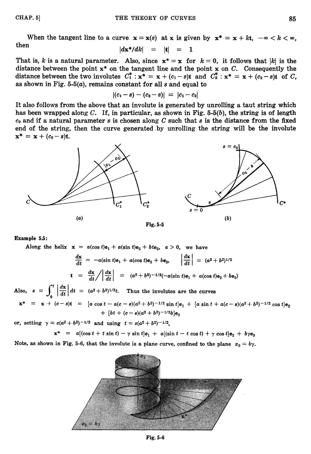
THE THEORY OF CURVES ...................................... 80
Frenet equations. Intrinsic equations. The fundamental existence and unique-
ness theorem. Canonical representation of a curve. Involutes. Evolutes. Theory
of contact. Osculating curves and surfaces.
Chapter 6
ELEMENTARY TOPOLOGY IN EUCLIDEAN SPACES........... 102
Open sets. Closed sets. Limit points. Connected sets. Compact sets. Continuous
mappings. Homeomorphisms.
Chapter 7
VECTOR FUNCTIONS OF A VECTOR VARIABLE ................ 121
Linear functions. Continuity and limits. Directional derivatives. Differentiable
functions. Composite functions. Functions of class Cm. Taylor's formula. Inverse
function theorem.
'-
CONCEPT OF A SURFACE ....................................... 150
Regular parametric representations. Coordinate patches. Definition of a simple
surface. Tangent plane and normal line. Topological properties of simple surfaces.
"

CONTENTS
- FIRST AND SECOND FUNDAMENTAL FORMS ................. 171
First fundamental form. Arc length and surface area. Second fundamental form.
Normal curvature. Principal curvatures and directions. Gaussian and mean curva-
ture. Lines of curvature. Rodrigues' formula. Asymptotic lines. Conjugate
families of curves.
THEORY OF SURFACES - TENSOR ANALYSIS ............ '"... 201
Gauss-Weingarten equations. The compatibility equations and the theorem of Gauss.
The fundamental theorem of surfaces. Some theorems on surfaces in the large.
Elementary manifolds. Tensors. Tensor algebra. Applications of tensors to the
equations of surface theory.
Chapter 11
INTRINSIC GEOMETRY .......................................... 227
Mappings of surfaces. Isometric mappings. Intrinsic geometry. Geodesic curvature.
Geodesic coordinates. Geodesic polar coordinates. Arcs of minimum length. Sur-
faces with constant Gaussian curvature. Gauss-Bonnet theorem.
Appendix I
EXISTENCE THEOREM FOR CURVES
263
Appendix II
EXISTENCE THEOREM FOR SURFACES
264
INDEX
........ ....... ... .1.... ...... ...... .............. ...........
267

..
Cha pter 1
Vectors
INTRODUCTION
Differential geometry is the study of geometric figures using the methods of calculus.
In particular the introductory theory investigates curves and surfaces embedded in three
dimensional Euclidean space Ea.
Properties of curves and surfaces which depend only upon points close to a particular
point of the figure are called local properties. The study of local properties is called dif-
ferential geometry in the small. Those properties which involve the entire geometric
figure are called global properties. The study of global properties, in particular as they
relate to local properties, is called differential geometry in the large.
Example 1.1.
I
Let Q and R be two points near a point P on a curve r in a plane and let G QR be the circle through
P, Q and R, as shown in Fig. 1-1. Now consider the limiting position of the circles CQR as Q and R
approach P. In general, the limiting position will be a circle C tangent to r at P. The radius of C is the
radius of curvature of r at P. The radius of curvature is an example of a local property of the curve,
for it depends only on the points on r near P.
Fig. 1-1
Fig. 1-2
Example 1.2.
The Moebius strip shown in Fig. 1-2 is an example of a one-sided surface. One-sidedness is an example
of a global property of a figure, for it depends on the nature of the entire surface. Observe that a small
part of the surface surrounding an arbitrary point P is a regular two-sided surface, i.e. locally the Moebius
strip is to-sided.
We first investigate local properties of curves and surfaces and then apply the results to
problems of differential geometry in the large. We begin with a review of vectors in E3.
VECTORS
By Euclidean space ES we mean the set of ordered triplets a = (al, a2, as) with ai, lI2, as
real. A vector is a point in E3 and in general will be denoted by a, b, c, x, y, . . . or P, Q, R, . . . .
The negative of a vector a is the vector -a defined by -a = (-al, -a2, -aa). The zero vector
is the vector 0 = (0,0,0). The length or magnitude of a vector a = (al, a2, 4a) is the real
number lal = vi a + a + a. Clearly lal =::: 0 and lal = 0 if and only if a = O.
1

2
VECTORS
[CHAP. 1
ADDITION OF VECTORS
Given two vectors a = (aI, a2, a3) and b = (bI, b 2 , b 3 ) in ES, their sum a + b is the vector
defined by
a + b = (at"r b 1 , a2 + b 2 , a3 + b s )
The difference of two vectors a and b is the vector a - b = a + (-b).
prove that vector addition satisfies
[A 1 ] a + b = b + a (Commutative Law)
[A2] (a + b) + c = a + (b + c) (Associative Law)
[As] 0 + a = a for all a
[] a+ (-a) = 0 for alIa
In Problem 1.1 we
Example 1.3.
Let a = (1, -2, 0) and b = (0,1,1). Then a + b = (1, -1,1), -a = (-1,2,0), b - a = (-1,3,1),
lal = v'5 ·
Example 1.4.
Using [Al] through [] we see that for any a and b,
a + (b - a) = a + (b + (-a» = a + (-a) + b = 0 + b = b
Thus the vector equation a + x = b has a solution x = b - a. It is also the only solution. For if
a + y = b, then
(-a) -+:- a + y = (-8) + b = b - a, or 0 + y = b - a, or y = b - a
Given two points P and Q in ES (that is, two vectors P and Q) we
introduce the special notation PQ for their difference Q - P and we
picture PQ as an arrow drawn from P to Q as shown in Fig. 1-3. By
the distance from P to Q we mean the length IPQI. Evidently
PQ = -QP, IPQI = IQPI, PQ = P'Q' if and only if Q - P = Q' - P', P
and PP = 0 for all P. Fig. 1-3
Example 1.5.
Let a = PQ, b = QR and e = RS, d = SP as shown in Fig. 1-4.
Then
a+b = PQ+QR = Q-P+R-Q = R-P = PH
a+b+e = PR+RS = R-P+S-R = S-p
= PS = -d
a+b+c+d = PS+SP = S-P+P-S = 0
Q b
R
p d S
Fig. 1-4
MULTIPLICATION OF A VECTOR BY A SCALAR
If k is a real number and a = (aI, a2, as) a vector, we define the product ka to be the
vector
ka = (kal, ka2, kas)
Clearly Oa = kO = 0 for all k and 8.
. In the study of vectors we usually refer to the real numbers as scalars. The product ka
is called multiplication of a vector by a scalar.
In Problem 1.4 we prove that multiplication of vectors by scalars satisfies
[81] k l (k 2 a) = (k l k 2 )a = k l k 2 8
(k l + k 2 )a = k I 8 + k 2 8
[8 2 ] k(a + b) = ka + kb (Distributive Laws)
[Bs] la = a
Finally, if a = (al, a2, as), then

CHAP. 1]
VECTORS
3
Ikal
Thus for all k and a,
..1J(f V a2 + a 2 + a 2
V /V- 1 2 3
V (k a l)2 + (ka2)2 + (ka3)2 -
Ikat = Ikllal
(1.1 )
Example 1.6.
Let a:= (1, 7T, 0) and b = (0,2, -1). Then 2a == (2,217',0), (-l)a == (-1, -17",0) == -a, and a - 3b =
(1, 7'f - 6, 3).
Example 1.7.
Let Ul' U2' U3 be given vectors and let a = Ul - 2U2, b = -U2 + 2U3, and c == Ul + U2 + U3. Then
a - 2b - C (U1 - 2U2) - 2(-U2 + 2U3) - (U1 + U2 + U3)
= Ul - 2U2 + 2U2 - 4U3 - U1 - U2 - U3 == -U2 - 5U3
A vector a is said to have the same direction as a nonzero vector b if for some k  0,
a = kb. If a has the same direction as b and also the same length as b, then from equa-
tion (1.1), lal = IkllbJ = klbl == Ibl. Thus k == 1, and a equals b. A vector is thus uniquely
determined by its direction and length. If a = kb, b  0 and k  0, then a has the
opposite direction to b. If a = 0, b = 0 or a has the same or opposite direction to b, i.e.
a = kb for some real k, then a is parallel to b.
We call a vector u of unit length a unit vector. In general Ua shall denote the unit vector
in the direction of a nonzero vector 8. Clearly this is obtained by multiplying a by l/lal, i.e.
Ua = allal (1.)
Example 1.8.
Let a == (1, -1, 3), b = (2, -2,6) and c = (-3, 3, -9). Since a == ib, the vectors a and b have the
same direction. The vectors band c have opposite directions since b = -(2/3)c. The unit vector in the
direction of a is the vector U a = alia I = (1/y'il, -l/v'il, 3/v'il ).
Example 1.9.
In the triangle DAB shown in Fig. 1-5, let a = OA and b = OB,
and let M be the midpoint of side AB. Then the vector OM can be
expressed in terms of a and b as follows:
OM = a + AM = a + .lAB
. 2
= a+  (b-a) == a+!b-!a
=  a + !b
A
o
B
Fig. 1-5
LINEAR DEPENDENCE AND INDEPENDENCE
We now define the very important concepts of linear dependence and linear independence.
Namely, the vectors Ul, U2, . . ., Un are said to be linearly dependent if there exist scalars
k 1 , k 2 , . . ., k n not all zero such that
k 1 U1 + k 2 u2 + · · · + k",u"" = 0 (1.3)
The vectors Ut, U2, . . ., Un are said to be linearly independent if they are not linearly depend-
ent. That is, Ul, U2, . . ., Un are linearly independent if (1.3) implies all k 1 = k 2 = · · · = k n = o.
Note that a set of vectors which includes the zero vector is dependent; for we can always
write 10 + OUt + · · · + Ou", = o.
Example 1.10.
The vectors a == (1, -1, 0), b = (0,2, -1), c == (2,0, -1) are linearly dependent, since 2a + h - e = o.
Example 1.11.
Suppose a is parallel to b. Then a = 0, b = 0 or a = kb, i.e. a - kb = o. Thus a and bare
dependent. Conversely, suppose a and b are dependent. Then k 1 a + k 2 b = 0 where, say, k 1 ¥= O. But
then a = -(k2lk t )b. Thus two vectors are dependent if and only if they are parallel.

4
VECTORS
[CHAP. 1
In Problem 1.10 we prove the following important property of linearly independent
vectors:
Theorem 1.1. If a vector is expressed as a linear function of independent vectors, then it
is expressed so uniquely. That is, if Ut, U2, . . ., Un are independent, and if

U == k t Ul+k 2 u2+ ... +knU n == k{UI+kU2+ ... +kun
then k i == kf, k 2 = k, ..., k n = k.
BASES AND COMPONENTS
The three vectors el == (1,0,0), e2 == (0, 1, 0) and eg = (0,0, 1) are independent. For
k 1 el + k 2 e2 + kse3 == (k l , k 2 , k 3 ) and so if k 1 el + k 2 e2 + k 3 e3 = 0, then k 1 = k 2 == kg == o. Also
any vector a == (al, a2, a3) can be written a == atel + a2e2 + a3e3 as a linear combination of
el, e2 and e3, and by Theorem 1.1 this representation is unique.
In general we call a set of vectors B a basis for E3 if (i) every vector in ES can be written
as a linear combination of the vectors in B, (ii) B is a linearly independent set of vectors.
In Problem 1.11 we prove
Theorem 1.2. Any three linearly independent vectors form a basis in Eg. Conversely,
every basis in E3 consists of three linearly independent vectors.
Let Ut, U2, Us be a basis in space and let a == alUI + a2U2 + a3Ug. The scalars ai, a2, as,
for short, ,i == 1, 2, 3, are called the components of a with respect to the basis UI, U2, us.
It follows from Theorem 1.1 that the components of a vector with respect to a given basis
are unique. However, note that the components of a vector depend upon the basis chosen
and in general the components will change if there is a change in basis. An exception is
the vector 0 whose components are always 0, 0, O.
In general we shall denote the components of vectors a, b, x, y, U, . .. with respect to some
prescribed basis by ai, b i , Xi, Yi, Ui, . .'. .
Example 1.12..
Let Ut, U2' Ug be a basis and let a == 2Ul - U2, b = U2 - 2u3' and c == 3Ul + U3. We will show that
a, b, c are linearly independent and hence also form a basis.. For, suppose
k 1 8 + k 2 b + ksc = (2k 1 + 3k g )UI + (-k 1 + k 2 )U2 + (-2k 2 + ks)us 0
Since the 11i are independent, it follows that
2k 1 + 3k 3 == 0, -k 1 + k 2 = 0, -2k 2 + kg == 0
This is a system of three homogeneous linear equations in k 1 , k 2 , kg. Since the determinant of the coef-
ficients
( 20
det -1 1
o -2
:) = 8  0
the only solution is k 1 == k 2 == k3 = o. Hence the vectors a, b, c are independent. Observe that the com-
ponents of a, b, c appear as the columns in the above determinant.
As suggested in the above example, we have in general
Theorem 1.3. Let Ul, U2, 113 be a basis and let
VI allUI + a21u2 + a31Ug
V2 al2ul + a22U2 + aS2US
V3 - alSUt + a2Su2 + aggUS

CHAP. 1]
VECTORS
5
3
or, in short, Vi =  jUi, j = 1, 2, 3. Then VI, V2, Va is a basis if and only if
i=1
( all al! a 13 )
det a21 a22 a23
a3! a32 ass
 0
SCALAR PRODUCT OF VECTORS
The dot or scalar product of two vectors a = (ai, a2, aa) and b = (b 1 , b 2 , b a ) is the real
number
a · b = a 1 b 1 + b2 + asb a
In particular, for a = b we have the formula
a · a = lal 2
In Problem 1.14 we prove that scalar multiplication satisfies
[C 1 ] a. b = b. a (Symmetric Law)
[C 2 ] (ka) · b = k(a. b) (k = scalar)
[C s ] a. (b + c) = a. b + a. c (Distributive Law)
[C 4 ] Scalar multiplication is positive definite; that is,
(i) a · a  0 for all a
(ii) a. a = 0 if and only if a = 0
Clearly, from the definition, a · 0 = 0 for all a. Also, if a. b = 0 for all a, then
b. b = 0, and hence from [C4](ii), b = o.
(1.4)
Example 1.13.
Let a = (-2, 1,0) and b = (2, 1, 1). Then a. b = -3 and a. a = 5 = lal 2 .
Example 1.14.
Let UI and U2 be given vectors and let a = Ul - U2 and b == 2Ul + U2" Then
a · b == (Ut - U2) · ( 2U l + U2) == 2ul. Ul - 2Ul · U2 + Ul. U2 - U2. u2 - 21ul12 - U1. U2 - IU212
In Problem 1.16 we prove the Cauchy-Schwarz inequality
la · bl  laf Ibl
with equaJ,ity holding if and only if a and b are linearly dependent. The angle between two
nonzero vectors a and b, denoted by f) = 4-.(8, b), is the unique solution of
a · b = I alibI cos 9
(1.5)
satisfying 0 '£ (J  7('.
Example 1.15.
In the triangle ABC shown in Fig. 1-6, let a = BC, b = AC,
c = BA = a - b, and IJ = 4ACB = 4(a, b). If we consider
Icl 2 = la - bl 2 = (a - b) · (a - b) = a · a - 2a. b + b. b B
we have the law of cosines
.0
A
Jcl 2 = lal 2 - 21allbl cos (J + Ibl 2 Fig.I-6
Let b be a nonzero vector. The scalar projection of a onto b, denoted by P b (a), is the
scalar P b (a) = (a. b)/Ibf. The vector P b (a)ub' where Ub is the unit vector in the diTectitm of
b, is called the vector projection of a onto b and is denoted by P b (a). It follows that

6
VECTORS
[CHAP. 1
P b (a) = P b (a)Ub = «a' b)/lbJ) (b/lbl) = (al}b (1.6)
Clearly P b (0) = 0 and P b (0) = O. If 8 # 0, then from equation (1.5), P b (a) = lal cos (J
and P b (a) = lal cos (JUb, where (J = 4(a, b). It follows that P b (a) and P b (a) are independent
of the length of b but depend only on its direction as indicated in Fig. 1-7. In fact, the
vector P b (a) is also independent of the sense of b; that is, P -b (8) = P b (a). For
a- ( -b) a · b
P-b(a) l-bl 2 (-b) - Ibl 2 b Pb(a)
The scalar P b (a) changes sign with a change in the sense of b.
b
 Pb(a)
Pb{a)
Fig. 1-7
b
ORTHOGONAL VECTORS
Two vectors a and b are said to be orthogonal, written a..L b, if a - b = O. It follows
from equation (1.5) that a and b are orthogonal if and only if either a = 0, b = 0 or
() = 4(a, b) = 7i/2.
Example 1.16.
Let a and b be linearly independent and let c = a - P b (a). Then c is a nonzero vector, orthogonal to b.
For sUPPQse c = 0; then from equation (1.6), 0 = 1a - P b (a) = 1a - kb, where k = (a. b}/lbI2, which is
impossible since a and b are independent. Hence c =1= o. Finally,
( a b}b ) (a. b)(b - b)
c · b = a - 112 · b = a' b - 1b12 -
(a-b) - (a-b) - 0
ORTHONORMAL BASES
Let et, e2, e3 be three mutually orthogonal unit vectors
as shown in Fig. 1-8. These vectors are independent; for if
k 1 el + k 2 e2 + kSe3 = 0, then 0 = ei. 0 = ei - (k 1 el + k 2 e2 + kse3) =
ei - kiei = k i or k i = 0 for each i. Therefore they form a basis
called an orthonormal basis.
We observe that Ci, i = 1,2,3, is an orthonormal basis if and
only if
el · el = e2. e2 = e3. es = 1 (Unit vectors)
el · e2 = e2 - es = el - ea = 0 (Mutually orthogonal)
or, in short,
{ 1, if i:= i
ej' ej = 8ij = 0, if j ¥' i (i, j = 1,2,3)
The quantity 8ij is called the Kronecker symbol and will be used repeatedly.
Thus c J.. b.
82
Fig. 1-8
(1.7)

CHAP. 1]
VECTORS
7
In Problem 1.23 we prove
Theorem 1.4. Let el, e2, ea be an orthonormal basis and let a = aiel + 2 + aaea and
b == b 1 el + b 2 e2 + baea. Then
a
(i) a- b == a l b 1 + a 2 b 2 + aab a =  Uib i
i=l
(ii) lal = ya:a = via: + a + a: =  t a
1=1
(iii) ai == a. ei, (i = 1,2,3).
Example 1.17.
Let a = el + 2ea, b == 2el + e2 - 2ea, and c = -2e2 + ea. Then
a - b == (1)(2) + (0)(1) + (2)(-2) = -2
(a - c)b == [(1)( 0) + (0)(-2) + (2)(1)] (2el + e2 - 2ea)
\al - V 12+22 == V5
a
Ua - j;j = (1/v'5)el + (2/V5 )e3
a-b -2
cos 4. (a, b) = I II I = -
a b 3V5
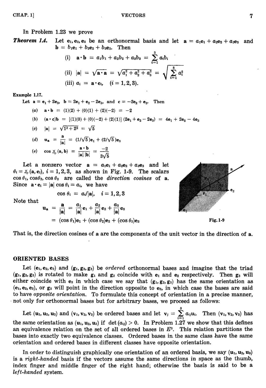
Let a nonzero vector a == aIel + a2 + asea and let
(h == 4-(a, ei), i = 1,2,3, as shown in Fig. 1-9. The scalars
cos ()t, COS()2, COS ()s are called the direction cosines of a.
Since a. ei == jal cos (h == ai, we have
cos ()i = tli/lal, i == 1,2,3
(a)
(b)
(0)
(d)
4el + 2e2 - 4e3
(e)
a at a2 as
U a - lal = 1;Je 1 + fal e2 + lal ea
- (cos (1)el + (cos (2)e2 + (cos 63)ea
Note that
Fig. 1-9
That is, the direction cosines of a are the components of the unit vector in the direction of a.
ORIENTED BASES
Let (el, e2, ea) and (gl, g2, ga) be ordered orthonormal bases and imagine that the triad
(gt, g2, ga) is rotated to make gl and g2 coincide with el and e2 respectively. Then ga will
either coincide with ea in which case we say that (gl, g2, gs) has the same orientation as
(et, e2, es), or g3 will point in the direction opposite to ea, in which case the bases are said
to have opposite orientation. To formulate this concept of orientation in a precise manner,
. not only for orthonormal bases but for arbitrary bases, we proceed as follows:
3
Let (Ul, U2, U3) and (VI, V2, V3) be ordered bases and let VJ ==  UrijUi. Then (VI, V2, Va) has
i=l
the same orientation as (ut, Uz, U3) if det (llij) > O. In Problem 1.27 we show that this defines
an equivalence relation on the set of all ordered bases in E3. This relation partitions the
bases into exactly two equivalence classes. Ordered bases in. the same class .have the same
orientation and ordered bases in different classes have opposite orientation.
In order to distinguish graphically one orientation of an ordered basis, we say (Ul, U2, U3)
is a right-handed basis if the vectors assume the same directions in space as the thumb,
index finger and middle finger of the right hand; otherwise the basis is said to be a
left-handed system.

8
VECTORS
[CHAP. 1
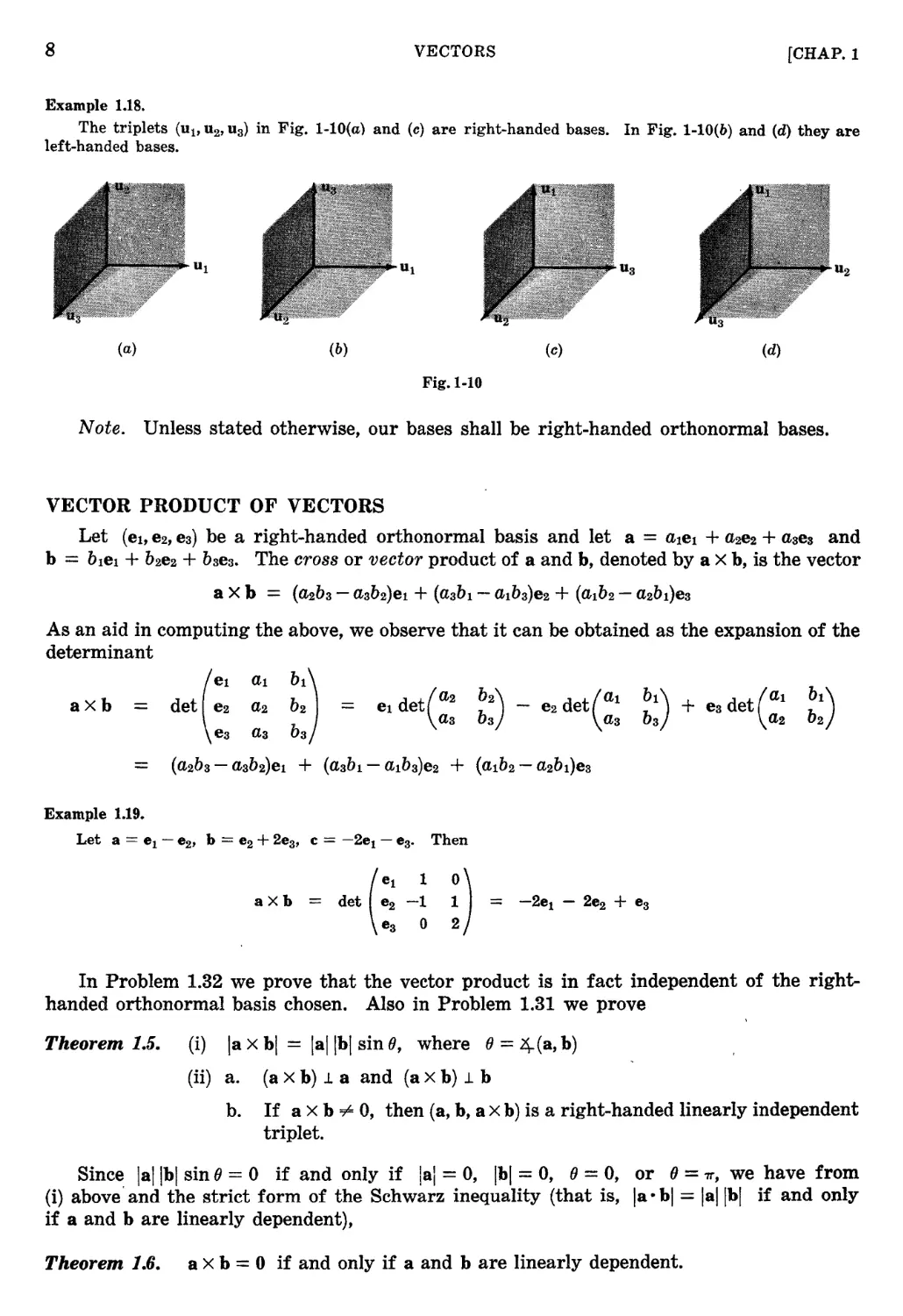
Example 1.18.
The triplets (Uh U2, U3) in Fig. 1-10(a) and (c) are right-handed bases. In Fig.. 1-10(b) and (d) they are
left-handed bases.
U1
U1
Us
U 2
(a)
(b)
(c)
(d)
Fig.l-lO
Note. Unless stated otherwise, our bases shall be right-handed orthonormal bases.
VECTOR PRODUCT OF VECTORS
Let (el, e2, es) be a right-handed orthonormal basis and let a = aIel + a2C2 + aaes and
b = b 1 el + b 2 e2 + b s e3. The crOBB or vector product of a and b, denoted by a x b, is the vector
a X b = (a 2 b a - a S b 2 )el + (aab 1 - a 1 b a )e2 + (a 1 b 2 - a 2 b 1 )ea
As an aid in computing the above, we observe that it can be obtained as the expansion of the
determinant
axb
det ( :: :: ::
ea as b s
el d et ( a 2
as
b 2 ) _ e2 det ( a 1
b a as
:) + es det(:; ;)
(a 2 b s - aab 2 )el + (aab 1 - a 1 b a )e2 + (a 1 b 2 - a 2 b 1 )ea
Example 1.19.
Let a == el - e2' b == e2 + 2ea, c = - 2e l - ea- Then
aXb - det (:: - )
- 2e l - 2e2 + ea
In Problem 1.32 we prove that the vector product is in fact independent of the right-
handed orthonormal basis chosen. Also in Problem 1.31 we prove
Theorem 1.5. (i) la x bl = lallbl sin (), where () = 4-(a, b)
(ii) a. (a X b) 1 a and (a X b) 1. b
b. Ifax b # 0, then (a, b, a x b) is a right-handed linearly independent
triplet.
Since Jallbl sin () == 0 if and only if lal = 0, Ibl = 0, (J = 0, or () = 7(', we have from
(i) above' and the strict form of the Schwarz inequality (that is, la. bl = lallbl if and only
if a and b are linearly dependent),
Theorem 1.6. a x b = 0 if and only if a and b are linearly dependent.

CHAP. 1]
VECTORS
9
If a and b are not linearly dependent, i.e.
if aX b # 0, Theorem 1.5(ii) states that a x b
is orthogonal to a and to b and such that a X b
(a, b, a X b) is a right-handed triplet, as shown
in Fig. 1-11(a).
Observe that the vector product is in gen-
eral not commutative. Although b x a has the
same magnitude as a X b (Theorem 1.5(i)) and
is parallel to a X b (Theorem 1.5(ii)a), it has the
opposite direction (Theorem 1.5(ii)b). Thus
b x a = -(a X b), as shown in Fig. 1.11(b).
b
hXa
(a)
(b)
Fig. I-II
Example 1.20.
For an orthonormal basis (gt, g2' g3) shown in Fig. 1-12, it follows
from Theorem 1.5 that
g1 X g1 = 0
gl X g2 = g3
g1 X ga = -g2
g2 X gl- = -13
g2 X g2 = 0
g2 X g3 = gt
(3 X gl = 12
g3 X g2 = -gl
g8 X g3 = 0
'2
Fig. 1-12
In Problem 1.29 we prove that the vector product satisfies
[E 1 ] a X b = -(b X a) (Anticommutative Law)
[E 2 ] a X (b + c) = a X b + a X c (Distributive Law)
[Eal (ka) x b = k(a x b) (k = scalar)
[E4] a x a = 0
Note that the vector product is not only not commutative but also not associative; that is,
in general a X (b X c) -# (a X b) X c. For as shown in Example 1.20, gl X (gl x g2) =
gl X g3 = -g2, whereas (gl X gl) X g2 = 0 X g2 = o.
Example 1.21.
Consider the triangle ABC shown in Fig. 1-13. Let a = BC, b = AC, e =: AB = b - a, a == 4- (b, c),
/3 = 4- (c, a), and y = 4- (a, b). Now,
o = c X c = c X (b - a) = c X b - c X a
or
Similarly,
cXb = cXa
Hence c X b = c X a == b X a
A
c X b - (b - a) X b == b X b - a X b
bXa
But then
Ie X bl = Ie X al = Ib X al
lellbl sin a = lei !al sin fJ = Ibllal sin y
or
which gives the law of sines
sin a
lal
sin p
Ibl
sin y
lei
Fig. I-IS
TRIPLE PRODUCTS AND VECTOR IDENTITIES
The product a. b X c is called the mixed or triple scalar product. Note that parentheses
are not required; for this can only mean a. (b x c), the scalar product of the vector a and
the vector b X c. This product is also conveniently given in terms of a determinant. For, let

10
VECTORS
[CHAP. 1
a = alel + a2e2 + a3e3, b = blel + b 2 e2 + b S e3, c = Clel + C2e2 + CgeS
Then
a-bXc
( e 1 bl Cl )
(aiel + a2e2 + a3e3) · det e2 b 2 C2
eg b a Cg
al(b 2 c s - b 3 C 2) - a2( cab l - c l b 3 ) + as(btC2 - b2Cl)
(1.8)
at b 1 CI
det a2 b 2 C2
a3 b s C3
It follows from properties of the determinant that
a-bxc == c-axb = b-cxa = -(b-axc) == -(c-bxa) = -(a-cxb) (1.9)
In particular, it follows that a. b X c = a X b · c. Thus we can drop the dot and cross in
the notation of the triple scalar product and use instead the notation
[abc] == a - b X c = a X b - c
As immediate consequence of Theorem 1.3 and equation (1.8) we have
Theorem 1.7. [abc] == 0 if and only if a, b, c are linearly dependent.
A number of useful identities relate vector and scalar products of vectors. A basic
identity, which is derived in Problem 1.35, is
Theorem 1.8. a X (b X c) = (a. c)b - (a. b)c
Others, easily derived from the above, are
[F 1 ] (ax b) · (cxd) = (a.c)(bed) - (aed)(b-c)
[F 2 ] (a X b) X (c X d) = [abd]c - [abc]d
#'
Example 1.22.
Let u = c X d. Then
a X b. u = a e b X u = a- [b x (c X d)] == a. [(b. d)c - (b. c)d]
where we used (1.9) and Theorem 1.8. It follows that
(a X b) · (c X d) = (a - c) (b · d) - (a. d) (b · c)
which proves [F 1] above.
Solved Problel11s
VECTOR ADDITION
1.1. Prove properties [At] through [] for vector addition. That is, prove that [AI]
a + b = b + a, [A2] (a + b) + c = a + (b + c), [As] a + 0 == a, [A4] a + (-a) =:: O.
[At]: a + b = (al + b l , a2 + b 2 , as + b s ) = (b t + ah b 2 + a2, b 3 + as) == b + a
[A 2 ]: (a + b) + c = [(al + b l ) + cl, (a2 + b 2 ) + c2, (as + b s ) + cs]
== [at + (b i + Ct), u2 + (b 2 + C2), a3 + (b 3 + cs)] == a + (b + c)
[As]: a + 0 == (al + 0, a2 + 0, ag + 0) = (at, a2, ag) = a
[A.t]: a + (-a) == (at - aI' a2 - a2, as - as) == (0, 0, 0) 0

CHAP. 1]
VECTORS
11
1.2. In the parallelepiped shown in Fig. 1-14
let a == OP, b = OR, c == OS. Find OV,
VQ and RT in terms of a, b, c.
OV OR + BV OR + OS = b + e
VQ VR+RQ - -RV+RQ
-OS + OP = -e + 8
T
u
RT
KS + ST RO + OS + ST
= -b + c + a
o
Fig. 1..14
1.3. It has been shown (Example 1.4.) using the properties [At] through [Ai] that the
vector equation a + x = b has a unique solution x = b + (-a) = b - a. Using this
result, show that:
(a) the vector 0 is unique, that is, if 0' + 8 == a, then 0' = 0;
(b) the vector -8 is unique, that is if a' + a == 0, then a' == -a;
(c) - (-a) = a for all a.
(a.) follows from the uniqueness of the solution to the equation x + a = 8.
(b) follows from the uniqueness of the solution to the equation x + a = o.
(0) follows when we consider the equation -8 + x = O. This has the solution x = 0 - (-8) =
-(-a). But also -a + a = 0; thus -(-a) == a, by uniqueness of the solution to the equation.
MULTIPLICATION BY A SCALAR
1.4. Prove properties [B 1 ] through [Ds] for multiplication of a vector by a scalar. That
is, prove that: [B 1 ] k 1 (k 2 a) = (k l k 2 )a; [B2] (k 1 + k 2 )a == k l 8 + k2a, k(a + b) = ka + kb;
[Ba] 1a = 8.
[8 1 ]: k 1 (k 2 8) = (k 1 (k 2 a t), k l (k#2)' k t (k 2 a a »
- «k 1 k 2 )al, (klk2)' (kt k 2)a.g) == (kt k 2)a
[B2]: (k 1 + k 2 )a
«k 1 + k 2 )ah (k l + k 2 )a2, (k 1 + k 2 )aa)
(klal + k 2 a lJ k 1 a 2 + k2' kla. a + k 2 a a ) = k 1 8 + k 2 8
k(a + b)
(k(al + bl), k( + b 2 ), k(Q,3 + b s »
(kat + kblJ k + kb 2 , ka a + kb s ) ka + kb .
[Ds]: 1a
( la t, 1, 1as) = (at, a2, Q,3) = a
1.5. If a = Ut - 2U2 + 3118, b == U2 - Us and c = U1 + 2U2, find 2a - 3(b - c) in terms of
Ut, U2, us.
2a - 3(b - e) == 2a - 3b + 3e
2(Ul - 2U2 + 3us) - 3(U2 - us) + 3(Ul + 2U2)
2U1 - 4U2 + 6ua - 3U2 + 3us + 3U1 + 6U2 = 5U1 - U2 + 9U3
1.6. Prove that the line joining the midpoints of two
sides of a triangle is parallel to the third side and
has one-half its magnitude.
Let M and M' be the midpoints of the sides AB and AC re-
spectively of a triangle ABC shown in Fig. 1-15. Then AM =
lAB, AM' = lAC and MM' == AM' - AM = !(AC - AB) =
i DC . Thus MM' is paraIlel to BC and has half the magnitude.
A
c
Fig. 1-15

12
VECTORS
[CHAP. 1
1.7. Let a == OA, b = OB,. b ::/:: a and c == OC
as shown in Fig. 1-16. Show that C lies on
the line L determined by A and B if and
only if c = k 1 a + k 2 b where k 1 + k 2 == 1.
If C is on L, then BA == a - band BC ==
c - b are parallel. Hence there exists k such that
o
Fig. 1..16
c - b == k(a - b) or c == ka + (1 - k)b = k1a + k 2 b
where k 1 + k 2 == k + 1 - k == 1. Conversely, if c == k 1 a + k 2 b, where k 1 + k 2 == 1, b :F a, then
c - b == k 1 a + k 2 b - b == k 1 a - (1- k 2 )b == k1a - k1b == kt(a - b)
That is, c - b == BC and a - b == BA are parallel, so that C is on the line determined by A and B.
LINEAR DEPENDENCE AND INDEPENDENCE
1.8. Show that the vectors ut, U2, . . ., Un are dependent if and only if one of the vectors
is a linear combination of the others.
Suppose, say, Ul is a linear combination of U2'...' un; i.e. Ul == k 2 U 2 + · · · + knu n . Then
Ul - k 2 U 2 - · · · - knu n == 0 where at least the coefficient 1 of U1 is not zero. Hence Ul, . . ., Un are
dependent.
Conversely, if U1' . . ., Un are dependent, then there exists k 1 ,..., k n not all zero such that
klUl + k2U2 + · · · + knUn == O. Suppose, say, 'k 1 =F 0; then Ul == -(kkt)U2 - · · · - (k n lk 1 )u n and so
Ul is a linear combination of U2' . . ., Un.
1.9. Prove that a set of vectors which contains a linearly dependent subset is linearly
dependent.
Suppose, say, the subset {Ut, U2, ..., Uk} of the set {Ub U2' ..., Uk' Uk+l, ..., Un} is dependent.
Then there exist k h . . ., kk not all zero such that ktUt + k2,U2 + .. · + kkUk = O. But then
k l U l + k 2 U 2 + ... + kkUk + OUk+ 1 + ... + Onn == 0
and so Ul' U2, . . ., Un are dependent.
1.10. Prove Theorem 1.1: If Ul, . . ., Un are independent and
k1u! + k 2 u2 + · · · + knu n = k u! + kU2 + · · · + kun
then k 1 = k, k 2 == k, ..., k n = k.
,
Suppose some k j =F k j ; then
" I ,
(k 1 - k 1 )Ul + (k 2 - k 2 )U 2 + ... + (k j - k j )Uj + ... + (k n - kn}u n == 0
where k j - k; ¥= o. But this implies Ub . .., un are dependent, which is a contradiction.
BASES AND COMPONENTS
1.11. Show that any vector in E3 can be written as a linear combination of three inde-
pendent vectors; hence three independent vectors form a basis in E3.
If a, b, c are linearly independent, then the equation
a + yb + zc = 0
has only the solution x == y = z = o. Equivalently, the system

CHAP. 1]
VECTORS
13
xal + yb t + ZCl 0
xa2 + yb 2 + ZC2 0
xa3 + yb s + zCa - 0
has only the trivial solution x = y = Z == 0, ,vhich is the case only if the matrix of coefficients has
determinant not zero, that is,
det ( : : : ) ¥= 0
a3 b 3 C3
But then for any vector U = (Ut, u2' us) in ES the system
xal + yb 1 + zCl Ut
xa2 + yb 2 + ZC2 == u2
xas + yb g + zC3 = Us
has a solution x = kt, y = k 2 , Z == kg which means that u == k1a + k 2 b + kac as required.
1.12. Show that any four or more vectors in E3 are linearly dependent.
Consider the vectors U1, U2, U3, U4, .. ., Un- We can assume that Uh U2, us, are independent. For
otherwise, U1, u2, U3, U4, · - ., un' having a dependent subset, would be dependent. But if Ub U2' U3
are independent, they form a basis and so U4 == ktUt + k2U2 + kaua, which implies Ut, U2' Us, U4
are dependent. Hence U1, U2, U3, 1.14' . . ., Un are dependent.
1.13. Let Ul, U2, Ua be a basis and let a = Ul - U2 + 2us, b = U2 - Ua and c = -U2. Find
the components of 2a - b - 2c in terms of Ul, U2, us.
2a - b - 2c :::: 2(U1 - U2 + 2U3) - (U2 - U3) - 2( -U2)
= 2U1 - 2U2 + 4U3 - U2 + U3 + 2U2 == 2U1 - U2 + 5ua
Thus the components of 28 - b - 2c with respect to Ul, U2' ua are 2, -1, 5.
SCALAR PRODUCT
1.14. Prove properties [C 1 ] through [C 4 ], page 5, for the scalar product of vectors.
[C I ]: a. b = al b l + a2 b 2 + a3 b a == blal + b2a2 + baa3 == b. a
[C 2 ]: (ka) · b = kalbl + kb2 + ka3ba = k(a1b 1 + a2b2 + aab3) == k(a. b)
lC a ]: a. (b + c) al(b 1 + cl) + a2(b 2 + C2) + a3(b s + ca)
== a1 b 1 + a2 b 2 + a3 b g + al Cl + a2 c 2 + aa C 3 == a. b + a. c
(C ] Cl 1 2 2 2 ::::... 2 2 2
4 : ear Y a · a == at + a 2 + a 3 - 0 and a · a == al + a 2 + a 3 == 0 iff a1 = a2 == as == O.
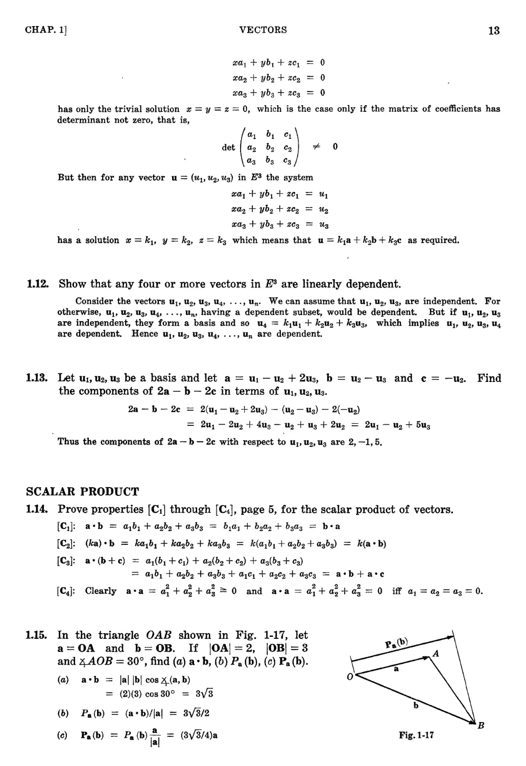
1.15. In the triangle OAB shown in Fig. 1-17, let
a = OA and b == OB. If IOAI = 2, lOBI = 8
and 4AOB = 80°, find (a) a. b, (b) Pa (b), (c) Pa (b).
(a) a. b lallbl cos 4(a, b)
== (2)(3) cos 30° = 3V3
(b) p. (b)
(c) p. (b)
(a. b)/Ial == 3V3/2
p. (b) ,:, = (3V3/4)a
B
Fig. 1-17

14
VECTORS
[CHAP. 1
1.16. Prove the Cauchy-Schwarz inequality, la. bl  lallbl, with equality holding if and
only if a and b are linearly dependent.
The inequality is clearly valid if a == 0 or b == 0, and so we may assume that a, b =F- 0..
Then from [C 4 ] ,
o  (  ::: a =  ::: b) · (::: a =  ::: b)  2/allbl = 2a. b
or ::t2a. b  21 a llbl which gives the desired inequality la. bl  lallbl. The remaining statement
follows from the fact that equality can hold if and only if either  ::: a +  ::: b = 0 or
 Ibl a - jl b = 0 which is the case if and only if a and b are linearly dependent.
lal Ibl
1.17. Prove the triangle inequality, la:t bl  la( + Ibl.
fa + bl 2 == (a:t: b) · (a :t: b) == lal 2 + Ibl 2 ::t 2(a · b)  lal 2 + Ibl 2 + 21allbl  (Ial + Ib!)2
and the desired result follows upon taking square roots.
1.18. Show that Iial - jbll  la:t= bl for all a and b.
From the triangle inequality,
lal == la:t: b + bl  la + bl + Ibl or
Ibl = I:t:bl == la + b - al  la + bl + lal
Also
lal - Ibl  la:t: bl
or [bl - lal  la + bl
Thus lIal - Ibll == Max (jal-Ibj, Ibl-laD === la + bl, which is the required result.
ORTHOGONAL VECTORS
1.19. Let c be orthogonal to a and b. Show that c is orthogonal to k1a + k 2 b for all k l , k 2 _
Since c is orthogonal to a and b, c. a == 0 and c. b == o. Hence
c. (k1a + k 2 b) == kl(c. a) + k 2 (c. b) =: 0
Thus c is orthogonal to k1a + k 2 b.
1.20.
Let Uh U2, U3 be a basis and define
a=Ut, b=U2- P a(U2), c=Ug-Pa(U3)-Pb(U3)
Show that a, b, c are nonzero mutually orthogonal vectors.
a · b a · (U2 - Pa (U2)) == a. [U2 - (a. u2)a/laI2]
== a. U2 - (a. u2)(a. a)/la[2 = a. U2 - a. U2 = 0
and so a 1. b. Also,
,a · c = a. [U3 - Pa (U3) - Pb(U3)] == a. [U3 - (a · u3)a/laI 2 - (b. u3)b/lbI 2 ]
== a. Us - a. U3 - (b · u3)(a · b)ilbl 2
Since a · b = 0, a · c == a. U3 - a · Us == 0 and so a J.. c. Finally,
b. c == b. [U3 - (a · u3)a/laI 2 - (b. u3)b/lbI2]
== (b  ua) - (a · u3)(a · b)/l a l 2 - (b. us)(b. b)/lbI 2 == (b. U3) - (b. U3) = 0
Thus a, b, c are mutually orthogonal. They are also nonzero vectors, because: a == U1 # 0; if b == 0,
o == b == U2 - Pa (U2) == U2 - ka == U2 - kUl
which is impossible since Ul and u2 are independent; if c == 0,
o == c == Us - Pa (us) - Pa (U3) == Us - k1a - k 2 b == U3 - k1u! - k 2 (U2 - kU1) u3 - kaul - k 2 U 2
which is impossible since u1' U2, U3 are independent..

CHAP. 1]
VECTORS
15
ORTHONORMAL BASES
s
1.21. Show that (a) 28 21 + 38 22 + 48 23 = 3, (b)  8..b. = b..
;= 1 13 J to
(0;)
(b)
{ l if j = i
8 ij = 0 if i ¥= i. Hence 28 21 + 38 22 + 4B 23 =: 2(0) + 3(1) + 4(0) =: 3.
3
As above , the onl y contribution comes from 8.:. Thus  8.b. =: B..b.
.." . 1.:1 :I n 'I.
3=1
bi.
S 3 3
1.22. Let Ul, U2, 113 be a basis and let Vj =  aijUi and Uj =  bijVi. Show that  aucbkJ = 8ij.
I i=l k=l
3 3 i=
We write Uj =  8ij11i =  bkjVk where we have changed the name of the index from
i=1 k=1
3
i to k. Also, Vk =  o;ikUi. Substituting,
i=l
:i 8 i '11i - :i b kj :i ltik11i - .:i [ :i Itikbk j ] Ui
i=l J k=1 i=l 1=1 k=1
Since u 1 , U2, Us are independent equate components and obtain 8ij
3
 aikbkj ·
k=l
1.23. Prove Theorem 1.4: If el, e2, eg is an orthonormal basis and a == aIel + G2e2 + a3e3
and b = b 1 el + b 2 e2 + bses, then
(a) a. b == a 1 b 1 + a 2 b 2 + aab s , (b) lal = y a + a + a;, (c) ai = a. ei, i == 1,2,3.
(a) a. b - (aiel + a2e2 + ages) · (btel + b 2 e 2 + b3es)
albt(et · et) + al b 2(el · e2) + al b S(e l · eg)
+ a2 b t(e2 · el) + a2 b 2(e2 · e2) + a2 b S(e2 · e3)
+ a3 b l (eg · el) + a g b 2 (e3 · e2) + asbg(ea · e3)
al b 1 + a2 b 2 + a g b 3
In short, we have
a.b
( :i a.e. ) · ( :i b .e. )
. I t t . 1 j:1
t= ,=
s s
  aiblei. ej)
i=l ;=1
or
a.b
S 3
 
i=l J=1
n..b.8. .
"""l. 1 11
s
 a.b.
 1. 
i=t
(b) lal == ya;-a
v a 2 + a 2 + a 2
123
(c) a. e. = (  a.e. ) · e. =  a.(e.. e.) -
. ; 3 3 \ ; 3 J t.
 a.8..
..;. J Jt.
3
a.
1.
1.24.
Let a == el - 2e2 + Ses and b == e2 - ea. Find (a) a. b, (b) lal, (c) U a , (d) Pa (b),
(e) Pa (b), (I) cos 4-(a, b), (g) a. el, a. e2, a. es, (h) direction cosines of a.
(a) a. b = (1)(0) + (- 2)(1) + (3}(-1) = -5
(b) lal va:; == V (1)2 + {-2)2 + (3)2 = VI4
(c) U a a/I a 1 = (1/v'i4)(et - 2e2 + 3ea)
(d) Pa (b) == (a. b)/Ial = -5/Vf4
(e) Pa (b) = Pa {b)u a == -(5/14)(el - 2e2 + 3es)
(I) cos-<a,b) == (a.b)/Iallbl = (-5/Vf4V2> - -5/(2,;7>
(g) a. el == 1, a. e2 = -2, a. es = 3
(h) cos -<a, et) = at/lal = 1/v'i4, cos 2\-(a, e2) = a2/lal == -2/VJj, cos (a, es) == a3/1al = 3/V14

16
VECTORS
[CHAP. 1
I
1.25. Let Ut, U2, Us be an arbitrary basis. Show that there exists a unique basis VI, V2, Va
such that
VI · Ul = 1 V2 · Ul = 0 V3 · Ul = 0
VI · U2 = 0 V2 · U2 = 1 Va · U2 = 0
VI · Us = 0 V2 · 118 = 0 Vg · Us = 1
or Vi. Uj = 8ij, i, j = 1, 2, 3. The basis VI, V2, Va is called the dual or reciprocal bas1.S
to Ut, U2, Us. Accordingly if a = aIUl + a2U2 + agU3 and b = b 1 vl + b 2 v2 + bavs, then
a' b = (lLilli) · (  bjVi) =   lLibj(Uj' Vi) -   lLib j 8ii -  lLib i
Observe that an orthonormal basis is its own dual.
Let el, e2, ea be an orthonormal basis and let
Ul all e l + a12 e 2 + alS e S
U2 lel + 2e2 + a2S e S
U3 aal e l + 4S2 e 2 + asses
and VI lel + a12e2 + 3eS
Then VI · Ul o,l11 + a122 + a133 - 1
VI. U2 0,21 a11 + a22 re 2 + 3re3 - 0
VI. U3 - aSl z l + 1Is2 X 2 + a333 - 0
is a system of three equations for a11' X2' 3. Since det (0,4;) =F 0, there exists a unique solution
VI = leI + re2e2 + 3e3. Similarly we have unique solutions for V2 and Va. It remains to show
that Vb V2' Va are independent and hence form a basis.. We consider
a
k 1 V l + V2 + kava -  kiVi - 0
i=1
If we multiply by Uj, i = 1,2, 8, we obtain
L! kiVi] · ui il kj(Vi · Uj) - tl k i 8ij - k j
Thus k 1 = k 2 = ka = 0 and so VI' V2J V3 are indepndent and form a basis.
0,
i = 1,2,3
ORIENTATION
1.26. Show that the triplet (VI, V2, Va), where VI = 2Ul - U2 + 2113, V2
V3 = -Ul + 2U2 + 113,' has the same orientation as (Ut, U2, us).
The determinant of the components is det ( - ; -  ) = 1 > O.
Hence (Vh v2' V3) has the same orientation as (Ub U2' U3).
U2 + Us and
1.27. Show that orientation is an equivalence relation on the set of all ordered bases in ES.
That is, show that:
(a) (VI, V2, Va) has the same orientation as (VI, V2, va) for all (Vt, V2, vs).
(b) If (Vl, V2, vs) has the same orientation as (U1 1 U2, Ua), then (Ut, U2, U3) has the same
orientat.ion as (VI, V2, Va).
(c) If (WI, W2, Wa) has the same orientation as (VI, V2, vs) and (VI, V2, Va) has the same
orientation as (U1, U2, us), then (WI, W2, wa) has the same orientation as (Ut, U2, 113).

CHAP. 1]
VECTORS
17
3
(a) We write Vj ==  8ijVh j = 1, 2, 3. Since det (8 ij ) = 1, (Vh V2, vs) has the same orientation as
( ) i-I
VI' v2' Vs · -
g
(b) Let Vj =  aijui and Uj =  biivi. From Problem 1.22, kl aikbkj == Bijo It is also easily 
verified by expanding that det ( :i aikb kj ) = det (aij) det (b ij ), and so
k=l
det (8ij) 1
det (bi;) = det (aij) det (aij)
Since (Vt, V2, Vg) has the same orientation as (Ut, U2' us), det (aij) > O. Hence. det (b ii ) > 0,
and thus (Ult U2' us) has the same orientation as (V1' V2' Vs).
3 3
,(c) Let Vk =  aikui and Wj =  bkjVk. Substituting, we obtain
i=l k=t
W'
1
3 S
 b k .  a'k l1 .
1 . !. -&
k=1 1.=1
:i ( :i kbkj ) Ui
i=l k=l
Thus
3
Wj = . CijUi where
=1
g
cij =  aikbki' i, j = 1,2,3.
k=l
Also,
det (Cij) = det (  aikb kj ) = det (j) det (bij)
Since (WI' W2, ws) has the same orientation as (VI' V2, vs) and (v1, V2, vs) has the same orienta-
tion as (Ub U2, us), then det (b ij ) >"0 and det (aij) > 0; hence det (Cij) > o. Thus (Wb W2, ws)
has the same orientation as (U11 U2, us).
VECTOR PRODUCT
1.28. Let a = 2el - e2 + es, b = e1 + 2e2 - es, c = e2 + 2es_ Determine (a) a,X b, (b) b x a,
(c) a x (b x c), (d) (a x b) x c, (e) (a X b) · c, (I) a x (b + c) - a x b - a X c.
(a) a X b
( e 1 2 1 )
det e2 -1 2
es 1-1
-et + 3e2 + 5eg
( -1 2 ) ( 2 1 ) ( 2
= et det 1 - e2 det + eg det
-1 1 -1 -1
)
(b) b X a
( el 1 2 )
det e2 2-1
es -1 1
el - 3e2 - 5eg. Observe that a X b  -(b X a).
( c) a X (b X c)
(2el - e2 + eg) X det ( : 
eg -1
o
= det ( :: - -: ) -
e3 1 1
el+ 3e 2+ e g
- ( 2e l - e2 + es) X ( 5e l - 2e2 + ea)
(d) (a X b) Xc = (-el + 3e2 + 5eg) X (e2 + 2es)
det (:: -: 0
el + 2e2 - eg
Observe that a X (b X c) =F (a X b) Xc.
(e) (a X b) · c
(-el + 3ez + 5eg) · (e2 + 2es)
(-1)(0) + (3)(1) + (5)(2) - 13
"

18
VECTORS
[CHAP. 1
(I) a X (b + c) == det ( : -
e3 1
4e2 + 2eg. Then
a X (b + c) - a X b - a X c
: ) = -4el - e2 + 7ea. a X b = -el + 3e2 + 5ea. and a X c = -3e l -
(- 4e l - e2 + 7eg) - (-el + 3e2 + 5e3) - (-3el - 4e2 + 2eg) 0
1.29. Prove that (a) a x (b + c) = a X b + a X c, (b) (ka) X b = k(a X b).
Let a == aIel + a2eZ + ageg, b == b 1 e! + b2e2 + bge3' C == cle1 + cZe2 + C3e3.
(a) a X (b + c) == [a Z (b 3 + Cg) - ag(b z + CZ)]el + [a3(b t + Cl) - al(b 3 + cs)]ez
+ [al(b z + c0 - a2(b 1 -1- Cl)]eg
(a2 b 3 - a g b Z )el + (a3 b l - a l b s )e2 + (a 1 b 2 - a Z b t )e3
+ (a2 C g - 0'3 C 2)el + (agCI - 0,1 C3)e2 + (0,1 C2 - Cl)eg
aXb+aXc
(b) (ka) X b - (kbs - ka s b 2 )el + (kagb 1 - kal b 3 )ez + (kat b 2 - ka2bl)e3
k[(a2 b S - a g b 2 )el + (a3b! - a 1 b 3 )ez + (a l b 2 - a2bl)e3] = k(a X b)
1.30. Show that la x biz = Jal21bJ2 - la. biz.
Let a = aIel + a Z e2 + a3eg and b = blel + b2 + b 3 eg_
la X biz == (a X b). (a X b) = [(azb g - a g b 2 )el + (aSb l - a l b 3 )e2 + (a 1 b 2 - bl)e3]
· [(a2 b g - a 3 b z )el + (agb l - a1bs)ez + (a1b z - a2 b l)e3]
(a Z b 3 - a3 b 2)2 + (a g b 1 - a l b 3 )Z + (a1b z - a2 b l)2
22 Z2 22 22 22 22
a 2 b g + a S b 2 + agb 1 + a l b 3 + a 1 b 2 + a 2 b 1
- 2a2b2asbs - 2o' 1 b 1 a s b g - 2a l b 1 a 2 b Z
lal21bl2 - la. bl 2 (a. a)(b. b) - (a. b}(a. b)
(a; + a + a;)(b + b; + b:) - (a 1 b 1 + b2 + a g b g )2
Z 2 Z 2 2 b 2 Z b 2 2 b Z 2 2 b b
a l b 2 + albg + 0,2 I + a z 8 + as 1 + a 3 b 2 - 2a 1 b 1 a z b 2 - 2a 1 b 1 a 3 b g - 20,2 Z a 3 3
The required identity follows by comparing the above.
1.31. Prove Theorem 1.5:
(i) la x bl = lallbl sin B, (j = 4(a, b)
(ii) a. (a X b) .1 a and (a'x b) 1. b
b. If (a X b) ¥= 0, then (a, b, a X b) has the same orientation as (el, e2, es).
(i) Using the preceding problem,
la X biz = lal 2 Iblz - la. bl 2 == lal 2 Ibl 2 - lal z Ibl 2 cos 2 8
== la1 2 1b1 2 (1 - cos 2 0) == la/ 2 [b1 2 sin Z 8 == ([alibI sin 0)2
Since sin 6 =::: 0 for 0  8 -= 'If, we have la X bl = lallbl sin 8.
(ii) a. Let a == aIel + a2eZ + ageg and b = b i e l + b 2 e 2 + b3e3-
(a X b) · a == [(b3 - a 3 b z )el + (aSb l - a 1 b a )e2 + (aI b 2 - a2 b l)e3] · (aIel + a2 e 2 + ages)
= o'la2 b 3 - ala g b 2 + a2 a S b l - a20'lb g + a3 a l b 2 - a3bl == 0
Similarly, (a X b) · b = O. Hence (a X b) ..1 a and (a X b) 1. b.
b. The determinant of the components of (a, b, a X b) is
( 0,1 b 1 (azb s - agb z ) )
det 0,2 b z (agb! - albs) == (a2 b g - a3 b 2)2 + (a g b 1 - al b g)Z + (al b 2 - a2 b l)2 == la X biZ
as b s (a 1 b 2 - a2 b 1)
If aX b ::/= 0, then la X bl 2 > 0 and (a, b, a X b) has the same orientation as (el' e2, e3).

CHAP. 1]
VECTORS
19
1.32. Prove that the definition of the vector product is independent of the basis.
Let c and c' be the vector products of a and b with respect to two di1ferent right-handed
orthonormal bases. We may assume that a and b are independent. Otherwise, from Theorem 1.6,
c == c' = O. From Theorem 1.5(ii), (a, b, e) is a basis and we can write c' == a8 + pb + yc. Also
from Theorem 1.5(ii), a. e' = alal 2 + fl(a. b) = 0 and b. c' = a(b. a) + 'Yl b l 2 = O. Since a and h
are independent, Jal 2 1bJ2 - fa. bl 2 # o. Hence a = p = 0 and c' = ye. Since (a, b, c') and
(a, b, c) are both right-handed, y > o. From Theorem 1.5(i), Ic'l = lei = rle'l. Thus y = 1 and
c == c'.
TRIPLE PRODUCTS
1.33. Let a = el + 2e2  eg,
b = -el + e2, c = -e2 + 2es.
-1 0 )
1 -1
o 2
Find a. b X c.
a · b X c = det ( 
-1
= 5
1.34. Show that a. b x c == a X b · c.
Let a = alel + e2 + ageS, b == blel + b2e2 + baeg, e == clel + C2e2 + cges. Then
a.bXc = det ( : :: :: ) = -det ( ::: :: ) = det ( :::: :: ) = e.aXb
ag b g Cs a3 Cg b g C3 a3 b 3
axb.c
1.35. Prove Theorem 1.8: a x (b x c) = (a. c)b - (a. b)c.
Let a == aIel + a2e2 + a3eg, b = blel + b2e2 + bgeg, e == clel + c2e2 + cses. Then
a X (b X e)
(aIel + a2 e 2 + ages) X [(bzC3 - b S ( 2)el + (bac! - c g b 1 )e2 + (b 1 C 2 - b 2 c l)e3]
(a2 b l c 2 - a2 b 2 c 1 - agbgCI + a S b 1 c S )e1
+ (a g b 2 C a - aa b s C 2 - al b l c 2 + a 1 b 2 C t)e2
+ (al baCt - a l b i Cs - b2C3 + a2 b 3 c 2)eS
Thus comparing with the above,
(a. e)b - (a. b)c = (aic i + a2 c 2 + ascs) (b 1 e l + b2e2 + bsea)
- (al b l + a2 b 2 + a S b g )(c1 e l + c2 e Z + cses)
"
(a2 b l c 2 + a S b 1 c 3 - a2 c l b 2 - a3 c l b 3)el
+ (b 2 a 1 cl + b 2 agcs - C2 a l b! - C2 a S b S)e2
+ (b S a l c 1 + bgC2 - csa l b 1 - cSa2 b 2)eS
a X (b Xc)
Supplern.entary ProblelDs
1.36. In the tetrahedron OPQR shown in Fig. 1-18, let a == OP, b = OQ,
c == OR and let M be the midpoint of edge RQ. Find PM in terms of
a, b, c. A 11,8. PM == !b + !c - a
o
Q
1.37. Let a == 2Ul + U2 - 3U3' b = Ul - 2u2 + us, c = -Ul + 2U2 - U3. Find
3a - 2b + e in terms of u1, u2, U3. A ns. 3U1 + 9u2 - 12u3
1.38. Show that la + b + el  lal + Ibl + lei.
Fig.I-18

20
VECTORS
[CHAP. 1
1.39. Show that the midpoints of the lines joining the midpoints of opposite sides of a quadrilateral
coincide.
,
1.40. Show that the angle bisectors of a triangle meet at a point.
1.41. Show that the medians of a triangle meet at a point.
1.42. Prove that a subset of a linearly independent set of vectors is linearly independent.
1.43. Prove that two linearly independent vectors in E2 form a basis in E2.
1.44. Prove that three or more vectors in E2 are linearly dependent.
1.45. Prove that if aiJ bi' OJ are the components of a, b, c with respect to a basis, then (i) a = b iff ai = bb
(ii) c = a + b iff ci = ai + hi' (iii) b = ka iff b i == kai.
1.46. Let Uh U2' Us be a basis. Determine whether a = U1 - 2U2 + Us, b = U2 - Us, e = 2Ul - 02 + 5ua
are linearly independent. Am. Yes
1.47. Let Ut, U2, Us be a basis and let V1 = -U1 + u2 - Us, V2 = Ul + 2U2 - us, Vs = 2Ul + Us. Show that
Vb V2' Va is a basis and find the components of a = 2U1 - Us in terms of V1, V2' va.
Ans. Ul = - 2v l + V2 - Va, U2 = 3v1 - V2 + 2vg, Us = 4v1 - 2v2 + 3vs, a = -Bvl + 4V2 - 5va
1.48. Let a == -e1 + e2 - 2ea and b = e1 - e2 + ea. Find (a) a. b, (b) lal, (c) cos 4-<a, b), (d) P b (a), (e) P b (a).
Am. (a) -4, (b)..;6, (c) -4/(S{2), (d) -4/V3, (e) -(4/S)(e1 - e2 + eg)
1.49. Find the direction cosines of the vector a = 2el + e2 - Sea-
Ans. 2/ V14, l/lfi, -3/v'f4
1.50. Determine z so that a = zet + e2 - ea and b = 2el - e2 + es are orthogonal.
Am. z=1
1.51. Factor aylal 2 - (a + 13y)(a e b) + /38IbI2.
Am. (aa - ,8b) · (ya - 8b)
1.52. Let a = el + e2 - ea and b = -el + 2e2 - 2es. Find a vector c so that a, b, c form the sides of a
right triangle. Ans. c = :t(2el - e2 + ea)
1.53. Show that gl = (1/S)(2el - 2e2 + es), g2 = (1/3)( e1 + 2e2 + 2ea) and la = (1/3)( 2e 1 + e2 - 2es) form
an orthonormal basis and find (elJ e, es) in terms of (11,12' Is).
An8. e1 = (1/3)(2g 1 + g2 + 213)' e2 = (1/3)(-2g 1 + 212 + 13), es = (l/3)(g1 + 2g 2 - 2g s )
1.54. Show that the sum of the squares of all the sides of a parallelogram is equal to the sum of the
squares of its diagonals.
1.55. If a = e1 - 2e2 + Ses, b = 2el - e2 - ea and c = e2 + eg, find (a) a X b, (b) b X a, (0) a. b X e = [abc),
(d) a X (b X c). Ans. (a) 5e1 + 7e2 + Seg, (b) -5e1 - 7e2 - Sea, (0) 10, (d) 2el - 2e2 - 2es
J .56. Find a unit vector orthogonal to a = el + e2 - es and b = -el - 2e2 + ea.
Am. + (l/v'2)(el + es)
1.57. Find the distance d from the point P to the plane S where a = OP = el + e2 - ea is the vector
from a point 0 on StoP and b = -el + eg and c = el - e2 are along S. Ans. d = IP b x c(a)1 ·
{ U1. V1 u1. v 2 Utevs )
1.58. Prove that [U1U2U3] [VtV2VS] = det U2 e Vl U2. V2 U2. V3 -
Us · V 1 us. V 2 Ua e V S
1.59. Prove that (8 X b) · (c X d) + (b X C). (8 X d) + (c X a) · (b X d) O.
1.60. Prove that [(8 X b)(c X d}(e X f)] = [abd][cef] - [abc][def].
1.64.
Show that if 8 and b lie in a plane normal to a plane containing e and d, then (a X b). (c X d) = O.
U2 X U3 Ug X U1 U1 X U2
Let (Ub U2, us) be an arbitrary basis and let VI = [ ] ' v2 = [ ] ' Va = [u U U ] . Show
U1 U 2 U S U1 U 2 u a 1 2 s
that (Vh V2' vs) is dual to (UI1 U2' us), i.e. 1li e Vj = 8 ij , i, j = 1,2,3.
Let (Ub U2' us) and (VI' V2, Va) be dual bases. Show that (VI, V2' vs) has the same orientation as
(Ub U2, U3).
Show that there exist two equivalent classes of oriented bases. Namely, show that if (Vb V2' Va)
and (Wh W2' wa) do not have the same orientation as (U1' u2, us), then (Vb V2, Va) and (Wb W2' ws)
have the same orientation. Thus we can say that two ordered bases have the same or opposite
orientation.
] .61.
1.62.
1.63.

Chapter 2
Vector Functions of a Real Variable
LINES AND PLANES
Let a and u be vectors in ES with u ¥= o. By the straight line through a parallel to- u
we mean the set of x in E3 which can be represented by
x = ku + a, -00 < k < co (2.1)
or in component form,
Xl = kUI + aI, X2 = kU2 +, Xs = kus + as,
-00 < k < 00
(2.2)
The equations (2.1) or (2.2) are called the parametric equations of the line. We say that the
point x generates the line as the parameter k varies over the real line. Any vector which is
linearly dependent on u will be said to be pOJrQ1,lel to this line. Two lines will be said to be
parallel if their respective vectors u are linearly dependent.
Example %.1.
The parametric equation of the line through a = el + 2e2 parallel to u = el - es is
x =: ku + a = k(el - es) + (el + 2e2) = (k + 1)et + 2e2 - kes
or Xl = k + 1, x2 = 2, za = -k.
Example 2.2.
. If a and b are distinct points on a line, then b - a is a nonzero vector parallel to the line. Thus the
equation of the line through a and b is x = k(b - a) + a, or
Xl = k(b l - al) + ah X2 = k(b 2 - a2) + a2J X3 = k(b 3 - as) + a3
By the plane thr01.tgh a parallel to two independent 'Vectors u and v we mean the set of
x in E3 which can be represented by it
X = hu + kv + a, -00 < k < co, -00 < k < 00 (2.3)
or, equating components,
Xl = hUt + kVl + al, X2 = hU2 + kV2 + a2, Xs = hus + kvs + a3 (2.4)
The equations (2.3) and (2.4) are called the parametric equations of the plane. We say that
x generates the plane as the parameters hand k vary independently over the real numbers.
A vector will be said to be parallel to the plane if it is linearly dependent upon u and v, and
it will be said to be normal to the plane if it is orthogonal to both u and v.
If n is a nonzero vector normal to the plane x = hu + kv + a, then the point x lies on
the plane if and only if x - a is orthogonal to n, or
(x-a). n = 0 (2.5)
In terms of the components of x, a and u, this becomes
(Xl - al)nl + (X2 - a2)n2 + (Xa - aa)na
o
(2.6)
21

22'
VECTOR FUNCTIONS OF A REAL VARIABLE
[CHAP. 2
If a, b, care noncollinear points on a
plane, then b - a and c - a are linearly inde-
pendent vectors parallel to the plane and
(b - a) X (c - a) is a nonzero vector normal to
the plane as indicated in Fig. 2-1. It follows
from equation (2.5) that the equation of the
plane through a, b, c is
(b - a) X (c - a)
[(x - a)(b - a)(c - a)] = 0
(2.7)
Fig. 2-1
Example 2.3.
The parametric equation of the plane through a == e2 parallel to u = el and v == -el + es is
x == hu + kv + a
(h - k)el + e2 + kea or l == h - k, X2 == 1, xa == k
The plane is also given by
[(x-a)uv] - det (::-1 : -0
o or x2-1
o
NEIGHBORHOODS
Local properties of functions are conveniently described in terms of the concept of a
spherical neighborhood. Namely, the E-open sphere or f.-8pherical neighborhood of a vector
a, denoted by 8£(8), is the set of x satisfying Ix - al < E. As shown in Fig. 2-2, a point x is
in S£(a) if and only if x is in the interior of the sphere of radius ( about 8. In E2, SE(a) is
the interior of the circle of radius E about a; and in EI, SE(a) is the open interval of length
2£ with a at its center, as shown in Fig. 2-3.
o
a
. 0
E-1
Fig. 2-2
Fig. 2-3
It is also convenient to consider a spherical neighborhood of a less a itself. The set
SE(a) excluding a is called the E-deleted 8pherical neighborhood of a and is denoted by S(a).
Since Ix - al = 0 if and only if x == a, S(a) consists of the vectors x satisfying 0 < Ix - at < £.
Example 2.4.
The 1/10 spherical neighborhood of the vector a = el + 2e2 + 3es, i.e. Sl/lO(el + 2e2 + 3e3)' consists of
the vectors x == X1et + X2e2 + xsea satisfying
Ix - af == [(Xl - 1)2 + (X2 - 2)2 + (X3 - 3)2] 1/2 < 1/10 or (:tl - 1)2 + (X2 - 2)2 + (xs - 3)2 < 1/100
Example 2.5.
8 1 / 100 (5) on El is the set of numbers  satisfying Ix - 51 < 1/100 or 5 -1/100 < x < 5 + 1/100. Note
that 8 1 / 100 is the open interval of length 1/50 centered about 5.

CHAP. 2]
VECTOR FUNCTIONS OF A REAL VARIABLE
23
VECTOR FUNCTIONS
The assignment of a vector f(t) to each real number t of a set of real numbers S defines
a vector function f of the single real variable t in S. As in the case of scalar functions of a
real variable, the set 8 is called the domain of definition of f; and the set of assigned vectors,
denoted by f(8), is called the image of f.
Example 2.6.
Let a, b, c be fixed vectors in space. The equation
f(t) == a - 2tb + t 2 c, -2  t  2
defines a vector function of t with domain -2 == t .0::::: 2. A table of some assigned vectors is
t -2 -1 0 1 2
f(t) a + 4b + 4c a + 2b + c a a-2b+c a - 4b + 4c
Example 2.7.
In Example 2.6 suppose that a == el + 2e2' b == e2 - e3, c == el.- ea- Then
f(t) == (el + 2e2) - 2t(e2 - e3) + t 2 (el - e3) = (1 + t 2 )el + (2 - 2t)e2 + (2t - t 2 )e3
Here f is expressed in terms of the three scalar functions fl(t) == 1 + t 2 , f2(t) = 2 - 2t, fa(t) = 2t - t 2 ,
its components with respect to (el J e2' e3).
As indicated in the example above, f(t) uniquely determines three scalar functions
11 (t), 12(t), la(t), its components with respect to the basis. Conversely, three scalar functions
fl(t), f2(t), f3(t) on a common domain S uniquely define a vector function
f(t) = 11 (t)el + f2(t)e2 + fa (t)ea
on S whose components with respect to (e1, e2, ea) are 11,12, /s.
Vector functions will be used to define curves. Let x = f(t); then as t varies, the point
x will trace out a curve, as shown in Fig. 2-4. The equation x = f(t) or, componentwise, the
three scalar equations
Xl = 11 (t), X2 = f2(t), Xg = fa(t)
will be called a parametric representation of the curve, and the variable t will be the
parameter.
X2
X2
Xl
Fig. 2-4
Fig. 2-5
Example 2.8.
The equation x == a(cos t)el T a(sin t)e2 or Xl == a cos t, X2 == a sin t, a > 0, O  t ::=: 21J" is a para-
metric representation of the circle of radius a about the origin. As t increases through the interval
o  t  21J", the circle is traced in a counterclockwise direction, as shown in Fig. 2-5 above.

24
VECTOR FUNCTIONS OF A REAL VARIABLE
[CHAP. 2
For the most part we shall assume that our functions are defined on intervals. These
consist of the finite open and closed intervals a < t < b and a  t  b, the finite half-open
intervals a  t < b and a < t  b, and the infinite intervals such as -00 < t < 00, a .£ t < 00,
- 00 < t < a, etc.
BOUNDED FUNCTIONS
A function f(t) is said to be bounded on the interval I if there exists a scalar M > 0
such that If(t)l .£ M for t in I. Observe in Fig. 2-6 that if x = f(t), then f(t) is bounded
on I if and only if there exists a sphere of radius M about the origin such that the point x
is in the sphere for t in I.
,
I
,
I
I
I
I
-1/'/2
I
I
I
I
I
I
I
Zt = tan t
1 7r12
I
I
I
I
I
I
Xl = t
Fig. 2-6
Fig. 2-7
Example 2.9.
The curve traced by x = tel + (tan t)e2 on -71'/2 < t < 71'/2 is shown in Fig. 2-7. Observe that Ixl
becomes arbitrarily large for t close to 71"/2. Thus x is not bounded on -1f/2 < t < 7r/2. Note, however,
that x is bounded on the interval -7r/2 + € < t < 1r/2 - E for any € > O. For these t,
Ixl = !tel -1- (tan t)e21  Itlletl + Itan tlle21  Itl + ltan tl :::: M
where M = 71'/2 - E + tan (7r/2 - e).
A function f(t) is said to be bounded at t = to if there exists an £ > 0 such that f(t) is
bounded for t in S€(t o ); or, equivalently, f(t) is bounded at to if there exists an M > 0 and an
 > 0 such that If(t)1  M for It - tor < f:.
Clearly if f(t) is defined and bounded on an interval 1, then it is bounded at each to in I.
However, the converse is not true, as shown by the example above, where f(t) is bounded at
each to in -7r/2 < t < 11'/2 but not on the whole interval.
LIMITS
A vector function f(t) has a limit
L as t approaches to, written
lim f(t) = L
t -+ to
or f(t) -?> L as t  to, if for every
€ > 0, one can find a 8 > 0, depending
on E:, such that the vectors f(t) are
in S€(L) for t in S(to). Observe in
Figo 2-8 that x = f(t)  L as t  to
if and only if for every open sphere
S (L) about the point L, one can find
, .
a deleted So("to) such that the points x
are in SE(L) for t in S(to).
o
to - 3
c . 0
to t to + 3
./
/
/
I
I
I
\.--£
\
,
"-
"'-
.......---
........
......
"
\
\
\
,
I
I
/
/
./
Fig. 2-8

CHAP. 2]
VECTOR FUNCTIONS OF A REAL VARIABLE
25
Note that the existence of a limit at to is a local property of a function, depending only
on the nature of the function in a deleted neighborhood of to. Moreover, f(t) need not be
defined at to. For example, its domain could be the open interval a < t < to.
Example 2.10.
Let f(t) == a == constant. Then for any to,
and hence for all So(t o ) for all to.
Um f(t) == a. For f(t) - a is in every 8e(a) for al t
t -+ to
Example 2.11.
The function
{ tel + e2' t ::::- 0
X == f ( t ) ==
t < 0 '
tel - e2'
shown in Fig. 2-9, does not have a limit as t  0;
for any point L has a neighborhood 8 e (L) which does
not intersect both the line X2':= 1 and the line
X2 == -1. (For example, as shown, 8 1 / 2 (0, 1) will not
include points on X2 == -1.) For these SE(L) there
will not exist a 8 > 0 such that for all 0 < 1 tl < 8
the points x == f(t) are in Se(L). Since L is arbi-
trary, there is no limit. On the other hand, the
function does have a limit for any other choice of to.
For example, as t  i the limit is lei + e2.
{ 1, t "" 0
 -
2 - -1, t < 0
- .........
,/
/ '\
I (0, 1) \ Z2 = 1
l I
\
\ I
"- ......./
'-
t-8 t+ 8
{ 1,
or xl == f1(t) == t, X2 == f2(t) =
-1,
t===O
t < 0 '
X2 = -1
Fig. 2-9
Now, we recall that a scalar function g(t)  0 as t -+ to if for every € > 0 there exists
a 8 > 0 such that Ig(t)J < € for t in S'(t o ). If we let g(t) = If(t) - LI, then Ig(t)1 =
If(t) - LI < € if and only if f(t) is in Se(L). Thus we have the important
Theorem 2.1. f(t)  L as t  to iff If(t) - LI  0 as t  to.
Example 2.12.
Iim (t2el - (t + 1 )ez) == el - 2e 2 , since
t-+l
lim If(t) - LI = lim l(t 2 -l)el - (t -1)e21 == Hrn [(t 2 -1)2 + (t -1)2]1/2 == 0
t-+l t-+l t-+l
Finally, suppose f(t)  L as t  to. Then for an arbitrary € > 0, there exists 8 > 0
such that If(t) - LI < € for t in S(to). Hence for t in S6(t O ),
If(t) I = If(t) - L + Lf  jf(t) - LI + ILl  M
where M == Max (€, If(t o ) - LI) + ILl. Thus we have
Theorem 2.2. If f(t) has a limit as t  to, then f(t) is bounded at to.
PROPERTIES OF LIMITS
Suppose lim fi(t) = L i , i = 1,2,3; then
t -+ to
lim [fl(t)el + f2(t)e2 + f3(t)e3] = LIe! + L 2 e2 + L 3 es
t -+ to
For, let f(t) = fl(t)el + f2(t)e2 + f3(t)e3 and L == L l el + L 2 e2 + L 3 e3; then
lim [f( t) - Lf
t -+ to
Jim I(fl(t)el + f2(t)e2 + fS(t)e3) - (L 1 el + L 2 e2 + L 3 e3) I
t -+ to I
lim [(fl(t) - L 1 )2 + (f2(t) - L 2 )2 + (f3(t) - £3)2]1/2
t -+ to
o

26
VECTOR FUNCTIONS OF A REAL VARIABLE
[CHAP. 2
The converse of the above is also true. Namely, we have
Theorem 2.3. The function f(t) == fl(t)el + 12 (t)e2 + f3(t)e3 has a limit as t  to if and only
if li(t), i == 1,2,3, have limits as t  to, in which case
lim f(t) - ( lim 11 (t» ) el + ( lim f2(t» ) e2 + ( lim f3(t» ) e3
t -+ to t -+ to t -+- to t -+ to
Example 2.13.
lirn «sin t)el + (cos t)e2 + te3) -
t-+O
( lim sin t ) et + ( lim cos t ) e2 + ( Urn t ) e3 - e2
t-+O t-+-O t-+-O
Example 2.14.
Let f(t) = t2et + te 2 - Then
lim 1(2 + h) - f(2) _
h-+-O h
. «2 + h)2el + (2 + h)e2) - ( 4e l + 2e2)
11m h
h-+O
. [ «2 + h)2 - 4)el he 2 ]
- 11m h + - h == 4el + e2
h-+O
Now suppose f(t) -+ L as t  to; then If(t)l-+ ILl as t -+ to. For, letting f(t) = fl(t)el +
f2(t)e2 + fg(t)e3 and L = L 1 el + L 2 e2 + Lgeg,
lim If(t)t - lim [/(t) + f;(t) + f:(t)]1/2
t -+ to t ..... to
_ [( lim f 1 (t) ) 2 + ( Jim f 2 (t» ) 2 + ( Jim fg(t» ) 2 J l/2
t-+ t-+ t-+-
[L + L; + £;]1/2 == ILl
Note, however, that the converse of the above is not true. That is, If(t)t may have a
limit even though f(t) does not. This happens in Example 2.11 at to = O.
We state the above result formally as
Theorem 2.4. If f(t) -+ L as t -+ to, then If(t) I  ILl as t -+ to.
Finally, we have: If Jim f(t) == L, Jim g(t) = M and lim h(t) == N, then
t -+ to t -+ to t -+ to
[HI]
[H 2 ]
[H3]
[IL]
[8 5 ]
[8 6 ]
Jim (f(t) + g(t»
t -+ to
lim f(t) + lim g(t) == L + M
t -+ to t .... to
Jim (h(t)g(t» == lim h(t) lim g(t)
t -+ to t -+ to t -+ to
NM
If N =F 0, then lim (f(t)/h(t» = lim f(t)/lim h(t) L/N.
t-+t o t....t o t-+t o
lim (f(t). g(t» lim f(t). Jim g(t) = L. M
t -+- to t -+ to t -+ to
lim (f(t) X g(t» lim f(t) X lim g(t) = L x M.
t-+t o t-+t o t-+t o
If lim f(t) = f(t o ) and lim h(fJ) == to, then lim f(h(O»)
t-+to 6-+8 0 8......00
f ( lim h(O» ) - f(t o ).
6 -+ 8 0
Example 2.15.
Let lirn f(t) = L, lirn g(t) == M, lirn h(t) == N. Then
t -+ to t -+ to t -+ to
lim [f(t) g(t) h(t)] -
t -+ to
Hm (f(t). g(t) X h(t» = Urn f(t). 100 (g(t) X h(t»
t -.. to t.... to t -+ to
lirn f(t) · lim g(t) X lirn h(t) == [LMN]
t -+ to t -+ to t -+ to

CHAP. 2]
VECTOR FUNCTIONS OF A REAL VARIABLE
27
CONTINUITY
A vector function f(t) defined at to is continuous at to if for every £ > 0 there exists a
8 > 0, depending on , such that f(t) is in Se(f(t o ») for all t in S6(t O ); or, equivalently, f(t) is
continuous at to if lirn f(t) f(to) (2.8)
t -+ to
The function f(t) is said to be continuous on I if it is continuous at all t = to in I.
It follows from Theorem 2.3 that f(t) is continuous if and only if its components
fi(t), i = 1, 2, 3, are continuous. Also it follows from [H 1 ] through [H6] that the sum,
product, and scalar and vector products of continuous functions are continuous and that a
continuous function of a continuous function is continuous.
Finally, we note that (2.8) is equivalent to
lim (f(t) - f(to) - 0
t ... to
or, if we let h = t - to, lim (f(t o + h) - f(t o » 0
h...O
Example 2.16.
Let f(t) = a + bt + ct 2 with a, b, c = constants. Then
lim f(t) = lim (a + bt + et 2 ) - a + bt o + ct f(t o )
t... to t... to
Hence f( t) is continuous for all t.
Example 2.17.
Let f( t)
{ t:: el+t3e2' t#l
2el + e2' t = 1
. ( t 2 - 1 )  - 1 3
Um f( t) = hm t 1 el + t3e2 = tI el + t Oe2
t-..t o t-+t o - 0 -
Then f(t) is continuous for all t. For to =F 1,
f(t o )
For to = 1,
lim f( t)
t....l
( t 2 - 1 )
1 t - 1 el + t3e2
lim «t + l)el + t3e2)
t-+l
2el + e2
f(l)
Example 2.18. { tel + e2' t  0
The function f(t) =
. . te -e, t<O
the lImIt does not exist. 1 2
in Example 2.11 is continuous at all t except t = 0 where
DIFFERENTIATION
Iim f(t) - f(to)
t.... to t - to
if it exists, defines the derivative of f(t) at t = to. If f'(to) exists, we say f(t) is differentiable
at to.
Observe that if we substitute t = to + ilt in the above, the derivative at to is also
given as
The limit
f' ( to)
(2.9)
f' (to)
I . f(to + llt) - f(t o )
1m
At-+O llt
(2.10)
Example 2.19.
Let f(t) = a + bt + ct 2 , with a, b, c = constants. Then
2
. f(t o + t) - f(t o ) . [a + b(to + t) + e(t o + At)2] - (a + bt o + eto)
f ' ( t ) hm = 11m
o At-+O fJ.t At-..O At
b t + 2ct o At + C(At)2
lirn == lim (b + 2ct o + e t) = b + 2et o
At...O At At..., 0
Thus f(t) is differentiable at to, with derivative f'(t o } = b + 2et o .

28
VECTOR FUNCTIONS OF A REAL VARIABLE
[CHAP. 2
Now, if
f' ( to)
f(t) == fl(t)el + f2(t)e2 + fs(t)es, then it follows from Theorem 2.8 that
lim f(t) - f(t o )
t....t o t - to
I . [ fl(t) - fl(tO) + f2(t) - f2(tO) + fs(t) - f3(t O ) ]
1m t _ t el t - t e2 t - t es
t.... to 0 0 0
[ I . fl(t) - f1(to) ] + [I . f2(t) - f 2 (to) ] + [I . fs(t) - fg(t o ) ]
1m el 1m e2 1m eg
t...t o t - to t-+t o t - to t-+t o t - to
f;(to)el + f;(t o )e2 + j;(to)es
Thus we have
Theorem 2.5. A function f(t) = fl(t)el + f2(t)e2 + fs(t)e3 is differentiable at to if and only
if each component fi(t), i == 1,2,3, is differentiable at to, in which case
I , ,
f'(t o ) == fl(to)el + f2(to)e2 + f3(t o )es
If f(t) is differentiable on an interval I, then f'(t) is again a vector function on 1 which
may again be differentiable. This will give the second order derivative of f(t), denoted by
f/1(t). Higher order derivatives are defined similarly.
As with scalar functions, if u == f(t), we use the notation
u' = ; = f'(t), u" =  (;) = : = f"(t) , etc.
Example 2.20.
If u = (t3 + 2t)el + (sin t)e2 + eteg, then
u'  = : (t3 + 2t)e l + : (sin t)e2 + : (et)ea = (3t 2 + 2)el + (cos t)e2 + etea
d ( dU ) d d d .
u" dt dt = dt (3t 2 + 2)el + dt (cos t)e2 + dt (et)eg = 6tel - (sIn t)e2 + etea
u'" = ;t:- : (6t)el - : (sin t)e2 - : (et)ea 6el - (cos t)e2 + e t e3
Example 2.21.
x == a(cos t)el + a(sin t)e2 traces the circle of radius a about the origin, as shown in Fig. 2-10. The
derivative x' == dx/dt == - a(sin t)el + a(cos t)e2 is tangent to the circle at x and, as we expect, orthog-
onal to x, since x. x' == o.
X2
Xl
Fig. 2...10
Many properties of scalar functions carryover to vectors. For example, in Problem
2.26 we prove
Theorem 2.6. If f(t) is differentiable at to, then f(t) is continuous at to.

CHAP. 2]
VECTOR FUNCTIONS OF A REAL VARIABLE
29
DIFFERENTIATION FORMULAS
If u, v, h are differentiable functions of t on 1, then
[J 1 ] u + v is differentiable on I and :t (u + v) =  + ;
[J 2 ] hu is differentiable on I and :t (hu) = h  +  u
.
[J 3 ] U. v is differentiable on I and :t (u. v)
dv du
U.-+ -.v
dt dt
d dv du
[J 4 ] U X v is differentiable on I and dt (Ii x v) u x dt + dt x v
Finally we have the chain rule:
[J 5 ] If u = f(t) is differentiable on It and t = h(O) is differentiable on 1 8 , where the image
h(Ie) is contained in It, then u = g(8) = f(h(O» is differentiable on 19 and
du du dt
dO - dt dO
Example 2.22.
Let u = a(cos t)el - a(sin t)e2' 8 = (1 + t 2 )1/2, t > O. Then
du du dt du / dO .
de - (it dfJ - dt dt = (-a(sln t)el - a(cos t)e2)/[t(1 + t 2 )-1/2]
= -(a/t)(l + t 2 )1/2 (sin t)el + (cos t)e2)
where we used the fact that for scalar functions (J = h(t) such that de/dt ¥= 0, we have dt/dfJ = 1/(d8/dt).
Example 2.23.
d (dU ) d ( dU ) du du d2u I du / 2
dt \U · dt = U  dt dt + dt . dt = U. dt 2 + dt
Example 2.24.
d [ du d2U ]
dt U dt dt 2
d ( du d2u ) d ( dU d2u ) du ( dU d2U )
dt . U. dt X dt2 = U. dt dt X dt2 + dt . dt X dt
[( dU d3U ) ( d2U d2U )] ( dU d3U )
u · dt X dt 3 + dt 2 X dt 2 + 0 = u. dt X dt 3 =
[ du d 3 U ]
u dt dt3
Finally, if u is a vector function of constant magnitude, i.e. if lu) = constant, then
u · u = constant, and, differentiating, we obtain
du du du
u · - + -. u = 0 or u · - = 0
dt dt dt
Hence u is orthogonal to du/dt. In particular we have
Theorem 2.7. If u is a unit vector function, then du/dt is orthogonal to u.
This theorem is an important result which will be used often.
FUNCTIONS OF CLASS Cm
In general we require that our functions can be differentiated at least once and usually
twice, or more often. Also we will want to know the largest class of functions for which a
result will be valid. Accordingly we say a scalar or vector valued function f belongs to
class Cm on an intervall if the mth order derivative of f exists and is continuous on 1. We
denote the class of continuous functions by Co and the class of functions which have deriva-
tives of an orders by Coo.

80
VECTOR FUNCTIONS OF A REAL VARIABLE
[CHAP. 2
Since a vector function is continuous or has a derivative if and only if all components
are continuous or have derivatives, we have
Theorem 2.8. A vector function f(t) = fl(t)el + f2(t)e2 + f3(t)e3 belongs to Cm on I if and
only if its components fl(t), f2(t) and fa(t) belong to Cm on I.
Note that since a differentiable function is continuous, if a function belongs to Cm it
belongs to Cj for all j  m.
Example 2.25.
Consider the vector function f( t) = t3el + (sin t)e2 + t 8 / 3 e3' - 00 < t < 00. Here
f'(t) == 3t2el + (cos t)e2 + (8/3)t 5 / 3 e3 and f"(t) == 6te! - (sin t)e2 + (40/9)t 2 / 3 ea
are continuous for, all t. However, f"'(t) == 6el - (cos t)e2 + (80/27)t-1/3e3 does not exist at t = 0,
since t 1/3 appears in the denominator. Hence f(t) is in C2 on -00 < t < 00 but not in ca. In any interval
not containing the origin, f has continuous derivatives of all orders and hence in such an interval f belongs
to class Ceo.
As a consequence of the differentiation formulas [J 1 ] through [J 5 ] we have
Theorem 2.9. If f, g, h belong to Cm on I, then hf, f + g, f. g and f x g belong to Cm on I.
Theorem 2.10. If f(t) belongs to Cm on It and if t(8) belongs to Cm on 1 6 , where t(I(J) is con-
tained in It, then the composite function g(9) = f(t(8» belongs to class C m
on I. In other words, a function of class Cm of a function of class Cm is a .
8
function of class Cm.
TAYLOR'S FORMULA
Let f(t) be of class Cm on I. Then (Taylor's formula) for every t and to in I,
f(t) f(t o ) + f'o) (t - to) + ... + t<:(o) (t - to)m + Rm(t, to)
where the remainder Rm(t, to) has the property that
Rm(t, to) -+ 0 as t -+ to
(t - to)m
Clearly, by applying the formula to the components of a vector function f(t) we have
Theorem 2.11. Taylor's Formula. Let f(t) belong to Cm on I; then for every t and to in I,
i' ( to)
f(t) f(to) + 1 (t - to) + · · ·
+ f(:(o) (t - to)m + Rm(t, to)
where Rm(t, to}  0 as t  to
(t - to)m
Example 2.26.
If f(t) == (cos t)el + (sin t)e2' then f(O) == eh £'(0) == e2, £"(0) == -eH f'''(O) == -e2' f(4)(0) == et.
Hence about to == 0 we have
{sin t)el + (cos t)e2 == el + e2t - (el/2 !)t 2 - (e2/3 !)t 3 + (el/4!)t4 + R 4 (t)
where R 4 (t)/t4 -) 0 as t::7 o.
It is often convenient to use the Landau symbols 0 and 0, to invesigate the behavior of
a function in the neighborhood of a point. Namely, let a scalar funtion g(t) be different
from zero in some deleted neighborhood of to. A scalar or vector function f(t) is said to be
Il sma ll oh" of g(t) at to, denoted by f(t) = o(g(t», if f(t)/g(t)  0 as t  to. A scalar or
vector function f(t) is said to be "big ok" of g(t) at to, denoted by f(t) = O(g(t)), if f(t)/g(t)
is bounded at to.

CHAP. 2]
VECTOR FUNCTIONS OF A REAL VARIABLE
31
Example 2.27.
If f(t) = at4 + bt 5 + et 6 , a, b, e = constants, then f(t) = o(t3) at t = o. For,
lim l(t)/t3 = Iim (at + bt 2 + eta) = 0
t-+O t-+o
Note also that f(t) = o(t 2 ). However, f(t) ¥= o(t n ) for integers n > 3.
Example 2.28.
If f(t) = (sin 2 t)el + (t 2 + t3)e2 + t4es, then f(t) = O(t 2 ). For,
lim f(t)/t 2 = lim [ Sin 2 2 t el + (1 + t)e2 + t 2 e s ] el + e2
t-+O t-+O t
Since the limit exists, f(t)/t 2 is bounded; thus f(t) = O(t 2 ). Note that f(t)/t -+ 0 as t -+ 0; thus also
f(t) = O(t). But O(t 2 ) is the best estimate, since If(t)/tal -+ co as t -+ 0 for a > 2.
Example 2.29.
Let f(t) be of class em on 1. It follows from Taylor's formula that at to
f'(t ) f(m>(t o )
f(t) = f(t o ) + _ 1 ° (t - to> + + , (t - to)m + o[(t - to)m]
m.
ANALYTIC FUNCTIONS
Suppose f(t) i of class C«J on I. Then for every m and all t and to in I, we have
£(t) £(to) + £yo) + ... + £<:(:0), (t - to)m + Rm(t, to)
Now, if in addition, lim Rm(t, to) = 0, then f(t) can be expressed in I as a power series
m -+ «J
£(t) f £<")(;0) (t - to)"
n=O n.
When such is the case, f(t) is said to be analytic in 1, or, more generally, f(t) is analytic in
I if for every to in I, there exists a neighborhood S(j(t o ) such that f(t) has a power series
expansion 00
f(t)  8n(t - to)ft
n=O
which converges to f(t) for all t in Sl)(to). The class of analytic functions on I shall be
denoted by CA.
As shown in the example below, a function of class Ctn need not be analytic.. However, it
can be shown that any function represented by a power series can be differentiated in the
interior of the interval of convergence and the derivative is represented by the power series
formed by differentiating the original power series term by term. Thus every ,analytic
function is of class C«J. Moreover, f<ft>(to) = ann!
It follows from the sum, product and substitution theorems for power series that the
sum, product and scalar and vector products of analytic functions are analytic and that an
analytic function of an analytic function is again analytic.
Example 2.30.
The function I(t) = e- 1 /t!- is continuous for all t except t = O. If we define f(O) = 0, then f(t)
will be continuous and in fact will belong to C«J for all -00 < t < 00. However, f(t) is not analytic in
any interval containing t = o. For it can be shown that 1(0) = 0, 1'(0) = 0, 1"(0) = 0, etc., so that if
f(t) did have a power series expansion in some ScS(O), the series would converge to zero for every t in 8 6 (0),
which is impossible since f(t) is not identically zero in any ScS(O).
Finally we note that .the elementary functions, i.e. polynomials, rational functions,
trigonometric functions and .exponential functions, are analytic in any interval in which
they are continuous and that their inverses are analytic in any interval in which they are
differentiable.

32
VECTOR FUNCTIONS OF A REAL VARIABLE
[CHAP. 2
.
Solved Problems
LINES AND PLANES
2.1. Find a unit vector normal to the plane S containing P(O, 1, 1), Q(I, 0, -1), R(l, -1, 0).
PQXPR ( :; - - ) = -3e1 - e2 - es
ea -2 -1
+ PQ x PH _ r:;-:;-
is normal to S, and - IPQ X PR( = :t:(l/v 11 )( 3e l + e2 + es)
are unit normals to S.
2.2. Find the equation of the line through A(I, -1,2) and parallel to the Xa axis.
Let x = OP, a = OA. Then P is on the line if and only if -AP = (x - a) = ke a or
(Zl - l)el + (z2 + 1)e2 + (zs - 2)es = kes
or 1=1, z2=-1, 3=k+2 (-oo<k<oo).
2.3. Let d  0 and let n = nlel + 'n2e2 + nsea be a unit vector. Show that
nix! + X2 + naxa d
is the equation of the plane S whose distance from the origin is d and whose unit
normal vector directed away from the origin is D.
Let x be a general point on S. Then
ntzt + z2 + naza = n.x = Ixl cos4(n,x) = d  0
implies cos 4-(n, x) ==== 0 or 0  -<D, x)  1T'/2. That is, n is directed from the origin to S.
As indicated in Fig. 2-11, the distance from the origin to S is
IPn (x) I = In. xl/lnl = In. xl = Idl = d
Fig. 2-11
Fig. 2-12
2.4. Derive the equation of the sphere of radius T about a.
Ix - at = r or (x - a) · (x - a) = r 2
2.5. Let a be the vertex of a right circular cone with axis in the direction of a unit vector
n, and half angle (J = cos- 1 k, k > o. Show that the equation of the cone is
[(x - a) · n]2 - k 2 (x - a) · (x - a) 0
As shown in Fig. 2-12, x lies on the cone if and only if 4(x - a, n) = 9 or (71' - 8), i.e. iff
Icos -<x - a, n)l = Icos 81 = k or I(x - a) · nl = klx - 81
or, squaring, [(x - a) · n]2 = k 2 (x - a) · (x - a) from which the result follows.

CHAP. 2]
VECTOR FUNCTIONS OF A REAL VARIABLE
83
2.6. Let (UI, U2, Us) be an arbitrary basis in Ea, let 0 be a fixed point in FJ3, and let the
coordinates (Xl, X2, X3) of P be defined as the components of the vector
x = OP = ZtU1 + Z2U2 + Z3US
with respect to the basis (U1, U2, U3). A coordinate system established in this way is
called an affine coordinate system. Show that in an affine coordinate system the
square of the distance between P(Xl, X2, X3) and Q(Yl, Y2, Y3) is given by
IPQI2 = g11(Xl - Yl)2 + g12(X1 - Yl)(X2 - Y2) + g13(X1 - Yl)(X3 - Ya)
+ g21(X2 - Y2)(Xt - Yl) + g22(X2 - Y2)2 + g23(X2 - Y2)(XS - Ya)
+ g31(X3 - YS)(XI - YI) + g32(Xg - YS)(X2 - Y2) + g33(XS - ys)2
or, in short,
IPQI2 =   gij(Xi - Yi)(Xj - Yj), i, j = 1,2,3
i ;
where the Uii satisfy (a) gij = gji, (b) det (gii) > o.
IPQf2 - IQPl2 = lOP - OQI2 = fx - yJ2 = (x - y) · (x - y)
- [ (i -1/i)Uo] · [  (; - Y;)U;] = f  (110. U;)(i - Yi)(; - Y;)
or (PQI2 =   Uij(Zi - 'Yi)«(l;j - 'Yj> where Uij = 1Ii · Uj, i, i = 1, 2, 3.
, ,
Clearly (a) gij = Ui · Uj = Uj -1Ii = 9 jb i, j = 1,2,3. Also, from Problem 1.58,
( Ul · U1 U1 - U2 U1. U3 )
(b) det (gii) == det U2 · u1 U2 · U2 U2 · Us = [UI U 2 U 3] 2 > 0
Ua · Ul U3 · U2 U3 · U3
FUNCTIONS
2.7. Compute the vectors x = t 2 el + (1- t)e2 for t any integer between -4 and 4 and
sketch the curve traced by the terminal points of x.
t x
-4 16el + 5e2
-3 gel + 4e2
-2 4el + 3e2
-1 el + 2e2
0 e2
1 e1
2 4e1 - e2
3 gel - 2e2
4 16el - 3e2
X2
(16, 5)
Xl
(16, -3)
Fig. 2-13
2.8. Let f(t) = (1 + t 3 )el + (2t - t 2 )e2 + tes, g(t) = (1 + t 2 )e1 + t'e2, h(t) = (2t -1). Find
(a) h(2)(f(l) + g(-I», (b) Ig(2)1, (c) f(a). g(b), (d) f(t) x g(t), (e) g(2a - b), (I) f(t o + t)-
f(t o ), (g) f(h(t)).
(4) h(2)(f(1) + g(-l» == (3)[(2el + e2 + e3) + (2el - e2)] == 12el + Ses
(b) Ig(2)1 = 1 5e l + 8e21 == V89
(c) 1«(1,). g(b) = [(1 + a 3 )et + (2a - a 2 )e2 + tresl · [(1 + b 2 )et + b 3 e21
= (1 + a 3 )(! + b 2 ) + b 3 (2a - 0,2)

34
VECTOR FUNCTIONS OF A REAL VARIABLE
[CHAP. 2
(d) f(t) X g(t)
( e l (1 + t S ) (1 + t 2 » )
det e2 (2t - t 2 ) t 3
es t 0
-t;4el + (t + t 3 )e2 + (t6 + t4 - t3 + t 2 - 2t)e3
(e) g(2a - b) = (1 + (2a - b)2)el + (2a - b)3e2
(I) f(t o + t) - f(t o ) = [1. + (to + t)a]el + [2(t o + t) - {to + t)2]e2
+ (to + t)e3 - (1 + t)el - (2t o - )e2 - toea
(St flt + St o flt 2 + ta)el + (2 t - 2t o t - t2)e2 + t ea
f(2t - 1) = (1 + (2t - 1)3)el + (2(2t - 1) - (2t - 1)2)e2 + (2t - 1)es
= (8t 3 -12t 2 + 6t)el + (-4t 2 + 8t - 3)e2 + (2t -l)ea
(g) f(k(t»
2.9. Show that the curve generated by
x = (-1 + sin 2t cos 3t)el + (2 + sin 2t sin 8t)e2 + (-8 + cos 2t)ea
lies on the sphere of radius 1 about a = -el + 2e2 - 8ea.
Ix - a) = I(sin 2t cos 3t)el + (sin 2t sin 3t)e2 + (cos 2t)esl
= (sin 2 2t cos 2 St + sin 2 2t sin 2 3t + cos 2 2t)1/2 = (sin 2 2t + cos 2 2t)1/2 1
from which the result follows.
2.10. Show that the curve generated by
x = (-2 + sin t)el + (t 2 + 2)e2 + (t 2 - 1 + 2 sin t)e3
lies on the plane through a = e2 + 2ea and normal to N = 2el + e2 - ea.
(x - a) · N = [(-2 + sin t)el + (t 2 + 1)e2 + (t 2 - 3 + 2 sin t)e3J · [ 2e l + e2 - ea] 0
It follows that x lies on the plane through a and normal to N.
2.11. Let a = el - 2e2 + es and b = 2el - 8e2 + ea. (a) Show that b is in 8 3 (a). (b) Find a
8 > 0 such that S6(b) is contained in 8s(a). (c) Find £1 and £2 such that SE1(a) and SE2(b}
are disjoint.
(a) Since Ib - al = ...;2 < 3, b is in 8 3 (a).
(b) Let   S -Ib - 81 == 3 - ...;2. If x belongs to 8 6 (b), i.e. if Ix - bl < 8, then
Ix-al = Ix-b+b-al .£ Ix-bl + Ib-al <  +...;2 ::: 3 -...;2 + V2 = 3
that is, Ix - al < S and x is in 8 3 (a). Since any x in S6(b) is in 8 a (a), 8 6 (b) is contained in
8 3 (a). See Fig. 2..14.
8  3-V2
Fig. 2-14
El = E2 :::: ...;2/2
(c) Let el = E2 :::= fib - a\ = -12/2; then SEI (a) and SE2(b) are disjoint. For suppose otherwise, i.e.
suppose y is in SEl (a) and SE2(b}; then Iy - al < ...;2/2 and Iy - bl < -12/2. But
...;2 = Ib-al = Ib-y+y-al  Iy-bl + Iy-al < ...;2/2 + ...;2/2
which is impossible. Thus SEl (a) and SE2(b) are disjoint.

CHAP. 2]
VECTOR FUNCTIONS OF A REAL VARIABLE
85
2.12. Show that the points P(t 2 , -t, 2t) lie in 81/3(1, -1,2) for all t in 81/10(1).
If t is in 8 1 / 10 (1), then It -11 < 1/10 or (t -1)2 < 1/100. Also,
(t + 1)2 = «t -1) + 2)2 = (t -1)2 + 4(t -1) + 4
 (t -1)2 + 41t - 11 + 4 = (1/100) + (4/10) + 4  5
Now, for these t, the distance between P(t 2 , -t, 2t) and (1, -1, 2) is
[(t 2 -1)2 + (-t + 1)2 + (2t - 2)2]1/2 = [(t + l)2(t -1)2 + (t -1)2 + 4(t -1)2]1/2
 [(5/100) + (1/100) + (4/100)]1/2  l/VIO < 1/3
Thus P is in 8 1 / 3 (1, -1, 2) for all t in 8 1 / 10 (1).
2.13. Find a 8 > 0 such that the vectors x = t 2 el - te2 + 2te a are in 8 1 / 100 (el - e2 + 2ea)
for all t in 8 6 (1).
Let 8 = el - e2 + 2ea. Then
Ix - 81 l(t 2 -l)el - (t - l)e2 + (2t - 2)eal
 It 2 -111ell + It-llle21 + 12t-211 e 21  It-lllt+ll + It-II + 2lt-ll
:::: It -I) (It + 11 + 3) = It -11 (It -1 + 2\ + 3)  It -1\ (It-I) + 5)
Now suppose It-lj < 1; then Ix-al  It-1\6 < 1/100 if It- 1 1 < 1/600. Thus if It-II <
1/600, i.e. if t is in 81)(1) where  = 1/600, then certainly It -11 < 1 and
Ix - al = It -11 (It -1\ + 5) = It - 116 < (1/600)6 = 1/100
that is, x is in 8 1 / 1oo (a), which is the required result.
LIMITS AND CONTINUITY
2.14. Evaluate lim [(3t 2 + 1)el - t 3 e2 + es].
t-+2
lirn [(3t 2 + l)el - t3e2 + es] = ( Jim (3t2 + 1» ) el - ( Urn t3 ) e2 + ( lim 1 ) ea - 13el - 8e2 + ea
t-+2 t-+2 t-+2 t-+2
2.15. Let f(t) = (sin t)el + tea and g(t)
(b) lim (f(t) x g(t)).
t-+O
(a) lim (f(t) · g(t»
t-+O
(t 2 + l)el + e t e2.
Find (a) lim (l(t) · g(t»,
t-+O
lim f( t) · Urn g( t)
t-+o t-+O
lim «sin t)el + te 3 ) · lim «t 2 + l)el + e t e2)
t-toO t-+O
o · (el + e2) = 0
(b) lim (f(t) X g(t» - lim f(t) X Jim g(t)
t-+O t-+O t....O
- Urn «sin t)el + te 3 ) X lim [( t 2 + 1 )el + e t e2]
t-+O t....O
o X (el + e2) = 0
. sin t
2.16. Define the functIon f(t) = t el + (cos t)e2 at t = 0 so that f(t) is continuous at
t == O.
lim f(t) = lim ( sin t t el + (cos t)e 2 ) = el + e2
t....o t-+O
Thus if we define f(O) = el + e2, then lim f(t) = f(O) and f(t) will be continuous at t = O.
t....O
2.17. Prove that if f(t), g(t) and h(t) are continuous at to, then [let) g(t) h(t)] is continuous
at to.
It is given that lim f(t) = f(t o ), Um g(t) = g(t o ), and Jim h(t) = h(t o ). It follows from
Example 2.15 that t-+t o t-+t o t-+t o
lim [f(t) g(t) h(t)] = [f(t o ) g(t o ) h(t o )]
t -+ to
Hence [f(t) g(t) h(t)] is continuous at to.

86 VECTOR FUNCTIONS OF A REAL VARIABLE [CHAP. 2
2.18. Using the definition of the limit, show that
lim (t 2 el + (t + 1)e2) el + 2e2
t...t
Let f(t) = t2e1 + (t + l)e2 and L = el + 2e2, and consider
If(t) - LI = l(t 2 -l)el + (t -l)e21  It 2 -lilell + It -111e21
 It- 1 1I t + 1 \ + It-II  It-ll(lt-l\+2+1) ...:: It-ll{[t-ll+3)
If we take It - 1\ < 1, it follows further that
I f( t) - LI  It - 1\4 < e if It - 11 < e/4
Thus given an arbitrary e > 0, we are led to choose 8 = min (1, e/4). Then if It -11 < 8, i.e.
if t is in 8 6 (1), we have both It -1\  1 and It -11 < e14; and for these t,
I(t) - LI :=:: It -11 (It -11 + 3) = It -114 < e
i.e. f(t) is in 8 E (L), which is the required result.
2.19. If f(t) is bounded at to and g(t)  0 as t -+ to, show that f(t) x g(t) -+ 0 as t -+ to.
Let e > 0 be arbitrary_ Since f(t) is bounded at to, there exist M > 0 and 8 1 > 0 such that
If(t)1  M for all 0 < It - tol < 8 1 . Also, since g(t) -7 0 as t -7 to, there exists 8 2 > 0 such that
Ig(t)1 < ElM for 0 < It - tol < 8 2 - Now choose 8 = min (8 1 , 8 2 ); then for 0 < It - tol < 8 we have
o < It- tol < 8 1 and 0 < It- tol < 8 2 . Hence
ff(t) X g(t) - 01 = If(t) X g(t)1 = If(t)llg(t)llsin -<f, g)1  If(t)llg(t)1 < M(e/M) = e
Thus f(t) X g(t)  0 as t  to.
2.20. If f(t) -+ Land g(t) -+ M as t -+ to, show that f(t) x g(t) -+ L x M as t -+ to.
Now let e > 0 be arbitrary. Since g(t)  M as t  to, there exists a 8 1 > 0 such that
Ig(t) - MI < e/(2ILI} for 0 < It - tol < 8 1 . Also get) is bounded at to, and so there exist 8 2 > 0
and K > 0 such that Ig(t)1  K for 0 < It - tol < 8 2 - Finally, since f(t)  L as t  to there
exists a 3 > 0 such that If(t) - LI < e/2K whenever 0 < It - tol < a. Then if 0 < It - tot < 8 =
min (8 1 , 8 2 , 8 3 ), we have 0 < It - tol < 8 1 , 0 < It - tol < 8 2 and 0 < It - tol < 8 3 and so
I(f X g) - (L X M) 1_ ::= If - Lllgf"+ ILlig - MI < (eI2K)(K) + ILl (e121LI) = e
DIFFERENTIATION
2.21. Let u = a(cos t)el + a(sin t)e2 + btea, a, b ¥= O.
(d) I  ·
du du d 2 u
Find (a) dt' (b) dt ' (c) dt 2 '
(c)
du d d. d
(a) dt == dt a(cos t)e1 + dt a(Sln t)e2 + dt (bt)e3 == -a(sin t)e1 + a(cos t)e2 + beg
I  I = (a 2 sin 2 t + a 2 cos 2 t + b 2 )1/2 = (a 2 + b2)1/2
d 2 u d ( dU ) d. d d
dt 2 == dt dt = dt (-a(sln t»el + dt a(cos t)e2 + dt beg - -a(cos t)el - a(sin t)e2
I : I = (a 2 cos 2 t + a 2 sin 2 t)1I2 = lal
(b)
(d)
2.22. Find the equation of the line tangent to the
curve generated by x = tel + t 2 e2 + t3e3 at
t = 1.
A vector tangent to the curve at the point x: is
dx/dt = e1 + 2te2 + 3t 2 eg. If y denotes a generic point
on the tangent line, then the equation of the tangent
line (see Fig. 2-15) is
(y - x) = k : or y = k  + x, -00 < k < 00
/ .x d X/
Fig. 2-15

CHAP. 2]
VECTOR FUNCTIONS OF A REAL VARIABLE
87
At t = 1, x = el + e2 + eg and dx/dt = el + 2e2 + Ses. Hence the tangent line at t = 1 is
y = k(el +2e2+3ea) + (el +e2+ea), -00 < k < 00
or
y = (k + 1)et + (2k + 1)e2 + (Sk + l)ea, -00 < k < 00
2.23.
If u = (3t 2 + l)el + (sin t)e2
d
(c) dt lut.
d
(a) dt (u · v)
d d
and v = (cos t)el + etea, find (a) dt (u. v), (b) dt (u x v),
dv du
u.-+-.v
dt dt
«St 2 + l)el + (sin t)e2) · (-(sin t)el + etea)
+ (6te 1 + (cos t)e2) · «cos t)el + etea)
- -(St 2 + 1) sin t + 6t cos t
(b)
d dv du
dt (u X v) - u X dt + dt X v
( e l 3t2 + 1 -sint\ ( e 1 6t COS O t )
'det e2 sin t 0 ) + det e2 cos t
ea 0 e t es 0 e t
- (sin t)e t el - (St 2 + 1)e t e2 + (sin 2 t)ea + (COB t)e t el - 6tete2 - (cos 2 t)ea
- (sin t + COB t)e t el - (St 2 + 6t + 1)e t e2 + (sin 2 t - cos 2 t)ea
Another method:
( e 1 3t2 + 1 cos t )
u X v = e2 sin t 0 = (sin t)etel - (3t 2 + 1)e t e2 - (sin t cos t)ea
ea 0 e t
and
d
dt (u X v) - [(sin t)e t + (cos t)e t ]el - [(St 2 + l)e t + 6te t ]e2 - [- sin 2 t + cos 2 t]ea
(sin t + COB t)e t el - (3t 2 + '6t + 1)e t e2 + {sin 2 t - cos2 t)ea
(c)
d d
dt lu} - dt (u · U)I/2
t(u. U)-1/2  (u. u) = i(u. U)-1/22 (u · ) = (u/lul). 
[(at 2 + l)el + (sin t)e2]/[(8t 2 + 1)2 + sin 2 t]1/2. (6te! + (COB t)e2)
(18ts + 6t + sin t cos t)/[(8t 2 + 1)2 + sin 2 t] 1/2
2.24. Let u = (sin t)el + 2t 2 e2 + tea, (t > 0), and t = log 8. Find du/dB as a (a,) function
of (), (b) function of t.
(a)
du du dt
dfJ - dt do - «COB t)et + 4te 2 + es)(l/I). Substituting for t,
du/dIJ = (l/I)«cos log 8)el + 4(log fJ)e2 + eg)
Another method:
Substituting for t, we have u = (sin log 8 )el + 2(log2 8 )e2 + (log I) )ea. Hence
du/dB - (COB log 8)(1/iJ)el + 4(log (I)(1/fJ)e2 + (l/fJ)es
- (l/e)«cos log e)el + 4(log fJ)e2 + ea)
(b)
du
dB
du dt
dt dB - «cos t)el + 4te 2 + e3)(1/fJ) = e-t«cos t)el + 4002 + es)
Another method:
Since (I = e t , dBldt = e t . Hence
du = du dt = du / dfJ
dfJ dt d8 dt dt
e-t«cos t)el + 4te2 + ea)

38
VECTOR FUNCTIONS OF A REAL VARIABLE
[CHAP. 2
.2.25. Using the definition of the derivative, show that:
(a) If f(t) = a, a = constant, then f'(t) = o.
(b) If f(t) = ah(t), a = constant, then f'(t) == ah'(t).
(a)
f' (t)
Urn f(t + 4t) - f(t)
At..... 0 4t
1 . a - a
1m =
, t..... 0 t
Urn 0
t..... 0
o
(b) f'(t)
lim f(t + At) - f(t)
At....O At
I . ah(t + At) - ah(t)
1m
6t....O At
1 - I . rn h(t + At) - h(t) h
1m a 1 == a I (t)
t ..... 0 At ..... 0 At
2.26. Prove Theorem 2.6: If f(t) is differentiable at to, then f(t) is continuous at to.
We consider
(>
lim [f(t) - f(t o )]
t .... to
I - f(t) -- f(t o )
1m ( t - t )
t.... to t -- to 0
. f(t) - f(t o ) .
hm hm (t-t o )
t..... to t - to t-+ to
[f'(t o )] 0
o
and so f(t) is continuous at to-
2.27. If u and v are differentiable functions of t, show that
.
d. du + dv
dt (u + v) - dt dt
We write w(t) == u(t) + v(t). Then
d
dt (u+v)
dw
dt
Um w(t + At) - w(t)
At..... 0 At
lirn u(t + At) + v(t + 4t) - u(t) - v(t)
At..... 0 At
lim u(t + At) - u(t) + lim v(t + At) - v{t)
At-+O At At..... 0 At
du + dv
dt dt
2.28.
d dv du
If u and v are differentiable functions of t, show that dt (u x v) = u x dt + dt x v.
Let w(t) == u(t) X v(t). Then
d ( X ) dw 1 - w(t+t) - w{t)
dt U v dt A:O At
1 - u(t + At) X v(t + At) - u(t) X v(t)
1m
At..... 0 t
Iim [ U(t + t) X (v(t + At) - v(t» + (u(t + t) - u(t» X V(t) ]
At..... 0 t t
lim u(t + 4t) X lim v(t + At) - v(t) + lim u(t + t) - u(t) X lim v(t)
At-+O At..... 0 t At-+O t At-+O
dv du
U X dt + dt X v
where we used the fact that u(t), since it is differentiable, is continuous. Then lim u(t + At) = u(t),
At..... 0
and v(t) is independent of At; hence lim v(t) == v(t). Another method is to find u and v in terms
t-+O
of a basis and to differentiate componentwise.

CHAP. 2]
VECTOR FUNCTIONS OF A REAL VARIABLE
89
2.29. Show that u = a cos kt + b sin kt, 8, b = constant, is a solution to d 2 u/dt 2 = -k 2 u.
du/dt = a  cos kt + b :t sin kt = -ak sin kt + bk cos kt
d 2 u/dt 2 = - ak 2 cos kt - bk 2 sin kt = -k 2 (a cos kt + b sin kt) == -k 2 u
du dlul
2.30. Show that u. dt = lul dt ·
d d
dt (u · u) = dt lul 2 ,
du du
U--+-.U
dt dt
du
2u.-
dt
21 I dlul
u dt '
or
du
U.-
dt
I I dlul
U dt
2.31. If f(t) is differentiable at to, prove that
f(t o + t) f(t o ) + f'(to)t + R(t o , t)
where (R(t o , dt)/dt)  0 as t  o.
Define R = f( to + At) - f( to) - f' (to) At. Then
Um RI At - lim [f(t o + At) - f(t o > - f'(t o ) &t]/ At
At -+ 0 i1t .... 0
- [ f(t o + t) - f(t o ) ]
llo At - f'(t o } = f'(t o ) - f'(t o } =, 0
which is the required result.
2.32. Prove the converse of Problem 2.31. That tis, if there exists a linear function a Llt of
dt, such that f(t o + t) = f(t o ) + a Llt + R, where lim RI ilt = 0, then f(t) is differen-
tiable at to and a = f'(to). At-+O
. f(t o + At) - f(t o ) I - at + R
11m == 1m lim a + Urn R/dt - a
At-+O D..t At-+O At t-+O At.... 0
Hence f(t) is differentiable at to and f'(t o ) = 8.

TAYLOR'S THEOREM AND ANALYTIC FUNCTIONS
2.33. Show that
(sin t)el + (t 2 + 1)e2 = el '+ 1(17'2 + 4)e2 + -rre2(t -17'/2)
+ t( -el + 2e2)(t - 17'/2)2 + o[(t -17'/2)2]
We find the first three terms of the Taylor expansion of f(t) == (sin t)el + (t 2 -h 1)e2 about
t = 7r/2. Namely,
f(t)
f'( t)
f" (t)
(sin t)el + (t 2 + 1 )e2
cos tel + 2te2
- sin tel + 2e2
f(/2) el + !(11'2 + 4)e2
f'(1T12) 11'e2
f"(11'/2) - -e1 + 2e2
Thus (sin t)el + (t 2 + 1)e2 == e 1 + !(7T 2 + 4)e2 + '1Te2(t - '1T/2) + !( -el + 2e2)(t - 11'/2)2 + R
where lim R/(t -1T/2)2 == o.
t-+11'/2
2.34. Show that at t == 0: (a) to(t 2 ) == o(t3), (b) o(t 2 ) + o(t3) == o(t 2 ), (c) o(t 2 ). o(t 3 ) == o(t 5 ).
(a) lim to(t 2 )/t 3 == lirn (t/t)(o(t 2 )/t 2 ) = Urn o(t 2 )/t 2 = 0
t....o tO t-+O
(b) Iim (o(t 2 ) + o(t 3 »/t 2 == Um o(t 2 )/t 2 + lim t(o(t 3 )/f!J) -.. 0
t....O t-+O t-+O
(c) Urn o(t 2 ) · o(t 3 )/t 5 = lim o(t 2 )/t 2 lim o(t 3 )/t 3 == 0
t-+O t-+O t-+O

40
VECTOR FUNCTIONS OF A REAL VARIABLE
i [CHAP.. 2
2.35. If f(t} is of class Cm on I, show that
f(t) f(t o ) + f'o) (t - to) +
. .. +
f(m-l> ( t )
(m _ 1)0! (t - to)m-l + O[(t - to)m]
By Taylor's theorem,
f' (t )
f(t) = f(t o > + T (t - to) + ... +
fCm-l>(t ) fCm>(t )
( -1)  (t - to)m-l + ,0 (t - to)m + o[(t - to)m]
m . m.
Hence it remains to show that
fCm> (to)
, (t - to)m + o[(t - to)m] = O[(t - to)m]
m.
But
lrr:o {[ f(mto) (t - to)m + o[(t - to)m]J/(t - to)m}
fm(t o )
= lim , + Urn o[(t - to)m]/(t - to)m -
t ..... to m . t ..... to
fm(t o )
m!
Hence [ f(:to) (t - to)m + o[(t - to)m] J/(t  to)m is bounded, which gives the required result.
2.36. If f(t) = o(g(t» at to, show that f(t) = O(g(t» at to.
Since f(t) = o(g(t», f(t)/g(t) -+ 0 as t -+ too Hence by Theorem 2.2, f(t)/U(t) is bounded at to.
Thus f(t) = O(U(t» at to.
2.37. If fl(t) = O(gl(t» and f 2 (t) = O(g2(t» at to, show that
fl(t) x f 2 (t) = O(gl(t)g2(t» at to
or, as we say, O(gl(t» x O(gl(t» = O(gl(t)g2(t».
Since f 1 (t)/Ul(t) -+ 0 and f 2 (t)/U2(t) is bounded at t = to, it follows from Problem 2.19 that
f 1 (t) X f 2 (t) f 1 (t) f 2 (t)
== -x- -+ 0
Ul(t)U2(t) gl(t) U2(t)
Hence f 1 (t) X f 2 (t) = O(gl(t)U2(t».
2.38. If Igl(t)1  Ig2(t)1 in some Sfj(t o ), show that at to
O(gl(t) + O(g2(t» O(g2(t»
Consider
O(Ul(t» + O(U2(t» I  O(gl(t» + O(U2(t» 
U2(t) U2(t) U2(t)
O(gl (t» O(UI (t»
where we used IU1(t)1  IU2(t) I and thus U2(t) === Ul(t)
O(g2(t»/U2(t)  0, for a sufficiently small neighborhood of to,
O(Ut(t» 0(g2(t»
gl(t) + g2(t)
Since o(Ut(t»/Ul(t) -+ 0 and
for arbitrary £ > o.
O(Ul(t»
gt(t) < /2
O(Ul(t» + 0(U2(t»
Hence U2(t)
and
O(g2(t»
U2(t)
< e/2
< e and so
O(gl(t» + 0(g2(t»
U2(t)
 0
or
O(Ul(t» + O(U2(t» - O(g2(t»

CHAP. 2]
VECTOR FUNCTIONS OF A REAL VARIABLE
41
Supplementary Problems
2.39. Find the equation of the plane through A(I, 0, -1), B(O, 0,1), 0(-1, -1, 0).
Am. 2XI - 3X2 + 3 = 1
2.40. Find the equation of the plane through A(I, -1,0) and normal to the line l = -k + 1, 2 = k + 1,
3 = 3. Ans. Xl - 2 = 2
2.41. Find the equations of the line which is the intersection of the planes 3z 1 - 2x2 + Xs = 5 and
2xI + 3x2 - Xs = -1. Ans. zl = -k + 1, 2 = 5k -1, 3 = 13k (-co <k< 00)
2.42. Prove that the equation of the line through a and normal to the plane x · D = d, Inl =F 0, is
x = kn+a, -00 <k< 00.
2.43. Prove that the equation of the line through a and orthogonal to e and d, e X d =F 0, is
x = k(e X d) + 8.
2.44. Find the equation of the cone with vertex at A(O, 1, 1), with axis parallel to the l axis, and half
angle (J = 60°. A nB. 3x - (X2 - 1)2  (S - 1)2 = 0
2.45. Calculate the vectors x = (t a + l)el + (1- t 2 )e2 for integer t in -4  t  4 and sketch.
2.46. Let f(t) = (t 2 + l)el + tSe3 and g(t) = (sin t)e1 - (cos t)e2. Find (a) f(a + b), (b) g(t + 4t),
(c) f(sin t) X g(t 2 + 1).
Am. (a) (a 2 + 2ab + b 2 + l)el + (as + 3a 2 b + 3b 2 a + bS)es
(b) sin (t + At)el - cos (t + At)e2
(c) (COB (t 2 + 1) sins t)el + (sin (t 2 + 1) sin 3 t)e2 - (cos (t 2 + 1)(1 + sin 2 t»e3
2.47. If a = 2el - e2 + e3 and b = el + e2 + e3' show that b is in 8 4 (a) and find 8 > 0 such that
8l)(b) is contained in 8 4 (a).
2.48. Evaluate lim [(t 2 + l)el + e t e2 + [(t 2 - 1)/(t + l)]ea].
t-+ -1
Am.. 2el + (l/e)e2 - 2es
2.49. Determine the values of t for which f(t) = [(t 2 + 1)/(t 2 -1)]el + (tan t)e2 is discontinuous.
Am. t = 1, -1, !1T::t: n2T, n = 0,1,2, . . .
2.50. Let f(t) = (t 2 - 1)e2 + (cos t)eg and g(t) - (sin t)el + e t e2.
(b) Urn (f(t) X g(t». Ans. (a) -1, (b) -el
t-+O
Find (a) Um (f(t) · g(t»,
t....O
2.51.
2.52.
2.53.
2.54.
2.55.
2.56.
2.57.
If f(t), g(t) and h(t) are continuous on 1, show that f(t) X (g(t) X h(t» is continuous on 1.
If u = (t 2 + l)el - tete2 + (log t)e3' t > 0, find (a) du/dt, (b) d2u/dt 2 .
Ahs. (a) 2tel - (t + l)e t e2 + (l/t)eg, (b) 2el - (t + 2)e t e2 - (1/t 2 )es
Find the equation of the line tangent to the curve traced by x = (t 2 - 2)el + (t + 3)e2 + (t4 + 4t + l)ea
at t = 1.. Ans. x = (2k - l)el + (k + 4)e2 + (8k + 6)es, -00 < k < 00
d d
If u = (2 + t)e2 + (log t)e3 and v = (sin t)el - (cos t)e2' t > 0, find (a) dt (u. v), (b) dt (u X v).
Am. (a) (2 + t) sin t - cos t
(b) [(lIt) cos t - log t sin t]el + [(lIt) sin t + log t COB t]e2 - [(2 + t) cos t + sin t]es
Let u = e t el + 2(sin t)e2 + (t 2 + 1)e3 and t = 8 2 + 2, t  2. Find du/d8 and d2u/d(J as functions
of t.
Ans. du/d8 = 2(t - 2)1/2 (etel + 2(cos t)e2 + 2te a )
d2U/d8 2 = (4t - 6)e t el + [4 cas t - (8t -16) sin t]e2 + (12t -16)es
d ( dv dU ) d2V d2u
Show that dt U. dt - dt . v = U. dt 2 - dt 2 . V .
Find the first three terms of the Taylor expansion of f(t) = (cos t)el + (t 2 + 2t + 1)e2 about t = o.
Ans.. (el + e2) + 2e2t - elt2/2 + t2e2

42
2.58.
2.59.
2.60.
2.61.
2.62.
2.63.
2.64.
2.65.
VECTOR FUNCTIONS OF A REAL VARIABLE
[CHAP. 2
Using the definition of the derivative (A process), show that
d
dt [(t 2 + l)et + (l/{t + 1»e2 + ea] = 2te 1 - (l/(t + 1)2)e2
d dv du
If u and v are differentiable functions of t, show that dt (u. v) == u. dt + dt · v.
Find all u such that du/dt = (3t 2 + l)el + t3e2 - (sin t)es.
Am. u = (t3 + t + Ct)et + (1;4/4 + C 2 )e2 + (cos t + Ca)ea
Find all u such that d2u/dt 2 = at 2 + bt + e, a, b, e == constants.
AnB. U = l2 at4 + lbt3 + ict2 + Ctt + C 2
Show that u X du/dt = 0 if and only if u has constant direction.
Show that (tan 2 t)et + (2t3 + t4)e2 = O( t 2 ) at t == o.
Let f( t) be analytic at t == to and let
f'(t o ) = 0, f"(t o ) = 0, ..., f(n)(t o ) == 0, f(n+ O(t o ) =F 0
Show that f(n+ l)(t o ) represents a vector tangent to the curve x == f(t) at f(t o ).
{ e- (l/ti'
If f(t) ==
o
for t =F 0
for t = 0 '
show that f(n)(o) == 0 for all n.
2.66. Show that the vectors x = (t 2 + l)el + (t + 1)e2 - tea lie in Sl/10(5et + 3e2 - 2es) for all t in
8 1 / 100 (2).
2.67. If lirn [fl(t)el + f 2 (t)e2 + f 3 (t)es] == LIe1 + L2e2 + Lses, show that lim fi(t) == L i , i = 1,2,3.
t-+to t-+ to
2.68. If f(t)  Land g(t)  M as t  to, show that f(t). g(t)  L. M as t  to.
2.69. Show that [at 2 + o(t3)] · [bt + o(t2)] == a. bt3 + o(t4), a, b, = constants.
2.70. Show that g(t) = O(g(t».
2.71. Show that O(gl(t» · O(g2(t» = O(Ul(t)U2(t».
2.72. Show that O(gl(t» X O(U2(t» = O(Ul(t)U2(t».
2.73. If f(t)  f(t o ) as t -+ to, and h(e) -+ to as (J  80' show that f(h(9»  f(t o > as IJ  90.
2.74. Prove the chain rule: If u = f(t) and t = h«(J) are differentiable functions of t and tJ respectively,
du du dt
then dB - dt dtJ .

Chapter 3
Concept of a Curve
REGULAR REPRESENTATIONS
By a regular parametric representation we mean a vector function
x = x(t), tEl (3.1)
of t in an interval I with the property that
(i) x(t) is of class Cl in I
(ii) x'(t)  0 for all t in I
The variable t is called the parameter of the representation.
If a basis is chosen in E3, the equation x = x(t) is equivalent to three scalar equations
Xl = XI(t), X2 = X2(t), Xs = X3(t), tEl (3.2)
the components of x = x(t) with respect to the basis. Evidently x = x(t) is a regular
parametric representation if and only if each Xi(t) is in class C1 and if for each t in I at
least one of the x: (t) =1= o.
Example 3.1.
The function
x = (t + l)el + (t 2 + 3)e2'
-00 < t < 00
is a regular parametric representation, since x' = el + 2te2 is continuous and x' =F 0 for all t. The image
of the function is the parabola shown in Fig. 3-1.
8=71'
(-3,77)
8=0
Xl
(J = 377/2
Fig. 3-1
Fig. 3-2
Example 3.2.
The graph of the equation r = 2 cos 8 - 1, 0  9  277', in polar coordinates is shown in Fig. 3-2.
Polar and rectangular coordinates are related by the equations Xl = r cos 8, 2 = T sin 8. Upon substi-
tution for r, we obtain the representation
l = (cos 6)(2 cos IJ - 1), 2 = (sin 6)(2 cos IJ - 1), 0  8  27t
X = (cos 6)(2 COB IJ - l)el + (sin 8)(2 cos (J - 1)e2
or
43

44
CONCEPT OF A CURVE
[CHAP. 3
This representation is regular, since
x' = [-4 sin IJ COB IJ + sin ,Je l + [2 cos 2 (J - 2 sin 2 8 - cos e]e2
is continuous and it can be computed that Ix'i = "'; 5 - 4 cos (J ¥= 0 for all fJ and hence x'::;6 0 for all 9.
A regular parametric representation x = x(t) on I can have multiple points, i.e. tl =F t 2
in I for which x(t l ) = x(t 2 ). However, locally this will not be the case. In Problem 3.7 we
prove
Theorem 3.1. If x = x(t) is a regular parametric representation on 1, then for each to
in 1 there exists a neighborhood of to in which x(t) is one-to-one.
Example 3.3.
The function x = a(cos 9)el + a(sin 8)e2, 0,::;6 0, (-co < (J < 00) is a regular representation of the circle
of radius (0,1 about the origin, since dx/d8 == -a(sin 9)el + a(cos 8)e2 is continuous for all 8 and
) dx/d8 I = I-a(sin 8)el + a(cos 9)e21 = 10,1 ::;6 0
Observe that every point on this representation is a multiple point, since for any 90'
a cos (9 0 + 271')el + a sin (90 + 271')e2 = a(cos 90)el + a(sin (0)e2
However, restricted to, say, the interval 8 0 - 1-71' < (J < 8 0 + !7T, the function x = a(cos 8)el + a(sin 8)e2
is one-to-one.
Example 3.4.
The function
Xl = t 2 ,
{ O,
x2 == t2 sin lit, if t > 0
iftO
-00 < t < 00
X2(t l ) = 0 = (1/47T2N2) sin 271'N = X2(t 2 )
Thus we have a multiple point in -8 < t < .
Xl
shown in Fig. 3-3 has continuous derivatives for all t;
however, at t = 0, dz1/dt == dxfldt = 0 and hence it
is not a regular representation. Note that this function
has multiple points in every neighborhood of t == o.
For consider an arbitrary B > O. Select an integer
N > 0 so that 1/211'N <  and consider t 1 = -(1/211'N)
and t 2 == +(1/27TN). Clearly, -8 < t 1 < t 2 < 8; more-
over, ·
Zl(tt) == 1/411'2N2 == Xl(t 2 )
and
Fig. 3-3
REGULAR CURVES
A real valued function t = t(O) on an interval Ie is an allowable change of parameter if
(i) t(O) is of class Cl in 1 8 , (ii) dt/dO # 0 for all 0 in 16
Note that if t = t(8) is an allowable change of parameter on 1 6 , then dt/d8 is continuous
and dt/d8 ¥= o. Hence either dt/d8 > 0 on 1 8 , in which case t(8) is a smooth increasing
function, or dt/ dO < 0 on 18 and t( 8) is a smooth decreasing function. This will enable us
to prove (Problem 3.13)
Theorem 3.2. If t = t( 0) is an allowable change of parameter on 1 0 , then
(i) t = t(O) is a one-to-one mapping of 18 onto an interval It = t(I(J).
(ii) The inverse function 8 = 8(t) is an allowable change of parameter
on It. .

CHAP. 3]
CONCEPT OF A CURVE
45
Example 3.5.
(a) The function t = (b - a)e + a, 0 === (J  1, a < b, is an allowable change of parameter which takes
the interval 0  fJ  1 onto a  t === b. The inverse (J = (t - a)/(b - a) is an allowable change of
parameter which takes a === t  b onto 0 === 8 === 1.
{b) The function t = tan (17"8/2), 0  8 < 1, is an allowable change of parameter which takes 0  0 < 1
onto 0  t < 00. The inverse is 8 = (2/1/') Tan- 1 t which takes O .L. t < 00 onto O .L. () < 1.
A regular parametric representation x = x(t), t E It, is equivalent to a regular
parametric representation x = x*(8), 6 E Ie' if there exists an allowable change of param-
eter t = t(8) on Ie such that
(i) t(I e ) = It' (ii) x(t(8» = x*(6)
In Problem 3.14 we show that this defines an equivalence relation on the set of regular
representations. We define a regular curve to be an equivalence class of regular parametric
representations.
Note that a representation x = x(t) uniquely determines a curve C consisting of all
representations related to it by an allowable change of parameter. Thus we may say "the
curve C given by x = x(t). . .". However, a property of x = x(t) may not necessarily be a
property of the curve. Any property of the curve must be common to all representations
or, as we say, "independent of the parameter." fa
Example 3.6.
Suppose we introduce the allowable change in parameter fJ = t + 1, -1  t  21/' -1, in the rep-
resentation
x = (cos 8)(2 cos (J -1)el + (sin fJ)(2 cos 8 -1)e2'
of Example 3.2. This gives the equivalent parametric representation
o  8  212"
x = [cos (t + 1)][2 cos (t + 1) - 1Jel + (sin (t + 1)] [2 cos (t + 1) - IJe2'
-1  t  227" - 1
As t increases through the interval -1  t === 2'17' - 1, the quantity (J = t + 1 increases smoothly through
o  (J  277', and the transformed equation traces the same set of points in the same direction as before,
as shown in Fig. 3-4(a). If we introduce the allowable change in parameter 8 = -t, -2'17'  t  0, we
obtain the equivalent representation
x = (cos t)(2 cos t - 1)el - (sin t)(2 cos t - 1)e2'
-212"  t  0
Here as t increases through -2'17'::::: t .L. 0, the quantity (J = -t decreases through the interval
o :=: fJ  277' and the set of points is traced in the opposite direction or sense as shown in Fig. 3-4(b).
Thus the sense in which a curve is traced is a property of the representation and not of the curve
If we introduce the change of parameter
8 = e(t) =
{ t,
-t + 217", for 17"/3 < t < 5wi3
t, for 51/' /3  t === 227"
for 0 .L. t .L. 1T/3
which we note is not an allowable change in parameter, the transformed equation
x :: [cose(t)](2 COS8(t) -l)el + [sin 8(t)] (2 coso(t) - 1)e2'
Ot277'
will trace the same set of points but in the direction shown in Fig. 3-4(c). With our definition this curve
is not the same as the one above. Thus a curve should be thought of not simply as a set of points in E3
but as a general method of traversing the set of points specified by a collection of equivalent parametric
representations.
(a)
(b)
Fig. 3-4
(c)

46
CONCEPT OF A CURVE
[CHAP. 3
Example 3.7.
An important example of a space curve is the circular helix
x = a(cos t)et + a(sin t)e2 + bOO 3 ,
a, b ¥= 0, - 03 < t < co
or Xl == a cos t, X2 = a sin t, X3 = bt, a, b 7' 0, -00 < t < IX)
shown in Fig. 3-5. The curve lies on the right circular cylinder of radius 10,1: 1 = a cos t, X2 = a sin t,
-00 < xa < 00. The equation Xa = bt "moves" the points of the curve uniformly in the X3 direction. When
t increases by 21f, then xl and X2 return to their original values, while X3 increases (b > 0) or decreases
(b < 0) by 21rlbl, the pitch of the helix.
Example 3.8.
It is interesting to note that the unit interval 0  t  1 can be mapped continuously onto the unit
square Q: 0  Xl  1, 0  x2 := 1 in E2, giving a "curve" which fills a two dimensional region. Such a
mapping, called a Peano curve, is constructed as follows. We divide Q into four equal squares which
together with their boundaries are denoted by Qo, Ql' Q2J Q3. Suppose further that each of the Qi is again
subdivided into four equal squares QiO, Qib QiZ, Qi3' and each of the latter subdivided again, etc. We also
suppose the squares are indexed so that if we pass through the squares in the order of increasing subscripts,
we obtain an arc which does not cross itself, as shown in Fig. 3-6. That this can be done is left to the
reader as an exercise.
Circular Helix
(a, b > 0)
X2
Qu Q12 Q21 Q22
QI0 Q13 Q20 Q23
Qoa Q02 Q31 Q30
Qoo QOl Q32 Q33
I
21Tb

Fig. 3-5
Fig. 3-6
with integers 0:::= ai  3.
.!.+ ... = !+ )
4 4 4 4 2 ·
Every to in 0:::= t  1 can be expressed uniquely as an infinite decimal:
al az as
to = .ala#3... = 10 + 102 + 10 3 + ...
The same is true with base four, that is, each to can be expressed uniquely as a series
at a2 a3
to = 4 + 4 2 + 43 + ...
( 1 1 3
Uniqueness is obtained by omitting series ending in .3's, i.e. 4 + 4 2 + 4 3 +
To each to =  a/4 i we now assign the unique
i
point Po in Q which is common to the infinite sequence
of closed nested squares Qat' Qa t a 2' Qa t Q 2 a 3' . . .. This
mapping is onto Q, for it can be shown that every
P in Q will be a point common to an allowable se-
quence of nested intervals.
Finally, this mapping is continuous. For let
SE(P O ) be an arbitrary neighborhood of Po. As shown
in Fig. 3-7, we chooe Qa t a 2" .a n containing Po so
small that it and its adjacent squares of the same size
(On -1)
 o
· QOt02' .4n
Qal.' '(On + 1)
Fig. 3-7

CHAP. 3]
CONCEPT OF A CURVE
47
are contained in SE(P O ). But then all t in the following open interval containing to
at a2 an - 1 a1  an + 1
4 + 4 2 + ... + 4 ft < t < "4 + 4 2 + + 4ft
will be mapped into SE(P O ). Hence the mapping is continuous.
This mapping is not one-to-one since points on the boundaries of the squares are common to more
than one sequence of nested squares. In fact it can be shown that no continuous mapping of the line
onto the square can be one-to-one.
A regular curve x = x(t), tEl, is said to be simple if there are no multiple points; that
is, if t 1 =1= t 2 implies x(t 1 ) ¥= X(t2). This is clearly a property of the curve, not of the
representation.
A regular curve x = x(t), tEl, is called a regular arc if I is a closed interval a  t  b.
The points x(a) and x(b) are called the end points of the arc. An arc segment of a curve
x = x(t) on I is an arc x = x*(t), t E 1*, where 1* is any closed interval contained in I and
x*(t) is the restriction of x(t) to 1*.
Example 3.9.
The curve in Example 3.2 is a regular arc, since
1 == (cos 0)(2 cos 6 - 1)
2 == (sin 0)(2 cos () - 1)
o ..::::. (J  2.".
is a regular representation on the closed interval 0 "::::' IJ  2."..
Observe that here the end points of the curve are equal. The
part of the curve restricted to, say, the interval 0  (J  11'
is a simple arc segment of the curve and is shown in Fig. 3-8.
Xl
Fig. 3-8
Finally, let x = x(t) and x == x*(8) be two representations of a regular curve. If
dt/dO > 0, then t increases with increasing (), and x = x(t) and x = x*(8) trace the curve
in the same direction. If dt/dO < 0, then t decreases with increasing (J, and x = x(t) and
x = x*(O) will trace the curve in opposite directions. A regular oriented curve is a curve
along which a specific direction is chosen. That is, a regular oriented curve is a collection
of regular parametric representations any two of which are related by an allowable change
of parameter having a positive derivative.
ORTHOGONAL PROJECTIONS
Let x = x(t) represent a curve C, as shown in
Fig. 3-9. For a fixed to the equation
x = x1(to)el + x2(to)e2 + ke3, -00 < k < 00
or
Xl = Xl(tO), X2 == X2(t O ), Xs = k, -00 < k < 00
is the equation of the line orthogonal to the XIX2
plane and passing through the point x(to). It follows
that the family of lines
Xl == X1(t), X2 = X2(t), X3 = k, -00 < k < 00
(3.3)
generate a cylindrical surface orthogonal to the XIX2
plane and containing the curve C.
Fig. 3..9

48
CONCEPT OF A CURVE
[CHAP. 8
The intersection of the cylinder (3.3) with the XtX2 plane, 3:3 = 0, is the orthogonal
projection r of x = x(t) onto the' XIX2 plane. Hence the orthogonal projection of
x = x(t) is given by
Xl = XI(t),
X2 = X2(t),
Xs = 0
The orthogonal projections of x = x(t) onto the X2XS and XtXS planes are respectively
Xl 0, X2 = X2(t), Xs xs(t)
and Xl - Xl(t), X2 = 0, Xs - xs(t)
Example 3.10.
The orthogonal projection of the space curve xl = t, 2 == t 2 , s == t 3 , -GO < t < 00, onto the 12:2
plane is the parabola l = t, 2 = t 2 , 3 = O. The projection onto the 12:S plane is the cubic l = t,
X2 == 0, s = t S . The curve itself is the intersection of the two cylinders
Xl == t, X2 = t 2 , -00 < Xs < 00 and Xl = t, Zs == t3, -00 < X2 < 00
as shown in Fig. 3-10.
Fig. 3-10
IMPLICIT REPRESENTATIONS OF CURVES
A curve in space can be determined as the intersection of two surfaces, i.e. as those
points (Xl, X2, xs) satisfying two relations of the form
F 1 (Xl,X2,XS) = 0 and F 2 (Xl,X2,XS) = 0 (3.4>
If at a point (Xl, X2, 3.:3) satisfying the above,
( iJFI/aXI OFt/aX2 )
det =F 0
 aFJaxl aFJax2
then it follows from the implicit function theorem that for some neighborhood of :1;3 we can
solve (3.4) for Xl and X2 as functions of Xs, obtaining a representation of the form
Xl = XI(Xa), X2 = X2(Xa), Xs = Xs
with Xs itself the parameter. This defines at least locally a regular curve.
Example 3.11.
The intersection of the two second degree surfaces X2 - x; == 0 and Sl -: == 0 is the third degree
curve Xl = t3, X2 = t 2 , Xs = t together with the Xl axis, Xl == t, X2 == 0, Xs = O. These are obtained as
follows. For a ¥= 0 we can solve the given relations for Xl and X2 in terms of 2:s, obtaining
X2 == x;, Xl = x:/xs = x:/xs X:
or, if we let Xs == t,
Xl = t 3 , 2 == t 2 , Xa = t
If X3 == 0, then X2 = x; == 0 and Xl can be arbitrary. This gives the Xl axis, Xl = t, 2 = 0, Xs == o.
Observe that the point (0,0, OJ is the intersection of the two curves.

CHAP. 3]
CONCEPT OF A CURVE
49
REGULAR CURVES OF CLASS Cm
We define a regular parametric representation x = x(t) on I to be a regular parametric
representation of class Cm (m  1) if x(t) is of class Cm on I. Similarly, an allowable change
of parameter t == t(O) on 10 shall be called an allowable change of parameter of class Cm
if t((J) is of class Cm on 10. Finally, two regular representations of class Cm define the same
regular curve of class Cm if they are related by an allowable change of parameter of class
Cm. Thus a regular curve of class Cm is a collection of representations of class Cm any two
of which are related by an allowable change of parameter of class Cm.
Although a representation x == x(t) of class Cm is also of class CJ for all j  m, the
curve x == x(t) of class Cm is not a curve of class CJ for j < m, since the curve x = x(t)
of class Cm contains only representations related to x = x(t) by allowable changes of param-
eter of class Cm, whereas the curve x = x(t) of class CJ for j < m contains in addition
representations related to x == x(t) by allowable changes of parameter which are, say, of
class CJ but not of class Cm.
Example 3.12.
The vector function w(t)  a(cos t)et + a(sin t)e2 + bte 3 , -00 < t < 00, is analytic. Thus the helix
x = w(t) can be considered as a regular analytic curve provided we consider only those representations
which are related to it by an analytic change in parameter.
Example 3.13.
The representation
{ tel + e- 1/r ea
x = 0
tel + e-l/ e2
for t < 0
for t = 0
for t > 0
is of class C«> (see Example 2.30, page 31), and together
with all related representations of class C«> defines the
curve of class C«> shown in Fig. 3-11. Observe that for
all t < 0 the curve lies in the ZlZS plane, and for all
t > 0 the curve lies in the l x2 plane.
Fig. 3.11
DEFINITION OF ARC LENGTH
,
The length of an arc is defined in terms of the lengths of approximating polygonal arcs.
Namely, let an arc C, not necessarily regular, be given by x == x(t), a  t  b, and consider
a subdivision
a -
to < tl < ... < t n
b
of the interval a '::; t  b. This determines a sequence of points in E3
XO == x(t o ), Xl = X(tl), . . . , X n == x(t n )
which are joined in sequence to form an approximating polygonal arc P as shown in Fig.
3-12. The length of the line between two adjacent points Xi-l and Xi is (Xi - Xi-Ii. Hence the
length of P is n n
· 8(P) -  IXi - Xi-11  Ix(t i ) - x(t i - 1 )1 (3.5)
i=l i=l
Now suppose we introduce a better approxi-
mating PC?lygonal arc P' by introducing additional
points as shown. Since the length of one side of a
polygon is less than or equal to the sum of the
lengths of the other sides, it follows that the length
of P is less than or equal to the length of P', i.e.
s(P)  s(P').
------p'
Fig. 3-12

50
CONCEPT OF A CURVE

[CHAP. 8
Thus we are led to define the lengt of the arc C as the greatest of lengths of all pos-
sible approximating polygonal arcs P. Specifically, an arc x = x(t), Q,  t  b, is said to
be rectifiable if the set S of all possible s(P) is bounded from above. In this case the set S
has a supremum which is defined to be the length of the arc.
A set of S of real numbers is said to be bounded from above if there is a real number
M such that x  M for all x in S. In this case the number M is called an upper bound for
S. Note that if M is an upper bound of S, then any L such that M  L is also an upper
bound. One of the basic properties of the real numbers is that if S has an upper bound M,
then it has a least upper bound or supremum, that is, an upper bound s -such that if L is any
upper bound, then L  8.
Note that the length of an arc C is independent of the parameter. For let x = x(t) on
It and x = x*(6) on 18 be two representations of C such that t = t(8) is one-to-one. To every
subdivision ()o < ° 1 < · · · < On of Ie there corresponds a unique subdivision to < tt < · · · < t n
of It, or, depending upon orientation, tn < t n - 1 < · · · < to, where t i = t i (8), . i = 1, . . .,11"
which gives the same polygonal arc P, and conversely. Thus the set S of the lengths of all
approximating polygonal arcs is independent of the parameter and hence so is the supremum
of S, which is the length of C.
Example 3.14.
The arc x = tel + t2e2' 0  t  1, is rectifiable. For consider a subdivision 0 = to < t 1 < .. · < tft = 1.
The length of the approximating polygonal arc is
n
s(P) -  I (tiel + t:e2) - (t i - 1 e l + t-le2) I
i=l
 I (t i - ti-l)el + (t; - t:-t)e21
i
  [lti - t i - l ! !ell + It; - ti-llle2\]
i
  [(t i - t i - 1 ) + (t i - ti-1)(t i + t i - 1 )]
i
.£  (t i - t i - I )(1 + t i + t i - 1 )
i
.£ 3  (t i - ti-t) == 3
i
where we used the fact that for 0  t i - l < t i ::== 1, 1 + ti-t + t i  3, and  (t i - ti-I) = t n - to == 1.
i
Thus for any P the quantity s(P) is bounded by 3. Hence the arc is rectifiable and has a length equal
to the supremum of the s(P).
Example 3.15.
The curve
Xl
t
{ t o cos (lIt) for 0 < t  1
for t == 0
(0  t .£ 1)
X2
shown in Fig. 3-13 below is not rectifiable. For, using the subdivision 0, 1/(N -1)'17', ..., 1/2'17', 1/'17', 1,
we have
s(P) = I (N  1)17 el + (N  1)17 [cos (N -1)17]ezl
+ I [ (N  2)17 - (N  1)l7 J el + LN  2)v cos (N - 2)17 - (N  1)17 cos (N - 1)17 ] ezl
+ ... + I[ 1 -  ] el + [COS 1 -  COS 17 ] ezl
If we drop the first and last terms, then

CHAP. 3]
CONCEPT OF A CURVE
51
 N- 2 1 [ 1 1 J [ 1 1. ] I
s(P) n1 n1T - (11. + 1)7T el + ;; cos n7T' - n + 1 cos (n + 1)17" e2
N- 2 1 [ 1 1 ] I
  -COB n71' - + 1 cos (n + 1)71' fi!2
n=l 11,1T .",
N- 2 1 1 1 I 2 N-2 1
=  -+  - 
n=l n1T (n + 1)17' 11' n=1 11, + 1
Xl == t
N-2 1 1 1 I
 (-l)n- - (-l)n+l
n=1 n1T (11. + 1)17
where in going from the first to the second line we have used
N-2
the inequality IUt + be21 O!: Ibl. But the sum   1
n=1 n
diverges to infinity. That is, s(P) can be made arbitrarily
large by making N sufficiently large. Thus the curve is not
rectifiable.
Fig. 3-13
In Problem 3.24 we prove
Theorem 3.3. A regular arc x = x(t), a  t  b, is rectifiable and its length is given by
the integral
8
- ibl  Idt
i b
(t Y + (2Y + (3X dt
(3.6)
Example 3.16.
The length of the arc segment of the helix x == (a cos t)el + (a sin t)e2 + bteg, 0  t  21T, is
f 211' f 21T
8 = v a 2 sin 2 t + a 2 cos 2 t + b 2 dt = (a 2 + b 2 )1/2 dt = 217(a 2 + b 2 )1/2
o 0
ARC LENGTH AS A PARAMETER
Let x = x(t) be a regular curve on 1, and consider the function
8
i t I dx
s(t) = to dt dt
(3.7)
If t  to, then 8  0 and is equal to the length of the arc segment of the curve between
x(to) and x(t). If t < to, then 8 < 0 and is equal to minus the length of the arc segment
between x(to) and x(t).
Now, it follows from the Fundamental Theorem of Calculus that (3.7) has a continuous
nonvanishing derivative given by
ds d r t dx I
dt = dt Jto I dt dt
I  I
Hence 8 = 8(t) is an allowable change of parameter on I. Also s(t) is of class Cm on I if
x(t) is of class Cm. Thus the arc length s can be introduced along the curVt as a parameter.
Note that a representation in terms of arc length is not unique, for it depends upon the
chosen initial point to (where 8 = 0) and on orientation; that is, we could take
,to I dx
s(t) = Jt dt I dt =
_ i t I dx I dt
to dt

52
CONCEPT OF A CURVE
[CHAP. 3
To be precise, therefore, -we define a representation x == x(s) on Is to be a representation in
terms of arc length or a natural representation if I dx/ds I == 1. From this we :prove (Prob-
lems 3.19 and 3.20)
Theorem 3.4. If x = x(s) is a natural representation of a curve C, then
(i) IS2 - 811 is the length of the arc segment of C between X(81) and X(82).
(ii) If x == x*(s*) is any other natural representation of C, then 8 == :t 8* +
constant.
(iii) If x = x*(t) is any representation of C of the same orientation as
x == x(s), then ds/dt == Idx/dtl. Otherwise ds/dt = -Idx/dtl.
Note finally that if s = s(t) is defined by the integral in (8.7), then x = x(t(s» is a
natural representation since
dx /
ds
I dx I dt I J
dt ds
I  V :
= I  1/1  I
1
we consider
Example 3.17.
To obtain a natural representation of the helix
x = (a cos t)e1 + (a sin t)e2 + bte 3
8 = it I dx I dt = f t (a 2 + b 2 )l/2 dt = (a2 + b 2 ) 1/2 t
o dt )0
If we substitute t = (a2 + b 2 )-1/2 8 into the above, we obtain the natural representation
x = a COS [(0,2 + b 2 )-1/2 s ]el + a sin [(a 2 + b 2 )-1/2 s ]e2 + b(a 2 + b 2 )-1/2 sea
Unless otherwise stated, differentiation with respect to a natural parameter s will be
denoted by dots and differentiation with respect to any other parameter will be denoted by
primes; for example,
. dx
x= ds '
.. d2x
x = dS 2 1
dx
x' =-
dt '
II d2x t
x = dt 2 ' e c.
Solved ProbleIns
REGULAR REPRESENTATIONS
3.1. Show that x = tel + (t 2 + 1)e2 + (t -1)3es is a regular parametric representation for
all t and find the projections onto the XlX2 and X1Xa planes.
dx/dt = el + 2te 2 + S(t -1)2ea is continuous and Idx/dtl = [1 + 4t2 + 9(t -1)4]1/2 =F 0 for all
t. Hence x is regular for all t. The projection onto the 1z2 plane is the parabola 1 = t, 2 = t 2 + 1,
Za = 0, or 2;2 = + 1, Za = o. The projection onto the zl3 plane is the cubic 1 = t, 3 = (t-l)3,
Z2 = 0, or 3 = (zl -1)3, Z2 = O. The curve is the intersection of the cylinders 2 = z+ 1 and
Xa = (zl - 1)3.
3.2. Show that the representation Xt = (1 + cos 0), X2 = sin 8, Zs = 2 sin (0/2), '-27r  ()  27r,
is regular and lies on the sphere of radius 2 about the origin and the cylinder
(Xl -1)2 + x; = 1.

CHAP. 8]
CONCEP1; OF A CURVE
5
dXl/dtJ = - sin tJ, dX2/dtJ = cos tJ, dXg/dfJ =: os (8/2)
are continuous and
[ (1} + (:2 )2 + ( :3J J/2
== [1 + cos 2 (0/2)]1/2 # 0
Hence the representation is regular. Since
x + x +; == (1 + cos tJ)2 + sin 2 0 + 4 sin 2 (9/2)
== (1 + COS 8)2 + sin 2 (J + 2(1 - cos 8) == 4
and (l - 1)2 + x: == cos 2 (J + sin 2 (J == 1, the curve lies
on the sphere of radius 2 and the circular cylinder
(Xl - 1)2 + x; == 1. It is the intersection of these surfaces
as shown in Fig. 3-14.
Fig. 3-14
3.3. The equation of the CiS80id of Diocles in polar coordinates is r = 2 sin (J tan (J,
-7r/2 < () < -rr/2. Sketch the curve and find a parametric representation in rectangular
coordinates.
9 2 sin (J tan fJ r
-7T/2+ -2 -co co
-1r/4 -Vi -1 Vi
0 0 0 0
11'/4 V2 1 V2
11'/2- 2 +00 00
X2
Xl = 2
Zl
Fig. 3-15
Since Xl == r cos e and X2 = r sin 8, we have the parametric representation
zl == 2 sin 2 6, x2 == 2 sin 2 tJ tan fJ, -7T/2 < (J < 11'/2
Observe that Xl  2 as (J -) -1r/2 .or as 6 -+ 1r/2. Note that the representatio above is not regular
at IJ = 0, since both
dl/dfJ = 4 sin () cos (J and dX2/do == 2 sin 2 (J sec 2 (J + 4 sin fJ cos (J tan (J
vanish at fJ == O.
3.4. The epicycloid is a plane curve gen-
erated by a point P on the circumfer-
ence of a circle C as C rolls without
sliding on the exterior of a fixed circle
Co as shown in Fig. 3-16. Find a
parametric representation of the epi-
cycloid when C has radius r, Co is at
the origin with radius To, and P is
initially located at (ro,O).
Let A denote the center of C and fJ the
angle that OA makes with el. Then
OA IOAI (cos 8)el + IOAI (sin o)e2
== (ro + r)(cos 8)et + (ro + r)(sin s)e2
.
Fig. 3-16

54
CONCEPT OF A CURVE
If /3 is the angle that AP makes with el' then.
13 = 4 0AP + 8 - 'ff or
It follows that
(CHAP. 3
"0 "0 + ,.
P = (J- + 6 - 1f' = 6 - 'ff
r T
r[cos( ro:r 0 - v)Je 1 + r[Sin( ro:r o - )Je2
- r [COS ( ro : r 0)] el  r [sin ( ro : r 0)] e2
AP = lAPI (cos p)e1 + IAPI (sin P)"e 2
Hence
- [(ro+r) coso - r COs( ro: r 0)] el
+ [ (ro + r) sin 0 - r sin ( ro : r 0) ] 
x = OP - OA + AP
which is the required result.
3.5. If in the preceding problem To = 3 and r = 1,
the equation of the epicycloid is
Xl = 4 cos (J - cos 49, X2 = 4 sin IJ - sin 49
Determine the singular (non-regular) points
and sketch.
dXl/d6 = -4 sin 6 + 4 sin 49 = 0 iff sin 6 =
sin 4(J, or 6 = 211,1r/3, (211, + 1)'17/5, n = 0, :1::1, . . . .
dX2/ dB == 4 cos 9 - 4 cos 48 = 0 i1f cos 9 == cos 48,
or 8 = 2n1f/3,2n1f/5, n ::: 0, :1::1, . . . .
It follows that both derivatives vanish if and only
if (J = 2n7T'/3, n = 0, + 1, . . .. Observe that the curve
has period 217-.
6=0
Fig. 3-17
3.6. Determine a parametric representation for the intersection of the cylinder x + x = 1
and the plane Xl + X2 + X3 = 1 that does not .involve radicals.
We are led to take xl=cosfJ and x2=sinfJ, 0821f'. Then x3=1-x1-2= 1-COS8-
sin 8. Thus
x = cos 8el + sin 8e2 + (1 - COS 8 - sin 8)e3, 0  () ::: 21r
is a parametric representation of the intersection.
3.7. If g(t) is continuous at t = to and g(t o )  0, show there exists a 8 > 0 such that
g(t)  0 for t in S6(tO). Use this to prove Theorem 3.1: If x = x(t) is a regular
representation on I, then for every to in 1 there exists a neighborhood of to in which
x(t) is one-to-one.
Take e == ilg(to)l. Since g(t) is continuous at to, there exists a 8 > 0 such that Ig(t) - g(to>1 < E
for t in S(to). Hence for t in Sl)(t o ),
Ig(to)1 = Ig(t o ) - g(t) + g(t)(  Ig(t) - g(t o )! + Ig(t)1 = e + Ig(t)1 === ilg(t o )1 + Ig(t)1
or Ig(t)1  !Ig(to)l. Since g(t o ) ¥= 0, then g(t) #= 0 for t in Sl)(t o ).
Since x == x(t) is regular on 1 and to is in I, at least one of the derivatives, say f (to> #= O.
Also x{ (t) is continuous at to. It follows that there exists a 8 > 0 such that xf (t) =F 0 for all t
in S(to). Now, in S(to), x(t) is one-to-one, for otherwise there would exist t 1 #= t 2 in S6(t O ) such
that x(t 1 ) == x(t 2 ). Hence Xt(t 1 ) == 1(t2). But applying the mean value theore,
o = l(tl) - Xt(t 2 ) = x{ (t f ), t 1 < t' < t 2
tt - t 2
which is impossible since x (t) =F 0 on S6(t O ). Thus the theorem is proved.

CHAP. 3]
CONCEPT OF A CURVE
55
3.8. If x = x(t) is a regular representation on I with xf (to)  0, show that there exists
a neighborhood of to in which x == x(t) can be represented implicitly in the form
X2 = FI(XI), Xg == F 2 (XI).
Since z (to) =F 0, in some SI)(t o ), Xl = XI(t) is one-to-one and has an inverse t = t(XI). Sub-
stitute into the parametric equations Xl = XI(t), X2 = X2(t), Xs = xs(t) to obtain X2 = X2(t(XI»,
Xs == XS(t(Xl» or X2 = FI (Xl), Xs = F 2 (XI).
REGULAR CURVES
39. Show that t == ()2/«()2+ 1) is an allowable change of parameter on 0 < () < 00 and
takes the interval 0 < () < 00 onto 0 < t < 1.
dt/d8 == 28/(8 2 + 1)2 is continuous and dt/de =F 0 on 0 < 6 < 00. Hence it is an allowable
change of parameter on 0 < 0 < 00. Since 0 2 /(0 2 + 1)19=0 = 0 and lim 02/«()2 + 1) = 1, it takes
the interval 0 < (J < 00 onto 0 < t < 1. 0.... 00
3.10. Introduce t = Tan- I «()/4) as a parameter along the circle Xl = a cos (1, X2 = a sin 8,
-7T  ()  7r.
The half angle identities give
cos (J - cos 4 (0/4) - 6 cos 2 (8/4) sin 2 (8/4) + sin 4 (0/4)
1 t 2 t4 t 4 - 6t 2 + 1
(t2+1)2 - 6 (t 2 +1)2 + (t 2 +1)2 - (t 2 +1}2
and
sin 6
t
4(sin (914) cos s (1/4) - sin 3 (6/4) COS (9/4» = 4 (t 2 + 1)2
t a _ 4t(1 - t 2 )
(t 2 + 1)2 - (t 2 + 1)2
_ (t4 - 6t 2 + 1) 4at(t - 1)
Thus Xl - a (t 2 + 1}2 ' X2 = (t 2 + 1}2 ' -1 == t  1, is the desired representation.
3.11. Introduce the parameter t = 2 sin (1 along the cissoid
Xl = 2 sin 2 (1, X2 = 2 sin 2 0 tan (), -.,,/2 < () < 7r/2
and obtain the first two nonzero terms of the power series expansion of Xl and X2
about the singular point t = o. (See Problem 3.3.)
1 = 2(lt)2 = i t2 , X2 = it2 tan (Sin-lit) = lt3(4 - t 2 )-1/2
The expansion of (4 - t 2 )-1/2 is ! + l6 t2 + o(t 2 ). Thus Xl = !t2, 2 = -its + a12 t5 + o(t 5 ). Observe
that in the neighborhood of t = 0 the curve is shaped like the cusp :r;2 =  :r;13/2 + o(:r;:).
3.12. Show that there exists an allowable change of parameter t = t(O) which takes any
interval I onto one of the following three intervals: (i) 0  t  1, (ii) 0 < t < 1,
(iii) 0  t < 1. Hence every regular curve has a representation defined in one of the
above three intervals.
As shown in Example 3.5, page 45, the linear function t = (I - a)/(b - a) is an allowable change
of parameter which takes a === (J  b onto 0  t  1, a < 8 < b onto 0 < t < 1, and a,:::: (J < b
onto 0::::: t < 1. The linear function t = -(I - a)/(b - a) + 1 will take Q, < 0 ::::: b onto 0  t < 1.
It. remains to consider the infinite intervals. The function 8 = Tan -1 s takes the interval
-00 < 8 < 00 onto -11'/2 < (J < 11'/2, and t = «(J + !11')/'lr takes the interval -1T'/2 < (J < wl2 onto
o < t < 1. Hence the composite function t == ('iT/2 + Tan-Is)!" takes -00 < 8 < 00 onto 0 < t < 1.
The function 9 = Tan- 1 8 takes the interval a === 8 < co onto Tan- 1 a  e < 1f/2 and t =
«(J - Tan- 1 a}/(Tr/2 - Tan- 1 a) takes Tan- 1 a.=== () < Tr/2 onto 0  t < 1. Hence the composite func-
tion t == Tan-Is - Tan- l a takes a == 8 < 00 onto 0  t < 1. We leave the remaining cases as
11'/2 - Tan- l a
exercises for the reader.
Note that all the above functions are analytic. Thus, in fact, there are allowable changes of
parameter of any class which give the above results.

56
CONCEPT OF A CURVE
[CIIAP. 3
3.13. Prove Theorem 3.2: If t = t(O) is an allowable change of parameter on 1 6 , then t(8)
is one-to-one and its inverse () = O(t) is an allowable change of parameter on It == t(I 6 ).
Since dtldfJ is continuous and dt/dfJ # 0, it follows that dt/d6 > 0 or dtlde < 0 on Ie.
Suppose dt/do > 0 on Ie; then t(fJ) is strictly increasing. For if otherwise, Le. if t(Ol) ===: t(S2) with
01 < 82' then, using the mean value theorem,
o =::: t(fJt) - t(8 2 ) = t'(O')
9 1 - 9 2
which is impossible, since dt/d8 > 0 on Ie. Since t(s) is strictly increasing, it is one-to-one and
has an inverse o(t). Now, since t(o} is increasing and continuous, it follows that its inverse B(t) is
increasing and continuous. This we leave to the reader as an exercise. But then 8(t) also has a
derivative
dB = lim As == 1 / Hrn ilt == 1 / dt
dt t-+o ;1t 8-+0 l10 do
which is continuous and different from zero since dt/dB is continuous and different from zero, which
completes the proof.
3.14. We recall that a regular parametric representation x = x(t) on It is defined to be
equivalent to a regular parametric representation x = x*(8) on Ie if there exists an
allowable change of parameter t == t(e) such that t(I o ) = It and x(t(O) = x*(8).
Show that this defines an equivalence relation on the set of regular representations.
x == x(t) is equivalent to itself under the identity change of parameter t = 8. If x = x(t) is
equivalent to x = X*(6) under the change of parameter t == t(e), then x == x*(tJ) is equivalent
to x = x(t) under the inverse function () = e(t), since 9(lt) = 10 and x*(o(t» = x(t(6(t») = x(t).
Finally, suppose x = x(t) is equivalent to x = X*(8) under t = t(s), and x == X*(8) is equivalent
to x = x**(q,) under B = 8(q,). Consider the composite function t = t(8(cp». It follows that
;: - ; ;: is continuous and dt/drp =F 0 on 14>' Hence t = t(o(<t>)) is an allowable change of
parameter on IcP. Also, t(8(Iq,» == t(I 6 ) = It and x(t(iJ(CP») = x*(iJ(cp» = x**(cp). Thus x = x(t) is
equivalent to x = x**(4)), which completes the proof.
ARC LENGTH
3.15. Compute the length of the arc x = 3( cosh 2t)el + 3(sinh 2t)e2 + 6te3, 0  t  7r.
8 = '''I  I dt = J:" 16 sinh 2te l + 6 cosh 2te 2 + 6esl dt
- i" 6[sinh 2 2t + cosh 2 2t + 1]112 dt
o
i" 6[2 cosh2 2t]1/2 dt = S" 6V2 cosh 2t dt 3..,{2 sinh 2"
o 0
3.16. Find the arc length as a function of (J along the epicycloid
Xl = (ro + r) cos (J - r cos ( TO: r (J ) , X2 = (ro + r) sin (J - r sin ( r o : r (J )
See Problem 3.4.
8 = 9 [( :lJ + (:2 fJ/2 do
.{\'o + r{ ( - sino + sin ( ro:. r 0) f + (cos 6 - cos ( ro: r 0) jJ/2 do
(ro + r) iO [2 - 2 cos (roo/r)] 1/2 dB = 2(ro + r) iO sin (r o o/2r) do
o 0
(ro + r)r J 6 (ro + r)r
4 cos (roo/2r) = 4 [cos (ro9/2r) - 1]
ro 0 ro

CHAP. 3]
CONCEPT OF A CURVE
57
3.17. Introduce arc length as a parameter along
x == (e t cos t)el + (e t sin t)e2 + eteg, -00 < t < 00
s  t I  I dt = t I (e t cos t - e t sin t)el + (e t sin t + (Jt cos t)e2 + e t e31dt
it [e 2t (-2 cos t sin t + 1) + e 2t (2 cos t sin t + 1) + e2t] 112 dt = vs f t et dt = VS (e t -1)
o 0
Solving, t == log (8/V3 + 1), -VS < 8 < 00.. Introducing arc length 8 as a parameter,
x = (s/-13 + 1)(cos log (s/V3 + l)e1 + sin log (8/13 + 1)e2 + e3)
3.18. Show that
Hence
x = !(8 + \1 8 2 + 1 )el + i(8 + \1 8 2 + 1 )-1 e2 + tV2 (log (8 + \1 8 2 + 1 »es
is a natural repr esent ation, i.e. Idx/d81 = 1.
Let u = s + V 8 2 + 1. Then x = fuel +  u-le2 +  V2 (logu)eg and
x = d dx d d u == (let - !U-2e2 + !V2 u-1eg) ( 1 + 8 )
8 U 8 V 82 + 1
8+ V 8 2 +1
.1(1 + u- 4 + 2u- 2 )1/2
2 V s 2 + 1
8 2 + svs 2 + 1 + 1
(8 + V 82+1) V 82+1
I : 1
I : II : I
!(l +u- 2 ) U !. u 2 + 1
2 vi 8 2 + 1 ,2 U V 8 2 + 1
Since Idx/dBl == 1, 8 is a natural parameter.
1
3.19. Prove Theorem 3.4(i): If x = x(s) is a natural representation on Is, then '82 - 811 is
the length of the arc x = x(s) between the points corresponding to f(Sl) and f(82).
f S2 1 dx I I S2
If 81  82' the length of the arc is d8 d8 = 1 d8 = 82 - 81 == 1 8 2 - 811.
S1 S1
f S! I dx I f S!
If 81 > 82, the length of the arc is S 2 ds ds = d8 == 81 - 82 == (82 - 81\.
s2
3.20. Prove Theorem 3.4(ii): If x = X(8) and x = x*(s*) are natura representations of the
same curve, then 8 = :t: 8* + constant.
Let 8 = 8(8*). Then :'; = :: ::* and I '; I = I : II :* I.
I dX I I dx l '
But ds = d8* == 1.
Hence I :!ss* I = 1 or ::* =:!:1 or 8 = ::!:s* + constant.
3.21. Show that the arc x = t 2 el + sin t e2, 0  t  7r/2, is rectifiable.
We consider an arbitrary subdivision 0 == to < t l < t 2 < ... < t n = 1{'/2 and compute the
length of the polygonal arc:
n
s(P) =  I - "i-II
i=l
 I (tel + (sin t i )e2) - (tt-le1 + (sin t i - 1 )e2)1
i
::::  [(t - tf-l) Jell + Jsin t i - sin t i - 1 11 e 21J
. ...
"

58
CONCEPT OF A CURVE
[CHAP. 3
Using the mean value theorem, we have
s(P)   [(t i - ti-1)(t i + t i - 1 ) + leos oil (t i - t i - 1 )]
i

 (t i - t i - 1 ) [t i + t i - 1 + Icos 8il]
i
t i - 1 < (Ji < t i
Since Icos oil  1 and (t i + t i - 1 ) === 11' for 0 === t i - 1 < t i  7r/2,
s(P) ::: (11' + 1)  (t i - t i - 1 ) L (71'/2)(11' + 1)
i
Since the s(P) are bounded, the arc is rectifiable.
3.22. If x = f(t), a  t  b, is a rectifiable arc, show that given an arbitrary 8 > 0 and
£ > 0, there exists a subdivision a == to < tt < · · · < t n == b with polygonal approxi-
mation P such that
(i) t i - t i - 1 < 8, i = 1,..., n (ii) Is - s(P)1 < £
where 8 and (P) are lengths of x == f(t) and P respectively.
Since 8 is the supremum of all possible s(P), there exists a subdivision a = t < t < · · · < t = b
with polygonal approximation P' such that s(P') > 8 - E. For otherwise, s(P):::= 8 - E for all s(P),
so that 8 - E is an upper bound of the s(P) less than the supremum 8, which is impossible. Now, if
the above subdivision does not satisfy (i), a finer subdivision a = to < t 1 < ... < t n = b satisfying
(t i - t i - 1 ) < 8 can be obtained by introducing additional points. But the new polygonal arc pI
obtained this way satisfies 8(P)  s(P')  s and therefore also Is - s(P)1 < e, as required.
3.23. Show that a regular arc x = f(t), a  t  b, is rectifiable.
Consider an arbitrary subdivision a == to < t 1 < t 2 < ... < t n == b. Then
s(P)  l"i - -1\ =  If(t i ) - f(t i - 1 )!
i i
 1(11 (t i ) - 11 (t i - 1 »el + (!2(t i ) - !2(t i - 1 »e2 + (!s(t i ) - !3(t i »esl
i
..:=::  [111 (t i ) - fl(t i - 1 ) ( + \/ 2 (t i ) - f2(t i - 1 > ( + If3(t i ) - fa(t i - 1 )\]
i
  [If: (ei) I (t i - t i - 1 ) + 1!(9) I(t i - t i - 1 ) + If;(8/) l(t i - ti-t)]
i
where we used the mean value theorem for the li(t). Since the fI(t) are continuous on the closed
interval a  t  b, they are bounded on a  t = b, say by Mi. Hence
8(P)  (Mt + M 2 + Ms)  (t i - t i - 1 )  (M 1 + M 2 + Ms)(b - a)
i
Thus the 8(P) are all bounded by (M 1 + M 2 + M 3 )(b - a) and so the arc is rectifiable.
3.24. Show that the length of a regular arc x == f(t), a  t  b, is given by the integral
8 = i b I  It .= ib1f/(t)1 dt. This together with Problem 3.23 proves Theorem
3.3, page 51.
Let e be arbitrary. Since the fI(t), i == 1,. 2,3, are continuous on a closed interval a  t  b,
they are uniformly continuous on the interval. Namely, there exists l > 0 such that
(i) {fI(t) - fI<t') I < 9(b  a) ' i = 1, 2, 3
for all It - t'l < 8 1 . Also, by definition of the integral, there exists a 8 2 such that for It i - t i - 1 1 < 8 2
we have
(ii)
b 1f'(t)1 dt - il If'(Oi)l(t i - t i - 1 ) < E/3
t i - 1 === 8 i === t i

CHAP. 3]
CONCEPT OF A CURVE
59
Now let 8 == min(8 i , 8 2 ). It follows from Problem 3.22 that there exists a subdivision
a == to < t 1 < ... < t n = b and polygonal approximation P such that (t i - t i - l ) < 8 and
( iii )
18 - s(P)j < E/3
Now consider the quantity
I = 8 - jb If'(t)1 dt "'" \8 - 8(P)\ + 8(P) - jb 1f'(t)1 dt
a a
  +  If(t i ) - f(ti-1)1 - j b )f'(t)j dt.
3 , a
"'" ; +  l(fl(t i ) - fl(t i - 1 »el + (f2(t i ) - Mt i - 1 »ez + (f3(tJ - f3(t i '-1»esl - fb \f'(t)1 dt
 a
It follows from the mean value theorem that
I  e/3 +  Iff (ti)el + f(t')e2 + f(ti")e31 (t i - t i - l ) - f b If'(t)I dt
i a
and, adding and subtracting  If'(ti>1 (t i - t i - 1 ),
i
I "'" e/3 +  f'(ti)(t i - t i - 1 ) - fb f'(t) dt
t a
+  [If{ (t;)el + /;(tr)e2 + 1(ti")e31
i
If'(tJI (t i - t i - 1 )] I
Using (ii) above and the inequality flal - Ibll  la + bl, we bave
I < e/3 + e/3 +  [lff(tD - t;(tJI + If2(t/) - f(ti)1 + If(t") - I(ti)\](ti - t i - 1 )
Finally, using (i), we obtain
E E e 
I < :3 + 3 + 3(b - a) f (t i - t i - l ) < e
Since e is arbitrary,
I
8 - f b If'(t)! dt
a
o
or
8 = fb If'(t)! dt
a
SuppleDlentary Problems
3.25. Show that the representation
x = tel + (t 2 + 2)e2 + (t3 + t)ea
is regular for all t and sketch the projections on the xla and 12 planes.
3.26. The conchoid of Nicomedes in polar coordinates is r =  + 0, a #= O c 9'= 0, -11'  6  'IT. Sketch
cos 9
and find a representation in rectangular coordinates.
A ns. Xl == a + 0 cos (J, X2 == a tan (J + c sin (J
3.27. Find a representation of the intersection of the cylinders x; = Xl' x = 1 - l that does not involve
radicals. Hint. x + x; = 1.
Ans. Xl == COS 2 8, x2 == sin 8, Xa == cos 8, 0  6  2

60
CONCEPT OF A CURVE
[CHAP. 3
3.28. The hypocycloid is the plane curve generated by  point
P on the circumference of a circle C as C rolls without
sliding on the interior of a fixed circle Co, as shown in
Fig. 3-18. If C has radius r and Co is at the origin
with radius ro and P is initially located at (ro, 0), find a
representation of the hypocycloid.
( r -r )
Am. Xl == (ro - r) cos (J + r cos 0 r 9
X2 = (ro-r) sin 0 - r sin ( ro; r 0)
3.29. If in the preceding problem TO == 5 and r == 2, the
equation of the hypocycloid is
Xl = 3 cos 8 + 2 cos 39/2, X2 = 3 sin (J - 2 sin 3fJ/2
Find the singular points and sketch.
Ans. (J == (4/5)nW', n == 0, ::t1, . . .
Fig. 3-18
3.30. Show that (} == 3t 5 + lOt3 + 15t + 1 is an allowable change of parameter for all t.
3.31. Find an allowable change of parameter which maps the interval 0 < t  2 onto -00 < 8  o.
3.32. Compute the length of the arc x == et(cos t)el + et(sin t)e2 + eteg, 0  t  11".
Ans. 3(e 1T -1)
3.33. Referring to Problem 3.28, find arc length as a function of fJ along the hypocycloid.
Xl = (ro-r) coso +rcos{ ro; r o), X2 = (ro-r)SinO-rSin( ro;r o ) ,
4r(ro - r)
Ans. 8 == [1 - cos (ro8/2r)]
TO
TO> r
3.34. Show that x == tel + (sin t)e2 + eteg, -00 < t < 00
and x == (log t)et + sin (log t) e2 + te g , 0 < t < 00
are representations of the same oriented curve.
3.35. Show that an oriented regular curve has a representation defined on one of the following four
intervals: (i) 0 === t  1, (ii) 0 < t < 1, (iii) 0::::: t < 1, (iv) 0 < t  1.
3.36. Suppose two regular representations x == x(t) on It and x == x*(fJ) on Ie are said to be equivalent
if they represent the same oriented curve; i.e. if there exists an allowable change of parameter
t = t(8) such that dt/d(J > 0, t(I e ) == It and x(t(fJ» == x*(8). Show that this is an equivalence
relation on the set of regular representations. Thus a regular oriented curve is an equivalence
class of regular representations related by allowable changes of parameter with a positive
derivative.
3.37. Show that an arc segment x == x(t) on 1* of a rectifiable arc x = x(t) on I is rectifia1?le.
3.38. If x = x(t) on a  t  b is a rectifiable arc with length 8 and a < to < b, show that the arc
segments x == x(t) on a::: t  to and x = x(t) on to === t  b are both rectifiable with lengths
81 and 82 respectively and 8 == 81 + 82.
3.39. Prove Theorem 3..4(iii): If x = X(8) is a natural representation of an oriented curve C and
x = x*(t) is any other representation of C, then ds/dt = Idx/dtl.

Cha pter 4 .
Curvature and Torsion
INTRODUCTION
One of the basic problems in geometry is to determine exactly the geometric quantities
which distinguish one figure from another. For example, line segments are uniquely
determined by their lengths, circles by their radii, triangles by side-angle-side, etc. It
turns out that this problem can be solved in general for sufficiently smooth regular curves.
We will see that a regular curve is uniquely determined by two scalar quantities, called
curvature and torsion, as functions of the natural parameter.
Let x = x(s) be a natural representation of
a regular curve C. The derivative dx/ds = x(s)
will be used to define the tangent direction to
C at the point x(s). This agrees with our geo-
metric intuition, since
- ( ) I . x(s + dS) - x(s)
xs = 1m
s-+O S
x(s + s) - xes) .
and Ll8 IS a secant to C as shown
in Fig. 4-1. The vector x is also of unit length,
for in a natural representation Idx/dsl = Ixl = 1. Fig. 4-1
If x = x(s*) is any other natural representation of C, then from Theorem 3.4, page 52,
s = :!: s* + constant and dx dx ds d
+.-!
ds* = ds ds* = - d8
That is, dx/ds* has the same or opposite sense as dx/ds depending on the orientation of
x = x(s*). Thus x is an oriented quantity. As shown in Fig. 4-1, it is in the direction of
increasing 8.
The vector x(s) is called the unit tangent vector to the oriented curve x = xes) at x(s) and
shall be denoted by t = t(s) = x(s).
UNIT TANGENT VECTOR
X(8 + S) - x( &
As
L(8 + 8)
Example 4.1.
Along the helix x, == a(cos t)el + a(sin t)e2 + bte3, ct, b ¥= 0, we have
 = -a(sin t)el + a( cos t)e2 + bea and I : I = (a 2 + b 2 ) 1/2
Then
t : - : = : / : = : /I  I = (a 2 +b 2 )-1/2(-a(sint)el+a(cost)e2+bea)
where we used the fact that ds/dt = Idx/dtl (Theorem 3.4). Observe that along the helix the unit tangent t
makes a constant angle () = cos- 1 (t. e3) == cos- 1 b(a 2 + b 2 )-1/2 with the Xs axis.
As in the case of the unit tangent, other geometric quantities along the curve will be
definetl in terms of a natural representation. However, by using the chain rule and the
relation ds/dt = Jdx/dtl, these quantities can all be derived in terms of an arbitrary param-
eter, as in the example above.
61

62
CURV A TURE AND TORSION
[CHAP. 4
If x == x(t)
x == x(s), then
is an arbitrary representation of C with the same orientation as
dx dx ds 'dx
x' dt ds dt == t dt tlx'i
where again we used ds/dt == Idx/dtl. Thus as we expect, the derivative x' has the same
direction as t, namely, it is also a tangent vector to the curve and we have the formula
t == x' flx'i
(4.1)
TANGENT LINE AND NORMAL PLANE
The straight line through a point x on a
regular curve C parallel to the tangent vec-
tors at x is called the tangent line to C at x.
See Fig. 4-2. It follows from equation (2.1),
page 21, that the tangent line at the point
Xo == x(t o ) is given by
x
Xo + kto,
-00 < k < 00
where to = t(to) is a unit tangent at Xo. Fig. 4-2
The plane through x orthogonal to the tangent line at x is called the normal plane to
C at x. It follows from equation (2.5), page 21, the normal plane at Xo is given by
(x-xo). to = 0
It is convenient to introduce a second variable, say y, to denote a generic point on a
figure related to x = x(t}. Using this, we can express the equation of the tangent line at an
arbitrary point x on C as ·
y
and the normal plane at x as
x+kt,
-00 < k < 00
(4.2)
(4.3)
(y - x) · t = 0
. Finally we note that x' is parallel to t, so that the tangent line and normal plane are
also given by
y
x + lex',
-00 < k < 00
and
respectively.
(y-x). x' = 0
Example 4.2.
The tangent line to the curve x = tel + t2e2 + t3e3 at t == 1 is
y = x(l) + kx'(l) or y == (1 + k)el + (1 + 2k)e2 + (1 + 3k)e3' -00 < k < 00
The normal plane at t = 1 is
o or (Yl - 1) + (Y2 - 1)2 + (Y3 - 1)3' == 0
(y - x(l)) · x'(l)
or 'Yl + 2Y2 + 3Y3 == 6.
CURVATURE
We now assume that x = x(s} is a regular curve of class  2. Then the tangent vector
. t = t(s} = i(s) is of class CI, and we can consider its derivative
dt/ds
iT
.
t(s)
x(s)

CHAP. 4]
CURVATURE AND TORSION
63
.
Whereas the sense of the unit tangent t depends upon the orientation of C, t is inde-
pendent of orientation. For let x == x(s*) be any other natural representation of C with,
say, unit tangent t* = dx/ds*. Then 8 = + 8* + constant and
dt* _  ( dX ) _  ( + dX ) _ + ( dX )  _ (+1)2 ( dx ) _ dt
ds* - ds* ds* - ds* - ds - - ds ds ds* - - ds ds - ds
Thus i is independent of orientation.
.
The vector t(s) is called the curvature vector on C at the point x(s) and is denoted by
.
k = k(s) = t(8).
Since t is a unit vector, it follows from
.
Theorem 2.7, page 29, that k = t is orthog-
onal to t and hence parallel to the normal plane.
When different from zero, it is in the direction
in which the curve is turning, as indicated in
Fig. 4-3.
The magnitude of the curvature vector is
denoted by
IKI
Ik(s)1
(4.4)
and is called the curvature of C at x(s). The
reciprocal of the curvature is denoted by
Fig. 4-3
p
1

1
(k( s) I
(4.5)
and is called the radius of curvature at x(s).
A point on C where the curvature vector k = 0 is called a point of inflection. Thus
at a point of inflection the curvature IKI is zero and the radius of curvature p is infinite.
In Problem 4.9, page 73, we prove that the curvature is equal to the rate of change of
the direction of the tangent with respect to arc length. Thus along a curve which has a
rapidly changing tangent direction with respect to arc length, such as a circle with a small
radius, the curvature is relatively large, or, equivalently, the radius of curvature is small.
Example 4.3.
Along the circle of radius a, x = a( cos t)el + a(sin t)e2' a > 0, we have
dx
dt
-a(sin t)el + a(cos t)e2'
I  I = a
t : /1  I = -(sin t)el + (cos t)e2
and
.
k = t
dt
ds
dt dt dt / d8 dt /I dx l 1 .
dt ds == dt dt = dt dt = - a ((cos t)el + (sIn t)e2)
Note that k is directed towards the origin. The curvature is constant, equal to llel = Ikl = l/a and the
radius of curvature is p = t/llel == a. Hence as we expect, the radius of curvature of a circle is simply
its radius.
Example 4.4.
Along the helix x = a(cos t)el + a(sin t)e2 + bte3' a > 0, b =1= 0, we have
dx I d d X t I - -
dt == -a(sin t)el + a(cos t)e2 + bea, (a 2 + b 2 )1/2
t = : /1  I = (a 2 + b 2 )-1/2(-a(sin t)el + a(cos t)e2 + be:J

64
CURVATURE AND TORSION
[CHAP. 4
and
· _ dt /I dx I
t dt dt
(a 2 + b 2 ) -1/2( -a( cos t)el
- a(sin t)e2)/(a 2 + b 2 )1/2
- a 2  b 2 « cos t)e1 + (sin t)e2)
Observe that k is parallel to the Zlz2 plane and directed
toward the origin, as shown in Fig. 4-4. The curvature is
constant, equal to I "I = jkl = al (a 2 + b 2 ).
k
If the curvature is identically zero along a
.
curve C, i.e. if Ikl = 0, then t = 0 and, integrating,
t = a, a = constant '¥= 0
Since t = X, we have, integrating again,
x = a8 + b, b = constant
Fig. 4-4
that is, C is a straight line through (b 1 , b 2 , b a ) parallel to a = aiel + a2e2 + a3ea. Con-
versely, if C is the straight line
x = at + b, a ::F 0
then
dx / dx a
t - dt dt = 18i and
Ikl
.
It I - 0
Thus we have
Theorem 4.1. A regular curve of class  2 is a straight line if and only if its curvature
is identically zero.
A formula can be derived which expresses the curvature directly in term of the deriva-
tives of an arbitrary representation. Namely, in Problem 4.7, page 73, we prove
Theorem 4.2. If x = x(t) is an arbitrary representation of a curve of class  2, then
IKI lx' x x"I/lx'13
PRINCIPAL NORMAL UNIT VECTOR
. ..
Since C is of class  2, the curvature vector k = t = x varies continuously along C;
however, the unit vector in the direction of k,
Uk = k/lkl
is not defined where k = 0, and may jump, as in the examples below. Thus we are led to
consider not Uk itself but a unit vector parallel to k with its sense chosen arbitrarily but
in such a way as to be continuous along C wherever possible. This vector shall be denoted
by n = n(s) and is called the principal normal unit vector to C at the point x(s).
Note that if there are no points, of inflection on C, i.e. if k(s)::I= 0 for aIls, we can simply
choose
n = k(s)/Ik(s)I
the unit vector in the direction of k. Note also that along a straight line we have k = 0,
so that the principal normal unit vector n is undetermined.

CHAP. 4]
CURVATURE AND TORSION
65
Having selected n(s), there will be a continuous function I«s) along C such that
"
k(s)
I«s) n(s)
(4.6)
At a point on th'e curve where n has the same direction as k, we have K = (kl; where n is
opposite to k, I< = -Ikl; at a point of inflection, k = 0 and I< = o.
The quantity 1«8) defined by equation (4.6) is also called the curvature of C at the point
x(s). Note, however, since the sense of n is initially arbitrary, the function K(S) is deter-
mined only within a sign; and locally only its absolute value II<I = (kl, the curvature as
dfined previously, is an intrinsic property of the curve.
If we multiply (4.6) by n and use n. n == InJ2 = 1, we have the formula
I<
k(s) · n(s)
(4.7)
Example 4.5.
Along the third degree curve x == tel + lt3e2 shown in Fig. 4-5,
dx _ +2 I 7 1 (1 + t4)1/2, t = dx / I dx I (1 + t;4)-1/2(el + t2e2)
dt - el t e2, dt dt
. dt dt/ l dx l -2t(1 + t4) - 2( t2el - e2)
and k == t dB dt dt
The direction of k is shown in Fig. 4-5(a).
X2
X2

Xl
Xl
Xl
(a) The vector k
(b) The vector uk == k/lkl
Fig. 4-5
{ -Uk
(c) The vector n == e2
uk
for t < 0
for t == 0
for t > 0
At t == 0, k == 0 and we have a point of inflection. Here uk has a jump in sense as shown in
Fig. 4-5(b). For, the limit of uk as t approaches 0 through positive t is
o -( t2el - e2)
 (1 + t4)1/2
lim uk =
t..... 0 +
1 0 k
1m - ==
t.....o+ Ikl
llrrf+ It I (1 :tt4)1/2 ( t2e l -)
e2
whereas the limit of uk as t approaches 0 through negative t is
where we used the fact that
t
m
t1!.rrf- It I (1 :tti)1/2 (t 2 e 1 .- e
{ 1 for t > 0
-1 for t < 0 ·
. t2el - e2
 (1 + t4)1/2
-e2
1 . I . k
1m Uk = Im-
t.....O- t.....O- Ikl
If we choose

66
CURVATURE AND TORSION
[CHAP. 4
n := { -::Ik l
k/lkl
for t < O }
for t == 0 == -(1 + t4)-1/2(t2el - e2)
for t > 0
n will vary continuously along the curve as shown in Fig. 4-5(c). For this n we have, from equation (4.7),
" == k. n := [-2t(1 + t4)-2(t2el - e2)] · [-(1 + t4)-1/2(t2el - e2)] == 2t(1 + 1;4)-3/2
Example 4.6.
We consider the curve of class CrLJ (see Example
3.13, page 49):
x ==
tel + e- l/t2 e3 for t < 0
o
tel + e- 1 /t;2 e 2
for t == 0
for t > 0
As shown in Fig. 4-6, the curve lies in the Xlx3 plane
for t < 0 and in the Xlx2 plane for t > O. It fol-
lows that k lies in the XIXS plane for t < 0 and in
the lX2 plane for t > o. Here it is impossible to
define n so that it is continuous at t == 0, since k
jumps from the xlx3 plane to the XtX2 plane.
Fig. 4-6
As shown in the example above, even a curve of class C«J may not have a definite
principal normal at a point of inflection. However, if the curve is analytic, a continuous
principal normal will always exist. Namely, in Problem 4.15, page 75, we prove
Theorem 4.3. An analytic curve which is not a straight line will have a definite continuous
principal normal unit vector in a neighborhood of a point of inflection.
PRINCIP AL NORMAL LINE AND OSCULATING PLANE
The straight line passing through a point
. x on a curve C parallel to the principal unit
normal as shown in Fig. 4-7 is called the
principal normal line to C at x. It follows
that the equation of the principal normal line
at x is
y == x + kn, -00 < k < 00 (4.8)
The plane parallel to the unit tangent
and the principal unit normal is called the
osculating plane to C at x. It follows from
Example 2.3, page 22, that the equation of
the osculating plane at x is given by the
triple scalar product
[(y - x)tn]
o
(4.9)
Fig. 4-7
.
If we use the fact that t == x and that t = x is parallel to n, then at a point where
k =1= 0, the equation of the osculating plane is also given by
[(y-x)xx] == 0
(4.10)
We recall that the tangent line at a point on a curve can be defined as the limiting
position of a line passing through two neighboring points on the curve as the two points

CHAP. 4]
CURV A TURE AND TORSION
67
approach the given point. In his way a line is obtained that in a sense best fits the curve
at a point. Similarly, the osculating plane at a point can be defined as the limiting position
of a plane passing through three neighboring points on the curve as the points approach
the given point. The tangent line and osculating plane are examples of geometric figures
which have a certain order of contact with the curve. The theory of contact between curves
and surfaces will be considered in the next chapter and the osculating plane will be con-
sidered again from this point of view.
Example 4.7.
Consider the helix x = (cos t)el + (sin t)e2 + teg.
x' == (- sin t)el + (cos t)e2 + eg, Ix'i = V2
t - x'/lx'l = (1/V2)(- sin t)el + (cos t)e2 + eg)
and
and, since k =F 0 for all t,
.
k = t == t'/lx'l == -(-!)((cos t)el + (sin t)e2)
n == k/lkl == -«cos t)el + (sin t)e2)
The equation of the principal normal at t == 11'/2 is
y = x(11'/2) + kn(11'/2) or y == (1 - k)e2 + 1f/2e3,
-00 < k < 00
and the equation of the osculating plane at t = 11'/2 is
[(y - x(11'/2»t(1T/2)n(11'/2)] 0
or
( Yl
det Y2 - 1
Y3 - 1f/2
-1/V2 0 )
o -1 == 0
1/....;2 0
or
Yl + Y3
11'/2
BINORMAL. MOVING TRIHEDRON
Let x = x(s) be a regular curve C of class  2 along which n is continuous. Then at
each point on C we have two orthogonal and continuous unit vectors: the unit tangent t
and the unit principal normal n. Now consider the vector
b(s) t(s) x n(s)
We observe that b is continuous and of unit
length, and that (t, n, b) forms a right-handed
orthonormal triplet as shown in Fig. 4-8. The
vector b(s) is called the unit binormal vector to
C at the point x(s) and the triplet (t(8), n(s), b(s»
is called the moving trihedron of C.
The straight line through x parallel to b
is called the binormal line to C at x. It follows
that the equation of the binormal at x is
y = x + kb, -00 < k < 00 (4.11)
The plane through a point x on C parallel to
t and b is called the rectifying plane at x. The
equation of the rectifying plane at x is
(y - x) · n
o
(4.12)
Fig. 4-8

68
CURVATURE AND TORSION
[CHAP. 4
N orrnal Line
Fig. 4-9
Thus at each point x on C we have the following three characteristic lines and planes:
Tangent line: y
Principal normal line: y
Binormal line: y
x + kt
x+ kn
x+kb
Normal plane:
Rectifying plane:
Osculating plane:
(y - x) · t = 0
(y - x) · n 0
(y - x) · b = 0
Example 4.8.
Referring to the helix in Example 4.4, we have
x = a(cos t)el + a(sin t)ez + bte3, a > 0, b # 0
t = (a 2 + b 2 )-1/2(-a(sin t)el + a(cos t)e2 + be3)
k - a 2  b 2 «cos t)el + (sin t)e2)' n = 1=1 = -«cos t)el + (sin t)e2)
( e 1 -a(a2 + b 2 )-1I2 sin t
b t X n = det e2 a(a 2 + b 2 )-1/2 cos t
e3 b(a 2 + b 2 ) -1/2
= (a 2 + b 2 )-1/2(b{sin t)el - b(cos t)e2 + ae3)
- cos t )
- sin t
o
The equation of the binormal line at t = to is
y = x(t o ) + kb(t o )
{a cos to + kb(a 2 + b 2 )-1/2 sin to)el + (a sin to - kb(a 2 + b 2 )-1/2 cos t o )e2
+ (bt o + ak(a 2 + b Z )-1/2)e3' -QO < k < QO
Or, if we introduce the change in parameter (j = k(a 2 + b 2 )-1/2,
or
y
y = (a cos to + 8b sin to)el + (a sin to - ob cos t o )e2 + (bt o + a8)es,
The equation of the rectifying plane at t = to is
(y - x(t o » · n(t o ) = 0
-00 < 0 < 00
or
(Yl - a cos toH - cos to) + (Y2 - a sin toH - sin to)

o
or
Yl COS to + Y2 sin to = a
Observe that rectifying planes are parallel to the X3 axis.

CHAP. 4]
CURV A TURE AND TORSION
69
TORSION
We now suppose that x = x(s) is a regular curve of class ::::" 3 along which n(s) is of
class Cl. Then we can differentiate b(s) == t(s) X n(s), obtaining
... ..
b(s) == t(s) x n(s) + t(s) x n(s) == K(s)[n(s) x n(s)] + t(s) x n(s) == t(s) x n(s) (4.19)
where we used equation (4.6) and the fact that a X a == 0 for all a. Since n is a unit vector,
it is orthogonal to n and therefore is parallel to the rectifying plane. It follows that it is a
linear combination of t and b, say
n(s) (8) t(s) + 7(S) b(s)
Substituting into (4.13),
.
b(s)
t(s) x [It(s) t(s) + 7(S) b(s)]
T(S)[t(S) X b(s)]
or
.
b(s)
-7(S) n(s)
(4.14 )
where we use the fact that (t, n, b) is a right-handed orthonormal triplet and hence
t x b == -n.
The continuous function 7(8) defined by (4.14) is called the second curvature or torsion
of C at x(s). Note that if we take the scalar product of (4.14) with n, we obtain the formula
.
T - -b(s) n(s)
(4.15)
Note that the sign of 7 is independent of the sense of n and the orientation of C, and
hence is an intrinsic property of the curve. For suppose first that we change the sense of
n, i.e. suppose n* == -n, then b* == t x n* = t x (-n) == -b and, from equation (4.15),
T*
.
-b* · n*
.
-(-b) · (-n)
.
-b · n = T
Thus 7 is independent of the sense of n. Next, suppose we introduce a change in orientation;
that is, suppose s = -8* + constant. Then t* = -t. Also,
so that again
b* t* Xn -(t x n) -b
db* db* ds db db
ds* ds ds* -- (-1) ds
ds
7* db* db
--en --en 7
ds* ds
and
which is the required result.
Example 4.9.
We consider again the helix
x == a( cos t)el + a(sin t)e2 + btes,
a > 0, b =I: 0
Referring to Example 4.8, we have
b (a 2 + b 2 )-1/2(b(sin t)el - b(cos t)e2 + aes)
.
b
db
ds
: /1  I = (a 2 + b 2 )-1(b(cos t)el + b(sin t)e2)
The torsion is constant, equal to
.
T == -b. n == -(a 2 + b 2 )-1(b(cos t)el + b(sin t)e2> · «- cos t)el - (sin t)e2) == b/(a 2 + b 2 )
Note that if b > 0 (so that T> 0) the helix is a right-handed curve as shown in Fig. 4-10(0,) below.
If b < 0 (so that T < 0) the curve is a left-handed helix as shown in Fig. 4-10(b). Since the sign of T is
an intrinsic property, we conclude that these two curves cannot be superimposed.

 70
CURVATURE AND TORSION
[CHAP. 4
I
(a) Right-handed helix, 'T > 0
(b) Left-handed helix, 'T < 0
Fig. 4-10
.
If the torsion vanishes identically along a curve x == x(s), i.e. if T = 0, then b = -Tn = o.
Hence b = constant = b o . N ow consider
d
ds (x · b o ) x · b o t · b o
Since t and bo are orthogonal, then : (x, b o ) == 0
and, integrating again, 8
x · b o - constant (1".16)
That is, x == x(s) is a plane curve confined to
the plane x. b o = constant. In particular,
x = x(s) lies in its osculating plane as shown
in Fig. 4-11. The converse is also true. Thus
Fig. 4-11
.
Theorem 4.4. A curve of class  3 along which n is of class Cl is a plane curve if and
only if its torsion vanishes identically.
Unless otherwise stated we shall assume that our curves are regular curves of class:=::: 3
and that along the curve n is of class Ct. In this case it follows that T is continuous and
that K, t, nand b are of class Ct.
A convenient formula is also available for torsion in terms of an arbitrary representa-
tion. In Problem 4.19, page 77, we prove
Theorem 4.5. At a point on a curve x = x(t) at which K =F 0,
'T -
[ x'x"x"']
Ix' x X"!2
SPHERICAL INDICATRICES
The unit tangent vectors along a curve C generate
a curve r on the sphere of radius 1 about the origin as
shown in Fig. 4-12. The curve r is called the spherical
indicatrix of t.
1
If x = x(s) is a natural representation of C, then
Xl = t(s) == i(8) will be a representation of r. However,
in general s will not be a natural parameter along
Xl = t(s), since
dXI
ds
dt
ds
It I
IKI
In fact Xl == t(s) is a natural representation of r iff
the curvature IKI = 1 along x = x(s).
Fig. 4..12

CHAP. 4]
CURVATURE AND TORSION
71
Similarly one considers the spherical indicatrix of the unit normal X2 = n(s) and the
spherical indicatrix Xg == b(s) of the unit binormal.
Example 4.10.
Referring to the helix in Examples 4.8 and 4.9, we have
,
x = a(cos t)el + a(sin t)e2 + bteg a > 0, b ¥= 0
t = (a 2 + b 2 )-1/2(-a(sin t)et + a(cos t)e2 + beg)
n = -«cos t)el + (sin t)e2)
b = (a 2 + b 2 ) -1/2(b(sin t}el - b(cos t)e2 + aeg)
Observe that t, n, b all have constant components with respect to eg, so that their spherical images are
circles about the 3 axis.
The radius of the spherical indicatrix of t and hence its radius of curvature, is
( b 2 ) 1/2 a
Pt = 1 - a 2 + b 2 = (a2 + b 2 )1/2
The radii of curvature of the spherical indicatrix of nand bare Pn
respectively.
1 and Ph
b
-
(a + b 2 )1/2
Solved Problems
TANGENT LINE AND NORMAL PLANE
4.1. Find the equations of the tangent line and normal plane to the curve
x - (1 + t)el - t 2 e2 + (1 + t3)es
at t = 1.
x' = el - 2te 2 + St2e3' x(l) = 2el - e2 + 2e3' x'(l) = el - 2e2 + Seg.
The equation of the tangent line at t = 1 is
y = x(l) + kx'(l) or y == (2 + k)el - (1 + 2k)e2 + (2 + 3k)eg
The equation of the normal plane is
(y - x(l» · x'(l} = 0 or (Yt - 2) + (Y2 + 1)(-2) + (Ys - 2)3 - 0 or tit - 2Y2 + 3Y3 10
4.2. Find the intersection of the XIX2 plane and the tangent lines to the helix
x - (cos t)el + (sin t)e2 + te3 (t > 0)
The tangent line at an arbitrary point x is
y == x + kx' or y = (cos t - k sin t)el + (sin t + k cos t)e2 + (t + k }e3
or, using x as the position vector,
1 = cos t - k sin t, X2 = sin t + k cos t, Xg == t + k
The equation of the Xl X2 plane is res = o. Hence along the intersection, t + k = 0 or k = -t.
Thus the intersection is the curve
Xl = COS t + t sin t, X2 = sin t - t cos t, X3 == 0

72
CURVATURE AND TORSION
[CHAP. 4
4.3. Show that the tangent vectors along the curve x = atel + bt 2 e2 + t3e3 where 2b 2 = Sa,
make a constant angle with the vector a = el + ea.
x' = ael + 2bte2 + 3t2ea
'x'l = (a 2 + 4b 2 t 2 + 9t4)1/2 = (a 2 + 6at 2 + 9t4)1/2 == a + 3t 2
where we have used 2b 2 = Sa. Then the angle between the tangent x' and a is
cos- 1 { ::I.I: } = cos- 1 ta: :t:: } = cos- 1 (1/V2) = 1T/4
4.4.
A curve is called a general or cylindrical helix or a curve of constant slope, if, as in the
preceding problem, there is a fixed vector in space, called the axis of the helix, such
that the angle a between the tangent vectors and the axis is constant. We exclude the
case a = 0 for which the tangent vectors are all parallel, in which case (see Problem
4.28) the curve is a straight line. Show that a general helix has a natural representa-
tion of the form
x
=' xl(s*)el + x2(s*)e2 + s*(COS a)es
We suppose that the helix is positioned so that the origin is on the curve and ea is parallel to
the axis of the helix. Then
. \.
cos a == cos j t, ea) = t. e3 == x. e3 == Xa
Integrating 3 = COS a gives
X3 = 8 COS a + c, c:=: constant
If a =F 7rf2, set 8* == 8 + c/(cos a). Then X3 = 8* COS a and we have a natural representation of
the form
x == Xl (s*)el + X2(s*)eg + S*(COS a)ea
as required. If a = 11'/2, then Xs = c = 0 since the origin is on the curve. Thus
x = xl(s)el + x2(s)ea
In this case the curve is confined to the xlx2 plane.
CURVATURE
4.5. Find the curvature vector k and curvature llel on the curve
x tel + !t 2 e2 + it3ea
at the point t = 1.
x' = el + te 2 + t 2 eg, Ix' I == (1 + t 2 + t4)1/2
t == x' fix' I = (1 + t 2 + t4)-1/2(el + te 2 + t2ea)
t f - (1 + t 2 + t4)-1/2(e2 + 2te a ) - (el + te2 + t 2 eg)(1 + t 2 + t4)-a/2(t + 2t8)
-(1 + t 2 + t4)-a/2 [(2t S + t)el + (t4 - 1)e2 - (t3 + 2t)e3J
.
k t = t f fix' I = -(1 + t 2 + t 4 )-2[(2t3 + t)el + (1;4 - 1)e2 - (t a + 2t)eaJ
At t = 1 we have k = -}(el - ea) and llel == Ikl == lV2.
4.6. Show that the curvature IK*I of the projection of a general helix (see Problem 4.4)
onto a plane normal to its axis is given by IIC*I = 11C1/sin 2 a where a ¥= 0 is the angle
between the axis and the tangent vectors of the helix and IKI is the curvature of the
helix.

CHAP. 4]
CURVATURE AND TORSION
Let x = x(s) be the helix and u, a vector of unit
length, its axis. As indicated in Fig. 4-13, the projection
on a plane perpendicular to u and passing through the
origin is the curve .
x* = x(s) - (u. x(s»u
Note that in general s will not be a natural parameter
for the projection x* == x*(s). Differentiating gives
dx*
dB = t - (u' t)u == t - (cos a)u
and
I d;: I
[ dX* . dX* ] 1/2
ds ds
[(t. t) - 2(cos a)(t. u) + (cos 2 a)(u. U)]1/2
[1 - 2 cos 2 a + cos 2 a]1/2 = sin a,
0<0:<1T
Thus
t* = :* I I d* I = t - s;: a)u
JK*! = It*1 = I : 1/1 d* I
and finally
73
Fig. 4-13
and
dt*
ds
.
t/sin a
It Ifsin 2 a = IKlfsin 2 a
4.7. Prove Theorem 4.2: Along a curve x = x(t) of class  2, IKf = Ix' x x"I/lx'13.
dx _ dx ds _ . , d . . ds' dx '" ( ' )2 "
x' == dt - ds dt - xs, x" == dt (X8') == X dt + 8' dt = X8 + 8 x
x' X x" = (xs') X (is" + X (s')2) = (s')3(x X x) = Ix'f3(x X x)
where we have used 8' = ds/dt = Ix'i. Then
Ix' X x"l = Ix'13/x x xl = Ix'I31xlix I sin 4 Jx , x)
But x = t and x == i are orthogonal, Ixl == 1, and Ix I = It I == llel. Hence llel = Ix' xx"I/lx'13.
4.8. Show that a curve x = x(t) of class ==== 2 is a straight line if x(t) and x"(t) are linearly
dependent for all t.
Since lx' X x"l == 0 if x' and x" are dependent, we have llel == Ix' X x"lIlx'13 = 0 for all t.
Hence from Theorem 4.1, page 63, x == x(t) is a straight line.
4.9. Let x = x(s) be of class  2 and let flO denote the angle between the unit tangent
t(s) at x(s) and t(s + s) at a neighboring point x(s + AS), 1:::.8 > 0, as shown in Fig.
4-14(a). Show that the curvature
II I . AO dO
I( A: As ds
Namely, IKI is a measure of rate of change of direction of the tangent with respect to
arc length.
t(s + 8)
L(s + .1s)
(a)
Fig. 4-14
(b)

74
CURVATURE AND TORSION
[CHAP. 4
Since t is a unit vector, It(8 + s) - t(s)l is the base of an isosceles triangle with sides of
length 1, as shown in Fig. 4-14(b). Hence
It(s + s) - t(s)1 = 2 sin (l8) = 8 + O(8)
where we have used the Taylor expansion for the sine function. Then
1,,1 == It I == I lim t(s + s) - t(s) I == lim I t(s + s) - t(s) I
s"'O 8 s"'O 8
lim (J + 0(8) == lim [ (J ( 1 + O(f}) )J
...o s s...o s o
.
lim 8 0, then Urn 0(8) 0 and IKI lim (J == do
As'" 0 S.... 0 9 S... 0 s ds ·
Since
4.10. Show that a curve x = X(8) of class  2 is a straight line if all tangent lines have a
common intersection.
Suppose Yo is a common intersection of the tangent lines y == xes) + kt(s). Then for each 8
along the curve, there exists k == k(s) such that
Yo == xes) + k(s)t(s)
Note that along a tangent line y == xes) + kt(s) we have k == 0 if and only if y is on the curve.
Thus if we assume that the curve is simple, which is the case locally, k(s) ¥= 0 except perhaps for a
. single value of s, say 80. Differentiating the above,
.. . .
o == x + kt + kt == (1 + k)t + kt
. .. ..
Multiplying by t, 0 == (1 + k)(t. t) + k(t. t)
. .
Since t is orthogonal to t, then 0 = kit 1 2 or 0 == k IKI2. Since k(s) # 0 for 8  So, IKI == 0 for
s =F 80. But IKI is continuous. Hence 1,,1 == 0 for all 8, and it follows from Theorem 4.1, page 64,
that x = x(t) is a straight line.
MOVING TRIHEDRON
4.11. Find a continuous unit principal normal and unit binormal along the curve
x - (St - t 8 )el + 3t 2 e2 + (St + t3)es
Ix'i
x' = (3 - 3t 2 )el + 6te 2 + (3 + 3t 2 )eg
3[(1- t 2 )2 + (2t)2 + (1 + t 2 )2Jl/2 == sv'2 (1 + 2t 2 + t4)1/2
, 1
t == 1 1 1 == [(1- t 2 )et + 2te 2 + (1 + t 2 )e3]
-12 (1 + t 2 )
-2te 1 + (1 - t 2 )e2 [(2t)2 + (1 - t 2 )2] 1/2
Ikf =
3(1 + t 2 )3 3(1 + t 2 )3
3-12 (1 + t 2 )
.
k == t
t'
Ix'i
1
3(1 + t 2 )2
Since k =F 0 for all t, we can choose
k
D ==
lkf
-2t 1 - t 2
1 + t 2 el + 1 + t2 e2
and
b
tx n
( e 1 1 - fl. -2t )
1 det e2 2t 1 - t 2
-12 (1 + t 2 )2 es 1 + t 2 0
1 [-(1 + t 2 )(1 - t 2 )el - 2t(1 + t 2 )e 2 + (1 + t 2 )2 e3 ]
v'2(1 + t 2 )2
1
[(t 2 -l)et - 2te2 + (1 + t 2 )es]
V2(1 + t 2 )

CHAP. 4]
CURVATURE AND TORSION
75
4.12. Show that along a curve x == x(t) the vector x" is parallel to the osculating plane
and that its components with respect to t and n are Ix'I' and IClx'r 2 respectively.
Differentiating x' = :: : = ts' with respect to t, we obtain
.
x" == u" + t's' == u" + ts'2 == ts" + nKs'2
.
where from equation (4.6), t = Kn. It follows that x" is parallel to the osculating plane and that
its components with respect to t and n are Ix'I' = 8" and "lx'12 == /(8'2 respectively.
4.13. (a) If x' and x" are linearly independent at a point x along x == x(t), show that the
osculating plane at x is [(y - x)x'x/'] == O. (b) Use this formula to find the osculating
plane to the curve x == tel + t 2 e2 + t 3 e3 at t == 1.
(a) We saw in the above problem that x" is parallel to the osculating plane and we know that
x', being a multiple of t, is parallel to the osculating plane. Since we are given that x' and
x" are independent, it follows that x' X x" is a nonzero vector normal to the osculating plane
at x. Therefore the equation of the osculating plane at x is [(y - x)x'x"] == O.
(b) x' == el + 2te 2 + 3t2e3, x" == 2e2 + 6te3
Thus the osculating plane at t = 1 is [(y - x(l))x'(l)x"(l)] = 0 or
Yl - 1 1 0
det Y2 - 1 2 2
Y3 - 1 3 6
o
from which
(Yl - 1)6 - (Y2 - 1)6 + (Y3 - 1)2
o or
3Yt - 3Y2 + Y3
1
4.14. Show that the points on the helix x == a(cos t)el + a(sin t)e2 + bte3 at which the
osculating planes pass through a fixed point are confined to a plane.
Let x A = a(cos t A )el + a(sin t A )e2 + bt>..e3 denote the points on the helix at which the osculat-
ing plane passes through the point Yo == YOle! + YO2 + Y03 e 3- It is easily verified that x' and x"
are independent for all t. Thus the equation of the osculating plane at x is [(y - x)x'x"] == o.
Hence for each A.,
[(Yo - x(tA»X'(t A ) x"(t A )] == 0
or
( YOl - a cos t A - a sin t A
det Y02 - a sin t A a cos t A
Y03 - bt A b
- a cos tA )
- a sin t A
o
o
or, expanding,
(bY02)(a cos tA) - (bYol)(a sin tA) + (a 2 )(bt A ) == a 2 Yo3
Thus the X A = a(cos tA)el + a(sin t A )e2 + btAe3 lie on the plane bY02Xl - bYOIX2 + a2xa == a 2 Yo3_
4.15. Prove Theorem 4.3: If X(8o) is a point of inflection on an analytic curve x = x(s)
which is not a straight line, then there exists a continuous principal normal unit
vector n(8) to the curve in a neighborhood of so.
Let x(k)(SO) be the first nonvanishing derivative of x(s) at So of order k > 1. Since x == x(s)
. ..
is not a straight line, such a nonvanishing derivative exists. In fact k > 2, since t(80) = x (so) == 0
at a point of inflection. Thus we can write
x(k)(sO) x(k+ 1)(80)(8 - 80)k+l
X == X(80) + X(So}(s - 80) + k! (8 - 80)k + (k + 1)! + -..

76
CURVATURE AND TORSION
[CHAP. 4
Then
t ==
. . xCk)(so)(s - SO)k-l X Ck + 0(80)(8 - SO)k
X = X(SO) + (k - 1) ! + k! + ...
X(k)(SO)(S - 80)k-2 X(k + 1)(so)(s - SO)k-l
(k - 2) ! + (k - 1) ! + ...
_ k-2 [ x(k)(sO) x(k + 1) (SO)(S - so) . · . J _
(S so) (k _ 2)! + (k -1)! + - (s - sO)k- 2 W(s)
x(k)(so)
where w(s) is analytic at So and w(so) = (k _ 2)  O. Since w(s) is certainly continuous at so,
there exists a neighborhood Sl)(so) such that w(s)  0 for s in 8 0 (so). Now consider the vector
n = w(s)/lw(s)l. For s in 8 0 (so), the vector n is continuous, of unit length, and k == t is a multiple
of n; for,
and
k
.
t
k = (s - so)k- 2 w(S) == (s - so)k- 2 1w(s)! W(S) = (8 - SO)k-2!w(s)! n = I«s)n
Iw(s)1
which is the 1 required result. Note that for this n, ,,== IkJ iff k is even «8 - sO)k-2  0).
Otherwise
{ Ikl
I( == -Ikl
for s =:: So
for 8 < So
TORSION
4.16. Using the formulas of Theorems 4.2 and 4.5, find the curvature and torsion along
the curve
x (St - t3)el + 3t 2 e2 + (St + tS)es
llel
Ix' x xlfl 1[(3 - 3t 2 )el + 6te2 + (3 + 3t 2 )esJ X [- 6te l + 6e2 + 6te s ] I
Ix/l s I (3 - 3t 2 )el + 6te 2 + (3 + 3t 2 )es1 3
181 (t 2 -l)el - 2te 2 + (1 + t 2 )esl 2
271 (1 - t 2 )el + 2te 2 + (1 + t 2 )esl 3 3(1 + t 2 )2
[x'x"x"'] (x' x x") . ,,,"
T -
Ix' x x" 1 2 Ix' x x" 1 2
Observe that along this curve, I/(I == '7'.
18[(t 2 -l)el - 2te2 + (1 + t 2 )esJ · 6[ -el + e3]
18 2 1 (t 2 -l)et - 2te 2 + (1 + t 2 )e31 2
2
3(1 + t 2 )2
4.17. Show that along a curve x == x(S), x. == -K 2 t + ;n + TKb.
Differentiating x == t = lCD, we have
... .. d (b ) ·
x = ,,0 + "n == /( dt X t + "n
. .
,,(b X t + b X t) + ;0
where we use the fact that t, n, b is a right-handed orthonormal triplet and hence n == b X t.
. .
Again using t == ICn and also b = -Tn, . we have
.x. == ,,2(b X n) - IeT(D X t) +;n == ,,2( -t) + "Tb + ;n
4.18. Show that along a curve x == x(s), [xxx.] == K 2 T.
U sing the result of the above problem, we have
x X .x. == t X .x. == len X (-,,2t +;n + TKb) == -,,3(n X t) + ,,;(n X n) + T,,2(n X b)
since t, n, b is a right-handed orthonormal triplet. Finally,
b + 'T,,2t
[ - .. ... ] ... ... .. ... 3(t b) + 2(t t)
x x x == X. x X x == t. x X x == Ie. 'T".
TK 2
since t. b = 0 and t. t == 1.

CHAP. 4]
CURVATURE AND TORSION
77
4.19. Prove Theorem 4.5:
given by
At a point on a curve x = x(t) where K -:/= 0, the torsion is
T
[x' XliX''']
Ix' X X"12
 (x't)
.. ( d ) ·
x' t + ds x' t
.. .
x' t + x" t 2
.
x
dx
ds
dx dt
--
dt ds
x'i,
..
x
...
x
.!!. (x' r + x" t 2 )
ds
... . .. . .. .
x't + x"t t + x fl 2t t + x'''t 3
x' fIt. + 3x" t r + x'" f3
Hence
[ . .. ... ]
xx x
. .. . ... . .. .
(x't). (x't + x"t 2 ) X (x't + 3x"t t + x 'fl t 3 )
. .. . .. . . ... .
(x't) · [3 t 2 t(x' X x") + t t 3 (x' X x"') + t 2 t (x" X x') + t 5 (x" X x''')]
. .. .. " . ... .
t 2 t 2 [x'x'x"] + t t 4 [x'x'x"] + t 3 t [x'x"x'] + t 6 [x'x"x''']
Since [x'x'x"] = Ot
[ . .. ... ] .
x x x - t 6 [x'x"x''']
or
[ . .. ... )
xx x
[x'x"x"']
Ix'16
. dt 1 1 Ix' X x")
since t ds Ix'i · U sing the results of the above problem and " - !x ' 1 3
dB/dt
(Theorem 4.2), we have [. .. .'''] [x'x"x"'] [x'x"x"']
xx X
T - ,,2Ix'16 - ix' X x"12
,,2
4.20. Show that a curve is a plane curve if all osculating planes have a common point of
intersection.
The equation of the osculating plane at x is (y - x) · b = o. Thus if Yo is the common intersec-
tion, (Yo - x) · b == 0 for all 8. Differentiating and using the fact that x == t and b are orthogonal,
we have .
(Yo - x) "b == 0 or T(y 0 - x) · n == 0
"
since b == -rD. Now suppose the curve is not a plane curve. Then from Theorem 4.4, page 70,
there exists a point So and hence a neighborhood Sjj(so) where T ¥= O. Thus in 8 5 (so), we have
(Yo - x) · n == 0; that is, Yo - x is orthogonal to n. But also, (Yo - x) · b == 0; hence Yo - x is
parallel to t. Thus there exists k = k(s) such that for s in S(SO)7 Yo - x == kt or Yo == x + kt;
that is (see Problem 4.10), the point Yo is also the intersection of the tangent lines. But then in
Sjj(so) the curve is a straight line, which is impossible since T ¥= 0 in S(80). Hence T == 0 for all
8 and the curve is a plane curve.
4.21. Show that a curve is a general helix if and only if T/K is constant where K =F 0 and
T = 0 whenever K = O.
Suppose x == x(s) is a general helix 'with axis u of unit length and that t" u == COS a. Recall
(Problem 4.4) that we have excluded the case a == 0 which would correspond to a straight line
parallel to u. Thus for each s there is a unique unit vector b*(s) orthogonal to t(s) such that
u = t cos a + b* sin ll. Evidently b*(s) and also n*(8) == b*(s) X t(s) are continuously differenti-
. .
able. Differentiating t. u == COS II we obtain t. (t cos ex + b* sin a) == 0 and, since t. t == 0, there
.
follows t. b* = o. Thus n == n* and b = b* can be chosen respectively as the principal unit
normal and unit binormal along the curve. From
. . .
o == u = t cos II + b sin a == #cD COS a - 'Tn sin a
we conclude that 'TI" == cot a == constant whenever K ¥= 0 and that T == 0 whenever Ie == o.
Conversely, suppose that The == cot a whenever 1C ¥= 0 and T == 0 whenever IC = O. Then
. .
K COS ex - 'T sin a: = 0 and hence t cos a + b sin a = 0 or, integrating, t cos a + b sin a == U == constant.
Thus u is of unit length and t. u == COS a = constant; that is, x = x(s) is a helix.

78
CURVATURE AND TORSION
[CHAP. 4
4.22. Show that along a regular curve x = x(s) of class  4,
5!£ ( r )
K ds K
[ ..... (4) ]
xxx
and hence x = x(s) is a general helix if and only if [XX.X(4)] = o.
Referring to Problem 4.18, x X .x. == 1( 3 b + 7'K 2 t. Differentiating,
x X x(4) = (:8 ,,3) b + ,,3b + (1s .,,(2) t + .,,,2t
(1s ,(3) b - .,,,3 n + (1s .,,(2)t + .,,,3 n = ( 1s ,(3) b + (1s ",(2) t
Then, applying Problem 4.17,
'x'. x X x(4) = (_,,2t +;n + .,,,b) · [ ( 1s '(3) b + ( :8 .,,,2) tJ
d d
== _1(2 ds 7'1(2 + TI( ds IC3
-/C4;' - 2TI(3 K + 37'K 3 ; == _1(3[KT - ::7] ==
_/C5!£ ( 7 )
, ds "
Thus
[ ..... (4) ] [ ..... ( 4 )] - 5 d ( '1' )
XXX == -xxx - " d - -
s K
If x == x(s) is a general helix, then everywhere on the curve either Ie == 0 or TIle is constant so
that [x .x. x(4)] == O. Conversely, if [ x .x. x(4)] == 0 and if there are no points of inflection so
that ,,# 0, then we can conclude that "/T == constant and therefore x == x(s) is a general helix.
SPHERICAL INDICATRICES
4.23. Show that the tangent to the spherical indicatrix of the tangent t!J a curve v C is
parallel to the principal normal to C at corresponding points.
Let Xl == t(s) denote the spherical indicatrix of the tangent to the curve x == x(s). But a
tangent vector to" Xl == t(s) is d
Xl .
ds == t(s) == 1(8) 0(8)
which gives the required result.
r
4.24. Show that the curvature of the spherical indicatrix Xl = t(8) of the tangent is
K: = (K 2 + T 2 )/K 2 .
From Theorem 4.2, page 64, 1"11
It X .{,
.
I tl 3
I x X .x. I
1«1 3
From Problem 4.18,
/"11 ==
1!C 3 b + 7",,2tl
IKI3
I"b + Ttl
I" I
or
,,2
1
IKb + rtl 2
,,2
(leb + 7"t) · ("b + 7"t)
1(,2
,,2 + 72
,,2
4.25. Show that the torsion of the binormal indicatrix X3 = b(s) of a sufficiently regular
. .
. TK - KT
curve IS T 3 = T(K2 + T2) ·
.
We use Theorem 4.5, page 70, to find 7"3. From b == -7'n we have
-b ;n +.,0. = ;'n + ., 1s (b X t) = ;'n + .,[ (b X t) + (b X t)]
Tn + 7[-'1'(n X t) + ,,(b X n)] == Tn + T 2 b - ICTt
Then
. ..
bxb
(Tn) X (;n + -r2b - K7't) == 73(n X b) - 7 2 K(n X t) == 7' 3 t + 7" 2 1Cb
T2( 'Tt + Kb)

CHAP. 4]
CURVATURE AND TORSION
79
and
. ...
bXb
d. ..
ds (b x b)
 r(Tt+/(b) = 2T;'(Tt+i<b) + r(H+..t+Kb+i<b)
- 2T;( Tt + ICb) + r 2 ( Tt + KTD + Kb - 'TlCn)
- 2'TT( Tt + ICb) + r 2 ( ft + "b) = 3'T 2 ft + (2'7';" + 'T 2 ,c)b
Thus
. .. ...
[bb b]
.. . ...
-b · (b X b) - (Tn + r 2 b - ICrt) · [3r 2 ;t + (2TTIC + Kr2)b]
[-SICT + 2KT + riC] == ('1'ic - ".;.)
T3
. ... ...
[bb b]
. ..
rb X bI2
T3( 'TK: - Ie;)
'T4(1C 2 + 7 2 )
. .
TIC - 1C7'
and finally
.
'1'(,,2 + 7'2)
Supplementary Problems
4.26. Find the intersection of the XlX2 plane and the normal plane to the curve x == (cos t)el +
(sin t)e2 + te g at the point t == 11"/2. Ans. xl == -1r12, X2 = k, Xs = 0, -00 < k < 00
4.27. Find the intersection of the XIX2 plane and the tangent line to the curve x == (1 + t)el - t2e2 +
(1 + t 3 )e3 at t == 1. Am. (4/3, 113, 0)
4.28. Show that a curve is a straight line if all tangent lines are parallel.
4.29. Let f:.(J be the angle between the unit tangents t(s + 88) and t(s), 8S > O. Show that Um ilfJ == O.
As-+O
4.30. Show that along the plane curve x == xl(t)el + x2(t)e2 the curvature is
I '" , " 1
XIX2 - X2 X l
[(xD2 + (x)2]3/2
tKI =
4.31. Show that a curve is a straight line if x' and x" are linearly dependent for all t.
4.32. Find the curvature along the' curve x = (t - sin t)el + (1 - cos t)e2 + tes.
Ans. 1,,1 = (1 + 4 sin 4 t/2)1/2/(1 + 4 sin 2 t/2)3/2
4.33. Find the torsion along the curve x == (t - sin t)e1 + (1 - cos t)e2 + te 3 .
Ans. T == -1/(1 + 4 sin 4 t12)
. .
4.34. Show that KT == It. bl.
4.35. Show that the curve x
l+t I-t 2
tel + t e2 + t e3 lies in a plane.
4.36.
Find the most general function f(t) so that the curve x == a(cos t)e1 + a(sin t)e2 + f(t)e3 will be
a plane curve. Ans. f(t) == A sin t + B cos t + C, A, B, C == constant
4.37.
Show that the osculating planes at any three points on the curve x == tel + !t2e2 + -lt3e3 meet at a
point lying in the plane -determined by these three points.
4.38.
Show that x:= x(t) is a plane curve if and only if [x'x"x"'] == o.
4.39.
Prove the converse of Theorem 4.4, page 70: If x == x(s) is a plane curve, then 'T = o.
4.40.
Show that a curve is a general helix iff the tangent indicatrix is a circle.
4.41.
Show that the tangent to the tangent indicatrix of a curve C is parallel to the tangent to the
binormal indicatrix at corresponding points.
4.42.
Show that the curvature along the binonnal indicatrix is K3 == (,,2 + '1'2)/ K 2 .
4.43.
. .
TIC - K7
Show that the torsion alon g the tangent indicatrix is T1 -
- K(K 2 + '1'2) ·

Chapter 5
The Theory of Curves
FRENET EQUATIONS
Theorem 5J.. Along a curve x == X(8), the vectors t, nand b satisfy
.
t Kn
.
n
-Kt + Tb
( 5 .1 )
.
b -Tn
The above equations are called the Serret-Frenet equations of a curve. They are basic
in the development of the theory of curves and should be committed to memory. The first
and third equations, (4.6) and (4.14), have already been derived. To obtain the second we
simply differentiate n = b x t. This gives, using the first and third equations,
. .
it == bxt+bxt = -T(nxt)+bx(Kn) = (-.,)(-b)+K(-t) == -Kt+Tb
Observe that if we write the Frenet equations as
.
t == Ot + Kn + Ob
n == -Kt + On + Tb
.
b == Ot - 'Tn + Ob
the coefficients of t, n, b form the matrix
( -   )
o -7 0
INTRINSIC EQUATIONS
As a first consequence of the Frenet equations we will show that a curve is completely
determined by its curvature and torsion as functions of a natural parameter. We will prove
that if C and C* are two curves in space such that K(S) == K*(S) and 1"(8) == 1"*(8) for all 8,
then C and C* are the same except for their position in space. For, given two such curves,
let C* be translated so that for some 8 = 80 the corresponding points on C* and C are made
to coincide. Let C* then be rotated about this point so that at 80 the triads (t, n, b) and
(to, Do, b o ) also coincide. Now by differentiating the product t. t* and using the Frenet equa-
tions, we obtain
Also,
d
d8 (t. t*)
d
d8 (n. n*)
. .
t · t* + t. t*
t. K*n* + KD. t* = K(t. n* + n. t*)
n e 1i* + n.n* = ne(-K*t*+,*b*) + (-Kt+Tb)en*
- -K(net* + t.n*) + .,(n.b* + b.n*)
and
.! (b · b*)
dB
. .
beb* + b.b* = b. (-T*n*) + (-Tn).b*
-,(b.n* + n-b*)
80

CHAP. 5]
THE THEORY OF CURVES
81
Integrating,
d
d8 (t-t* + n-n* + b-b*) = 0
t - t* + n - n* + b - b* = constant
Adding the above,
But at 80, to = t, Do = D, b o = b:; so that to - t = no. n == b o - b = 1.
hence for all 8,
Thus at 80, and
t-t* + n-n* + b.b* = 3
Now two unit vectors, say t and t*, have the property that -1 .L t - t* == cos 4-(t, t*) === 1.
Hence if t-t* + n-n* + b-b* = 8, then
t-t* = 1, n-n* = 1, b.b* = 1
Thus for aIls, t = t*, n = n* and b = b*. FinalIy, since t = dx/ds = t* = dx*/ds, it follows
that x(s) = X*(8) + constant. But at so, X(8o) = x*(so). Hence x(s) = x*(s) for all s, that is,
the curves C and C* coincide. This proves
Theorem 5.2. A curve is defined uniquely by its curvature and torsion as functions of a
natural parameter.
The equations I( == 1(8), T == 7"(8)
which give the curvature and torsion of a curve as functions of 8 are called
the natural or intrinsic equations of a curve, for they cqmpletely define
the curve.
Example 5.1:
(a) It follows from Theorem 4.1, page 64, and Theorem 4.3, page 66, that the intrinsic equations of a
straight line are ,, = 0 and 't' = o.
(b) The equations ,,= constant  0, ". = 0, (s2e Example 4.3, page 68), are the intrinsic equation of a
circle of radius p = 1/1,,1.
(0) The intrinsic equations of a circular helix (see Examples 4.4 and 4.9) are
" = constant # 0, .,. = constant ¥= 0
This helix lies on a circular cylinder of radius 1,,1/(,,2 + .,.2) and its pitch is equal to 2w+rl/(1C 2 + .,.2).
It is a right-handed helix if 'T > 0 and left-handed if .,. < o.
THE FUNDAMENTAL EXISTENCE AND UNIQUENESS THEOREM
We observe that the Frenet equations form a system of three vector differential equa-
tions of the first order in t, nand b. It is reasonable to ask, therefore, given arbitrary
continuous functions K and 7", whether or not there exist solutions t, n, b of the Frenet equa-
tions, and hence, since x = t, a curve
x f tds + C
with the prescribed curvature and torsion. The answer is in the affirmative and is given by
Theorem 5.3. Fundamental existence and uniqueness theorem for space curves.
Let K(S) and ".(s) be arbitrary continuous functions on a .L s  b. Then
there exists, except for position in space, one and only one space curve C for
which 1«8) is the curvature, T(S) is the torsion and 8 is a natural parameter
along C.

82
THE THEORY OF CURVES
[CHAP. 5
The uniqueness of a curve with given torsion and curvature has already been proved
(Theorem 5.2). A proof of the existence of such a curve is given in Appendix 1.
In general, solutions to the Frenet equations cannot be obtained by integration. A
method is available, however, for reducing the system to that of a first order differential
equation, called the Riccati equation, which has been thoroughly investigated. The details
may be found in L. P. Eisenhart, A Treatise on the Differential Geometry of Curves and
Surfaces, Ginn and Co., 1909.
However, in the case of a plane curve, i.e. if
T = 0, integration of the Frenet equations is always
possible. For, let 4> denote the angle that t makes
with the Xl axis, as shown in Fig. 5-1. Then
t = (cos cp)el + (sin 4»e2
Also, since n is orthogonal to t, we can write
n = (- sin cp)el + (cos cf»e2
Differentiating,
i =  [ ( - sin 4> )el + (cos 4> )e2 ] = n
n = -[(cos</»el + (sincp)e2] = -t
2
(5.3)
t
(5.2)
el
Zl
and
But when T = 0 the Frenet equations reduce to
. .
t = Kn, n = -Kt
Thus t and n above are solutions if  = K, or
f/J = f Kds + Ct
Fig. 5-1
(5.4)
Having determined cf>, we obtain from (5.2)
x = f tds + C2 - f (cosf/J(s))el + (sinf/J(s))] ds + C 2 (5.5)
Observe that a ch!lKe in the constant of integration in (5.4) defines a translation in cp
and hence a rotation of the curve about the origin. A change in the constant of integration
in (5.5) defines a translation of the curve.
Note that if K =F 0 for all 8, then  =F 0 for all s. This allows us to introduce 4> = cf>(8)
as a parameter in (5.5), obtaining
x f «CDS f/J)et + (sin f/J))  d4> + C 2 - f K() «CDS f/J)et + (sin f/J)) dcJ> + C 2 (5.6)
Example 5.2:
The equations Ie == 1/8, T == 0, 8 > 0 are the intrinsic equations of a logarithmic spiral. For, set .
; == " == 1/8. Then rp = log 8 + C t - This gives 8 == e$-C 1 and K == lIs = e-(q,-c t ) . It follows that
x = f ,,() «cos cj»et + (sin cj»e2) dcp + C 2 f e<.p-c t ) «cos cj»el + (sin cj»e2) dcj> + C 2
- !e(4)-C t ) (cos cf> + sin </»el
+ !e(-Cl) (sin cf> - cos </»e2 + C 2
!e{<b- C t ) [V2 (cos (cf> - ?T14)el + 2(sin (</> - ?T/4))e2] + C 2
If we choose C l == 1r/4, C 2 == 0, and set rp - ?T/4 = 8, we obtain
x = e8[(cos 6)el + (sin 6)e2]
V2
which, in polar coordinates, is the logarithmic spiral r = (1/V2)e 6 .

CHAP. 5]
THE THEORY OF CURVES
83
CANONICAL REPRESENTATION OF A CURVE
Let P be an arbitrary point on a curve C. We suppose that the curve is positioned so
that P is at the origin, and we suppose that a basis (el, e2, e3) is chosen to coincide with
(t, n, b) at P. Finally, we suppose that a natural parameter is chosen along C so
that 8 = 0 at P. If C is now represented by x = X(8), then x(O) = 0, i(O) = t(O) = el, and
.
x(O) = t(O) = K(O) n(O) = K o e 2 . Also, since
x :s i = :8 KD = Kn + ;cD K( -Kt + Tb) + KD -K 2 t + ,cD + KTb
we have
.x (0) = -Kel + K o e 2 + KoT o e 3
Finally, since C is of class  3, we can write
2 3
X(8) x(O) + X(0)8 + x(O) ! + .x (0) ;! + 0(8 3 )
8 2 ( 2. ) 83 ( 3 )
eis + I< O e 2 2! + -KOe t + K o e 2 + KoT o e 3 3! + 0 8
( 1(2 0 ) ( KO K o ) K T
8 - 6'8 3 e 1 + "2 82 + 6 83 e 2 + 6 0 S3 C3 + 0(8 3 )
In terms of the components of X(8) this becomes
Xl = 8 - tKg3 + 0(8 3 ), X 2 = !1< 0 8 2 + licos 3 + 0(8 3 ), X 3 = lKoTos3 + 0(8 3 )
The above equations are called the canonical representation of C at P. Its leading terms
conveniently describe the behavior of C near P.
Example 5.3:
As shown below, in the canonical representation at P, the projction of x onto the tangent line is given
by the vector xleto Since xl is of first order in 8, we see that for the most part a curve lies along its
tangent line. The projection of x onto the principal normal line is the component X2 and is of second
order in 8; and the projection onto the binormal is of third order in 8. Observe further that if #Co -:F 0,
the curve lies on one side of the rectifying plane, since the component X2' which is like 8 2 , does not change
sign across P. If in addition 'To ¥= 0, the curve pierces the osculating plane at P, since X3' which is like 8 3 ,
changes sign across P. If 'To > 0, as shown in Fig. 5-2(a), the triad (t, D, b) rotates as a right-handed
screw about P. If 'To < 0, then (t, n, b) rotates as a left-handed screw about P, as shown in Fig. 5-2(b).
Normal Plane
Normal Plane
Rectifying
Plane
Osculating Plane
Rectifying
Plane
Osculating Plane
TO> 0
"'0 < 0
(a)
(b)
Fig. 5-2

84
THE THEORY OF CURVES
[CHAP. 5
Example 5.4:
Consider the leading terms of the canonical representation of a curve,
1 = 8, 2 = i"o8 2 , 3 = llCo'Tos3
and assume "0 > 0, 'To > O. By eliminating 8 in the first two equations, we see that in the neighborhood
of a point the projection of the curve onto the osculating plane (12 plane) is like the parabola 2 = t"o,
shown in Fig. 5-3 (a).. The projection onto the rectifying plane is like the cubic 3 = lKo'TO shown in
Fig. 5-3(b). The projection onto the normal plane is like the curve  = i('T/"o): shown in Fig. 5-3(c).
3
2
(a)
(b)
Fig. 5-3
3
b
2
p
(c)
INVOLUTES
The tangent lines to a curve C generate a surface called the tangent surface of C. A
curve C* which lies on the tangent surface of C and intersects the tangent lines orthogonally
is called an involute of C.
If C is given by x = x(s) and if, as shown in
Fig. 5-4, x* is a point on an involute C*, where C*
crosses the tangent line at x(s), then x* - X(8) is
proportional to t(s). Thus C* will have a representa-
tion of the form x* = x(s) + k(s) t(s). Moreover,
on an involute, the tangent vector
dx* .. ·
ds = x + kt + kt = (1 + k)t + kKn
is orthogonal to the tangent vector t on C; that is,
dx* - ·
ds -t = (l+k)(t-t) + kK(n.t) = 1 + k = 0
C*
Fig. 5-4
Integrating gives k = -s + c, c = constant. Thus there exists an infinite family of involutes,
one for each c, x* = x + (c - s)t.
Note that x* is not regular where x has a point of inflection. For,
dx* dx dt ·
- = - +- (c-s)- - t = (c-s)t = (c-s)Kn
ds ds ds
and hence dx*fds = 0 where K = O. Thus we assume that along C, K -=F o. From this it
also follows that K* # 0 along the involute of C. For in Problem 5.15, page 97, we show
that the curvature of the involute satisfies
1(*2
K2+T2
(c - S)2 K 2
Thus K* # 0 for K # O.

CHAP. 5]
THE THEORY OF CURVES
85
When the tangent line to a curve x = X(8) at x is given by x* = x + kt, -00 < k < 00,
then
Idx*/dk(
It I
1
That is, k is a natural parameter. Also, since x* = x for k = 0, it follows that Ikl is the
distance between the point x* on the tangent line and the point x on C. Consequently the
distance between the two involutes cr : x* = x + (Cl - 8)t and C: : x* = x + (C2 - 8)t of C,
as shown in Fig. 5-5(a), remains constant for all 8 and equal to
I(CI - 8) - (C2 - 8)1 = Ic! - c21
It also follows from the above that an involute is generated by unrolling a taut string which
has been wrapped along C. If, in particular, as shown in Fig. 5-5(b), the string is of length
Co and if a natural parameter 8 is chosen along C such that 8 is the distance from the fixed
end of the string, then the curve generated, by unrolling the string will be the involute
x* = x + (Co-8)t.
8 = Co
C.
8==0
(a)
(b)
Fig. 5-5
Example 5.5:
Along the helix x = a(cos t)el + a(sin t)e2 + bte3' a > OJ we have
 = -a(sin t)el + a(cos t)e2 + bes, I :; I = (a 2 + b 2 )1/2
t = : /1 : I = (a 2 + b 2 )-1/2(-a(sin t)el + a(cos t) + be3)
Also, 8 = t I : I dt = (a 2 + b 2 ) 1I2 t. Thus the involutes are the curves
x* x + (c - s)t = [a cos t - a(c - s)(a 2 + b 2 )-1/2 sin t]el + [a sin t + a(c - 8)(a 2 + b 2 )-1/2 cos t]e2
+ [bt + (c - s)(a 2 + b 2 )-1/2b]e3
or, setting y = C(a,2 + b 2 )-1/2 and using t == s(a 2 + b 2 )-1/2,
x* = a[(cos t + t sin t) - Y sin t]el + a[(sin t - t cos t) + y cos t]e2 + bye3
Note, as shown in Fig. 5-6, that the involute is a plane curve, confined to the plane 3 = by.
Fig. 5..6

86
THE THEORY OF CURVES
[CHAP. 5
EVOLUTES
.
(c*
If a curve G is an involute of a curve C*, then by
definition G* is an evolute of C. Hence given C, its
evolutes are the curves whose tangent lines intersect
C orthogonally. If C is given by x = x(s) and if x*(s)
is the point of contact on the evolute to the tangent
line which intersects C at x(s), then
x*(s) = xes) + a(8) n(8) + ,8(s) b(s)
For, as shown in Fig. 5-7, x* -xes) is orthogonal to
t(8) and so it is a linear combination of n(s) and b(8).
Differentiating the above, Fig. 5-7
dx* · · ·
d8 = it + n + aD. + f3b + f3b - t + an + a{ -Kt + .b) + f3b - f3.n
.
- (1- aK)t + (a - f3T)n + (f3 + Ta)b
Now, since dx*/d8 is also tangent to C*, it is proportional to x* - x = an + pb. Hence
there exists k such that .
1 - aK = 0,
(a - f3T) = ka,
and
.
(,8 + Ta) = kp
It follows that a = 1/K and, eliminating k in the last two equations,
.
pea - {JT) - a(p + Ta) = 0
.
I . f - pa - af3 -  C t -l P
or, so vlng or T, T -  + f32 - d8 0 a
Integrating gives p = a cot [f T ds + cJ. Since a = IlK, we have p = (lIK) cot [f T ds + cJ .
Thus we have an infinite family of evolutes, one for each choIce of c:
x* = x +  n + cot(f Tds+C)b
.
Note that we must assume that (a - PT)2 + (,8 + Ta)2 =F 0 along C. For differentiating
x* = x + an + pb gives
dx*. ·
ds = (a - pT)n + (,8 + 'Ta)b
.
so that C* is not regular where (a - /3T)2 + (P + Ta)2 = O. In particular if C is a plane
.
curve, then T = 0, a = y{3, y = constant and (ex - {JT)2 + (P + Ta)2 = (ic 2 /K4)(1 + )'2). Thus
for plane curves C we assume that K =1= o.
Example 5.6:
If C is a plane curve, then T = 0 and its
evolutes are
1 y
x* = x + - n + - b y = constant
Ie Ie'
As shown in Fig. 5-8, for y:= 0 the evolute lies
in the same plane as C, the osculating plane of C.
In fact, it is the only evol ute of C in the same
plane and is called the plane evolute of C. We
observe further that, since b = constant, the
other evolutes lie on a cylinder whose generating
lines are perpendicular to the plane of C and
pass through the plane evolute of C.
Fig.5..8 .

CHAP. 5]
THE THEORY OF CURVES
87
THEORY OF CONTACT
Intuitively, it seems that the planes which intersect a curve C at a point x and also
contain the tangent line at x have a higher degree of "contact" with C at x than the planes
not containing the tangent line. Also, of all planes containing the tangent line at x, the one
with greatest contact seems to be the osculating plane.
In order to investigate the degree to which a curve C can make contact with a surface
in general, we suppose C, of sufficiently high class, is given by x == xl(t)el + x2(t)e2 + x3(t)e3,
a surface S is given by F(Xl, X2, X3) == 0, and that C and S intersect not only at a single point
Xo = x(t o ) but also at n - 1 other points, Xl == x(t 1 ), . . ., Xn-l == X(t n -l) in a neighborhood of
Xo. Now consider the function
Clearly,
! ( to)
f( t 1 )
f(t) == F(Xl(t), X2(t), X3(t)
F(Xl(t O ), X2(t O ), Xa(t o » == 0
F(Xl(t 1 ) X2(t 1 ), X3(ti» == 0
!(t n - I ) == F(Xl(t n - 1 ), X2( tn-I), Xs(t n - 1 » == 0
since C and S intersect at Xo, Xl, . . . , Xn-l. From Rolle's theorem, it follows that there exist
t:, t, . . ., t-l, where
to  t;  tl, t 1  t;  t 2 , ..., t n - 2 .L: t-l  t n - 1
such that
f'(t) == f'(t) == ... = f'(t-l) == 0
But then again from Rolle's theorem, there exist t', t', . . ., t!;-l, where
t '  t "  t ' t '  t "  t ' t '..-=::::: t "  t '
1 - 2 - 2, 2 - 3 - 3, ..., n-2 - n-l - n-l
such that
f"(t') == f"(t') == ... == f"(t::-l) == 0
Continuing in this manner, we find that there exist to, t, t', . . ., tl) all in a neighborhood
of to such that
/(t o ) == f'(t) == !"(t') == .. = f(n-l)(t11») == 0
N ow suppose we consider the limit as Xl, X2, . . ., X n -l approach Xo. That is, we suppose
now S is the limiting position, as Xl, X2, . . ., Xn-l approach Xo, of a family of surfaces each
of which intersects C at Xo and n - 1 points in a neighborhood of Xo. As Xl, X2, . . ., Xn-l
approach Xo, the numbers t, t2', . .., tll) approach to, and hence in the limit
!(t o ) == f'(t o ) == f"(t o ) == ... == f<n-l)(t o ) == 0
Thus we are led to the following definition:
A curve x == xl(t)el + x2(t)e2 + Xa(t)e3 has n-point contact with a surface F(Xl, X2, X3) = 0
at the point corresponding to t == to if the function
satisfies
!(t) == F(Xl(t), X2(t), xs(t)
/(to) = /'(t o ) == ... == f(n-1)(t o ) == 0 but f(n)(t o )  0
We note that the above definition is independent of the parameterization of the curve.
For suppoe
x = xi(O)el + x(O)e2 + x;(O)e3
is another representation of the curve. Then

88
THE THEORY OF CURVES
[CHAP. 5
and
g(O)
g'(O)
g"( fJ)
xt(O) = Xi(t(O», i = 1,2,3
F(x! (fJ), x; (0), x; (0) == F(Xl(t(O», X2(t(0», X3(t(O»)
t' f'(t(O))
(t')2 f"(t(O» + t" f'(t(O»
t(t(O»
In general, g(i)(O) will be a linear combination of j(i)(t(O» and lower order derivatives
g<O(O) = (t')i f(i)(t(O» + C 1 f(i-l)(t(O» + ... + t(n f'(t(O»
But if f(i)(t o ) == f(i)(t( (0» == 0, i == 1, . . ., n-1 and f(n)(t o ) = f(n)(t(8o» # 0, then g(i)(Oo) = 0,
i == 1, .  ., n-l, and since t'(Oo) -F 0, g(n)(80) =1= 0, which is the required result.
Example 5.7:
The equation of an arbitrary plane with unit normal N passing through the point Xo = x(so) on a curve
x == X(8) is (x - xo) · N == o. Now consider the function
1(8) = (x(s) - xo>. N
and its derivatives
1'(8) - X(8). N = t(s). N
.
I"(s) - t(s). N = K(S} n(8) · N
Clearly, 1(80) = (x(so) - xo). N == o. Now,
1'(80) == t(so). N = 0
if and only if N is orthogonal to t(80)' the unit tangent at Xo. Thus a plane has at least 2-point contact
with a curve iff it contains the tangent line. We have further that if ,,(so)  0, then
{"(80) == K(80) n(so) · N = 0
iff N is orthogonal to n(8o), the principal normal at xo. Thus if ,,(so) #- 0, the plane has at least 3-point
contact with the curve iff N is orthogonal to t(80) and n(8o), i.e. iff the plane is the osculating plane
(x - KO) · b(so) == 0 at Xo. We note also that at a point of inflection, i.e. where K(So) = 0, all planes con-
taining the tangent line -have at least 3-point contact with the curve.
The degree of contact between two curves in space is defined in a similar way. Namely,
let a curve C of sufficiently high class be given by
x = Xl(t) el + X2(t) e2 + X3(t) E,
and let a curve r be given as the intersection of two surfaces
F(Xl, X2, X3) 0
G(Xl, X2, X3) 0
Then C has n-point contact with r at the point corresponding to t = to if the functions
satisfy
f(t o )
g (to)
f(t) - F(Xl(t), X2(t), X3(t»
g(t) - G(Xl(t), X2(t), X3(t»
{'(to) = f"(t o ) = ... = f<n-l)(t o ) = 0
g'(t o ) = g"(t o ) = ... = g<n-l)(t o ) = 0
but f(n)(to) -# 0 or g(n>(t o ) ¥= o. Accordingly C has n-point contact with r iff C has n-point
contact with one of the surfaces defining r and at least n-point contact with the other.

CHAP. 5]
THE THEORY OF CURVES
89
Example 5.8:
We wish to determine a circle r which has at least 8-point contact with a curve x = X(8) at a point
Xo = X(80). Our remarks above suggest that we define r as the intersection of a sphere with at least
3-point contact with x = x(s) at Xo and a plane with at least 3-point contact with x = X(8) at Xo. Now
the equation of an arbitrary sphere with center at Yo and passing through Xo is
We consider the functions
IX-YoI2 = I X o-YoI2
1(8) Ix(s) - Yol2 - IXo - YOl2 = (x(s) - Yo) · (x(s) - Yo) - Ixo - Yol2
1'(8) 2(x(s) - Yo) · x(s) = 2(x(s) - Yo) · t(8)
.
1"(8) 2(x(s) - Yo) · t(s) + 2t(8). t(s) - 2K(S)(X(S) - Yo) · n(s) + 2
Clearly 1(80) = O. Now, I'(so) = 2(xo - Yo) · to = 0
iff (Yo - xo) · to = O. Namely, a sphere has at least
2-point contact iff its center, as shown in Fig. 5-9, lies
on the normal plane. Continuing, we have I"(so) =
2Ko(xo - Yo) · DO + 2 = 0 iff "o(Yo - xo) · DO = 1.
Thus a sphere has at least 3-point contact iff its
center is on the normal plane and the projection of
the vec'oor Yo - Xo onto DO equals 1/"0. Notice that
a sphere with at least a-point contact does not exist
at a point of inflection, i.e. where "0 = O. Finally,
the intersection of such a sphere and the osculating
plane at Xo, which, since "0 =F 0, is the only plane
with at least three point contact at xo, will be a
circle r of at least 3-point contact at xo. Note that
this circle is unique; for although there exist an
infinite number of spheres of at least 3-point contact
at Xo, the vectors Yo - Xo all lie on the normal plane
and have a constant projection 1/"0 onto DO.

Fig. 5-9
The circle determined in the above example, which has at least 3-point contact with a
curve C at x, is called the osculating circle to C at x. It lies on the osculating plane, its
center is on the principal normal line on the side of the curvature vector to C at x, and its
radius is equal to the radius of curvature p = l/IKI at x. The center of the osculating
circle is called the center of curvature, and its position is y = x + (l/K)n.
OSCULATING CURVES AND SURFACES
We recall that of all planes intersecting a curve at a point, the osculating plane is the
one with greatest contact. In general, given a family of surfaces SA which intersect a curve
C at a point x, a member So of Sx is called an osculating 8urface of the family SA to C if the
degree of contact of C with So at x is greater than or equal to the degree of contact of C
with any other of the surfaces SA. Similarly, a member To of a family of curves Tx which
intersect C at x is called an osculating curve of the family T A to C if the degree of contact of
C with To at x is greater than or equal to the degree of contact of C with any other of the
curves r A .
In order to investigate osculating surfaces in more detail we suppose C, of sufficiently
high class, is given by x = XI(t) el + X2(t) e2 + xs(t) e3, and Sx is an n-l parameter family
of surfaces given by
F(XI, X2, X3, at, a2, . . ., an-I) = 0
and that C and Sx intersect at the point corresponding to t = to. We consider again the
function
f(t, aI, . . ., an-I) = F(XI(t), X2(t), X3(t), at, a2, . . ., an-I)

90
THE THEORY OF CURVES
[CHAP. 5
Clearly f(t o , at, . . ., an-I) = 0, since it is assumed that the family of surfaces intersects
C at x(t o ). Now consider the equations
iJ
at f(to, at, · · ., an-I) 0
i:J2
i:Jt 2 f(t o , at, · · ., an-I) 0
a(n-l)
at<n-l) f(t o , aI, · · ., an-I) 0
This is a system of n - 1 equations in the n - 1 unknowns al,..., an-I. In principle,
a solution at == at' U 2 = (t2' ..., U n - I = a n - t will exist, and then clearly the surface
[(Xl' X 21 X 3 , aI' a 2 , . · ., an-I) = 0 will have at least n-point contact with C at x. But the
osculating surface of the family has contact with C at x of degree greater than or equal the
degree of contact of any other member of the family. A similar argument holds for curves.
Thus in general, the osculating surface (curve) of an n -1 parameter family of surfaces
(curves) which intersect a curve C at a point x has at least n-point contact with C at x.
Example 5.9:
The family of all planes passing through the point corresponding to Xo = x(so) on the curve x = X(B)
is a 2-parameter family of surfaces (x - xo) · N = o. (The three components of N are related by the equa-
tion INI = 1.) If "0 =F 0, the osculating plane at Xo is the unique osculating plane of this family. As has
been shown in Example 5.7, it has at least 3-point contact with the curve at Xo, and any other plane in
this case has less than 3-point contact at xo.
Example 5.10:
The family of all spheres through Xo on the curve x = x(s) is a three parameter (the components of
the center Yo) family of spheres
IX-YoI2 = I X o-YoI2
If we assume "0 and 'To are different from zero, the osculation sphere of this family will be unique and have
at least 4-point contact with the curve at Xo. The center and radius of this sphere are determined as
follows. We consider the functions
Ix(s) - YI2 - Ixo - Yol2 = (x(s) - Yo) · (x(s) - Yo) - IXo - Yol 2
2(x(s) - Yo) · i(s) = 2(x(s) - Yo) · t(s)
2(x(s) - Yo) · t(s) + 2t(s) · t(s) = 2 K(S) (x(s) - Yo) · n(s} + 2
2 K(S) (x(s) - Yo) · n(s) + 2 "(8) t(8) - n(s) + 2 "(S)(X(8) - Yo) · n(s)
2 K(S) (x(s) - Yo) · n(8) + 2 "(8) (X(8) - yo)[-,,(s)t(s) + 'T(s)b(s)]
2 ;(s) (x(s) - Yo) · n(s) - 2 ,,2(8) (x(s) - Yo) · t(8) + 2 "(S)T(S)(X(s) - Yo) · b(s)
Clearly, 1(80) = O. Also, I'(so) = 0 iff (Yo-xo) -to = 0,
and 1"(80) = 0 iff (Yo - xo) · no = 1/1'0. Finally,
using both of these conditions, we have in addition
that 1'''(80} = 0 iff
- 2K o/"fJ - 2"o'To(Yo - xo) · b o = 0
I{s)
/'(8)
I" ( 8 )
f"'(8)
Thus as shown in Fig. 5-10, if #Co =F 0 and TO  0
there exists a unique osculating sphere with at least
4-point contact with the curve, whose center Yo is
such that the components of the vector Yo - Xo with
respect to the vectors to, Do, b o are 0, 1/"0' -KOj,(TO
respectively. It is clear that the radius of this
sphere is

or
(Yo - xo) · b o = -ico/"'To
IYo-xol =
CloY + ( K;;OY
Fig. 5-10

CHAP. 5]
THE THEORY OF CURVES
91
The sphere determined in the example above is called the osculating sphere to C at x.
The center of the sphere is called the center of spherical curvature and its position is
1 K
y = x + -n - -b
I( 1(2T
It is sometimes convenient to introduce the radius of torsion u == liT. In terms of u and the
radius of curvature p == 1/11<1 the above becomes, for I( > 0,
Y = x + pn + pub
Finally, suppose again that F(X1, X2, Xg, a1, a2, . . ., an-1) = 0 is an n -1 parameter family
of surfaces which intersect a curve x(t) = Xl(t) el + X2(t) e2 + xs(t) s at the point corre-
sponding to t = to. Note that in principle an n - 1 parameter family can be made to
satisfy n - 1 conditions, so that in general a member of the family can be found which in
addition intersects the curve at the n - 1 points, say, corresponding to t 1 , . . ., tn-1 in a
neighborhood of to. Now consider the limit .as t 1 , . . ., t n -1 approach to. If a limit surface
S exists and is given by F(Xl, X2, X3) = 0, then it follows by an argument similar to the one
on page 87 that the function
satisfies
f(t) = F(Xl(t), X2(t), X3(t»
!(t o ) = f'(t o ) = ... = f(n-l)(t o ) = 0
That is, the limit surface S has at least n-point contact with the curve at to. A similar
argument holds for an n - 1 parameter family of eurves. Thus in general if the osculating
surface (curve) of an n -1 parameter family of surfaces (curves) is unique and has n-point
contact with C at x, then it is the limit of those surfaces (curves) of the family which pass
through n - 1 neighboring points on C as they approach x.
Example 5.11:
The osculating circle to a curve C at a point x is the limit of the circles which pass through x and
two neighboring points on C as they approach x. Similarly, the osculating sphere is the limit of the
spheres which pass through x and three neighboring points on C as they approach x.
Solved ProbleDls
INTRINSIC EQUATIONS. FUNDAMENTAL THEOREM
5.1. Determine the intrinsic equations of the catenary
x = a(cosh (tla) el + te2,
a = constant
Since it is a plane curve, T = O. It remains to find IC as a function of 8. We compute
x' == sinh (tla)el + e2, Ix'i == [sinh 2 (tla) + 1]1/2 == cosh (tla)
x" == (lla)(cosh (tla» el' x' X x" == -(l/a)(cosh (tla» es
From Theorem 4.2, page 64,
(x' X x") · (x' X x") _ (1/a 2 ) cosh 2 (tla) 1
,,2 ==
(X' · x')3 - (sinh 2 (tla) + 1)3 a 2 cosh 4 (tla)
8 = it Ix'i dt = it cosh (t/a) dt a sinh (t/a)
o 0
8 2 + a 2 == a 2 sinh 2 (t/a) + a 2 == a 2 cosh 2 (tla)
Also
Hence
Eliminating t gives ,,== a/(s2 + a 2 ), which is the required result.

92
THE THEORY OF CURVES
[CHAP. 5
5.2.
Determine the intrinsic equations of the epicycloid
[ ( ro + rl )J [ ·
(ro + Tl) cos (J - Tl cos rl () el + (ro + r1) SIn ()
We compute
x
· ( r o + rl )J
- T1 SIn rl () e2
X'
dx
dfJ
[ ( ro + rl )J
-(ro + r1) sin (J + (ro + r1) sin rl fJ el
[ ( ro + rl )J
+ (ro + rl) cos (J - (ro + r1) COS '71 (} e2
x" -
dx'
de
[ (ro + rl)2 ( ro + rl )J
-(ro + rl) cos 8 + '71 COS rl (J el
[ (ro + r1)2 ( ro + '71 )J
+ -(ro + '71) sin 8 + rl sin '71 8 e2
X' X x"
(TO + '71)2(ro + 2rl) [ ( . . ( ro + rl )
- 1 - SIn e SIn 6
rl '71
(ro + rl)2(ro + 2r1)
[1 - cos (rO/rl)o]e3
r1
( ro + rl ))J
+ COB 8 COS rl (J e3
X' · X'
(ro + r1)4(ro + 2r1)2
 [1 - cos (ro/rl)8]2
1
2(ro + rl)2 [1 - (sin (J sin ( ro  rl (J )
- 2(ro + rl)2[1 - cos (r o lr1)0]
( ro + Tl ))J
+ COB 8 COS Tl 8
(x' X x") · (x' X x")
JC2
(x' X XU) · (x' X x")
(x' · x')3
(ro + 2r1)2
8ri(ro + r1)2[1 - COB (r o lrl)8]
(TO + 21'1)2
16(ro + r1)2 sin 2 (r0l2rl)9
f 8 I dx l 4rl(rO+rl)
8 = - d de = cos (rO/2rl)6, 8 2
w/2 (J rO
Eliminating (J in the equation for ,,2 and 8 2 gives
8 2 1 8 2 p2
A 2 + ,,2B2 = 1 or A 2 + B2 = 1
4rl(rO + rl) 4rl(rO + rl)
where A = and B 9_ which is the required result. Observe that A > B.
TO - TO + 2r1 '
For a hypocycloid, B > A (see Problem 3.28, page 60).
Also
16r(ro + rl)2
2 cos 2 (rO/ 2r l)9
ro
,
5.3. Determine the curve whose intrinsic equations are
K = (1/2as)1/2, T = 0, a > 0, S > 0
We set ;p == Ie == (1/2a8)1/2. Integrating gives cp == (2s/a)1/2 or 8 == acp2/2, so that ,,== l/aq,.
It follows from equation (5.6) that the curve is
x = a f [(cos )el + (sin )e2) d a(cos  +  sin )el + a(sin  -  cos )e2
5.4. Show that the curve whose intrinsic equations are K = V2/(S2 + 4), . 'T = V2/(S2 + 4)
is a general helix on a cylinder whose cross section is a catenary.
From Problem 4.21, page 77, the curve is a general helix, since KIT == 1 == constant. Now
let x == x(s) be a natural representation of the helix, the unit vector u its axis, and a = 4(t, u).
Also from Problem 4.21, ICIT = tan a; thus a = 1T/4. To find the intrinsic equations of the pro-
jection x* == x(s) - (x(s). u)u onto the plane through the origin and perpendicular to u, as shown
in Fig. 5-11, we compute

CHAP. 5]
THE THEORY OF CURVES
93
dx..
ds
t - (t. u)u == t - (cos a)u == t - u/V2
I d: s * \ = [(t - u/V2). (t - U/V2)]1/2 = 1/..;2
A natural parameter along the projection is
I s I d * I
s* = 0 :s ds = s/..;2
From Problem 4.6, page 72, we have
,,* == ,,/sin 2 a == 2...;2/(8 2 + 4)
Hence K* == ...;2/(S*2 + 2) is the intrinsic equation of
the projection. It follows from Problem 5.1 that the
projection is a catenary.
Fig. 5-11
5.5. Show that for a curve lying on a sphere of radius a and such that the torsion T is
never 0, the following equation is satisfied
( y + CTY a 2
Let x == x(s) lie on the sphere with center Yo and radius G. Then for all 8,
(x(s) - Yo) · (x(s) - Yo) = a 2
Differentiating,
Differentiating again,
.
2(x - Yo) · x
o or (x - Yo) · t = 0
. .
(x - Yo) · t + x · t == 0
or
,,(x - Yo) · n + 1 == 0
N ate it follows that ,,¥= 0 and (x - Yo) · n == -1/ IC. Finally, differentiating again,
- · - , 2
x.n + (x-yo)-n == Ie Ie
or
(x - Yo) · (-"t + -rb) == ie/,,2
Thus the components of x - Yo
Using (x - Yo) · t == 0, we have, where T ¥= 0, (x - Yo) · b == icf,,2 T ..
with respect to t, n, bare 0, -1/1(, :C/1(2 T . Hence
-1 K
x - Yo = ---;;n + ,,2T b
But on the sphere,
(x-Yo)-(x-yo)
( -!n + 1-b ) - ( -!n + b )
" 1(,2". Ie 1(2T
(/ + ( K Y - a2
Show tat if the position vector x of a plane curve x = x(s) makes a constant angle
a with the tangent t = t(8), then x = X(8) is a logarithmic spiral.
We have x. t = (cos a) Ixl. Also, since n..l t, Ix. nl = Isin allxl and we can choose the direc-
tion of n so that x. n = (- sin a) Ixl. Differentiating the first gives
. · x.t
x · t + x. t == (COB a) Ix I
5.6.
or
1 + lCx-n
cos 2 a
Differentiating again,
.
. - -
Kx-n + lCx.n + ICx.n = 0
Since ". = 0, it = -let; thus icx. n - ,,2x - t = 0 and
IxJ (-,c sin a - ,,2 COS a) == 0 or :: == -(cot a),,2
This differential equation for" can be solved by separating variables, giving
1
" =
(cot a)S + c

94
THE THEORY OF CURVES
[CHAP. 5
which is the intrinsic equation of a logarithmic
spiral (see Example 5.2 and Problem 5.29).
Another method consists in introducing
tp = 4(t, et), the polar angle (J = 4(x, et) ==
 - a, and r = lxi, as shown in Fig. 5-12.
Then x. t = (cos a)r and x. n = (- sin a)r.
Differentiating the latter gives
. dr d ( ) ds tLp
- SIn a d(J dB X. n iLp dfJ
. .
- (x · n + x. n) (l{,e)
.
(x · n)(1;'c)
where we used dcfJ/d8 = Ie and dq,/dfJ = 1. Then
- sin a ; = -(X" t) = -(cos a)r
Fig. 5-12
where we used it = -let. Integrating dr/dtJ = r cot a gives r = e(cota)8 + c, a logarithmic spiral.
5.7. Let a curve C be defined by
x = a f g(t) x g'(t) dt, a = constant  0
where g(t) is a vector function satisfying Ig(t)1 = 1 and [gg'g"] ¥= o. Show that
I( =F 0 and T = Ita.
x' a(g X g')
x" a(g X g") + a(g' X g') - a(g X g")
X"' a(g X g''') + a(g' X g")
Since Igi = 1, g 1.. g'; and using the identity in Example 1.19, page 8,
x' · x' == a 2 (g X g') · (g X g') = a 2 (g'. g/) (g · g)
From identity [F 2 ], page 10,
x' X x" = a 2 (g X g') X (g x g")
a 2 Ig'I2
a 2 {[gg'g"] g - [gg'g] g"}
a 2 [gg'g"] g
, Ix' X x") I [gg'g"] I
But from Theorem 4.2, Ie == and so ,,= a Ig' 1 3 ¥= 0; also
Ix'1 3
[x'x"x"'] = (x' X x") · x'" = a 2 [gg'g"]g. [a(g X g''') + a(g' X g")]
From Theorem 4.5, page 70,
a 3 [gg'gll]2
T =
[x'x"x''']
(x' X x") · (x' X x")
a3 [gg'g"]2
a 4 [gg'g"]2
constant ¥= 0
1
a
5.8. Prove the converse of the preceding problem: If T = constant = I/a along a curve,
it can be expressed in the form x = a f g(t) x g'(t) dt where Ig(t)1 = 1 and
[gg'g"] =F o. 
From Frenet's equations,
. .
t == n X b = -b X n = -b X (-bIT) ab X b
Thus x = f t ds = a, f b X b ds. From b = -Tn = -(l/a,)n and "b = -(l/a,)n = -(l/a,)(-o:t + Tb),
. .. . ..
it follows that b, band b are linearly independent or [b b b] ¥= o.

CHAP. 5]
THE THEORY OF CURVES
95
5.9. Show that the difference in the length s of a sufficiently small arc of a curve and the
length IPQI of the corresponding chord is of the order s3.
We use the canonical representation
Zl = S - !tes3 + 0(s3), Z2 = 1-"os2 + tos3 + 0(8 3 ),
Squaring each component,
z = 8 2 - tteS4 + 0(S4), z = !te84 + 0(8 4 ),
Z3 == l"oros8 + 0(8 3 )
zi 0(8 4 )
Now
IPQI
(x + z; + zi)1/2 == [S2 - l2 ,,s4 + O{s4)]1/2
[(s - l4 "s3 + o(s8»2]1/2 = 8 - l4 "s3 + o(s3)
Thus IPQI - 8
,,2
- 2 g3 + 0(s3) and the difference is of order g3.
5.10. If the principal normal lines of a curve C are the same as the binormal lines of a
curve C*, show that along C,
a(K 2 + T2) = K, a = constant
Let C be given by x = xes) and let x* denote a
point on C* where the binormal equals the principal
normal at xes), as shown in Fig. 5-13. Then x* - xes)
is paralIeI to n(8), so that
x* = xes) + a(s) n(s)
We consider the tangent vector
dx.* d ...
d8 d8 (x + an) = (x + n + an)
(t + n - a"t + arb) = (1- ate)t + n + arb
dx* 1.. b * dx*
Since d8 ' also ds .l. n. Thus Fig. 5-13
dx*
o == n. ds = (1- a,,)(t. n) + a(n. n) + ar(b. n) = a
and
and so a == constant, and dx*/ds = (1 - a,,)t + arb. Now
dx* dx* d8 ds
t* = ds* == ds ds* = [(1 - (Xx)t + arb] d8*
d d8 
ds [(1 - a,,)t + arb] d8* + [(1 - ale)t + a'Tb] d8*2
. ..' ds dJ.s
[-a"t + (1 - ale)t + arb + a'Tb] d8* + [(1 - ale)t + arb] ds*2
[-<.rKt + [(1- a/C) - a-r2]n + IXTb] :i:. + [(1- a/C)t + IX'Tb] :;:2
dt* dt*
ds* = ,,*n*. Thus d8* 1.. nand
dt*
ds*
But dt* 1.. b* since
ds* ,
o = n' ;:: = [(1- wc)/C - IX'T2] 
Since ds/d8*:F 0 (otherwise s = constant), we have (1- alC)1C - a'T 2 = 0 or a(te 2 + ) = IC.
5.11. Two curves C and C* are called Bertrand curves if they have common principal
..
normal lines, as shown in Fig. 5-14 below.
(a) Show that the distance between corresponding points on two Bertrand curves
is constant.
(b) Show that the angle between corresponding tangent lines on two Bertrand curves
is constant.

96
THE THEORY OF CURVES
[CHAP. 5
dx*/ds
.. .
- x+an+an
(a) Let C be given by x = x(s), and let x* denote
the point on C* where the principal nonnal line
is also the principal normal line at x(s). Then
x* - xes) is proportional to n(8), so that
x* = X(8) + a(8) n(8)
Differentiating,
- t + an + a(-I(t + Tb)
(1 - aIC)t + an + aTb Fig. 5-14
But dx*/d8 is tangent to C*, hence orthogonal to n* and D. Thus n. (dx*/ds) = a = 0 and
a = constant, and so the distance between corresponding points is Ix* - X(s) I = la n(8») = lal =
constant.
(b) Let t and t* be the unit tangent vectors on x = X(8) and x* = x + an respectively and consider
:s (t* · t) - : . t + t*. t (::. t) ;:* + t*. /CD
ds*
Ie* dB (n*. t) + I(t*. n)
d
Since n* = j:n, n* 1. t and n 1. t*. Thus dB (t* · t) = 0 and so t*. t = constant.
5.12.
If T # 0 along C, show that C is a Bertrand curve (i.e. there exists a curve C* such
that C and C* are Bertrand curves) iff there are constants 1 and a such that
K + 17 = 1/ a.
Suppose C is given by x = x(s), along C, l'  0, and Ie +)'r = l/a. Define C* by
x* = X(8) + a n(8)
To show that C and C* are Bertrand curves, we compute
dx*
ds
(x + an) = t - ttlCt + aTb = (1 - aIC)t + aT-b -
aTl't + arb
ttT()'t + b)
I d* 1
t*
laTI (1'2 + 1)1/2
d::1 1 d* I
+ (y2 + 1)-1/2(l't + b)
dt*

. .
:!:()'2 + 1)-1/2 (I't + b) = j:(y2 + 1)-1/2 (1'1( - T)n
dt* d1 / 1 d ds x* I + (y" - T) n == I(*n*
dB* tWJ la'r! (1'2 + 1)
It follows that n = + n*, which proves the curves are Bertrand curves.
Conversely, suppose C, given by x = x(s), is a Bertrand curve and T =F 0 along C. From the
preceding problem, C* can be represented by
x* - :X(8) + a n(8), a == constant =;i=. 0
-
We compute dx* . (1 - ale)t + aTb
ds - t + an
t* dx* d8 ds
- ds ds* [(1 - aIC)t + aTb] dB*
Now, from the preceding problem, t. t* = constant == COB {3. Then
ds
t. t* == (1- afC) ds* == cos'p
Since t* is a unit vector in the plane of t and b, and t. t* == cos /3, we have b. t* = :t: sin {3. Thus
dB
b · t* == aT ds* = + sin fJ
Since a =;i=. 0, T  0 and ds/d8* =F 0, then sin f3 =F O. Finally, eliminating d8/ds*, we have
:t:(1 - a,,) sin /3 == a'f cos /3 or ,,:t T cot P = Ita or Ie + )'1' = 1/a, where y == j: cot /3.

CHAP. 5]
THE THEORY OF CURVES
97
5.13. If T =F 0 along C, show that more than one curve C* exists such that C and C* are
Bertrand curves, iff C is a circular helix.
Suppose C is a circular helix. Then along C, 7 == constant ¥= 0 and ,,= constant =F O. Thus
for any a ¥= 0 one can find y == constant ¥= 0 such that ,,+ "'IT = l/a. It follows from the preceding
problem that C has an infinite number of Bertrand partners.
Conversely, suppose C, C* and C** are Bertrand curves and along C, '1' ¥= o. Then the preceding
problem shows that there exist constants y, y*, a, a* (a =F a*, otherwise C* == C**) such that
IC + 1'1' == l/a and " + Y*'r = 1/0:*
Thus y ¥= "'1* and T == (1/a* -l/a)/(y* - "'I) == constant and solving the above equations gives
" = (y*/a - yla*)(y* - y) = constant. Since IC = constant and 'T' == constant are the intrinsic equa-
tions of C, the curve C is a circular helix.
INVOLUTES AND EVOLUTES
5.14. Find the equation of the involute of the circle
x == a(cos fJ)el + a(sin O)e2, a > O. The invo-
lute is generated by unwinding a string,
starting at (j = 0 as shown in Fig. 5-15.
If 8 is a natural parameter along the circle such
that 8 = 0 when fJ = 0, then the equation of the
involute is x* = x - 8t. Clearly 8 = ao, the arc
::h. Also, t = ::/ 1 : I = (- sin l1)el + (cos 11).
x* = (a(cos 9)el + a(sin 8)e2)
- au( ( - sin fJ )el + (cos fJ )e2)
a(cos fJ + fJ sin fJ)el + a(sin fJ - (J cos 8)e2
is the required result.
Xt
. Fig. 5-15
5.15. Show that the curvature of the involute x* = x + (c - s)t of x = x(s) is given by
K2+T2
(c - S)2 K 2
dx*
d8
t*
dt*
d8
dt*
d8*
Thus ,,*2
1<*2
x - t + (c - 8)t = (c - s)"n,
I d* I
I(c - 8),,1
d* I I * I = sign [(c - s)lC]n
sign [(c - 8),,]n = sign [(c - 8)"] (-"t + Tb)
dt* / I dx* I =
ds ds
-let + 7'b
(c - 8)"
! dt* 1 2 =
ds*
1<.2 + 7 2
(c - 8)2JC2
5.16. Show that the unit binormal of the involute x* = x + (c - 8)t of x = x(s) is
I<b + Tt
I(c - s)KIK*
b*
From the preceding problem
t* == sign [(c - 8)I<.]n
Hence
-/(t + Tb
(c - s)JC/(*
n*
and
dt*
d8*
-let + 'Tb
= "*0*
(c - B)lC
n X (-/(t + 7b)
I(c - 8)KI /(*
and b*
"b + 7't
l{c - 8)/(1 ,,*
t* X n* ==

98
THE THEORY OF CURVES
[CHAP. 5
5.17. Show that two involutes of a plane
curve are Bertrand curves (see Prob-
lem 5.11).
As shown in Fig. 5-16, if C and C: are
involutes of the plane curve C at correspond-
ing points along a tangent line L of C, the
tangent lines of C! and C: are both perpen-
dicular to L. Hence their principal normal
lines at these points coincide and in fact
are L, which proves that ct and C are
Bertrand curves.
c;
Fig. 5-16
5.18. Prove that the principal normal line of an evolute C* of a curve C is. parallel to the
tangent line of C.
By definition C* is an evolute of C if C is an involute of C*. Thus the problem is equivalent
to showing that the tangent line of an involute C of a curve C* is parallel to the normal line of C*.
But this follows from the equation
t* = sign I(c - 8),,1 n = + n
derived in Problem 5.15.
5.19. Show that the intersection of the tangent surface of a curve C and the normal plane
to C at a point P where TO' KO =1= 0 is a curve which has a cusp at P, as shown in
Fig. 5-17.
Fig. 5-17
We use the leading terms
8 ,... - 1 8 2
Xl = , 2 - "2"0 ,
X3 == t"oTos3
of the canonical representation of C near P, in which case the tangent surface y == x + kt,
-co < k < co near P is like
'Yl = 8 + k, 'Y2 - !1C 0 8 2 + k1C08, Y3 == i"OTOs3 + ikKOTos2
The normal plane at P is the Y2Y3 plane, i.e. Yl = O. Then along the intersection, Yl = 8 + k = 0
or 8 = -k. Thus near P the intersection is like
Y2 = -1-"0 82 - "0 82 = -!"os2,
Y3 = tlCo'Tos3 - !"01'OS3 = -tlCoTo s3
or Y2 = _!,,/3 (3/1'o)2/3 y ;/3, which is the cusp shown in Fig. 5-17.

CHAP. 5]
THE THEORY OF CURVES
99
THEORY OF CONTACT, OSCULATING SURF ACES
5.20. Show that the curve x = tel + t 2 e2 + t 3 e3 has 6-point contact with the paraboloid
x + xi - X2 = 0 at the origin (t = 0).
We consider
f(t) = (t 2 ) + (t8)2 - t 2 = t 6
f'(t) = 6t 5 , f"(t) = 30t4, f'll(t) = 120t 3 , f(4)(t) == 360t 2 , f(5)(t) = 720t, f<6>(t) = 720
Clearly 1(0(0) == 0, i == 1, 2, 8, 4, 5 and 1(6)(0) =F o. Hence the curve has 6-point contact with the
paraboloid at t == o.
5.21. Show that the osculating plane has at least 4-point contact with a curve at P iff either
the curvature or the torsion vanishes at P.
The osculating plane to the curve x == x(s) at s == 80 is (x - xo) - b o = o. We consider
1(8) == (X(8) - xo} · b o
.
1'(8) == x. b o = t. b o , 1"(8} = t - b o = "D. b o
1"'(8) = ,cD. b o + leD. b o == ;n. b o - ,,21;. b o + lC'Tb. b o
Clearly I(so} == 0, I' (80) == to. b o = 0, 1"(80) == "ORo. b o = 0
1"'(80) = KoRo. b o - ,,to - b o + "oToho. b o == lCo'To = 0
iff "0 == 0 or TO = 0, which is the required result.
5.22. Show that the locus of centers of curvature of a curve is an evolute of the curve
iff the curve is a plane curve.
The locus of centers of curvature of the curve x == X(8) is the curve y == x + (l/Ie)n and there-
fore is the unique plane evolute of x = X(8). (See Example 5.6.) On the other hand the evolutes of
x = x(s) are of the form .
x* = x + (l/Ic)n + (1M [cot (f or dB + c ) ] b
Since nand b are linearly independent, y can be equal to some x* iff for some c,
cot (f or ds + c) = 0
or
f r ds = 71"/2 - c = constant
Hence T = 0 and so x == x(s) is a plane curve.
5.23. If K does not change sign between two points on a plane curve, show that the difference
of the radii of curvature at the points is equal to the arc length between the corre-
sponding points on the locus of centers of curvature of the curve.
The locus of centers of curvature is y =  + (l/«)n. Differentiating,
dy - · 1 . :c 1
ds x - :2 n + ;; n == t - ,,2 n + le (-let) =
-
-le
-n
«2
where we used T = 0 since the curve is plane. Now suppose K  0 between the points X(sl)
and X(S2)' (81 < 8. Then for 81  S ==== 82'
I  I =
- , '.
-Ie "
1 1(2 = 1(2
and the length of the corresponding arc of the locus of centers of curvature is
f S 2 d I f S2 · f S 2 d ( 1 ) 1 1
i ds - d8 - - - d8 == - - - =
"I I dB -"1 1(2 -"1 ds I( 1((82) ,,(81)
which is the required result.
P(S2) - P(sl)

100
THE THEORY OF CURVES
[CHAP. 5
5.24. Show that tangent lines to the locus of the centers of spherical curvature of a curve
are parallel to the binormal lines of the curve at corresponding points.
The locus of centers of spherical curvature is
.
"
y == x + (If,c)n - 2 b
"7'
A tangent vector to the locus is
· d ( . ) ..
x - n + (1/ ,,)n - -  b -  b
1(2 ds ,,27' ,,21'
= t - ic n + (lj,C)(-Kt+rb) - d ( K ) b
1(2 ds ,,27'
dy
ds
.
"
- -(-7'n)
1(21'
[: - C) }
from which the required result follows.

Supplementary Problems
5.25. Find the intrinsic equations of the curve x = et(a(cos t)el + a(sin t)e2 + beg).
a b
Ans. Ie == s(2a 2 + b 2 )1/2 ' 'f' == s(2a 2 + b 2 )112
5.26. Find the intrinsic equations of the hypocycloid
x = [<r o -r 1 )COS9'- rlCOS( ror1 9)Jel + [<ro-r 1 ) sin 9 - rlSin( ror1 9)Je2
8 2 1
Ans. A2 + K 2 B2 =:: 1, T == 0, A < B
5.27. If C is a plane curve, show that there is always a curve C* such that C and C* are Bertrand curves.
5.28. Determine the curve whose intrinsic equations are
_ 1
Ie - , 'f' = 0,
as + b
Ans. Logarithmic spiral r == cey(J.
8 > 0, a > 0
5.29. Find the equation of the tangent surface to the curve x = tel + t2e2 + t3e3.
Am. x = (t + k)el + (t 2 + 2kt)e2 + (t3 + 3kt3)e3' -00 < k < 00
5.30. Show that all involutes" of a circle are congruent.
5.31. If two curves have the same binormal lines at corresponding points, show that the curves are
plane curves.
5.32. Show that a curve x == x(s) of class  4 satisfies the differential equation
( . . ) ( · · 2 -2 .. ) ( · · )
x (4) _ 21C +!. .x. + tc 2 + T 2 + Ie l' + tc - IC IC X + 1(2 !!.. _ 7' X
I( T I(T 1(2 K T
(H . .... .... .. 2t + b d (4)
nt. Compute x == t, x == t == KD, X == /CD + KD == "n - K KT an x ==. ..
nations of n, t, b and substitute.)
o
as linear combi-

CHAP. 5]
THE THEORY OF CURVES
101
5.33. If a curve lies on the surface of a sphere, show that  (":1" ) + :; o.
5.34.
5.35.
5.36.
5.37.
5.38.
5.39.
5.40.
5.41.
5.42.
5.43.
5.44.
(a) Show that the projection of a helix on a cone of revolution onto a plane perpendicular to the
axis of the cone is a logarithmic spiral.
(b) Show that the intrinsic equations of a helix on a cone of revolution are
Ie = lias, ". == llb8, a, b = constant
Show that the torsion of the involute x* = x + (c - s)t to the curve x == x(s) is
'7"* = (K1' - ,,;')
I(c - 8),,1 (,,2 + '7"2)
Show that the evolutes of a plane curve are helixes.
Show that cot [f 1" ds + c ] is the ratio of the torsion of an evolute to its curvature. (Hint: Use
the relation in Problem 5.35 between a curve C and an involute C*, or, equivalently, between a curve
C* and its evolute C.)
Show that the locus of the centers of curvature of a circular helix is a coaxial helix of the same
pitch and that the locus of centers of curvature of the locus of centers of curvature is the original
helix.
Prove that the product of the torsion of a circular helix and the torsion of the locus of centers of
the helix at corresponding points is equal to ,,2.
Integrate the Frenet equations for the case of constant curvature and torsion.
If a helix lies on a sphere, show that its projection on a plane perpendicular to its axis is an arc
8 2 1
A2 + 1(2B2 = 1,
of an epicycloid. (Hint:
A > B. See Problem 5.2.)
Show that the intrinsic equation of the projection is
Show that the projection of a helix on a paraboloid of revolution onto a plane perpendicular to its
axis is an involute of a circle.
Prove that the product of the torsions of two Bertrand' curves is constant.
If a curve C is defined by
x = a f g(t)dt + b f g(t) X g'(t)dt
where Ig(t) I = 1 and jg'(t)\ = 1, show that C is a Bertrand curve.

Chapter 6
Elementary Topology
in Euclidean Spaces
INTRODUCTION
The concept of a surface in the theory of differential geometry is much more involved
than that of a curve. For example, the most general curve can be given in its entirety by
a single regular parametric representation, but a surface as simple as a sphere requires at
least two different regular parametric representations to describe it completely. A curve
might or might not include its endpoints or boundary points; whereas, for example, the
upper hemisphere with its boundary, the great circle, will not be considered an allowable
surface, but the upper hemisphere without its boundary is allowable. In order to define a
surface, some elementary concepts of topology are required.
It is convenient to,..have a single symbol denote either the Euclidean line, plane or three
dimensional space. Thus by "Euclidean space E" we mean El, E2 or E3.
OPEN SETS
Observe in Fig. 6-1 that every point in the interior of a
circle in the plane can be enclosed in a spherical neighbor-
hood which is also contained in the interior. A set with
this property is said to be open; that is, a set S in Euclidean
space E is open if, for every P in S, there exists a spherical
neighborhood S(P) of P which is completely contained in S.
.,.., --
,/ .........,
/ ,
I \
I \
\ 1/ -', J
\ I. P I I
\ \ I /
'- " /
......... -- ,
- - "'"
Fig. 6-1
Example 6.1:
(a) An open interval a < x < b is an open set in El. The interval
a < x  b is not open; for every S(b) will contain points x' > b,
and hence not in a < x  b.
(b) The half plane Xl > 0 in E2 is open. But the set consisting of
the half plane Xl > 0 and the Xl axis shown in Fig. 6-2 is not
open. For if P is a point on the Xl axis to the left of the origin,
every S(P) will contain points left of the origin which are not
on the Xl axis and hence not in the set.
(c) A spherical neighborhood of a point is itself open. In El, it is
an open finite interval; in E2, it is the interior of a circle, called
an open disk; and in E3, it is the interior of a sphere, caned an
open sphere.
(d) Euclidean space E itself is open. Also the null set p is open;
for otherwise there would be a point P in 0 such that every S(P)
contains points not in 0. But there is no P in 0. Fig. 6-2
N ate. The open disk is an open set in E2, but it is not open when considered as a
subset of a plane in E3; for every neighborhood of a point on a plane in E3 contains points
off the plane. Thus openness is a relative property of a set, depending upon the space in
which the set is considered to lie.
-"
I p \
I 1 I
\ I
,_/
+ X2
I .
I
t
I
I
I
I
I
I
I
I
I
I
 Xl
102

CHAP. 6]
ELEMENTARY TOPOLOGY IN EUCLIDEAN SPACES
103
If {Oa} is any family of open ses, finite or infinite, then the union ljOa is open. For
let P be in ld Oa, then P is in some 00:0. Since Oa o is open, there is an S(P) in Oao. But then
Hence uO a is open.
a _
S(P) is in U Oa. Thus for any P in U 00: there exists an S ( P ) in U Oa.
a a ex
If {Oi}, i == 1, . . ., n, is a finite family of open sets, then
also the intersection (1 Oi is open. For let P be in (1 Oi.
, 1
Then P is in each Oi. Since the Oi are open, there exist
SE i (P) in each Oi. Now let 'E == mIn (E i ). Then SE (P) is
contained in 0i for all i. Thus BE (P) is in (10i and () 0i is
t 
open.
Note that the intersection of an infinite number of open
sets need not be open. For example, as shown in Fig. 6-3,
the intersection of the infinite family of concentric open
disks of radius 1 + 11n, n == 1,2, . . . , about a point P in
E2 is the open disk of radius 1 about P together with its
boundary, the circle of radius 1. This is not an open set.
As a consequence of the above we have
Theorem 6.1. Open sets in E have the following properties:
(a) E is open;  is open.
(b) If 00: are open, then UO a is open.
ex
(c) If Oi, i .. 1, . . ., n, are open, then (10i is open.
t
,....,.. - .........
/' ........
/ "'-
I ,,- '\
./ \
1/\
I I \
I I I
\
\ I
'\ I
" I
...... - - . .
/.
Fig. 6-3
Also, let P and Q be distinct points in E. Clearly by taking f 1 and £2 sufficiently small,
say £1 == (2 =  IPQJ, the neighborhoods SE (P) and S E (Q) are disjoint. Since neighborhoods
1 2
are open sets, we have
Theorem 6.2. If P and Q are distinct points in E, there exist open sets Op and OQ con-
taining P and Q respectively such that Op n OQ = .
CLOSED SETS. LIMIT POINTS
A set S in E is closed if the set of points not in S is open, i.e. S is closed if its comple-
ment se is open.
Example 6.2:
(a) The closed interval a  x  b in E1 is closed, for its complement is the union of the open sets
 > b and x < G. The interval a < x  b is neitn:er open nor closed.
(b) The set of rational points in the X1X2 plane, i.e. the set S {)f points (p, q) where p and q are rational
numbers, is neither open nor closed. Since every neighborhood of a rational number contains an
irrational number, every S(p, q) contains points not in S. Hence S is not open. Also, since every
neighborhood of an irrational number contains rational numbers, the complement of S is not open.
Hence S is not closed.
(c) A set in E consisting of a single point is closed. Also, a set in E consisting of any finite number of
points is closed.
(d) E is closed since 0 is open. 0 is closed since E is open.
(e) The following are examples of closed sets:
(i) The open disk in E2 together with its boundary, called the closed disk.
(ii) The open sphere in E3 together with its boundary, called the closed sphere.
(iii) The sphere in E3 itself, since its complement is the union of its open interior and exterior.

104
ELEMENTARY TOPOLOGY IN EUCLIDEAN SPACES
[CHAP. 6
(iv) A torus in E3 is the surface in E3, shown in Fig. 6-4, which is obtained by revolving a circle
about a line not passing through the circle. A torus in E8 is closed.
Fig. 6-4
A point P is said to be an accumulation point or limit point of a set S in E if every
deleted spherical neighborhood S'(P) of P contains at least one point of S. We recall that
the deleted spherical neighborhood S'(P) of P consists of S(P) without the point P.
Example 6.3:
(a) Let S be an open disk in E2, shown in Fig. 6-5. Clearly every point in S is a limit point of S, for every
deleted neighborhood of such a point contains points of S. The points on the circle itself, although not
in S, are also limit points of S, since every deleted neighborhood of a point on the circle will have a
nonempty intersection with S.
-
c
/ l/n
a 0..
Oil
.
!
..
s
Fig. 6-5
Fig. 6.6
(b) Let S be the infinite set of points 1, 1/2, 1/3, . . . , 1/n, . .. on the x axis shown in Fig. 6-6. Here 0 is
a limit point of S since every deleted neighborhood of 0 contains at least one point of S. It can be
shown that 0 is the only limit point of the set.
Now suppose a set S in E has the property that every limit point of S is in S. Let P
be an arbitrary point not in S, i.e. let P be a point in SC. Clearly P is not a limit point of S,
since S contains its limit points. Thus there exists some full S(P) which contains no point
of S. It follows that SC is open since, for an arbitrary P in SC, we found an S(P) in SC.
But if se is open, then S is closed. Thus if a set contains its limit points, it is closed.
The converse, which is also true, is proved in Problem 6.5. Thus we have
Theorem 6.3. A 'set in E is closed if and only if it contains its limit points.
A
The closure of a set S, denoted by S, is the set consisting of S and the set of limit
A
points of S. As a solved problem we will show that S is the smallest closed set containing
A A
S; that is: (a) S is closed; (b) if T is closed and S e T, then S e T.
Example 6.4:
(a) We refer to the set in Example 6.1(b) consisting of the half plane xl > 0 and the Xl axis. This set
is neither open nor closed. The points on the x2 axis are limit points of the set which do not belong
to the set. If we include these limit points, that is, if we consider the set consisting of the half plane
Xl  0 and the xl axis, we have a closed set which is the closure of the given set.

CHAP. 6]
ELEMENTARY TOPOLOGY IN EUCLIDEAN SPACES
105
(b) Since every deleted neighborhood of every point in the xlx2 plane contains a rational point, every point
in E2 is a limit point of the set of rational points in E2. Thus the closure of the set of rational points
in E2 is E2.
Finally, a set in E is bounded if it is contained in some neighborhood of a point. Thus
in El, S is bounded if and only if it lies in a finite open interval; in E2, S is bounded if and
only if it lies in an open disk; and in E3, S is bounded if and only if it is contained in an
open sphere.
Example 6.5:
(a) The set of points 1, 1/2, 1/3, . .. in El is bounded. It lies in the interval 0 <  < 2.
(b) The rational points (p, q) in the Xlx2 plane are not bounded.
(c) A finite set of points in E is clearly bounded.
As shown in Fig. 6-7, let a set S consist of two disjoint closed disks in E2. Since there
is a nonzero distance between the disks, there exist open sets 0 1 and O 2 whose union contains S
such that their respective intersections with
S are nonempty and disjoint. In general, a
set S in E is said to be disconnected if, as
above, there exist open sets 0 1 and O 2 such
that (a) S C 01U02 (0 1 and O 2 cover 8),
(b) OinS , 02nS   (0 1 and O 2 each
have nonempty intersections with S), and (c)
(OInS) n (02nS) = 01n02nS =. (The in-
tersections of 0 1 and O 2 with S are disjoint.)
A nonempty set S is said to be connected if it
is not disconnected.
CONNECTED SETS
--
...-. --- ,- .........
/'
/
I
I
I
\ 0 1
\
"
'\
. 0 ..' \
'2
,
J
/'
........
-- -",--, ,......
-,.,...,..
Fig. 6-7
Example 6.6:
(a) It follows from (b) and (c) above that a disconnected set must have at least- two points. Thus a set
consisting of a single point is connected. On the other hand, a finite set in E consisting of two or more
points is disconnected.
(b) In Problem 6.14, page 115, we prove that the only connected sets in El are the intervals. (We include a
single point, a  x === a.)
(c) The following are examples of connected sets in E3: (i) a line segment; (ii) an open sphere; {iii} a torus;
(iv) a torus together with its interior, called the 80lid or closed. toru8.
An open and connected set in E is called a domain.
Example 6.7:
(a) The following are examples of domains:
(i) The open set between two concentric spheres in E3.
(ii) The half plane Xl > a in E2.
(iii) The interior of a torus, or open torus.
(b) The following are not domains:
(i) The solid torus in E3 (connected but not open).
(ii) Two disjoint open disks in E2 (open but not connected).
A nonempty set S in E is said to be arcwise connected if any two points in S can be
connected by a continuous arc completely contained in S. To be precise, S is arcwise con-
nected if, given any two points in S, say, Xl and X2, there exists a continuous function x(t),
defined in 0  t  1, such that (a) x(t) is in S for all t and (b) x(O) = Xl, x(l) = X2.

106
ELEMENTARY TOPOLOGY IN EUCLIDEAN SPACES
[CHAP. 6
Example 6.8:
(a) A set consisting of a single point xl is arcwise connected. x( t) == constant == Xl will do.
(b) Clearly E itself is arcwise connected, for the linear function x(t) == Xl + t(X2 - Xl)' 0  t  1, is a
straight line connecting any Xl and X2.
(c) It can be shown that in El a set is arcwise connected if and only if it is an interval. Thus in El the
connected and arcwise connected sets are the same. .
If a set S in E is arcwise connected, then it is connected. For suppose S is arcwise
connected but disconnected. Then there exist open sets 0 1 and O 2 containing S and having
nonempty and disjoint intersections with S, as shown in Fig. 6-8.
..-.-
-.....
..........
.........
..........
"
"-
0 1 "-
"
\

/'"
,/'"
./
,/ O 2
/
/
/
\ /
\/
/\
f I
, J
\/
/\
/ \
/ '\
/' "
/' '-
-
Fig. 6..8
Let P belong to S n 0 1 and let Q belong to S n O 2 and let x = x(t), 0  t  1, be a con-
tinuous arc from P to Q in S. Now consider the real-valued function f(t) on the interval
o  t  1 defined by
{ I, ifx(t)isinSnOI
-1, if x(t) is in Sn02
Since x(t) is in Sand S C 01U02, it follows that f is defined for all t in 0  t  1. It is also
single-valued, since SnOl and Sn0 2 are disjoint. Now we wish to show that f(t) is con-
tinuous for all t. We consider t == to and suppose x(to) is in, say, SnQI as shown in the
figure. Then x(to) is in 01, and, since 0 1 is open, there is an Se (x(to») also in 0 1 . Since x(t)
is continuous at to, there is an S6(tO), such that x(t) is in Se (x(t o )), and hence S n 0 1 for t in
Slj(t o ). But then f(t) = 1 for t in S6(t O ). It follows that f(t) is continuous at to. The
argument is similar if x(t o ) is in Sn02. Thus f(t) is continuous for all 0  t  1. But this
is impossible, for a continuous function which is 1 at t = 0 and -1 at t = 1 must take on
all values between -1 and 1 by a theorem of elementary calculus, which is not the case with
f(t). Thus we have
f(t)
Theorem 6.4. If a set S in E is arcwise connected, then it is connected.
Although the converse of the above is true in El, it is not true for E in general, as
shown in Problem 6.20. That is, there are connected sets in E2 which are not arcwise
connected. However, if S is connected and open in E, then it is arcwise connected in E.
Namely, in Problem 6.13 we prove
Theorem 6.5. A domain is arcwise connected.

CHAP. 6]
ELEMENTARY TOPOLOGY IN EUCLIDEAN SPACES
107
COMPACT SETS
An open covering of a set S in E is a family of open sets whose unin contains S. A
8ubcovering is a subset of the open covering with the same property, and a finite covering
is an open covering consisting of a finite number of sets. Clearly, for every set in E there
exists an open covering, namely the family consisting of only the set E itself.
Now a set S in E is compact if for every open covering {Oa} of S there exists a finite
subcovering {Oal' Oa2' · · .., Oa n }.
Example 6.9:
Every finite set of points is compact. For, let S = {Pl' . . ., P n} be a finite set and let {Oa} be an
arbitrary open covering of S; i.e. the Oa are open and S C uO a . Now for each Pi in S select an Oa. of the
a' 1
covering which contains Pi. Clearly then {Oa ,Oa , . . _, Oa } is a finite subcovering of St- Since {Oa} was
1 2 n
arbitrary, S is compact. -
Example 6.10:
Let S be the infinite set {I, 1/2,1/3, . . .} in El
shown in Fig. 6-9. This set is not compact, for we
can exhibit an open covering of S which has no finite
subcovering. Namely, let 0 1 = {t <!C < 2} and let
On denote the open interval n  1 < IX: < n  1 for
n  2. Clearly On contains lln and so the infinite
family {On}, n = 1, . . _, is an open covering of S.
But note that each On contains only the point I/n of
S and so no finite subcovering could contain all of S. Fig. 6-9
Now suppose S is a compact set. For each P in S select an arbitrary S(P). The collec-
tion of these neighborhoods is an open covering of S, and, since S is compact, there exists
a finite subcovering S(Pl), S(P2), . . ., S(Pn). But the union of such a finite set of neighbor-
hoods is clearly a bounded set. Since S is contained in the union, S is bounded. Thus a
compact set is bounded.
A compact set S is also closed. For, let Q be an arbitrary point in its complement SC.
For each P in S there exists an S(P) and an SP(Q) such that S(P) n SP(Q) = y). Clearly the
family {S(P)} is an open covering of S, and, since S is compact" there exists a finite sub-
covering {S(P 1 ), S(P 2 ), .. ., S(P-n)}. Now let 0 = ()SPi(Q) be the intersection of the corre-

sponding neighborhoods of Q. Note that 0 contains Q and is open. But also
On(S(Pj» = V(OnS(P j » = L)(nSPi(Q)nS(P j »
, 3 1 1-
But SPi(Q)nS(P j ) =. Hence On (l)S(P j » = yJ, Sin'ce the S(P j ) cover S, it follows that
3
OnS =. Thus O c S c . But 0 is open and contains Q. Hence there exists S(Q) C Sc.
Thus for an arbitrary Q in SC there exists a neighborhood of Q in SC. It follows that se is
open, and hence S is closed.
Thus a compact set is closed and bounded. The converse of this is also true in E and is
known as the Heine-Borel theorem. The reader is referred to a text in advanced calculus
for a proof. Hence we have
Theorem 6.6. A set in E is compact if and only if it is closed and bounded.
1 1
n+l\ i n - 1
. c . . .
0 1 1 1 1
11. "3 2:
CONTINUOUS MAPPINGS
Let E and F be Euclidean spaces and S a subset of E. Let f be a mapping of S into F;
i.e. to each P in S there is assigned a point !(P) in F. The mapping f is continuous at a
point Po in S if, as indicated in Fig. 6-10 below, for every neighborhood S(j(P o » in F, there
exists a neighborhood S(P o ) in E such that f(P) is in S(f(Po» for all P in S(Po) nS. Or,
equivalently, f is continuous at Po if for every S(f(Po» there exists an S(Po) such that

108
ELEMENTARY TOPOLOGY IN EUCLIDEAN SPACES
[CHAP. 6
i(S(Po} n S) c S(f(Po)). The mapping f is said to be continuous on S, or simply continuous,
if it is continuous at each point in S.
E
F
. f
------------...
Fig. 6-10
Example 6.11:
(a) The constant mapping /(P) = Qo, which assigns to each P of a set S in E a fixed point Qo in F, is
continuous on S. For, let Po be an arbitrary point in S and let S(f(Po» = S(Qo) be an arbitrary
neighborhood of f(Po}. But for all P in S, and hence for all P in any S(Po} of Po, we have I(P) = Qo
in S(Qo). Thus I is continuous at Po. Since Po is an arbitrary point in S, f is continuous on S.
(b) Let S be a sphere in E3 and L a tangent plane as hown in Fig. 6-11. Suppose for each P on S, I(P)
is the orthogonal projection of Ponto L. This mapping is continuous for all Po in S. For, given
SE(!(P O », select 8 = E. Then for P in So(Po} n S, the projection f(P) is in Se(f(Po».
Fig. 6...11
(c) The polar equations
x == 'r cos 8, Y = T sin (J
define a mapping f of the half strip r  0, 0  6  11/2, in the r6 plane into the xy plane. This
mapping is continuous at each (ro, ( 0 ). Consider first ro:F 0 and let SE(/(rO' 80.» = SE(XO' Yo) be an
arbitrary neighborhood of f(ro, (0). As shown in Fig. 6-12, choose r > 0 and 8 > 0 sufficiently
small so that the points (x, y) with polar coordinates (r, 8), where 0 < TO - Ar < r < ro + Ar and
(Jo - AD < (J < eo + A8, are in S£(xo, Yo). Then for all (r,6) in the open rectangular region R given by
f
--...
Xl
8
Fig. 6-12

CHAP. 6]
ELEMENTARY TOPOLOGY IN EUCLIDEAN SPACES
109
ro - r < T < TO + bor, 90 - boB < fJ < '0 + 41, we have f(r, fJ) in SE(:CCP:VO). But now, select any
S6(rO' ( 0 ) in R. Then for (r,6) in S,,(ro, 60), we have f(r, B) in Se(a:o, 'Yo). Since SE(XO, '/10) is arbitrary, f
is continuous at (ro, ( 0 ). For the case TO = 0 (we note that 1(0, (0) = (0,0» choose B = e. Then for
(r, 8) in 8 6 (0, '0), we have 0  r < 8, or 0  r < e; hence f(r,9) = (z, y) is in SE(O,O). Thus f is
continuous on 0  r, 0 :::: (J  11'/2.
(d) The equations
z = { U 2 +V 2 ,
1,
for u :::: 0
for u < 0
x = u, y = v,
define a mapping of the Ul1 plane into ES. As
shown in Fig. 6-13 the set of assigned points is a
surface consisting of a half plane (u < 0) and a
half paraboloid (u :::: 0). The mapping is continuous
for u < 0, u > 0, and the two points (0, 1) and
(0, -1) where the plane and paraboloid intersect.
The mapping is not continuous for the remaining
points on the 11 axis.
For example consider the point (O,!). Here
I(O,!) = (0, 1-,1) is a point on the boundary of the
paraboloid. Now let e be so small that Sif(O, i»
does not intersect the plane; e ! will do. Now
if f were continuous at (0, i), there would exist
8 0 (0, -1) such that for every (u, v) in 8 0 (0, i), f(u,.v)
would lie in Se(f(O, !». But in every 8 6 (0, t> there
exist (U,11) where u < o. For these (U,11), f(U,11)
is on the plane and hence not in SE(f(O, i». Thus
f is not continuous at (O,!). .
z
Fig. 6-13
Let E and F be Euclidean spaces. Let S be a connected set in E and 1 a continuous
mapping of S into F. We will show that the image f(S) is a connected set in F. For suppose
otherwise. Then there are open sets 0 1 and O 2 such that 1(8) C 0 1 U O 2 , 1(8) n 0 1 7'= Y',
/(S) n O 2 =,I=, and 1(8) n 0 1 n O 2 = fO.
Let At denote the set 1(8) n 0 1 and A 2 the set I(S) n O 2 , and let P be a point in 8 such that
f(P) is in Al and Q a point in S such that f(Q) is in A 2 . Such points exist since Al and A 2
are not empty. Since At is in 0 1 , and Ot is open, there exists S(/(P») in 0 1 - Since f is con-
tinuous, there exists S(P) in E such that f(S(P») is in S(f(P)) and hence in 0 1 . Now let
WI = US(P) for all such P in S such that f{P) is in AI. Similarly, let W 2 = US(Q) where
p
f(Q) belongs to A 2 . Here f(8(Q» is in O 2 for all Q. Now clearly WI and W 2 are open in E,
since they are a union of open sets (neighborhoods). Also S C WI U W 2 and S n WI  9)
and Sn W 2 ¥=. Finally, Sn WI and Sn W 2 are disjoint. For suppose that p* belongs to
SnW 1 nW 2 . Since p* belongs to both W l and W 2 , there are points P in Wi and Q in W 2
such that p* belongs to both S(P) and S(Q). Thus f(P*) belongs to both 0 1 and O 2 . But
also p* belongs to S and so f(P*) belongs to 1(8), which is impossible since 0 1 n O 2 n 1(8) == .
Thus we have
Theorem 6.7. The image of a connected set under a continuous mapping is connected.
Also, in Problem 6.24, page 118, we prove
Theorem 6.8. The image of a compact set under a continuous mapping is compact.
We recall from calculus that a continuous real-valued function f(t) defined on a closed
interval I takes on its absolute maximum and absolute minimum. That is, there exist tl
and t 2 in I such that f(t)  l(t 1 ) for all t in I and f(t)  l(t 2 ) for all t in I. The same is
true for real-valued continuous functions defined on compact sets in general. For let f
be a real-valued continuous function defined on a compact set C or, equivalently, let f be a
continuous mapping of C into El. Then from Theorem 6.8 the image f(C) in El is also

110
ELEMENTARY TOPOLOGY IN EUCLIDEAN SPACES
[CHAP. 6
compact. Since f(C) is compact, it is closed and bounded. Since it is bounded, it has a
supremum M and infimum m. It remains to show that M and m belong to f(C), in which
case there exist P1 and P 2 in C such that f{P)  M = f{Pl) and f{P)  m = f(P2) for all
P in C and hence t takes on" its maximum and minimum in C. But if M'  I(C); then
M E [f(C)]c. Since I(C) is closed, [/(C)]C is open. But then there exists an open interval
M - € < M < M + € in [f(C)]c. In particular, there exists an M 1 in M - £ < M < M + E:
such that f(P}  M 1 < M for all P in C. But this is impossible since M is the least of the
upper bounds of f(C). Similarly one proves that m E f(C). Thus
Theorem 6.9. A continuous real-valued function on a compact set takes on its absolute
maximum and absolute minimum.
Finally, suppose E, F and G are Euclidean spaces, S a subset of E, T a subset of F, f a
mapping of S into F such that 1(8) c T, and g a mapping of T into G. Then for all P in S,
there is a composite mapping g 0 f of S into G defined by (g 0 f)(P) = g(f(P)) as shown in
Fig. 6-14.
E
F
G
f
---------...
9
-
s
T
Fig. 6-14
As a solved problem we will show that if f and g are continuous, then g 0 f is continuous.
Namely
Theorem 6.10. A continuous mapping composed with a continuous mapping is a continuous
mapping.
HOMEOMORPHISMS
Let f be a continuous mapping of a set S (in E) into F. If f is one-to-one, there exists
an inverse mapping /-1 of the image f(S) of 1 back onto 8. If /-1 is continuous on 1(8),
then f is called a 1-1 bicontinuous mapping of S into Fe
A 1-1 bicontinuous mapping of a set S (in E) onto a set T (in F) is called a topological
mapping or homeomorphism of S onto T. Clearly a 1-1 bicontinuous mapping of S (in E)
into F determines a homeomorphism of S onto the image 1(8). Also if f is a homeomorphism
of S onto T, then /-1 is a homeomorphism of T onto S. Finally, a set S in E is said to be
topologically equivalent or homeomcwphic to a set T in F if there exists a homeomorphism
of S onto T.
Intuitively one thinks of a homeomorphism as a mapping in which neighboring points
remain neighboring points. Thus two figures are topologically equivalent if there exists
an elastic motion which will make one figure coincide with the other.

CHAP. 6]
ELEMENTARY TOPOLOGY IN EUCLIDEAN SPACES
111
Example 6.12:
(a) The equations
Xl == cos t, X2 = sin t,
o  t < 2".
define a continuous and one-to-one mapping f of the interval 0::= t < 2". onto the circle of radius
one about the origin in the Xlx2 plane. The mapping, however, is not bicontinuous, for the inverse
mapping 1-1 which maps the circle back onto the interval is not continuous at (1, 0). As shown in
Fig. 6-15, every neighborhood of (1, 0) contains points (those below the Xl axis) which are mapped by
1-'-1 into points near 2".. Thus if we consider, say, the i neighborhood of 1- 1 (1,0) == 0, no neighborhood
of (1,0) can be found whose images are all contained in 8 1 / 2 (/- 1 (1,0». Note that if the mapping f is
restricted to the interval O:=:: t :=:: 1T', as shown in Fig. 6-16, then f is a homeomorphism onto the
semicIrcle. Thus the line segment and semicircle are topologically equivalent.
X2
/-1
- ---......
Xl
- - -...
./ .......
/ "
/ \
I 1 ,-1(1.0)\
I ,
\ 0 J
\ /
, /
" /
........ ./
--........
8 112 (/-1(1,0»
-
211"
· t
(1, 0)
Fig. 6-15
/ X2
-- 
Xl
.
o
.
11'
· t
Fig. 6-16
(b) An important class of two-sided surfaces in E3 is called the spheres with n handles. These surfaces are
obtained by cutting 2n holes in a sphere and bending n different tubes so that their ends fit in these
holes. A sphere with 3 handles is shown in Fig. 6-17. Observe that these surfaces are closed and
bounded (compact) sets of points in E3. It can be shown that every compact two-sided surface, as we
shall soon define a surface, is topologically equivalent to a sphere with some nun1ber of handles. The
torus, for example, is topologically equivalent to the sphere with one handle.
Fig. 6-17

112
ELEMENTARY TOPOLOGY IN EUCLIDEAN SPACES
[CHAP. 6
Solved ProblelDs
OPEN SETS. CLOSED SETS
6.1. Determine which of the following sets is (i) open, (ii) closed, (iii) bounded. Find
(iv) its set of limit points and (v) its closure.
(a) The integers {O, + 1, :t2, . . .} along El.
(b) All (x, y) in the xy plane such that xy # o.
(c) The set {I +  , -(1 +-l), (1 +1), -(1 +!), ..., (-l)n(l +), ...} in El.
(d) A torus in E3.
(a) The set is closed, since its complement is a union of open sets n - 1 < x < n, n == 0, + 1, + 2, . . . .
The set is clearly not bounded. The set has no limit points; for given any real number xo, one
can find a deleted neighborhood of Xo which will not contain an integer. Its closure is itself.
(b) This set is the xy plane less the  and y axes. The set is open, for any point (xo.. Yo) in the set
will have a minimum nonzero distance d = min {lxol, IYol} to the x or 11 axis and therefore
can be enclosed in a neighborhood which is entirely in the set. It is not bounded. Every point
in the set is a limit point of the set. But also the points on the x and y axes are limit points.
Thus the set of limit points is the whole xy plane and its closure is the whole xy plane.
(c) This set is neither open nor closed. As shown in Fig. 6-18, there is a point in the set, (1 + t),
such that every neighborhood of it contains points not in the set. Hence the set is not open.
On the other hand, every neighborhood of the number 1 in the complement of the set contains
a number of the set (that is, a point not in the complement). Thus the complement is not open.,
so that the set i.s not closed. The set is bounded, since it is contained in the interval -2 < x < 2.
Its limit points are the numbers 1 and -1. These numbers together with the set make up
its closure.
· /... 0
-It l -1
-11-
o .... 0 . '0'
1 11 1i
..
Fig. 6-18
(d) The surface of a torus is closed, for every point in its complement will have a nonzero distance
to the torus and hence is contained in a neighborhood which is entirely contained in the comple-
ment. Thus the complement is open; so the surface is closed. The torus is bounded. Every
point on the torus is a limit point, since every deleted neighborhood of a point on the torus has
a nonempty intersection with the torus. There are no other limit points, since a closed set
contains its limit points. The closure of the torus is the torus.
6.2.
State the negation of "8 is an open set in E".
S is not an open set in E if there exists a point P in S such that every neighborhood of P
contains a point not in S.
6.3.
State the negation of up is a limit point of S".
P is not a limit point of S if there exists a deleted neighborhood of P which contains no point
of S, or, equivalently, P is not a limit point of S if there exists a deleted neighborhood of P which is
contained in the complement of S.
6.4.
Prove that the union of a finite number of closed sets in E is closed.
One of DeMorgan's laws for sets states that the complement of a union of sets is the inter-
section of the complements, i.e.
( L) Si)C = Q (Sf)
t .
Thus if Si, i = 1, . . . , n, is a finite number of closed sets, then each Sf is open. Since the inter-
section of a finite number of open sets is open, it follows from DeMorgan's theorem that
r) Sf = (y Si)C is open. Hence L) Si is closed, which is the required result. Note that the union
f an infiite number of closed set need not be closed. For example, the union of the closed intervals
-1 + 11n  x :::= 1 - 11n, n = 1,2, . . ., in El is the open interval -1 < x < 1.

"
CHAP. 6]
ELEMENTARY TOPOLOGY IN EUCLIDEAN SPACES
113
6.5. Prove that a c10sed set contains its limit points.
Suppose otherwise. That is, suppose S is closed, P is a limit point of S, but P does not belong
to S. Since S is closed, SC is open. Since P belongs to se and SC is open, there exists a neighborhood
S(P) of P contained in SC. That is, there is an S(P) which does not contain points of S. But this is
impossible, since P is a limit point of S and every deleted neighborhood must contain a point of S,
which proves the proposition.
6.6. If P is a limit point of S, show that every neighborhood of P contains an infinite
number of points of S.
Suppose the contrary. That is, suppose P is a limit point of S and there exists a neighborhood
of P containing only a finite number of points of S distinct from P, say Ql, Q2, . . ., Qn. Note that
there is at least one such Q, since P is a limit point of S. Now let e be the distance between P and
the closest Qi. That is, let  = min {d(P, Qt), d(P, Q2)' ..., d(P, Qn)}. Then SE(P) contains no points
of S distinct from P. But this is impossible, since P is a limit point of S. Thus the proposition is
proven.
6.7. Prove that the closure of a Bet is a closed set.
A
By Theorem 6.3 it suffices to show that the closure S of a set S contains all of its limit points.
For this purpose suppose that P is a limit point of S. Then every neighborhood S(P) of P contains
at least one point Q in S with Q ¥= P. Either Q itself belongs to S or else Q is a limit point of
S and then every neighborhood S(Q) of Q contains a point Q* in S. Since we may choose S(Q) so
that S(Q) lies in S(P) and P e S(Q), we can insure that Q* E S(P) and Q* # P. Thus in either
case S(P) contains a point of S distinct from P and P is a limit point of S as required.
6.8. A point P in S is called an interior point of S if
there exists a spherical neighborhood of P com-
pletely contained in S. The set of interior points
of S is cal1ed the interior of S. Note that every
point of an open set is an interior point of the set. :;;
Thus an open set is equal to its interior. Prove in
general that the interior of a set is an open set.
Let T denote the interior of S and let P be an arbitrary
point in T. Since P is an interior point of S, there exists
a neighborhood S(P) contained in S as shown in Fig. 6-19.
Let Q be a point in S(P). Since S(P) is open, there exists
S*(Q) contained in S(P) and hence in S. It follows that Q
is also in T, the interior of S. Since Q is an arbitrary
point in S(P), all of S(P) is in T. Since P is an arbitrary
point in T, it follows that T is open.
Fig. 6-19
CONNECTED SETS. COMPACT SETS
6.9. Determine which of the following sets are (a) connected, (b) compact.
. (i) The infinite open wedge-shaped region be-
tween two intersecting lines in the plane shown in
Fig. 6-20. (ii) The set of points (Xl, X2, Xa) in E3
such that Xl =F. (iii) The solid torus.
(i) Any two points in the wedge can be connected by a
straight line segment. Hence the set is arcwise con-
nected and therefore, by Theorem 6.4, connected. The
wedge is not closed and therefore, from Theorem 6.6,
not compact. Fig. 6-20

114
ELEMENTARY TOPOLOGY IN EUCLIDEAN SPACES
[CHAP. 6
(ii) This set consists of the two half spaces xl > 0 and Xl < o. They themselves are non empty,
disj oint, open sets; hence the set is not connected. The set is not closed, so it is not compact.
(Hi) The solid torus is arcwise connected and therefore connected. It is closed and bounded and
hence compact.
6.10. Show that the set of points (Xl, X2) in E2 satisfying
{ sin 1/XI, for 0 < Xl  1
X2
0, for Xl = 0
is connected.
/'
/
/
/
I
,
\
\ 0'
\ 1
"-
........
.........
.......
./
/
/
I
(a, sin l/a)
.....- - -
(0, 0)
Xl
---
Fig. 6-21
Suppose this set S is not connected. Then there exist open sets 0 1 and O 2 which contain S
and have nonempty disjoint intersections with S. Now suppose the origin (0,0) belongs to S n OlJ
and say the point (b, sin lib), 0 < b  1, is in S n O 2 , as shown in Fig. 6-21. Since 0 1 is open,
there exists an 8(0,0) which is contained in 01. But a neighborhood of the origin will contain a
point (a, sin 11 a) of S, where 0 < a < b. Now consider the subset S* of S consisting of the points
(Xb X2) where a  xl  b. Certainly S* C 0 1 U 02' since 8 C 0 1 U 02. Also S* n 0 1 '¥=!O and
8* n O 2 ¥=!O, since (a, sin 1/a) is in 0 1 and (b, sin lIb) is in 02. Finally S* n 0 1 and S* n O 2 are
disjoint, since S n 0 1 and 8 n O 2 are disjoint. Thus S* is also disconnected. But this is a contra-
diction, for S* is arcwise connected by the continuous curve X2 == sin 1/X1' 0 < a === xl  b, and
hence connected. Thus S is connected. Note that S is not arcwise connected, as -shown in
Problem 6.20.
6.11. Sho"\v directly from the definition, not using Theorem 6.6, that an open disk in E2
is not compact.
We want to construct an open covering of the given set S which does not contain a finite
subcovering. Suppose the given disk is of radius r. Consider the infinite family of concentric open
disks {On} of radii r -1/n, n == 2,3, . . .. Clearly {On} covers S, in fact S == U On. But the union
n
of any finite subset of the On will have a maximum radius r -1/N, less than T, and hence will not
cover all of S.
A
6.12. Prove that the closure S of a connected set S is connected.
A A-
Suppose S is not connected; then there are open sets 01 and O 2 which contain S and have
A- A
nonempty disjoint intersections with S. Let P be a point in S n 0 1 . Now P mayor may not be in S.
If not, it is a limit point of 8, in which case there exists, since 0 1 is open, an S(P) in 0 1 which does
contain a point p* of S. The same argument gives a point Q* of S in S n 02. But this implies that
A-
S itself is not connected, for clearly Ol"and O 2 contain S since S is a subset of S. Also Sn 0 1 '¥= 
and S n O 2 ¥= P, since p* is in S n 0 1 and Q* is in S n O 2 , Finally S n 0 1 and S n O 2 are disjoint,
since S n 0 1 and SOn O 2 are disjoint. But this is impossible, since S is connected. Hence S is con-
nected, which is the required result.

CHAP. 6]
6.13.
6.14.
6.15.
ELEMENTARY TOPOLOGY IN EUCLIDEAN SPACES
Prove Theorem 6.5: A domain (open connected set) is arcwise connected.
Suppose D is a domain which is not arc-
wise connected, and suppose Po and Qo are
two points in D which cannot be connected.
Let A denote the set of points in D which can
be connected to Po and let B denote the set of
points in D which cannot be connected to Po.
Clearly A and B form a partition of D; that
is, D=AuB, AnB=, A¥=, B¥=0.
If it can be shown that both A and Bare
open, this would imply that D is not con-
nected, which is a contradiction. To show
that A is open, let p* be an arbitrary point
in A and let S(P*) be a neighborhood of p*
contained in D as shown in Fig. 6-22. Such
a neighborhood exists, since D is open. But,
as shown in the figure, every point P in S(P*)
can be joined to p* with a straight line seg-
ment. Hence every point in S(P*) can be
joined to Po, since p* can be joined to Po.
Thus S(P*) is contained in A. Hence A is
open.
Similarly let Q* be in Band S(Q*) in D.
Since every point Q in S( Q*) can be joined
to Q*, every point in S(Q*) cannot be joined
to Po, for otherwise Q* could be joined to Po.
Thus B is also open, which gives the required
result.
115
-
--
--
-
..........
"
"-
" /'
'<
\
\
----
/
/"
--\--------
",;:::: - \ --.
// ' \ /--.',
,/ /" ......
/ /' I p* \ \ I \"' ,
/ I pI \ I Q* \ \
/ " / \ \ " J \
I "// \ \ Q /' \
I A " ./ B I
\ \ '--
\ I
" \ -Qo//
, \ /
...... /
'-- \ -",,""
-----r--
,
I...... .......
I
I
I
I
---- .---. -- - - .....
Fig. 6..22
Prove that the only connected sets in El are the intervals.
Certainly the intervals are arcwise connected and hence connected. Conversely, let S be a con-
nected set in El. We suppose S is bounded from above and b is the supremum of S. Also suppose S
is bounded from below and a is the infimum of S. We wish to show that any c such that a < c < b,
is in S. If not, consider the open sets 0 1 = {x 1 x < c} and O 2 = {x I x > c}. Certainly,
S h 0 1 U O 2 . Also S n 0 1 =F!O, for otherwise c would be an upper bound of S less than b, which
is impossible. Similarly S n O 2 ¥=!O. Finally 0 1 n Sand O 2 n S are disjoint, since 0 1 and O 2 are
disjoint. But this is impossible, since S is connected. Thus every c such that a < c < b, is in S.
Since no number greater than b is in S and no number less than a is in S, it follows that S is a
finite interval. The case where S is not bounded from above or from below is left as an exercise
for the reader.
Prove that S is a connected set in E2 if and only if S is a connected set when regarded
as a set in a plane in E3.
Suppose S is connected in E2 but not connected in E3; then there exist open sets 0 1 and O 2 in
E3 such that S = 0 1 u0 2 , OInS ¥= !O, 02nS  0, (DInS) n (02nS) =!O. Now let A be the inter-
section of 0 1 and the plane containing S, and B the intersection of O 2 and the plane. Note that
S CAuB, AnS =F , BnS ¥= , and (AnS) n (BnS) = 0.
If it can be shown that A and B are open sets in the plane, we would have that S is disconnected
in E2, which is a contradiction. To prove that A is open, let P be a point in A. Then P is in 01.
Let S*(P) be a neighborhood of P in 0 1 (in E3). Then the intersection of S*(P) and the plane con-
taining A is a neighborhood S(P) in A. Thus A is open in the plane. Similarly B is open, which.
proves that if S is connected as a set in E2, then it is connected as a set in Ea.
Conversely, suppose S is connected as a set in E3, and suppose it is disconnected in the plane.
Then there exist open sets A and B in the plane such that SCAuB, SnA =F 0, SnB ¥=!OJ and
(SnA) n (SnB) =. Now since A is open in the plane, for each P in A there exists an S(P) in the
plane which is contained in A. Let S*(P) be the neighborhood of P in E3 whose intersection with
the plane is S(P} and let 0 1 = U S*(P). Similarly, for the points Q in B let O 2 = U S*(Q). It
p Q
follows that 0 1 and O 2 are open sets in E3 such that S  0 1 u0 2 ,. 01nS = A, A ¥= , 02nS = B,
B ¥= 0, and (0 1 nS) n (02nS) =!O. But this is impossible, since S is conncted in E3, which proves
the proposition.

116
ELEMENTARY TOPOLOGY IN EUCLIDEAN SPACES
[CHAP. 6
CONTINUOUS MAPPINGS. HOMEOMORPHISMS
6.16. Let f be a mapping of a set of points S in E into the x axis. If f is continuous at a
point Po in S, and if f(Po) > 0, show that there exists an S3(P O ) such that f(P) > 0
for P in Sl)(Po)nS.
As shown in Fig. 6..23, let £ = If(Po) and consider Se(!(P O )), i.e. the interval !f(Po} <  < If(Po}.
Note that !f(Po) > o. Since f is continuous at Po, there is an S3(P O ) such that !(P) is in SE(!(P O ».
Hence f(P) > 0 for all P in Slj(Po), which gives the required result.
f
-- 
.
o
!f(P 0>
.
f{Po)
t' .. 
! f{P 0)
o
Fig. 6-23
6.17. Let f be a one-to-one continuous mapping of S (in E) into F and let Po in S be a limit
point of S. Prove that f(Po) is a limit point of the image 1(8).
..
- Let S(f(Po» be an arbitrary neighborhood of f{Po) as shown in Fig. 6-24. Since f is continuous
on S, there exists' an S(P 0) such that f(P) is in S(f(P 0» for P in S(P 0) n S. Since Po is a limit point
of S, there is a Q =F Po in S and in S(P o ). Hence I(Q) is in S(f(Po». Also I(Q) # !(Po), since
! is one-to-one. Thus for an arbitrary S(f(Po» there exists j(Q) =P !(P o ) such that !(Q) is in
S(f(P 0». It follows that I(P 0) is a limit point of 1(8).
I
..........-----
- --....
......
,
\ S(P 0)
\
I
Q. //
./
/
I
/
I
,
\
\
'\
"
" /
----
"
"\ S(f(P 0»
\
· !{Po} \
/
· !(Q) II
Fig. 6-24
6.18. Show that the mapping of the uv plane into the xy plane given by the equations
x u + v, y - u - v
is one-to-one and continuous.
Clearly the mapping is one-to-one onto the fJ;Y plane with inverse u = !(fJ; + y), 11 = t( - y),
obtained by solving for u and 'v in terms of  and y. Now observe in Fig. 6-25 below that the mapping
takes the coordinate lines u = c = constant onto the family of parallel lines f» + 'Y = 2c and the
family v == k == constant onto the orthogonal family  - Y = 2k. Thus given a neighborhood
SE(XO' Yo) of (xo, Yo) in the xy plane, select Au and Av sufficiently small such that the rectangle with
sides x + y = 2(uo + u), x + y = 2(uo - Au), x - y = 2(vo + AV), x - y == 2(vo - Av) is containetl in
SE(XO' Yo). Now select 8 such that Slj(uo,1'o) is contained in rectangle Uo - 4U < U < Uo + Au,
Vo - A1' < v < Vo + Av. But then for (u, v) in S/j(uo, vo) we have (, y) in SE(O' Yo). Since (uo, vo) is
arbitrary, i,t follows that the mapping is continuous on the uv plane.

CHAP. 6]
ELEMENTARY TOPOLOGY IN EUCLIDEAN SPACES
117
u
y
x + y = 2(uo + Au)
v
1.'0 + Av
.
(Uo, vo)
Vo - Av
'Uo - Au Uo + Au
x
x - y = 2(1.'0 + Av}
Fig. 6-25
6.19. Let f be a mapping of a set S (in E) into F. Show that f is continuous at a point Po
in S if and only if for every open set 0* in F containing f(Po), there exists an open set
o in E containing Po such that f(P) is in 0* for all P in OnS.
Suppose f is continuous at Po and 0* is an open set containing f(P 0). Since 0* is open, there
is an S(f(P 0» contained in 0*. Since f is continuous, there is an S(P 0) such that f{P) is in
S(f(Po» and hence 0* for P in S(Po} n S. But S(P o ) itself is an open set containing Po, which
completes the proof. To prove the converse, suppose S(f(Po» is an arbitrary neighborhood of !(P o ).
Since S(f(Po» is an open set, by hypothesis there is an open set 0 in E containing Po such that
f(P) is in S(f(Po» for P in 0 n S. Since 0 is open and contains Po, there is an S(Po} contained
in O. It follows that !(P) is in S(f(Po» for P in S(P o ) n S. Thus f is continuous at Po, which is
the required result.
6.20. Prove that the set of points (Xl, X2) in E2 such that
{ sin l/xl, for 0 < Xl  1
X2
0, for Xl = 0
is not arcwise connected. (See Problem 6.10.)
Suppose this set S were arcwise connected and x = x(t), 0  t  1, was a continuous arc
connecting (0,0) and (1, sin 1). We wish to show first that x(t) passes through every point on S,
or, equivalently, if R denotes the image of the mapping x == x(t) into S, then R == S. For if not,
there is a point (b, sin lIb) on S, where 0 < b < 1, which is not contained in R. As shown in
Fig. 6-26, it follows that the open sets Xl < b and 1 > b in the 12 plane cover R and have
nonempty disjoint intersections with R, implying R is disconnected, which would contradict Theorem
6.7 since [0, 1] is connected. Thus R = S. But now it follows that S is compact, since it is the
continuous image of a compact set 0  t === 1 (Theorem 6.8). But then S must be closed, which it is
not, since it does not contain all its limit points. For example, every deleted neighborhood of
(O,}) contains a point of S. Hence (O,!) is a limit point of S. But (O,!) does not belong to S.
Thus S is not arcwise connected and the proposition is proved.
X2
Xl < b
Xl> b
(0, !)
Xl
Fig. 6-26

118
ELEMENTARY TOPOLOGY IN EUCLIDEAN SPACES
[CHAP. 6
6.21. Let f be a continuous mapping of an open set 0 (in E) into F. Let 0* be any open
set in F. Show that the set of points P in 0 such that f(P) is in 0* is an open set in E.
Let S be the set of points P in 0 such that I(P) is in 0*. Let Po be in S. Since 0* is open,
there is an S(f(Po» contained in 0*. Since / is continuous n 0, there exists an So (Po) such that
for P in S,,(P o ) n 0, we have f(P) in S(f(Po» and hence in 0*. Now if S,,(P o ) is contained in 0,
then for all P in S{j(P 0) we have f{P) in 0*, so that S{j(P 0) is in S. However, if S{j(P 0) is not con-
tained in 0, since 0 is open, there exists some smaller Sy (Po) in 0 contained in S6(P O )' as shown
in Fig. 6-27. But then for all P in S..,,(P o ), we have I(P) in 0* and hence S..,,(Po) is in S. In any
case, for an arbitrary Po in S there exists S(P o ) in S. Hence S is open, which is the required result.
f
.......
-- - -......
O. "
\
\
/'
,/
/
/
/
I
\
/
/
I
I
I
\
/"
.--
Fig. 6-27
6.22. Let f be a mapping of a set S (in E) into F such that if C is any closed set in F, the
set of points P in S for which f(P) is in C is a closed set in E. Show that f is then
continuous on S.
Note that it follows that 8 itself must be closed, since 1(8) is in the closed set F. Now let Po
be in S and suppose f is not continuous at Po. Then there exists an S(f(Po» such that every S(P o )
contains a point P such that f(P} is not in S(f(P 0»; or, since f(P 0) is in S(f(P 0»' every deleted
neighborhood S'(Po) contains a point P such that f{P} is in [S(f(Po»]c. Now let S* be the set of
points P in S such that /(P) is in [S(f(Po»]c. We note that [S(f(Po»)C is closed. Thus by
hypothesis S* is closed. But we have shown that Po is a limit point of S*. Hence Po is in S*.
But this is impossible, since I(P 0) is in S(/(P 0», which completes the proof.
6.23. Prove Theorem 6.9: If f is a continuous mapping of a set S (in E) into F and g is a
continuous mapping of the image 1(8) (in F) into G, show that the mapping
(g 0 f)(P) = g(f(P)) is a continuous mapping of S into G.
.
Let S«g 0 f)(Po» = S(g(f(Po») be an arbitrary neighborhood of (g o I) (Po). Since 9 is con-
tinuous on 1(8), there exists an 8(f(Po» such that g(Q) is in S(g(f(Po») for Q in S(/(P o » n f(8).
Since 1 is continuous on S, there exists an S(P 0) such that f{P) is in S(/(P 0» for P in S(P 0) n S.
Hence for P in S(Po} n S, we have /(P) in S(/(P o » n /(S) and hence g(f(P» in S(g(f(P o »). Thus
9 0 1 is continuous at Po, which is the required result.
6.24. Prove Theorem 6.8: If f is a continuous mapping of a compact set S (in E) into F,
then the image of f is compact.
Let {a:} be an arbitrary open covering of 1(8). For each point Q in S, let O denote an open
set of the family {a:} containing I(Q). Since / is continuous on 8, it follows from Problem 6.19
that there exists an open set OQ in E, containing Q, such that for P in OQ n S, we have f{P} in 0a,
or, equivalently, f(Oo) is contained in O. The family {OQ}, since it contains every Q in S, is an
open covering of S. Since S is compact, there exists a finite subcovering {OQt,OQ2'...' Oan}.
Since I(OQ.) is contained in O. for i = 1, . . ., n, and {OQ.} is a covering of S, it follows that
\  .
{O ,O , . . ., O } is a finite subcovering of /(8). Thus I(S) is compact.
1 2 n

CHAP. 6]
ELEMENTARY TOPOLOGY IN EUCLIDEAN SPACES
119
6.25. If f is a continuous and 1-1 mapping of a compact set S (in E) into F, prove that f
is a homeomorphism of S onto its image.
It remains to show that /-1 is a continuous mapping of the image of / (in F) into E. Let C be
any closed set in E and let S* be the set of points f{P) in /(8) such that f-l(f(P» = P is in C.
As shown in Fig. 6-28, it follows that 1- 1 (8*) = CnS. Now since the compact set S is closed and
C is closed, /-1(8*) is closed. Since a closed subset of a compact set is compact (Problem 6.39),
/-1(8*) is compact. Since the image of a compact set under a continuous mapping is compact, it
follows that 1(/-1(8*» = S* is compact. Since a compact set is closed, S* is closed. Thus, given
an arbitrary closed set C in E, the set S* of points P in F such that j-1(P) is in C is closed. It
follows from Problem 6.20 that /-1 is continuous on the image 1(8).
E
F
Fig. 6-28
Supplementary Problems
6.26. Determine which of the following sets are (i) open, (ii) closed, (iii) bounded, (iv) connected,
(v) compact.
(a) Two disjoint closed finite intervals in El.
(b) Two open disjoint disks in E2.
(c) The complement of two open disjoint disks in E2.
(d) Two disjoint closed spheres in E3.
(e) The complement of two disjoint closed spheres in E3.
(!) A torus in E3.
(g) The complement of a torus in E3.
Ans. (a) Closed, bounded, not connected, compact.
(b) Open, bounded, not connected, not compact.
(c) Closed, not bounded, connected, not compact.
(d) Closed, bounded, not connected, compact.
(e) Open, not bounded, connected, not compact.
(I) Closed, bounded, connected, compact.
(g) Open, not bounded, not connected, not compact.
6.27. Prove that the intersection of any number of closed sets in E is closed.
6.28. Prove that P is a limit point of a set S in E if and only if every open set containing P contains a
point of S other than P.
6.29. If P is a limit point of 8 in E, show that every open set containing P contains an infinite number
of points of S.
6.30. Show that a set consisting of a finite number of points in E is bounded.
6.31. Show that the union of a finite number of spherical neighborhoods in E is bounded.
6.32. Show that the set of limit points of a set in E is a closed set.

120
ELEMENTARY TOPOLOGY IN EUCLIDEAN SPACES
[CHAP. 6
A
6.33. If T is a closed set containing a set S in E, show that T contains the closure S of S.
6.34. A point P is said to be an exterior point of a set S if P is an interior point of the complement of S.
See Problem 6.8. Prove that the set of exterior points of S, called the exterior of S, is an open set.
6.3:>. A point P is said to be a boundary point of S if P is neither an interior nor exterior point of S.
Prove that the set of boundary points of S, called the boundary of S, is a closed set.
6.36. Prove that E is connected.
6.3.7. Prove that S is a compact set in E2 if and only if S is a compact set when regarded as a subset of
a plane in E3.
6.38. Show directly from the definition (not using Theorem 6.6) that E is not compact.
6.39. Show directly (not using Theorem 6.6) that a closed subset of a compact set in E is compact.
6.40. Prove that every infinite subset S* of a compact set S in E has a limit point in S.
6.41. Prove that x == u, y == v, z == f(u, v) defines a one-to-one bicontinuous mapping of a set S (in E2)
into E3. if f(u, v) is continuous on S.
6.42. Show that z = au + bv + c, y = du + ev + f, ae - bd ¥= 0, defines a one-to-one bicontinuous mapping
of the U'V plane onto the xy plane.
6.43. Let f be a mapping of a set S (in E) into F. Define: f is discontinuous at the point Po in S.
Ans. f is discontinuous at Po if there exists a neighborhood S(f(Po» such that for every S(P o ),
there is a point P in S(Po} for which f{P) is in [S(f(Po»)]c.
6.44.
Show that the mapping
 _ _ { U2 + v 2 , for u  0
x == u, y == 'V, N
1, for u < 0
is (a) continuous at (-1, -1), (b) continuous at (1 1), (c) continuous at (1,0),
at (2, 0).
(d) discontinuous
6.45. Show that the perimeter of a square is topologically equivalent to a circle by exhibiting a 1-1 bicon-
tinuous mapping of the square onto the circle.
6.46. Let f be a mapping of a set S (in E) into F which preserves distances between points; i.e. for any
P and Q in S, d(P, Q) == d(f(P), f(Q). Show that f is a homeomorphism of S onto its image.
6.47. Let f be a continuous mapping of a connected set S (in E) into the a; axis. If f{P) = a and
f(Q) == b, a < b, and c is any number in the interval a < x < b, show that there exists a Po in S
such that f(Po) == c.
6.48. If f is a contjnuous mapping of a compact set S (in E) into F, show directly (not using Theorems
6.6 and 6.8) that the image 1(8) is a bounded set in F.
6.49. Let f be a continuous mapping of a closed set C (in E) into F. Let C* be any closed set in F.
Show that the set of points P in E for which f(P} is in C* is a closed set in E.
6.50. Let f be a mapping of a set S (in E) into F such that if 0 is any open set in F, the set of points
P in S for which f(P} is in 0 is open. Show that f is continuous on S.
6.51. Show that the property of being topologically equivalent is an equivalence relation between sets in
Euclidean spaces.

Chapter 7
Vector Functions
of a Vector Variable
VECTOR FUNCTIONS
Let f be a mapping of a set of vectors V (in E) into F. Since f assigns a vector f(x) in
F to each vector x in V, f is called a vector valued function of a vector variable.
N ow suppose the dimension of E is n and. the dimension of F is m. Here m and n are
anyone of the numbers 1, 2 or 3. If a basis (el, . . ., en) is fixed in E and x = Xlel + ·  · + xnen,
we will denote the vector assigned to x by f(Xl, . . ., x n ). Here f assigns a vector to a set of
real numbers and as such is called a vector valued function of Xl,..., Xn. If a basis
(gl, · · ., gm) is chosen in F then for each x, f is a linear combination
f(x) = !t(x)gt + · · · + fm(x)gm
In this case f is associated with m real-valued functions, fl(X), . . ., /m(X) of x, the components
of f with respect to (gl, . . ., gm). With respect to both bases f is represented by m real-valued
functions !1(Xl, . . ., x n ), . .. ., fm(XI, .. . ., Xn) of Xl, . . ", X n , the components of f(XI, . . ., Xn).
Example 7..1:
(a) Let n(x} be the outward unit normal at a point x on the surface of a sphere S of radius r about the
origin in E3, as shown in Fig. 7-1. Then n == x/r is a vector function of x from the set IxJ == r
(in E3) into E3. If (eb e2, e3) is a basis in E3 and x = xlel + x2e2 + x3e3' then n is given by
x Xl X2 X3
n == - == - el + - e2 + -e3' Ixl == r
r r r r
The components of n are the real valued functions of (Xl' X2' X3),
nl == Xl/r, n2 == X2/ r , n3 == X3/ r
e2
Xl
X2
x
.
el
Fig. 7-1
Fig. 7-2
(b) Let x == xlel + X2e2 and Y == Ytgl + Y2 + Y3g3. The equation
Y == (Xl + X2)gl + (Xl - X2)g2 + (X + X;)g3
determines a mapping of E2 into E3, as shown in Fig. 7-2. The components of yare
Yl == Xl + X2, Y2 == Xi - X2, Ya == x + x;
By eliminating Xl and X2' we find that the range of the ma!pping is the elliptic paraboloid
Y3 == !(y + y)
121

122
VECTOR FUNCTIONS OF A VECTOR VARIABLE
[CHAP. 7
LINEAR FUNCTIONS
A vector function f on E into F is said to be linear, if for all a and b in E,
(i) f(a + b) = f(a) + f(b)
(ii) f(ka) == kf(a) k = scalar
If £ is linear and x == Xlel + .. .. .. + xnen then, using the above,
f(x) == f(xlel + · · · + Xne n ) == f(xlel) + .. · .. + f(xne n ) == x 1 f(el) + · .. .. + xnf(en)
If in addition (gl, . . ., gm) is a basis in F and the vectors f(ei) are
f( el) al1g1 + a21g2 + .. · · + amlgm
f( e2) a12g1 + a22g2 + · .. · + a m 2gm
f(en) == alngl + a2ng2 + · · · + amngm
then f(x) can be expressed as
f(x) Xl( al1g1 + · · · + llmlgm) + X2( a12g1 + · · · + am2gm) + · . · + x n ( alngl + · · .. + amngm)
(al1xl + · .. · + al n X n )gl + (a21xl + · · · + a2 n Xn)g2 + .. .. · + (Uml X I + .. ... + UmnXn)gm
Thus the components of a linear function f(x) are real-valued linear homogeneous functions
of (Xl, .. . ., X n ),
!t(X)
f2(X)
al1Xl + a12X2 + · · · + alnX n
a21xl + a22X2 + · · · + a2nX n
1m (x) == UmlXl + llm2X2 + · · · + llmnXn
Note that the coefficients Gtij depend on the bases in E and F.
The converse of the above is also true. In Problem 7.5 we will show that if the com-
ponents of a vector function f are linear homogeneous functions of (Xl, .. . ., Xn), then f is
linear.
The matrix of coefficients
/ all a12 al n
{a21 a22 a211
\  · · 2' · ....... · · 11'
is called the matrix representation of f with respect to the bases (el, . .. .., en) and (gl, . .. .., gm).
The rank of the matrix, i.e. the order of largest nonvanishing minor of the matrix, can be
shown to be independent of the bases and is called the rank of f.
Note that, if f is linear,
f(O) == f(O - 0) = f(O) - £(0) == 0
Thus if f is a linear mapping of E into F, the origin in E is always mapped into the origin
in F.
Now suppose f is a linear mapping of E3 into E3. In Problem 7.3 we will show that the
mapping is 1-1 and onto if and only if the images of the basis vectors
f( el) aIle! + a21e2 + a:ne3
f(e2) a12el + a22e2 + a32e3
f(e3) a13el + a23e2 + a33e3

CHAP. 7]
VECTOR FUNCTIONS OF A VECTOR VARIABLE
123
are independent. But from Theorem 1.5 the above vectors are independent if and only if
( all
det a21
a31
:: : )
a32 aS3

o
that ..is, if and only if the rank of the matrix representation of f is 3. Thus a linear mapping
f of E3 into E3 is 1-1 and onto if and only if the rank of f equals 3.
If f(el), f(e2), f(e3) are dependent but, say, f(el) and f(e2) are independent, then all linear
combinations of f(el), f(e2)' f(e3) lie in the plane through the origin containing f(el) and
f(e2). We leave as an exercise for the reader to show that this is the case if and only if
the rank of f is 2.
Finally, if no two of the vectors f(el), f(e2), f(e3) are independent but, say, f(el) ¥= 0, then
f maps E3 onto the line through the origin containing f(el). This is the case if and only if
the rank of f is 1.
Thus we have
Theorem 7.1. Let f be a linear mapping of E3 into E3. Then
(i) f is 1-1 and onto if and only if the rank of f equals 3.
(ii) f maps E3 onto a plane in E3 if and only if the rank of f equals 2.
(iii) f maps E3 onto a line in E3 if and only if the rank of f equals 1.
We will also prove
Theorem 7.2. Let f be a linear mapping of E2 into E3. Then
(i) f maps E2 1-1 onto a plane in E3 if and only if the rank of f equals 2.
(ii) f maps E2 onto a line in E3 if and only if the rank of f equals 1.
Example 7.2:
(a) The equations
Xl
2u - v
X2 U + v
X3 -u + v
define a linear mapping of E2 into E3. The matrix representation is
( : - )
-1 1
Since
( 2 -1 )
det 1 1 = 3 # 0
the mapping is of rank 2. It is easily verified by eliminating u and v that the mapping takes E2 onto
the plane 2Xl - x2 + 3x3 == o.
(b) The equations Yt 2Xl + X2 - 2X3
Y2 Xl + X2 - X3
Y3 -Xl + X3
define a linear mapping of E3 into E3. Since
det (  1 -2)
1 -1 0
-1 O. 1

124
VECTOR FUNCIONS OF A VECTOR VARIABLE
[CHAP. 7
but
det ( ) = 1 # 0
the rank of the mapping is 2. Here the mapping takes E3 onto the plane Yt - Y2 + 'U3 = o.
CONTINUITY AND LIMITS
Recall that an £-spherical neighborhood of a vector
Xo in E, denoted by SE(XO), consists of the vectors x
satisfying Ix - xol < £. As shown in Fig. 7-3, SE(XO)
consists of the vectors whose distance from Xo is less
than £. Recall further that a function f from V (in E)
into F is continuous at xo in V if for every spherical
neighborhood S(f(xo» of f(xo), there exists S(xo) such
that f(x) is in S(f(xQ» for x in S(xo) n V. Thus f is
continuous at Xo iff for every E > 0 there exists 8 > 0
such that (f(x) - f(xo)J < £ for x in V and Ix - xol < 3.
Example 7.3:
Fig. 7-3
Consider the function
_ { x/lxi, if x  0
f(x) - 0, if x = 0 ·
For Xo ¥= 0 and x =F 0,
If(x) - f(xo) I I ,:, - 'I I  I i:' - II I + 1 ':01 - ,::, 1
-" Ix, "x ol - Ixll + ....!...Ix _ x I  21x - xol
Ixllxol Ixol 0 IXoI
t
where we used the triangle inequalities Iial - Ibl I  la - bl  lal + Ibl. Thus for Ix - xol < i IXol,
If(xo) - l(x) I < e and so f is continuous for all Xo  O. At Xo = 0, however, f(x} is not continuous since
If(x) - 1(0) I = [xl/Ix) = 1 which can not be less than e if €  1.
As in the case of vector functions of a single variable, we have
Theorem 7.3. The function f = 11gt + · · · + fmgm is continuous at x if and on1y if ech
component Ii, i = 1, . . ., m is continuous at x.
Theorem 7.4. If f, g and h are continuous at x, then If I , f + g, hf, f. g and f x g are con-
tinuous at x.
A function f from V (in E) into F has a limit L at xo, denoted by lim f(x) = L, if for
][ -+ %0
every S(L) .there is a deleted S'(xo) such that f(x) is in S(L) for x in S'(xo) n V. Thus f has
a limit L at Xo iff for every t: > 0 there exists 8 > 0 such that If(x) - LI < E for x in V and
0< Ix-xol < 3. Here Xo need not be in V; however, it is assumed that Xo is a limit vector
of V, that is, every S(xo) contains a vector in V other than Xo. In Problem 7.10 we show
that if Xo is a limit vector of V and f is continuous at X(}, then lim f(x) = f(xo). Also if
lim f(x) = Land f(xo) = L, then f is continuous at Xo. %-+%0
J( -+][0
Fina1Iy, as in the study of vectors of a single variable, we introduce the Landau notation
o and o. Namely let a scalar function g(x) be different from zero in some deleted neighbor-
hood of Xo. A function f(x) is "smaIl oh" of g(x) at Xo, denoted by f(x) = o(g(x), if
f(x)/g(x)  0 as x  Xo. The function f(x) is "big oh" of g(x) at Xo, denoted by f(x) = O(g(x»),
if f(x)/g(x) is bounded at Xo; i.e. if there exists a scalar M > 0 such that If(x)/g(x)1  M
in some neighborhood of Xo.

CRAP. 71
VECTOR FUNCTIONS OF A VECTOR VARIABLE
125
Example 7.4:
Let f(x) = x X2el + Xl (xi + x )e 2 . Then f(x) = o(!xI 2 ).
Ixl COS 8, X2 = Ixl sin 0, we have
If(x)I'x/ 2 1 = 'lxl(cos 2 8 sin 8)el + Ix/(cos 6)e2! = 'xll(cos 8 sin 8)el + (cos 8)e2! .L: Ixl2 < £
for Ixl < £/2. Thus f(x)lxI2  0 as x  0 and hence f(x) = o(/xI 2 ). Also f(x) = O(Jx/3), since
r
. ,..
"'I
For, introducing polar coordinates, -
[f(x)/lxj3[ = I (cos 2 8 sin 8)e l + (cos 8)e21 .L: 2
That is, f(x)/lxj3 is bounded at x = 0 and thus f(x) = O(lxI3).
Our vector functions will usually be defined on open sets. Recall that V is open
if for every Xo in V there exists a neighborhood S(xo) of vectors also in V.
DIRECTIONAL DERIVATIVES
Let f be defined on an open set V (in E), let Xo be in V, and let Uo be a nonzero vector in
E. The directional derivative of f at Xo in the direction of Uo is the vector
I . f(xo + huo)  f(xo)
1m
h ..... 0 h
Duof(xo)
whenever the limit exists. If we consider f as a function of h along x = Xo + huo, i.e. if we
introduce the function F(h) = f(xo + huo), then
Duof(xo} lim f(xo + huo} - f(xo) lim F(h) - F(O) F/(O)
h-t-O h h-+O h
Namely Duof(xo) is the derivative of F(h} = f(xo + huo} at h = o.
As shown in Fig. 7-4, let f be a mapping of E2 into E3. Observe that x = xo + huo
is a line through Xo parallel to Uo and that y = F(h) = f(xo + huo), the image of the line, is
a parametric representation of a curve on the surface y = f(x). It follows that the direc-
tional derivative Duof(xo) = F'(O) is a vector which is tangent to the curve y = F(h) at the
point f(xo).
E2
E3
f

Fig. 7-4
Example 7.5:
(a) Consider the function
Here
F(h) = f(x + ku)
f(x) = xlg1 + x2g2 + (x + X)g3
(Xl + hUt)gl + (X2 + hU2)g2 + [(Xl + hUl)2 + (X2 + hU2)2]g3
F'(h) = ulgl + u2g2 + [ 2U l(Xl + kUl) + 2U2(X2 + hU2)]g3
and
F'(O) = ulgi + u2g2 + ( 2U IXI + 2U2X2)g3

126
VECTOR FUNCTIONS OF A VECTOR VARIABLE
[CHAP. 7
Thus the derivative of f exists at every x == xlel + X2e2 in any direction u == Ute1 + u2e2 and is
given by
Duf(x) = t£tgl + u2 + 2(Ul X l + U2 X 2)g3
(b) A function can have a derivative in one direction and not in another. For consider the real-valued
function on E2,
f(x) == l(x1' x2)
= { Xl + X2'
1,
if Xl::::: 0 or X2 == 0
otherwise
At x == 0 and in the direction u::::: eb
F(h) == f(ku) == f(h,O) == h, and F'(h) 1
Thus Detf(O) == F'(O) == 1. Also, at x == 0 in the direction u::::: e2,
F(h) ::::: f(hu) == 1(0, h) == h, and F'(h) == 1
Hence D e2 / (0) = 1. In any other direction, howver, i.e. for x = 0 and u == Ute! + u2el' where
Ut ¥= 0 and U2::F 0, we have
F(k) ::::: I(ku) == !(hUl, hU2) ==
{ O,
1,
otherwise
if h == °
which does not have a derivative at h:= O. Thus! has a derivative only in the directions u == el
and u == e2 at x == o.
Now suppose a basis (el, . . ., en) is fixed in E. The derivative in tbe direction of a basis
vector ek at x, i.e. Dekf(x), is called the partial derivative of f with respect to the kth com-
ponent of x. If we write
f(x) = fl(Xl, . . ., Xn)gl + · · .. + !m(Xl, . . ., Xn)gm
then
Dekf(X)
I - f(x + hek) - f(x)
1m
h....O h
1 - f(XI,..., Xk + h, · · ., X n ) - f(Xl, - · ., X n )
1m
hO h
I . fl(Xl,. · ., Xk + h, · · ., X n ) - f(Xl, · · ., Xn)
-  h 
h...O
+ + I . fm(Xl,..., Xk + h, - · ., X n ) - fm(Xt, · . ., X m ) g
· · · 1m m
h....O k
all a!2 aim
iJXk gl + iJXk g2 + ... + iJXk gm
Thus Dekf(x) is a vector whose components are the partial derivatives afilaXk at x of the
components of f. The derivative Dekf is also denoted by Dkf or af/aXk.
Example 7.6:
Let f(u, v) = ueVgl + (u 2 + V 2 }g2 + uvg3. Then

af a a a
;- -;- (ue v )gl + -;-(u 2 + V 2 }g2 + -(uv)gs
uU aU uU au
eVgl + 2ug2 + vg 3
and
af
(Jv
a a d
av (ueV)gt + ov (u 2 + v 2 )g2 + iJv (UV)g3
ue V gl + 2Vg2 + ugg
DIFFERENTIABLE FUNCTIONS
If a function of a single variable has a derivative at a point, then it is continuous there.
However, such is not the case for a function of a vector variable. As shown in Problem
7.14, page 140, f may have a derivative in every direction at Xo and not be continuous at
Xo. The reason for this is that a directional derivative at a point depends upon the function
only along a line near the point and not in a complete neighborhood Qf the point.

CHAP. 7]
VECTOR FUNCTIONS OF A VECTOR VARIABLE
127
If a function of a single variable has a derivative at a point, it can be linearly approxi-
mated in a neighborhood of the point. It is this property that we use to define differenti-
ability for a function of vector variable:
A function f, defined on an open set V (in E) into F, is said to be differentiable at Xo
in V if there exists a linear function Lxo(v) mapping v in E into F such that
f(xo + v) = f(xo) + Lxo(v) + R(xo, v)
where (R(xo, v)/Iv[)  0 as v  o.
Now suppose f is differentiable at Xo. Then for any nonzero vector u and scalar h
sufficiently small,
f(xo + ku) - f(xo) = Lxo(hu) + R(xo, ku)
Since Lxo is linear, Lxo(hu) = hLxo(u). Thus, dividing by h,
f(xo + hu) - f(xo) L ( ) + R(xo, hu)
h xou h
In Problem 7.12 we will show that (R(xo, hu)/h)  0 as h  O. It follows that the derivative
of f exists at Xo in every direction u and is given by
Duf(xo)
I - f(xo + hu) - f(xo)
1m
h--+O h
Urn LXo(u) + Urn R(Xo, hu)
h--+O hO h
Lxo(U)
Thus
Theorem 7.5. If f is differentiable at Xo, then f has a derivative in every direction at Xo.
AlBO, in Problem 7.19, page 143, we prove
Theorem 7.6. If f is differentiable at Xo, then f is continuous at Xo.
Note. It follows from the fact that Dvf(xo) = Lxo(v), that Lxo is unique. In particular
it is uniquely determined by its values at a basis, which are the partial derivatives
af
LX o (ei) = De.f(xo) = -;- (xo).
1. (}Xi
The linear function Lxo is called the differential of f at Xo and shall be denoted by df(xo).
The value of df(xo) at v shall be denoted by df(xo)(v) instead of Lxo(v). If f is differentiable
at each x of an open set V, then f is called a differentiable function. The dijJerenticd of a
differentiable function f is the function df whose value at each x is df(x).
Now suppose that f is a differentiable function from V (in E) into F. At each x, df is
linear in v; thus
df(v) = df( Viei + · · . + 'Vne n ) == 'Vldf( et) + · · · + 'Vndf( en)
We saw above that df(ei) = L(ei) = DSif = af/axi. Thus
af af
df(v) 111- + ... + 11n-
aXI iJx n
(7.2)
Recall that if f = !lg1 + · · - + !mgm, then
af at 1
- - gl + ...
aXj aXj
afm
+ ax; gm
j = 1, . . .; n
Thus equation (7.2) becomes
( a fl aim )
VI - gl + ... + - gm +
ax! aX1
( afl afl )
- Vt + ... + - V n gl +
ax 1 aX11.
df(v)
( afl 1m )
+ V n - gl + -.. + -gm
oX n X n
( aim 1m )
+ - VI + ... + -V n gm
aXI X n

128
VECTOR FUNCTIONS OF A VECTOR V4RIABLE
[CHAP. 7
The components of df(v) are the differentials
dfl(v)
afl '01 + ... + all V n
aX1 oX n
......... ...... ............ ....
df m(V)
aim afm
= -171 + ... + -V n
aX1 aX n
and the matrix representation of df as a linear function is the m by n matrix
all afl alt
aXl aX2 OX n
(7.3)
aim aim aim
--
aXl dX2 aX n
The above matrix is called the Jacobian matrix of f with respect to the bases (et, . . ., en)
and (gl, . . ., gm). If m = n, the determinant of the Jacobian matrix of f is called simply
the Jacobian of f and is denoted by J(f) or :?1' · · ., f n)) ,i.e. J(f) = :r 1 ' · · ., f n)) = det ( fi. ) .
Xl, . . ., X n Xl, . . ., X n uX 1
It is easy to check that the coordinate functions Xl(X) = Xl, ..., Xn(X) = X n are dif-
ferentiable functions from E into El and that their differentials dXl, . . ., dXn, which are
linear functions from E into Et, satisfy dXi(V) = 'Vi, i = 1, . . ., n, for any vector v =
Vlet + · · · + vnen in E. Hence from equation (7.2),
df(v) af af af af
- 'Vl- + . . . + Vna- dXl(V) a + . . . + dXn(V) oX n
aXl X n Xl
which establishes the formula
df af of (7.4)
-dXI + . . . + a- dxn
ax! X n
In practice we will interpret formula (7.4) in a slightly different manner. We interpret
dXi not as the differential of the coordinate function Xi on E but as the ith component of a
typical vector dx in E, and we interpret df as the image of dx under the action of the dif-
ferential of f. Then (7.4) expresses the image df in terms of the components dXi of the
generic vector dx in E.
Example 7.7:
Consider the function from E8 into E3,
f(x) = (2Xl - x2)el + xlxge2 + (x - x;)e3
The differential of f is
df
af af af
 dXl + ;- dX2 + -;-- dXg
uXt uX2 UX3
(2el + X3e2) dXl + (-el + 2x2e3) dX2 + (xle2 - 2X3eg) dXg
The Jacobian matrix of f at x is
all all aft 2 -1 0
- - -
dXj aX2 aX3
af2 af2 af2 X3 0
- - - xl
aX1 aX2 aX3
al s a!s · ala 0 2xz - 2X 3
- -
aX1 iJx2 iJX3

CHAP. 7]
VECTOR FUNCTIONS OF A VECTOR VARIABLE
129
and the Jacobian of f at x is
J(f) (x) = det ( aft ) = -2(2xl2 + x:)
ax.
3
Recall that if f is a mapping of E2 into E3, then the directional derivative
Ddxf(xo) = df(xo) is a vector which is tangent to a curve on the surface y = f(x) through
yo = f(xo). In particular, if the rank of df as a linear function of dx at Xo is 2, i.e. if the rank of
the Jacobian matrix (iJfi/iJXj) at Xo is 2, it follows from Theorem 7.2(i) that df(xo) is a
mapping of the vectors dx in E2 one-to-one onto a plane as shown in Fig. 7-5. The plane
through yo parallel to the vectors df(xo) is called the tangent plane to y = f(x) at yo. The
equation of the tangent plane is y = yo + df(xo).
E2
f
-- 
E3
dx
t.
xo+dx
.
Xo
Fig. 7-5
Example 7.8:
Consider the mapping of E2 into E3 given by
y = (u - V)gl + (u + V)g2 + (u 2 + v2)g3
4
..'
The differential
dy
dY du + oy dv = (gl + g2 + 2ug3) du + (-gt + g2 + 2Vg3) dv
iJu 01.7
= (du - dV)gl + (du + dV)g2 + (2u du + 2v dV)g3
At u = 1, v = -1, we have Yo = 2g 1 + 2g 3 , and
dyo = (du - d1.7)gl + (du + dV)g2 + (2du - 2dv)gg
Hence the tangent plane at Yo is
y = Yo + dyo = (2 + du - dV)gl + (du + dV)g2 + (2 + 2du - 2dv)g3
or
Yl = 2 + du - d1.7, 'Y2 = du + dv, Y3 = 2 + 2du - 2d1.7
or, eliminating du and d1.7, 2Yt - Ys = 2.
As n the case of derivatives of functions of a single variable, we have
Theorem 7.7. Let f and g be vector functions from an open set V (in E) into F, and h a
scalar function on V. If f, g and h are differentiable at x, then f + g, hf,
f · g and f x g are differentiable at x and
(i) d(f + g) = df + dg
(ii) dhf = hdf + (dh)f
(iii) d(f. g) = f. dg + (df) · g
(iv) d(f x g) = f x dg + (df) x g
Finally, if f is differentiable at each x in V, then df is a function of two vector variables,
x and dx. If df is continuous in x and dx, then f is said to be continuously differentiable in V

130
VECTOR FUNCTIONS OF A VECTOR' VARIABLE
[CHAP. 7
If f is continuously differentiable in V, then the af/aXi are continuous in V, and hence
all partial derivatives iJfi/aXj are continuous in V" tThe converse is also true. That is,
Theorem 7.8. A vector functioll f on an open set V (in E) into F is continuously dif-
ferentiable in V if and only if with respect to bases in E and F all partial
derivatives afi/aXj, i == 1, . . ., m; j = 1, . . 0' n are continuous in V.
COMPOSITE FUNCTIONS. CHAIN RULE
Let E, F and G be Euclidean spaces. Let f be a function from a set V (in E) into F,
and g a function from a set U (in F) into G. For all x in V such that f(x) is in U, the com-
posite function go f of x in E into G is defined by (g 0 f)(x) = g(f(x)).
Example 7.9:
(a)
_ 2 I 2 _
f(x) - (Xl - X2)g1 + (Xl T X 2 )g2 -J (XIX2)g3
takes x = xlel + x2e2 (in E2) into E3; and
g(y) = (Yl + Y2 + YJ)gl + Y1Y2g2 -1- (y - y )g3
takes Y == Ylgl + Y2g2 + Y3ll3 in E3 into E3. If we set
y = f(x) == (xl - X2)g'l + (x + x )g2 + X1 X 2g3
so that
Yl == Xl - X2'
Y2 ==
042 I ,.,..2
:..vI -r w2'
Y3 == XIX2
we see that the composite function g(f(x)), which is a function taking x (in E2) into E3, is
g(f(x» == [(Xl - xz) + (xi -r x) + X 1 XZ]gl + (Xl - xz)(xi + X)g2 + [(x + x)2 - (XIX2)2]g3
(b) The equations
x = f(t) = (t 2 + l)el -r te2, or :1 = t 2 + 1, X2 t
define a mapping of El into E2 and represent a curve in E2. The equation
y = g(x) =- xlg 1 + Xzg2 -f- (: + x)g
defines a mapping of E2 into E3 and represents a surface in E3. The composite mapping
y = g(f(t» = (t 2 + l)gl + tg z + [(t2 + 1)2 + t 2 Jg3 == "(t 2 + l)gl + tg 2 + (f;4 + 3t 2 + 1)g3
is a mapping of El into E3 and represents a curve on the surface y = g(x) in E3, as shown in Fig. 7-6.
E2
E3
 j
Fig. 7-6
If f is a linear function from E into F and g is a linear function from F into G, then the
composite function h = go f is a linear function from E into G" For, let a and b be vectors
in E; then
h(a + b) = g(f(a + b)) = g[f(a) + f(b)] = g(f(a)) + g(f(b)) := h(a) + h(b)

CHAP. 7]
VECTOR FUNCTIONS OF A VECTOR VARIABLE
131
Also, h(ka) == f(g(ka)) = f(kg'(a)) =--= kf(g(a)) == kh(a)
Thus h is linear on E. Suppose further that bases are fixed in E, F and G, and that the
components of y = f(x) and z = g(y) are given by the linear equations
Yl al1Xl + a12X2 + · · · + alnX n
Y2 a21Xl -}-- a22X2 + .. . · + a2n X n
f\.. ....tI..., .I!I. .......0111I...41..
Ym == lLrnlXl + U- m 2X2 + · e · + amnX n
and
Zl
b ll Yl + b 12 Y2 + .. . · + b1mYm
b 21 Yt + b 22 Y2 + .. OJ .. + bzmYm
Z2
......... ". .......11I...... .....
Zr == br1Yl + b12Y2 + .. · · + brmYm
Zi
n
 akjXj,
j=1
rn.
 bikYk,
k=l
k==l,...,m
or, in short,
Yk
i == 1, .. .. .., r
Substituting, we find that the components of z == g(f(x)) are
Zj f bik (i akjXj i; ( i bikakj ) Xj1 i == 1, .. . ., r
k=l \3=1 / ;=1 k=l
If (au) and (b i ;) are the matrix representations of f and g respectively, we recognize that
the matrix representation (Cij) = (f b'kakj') of the composite function is the matrix product
(Cij) == (bij) (ail). k=-l J
Example 7.10:
The equations
Ifl
Y2
Y3
2Xl + X2
-Xl + 2x2 and
z..
J.
Xl - X2
Z2
Yl - Yz + Y3
2Yl + Y2 - Y3
define linear mappings of E2 into E3 and back again into E2. The composite mapping is a linear mapping
of E2 into E2 given by
Zl == ( 2X l + X2) - (-xl + 2X2) + (Xl - X2) == 4Xl - 2X2
Zz = 2( 2x l + X2) + (-Xl + 2X2) - (Xl - X2) = 2XI + 5X2
Observe that the matrix representation of z as a function of x is the product
(: -:)
) (2 1 )
_' (1 -1 1,_
- \2 1 -1 1 \ : 2
 -1
If f is continuous at x, and g is continuous at y == f(x), then go f is continuous at x.
Namely,
Theorem 7.9. The composite of two continuous functions is continuous.
The same is true for differentiable functions. This, together with the chain rule, i.e.
the rule for determining the derivatives of the composite functions, is given in the following
important theorem:
Theorem 7.10. If f is differentiable at x with differential Lx(v) and g is differentiable at
y == f(x) with differential M y ( u), tllen h == go f is differentiable at x with
differential equal to the composite of the differentials
Hx(v) == (MoL)x(v) == Mf(x)(Lx(v))

132
VECTOR FUNCTIONS OF A VECTOR VARIABLE
[CHAP. 7
We recall that the matrix representation of the differential of f is the Jacobian matrix
(iJfi/aXj), i == 1, . . 'I' m; j = 1, . . ., n, and the matrix representation of the differential of
g is (agi/aYj), i == 1, . . .., r; u == 1, . . ., m. It follows that the matrix representation of the
differential of h == go f is the product 
( ahi )
aXj
( agi ) ( aYi )
aYi aXj
( m )
 agi aYk
k=l aYk ax;
Thus the formula
iJ = agi aYl + agi aY2 + ... + aUi aYm .. 1 .. 1
   .:) ,  = ,... , r; J = ,... , n
uXj UYI uX; UY2 uXj aYm oXj
which is the chain rule for computing the partial derivatives of the components of cQm-
posite functions. If h = hlel + · · · + hne T , then
dh ah 1 ah T
-el + ... + -er
ax; aXi aXi
_ ( a Ul iJYt + .... + aUt oYm ) el + 'I..
aYi ax; aYm ax;
_ ( a Ul el + .... + aUT e r ) aYt + ... +
aYl aYl aXj
(7.5)
+ ( aUT aYl +
aYl ax;
( a UI el + ....
aYm
. ... + agT aym ) er
aYm aXj
+ oUr e T ) aYm
aYm aX;
Thus ah ag aYl + ag aY2 + ... + ag aYm (7.6)
aXj aYl aXj aY2 ax; aYm aXj
which is the chain rule for the partial derivatives of the composite vector function itself.
Example 7.11.
(a) Let y == (Xl + X2)el + (Xl - X2)e2 + (x + x )e3,
dy By dx l ay dX2'
- - --+--
dt ax! dt 8X2 dt
Xl = t 2 + 1, x2 == sin t. Then
(el + e2 + 2xlea)(2t) + (el - e2 + 2x2ea) cos t
(2t + cos t)el + (2t - cos t)e2 + (4t3 + 4t + 2 sin t cos t)e3
(b) Let y == u( cos v)el + u(sin v)e2 + vea, U == 9 + cp, v == 9cp. Then
ay
ao
ayau + oy oV
au dO dV of}
(cos v)el + (sin v)e2 + (-u(sin v)el + u(cos v)e2 + eg)cp
(cos (Bcp) - cp(9 + cp) sin (Bcp»el + (sin (ocp) + cp(6 + cp) cos (ocp»e2 + cpea
iJy
o
iJy au + iJy av
au a ov at/>
(cos v)el + (sin v)ez + (-u(sin v)el + u(cos v)e2 + e3)9
(COB (Be/» - 8(8 + cp) sin (scp»el + (sin (orp) + 9(0 + 4» cos (9cp»e2 + sea
FUNCTIONS OF CLASS Cm. TAYLOR'S FORMULA
Suppose f has a derivative in a fixed direction u at each x in an open set V in E. Then
Du f itself is a function of x in V and we can consider its derivative in a direction v at x.
Namely, Dv(Duf)(x), if it exists, is called a second order directional derivative of f at x
and is denoted by D;uf(x).
If (el, . . 'I' en) is a basis in E, we recall that
D af of I + 012 +
ei f OXi OXi gl aXi g2
+ aim
OXi gm
Hence
D;.e.f
1 t
a 2 f
aXj iJXi
0 2 /1 a 2 f2 a 2 fm
g l + g2 + 'I.. + a gm
aa aa a 

CHAP. 7]
VECTOR FUNCTIONS OF A VECTOR VARIABLE
183
That is, the' components of the second order derivatives in the direction of the basis are the
second order partial derivatives of the components..
Higher order derivatives are defined in the same way. For example, Dw(Duf)(x) is a
third order directional derivative at x and is denoted by v:,vu f(x). Here again the derivatives
in the direction of the basis are the partial derivatives,
a 3 f 0 3 /1
gl +
dXk dXj dXi dXk aXj iJXi
D:kejeif
a 3 fm
+ gm
dXk aXj dXi
If f is continuous in V, we say f belongs to class Co in V. If with respect to a basis in
I
E, the derivatives :f , af, . . ., af are all continuous in V, then f is said to belong to class
uXl uX2 uX n m
C1 in V. In general, f is of class Cm in V if all mth order derivatives a a f a exist and
are continuous in V. Xii · ... Xi m
Note that it follows from Theorems 7.6 and 7.8 that functions in class C1 are in class Co.
But then functions in class C2 are in class Ct. In general, functions of class Cm are in
class Cm-t.
Example 7.12.
The real-valued function f(x) = Ixl 8/3 belongs to C'J. for all x in E but not to C3 for all x in E. For,
af(x) 8 a 8 8 8
iJz i = 3"l x I 5 / 3 iJxi Ixl = 3 Ixl 5/s !xl- 1 xi = 3 Jxl 2/3 xi = g lxI5/3 cos 4-(x, ei)
where we used Zi = Ix I cos jx, ei). Similarly,
o2f(x} _ 8 16
3 fxl2/38ij + _ 9 Ixl2/S cos 4(x, ej) cos 4(x, ei)
ax} aXi
A third order derivative, howevr, will contain the term
64
27 1xl-1/3 cos 4.-(x, ek) cos .-<x, ej) cos -4 jx , ei)
which is not bounded at x = o.
Note that it is possible that a a =F a a: . However, this wilt not happen if f is of
Xl X2 X2 Xl
class C2. In general, if f is of class Cm, then in any mth order partial derivative only the
number of differentiations with respect to each variable matters and not their order. For
a proof of this we refer the reader to a text in advanced calculus.
Now suppose f is of class C2 in V. Then from Theorem 7.8, f is differentiable in V; and
from equation (7.2),
af af
-Ul + .. S + -Un
aX! dX n
But also Duf is differentiable in V. Hence
Duf
[ a2f
Ul +
aXldXl
( a:1 Duf) '171 + ... + (a:n Du f ) Vn
a 2 f ] [ a2f
+ ax! aX n Un VI + .... + dX n aXI Ul +
n iJ2f
 ViUj
i,,; = 1 dXi OXj
a 2 f ]
· .. + aX n aX n Un V n
Diuf
D.,(Du f )
or,
D;uf
(7.7)
Similar formulas hold for higher order derivatives. For example,
n iJ3f
D;'vuf  WiVjUk
i,,;.k =] dXi ax; OXk

134
Thus we have
VECTOR FUNCTIONS OF A VECTOR VARIABLE
[CHAP. 7
Theorem 7.11. If f belongs to class em in V, then all mth order directional derivatives are
continuous in V, independent of the order of differentiation, and are given
by
Example 7.13.
Suppose
Then
Duf(x)
D2f(x)
Dv f(x)
D 2Vf(X)
D'::l" . U m f
n iJmf
.  _ iJXi '" iJXi (Ui)ii (U2)i 2 · · . (Um)i m
tl" . d 1. m - 11m
f(x) == XIXl + (x + X)g2 + XX2g3
af af
- ;-Ul + ;-U2 == (X2g1 +3Xig2+3xX2g3)Ul + (XIgl +3xig2+Xg3)U2
uX'1 uX2
a 2 f 82f a 2 f o2f 2
U 2 + UlU2 + U2 U l + U2
aXI aXI I aXl aX2 aX2 aXl aX2 aX2
( 6x 1g2 + 6X1X3)U + 2(gl + 3Xg3)UlU2 + 6X2U;
a 2 f o2f i)2f ;)2f
UIVI + UIV2 + U2 U l + U2 V 2
ax! ax! ax! dX2 aX2 aXl aX2 c3X2
( 6x lg2 + 6XIX2g3)UIVl + (gl + 3x g3)(UlV2 + VIU2) + 6x2U2V2
o3f 2 03f o3f (J3f
a a (J U I VI + a 0 a UIUlV2 + a a (J UI U 2 V l + a 0 a U2 U I V l
xl Xl Xl Xl Xl X2 Xl X2 Xl X2 Xl Xl
(J3f (Jaf o3f i)3f
+ aXl aX2 aX2 UIU2 V 2 + aX2 aXl aX2 U2 U I V 2 + aX2 c3x2 i)Xt u2vl + iJx2 8X2 iJx2 V2
(J3f 2 a 3 f 2 a 3 f 2 a 3 f 2
aUI VI + a 20 (U 1 V2 + 2UIU2Vt) + 2 ( 2U I U 2 V 2 + U2 V l) + U2V2
aX 1 x I X2 aX1 OX 2 iJx 2
(6g 2 + 6X2l3)UVl + 6Xlg3(UV2 + 2UIU2Vl) + 6g2UV2
Theorem 7.12. Taylor's Formula. If f is of class Cm in a neighborhood of Xo, then for x
sufficiently close to Xo,
Example 7.14.
Let f(Xl' X2)
D vf(x)
D2f(x)
At Xo == el - e2'
(3el + e2)(x2 + 1),
f(x)
f(xo) + D(x-xo)f(xo)
1 m
+ mI D(x-xo>mf(xO) + Rm(x,xo)
+ ...
where Rm(x, xo)/Ix - xojm -7 0 as x -7 Xo.
(Xi + x )e1 + x X2e2- Then
af af
 VI + -;-V2 ( 2X l e 1 + 3XX2e2)Vl + (3xi e l + xe2)V2
uXI uX2
a 2 f 2 a 2 f a 2 f 2 _ 2 2 2
--"2 V l + 2 iJ a v1 v 2 + 2V2 - ( 2e l + 6xIX2e2)Vt + 6X l e 2 v 1 v 2 + 6x2elv2
i)X 1 xl X2 dX 2
we have x - Xo = (Xl - l)el + (X2 + 1)e2' f(xo) == -e2, D (x -xo) f(xo) = ( 2e l - 3e2)(Xl - 1) +
Dtx-x )2f(xo) = (2el - 6e2)(Xl -1)2 + 6e 2 (XI -1)(X2 + 1) - 6el(X2 + 1)2. Thus
o
f(x) f(xo) + D(x-xo)f(xo) + !Dx-xo)2f(xo) + o(lx - xol2)
-e2 + ( 2e l - 3e2) (Xl - 1) + (3el + e2)(X2 + 1) + (el - 3e2)(Xl -1)2
+ 3e2(XI -1)(x2 + 1) - 3el(X2 + 1)2 + O(XI -1)2 + (X2 + 1)2)
This result can also be obtained directly by expanding f in powers of (xl -1) and (x2 + 1) as follows_
We have
Xi [(Xl -1) + 1]2 == (Xl -1)2 + 2(xl -1) + 1
x [(X2 + 1) -1]3 == (X2 + 1)3 - 3(X2 + 1)2 + 3(X2 + 1) - 1
XX2 [(xl -1) + 1]3 [(X2 + 1) -1] = [(Xl -1)3 + 3(Xl -1)2 + 3(x 1 -1) + 1] [(X2 + 1) - 1]

CHAP. 7]
VECTOR FUNCTIONS OF A VECTOR VARIABLE
135
and so
f(x) - <a1 + x;)el + xx2e2 = {(Xl -1)2 + 2(xl -1) + 1 - 3(x2 + 1)2 + 3(x2 + 1) - 1}el
+ {3(Xl -1)(x2 + 1) + (X2 + 1) - 3(XI - 1)2 - 3(Xl - 1) - 1}e2
+ {(X2 + 1) 3e l + [(Xl -1)3(X2 + 1) + 3(Xl -1)2(x2 -1)]e2}
Note that the last term is indeed O«XI -1)2 + (X2 + 1)2) and the result agrees with the first result. The
second method for obtaining the Taylor expansion can always be applied when the components of fare
polynomials, but in general it is necessary to apply the formula of Theorem 7.12.
INVERSE FUNCTION THEOREM
Let f be a function of x from an open set V in E3 into E3. In general, such a function
will not be 1-1. However, suppose that at a point Xo in V we have the Jacobian J(f) =
det(afilaxj)::F o. We recall that (afilaxj) is the matrix representation of the differential
df as a linear function. Since det (afi/axj) ::F 0 at Xo, the rank of df(xo) is 8. Hence from
Theorem 7.1(i), df(xo) is 1-1. But f(x) is approximated by f(xo) + df(xo)(x - xo) near Xo.
Thus we expect that f will be 1..1 at least in some neighborhood of Xo. This result is part
of the following important theorem, called the inverse function theorem:
Theorem 7.13. Let f be a function of x of class Cm (m  l) on an open set V (in E) into E.
Let the Jacobian J(f) = det (afilaxj) =F 0 at a point Xo in V. Then there
exists a neighborhood S(xo) contained in V such that:
(i) The restriction of f to S(xo) is 1-1.
(ii) The image f(S(xo) of S(xo) is open.
(iii) The inverse f- l of f is of class Cm on f(S(xo». (See Fig. 7-7.)
E
E
f
.--------.

f- 1
Fig. 7-7
Here again we refer the reader to a text in advanced calculus for a proof.
ExampJe 7.15.
The equations
YI == Xl COS X2, Y2 == Xl sin X2,
(Xl> 0)
define a mapping of the right half of the xlx2 plane onto the YIY2 plane less its origin, as indicated in
Fig. 7-8(a) below. For Xl > 0,
J(f) det ( a y i )
ax-
3
( COS X2
det .
SIn X2
-Xl sin X2 )
xl COS X2
Xl
¥=
o
Hence about any point (xf, X2) in the right half plane there will be an S(xl' X2) in which the mapping is 1-1
and onto an open set in the YIY2 plane. The inverse mapping is given by
Xl = (y + y)1/2, X2 = tan -1 (Y2/Yl)

136
VECTOR FUNCTIONS OF A VECTOR VARIABLE
[CHAP. 7
where the appropriate branch of the arc tangent must be taken. Note that the mapping of the right half
plane itself is not 1-1 although det (iJy/iJxi)  0 at each point, since just the half strip 0  X2 < 217"
covers all of the YlY2 plane less the origin as shown in Fig. 7-8(b). Thus the inverse function theorem pro-
vides us with a local inverse but in general not a global inverse.
I z2
217"1
(4)
(b)
Fig. 7-8
Solved Problel11s
VECTOR FUNCTIONS. LINEAR FUNCTIONS
7.1. Show that
y - (sin Xl COS X2)gt + (sin Xl sin X2)g2 + (cos Xl)gg
defines a mapping of the region 0  Xl ::::: 7r, O  X2 < 27r in E2 onto the sphere of
radius 1 about the origin in E3. Is the mapping 1-1 ?
fyl2 = y + Yi + y = sin 2 l cos 2 X2 + sin 2 Xl sin 2 x2 + cos 2 Xl = sin 2 Xl + cos 2 Xl = 1
Thus the mapping is into the sphere. To show that this mapping is onto, for fixed y satisfying
fyf2 = Y + Y; + y:, let
YI
COS-l
vy 2+y2
1 2
for Y2 > 0
and
X2
Yl
211" - Cos- 1
Vy  +y
for Y2 < 0
for Y2 = Yl == 0
for Y2 = 0 and Yl > 0
for Y2 = 0 and Yl < 0
Xl
COS-l Y3
o
o
11'

CHAP. 7]
VECTOR FUNCTIONS OF A VECTOR VARIABLE
137
In every case cos Xl == Ys. If Y2 =ft 0, then
sin xl COS X2 V l-y2 YI YI
S v' y +y
If Y2 > 0, then
sin Xl sin X2 V 1 - y2 !Y21 IY21 Y2
8 VY  +y;
If Y2 < 0, then
sin Xl sin X2 V 1 - y2 -IY2( -IY2\ - Y2
-
3 V Y  + u;
If Yl = Y2 == 0, then IY3t == 1. This implies Xl = 0 or 11', and so
sin Xl COS X2 == 0 == Yb
sin Xl sin x2 = 0 == Y2
If Y2 = 0 and YI > 0, then X2 == 0 a nd so
sin Xl COS X2 == sin Xl == V 1 - Y := Yh
sin Xl sin X2
o
Y2
If Y2 == 0 and Yt < 0, then X2 == 11' and s o
sin xl cos X2 == - sin Xl == - V 1 - Yi
-IYII == Yl'
, sin Xl sin X2 == 0 == Y2
Thus sin Xl cos X2 == Yl, sin xl sin X2 == Y2 and cos Xs = Y3 is established in every case and the
mapping is onto the sphere.
7.2. Determine the rank and image of the linear mapping
Yl 2Xl + X2
Y2 -4Xl - 2X2
Y3 -2Xl - X2
The matrix representation of the mapping is
( -: - )
-2 -1
Since det ( 2 1 ) == 0, det ( 2 1 ) == 0 and det ( -4 2 -2 ) == 0, the rank of tile
-4 -2 -2 -1 - -1
matrix is 1. From the first two equations we obtain 2Yl + Y2 == 0, and from the last two equa.:r..
we obtain Y2 - 2Y3 == O. Thus the image of the mapping is the intersection of the planes 2Yl +.z = .
and Y2-2y == o.
7.3. Show that a linear function from E3 into E3 is 1-1 and onto if and only if the ,
of a basis are linearly independent.
Suppose (el' e2, e3) is a basis and f is a linear function from E3 into E3 such that f(el),f(.W
are independent. Then (f(el)' f(e2)' f(e3» is also a basis and every b can be written as
b == b i f(el) + b 2 f(e2) + b 3 f(e3)
Now define a == b1e! + b2e2 + bSe3. Then
f(a) == f(b I e! + b2e2 + bSe3)
b 1 f(el) + b 2 f(e2) + b s f(es) = b
Hence f is onto E3. To show that £ is 1-1, suppose that £(a') == £(a). Then
o f(a') - f(a) == f(a' - a) == f«a - al)el + (a - a2)e2 + (a - a3)e3)
= (aI - al) f(el) + (a - a2) f(e2) + (a - as) f(es)

VECTOR FUNCTIONS OF A VECTOR VARIABLE
[CHAP. 7
Since f(el)' f(e2)' f(e3) are independent, it follows that a "- a1 == 0, a - a2 == 0, a - a3 = o. Thus
a' = a and f is 1-1. Conversely if f is 1-1, then f(e t ), f(ez), f(e3) are independent. For otherwise,
there exist bIt b 2 , b 3 not all zero and hence a == bIe1 + b2e2 + b3e3 ¥= 0 such that
o == b I f(e1) + b 2 f(e2) + b 3 f(e3) == f(b 1 e! + b 2 e 2 + b3e3) == f(a)
But for every linear function also £(0) == 0, which is impossible since f is 1-1. Thus the proposition
is proved.
Prove Theorem 7.2(i): A linear mapping f of E2 into E3 is 1-1 and onto a
plane in E3 if and only if the rank of f equals 2.
Suppose (eh e2) is a basis in E2 and the vectors f(el) and f(e2) are linearly independent in E3.
Since f(x) == f(xiel + X2e2) =: Xl f(el) + X2 f(e2)' every x in E2 is mapped onto the plane generated
by f(el) and f(e2)' as shown in Fig. 7-9. But also every b in the plane can be uniquely written as
a combination of f(el) and f(e2). It follows; as in the problem above, that f maps E2 1-1 onto
a plane in E3. Conversely, if f is a 1-1 mapping onto a plane, then, as in the problem above,
f(el) and f(e2) are linearly independent. We leave the proof of this for the reader. Thus the
mapping is 1-1 onto a plane, if and only if f(e 1 ) and f(e2) are independent.
E2
E3
XJ
X2
e 2
x == X1el + x2e2
e 1
Fig. 7-9
It remains to show that f(e1) and f(e2) are independent if and only if the rank of f equals 2.
Suppose
f(l) == aug 1 + a21g2 + a31g3
and
f( e2) == al2g 1 + a22gz + a32g3
We recall that f(e1) and f(e 2 ) are independent if and only if
f(el) X f(e2) = (a21 a 32 - a31 a 22)gl + (a12 a 3I - aU a 32)g2 + (all a 22 - a12 a 21)g3 ¥= 0
But the components of the above are the three 2 X 2 determinants of the matrix representation of f,
( : :: )
a31 a32
Thus f(el) and f(e2) are independent if and only if at least one of three 2 X 2 minors of the matrix
representation of f is different from zero, that is, if and only if the rank of f equals 2, which proves
the theorem.
If the components of a vector function f(x) are linear homogeneous functions of
(Xl, . . ., x n ), show that f is a linear function of x.
It is given that
f(x) =:
 [ i aijXi ] gi
i=l ;=1
Then for all u == U1e! + .. · + une n and v == viel + · . · + vne n , we have
f(u + v)  [  ai'(u, + v.) ] gi =: .  [ i aijUj ] gi + .  [ . _ n aijVj ] gi
i=l ;=1 J 1 1 1.=1 j=l 1.=1 3-1
f(u) + f(v)
and
f(ku) =:
 [  aiokU' ] gi == k  [ i aijUj ] gi  kf(u)
i=l j=1 1 J i=1 ;=1
Thus f is linear, which is the required result.

CHAP. 7]
VECTOR FUNCTIONS OF A VECTOR VARIABLE
139
CONTINUITY AND LIMITS
7.6. Evaluate lim [(x + x)el - xlx2e2].
%...0
Since f(x) == (x + x)el - Xlx2e2 is continuous at x == 0, lirn f(x) == f(O). Hence
x.....o
Urn [(x + xi)el - XIX2e2] = 0
x.....o
7.7. Show that the real-valued function
{ XlXi/(X + x),
f(x)
0,
if xO
if x=O
is continuous at x = o.
We write Xl == Ixl COS 4..(x, el)' X2 == jxj cos ..(x, e2). - Then
I !X[3 cos ..(x, el) cos 2 4..(x, e2) I
I!(x) - 1(0) 1 IXJ2  Ixllcos ..(x, el) [ Icos 2 4(x, e2) I .?- Ixl < €
for Ixl < 8 == €. It follows that f(x) is continuous at o.
7.8. Show that the real-valued function
{ XIX/(Xi + x),
0,
f(x)
if xO
if x = 0
is not continuous at x = o.
We consider the vectors near 0 of the form x == h2el + he2, h '# O. Then Xl == h 2 and X2 == h
and
If(x) - 1(0) I
h 4 1
(h4 + k4) - 0 == 2
which cannot be less than E for
 === 1..
 2.
7.9. A function f is said to be bounded at Xo if there exist scalars M > 0 and 8 > 0 such
that [f(x)!  M for Ix - xol < 8. Show that f is bounded at Xo if f is continuous at Xo.
Select any e > O. Since f is continuous at Xo, there exists  > 0 such that If(x) - f(xo) I < e
for Ix - xol <. Using the inequality Jal-lbJ  la - bl, it follows that If(x) I ::= If(xo)f + € == M
for [x - xol <, which proves the proposition.
7.10. If lim f(x) = f(xo), show that f is continuous at Xo.
x..... Xo
Since Urn f(x) == f(xo), given e > 0, there is a  > 0 such that If(x) - f(xo)! < E for x in the
X-+Xo
deleted neighborhood 0 < [x - xol <. But at x == Xo we have f(x) = f(xo). Hence If(x) -f(xo)! < e
for x in the complete neighborhood Ix - xol < 8. That is, f is continuous at Xo.
7.11. Show that f = fIgl + · · . + fmgm is continuous at Xo if and only if each Ii is con-
tinuous at Xo.
Suppose f is continuous at xo. Then for Ix - xo/ < , ]f(x) - f(xo) I < e. But then for
Ix - xol < ,
!fi(x) - fi(xo) I == If(x) - f(xo) Ilcos jf(x) - f(xo), gi)!  If(x) - f(xo) I < e
Hence Ii is continuous at Xo. Conversely, suppose each ii, i == 1, . . ., m, is continuous at xo.
Then for Ix - xol < i' i == 1, . . ., m, Ifi(X) - fi(XO) \ < elm. It follows that for Ix - xo\ < 8 ==
min (h . . ., 8 m ), we have

140
VECTOR FUNCTIONS OF A VECTOR VARIABLE
[CHAP. '7
If(x) - f(xo)!. = I (!1(X) - 11(:'O»g1 + ... + (Im(x) - Im(xo»gml
 Ifl(X) - fl(XO> I + ... + I/m(x) - Im(xo)! < mE/m - €
which proves the proposition.
7.12. If i i) = 0, show that li R(uo) = 0 (u o =/= 0).
Since (R(v)/Ivl)  0 as v  0, given € > 0 there exists  > 0 such that IR(v)/lvll ==
IR(v) [/Ivl < e/luol for 0 < Ivl <. But then
IR(huo)/h] == <IR(huo)I/]huoD IUol < (elluol> IUol - E
for 0 < [huol < 8 or 0 < I hi < 811uol. Thus (R(huo)/h)  0 as h  o.
7.13. If f and g are continuous at Xo, show that f. g is continuous at Xo.
We consider
If(x) · g(x) - f(xo). g(xo) I

If(x) · g(x) - f(x). g(xo) I + If(x). g(xo) - f(xo). g(xo) I
If(x) Ilg(x) - g(xo) I + Ig(xo) Ilf(x) - f(xo) I
Since f and g are continuous at Xo and in particular f is bounded at Xu' for every f > 0 there exist
8 1 , 8 2 , 8 3 and M > 0 such that
If(x) [  M for Ix-xol < 8 1
If(x) - f(:!Co>! < I E I for Ix-xol < 8 2
2 g(xo)
e Ix-xol < 8 3
Ig(x) - g(xo) [ < 2M for
Then for Ix - xol < 8 == min (8 h 8 2 , 3)'
If(x) · g(x) - f(xo). g(xo) I < M  + Ig(xo) I 2lgxo>l = E
and so f. g is continuous at Xo.
DIRECTIONAL DERIVATIVES. DIFFERENTIABLE FUNCTIONS
7.14.
Show that the real-valued function
{ XIX;/(X + x:),
f(x) -
0,
has a derivative in every direction at x = o. Note that f is not continuous at x = 0,
as shown in Problem 7.8.
if
if
xo
x=o
Let u == ulel + U2e2 be a nonzero vector such that Ul -# O. Then
2
UlU 2
lim
h-+O (u + k 2 ui)
U
Ul
Du/(O) = lim 1(0 + h - 1(0)
h-+O
.
For ul == 0, i.e. for u == u2e2, we have
Du/(O) = lim 1(0 + h - 1(0) = lim 0 = Q
hO h-+O
Thus / has a derivative in every direction at O. Note that Duf(O) as a function of u is not linear.
This is in contrast to the case when f is differentiable, for then D uf = df(u) is linear in u.

CHAP. 7]
VECTOR FUNCTIONS OF A VECTOR VARIABLE
141
7.15. Find the derivative of
f(x) - (Xl sin x2)el + (Z2 sin zl)ea
in the direction uo == (l/Y5)et + (2/Y5)e2 at Xo = (1T/2)el + (1T/4)e2.
Since the partial derivatives of f are continuous, it follows from Theorem 78 that f is differ-
entiable. Thus we can use equation (7.2), obtaining
af af
Duf(x) df(x)(u) == ;- Ul + -;-tt2
{Ix! uX2
«sin x2)el + (x cos xl)e2}ul + ({Xl cos X2)el + (sin Xt)e2)u2
Hence
Duof(xo)
)w et + (2 et + e 2 )  =
2+7T 2
el + -e2
2V1O V5
7.16. For each of the following functions on E2 into E3 determine (i) the set V on which
f is continuously differentiable, (ii) the differential of f on V, (iii) the rank of df on V.
(a) f(x) == (Xl COS X2)gl + (Xl sin X2)g2 + X2gS
(b) f(x) = IXl + X2!gl + IXl - x21g2 + gs
(a) (i) f(x) = (Xl COS x2)gl + (Xl sin X2)g2 + x3 has continuous derivatives for all x. Hence f
is continuously differentiable on all of E2.
(ii) The differential of f is
af af
df !1 dXl + -;- dX2
vZl vZ2
[(cos X2)gl + (sin x2)g2] dXl + [(-Xl sin x2)gt + (xl COS X2)g2 + g3] dX2
(iii) The matrix of the differential is
( a/i )
aXj x
( cs X2
SIn X2
o
-Xl sin X2 )
Xl COS X2
1
Since
[ det ( cs X2 -Xl sin X2 )J 2 + [ det ( cos X2 -Xl sin X2 )J 2 +
SIn X2 Xl COSX2 0 1
x + COS 2 X2 + sin 2 x2 x + 1 > 0
it follows that the rank of df is 2 for all x in E2.
[ ( sin x2
det 0
Xt C;SX 2 ) J
(b) (i) The function f(x) == IXI + X2!gl + IXl - X2!g2 + g3
has continuous derivatives provided that Xl + X2 ¥= 0
and Xl - x2 ¥= O. That is, f is continuously differen-
tiable in the four open sets
A {Xl + x2 > 0 and Xl - x2 > O}
B {Xl + X2 < 0 and Xl - X2 > O}
C {Xl + X2 < 0 and Xl - X2 < O}
D - {Xl + X2 > 0 and Xl - x2 < O}
shown in Fig. 7-10.
Xl
Fig. 7-10
For x in B, IXI + x21
Xl + X2, IXl - x21 == Xl - x2 and the differential is
df := (gl + g2) dXl + (gl - g2) dX2
-Xl - x2, IXI - x21 == Xl - X2 and
df = (-g1 + g2) dXl - (gl + g2) dX2
(ii) For x in A, IXI + x21

142
VECTOR FUNCTIONS OF A VECTOR VARIABLE
[CHAP. 7
For x in C, Ix! + x21
-Xl - X2' I X 1 - x21 == -Xl + X2 and
df == -(g1 + g2) dXl + (-gl + g2) dX2
For x in D, IXl + X2!
Xl + X2, IXl - x21 == -Xl + X2 and
df == (gl - g2) dXl + (gl + g2) dX2
(iii) The matrix representations of df are
ABC D
(: -:) (-: =:) ( : -:) (-::)
On each set, the rank of df equals 2.
7.17. Let f == flgl + !2g2 + fag3 be a vector function from E2 into E3 which is differentiable
at x == Xlel + X2e2. Show that the rank of df at x equals 2 if and only if
af x af # o. ..
ax! aX2
af x af
aXI iJx2
( afl af 2 ( 1 3 ) ( all af2 a l g )
- +- +- x - +- +-
aXl gl aX1 g2 ax! g3.. c3x2 g1 aX2 g2 aX2 g3
( af2 aig _ a/ g a f 2 ) gl + ( a i a afl _ af l af3 ) g2 + ( af l al2 _ af 2 O/I ) gg
ax! dX2 ax! iJx2 aXl aX2 ax! dX2 aXl iJx2 aXI aX2
Observe that the components of af X jL except for a sign, are the three 2' X 2 minors of
the matrix ax! aX2'
all af l
iJx 1 aX2
Cfi ) ai 2 iJf2
- -
aX, aXl aX2
3
a/ 3 ala
- -
aXl dX2
af af .
It follows that - x - # 0 if and only if one of the 2 X 2 minors does not vanish, i.e. if
aX1 aX2
and only if the rank of df equals 2.
7.18. Show that if f is differentiable at Xo, there exists an M :::... 0 such that df(jo?(v) L:. M
for all v # o. v
From equation (7.2), page 127,
Idf(xo)(v)I
Ivl
VI ::1 (xo) + ... + V n ::n (xo) }VI

af af
cos .q..(v, el) ;- (Xo) + ... + cos 4-(v, en) -;- (Xo)
UX1 UX n
..,c.
af
 (Xo) + ... +
uXI
af
ax (Xo)
n

M
which is the required result.

CHAP. 7]
VECTOR FUNCTIONS OF A VECTOR VARIABLE
, 143
7.19. Prove that f(x) is continuous at Xo if f(x) is differentiable at Xo-
Since f is differentiable at Xo,
f(xo + v) == f(xo) + df(xo)(v) + R(xo, v)
or, if we let v = x - xo,
f(x) = f(xo) + df(xo)(x - xo) + R(xo, x - xo)
where (R(xo, x - xo)/lx - xo/)  0 as x  Xo- It follows that for x # xo,
If(x) - f(xo) I
Idf(xo}(x - xo) + R(xo, x - xo)1
Idf(xo)(x - xo) I IR(xo, x - xo) I
I I Ix-xol + I I Ix-xol
x -Xo X-Xo

(M 1 + M 2 ) Ix - Kol

where we used the result of the preceding problem and the fact that R(xo, x - xo)/lx - xol is also
bounded in a deleted neighborhood of Xo since (R(xo, x - xo)/lx - xo\)  0 as x  Xo- It follows that
If(x) - f("o)1 <  for 0 < Ix - xol < €/(M 1 + M 2 ). Namely Urn f(x) == f(xo) and hence f(x) is con-
tinuous at Xo. x -+ Xo
7.20. Prove Theorem 7.7(iii): If f and g are differentiable at x, then f. g is differentiable
at x and d(f. g) = f. dg + (df). g.
Consider the function of v,
.
R(x, v) f(x + v) · g(x + v) - f(x). g(x) - f(x). dg(x)(v} - df(x)(v). g(x)
-- f(x + v) · [g(x + v) - g(x) - dg(x)(v)]
+ [f(x + v) - f(x) - df(x)(v)] · g(x) + [f(x + v) - f(x)] · dg(x)(v)
Now, since f and g are differentiable,
where
f(x + v) == f(x) + df(x)(v) + R 1 (x, v)
.. IR 1 (x, v) I . IR 2 (x, v) I
hm I I == hm I I == o.
.......0 v .......0 v
IR(x, v) I
Ivl
and
g(x + v) = g(x) + dg(x)(v) + R 2 (x s v)
Thus, substituting in the above,
If(x + v). R 2 (x, v) + g(x). R 1 (x, v) + [f(x + v) - f(x)] · dg(x)(v) II Iv I
.d' If(x + v)1 'R2:i v)! + Ig(x)I IRl:i v)1 + If(x + v) - f(x)l ldg:t)1
But f(x + v) is bounded for v in a neighborhood of 0 since f is continuous at x and Idg(x)(v)/vl is
, . ]R 1 (x,v)1 . IR 2 (x,v)1
bounded for v # 0 by Problem 7.18. Also hm I I == 0 and 11m I I == 0 as stated
........0 v .......0 v
above and lirn If(x + v) - f(x) I = 0 since f is continuous at x, and so Urn IR(j' IV) I = O. . Thus
y .... 0 y ..... 0 v
l(x + v) · g(x + v) == f(x). g(x) + f(x). dg(x)(v) + df(x)(v). g(x) + R(x, v)
where lim R(j,t) = o. It follows that f. g is differentiable at x and d(f. g) = f. dg + (df)' g,
\'-+0 V
which proves the theorem.
7.21. Mean Value Theorem. Let f be a real-valued func-
tion of x on an open set in E and let f be differentiable
at every point along the line x* = Xo + tvo, 0  t  1,
as shown in Fig. 7-11. Show that there exists a to,
o < to < 1, such that f(xo + vo) == f(xo) + Dvof(xo + tovo). Fig. 7...11
We want to show that the function F(t) == f(xo + tvo) has a derivative at each 0  t === 1 and
then apply the mean value theorem for a function of a single'real variable. Since f is differen-
tiable along Xo + tvo, df(xo + tvo)(v) == Dvf(xo + tvo) and is linear in v. Thus

144
VECTOR FUNCTIONS OF A VECTOR VARIABLE
[CHAP. 7
f(xo + tv o + hvo) - f(xo + tvo)
h
D f( + tv ) I R(xo + tv o , hvo}
v 0 xo 0 I h
R(xo + tvo, hvo)
where Urn {k I == 0 and hence from Problem 7.12,
hvo-+ 0 Vo
lows that F'(t) exists at each 0 === t  1 and is given by
F(t + h) - F(t)
h
F'(t) ==
D hvO f(xo + tvo) + R(xo + tvo, hvo)
k
1 - R(xo + tv o , hvo)
1m = o. It fol-
h-+O It
Um F(t + h) - F(t) == Dy f(xo + tvo)
hO h 0
From the mean value theorem for 'a real-valued function of a real variable, it follows that there
exists a to, 0 < to < 1, such that F(l) == F(O) + F'(t o ) or,
f(xo + Yo) := !(xo) + Dy f(xo + tovo)
o
COMPOSITE FUNCTIONS. CHAIN RULE
7.22. Let y = (x + xi)el + xlxe2, x = (UI cos U2)el + (Ul sin u2)e2
Find: (a) The partial derivativs aYl/iJuI, aY2/aUl, aYl/atbJ and aY2/aU2 as functions of u.
(b) The differential dy as a function of u.
(a) aYl aYI aXI oYl dX2
- --+--
aUl aXl aUl aX2 oUl
CJY2 aY2 iJx1 OY2 dX2
- - --+--
au! aXl aUt aX2 aU1
CJYl iJYl aX1 iJYI aX2
- --+--
iJu2 ax! dU2 aX2 dU2
CJY2 aY2 aXl oY2 dX2
- - --+-
aU2 aX l a dZ 2 aU2
2Xl COS U2 + 2X2 sin U2
2U1 cos 2 U2 + 2UI sin 2 U2
2Ul
xi COS U2 + 2xIX2 sin U2
ui sin 2 U2 COB U2 + 2u COS U2 sin 2 U2
Su COS U2 sin 2 U2
-2X 1 U 1 sin U2 + 2x2uI COS u2
-2u cos u2 sin u2 + 2u cos U2 sin U2
o
2 - + 2
-X 2 u l SIn  XIX2Ul COS U2
-U sin 3 U2 + 2u; cos 2 U2 sin U2
u(sin u2)(2 cos 2 U2 - sin 2 u
Another method:
y = (u cos 2 u2 + ui sin 2 u2)el + (u cos u2 sin 2 u2)e2 := uie1 + (u cos u2 sin 2 )e2
aY1 _ iJY2 _ 2 . iJYI
-;-- - 2U1, -;-- - SUI COS U2 sln 2 U2, -;-- =: 0
uUl {JUt uU2
u (2 cos 2 U2 sin U2 - sin 3 U2) === u (sin U2) (2 cos 2 u2 - sin 2 U2)
fJY2
dU2
(b) dy
fJy dY
;- dUl + -;-- dU2
UUI vU2
( OYt CJY2 ) ( iJY1 iJY2 )
-el + -;-e2 dUl + -el +-;--e2 dU2
aUt vUl aU2 lI1u2
(2ulel + (3u cos u2)e2) dUl + u sin u2(2 cos 2 U2 - sin 2 u 2 )e2 dU2
7.23. If y = f(x) and w = g(y) are differentiable mappings of E into E, show that the
Jacobian of the composite mapping w = h(x) = g(f(x)) at x is the product of the
Jacobian of g at f(x) with the Jacobian of f at x, i.e.,
a(wl · · · 'U?n) a(Wl · · · w n ) a(Y1 · · · Yn)
a(XI · · · Xn} a(YI · · · Yn) a(Xl... x n )
We recall that the determinant of a product of matrices is the product of the determinants;
i.e. if (cij) = (aij)(b ij ), then det (Cij) = det (aij) det (b ij ). Since the Jacobian matrix of the com-
posite function w == h(x) is ( :Wi ) := ( aWi ) ( iJYi ) , it foliows that det ( :W i ) := det ( :W i ) det ( y ) ,
uX; ay j ax; uX; uy j uX 3
which gives the required result.

CHAP. 7]
VECTOR FUNCTIONS OF A VECTOR VARIABLE
145
7.24. Let y = f(x) be a mapping of class 0 1 from E2 into E3 such that the rank of df equals
2 for all x, and let x = x(t) be a regular curve of class Cl in E2. Show that
(a) y = f(x(t) is a regular curve of class Cl in E3.
(b) dy 2  2 ( dXl ) 2 + 2 ( ay . .EL ) dXl dX2 + j .EL / 2 ( dX2 ) 2
dt OXI dt aXI iJX2 dt dt dX2 dt
(a) It follows from Theorem 7.10 that y = f(x(t» belongs to Cl and that
dy _ ay dX 1 dY dX2 _
dt aXl dt + aX2 dt - Ddx/dtf
It remains to show that dy/dt #- O. Since the rank of df equals 2, it follows from Theorem 7.2(i)
that at each t the linear function Dvf of v is 1-1. Hence since dx/dt:F 0, dy/dt == Ddx/dtf ¥= O.
(b) By expanding the above,
I d d Y t 1 2 == ( dY . d Y ) ( kL dXI +  dX2 ) . ( !L dXl + kL dX 2 )
dt dt 8XI dt dX2 dt aXI dt aX2 dt
( kL .  ) ( dXl ) 2 + ( ay ;Jy ) dXl dX2 ( ay By ) ( dX2 ) 2
aX1 aX1 dt 2 ax! . iJx2 dt dt + iJX2 . aX2 dt
which gives the required result.
7.25. Prove Theorem 7.10: If f is differentiable at x and g is differentiable at f(x) , then
the composite function h = go f is differentiable at x and its differential Hx =
Mf(x) 0 Lx, where Lx is the differential of f at x and Mf(x) is the differential of g
at f(x).
It is required to show that
hex + v) == hex) + (Mf(x) 0 Lx)(v) + R(x, v)
where lim R(j', v) = 0, or, equivalently,
v-+o v
g(f(x + v» := g(f{x» +  Mf(x) (Lx(v» + R(x, v)
where lim R(x, .v) == o.
V-+O Ivl
Now, since f is differentiable at x,
f(x + v) = lex) + Lx(v) + R 1 (x, v)
where lim Rl (x, v) == O. Also, since g is differentiable at f(x),
v..... 0 Ivl
g(f(x) + u)  g(f(x» + Mf(x) (u) + R 2 (f(x), u)
where Urn R 2 (f(x), u ) = o. Now let
u.....o lul
u = f(x + v) - f(x) == Lx(v) + R 1 (x, v)
Then, substituting in the above and using the fact that M is linear, we have
g((x + v» = g(f(x) + Mf(x) (Lx (v) + R 1 (x, v» + R 2 (f(x), u)
g(f(x» + M(x) (Lx{v» + Mr(x) (R 1 (x, v» + R 2 (f(x), u)
Thus it remains to show that
lim IMf(x) (Rt(x, v» + R 2 (f(x), u)1 _ 0
v.....o Ivl
From Problem 7.18, there exists a constant K such that
IMf(x> (R 1 (x, v) + (f(x), u»1  KIR 1 (x, v) + R 2 (f(x), u)1  K JR 1 (x, v)1 + K IR 2 (f(x), u)1
But lim [HI (x, v) I == 0 since f is differentiable at x. On the other hand (f(x), u) == 0 when u = 0,
vo Ivl
and otherwise
I(f(x), u) I
Ivl
I(f(x), u) I lul
lul Ivl

146
VECTOR FUNCTIONS OF A VECTOR VARIABLE
[CHAP. 7
lu[ fLx(v) + R 1 (x, v) I
Now j;j = Ivl is bounded for v in a neighborhood of 0 because of Problem 7.18
d b 1 . !R1(X, v)1 0 · f 0 d O ff 0 hI S . 0 0 d o
an ecause 1m I I = SInce 18 1 erentla e at x. lnce u  as v -? an SInce
v-+ 0 v
lur 0 b d d d 1 . IR2(f(x), u)1 b 0 d O ff 0 bI f( )
- , I IS oun e an 1m I I = 0 ecause g IS I erentla e at x,
v uo U
o IR 2 (f(x), u) I
hm
v... 0 fvl
. IR 2 (f(x), u) I
hm
u-+ 0 !vl
== 0
Putting all this together, we conclude that
_ Mf(X) (R 1 (x, v» + R 2 (f(x), u)
hm
vo Ivl
o
which proves the theorem.
FUNCTIONS OF CLASS Cm. INVERSE FUNCTION THEOREM
7.26. Find the following derivatives of f(x) == (x + X;)gl + Xte X2 g2 + x2e Xt g3 at the point
Xo = e1 - e2: (a) a 2 f/aXI iJX2, (b) a3f/ax iJX2, (c) D;onof in the directions Uo = (el + (2)
and Vo = (e! - 2e2).
(a)
a 2 f a [ af ]
ax! aX2 =: ax! aX2
a
=  [2X2g1 + XteX2g2 + e X1 g3]
UX 1
e X 2 gz + eX! g3
(b)
a 2 f e- 1 g 2 +
8Xl aX2 (xo) eg3
a 3 f a ( a 2 f ) eXt gs, a 3 f (xo)
axi aX2 ax! 8Xl aX2 ax dX2
eg3
(c)
Du lex)
a 2 f a 2 f a 2 f
2 u1 'Vl + a d (U 1 'V2 + u 2 'Vt) + Z U 2'V2
aXl Xl X2 aX2
(2g 1 + X2 ex1 g3)U1 V l + (e X2 g 2 + e X1 g3)(Ul112 + U2'Vl) + (2g 1 + Xt ex2 g2)U2'V2
Douo f(xo) == (2g 1 - egg) + (e- 1 g2 + egg)(-l) + (2g 1 + e- 1 g2)(-2) == -(2g 1 + 3e- 1 g2 + 2egg)
72.7. Let w = g(Yl, Y2), 'l/l == Yl(Xt, X2), Y2 = Y2(Xl, X2). Show that
a2w iJ2w iJYl aYl + iJ 2 w [ fJY2 iJYl + aYl a Y 2 ]
iJXl aX2 ay aXl aX2 aYI aY2 aXI aX2 iJx! iJX2
+ a2w fJY2 aY2 + iJw a 2 Yl + aw a 2 Y2
ay aXI aX2 iJYl dX1 aX2 aY2 aX1 aX2
iJw oW aYl + oW fJY2
iJx2 iJYl iJx2 aY2 aX2
a 2 w
iJxliJx2
iJ ( OW )
aX1 aX2
a ( aw iJYt + oW a y 2 )
aXl iJYt aX2 aY2 iJx2
[ '0 ( ow )] fJYI oW iJ2Yl [ a ( aw )] ayz
oXl CJYl dX2 + CJY1 aXl aX 2 + aXI fJY2 OX2 +
[ 8 2 W aYt a 2 w OY2 ] aYl iJw a 2 Yl
dyr aXl + iJY2 aYI oXl iJx2 + aY1 aX l aX 2
[ iJ2w OYl a 2 w dY2 ] dY2 dW f)2 Y2
+ iJYl a Y2 aXl + ay ax! dX2 + aY2 OX1 iJx 2
which gives the required result.
aw a 2 Y2
OY2 ax! iJx2

CHAP. 7]
VECTOR FUNCTIONS OF A VECTOR VARIABLE
147
7.28. Show that the function
f(x) = (eXt COS X2)el + (eX! sin x2)e2
satisfies the conditions of the inverse function theorem on E2 but is not I-Ion E2.
Clearly f is of class C1 on E2. Also
( eXt cos X 2 -eXt sin x )
det 2 -
eXt sin x2 eXt cos X2
for all x. Since f(x + 27Te2) =: f(x), the function is not 1-1 on E2.
J(f) (x)
e 2x t -# 0
7.29. Suppose that the mapping Y1  11 (Xl, X2), Y2 = !2(Xl, X2) satisfies the condition of the
inverse function theorem and suppose that the inverse mapping is given by
Xl == Fl (Yt, Y2), X2 == F 2 (YI, Y2). If J == a(flf2)/a(xlX2), show that
aF I 1 iJ/2 iJF 2 1 af2 aFt 1 aft aF 2 1 afl
aYl - J OX2 ' aYl - J aXt ' aY2 - J aX2 ' aY2 J aXl
From the chain rule
1 iJYt all aFt aft aF 2 0 iJY2 af 2 aF I af 2 aF 2
- - --+-- - --+--
-
aYl aXI aYI oX2 aYl oYl aXI BYt aX2 OYI
0 aYt af l aF I af l aF 2 1 iJY2 af2 aFt af 2 aF 2
- --+-- - --+--
- -
aY2 aXl iJY2 aX2 aY2 aY2 OXI aY2 iJx2 iJY2
The quantities aFl/aYl and aF 2 /aYl are solved for in the first and third equations, obtaining
det
Xl
det
1 af 2
---
J ax!
det
1 af 2
J iJX2 '
aF 2
iJYl
aF I
iJYl
af 2
aXl
similarly for aF 1 /aY2 and aF 2 /aY2' which completes the problem.
Supplementary ProbleIns
7.30. Show that y = cos xlgt + sin xlg2 + x2g2 maps the half strip 0  Xl < 277", -00 < x2 < 00 1-1 onto
the circular cylinder of radius 1 about the Ya axis.
7.31. Show that y = sinh Xl sin x2g1 + sinh Xl cos x2 + sinh Xtga maps the half strip Xl  0, 0 < X2 < 277'
onto a circular cone about the Ya axis.
7.32. Show that the rank of the linear mapping
Yl == 2Xl + x2 - XS, Y2 =: Xl - X2 - 2xa, Y3
is equal to 2 and determine the plane onto which E3 is mapped.
3Xl + 3x2

148
VECTOR FUNCTIONS OF A VECTOR VARIABLE
[CHAP. 7
7.33. Prove Theorem 7.1 (ii): A linear mapping f of ES into ES maps E3 onto a plane in ES if and
only if the rank of f equals 2.
7.34. Prove Theorem 7.2(ii): A linear mapping f of E2 into ES maps E2 onto  line in E3 if and only
if the rank of f equals 1.
7.35.
Show that lex)
is continuous at x = o.
{ XI sin 1/X2 + X2 sin l/Xl1
0,
if XIX2 ¥= 0
if XIX2 == 0
7.36. If f is a linear function of x, show that there exists an M > 0 such that If(x) I < M IxJ for all x.
7.37. If f and g are continuous at x, show that f + g is continuous at x.
7.38. If f is continuous on a compact set V, show that there exists an M :::::" 0 such that If(x) I === M
for x in V.
7.39. Show that Urn f(x) = L if and only if lim fi(x) = L i , i = 1, . . .,m, where f = flgt + .. · + fmgm.
xxo xxo
and L = Ltg! + · · . + Lmgm.
7.40. If lim f(x) = Land lim g(x) == M, show that lim f(x}. g(x) = L. M.
x-+xo xxo X"'Xo
7.41. If f is a linear function on E, show that f is continuous on E.
7.42. Find the derivative of f(x} = Xlx2el + (x + x)e2 in the direction DO = (el - e2)/{2 at Xo = el + e2.
Am. 0
7.43. Determine (a) the set of points (Xl' X2) where f(x) = (x; + x)-lel + (x - x)-le2 is continuously
differentiable and (b) the Jacobian of f. Ans. (a) xl ¥= :tx2, (b) -8XIX2(X + X:)-2(x - x)-2
7.44. Determine the set of points (Xl' X2, xs) where the rank of
f(x) = (Xl sin X2 COS Xg)el + (Xl sin X2 sin xg)e2 + (Xl cos x2)e3
equals 8. A nB. x sin X2 ¥= 0
7.45. Find the equation of the plane tangent to the surface in E3 defined by
y = (x + x)el - xlxe2 + xe3
at the point corresponding to Xo = el + e2.
Am. 'Ul == 2 + 2'0 1 + 2'02' 'Y2 = -1- VI - 2'02' Yg == 1 + 2'01 + '02
7.46. Show that the Jacobian of a function f on E3 is given by the triple product
J(f)
[ af af af J
---
aXI QX2 axs
7.47. If f and g are differentiable at x, show that
(a) f + g is differentiable at x and d(f + g) = df + dg,
(b) f X g is differentiable at x and d(f X g) == (df) X g + f X dg.
7.48.
{ WI == 'Yt + Y2 + 'Us
Let w2 = YtY2 and
Wg == YIYg
Ans. xlxxieX2+X3(XlX2X3 - e X 2 - exa.)
{ Yl
Y2
Y3
Xt X 2 X g
e X 2
eXa
. a (WIW2W3)
DetermIne a( )
12a

CHAP. 7]
VECTOR FUNCTIONS OF A VECTOR VARIABLE
149
7.49. Find the following derivatives of f(x) = (Xl + X2)2 e1 + x sin X2e2 at Xo = el + 1Te2:
2f oSf
(a) ax! iJx2 ' (b) aX1 ax ' (c) Dv OUo f; Uo = (el + 2e2) and Vo == (el - e2)
Am. (a) 2el - e2, (b) 0, (c) -e2
7.50. If w = (Yl + Y2)el + eYl +Y2e2 and y = XIX;et + xx2e2' find iJ2W/aXl dX2 using the chain rule.
Ans. (2X2 + 2xl)el + eYl +312 [(xi + 2XIX2)(xi + 2XIX2) + (2X2 + 2Xt)]e2
7.51. Show that f(x) == (xi - x;)e l + Xlx2e2 satisfies the conditions of the inverse function theorem for
all x except x = 0 but is not 1-1 on this set.
7.52. Show that the function
Xl X2 Xs
f(x) = gl + + + g2 + ga
1 + Xl + 2 + Xs 1 xl 2 + Xs 1 + xl + x2 + Xs
satisfies the conditions of the inverse function theorem for all x in E3 for which 1 + Xl + x2 + Xs  O.
Show that f is 1-1 where defined, and find f-l(x) explicitly.
l x2 xa
Ans. f-1(x} = 1 gl + 1 g2 + 1 gg
- Xl - Xz - Xs - Xl - x2 - x3 - Xl - Xz - Xs
7.53. If f satisfies the conditions of the inverse function theorem on an open set V in E, show that
J(f- 1 )J(f) = 1 where f is 1-1.
7.54. Find the first three terms of the expansion of lex)
Am. lre2 + e2(x2 - 1T) - -!1Te2x - etXl(x2 - 1T)
(Xl sin x2)el + (x2 cos 1)e2 about Xo = 1Te2.

Chapter 8
Concept of a Surface
REGULAR PARAMETRIC REPRESENTATIONS
Intuitively we think of a surface as a set of points in space which resembles a portion
of a plane in the neighborhood of each of its points. This will be the case if the surface
is the image of a sufficiently regular mapping of a set of points in the plane into ES. Since
we want to apply the methods of calculus, we assume that the mapping is at least of class
C 1 . Also, in order to insure that the surface has a tangent plane at each point, we assume
that the rank of the Jacobian matrix of the mapping is two at each point. Thus we are
led to the following definition:
A regular parametric representation of class Cm (m  1) of a set of points S in E3 is a
mapping x = f(u, v) of an open set U in the uv plane onto S such that
(i) f is of class Cm in U.
(ii) If (el,e2,es) is a basis in 3 and f(u,v) = fl(u,v)el + f2(u,v)e2 + fs(u,v)es, then for all
(u, v) in U,
afl afl
au av
rank af2 af2 2
iJu iJv
a/s (J/s
au iJv
We recall that f is of class Cm in U if all partial derivatives of f of order m or less are
continuous in U. We also recall that the rank of a matrix is the order of the largest
.. nonvanishing minor of the matrix. Thus the rank of the above matrix is 2 if and only
if at least one of the three 2 x 2 minors of the matrix is different from zero.
As in the case of curves, the variables u and v'are called parameters. Also, a parametric
representation will be denoted by x = x(u, v) and its partial derivatives by
ax dX a 2 x (J2X
xu = au ' Xu = dV ' Xuu. = dU2 ' Xu-v = iJv au ' etc.
Note that strictly speaking a parametric representation x = x(u, v) is a mapping. How-
ever, sometimes we will speak rather loosely and identify the mapping with its image,
a set of points in E3. Thus we might say that P is a point on the parametric representation
,x = x(u, v) when P is a point on the image of x = x(u, v), or we might say that the
parametric representation x = x(u, v) is contained in a set of points S in E3 when the
image of x = x(u, v) is a subset of S.
150

CHAP. 8]
CONCEPT OF A SURFACE
151

Now suppose that x = x(U, v) is a regular parametric representation of S defined on U,
as indicated in Fig. 8-1. Observe that the image of the coordinate line v = vo in U will be
a curve x = x(u,1)o) on S along which u is a parameter. This curve is called the u-parameter
curve, v = Vo. Similarly, the image of the coordinate line u = Uo is the curve x = x(uo, v)
on S, called the v-parameter curve, U = Uo. Xhus the parametric representation covers
, .
S with two families of curves, the image o,f the coordinate lines v = constant and
u = constant.
x
-- 
,/
v = 1'0
/
u
\
/
./
-......
-'
U==Uo
Fig. 8-1
We recall further that xu(uo, vo) is the derivative of x at (uo, vo) in the direction of the
u axis. Hence xu(Uo, vo) is a vector which is tangent to the u-parameter curve at x(uo, 'Vo) in
the direction of increasing u. Similarly, xv(tto, vo) is a vector tangent to the v-parameter
curve at x(Uo, vo) in the direction of increasing( v.
Finally we note that the three components of the vector product
e1
aX1 aX1
- -
au av
aX2 aX2
- -
au (1)
aXa aXa
- -
au av
Xu Xxv
det e2
eg
( iJX2 oXs _ iJX3 a X 2 ) e + ( iJ X 3 ax! _ iJx! . ax 3 ) e + ( aXl aX2 _ aX2 aX1 ) e
auov auav 1 auov 8uiJv 2 aUdV auav g
differ from the 2 x 2 minors of the Jacobian matrix of x at most by a sign. Hence
the rank of the Jacobian matrix of x is two if and only if Xu X Xv  O. Thus a mapping
x = x(u,1) of an open set U onto S is a regular parametric representation of class Cm of
S if and only if
(i) x belongs to class Cm (m 1) on U.
(ii) Xu x Xu + 0 for all (u, v) in U.
Example 8.1.
(a) The equation
x == (u + v)el + (u - v)e2 + (u 2 + v 2 )e3 .
defines a mapping of the uv plane onto the elliptic
paraboloid g == !(a; + x;) shown in Fig. 8-2.-
Clearly x has continuous partial derivatives of all
orders. Also, for all (u, v),
IXu X Xvi == det ( ::  - )
eg 2u 211
[4 + 8(u 2 + v2)] 1/2 #: 0
Fig. 8",2

152
CONCEPT OF A SURFACE
[CHAP. 8
Thus x is a regular parametric representation of the paraboloid of class C«J. By eliminating u from
the components xl == U + VO, X2 == U - Vo of x, we find that the u-parameter curve, 11 = 11o is the
intersection of the paraboloid and the vertical plane Xl - X2 = 2vo. Similarly, the v-parameter curve,
U == uo, is the intersection of the paraboloid and the vertical plane Xl + x2 = 2uo.
(b) We recall (see Problem 7.1, page 136) that
x = (cos 8 sin )el + (sin 8 sin cp)e2 + (cos )e3
defines a mapping of the 81> plane onto the unit sphere Ixl = z + z + z = 1. Again, x has partial
derivatives of all orders. Note however, that the mapping is not regular along the coordinate lines
1> = ::!:17"n, n = 0, 1, . . ., where
( el - sin 8 sin,p cos (J cos 1»
I X 9 X  I det e e 2 3 cos 8 sin  sin f) cos cp
o - sin cp
I( - cos (J sin 2 <t»el - (sin 0 sin 2 q,)e2 - (sin cp cos )e31 Isin <pI 0
If the mapping is restricted to the infinite strip -00 < 8 < 00, 0 <  < 17", it will be a regular
parametric representation of class CCQ of the sphere punctured at the north and south poles, as shown
in Fig. 8-3.
f/>
x
X2
----
11'
4' = o
o
- - - --(J
(J = 90
Fig. 8-3
The family of (J-parameter curves,  = CPo, are called the parallels o/latitude. They are the inter-
sections of the sphere and the family of horizontal planes Zs = cos CPo. The family of cp-parameter
curves, (J == (Jo, are called meridians of longitude. They are the intersections of the sphere and the
family of planes through the X3 axis, Zl sin 60 - X2 COS (Jo = o. Note that the parallels of longitude
and the meridians of longitude intersect at right angles, since
Xo. x<t> = «-.sin 6 sin cp)el + (cos (J sin cp)e2) · «(cos 8 cos cp)el + (sin 8 cos cp)e2 - (sin cp)e3) == 0
(0) A cylinder is a surface generated by a line L as it moves parallel to itself along a curve C. As
indicated in Fig. 8-4, if C is given by y = y(u), and g is a unit vector in the direction of L, then the
cylinder is represented by x = y(u) + vg. Clearly, x is a regular representation of class Cm if y is
of class Cm and Xu X Xv == y' X g ::F 0 for all '1,(.. The u- parameter curves are translations of C in the
direction of g. The v-parameter curves are the copies of L and are called the rulings of the cylinder.
Fig. 8-4

CHAP. 8]
CONCEPT OF A SURFACE
153
COORDINATE PATCHES
Suppose x = x(u, v) is a regular parametric representation of class Cm of S defiried on
U as shown in Fig. 8-5 and suppose () = O(u, v), <p = (u, v) is a mapping of crass Cm of U
into the Ocp plane such that at each (u, v) the Jacobian a(B, cp)/a(u, v) =1= o. Now, in general,
such a mapping 0 = O(u, v), <p = <p(u, v) is not 1-1. However, it follows from the inverse
function theorem that this is the case at least locally. That is, for every (Uo, vo) in U there
exists an open set W containing (uo, vo) such that () = 6(u, v), cp = <p(u, v) maps W 1-1 onto
an open set W* and such that its inverse u = u(O, ), v = v(O, <p) is of class Cm on W*. Now
consider the composite mapping x = x*(O, cp) = x(u(O, cj», v(O, cp» of W* into S. It follows
from the chain rule that x*(B, cp) is of class Cm. Also, .
x: x x: = (xuu e + x,,'V e ) X (xu,p + x,;v,p) = (xu X x,,)(ue'V,p - 'Veu,p) = (xu X x,,) ::: : #- 0
since Xu X x" #- 0 and the Jacobian ::: = [ ::n -l #- o. Thus x = x*(O,cp) is a reg-
ular parametric representation of class Cm, but, note, only of a part of S. Since it would
be much too restrictive to consider only those changes of parameter u = u(6, cp), v = v(9, cp)
which are 1-1 over all of U, we are led to define a surface in terms of a collection of such
partial representations of the surface, instead of a single representation of the whole surface.
Namely, we define:
A coordinate patch of class C m (m  1) in S is a mapping x = x(u, v) of an open set
U into S such that
(i) x is of class Cm on U.
(ii) Xu x Xv # 0 for all (u, v) in U.
(iii) x is 1-1 and bicontinuous on U.
Thus a coordinate patch is a regular parametric representation of a part of S, which is 1-1
and bicontinuous.
v
/'
/
I
t
\
\
y
,
-,
\
)
I
I
t/J
u u(s, <1»
fJ
""'"
..
S ::= o(u,v}
tfJ tfJ(u, v)
it
Fig. 8-5
Example 8.2.
(a) x = uel + ve2 + V I - (u 2 + v 2 )ea, u 2 + v 2 < I
defines a mapping .of the unit disk u 2 + v 2 < 1 onto the upper hemisphere of the unit sphere IxJ = 1.
Clearly x is of class CrxJ. Also,
Ixu X x" 1 = I [1 _ (u 2U + '/)2)]1/2 el + [1 _ (u 2 '/)+ '/)2)]1/2 e2 + e31 = [1 + (u 2 + '/)2)] -1/2 #- 0
for all (u, v). Thus x is a regular parametric representation of the hemisphere of class CrxJ. The
mapping is also 1-1; for x(u, v) == x(u', v') implies (u, v) == (u', v'), since Xl == u and X2 == v.
The mapping is also bicontinuous; for clearly x is continuous, and the inverse mapping, which is the
projection u == Xl' V = X2' is continuous. Thus the mapping is a coordinate patch of class CrxJ on
the sphere.

154
CONCEPT OF A SURFACE
[CHAP. 8
(b) Consider the cylinder generated by a vertical line
as it moves along the curve in the xlx2 plane whose
polar equation is r == sin 28 for (J in the interval
o < 8 < 371"/4, as shown in Fig. 8-6. Note that
the cylinder does not quite intersect itself, since we
excluded the endpoint 6 = O. It is easily verified
that
x = (sin 28 cos 8)el + (sin 26 sin 6)e2 + ues
(0 < 8 < 371"/4, -00 < U < 00) is a regular para-
metric representation of the cylinder of class CfXJ
and is 1-1. The inverse mapping, however, is not
continuous, since any neighborhood of a point on
the X3 axis, i.e. where 6 == 71"/2, will include points
of the cylinder near the edge, 6 == O. Thus this
representation is not a coordinate patch on the
cylinder. The restriction of x to (a) 0 < 6 < 71"/2,
-co < U < co and (b) 11'/4 < (J < 311'/4, -IX) < U < co
defines two coordinate patches which cover the
cylinder.
Fig. 8-6
In Problem 8.7 we show that functions of the form x = uel + ve2 + f(u,v)es, or x =
uel + f(u, v)e2 + ves, or x = f(u, v)el + ue2 + ves defin coordinate patches of class Cn!.
simply if f(u, v) is a function of class Cm. These patches are called Monge patches and are
very useful in the study of surfaces. In fact we will prove that if a set S can be represented
by a regular parametric representation of class Cm, then for every Po in S there exists a
Monge patch of class Cm in S containing Po. For suppose x = x(u, v) is a regular parametric
representation of class Cm of S defined on U and (uo, vo) is a point in U which maps into Po,
as shown in Fig. 8-7. Since x(u, v) is regular, at least one of the 2 x 2 minors of the
Jacobian matrix of x is not zero at (uo, vo). Without loss of generality we can assume that
det
aX1
iJv
# 0
aX2 aX2
au av
at (uo, vo). Now consider the mapping Xl = X1(U, v), X2 = X2(U, v) of U into the X1X2 plane
defined by the first two components of x. Clearly this mapping is of class Cm on U, since
x is of class Cm on U. Also its Jacobian, the above determinant, is different from zero in
some neighborhood of (uo, vo), since it is continuous and different from zero at (uo, vo). But
then it follows from the inverse function theorem that there exists an open set W in U
containing (uo, vo) in which the mapping is 1-1 and has an inverse 'u = U(Xl, X2), V = V(XI, X2)
which is of class Cm on an open set W* in the X1X2 plane. But then the composite mapping
of W* into S,
1J
x
..",.."..--- ..........
I
,
t
\ U
u
Fig. 8-7

CHAP. 8]
CONCEPT OF A SURFACE
155
x - Xl(U(Xl, X2), V(XI, X2)el + X2(U(Xl, X2), V(Xl, X))e2 + Xa(U(Xl, X2), V(Xl, x2)ea
Xlel + X2e2 + Xg(U(Xl, X2), V(Xl, x2»e3
is a Monge patch of class Cm in S defined on W* whose image contains Po. Thus
Theorem 8.1. If a set S in Ea has a regular parametric representation of class cm, then
for every point P in S there exists a Monge patch of class Cm in S
containing P.
DEFINITION OF A SIMPLE SURFACE
Let S be a set of points in E3 for which
there exists a collection 'B of coordinate patches
of class Cm (m  1) on S satisfying
(i) 'B covers S, Le. for every point P in S
there exists a coordinate patch x = x(u, v)
in CJ3 containing P.
(ii) Every coordinate patch x = x(u, v) in 'B
is the intersection of an open set 0 in E3
with S, as shown in Fig. 8-8.
Fig. 8-8
Then S together with the totality of coordinate patches of class Cm in S is a simple
surface of class C m in E3.
A set of patches 'B on S satisfying (i) and (ii) above is called a basis or a coordinate patch
representation of S. Thus if a basis of class Cm can be found for a set of points S in E3,
then S together with the set of all patches of class Cm on S is a simple surface of class Cm.
Note that it is not unusual to refer to the set of points S itself as the surface. However,
strictly speaking, the surface consists of S together with all patches of the given class on S.
Since a function of class Cm is also of class CJ for j  m, a basis of class Cm is a basis
of class CJ, j  m. Thus a simple surface of class Cm can always be extended to a simple
surface of class C i , j  m, by adjoining all coordinate patches of class CJ.
Example 8.3.
(a) The upper hemisphere (not including the equator) of the sphere x +  + x: = 1 is a simple surface
of class , since as a basis we can take the M onge patch of class C,
x = zlel;t- X2e2 + Y 1 - x -  eg, x + xi < 1 ..
which covers the hemisphere and is the intersection of the hemisphere and the open set Ea itself.
(b) A simple surface does not have a boundary. For
example, the upper hemisphere of  + x + z == 1
including the equator, is not a simple surface. For
suppose otherwise, and let P(10' 20' 0) be a point on
the equator and x = X(U,l1) a patch on the hemi-
sphere containing P. Since x = x(u, v) is a regular
representation containing P, it follows from the pre-
vious theorem that there exists a Monge patch con-
taining P of the form
x = lel + 2e2 + V l- - eg
and which is defined on an open set W in the xl2
plane, where  +   1 for (1' 2) in W, as shown
in Fig. 8-9. But every I!eighborhood of the point
(Xl o ' x2 o ' 0) in W contains points not in W, which is
impossible, since W is open. '
Fig. 8-9
..

156
CONCEPT OF A SURFACE
[CHAP. 8
(c) The whole sphere, however, is again a simple surface of class C. As a basis we can take the six
Monge patches
x = 1el + x2e2 + V 1 -  - xi es, x == Xl e 1 :t V 1  x - x e2 + X3 e 3'
x == + V l- - el + X2 e 2 + X3e3
These hemispheres clearly cover the sphere and each is the intersection of the sphere and an
appropriate open half space of ES. For example, the patch x = Xlel + Z2 + V 1 -  - x es is the
intersection of the sphere and the half space X3 > o.
(d) A simple surface cannot intersect itself. For example,
consider the cylinder shown in Fig. 8-10 and suppose
x = x(u, v) is a patch containing a point P on the inter-
section. Since x = x(u, v) is a 1-1 bicontinuous mapping
of an open set in the plane, it can be on only one piece
of the intersection. On the other hand, every open set
in E3 containing P must include points on both pieces
of the intersection. Thus no patch containing P can be
the intersection of an open set in E3 with the cylinder.
Fig. 8-10
Let P be a point on a simple surface S of class Cm and let x = x(u, v) be an arbitrary
coordinate patch of class Cm on S defined on an open set U and containing P as shown in
Fig. 8-11. Note that the patch is not a connected set in E3 if U is not connected. However,
let (u, v) be the point in U which is mapped into P and let S(u, v) be a spherical neighborhood
of (u, v) contained in U. S(u, v) exists since U is open. But then the restriction of x to
S(u, v) is a patch on S of class Cm which is connected and which contains P. Namely, we have
Theorem 8.2. For every point P on a simple surface S of class Cm there exists a connected
patch of class Cm on S containing P.
x
 --..
v
",..,...."""'"
/'
/'
u
Fig. 8-11
Now suppose that' x = x(u, v) and
x = x*(O,) are two patches on a sim- .
pIe surface S of class Cm with a non-
empty intersection G. Let W be the
set in the uv plane which x maps onto
G and W* the set in the (J</> plane which
x* maps onto G, as shown in Fig. 8-12.
Since both x and x* are 1-1, there
exists a 1-1 parameter transformation
f) = O(u, v), cp = cp(u, v) of W onto W*
such that for all (u, v) in W* we have
x(u, v) = x*(6(u, v), cp(u, v». In Prob-
lem 8.16, page 166, we will show that
W is open, 8 = 6(u, v), cp = </>(u, v) j
is of class Cm, and for all (u, v) the
Jacobian a(8, cp)/a(u, v) =F o.
"
./
I
I
..",
,..", - ........
,
\
\
,
-.... / 'x
'\
;'
/'
/
I
*"'"
"
\
..",
Fig. 8.12

CHAP. 8]
CONCEPT OF A SURFACE
157
A mapping () = O(u, v), <P = cp(u, v) of class Cm (m  1) of an open set W in the uv plane
into the 8</> plane which is 1-1 and such that for all (u, v) in W the Jacobian iJ(O, q,)/8(u, v) =F 0
is called an allowable parameter transformation. Note that it follows directly from the
inverse mapping theorem that if (j = 8(u, v), cp = q,(u, v) is an allowable parameter trans-
formation of class Cm with image W*, then W* is open, the inverse mapping u = u( (), <p) 1
V = v(o,) is of class Cm on W*, and for all (O,cp) in W* the Jacobian :::: = [ ::n -l =1= O.
Namely, the inverse of an allowable coordinate transformation is an allowable coordinate
transformation. As a result of the above we have
Theorem 8.3. On the intersection of two coordinate patches on a simple surface of class
Gm, the parameters are related by allowable coordinate transformations of
class Cm.
Example 8.4.
The equations
x = uel + ve2 + v 1 - u 2 - v 2 ea,
Za
u 2 + v 2 > 1
and
x = (cos () sin tp)el + (sin IJ sin rp)e2 + (cos rp)ea, 0 < fJ < 'ff, 0 < l/> < '1r
<
define coordinate patches of class C on the sphere z + x + x == 1.
Their intersection is half the upper hemisphere as shown in Fig.
8-13. Along the intersection we have the parameter transformation
u = cos fJ sin tp and v = sin fJ sin, where 0 < (J < 71' and 0 < t/J < 71'/2.
This mapping is 1-1, of class C, and, since 0 < 4> < 7T'/2,
iJ(u, v)/a(fJ, rp) = sin 4> cos t/J  0
The inverse transformat ion is
tp = cos- 1 V I - u 2 - 1)2, fJ == COS -1 u/(u 2 + 1)2)
where here u 2 + 1)2 < 1 and v > o.
Fig. 8..13
A property defined in terms of a given basis of a surface mayor may not be independent
,
of the choice of the particular basis. If it is independent of the basis we say that the
property is a property of the surface. In particular, a local property is a property of the
surface if and only if it is independent of an allowable parameter transformation.
TANGENT PLANE AND NORMAL LINE
Let x = x(u, v) be a patch on a simple surface of class Cm and let u = u(t), 'V = v(t) be
a regular curve C of class Cm in the parameter plane. Now consider the image x = y(t) =
x(u(t), v(t» of C on the surface. Clearly y(t) is a function of class Cm since it is a composite
of functions of class Cm. Also, for all t, the tangent vector dy/dt  O. For, suppose other-
wise. Since Xu x Xv =F 0 for all (u, v), it follows that Xu and Xv are linearly independent.
Thus if  = Xu  + Xv  = 0 at some t, then du/dt = 0 and dvldt = 0 at t. But this
is impossible, since C is regular. Thus every regular curve u = u(t), v = v(t) of class Cm
in the parameter plane maps onto a regular curve x = y(t) = x(u(t), v(t» of class Cm on
the surface.
Suppose now we start with a regular curve x = y(t) of class Cm on the surface. It may
not be possible to find a single coordinate patch containing the complete curve. However,
consider any connected part of the curve which is contained in a coordinate patch X = x(u, 11).
Since x(u, v) is 1-1, there exists a unique curve C, u = u(t), v = v(t), in the parameter
plane such that y(t) = x(tt(t), v(t». It can be shown that C is also regular and of class Cm.
Thus locally every regular curve x = y(t) of class Cm on the surface is the image of a
unique regular curve u = u(t), v == v(t) of class Cm in the parameter plane of a patch
x = x(u, v).

158

CONCEPT OF A SURFACE
[CHAP. 8
Now a nonzero vector T is tangent to a
surface S at a point P if there is a regular
curve x = y(t) on S through P such that
T = dyldt. If x == x(u, v) is a patch con-
taining P and x' == yet) = x(u(t), vet), then
dy _ du dv
dt - Xu dt + Xv dt  Thus the tangents to
the surface at P are all linearly dependent
upon the two linearly independent vectors
Xu and Xv at P as shown in Fig. 8-14.
Fig. 8-14
We recall that Xu and Xv are tangent to the u-parameter and v-parameter curves respec-
tively. Also every nonzero vector linearly dependent upon Xu and Xv is the tangent vector
dyldt of some curve through P. The proof of this is left to the reader as an exercise.
The plane through P parallel to Xu and Xv at P is called the tangent plane to S at P. It
follows from the above that it is independent of the patch containing P and that a nonzero
vector T is tangent to S at P if and only if it is parallel to the tangent plane at P. Clearly
the tangent plane at a point x on a patch x = x(u, v) is given by
y == x + hxu + lex" -00 < h, k < 00 (8.1)
Now, at each point P on the surface there are two unit vectors, of opposite sense, each
perpendicular to the tangent plane at P. We will see that it is not always possible to select
one of them at every point so that they vary continuously through out the whole surface.
However, on anyone patch x = x(u, v) our convention is to choose the one which makes a
right-handed system with Xu and x" at P. Namely, we take the vector N = ,xu x X", .
Xu X Xv
Clearly N is of unit length, perpendicular to the tangent plane at P, since it is perpendicular
to Xu and Xv, and varies continuously through the patch since Xu and Xv are at least of class
Co and Xu x Xv =F O. The vector N is called a unit normal vector to the surface at P.
If x = x*(O, cp) is any other patch containing P, then on the intersection,
a(u v)
x: x x: = (xuu y + X,,'lJ 0) x (xuu", +x,,'lJ </» = (xu X xv)(u o 'lJ 0 - u</>'lJ </» = (xu X xv) a«(J: 4»
x: x x: Xu x Xv a(u, V) V a(u, v) N . ( o(U, V) )
sIgn
Ix: xx:1 Ixuxxvl a(O,cp) a(O,cp) a(O,cp)
Thus N* will have the same sense as N at P if and only if a(u, v)/a«(), cJ» > 0 at P.
so that
N*
In any case, the straight line through P perpendicular to the tangent plane at P is
independent of the coordinate patch and is called the normal line to the surface at P. It
follows that the normal line at X is given by
y = x + kN, -00 < k < 00 (8.2)
Example 8.5.
As a circle revolves about a fixed line in the plane of the circle, it generates a torus. Suppose that the
circle is initially in the XtX3 plane with center on the XI axis, at a distance b from the origin, and its radius
is a (a < b). Now consider the circle after it has been rotated through an angle (J about the Xa axis, as
shown in Fig. 8-15. If u is the vector from the origin to the center of the circle and r is the radius vector
of the circle, then u == (b cos 8)el + (b sin 6)e2 and r == (a sin tp cos 8)el + (a sin tp sin (J)e2 + (a cos tp)ea,
where ifJ is the angle that r makes with the x3 axis. It follows that
x = u + r = (b + a sin cp)(cos (J)el + (b + a sin cp)(sin 9)e2 + (a cos cf»es
where -00 < (J < 00 and -00 < cf> < 00. Clearly x is of cls Coo; also

CHAP. 8]
CONCEPT OF A SURFACE
159
X2
Fig. 8-15
XB -(b + a. sin <p)(sin o)e1 + (b + a sin <p)(cos o)e2
xtj> (a cos cf> cos 0 )el + (a cos cf> sin 9 )e2 - (a sin  )eg
and
I X 8 X x4J1 = la(b + a sin cf»«- sin cf> cas 9)el - {sin <p sin o)e2 - (cos cf»ea)f = a(b + a sin tp) ¥= 0
for all (8, cp). Thus x is a regular parametric representation of the torus of class C t4 . The torus is a simple
surface. As a basis we can take a sufficient number of overlapping parts of the above representation which
are 1-1 and cover the torus. For example, it is easily verified that a basis is obtained by restricting x to
the following three open sets in the 9cf> plane: (a) 0 < fJ < 217", 0 < cf> < 217", (b) -11" < (J < 11", -17" < cf> < '11"
and (c) -(1/2)11" < () < (3/2)17", -(1/2)'11" <  < (3/2)". Every regular curve in the (0, </» parameter plane
will map onto a regular curve on the torus. For example, the coordinate lines (J = constant map into the
cp-parameter curves on the surface which are the copies of the circle which generates the torus. The
coordinate lines tp == constant map into the 9-parameter curves on the surface which are the circles on
the torus generated by a fixed point on the generating circle as it revolved about the Zs axis. Note that
Xo. xci> == o. Hence the parameter curves on the surface intersect orthogonally. Also of interest is the
image on the torus of the straight line 9 = t, 4' == kt, k = positive integer, in the parameter plane. This
is the curve
x = (b + a sin kt)(cos t)el + (b + a sin kt)(sin t)e2 + (cos kt)e3
It is a helix on the ;torus which wraps around the torus
exactly k times as shown in Fig. 8-16. A unit normal vector
on the torus is the vector
Xo X x4J
N = I I = - (sin  cos o)el - (sin cf> sin 8}e2 - (cos )e3
Xo X xt/>
Here N varies continuously throughout the surface. It is
directed into the torus opposite to the direction of the radius
vector of the generating circle,
r == (a sin q> cos (J)el + (a sin 4» sin (J)e2 + (<< cos )e3
Fig. 8-16
TOPOLOGICAL PROPERTIES OF SIMPLE SURFACES
A simple surface is connected if it is connected as a point set in E3. Thus S is connected
if there do not exist open sets 0 1 and O 2 in E3 which cover S and have nonempty and disjoint
intersections with S. In Problem 8.23, page 168, we prove
Theorem 8.4. If S is a connected simple surface and if P and Q are arbitrary points on
S, then there exists a regular arc connecting P and Q. Thus a connected
surface is arcwise connected by regular arcs.
In Problem 8.22 we also prove the interesting and very important
Theorem 8.5. Let Sand T be simple surfaces such\ that S is closed, T is connected, and S
is contained in T. Then, as point sets in E3, S equals T.

160
CONCEPT OF A SURFACE
[CHAP. 8
Thus a closed simple surface is complete, in the sense that it cannot be a proper subset of a
connected simple surface.
A simple surface is compact if it is a compact point'set in E3. Thus S is compact if
every open covering of S has a finite subcovering; or, equivalently, S is compact if it is
closed and bounded. Thus a compact surface does not have ,open edges. It must be finite
in size and closed up everywhere like a sphere or a torus.
Although orientability is also a topological property of a simple surface and can be
defined using the notions of continuity, etc., we will use the differential structure (coordinate
patches) on the surface to define it.. Namely, a simple surface S is orientable if there exists
a basis for S such that if x = x(u, v) and x = x*(6, cp) are any two overlapping patches of
the basis, then everywhere on the intersection iJ(u, v)/a(O, cp) > o. Recall that the normals
Nand N* are equal at a point if and only if a(u, v)/«(), cp) > o. Thus S is orientable if and
only if a unit normal can be defined on the surface which varies continuously throughout
the surface.
Intuitively, an oriented surface is an orientable surface on which one of the two normal
directions has been specified so that it varies continuously throughout the surface. To be
precise, let S be a set of points in E3 and let J? be a collection of coordinate patches on S
of class Cm satisfying
(i) There exists a set of coordinate patches in jl which forms a basis for S.
(ii) If x = x(u, v) and x = x!(8, cp) are any two overlapping patches in 1', then on the
intersection a(u, v)/a(O, cf» > o.
(iii) r is maximal. That is, if a coordinate patch on S not in l' is adjoined to r, then
property (ii) fails.
The point set S together with the collection r is an oriented simple surface of class Cm.
Note that if a simple surface is orientable, then it can be oriented by adjoining to a basis
satisfying (ii) all patches which preserve property (ii). Also a conn,ected orientable surface
S can be oriented in one of two and only two ways; that is, the coordinate patches on S
belong to one of two sets, 1'1 and '1'2' each satisfying (i) (ii) and (iii) above. The proof of
this is left to the reader as an exercise.
Finally, we define an elementary surface to be a simple surface for which there exists
a basis consisting of a single coordinate patch. It follows that an elementary surface is
homeomorphic to an open set in the plane and is orientable.
Example 8.6.
The sphere and torus are examples of connected, compact and orientable simple surfaces. The elliptic
paraboloid and the plane are examples of connected elementary surfaces. The Moebius strip shown in
Fig. 8-17 is not orientable. As indicated in the figure, a normal vector which is continued around the
surface returns in the opposite direction.
Fig. 8-17
Note. Unless stated to the contrary, we assume that our surfaces are connected. Thus
by a "surface of class Cm" we mean a "connected simple surface of class Cm"..

CHA.P. 8)
CONCEPT OF A SURF ACE
Solved Problems
161
REGULAR PARAMETRIC REPRESENTATIONS
8.1. Show that x = uel + ve2 + f(u, v)es is a regular parametric representation of class
Cm if f(u, v) is of class Cm.
x is of class Cm, since f is of class Cm. Also,
Xu = el + fues, Xv = e2 + fves
and
IXu X xvi
I-fuel - fve2 + esl = [! + f + 1]1/2 ¥:= 0
which gives the required result.
8.2. Show that x = (a sin cp cos 8)el + b(sin c/> sin 8)e2 +
c(cos c/»es, a, b, c > 0, -00 < (J < 00, 0 < cp < 7r, is a
regular parametric representation of class Ct;Q
 2 2
of the ellipsoid  + X b : + x: = 1 punctured at
a c
(0, 0, c) and (0, 0, -c), as shown in Fig. 8-18.
Describe the 8- and cp-parameter curves.
z xi
oJ. + b2 + C2 = sin 2 f/J cos 2 (J + sin 2 f/J sin 2 6 + cos 2 q, == 1
X2
Fig. 8-18
Also, Xe (-a sin f/J sin (J )el + (b sin rp cos fJ )e2
 (a cos f/J cos 8)el + (b cos q, sin e)e2 - (c sin rp)es
and IXe X xcf,1 I(-bc sin 2 f/J cos o)el - (ac sin 2 4> sin 8)e2 - (ab sin q, cos q,)esl
Isin f/JI [(a 2 sin 2 8 + b 2 cos 2 6)C 2 sin 2 cp + a 2 b 2 cos 2 f/J]1/2
We can assume 0 < a .c::= b  c. Then
IXe X x.p I  I sin f/J I [( a 2 sin 2 6 + a 2 cos 2 (J )a 2 sin 2 rp + a 4 cos 2 cp] 1/2  I sin cp [ a 2 ¥:= 0
for 0 < rp < 7r. Also x is of class Ct;Q. Thus x is a regular parametric representation of class Cr.o.
The 8-parameter curves (q, == constant) are the intersections of the ellipsoid and the family of
Z2 x 2
horizontal planes za == c COS cp, 0 < cp < 1T'. These are the ellipses  + b: == 1 - cos 2 rp. The
cp-parameter (8 = constant) curves are the intersection of the ellipsoid and the family of half planes
Xl == aR cos (J, X2 == bR sin 8, R > o. These are semi-ellipses. For, let the intersection of such
a half plane with the XtX2 plane be parameterized by the distance t from the origin. Then
a(cos 6)t b{sin 6)t
Xl = d ' X2 == d
where c1J. := a 2 cos 2 fJ + b 2 sin 2 8
t2 Xg
Hence the intersection is the semi-ellipse d2 + C2 == 1, t > o.
8.3. A surface of revolution S is obtained by revolving
a plane curve C about a line L in its plane. C is
called the profile curve and L the axis of S. The
different positions of C are called the meridians
of S and the circles generated by each point on
C are called the parallels of S.
If Xl = f(t), X3 = g(t), a < t < b, is a regular
curve C of class Cm in the XtXS plane and f > 0,
show that x = (f(t) cos O)e1 + (f(t) sin 8)e2 + g(t)es,
L13
2
Fig. 8-19

162
CONCEPT OF A SURFACE
[CHAP. 8
-00 < () < 00, is a regular parametric representation of class Cm of the surface
obtained by revolving C about the X8 axis. Also show that the t-parameter curves
(meridians) and the ()-parameter curves (parallels) intersect orthogonally.
Let (11' 12' '3) be a basis obtained by rotating (eH e2, e8) through an angle 0 about the xa axis
as shown in Fig. 8-19. The position vector of a point on the profile curve Xl == I(t), 8 = g(t)
when it is in the plane containing 11 and ga is x == f(t) gl + g(t) la. But gl == (cos o)el + (sin o)e2
and ga = ea- Thus x == (I(t) cos 0 )el + (f(t) sin 9)e2 + g(t) ea. x is of class em, since I and 9 are
of class Cm. Also,
Xt = (I' cos 9)el + (I' sin B)e2 + g'ea,
Xo = (-I sin o)el + (I cos o)e2
and !Xt X xol == J(-g'/ cos 9)el - (g'f sin 9)e2 + I'fea! == I V (g')2 + (1')2 # 0
since / > 0 and Xl == f(t), Xa = g(t) is regular. Thus x is regular and of class Cm. Also Xt'XO == 0
and so t- and o-parameter curves intersect orthogonally.
8.4. A ruled surface is a surface generated by a one parameter family of lines. The
various positions of the generating lines are called the rulings of the surface. Let
y = y(u) be a regular curve of class Cm and let g(u) be a nonzero vector of class Cm
along y = y(u). Show that x = y(u) + 'vg(u) is a regular parametric representation
of a ruled surface of class Cm provided that y and g are of class Cm and (y' + vg') x
g 7'= 0 for all (u, v). A parameterization of the surface in the above form is called a
parameterization in ruled form. The curve y == y(t) is called the base curve of the
parameterization. Note that the cylinder (Example 8.1(c), page 152) is a ruled surface
with parallel rulings, i.e. g = constant.
As shown in the adjacent Fig. 8-20, a
general point on the surface is x = y(u) + vg(u)
where v is a parameter along the rulings.
Also x is of class em, since y and I are of
class Cm, and, since
Xu == dy + v dg
du du '
x is regular if and only if for all (u, v),
Xu X Xv = ( + v  ) X g # 0
which is the required result. Observe that the
v-parameter curves along which u == constant
in the above representation are the rulings
themselves.
Xv == g
Fig. 8-20
8.5. Show that the hyperbolic paraboloid Xa = x - x is a doubly ruled surface; that is,
it can be generated by two different families of lines. Find parametric representa-
tions of the surface in ruled form representing both rulings.
Observe that Xg:= (Xl - X2)(XI + X2). Thus the intersection of the plane Xl - X2 == Uo and the
surface is the straight line determined by the planes Xl - X2 == Uo and Xa == uO(Xl + X2). Hence
we are led to set Xl - X2 == U, Xl + X2 == v; so that Xl = t(u + v), X2 == !(u - v), and Xa = uv.
This gives the representation
x = i(u + v)el + i(u - v)e2 + uvea
in which the u-parameter curves v == constant and v-parameter curves u = constant are straight
lines. Thus the hyperboloid is a doubly ruled surface. Rewriting x in the form
x == (!uel + !ue2) + V(tel - ie2 + ueg) = y(u) + vg(u)
gives a representation in ruled form, where y == tuel + !ue2, the u-parameter curve v == 0, is the
base curve and I == <-lei - ie2 +) is in the direction of the v-parameter curve at u. Similarly,

CHAP. 8]
CONCEPT OF A SURFACE
163
x = (!vel - !ve2) + u(!el + le2 + vea)
is a representation in ruled form in which y = ivel - !v, the v-parameter curve u = 0, is the
base curve and g = (!et + ie2 + vea) is in the direction of the u-parameter curve at v.
8.6. A right conoid is a ruled surface with rulings
parallel to a plane P and passing through a
line L perpendicular to the plane. The line L
is called the axis of the conoid. If L is taken
to be the Xa axis, as shown in Fig. 8-21, show
that the conoid has a parameter representa-
tion of the form
x = (v COB O(u))el + (v sin 8(u))e2 + ue3
where the function (J is the" angle that the
ruling makes with the XIXa plane. Show that
the representation is regular and of class Cm
provided that 8(u) is of class Cm.
2
p
Fig. 8-21
As a base curve for the surface we take the 3 axis, y = ues. Since the rulings are parallel
to the XIX2 plane, a unit vector in the direction of the rulings as function of u can be written in the
form
g = (cos o(u»et + (sin '(u»e2
x = y + l1g = (v cos '(u»el + (v sin e(u»e2 + ue3
Hence
,.
is a representation of the surface in ruled form. Here
Xu == (-V9' sin s(u»el + (116' cos s(u» + es, Xv == (cos o(u»el + (sin 8(u»e2
Ixu X Xvi = I(-sin '(u»el + (cos o(u»e2 - v8'eaf == [v 2 S'2 + 1]1/2  0
for all (1),8). Thus x is a regular representation of class em provided simply that B(U) is of class
Cm. Note that if 8'  0, the function 8(U) has an inverse and the surface has a representation
of the form
x == (v cos 8)el + (v sin 8)e2 + U(8) e3
SIMPLE SURFACES
8.7. Show that x = uel + ve2 + f(u, v) e3 is a coordinate patch of class Cm if f(u, 'V) is of
class Cm.
From Problem 8.1, x is a regular parametric representation of class em. It remains to show
that x is 1-1 and its inverse is continuous. Since 1 = u, Z2 = v, it follows that X(U,11) = x(u', v')
implies U = u' and 'V = 'V'. Hence x is 1-1. The inverse mapping is u = Zh V = 2 and is con-
tinuous. Thus x is a coordinate patch of class Cm.
8.8. Show that the mapping x == u 2 et + uve2 + v 2 e3 is a coordinate patch of class Coo on
the first quadrant u > 0, v > o.
Clearly x is of class C and
IXu X Xvi = J 2v2e l - 4ul1e2 + 2u2e3\
2 V V4 + 4u 2 V 2 + u 4  0
for u > 0 and v > o. Since 1 ':'" u 2 , 2 = uv, it follows that x(u, v) = x(u', v') implies u 2 = U'2
and U'V = u'v'. Since u > 0 and u' > 0, it follows first that u = u' and then 11 = 11'. Thus the
mapping is 1-1. The inverse is u == , 'V := X2/..;-x.. Since u > 0, we have zl > 0 and the inverse
is defined and continuous. Thus the mapping is a coordinate patch of class Coo.

164
CONCEPT OF A SURFACE
[CHAP. 8
.
8.9.
Show that the hyperbolic paraboloid X3 = x/a2 - xilb 2 is a simple surface of class Ceo.
The mapping
x == xlel + X2e2 + (x/a2 - xi/b 2 )e3
is a Monge patch (hence a proper coordinate patch) of class C which covers the surface and is
the intersection of the surface and the open set E3.
8.10.
Surfaces are often represented implicitly, i.e. as the set of points S in ES which satisfy
an equation of the form I(Xl, X2, X3) = c, c = constant. As a consequence of the im-
plicit function theorem which can be found in any text in advanced calculus, S
together with all coordinate patches of class Cm in S is a simple surface provided
that I is of class Cm and at least one of the partial derivatives Ix)' IX2' f X 3 is different
from zero at each point in S. Using these criteria, determine the values of c for
which x - 2XI + X2X3 =: C is a simple surface.
fx == 2Xl - 2, fx == x3, Ix == X2. These vanish simultaneously if and only if Xl == 1, X2 = Ot
1 2 3
X3 == o. But this is a point satisfying x - 2x,! + x2x3 == c if and only if c == -1. Thus x - 2xI +
X2X3 == c is a simple surface for all c # -1, which is the required result.
8.11. The quadratic surfaces are defined by equations of the form
3 3
f  lLijXiXj +  bixi + C 0
ij=l i=l
By a rotation and translation of the coordinates it can be shown that the nontrivial
ones can be brought into one of the following six sketched in Fig. 8-22.
2 2 2
(1) Ell - . d Xl X2 X3 1
IpSOI : 2" + b 2 + 2 =
a c
2 2 2
(2) Hyperboloid (one sheet): x + X b : - X23 = 1
a C
2 X2 2
(3) Hyperboloid (two sheets): x; - b : - x; = 1
a c
2 2
(4) Elliptic paraboloid:  + = - X3 0
2 2
(5) Hyperbolic paraboloid: : - = - X3 -:- 0
2 2 2
(6) Q - Xl + X2 X3_
uadrIc cone: a 2 b 2 - c 2 - 0, (Xl, X2, xs) =F (0, 0, 0)
Fig. 8-22

CHAP. 8]
CONCEPT OF A SURFACE
165
Using the criteria in Problem 8.9, show that each of the above is a simple surface of
class C«J.
i xi xi 2XI 2X2 2X3 .
For f = oJ. + b 2 :t c 2 we have f Xl = a 2 ' f x2 = + b2' f x3 = :t: C2 · These all vanish together
if and only if (Xl' x2' Xg) = (0,0,0). But the origin is not on the surfaces (1), (2) and (3) above and
x2 x 2
has been removed from (6). For the remaining two, f = a + b= - 8' so that fX3:= -1 =F O.
Finally f is of class C«J in all cases. Hence each is a simple surface of class C«J.
8.12. Prove that a regular parametric representation is locally 1-1 and bicontinuous. That
is, if x = x(u, v) is a regular parametric representation defined on an open set U,
prove that for every (u, v) in U there exists a neighborhood S(u, v) on which x is 1-1
and bicontinuous.
Recall in the proof of Theorem 8.1 that since the rank of the Jacobian matrix of x is two, we
can assume that at each (u, v) there exists a 1-1 mapping Xl = Xt(u, v), x2 = x2(U, v) of class
m  1 with inverse of the same class defined on an open set W containing (u, v) and a Monge patch
x == Xlet + x2 + !(:el, 2)e3 defined on the image of W such that x, restricted to W, is the composite
mapping
x = Xt(u, v)el + X2(u, v)e2 + f(Xl{U, v), X2(U, v»e3
Namely on W, x is a composite of two 1-1 and bicontinuous mappings and hence it is itself 1-1 and
bicontinuous, which proves the proposition.
8.13. It can be shown that if x == x(u, v) is a coordinate patch on a simple surface Sand P
is a point on x = x(u, v), then there exists a spherical neighborhood S(P) in E8 such
that the intersection of S(P) with the surface S is contained in the patch x == x(u, v).
Use this result to prove that every patch on S is the intersection of S with an open set
in E3. From this it follows that any set of patches which covers a simple surface S
is a basis for S.
Let G be the image of an arbitrary patch x = x(u, v) on S. For each P in G there is S(P) such
that S(P)n S c G. Let 0 = uS(P). Note that 0 is open since it is a union of open sets. Now
p
suppose Q is a point in G. Since Q E S(Q), it follows that Q E 0 = uS(P). Also Q E S. Hence
p
Q E SnO. Thus G c SnO. Conversely, suppose Q E SnO. Since SnO = Sn [US(P)] =
p
u [SnS(P)], it follows that Q belongs to some SnS(P). But SnS(P) c G. Hence Q E G. Thus
p .
SnO c G. It follows the G = SnO; which is the required result; namely, every patch in S is the
intersection of S with an open set in E3.
8.14. Let x = x(u, v) and x == x*(O, cp) be coordinate patches on a simple surface S defined
on open sets U and U* respectively and having overlapping images G and G* on S.
Let Wand W* be the subsets of U and U* respectively which map onto G n G* .
Show that Wand W* are open sets in their respective parameter planes.
Let (uo,vo) be a point in W with image Po in GnG*. Let Se(Po) and S{j(Po) be neighborhoods
of Po such that SE(PO)nS c G and S{j(Po)nS c G*. Suppose E  s. Then Se(Po)nS c GnG*. Since
x(u, v) is continuous, there exists SfJ (uo, vo) such that for all (u, v) in S/) n U we have x(u, v) in
1 1
Se(PO) and hence in GnG*. But U is open. Thus for sufficiently small 8 2 we have x(u,v) in GnG*
for all (u, v) in S02(uO' vo). Namely, (u, v) is in W for all (U,. v) in S6 2 (UO, vo). Since (uo, vo) is an
arbitrary point in W it follows that W is open. A similar argument proves that W* is open.
8.15. Let x = x(u, v) be a patch on a simple surface S of class Cm defined on an open set
U with image G and let x == x*(Xt, X2) == Xlel + X2eZ + x: (Xl, X2)eS be a Monge patch
on S defined on an open set V* with image G* contained in G, as shown in Fig. 8-23.

166
CONCEPT OF A SURFACE
[CHAP. 8
Show that there exists an open set W in U and a 1-1 mapping Xl == Xl(U, v), X2 = X2(U, v)
of class Cm of W onto V*, where a(xl, x2)/a(u, v) =F: 0 for all (u, v) in U*, such that on
W x = x(u, v) is the composite mapping x = X*(Xl(U, v), X2(U, v».
/
,-
"
I
I
I
f
I
,
Fig. 8-23
From the preceding problem there exists an oppn set W in U such that x maps U* onto
GnG* == G*. Since x and x* are both 1-1, there is a 1-1 mapping Xl == Xt(U, V), X2 == X2(U, v) of W
onto V* such that on W x(u, v) == X*(Xl(U, v), X2(u, v». It remains to show that Xl  Xt(U, V),
X2 == X2(U, v) are of class Cm and a(xh X2)/a(u, v) =F o. But Xl == Xt(U, v) and X2 == x2(U, v) are
simply the first two components of x == x(u, v). Since x(u, v) is of class Cm it follows that
Xl == X1(U, v), X2 == X2(U, v) is of class Cm. Finally, since the rank of the Jacobian matrices of
x == x(u, v) and x == x*(xl' X2) is two at each point, the differential of both functions at each
point is a 1-1 linear mapping of the vectors in their respective planes onto a plane in E3. We
recall that the differential of a composite function is the composite linear mappings of the individual
mappings. Thus at each point the differential of Xl == Xl(U' V), X2 == X2(U, V) is a 1-1 linear mapping
of the vectors in the uv plane onto the vectors in the Xlx2 plane. Thus the rank of the Jacobian
_ ( iJX1/iJU aXl/iJV )
matrix of xl = xl(fJ, </J), x 2 == X2(8, </J) is also two at each point; that is, det ::f= 0
for all (u, v) in W, which is the required result. aX2/iJu iJx2/av
.
8.16. Prove Theorem 8.3. That is, on the intersection of two overlapping coordinate patches
x = x(u, v), x = x*(O, cf» on a simple surface S of class Cm, show that the parameters
are related by a 1-1 transformation 0 == (}(u, v), cp = cf>(u, v) of class Cm defined on an
open set and such tha-t' a(O, cp)/a(u, v) =1= 0 for all (u, v).
From Problem 8.14, there exist open sets Wand W* in the uv and 84> planes respectively which
map onto the intersection of the patches and a 1-1 mapping (J = o(u, v), rp = 4>(u, v) of W onto W*
such that x(u, v) == x*(o(u, v), cp(u, v». It remains to show that o(u, v) and <fJ(u, v) are of class Cm
and iJ(o, 4»/iJ(u, v) =/== 0 for all (u, v) in W.
,
Let (uo, v o ) be a point in W with image P in S. From Theorem 8.2 there exists a Monge patch
x == x(xv X2) := xlel + X2e2 + Xa(Xh x2)ea in S containing P. From the preceding problem there
exists a 1-1 mapping xl == Xl(u, v), X2 == X2(U, v) of an open set V containing (Uo, v o) onto an open
set V** in the XtX2 plane which is of class Cm in V and a(Xb x2)/a(u, v)  o. Also there exists a 1-1
mapping Xl == Xt(8,4», X2 == x2(O,4» of an open set V* in the (J<fJ plane containing (o(uo, vo), <fJ(uo, vo»
onto V** which is of class Cm on V* and a(xv> x2)/a«(J, </J) ¥:. o. From the inverse function theorem,
the inverse mapping (J == e(xb X2), q, == q,(xtJ x2) is of class Cm and a(tJ, </J)/a(Xh X2) =F o. Thus
8 == O(U 7 v) == 0(X1(U, v), X 2 (U, v» and cf> == cp(u, v) == CP(Xl(U, v), X2(u, v» is of class Cm on V and
iJ«(J, cp) 0(0, 0) a(xl' X2) · V t . ( ) d ( ) · b . t · t . W . t
( ) == ( () ¥:. o. SInce con a1ns Uo, Vo an Uo,170 IS an ar 1 rary pOln In , I
a u,v a XhX2) iJ U,V .
follows that 0 = o(u, v), cp == </J(U, v) is of class Cm in W and a(o rp)/a(u, v) ¥:. 0 in W.

CHAP. 8]
CONCEPT OF A SURFACE
167
TANGENT PLANE AND NORMAL LINE
8.17. Find the equation of the tangent plane and normal line to the surface represented by
x = uel + ve2 + (u 2 - v 2 )ea
,
at the point corresponding to u = 1, v = 1.
x(1,1) = el + e2, x u (l,l) == el + 2e3, x v (1,1) == e2 - 2e3
Thus y == x(l, 1) + hx u (1,1) + kx v (1, 1) == (1 + h)el + (1 + k)e2 + 2(h - k)eg
is the tangent plane at x(l, 1).
Thus
x u (1,1) X x v (1,1)
N := = 1/3(-2el + 2e2 + eg)
Ix u (1,1) X xv(1, 1)1
y == x(l, 1) + kN(1, 1) = (1 - fk)el + (1 + i k )e2 + lke3
or, if we let t = k13,
y = (1 - 2t)el + (1 + 2t)e2 + teg,
is the equation of the normal line at x(1, 1).
-00 < t < 00
8.18. Show that the image of the curve () = log t, cp = 2 Tan-It,
t > 0, on the sphere
x = (cos () sin </»el + (sin 0 sin <t»e2 + (cos 4»e8
intersects the meridians, </>-parameter curves, at a con-
stant angle of 7('/4. Observe that as t varies from 0 to 1
to 00, the angle () varies from -00 to 0 to 00 and the angle
cp from 0 to 7['/2 to 7T. Thus the curve spirals around
north and south poles as shown in Fig.. 8-24.
Fig. 8-24
X(J = (- sin (J sin 4> )el + (cos (J sin rp )e2,
X = (cos (J cos rp)el + {sin 8 cos rp)e2 - (sin <p)ea
Xo · Xo == sin 2 </>, Xo · Xq, = 0, "<p · x$ == 1
d8 _ 1
dt -- t'
d
dt
2
1 + t 2
The cosine of the angle a between the tangent  = Xo  + x.p  to the curve on the surface and
the tangent X«f> to the cp-parameter curve is
(dy/dt) · 'Xcp d<p [ . ( d8 ) 2 ( d ) 2 J -1/2
COS a == Idy/dtll1 == dt sln 2  dt + dt
2 [ Sin 2 (2 Tan- 1 t) + 4 J -1/2
1 + t 2 t 2 {1 + t 2 )2
2 [ 4t2 1 4 J -1I2
1 + t 2 (1 + t 2 )2 t 2 + (1 + t2)2 1/12 -
Thus a = 1r/4 := constant, which is the required result.
8.19. Show that the tangent plane is the same at all points along a ruling of (a) a cylinder,
(b) a branch of the tangent surface of a curve.
(a) The cylinder is represented in ruled form as
x == y(t) + vg, g == constant # 0', y' X g¥:-O
Here
Xt == y', Xv == g,
Xt X Xu == y' X g,
and
y' X g
N =
Iy' X gl
Since N is independent of the parameter v along a ruling, the required result follows.

168
CONCEPT OF A SURFACE
[CHAP. 8
(b) The tangent surface to a curve x = y(s) with no points of inflection is defined by the repre-
sentation
x == y(s) + vt(s)
This surface is not regular where v == 0, i.e. along the curve x == y(s), and we speak of it
as two branches corresponding to v > 0 and v < o. For v > 0,
. . e
Xs = t + v t, Xv == t, Xs X Xv == (t + v t) X t == vt X t
XsXXv txt
and N == == is independent of the parameter v along a ruling. A similar
Ixs X Xvi It X tl
computation is valid for 11 < 0..
TOPOLOGICAL PROPERTIES OF SIMPLE SURFACES
8.20. If f(x) is continuous at all x in E3, show that the set of points M in E3 satisfying
f(x) = c = constant is closed.
Suppose Xo is in the complement MC of M.. Then f(xo) = c* ¥= c. Since f is continuous at Xo and
defined for all x, there is a 8 > 0 such that for all x in 8 5 (xo),
I/(x) - f(Xo) { < !Io - 0*1, or ]!(x) - c*1 < tIc - 0*1
It follows that f(x) ¥- c for all x in S5(XO). Thus all x in 8 5 ("0) are also in MC. Since Xo is an
arbitrary point in MC, it follows that MC is open. Hence M is closed, which is the required result.
8.21. Using Problem 8.20, determine which of the following surfaces are compact:
(a) x + xi = 1, (b) x + x +xg == 1.
(a) From Problem 8.20, the set of points satisfying x + xx; = 1 is closed. However, it is not
bounded. For let Xl = 1/Y2. Then the equation becomes x; = 1/2x:. But this can be satisfied
. for arbitrarily large X2 for sufficiently small x3. Thus the surface is not compact.
(b) Again the set of points satisfying x + x + x = 1 is closed. But here it is also bounded.
In fact it is bounded by IXll  1, IX21  1, IXal  1.
8.22. Prove Theorem 8.5: If Sand T are simple surfaces such that S is closed, T is con-
nected, and S is contained in T, then S, as point sets in E3, equals T.
Suppose 8 ¥= T. Let M* be the set of points in T not in 8. Note M*  0, M*uS = T, and
M*nS == 0. Now let P be an arbitrary point in S. We want to show that there is an open set Op
in E3 containing P such that Opn T c S. Let G be the image of a patch in S containing P. Then
there is an open set Op such that OpnS == G. But G is also a patch in T. Thus OpnT == GcS.
Now let Q be a point in M*. Since S is closed and Q  8, there is a neighborhood S(Q) such that
S(Q)nS == {O. Hence S(Q)nTcM*. Let 0 1 == uOp and O 2 == U8(Q). Then 0 1 and O 2 are open
P Q
and both have nonempty disjoint intersections with T, namely Sand M*. But this is impossible,
since T is connected, which proves the theorem.
8.23. Prove Theorem 8.4: If S is a connected simple surface, then S is arcwise connected
by regular arcs.
Suppose 8 is connected, but P and Q are points in S which cannot be connected by a regular
arc. Let M 1 be the set of points in 8 which can be joined to P, and M 2 those which cannot be joined
to P. Note M2:=. Now let p* E MI. We want to show that there is an open set Op* containing
P* such that Op*nScM 1 - Let x == x(u,v) be a patch containing P*, C a regular arc from P
to P*, and (uo, vo) the point in the parameter plane which maps into P*. In the parameter plane,
C is a regular curve u == u(t), v == v(t) with an endpoint at (uo,vo), as shown in Fig. 8-25 below.
Now let S(uo, vo) be a neighborhood of (uo J vo) on which x is defined. Note that 8(uo, vo) exists since
x is defined on an open set. It is easy to see that 'It == u(t), v == v(t) can be continued as a regular

CHAP. 8]
CONCEPT OF A SURFACE
169
arc to any point (u, v) in S(uo, 'Vo). But then the mapping x restricted to S(uo, vo) is a patch on S
all of whose points can be joined to P* and hence to P. But as a patch in S it is the intersection
of an open set Op* with S. Thus there is an open set Op* in E3 containing p* such that Op.nS c MI.
A similar argument will prove that if Q* is a point in M 2 then there exists an open set OQ* con-
taining Q* such that OQ*nS c M 2 . Now let 0 1 = U Op* and O 2 == U OQ... The sets 0 1 and O 2 are
p* Q*
open, cover S, and have nonempty and disjoint intersections with S, nameiy M 1 and M 2 . But this
is impossible since S is connected, which proves the theorem.
u == u(t)
v = v ( t f .....
,,/
.
I
x = x(u, v)

...... ..- -  .........
"," . " p*
I 
.I
....... __ _--..," M 1
 C -----
....... - -- --- ......
--_..-.-
(uo, vo)
,
"
'........
.............
I
,/
..".'
- - - ......
S(uo, v{»
u
Fig. 8-25
Supplelllentary Problellls
8.24. Show that x == t(u + v)el +  (u - v)e2 + uves is a regular parametric representation of class CrxJ .
of the hyperbolic paraboloid Xg == x - x . Describe its u- and v-parameter curves.
8.25.
xi xi
Find a regular parametric representation of the right cylinder through the ellipse a 2 + b 2
in the XIX2 plane.
1
8.26.
2 2 2
Xl X2 X3
Find a basis of coordinate patches for the ellipsoid a 2 + b 2 + c 2
1.
8.27. If G and G* are the images of two coordinate patches on a simple surface S, show that there exists
a patch in S with image equal to the intersection G n G*.
8.28. Show that the unit normal to a surface of revolution x == f(u)(cos 8)el + f(u)(sin 8)e2 + g(u) eg,
f > 0 is N = [(-g' cos o)el - (g' sin o)e2 + f'e3]/[(f')2 + (g')2]1/2.
8.29. Show that the hyperboloid z + xi - z = 1 is a doubly ruled surface.
8.30. Find the equation of the tangent plane and normal line to x: = (u + v)el + (u - v)e2 + uvea at
u := 1, v = -1.
8.31.
Show that the restriction of the representation of the torus
x == (b + a sin cp)(cos 8)e l + (b + a sin if>)(sin 8)e2 + (a cos cp)es
to each of the following three open sets is a basis for the torus. (a) 0 < 8 < 271",
(b) -71" < 8 < 71", -1l' < if> < 1l', (c) -t71" < 8 < i71", -!?T < cp < !?T.

o < cp < 271",
8.32. Find the representation in ruled form of the ruled surface with base curve y = uel + u2e2 + uSes,
u > 0, and rulings in the direction of g = (cos u)el + (sin u)e2. Show that the representation is
regular and of class Ca).

170
CONCEPT OF A SURFACE
[CHAP. 8
8.33. A cone is a ruled surface in which the rulings pass through a fixed point p called the vertex. If
g(u) is a nonzero vector in the direction of the rulings, show that x = p + vg(u) is a regular
parametric representation of the cone of class Cm if v # 0, g is of class cm, and g X g' ¥= 0
for all u.
8.34. Show that the tangent plane is constant along a ruling of a cone.
8.35. A right helicoid is a right conoid (see Problem 8.6, page 163) in which the rulings rotate with
constant speed about the axis. Show that a right helicoid with the Xg axis as its axis has a
representation of the form
x = ('V cos 6)el + (v sin 6)e2 + (a + be)e3' b =F 0
8.36. As a point P moves along a ruling of a right helicoid (see Problem 8.35), show that the unit normal
turns about the ruling such that the angle it makes with the axis varies from 0 to 1r/2 at co. Show
that the tangent of this angle is proportional to the distance to the axis.
8.37. Show that the tangent plane along a ruling of the tangent surface of a curve coincides with the
osculating plane to the curve at the point on the curve through which the ruling passes.
8.38. The Moebius strip can be represented as the ruled
surface x == Y(6) + vg(8), -! < v <!, where
y(s) = (cos 9)el + (sin o)e2
and
g(fJ) == (sin!9 cos s)e1 + (sin to sin S)e2 + (cos !6)e3
Verify that the unit normal changes its sense as
it is continued around the circle y = (cos e)el +
(sin 8 )e2 once. See Fig. 8-26.
8.39. If the circle x = (cos 6)el + (sin 6)e2 is removed
from the Moebius strip in Problem 8.38, prove that
the resulting sur!ace is connected and orientable.
X2
Fig. 8..26
8.40. If x == y(t) is a regular curve of class Cm on a patch x = x(u, v) of class Cm, show that its
image u = u(t), v == v(t) is a regular curve of class Cm in the parameter plane.
8.41.
X2 x2 x 2
Show that the cone  +  - -2
class C. a 2 b 2 c 2
0, (xv x2' X3) =F- (0, 0, 0), is an elementary surface of
8.42. If T is a nonzero vector parallel to the tangent plane of a simple surface at a point P, show that
there is a curve x == y(t) on the surface through P such that T == dy/dt at P.
8.43.
Determine which of the following surfaces is compact:
x + xi == 1. An8. (a) Not compact, (b) Compact.
( a ) x2 - 4 + 6 == 1
1 2 3 '
(b) x - 2XI +
8.44. Let C be a regular arc of class C 1 in the uv plane with an endpoint at (uo,vo), and let S(uo, 't'o) be
an arbitrary neighborhood of (uo, vo). Show that C can be continued as a regular arc of class Cl
in S(uo, vo) to any point (u*, 17*) in S(uo, vo).
8.45. If S is a connected orientable simple surface, prove that there exists one and only one partition of
the collection l' of all patches in S into non empty disjoint sets 'F1 and 1'2 such that for each r:Fi'
i = 1,2: (i) 1'i is a basis. (ii) If x == x(u, v) and x == x*(s q,) are in 1'h then a(u, V)/iJ(6, q,) > 0
on the intersection. (iii) 1'i is maximal, i.e. if any patch in S is adjoined to 1'i, then property (ii) fails.

Chapter 9
First and Second
Fundamental Forms
FIRST FUNDAMENTAL FORM
We recall that a curve in E3 is uniquely determined by two local invariant quantities,
curvature and torsion, as functions of arc length. Similarly, a surface in E3 is uniquely
determined by certain local invariant quantities called the first and second fundamental
forms.
Let x = x(u, v) be a coordinate patch on a surface of class  1. We recall that the
differential of the mapping x = x(u, v) at (u, v) is a 1-1 linear mapping dx == Xu du + Xv dv
of the vectors (du, dv) in the uv plane onto the vectors Xu du + Xv dv parallel to the
tangent plane at x(u, v), as shown in Fig. 9-1. Note that we are using the symbols du, dv
both for the differentials of the coordinate functions in the uv plane and for the components
of a typical vector in the uv plane. In the same spirit, we denote the image Xu du + Xv dv
simply by dx. We recall further that dx has the property that
x(u + du, v + dv) = x(u, v) + dx + o«du 2 + dV 2 )1/2)
Thus the vector dx is a first order approximation to the vector x(u + du, v + dv) - x(u, v)
from the point x(u, v) on the patch to the neighboring point x(u + du, v + dv).
v
u
p+
(u + du, 1) + d1)
Fig. 9-1
We now consider the quantity
I = dx. dx = (xudu + xvdv). (xudu + xvdv)
= (xu.xu)du 2 + 2(xu.xv)dudv + (xv.xv)dv 2 Edu 2 + 2Fdudv + Gdv 2
where we set E == Xu,. Xu, F == xu. Xv, G = xv. Xv (9.1)
The function I = dx. dx = E du 2 + 2F du dv + G dv 2 is called the first fundamental form
of x = x(u, v). It is a homogeneous function of second degree in du and dv with coefficients
E, F and G, called the first fundamental coefficients, which are functions of u and v and
vary from point to point on the coordinate patch. Thus the first fundamental form I is
the quadratic form defined on vectors (du, dv) in the uv plane by
I(du,dv) = Edu 2 + Fdudv + Gdv 2
171

172
FIRST AND SECOND FUNDAMENTAL FORMS
[CHAP. 9
Recall that dx at (u, v) is the principal part of the vector from the point x(u, v) on the
patch to the 'point x(u + du, v + dv). This suggests that in some sense I depends only on
the surface and not on the particular representation. In fact this is true in the following
sense. Suppose that x = x*(O, cf» is another coordinate patch containing a neighborhood
of x(u, v). Then the parameter transformation () = {}(u, v), cP = cf>(u, v) has a differential
at (u, v) which maps the vector (du, dv) into the vector (dB, dcp) given by dO = ()u du + (}v dv,
dcf> = CPu du + CPv dv. The statement that I is independent of the representation is interpreted
to mean that I and 1* agree under this correspondence; that is, I(du, dv) = I*(dO, dq,). This
can be verified analytically using the chain rule:
I*(dO, dcp) Idx*12 = I(x: dO  x: dcp)J2
- Ix:(Oudu + 0vdv) + x:(cpdu + cf>vdv)12
- I (x: 8t + x: CPu) du + (x: 0 v + x: cf>v) dvl2
- Ixudu+xvdvl2 = Idxl2 = I(du,dv)
The first fundamental coefficients themselves are not invariant under a parameter
transformation, but instead they transform as follows:
Ex. x = ( x* (} + x*,I.. ) · ( x* 0 + x*,I.. )
u U 8 U u 6 U u
x* · x* (}2 + 2x*. x*{},I.. + x* · X*.rl..2 ( 9.2 )
8 0 U 6 tP u'Yu tP tP 'f'u
E*02 + 2F*O,l.. + G*,l..2
u uu u
and similarly,
F
G
E*OuOv + F*(OuCPv + CPu O ,,) + G*<puCPv
E*(J2 + 2F*(},I.. + G*,l..2
v v'Yv v
(9.3)
Finally, we note that the first fundamental form is positive definite. That is, I  0,
and I = 0 if and only if du = 0 and dv = O. For, clearly I = Jdxl2  0, and, since Xu
and Xv are independent, I = Idxl2 = Ixu du + Xv dv12 = 0 if and only if du = 0 and dv = O.
Since I is positive definite its coefficients must satisfy E > 0, G > 0 and EG - F2 > o.
This can also be verified directly. For again, since Xu and "xv are independent, Xu =F 0,
Xv ::F 0, and hence E = Xu · Xu = Ixul 2 > 0 and G = Xv · Xv = Jxvl2 > o. Also, using the vector
identity [Fs], we find that
EG - F2 = (xu. xu)(xv. xv) - (xu. xv) (xu. xv) = (xu X xv) · (xu X xv) = Ixu X xvl 2 (9.4)
But at every point Xu x Xv ¥=- 0, and so EG - F2 > o.
Example 9.1.
Consider the surface given by
x == (u + v)el + (u - v)e2 + uvea
Here Xu == el + e2 + vea, Xv == el - e2 + ues, E:= Xu. Xu == 2 + v 2 , F == xu. Xv == uv, G == Xv. Xv == 2 + u 2
and I == E du 2 + 2F du dv + G dv 2 = (2 + v 2 ) du 2 + 2uv du dv + (2 + u 2 ) dv 2
Observe that at all (u, v) we have E > 0, G > 0, and EG - F2 == 4 + 2u 2 + 2v 2 > O. If we introduce
(J == u + v, t:p == u - v, then the surface is also represented by
,
x == eel + CPe2 + 1< (J2 - cp2)ea
Here Xli == el +  8e3' xci> == e2 -  q;ea' E* == Xe. Xli == 1 + !-8 2 , F* == xe. Xq, == -!-8</>, G* == Xq, · Xq, == 1 + lcp2.
Observe that at the point corresponding to u == 1, v == 1 we have E == 3, F == 1, G == 3. But at the
same point (J == 2, r:p == 0, and E* == 2, F* == 0, G* == 1. The first fundamental coefficients are not invari-
ant quantities.

CHAP. 9]
FIRST AND SECOND FUNDAMENTAL FORMS
173
ARC LENGTH AND SURF ACE AREA
The first fundamental coefficients play a basic role in calculating arc length, angles,
and surface area. For, let x = x(U(t), v(t», a  t  b, be a regular arc on a patch
x == x(u, v). We recall that its length is the integral
i b  dt i b ( . ) 1/2 dt = i b [( Xu  + Xv ) · (xu  + XV ) J/2 dt
== i b [ E ( dU ) 2 + 2F du dv + G ( dv ) 2 ] 1/2 dt
8 a dt dt dt dt
8
Hence expanding,
(9.5)
Thus arc length on the surface is the integral of the square root of the first fundamental
form.
Suppose further that dx == Xu du + Xv dv and ax = Xu 8u + Xv 8v are two vectors
parallel to the tangent plane at a point x. If Cl is the angle between dx and 8x, then
dx. ax (xudu + xvdv) · (xu au + Xv 8v)
Idxl18xl Jxu du + Xv dvllxu 8u + Xv 8vl
Edu8u + F(du8v + dv8u) + Gdv8v
[E du 2 + 2F du dv + G dv2] 1/2 [E 8'u 2 + 2F 8u 8v + G 8V 2 ]1/2
COSa
(9.6)
In particular, if p is the angle between the u- and v-parameter curves at x, i.e. the angle
between Xu and Xv, then
Ixul fxvl
As a result of the above we have
cos f3
Xu · Xv
Xu · Xv
v xu.xu V Xv.xv
F
,
VEG
(9.7)
Theorem 9.1. (a) The tangent vectors dx == xudu+xvdv and 8x = xuBu+x v 8v are per-
pendicular if and only if
Edu8u + F(du8v + dv8u) + Gdv8v = 0
(b) The u- and v-parameter curves at a point are perpendicular if and only
if F = O.
Example 9.2.
Consider the image on the unit sphere
x = (cos (J sin ,p)el + (sin (J sin rp)e2 + (cos cp)e3
of the curve fJ = log cot (1l'/4 - t/2), rp == 1T'/2 - t, 0 === t  1T'/2.
As shown in Fig. 9-2, the curve starts at the equator and
Winds like a spiral about the north pole. To determine its
length we compute
Xo (- sin (J sin rp )el + (cos (J sin rp )e2
xci> = (cos 8 COS rp )el + {sin 8 COS rp )e2 - {sin cp )e3
E = Xo · Xo = sin 2 rp, F = Xo. Xq, = 0, G == xtj>'. xtj> = 1
do _ cosec 2 ('/1/4 - t/2) _ 1
dt - 2 cot (11/4 - t/2) - 2 sin (1l'/4 - t12) cos (71/4 - t/2)
Fig. 9..2
1
sin (1l'/2 - t)
and
drf>
dt
-1
Thus along the curve, where cp == 71"/2 - t,
I == E ( dO ) 2 + 2F dtJ dcp + G ( dCP ) 2 sin2 rp + 1 2
dt dt dt dt sin 2 (71"/2 - t)
(Tr/2 {,"/2
and s == In VI dt == Jf\ Vi dt = 11'IVi
o 0

174
FIRST AND SECOND FUNDAMENTAL FORMS
[CHAP. 9
Note that the curve makes a constant angle a with the parallels 1J == constant. For, ,using 1J == 1T/2 - t,
COSa
dX ) (xo : + x ) .xo
cos 4- ( dt ' Xo = dB d<p I
I Xo dt + x dt Ixol
= ( Sin(t» )( Si;<P ) = 
dB dIJ
Edt + Fdi
VfVE
o :.-=: t  1T/2
Now suppose R is a small region on a patch bounded by neighboring v-parameter
curves, u and u + du, and u-parameter curves, v and v + dv, as indicated in Fig. 9-3. As a
first approximation to the area of 8R we take the area of the parallelogram whose sides
are the vectors AXl == Xu du and X2 == Xv dv. Assuming du > 0 and dv > 0, this is the
quantity
88 == 1LU:1 X Ax21 = IXu x Xvi du dv == V EG - F2 du dv
Thus we are led to define the area of a region R on x = x(u, v) as the double integral, if it
exists,
A
Sf v EG - F2 dud'/)
w
(9.8)
where W is the set of points in the parameter plane which maps onto R.
illE: 1 X X2
Fig. 9-3
Note that on an oriented surface the above definition of area is independent of the
representation of R. For let x = x*(O, <p) be any other patch containing R and such that
a(O, cp)/a(u, v) > 0 for all (u, v) in W. It can easily be computed from equations (9.2) and
(9.3) that
EG - F2 == (E*G* - F*2) [a(O, <p)/a(u, V)]2
(9.9)
and so it follows from the transformation theorem for multiple integrals that
A = Sf -.,jEG - F2 dud'/) = Sf -.,jE*G* - F*2 :: dudv
w w
ff v E*G* - F*2 d8dq, A*
w*
where W* is the image of W in the O<p plane, which is the required result.

CHAP. 9]
FIRST AND SECOND FUNDAMENTAL FORMS
175
Example 9.3.
Consider the torus (see Example 8.5, page 158)
x = (b + a sin cp)(cos 6)el + (b + a sin cp)(sin o)e2 + (a cos cp)e3
Here E = Xo. Xo == (b + a sin cp)2, F:= Xo. xci> = 0, G:::: X cP · X cP = a 2 and its surface area
S = SS y EG - F2 d(J d<J> = 1 2 ... [i 2 11" a(b + a sin rp) drp ] d(J = 4'IT2ab
o  6  21r 0 0
o L cP  21T
SECOND FUNDAMENTAL FORM
We now suppose x = x(u, v) is a patch on a surface of class'  2. Then at each point
on the patch there is a unit normal N = ,xu x xv" which is a function of u and v of class
Xu X XV
C 1 with differential dN = N u du + N v dv. Observe in Fig. 9-4 that dN is orthogonal to N
since it is parallel to the tangent plane of the spherical image of N. This also follows from
o = d(l) = d(N. N) = 2dN. N. Thus dN is a vector parallel to the tangent plane at x as
shown- in Fig. 9-4(b).
(a)
(b)
Fig. 9-4
Now consider the quantity
II = -dx. dN = -(xu du + Xv dv). (N u du + N v dv)
= -xu. N u du 2 - (xu. N v + xv. N u ) dudv - xv. N v dv 2 == L du 2 + 2M dudv + N dv 2
where L = -xu. N u , M = -!(xu. N v + xv. N u ), N == -xv. N v (9.10)
The function II = -dx. dN = L du 2 + 2M du dv + N dv 2 is called the second fundamental
form of X = x(u, v). Here again II is a homogeneous function of second degree in du and
dv with coefficients L, M and N, called the second fundamental coefficients, which are con-
tinuous functions of u and v.
It is easily shown that II is invariant in the same sense that I is invariant under a
parameter transformation which preserves the direction of N; otherwise II changes its
sign. Also its coefficients transform in the same way as the first fundamental coefficients.
That is, if x = x*(O, cp) is any other patch on the surface, then at a point on the intersection
where iJ((), <p)/a(u, v) > 0, we have
L = L*()2 + 2M*O,l,. + N*,I,.2
u uu u
M = L*OuOv + M*(cpuOv + 0ucJ>v) + N*cpu<Pv (9.11)
N = N*()2 + 2M*O A.. + N*A..2
v 'I)'Yv 'Yv
The proof of the above properties of II is left to the reader as an exercise.
Since Xu and Xv are perpendicular to N for all (u, v), we have
o = (xu. N)u = Xuu. N + Xu · N u , 0 = (xu. N)v == Xuv. N + Xu · N v ,
o = (xv. N)u = xvu. N + Xv · N u , and 0 == (xv. N)v = Xvv. N + xv. N v
Hence
Xuu. N = -xu. N u ,
xuv. N = -xu. N v = ":"xv. N u ,
and
Xvt' · N == -xv. N v

176
FIRST AND SECOND FUNDAMENTAL FORMS
[CHAP. 9
This gives alternative expressions for L, M, and N. Namely from (9.10),
L = xuu.N, M = xuv.N, N = xvv.N
(9.12)
Also we have
II = L du 2 + 2M du dv + N dv 2 = Xuu. N du 2 + 2xuv. N du dv + Xvv. N dv 2 d2x · N
(9.19)
where d2x = Xuu du 2 + 2xuv du dv + Xvv dv 2 is the second order derivative of x at (u, v) in
the direction du, dv.
Example 9.4.
Consider the surface represented by
x == uel + ve2 + (u 2 - v 2 )eg
Here
Xu
el + 2ue3, Xv = e2 - 2ve3' Xuu = 2e3' Xuv == 0, Xv
- 2e 3
Xu XXv
N == I I = (4u 2 + 4v 2 + 1)-1/2(- 2ue l + 2ve2 + e3)
Xu XXv
Thus the second fundamental coefficients are
L == Xuu. N = 2(4u 2 + 4v 2 + 1)-1/2, M = "',.u,. N == 0, N == Xvv. N == -2(4u 2 + 4v 2 + 1)-1/2
and the second fundamental form is
II == L du 2 + 2M dudv + N dv 2 == 2(4u 2 + 4v 2 + 1)-1/2 (du 2 - dv 2 )
Suppose P is a point on a surface of
class  2, Q is a point in the neighborhood
of P and x = x(u, v) is a patch containing
P and Q. Let d = PQ. N be the projec-
tion of PQ onto the unit normal N at P,
as shown in Fig. 9-5. Observe that d is
positive or negative depending on whether
Q is on one or the other side of the tangent
plane at P and that Idl is the perpendicular
distance from Q to the tangent plane at P.
Now suppose P and Q are the points x(u, v)
and x(u + du, v + dv) respectively. Taylor's
theorem gives
Fig. 9-5
x(u+du,'JJ+dv) == x(u,v) + dx + ld2x + o(du 2 +dv 2 )
d - PQ. N = (x(u + du, v + dv) - x(u, v» · N
[dx + !d2x + o(du 2 + dv 2 )] · N
- dx.N + !d2x.N + o(du 2 +dv 2 )
But dx. N = 0, since dx is parallel to the tangent plane at P. Hence from (9.13),
d =  d2x. N + o(du 2 + dv 2 ) = ill + 0(du 2 + dv 2 )
Thus II is the principal part of twie the projection of PQ onto Nand 1111 is the principal
part of twice the perpendicular distance from Q onto the tangent plane at P.
The function
8 = ill = !(L du 2 + 2M du. dv + N dv 2 )
is called the osculating paraboloid at P. The nature of this paraboloid determines quali-
tatively the nature of the surface in the neighborhood of P. We distinguish four cases,
depending upon the discriminal1t LN - M2.
Thus

CHAP. 9)
FIRST AND SECOND FUNDAMENTAL FORMS
177
(i) Elliptic case: A point is called an eUiptic point if LN - M2 > o. In this case 8 as a
function of du and dv is an elliptic paraboloid as shown in Fig. 9-6(a). Observe that
8 maintains the same sign for all (du, dv). In the neighborhood of an elliptic point the
surface lies on one side of the tangent plane at the point and is shaped like the figure.
(b) LN-M2 < 0
(a) LN-M2> 0
(c) LN - M2 == 0,
L2+M2+N2=1=O
Fig. 9-6
(ii) Hyperbolic case: A point is called a hyperbolic point if LN - M2 < o. In this case 8
as a function of (du, dv) is a J:1yperbolic paraboloid as shown in Fig. 9-6(b). Her there
are two distinct lines in the tangent plane through P which divide the tangent plane
into four sections in which 8 is alternately positive and negative. On the two lines,
8 == O. In the neighborhood of a hyperbolic point the surface lies on both sides of the
tangent plane as in the figure.
(iii) Parabolic case: A point is called a parabolic point if LN - M2 = 0 and L2 + M2 +
N2 # 0, i.e. if LN - M2 = 0 and the coefficients L, M and N are not all zero. In
this case 8 as a function of (du, dv) is a parabolic cylinder, as shown in Fig. 9-6(c).
Here there is a single line in the tangent plane through P along which 8 = 0, otherwise
8 maintains the same sign. It is to be noted that in the neighborhood of a parabolic
point the surface itself may lie on both sides of the tangent plane. See Problem 9.8.
(iv) Planar case: A point is called a planar point if L == M == N == o. Here 8 = 0 for all
(du, dv). In this case the degree of contact of the surface and the tangent plane is of
higher order than in the preceding cases.
We expect from the above geometric discussion that the property of a point on a surface
being elliptic, hyperbolic, parabolic or planar is independent of the representation of the
surface. This can be verified analytically. For if x = x*({}, cJ» is any other patch on the
surface, it can be shown from equations (9.11) that at each point on the intersection
L* N* - M*2 ( d(U, V) ) 2 (LN _ M2)
a( {}, )
Since a(u,v)/a(O,</»  0, it follows that L*N* - M*2 is positive, negative, or zero together
with LN - M2. It also follows from equations (9.11) and their corresponding inverse
equations that L = M = N = 0 if and only if L* = M* = N* == O.

.178
FIRST AND SECOND FUNDAMENTAL FORMS
[CHAP. 9
Example 9.5.
We refer to the torus
x == (b + a sin </>)(cos o)el + (b + a sin cf>)(sin o)e2 + (a cos </»ea b > a
Here
X68
xo</>
xcJ>cJ>
-(b + a sin </>)(cos 8)el - (b + a sin </>)(sin 6)e2
-(a cos </> sin e)el + (a cas </> cas 8)e2
-(a sin </> cos o)el - (a sin </> sin e)e2 - (a cas </»eg
L
(b + a sin </» sin cf>
N == (- cas (J sin </»el - (sin 8 sin </»e2 - (cos </»e3
X86 · N
M=x9<P. N =O
N = "4>q,.N - a
and
LN - M2 == a(b + a sin </» sin </>
Observe that the second fundamental coefficients
depend only on cf>. They are constant along a par..
allel cf> = </>0. Since 0 < a < b, a(b + a sin </» > o.
Hence the sign 'of LN - M2 agrees with the sign
of sincp. Thus LN - M2 > 0 for 0 < cp < 1T,
LN - M2 == 0 for cp == 0 or cp = 1f', and LN-
M2 < 0 for 1T < cp < 271". Thus as shown in
Fig. 9-7, the points towards the outside of the
torus (0 < cp < 'IT) are elliptic. Here the surface
lies on one side of the tangent plane in the neigh-
borhood of each point. The points on the inside
of the torus ('IT < cp < 217") are hyperbolic. Here
the surface lies on both sides of the tangent plane
in the neighborhood of each point. The top and
bottom parallels of torus, <I> == 0 and </> = 1T are
parabolic points.
--. X2
Fig. 9-7
The nature of the surface at a planar point is described by the next higher order terms
of the expansion of x(u, v). Namely, suppose x = x(u, v) is of class C3 and P = x(u, v)
is a planar point; then
x(u + du, v + d.v) :::: x(u, v) + dx + !d2x + ld3x + o[(du 2 + dV 2 )3/2]
and d [x(u + du, v + dv) - x(u, v)] · N
dx.N + id 2 x.N + 1d3x.N + 0[(du 2 +dv 2 )3/2]
- ill + id3x.N + o[(du 2 +dv 2 )3/2]
Since L = M == N == 0 at P, we have II == o. Hence the surface is approximated by
8 = ld 3 x · N - t[xuuu · N du 3 + 3xuuv. N du 2 dv + 3xuvv. N du dv 2 + Xvoo. N dv 3 ]
i[A dus + B du 2 dv + C du dv 2 + D dv 3 ]
If the cubic Ax 3 + BX2 + Cx + D has three
distinct roots, then there are three lines
in the tangent plane through P which
divide the tangent plane at P into six sec-
tors on which 8 is alternately positive and
negative. In this case 8 as a function of
(du, dv) describes a monkey saddle as shown
in Fig. 9-8. Variations will occur de-
pending on the nature of the roots of
Ax3 + BX2 + Cx + D.
Example 9.6.
Consider the surface
x == uel + ve2 + (u 3 + v 3 + u 4 )es
Fig. 9-8

CHAP. 9]
FIRST AND SECOND FUNDAMENTAL FORMS
179
Here
Xu
el + (3u 2 + 4u 3 )e3' Xv == e2 + 3v2e3' Xuu == (6u + 12u 2 )e3' Xuv == 0, Xvv
N = [(3u 2 + 4U 3 )2 + 9v 4 + 1] -1/2 (-(3u 2 + 4u 3 )el - 3v 2 e2 + e3)
xuuu == (6 + 24u)e3' Xuuv = 0, xuvv == 0, Xvvv == 6e3
6ves
At u == 0, v == 0, we have Xuu == Xuv == Xvv == 0 so that L = M == N == 0 and the point is planar. The
surface is described at this point by
o == -l(x uuu . N du 3 + 3Xuuv. N du 2 dv + 3xuvv. N du dv 2 + Xvvv. N dv 3 )
At u == 0, v = 0 this is the function
o 1[6e 3 · e3 du 3 + 6ea. es dv 3 ]
== du 3 + dv 3
== (du + dv)(du 2  du dv + dv 2 )
Here there is a single line, du + dv == 0, in the
tangent plane along which 8 == o. The second
factor (du 2 - du dv + dv 2 ) is positive definite for
all real (du, dv). In the neighborhood of this
point the surface is shaped as shown in Fig. 9-9.
Fig. 9..9
NORMAL CURVATURE
Let P be a point on a surface of class  2, x = x(u, v) a patch containing P, and
x = x(u(t), v(t») a regular curve C of class C 2 through P. The normal curvature vector to
C at P, denoted by k n , is the vector projection of the curvature vector k of C at P onto the
normal N at P; i.e.,
k n = (k. N)N (9.1)
Note that k n is independent of the sense of N. It is also independent of the sense of C
since k is independent of the sense of C.
The component of k n in the direction of N is called the normal curvature of C at P and
is denoted by Kn. That is,
Kn = k. N ( 9.15)
Here the sign of Kn depends upon the sense of N; but it is independent of the sense of C.
We recall that the unit tangent to C at P is the vector t =  = / \  \' and the
curvature vector is k = ::: = I ; I. Thus using the fact that t is perpendicular to
d dt dN
N along the curve, so that 0 = dt (t. N) = dt . N + t. dt ' we have
k · N = dt . N / 1 dx I -t . dN V I dx
dt Y dt dt dt
_ dx . dN / dx 1 2 _ dx . dN /dx . dx
dt dtl dt dt dt / -dt dt
- (xu  + Xv ) · (Nu  + N v  )j( Xu  + Xv ) · (xu  + Xv )
Kn
Hence
Kn
L(du/dt)2 + 2M(duldt)(dvldt) + N(dv/dt)2
E(duldt)2 + 2F(duldt)(dv/dt) + G(dv/dt)2
(9.16)
Observe that Kn as function of du/dt and dv/dt depends only upon the ratio (du/dt)/(dv/dt),
i.e. the direction of the tangent line to C at P. Otherwise K is a function of the first and
n
second fundamental coefficients which depend only upon P. Thus
Theorem 9.2. All curves through a point P on a patch which are tangent to the same line
through P have the same normal curvature at P.

180
FIRST AND SECOND FUNDAMENTAL FORMS
[CHAP. 9
Suppose now C is a curve with a con-
tinuous principal normal n at P, and
suppose the sense of n along C is chosen
so that 0  4-(n,N)  7r/2 at P. From
equation (9.15),
Kn = k. N = t. N = K(n. N) = K COS a
( 9.17)
where a = 4(n, N). Since Kn depends only
upon the direction of the tangent to C
and COB a is determined by the direction
of the principal normal line to C, it fol-
lows that if cos a  0, the curvature K of
C at P is uniquely determined by the os-.
cuIating plane to C, as shown in Fig. 9-10.
Note that cos a = 0 if and only if n
is parallel to the tangent plane at P or,
equivalently, if and only if the osculating
and tangent planes coincide. Thus we have Fig. 9-10
Theorem' 9.3. All curves on a surface through a point P which have the same osculating
plane through P have the same curvature K at P provided that the osculating
plane is not tangent to the surface.
It follows from the above theorem that except for curves whose osculating plane is
tangent to the surface, all possible value for the curvature of a curve through P can be
obtained by considering the curves cut out by passing planes through P. In particular
suppose C is a curve through P cut out by a plane containing N, i.e. suppose C is a normal
section of the patch. Then n. N = 1 and from (9.17) we have Kn = K. Hence
Theorem 9.4. The curvature of a normal section of a patch at a point P is equal to the
normal curvature of the section at P.
Since the normal curvature to C at P depends only upon P and the direction of the
tangent line to C at P, we can speak of the normal curvature at P in the direction du: dv,
du 2 + dv 2 =F 0, and write, from (9.16),
Ldu 2 + 2M dudv + N dv 2
Edu 2 + 2Fdudv + Gdv 2
Kn
II
I
( 9.18)
Here du: dv are the direction numbers of the line in the tangent plane parallel to vector
Xu du + X1.' dv. Direction numbers du: dv and du': dv' determine the same line if and only
if they are proportional, i.e. if and only if there exists A =F 0 such that du = A du' and
dv = Adv'.
From equation (9.18) it follows that Kn is invariant (in the same sense as I and II) under
a parametric transformation which preserves the sense of N and that J(n changes sign under
a parametric transformation which reverses the sense of N. Also, since I is positive
definite, it follows that Kn is positive, negative, or zero together with II. If P is an elliptic
point, Kn =;6= 0 and maintains the same sign for all du: dv. If P is hyperbolic, Kn is positive,
negative, or zero, depending on du: dv. If P is parabolic, Kn maintains the same sign and is
zero for the one direction for which II = O. At a planar point, Kn = 0 in all directions.
Example 9.7.
Consider the sphere of radius a,
x = (a cos (} sin <p)el + (a sin (} sin cp)e2 + (a cos cp)e3
o < (} < 21T, 0 < cp < 11'

CRAP. 91
FIRST AND SECOND FUNDAM.ENTAL FORMS
Here
Xe
-(a sin fJ sin cp)el + (a cos fJ sin cp)e2
(a cos 8 cos cp)el + (a sin 9 cos )e2 - (a sin cp)e3
-( a cos fJ sin 4> )el - (a sin fJ sin cp )e2
Xci>
xe8
X8f/J -(a sin fJ COB cp)e1 + (a cos fJ cos cp)e2
X.pf/J -(a cos fJ sin cp)el - (a sin fJ sin cp)e2 - (a COB cp)e3
N = -(COS fJ sin cp)el - (sin fJ sin cp)e2 - (cos )e3
E Xo · Xo = a 2 sin 2 cp, F = Xo. xf/J == 0, G == "cf,. X cP = a 2
L Xe8. N = a sin 2 <p, M = x8cb. N = 0, N == 'Xq,f/J. N = a
_ L do 2 + 2M dfJ d.-p + 2N dcp2 _ a sin 2 cp dfJ2 + a dcp2 11 a
"n E do 2 + 2F do dcp + G dcp2 - a 2 sin 2 if> d9 2 + a 2 dcp2 -
Here "n == constant = l/a at every point and in every direction. This is consistent with the well-known
fact that every normal section of the sphere at every point intersects the sphere in a great circle with
radius a and curvature l/a.
Example 9.8.
Consider the surface
x = uel + ve2 + (u 2 - v 2 )eg
Here
Xu == e1 + 2ue3, Xv == e2 - 2ve3' Xuu = 2e3, Xuv = 0, Xoo = - 2e 3
N = (4u 2 + 4v 2 + 1)-1/2 (- 2ue l + 2ve2 + e3)' E = 1 + 4u 2 , F = -4uv, G = 1 + 4v 2
L = 2(4u 2 + 4v 2 + 1)-1/2, M = 0, N = -2(4u 2 + 4v 2 + 1)-1/2, LN - M2 = -4(4u 2 + 41'2 + 1)-1
Observe that every point is hyperbolic. In particular, at the origin we have E = 1, F = 0, G = 1,
2(du 2 - dv 2 )
L == 2, M == 0, N == -2 so that IC n = du 2 + dv 2 . If we assume du 2 + dv 2 = 1 and set du = cos 8,
dv = sin (J we have "n = 2(cos 2 fJ - sin 2 9) = 2 cos 2(J. Thus as shown in Fig. 9-11, "'11. varies between
positive and negative values in the four intervals -11"/4  9 === 11"/4, 11'/4  IJ  311"/4, 3'27'/4 === fJ  511"/4, 511"/4 
()  711"/4. The curvature K of a normal section through the origin will vary as "n itself, between -2 and 2.
Kn = 2 cos 29
11
()
"n > 0
'It
2
Fig. 9-11
PRINCIPAL CURV ATURES AND DIRECTIONS
We want to investigate the normal
curvature at point P on a surface in detail.
Because of the invariant properties of Kn'
we can assume that a neighborhood of P is
represented by a Monge patch of the form
x = uel + ve2 + j(u, v)es such that Xu = el
and Xv = e2 at P. This is accomplished by
positioning the surface so that P is at the
origin and so that the tangent plane coincides
with the XtX2 plane as shown in Fig. 9-12.
X2 = 1J
Fig. 9...12

182
FIRST AND SECOND FUNDAMENTAL FORMS
[CHAP. 9
It follows that E = Xu · Xu = 1, F = Xu · Xv = 0, G = xv. Xv = 1, and
Kn
Ldu 2 + 2Mdudv + Ndv 2
Edu 2 + 2Fdudv + Gdv 2
Ldu 2 + 2M dudv + N dv 2
-
du 2 + dv 2
Since Kn depend only on the ratio du/dv, we can assume that du 2 + dv 2 = 1 and set
du = cos () and dv = sin (). Thus
Kn = L cos 2 () + 2M cos 8 sin (J + N sin 2 (J
Finally we let IKnl = 1/r 2 and set Xl = r cos 8, X2 = r sin 8, obtaining
:!::1 = Lx + 2MXtX2 + Nx
(9.19)
The above equation determines a conic section in the XIX2 plane, called Dupin's indicatrix,
such that the distance r from a point (Xl, X2) to the origin is the reciprocal of the square
root of IKnl in the direction cos (J : sin O.
Jf P is an elliptic point (LN - M2 > 0), the indicatrix is an ellipse as shown in Fig.
9-13(a). If P is a hyperbolic POil1t (LN - M2 < 0), the indicatrix consists of a pair of con-
jugate hyperbolas (see Fig. 9-13(b». Along one of the hyperbolas Kn is positive and along
the other Kn is negative. The common asymptotes correspond to the directions for which
Kn = o.  In the parabolic case (LN - M2 = 0, £2 + N2 + M2 ¥= 0) the quantity
Lx + 2MxIX2 + Nx factors and the indicatrix is a pair of parallel lines as shoWn in Fig.
9-13(c), whose directions are also in the direction in which Kn = O. In the planar case
(L = M ::::: N = 0) the indicatrix does not exist.
Xl
X2
X2
Xl
Xl
(a) LN - M2 = 0
(b) LN-M2 == 0
(c) LN-M2 = 0
L2+M2+N2¥=O
Fig. 9-13
Recalling that IKni == 1/r 2 , we see that if the indicatrix exists and is not a circle, then
Kn takes on distinct maximum and minimum values, say K 1 and 1(2' in two perpendicular
directions, the axes of the indicatrix. At an elliptic point, assuming Kn > 0, we see that
the maximum K 1 is taken on in the direction of the minor axis of the indicatrix, i.e. the
minimum distance to the origin, and the minimum 1(2 is taken on in the direction of the
major axis. At a hyperbolic point the maximum 1<1 is positive and is taken on in the
direction of the axis of the hyperbola along which I<n > o. The minimum 1<2 is negative
and is taken on in the direction of the axis of the hyperbola along which Kn < O. At a
parabolic point, assuming Kn  0, the maximum 1<1 is taken on in the direction perpendicular
to the parallel lines, and the minimum K 2 == 0 is taken on in the direction of the parallel
lines of the indicatrix. The two perpendicular directions for which the values of Kn take
on maximum and minimum values are called the principal directions, and the corresponding
normal curvatures, 1<1 and 1<2' are called the principal curvatures.

CHAP. 9]
FIRST AND SECOND FUNDAMENTAL FORMS
188
It remains to consider the elliptic point where the indicatrix is a circle and the planar
· point where the indicatrix does not exist. At the elliptic point K == constant =F 0 and all
n .
directions are called principal directions. Similarly at a planar point Kn = constant = 0
and again all directions are principal directions. A point on the surface at which
Kn = constant is called an umbilical point. The elliptic case is called an elliptic umbilical
point. The planar point is also called a parabolic umbilical point.
/ Example 9.9.
(a) From Example 9.7, at every point on a sphere of radius a, the normal curvature "n = constant = 1/a.
Every point on a sphere is an elliptic umbilical point and every direction is a principal direction.
(b) The equation of a plane is x = a + bu + CV, a, b, c == constant. Here Xuu = Xuv = Xvv = o. Hence
L := M = N = o. Every point on a plane is a planar or parabolic umbilical point. Every direction
on a plane is a principal direction.
(c) From Example 9.8, the normal curvature at the
origin of
x = uel + ve2 + (u 2 - v 2 )ea
. 2(du 2 - dv 2 )
IS Kn = du 2 + dv 2 · For du 2 + dv 2 == 1, du == cos 8,
dv == sin (J, r 2 == l/I"nf, Xl == r cos 8, X2 = r sin 8, we
obtain t)1e indicatrix + 1 == 2(x - x;). These are con-
jugate hyperbolas, as shown in Fig. 9-14. Here the
maximum value of Kn is 2 and is taken on in the direc-
tion of the Xl axis. The minimum value of Kn is -2 and
is taken on in the direction of the x2 axis. The direc-
tions of the xl and X2 axes are the principal directions.
Xl
Fig. 9-14
Suppose now x = x(u, v) is an arbitrary patch on the surface containing P. In Problem
9.16 we prove
Theorem 9.5.
A real number K is a principal curvature at P in the direction du: dv if and
only if K, du and dv satisfy
(L - KE) du + (M - KF) dv
(M-KF)du + '(N-KG)dv - 0
where du 2 + dv 2  o.
o
(9.20)
The above is a homogeneous system of equations and will have a nontrivial solution
du, dv if and only if
or, expanding,
det ( L - KE
M-KF
M - KF )
N-KG
.
o
(EG - F2)1<2 - (EN + GL - 2FM)1< + (LN - M2) = 0
In Problem 9.14 we show that the discriminant of the above equation is greater than or
equal to zero. Thus the equation has either two distinct real roots 1<1 and 1(2' the principa1
curvatures at a nonumbilical point, or a single real root K with multiplicity two, the
curvature at an umbilical point. Thus we have
Theorem 9.6.
A number K is a principal curvature if and only if K is a solution of the
equation
(EG - F2)K 2 - (EN + GL - 2FM)K + (LN - M2) = 0
(9.21 )
Finally we note that at an umbilical point every' direction is a principal direction.
But this can only be the case if and only if all coefficients of equations (9.20) vanish. Thus
we have

184
FIRST AND SECOND FUNDAMENTAL FORMS
[CHAP. 9
Theorem 9.7. A point is an umbilical point if and only if the fundamental coefficients
are proportional, in which case the normal curvature
K
L
E
M
F
N
G
(9.22)
GAUSSIAN AND MEAN CURVATURE
If we divide equation (9.21) by EG - F2, we can write it in the form
where
H
K 2 - 2HK + K 0
EN + GL - 2FM
2(EG - F2)
(9.23)
 (Kl + K 2 )
is the average of the roots Kl and K 2 and is called the mean curvature at P and
LN - M2
EG - F2
K
K 1 1C 2
(9.24 )
is the product of the roots and is called the Gaussian curvature at P.
Since the normal curvature Kn of a curve at most changes sign with a change in
orientation of the surface, the extreme yalues of Kn remain extreme values and, at most,
both change sign with a change in orientation (the maximum becoming the minimum, etc.).
It follows that the Gaussian curvature K = K 1 K 2 is an invariant property of the surface,
independent of its representation. Note also that EG - F2 > O. Thus the sign of K
agrees with the sign of LN - lJ,f2. Namely,
Theorem 9.8. A point on a surface is elliptic if and only if K > 0; hyperbolic if and only
if K < 0; parabolic or planar if and only if K = O.
Example 9.10.
(a) From Example 9.9(a) we see that at each point on a sphere of radius a, the Gaussian curvature
K == constant = 1/a 2 . The mean curvature is H = + 1/0, depending on the orientation of the sphere.
(b) From Example 9.9(b) we see that at each point on a plane the Gaussian curvature K == 0 and the
mean curvature H == o.
(c) Consider the torus
x == (b + a sin cp)(cos 8)el + (b + a sin cp)(sin 8)e2 + (a cos cp)eg
From Example 9.5, page 178, E == (b + a sin rp)2, F == 0, G = a 2 , L == (b + a sin ifJ) sin if> M = 0,
N == a. From equation (9.21), the principal curvatures are the roots of
a 2 (b + a sin cp)2JC2 - [a(b + a, sin cp)2 + a 2 (b + a sin rp) sin <I>]JC + a(b + a sin cp) sin <I> 0
From the quadratic fornlula,
_ (b + 2a sin cp) :t: b
" -
2a(b + a sin rp)
_ 2b + 2a sin c;f> _ 1 sin c;f>
or "1 - 2a(b + a sin cf» - a which is the maximum curvature, and "2 - b + a sin c;f> which is the
minimum curvature. Observe that "1 is the same at every point and is equal to the curvature of
the circle generating the torus. The minimum curvature "2 varies with cp along a meridian. It takes
on its maximum l/(b + a) on the outside parallel rp == rr/2. It is zero on the parallels if> = 0 and
rp == 1i, and it takes on its minimum -l/(b - a) on the inside parallel cp == -rr/2. The Gaussian curva-
. sin c;f>
ture IS K = "1"2 == (b+ · ) .
a a sIn rp
LINES OF CURVATURE
Suppose again that P is a point on a patch x = x(u, v) on a surface of class  2. In
Problem 9.24, page 197, we prove

CAP. 9]
FIRST AND SECOND FUNDAMENTAL FORMS
185
Theorem 9.9. A direction du: dv is a principal direction at P if and only if du and dv
satisfy
(EM - LF) du 2 + (EN - LG) du dv + (FN - MG) dv 2 == 0
( 9.25)
At a nonumbilical point the above can be shown to factor into two linear equations of
the form A du + B dv == 0 for the two perpendicular principal directions.
Note that since the normal curvature K of a curve is invariant except for sign, it
n
follows that the directions in which Kn takes on its extreme value, i.e. the principal directions,
are also invariant. In particular if x*(O; cp) is any other patch containing P, then dB: dcp is
a principal direction if and only if dB = B u du + 0 v dv and dcp == CPu du + CP1) dv, where
du: v is a principal direction at P with respect to x == x(u, v).
N ow a curve on a surface whose tangent at each point is along a principal direction is
called a line of curvature. It follows from the above that a curve is a line of curvature if
and only if at each point the direction of its tangent satisfies (9.25) for some patch x = x(u, v)
containing the point. It follows that (9.25) can be regarded as a differential equation for
two families of lines of curvature. From an existence and uniqueness theorem for dif-
ferential equations, solutions to (9.25) exist if the coefficients are of class Cl. Thus we have
Theorem 9.10. In the neighborhood of a nonumbilical point on a surface of class ====-. 3 there
exist two orthogonal families of lines of curvature.
Example 9.11.
Consider the surface
x = uel + ve2 + (u 2 + v 2 )e3
It can be computed that E = 1 + 4u 2 , F = 4uv,
G = 1 +4v 2 , L = 2(4u 2 +4v 2 + 1)-1/2, M = 0, N =
2(4u 2 + 4v 2 + 1)-1/2. From (9.25) we obtain, after
dividing by -8(4u 2 + 4v 2 + 1)-1/2,
uv du 2 + (v 2 - u 2 ) dudv - uv dv 2 = 0
or (u du + v dv)(v du - u dv) = 0, or
u du + v dv = 0, v du - u dv := 0
The solutions to the first equation is the family of
circles u 2 + v 2 = r2, and the solutions to the second
equation is the family of lines through the origin,
u = bv. The images of those curves on the surface
are the lines of curvature, as shown in Fig. 9-15.
Note that at the origin u = 0, v == 0, we have E == 1,
F = 0, G == 1, L == 2, M = 0, N:= 2. Namely, the first
and second fundamental coefficients are proportional
and we have an umbilical point, with every direction
a principal direction.
1 Xa
X2 = V
Fig. 9..15
As a consequence 9f Theorem 9.10, if a surface is sufficiently smooth, one can introduce
a coordinate patch of class C2 in the neighborhood of a nonumbilical point P such that the
u and v parameter curves are themselves the lines of curvature. In many problems however
it is sufficient to have a coordinate patch of class C 2 containing P such that the u and v
parameter curves are in the direction of the principal direction simply at P. In Problem
9.21 we prove
Theorem 9Jl. For every point P on a surface of class  2 there exists a coordinate patch
containing  such that the directions of the u and v parameter curves at
P are principal directions.

186
FIRST AND SECOND FUNDAMENTAL FORMS
[CHAP. 9
N ow suppose that the directions of the u- and v-parameter curves at a nonumbilical
point P on a patch are principal directions. Since Xu. == 1xu + OX v is tangent to the
u-parameter curves and Xv == OX u + 1xv is tangent to the v-parameter curves, it follows
that at P equation (9.25) must be satisfied for du = 1, dv == 0 and dv == 1, du == o. Sub-
stituting, we find that
FN - MG == 0
and
EM-LF = 0
We recall further that the principal directions at a nonurnbilical point are orthogonal.
Hence from Theorem 9.1, page 173, F == 0 at P and so MG == EM = O. Finally, since I is
positive definite, E > 0 and so M == O. Thus F == M = 0 at P. The converse is also true.
Namely,
Theorem 9.12. The directions of the u- and v-parameter curves at a nonumbilical point
on a patch are in the direction of the principal directions if and only if
F == M == 0 at the point.
As a consequence of the above we also have
Corollary: The u- and v-parameter curves on a patch without umbilical points are lines
of curvature if and only if at every point on the patch F = M == O.
If the directions of the u- and v-parameter curves at a point P on a patch are principal
directions, we obtain simple expressions for the principal curvatures. Namely, suppose
first that P is a nonumbilical point. Then, from Theorem 9.12 above, F == M == 0 at P and
equations (9.20) for the principal curvatures and directions at P reduce to (L - KE) du = 0
and (N - KG) dv == o. Since du == 1, dv == 0 are the direction numbers for the u-parameter
.
curve through P, it follows that the principal curvature in this direction is K 1 == LIE. The
principal curvature in the direction of the v-parameter curve is K 2 == N IG and is obtained
by using du == 0 and dv == 1. If P is an umbilical point then in any case from Theorem
9.7, K == LIE == MIF == NIG. Thus we have proved
Theorem 9.13. If the directions of the u- and v-parameter curves at a point P on a patch
are principal directions, then the principal curvatures at P are given by
Kl == LIE and K 2 = NIG
Corollary: If the u- and v-parameter curves on a patch are lines of curvature, then at
each point the principal curvatures are given by
K 1 = LIE and K 2 = NIG
Example 9.12.
Consider the surface
x == uel + ve2 + (u 2 + v 2 )e3
From Example 9.11 the lines of curvature are the images of the circles u 2 + v 2 == r 2 and lines u == bv.
The lines of curvature can be introduced as parameter lines by the parameter transformation u == r cos 9,.
v == r sin 9. This gives the representation
x == (r cos 8)el + (r sin 8)e2 + r 2 eg, r > 0
It can be computed that here the first and second fundamental coefficients have the simpler form E == r 2 ,
F == 0, G == 1 + 4r 2 , L == -2r 2 (1 + 4r 2 )-1/2, M == 0, N == -2(1 + 4r 2 )-1/2 and the principal curvatures are
"1 == LIE == -2(1 + 4r 2 )-1/2 and "2 == N/G == -2(1 + 4r 2 )-3/2.
RODRIGUES' FORMULA
Suppose du: dv is a principal direction at a point P on a patch and K the corresponding
principal curvature. Then from equations (9.10), (9.12) and (9.20) we obtain
(-Nu.xu-Kxu.xu)du + (-Nv.XU-KXv.xu)dv 0
(-Nu.XV-KXu.xv)du + (-Nv.xv- KXv.xv)dv = 0

CHAP. 9]
FIRST AND SECOND FUNDAMENTAL FORMS
187
or
[(Nudu + Nvdv) + K(Xudu + xvdv)] · Xu
[(Nudu+Nvdv) + K(xudu + xvdv)] .Xv
o
o
or
(dN + K dx) · Xu = 0,
(dN + I(dx).xv = 0
But dN + I( dx is parallel to the tangent plane at P since dN and dx are; and the vectors Xu and
Xv are independent. Hence dN + I( dx = 0 or dN = -K dx. Thus, in the direction of a
principal direction, the vector dN is parallel to dx and is given by dN = -I( dx, where K is
the principal curvature in that direction. The converse of this is proved in Problem 9.23,
page 196. Thus
Theorem 9.14. The direction du: dv is a principal direction at a point on a patch if and
only if for some scalar K, dN = N u du + N v dv and dx = Xu du + Xv dv
satisfy
dN = -Kdx
(9.26)
When such is the case I( is the principal curvature in the direction du: dv.
The above formula, which completely characterizes the principal directions, is called
Rodrigues' formula, and should be committed to memory.
ASYMPTOTIC LINES - CONJUGATE FAMILIES OF CURVES
A direction at a point on a patch for which
II = Ldu 2 + 2Mdudv + Ndv 2 = 0
( 9.27)
is called an asymptotic direction. Since Kn = 11/1 and I is positive definite, the asymptotic
directions are also the directions in which I(n = o. At an elliptic point there are no asymp-
totic directions; at a hyperbolic point there are two distinct asymptotic directions; at a
parabolic point there is one asymptotic direction; and at a planar point every direction is
asymptotic..
A curve on a surface which is tangent to an asymptotic direction at every point is called
an asymptotic line. Thus a curve on a surface is an asymptotic line if and only if the
direction of the tangent line to the curve at each point satisfies (9.27) for some patch
x = x(u, v) containing the point. At a hyperbolic point this equation has two real distinct
factors of the form A du + B dv = 0, which can be regarded as first order differential
equations for the asymptotic lines. As in the case of the lines of curvature, we have
Theorem 9.15. In a neighborhood of a hyperbolic point on a surface of class  3 there
exist two distinct families of asymptotic lines.
If the u- and v-parameter curves on a patch are themselves asymptotic lines, then at
each point (9.27) must be satisfied for du = 1, dv = 0 and du = 0, dv = 1. Hence L = N = O.
The converse is also true. Namely,
Theorem 9.16. The u- and v-parameter curves on a patch are asymptotic lines if and only
if at each point L = N = o.
Example 9.13.
Consider the surface
x == (r cos e)el + (r sin o)e2 + (log r)e3, r > 0
It can be computed that
L == -r/(l + r 2 )1/2, M = 0, N == l/r(l + r2)1/2

188
FIRST AND SECOND FUNDAMENTAL FORMS
[CHAP. 9
Multiplying (9.27) by (1 + r 2 )1/2 gives the differential equation -rdo 2 + dr 2 /r == 0 or do + di/r = 0,
d(J - dr/r == O. These have solutions f) + u == log rand (J + v == - log r, where u and 11 are the constants
of integration. The images of these curves on the surface are two families of asymptotic lines. Solving
for f) and r in terms of u and v gives f} == -(u + v)/2, r = e(u-v)/2. Then
x == e(u-v)/2 (cos i(u + v»el + e(u-v)/2 (sin t(u + v»e2 + !(u - v)eg
which is a parameterization of the surface by asymptotic lines.
Now we recall that at each point on a curve on a patch the normal curvature
I( = 11/1 == k. N
n

where k is the curvature vector of the curve. It follows that a curve is an asymptotic line
if and only if at each point k. N = 0; Le. if and only if k = 0, or k is perpendicular to N.
Thus we have
Theorem 9.17. A curve on a surface is an asymptotic line if and only if every point on the
curve is either a point of inflection (k = 0) or the osculating plane at the
point is tangent to the surface.
Since along a straight line k == 0, we have
Corollary: A straight line on a surface is an asymptotic line.
For asymptotic lines which are not straight lines we will prove in Problem 9.30, page 199,
Theorem 9.18. (Beltrami-Enneper). At each point on an asymptotic line which is not a
straight line the torsion satisfies
T 2 = -K
where K is the Gaussian curvature at the point.
A direction 8u: 8v at a point on a patch is said to be conjugate to a direction du: dv if
dx · 8N = 0
(9.28)
where dx = xudu+xvdv and 8N = N u 8u+N v 8v. Expanding and using (9.10), we find
that the above is equivalent to
Ldu8u + M(du8v + dv8u) + Ndv8v = 0
(9.29)
Note. Because of symmetry, it follows that 8u: 8v is also conjugate to du: dv, so that we
can speak of the conjugate directions du: dv and 8u: 8v. Also note that an asymptotic
direction is self -conjugate.
Given an arbitrary direction du:dv, (9.29) is a linear equation
(Ldu + M dv) 8u + (M du + N dv) 8v = 0
for 8u: 8v. In Problem 9.29 we will prove that this equation has a unique solution 8u: 8v
if LN - M2 ¥: o. Namely,
Theorem 9.19. At an elliptic or hyperbolic point on a surface every direction has a unique
conjugate direction.
Two families of curves on a surface are said to be conjugate families of curves if the
direction of their tangents are conjugate at each point. Given a one parameter family of
curves f(u, v) = C l in the parameter plane, equation (9.29) can be regardd as a first order
differential equation for a conjugate family g(u, v) = C 2 .

CHAP. 9]
FIRST AND SECOND FUNDAMENTAL FORMS
189
If the u- and v-parameter curves on a patch are themselves conjugate families of curves,
then (9..29) must be satisfied at each point by du = 1, dv = 0 and 8u = 0, 8v = 1. Sub-
stituting into (9.29) gives M = o. The converse is also true. That is, we have
Theorem 9.20. The u- and v-parameter curves on a patch are conjugate families of curves
if and only if at each point M = o.
Note, as a consequence of the above theorem and the corollary to Theorem 9.12 we have
Corollary: The u- and v-parameter curves on a patch without umbilical points are
orthogonal and conjugate families of curves if and only if they are lines of
curvature.
Example 9.14.
Consider the surface (see Example 9.11)
x == uel + ve2 + (u 2 + v2)e3
Here L == N == 2(u 2 + v 2 + 1)-1/2, M == o. Observe that the surface is already represented by conjugate
families of arameter curves, since M = 0 everywhere. Now consider the family of curves in the
parameter plane given by I(u,v) == u 2 + v 2 == C. Since dl == ludu + Ivdv = 2udu + 2vdv == 0 we
have du: dv = 'v: -/u = -v: u. Using (9.29) and dividing by 2(1 + u 2 + 1)2)-1/2 gives -1) 8u + u V = 0,
which has as solutions the family of lines u = C 2 v. The two families of curves u 2 + v 2 = C and u = C 2 v
define two conjugate families of curves on the surface which are in fact the lines of curvature.
Solved Problents
FIRST FUNDAMENTAL FORM. ARC LENGTH. SURFACE AREA
9.1. Show that the first fundamental form on the surface of revolution
x - f(t)(cos 8)el + f(t)(sin O)e2 + g(t) ea
is
I - r d()2 + (/'2 + g'2) dt 2
Xe = -(I sin 0 )el + (I cos (J )e2' Xt == (I' cos 0 )el + ({' sin (J )e2 + g' ea
E = xo.xe == f2, F:= xo.Xt == 0, G = Xt.Xt = 1'2 + g'2
from which the result follows.
9.2. Find the length of the arc u = e 8 (Cotfj)/Vi, 0 = 8, O .L. (J  7r, f3 = constant, on the cone
x = (u cos O)el + (u sin O)e2 + ues
E = Xe .'Xe == u 2 , F = Xe. Xu == 0, G == Xu. Xu == 2, du/d(J == u(cot /3)/....[2, do/de == 1.
s == f Tr [ E ( d8 ) 2 + 2F de du + G ( dU ) 2 J 1I2 d8
o d8 d8 de do
f... [u 2 + (cot 2 P )u 2 J1/2 de =
o
> . Vi + cot 2 P f... e B (cot/3)/lf2 de
. . 0
which is the required result.
Vi + cot 2 p S'" udtJ
o
Vi.
(e 1T (cot a)/ V2 - 1)
cosp


190
FIRST AND SECOND FUNDAMENTAL FORMS
[CHAP. 9
9.3. Show that the curve in Problem 9.2 above intersects the generating lines () == constant
on the cone at a constant angle {3.
( dX ) (dx/do).  (x(ido/do) + Xu(du/do». Xu 'F + G(du/do)
cos 4- d(J ' Xu == Idx/dollXuI == IX(J(do/d9) + Xu,(duldlJ)II:xu1 == yE + F(du/do) + G(du/d(J)2 VG
V2 (du/do) u cot f3 cot {3
== cos fi
yu 2 + 2(du/d(J)2 y u 2 + u 2 cot 2 P Y l + cot 2 /3
which is the required result.
9.4. If the first fundamental form on a patch is of the form I = du 2 + feu, v) dv 2 , prove that
the v-parameter curves cut off equal segments from all u-parameter curves. Note, since
F = 0, the parameter curves are also orthog-
onal. In this case the v-parameter curves are
said to be parallel, as shown in Fig. 9-16.
The distance along a u-parameter curve u == u,
1) = 'Vo between 'it == Ul and u ==, UI < U2' is
d = SUS [(duldu)2 + f(u, vo)(dvldu)2]1/2 du
U.l
Since du/du = 1 and dv/du = 0, we have
d = fUs du = U2-Ul
U,1 U = Ul U == U2
which shows that d is th same for each 1) == vo. Fig. 9-16
9.5. Show that for a surface represented by f(Xt, X2, xs) = C, we have 1:&1 dXl + fZ 2 dX2 +
!xg dXs = 0 where dx = (dxl, dxz, dxs) is an arbitrary tangent vector to the surface
at P(Xl, X2, Xs).
Suppose x = Xl(t) el + x2(t) e2 + Xg(t) eg is a regular curve on the surface through P(Xl' X2' Xg).
Then for all t, f(Xl(t), X2(t), xs(t» == C. Hence df/dt == !Xl(dxl/dt) + !x2(dx2Idt) + !xg(dxg/dt) = o.
Namely, if dx = dXl el + dX2 e2 + dXg es is an arbitrary vector in the tangent plane at P, then
fXl dXl + fX2 dx 2 + fxg dXg == o.
9.6. Show that the parameter transformation u = sinh t, cf> = 0, -00 < t < 00, 0 <'(J < 271",
between the points in the parameter plane of the surface of revolution M 1,
X = (cosh t cos 8)el + (cosh t sin O)e2 + teg, 0 < () < 27r
, .
and the points in the parameter plane of the right conoid M 2 ,
y = (u cos </J)el + (u sin cf»e2 + cpeg, 0 < cp < 21r
determines a 1-1 correspondence between the points on the surfaces themselves such
that the first fundamental forms agree 'on corresponding vectors.
cp
217"
0
M 1
7
9
271"
o
u = sinh t
..
t cp = (J
Fig. 9-17
u

CHAP. 9]
FIRST AND SECOND FUNDAMENTAL FORMS
191
Since x and yare both 1-1 mappings of their corresponding domains onto the surfaces M 1 and
. \
M 2 and u == sinh t, tp == tJ, defines a 1-1 correspondence between the domains, it follows that the
composite mapping x-I followed by u == sinh t,  = fJ, followed by y is a 1-1 mapping of the sur-
face M 1 onto M 2 .
Now, at the point X(t,8) on M l we have E = Xe. Xe == cosh 2 t, F:= Xe. Xt = 0, G == Xt. Xt ==
cosh 2 t and I == cosh 2 t(de 2 + dt 2 ). At y(u, cp) on M 2 , E*::::: y</>. Yep = u 2 + 1, F* = Y<f> · Yu = 0, G* ==
Yu · Yu = 1 and 1* == (u 2 + 1) d2 + du 2 , but u = sinh t, cp == 8, d == dfJ, du == cosh t dt. Hence
1* == (sinh 2 t + 1) do 2 + cosh 2 t dt 2 == cosh 2 t(do 2 + dt 2 ) == I
which is the required result.
SECOND FUNDAMENTAL FORM
9.7. Show that the surface
x = uel + ve2 + (U 2 + 1J3)ea
is elliptic where v > 0, hyperbolic where v < 0, and parbolic for v = o.
II
Xu == el + 2ueg,
Xv == e2 + 3v2ea
N
Xu X Xv
== (4u 2 + 9v 4 + 1)-1/2 (- 2ue l - 3v 2 e2 + eg)
Ixu x Xvi
Xuu == 2e3' Xuv = 0, Xvv == 6veg
L == Xuu. N == 2(4u 2 + 9v 4 + 1)-1/2,
M
Xuv · N = 0
N == xvv. N == 6v(4u 2 + 9v 4 '+ 1)-1/2, LN - M2 12v
- (4u 2 + 9v 4 + 1)
Since (4u 2 + 9v 2 + 1) > 0 for all (u, v), we have LN - M2 > 0 for 11 > 0, LN - M2 < 0 where
1) < 0, and LN - M2 == 0 where v == o. Thus the surface is elliptic for v > 0, hyperbolic for
v < 0, and since L =F 0 for all (u, v), parabolic for 11 == O.
9.8. Show that the surface in Problem 9.7 lies
on both sides of the tangent plane in
every neighborhood of the parabolic point
P(O,O).
At u == 0, 11 = 0 we have Xu == el and
Xv = e2; hence the tangent plane at P(O, 0) is
the coordinate plane Zg == o. The v-parameter
curve u = 0 is the cubic x = ve2 + v3e3 which
lies on both sides of the tangent plane in every
neighborhood of P(O,O) as shown in Fig. 9-18.
Fig. 9-18
9.9. Prove that all points on the tangent surface of a curve are parabolic.
The tangent surface to the curve y = y(s) is x = y(s) + ut(s). Here
Xs = y + ut == t + UICD, Xu = t
Xu X Xs ulCb ... .
N - Xss = t + u"n + UKn == -ulC 2 t + (UIC + lC)n + UICTb
= Ixu X xsl - IUICI '
.
Xsu = t = ICn, Xuu = 0, L = xss.N = IUlcIT, M == xsu. N = 0, N = Xuu.N 0
Hence at all points LN - M2 = 0, which is the required result.
9.10. Show that every point on the surface of revolution
x = f(t)(cos O)el + f(t)(sin O)e2 + tes, j(t) > 0
is a parabolic point if and only if the surface is a right circular cylinder f = a, or a
cone f = at + b, a = constant -# 0, b = constant.

192
FIRST AND SECOND FUNDAMENTAL FORMS
[CHAP. 9
f ' "
It can be computed that L ....: - M = 0 N = Hence
[1 + !'2] 1/2 ' , [1 + !'2] 1/2 ·
-ff"
LN - M2 == 1 + !'2
Since f > 0, LN - M2 = 0 if and only if f" = O. That is, if and only if f = a,  0 or f == at + b,
a ::F 0, which completes the proof.
9.11. Prove that a surface lies on one side of the tangent plane in a neighborhood of an
elliptic point.
Let P = x(u, v) be an elliptic point, and Q = x(u + du, v + dv) a neighboring point. We recall
that d = PQ. N = ill + o(du 2 + dv 2 ), where ill = i(L du 2 + 2M du dv + N dv 2 ) is an elliptic
paraboloid in (du, dv) maintaining the same sign for all (du, dv) and equal to zero if and only if
du == 0, dv == o. Without loss of generality we can aSSlime -III  o. Now let du = r COS 9,
dv = r sin 8 and consider the quantity
1 II _ 1 L du 2 + 2M du dv + N dv 2 _ 1 2 .. 2 )
2 du2 + dv2 - 2 du2 + dv2 - 2 (L cos (J + 2M cos 6 SIn (J + N SIn (J
But this is just ill evaluated on the unit circle du = cos 8, dv = sin 9. Since ill is continuous
and greater than zero on the circle, !II/(du 2 + dv 2 ) takes on a minimum m > o. Now select e
such that 0(du 2 + dv 2 ) < m for du 2 + dv 2 < e.2. But then
du 2 + dv 2
d 1 II + 0(du 2 + dv 2 ) > 0 for 0 < du 2 + dv 2 < e2
du 2 + dv 2  2 du 2 + dv 2 du 2 + dv 2
It follows that d  0 or Q lies on the same side of the tangent plane for du 2 + dv 2 < e 2 , which
completes the proof.
NORMAL CURVATURE. GAUSSIAN AND MEAN CURVATURE
9.12. Find the normal curvature vector k n and normal curvature Kn of the curve 'it = t 2 ,
V = t on the surface x = uel + ve2 + (u 2 + v 2 )e3 at the point t = 1.
E = 1 + 4u 2 , F == 4uv, G = 1 + 4v 2 , N = (4u 2 + 4v 2 + 1)-1/2(-2uel - 21Je2 + es), L =
2(4u 2 + 4v 2 + 1)-1/2, M, = 0, N == 2(4u 2 + 41'2 + 1)-1/2, du/dt = 2t, dvldt = 1.
At t = 1: u = 1, v == 1, E = 5, F = 4, G == 5, N = -1/3[2el + 2e2 - ea], L = 2/3, M = 0,
N = 2/3, du/dt = 2, dv/dt = 1. Hence
_ L(du/dt)2 + 2M(du/dt)(dv/dt) + N(dv/dt)2 _ 10
1(" - E(du/dt)2 + 2F(du/dt)(dv/dt) + G(dv/dt)2 - 123
and k,. = "n N = - ;-:9 [ 2e l + 2e2 - ea], which are the required results.
9.13. Let L be a tangent line to a surface at a
point P in a direction in which Kn # 0 (i.e.
a nonasymptotic direction). Prove that the
osculating circles of all curves through P
tangent to L lie on a sphere.
Let C be a curve through P tangent to L. Since
Ie" = k. N::F 0, it follows that k * 0 and we can
write "n = ,,(n. N) = /( COS a where, by selecting
N so that "n > 0 and n in the direction of k, we
have left > 0, ,,> 0, and 0:::;; a = 4-<n, N)  11'/2.
N ow let p = 1/ Ie, R = 1/ "n; then p = R cos a where
R = constant and p is the radius of curvature of
the osculating circle to C. It follows that the
osculating circle is the intersection of the oscu-
lating plane and the sphere of radius R tangent
to the tangent plane at P as shown in Fig. 9-19,
which is the required result.
Fig. 9-19

CHAP. 9]
FIRST AND SECOND FUNDAMENTAL FORMS
193
9.14. Prove that the discriminant of the equation
(EG - F2)1(2 - (EN + GL - 2FM)K + (LN - M2) 0
is greater than or equal to zero, and equal to zero if and only if LIE = MIF = N/G.
The discriminant is (EN + GL - 2FM)2 - 4(EG - F2)(LN - M2), which can be shown to be
identically equal to
4 (EG;F2 )(EM-FL)2 + [EN-GL-  (EM-FL)r
Hence the discriminant is greater than or equal to zero. Since EG - F2 > 0, the above is zero if
and only if EM-FL = 0 and EN-GL-  (EM-FL) = 0, or if and only if EM-FL = 0
and EN - GL == 0 or if and only if LIE == MIF := NIG.
9.15.
9.16.
Prove that at every point P on a surface there is a paraboloid such that the normal
curvature of the surface at P in any direction is the same as the paraboloid.
Suppose the surface is translated and rotated so that P is at the origin and the tangent plane
is the Xlx2,plane. Then a neighborhood of P can be represented by
x = uel + l1e2 + f(u,v)es
where x(O, 0) = 0, XU(O, 0) = ell Xv(O,O) = e2. From Taylor's theorem,
x = uel + ve2 + !(au 2 + 2buv + cv 2 )ea + o(u 2 + 1'2)
where Xuu(O,O) = aea, Xuv(O,O) = bea and Xvv(O,O) == ces, N(O,O) = es, and hence "n -
a du 2 + 2b du dv + C dv 2 . .
du 2 + dv 2 · The srface represented by the approXImatIon
x* = uel + ve2 + !(au 2 + 2buv + cv 2 )e s
is a paraboloid tangent to the lX2 plane at u = 0, 1J == 0 and such that Ie: = len' which is the
required result.
Prove Theorem 9.5. That is, prove that KO is a principal curvature with principal
direction duo: dv o if and only if KO' duo' dv o satisfy
(L - KoE) duo + (M - KoF) dv o - 0
(M - KoF) duo + (N - KOG) dv o 0
(a)
Suppose KO is a principal curvature with associated principal direction duo: dvo. Recall that
the principal curvatures are the maximum or minimum values of the normal curvature "ft. Thus if
II L du 2 + 2M du dv + N dv 2
"n = T == E du 2 + 2F du dv + G dv 2
takes on a maximum or minimum "0 at (duo, dvo), then, from calculus, the partial derivatives
O/C n
= 0
a du (duo duO)
and
dIC n
== 0
iJ dv (duO' dvO
or, differentiating,
I lId", - II I du
1 2
1 II dv - II I dv
1 2
o
and
o
(duOdvO)
(duO..dvO)
Multiplying by I gives
II
II du - T I du
(duo,dvO)
But (II/I)I(duo..dVo) == ICnl<duo,dV o ) = /Co. Hence
(II du - KOIdu) I (duo' dvO) == 0 and (II dv - ICoI dv ) I (duO dvO)
2£ du + 2M dv and I du = 2E du + 2F dv, etc.,
(L duo + M dvo) - "o(E duo + F dvo)
(M duo + N dvo) - ICo(F duo + G dvo)
== 0
and
II
II dv - T I dv
(duodvO)
o
o
Since II du
o
o

194
FIRST AND SECOND FUNDAMENTAL FORMS
[CHAP. 9
which gives the required result. Now conversely, suppose that "0' duo, dvo, du + dv ¥= 0, satisfy
equation (a) above. Then 1(0 together with the principal curvatures must satisfy
( L - "E
det M - "F
M. - "F )
N - "G
o
or, expanding,
(EG - F2),,2 -- (EN + GL - 2FM)te + (LN - M2) == 0
(b)
N ow suppose P is an umbilical point with curvature Ie. Since" is taken in every direction, the
coefficients of (a) must all be zero, i.e. te == ElL = MIF = NIG. But then it follows from Prob-
lem 9.14 that equation (b) has a single root with multiplicity two and therefore ,,== ICO' Thus "0 is
the principal curvature, and every direction including duo: dvo is a principal direction. If P is a
nonumbilical point, teo must be one of the two distinct roots of (b), i.e. one of the two principal
curvatures at a nonumbilical point with principal direction duo: dvo, which proves the theorem.
9.17. Show that the curvature K at a point P on the curve C of intersection of two surfaces
satisfies
K 2 sin 2 a = K 2 + K 2 - 2K K COSa
1 2 1 2
where K 1 and K 2 are the normal curvatures of the surfaces in the direction of C at P,
and a is the angle between the normals to the surfaces at P.
From equation (9.15), page 179,
telN2 == ,,(n. N 1 )N 2 and te2Nl == te(n. N 2 )N 1
Subtracting and using the vector identity of Theorem 1.8, page 10,
"lN 2 - te2N1 == ,,[(n. N 1 )N 2 - (n. N 2 )N 1 ] == ,,(N 1 X N 2 ) X n
It follows further, using the identity [F 1]' page 10, that
te 2 [(N l X N 2 ) X n] · [(N 1 X N 2 ) X n]
,,2[(N l X N 2 ) · (Nt X N 2 ) - «N 1 x N 2 ) · n)2]
te 2 (N l X N 2 ) · (N l X N 2 )
where we used the fact that Nt X N 2 is a vector parallel to the tangent to the curve and hence
(N l X N 2 ). n == o. Expanding,
("I N 2 - "2N) · ("lN 2 - 1C2N1)
ICI(N 2 · N - 2"1"2(N 1 · N 2 ) +  (N l · N 1 ) == ,,21N l X N 2 1 2
or
,, - 2"1"2 COS a + IC = JC2 sin 2 a
9.18. Prove that at each point on a patch,
NuxN v = K(xuxxv)
where K is the Gaussian curvature at the point.
Since N is a function of unit length, N u and Nt) are orthogonal to N and hence parallel to the
tangent plane. It follows that we can write N u = a:xu + bXv and N t7 = CXu + dXv where a, b, c, d
are to be determined. Note that
N u X N v = (a:xu + bx.v) X (cx u + dx.v) := (ad - bc)(Xu X Xv)
Thus it remains to show that ( )
ad - cb = det :: = K
From the above and (9.10), page 175, we have
Xu.N u = axu.Xu + bxu.Xv == aE + bF -L

CHAP. 9]
FIRST AND SECOND FUNDAMENTAL FORMS
195
Similarly, Xv · N u aF + bG -M
Xu · N v cE+dF - -M
Xv · N v cF + dG - -N
These equations can be written as the matrix product
(; :)(; )
( - =)
det ( _ =)
Hence
det (: :) det (; )
or
ad - cb
LN - M2
-
EG - F2
K
which completes the proof.
LINES OF CURVATURE
9.19. Determine the principal directions to x = uel + ve2 + (u 2 + v 2 )es at u = 1, v = 1
and verify Rodrigues' formula in each direction.
From Example 9.11, page 185, E == 1 + 4u 2 , F = 4uv, G = 1 + 4v 2 , L = 2(4u 2 + 4v 2 + 1)-1/2,
M = 0, N = 2(4u 2 + 4v 2 + 1)-1/2. At u = 1, v = 1, we have E = 5, F = 4, G = 5, L = 2/3,
M = 0, N = 2/3. From equation (9.25), page 185, the principal directions at 11, = 1, v = 1 are the
solutions of
_dU2 + ldv 2 = 0 or (du + dv)(du - dv) == 0
Hence dUl: d'Vl = 1 : -1 and dU2 : dV2 == 1 : 1. We have further,
Xu el + 2ueg, Xv = e2 + 2veg
N (4U2 + 4v 2 + 1)-1/2 (- 2ue l - 2ve2 + eg)
N u - (4U2 + 4v 2 + 1)-3/2 [-(8v 2 + 2)el + 8uve2 - 4ueg]
N v - (4u 2 + 4v 2 + 1)-3/2 [ 8uve l - (8u 2 + 2)e2 - 4veg]
At u = 1, v = 1,
Xu, = el + 2ea, Xv = e2 + 2e3, N u == i7 (-10el + 8e2 - 4e3)' N v == i7 ( 8e l - 10e2 - 4ea)
dN l = N u dUl + N v dVl = i7 (- 18e l + 18e2) == -  (el - e2)' dXl = Xu dUI + Xv dVl = el - e2
Thus dN l = -  dXl. Also,
dN 2 = N u dU2 + N v dV2 == 2 1 7 [- 2e l - 2e2 - 8e3] = - ;7 [el + e2 + 4e3]
dX2 = Xu dU 2 + Xvd'V2 == el + e2 + 4e3
Hence tIN 2 == - ;7 dx 2 , verifying Rodrigues' formula.
9.20. Prove that the solutions to A du 2 + 2B du dv + G dv 2 = 0 form orthogonal families
of curves on a patch if and only if EC - 2FB + ,GA = o.
Suppose
A du 2 + 2B du dv + C2 dv 2 = (A'du + B' dv)(C' du + D'dv)
Then one of the family of curves is the solution to A'du + B'dv = 0 and the other is the solution
to, say, C' 8u + D' av = o. Along the first, du: dv == B' : -A'; and along the second, 8u: 81' ==
D': -C'. But from Theorem 9.1, page 173, the families are orthogonal if and only if
E du au + F(du 8v + dv 8u) + G dv 8v - EB'D' - F(B'C' + D'A') + GA'C'
= EC - 2FB + GA = 0

196
FIRST AND SECOND FUNDAMENTAL FORMS
[CHAP. 9
9.21. Prove Theorem 9.11. That is, prove that if P is a point on a surface of class  2,
then there exists a coordinate patch containing P such that the dire,ctions of the
parameter lines are principal directions.
It is sufficient to consider the case where P is a nonumbilical point. For otherwise every
direction is a principal direction and any patch containing P will suffice. Now suppose x = x(u, v)
is an arbitrary patch containing the nonumbilical point P and suppose dUl: dVl and dU2: dV2 are
the principal directions at P. Consider the linear parameter transformation u == dU16 + dU24',
o(u v) ( dU 1 d ) 
v = dV I (J + dV24>. Note that fJ(6: (,6) = det dV1 dV2  0, since the directions dUl: d111 and
dU2: dV2 are distinct. Thus the parameter transformation is an allowable transformation of class
C«>. It follows that x = x*«(J, cp) = X(U(6, cp), V(8,4'» is a patch of class 0 2 containing P and that
X<p
Xu,(aU/(j8) + x v (iJV/iJ8)
xu(au/a) + xv(iJu/a)
Xu du! + Xv dVI
Xu dU2 + Xv dV2
Xe
Namely the (J and cp parameter curves at P are in the direction of the principal directions.
9.22. Euler's Theorem. Prove that the normal curvature at a point on a surface of class  2
in the direction of a tangent line L is given by
Kn = K 1 COS2 + K 2 sin 2 a
where K 1 and K 2 are the principal curvatures at P and a is the angle between L and a
tangent line in the principal direction corresponding to K 1 -
The theorem is clearly true if P is an umbilical point where 1C1 = 1C2 = "n. Otherwise let
x = x(u, v) be a patch containing P such that the u- and v-parameter curves are in the direction
of the principal directions. Then from Theorem 9.12, page 186, F::: M = 0 and the normal
· d .. d d · L du 2 + N dv 2 F Th 9 1 3 . t f 11 th t
curvature In any lrectlon u: v IS IC n ::= E du 2 + G dv2 . rom eo rem . 1 0 ows a
the principal curvatures are "1 = LIE and "2 = N/G respectively. Substituting,
E du 2 G dv 2
"n == "1 E du 2 + G dv 2 + "2 E du 2 + G dv 2
Now if a and p are the angles between an arbitrary tangent line L with direction numbers du: dv
and the tangent lines in the principal directions 1 : 0 and 0: 1 respectively, we have from equation
(9.6), page 173,
Edu
COSa = and
y Edu 2 + Gd'll 2 ¥E
Gd'll 2
cos /3 ==
yE du 2 + Gd'llVG
Squaring and substituting,
Kn = "1 COS; a + "2 COs 2 p
But the principal directions are perpendicular, Le. p == 11"/2 - a. Hence "n == "1 cos 2 a + "2 sin 2 lr.
9.23. Complete the proof of Theorem 9.14. That is,. prove that du: dv is a principal
direction at a point on a patch if for some scalar K
dN = -Kdx
in the direction du: dv.
From dN = -Ie dx we have (dN + "dx) · Xu == 0 and (dN + "dx) · Xv == 0 or
[(N u du + N v dv) + ,,(xu du + Xv dv)] · Xu 0
[(N u du + N v d'll) + ,,(xu du + Xv d'll)] · Xv 0
or
(-N u · Xu - ICX u · xu) du + (-N v . Xu - "Xv · Xu) d'll
o
(-NU.Xv-KXU.xv)du + (-Nv.Xv-ICXv.xv)dv 0

CHAP. 9]
FIRST AND SECOND FUNDAMENTAL FORMS
197
or
(L - ICE) du + (M - ICF) dv - 0
(M - IeF) du + (N - leG) dv 0
From Theorem 9.5, page 183, it follows that I(, is a principal curvature and du: dv is the correspond-
ing principal direction.
9.24. Prove Theorem 9.9. That is, prove that du: dv is a principal direction at a point
on a patch if and only if du and dv satisfy
(EM - LF) du 2 + (EN - LG) du dv + (FN - MG) dv 2 = 0
or
From Theorem 9.5, du: dv is a principal direction if and only if for some Ie,
(L - ICE) du + (M - ICF) dv 0
, (M - ICF) du + (N - K.G) dv = 0
(Ldu+Mdv) - ,,(Edu+Fdv) 0
(Mdu+Ndv) - K(Fdu+Gdv) 0
But the above can have a nontrivial solution (1, -Ie) if and only if
or, expanding,
( L du + M dv
det M du + N dv
E du + F dV )
Fdu + Gdv
o
(EM - LF) du 2 + (E'N - LG) du dv + (FN - MG) dv 2 0
9.25. If two surfaces intersect at a constant angle and if the curve of intersection is a line
of curvature on one of the surfaces, prove that it is a line of curvature on the other
surface.
Since the surfaces, say M 1 and M 2 , intersect at a constant angle, along the curve of inter-
section N 1 . N 2 == constant. Hence
0= :t (N 1 'N 2 ) = (:t N1 )'N 2 + N 1 ' ;t N2
Assuming the curve of intersection is a line of curvature along Mt, then (Rodrigues' formula)
dN l dx
dt = -Jet dt . Hence dx dS 2
--Jet dt · N 2 + Nt · & 0
But dx/dt is orthogonal to N 2 , i.eG (dx/dt) · N 2 = O. Thus N 1 . (dN 2 /dt) = o. Hence dN 2 /dt is
orthogonal to N l . But dN 2 /dt is also orthogonal to N 2 , since N 2 is of unit length. It follows that
dN 2 /dt is parallel to dx/dt. Namely, there exists 1(,2 such that dNdt = -1(,2(dx/dt). Hence the
curve of intersection is also a line of curvature along M 2 .
9.26. Third Fundamental Form. The third fundamental form is defined by III = dN. dN.
Prove that III - 2H II + K I = 0 where Hand K are the mean and Gaussian
curvatures respectively.
It is easily verified that III is invariant, in the same sense as I. Note that II and H change
sign with a change in orientation. Thus it is sufficient to consider a fixed point P and a coordinate
patch containing P such that the directions of the 'u- and v-parameter curves at P are principal
directions. From Rodrigues' formula,
N u == -JC1Xu and N v == -1(2'Xv
where "1 and Je2 are the principal curvatures. It follows that for arbitrary (du, dv),
dN N u du + N v dv == -JC1Xu du - "2Xv dv
-ICIXu du - "lX v dv + KIX v dv - "2Xv dv
-"1 dx + {"1 - le2)Xv dv
or
dN + "1 dx == (1 - J(2)Xv dv

198
FIRST AND SECOND FUNDAMENTAL FORMS
[CHAP. 9
Also,
dN
-K1Xu du + "2 X u du - "2 x u du - "2 X v dv == -"2 dx + (1C2 - "l)X u du
Thus
dN + "2 dx
(dN + leI dx) - (dN + lC2 dx)
("2 - "t)Xu du
(leI - 1C2)("2 - "1) du dv Xu - Xv
or
Since the lines of curvature are orthogonal at P, we have Xu. Xv = o. Then
(dN + 1C1 dx) · (dN + 1C2 dx) == 0
or
dN. dN + (rei + #(2) dN - dx + "I#(2 dx - dx
o
Hence III - 2H II + K I == o.
9.27.
Show that the principal directions on a surface given b I(XI, X2, xs) = C are solutions to
( dXl IXI df xl )
det dX2 tX2 dfx2
dXa fX3 dtxs
0,
tXI dXI + tX2dx2 + fX3dxa
o
If dx = dXl el + dX2 e2 + dXa e3 is tangent, then f Xl" dXI + f x2 dX2 + f %3 dXa = o. Hence
G = fXIel + fX2e2 + fxses is normal, and N == 6/161. Thus
dG _ (G-dG)G
161 IGI3
where dG == df Xl el + df %2 e2 + df xa e3 . Now suppose dx = dZ I el + dX2 e2 + dX3 eg is in a
principal direction. Then from Rodrigues' formula, dx is parallel to dN. Hence the three vectors
dx, Nand dN are dependent, or
, [ G ( dG ( G-dG)G )] 1 C-dG
o = [dx N dN] == dx 1GT jGj - IGla == IGI2 [dx G dG] - IGI4 [dx GG]
But [dx GG] == 0; hence [dx G dG] == o. The required result follows.
dN
ASYMPTOTIC LINES - CONJUGATE FAMILIES OF CURVES
9.28. Prove that the parameter curves on the surface x = Xl(U) + X2(V) where 'XI and X2
are arbitrary, are conjugate families of curves.
Xu = x{ (u), Xv = x(v), Xuv = O. Hence M == Xuv. N - O. Thus from Theorem 9.20, page 189,
the parameter curves are conjugate families.
9.29. Prove Theorem 9.20; that is, prove that at an elliptic or hyperbolic point every direc-
tion has a unique conjugate direction.
From equation (9.29), page 188, u: Bv is conjugate to du: dv if and only if
(Ldu+Mdv)8u + (Mdu+Ndv)8v == 0
The above equation has a unique solution 8u: ov, ou 2 + 8v 2 ¥= 0, if and only if the coefficients do
not both vanish. Thus, given du: dv, there exists a unique aU: v if and only if
(Ldu+Mdv)2 + {Mdu+Ndv)2 ¥= 0
(L2 + M2) du 2 + 2(LM + MN) du dv + (M2 + N2) dv 2 # 0
or
But this equation is different from zero for all du: dv, du 2 + dv 2 # 0, if and only if its discriminant
(L2 + M2)(M2 + N2) - (LM + MN)2 > 0
or, expanding, (LN - M2)2 > 0 or LN - M2 :;6 O. Thus every direction du: dv has a unique con-
jugate direction, oU: a'll if and only if LN - M2 # 0, which proves the theorem and in fact also
its converse.

CHAP. 9]
FIRST AND SECOND FUNDAMENTAL 'FORMS
199
9.30. Prove Theorem 9.18; that is, prove that the torsion along an asymptotic line which
is not a straight line satisfies 7 2 = -K. '
From Theorem 9.17, page 188, the osculating plane at each point on the asymptotic line is
tangent to the surface. Hence along the curve the binormal b = :tN. It follows that
b == -z.(dN/ds) == -Tn and (tiN/ds). (dN/ds) = 'J"2(n. n) = T 2 . From Problem 9.26, III - 2H II +
K I = O. But along an asymptotic line II == 0, III == (dN/ds) · (dN/ds) == T 2 and I = (dxlds) · (dx/ds) = 1.
Hence 7 2 + K  0 or 7 2 == -K.
9.31. Show that the asymptotic directions on a surface given by I(Xl, X2, xs) = C
solutions of
dXldfxl + dX2dfx2 + dxsdtxs = 0, fXl dXl + fX2dx2 + txsdxs = 0
are
G
From Problem 9.27, G == 1Xlel + fX2e2 + fxses is normal to the surface. N = rGI
dN = dG - (G · dG)G Hence if dx = dXl el + dX2 e2 + dxs ea is in an asymptotic direction,
IGI r13.
o == II == - d . dN = _ dx · dG _ (G. dG)(dx · G)
 IGI IGI3
But dx. G == o. Thus dx. dG = 0, or dXl dtxl + dx 2 dfx2 + dxs dfxa == o.
and
9.32. Use the above to find the asymptotic curves on the surface f = Xa - Xl sin X2 = 0,
--rr/2 < X2 < 7T/2, Xl > o.
IXI == - sin x 2 , IX2 = -xl COS X2, Ixa == 1, dfxl == - COS X2 dX2' df:C 2 == - COS X2 dXl + Xl sin x2 dX2'
df X3 = o. The equation
df:c dXI + df x dX2 + df % dZ 3 = -2 COS x2 dXl dX2 + xl sin X2 dxi == 0
1 2 3
has factors dX2 == 0 and -2 cos x2 dXl + zl sin X2 d2 == 0 which have solutions X2 == C and
Xl = K sec 1 / 2 X2. Substituting the first into Xg - Xl sin X2 == 0 gives the family of straight lines
Xl = t, X2 = 0, X3 == t sin 0, t > o. The second gives the family of curves Xl = K sec 1 / 2 u, X2 = u,
Xs = K sec l/2 u sin u, -71-/2 < u < 71'/2.
SuppleDlentary Problems
9.33. Show that the parameter curves on a Monge patch x == uel + ve2 + f(u, v) es are an orthogonal
family of curves if and only if f uf v = o.
9.34. Show that the first fundamental form on the tangent surface x = y(s) + ut(s) to the curve
y = y(s) is I == (1 + u 2 ,,2) ds 2 + dB du + du 2 .
9.35. Show that the first fundamental form of the surface x == y(s) + ub(s) generated by the
binormal b(s) of a curve y = y(s) is I == (1 + u 2 ,.2) ds 2 + du 2 .
f t 1
9.36. Find the length of the arc (J == ---;-- dT, f/J = t, 'IT'/4 === t  1T/2, on the sphere x == (sin f/J cos 9)el +
Tr/4 SIn T
(sin 4> sin 6)el + (cos cp)ea. Ans. V2 '11'/4
9.37. Show that t he surface area on a Monge patch x = uel + ve2 + f(u, v)eg is given by the integral
A = ff V 1 + f;+ f dud'/).
w
9.38. Prove that on the intersection of two coordinate patches x == x(u, v) and x = x*(o, rp) on a surface,
EG - F2 = (E*G* - F*2) [ 8(8, 4» J 2
iJ(u, v) ·

200 FIRST AND SECOND FUNDAMENTAL FORMS [CHAP. 9
9.39. Show that the curves on the surface x = (u cos e)el + (u sin 9)e2 + (as + b)ea satisfying
(u 2 + a 2 ) de 2 - du 2 = 0 are orthogonal families of curves.
9.40. Show that the 6-parameter curves on the surface x = (r cos e)el + (r sin s)e2 + f(8)ea are parallel.
9.41. Show that the second fundamental form on a Monge patch x == ue 1 + ve2 + feu, v)ea is
II = (I; + I + 1)-1/2 [fuu du 2 + 2fuv du dv + fvv dv 2 ]
9.42. Show that all points on the general cylinder x = y(s) + ug, g == constant, are parabolic or planar.
9.43. If x = x(u, v), x = X*(6, q,) are patches on a surface such that on the intersection iJ(s, q,)/iJ(u, v) > 0,
show that the second fundamental coefficients transform as follows:
L L*S2 + 2M*8 A. + M*A.2
u U'f'U, 'f'u
M L*9u9v + M*(8urpv + rpu 8 v) + N*cpurpv
N L*e 2 + 2M*o A. + N*A..2
v V'f'v 'f'v
9.44. Show that the Gauss and mean curvatures.on x = (u + v)el + (u - 'O)e2 + U,vea at 'U, = 1, 11 = 1
are K = 1/16 and H = 1/8V2.
9.45. Show that the mean curvature is zero at every point on the surface of revolution
,
x == (cosh u cos s)el + (cosh u sin o)e2 + uea
9.46. Show that the principal curvatures of the surface xl sin Xa - X2 COS Xs = 0 are :!:1/( +  + 1).
9.47. Show that the lines of curvature on the surfac e x = (u cos s}el + (u sin 9)e2 + uea are the images
of log (u + y u 2 + 1) - 'V = C and log (u + y u 2 + 1) t '0 = K.
9.48. Find the principal curvatures and principal directions on
x = uel + 'Ve2 + (4u 2 + v 2 )ea
at u = 0, v = 0 using Dupin's indicatrix.
i
9.49. Prove that the family of curves on a patch which are orthogonal to the family of curves given by
A du + B dv = () are given by the solutions to (EB - FA) du + (FB - GA) dv = O.
9.50. The parameter curves on the surface
x = 6(,.-,,)/2 (COB U ; '!1 ) el + 6(,.-,,)/2 (Sin u ; '!1 ) e2 + ( u ; 'IJ ) e3
are asymptotic lines. Verify that along the u-parameter curve 'V = 0, the torsion satisfies
7 2 = -K.
9.51. Show that the asymptotic lines on the surface X3 - xi + x = 0 are the intersections of the
surface and the families of cylinders  + x = C and x - x; = K.
9.52. Prove that the directions of curvature bisect the asymptotic directions.
9.53. Show that the mean curvature is zero on a surface whose asymptotic lines are orthogonal
families of curves..
9.54. If a sphere or a plane intersects a surface at a constant angle, prove that curve of intersection
is a line of curvature.
9.55. Prove that the sum of the normal curvatures at a point on a surface in any pair of orthogonal
directions is constant.
9.56. If a surface has a one-parameter family of plane asymptotic curves other than straight lines,
prove that the surface is a plane.
9.57. Suppose R is a region on a patch on a surface. The endpoints of the unit normals in R form a set
R' on the unit sphere called the spherical image of R. Show that the ratio of the area of R' to the
area of R tends to IKI at a point P when R shrinks down to the point P. Hint. Problem 9.18,
page 194.
9.58. If K =F 0 at a point P on a surface, show that there is a neighborhood of P in which the points
can be put into a 1-1 correspondence with the spherical image of the neighborhood (see Problem 9.57).

Chapter 10
Theory of Surfaces
Tensor Analysis
GAUSS-WEINGARTEN EQUATIONS
The Gauss-Weingarten equations for surfaces are analogous to the Frenet equations
. .
for curves. We recall that the Frenet equations express the vectors t, nand b as linear
combinations of t, nand b with coefficients depending upon K and 7'. Similarly the Gauss-
Weingarten equations express the derivatives of the vectors Xu, Xv and N as linear combina-
tions of these vectors with coefficients which are functions of the first and second
fundamental coefficients.
We assume that x = x(u, v) is a patch on a surface of class  2. Then Xu, Xv and N are
functions of class Cl and have continuous derivatives Xuu, Xuv, X'DV, N u and N v . Since the
vectors Xu, Xv and N are linearly independent, we can write
xuu rl Xu + ril Xv + all N
Xuv r2xu + r2xv + Cl 12 N
Xvv r2xu + r2xv + a 22 N (10.1)
N u pxu + pxv + 1 l N
N v {3xu + {3xv + 12 N
where the coefficients r, Cl ij , p, i'i are to be determined.
Since N is of unit length, N u and N v are orthogonal to N. Hence
o Nu.N pxu.N + pxv.N + i'l N . N
o = N v . N = pxu. N + {3xv. N + 12 N . N
But xu. N = Xv · N == 0 and N. N = 1. Thus 1'1 = 12 = o. It follows further that
-L - xu. N u ,Bxu. Xu + xu. Xv - f3E + f3F
-M xv.Nu pxv.xu + pxv.xv - pF + pG
-M XU · N v f3xu · Xu + f3i x u. Xv f3iE + f3;F
-N XV · N v pi x v · Xu + f3i x v. Xv pF + piG
Solving the first two equations for f3 and f3 and the second two for p and pi gives
1 _ MF-LG Q2 _ LF-ME 1_ NF-MG Q2 _ MF-NE
P1 - EG _ J!'2 ' t'1 - EG - J!'2 ' P2 - EG - J!'2 ' t'2 - EG - J!'2 (10.2)
Continuing, we obtain
L
M
N
Xuu · N
xuv · N
xvv · N
r 1 x · N + r2 11 x · N + aN. N
11 11. v 11
- ri 2X u. N + ri 2x v. N + (l12 N . N
r2xu.N + r2xv.N + Cl 22 N.N
a 1t = L, a 12 = M, a 22 = N
£lIt
a 12
a 22
Thus
(10.3)
201

202
THEORY OF SURFACES - TENSOR ANALYSIS
[CHAP. 10
It remains to determine the rt.
1 GEu - 2FFu + FE1)
rll - 2(EG - F2)
2 2EFu - EEv + FEu
T 11 =
2(EG - F2)
Thus we have
Theorem 10.1. On a patch x == x(u, v) on a surface of class  2 the vectors Xu, Xv, Nand
their derivatives satisfy
In Problem 10.3, page 216, we prove that they are given by
r 1 _ GEv - FG u 1 2GF v - 'GG u - FG v
12 - 2(EG - F2) r 22 2(EG - F2)
(10.4)
2 EGu - FEv 2 EGv - 2FFv + FG u
r - r
12 - 2(EG - F2) 22 2(EG - F2)
Xuu rlXU + rrlX v + LN
XUV r2XU + ri2xv + MN
Xvv r2XU + r2Xv + NN (10.5)
N u ,8 Xu + f3xv
N v (3 Xu + /1;x v
where the coefficients pf and r are given by equations (10.2) and (10.4).
The first three of the above equations are called the Gauss equations and the last two
the Weingarten equations. The quantities r are called the Christoffel symbols of tlte
second kind. Observe in (10.4) that the r depend only upon the first fundamental coeffi-
cients and their derivatives as compared to the f31 which depend on both the first and
second fundamental coefficients. We also define rl = r2 and rl = r2. Thus r = ri
for all i, j, k = 1, 2.
Example 10.1.
We want to verify equations (10.2) and (10.4) for the surface of revolution
x == (u cos e)el + (u sin e)e2 + g(u)e3' u > 0
Here Xu == (cos 8)el + (sin e)ez + g'e3' Xo = -(u sin .o)el + (u CDS o)e2
N == -(1 + g'2)-1/2(g'(cos e)et + g'(sin o)e2 - e3)
Xuu == g"e3' x u 6 == -(sin o)e1 + (cos o)ez, x69 == -(u cos o)el - (u sin o)e2
E == xu. Xu = 1 + g'2, F = xu. Xo = 0, G == Xo. Xo == u 2
L == xuu. N == g"(l + g'2)-1/2, M == X u 6. N == 0, N == xe6. N == ug'(l + g'2)-1/2
U sing equations (10.2) and (10.4) it can be computed that
p == -g"(l + g'2) -3/2, pi:=,8 == 0,
r l - g ' g "/ ( l + g '2 ) r2 - r 1 - r 2 - 0
11 - '11 - 12 - 22 - ,
pi == -u -lg' (1 + g'2) -1/2
r i2 u- 1 , r2 == -u/(l + g'2)
It follows that
rlXu + rlxO + LN =: g'g"/(l + g'2)xu + g"(l + g'2)-1/2N == g"e3 == Xuu
r2XU + r2X8 + MN == u-1xo == -(sin 8)el + (cos o)e2 == Xuv
r2xU + r;2 X e + NN == -u/(l + g'2)xu + ug'(l + g'2)-1!2N == -(u CDS o)e1 - (u sin o)e2 Xeo
pxu + pxo == -g"(l + g'2)-3/2x u == -g"(l + g'2)-3/2«cos o)el + (sin o)ez + g'e3) == N u
,8xu + ,8xo = -u-1g'(1 + g'2)-1/2x e = g'(l + g'2)-1/2«sin o)el - (cos o)e2) =: No
which is the required result.
THE COMPATIBILITY EQUATIONS AND THE THEOREM OF GAUSS
Given functions E, F, G, L, M and N of u and v of sufficiently high class, we want to
investigate whether or not there exists a surface x = x(u, v) for which E, F, G, L, M and N
are the first and second fundamental coefficients. In general, the answer is in the negative

CHAP. 10]
THEORY OF SURFACES - TENSOR ANALYSIS
203
unless certain "compatibility" conditions are satisfied. These conditions arise from the
fact that if x(u, v) is a function of class C 3 , then the third order mixed partial derivatives
of x are independent of the order of differentiation; i.e.,
(xu)uv = (xu)vu, (xv)uv = (xv)vu (10.6)
In Problem 10.28, page 224, we prove
Theorem 10.2.
Let x == x(u, v) be a patch on a surface of class  2 such that the coefficients
of the Gauss-Weingarten equations are of class Ct. Then the mixed
derivatives Xuuv, Xuvu, X vuv , Xvvu exist and satisfy (10.6) above if and only if
the first and second fundamental coefficients satisfy the compatibility
equations
Mv - N u
Lr2 + M(r2 - rl) - Nrl
Lr2 + M(r2 - r2) - Nr2
(10.7)
Lv - Mu
and
LN - M2
F[(r2)U - (r2)V + r2r1 - r2r2] + E[(r2)U - (r2)V
+ rr1 + r2r2 - r2r2 "-- ri2r2]
(1 0.8)
The compatibility equations can be written in various analytical forms. In this form
the first two equations (10.7) are called the Mainardi-Codazzi equations.
Equation (10.8) is of particular interest. We recall that the rt depend only upon the
first fundamental coefficients and their derivatives. Hence LN - M2 depends only on
E, F, G and their derivatives. But then the Gaussian curvature K = (LN - M2)/(EG - F2),
which was originally defined in terms of the second fundamental form, depends only upon
the coefficients of the first fundamental form. This is one of the most important results
of the theory of surfaces and we will see that it has many important consequences. Thus
we have
Theorem 10.3. Theorema Egregium of Gauss. The Gaussian curvature on a surface of
class  3 is a function only of the coefficients of the first fundamental form
(and their derivatives). .
THE FUNDAMENTAL THEOREM OF SURFACES
Theorem 10.4. Fundamental Theorem of Surfaces. Let E, F and G be functions of u and
v of class C2 and let L, M and N be functions of u and v of class Cl all
defined on an open set containing (Uo, vo) such that for all (u, v),
(i) EG - F2 > 0, E > 0, G > 0
(ii) E, F, G, L, M, N satisfy the compatibility equations (10.7) and (10.8).
Then there exists a patch x = x(u, v) of class C3 defined in a neighborhood of (Uo, vo) for
which E, F, G, L, M, N are the first and second fundamental coefficients. The surface rep-
resented by x == x(u, v) is unique except for position in space.
A proof of the existence of the surface with the given functions E, F, G, L, M, N as first
and second fundamental coefficients is given in Appendix 2. We now prove uniqueness.
We suppose there are two patches, x == x(u,v) and x == x*(u,v), defined in an open con-
nected set U containing (uo, vo) and such that for all (u, v) the coefficients E = E*, F = F*,
G == G*, L = L*, M == M* and N = N*. We suppose that the surface represented by
x == x*(u, v) is translated and then rotated so that the point corresponding to x*(uo, vo)
coincides with x(uo, vo) and that tangent vectors x; (uo, vo) and x; (uo, vo) coincide with
xu(uo, vo) and xv(uo, vo) respectively. This is possible since the lengths of the vectors
x and x; and the angle between them are determined by E*, F* and G* which agree with

204
THEORY OF SURFACES - TENSOR ANALYSIS
[CHAP. 10
E, F and G at (uo, vo). Now let u == u(t), 'V == v(t) be a regular arc connecting (Uo,vo) with
an arbitrary point (u, v) in U, and consider the functions x(t)
xu(u(t), v(t» and xv(t) == xv(u(t), v(t»). Differentiating,
dx du dv dxu du dv dxv
dt Xu dt + Xv dt ' dt - Xuu dt + Xuv dt ' dt
== x(u(t), v(t», xu(t)
du dv
Xvu dt + Xvv dt
dxu
dt
dxv
dt
h ( ) du dv 1 du 1 dv
were a t == dt ' b(t) dt ' c(t) == T l1 dt + r 12 dt ' etc.
We now regard the above equations as a system of first order ordinary differential equations
for the functions x(t), xu(t) and xv(t). We note also that the coefficients a(t), b(t), etc.,
depend only upon the curve u(t), v(t) and the first and second fundamental coefficients
E, F, G, L, M, N and the derivatives of E, F and G along u = u(t), v =="v(t). Since E = E*,
F == F*, G == G*, L == L*, M == M* and N = N* for all (u,v), the corresponding functions
x*(t) == x*(u(t), v(t», x: (t) = x:(u(t), v(t», and x: (t) == x(u(t), v(t» along the patch
x = x*(u, v) satisfy the same system of equations (10.9). Also initially x(t o ) == x(Uo, vo) =
x*(uo, vo) == x*(to), xu(t o ) = xu(Uo"vo) = x; (uo, vo) = x*(t o ) and xv(t o ) == xv(uo, vo) == x; (uo, 170) ==
x (to). It follows from the uniqueness theorem for ordinary differential equations that
x(t) = x*(t) everywhere along the curve u == u(t), v == v(t). Hence the patches x = x(u, v)
and x == x*(u, v) coincide, which proves the theorem.
Using the first three equations of (10.5) and the fact that N == Xu x Xv
we obtain Jxu x xvi
dx du dv
dt Xu dt + Xv dt
( 1 du 1 dV ) ( 2 du 2 dV )
r 11 dt + T 12 dt Xu + TIt dt + r 12 dt Xv
+ (L  + M  )(xuXxv)(EG-F2)-1I2
( 1 du 1 dV ) ( 2 du 2 dV )
r 12 dt + r 22 dt Xu + r l2 dt + T 22 dt Xv
+ (M  + N  )(xuXxv)(EG-F)-1I2
dxu
dt
dxv
.. dt
or
dx
dt
a(t)xu + b(t)xv
c(t)Xu + d(t)x v + e(t)xu x Xv
f(t)x u + g(t)x v + h(t)xu x Xv
Xu X Xv
y EG-F2'
(10.9)
Example 10.2.
We want to determine the surface whose fundamental coefficients are E =- 1, F == 0, G == sin 2 u,
L == 1, M == 0 and N == sin 2 U, 0 < U < 1['. From equations (10.2) and (10.4) we obtain p == -1,
p == p == 0, pi == -1, rl == rl == r}2 == r2 == 0, r2 == cot u, rj2 == - sin u cos u. Thus the Gauss-
Weingarten equations are
Xuu == N, xuv == (cot u)x.v, Xvv == -(sin u cos u)"u, + (sin 2 u)N, N u == -Xu, N v := -xv
From the first and fourth equations we obtain Xuuu == -XU. Integrating gives
x == a(v) sin u + b(v) os u + c(v)
From the second equation we obtain
Xuv == a' cos u - b ' sin u == (cot u)xv == a' cos u + b ' cos u cot u + c' cot u
Thus b'(sin u + cos u cot u) = -c' cot u or b' == -c' cos u. Since b ' and c' are functions only of '0, it
follows that b' == c' == o. Hence b == constant and c == constant. From the first and third equations we
obtain further that
xvv = a" sin u == -(sin u cos u)x u + (sin 2 u)xuu == -a sin u

CHAP. to] THEORY OF SURFACES - TENSOR ANALYSIS 205
Hence a" = -a and a = d cos v + e sin v, where d == constant and e == constant. Thus
x = d cos v sin u + e sih v sin u + b eos u + c
It remains to show that the vectors d, e and b form an orthonormal set. For then
Ix-CJ2 = (de d) cos 2 v sin 2 u + 2(d o e) cosv sin v sin 2 u
+ 2(d e b) cos 1) sin u cos u + (e. e) sin 2 v sin 2 u
+ 2(e. b) sin v sin u cosu + (b - b) cos 2 u
cos 2 v sin 2 u + sin 2 v sin 2 u + cos 2 U = 1
That is, x is on a sphere of radius 1 about c. In order to show that d, e and b fornl an orthonormal set,
we observe that
Xv.Xv == G = sin 2 u = (de d) sin 2 v sin 2 u - 2(d-e) sin v cosv sin 2 u + (e-e) cos 2 v sin 2 u
or 1 = (d-d) sin 2 v - 2(d.e) sin v cosv + (eee) cos 2 v
Hence e. e == 1, d. e = 0, d e d == 1. U sing this, we obtain further that
Xv e Xu = F = 0 = (b - d) sin v sin 2 u - (e. b) cos v sin 2 u
Hence h. d = e e b == o. Finally
Xu.Xu .= E == 1 == coS 2 vCOS 2 u + sin 2 vcos 2 u + (b-b)sin 2 u
Thus b - b = 1, which is the required result. Accordingly the surface with the given fundamental
coefficients is a sphere of radius one.
SOME THEOREMS ON SURFACES IN THE LARGE
We want to prove that the sphere is the only connected and closed surface of class  3
all points of which are spherical umbilical points" Suppose then that S is a surface of class
 3 which is connected, closed and that every point on S is a spherical umbilical point. Let
P be an arbitrary point on S and x = x(u, v) a connected patch on S containing P. We
recall that at a spherical umbilical point the normal curvature I( = constant :F 0 in every
direction and so every direction on the patch is a principal direction. Thus every curve on
the patch and in particular the parameter curves are lines of curvature. It follows from
Rodrigues' formula that N = -leX and N = -I(X. Note that at a fixed point K is constant
u u v - v
in every direction but it is not known a priori that Ie is constant from point to point on the
patch. To prove this we use the fact that x(u, v) is of class ca and compute N uv ==
-KX uv - KvXu and N vu == -KX vu - KuXv. Subtracting gives KvXu - KuXv == o. But at each point
Xu and Xv are linearly independent. Thus I(v = 0 and leu == o. Hence Ie = constant on the
patch. Thus every point on S belongs to a patch on which K = constant ¥= o. Now consider
P to be fixed and Q to be any other point on S. Since S is connected, there exists a regular
arc r: x = x(t) on S connecting P and Q. Since every point on S is a spherical umbilical
point, every curve on S is a line of curvature. Thus again from Rodrigues' formula along r,
dN/dt = -K(dxldt) where we note that K = constant since at each point on r, Ie = constant
on a patch containing the point. It follows by integrating that
N == -KX + C, or Ix - CIKI == 1/IKI (C = constant)
Thus x and in particular Q is on the sphere  of radius 1/IKI with center at CIK. Since Q
is arbitrary it follows that S is on. Since  is connected and S is closed it follows from
Theorem 8.5, page 159, that S = ; this proves
Theorem 10.5. The only connected and closed surfaces of class :::... 3 of which all points are
spherical umbilical points are spheres.
Similarly one can prove
Theorem 10_6. The only connected and closed surfaces of class  2 of which all points are
planar points are planes.
The proof of the above theorem is left to the reader as an exercise (Problem 10.38).

206
THEORY OF SURFACES - TENSOR ANALYSIS
[CHAP. 10
In Problem 10.10 we also prove
Theorem 10.7. (Liebmann). The only connecteEl and compact surfaces of sufficiently high
class with constant Gaussian curvature are spheres.
We note that as a result of the above theorem we have a particularly important property
of spheres which will be considered in greater detail in the next chapter. Namely, suppose
there exists a continuous mapping f of a surface  onto a surface S which is locally 1-1
and preserves the first fundamental form, Le. for each point P on  there exists a patch
x = x(u, v) containing P such that f is a 1-1 mapping of x = x(u, v) onto a patch x' = x*(u, v)
on S and such that first fundamental coefficients agree at corresponding points. Note that
as shown in Problem 9.6, page 190, the two surfaces need not be the same since a surface
is uniquely determined by both its first and second fundamental coefficients. However, if
 is a sphere then S must be a sphere of the same radius. For a sphere  has constant
Gaussian curvature equal to K = 1/R2, where R is the radius of , and since the Gaussian
curvature is a function only of the first fundamental coefficients it follows that S also has
constant Gaussian curvature equal to K = 1/R2. Also since the sphere  is connected and
compact and the mapping f of  onto S is continuous, it follows that S is connected and
compact. But then it follows from the above theorem that S is also a sphere and, moreover,
its radius is 1/K2 = R.
NOT A TION
The formalism of the theory of surfaces can be greatly simplified with the use of
tensors and tensor notation. However, this will require a change in notation. 'Fhe com-
ponents of a vector will be denoted by superscripts in place of subscripts. Thus a
vector in E3 is x = x 1 el + x 2 e2 + x3es, a point in the parameter plane is (U 1 ,U 2 ), and a patch
is x = X(U 1 ,U 2 ).
Also the partial derivatives of x shall be de'noted by
ax
Xl = au! '
ax
X2 = au 2 '
iJ 2 x
X -
12 - aul iJu 2 '
X22
a2x
iJu 2 ou 2 '
etc.
It follows that a tangent vector is dx = Xl du 1 + X2 du 2 and the first fundamental form is
I dx · dx = Xl. Xl du 1 du 1 + 2X1. X2 du 1 du 2 + X2. X2 du 2 du 2
= Ull du 1 du 1 + gl2 du 1 du 2 + g21 du 2 du l + g22 du 2 du 2 =  Uik du i du k
ik
(10.10)
where g11 == Xl · Xl == E, g12 == g21 = Xl · X2 == F and U22 = X2. X2 == G
mental coefficients and i, k == 1,2.
We also use g to denote the discriminant of I; Le.,
det ( Ul1 U12 )
g U11U22 - g21g12
g21 g22
and introduce the quantities
gll == g22/g, g12 == g21 = -g12/g = -g21/g, g22
denote the first funda-
EG - F2
g 11/ g
(10.11)
In Problem 10.12, page 220, we show that
, { I, if i == j
 gikg kj 8
k 0, otherwise
That is, the matrix (gij) is the inverse of (Uii), and the product
(::: :::)(::: :::) - ( )
(10.12)

CHAP. 10]
THEORY OF SURFACES - TENSOR ANALYSIS
207
Finally, the differential of the normal is the vector dN = Nt du 1 + N 2 du 2 and the second
fundamental form is
II = -dx-dN
-XI · Nt du 1 du t - Xl. N2 du 1 du 2 - X2. N 1 du 2 du 1 - X2. N 2 du 2 du 2
- b 11 du 1 du 1 + b 12 du l du 2 + b 21 du 2 du 1 + b 22 du 2 du 2
 b ik du i dUk
ik (10.13)
where
bit
-Xl. Nt = Xll.N = L
b 12 - b 21 = -X2. Nt = -Xl- N 2
b 22 -x2.N 2 = X22-N = N
now denote the second fundamental coefficients. We also define
X12 · N
X2l - N
M
(10.1J,,)

b = det (b i ;) = (b ll b 22 - b 12 b 21 ) = LN - M2
The summation convention to be used is as follows: Consider the sum
(10.15)
3
 Cliab a == a u b 1 + a i2 b 2 + Gti 3 b 3
a=1
Observe on the left that a appears in the product Gtiab a exactly once as a subscript and once
as a superscript. When this is the case we omit the  sign and write simply Oriab a . Thus
Q,;.ab a ==  auxb a = aub l + 2b2 + 0ri3b 3
a
The index a which is summed over is called a summation or dummy index. A dummy index
can always be changed in a computation. That is,
lLiab a = ail3ba = aiyb Y
The index i is called a free index. It cannot be changed. Finally in a derivative
afJi/au i or Xj = ax/au;, the index i is considered a superscript and i a subscript.
Example 10.3.
(a) Let f = f(x l , 2, 8) and i I i(ul, u 2 ), i = 1,2,3. The chain rule for the derivatives of f with respect
to the u i is
at. == at dX + iJt dX 2 + at iJx 3 ==
au'" ol 8u ox 2 QUi ax3 oui
3 81 iJxa
al iJxe! iJu i :
i == 1, 2
Since 0: occurs as "subscript" in !}8 f and as a "superscript" in ax , this can be written as
uxO! au'"
af ul axe!
ou i = axCi. oui
(b) Let S = aa{3x a x f3 , a, p =1, 2,3. Since both a and f3 occur once as a subscript and once as a super-
script, S is the double sum
3 3
S   aa(3x a x tJ
a=1.6=1
al1xlxl + a12xlx2 + a13x 1 x 3 + a21x 2 x 1 + a22x 2 x 2 + a23x2x3 + a31x3x1 + a32 x3x2 + a3s x3x3
Example 10.4.
Using the summation convention, we can write a tangent vector as dx = Xa du a and the first fun-
damental form as I == Xa · x/3 duO: dul3. The differential of the normal is dN == No: du a and the second
fundamental form is II == -Xa. N 13 duo: dul3 = x a /3 - N du a du f3 == b a {3 duO! dul3. The Gauss-Weingarten equa-
tions (10.5) are written as
xlI == rIXa + b 1I N,. X12 == rXa + b 12 N, X22 == r2Xa + b 22 N, N l = fJxa' N 2 = fJxa
or simply
Xij == rijXa + bijN, N i == fJxa'
i, j == 1, 2

208
THEORY OF SURFACES - TENSOR ANALYSIS
[CHAP. 10
ELEMENTARY MANIFOLDS
Since tensors have a wide variety of applications in addition to surfaces in ES, we will
introduce a generalization of the concept of an elementary surface as follows: We assume
we have an abstract collection M of objects P called "points" which can be put into a 1-1
correspondence with a set S of n-tuples of real numbers (u 1 , u 2 , . . ., un) called the coordinates
of P. This correspondence P( u l , . . ., un) between the points in M and the set of n-tuples
S is called a coordinate system on M. A coordinate system P(u 1 , .. .,u n ) on M is analogous
to a patch x = x(u 1 , u 2 ) on a surface, which determines a 1-1 correspondence with the points
on the patch and a set of points in the U 1 U 2 plane. Any other coordinate system P(ii 1 , . . ., un)
on M defined on a set of n-tuples S will determine a 1-1 correspondence (u l ,..., un) 
(u l , . . ., un) between the two sets of n-tuples Sand S called a coordinate transformation.
This correspondence can be written as 1j} = ii,i(u 1 , . . ., un), i == 1, . . ., n, with inverse equa-
tions u i = Ui(U l , . . ., un). Here the fj} are real valued functions on S and the u t are real
valued functions on S . These equations correspond to the parameter transformation
ij,l = Ul(U 1 , u 2 ), 11 2 = U 2 (U 1 , u 2 ) with inverse u 1 = ul(iit, u 2 ), u 2 = U 2 (U 1 , u 2 ) which exist on
the intersection of two patches on a surface.
We assume that the sets S of n-tuples of real numbers on which the coordinate systems
are defined are open. A set S of n-tuples of real numbers (u l ,.. .,u n ) is open if
for every (u, . . ., u) in S there exists a real € > 0 such that all (u 1 ,..., un) satisfying
[ (u i - U}2J/2 < £ are in S.
We also assume that the transformations ii} = Ui(U l , . . ., un) and their inverses
h · rt . I d · t . au} d aui .. 1 d
u i = u i (ft 1 , . . ., un} aye contInuous pa la erlva Ives au; an au; ' " = ,..., n, an non-
vanishing Jacobians :u:,.. .,u: = det ( au: ) ¥= 0 and a:,.. .,n = det (  )  o. In
u , . . ., u au iJ u , . . ., un uU'
Problem 10.17, page 221, we prove that since the  and Ui are functions which are inverse
to each other, we have au} aua .
- 8 3
fJu a au' - i
A real valued function ii,i(ut, . . ., un) defined on S is continuous at (u, . . ., u) if given
an € > 0 there exists a 8 > 0 such that [  (Ui(Ut, .. .,u n ) - Ui(U, .. .,U»2 J l/2 < £ for
1/2 i
[ (u i - U}2 ] < 8. The function ui(ut, . . ., un) is continuous on S if it is continuous at
each (u, . . ., u) in S. The partial derivative fjii}/iJu i at (u, . . ., 'U) is defined by the limit
-" -i ( 1 j + k n ) -i ( 1 n )
au'" ( In ) _ I . u U O ' · · ., U o , · · ., U o - U U O ' · · ., u o
 U O ' · · ., Uo - 1m k
uU' kO
The underlying collection of points M together with the totality of allowable coordinate
systems as defined above is called an elementary coordinate manifold of n dimensions.
Example 10.5.
(a) A regular simple (nonintersecting) curve in E3 is an elementary coordinate manifold of dimension 1.
(b) An elementary (covered by a single patch) surface in E3 is an elementary coordinate manifold of 2
dimensions.
(c) E3 itself together with all coordinate systems P(Zl, X2,) defined on E3 for which the coordinate
transformations zi == x i (x 1 , x 2 , x 3 ), i := 1,2,3, and their inverses i = zi(x 1 , 2, 3), i = 1,2,3,' are of
1 C l . th J b . a(xl, x 2 , z3) ...J- 0 a(l, x 2 , z3) -L O . 1 t d . te - f ld
c ass WI aco 1ans a( 1 2 3) -r- and a( -1 -2 -S) -r- , 1S an e emen ary coor IDa manl 0
f 3 d .. x ' x ' x x ' x ' x
o ImenSlons.
(10.16)
TENSORS
A tensor T at a point P on a coordinate manifold can be thought of as a certain geometric
"object" attached to P with the following properties:

CHAP. 10]
THEORY OF SURFACES - TENSOR ANALYSIS
209
(i) With respect to each coordinate system P(U 1 , . . ., un) on the manifold, T is represented
by a set of scalars C called the components of T with respect to the coordinate system
P(u l , . . ., un).
(ii) If P(ii}, . . ., un) is any other coordinate system on the manifold, the components C of
T with 'respect to P(u l ,..., un) are related to the components C by certain trans..
formation laws which depend upon the coordinate transformation ii} == Ui(U l , . . ., un),
i == 1, . . ., n, and its inverse u i == Ui(U l , . . ., un).
An important example of a tensor at a point P on a surface is the one whose components
with respect to a patch x = x(u 1 , u 2 ) containing P are the first fundamental coefficients
gij, i, j == 1,2. If x = x*(u 1 , u 2 ) is another patch containing P with first fundamental
coefficients gu, then it follows from equations (9.2) and (9.3) that the gij are related to the
{jij by the transformation law
Uij
auO! au t3
g a{3 aui au} '
a, f3 == 1, 2
(10.17)
This tensor is called the covariant metric tensor of the surface at P.
As for the metric tensor considered above, the tensor T will usually depend on the
point P in the manifold, the components of T(P) being given by functions of the coordinates
(u l , . . ., un) of P. The function which assigns to each point P in the manifold the tensor
T(P) is called a tensor field.
Tensors are classified according to their transformation laws as follows:
(i) A tensor is called a contravariant tensor of rank 1 or a contravariant vector if it has
n components A 1 , . . ., An which transform in accordance with the law
A . A iJu}
 - ot_
- iJu Cl ,
a,i==l,...,n
(10.18)
(ii) A tensor is called a covariant tensor of rank 1 or a covariant vector if it has n com-
ponents Al, . . ., An which transform in accordance with the law
au ex
Ai == Aa aU i '
a,i=l,...,n
(10.19)
(iii) A tensor is called a contravariant tensor of rank 2 if it has n 2 components AU
i, j = 1, . . ., n, which transform in accordance with the law
A .. A Q aii} au';
3 - ex,.,__
- auO! au 13 '
a, p, i, j = 1, . . ., n
(10.20)
(iv) A tensor is called a covariant tensor of rank 2 if it has n 2 components A ij , i, j = 1, . . ., n,
which transform in accordance with the law
iJu a iJu 13
Ai; A a{3 ajj} au j (10.21)
The above four tensors are special cases of
(v) A tensor is called a mixed tensor, contravariant of order r and covariant of order 8
with weight N, if it has n T + S components A::::t, ik,;m = 1, .. .,n, which transform
in accordance with the law
Ait".'i,. _
;1. " . is -
[ ( aUi )J N at" . . a,. dii,il ail}r aU 131 oUl3 s
det aUj Al . . . fJ s dUal .. · · aUar aU}l ... iJil}s
(10.22)

210
THEORY OF SURFACES - TENSOR ANALYSIS
[CHAP. 10
If the exponent N of the Jacobian det (auijau') is zero, the tensor is called an absolute
tensor. If s = 0, the tensor is purely contravariant. If r =:: 0, the tensor is purely
covariant. The sum r + 8 is called the rank of the tensor. Note that the tensors
(i), (ii), (iii) and (iv) above are absolute tensors. We also define
(vi) A scalar is a tensor of rank zero.
Finally we note that the transformation law of a general tensor is transitive. For
example, consider the transformation law Ai = A'" :: which expresses the relation between
the components of a contravariant vector in the P(u 1 , .. .,u n ) and P(u 1 , . . .,u n ) coordinate
systems. From equation (10.18) it follows by substitution and the chain rule that
Ai ( Ati oua ) ai Aa ( au i iJua ) A/3 au i
au li dU a dU a oul3 dU fJ
which is exactly the transformation law relating the components of the vector with respect
to the P( ut, . . ., un) and P(ut, . . ., un) coordinate systems. -
Example 10.6.
(a) Let f(x l , x 2 , x 3 ) be a real valued function of class Cl defined on an open set U in ES. If i = X i (ro 1 , ro 2 , ro 3 ),
i = 1,2,3, is an allowable coordinate transformation, then it follows from the chain rule that at
each point
af afax!!
aro i - axel ax i '
i = 1, 2, 3
Thus from equation (10.19) we see that the af/ax i , i == 1,2,3, are the components of a covariant
vector field on U called the gradient of f.
(b) It follows from equations (10.17) and (10.21) that the covariant metric tensor, i.e. the tensor field on a
surface whose components are the first fundamental coefficients gik, is an absolute covariant tensor
field of rank 2.
(c) We recall (see equation (9.11), page 175) that the second fundamental coefficients b i ; transform in
the same way as the gi;' i.e. on the intersection of two patches x = x(u l , u 2 ) and x = x*(u l , U2)
we have
- au el au 13
bij == b a /3 au i au}
Thus the second fundamental coefficients are also the components of an absolute covariant tensor
field on the surface of rank 2.
(d) Let ili = Ui(u 1 , . . ., un) be an allowable coordinate transformation on a coordinate manifold of dimen-
a -j a a
sion n and consider at a point the sum 8 u a . . Since the only contribution occurs when a == /1,
we have au aut
13 ail' aucx. ail} au a
8a au 13 iJui = aua au} ==
8 == {
where we used equation (10.16). It follows from equation (10.22) that the Kronecker delta ol is a
mixed absolute tensor of rank 2, covariant of order 1 and contravariant of order 1. Note that this
is a tensor whose components are the same with respect to every coordinate system on the manifold.
) h f I A .. fJ ail i au} h h . .
( e At a point on the intersection of two pate es on a sur ace et 13 = ga tJ - --a were t e g1 1 are
aucx. rJU tJ '
defined in equation (10.11), and consider the sum
au'}' au U aa auk oW _ ( au u ailk ) aJ3 au"'! au;
Uik Akj == U'Yu aili auk g dUel dU13 - dUk dUCK. g'Yu U iJui iJu/3
8u a/3 au"'! au; al3 au"'! au] 813 au"'! au'
aU"'!uU iJui iJu13 Dyag aUi aU 13 'Y iJu i aU13
aufl au' = 8 = s!
dUi au 13 '/, '/,

CHAP. 10]
THEORY OF SURFACES - TENSOR ANALYSIS
211
Since UikAk; == 8l it follows that
 -i -j
iiii = AU == al3 
9 iJua rJu 13
Thus from equation (10.20) we see that the gi3 are the components of an absolute contravariant tensor
field on the surface of rank 2, called the contravariant metric tensor.
(I) Consider the 27 scalars e ijk , i, j, k == 1,2, 3, defined as follows:
ei;k
{-:
if two indices i, j, k are the same
if i, j, k is an even permutation of 1,2,3
if i, j, k is an odd permutation of 1,2,3
For example e l12 = 0, e 212 == 0, e 123 == 1, e 213 == -1, e 231 == 1. We recall that
a 1 a 2 a 3
I 1 I
det (a{) det a 1 a 2 a 3  1 2 3
2 2 2 + a i aj ak
a l a 2 a 3
3 3 3
where + is taken when i, j, k is an even permutations of 1,2,3 and - is taken when i, j, k is an odd
permutation of 1,2,3. But then it follows from the definition of eijk that we can write
det ( a? ) ==  e a13 'Ya l a 2 a 3
, 13 al3'Y
a 'Y
ea13'Ya1 a 2 a 3
a 13 'Y
, where we sum over all a, p, y. We note further that
ea13'Y (Lv a q a '1'
a 13 'Y
{ + det (a)
- det (aD
if p, q, r is an even permutation of 1,2,3
if p, q, r is an odd permutation of 1,2,3
Thus
e PqT det (a{) = e a13 'Y aaga;
Now let i1,i == ui(u l , u 2 , uS) be a coordinate transformation on a coordinate manifold of 3 dimensions.
Then it follows from the above that
( au) ) oW' ou q ail T
e pqT det --;- == e a13 'Y - - -
au'" dU a dU 13 au'Y
[ ( au; )] -1 aiiP (Jii q ail'1' ( au j ) iJuP au q auT
or e pqT == e pQ '1':= det auk e a13 'Y au a aul3 iJu'Y == det iJil i e a13 'Y iJuOf. iJu13 GU'Y
It follows that the e ijk are the components of a contravariant tensor of rank 3 and weight 1. We note
that the quantities eijk, i, j, k = 1,2,3, where eijk = ei;k, are the components of a covariant tensor
of rank 3 and weight -1. The proof of this is left to the reader as an exercise.
A set of components of a tensor is said to be symmetric with respect to two contravariant
indices (superscripts) or with respect to two covariant indices (subscripts) if the com-
ponents remain the same when the indices are interchanged. For example A is symmetric
with respect to the first and third contravariant indices if A = Ai for all i and k.
The component of a tensor is said to be skew-symmetric with respect to two contra-
variant indices or with respect to two covariant indices if ,the algebraic signs of the com-
ponents change when the indices are interchanged. Thus A is skew-symmetric with
respect to the first and third contravariant indices if A: = _A:i for all i, k.
A tensor is said simply to be symmetric if it is symmetric with respect to all pairs of
contravariant and all pairs of covariant indices. If the tensor is skew-symmetric with
respect to all pairs of contravariant and all pairs of covariant indices it is said to be
skew -symmetric.

212
THEORY OF SURFACES - TENSOR ANALYSIS
[CHAP. 10
In Problem 10.19 we show that if the components of a tensor with respect to one
coordinate system are symmetric with respect to a pair of indices, then the components
of the tensor are symmetric with respect to the same indices in any other coordinate system.
Thus the property of being symmetric with respect to a pair of indices is a property of the
tensor. The same is true for skew-symmetry.
Example 10.7.
(a) Both the covariant and contravariant metric tensors are symmetric tensors, since gii = gii, i, j = 1,2,
and Uij = Ujb i,j = 1,2.
(b) The Kronecker delta can be extended as follows:
8f!
,
{-:
if i == p, j == q, and i::F j
if i = q, i == p, and i::F:i
otherwise
(i, i, p, q = 1, . . ., n)
In Problem 10.14, page 220, we show that the 8l! are the components of an absolute tensor of rank 4,
u
covariant of order 2 and contravariant of order 2. It is clearly skew-symmetric with respect to its
t · t . d . F . f . - . - d .. qp - 1 d pq - 1 . h pq - qp
con ravarlan In Ices. or 1 't - p, :J - q an ." ::F :J, 8 ii - an Si; - -, ence 8ij - -Si; ·
If i = q, 1 == p and i::F j, then Bq = -1 , t/!!' = 1 and B1!!l = -B?!' . Otherwise .q = 0, B?!' = 0
, J  1 .,,,,
and ,q = -8'P. Similarly it is skew-symmetric with respect to its covariant indices.
\3 3
(c) The above can be generalized as follows:
;1 ' , . 3m
8 i l ' , . i
. m
{-
if the ii' . . ., '4n are distinct and 11, . . ., i m is an even permutation of iI' · . ., i m
if the iI' . . ., i m are distinct and ;1' . . ., i m is an odd permutation of ii' · · ., im
otherwise
For example,
1245 - 0 1134 = 0 5678 = 0 2134 = _ 1 23l4 - +1 s:!3465 = _ 1 s:!4356 == 1
°1122 - , u 1234 ' U 1234 ' °1234 ' °1234 - , u 3456 ' u 4356
It can be shown that the 8:::: ::: are the components of a skew-symmetric absolute tensor covariant
of order m and contravariant of order m.
TENSOR ALGEBRA
(a) Addition. Let A::::t. and B',:t be the components of two tensors A and B contra-
variant and covariant of the same order and of the same weight. In Problem 10.18,
page 221, we show that the sum
C 1 ' , 'i:
31 . , .3 8
A il' , . 4 B it' , . i,.
it, , . is + it, , . 38
obtained by adding corresponding components of A and B are the components of a
tensor C contravariant and covariant of the same orders and of the same weight as
A and B. The tensor C is called the sum of A and B.
(b) Outer product of tensors. If the components B:::::;; of a tensor B of rank p + q are
multiplied by the component A:',', ',t of a tensor A of rank r + 8, the result will be a set
of n r + s + p + q numbers
C il' , ,iTal' . 'a p
h' , '3 8 131' . 'J3 q
A il' , . i,. B al' , 'a p
it. . ,is 131" ' . J3 q
It is easily verified that the C:: ::: are the components of a tensor C, contravariant of
order r + p, covariant of order 8 + q, and of weight Nt + N 2 , where Nt is the weight of
A and N 2 is the weight of B. The tensor C is called the outer product of A and B. As
a special case A can be a tensor of rank 0, i.e. A = scalar.

CHAP. 10]
THEORY OF SURFACES - TENSOR ANALYSIS
218
(i:) Contraction. Let A;::::t be the components of a tensor A contravariant of order r,
covariant of order 8, and of weight N. The set of n T + s - 2 scalars
"".i.,.
Bi!". -is
a" - -4
A ai2 - "-3 s
obtained by identifying the first contravariant index with the first covariant index and
summing, can be shown to be the components of a tensor H, contravariant of order r - 1,
covariant of order 8 -1 and of weight N. The tensor B is said to be a contraction of
the tensor A. Such a contracted tensor can be formed for any choice of one covariant
and one contravariant index.
Example 10.8.
(a) loiet Ai; be the components of an arbitrary contravariant tensor of rank 2, and let
that the Bii are also the components of a contravariant tensor of rank 2, since
( aui ) N oiti aii' ( aui ) N oui au i ( iJUi ) N 8u'; au i
B a f3 det (Ju j iJu a ou a = Al3a det oui au a oul3 = Al3a det aU) QUa ou a
Bij = A;i. Note
Aii = iJii
Now consider the tensors defined by
Cii - t(Ai; + BiJ)
Dii i(Aii - Bii)
Here Cii  (A;i + Bii) !(Bii + Ai;) Ci;
and Dii - !(AJi - Bii) i(Bii - A ii) - -Di;
Thus 0; is symmetric and Dii is skew-symmetric. But CiJ + DiJ = Ai; and so every contravariant
tensor of rank 2 is the sum of a symmetric and a skew-symmetric contravariant tensor of rank 2.
(b) Let ell == ell == 0, e 12 = e12 == 1, e 21 = e21 = -1 and e 22 = 622 = o. Here e ii and eij are the two
dimensional analogs of ei3k and eijk in Example 10.6(/). Now consider the outer product
A i; --
pq = e t3 e pq
Observe that if the p;q are distinct, then Aq = 1 if i = p and i = q, and Aq = -1 if i = q
ij
and j == p. Otherwise A pq == o. Namely from Example 10.7(b),
A i;
pq -
e ii e pq =
ij
Opq
We see further that the contraction
exi -
Baq = e a :1 e aq
e li elq + e 2i e2q
{ 1 if j = q }
o otherwise
8
APPLICATIONS OF TENSORS TO THE EQUATIONS OF SURFACE THEORY
We consider the Gauss equations
Xij = rijx a + bijN (a, i, j = 1,2)
By taking the scalar product of the Gauss equations with Xk, we obtain
(10.23)
.
Xij · Xk = r(Xa. Xk) = rijgak
The quantities riik == (Xii. Xk) are called the Christoffel symbols of the first kind. Using
giag a ; == 8{, it follows further that
Tiil3g 13k == r u g a l3g ak = rti8 = rt
Thus the Christoffel symbols of the first kind are related to the Christoffel symbols of the
second kind by the equations
riik
gkar apd rt = gkari;a
(10.24)

214
THEORY OF SURFACES - TENSOR ANALYSIS
[CHAP. 10
In Problem 10.24, page 223, we prove that the rijk are given by
ri;k ! [ a g j + iJgi _ a gii ]
2 iJut, au' auk
(10.25)
and hence the rij are given by
k
r..
t.1
.1. ka [ ag + aga. i _ agi i ]
2 g aut au:J au a
(10.26)
We note that the Christoffel symbols are not the components of a tensor as previously
defined. Their transformation laws involve the second derivatives of the parameter trans-
formation. In Problem 10.27, page 223, we prove
Theorem 10.8. The Christoffel symbols transform in accordance with the laws
-k [ dUO! au fJ {J2U'Y ] auk
rij rfJ aii} ail} + au} ail} dUY
[ dUel dU fJ d 2 Ua. J auY
rijk r a{3y au} aui + gay ail} au} auk
We consider next the Weingarten equations
"
Ni = fir x.a ,
a,i = 1,2
(10.27)
By taking the scalar product with Xj, we find that the second fundamental coefficients bi i
satisfy
-bi; = Ni. Xj = {3fx.a. x; = f3rUaj
If we define bt = biag ai , it follows that
b{ = b iy gY; = - Pi gay g'Y;
-Q 8;
1-11 a
-p1
Thus the Weingarten equations can be w,ritten as
N i = -bxa,
where the bi and bi; are related by
b  - g ai b . and b - g b
1, - 1.a ij - ai f
i = 1, 2
(10.28)
(10.29)
Here the bij are the components of an absolute covariant tensor of rank 2 and the b are the
components of an absolute tensor of rank 2 contravariant of order 1 and covariant of order 1.
We now define the Riemann symbols of the second kind,
Rmijk = bikb jm - bijb km
(10.30)
and the associated Riemann siJmbols of the first kind,
R p - g aP R
uk - aijk
(10.31)
We see that the R mijk are the components of an absolute covariant tensor of rank 4 and that
the Rg k are the components of an absolute tensor of rank 4 covariant of order 3 and
contravariant of order 1, called the covariant Riemann curvature tensor and mixed Riemann
curvature tensor respectively. From equations (10.29) and (10.31) it follows that
Rk = gap(b ik b ja - b ii b ka ) == bik bY - bij bk
(10.32)
Observe in (10.30) that the R mijk are skew-symmetric with respect to the first two indices
and the last two indices, i.e.,
R imik = - R mijk and Rmiki = - R mijk
(10.33)

CHAP. 10]
THEORY OF SURFACES - TENSOR ANALYSIS
215
Thus R imjk = 0 whenever the first two or last two indices are the same. Thus only four
of the components are different from zero. They are
R 1212 == R 2121 = b 22 b 11 - b 12 b 21 == LN - M2 == b (10.34)
and R 1221 == R 2112 = b 12 b 21 - b 22 b 1 1 = -(LN - M2)  -b (10.35)
Although the curvature tensors were defined in terms of the coefficients of the second
fundamental form, they can in fact be expressed only in terms of the coefficients of the
first fundamental form, i.e. the metric tensors, and their derivatives. In Problem 10.29,
page 224, we prove
Theorem 10.9.
Rmi;k
a a
au J rikm - auk rijm + rrmkCl - rmja
Since the Christoffel symbols depend only upon the metric tensors and their derivatives,
it follows that the same is true for the curvature tensors. We note that this is equivalent
to Gauss's theorem, since from equation (10.34) the Gaussian curvature
LN - M2 b R 1212
EG - F2 g - g
K
Solved Problems
THEORY OF SURFACES
...
10.1. Show that the Gauss-Weingarten equations for a Monge patch x
f{u, v)e3 are
gxuu prxu + qrx v + rg 1 / 2 N
uel + ve2 +
gx u : v - pSXu + qsxv + sgl/2N
gxvv ptxu + qtx v + tg 1/2 N
where p=fu, q=fvI r=fuu, 8=fuv, t=f1)1), g=1+p2+q2.
g3/2N u
(spq - rq2 - r)xu + (rpq - Sp2 - s)xv
(tpq - sq2 - s)xu + (spq - t p 2 - t)xv
g3/2Nv
Xu == el + pes, Xv = e2 + qes, Xuu = reg, Xuv =, seg, Xvv = te3
E == Xu. Xu = 1 + p2, F == Xu. Xv = pq, G = Xv. Xv = 1 + q2
 EG - F2 = 1 + p2 + q2 = g, N = Xu x xv/lxu X Xvi = -(pel + qe2 - e3)/gl/2
L = Xuu. N = r/gI/2, M == Xuv. N = 8/g 1 / 2 , N == Xvv. N t/g 1l2
Eu = 2pr, Ev = 2ps, Fu = p8 + qr, Fv = pt + q8, G u
2qs, G v
2qt
From equations (10.2) and (10.4) we obtain
rl prIg r2
ril = qrlg r2
p
p
(spq - ,.q2 - ,.)/g3/2
(rpq - 8p2 - 8)/g3/2
ps/g r2 = pt/U
qs!g r2 = qt/g
p (tpq - sq2 - 8)/g3/2
p _ (spq - t p 2 - t)/g3/2
from which the result follows.

216
THEORY OF SURFACES - TENSOR ANALYSIS
[CHAP. 10
10.2.
Using the Weingarten equations, show that
III - 2HII + KI
where the third fundamental form III = dN. dN,
is the Gaussian curvature.
U sing equation (10.2), page 201, we obtain
N u · N u (,8 Xu + Pxv) · (,B Xu + ,Bxv)
(MF - LG)2E + 2(MF - LG)(LF - ME)F + (LF - ME)2G
(EG - F2)2 . (EG - F2)2 (EG - F2)2
(-2LMF + L2G + EM2)(EG - F2) (EN - 2MF + LG)L -- (LN - M2)E
(EG - F2)2 EG - F2
2HL - KE
o
H is the mean curvature and K
Similarly
N u · N v - (,Btx u + ,BiXv) · (,8xu + ,8xv)
(MF - LG)(NF - MG)E + (NF - MG)(LF - ME)F
(EG - F2)2 (EG - F2}2
+ (MF - LG)(MF - NE)F + (LF - ME}(MF - NE)G
(EG-F2)2 (EG-F2)2
(MEN - M2F + LGM - FLN)(EG - F2) (EN - 2MF + LG)M
(EG - F2)2 EG - F2
(LN - M2)F
EG - F2
Also
N v · N v
2HM - KF
(,8xu + ,B;Xv) · (,exu + ,eix v )
(NF - MG)2E + 2(NF - MG)(MF - NE)F + (MF - NE)2G
(EG - F2)2 (EG - F2)2 (EG - F2)2
(EN2 - 2MFN + M2G)(EG - F2) (EN - 2MF + LG)N
(EG-F2)2 EG - F2
2HN - KG
(LN - M2)G
EG - F2
It follows that
III dN. dN == (N u du + N v dv). (N u du + N v dv) == N u . N u du 2 + 2N u . Nvdv dv + N u . N v dv2
== (2HL - KE) du 2 + 2(2HM - KF) du dv + (2HN - KG) dv 2
= 2H(L du 2 + 2M du dv + N dv 2 ) - K(E du 2 + 2F du dv + G dv 2 ) 2Hll - KI
which gives the required result.
10.3. Prove that the Christoffel symbols r are given by equations (10.4), page 202.
Observe that
Xu · Xuu
!(X u · xu)u
t(x v · xv)v
- tEu,
 Gv,
Xu · xuv
I(Xu. · Xu,)v
i(Xv · xv)u
.1. E
2 v
tGu
Xv · Xvv
Xv · Xuv
Also using the above,
Hence
F1I, (Xu .. Xv)u == Xuu. Xv + Xu · Xuv Xuu · Xv + i E v
Fv (Xu. Xv)v == Xuv. Xv + Xu. Xvv j-G u + Xu.. Xvv
Xv. Xuu == Fu - tEv1 Xu · Xvv == Fv - lG u
.
Now from the Gauss equations and the above,
lEu == Xu.Xuu = rilXu.Xu+rit x u. x v = rlE+rlF
Fu - -lEv :.= xv.xuu == rlXv.Xu + rlXv.Xv == rft F + rlG
!Ev == Xu. Xuv == r2XU · Xu + ri2Xu. Xv == r2E + ri2 F
iGu = Xv. Xuv == r2XV. Xu + r2XV. Xv == r2F + r2G
F v - !G u == Xu. xvv == r2XU · Xu + r2Xu. Xv == r2E + r;2 F
tGv = Xv. Xvv = r2XV · Xu + r2Xv. Xv = r2F + r2G
Solving the first two equations for rl and ril' the second two equations for r2 and r2' and the
last two equations for r 2 and r2' we obtain

CHAP. 10)
THEORY OF SURFACES - TENSOR ANALYSIS
217
1 GEa - 2FFU + FE." 1 GEv - FGv, 1 2GF v - GG u - FG v
r 11 2(EG - F2) r 12 - 2(EG - F2) r 22 - 2(EG - F2)
2 2EFu - EEV + FEu 2 EG u - FE?) 2 EG V - 2FFv + FG u
r 11 - 2(EG - F2) r 12 - 2(EG - F2) r 22 2(EG - 1'2)
which are the required results.
10.4. Prove that K(EG - F2)2 = [xuuxuxv] [xuvxuxv] - [XuvXuXv]2.
L = Xuu. N = Xuu.. Xu x :xvl\xu x XvI = [XuuXuXv]/\Xu x xvI
M - xuv. N = [XuvXuxv]/lx u x Xvi,
N = Xvv. N = [XvvxuXv]/IXu. x xvi
Also
lXu X xvl 2
\xuu.Xux,,1 \X""Xu.x,,1 - \Xu,,,xu X v12.
LN - M2 =
\Xu X x,,\2
(Xu x Xv) · (Xu x Xv) = (Xu. Xu) (x" · xv) - (xu · Xv)2
Thus
EG - F2
Hence
K _ LN-M2
EG - F2
[XuuXux,,] [Xv"xuXv] - [XuvXuXvJ2
(EG - F2)2
10.5. Using the result of the above problem, prove that
K(EG - F2)2 - (Fuv - -lEvv - -lGuu)(EG - F2)
o Fv-iG u !G v
+ det lEu E F
Fu-!E" F G
( 0  ; E v i  Gu )
- det  Ev
!G u
Note that this is a direct proof of Gauss' Theorem.
We note that
[abc] [def]
( d 1 d2 d a ) ( Gl b 1 Cl )
det el e2 ea det  b 2 c2
'1 f 2 f s as b s Cg
( dl d 2 d g
det el e2 ea
11 12 fa
at b l Cl )
G2 b 2 C2
Ga b g Ca
det ( ::: : : :
a.f b.f
C.d )
c.e
c.f
Thus from Problem 10.4 and the computations from Problem 10.3, we have
( xuu · x"v Xu · Xvv Xv · Xvv ) ( Xuv Xu"
K(EG - .F2)2 det Xuu. Xu Xu · Xu Xv · Xu det Xu" : Xu
Xuu · Xv Xu · Xv Xv · Xv Xuv · Xv
( Xuu. Xvv Fv - -j-G u !G v ) ( xuv. Xuv
det !Eu E F - det E v
Fa-lEv F G !G u
Xu · Xuv Xv. x uv )
Xu · Xu Xv · Xu
Xu · Xv Xv · Xv
t;" tu)
Since both determinants have the common minor ( ), it follows that
K(EG - F2)2 (xuu · Xvv - Xuv · Xuv) (EG - F2)
( 0 Fv -  Gu
+ det lEu E r
Fu-iEv F
!;,, ) _ det ( t" i;" t F G Gu )
G -tGu F

218
THEORY OF SURFACES - TENSOR ANALYSIS
[CHAP. 10
In Problem 10..3 we obtained Xuu. Xv = Fu - lEv and Xuv. Xv == !G u .. Hence
(F u - !E v)v == (xuu. xv)v = Xuuv. Xv + Xuu · Xvv, (!G u)u == (xuv. Xv)u == Xuvu. Xv + Xuv · Xuv
Subtracting,
Xuu · Xvv - Xuv. Xuv
(F _I E) -l G - r;T _11;7 -1 G
u "2 v v '2 uu - J.1 uv 2'£.I vv "2 UU
which gives the required result.
10.6. If the parameter curves on a patch are lines of curvature, show that the Codazzi-
Mainardi equations (10.7) take the form
OK 1 l'Ev dK 2 _ 1 G u
oV = 2 E("2 - '(1)' au - 2 (J(K 1 - K 2 )
where Kl and "2 are the principal curvatures.
When the parameter curves are lines of curvature, F == M == o. Thus equations (10.7) reduce to
Lv = Lr2 - Nril =
LGE v NEE v
2EG + 2EG
l E ( L + N )
"2 v E G
LGG u NEG u (L N)
+ - I G + -
2EG 2EG - "2 u E G
( ) u = : ( - )
and
N u = -Lr2 + Nri2 =
or
( ) v = :; ( - )
and
But from Theorem 9.13, page 186, if the parameter curves are lines of curvature, Jet == LIE and
"2 == N/G, which gives the required result.
10.7. Prove that there does not exist a compact surface in E3 of class  2 with Gaussian
curvature K::=:: o.
Suppose otherwise, i.e. suppose S is a compact surface of class == 2 with K  0 at each
point. Now consider the real-valued function I(P) = Ixl 2 = X · x, where x is the point P..
We leave as an exercise for the reader to show that f is continuous on S. Hence from Theorem 6..9,
page 110, f takes on its maximum, say, f(Po) = IXol2 = r 2 at some point Po on S.. Note that r 2 > o.
Otherwise, we would have f = 0 on S, since f  0 and r 2 is its maximum. But then S would
consist of a single point x = 0, which is impossible. Now let x = x(u, v) be a patch on S contain-
ing Po such that the u and 'V parameter curves have principal directions at Po. Since
f{P} == f(X(u, v» has a maximum at Po,
at Po. Also
a 2 flau 2 2Xu · Xu + 2x. Xuu === 0 and iJ2f/av 2 == 2xv. Xv + 2x. Xvv  0
at Po. From the first two equations above we obtain that x is orthogonal to Xu and Xv at Po. Hence
N := + x/lxl == + xlr at Po.. We may assume that the sense of N is such that N = xlr. Substituting
into the second two equations above, we obtain that Xu. Xu + rN · xuu === 0 and xv. Xv + rN · Xvv === 0,
or E + rL  0 and G + rN  0, or LIE  -l/r < 0 and NIG === -llr < 0 at Po- Since the
u and v parameter curves have principal directions at Po, it follows from Theorem 9.11, page 185,
that 1 = LIE and "2 == N/G, and hence from the above K == "1"2 = LNIEG  l/r 2 > 0 at Po,
which is again impossible since K  0 on S. Thus the proposition is proved.
of/au = 2x. Xu. == 0
and
af/av == 2x. Xu == 0
10.8. Prove that f(P} == [K 1 (P) - K 2 (P)]2 is a continuous function on a surface.
Recall that the principal curvatures at a point P on a surface S depends on the orientation of
the patch containing P, changing sign when there is a change in the sense of N. Thus unless S is
orientable, it may not be possible to define "l(P) and "2(P) themselves as continuous functions
throughout S. Note however that f is independent of a change in sign of both "1 and K2 and hence
is an intrinsic property of S, independent of the patch containing P.

CHAP. 10]
THEORY OF SURFACES - TENSOR ANALYSIS
219
To prove that f is continuous at a point Po, we suppose that x = x(u, v) is a patch containing
Po. Since let and K2 are continuous functions of the first and second fundamental coefficients,
f(P) == f(x(u, v» is a continuous function of u and v. Thus given e > 0, there exists B 1 > 0 such
that If(x(u, v» - f(x(uo, vo»1 < E for (u, v) in Sijl(uO, vo). From Problern 8.13, page 165, the image
M of Sij1(uO' vo) on S is the intersection of an open set 0 in E3 with S. It follows that there exists
an Sij(xo) in E3 such that Si)(xo> n S is contained in M. Thus for x in Si)(xo) n S we have
If{x) - f(xo) I < E. This shows that f is continuous at Po, which proves the proposition.
10.9. Prove Hilbert's lemma: If at a point Po on a surface of sufficiently high class,
(i) K 1 (P O ) is a local maximum, (ii) K 2 (P O ) local minimum, (iii) K 1 (P O ) > K2(PO)' then
K(Po)  o.
Since Jel (Po) # Je2(P 0), Po is not an umbilical point. Thus from Theorem 9.10, page 185, there
exists a patch x == x(u, v) containing Po for which the parameter curves are'lines of curvatures.
From Problem 10.6 it follows that
aJel 1 Ev
av 2 E ( Je 2 - Jel)
and
aK2
au
1 G u
== - - ("1 - Je2)
2 G
Differentiating,
a 2 "1 1 ( EEoo - E ) 1 Ev
dV2 2 E2 ("2 - '(1) + 2" E("2 - "l)v
a2Je2 1 ( GG uu - Gu ) 1 G u
iJu 2 2 G2 2 ("1 - "2) + 2 G ("1 - '(2)u
Since "1 and "2 are extreme values at Po, a"l/aV:= a"zlau == 0 at Po. Also "1::F /C2 at Po. Thus
from the first two equations above, Ev == G u == 0 at Po. Substituting into the second two equations
above, it follows that
a 2 "1
ov 2
1 E vv
2 E ("2 - '(1)
and
a"2
au 2
1 G uu
- -("1 - "2)
2 G
Since Jel is a maximum at Po, a2"1/av2 === 0 at Po. Also "1 > "2 at Po and E > o. Hence from the
first equation above, E V 1)  0 at Po. Since "2 is a minimum at Po, a 2 "21iJu 2 ::::: 0 at Po. Also G > o.
Hence G uu  0 at Po. Finally, since the parameter curves are lines of curvature, we have
F == M == o. Also at Po, Ev == 0 and G u == o. From Problem 10.5 it follows that at Po
1 Evv + G uu
2 EG
K ==
Since Evv  0 and G uu  0 it follows that K  0, which is the required result.
10.10. Prove Theorem 10.7: The only connected and compact surfaces of sufficiently
high class with constant Gaussian curvature are spheres.
Suppose S is a connected and compact surface with K == constant. From Problem 10.7, not
every point on S can have K .L o. Hence we can assume K == constant> o. Now if we can show
that every point on S is a spherical umbilical point, then it would follow from Theorem 10.5,
page 205, that S is a sphere and we are finished. In order to show that every point on S is a
spherical umbilical point, we consider the function f(P} == [("l(P) - "2(P)]2. Frorn Problem 10.8,
f(P) is continuous on S. Since S is compact, f takes on an absolute maximum at some point Po
on S. Now suppose f > 0 at Po. Since f is continuous at Po, f > 0 in some neighborhood S(P o ).
Since f == ("1 - Je2)2 > 0 in S(P 0), "1 =F "2 in S(P 0). Also "1 and K2 have the same sign in S(P 0)
since K == "1"2 > 0 in S(P 0). Thus we can assume Kl > "2 > 0 in S(P 0). Since "1 - "2 > 0 if}.
S(P 0) and (Jel - Je2)2 has a maximum at Po, it follows that "1 - /C2 has a local maximum at Po.
Since K = Je1!'2 = constant> 0, Je2 decreases when "1 increases and it follows that "1 has a local
maximum at Po and "2 has a local minimum at Po. Thus we see that if f > 0 at Po, then (i) "1 has
a local maximum at Po, (ii) "2 has a local minimum at Po and (iii) "1 > "2 at Po. It follows from
Problem 10.9 that K === 0 at Po. But this is impossible since K > 0 on S. Thus f is not positive
at Po- But f takes on its maximum at Po and f(P)  O for all P. Hence f = 0 on S. It follows
that "1 == "2 at each P on S. Since the principal curvatures are extreme values of the normal
curvature at P and since K > 0, it follows that the normal curvature ,,== constant =;6 0 at each
P. Namely, every point on S is a spherical umbilical point and hence S is a sphere.

220
THEORY OF SURFACES - TENSOR ANALYSIS
[CHAP. 10
TENSORS
10.11. If Vi = aua and Wi = bva, show that Wi = bau.
We write va = :I 0,[; u 13 . Hence

Wi == bva
a
:Ib au
a J3
  b i aaUJJ
faJ3
b i (ta. U I3
a 13
10.12. Show that giaga; = 8{, ex, i, j = 1,2, where the god are defined in equation (10.11).
glaO al UI10 11 + 0120 21 01102210 - 0120121g == gIg == 1
Ul a 0 0l2
UlI0 12 + 0120 22
-011U12/g + g12g11/0 == 0
U2a,Oal
0210 11 + U22U 21
021022 1 0 - 022U12 1 0 == 0
-U21U21/g + 022U11/0 == ulg
1
g2a.00l. 2 - U21g 12 + U22g 22
Hence
Uiago d
{ 1 if i = j
o otherwise
8
t
10.13. Show that 8fi q = 8f 8J - 8f81, where the 8t q are defined in Example 10.7(b), page 212.
Let Aq = 8f 81 - 8f 81. Clearly Aq == 0 if i = j. Now suppose i ; and p =F i. Then
8f == 0 and At q = 0 unless p == i and q == i, in which case Aq == -1. If i -=F j and p = i,
then 8) == O. Hence Aq == 0 unless also q == j, in which case Aq == 1. Thus
A 1?q
t3
{ -:
if i ¥= j, P == i, q ==  }
if i ¥= j, q == i, p == J
otherwise
8.q
"
which is the required result.
10.14. Show that the 8q in the above problem are the components of an absolute tensor
covariant of order 2 and contravariant of order 2.
8 YU ailP (Jil q au a iJu 13
al3 iJuY auU' au i iJil3
 u 'Y U (Jil P (Ju q iJu a au/3
(80: 8a - 8 8a ) au Y auD" aili au;
( 'Y ail P ) ( U au q ) ( iJU aU(3 ) _ ( 'Y fJ UP ) ( u fJU q ) ( au a aUfJ )
8a au'" 8 a auu au au; 8$ iJu')' 8a au U iJil i aw
ail,P iJilq au a au8 ail,P iJil q au a au/3
---- ---
8u a au/3 iJil i ail; iJu 13 au a au i iJu;
( ou P oua ) ( auq OUfJ ) _
ou a ou i au$ au}
p  q p q
U t O' - o. 8.
, 'I
( au p dU$ ) ( auq dua )
iJu 13 iJu i dU a ail i
-pq
8ii
P.q
Ut,
Thus 8q are the components of an absolute tensor covariant of order 2 and contravariant of order 2.
Another Method. The products 8f 81 and 8f 81 are the outer products of mixed absolute tensors
covariant of order 1 and contravariant of order 1. Hence they are the components of absolute'
tensors covariant of order 2 and contravariant of order 2. It follows that the differences
pq - p q - p q
Ui; - 0i 0; OJ 0i
are the components of an absolute tensor covariant of order 2 and contravariant of order 2.

CHAP. 10]
THEORY OF SURFACES - TENSOR ANALYSIS
221
10.15. Show that the contraction A: of the components A{ of an absolute mixed tensor is a
scalar invariant.
. _ {3 iJu a au; -" {3 CJu a ailY .
Since A - Aa ail i iJu/3' we have A'Y =  oilY au/3. From equatIon (10.16), page 208,
iJu a au Y a - 'Y a a a
au')' du,13 =  13 · Hence A'Y = Aa 813 = Aa, which is the required result.
10.16. If Aq are the components of a tensor contravariant of order 2, covariant of order
2, and of weight N, show that the contraction AJ are the components of a mixed
tensor contravariant of order 1, covariant of order 1, and of weight N.
-pq [ ( OUi )] N "Yv auP dU q oua. oul3
Au == det OUj Aal3 au'Y aua' iJu i au'; '
Since
we have
-'1}Q [ ( aUi )] N A 'YU' iJu'" iJu(l au a oul3
A 1)3 - det a11i 0;13 au'Y ouu au71 oU;
[ ( aUi )] N "YCF  (Ju q 8u 13 [ ( OUi )] N au oll q iJu 13
det \ oil; Aal3 8Y ouU' ail; - det ail' Aal3 aua' au}
That is, the A:J transform as an absolute mixed tensor of weight N, which is the required result.
10.17. If u} = ij}(ut, . . ., un), i = 1, . . ., n, is an allowable coordinate transformation on a
coordinate manifold of n dimensions and u i = ui(u}, .. .,u n ) is its inverse, show
iJil} au a .
that dU a au} = 8l.
From the chain rule,
au;
ou i
au; ou 1 au; ou 2 qW ou n
aut au} + au 2 ail} + ... + au n ail}
oil; o'J,ta
auG: au i
But
ail;
oili
{ l O if i == j l
otherwise J
j
8i.
au i dU a .
Thus au a ail i := 81.
10.18. If AJ::::t and B:::t are the components of two tensors A and B, contravariant and
covariant of the same orders and of the same weight, show that
C il' . . ir A it- . - i,. B it - - . i,.
it. . . is - it - , '3. + h. - - is
are the components of a tensor, contravariant and covariant of the same orders and
of the same weight as A and B.
-it"' .i,.
C;I' - ,;s
-it' . -4 - it ..i,.
Ail".is + Bh"'js
[ (  . )I N 'Q [ (  , )] N -' Q
(]u al' - . aT aU"'! aUIJB uu 1 al - . . er" aU t 1 aUIJa
det au} Aat' - .13 s aua; ... oW. + det oil} Bat. . -13. au Cl 1 ... ail}a
[ ( , )] N . Q
au al . . . aT al. . . aT ailtl dUlJa
- det oW [A131' . -{3s + B(31"' .a s ] OUa1 ... aWs
[ ( aui )] N ai'" aT dil i l ... oU/3 B
det aU} C 131' . -13 8 {Juat iJws
which is the required result.
10.19. If the components A:::t of a tensor are symmetric with respect to, say, the it and i2
indices, show that the transformed components
[ ( . )I N  u -il (Ju aB
au'" at' - . aT U
det ail; A 131 , - .l3 s dUal ... aii}s
A - il . - . iT
h' , '3s

222
THEORY OF URFACES - TENSOR ANALYSIS
[CHAP. 10
are also symmetric with respect to it and i 2 .
-it' . .i,.
Ait. . .i.
[ ( dUi )J N al. . .a.,. au dUit dUl3 s
det aU) All! . . . Ps dUal nU a 2 ... iJii}s
[ det ( a ) I N A as : . . a. iJii,i1 iJii,is ... iJ.
oW 131 13 8 aU2 iJuat {Jii)s
A i1i2' . . i.,.
;1 . . .;s
10.20. If the quantity J = CiiAJJ; is a scalar invariant with respect to the components Ai
and B j of any two covariant vectors, show that the CiS are the components of an
absolute contravariant tensor of rank 2.
It is given that the sum (Ji;AiB j = cal3AaB/3 for any Ai and Bj. Hence
- - - - au'Y oup. - au'Y EJua'
C ii A . B . = C a13 A B et == C ct l3 A - B - = C a[3 - - A B
 3 a  'Y oUct a' aiift ailer dil6 'Y a'
- ou i dU;
Identifying coefficients gives Cij = C a13 au a ailfl which shows that the Cij are the components of
an absolute tensor of rank 2.
10.21. If Au and B ij are the components of symmetric tensors, and if Xi and Y i are com-
ponents of contravariant vectors such that
(Ai} - KtBij)X i = 0, (Ai; - K 2 B ij )yi = 0, i, j = 1,..., n, K 1 =1= 1(2
show that AijXiX; = BiiXiX; = 0 and that K 1 is a scalar invariant.
Since (A ij - ICIBij)X i == 0 for all';, we have (Aij - "l B ij)xiyi = o. Similarly from the second
equation (Ai; - "2 B ij)yi x ; == 0, or, since the Ai; and B ij are symmetric, (Ai; - 1C2Bij)xiyi = O. Sub-
tracting, we obtain ("1 - IC2)Bijxiy; = o. Since "1 ¥= "2' it follows that Bijxiyi == 0 and hence
Aijxiy; == o. To show that 1C1 is a scalar invariant, we suppose that zi are the components of an
arbitrary contravariant vector and we consider the sum .
- iJu a dU ou i au;
(A ij - "l B ij)x i z i == (Aa - "lBaP) iJu i au} x" au Y ZU aua'
(Aa - KIB)xYz" (:; :::) (  ::)
(A a13 - ICIBal3)X1'ZCTa  (Aa - ICI B aJ3}X a z fj
Since (A ali -ICIBa}xa. == 0 for all {J, (.A ij - 1C1Bij)XiZ; = o. But the Zi are arbitrary. Hence
(A ii - ICIBij)X i == 0 for all j. Thus 1(1 is a scalar invariant.
APPLICATIONS OF TENSORS
10.22. Show that the components du i , i = 1, 2, of a tangent vector dx = Xa dua. transform
as the components of a contravariant vector. They are called the contravariant
components of dx.
Suppose ii,i == Ui(u l , u 2 ), i == 1,2, is an allowable parameter transformation with inverse
ax oX ou l ax iJil 2 ax au i
u i = u i (u 1 , u 2 ), i = 1,2. Then from the chain rule, Xa == aua = dill QUa + iJu2 dUa = dUi iJu a .
It follows that dx = X a duct = . ii,: du a = . dil i . Hence dii,i = dua au i which is the required
uU1. uu uU au a '
result.
agij
10.23. Show that auk = rikj + rjki.
Differentiating Uij = "i · Xj with respect to uk, iJUij/iJU k == "ik. X; + "i · Xjk. By definition,
r ijk = Xii · Xk. Hence ogij!iJu k == r ikj + r jki.

CHAP. 10]
..
THEORY OF SURFACES - TENSOR ANALYSIS
223
1 0 24 S h th t .! [ agik + fJUki - a gU ]
.. ow a ri;k = 2 aui auJ auk.
8g jk 8Uki
From the above prQblem, 8u i = r jik + rkij, au' = r kii + r ijk ,
iJg jk aUki aUij
Since r ijk = r jik for all i, j, k, it follows that oui + au; - auk = 2r ij k.
and
aUij
auk - rikJ + rjki.
10.25. Show that :i = 2gr.
au a 8Ul1 oU22 0U12
dUi aui (UII022 - (U12)2) - 8u i 022 + gll aui - 2g 12 auf
[ 11 aUl1 + 22 iJU22 + 2 12 a U 12 ] al3 iJga.{3
- 9 U OUi 0 aUi 9 aU i gg dU i
where we used equation (10.11), page 206. From Problem 10.23,
: = ggal3(r ai/J + r l3ia) = g(g a13 r ail3 + gaJJr l3ia) = g(r + r: i ) 2gr
k
where we used rii = gka.r ijaJ and where we replaced the dummy index p by a.
10.26. Show that Rmiik = UamRijk,
From (10.81), page 214, UamRk = Uamg fJaR /3ijk = 8R{3ijk = R mijk .
10.27. Show that the Christoffel symbols of the first kind transform in accordance with
the law
rijk
{ aua au t3 a 2 u a } auY
r a (3y au} au} + gay au} ail} ailk
We recall that the Ujk are the components of a covariant tensor of rank 2. Thus Ojk =
iJu t3 aui' D .# t " t - . th t t -.
U /31' oW auk . 111 eren la lng WI respec 0 u',
iJU a1' dU 13 iJu Y (J2u t3 au Y du(3 a 2 u Y
dU i au; auk + 9 fJ"I dU i au; ailk + 9 a"l au' au} auk
dU /3"1 oUa dU a dUY a 2 u a aU Y . a 2 U a dU'Y
aUO: au i oW OU k + gay aui au; auk + gay ou i auk ail}
aUf3y aU(3y dU a
where we used the chain rule  _,; = -;- -=:-, changed a few dummy indices, and used the fact
. . (JU" (JUG:. au'"
that Uafj = Ufja. SImIlarly .
ag ki iJU""o: aufl au"l au a a 2 ua au"l a 2 u a au Y
ail; - du/3 dU; auk oii,i + Day oW oil k ou i + gay aU) ou i auk
a Ii jk
ail i
and
a g ..
'1,1
iJuk
= .
og1'a au 13 au"" iJu a (J2U a ou'Y a 2 uo: au"l
aut! auk au i aw + gay oUk ail i aU) + gay auk aU) au i
It follows from equation (10.25), page 214, that
1- [ a g ik anki _ aD ii ]
2 iJu i + aw auk
! [ OU(3y + oU ya _ aUa13 ] iJua au 13 au"! (j2u a iJu'Y
2 au a dUf3. auY iJii i au' auk + gay au i aU; auk
{ (JuO: au fJ a 2 u a } ou'Y
r O:/3y ail i ai1. j + U 0:1' ail i aw auk
r.O k
tJ

224
THEORY OF SURFACES - TENSOR ANALYSIS
[CHAP. 10
10.28. Prove Theorem 10.2: Let x == x(u, v) be a patch on a surface of class  2 such that
the coefficients of the Gauss-Weingarten equations are of class C 1 . Then the mixed
derivatives Xu'Uv, Xuvu, Xvuv, Xvvu exist and satisfy equation (10.6) if and only if the first
and second fundamental coefficients satisfy the compatibility equations (10.7) and
(10.8).
Since it is assumed the coefficients of the Gauss equations Xii = ri;xa + bijN are of class Cl,
we can compute the third order derivatives.
°Xi'
1 _
- - "-i"k
OUk 3
(rU)kXa + rijXak + (bij)k N + bijN k
(rij )kXa + ru [rkXI3 + bo:kN] + (bii)k N + bij( -b xa)
[(rij)k + rrk - bijb]xo: + [rUbak + (bij)k]N
Observe that we used the Weingarten equation N i == -bfxa. Similarly
Xjkj = [(r)j + rfkrj - bikbj]x a + [rbaj + (bik)j]N
Now the third order derivatives are independent of the order of differentiation if and only if
jk = Xjkj' i, k, j = 1,2, or, if and only if
xijk - "-ik; == [(rij)k - (rfk)j + rrk - rkrj - bijb + bikbf]xa:
+ [r u b ak + (bij)k - rfkbaj - (b ik )3]N ::::: 0
Since Xl' X2' N are independent, the equation is equivalent to
(a) (rff)k - (rfk)j + rrak - rfkrai - bijb + bikbj == 0,
(b) rilbO:k + (bij)k - rfkbaj - (b ik ); = 0, i, j, k == 1,2
We consider first equation (b). Observe that the equation is obviously satisfied if i = k. Also the
left hand side simply changes sign if j and k are interchanged. Thus (b) is equivalent to the two
equations obtained by taking i == 1, j == 1, k == 2 and i == 2, j == 1, k == 2:
(b 11 )2 - (b 12 )1 == r2ba1 - rl b a2J (b 21 )2 - (b 22 )1 = r2bal - rlbex2
If we expand the right hand sides of the above and use b 11 == L, b 12 = b 21 == M, b 22 == N, u == u 1
and v = u 2 we obtain the Mainardi-Codazzi equations (10.7):
Lv - Mu == r2L + (r2 - rl)M - rlN
Mv - N u == r2L + (r2 - r2)M - r2N
We now consider equation (a) above which we can write, using equation (10.32), as
(c) Rijk == (rk); - (r)k + rkri - r.rk' a, i, j, k == 1,2
From equation (10.31) and Problem 10.26, the above is equivalent to
R pijk == gapRijk == Uap(rfk)j - Uap(rU)k + gaprkraj - gaprrk
From the skew-symmetric properties of R pijk (see equation (10.33» and equations (10.34) and (10.35),
it follows that the above equation is equivalent to the single equation,
R l212 == g0:1(r2)1 - gal(r1)2 + galr2ral - Ualrlr2
or expanding and collecting terms,
R 1212 == gl1{(r2)1 - (r1)2 + r2r1 + r;2r1 - rlr2 - rlr2}
+ g21{(r2)1 - (r1)2 + r2r1 - rlr2}
a, i, j, k == 1, 2
If we use g11 == E, U21 = F, u 1 == U, u 2 == v, r{2 := rl' and, from equation (10.84), R l212 ==
LM - N2, we obtain
LM - N2 == E{(r2)U - (r2)V + r2rl + r2r2 - r2r2 - r2r2}
+ F{(r2)U - (r2)V + r2ril - r2r2}
which is the third of the compatibility equations (10.8).
10.29. Prove Theorem 10.9: Rmi;k = (rikm)j - (rijm)k + rUrmkex - rfkrmja..
From Problem 10.28, equation (c),
R ot ( a ) ( ex ) + 13 ex 13 0:
ilk ,r ik j - rij k r ik r/3j - r ijrk
From Problem 10.26,
R mijk
gcxmRUk
gam(rfk)j - ga:m(r)k + gamrkr3 - gamrrk

CHAP. 10]
THEORY OF SURFACES - TENSOR ANALYSIS
225
Now Uam(rrk)j == (Uamr)j - (U am )j!1k = (rikm)j - (r aim + rmja)rfk
where we used equation (10.24) and Problem 10.23. Similarly
Uam(r)k == (rijm)k - (rakm + rmka)r
Also gamrrkr; == rkgamr; == rkrJ3jm and similarly UamrZrgk == rZ r l3km. Thus substituting in the
above
R mijk = (rikm)j - rkrajm - rkrmja - (rijm)k + rrakm + rijr mka + rkr13jm - rrJ3km
which gives the required result.
Supplementary Problems
THEORY OF SURF ACES
10.30. Obtain the Christoffel symbols rt for the cylinder x = y(u) + vg, g == constant, Igi == 1.
An8. rl = y'. y"/Iy' X g12, rl = (g. y')(y'. y")/Iy' X u1 2 , otherwise rt == o.
10.31. Verify that the functions E == 1 + 4u 2 , F == -4uv, G == 1 + 4v 2 , L = 2(4u 2 + 4v 2 + 1)-1/2, M ..:... 0,
N = -2(4u 2 + (1)2 + 1)-1/2 satify the compatibility conditions, equations (10.7) and (10.8), page 203.
10.32. Using the Weingarten equations, prove that Nu. X N v = (EG - F2)KN.
10.83. Solve the Gauss-Weingarten equations for the surface whose fundamental coefficients are E == 1,
F = 0, G = 1, L == -1, M == 0, N == O. Ans. Circular cylinder of radius 1.
10.34. Derive Rodrigues' formula from the Weingarten equations.
10.35. If the parameter curves on a patch are orthogonal, prove that
K = - k [ :u( a) + :v( a )J
10.36. Prove that f(P) == x. x is a continuous function of a point P on a surface.
10.37. Prove that the principal curvatures "t(P) and "2(P) are continuous functions of a point P on an
oriented surface.
10.38. Prove Theorem 10.6: The only connected and closed surfaces of class = 2 of which all points are
planar points are planes.
10.39. Prove that the spheres are the only connected compact surfaces with positive Gaussian curvature
and constant mean curvature.
TENSORS
10.40. If Ai and Bj are the components of two covariant vectors, show that the outer product C ij = AiR;
are the components -of a covariant tensor of rank 2.
10.41. Show that
( at a1 a 1 )
1 2 3
det 0,2 a,2 a 2
123
a,3 a 3 a,3
123
eiika,: a,: a:
where e iik is defined in Example 10.6, page 210.
10.42. Show that f Aal3 = A ij - A ji.

226
THEORY OF SURFACES - TENSOR ANALYSIS
[CHAP. 10
10.43. If Ai; are the components of an absolute contravariant tensor and AiaAa; = , show that Aai are
the components of an absolute covariant tensor. The two tensors are said to be reciprocal.
10.44. If AU and A ij are the components of reciprocal symmetric tensors, and if rei are the components
of a covariant vector, show that Aijixj == Aiizirej where rei == Aiax a .
10.45. Show that the quantities eijk == ei;k, where the e iik are defined in Example 10.6(/), page 211, are
the components of a covariant tensor of rank 3 and weight -1.
10.46. Let Ell == 0, el2 == fi, e21 = -fi, e22 = 0, where g = gllg22 - (g12)2. Show that the £ij' i, j == 1, 2,
are the components of a skew-symmetric covariant tensor such that ell == 0, e12 == VU, E21 == -yg,
e22 == o.
10.47. Let e ii == e a /3 giagifj where e a l3 is defined in the preceding problem. Show that ell == 0, e 12 == l/Vi,
e 21 == -1/"VU, e2 2 = o.
10.48. Show that br bj - b: bfji == 0, i, i == 1, 2.
-k _ [ " oUO: au a a2u" ] auk
10.49. Prove that riJ - r a(3 iJui oU; + iJu i aw au" .
10.50. Prove that : -
. i . j
-gWrak - ga'rak.
10.51. Show that
R12
2 1 2 LN-M2
R221 = -R121 == -R212 - F EG _ F2
1
R212 -
-R21
LN - M2
- G EG - F2
LN - M2
E EG - F2
2
R l2 1
2
-Rl21
p
and otherwise Rijk == o.
10.52. Prove that
P
Rijk
p p
Or ik ar ij a pap
au' - auk + rikr a; - riJr ak-
10.53. Prove that
! a log g 1 2
2 au! == r ll + r 12 ,
1 a log g
'2 ou 2
1 + 2
r 12 r 22.

Chapter 11
Intrinsic Geometry
MAPPINGS OF SURF ACES
Let S be a surface of class Cm, S* a surface of class Cn and f a mapping of S into S* as
shown in Fig. 11-1. If for every coordinate patch x = x(u, v) on S with domain V, the
composite mapping x* = x*(u, v) = f(x(u, v}) of U into S* is a regular parametric rep-
resentation of class Cr (r  Min (m, n»), then f is called a regular differentiable mapping of
S into S* of class Cr. We recall that x* = x*(u, v) is a regular parametric representation
of class Cf' if
(i) x* belongs to Cr on U,
(ii) x: X x =F 0 for all (u, v) in U.
f
\ s*
/' - -.............
/x* = fox "
" ./
,-----./
-...
/
/
'..... - ---- ------- - -- --" "
Fig.lt-l
In Problem 11.3, page 247, we prove that if a mapping f of S into S* has the property
that x* = f(x(u, v» is a regular parametric representation of class Cr for every patch
x = x(u, v) of a basis for S, then f has the property that x* = f(x(u, v» is a regular
parametric representation of class Cr for all patches on S. Thus in applying the above
definition it is sufficient to check f on enough patches to cover S.
Example 11.1.
(a) Let S be the sphere of radius 1 with center at Xo = eg
punctured at the north pole and let S* be the Xlx2 plane
as shown in Fig. 11-2. Let f be the mapping that projects
a point x on the sphere into S* along a line through the
north pole. This mapping f is called the stereographic
proj ection of S onto S*. I t is easily shown that x* =
2 2 (Xtet + x2). For a basis for S we can use two
- Xg
patches obtained from
x == (COS 9 sin cp)el + (sin 6 sin cp)e2 + (COB cP + l)eg
(0 < <p < 'IT) when 0 < fJ < 31T'/2 and 11'/2 < fJ < 5'/1'/2, and
the Monge patch
X2
x* = f(x)
Xl
Fig.ll-!
227

228
INTRINSIC GEOMETRY
[CHAP. 11
x = Xtet + X2e2 + (1 - V i -  - z )e3, z + z; < 1
to cover the south pole. On the first two patches,
x* = f(x(e, <J>)} - 1 _ os <J> «cos (J sin <J»et + (sin (J sin <J»), 0 < <J> < 'IT
Here x* is of class C and
Ix: X  I - 4 sin rp/(I- cos 4»2 -:/= 0
On the Monge patch we have
x* = f(x(xl' x2»
2
1 + (1 - x - X )1/2 (Xle1 + X2 e :J
Again, x* is of class Coo and
IX;1 X x: 2 1 4/(1- x - x)1/2 [1 + (1- z - z)1/2]2  0
Thus the stereographic projection of the punctured sphere onto the plane is a regular differential
ma pping of class C«J.
(b) Let S be the XtX2 plane and S* the circular cylinder of radius 1 about the Xg axis. The function
x* = f(x) == (cos xl)el + (sin zl)e2 + !e2e3
defines a mapping of S onto S* which wraps the plane around the cylinder such that the lines
Xl = constant map onto the rulings of the cylinder and the lines X2 = constant map onto the
cross-sectional circles of the cylinder. Here x = Bel + tpC!2 is a patch covering S on which
x* = f(x(e,4») = (cos 9)el + (sin o)e2 + 4>e3
is clearly of class C and
IX: X x; I = I(cos 9)el + (sin B)e 2 1 = 1  0
Thus f is a regular differentiable mapping of class Coo of the plane onto the cylinder.
We recall (Problem 8.12, page 165) that a regular parametric representation is locally
1-1 and bicontinuous. Thus if f is a regular differentiable mapping of S into 8*, P a point
on S, and x = x(u, v) a coordinate patch on S containing P such that P is the image of
(u, v), then there exists a neighborhood S(u, v) of (u, v) on which x* = f(x(u, v)) is 1-1 and
bicontinuous and hence a patch on S* containing f(P) as shown in Fig. 11-3. Since the
restriction of x = x(u, v) to S(u, v) is a coordinate patch on S, we have
Theorem 11.1. If f is a regular differentiable mapping of a surface S into a surface S*,
then for every point P on S there exists a coordinate patch x = x(u, v) on
S containing P such that x* = f(x(u, v) is a coordinate patch on S*.
........-----
/'" '\.
I ) /
I __ - -"""
,- - ----:,.. - - -."
S ,//// 'Z
----
f
,....---...........
/ "
( U \
\ I
" /
...... -,.. - ...... - .".,
,
'"
........----
........,
Y * "
" ;'
........----"
.
(u, v)
Fig. 11-3
We note further that for every patch x = x(u, v) on 8, the mapping f is the com-
posite mapping x* 0 X-I where x* = f(x(u, v)). Since the" composite of two 1-1 and bicon-
tinuous mappings is 1-1 and bicontinuous, we have

CHAP. 11]
INTRINSIC GEOMETRY
229
Corollary: A regular differentiable mapping is locally 1-1 and bicontinuous. That is,
if f is a regular differentiable mapping of a surface S into a surface S*, then
for every point P on S there exists a coordinate patch x = x(u, v) on S con-
taining P on which f is a 1-1 and bicontinuous mapping into S*.
Finally we have
Theorem 11.2. If f is a regular differentiable mapping of class C'" of S into S* and x = x(t)
is a regular curve C of class Cr on S, then x* = x*(t) = f(x(t» is a regular
curve of class Cr on S*.
The proof of the above is left to the reader as an exercise.
Note. Unless stated to the contrary, by a "mapping of class Cm" of a surface S into a
surface T we shall mean a "regular differentiable mapping of class Cm" of S into T.
ISOMETRIC MAPPINGS. INTRINSIC GEOMETRY
A 1-1 mapping f of a surface S onto a surface S* is called an isometric mapping or
isometry if the length of an arbitrary regular arc x == x(t) on S is equal to the length of
its image x* = x*(t) == f(x(t» on S*. In Problem 11.5 we show that if f is an isometry
from S onto S*, then f- 1 is an isometr from S* into S.
If there exists an isometry from S onto S*, then Sand S* are said to be isometric. It
is intuitively clear that if a sheet of paper is bent into various shapes smoothly and without
stretching, the resulting surfaces are all isometric as shown in Fig. 11-4.
Fig. 11-4
Now suppose f is a 1-1 mapping of S onto S* such that the fundamental coefficients
E, F and G on every patch x == x(u, v) on S are equal to the funqamental coefficients
E*, F* and G* along its image x* = x*(u, v) = f(x(u, v). Then f is an isometry. For
suppose x = x(t), a  t  b, is an arbitrary arc C on S. In general C may not lie in any
one patch on S. However, since C is compact (the continuous image of the compact interval
a  t  b), it will consist of a finite number of arcs Ci, ti  t  t i +l, i == 0, . . .,n-l, placed
end to end such that each C i is on some patch Xi == Xi(U, v). Now we recall that the length
of an arc on a patch is the integral of the square root of the first fundamental form. Thus
the length L(C) of C is given by
 [.(t l +1 Ei( r + 2F i ()() + Gi ( r dtJ
L(C)
 L( Ci)
i
But it is given that for all i, E i == Er, F i == * and G i == G i * where Et, *, G!
fundamental coefficients on xI:= f(Xi(U, v»). Hence
E * ( dU ) 2 2 1;1* ( dU ) ( dV ) G * ( dV ) 2 dtJ
i dt + Pi dt dt + i dt
L( C*)
are the
L(C)
 [i l, + 1
 ti
 L( Ct)
i

230
INTRINSIC GEOMETRY
[CHAP. 11
Thus the length of any arc C on S is equal to the length of its image C* on S*. Hence f is
an isometry. In Problem 11.9, page 249, we prove the converse. Thus
Theorem 11.3. .A 1-1 mapping f of S onto S* is an isometry if and only if on every patch
x = x(u, v) on S the first fundamental coefficients
E = E*, F = F* and G = G*
..
where E*, F* and G* are the first fundamental coefficients on its image
x* = f(x(u, v».
Example 11.2.
Let S be the surface of revolution
x = (cos (J cosh 1J )el + (sin (J cosh 1J )e2 + 1Jes, 0 < (J < 27/, - 00 < 1J < co
and S* the right conoid
x* = (u cos cp)el + (u sin cp)e2 + cpes, 0 < cp < 2'17", -ctJ < u < co
Let f be the mapping which takes the point X(8, v) on S into the point x*(cp, u) on S*, where  = () and
u = sinh 1J. Namely f is the composite mapping X-I followed by 1> = 8, U = sinh v, followed by x*, as
showp in Fig. 11-5. For any part of the strip 0 < 8 < 27T, -co < 1) < co, on which x is a patch (bicon-
tinuous), its image on S*
x* == X**(8,1) = f(X(8, v» = X*(8, sinh v) = (sinh 1) cos e)el + (sinh v sin 8)e2 + ees
is of class C«) and x:* X X:* == cosh 2 V ¥= o. Thus f is regular and of class Ceo. Also f is 1-1 and onto.
We leave the proof of this as an exercise for the reader . Finally, it is easily computed that
E Xe. xe cosh 2 v == x:*. x:* = E**
F = Xe. Xv = 0 = x:*. x:* = F**
G = Xv. Xv = COSh 2 17 == x*x:* = G**
Thus from the theorem above, f is an isometry from S onto S*.
\1
f

s
8
277"
q,=8
.
U = sinh v
q,J
211"
v
u
-
--
o
-
Fig. 11..5
Consider the mapping of the plane around the cylinder in Example 11.1(b). Intuitively
we see that the image of every curve on the plane is a curve of equal length on the cylinder.
The mapping however is not 1-1 and hence not an isometry. The plane and the cylinder
however are locally isometric. Namely, we define a locally isometric mapping of S into
S* to be a mapping of S into S* which preserves the length of arcs but is not necessarily
1-1 and onto.

CHAP. 11]
INTRINSIC GEOMETRY
231
.
An important aspect of geometry is the study of the properties of a surface which
remain invariant under a given class of 1-1 mappings. For example, a topological
property of a surface is a property which remains invariant under a 1-1 bicontinuous
(topological) mapping. Compactness is an example of a topological property of a surface.
A property of a surface which remains invariant under an isometry of the surface is called
an intrinsic property of the surface. The totality of intrinsic properties of the surface is
called the intrinsic geometry of the surface.
It follows from Theorem 11.3 above that a property of a surface is an intrinsic property
if and only if it depends only on the first fundamental form. Thus we see that the Gaussian
curvature is an intrinsic property of the surface.
Let P and Q be two points on a surface S. We define the intrinsic distance from P to Q,
denoted by D(P, Q), to be the infimum (greatest lower bound) of the lengths L(C) of all
possible regular arcs C on S joining P to Q. It is clear that the intrinsic distance between
two points on a surface always exists since the set of real numbers L(8) is not empty (8 is
connected and hence arcwise connected) and is bounded from below by the Euclidean distance
between P and Q, IP - QI. Clearly the intrinsic distance between two points on a surface
is an intrinsic property of the surface. In Problem 11.6, page 248, we prove
Theorem 11.4. (i) D(P, Q) D(Q,P)
(ii) D(P, R)  D(P, Q) + D(Q, R)
(iii) D(P, Q)  0, D(P, Q) = 0 iff P = Q
Now, given P and Q, if there exists a regular arc C joining P and Q whose length is
equal to the intrinsic distance between P and Q, then.C is called an arc of minimum length
between P and Q.
It follows from the definition of the infimum that if C is an arc of minimum length
between P and Q, then its length £(C) satisfies:
(i) L(C)  L(C'), where C/ is any other arc joining P and Q. (L(C) = D(P, Q} is a
lower bound.)
(ii) For an arbitrary f > 0, there exists a regular arc C' joining P and Q such that
L(C) + £ > L(C'). (£(C) = D(P, Q) is the greatest of the lower bounds.)
Again it is clear that the arcs of minimum length between points belong to the intrinsic
geometry of the surface.
In the plane, D(P, Q) is the Euclidean distance and an arc of minimum length always
exists, is unique and is the straight line segment between P and Q. In general, however,
as shown in Example 11.3(a) below, there need not exist an arc of minimum length between
two given points on a surface or, as shown in Example 11.3(b), stich an arc if it exists need
not be unique. )
Example 11.3.
(a) Let S be the xy plane less the orIgIn and let
P = (0,1) and Q == (0, -1) as shown in Fig. 11-6.
Clearly, for any E > 0, there exists an arc joining
P and Q of length less than 2 + E. One could take
the segment of a circle between P and Q with
center at (R, 0), R > 0, for sufficiently large R.
Also the length of any arc between P and Q must
be greater than or equal to 2. Thus D(P, Q) == 2.
On the other hand there does not exist an arc in
S joining P and Q with length equal to 2, since the
origin must be avoided. Thus there does not exist
an arc of minimum length between P and Q on S.
x
Fig. 11-6

232
INTRINSIC GEOMETRY
[CHAP. 11
(b) Let S be a sphere. Intuitively we see that every great circle joining the north and south poles is an
arc of minimum length between the poles. Thus we see that there may exist an infinite number of
different arcs of minimum length between two points on a surface.
GEODESIC CURVATURE
Suppose C is an arc of minimum length between two points on a surface S. If P is any
point on C and Q a neighboring point on C, then intuitively the part of the arc between
P and Q is also an arc of minimum length between P and Q. Also it seems that the
orthogonal projection C* of the part of C between P and Q onto the tangent plane of S at
P, as shown in Fig. 11-7, is an arc of minimum length on the tangent plane between P and
the projection Q* of Q onto the tangent plane. But then C* must be a straight line or,
equivalently, a curve with zero curvature. Thus as candidates for the arcs of minimum
length we are led to consider those curves where the curvature vector of the orthogonal
projection of the curve onto the tangent plane is zero.
Fig. 11-7
Fig. 11-8
The curvature vector at P of the projection of a curve C onto the tangent plane at P
is called the geodesic curvature vector of C at P and is denoted by kg. In order to calculate
kg, we suppose that S is a surface of class :=::: 2, x = x(u, v) is a patch containing P, and
x = x(s) == x(u(s)/v(s) is a natural representation of C of class C 2 . Let T, for the moment,
denote the unit tangent vector to C at P and let U be the vector in the tangent plane at P
such that (T, U, N) is a right-handed orthonormal triad as shown in Fig. 11-8. Without
loss of generality we can assume that P is the origin. Then the projection of C onto the
tangent plane at P is given by x* == (x. T)T + (x. U)U. Differentiating,
dx*/ds = (x. T)T + (x. U)U = (t. T)T + (t. U) U
. .
d2x* Ids 2 == (t. T)T + (t. U)U == (k. T)T + (k. U)U
( dX* . dx* ) d2x* _ ( dx* . d2x* ) dx*
t * = dX* j I dx* I = dt* == dt* j I dx* I = ds ds ds 2 ds ds 2 ds
ds ds and k* ds* ds ds dx* 4
ds
Now at P, t = T; thus at P,
d:s* = (T. T)T + (T. U)U = T, I d: s * I = 1, d: (k · T)T + (k. U)U = (k. U)U
and hence k* = kg = (k. U)U - (k. U) (U. T)T. But U is orthogonal to T. Thus the formula
kg = (k. U)U (11.1)
As a consequence of (11.1) we see that kg is in fact the orthogonal projection onto the
tangent plane of the curvature vector k of C at P. Since k is orthogonal to T, its orthogonal
projection onto the tangent plane is simply its projection (k. U)U onto U. Thus we have
Theorem 11.5. The geodesic curvature kg of a curve C at P is the vector projection of the
curvature vector k of C at P onto the tangent plane at P.

CHAP. 11]
INTRINSIC GEOMETRY
233
F.rom equation (11.1) and the fact that k. T = 0, we can write
k = kg + k n = (k.U)U + (k.N)N
(1 i .2)
where we recall k n = (k. N)N is the normal curvature vector of C at P. Thus kg is
independent of the orientation of the surface S and the curve C, since k and k n are.
The scalar function Kg defined by kg = KgU is called the geodesic curvature of C at P.
It follows from equation (11.2) that Kg = k. U. Also, since U was chosen such that (T, U, N),
i.e. (t, U,, is a right-handed orthonormal triplet, we have U = N x t. Hence Kg = k. U =
k. (N x t). Thus the formula
Kg = [tkN] or Kg = [xxN] (11.3)
Note that Kg depend both on the orientation of S (the sense of N) and on the orientation of
C (the sense of t).
Contrary to Kn' which depends on both the first and second fundamental coefficients,
the geodesic curvature Kg depends only on the first fundamental coefficients (and their
derivatives) and is hence an intrinsic property of the surface. This can be shown by
finding Kg explicitly in terms of E, F and G. In Problem 11.13, page 250, we prove that
[ 2 ( dU ) 3 2 1 ( dU ) 2 dv 2 1 du ( dV ) 2
rl1 ds + (2r12 - rl1) ds ds + (r22 - 2r 1 2) ds ds
_ r 2 ( dV ) 3 + du d 2 v _ d 2 u dV ] yEG _ F2
ds ds ds 2 ds 2 ds
Kg
(11.4)
and hence
Theorem 11.6. The geodesic curvature along a curve on a surface is an intrinsic property
of the surface.
Note that along the u-parameter curves v = constant, dvlds = 0 and dulds = lIVE;
and that along the v-parameter curves v = constant, du/ds = 0 and dv/ds = 1/¥G. Thus
for the geodesic curvature of the parameter curves, equation (11.4) becomes
(Kg)" = constant dl (r yEG - F'2
(Kg}u=constant = -d2 (r yEG-F'2
yE G-F2
r 2
II EVE
. yE G-F2
-r 1
22 G¥G
( 11.5)
If in addition the parameter curves are orthogonal, then F = 0, rl = -!Ev/G and
r2 = -lGuIE. Thus
(Kg)V = constant =
Ev
2EVG '
(K)u=constant = 2G
(11.6)
Example 11.4.
Consider the paraboloid x = (r cos 8 )el + (r sin fJ )e2 + r2e3, 0 < r < 00, - 00 < (J < co. Here
X r == (cos 8)el + (sin fJ)e2 + 2re3, Xo == (-r sin fJ)el + (r cos s)e2
E
X r · X r == 1 + 4r 2 ,
xrXxo
IXr X xol
F == Xr. Xo = 0,
G = xo.xo = r 2
N
(1 + 4r 2 )-1/2 (-2r(cos o)el - 2r(sin o)e2 + e3)
The 8-parameter curve r = ro is
x - (ro cos s)el + (ro sin lI)e2 + e3
Along this curve,
x' == (-ro sin 9)el + (ro cos s)e2' Ix'i == ro
t == x' flx'i = (-sin lI)el + (cos 8)e2' t' = (-cos o)el - (sin e)e2

234
INTRINSIC GEOMETRY
[CHAP. 11
k = t' fix') = rol«-cos o)el - (sin 8)e2)
N = (1 + 4r)-1/2(-2ro(cos 8)el - 2ro(sin 8)e2 + eg)
U = N X t == (1 + 4r)-1/2«-cos 6)el - (sin 8)e2 - 2rOeg)
kg = (k. U)U = ro1 (1 + 4r)-1 «-cos 8)el - (sin 8)e2 - 2rOeg) .
. IC g = k. U = (1/ro)(1 + 4r)-1/2
and as we expect, leg is independent of 8. Note that the above agrees with formula (11.6),
G r 2r
(lCg)r=ro = - = (l/ro)(l + 4r) -1/2
2G¥E r=ro 2r 2 y l + 4r 2 r=To
GEODESICS
Recall that our candidates for arcs of minimum length were the curves along which the
geodesic curvature vector vanishes. A curve C along which kg = 0 is called a geodesic
line or simply a geodesic. Along a straight line, k == 0 and hence kg == (k. U)U = o. If C
is not a straight line, then it follows from k = kg + k n that kg == 0 if and only if
k = k n == (k. N)N, or if and only if the osculating plane, which we recall is the plane
parallel to k and t, contains the normal line to S. Thus
Theorem 11.7. All straight lines on a surface are geodesics. A curve not a straight line is
a geodesic if and only if the osculating plane of the curve is perpendicular
to the tangent plane to the surface at each point.
Note that an asymptotic curve is a straight line or a curve along which the osculating
plane and tangent plane to the surface coincide, while a geodesic is a straight line or a
curve along which the osculating plane is perpendicular to the tangent plane. Also, a curve
is an asymptotic curve if k n == 0; a curve is a geodesic if kg = O.
In Problem 11.14, page 251, we prove
Theorem 11.8. A natural representation of a curve x = x(s) = x(u(s), v(s)) of class C2 on
a patch x = x(u, v) of class C2 is a geodesic if and only if u(s) and 1)(s)
satisfy
d 2 u 1 ( du ) 2 1 du dv 1 ( dV ) 2
ds 2 + rl1 ds + 2r 12 ds ds + r22 ds 0
(11.7)
d 2 v 2 ( du ) 2 2 du dv 2 ( dV ) 2
ds2 + r11 ds + 2r 12 ds ds + r22 ds = 0
Thus we are led to consider as a candidate for the geodesic through an arbitrary point
x(u.o, vo) in an arbitrary direction (dulds)o: (dvlds)o the curve x(u(s), v(s», where u(s), v(s)
are the solution to equations (11.7) satisfying the initial conditions
u(O) = Uo, v(O) = Vo, : (0) = () 0'  (0) = () 0
If in equations (11.7) the r are of class C 1 , then from the theory of differential equations there
will indeed exist a unique solution u(s), v(s) in a neighborhood of s = 0 satisfying the given
initial conditions. In general, however, s will not epresent arc length along x = x(u(s), v(s»
and hence it does not follow directly from the theorem above that x = x(u(s), v(s») is a
geodesic. In Problem 11.15, page 251, however, we prove that if (dulds)o: (dv/ds)o is chosen
so that initially I dx l 2 = E ( du ) 2 + 2F ( dU ) ( dV ) + G ( dV ) 2 = 1
ds ds o dsodso ds o
then Idxldsl2 = 1 for all s, i.e. 8 equals arc length, and hence from the theorem above
x = x(u(s), v(s» is the unique geodesic through x(uo, vo) in the given direction (dulds)o: (dvlds)o.

CHAP. 11]
INTRINSIC GEOMETRY
235
Clearly direction numbers (du/ds)o: (dv/ds)o satisfying the above equation can be found
for any direction duo: dvo by setting (dulds)o == dUo/A and (dvlds)o == dVo/A, where
A = Eo du + 2Fo duo dvo + G dv. Finally, the r will be of class Cl if x = x(u, v) is of
class C3. Thus
Theorem 11.9. In the neighborhood of a point P on a surface of class  3 there exists one
and only one geodesic through P in any given direction. The geodesic is of
class C3.
Example 11.5.
(a) Plane. On a plane, k == kg. Hence a curve is a geodesic if and only if it is a straight line. Through
every point clearly passes a geodesic in every direction.
(b) Sphere. Since the osculating planes along a geodesic are parallel to N, the planes must all pass through
the center of the sphere. But from Problem 4.20, page 77, a curve whose osculating planes pass
through a fixed point lies on a plane. Thus a geodesic on a sphere is a great circle, and conversely.
Again it is clear that through any point passes a geodesic in every direction.
(c) General Cylinder. Suppose the rulings of the cylinder are in the direction of the constant unit vector
g. Since C is a geodesic if and only if k == k n == (k. N)N and since on the cylinder N. g := 0, it
.
follows that C is a geodesic if and only if k. g == 0 or t. g == 0 or, integrating, t. g == constant. Thus
the geodesics on a cylinder are general helixes. These include the rulings themselves where t. g = + 1
and the cross sections of the cylinder where t. g == O.
Finally, suppose x = x(u, v) is a patch on a surface such that the u- and v-parameter
curves are orthogonal and such that the first fundamental coefficients depend on only one
of the parameters. Then the geodesics can always be found by quadratures. Namely, in
Problem 11.17, page 252, we prove
Theorem 11.10. Let x = x(u, v) be a patch on a surface of class  2 such that E == E(u),
F = 0 and G = G(u). Then
(i) The v-parameter curves u = constant are geodesics.
(ii) The u-parameter curve v == vo is a geodesic if and only if
Gu(uo) == o.
(iii) A curve of the form x == x(u, v(u)) is a geodesic if and only if
f cVE
+ du
- VG V G - C2
v
(C = constant)
GEODESIC COORDINATES
It is often convenient to be able to introduce coordinates on a surface where the
parameter curves have some special properties. A coordinate patch where the parameter
curves are orthogonal and one of the families of parameter curves are geodesics is called
a set of geodesic coordinates.
Geodesic coordinates can be introduced
on a surface in an infinite number of ways.
For let x = x( v}, a  'V ::::: b, be an arbitrary
arc Co of class C2 on a surface of class  3.
From Theorem 11.9, through each point
x(vo} on Co there passes a unique geodesic
x = x(u, vo) perpendicular to Co along which
u equals arc length and such that X(O,11o) =
x(vo). See Fig. 11-9.
In Problem 11.20, page 253, we prove
that for a sufficiently small £, the function
x = x(u, v), -E: < U < E:, a < 1) < b, is a reg-
ular parametric representation of ela...qg (J2.
u=o
X :::: x( U, 'V 0)
u-parameter
curves
y
v-parameter
curves
Fig. 11-9


236
INTRINSIC GEOMETRY
[CHAP. 11
It remains to show that the u- and v-parameter curves are orthogonal. Consider the
derivative
Fu = (xu.xv)u = Xuu.Xv + Xu.Xuv (11.8)
Since u is arc length, E = Xu · Xu = 1. Hence Ev = 2xuv. Xu = O. Also, since u is arc length,
Xu is the unit tangent to the u-parameter curves and Xuu is the curvature vector to the
u-parameter curves. But along a geodesic the curvature vector is in the direction of the
normal to the surface. Thus also Xuu. Xv = o. Hence from equation (11.8), Fu = o. Thus
F == constant at all points along the geodesic v = constant. But the geodesic v = constant
is orthogonal to Co. That is, F = 0 for u = 0 and for every v. Hence F = o. It follows
that the u- and v-parameters are orthogonal and hence x = x(u, v) is a set of geodesic
coordinates. Thus we have
Tlleorem 11.11. Let X = x(v), a  v  b, be an arbitrary arc of class C2 on a surface S
of class  3. Then there exists a set of geodesic coordinates x = x(u, v),
-€ < U < €, a < v < b, on S of class C2 such that x(O, v) = x(v) and such
that the u-parameter curves are natural representations of geodesics.
Note that in the above construction the distances along the geodesics included between
any two orthogonal trajectories are equal since the parameter along each geodesic is a
natural parameter. But this is the case for any set of geodesic coordinates. For let
x = x(u, v) be a set of geodesic coordinates where the u-parameter curves are geodesics.
Since the u- and v-parameter curves are orthogonal, equation (11.6) applies and so
( K g) t t = -Ev/2E"1(}. = o. Hence Ev == 0 or E = E ( u ) . Also F == O. Thus the first
v = cons an V \...T
fundamental form of x == x(u, v) is of the form
I = E(u) du 2 + G(u, v) dv 2
.
Now along a geodesic v = constant, dv == o. Hence the arc length along a geodesic between
the orthogonal trajectory u == Ul and u = U2 is
s i' v'I = i: yE(u) du
which is independent of v and hence of the geodesic.
It follows from the discussion above that arc length can always be introduced as a
parameter along the geodesics of a set of geodesic coordinates by introducing the parameter
transformation
u* . .£ v.E(t) dt, v = v
If this is done or, equivalently, if x == x(u, v) is a set of geodesic coordinates such that u
is a natural parameter along the geodesics, then E == xu · Xu == 1 and the first fundamental
form is of the form
I = du 2 + G(u, v) dv 2
(11.9)
Finally, directly from the formula
1 [ iJ ( 1 ava- ) a ( 1 aVE ) ;l
K - yEG au VE au + av va av j
(11.10)
for the Gaussian curvature when F == 0 derived in Problem 10.35 we obtain
Theorem 11.12. If x = x(u, v) is a set of geodesic coordinates on a surface of class  3
such that the u-parameter curves are geodesics and u is a natural
parameter, then 1 a2VG
K - va au 2
(11.11 )

CHAP. 11]
INTRINSIC GEOMETRY
237
Example 11.6.
x = (r cos e)el + (r sin o)e2 + r 2 eg, 1 < r < 3, -00 < fJ < 00, is a set of geodesic coordinates on the
paraboloid Xg == x + x;. For it is easily verified that E == xr. X r = 1 + 4r 2 , F:::: xr. Xo == 0,
G = xe. Xe = r 2 . Thus the parameter curves are orthogonal and since, from equation (11.6), (K g ) e t t ==
= cons an
-EeI2EVG = 0, the r-parameter curves (J = constant are geodesics. If we introduce the parameter
r* = iT VE dp = iT vI + 41'2 dp in place of r, the patch x* = x*(o, r*) = x(e, r(r*» will be a set of
2 2
geodesic coordinates with r* a natural parameter. Then
E* x* · x* - (xr. xr)(dr/dr*)2 (xr. xr)/(dr* /dr) 2 1
r* r* - -
F* x* · x* - (x r · xe)(dr/dr*) - 0
r* e
G* * * - - r 2
xe · xe - xe · X8 -
and
where r = r(r*).
K
1 iJ 2 VG*
--
VG* or*2
1 d 2 r
---
r dr*2
4/(1 + 4r 2 )
GEODESIC POLAR COORDINATES
Let P be a point on a surface of class  3 and let
gl and g2 be arbitrarily chosen orthonormal vectors
parallel to the tangent plane at P, as shown in
Fig. 11-10. From Theorem 11.9, for each real 00
there exists a unique naturally represented geo-
desic x = x(r, (0) through P in the direction of
the tangent vector (cos OO)gl + (sin OO)g2. In Prob-
lem 11.21, page 254, we prove that there exists
an € > 0 such that for 0 < r < €, X = x(r, ()) is
a regular parametric representation of class C2
and hence a set of geodesic coordinates, called a
set of geodesic polar coordinates at P. We also
prove that for 0 < r < £, 0:::: 0 < 271", X = x(r, 0)
is a 1-1 mapping onto a deleted neighborhood of
P. Thus a unique geodesic joins P with every
point in the neighborhood of P. The O-parameter
curves, r = constant, are called geodesic circles
and the corresponding value of r is called the
radius of the geodesic circle. Fig. It-tO
As in the case of geodesic coordinates in general, the first fundamental form for geodesic
polar coordinates x = x(r,O), r > 0, is of the form
I = dr 2 + G(r, 8) d(J2 (11.12)
A simple example of geodesic polar coordinates is a polar coordinate system at the
origin of the XIX2 plane. It is given by x = r cos (}el + r sin fJe2, r > 0, -00 < () < 00. Clearly
E = X r . X r == 1, F = x,.. Xe = 0 and G == Xe. Xe = r 2 and hence I = dr 2 + r 2 d()2. In Prob-
lem 11.23, page 255, we prove that the behavior of G(r,O) for small r: in the general case
is like polar coordinates in the plane. In particular we prove the interesting
Theorem 11.13. If x = x(r,8) is a set of geodesic polar coordinates at a point P on a
surface of sufficiently h igh cla ss, then
y G(r,O) = r - iK(P)r3 + R(r, 0) (11.13)
where lim (R(r, 8)/r3) == 0 and K(P) is the Gaussian curvature at P.
,.....0

238
INTRINSIC GEOMETRY
[CHAP. 11
Example 11.7..
The parameter representation
x = (a cos (J sin (r/a»el + (a sin (J sin (rla»e2 + (a cos (r/a»)eg a > 0, 0 < r < 'ff/2a, -00 < (J < 00
is a set of geodesic polar coordinates at the north pole of the sphere of radius a about the origin as shown
in Fig. 11-11. The r-parameter curves (J = 60 are the great circles around the north pole and the
e-parameter curves r == ro are the parallels of latitude near the pole. It is easily computed that
E == Xr. X r == 1, F == xr. Xo == 0, G == xe. xe == a 2 sin 2 (rIa) and so I = dr 2 + a 2 sin 2 (rIa) do 2 . Since
sin x == x - ix3 + o(xS), Vii = a sin (rIa) == r - r3/6a 2 + o(r'3), which agres with equation (11.13).
Xa
...
Fig..I!-!1
As a consequence of Theorem 11.13 we obtain some very interesting and important inter-
pretations of the Gaussian curvature. For along the geodesic circle r = constant, we have
dr = O. Thus its circumference is given by the integral
C(r) = i 2 11" yG(r, e) de = 27rr - iK(P)7rr + 0(r3) (11.14)
Hence K(P) : ( 27rr  C(r» ) + 0(1)
or, since K(P) is independent of r,
K(P) = lim 3 ( 21Tr - C(r) ) (11..15)
r-+O 7T r3
Thus we see the Gaussian curvature again expressed in terms of intrinsic properties of the
surface.
Finally, recalling the formula SS yEG-F'2 dudv for surface area, we find that the
R
surface area enclosed by a geodesic circle is
A(r) = j:r i 2 11" VG de dr = 7rr - (7r/12) K(P) r4 + 0(r4)
Hence as above, K(P) == lim 12 ( 7fr 2 - A(r) ) (11.16)
1'-+0 7f r4 ..
Thus we have
Theorem 11.14. The Gaussian curvature at a point P on a surface of class  3 is given by
K(P) = lim 3 ( 27fr - c(r) ) or K(P) = lim 12 ( -rrr2 - A(r) )
r-+O 7r r r-+O 7T r4
where r, C(r), and A(r) are respectively the radius, ircumference, and
surface area enclosed by a geodesic circle about P.

CHAP. 11]
INTRINSIC GEOMETRY
239
ARCS OF MINIMUM LENGTH
Let P and Q be points on a surface close enough such that there exists a set of geodesic
polar coordinates x =: x(r, 0) at P containing Q, as shown in Fig. 11-12. Then we will
prove that the geodesic 0 == constant containing Q is the unique arc of minimum length
between P and Q.
8 == 8*
Fig. 11-12
Fig. 11..13
We suppose that Q is on the geodesic circle r == ro and on the geodesic 0 == (}o and that
x == x(t), a  t  b, is an arc C on S connecting P and Q. For the moment we assume that
C is contained in x == x(r, 0). Then the length L(C) of C is given by the integral
L(C) = .s:b V(dr/dt)2 + G(r, B)(dB/dW dt
Since G > 0,
L(C) "'-- i b V(dr/dW dt "'-- i b (dr/dt) dt = iT" dr = ro
But ro is the length of the geodesic () == ()o between P and Q, and the equality sign above
holds if and only if dO/dt == 0 or () == constant. Thus the geodesic () == ()o is the unique
arc of minimum length between P and Q among arcs contained in x == x(r, e). But now
we can show that it is in fact the shortest of all regular arcs on S between P and Q. For
let x == x(t), a  t  b, be an arc C from P to Q which leaves x == x(r, () as shown in
Fig. 11-13. Then it can be shown that at some point x == x(t*), where t* < t, C intersects
the geodesic circle r = To at, say, e* and is contained in x == X(T, e) for a -: t  t*. Now
let C* denote the part of C on the interval a  t  t*. Then C* is a regular arc in
x == x(r,O) connecting P and the point p* corresponding to (ro, e*). The above argument
applied to the points P and p* gives L(C*) ::::"" rOe But L(C) > L(C*). Hence L(C) > ro, the
,length of the geodesic () == ()o connecting P and Q. Thus
Theorem 11.15. If P and Q are points on a surface such that there exists a set of geodesic
polar coordinates at P containing Q, then there exists a unique arc of
minimum length between P and Q given by the geodesic joining P and Q.
Using the above theorem we now prove that if C is an arc of minimum length between
any two points Pi and P 2 on a surface of class C 3 , then C is a geodesic. We suppose that
C is given by x == x(t), a  t  b, and that P is an arbitrary point on C different from
P 1 and P 2 . Since S is of class C 3 , there exists a set of geodesic polar coordinates x == x(r, 0)
at P. Now let € > 0 be chosen, sufficiently small, so that the points P€ and P -e, which
correspond to t + € and t - €, lie in x == x(r, 0), as shown in Fig. 11-14. Let C e denote the
part of C between P and Pe. We want to show that C is an arc of minimum length
between P and Pe. For suppose otherwise, Le. suppose re is a regular arc between P and

240
INTRINSIC GEOMETRY
[CHAP. 11
Fig. 11-14
P E such that the length L(r) is strictly less than L(C E ). In particular let L(re) + 8 = L(C e ).
Now consider the arc r obtained by replacing Cf. on C by re. Note that this arc may not be
regular at P and PI;. However, it can be shown that such an arc can be rounded off at P
and  to give an arc C* whose length differs from the length of r by at most 8/2. Since
L(I') + 3 = L(C), it follows that C* is a regular arc between P l and P 2 such that
L(C*) + 812  L(C) or L(C*) < L(C)
which is impossible, since C is a regular arc of minimum length between Pl and P2. Thus
C f is an arc of minimum length between P and . For the same reason C- E , the part of
C between P- E and P, is an arc of minimum length between P- f and P.
But then as a consequence of the preced-
ing theorem, C -E and C E are geodesic curves,
say (J = OE and (J = (J-E from P to P E and
P -E respectively, as shown in Fig. 11-15. But
C is regular at P; hence O-e = OE + w. Namely,
near P, C is the unique geodesic through P
in the direction 8. Since P is an arbitrary
point on C, the theorem is proved. Thus
Theorem 11.16. If C is an arc of minimum
length between two points
on a surface of class  3,
then C is a geodesic.
Fig. 11-15
SURFACES WITH CONSTANT GAUSSIAN CURVATURE
Recall that the Gaussian curvature K is invariant under isometric mappings. Thus at
corresponding points of two isometric surfaces, the Gaussian curvatures are the same.
The converse of this in general is not true, as shown in Problem 11.28. However, if two
surfaces have the same constant Gaussian curvature, then we will prove that any two
sufficiently small neighborhoods of the surfaces are isometric. For suppose that x = x(r,8)
is a set of geodesic polar coordinates at a point on a surface of co nstan t Gaussian curvature
K. From equations (11.11) and (11.13), it follows that VG = V Xe. Xe satisfies the second
order linear differential equation with constant coefficients
with initial conditions
a 2
or VG + KVG = 0
lim VG == 0, lim(aVGlar) = 1
.,.o T.....O
(11.17)
(11.18) .
If K = 0, then the general solution to equation (11.17) is VG = rCl(8) + C2(0). Apply-
ing the initial condition (11.18) gives C 1 == 1 and C 2 = 0, and so G =-= r. Thus the first
fundamental coefficients of x == x(r, 8) must be E == 1, F = 0 and G = r 2 . If K > 0, then

CHAP. 11]
INTRINSIC GEOMETRY
241
the general solution to (11.17) is VG = C 1 «() Sla (ry'K) + C2«() cos (rv'K). Here the initial
conditions (11.18) imply that C 1 = llYK and C 2 == o. Thus the first fundamental
coefficients of x = x(r,8) in this case must be E == 1, F = 0, G = (IlK) sin 2 (ry'K). :Win ally,
if K < 0, then the general solution to (11.17) is
VG == C 1 (8) sinh ( rV=K ) + C 2 (8) cosh (r v' K)
Applying the initial condition gives C 1 == II v' K and C 2 = o. Thus in this case E = 1,
F = 0, G = ;1/ v' K ) sinh n;:::K .
Thus we see that the first fundamental coefficients of a set of geodesic polar coordinates
at any point P on a surface S of constant K are uniquely determined and depend only on K.
But then it is clear that if p* is any point on any other surface of the same constant
Gaussian curvature K and x* = x*(r, 0) is a set of geodesic polar coordinates at P*, then
the mapping f defined by f(x(r, 0» == x*(r, 8) is an isometric mapping of a neighborhood
of P onto a neighborhood of P*. Thus
Theorem 11J.7. (Minding). Any two sufficiently small neighborhoods of surfaces of class
:=::: 3 having the same constant Gaussian curvature are isometric.
A sphere is -an example of a surface of constant positive Gaussian curvature. In
Example 11.8 we construct a surface of constant negative curvature called the pseudosphere.
Example 11.8.
Let C be the curve in the XIXS plane which starts at the 'point
1 = a, Xs = 0, a > 0, with the property that the segment of the
tangent between the point of tangency P and the xa axis has length
a as shown in Fig. 11-16. C is called a tractrix and is clearly
given by the solution of the differen tial equation
dXaldxl = - y a 2 - x Ix!, xa(a) == 0
The pseudosphere of pseudoradius a is the surface of revolution
generated by C as it revolves about the Xa axis. It follows that
the pseudosphere is represented by
x == (r cos 9)el + (r sin 6) e2 + f(r)ea, 0 < r < a, - 00 < 6 < 00
where f'(r) == - y a 2 - r 2 lr. Here E == X r · X r == 1 + (/')2 := a 2 /r 2 ,
F = Xr. Xo = 0 and G = Xo. Xo == r 2 ; hence from equation (11.10),
page 236, K == -1/a 2 . Thus the pseudosphere of pseudoradius a
has constant Gaussian curvature equal to -1/a 2 .
Xs
IY

Xl
(a, 0)
Fig. 11-16
"
Recall that the direction chosen to correspond to () = 0 on a set of geodesic coordinates
is entirely arbitrary. Thus from Theorem 11.17, neighborhoods of two different points
on a surface of constant Gaussian curvature can be mapped isometrically onto each other
in such a way that any given direction at one of the points can be made to correspond to
any chosen direction through the other point. Intuitively this Il1:eans that a geometric
figure on a surface of constant Gaussian curvature can be translated and rotated freely
without changing lengths of curves. It follows that the surfaces of constant posItive and
negative curvature lead to models of elliptic and hyperbolic non-Euclidean geometries.
These models identify the geodesics o the surfaces with the "straight lines" of the geometry.
The principal difference in the plane (K = 0), elliptic (K > 0) and hyperbolic (K < 0)
geometries lies in the "parallel" axiom. In Euclidean geometry this axiom states that
through any point not on a given straight line there exists a unique paralel (nonintersecting)
line.. In elliptic geometry (the sphere) no parallel lines can be drawn, since any two
"straight lines" (great circles) always intersect. In hyperbolic geometry there exist
infinitely many parallel lines to a given "straight line" as shown in the example below.

242
INTRINSIC GEOMETRY
[CHAP. 11
Example 11.9. Hyperbolic Plane.
1 We consider the interior of the circle of radius 2 in the Xt X 2 plane as a coordinate manifold of two
dimensions, and with respect to a polar coordinate system (r,9) at the origin we define the metric tensor
Ul1 = E == 1/(1- r2/4)2, U12 = U21 = F == 0, 022 == G == r 2 /(1- r2/4)2
From equation (11.10) it is easily computed that K == -1. This "surface" of constant Gaussian curvature
K == -1 is called the hyperbolic plane. Referring to Theorem 11.10 we find that the geodesics consist of
the r-parameter curves, i.e. the Euclidean straight lines through the origin, and the curves
(J - -+ f eYE dr - + J C(l - r2/4) dr
- (C == constant)
- Vii V G - C 2 - - r y r 2 - C2(1- r2/4)2
If we let u = a(1 + r 2 /4)/r, where a = C/ "'; 1 + C 2 , then
1 - u 2 == [r2 - C 2 (1- r2/4)2]/r 2 (1 + (2),
du == -(1 - r 2 /4) dr/r 2
and
f C(1- r 2 /4) dr J du
8 - -+ - -
- - r V r 2 - C2(1- r2/4)2 - + y 1- u 2
Integrating gives
8 - (Jo = cos- 1 u or u = a(l + r 2 /4)/r == COS (8 - 80)
or r 2 + r - 2ror cos (8 - ( 0 ) = p2, where we let ro = 2/0, and p2 = r - 4. This is the equation in
polar coordinates of the circle with center at (ro, (0) and radius p, as shown in Fig. 11-17(0,). Observe
that r = p2 + 4 > 4; hence the center lies outside the boundary r = 2 and intersects r == 2 orthogonally.
Thus the "straight lines" (geodesics) of the hyperplane are the straight lines through the origin and the
circles which intersect the boundary r:= 2 orthogonally. As shown in Fig. 11-17(b), through a point P,
not on the "straight line" C, there exist infinitely many "parallel lines" to C.
(ro, (Jo)
- -.......
"
"-
'\
\
-----
;""" ........
r =: 2// "-
/ "-
I
I
I
\
\
\
"-
.........
--
\
" /
......... .,../
'---
/r=2
«(1,)
(b)
Fig. 11-17
GAUSS-BONNET THEOREM
A finite sequence of regular arcs C i , i == 1, . . ., n, of class Cm placed end to end, as
shown in Fig. 11-18, is called a Jordan arc C of class Cm. It is intuitively clear that a Jordan
arc C has a single continuous representation x == x(t), to::::: t  tn, such that its components
C i are represented by x = x(t) on sub-intervals, t i - 1 :::: t  t i . It is also clear that a Jordan
arc is rectifiable and that its length is equal to the sum of the lengths of its components.
We leave the proofs of the above as exercises for the reader.
Fig. 11-18
Fig. 11-19

CHAP. 11]
INTRINSIC GEOMETRY
248
If the end points of a Jordan arc are equal, the Jordan arc is said to be closed. A
simple closed Jordan arc or curvilinear polygon is a closed Jordan arc which has no multiple
points other than its end points as shown in Fig. 11-19 above. A regular component of a
curvilinear polygon is called an edge of the polygon and the point between two edges is
called a vertex of the polygon.
If C: u = u(t), v = v(t) is a curvilinear polygon in the plane, it can be shown (Jordan
Curve theorem) that C is the boundary of a bounded simply connected domain D called its
interior. (A point set D in Euclidean space E is simply connected if every closed curvi-
linear polygon in D can be contracted continuously into a point without leaving D.) Also,
if P(u, v) and Q((" v) are differentiable functions on an open set U in the plane containing
a curvilinear polygon C and its interior D and if C has a positive orientation around D, i.e.
if a small positive rotation of a tangent vector to C points into D, then it can be shown
that (Green's theorem)
£ ( p du + Q dV ) dt = I J ( 8Q _ fJP ) dudv (11.19)
Yc dt dt / J.. au iJv
R
where R is the closed set DuC.
Now suppose x = x(u, v) is a coordinate patch on a surface S defined on an open set
U. Clearly a curve C: x = x(t) = x(u(t), v(t» is a curvilinear polygon on the patch if and
only if u = u(t), v = v(t) is a curvilinear polygon in U. If C is a curvilinear polygon on
the patch, we define the interior W of C on x = x(u, v) to be the image of the interior of
u = u(t), v = v(t) in U; also we say C has positive orientation on the patch if u = u(t), v = v(t)
has a positive orientation in the parameter plane. Finally we note that it can be shown that
the interior W of C on the patch is a simply connected subset of the patch if and only if
the interior of u = u(t), v = v(t) is contained in U as shown in Fig. 11-20.
-- - - .........
".,.,.---- '"
;"" ",- ---" \
,/ " I
/ 1;/ I
I '---- .",., /
I ",,,,,,/
\ /
\ U /
" /
" -------/
Fig. 11-20
Now suppose that x = x(u, v) is a patch on a surface of class  8 such that the parameter
curves are orthogonal, and suppose that x = x(s) = x(u(s), v(s) is a natural representation
of a curvilinear polygon C of class C2 on x = x(u, v) which has a positive orientation and
whose interior is simply connected. Let
gl = xu/lxul = xulVE and g2 = xv/lxvl = xv/VG
be the unit vectors along C in the direction of the
u- and v-parameter respectively and 8(s) the piece-
wise di.fferentiable function defined by t = (cos 8)gl +
(sin O)g2 where t is the unit tangent along C- as
shown in Fig. 11-21. Note that O(s) has a jump at
each vertex Pi of C equal to an angle ai' where
-71" < a. < 71". The angle a. is called the exterior
 
angle of C at Pie
Now in Problem 11.19, page 253, we will prove
(Liouville's formula) that along each edge of C the
geodesic curvature is given by Fig. 11-21

244
INTRINSIC GEOMETRY
[CHAP. 11
Kg = dO/ds + Kl COS 0 + K 2 sin 0
(11.20)
where Kl and K 2 are the geodesic curvatures of the parameter curves 1) = constant and
u = constant respectively. Thus
i Kg ds = i : as + J: (K 1 COS (J + K 2 sin (J) as
Now (J t . Xu ( dU. + dV ) Xu Xu. Xu du
cos VE Xu as Xv as · VE yE ds
and sin (J t . ;e = (xu  + Xv  ) . ;e = Xv :
where we used the fact that the parameter curves are orthogonal and so
substituting in the above integral,
i Kg ds = i d(J + i (K 1 v'E : + K 2 VG :) ds
From Green's theorem [(11.19), page 243] it follows that
i Kgds = i d(J + SS [ :U (K 2 VG) - a (K1y'E)JdUdV
R'
,.
.. m E du ( )
v.cJ ds 11.21a
v'G dv ( 11.21b)
ds
Xu. Xv = o. Thus,
where R' is the interior and boundary of u = u(s), v = v(s) in the plane. From equation
(1.6), page 233,
I e Kgds r dO + i f [  Gu +  Ev ] dUdV
J" J c R' au 2 V EG iJv 2 v'EG
f if 1 [ a G u a Ev ] ... r;;;r;
- J c d(J + R' 2 v'EG au v'EG + av yEG v EG du dv
and hence from the formula (11.10) for the Gaussian curvature,
i Kg ds
i d(J - Sf K yEG dudv
R'
Thus the formula i Kg ds i d(J - Sf K ds
R
where R is the union of C and its interior on S. It remains to evaluate i d(J. Since C is a
simple curve, it can be shown that the total change in () around C is 27r. A proof of this
can be found in a textbook on topology. Since i d(J measures the change in 0 along the
edges, we have i d(J +  a i = 21T. Thus c
Theorem 11.18. Gauss-Bonnet Formula. Let C be a curvilinear polygon of class C2 on a
patch on a surface of class'  3. Suppose that C has a positive orientation
and suppose that its interior on the patch is simply connected. Then
i Kg ds + S S K dS =
R
27T -  a.
4-,
1.
(11.22)
where K is the geodesic curvature along C, R is the union of C and its
g
interior, K the Gaussian curvature and a i are the exterior angles of C.

CHAP. 11]
INTRINSIC GEOMETRY
245
Example 11.10.
Suppose that C consists of three geodesics, forming a geodesic
triangle. Since Kg == 0 on C, the Gauss-Bonnet formula becomes
f f K dB = 2". -  lri. If Pi = ". - lri, i = 1,2, 3, denotes the interior
R '
angles of the triangle as shown in Fig. 11-22, then
ff KdB =
3
 Pi - 11"
i=l
P2
R
For a sphere of radius a, K = 1/a 2 , and the formula becomes
3
 Pi = 11" + A/a 2
i=l
PI
Fig. 11-22
3
where A is the area of the geodesic triangle. If K = -1, a pseudosphere, then  Pi = 'TT' - Ala 2 .
i=l
Thus the sum of the interior angles of a geodesic triangle is greater than, less than, or equal to 'TT',
depending on whether the Gaussian curvature is positive, negative, or zero.
We now suppose that S is a compact (closed and bounded) and orientable surface. It
can be shown that such a surface can be covered by a finite number of regions Ri,
i -:- 1, . . ., n, where each R i consists of a curvilinear polygon C i with its interior Wi, such
that if any two of the R i overlap they do so on either a single common edge or a common
vertex as shown in Fig. 11-23. The covering R i , i = 1, . . ., n, is called a polygonal decom-
position of S. In particular if an orientation is selected, then there exists a polygonal
decomposition with positively oriented polygons such that on any two overlapping edges the
orientations are opposite as shown in Fig. 11-24.
o
Fig. 11-23
Fig. 11-24
Now suppose that the Gauss-Bonnet formula is applied to each polygon
covering. This gives
ii Kg ds + S S K ds
R.

C i of such a
21r - k i 7r +  P ii
;
where k i is the number of edges of C i and fi ij = 7r - (Xii is the interior angle at a vertex as in
the example above. Suppose further that the above equ'ation is summed over all polygons
C i . Since each edge is covered twice in the sum with opposite orientations, we have
 Lf KgdsJ = O. Thus SS K dA = 21T f 1 - 1T f k i + f !3w Since each edge
i. C i n S i=l i=1 i=l J n
occurs twice in the sum  k i and since each vertex contributes 27r to the sum   f3 ii , we
have finally the formula'=l i=l J
SS KdA 21T(a2- a l+aO) (11.23)
s

,
246
INTRINSIC GEOMETRY
[CHAP. 11
where a2 == n is the total number of polygons, Ul the total number of edges and uo the
total number of vertices of the decomposition. The integral S S K dS is called the total
curvature of S. s
As a first consequence of the above equation we see that the integer X = a2 - al + ao
depends only on the surface and not on the polygonal decomposition of the surface. It is
called the Euler;. characteristic of the surface. But also the Euler characteristic is invariant
under 1-1 bicontinuous mappings of surfaces. for it is intuitively clear that a polygonal
decomposition of a surface S will map into a polygonal decomposition of its image with the
same number of polygons, edges and vertices. But then it follows that for such compact
orientable surfaces the total curvature SS K dS is in fact a topological invariant!
s
We state equation (11.23) formally as
Theorem 11.19. Gauss-Bonnet Theorem. If S is an orientable compact surface of class
C 3 , then
SS K dS = 271"X(s)
s
where K is the Gaussian curvature of Sand x(s) is the Euler characteristic
of S. \
Example 11.11.
(a) Observe in Fig. 11-25 a polygonal decomposition of a sphere consisting of 4 polygons, 6 edges and
4 vertices. Thus the Euler characteristic of the sphere is two, and from equation (11.29) the total
curvature of the sphere is 47To
Fig. 11-25
Fig. 11-26
(b) In Fig. 11-26 we observe a polygonal decomposition of the torus consisting of 4 polygons, 8 sides and
4 vertices. Thus the Euler characteristic of a torus is o. The total curvature is also o.
(c) The torus is an example of a sphere with one handle.
See page 258. As illustrated in Fig. 11-27, a sphere
with two handles is obtained by attaching a torus
to a sphere with one handle along a polygon. This
has the effect of reducing the total number of poly-
gons of both surfaces by 2, the total number of edges
by the number of edges of the polygon, and the total
number of vertices by the number of vertices of the
polygon. Since the number of edges and vertices
of a polygon are the same, the Euler characteristic
of the sphere with two handles is -2. In general
the Euler characteristic of the surface obtained by
adding a handle to a surface with p - 1 handles is 2
less than the Euler characteristic of the original
surface. Thus the formula X == 2(1- p) for the
Euler characteristic of a surface with p handles. Fig. 11-27

CHAP. 11]
INTRINSIC GEOMETRY
247
Solved Problems
MAPPINGS OF SURFACES
11.1. Prove that a regular differentiable mapping f of a surface S into a surface S* is a
continuous mapping of S into S*.
Suppose f(Po} = P is a point on 8* and SE(P) is an arbitrary neighborhood of P. From
the corollary on page 229, there exists a patch D on S containing Po on which f is continuous.
Thus there exists a neighborhood 8 8 {Po} such that f(P) E Se(P) for P in So (Po) n D. Now, fron1
1 1
Problem 8.13, for any point Po on a patch D on a surface S there exists a neighborhood 86 2 (Po)
such tha S6 2 (P O )n8cD. Thus for P in S(j(Po}nS, where 8=min(8 1 ,8 2 ), we have P in
8 6 {Po} n D and hence f(P) in S€(P). It follows that f is continuous at Po. Since Po is arbitrary
1
f is a continuous mapping of S into S*.
11.2. Prove that if f is a regular differentiable mapping of S into S* and g is a regular
differentiable mapping of S* into S**, then the composite mapping gof is a regular
differentiable mapping of S into S**.
Let x = x(u, v) be a patch on 8 defined on U. It is required to show that x** = (g 0 f) (x(u, v»
is a regular parametric representation on S**. Since f is a regular differentiable mapping of S
into S*, it follows from Theorem 11.1 that there exists a neighborhood S(u, v) of each (u, v) in U
such that x* = f(x(u, v» is a coordinate patch on S* for (u, v) in S(u, v). Since g is a regular
\
differentiable mapping of 8* into S**, then x** == g(x*(u, v» == g(f(x(u, v») == (g 0 f)(x(u, v» is a
regular parametric representation on S** for (u, v) in S(u, v). Since (u, v) is an arbitrary point in
U, x** == (g 0 f) (x(u, v» is a regular parametric representation on S** defined on U, which is the
required result.
11.3. Let f be a mapping of S into S* such that for every coordinate patch x = x(u, v) of
a basis of patches for S the mapping x* = f(x(u, v» is a regular parametric rep-
resentation of class Cr. Prove that x* = f(x(u, v» is a regular parametric representa-
tion of class Cr for all coordinate patches x = x(u, v) on S and hence f is a regular
differentiable mapping of class Cr of S into S*.
Let x = x(u, v) be an arbitrary patch on S defined on U. It is required to show that
x* == f(x(u, v» is a regular parametric representation on S*. Let (u, v) be an arbitrary point in U
and let P be the point on x == x(U,. v) corresponding to (u, v). Let x == y(n,1» be a patch of the
basis which contains P. From Theorem 8.3, page 157, the intersection of x = x(u, v) and
x = y{n, cp) is a patch on S defined on an open set W containing (u, v) on which (J:= e(u, v), if> = cp(u, 'V)
is an allowable parameter transformation. Since x* = f(x(u, v» = f(y(o(u, v), cp(u, v», where
f(y(n,4») is a regular parametric representati9n it follows that x* = f(x(u,1,'» is a regular para-
metric representation defined on W. Since (u, v) is an arbitrary point in U, it follows that
x* = f(x(u, v» is a regular parametric representation defined on U.
11.4. If f is 'a 1-1 regular differentiable mapping of a surface S onto a surface S*, prove
that £-1 is a regular differentiable mapping of S* onto S.
Let x* = x*(u, v) be a patch on S* defined on U. It is required to show that x = f- 1 (x*(u, v»
is a regular parametric representation on S. As in the preceding problems, it is sufficient to show
that x  f-l(X*(U, v» is a regular parametric representation for some neighborhood of an arbitrary
point (u,v) in U. We let p* denote the image of (u,v) under x* =x*(u,v) and P the image of
P* under f- 1 . Now let x = x(e,4» be a patch on 8 containing P. Since f is a regular differentiable
mapping of S into S*" x* = x*{e, <p) = f(x(o, <p» is a regular parametric representation on S*
which contains P*. From Theorem 11.1, page 228, we can assume that x* == x*(o, rp) is a patch.
From Theorem 8.3, page 157, the intersection of the patches x* = x*(u, v) and x* == x*(e,4» on
S* is a patch which contains P* such that e == e(u, v), cp = <p(u, v) is an allowable parameter trans-
formation. But then on the intersection, x == f-l(x*(U, v» = X(9(U, v}, cp(U,. v) is a regular para-
metric representation on S, which completes the proof.

248
INTRINSIC GEOMETRY
[CHAP. 11
ISOMETRIC MAPPINGS
11.5. If f is an isometry of a surface S onto a surface S*, prove that f- 1 is an isometry of
S* onto S.
From Problem 11.4, f- 1 is a regular differential mapping of S* on S. Thus for any arc C* on S*,
f-1(C*) is a regular arc on S and, since £ is an isometric mapping of S into S*,
L(f- 1 (C» = L(£(£-l(C*» = L(O*)
where L(O*) is the length of C*, which proves that f- 1 is an isometry from S* onto S.
11.6. Prove Theorem 11.4: The intrinsic distance D(P, Q) from a point P to a point Q on
a surface satisfies
(i) D(P, Q) = D(Q, P)
(ii) D(P, R)  D(P, Q) + D(Q, R)
(iii) D(P, Q)  0, D(P, Q) = 0 iff P == Q.
(i) Since the length L(C) of a regular arc C from P to Q is independent of the orientation of C,
the set of numbers L(G) for all regular arcs C from P to Q is independent of the orientation of
C. Thus D(P, Q}, which is the infimum of the numbers L(G), is independent of the orientation
of C. Hence D(P, Q) = D(Q,P).
(ii) Since D(P, Q) is the infimum of the lengths of the arcs from P to Q, for arbitrary e > 0 there
exists a regular arc C 1 from P to Q such that L(C 1 ):=:: D(P, Q) + e. For the same reason there
exists a regular arc C 2 from Q to R such that L(C 2 )  D(Q, R) + e. Now the arc obtained by
joining C 2 to C 1 will in general have a "corner" at Q and hence not be a regular arc from P
to R. However, it can be shown that there exists a regular arc from P to R which at worst
f
is slightly longer. Namely, there exists an arc C from P to R such that L(C) === L(C 1 ) +
L( C 2 ) + e. But then it follows that
D(P, R)  L(C) === £(C 1 ) + L(C 2 ) + e  D(P, Q) + D(Q, R) + 3e
Since e is arbitrry, we have D(P, R) :=:: D(P, Q) + D(Q, R).
(iii) Since L(C) ::::'" 0, for any arc C from P to Q, D(P, Q) ==== O. If P = Q, for any e > 0, there
exists a regular arc 0 from P to Q such that L(C) === e. Since D(P, Q) === L(C)  e for
arbitrary e, it follows that D(P, Q) == o. Conversely, suppose D(P, Q) = o. Then for an
arbitrary e > 0 there exists an arc C from P to Q such that L(C)  D(P, Q) + e = e. But the
Euclidean distance IP - QI === L(C). Since e is arbitrary, IP - QI = 0 or P = Q.
11.7.
11.8.
Let f be a local isometric mapping of a surface S into a surface S*. Prove that for
any two points P and Q on S, the intrinsic distance D(P, Q) = D(f(P), f(Q».
Since D(P, Q) is the infimum of the lengths of the arcs between P and Q, given an arbitrary
e > 0, there exists an arc C joining P and Q such that its length L(C) satisfies L(C):=: D(P, Q) + €.
Now let C* = f(C). Since f is a local isometry, £(C*) == L(C). Thus D(f(P), f(Q»  £(C*) == L(C) 
D(P, Q) + e. Since e is arbitrary, the required result follows.
Let y = y(s, v) = x(s) + vt(s), v > 0, be a branch of the tangent surface of a natural
represented curve x == x(s) without points of inflection (see Problem 8.19, page 167).
Prove that a neighborhood of every point on the tangent surface can be mapped
isometrically onto a subset of the plane.
From the fundamental theorem for curves, there exists a natural representation of a curve
x* == x*(s) in the X1X2 plane such that along x* == x*(s) the curvature IC*(S) is equal to the curvature
IC(S) along x == x(s). Given a point P on the tangent surface and a patch y = Y(S,17) containing P,
define the mapping f of the patch into the plane by y* == f(y(s, v» = f(x(s) + vt(s» == x*(s) + vt*(s).
.
Here y: == x* + v t == t* + vlC*n* and y == t* are continuous and fy: X y: I = VIC* =F 0, since
v > 0 and x* == " ::;6 0; hence f is a regular differentiable mapping. From Theorem 11.1, page 228,
we can assume that the patch containing P is small enough so that f is 1-1. Now along the patch
y == y(s, v) we have
E = Ys. Ys == (t + vICn) · (t + vlCn) = 1 + V 2 JC2
F = y s · Y v = (t + VlCn) · (t) = 1, G = y v · Y v == t. t
1

CHAP. 11]
INTRINSIC GEOMETRY
249
On y* = f(y(s, v» = x*(s) + vt*(s) we have
E* = y:. y: == 1 + v 2 (,,*)2, F* = y;. y = 1, G* = y:. y == 1
But ,,== ,,*. Hence E = E*, F = F*, G = G*. From Theorem 11.3, page 230, it follows that f is
an isometry.
11.9. If f is an isometry from 8 onto S* and x = x(u, v) is a patch on S, prove that
E = E*, F = F*, G = G*, where E, F and G are the first fundamental coefficients on
x = x(u,v) and E*, F* and G* are the first fundamental coefficients on x* = f(x(u,v».
Let (u, v) be an arbitrary point in the domain of x = x(u, v). Let u = u(t), v = v(t), a  t === b,
be an arbitrary arc through (u, v) and let C-r and C: be the images on Sand S* respectively of
U = u(t), v == (t) on the interval a === t === T. Since f is an isometry of S onto S*,
f T
L(G,,) =
a
iT
a
E ( dU ) 2 + 2F du d'lJ + G ( dV ) 2 dt = L(C!)
dt dt dt dt ·
E* ( dU ) 2 + 2F* du dv + G* ( dV ) 2 dt
dt dt dt dt
B 1 1t the above is valid for all T. Hence for all t, and in particular at (u, v),
E ( dU ) 2 + 2F du dv + G ( dV ) 2 = E* ( dU ) 2 + 2F* du dv + G* ( dV ) 2
dt dt dt dt dt dt dt dt
But the curve u == u(t), v == v(t) through (u, v) is arbitrary. Hence the above equation is also
valid at (u, -v) for all du/dt, dv/dt. It follows that E == E*, F:= F* and G == G* at (u, v). Since
(u, v) is arbitrary, the result follows.
11.10. A regular differentiable mapping f of a surface S into a surface S* is said to be
conformal if for every patch x = x(u, v) on 8 there exists a function A(U, v) > 0 such
that for all (u, v)
E = AE*, F = AF* and G = AG*
where E, F and G and E*, F* and G* are the first fundamental coefficients on
x = x(u, v) and x* = f(x(u, v» respectively. Prove that a conformal mapping
preserves the angle between intersecting oriented curves. By the angle between two
intersecting oriented curves x = x(t) and  = e(T) we mean the angle () = 4(X',e'),
between their tangents at the point. of intersection.
Suppose x = x(u, v) is a patch containing P and x == x(u(t), v(t» and E = X('1(T), r(T» are two
curves on S intersecting at P with tangents x' = Xy,u' + Xvv' and ' == "u1J' + Xvr' at P respec-
tively. If (J = 4(x', '), then from equation (9.6), page 172,
Eu'1/' + F(u'r' + V'11') + Gv'f'
cos (J == [E(u')2 + 2Fu'v' + G(V')2] 1/2 [E(-l1')2 + 2F11'f' + G(r')2]1/2
On the other hand if e* is the angle between the tangents x*' =  u' + x: v' and E*' =
x: 1/' + X; r' o the images x* == x*(u(t), v(t» and E* = X*(q(T), r(T» of the curves on S*, then
E*u'1J' + F*(u'r' + V'1J') + G*v'r'
COS 8* = [E*(u')2 + 2F*u'v' + G*(V')2] 1/2 [E*(1J')2 + 2F*1J'r' + G*(r')2]1/2
But at corresponding points E = AE*, F = 'AF* and G == 'AG*. Hence cos 8 == cos 8* or fJ == 8*,
which completes the proof.
11.11. Two surfaces Sand S* are said to be applicable if there exists a continuous family fA'
o  A  1, of mappings of S into E3 such that (i) fo(8) = S, (ii) f 1 (8) = S*, (iii) for
all A the mappings fx are isometric mappings of S onto fx(S). Intuitively Sand S*
are applicable if S can be continuously and isometrically bent onto S*. If Sand S*
are applicable, we say that S* can be obtained from S by bending. A property of a
surface which is invariant under such a continuous family of isometries is called a

250
INTRINSIC GEOMETRY
[CHAP. 11
bending invariant. Clearly if Sand S* are applicable, then they are isometric. The
converse is not true in general. Prove that a neighborhood of every point on a branch
of the tangent surface of a curve can be bent onto the plane (see Problem 11.8).
Let Y == y(s, v) = x(s) + vt(s), v > 0, be the tangent surface of a curve x = xes) without points
of inflection. From the fundamental theorem of curves for each X, 0  X === 1, there exists a curve
x == xJs), with curvature K(8) and torsion (1 - X)7"(s), where 1(8) and 7(8) are the curvature and
torsion along x == x(s). Note that x = xo(s) = x(s) and that x == Xl(S) is a plane curve since its
torsion is zero. It can also be shown that X,(8) is continuous in X. Now consider the family of
mappings fx of the tangent surface defined by x == fA(y(s, v» = xx(s) + vtx(s), v > o. As in Prob-
lem 11.8 it is easily verified that for each X, fx is a regular differentiable mapping of a patch on
the tangent surface onto its image. Clearly fo(Y(s, v» == yes, v) and f 1 (y(s, v» is a subset of the
plane generated by the tangents to the plane curve x = Xl(S). Finally, for each X, E). == (xx)s. (xx)s =
1 + V 2 K 2 := Eo, F'A == (xx}s. (xx)v := 1 == F, and G x == (xx)v. (xx)v = 1 == E, which proves the
proposi tion.
GEODESICS
11.12. Determine the geodesics on the right circular cone
x = (u sin a cos O)el + (u sin a sin O)e2 + (u cos a)es a = constant, 0 < a < -rr/2, u > 0
by solving equations (11.7), page 234.
E = Xu · u == 1, F . Xu. X8 = 0, G == X8. X8 == u 2 sin 2 a; rl == r2 = ril = r;2 = 0,
rk = -u sin 2 a, r2 = 1/u. Thus the second of equations (11.7) is ; = -(2/u) : : . Setting </> = :
gives .! d d tp = -2 d d u . Hence log cp = -2 log u + K or q, = d dfJ == C/u 2 sin 2 a, where C = e K sin 2 a.
q, 8 U 8 8
Since 8 is arc length,
1 == I d d X s 1 2 I du do 1 2
== XU ds + X8 ds
or 1 = (i) 2 + u2 sin2 a (: ) 2 . Substituting
== E ( dU ) 2 + 2F du dB + G ( d8 ) 2
ds ds ds ds
de/ds == C/u 2 sin 2 a gives
du/ ds == vu 2 sin 2 a - C2/ u sin a
Hence du/de = (l/C)u sin a V u 2 sin 2 a - C2 or u == A see [(sin a)e + B]
where A = constant, B == constant.
11.13. Show that the geodesic curvature Kg of a naturally represented curve x = x(s) =
x(u(s), V(8» of class C2 on a patch x = x(u, v) of class C2 is given by
[ 2 ( dU ) 3 (2 2 1 ) ( dU ) 2 ( dV ) ( 2 1 )( dU ) ( dV ) 2
I'll ds + 1'12-1'11 ds ds + I'22- 2r 12 ds ds
_ r 1 ( dV ) 3 + du d 2 v _ fl2u dV ] v' EG _ F2
22 ds ds ds 2 ds 2 ds
t = : = Xu : + Xv : ' k = ;: = Xuu (:Y + 2Xuv (:)(: ) + Xvv (:r + Xu : + Xv ::
Thus from equation (11.3), page 233,
leg = [tkNJ = [XuXuu N ] ( : ) 3 + (2[xuXuvNJ + [X"Xu"NJ) ( : J (: )
+ ([XuXvuN"] + 2[vNJ) (: ) (: J + [XvXvvN] (:) 3 + [XuXvNJ ( : : -  :)
Now from the Gauss equation Xuu == rIXU + rlXv + LN on page 202, we obtain
[Xuxuu N ] = rl [xuXuN] + ril [xuXvN] + L[xu N N ] = rl [xuxv N ]
But [xuxvN] == (xu X xv) · (xu X x v)/Ix u X Xvi == IXu X Xvi = V EG - F2. H ence [xuXuuN] == rl VEG - F2 .
Similarly, [x vXuuN] == - rl V EG - F2, [ XuXuvN] == r2 vE G - F2, [vN] = -r2 y EG - F2,
[xuxvv N ] == r2 V EG - F2, [x.vXvvN] = -r2 y EG - F2 . Substituting in the equation for "0 above
gives the required result.
Kg

CHAP. 11]
INTRINSIC GEOMETRY
251
11.14. Prove Theorem 11.8: A natural representation of a curve x = X(S) = X(U(S), v(s» of
class C2 on a patch x = x(u, v) of class C2 is a geodesic if and only if u(s) and v(s)
satisfy d 2 (d ) 2 d d ( ) 2
U 1 U 1 U V 1 dv
ds 2 + T 1t ds + 2r 12 ds ds + T 22 ds 0
: + dl (y + 2d2 :: + r2 ( : r 0
Recall that IC g == k. U where t, U, N is an orthonormal triad. Thus x:= x(s) is a geodesic iff
k. U = O. Since k is always orthogonal to t, it follows that x = x(s) is a geodesic if and only if
k · Xu == 0 and k. Xv == o. From t == Xu · (dulds) + Xv · (dvlds) we obtain
k = : = Xuu (:Y + 2Xuv : : + Xvv ( :y + Xu ; + Xv ;
Hence x = x(s) is a geodesic if and only if
k · Xu (Xuu · x,J (: y + 2(Xuv. xu) : : + (Xvv. xu) ( : r + (xu. xu) : + (xu. Xv) : 0
k · Xv = (Xuu. xv) ( : r + 2(Xuv. xv) : : + (Xvv. xv) (: y + (Xu. xv)  + (xv. Xv) : = 0
Solving for d 2 ulds 2 and d 2 v/ds 2 and using the vector identity (a X b) · (c X d) == (a. c)(b · d) -
(a. d)(b. c) gives the equivalent equations
2 d 2 u ( dU )
(EG - F ) ds 2 (Xv X xuu) · (Xu X Xv) ds 2
+ 2(Xv X xuv) · (Xu X xv) : : + (xv X Xvv) · (Xu X Xv) (: r
(Xu X Xuu) · (Xv X Xu) ( : ) 2
du dv ( dV ) 2
+ 2(x u X Xuv). (Xv X Xu) ds ds + (Xu. X Xvv) · (Xv X xu) ds
Using N = Xu X xv/lXu X xvi == Xu X xv/ V EG - F2 and the expressions for [XuXuuN], etc.,
preceding problem gives the required equations.
(EG - F2) d 2 v
ds 2
in the
11.15. If u(s) and v(s) are solutions to the differential equations in the preceding problem
such that at some point 8=80, Eo (:) : + 2Fo (:\(;) 0 + Go (;) : = 1, prove
that 8 is a natural parameter along the curve x = x(u(s), v(s».
From the preceding problem, u(s), v(s) is a solution to the differential equations if and only if
dt dx du dv . dt dt .
the vector ds ' where t == ds := Xu ds + Xv ds ' satIsfies ds . Xu := 0 and ds . Xv == 0, or, equIva-
lently : . U = 0 for every tangent vector U. But then :is Itl 2 = :is (t. t) = 2 ;: . t = 0 since t is a
tangent vector. Hence integrating gives It!2 == C == constant. But at s == so,
It o l 2 = (Xu)o (:) o + (Xv)o ( )o 2 = Eo (:) : + 2Fo (: )0 (:) 0 + G o (:) : 1
Thus Itl 2 = Idx/dsl 2 == 1 for all s, which completes the proof.
11.16. If X = x(s) = x(u(s), v(s» is a natural representation of a geodesic on a patch
x = x(u, v) such that E = E(u), F = 0 and G = G(u), prove that va cos (J =
C = constant, where () is the angle between the geodesic and the v-parameter curves
u = constant, i.e. () = 4(t, xv).
It is easily computed from equation (10.4), page 202, that rl == 0, r2 == G u /2G, r: 2 = O. Hence
. . d2v G u du dv . d ( dV ) d2v du dv
the second of the equatIons (11.7) IS ds 2 + G ds ds = O. SInce ds G dB = G ds2 + G u ds ds '

252
INTRINSIC GEOMETRY
[CHAP. 11
this is equivalent to d d ( G d d 11 ) = o. Hence G d d l1 = C = constant. Using F = Xu · Xu = 0, we find
 8 8 8
G : = (Xv · Xv) : = (x,.  + Xv :) · Xv = t · Xv = ItIIXv\ cos 4(t, Xv) = VG coS9
Thus Vii cos (J = C = constant.
11.17. Prove Theorem 11.10: If x = X(u, v) is a patch on a surface of class  2 such that
E = E(u), F = 0 and G = G(u), then J
(i) the u-parameter curves v = constant are geodesics,
(ii) the 'V-parameter curve u = Uo is a geodesic iff Gu(Uo) = 0,
(iii) a curve x=x(u,1J(u» is a geodesic iff 'V = + S ..;cCYE du, C=constant.
G y G - C 2
.  Ev
(t) From equation (11.6), page 233, (ICg)v=constant = = o. Hence the u-parameter curves
11 = constant are geodesics. 2EVG
G u( 11,0)
(ii) Again from equation (11.6), (ICg)u=u O = . Hence 11, = Uo is a geodesic if and
only if G.(Uo) = o. 2G(uo) y E(uo)
(iii) As in the preceding problem, G : = C = constant. Also, since 8 equals arc length,
1 = 1 : 1 2 = \x,. : +Xv :r = E (:Y + G (:Y . Substituting : - g gives 1 =
( dU ) 2 (J2 du _ + ya - C 2 dl1 _ dv ) au _ + eVE .
E d + - G or - d - - _ID_/;;. Thus - d - - d - d - - _r;:; , from WhICh the
B B vEvG U 8 8 v G V G-C 2 '
required result follows.
11.18. A patch x = x(u, -v) is called a Liouville patch if E = G = U + V and F = 0, where
U is a function only of 'U and V is a function only of 'V. If x = x(s) = x(u(S),1'(8) is
a natural representation of a geodesic on such a patch, prove that
It U sin 2 (J - V cos 2 (J = C, C = constant
where () is the angle between the geodesic and the u-parameter curves, 11 = constant;
i.e. (J = (t, xu).
U' V'
Here 2(U + V) = rl = -r2 = r2 and 2(U + V) = r2 = -rl = r: 2 . Substituting into equa-
tion (11.4), page 233, and setting Kg = 0,
_V, ( dU ) 8 + U 1 ( dU ) 2 ( d1J ) _ V, du ( dl1 ) 2 + U/ ( dV ) 3 + 2(U + V) ( dU d2'V _ d2u d'V ) _ 0
dB ds dB ds dB d8 ds ds 2 dB2 dB
[ ( dU ) 2 + ( d'V ) 2 ] ( UI d'V _ V' dU ) + 2(U + V) ( dU d21J _ d 2 u d'V ) _ 0
or ds dB ds dB dB ds 2 ds 2 ds
This is equivalent to !!:.... [ U(d'Vlds)2 - V(dUldB)2 ] = 0
dB (dulds)2 + (dvldB)2
Hence
(a)
[U (:Y - v (:J J/ [(Y + (: )2J = C = constant
t · Xu (Xu dulds + Xv dv/ds) · Xu I I du S . . 1 1 . t · Xv
Now cos, = (tlIXuI IXuI = Xu ds . Inn ar Y SIn' = fXvr -
Since 8 equals arc length,
dv
IXvI dB .

CHAP. 11]
INTRINSIC GEOMETRY
258
1 - \ : r - IXu : + :: 12 = (u+V) [ (:J + (:: JJ
- IxvI2[( :Y + ( :) J = IXuI 2 [(:J + (: jJ
Thus COS 2 8 = (: ); [ (: j + ( : J J and sin 2 8 = (; ) /.[ (: j + (: j ]. Substi-
tuting in (a) above gives the required result.
11.19. Liouville's Formula. Let x = x(u, v) be a patch on a surface of class  2 such that
the u- and v-parameter curves are orthogonal and Jet x = x(s) = x(u(S),V(8» be a
naturally represented curve C on the patch of class 0 2 . Let g1 = xullxu) and
g2 = Xv/I xv I be the unit vectors in the direction of the parameter curves and let
8 = 0(8) be the function along C defined by t = (COB 8)gl + (sin 0)g2, where t is the
unit tangent along C. Prove that the geodesic curvature of C is given by
Kg - dB/ds + "I COB 0 + "2 sin 0
where 1(1 is the geodesic curvature of the u-parameter curve and "2 is the geodesic
curvature of the v-parameter curve.
Differentiating gt along C and using equations (11.21), page 244, gives
dg 1 ag t du ag l dv dg 1 dBI du dg 1 d82 dv
dB - au dB + oV d8 d8 l du dB + dB 2 dv ds
I
dg 1 du dg 1 dv dg 1 dg 1 .
- d8! IXuI d8 + dS 2 IXvI dB = dBI COS 9 + d82 SIn 9
where 81 is arc length along the u-parameter curves and 82 is arc length along the 'Vparameter
.. dg 2 dg 2 dg 2 .
curves. Slm1larly, - d = - d cos (J + - d sin (J. Differentiating t along C and using the above gives
B 81 81
· dg 1 dB dg 2 ..do
k = t - (cos 9) d8 - (sin 6)11 ds + (sin 9) ds + (COS 6)12 dB
dg 1 ( d g l dg2 ) . dg 2 . dfJ
- - cos 2 9 + - + - cos 9 SIn 6 + - Sln 2 (J + U-
dB 1 dS 2 dB1 ds 2 d8
where U = -g1 sin 8 + g2 COS 8. From equation (11.2), page 233, and the fact that g1" "1 =
dg t dg 2 dg 2 )Bl
11 · - = g2 · - = g2 · - = 0, we have
dB2 d8t d82
Kg = k.U
k. (-gl sin 6 + g2 COS 9)
(g2. ::) OS3 8 + (g2. :) COs 2 8 sin 8
- ( 11. d g 2 ) sin2 (J COS 6 - ( gl. d g 2 ) sin39 + dB
1  
Finally we observe that the geodesic curvature along the u-parameter curves is
- '.-
Kl = g2. d and the curvature along the v-parameter curve IS 1(2 = -gl · d
81 dg 2 dg t 82
g1 · g2 = 0 also Kl = -gl · - d and 1(2 = g2 · - d · Thus
81 82
Kg = d(Jld8 + Kl cos 3 fJ + K2 cos 2 (J sin 6 + 1(1 sin 2 (J cos (J + 1(2 sin 3 B
which gives the required result.
given by
and since
GEODESIC COORDINATES
11..20. Let x = x(t), a  t  b, be a curve C of class C2 on a surface of class  8. Let
x = x(s, t) be the family of naturally represented geodesics issuing from C and
orthogonal to C, i.e. x(O, t) = x(t) and xs(O, t) · x(t) = o. Prove that there exists an
£ > 0 such that x = x(s, t) is a regular parametric representation of class C2 for
-f < 8 < f and a < t < b.

254
INTRINSIC GEOMETRY
[CHAP. 11
Let P be an arbitrary point on 0 and x = x(u, v) a patch containing P. Let u = uo(t), 11 = vo(t)
be the curve in the parameter plane which maps onto 0 in a neighborhood of P and let
u = u(s, t), v = V(8, t) be the family of curves which map onto the geodesics x = x(s, t). From
Theorem 11..8, page 234, for all' t, U(8, t) and v(s, t) are the unique solutions to the differential
equations (11.7), page 234, satisfying the initial conditions
u(O, t) = uo(t), v(O, t) = vo(t), us(O, t) = (t), vs(O, t) - '1(t)
where the (t), 71(t) are of class 0 1 and are uniquely determined by the equations
(i)
E2 + 2F7J + G'1J2 = 1
duo ( dvo dUo ) dvo
(ii) E dt + F  dt + 1J dt + G1J dt = 0
Equation (i) states that initially Ixs(O, t») = 1; equation (ii) states that cos jxs(O, v), dx/dt) = 0,
i.e.. the geodesics cut C orthogonally; and equation (iii) determines the orientation of the geodesics
x = x(s, t). Note that the determinant is different from zero since the geodesics cut C orthogonally.
But then from the theory on the dependence on initial conditions of solutions to differential equa-
tions, it follows that the functions u(s, t) and V(8, t) have continuoJ,1s second order derivatives in
some neighborhood of C. Also the Jacobian c3(u, V)/0(8, t) is different from zero in a neighborhood
of C since it is continuous and at (0, t)
c3{u, v) I _ det ( Us(O, t) Ut(O, t» ) det (  d d UO / / d dt )  0
c3(s, t) (O t) vs(O, t) 11t(O, t) 7J Vo t -
. Thus in a neighborhood. of the point P the function x = X(8, t) = x(u(s, t), V(8, t» is a regular
parametric representation of class 0 2 . Since C is compact, there exists an e > 0 such that
x = x(s, t) is a regular parametric representation of class 0 2 for -e < 8 < e, Q, < t < b.
(iii)
(  dUo/dt )
det
TJ dvo/dt
> 0
11.21. Prove that there exists an E > 0 such that a geodesic polar coordinate system
x = x(r,8) at a point P on a surface of class  3 is a regular parametric representa-
tion of class C2 for 0 < r < f, -00 < 8 < 00, mapping 0 < r < £, 0  0 < 27T, one-to-one
onto a deleted neighborhood of P.
Let x = x(u, v) be a coordinate patch containing P such that (0,0) maps into P and such that
at P, Xu = gl and Xv = g2, where gl and g2 are the orthogonormal tangent vectors with respect
to which (J is measured. Note that at P, E == Xu · Xu = 1, F = Xu · 1" = 0 and G = Xv. Xv = 1.
Now with respect to the patch x == x(u, v) consider the differential equations (11.7)
u" + r1 (U')2 + r2 u'v' + r2 (u')2 - 0
v" + r 2 ( U' ) 2 + r 2 u' v' + r 1 ( V' ) 2 - 0
11 12 22
(a)
with initial conditions
(b)
u(O) == 0, v(O) = 0, u'(O) =, v'(O) = 1J
From the theory of differential equations, for all , 1J there exists a unique solution u( t; , 1J),
v == (t; , 1/) in a neighborhood of t = 0 which has continuous second order derivatives with respect
, to t,, TJ. Since the equations are linear homogeneous in the second order derivatives and products
of two first derivatives, it follows that for any solution u(t; ,"1), v(t; , 71), the functions u(s; P' P1J),
V(8, P, P1J) where t = p8, is also a solution to the differential equation for small p8 and satisfies the
initial conditions uls=o = u!t=o = 0, vls=o = vlt=o = 0, usls=o = Utlt=o = p and 1)81s=0 = Vtlt=o = PTJ.
Hence u(t;, TJ) == u(s; P, PTJ} and v(t;, TJ) = V(8; pE, P71). In particular, for 8 = 1 we have
u( t; , 1J) = u(l; p, P71) and v( t; , TJ) == v(1; p, P71). We now set x = P, Y = PTJ and consider the
parameter transformation u = u*(x, y), v == 1J*(x, y), where u*(x, y) = u(l; x, y) and
v*(x, y) == v(1; x, y). The above maps a neighborhood of the origin in the xy plane into a neighbor-
hood of the origin in the uv plane. From the differential equations and initial conditions we see'
that u*(O, 0) = 0 and v*(O,O) = o. Also, at t = 0, x = 0, y = 0 and all , 1J we have
 = Ut = u Xt + u: Yt = u:  + u:; TJ, TJ == V t = v: Xt + v; Yt = v;  + V*71
Hence u* == 1 u* = 0 v* = 0 and V y * = 1 and so the Jacobian
x , y , x
a(u*, v*) I
a(x, y) (0.. 0)
( u*
det :
V x
u* )
11; <0,0)
1

CHAP. 11]
INTRINSIC GEOMETRY
255
Since the Jacobian is continuous, it is different from zero in a neighborhood of (0, 0). Thus
u = u*(x, y), v = v*(x, y) is an allowable coordinate transformation of class C2 mapping a
neighborhood of the origin of the xy plane 1-1 onto a neighborhood of the origin of the uv plane.
We now consider the mapping x = x*(:c, y) = x(u*(z, y), v*(:c, y». It is a coordinate patch of class
(J2 on the surface in a neighborhood of P mapping (0,0) into P, called a set of Riemann normal
coordinates at P. It is easily verified that at P, x: = Xu, X; = Xv; and so at P, E* = 1, F* = 0,
G* = 1.
Finally we set  = cos <I> and  == sin <1>, so that x = p cos <I> and y = p sin q" and consider
the function x = x**(p, <1» = x*(p cos <1>, p sin <1». Clearly x = x**(p, <1» is a regular parametric
representation of class C2 for 0 < p < E and -00 < q, < 00 and maps 0 < p < E, 0 ::::::: if' < 211' one-to-
one onto a deleted neighborhood of P since for these p, <1>, x = p cos <1>, Y = p sin t/> is one-to-one in a
deleted neighborhood of the origin of the xy plane. It remains to show that in fact x = x**(P,.<I»
is the given geodesic polar coordinate system, i.e. x**(r,o) == x(r, B). For a fixed <1>0 we have
x = x**(p, <1>0) = x(u*(p cos <1>0' p sin <1>0), v*(p cos <1>0' P sin <1>0))
where u*(p cos <1>0' P sin 1Jo) = u(1; p cos o, P sin o) = u(p; cos ifJo, sin f/Jo)
and similarly v*(p cos <1>0' p sin <1>0) = v(p, cos <1>0' sin <1>0). But u and v are solutions of the differential
equations (a) satisfying the initial condition (b) where initially,
E(u')2 + 2Fu'v' + G(v')2 = 2 +' 71 2 = sin <I> + cos f/J = 1
It follows that x = x*(p, <1>0) is the naturally represented geodesic through P in the direction of
the tangent vector Xu cos <1>0 + Xv sin <1>0 = gl cos,po + g2 COS <1>0. Since these geodesics are unique
it follows that x**(r, o) = x(r, B), which completes the proof.
11.22. Prove that all partial derivatives of the first fundamental coefficients of a set of
Riemann normal coordinates at P vanish at P.
Let x = x(x, y) be a set of Riemann normal coordinates at P. Then for each 00 and
x = r cos 90' y = r sin 9 0 , the curve x = x(r) = x(x(r, 60), y(r, 60» is a naturally represented geo...
desic through P. Hence x(r, ( 0 ), y(r, (0) satisfy
;; + rtl ()2 + 2rf2zy + r2(y)2 - 0
.. 2. ) 2 2 · · 2. )2
'U + rl1( + 2r 12 xy + r 22 (y
o
Since  = :, (r cos 60) = cos 6 0 , X = 0, y = sin 60 and ii = 0, it follows that
rl COS 2 8 0 + 2rt2 co 00 sin 60 + r sin260 0
r1 COS260 + 2rf2 cos 00 sin 6 0 + r sin200 - 0
But at P the above is true for all 00. Hence at P, r == 0 for all i, j, k = 1, 2. We recall further
that E = G = 1, F = 0 at P. Hence from equations (10.4), page 202, at P,
1 lEx = 0 1 lEy 0 1 !(2F y - G x ) = 0
r 11 - r 12 r 22
2 l< 2F x- E y) = 0 2 lG x 0 2 lG y = 0
rl1 - r 12 r 22 -
from which the required result follows.
11.23. Prove Theorem 11.13: If x = x(r, 8) is a set of geodesic polar coordinates at a
point P on a surface of sufficiently high class, then
va - r - !K(P)r8 + R(r,8)
where lim (R(r, fJ)/r) = 0 and K(P) is the Gaussian curvature at P.
,.*0
Let x = x*(:c, '0) be Riemann normal coordinates at P. Then for r > 0, and any wedge
6 1 < (J < 6 2 , where, say, 8 2 - 9 1 ::::::: W", x = r cos 9, 11 = r sin 9 is an allowable coordinate trans-
formation and from equations (9.8), page 172,
G = E*(:Co)2 + 2F*x(JY8 + G*lI: = r 2 (E* sin 2 (J - 2F* sin 6 COS (J + G* cos 2 6)

256
INTRINSIC GEOMETRY
[CHAP. 11
From the preceding problem E* = G* = 1, F* == 0, Ei == E: == Fi = F; == G == G; == 0 at P.
Using this, it is easily calculated from the above that
(a)
lim VG := 0
'1"-+0
and
lirn aVG := 1
T 0 ar
Also from equation (11.11), page 232, we have a:'f!I = -KfG. Differentiating gives a:f!
-K a...;G - aK ...;G. Thus, using (a) above,
or ar
lim fj2VG = 0 and lim fja...jG = -K(P)
r-+O iJr 2 . rO ar 3
For each (J we can write ( ) ( )
- tn G == ( - r71 G )0 + ova r + .! fJ 2 va r 2 + 1 ( a 3YG ) 3 + R( )
V u- V U' 2 _ 6  r3 O r r, ()
or 0 2 or 0 u
(b)
Hence from equations (a) and (b) above,
va == r - K(P)r8 + R(r, 0)
where lim (R(r, (J)/r3) = 0, which completes the proof.
,..o
SURFACES OF CONSTANT GAUSSIAN CURVATURE
11.24. Suppose R is a region on a patch x = x(u, v) on a surface of sufficiently high class.
The endpoints of the unit normal N in R form a set R' on the unit sphere called the
spherical image of R. Show that the ratio of the area of R' to the area of R tends to
K at a point P where R shrinks down to P.
From equation (9.8), page 174, the eleme nt of surface area on the patch is
dR = V EG-F 2 dudv = IXuXxvldudv
and the element of surface area on the spherical image is dR' == IN u X Nvl du dv. From Problem
9.18, page 194, N u X N v = K!xu X xvI. Thus dR'/dR == K, which proves the propositioQ.
11.25. A ruled surface (see Problem 8.4, page 183) is called a developable surface if
the tangent plane is constant along each ruling. Prove that the ruled surface
x = y(s) + vg(s), fg(s)1 = 1, where y = y(s) is a naturally represented base curve, is a
developable if and only if [ygg] = O.
The tangent plane at a point on the ruling x = x(so, v) is spanned by the vectors xs(so, v) =
y(so) + Vg(80) and Xv(so, v) = g(so). At v = 0 these are the vectors xs(so,O) == y(so) and xv(so, 0) =
g(so) = Xv(so, v). It follows that the tangent plane is the same along a ruling if and only if the
three vectors y + vg, g and yare dependent, i.e. if and only if
o == [(y+ Vg)gy] = y X (:y+ vg). g == vy X g. g = -v [ygg]
which proves the proposition.
11.26. Let x = y(s) + vg(s), jg(s)1 == 1, a < s < b, be a developable surface. Prove that the
interval a < 8 < b can be subdivided into subintervals Si-l < S < Si such that on each
of the subdivisions the surface is either a plane, a cylinder, a cone, or the tangent
surface of a curve.
From the preceding problem the vectors y, g and g are dependent. Thus there exist k 1 (s), k 2 (s)
and k 3 (s), where k + k; + k; #- 0, such that kly + k 2 g + k 3 g == o. Now suppose k 1 = 0 in an
interval 8i-l < 8 < 8i. Then k 2 g + k 3 g :::: 0 where k + k; ::p. o. Since [gl == 1, g. g == o. Thus
o = (k 2 g + k 3 g). g := k 2 1g1 2 . Hence k 2 = O. But then kg # o. Hence g = 0 or g == constant. It
foUows that in this case the surface is a portion of a plane or a cylinder. N ow suppose k 1  0 in
8i-l < 8 < 8i. Then we can write y == Clg + C2g where c1 == -k 2 /k l and C2:= -k 3 /k 1 . Now let
y*=y- c 2g. Then y*=y-c2g-C2g==C3g where Cg=CI-C2. If C3 = 0 in Si-l<S<8i,
then y* = constant == y. Hence the surface is of the form x == y + (v + c2)g. But this is either
the equation of a cone or part of a plane. Finally we have the case where y* == Cgg and 03::F 0 in
some subinterval of 8i-l < 8 < 8i. Then Y = y*/cs and so the surface is of the form
x := y + vg == y* + uy*, where u == (v + c/Cg, which is the tangent surface of the curve x = y*(s).

CHAP. 11]
INTRINSIC GEOMETRY
257
11.27. Prove that a surface of sufficiently high class without planar points has constant
zero Gaussian curvature if and only if a neighborhood of every point on the surface
is a developable surface. Note. It then follows from Theorem 11.17, page 241, that
a neighborhood of every point on a surface of sufficiently high class without planar
points can be mapped isometrically onto a plane if and only if a neighborhood of
every point on the surface is a developable surface.
It is easily verified directly that a plane, cylinder, cone, or tangent surface of a curve has
constant zero Gaussian curvature. Thus it follows from the preceding problem that if a neighbor-
hood of every point on a surface is a developable surface, then K == 0 on the surface.
Another interesting proof of this, is to consider the spherical image of a developable surface.
Since the tangent plane is constant along the family of rulings of the surface, its spherical image
is either a point (in the case of a plane) or a line. Now let P be a point on the surface, R a region
containing th point and R' the spherical image of R. From Problem 11.24 the Gaussian curvature
at P in absolute value is equal to the ratio of the area of R' to the area of R as R shrinks down
to P. But the spherical image of a developable surface is at best a line. Thus for all R the area
of R' is zero. Hence K = o.
Now suppose that K = 0 on the surface. Let P b/e a point on the surface and x = x(u, 1) a
patch containing P. Since K =  =- ;: = 0, we have LN - M2 = O. Since there are no planar
points on the patch, it follows that each point is a parabolic point with a single asymptotic direction
du : dv satisfying II = L du 2 + 2M du dv + N dv 2 = (VL du + YN dv)2 = 0 where we used
the fact that II = 0 has a single real root and so can factor into a square. The above equation
provides a one-parameter family of asymptotic lines in the neighborhood of P which we suppose to
have been chosen as the u-parameter curves v = constant. Note that at a parabolic point the
asymptotic direction coincides with a principal direction and so the u-parameter curves are also
lines of curvature. Now along these curves we have dv = o. Thus from the above differential
equation, VL du = O. Since du ¥= 0, L := o. But LN - M2 = o. Hence also M = o. Since the
u-parameter curves cover a neighborhood of P, L = M = 0 in the neighborhood. From the
Weingarten equations (10.5), page 202, it follows that N u == 0 and thus N is constant along each
u-parameter curve. It remains to show that the u-parameter curves are straight lines. Since they
are also lines of curvature, we have, from the Rodrigues formula, N v = -"Xu,. Since N u = 0,
Ie = 0 and so the neighborhood of P is a developable surface with the u-parameter curves as rulings
along which the tangent plane is constant.
11.28. Prove that at (u,O) the surface
x (u cos O)el + (u sin 0)e2 + (Iogu)e3, u > 0
has the same Gaussian curvature as the surface
x* (u* cos {/*)et + (u* sin 0*)e2 + u*e3, u* > 0
at u* = u and 0* = {/ but the surfaces are not isometric.
We leave as an exercise for the reader to verify that on x we have E = (1 + 1/u 2 ), F = 0, G = u 2
and K == -1/(1 + U 2 )2; and on x* we have E* = 1, F* = 0, G* = 1 + (u*)2 and K* == -1/(1 + (u*)2)2.
Thus the surfaces have the same Gaussian curvature at corresponding points. Now suppose the
surfaces are isometric. Then there exists a parameter transformation 8* = 8*(fJ, u), u* == U*(8, u)
such that at corresponding points E == E*, F == F*, G = G* and K == K*. From K == K* we
obtain 1 + (U*)2 = 1 + {U)2. Then u* = + u or u* == "'; -2 -u 2 . Using the transformation proper-
ties of the first fundamental coefficients (equations (9.2) and (9.8), page 172) and assuming
u* = :t:u, it is easily computed that the parameter transformation must also satisfy
(a) 1 + (1 + U 2 )(8:)2 == 1 + 1/u 2 , (b) 0: 8: = 0 and (c) (1 + U2)8i = u 2
Since u* is independent of (J, u: = o. Since we must have a«(J*, u*)/a(fJ, u)  0, we must have
8: ::F O. Hence from equation (b), 0: =: O. But then it is impossible to satisfy (a) and the theorem
is proved.
GAUSS-BONNET THEOREM
11.29. Determine the total curvature of an ellipsoid.
The ellipsoid is homeomorphic to the sphere. Hence the total curvature of the ellipsoid is equal
to the total curvature of sphere which is 411".

258
INTRINSIC GEOMETRY
[CHAP. 11
11.30. Determine the total curvature of the surface shown in Fig. 11-28(a).
(a)
(b)
Fig. 11-28
(c)
As shown in Fig. 11...28(b) and (c), the surface is homeomorphic to a sphere with 3 handles.
It follows from the formula X = 2(1 - p), where p is the number of handles of the surface,
(see Example 11.11, page 246), that the total curvature of the surface is 2rx = -871".
11.31. Determine directly all terms of the Gauss-Bonnet formula (11.22), page 244, for the
image of the polygon with edges C: (J = t, cp = -rr/4, 0  t .L. -rr/2; C: () = -rr/2, cf> = t,
-rr/4  t  -rr/2; C: () = -rr/2 - t, cp = -rr/2, 0  t .L. -rr/2; C: (J = 0, cp = 1r/2 - t, 0  t  7r/4
on the sphere of radius one
x - (cos (J sin cp)el + (sin (} sin </»e2 + (cos q,)e3
See Fig. 11-29.

(J
C'
11'/2 8_

"c .. c
1T/4 ..
c; ..
I
.
11'/2
Fig. 11-29
Here E = sin 2 cp, F = 0, G = 1 and the Gaussian curvature K = 1. Hence
(a) SS KdS = SS V E G-F2 d8dt/> = J1I"/2 [f1l"/2 Sint/>d4>Jdl1 1TV2/4
R Rf 0 11'/4
From equation (11.6), page 233, (Kg}«t>=constant = - cot eft and so
f (1I'12 F(W d ) 2 I 1T'12
leg dS = - JI\ cot ("./4) E d: dt = - cos (71/4) dt = -71'V2/4
c 1 0 0
Since C2> C 3 and C 4 are geodesics, i "g ds = i "g ds = f "g ds = o. Thus
C z C a C 4
(b) f "g ds = f "g dB = -1TV2/4
C C 1
Finally, since the parameter curves are orthogonal,
4
(c)  tli == 4(11/2) - 271"
i=l

CHAP. 11]
INTRINSIC GEOMETRY
259
11.32. Prove that a surface has constant zero Gaussian curvature if in the neighborhood
of each point there exist two families of geodesics which intersect at a constant angle.
Let P be an arbitrary point on the surface and C a quadrilateral made up of geodesics and con-
taining P in its interior. Applying the Gauss-Bonnet formula gives iT K dB = 211" -  ltj. Since
i-I
the geodesics intersect at a constant angle, f tli = 211". Thus SS K d; = O. Since R can be chosen
R
arbitrarily small, it follows that K(P) = 0, which proves the proposition.
11.33. Prove that on a surface with K < 0, a geodesic cannot have a multiple point as
shown in Fig. 11-30(a), nor can two geodesics have more than one intersection as
shown in Fig. 11-30(b), assuming the geodesics bound a simply connected domain.
P3
P 2
/33 = 7r
P2 = Pa = 7T
(a)
(b)
Fig. 11-30
Suppose geodesitz IuniDg either of the two properties exist. By adding additional vertices to
the geodesics, as shown ill the figure, both cases become geodesic triangles, for which the Gauss-
Bonnet formula is II K tIS = il Pi - 11" where Pi are the interior angles of the triangles. But
3 . 
in both cases  Pi >... wIIKh is impossible since K < o.
1=1
&.ppIem.entary Problell1s
..'
11.34. If S is a compact IPII - e  f _ . regular differentiable mapping of S onto a surface S*, prove
that S* is compact.
11.35. Prove Theorem It.%: Iflill. .... .. · diiferentiable mapping of class Or of S into S* and x = x(t)
is a regular curve C'" 'T - ",_ 8. then x* = f(x(t» is a regular curve of class Cr on S*.
11.36. Show that the s ... __-- __ --.: _ of a sphere onto a plane (see Example 11.1, page 227) is a
conformal mapping.
11.37. Prove that a 1-1 fto& - -41 - --w T IIIBpping of a surface S onto a surface S* is a 1-1 bicon-
tinuous (topological) j  ..u.. .. . ... S*.
...

260
INTRINSIC GEOMETRY
[CHAP. 11
11.38. Prove that a mapping f of a surface S into a surface S* is a local isometry if and only if for every
patch x = x(u,v) on S we have E = E*, F = F* arid G = G* where E,F,G are the first funda-
mental coefficients on x == x( u, v) and E* , G* , F* are the first fundamental coefficients on
x* = f(x(u, v».
11.39. Show that the differential equations of the geodesics on a Monge patch x = uel + ve 2 + f(u, v)es
are
(1 + p2 + q2) it + prU2 + 2psuv + ptv 2 0
(1 + p2 + q2) V + qru 2 + 2qsuv + qtv 2 - 0
where p = ''lL' q = Iv, v = fuu, 8 = fuv, t = fvv.
11.40. Find the geodesics on the plane by solving equations (11.7), page 234, in polar coordinates.
11.41. Show that the solutions to the equation
Cadr
d9 =
r y r 2 - C2 v a 2 - (r- b)2
where r = b + a sin cp, are geodesics on the torus
x = (b + a sin cp)(cos 9)el + (b + a sin cp)(sin 9)e2 + (a cos cp)e3
11.42. Show that the geodesics on a Liouville surface (see Problem 11.18) are given by
f (U - C)- 1I2 du + f (V + C)-1/2 dv = constant, C = constant
/
11.43. Let x = x(u, v) be a patch on a surface of class  3 such that the parameter curves are orthogonal.
Prove that
d(K g )l d(K g )2 2 2
K = d81 dS 2 - (1C 9 )1 - (1C 9 )2
where (1C 9 )1 and (lC g )2 are the geodesic curvatures along the u- and v-parameter curves respectively
and 81 and 82 are natural parameters along the respective u- and v-parameter curves.
11.44. Let P and Q be two points on a geodesic v = constant of a coordinate patch of geodesic coordinates
x = X(U,11). Prove that of all regular arcs on the patch joining P to Q, the geodesic containing
P and Q is the one of shortest length.
11.45. Prove that the surface of revolution
x = (u cos 6)e1 + (u sin 6)e2 + f(v)es
where u = C 1 os (via) + C 2 sin (via) and f(v) = f "'; 1 - (duldv)2 dv is a surface of constant
positive Gaussian curvature K = 1/a 2 for all C I , C 2 . For what values of C l and C 2 is the surface
a sphere? Ans. C I == a, C 2 == 0 or C 1 = 0, C 2 = a.
11.46. Prove that the surface of revolution
x = u(cos 9)el + u(sin 9)e2 + f(v)es
where u = C 1 e v / a + C 2 e- v / a and f(v) = f "';1 - (duldv)2 dv is a surface constant negative
Gaussian curvature K = -1/a 2 .
11.47. Prove that x = 2(tanh (,./2) cos 9)e1 + 2(tan {r/2} sin 6)e2
is a set of geodesic polar coordinates at the origin of the hyperbolic plane. See Example 11.9,
page 242.
11.48. Determine the intrinsic distance from the origin to a point P in the hyperbolic plane.
A nB. D(O, P) = tanh (IP1/2).

CHAP. 11]
INTRINSIC GEOMETRY
261
11.49. Let x = y(s) be a naturally represented curve C without points of inflection. Prove that the ruled
surface x = y(s) + v n(s), where n is the unit principal normal to C, is a developable surface if
and only if x == y(s) is a plane curve. .
11.50. Prove that a curve x == y(s) on orientable surface S is a line of curvature on S if and only if the
ruled surface x = y(s) + vN(s), where N is the normal to S, is a developable surface.
11.51. Let x == y(s) + vg(s), fgl == 1, be a developable surface such that g · y == 0 and let 4»(s) =
4(g, n) where n is the principal normal to x = y(s). Prove that r/J = -". where '1" is the torsion
along x = y(s).
11.52. If S is a surface with constant Gaussian curvature K  0, prove that the area of a geodesic
polygon is determined by its interior angles.
11.53. Let Cn' n = 1, 2, . . ., be an infinite sequence of geodesic triangles which shrink to a point P
3
 Pin - '1T
as n  00. Prove that K(P) = lim i=1 where An is the area of Cn' and Pin are its
interior angles. n  00 An
11.54. Let S be a sphere with p handles. Prove that there exists a point P on S such that (a) K(P) > 0
if p = 0, (b) K(P) = 0 if p = 1, (c) K(P) < ° if p > 1.
11.55. Let S be a surface with Gaussian curvature K < o. Let Pl,P2,P3,P4 be the vertices of a geodesic
quadrilateral with simply connected interior such that the lengths of two opposite sides P I P 2 and
PaP4 are equal and perpendicular to the third side P2Pa. Prove that the interior angles at PI and
p 4 are acute.
11.56. Let x:;= x(u, v) be a set of geodesic coordinates such that the u-parameters are natural representa-
tions of geodesics. Prove that if C is a naturally represented geodesic on the patch and 9(S) is the
function defined by t = (cos 9)gl + (sin 8)g2 where gl and g2 are unit vectors in the direction of
the u- and v-parameter curves respectively and t is the unit tangent to C, then : + a'[! ; = 0
along C.
11.57. Using the results of the preceding problem, derive the Gauss-Bonnet formula for a geodesic triangle
by taking one of the vertices as the center of a set of geodesic polar coordinates.

Appendix I
Existence Theorem for Curves_
Let K(S) and T(s} be continuous functions of a real variable 8 for 0  8  a. Then there
exists a curve x' / x(s), 0  s  a, of class C2 for which Ie is the curvature, T is the torsion
and 8 is a natural parameter.
Pr.oof: We consider the system of nine scalar differential equations
. e
ti = K, ni == -Kt i + Tb i , b i = -Tni (i = 1,2,3)
with initial conditions t 1 (O) = 1, t2(O) = 0, t 3 (O) = 0, nl(O) = 0, n2(O) = 1, n3(0) = 0, b 1 (0) = 0,
b 2 (O) = 0, ba(O) = 1. This is a system of linear homogeneous differential equations with
continuous coefficients and, from an existence and uniqueness theorem for an initial value
problem of this type, there exist unique solutions ti(s), ni(S) , bi(s) , i = 1,2, 3, of class Cl
for 0  s  a satisfying the given initial conditions.
Now let t = tIel + t 2 e2 + t a e3, n = nlel + n2e2 + nae3 and b = b 1 el + b 2 e2 + b a e3. We
want to show that (t, n, b) is a right-handed orthonormal triplet for all 8. To this end we
consider a system of differential equations for the quantities t. t, t. n, t · b, n. n, n. band
. - .
b - b. Clearly t = KD, n = -Kt + Tb, b == -Tn and t(O) == el, n(O) == e2, b(O) = ea. Using
this it is easily computed that the functions t. t, ten, t · b, n e n, n. band b. b satisfy the
linear homogeneous differential equations
d
ds (t. t)
2K(t - n)
d
-(n - n)
ds
-2K(t - n) + 2T(b. n)
d
-(ten)
ds
K(nen) - K(t.t) + T(t.b)
d
-(neb)
ds
-K(teb) + T(b-b) - T(n.n)
%s (tob) = K(nob) - T(ton)  (bob) = -2T(n o b)
with initial conditions (t. t)(O) = 1, (t. b)(O) = 0, (t - n)(O) = 0, (n e n)(O) = 1, (n. b)(O) = 0,
(b. b)(O) == 1. But the solution to an initial value problem of this type is unique and it is
easily verified by substitution that a solution is given by the functions (t. t)* == 1, (t. n)* == 0,
(t-b)* = O, (n-n)*=l, (n.b)* = O, (b.b)* = I. Hence indeed t.t=l, t-n=O, t-b=O,
n. n == 1, n. b = 0, b - b = 1 for all s. Thus (t, n, b) is an orthonormal triad fgr all 8.
It is also a right-handed triplet since t, nand b are continuous and (t, n, b) is a right-handed
system initially.
We now define the curve x = X(8) = is t(u) duo Clearly X(8) is of class C 2 . Also
o .
Ixl == It I == 1. Hence s is a natural parameter. Since t = KD where Inl = 1, it follows that
K is its curvature. Finally, since b == t x nand
- .
b == tXn + txn == K(nxn) + (-K(tx t)) + T(txn) = Tb
where Ibl = 1, it follows that T is the torsion of the curve, which proves the theorem.
263

A ppendix I I
Existence Theorem for Surfaces.
Let E, F and G be functions of u and v of class C2 and L, M and N functions of u and v
of class Cl defined on an open set containing (uo, vo) such that
(i) EG - F2 > 0, E > 0, G > 0
(ii) E, F, G, L, M, N satisfy the compatibility equations (10.7) and (10.8).
Then there exists a regular parametric representation x = x(u, v) of class C 3 defined in a
neighborhood of (uo, vo) for which E, F, G, L, M and N are the first and second fundamental
coefficien ts.
Proof.
(Ui)u
(Ui)v
{Vi)u
We consider the scalar system of partial differential equations
rl U i + rit Vi + LN i (Vi)v r2Ui + r;2 Vi + NN i
= r2Ui+r2Vi+MNi (Ni)u = f3Ui+f3Vi (i=I,2,8)
= r2 U i + r2 Vi + MN i (Ni)v = f3 U i + f3:V i
. .
with initial condition
Ul(uo,vo) v'"lh Vl(UO,VO) F o/ Nl(uo,vo) 0
U 2 (Uo, vo) = 0 V 2 (uo, vo) y EoG o - F/yflh N 2 (uo, vo) 0
Us(Uo, vo) = 0 V 3 (uo, vo) 0 Ns(uo, vo) 1
(Eo = E(uo, Vo), Fo = F(uo, vo), Go = G(uo, vo» where the Christoffel symbols rt are given
in equation (10.4), page 202, and the f3i in equation(10.2). This is a system of eighteen
first order linear homogeneous partial differential equations with coefficients of class C t
for the nine functions Ui(u, v), Vi(u, v), Ni(u, v), i = 1,2,8. Since in addition the com-
patibility conditions for these equations are satisfied, it follows from an existence and
uniqueness theorem for a system of this type that there exists a unique solution
Ui(u, v), Vi(u, v) and Ni(u, v), i = 1,2,8, of class C2 in a neighborhood of (uo, vo) atisfying
the given initial conditions.
Now let U = Ulel.t- U 2 e2 + U g e3, V = V 1 el + V 2 e2 + V 3 eg and N = Nlel +N 2 e2 + Naes.
It is easily computed from the initial conditions that at (uo, vo) we have U - U = E , U - V = F,
V-V = G, U-N = 0, VeN = 0, N.N = 1. We want to show that this is the case for all
(u, v) in a neighborhood of (Uo, vo). As in the case of the existence theorem for curves, we
consider a system of differential equations for the quantities U. U, U. V, V. V, U. N, V. N
and N. N. It is easily computed from the first system of differential equations above that
these functions satisfy the partial differential equations
(U. U)u 2rl (U. U) + 2rl(U. V) + 2L(U. N)
(U. U)v 2r: 2 (U. U) + 2r2(U. V) + 2M(U. N)
(U - V)u r2(U. U) + (rl + r2)(u. V) + rl(V. V) + M(U. N) + L(V. N)
(U. V)v r2(U. U) + (r2 + r2)(U. V) + ri2(V. V) + N(U. N) + M(V. N)
264

APPENDIX II
265
(V · V)u 2rI2 (U · V) + 2r2(V · Y) + 2M(V. N)
(V. V)" = 2r2(U.V) + 2r: 2 (Y.Y) + 2N(V.N)
(y. N)u = ,8(U. V) + ,8(V. V) + ri2(U. N) + rf2(V. N) + M(N. N)
(V.N)v = ,8(U.Y) + ,8:(V.V) + r2(U.N) + r(V.N) +N(N.N)
(U. N)u = ,8(U. U) + ,8(U. V) + r: 1 (U. N) + rl(Y. N) + L(N. N)
(U. N)v = ,8(U. U) + fii(u. V) + r2(U. N) + r2(V. N) + M(N. N)
(N. N)u = 2,8 (U. N) + 2,8(V. N)
(N. N)v = 2,8(U. N) + 2,B;(V. N)
with initial conditions
(U. U)(Uo, vo) = Eo
(U. N)(uo, vo) = 0
(U. V) (uo, vo) = Fo
(V. N)(uo, vo) = 0
(V. V)(Uo, vo) = Go
(N · N)(Uo, vo) = 1
This is again a linear homogeneous first order system of partial differential equations.
Since we know that these equations possess solutions of class C 2 , it follows that the com-
patibility conditions for this system are also satisfied. Thus from the existence and
uniqueness theorem for an initial valued problem of this type, we know that a solution
satisfying the initial conditions is unique. But it is easily verified by substitution that a
solution of the equations satisfying the initial conditions ,is given by the functions
(U.U)* = E, (U.Y)* = F, (V.V)* = G, (U.N)* == 0, (Y-N)* == 0, (N-N)* == 1. ,Hence
U. U = E, U. V = F, y. V = G, U. N = 0, V. N = 0 and N. N = 1 for all (u,1) in a
neighborhood of (uo, vo).
Now we define the candidate for the surface in terms of a solution to the partial
differential equations Xu = U and Xv = V. Since' U v = Vu, a solution x = x(u,v) of class
ca exists and in fact can be given by x = x(u, v) = (U U(E, v) dE + i " V(Uo, '1) a'lo It
.Juo Vo
remains to show that x = x(u, v) is regular, that is, Xu x Xv # 0, and that its first and
second fundamental coefficients are E, F, G, L, M and N. Since Xu X Xv = U X V is con-
tinuous and (xu x xv)(uo, vo) = (U x V)(uo, vo) = yE oG o - F es  0 initially, it follows that
Xu x Xv  0 in some neighborhood of (uo, vo). It is also clear that ,Xu. xu = U. U = E,
xu. Xv == U. V = F and xv. Xv = G. Finally from the first system of partial differential
equations and the fact that U. N = 0, V · N = 0 and N · N = 1, it follows directly that
Xuu. N = U u . N == L, Xuv. N = V v . N = M and Xvv. N = V v . N == N. Hence the second funda-
mental coefficients of X = x(u, v) are L, M and N, which completes the proof of the theorem.
1t.. .. '\
,

Absolute tensor, 210
Accumulation point, 104
Addition, of tensors, 212
of vectors, 2
Affine coordinate system, 33
Allowable, change of parameter, 44, 49
parameter transformation, 157
Analytic function, 31, 39
Angle, between vectors, 5
between tangent vectors, 173
exterior, 243
interior, 245
A pplicable surfaces, 249
Are, 47
Jordan, 242
of a curve, 49
of minimum length, 231
rectifiable, 50
Arcwise connected, 105, 106
Area, 174
Basis, 4
dual, 16
oriented, 7
orthonormal, 6
Beltrami-Enneper formula, 188
Bending invariant, 250
Bertrand curve, 95, 98, 100
Bicontinuous mapping, 110
Binormal, 67
indicatrix, 71, 79
Boundary, 120
Bounded set, 105
Canonical representation, 83
Catenary, 91, 93
Cauchy-Schwarz inequality, 5
Center, of curvature, 89, 99
of spherical curvature, 91, 100
Chain rule, 29, 130, 131
Christoffel symbols, 202, 213
Cissoid of Diocles, 53, 55
· Closed set, 103
Closure, 104
Compact, set, 107, 109
surface, 160
Compatibility equations, 203
Conchoid of Nicomedes, 59
Cone, 32, 170
Conformal mapping, 249
Conjugate, direction, 188
families of curves, 188
INDEX
267
Connected, set, 105
surface, 159
Contact, 87
Contraction of tensors, 213
Contravariant tensor, 209
Coordinate function, 128
Coordinate patch, 153
Curvature, 62, 65,73
center of, 89, 99
center of spherical, 91
Gaussian, 184
geodesic, 232
line of, 184
mean, 184
normal, 179
radius of, 1, 63
total, 246
Curve, definition, 45, 49
existence and uniqueness theorem, 81
of constant slope, 72
oriented, 47
Peano,46
simple, 47
Curvilinear polygon, 243
Cylinder, 152
rulings of, 152
Developable surface, 256
Differentiable functions, 126, 129
Differential, 127
Direction,
cosines, 7
numbers, 180
Directional derivative, 125, 132
Disk, 103
Domain, 105, 106
Dot product, 5
Dummy index, 207
Dupin's indicatrix, 181
Ellipsoid, 164
Elliptic, geometry, 241
paraboloid, 164
point, 177
Epicycloid, 53, 56, 92
Euclidean space, 1
Euler characteristic, 246
Euler's theorem, 196
Evolute, 86, 98
Exterior, 120
angle, 243

268
Free index, 207
Frenet equations, 80
Function, analytic, 31, 39
bounded, 24
composite, 130
continuous, 27, 124
differentiable, 126, 129, 131
differentiation of, 27, 29, 126
limit of, 24, 124
linear, 122, 123
of class Gm, 29, 133
Fundamental coefficients, first, 171
second, 175
Fundamental form, first, 1 71
second, 175
third, 197
.
Ga uss, equations, 202
Theorema egregium, 203
Gauss..Bonnet, formula, 244
theorem, 242,246
Gaussian curvature, 184
Geodesic, 234
circle, 237
coordinates, 235
curvature, 232
polar coordinates, 237
triangle, 245
Global property, 1, 136
Green's theorem, 243
Heine-Borel theorem, 107
Helix, circular, 46, 52, 63, 68, 69, 71, 81, 85, 97
general, 72, 77, 79, 92, 101
Homeomorphism, 110
Hyperbolic, geometry, 241
paraboloid, 162
plane, 242
point, 1 77
Hyperboloids,164
Implicit representation, of curves, 48
of surfaces, 164
Inflection point, 63, 66, 75
Interior, 113, 243
angle, 245
Intrinsic, distance, 231
'equations, 80
geometry, 229, 231
Inverse function theorem, 135
Involute, 84, 97
Isometric mapping, 229
Isometry, 229
Jacobian, 128
matrix, 128

Jordan arc, 242
Kronecker symbol, 6
Landau symbols, 30, 124
Length, of an arc, 49
of a vector, 1
Limi t point, 104
INDEX
Linear dependence, 3
Linear function, 122, 123
matrix representation of, 123
Lines of curvature, 184
Liouville surface, 252, 260
Liouville's formula, 253
Local property, 1, 136
Logarithmic spiral, 82, 93, 100
Mainardi-Codazzi equations, 203
Manifold, 208
Mapping, bicontinuous, 110
conformal, 249
continuous, 107
isometric, 229
locally isometric, 230
of surfaces, 227
topological, 110
Mean curvature, 184
Mean value theorem, 143
Minding's theorem, 241
Moebius strip, 1, 170
Monge patch, 154, 155
Monkey saddle, 178
Moving trihedron, 67
Natural, equations, 81
parameter, 52
representation, 52
Neighborhood, 22
Non-Euclidean geometry, 241
Normal, coordinates, 255
curvature, 179
section, 180
Open, covering, 107
set, 102
Oriented, basis, 7
curve, 47, 60
surface, 160, 170
Orthogonal, proj ection of curves, 47
vectors, 6
Orthonormal basis, 6
Osculating, circle, 89
paraboloid, 176
plane, 66, 88, 90
sphere, 91
Outer product of tensors, 212
Parabolic point, 177
Parallel parameter curves, 190
Parameter, 43, 151
curves, 151
Partial derivative, 126
Patch, coordinate, 153
Monge, 154
Peano curve, 46
Planar point, 177, 178
Principal, curvature, 181
direction, 181
Principal normal, 64, 66
indicatrix,71
Pseudosphere,241

INDEX
Quadratic surface, 164
Radius, of curvature, 1, 63
of torsion, 91
Rank of matrix, 122
Reciprocal tensors, 226
Rectifiable are, 50
Rectifying plane, 67
Regular parametric representation,
of curves, 43, 56
of surfaces, 150
Riccati equation, 82
Riemann, symbols, 214
curvature tensor, 214
normal coordinates, 255
Right, conoid, 163, 190
helicoid, 170
Rodrigues' formula, 186
Ruled surface, 162
base curve of, 162
rulings of, 162
Scalar, 2
product, 5
projection, 5
Second curvature, 69
Serret-Frenet equations, 80
Simple curve, 47
Skew-symmetric tensor; 211
Sphere, open, 102
closed, 103
meridians of, 152
parallels of, 152
with handles, 111, 246
Stereographic projection, 227
Supremum, 50
Surface, compact, 160
connected, 159
definition, 155
developable, 256
existence and uniqueness theorem 203
of constant Gaussian curvature, 240
of revolution, 161
orientable, 160
ruled, 162, 170
269
Symmetric tensor, 211
Tangent (curve), 61, 62, 66
indicatrix, 70, 79
Tangent, plane, 157, 158
surface of a curve, 84, 98, 167, 191
Taylor's formula, 30, 134
Tensor, absolute, 210
addition, 212
contraction of, 213
contravariant, 209
covariant, 209
definition, 208
field, 209
outer product, 212
reciprocal, 226
skew-symmetric, 211
symmetric, 211
Theorema egregium of Gauss, 203
Topological mapping, 110
Torsion, 69
radius of, 94
Torus, 104, 105,158, 178,184
Total curvature, 257
Tractrix,241
Triangle inequality, 14
Umbilical, elliptic, 183
parabolic, 183
U nit, binormal, 67
normal (surface), 158
principal normal, 64
tangent, 61
vector, 3
Vector, 1
addition, 2
identities, 9
multiplication by a scalar, 2
scalar product of, 5
triple product of, 9
vector product of, 8
Weingarten equations, 202

ILLI
Students love Schaum's Outlines because they
produce results. Each year, hundreds of thousands of
students Improve their test scores and final grades
with th s In Ispensable stud gUides.
Get the edg on our classmates Use Schaum sl
If you don t have a lot of time but want to excel In
class. this book helps you.
Brush up be ore tests
Find answers fast
Study quickly and more effectively
Get the big pictur ithout spen ing hou s
poring over I ngthy t xtboo s
Schaum s Outlines give you the information our
teachers e pect you to know In a handy and succinct
format-without overwhelming you with unnecessary
details You get a complet overview of th subj ct.
Plus, you get plenty of practice exercises to test your
s III. Compatible with an classroom text Schaum's
let you study at your own pace and reminds you of all
the Important facts you ne d to remember-fast! And
Schaum s ar so complete, they're rfecl for
preparing for graduate or professional exam
VI u n
arid t
b I
ch um com
ill
If
I . !'
ISB D-D7-D37S-
I I I
9 · 00 0 3