MATHEMATICAL Methods
A·
^ S
SIXTH EDITION
ARFKEN & WEBE!
: · ι\rnmm

Vector Identities
A=AX± + Ayf + Azt, A2 = A% + A2y + A% A · Β = AXBX + AvBy + AZBZ
AxB =
A(BxC) =
Ay AZ
By Bz
X —
Αχ Aqj Az
Αχ Az
Βχ Bz
= Cr
y +
Αχ Ay
Βχ By
Ay AZ
By BZ
— Cy
Ax Az
Bx Bz
+ cz
Αχ Ay
Βχ By
Βχ By BZ
I CX Cy CZ
Ax(BxC) = BA C-CA B, ^ ^ijk^pqk = &ip$jq — ^8
JP
Veetor Calculus
F = -WW = -^ = -f¥· V.(r/(r)) = 8/(r) + rf,
V-(rrre-1) = (TO + 2)rw-1
V(AB) = (A· V)B + (B · V)A +A x (V χ Β) + Β χ (V χ Α)
V · (SA) = VS· A + SV · A, V · (A x B) = B · (V χ A) -A· (V χ Β)
V(VxA) = 0, Vx(SA) = VSxA + SVxA, Vx(r/(r)) = 0,
V xr = 0
Vx(AxB) = AV-B-BVA + (B- V)A - (A · V)B,
V χ (V χ A) = V(V · A) - V2A
/ V · Bd3r = / Β · da, (Gauss), / (V χ A) · da= φ A ¦ d\, (Stokes)
Jv Js Js J
[ (<£VV - ψν2φ}ι^τ = ί(ψνψ - ψνφ) ¦ da, (Green)
Jv Js
V2± =-4*i(r), «(«0 = -£-«(*), *</(*)) = Σ TF^P
oo
«=o

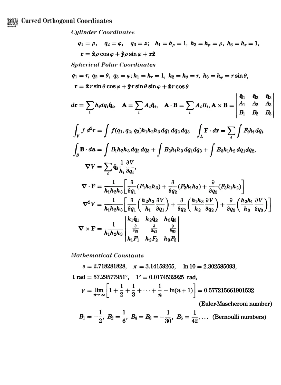
Curved Orthogonal Coordinates
Cylinder Coordinates
Qi = P, Q2 = φ> Q3 = Z] hi = hp = 1, &2 = Κ = p> h3-hz- 1,
r = xp cos#> + ypsin φ + #z
Spherical Polar Coordinates
Q\ =r, q2 = 6, q3 = <p;hi=hr = 1, h2 = he = r, ks = Jfy = rsin0,
r = xrsm0cos0> + yrsin0sin^ + zrcos0
rfr = ^ftjdgi4i> A=^Ai4i, A-B = ^iifii?AxB =
Qi 02 Q3
^1 A2 -A3
B\ B2 B3
fd3r= f(gu q2, qz)h\h2h3 dqi dq2 dq3 Fdr = J2 Fihi dch
I Bda= / Bih2h3dq2dq3-\- I B2hih3dq\dq3 + I B3h\h2dq\dq2,
hi dqi'
ο ο "Ι
(iifeafta) + τ— (ΉΛιΛβ) + T-(*a*ifc2)
3«2 3«3 J
V2V = 1 Γ 9 A2fc3 3V\ , 9 /feife33V\ + 3 /fe2fei9V\1
w = E4f
V F =
V xF =
h\h2h3
hi<ii h2^2 h3q3
d d d
dq\ dq2 3^3
hiFi h2F2 h3F3
Mathematical Constants
e = 2.718281828, π = 3.14159265, In 10 = 2.302585093,
1 rad = 57.29577951°, 1° = 0.0174532925 rad,
γ = lim
n-*oo
L1 + 2 + 3
1
>]"
+ ··· + -- ln(w + 1) = 0.577215661901532
η J
(Euler-Mascheroni number)
Bi = --, Bl = -, B4 = Bs = -—, ^ = —,... (Bernoullinumbers)

yO
/

MATHEMATICAL
METHODS FOR
PHYSICISTS
SIXTH EDITION
>&

yO
/

MATHEMATICAL
METHODS FOR
PHYSICISTS
SIXTH EDITION
George Β. Arfken
Miami University
Oxford, OH
Hans J. Weber
University of Virginia
Charlottesville, VA
ACADEMIC
PRESS
Amsterdam Boston Heidelberg London New York Oxford
Paris San Diego San Francisco Singapore Sydney Tokyo

Acquisitions Editor Tom Singer
Project Manager Simon Crump
Marketing Manager Linda Beattie
Cover Design Eric DeCicco
Composition VTEX Typesetting Services
Cover Printer Phoenix Color
Interior Printer The Maple-Vail Book Manufacturing Group
Elsevier Academic Press
30 Corporate Drive, Suite 400, Burlington, MA 01803, USA
525 Β Street, Suite 1900, San Diego, California 92101-4495, USA
84 Theobald's Road, London WC1X 8RR, UK
This book is printed on acid-free paper. ®
Copyright © 2005, Elsevier Inc. All rights reserved.
No part of this publication may be reproduced or transmitted in any form or by any means, electronic or
mechanical, including photocopy, recording, or any information storage and retrieval system, without permission in
writing from the publisher.
Permissions may be sought directly from Elsevier's Science & Technology Rights Department in Oxford, UK:
phone: (+44) 1865 843830, fax: (+44) 1865 853333, e-mail: permissions@elsevier.co.uk. You may also complete
your request on-line via the Elsevier homepage (http://elsevier.com), by selecting "Customer Support" and then
"Obtaining Permissions."
Library of Congress Cataloging-in-Publication Data
Appication submitted
British Library Cataloguing in Publication Data
A catalogue record for this book is available from the British Library
ISBN: 0-12-059876-0 Case bound
ISBN: 0-12-088584-0 International Students Edition
For all information on all Elsevier Academic Press Publications
visit our Web site at www.books.elsevier.com
Printed in the United States of America
05 06 07 08 09 10 9 8 7 6 5 4 3 2 1
Working together to grow
libraries in developing countries
www.elsevier.com | www.bookaid.org | www.sabre.org

Contents
Preface xi
1 Vector Analysis 1
1.1 Definitions, Elementary Approach 1
1.2 Rotation of the Coordinate Axes 7
1.3 Scalar or Dot Product 12
1.4 Vector or Cross Product 18
1.5 Triple Scalar Product, Triple Vector Product 25
1.6 Gradient, V 32
1.7 Divergence, V 38
1.8 Curl, Vx 43
1.9 Successive Applications of V 49
1.10 Vector Integration 54
1.11 Gauss' Theorem 60
1.12 Stokes' Theorem 64
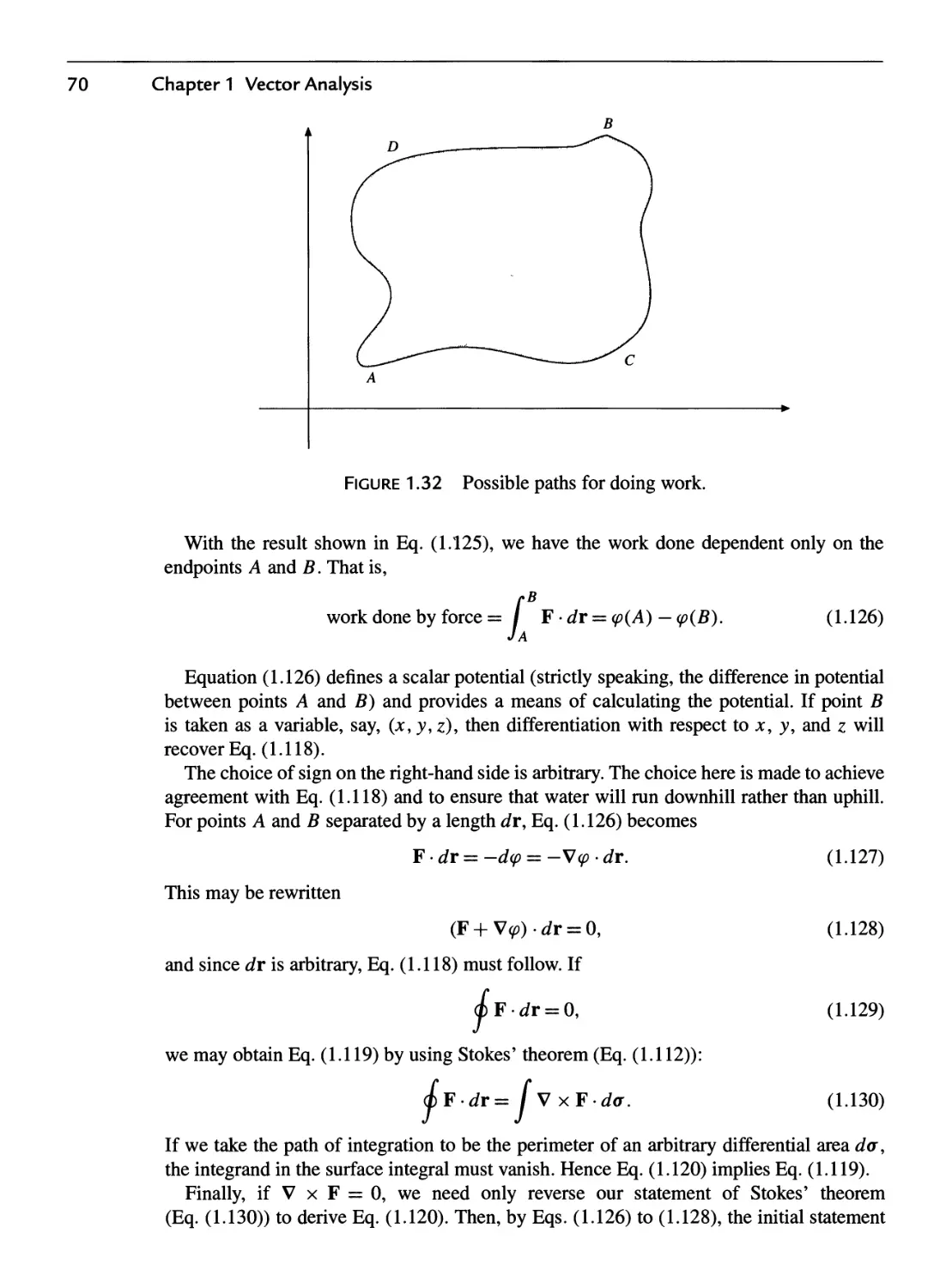
1.13 Potential Theory 68
1.14 Gauss' Law, Poisson's Equation 79
1.15 Dirac Delta Function 83
1.16 Helmholtz's Theorem 95
Additional Readings 101
2 Vector Analysis in Curved Coordinates and Tensors 103
2.1 Orthogonal Coordinates in R3 103
2.2 Differential Vector Operators 110
2.3 Special Coordinate Systems: Introduction 114
2.4 Circular Cylinder Coordinates 115
2.5 Spherical Polar Coordinates 123
ν

2.6 Tensor Analysis 133
2.7 Contraction, Direct Product 139
2.8 Quotient Rule 141
2.9 Pseudotensors, Dual Tensors 142
2.10 General Tensors 151
2.11 Tensor Derivative Operators 160
Additional Readings 163
3 Determinants and Matrices 165
3.1 Determinants 165
3.2 Matrices 176
3.3 Orthogonal Matrices 195
3.4 Hermitian Matrices, Unitary Matrices 208
3.5 Diagonalization of Matrices 215
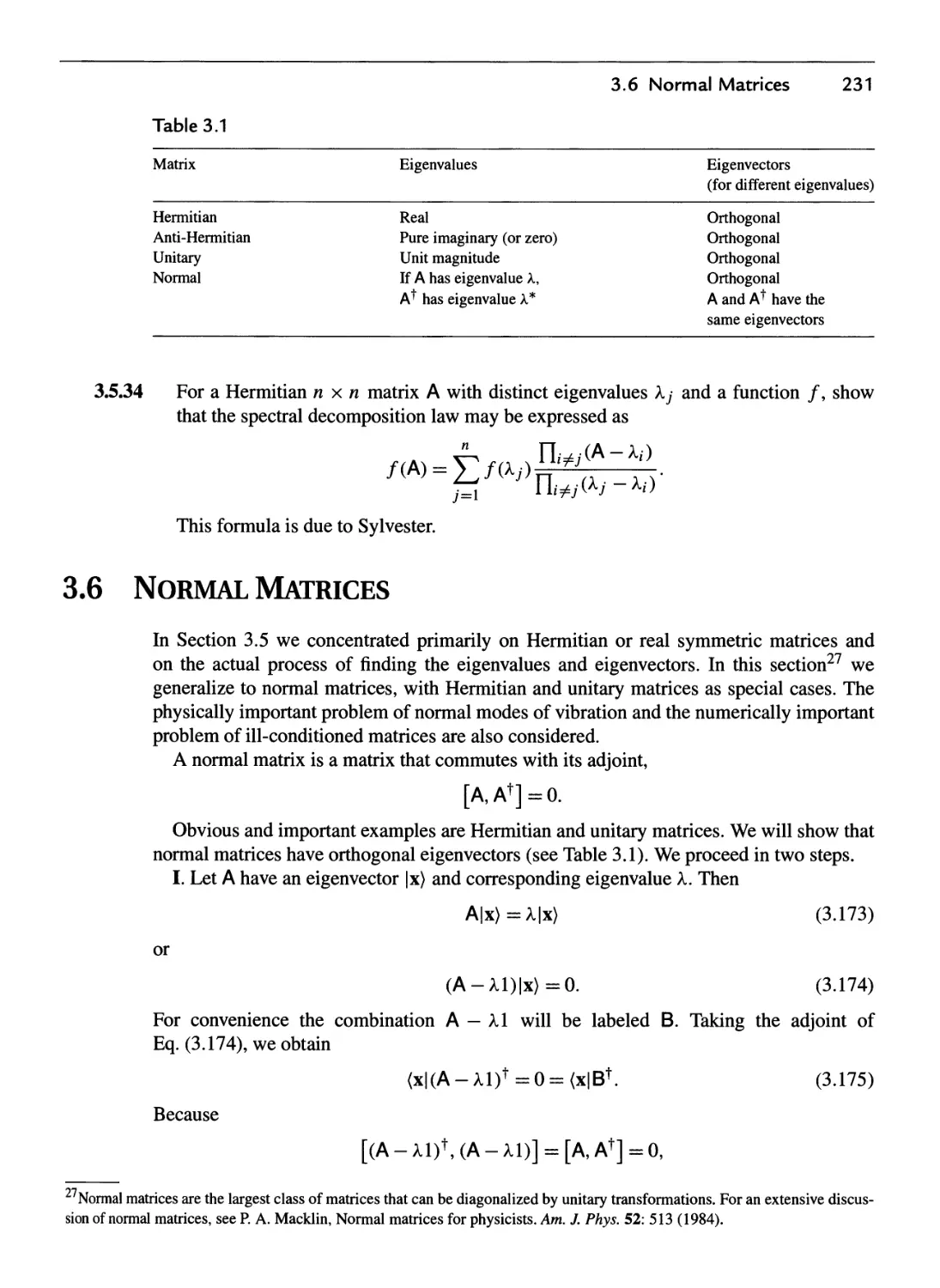
3.6 Normal Matrices 231
Additional Readings 239
4 Group Theory 241
4.1 Introduction to Group Theory 241
4.2 Generators of Continuous Groups 246
4.3 Orbital Angular Momentum 261
4.4 Angular Momentum Coupling 266
4.5 Homogeneous Lorentz Group 278
4.6 Lorentz Covariance of Maxwell's Equations 283
4.7 Discrete Groups 291
4.8 Differential Forms 304
Additional Readings 319
5 Infinite Series 321
5.1 Fundamental Concepts 321
5.2 Convergence Tests 325
5.3 Alternating Series 339
5.4 Algebra of Series 342
5.5 Series of Functions 348
5.6 Taylor's Expansion 352
5.7 Power Series 363
5.8 Elliptic Integrals 370
5.9 Bernoulli Numbers, Euler-Maclaurin Formula 376
5.10 Asymptotic Series 389
5.11 Infinite Products 396
Additional Readings 401
6 Functions of a Complex Variable I Analytic Properties, Mapping 403
6.1 Complex Algebra 404
6.2 Cauchy-Riemann Conditions 413
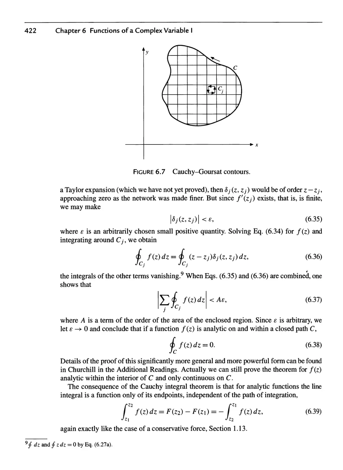
6.3 Cauchy's Integral Theorem 418

Contents vii
6.4 Cauchy's Integral Formula 425
6.5 Laurent Expansion 430
6.6 Singularities 438
6.7 Mapping 443
6.8 Conformal Mapping 451
Additional Readings 453
7 Functions of a Complex Variable II 455
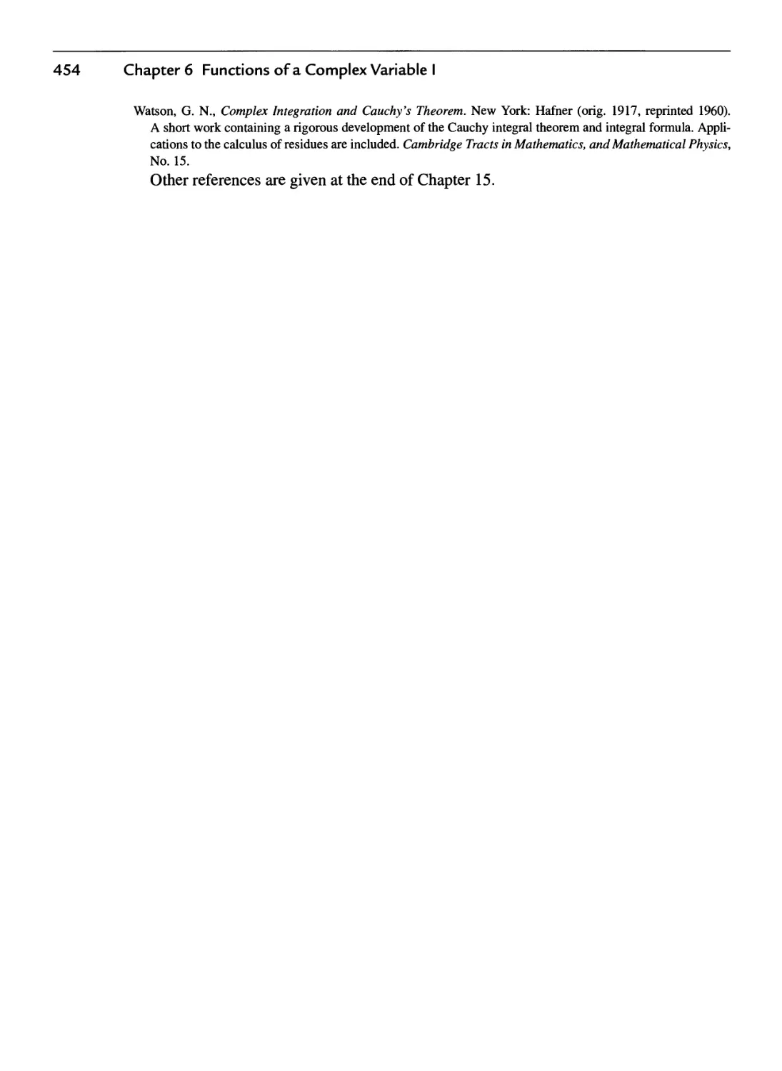
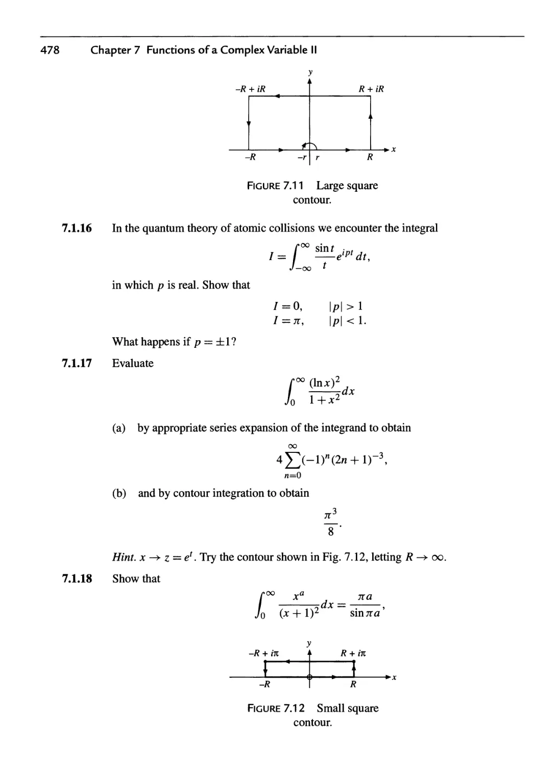
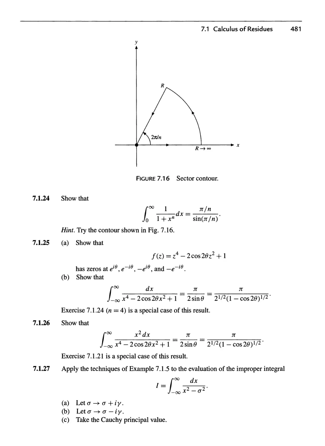
7.1 Calculus of Residues 455
7.2 Dispersion Relations 482
7.3 Method of Steepest Descents 489
Additional Readings 497
8 The Gamma Function (Factorial Function) 499
8.1 Definitions, Simple Properties 499
8.2 Digamma and Polygamma Functions 510
8.3 Stirling's Series 516
8.4 The Beta Function 520
8.5 Incomplete Gamma Function 527
Additional Readings 533
9 Differential Equations 535
9.1 Partial Differential Equations 535
9.2 First-Order Differential Equations 543
9.3 Separation of Variables 554
9.4 Singular Points 562
9.5 Series Solutions—Frobeniusy Method 565
9.6 A Second Solution 578
9.7 Nonhomogeneous Equation—Green's Function 592
9.8 Heat Flow, or Diffusion, PDF 611
Additional Readings 618
10 Sturm-Liouville Theory—Orthogonal Functions 621
10.1 Self-Adjoint ODEs 622
10.2 Hermitian Operators 634
10.3 Gram-Schmidt Orthogonalization 642
10.4 Completeness of Eigenfunctions 649
10.5 Green's Function—Eigenfunction Expansion 662
Additional Readings 674
11 Bessel Functions 675
11.1 Bessel Functions of the First Kind, Jv(x) 675
11.2 Orthogonality 694
11.3 Neumann Functions 699
11.4 Hankel Functions 707
11.5 Modified Bessel Functions, Iv(x) and Kv(x) 713

11.6 Asymptotic Expansions 719
11.7 Spherical Bessel Functions 725
Additional Readings 739
12 Legendre Functions 741
12.1 Generating Function 741
12.2 Recurrence Relations 749
12.3 Orthogonality 756
12.4 Alternate Definitions 767
12.5 Associated Legendre Functions 771
12.6 Spherical Harmonics 786
12.7 Orbital Angular Momentum Operators 793
12.8 Addition Theorem for Spherical Harmonics 797
12.9 Integrals of Three Y's 803
12.10 Legendre Functions of the Second Kind 806
12.11 Vector Spherical Harmonics 813
Additional Readings 816
13 More Special Functions 817
13.1 Hermite Functions 817
13.2 Laguerre Functions 837
13.3 Chebyshev Polynomials 848
13.4 Hypergeometric Functions 859
13.5 Confluent Hypergeometric Functions 863
13.6 Mathieu Functions 869
Additional Readings 879
14 Fourier Series 881
14.1 General Properties 881
14.2 Advantages, Uses of Fourier Series 888
14.3 Applications of Fourier Series 892
14.4 Properties of Fourier Series 903
14.5 Gibbs Phenomenon 910
14.6 Discrete Fourier Transform 914
14.7 Fourier Expansions of Mathieu Functions 919
Additional Readings 929
15 Integral Transforms 931
15.1 Integral Transforms 931
15.2 Development of the Fourier Integral 936
15.3 Fourier Transforms—Inversion Theorem 938
15.4 Fourier Transform of Derivatives 946
15.5 Convolution Theorem 951
15.6 Momentum Representation 955
15.7 Transfer Functions 961
15.8 Laplace Transforms 965

Contents ix
15.9 Laplace Transform of Derivatives 971
15.10 Other Properties 979
15.11 Convolution (Faltungs) Theorem 990
15.12 Inverse Laplace Transform 994
Additional Readings 1003
16 Integral Equations 1005
16.1 Introduction 1005
16.2 Integral Transforms, Generating Functions 1012
16.3 Neumann Series, Separable (Degenerate) Kernels 1018
16.4 Hilbert-Schmidt Theory 1029
Additional Readings 1036
17 Calculus of Variations 1037
17.1 A Dependent and an Independent Variable 1038
17.2 Applications of the Euler Equation 1044
17.3 Several Dependent Variables 1052
17.4 Several Independent Variables 1056
17.5 Several Dependent and Independent Variables 1058
17.6 Lagrangian Multipliers 1060
17.7 Variation with Constraints 1065
17.8 Rayleigh-Ritz Variational Technique 1072
Additional Readings 1076
18 Nonlinear Methods and Chaos 1079
18.1 Introduction 1079
18.2 The Logistic Map 1080
18.3 Sensitivity to Initial Conditions and Parameters 1085
18.4 Nonlinear Differential Equations 1088
Additional Readings 1107
19 Probability 1109
19.1 Definitions, Simple Properties 1109
19.2 Random Variables 1116
19.3 Binomial Distribution 1128
19.4 Poisson Distribution 1130
19.5 Gauss'Normal Distribution 1134
19.6 Statistics 1138
Additional Readings 1150
General References 1150

yO
/

mwmmw
Preface
Through six editions now, Mathematical Methods for Physicists has provided all the
mathematical methods that aspirings scientists and engineers are likely to encounter as students
and beginning researchers. More than enough material is included for a two-semester
undergraduate or graduate course.
The book is advanced in the sense that mathematical relations are almost always proven,
in addition to being illustrated in terms of examples. These proofs are not what a
mathematician would regard as rigorous, but sketch the ideas and emphasize the relations that
are essential to the study of physics and related fields. This approach incorporates
theorems that are usually not cited under the most general assumptions, but are tailored to the
more restricted applications required by physics. For example, Stokes' theorem is usually
applied by a physicist to a surface with the tacit understanding that it be simply connected.
Such assumptions have been made more explicit.
Problem-Solving Skills
The book also incorporates a deliberate focus on problem-solving skills. This more
advanced level of understanding and active learning is routine in physics courses and requires
practice by the reader. Accordingly, extensive problem sets appearing in each chapter form
an integral part of the book. They have been carefully reviewed, revised and enlarged for
this Sixth Edition.
Pathways Through the Material
Undergraduates may be best served if they start by reviewing Chapter 1 according to the
level of training of the class. Section 1.2 on the transformation properties of vectors, the
cross product, and the invariance of the scalar product under rotations may be postponed
until tensor analysis is started, for which these sections form the introduction and serve as
XI

xii Preface
examples. They may continue their studies with linear algebra in Chapter 3, then perhaps
tensors and symmetries (Chapters 2 and 4), and next real and complex analysis
(Chapters 5-7), differential equations (Chapters 9, 10), and special functions (Chapters 11-13).
In general, the core of a graduate one-semester course comprises Chapters 5-10 and
11-13, which deal with real and complex analysis, differential equations, and special
functions. Depending on the level of the students in a course, some linear algebra in Chapter 3
(eigenvalues, for example), along with symmetries (group theory in Chapter 4), and
tensors (Chapter 2) may be covered as needed or according to taste. Group theory may also be
included with differential equations (Chapters 9 and 10). Appropriate relations have been
included and are discussed in Chapters 4 and 9.
A two-semester course can treat tensors, group theory, and special functions
(Chapters 11-13) more extensively, and add Fourier series (Chapter 14), integral transforms
(Chapter 15), integral equations (Chapter 16), and the calculus of variations (Chapter 17).
Changes to the Sixth Edition
Improvements to the Sixth Edition have been made in nearly all chapters adding examples
and problems and more derivations of results. Numerous left-over typos caused by
scanning into LaTeX, an error-prone process at the rate of many errors per page, have been
corrected along with mistakes, such as in the Dirac γ -matrices in Chapter 3. A few
chapters have been relocated. The Gamma function is now in Chapter 8 following Chapters 6
and 7 on complex functions in one variable, as it is an application of these methods.
Differential equations are now in Chapters 9 and 10. A new chapter on probability has been
added, as well as new subsections on differential forms and Mathieu functions in response
to persistent demands by readers and students over the years. The new subsections are
more advanced and are written in the concise style of the book, thereby raising its level to
the graduate level. Many examples have been added, for example in Chapters 1 and 2, that
are often used in physics or are standard lore of physics courses. A number of additions
have been made in Chapter 3, such as on linear dependence of vectors, dual vector spaces
and spectral decomposition of symmetric or Hermitian matrices. A subsection on the
diffusion equation emphasizes methods to adapt solutions of partial differential equations to
boundary conditions. New formulas have been developed for Hermite polynomials and are
included in Chapter 13 that are useful for treating molecular vibrations; they are of interest
to the chemical physicists.
Acknowledgments
We have benefited from the advice and help of many people. Some of the revisions are in
response to comments by readers and former students, such as Dr. K. Bodoor and J. Hughes.
We are grateful to them and to our Editors Barbara Holland and Tom Singer who organized
accuracy checks. We would like to thank in particular Dr. Michael Bozoian and Prof. Frank
Harris for their invaluable help with the accuracy checking and Simon Crump, Production
Editor, for his expert management of the Sixth Edition.

Chapter 1
Vector Analysis
Definitions, Elementary Approach
In science and engineering we frequently encounter quantities that have magnitude and
magnitude only: mass, time, and temperature. These we label scalar quantities, which
remain the same no matter what coordinates we use. In contrast, many interesting physical
quantities have magnitude and, in addition, an associated direction. This second group
includes displacement, velocity, acceleration, force, momentum, and angular momentum.
Quantities with magnitude and direction are labeled vector quantities. Usually, in
elementary treatments, a vector is denned as a quantity having magnitude and direction. To
distinguish vectors from scalars, we identify vector quantities with boldface type, that is, V.
Our vector may be conveniently represented by an arrow, with length proportional to the
magnitude. The direction of the arrow gives the direction of the vector, the positive sense
of direction being indicated by the point. In this representation, vector addition
C = A + B A.1)
consists in placing the rear end of vector Β at the point of vector A. Vector C is then
represented by an arrow drawn from the rear of A to the point of B. This procedure, the
triangle law of addition, assigns meaning to Eq. A.1) and is illustrated in Fig. 1.1. By
completing the parallelogram, we see that
C = A + B = B + A, A.2)
as shown in Fig. 1.2. In words, vector addition is commutative.
For the sum of three vectors
D = A + B + C,
Fig. 1.3, we may first add A and B:
A + B = E.
1

2 Chapter 1 Vector Analysis
Β
Figure 1.1 Triangle law of vector
addition.
Β
Β
Figure 1.2 Parallelogram law of
vector addition.
Β
D
Figure 1.3 Vector addition is
associative.
Then this sum is added to C:
D = E + C.
Similarly, we may first add Β and C:
B + C = F.
Then
D = A + F.
In terms of the original expression,
(A + B) + C = A + (B + C).
Vector addition is associative.
A direct physical example of the parallelogram addition law is provided by a weight
suspended by two cords. If the junction point (O in Fig. 1.4) is in equilibrium, the vector

1.1 Definitions, Elementary Approach 3
Figure 1.4 Equilibrium of forces: Fi + F2 = —F3.
sum of the two forces Fi and F2 must just cancel the downward force of gravity, F3. Here
the parallelogram addition law is subject to immediate experimental verification.1
Subtraction may be handled by defining the negative of a vector as a vector of the same
magnitude but with reversed direction. Then
In Fig. 1.3,
A-B = A + (-B).
A = E-B.
Note that the vectors are treated as geometrical objects that are independent of any
coordinate system. This concept of independence of a preferred coordinate system is developed
in detail in the next section.
The representation of vector A by an arrow suggests a second possibility. Arrow A
(Fig. 1.5), starting from the origin,2 terminates at the point (A*, Ay,Az). Thus, if we agree
that the vector is to start at the origin, the positive end may be specified by giving the
Cartesian coordinates (A*, Ay, Az) of the arrowhead.
Although A could have represented any vector quantity (momentum, electric field, etc.),
one particularly important vector quantity, the displacement from the origin to the point
1 Strictly speaking, the parallelogram addition was introduced as a definition. Experiments show that if we assume that the
forces are vector quantities and we combine them by parallelogram addition, the equilibrium condition of zero resultant force is
satisfied.
2We could start from any point in our Cartesian reference frame; we choose the origin for simplicity. This freedom of shifting
the origin of the coordinate system without affecting the geometry is called translation invariance.

Chapter 1 Vector Analysis
ζ
A
Az
^ ^
_/ A^-^
S^Kf^
/ & ""~~~^
/
(Ar> ^2/> A&)
Α^
,.''''
,'
X
Figure 1.5 Cartesian components and direction cosines of A.
(jc, y, z), is denoted by the special symbol r. We then have a choice of referring to the
displacement as either the vector r or the collection (x, y, z), the coordinates of its endpoint:
r<*(x,y9z). A.3)
Using r for the magnitude of vector r, we find that Fig. 1.5 shows that the endpoint
coordinates and the magnitude are related by
;c=rcosa, y = rcos/?, z = rcosy. A.4)
Here cos a, cos β, and cos γ are called the direction cosines, a being the angle between the
given vector and the positive x-axis, and so on. One further bit of vocabulary: The
quantities AXyAy, and Az are known as the (Cartesian) components of A or the projections
of A, with cos2 a 4- cos2 β + cos2 γ = 1.
Thus, any vector A may be resolved into its components (or projected onto the
coordinate axes) to yield Ax = A cos of, etc., as in Eq. A.4). We may choose to refer to the vector
as a single quantity A or to its components (Ax, Ay, Az). Note that the subscript χ in Ax
denotes the χ component and not a dependence on the variable x. The choice between
using A or its components (Ax, Ay, Az) is essentially a choice between a geometric and
an algebraic representation. Use either representation at your convenience. The geometric
"arrow in space" may aid in visualization. The algebraic set of components is usually more
suitable for precise numerical or algebraic calculations.
Vectors enter physics in two distinct forms. A) Vector A may represent a single force
acting at a single point. The force of gravity acting at the center of gravity illustrates this
form. B) Vector A may be defined over some extended region; that is, A and its
components may be functions of position: Ax = Ax(x, y, z), and so on. Examples of this sort
include the velocity of a fluid varying from point to point over a given volume and electric
and magnetic fields. These two cases may be distinguished by referring to the vector
defined over a region as a vector field. The concept of the vector defined over a region and

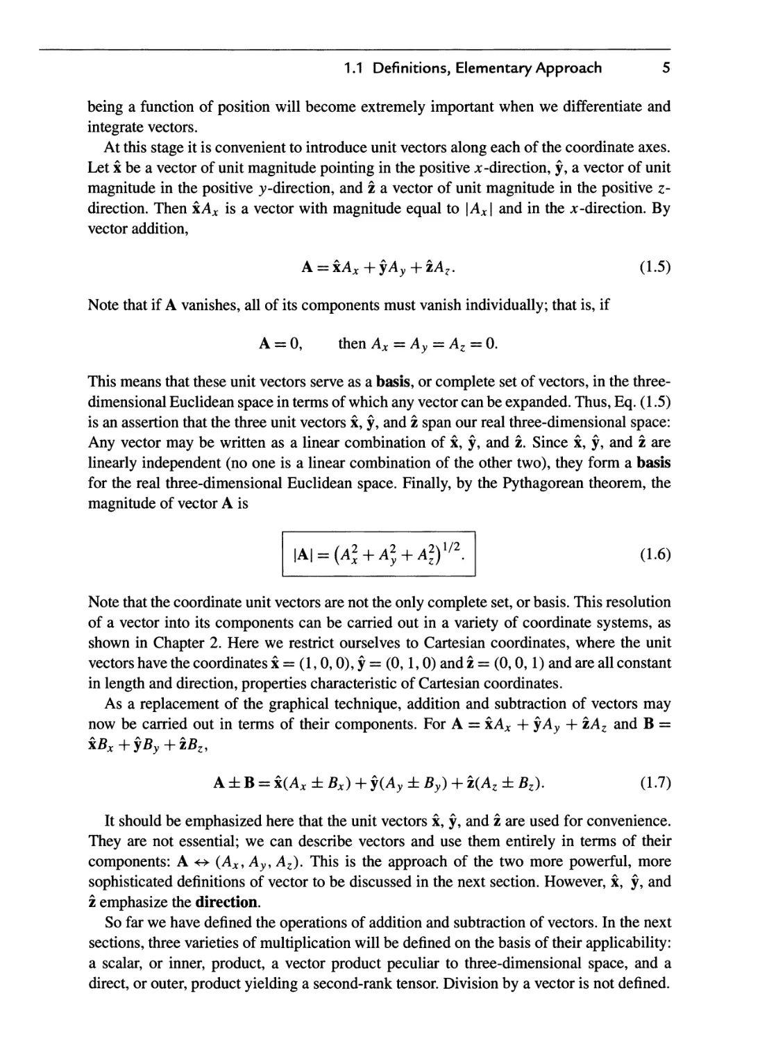
1.1 Definitions, Elementary Approach 5
being a function of position will become extremely important when we differentiate and
integrate vectors.
At this stage it is convenient to introduce unit vectors along each of the coordinate axes.
Let χ be a vector of unit magnitude pointing in the positive χ-direction, y, a vector of unit
magnitude in the positive y-direction, and ζ a vector of unit magnitude in the positive z-
direction. Then xAx is a vector with magnitude equal to \AX\ and in the χ -direction. By
vector addition,
A = iAx+yAy+iAz. A.5)
Note that if A vanishes, all of its components must vanish individually; that is, if
A = 0, then Ax = Ay = Az = 0.
This means that these unit vectors serve as a basis, or complete set of vectors, in the three-
dimensional Euclidean space in terms of which any vector can be expanded. Thus, Eq. A.5)
is an assertion that the three unit vectors x, y, and ζ span our real three-dimensional space:
Any vector may be written as a linear combination of x, y, and z. Since x, y, and ζ are
linearly independent (no one is a linear combination of the other two), they form a basis
for the real three-dimensional Euclidean space. Finally, by the Pythagorean theorem, the
magnitude of vector A is
2 , Λ2Ν1/2
\A\ = (A2X + A2y + Al)
A.6)
Note that the coordinate unit vectors are not the only complete set, or basis. This resolution
of a vector into its components can be carried out in a variety of coordinate systems, as
shown in Chapter 2. Here we restrict ourselves to Cartesian coordinates, where the unit
vectors have the coordinates χ = A,0,0), y = @,1,0) and ζ = @,0,1) and are all constant
in length and direction, properties characteristic of Cartesian coordinates.
As a replacement of the graphical technique, addition and subtraction of vectors may
now be carried out in terms of their components. For A = xAx + yAy + ΪΑΖ and Β =
xBx+fBy + zBz,
A ±B = x(Ax ± Bx) + y(Ay ± By) + z(Az ± Bz). A.7)
It should be emphasized here that the unit vectors x, y, and ζ are used for convenience.
They are not essential; we can describe vectors and use them entirely in terms of their
components: A *» (AXJ Ay, Az). This is the approach of the two more powerful, more
sophisticated definitions of vector to be discussed in the next section. However, x, y, and
ζ emphasize the direction.
So far we have defined the operations of addition and subtraction of vectors. In the next
sections, three varieties of multiplication will be defined on the basis of their applicability:
a scalar, or inner, product, a vector product peculiar to three-dimensional space, and a
direct, or outer, product yielding a second-rank tensor. Division by a vector is not defined.

6 Chapter 1 Vector Analysis
Exercises
1.1.1 Show how to find A and B, given A + Β and A — B.
1.1.2 The vector A whose magnitude is 1.732 units makes equal angles with the coordinate
axes. Find AXi Ay, and Az.
1.1.3 Calculate the components of a unit vector that lies in the jcy-plane and makes equal
angles with the positive directions of the x- and y-axes.
1.1.4 The velocity of sailboat A relative to sailboat B, vrei, is defined by the equation vrei =
ν a — vb, where ν a is the velocity of A and v^ is the velocity of B. Determine the
velocity of A relative to Β if
ν a = 30 km/hr east
γΒ = 40 km/hr north.
ANS. vrei = 50 km/hr, 53.1° south of east.
1.1.5 A sailboat sails for 1 hr at 4 km/hr (relative to the water) on a steady compass heading
of 40° east of north. The sailboat is simultaneously carried along by a current. At the
end of the hour the boat is 6.12 km from its starting point. The line from its starting point
to its location lies 60° east of north. Find the χ (easterly) and y (northerly) components
of the water's velocity.
ANS. i;east = 2.73 km/hr, i;n0rth ^ 0 km/hr.
1.1.6 A vector equation can be reduced to the form A = B. From this show that the one vector
equation is equivalent to three scalar equations. Assuming the validity of Newton's
second law, F = ma, as a vector equation, this means that ax depends only on Fx and
is independent of Fy and Fz.
1.1.7 The vertices A, B, and C of a triangle are given by the points (—1,0,2), @,1,0), and
A,-1,0), respectively. Find point D so that the figure ABCD forms a plane
parallelogram.
ANS. @,-2,2) or B,0,-2).
1.1.8 A triangle is defined by the vertices of three vectors A, B and C that extend from the
origin. In terms of A, B, and C show that the vector sum of the successive sides of the
triangle (AB + BC + CA) is zero, where the side AB is from A to B, etc.
1.1.9 A sphere of radius a is centered at a point ri.
(a) Write out the algebraic equation for the sphere.
(b) Write out a vector equation for the sphere.
ANS. (a) (x - χλγ + (y - yiJ + (z - ZiJ = a2.
(b) r = ri + a, with ri = center,
(a takes on all directions but has a fixed magnitude a.)

1.2 Rotation of the Coordinate Axes 7
1.1.10 A comer reflector is formed by three mutually perpendicular reflecting surfaces. Show
that a ray of light incident upon the comer reflector (striking all three surfaces) is
reflected back along a line parallel to the line of incidence.
Hint. Consider the effect of a reflection on the components of a vector describing the
direction of the light ray.
1.1.11 Hubble's law. Hubble found that distant galaxies are receding with a velocity
proportional to their distance from where we are on Earth. For the ith galaxy,
v{=//0r/,
with us at the origin. Show that this recession of the galaxies from us does not imply
that we are at the center of the universe. Specifically, take the galaxy at π as a new
origin and show that Hubble's law is still obeyed.
1.1.12 Find the diagonal vectors of a unit cube with one comer at the origin and its three sides
lying along Cartesian coordinates axes. Show that there are four diagonals with length
λ/3. Representing these as vectors, what are their components? Show that the diagonals
of the cube's faces have length \fl and determine their components.
1.2 Rotation of the Coordinate Axes3
In the preceding section vectors were defined or represented in two equivalent ways:
A) geometrically by specifying magnitude and direction, as with an arrow, and B)
algebraically by specifying the components relative to Cartesian coordinate axes. The
second definition is adequate for the vector analysis of this chapter. In this section two more
refined, sophisticated, and powerful definitions are presented. First, the vector field is
defined in terms of the behavior of its components under rotation of the coordinate axes. This
transformation theory approach leads into the tensor analysis of Chapter 2 and groups of
transformations in Chapter 4. Second, the component definition of Section 1.1 is refined
and generalized according to the mathematician's concepts of vector and vector space. This
approach leads to function spaces, including the Hubert space.
The definition of vector as a quantity with magnitude and direction is incomplete. On
the one hand, we encounter quantities, such as elastic constants and index of refraction
in anisotropic crystals, that have magnitude and direction but that are not vectors. On
the other hand, our naive approach is awkward to generalize to extend to more complex
quantities. We seek a new definition of vector field using our coordinate vector r as a
prototype.
There is a physical basis for our development of a new definition. We describe our
physical world by mathematics, but it and any physical predictions we may make must be
independent of our mathematical conventions.
In our specific case we assume that space is isotropic; that is, there is no preferred
direction, or all directions are equivalent. Then the physical system being analyzed or the
physical law being enunciated cannot and must not depend on our choice or orientation
of the coordinate axes. Specifically, if a quantity S does not depend on the orientation of
the coordinate axes, it is called a scalar.
This section is optional here. It will be essential for Chapter 2.

8 Chapter 1 Vector Analysis
Figure 1.6 Rotation of Cartesian coordinate axes about the z-axis.
Now we return to the concept of vector r as a geometric object independent of the
coordinate system. Let us look at r in two different systems, one rotated in relation to the
other.
For simplicity we consider first the two-dimensional case. If the x-, y-coordinates are
rotated counterclockwise through an angle φ9 keeping r, fixed (Fig. 1.6), we get the
following relations between the components resolved in the original system (unprimed) and
those resolved in the new rotated system (primed):
xf =xcos<p +y sirup,
I ' , U-°)
y = — jcsm<p + ycos^.
We saw in Section 1.1 that a vector could be represented by the coordinates of a point;
that is, the coordinates were proportional to the vector components. Hence the components
of a vector must transform under rotation as coordinates of a point (such as r). Therefore
whenever any pair of quantities Ax and Ay in the xy-coordinate system is transformed into
(Afx, Afy) by this rotation of the coordinate system with
A'x=Axcos<p + Aysin<p9
A' =—Ax ύτιφ +Ay cos<p,
we define4 Ax and Ay as the components of a vector A. Our vector now is defined in terms
of the transformation of its components under rotation of the coordinate system. If Ax and
Ay transform in the same way as χ and y, the components of the general two-dimensional
coordinate vector r, they are the components of a vector A. If Ax and Ay do not show this
4 A scalar quantity does not depend on the orientation of coordinates; S' = S expresses the fact that it is invariant under rotation
of the coordinates.

1.2 Rotation of the Coordinate Axes 9
form invariance (also called covariance) when the coordinates are rotated, they do not
form a vector.
The vector field components Ax and Ay satisfying the defining equations, Eqs. A.9),
associate a magnitude A and a direction with each point in space. The magnitude is a scalar
quantity, invariant to the rotation of the coordinate system. The direction (relative to the
unprimed system) is likewise invariant to the rotation of the coordinate system (see
Exercise 1.2.1). The result of all this is that the components of a vector may vary according to
the rotation of the primed coordinate system. This is what Eqs. A.9) say. But the variation
with the angle is just such that the components in the rotated coordinate system Ax and Afy
define a vector with the same magnitude and the same direction as the vector defined by
the components Ax and Ay relative to the x-, y-coordinate axes. (Compare Exercise 1.2.1.)
The components of A in a particular coordinate system constitute the representation of
A in that coordinate system. Equations A.9), the transformation relations, are a guarantee
that the entity A is independent of the rotation of the coordinate system.
To go on to three and, later, four dimensions, we find it convenient to use a more compact
notation. Let
X~^Xl A.10)
y -* χι
a11=cos^, <zi2 = sin<p,
A.11)
021 =-sin<p, a22 = cos<p.
Then Eqs. A.8) become
x[ = 011*1 + «12*2, ,j 12)
Xf2= «21*1 +022*2-
The coefficient atj may be interpreted as a direction cosine, the cosine of the angle between
x\ and Xj; that is,
tfi2 = cos(.xi,X2) = sin<p,
d2\ = cosOt^, *i) = cos(<p + j) = — sin<p.
The advantage of the new notation5 is that it permits us to use the summation symbol ^
and to rewrite Eqs. A.12) as
2
Χί=Σ,α*ίχ1' ί = 1»2. A.14)
y=i
Note that i remains as a parameter that gives rise to one equation when it is set equal to 1
and to a second equation when it is set equal to 2. The index j, of course, is a summation
index, a dummy index, and, as with a variable of integration, j may be replaced by any
other convenient symbol.
5
You may wonder at the replacement of one parameter φ by four parameters ay. Clearly, the ay do not constitute a minimum
set of parameters. For two dimensions the four ay are subject to the three constraints given in Eq. A.18). The justification for
this redundant set of direction cosines is the convenience it provides. Hopefully, this convenience will become more apparent
in Chapters 2 and 3. For three-dimensional rotations (9 ay but only three independent) alternate descriptions are provided by:
A) the Euler angles discussed in Section 3.3, B) quaternions, and C) the Cayley-Klein parameters. These alternatives have their
respective advantages and disadvantages.

10 Chapter 1 Vector Analysis
The generalization to three, four, or Ν dimensions is now simple. The set of Ν quantities
Vj is said to be the components of an Ν -dimensional vector V if and only if their values
relative to the rotated coordinate axes are given by
Ν
V! = T,aiJvJ> i = l,2,...,tf. A.15)
y=i
As before, a^ is the cosine of the angle between x\ and Xj . Often the upper limit Ν and
the corresponding range of / will not be indicated. It is taken for granted that you know
how many dimensions your space has.
From the definition of a^ as the cosine of the angle between the positive x[ direction
and the positive Xj direction we may write (Cartesian coordinatesN
dxf.
(*ij = T7-- (L16a)
dxi
Using the inverse rotation (φ -* — φ) yields
2
Σι i$X\
av*i or T7=aiJ- (L16b)
i=l
Note that these are partial derivatives. By use of Eqs. A.16a) and A.16b), Eq. A.15)
becomes
1 f-f dxf J 4-*l dx J
The direction cosines a^ satisfy an orthogonality condition
Y^aijaik = 8jk A.18)
or, equivalently,
^ajiaki=8jk. A.19)
A.20)
Here, the symbol 8jk is the Kronecker delta, defined by
8jk = 1 for j = k,
8jk = 0 for j φ k.
It is easily verified that Eqs. A.18) and A.19) hold in the two-dimensional case by
substituting in the specific a^ from Eqs. A.11). The result is the well-known identity
sin2#? + cos2 φ = 1 for the nonvanishing case. To verify Eq. A.18) in general form, we
may use the partial derivative forms of Eqs. A.16a) and A.16b) to obtain
E^^=^dxj_dx^^dxj_
dxf{ dxf. ^ dx'} dxk dxk' K * )
111 ι I
differentiate x't with respect to Xj. See discussion following Eq. A.21).

1.2 Rotation of the Coordinate Axes 11
The last step follows by the standard rules for partial differentiation, assuming that Xj is
a function of x[ ,x'vx!v and so on. The final result, dxj/dxjc, is equal to <57#, since Xj and
Xk as coordinate lines (j φ k) are assumed to be perpendicular (two or three dimensions)
or orthogonal (for any number of dimensions). Equivalently, we may assume that Xj and
xk (j φ k) are totally independent variables. If j = k, the partial derivative is clearly equal
tol.
In redefining a vector in terms of how its components transform under a rotation of the
coordinate system, we should emphasize two points:
1. This definition is developed because it is useful and appropriate in describing our
physical world. Our vector equations will be independent of any particular coordinate
system. (The coordinate system need not even be Cartesian.) The vector equation can
always be expressed in some particular coordinate system, and, to obtain numerical
results, we must ultimately express the equation in some specific coordinate system.
2. This definition is subject to a generalization that will open up the branch of
mathematics known as tensor analysis (Chapter 2).
A qualification is in order. The behavior of the vector components under rotation of the
coordinates is used in Section 1.3 to prove that a scalar product is a scalar, in Section 1.4
to prove that a vector product is a vector, and in Section 1.6 to show that the gradient of a
scalar ψ, νψ, is a vector. The remainder of this chapter proceeds on the basis of the less
restrictive definitions of the vector given in Section 1.1.
Summary: Vectors and Vector Space
It is customary in mathematics to label an ordered triple of real numbers (x\,X2,x?>) a
vector x. The number xn is called the nth component of vector x. The collection of all
such vectors (obeying the properties that follow) form a three-dimensional real vector
space. We ascribe five properties to our vectors: If χ = (x\, Χ2, Χ3) and y = (y\, V2, V3),
1. Vector equality: χ = y means jcj = y;, / = 1,2, 3.
2. Vector addition: χ + y = ζ means jc,· + yt¦ = n, i = 1,2,3.
3. Scalar multiplication: αχ <± (αχ\, αχ2, ax?) (with a real).
4. Negative of a vector: —χ = (— l)x «-> (—x\, —JC2, — X3).
5. Null vector: There exists a null vector 0 «-» @,0,0).
Since our vector components are real (or complex) numbers, the following properties
also hold:
1. Addition of vectors is commutative: χ + y = y + x.
2. Addition of vectors is associative: (x + y) + ζ = χ + (y + z).
3. Scalar multiplication is distributive:
a(x + y) = ax + ay, also (a + b)x = ax + bx.
4. Scalar multiplication is associative: (ab)x = a(bx).

12 Chapter 1 Vector Analysis
Further, the null vector 0 is unique, as is the negative of a given vector x.
So far as the vectors themselves are concerned this approach merely formalizes the
component discussion of Section 1.1. The importance lies in the extensions, which will be
considered in later chapters. In Chapter 4, we show that vectors form both an Abelian group
under addition and a linear space with the transformations in the linear space described by
matrices. Finally, and perhaps most important, for advanced physics the concept of vectors
presented here may be generalized to A) complex quantities,7 B) functions, and C) an
infinite number of components. This leads to infinite-dimensional function spaces, the Hilbert
spaces, which are important in modern quantum theory. A brief introduction to function
expansions and Hilbert space appears in Section 10.4.
Exercises
1.2.1 (a) Show that the magnitude of a vector A, A = (A2 + A2I/2, is independent of the
orientation of the rotated coordinate system,
that is, independent of the rotation angle φ.
This independence of angle is expressed by saying that A is invariant under
rotations,
(b) At a given point (jc, y), A defines an angle a relative to the positive jc-axis and
a' relative to the positive x'-axis. The angle from χ to x' is φ. Show that A = A'
defines the same direction in space when expressed in terms of its primed
components as in terms of its unprimed components; that is,
α' — α —φ.
1.2.2 Prove the orthogonality condition Σί ajiaki = &jk- As a special case of this, the
direction cosines of Section 1.1 satisfy the relation
cos2 α + cos2 β + cos2 γ = 1,
a result that also follows from Eq. A.6).
1.3 Scalar or Dot Product
Having defined vectors, we now proceed to combine them. The laws for combining vectors
must be mathematically consistent. From the possibilities that are consistent we select two
that are both mathematically and physically interesting. A third possibility is introduced in
Chapter 2, in which we form tensors.
The projection of a vector A onto a coordinate axis, which gives its Cartesian
components in Eq. A.4), defines a special geometrical case of the scalar product of A and the
coordinate unit vectors:
Ax = Acosof = A x, Ay = A cos β = A -y, Az = A cosy == A z. A.22)
7The «-dimensional vector space of real «-tuples is often labeled M.n and the «-dimensional vector space of complex «-tuples is
labeled Cn.

1.3 Scalar or Dot Product 13
This special case of a scalar product in conjunction with general properties the scalar
product is sufficient to derive the general case of the scalar product.
Just as the projection is linear in A, we want the scalar product of two vectors to be
linear in A and B, that is, obey the distributive and associative laws
A B + A C
A-(B + C):
Α-(νΒ) = (νΑ).Β = νΑ·Β,
A.23a)
A.23b)
where y is a number. Now we can use the decomposition of Β into its Cartesian components
according to Eq. A.5), Β = Bxx + Byy + Bzz, to construct the general scalar or dot product
of the vectors A and Β as
A-B = A-(Bxx+Byy + Bzi)
= BXA · χ + By A · y + BZA · ζ upon applying Eqs. A.23a) and A.23b)
= BXAX + Βγ Ay + BZAZ upon substituting Eq. A.22).
Hence
Α.Β = ΣΒ*Α*=ΈΑ*Β*=Β'Α·
A.24)
If A = Β in Eq. A.24), we recover the magnitude A = (Σ A?I/2 of A in Eq. A.6) from
Eq. A.24).
It is obvious from Eq. A.24) that the scalar product treats A and Β alike, or is
symmetric in A and B, and is commutative. Thus, alternatively and equivalently, we can first
generalize Eqs. A.22) to the projection Ab of A onto the direction of a vector Β φ 0
as Α β = A cosO = A · B, where Β = Β/Β is the unit vector in the direction of Β and θ
is the angle between A and B, as shown in Fig. 1.7. Similarly, we project Β onto A as
Ba = Β cos# = Β · A. Second, we make these projections symmetric in A and B, which
leads to the definition
A B = ABB = ABA = ABcos0.
A.25)
+>v
Figure 1.7 Scalar product AB = ABcosO.

14 Chapter 1 Vector Analysis
+ (B + C)A >
Figure 1.8 The distributive law
A · (B + C) = ABA + ACA = A(B + C)A, Eq. A.23a).
The distributive law in Eq. A.23a) is illustrated in Fig. 1.8, which shows that the sum of
the projections of Β and C onto A, Β a + Ca is equal to the projection of Β + C onto A,
(B + C)A.
It follows from Eqs. A.22), A.24), and A.25) that the coordinate unit vectors satisfy the
relations
x-x = y-y = z-z=l, A.26a)
whereas
x.y = x-z = yz = 0. A.26b)
If the component definition, Eq. A.24), is labeled an algebraic definition, then Eq. A.25)
is a geometric definition. One of the most common applications of the scalar product in
physics is in the calculation of work = force-displacement- cos#, which is interpreted as
displacement times the projection of the force along the displacement direction, i.e., the
scalar product of force and displacement, W = F · S.
If A · Β = 0 and we know that Α φ 0 and Β φ 0, then, from Eq. A.25), cos0 = 0, or
0 = 90°, 270°, and so on. The vectors A and Β must be perpendicular. Alternately, we
may say A and Β are orthogonal. The unit vectors x, y, and ζ are mutually orthogonal. To
develop this notion of orthogonality one more step, suppose that η is a unit vector and r is
a nonzero vector in the Jty-plane; that is, r = xx + yy (Fig. 1.9). If
nr = 0
for all choices of r, then η must be perpendicular (orthogonal) to the xy -plane.
Often it is convenient to replace x, y, and ζ by subscripted unit vectors em, m = 1,2,3,
with χ = ei, and so on. Then Eqs. A.26a) and A.26b) become
em -en=<5mn. A.26c)
For m φ η the unit vectors em and en are orthogonal. For m = η each vector is
normalized to unity, that is, has unit magnitude. The set em is said to be orthonormal. A major
advantage of Eq. A.26c) over Eqs. A.26a) and A.26b) is that Eq. A.26c) may readily be
generalized to Ν -dimensional space: m,n = l,2, ...,N. Finally, we are picking sets of
unit vectors em that are orthonormal for convenience - a very great convenience.

1.3 Scalar or Dot Product
Figure 1.9 A normal vector.
Invariance of the Scalar Product Under Rotations
We have not yet shown that the word scalar is justified or that the scalar product is indeed
a scalar quantity. To do this, we investigate the behavior of A · Β under a rotation of the
coordinate system. By use of Eq. A.15),
A'XB'X + A'yB'y + A'ZB'Z = Y^axiAi Σα*1Β1 + Σ>*Ai ΣαηΒί
+ Y^aziAiY^azjBj. A.27)
i J
Using the indices k and / to sum over jc, y, and z, we obtain
Σ^=ΣΣΣ^^^· (L28)
k l i j
and, by rearranging the terms on the right-hand side, we have
Σ,ΑΊ<Βΐ<=ΣΣΈ<-α»α'Μ>*=ΈΣ8υΑ>^=ΣΑ'Β'· A·29)
k l i j i j i
The last two steps follow by using Eq. A.18), the orthogonality condition of the direction
cosines, and Eqs. A.20), which define the Kronecker delta. The effect of the Kronecker
delta is to cancel all terms in a summation over either index except the term for which the
indices are equal. In Eq. A.29) its effect is to set j = i and to eliminate the summation
over j. Of course, we could equally well set / = j and eliminate the summation over /.

16 Chapter 1 Vector Analysis
Equation A.29) gives us
ΣΑ*Β*=ΣΑ'·Β'·
A.30)
which is just our definition of a scalar quantity, one that remains invariant under the rotation
of the coordinate system.
In a similar approach that exploits this concept of invariance, we take C = A + Β and
dot it into itself:
Since
C-C = (A + B).(A + B)
= A A + B -B + 2A B.
C C = C2,
A.31)
the square of the magnitude of vector C and thus an invariant quantity, we see that
1
AB=-(C2-A2-£2),
invariant.
A.32)
A.33)
Since the right-hand side of Eq. A.33) is invariant—that is, a scalar quantity — the left-
hand side, A · B, must also be invariant under rotation of the coordinate system. Hence
A · Β is a scalar.
Equation A.31) is really another form of the law of cosines, which is
C2 = A2 + £2 + 2AJ3cos<9.
A.34)
Comparing Eqs. A.31) and A.34), we have another verification of Eq. A.25), or, if
preferred, a vector derivation of the law of cosines (Fig. 1.10).
The dot product, given by Eq. A.24), may be generalized in two ways. The space need
not be restricted to three dimensions. In «-dimensional space, Eq. A.24) applies with the
sum running from 1 to n. Moreover, η may be infinity, with the sum then a convergent
infinite series (Section 5.2). The other generalization extends the concept of vector to embrace
functions. The function analog of a dot, or inner, product appears in Section 10.4.
Figure 1.10 The law of cosines.

1.3 Scalar or Dot Product 17
Exercises
1.3.1 Two unit magnitude vectors ez and ey are required to be either parallel or perpendicular
to each other. Show that e, ¦ e7 provides an interpretation of Eq. A.18), the direction
cosine orthogonality relation.
1.3.2 Given that A) the dot product of a unit vector with itself is unity and B) this relation is
valid in all (rotated) coordinate systems, show that x' · x' = 1 (with the primed system
rotated 45° about the z-axis relative to the unprimed) implies that χ · y = 0.
1.3.3 The vector r, starting at the origin, terminates at and specifies the point in space (x, y, z).
Find the surface swept out by the tip of r if
(a) (r — a) · a = 0. Characterize a geometrically.
(b) (r — a) · r = 0. Describe the geometric role of a.
The vector a is constant (in magnitude and direction).
1.3.4 The interaction energy between two dipoles of moments μι and μ2 may be written in
the vector form
v_ Pi'to 3(μι·τ)(μ2·τ)
and in the scalar form
M1M2
V = —5— B cos θ\ cos θ2 — sin θι sin θ2 cos φ).
ri
Here θι and 02 are the angles of μι and μ2 relative to r, while φ is the azimuth of μ2
relative to the μ^-Γ plane (Fig. 1.11). Show that these two forms are equivalent.
Hint: Equation A2.178) will be helpful.
1.3.5 A pipe comes diagonally down the south wall of a building, making an angle of 45°
with the horizontal. Coming into a corner, the pipe turns and continues diagonally down
a west-facing wall, still making an angle of 45° with the horizontal. What is the angle
between the south-wall and west-wall sections of the pipe?
ANS. 120°.
1.3.6 Find the shortest distance of an observer at the point B,1,3) from a rocket in free
flight with velocity A,2,3) m/s. The rocket was launched at time t = 0 from A,1,1).
Lengths are in kilometers.
1.3.7 Prove the law of cosines from the triangle with corners at the point of C and A in
Fig. 1.10 and the projection of vector Β onto vector A.
Figure 1.11 Two dipole moments.

18 Chapter 1 Vector Analysis
1.4 Vector or Cross Product
A second form of vector multiplication employs the sine of the included angle instead
of the cosine. For instance, the angular momentum of a body shown at the point of the
distance vector in Fig. 1.12 is defined as
angular momentum = radius arm χ linear momentum
= distance χ linear momentum χ sin#.
For convenience in treating problems relating to quantities such as angular momentum,
torque, and angular velocity, we define the vector product, or cross product, as
C = Α χ Β, with C = AB sin(9.
A.35)
Unlike the preceding case of the scalar product, C is now a vector, and we assign it a
direction perpendicular to the plane of A and Β such that A, B, and C form a right-handed
system. With this choice of direction we have
AxB = —Β χ A, anticommutation.
From this definition of cross product we have
XXX = yxy = ZXZ = 0,
whereas
xxy = z, yxz = x, zxx = y,
y χ χ = —ζ, ζ χ y = —χ, χ χ ζ = —y.
A.36a)
A.36b)
A.36c)
Among the examples of the cross product in mathematical physics are the relation between
linear momentum ρ and angular momentum L, with L defined as
L = r χ p,
Figure 1.12 Angular momentum.

1.4 Vector or Cross Product
19
y<
Β sin θ
i
/ θ
/β
A
Figure 1.13 Parallelogram representation of the vector product.
and the relation between linear velocity ν and angular velocity ω,
ν = ω χ r.
Vectors ν and ρ describe properties of the particle or physical system. However, the
position vector r is determined by the choice of the origin of the coordinates. This means that
ω and L depend on the choice of the origin.
The familiar magnetic induction Β is usually defined by the vector product force
equation8
YM = qs χ Β (mks units).
Here ν is the velocity of the electric charge q and F^ is the resulting force on the moving
charge.
The cross product has an important geometrical interpretation, which we shall use in
subsequent sections. In the parallelogram defined by A and Β (Fig. 1.13), Β sin θ is the
height if A is taken as the length of the base. Then |A χ B| = A B sin# is the area of the
parallelogram. As a vector, Α χ Β is the area of the parallelogram defined by A and B, with
the area vector normal to the plane of the parallelogram. This suggests that area (with its
orientation in space) may be treated as a vector quantity.
An alternate definition of the vector product can be derived from the special case of the
coordinate unit vectors in Eqs. A.36c) in conjunction with the linearity of the cross product
in both vector arguments, in analogy with Eqs. A.23) for the dot product,
Ax(B + C)=AxB + AxC,
(A + B)xC = AxC + BxC,
A x (yB) = yA χ Β = (yA) χ Β,
A.37a)
A.37b)
A.37c)
'The electric field Ε is assumed here to be zero.

20 Chapter 1 Vector Analysis
where y is a number again. Using the decomposition of A and Β into their Cartesian
components according to Eq. A.5), we find
AxB
= C = (C„
= (AxBy -
+ 04, B,
Cy,Cz) = (Axx + Ayy + Azz)x
(Bxx
AyBx)x xy + (AxBz - AzBx)x χ ζ
-AzBy)yxz
+ Byy
+ Bzz)
upon applying Eqs. A.37a) and A.37b) and substituting Eqs. A.36a), A.36b), and A.36c)
so that the Cartesian components of Α χ Β become
Cx = AyBz - AzBy, Cy = AZBX - AXBZ, Cz = AxBy - AyBx, A.38)
or
d = AjBk - AkBj, /, j, k all different, A.39)
and with cyclic permutation of the indices i, j, and k corresponding to x, y, and z,
respectively. The vector product C may be mnemonically represented by a determinant,9
Ay AZ
By BZ
-y
Αχ Αζ
Βχ Βζ
ι Λ
+ z
Αχ Ay
BX By
which is meant to be expanded across the top row to reproduce the three components of C
listed in Eqs. A.38).
Equation A.35) might be called a geometric definition of the vector product. Then
Eqs. A.38) would be an algebraic definition.
To show the equivalence of Eq. A.35) and the component definition, Eqs. A.38), let us
form A · C and Β · C, using Eqs. A.38). We have
A C = Α (Α χ Β)
= Ax(AyBz - AzBy) + Ay(AzBx - AXBZ) + Az(AxBy - AyBx)
= 0. A.41)
Similarly,
Β C = B (AxB) = 0. A.42)
Equations A.41) and A.42) show that C is perpendicular to both A and Β (cos0 = 0, Θ =
±90°) and therefore perpendicular to the plane they determine. The positive direction is
determined by considering special cases, such as the unit vectors xxy = z(Q = +AX By).
The magnitude is obtained from
(Α χ B) · (A x B) = A2B2 - (A · BJ
= A2B2-A2B2 cos2 θ
= A2 B2 sin2 (9. A.43)
'See Section 3.1 for a brief summary of determinants.
c =
χ
Ax
y
av
ζ
A7
Bx Bv B7

1.4 Vector or Cross Product 21
Hence
C = AB sin (9. A.44)
The first step in Eq. A.43) may be verified by expanding out in component form, using
Eqs. A.38) for Α χ Β and Eq. A.24) for the dot product. From Eqs. A.41), A.42), and
A.44) we see the equivalence of Eqs. A.35) and A.38), the two definitions of vector
product.
There still remains the problem of verifying that C = Α χ Β is indeed a vector, that
is, that it obeys Eq. A.15), the vector transformation law. Starting in a rotated (primed
system),
C\ = AfjB'k - AfkB'j, i, j, and k in cyclic order,
= z2aJlAl z2akmBm ~ 22aklAl /.aJmBm
I m I m
= ^2(cijiakm - akiajm)AiBm. A.45)
Urn
The combination of direction cosines in parentheses vanishes for m = I. We therefore have
j and k taking on fixed values, dependent on the choice of i, and six combinations of
/ and m. If / =3, then j — 1, k = 2 (cyclic order), and we have the following direction
cosine combinations:10
011^22 -«21^12= «33,
013021 - 023^11 = 032, A-46)
012023 -022013 =031
and their negatives. Equations A.46) are identities satisfied by the direction cosines. They
may be verified with the use of determinants and matrices (see Exercise 3.3.3). Substituting
back into Eq. A.45),
Cf3 =a^A\B2-\-α^Α^Βχ +ατ>\ΑιΒ>$ -α^ΑιΒχ -α^ΑχΒ^ -α3\Α3Β2
= 031^1 +032^2 + 033^3
= £>3*CM. A.47)
η
By permuting indices to pick up C[ and Cf2, we see that Eq. A.15) is satisfied and C is
indeed a vector. It should be mentioned here that this vector nature of the cross product
is an accident associated with the three-dimensional nature of ordinary space.11 It will be
seen in Chapter 2 that the cross product may also be treated as a second-rank antisymmetric
tensor.
10Equations A.46) hold for rotations because they preserve volumes. For a more general orthogonal transformation, the r.h.s. of
Eqs. A.46) is multiplied by the determinant of the transformation matrix (see Chapter 3 for matrices and determinants).
11 Specifically Eqs. A.46) hold only for three-dimensional space. See D. Hestenes and G. Sobczyk, Clifford Algebra to Geometric
Calculus (Dordrecht: Reidel, 1984) for a far-reaching generalization of the cross product.

22 Chapter 1 Vector Analysis
If we define a vector as an ordered triplet of numbers (or functions), as in the latter part
of Section 1.2, then there is no problem identifying the cross product as a vector. The cross-
product operation maps the two triples A and Β into a third triple, C, which by definition
is a vector.
We now have two ways of multiplying vectors; a third form appears in Chapter 2. But
what about division by a vector? It turns out that the ratio B/A is not uniquely specified
(Exercise 3.2.21) unless A and Β are also required to be parallel. Hence division of one
vector by another is not defined.
Exercises
1.4.1 Show that the medians of a triangle intersect in the center, which is 2/3 of the median's
length from each corner. Construct a numerical example and plot it.
1.4.2 Prove the law of cosines starting from A2 = (B — CJ.
1.4.3 Starting with C = A + B, show that C χ C = 0 leads to
Α χ Β = -Β χ Α.
1.4.4 Show that
(a) (A - B) · (A + B) = A2 - B2,
(b) (A - Β) χ (A + B) = 2A χ Β.
The distributive laws needed here,
A (B + C)=A B + A C,
and
Ax (B + C)=AxB + AxC,
may easily be verified (if desired) by expansion in Cartesian components.
1.4.5 Given the three vectors,
Ρ = 3x + 2y - z,
Q = -6x - 4y + 22,
R = x-2y-z,
find two that are perpendicular and two that are parallel or antiparallel.
1.4.6 If Ρ = xPx + yPy and Q = xQx + y Qy are any two nonparallel (also nonantiparallel)
vectors in the jcv-plane, show that Ρ χ Q is in the z-direction.
1.4.7 Prove that (Α χ Β) · (Α χ Β) = (ABJ - (A · ΒJ.

1.4 Vector or Cross Product 23
1.4.8 Using the vectors
P = xcos# + ysin#,
Q = xcos<p — ysin<p,
R = xcos<p + ysin<p,
prove the familiar trigonometric identities
sin@ + <p) = sin Θ cos φ + cos Θ sin φ,
cos(# + φ) = cos 0 cos φ — sin 0 sin φ.
1.4.9 (a) Find a vector A that is perpendicular to
U = 2x + y-z,
V = x-y + z.
(b) What is A if, in addition to this requirement, we demand that it have unit
magnitude?
1.4.10 If four vectors a, b, c, and d all lie in the same plane, show that
(a x b) χ (c χ d) = 0.
Hint. Consider the directions of the cross-product vectors.
1.4.11 The coordinates of the three vertices of a triangle are B,1,5), E,2, 8), and D, 8,2).
Compute its area by vector methods, its center and medians. Lengths are in centimeters.
Hint. See Exercise 1.4.1.
1.4.12 The vertices of parallelogram ABCD are A,0,0), B, -1,0), @, -1,1), and (-1,0,1)
in order. Calculate the vector areas of triangle ABD and of triangle BCD. Are the two
vector areas equal?
ANS. AreaA*D = -^(x + y + 2z).
1.4.13 The origin and the three vectors A, B, and C (all of which start at the origin) define a
tetrahedron. Taking the outward direction as positive, calculate the total vector area of
the four tetrahedral surfaces.
Note. In Section 1.11 this result is generalized to any closed surface.
1.4.14 Find the sides and angles of the spherical triangle ABC defined by the three vectors
A = A,0,0),
Each vector starts from the origin (Fig. 1.14).

Chapter 1 Vector Analysis
Figure 1.14 Spherical triangle.
1.4.15 Derive the law of sines (Fig. 1.15):
sin α
1.4.17
1.4.18
sin β sin γ
|A| |B| |C|
1.4.16 The magnetic induction Β is defined by the Lorentz force equation,
¥ = q(\xB).
Carrying out three experiments, we find that if
F
v = x,
v = y,
= 2z-4y,
= 4x — z,
:Z,
F
- = y - 2x.
From the results of these three separate experiments calculate the magnetic induction B.
Define a cross product of two vectors in two-dimensional space and give a geometrical
interpretation of your construction.
Find the shortest distance between the paths of two rockets in free flight. Take the first
rocket path to be r = ri -f ίινι with launch at ri = A,1,1) and velocity vi = A,2,3)

1.5 Triple Scalar Product, Triple Vector Product 25
Figure 1.15 Law of sines.
and the second rocket path as r = Γ2 + ί2^2 with Γ2 = E,2,1) and V2 = (— 1, — 1,1).
Lengths are in kilometers, velocities in kilometers per hour.
Triple Scalar Product, Triple Vector Product
Triple Scalar Product
Sections 1.3 and 1.4 cover the two types of multiplication of interest here. However, there
are combinations of three vectors, A · (Β χ C) and Α χ (Β χ C), that occur with sufficient
frequency to deserve further attention. The combination
A · (Β χ C)
is known as the triple scalar product. Β χ C yields a vector that, dotted into A, gives a
scalar. We note that (A · Β) χ C represents a scalar crossed into a vector, an operation that
is not defined. Hence, if we agree to exclude this undefined interpretation, the parentheses
may be omitted and the triple scalar product written A BxC.
Using Eqs. A.38) for the cross product and Eq. A.24) for the dot product, we obtain
Α Β χ C = Ax(ByCz - BzCy) + Ay(BzCx - BXCZ) + Az(BxCy - ByCx)
= B Cx A = C AxB
= -A C χ Β = -C Β χ Α = -Β Α χ C, and so on. A.48)
There is a high degree of symmetry in the component expansion. Every term contains the
factors A,·, Bj, and C*. If i, j, and k are in cyclic order (x, y, z), the sign is positive. If the
order is anticyclic, the sign is negative. Further, the dot and the cross may be interchanged,
ABxC = AxBC.
A.49)

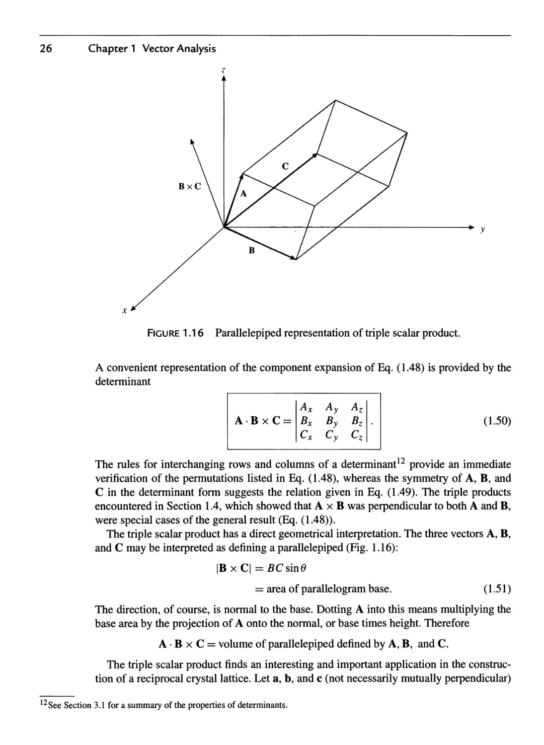
26 Chapter 1 Vector Analysis
Figure 1.16 Parallelepiped representation of triple scalar product.
A BxC =
Ax
Bx
cx
Ay
By
Cy
Az
Bz
Cz
A convenient representation of the component expansion of Eq. A.48) is provided by the
determinant
A.50)
The rules for interchanging rows and columns of a determinant12 provide an immediate
verification of the permutations listed in Eq. A.48), whereas the symmetry of A, B, and
C in the determinant form suggests the relation given in Eq. A.49). The triple products
encountered in Section 1.4, which showed that Α χ Β was perpendicular to both A and B,
were special cases of the general result (Eq. A.48)).
The triple scalar product has a direct geometrical interpretation. The three vectors A, B,
and C may be interpreted as defining a parallelepiped (Fig. 1.16):
IB χ CI = £C sin(9
= area of parallelogram base.
A.51)
The direction, of course, is normal to the base. Dotting A into this means multiplying the
base area by the projection of A onto the normal, or base times height. Therefore
A BxC = volume of parallelepiped defined by A, B, and C.
The triple scalar product finds an interesting and important application in the
construction of a reciprocal crystal lattice. Let a, b, and c (not necessarily mutually perpendicular)
See Section 3.1 for a summary of the properties of determinants.

1.5 Triple Scalar Product, Triple Vector Product 27
represent the vectors that define a crystal lattice. The displacement from one lattice point
to another may then be written
r = naa + ftfcb + ncc,
with na,rib, and nc taking on integral values. With these vectors we may form
a =
b χ c
a-bxc'
b' =
c χ a
a-bxc'
c' =
a x b
a-bxc*
A-52)
A.53a)
We see that a' is perpendicular to the plane containing b and c, and we can readily show
that
whereas
a' a = b' b = c' -c=l,
a' b = a c = b' a = b c = c a = c' b = 0.
A.53b)
A.53c)
It is from Eqs. A.53b) and A.53c) that the name reciprocal lattice is associated with the
points r' = n'aaf + nfbbf + nrco!. The mathematical space in which this reciprocal lattice
exists is sometimes called a Fourier space, on the basis of relations to the Fourier analysis of
Chapters 14 and 15. This reciprocal lattice is useful in problems involving the scattering of
waves from the various planes in a crystal. Further details may be found in R. B. Leighton's
Principles of Modern Physics, pp. 440-448 [New York: McGraw-Hill A959)].
Triple Vector Product
The second triple product of interest is Α χ (Β χ C), which is a vector. Here the parentheses
must be retained, as may be seen from a special case (xxx)xy = 0, while χ χ (χ χ y) =
χ χ ζ = —y.
Example 7.5.7 a triple vector product
For the vectors
A = x + 2y-i = A,2,-1), B = y + z = @,1,1), C = i-y=@,1,1),
BxC =
χ y ζ
0 1 1
1 -1 0
= x + y-z,
and
Α χ (Β χ C) =
χ y ζ
1 2 -1
1 1 -1
= -χ - ζ = -(y + ζ) - (χ - y)
= -Β - C.
By rewriting the result in the last line of Example 1.5.1 as a linear combination of Β and
C, we notice that, taking a geometric approach, the triple vector product is perpendicular

Chapter 1 Vector Analysis
Ax(BxC)
Figure 1.17 Β and C are in the xy-plane.
Β χ C is perpendicular to the xy-plane and
is shown here along the z-axis. Then
Α χ (Β χ C) is perpendicular to the z-axis
and therefore is back in the xy-plane.
to A and to Β χ C. The plane defined by Β and C is perpendicular to Β χ C, and so the
triple product lies in this plane (see Fig. 1.17):
Α χ (Β χ C) = wB + vC.
A.54)
Taking the scalar product of Eq. A.54) with A gives zero for the left-hand side, so
wA · Β + vA · C = 0. Hence u = wA · C and ν = —wA · Β for a suitable w.
Substituting these values into Eq. A.54) gives
Α χ (Β χ C) = w[B(A · C) - C(A · B)];
A.55)
we want to show that
w = 1
in Eq. A.55), an important relation sometimes known as the BAC-CAB rule. Since
Eq. A.55) is linear in A, B, and C, w is independent of these magnitudes. That is, we
only need to show that w = 1 for unit vectors A, B, C. Let us denote Β · C = cos a,
C · A = cos β, Α · Β = cos γ, and square Eq. A.55) to obtain
[Α χ (Β χ C)]2 = A2(B χ CJ - [A · (Β χ C)]2
= l-cos2a-[A-(BxC)]2
= w2[(A · CJ + (A · BJ - 2(A · B)(A · C)(B · C)]
= w2(cos2 β +cos2y — 2cosacos^cosy), A.56)

1.5 Triple Scalar Product, Triple Vector Product 29
using (A x BJ = A2B2 — (A · BJ repeatedly (see Eq. A.43) for a proof). Consequently,
the (squared) volume spanned by A, B, C that occurs in Eq. A.56) can be written as
[A · (Β χ C)] = 1 —cos2 α — w2(cos2 β + cos2)/ — 2 cos a cos β cosy).
Here w2 = 1, since this volume is symmetric in α, β, γ. That is, w = ±1 and is
independent of A, B, C. Using again the special case χ χ (χ χ y) = — y in Eq. A.55) finally
gives w = \. (An alternate derivation using the Levi-Civita symbol Sjjk of Chapter 2 is the
topic of Exercise 2.9.8.)
It might be noted here that just as vectors are independent of the coordinates, so a vector
equation is independent of the particular coordinate system. The coordinate system only
determines the components. If the vector equation can be established in Cartesian
coordinates, it is established and valid in any of the coordinate systems to be introduced in
Chapter 2. Thus, Eq. A.55) may be verified by a direct though not very elegant method of
expanding into Cartesian components (see Exercise 1.5.2).
Exercises
1.5.1 One vertex of a glass parallelepiped is at the origin (Fig. 1.18). The three adjacent
vertices are at C,0,0), @,0,2), and @,3,1). All lengths are in centimeters. Calculate
the number of cubic centimeters of glass in the parallelepiped using the triple scalar
product.
1.5.2 Verify the expansion of the triple vector product
Α χ (Β χ C) = B(A C) - C(A B)
/
/
/
_ «- ""
»- "-
—· ¦"¦
^ ^
^ — **
^ ~~
-
- -~ "/1
/ ι
/ |
/
Λ J
1
1
I /
1 '
Figure 1.18 Parallelepiped: triple scalar product.

Chapter 1 Vector Analysis
by direct expansion in Cartesian coordinates.
Show that the first step in Eq. A.43), which is
(A x B) · (A x B) = A2B2 - (A · BJ,
is consistent with the BAC-CAB rule for a triple vector product.
You are given the three vectors A, B, and C,
A = x + y,
B = y + z,
C = χ - z.
(a) Compute the triple scalar product, A BxC. Noting that A = Β + C, give a
geometric interpretation of your result for the triple scalar product.
(b) Compute Α χ (Β χ C).
1.5.5 The orbital angular momentum L of a particle is given by L = r χ ρ = mr χ ν, where
ρ is the linear momentum. With linear and angular velocity related by ν = ω χ r, show
that
L = mr2[fc> — f(f ·ώ)\
Here f is a unit vector in the r-direction. For r · ω = 0 this reduces to L = Ι ω, with the
moment of inertia / given by mr2. In Section 3.5 this result is generalized to form an
inertia tensor.
1.5.6 The kinetic energy of a single particle is given by Τ = ηπιν2. For rotational motion this
becomes |m(ft) χ rJ. Show that
Τ = -m[r2(o2 - (r · ωJ].
For r · ω = 0 this reduces to Τ = \ΐω2, with the moment of inertia / given by mr2.
1.5.7 Show that13
a χ (b χ c) + b χ (c χ a) + c χ (a x b) = 0.
1.5.8 A vector A is decomposed into a radial vector Ar and a tangential vector A*. If f is a
unit vector in the radial direction, show that
(a) Ar = f (A · f) and
(b) A, = — r χ (f χ A).
1.5.9 Prove that a necessary and sufficient condition for the three (nonvanishing) vectors A,
B, and C to be coplanar is the vanishing of the triple scalar product
Α Β χ C = 0.
13This is Jacobi's identity for vector products; for commutators it is important in the context of Lie algebras (see Eq. D.16) in
Section 4.2).
1.5.3
1.5.4

1.5 Triple Scalar Product, Triple Vector Product 31
1.5.10 Three vectors A, B, and C are given by
A = 3x - 2y + 2z,
Β = 6x + 4y - 22,
C = -3x - 2y - 4z.
Compute the values of A · Β χ C and Α χ (Β χ C), C χ (Α χ Β) and Β χ (C χ Α).
1.5.11 Vector D is a linear combination of three noncoplanar (and nonorthogonal) vectors:
D = aA + bB + cC.
Show that the coefficients are given by a ratio of triple scalar products,
DBxC
a = -—-——, and so on.
A BxC
1.5.12 Show that
(A x B) · (C χ D) = (A · C)(B · D) - (A · D)(B ¦ C).
1.5.13 Show that
(Α χ Β) χ (C χ D) = (Α Β χ D)C - (Α Β χ C)D.
1.5.14 For a spherical triangle such as pictured in Fig. 1.14 show that
sin A sin Β sin C
sin Z?C sinCA sin AB
Here sin A is the sine of the included angle at A, while BC is the side opposite (in
radians).
1.5.15 Given
bxc . cxa , axb
, ILT XX %, .
a = — , b =
c =
abxc' abxc' abxc'
and a · b χ c φ 0, show that
(a) x-y' = <$;c>,,(x,y = a,b,c),
(b) a'-b'xc' = (a-bxc),
bxc'
(C) a=^b^7·
1.5.16 If χ · y' = 8xy, (x, y = a, b, c), prove that
bxc
a
abxc
(This is the converse of Problem 1.5.15.)
1.5.17 Show that any vector V may be expressed in terms of the reciprocal vectors a', b;, c' (of
Problem 1.5.15) by
V = (V · a)ar + (V · b)b7 + (V ¦ c)c'.

32 Chapter 1 Vector Analysis
1.5.18 An electric charge q\ moving with velocity vi produces a magnetic induction Β given
by
μ0 vi χ f
Β = —q\ —ζ— (mks units),
Απ rL
where r points from q\ to the point at which Β is measured (Biot and Savart law).
(a) Show that the magnetic force on a second charge qi, velocity V2, is given by the
triple vector product
F^fUf^xCv.xr).
Απ rL
(b) Write out the corresponding magnetic force Fi that qi exerts on q\. Define your
unit radial vector. How do Fi and F2 compare?
(c) Calculate Fi and F2 for the case of q\ and #2 moving along parallel trajectories
side by side.
ANS.
(b) Γΐ=-^νΐχ(ν2ΧΓ).
Απ r1
In general, there is no simple relation between
Fi and F2. Specifically, Newton's third law, Fi = — F2,
does not hold.
(c) F1 = £°iifVr = -F2.
Απ rL
Mutual attraction.
1.6 Gradient, V
To provide a motivation for the vector nature of partial derivatives, we now introduce the
total variation of a function F(x,y),
JF, 3F J dF J
dF = —dx Η dy.
ox ay
It consists of independent variations in the x- and v-directions. We write dF as a sum of
two increments, one purely in the x- and the other in the y-direction,
dF{x, y) = F(x + dx, y + dy) — F(x, y)
= [F(x + dx, y + dy) - F(x, y + dy)] + [F(x, y + dy)- F(jc, y)]
dF , dF ,
= τ-dx + —dy,
ax ay
by adding and subtracting F(x, y + dy). The mean value theorem (that is, continuity of F)
tells us that here dF/dx, dF/dy are evaluated at some point ξ, η between χ and χ -h dx, y

1.6 Gradient, V 33
and ν + dy, respectively. As dx -> 0 and dy -> 0, £ -> jc and r? -> y. This result
generalizes to three and higher dimensions. For example, for a function φ of three variables,
d(p(x, y, z) = [φ(χ + dx,y + dy, z + dz)- φ(χ, y + dy, ζ + dz)]
+ [<?(*> y + dy, ζ + dz) - φ(χ, y,z + dz)]
+ [φ(χ, y,z + dz) - <p(x, y, z)] A.57)
= —dx + — ί/y + — i/z.
3λ: 3y dz
Algebraically, άφ in the total variation is a scalar product of the change in position dr and
the directional change of φ. And now we are ready to recognize the three-dimensional
partial derivative as a vector, which leads us to the concept of gradient.
Suppose that φ(χ, y, z) is a scalar point function, that is, a function whose value depends
on the values of the coordinates (x, y, z). As a scalar, it must have the same value at a given
fixed point in space, independent of the rotation of our coordinate system, or
φ'(χ[, χ'2, χ'3) = φ(χ\, χι, xj). A.58)
By differentiating with respect to x[ we obtain
d(p'(x[,X2,xf3) _ d<p(x\,X2,X3) _ γ^ ΰψ dxj _ γ^ d<P_
dx[ " dx[ " ^ dxj dx[ " ^atj dxj (L5y)
l l j J I j J
by the rules of partial differentiation and Eqs. A.16a) and A.16b). But comparison with
Eq. A.17), the vector transformation law, now shows that we have constructed a vector
with components ΰφ/dxj. This vector we label the gradient of φ.
A convenient symbolism is
V<p = x^+y^+z^ A.60)
ax ay dz
or
Ι λ ^ λ I
A.61)
V'φ (or del φ) is our gradient of the scalar φ, whereas V (del) itself is a vector differential
operator (available to operate on or to differentiate a scalar φ). All the relationships for V
(del) can be derived from the hybrid nature of del in terms of both the partial derivatives
and its vector nature.
The gradient of a scalar is extremely important in physics and engineering in expressing
the relation between a force field and a potential field,
force F = -V(potential V), A.62)
which holds for both gravitational and electrostatic fields, among others. Note that the
minus sign in Eq. A.62) results in water flowing downhill rather than uphill! If a force can
be described, as in Eq. A.62), by a single function V(r) everywhere, we call the scalar
function V its potential. Because the force is the directional derivative of the potential, we
can find the potential, if it exists, by integrating the force along a suitable path. Because the

34 Chapter 1 Vector Analysis
total variation d V = V V · dr = —F · dr is the work done against the force along the path
dr, we recognize the physical meaning of the potential (difference) as work and energy.
Moreover, in a sum of path increments the intermediate points cancel,
[V(r + dri + dr2) - V(r + dr{)] + [V(r + dn) - V(r)] = V(jr + dr2 + dri) - V(r),
so the integrated work along some path from an initial point rf· to a final point r is given by
the potential difference V(r) — V(r;) at the endpoints of the path. Therefore, such forces
are especially simple and well behaved: They are called conservative. When there is loss of
energy due to friction along the path or some other dissipation, the work will depend on the
path, and such forces cannot be conservative: No potential exists. We discuss conservative
forces in more detail in Section 1.13.
Example 7.6.1 the Gradient of a Potential V(r)
Let us calculate the gradient of V(r) = V(y/x2 + y2 + z2), so
VV(r)=x——+ y——+ z——.
dx ay az
Now, V(r) depends on χ through the dependence of r on x. Therefore14
8V(r) _dV(r) dr
dx dr dx
From rasa function of x, v, z,
dr _ a(;t2 + y2 + z2I/2 _ χ _x
ίχ~~ dx ~(jc2 + y2 + z2I/2~7'
Therefore
dV(r) _ dV(r) χ
dx dr r
Permuting coordinates (jc -> y, y -> ζ, ζ -^ x) to obtain the y and ζ derivatives, we get
~~Λ ldV I
VV(r) = (xx+yy + zz)--—
r <ir
_Γί/ν_Λί/ν
r dr dr
Here r is a unit vector (r/r) in the positive radial direction. The gradient of a function of
r is a vector in the (positive or negative) radial direction. In Section 2.5, f is seen as one
of the three orthonormal unit vectors of spherical polar coordinates and f d/dr as the radial
component of V. ¦
14This is a special case of the chain rule of partial differentiation:
dV(r,9,<p) _ dV dr dV_dO_ <W_d(p_
dx dr dx d0 dx d<p dx'
where dV/dO = dVjdtp = 0, dV/dr -> dV/dr.

1.6 Gradient, V 35
A Geometrical Interpretation
One immediate application of V φ is to dot it into an increment of length
dr = χ dx + ydy + idz.
Thus we obtain
dw dw d(p
V<p · dv = -^-dx + -^-dy + -^-dz = d<p,
ox ay az
the change in the scalar function φ corresponding to a change in position dr. Now consider
Ρ and Q to be two points on a surface <p(x, v, z) = C, a constant. These points are chosen
so that β is a distance dx from P. Then, moving from Ρ to β, the change in φ(χ, ν, ζ) = C
is given by
d<p = (V<p)-dr = 0 A.63)
since we stay on the surface <p(x, v, z) = C. This shows that V<p is perpendicular to dr.
Since dr may have any direction from Ρ as long as it stays in the surface of constant φ,
point Q being restricted to the surface but having arbitrary direction, V^? is seen as normal
to the surface φ = constant (Fig. 1.19).
If we now permit dr to take us from one surface φ = C\ to an adjacent surface φ = Ci
(Fig. 1.20),
dtp = Ci - C2 = AC = (V<p) · dr. A.64)
For a given d<p, \dr\ is a minimum when it is chosen parallel to Vcp (cos0 = 1); or, for
a given \dr\, the change in the scalar function φ is maximized by choosing dr parallel to
Figure 1.19 The length increment dr has to stay on the surface φ = ϋ.

36 Chapter 1 Vector Analysis
Figure 1.20 Gradient.
V<p. This identifies V<p as a vector having the direction of the maximum space rate
of change of φ, an identification that will be useful in Chapter 2 when we consider non-
Cartesian coordinate systems. This identification of V(p may also be developed by using
the calculus of variations subject to a constraint, Exercise 17.6.9.
Example 1.6.2 force as Gradient of a Potential
As a specific example of the foregoing, and as an extension of Example 1.6.1, we consider
the surfaces consisting of concentric spherical shells, Fig. 1.21. We have
φ(χ, j, Z) = (χ1 + v2 + z2) l/2 = r = C,
where r is the radius, equal to C, our constant. AC = Αφ = Ar, the distance between two
shells. From Example 1.6.1
„d<p(r) Λ
\φ{Γ) = r = r.
dr
The gradient is in the radial direction and is normal to the spherical surface φ = C. ¦
Example 1.6.3 Integration by Parts of Gradient
Let us prove the formula / A(r) · V/(r) d3r = — f f(r) V · A(r) d3r, where A or / or both
vanish at infinity so that the integrated parts vanish. This condition is satisfied if, for
example, A is the electromagnetic vector potential and / is a bound-state wave function ψ(τ).

1.6 Gradient, V 37
FiguRE 1.21 Gradient for
φ(χ, y, z) = (x2 + y2 + z2I/2, spherical
shells: (x2 + y2 + z^I/2 = r2 = C2,
(jcf + yf + z^^^n^Ci.
Writing the inner product in Cartesian coordinates, integrating each one-dimensional
integral by parts, and dropping the integrated terms, we obtain
f A(r) · Wf(r)d3r = ff\^xf\^-oo ~ f f^dx] dydz + '''
= " ///^B-£dxdydz- ffj'f^dydxdz-jfff^dzdxdy
= -jf(r)V-A(r)d3r.
If A = elkze describes an outgoing photon in the direction of the constant polarization unit
vector e and f = ψ(γ) is an exponentially decaying bound-state wave function, then
f eikze-VY(r)d3r = -ez (
deikz C
ψ(τ) d3r = -ikez / f{r)eikzd3r,
dz J
because only the ζ-component of the gradient contributes.
Exercises
1.6.1 If 5(jc, y, z) = (x2 + y2 + ζ2Γ3/2, find
(a) VS at the point A,2,3);
(b) the magnitude of the gradient of S, |V S| at A,2,3); and
(c) the direction cosines of VS at A,2,3).

38 Chapter 1 Vector Analysis
1.6.2 (a) Find a unit vector perpendicular to the surface
x2 + y2 + z2 = 3
at the point A,1,1). Lengths are in centimeters,
(b) Derive the equation of the plane tangent to the surface at A,1,1).
ANS. (a) (x + y+ z)/V3, (b) χ + y + z = 3.
1.6.3 Given a vector ri2 = x(x\ — X2) + y(y\ — yi) + z(zi — zi), show that Viri2 (gradient
with respect to jci, yi, and z\ of the magnitude ryi) is a unit vector in the direction of
Γ12-
1.6.4 If a vector function F depends on both space coordinates (x, y, z) and time t, show that
d¥ = (dr-V)F + — dt.
at
1.6.5 Show that W(uv) = vVu 4- uVv, where u and υ are differentiable scalar functions of
x,y, andz.
(a) Show that a necessary and sufficient condition that u(x, y, z) and υ(χ, y, z) are
related by some function /(w, υ) = 0 is that (Vw) χ (Vi;) = 0.
(b) If u = w(x, y) and υ = v(x, y), show that the condition (Vm) χ (Vi;) = 0 leads to
the two-dimensional Jacobian
The functions u and υ are assumed differentiable.
= 0.
1.7 Divergence, V
Differentiating a vector function is a simple extension of differentiating scalar quantities.
Suppose r(i) describes the position of a satellite at some time t. Then, for differentiation
with respect to time,
dr(t) Γ(ί + Δί)-Γ(ί)
= lim = v, linear velocity.
dt δ-*ο At
Graphically, we again have the slope of a curve, orbit, or trajectory, as shown in Fig. 1.22.
If we resolve r(i) into its Cartesian components, dr/dt always reduces directly to a
vector sum of not more than three (for three-dimensional space) scalar derivatives. In other
coordinate systems (Chapter 2) the situation is more complicated, for the unit vectors are
no longer constant in direction. Differentiation with respect to the space coordinates is
handled in the same way as differentiation with respect to time, as seen in the following
paragraphs.

1.7 Divergence, V
lim Δτ.
-Ο Δί
39
Figure 1.22 Differentiation of a vector.
In Section 1.6, V was defined as a vector operator. Now, paying attention to both its
vector and its differential properties, we let it operate on a vector. First, as a vector we dot
it into a second vector to obtain
A.65a)
V
¦ v =
nvx
—
dx
+
SVy
dy
+
<>vz
dz
known as the divergence of V. This is a scalar, as discussed in Section 1.3.
Example 1.7.1 Divergence of Coordinate Vector
Calculate V · r:
Λ a .a Λ a \ /Λ
lxax+ya~ + zaz J ,(χχ + ^ + ζζ)
ax ay az
ax dy dz'
orV-r = 3.
Example 1.7.2 Divergence of Central Force Field
Generalizing Example 1.7.1,
V "(r/(r)) = Yx^ /(r)] + Yy[y /@] + 1Z[Z /(Γ)]
.,,, x2df y2df z2df
= 3/(r) + — -f + —-f + --f
= 3/(r) + r —.
dr

40 Chapter 1 Vector Analysis
The manipulation of the partial derivatives leading to the second equation in Example 1.7.2
is discussed in Example 1.6.1. In particular, if f(r) = r"_1,
V · (it") = V
rr
= 3rw_1 + (n - l)rn~l
= (n + 2)rn~l. A.65b)
This divergence vanishes for η = —2, except at r — 0, an important fact in Section 1.14. ¦
Example 1.7.3 Integration by Parts of Divergence
Let us prove the formula //(r)V · A(r)d3r = — f A · V/d3r, where A or / or both
vanish at infinity.
To show this, we proceed, as in Example 1.6.3, by integration by parts after writing
the inner product in Cartesian coordinates. Because the integrated terms are evaluated at
infinity, where they vanish, we obtain
f /(r)V · A(r)d3r = f f(^-dxdydz + ^dydxdz + ^dzdxdy)
Γ / i)f i)f ?\f \
= — I [ Ax —dxdydz + Ay—dydxdz + Az —dzdxdy )
J \ dx dy dz )
= -fA-Vfd3r. m
A Physical Interpretation
To develop a feeling for the physical significance of the divergence, consider V · (pv) with
v(jc, y, z)9 the velocity of a compressible fluid, and p(x, y, z), its density at point (jc, y, z).
If we consider a small volume dx dy dz (Fig. 1.23) at χ = y = ζ = 0, the fluid flowing into
this volume per unit time (positive χ -direction) through the face EFGH is (rate of flow
in)EFGH = pvx\x=Q = dy dz. The components of the flow pvy and pvz tangential to this
face contribute nothing to the flow through this face. The rate of flow out (still positive
jc-direction) through face ABCD is pvx \x=dx dy dz. To compare these flows and to find the
net flow out, we expand this last result, like the total variation in Section 1.6.15 This yields
(rate of flow out)abcd = pvx \x=dx dy dz
= \pvx + — (pvx) dx dydz.
Here the derivative term is a first correction term, allowing for the possibility of nonuniform
density or velocity or both.16 The zero-order term pvx \x=o (corresponding to uniform flow)
15Here we have the increment dx and we show a partial derivative with respect to χ since pvx may also depend on ν and z.
16Strictly speaking, pvx is averaged over face EFGH and the expression pvx + (d/dx)(pvx)dx is similarly averaged over face
ABCD. Using an arbitrarily small differential volume, we find that the averages reduce to the values employed here.

1.7 Divergence, V 41
c
<fe
ζ
A
/
Ε
G
D
B.
^dx
Η
F
dy
Figure 1.23 Differential rectangular parallelepiped (in first octant).
cancels out:
Net rate of flow out|x = — (pvx)dx dy dz.
ox
Equivalently, we can arrive at this result by
lim
Δ*->-0
ρν,(Δ*,0,0)-ρι;χ@,0,0) d[pvx(x9y9z)]
Ax
dx
0,0,0
Now, the x-axis is not entitled to any preferred treatment. The preceding result for the two
faces perpendicular to the jc-axis must hold for the two faces perpendicular to the ν-axis,
with χ replaced by ν and the corresponding changes for y and z: y -> ζ, ζ -> χ. This is
a cyclic permutation of the coordinates. A further cyclic permutation yields the result for
the remaining two faces of our parallelepiped. Adding the net rate of flow out for all three
pairs of surfaces of our volume element, we have
net flow out
(per unit time)
¦[
rl r) r)
ax ay az
«*)]
dx dy dz
= V · (p\)dxdydz.
A.66)
Therefore the net flow of our compressible fluid out of the volume element dx dy dz per
unit volume per unit time is V · (pv). Hence the name divergence. A direct application is
in the continuity equation
θρ
dt
+ V.(pv)=0,
A.67a)
which states that a net flow out of the volume results in a decreased density inside the
volume. Note that in Eq. A.67a), ρ is considered to be a possible function of time as well
as of space: p(x,y,z,t). The divergence appears in a wide variety of physical problems,

42 Chapter 1 Vector Analysis
ranging from a probability current density in quantum mechanics to neutron leakage in a
nuclear reactor.
The combination V · (/V), in which / is a scalar function and V is a vector function,
may be written
V · (/V) = ^-(fVx) + -H-(fVy) + ^-(fVz)
ox oy az
of JVX df JVy df dVz
= irvx + fir + irvy + fir + irvz + fir
ox ox ay ay az az
= (V/)-V + /V-V, A.67b)
which is just what we would expect for the derivative of a product. Notice that V as a
differential operator differentiates both / and V; as a vector it is dotted into V (in each
term).
If we have the special case of the divergence of a vector vanishing,
V B = 0, A.68)
the vector Β is said to be solenoidal, the term coming from the example in which Β is the
magnetic induction and Eq. A.68) appears as one of Maxwell's equations. When a vector
is solenoidal, it may be written as the curl of another vector known as the vector potential.
(In Section 1.13 we shall calculate such a vector potential.)
Exercises
1.7.1 For a particle moving in a circular orbit r = xr cos ωί + yr sin ωί,
(a) evaluate rxr, with r = ^ = v.
(b) Show that r + co2r = 0 with r = ^.
The radius r and the angular velocity ω are constant.
ANS. (a) των1.
1.7.2 Vector A satisfies the vector transformation law, Eq. A.15). Show directly that its time
derivative dA/dt also satisfies Eq. A.15) and is therefore a vector.
1.7.3 Show, by differentiating components, that
(a) £(A.B) = f-B + A.f,
(b) £(AxB) = f xB + Axf,
just like the derivative of the product of two algebraic functions.
1.7.4 In Chapter 2 it will be seen that the unit vectors in non-Cartesian coordinate systems are
usually functions of the coordinate variables, e,· = e,· (q\ ,qi,qz) but |e,· | = 1. Show that
either 3e//3^7 = 0 or dei/dqj is orthogonal to e,·.
Hint, dej/dqj = 0.

1.8 Curl, V χ 43
1.7.5 Prove V · (a x b) = b · (V χ a) - a · (V χ b).
Hint. Treat as a triple scalar product.
1.7.6 The electrostatic field of a point charge q is
E =
4π£ο r2'
Calculate the divergence of E. What happens at the origin?
1.8 Curl, Vx
Another possible operation with the vector operator V is to cross it into a vector. We obtain
\dy z 3z y) \dz dx V \d* dy /
X
d_
dx
Vx
y ζ
JL i_
dy dz
A.69)
which is called the curl of V. In expanding this determinant we must consider the derivative
nature of V. Specifically, V χ V is defined only as an operator, another vector differential
operator. It is certainly not equal, in general, to —V χ V.17 In the case of Eq. A.69) the
determinant must be expanded from the top down so that we get the derivatives as shown
in the middle portion of Eq. A.69). If V is crossed into the product of a scalar and a vector,
we can show
V X (/V)|;
= Vl? + £v'-flir-£v>)
= /VxVU + (V/)xVL.
A.70)
If we permute the coordinates x—*-y,y-*z,z—> x to pick up the y -component and
then permute them a second time to pick up the z-component, then
Vx(/V) = /VxV + (V/)xV,
A.71)
which is the vector product analog of Eq. A.67b). Again, as a differential operator V
differentiates both / and V. As a vector it is crossed into V (in each term).
17In this same spirit, if A is a differential operator, it is not necessarily true that A x A = 0. Specifically, for the quantum
mechanical angular momentum operator L = —i(r χ V), we find that L χ L = /L. See Sections 4.3 and 4.4 for more details.

44 Chapter 1 Vector Analysis
Example 1.8.1 Vector Potential of a Constant Β Field
From electrodynamics we know that V · Β = 0, which has the general solution Β = V χ A,
where A(r) is called the vector potential (of the magnetic induction), because V · (V χ A) =
(V χ V) · A = 0, as a triple scalar product with two identical vectors. This last identity will
not change if we add the gradient of some scalar function to the vector potential, which,
therefore, is not unique.
In our case, we want to show that a vector potential is A = j (Β χ r).
Using the BAC-BAC rule in conjunction with Example 1.7.1, we find that
2V χ A = V χ (Β χ r) = (V · r)B - (B · V)r = 3B - Β = 2B,
where we indicate by the ordering of the scalar product of the second term that the gradient
still acts on the coordinate vector. ¦
Example 1.8.2 curl of a central force field
Calculate V χ (r/(r)).
By Eq. A.71),
V χ (r/(r)) = /(r)V χ r+ [V/(r)] χ r.
First,
V xr =
χ y ζ
A. A A
dx dy dz
x y z
= 0.
A.72)
A.73)
Second, using V/(r) = r(df/dr) (Example 1.6.1), we obtain
df *
V χ τ fir) = — f χ r = 0. A.74)
dr
This vector product vanishes, since r = f r and f χ f = 0. ¦
To develop a better feeling for the physical significance of the curl, we consider the
circulation of fluid around a differential loop in the jcy-plane, Fig. 1.24.
x<y y0 + dy
x0 + dx, yQ + dy
(xQ + dx, y{))
-> χ
Figure 1.24 Circulation around a differential loop.

1.8 Curl, V χ 45
Although the circulation is technically given by a vector line integral / V · dk
(Section 1.10), we can set up the equivalent scalar integrals here. Let us take the circulation to
be
circulation 1234 = / Vx(x, y)dkx + / Vy(x,y)dky
+ jvx{x,y)dkx + jvy(x,y)dky. A.75)
The numbers 1, 2, 3, and 4 refer to the numbered line segments in Fig. 1.24. In the first
integral, dkx = +dx; but in the third integral, dkx = —dx because the third line segment
is traversed in the negative χ -direction. Similarly, dky = +dy for the second integral, —dy
for the fourth. Next, the integrands are referred to the point (jco, yo) with a Taylor
expansion18 taking into account the displacement of line segment 3 from 1 and that of 2 from 4.
For our differential line segments this leads to
circulationi234 = V*(*o, yo)dx + Vy(xo, yo) + ~~*r~dx dy
Γ Wx 1
+ Vx(xo, yo) + -7j-dy \(-dx) + Vy(xo, yo)(~dy)
Dividing by dx dy, we have
circulation per unit area = V χ V|z. A.77)
The circulation19 about our differential area in the xy-plane is given by the z-component
of V χ V. In principle, the curl V χ V at (jco>yo) could be determined by inserting a
(differential) paddle wheel into the moving fluid at point (xo, yo). The rotation of the little
paddle wheel would be a measure of the curl, and its axis would be along the direction of
V χ V, which is perpendicular to the plane of circulation.
We shall use the result, Eq. A.76), in Section 1.12 to derive Stokes' theorem. Whenever
the curl of a vector V vanishes,
VxV = 0, A.78)
V is labeled irrotational. The most important physical examples of irrotational vectors are
the gravitational and electrostatic forces. In each case
V = C^ = C-^, A.79)
where C is a constant and f is the unit vector in the outward radial direction. For the
gravitational case we have C = —Gm\m2, given by Newton's law of universal gravitation.
If C = qiqi/^neo, we have Coulomb's law of electrostatics (mks units). The force V
18Here, V^(jco + dx, yo) = Vy(xQ, y$) + (-fijr)xoyQ dx -\ . The higher-order terms will drop out in the limit as dx ->· 0.
A correction term for the variation of Vy with y is canceled by the corresponding term in the fourth integral.
9 In fluid dynamics V χ V is called the "vorticity."

46 Chapter 1 Vector Analysis
given in Eq. A.79) may be shown to be irrotational by direct expansion into Cartesian
components, as we did in Example 1.8.1. Another approach is developed in Chapter 2, in
which we express V χ, the curl, in terms of spherical polar coordinates. In Section 1.13 we
shall see that whenever a vector is irrotational, the vector may be written as the (negative)
gradient of a scalar potential. In Section 1.16 we shall prove that a vector field may be
resolved into an irrotational part and a solenoidal part (subject to conditions at infinity).
In terms of the electromagnetic field this corresponds to the resolution into an irrotational
electric field and a solenoidal magnetic field.
For waves in an elastic medium, if the displacement u is irrotational, V χ u = 0, plane
waves (or spherical waves at large distances) become longitudinal. If u is solenoidal,
V · u = 0, then the waves become transverse. A seismic disturbance will produce a
displacement that may be resolved into a solenoidal part and an irrotational part (compare
Section 1.16). The irrotational part yields the longitudinal Ρ (primary) earthquake waves.
The solenoidal part gives rise to the slower transverse S (secondary) waves.
Using the gradient, divergence, and curl, and of course the BAC-CAB rule, we may
construct or verify a large number of useful vector identities. For verification, complete
expansion into Cartesian components is always a possibility. Sometimes if we use insight
instead of routine shuffling of Cartesian components, the verification process can be
shortened drastically.
Remember that V is a vector operator, a hybrid creature satisfying two sets of rules:
1. vector rules, and
2. partial differentiation rules — including differentiation of a product.
Example 1.8.3 gradient of a dot product
Verify that
V(A · B) = (B · V)A + (A · V)B + Β χ (V χ A) + A x (V χ Β). A.80)
This particular example hinges on the recognition that V(A · B) is the type of term that
appears in the BAC-CAB expansion of a triple vector product, Eq. A.55). For instance,
A x (V χ B) = V(A · B) - (A · V)B,
with the V differentiating only B, not A. From the commutativity of factors in a scalar
product we may interchange A and Β and write
Β χ (V χ A) = V(A B) - (B V)A,
now with V differentiating only A, not B. Adding these two equations, we obtain V
differentiating the product A · Β and the identity, Eq. A.80). This identity is used frequently
in electromagnetic theory. Exercise 1.8.13 is a simple illustration. ¦

1.8 Curl, V χ 47
V
3r
Example 1.8.4 Integration by Parts of Curl
Let us prove the formula / C(r) · (V χ A(r)) d?r = f A(r) · (V χ C(r)) d3r, where A or
C or both vanish at infinity.
To show this, we proceed, as in Examples 1.6.3 and 1.7.3, by integration by parts after
writing the inner product and the curl in Cartesian coordinates. Because the integrated
terms vanish at infinity we obtain
ic(r).(VxA(r))d3r
-/K£-£)^£-£M£-£)]<
-/Kt-£)W£-£)WS-£)]'
= iA(r).(VxC(r))J3r,
just rearranging appropriately the terms after integration by parts.
Exercises
1.8.1 Show, by rotating the coordinates, that the components of the curl of a vector transform
as a vector.
Hint. The direction cosine identities of Eq. A.46) are available as needed.
1.8.2 Show that u χ ν is solenoidal if u and ν are each irrotational.
1.8.3 If A is irrotational, show that A x r is solenoidal.
1.8.4 A rigid body is rotating with constant angular velocity ω. Show that the linear velocity
ν is solenoidal.
1.8.5 If a vector function f (jc , y, z) is not irrotational but the product of / and a scalar function
g(x, y, z) is irrotational, show that then
f.V xf=0.
1.8.6 If (a) V = xVx(xt y) + yVy(x, y) and (b)VxV^O, prove that V χ V is perpendicular
toV.
1.8.7 Classically, orbital angular momentum is given by L = r χ ρ, where ρ is the linear
momentum. To go from classical mechanics to quantum mechanics, replace ρ by the
operator —/V (Section 15.6). Show that the quantum mechanical angular momentum

48 Chapter 1 Vector Analysis
operator has Cartesian components (in units of h)
( 9 3\
*-> = -\ζτ:-χΤζ)'
1.8.8 Using the angular momentum operators previously given, show that they satisfy
commutation relations of the form
L^JC? Ly\ Ξ LxLy LyLX = I LZ
and hence
L χ L = /L.
These commutation relations will be taken later as the defining relations of an angular
momentum operator—Exercise 3.2.15 and the following one and Chapter 4.
1.8.9 With the commutator bracket notation [Lx, Ly] = LxLy — LyLx, the angular
momentum vector L satisfies [Lx, Ly] = iLz, etc., or L χ L = /L.
If two other vectors a and b commute with each other and with L, that is, [a, b] =
[a, L] = [b, L] = 0, show that
[a-L,b-L] = /(axb)-L.
1.8.10 For A = xAx (x, v, z) and Β = ίίΒχ (x, y, z) evaluate each term in the vector identity
V(A · B) = (B · V)A + (A · V)B + Β χ (V χ Α) 4- A x (V χ Β)
and verify that the identity is satisfied.
1.8.11 Verify the vector identity
V χ (Α χ B) = (B · V)A - (A · V)B - B(V · A) + A(V · B).
1.8.12 As an alternative to the vector identity of Example 1.8.3 show that
V(A . B) = (A x V) χ Β + (Β χ V) χ Α + A(V · Β) + B(V . A).
1.8.13 Verify the identity
A x (V χ A) = -V(A2) - (A · V)A.
1.8.14 If A and Β are constant vectors, show that
V(A Bxr)=AxB.

1.9 Successive Applications of V 49
1.8.15 A distribution of electric currents creates a constant magnetic moment m = const. The
force on m in an external magnetic induction Β is given by
F = V χ (Bxm).
Show that
F = (m V)B.
Note. Assuming no time dependence of the fields, Maxwell's equations yield VxB = 0.
Also, V · Β = 0.
1.8.16 An electric dipole of moment ρ is located at the origin. The dipole creates an electric
potential at r given by
pr
4neor3'
Find the electric field, Ε = — Vi/s at r.
1.8.17 The vector potential A of a magnetic dipole, dipole moment m, is given by A(r) =
(μο/4ττ)(ιη χ r/r3). Show that the magnetic induction Β = V χ A is given by
μ0 3f (r m) - m
Note. The limiting process leading to point dipoles is discussed in Section 12.1 for
electric dipoles, in Section 12.5 for magnetic dipoles.
1.8.18 The velocity of a two-dimensional flow of liquid is given by
If the liquid is incompressible and the flow is irrotational, show that
du dv du dv
dx dy dy dx
These are the Cauchy-Riemann conditions of Section 6.2.
1.8.19 The evaluation in this section of the four integrals for the circulation omitted Taylor
series terms such as dVx/dx, dVy/dy and all second derivatives. Show that dVx/dx,
dVy/dy cancel out when the four integrals are added and that the second derivative
terms drop out in the limit as dx ->0,dy-> 0.
Hint. Calculate the circulation per unit area and then take the limit dx ->0,dy-^ 0.
1.9 Successive Applications of V
We have now defined gradient, divergence, and curl to obtain vector, scalar, and vector
quantities, respectively. Letting V operate on each of these quantities, we obtain
(a) V · V<p (b) V χ Vp (c) V V · V
(d) V · V χ V (e) V χ (V χ V)

50 Chapter 1 Vector Analysis
all five expressions involving second derivatives and all five appearing in the second-order
differential equations of mathematical physics, particularly in electromagnetic theory.
The first expression, V · V<p, the divergence of the gradient, is named the Laplacian of φ.
We have
32φ
d2<p
d2<p
dx2 dy2 dz2
When φ is the electrostatic potential, we have
V· V<p = 0
A.81a)
A.81b)
at points where the charge density vanishes, which is Laplace's equation of electrostatics.
Often the combination V · V is written V2, or Δ in the European literature.
Example 1.9.1 uplacian of a potential
Calculate VVV(r).
Referring to Examples 1.6.1 and 1.7.2,
V7 „I;/ X V7 ~dV 2dV ^
V · VV(r) = V . r— = -— + —T,
dr r dr drz
replacing f(r) in Example 1.7.2 by 1/r · dV/dr. If V(r) = rn, this reduces to
V -Vrn=n(n + l)rn-2.
This vanishes for η = 0 [V(r) = constant] and for η = — 1; that is, V(r) = 1/r is a solution
of Laplace's equation, V2 V(r) = 0. This is for r φ 0. At r = 0, a Dirac delta function is
involved (see Eq. A.169) and Section 9.7). ¦
Expression (b) may be written
V χ V<p =
By expanding the determinant, we obtain
\3y3z dzdy/ \dzdx dxdzj
\dxdy dydxj
X
a
dx
d<p
dx
y
a
ay
a^
ay
ζ
a
3z
a^
az
A.82)
; dy dy dx /
assuming that the order of partial differentiation may be interchanged. This is true as long
as these second partial derivatives of φ are continuous functions. Then, from Eq. A.82),
the curl of a gradient is identically zero. All gradients, therefore, are irrotational. Note that

1.9 Successive Applications of V 51
the zero in Eq. A.82) comes as a mathematical identity, independent of any physics. The
zero in Eq. A.81b) is a consequence of physics.
Expression (d) is a triple scalar product that may be written
V-VxV =
JL JL A
dx dy dz
A. _L i_
dx dy dz
Vx Vy Vz
A.83)
Again, assuming continuity so that the order of differentiation is immaterial, we obtain
V-VxV = 0. A.84)
The divergence of a curl vanishes or all curls are solenoidal. In Section 1.16 we shall see
that vectors may be resolved into solenoidal and irrotational parts by Helmholtz's theorem.
The two remaining expressions satisfy a relation
V χ (V χ V) = VV . V - V · VV, A.85)
valid in Cartesian coordinates (but not in curved coordinates). This follows immediately
from Eq. A.55), the BAC-CAB rule, which we rewrite so that C appears at the extreme
right of each term. The term V · VV was not included in our list, but it may be defined by
Eq.A.85).
Example 1.9.2 Electromagnetic Wave Equation
One important application of this vector relation (Eq. A.85)) is in the derivation of the
electromagnetic wave equation. In vacuum Maxwell's equations become
VB = 0, A.86a)
VE = 0, A.86b)
3E
VxB = vot- · (l-86c)
at
VxE = - —. A.86d)
dt
Here Ε is the electric field, Β is the magnetic induction, εο is the electric permittivity,
and μο is the magnetic permeability (SI units), so soMo = 1/c2, c being the velocity of
light. The relation has important consequences. Because εο, μο can be measured in any
frame, the velocity of light is the same in any frame.
Suppose we eliminate Β from Eqs. A.86c) and A.86d). We may do this by taking the
curl of both sides of Eq. A.86d) and the time derivative of both sides of Eq. A.86c). Since
the space and time derivatives commute,
—V xB = V χ —,
dt dt
and we obtain
V x(VxE) = -£0^.

52 Chapter 1 Vector Analysis
Application of Eqs. A.85) and A.86b) yields
V VE = εο/χο
d2E
A.87)
the electromagnetic vector wave equation. Again, if Ε is expressed in Cartesian
coordinates, Eq. A.87) separates into three scalar wave equations, each involving the scalar
Laplacian.
When external electric charge and current densities are kept as driving terms in
Maxwell's equations, similar wave equations are valid for the electric potential and the
vector potential. To show this, we solve Eq. A.86a) by writing Β = V χ A as a curl of the
vector potential. This expression is substituted into Faraday's induction law in differential
form, Eq. A.86d), to yield V χ (Ε + ^) = 0. The vanishing curl implies that Ε + ^ is a
gradient and, therefore, can be written as — V<p, where <p(r, t) is defined as the (nonstatic)
electric potential. These results for the Β and Ε fields,
B = VxA, E = -V<p
dA
It'
A.88)
solve the homogeneous Maxwell's equations.
We now show that the inhomogeneous Maxwell's equations,
Gauss' law:
V-E = p/<?o.
Oersted's law:
A.89)
in differential form lead to wave equations for the potentials φ and A, provided that V · A is
determined by the constraint \ -£ -f V · A = 0. This choice of fixing the divergence of the
vector potential, called the Lorentz gauge, serves to uncouple the differential equations of
both potentials. This gauge constraint is not a restriction; it has no physical effect.
Substituting our electric field solution into Gauss' law yields
εο at cl dtz
A.90)
the wave equation for the electric potential. In the last step we have used the Lorentz
gauge to replace the divergence of the vector potential by the time derivative of the electric
potential and thus decouple φ from A.
Finally, we substitute Β = V χ A into Oersted's law and use Eq. A.85), which expands
V2 in terms of a longitudinal (the gradient term) and a transverse component (the curl
term). This yields
MoJ+ \ψ- = V x (V χ A) = V(V · A) - V2A
cl at
= /xoJ-^
d<p d2A\
dt
dt2J'
where we have used the electric field solution (Eq. A.88)) in the last step. Now we see that
the Lorentz gauge condition eliminates the gradient terms, so the wave equation
ι a2A
V2A = mqJ
A.91)

1.9 Successive Applications of V 53
for the vector potential remains.
Finally, looking back at Oersted's law, taking the divergence of Eq. A.89), dropping
V · (V χ B) = 0, and substituting Gauss' law for V · Ε = p/€o, we find μο V · J = —l— ¦£,
where 6ομο = Vc2> tnat 1S>tne continuity equation for the current density. This step
justifies the inclusion of Maxwell's displacement current in the generalization of Oersted's law
to nonstationary situations. ¦
Exercises
1.9.1 Verify Eq. A.85),
V χ (V χ V) = VV · V - V · VV,
by direct expansion in Cartesian coordinates.
1.9.2 Show that the identity
V χ (V χ V) = VV · V - V . VV
follows from the BAC-CAB rule for a triple vector product. Justify any alteration of the
order of factors in the BAC and CAB terms.
1.9.3 Prove that V χ (<pV<p) = 0.
1.9.4 You are given that the curl of F equals the curl of G. Show that F and G may differ by
(a) a constant and (b) a gradient of a scalar function.
1.9.5 The Navier-Stokes equation of hydrodynamics contains a nonlinear term (v · V) v. Show
that the curl of this term may be written as —V χ [ν χ (V χ ν)].
1.9.6 From the Navier-Stokes equation for the steady flow of an incompressible viscous fluid
we have the term
V χ [vx (V xv)],
where ν is the fluid velocity. Show that this term vanishes for the special case
y = xv(y,z).
1.9.7 Prove that (Vw) χ (Vt>) is solenoidal, where u and ν are differentiable scalar functions.
1.9.8 φ is a scalar satisfying Laplace's equation, ν2φ = 0. Show that V<p is both solenoidal
and irrotational.
1.9.9 With ψ a scalar (wave) function, show that
(rxV).(rx V)V = r2V2f - r2^- - 2r —.
dr1 dr
(This can actually be shown more easily in spherical polar coordinates, Section 2.5.)

54 Chapter 1 Vector Analysis
1.9.10 In a (nonrotating) isolated mass such as a star, the condition for equilibrium is
Here Ρ is the total pressure, ρ is the density, and φ is the gravitational potential. Show
that at any given point the normals to the surfaces of constant pressure and constant
gravitational potential are parallel.
1.9.11 In the Pauli theory of the electron, one encounters the expression
(p — eA) χ (p — βΑ)ψ,
where ψ is a scalar (wave) function. A is the magnetic vector potential related to the
magnetic induction Β by Β = V χ A. Given that ρ = — / V, show that this expression
reduces to ieBi/s. Show that this leads to the orbital g-factor gi = 1 upon writing the
magnetic moment as μ, = gz,L in units of Bohr magnetons and L = -irxV. See also
Exercise 1.13.7.
1.9.12 Show that any solution of the equation
Vx(VxA)-A:2A = 0
automatically satisfies the vector Helmholtz equation
V2A + A;2A = 0
and the solenoidal condition
VA = 0.
Hint. Let V· operate on the first equation.
1.9.13 The theory of heat conduction leads to an equation
ν2Ψ = Α:|νΦ|2,
where Φ is a potential satisfying Laplace's equation: ν2Φ = 0. Show that a solution of
this equation is
ψ = -&Φ2.
2
1.10 Vector Integration
The next step after differentiating vectors is to integrate them. Let us start with line integrals
and then proceed to surface and volume integrals. In each case the method of attack will be
to reduce the vector integral to scalar integrals with which the reader is assumed familiar.

1.10 Vector Integration 55
Line Integrals
Using an increment of length dx = χ dx -f y dy 4- ζ dz, we may encounter the line integrals
/ <pdr,
i
A.92a)
V-A\ A.92b)
c
ivxi/r, A.92c)
in each of which the integral is over some contour C that may be open (with starting point
and ending point separated) or closed (forming a loop). Because of its physical
interpretation that follows, the second form, Eq. A.92b) is by far the most important of the three.
With φ, a scalar, the first integral reduces immediately to
/ (pdr = xl <p(x,y,z)dx+y Ι φ(χ, ν, z)dy + z / <p(x,y,z)dz. A.93)
This separation has employed the relation
Ι χφάχ=χ Ι φάχ, A.94)
which is permissible because the Cartesian unit vectors x, y, and ζ are constant in both
magnitude and direction. Perhaps this relation is obvious here, but it will not be true in the
non-Cartesian systems encountered in Chapter 2.
The three integrals on the right side of Eq. A.93) are ordinary scalar integrals and, to
avoid complications, we assume that they are Riemann integrals. Note, however, that the
integral with respect to χ cannot be evaluated unless y and ζ are known in terms of χ
and similarly for the integrals with respect to y and z. This simply means that the path
of integration C must be specified. Unless the integrand has special properties so that
the integral depends only on the value of the end points, the value will depend on the
particular choice of contour C. For instance, if we choose the very special case φ = 1,
Eq. A.92a) is just the vector distance from the start of contour C to the endpoint, in this
case independent of the choice of path connecting fixed endpoints. With dx = χ dx+y dy +
zdz, the second and third forms also reduce to scalar integrals and, like Eq. A.92a), are
dependent, in general, on the choice of path. The form (Eq. A.92b)) is exactly the same
as that encountered when we calculate the work done by a force that varies along the
path,
W
= i¥dx= I Fx(x,y,z)dx+ j Fy(x,y,z)dy+ j Fz(x,y,z)dz. A.95a)
In this expression F is the force exerted on a particle.

56 Chapter 1 Vector Analysis
A,1)
-$-
A,0)
->x
Figure 1.25 A path of integration.
Example 1.10.1 path-dependentvvork
The force exerted on a body is F = — xy + yx. The problem is to calculate the work done
going from the origin to the point A,1):
/•U /*1,1
W= ¥dr= (-ydx+xdy). A.95b)
Jo,o Jo,o
Separating the two integrals, we obtain
- / ydx +
Jo Jo
W·
xdy.
A.95c)
The first integral cannot be evaluated until we specify the values of y as χ ranges from 0
to 1. Likewise, the second integral requires χ as a function of y. Consider first the path
shown in Fig. 1.25. Then
W
= - [ 0dx+ [ ldy = l,
Jo Jo
A.95d)
since y = 0 along the first segment of the path and χ = 1 along the second. If we select the
path [x = 0,0 < y < 1] and [0 < χ ^ 1, y = 1], then Eq. A.95c) gives W = -1. For this
force the work done depends on the choice of path. ¦
Surface Integrals
Surface integrals appear in the same forms as line integrals, the element of area also being
a vector, da.20 Often this area element is written ndA, in which η is a unit (normal) vector
to indicate the positive direction.21 There are two conventions for choosing the positive
direction. First, if the surface is a closed surface, we agree to take the outward normal
as positive. Second, if the surface is an open surface, the positive normal depends on the
direction in which the perimeter of the open surface is traversed. If the right-hand fingers
20Recall that in Section 1.4 the area (of a parallelogram) is represented by a cross-product vector.
2i Although η always has unit length, its direction may well be a function of position.

1.10 Vector Integration
57
Figure 1.26 Right-hand rule for
the positive normal.
are placed in the direction of travel around the perimeter, the positive normal is indicated by
the thumb of the right hand. As an illustration, a circle in the xy-plane (Fig. 1.26) mapped
out from χ to y to —x to —y and back to χ will have its positive normal parallel to the
positive z-axis (for the right-handed coordinate system).
Analogous to the line integrals, Eqs. A.92a) to A.92c), surface integrals may appear in
the forms
[φάσ, ίγ-da, ί\
χ da.
Again, the dot product is by far the most commonly encountered form. The surface integral
/ V da may be interpreted as a flow or flux through the given surface. This is really what
we did in Section 1.7 to obtain the significance of the term divergence. This identification
reappears in Section 1.11 as Gauss' theorem. Note that both physically and from the dot
product the tangential components of the velocity contribute nothing to the flow through
the surface.
Volume Integrals
Volume integrals are somewhat simpler, for the volume element dx is a scalar quantity.22
We have
/ \dr=x f Vxdr+y f Vydx+i f Vzdx,
Jv Jv Jv Jv
again reducing the vector integral to a vector sum of scalar integrals.
A.96)
Frequently the symbols d?r and d?x are used to denote a volume element in coordinate (xyz or χ 1*2*3) space.

58 Chapter 1 Vector Analysis
+ y
Figure 1.27 Differential rectangular parallelepiped (origin at center).
Integral Definitions of Gradient, Divergence, and Curl
One interesting and significant application of our surface and volume integrals is their use
in developing alternate definitions of our differential relations. We find
V(p = lim
f<pda
V-V= lim
fdr^O f dx
/V. At
V χ V = lim
fdr-+o f dx
fdax\
fdr^O f dx
A.97)
A.98)
A.99)
In these three equations / dx is the volume of a small region of space and da is the vector
area element of this volume. The identification of Eq. A.98) as the divergence of V was
carried out in Section 1.7. Here we show that Eq. A.97) is consistent with our earlier
definition of V(p (Eq. A.60)). For simplicity we choose dx to be the differential volume
dx dy dz (Fig. 1.27). This time we place the origin at the geometric center of our volume
element. The area integral leads to six integrals, one for each of the six faces. Remembering
that da is outward, da · χ = —\da\ for surface EFHG, and +\da\ for surface ABDC, we
have
/
φ da = — χ
dydz
f L-£'*)dydz+if (φ+ψ±)
JefhgK dx 2 J Jabdc\ dx 2 J
-if (<P-¥di)dX<iz + y[ (, + ^fW
JaegcK dy 2 J Jbfhd\ dy 2 J
~z/ \<P-T-z-)dxdy + zl [<P +-z—z-)dxdy.
JaBFE\ OZ λ J JCDHG\ OZ I J

1.10 Vector Integration 59
Using the total variations, we evaluate each integrand at the origin with a correction
included to correct for the displacement (±dx/29 etc.) of the center of the face from the
origin. Having chosen the total volume to be of differential size (/ dx = dxdydz), we
drop the integral signs on the right and obtain
j φ da = (χ^+y^+z^J dxdydz. A.100)
Dividing by
dx = dxdydz,
l·
we verify Eq. A.97).
This verification has been oversimplified in ignoring other correction terms beyond the
first derivatives. These additional terms, which are introduced in Section 5.6 when the
Taylor expansion is developed, vanish in the limit
/
dx -* 0 {dx -> 0, dy -> 0, dz -> 0).
This, of course, is the reason for specifying in Eqs. A.97), A.98), and A.99) that this limit
be taken. Verification of Eq. A.99) follows these same lines exactly, using a differential
volume dxdydz.
Exercises
1.10.1 The force field acting on a two-dimensional linear oscillator may be described by
F = —xkx —yky.
Compare the work done moving against this force field when going from A,1) to D,4)
by the following straight-line paths:
(a) A,1)-* D,1)^D,4)
(b) A,1)->A,4)^D,4)
(c) A, l)-> D,4) along x = y.
This means evaluating
/•D,4)
-/ F-rfr
Λι,ΐ)
along each path.
1.10.2 Find the work done going around a unit circle in the χ v-plane:
(a) counterclockwise from 0 to π,
(b) clockwise from 0 to — π, doing work against a force field given by
* = —*-. η +
χ2 + ν2 χ2 + ν2'
Note that the work done depends on the path.

60 Chapter 1 Vector Analysis
1.10.3 Calculate the work you do in going from point A,1) to point C,3). The force you exert
is given by
F = x(x-y)+y(x + y).
Specify clearly the path you choose. Note that this force field is nonconservative.
1.10.4 Evaluate § r · dr.
Note. The symbol <f means that the path of integration is a closed loop.
1.10.5 Evaluate
lfsrd<T
over the unit cube defined by the point @,0,0) and the unit intercepts on the positive
x-, y-, and z-axes. Note that (a) r · da is zero for three of the surfaces and (b) each of
the three remaining surfaces contributes the same amount to the integral.
1.10.6 Show, by expansion of the surface integral, that
lim ^—r =VxV.
fdr^O jdx
Hint. Choose the volume / dz to be a differential volume dx dy dz.
1.11 Gauss' Theorem
Here we derive a useful relation between a surface integral of a vector and the volume
integral of the divergence of that vector. Let us assume that the vector V and its first derivatives
are continuous over the simply connected region (that does not have any holes, such as a
donut) of interest. Then Gauss' theorem states that
#\-da = fff
dv JJJv
V-Vdr.
ν
A.101a)
In words, the surface integral of a vector over a closed surface equals the volume integral
of the divergence of that vector integrated over the volume enclosed by the surface.
Imagine that volume V is subdivided into an arbitrarily large number of tiny
(differential) parallelepipeds. For each parallelepiped
Σ V-i/a = V.VJr A.101b)
six surfaces
from the analysis of Section 1.7, Eq. A.66), with p\ replaced by V. The summation is
over the six faces of the parallelepiped. Summing over all parallelepipeds, we find that the
V · da terms cancel (pairwise) for all interior faces; only the contributions of the exterior
surfaces survive (Fig. 1.28). Analogous to the definition of a Riemann integral as the limit

1.11 Gauss'Theorem 61
I
I A I
Ι Τ I
TT/
Figure 1.28 Exact
cancellation of da's on
interior surfaces. No
cancellation on the
exterior surface.
of a sum, we take the limit as the number of parallelepipeds approaches infinity (-> oo)
and the dimensions of each approach zero (-> 0):
exterior surfaces volumes
fs\-da = fvV-\dx.
The result is Eq. A.101a), Gauss' theorem.
From a physical point of view Eq. A.66) has established V · V as the net outflow of
fluid per unit volume. The volume integral then gives the total net outflow. But the surface
integral / V · da is just another way of expressing this same quantity, which is the equality,
Gauss' theorem.
Green's Theorem
A frequently useful corollary of Gauss' theorem is a relation known as Green's theorem. If
u and ν are two scalar functions, we have the identities
V · (u Vv) = wV · Vv + (Vii) · (Vv), A.102)
V . (v ViO = uV . Vw + (Vv) · (Vw). A.103)
Subtracting Eq. A.103) from Eq. A.102), integrating over a volume (μ, υ, and their
derivatives, assumed continuous), and applying Eq. A.101a) (Gauss' theorem), we obtain
f (wV . Vv - vV ¦ Vw)^t = (fl) (kVv - vWu) · </σ.
A.104)

62 Chapter 1 Vector Analysis
This is Green's theorem. We use it for developing Green's functions in Chapter 9. An
alternate form of Green's theorem, derived from Eq. A.102) alone, is
#uVv-da= III wV.VvdT+ fff VwVvdr. A.105)
dv JJJv JJJv
This is the form of Green's theorem used in Section 1.16.
Alternate Forms of Gauss' Theorem
Although Eq. A.101a) involving the divergence is by far the most important form of Gauss'
theorem, volume integrals involving the gradient and the curl may also appear. Suppose
Y(x,y,z) = V(x,y,z)*, A.106)
in which a is a vector with constant magnitude and constant but arbitrary direction. (You
pick the direction, but once you have chosen it, hold it fixed.) Equation A.101a) becomes
a· if) Vda= fff V.aV</r=a· fff VVdr A.107)
by Eq. A.67b). This may be rewritten
a· Γ β Vda- fff VVrfr|=0. A.108)
Since |a| φ 0 and its direction is arbitrary, meaning that the cosine of the included angle
cannot always vanish, the terms in brackets must be zero.23 The result is
#Vda= fff VVdr. A.109)
dv JJJv
In a similar manner, using V = a x Ρ in which a is a constant vector, we may show
#daxP= fff VxPdr. A.110)
dv JJJv
These last two forms of Gauss' theorem are used in the vector form of Kirchoff diffraction
theory. They may also be used to verify Eqs. A.97) and A.99). Gauss' theorem may also
be extended to tensors (see Section 2.11).
Exercises
1.11.1 Using Gauss' theorem, prove that
if 5 = d V is a closed surface.
#da=0
s
23This exploitation of the arbitrary nature of a part of a problem is a valuable and widely used technique. The arbitrary vector
is used again in Sections 1.12 and 1.13. Other examples appear in Section 1.14 (integrands equated) and in Section 2.8, quotient
rule.

1.11 Gauss'Theorem 63
1.11.2 Show that
1.11.4
1.11.5
1.11.6
1.11.7
\l
rda = V,
where V is the volume enclosed by the closed surface S = dV.
Note. This is a generalization of Exercise 1.10.5.
1.11.3 If Β = V χ A, show that
JJs
Β da = 0
for any closed surface S.
Over some volume V let ψ be a solution of Laplace's equation (with the derivatives
appearing there continuous). Prove that the integral over any closed surface in V of the
normal derivative of ψ (dx/s/dn, or Vx// · n) will be zero.
In analogy to the integral definition of gradient, divergence, and curl of Section 1.10,
show that
V2(p =
lim
fdz->0
fV<p-da
fdr '
The electric displacement vector D satisfies the Maxwell equation V · D = p, where ρ
is the charge density (per unit volume). At the boundary between two media there is a
surface charge density σ (per unit area). Show that a boundary condition for D is
(D2-Di) η = σ.
η is a unit vector normal to the surface and out of medium 1.
Hint. Consider a thin pillbox as shown in Fig. 1.29.
From Eq. A.67b), with V the electric field Ε and / the electrostatic potential φ, show
that, for integration over all space,
/ ρφάτ=ε0 /
Ε2άτ.
This corresponds to a three-dimensional integration by parts.
Hint. E = —V^,V-E = ρ/εο· You may assume that φ vanishes at large r at least as
fast as r.
medium 2
medium 1
Figure 1.29 Pillbox.

64 Chapter 1 Vector Analysis
1.11.8 A particular steady-state electric current distribution is localized in space. Choosing a
bounding surface far enough out so that the current density J is zero everywhere on the
surface, show that
///
Jdr=0.
Hint. Take one component of J at a time. With V · J = 0, show that J, = V · (jc, J) and
apply Gauss' theorem.
1.11.9 The creation of a localized system of steady electric currents (current density J) and
magnetic fields may be shown to require an amount of work
¦-!///-...
W = - HI Η Β Jr.
Transform this into
W = i- ΠΙ J-Αάτ.
Alll·
Here A is the magnetic vector potential: V χ A = B.
Hint. In Maxwell's equations take the displacement current term 3D/3i = 0. If the fields
and currents are localized, a bounding surface may be taken far enough out so that the
integrals of the fields and currents over the surface yield zero.
1.11.10 Prove the generalization of Green's theorem:
/// (vCu — uCv)dx — (th p(vVu — uWv) ·da.
JJJv JJ dv
Here C is the self-adjoint operator (Section 10.1),
£ = V.[p(r)V]+*(r)
and /?, g, w, and ν are functions of position, ρ and q having continuous first derivatives
and u and ν having continuous second derivatives.
Note. This generalized Green's theorem appears in Section 9.7.
1.12 Stokes' Theorem
Gauss' theorem relates the volume integral of a derivative of a function to an integral of
the function over the closed surface bounding the volume. Here we consider an analogous
relation between the surface integral of a derivative of a function and the line integral of
the function, the path of integration being the perimeter bounding the surface.
Let us take the surface and subdivide it into a network of arbitrarily small rectangles.
In Section 1.8 we showed that the circulation about such a differential rectangle (in the
jcy-plane) is V χ V|z dx dy. From Eq. A.76) applied to one differential rectangle,
]Γ ν·</λ = ν xV-t/σ. A.111)
four sides

1.12 Stokes'Theorem 65
Figure 1.30 Exact cancellation on
interior paths. No cancellation on the
exterior path.
We sum over all the little rectangles, as in the definition of a Riemann integral. The surface
contributions (right-hand side of Eq. A.111)) are added together. The line integrals (left-
hand side of Eq. A.111)) of all interior line segments cancel identically. Only the line
integral around the perimeter survives (Fig. 1.30). Taking the usual limit as the number of
rectangles approaches infinity while dx -+0,dy -> 0, we have
exterior line
segments
_ Σ V χ V · da
rectangles
A.Π2)
/v.*-/
VxV-rfa.
This is Stokes' theorem. The surface integral on the right is over the surface bounded
by the perimeter or contour, for the line integral on the left. The direction of the vector
representing the area is out of the paper plane toward the reader if the direction of traversal
around the contour for the line integral is in the positive mathematical sense, as shown in
Fig. 1.30.
This demonstration of Stokes' theorem is limited by the fact that we used a Maclaurin
expansion of V(jc, y, z) in establishing Eq. A.76) in Section 1.8. Actually we need only
demand that the curl of V(jc, y, z) exist and that it be integrable over the surface. A proof
of the Cauchy integral theorem analogous to the development of Stokes' theorem here but
using these less restrictive conditions appears in Section 6.3.
Stokes' theorem obviously applies to an open surface. It is possible to consider a closed
surface as a limiting case of an open surface, with the opening (and therefore the perimeter)
shrinking to zero. This is the point of Exercise 1.12.7.

66 Chapter 1 Vector Analysis
Alternate Forms of Stokes' Theorem
As with Gauss' theorem, other relations between surface and line integrals are possible.
We find
da χ V<p= φ φάλ A.113)
J S JdS
and
f(daxV)xF=(j) dkxP. A.114)
JS JdS
Equation A.113) may readily be verified by the substitution V = a<p, in which a is a
vector of constant magnitude and of constant direction, as in Section 1.11. Substituting into
Stokes' theorem, Eq. A.112),
/ (V χ a<p) da = — I ax V<p · da
= -a· I Vcpxda. A.115)
For the line integral,
and we obtain
φ a(p-dX = 2i'(p φάλ, A.116)
JdS JdS
a(<* φάλ+ [νφχάσ\=0. A.117)
Since the choice of direction of a is arbitrary, the expression in parentheses must vanish,
thus verifying Eq. A.113). Equation A.114) may be derived similarly by using V = a x P,
in which a is again a constant vector.
We can use Stokes' theorem to derive Oersted's and Faraday's laws from two of
Maxwell's equations, and vice versa, thus recognizing that the former are an integrated
form of the latter.
Example 7.12.1 Oersted's and Faraday's Laws
Consider the magnetic field generated by a long wire that carries a stationary current /.
Starting from Maxwell's differential law V χ Η = J, Eq. A.89) (with Maxwell's
displacement current dO/dt = 0 for a stationary current case by Ohm's law), we integrate over a
closed area S perpendicular to and surrounding the wire and apply Stokes' theorem to get
/= f J-da= f(V xH)-da = (f> HJr,
JS JS JdS
which is Oersted's law. Here the line integral is along 35, the closed curve surrounding the
cross-sectional area S.

1.12 Stokes'Theorem 67
Similarly, we can integrate Maxwell's equation for V χ Ε, Eq. A.86d), to yield Faraday's
induction law. Imagine moving a closed loop C5) of wire (of area S) across a magnetic
induction field B. We integrate Maxwell's equation and use Stokes' theorem, yielding
[ Erfr = i(VxE).(/a = ~ f Β da = —^,
Jds Js at Js at
which is Faraday's law. The line integral on the left-hand side represents the voltage
induced in the wire loop, while the right-hand side is the change with time of the magnetic
flux Φ through the moving surface S of the wire. ¦
Both Stokes' and Gauss' theorems are of tremendous importance in a wide variety of
problems involving vector calculus. Some idea of their power and versatility may be
obtained from the exercises of Sections 1.11 and 1.12 and the development of potential theory
in Sections 1.13 and 1.14.
Exercises
1.12.1 Given a vector t = —xv + yjc, show, with the help of Stokes' theorem, that the integral
around a continuous closed curve in the xv-plane
- φ t · άλ = - φ (χ dy — y dx) = A,
the area enclosed by the curve.
1.12.2 The calculation of the magnetic moment of a current loop leads to the line integral
r χ dr.
l·
(a) Integrate around the perimeter of a current loop (in the χy -plane) and show that
the scalar magnitude of this line integral is twice the area of the enclosed surface.
(b) The perimeter of an ellipse is described by r = χα cos0 + yb sin#. From part (a)
show that the area of the ellipse is nab.
1.12.3 Evaluate § r χ dx by using the alternate form of Stokes' theorem given by Eq. A.114):
[{do xV)xP=laxP.
Take the loop to be entirely in the jcy-plane.
1.12.4 In steady state the magnetic field Η satisfies the Maxwell equation V χ Η = J, where J
is the current density (per square meter). At the boundary between two media there is a
surface current density K. Show that a boundary condition on Η is
nx(H2-Hi)=K.
η is a unit vector normal to the surface and out of medium 1.
Hint. Consider a narrow loop perpendicular to the interface as shown in Fig. 1.31.

68 Chapter 1 Vector Analysis
medium 2
1 >—¦
medium 1
Figure 1.31
Integration path
at the boundary
of two media.
1.12.5 From Maxwell's equations, VxH = J, with J here the current density and Ε = 0. Show
from this that
Η dr = I,
where / is the net electric current enclosed by the loop integral. These are the differential
and integral forms of Ampere's law of magnetism.
1.12.6 A magnetic induction Β is generated by electric current in a ring of radius R. Show that
the magnitude of the vector potential A (B = V χ A) at the ring can be
where φ is the total magnetic flux passing through the ring.
Note. A is tangential to the ring and may be changed by adding the gradient of a scalar
function.
1.12.7 Prove that
ί V χ V · Λσ = 0,
if S is a closed surface.
1.12.8 Evaluate <fr-dr (Exercise 1.10.4) by Stokes' theorem.
1.12.9 Prove that
1.12.10 Prove that
ώ uVv · dX = — ώ vVu · d\.
ψ uVv d\= (Vm) χ (Vv) · da.
1.13 Potential Theory
Scalar Potential
If a force over a given simply connected region of space S (which means that it has no
holes) can be expressed as the negative gradient of a scalar function φ,
F=-V<p, A.118)

1.13 Potential Theory 69
we call φ a scalar potential that describes the force by one function instead of three. A scalar
potential is only determined up to an additive constant, which can be used to adjust its value
at infinity (usually zero) or at some other point. The force F appearing as the negative
gradient of a single-valued scalar potential is labeled a conservative force. We want to
know when a scalar potential function exists. To answer this question we establish two
other relations as equivalent to Eq. A.118). These are
VxF = 0 A.119)
and
rFJr = 0, A.120)
/>
for every closed path in our simply connected region S. We proceed to show that each of
these three equations implies the other two. Let us start with
F=-V<p. A.121)
Then
VxF = -VxV<p = 0 A.122)
by Eq. A.82) or Eq. A.118) implies Eq. A.119). Turning to the line integral, we have
iF.Jr = -iv^i/r = -i^, A.123)
using Eq. A.118). Now, άφ integrates to give φ. Since we have specified a closed loop,
the end points coincide and we get zero for every closed path in our region S for which
Eq. A.118) holds. It is important to note the restriction here that the potential be single-
valued and that Eq. A.118) hold for all points in S. This problem may arise in using a scalar
magnetic potential, a perfectly valid procedure as long as no net current is encircled. As
soon as we choose a path in space that encircles a net current, the scalar magnetic potential
ceases to be single-valued and our analysis no longer applies.
Continuing this demonstration of equivalence, let us assume that Eq. A.120) holds. If
<£F · dx = 0 for all paths in S, we see that the value of the integral joining two distinct
points A and Β is independent of the path (Fig. 1.32). Our premise is that
A.124)
Therefore
ώ ¥-dr = 0.
Jacbda
1 ¥-dr = - f ¥-dr= f F Jr,
Jacb Jbda Jadb
A.125)
reversing the sign by reversing the direction of integration. Physically, this means that
the work done in going from A to Β is independent of the path and that the work done in
going around a closed path is zero. This is the reason for labeling such a force conservative:
Energy is conserved.

70
Chapter 1 Vector Analysis
Figure 1.32 Possible paths for doing work.
With the result shown in Eq. A.125), we have the work done dependent only on the
endpoints A and B. That is,
work done by force = / F · dv = φ (A) - <p(B). A.126)
Equation A.126) defines a scalar potential (strictly speaking, the difference in potential
between points A and B) and provides a means of calculating the potential. If point Β
is taken as a variable, say, (jc, y, z), then differentiation with respect to x, y, and ζ will
recover Eq. A.118).
The choice of sign on the right-hand side is arbitrary. The choice here is made to achieve
agreement with Eq. A.118) and to ensure that water will run downhill rather than uphill.
For points A and Β separated by a length dr, Eq. A.126) becomes
F · dr = -d<p = -Vcp · dr. A.127)
This may be rewritten
(F + V^)-i/r = 0, A.128)
and since dr is arbitrary, Eq. A.118) must follow. If
Fi/r = 0,
we may obtain Eq. A.119) by using Stokes' theorem (Eq. A.112)):
(t¥-dr = fv xFda.
If we take the path of integration to be the perimeter of an arbitrary differential area da,
the integrand in the surface integral must vanish. Hence Eq. A.120) implies Eq. A.119).
Finally, if V χ F = 0, we need only reverse our statement of Stokes' theorem
(Eq. A.130)) to derive Eq. A.120). Then, by Eqs. A.126) to A.128), the initial statement
f
A.129)
A.130)

1.13 Potential Theory 71
F = -V>A.118)
VxF = 0(U19)
Figure 1.33 Equivalent formulations of a conservative force.
Figure 1.34 Potential energy versus distance (gravitational,
centrifugal, and simple harmonic oscillator).
F = — V<p is derived. The triple equivalence is demonstrated (Fig. 1.33). To summarize,
a single-valued scalar potential function φ exists if and only if F is irrotational or the work
done around every closed loop is zero. The gravitational and electrostatic force fields given
by Eq. A.79) are irrotational and therefore are conservative. Gravitational and electrostatic
scalar potentials exist. Now, by calculating the work done (Eq. A.126)), we proceed to
determine three potentials (Fig. 1.34).

72 Chapter 1 Vector Analysis
Example 1.13.1 Gravitational Potential
Find the scalar potential for the gravitational force on a unit mass m\,
F GW = _»
radially inward. By integrating Eq. A.118) from infinity in to position r, we obtain
/»r /»oo
φβ(Γ)-φβ(οο) = - I *G-dr = + FGdr. A.132)
Joo Jv
By use of Fg = — Fappiied, a comparison with Eq. A.95a) shows that the potential is the
work done in bringing the unit mass in from infinity. (We can define only potential
difference. Here we arbitrarily assign infinity to be a zero of potential.) The integral on the
right-hand side of Eq. A.132) is negative, meaning that (pG{r) is negative. Since ¥q is
radial, we obtain a contribution to φ only when dx is radial, or
f°° kdr k Gm\m2
<PG(r) = - / —y = = ·
Jr r r r
The final negative sign is a consequence of the attractive force of gravity. ¦
Example 1.13.2 centrifugal potential
Calculate the scalar potential for the centrifugal force per unit mass, Fc = &>2rr, radially
outward. Physically, you might feel this on a large horizontal spinning disk at an
amusement park. Proceeding as in Example 1.13.1 but integrating from the origin outward and
taking <pc@) = 0, we have
Γ ω2ν2
<Pc(r) = - / Fc-rfr=-
Jo
2
If we reverse signs, taking Fsho = — kr9 we obtain <psho = \kr2, the simple harmonic
oscillator potential.
The gravitational, centrifugal, and simple harmonic oscillator potentials are shown in
Fig. 1.34. Clearly, the simple harmonic oscillator yields stability and describes a restoring
force. The centrifugal potential describes an unstable situation. ¦
Thermodynamics — Exact Differentials
In thermodynamics, which is sometimes called a search for exact differentials, we
encounter equations of the form
df = P(x, y) dx + Q(x, y)dy. A.133a)
The usual problem is to determine whether f(P(x, y)dx + Q(x, y)dy) depends only on
the endpoints, that is, whether df is indeed an exact differential. The necessary and
sufficient condition is that
df df
df = ^-dx + ^-dy A.133b)
ax ay

1.13 Potential Theory 73
or that
P(x, y) = df/dx,
Q(x.y) = 8f/*y. (U33c)
Equations A.133c) depend on satisfying the relation
dP(x,y) ^dQ(x,y)
dy dx
A.133d)
This, however, is exactly analogous to Eq. A.119), the requirement that F be irrotational.
Indeed, the ζ-component of Eq. A.119) yields
A.133e)
with
Vector Potential
9FX
dy
F -df
ox
dFy
dx
y~By-
In some branches of physics, especially electrodynamics, it is convenient to introduce a
vector potential A such that a (force) field Β is given by
B = VxA. A.134)
Clearly, if Eq. A.134) holds, V · Β = 0 by Eq. A.84) and Β is solenoidal. Here we want
to develop a converse, to show that when Β is solenoidal a vector potential A exists. We
demonstrate the existence of A by actually calculating it. Suppose Β = xb\ + y^2 + z&3
and our unknown A = xa\ + y«2 + 203. By Eq. A.134),
A.135a)
A.135b)
A.135c)
Let us assume that the coordinates have been chosen so that A is parallel to the yz-plane;
that is, a\ = 0.24 Then
u 3ΪΪ <U36>
dx
das
"97"
da\
~d~Z~
dd2
dx
da2
~~dz
da3
dx
da\
"a7
= bu
= *2,
= b3.
24Clearly, this can be done at any one point. It is not at all obvious that this assumption will hold at all points; that is, A will be
two-dimensional. The justification for the assumption is that it works; Eq. A.141) satisfies Eq. A.134).

74 Chapter 1 Vector Analysis
Integrating, we obtain
a2 = b3dx + fa(y,z),
JxofX A.137)
03 = -/ b2dx + fa(y,z),
Jx<\
JXQ
where fa and fa are arbitrary functions of y and ζ but not functions of x. These two
equations can be checked by differentiating and recovering Eq. A.136). Equation A.135a)
becomes25
da?, da2
Λο V dy dz) dy dz
J Χι
ψάχ + ψ-ψ, A.138)
using V · Β = 0. Integrating with respect to x, we obtain
ψ-ψ^ι{χ,γ,ζ)-^Χ0,γ,ζ) + ψ-ψ. A.139)
ay az oy dz
Remembering that fa and fa are arbitrary functions of y and z, we choose
/2 = 0,
/·> A.140)
/3= / fci(*0,y,z)dy,
so that the right-hand side of Eq. A.139) reduces to Z?i(x,y,z), in agreement with
Eq. A.135a). With fa and fa given by Eq. A.140), we can construct A:
A = yl bi>{x,y,z)dx+z I b\(xo,y,z)dy - I b2(x,y,z)dx\. A.141)
However, this is not quite complete. We may add any constant since Β is a derivative of A.
What is much more important, we may add any gradient of a scalar function V<p without
affecting Β at all. Finally, the functions fa and fa are not unique. Other choices could
have been made. Instead of setting a\ = 0 to get Eq. A.136) any cyclic permutation of
1,2, 3, x, y, z, xo, yo, zq would also work.
Example 1.13.3 A Magnetic Vector Potential for a Constant Magnetic Field
To illustrate the construction of a magnetic vector potential, we take the special but still
important case of a constant magnetic induction
B = iBz, A.142)
Leibniz' formula in Exercise 9.6.13 is useful here.

1.13 Potential Theory 75
in which Bz is a constant. Equations A.135a to c) become
dy dz
ψ~ψ=0, A-143)
dz ox
dai _ da]_ _ R
dx dy
If we assume that a\ = 0, as before, then by Eq. A.141)
Bzdx=yxBz, A.144)
-r
setting a constant of integration equal to zero. It can readily be seen that this A satisfies
Eq. A.134).
To show that the choice a\ = 0 was not sacred or at least not required, let us try setting
a3 =0. From Eq. A.143)
da?
-^ = 0, A.145a)
dz
^-=0, A.145b)
dz
ψ~ψ = Β, A.145c)
ox ay
We see a\ and ai are independent of z, or
a\=a\(x,y), d2 = a2(x,y). A.146)
Equation A.145c) is satisfied if we take
a2=pfBzdx=psBz A,47)
and
ax = (p - 1) Γ Βζ dy = (p- l)yBZi A.148)
with ρ any constant. Then
A = x(p-l)yBz+ypxBz. A.149)
Again, Eqs. A.134), A.142), and A.149) are seen to be consistent. Comparison of Eqs.
A.144) and A.149) shows immediately that A is not unique. The difference between
Eqs. A.144) and A.149) and the appearance of the parameter ρ in Eq. A.149) may be
accounted for by rewriting Eq. A.149) as
a = -^y - yx^Bz + ί ρ - jj&y+y*)*z
= -^(xy - yx)Bz + (p - \)bzV<p A.150)

76 Chapter 1 Vector Analysis
with
φ =xy-
A.151)
The first term in A corresponds to the usual form
A=^(Bxr)
A.152)
for B, a constant.
Adding a gradient of a scalar function, Λ say, to the vector potential A does not affect
B, by Eq. A.82); this is known as a gauge transformation (see Exercises 1.13.9 and 4.6.4):
A^A' = A + VA. A.153)
Suppose now that the wave function ψο solves the Schrodinger equation of quantum
mechanics without magnetic induction field B,
i^(-^vJ + y-£U0 = o,
A.154)
describing a particle with mass m and charge e. When Β is switched on, the wave equation
becomes
A.155)
Its solution ψ picks up a phase factor that depends on the coordinates in general,
iKr) = expl"^ jT A(r') · rf/Lir).
A.156)
From the relation
(-/AV - βΚ)ψ = exp ^ / A · drf\ I (-/ft V - eA)ir0 - i
= exp|~^ JA.dr'](-ihVxlr0),
te
hir0jA\
A.157)
it is obvious that ψ solves Eq. A.155) if ψο solves Eq. A.154). The gauge covariant
derivative V — i (e/h)A describes the coupling of a charged particle with the magnetic field. It is
often called minimal substitution and plays a central role in quantum electromagnetism,
the first and simplest gauge theory in physics.
To summarize this discussion of the vector potential: When a vector Β is solenoidal, a
vector potential A exists such that Β = V χ A. A is undetermined to within an additive
gradient. This corresponds to the arbitrary zero of a potential a constant of integration for
the scalar potential.
In many problems the magnetic vector potential A will be obtained from the current
distribution that produces the magnetic induction B. This means solving Poisson's (vector)
equation (see Exercise 1.14.4).

1.13 Potential Theory 77
Exercises
1.13.1 If a force F is given by
F = (x2 + y2 + z2)n(xx + yy + fe),
find
(a) V · F.
(b) V χ F.
(c) A scalar potential φ(χ, y, z) so that F = — V<p.
(d) For what value of the exponent η does the scalar potential diverge at both the origin
and infinity?
ANS. (a) Bn + 3)r2n, (b) 0,
(c)-^^2, n#-l,(d)n = -l,
φ = — In r.
1.13.2 A sphere of radius α is uniformly charged (throughout its volume). Construct the
electrostatic potential <p(r) for 0 < r < oo.
f/mf. In Section 1.14 it is shown that the Coulomb force on a test charge at r = ro
depends only on the charge at distances less than ro and is independent of the charge
at distances greater than ro. Note that this applies to a spherically symmetric charge
distribution.
1.13.3 The usual problem in classical mechanics is to calculate the motion of a particle given
the potential. For a uniform density (po), nonrotating massive sphere, Gauss' law of
Section 1.14 leads to a gravitational force on a unit mass mo at a point ro produced by
the attraction of the mass at r ^ ro. The mass at r > ro contributes nothing to the force.
(a) Show that F/rao = — DttGpo/3)r, 0 < r ^ a, where a is the radius of the sphere.
(b) Find the corresponding gravitational potential, 0 ^ r ^ a.
(c) Imagine a vertical hole running completely through the center of the Earth and out
to the far side. Neglecting the rotation of the Earth and assuming a uniform density
po = 5.5 gm/cm3, calculate the nature of the motion of a particle dropped into the
hole. What is its period?
Note. F oc r is actually a very poor approximation. Because of varying density,
the approximation F = constant along the outer half of a radial line and F oc r
along the inner half is a much closer approximation.
1.13.4 The origin of the Cartesian coordinates is at the Earth's center. The moon is on the z-
axis, a fixed distance R away (center-to-center distance). The tidal force exerted by the
moon on a particle at the Earth's surface (point jc, y, z) is given by
Fx = -GMm^, Fy = -GMm^, Fz = +2GMmA?.
R5 R0 R*
Find the potential that yields this tidal force.

78 Chapter 1 Vector Analysis
AN,-^-1^-14
In terms of the Legendre polynomials of
Chapter 12 this becomes
GMm 0
^3-r2P2(cos0).
1.13.5 A long, straight wire carrying a current / produces a magnetic induction Β with
components
Find a magnetic vector potential A.
ANS. A = —ϊ{μοΙ/Απ) 1η(χ2 + v2). (This solution is not unique.)
1.13.6 If
r2 ^Γ3' r3' r3 J'
find a vector A such that V χ A = B. One possible solution is
A_ xyz yxz
~~ r(x2 + y2) r(x2 + y2)'
1.13.7 Show that the pair of equations
A=-(Bxr), B = VxA
2
is satisfied by any constant magnetic induction B.
1.13.8 Vector Β is formed by the product of two gradients
B = (Vk)x(Vi;),
where u and ν are scalar functions.
(a) Show that Β is solenoidal.
(b) Show that
A= -(uWv — vWu)
2
is a vector potential for B, in that
Β = V χ A.
1.13.9 The magnetic induction Β is related to the magnetic vector potential A by Β = V χ A.
By Stokes' theorem
i*da=$
k-dx.

1.14 Gauss' Law, Poisson's Equation 79
Show that each side of this equation is invariant under the gauge transformation, A ->
Note. Take the function φ to be single-valued. The complete gauge transformation is
considered in Exercise 4.6.4.
1.13.10 With Ε the electric field and A the magnetic vector potential, show that [E + dA/dt] is
irrotational and that therefore we may write
sa
1.13.11 The total force on a charge q moving with velocity ν is
F = 4(E + vxB).
Using the scalar and vector potentials, show that
¥ = q
_V<p-—- + V(A.v)
at
Note that we now have a total time derivative of A in place of the partial derivative of
Exercise 1.13.10.
1.14 Gauss' Law, Poisson's Equation
Gauss' Law
Consider a point electric charge q at the origin of our coordinate system. This produces an
electric field Ε given by26
Ε =--^-2. A.158)
We now derive Gauss' law, which states that the surface integral in Fig. 1.35 is q/εο if the
closed surface S = 3V includes the origin (where q is located) and zero if the surface does
not include the origin. The surface S is any closed surface; it need not be spherical.
Using Gauss' theorem, Eqs. A.101a) and A.101b) (and neglecting the q/4neo), we
obtain
by Example 1.7.2, provided the surface S does not include the origin, where the integrands
are not defined. This proves the second part of Gauss' law.
The first part, in which the surface S must include the origin, may be handled by
surrounding the origin with a small sphere S' = d V of radius 8 (Fig. 1.36). So that there
will be no question what is inside and what is outside, imagine the volume outside the
outer surface S and the volume inside surface S'(r < 8) connected by a small hole. This
26The electric field Ε is defined as the force per unit charge on a small stationary test charge qf. Ε = ¥/qt. From Coulomb's law
the force on qt due to q is F = (qqt/4neo)(r/r2). When we divide by qt, Eq. A.158) follows.

80 Chapter 1 Vector Analysis
Ε · da = 0
Ε do-
Figure 1.35 Gauss' law.
Figure 1.36 Exclusion of the origin.
joins surfaces S and S', combining them into one single simply connected closed surface.
Because the radius of the imaginary hole may be made vanishingly small, there is no
additional contribution to the surface integral. The inner surface is deliberately chosen to be

1.14 Gauss' Law, Poisson's Equation 81
spherical so that we will be able to integrate over it. Gauss' theorem now applies to the
volume between S and Sf without any difficulty. We have
Js r2 Js*
rdaf
—£2-=°· A16°)
We may evaluate the second integral, for da' = —r82d£2, in which άΩ is an element of
solid angle. The minus sign appears because we agreed in Section 1.10 to have the positive
normal f' outward from the volume. In this case the outward F is in the negative radial
direction, F = —f. By integrating over all angles, we have
f τ-da' f r.rS2dQ
independent of the radius 8. With the constants from Eq. A.158), this results in
/.
Ε · da = -^—4π = —, A.162)
4πεο εο
completing the proof of Gauss' law. Notice that although the surface S may be spherical,
it need not be spherical. Going just a bit further, we consider a distributed charge so that
q= f pdr. A.163)
Jv
Equation A.162) still applies, with q now interpreted as the total distributed charge
enclosed by surface S:
[Eda=[ —dr. A.164)
Js Jv £o
Using Gauss' theorem, we have
[ V-Edr= f —dr. A.165)
Jv Jv εο
Since our volume is completely arbitrary, the integrands must be equal, or
V-E=—, A.166)
one of Maxwell's equations. If we reverse the argument, Gauss' law follows immediately
from Maxwell's equation.
Poisson's Equation
If we replace Ε by — V<p, Eq. A.166) becomes
V.V<p = - —, A.167a)

82 Chapter 1 Vector Analysis
which is Poisson's equation. For the condition ρ = 0 this reduces to an even more famous
equation,
VV<p = 0, A.167b)
Laplace's equation. We encounter Laplace's equation frequently in discussing various
coordinate systems (Chapter 2) and the special functions of mathematical physics that appear
as its solutions. Poisson's equation will be invaluable in developing the theory of Green's
functions (Section 9.7).
From direct comparison of the Coulomb electrostatic force law and Newton's law of
universal gravitation,
4π£ο rz rL
All of the potential theory of this section applies equally well to gravitational potentials.
For example, the gravitational Poisson equation is
V -V(p = +4nGp, A.168)
with ρ now a mass density.
Exercises
1.14.1 Develop Gauss' law for the two-dimensional case in which
\np ^ ,_, ρ
<p = -q- , E = -V(p = q-
2ttsq ΙπεοΡ
Here q is the charge at the origin or the line charge per unit length if the two-dimensional
system is a unit thickness slice of a three-dimensional (circular cylindrical) system. The
variable ρ is measured radially outward from the line charge, ρ is the corresponding
unit vector (see Section 2.4).
1.14.2 (a) Show that Gauss' law follows from Maxwell's equation
Here ρ is the usual charge density,
(b) Assuming that the electric field of a point charge q is spherically symmetric, show
that Gauss' law implies the Coulomb inverse square expression
E= H
4nsor2
1.14.3 Show that the value of the electrostatic potential φ at any point Ρ is equal to the average
of the potential over any spherical surface centered on P. There are no electric charges
on or within the sphere.
Hint. Use Green's theorem, Eq. A.104), with u~l = r, the distance from P, and υ = φ.
Also note Eq. A.170) in Section 1.15.

1.15 Dirac Delta Function 83
1.14.4 Using Maxwell's equations, show that for a system (steady current) the magnetic vector
potential A satisfies a vector Poisson equation,
V2A = -μ03,
provided we require V · A = 0.
1.15 Dirac Delta Function
From Example 1.6.1 and the development of Gauss' law in Section 1.14,
-Απ
/"C)*~/'®H*
A.169)
depending on whether or not the integration includes the origin r = 0. This result may be
conveniently expressed by introducing the Dirac delta function,
<(}>-
4πδ(τ) = -4πδ(χ)δ(γ)δ(ζ).
A.170)
This Dirac delta function is defined by its assigned properties
6(jc) = 0, χφΰ
/oo
f(x)8(x)dx,
-OO
A.171a)
A.171b)
where f(x) is any well-behaved function and the integration includes the origin. As a
special case of Eq. A.171b),
f
J—C
δ(χ)άχ = 1.
A.171c)
From Eq. A.171b), 5(jc) must be an infinitely high, infinitely thin spike at χ = 0, as in the
description of an impulsive force (Section 15.9) or the charge density for a point charge.27
The problem is that no such function exists, in the usual sense of function. However, the
crucial property in Eq. A.171b) can be developed rigorously as the limit of a sequence
of functions, a distribution. For example, the delta function may be approximated by the
27The delta function is frequently invoked to describe very short-range forces, such as nuclear forces. It also appears in the
normalization of continuum wave functions of quantum mechanics. Compare Eq. A.193c) for plane-wave eigenfunctions.

84 Chapter 1 Vector Analysis
>> = δ ω
Figure 1.37 5-Sequence
function.
Figure 1.38 S-Sequence
function.
sequences of functions, Eqs. A.172) to A.175) and Figs. 1.37 to 1.40:
δη(χ)= {
o,
η,
0,
χ < —
In
~Τη<Χ<Τη
8n(x) = -^exp^wV)
8η(χ) =
8η(χ) =
1
η
π 1+η2χ2
sinnx
πχ
2π J-n
dt.
A.172)
A.173)
A.174)
A.175)

1.15 Dirac Delta Function
85
Figure 1.39 ό-Sequence function.
Figure 1.40 5-Sequence function.
These approximations have varying degrees of usefulness. Equation A.172) is useful in
providing a simple derivation of the integral property, Eq. A.171b). Equation A.173)
is convenient to differentiate. Its derivatives lead to the Hermite polynomials.
Equation A.175) is particularly useful in Fourier analysis and in its applications to quantum
mechanics. In the theory of Fourier series, Eq. A.175) often appears (modified) as the
Dirichlet kernel:
8n(x) =
1 sin[(« + \)x]
2π
A.176)
sin(^jc)
In using these approximations in Eq. A.171b) and later, we assume that f(x) is well
behaved— it offers no problems at large jc.

86 Chapter 1 Vector Analysis
For most physical purposes such approximations are quite adequate. From a
mathematical point of view the situation is still unsatisfactory: The limits
lim 8n(x)
n-+oo
do not exist.
A way out of this difficulty is provided by the theory of distributions. Recognizing that
Eq. A.171b) is the fundamental property, we focus our attention on it rather than on 8(x)
itself. Equations A.172) to A.175) with η = 1,2,3,... may be interpreted as sequences of
normalized functions:
/
00
8n(x)dx = l. A.177)
00
The sequence of integrals has the limit
/oo
8n(x)f(x)dx = f@). A.178)
-00
Note that Eq. A.178) is the limit of a sequence of integrals. Again, the limit of 8n(x),
η -* oo, does not exist. (The limits for all four forms of 8n(x) diverge at χ = 0.)
We may treat 8(x) consistently in the form
/OO /«OO
8(x)f(x)dx= lim / 8n(x)f(x)dx. A.179)
-oo n->°°J-oo
8(x) is labeled a distribution (not a function) defined by the sequences 8n(x) as indicated
in Eq. A.179). We might emphasize that the integral on the left-hand side of Eq. A.179) is
not a Riemann integral.28 It is a limit.
This distribution 8(x) is only one of an infinity of possible distributions, but it is the one
we are interested in because of Eq. A.171b).
From these sequences of functions we see that Dirac's delta function must be even in x,
8(-x) = 8(x).
The integral property, Eq. A.171b), is useful in cases where the argument of the delta
function is a function g(x) with simple zeros on the real axis, which leads to the rules
8(ax) = -8(xI a>0, A.180)
a
g(a)=0,
Equation A.180) may be written
Γ f(x)8(ax)dx = - Γ fU)s(y)dy = 1/@),
J-oo a J-oo \aj <*
28It can be treated as a Stieltjes integral if desired. S(x)dx is replaced by du(x), where u(x) is the Heaviside step function
(compare Exercise 1.15.13).

1.15 Dirac Delta Function 87
applying Eq. A.171b). Equation A.180) may be written as 8(ax) = τ^8(χ) for a < 0. To
prove Eq. A.181a) we decompose the integral
/oo ηα+ε
f(x)8(g(x))dx = J2 f(x)S((x-a)g'(a))dx A.181b)
-oo a Ja—ε
into a sum of integrals over small intervals containing the zeros of g(x). In these intervals,
g(x) « g(a) + (x - a)gr(a) = (x - a)g\a). Using Eq. A.180) on the right-hand side of
Eq. A.181b) we obtain the integral of Eq. A.181a).
Using integration by parts we can also define the derivative 8f(x) of the Dirac delta
function by the relation
/OO /»O0
f{x)8\x-x')dx = - f\x)8{x-x)dx = -/'(*').
-oo J—oo
poo
A.182)
We use 8{x) frequently and call it the Dirac delta function29—for historical reasons.
Remember that it is not really a function. It is essentially a shorthand notation, defined
implicitly as the limit of integrals in a sequence, 8n(x), according to Eq. A.179). It should
be understood that our Dirac delta function has significance only as part of an integrand.
In this spirit, the linear operator / dx 8 (x — xq) operates on f(x) and yields /(jcq):
/oo
-00
C(x0)f(x)= 8(x-x0)f(x)dx = f(x0). A.183)
«/-OO
It may also be classified as a linear mapping or simply as a generalized function.
Shifting our singularity to the point jc = x\ we write the Dirac delta function as 8(x — xf).
Equation A.171b) becomes
f
f(x)8(x-x')dx = f(xf). A.184)
As a description of a singularity at χ = xf, the Dirac delta function may be written as
8(x — x') or as 8{x' — x). Going to three dimensions and using spherical polar coordinates,
we obtain
/»2π /»7Γ /»οο Γ Γ Γ°°
/ / / 8(r)r2dr ϊϊηθ d6d(p= /// 8(x)8(y)8(z)dxdydz = l. A.185)
Jo J0 J0 JJJ-oo
This corresponds to a singularity (or source) at the origin. Again, if our source is at r = Γχ,
Eq. A.185) becomes
///
O(r2-ri)r|i/r2sin^2^2^2 = l. A.186)
29Dirac introduced the delta function to quantum mechanics. Actually, the delta function can be traced back to Kirchhoff, 1882.
For further details see M. Jammer, The Conceptual Development of Quantum Mechanics. New York: McGraw-Hill A966),
p. 301.

88 Chapter 1 Vector Analysis
Example 1.15.1 total Charge inside a sphere
Consider the total electric flux § Ε · da out of a sphere of radius R around the origin
surrounding η charges ej, located at the points ry with r/ < R, that is, inside the sphere.
The electric field strength Ε = — V<p(r), where the potential
7tilr-ry| J |r-
*V"
is the sum of the Coulomb potentials generated by each charge and the total charge density
is p(r) = ]jT . ej8(r — r7). The delta function is used here as an abbreviation of a pointlike
density. Now we use Gauss' theorem for
&K>da = -iv<p-da = - Ι\2φάτ = [ — dx = =^-
J J J J so £o
in conjunction with the differential form of Gauss's law, V · Ε = —ρ/εο, and
J^ejJ8(r-Tj)dT = Y^ej.
Example 1.15.2 phase space
In the scattering theory of relativistic particles using Feynman diagrams, we encounter the
following integral over energy of the scattered particle (we set the velocity of light c = 1):
fd4p8(p2-m2)f(p) ^Jd3pjdp08(p2-p2-m2)f(p)
= C d3pf(E,p) [ Γ d3pf(E,p)
Je>o lyjm1 + p2 Je<o 2y/m2 + p2 '
where we have used Eq. A.181a) at the zeros Ε = ±^/m2 + p2 of the argument of the
delta function. The physical meaning of 8(p2 — m2) is that the particle of mass m and
four-momentum ρμ = (/?o, p) is on its mass shell, because p2 = m2 is equivalent to Ε =
±y/m2 + p2. Thus, the on-mass-shell volume element in momentum space is the Lorentz
invariant -^, in contrast to the nonrelativistic d3p of momentum space. The fact that
a negative energy occurs is a peculiarity of relativistic kinematics that is related to the
antiparticle. ¦
Delta Function Representation by Orthogonal
Functions
Dirac's delta function30 can be expanded in terms of any basis of real orthogonal functions
{<Pn(x), η = 0,1,2,...}. Such functions will occur in Chapter 10 as solutions of ordinary
differential equations of the Sturm-Liouville form.
30This section is optional here. It is not needed until Chapter 10.

1.15 Dirac Delta Function 89
They satisfy the orthogonality relations
f
Ja
<Pm(x)<Pn(x)dx = 8mn, A.187)
where the interval (<z, b) may be infinite at either end or both ends. [For convenience we
assume that φη has been defined to include (w(jc)I/2 if the orthogonality relations contain
an additional positive weight function w(x).] We use the <pn to expand the delta function
as
00
δ{χ-ί) = Σαη{ί)φη{χ), A.188)
«=0
where the coefficients an are functions of the variable t. Multiplying by <pm(x) and
integrating over the orthogonality interval (Eq. A.187)), we have
<*m(t) =
Ja
b
8{x - t)<pm{x)dx = (pm{t) A.189)
or
S(x - t) = Σφη(!)φη(χ) = 8(t - x). A.190)
This series is assuredly not uniformly convergent (see Chapter 5), but it may be used as
part of an integrand in which the ensuing integration will make it convergent (compare
Section 5.5).
Suppose we form the integral / F(t)8(t — x)dx, where it is assumed that F(t) can be
expanded in a series of orthogonal functions φ pit), a property called completeness. We
then obtain
/^ oo oo
F(t)8(t-x)dt= / Υ^αρφρ(ί)Υ^φη(χ)φη(ί)άί
J p=o n=0
oo
= Σ«ρΨρίχ) = Πχ\ A.191)
the cross products f<pp(pndt(n Φ ρ) vanishing by orthogonality (Eq. A.187)). Referring
back to the definition of the Dirac delta function, Eq. A.171b), we see that our series
representation, Eq. A.190), satisfies the defining property of the Dirac delta function and
therefore is a representation of it. This representation of the Dirac delta function is called
closure. The assumption of completeness of a set of functions for expansion of 8(x — t)
yields the closure relation. The converse, that closure implies completeness, is the topic of
Exercise 1.15.16.

90 Chapter 1 Vector Analysis
Integral Representations for the Delta Function
Integral transforms, such as the Fourier integral
/oo
f(t)exp(ia)t)dt
-oo
of Chapter 15, lead to the corresponding integral representations of Dirac's delta function.
For example, take
sinn(t — x) \ Cn , , ,
8n(t-x) = —-^ - = — / exO(i(o(t-x))da), A.192)
π(ί-χ) 2π]_Μ
using Eq. A.175). We have
/oo
f(t)8n(t-x)dt, A.193a)
-00
where 8n(t — x) is the sequence in Eq. A.192) defining the distribution 8(t — x). Note that
Eq. A.193a) assumes that f(t) is continuous at t = x. If we substitute Eq. A.192) into
Eq. A.193a) we obtain
ι /»00 rn
/(*)= lim — / f{t) / exp(ia)(t-x))d(udt. A.193b)
"->oo 2π J_00 J_n
Interchanging the order of integration and then taking the limit as η -> oo, we have the
Fourier integral theorem, Eq. A5.20).
With the understanding that it belongs under an integral sign, as in Eq. A.193a), the
identification
1 f°°
8(t — x) = — J exp(/<y(i — χ))άω
A.193c)
provides a very useful integral representation of the delta function.
When the Laplace transform (see Sections 15.1 and 15.9)
/•OO
L8(s) = / exp(-st)8(t - t0) = exp(-s/0), t0>0 A.194)
Jo
is inverted, we obtain the complex representation
γ /»}/+*'00
'γ
8(t -10) = — / exp(s(t - to))ds, A.195)
£7tl Jy—iOQ
which is essentially equivalent to the previous Fourier representation of Dirac's delta
function.

Exercises
1.15 Dirac Delta Function 91
1.15.1 Let
Show that
o,
n,
0,
χ <
1
2n
1
2n'
< X <
2n-<X-
I
2n
lim f
00
/(jc)iB(*)d* = /@),
-oo
assuming that f(x) is continuous at χ = 0.
1.15.2 Verify that the sequence <5n (x), based on the function
ίθ, χ < 0,
1 ne , jc > 0,
is a delta sequence (satisfying Eq. A.178)). Note that the singularity is at +0, the
positive side of the origin.
Hint. Replace the upper limit (oo) by c/n, where c is large but finite, and use the mean
value theorem of integral calculus.
1.15.3 For
*«w = -
7Γ 1 + n2x2'
(Eq. A.174)), show that
/oo
8n(x)dx — 1.
-00
1.15.4 Demonstrate that 8n = sinnx/πχ is a delta distribution by showing that
lim /
00 sinnx
fix) dx = f@).
, πχ
Assume that f(x) is continuous at χ = 0 and vanishes as χ —> ±οο.
Hint. Replace χ by y/n and take limn -> oo before integrating.
1.15.5 Fejer's method of summing series is associated with the function
i2
jTsin(ni/2)y
nK) 2πη [ sin(i/2) J
Show that <5„(i) is a delta distribution, in the sense that
i2
n-^oo 27T« J-oo [ Sin(i/2) J

92 Chapter 1 Vector Analysis
1.15.6 Prove that
8[a(x — jci)] = —8(x — x\).
Note. If 8[a(x — x\)] is considered even, relative to jci, the relation holds for negative a
and \/a may be replaced by \/\a\.
1.15.7 Show that
8[(X - X\)(X - X2)] — [8(X - X\) + 8(X - X2)]/\X\ - Xll
Hint. Try using Exercise 1.15.6.
2 2
1.15.8 Using the Gauss error curve delta sequence (8n = -A= e~n x ), show that
d
x— 8(x) = —8(x),
ax
treating 8(x) and its derivative as in Eq. A.179).
1.15.9 Show that
Γ
J-a
S\x)f(x)dx = -f'@).
Here we assume that f'(x) is continuous at χ = 0.
1.15.10 Prove that
df(x)
dx
-1
8(x-x0),
X=XQ
«(/(*)) =
where jco is chosen so that f(xo) = 0.
Hint. Note that 8(f) df = 8(x) dx.
1.15.11 Show that in spherical polar coordinates (r, cos#, φ) the delta function <5(ri — Γ2)
becomes
-^8(r\ -Γ2)8(οο$Θ\ -cosfe)<5(^i —φύ-
Generalize this to the curvilinear coordinates (q\, q2, q?) of Section 2.1 with scale
factors h\, ti2, and/13.
1.15.12 A rigorous development of Fourier transforms31 includes as a theorem the relations
2 r*2
lim — / f(u
0-+OO 7Γ JXl
smax
'. +x) dx
f(u + 0) + f(u - 0), jci < 0 < jc2
f(u +0), X\ =0<JC2
f(u —0), JCi < 0 = JC2
0, jci < X2 < 0 or 0 < x\ < X2.
Verify these results using the Dirac delta function.
31I. N. Sneddon, Fourier Transforms. New York: McGraw-Hill A951).

1.15 Dirac Delta Function
93
Figure 1.41 \ [1 + tanh nx] and the Heaviside unit step
function.
1.15.13 (a) If we define a sequence 8n (x) = n/B cosh2 nx), show that
/oo
δ„
-oo
(χ) dx = 1, independent of η.
(b) Continuing this analysis, show that32
J—oo
(x)dx = -[1 +tanhn;c] = un(x),
v n 0, jc<0,
/i->oo II, X > U.
This is the Heaviside unit step function (Fig. 1.41).
1.15.14 Show that the unit step function u(x) may be represented by
, x l l r, f™ ixtdt
where Ρ means Cauchy principal value (Section 7.1).
1.15.15 As a variation of Eq. A.175), take
8n(x)
"λ*λ,
Show that this reduces to (π/πI/A + nzJC2), Eq. A.174), and that
J— <
<$«(*) ί/x = 1.
Afote. In terms of integral transforms, the initial equation here may be interpreted as
either a Fourier exponential transform of β~^η or a Laplace transform of elxt.
32
Many other symbols are used for this function. This is the AMS-55 (see footnote 4 on p. 330 for the reference) notation: w for
unit.

94 Chapter 1 Vector Analysis
1.15.16 (a) The Dirac delta function representation given by Eq. A.190),
oo
w=0
is often called the closure relation. For an orthonormal set of real functions,
φη, show that closure implies completeness, that is, Eq. A.191) follows from
Eq. A.190).
Hint. One can take
F(x)= / F(t)8(x-t)dt.
(b) Following the hint of part (a) you encounter the integral / F(t)(pn{t) dt. How do
you know that this integral is finite?
1.15.17 For the finite interval (—π, π) write the Dirac delta function 8(x — t) as a series of
sines and cosines: sinrcjc, coshjc, η = 0,1,2,... . Note that although these functions
are orthogonal, they are not normalized to unity.
1.15.18 In the interval (—π, π), 8η(χ) = -γ= exp(—η2χ2).
(a) Write 8n(x) as a Fourier cosine series.
(b) Show that your Fourier series agrees with a Fourier expansion of 8(x) in the limit
as η -» oo.
(c) Confirm the delta function nature of your Fourier series by showing that for any
f(x) that is finite in the interval [—π, π] and continuous at χ = 0,
/(x)[Fourier expansion of <$oo(*)] dx = /@).
/"
1.15.19 (a) Write 8n(x) = -4= exp(—n2x2) in the interval (—oo, oo) as a Fourier integral and
compare the limit η -> oo with Eq. A.193c).
(b) Write 8n(x) = η exp(—nx) as a Laplace transform and compare the limit η -> oo
with Eq. A.195).
Hint. See Eqs. A5.22) and A5.23) for (a) and Eq. A5.212) for (b).
1.15.20 (a) Show that the Dirac delta function 8(x — a), expanded in a Fourier sine series in
the half-interval @, L), @ < a < L), is given by
2 ^ . (ηπα\ . /
8{x — a) = — > sinl I sinl
ηπχ
L )
Note that this series actually describes
—8(x + a) + 8(x — a) in the interval (—L,L).
(b) By integrating both sides of the preceding equation from 0 to jc, show that the
cosine expansion of the square wave
0, 0 ^ χ < a
/(X)~ ! 1, a<x<L,

1.16 Helmholtz's Theorem 95
is, for 0 ίζ χ < L,
00
2 ^-^ 1 . (ηπα\ 2 χ—ν 1 . (ηπα\ (ηπχ\
f(x) = —y -sin > -sin cos .
(c) Verify that the term
2^1, (ηπα\ . . . 1 CL r/ x ,
1.15.21 Verify the Fourier cosine expansion of the square wave, Exercise 1.15.20(b), by direct
calculation of the Fourier coefficients.
1.15.22 We may define a sequence
}n, \x\ < l/2n
5nW">0, |x| > l/2/ι.
(This is Eq. A.172).) Express 8n(x) as a Fourier integral (via the Fourier integral
theorem, inverse transform, etc.). Finally, show that we may write
S(x) = lim 8n(x) = -- I e~ikxdk.
n->oo
1.15.23 Using the sequence
8n(x) = —=exp(-n2x2),
<s/Tt
show that
1 C°°
8(x) = ^- / e~ikxdk.
2tt J-oo
Note. Remember that 8(x) is defined in terms of its behavior as part of an integrand —
especially Eqs. A.178) and A.189).
1.15.24 Derive sine and cosine representations of 8(t — x) that are comparable to the exponential
representation, Eq. A.193c).
ANS. ^ /0°° sin cot sin ωχ άω, ^ /0°° cos cot cos ωχ άω.
1.16 Helmholtz's Theorem
In Section 1.13 it was emphasized that the choice of a magnetic vector potential A was not
unique. The divergence of A was still undetermined. In this section two theorems about the
divergence and curl of a vector are developed. The first theorem is as follows:
A vector is uniquely specified by giving its divergence and its curl within a simply
connected region (without holes) and its normal component over the boundary.

96 Chapter 1 Vector Analysis
Note that the subregions, where the divergence and curl are defined (often in terms of
Dirac delta functions), are part of our region and are not supposed to be removed here or
in Helmholtz's theorem, which follows. Let us take
V.Vi=j,
A.196)
V χ Vi =c,
where s may be interpreted as a source (charge) density and c as a circulation (current)
density. Assuming also that the normal component V\n on the boundary is given, we want
to show that Vi is unique. We do this by assuming the existence of a second vector, V2,
which satisfies Eq. A.196) and has the same normal component over the boundary, and
then showing that Vi — V2 = 0. Let
W = Vi-V2.
Then
V-W = 0 A.197)
and
VxW = 0. A.198)
Since W is irrotational we may write (by Section A.13))
W = -V<p. A.199)
Substituting this into Eq. A.197), we obtain
V-V^ = 0, A.200)
Laplace's equation.
Now we draw upon Green's theorem in the form given in Eq. A.105), letting u and υ
each equal φ. Since
Wn = Vln-V2n=0 A.201)
on the boundary, Green's theorem reduces to
[ (ytp)-(y<p)dT= iw-Wi/r = 0. A.202)
Jv Jv
The quantity W · W = W2 is nonnegative and so we must have
W = Vi-V2 = 0 A.203)
everywhere. Thus Vi is unique, proving the theorem.
For our magnetic vector potential A the relation Β = V χ A specifies the curl of A.
Often for convenience we set V · A = 0 (compare Exercise 1.14.4). Then (with boundary
conditions) A is fixed.
This theorem may be written as a uniqueness theorem for solutions of Laplace's
equation, Exercise 1.16.1. In this form, this uniqueness theorem is of great importance in
solving electrostatic and other Laplace equation boundary value problems. If we can find a
solution of Laplace's equation that satisfies the necessary boundary conditions, then our
solution is the complete solution. Such boundary value problems are taken up in
Sections 12.3 and 12.5.

1.16 Helmholtz's Theorem 97
Helmholtz's Theorem
The second theorem we shall prove is Helmholtz's theorem.
A vector V satisfying Eq. A.196) with both source and circulation densities vanishing
at infinity may be written as the sum of two parts, one of which is irrotational, the other of
which is solenoidal.
Note that our region is simply connected, being all of space, for simplicity. Helmholtz's
theorem will clearly be satisfied if we may write V as
V = -V^ + V xA, A.204a)
—V(p being irrotational and V χ A being solenoidal. We proceed to justify Eq. A.204a).
V is a known vector. We take the divergence and curl
V-V = j(r) A.204b)
VxV = c(r) A.204c)
with s (r) and c(r) now known functions of position. From these two functions we construct
a scalar potential φ(τ\),
φ(ϊύ = ^- f—</τ2, A.205a)
4π J rn
and a vector potential A(ri),
1 C cfr?}
A(n) = — / -^dr2. A.205b)
4tt J rn
If s = 0, then V is solenoidal and Eq. A.205a) implies φ = 0. From Eq. A.204a), V =
V χ A, with A as given in Eq. A.141), which is consistent with Section 1.13. Further,
if c = 0, then V is irrotational and Eq. A.205b) implies A = 0, and Eq. A.204a) implies
V = — V#>, consistent with scalar potential theory of Section 1.13.
Here the argument ri indicates (x\,yi,zi), the field point; r2, the coordinates of the
source point (x2, y2, z2), whereas
rn = [(χι - χιJ + (vi - y2J + (zi - z2J]1/2· A.206)
When a direction is associated with rn, the positive direction is taken to be away from
the source and toward the field point. Vectorially, Yn = ri — r2, as shown in Fig. 1.42.
Of course, s and c must vanish sufficiently rapidly at large distance so that the integrals
exist. The actual expansion and evaluation of integrals such as Eqs. A.205a) and A.205b)
is treated in Section 12.1.
From the uniqueness theorem at the beginning of this section, V is uniquely specified
by its divergence, s, and curl, c (and boundary conditions). Returning to Eq. A.204a), we
have
V-V = -V-V<p, A.207a)
the divergence of the curl vanishing, and
V χ V = V χ (V xA),
A.207b)

98
Chapter 1 Vector Analysis
Source point
(xTyTz2)
Figure 1.42 Source and field points.
the curl of the gradient vanishing. If we can show that
-V.Vp(ri)=j(n)
and
V χ (V χ A(ri))=c(ri),
A.207c)
A.207d)
then V as given in Eq. A.204a) will have the proper divergence and curl. Our description
will be internally consistent and Eq. A.204a) justified.33
First, we consider the divergence of V:
1 f sivo)
V · V = -V . V<p = -—V · V / -^/r2.
4tt J r\i
A.208)
The Laplacian operator, V · V, or V2, operates on the field coordinates (x\, y\, z\) and so
commutes with the integration with respect to (*2, J2? zi). We have
V.V = -±/i(r2)V?(-L)^
A.209)
We must make two minor modifications in Eq. A.169) before applying it. First, our source
is at r2, not at the origin. This means that a nonzero result from Gauss' law appears if and
only if the surface S includes the point r = γ2. To show this, we rewrite Eq. A.170):
V12
a-
-4πδ(τ\ — Γ2).
A.210)
33 Alternatively, we could solve Eq. A.207c), Poisson's equation, and compare the solution with the constructed potential,
Eq. A.205a). The solution of Poisson's equation is developed in Section 9.7.

1.16 Helmholtz's Theorem 99
This shift of the source to r2 may be incorporated in the defining equation A.171b) as
<$(n-r2) = 0, ri#r2, A.211a)
/(ri)i(n -r2)dri =/(n). A.211b)
/
Second, noting that differentiating r12* twice with respect to x2, y2, z2 is the same as
differentiating twice with respect to x\, y\, z\, we have
v?DHG!i)=-4*s<r'-r2)
= -4π5(Γ2-Γι). A.212)
Rewriting Eq. A.209) and using the Dirac delta function, Eq. A.212), we may integrate to
obtain
v-v=-i/s(r2)v^),it2
= -— J s(r2)(-4n)8(r2 - τχ)άτ2
= s(n). A.213)
The final step follows from Eq. A.211b), with the subscripts 1 and 2 exchanged. Our
result, Eq. A.213), shows that the assumed forms of V and of the scalar potential φ are in
agreement with the given divergence (Eq. A.204b)).
To complete the proof of Helmholtz's theorem, we need to show that our assumptions are
consistent with Eq. A.204c), that is, that the curl of V is equal to c(ri). From Eq. A.204a),
VxV = Vx(VxA)
The first term, VV · A, leads to
= VV-A-V2A. A.214)
4πνν·Α= ic(r2)-ViVi(— \dx2 A.215)
by Eq. A.205b). Again replacing the second derivatives with respect to x\, y\, z\ by second
derivatives with respect to jc2, yi> z2, we integrate each component34 of Eq. A.215) by
parts:
4ttVV · AU = fc(r2). V2^(-j-W
- j[Vl.c(ri)]±(±-ytl. A.216)
^This avoids creating the tensor c(r2)V2·

100 Chapter 1 Vector Analysis
The second integral vanishes because the circulation density c is solenoidal.35 The first
integral may be transformed to a surface integral by Gauss' theorem. If c is bounded in
space or vanishes faster that \/r for large r, so that the integral in Eq. A.205b) exists,
then by choosing a sufficiently large surface the first integral on the right-hand side of
Eq. A.216) also vanishes.
With VV · A = 0, Eq. A.214) now reduces to
VxV=-V2A = --?- ic(X2)V\(—y\dT2. A.217)
This is exactly like Eq. A.209) except that the scalar sfo) is replaced by the vector
circulation density cfo). Introducing the Dirac delta function, as before, as a convenient way
of carrying out the integration, we find that Eq. A.217) reduces to Eq. A.196). We see that
our assumed forms of V, given by Eq. A.204a), and of the vector potential A, given by
Eq. A.205b), are in agreement with Eq. A.196) specifying the curl of V.
This completes the proof of Helmholtz's theorem, showing that a vector may be
resolved into irrotational and solenoidal parts. Applied to the electromagnetic field, we have
resolved our field vector V into an irrotational electric field E, derived from a scalar
potential φ, and a solenoidal magnetic induction field B, derived from a vector potential A.
The source density s(r) may be interpreted as an electric charge density (divided by
electric permittivity £), whereas the circulation density c(r) becomes electric current density
(times magnetic permeability μ).
Exercises
1.16.1 Implicit in this section is a proof that a function ψ (r) is uniquely specified by requiring
it to A) satisfy Laplace's equation and B) satisfy a complete set of boundary conditions.
Develop this proof explicitly.
1.16.2 (a) Assuming that Ρ is a solution of the vector Poisson equation, V jP(ri) = — V(ri),
develop an alternate proof of Helmholtz's theorem, showing that V may be written
as
V = -V<p + V χ A,
where
A = V χ Ρ,
and
φ = V · P.
(b) Solving the vector Poisson equation, we find
P(ri) ' [YMd,,
4tt Jv r\2
Show that this solution substituted into φ and A of part (a) leads to the expressions
given for φ and A in Section 1.16.
Remember, c = V χ V is known.

1.16 Additional Readings 101
Additional Readings
Borisenko, A. I., and I. E. Taropov, Vector and Tensor Analysis with Applications. Englewood Cliffs, NJ: Prentice-
Hall A968). Reprinted, Dover A980).
Davis, H. E, and A. D. Snider, Introduction to Vector Analysis, 7th ed. Boston: Allyn & Bacon A995).
Kellogg, O. D., Foundations of Potential Theory. New York: Dover A953). Originally published A929). The
classic text on potential theory.
Lewis, P. E., and J. P. Ward, Vector Analysis for Engineers and Scientists. Reading, MA: Addison-Wesley A989).
Marion, J. B., Principles of Vector Analysis. New York: Academic Press A965). A moderately advanced
presentation of vector analysis oriented toward tensor analysis. Rotations and other transformations are described
with the appropriate matrices.
Spiegel, M. R., Vector Analysis. New York: McGraw-Hill A989).
Tai, C.-T., Generalized Vector and Dyadic Analysis. Oxford: Oxford University Press A996).
Wrede, R. C, Introduction to Vector and Tensor Analysis. New York: Wiley A963). Reprinted, New York: Dover
A972). Fine historical introduction. Excellent discussion of differentiation of vectors and applications to
mechanics.

yO
/

ffflnmwj
Chapter 2
Vector Analysis in
Curved Coordinates
and Tensors
In Chapter 1 we restricted ourselves almost completely to rectangular or Cartesian
coordinate systems. A Cartesian coordinate system offers the unique advantage that all three unit
vectors, x, y, and z, are constant in direction as well as in magnitude. We did introduce the
radial distance r, but even this was treated as a function of jc, y, and z. Unfortunately, not
all physical problems are well adapted to a solution in Cartesian coordinates. For instance,
if we have a central force problem, F = f F(r), such as gravitational or electrostatic force,
Cartesian coordinates may be unusually inappropriate. Such a problem demands the use of
a coordinate system in which the radial distance is taken to be one of the coordinates, that
is, spherical polar coordinates.
The point is that the coordinate system should be chosen to fit the problem, to exploit
any constraint or symmetry present in it. Then it is likely to be more readily soluble than if
we had forced it into a Cartesian framework.
Naturally, there is a price that must be paid for the use of a non-Cartesian coordinate
system. We have not yet written expressions for gradient, divergence, or curl in any of the
non-Cartesian coordinate systems. Such expressions are developed in general form in
Section 2.2. First, we develop a system of curvilinear coordinates, a general system that may
be specialized to any of the particular systems of interest. We shall specialize to circular
cylindrical coordinates in Section 2.4 and to spherical polar coordinates in Section 2.5.
Orthogonal Coordinates in E3
In Cartesian coordinates we deal with three mutually perpendicular families of planes:
χ = constant, y = constant, and ζ = constant. Imagine that we superimpose on this system
103

104 Chapter 2 Vector Analysis in Curved Coordinates and Tensors
three other families of surfaces qt(x, y, z), i = 1,2,3. The surfaces of any one family q\
need not be parallel to each other and they need not be planes. If this is difficult to visualize,
the figure of a specific coordinate system, such as Fig. 2.3, may be helpful. The three new
families of surfaces need not be mutually perpendicular, but for simplicity we impose this
condition (Eq. B.7)) because orthogonal coordinates are common in physical applications.
This orthogonality has many advantages: Orthogonal coordinates are almost like Cartesian
coordinates where infinitesimal areas and volumes are products of coordinate differentials.
In this section we develop the general formalism of orthogonal coordinates, derive from
the geometry the coordinate differentials, and use them for line, area, and volume elements
in multiple integrals and vector operators. We may describe any point (x, y, z) as the
intersection of three planes in Cartesian coordinates or as the intersection of the three surfaces
that form our new, curvilinear coordinates. Describing the curvilinear coordinate surfaces
by q\ = constant, qi = constant, 43 = constant, we may identify our point by (q\, q2, qi)
as well as by (jc,y, z):
General curvilinear coordinates Circular cylindrical coordinates
#1,42,43 Ρ,φ,ζ
x = x(q\,q2, 43) — 00 < χ = ροο$φ < oo
y = yDi>42,43) -oo <y = psincp <oo B.1)
Ζ = zDl,42,43) -00 <z = z<OQ
specifying jc, y, ζ in terms of q\, 42, 43 and the inverse relations
q\=q\(x>y,z) 0^p = (x2 + y2) < 00
42 = 42(*, y,z) 0^φ = arctan(y/;c) < 27Γ B.2)
43 = 43(*, y, z) -00 < ζ — ζ < oo.
As a specific illustration of the general, abstract q\, #2, 43, the transformation equations
for circular cylindrical coordinates (Section 2.4) are included in Eqs. B.1) and B.2). With
each family of surfaces qt — constant, we can associate a unit vector q,· normal to the
surface qi = constant and in the direction of increasing qi. In general, these unit vectors
will depend on the position in space. Then a vector V may be written
V = qiVi +q2V2 + <bV3,
B.3)
but the coordinate or position vector is different in general,
r^qi4i+<l242 + q343,
as the special cases r = rx for spherical polar coordinates and r = pp + zz for
cylindrical coordinates demonstrate. The q,· are normalized to q? = 1 and form a right-handed
coordinate system with volume qi · (q2 χ <b) > 0.
Differentiation of jc in Eqs. B.1) leads to the total variation or differential
δχ , d* , dx ,
dx = —dqi + —-dq2 + —<Ztf3, B.4)
941 dq2 343
and similarly for differentiation of y and z. In vector notation dr = Σί l&dqi. From
the Pythagorean theorem in Cartesian coordinates the square of the distance between two
neighboring points is
ds2 = dx2 + dy2 + dz2.

2.1 Orthogonal Coordinates in R3 105
Substituting dr shows that in our curvilinear coordinate space the square of the distance
element can be written as a quadratic form in the differentials dqi:
ds = drdr — dr = > — · dqi dqi
= £11 dq\ + gn dq\ dq2 + gi3 dqi dq>$
+ 821 dq2 dq\ + gn dq% + #23 dqi dq^
+ £31 dq3 dqi + £32 dq^ dqi + #33 dtff
= ^28ijdqidqj, B.5)
«7
where nonzero mixed terms dqi dqj with / φ j signal that these coordinates are not
orthogonal, that is, that the tangential directions q,· are not mutually orthogonal. Spaces for
which Eq. B.5) is a legitimate expression are called metric or Riemannian.
Writing Eq. B.5) more explicitly, we see that
dx dx dy dy dz dz dr dr
gij(quqi>qi) = τ~τ— + τ~τ— + — — = — · τ~ B.6)
3# θ#; 3# dqj dqi dqj dqi dqj
are scalar products of the tangent vectors ^- to the curves r for qj = const., j φι. These
coefficient functions gij, which we now proceed to investigate, may be viewed as
specifying the nature of the coordinate system (qi,qi, #3). Collectively these coefficients are
referred to as the metric and in Section 2.10 will be shown to form a second-rank
symmetric tensor.1 In general relativity the metric components are determined by the
properties of matter; that is, the gij are solutions of Einstein's field equations with the energy-
momentum tensor as driving term; this may be articulated as "geometry is merged with
physics."
At usual we limit ourselves to orthogonal (mutually perpendicular surfaces) coordinate
systems, which means (see Exercise 2.1.1J
Sy=0, ϊφ], B.7)
and qf · q7 = 5,·7·. (Nonorthogonal coordinate systems are considered in some detail in
Sections 2.10 and 2.11 in the framework of tensor analysis.) Now, to simplify the notation,
we write gu = h2 > 0, so
ds2 = (hi dqiJ + (A2 dqiJ + (A3 dqiJ = £(A* dqiI
B.8)
The tensor nature of the set of gij 's follows from the quotient rule (Section 2.8). Then the tensor transformation law yields
iq. B.5).
In relativistic cosmology the nondiagonal elements (
assumptions such as no rotation, as for άψ dt, dO dt.
Eq. B.5).
2In relativistic cosmology the nondiagonal elements of the metric gij are usually set equal to zero as a consequence of physical

106
Chapter 2 Vector Analysis in Curved Coordinates and Tensors
The specific orthogonal coordinate systems are described in subsequent sections by
specifying these (positive) scale factors h\, hi, and /13. Conversely, the scale factors may be
conveniently identified by the relation
3r
dsi = hi dqi, — = λ,·φ
dqi
B.9)
for any given dqi, holding all other q constant. Here, dsi is a differential length along the
direction q,. Note that the three curvilinear coordinates q\, #2, #3 need not be lengths. The
scale factors hi may depend on q and they may have dimensions. The product hi dqi must
have a dimension of length. The differential distance vector dr may be written
dx = h\ dq\ qi + *2^2Q2 + Λ3dqi <b = Y^hi dqi q,·.
i
Using this curvilinear component form, we find that a line integral becomes
fY-dr = J2JVihidqi.
From Eqs. B.9) we may immediately develop the area and volume elements
doij = dsi dsj = hihj dqi dqj
and
dx = ds\ dsidss = h\h2h^dq\ dqidq^.
B.10)
B.11)
The expressions in Eqs. B.10) and B.11) agree, of course, with the results of using
the transformation equations, Eq. B.1), and Jacobians (described shortly; see also
Exercise 2.1.5).
From Eq. B.10) an area element may be expanded:
da = ds2 ds$ q\ + ds$ ds\ q2 + ds\ ds2 q3
= /12Λ3 dq2 dqi qi + h3h 1 dqi dq\ q2
+ h\h2dq\dq2QL?>.
A surface integral becomes
Λ·*-/
V\h2h3dq2dq3+ / Vihzh\dq?>dq
I
¦I
+ / V3h\h2dq\dq2.
(Examples of such line and surface integrals appear in Sections 2.4 and 2.5.)

2.1 Orthogonal Coordinates in R3 107
In anticipation of the new forms of equations for vector calculus that appear in the
next section, let us emphasize that vector algebra is the same in orthogonal curvilinear
coordinates as in Cartesian coordinates. Specifically, for the dot product,
Α Β = Σ Α& ' ^Bk = ΣΑίΒ*8"<
ik ik
= J2AiBi = MB\+ A2B2 + A3B3,
B.12)
where the subscripts indicate curvilinear components. For the cross product,
AxB =
<h
Ai
Bi
<b <b
A2 A3
B2 B3
,
B.13)
as in Eq. A.40).
Previously, we specialized to locally rectangular coordinates that are adapted to special
symmetries. Let us now briefly look at the more general case, where the coordinates are
not necessarily orthogonal. Surface and volume elements are part of multiple integrals,
which are common in physical applications, such as center of mass determinations and
moments of inertia. Typically, we choose coordinates according to the symmetry of the
particular problem. In Chapter 1 we used Gauss' theorem to transform a volume integral
into a surface integral and Stokes' theorem to transform a surface integral into a line
integral. For orthogonal coordinates, the surface and volume elements are simply products
of the line elements A; dqi (see Eqs. B.10) and B.11)). For the general case, we use the
geometric meaning of dr/dqi in Eq. B.5) as tangent vectors. We start with the Cartesian
surface element dxdy, which becomes an infinitesimal rectangle in the new coordinates
q\, qi formed by the two incremental vectors
dr
dx\ = x(q\ + dq\, q2) - r(qx, qi) = —dqi,
dqi
dr
dr2 = r(q\, q2 + dqi) - r{q\, qi) = —^42,
oqi
whose area is the z-component of their cross product, or
By dx
B.14)
dx dy = dr\ χ dr2
_ Γ dx
dqi oq2 oq\ J
I _9^_ dx_
_ dqi dq2
— \dy_ d^_
I dq\ dq2
dq\ dq2.
B.15)
The transformation coefficient in determinant form is called the Jacobian.
Similarly, the volume element dx dy dz becomes the triple scalar product of the three
infinitesimal displacement vectors dv\ = dqi ^- along the qi directions φ, which, according

108 Chapter 2 Vector Analysis in Curved Coordinates and Tensors
to Section 1.5, takes on the form
dx dy dz =
dx
dq\
dy_
dqi
dz
dqi
dx
dqi
dy_
dqi
dz
dqi
dx ι
dqz
dy_
dq3
dz
dq\dq2dqi.
dq3 \
B.16)
Here the determinant is also called the Jacobian, and so on in higher dimensions.
For orthogonal coordinates the Jacobians simplify to products of the orthogonal
vectors in Eq. B.9). It follows that they are just products of the Λ,·; for example, the volume
Jacobian becomes
hih2h3(qi χ q2) · <b = h\h2h3,
and so on.
Example 2.1.1 Jacobians for Polar Coordinates
Let us illustrate the transformation of the Cartesian two-dimensional volume element dx dy
to polar coordinates ρ, φ, with χ = ρ cos#>, y = ρ sin^. (See also Section 2.4.) Here,
dxdy —
dx
dp
dy
dp
dx
d(p
dy
dip
άράφ =
cos#) — ρ sin φ
sin φ ρ cos φ
άράφ = ρ άράφ.
Similarly, in spherical coordinates (see Section 2.5) we get, from χ = r sin θ cos φ, y ¦¦
r sin# sin<p, ζ = r cos#, the Jacobian
J =
dx dx dx
dr d9 d(p
dy_ dy_ dy_
dr d9 d<p
dz dz, dz.
dr dB d<p
sin θ cos φ rcos0cos#) — rsinflsin^
sin θ sin φ rcos0sin0? rύviθcosφ
cos# — rsin# 0
r cos θ cos φ —r sin θ sin φ
r cos θ sin φ r sin θ cos φ
= COS0
| r cos υ sin φ r sin t
= r2(cos2 θ sin θ + sin3 θ) = r2 sin0
+ rsin#
sin θ cos ^ — rsinflsin^
sin θ sin φ r sin 0 cos φ
by expanding the determinant along the third line. Hence the volume element becomes
ax ay άζ = r2 ar δϊηθάθ άφ. The volume integral can be written as
/ f(x,y,z)dxdydz= I f(x(r,θ,φ),y(r,θ,φ),z(r,θ,φ))r2άrsmθάθάφ. _
In summary, we have aevelopea the general formalism for vector analysis in orthogonal
curvilinear coorainates in R3. For most applications, locally orthogonal coorainates can
be chosen for which surface ana volume elements in multiple integrals are proaucts of line
elements. For the general nonorthogonal case, Jacobian aeterminants apply.

2.1 Orthogonal Coordinates in R3 109
Exercises
2.1.1 Show that limiting our attention to orthogonal coordinate systems implies that gij = 0
fori ^;(Eq. B.7)).
Hint. Construct a triangle with sides ds\, ds2, and ds2. Equation B.9) must hold
regardless of whether gij = 0. Then compare ds2 from Eq. B.5) with a calculation using the
law of cosines. Show that cosθη = g\i/*Jgngn·
2.1.2 In the spherical polar coordinate system, q\ =r, q2 = Θ, #3 = φ. The transformation
equations corresponding to Eq. B.1) are
χ =rsin0cos#>, y = rsin0sin<p, z = rcos0.
(a) Calculate the spherical polar coordinate scale factors: hr,ho, and ηφ.
(b) Check your calculated scale factors by the relation dsi = hi dqi.
2.1.3 The u-, υ-, ζ-coordinate system frequently used in electrostatics and in hydrodynamics
is defined by
xy = u, x2 — y2 = t>, z = z.
This w-, υ-, z-system is orthogonal.
(a) In words, describe briefly the nature of each of the three families of coordinate
surfaces.
(b) Sketch the system in the xy -plane showing the intersections of surfaces of constant
u and surfaces of constant ν with the xy -plane.
(c) Indicate the directions of the unit vector u and ν in all four quadrants.
(d) Finally, is this w-, υ-, z-system right-handed (uxv = +z) or left-handed (uxv =
-z)?
2.1.4 The elliptic cylindrical coordinate system consists of three families of surfaces:
22 22
X V X V
1) 2 u2 + , y u2 =1; 2)-5—5 rh- = 1= 3)z = z-
azcosh u <2zsinlrw azcoszf <zzsnrt;
Sketch the coordinate surfaces u = constant and υ = constant as they intersect the first
quadrant of the xy-plane. Show the unit vectors u and v. The range of u is 0 < u < 00.
The range of ν is 0 < υ < 2π.
2.1.5 A two-dimensional orthogonal system is described by the coordinates q\ and #2- Show
that the Jacobian
J x,y \ _ d(*,y) _ dx dy _ dx_dy__
\q\,qi)~ 9D1,42) ~~ 3^1 Hi Hi $q\
is in agreement with Eq. B.10).
Hint. It's easier to work with the square of each side of this equation.

110 Chapter 2 Vector Analysis in Curved Coordinates and Tensors
2.1.6 In Minkowski space we define x\ =x,x2 = y, X3 = z, and xo = ct. This is done so that
the metric interval becomes ds2 = dx^-dx2-dx2-dx2 (with c = velocity of light).
Show that the metric in Minkowski space is
0 \
0
-1 0
0 -1/
We use Minkowski space in Sections 4.5 and 4.6 for describing Lorentz transformations.
(8ij) =
1
0
0
0
0
-1
0
0
0
0
-]
0
2.2 Differential Vector Operators
We return to our restriction to orthogonal coordinate systems.
Gradient
The starting point for developing the gradient, divergence, and curl operators in curvilinear
coordinates is the geometric interpretation of the gradient as the vector having the
magnitude and direction of the maximum space rate of change (compare Section 1.6). From
this interpretation the component of Vψ(q\, #2, #3) in the direction normal to the family
of surfaces q\ = constant is given by3
df _ 1 3ψ
ds\ h\ Sq\'
since this is the rate of change of ψ for varying q\, holding qi and #3 fixed. The quantity
ds\ is a differential length in the direction of increasing q\ (compare Eqs. B.9)). In
Section 2.1 we introduced a unit vector qi to indicate this direction. By repeating Eq. B.17)
for qi and again for #3 and adding vectorially, we see that the gradient becomes
q!.V^ = V^|i =
B.17)
Vif{qx
><72
<73>
= qi7-+q2—
ds 1 OS2
. 1 a* _,_«
h\ oq\
+ Q3 —
9*3
-—+q3
^2 d#2
1 df
/l3 9#3
B.18)
Exercise 2.2.4 offers a mathematical alternative independent of this physical interpretation
of the gradient. The total variation of a function,
<-7* hi dqi *-" 3qi
is consistent with Eq. B.18), of course.
3 Here the use of φ to label a function is avoided because it is conventional to use this symbol to denote an azimuthal coordinate.

2.2 Differential Vector Operators 111
Divergence
The divergence operator may be obtained from the second definition (Eq. A.98)) of
Chapter 1 or equivalently from Gauss' theorem, Section 1.11. Let us use Eq. A.98),
V-V@i,tf2,03)= Urn
/V. da
fdr^o Jdx
B.19)
with a differential volume /π Α2Α3 dq\ dq2dq$ (Fig. 2.1). Note that the positive directions
have been chosen so that (ήι, q2, <b) form a right-handed set, qi x <h = q3-
The difference of area integrals for the two faces q\ — constant is given by
ViA2*3 + -r—(^1*2*3)^1 \dq2dq3- V\h2h3dq2dq3
= — (V\h2h3)dqidq2dq3,
dq\
B.20)
exactly as in Sections 1.7 and 1.10.4 Here, V/ = V · q,· is the projection of V onto the
q,· -direction. Adding in the similar results for the other two pairs of surfaces, we obtain
/
V(quq2iq*)'da
-[
^-(Vih2h3) + f(V2¥i) + ^-(V3AiA2)
oq\ dq2 oq3
dq\dq2dq3.
ds3 = h3dq3
ds2 = h2 dq2
dsx = h, dqx
Figure 2.1 Curvilinear volume element.
4Since we take the limit dq\, dq2, dq3 —> 0, the second- and higher-order derivatives will drop out.

112 Chapter 2 Vector Analysis in Curved Coordinates and Tensors
Now, using Eq. B.19), division by our differential volume yields
V-V@i,02,tf3) =
1
h\h2h3 \_3q\
\J-(Vih2h3) + ^-(V2h3hl) + JL(y3hih2)\
dqi
3q3
B.21)
We may obtain the Laplacian by combining Eqs. B.18) and B.21), using V =
Vif(qi, q2, q3). This leads to
V· VY(quq2,q3)
1 Γ 3 ίΗ2Η33ψ\ 3 ih3hx3f\ 3 ihxh23fs
hih2h3\_3qi\ h\ 3q\) 3q2\ h2 3q2) 3q3\ h3 3q3/
B.22)
Curl
Finally, to develop V χ V, let us apply Stokes' theorem (Section 1.12) and, as with the
divergence, take the limit as the surface area becomes vanishingly small. Working on one
component at a time, we consider a differential surface element in the curvilinear surface
q\ = constant. From
/¦
V χ V · da = qi · (V χ \)h2h3 dq2 dq3
(mean value theorem of integral calculus), Stokes' theorem yields
qi ¦ (V χ V)h2h3dq2dq3 = <t> V · dr,
B.23)
B.24)
with the line integral lying in the surface q\ = constant. Following the loop A, 2, 3, 4) of
Fig. 2.2,
i
\(q\,q2,q3)-dr= V2h2dq2 +
\v3h3 + ^-(V3h3)dq2]
-[^2 + ^(^2)^3]
= \^-(h3V3)-^-(h2V2)]
I3q2 3q3 J
V2h2 + -—(^2^2)^3 \dq2 - V3h3dq3
3q3
\dq2dq3.
B.25)
We pick up a positive sign when going in the positive direction on parts 1 and 2 and
a negative sign on parts 3 and 4 because here we are going in the negative direction.
(Higher-order terms in Maclaurin or Taylor expansions have been omitted. They will
vanish in the limit as the surface becomes vanishingly small (dq2 -> 0, dq3 -> 0).)
From Eq. B.24),
VxV|i =
1
h2h3
Α(Λ3ν3)_ J_(A2v2)l
3q2 3q3 J
B.26)

2.2 Differential Vector Operators 113
(%.03)
dS2 = /Z2^<?2
i/s\ = h^dq ^
Figure 2.2 Curvilinear surface element with q\ = constant.
The remaining two components of V χ V may be picked up by cyclic permutation of the
indices. As in Chapter 1, it is often convenient to write the curl in determinant form:
B.27)
V χ V —
hyh2h3
qi*i Q2^2 q3^3
a a a
dq\ dq2 dq3
hiVi h2V2 h3V3
Remember that, because of the presence of the differential operators, this determinant must
be expanded from the top down. Note that this equation is not identical with the form for
the cross product of two vectors, Eq. B.13). V is not an ordinary vector; it is a vector
operator.
Our geometric interpretation of the gradient and the use of Gauss' and Stokes' theorems
(or integral definitions of divergence and curl) have enabled us to obtain these quantities
without having to differentiate the unit vectors q,·. There exist alternate ways to
determine grad, div, and curl based on direct differentiation of the qf. One approach resolves the
q; of a specific coordinate system into its Cartesian components (Exercises 2.4.1 and 2.5.1)
and differentiates this Cartesian form (Exercises 2.4.3 and 2.5.2). The point here is that the
derivatives of the Cartesian x, y, and ζ vanish since x, y, and ζ are constant in direction
as well as in magnitude. A second approach [L. J. Kijewski, Am. J. Phys. 33: 816 A965)]
assumes the equality of d2r/dqi dqj and d2r/dqj dqi and develops the derivatives of q, in
a general curvilinear form. Exercises 2.2.3 and 2.2.4 are based on this method.
Exercises
2.2.1 Develop arguments to show that dot and cross products (not involving V) in orthogonal
curvilinear coordinates in R3 proceed, as in Cartesian coordinates, with no involvement
of scale factors.
2.2.2 With qi a unit vector in the direction of increasing q\, show that

114 Chapter 2 Vector Analysis in Curved Coordinates and Tensors
h\h2hz dq\
(b) V xqi = — q2 — q3 I
h\\_ h3dq3 h2dq2\
Note that even though qi is a unit vector, its divergence and curl do not necessarily
vanish.
2.2.3 Show that the orthogonal unit vectors qy may be defined by
1 dr
hi dqi
In particular, show that q,· · q,· = 1 leads to an expression for hi in agreement with
Eqs. B.9).
Equation (a) may be taken as a starting point for deriving
dqi Λ 1 dhj
dqj hi dqi
and
2.2.4 Derive
Λ 1 9ψ 1 dx/r 1 df
V^ = qi —-—+q2 —_-+q3 —-—
h\ aq\ h2 oq2 h3 dqi
by direct application of Eq. A.97),
νψ= lim J ; , .
//mi. Evaluation of the surface integral will lead to terms like (h\h2h3)~*(d/dq\) χ
(q\h2h3). The results listed in Exercise 2.2.3 will be helpful. Cancellation of unwanted
terms occurs when the contributions of all three pairs of surfaces are added together.
2.3 Special Coordinate Systems: Introduction
There are at least 11 coordinate systems in which the three-dimensional Helmholtz
equation can be separated into three ordinary differential equations. Some of these coordinate
systems have achieved prominence in the historical development of quantum mechanics.
Other systems, such as bipolar coordinates, satisfy special needs. Partly because the needs
are rather infrequent but mostly because the development of computers and efficient
programming techniques reduce the need for these coordinate systems, the discussion in this
chapter is limited to A) Cartesian coordinates, B) spherical polar coordinates, and C)
circular cylindrical coordinates. Specifications and details of the other coordinate systems
will be found in the first two editions of this work and in Additional Readings at the end of
this chapter (Morse and Feshbach, Margenau and Murphy).

2.4 Circular Cylinder Coordinates
2.4 Circular Cylinder Coordinates
115
In the circular cylindrical coordinate system the three curvilinear coordinates (gi, #2, #3)
are relabeled (ρ,φ,ζ). We are using ρ for the perpendicular distance from the z-axis and
saving r for the distance from the origin. The limits on ρ, φ and ζ are
0 ^ ρ < oo, Ο^φ ^ 2π, and — oo < ζ < oo.
For ρ = 0, <p is not well defined. The coordinate surfaces, shown in Fig. 2.3, are:
1. Right circular cylinders having the ζ-axis as a common axis,
ρ = (χ2 + j2) / = constant.
2. Half-planes through the z-axis,
-ify\
φ = tan I — J = constant.
3. Planes parallel to the jcv-plane, as in the Cartesian system,
ζ = constant.
Figure 2.3 Circular cylinder coordinates.

116 Chapter 2 Vector Analysis in Curved Coordinates and Tensors
Figure 2.4 Circular cylindrical
coordinate unit vectors.
Inverting the preceding equations for ρ and φ (or going directly to Fig. 2.3), we obtain
the transformation relations
x = pcos<p,
y = yOSin<p,
z = z.
B.28)
The ζ-axis remains unchanged. This is essentially a two-dimensional curvilinear system
with a Cartesian z-axis added on to form a three-dimensional system.
According to Eq. B.5) or from the length elements dsi, the scale factors are
h\=hp = l, h,2 = h<p = p, h3=hz = l.
B.29)
The unit vectors qi, q2, q3 are relabeled (ρ, φ, ζ), as in Fig. 2.4. The unit vector ρ is normal
to the cylindrical surface, pointing in the direction of increasing radius p. The unit vector
φ is tangential to the cylindrical surface, perpendicular to the half plane φ = constant and
pointing in the direction of increasing azimuth angle φ. The third unit vector, z, is the usual
Cartesian unit vector. They are mutually orthogonal,
ρ φ = φ ·ζ = ζ· /δ = 0,
and the coordinate vector and a general vector V are expressed as
r = /Sp + zz, \ = βνρ + φνφ+ζνζ.
A differential displacement dx may be written
dx = pdsp Λ-φάδφ + zdz
= pdp + <ppd<p + idz.
B.30)
Example 2.4.1 Area Law for Planetary Motion
First we derive Kepler's law in cylindrical coordinates, saying that the radius vector sweeps
out equal areas in equal time, from angular momentum conservation.

2.4 Circular Cylinder Coordinates 117
We consider the sun at the origin as a source of the central gravitational force F = f(r)r.
Then the orbital angular momentum L = mrxvofa planet of mass m and velocity ν is
conserved, because the torque
dL· dr dr d\ ^ f(r)
— =m— χ hrxm— =rxF= r χ r = 0.
dt dt dt dt r
Hence L = const. Now we can choose the z-axis to lie along the direction of the orbital
angular momentum vector, L = Lz, and work in cylindrical coordinates r = (ρ, <ρ, ζ) = ρ ρ
with ζ = 0. The planet moves in the χ v-plane because r and ν are perpendicular to L. Thus,
we expand its velocity as follows:
dr dp
From
ρ = (cos φ, sin φ), — = (— sin<p,cos#0 = φ,
άφ
we find that -£¦ = ^ -£ = φφ using the chain rule, so ν = ρ β + p-£- = ρ ρ + ρφφ. When
we substitute the expansions of ρ and ν in polar coordinates, we obtain
L = mp χ ν = ιηρ(ρφ)(ρ χ φ) = ιηρ2φϊ = constant.
The triangular area swept by the radius vector ρ in the time dt (area law), when
integrated over one revolution, is given by
*=\lM*=\lf*«=tfdt=£> B31)
if we substitute mp2<p = L = const. Here τ is the period, that is, the time for one revolution
of the planet in its orbit.
Kepler's first law says that the orbit is an ellipse. Now we derive the orbit equation
ρ (φ) of the ellipse in polar coordinates, where in Fig. 2.5 the sun is at one focus, which is
the origin of our cylindrical coordinates. From the geometrical construction of the ellipse
we know that p' + ρ = 2a, where a is the major half-axis; we shall show that this is
equivalent to the conventional form of the ellipse equation. The distance between both foci
is 0 < 2ae < 2a, where 0 < e < 1 is called the eccentricity of the ellipse. For a circle 6=0
because both foci coincide with the center. There is an angle, as shown in Fig. 2.5, where
the distances pf = ρ = α are equal, and Pythagoras' theorem applied to this right triangle
Figure 2.5 Ellipse in polar coordinates.

118 Chapter 2 Vector Analysis in Curved Coordinates and Tensors
gives b2 + a2€2 = a2. As a result, Vl — e2 = &/a is the ratio of the minor half-axis (b) to
the major half-axis, a.
Now consider the triangle with the sides labeled by //, p, 2ae in Fig. 2.5 and angle
opposite pf equal to 7Γ — ψ. Then, applying the law of cosines, gives
pfl = p2 + 4a262 + 4pae cos <p.
Now substituting p' = 2a — p, canceling p2 on both sides and dividing by 4a yields
p(l+€COS<p)=a(l -e2) = p, B.32)
the Kepler orbit equation in polar coordinates.
Alternatively, we revert to Cartesian coordinates to find, from Eq. B.32) with χ =
ρ cos φ, that
p2 = Χ2 + V2 = (ρ - Χ€J = ρ2+ Χ2€2 - 2/7JC6,
so the familiar ellipse equation in Cartesian coordinates,
obtains. If we compare this result with the standard form of the ellipse,
(x - x0J y2 _
a2 + b2~ '
we confirm that
Vi-62 i-^2
and that the distance xo between the center and focus is ae, as shown in Fig. 2.5. ¦
The differential operations involving V follow from Eqs. B.18), B.21), B.22), and
B.27):
νψ(ρ,φ,ζ) = ρ—+φ-—+τ—,
αρ ρ αφ αζ
ρ dp Ρ οφ dz
2 1 3/ 3ψ\ 1 32ψ 82ψ
VxV=-
Ρ
β ρφ ζ
9 θ θ
dp d(p dz
νΡ ρνφ vz
B.33)
B.34)
B.35)
B.36)

2.4 Circular Cylinder Coordinates 119
Finally, for problems such as circular wave guides and cylindrical cavity resonators the
vector Laplacian V2V resolved in circular cylindrical coordinates is
v2viP = v2vp-VP-4^,
p2 d(p
1 9 1 2 dVn
V2V|Z = V2V„
B.37)
which follow from Eq. A.85). The basic reason for this particular form of the z-component
is that the z-axis is a Cartesian axis; that is,
ν2(βνρ+φνφ+ζνζ) = ν2(ρνρ+φνφ) + ζν2νζ
= Pf(Vp, νφ) + w(Vp, νφ) + zV2V,.
Finally, the operator V2 operating on the β, φ unit vectors stays in the p^-plane.
Example 2.4.2 a navier-stokes term
The Navier-Stokes equations of hydrodynamics contain a nonlinear term
V χ [vx (V xv)],
where ν is the fluid velocity. For fluid flowing through a cylindrical pipe in the z-direction,
\ = zv(p).
From Eq. B.36),
Vxv=-
P
ρφ
3
dp d<p dz
0 0 v(p)
dp
Finally,
ν χ (V χ v) =
Ψ
0
dv
~Yp
= fiv(j>)
dv
Yp'
V χ (ν χ (V χ v)) = -
Ρ
so, for this particular case, the nonlinear term vanishes.
Ρ
d
dp
dv
ν —
dp
ρφ
d
d<p
0
ζ
d
dz
0
= 0,

120 Chapter 2 Vector Analysis in Curved Coordinates and Tensors
Exercises
2.4.1 Resolve the circular cylindrical unit vectors into their Cartesian components (Fig. 2.6).
ANS. ρ = xcos^ + ysin<p,
φ = — xsin<p + ycos<p,
z = z.
2.4.2 Resolve the Cartesian unit vectors into their circular cylindrical components (Fig. 2.6).
ANS. x = ρ cos φ — $sin<p,
y = /3sin<p + $cos<p,
z = z.
2.4.3 From the results of Exercise 2.4.1 show that
and that all other first derivatives of the circular cylindrical unit vectors with respect to
the circular cylindrical coordinates vanish.
2.4.4 Compare V · V (Eq. B.34)) with the gradient operator
J 18 8
V = />—+^-—+z—
dp ρ αφ dz
(Eq. B.33)) dotted into V. Note that the differential operators of V differentiate both
the unit vectors and the components of V.
Hint. φA/ρ)C/3φ) · pVp becomes φ · j^-bipVp) and does not vanish.
2.4.5 (a) Show that r = pp -f zz.
Figure 2.6 Plane polar coordinates.

2.4 Circular Cylinder Coordinates 121
(b) Working entirely in circular cylindrical coordinates, show that
V · r = 3 and V χ r = 0.
2.4.6 (a) Show that the parity operation (reflection through the origin) on a point (ρ,φ,ζ)
relative to fixed jc-, v-, ζ-axes consists of the transformation
p-+p, φ-*φ±π, z^>-z.
(b) Show that ρ and φ have odd parity (reversal of direction) and that ζ has even
parity.
Note. The Cartesian unit vectors x, y, and ζ remain constant.
2.4.7 A rigid body is rotating about a fixed axis with a constant angular velocity ω. Take ω to
lie along the z-axis. Express the position vector r in circular cylindrical coordinates and
using circular cylindrical coordinates,
(a) calculate ν = ω χ r, (b) calculate V χ v.
ANS. (a) \ = φωρ,
(b) V χ ν = 2ω.
2.4.8 Find the circular cylindrical components of the velocity and acceleration of a moving
particle,
vp =p, ap=p- ρφ2,
υφ = ρφ, αφ = ρφ + 2ρφ,
νζ=ζ, αζ=ζ.
Hint.
r(f) = fi(t)p(t) + zz(t)
= [xcos^@ + ystap(f)]p@ + £z@.
Note, ρ = dp/dt, p = d2p/dt2, and so on.
2.4.9 Solve Laplace's equation, V2^ = 0, in cylindrical coordinates for ψ = ψ (ρ).
ANS.Y = k\n—.
PO
2.4.10 In right circular cylindrical coordinates a particular vector function is given by
V(p, φ) = pVp(p, φ) + φνφ(ρ, φ).
Show that V χ V has only a z-component. Note that this result will hold for any vector
confined to a surface q?> = constant as long as the products h\V\ and ft2Y2 are each
independent of q$.
2.4.11 For the flow of an incompressible viscous fluid the Navier-Stokes equations lead to
-V χ (ν χ (V χ v)) = —V2(V χ v).
PO
Here η is the viscosity and po is the density of the fluid. For axial flow in a cylindrical
pipe we take the velocity ν to be
ν = ζυ(ρ).

122 Chapter 2 Vector Analysis in Curved Coordinates and Tensors
From Example 2.4.2,
for this choice of v.
Show that
V χ (ν χ (V χ v)) = 0
V2(V xv) = 0
leads to the differential equation
d2v
1 d ( d2v\ 1 dv
ρ dp\ dp2 J p2 dp
and that this is satisfied by
υ = υο + β2ρ2.
2.4.12 A conducting wire along the z-axis carries a current /. The resulting magnetic vector
potential is given by
A = z—
2ττ
Ό
Show that the magnetic induction Β is given by
B = ?-—
2πρ
2.4.13 A force is described by
F = -x-T—-^+y-
Xl _|_ yl " χ2 _j_ yl
(a) Express F in circular cylindrical coordinates.
Operating entirely in circular cylindrical coordinates for (b) and (c),
(b) calculate the curl of F and
(c) calculate the work done by F in travers the unit circle once counterclockwise.
(d) How do you reconcile the results of (b) and (c)?
2.4.14 A transverse electromagnetic wave (TEM) in a coaxial waveguide has an electric field
Ε = Ε(ρ, φ)βί(Ιζζ-ωί) and a magnetic induction field of Β = Β(ρ, φ)βί{Ι(Ζ-ωί). Since the
wave is transverse, neither Ε nor Β has a z component. The two fields satisfy the vector
Laplacian equation
V2E(p,^)=0
V2B(p,^)=0.
(a) Show that Ε = βΕ0(α/ρ)β^ζ-ωί) and Β = φΒ0(α/ρ)βί{Ιίζ-ωί) are solutions. Here
a is the radius of the inner conductor and Eq and Bq are constant amplitudes.

2.5 Spherical Polar Coordinates 123
(b) Assuming a vacuum inside the waveguide, verify that Maxwell's equations are
satisfied with
Bo/Eo = k/ω = μ0εο(ω/Ιζ) = 1/c.
2.4.15 A calculation of the magnetohydrodynamic pinch effect involves the evaluation of
(B · V)B. If the magnetic induction Β is taken to be Β = φΒφ(ρ), show that
(B-V)B = -pB*/p.
2.4.16 The linear velocity of particles in a rigid body rotating with angular velocity ω is given
by
\ = φρω.
Integrate j> ν · dX around a circle in the xy-plane and verify that
fy-dX
area
= Vxv|z.
2.4.17 A proton of mass ra, charge +e, and (asymptotic) momentum ρ = mv is incident on
a nucleus of charge +Ze at an impact parameter b. Determine the proton's distance of
closest approach.
2.5 Spherical Polar Coordinates
Relabeling (q\, qi,q-h) as (r, 0, φ), we see that the spherical polar coordinate system
consists of the following:
1. Concentric spheres centered at the origin,
r = (jc2 + v2 + z2I/2 = constant.
2. Right circular cones centered on the z-(polar) axis, vertices at the origin,
θ = arccos —= = τ-τ-ττ = constant.
(χ2 + };2 + ζ2I/2
3. Half-planes through the z-(polar) axis,
y
φ = arctan — = constant.
χ
By our arbitrary choice of definitions of 0, the polar angle, and φ, the azimuth angle, the
z-axis is singled out for special treatment. The transformation equations corresponding to
Eq. B.1) are
χ = rsin0cos^, v = r sin0sin<p, z = rcos0, B.38)

124 Chapter 2 Vector Analysis in Curved Coordinates and Tensors
rsinfldp
dA of
Eq. B.40)
Figure 2.7 Spherical polar coordinate area
elements.
measuring θ from the positive z-axis and φ in the Jty-plane from the positive x-axis. The
ranges of values are 0 ^ r < oo, 0 < θ < π, and 0 < φ ^ 2π. At r — 0, 0 and φ are
undefined. From differentiation of Eq. B.38),
This gives a line element
so
dsl
h\ = hr = 1,
/*3 = ftp =rsin0.
dr = rdr + 0rd0 +φτήχ\θάφ,
:drdr = dr2 + r2d02 + r2 sin2 θ άφ2,
B.39)
the coordinates being obviously orthogonal. In this spherical coordinate system the area
element (for r = constant) is
dΑ =άσοφ =r ύηθάθάφ,
B.40)
the light, unshaded area in Fig. 2.7. Integrating over the azimuth φ, we find that the area
element becomes a ring of width d0,
dAe = 2nrz sin0 d0.
B.41)
This form will appear repeatedly in problems in spherical polar coordinates with azimuthal
symmetry, such as the scattering of an unpolarized beam of particles. By definition of solid
radians, or steradians, an element of solid angle dQ is given by
dA
dQ = -T= ύηθάθάφ. B.42)

2.5 Spherical Polar Coordinates 125
*> y
Figure 2.8 Spherical polar coordinates.
Integrating over the entire spherical surface, we obtain
dQ = 4π.
/
dx = r2 dr sinO dO d<p = r2 dr dQ.
From Eq. B.11) the volume element is
B.43)
The spherical polar coordinate unit vectors are shown in Fig. 2.8.
It must be emphasized that the unit vectors f, 0, and φ vary in direction as the angles
θ and φ vary. Specifically, the θ and φ derivatives of these spherical polar coordinate unit
vectors do not vanish (Exercise 2.5.2). When differentiating vectors in spherical polar (or
in any non-Cartesian system), this variation of the unit vectors with position must not be
neglected. In terms of the fixed-direction Cartesian unit vectors x, y and ζ (cp. Eq. B.38)),
f = xsin#cos#) + ysin# sin#) + zcos#,
dr
θ =xcos#cos<p + ycos0sin<p — zsin# =
1 dr
φ = -xsin<p + ycos<p = —: —»
sm0 αφ
a<9'
B.44)
which follow from

126 Chapter 2 Vector Analysis in Curved Coordinates and Tensors
Note that Exercise 2.5.5 gives the inverse transformation and that a given vector can
now be expressed in a number of different (but equivalent) ways. For instance, the position
vector r may be written
,2\l/2
r = rr = r(x2 + y2 + z2I
= xx + yy + iz
= xr sin# cos#> + yr sin0 ύηφ + zr cos#.
B.45)
Select the form that is most useful for your particular problem.
From Section 2.2, relabeling the curvilinear coordinate unit vectors qi, %, and q3 as f,
0, and φ gives
\ψ = r \-θ \-φ ,
dr r d9 rsinO 8φ
B.46)
B.47)
1 Γ 9 , 9 ΰνω~\
V.\=——\sine-(r2Vr)+r — (smeVe)+r-£\,
rlsm9 L dr 90 9<p J
V xV =
1
r2sin#
f rO runOip
d_ d_ d_
~dr Μ ίφ
Vr rVe rsin6%
B.49)
Occasionally, the vector Laplacian V2V is needed in spherical polar coordinates. It is
best obtained by using the vector identity (Eq. A.85)) of Chapter 1. For reference
V2V, _ / 2 2 9 d2 cos6> d l d2 l d2 \
ί-λΑ- _ 2cos0\v ( 2 d \
+ V r2W r2sine) ° * \ r2sm0d<p) φ
= Wr--Vr--—1
2 8V9 2cos(9
r2 3Θ r2sin0
νθ
dVw
r2sin# 3φ
ν2\\θ = ν2νθ
ν2ν\φ = ν2νφ-
1
r2sin20
1
νθ
( 2 dVr 2cosfl 3Υφ
^Τ2^' Γ2ύη2θ~δφ'
-V0 +
2 dVr 2cos(9 dVo
r2sin20 Ψ r2sin(9 3φ r2sin20 δφ '
B.50)
B.51)
B.52)
These expressions for the components of V2V are undeniably messy, but sometimes they
are needed.

2.5 Spherical Polar Coordinates 127
Example 2.5.1 ν, ν ·, ν χ for a Central force
Using Eqs. B.46) to B.49), we can reproduce by inspection some of the results derived in
Chapter 1 by laborious application of Cartesian coordinates.
From Eq. B.46),
V/(r) = r^,
dr
Vrn = rnrn~l.
B.53)
Ze
For the Coulomb potential V = Ze/(AnsQr), the electric field is Ε = — W = 4πε μ
From Eq. B.47),
r.
V.r/(r) = -/(r) + ^,
r dr
V -rrn = (n + 2)rn-{.
B.54)
For r > 0 the charge density of the electric field of the Coulomb potential is ρ = V · Ε =
4f^V.^=0becauserc = -2.
From Eq. B.48),
„2^x 2df d2f
r dr drL
V2r"=«(« + l)r"-2,
B.55)
B.56)
in contrast to the ordinary radial second derivative of rn involving η — 1 instead of η + 1.
Finally, from Eq. B.49),
V xf/(r)=0.
B.57)
Example 2.5.2 magnetic vector potential
The computation of the magnetic vector potential of a single current loop in the χy -plane
uses Oersted's law, V χ Η = J, in conjunction with μοΗ = B = VxA (see Examples 1.9.2
and 1.12.1), and involves the evaluation of
jLioJ = Vx[Vx£Ap(rf0)].
In spherical polar coordinates this reduces to
f r$ r sin# φ
μοJ = V χ
= V χ
1
r2sin0
d 3 d
~dr ~W 3φ
0 0 r sm6 A<p(r, θ)
1 L d - 3
-1-—\r—(rsmeA(p)-rO — (rsmeA
rzsm6 l
3Θ
dr
*)}

128 Chapter 2 Vector Analysis in Curved Coordinates and Tensors
Taking the curl a second time, we obtain
MoJ =
1
r2sin0
r
d_
a7
3
rsmO<p
3
d(p
30
id id
^-T-r —(r sin 6>A^) — — {π\ηθΑψ) 0
r2sm0 30 rsin0 3r
By expanding the determinant along the top row, we have
^ο3=-φ\-^μ(τΑ
ι d Γ ι 3 11
= -φ\ν2Αφ(Γ,θ) - —1—Αφ(τ9θ)\
I rl smz 0 J
B.58)
Exercises
2.5.1 Express the spherical polar unit vectors in Cartesian unit vectors.
ANS. f = xsin0cos#> + ysin0sin^ + zcos0,
θ = xcos0cos<p + ycos0sin£) — zsin0,
φ = —xsin^ + ycos^.
2.5.2 (a) From the results of Exercise 2.5.1, calculate the partial derivatives of r, 0, and φ
with respect to r, 0, and φ.
(b) With V given by
Λ 3 -13 .1 3
r h0 νφ
dr r 30 rsin0 3φ
(greatest space rate of change), use the results of part (a) to calculate V · Vi/r. This
is an alternate derivation of the Laplacian.
Note. The derivatives of the left-hand V operate on the unit vectors of the right-hand V
before the unit vectors are dotted together.
2.5.3 A rigid body is rotating about a fixed axis with a constant angular velocity ω. Take ω to
be along the z-axis. Using spherical polar coordinates,
(a) Calculate
ν = ω χ r.
(b) Calculate
V xv.
ANS. (a) v = φωτ sin0,
(b)Vxv = 2ω.

2.5 Spherical Polar Coordinates 129
2.5.4 The coordinate system (x, y, z) is rotated through an angle Φ counterclockwise about an
axis defined by the unit vector η into system (jc', y', zf). In terms of the new coordinates
the radius vector becomes
Γ/ = Γΰθ8Φ + Γ χ nsinO + n(nr)(l — cosO).
(a) Derive this expression from geometric considerations.
(b) Show that it reduces as expected for η = z. The answer, in matrix form, appears in
Eq. C.90).
(c) Verify that r/2 = r2.
2.5.5 Resolve the Cartesian unit vectors into their spherical polar components:
χ = f sin0cos^ + 0cos0cos<p — $sin^,
y = f sin 0 sin φ + θ cos 0 sin φ + φ cos φ,
z = rcos0 — 0sin0.
2.5.6 The direction of one vector is given by the angles θ\ and φ\. For a second vector the
corresponding angles are 02 and φ^. Show that the cosine of the included angle γ is
given by
cosy = cos0i cos02 H- sin0i sin02cos(^i — ψ£).
See Fig. 12.15.
2.5.7 A certain vector V has no radial component. Its curl has no tangential components.
What does this imply about the radial dependence of the tangential components of V?
2.5.8 Modern physics lays great stress on the property of parity — whether a quantity remains
invariant or changes sign under an inversion of the coordinate system. In Cartesian
coordinates this means χ -> —χ, y -> —y, and ζ -> —ζ.
(a) Show that the inversion (reflection through the origin) of a point (r, 0, φ) relative
to fixed jc-, y-, z-axes consists of the transformation
r-+r, 0-> π — 0, φ^φ±π.
(b) Show that r and φ have odd parity (reversal of direction) and that θ has even parity.
2.5.9 With A any vector,
A Vr = A.
(a) Verify this result in Cartesian coordinates.
(b) Verify this result using spherical polar coordinates. (Equation B.46) provides V.)

130 Chapter 2 Vector Analysis in Curved Coordinates and Tensors
2.5.10 Find the spherical coordinate components of the velocity and acceleration of a moving
particle:
vo = r0,
νφ = Γύηθφ,
ar=r- rO2 - r sin2 θψ2,
αθ = rS + 2ΪΘ -rsm0cos0<p2,
αφ =τύηθφ + 2ϊ ύηθφ + 2rcos60<p.
Hint.
Γ(ί) = r(t)r(t)
= [xsine(t)cos(p(t) +ysine(t)sm<p(t) +icos0(t)]r(t).
Note. Using the Lagrangian techniques of Section 17.3, we may obtain these results
somewhat more elegantly. The dot in r, θ, φ means time derivative, r = dr/dt, θ =
dO/dt, φ = άφ/dt. The notation was originated by Newton.
2.5.11 A particle m moves in response to a central force according to Newton's second law,
mr = rf(r).
Show that r χ r = c, a constant, and that the geometric interpretation of this leads to
Kepler's second law.
2.5.12 Express 3/3x, 3/3y, d/dz in spherical polar coordinates.
A Tn ^ . Λ 3 Λ 19 ύηφ 3
ANS. — = sm#cos<p h cost? cos #>
3x dr r 3Θ rsinO 3φ'
3 . . 3 .13 cos#? 3
— = smO sin<p — + cos# sm<p h
3y dr r 3Θ rsinO 3φ"
9 Λ a
— = cos θ —
3z 3r
. J d
— sin θ .
r 3Θ
Hint. Equate Vxyz and V,^.
2.5.13 From Exercise 2.5.12 show that
3
3φ
This is the quantum mechanical operator corresponding to the z-component of orbital
angular momentum.
-,'H-y^)=-i·
2.5.14 With the quantum mechanical orbital angular momentum operator defined as L =
—/(r χ V), show that
(a) Li + iL^'fl + iccteJLy

2.5 Spherical Polar Coordinates 131
(b) Lx-iLy = -e-i*(Jz-icote-d
κ3θ d<pj
(These are the raising and lowering operators of Section 4.3.)
2.5.15 Verify that L χ L = i'L in spherical polar coordinates. L = — i(r χ V), the quantum
mechanical orbital angular momentum operator.
Hint. Use spherical polar coordinates for L but Cartesian components for the cross
product.
2.5.16 (a) From Eq. B.46) show that
L= —/(r χ
\ sin0 3φ 90/
(b) Resolving θ and φ into Cartesian components, determine Lx, Ly, and Lz in terms
of 0, <p, and their derivatives.
(c) From L2 = L2X + Ll + L2 show that
L = —r-τττί sin©— =
sin (9 90 V 30/ sin2
0θ<ρ2
= _r2v2 + l
This latter identity is useful in relating orbital angular momentum and Legendre's
differential equation, Exercise 9.3.8.
2.5.17 With L = — iv χ V, verify the operator identities
, , ^ .9 .rxL
(a) V = r— -i——,
or rL
(b)
rV2 -vil + r-j = iV χ L.
2.5.18 Show that the following three forms (spherical coordinates) of ν2ψ(r) are equivalent:
>df(r)~\ ^ 1 d2 r , / , , x d2^(r) 2rfi/r(r)
(a)
1 d Γ 2rf^(rI 1 rf2 r , ^V(r)
r dr
The second form is particularly convenient in establishing a correspondence between
spherical polar and Cartesian descriptions of a problem.
2.5.19 One model of the solar corona assumes that the steady-state equation of heat flow,
V.(*VD = 0,
is satisfied. Here, &, the thermal conductivity, is proportional to Γ5/2. Assuming that
the temperature Τ is proportional to rn, show that the heat flow equation is satisfied by
r = 7b(r0/rJ/7.

132 Chapter 2 Vector Analysis in Curved Coordinates and Tensors
2.5.20 A certain force field is given by
„2Pcos0 -P .
F = f =— + θ-τ sin<9, r > P/2
(in spherical polar coordinates).
(a) Examine V χ F to see if a potential exists.
(b) Calculate <^F · dX for a unit circle in the plane θ = 7Γ/2. What does this indicate
about the force being conservative or nonconservative?
(c) If you believe that F may be described by F = — Vi/r, find ψ. Otherwise simply
state that no acceptable potential exists.
2.5.21 (a) Show that A = — φ cotO/r is a solution of V χ A = r/r2.
(b) Show that this spherical polar coordinate solution agrees with the solution given
for Exercise 1.13.6:
Xr(x2 + J2) yr(jc2 + y2)·
Note that the solution diverges for θ = 0, π corresponding to x, y = 0.
(c) Finally, show that A = —θφ sinO/r is a solution. Note that although this solution
does not diverge (r Φ 0), it is no longer single-valued for all possible azimuth
angles.
2.5.22 A magnetic vector potential is given by
Mpmxr
Show that this leads to the magnetic induction Β of a point magnetic dipole with dipole
moment m.
ANS. form = zm,
„ A Λ μο 2m cos θ - μο m sin θ
Vx A = r- =—+«- ^—.
47Γ r3 47Γ r3
Compare Eqs. A2.133) and A2.134)
2.5.23 At large distances from its source, electric dipole radiation has fields
J(kr—a)t) λ J{kr—a>t)
E = cie sinO 0, B = as sin0 φ.
r r
Show that Maxwell's equations
3B 8E
VxE = and VxB = £nMo —
dt ^ dt
are satisfied, if we take
aE ω 1/2
— = -=ο = (ε0μο) ' ·
Hint. Since r is large, terms of order r~2 may be dropped.

2.6 Tensor Analysis 133
2.5.24 The magnetic vector potential for a uniformly charged rotating spherical shell is
Λμοα4σω sin#
A =
2 ' Γ>α
3 rL
k μοασω
• rcosfl, r <a.
3
(a = radius of spherical shell, σ = surface charge density, and ω = angular velocity.)
Find the magnetic induction Β = V χ A.
ANS. £r(r, 0) = -^- ^-, r > a,
3 rJ
D / m Μ0«4σω sin0
3 rJ
^2μ0ασω
B = z , r<fl.
2.5.25 (a) Explain why V2 in plane polar coordinates follows from V2 in circular cylindrical
coordinates with ζ = constant,
(b) Explain why taking V2 in spherical polar coordinates and restricting θ to π/2 does
not lead to the plane polar form of V.
Note.
Id Id2
dp2 ρ dp p2 d<p2
° r»2 λ 5}Λ λ2 ί)/·/ι2
2.6 Tensor Analysis
Introduction, Definitions
Tensors are important in many areas of physics, including general relativity and
electrodynamics. Scalars and vectors are special cases of tensors. In Chapter 1, a quantity that did not
change under rotations of the coordinate system in three-dimensional space, an invariant,
was labeled a scalar. A scalar is specified by one real number and is a tensor of rank 0.
A quantity whose components transformed under rotations like those of the distance of a
point from a chosen origin (Eq. A.9), Section 1.2) was called a vector. The transformation
of the components of the vector under a rotation of the coordinates preserves the vector as
a geometric entity (such as an arrow in space), independent of the orientation of the
reference frame. In three-dimensional space, a vector is specified by 3 = 31 real numbers, for
example, its Cartesian components, and is a tensor of rank 1. A tensor of rank η has 3n
components that transform in a definite way.5 This transformation philosophy is of central
importance for tensor analysis and conforms with the mathematician's concept of vector
and vector (or linear) space and the physicist's notion that physical observables must not
depend on the choice of coordinate frames. There is a physical basis for such a philosophy:
We describe the physical world by mathematics, but any physical predictions we make
Ίη Ν -dimensional space a tensor of rank η has N" components.

134 Chapter 2 Vector Analysis in Curved Coordinates and Tensors
must be independent of our mathematical conventions, such as a coordinate system with
its arbitrary origin and orientation of its axes.
There is a possible ambiguity in the transformation law of a vector
4 = Σ>νΑ;· B·59)
J
in which aij is the cosine of the angle between the x^-axis and the jc;-axis.
If we start with a differential distance vector dr, then, taking dx\ to be a function of the
unprimed variables,
dx'i=Yt-r±dxj B.60)
by partial differentiation. If we set
dxj
j J
dxf;
Eqs. B.59) and B.60) are consistent. Any set of quantities A*7 transforming according to
dx
~dx
Afi =y^-^-Aj B.62a)
^ dxj
j J
is defined as a contravariant vector, whose indices we write as superscript; this includes
the Cartesian coordinate vector xl = *,· from now on.
However, we have already encountered a slightly different type of vector transformation.
The gradient of a scalar V^, defined by
^=*£^ύ+τύ B·63)
(using jc1, x2, x3 for jc, v, z), transforms as
^ = V^^i, B.64)
dx/l ^ dxJ dxfl y }
j
using φ = φ(χ, y, ζ) = <p(xf, y\ zf) = φ', φ defined as a scalar quantity. Notice that this
differs from Eq. B.62) in that we have dxj/dxfi instead of dxfi/dxJ. Equation B.64)
is taken as the definition of a covariant vector, with the gradient as the prototype. The
covariant analog of Eq. B.62a) is
, χ—ν dxJ
j
Only in Cartesian coordinates is
dxJ dx"
3^ = ^J=a- A65)

2.6 Tensor Analysis 135
so that there no difference between contravariant and covariant transformations. In other
systems, Eq. B.65) in general does not apply, and the distinction between contravariant
and covariant is real and must be observed. This is of prime importance in the curved
Riemannian space of general relativity.
In the remainder of this section the components of any contravariant vector are denoted
by a superscript, A1, whereas a subscript is used for the components of a covariant
vector Ai .6
Definition of Tensors of Rank 2
Now we proceed to define contravariant, mixed, and covariant tensors of rank 2 by the
following equations for their components under coordinate transformations:
SxfidxfJ Akl
kl
kl
_ ^ dxk dx1 ^
CiJ-2-<dx>idx>JCkl'
kl
Clearly, the rank goes as the number of partial derivatives (or direction cosines) in the
definition: 0 for a scalar, 1 for a vector, 2 for a second-rank tensor, and so on. Each index
(subscript or superscript) ranges over the number of dimensions of the space. The number
of indices (equal to the rank of tensor) is independent of the dimensions of the space. We
see that Akl is contravariant with respect to both indices, C\a is covariant with respect to
both indices, and Bki transforms contravariantly with respect to the first index k but covari-
antly with respect to the second index /. Once again, if we are using Cartesian coordinates,
all three forms of the tensors of second rank contravariant, mixed, and covariant are—the
same.
As with the components of a vector, the transformation laws for the components of a
tensor, Eq. B.66), yield entities (and properties) that are independent of the choice of
reference frame. This is what makes tensor analysis important in physics. The independence
of reference frame (invariance) is ideal for expressing and investigating universal physical
laws.
The second-rank tensor A (components Akl) may be conveniently represented by writing
out its components in a square array C χ 3 if we are in three-dimensional space):
i11 A12 A13\
A21 A22 A23 . B.67)
i31 A32 A33/
This does not mean that any square array of numbers or functions forms a tensor. The
essential condition is that the components transform according to Eq. B.66).
"This means that the coordinates (x, y, z) are written (jc1 , x2, x3) since r transforms as a contravariant vector. The ambiguity of
x2 representing both χ squared and ν is the price we pay.

136 Chapter 2 Vector Analysis in Curved Coordinates and Tensors
In the context of matrix analysis the preceding transformation equations become (for
Cartesian coordinates) an orthogonal similarity transformation; see Section 3.3. A
geometrical interpretation of a second-rank tensor (the inertia tensor) is developed in Section 3.5.
In summary, tensors are systems of components organized by one or more indices that
transform according to specific rules under a set of transformations. The number of
indices is called the rank of the tensor. If the transformations are coordinate rotations in
three-dimensional space, then tensor analysis amounts to what we did in the sections on
curvilinear coordinates and in Cartesian coordinates in Chapter 1. In four dimensions of
Minkowski space-time, the transformations are Lorentz transformations, and tensors of
rank 1 are called four-vectors.
Addition and Subtraction of Tensors
The addition and subtraction of tensors is defined in terms of the individual elements, just
as for vectors. If
A + B = C, B.68)
then
Aij + Bij = Cij.
Of course, A and Β must be tensors of the same rank and both expressed in a space of the
same number of dimensions.
Summation Convention
In tensor analysis it is customary to adopt a summation convention to put Eq. B.66) and
subsequent tensor equations in a more compact form. As long as we are distinguishing
between contravariance and covariance, let us agree that when an index appears on one side
of an equation, once as a superscript and once as a subscript (except for the coordinates
where both are subscripts), we automatically sum over that index. Then we may write the
second expression in Eq. B.66) as
with the summation of the right-hand side over k and / implied. This is Einstein's
summation convention.7 The index i is superscript because it is associated with the contravariant
xfl; likewise j is subscript because it is related to the covariant gradient.
To illustrate the use of the summation convention and some of the techniques of tensor
analysis, let us show that the now-familiar Kronecker delta, 8u, is really a mixed tensor
7In this context dxn /dxk might better be written as alk and dxl/dx'J as bl..

2.6 Tensor Analysis 137
of rank 2, <5*/.8 The question is: Does 8ki transform according to Eq. B.66)? This is our
criterion for calling it a tensor. We have, using the summation convention,
k ^d^=d_x^_dxk_
1 dxk dx'j dxk dx'J
by definition of the Kronecker delta. Now,
dxfi dxk dxfi
dxk dx'J dx'J
B.71)
by direct partial differentiation of the right-hand side (chain rule). However, xtl and x'J
are independent coordinates, and therefore the variation of one with respect to the other
must be zero if they are different, unity if they coincide; that is,
Hence
.,. dx" dxl ik
8 j=^J7J8h
showing that the 8ki are indeed the components of a mixed second-rank tensor. Notice that
this result is independent of the number of dimensions of our space. The reason for the
upper index i and lower index j is the same as in Eq. B.69).
The Kronecker delta has one further interesting property. It has the same components in
all of our rotated coordinate systems and is therefore called isotropic. In Section 2.9 we
shall meet a third-rank isotropic tensor and three fourth-rank isotropic tensors. No isotropic
first-rank tensor (vector) exists.
Symmetry-Antisynimetry
The order in which the indices appear in our description of a tensor is important. In general,
Amn is independent of Anm, but there are some cases of special interest. If, for all m and n,
Amn = Anm1 B.73)
we call the tensor symmetric. If, on the other hand,
Amn = -Anm, B.74)
the tensor is antisymmetric. Clearly, every (second-rank) tensor can be resolved into
symmetric and antisymmetric parts by the identity
Amn = ^Amn + A«m) + 1 ^mn _ Anmy B ?5)
the first term on the right being a symmetric tensor, the second, an antisymmetric tensor.
A similar resolution of functions into symmetric and antisymmetric parts is of extreme
importance to quantum mechanics.
8It is common practice to refer to a tensor A by specifying a typical component, Ay. As long as the reader refrains from writing
nonsense such as A = Ay, no harm is done.

138 Chapter 2 Vector Analysis in Curved Coordinates and Tensors
Spinors
It was once thought that the system of scalars, vectors, tensors (second-rank), and so on
formed a complete mathematical system, one that is adequate for describing a physics
independent of the choice of reference frame. But the universe and mathematical physics
are not that simple. In the realm of elementary particles, for example, spin zero particles9
(π mesons, a particles) may be described with scalars, spin 1 particles (deuterons) by
vectors, and spin 2 particles (gravitons) by tensors. This listing omits the most common
particles: electrons, protons, and neutrons, all with spin ^. These particles are properly
described by spinors. A spinor is not a scalar, vector, or tensor. A brief introduction to
spinors in the context of group theory (J = 1/2) appears in Section 4.3.
Exercises
2.6.1 Show that if all the components of any tensor of any rank vanish in one particular
coordinate system, they vanish in all coordinate systems.
Note. This point takes on special importance in the four-dimensional curved space of
general relativity. If a quantity, expressed as a tensor, exists in one coordinate system, it
exists in all coordinate systems and is not just a consequence of a choice of a coordinate
system (as are centrifugal and Coriolis forces in Newtonian mechanics).
2.6.2 The components of tensor A are equal to the corresponding components of tensor Β in
one particular coordinate system, denoted by the superscript 0; that is,
A0 -R°
Show that tensor A is equal to tensor Β, Αη = Z?,y, in all coordinate systems.
2.6.3 The last three components of a four-dimensional vector vanish in each of two reference
frames. If the second reference frame is not merely a rotation of the first about the xq
axis, that is, if at least one of the coefficients a/o 0' = 1,2, 3) φ 0, show that the zeroth
component vanishes in all reference frames. Translated into relativistic mechanics this
means that if momentum is conserved in two Lorentz frames, then energy is conserved
in all Lorentz frames.
2.6.4 From an analysis of the behavior of a general second-rank tensor under 90° and 180°
rotations about the coordinate axes, show that an isotropic second-rank tensor in three-
dimensional space must be a multiple of Sy.
2.6.5 The four-dimensional fourth-rank Riemann-Christoffel curvature tensor of general
relativity, Rikim* satisfies the symmetry relations
Riklm = —Rikml = —Rkilm-
With the indices running from 0 to 3, show that the number of independent components
is reduced from 256 to 36 and that the condition
Riklm — Rlmik
9The particle spin is intrinsic angular momentum (in units of h). It is distinct from classical, orbital angular momentum due to
motion.

2.7 Contraction, Direct Product 139
further reduces the number of independent components to 21. Finally, if the components
satisfy an identity Rikim + Rilmk + Rimki = 0, show that the number of independent
components is reduced to 20.
Note. The final three-term identity furnishes new information only if all four indices are
different. Then it reduces the number of independent components by one-third.
2.6.6 Tikim is antisymmetric with respect to all pairs of indices. How many independent
components has it (in three-dimensional space)?
2.7 Contraction, Direct Product
Contraction
When dealing with vectors, we formed a scalar product (Section 1.3) by summing products
of corresponding components:
A · Β = Αι Bi (summation convention). B.76)
The generalization of this expression in tensor analysis is a process known as contraction.
Two indices, one covariant and the other contravariant, are set equal to each other, and then
(as implied by the summation convention) we sum over this repeated index. For example,
let us contract the second-rank mixed tensor Bfij,
... dxn dxl u dxl u
Bni = —T—-rBki = -^-Bki B.77)
dxk dxn dxk
using Eq. B.71), and then by Eq. B.72)
Bni=8lkBki = Bkk. B.78)
Our contracted second-rank mixed tensor is invariant and therefore a scalar.10 This is
exactly what we obtained in Section 1.3 for the dot product of two vectors and in Section 1.7
for the divergence of a vector. In general, the operation of contraction reduces the rank of
a tensor by 2. An example of the use of contraction appears in Chapter 4.
Direct Product
The components of a covariant vector (first-rank tensor) a\ and those of a contravariant
vector (first-rank tensor) W may be multiplied component by component to give the general
term αφΚ This, by Eq. B.66) is actually a second-rank tensor, for
„,, dxk dx'J Ί ι dxk dx'i, l/x ^_
<bi = ^akJ7b=^JJ^- B'79)
Contracting, we obtain
a\bn =akbk, B.80)
In matrix analysis this scalar is the trace of the matrix, Section 3.2.

140 Chapter 2 Vector Analysis in Curved Coordinates and Tensors
as in Eqs. B.77) and B.78), to give the regular scalar product.
The operation of adjoining two vectors at and W as in the last paragraph is known as
forming the direct product. For the case of two vectors, the direct product is a tensor of
second rank. In this sense we may attach meaning to VE, which was not defined within
the framework of vector analysis. In general, the direct product of two tensors is a tensor
of rank equal to the sum of the two initial ranks; that is,
AijBkl = Cijkl, B.81a)
where Cl jkl is a tensor of fourth rank. From Eqs. B.66),
., kl dxfi dxn dx'k dxn ^m na
C i =-—:—t^t—ir—C npq. B.81b)
J dxm dx'J dxP dxi
The direct product is a technique for creating new, higher-rank tensors.
Exercise 2.7.1 is a form of the direct product in which the first factor is V. Applications appear
in Section 4.6.
When Τ is an nth-rank Cartesian tensor, (d/dxl)Tjki... , a component of VT, is a
Cartesian tensor of rank η -f1 (Exercise 2.7.1). However, (d/dxl)Tjki... is not a tensor
in more general spaces. In non-Cartesian systems d/dxn will act on the partial derivatives
8xp/dx,q and destroy the simple tensor transformation relation (see Eq. B.129)).
So far the distinction between a covariant transformation and a contravariant
transformation has been maintained because it does exist in non-Euclidean space and because it is
of great importance in general relativity. In Sections 2.10 and 2.11 we shall develop
differential relations for general tensors. Often, however, because of the simplification achieved,
we restrict ourselves to Cartesian tensors. As noted in Section 2.6, the distinction between
contravariance and covariance disappears.
Exercises
2.7'.1 If T...i is a tensor of rank n, show that dT...i/dx-ί is a tensor of rank η + 1 (Cartesian
coordinates).
Note, In non-Cartesian coordinate systems the coefficients a^ are, in general, functions
of the coordinates, and the simple derivative of a tensor of rank η is not a tensor except
in the special case of η = 0. In this case the derivative does yield a covariant vector
(tensor of rank 1) by Eq. B.64).
2.7.2 If Tijk... is a tensor of rank n, show that J2j dTijk.../dx-J is a tensor of rank η — 1
(Cartesian coordinates).
2.7.3 The operator
V2-
c2dt2
may be written as

2.8 Quotient Rule 141
using X4 = ict. This is the four-dimensional Laplacian, sometimes called the d'Alem-
bertian and denoted by D2. Show that it is a scalar operator, that is, is invariant under
Lorentz transformations.
2.8 Quotient Rule
If Ai and Bj are vectors, as seen in Section 2.7, we can easily show that A, Bj is a second-
rank tensor. Here we are concerned with a variety of inverse relations. Consider such
equations as
KiAi = Β B.82a)
KijAj = Bi B.82b)
KijAjk = Bik B.82c)
KijkiAij = Bkl B.82d)
KijAk = Bijk. B.82e)
Inline with our restriction to Cartesian systems, we write all indices as subscripts and,
unless specified otherwise, sum repeated indices.
In each of these expressions A and Β are known tensors of rank indicated by the number
of indices and A is arbitrary. In each case Κ is an unknown quantity. We wish to establish
the transformation properties of K. The quotient rule asserts that if the equation of interest
holds in all (rotated) Cartesian coordinate systems, Κ is a tensor of the indicated rank. The
importance in physical theory is that the quotient rule can establish the tensor nature of
quantities. Exercise 2.8.1 is a simple illustration of this. The quotient rule (Eq. B.82b))
shows that the inertia matrix appearing in the angular momentum equation L = /ω,
Section 3.5, is a tensor.
In proving the quotient rule, we consider Eq. B.82b) as a typical case. In our primed
coordinate system
KljA^B'^aikBk, B.83)
using the vector transformation properties of B. Since the equation holds in all rotated
Cartesian coordinate systems,
aikBk=aik(KkiAi). B.84)
Now, transforming A back into the primed coordinate system11 (compare Eq. B.62)), we
have
KljA^aikKuajiA'j. B.85)
Rearranging, we obtain
(Klj-aikajiKktiA^O. B.86)
1 Note the order of the indices of the direction cosine α·}\ in this inverse transformation. We have

142 Chapter 2 Vector Analysis in Curved Coordinates and Tensors
This must hold for each value of the index i and for every primed coordinate system. Since
the A'· is arbitrary,12 we conclude
K^mtajiKu, B.87)
which is our definition of second-rank tensor.
The other equations may be treated similarly, giving rise to other forms of the quotient
rule. One minor pitfall should be noted: The quotient rule does not necessarily apply if Β
is zero. The transformation properties of zero are indeterminate.
Example 2.8.1 Equations of Motion and Field Equations
In classical mechanics, Newton's equations of motion rav = F tell us on the basis of the
quotient rule that, if the mass is a scalar and the force a vector, then the acceleration a = ν
is a vector. In other words, the vector character of the force as the driving term imposes its
vector character on the acceleration, provided the scale factor m is scalar.
The wave equation of electrodynamics 92Αμ = ]μ involves the four-dimensional
version of the Laplacian 32 = -L·^ — V2, a Lorentz scalar, and the external four-vector current
7μ as its driving term. From the quotient rule, we infer that the vector potential Αμ is a
four-vector as well. If the driving current is a four-vector, the vector potential must be of
rank 1 by the quotient rule. ¦
The quotient rule is a substitute for the illegal division of tensors.
The double summation KijAiBj is invariant for any two vectors A,· and Bj. Prove that
Kij is a second-rank tensor.
Note. In the form ds2 (invariant) = gij dxl dx*, this result shows that the matrix gij is
a tensor.
The equation KijAjk = Bik holds for all orientations of the coordinate system. If A and
Β are arbitrary second-rank tensors, show that Κ is a second-rank tensor also.
The exponential in a plane wave is exp[/(k · r — cot)]. We recognize χμ = (ct, x\, *2, JC3)
as a prototype vector in Minkowski space. If k · r — cot is a scalar under Lorentz
transformations (Section 4.5), show that &μ = (ω/c, k\,k2, £3) is a vector in Minkowski space.
Note. Multiplication by h yields (E/c, p) as a vector in Minkowski space.
2.9 PSEUDOTENSORS, DUAL TENSORS
So far our coordinate transformations have been restricted to pure passive rotations. We
now consider the effect of reflections or inversions.
12We might, for instance, take Aj = 1 and A'm = 0 for m φ 1. Then the equation K^ = α^αχιΚ^ι follows immediately. The
rest of Eq. B.87) comes from other special choices of the arbitrary A'·.
Exercises
2.8.1
2.8.2
2.8.3

2.9 Pseudotensors, Dual Tensors 143
X, X .«*-
Fig υ re 2.9 Inversion of Cartesian coordinates—polar vector.
If we have transformation coefficients aij = — 6,-j?, then by Eq. B.60)
B.88)
which is an inversion or parity transformation. Note that this transformation changes our
initial right-handed coordinate system into a left-handed coordinate system.13 Our
prototype vector r with components (jc1 , x2, x3) transforms to
v' = (x'\x,2,x'3) = (-
-Λ
This new vector r' has negative components, relative to the new transformed set of axes.
As shown in Fig. 2.9, reversing the directions of the coordinate axes and changing the
signs of the components gives r' = r. The vector (an arrow in space) stays exactly as it
was before the transformation was carried out. The position vector r and all other vectors
whose components behave this way (reversing sign with a reversal of the coordinate axes)
are called polar vectors and have odd parity.
A fundamental difference appears when we encounter a vector defined as the cross
product of two polar vectors. Let C = A x B, where both A and Β are polar vectors. From
Eq. A.33), the components of C are given by
Cl=A2B3-A3B2
B.89)
Bj~+
B'j, but from
and so on. Now, when the coordinate axes are inverted, A1 -» —A!1
its definition Ck -> +C,k\ that is, our cross-product vector, vector C, does not behave like
a polar vector under inversion. To distinguish, we label it a pseudovector or axial vector
(see Fig. 2.10) that has even parity. The term axial vector is frequently used because these
cross products often arise from a description of rotation.
This is an inversion of the coordinate system or coordinate axes, objects in the physical world remaining fixed.

144 Chapter 2 Vector Analysis in Curved Coordinates and Tensors
Figure 2.10 Inversion of Cartesian coordinates — axial vector.
Examples are
angular velocity,
orbital angular momentum,
torque, force = F,
magnetic induction field B,
ν = ω χ r,
L = r χ p,
N = rxF,
dt
= -V χ Ε.
In ν = ω χ r, the axial vector is the angular velocity ω, and r and ν = dr/dt are polar
vectors. Clearly, axial vectors occur frequently in physics, although this fact is usually
not pointed out. In a right-handed coordinate system an axial vector C has a sense of
rotation associated with it given by a right-hand rule (compare Section 1.4). In the inverted
left-handed system the sense of rotation is a left-handed rotation. This is indicated by the
curved arrows in Fig. 2.10.
The distinction between polar and axial vectors may also be illustrated by a reflection.
A polar vector reflects in a mirror like a real physical arrow, Fig. 2.11a. In Figs. 2.9 and 2.10
the coordinates are inverted; the physical world remains fixed. Here the coordinate axes
remain fixed; the world is reflected—as in a mirror in the xz-plane. Specifically, in this
representation we keep the axes fixed and associate a change of sign with the component
of the vector. For a mirror in the χ ζ -plane, Py -> —Py. We have
r = (px,py9pz)
F' = (Px,-Py,Pz)
polar vector.
An axial vector such as a magnetic field Η or a magnetic moment μ, (= current χ area
of current loop) behaves quite differently under reflection. Consider the magnetic field
Η and magnetic moment μ to be produced by an electric charge moving in a circular path
(Exercise 5.8.4 and Example 12.5.3). Reflection reverses the sense of rotation of the charge.

2.9 Pseudotensors, Dual Tensors 145
a χ
Figure 2.11 (a) Mirror in jcz-plane; (b) mirror
in jcz-plane.
The two current loops and the resulting magnetic moments are shown in Fig. 2.11b. We
have
μ = (μχ,μγ,μζ)
μ! = (—μχ, μγ, —μζ) reflected axial vector.

146 Chapter 2 Vector Analysis in Curved Coordinates and Tensors
If we agree that the universe does not care whether we use a right- or left-handed
coordinate system, then it does not make sense to add an axial vector to a polar vector. In the
vector equation A = B, both A and Β are either polar vectors or axial vectors.14 Similar
restrictions apply to scalars and pseudoscalars and, in general, to the tensors and pseudoten-
sors considered subsequently.
Usually, pseudoscalars, pseudovectors, and pseudotensors will transform as
S' = JS, C\ = JciijCj, Α'^ = JdikdjiAki,
B.90)
where J is the determinant15 of the array of coefficients amn, the Jacobian of the parity
transformation. In our inversion the Jacobian is
J =
-10 0
0-10
0 0-1
For a reflection of one axis, the χ -axis,
J =
-1 0
0 1
0 0
= -1,
B.91)
B.92)
and again the Jacobian J = — 1. On the other hand, for all pure rotations, the Jacobian J is
always +1. Rotation matrices discussed further in Section 3.3.
In Chapter 1 the triple scalar product S = Α χ Β · C was shown to be a scalar
(under rotations). Now by considering the parity transformation given by Eq. B.88), we see
that S -> — S, proving that the triple scalar product is actually a pseudoscalar: This
behavior was foreshadowed by the geometrical analogy of a volume. If all three parameters
of the volume — length, depth, and height—change from positive distances to negative
distances, the product of the three will be negative.
Levi-Civita Symbol
For future use it is convenient to introduce the three-dimensional Levi-Civita symbol ε,^·*,
defined by
£123 =£231 =£312 = 1,
£132 = £213 =£321 = -1,
all other e^k = 0.
B.93)
Note that e^k is antisymmetric with respect to all pairs of indices. Suppose now that we
have a third-rank pseudotensor Sijk, which in one particular coordinate system is equal to
Sijk. Then
&ijk — \a\aipajqakr£pqr
B.94)
14The big exception to this is in beta decay, weak interactions. Here the universe distinguishes between right- and left-handed
systems, and we add polar and axial vector interactions.
15Determinants are described in Section 3.1.

2.9 Pseudotensors, Dual Tensors 147
by definition of pseudotensor. Now,
d\Pa2qairepqr = \a\ B.95)
by direct expansion of the determinant, showing that <$'123 = \a\2 = 1 = £123. Considering
the other possibilities one by one, we find
S'uk = etjk B.96)
for rotations and reflections. Hence eijk is a pseudotensor.16,17 Furthermore, it is seen to
be an isotropic pseudotensor with the same components in all rotated Cartesian coordinate
systems.
Dual Tensors
With any antisymmetric second-rank tensor C (in three-dimensional space) we may
associate a dual pseudovector Q defined by
Q = \eijkdk. B.97)
Here the antisymmetric C may be written
/ 0 C12 -C31\
C = -C12 0 C23 . B.98)
V c31 -c23 0 /
We know that C/ must transform as a vector under rotations from the double contraction of
the fifth-rank (pseudo) tensor SijkCmn but that it is really a pseudovector from the pseudo
nature of εί;&. Specifically, the components of C are given by
(Ci, C2, C3) = (C23, C31, C12). B.99)
Notice the cyclic order of the indices that comes from the cyclic order of the components
of Sijk- Eq. B.99) means that our three-dimensional vector product may literally be taken
to be either a pseudovector or an antisymmetric second-rank tensor, depending on how we
choose to write it out.
If we take three (polar) vectors A, B, and C, we may define the direct product
ViJk = AiBJCh. B.100)
By an extension of the analysis of Section 2.6, VlJk is a tensor of third rank. The dual
quantity
ν = ^ευΐίν^ B.101)
3\£ijk
16The usefulness of Spqr extends far beyond this section. For instance, the matrices M^ of Exercise 3.2.16 are derived from
(Mr)pq = —ispqr. Much of elementary vector analysis can be written in a very compact form by using ε^ and the identity of
Exercise 2.9.4 See A. A. Evett, Permutation symbol approach to elementary vector analysis. Am. J. Phys. 34: 503 A966).
17The numerical value of spqr is given by the triple scalar product of coordinate unit vectors:
Xjp ¦ X^ X Xr ·
From this point of view each element of Epqr is a pseudoscalar, but the epqr collectively form a third-rank pseudotensor.

148 Chapter 2 Vector Analysis in Curved Coordinates and Tensors
is clearly a pseudoscalar. By expansion it is seen that
\Al Bl C1
V =
A2 B2 C2
A3 B3 C3
B.102)
is our familiar triple scalar product.
For use in writing Maxwell's equations in covariant form, Section 4.6, we want to extend
this dual vector analysis to four-dimensional space and, in particular, to indicate that the
four-dimensional volume element dx°dxl dx2dx3 is a pseudoscalar.
We introduce the Levi-Civita symbol £/;&/, the four-dimensional analog of ε;^. This
quantity Siju is defined as totally antisymmetric in all four indices. If (ijkl) is an even
permutation18 of @, 1, 2, 3), then Siju is defined as +1; if it is an odd permutation,
then Eijki is —1, and 0 if any two indices are equal. The Levi-Civita s^m may be proved a
pseudotensor of rank 4 by analysis similar to that used for establishing the tensor nature of
Sijk. Introducing the direct product of four vectors as fourth-rank tensor with components
Hijkl = AiBjCkDl, B.103)
built from the polar vectors A, B, C, and D, we may define the dual quantity
H = \-eimHiJk\
tfijkinlJK> B-104)
a pseudoscalar due to the quadruple contraction with the pseudotensor Sijki. Now we let
A, B, C, and D be infinitesimal displacements along the four coordinate axes (Minkowski
space),
A = (djc°,0,0f0)
B.105)
Β = @, dxl, 0,0), and so on,
and
H = dx°dxldx2dx3. B.106)
The four-dimensional volume element is now identified as a pseudoscalar. We use this
result in Section 4.6. This result could have been expected from the results of the special
theory of relativity. The Lorentz-Fitzgerald contraction of dxl dx2dx3 just balances the
time dilation of dx°.
We slipped into this four-dimensional space as a simple mathematical extension of the
three-dimensional space and, indeed, we could just as easily have discussed 5-, 6-, or N-
dimensional space. This is typical of the power of the component analysis. Physically, this
four-dimensional space may be taken as Minkowski space,
(jc°, xl, jc2, x3) = (ct, x, y, z), B.107)
where / is time. This is the merger of space and time achieved in special relativity. The
transformations that describe the rotations in four-dimensional space are the Lorentz
transformations of special relativity. We encounter these Lorentz transformations in Section 4.6.
18 A permutation is odd if it involves an odd number of interchanges of adjacent indices, such as @ 1 2 3) —> @ 2 1 3). Even
permutations arise from an even number of transpositions of adjacent indices. (Actually the word adjacent is unnecessary.)
*0123 = +1·

2.9 Pseudotensors, Dual Tensors 149
Irreducible Tensors
For some applications, particularly in the quantum theory of angular momentum, our
Cartesian tensors are not particularly convenient. In mathematical language our general second-
rank tensor A;y is reducible, which means that it can be decomposed into parts of lower
tensor rank. In fact, we have already done this. From Eq. B.78),
A = Aii B.108)
is a scalar quantity, the trace of A;y.19
The antisymmetric portion,
Bij = \(Aij-Aji), B.109)
has just been shown to be equivalent to a (pseudo) vector, or
Bij = Ck cyclic permutation of i,j,k. B.110)
By subtracting the scalar A and the vector C* from our original tensor, we have an
irreducible, symmetric, zero-trace second-rank tensor, 5/y, in which
Sij = kAij + Aji)-%A8ij, B.111)
with five independent components. Then, finally, our original Cartesian tensor may be
written
Aij = ±ASij + Ck + Sij. B.112)
The three quantities A, Q, and 5,-y form spherical tensors of rank 0, 1, and 2,
respectively, transforming like the spherical harmonics Y^ (Chapter 12) for L = 0, 1, and 2.
Further details of such spherical tensors and their uses will be found in Chapter 4 and the
books by Rose and Edmonds cited there.
A specific example of the preceding reduction is furnished by the symmetric electric
quadrupole tensor
Qij = / CxiXj -r28ij)p(xux2,X3)d3x.
The —r28ij term represents a subtraction of the scalar trace (the three i = j terms). The
resulting Qij has zero trace.
Exercises
2.9.1 An antisymmetric square array is given by
/ 0 C3 -C2\ / 0 C12 C13\
-C3 0 CX = -C12 0 C23 ,
V c2 -Ci ο / V-c13 -c23 ο /
An alternate approach, using matrices, is given in Section 3.3 (see Exercise 3.3.9).

150 Chapter 2 Vector Analysis in Curved Coordinates and Tensors
where (C\, C2, C3) form a pseudovector. Assuming that the relation
C[ = ~^£ijkC
holds in all coordinate systems, prove that C^k is a tensor. (This is another form of the
quotient theorem.)
2.9.2 Show that the vector product is unique to three-dimensional space; that is, only in three
dimensions can we establish a one-to-one correspondence between the components of
an antisymmetric tensor (second-rank) and the components of a vector.
2.9.3 Show that in R3
(a) Su = 3,
(b) 8ijSijk = 0,
(c) &ipq £jpq = ^ij »
(d) SijkSijk = 6.
2.9.4 Show that in IR3
£ijk£pqk = vipbjq ~ ^iq^jp-
2.9.5 (a) Express the components of a cross-product vector C, C = Α χ Β, in terms of ε,·^
and the components of A and B.
(b) Use the antisymmetry of Sijk to show that A · Α χ Β = 0.
ANS. (a) Ci=€ijkAjBk.
2.9.6 (a) Show that the inertia tensor (matrix) may be written
fy =m(xiXj8ij —X(Xj)
for a particle of mass m at (jci , X2,xj).
(b) Show that
Iij = -MuMij = -meukXkSijmXm,
where M,·/ =ml/2sukXk> This is the contraction of two second-rank tensors and is
identical with the matrix product of Section 3.2.
2.9.7 Write V · V χ A and V χ V<p in tensor (index) notation in R3 so that it becomes obvious
that each expression vanishes.
ANS. V-V χ A = £,·,·*—r—r A*,
J dxl dxJ
2.9.8 Expressing cross products in terms of Levi-Civita symbols (ε//*), derive the BAC-CAB
rule, Eq. A.55).
Hint. The relation of Exercise 2.9.4 is helpful.

2.10 General Tensors 151
2.9.9 Verify that each of the following fourth-rank tensors is isotropic, that is, that it has the
same form independent of any rotation of the coordinate systems.
(a) Aijki =SijSu,
(b) Bijki = SikSji + SuSjk,
(c) Ciju = SikSji - SuSjk.
2.9.10 Show that the two-index Levi-Civita symbol £;7 is a second-rank pseudotensor (in two-
dimensional space). Does this contradict the uniqueness of <5;7 (Exercise 2.6.4)?
2.9.11 Represent £;;- by a 2 χ 2 matrix, and using the 2 χ 2 rotation matrix of Section 3.3 show
that Sij is invariant under orthogonal similarity transformations.
2.9.12 Given Ak = \eijkBij with Bij = -BJi, antisymmetric, show that
Bmn=smnkAk.
2.9.13 Show that the vector identity
(A x B) · (C χ D) = (A · C)(B · D) - (A · D)(B · C)
(Exercise 1.5.12) follows directly from the description of a cross product with Sijk and
the identity of Exercise 2.9.4.
2.9.14 Generalize the cross product of two vectors to η-dimensional space for η = 4,5,
Check the consistency of your construction and discuss concrete examples. See
Exercise 1.4.17 for the case η = 2.
2.10 General Tensors
The distinction between contravariant and covariant transformations was established in
Section 2.6. Then, for convenience, we restricted our attention to Cartesian coordinates
(in which the distinction disappears). Now in these two concluding sections we return to
non-Cartesian coordinates and resurrect the contravariant and covariant dependence. As in
Section 2.6, a superscript will be used for an index denoting contravariant and a subscript
for an index denoting covariant dependence. The metric tensor of Section 2.1 will be used
to relate contravariant and covariant indices.
The emphasis in this section is on differentiation, culminating in the construction of
the covariant derivative. We saw in Section 2.7 that the derivative of a vector yields a
second-rank tensor—in Cartesian coordinates. In non-Cartesian coordinate systems, it is
the covariant derivative of a vector rather than the ordinary derivative that yields a second-
rank tensor by differentiation of a vector.
Metric Tensor
Let us start with the transformation of vectors from one set of coordinates (ql,q2,q3)
to another r = (jc1, x2, x3). The new coordinates are (in general nonlinear) functions

152 Chapter 2 Vector Analysis in Curved Coordinates and Tensors
xl(ql,q2,q3) of the old, such as spherical polar coordinates (r, θ,φ). But their
differentials obey the linear transformation law
dx*
dxl = —rdqJ, B.113a)
dqJ
or
dr = ejdqj B.113b)
in vector notation. For convenience we take the basis vectors e\ = (fn-» f^i» f^i)» e2>
and £3 to form a right-handed set. These vectors are not necessarily orthogonal. Also, a
limitation to three-dimensional space will be required only for the discussions of cross
products and curls. Otherwise these ε/ may be in N-dimensional space, including the
four-dimensional space-time of special and general relativity. The basis vectors β; may
be expressed by
dr
aql
as in Exercise 2.2.3. Note, however, that the β,· here do not necessarily have unit magnitude.
From Exercise 2.2.3, the unit vectors are
1 dr
e* = (no summation),
hi dqt
and therefore
ei=hiti (no summation). B.115)
The Si are related to the unit vectors e,· by the scale factors hi of Section 2.2. The e,· have no
dimensions; the Si have the dimensions of A;. In spherical polar coordinates, as a specific
example,
er=er=r, sq =ree =r$, e<p = rux\et<p = runO<p. B.116)
In Euclidean spaces, or in Minkowski space of special relativity, the partial derivatives in
Eq. B.113) are constants that define the new coordinates in terms of the old ones. We used
them to define the transformation laws of vectors in Eq. B.59) and B.62) and tensors in
Eq. B.66). Generalizing, we define a contravariant vector V1 under general coordinate
transformations if its components transform according to
Vn = —jVJ, B.117a)
dqJ
or
Y' = Vj6j B.117b)
in vector notation. For covariant vectors we inspect the transformation of the gradient
operator
d 3qJ d
—- = ^γ-τγ-- B.118)
ox1 ax1 dqJ

2.10 General Tensors 153
using the chain rule. From
it is clear that Eq. B.118) is related to the inverse transformation of Eq. B.113),
dqJ = ^idx\ B.120)
dxl
Hence we define a covariant vector V/ if
v! = %vj <2-121a>
holds or, in vector notation,
V' = VjeJ, B.121b)
where s·7 are the contravariant vectors g*1 Si = e*7.
Second-rank tensors are defined as in Eq. B.66),
AHJ = ^.^LAUt B.122)
dqk dql
and tensors of higher rank similarly.
As in Section 2.1, we construct the square of a differential displacement
{dsf = drdr = (*,· dq1I = et · Sj dql dqj. B.123)
Comparing this with (dsJ of Section 2.1, Eq. B.5), we identify £; · Sj as the covariant
metric tensor
*i'*j=gij· B.124)
Clearly, gij is symmetric. The tensor nature of gij follows from the quotient rule,
Exercise 2.8.1. We take the relation
gikgkj=Vj B.125)
to define the corresponding contravariant tensor glk. Contravariant glk enters as the
inverse20 of covariant gkj. We use this contravariant glk to raise indices, converting a co-
variant index into a contravariant index, as shown subsequently. Likewise the covariant gkj
will be used to lower indices. The choice of glk and gkj for this raising-lowering operation
is arbitrary. Any second-rank tensor (and its inverse) would do. Specifically, we have
g^ej = ε1 relating covariant and
contravariant basis vectors, . 1 ?,.
gli Fj = Fl relating covariant and
contravariant vector components.
20If the tensor gkj is written as a matrix, the tensor glk is given by the inverse matrix.

154 Chapter 2 Vector Analysis in Curved Coordinates and Tensors
Then
gij8J = Si
as the corresponding index
lowering relations.
B.127)
It should be emphasized again that the e, and e·7 do not have unit magnitude. This may
be seen in Eqs. B.116) and in the metric tensor gij for spherical polar coordinates and its
inverse g{
A/·
(gij) =
(sij) =
(l
0
1 0
0
1
μ
0
0
0
1
r2sin2<9/
Christoffel Symbols
Let us form the differential of a scalar ψ,
df = —dq.
B.128)
Since the dql are the components of a contravariant vector, the partial derivatives
dx/s/dq1 must form a covariant vector—by the quotient rule. The gradient of a scalar
becomes
Sxlr .
Ψ dql
B.129)
Note that dx/s/dq1 are not the gradient components of Section 2.2 — because ε1 φ e,· of
Section 2.2.
Moving on to the derivatives of a vector, we find that the situation is much more
complicated because the basis vectors e,· are in general not constant. Remember, we are no longer
restricting ourselves to Cartesian coordinates and the nice, convenient x, y, z! Direct
differentiation of Eq. B.117a) yields
i)rk <Wl 32r*
B.130a)
or, in vector notation,
dV,k
dqJ ~
8V
~3qJ
dxk dVl
Jq^Jql
= -£i
dqJ
82xk
dqJdq*
-t
v,
B.130b)
The right side of Eq. B.130a) differs from the transformation law for a second-rank mixed
tensor by the second term, which contains second derivatives of the coordinates xk. The
latter are nonzero for nonlinear coordinate transformations.
Now, dei/dqj will be some linear combination of the e*, with the coefficient depending
on the indices / and j from the partial derivative and index k from the base vector. We
write
dqi 'J k
B.131a)

2.10 General Tensors 155
Multiplying by em and using em · ek = $™ from Exercise 2.10.2, we have
rm m^ B.131b)
" dqJ
The Γ*. is a Christoffel symbol of the second kind. It is also called a coefficient of
connection. These Γ*. are not third-rank tensors and the SVl /dqJ of Eq. B.130a) are not
second-rank tensors. Equations B.131) should be compared with the results quoted in
Exercise 2.2.3 (remembering that in general e,· φ e,·). In Cartesian coordinates, Γ*. = 0 for all
values of the indices i, j, and k. These Christoffel three-index symbols may be computed
by the techniques of Section 2.2. This is the topic of Exercise 2.10.8. Equation B.138)
offers an easier method. Using Eq. B.114), we obtain
3?U_il. = ^ = rU. B.132)
dqJ dqJdq1 dql Jl *
Hence these Christoffel symbols are symmetric in the two lower indices:
Γ£.=Γ£.. B.133)
Christoffel Symbols as Derivatives of the Metric Tensor
It is often convenient to have an explicit expression for the Christoffel symbols in terms of
derivatives of the metric tensor. As an initial step, we define the Christoffel symbol of the
first kind [ij, k] by
[ij,k] = gmkr?j, B.134)
from which the symmetry [//, k] = [ji, k] follows. Again, this [ij, k] is not a third-rank
tensor. From Eq. B.131b),
deli j, k] = gmkem · —j
dqJ
de;
= «*·1Γ7· B·135)
dqJ
Now we differentiate gij = &i · €j, Eq. B.124):
j
by Eq. B.135). Then
and
dqk " dqk'*j+*im dqk
= [ik,j] + [jk,i] B.136)
^t^Ife + ^-Μ B.137)
J 2[dqJ dql dqk\
Γ£=Λϊ,*]

156 Chapter 2 Vector Analysis in Curved Coordinates and Tensors
These Christoffel symbols are applied in the next section.
Covariant Derivative
With the Christoffel symbols, Eq. B.130b) may be rewritten
Now, / and k in the last term are dummy indices. Interchanging i and k (in this one term),
we have
d\' /dVi k , \
w=w+vnOei- B·140)
The quantity in parenthesis is labeled a covariant derivative, V!.. We have
vij=w+ykrij- B·141)
The \j subscript indicates differentiation with respect to qK The differential dY' becomes
dV = —dqJ= [V!j dqJfa. B.142)
aqJ ,J
A comparison with Eq. B.113) or B.122) shows that the quantity in square brackets is
the ith contravariant component of a vector. Since dqi is the yth contravariant component
of a vector (again, Eq. B.113)), V!· must be the ijth component of a (mixed) second-rank
tensor (quotient rule). The covariant derivatives of the contravariant components of a vector
form a mixed second-rank tensor, V!·.
Since the Christoffel symbols vanish in Cartesian coordinates, the covariant derivative
and the ordinary partial derivative coincide:
dV1
—r = v.: (Cartesian coordinates). B.143)
dqJ ,J
The covariant derivative of a covariant vector V/ is given by (Exercise 2.10.9)
Vi'j = W~Vkr'j- B·144)
Like V/;, V; , is a second-rank tensor.
The physical importance of the covariant derivative is that "A consistent replacement
of regular partial derivatives by covariant derivatives carries the laws of physics (in
component form) from flat space-time into the curved (Riemannian) space-time of general
relativity. Indeed, this substitution may be taken as a mathematical statement of Einstein's
principle of equivalence.1
C. W. Misner, K. S. Thome, and J. A. Wheeler, Gravitation. San Francisco: W. H. Freeman A973), p. 387.

2.10 General Tensors 157
Geodesies, Parallel Transport
The covariant derivative of vectors, tensors, and the Christoffel symbols may also be
approached from geodesies. A geodesic in Euclidean space is a straight line. In general, it is
the curve of shortest length between two points and the curve along which a freely falling
particle moves. The ellipses of planets are geodesies around the sun, and the moon is in
free fall around the Earth on a geodesic. Since we can throw a particle in any direction, a
geodesic can have any direction through a given point. Hence the geodesic equation can
be obtained from Fermat's variational principle of optics (see Chapter 17 for Euler's
equation),
i f ds = 0,
B.145)
where ds2 is the metric, Eq. B.123), of our space. Using the variation of ds2,
2ds8ds = dql dqj 8 gu + gu dql δ dqj + g(j dqj 8 dql B.146)
in Eq. B.145) yields
where ds measures the length on the geodesic. Expressing the variations
hij = TT^dqk^(dkgij)8dqk
in terms of the independent variations 8dqk, shifting their derivatives in the other two
terms of Eq. B.147) upon integrating by parts, and renaming dummy summation indices,
we obtain
1 [\dq* dq\ d ( dql dqj\
2 J l^^dk8iJ-Ts{8ik^s-+gkj^s-)
8dqkds = 0. B.148)
The integrand of Eq. B.148), set equal to zero, is the geodesic equation. It is the Euler
equation of our variational problem. Upon expanding
dgik (X „ \dqJ dgkJ (* n ^ (Ί ΛΛΟ\
—j— = (dj8ik)-j-> -l— = (di8kJ)-T B.149)
ds ds ds ds
along the geodesic we find
Multiplying Eq. B.150) with gkl and using Eq. B.125), we find the geodesic equation
where the coefficient of the velocities is the Christoffel symbol Γ?. of Eq. B.138).
Geodesies are curves that are independent of the choice of coordinates. They can be
drawn through any point in space in various directions. Since the length ds measured along

158 Chapter 2 Vector Analysis in Curved Coordinates and Tensors
the geodesic is a scalar, the velocities dql /ds (of a freely falling particle along the geodesic,
for example) form a contravariant vector. Hence V* dqk/ds is a well-defined scalar on
any geodesic, which we can differentiate in order to define the covariant derivative of any
covariant vector V*. Using Eq. B.151) we obtain from the scalar
ds \ ds )
When the quotient theorem is applied to Eq. B.152) it tells us that
av3k ,
VtJ = W~ ikVl B'153)
is a covariant tensor that defines the covariant derivative of V*, consistent with Eq. B.144).
Similarly, higher-order tensors may be derived.
The second term in Eq. B.153) defines the parallel transport or displacement,
8Vk = TlkiVl8qi, B.154)
of the covariant vector Vk from the point with coordinates ql to ql + 8ql. The parallel
transport, 8 Uk, of a contravariant vector Uk may be found from the invariance of the scalar
product Uk Vk under parallel transport,
8(UkVk) = 8UkVk + Uk8Vk = 0, B.155)
in conjunction with the quotient theorem.
In summary, when we shift a vector to a neighboring point, parallel transport prevents it
from sticking out of our space. This can be clearly seen on the surface of a sphere in
spherical geometry, where a tangent vector is supposed to remain a tangent upon translating it
along some path on the sphere. This explains why the covariant derivative of a vector or
tensor is naturally defined by translating it along a geodesic in the desired direction.
Exercises
2.10.1 Equations B.115) and B.116) use the scale factor hi, citing Exercise 2.2.3. In
Section 2.2 we had restricted ourselves to orthogonal coordinate systems, yet Eq. B.115)
holds for nonorthogonal systems. Justify the use of Eq. B.115) for nonorthogonal
systems.
2.10.2 (a) Show that j ¦ Sj = «j.
(b) From the result of part (a) show that
= dVkdqk | d2qk
ds ds ds2
dql ds ds lJ ds ds
ds ds Utf' '* 7"
B.152)
F'=F-el and F/=F-e,·.

2.10 General Tensors 159
2.10.3 For the special case of three-dimensional space (ε\, ει, e?> defining a right-handed
coordinate system, not necessarily orthogonal), show that
/, j, k = 1, 2, 3 and cyclic permutations.
*j x ** · *i
Note. These contravariant basis vectors el define the reciprocal lattice space of
Section 1.5.
2.10.4 Prove that the contravariant metric tensor is given by
giJ =ei V.
2.10.5 If the covariant vectors ει are orthogonal, show that
(a) gij is diagonal,
(b) gu = l/ga (no summation),
(c) |*i = l/|e;|.
2.10.6 Derive the covariant and contravariant metric tensors for circular cylindrical
coordinates.
2.10.7 Transform the right-hand side of Eq. B.129),
νψ = ^ε\
dql
into the e, basis, and verify that this expression agrees with the gradient developed in
Section 2.2 (for orthogonal coordinates).
2.10.8 Evaluate d8i/dqj for spherical polar coordinates, and from these results calculate Γ*.
for spherical polar coordinates.
Note. Exercise 2.5.2 offers a way of calculating the needed partial derivatives.
Remember,
ei=f but S2 = r0 and ε?>=τύηθφ.
2.10.9 Show that the covariant derivative of a covariant vector is given by
ν -dVi vr*
Hint. Differentiate
2.10.10 Verify that Vi;j = gik V.j by showing that
3v, „„, \dvk , ΈΐΜτΛ
*]
2.10.11 From the circular cylindrical metric tensor gij, calculate the Γ*. for circular cylindrical
coordinates.
Note. There are only three nonvanishing Γ.
aqj v^j=^\w + vmr^

160 Chapter 2 Vector Analysis in Curved Coordinates and Tensors
2.10.12 Using the Γ*. from Exercise 2.10.11, write out the covariant derivatives V! Of a vector
V in circular cylindrical coordinates.
2.10.13 A triclinic crystal is described using an oblique coordinate system. The three covariant
base vectors are
ε\ — 1.5x,
&2 = 0.4x+ 1.6y,
e3 = 0.2x + 0.3y+1.0z.
(a) Calculate the elements of the covariant metric tensor gij.
(b) Calculate the Christoffel three-index symbols, Γ*. . (This is a "by inspection"
calculation.)
(c) From the cross-product form of Exercise 2.10.3 calculate the contravariant base
vector e3.
(d) Using the explicit forms e3 and e,·, verify that e3 · e,· = 83i.
Note. If it were needed, the contravariant metric tensor could be determined by finding
the inverse of gij or by finding the el and using glJ = el · e·7.
2.10.14 Verify that
Hint. Substitute Eq. B.135) into the right-hand side and show that an identity results.
2.10.15 Show that for the metric tensor gij-k = 0, glJ';k = 0.
2.10.16 Show that parallel displacement 8dql = d2ql along a geodesic. Construct a geodesic
by parallel displacement of 8 dql.
2.10.17 Construct the covariant derivative of a vector V1 by parallel transport starting from the
limiting procedure
lim —: .
dqJ-+o dqJ
2.11 Tensor Derivative Operators
In this section the covariant differentiation of Section 2.10 is applied to rederive the vector
differential operations of Section 2.2 in general tensor form.
Divergence
Replacing the partial derivative by the covariant derivative, we take the divergence to be
dV* h ·
V'\=V;i = -J + Vkr<k. B.156)

2.11 Tensor Derivative Operators
161
Expressing Vlik by Eq. B.138), we have
ri = 1 im ί dSim dgkm _ dgik^
ik 28 J dqk dq( dqm
When contracted with gim the last two terms in the curly bracket cancel, since
im fyttm = mi ^Ski_ = iw <*£/*
* dqi S dqm g dqm'
Then
ri _ 1 im dgim
iik~2g dqk'
From the theory of determinants, Section 3.1,
dg
dqk ** dqk '
B.157)
B.158)
B.159)
B.160)
where g is the determinant of the metric, g = det(g,y). Substituting this result into
Eq. B.158), we obtain
n; =
1 dg 1 Bg
1/2
ik 2g3qk gV2 dqk
This yields
ν · ν = v!s =
1
:(gl/2Vk).
B.161)
B.162)
;i gl/2dqk}
To compare this result with Eq. B.21), note that hxh^h^ = g1^2 and V1 (contravariant
coefficient of e;) = Vi/hj (no summation), where V; is Section 2.2 coefficient of er.
Laplacian
In Section 2.2, replacement of the vector V in V · V by V^ led to the Laplacian V · V^.
Here we have a contravariant V1. Using the metric tensor to create a contravariant Vi/r, we
make the substitution
''--$·
Then the Laplacian V · V^ becomes
"*=w(«w4)'
B.163)
For the orthogonal systems of Section 2.2 the metric tensor is diagonal and the
contravariant g" (no summation) becomes
g" = (hiY

162 Chapter 2 Vector Analysis in Curved Coordinates and Tensors
Equation B.163) reduces to
in agreement with Eq. B.22).
Curl
h\h.2h3 dq
The difference of derivatives that appears in the curl (Eq. B.27)) will be written
dVj dVj
Jq^~ ~dqi~'
Again, remember that the components V; here are coefficients of the contravariant
(nonunit) base vectors ε1. The V/ of Section 2.2 are coefficients of unit vectors e,·. Adding
and subtracting, we obtain
dqj dq1 dqJ * lJ dq1 * Jl
= Vfj ~ Vj-j B.164)
using the symmetry of the Christoffel symbols. The characteristic difference of derivatives
of the curl becomes a difference of covariant derivatives and therefore is a second-rank
tensor (covariant in both indices). As emphasized in Section 2.9, the special vector form of
the curl exists only in three-dimensional space.
From Eq. B.138) it is clear that all the Christoffel three index symbols vanish in
Minkowski space and in the real space-time of special relativity with
8λμ =
(ι
0
0
u
0
-1
0
0
0
0
-1
0
0\
0
0
-w
Here
XQ = Ct,
X\ =X,
*2 = y,
and
X3=Z.
This completes the development of the differential operators in general tensor form. (The
gradient was given in Section 2.10.) In addition to the fields of elasticity and electromag-
netism, these differentials find application in mechanics (Lagrangian mechanics, Hamil-
tonian mechanics, and the Euler equations for rotation of rigid body); fluid mechanics; and
perhaps most important of all, the curved space-time of modern theories of gravity.
Exercises
2.11.1 Verify Eq. B.160),
dg ooim dgim
dqk gg dqk
for the specific case of spherical polar coordinates.

2.11 Additional Readings 163
2.11.2 Starting with the divergence in tensor notation, Eq. B.162), develop the divergence of a
vector in spherical polar coordinates, Eq. B.47).
2.11.3 The covariant vector A; is the gradient of a scalar. Show that the difference of covariant
derivatives Ai;; — Aj.j vanishes.
Additional Readings
Dirac, P. A. M., General Theory of Relativity. Princeton, NJ: Princeton University Press A996).
Hartle, J. B., Gravity, San Francisco: Addison-Wesley B003). This text uses a minimum of tensor analysis.
Jeffreys, H., Cartesian Tensors. Cambridge: Cambridge University Press A952). This is an excellent discussion
of Cartesian tensors and their application to a wide variety of fields of classical physics.
Lawden, D. ¥., An Introduction to Tensor Calculus, Relativity and Cosmology, 3rd ed. New York: Wiley A982).
Margenau, H., and G. M. Murphy, The Mathematics of Physics and Chemistry, 2nd ed. Princeton, NJ: Van Nos-
trand A956). Chapter 5 covers curvilinear coordinates and 13 specific coordinate systems.
Misner, C. W., K. S. Thome, and J. A. Wheeler, Gravitation. San Francisco: W. H. Freeman A973), p. 387.
Moller, C, The Theory of Relativity. Oxford: Oxford University Press A955). Reprinted A972). Most texts on
general relativity include a discussion of tensor analysis. Chapter 4 develops tensor calculus, including the
topic of dual tensors. The extension to non-Cartesian systems, as required by general relativity, is presented in
Chapter 9.
Morse, P. M., and H. Feshbach, Methods of Theoretical Physics. New York: McGraw-Hill A953). Chapter 5
includes a description of several different coordinate systems. Note that Morse and Feshbach are not above using
left-handed coordinate systems even for Cartesian coordinates. Elsewhere in this excellent (and difficult) book
there are many examples of the use of the various coordinate systems in solving physical problems. Eleven
additional fascinating but seldom-encountered orthogonal coordinate systems are discussed in the second A970)
edition of Mathematical Methods for Physicists.
Ohanian, H. C, and R. Ruffini, Gravitation and Spacetime, 2nd ed. New York: Norton & Co. A994). A well-
written introduction to Riemannian geometry.
Sokolnikoff, I. S., Tensor Analysis — Theory and Applications, 2nd ed. New York: Wiley A964). Particularly
useful for its extension of tensor analysis to non-Euclidean geometries.
Weinberg, S., Gravitation and Cosmology. Principles and Applications of the General Theory of Relativity. New
York: Wiley A972). This book and the one by Misner, Thorne, and Wheeler are the two leading texts on
general relativity and cosmology (with tensors in non-Cartesian space).
Young, E. C, Vector and Tensor Analysis, 2nd ed. New York: Marcel Dekker A993).

yO
/

Chapter 3
Determinants and
Matrices
Determinants
We begin the study of matrices by solving linear equations that will lead us to
determinants and matrices. The concept of determinant and the notation were introduced by the
renowned German mathematician and philosopher Gottfried Wilhelm von Leibniz.
Homogeneous Linear Equations
One of the major applications of determinants is in the establishment of a condition for
the existence of a nontrivial solution for a set of linear homogeneous algebraic equations.
Suppose we have three unknowns x\, *2, X3 (or η equations with η unknowns):
a\x\ + #2*2 + C13X3 = 0,
&l*l+*2*2 + *3*3=0, C.1)
ci*i +C2X2 + C3X3 =0.
The problem is to determine under what conditions there is any solution, apart from
the trivial one x\ = 0, X2 = 0, x$ = 0. If we use vector notation χ = (x\, jc2, X3) for the
solution and three rows a = (a\, #2, «3), b = φι ,b2,bi), c = (c\, C2, C3) of coefficients,
then the three equations, Eqs. C.1), become
a-x = 0, b-x = 0, c-x = 0. C.2)
These three vector equations have the geometrical interpretation that χ is orthogonal to
a, b, and c. If the volume spanned by a, b, c given by the determinant (or triple scalar
165

166 Chapter 3 Determinants and Matrices
product, see Eq. A.50) of Section 1.5)
D3 = (a x b) · c = det(a, b, c) =
a\ «2 tf3
b\ &2 ^3
C\ C2 C3
C.3)
is not zero, then there is only the trivial solution χ = 0.
Conversely, if the aforementioned determinant of coefficients vanishes, then one of the
row vectors is a linear combination of the other two. Let us assume that c lies in the plane
spanned by a and b, that is, that the third equation is a linear combination of the first
two and not independent. Then χ is orthogonal to that plane so that x~axb. Since
homogeneous equations can be multiplied by arbitrary numbers, only ratios of the jc, are
relevant, for which we then obtain ratios of 2 χ 2 determinants
X]_ _ Q2^3 ~ <33ΐ?2
x3 a\b2-a2b\
X2 a\bi — α-φ\
X3 a\b2-a2b\
from the components of the cross product a x b, provided X3 ~ a\b2 — aib\ φ 0. This is
Cramer's rule for three homogeneous linear equations.
Inhomogeneous Linear Equations
The simplest case of two equations with two unknowns,
a\X\ + 02*2 = ^3, b\X\ + ^2*2 = £>3,
C.5)
can be reduced to the previous case by imbedding it in three-dimensional space with a
solution vector χ = (x\, *2, — 1) and row vectors a = (a\, «2, #3), b = (b\, &2> ^3). As before,
Eqs. C.5) in vector notation, a · χ = 0 and b · χ = 0, imply that χ ~ a x b, so the analog of
Eqs. C.4) holds. For this to apply, though, the third component of a x b must not be zero,
that is, a\b2 — a2b\ Φ 0, because the third component of χ is —1 φ 0. This yields the jc,·
as
x\ =
a2>bi ~ b^a2
a\b2 — d2b\
|«3
|*3
\a\
\b\
a-A
bi\
a2\
b2\
x2
a\b3 -a^b\
a\b2 — a2b\
\a\
1*1
\a\
\b\
a3|
h\
a2\
b2\
C.6a)
C.6b)
The determinant in the numerator of x\(x2) is obtained from the determinant of the
coefficients \ll2l22\ by replacing the first (second) column vector by the vector (£3) of the
inhomogeneous side of Eq. C.5). This is Cramer's rule for a set of two inhomogeneous
linear equations with two unknowns.

3.1 Determinants 167
These solutions of linear equations in terms of determinants can be generalized to η
dimensions. The determinant is a square array
Dn =
a\
bx
c\
a2 ··
b2 ··
c2 ··
an
bn
Cn
C.7)
of numbers (or functions), the coefficients of η linear equations in our case here. The
number η of columns (and of rows) in the array is sometimes called the order of the
determinant. The generalization of the expansion in Eq. A.48) of the triple scalar product
(of row vectors of three linear equations) leads to the following value of the determinant
Dn in η dimensions,
£>n = Σ sijk-MibjCk·
C.8)
where ε//*···» analogous to the Levi-Civita symbol of Section 2.9, is +1 for even
permutations1 (ijk -") of A23 ···/!),— 1 for odd permutations, and zero if any index is repeated.
Specifically, for the third-order determinant D3 of Eq. C.3), Eq. C.8) leads to
D3 = +aib2C3 -a\b3C2 - a2b\c?> +a2b?>c\ +a?>b\c2- αφ2β\.
C.9)
The third-order determinant, then, is this particular linear combination of products. Each
product contains one and only one element from each row and from each column. Each
product is added if the columns (indices) represent an even permutation of A23) and
subtracted if we have an odd permutation. Equation C.3) may be considered shorthand
notation for Eq. C.9). The number of terms in the sum (Eq. C.8)) is 24 for a fourth-order
determinant, n\ for an nth-order determinant. Because of the appearance of the negative
signs in Eq. C.9) (and possibly in the individual elements as well), there may be
considerable cancellation. It is quite possible that a determinant of large elements will have a very
small value.
Several useful properties of the nth-order determinants follow from Eq. C.8). Again, to
be specific, Eq. C.9) for third-order determinants is used to illustrate these properties.
Laplacian Development by Minors
Equation C.9) may be written
D3 =a\(b2C3 -b3C2)
= a\
¦ a2(b\C3 - b3ci) + a3(b\c2 - b2c\)
b2 b3
C2 C3
-a2
b\ b3
C\ C3
+ 03
b\ b2
C\ C2
C.10)
In general, the nth-order determinant may be expanded as a linear combination of the
products of the elements of any row (or any column) and the (n — l)th-order determinants
!In a linear sequence abed · · ·, any single, simple transposition of adjacent elements yields an odd permutation of the original
sequence: abed -> bacd. Two such transpositions yield an even permutation. In general, an odd number of such interchanges of
adjacent elements results in an odd permutation; an even number of such transpositions yields an even permutation.

168 Chapter 3 Determinants and Matrices
formed by striking out the row and column of the original determinant in which the element
appears. This reduced array B χ 2 in this specific example) is called a minor. If the element
is in the zth row and the jth column, the sign associated with the product is (— l)*4"·7. The
minor with this sign is called the cofactor. If M\j is used to designate the minor formed by
omitting the ith row and the y'th column and C/y is the corresponding cofactor, Eq. C.10)
becomes
3 3
D3 = Y^(-l)J+lajMij = J^ajdj
7 = 1 7 = 1
C.11)
1 and the summation over j, the
In this case, expanding along the first row, we have i
columns.
This Laplace expansion may be used to advantage in the evaluation of high-order
determinants in which a lot of the elements are zero. For example, to find the value of the
determinant
D·
we expand across the top row to obtain
0 1
-1 0
0 0
0 0
rt-(D
0
0
0
-1
-1
0
0
0
0
1
0
0
0
-1
5
0
1
I 0
C.12)
Again, expanding across the top row, we get
D = (-!)· (-1I+1. (-1)
0
-1
0
-1
= 1.
C.13)
C.14)
(This determinant D (Eq. C.12)) is formed from one of the Dirac matrices appearing in
Dirac's relativistic electron theory in Section 3.4.)
Antisymmetry
The determinant changes sign if any two rows are interchanged or if any two columns are
interchanged. This follows from the even-odd character of the Levi-Civita ε in Eq. C.8)
or explicitly from the form of Eqs. C.9) and C.10).2
This property was used in Section 2.9 to develop a totally antisymmetric linear
combination. It is also frequently used in quantum mechanics in the construction of a many-particle
wave function that, in accordance with the Pauli exclusion principle, will be antisymmetric
under the interchange of any two identical spin ^ particles (electrons, protons, neutrons,
etc.).
2The sign reversal is reasonably obvious for the interchange of two adjacent rows (or columns), this clearly being an odd
permutation. Show that the interchange of any two rows is still an odd permutation.

3.1 Determinants 169
As a special case of antisymmetry, any determinant with two rows equal or two
columns equal equals zero.
If each element in a row or each element in a column is zero, the determinant is equal
to zero.
If each element in a row or each element in a column is multiplied by a constant, the
determinant is multiplied by that constant.
The value of a determinant is unchanged if a multiple of one row is added (column by
column) to another row or if a multiple of one column is added (row by row) to another
column.3
We have
a\ + kd2 CL2 #3
b\ + kb2 b2 b3
C\ + kC2 C2 C3
Using the Laplace development on the right-hand side, we obtain
a\
bi
c\
a2
b2
ci
«3
b3
C3
=
C.15)
a\ + ka2
b\ + kb2
c\ + kc2
a2
b2
C2
a3
C3
bi
c\
a2
b2
C2
«3
h
C3
+ k
ai <*2 &3
b2 b2 b3
C2 C2 C3
C.16)
then by the property of antisymmetry the second determinant on the right-hand side of
Eq. C.16) vanishes, verifying Eq. C.15).
As a special case, a determinant is equal to zero if any two rows are proportional or any
two columns are proportional.
Some useful relations involving determinants or matrices appear in Exercises of
Sections 3.2 and 3.4.
Returning to the homogeneous Eqs. C.1) and multiplying the determinant of the
coefficients by *i, then adding X2 times the second column and X3 times the third column, we
can directly establish the condition for the presence of a nontrivial solution for Eqs. C.1):
x\
a\ a2 «3
b\ b2 b3
C\ C2 C3
a\x\ αϊ
a3
b\x\ b2 b3
c\x\ c2 c3
0 «2 03
0 b2 b3
0 C2 C3
=
= 0.
a\X\+ a2X2 + 03*3 «2 A3
b\x\ + b2X2 + £3*3 b2 b3
C\X\+C2X2 + C3X3 C2 C3
C.17)
Therefore x\ (and X2 and X3) must be zero unless the determinant of the coefficients
vanishes. Conversely (see text below Eq. C.3)), we can show that if the determinant of the
coefficients vanishes, a nontrivial solution does indeed exist. This is used in Section 9.6 to
establish the linear dependence or independence of a set of functions.
jThis derives from the geometric meaning of the determinant as the volume of the parallelepiped spanned by its column vectors.
Pulling it to the side without changing its height leaves the volume unchanged.

170 Chapter 3 Determinants and Matrices
If our linear equations are inhomogeneous, that is, as in Eqs. C.5) if the zeros on
the right-hand side of Eqs. C.1) are replaced by 04, £4, and C4, respectively, then from
Eq. C.17) we obtain, instead,
a4
k
|c4
\a\
\bx
\c\
a2
b2
C2
a2
b2
c2
«3I
*>3
C3|
a3\
b3\
C3\
which generalizes Eq. C.6a) to η = 3 dimensions, etc. If the determinant of the coefficients
vanishes, the inhomogeneous set of equations has no solution — unless the numerators also
vanish. In this case solutions may exist but they are not unique (see Exercise 3.1.3 for
a specific example).
For numerical work, this determinant solution, Eq. C.18), is exceedingly unwieldy. The
determinant may involve large numbers with alternate signs, and in the subtraction of two
large numbers the relative error may soar to a point that makes the result worthless. Also,
although the determinant method is illustrated here with three equations and three
unknowns, we might easily have 200 equations with 200 unknowns, which, involving up to
200! terms in each determinant, pose a challenge even to high-speed computers. There
must be a better way.
In fact, there are better ways. One of the best is a straightforward process often called
Gauss elimination. To illustrate this technique, consider the following set of equations.
Example 3.1.1 Gauss Elimination
Solve
3x + 2y + z=ll
2jc + 3v + z = 13 C.19)
* + y+4z=12.
The determinant of the inhomogeneous linear equations C.19) is 18, so a solution exists.
For convenience and for the optimum numerical accuracy, the equations are rearranged
so that the largest coefficients run along the main diagonal (upper left to lower right). This
has already been done in the preceding set.
The Gauss technique is to use the first equation to eliminate the first unknown, x, from
the remaining equations. Then the (new) second equation is used to eliminate ν from the
last equation. In general, we work down through the set of equations, and then, with one
unknown determined, we work back up to solve for each of the other unknowns in
succession.
Dividing each row by its initial coefficient, we see that Eqs. C.19) become
jc + y + 4z= 12.

3.1 Determinants 171
Now, using the first equation, we eliminate χ from the second and third equations:
5V , I7_ 17
Iv + I! 25
C.21)
and
y + \\z = 25.
C.22)
Repeating the technique, we use the new second equation to eliminate y from the third
equation:
54z = 108,
C.23)
or
z = 2.
Finally, working back up, we get
or
y + ^x2:
y = 3.
11
5 '
Then with ζ and y determined,
JC \~ η X «J ι- /] X ^f ο ,
and
jc = 1.
The technique may not seem so elegant as Eq. C.18), but it is well adapted to computers
and is far faster than the time spent with determinants.
This Gauss technique may be used to convert a determinant into triangular form:
D =
for a third-order determinant whose elements are not to be confused with those in Eq. C.3).
In this form D = axb^c^. For an nth-order determinant the evaluation of the triangular
form requires only η — I multiplications, compared with the n! required for the general
case.
a\
0
0
b\ c\
b2 c2
0 c3

172 Chapter 3 Determinants and Matrices
A variation of this progressive elimination is known as Gauss-Jordan elimination. We
start as with the preceding Gauss elimination, but each new equation considered is used to
eliminate a variable from all the other equations, not just those below it. If we had used
this Gauss-Jordan elimination, Eq. C.23) would become
z = 2,
using the second equation of Eqs. C.22) to eliminate y from both the first and third
equations. Then the third equation of Eqs. C.24) is used to eliminate ζ from the first and second,
giving
χ =1
y =3 C.25)
ζ = 2.
We return to this Gauss-Jordan technique in Section 3.2 for inverting matrices.
Another technique suitable for computer use is the Gauss-Seidel iteration technique.
Each technique has its advantages and disadvantages. The Gauss and Gauss-Jordan
methods may have accuracy problems for large determinants. This is also a problem for
matrix inversion (Section 3.2). The Gauss-Seidel method, as an iterative method, may have
convergence problems. The IBM Scientific Subroutine Package (SSP) uses Gauss and
Gauss-Jordan techniques. The Gauss-Seidel iterative method and the Gauss and Gauss-
Jordan elimination methods are discussed in considerable detail by Ralston and Wilf and
also by Pennington.4 Computer codes in FORTRAN and other programming languages
and extensive literature for the Gauss-Jordan elimination and others are also given by
Press etal.5 ¦
Linear Dependence of Vectors
Two nonzero two-dimensional vectors
*-(£)** *-(Ξ)*°
are defined to be linearly dependent if two numbers x\,X2 can be found that are not both
zero so that the linear relation jciai + X2&2 = 0 holds. They are linearly independent if
x\ = 0 = X2 is the only solution of this linear relation. Writing it in Cartesian components,
we obtain two homogeneous linear equations
a\\X\ -\-a2\X2 = 0, 012*1 + ^22*2 = 0
4A. Ralston and H. Wilf, eds., Mathematical Methods for Digital Computers. New York: Wiley A960); R. H. Pennington,
Introductory Computer Methods and Numerical Analysis. New York: Macmillan A970).
5W. H. Press, B. P. Flannery, S. A. Teukolsky, and W. T. Vetterling, Numerical Recipes, 2nd ed. Cambridge, UK: Cambridge
University Press A992), Chapter 2.

3.1 Determinants 173
from which we extract the following criterion for linear independence of two vectors using
Cramer's rule. If ai, a2 span a nonzero area, that is, their determinant \%\\ ^| φ 0,
then the set of homogeneous linear equations has only the solution x\ —h — xi. If
the determinant is zero, then there is a nontrivial solution x\,X2, and our vectors are
linearly dependent. In particular, the unit vectors in the x- and v-directions are linearly
independent, the linear relation x\x\ + X2X2 = (**) = @) having only the trivial solution
x\ =0 = χ2.
Three or more vectors in two-dimensional space are always linearly dependent. Thus,
the maximum number of linearly independent vectors in two-dimensional space is 2. For
example, given ai, a2, a3, the linear relation x\2k\+ xi&i + x^^ = 0 always has nontrivial
solutions. If one of the vectors is zero, linear dependence is obvious because the coefficient
of the zero vector may be chosen to be nonzero and that of the others as zero. So we assume
all of them as nonzero. If ai and a2 are linearly independent, we write the linear relation
a\\X\ +«21X2 = —031*3» «12*1 +«22*2 = —«32*3,
as a set of two inhomogeneous linear equations and apply Cramer's rule. Since the
determinant is nonzero, we can find a nontrivial solution x\,X2 for any nonzero X3. This argument
goes through for any pair of linearly independent vectors. If all pairs are linearly
dependent, any of these linear relations is a linear relation among the three vectors, and we are
finished. If there are more than three vectors, we pick any three of them and apply the
foregoing reasoning and put the coefficients of the other vectors, Xj = 0, in the linear relation.
• Mutually orthogonal vectors are linearly independent.
Assume a linear relation Σϊ ciyi = 0· Dotting \j into this using \j · v; = 0 for j'φ /, we
obtain c/V/ · \j — 0, so every Cj = 0 because Vy φ 0.
It is straightforward to extend these theorems to η or more vectors in η -dimensional
Euclidean space. Thus, the maximum number of linearly independent vectors in
η-dimensional space is n. The coordinate unit vectors are linearly independent
because they span a nonzero parallelepiped in η-dimensional space and their determinant
is unity.
Gram-Schmidt Procedure
In an η-dimensional vector space with an inner (or scalar) product, we can always construct
an orthonormal basis of η vectors w,· with wf · w; = Sij starting from η linearly independent
vectors v,·, i = 0, 1,..., η — 1.
We start by normalizing vo to unity, defining wo = -^7. Then we project vo from vi,
VVo
forming ui = vi + tfiowo, with the admixture coefficient a\o chosen so that vo · ui = 0.
Dotting vo into u\ yields a\o = —iQjUr = —vi · wo- Again, we normalize ui defining wi =
Vvo
-y^=. Here, u^ φ 0 because vo, vi are linearly independent. This first step generalizes to
Uy = \j + β/oWo + Clj\Wi + h ajj-iWj-U
with coefficients α μ = —\j · w/. Normalizing wy = —J= completes our construction.

174 Chapter 3 Determinants and Matrices
It will be noticed that although this Gram-Schmidt procedure is one possible way of
constructing an orthogonal or orthonormal set, the vectors w; are not unique. There is an
infinite number of possible orthonormal sets.
As an illustration of the freedom involved, consider two (nonparallel) vectors A and Β
in the χy-plane. We may normalize A to unit magnitude and then form B' = aA + Β so
that B' is perpendicular to A. By normalizing B' we have completed the Gram-Schmidt
orthogonalization for two vectors. But any two perpendicular unit vectors, such as χ and y,
could have been chosen as our orthonormal set. Again, with an infinite number of possible
rotations of χ and y about the z-axis, we have an infinite number of possible orthonormal
sets.
Example 3.1.2 Vectors by Gram-Schmidt Orthogonalization
To illustrate the method, we consider two vectors
v°=(!)' νι=(Λ)·
which are neither orthogonal nor normalized. Normalizing the first vector wo = vo/\/2,
we then construct ui = vi + aiowo so as to be orthogonal to vo. This yields
ui ·νο = 0 = νι ·ν0 + -τ=νο = -1+αι0Λ/2,
so the adjustable admixture coefficient a\o = \/\fl. As a result,
-(ΛΗ0Η(-.)·
so the second orthonormal vector becomes
wi
-£(-'.)¦
We check that wo · wi = 0. The two vectors wo, wi form an orthonormal set of vectors,
a basis of two-dimensional Euclidean space. ¦
Exercises
3.1.1 Evaluate the following determinants:
(a)
1 0 1
0 1 0
1 0 0
(b)
1 2 0
3 1 2
0 3 1
(c)
y/2
0
V3
0
0
V3 0
0 2
2 0
0 V3
0
0
V3
0
3.1.2 Test the set of linear homogeneous equations
x + 3y + 3z = 0, x-y + z = o, 2x + y + 3z = 0
to see if it possesses a nontrivial solution, and find one.

3.1 Determinants 175
3.1.3 Given the pair of equations
;t+2y = 3, 2x+4;y = 6,
(a) Show that the determinant of the coefficients vanishes.
(b) Show that the numerator determinants (Eq. C.18)) also vanish.
(c) Find at least two solutions.
3.1.4 Express the components of Α χ Β as 2 χ 2 determinants. Then show that the dot product
A · (A x B) yields a Laplacian expansion of a 3 χ 3 determinant. Finally, note that two
rows of the 3 χ 3 determinant are identical and hence that A ¦ (Α χ Β) = 0.
3.1.5 If Cij is the cofactor of element az; (formed by striking out the /th row and jth column
and including a sign (— l)'+y), show that
(a) Σϊ aU Cij = Σι aji Cji = \A\, where | A | is the determinant with the elements αη,
(b) Σι aU Cik = Σι aJi Cki =0J^k.
3.1.6 A determinant with all elements of order unity may be surprisingly small. The Hilbert
determinant Hl} — (/ + j — 1)_1, /, j = 1,2,..., η is notorious for its small values.
(a) Calculate the value of the Hilbert determinants of order η for η = 1, 2, and 3.
(b) If an appropriate subroutine is available, find the Hilbert determinants of order η
for η =4, 5, and 6.
ANS.
η
1
2
3
4
5
6
Uet{H„)
1.
8.33333 χ 10
4.62963 χ 1(Γ4
1.65344 χ ΙΟ-7
3.74930 χ 1(T12
5.36730 χ ΙΟ-18
3.1.7 Solve the following set of linear simultaneous equations. Give the results to five decimal
places.
1 .Οχι + 0.9x2 + 0.8x3 + 0.4x4 + 0. lx5 =1.0
0.9xi + 1.0x2 + 0.8x3 + 0.5x4 + 0.2x5 + 0.1x6 = 0.9
0.8xi + 0.8x2 + 1.0x3 + 0.7x4 + 0.4x5 + 0.2x6 = 0.8
0.4xi + 0.5x2 + 0.7x3 + 1.0x4 + 0.6x5 + 0.3x6 = 0.7
O.lxi + 0.2x2 + 0.4x3 + 0.6x4 + 1.0x5 + 0.5x6 = 0.6
0.1x2 + 0.2x3 + 0.3x4 + 0.5x5 + 1.0x6 = 0.5.
Note. These equations may also be solved by matrix inversion, Section 3.2.

176 Chapter 3 Determinants and Matrices
3.1.8 Solve the linear equations a · χ = c, a χ χ + b = 0 for χ = (x\, *2, *3) with constant
vectors a φ 0, b and constant c.
ANS.x= J>a+(axb)/a2.
3.1.9 Solve the linear equations a · χ = d, b · χ = e, c · χ = /, for χ = (jci , *2, x?>) with constant
vectors a, b, c and constants d, e, f such that (axb)-c^O.
ANS. [(a x b) · c]x = d(b χ c) + e(c χ a) + /(a x b).
3.1.10 Express in vector form the solution (x\, X2, X3) of ax\ +b*2+CX3 +d = 0 with constant
vectors a, b, c, d so that (a x b) · c φ 0.
3.2 Matrices
Matrix analysis belongs to linear algebra because matrices are linear operators or maps
such as rotations. Suppose, for instance, we rotate the Cartesian coordinates of a two-
dimensional space, as in Section 1.2, so that, in vector notation,
\x2/ \-X2sin(P + X2COS(p) \J2ja2jXj)'
We label the array of elements (£*} %£) a 2 χ 2 matrix A consisting of two rows and two
columns and consider the vectors jc, xf as 2 χ 1 matrices. We take the summation of
products in Eq. C.26) as a definition of matrix multiplication involving the scalar
product of each row vector of A with the column vector x. Thus, in matrix notation
Eq. C.26) becomes
xf = Ax. C.27)
To extend this definition of multiplication of a matrix times a column vector to the
product of two 2x2 matrices, let the coordinate rotation be followed by a second rotation given
by matrix Β such that
x" = Bxf. C.28)
In component form,
x'l=ς bijxj=Σ biJ Σ aJkXk=Σ (Σ biJaJk )xk' C·29)
j j k k K j /
The summation over j is matrix multiplication defining a matrix C = BA such that
k
or xf/ = Cx in matrix notation. Again, this definition involves the scalar products of row
vectors of Β with column vectors of A. This definition of matrix multiplication generalizes
to m χ η matrices and is found useful; indeed, this usefulness is the justification for its
existence. The geometrical interpretation is that the matrix product of the two matrices BA
is the rotation that carries the unprimed system directly into the double-primed coordinate

3.2 Matrices 177
system. Before passing to formal definitions, the your should note that operator A is
described by its effect on the coordinates or basis vectors. The matrix elements α,·;· constitute
a representation of the operator, a representation that depends on the choice of a basis.
The special case where a matrix has one column and η rows is called a column vector,
|jc), with components jc,·, i = 1,2,..., n. If A is an η χ η matrix, |jc) an η-component
column vector, A\x) is defined as in Eqs. C.27) and C.26). Similarly, if a matrix has one
row and η columns, it is called a row vector, (x\ with components jc,·, / = 1,2,..., n.
Clearly, (x\ results from \x) by interchanging rows and columns, a matrix operation called
transposition, and transposition for any matrix A, A is called6 "A transpose" with matrix
elements (A),·* = Aki. Transposing a product of matrices AB reverses the order and gives
BA; similarly A|jc) transpose is (x|A. The scalar product takes the form (x\y) = Σί xiyi
(xf in a complex vector space). This Dirac bra-ket notation is used in quantum mechanics
extensively and in Chapter 10 and here subsequently.
More abstractly, we can define the dual space V of linear functionals F on a vector
space V, where each linear functional F of V assigns a number F(v) so that
F(civi + c2v2) = c\ F(\\) + c2F(\2)
for any vectors vi, v2 from our vector space V and numbers c\, c2. If we define the sum
of two functionals by linearity as
(Fi + F2)(v) = Fi(v) + F2(v),
then V is a linear space by construction.
Riesz' theorem says that there is a one-to-one correspondence between linear
functionals F in V and vectors f in a vector space V that has an inner (or scalar) product (f|v)
defined for any pair of vectors f, v.
The proof relies on the scalar product by defining a linear functional F for any vector f
of V as F(v) = (f | v) for any ν of V. The linearity of the scalar product in f shows that these
functionals form a vector space (contained in V necessarily). Note that a linear functional
is completely specified when it is defined for every vector ν of a given vector space.
On the other hand, starting from any nontrivial linear functional F of V we now
construct a unique vector f of V so that F(v) = f · ν is given by an inner product. We start
from an orthonormal basis w,· of vectors in V using the Gram-Schmidt procedure (see
Section 3.2). Take any vector ν from V and expand it as ν = Σίw* * vw* · Then the
linear functional F(v) = Σι; wi * v^(w;) is weU defined on V. If we define the
specific vector f = Σι ^(wi)w/, then its inner product with an arbitrary vector ν is given
by (f|v) = f · ν = Σί ^(w«)w/ *v = F(\), which proves Riesz' theorem.
Basic Definitions
A matrix is defined as a square or rectangular array of numbers or functions that obeys
certain laws. This is a perfectly logical extension of familiar mathematical concepts. In
arithmetic we deal with single numbers. In the theory of complex variables (Chapter 6) we
deal with ordered pairs of numbers, A,2) = 1 + 2/, in which the ordering is important. We
6Some texts (including ours sometimes) denote A transpose by AT.

178 Chapter 3 Determinants and Matrices
now consider numbers (or functions) ordered in a square or rectangular array. For
convenience in later work the numbers are distinguished by two subscripts, the first indicating
the row (horizontal) and the second indicating the column (vertical) in which the number
appears. For instance, An is the matrix element in the first row, third column. Hence, if A
is a matrix with m rows and η columns,
'an a\2 ··· a\n\
ai\ 022 ··· &2η
A =
C.31)
yClm\ Clm2 ··* Clmn J
Perhaps the most important fact to note is that the elements a/; are not combined with
one another. A matrix is not a determinant. It is an ordered array of numbers, not a single
number.
The matrix A, so far just an array of numbers, has the properties we assign to it. Literally,
this means constructing a new form of mathematics. We define that matrices A, B, and C,
with elements αη, fyj, and c//, respectively, combine according to the following rules.
Rank
Looking back at the homogeneous linear Eqs. C.1), we note that the matrix of coefficients,
A, is made up of three row vectors that each represent one linear equation of the set. If
their triple scalar product is not zero, than they span a nonzero volume and are linearly
independent, and the homogeneous linear equations have only the trivial solution. In this
case the matrix is said to have rank 3. In η dimensions the volume represented by the
triple scalar product becomes the determinant, det(A), for a square matrix. If det(A) φ 0,
the η χ η matrix A has rank n. The case of Eqs. C.1), where the vector c lies in the plane
spanned by a and b, corresponds to rank 2 of the matrix of coefficients, because only two
of its row vectors (a, b corresponding to two equations) are independent. In general, the
rank r of a matrix is the maximal number of linearly independent row or column
vectors it has, with 0 < r < n.
Equality
Matrix A = Matrix Β if and only if aij = bjj for all values of / and j. This, of course,
requires that A and Β each be/nxn arrays (m rows, η columns).
Addition, Subtraction
A ± Β = C if and only if atj ± bij = c,y for all values of i and j, the elements combining
according to the laws of ordinary algebra (or arithmetic if they are simple numbers). This
means that A + Β = Β + A, commutation. Also, an associative law is satisfied (A + B) +
C = A 4- (B -f C). If all elements are zero, the matrix, called the null matrix, is denoted
by O. For all A,
A + 0 = 0 + A = A,

3.2 Matrices 179
with
0 =
0
0
0
0
0
0
0 · · ·
0 · · ·
0 ¦ · ·
C.32)
Such m χ η matrices form a linear space with respect to addition and subtraction.
Multiplication (by a Scalar)
The multiplication of matrix A by the scalar quantity a is defined as
αΑ = (α?Α),
C.33)
in which the elements of α A are aatj; that is, each element of matrix A is multiplied by the
scalar factor. This is in striking contrast to the behavior of determinants in which the factor
a multiplies only one column or one row and not every element of the entire determinant.
A consequence of this scalar multiplication is that
If A is a square matrix, then
αΑ = Aa, commutation.
det(aA)=a"det(A).
Matrix Multiplication, Inner Product
AB = C
if and only if7
C.34)
The ij element of C is formed as a scalar product of the ith row of A with the y'th column
of Β (which demands that A have the same number of columns (n) as Β has rows). The
dummy index k takes on all values 1,2,..., η in succession; that is,
Cij = anb\j + 0/2*2./ + 0/3*37
C.35)
for η = 3. Obviously, the dummy index k may be replaced by any other symbol that is
not already in use without altering Eq. C.34). Perhaps the situation may be clarified by
stating that Eq. C.34) defines the method of combining certain matrices. This method of
combination, to give it a label, is called matrix multiplication. To illustrate, consider two
(so-called Pauli) matrices
σι = (ι ο)
and
<73
¦a -0
C.36)
Some authors follow the summation convention here (compare Section 2.6).

180 Chapter 3 Determinants and Matrices
The 11 element of the product, (σι σ^) \ \ is given by the sum of the products of elements of
the first row of a\ with the corresponding elements of the first column of σ?>:
^01 + 10 = 0.
Continuing, we have
/Ο-1 + 1-0 00+l(-l)\ /0 -l\ „w
σισ3 = ^1.1+0-0 l.0 + 0-(-l)J = (vl Oj' C*37)
Here
Direct application of the definition of matrix multiplication shows that
σ?>σ\
¦(-β. i)
C.38)
and by Eq. C.37)
σ3σι=-σισ3. C.39)
Except in special cases, matrix multiplication is not commutative:8
AB^BA. C.40)
However, from the definition of matrix multiplication we can show9 that an associative law
holds, (AB)C = A(BC). There is also a distributive law, A(B + C) = AB + AC.
The unit matrix 1 has elements 5,y, Kronecker delta, and the property that 1A = Al = A
for all A,
1 =
/l
0
0
0
0
1
0
0
0
0
1
0
0
0
0
1
v·
C.41)
It should be noted that it is possible for the product of two matrices to be the null matrix
without either one being the null matrix. For example, if
=(i J) and B=(-i o)<
AB = O. This differs from the multiplication of real or complex numbers, which form
a field, whereas the additive and multiplicative structure of matrices is called a ring by
mathematicians. See also Exercise 3.2.6(a), from which it is evident that, if AB = 0, at
8Commutation or the lack of it is conveniently described by the commutator bracket symbol, [A, B] = AB — BA. Equation C.40)
becomes [Α, Β] φ 0.
9Note that the basic definitions of equality, addition, and multiplication are given in terms of the matrix elements, the aty. All our
matrix operations can be carried out in terms of the matrix elements. However, we can also treat a matrix as a single algebraic
operator, as in Eq. C.40). Matrix elements and single operators each have their advantages, as will be seen in the following
section. We shall use both approaches.

3.2 Matrices 181
least one of the matrices must have a zero determinant (that is, be singular as defined after
Eq. C.50) in this section).
If A is an η χ η matrix with determinant |A| φ 0, then it has a unique inverse A-1
satisfying AA_1 = A-1 A = 1. If Β is also annxw matrix with inverse B_1, then the
product AB has the inverse
(AB)-1=BA-1 C.42)
because ABB-1 A-1 = 1 = B_1 A_1AB (see also Exercises 3.2.31 and 3.2.32).
The product theorem, which says that the determinant of the product, | AB|, of two η χ η
matrices A and Β is equal to the product of the determinants, |A| |B|, links matrices with
determinants. To prove this, consider the η column vectors c# = (]T · ajjbjk, i = 1,2,..., n)
of the product matrix C = AB for k = 1,2,..., n. Each c* = ]T^ bjkkSijk is a sum of η
column vectors a;jfc = (aijk,i = 1,2,..., n). Note that we are now using a different
product summation index jk for each column c*. Since any determinant D(b\SL\ + ^2^2) =
b\ D(ai) + b2D(si2) is linear in its column vectors, we can pull out the summation sign in
front of the determinant from each column vector in C together with the common column
factor bjkk so that
l°l = Σ bh 1 bh2 · · · bjnn det(ay-, a,-2,..., *jn). C.43)
Jis
If we rearrange the column vectors a^ of the determinant factor in Eq. C.43) in the proper
order, then we can pull the common factor det(ai, a2,..., an) = | A| in front of the η
summation signs in Eq. C.43). These column permutations generate just the right sign Sj{j2...jn
to produce in Eq. C.43) the expression in Eq. C.8) for |B| so
I0| = |A| Σ>Λλ»·Α*Λ1*λ2 . ..hjnn = |A||B|, C.44)
which proves the product theorem.
Direct Product
A second procedure for multiplying matrices, known as the direct tensor or Kronecker
product, follows. If A is an m χ m matrix and Β is an η χ η matrix, then the direct product
is
A<g>B = C. C.45)
C is an mn χ mn matrix with elements
Cafi = AijBkh C.46)
with
a = m(i -!)+*:, β= n(j - 1) + /.

182 Chapter 3 Determinants and Matrices
For instance, if A and Β are both 2x2 matrices,
~ \fl2iΒ «22B/
C.47)
(a\\b\\ a\\bn ayib\\ ai2b\2\
_ I a\\b2\ a\\b22 ^12^21 «12^22 I
I 021^11 «21^12 «22^11 «22^12 I
\ 021^21 «21^22 «22^21 «22^22/
The direct product is associative but not commutative. As an example of the direct
product, the Dirac matrices of Section 3.4 may be developed as direct products of the Pauli
matrices and the unit matrix. Other examples appear in the construction of groups (see
Chapter 4) and in vector or Hubert space in quantum theory.
Example 3.2.1 direct product of vectors
The direct product of two two-dimensional vectors is a four-component vector,
(xoyo\
ο®-
xoyi
*\yo
\x\y\/
while the direct product of three such vectors,
(:K:K:)=
/xoyozo\
xoyozι
xoyizo
xoyizi
x\yozo
xiyozi
x\y\zo
\x\y\z\/
is a B3 = 8)-dimensional vector. ¦
Diagonal Matrices
An important special type of matrix is the square matrix in which all the nondiagonal
elements are zero. Specifically, if a 3 χ 3 matrix A is diagonal, then
A =
A physical interpretation of such diagonal matrices and the method of reducing matrices to
this diagonal form are considered in Section 3.5. Here we simply note a significant property
of diagonal matrices — multiplication of diagonal matrices is commutative,
AB = BA, if A and Β are each diagonal.
a\\
0
0
0
an
0
0
0
<*33

3.2 Matrices 183
Multiplication by a diagonal matrix [d\, di,..., dn] that has only nonzero elements in the
diagonal is particularly simple:
A 0\/l 2W 1 2 \ A 2\
\0 2J\3 A) \2-3 2-4/ \6 8/'
while the opposite order gives
A 2\/l 0\/l 2-2\ /I 4\
\3 4J\0 2) \3 24/ \3 %)'
Thus, a diagonal matrix does not commute with another matrix unless both are
diagonal, or the diagonal matrix is proportional to the unit matrix. This is borne out by the
more general form
[d\,d2, ...,dn]A =
whereas
A[dud2,...,dn] =
(dx 0
0 d2
\0 0
d\CL\\ d\CL\2
,dnan\ dnan2
a\\ αγι ···
021 <Z22 ··'
Ka>n\ an2 -"
d\a\\ d2d\2
d\d2\ #2022
Kd\an\ d2an2
0\
0
dn)
(a\\ a\2
«21 «22
\an\ an2
d\a\n\
d2d2n
&η&ηη /
(dx 0
0 02
\0 0
dna\n\
dnCl2n
dndnn /
01n\
02n
βηη/
Here we have denoted by [d\,..., dn] a diagonal matrix with diagonal elements d\,..., dn.
In the special case of multiplying two diagonal matrices, we simply multiply the
corresponding diagonal matrix elements, which obviously is commutative.
Trace
In any square matrix the sum of the diagonal elements is called the trace.
Clearly the trace is a linear operation:
trace(A - B) = trace(A) - trace(B).

184 Chapter 3 Determinants and Matrices
One of its interesting and useful properties is that the trace of a product of two matrices A
and Β is independent of the order of multiplication:
trace(AB) = βΑΒ),-,· = ΣΣαν^
i i J
= ΣΣΜν=Σ<ΒΑ>" C·48)
J i J
= trace(BA).
This holds even though AB φ ΒΑ. Equation C.48) means that the trace of any commutator
[A, B] = AB - BA is zero. From Eq. C.48) we obtain
trace(ABC) = trace(BCA) = trace(CAB),
which shows that the trace is invariant under cyclic permutation of the matrices in a
product.
For a real symmetric or a complex Hermitian matrix (see Section 3.4) the trace is the
sum, and the determinant the product, of its eigenvalues, and both are coefficients of the
characteristic polynomial. In Exercise 3.4.23 the operation of taking the trace selects one
term out of a sum of 16 terms. The trace will serve a similar function relative to matrices
as orthogonality serves for vectors and functions.
In terms of tensors (Section 2.7) the trace is a contraction and, like the contracted second-
rank tensor, is a scalar (invariant).
Matrices are used extensively to represent the elements of groups (compare
Exercise 3.2.7 and Chapter 4). The trace of the matrix representing the group element is known
in group theory as the character. The reason for the special name and special attention
is that, the trace or character remains invariant under similarity transformations (compare
Exercise 3.3.9).
Matrix Inversion
At the beginning of this section matrix A is introduced as the representation of an operator
that (linearly) transforms the coordinate axes. A rotation would be one example of such
a linear transformation. Now we look for the inverse transformation A-1 that will restore
the original coordinate axes. This means, as either a matrix or an operator equation,10
AA=A_1A=1. C.49)
WithiA-1)^^^1),
4n-% <)
10Here and throughout this chapter our matrices have finite rank. If A is an infinite-rank matrix (nxn with η -> oo), then life is
more difficult. For A-1 to be the inverse we must demand that both
AA_1 = 1 and A_1A=1.
one relation no longer implies the other.

3.2 Matrices 185
with Cji the cofactor (see discussion preceding Eq. C.11)) of a/y and the assumption that
the determinant of A, | A| φ 0. If it is zero, we label A singular. No inverse exists.
There is a wide variety of alternative techniques. One of the best and most commonly
used is the Gauss-Jordan matrix inversion technique. The theory is based on the results of
Exercises 3.2.34 and 3.2.35, which show that there exist matrices M^ such that the product
MLA will be A but with
a. one row multiplied by a constant, or
b. one row replaced by the original row minus a multiple of another row, or
c. rows interchanged.
Other matrices Mr operating on the right (AM/?) can carry out the same operations on
the columns of A.
This means that the matrix rows and columns may be altered (by matrix multiplication)
as though we were dealing with determinants, so we can apply the Gauss-Jordan
elimination techniques of Section 3.1 to the matrix elements. Hence there exists a matrix Ml (or
MR) such that11
MLA=1. C.51)
Then Ml = A-1. We determine Ml by carrying out the identical elimination operations on
the unit matrix. Then
ML1 = ML. C.52)
To clarify this, we consider a specific example.
Example 3.2.2 Gauss-Jordan matrix inversion
We want to invert the matrix
A= 2 3 1 . C.53)
For convenience we write A and 1 side by side and carry out the identical operations on
each:
and 0 10. C.54)
To be systematic, we multiply each row to get a^\ = 1,
Ί 1 IN
1 3 3
1 \ \ | and | 0 \ 0 | . C.55)
1 1 4,
1
3
0
0
0
1
2
0
0
0
1
Remember that det(A) φ 0.

186 Chapter 3 Determinants and Matrices
Subtracting the first row from the second and third rows, we obtain
2 I \ /I
3
Ί 2 1 \
1 1 7. \
3 3
5 I
6 6
1 11
0 0>
and -± I 0 | . C.56)
3 T/ W °
Then we divide the second row (of both matrices) by | and subtract | times it from the
first row and ^ times it from the third row. The results for both matrices are
1
0
0
0
1
0
1
5
1
5
18
5
and \-i $ 0 . C.57)
We divide the third row (of both matrices) by ψ. Then as the last step ^ times the third
row is subtracted from each of the first two rows (of both matrices). Our final pair is
ii _JZ_ __L
18 18 18
and A-!=|-£ ft -^|. C.58)
J_ 1_ _5_
18 18 18
The check is to multiply the original A by the calculated A-1 to see if we really do get
the unit matrix 1. ¦
As with the Gauss-Jordan solution of simultaneous linear algebraic equations, this
technique is well adapted to computers. Indeed, this Gauss-Jordan matrix inversion technique
will probably be available in the program library as a subroutine (see Sections 2.3 and 2.4
of Press etal, loc. cit.).
For matrices of special form, the inverse matrix can be given in closed form. For
example, for
A= lb d b , C.59)
\c b e)
the inverse matrix has a similar but slightly more general form,
(α βχ y\
A = \βχ δ β2\, C.60)
with matrix elements given by
Da=ed-b2, Dy = -(cd-b2), Dfi\=(c-e)b, ϋβ2 = (ο-α^,
D8=ae- c2, De=ad- b2, D = b2Bc -a-e)+ d(ae - c2),
where D = det(A) is the determinant of the matrix A. If e = a in A, then the inverse matrix
A-1 also simplifies to
β\=β2, 6= α, D = (a2-c2)d + 2(c-a)b2.

3.2 Matrices 187
As a check, let us work out the 11-matrix element of the product AA l = 1. We find
'.+bfii+cy = —[a(ed - b2) + b2(c - e) - c(cd - b2)]
aa- d.
= - ( - ab2 + aed + 2b2c - b2e - c2d) = ^ = 1.
Similarly we check that the 12-matrix element vanishes,
αβχ + b8 + cfi2 = — [ab(c - e) + b(ae - c2) + cb(c - a)] = 0,
and so on.
Note though that we cannot always find an inverse of A-1 by solving for the matrix
elements a,b,... of A, because not every inverse matrix A-1 of the form in Eq. C.60) has
a corresponding A of the special form in Eq. C.59), as Example 3.2.2 clearly shows.
Matrices are square or rectangular arrays of numbers that define linear transformations,
such as rotations of a coordinate system. As such, they are linear operators. Square
matrices may be inverted when their determinant is nonzero. When a matrix defines a system of
linear equations, the inverse matrix solves it. Matrices with the same number of rows and
columns may be added and subtracted. They form what mathematicians call a ring with
a unit and a zero matrix. Matrices are also useful for representing group operations and
operators in Hilbert spaces.
Exercises
3.2.1 Show that matrix multiplication is associative, (AB)C = A(BC).
3.2.2 Show that
(A + B)(A-B)=A2-B2
if and only if A and Β commute,
[A,B] = 0.
3.2.3 Show that matrix A is a linear operator by showing that
A(ciri + c2r2) = c\Ar\ + c2Ar2.
It can be shown that annxn matrix is the most general linear operator in an π-
dimensional vector space. This means that every linear operator in this «-dimensional
vector space is equivalent to a matrix.
3.2.4 (a) Complex numbers, a + ib, with a and b real, may be represented by (or are
isomorphic with) 2x2 matrices:
a + ib ο
\-b a)'
Show that this matrix representation is valid for (i) addition and (ii) multiplication,
(b) Find the matrix corresponding to (a + ib)~l.

188 Chapter 3 Determinants and Matrices
3.2.5 If A is an η χ η matrix, show that
det(-A) = (-l)ndetA.
3.2.6 (a) The matrix equation A2 = 0 does not imply A = 0. Show that the most general
2x2 matrix whose square is zero may be written as
( ab b2 \
\-a2 -ab)'
where a and b are real or complex numbers,
(b) IfC = A + B, in general
detC^detA + detB.
Construct a specific numerical example to illustrate this inequality.
3.2.7 Given the three matrices
*K"o' -.)· B<°> i)· C = (-°. "o')·
find all possible products of A, B, and C, two at a time, including squares. Express your
answers in terms of A, B, and C, and 1, the unit matrix. These three matrices, together
with the unit matrix, form a representation of a mathematical group, the vierergruppe
(see Chapter 4).
3.2.8 Given
K =
show that
Kn = KKK...(n factors) = 1
(with the proper choice of rc, η φ 0).
3.2.9 Verify the Jacobi identity,
[A>[B,C]] = [B,[A,C]]-[C,[A,B]].
This is useful in matrix descriptions of elementary particles (see Eq. D.16)). As a
mnemonic aid, the you might note that the Jacobi identity has the same form as the
BAC-CAB rule of Section 1.5.
3.2.10 Show that the matrices
A= I 0 0 0 1 , B= I 0 0 1 I, C =
satisfy the commutation relations
[A,B] = C, [A,C]=0, and [B,C] = 0.

3.2 Matrices 189
3.2.11 Let
3.2.12
3.2.14
0 1 0 0\
-10 0 0
0 0 0 1
0 0-10/
/ο ο ο -i\
0 0-10
0 10 0
\1 0 0 0 /
and
k =
/O 0 -1 0\
0 0 0 1
10 0 0
\0 -1 0 0/
Show that
(a) i2 = j2 = k2 = — 1, where 1 is the unit matrix.
(b) ij = -ji = k,
jk=-kj = i,
ki = -ik = j.
These three matrices (i, j, and k) plus the unit matrix 1 form a basis for quaternions.
An alternate basis is provided by the four 2x2 matrices, ia\, 102, —ia^, and 1, where
the σ are the Pauli spin matrices of Exercise 3.2.13.
A matrix with elements ay = 0 for j < i may be called upper right triangular. The
elements in the lower left (below and to the left of the main diagonal) vanish. Examples
are the matrices in Chapters 12 and 13, Exercise 13.1.21, relating power series and
eigenfunction expansions.
Show that the product of two upper right triangular matrices is an upper right triangular
matrix.
3.2.13 The three Pauli spin matrices are
σι = (? ο)' σ2 = (°ΐ ~o)
and
σ3
¦α -βο·
Show that
(a) toJ = l2,
(b) ajOk = iou 0\ k, I) = A,2, 3), B,3,1), C,1,2) (cyclic permutation),
(c) GiGj + GjGi = 28ij I2; I2 is the 2 χ 2 unit matrix.
These matrices were used by Pauli in the nonrelativistic theory of electron spin.
Using the Pauli σ,· of Exercise 3.2.13, show that
(σ · a)(a ¦ b) = a · b I2 + ισ · (a x b).
Here
σΞ=χσι +ya2 + za3,
a and b are ordinary vectors, and 12 is the 2 χ 2 unit matrix.

190 Chapter 3 Determinants and Matrices
3.2.15 One description of spin 1 particles uses the matrices
0
i
0
—i
0
i
0
—i
0
and
M,=
Show that
(a) [M*, My] = /Mz, and so on12 (cyclic permutation of indices). Using the Levi-
Civita symbol of Section 2.9, we may write
[MpiMq] = i£pqrMr.
(b) M2 = M2 + M2 + M2 = 2 13, where 13 is the 3 χ 3 unit matrix.
(c) [M2,M/] = 0,
[MZ,L+] = L+,
[L+fL"] = 2MZf
where
L+ = Mx + iMy,
L~ = Mx-iMy.
3.2.16 Repeat Exercise 3.2.15 using an alternate representation,
/0 0 0 \
Mx = I 0 0 —ί I , My =
\0 i 0 /
and
In Chapter 4 these matrices appear as the generators of the rotation group.
3.2.17 Show that the matrix-vector equation
(M.v + i3i£)* = o
reproduces Maxwell's equations in vacuum. Here ψ is a column vector with
components i/tj — Bj — iEj/c, j = jc, ν, ζ. Μ is a vector whose elements are the angular
momentum matrices of Exercise 3.2.16. Note that εομο = 1/c2, I3 is the 3 χ 3 unit
matrix.
12
[A,B]=AB-BA.

3.2 Matrices 191
From Exercise 3.2.15(b),
Μ2ψ = 2ψ.
A comparison with the Dirac relativistic electron equation suggests that the "particle"
of electromagnetic radiation, the photon, has zero rest mass and a spin of 1 (in units
of A).
3.2.18 Repeat Exercise 3.2.15, using the matrices for a spin of 3/2,
and
3.2.19 An operator Ρ commutes with Jx and J^, the χ and y components of an angular
momentum operator. Show that Ρ commutes with the third component of angular momentum,
that is, that
[P,Jz] = 0.
Hint. The angular momentum components must satisfy the commutation relation of
Exercise 3.2.15(a).
3.2.20 The L+ and L~ matrices of Exercise 3.2.15 are ladder operators (see Chapter 4): L+
operating on a system of spin projection m will raise the spin projection to m + 1 if m is
below its maximum. L+ operating on mmax yields zero. L~ reduces the spin projection
in unit steps in a similar fashion. Dividing by V2, we have
L+ =
Show that
L+|-l) = |0), L~|-l) = null column vector,
L+|0) = |1),L-|0) = |-1>,
L+11 > = null column vector, L~ 11) = |0),
where
/o\ /o\
|0>= 1 , and |1) =
represent states of spin projection —1,0, and 1, respectively.
Note. Differential operator analogs of these ladder operators appear in Exercise 12.6.7.

192 Chapter 3 Determinants and Matrices
3.2.21 Vectors A and Β are related by the tensor T,
B = TA.
Given A and B, show that there is no unique solution for the components of T. This is
why vector division B/A is undefined (apart from the special case of A and Β parallel
and Τ then a scalar).
3.2.22 We might ask for a vector A-1, an inverse of a given vector A in the sense that
A-A-1=A_1.A=1.
Show that this relation does not suffice to define A-1 uniquely; A would then have an
infinite number of inverses.
3.2.23 If A is a diagonal matrix, with all diagonal elements different, and A and Β commute,
show that Β is diagonal.
3.2.24 If A and Β are diagonal, show that A and Β commute.
3.2.25 Show that trace(ABC) = trace(CBA) if any two of the three matrices commute.
3.2.26 Angular momentum matrices satisfy a commutation relation
[My, Mfc] = i'M/, j, k, I cyclic.
Show that the trace of each angular momentum matrix vanishes.
3.2.27 (a) The operator trace replaces a matrix A by its trace; that is,
trace(A) = ^ ag.
i
Show that trace is a linear operator,
(b) The operator det replaces a matrix A by its determinant; that is,
det(A) = determinant of A.
Show that det is not a linear operator.
3.2.28 A and Β anticommute: BA = -AB. Also, A2 = 1, B2 = 1. Show that trace(A) =
trace(B) = 0.
Note. The Pauli and Dirac (Section 3.4) matrices are specific examples.
3.2.29 With |jc) an Ν -dimensional column vector and (v| an Ν -dimensional row vector, show
that
trace(|x)(y|) = (y|x).
Note. \x)(y\ means direct product of column vector |jc) with row vector (y |. The result
is a square Ν χ Ν matrix.
3.2.30 (a) If two nonsingular matrices anticommute, show that the trace of each one is zero.
(Nonsingular means that the determinant of the matrix nonzero.)
(b) For the conditions of part (a) to hold, A and Β must be η χ η matrices with η even.
Show that if η is odd, a contradiction results.

3.2 Matrices 193
3.2.31 If a matrix has an inverse, show that the inverse is unique.
3.2.32 If A~1 has elements
(A )ij-aij - |A|·
where C/,· is the y/th cofactor of |A|, show that
A~1A=1.
Hence A-1 is the inverse of A (if | A| φ 0).
3.2.33 Show that det A~l = (det A)"l.
Hint. Apply the product theorem of Section 3.2.
Note. If det A is zero, then A has no inverse. A is singular.
3.2.34 Find the matrices Ml such that the product M^A will be A but with:
(a) the /th row multiplied by a constant k {atj -> kaij, j = 1,2,3,...);
(b) the /th row replaced by the original /th row minus a multiple of the mth row
(aij -> aij - Kamj, i = 1,2, 3,...);
(c) the /th and mth rows interchanged (a,y ->> amj, amj -> a^, j = 1,2, 3,...).
3.2.35 Find the matrices Mr such that the product AM/? will be A but with:
(a) the /th column multiplied by a constant k (aji -> kaji, j — 1,2, 3,...);
(b) the /th column replaced by the original /th column minus a multiple of the mth
column (αμ -> aji — kajm, j = 1,2, 3,...);
(c) the /th and mth columns interchanged {aji -> ajm, ajm -> ay/, y = 1, 2, 3,...).
3.2.36 Find the inverse of
3.2.37 (a) Rewrite Eq. B.4) of Chapter 2 (and the corresponding equations for dy and dz) as
a single matrix equation
\dxk)=J\dqj).
J is a matrix of derivatives, the Jacobian matrix. Show that
{dxk\dxk} = (dqi\G\dqj),
with the metric (matrix) G having elements gij given by Eq. B.6).
(b) Show that
det (J) dq\ dq2 dqi = dx dy dz,
with det(J) the usual Jacobian.

194 Chapter 3 Determinants and Matrices
3.2.38 Matrices are far too useful to remain the exclusive property of physicists. They may
appear wherever there are linear relations. For instance, in a study of population movement
the initial fraction of a fixed population in each of η areas (or industries or religions, etc.)
is represented by an η -component column vector P. The movement of people from one
area to another in a given time is described by an η χ η (stochastic) matrix Τ. Here 7}/
is the fraction of the population in the y'th area that moves to the /th area. (Those not
moving are covered by / = j.) With Ρ describing the initial population distribution, the
final population distribution is given by the matrix equation TP = Q.
From its definition, Σί=ι Λ = 1·
(a) Show that conservation of people requires that
η
Στν = ί> 7 = 1.2,...,/ι.
ι = 1
(b) Prove that
ϊ = 1
continues the conservation of people.
3.2.39 Given a 6 χ 6 matrix A with elements a\j = 0.5'1"·7'', / = 0,1,2,..., 5; / = 0,1,
2,..., 5, find A-1. List its matrix elements to five decimal places.
D
-2
0
0
0
\°
-2
5
-2
0
0
0
0
-2
5
-2
0
0
3.2.40 Exercise 3.1.7 may be written in matrix form:
AX = C.
Find A-1 and calculate X as A_1C.
3.2.41 (a) Write a subroutine that will multiply complex matrices. Assume that the complex
matrices are in a general rectangular form,
(b) Test your subroutine by multiplying pairs of the Dirac 4x4 matrices, Section 3.4.
3.2.42 (a) Write a subroutine that will call the complex matrix multiplication subroutine of
Exercise 3.2.41 and will calculate the commutator bracket of two complex
matrices,
(b) Test your complex commutator bracket subroutine with the matrices of
Exercise 3.2.16.
3.2.43 Interpolating polynomial is the name given to the (n — l) -degree polynomial determined
by (and passing through) η points, (jc,·, v;) with all the #,· distinct. This interpolating
polynomial forms a basis for numerical quadratures.
0 0 0\
0 0 0
-2 0 0
5-2 0
-2 5 -2
0-24/

3.3 Orthogonal Matrices 195
(a) Show that the requirement that an (n — 1)-degree polynomial in χ pass through
each of the η points (jc,·, y;) with all jc,· distinct leads to η simultaneous equations
of the form
n-\
Y^ajxj =y,·, ι = 1,2, ...,n.
j=o
(b) Write a computer program that will read in η data points and return the η
coefficients aj. Use a subroutine to solve the simultaneous equations if such a subroutine
is available.
(c) Rewrite the set of simultaneous equations as a matrix equation
XA = Y.
(d) Repeat the computer calculation of part (b), but this time solve for vector A by
inverting matrix X (again, using a subroutine).
3.2.44 A calculation of the values of electrostatic potential inside a cylinder leads to
V@.0) = 52.640 V@.6) = 25.844
V@.2) = 48.292 V@.8) = 12.648
V@.4) = 38.270 V A.0) = 0.0.
The problem is to determine the values of the argument for which V = 10, 20, 30, 40,
and 50. Express V(x) as a series Σ5η=οα2ηΧ2η· (Symmetry requirements in the original
problem require that V(x) be an even function of x.) Determine the coefficients <X2n.
With V(x) now a known function of jc, find the root of V(x) — 10 = 0, 0 < χ < 1.
Repeat for V(x) — 20, and so on.
ANS.a0 = 52.640,
a2 = -117.676,
V@.6851)=20.
3.3 Orthogonal Matrices
Ordinary three-dimensional space may be described with the Cartesian coordinates
(*ι,*2»*3)· We consider a second set of Cartesian coordinates (x[,x;2,x$), whose
origin and handedness coincides with that of the first set but whose orientation is different
(Fig. 3.1). We can say that the primed coordinate axes have been rotated relative to the
initial, unprimed coordinate axes. Since this rotation is a linear operation, we expect a
matrix equation relating the primed basis to the unprimed basis.
This section repeats portions of Chapters 1 and 2 in a slightly different context and
with a different emphasis. Previously, attention was focused on the vector or tensor. In
the case of the tensor, transformation properties were strongly stressed and were critical.
Here emphasis is placed on the description of the coordinate rotation itself—the matrix.
Transformation properties, the behavior of the matrix when the basis is changed, appear
at the end of this section. Sections 3.4 and 3.5 continue with transformation properties in
complex vector spaces.

196 Chapter 3 Determinants and Matrices
Figure 3.1 Cartesian coordinate systems.
Direction Cosines
A unit vector along the xj-axis (x[) may be resolved into components along the x\-, *2-,
and *3-axes by the usual projection technique:
x[ = x\ cos(jcJ,x\)+X2 cosOcJ, Χ2) + X3 cos(x[, X3). C.61)
Equation C.61) is a specific example of the linear relations discussed at the beginning of
Section 3.2.
For convenience these cosines, which are the direction cosines, are labeled
cos(jcJ,^i) =x[ -x\ =011,
COS(jCj, X2) = X.\ · X2 = # 12Γ
cos(jtJ, *3) =x\ -X3 =a\3.
Continuing, we have
COS(jC2,*l) =X2 -Xl =#21,
COS^, Xl) = X2 * X2 = «22,
and so on, where αι\ Φ an in general. Now, Eq. C.62) may be rewritten
x[ = Xiflu +X2012 + Χ3Λ13, C.62c)
and also
X2 = X\a2\ + X2«22 + X3«23,
C.62d)
x'3 = X1031 + X2032 + X3«33-
C.62a)
C.62b)

3.3 Orthogonal Matrices 197
We may also go the other way by resolving χι, Χ2, and £3 into components in the primed
system. Then
χι =χ\αη + x!2a2\ +X3031»
X2 = x[a\2 + Χ2Λ22 + ^3a32, C.63)
X3 = x\a\3 + X2fl23 + Χ3Λ33·
Associating xi and Xj with the subscript 1, X2 and x2 with the subscript 2, X3 and xf3
with the subscript 3, we see that in each case the first subscript of aij refers to the primed
unit vector (ΧρΧ^,χ^), whereas the second subscript refers to the unprimed unit vector
(Xl,X2,X3).
Applications to Vectors
If we consider a vector whose components are functions of the position in space, then
V(*i, X2, xi) = x\ V\ + X2 V2 + X3 V3,
C.64)
Y(x'vx'2,x/3) = x'lv{ + x'2vi + x,3v;,
since the point may be given both by the coordinates (x\,X2,X3) and by the coordinates
(x[ ,x'2,x3). Note that V and V are geometrically the same vector (but with different
components). The coordinate axes are being rotated; the vector stays fixed. Using Eqs. C.62)
to eliminate xi, x2, and £3, we may separate Eq. C.64) into three scalar equations,
V{ = a\\Vi +«12^2+^13^3,
V2' = a2\Vi + a22 V2 + a23 V3, C.65)
V3 =a3\V\ +B32^2+^33^3.
In particular, these relations will hold for the coordinates of a point (x\,x2,X3) and
(*}, x'v x'3), giving
x[ = a\\Xi + 012*2 + 013*3,
x2 = a2\x\ + «22*2 + «23*3, C.66)
X3 = «31*1 + «32X2 + «33*3,
and similarly for the primed coordinates. In this notation the set of three equations C.66)
may be written as
3
χ'ί=Σανχί' 0.61)
7 = 1
where i takes on the values 1, 2, and 3 and the result is three separate equations.
Now let us set aside these results and try a different approach to the same problem. We
consider two coordinate systems {x\,x2,X3) and (x[,x2,x3) with a common origin and
one point (jci , χ2, X3) in the unprimed system, (x[, x2, x'3) in the primed system. Note the
usual ambiguity. The same symbol χ denotes both the coordinate axis and a particular

198 Chapter 3 Determinants and Matrices
distance along that axis. Since our system is linear, xft must be a linear combination of
the χι. Let
3
x[ = Σ a*JxJ' C.68)
7 = 1
The dij may be identified as the direction cosines. This identification is carried out for the
two-dimensional case later.
If we have two sets of quantities (V\, V2, V3) in the unprimed system and {V[, V2', V3) in
the primed system, related in the same way as the coordinates of a point in the two different
systems (Eq. C.68)),
3
ν/=Εα</ΐο·. C·69)
then, as in Section 1.2, the quantities (Vi, V2» V3) are defined as the components of a vector
that stays fixed while the coordinates rotate; that is, a vector is defined in terms of
transformation properties of its components under a rotation of the coordinate axes. In a sense
the coordinates of a point have been taken as a prototype vector. The power and
usefulness of this definition became apparent in Chapter 2, in which it was extended to define
pseudovectors and tensors.
From Eq. C.67) we can derive interesting information about the aij that describe the
orientation of coordinate system (jtj, x'2, xf3) relative to the system (x\, *2, JC3). The length
from the origin to the point is the same in both systems. Squaring, for convenience,13
Σχΐ = Σ*<·2=Σ(Σ^λ )(Σ^χ*)
i i i v j ' v k '
= Σ*./** Σα,,./α/*· C,7°)
This can be true for all points if and only if
^aUaik = 8jk, 7, £=1,2,3. C.71)
i
Note that Eq. C.71) is equivalent to the matrix equation C.83); see also Eqs. C.87a)
to C.87d).
Verification of Eq. C.71), if needed, may be obtained by returning to Eq. C.70) and
setting r = (jci, JC2,X3) = A,0,0), @,1,0), @,0,1), A,1,0), and so on to evaluate the
nine relations given by Eq. C.71). This process is valid, since Eq. C.70) must hold for all r
for a given set of αη. Equation C.71), a consequence of requiring that the length remain
constant (invariant) under rotation of the coordinate system, is called the orthogonality
condition. The a^, written as a matrix A subject to Eq. C.71), form an orthogonal matrix,
a first definition of an orthogonal matrix. Note that Eq. C.71) is not matrix multiplication.
Rather, it is interpreted later as a scalar product of two columns of A.
'Note that two independent indices j and k are used.

3.3 Orthogonal Matrices
199
In matrix notation Eq. C.67) becomes
\x')=A\x).
C.72)
Orthogonality Conditions—Ttoo-Dimensional Case
A better understanding of the αη and the orthogonality condition may be gained by
considering rotation in two dimensions in detail. (This can be thought of as a three-dimensional
system with the x\-9 JC2-axes rotated about X3.) From Fig. 3.2,
Therefore by Eq. C.72)
jtj = x\ cos φ + JC2 sin φ,
xr2 = —x\ sin φ + Χ2 cos φ.
κ_( cos φ sin φ \
~~ \ — ύηφ cos^y '
C.73)
C.74)
Notice that A reduces to the unit matrix for φ = 0. Zero angle rotation means nothing has
changed. It is cleiar from Fig. 3.2 that
a\ 1 = cos φ = cos(xJ, x\),
a\i = sin#> = cos(^· —φ)= cos(*i, Χ2),
C.75)
and so on, thus identifying the matrix elements atj as the direction cosines. Equation C.71),
the orthogonality condition, becomes
sin2 φ Η- cos2 φ = 1,
sin#)cos<p — sin<pcos<p = 0.
C.76)
Figure 3.2 Rotation of coordinates.

Chapter 3 Determinants and Matrices
The extension to three dimensions (rotation of the coordinates through an angle φ
counterclockwise about X3) is simply
(cos<p sin#) 0\
-sin<p cos<p 0 1. C.77)
0 0 1)
The #33 = 1 expresses the fact that x'3=xi, since the rotation has been about the Jt3-axis.
The zeros guarantee that χ[ and xf2 do not depend on JC3 and that x'3 does not depend on x\
and*2.
Inverse Matrix, A l
Returning to the general transformation matrix A, the inverse matrix A l is defined such
that
|jt)=A-V>. C.78)
That is, A-1 describes the reverse of the rotation given by A and returns the coordinate
system to its original position. Symbolically, Eqs. C.72) and C.78) combine to give
|jc)=AA|x), C.79)
and since |jc) is arbitrary,
A_1A = 1, C.80)
the unit matrix. Similarly,
AA = 1, C.81)
using Eqs. C.72) and C.78) and eliminating |jc) instead of |jc')·
Transpose Matrix, A
We can determine the elements of our postulated inverse matrix A-1 by employing the
orthogonality condition. Equation C.71), the orthogonality condition, does not conform to
our definition of matrix multiplication, but it can be put in the required form by defining a
new matrix A such that
Equation C.71) becomes
AA=1.
C.82)
C.83)
This is a restatement of the orthogonality condition and may be taken as the constraint
defining an orthogonal matrix, a second definition of an orthogonal matrix. Multiplying
Eq. C.83) by A-1 from the right and using Eq. C.81), we have
A = A
-1
C.84)

3.3 Orthogonal Matrices 201
a third definition of an orthogonal matrix. This important result, that the inverse equals
the transpose, holds only for orthogonal matrices and indeed may be taken as a further
restatement of the orthogonality condition.
Multiplying Eq. C.84) by A from the left, we obtain
AA=1
or
2ZaJiaki = 8Jk>
C.85)
C.86)
which is still another form of the orthogonality condition.
Summarizing, the orthogonality condition may be stated in several equivalent ways:
i
C.87a)
C.87b)
AA = AA=1,
A = A.
C.87c)
C.87d)
Any one of these relations is a necessary and a sufficient condition for A to be orthogonal.
It is now possible to see and understand why the term orthogonal is appropriate for
these matrices. We have the general form
@11 «12 013
«21 022 023
031 032 033,
a matrix of direction cosines in which a^ is the cosine of the angle between x'{ and Xj.
Therefore a η, α χι, an are the direction cosines of x[ relative to x\, X2, *3. These three
elements of A define a unit length along χ[, that is, a unit vector x^,
χΊ=Χιαιι+Χ2012 + Χ3013.
The orthogonality relation (Eq. C.86)) is simply a statement that the unit vectors x'p xf2,
and X3 are mutually perpendicular, or orthogonal. Our orthogonal transformation matrix A
transforms one orthogonal coordinate system into a second orthogonal coordinate system
by rotation and/or reflection.
As an example of the use of matrices, the unit vectors in spherical polar coordinates may
be written as
= C
C.88)

202 Chapter 3 Determinants and Matrices
where C is given in Exercise 2.5.1. This is equivalent to Eqs. C.62) with Xj, xf2, and X3
replaced by f, Θ, and φ. From the preceding analysis C is orthogonal. Therefore the inverse
relation becomes
(ί)"°"A)A)·
and Exercise 2.5.5 is solved by inspection. Similar applications of matrix inverses appear in
connection with the transformation of a power series into a series of orthogonal functions
(Gram-Schmidt orthogonalization in Section 10.3) and the numerical solution of integral
equations.
Euler Angles
Our transformation matrix A contains nine direction cosines. Clearly, only three of these
are independent, Eq. C.71) providing six constraints. Equivalently, we may say that two
parameters (Θ and φ in spherical polar coordinates) are required to fix the axis of rotation.
Then one additional parameter describes the amount of rotation about the specified axis.
(In the Lagrangian formulation of mechanics (Section 17.3) it is necessary to describe
A by using some set of three independent parameters rather than the redundant direction
cosines.) The usual choice of parameters is the Euler angles.14
The goal is to describe the orientation of a final rotated system (x^\ x2, x^) relative to
some initial coordinate system (jci,X2>*3)· The final system is developed in three steps,
with each step involving one rotation described by one Euler angle (Fig. 3.3):
1. The coordinates are rotated about the jC3-axis through an angle a counterclockwise
into new axes denoted by jcJ-, x2-, Xy (The JC3- and jc^-axes coincide.)
Figure 3.3 (a) Rotation about x$ through angle a; (b) rotation about xf2 through
angle β; (c) rotation about x% through angle γ.
14There are almost as many definitions of the Euler angles as there are authors. Here we follow the choice generally made by
workers in the area of group theory and the quantum theory of angular momentum (compare Sections 4.3,4.4).

3.3 Orthogonal Matrices 203
2. The coordinates are rotated about the jc^-axis15 through an angle β counterclockwise
into new axes denoted by jcJ'-, x%-, x%. (The xr2- and x%-axes coincide.)
3. The third and final rotation is through an angle y counterclockwise about the x%-axis,
yielding the x'", x™, x™ system. (The x%- and x^'-axes coincide.)
The three matrices describing these rotations are
(cosor sina 0\
-sin α cos α 0 1, C.90)
0 0 \)
exactly like Eq. C.77),
(cos β 0 -sinj8\
0 10 C.91)
sin β 0 cos β /
and
(cosy siny 0\
-siny cosy 0 1. C.92)
0 0 \)
The total rotation is described by the triple matrix product,
Α(α, £, y) = Rz(y)RyG8)Rz(a). C.93)
Note the order: Rz(a) operates first, then Ry (β), and finally Rz(y). Direct multiplication
gives
A(cx,£,y)
(cos y cos β cos a — siny sin a cos y cos β sin a + sin y cos a — cosy sin /Γ
— sin y cos β cosa — cos y sin α — sin y cos β sina + cos y cos or sin y sin β
sin β cos α sin β sin α cos β
C.94)
Equating Α(α,·;·) with Α(α, β, y), element by element, yields the direction cosines in terms
of the three Euler angles. We could use this Euler angle identification to verify the direction
cosine identities, Eq. A.46) of Section 1.4, but the approach of Exercise 3.3.3 is much more
elegant.
Symmetry Properties
Our matrix description leads to the rotation group SOC) in three-dimensional space R3,
and the Euler angle description of rotations forms a basis for developing the rotation
group in Chapter 4. Rotations may also be described by the unitary group SUB) in two-
dimensional space C2 over the complex numbers. The concept of groups such as SUB)
and its generalizations and group theoretical techniques are often encountered in modern
15Some authors choose this second rotation to be about the x\ -axis.

204 Chapter 3 Determinants and Matrices
particle physics, where symmetry properties play an important role. The SUB) group is
also considered in Chapter 4. The power and flexibility of matrices pushed quaternions into
obscurity early in the 20th century.16
It will be noted that matrices have been handled in two ways in the foregoing discussion:
by their components and as single entities. Each technique has its own advantages and both
are useful.
The transpose matrix is useful in a discussion of symmetry properties. If
A = A,
the matrix is called symmetric, whereas if
A=-A,
an = —a\
C.95)
C.96)
it is called antisymmetric or skewsymmetric. The diagonal elements vanish. It is easy to
show that any (square) matrix may be written as the sum of a symmetric matrix and an
antisymmetric matrix. Consider the identity
A=i[A + A] + i[A-A].
C.97)
[A + A] is clearly symmetric, whereas [A — A] is clearly antisymmetric. This is the
matrix analog of Eq. B.75), Chapter 2, for tensors. Similarly, a function may be broken up
into its even and odd parts.
So far we have interpreted the orthogonal matrix as rotating the coordinate system. This
changes the components of a fixed vector (not rotating with the coordinates) (Fig. 1.6,
Chapter 1). However, an orthogonal matrix A may be interpreted equally well as a rotation
of the vector in the opposite direction (Fig. 3.4).
These two possibilities, A) rotating the vector keeping the coordinates fixed and B)
rotating the coordinates (in the opposite sense) keeping the vector fixed, have a direct
analogy in quantum theory. Rotation (a time transformation) of the state vector gives the
Schrodinger picture. Rotation of the basis keeping the state vector fixed yields the Heisen-
berg picture.
Figure 3.4 Fixed coordinates —
rotated vector.
6R. J. Stephenson, Development of vector analysis from quaternions. Am. J. Phys. 34: 194 A966).

3.3 Orthogonal Matrices 205
Suppose we interpret matrix A as rotating a vector r into the position shown by ri; that
is, in a particular coordinate system we have a relation
Π = Ar. C.98)
Now let us rotate the coordinates by applying matrix B, which rotates (*, y,z) into
r; = Bn = BAr = (Ar)' = BA(B B)r
= (BAB-1) Br = (BAB)^. C.99)
Bri is just ri in the new coordinate system, with a similar interpretation holding for Br.
Hence in this new system (Br) is rotated into position (Bri) by the matrix BAB-1:
Bri = (BAB-1) Br
\ I 1
ri = A' r'
In the new system the coordinates have been rotated by matrix B; A has the form A', in
which
A^BAB. C.100)
A' operates in the x\ /, zf space as A operates in the x, y, ζ space.
The transformation defined by Eq. C.100) with Β any matrix, not necessarily
orthogonal, is known as a similarity transformation. In component form Eq. C.100) becomes
k,l
Now, if Β is orthogonal,
(B-l)lj = (JB)ij=bjh C.102)
and we have
alj = ^2bikbjiakh C.103)
k,l
It may be helpful to think of A again as an operator, possibly as rotating coordinate axes,
relating angular momentum and angular velocity of a rotating solid (Section 3.5). Matrix A
is the representation in a given coordinate system — or basis. But there are directions
associated with A — crystal axes, symmetry axes in the rotating solid, and so on — so that the
representation A depends on the basis. The similarity transformation shows just how the
representation changes with a change of basis.

206 Chapter 3 Determinants and Matrices
Relation to Tensors
Comparing Eq. C.103) with the equations of Section 2.6, we see that it is the definition
of a tensor of second rank. Hence a matrix that transforms by an orthogonal similarity
transformation is, by definition, a tensor. Clearly, then, any orthogonal matrix A,
interpreted as rotating a vector (Eq. C.98)), may be called a tensor. If, however, we consider
the orthogonal matrix as a collection of fixed direction cosines, giving the new orientation
of a coordinate system, there is no tensor property involved.
The symmetry and antisymmetry properties defined earlier are preserved under
orthogonal similarity transformations. Let A be a symmetric matrix, A = A, and
A' = BAB_1. C.104)
Now,
A' = B_1AB = BAB, C.105)
since Β is orthogonal. But A = A. Therefore
A^BAB-^A', C.106)
showing that the property of symmetry is invariant under an orthogonal similarity
transformation. In general, symmetry is not preserved under a nonorthogonal similarity
transformation.
Exercises
Note. Assume all matrix elements are real.
3.3.1 Show that the product of two orthogonal matrices is orthogonal.
Note. This is a key step in showing that all η χ η orthogonal matrices form a group
(Section 4.1).
3.3.2 If A is orthogonal, show that its determinant = ± 1.
3.3.3 If A is orthogonal and det A = +1, show that (det A)«/; = C/y, where C// is the cofactor
of ciij. This yields the identities of Eq. A.46), used in Section 1.4 to show that a cross
product of vectors (in three-space) is itself a vector.
Hint. Note Exercise 3.2.32.
3.3.4 Another set of Euler rotations in common use is
A) a rotation about the JC3-axis through an angle φ, counterclockwise,
B) a rotation about the x[ -axis through an angle Θ, counterclockwise,
C) a rotation about the x%-axis through an angle ψ, counterclockwise.
If
a = φ — π/2 φ = a + π/2
β=θ θ=β
γ = ψ + π/2 ψ = γ- π/2,
show that the final systems are identical.

3.3 Orthogonal Matrices 207
3.3.5 Suppose the Earth is moved (rotated) so that the north pole goes to 30° north, 20° west
(original latitude and longitude system) and the 10° west meridian points due south.
(a) What are the Euler angles describing this rotation?
(b) Find the corresponding direction cosines.
@.9551 -0.2552 -0.1504\
0.0052 0.5221 -0.8529 .
0.2962 0.8138 0.5000 /
3.3.6 Verify that the Euler angle rotation matrix, Eq. C.94), is invariant under the
transformation
α^α + π, β->—β, y—>/—π.
3.3.7 Show that the Euler angle rotation matrix Α(α, β, γ) satisfies the following relations:
(a) Α-\α,β,γ)=Α(α,β,γ\
(b) A-W,K) = A(-K,-£,-«).
3.3.8 Show that the trace of the product of a symmetric and an antisymmetric matrix is zero.
3.3.9 Show that the trace of a matrix remains invariant under similarity transformations.
3.3.10 Show that the determinant of a matrix remains invariant under similarity
transformations.
Note. Exercises C.3.9) and C.3.10) show that the trace and the determinant are
independent of the Cartesian coordinates. They are characteristics of the matrix (operator)
itself.
3.3.11 Show that the property of antisymmetry is invariant under orthogonal similarity
transformations.
3.3.12 A is 2 χ 2 and orthogonal. Find the most general form of
Compare with two-dimensional rotation.
3.3.13 |x) and |y> are column vectors. Under an orthogonal transformation S, |x') = S|x),
|y') = S|y). Show that the scalar product (χ | y) is invariant under this orthogonal
transformation.
Note. This is equivalent to the invariance of the dot product of two vectors, Section 1.3.
3.3.14 Show that the sum of the squares of the elements of a matrix remains invariant under
orthogonal similarity transformations.
3.3.15 As a generalization of Exercise 3.3.14, show that
Y^sjkTjk = J2sLTim>
jk l,m

208 Chapter 3 Determinants and Matrices
where the primed and unprimed elements are related by an orthogonal similarity
transformation. This result is useful in deriving invariants in electromagnetic theory
(compare Section 4.6).
Note. This product Mjk = Σ SjkTjk is sometimes called a Hadamardproduct. In the
framework of tensor analysis, Chapter 2, this exercise becomes a double contraction of
two second-rank tensors and therefore is clearly a scalar (invariant).
3.3.16 A rotation φι + φι about the z-axis is carried out as two successive rotations φι and
φ2, each about the ζ-axis. Use the matrix representation of the rotations to derive the
trigonometric identities
cos(#>i + φ2) = cos^i cos ^2 — sin^i sin^2>
sin(^i + φ2) = sin<pi cos φι + cos^i sin ψζ.
3.3.17 A column vector V has components Vi and V2 in an initial (unprimed) system. Calculate
V{ and V{ for a
(a) rotation of the coordinates through an angle of θ counterclockwise,
(b) rotation of the vector through an angle of θ clockwise.
The results for parts (a) and (b) should be identical.
3.3.18 Write a subroutine that will test whether a real Ν χ Ν matrix is symmetric. Symmetry
may be defined as
0<\aij-aji\<e,
where ε is some small tolerance (which allows for truncation error, and so on in the
computer).
3.4 Hermitian Matrices, Unitary Matrices
Definitions
Thus far it has generally been assumed that our linear vector space is a real space and
that the matrix elements (the representations of the linear operators) are real. For many
calculations in classical physics, real matrix elements will suffice. However, in quantum
mechanics complex variables are unavoidable because of the form of the basic
commutation relations (or the form of the time-dependent Schrodinger equation). With this in mind,
we generalize to the case of complex matrix elements. To handle these elements, let us
define, or label, some new properties.
1. Complex conjugate, A*, formed by taking the complex conjugate (i -> —i) of each
element, where i = V^T.
2. Adjoint, A^, formed by transposing A*,
At=A*=A*.
C.107)

3.4 Hermitian Matrices, Unitary Matrices 209
Hermitian matrix: The matrix A is labeled Hermitian (or self-adjoint) if
A = Af. C.108)
If A is real, then A^ = A and real Hermitian matrices are real symmetric matrices.
In quantum mechanics (or matrix mechanics) matrices are usually constructed to be
Hermitian, or unitary.
Unitary matrix: Matrix U is labeled unitary if
U^U.
C.109)
If U is real, then U 1 = LI, so real unitary matrices are orthogonal matrices. This
represents a generalization of the concept of orthogonal matrix (compare Eq. C.84)).
5. (AB)* = A*B*, (ΑΒ)+ = BW.
If the matrix elements are complex, the physicist is almost always concerned with
Hermitian and unitary matrices. Unitary matrices are especially important in quantum
mechanics because they leave the length of a (complex) vector unchanged—analogous to the
operation of an orthogonal matrix on a real vector. It is for this reason that the S matrix
of scattering theory is a unitary matrix. One important exception to this interest in unitary
matrices is the group of Lorentz matrices, Chapter 4. Using Minkowski space, we see that
these matrices are not unitary.
In a complex η-dimensional linear space the square of the length of a point χ =
jcr(jci, JC2,..., xn), or the square of its distance from the origin 0, is defined as jc^jc =
]Γ χ*χι = Σ \xi |2. If a coordinate transformation y = \Jx leaves the distance unchanged,
then x^x = y^y = (UxYUx = jc^U^U*. Since χ is arbitrary it follows that U^U = \n\
that is, U is a unitary η χ η matrix. If χ' = Αχ is a linear map, then its matrix in the new
coordinates becomes the unitary (analog of a similarity) transformation
A^UAU1^ C.110)
because Ujc' = / = UAjc = UAU_1y = UAUfy.
Pauli and Dirac Matrices
The set of three 2x2 Pauli matrices σ,
-(ϊί)· -=("«)¦ «-(ί-°0· «¦·»»
were introduced by W. Pauli to describe a particle of spin 1/2 in nonrelativistic quantum
mechanics. It can readily be shown that (compare Exercises 3.2.13 and 3.2.14) the Pauli σ
satisfy
at Gj H- Gj G[ = 28ij 12, anticommutation C.112)
GiGj = iGk, /, j, k a cyclic permutation of 1, 2, 3 C.113)
(σ;J = 12, C.114)

210 Chapter 3 Determinants and Matrices
where 12 is the 2 χ 2 unit matrix. Thus, the vector σ/2 satisfies the same commutation
relations,
[σ,·, aj] = aiOj - GjOi = 2isijkak, C.115)
as the orbital angular momentum L(LxL = iL, see Exercise 2.5.15 and the SOC) and
SUB) groups in Chapter 4).
The three Pauli matrices σ and the unit matrix form a complete set, so any Hermitian
2x2 matrix Μ may be expanded as
Μ = mol2 + m\a\ +mi02 Λ-m^o^ =mo + ιη·σ, C.116)
where the m,· form a constant vector m. Using (σ,·J = Ι2 and trace(a;) = 0 we obtain from
Eq. C.116) the expansion coefficients m,· by forming traces,
2m0 = trace(M), 2m/ = trace(Ma/), i = 1,2,3. C.117)
Adding and multiplying such 2x2 matrices we generate the Pauli algebra.17 Note that
trace(σ,·) = 0 for i = 1,2, 3.
In 1927 P. A. M. Dirac extended this formalism to fast-moving particles of spin ^,
such as electrons (and neutrinos). To include special relativity he started from Einstein's
energy, E2 = p2c2 + ra2c4, instead of the nonrelativistic kinetic and potential energy,
Ε = ρ2/2m + V. The key to the Dirac equation is to factorize
E2 - p2c2 = E2 - (ca · pJ = (E-ca- p)(£ + ca · p) = m2cA C.118)
using the 2 χ 2 matrix identity
(σ·ρJ = ρ212. C.119)
The 2x2 unit matrix I2 is not written explicitly in Eq. C.118), and Eq. C.119) follows
from Exercise 3.2.14 for a = b = p. Equivalently, we can introduce two matrices γ' and γ
to factorize E2 — p2c2 directly:
[Εγ' (8) h - c(y ® σ) · ρ]2
= £V2 ® 12 + c2y2 ® (σ · ρJ - Ec(y'y + γγ') ® σ ρ
= E2-p2c2 = m2c4. C.1190
For Eq. C.119') to hold, the conditions
y'2 = 1 = -κ2, γ'γ + γγ' = 0 C.120)
must be satisfied. Thus, the matrices γ' and γ anticommute, just like the three Pauli
matrices; therefore they cannot be real or complex numbers. Because the conditions C.120)
can be met by 2 χ 2 matrices, we have written direct product signs (see Example 3.2.1) in
Eq. C.1190 because y', y are multiplied by I2, σ matrices, respectively, with
,'-(i -0,)· r-(_o, j)·
For its geometrical significance, see W. E. Baylis, J. Huschilt, and Jiansu Wei, Am. J. Phys. 60: 788 A992).

3.4 Hermitian Matrices, Unitary Matrices 211
The direct-product 4x4 matrices in Eq. C.1190 are the four conventional Dirac
y -matrices,
A0 0 0 \
0 10 0
0 0-1 0 l·
0 0 0 -1/
@ 0 0 1\
0 0 10
0 -10 0·
-10 0 0/
0 0 1
3 ^ / 0 σ3\ 0 0 0
y =y*°>={-o> o)= -ι ο ο
-1
0
0 10 0/
C.122)
and similarly for y2 = y ® σι. In vector notation γ — y <g) σ is a vector with three
components, each a 4 χ 4 matrix, a generalization of the vector of Pauli matrices to a
vector of 4 χ 4 matrices. The four matrices γ1 are the components of the four-vector
Υμ = (y°,
y1, y2, y3)· If we recognize in Eq. A.119')
Εγ' ® 12 - c(y Θ σ) · ρ = χμ/?μ = y · ρ = (y0, γ) · (£, cp)
C.123)
as a scalar product of two four-vectors yM and /?μ (see Lorentz group in Chapter 4), then
Eq. C.119') with ρ2 = ρ · ρ = Ε2 — p2c2 may be regarded as a four-vector generalization
of Eq. C.119).
Summarizing the relativistic treatment of a spin 1/2 particle, it leads to Ay. A matrices,
while the spin 1/2 ofa nonrelativistic particle is described by the2x2 Pauli matrices σ.
By analogy with the Pauli algebra, we can form products of the basic γμ matrices
and linear combinations of them and the unit matrix 1 = I4, thereby generating a 16-
dimensional (so-called Clifford18) algebra. A basis (with convenient Lorentz
transformation properties, see Chapter 4) is given (in 2 χ 2 matrix notation of Eq. C.122)) by
l4,W = i>VW = A°2 ο2). Υμ,Υ5Υβ,σ'ίν=ί(γ'ίγν-γνγη/2.CΛ7Α)
The y-matrices anticommute; that is, their symmetric combinations
yV
+ yV = 2^14,
C.125)
g22 = —g33, and g^v = 0 for μ φ ν, are zero or proportional
where g00 = 1 = — gn =
to the 4 χ 4 unit matrix I4, while the six antisymmetric combinations in Eq. C.124) give
new basis elements that transform like a tensor under Lorentz transformations (see
Chapter 4). Any 4x4 matrix can be expanded in terms of these 16 elements, and the
expansion coefficients are given by forming traces similar to the 2 χ 2 case in Eq. C.117) us-
'D. Hestenes and G. Sobczyk, loc.cit.; D. Hestenes, Am. J. Phys. 39: 1013 A971); and J. Math. Phys. 16: 556 A975).

212 Chapter 3 Determinants and Matrices
ing traceiU) = 4, traced) = 0, trace(yM) = 0 = trace^y^), trace(a^v) = 0 for /χ, ν =
0,1,2, 3 (see Exercise 3.4.23). In Chapter 4 we show that ys is odd under parity, so γ5γμ
transform like an axial vector that has even parity.
The spin algebra generated by the Pauli matrices is just a matrix representation of the
four-dimensional Clifford algebra, while Hestenes and coworkers (loc. cit.) have developed
in their geometric calculus a representation-free (that is, "coordinate-free") algebra that
contains complex numbers, vectors, the quaternion subalgebra, and generalized cross
products as directed areas (called bivectors). This algebraic-geometric framework is tailored to
nonrelativistic quantum mechanics, where spinors acquire geometric aspects and the Gauss
and Stokes theorems appear as components of a unified theorem. Their geometric algebra
corresponding to the 16-dimensional Clifford algebra of Dirac γ -matrices is the
appropriate coordinate-free framework for relativistic quantum mechanics and electrodynamics.
The discussion of orthogonal matrices in Section 3.3 and unitary matrices in this
section is only a beginning. Further extensions are of vital concern in "elementary" particle
physics. With the Pauli and Dirac matrices, we can develop spinor wave functions for
electrons, protons, and other (relativistic) spin \ particles. The coordinate system rotations lead
to OJ(α, β, γ), the rotation group usually represented by matrices in which the elements
are functions of the Euler angles describing the rotation. The special unitary group SUC)
(composed of 3 χ 3 unitary matrices with determinant +1) has been used with considerable
success to describe mesons and baryons involved in the strong interactions, a gauge theory
that is now called quantum chromodynamics. These extensions are considered further in
Chapter 4.
Exercises
3.4.1 Show that
det(A*) = (detA)* = det(At).
3.4.2 Three angular momentum matrices satisfy the basic commutation relation
(and cyclic permutation of indices). If two of the matrices have real elements, show that
the elements of the third must be pure imaginary.
3.4.3 Show that (AB)f = Bf A1.
3.4.4 A matrix C = S^S. Show that the trace is positive definite unless S is the null matrix,
in which case trace (C) = 0.
3.4.5 If A and Β are Hermitian matrices, show that (AB + BA) and /(AB — BA) are also
Hermitian.
3.4.6 The matrix C is not Hermitian. Show that then C + C* and i(C — C1") are Hermitian.
This means that a non-Hermitian matrix may be resolved into two Hermitian parts,
C = i(C + Ct) + ii(C-Ct).
This decomposition of a matrix into two Hermitian matrix parts parallels the
decomposition of a complex number ζ into χ + iy, where χ = (ζ + z*)/2 and y = (z — z*)/2i.

3.4 Hermitian Matrices, Unitary Matrices 213
3.4.7 A and Β are two noncommuting Hermitian matrices:
AB-BA = /C.
Prove that C is Hermitian.
3.4.8 Show that a Hermitian matrix remains Hermitian under unitary similarity
transformations.
3.4.9 Two matrices A and Β are each Hermitian. Find a necessary and sufficient condition for
their product AB to be Hermitian.
ANS. [A, B] = 0.
3.4.10 Show that the reciprocal (that is, inverse) of a unitary matrix is unitary.
3.4.11 A particular similarity transformation yields
A^UAIT1,
A/t = UAtU.
If the adjoint relationship is preserved (A^ = Α ΐ) and det U = 1, show that U must be
unitary.
3.4.12 Two matrices U and Η are related by
\J = eiaH,
with a real. (The exponential function is defined by a Maclaurin expansion. This will
be done in Section 5.6.)
(a) If Η is Hermitian, show that U is unitary.
(b) If U is unitary, show that Η is Hermitian. (H is independent of a.)
Note. With Η the Hamiltonian,
ψ(χ, t) — U(jc, ί)ψ(χ, 0) = exp(-itH/h)ir(x, 0)
is a solution of the time-dependent Schrodinger equation. U(x, 0 = exp(—itH/h) is the
"evolution operator."
3.4.13 An operator T(t + £, t) describes the change in the wave function from t to t + ε. For ε
real and small enough so that ε2 may be neglected,
r(i+e,0 = l-ieH(f).
η
(a) If Τ is unitary, show that Η is Hermitian.
(b) If Η is Hermitian, show that Τ is unitary.
Note. When H(f) is independent of time, this relation may be put in exponential form—
Exercise 3.4.12.

214 Chapter 3 Determinants and Matrices
3.4.14 Show that an alternate form,
l-igH(Q/2ft
(' + M)~l+/eH(f)/2ft'
agrees with the Τ of part (a) of Exercise 3.4.13, neglecting £2, and is exactly unitary
(for Η Hermitian).
3.4.15 Prove that the direct product of two unitary matrices is unitary.
3.4.16 Show that 3/5 anticommutes with all four γμ.
3.4.17 Use the four-dimensional Levi-Civita symbol εχμνρ with £0123 = —1 (generalizing
Eqs. B.93) in Section 2.9 to four dimensions) and show that (i) 2γ^σμν = —ίεμναβσαβ
using the summation convention of Section 2.6 and (ii) γχγμγν = gx^Yv — £λνΧμ +
£μνΚλ + ίεχμ,νρΥρΥ5' Define γμ = %μνγν using g^v = #μν to raise and lower indices.
3.4.18 Evaluate the following traces: (see Eq. C.123) for the notation)
(i) trace(y · αγ · fe) = 4a · fe,
(ii) trace(y αγ · by · c) = 0,
(iii) trace(y · αγ - by · cy · d) = 4(a · be · d — a · cb · d + a · dfr ¦ c),
(iv) trace(y5y · ay · fey · cy · d) = 4ίεαβμναα^€μάν.
3.4.19 Show that (i) y^yV = -2ya, (ii) yMyay^y/z = 4^, and (iii) γμγαγβγνγμ =
-2γνγβγ<*.
3.4.20 If Μ = \A + y5), show that
M2 = M.
Note that ys may be replaced by any other Dirac matrix (any Γ,· of Eq. C.124)). If Μ is
Hermitian, then this result, M2 = M, is the defining equation for a quantum mechanical
projection operator.
3.4.21 Show that
α χ α = 2ίσ (8) h,
where a = yoy is a vector
α = (αι,α2,«3).
Note that if α is a polar vector (Section 2.4), then σ is an axial vector.
3.4.22 Prove that the 16 Dirac matrices form a linearly independent set.
3.4.23 If we assume that a given 4x4 matrix A (with constant elements) can be written as a
linear combination of the 16 Dirac matrices
16
A = ]£<:,¦ Γ/,
i=l
show that
Ci ~trace(Ar,·).

3.5 Diagonalization of Matrices 215
3.4.24 If C = ίγ2γ° is the charge conjugation matrix, show that CyMC_1 = — γμ9 where
~ indicates transposition.
3.4.25 Let xf = Avxv be a rotation by an angle θ about the 3-axis,
x'0 = x0, jC| = x\ cos# +X2sin^,
x2 = —x\ sinO + *2cos0, xf3 = X3.
Use R = exp(/(9a12/2) = cos<9/2 + ia12sinO/2 (see Eq. C.170b)) and show that
the y's transform just like the coordinates χμ, that is, Ανμγν = R~ly^R. (Note that
Υμ = gvvYv and that the γμ are well defined only up to a similarity transformation.)
Similarly, if xf = Ax is a boost (pure Lorentz transformation) along the 1-axis, that is,
x'0 = xq cosh ζ — x\ sinh ζ, x[ = —xo sinh ζ +x\ cosh ζ,
** == "^2» -*3 :=: -^3»
with tanhf = v/c and Β = exp(-/fa01/2) = coshf/2 - /a01sinhf/2 (see
Eq. C.170b)), show that Ανμγν = ΒγμΒ~ι.
3.4.26 (a) Given r' = Ur, with U a unitary matrix and r a (column) vector with complex
elements, show that the norm (magnitude) of r is invariant under this operation,
(b) The matrix U transforms any column vector r with complex elements into r',
leaving the magnitude invariant: r^r = r7 V. Show that U is unitary.
3.4.27 Write a subroutine that will test whether a complex η χ η matrix is self-adjoint. In
demanding equality of matrix elements atj = a]., allow some small tolerance ε to
compensate for truncation error of the computer.
3.4.28 Write a subroutine that will form the adjoint of a complex Μ χ Ν matrix.
3.4.29 (a) Write a subroutine that will take a complex Μ χ Ν matrix A and yield the product
ΑΐΑ.
Hint. This subroutine can call the subroutines of Exercises 3.2.41 and 3.4.28.
(b) Test your subroutine by taking A to be one or more of the Dirac matrices,
Eq. C.124).
3.5 Diagonalization of Matrices
Moment of Inertia Matrix
In many physical problems involving real symmetric or complex Hermitian matrices it is
desirable to carry out a (real) orthogonal similarity transformation or a unitary
transformation (corresponding to a rotation of the coordinate system) to reduce the matrix to a
diagonal form, nondiagonal elements all equal to zero. One particularly direct example
of this is the moment of inertia matrix I of a rigid body. From the definition of angular
momentum L we have
L=lo>,
C.126)

216 Chapter 3 Determinants and Matrices
ω being the angular velocity.19 The inertia matrix I is found to have diagonal components
Ixx = ^p m,· (rf - xf), and so on, C.127)
i
the subscript i referring to mass m,· located at r,· = (jc/, y/, n). For the nondiagonal
components we have
t*y = ~ Σ™***?' = !yx' C.128)
i
By inspection, matrix I is symmetric. Also, since I appears in a physical equation of the
form C.126), which holds for all orientations of the coordinate system, it may be
considered to be a tensor (quotient rule, Section 2.3).
The key now is to orient the coordinate axes (along a body-fixed frame) so that the
Ixy and the other nondiagonal elements will vanish. As a consequence of this orientation
and an indication of it, if the angular velocity is along one such realigned principal axis,
the angular velocity and the angular momentum will be parallel. As an illustration, the
stability of rotation is used by football players when they throw the ball spinning about its
long principal axis.
Eigenvectors, Eigenvalues
It is instructive to consider a geometrical picture of this problem. If the inertia matrix I is
multiplied from each side by a unit vector of variable direction, ή = (α, β, γ), then in the
Dirac bracket notation of Section 3.2,
<n|l|n> = /, C.129)
where / is the moment of inertia about the direction η and a positive number (scalar).
Carrying out the multiplication, we obtain
/ = Ixxa2 + Ιγγβ2 + Ιζζγ2 + 2Ιχγαβ + 2Ixzay + 2Iyzfiy, C.130)
a positive definite quadratic form that must be an ellipsoid (see Fig. 3.5). From analytic
geometry it is known that the coordinate axes can always be rotated to coincide with the
axes of our ellipsoid. In many elementary cases, especially when symmetry is present, these
new axes, called the principal axes, can be found by inspection. We can find the axes by
locating the local extrema of the ellipsoid in terms of the variable components of n, subject
to the constraint ή2 = 1. To deal with the constraint, we introduce a Lagrange multiplier λ
(Section 17.6). Differentiating (ή|Ι|η) - λ(ή|ή),
^((ή|Ι|η)-λ(ή|ή))=2^/7^-2λη,·=0, 7 = 1,2,3 C.131)
* k
yields the eigenvalue equations
Ι|ή)=λ|ή). C.132)
19The moment of inertia matrix may also be developed from the kinetic energy of a rotating body, Τ = \/2{ω\\\ω).

3.5 Diagonalization of Matrices 217
Ή
Figure 3.5 Moment of inertia ellipsoid.
The same result can be found by purely geometric methods. We now proceed to develop
a general method of finding the diagonal elements and the principal axes.
If R_1 = R is the real orthogonal matrix such that n' = Rn, or |n') = R|n) in Dirac
notation, are the new coordinates, then we obtain, using (n'|R = (n| in Eq. C.132),
(n|l|n) = <n'|RIR|n') = l[n\2 + I^22 + /^'32,
C.133)
where the l[ > 0 are the principal moments of inertia. The inertia matrix V in Eq. C.133)
is diagonal in the new coordinates,
, (I[ 0 0
Γ = RIR = I 0 1'2 0
V° ° *L
If we rewrite Eq. C.134) using R_1 = R in the form
Rr = IR
C.134)
C.135)
and take R = (vi, V2, V3) to consist of three column vectors, then Eq. C.135) splits up into
three eigenvalue equations,
lv,· = //΅,·, i = l,2,3
C.136)
with eigenvalues // and eigenvectors v,·. The names were introduced from the German
literature on quantum mechanics. Because these equations are linear and homogeneous

218 Chapter 3 Determinants and Matrices
(for fixed *), by Section 3.1 their determinants have to vanish:
= 0.
hi - I'i hi Λ3
hi hi -// Ii3
l\3 Il3 h3 - //
C.137)
Replacing the eigenvalue /' by a variable λ times the unit matrix 1, we may rewrite
Eq. C.136) as
(|-λ1)|ν>=0.
The determinant set to zero,
|Ι-λ1|=0,
C.136')
C.1370
is a cubic polynomial in λ; its three roots, of course, are the //. Substituting one root at
a time back into Eq. C.136) (or C.1360), we can find the corresponding eigenvectors.
Because of its applications in astronomical theories, Eq. C.137) (or C.1370) is known as
the secular equation.20 The same treatment applies to any real symmetric matrix I, except
that its eigenvalues need not all be positive. Also, the orthogonality condition in Eq. C.87)
for R say that, in geometric terms, the eigenvectors Vi are mutually orthogonal unit vectors.
Indeed they form the new coordinate system. The fact that any two eigenvectors ν;, νj are
orthogonal if l[ φ V- follows from Eq. C.136) in conjunction with the symmetry of I by
multiplying with V; and \j, respectively,
<V;|I|V/) = //v; · Vf = <V;|I|V;> = /jv/ · V;.
C.138a)
Since // φ I*. and Eq. C.138a) implies that (/j - 7/)v,· · \j = 0, so vf · vy = 0.
We can write the quadratic forms in Eq. C.133) as a sum of squares in the original
coordinates |n),
(n|l|n) = (n/|RIR|nO=^]//(n.v/J
C.138b)
because the rows of the rotation matrix in n' = Rn, or
'vi ·ηΝ
ηΊ I = I v2 η
v3 η,
componentwise, are made up of the eigenvectors v,·. The underlying matrix identity,
C.138c)
20Equation C.126) will take on this form when ω is along one of the principal axes. Then L = λω and \ω = λα>. In the
mathematics literature λ is usually called a characteristic value, ω sl characteristic vector.

3.5 Diagonalization of Matrices 219
may be viewed as the spectral decomposition of the inertia tensor (or any real symmetric
matrix). Here, the word spectral is just another term for expansion in terms of its
eigenvalues. When we multiply this eigenvalue expansion by (n| on the left and |n) on the right
we reproduce the previous relation between quadratic forms. The operator Pi = |v,·) (ν,· | is
a projection operator satisfying Pf = Pi that projects the f th component Wi of any vector
|w) = J2j wj\Yj) mat is expanded in terms of the eigenvector basis |v;>. This is verified
by
Pi IW) = Σ WJ \yi> (yi IyJ> = wi Ivi) = V'' * Wlyi> ·
J
Finally, the identity
Σ|ν,·>(ν,·| = 1
ί
expresses the completeness of the eigenvector basis according to which any vector |w) =
Σϊ Wi\Vi) can be expanded in terms of the eigenvectors. Multiplying the completeness
relation by |w) proves the expansion |w) = X^(v;|w)|v;).
An important extension of the spectral decomposition theorem applies to commuting
symmetric (or Hermitian) matrices A, B: If [A, B] = 0, then there is an orthogonal (unitary)
matrix that diagonalizes both A and B; that is, both matrices have common eigenvectors if
the eigenvalues are nondegenerate. The reverse of this theorem is also valid.
To prove this theorem we diagonalize A: Av; = a\ v,·. Multiplying each eigenvalue
equation by Β we obtain BAv; = β/Βν; = Α(Βν,), which says that Bv; is an eigenvector of A
with eigenvalue αζ·. Hence Bv; = fr/V; with real bj·. Conversely, if the vectors v, are
common eigenvectors of A and B, then ABv/ = Afc,-v,· = 0;fe/Vj = BAv,·. Since the
eigenvectors v,· are complete, this implies AB = BA.
Hermitian Matrices
For complex vector spaces, Hermitian and unitary matrices play the same role as symmetric
and orthogonal matrices over real vector spaces, respectively. First, let us generalize the
important theorem about the diagonal elements and the principal axes for the eigenvalue
equation
Α|Γ)=λ|Γ),
C.139)
We now show that if A is a Hermitian matrix,21 its eigenvalues are real and its eigenvectors
orthogonal.
Let λί and Xj be two eigenvalues and |r,·) and \rj), the corresponding eigenvectors of A,
a Hermitian matrix. Then
Α|Γι·)=λι·|Γί), C.140)
Α|Γ,·)=λ7·|Γ;·). C.141)
If A is real, the Hermitian requirement reduces to a requirement of symmetry.

220 Chapter 3 Determinants and Matrices
Equation C.140) is multiplied by (ry |:
(Γ7·|Α|Γι·)=λ/(Γ7·|Γι·). C.142)
Equation C.141) is multiplied by (r,-| to give
(Γι·|Α|Γ7·)=λ;·(ΓΙ·|Γ;·>. C.143)
Taking the adjoint22 of this equation, we have
(rj\A*\ri)=X*{rj\ri), C.144)
or
(Γ7·|Α|Γί)=λ}(Γ7|Γί> C.145)
since A is Hermitian. Subtracting Eq. C.145) from Eq. C.142), we obtain
(λ/-λ*)(Γ7·|Γ/)=0. C.146)
This is a general result for all possible combinations of i and j. First, let j = i. Then
Eq. C.146) becomes
(λί-λ?)(ΓΙ·|Γί>=0. C.147)
Since (r; |r,·) = 0 would be a trivial solution of Eq. C.147), we conclude that
λ,·=λ*, C.148)
or λ,· is real, for all /.
Second, for / φ j and λ,· Φ λ7·,
(Xi-Xj)(rj\ri)=0, C.149)
or
(r;-|ri>=0, C.150)
which means that the eigenvectors of distinct eigenvalues are orthogonal, Eq. C.150) being
our generalization of orthogonality in this complex space.23
If λ,· = kj (degenerate case), |r,·) is not automatically orthogonal to |ry), but it may be
made orthogonal.24 Consider the physical problem of the moment of inertia matrix again.
If x\ is an axis of rotational symmetry, then we will find that λ2 = λ3. Eigenvectors |r2> and
|Γ3> are each perpendicular to the symmetry axis, |ri), but they lie anywhere in the plane
perpendicular to |ri); that is, any linear combination of |r2> and |Γ3> is also an eigenvector.
Consider (Λ2ΙΓ2) + #3 to)) with ai and 03 constants. Then
Α(ύΕ2|Γ2)+«3|Γ3>) =«2λ2|Γ2)+«3λ3|Γ3>
= λ2(α2|Γ2)+α3|Γ3)), C.151)
22Note (ry I = |rj)^ for complex vectors.
23 The corresponding theory for differential operators (Sturm-Liouville theory) appears in Section 10.2. The integral equation
analog (Hilbert-Schmidt theory) is given in Section 16.4.
24We are assuming here that the eigenvectors of the «-fold degenerate λ,· span the corresponding «-dimensional space. This
may be shown by including a parameter ε in the original matrix to remove the degeneracy and then letting ε approach zero
(compare Exercise 3.5.30). This is analogous to breaking a degeneracy in atomic spectroscopy by applying an external magnetic
field (Zeeman effect).

3.5 Diagonalization of Matrices 221
as is to be expected, for x\ is an axis of rotational symmetry. Therefore, if |ri> and |Γ2>
are fixed, |r3> may simply be chosen to lie in the plane perpendicular to |ri) and also
perpendicular to |r2>. A general method of orthogonalizing solutions, the Gram-Schmidt
process (Section 3.1), is applied to functions in Section 10.3.
The set of η orthogonal eigenvectors |r,·) of our η χ η Hermitian matrix A forms a
complete set, spanning the η-dimensional (complex) space, Σί ΙΓί)(ΓΐΙ = 1· This fact is
useful in a variational calculation of the eigenvalues, Section 17.8.
The spectral decomposition of any Hermitian matrix A is proved by analogy with real
symmetric matrices
Α = ^λι·|ΓΙ·)(Γι·|,
with real eigenvalues λ,· and orthonormal eigenvectors |r/>.
Eigenvalues and eigenvectors are not limited to Hermitian matrices. All matrices have
at least one eigenvalue and eigenvector. However, only Hermitian matrices have all
eigenvectors orthogonal and all eigenvalues real.
Anti-Hermitian Matrices
Occasionally in quantum theory we encounter anti-Hermitian matrices:
Af = -A.
Following the analysis of the first portion of this section, we can show that
a. The eigenvalues are pure imaginary (or zero).
b. The eigenvectors corresponding to distinct eigenvalues are orthogonal.
The matrix R formed from the normalized eigenvectors is unitary. This anti-Hermitian
property is preserved under unitary transformations.
Example 3.5.1 Eigenvalues and Eigenvectors of a Real Symmetric Matrix
Let
The secular equation is
-λ 1 0
1 -λ 0
0 0 -λ
= 0,
C.152)
C.153)
or
-λ(λ2-ΐ)=0,
C.154)

222 Chapter 3 Determinants and Matrices
expanding by minors. The roots are λ = — 1,0,1. To find the eigenvector corresponding to
λ = — 1, we substitute this value back into the eigenvalue equation, Eq. C.139),
-λ 1
1 -λ
0 0
0
0
'(Γ
= Ι ο
,0,
C.155)
With λ = -1, this yields
x + y = 0,
z = 0.
C.156)
Within an arbitrary scale factor and an arbitrary sign (or phase factor), (ri | = A, — 1,0).
Note that (for real |r) in ordinary space) the eigenvector singles out a line in space. The
positive or negative sense is not determined. This indeterminancy could be expected if we
noted that Eq. C.139) is homogeneous in |r). For convenience we will require that the
eigenvectors be normalized to unity, (ri |ri) = 1. With this condition,
is fixed except for an overall sign. For λ = 0, Eq. C.139) yields
y = 0, x = 0,
(r2\ = @,0,1) is a suitable eigenvector. Finally, for λ = 1, we get
-x + y = 0, ζ = 0,
C.157)
C.158)
C.159)
or
to I
=(titA
The orthogonality of ri, Γ2, and Γ3, corresponding to three distinct eigenvalues,
easily verified.
The corresponding spectral decomposition gives
V2
Α-<-,)(^-ά·°) "Λ +<+1)θΐ·7Ι·0) Α Γ010'0·"
C.160)
may be
'0>
4 o\
0
ι
2
_I i
2 2
0 0 0
+
2" 2" °\ /0 1 0N
I i 0=1 0 0
0 0 0/ V° 0 °-

3.5 Diagonalization of Matrices 223
Example 3.5.2 Degenerate Eigenvalues
Consider
The secular equation is
1 0 (Γ
A= | 0 0 1
,0 1 0.
1-λ 0 0
0 -λ 1
0 1 -λ
C.161)
= 0
or
A-λ)(λ2-ΐ)=0, λ = -1,1,1,
a degenerate case. If λ = —1, the eigenvalue equation C.139) yields
2x = 0, y + z = 0.
A suitable normalized eigenvector is
(ri
ForA= 1, we get
= (°'^>
-y+Z=Q.
C.162)
C.163)
C.164)
C.165)
C.166)
Any eigenvector satisfying Eq. C.166) is perpendicular to ri. We have an infinite number
of choices. Suppose, as one possible choice, Γ2 is taken as
"-(**£)·
C.167)
which clearly satisfies Eq. C.166). Then Γ3 must be perpendicular to ri and may be made
perpendicular to r2 by25
r3=ri xr2 = A,0,0).
The corresponding spectral decomposition gives
V 41' \Ji>
C.168)
0 0 0'
+ (i,o,o)| ο
0,
1 0 0\ /l 0 0'
2 -\ l + l° 2 H + l° ° 0 = 0 ° l
I I ) \o I 1/ \0 0 0/ \0 1 0,
25The use of the cross product is limited to three-dimensional space (see Section 1.4).

224 Chapter 3 Determinants and Matrices
Functions of Matrices
Polynomials with one or more matrix arguments are well defined and occur often. Power
series of a matrix may also be defined, provided the series converge (see Chapter 5) for
each matrix element. For example, if A is any η χ η matrix, then the power series
oo 1
exp(A) = £-A'\
7=0'
oo
sin
¦<a) = Et£^a2'+1·
y=o
00
Bj + D!
cos
(A) = E^A2y'
j=Q
B7)!
C.169a)
C.169b)
C.169c)
are well defined η χ η matrices. For the Pauli matrices σ* the Euler identity for real θ and
k = 1,2, or 3
βχρ(/σ*0) = 12COS0 + icrjfcsin0,
C.170a)
follows from collecting all even and odd powers of 0 in separate series using σ£ = 1. For
the 4 χ 4 Dirac matrices a^k = 1 with (σ·7^J = 1 if j φ k = 1,2 or 3 we obtain similarly
(without writing the obvious unit matrix I4 anymore)
exp(iajke) — cos (9 + iajk sin0,
while
exp(ia°*c) = cosh£ + ia0k sinh^
C.170b)
C.170c)
holds for real ζ because (ia0kJ = 1 for k = 1, 2, or 3.
For a Hermitian matrix A there is a unitary matrix U that diagonalizes it; that is, UAl/ =
[a\,a2,...,an]. Then the trace formula
det(exp(A)) = exp(trace(A))
C.171)
is obtained (see Exercises 3.5.2 and 3.5.9) from
det(exp(A)) = det(Uexp(A)Ut) = det(exp(UAUt))
= detexp[tfi, a2,...,an] = det[^!, ea2,..., ea"]
= Y\eai = cxpC^ai) = exp(trace(A)),
using UA'U^OIAU^'inthe power series Eq. C.169a) for exp(UAU^) and the product
theorem for determinants in Section 3.2.

3.5 Diagonalization of Matrices 225
This trace formula is a special case of the spectral decomposition law for any (infinitely
differentiable) function /(A) for Hermitian A:
/(Α) = ^/(λΙ·)|Γί)(ΓΙ·|,
where |r/> are the common eigenvectors of A and ΑΛ This eigenvalue expansion follows
from AJ|rf) = λ/|Γ/>, multiplied by f^\0)/j\ and summed over j to form the Taylor
expansion of /(λ,·) and yield /(A)|r,·) = /(λ,·)|Γ,·). Finally, summing over i and using
completeness we obtain /(A) £f |γ,·>(γ,· I = Ε/ /(λ,ΟίΓ,-ΧΓ,· | = /(A), q.e.d.
Example 3.5.3 Exponential of a Diagonal Matrix
If the matrix A is diagonal like
*=(ί -0·
then its nth power is also diagonal with its diagonal, matrix elements raised to the nth
power:
(<*3)"=(i (_°υ„).
Then summing the exponential series, element for element, yields
If we write the general diagonal matrix as A = [a\, ai,..., an] with diagonal elements aj,
then Am = [a™, a™, ...,a%], and summing the exponentials elementwise again we obtain
έ?Α = [έ?β1,έ?β2,...,*βΛ].
Using the spectral decomposition law we obtain directly
ewA,o>Q+e-(o,>©=(;;,).
Another important relation is the Baker-Hausdorff formula,
exp(/G)Hexp(-/G) = Η + [iG, H] + ^[/G, [/G, H]] + · · · , C.172)
which follows from multiplying the power series for exp(/G) and collecting the terms with
the same powers of iG. Here we define
[G, H] = GH - HG
as the commutator of G and H.
The preceding analysis has the advantage of exhibiting and clarifying conceptual
relationships in the diagonalization of matrices. However, for matrices larger than 3 χ 3, or
perhaps 4x4, the process rapidly becomes so cumbersome that we turn to computers and

226 Chapter 3 Determinants and Matrices
iterative techniques.26 One such technique is the Jacobi method for determining
eigenvalues and eigenvectors of real symmetric matrices. This Jacobi technique for determining
eigenvalues and eigenvectors and the Gauss-Seidel method of solving systems of
simultaneous linear equations are examples of relaxation methods. They are iterative techniques
in which the errors may decrease or relax as the iterations continue. Relaxation methods
are used extensively for the solution of partial differential equations.
Exercises
3.5.1 (a) Starting with the orbital angular momentum of the /th element of mass,
L; = r,· χ pi = miXi χ (ω χ rf·),
derive the inertia matrix such that L = \ω, |L) = l|a>).
(b) Repeat the derivation starting with kinetic energy
1 ?
7/ = -m/(a>xrir
(τ = ^(ω\\\ω)\
3.5.2 Show that the eigenvalues of a matrix are unaltered if the matrix is transformed by a
similarity transformation.
This property is not limited to symmetric or Hermitian matrices. It holds for any
matrix satisfying the eigenvalue equation, Eq. C.139). If our matrix can be brought into
diagonal form by a similarity transformation, then two immediate consequences are
1. The trace (sum of eigenvalues) is invariant under a similarity transformation.
2. The determinant (product of eigenvalues) is invariant under a similarity
transformation.
Note. The invariance of the trace and determinant are often demonstrated by using the
Cayley-Hamilton theorem: A matrix satisfies its own characteristic (secular) equation.
3.5.3 As a converse of the theorem that Hermitian matrices have real eigenvalues and that
eigenvectors corresponding to distinct eigenvalues are orthogonal, show that if
(a) the eigenvalues of a matrix are real and
(b) the eigenvectors satisfy rjry = <5/;· = A7 |ry·),
then the matrix is Hermitian.
3.5.4 Show that a real matrix that is not symmetric cannot be diagonalized by an orthogonal
similarity transformation.
Hint. Assume that the nonsymmetric real matrix can be diagonalized and develop a
contradiction.
26In higher-dimensional systems the secular equation may be strongly ill-conditioned with respect to the determination of its
roots (the eigenvalues). Direct solution by computer may be very inaccurate. Iterative techniques for diagonalizing the original
matrix are usually preferred. See Sections 2.7 and 2.9 of Press et ai, loc. cit.

3.5 Diagonalization of Matrices 227
3.5.5 The matrices representing the angular momentum components JXt Jy, and Jz are all
Hermitian. Show that the eigenvalues of J2, where J2 = J% + Jy + J?, are real and
nonnegative.
3.5.6 A has eigenvalues λ; and corresponding eigenvectors |x,·). Show that A-1 has the same
eigenvectors but with eigenvalues λΓ1.
3.5.7 A square matrix with zero determinant is labeled singular.
(a) If A is singular, show that there is at least one nonzero column vector ν such that
A|v)=0.
(b) If there is a nonzero vector | v) such that
A|v)=0,
show that A is a singular matrix. This means that if a matrix (or operator) has zero
as an eigenvalue, the matrix (or operator) has no inverse and its determinant is
zero.
3.5.8 The same similarity transformation diagonalizes each of two matrices. Show that the
original matrices must commute. (This is particularly important in the matrix (Heisen-
berg) formulation of quantum mechanics.)
3.5.9 Two Hermitian matrices A and Β have the same eigenvalues. Show that A and Β are
related by a unitary similarity transformation.
3.5.10 Find the eigenvalues and an orthonormal (orthogonal and normalized) set of
eigenvectors for the matrices of Exercise 3.2.15.
3.5.11 Show that the inertia matrix for a single particle of mass m at (jc, y, z) has a zero
determinant. Explain this result in terms of the invariance of the determinant of a matrix
under similarity transformations (Exercise 3.3.10) and a possible rotation of the
coordinate system.
3.5.12 A certain rigid body may be represented by three point masses: m\ — 1 at A,1, —2),
tfi2 = 2 at (-1,-1,0), and m3 = 1 at(l, 1,2).
(a) Find the inertia matrix.
(b) Diagonalize the inertia matrix, obtaining the eigenvalues and the principal axes (as
orthonormal eigenvectors).
3.5.13 Unit masses are placed as shown in Fig. 3.6.
(a) Find the moment of inertia matrix.
(b) Find the eigenvalues and a set of orthonormal eigenvectors.
(c) Explain the degeneracy in terms of the symmetry of the system.
D -1 -1\ λι=2
-14-1 η = A/V3,1/V3,1/V3)
-1-1 4/ λ2 = λ3 = 5.

Chapter 3 Determinants and Matrices
A,0, 1) Τ
Τ (Ο,ι,υ
A,1,0)
Figure 3.6 Mass sites for inertia tensor.
3.5.14 A mass m\ = 1/2 kg is located at A,1,1) (meters), a mass W2 = 1/2 kg is at
(—1,-1,-1). The two masses are held together by an ideal (weightless, rigid) rod.
(a) Find the inertia tensor of this pair of masses.
(b) Find the eigenvalues and eigenvectors of this inertia matrix.
(c) Explain the meaning, the physical significance of the λ = 0 eigenvalue. What is
the significance of the corresponding eigenvector?
(d) Now that you have solved this problem by rather sophisticated matrix techniques,
explain how you could obtain
A) λ = 0 and λ =? — by inspection (that is, using common sense).
B) Γλ=ο =? — by inspection (that is, using freshman physics).
3.5.15 Unit masses are at the eight corners of a cube (± 1, ± 1, ± 1). Find the moment of inertia
matrix and show that there is a triple degeneracy. This means that so far as moments of
inertia are concerned, the cubic structure exhibits spherical symmetry.
Find the eigenvalues and corresponding orthonormal eigenvectors of the following
matrices (as a numerical check, note that the sum of the eigenvalues equals the sum of the
diagonal elements of the original matrix, Exercise 3.3.9). Note also the correspondence
between det A = 0 and the existence of λ = 0, as required by Exercises 3.5.2 and 3.5.7.
3.5.16 A =
3.5.17
ANS.X = 0,1,2.
ANS.X = -1,0,2.

3.5 Diagonalization of Matrices 229
1 1 (T
3.5.18 A= | 1 0 11.
,0 1 1
1 V8 0
3.5.19 A= | V8 1 V8
0 V8 1
1 0 0>
3.5.20 A = | 0 1 1 |.
.0 1 1
10 0
3.5.21 Α=|θ 1 V2
,0 V2 0
Ό 1 0N
3.5.22 A = | 1 0 1 |.
,0 1 0,
'2 0 0N
3.5.23 A = | 0 1 1
,0 1 1
'0 1 1
3.5.24 A= I 1 0 1
1 1 0,
ι -ι -r
3.5.25 A=| -1 1 -1
-1 -1 1
1 1 Γ
3.5.26 A= | 1 1 1 |.
1 1 1
ANS. λ = -1,1,2.
ANS. λ = -3,1,5.
ANS. λ = 0,1,2.
ANS. λ = -1,1,2.
ANS. λ = -λ/2,0, V2.
ANS. λ = 0,2,2.
ANS. λ = -1,-1,2.
ANS. λ = -1,2,2.
ANS. λ = 0,0,3.

230 Chapter 3 Determinants and Matrices
3.5.27 A =
ANS. λ = 1,1,6.
3.5.28 A =
ANS. λ = 0,0,2.
3.5.29 A =
3.5.30 (a) Determine the eigenvalues and eigenvectors of
ANS. λ = 2,3,6.
CO·
Note that the eigenvalues are degenerate for ε = 0 but that the eigenvectors are
orthogonal for all ε φ 0 and ε -> 0.
(b) Determine the eigenvalues and eigenvectors of
α ο-
Note that the eigenvalues are degenerate for ε = 0 and that for this (nonsymmetric)
matrix the eigenvectors (ε = 0) do not span the space,
(c) Find the cosine of the angle between the two eigenvectors as a function of ε for
0<£< 1.
3.5.31 (a) Take the coefficients of the simultaneous linear equations of Exercise 3.1.7 to be
the matrix elements a^ of matrix A (symmetric). Calculate the eigenvalues and
eigenvectors,
(b) Form a matrix R whose columns are the eigenvectors of A, and calculate the triple
matrix product RAR.
ANS. λ = 3.33163.
3.5.32 Repeat Exercise 3.5.31 by using the matrix of Exercise 3.2.39.
3.5.33 Describe the geometric properties of the surface
x1 + 2xy + 2y2 + 2yz + z2 = 1.
How is it oriented in three-dimensional space? Is it a conic section? If so, which kind?

Table 3.1
3.6 Normal Matrices 231
Matrix
Hermitian
Anti-Hermitian
Unitary
Normal
Eigenvalues
Real
Pure imaginary (or zero)
Unit magnitude
If A has eigenvalue λ,
A^ has eigenvalue λ*
Eigenvectors
(for different eigenvalues)
Orthogonal
Orthogonal
Orthogonal
Orthogonal
A and A1" have the
same eigenvectors
3.5.34 For a Hermitian η χ η matrix A with distinct eigenvalues Xj and a function /, show
that the spectral decomposition law may be expressed as
^-S^fe!^·
This formula is due to Sylvester.
3.6 Normal Matrices
In Section 3.5 we concentrated primarily on Hermitian or real symmetric matrices and
on the actual process of finding the eigenvalues and eigenvectors. In this section27 we
generalize to normal matrices, with Hermitian and unitary matrices as special cases. The
physically important problem of normal modes of vibration and the numerically important
problem of ill-conditioned matrices are also considered.
A normal matrix is a matrix that commutes with its adjoint,
[A,Af]=0.
Obvious and important examples are Hermitian and unitary matrices. We will show that
normal matrices have orthogonal eigenvectors (see Table 3.1). We proceed in two steps.
I. Let A have an eigenvector |x> and corresponding eigenvalue λ. Then
Α|χ)=λ|χ) C.173)
or
(Α-λ1)|χ)=0. C.174)
For convenience the combination A — λΐ will be labeled B. Taking the adjoint of
Eq. C.174), we obtain
(χ|(Α-λ1I*=0=(χ|Β1*. C.175)
Because
[(A - λΐI", (A - λΐ)] = [A, A1"] = 0,
11 Normal matrices are the largest class of matrices that can be diagonalized by unitary transformations. For an extensive
discussion of normal matrices, see P. A. Macklin, Normal matrices for physicists. Am. J. Phys. 52: 513 A984).

232 Chapter 3 Determinants and Matrices
we have
[B,Bt]=0. C.176)
The matrix Β is also normal.
From Eqs. C.174) and C.175) we form
(x|BfB|x)=0. C.177)
This equals
(x|BBt|x)=0 C.178)
by Eq. C.176). Now Eq. C.178) may be rewritten as
(Bt|x))t(Bt|x))=0. C.179)
Thus
Β1» = (Α1" -λ*ΐ)|χ) =0. C.180)
We see that for normal matrices, A^ has the same eigenvectors as A but the complex
conjugate eigenvalues.
II. Now, considering more than one eigenvector-eigenvalue, we have
A\xi)=Xi\Xi), C.181)
A\xj)=Xj\xj). C.182)
Multiplying Eq. C.182) from the left by (xt | yields
{xi\A\xj)=Xj(xi\xj). C.183)
Taking the transpose of Eq. C.181), we obtain
<x/|A=(At|x/))t. C.184)
From Eq. C.180), with A^ having the same eigenvectors as A but the complex conjugate
eigenvalues,
(A^\Xi)Y = (X?|Xf»t=X/(xi|. C.185)
Substituting into Eq. C.183) we have
Xi(Xi\xj)=Xj{xi\Xj)
or
(Xi-Xj)(xi\xj)=0. C.186)
This is the same as Eq. C.149).
For kt\φ Xj,
<X;|X;)=0.
The eigenvectors corresponding to different eigenvalues of a normal matrix are
orthogonal. This means that a normal matrix may be diagonalized by a unitary transformation. The
required unitary matrix may be constructed from the orthonormal eigenvectors as shown
earlier, in Section 3.5.
The converse of this result is also true. If A can be diagonalized by a unitary
transformation, then A is normal.

3.6 Normal Matrices
233
Normal Modes of Vibration
We consider the vibrations of a classical model of the CO2 molecule. It is an illustration of
the application of matrix techniques to a problem that does not start as a matrix problem. It
also provides an example of the eigenvalues and eigenvectors of an asymmetric real matrix.
Example 3.6.1 normal modes
Consider three masses on the jc-axis joined by springs as shown in Fig. 3.7. The spring
forces are assumed to be linear (small displacements, Hooke's law), and the mass is
constrained to stay on the x-axis.
Using a different coordinate for each mass, Newton's second law yields the set of
equations
k
x\ = - —Oi -x2)
x2
Μ
(*2 - *l) (*2 - *3)
m m
C.187)
•*3 = - — (*3
Μ
-*2)·
The system of masses is vibrating. We seek the common frequencies, ω, such that all
masses vibrate at this same frequency. These are the normal modes. Let
xi = Xioelcot, ι = 1,2, 3.
Substituting this set into Eq. C.187), we may rewrite it as
0
= +ωζ
C.188)
with the common factor el(x)t divided out. We have a matrix-eigenvalue equation with the
matrix asymmetric. The secular equation is
.1
m
Μ
-Jl
Μ
0
-Jl
m
Jl - Λ
Μ
¦ω"
= 0.
C.189)
Μ
-^660-
m
Cl
S&Sls-
Μ
*X2
FiguRE 3.7 Double oscillator.

234 Chapter 3 Determinants and Matrices
This leads to
The eigenvalues are
^-°>ψ-
2 Λ *
ω 2=0, —,
Μ
2k k\
" m m)~
k 2k
Μ m
all real.
The corresponding eigenvectors are determined by substituting the eigenvalues back into
Eq. C.188) one eigenvalue at a time. For ω2 = 0, Eq. C.188), yields
χγ — χ2 = 0, — X\ + 2^2 — *3 = 0, — X2 + JC3 = 0.
Then we get
X\ =*2=*3·
This describes pure translation with no relative motion of the masses and no vibration.
For ω2 = k/M, Eq. C.188) yields
X\ = — JC3, JC2 =0.
The two outer masses are moving in opposite direction. The central mass is stationary.
For ω2 = k/M + 2k/ra, the eigenvector components are
2M
*1=*3» X2 = *1·
m
The two outer masses are moving together. The central mass is moving opposite to the two
outer ones. The net momentum is zero.
Any displacement of the three masses along the χ -axis can be described as a linear
combination of these three types of motion: translation plus two forms of vibration. ¦
IU-Conditioned Systems
A system of simultaneous linear equations may be written as
A|x) = |y> or A-1|y) = |x>, C.190)
with A and |y) known and |x) unknown. When a small error in |y) results in a larger error
in |x), then the matrix A is called ill-conditioned. With \8x) an error in |x) and \8x) an error
in |y), the relative errors may be written as
[(8x\8x)V/2 A r(<Wy)l1/2
LwJ ir(AwJ ¦ <3·,9Ι)
Here A'(A), a property of matrix A, is labeled the condition number. For A Hermitian one
form of the condition number is given by28
tf(A) = l^. C.192)
l^lmin
28G. E. Forsythe, and C. B. Moler, Computer Solution of Linear Algebraic Systems. Englewood Cliffs, NJ, Prentice Hall A967).

3.6 Normal Matrices
235
An approximate form due to Turing29 is
^(A)=n[A,7]max[A|r.1]max,
in which η is the order of the matrix and [Aij]max is the maximum element in A.
C.193)
Example 3.6.1 an ill-conditioned matrix
A common example of an ill-conditioned matrix is the Hilbert matrix, Hij — (i + j — 1)_1.
The Hilbert matrix of order 4, H4, is encountered in a least-squares fit of data to a third-
degree polynomial. We have
(HiT1),, =
H4 =
(-Di+;
/ L 2 3
111
2 3 4
111
3 4 5
II I I
\4 5 6
1
5
1
6
ler n) are given by
(n +1 -
-!)!(« +J-
-1)!
C.194)
i + j-l [(i - D!0" - D!]2(n - «)!(n - 7)!'
C.195)
For η — 4,
Ηί^
C.196)
/ 16 -120 240 -140 \
-120 1200 -2700 1680
240 -2700 6480 -4200
\-140 1680 -4200 2800 /
From Eq. C.193) the Turing estimate of the condition number for H4 becomes
#Turing = 4 χ Ι χ 6480
= 2.59 χ 104.
This is a warning that an input error may be multiplied by 26,000 in the calculation
of the output result. It is a statement that H4 is ill-conditioned. If you encounter a highly
ill-conditioned system, you have two alternatives (besides abandoning the problem).
(a) Try a different mathematical attack.
(b) Arrange to carry more significant figures and push through by brute force.
As previously seen, matrix eigenvector-eigenvalue techniques are not limited to the
solution of strictly matrix problems. A further example of the transfer of techniques from one
area to another is seen in the application of matrix techniques to the solution of Fredholm
eigenvalue integral equations, Section 16.3. In turn, these matrix techniques are
strengthened by a variational calculation of Section 17.8. ¦
2y Compare J. Todd, The Condition of the Finite Segments of the Hilbert Matrix, Applied Mathematics Series No. 313.
Washington, DC: National Bureau of Standards.

236 Chapter 3 Determinants and Matrices
Exercises
3.6.1 Show that every 2x2 matrix has two eigenvectors and corresponding eigenvalues. The
eigenvectors are not necessarily orthogonal and may be degenerate. The eigenvalues are
not necessarily real.
3.6.2 As an illustration of Exercise 3.6.1, find the eigenvalues and corresponding eigenvectors
for
Note that the eigenvectors are not orthogonal.
ANS.Ai=0,ri = B,-l);
λ2 = 4,Γ2 = B,1).
3.6.3 If A is a 2 χ 2 matrix, show that its eigenvalues λ satisfy the secular equation
λ2 - λ trace(A) + det A = 0.
3.6.4 Assuming a unitary matrix U to satisfy an eigenvalue equation Ur = λι\ show that the
eigenvalues of the unitary matrix have unit magnitude. This same result holds for real
orthogonal matrices.
3.6.5 Since an orthogonal matrix describing a rotation in real three-dimensional space is a
special case of a unitary matrix, such an orthogonal matrix can be diagonalized by a
unitary transformation.
(a) Show that the sum of the three eigenvalues is 1+ 2 cos φ, where φ is the net angle
of rotation about a single fixed axis.
(b) Given that one eigenvalue is 1, show that the other two eigenvalues must be el<p
and *-'>.
Our orthogonal rotation matrix (real elements) has complex eigenvalues.
3.6.6 A is an «th-order Hermitian matrix with orthonormal eigenvectors |χ,·> and real
eigenvalues λι < λ2 < λβ < · · · < λη. Show that for a unit magnitude vector |y),
λι<(γ|Α|ν)<λ„.
3.6.7 A particular matrix is both Hermitian and unitary. Show that its eigenvalues are all ±1.
Note. The Pauli and Dirac matrices are specific examples.
3.6.8 For his relativistic electron theory Dirac required a set of four anticommuting matrices.
Assume that these matrices are to be Hermitian and unitary. If these are η χ η matrices,
show that η must be even. With 2x2 matrices inadequate (why?), this demonstrates that
the smallest possible matrices forming a set of four anticommuting, Hermitian, unitary
matrices are 4 χ 4.

3.6 Normal Matrices 237
3.6.9 A is a normal matrix with eigenvalues λη and orthonormal eigenvectors |x„). Show that
A may be written as
Α = ^λη|χη>(χΜ|.
η
Hint. Show that both this eigenvector form of A and the original A give the same result
acting on an arbitrary vector |y>.
3.6.10 A has eigenvalues 1 and —1 and corresponding eigenvectors (q) and (χ). Construct A.
*N*A-(J -¦)·
3.6.11 A non-Hermitian matrix A has eigenvalues λ,· and corresponding eigenvectors |u;). The
adjoint matrix A^ has the same set of eigenvalues but different corresponding
eigenvectors, |v/). Show that the eigenvectors form a biorthogonal set, in the sense that
(Villi,-) =0 for λ*^λ;.
3.6.12 You are given a pair of equations:
A|f„>=X„|g„>
A|g„)=X„|f„) with A real.
(a) Prove that |fn> is an eigenvector of (AA) with eigenvalue λ„.
(b) Prove that |g„> is an eigenvector of (AA) with eigenvalue λ*.
(c) State how you know that
A) The |f„) form an orthogonal set.
B) The \gn) form an orthogonal set.
C) >}n is real.
3.6.13 Prove that A of the preceding exercise may be written as
η
with the \gn) and (f„| normalized to unity.
Hint. Expand your arbitrary vector as a linear combination of |fn).
3.6.14 Given
_ *-*(? -<)· _
(a) Construct the transpose A and the symmetric forms AA and AA.
(b) From AA|gw> = A^|gn) find λη and |g„). Normalize the |g„).
(c) From AA|f„> =X^\gn) find λη [same as (b)] and |fn). Normalize the |fn).
(d) Verify that A|f„) = Xn\gn) and A|gn) = kn\tn).
(e) Verify that Α = Σ„λ„|&,)(ί,|.

238 Chapter 3 Determinants and Matrices
3.6.15 Given the eigenvalues λι = 1, λ2 = — 1 and the corresponding eigenvectors
(a) construct A;
(b) verify that A|f„) = X„|g„>;
(c) verify that A|g„> =A„|f„).
AN,A^(j -').
3.6.16 This is a continuation of Exercise 3.4.12, where the unitary matrix U and the Hermitian
matrix Η are related by
\J = eiaH.
(a) If trace Η = 0, show that det U = +1.
(b) If det U = +1, show that trace Η = 0.
Hint. Η may be diagonalized by a similarity transformation. Then interpreting the
exponential by a Maclaurin expansion, U is also diagonal. The corresponding eigenvalues
are given by Uj = exp(iahj).
Note. These properties, and those of Exercise 3.4.12, are vital in the development of the
concept of generators in group theory — Section 4.2.
3.6.17 Ann χ η matrix A has η eigenvalues A;. If Β = eA, show that Β has the same
eigenvectors as A, with the corresponding eigenvalues B\ given by 5/ = exp(A,·).
Note. eA is defined by the Maclaurin expansion of the exponential:
A , λ A2 A3
,A = 1+A+_ + _ + ...!
3.6.18 A matrix Ρ is a projection operator (see the discussion following Eq. C.138c)) satisfying
the condition
P2 = P.
Show that the corresponding eigenvalues (ρ2)χ and ρχ satisfy the relation
(ρ2)λ = (ΡλJ = Ρλ.
This means that the eigenvalues of Ρ are 0 and 1.
3.6.19 In the matrix eigenvector-eigenvalue equation
Α|ΓΙ·)=λι·|ΓΙ·),
A is an η χ η Hermitian matrix. For simplicity assume that its η real eigenvalues are
distinct, λι being the largest. If |r) is an approximation to |ri),
|r} = |ri) + £>|r;),
i=2

3.6 Additional Readings 239
yrS66u\
KS22SSS5H
UsmA/
Figure 3.8 Triple oscillator.
show that
(r|A|r)
(r|r)
<λι
and that the error in λι is of the order |δ,· |2. Take \8i-\ <3C 1.
Hint The η |r/) form a complete orthogonal set spanning the w-dimensional (complex)
space.
3.6.20 Two equal masses are connected to each other and to walls by springs as shown in
Fig. 3.8. The masses are constrained to stay on a horizontal line.
(a) Set up the Newtonian acceleration equation for each mass.
(b) Solve the secular equation for the eigenvectors.
(c) Determine the eigenvectors and thus the normal modes of motion.
3.6.21 Given a normal matrix A with eigenvalues Xj, show that A^ has eigenvalues λ^, its
real part (A + A^)/2 has eigenvalues 9^(λ;), and its imaginary part (A — A^)/2/ has
eigenvalues 3(λ;).
Additional Readings
Aitken, A. C., Determinants and Matrices. New York: Interscience A956). Reprinted, Greenwood A983). A
readable introduction to determinants and matrices.
Barnett, S., Matrices: Methods and Applications. Oxford: Clarendon Press A990).
Bickley, W. G., and R. S. H. G. Thompson, Matrices — Their Meaning and Manipulation. Princeton, NJ: Van
Nostrand A964). A comprehensive account of matrices in physical problems, their analytic properties, and
numerical techniques.
Brown, W. C, Matrices and Vector Spaces. New York: Dekker A991).
Gilbert, J. and L., Linear Algebra and Matrix Theory. San Diego: Academic Press A995).
Heading, J., Matrix Theory for Physicists. London: Longmans, Green and Co. A958). A readable introduction to
determinants and matrices, with applications to mechanics, electromagnetism, special relativity, and quantum
mechanics.
Vein, R., and P. Dale, Determinants and Their Applications in Mathematical Physics. Berlin: Springer A998).
Watkins, D. S., Fundamentals of Matrix Computations. New York: Wiley A991).

yO
/

Chapter 4
Group Theory
Disciplined judgment, about what is neat
and symmetrical and elegant has time and
time again proved an excellent guide to
how nature works
Murray Gell-Mann
Introduction to Group Theory
In classical mechanics the symmetry of a physical system leads to conservation laws.
Conservation of angular momentum is a direct consequence of rotational symmetry, which
means invariance under spatial rotations. In the first third of the 20th century, Wigner and
others realized that invariance was a key concept in understanding the new quantum
phenomena and in developing appropriate theories. Thus, in quantum mechanics the concept
of angular momentum and spin has become even more central. Its generalizations, isospin
in nuclear physics and the flavor symmetry in particle physics, are indispensable tools
in building and solving theories. Generalizations of the concept of gauge invariance of
classical electrodynamics to the isospin symmetry lead to the electroweak gauge theory.
In each case the set of these symmetry operations forms a group. Group theory is the
mathematical tool to treat invariants and symmetries. It brings unification and formalization
of principles, such as spatial reflections, or parity, angular momentum, and geometry, that
are widely used by physicists.
In geometry the fundamental role of group theory was recognized more than a
century ago by mathematicians (e.g., Felix Klein's Erlanger Program). In Euclidean geometry
the distance between two points, the scalar product of two vectors or metric, does not
change under rotations or translations. These symmetries are characteristic of this
geometry. In special relativity the metric, or scalar product of four-vectors, differs from that of
241

242 Chapter 4 Group Theory
Euclidean geometry in that it is no longer positive definite and is invariant under Lorentz
transformations.
For a crystal the symmetry group contains only a finite number of rotations at discrete
values of angles or reflections. The theory of such discrete or finite groups, developed
originally as a branch of pure mathematics, now is a useful tool for the development of
crystallography and condensed matter physics. A brief introduction to this area appears in
Section 4.7. When the rotations depend on continuously varying angles (the Euler angles
of Section 3.3) the rotation groups have an infinite number of elements. Such continuous
(or Lie1) groups are the topic of Sections 42-4.6. In Section 4.8 we give an introduction
to differential forms, with applications to Maxwell's equations and topics of Chapters 1
and 2, which allows seeing these topics from a different perspective.
Definition of a Group
A group G may be defined as a set of objects or operations, rotations, transformations,
called the elements of G, that may be combined, or "multiplied," to form a well-defined
product in G, denoted by a *, that satisfies the following four conditions.
1. If a and b are any two elements of G, then the product a * b is also an element of G,
where b acts before a; or (a, b) -> a * b associates (or maps) an element a * b of G
with the pair (a, b) of elements of G. This property is known as "G is closed under
multiplication of its own elements."
2. This multiplication is associative: {a * b) * c = a * (b * c).
3. There is a unit element2 1 in G such that \*a=a*\=a for every element a in G.
The unit is unique: 1 = Υ * 1 = Υ.
4. There is an inverse, or reciprocal, of each element a of G, labeled a~l, such that
a * a~x = a~x * a = \. The inverse is unique: If a-1 and a!~x are both inverses of a,
thena'-1 =af~l * (a *a/_1) = (a'~l *a) *a_1 =a~l.
Since the * for multiplication is tedious to write, it is customary to drop it and simply let it
be understood. From now on, we write ab instead of a * b .
• If a subset G' of G is closed under multiplication, it is a group and called a subgroup
of G; that is, G' is closed under the multiplication of G. The unit of G always forms a
subgroup of G.
• If gg'g~l is an element of Gf for any g of G and gf of G', then G' is called an
invariant subgroup of G. The subgroup consisting of the unit is invariant. If the group
elements are square matrices, then ggfg~l corresponds to a similarity transformation
(see Eq. C.100)).
• If ab = ba for all a, b of G, the group is called abelian, that is, the order in products
does not matter; commutative multiplication is often denoted by a + sign. Examples are
vector spaces whose unit is the zero vector and —a is the inverse of a for all elements
a in G.
1 After the Norwegian mathematician Sophus Lie.
2Following E. Wigner, the unit element of a group is often labeled E, from the German Einheit, that is, unit, or just 1, or / for
identity.

4.1 Introduction to Group Theory 243
Example 4.7.1 Orthogonal and Unitary Groups
Orthogonal η χ η matrices form the group 0(n), and SO(n) if their determinants are +1
(S stands for "special")· If O,· = Or1 for i = 1 and 2 (see Section 3.3 for orthogonal
matrices) are elements of 0(h), then the product
0^62 = Ο2Ο1 = O^ lO~l = (Οι02Γι
is also an orthogonal matrix in 0(n), thus proving closure under (matrix) multiplication.
The inverse is the transpose (orthogonal) matrix. The unit of the group is the «-dimensional
unit matrix \n. A real orthogonal η χ η matrix has η (η — l)/2 independent parameters.
For η = 2, there is only one parameter: one angle. For η = 3, there are three independent
parameters: the three Euler angles of Section 3.3.
If Oj = Or1 (for i = 1 and 2) are elements of SO(n), then closure requires proving in
addition that their product has determinant +1, which follows from the product theorem in
Chapter 3.
Likewise, unitary η χ η matrices form the group U(n), and SU(«) if their determinants
are +1. If UJ = Uj-1 (see Section 3.4 for unitary matrices) are elements of U(n), then
(UiU2)f = U^UJ = U^1 = (U1U2)-1,
so the product is unitary and an element of U(«), thus proving closure under multiplication.
Each unitary matrix has an inverse (its Hermitian adjoint), which again is unitary.
are elements of SU(n), then closure requires us to prove that their product
also has determinant +1, which follows from the product theorem in Chapter 3. ¦
• Orthogonal groups are called Lie groups; that is, they depend on continuously varying
parameters (the Euler angles and their generalization for higher dimensions); they are
compact because the angles vary over closed, finite intervals (containing the limit of
any converging sequence of angles). Unitary groups are also compact. Translations
form a noncompact group because the limit of translations with distance d ->> 00 is not
part of the group. The Lorentz group is not compact either.
Homomorphism, Isomorphism
There may be a correspondence between the elements of two groups: one-to-one, two-to-
one, or many-to-one. If this correspondence preserves the group multiplication, we say
that the two groups are homomorphic. A most important homomorphic correspondence
between the rotation group SOC) and the unitary group SUB) is developed in Section 4.2.
If the correspondence is one-to-one, still preserving the group multiplication,3 then the
groups are isomorphic.
• If a group G is homomorphic to a group of matrices G', then G' is called a
representation of G. If G and G' are isomorphic, the representation is called faithful. There
are many representations of groups; they are not unique.
3Suppose the elements of one group are labeled g;, the elements of a second group h\. Then gi *+ hi is a one-to-one
correspondence for all values of i. If gfgj = g* and hihj = h^, then g£ and h^ must be the corresponding group elements.

244 Chapter 4 Group Theory
Example 4.1.2 rotations
Another instructive example for a group is the set of counterclockwise coordinate rotations
of three-dimensional Euclidean space about its z-axis. From Chapter 3 we know that such a
rotation is described by a linear transformation of the coordinates involving a 3 χ 3 matrix
made up of three rotations depending on the Euler angles. If the z-axis is fixed, the linear
transformation is through an angle φ of the xy-coordinate system to a new orientation in
Eq. A.8), Fig. 1.6, and Section 3.3:
jc^ ( cos<p ύηψ 0\ fx\
D.1)
involves only one angle of the rotation about the z-axis. As shown in Chapter 3, the linear
transformation of two successive rotations involves the product of the matrices
corresponding to the sum of the angles. The product corresponds to two rotations, ^ζ(ψ\)^ζ(ψ2), and
is defined by rotating first by the angle φ2 and then by φ\. According to Eq. C.29), this
corresponds to the product of the orthogonal 2x2 submatrices,
(cos<pi sin^i \ / cos<p2 sin^2\
— sin<pi cos<pi / \ — sin ^2 cos φ2Ι
D.2)
cos(<pi + φ2) sin(<pi + ψ2) \
- sin(<pi + <p2) cos(<pi + φ2)/
¦(
using the addition formulas for the trigonometric functions. The unity in the lower right-
hand corner of the matrix in Eq. D.1) is also reproduced upon multiplication. The product is
clearly a rotation, represented by the orthogonal matrix with angle φ\+φ2. The associative
group multiplication corresponds to the associative matrix multiplication. It is
commutative, or abelian, because the order in which these rotations are performed does not matter.
The inverse of the rotation with angle φ is that with angle — φ. The unit corresponds to the
angle φ = 0. Striking off the coordinate vectors in Eq. D.1), we can associate the matrix
of the linear transformation with each rotation, which is a group multiplication preserving
one-to-one mapping, an isomorphism: The matrices form a faithful representation of the
rotation group. The unity in the right-hand corner is superfluous as well, like the coordinate
vectors, and may be deleted. This defines another isomorphism and representation by the
2x2 submatrices:
(cos φ sin φ \
— sin φ cos φ I
/ cos<p sin<p 0\
Ηζ(φ)= -sin<p cos<p 0 -> R(<p) = | / T J. D.3)
V 0 0 1/
The group's name is SOB), if the angle φ varies continuously from 0 to 2π\ SOB) has
infinitely many elements and is compact.
The group of rotations Rz is obviously isomorphic to the group of rotations in Eq. D.3).
The unity with angle φ = 0 and the rotation with φ = π form a finite subgroup. The finite
subgroups with angles 2nm/n, η an integer and m = 0,1,..., η — 1 are cyclic; that is, the
rotations RBnm/n) = RBn/n)m. ¦

4.1 Introduction to Group Theory 245
In the following we shall discuss only the rotation groups SO (ft) and unitary groups
SU(ft) among the classical Lie groups. (More examples of finite groups will be given in
Section 4.7.)
Representations — Reducible and Irreducible
The representation of group elements by matrices is a very powerful technique and has
been almost universally adopted by physicists. The use of matrices imposes no significant
restriction. It can be shown that the elements of any finite group and of the continuous
groups of Sections 4.2-4.4 may be represented by matrices. Examples are the rotations
described in Eq. D.3).
To illustrate how matrix representations arise from a symmetry, consider the
stationary Schrodinger equation (or some other eigenvalue equation, such as \vt = Uvi for the
principal moments of inertia of a rigid body in classical mechanics, say),
Ηψ = Εψ. D.4)
Let us assume that the Hamiltonian Η stays invariant under a group G of transformations
R in G (coordinate rotations, for example, for a central potential V (r) in the Hamiltonian
//); that is,
HR = RHR~l = H, RH = HR. D.5)
Now take a solution ψ of Eq. D.4) and "rotate" it: ψ ->- Ri/r. Then Ri/r has the same
energy Ε because multiplying Eq. D.4) by R and using Eq. D.5) yields
RH ψ = Ε(Ηψ) = (RHR~l)Rir = Η(Ηψ).
D.6)
In other words, all rotated solutions Rxjs are degenerate in energy or form what physicists
call a multiplet. For example, the spin-up and -down states of a bound electron in the
ground state of hydrogen form a doublet, and the states with projection quantum numbers
m = —/,—/ + 1,..., / of orbital angular momentum / form a multiplet with 2/ + 1 basis
states.
Let us assume that this vector space Vf of transformed solutions has a finite
dimension n. Let ψχ,ψι, ...,ψη be a basis. Since R\j/j is a member of the multiplet, we can
expand it in terms of its basis,
^·=ΣΓ^· D·7)
k
Thus, with each R in G we can associate a matrix (r/*). Just as in Example 4.1.2, two
successive rotations correspond to the product of their matrices, so this map R —> (r/fc) is a
representation of G. It is necessary for a representation to be irreducible that we can take
any element of Vf and, by rotating with all elements R of G, transform it into all other
elements of Vf. If not all elements of V-ψ are reached, then Vf splits into a direct sum of
two or more vector subspaces, Vf = V\ Θ Vi 0 · · · , which are mapped into themselves
by rotating their elements. For example, the 2s state and 2p states of principal quantum
number η = 2 of the hydrogen atom have the same energy (that is, are degenerate) and form

246 Chapter 4 Group Theory
a reducible representation, because the Is state cannot be rotated into the 2p states, and
vice versa (angular momentum is conserved under rotations). In this case the representation
is called reducible. Then we can find a basis in Vf (that is, there is a unitary matrix U) so
that
η ο \
υ@*I^= ° r2
D.8)
/
for all R of G, and all matrices (rjk) have similar block-diagonal shape. Here ri, Γ2,...
are matrices of lower dimension than (rjk) that are lined up along the diagonal and the O's
are matrices made up of zeros. We may say that the representation has been decomposed
into ri + Γ2 Η along with Ύψ = V\ Θ Vi Θ · · ·.
The irreducible representations play a role in group theory that is roughly analogous to
the unit vectors of vector analysis. They are the simplest representations; all others can be
built from them. (See Section 4.4 on Clebsch-Gordan coefficients and Young tableaux.)
Exercises
4.1.1 Show that an η χ η orthogonal matrix has n(n — l)/2 independent parameters.
Hint. The orthogonality condition, Eq. C.71), provides constraints.
4.1.2 Show that an η χ η unitary matrix has n2 — 1 independent parameters.
Hint. Each element may be complex, doubling the number of possible parameters. Some
of the constraint equations are likewise complex and count as two constraints.
4.1.3 The special linear group SLB) consists of all 2 χ 2 matrices (with complex elements)
having a determinant of +1. Show that such matrices form a group.
Note. The SLB) group can be related to the full Lorentz group in Section 4.4, much as
the SUB) group is related to SOC).
4.1.4 Show that the rotations about the z-axis form a subgroup of SOC). Is it an invariant
subgroup?
4.1.5 Show that if R, S, Τ are elements of a group G so that RS — Ί and R -» (r,·^), S ->
(sik) is a representation according to Eq. D.7), then
(m)(Sik) = [tik = ^nnSnkY
that is, group multiplication translates into matrix multiplication for any group
representation.
4.2 Generators of Continuous Groups
A characteristic property of continuous groups known as Lie groups is that the parameters
of a product element are analytic functions4 of the parameters of the factors. The analytic
1Analytic here means having derivatives of all orders.

4.2 Generators of Continuous Groups 247
nature of the functions (differentiability) allows us to develop the concept of generator and
to reduce the study of the whole group to a study of the group elements in the neighborhood
of the identity element.
Lie's essential idea was to study elements R in a group G that are infinitesimally close
to the unity of G. Let us consider the SOB) group as a simple example. The 2 χ 2
rotation matrices in Eq. D.2) can be written in exponential form using the Euler identity,
Eq. C.170a), as
(cos φ sin φ \
J = 12 cos<p + io2 sin<p = exp(/a2<p). D.9)
— sin φ cos φ J
From the exponential form it is obvious that multiplication of these matrices is equivalent
to addition of the arguments
R(<P2)R(<Pi) = exp(/a2<P2)exp(ia2<pi) = exp(/a2(<pi + φι)) = R(pi + φι).
Rotations close to 1 have small angle φ ^ 0.
This suggests that we look for an exponential representation
R = exp(isS) = 1 + ieS + 0(ε2), ε -> 0, D.10)
for group elements R in G close to the unity 1. The infinitesimal transformations are sS,
and the S are called generators of G. They form a linear space because multiplication
of the group elements R translates into addition of generators S. The dimension of this
vector space (over the complex numbers) is the order of G, that is, the number of linearly
independent generators of the group.
If R is a rotation, it does not change the volume element of the coordinate space that it
rotates, that is, det(R) = 1, and we may use Eq. C.171) to see that
det(R) = exp(trace(lnR)) = exp(/£trace(S)) = 1
implies £trace(S) = 0 and, upon dividing by the small but nonzero parameter ε, that
generators are traceless,
trace(S)=0. D.11)
This is the case not only for the rotation groups SO(n) but also for unitary groups SU(rc).
If R of G in Eq. D.10) is unitary, then S^ = S is Hermitian, which is also the case for
SO(n) and SU(rc). This explains why the extra / has been inserted in Eq. D.10).
Next we go around the unity in four steps, similar to parallel transport in differential
geometry. We expand the group elements
R,· = exp(ie;S|) = 1 + ιε,-S,· - ^sfSf Η ,
R = exp(-iefS,·) = 1 - ΐε,-S,· - £e?S? + · · · ,
to second order in the small group parameter ε,· because the linear terms and several
quadratic terms all cancel in the product (Fig. 4.1)
RriRT^R; = 1 + £i£j[Sj, St] + · · · ,
= 1+^£4S* + ..·, D.13)
k

248 Chapter 4 Group Theory
Figure 4.1 Illustration of Eq. D.13).
when Eq. D.12) is substituted into Eq. D.13). The last line holds because the product in
Eq. D.13) is again a group element, Ri;, close to the unity in the group G. Hence its
exponent must be a linear combination of the generators S&, and its infinitesimal group
parameter has to be proportional to the product SiSj. Comparing both lines in Eq. D.13)
we find the closure relation of the generators of the Lie group G,
[S;,S;] = £4S*. <4·14>
k
The coefficients c\'. are the structure constants of the group G. Since the commutator in
Eq. D.14) is antisymmetric in i and j, so are the structure constants in the lower indices,
c% = -4- D.15)
If the commutator in Eq. D.14) is taken as a multiplication law of generators, we see
that the vector space of generators becomes an algebra, the Lie algebra Q of the group G.
An algebra has two group structures, a commutative product denoted by a + symbol (this
is the addition of infinitesimal generators of a Lie group) and a multiplication (the
commutator of generators). Often an algebra is a vector space with a multiplication, such as a ring
of square matrices. For SU(/ 4-1) the Lie algebra is called Αι, for SOB/ + 1) it is 23/, and
for SOB/) it is T>i, where / = 1, 2,... is a positive integer, later called the rank of the Lie
group G or of its algebra Q.
Finally, the Jacobi identity holds for all double commutators
[[S,·, S;], Sk] + [[S;, S*], St] + [[S*. Sil Sj]=0, D.16)
which is easily verified using the definition of any commutator [A, B] = AB — Β A. When
Eq. D.14) is substituted into Eq. D.16) we find another constraint on structure constants,
^{^[Sm,S*] + c^[Sjn,Si] + c25[Sm,S;-]}=0. D.17)
m
Upon inserting Eq. D.14) again, Eq. D.17) implies that
£{c^S„ + cJkc"miSn + c£c«,.S„} = 0, D.18)
mn

4.2 Generators of Continuous Groups 249
where the common factor Sn (and the sum over n) may be dropped because the generators
are linearly independent. Hence
Ei'TjCk + cJkCt + «,·} = 0. D.19)
m
The relations D.14), D.15), and D.19) form the basis of Lie algebras from which finite
elements of the Lie group near its unity can be reconstructed.
Returning to Eq. D.5), the inverse of R is R-1 = exp(—isS). We expand Hr according
to the Baker-Hausdorff formula, Eq. C.172),
H = HR= exp(i6S)Hexp(-isS) = Η + ie[S, H] - ^2[S[S, #]] + ¦·· D.20)
We drop Η from Eq. D.20), divide by the small (but nonzero), ε, and let ε ->- 0. Then
Eq. D.20) implies that the commutator
[S,//] = 0.
D.21)
If S and Η are Hermitian matrices, Eq. D.21) implies that S and Η can be simultaneously
diagonalized and have common eigenvectors (for matrices, see Section 3.5; for operators,
see Schur's lemma in Section 4.3). If S and Η are differential operators like the Hamil-
tonian and orbital angular momentum in quantum mechanics, then Eq. D.21) implies that
S and Η have common eigenfunctions and that the degenerate eigenvalues of Η can be
distinguished by the eigenvalues of the generators S. These eigenfunctions and
eigenvalues, s, are solutions of separate differential equations, S^s = stys, so group theory (that
is, symmetries) leads to a separation of variables for a partial differential equation that is
invariant under the transformations of the group.
For example, let us take the single-particle Hamiltonian
_ h2 l d 2 d h2 2
2m r2 dr dr 2mr2
that is invariant under SOC) and, therefore, a function of the radial distance r, the radial
gradient, and the rotationally invariant operator L2 of SOC). Upon replacing the orbital
angular momentum operator L2 by its eigenvalue /(/ + 1) we obtain the radial Schrodinger
equation (ODE),
HRi(r) =
2m rL dr dr 2mrL
)W)=
where Ri(r) is the radial wave function.
For cylindrical symmetry, the invariance of Η under rotations about the ζ-axis would
require Η to be independent of the rotation angle φ, leading to the ODE
HRm(z, p) = EmRm(z, p),
with m the eigenvalue of Lz = —id/d(p, the z-component of the orbital angular momentum
operator. For more examples, see the separation of variables method for partial
differential equations in Section 9.3 and special functions in Chapter 12. This is by far the most
important application of group theory in quantum mechanics.
In the next subsections we shall study orthogonal and unitary groups as examples to
understand better the general concepts of this section.

250 Chapter 4 Group Theory
Rotation Groups SOB) and SOC)
For SOB) as defined by Eq. D.3) there is only one linearly independent generator, a2, and
the order of SOB) is 1. We get σ2 from Eq. D.9) by differentiation at the unity of SOB),
that is, φ = 0,
-ίάΗ(φ)/άφ\φ=ο = -i
— sin φ cos φ
-cos<p
-sin<p
φ=0
0 V
-1 o.
= σ2.
D.22)
For the rotations Rz(<p) about the z-axis described by Eq. D.1), the generator is given
by
-ΐάΒζ(φ)/(Ιφ\φ=ο = 8ζ
D.23)
where the factor i is inserted to make Sz Hermitian. The rotation Rz(<5^>) through an
infinitesimal angle δφ may then be expanded to first order in the small δφ as
Rz(8<P) = h + i8(pSz. D.24)
A finite rotation R(^>) may be compounded of successive infinitesimal rotations
RZ(^1 + δη) = A + «^iSz)(l + i^2Sz). D.25)
Let δφ — φ/Ν for Ν rotations, with Ν ->· oo. Then
Ηζ(φ) = lim [1 + ^/N)SZ]N = exp(i>Sz). D.26)
This form identifies Sz as the generator of the group Rz, an abelian subgroup of SOC),
the group of rotations in three dimensions with determinant +1. Each 3x3 matrix ϊ\ζ(φ)
is orthogonal, hence unitary, and trace(Sz) = 0, in accord with Eq. D.11).
By differentiation of the coordinate rotations
10 0
Rx(\jr)= | 0 cosi/f sin^
^0 — sin^ cosi/r,
'cos# 0 — sin#N
RyW =
0
1
0
D.27)
sin# 0 cos#
we get the generators
'0 0 0
Sx = I 0 0 -i
,0 ι 0
D.28)
of R^Ry), the subgroup of rotations about the x- (y-)axis.

4.2 Generators of Continuous Groups 251
Rotation of Functions and Orbital Angular Momentum
In the foregoing discussion the group elements are matrices that rotate the coordinates.
Any physical system being described is held fixed. Now let us hold the coordinates fixed
and rotate a function ψ(χ,γ,ζ) relative to our fixed coordinates. With R to rotate the
coordinates,
x' = Rx, D.29)
we define R on ψ by
RlKx, ν, ζ) = Ψ\χ, ν, ζ) = ψ(χ'). D.30)
In words, R operates on the function ψ, creating a new function ψ' that is numerically
equal to ψ(χ'), where x' are the coordinates rotated by R. If R rotates the coordinates
counterclockwise, the effect of R is to rotate the pattern of the function ψ clockwise.
Returning to Eqs. D.30) and D.1), consider an infinitesimal rotation again, φ -> δφ.
Then, using Rz Eq. D.1), we obtain
Ηζ(δφ)ψ(χ, ν, ζ) = ψ(χ + γδφ, y - χδφ, ζ). D.31)
The right side may be expanded to first order in the small δφ to give
Ηζ(δφ)ψ(χ, y, z) = f(x, y, z) - δφ{χ3ψ/3γ - ydf/dx) + 0(δφJ
= (l-/«tyL,)VK*,y,z), D.32)
the differential expression in curly brackets being the orbital angular momentum iLz
(Exercise 1.8.7). Since a rotation of first φ and then δφ about the z-axis is given by
Βζ(φ + &φ)ψ = ΐ\ζ{δφ)Ηζ{φ)ψ = A - ίδφΙζ)Βζ(φ)ψ, D.33)
we have (as an operator equation)
dKz v ηζ(φ + δφ)-Ηζ(φ)
—— = hm = -iLzRz(<P)· D·34)
αφ δφ^ο δφ
In this form Eq. D.34) integrates immediately to
RzfoO=exp(-i>Lz). D.35)
Note that Rz(<^) rotates functions (clockwise) relative to fixed coordinates and that Lz is
the ζ component of the orbital angular momentum L. The constant of integration is fixed
by the boundary condition Rz@) = 1.
As suggested by Eq. D.32), Lz is connected to Sz by
Lz = (x,y,z)Sz
/d/8x\
\d/dy)=-i(x^y-y-t)' D36)
\a/3z/
so Lx,Ly, and Lz satisfy the same commutation relations,
[Li,Lj] = ieijkLfc,
D.37)
as S*, Sy, and Sz and yield the same structure constants isijk of SOC).

252 Chapter 4 Group Theory
SUB) — SOC) Homomorphism
Since unitary 2x2 matrices transform complex two-dimensional vectors preserving their
norm, they represent the most general transformations of (a basis in the Hubert space of)
spin \ wave functions in nonrelativistic quantum mechanics. The basis states of this system
are conventionally chosen to be
It)
¦G)· «»-(?)¦
corresponding to spin \ up and down states, respectively. We can show that the special
unitary group SUB) of unitary 2x2 matrices with determinant +1 has all three Pauli
matrices σι as generators (while the rotations of Eq. D.3) form a one-dimensional abelian
subgroup). So SUB) is of order 3 and depends on three real continuous parameters §, η, ζ,
which are often called the Cayley-Klein parameters. To construct its general element, we
start with the observation that orthogonal 2x2 matrices are real unitary matrices, so they
form a subgroup of SUB). We also see that
/eia 0 \
is unitary for real angle a with determinant +1. So these simple and manifestly unitary
matrices form another subgroup of SUB) from which we can obtain all elements of SUB),
that is, the general 2x2 unitary matrix of determinant +1. For a two-component spin \
wave function of quantum mechanics this diagonal unitary matrix corresponds to
multiplication of the spin-up wave function with a phase factor eia and the spin-down component
with the inverse phase factor. Using the real angle η instead of φ for the rotation matrix
and then multiplying by the diagonal unitary matrices, we construct a 2 χ 2 unitary matrix
that depends on three parameters and clearly is a more general element of SI)B):
" ^-6-ί(α-β) sin η €-ί(α+β) cosr])'
Defining a + β Ξ=ξ,α — β = £, we have in fact constructed the general element of SUB):
/ e^cosn e'^sinw ... _ .
U(?, »?,?)= _/f . _,. 1 = 1 .. J D38)
\—e H sin?/ e ζ cos??
l) \-b* a*)
To see this, we write the general SUB) element as U = (^ J) with complex numbers
a,b,c,d so that det(U) = 1. Writing unitarity, U+ = U_1, and using Eq. C.50) for the

4.2 Generators of Continuous Groups 253
inverse we obtain
implying c = — Z?*, d = a*, as shown in Eq. D.38). It is easy to check that the determinant
det(U) = 1 and that l^U = 1 = UU1 hold.
To get the generators, we differentiate (and drop irrelevant overall factors):
-ί3Ό/3η1η=0,ζ=ο = Γ "' J = <x2. D.39b)
To avoid a factor l/sin?? for η -> 0 upon differentiating with respect to ζ, we use
instead the right-hand side of Eq. D.38) for U for pure imaginary b = ιβ with β -> 0, so
a = y/l —β2 from \a\2 + \b\2 = a2 + β2 = 1. Differentiating such a U, we get the third
generator,
β
yr^ ιβ
^T2
i
^=0 \ v^
/5=0
D.39c)
The Pauli matrices are all traceless and Hermitian.
With the Pauli matrices as generators, the elements Ui, U2, U3 of SUB) may be
generated by
Ui = exp(/aiai/2), U2 = exp(/«2^2/2), U3 = exp(/fl3a3/2). D.40)
The three parameters a\ are real. The extra factor 1/2 is present in the exponents to make
Si = σ,·/2 satisfy the same commutation relations,
[Si,Sj] = ieijkSk,
D.41)
as the angular momentum in Eq. D.37).
To connect and compare our results, Eq. D.3) gives a rotation operator for
rotating the Cartesian coordinates in the three-space R3. Using the angular momentum
matrix S3, we have as the corresponding rotation operator in two-dimensional (complex)
space Rz (φ) = exp(/<ρσ3/2). For rotating the two-component vector wave function (spinor)
or a spin 1/2 particle relative to fixed coordinates, the corresponding rotation operator is
Rz((p) = exp(—ίφσ^/Ι) according to Eq. D.35).
More generally, using in Eq. D.40) the Euler identity, Eq. C.170a), we obtain
U; = «»(y) +ίσ) sin(y)· <4·42>
Here the parameter aj appears as an angle, the coefficient of an angular momentum
matrixlike φ in Eq. D.26). The selection of Pauli matrices corresponds to the Euler angle rotations
described in Section 3.3.

Chapter 4 Group Theory
Figure 4.2 Illustration of
M' = UMU1 in Eq. D.43).
As just seen, the elements of SUB) describe rotations in a two-dimensional complex
space that leave \z\ |2 + \Z2\2 invariant. The determinant is +1. There are three independent
real parameters. Our real orthogonal group SOC) clearly describes rotations in ordinary
three-dimensional space with the important characteristic of leaving x2 + y2 + z2
invariant. Also, there are three independent real parameters. The rotation interpretations and the
equality of numbers of parameters suggest the existence of some correspondence between
the groups SUB) and SOC). Here we develop this correspondence.
The operation of SUB) on a matrix is given by a unitary transformation, Eq. D.5), with
R = U and Fig. 4.2:
M^UMU1. D.43)
Taking Μ to be a 2 χ 2 matrix, we note that any 2x2 matrix may be written as a linear
combination of the unit matrix and the three Pauli matrices of Section 3.4. Let Μ be the
zero-trace matrix,
(ζ χ — iy\
I, D.44)
x + iy -z J
the unit matrix not entering. Since the trace is invariant under a unitary similarity
transformation (Exercise 3.3.9), M' must have the same form,
(z' x'-iy'\
D.45)
χ + iy -z J
The determinant is also invariant under a unitary transformation (Exercise 3.3.10).
Therefore
-(x2 + y2 + z2) = ~(x'2 + y'2 + z'2), D.46)
or x2 + y2 + z2 is invariant under this operation of SUB), just as with SOC). Operations
of SUB) on Μ must produce rotations of the coordinates x,y,z appearing therein. This
suggests that SUB) and SOC) may be isomorphic or at least homomorphic.

4.2 Generators of Continuous Groups 255
We approach the problem of what this operation of SUB) corresponds to by considering
special cases. Returning to Eq. D.38), let a = el% and b = 0, or
le* 0
" " \ 0 e-*
U3=| Λ _.J. D.47)
In anticipation of Eq. D.51), this U is given a subscript 3.
Carrying out a unitary similarity transformation, Eq. D.43), on each of the three Pauli
a's of SUB), we have
U3„Ut=P ° \(° 'ψ" °
3 \ 0 β"*/ \1 0/\ 0 e*
_/ o J*\
" [e-2** 0 j '
D.48)
We reexpress this result in terms of the Pauli σ,·, as in Eq. D.44), to obtain
U3JcaiU3 =xaicos2^ -jca2sin2§. D.49)
Similarly,
U3ya2U3 = ya\ sin2£ + ya2COs2£,
υ3ζσ3υ^=ζσ3. D.50)
From these double angle expressions we see that we should start with a
halfangle: ξ = α/2. Then, adding Eqs. D.49) and D.50) and comparing with Eqs. D.44)
and D.45), we obtain
xr = χ cos α + ysina
y' = — jcsina + ycosa D.51)
z' = z.
The 2x2 unitary transformation using U3(a0 is equivalent to the rotation operator R(a)
ofEq.D.3).
The correspondence of
/ cos β/2 sin β/2 \
[}2(β)=[ D.52)
\-sin 0/2 cos β/2/
and Ry(fi) and of
(cos<p/2 isinw/2\
D.53)
i sin φ/2 cos φ/2 I
and Ri (φ) follow similarly. Note that 11* (V0 has the general form
U*(V0 = hcos^/2 + iak sin ι/Ά D.54)
where k = 1,2,3.

256 Chapter 4 Group Theory
The correspondence
0ia/2
cos α sin α 0Ν
0 e~ia/2 i
U3(a)= ( λ _.^η ) «> | -sina cosa 0 =Rz(a) D.55)
0 0 1
is not a simple one-to-one correspondence. Specifically, as a in Rz ranges from 0 to 27Γ,
the parameter in U3, a/2, goes from 0 to π. We find
Rz(a + 2n) = Rz(a)
= \ 0
, ^/2 0 \
U3(a + 2tt) = ( λ e_.a/2 \ = -U3(a). D.56)
D.58)
Therefore both 1K@?) and \iz(a. + 2π) = — O^ia) correspond to Rz(a). The
correspondence is 2 to 1, or SUB) and SOC) are homomorphic. This establishment of the
correspondence between the representations of SUB) and those of SOC) means that the known
representations of SUB) automatically provide us with the representations of SOC).
Combining the various rotations, we find that a unitary transformation using
U(a, j8, γ) = U3(y)U2(^)U3(a) D.57)
corresponds to the general Euler rotation Rz(y)Ry(fi)Rz(a). By direct multiplication,
(JY'2 0 \ / cos^/2 sin0/2\ (eia>2 0 \
U(af/»,y)=^ Q 6-ίγ/2)[_$ϊηβ/2 cosp/2)[0 e-i«,2)
/ βϋγ+<χ)/20Ο$β/2 ^^-a)/2sin^/2\
~ \-e-i<y-aV2smfi/2 e-^+a>/2cos0/2/ '
This is our alternate general form, Eq. D.38), with
ξ = (γ+α)/2, r? = j8/2, ζ = (γ-α)/2. D.59)
Thus, from Eq. D.58) we may identify the parameters of Eq. D.38) as
a = eiiY+*)/2cosp/2
b = ei{y-a)/2smfi/2. D.60)
SUB)-Isospin and SU C)-Flavor Symmetry
The application of group theory to "elementary" particles has been labeled by Wigner
the third stage of group theory and physics. The first stage was the search for the 32
crystallographic point groups and the 230 space groups giving crystal symmetries —
Section 4.7. The second stage was a search for representations such as of SOC) and
SUB) — Section 4.2. Now in this stage, physicists are back to a search for groups.
In the 1930s to 1960s the study of strongly interacting particles of nuclear and high-
energy physics led to the SUB) isospin group and the SUC) flavor symmetry. In the 1930s,
after the neutron was discovered, Heisenberg proposed that the nuclear forces were charge

4.2 Generators of Continuous Groups 257
Table 4.1 Baryons with Spin | Even Parity
d
Σ
Λ
Ν
Ξ
d
Σ~
Σ°
Σ+
Λ
η
Ρ
Mass (MeV)
1321.32
1314.9
1197.43
1192.55
1189.37
1115.63
939.566
938.272
Υ
-1
0
0
1
/
1
2
1
0
1
2
h
1
~2
+\
-1
0
+ 1
0
1
2
+i
independent. The neutron mass differs from that of the proton by only 1.6%. If this tiny
mass difference is ignored, the neutron and proton may be considered as two charge (or
isospin) states of a doublet, called the nucleon. The isospin I has ζ-projection I$ = l/2
for the proton and 1$ = —1/2 for the neutron. Isospin has nothing to do with spin (the
particle's intrinsic angular momentum), but the two-component isospin state obeys the
same mathematical relations as the spin 1/2 state. For the nucleon, I = τ/2 are the usual
Pauli matrices and the ±1/2 isospin states are eigenvectors of the Pauli matrix T3 = @ _t).
Similarly, the three charge states of the pion (π+, π°, π~) form a triplet. The pion is the
lightest of all strongly interacting particles and is the carrier of the nuclear force at long
distances, much like the photon is that of the electromagnetic force. The strong interaction
treats alike members of these particle families, or multiplets, and conserves isospin. The
symmetry is the SUB) isospin group.
By the 1960s particles produced as resonances by accelerators had proliferated. The
eight shown in Table 4.1 attracted particular attention.5 The relevant conserved quantum
numbers that are analogs and generalizations of Lz and L2 from SOC) are h and I2 for
isospin and Υ for hypercharge. Particles may be grouped into charge or isospin multiplets.
Then the hypercharge may be taken as twice the average charge of the multiplet. For the
nucleon, that is, the neutron-proton doublet, F = 2-^@+l) = l. The hypercharge and
isospin values are listed in Table 4.1 for baryons like the nucleon and its (approximately
degenerate) partners. They form an octet, as shown in Fig. 4.3, after which the
corresponding symmetry is called the eightfold way. In 1961 Gell-Mann, and independently
Ne'eman, suggested that the strong interaction should be (approximately) invariant under
a three-dimensional special unitary group, SUC), that is, has SUC) flavor symmetry.
The choice of SUC) was based first on the two conserved and independent quantum
numbers, H\ = I3 and H2 = Y (that is, generators with [/3, Y] = 0, not Casimir invariants;
see the summary in Section 4.3) that call for a group of rank 2. Second, the group had
to have an eight-dimensional representation to account for the nearly degenerate baryons
and four similar octets for the mesons. In a sense, SUC) is the simplest generalization of
SUB) isospin. Three of its generators are zero-trace Hermitian 3x3 matrices that contain
'All masses are given in energy units, 1 MeV = 106 eV.

258
Chapter 4 Group Theory
Σ°,Λ
Ρ
Σ+
-1/2
1/2
Figure 4.3 Baryon octet weight
diagram for SUC).
the 2 χ 2 isospin Pauli matrices τ; in the upper left corner,
°ϊ
Xi=\ 0 , i = l,2,3.
0 0 0/
D.61a)
Thus, the SUB)-isospin group is a subgroup of SUC)-flavor with I3 = λι/2. Four other
generators have the off-diagonal Γs of τι, and — /, i of X2 in all other possible locations to
form zero-trace Hermitian 3x3 matrices,
D.61b)
The second diagonal generator has the two-dimensional unit matrix I2 in the upper left
corner, which makes it clearly independent of the SUB)-isospin subgroup because of its
nonzero trace in that subspace, and —2 in the third diagonal place to make it traceless,
λ8 =
D.61c)

4.2 Generators of Continuous Groups 259
Η Η Η
strong strong strong
"*" electromagnetic
Figure 4.4 Baryon mass splitting.
Altogether there are 32 — 1 = 8 generators for SUC), which has order 8. From the
commutators of these generators the structure constants of SUC) can easily be obtained.
Returning to the SUC) flavor symmetry, we imagine the Hamiltonian for our eight
baryons to be composed of three parts:
" = "strong "l· "medium H~ "electromagnetic· D.62)
The first part, //strong, has the SUC) symmetry and leads to the eightfold degeneracy.
Introduction of the symmetry-breaking term, //medium» removes part of the degeneracy,
giving the four isospin multiplets (Ξ~, Ξ°), (Σ~, Σ°, Σ+), Λ, and Ν = (ρ, η) different
masses. These are still multiplets because //medium has SUB)-isospin symmetry. Finally,
the presence of charge-dependent forces splits the isospin multiplets and removes the last
degeneracy. This imagined sequence is shown in Fig. 4.4.
The octet representation is not the simplest SUC) representation. The simplest
representations are the triangular ones shown in Fig. 4.5, from which all others can be generated
by generalized angular momentum coupling (see Section 4.4 on Young tableaux). The
fundamental representation in Fig. 4.5a contains the u (up), d (down), and s (strange)
quarks, and Fig. 4.5b contains the corresponding antiquarks. Since the meson octets can
be obtained from the quark representations as qq, with 32 = 8 4- 1 states, this suggests
that mesons contain quarks (and antiquarks) as their constituents (see Exercise 4.4.3). The
resulting quark model gives a successful description of hadronic spectroscopy. The
resolution of its problem with the Pauli exclusion principle eventually led to the SUC)-color
gauge theory of the strong interaction called quantum chromodynamics (QCD).
To keep group theory and its very real accomplishment in proper perspective, we should
emphasize that group theory identifies and formalizes symmetries. It classifies (and
sometimes predicts) particles. But aside from saying that one part of the Hamiltonian has SUB)

260 Chapter 4 Group Theory
Figure 4.5 (a) Fundamental representation of SUC), the weight diagram for
the u, d, s quarks; (b) weight diagram for the antiquarks w, d, s.
symmetry and another part has SUC) symmetry, group theory says nothing about the
particle interaction. Remember that the statement that the atomic potential is spherically
symmetric tells us nothing about the radial dependence of the potential or of the wave function.
In contrast, in a gauge theory the interaction is mediated by vector bosons (like the photon
in quantum electrodynamics) and uniquely determined by the gauge covariant derivative
(see Section 1.13).
Exercises
4.2.1 (i) Show that the Pauli matrices are the generators of SUB) without using the
parameterization of the general unitary 2x2 matrix in Eq. D.38). (ii) Derive the eight
independent generators λ/ of SUC) similarly. Normalize them so that ιτ(λ;λ;) = 25,-y.
Then determine the structure constants of SUC).
Hint. The λ; are traceless and Hermitian 3x3 matrices,
(iii) Construct the quadratic Casimir invariant of SUC).
Hint. Work by analogy with σ\ + σ2 + σ\ of SUB) or L2 of SOC).
4.2.2 Prove that the general form of a 2 χ 2 unitary, unimodular matrix is
U =
with a* a + b*b = 1.
4.2.3 Determine three SUB) subgroups of SUC).
4.2.4 A translation operator Τ (a) converts ψ(χ) to ψ(χ + a),
Τ(α)ψ(χ) = ψ(χ+α).

4.3 Orbital Angular Momentum 261
In terms of the (quantum mechanical) linear momentum operator px = —id/dx, show
that Τ {a) — exp(iapx), that is, px is the generator of translations.
Hint. Expand ψ{χ + a) as a Taylor series.
4.2.5 Consider the general SUB) element Eq. D.38) to be built up of three Euler rotations:
(i) a rotation of a/2 about the z-axis, (ii) a rotation of b/2 about the new x-axis, and
(iii) a rotation of c/2 about the new z-axis. (All rotations are counterclockwise.) Using
the Pauli σ generators, show that these rotation angles are determined by
b = 2η =β
c=$ + ?-§=y-f.
Note. The angles a and b here are not the a and £ of Eq. D.38).
4.2.6 Rotate a nonrelativistic wave function ψ = (V^, ψ\,) of spin 1/2 about the z-axis by
a small angle άθ. Find the corresponding generator.
4.3 Orbital Angular Momentum
The classical concept of angular momentum, LciaSs = r χ p, is presented in Section 1.4
to introduce the cross product. Following the usual Schrodinger representation of quantum
mechanics, the classical linear momentum ρ is replaced by the operator —/ V. The quantum
mechanical orbital angular momentum operator becomes6
LQM = -ir χ V. D.63)
This is used repeatedly in Sections 1.8, 1.9, and 2.4 to illustrate vector differential
operators. From Exercise 1.8.8 the angular momentum components satisfy the commutation
relations
[Li,Lj] = ieijkLk. D.64)
The Sijk is the Levi-Civita symbol of Section 2.9. A summation over the index k is
understood.
The differential operator corresponding to the square of the angular momentum
L2 = L.L = L2X + L2y + L2z D.65)
may be determined from
L-L = (rxp).(rxp), D.66)
which is the subject of Exercises 1.9.9 and 2.5.17(b). Since L2 as a scalar product is
invariant under rotations, that is, a rotational scalar, we expect [L2, L{\ = 0, which can also
be verified directly.
Equation D.64) presents the basic commutation relations of the components of the
quantum mechanical angular momentum. Indeed, within the framework of quantum mechanics
and group theory, these commutation relations define an angular momentum operator. We
shall use them now to construct the angular momentum eigenstates and find the
eigenvalues. For the orbital angular momentum these are the spherical harmonics of Section 12.6.
'For simplicity, h is set equal to 1. This means that the angular momentum is measured in units of h.

262 Chapter 4 Group Theory
Ladder Operator Approach
Let us start with a general approach, where the angular momentum J we consider may
represent an orbital angular momentum L, a spin σ/2, or a total angular momentum L + σ/2,
etc. We assume that
1. J is an Hermitian operator whose components satisfy the commutation relations
Ui, Jj] = itijkJk, [J2, Ji] = 0. D.67)
Otherwise J is arbitrary. (See Exercise 4.3.1.)
2. \XM) is simultaneously a normalized eigenfunction (or eigenvector) of Jz with
eigenvalue Μ and an eigenfunction7 of J2,
Jz\kM) = M\kM), 32\λΜ)=λ\λΜ), (λΜ|λΜ) = 1. D.68)
We shall show that λ = /(/ + 1) and then find other properties of the \XM). The
treatment will illustrate the generality and power of operator techniques, particularly the use of
ladder operators.8
The ladder operators are defined as
J+ = Jx + ijyt J_ = JX- iJy. D.69)
In terms of these operators J2 may be rewritten as
J2 = i(/+y_ + /_/+) + Jl D.70)
From the commutation relations, Eq. D.67), we find
[Jz, /+] = +J+, [Jz, J-] = -/_, [/+, /_] = 2JZ.
D.71)
Since /+ commutes with J2 (Exercise 4.3.1),
J2G+|XM)) = 7+(j2|AM>) =λG+|λΑ#>). D.72)
Therefore, 7+|λΜ) is still an eigenfunction of J2 with eigenvalue λ, and similarly for
Λ_|λΜ). But from Eq. D.71),
Λ/+ = /+(Λ + 1), D.73)
or
JZ(J+\XM)) = J+(JZ + 1)|λΜ) = (Μ + 1O+|λΜ). D.74)
7That \λΜ) can be an eigenfunction of both Jz and J2 follows from [JZ, J2] = 0 in Eq. D.67). For SUB), (λΜ|λΜ) is the
scalar product (of the bra and ket vector or spinors) in the bra-ket notation introduced in Section 3.1. For SOC), \XM) is a
function Υ(θ, φ) and \XM') is a function y'@, φ) and the matrix element (XM\XMf) = /2^0 f^=Q Υ*(θ, φ)Υ\θ, ψ) ϊϊηθάθ άφ
is their overlap. However, in our algebraic approach only the norm in Eq. D.68) is used and matrix elements of the angular
momentum operators are reduced to the norm by means of the eigenvalue equation for Jz, Eq. D.68), and Eqs. D.83) and D.84).
8Ladder operators can be developed for other mathematical function's. Compare the next subsection, on other Lie groups, and
Section 13.1, for Hermite polynomials.

4.3 Orbital Angular Momentum 263
Therefore, J+\XM) is still an eigenfunction of Jz but with eigenvalue Μ +1. 7+ has raised
the eigenvalue by 1 and so is called a raising operator. Similarly, /_ lowers the eigenvalue
by 1 and is called a lowering operator.
Taking expectation values and using /J = Jx, Jy = Jy, we get
(XM\J2 - J2\XM) = (λΛί|J2 + J2\XM) = \JX\XM)\2 + |Λ|λΜ)|2
and see that λ - Μ2 > 0, so Μ is bounded. Let J be the largest M. Then 7+|λ7) == 0,
which implies J-J+\XJ) = 0. Hence, combining Eqs. D.70) and D.71) to get
J2 = 7_7+ + 7ZGZ + 1), D.75)
we find from Eq. D.75) that
0 = J-J+\XJ) = (J2 - J2 - Jz)\kJ) = (X-J2- j)\XJ).
Therefore
λ = /G + 1)>0, D.76)
with nonnegative J. We now relabel the states \XM) = \JM). Similarly, let Jf be the
smallest Μ. Then J-\JJ') = 0. From
J2 = 7+7_ + yz(/,-l), D.77)
we see that
0 = J+J-\JJ') = (J2 + Jz - J2)\Jf) = (λ + Jf - Jf2)\JJf). D.78)
Hence
λ = j {j +1) = ¦/'(/' -1) = (-J)i-J -1)·
So Jf = —J, and Μ runs in integer steps from —7 to +7,
-J <M<J. D.79)
Starting from |77> and applying 7_ repeatedly, we reach all other states \JM). Hence the
\JM) form an irreducible representation of SOC) or SUB); Μ varies and J is fixed.
Then using Eqs. D.67), D.75), and D.77) we obtain
J-J+\JM) = [J{J + 1) - M(M + l)]\JM) = (J - M)(J + Μ + 1)|7M),
J+J-\JM) = [J(J + 1) - M(M - l)]\JM) = (J + M)(/ - Μ + 1)|7M).
Because /+ and /_ are Hermitian conjugates,9
jl = J-, /! = /+, D.81)
the eigenvalues in Eq. D.80) must be positive or zero.10 Examples of Eq. D.81) are
provided by the matrices of Exercise 3.2.13 (spin 1/2), 3.2.15 (spin 1), and 3.2.18 (spin 3/2).
9The Hermitian conjugation or adjoint operation is defined for matrices in Section 3.5, and for operators in general in
Section 10.1.
10For an excellent discussion of adjoint operators and Hilbert space see A. Messiah, Quantum Mechanics. New York: Wiley
1961, Chapter 7.

264 Chapter 4 Group Theory
For the orbital angular momentum ladder operators, L+, and L_, explicit forms are given
in Exercises 2.5.14 and 12.6.7. You can now show (see also Exercise 12.7.2) that
GM|7_G+|7M>) = G+|7M))f7+|7M). D.82)
Since 7+ raises the eigenvalue Μ to Μ + 1, we relabel the resultant eigenfunction
\JM +1). The normalization is given by Eq. D.80) as
7+|7M) = y/{J -M){J + M+\)\JM + 1) = y/j(J + 1) - M(M + \)\JM + 1),
D.83)
taking the positive square root and not introducing any phase factor. By the same
arguments,
J-\JM) = J(J + M)(J-M+l)\JM - 1) = J(J(J + 1)- M(M -l)\JM - 1).
D.84)
Applying 7+ to Eq. D.84), we obtain the second line of Eq. D.80) and verify that Eq. D.84)
is consistent with Eq. D.83).
Finally, since Μ ranges from —7 to +7 in unit steps, 27 must be an integer; 7 is either
an integer or half of an odd integer. As seen later, if J is an orbital angular momentum L,
the set \LM) for all Μ is a basis defining a representation of SOC) and L will then be
integral. In spherical polar coordinates 0, <p9 the functions \LM) become the spherical
harmonics Υ^(θ, φ) of Section 12.6. The sets of \JM) states with half-integral 7 define
representations of SUB) that are not representations of SOC); we get 7 = 1/2,3/2,5/2,
Our angular momentum is quantized, essentially as a result of the commutation relations.
All these representations are irreducible, as an application of the raising and lowering
operators suggests.
Summary of Lie Groups and Lie Algebras
The general commutation relations, Eq. D.14) in Section 4.2, for a classical Lie group
[SO(n) and SU(w) in particular] can be simplified to look more like Eq. D.71) for SOC)
and SUB) in this section. Here we merely review and, as a rule, do not provide proofs for
various theorems that we explain.
First we choose linearly independent and mutually commuting generators Hi which are
generalizations of Jz for SOC) and SUB). Let / be the maximum number of such Hi with
[Hi,Hk] = 0. D.85)
Then / is called the rank of the Lie group G or its Lie algebra Q. The rank and dimension,
or order, of some Lie groups are given in Table 4.2. All other generators Ea can be shown
to be raising and lowering operators with respect to all the Hi, so
[Hu Ea\ = cciEa, ι = 1,2 Z. D.86)
The set of so-called root vectors (a\, «2,..., oti) form the root diagram of Q.
When the Hi commute, they can be simultaneously diagonalized (for symmetric (or
Hermitian) matrices see Chapter 3; for operators see Chapter 10). The Hi provide us with
a set of eigenvalues m\, rrt2,..., mi [projection or additive quantum numbers generalizing

4.3 Orbital Angular Momentum 265
Table 4.2 Rank and Order of Unitary and Rotational
Groups
Lie algebra A\ Bi V[
Lie group SU(/ + 1) SOB/ + l) SOB/)
Rank / / /
Order 1A + 2) 1B1 + 1) 1B1 -1)
Μ of Jz in SOC) and SUB)]. The set of so-called weight vectors (mi,m2,..., mi) for
an irreducible representation (multiplet) form a weight diagram.
There are / invariant operators C,·, called Casimir operators, that commute with all
generators and are generalizations of J2,
[C,·, Hj] = 0, [Q, Ea\ = 0, i = l,2,...,/. D.87)
The first one, C\, is a quadratic function of the generators; the others are more complicated.
Since the C/ commute with all Hj, they can be simultaneously diagonalized with the Hj.
Their eigenvalues c\, C2,..., Q characterize irreducible representations and stay constant
while the weight vector varies over any particular irreducible representation. Thus the
general eigenfunction may be written as
|(ci, C2,..., c/)mi,m2,..., mi), D.88)
generalizing the multiplet \JM) of SOC) and SUB). Their eigenvalue equations are
Hi |(c\, C2, · · ·, ci)m\, m2,..., mi) = mz-1(c\, C2,..., c/)mι, m2,..., mi) D.89a)
C,-|(ci,C2,...,c/)mi,m2, ...,m/) = c,-|(ci,C2, ...,c/)mi,m2, ...,m/). D.89b)
We can now show that Ea\(c\,C2, ...,c/)mi,m2,... ,m/> has the weight vector
(mi + αϊ, wi2 + «2,..., m/ + a/) using the commutation relations, Eq. D.86), in
conjunction with Eqs. D.89a) and D.89b):
HiEa | (ci, C2,..., c/)mι, m2,..., m/)
= (£aH/ + [ft, £¦«])|(ci, C2, · · ·, c/)mi, m2,..., m/)
= (m, + ai)£a|(ci, c2,..., Q)mi,m2,..., m/). D.90)
Therefore
Ea\(ci,C2, ...,c/)mi,m2, ...,m/)~ |(ci,...,c/)mi +«i,...,m/ +a/),
the generalization of Eqs. D.83) and D.84) from SOC). These changes of eigenvalues by
the operator Ea are called its selection rules in quantum mechanics. They are displayed in
the root diagram of a Lie algebra.
Examples of root diagrams are given in Fig. 4.6 for SUB) and SUC). If we attach the
roots denoted by arrows in Fig. 4.6b to a weight in Figs. 4.3 or 4.5a, b, we can reach any
other state (represented by a dot in the weight diagram).
Here Schur's lemma applies: An operator Η that commutes with all group operators,
and therefore with all generators ft of a (classical) Lie group G in particular, has as
eigenvectors all states of a multiplet and is degenerate with the multiplet. As a consequence,
such an operator commutes with all Casimir invariants, [ft C,·] = 0.

266 Chapter 4 Group Theory
β α + β
60°\X60°
< · > -a< )\ ^α
ΗΧ-β -β
a b
Figure 4.6 Root diagram for (a) SUB) and
(b) SUC).
The last result is clear because the Casimir invariants are constructed from the generators
and raising and lowering operators of the group. To prove the rest, let ψ be an eigenvector,
Η ψ = Ε ψ. Then, for any rotation R of G, we have HR\jr = ER\js, which says that Ryjr
is an eigenstate with the same eigenvalue Ε along with ψ. Since [H, Q] = 0, all Casimir
invariants can be diagonalized simultaneously with Η and an eigenstate of Η is an
eigenstate of all the Cz. Since [///, C/] = 0, the rotated eigenstates R\/r are eigenstates of C,·,
along with ψ belonging to the same multiplet characterized by the eigenvalues c, of C;.
Finally, such an operator Η cannot induce transitions between different multiplets of the
group because
((c[ , c2,..., c\)m\, m'2,..., m\ \ Η \ (c\, c2,..., ci)m\, m2,..., mi) = 0.
Using [//, Cj] = 0 (for any j) we have
0 = ((c/1,C2,...,c//)m/1,m/2,...,mi|[^, C;]|(ci,c2,...,c/)mi,m2, ...,m/)
= (c/ -Cy)((c/1,C2,...,c//)m,1,m2,...,m;|//|(ci,c2, ...,c/)mi,m2,...,m/).
If c'· t^ Cj for some j, then the previous equation follows.
Exercises
4.3.1 Show that (a) [/+, J2] = 0, (b) [/_, J2] = 0.
4.3.2 Derive the root diagram of SUC) in Fig. 4.6b from the generators λ,· in Eq. D.61).
Hint. Work out first the SUB) case in Fig. 4.6a from the Pauli matrices.
4.4 Angular Momentum Coupling
In many-body systems of classical mechanics, the total angular momentum is the sum
L = Σί Lf of the individual orbital angular momenta. Any isolated particle has conserved
angular momentum. In quantum mechanics, conserved angular momentum arises when
particles move in a central potential, such as the Coulomb potential in atomic physics,
a shell model potential in nuclear physics, or a confinement potential of a quark model in

4.4 Angular Momentum Coupling 267
particle physics. In the relativistic Dirac equation, orbital angular momentum is no longer
conserved, but J = L + S is conserved, the total angular momentum of a particle consisting
of its orbital and intrinsic angular momentum, called spin S = σ/2, in units of h.
It is readily shown that the sum of angular momentum operators obeys the same
commutation relations in Eq. D.37) or D.41) as the individual angular momentum operators,
provided those from different particles commute.
Clebsch-Gordan Coefficients: SUB)-SOC)
Clearly, combining two commuting angular momenta J,· to form their sum
J = Ji+J2, [Ji/,/2/] = 0, D.91)
occurs often in applications, and J satisfies the angular momentum commutation relations
[Jj, Jk\ = [J\j + Jij, J\k + hk\ = U\j, J\k\ + Uij, hu = i£jki(J\i + hi) = isjkiJi-
For a single particle with spin 1/2, for example, an electron or a quark, the total angular
momentum is a sum of orbital angular momentum and spin. For two spinless particles
their total orbital angular momentum L = Li + L2. For J2 and Jz of Eq. D.91) to be both
diagonal, [J2, Jz] = 0 has to hold. To show this we use the obvious commutation relations
[/;z,J2] = 0,and
J2 = J2 + J2 + 2Ji · J2 = j\ + 322 + 7ι+72- + J\-J2++2J\zhz D.910
in conjunction with Eq. D.71), for both J/, to obtain
[J , Jz] = U1-J2+ + J1+J2-, J\z + Jiz\
= [J\-, JM+ + J1-U2+, J2Z] + Ul+, J\z\J2- + J\+Ul-> J2z\
— 7i_/2+ - Jl-J2+ - J\+J2- + Jl+J2- = 0.
Similarly [J2, J2] = 0 is proved. Hence the eigenvalues of J2, J2, Jz can be used to label
the total angular momentum states \J\J2JM).
The product states \J\m\)\J2m2) obviously satisfy the eigenvalue equations
Jz\J\m\)\J2m2) = (J\z + J2z)\J\mi)\J2m2) = (rn\ +^2)|7ι^ι)|72^2>
= M\Jiml)\J2m2), D.92)
J2|/imi)|72m2) = //(// + l)\J\m\)\J2m2),
but will not have diagonal J2 except for the maximally stretched states with Μ =
±(J\ + 72) and J = J\ + 72 (see Fig. 4.7a). To see this we use Eq. D.910 again in
conjunction with Eqs. D.83) and D.84) in
32\Jimi)J2m2) = {Ji(J\ + 1) + /2(/2 + 1) + 2mim2}|7imi)|72m2)
+ {/1Ο/1 + 1) - mi(mi + l)}1/2{72G2 + 1) - m2(m2 - 1)}1/2
χ |7imi + l)\J2m2 - 1) + {/ι(/ι + 1) - mx(mx - 1)}1/2
x {J2U2 + 1) -m2(m2 + l)}1/2|7imi - l)\J2m2 + 1)· D.93)

268 Chapter 4 Group Theory
Figure 4.7 Coupling of two angular momenta:
(a) parallel stretched, (b) antiparallel, (c) general
case.
The last two terms in Eq. D.93) vanish only when m\ — J\ and W2 = Ji or m\ = — J\ and
ni2 = -h. In both cases J = J\ + J2 follows from the first line of Eq. D.93). In general,
therefore, we have to form appropriate linear combinations of product states
\J\J2JM)= ^2 C(j\J2J\mim2M)\J\mi)\J2m2),
D.94)
mi,W2
so that J2 has eigenvalue /(/ + 1). The quantities C(J\J2J\m\m2M) in Eq. D.94) are
called Clebsch-Gordan coefficients. From Eq. D.92) we see that they vanish unless Μ =
m\ +rri2, reducing the double sum to a single sum. Applying J± to \JM) shows that the
eigenvalues Μ of Jz satisfy the usual inequalities —J<M<J.
Clearly, the maximal 7max = J\ + h (see Fig. 4.7a). In this case Eq. D.93) reduces to a
pure product state
\JXJ2J = jx + J2M = 7i + J2) = \JiJi)\J2J2), D.95a)
so the Clebsch-Gordan coefficient
C(JiJ2J = Ji + WihJi + Ji) = 1. D.95b)
The minimal J = Jx — J2 (if J\> J2, see Fig. 4.7b) and J = J2 — h for J2 > J\ follow if
we keep in mind that there are just as many product states as \JM) states; that is,
•'max
/ J B*/ + 1) = (./max — «Λτιίη "h IJwmax Η" Ληιη Η" 1)
«':::=Ληιη
= B/i +l)B/2 + l). D.96)
This condition holds because the \J\JiJM) states merely rearrange all product states into
irreducible representations of total angular momentum. It is equivalent to the triangle rule:
Δ(/ι/2/) = 1, if|/i-/2l</</i + /2;
Δ(/ι/2/) = 0, else.
D.97)

4.4 Angular Momentum Coupling 269
This indicates that one complete multiplet of each / value from /min to /max accounts
for all the states and that all the \JM) states are necessarily orthogonal. In other words,
Eq. D.94) defines a unitary transformation from the orthogonal basis set of products of
single-particle states \J\m\\ h^i) = \J\m\)\Jim'2) to the two-particle states \J\J2JM).
The Clebsch-Gordan coefficients are just the overlap matrix elements
C(JiJ2J\mim2M) = (hJ2JM\hmi\ J2m2). D.98)
The explicit construction in what follows shows that they are all real. The states in
Eq. D.94) are orthonormalized, provided that the constraints
Σ C(J\J2J\m\m2M)C(J\hJ,\m\m2M')
m\,m2, m\+m2=M
= (hhJM\hJ2JfMf)=8jr8MM,
D.99a)
Y] C{J\J2J\m\m2M)C{J\J2J\m\mf2M)
JM D.99b)
= {J\m\\J\m\){J2m2\J2rnf2) =8mm^mim>2
hold.
Now we are ready to construct more directly the total angular momentum states starting
from 17max = J\ + J2 Μ = J\ + J2) in Eq. D.95a) and using the lowering operator /_ =
J\- + h- repeatedly. In the first step we use Eq. D.84) for
Ji-\JiJi) = [Ji{Ji + 1) - MJi - l)}y2\JiJi - 1) = {2JiY/2\JiJi - 1),
which we substitute into (J\- + h-)\hh)\hh)- Normalizing the resulting state with
Μ = J\ + J2 — 1 properly to 1, we obtain
|/ι/2/ι + hh + h - 1) = {/i/C/i + Ji)Y,2\J\J\ - \)\JiJi)
+ {h/{J\ + Ji)Yl2\J\J\)\J2J2 ~ 1). D.100)
Equation D.100) yields the Clebsch-Gordan coefficients
C(JiJ2Ji + J2\Ji - 1 h /1 + h - 1) = {/i/(/i + Ji)}l/2,
1 J D.101)
C(/i/2/i + /2I/1 J2-U\ + J2-l) = {J2/U1 + ^2)}1/2.
Then we apply /_ again and normalize the states obtained until we reach | J\ J2 J\ + J2M)
with Μ = —(/ι + J2). The Clebsch-Gordan coefficients C(J\J2J\ + J2\m\m2M) may
thus be calculated step by step, and they are all real.
The next step is to realize that the only other state with Μ = J\ + J2 — 1 is the top of the
next lower tower of |/i + J2 — \M) states. Since \J\-\-J2 — \ J\ + h — 1) is orthogonal to
\h + hh + h — 1) in Eq. D.100), it must be the other linear combination with a relative
minus sign,
|/i + J2 - 1 h + h - l> = -{h/(h + h)}l/2\hh - l)\hh)
+ {h/(h + /2)}VVi./i>l^2 - 1>, D.102)
up to an overall sign.

270 Chapter 4 Group Theory
Hence we have determined the Clebsch-Gordan coefficients (for J2 > J\)
C(J{J2 A + h - l\J\ - 1 h h + h ~ 1) = -[J2/U1 + Ji)Y/2,
C{JXJ2 h + h- l\Jx h-\Jx + h-\) = {J1/U1 + 72)}1/2.
D.103)
Again we continue using J- until we reach Μ = — (J\ + J2 — 1)> and we keep normalizing
the resulting states |/i + J2 — \M) of the J = J\ + J2 — 1 tower.
In order to get to the top of the next tower, | J\ + J2 — 2M) with Μ = J\ + J2 — 2, we
remember that we have already constructed two states with that M. Both \J\ + J2J\ +
J2 — 2) and \Ji + J2 — lJi + J2 — 2)zre known linear combinations of the three product
states \J\J\)\J2J2 - 2), \JiJ\ - 1) χ \J2J2 - 1), and \J\J\ - 2)\J2J2). The third linear
combination is easy to find from orthogonality to these two states, up to an overall phase,
which is chosen by the Condon-Shortley phase conventions11 so that the coefficient
C(J\ J2J\+J2 — 2\J\ J2 — 2J\+J2 — 2) of the last product state is positive for | J\ J2 J\ +
J2 — 2 J\ + J2 — 2). It is straightforward, though a bit tedious, to determine the rest of the
Clebsch-Gordan coefficients.
Numerous recursion relations can be derived from matrix elements of various angular
momentum operators, for which we refer to the literature.12
The symmetry properties of Clebsch-Gordan coefficients are best displayed in the more
symmetric Wigner's 3j -symbols, which are tabulated:12
C(J\J2h\m\m2,-m'$), D.104a)
,M
\m\m2m3 I BJt> + lI/2
obeying the symmetry relations
iJxhh\^{_l)h+j2+JJhJiJn\ D1Q4b)
χτηχτη^?,) \mkmimnf
for (k,l,n) an odd permutation of A,2,3). One of the most important places where
Clebsch-Gordan coefficients occur is in matrix elements of tensor operators, which are
governed by the Wigner-Eckart theorem discussed in the next section, on spherical
tensors. Another is coupling of operators or state vectors to total angular momentum, such
as spin-orbit coupling. Recoupling of operators and states in matrix elements leads to 67-
and 9j-symbols.12 Clebsch-Gordan coefficients can and have been calculated for other
Lie groups, such as SUC).
nE. U. Condon and G. H. Shortley, Theory of Atomic Spectra. Cambridge, UK: Cambridge University Press A935).
12There is a rich literature on this subject, e.g., A. R. Edmonds, Angular Momentum in Quantum Mechanics. Princeton, NJ:
Princeton University Press A957); Μ. Ε. Rose, Elementary Theory of Angular Momentum. New York: Wiley A957); A. de-Shalit
and I. Talmi, Nuclear Shell Model. New York: Academic Press A963); Dover B005). Clebsch-Gordan coefficients are tabulated
in M. Rotenberg, R. Bivins, N. Metropolis, and J. K. Wooten, Jr., The 3j- and 6j-Symbols. Cambridge, MA: Massachusetts
Institute of Technology Press A959).

4.4 Angular Momentum Coupling 271
Spherical Tensors
In Chapter 2 the properties of Cartesian tensors are defined using the group of nonsin-
gular general linear transformations, which contains the three-dimensional rotations as a
subgroup. A tensor of a given rank that is irreducible with respect to the full group may
well become reducible for the rotation group SOC). To explain this point, consider the
second-rank tensor with components Tjk = Xjyic for j, k = 1,2, 3. It contains the
symmetric tensor Sjk = (xjyic + *kyj)/2 and the antisymmetric tensor Ajk = (xjyk — Xkyj)/2> so
Tjk = Sjk + Ajk. This reduces Tjk in SOC). However, under rotations the scalar product
χ · y is invariant and is therefore irreducible in SOC). Thus, Sjk can be reduced by
subtraction of the multiple of χ · y that makes it traceless. This leads to the SOC)-irreducible
tensor
sjk = \(xjyk+xkyj) - 5* · y&jk>
Tensors of higher rank may be treated similarly. When we form tensors from products of
the components of the coordinate vector r then, in polar coordinates that are tailored to
SOC) symmetry, we end up with the spherical harmonics of Chapter 12.
The form of the ladder operators for SOC) in Section 4.3 leads us to introduce the
spherical components (note the different normalization and signs, though, prescribed by
the Yim) of a vector A:
A+i = -75(A, + iAy), A_i = -L{AX - iAy), A0 = Az. D.105)
Then we have for the coordinate vector r in polar coordinates,
r+i = -±r sin0e<> = rJ^Yn, r_i = -W unOe'^ = rJ*§-Y\t
ro = rJfYw,
D.106)
where Yim(9, φ) are the spherical harmonics of Chapter 12. Again, the spherical jm
components of tensors Tjm of higher rank j may be introduced similarly.
An irreducible spherical tensor operator Tjm of rank j has 2y + 1 components, just
as for spherical harmonics, and m runs from —j to +j. Under a rotation R(a), where a
stands for the Euler angles, the Y\m transform as
17« (?) = Ε Yim<r)Dlmfm(R), D.107a)
m'
where F = (θ\ φ!) are obtained from f = @, φ) by the rotation R and are the angles of the
same point in the rotated frame, and
Dm'm(<*>£' Υ) = {Jm\exp(iaJz)exp(ifiJy)zxp(iyJz)\Jm')
are the rotation matrices. So, for the operator Tjm, we define
RJ^R-1 = Σ Tjm,DJm,m(a). D.107b)

Chapter 4 Group Theory
For an infinitesimal rotation (see Eq. D.20) in Section 4.2 on generators) the left side of
Eq. D.107b) simplifies to a commutator and the right side to the matrix elements of J, the
infinitesimal generator of the rotation R:
Mi, Tjm] = ΣTjm>(Jm'\Jn\jm). D.108)
If we substitute Eqs. D.83) and D.84) for the matrix elements of Jm we obtain the
alternative transformation laws of a tensor operator,
[Jo, Tjm]=mTjm, [J±, Tjm] = TjM±i{U-m)(j±m + 1)}1/2. D.109)
We can use the Clebsch-Gordan coefficients of the previous subsection to couple two
tensors of given rank to another rank. An example is the cross or vector product of two
vectors a and b from Chapter 1. Let us write both vectors in spherical components, am and
bm. Then we verify that the tensor Cm of rank 1 defined as
c™ = Σ C(lll\mim2m)amibm2 = — (a x b)m. D.110)
m\m2 **
Since Cm is a spherical tensor of rank 1 that is linear in the components of a and b, it must
be proportional to the cross product, Cm = Ν (a x b)m. The constant Ν can be determined
from a special case, a = x, b = y, essentially writing χ χ y = ζ in spherical components as
follows. Using
BH = 1; (x)i = -1/V2, (x)_i = 1/V2;
(y)i = -i/V2, (y)_i = -//V2,
Eq. D.110) for m = 0 becomes
C(lll|l,-l,0)[(x)i(y)_i-(x)-i(y)i] = ^((z)o) = ^
V2L V2V y/2/ V2\ VlJ,
ι
where we have used C(lll|101) = -4= from Eq. D.103) for J\ — 1 = Ji, which implies
C(lll|l, -1,0) = ^ using Eqs. D.104a,b):
/l 1 1 \ 1 1 /l 1 l\ 1
( 1=—=C(lll|101) = -- = -( =—FCA11|1,-1,0).
\\ 0 -\) V3 6 \1 -1 0/ V3
A bit simpler is the usual scalar product of two vectors in Chapter 1, in which a and b
are coupled to zero angular momentum:
a-b = -(abH\/3 = -\/3^CA10|m,-m,0)iimfc_m. D.111)
m
Again, the rank zero of our tensor product implies a · b = n(ab)o. The constant η can
be determined from a special case, essentially writing z2 = 1 in spherical components:
z2 = l=nC(l 10|000) = --^.

4.4 Angular Momentum Coupling 273
Another often-used application of tensors is the recoupling that involves 6j-symbols for
three operators and 9y for four operators.12 An example is the following scalar product,
for which it can be shown12 that
1 0
σι ra2 r = -νΔσχ · σ2 + (σισ2J · (rr>2, D.112)
but which can also be rearranged by elementary means. Here the tensor operators are
defined as
(<na2Jm = Σ C(U2|mim2m)aimia2m2, D.113)
m\m2
Σ Ι ο7Γ λ Α
CA12|mim2m)rmirm2 =^— r^mCr), D.114)
m
and the scalar product of tensors of rank 2 as
(σισ2J · (rrJ = £(-l)m(aia2Jw(rrJ,_m = χ/5((σισ2J(π·JH. D.115)
m
One of the most important applications of spherical tensor operators is the Wigner-
Eckart theorem. It says that a matrix element of a spherical tensor operator Tkm of rank k
between states of angular momentum j and / factorizes into a Clebsch-Gordan coefficient
and a so-called reduced matrix element, denoted by double bars, that no longer has any
dependence on the projection quantum numbers m,m',n:
(fm'\Tkn\jm) = C(kjj'\nmm')(-l)k-^\f\\Tk\\j)/JBj' + 1). D.116)
In other words, such a matrix element factors into a dynamic part, the reduced matrix
element, and a geometric part, the Clebsch-Gordan coefficient that contains the rotational
properties (expressed by the projection quantum numbers) from the SOC) invariance. To
see this we couple Τ^η with the initial state to total angular momentum jf:
|/m'H = J2c(kjj'\nmm')Tkn\jm). D.117)
nm
Under rotations the state |/m')o transforms just like \j'mf). Thus, the overlap matrix
element (//n'l/mOo is a rotational scalar that has no m! dependence, so we can average over
the projections,
(JM\j'm'H= 8j2J'^ ^(//x|/m)o. D.118)
Next we substitute our definition, Eq. D.117), into Eq. D.118) and invert the relation
Eq. D.117) using orthogonality, Eq. D.99b), to find that
{JM\Tkn\jm) = Y^C{kjf\nmm,)b-^^^ D.119)
j'm' β
which proves the Wigner-Eckart theorem, Eq. D.116).13
13The extra factor (-1 )* J+J /y/Bjr + 1) in Eq. D.116) is just a convention that varies in the literature.

274 Chapter 4 Group Theory
As an application, we can write the Pauli matrix elements in terms of Clebsch-Gordan
coefficients. We apply the Wigner-Eckart theorem to
(IK|aa|^) = (aa)^ = -^C(lii|^y)(i||a||^ D.120)
Since (^|or0|32> = 1 with σ0 = σ3 and C(l^ | $\\) = -Ι/λ/3, we find
(i|a||i) = V6, D.121)
which, substituted into Eq. D.120), yields
(pa)yfi = -y/3C(l&\afiy). D.122)
Note that the a = ±1,0 denote the spherical components of the Pauli matrices.
Young Tableaux for SU(n)
Young tableaux (YT) provide a powerful and elegant method for decomposing products
of SU(n) group representations into sums of irreducible representations. The YT provide
the dimensions and symmetry types of the irreducible representations in this so-called
Clebsch-Gordan series, though not the Clebsch-Gordan coefficients by which the
product states are coupled to the quantum numbers of each irreducible representation of the
series (see Eq. D.94)).
Products of representations correspond to multiparticle states. In this context,
permutations of particles are important when we deal with several identical particles. Permutations
of η identical objects form the symmetric group Sn. A close connection between
irreducible representations of Sn, which are the YT, and those of SU(rc) is provided by this
theorem: Every Ν -particle state of Sn that is made up of single-particle states of the
fundamental η-dimensional SU(«) multiplet belongs to an irreducible SU(«) representation.
A proof is in Chapter 22 of Wybourne.14
For SUB) the fundamental representation is a box that stands for the spin +^ (up) and
— ^ (down) states and has dimension 2. For SUC) the box comprises the three quark states
in the triangle of Fig. 4.5a; it has dimension 3.
An array of boxes shown in Fig. 4.8 with λι boxes in the first row, λι boxes in the
second row, ..., and Xn-\ boxes in the last row is called a Young tableau (YT), denoted
by [λι,..., λη_ι], and represents an irreducible representation of SU(w) if and only if
λι>λ2>···>λ„_ι. D.123)
Boxes in the same row are symmetric representations; those in the same column are
antisymmetric. A YT consisting of one row is totally symmetric. A YT consisting of a single
column is totally antisymmetric.
There are at most η — 1 rows for SU(n) YT because a column of η boxes is the totally
antisymmetric (Slater determinant of single-particle states) singlet representation that
may be struck from the YT.
An array of Ν boxes is an Ν -particle state whose boxes may be labeled by positive
integers so that the (particle labels or) numbers in one row of the YT do not decrease from
B. G. Wybourne, Classical Groups for Physicists. New York: Wiley A974).

4.4 Angular Momentum Coupling 275
1
1
1
1
1
1
1
1
V,
λ3
λ2
Figure 4.8 Young tableau (YT) for SU(rc).
left to right and those in any one column increase from top to bottom. In contrast to the
possible repetitions of row numbers, the numbers in any column must be different because
of the antisymmetry of these states.
The product of a YT with a single box, [1], is the sum of YT formed when the box is
put at the end of each row of the YT, provided the resulting YT is legitimate, that is, obeys
Eq. D.123). For SUB) the product of two boxes, spin 1/2 representations of dimension 2,
generates
[1]®[1] = [2]©[1,1], D.124)
the symmetric spin 1 representation of dimension 3 and the antisymmetric singlet of
dimension 1 mentioned earlier.
The column of η — 1 boxes is the conjugate representation of the fundamental
representation; its product with a single box contains the column of η boxes, which is the singlet.
For SUC) the conjugate representation of the single box, [1] or fundamental quark
representation, is the inverted triangle in Fig. 4.5b, [1,1], which represents the three antiquaries
U,d,s, obviously of dimension 3 as well.
The dimension of a YT is given by the ratio
dimYT=—. D.125)
D
The numerator Ν is obtained by writing an η in all boxes of the YT along the diagonal,
{n + 1) in all boxes immediately above the diagonal, (n — 1) immediately below the
diagonal, etc. Ν is the product of all the numbers in the YT. An example is shown in Fig. 4.9a for
the octet representation of SUC), where Ν = 2 · 3 · 4 = 24. There is a closed formula that
is equivalent to Eq. D.125).15 The denominator D is the product of all hooks.16 A hook is
drawn through each box of the YT by starting a horizontal line from the right to the box in
question and then continuing it vertically out of the YT. The number of boxes encountered
by the hook-line is the hook-number of the box. D is the product of all hook-numbers of
15See, for example, M. Hamermesh, Group Theory and Its Application to Physical Problems. Reading, MA: Addison-Wesley
A962).
16F. Close, Introduction to QuarL· andPartons. New York: Academic Press A979).

276 Chapter 4 Group Theory
(b)
Ν = 2-34 = 24
Figure 4.9 Illustration
of (a) N and (b) Din
Eq. D.125) for the octet
Young tableau of SUC).
the YT. An example is shown in Fig. 4.9b for the octet of SUC), whose hook-number is
D = 1 · 3 · 1 = 3. Hence the dimension of the SUC) octet is 24/3 = 8, whence its name.
Now we can calculate the dimensions of the YT in Eq. D.124). For SUB) they are
2 χ 2 = 3 + 1 = 4. For SUC) they are 3 · 3 = 3 ¦ 4/A · 2) + 3 · 2/B · 1) = 6 + 3 = 9. For
the product of the quark times antiquark YT of SUC) we get
[1,1] Ο [1] = [2,1] Θ [1,1,1],
D.126)
that is, octet and singlet, which are precisely the meson multiplets considered in the
subsection on the eightfold way, the SUC) flavor symmetry, which suggest mesons are bound
states of a quark and an antiquark, qq configurations. For the product of three quarks we
get
([1] Θ [1]) Θ [1] = ([2] Θ [1,1]) <S> [1] = [3] Θ 2[2,1] θ [1,1,1],
D.127)
that is, decuplet, octet, and singlet, which are the observed multiplets for the baryons,
which suggests they are bound states of three quarks, q3 configurations.
As we have seen, YT describe the decomposition of a product ofS\J(n) irreducible
representations into irreducible representations ofS\J(n), which is called the Clebsch-Gordan
series, while the Clebsch-Gordan coefficients considered earlier allow construction of the
individual states in this series.

4.4 Angular Momentum Coupling 277
Exercises
4.4.1 Derive recursion relations for Clebsch-Gordan coefficients. Use them to calculate
C(UJ\mim2M) for J = 0,1,2.
Hint. Use the known matrix elements of 7+ = 7i+ + J2+, «A*+, and J2 = (Ji + J2J, etc.
4.4.2 Show that (Yix)JM = Y,C(l\j\mimsM)Yimixms, where χ±ι/2 are the spin up and
down eigenfunctions of σ^ = σζ, transforms like a spherical tensor of rank J.
4.4.3 When the spin of quarks is taken into account, the SUC) flavor symmetry is replaced by
the SUF) symmetry. Why? Obtain the Young tableau for the antiquark configuration
q. Then decompose the product qq. Which SUC) representations are contained in the
nontrivial SUF) representation for mesons?
Hint. Determine the dimensions of all YT.
4.4.4 For / = 1, Eq. D.107a) becomes
1
ΥΓ(β',φ')= Σ Dlm,m{a,fi,y)Yf(fi,<p).
m'=-\
Rewrite these spherical harmonics in Cartesian form. Show that the resulting Cartesian
coordinate equations are equivalent to the Euler rotation matrix Α(α, β, y), Eq. C.94),
rotating the coordinates.
4.4.5 Assuming that ZV (α, β, y) is unitary, show that
/
Σ ΥΓ<βΐ><Ρΐ)ΥΓ@2,φ2)
m=-l
is a scalar quantity (invariant under rotations). This is a spherical tensor analog of a
scalar product of vectors.
4.4.6 (a) Show that the a and y dependence of D·^ (a, β, γ) may be factored out such that
(b) Show that A^ (a) and C; (y) are diagonal. Find the explicit forms.
(c) Show that cl· (β) = D^'@, β, 0).
4.4.7 The angular momentum-exponential form of the Euler angle rotation operators is
R = Rz„(Y)RyW)Rz(a)
= cxp(—iyJzff)exp(~ifiJy)cxp(—iaJz).
Show that in terms of the original axes
R = exp(iaJz) exp(—ifiJy) exp(—iy Jz).
Hint. The R operators transform as matrices. The rotation about the v'-axis (second
Euler rotation) may be referred to the original y-axis by
Qxp(—ifiJy) = exp(—iaJz) exp(—ifiJy) exp(iaJz).

278 Chapter 4 Group Theory
4.4.8 Using the Wigner-Eckart theorem, prove the decomposition theorem for a spherical
vector operator (j'm'\Tim\jm) = {jm]^m) 8jr.
4.4.9 Using the Wigner-Eckart theorem, prove the factorization
{j'm'\JMi · T\\jm) = {jmf\JM\jm)8jfj{jm\i · T\\jm).
4·5 Homogeneous Lorentz Group
Generalizing the approach to vectors of Section 1.2, in special relativity we demand that
our physical laws be covariant17 under
a. space and time translations,
b. rotations in real, three-dimensional space, and
c. Lorentz transformations.
The demand for covariance under translations is based on the homogeneity of space and
time. Covariance under rotations is an assertion of the isotropy of space. The requirement
of Lorentz covariance follows from special relativity. All three of these transformations
together form the inhomogeneous Lorentz group or the Poincare group. When we exclude
translations, the space rotations and the Lorentz transformations together form a group —
the homogeneous Lorentz group.
We first generate a subgroup, the Lorentz transformations in which the relative velocity
ν is along the χ = χι -axis. The generator may be determined by considering space-time
reference frames moving with a relative velocity 8 v9 an infinitesimal.18 The relations are
similar to those for rotations in real space, Sections 1.2, 2.6, and 3.3, except that here the
angle of rotation is pure imaginary (compare Section 4.6).
Lorentz transformations are linear not only in the space coordinates jcz but in the time t
as well. They originate from Maxwell's equations of electrodynamics, which are invariant
under Lorentz transformations, as we shall see later. Lorentz transformations leave the
quadratic form c2t2 — x\ — x\ — x2 = Xq — x2 — x\ — x2 invariant, where x^ — ct. We
see this if we switch on a light source at the origin of the coordinate system. At time t
light has traveled the distance ct = J J] xf, so c2t2 — x2 — x\ — x2 = 0. Special relativity
requires that in all (inertial) frames that move with velocity ν < c in any direction relative
to the jc,·-system and have the same origin at time t = 0, cV2 — x[2 — x'2 — x'2 = 0 holds
also. Four-dimensional space-time with the metric χ · χ = χ2 = jcq — χ2 — χ2 — χ2 is called
Minkowski space, with the scalar product of two four-vectors defined as a b = αφο — a · b.
Using the metric tensor
(\ 0 0 0 \
0-100
0 0-10
\0 0 0 -1/
(*μν) = (*μν) =
D.128)
17To be covariant means to have the same form in different coordinate systems so that there is no preferred reference system
(compare Sections 1.2 and 2.6).
18This derivation, with a slightly different metric, appears in an article by J. L. Strecker, Am. J. Phys. 35: 12 A967).

4.5 Homogeneous Lorentz Group 279
we can raise and lower the indices of a four-vector, such as the coordinates χμ = (xo, x),
so that χμ = gμVxv = (xo, -x) and xllg^vxv =χο~ χ2> Einstein's summation convention
being understood. For the gradient, 3μ = (d/dxo, —V) = 3/3χμ and 3μ = (d/dxo, V), so
32 = 8β3μ = (d/dxoJ — V2 is a Lorentz scalar, just like the metric x2 = Xq — x2.
For υ <$C c, in the nonrelativistic limit, a Lorentz transformation must be Galilean. Hence,
to derive the form of a Lorentz transformation along the jti-axis, we start with a Galilean
transformation for infinitesimal relative velocity 8v:
xn =xl-8vt=xl -χ°8β. D.129)
Here, β = v/c. By symmetry we also write
χ,0 = χ° + αδβχ\ D.1290
with the parameter a chosen so that x^ — x2 is invariant,
xf2-xf2=x2-x2. D.130)
Remember, χμ = (χ°,χ) is the prototype four-dimensional vector in Minkowski space.
Thus Eq. D.130) is simply a statement of the invariance of the square of the magnitude of
the "distance" vector under Lorentz transformation in Minkowski space. Here is where the
special relativity is brought into our transformation. Squaring and subtracting Eqs. D.129)
and D.1290 and discarding terms of order (8βJ, we find a = — 1. Equations D.129) and
D.1290 may be combined as a matrix equation,
/V0\ /jc°\
σι happens to be the Pauli matrix, σ\, and the parameter δβ represents an infinitesimal
change. Using the same techniques as in Section 4.2, we repeat the transformation Ν times
to develop a finite transformation with the velocity parameter p = Ν8β. Then
, , .-*)"£)·
In the limit as Ν -> oo,
lim I 12 - ^-ί ) = exp(-pai). D.133)
As in Section 4.2, the exponential is interpreted by a Maclaurin expansion,
1 9 1 ,
exp(-pai) = 12 - ρσλ + -{ρσχΥ - ^(ρσιΓ + ¦ · · · D.134)
Noting that (σιJ = 12,
exp(—ρσ\) = 12 cosh ρ — σ\ sinhp. D.135)
Hence our finite Lorentz transformation is
/V°\ / cosh ρ -sinhp\ / x°\
\xn I \ — sinhp cosh ρ

280 Chapter 4 Group Theory
σι has generated the representations of this pure Lorentz transformation. The quantities
cosh ρ and sinhp may be identified by considering the origin of the primed coordinate
system, x/l = 0, or xl = vt. Substituting into Eq. D.136), we have
O^coshp-j^sinh/o. D.137)
With x1 = vt and jc° = ci,
ν
tanhp = β = -.
c
Note that the rapidity ρ φ v/c, except in the limit as ν ->- 0. The rapidity is the additive
parameter for pure Lorentz transformations ("boosts") along the same axis that corresponds
to angles for rotations about the same axis. Using 1 — tanh2 ρ = (cosh2 ρ)",
coshp = A - β2)~1/2 = γ, sinhp = βγ. D.138)
The group of Lorentz transformations is not compact, because the limit of a sequence of
rapidities going to infinity is no longer an element of the group.
The preceding special case of the velocity parallel to one space axis is easy, but it
illustrates the infinitesimal velocity-exponentiation-generator technique. Now, this exact
technique may be applied to derive the Lorentz transformation for the relative velocity ν not
parallel to any space axis. The matrices given by Eq. D.136) for the case of ν = xvx form
a subgroup. The matrices in the general case do not. The product of two Lorentz
transformation matrices L(vi) and L(v2) yields a third Lorentz matrix, L(v3), if the two velocities
vi and V2 are parallel. The resultant velocity, V3, is related to vi and V2 by the Einstein
velocity addition law, Exercise 4.5.3. If vi and V2 are not parallel, no such simple relation
exists. Specifically, consider three reference frames S, Sf, and S", with S and Sf related by
L(vi) and S' and S,f related by L(V2). If the velocity of S" relative to the original system S
is V3, S" is not obtained from S by L(v3) = L(v2)L(vi). Rather, we find that
L(v3) = RL(v2)L(vi), D.139)
where R is a 3 χ 3 space rotation matrix embedded in our four-dimensional space-time.
With vi and V2 not parallel, the final system, S", is rotated relative to S. This rotation
is the origin of the Thomas precession involved in spin-orbit coupling terms in atomic
and nuclear physics. Because of its presence, the pure Lorentz transformations L(v) by
themselves do not form a group.
Kinematics and Dynamics in Minkowski Space-Time
We have seen that the propagation of light determines the metric
r2-cV = 0 = r'2-cV2,
where χμ = (ct, r) is the coordinate four-vector. For a particle moving with velocity v, the
Lorentz invariant infinitesimal version
cdx = y/dxV> άχμ — yfc1 dt2 — dr2 = dty/c2 - v2
defines the invariant proper time τ on its track. Because of time dilation in moving frames,
a proper-time clock rides with the particle (in its rest frame) and runs at the slowest possible

4.5 Homogeneous Lorentz Group 281
rate compared to any other inertial frame (of an observer, for example). The four-velocity
of the particle can now be defined properly as
so u2 = 1, and the four-momentum ρμ = cmu^ = (j, p) yields Einstein's famous energy
relation
mc2 9 m 9
Ε = . = mc1 + —ν2 ± · · · .
y/\-V2/c2 ^
A consequence of u2 = 1 and its physical significance is that the particle is on its mass
shell p2 = m2c2.
Now we formulate Newton's equation for a single particle of mass m in special relativity
as -£- = Κμ, with Κμ denoting the force four-vector, so its vector part of the equation
coincides with the usual form. For μ = 1,2, 3 we use dx = dty/l — \2/c2 and find
1 dp F
y/1 - \2/c2 dt y/l-yl/c2
= K,
determining Κ in terms of the usual force F. We need to find K°. We proceed by analogy
with the derivation of energy conservation, multiplying the force equation into the four-
velocity
duv m du2
mUv— = ——=0,
dx 2 dx
because u2 = 1 = const. The other side of Newton's equation yields
1 K° F-v/c
0= -u Κ =
c Vl-v2/c2 yi-vVc2"'
so K° = , 'v\c is related to the rate of work done by the force on the particle.
Vl-v2/c2
Now we turn to two-body collisions, in which energy-momentum conservation takes
the form p\ + p2 = P3 + P4, where pf are the particle four-momenta. Because the scalar
product of any four-vector with itself is an invariant under Lorentz transformations, it is
convenient to define the Lorentz invariant energy squared s = (p\ + piJ = P2, where
Ρμ is the total four-momentum, and to use units where the velocity of light c = 1. The
laboratory system (lab) is defined as the rest frame of the particle with four-momentum
ρμ = (m2,0) and the center of momentum frame (cms) by the total four-momentum Ρμ =
(E\ + Z?2,0). When the incident lab energy E\ is given, then
s = p\ + p\ + 2pi · p2 = m\ + m\ + 2tm2E\
is determined. Now, the cms energies of the four particles are obtained from scalar products
p1.P = Ei(Ei + E2) = El^,

282 Chapter 4 Group Theory
so
substituting
E _ P\ -(P1+P2) _m\ + Pi 'Pi _m2-m2+s
E _ P2 · (P\ + Pi) _ ™\ + P\ ' Pi _ ™\ ~ m\ + s
_P3'(P3 + Pa) _mj + p3- P4 _m\-m\ + s
y/s y/s 2y/s
_P4-(P3 + P4) _ m\ + p3 · pa _ m\ - m2 + s
2p\ - pi = s — m\ — m2, 2/?3 · p4 = s — ra3 — m;
Thus, all cms energies Ei depend only on the incident energy but not on the scattering
angle. For elastic scattering, W3 = mi, wu = W2, so E$ = E\, £4 = £2· The Lorentz
invariant momentum transfer squared
t = (P\- Ρ3Ϋ = m\ + m\- 2/?i · p3
depends linearly on the cosine of the scattering angle.
Example 4.5.1 Kaon Decay and Pion Photoproduction Threshold
Find the kinetic energies of the muon of mass 106 MeV and massless neutrino into which
a K meson of mass 494 MeV decays in its rest frame.
Conservation of energy and momentum gives ιηκ = Εμ + Εν = yfs. Applying the rela-
tivistic kinematics described previously yields
Ρμ ' (Ρμ + Pv) ™1 + Ρμ' Pv
£μ = = ,
Ev =
mK mK
Pv ' (Ρμ + Pv) _ Ρ μ ' Pv
mK mK
2 _Μ2
Combining both results we obtain mLK = ml + 2ρμ · ρν, so
ifl -U jfi
Εμ = Τμ + ηιμ = -£ ± = 258.4 MeV,
2m κ
mi, — mf.
EV = TV = -^ = 235.6 MeV.
2m κ
As another example, in the production of a neutral pion by an incident photon according to
y + ρ -> π° + ρ' at threshold, the neutral pion and proton are created at rest in the cms.
Therefore,
s = (py + pJ = m2p + 2mpEy = (ρπ + ρ'J = (mn + mpJ,

4.6 Lorentz Covariance of Maxwell's Equations 283
so
Ε*;=ηιπ + %*- = 144.7 MeV.
Exercises
4.5.1 Two Lorentz transformations are carried out in succession: v\ along the χ-axis, then
V2 along the y-axis. Show that the resultant transformation (given by the product of
these two successive transformations) cannot be put in the form of a single Lorentz
transformation.
Note. The discrepancy corresponds to a rotation.
4.5.2 Rederive the Lorentz transformation, working entirely in the real space (x°, x1, x2, x3)
with x° = xo = ct. Show that the Lorentz transformation may be written L(v) =
exp(/oa), with
4.5.3
(°
-λ
-β
\-v
-λ
0
0
0
-β
0
0
0
-v\
0
0
ο )
and λ, μ, ν the direction cosines of the velocity v.
Using the matrix relation, Eq. D.136), let the rapidity p\ relate the Lorentz reference
frames (jc'0,*'1) and (x°,xl). Let p2 relate (χ'^,χ) and (x,0,xn). Finally, let ρ
relate (x"°, x) and (x°, x1). From ρ — ρ\Λ-ρι derive the Einstein velocity addition
law
V\ +V2
1 + V\V2/C2
4.6 Lorentz Covariance of Maxwell's Equations
If a physical law is to hold for all orientations of our (real) coordinates (that is, to be
invariant under rotations), the terms of the equation must be covariant under rotations
(Sections 1.2 and 2.6). This means that we write the physical laws in the mathematical form
scalar = scalar, vector = vector, second-rank tensor = second-rank tensor, and so on.
Similarly, if a physical law is to hold for all inertial systems, the terms of the equation must be
covariant under Lorentz transformations.
Using Minkowski space (ct = x°; χ = χ1, y = χ2, ζ = χ3), we have a four-dimensional
space with the metric g^v (Eq. D.128), Section 4.5). The Lorentz transformations are linear
in space and time in this four-dimensional real space.19
iy A group theoretic derivation of the Lorentz transformation in Minkowski space appears in Section 4.5. See also H. Goldstein,
Classical Mechanics. Cambridge, MA: Addison-Wesley A951), Chapter 6. The metric equation Xq — x2 = 0, independent of
reference frame, leads to the Lorentz transformations.

284 Chapter 4 Group Theory
Here we consider Maxwell's equations,
and the relations
VxE = -^, D.140a)
ot
dD
VxH=-+pv, D.140b)
ot
V D = p, D.140c)
VB = 0, D.140d)
D = e0E, B = /x0H. D.141)
The symbols have their usual meanings as given in Section 1.9. For simplicity we assume
vacuum (ε == εο, μ = μο)·
We assume that Maxwell's equations hold in all inertial systems; that is, Maxwell's
equations are consistent with special relativity. (The covariance of Maxwell's equations
under Lorentz transformations was actually shown by Lorentz and Poincare before
Einstein proposed his theory of special relativity.) Our immediate goal is to rewrite Maxwell's
equations as tensor equations in Minkowski space. This will make the Lorentz covariance
explicit, or manifest.
In terms of scalar, φ, and magnetic vector potentials, A, we may solve20 Eq. D.140d)
and then D.140a) by
B = VxA
E = ——--V<p. D.142)
ot
Equation D.142) specifies the curl of A; the divergence of A is still undefined (compare
Section 1.16). We may, and for future convenience we do, impose a further gauge
restriction on the vector potential A:
ν.Α + εομο^=0. D.143)
at
This is the Lorentz gauge relation. It will serve the purpose of uncoupling the differential
equations for A and φ that follow. The potentials A and φ are not yet completely fixed.
The freedom remaining is the topic of Exercise 4.6.4.
Now we rewrite the Maxwell equations in terms of the potentials A and φ. From
Eqs. D.140c) for V · D, D.141) and D.142),
V2^ + V.^ = -^, D.144)
at εο
whereas Eqs. D.140b) for V χ Η and D.142) and Eq. A.86c) of Chapter 1 yield
^ + V^ + -L{VV.A-V2A} = ^. D.145)
ot1 dt ε0μο εο
Compare Section 1.13, especially Exercise 1.13.10.

4.6 Lorentz Covariance of Maxwell's Equations 285
Using the Lorentz relation, Eq. D.143), and the relation εομο = 1/c2, we obtain
a2
Now, the differential operator (see also Exercise 2.7.3)
ι a2
c
idt2~ μ
is a four-dimensional Laplacian, usually called the d'Alembertian and also sometimes
denoted by D. It is a scalar by construction (see Exercise 2.7.3).
For convenience we define
D.147)
If we further define ζ
PVx _ .1
c
A1 = — =ce0Ax, A3 =
A2 = -^=ceoAyi A0 =
ι four-vector current density
pVy = .2 Pvz _ .3
C ' C
then Eq. D.146) may be written in the form
32Αμ=]μ.
ε0φ--
5
= C60AZt
= A°.
P = J0 = j°
D.148)
D.149)
The wave equation D.149) looks like a four-vector equation, but looks do not constitute
proof. To prove that it is a four-vector equation, we start by investigating the transformation
properties of the generalized current ]μ.
Since an electric charge element de is an invariant quantity, we have
de = pdxl dx2 dx3, invariant. D.150)
We saw in Section 2.9 that the four-dimensional volume element dx° dx1 dx2 dx3 was also
invariant, a pseudoscalar. Comparing this result, Eq. B.106), with Eq. D.150), we see that
the charge density ρ must transform the same way as dx°, the zeroth component of a four-
dimensional vector dxx. We put p = j°, with j° now established as the zeroth component
of a four-vector. The other parts of Eq. D.148) may be expanded as
Since we have just shown that j° transforms as dx°, this means that jl transforms as dx1.
With similar results for j2 and j3, We have jx transforming as dxx, proving that jk is a
four-vector in Minkowski space.
Equation D.149), which follows directly from Maxwell's equations, Eqs. D.140), is
assumed to hold in all Cartesian systems (all Lorentz frames). Then, by the quotient rule,
Section 2.8, Αμ is also a vector and Eq. D.149) is a legitimate tensor equation.

Chapter 4 Group Theory
Now, working backward, Eq. D.142) may be written
dAJ 8A°
SoEj- dx° dxJ'
1 dAk
μοο οχ}
dAJ
IF'
j = 1,2,3,
(i, 7,*) = cyclic A,2,3).
D.152)
We define a new tensor,
9μΑλ _ 9λΑμ =
ΘΑλ ΘΑ^
dXu
dxx
= F^ = -F^ (μ, λ = 0,1,2,3),
an antisymmetric second-rank tensor, since Αλ is a vector. Written out explicitly,
«0
0
-Ex
~Ey
-E,
Ex
0
cBz
-cBv
Lsy
-cBz
0
cBx
Ez \
CBy
-cBx
0
ρμλ
SO
/o
Εχ tLv
cBz
-cBv
-cBz
0
cBx
-Ez\
CBy
-cBx
0 /
D.153)
Notice that in our four-dimensional Minkowski space Ε and Β are no longer vectors but
together form a second-rank tensor. With this tensor we may write the two nonhomogeneous
Maxwell equations (D.140b) and D.140c)) combined as a tensor equation,
9Fkll
dXn
= 7λ·
D.154)
The left-hand side of Eq. D.154) is a four-dimensional divergence of a tensor and therefore
a vector. This, of course, is equivalent to contracting a third-rank tensor dF^/dx»
(compare Exercises 2.7.1 and 2.7.2). The two homogeneous Maxwell equations — D.140a) for
V χ Ε and D.140d) for V · Β — may be expressed in the tensor form
8F23 3F3i dFn
3xi dx2 3x3
for Eq. D.140d) and three equations of the form
= 0
3F30
dFo2 BF23 _0
D.155)
D.156)
3x2 3x3 3xo
for Eq. D.140a). (A second equation permutes 120, a third permutes 130.) Since
3χλ
is a tensor (of third rank), Eqs. D.140a) and D.140d) are given by the tensor equation
From Eqs. D.155) and D.156) you will understand that the indices λ, μ,, and ν are supposed
to be different. Actually Eq. D.157) automatically reduces to 0 = 0 if any two indices
coincide. An alternate form of Eq. D.157) appears in Exercise 4.6.14.

4.6 Lorentz Covariance of Maxwell's Equations 287
Lorentz Transformation of Ε and Β
The construction of the tensor equations (D.154) and D.157)) completes our initial goal of
rewriting Maxwell's equations in tensor form.21 Now we exploit the tensor properties of
our four vectors and the tensor FMV.
For the Lorentz transformation corresponding to motion along the z(jC3)-axis with
velocity v, the "direction cosines" are given by22
D.158)
xrj = y[xJ -βχ»),
where
and
γ = (\-β2)-ι/\ D.159)
Using the tensor transformation properties, we may calculate the electric and magnetic
fields in the moving system in terms of the values in the original reference frame. From
Eqs. B.66), D.153), and D.158) we obtain
x'0--
x'3--
= y(x°-
= γ(χΐ-
β=ν-
C
βχ3)
βχ%
E' = 7r=|f(£'-?e')·
D.160)
E'Z = EZ
and
b;=ttMs'-?4
D.161)
B' = B7.
This coupling of Ε and Β is to be expected. Consider, for instance, the case of zero electric
field in the unprimed system
Ex = hy = Ez = U.
2 Modern theories of quantum electrodynamics and elementary particles are often written in this "manifestly covariant" form
to guarantee consistency with special relativity. Conversely, the insistence on such tensor form has been a useful guide in the
construction of these theories.
22 A group theoretic derivation of the Lorentz transformation appears in Section 4.5. See also Goldstein, loc. cit, Chapter 6.

288 Chapter 4 Group Theory
Clearly, there will be no force on a stationary charged particle. When the particle is in
motion with a small velocity υ along the z-axis,23 an observer on the particle sees fields
(exerting a force on his charged particle) given by
E'x = -vBy,
E'y = vBx,
where Β is a magnetic induction field in the unprimed system. These equations may be put
in vector form,
E' = vxB
or D.162)
F = #vxB,
which is usually taken as the operational definition of the magnetic induction B.
Electromagnetic Invariants
Finally, the tensor (or vector) properties allow us to construct a multitude of invariant
quantities. A more important one is the scalar product of the two four-dimensional vectors
or four-vectors Αχ and jx. We have
aX a pvx A pvy A pvz
AAjx = -csoAx csoAy —- - csoAz \- εοφρ
c c c
= εο(ρφ — Α·]), invariant, D.163)
with A the usual magnetic vector potential and J the ordinary current density. The first
term, ρφ, is the ordinary static electric coupling, with dimensions of energy per unit
volume. Hence our newly constructed scalar invariant is an energy density. The dynamic
interaction of field and current is given by the product A · J. This invariant Axjx appears in
the electromagnetic Lagrangians of Exercises 17.3.6 and 17.5.1.
Other possible electromagnetic invariants appear in Exercises 4.6.9 and 4.6.11.
The Lorentz group is the symmetry group of electrodynamics, of the electroweak gauge
theory, and of the strong interactions described by quantum chromodynamics: It governs
special relativity. The metric of Minkowski space-time is Lorentz invariant and expresses
the propagation of light; that is, the velocity of light is the same in all inertial frames.
Newton's equations of motion are straightforward to extend to special relativity. The
kinematics of two-body collisions are important applications of vector algebra in Minkowski
space-time.
If the velocity is not small, a relativistic transformation of force is needed.

4.6 Lorentz Covariance of Maxwell's Equations 289
Exercises
4.6.1 (a) Show that every four-vector in Minkowski space may be decomposed into an
ordinary three-space vector and a three-space scalar. Examples: (cf, r), (p, pv/c),
(ε0φ, cs0A), (E/c, p), (ω/c, k).
Hint. Consider a rotation of the three-space coordinates with time fixed,
(b) Show that the converse of (a) is not true — every three-vector plus scalar does not
form a Minkowski four-vector.
4.6.2 (a) Show that
3^ = 3 .7 = |^=0.
(b) Show how the previous tensor equation may be interpreted as a statement of
continuity of charge and current in ordinary three-dimensional space and time.
(c) If this equation is known to hold in all Lorentz reference frames, why can we not
conclude that ]β is a vector?
4.6.3 Write the Lorentz gauge condition (Eq. D.143)) as a tensor equation in Minkowski
space.
4.6.4 A gauge transformation consists of varying the scalar potential φ\ and the vector
potential Ai according to the relation
<Ρ2 = φΐ + Έ,
Α2 = Αι-νχ.
The new function χ is required to satisfy the homogeneous wave equation
72.. 1 32X
V*-?#=0·
Show the following:
(a) The Lorentz gauge relation is unchanged.
(b) The new potentials satisfy the same inhomogeneous wave equations as did the
original potentials.
(c) The fields Ε and Β are unaltered.
The invariance of our electromagnetic theory under this transformation is called gauge
invariance.
4.6.5 A charged particle, charge q, mass m, obeys the Lorentz covariant equation
-τ- = Ρμ Pv,
ατ some
where pv is the four-momentum vector (E/c; ρ1, ρ2, ρ3), τ is the proper time, dx =
dtyfl — v2/c2, a Lorentz scalar. Show that the explicit space-time forms are
dE dp
— =q\E; -£=<?(E + vxB).
dt dt

290 Chapter 4 Group Theory
4.6.6 From the Lorentz transformation matrix elements (Eq. D.158)) derive the Einstein
velocity addition law
, u — υ u' + ν
or
\-{uv/c2) \ + (ufv/c2y
where u = cdx3/dx° and u' = cdx,3/dx'°.
Hint. If Li2(f) is the matrix transforming system 1 into system 2, Ι_23(μ') the matrix
transforming system 2 into system 3, Li3(w) the matrix transforming system 1 directly
into system 3, then I_i3(w) = L.23(uf)L\2(v). From this matrix relation extract the
Einstein velocity addition law.
4.6.7 The dual of a four-dimensional second-rank tensor Β may be defined by B, where the
elements of the dual tensor are given by
tfi = -sijklBkl.
2!
Show that Β transforms as
(a) a second-rank tensor under rotations,
(b) a pseudotensor under inversions.
Note. The tilde here does not mean transpose.
4.6.8 Construct F, the dual of F, where F is the electromagnetic tensor given by Eq. D.153).
/ 0 -cBx -cBy -cBz\
cBx 0 Ez -Ey
cBy —Ez 0 Ex
\cBz Ey -Ex 0
ANS. F^v = ε0
This corresponds to
cB -> -E,
E-> cB.
This transformation, sometimes called a dual transformation, leaves Maxwell's
equations in vacuum (p = 0) invariant.
4.6.9 Because the quadruple contraction of a fourth-rank pseudotensor and two second-rank
tensors εμχνσΕμλΕνσ is clearly a pseudoscalar, evaluate it.
ANS. -8egcB · E.
4.6.10 (a) If an electromagnetic field is purely electric (or purely magnetic) in one particular
Lorentz frame, show that Ε and Β will be orthogonal in other Lorentz reference
systems.
(b) Conversely, if Ε and Β are orthogonal in one particular Lorentz frame, there exists
a Lorentz reference system in which Ε (or B) vanishes. Find that reference system.

4.7 Discrete Groups 291
Show that c2B2 — E2 is a Lorentz scalar.
Since (dx°, dxl, dx2, dx3) is a four-vector, άχβάχμ is a scalar. Evaluate this scalar
for a moving particle in two different coordinate systems: (a) a coordinate system fixed
relative to you (lab system), and (b) a coordinate system moving with a moving particle
(velocity υ relative to you). With the time increment labeled dx in the particle system
and dt in the lab system, show that
dx=dtyj\ -v2/c2.
τ is the proper time of the particle, a Lorentz invariant quantity.
Expand the scalar expression
--Lf^ + I-JpA»
in terms of the fields and potentials. The resulting expression is the Lagrangian density
used in Exercise 17.5.1.
Show that Eq. D.157) may be written
dFaP
4.7 Discrete Groups
Here we consider groups with a finite number of elements. In physics, groups usually
appear as a set of operations that leave a system unchanged, invariant. This is an expression
of symmetry. Indeed, a symmetry may be defined as the invariance of the Hamiltonian of a
system under a group of transformations. Symmetry in this sense is important in classical
mechanics, but it becomes even more important and more profound in quantum
mechanics. In this section we investigate the symmetry properties of sets of objects (atoms in a
molecule or crystal). This provides additional illustrations of the group concepts of
Section 4.1 and leads directly to dihedral groups. The dihedral groups in turn open up the study
of the 32 crystallographic point groups and 230 space groups that are of such importance
in crystallography and solid-state physics. It might be noted that it was through the study
of crystal symmetries that the concepts of symmetry and group theory entered physics. In
physics, the abstract group conditions often take on direct physical meaning in terms of
transformations of vectors, spinors, and tensors.
As a simple, but not trivial, example of a finite group, consider the set 1, a, b, c that
combine according to the group multiplication table24 (see Fig. 4.10). Clearly, the four
conditions of the definition of "group" are satisfied. The elements a,b,c, and 1 are
abstract mathematical entities, completely unrestricted except for the multiplication table of
Fig. 4.10.
Now, for a specific representation of these group elements, let
1->1, a-*i, &->-!, c->-/, D.164)
4.6.11
4.6.12
4.6.13
4.6.14
24The order of the factors is row-column: ab = c'\n the indicated previous example.

Chapter 4 Group Theory
1
a
b
c
1
1
a
b
c
a
a
b
c
1
b
b
c
1
a
c
c
1
a
b
Figure 4.10 Group
multiplication table.
combining by ordinary multiplication. Again, the four group conditions are satisfied, and
these four elements form a group. We label this group C4. Since the multiplication of
the group elements is commutative, the group is labeled commutative, or abelian. Our
group is also a cyclic group, in that the elements may be written as successive powers of
one element, in this case in, η = 0,1,2,3. Note that in writing out Eq. D.164) we have
selected a specific faithful representation for this group of four objects, C4.
We recognize that the group elements 1, /, — 1, — / may be interpreted as successive 90°
rotations in the complex plane. Then, from Eq. C.74), we create the set of four 2x2
matrices (replacing φ by — φ in Eq. C.74) to rotate a vector rather than rotate the coordinates):
R(*0 =
and for φ = 0, π/2, π, and 3π/2 we have
1 =
Β
¦(-::.)
A =
C =
D.165)
This set of four matrices forms a group, with the law of combination being matrix
multiplication. Here is a second faithful representation. By matrix multiplication one verifies that
this representation is also abelian and cyclic. Clearly, there is a one-to-one correspondence
of the two representations
14>U1
a +>
i «* A bo— 1 «> Β c «> — ι'.+* C.
D.166)
In the group C4 the two representations A, /, — 1, — /) and A, A, B, C) are isomorphic.
In contrast to this, there is no such correspondence between either of these
representations of group C4 and another group of four objects, the vierergruppe (Exercise 3.2.7). The
Table 4.3
1
Vi
v2
v3
1
1
Vl
v2
v3
Vi
Vl
1
v3
v2
v2
v2
v3
1
Vl
v3
v3
v2
Vl
1

4.7 Discrete Groups 293
vierergruppe has the multiplication table shown in Table 4.3. Confirming the lack of
correspondence between the group represented by A, /, — 1, — i) or the matrices A, A, B, C)
of Eq. D.165), note that although the vierergruppe is abelian, it is not cyclic. The cyclic
group C4 and the vierergruppe are not isomorphic.
Classes and Character
Consider a group element χ transformed into a group element y by a similarity transform
with respect to gi, an element of the group
gixgrl = y- D·167)
The group element y is conjugate to x. A class is a set of mutually conjugate group
elements. In general, this set of elements forming a class does not satisfy the group postulates
and is not a group. Indeed, the unit element 1, which is always in a class by itself, is the
only class that is also a subgroup. All members of a given class are equivalent, in the sense
that any one element is a similarity transform of any other element. Clearly, if a group is
abelian, every element is a class by itself. We find that
1. Every element of the original group belongs to one and only one class.
2. The number of elements in a class is a factor of the order of the group.
We get a possible physical interpretation of the concept of class by noting that y is a
similarity transform of x. If gi represents a rotation of the coordinate system, then y is the
same operation as χ but relative to the new, related coordinates.
In Section 3.3 we saw that a real matrix transforms under rotation of the coordinates
by an orthogonal similarity transformation. Depending on the choice of reference frame,
essentially the same matrix may take on an infinity of different forms. Likewise, our group
representations may be put in an infinity of different forms by using unitary
transformations. But each such transformed representation is isomorphic with the original. From
Exercise 3.3.9 the trace of each element (each matrix of our representation) is invariant under
unitary transformations. Just because it is invariant, the trace (relabeled the character)
assumes a role of some importance in group theory, particularly in applications to solid-state
physics. Clearly, all members of a given class (in a given representation) have the same
character. Elements of different classes may have the same character, but elements with
different characters cannot be in the same class.
The concept of class is important A) because of the trace or character and B) because
the number of nonequivalent irreducible representations of a group is equal to the
number of classes.
Subgroups and Cosets
Frequently a subset of the group elements (including the unit element /) will by itself
satisfy the four group requirements and therefore is a group. Such a subset is called a
subgroup. Every group has two trivial subgroups: the unit element alone and the group itself.
The elements 1 and b of the four-element group C4 discussed earlier form a nontrivial

294 Chapter 4 Group Theory
subgroup. In Section 4.1 we consider S0C), the (continuous) group of all rotations in
ordinary space. The rotations about any single axis form a subgroup of SOC). Numerous
other examples of subgroups appear in the following sections.
Consider a subgroup Η with elements hi and a group element χ not in H. Then χ hi and
hix are not in subgroup H. The sets generated by
xhi, / = 1,2,... and hix, ι = 1,2,...
are called cosets, respectively the left and right cosets of subgroup Η with respect to x. It
can be shown (assume the contrary and prove a contradiction) that the coset of a subgroup
has the same number of distinct elements as the subgroup. Extending this result we may
express the original group G as the sum of Η and cosets:
G = H + xxH+x2H+ ...
Then the order of any subgroup is a divisor of the order of the group. It is this result
that makes the concept of coset significant. In the next section the six-element group D3
(order 6) has subgroups of order 1, 2, and 3. D3 cannot (and does not) have subgroups of
order 4 or 5.
The similarity transform of a subgroup Η by a fixed group element χ not in H, xHx~l,
yields a subgroup—Exercise 4.7.8. If this new subgroup is identical with Η for all x, that
is,
xHx = //,
then Η is called an invariant, normal, or self-conjugate subgroup. Such subgroups are
involved in the analysis of multiplets of atomic and nuclear spectra and the particles
discussed in Section 4.2. All subgroups of a commutative (abelian) group are automatically
invariant.
Two Objects—Twofold Symmetry Axis
Consider first the two-dimensional system of two identical atoms in the xy -plane at A,
0) and (—1, 0), Fig. 4.11. What rotations25 can be carried out (keeping both atoms in the
xy -plane) that will leave this system invariant? The first candidate is, of course, the unit
operator 1. A rotation of π radians about the z-axis completes the list. So we have a rather
uninteresting group of two members A, —1). The z-axis is labeled a twofold symmetry
axis — corresponding to the two rotation angles, 0 and π, that leave the system invariant.
Our system becomes more interesting in three dimensions. Now imagine a molecule
(or part of a crystal) with atoms of element X at ±a on the jc-axis, atoms of element Υ
at ±b on the v-axis, and atoms of element Ζ at ±c on the z-axis, as show in Fig. 4.12.
Clearly, each axis is now a twofold symmetry axis. Using Rx(n) to designate a rotation of
π radians about the jc-axis, we may
25Here we deliberately exclude reflections and inversions. They must be brought in to develop the full set of 32 crystallographic
point groups.

4.7 Discrete Groups 295
Figure 4.11 Diatomic molecules H2, N2, O2,
Cl2.
Figure 4.12 D2 symmetry.
set up a matrix representation of the rotations as in Section 3.3:
A 0 0\ /-l 0 0
0-1 0 I, R,(tt) =
0 0 -1/
-\ 0 (Γ
D.168)
Rz0O = 1 0 -1 0 I,
0 0 1,
These four elements [1, R^OO, R^Gr), Rz(tt)] form an abelian group, with the group
multiplication table shown in Table 4.4.
The products shown in Table 4.4 can be obtained in either of two distinct ways:
A) We may analyze the operations themselves — a rotation of π about the jc-axis
followed by a rotation of π about the y-axis is equivalent to a rotation of π about the z-axis:
Βγ(π)Ηχ(π) = Rz0r). B) Alternatively, once a faithful representation is established, we

296 Chapter 4 Group Theory
Table 4.4
1
RxOO
Ry(w)
Rz(n-)
1
1
R*
Ry
Rz
Ht&r)
R*
1
Rz
Ry
R,CT)
Rv
Rz
1
R*
RZ0O
R*
Ry
R*
1
can obtain the products by matrix multiplication. This is where the power of mathematics
is shown — when the system is too complex for a direct physical interpretation.
Comparison with Exercises 3.2.7, 4.7.2, and 4.7.3 shows that this group is the vier-
ergruppe. The matrices of Eq. D.168) are isomorphic with those of Exercise 3.2.7. Also,
they are reducible, being diagonal. The subgroups are A, R*), A, Rv), and A, Rz). They
are invariant. It should be noted that a rotation of π about the ν-axis and a rotation of π
about the z-axis is equivalent to a rotation of π about the x-axis: Rz(n)Ry(n) = Rx(n).
In symmetry terms, if y and ζ are twofold symmetry axes, χ is automatically a twofold
symmetry axis.
This symmetry group,26 the vierergruppe, is often labeled D2, the D signifying a
dihedral group and the subscript 2 signifying a twofold symmetry axis (and no higher symmetry
axis).
Three Objects—Threefold Symmetry Axis
Consider now three identical atoms at the vertices of an equilateral triangle, Fig. 4.13.
Rotations of the triangle of 0,27Γ/3, and 47Γ/3 leave the triangle invariant. In matrix form,
we have27
-R.ro-(J °)
/cos2^/3 -sin27i73\ 1-1/2 —\/3/2\
A = RzBjt/3)= 1 = 1 λ-
\sin2jr/3 cos2jt/3 / \V5/2 -1/2 /
/ -1/2 V3/2\
B = R^3>=(-V3/2 -,/*)· <4169)
The z-axis is a threefold symmetry axis. A, A, B) form a cyclic group, a subgroup of the
complete six-element group that follows.
In the xy -plane there are three additional axes of symmetry—each atom (vertex) and
the geometric center defining an axis. Each of these is a twofold symmetry axis. These
rotations may most easily be described within our two-dimensional framework by introducing
26 A symmetry group is a group of symmetry-preserving operations, that is, rotations, reflections, and inversions. A symmetric
group is the group of permutations of η distinct objects — of order η!.
27Note that here we are rotating the triangle counterclockwise relative to fixed coordinates.

4.7 Discrete Groups 297
i
b
D /
@,1)
\ ^£
'' \ *
./''''T"\.^-«
-''(=?-«
c
Figure 4.13 Symmetry operations on an
equilateral triangle.
reflections. The rotation of π about the C- (or y-) axis, which means the interchanging of
(structureless) atoms a and c, is just a reflection of the Jt-axis:
C = RCGT) =
-1 0>
0 1,
D.170)
We may replace the rotation about the D-axis by a rotation of 4π/3 (about our z-axis)
followed by a reflection of the jc-axis (x —> —jc) (Fig. 4.14):
D = Rz)Gr) = CB
-(.
-1 0\ / -1/2 V3/2\
0 lj\-V5/2 -1/2/
1/2 ->/3/2\
-λ/3/2 - 1/2 / '
D.171)
D-axis
Figure 4.14 The triangle on the right is the triangle on
the left rotated 180° about the D-axis. D = CB.

298 Chapter 4 Group Theory
In a similar manner, the rotation of π about the £-axis, interchanging a and b, is replaced
by a rotation of 2π/3(Α) and then a reflection28 of the x-axis:
E = Re(tt) = CA
D.172)
The complete group multiplication table is
1
A
Β
C
D
Ε
1
1
A
Β
C
D
Ε
A
A
Β
1
Ε
C
D
Β
Β
1
A
D
Ε
C
C
c
D
Ε
1
A
Β
D
D
Ε
C
Β
1
A
Ε
Ε
C
D
A
Β
1
Notice that each element of the group appears only once in each row and in each column, as
required by the rearrangement theorem, Exercise 4.7.4. Also, from the multiplication table
the group is not abelian. We have constructed a six-element group and a 2 χ 2 irreducible
matrix representation of it. The only other distinct six-element group is the cyclic group
[1,R,R2,R3,R4,R5],with
R
p2ni/6
or
[ = €~πίσ2/3 = (
1/2
V3/2
•V3/2\
1/2 )
D.173)
Our group [1, A, B, C, D, E] is labeled D3 in crystallography, the dihedral group with a
threefold axis of symmetry. The three axes (C, D, and E) in the *y-plane automatically
become twofold symmetry axes. As a consequence, A, C), A, D), and A, E) all form
two-element subgroups. None of these two-element subgroups of D3 is invariant.
A general and most important result for finite groups of h elements is that
J>? = A,
D.174)
where n,· is the dimension of the matrices of the ith irreducible representation. This
equality, sometimes called the dimensionality theorem, is very useful in establishing the
irreducible representations of a group. Here for D3 we have l2 + l2 + 22 = 6 for our three
representations. No other irreducible representations of this symmetry group of three
objects exist. (The other representations are the identity and ±1, depending upon whether a
reflection was involved.)
28Note that, as a consequence of these reflections, det(C) = det(D) = det(E) = — 1. The rotations A and B, of course, have a
determinant of+1.

4.7 Discrete Groups 299
Figure 4.15 Ruthenocene.
Dihedral Groups, Dn
A dihedral group Dn with an η -fold symmetry axis implies η axes with angular separation
of 2π/η radians, η is a positive integer, but otherwise unrestricted. If we apply the
symmetry arguments to crystal lattices, then η is limited to 1, 2, 3, 4, and 6. The requirement of
invariance of the crystal lattice under translations in the plane perpendicular to the η -fold
axis excludes η = 5,7, and higher values. Try to cover a plane completely with identical
regular pentagons and with no overlapping.29 For individual molecules, this constraint does
not exist, although the examples with η > 6 are rare, η = 5 is a real possibility. As an
example, the symmetry group for ruthenocene, (CsHs^Ru, illustrated in Fig. 4.15, is D5.30
Crystallographic Point and Space Groups
The dihedral groups just considered are examples of the crystallographic point groups.
A point group is composed of combinations of rotations and reflections (including
inversions) that will leave some crystal lattice unchanged. Limiting the operations to rotations
and reflections (including inversions) means that one point — the origin—remains fixed,
hence the term point group. Including the cyclic groups, two cubic groups (tetrahedron
and octahedron symmetries), and the improper forms (involving reflections), we come to a
total of 32 crystallographic point groups.
For Dg imagine a plane covered with regular hexagons and the axis of rotation through the geometric center of one of them,
actually the full technical label is D$h, with h indicating invariance under a reflection of the fivefold axis.

300 Chapter 4 Group Theory
If, to the rotation and reflection operations that produced the point groups, we add the
possibility of translations and still demand that some crystal lattice remain invariant, we
come to the space groups. There are 230 distinct space groups, a number that is appalling
except, possibly, to specialists in the field. For details (which can cover hundreds of pages)
see the Additional Readings.
Exercises
4.7.1 Show that the matrices 1, A, B, and C of Eq. D.165) are reducible. Reduce them.
Note. This means transforming A and C to diagonal form (by the same unitary
transformation).
Hint. A and C are anti-Hermitian. Their eigenvectors will be orthogonal.
4.7.2 Possible operations on a crystal lattice include Απ (rotation by π), m (reflection), and i
(inversion). These three operations combine as
A2n=m2 = i2 = \,
Απ -m — i, m · i = Απ, and / · Απ —m.
Show that the group A, Απ, m, i) is isomorphic with the vierergruppe.
4.7.3 Four possible operations in the xy-plane are:
1. no change
2. inversion
\x -> χ
Ix -^ — x
3. reflection
(a) Show that these four operations form a group.
(b) Show that this group is isomorphic with the vierergruppe.
(c) Set up a 2 χ 2 matrix representation.
4.7.4 Rearrangement theorem: Given a group of η distinct elements (/, a,b,c,..., n), show
that the set of products (al, a2, ab, ac... an) reproduces the η distinct elements in a
new order.
4.7.5 Using the 2 χ 2 matrix representation of Exercise 3.2.7 for the vierergruppe,
(a) Show that there are four classes, each with one element.

4.7 Discrete Groups 301
(b) Calculate the character (trace) of each class. Note that two different classes may
have the same character.
(c) Show that there are three two-element subgroups. (The unit element by itself
always forms a subgroup.)
(d) For any one of the two-element subgroups show that the subgroup and a single
coset reproduce the original vierergruppe.
Note that subgroups, classes, and cosets are entirely different.
4.7.6 Using the 2 χ 2 matrix representation, Eq. D.165), of C4,
(a) Show that there are four classes, each with one element.
(b) Calculate the character (trace) of each class.
(c) Show that there is one two-element subgroup.
(d) Show that the subgroup and a single coset reproduce the original group.
4.7.7 Prove that the number of distinct elements in a coset of a subgroup is the same as the
number of elements in the subgroup.
4.7.8 A subgroup Η has elements hi. Let χ be a fixed element of the original group G and
not a member of H. The transform
xhiX~ , i = 1,2,...
generates a conjugate subgroup xHx~l. Show that this conjugate subgroup satisfies
each of the four group postulates and therefore is a group.
4.7.9 (a) A particular group is abelian. A second group is created by replacing g,· by g7
for each element in the original group. Show that the two groups are isomorphic.
Note. This means showing that if αφι = c,·, then a^~lb^1 = cj .
(b) Continuing part (a), if the two groups are isomorphic, show that each must be
abelian.
4.7.10 (a) Once you have a matrix representation of any group, a one-dimensional
representation can be obtained by taking the determinants of the matrices. Show that the
multiplicative relations are preserved in this determinant representation,
(b) Use determinants to obtain a one-dimensional representative of D3.
4.7.11 Explain how the relation
i
applies to the vierergruppe (h = 4) and to the dihedral group D3 with h = 6.
4.7.12 Show that the subgroup A, A, B) of D3 is an invariant subgroup.
4.7.13 The group D3 may be discussed as a permutation group of three objects. Matrix B, for
instance, rotates vertex a (originally in location 1) to the position formerly occupied by c

302 Chapter 4 Group Theory
(location 3). Vertex b moves from location 2 to location 1, and so on. As a permutation
(abc) —> (bca). In three dimensions
/0 1 0\ /a\ /b\
\l 0 0/ W W
(a) Develop analogous 3x3 representations for the other elements of D3.
(b) Reduce your 3x3 representation to the 2 χ 2 representation of this section.
(This 3x3 representation must be reducible or Eq. D.174) would be violated.)
Note. The actual reduction of a reducible representation may be awkward. It is often
easier to develop directly a new representation of the required dimension.
4.7.14 (a) The permutation group of four objects P4 has 4! = 24 elements. Treating the four
elements of the cyclic group C4 as permutations, set up a 4 χ 4 matrix
representation of C4. C4 that becomes a subgroup of P4.
(b) How do you know that this 4x4 matrix representation of C4 must be reducible?
Note. C4 is abelian and every abelian group of h objects has only h one-dimensional
irreducible representations.
4.7.15 (a) The objects (abed) are permuted to (dacb). Write out a 4 χ 4 matrix representation
of this one permutation.
(b) Is the permutation (abdc) -» (dacb) odd or even?
(c) Is this permutation a possible member of the D4 group? Why or why not?
4.7.16 The elements of the dihedral group Dn may be written in the form
S*R£Bjr/n), λ = 0,1
μ = 0, Ι,.,.,η — 1,
where Rz Bπ/η) represents a rotation of 2π/η about the rc-fold symmetry axis, whereas
S represents a rotation of π about an axis through the center of the regular polygon and
one of its vertices.
For S = Ε show that this form may describe the matrices A, B, C, and D of D3.
Note. The elements Rz and S are called the generators of this finite group. Similarly,
i is the generator of the group given by Eq. D.164).
4.7.17 Show that the cyclic group of η objects, Cn, may be represented by rm,m =
0,1,2,..., η — 1. Here r is a generator given by
r = expBnis/n).
The parameter s takes on the values 5 = 1,2, 3, ...,n, each value of s yielding a
different one-dimensional (irreducible) representation of Cn.
4.7.18 Develop the irreducible 2x2 matrix representation of the group of operations (rotations
and reflections) that transform a square into itself. Give the group multiplication table.
Note. This is the symmetry group of a square and also the dihedral group D4. (See
Fig. 4.16.)

4.7 Discrete Groups 303
tz
,'
X
s' '
— * y
Figure 4.16
Square.
• B
Figure 4.17 Hexagon.
4.7.19 The permutation group of four objects contains 4! = 24 elements. From Exercise 4.7.18,
D4, the symmetry group for a square, has far fewer than 24 elements. Explain the
relation between D4 and the permutation group of four objects.
4.7.20 A plane is covered with regular hexagons, as shown in Fig. 4.17.
(a) Determine the dihedral symmetry of an axis perpendicular to the plane through the
common vertex of three hexagons (A). That is, if the axis has «-fold symmetry,
show (with careful explanation) what η is. Write out the 2 χ 2 matrix describing
the minimum (nonzero) positive rotation of the array of hexagons that is a member
of your Dn group.
(b) Repeat part (a) for an axis perpendicular to the plane through the geometric center
of one hexagon (B).
4 J.21 In a simple cubic crystal, we might have identical atoms at r ¦
and η taking on all integral values.
: (la, ma, na), with /, m,
(a) Show that each Cartesian axis is a fourfold symmetry axis.
(b) The cubic group will consist of all operations (rotations, reflections, inversion) that
leave the simple cubic crystal invariant. From a consideration of the permutation

304 Chapter 4 Group Theory
\ X
1
A
1
1
A
A- -
1 - -
A- -
Figure 4.18
Multiplication table.
of the positive and negative coordinate axes, predict how many elements this cubic
group will contain.
4.7.22 (a) From the D3 multiplication table of Fig. 4.18 construct a similarity transform table
showing xyx~l, where χ and y each range over all six elements of Dy.
(b) Divide the elements of D3 into classes. Using the 2 χ 2 matrix representation of
Eqs. D.169)-D.172) note the trace (character) of each class.
4.8 Differential Forms
In Chapters 1 and 2 we adopted the view that, in η dimensions, a vector is an η -tuple of real
numbers and that its components transform properly under changes of the coordinates. In
this section we start from the alternative view, in which a vector is thought of as a directed
line segment, an arrow. The point of the idea is this: Although the concept of a vector as
a line segment does not generalize to curved space-time (manifolds of differential
geometry), except by working in the flat tangent space requiring embedding in auxiliary extra
dimensions, Elie Cartan's differential forms are natural in curved space-time and a very
powerful tool. Calculus can be based on differential forms, as Edwards has shown by his
classic textbook (see the Additional Readings). Cartan's calculus leads to a remarkable
unification of concepts and theorems of vector analysis that is worth pursuing. In
differential geometry and advanced analysis (on manifolds) the use of differential forms is now
widespread.
Cartan's notion of vector is based on the one-to-one correspondence between the linear
spaces of displacement vectors and directional differential operators (components of the
gradient form a basis). A crucial advantage of the latter is that they can be generalized to
curved space-time. Moreover, describing vectors in terms of directional derivatives along
curves uniquely specifies the vector at a given point without the need to invoke coordinates.
Ultimately, since coordinates are needed to specify points, the Cartan formalism, though
an elegant mathematical tool for the efficient derivation of theorems on tensor analysis, has
in principle no advantage over the component formalism.
1-Forms
We define dx,dy,dz in three-dimensional Euclidean space as functions assigning to a
directed line segment Ρ Q from the point Ρ to the point Q the corresponding change in
x, y, z. The symbol dx represents "oriented length of the projection of a curve on the

4.8 Differential Forms 305
jt-axis," etc. Note that dx,dy, dz can be, but need not be, infinitesimally small, and they
must not be confused with the ordinary differentials that we associate with integrals
and differential quotients. A function of the type
Adx + Β dy + Cdz, A, B, C real numbers D.175)
is defined as a constant 1-form.
Example 4.8.1 constant 1 -form
For a constant force F = (A, B, C), the work done along the displacement from Ρ =
C,2,1) to Q = D,5,6) is therefore given by
W = AD - 3) + BE - 2) + CF - 1) = A + 3B + 5C.
If F is a force field, then its rectangular components A(x, y, z), B(x, y, z), C(x, y, z)
will depend on the location and the (nonconstant) 1-form dW = F · dr corresponds to
the concept of work done against the force field F(r) along dr on a space curve. A finite
amount of work
W = f [A(x, y, z)dx + B(x, y, z)dy + C(jc, y, z)dz] D.176)
involves the familiar line integral along an oriented curve C, where the 1-form dW
describes the amount of work for small displacements (segments on the path C). In this light,
the integrand f(x)dx of an integral fa f(x)dx consisting of the function / and of the
measure dx as the oriented length is here considered to be a 1-form. The value of the
integral is obtained from the ordinary line integral. ¦
2-Forms
Consider a unit flow of mass in the z-direction, that is, a flow in the direction of increasing
ζ so that a unit mass crosses a unit square of the xy-plane in unit time. The orientation
symbolized by the sequence of points in Fig. 4.19,
@,0,0) -* A,0,0) -> A,1,0) -> @,1,0) -> @,0,0),
will be called counterclockwise, as usual. A unit flow in the z-direction is defined by the
function dx dy31 assigning to oriented rectangles in space the oriented area of their
projections on the xy -plane. Similarly, a unit flow in the χ-direction is described by dy dz and a
unit flow in the y-direction by dzdx. The reverse order, dzdx, is dictated by the
orientation convention, and dz dx = — dx dz by definition. This antisymmetry is consistent with
the cross product of two vectors representing oriented areas in Euclidean space. This
notion generalizes to polygons and curved differentiable surfaces approximated by polygons
and volumes.
31 Many authors denote this wedge product as dx A dy with dy Adx = — dx A dy. Note that the product dxdy = dydx for
ordinary differentials.

306 Chapter 4 Group Theory
A
t A,1,0)
τ 1
k—> 1
>
Η >
ι χ
Figure 4.19
Counterclockwise-oriented
rectangle.
Example 4.8.2 Magnetic Flux Across an Oriented Surface
If Β = (A, B, C) is a constant magnetic induction, then the constant 2-form
A d y dz + Β dz dx + C dx dy
describes the magnetic flux across an oriented rectangle. If Β is a magnetic induction field
varying across a surface 5, then the flux
Φ = J [Bx (r) dy dz + By (r) dz dx + Bz (r) dx dy] D.177)
across the oriented surface S involves the familiar (Riemann) integration over
approximating small oriented rectangles from which S is pieced together. ¦
The definition of / ω relies on decomposing ω = Σι ωί»where the differential forms ω,
are each nonzero only in a small patch of the surface S that covers the surface. Then it can
be shown that Σί f ωί converges, as the patches become smaller and more numerous, to
the limit / ω, which is independent of these decompositions. For more details and proofs,
we refer the reader to Edwards in the Additional Readings.
3-Forms
A 3-form dx dy dz represents an oriented volume. For example, the determinant of three
vectors in Euclidean space changes sign if we reverse the order of two vectors. The
determinant measures the oriented volume spanned by the three vectors. In particular,
fv P(x>y> z)dxdydz represents the total charge inside the volume V if ρ is the charge
density. Higher-dimensional differential forms in higher-dimensional spaces are defined
similarly and are called £-forms, with k = 0,1,2,
If a 3-form
ω = A(x\,X2,X3)dx\ dx2dx$ = A'(x[, χ'2,χ^)άχ[ dx^dx^ D.178)

4.8 Differential Forms 307
on a 3-dimensional manifold is expressed in terms of new coordinates, then there is a one-
to-one, differentiable map x[ = x'{(x\, X2, X3) between these coordinates with Jacobian
d(x'vx'2,x'3)
J = —-—— = 1,
3(*1,*2,*3)
and A = A'J = A! so that
I co= I Adx\dx2clx3= I Af dx[dx'2dx'3. D.179)
Jv Jv Jv
This statement spells out the parameter independence of integrals over differential forms,
since parameterizations are essentially arbitrary. The rules governing integration of
differential forms are defined on manifolds. These are continuous if we can move continuously
(actually we assume them differentiable) from point to point, oriented if the orientation of
curves generalizes to surfaces and volumes up to the dimension of the whole manifold. The
rules on differential forms are:
• If ω — αω\ + α!ω\, with a, af real numbers, then fs ω = a fs oo\ + a' fs ω[, where S is
a compact, oriented, continuous manifold with boundary.
• If the orientation is reversed, then the integral fs ω changes sign.
Exterior Derivative
We now introduce the exterior derivative d of a function /, a 0-form:
df df df df
df ξ -fdx + -fdy + -fdz = -f-dxu D.180)
ox ay az
degenerating a 1-form ω\ = df, the differential of / (or exterior derivative), the gradient
in standard vector analysis. Upon summing over the coordinates, we have used and will
continue to use Einstein's summation convention. Applying the exterior derivative d to a
1-form we define
d(Adx + Bdy + Cdz)=dAdx + dBdy + dCdz D.181)
with functions A, B, C. This definition in conjunction with df as just given ties vectors
to differential operators 3/ = ^. Similarly, we extend d to £-forms. However, applying
d twice gives zero, ddf = 0, because
df 3f
d(df)=d^-dx + d^-dy
ox oy
/a2/ a2/ \ / d2f d2f \
= \Jx^dx + 3x^dy) dx + { oyo~xdX + Wdy) dy
( d2f d2f \
= π-" ft )dxdy = o· D·182)
\9v9x ox By J
This follows from the fact that in mixed partial derivatives their order does not matter
provided all functions are sufficiently differentiable. Similarly we can show άάω\ = 0 for
a 1-form ω\, etc.

308 Chapter 4 Group Theory
The rules governing differential forms, with ω^ denoting a A;-form, that we have used so
far are
• dx dx = 0 = dy dy = dz dz, dxf = 0;
• dxdy = —dy dx, dxi dxj — —dxj dxi,i φ j,
• dx\ dx2 - - - dxk is totally antisymmetric in the dx{, / = 1,2,..., k.
• d(a>k + Ω&) = da>k + dQk> linearity;
• ddcok = 0.
Now we apply the exterior derivative d to products of differential forms, starting with
functions @-forms). We have
dtfg) = ^f^-dxt = (f^- + ¥-g)dxi = fdg + dfg. D.183)
oxi \ dxi dxj )
If ωχ = -fodxi is a 1-form and / is a function, then
d(fco\) =dlf—dxi J = d[f^- ) dxi
-d{f^dxdx^(df dg \f dh )jxJxt
dxj J l \ dxj dxi dxi dxj J J
= dfo)i + fd<ou D.184)
as expected. But if ω[ = -${-dxj is another 1-form, then
/ / dg df \ ( Η df\
a\dxi dxj)
3xk
-dxk dxi dxj
-dxk dxi dx j — -—dxi -—-—dxk dx /
dxi dxk dxj dxi dxj dxk
= άω\ ω[ - ω\ άω[. D.185)
This proof is valid for more general 1-forms ω = fi dx\ with functions //. In general,
therefore, we define for &-forms:
d{<ok(u'k) = (<to*L + (-1)*α>*(<*ω£). D.186)
In general, the exterior derivative of a fc-form is a (k + l)-form.

4.8 Differential Forms 309
Example 4.8.3 potential en ergy
As an application in two dimensions (for simplicity), consider the potential V(r), a 0-form,
and d V, its exterior derivative. Integrating V along an oriented path C from ri to r2 gives
V(r2)-V(rl) = J dV = j(^dx + j-dy\=J VV^r, D.187)
where the last integral is the standard formula for the potential energy difference that forms
part of the energy conservation theorem. The path and parameterization independence are
manifest in this special case. ¦
Pullbacks
If a linear map £2 from the wv-plane to the jcy-plane has the form
x=au + bv + c, y = eu + fv + g, D.188)
oriented polygons in the wi;-plane are mapped onto similar polygons in the jcv-plane,
provided the determinant af — be of the map £2 is nonzero. The 2-form
dxdy = (adu -\-bdv)(edu + f dv) = (af — be)dudv D.189)
can be pulled back from the xy- to the wi>-plane. That is to say, an integral over a simply
connected surface S becomes
/ dx dy = (af - be) f du dv, D.190)
JC2 E) JS
and (af — be) du dv is the pullback of dx dy, opposite to the direction of the map £2 from
the wt>-plane to the jcy-plane. Of course, the determinant af — be of the map £2 is simply
the Jacobian, generated without effort by the differential forms in Eq. D.189).
Similarly, a linear map £3 from the wi«2W3-space to the xiJC2X3-space
xi=aijuj+bi, i = 1,2,3, D.191)
automatically generates its Jacobian from the 3-form
dxidxidx?, = I 2\,a\jduj ]( 2_.a2jduj II 22a3jduj I
— (^11^22^33 —012021033 ± " •)du\dU2dU2>
@11 012 013\
021 022 023 \du\du2du3. D.192)
031 032 033/
Thus, differential forms generate the rules governing determinants.
Given two linear maps in a row, it is straightforward to prove that the pullback under
a composed map is the pullback of the pullback. This theorem is the differential-forms
analog of matrix multiplication.

310 Chapter 4 Group Theory
Let us now consider a curve C defined by a parameter t in contrast to a curve defined
by an equation. For example, the circle {(cosi, sini); 0 < t < 2π] is a parameterization
by i, whereas the circle {(x, v); x2 + y2 = 1} is a definition by an equation. Then the line
integral
j [A(x, y)dx + B(x, y) dy] = j** \a^ + B^J-λ dt D.193)
for continuous functions A, 5, dx/dt, dy/dt becomes a one-dimensional integral over the
oriented interval *,· <t <tf. Clearly, the 1-form [A^- + B-^\dt on the Mine is obtained
from the 1-form Adx -\- Bdy on the jcv-plane via the map χ = x@, y = y(t) from the
Mine to the curve C in the jcy-plane. The 1-form [A^- + B-^] dt is called the pullback of
the 1-form Adx -\- Bdy under the map λ: = x{t), y = y(i)· Using pullbacks we can show
that integrals over 1-forms are independent of the parameterization of the path.
In this sense, the differential quotient ^ can be considered as the coefficient of dx in the
pullback of dy under the function y — f(x), or dy = /'(jc) dx. This concept of pullback
readily generalizes to maps in three or more dimensions and to &-forms with k > 1. In
particular, the chain rule can be seen to be a pullback: If
yi = Mx\,X2,.-,Xn), / = 1,2,...,/ and
Zj = gjiyun* · · · >?/)> ./ = 1,2,..., m D.194)
are differentiable maps from W1 -> Rl and R* -> Rm, then the composed map Rn -> Rm
is differentiable and the pullback of any fc-form under the composed map is equal to the
pullback of the pullback. This theorem is useful for establishing that integrals of fc-forms
are parameter independent.
Similarly, we define the differential df as the pullback of the 1-form dz under the
function ζ = f(x,y):
df df
dz = df= i-dx + -f-dy. D.195)
dx ay
Example 4.8.4 stokes' theorem
As another application let us first sketch the standard derivation of the simplest version
of Stokes' theorem for a rectangle S — [a < χ < b, c < y < d] oriented counterclockwise,
with 3S its boundary
ρ pb pd pa pc
/ (Adx + Bdy)= A(x,c)dx+ B(b,y)dy+ A(x,d)dx+ B(a,y)dy
JdS J a Jc Jb Jd
pd pb
= [B(b,y)-B(a,y)]dy- [A(x,d)-A(x,c)]dx
Jc Ja
rd rb dB , , rb rd dA , f
= / / T~dxdy- / / -z-dydx
Jc Ja d* Ja Jc ty

4.8 Differential Forms 311
which holds for any simply connected surface S that can be pieced together by rectangles.
Now we demonstrate the use of differential forms to obtain the same theorem (again in
two dimensions for simplicity):
d (A dx + Β dy) = dA dx + d Β dy
(dAj dA\j (dB J SB \ J (dB 8A\ J J
= \tedx + Ίϊάη dx + \tedx + Jjdy) dy = \Jx--^)dxdy>
D.197)
using the rules highlighted earlier. Integrating over a surface S and its boundary dS,
respectively, we obtain
[ (Adx + Bdy)= f d(Adx + Bdy)= Il — -^-)dxdy. D.198)
JdS JS Js\dx dy J
Here contributions to the left-hand integral from inner boundaries cancel as usual because
they are oriented in opposite directions on adjacent rectangles. For each oriented inner
rectangle that makes up the simply connected surface S we have used,
/ ddx = I
Jr Jd
dx = 0. D.199)
dR
Note that the exterior derivative automatically generates the ζ component of the curl.
In three dimensions, Stokes' theorem derives from the differential-form identity
involving the vector potential A and magnetic induction Β = V χ A,
d(Ax dx + Aydy + Az dz) = dAx dx + dAy dy + dAz dz
(dAx 3AX dAx \
-($-$)W£-£)**+(£-£)**·
D.200)
generating all components of the curl in three-dimensional space. This identity is integrated
over each oriented rectangle that makes up the simply connected surface S (which has no
holes, that is, where every curve contracts to a point of the surface) and then is summed
over all adjacent rectangles to yield the magnetic flux across S,
φ= / [Bxdydz + Bydzdx + Bzdxdy]
= f [Axdx + Aydy + Azdz\, D.201)
JdS
or, in the standard notation of vector analysis (Stokes' theorem, Chapter 1),
[b rfa= i(VxA).da= [ A-dr. D.202)
JS JS JdS

312 Chapter 4 Group Theory
Example 4.8.5 Gauss' Theorem
Consider Gauss' law, Section 1.14. We integrate the electric density ρ = ^-V · Ε over
the volume of a single parallelepiped V — [a<x<b,c<y<d,e<z<f] oriented by
dx dy dz (right-handed), the side χ = b of V is oriented by dy dz (counterclockwise, as
seen from χ > b), and so on. Using
Cb dE
Ex(b, v, z) - Εχ(β, y, z) = / -r*-dx, D.203)
Ja °X
we have, in the notation of differential forms, summing over all adjacent parallelepipeds
that make up the volume V,
f Exdydz= f ^dxdydz. D.204)
JdV Jv °x
Integrating the electric flux B-form) identity
d(Ex dy dz + Ey dz dx + Ez dx dy) = dExdydz + dEy dz dx + dEz dx dy
(dEx dEy 3ΕΛ
= (~a7 + "a7 + ~dt) dx dy dz D'205)
across the simply connected surface 3 V we have Gauss' theorem,
f f fdEx dEy dE7\
/ (Exdydz + Eydzdx-^Ezdxdy)= \—^-\-—^ + —^)dxdydz, D.206)
JdV Jv\9x dy dz )
or, in standard notation of vector analysis,
[ Ε rfa =
hv Jv εο
[ Ε·ί/3=ίν.ΕΛ = -. D.207)
JdV Jv
These examples are different cases of a single theorem on differential forms. To explain
why, let us begin with some terminology, a preliminary definition of a differentiable
manifold M: It is a collection of points (m-tuples of real numbers) that are smoothly (that
is, differentiably) connected with each other so that the neighborhood of each point looks
like a simply connected piece of an m -dimensional Cartesian space "close enough" around
the point and containing it. Here, m, which stays constant from point to point, is called the
dimension of the manifold. Examples are the m -dimensional Euclidean space Rm and the
m -dimensional sphere
m+l
[m-l-i η
(A...,*m+I); E^'J-1
1=1 J
Any surface with sharp edges, corners, or kinks is not a manifold in our sense, that
is, is not differentiable. In differential geometry, all movements, such as translation and
parallel displacement, are local, that is, are defined infinitesimally. If we apply the exterior
derivative d to a function f(xl,..., xm) on M, we generate basic 1-forms:
df = —dx\ D.208)
dxi

4.8 Differential Forms 313
where xl (P) are coordinate functions. As before we have d(df) = 0 because
d(df)=d(—Adxi = ^{^dxidx1
= Σ(:
dxJ dxl
a2/ a2/
, dxJ dxl dxl dxJ
idxUx^O D.209)
because the order of derivatives does not matter. Any 1-form is a linear combination ω =
Σί o)i dxl with functions ω,·.
Generalized Stokes' Theorem on Differential Forms
Let ω be a continuous (k — l)-form in x\X2 · · · xn-space defined everywhere on a compact,
oriented, differentiable A>dimensional manifold S with boundary dS in x\X2 · · -xn-space.
Then
JdS JS
dco. D.210)
is
Here
da) = d(A dx\ dx2 - · · dxk-\ Η ) =dA dx\dx2- *-dxk-\ Η . D.211)
The potential energy in Example 4.8.3 given this theorem for the potential ω = V, a 0-form;
Stokes' theorem in Example 4.8.4 is this theorem for the vector potential 1-form Σι Αϊ dxt
(for Euclidean spaces dxl = dxi); and Gauss' theorem in Example 4.8.5 is Stokes' theorem
for the electric flux 2-form in three-dimensional Euclidean space.
The method of integration by parts can be generalized to differential forms using
Eq. D.186):
dcuia>2= cu\aJ-(-l)kl a)idaJ. D.212)
JS JdS JS
This is proved by integrating the identity
ά{ω\ω2) = άω\ ω2 + {-\γλωχ doJ, D.213)
with the integrated term fs ά(ω\αJ) = fdS ω\ω2.
Our next goal is to cast Sections 2.10 and 2.11 in the language of differential forms. So
far we have worked in two- or three-dimensional Euclidean space.
Example 4.8.6 riemann manifold
Let us look at the curved Riemann space-time of Sections 2.10-2.11 and reformulate
some of this tensor analysis in curved spaces in the language of differential forms.
Recall that dishinguishing between upper and lower indices is important here. The metric gij
in Eq. B.123) can be written in terms of tangent vectors, Eq. B.114), as follows:
*>-ww D·214)

314 Chapter 4 Group Theory
where the sum over the index / denotes the inner product of the tangent vectors. (Here
we continue to use Einstein's summation convention over repeated indices. As before, the
metric tensor is used to raise and lower indices.) The key concept of connection involves
the Christoffel symbols, which we address first. The exterior derivative of a tangent vector
can be expanded in terms of the basis of tangent vectors (compare Eq. B.131a)),
'(£)-Γ*<Ί?*'· ,4·2ΐ5)
thus introducing the Christoffel symbols of the second kind. Applying d to Eq. D.214) we
obtain
( k 8xi dxl k dxl dxi \ . k k .
= X im V B? JmWdq~k) q = ( im8kJ im8ik) q '
Comparing the coefficients of dqm yields
j^ = rkimgkj+rkjmgik. D.217)
Using the Christoffel symbol of the first kind,
we can rewrite Eq. D.217) as
[ij,m] = gkmrkij, D.218)
f% = [imj] + [jm,il D.219)
which corresponds to Eq. B.136) and implies Eq. B.137). We check that
is the unique solution of Eq. D.219) and that
follows. ¦
Hodge * Operator
The differentials dxl, i = 1,2,..., m, form a basis of a vector space that is (seen to be)
dual to the derivatives 3,· = j^\ they are basic 1-forms. For example, the vector space V =
{{a\, <22, ai)} is dual to the vector space of planes (linear functions /) in three-dimensional
Euclidean space V* = {/ = a\x\ + 02*2 + #3*3 —d = 0}. The gradient
\ox\ 0x2 0x3/

4.8 Differential Forms 315
provides a one-to-one, differentiable map from V* to V. Such dual relationships are
generalized by the Hodge * operator, based on the Levi-Civita symbol of Section 2.9.
Let the unit vectors xz be an oriented orthonormal basis of three-dimensional Euclidean
space. Then the Hodge * of scalars is defined by the basis element
*1 = -sijkXiXjXk = xix2X3, D.223)
which corresponds to (χι χ x2) · £3 in standard vector notation. Here χ,·χ/χ* is the totally
antisymmetric exterior product of the unit vectors that corresponds to (χ; χ χ;·) · Xk in
standard vector notation. For vectors, * is defined for the basis of unit vectors as
«,· = ^SijkXjXk· D.224)
In particular,
*xi = X2X3, *X2 = X3X1, *X3 = X1X2· D.225)
For oriented areas, * is defined on basis area elements as
*(xiXj)=skijXk, D.226)
so
*(XiX2) = S312X3 = X3, *(XlX3) = ^213X2 = -X2,
*(X2X3)=^23X1=X1. D.227)
For volumes, * is defined as
*(χιχ2χ3) = εΐ23 = 1. D.228)
Example 4.8.7 Cross Product of Vectors
The exterior product of two vectors
3 3
a = Σ dxi, b = Σ b% D.229)
i=l i=l
is given by
ab
whereas Eq. D.224) implies that
3 3
= (ί>'*0(έ*%) = YWV-aW)%th D.230)
\=1 ' V=l i<J
*(ab) = axb. D.231)
Next, let us analyze Sections 2.1-2.2 on curvilinear coordinates in the language of
differential forms.

316 Chapter 4 Group Theory
Example 4.8.8 Laplacian in Orthogonal Coordinates
Consider orthogonal coordinates where the metric (Eq. B.5)) leads to length elements
dsi = hi dqt, not summed. D.232)
Here the dqt are ordinary differentials. The 1-forms associated with the directions q,· are
sl=hidqi, not summed. D.233)
Then the gradient is defined by the 1-form
df = ^dqi = (^)si. D.234)
dqi \hidqij
We apply the hodge star operator to df, generating the 2-form
\hidqi) \h\dq\) \h2dq2J \h3dq3)
= ~T~V~ )d(l2d<te+[ Γ~Τ~ )d<Kd<ll + \ -η—τ— )dq\dq2.
V Al H\J \ h2 d<l2/ V A3 dq3J
D.235)
Applying another exterior derivative d, we get the Laplacian
d(*df) = — I ——— )dq\dq2dq3 + —[ ———- \dq2dq\dq2dq3
dq\\ h\ dq\J dq2\ h2 dq2)
^ 9 (hXh2 df\
+ ^~~ ~T~^~ )dq3dqidq2dq3
dq3 V A3 3q3 )
.[.
(h2h3df\ d (hih3df\ 3 ihxh2dfV\
\ h\ dqi) dq2\ h2 dq2) dq3\ h3 dq3)\
A1A2A3 \_dq\ \ h\ dq\
. ειε2ε3 = W2fdq{ dq2dq3. D.236)
Dividing by the volume element gives Eq. B.22). Recall that the volume elements dx dy dz
and ε1 ε2ε3 must be equal because ε1 and dx,dy, dz are orthonormal 1-forms and the map
from the xyz to the q\ coordinates is one-to-one. ¦
Example 4.8.9 maxwell's equations
We now work in four-dimensional Minkowski space, the homogeneous, flat space-time of
special relativity, to discuss classical electrodynamics in terms of differential forms. We
start by introducing the electromagnetic field 2-form (field tensor in standard relativistic
notation):
F = —Exdtdx — Ey dt dy — Ez dt dz + Bx dy dz 4- By dz dx + Bz dx dy
1
2
= -Εμνάχμάχ\ D.237)

4.8 Differential Forms 317
which contains the electric 1-form Ε = Exdx + Eydy + Ezdz and the magnetic flux
2-form. Here, terms with 1-forms in opposite order have been combined. (For Eq. D.237)
to be valid, the magnetic induction is in units of c; that is, Bi -> cB[, with c the velocity of
light; or we work in units where c = 1. Also, F is in units of l/£o, the dielectric constant
of the vacuum. Moreover, the vector potential is defined as Ao = εοφ, with the nonstatic
electric potential φ and A1 = -7^,...; see Section 4.6 for more details.) The field 2-form
F encompasses Faraday's induction law that a moving charge is acted on by magnetic
forces.
Applying the exterior derivative d generates Maxwell's homogeneous equations
automatically from F:
(dEX , 3Εχ \ f , (dEy , dEy \ f ,
dF = -[ —-dy + —-dz \dtdx- —y-dx +—-dz \dtdy
\ dy dz J \ dx dz J
(dEz , dEz , \ , f (dBx f dBx , \ , ,
— I dx -\ dy \dtdz+ ( dx Η dt 1 dy dz
\dx dy J \ dx dt J
(dBy j dBy \j j /3B- 9BZj\J _,
+ —-dt-\ y-dy \dzdx+ —-dt Λ -dz \dxdy
\ dt dy J \ dt dz J
( dEx dEy 3ΒΛ ( dEx dEz dBy\
= {-^ + 17 + ^)dtdxdy^{-^ + ^x--^)dtdxdz
+ (J^+d^ + dir)dtdydz=0 D·238)
which, in standard notation of vector analysis, takes the familiar vector form of Maxwell's
homogeneous equations,
V χ Ε + — =0. D.239)
dt
Since dF = 0, that is, there is no driving term so that F is closed, there must be a 1-form
ω = Αμ άχμ so that F = άω. Now,
da> = 3νΑμ dxv dx*, D.240)
which, in standard notation, leads to the conventional relativistic form of the
electromagnetic field tensor,
Fμv = dμAv-^vAμ. D.241)
Maxwell's homogeneous equations, dF = 0, are thus equivalent to dvFiJiV = 0.
In order to derive similarly the inhomogeneous Maxwell's equations, we introduce the
dual electromagnetic field tensor
Fflv = ^etlvafiFafi9 D.242)
and, in terms of differential forms,
*F = *(Εμνάχμάχν) = FMy * (άχμάχν) = ^Εμυεμναβάχαάχβ. D.243)

318 Chapter 4 Group Theory
Applying the exterior derivative yields
d(*F) = )-εμχ)^{dYFilv)dxY dxa άχβ, D.244)
the left-hand side of Maxwell's inhomogeneous equations, a 3-form. Its driving term is the
dual of the electric current density, a 3-form:
*7 = Ja(*dxa) = </αε%νλ άχμ dxv dxx
= pdxdydz — Jx dt dy dz — Jy dt dz dx — Jz dt dx dy. D.245)
Altogether Maxwell's inhomogeneous equations take the elegant form
d(*F) = * J. D.246)
The differential-form framework has brought considerable unification to vector algebra
and to tensor analysis on manifolds more generally, such as uniting Stokes' and Gauss'
theorems and providing an elegant reformulation of Maxwell's equations and an efficient
derivation of the Laplacian in curved orthogonal coordinates, among others.
Exercises
4.8.1 Evaluate the 1-form a dx + 2b dy + Ac dz on the line segment Ρ Q, with Ρ = C,5,7),
Q = G,5, 3).
4.8.2 If the force field is constant and moving a particle from the origin to C,0,0) requires a
units of work, from (—1, —1,0) to (—1,1,0) takes b units of work, and from @,0,4)
to @,0,5) c units of work, find the 1-form of the work.
4.8.3 Evaluate the flow described by the 2-form dx dy + 2 dy dζ + 3 dz dx across the oriented
triangle PQR with corners at
Ρ = C,1,4), Q = (-2,1,4), R = A,4,1).
4.8.4 Are the points, in this order,
@,1,1), C, -1, -2), D,2, -2), (-1,0,1)
coplanar, or do they form an oriented volume (right-handed or left-handed)?
4.8.5 Write Oersted's law,
[ Η dr= f
Jds Js
V χ Η · da ~ /,
ids Js
in differential form notation.
4.8.6 Describe the electric field by the 1-form E\ dx -\-E2dy-\- £3 dz and the magnetic
induction by the 2-form B\ dy dz + #2 dz dx + B3 dx dy. Then formulate Faraday's induction
law in terms of these forms.

4.8 Additional Readings 319
4.8.7 Evaluate the 1-form
xdy ydx
x2 + y2 x2-\-y2
on the unit circle about the origin oriented counterclockwise.
4.8.8 Find the pullback of dx dz under χ = u cos v,y = u — v,z = usinv.
4.8.9 Find the pullback of the 2-form dy dz + dzdx + dx dy under the map χ = sin θ cos φ,
y = sin# sin^, ζ = cos#.
4.8.10 Parameterize the surface obtained by rotating the circle (x — 2J + z2 = 1, y — 0, about
the z-axis in a counterclockwise orientation, as seen from outside.
4.8.11 A 1-form Adx + Bdy is defined as closed if P- = |j. It is called exact if there is a
function / so that ^ = A and -φ- = Β. Determine which of the following 1-forms are
closed, or exact, and find the corresponding functions / for those that are exact:
ydx-\-xdy n / N Λ Ί , χ Ί
ydx-{-xdy, χ ζ—, ln(xy) + 1 \dx + -dy,
χλ + yz y
ydx xdy r/ x ,
—τ-—ο+"T^—9' f(z)dz with z = x + iy.
xL + yz xz + yz
4.8.12 Show that Σί=ιx? = al defines a differentiable manifold of dimension D = η — 1 if
tf/0andD = 0ifa = 0.
4.8.13 Show that the set of orthogonal 2x2 matrices form a differentiable manifold, and
determine its dimension.
4.8.14 Determine the value of the 2-form A dy dz + Β dz dx + C dx dy on a parallelogram
with sides a, b.
4.8.15 Prove Lorentz invariance of Maxwell's equations in the language of differential forms.
Additional Readings
Buerger, M. J., Elementary Crystallography. New York: Wiley A956). A comprehensive discussion of crystal
symmetries. Buerger develops all 32 point groups and all 230 space groups. Related books by this author
include Contemporary Crystallography. New York: McGraw-Hill A970); Crystal Structure Analysis. New York:
Krieger A979) (reprint, 1960); and Introduction to Crystal Geometry. New York: Krieger A977) (reprint,
1971).
Burns, G., and A. M. Glazer, Space Groups for Solid-State Scientists. New York: Academic Press A978). A well-
organized, readable treatment of groups and their application to the solid state.
de-Shalit, Α., and I. Talmi, Nuclear Shell Model. New York: Academic Press A963). We adopt the Condon-
Shortley phase conventions of this text.
Edmonds, A. R., Angular Momentum in Quantum Mechanics. Princeton, NJ: Princeton University Press A957).
Edwards, Η. Μ., Advanced Calculus: A Differential Forms Approach. Boston: Birkhauser A994).
Falicov, L. M., Group Theory and Its Physical Applications. Notes compiled by A. Luehrmann. Chicago:
University of Chicago Press A966). Group theory, with an emphasis on applications to crystal symmetries and
solid-state physics.

320 Chapter 4 Group Theory
Gell-Mann, M., and Y. Ne'eman, The Eightfold Way. New York: Benjamin A965). A collection of reprints of
significant papers on SUC) and the particles of high-energy physics. Several introductory sections by Gell-
Mann and Ne'eman are especially helpful.
Greiner, W, and B. Miiller, Quantum Mechanics Symmetries. Berlin: Springer A989). We refer to this textbook
for more details and numerous exercises that are worked out in detail.
Hamermesh, M., Group Theory and Its Application to Physical Problems. Reading, MA: Addison-Wesley A962).
A detailed, rigorous account of both finite and continuous groups. The 32 point groups are developed. The
continuous groups are treated, with Lie algebra included. A wealth of applications to atomic and nuclear
physics.
Hassani, S., Foundations of Mathematical Physics. Boston: Allyn and Bacon A991).
Heitler, W., The Quantum Theory of Radiation, 2nd ed. Oxford: Oxford University Press A947). Reprinted, New
York: Dover A983).
Higman, B., Applied Group-Theoretic and Matrix Methods. Oxford: Clarendon Press A955). A rather complete
and unusually intelligible development of matrix analysis and group theory.
Jackson, J. D., Classical Electrodynamics, 3rd ed. New York: Wiley A998).
Messiah, Α., Quantum Mechanics, Vol. II. Amsterdam: North-Holland A961).
Panofsky, W. K. H., and M. Phillips, Classical Electricity and Magnetism, 2nd ed. Reading, MA: Addison-Wesley
A962). The Lorentz covariance of Maxwell's equations is developed for both vacuum and material media.
Panofsky and Phillips use contravariant and covariant tensors.
Park, D., Resource letter SP-1 on symmetry in physics. Am. J. Phys. 36:577-584 A968). Includes a large selection
of basic references on group theory and its applications to physics: atoms, molecules, nuclei, solids, and
elementary particles.
Ram, B., Physics of the SUC) symmetry model. Am. J. Phys. 35: 16 A967). An excellent discussion of the
applications of SUC) to the strongly interacting particles (baryons). For a sequel to this see R. D. Young,
Physics of the quark model. Am. J. Phys. 41: 472 A973).
Rose, Μ. Ε., Elementary Theory of Angular Momentum. New York: Wiley A957). Reprinted. New York: Dover
A995). As part of the development of the quantum theory of angular momentum, Rose includes a detailed and
readable account of the rotation group.
Wigner, E. P., Group Theory and Its Application to the Quantum Mechanics of Atomic Spectra (translated by
J. J. Griffin). New York: Academic Press A959). This is the classic reference on group theory for the physicist.
The rotation group is treated in considerable detail. There is a wealth of applications to atomic physics.

Chapter 5
Infinite Series
Fundamental Concepts
Infinite series, literally summations of an infinite number of terms, occur frequently in both
pure and applied mathematics. They may be used by the pure mathematician to define
functions as a fundamental approach to the theory of functions, as well as for calculating
accurate values of transcendental constants and transcendental functions. In the mathematics
of science and engineering infinite series are ubiquitous, for they appear in the evaluation
of integrals (Sections 5.6 and 5.7), in the solution of differential equations (Sections 9.5
and 9.6), and as Fourier series (Chapter 14) and compete with integral representations for
the description of a host of special functions (Chapters 11,12, and 13). In Section 16.3 the
Neumann series solution for integral equations provides one more example of the
occurrence and use of infinite series.
Right at the start we face the problem of attaching meaning to the sum of an infinite
number of terms. The usual approach is by partial sums. If we have an infinite sequence of
terms u\,U2, «3, «4, «5,..., we define the ith partial sum as
i
n=\
This is a finite summation and offers no difficulties. If the partial sums Si converge to a
(finite) limit as i -> oo,
lim si = S, E.2)
i-+oo
the infinite series Σ™=ι un is said to be convergent and to have the value S. Note that we
reasonably, plausibly, but still arbitrarily define the infinite series as equal to S and that a
necessary condition for this convergence to a limit is that limrt_xx) un = 0. This condition,
however, is not sufficient to guarantee convergence. Equation E.2) is usually written in
formal mathematical notation:
321

322 Chapter 5 Infinite Series
The condition for the existence of a limit S is that for each ε > 0, there is a fixed
Ν = Ν(ε) such that
\S — Si\ < £, for/ > N.
This condition is often derived from the Cauchy criterion applied to the partial sums Si.
The Cauchy criterion is:
A necessary and sufficient condition that a sequence (si) converge is that for each ε > 0
there is a fixed number Ν such that
\sj —S(\ < ε, for all i, j > N.
This means that the individual partial sums must cluster together as we move far out in
the sequence.
The Cauchy criterion may easily be extended to sequences of functions. We see it in this
form in Section 5.5 in the definition of uniform convergence and in Section 10.4 in the
development of Hilbert space. Our partial sums s; may not converge to a single limit but
may oscillate, as in the case
oo
J^M« = 1 — 1 + 1 — 1H-1H C—1)Λ Η
Clearly, Si = 1 for / odd but Si = 0 for i even. There is no convergence to a limit, and
series such as this one are labeled oscillatory. Whenever the sequence of partial sums
diverges (approaches ±oo), the infinite series is said to diverge. Often the term divergent
is extended to include oscillatory series as well. Because we evaluate the partial sums
by ordinary arithmetic, the convergent series, defined in terms of a limit of the partial
sums, assumes a position of supreme importance. Two examples may clarify the nature of
convergence or divergence of a series and will also serve as a basis for a further detailed
investigation in the next section.
Example 5.7.1 The Geometric Series
The geometrical sequence, starting with a and with a ratio r (= an+\/an independent of n),
is given by
a + ar+ar2 + ar3-\ h arn~l Η .
The nth partial sum is given by1
\-rn
sn=a- . E.3)
1 — r
Taking the limit as η -> oo,
a
lim sn = , for \r\ < 1. E.4)
«->oo 1 — r
Multiply and divide sn = T!^=oarm by 1 - r.

5.1 Fundamental Concepts 323
Hence, by definition, the infinite geometric series converges for \r\ < 1 and is given by
E.5)
L·^ 1 -r
n=\
On the other hand, if \r \ > 1, the necessary condition un -> 0 is not satisfied and the infinite
series diverges. ¦
Example 5.1.2 The Harmonic Series
As a second and more involved example, we consider the harmonic series
X^1 ι 1 1 1 1
ν- = 1 + - + - + - + ··· + - + ···. E.6)
^—' η 2 3 4 η
w=l
We have the lim„_»oo un = limw_>oo \/n = 0, but this is not sufficient to guarantee
convergence. If we group the terms (no change in order) as
ι + ί + (* + έ) + (* + * + * + ί) + (* + - + ά) + -. <5·7)
each pair of parentheses encloses ρ terms of the form
> + _> + ... + _Ι_»Ζ ' E.8)
/? + l p + 2 p + p 2p 2
Forming partial sums by adding the parenthetical groups one by one, we obtain
5
*1 = 1,
3
S2 = r
4
i3>2'
S4>2'
6
i5>2'·"
n + 1
5n>^-
E.9)
The harmonic series considered in this way is certainly divergent.2 An alternate and
independent demonstration of its divergence appears in Section 5.2. ¦
If the un > 0 are monotonically decreasing to zero, that is, un > un+\ for all n, then
Ση un is converging to S if and only if sn — nun converges to S. As the partial sums sn
converge to S, this theorem implies that nun —> 0, for η -> oo.
To prove this theorem, we start by concluding from 0 < un+\ < un and
s«+i - in + l)w„+i =sn- nun+\ =sn- nun + n{un - un+\) >sn- nun
that sn — nun increases as η —> oo. As a consequence of sn — nun < sn < St sn — nun
converges to a value s < S. Deleting the tail of positive terms wz — un from / = ν + 1 to n,
2The (finite) harmonic series appears in an interesting note on the maximum stable displacement of a stack of coins. P. R.
Johnson, The Leaning Tower of Lire. Am. J. Phys. 23: 240 A955).

324 Chapter 5 Infinite Series
we infer from sn — nun > uo + (u\—un)-\ h (uv — un) — sv — vun that sn — nun > sv
for η -> oo. Hence also s > 5, so s = S and nun -> 0.
When this theorem is applied to the harmonic series Ση £ with n^ = 1 it implies that
it does not converge; it diverges to +oo.
Addition, Subtraction of Series
If we have two convergent series Ση un ~~^ s and Ση υ" ~^ ^» tne^r sum anc* difference
will also converge to s ± S because their partial sums satisfy
\sj ± Sj - (Si ± S/)| = \sj - Si ± (Sj - Si)\ < \Sj -Si\ + \Sj -Si\< 2e
using the triangle inequality
for a=Sj —Si,b = Sj — Si.
A convergent series Ση un ~* $ may ^e multiplied termwise by a real number a. The
new series will converge to a S because
\asj — asi\ = \a(sj — Sj)\ = \a\\sj — S(\ < \a\e.
This multiplication by a constant can be generalized to a multiplication by terms cn of a
bounded sequence of numbers.
If Ση un converges to S and 0 < cn < Μ are bounded, then Ση uncn is convergent, if
Ση un w divergent and cn > Μ > 0, then Ση uncn diverges.
To prove this theorem we take /, j sufficiently large so that |5^ — Si\ <e. Then
j J
/Juncn < Μ YJun = M\sj — Si\ < Me.
i+l i+1
The divergent case follows from
2_]unCn > ΜΎ^ΙΙπ -> 00.
η η
Using the binomial theorem3 (Section 5.6), we may expand the function A + x)~l:
= 1-x+jc2-jc3 + .-- + (-x)n~l + ··- . E.10)
1 +x
If we let χ -> 1, this series becomes
1-1 + 1-1 + 1-1 + ·.·, E.11)
a series that we labeled oscillatory earlier in this section. Although it does not converge
in the usual sense, meaning can be attached to this series. Euler, for example, assigned a
value of 1/2 to this oscillatory sequence on the basis of the correspondence between this
series and the well-defined function A + jc)_1. Unfortunately, such correspondence
between series and function is not unique, and this approach must be refined. Other methods
3 Actually Eq. E.10) may be verified by multiplying both sides by 1 + x.

5.2 Convergence Tests 325
of assigning a meaning to a divergent or oscillatory series, methods of defining a sum,
have been developed. See G. H. Hardy, Divergent Series, Chelsea Publishing Co. 2nd ed.
A992). In general, however, this aspect of infinite series is of relatively little interest to the
scientist or the engineer. An exception to this statement, the very important asymptotic or
semiconvergent series, is considered in Section 5.10.
Exercises
5.1.1 Show that
^ Bn - l)B#i +1) 2'
Hint. Show (by mathematical induction) that sm = m/Bm + 1).
5.1.2 Show that
^n(n + l)
n=l
Find the partial sum sm and verify its correctness by mathematical induction.
Note. The method of expansion in partial fractions, Section 15.8, offers an alternative
way of solving Exercises 5.1.1 and 5.1.2.
5.2 Convergence Tests
Although nonconvergent series may be useful in certain special cases (compare
Section 5.10), we usually insist, as a matter of convenience if not necessity, that our series be
convergent. It therefore becomes a matter of extreme importance to be able to tell whether
a given series is convergent. We shall develop a number of possible tests, starting with the
simple and relatively insensitive tests and working up to the more complicated but quite
sensitive tests. For the present let us consider a series of positive terms an > 0, postponing
negative terms until the next section.
Comparison Test
If term by term a series of terms 0 < un < an, in which the an form a convergent series,
the series £n un is also convergent. If un < an for all n, then Ση u" — Ση an and Ση un
therefore is convergent. If term by term a series of terms vn>bn, in which the bn, form a
divergent series, the series Ση νη is also divergent. Note that comparisons of un with bn
or vn with an yield no information. If vn > bn for all n, then Ση vn — Ση bn and Ση νη
therefore is divergent.
For the convergent series an we already have the geometric series, whereas the harmonic
series will serve as the divergent comparison series bn. As other series are identified as
either convergent or divergent, they may be used for the known series in this comparison
test. All tests developed in this section are essentially comparison tests. Figure 5.1 exhibits
these tests and the interrelationships.

326
Chapter 5 Infinite Series
ί Cauchy root J I
(Comparison with
geometric series) a _ ^
η
Kummer, a
f
f D'Alembert, Λ
V Cauchy ratio J
(Also by comparison
with geometric series)
1
1
(
an = n
)
Raabe
Inn
1
'
I Gauss J
Figure 5.1 Comparison tests.
Example 5.2.1 a dirichlet series
f Euler-Maclurin
I integral
(Comparison
with integral)
)
)
Test ΣΤ=ι η~ρ, ρ = 0.999, for convergence. Since n~0999 > n~l and bn = n~l forms the
divergent harmonic series, the comparison test shows that Ση n~°"9 is divergent.
Generalizing, J2n n~p is seen to be divergent for all ρ < 1 but convergent for ρ > 1 (see
Example 5.2.3). ¦
Cauchy Root Test
If (an)l/n < r < 1 for all sufficiently large n, with r independent of n, then Σηα" *s
convergent. If (αηγ/η > 1 for all sufficiently large n, then Ση αη ls divergent.
The first part of this test is verified easily by raising (an)l/n <r to the nth power. We
get
an<rn <1.
Since rn is just the nth term in a convergent geometric series, Ση αη ^s convergent by the
comparison test. Conversely, if (αηγίη > 1, then an>\ and the series must diverge. This
root test is particularly useful in establishing the properties of power series (Section 5.7).
D'Alembert (or Cauchy) Ratio Test
If an+\/an < r < 1 for all sufficiently large η and r is independent of n, then Σηαη *s
convergent. If an+\/an > 1 for all sufficiently large n, then Ση αη *s divergent.
Convergence is proved by direct comparison with the geometric series (l+r+r2H—).
In the second part, an+\ > an and divergence should be reasonably obvious. Although not

5.2 Convergence Tests 327
lim < 1,
>1,
= 1,
convergence,
divergence,
indeterminate.
quite so sensitive as the Cauchy root test, this D'Alembert ratio test is one of the easiest to
apply and is widely used. An alternate statement of the ratio test is in the form of a limit: If
E.12)
Because of this final indeterminate possibility, the ratio test is likely to fail at crucial points,
and more delicate, sensitive tests are necessary. The alert reader may wonder how this
indeterminacy arose. Actually it was concealed in the first statement, αη+\/αη < r < 1.
We might encounter an+\/an < 1 for all finite η but be unable to choose an r < 1 and
independent of η such that an+\/an < r for all sufficiently large n. An example is provided
by the harmonic series
= —— <1. E.13)
an n + l
Since
lim ^±l = i, E.14)
w-*oo an
no fixed ratio r < 1 exists and the ratio test fails.
Example 5.2.2 d'Alembert ratio test
Test Ση n/2n for convergence.
αη+ϊ _ (n + l)/2"+1 _ 1 n + l
an n/2n 2 η
Since
E.15)
an+l <-Λ for η > 2, E.16)
an 4
we have convergence. Alternatively,
lim = - E.17)
n^oo an 2
and again — convergence. ¦
Cauchy (or Maclaurin) Integral Test
This is another sort of comparison test, in which we compare a series with an integral.
Geometrically, we compare the area of a series of unit-width rectangles with the area under
a curve.

328 Chapter 5 Infinite Series
Αχ)
i
\
AD
= e.
^h.
£5^
' ' ' > *
12 3 4
b
Figure 5.2 (a) Comparison of integral and sum-blocks leading,
(b) Comparison of integral and sum-blocks lagging.
Let f(x) be a continuous, monotonic decreasing function in which f(n) = an. Then
Ση an converges if f^° f(x) dx is finite and diverges if the integral is infinite. For the /th
partial sum,
But
n=\ n=\
Si > I f(x)dx
E.18)
Si> jl f(x)dx E.19)
from Fig. 5.2a, f(x) being monotonic decreasing. On the other hand, from Fig. 5.2b,
Si — a\ <
κ)άχ,
E.20)
in which the series is represented by the inscribed rectangles. Taking the limit as ι -> oo,
we have
poo °° poo
/ f{x)dx < /_lan < / f{x)dx +a\.
E.21)
Hence the infinite series converges or diverges as the corresponding integral converges or
diverges. This integral test is particularly useful in setting upper and lower bounds on the
remainder of a series after some number of initial terms have been summed. That is,
oo Ν oo
Σαη=Σαη+ Σ αηι
n=N+l
n=\ «=1
where
poo °° poo
/ f(x)dx< Y] an< f(x)dx + aN+\.
Jn+i „_„., Jn+1
n=N+l

5.2 Convergence Tests 329
To free the integral test from the quite restrictive requirement that the interpolating
function f(x) be positive and monotonic, we show for any function f(x) with a continuous
derivative that
Nf pNf pNf
Τ f(n)= / f(x)dx+ / (*-[*])/'¦
n=Nt+l JN> J*
(x)dx
E.22)
holds. Here [x] denotes the largest integer below jc, so χ — [χ] varies sawtoothlike between
0 and 1. To derive Eq. E.22) we observe that
f f xf,(x)dx = Nff(Nf)-Nif(Ni)- f f f(x)dx, E.23)
JNi JNi
using integration by parts. Next we evaluate the integral
fNf Nf~l rn+l Nf~l
/ [x]f\x)dx =Ση f'^dx = Σn\f^n+ ]> -fw)
jNi n=Ni Jn n=Ni
Nf
= ~ Σ f(")-NifWi) + Nff(Nf).
n=Ni+l
E.24)
Subtracting Eq. E.24) from E.23) we arrive at Eq. E.22). Note that /(jc) may go up or
down and even change sign, so Eq. E.22) applies to alternating series (see Section 5.3) as
well. Usually /'(jc) falls faster than f(x) for χ -^ oo, so the remainder term in Eq. E.22)
converges better. It is easy to improve Eq. E.22) by replacing χ — [χ] by χ — [χ] — \, which
varies between — ^ and \\
Σ f(n) = f f f(x)dx + f f(x -[x] - \)?w
dx
Then the /'(jc)-integral becomes even smaller, if /'(jc) does not change sign too often. For
an application of this integral test to an alternating senes see Example 5.3.1.
Example 5.2.3 riemann zeta function
The Riemann zeta function is defined by
ζ(ρ)=Ση~ρ>
n=l
provided the series converges. We may take /(jc) = χ p, ana then
/
oo x~P^
x~p dx =
-p + l
ρφΐ
E.26)
E.27)

330 Chapter 5 Infinite Series
The integral and therefore the series are divergent for ρ < 1, convergent for ρ > 1. Hence
Eq. E.26) should carry the condition ρ > 1. This, incidentally, is an independent proof
that the harmonic series (p = 1) diverges logarithmically. The sum of the first million
terms Σ1'000'000 n~l is only 14.392 726.... ¦
This integral comparison may also be used to set an upper limit to the Euler-Mascheroni
constant,4 defined by
γ = lim ( 2_j m 1 ~~ m n ) ·
n~*°°\m=\ '
E.28)
Returning to partial sums, Eq. E.20) yields
n fn dx
'n= 7 m~l — Inn < I lnn + 1.
m=\
E.29)
Evaluating the integral on the right, sn < 1 for all η and therefore γ < 1.
Exercise 5.2.12 leads to more restrictive bounds. Actually the Euler-Mascheroni constant is
0.57721566....
Kummer's Test
This is the first of three tests that are somewhat more difficult to apply than the preceding
tests. Their importance lies in their power and sensitivity. Frequently, at least one of the
three will work when the simpler, easier tests are indecisive. It must be remembered,
however, that these tests, like those previously discussed, are ultimately based on comparisons.
It can be shown that there is no most slowly converging series and no most slowly
diverging series. This means that all convergence tests given here, including Kummer's, may fail
sometime.
We consider a series of positive terms m; and a sequence of finite positive constants a,·.
If
an -^- - an+x > C > 0 E.30)
w«+i
for all n>N, where Ν is some fixed number,5 then Σ^ΐγ U[ converges. If
un
and Y^iL\ aJX diverges, then Y^L\ «; diverges.
•^+i<0 E.31)
4This is the notation of National Bureau of Standards, Handbook of Mathematical Functions, Applied Mathematics Series-55
(AMS-55). New York: Dover A972).
5 With um finite, the partial sum s^ will always be finite for Ν finite. The convergence or divergence of a series depends on the
behavior of the last infinity of terms, not on the first Ν terms.

5.2 Convergence Tests 331
The proof of this powerful test is remarkably simple. From Eq. E.30), with C some
positive constant,
Cun+\ < a^UM — fliv+iww+i
Cuu+2 < aN+iUN+\ - CIM+2UN+2
Cun < an-\un-\ - anun.
Adding and dividing by C (and recalling that C φ 0), we obtain
E.32)
η
i=N+l
Hence for the partial sum sn,
Ν
Ν
i = l C
^ a^UN anun
- c c
anun
C
a constant, inc
E.33)
ndentofn. E.34)
The partial sums therefore have an upper bound. With zero as an obvious lower bound, the
series Σ ui must converge.
Divergence is shown as follows. From Eq. E.31) for un+\ > 0,
Thus, for an > 0,
and
anun>an-\un-i>'">a^UN, n>N. E.35)
^ aNUN /C 1£i\
un > E.36)
/^ Ui > cinun TJ ai · E.37)
i=N+l i=N+\
If Σ^ι aj~l diverges, then by the comparison test Σϊ ui diverges. Equations E.30) and
E.31) are often given in a limit form:
lim (an — an+\ ) = C. E.38)
n^oo\ Un+\ )
Thus for C > 0 we have convergence, whereas for C < 0 (and Σί ail divergent) we have
divergence. It is perhaps useful to show the close relation of Eq. E.38) and Eqs. E.30) and
E.31) and to show why indeterminacy creeps in when the limit C = 0. From the definition
of limit,
(*n <3n+l — C
w«+i
< ε E.39)

332 Chapter 5 Infinite Series
for all η > Ν and all ε > 0, no matter how small ε may be. When the absolute value signs
are removed,
un
C -ε <an <zM+i < C + ε. E.40)
w«+i
Now, if C > 0, Eq. E.30) follows from ε sufficiently small. On the other hand, if C < 0,
Eq. E.31) follows. However, if C = 0, the center term, an (un/un+\) — an+\, may be either
positive or negative and the proof fails. The primary use of Kummer's test is to prove other
tests, such as Raabe's (compare also Exercise 5.2.3).
If the positive constants an of Kummer's test are chosen an = n, we have Raabe's test.
Raabe's Test
If un > 0 and if
n(-^--\\>P>\ E.41)
for all n> N, where Ν is a positive integer independent of n, then Σί ui converges. Here,
Ρ = C + 1 of Kummer's test. If
π(^_Λ<ι, E.42)
\Mn+l /
then 2^ Ui diverges (as Ση n~l diverges). The limit form of Raabe's test is
lim n\-^--\\ = P. E.43)
n^oo \un+\ J
We have convergence for Ρ > 1, divergence for Ρ < 1, and no conclusion for Ρ = 1,
exactly as with the Kummer test. This indeterminacy is pointed up by Exercise 5.2.4, which
presents a convergent series and a divergent series, with both series yielding Ρ = 1 in
Eq. E.43).
Raabe's test is more sensitive than the d'Alembert ratio test (Exercise 5.2.3) because
Ση^ι n~l diverges more slowly than Ση^ι *· ^e °^tam a more sensitive test (and one
that is still fairly easy to apply) by choosing an=n\nn. This is Gauss' test.
Gauss' Test
If un > 0 for all finite η and
J^ = i + >L+W E.44)
un+\ η nL
in which B(n) is a bounded function of η for η -> oo, then Σί ui converges for h > 1 and
diverges for h < 1: There is no indeterminate case here.

5.2 Convergence Tests 333
The Gauss test is an extremely sensitive test of series convergence. It will work for all
series the physicist is likely to encounter. For A > 1 or A < 1 the proof follows directly
from Raabe's test
lim n[l + - + ^ - ll = Hm \h + *^1 = h. E.45)
If A = 1, Raabe's test fails. However, if we return to Kummer's test and use an = η Inn,
Eq. E.38) leads to
lim \n\nn\ 1 + - + ^M - (n + l)ln(n + 1) 1
n^ooy |_ η nz J J
= lim \nInn · (n + 1)\n(n + 1)
= \\Ώΐ^(η + 1) 1ηη-1ηη-1ηΠ + -) . E.46)
Borrowing a result from Section 5.6 (which is not dependent on Gauss' test), we have
lim -(n + l)ln(l + -) = lim -(n + 1)( - - -^ + A · · · )
= -l<0. E.47)
Hence we have divergence for A = 1. This is an example of a successful application of
Kummer's test when Raabe's test had failed.
Example 5.2.4 legendre series
The recurrence relation for the series solution of Legendre's equation (Exercise 9.5.5) may
be put in the form
02;+2 = 2yBy+ !)-/(/ + !)
a2j B;+ 1)B.7+2)
For uj = a2; and B(j) = 0A/j2) -> 0 (that is, \B(j)j2\ < C, C > 0, a constant) as
7 -> oo in Gauss' test we apply Eq. E.45). Then, for j ^> /,6
uj k Bj + l)B7+2)_2j+2 = 1+le (Μ9)
iiy+i 2jBy + 1) 2; 7
By Eq. E.44) the series is divergent.
6The / dependence enters Β (j) but does not affect h in Eq. E.45).

334 Chapter 5 Infinite Series
Improvement of Convergence
This section so far has been concerned with establishing convergence as an abstract
mathematical property. In practice, the rate of convergence may be of considerable importance.
Here we present one method of improving the rate of convergence of a convergent series.
Other techniques are given in Sections 5.4 and 5.9.
The basic principle of this method, due to Kummer, is to form a linear combination of
our slowly converging series and one or more series whose sum is known. For the known
series the collection
1
oo
n=\
oo
α3 = ^-ίη(« + 1)(«+2)(η + 3) 18
n(n + 1)
1
n(n + l)(/i + 2)
1
1
4
00 j
1
(n + p) ρ-pi
is particularly useful.7 The series are combined term by term and the coefficients in the
linear combination chosen to cancel the most slowly converging terms.
Example 5.2.5 Riemann Zeta Function, ζC)
Let the series to be summed be Σ^ι η~3- m Section 5.9 this is identified as the Riemann
zeta function, ζC). We form a linear combination
oo oo
Ση-3+α2α2 = Ση~3 + Τ·
a\ is not included since it converges more slowly than ζC). Combining terms, we obtain
on the left-hand side
00 f 1 J °°
2->( i? + n(fi + 1)(ii + 2) j = ^ »3(n+l)(» + 2)
V(l+a2) + 3n + 2
If we choose a2 = — 1, the preceding equations yield
00 -00
«»-z>-i-i+zu?1+x;+2)·
n=l n=\
7These series sums may be verified by expanding the forms by partial fractions, writing out the initial terms, and inspecting the
pattern of cancellation of positive and negative terms.

5.2 Convergence Tests 335
The resulting series may not be beautiful but it does converge as n~4, faster than η .
A more convenient form comes from Exercise 5.2.21. There, the symmetry leads to
convergence as η ~5. ¦
The method can be extended, including 03B3 to get convergence as n~5, 614014 to get
convergence as n~6, and so on. Eventually, you have to reach a compromise between how
much algebra you do and how much arithmetic the computer does. As computers get faster,
the balance is steadily shifting to less algebra for you and more arithmetic for them.
Exercises
5.2.1 (a) Prove that if
lim npun = A < 00, ρ > 1,
the series Σ^=\ un converges,
(b) Prove that if
lim nun = A > 0,
the series diverges. (The test fails for A = 0.)
These two tests, known as limit tests, are often convenient for establishing the
convergence of a series. They may be treated as comparison tests, comparing with
η
5.2.2 If
lim ^ = Κ,
n->oo an
a constant with 0 < Κ < oo, show that Ση ^ converges or diverges with Σαη·
Hint. If Σαη converges, use b'n = j% bn. If ]Tn an diverges, use b„ = \bn.
5.2.3 Show that the complete d'Alembert ratio test follows directly from Kummer's test with
fl|- = l.
5.2.4 Show that Raabe's test is indecisive for Ρ = 1 by establishing that Ρ = 1 for the series
(a) un = —— and that this series diverges.
nmn
(b) un = s· and that this series converges.
n(\nn)z
Note. By direct addition Σ^^ΜΙηηJ]-1 = 2.02288. The remainder of the series
η > 105 yields 0.08686 by the integral comparison test. The total, then, 2 to 00, is
2.1097.

336 Chapter 5 Infinite Series
5.2.5 Gauss' test is often given in the form of a test of the ratio
un n2 + a\n + ao
wn+i n2 + b\n + bo'
For what values of the parameters a\ and b\ is there convergence? divergence?
ANS. Convergent for a\ — b\ > 1,
divergent for a\ — b\ < 1.
5.2.6 Test for convergence
(a)^(lnn)-1 (dJ>(rc + l)]
n—2 n=\
oo . oo 1
n=l n=0
@Σ:
-1/2
£f 2nBn +1)
5.2.7 Test for convergence
oo ! oo -
/ι=2 n=l
oo -
n=l
5.2.8 For what values of ρ and # will the following series converge? Σ^2 nP(\nn)i *
4VTn ^ \p > 1, all <7, ,. Ι σ < 1, all <?,
ANS. Convergent for \ divergent for {
[p = l, q>l, [p = l, q<\.
5.2.9 Determine the range of convergence for Gauss's hypergeometric series
F(a,/3,x;.x) = l + —x + χ + ···.
1!}/ 2!y(y + l)
/fwf. Gauss developed his test for the specific purpose of establishing the convergence
of this series.
ANS. Convergent for —1 < χ < 1 and χ = ±1 if γ > a + β.
5.2.10 A pocket calculator yields
100
]TV3 = 1.202 007.
«=i

5.2 Convergence Tests 337
Show that
00
1.202056 < J2n~3 - L202 °57·
n=l
Hint. Use integrals to set upper and lower bounds on Σ«^ιοι n~3·
Note. A more exact value for summation of ζC) = Σ«^=ι n~3 *s 1-202 056 903...;
ζ C) is known to be an irrational number, but it is not linked to known constants such as
e,7T, y,ln2.
ι (\f\fl C\C]() ι
5.2.11 Set upper and lower bounds on Ση=ι η » assuming that
(a) the Euler-Mascheroni constant is known.
1,000,000
ANS. 14.392726 < Σ n~l < 14.392 727.
n=\
(b) The Euler-Mascheroni constant is unknown.
5.2.12 Given ^i'=i n~l ~ 7.485 470... set upper and lower bounds on the Euler-Mascheroni
constant.
ANS. 0.5767 < γ < 0.5778.
5.2.13 (From Olbers' paradox.) Assume a static universe in which the stars are uniformly
distributed. Divide all space into shells of constant thickness; the stars in any one shell
by themselves subtend a solid angle of ω$. Allowing for the blocking out of distant
stars by nearer stars, show that the total net solid angle subtended by all stars, shells
extending to infinity, is exactly 4π. [Therefore the night sky should be ablaze with
light. For more details, see E. Harrison, Darkness at Night: A Riddle of the Universe.
Cambridge, MA: Harvard University Press A987).]
5.2.14 Test for convergence
ΑΓ1·3·5·.·B«-1I2 1 9 25
^-fl 2-4-6··-Bn) I 4 64 256
n=l
5.2.15 The Legendre series JZ even uj(x) satisfies the recurrence relations
Q- + DQ- +2)-/(/+!) 2
Uj+2(X) = 0- + 2H- + 3) * "'W·
in which the index j is even and / is some constant (but, in this problem, not a non-
negative odd integer). Find the range of values of χ for which this Legendre series is
convergent. Test the endpoints.
ANS. -1<*<1.

338 Chapter 5 Infinite Series
5.2.16 A series solution (Section 9.5) of the Chebyshev equation leads to successive terms
having the ratio
Uj+l(x) _ (k + jJ-n2 2
uj(x) " (k + j + \)(k + j+2)X '
with k = 0 and k = 1. Test for convergence at χ = ± 1.
ANS. Convergent.
5.2.17 A series solution for the ultraspherical (Gegenbauer) function C%(x) leads to the
recurrence
(k + j)(k + j + 2a) - n(n + 2a)
aj+2'aj (k + j + l)(k + j+2) '
Investigate the convergence of each of these series at χ = ± 1 as a function of the
parameter a.
ANS. Convergent for a < 1,
divergent for a > 1.
5.2.18 A series expansion of the incomplete beta function (Section 8.4) yields
Bx(p,q)=xp\- + ^-x + -
[P P + l
(l-q)B-q) 2
-X + ¦
2!(/> + 2)
(l-g)B-g).¦¦(/,-?)
ι- , . . X ~T~
n\(p + n)
Given that 0<jc<1,/?>0, and q > 0, test this series for convergence. What happens
at* = l?
5.2.19 Show that the following series is convergent.
Bj-1)!!
Σ;
s=QBs)llBs + l)
Note. Bs-\)\l = Bs- 1)Bj-3)·· -31 with (-1)!! = 1; Bj)!! = Bj)Bj-2)-..4.2
with 0!! = 1. The series appears as a series expansion of sin-1(l) and equals π/2, and
sin-1 χ = arcsinχ φ (sinχ)-1.
5.2.20 Show how to combine ζB) = Σΐ^ι n~2 witn αι anc* a2 t0 obtain a series converging
as n~4.
Note, ζB) is known: ζB) = π2/6 (see Section 5.9).
5.2.21 The convergence improvement of Example 5.2.5 may be carried out more expediently
(in this special case) by putting «2 into a more symmetric form: Replacing η by η — 1,
we have
α2"^(η-1)η(η + 1)~4'
n=2

5.3 Alternating Series 339
(a) Combine ζ C) and af2 to obtain convergence as η 5.
(b) Let a'4 be a^ with n-^n — 2. Combine ζC), ar2, and afA to obtain convergence as
n~\
(c) If ζ C) is to be calculated to six = decimal = place accuracy (error 5 χ 10~7), how
many terms are required for £C) alone? combined as in part (a)? combined as in
part (b)?
Note. The error may be estimated using the corresponding integral.
5
ANS.(a)fC) = --^ 3 2
4 ^—' n5(nL — 1)
n=2
5.2.22 Catalan's constant (β B) of M. Abramowitz and I. A. Stegun, Handbook of
Mathematical Functions with Formulas, Graphs, and Mathematical Tables (AMS-55), Wash, D. C.
National Bureau of Standards A972); reprinted Dover A974), Chapter 23) is defined
by
00 111
βB) = £(-l)*BA + 1Γ2 = -j - -J + -2 ¦ ¦ ¦ .
k=0
Calculate β B) to six-digit accuracy.
Hint. The rate of convergence is enhanced by pairing the terms:
ο <¦> 16&
If you have carried enough digits in your series summation, J2\<k<N 16Λ:/A6/:2 — lJ,
additional significant figures may be obtained by setting upper and lower bounds on the
tail of the series, Σ21;ν+ι· These bounds may be set by comparison with integrals, as
in the Maclaurin integral test.
ANS. βB) = 0.9159 6559 4177....
5.3 Alternating Series
In Section 5.2 we limited ourselves to series of positive terms. Now, in contrast, we
consider infinite series in which the signs alternate. The partial cancellation due to alternating
signs makes convergence more rapid and much easier to identify. We shall prove the
Leibniz criterion, a general condition for the convergence of an alternating series. For series
with more irregular sign changes, like Fourier series of Chapter 14 (see Example 5.3.1),
the integral test of Eq. E.25) is often helpful.
Leibniz Criterion
Consider the series Σ£1ι (~1)η+1«η with an > 0. If an, is monotonically decreasing (for
sufficiently large n) and limn_^oo &n = 0, then the series converges. To prove this theorem,

340 Chapter 5 Infinite Series
we examine the even partial sums
Sin =fll-02+<Z3 «2n, E51)
$2n+2 = S2n + («2/1+1 — <*2η+2)·
Since fl2w+i > fl2«+2, we have
S2n+2>S2n- E.52)
On the other hand,
$2n+2 = <*\ - («2 - 03) -ifli-as) 02η+2· E.53)
Hence, with each pair of terms d2P — «2^+1 > 0,
sin+2<a\> E.54)
With the even partial sums bounded S2n < S2n+2 < «l and the terms an decreasing
monotonically and approaching zero, this alternating series converges.
One further important result can be extracted from the partial sums of the same
alternating series. From the difference between the series limit S and the partial sum sn,
S — sn= an+\ — an+2 + fln+3 — fln+4 Η
= an+\ - (««+2 - tfn+3) - (tfn+4 - fln+5) , E.55)
or
S-sn<an+\. E.56)
Equation E.56) says that the error in cutting off an alternating series whose terms are
monotonically decreasing after η terms is less than an+\, the first term dropped. A
knowledge of the error obtained this way may be of great practical importance.
Absolute Convergence
Given a series of terms un in which un may vary in sign, if Σ \un I converges, then Σ un is
said to be absolutely convergent. If Σ un converges but Σ \un I diverges, the convergence
is called conditional.
The alternating harmonic series is a simple example of this conditional convergence. We
have
£(-!)-'„-> = !-1+1-1 + ... + ^ + ..., E.57)
n=\
convergent by the Leibniz criterion; but
\ η =1 + - + - + - + ··· + - + ···
^ 2 3 4 η
n—\
has been shown to be divergent in Sections 5.1 and 5.2.

5.3 Alternating Series 341
Note that most tests developed in Section 5.2 assume a series of positive terms. Therefore
these tests in that section guarantee absolute convergence.
Example 5.3.1 Series with Irregular Sign Changes
For 0 < χ < 2π the Fourier series (see Chapter 14.1)
—- = -ln( 2sin- J E.58)
converges, having coefficients that change sign often, but not so that the Leibniz
convergence criterion applies easily. Let us apply the integral test of Eq. E.22). Using integration
by parts we see immediately that
f°°cos(nx) , [sm(nx)l°° 1 f°° sin(nx) ,
/ an = + - / =—an
J\ η |_ nx Ji x Jn=\ nz
converges, and the integral on the right-hand side even converges absolutely. The derivative
term in Eq. E.22) has the form
[°°( r i\J x - , λ cos(^0l
I [n — [n]) < — sin(rcjc) ^— | "n'
where the second term converges absolutely and need not be considered further. Next we
observe that g(N) = f{ (n — [n]) sin(rcjc) dn is bounded for Ν -> σο, just as / sin(nx) dn
is bounded because of the periodic nature of sin(njc) and its regular sign changes. Using
integration by parts again,
h η [ n Jn=i h n
we see that the second term is absolutely convergent and that the first goes to zero at the
upper limit. Hence the series in Eq. E.58) converges, which is hard to see from other
convergence tests.
Alternatively, we may apply the q = 1 case of the Euler-Maclaurin integration formula
in Eq. E.168b),
f]f(v)= Γ f(x)dx + \{f(n) + f{\)) + ±-{ff{n)-f'{l))
ι r1/ i\n_1
which is straightforward but more tedious because of the second derivative. ¦

342 Chapter 5 Infinite Series
Exercises
5.3.1 (a) From the electrostatic two-hemisphere problem (Exercise 12.3.20) we obtain the
series
Test it for convergence,
(b) The corresponding series for the surface charge density is
Test it for convergence.
The !! notation is explained in Section 8.1 and Exercise 5.2.19.
5.3.2 Show by direct numerical computation that the sum of the first 10 terms of
oo
lim ln(l + x) = ln2 = V(-ly1-1/!-1
*->i ^—¦'
differs from In 2 by less than the eleventh term: In 2 = 0.69314 71806....
5.3.3 In Exercise 5.2.9 the hypergeometric series is shown convergent for χ = ±1, if γ >
a + β. Show that there is conditional convergence for χ = — 1 for γ down to γ >
α + β-1.
Hint. The asymptotic behavior of the factorial function is given by Stirling's series,
Section 8.3.
5.4 Algebra of Series
The establishment of absolute convergence is important because it can be proved that
absolutely convergent series may be reordered according to the familiar rules of algebra or
arithmetic.
• If an infinite series is absolutely convergent, the series sum is independent of the order
in which the terms are added.
• The series may be multiplied with another absolutely convergent series. The limit of the
product will be the product of the individual series limits. The product series, a double
series, will also converge absolutely.
No such guarantees can be given for conditionally convergent series. Again consider the
alternating harmonic series. If we write

5.4 Algebra of Series 343
it is clear that the sum
g-ir^-ui.
E.60)
n=\
However, if we rearrange the terms slightly, we may make the alternating harmonic series
converge to |. We regroup the terms of Eq. E.59), taking
0 + * + *)-(i) + ti + * + i'r + A + *)-G)
+ (ϊ7+··· + έ)-Θ + E7+··· + 55)-(!) + ···· E-61)
Treating the terms grouped in parentheses as single terms for convenience, we obtain the
partial sums
^1 = 1.5333
53 = 1.5218
55 = 1.5143
57 = 1.5103
59 = 1.5078
52 = 1.0333
54 = 1.2718
56=1.3476
58 = 1.3853
5io = 1.4078.
From this tabulation of sn and the plot of sn versus η in Fig. 5.3, the convergence to
\ is fairly clear. We have rearranged the terms, taking positive terms until the partial sum
was equal to or greater than | and then adding in negative terms until the partial sum just
fell below | and so on. As the series extends to infinity, all original terms will eventually
appear, but the partial sums of this rearranged alternating harmonic series converge to |.
By a suitable rearrangement of terms, a conditionally convergent series may be made
to converge to any desired value or even to diverge. This statement is sometimes given
1.500
1.400 l·-
13
a.
1.300
1.200
1.100
4 5 6 7 8 9
Number of terms in sum, η
Figure 5.3 Alternating harmonic series — terms
rearranged to give convergence to 1.5.

344 Chapter 5 Infinite Series
as Riemann's theorem. Obviously, conditionally convergent series must be treated with
caution.
Absolutely convergent series can be multiplied without problems. This follows as a
special case from the rearrangement of double series. However, conditionally convergent
series cannot always be multiplied to yield convergent series, as the following example
shows.
Example 5.4.1 Square of a Conditionally Convergent Series May Diverge
The series Ση^ι (-1/- converges, by the Leibniz criterion. Its square,
has the general term in brackets consisting of η — 1 additive terms, each of which is greater
than ,—i j—^, so the product term in brackets is greater than ^4 and does not go to
V«—Wn—1 n~v
zero. Hence this product oscillates and therefore diverges. ¦
Hence for a product of two series to converge, we have to demand as a sufficient
condition that at least one of them converge absolutely. To prove this product convergence
theorem that if Ση un converges absolutely to £/, Ση νη converges to V, then
η
/ ^η·> cn — / J umVn—m
η m=0
converges to £/V, it is sufficient to show that the difference terms Dn = co + c\ -\ h
cin — Un Vn -> 0 for η -> oo, where Un, Vn are the partial sums of our series. As a result,
the partial sum differences
Dn = UQVQ + («0^1 + «Ι^Ο) Η l· (mV2n + U\V2n-\ Η h «2η^θ)
- (WO + Ml Η h Un){VQ + V\-\ \-Vn)
= Μ0(υη+ΐ Η h V2n) + Ul(Vn+l Η h V2n-l) Η h Un+\Vn+\
+ vn+i(vo Η h vn-\) Η h u2nvo,
so for all sufficiently large n,
I On I < *(NI + · · · + |κ„-1 I) + Af(|Mn+i | + · ¦ · + |«2nl) < β (a + M),
because |υη+ι + υη+2 Η h t>n+m | < e for sufficiently large η and all positive integers m
as £ υπ converges, and the partial sums Vn < Β of ]Tn vn are bounded by M, because the
sum converges. Finally we call Ση \un\ = <z> as ΣΗη converges absolutely.
Two series can be multiplied, provided one of them converges absolutely. Addition and
subtraction of series is also valid termwise if one series converges absolutely.

5.4 Algebra of Series 345
Improvement of Convergence,
Rational Approximations
The series
00 η
ln(l+jc) = V(-l)n-1 —, -1<jc<1, E.61a)
1 n
converges very slowly as χ approaches +1. The rate of convergence may be improved
substantially by multiplying both sides of Eq. E.61a) by a polynomial and adjusting the
polynomial coefficients to cancel the more slowly converging portions of the series.
Consider the simplest possibility: Multiply ln(l + jc) by 1 4- a\x\
00 n σο η+ι
A+£ΐΐχ)ΙηA+Λ) = ν)(-1)π-1— +aiy](-iy-1- .
H=l n=\
Combining the two series on the right, term by term, we obtain
A +aix)ln(l +x)=x + TVl)"-1 ( ^— )xn
n-=L
, ^( ^«(l-αϊ)-Ι η
= x+> (-1)" τ?—*·
^ n(n - 1)
n—L
Clearly, if we take a\ — 1, the η in the numerator disappears and our combined series
converges as n~2.
Continuing this process, we find that A + 2x + jc2) ln(l + x) vanishes as n~3 and that
A + 3x + 3jc2 + x3)ln(l + jc) vanishes as n~4. In effect we are shifting from a simple
series expansion of Eq. E.61a) to a rational fraction representation in which the function
ln(l + jc) is represented by the ratio of a series and a polynomial:
1ηA + χ) = ^Σ-2(-υ^/[»(»-ΐ)].
1 +jc
Such rational approximations may be both compact and accurate.
Rearrangement of Double Series
Another aspect of the rearrangement of series appears in the treatment of double series
(Fig. 5.4):
00 00
m=0 n=0
Let us substitute
n = q>0, m = p — q >0 (q<p)>

346 Chapter 5 Infinite Series
n = 0
1
2
3
m = 0 1
Figure 5.4 Double
series — summation over η
indicated by vertical dashed
lines.
This results in the identity
oo ρ
Σ Σα»^=ΣΣαι>ρ-<ΐ' E·62)
m=On=0 p=Oq=0
The summation over ρ and q of Eq. E.62) is illustrated in Fig. 5.5. The substitution
leads to
n = s > 0, m = r — 2s >
ο Η)
oo oo oo [r/2]
Σ X)an,m = ^ Σ a'.r-2*>
m=0«=0 r=0s=0
E.63)
q = 0
1
2
3
p = 0
«00
1
«01
•
•
•
«ίο
2
«02
•
•
•
«11
«20
3
«03
•
•
•
«12
«21
«30
Figure 5.5 Double series
— again, the first summation
is represented by vertical
dashed lines, but these
vertical lines correspond to
diagonals in Fig. 5.4.

5.4 Algebra of Series 347
5 = 0
1
2
r = 0
«00
1
«01
2
«02
•
•
•
«10
3
«03
•
•
•
«11
4
«04
•
•
•
a\2
«20
Figure 5.6 Double series. The
summation over s corresponds to a
summation along the almost-horizontal
dashed lines in Fig. 5.4.
with [r/2] = r/2 for r even and (r — l)/2 for r odd. The summation over r and s of
Eq. E.63) is shown in Fig. 5.6. Equations E.62) and E.63) are clearly rearrangements of
the array of coefficients anm, rearrangements that are valid as long as we have absolute
convergence.
The combination of Eqs. E.62) and E.63),
oo ρ oo [r/2]
ΣΣα^-ί=Σ Σas>r~2s> E·64)
p=0q=0 r=0s=0
is used in Section 12.1 in the determination of the series form of the Legendre polynomials.
Exercises
5.4.1
5.4.2
5.4.3
Given the series (derived in Section 5.6)
ln(l +jc) =x
X1 X3 X4
show that
K^tK
*3 X5
¦>
-1<jc<1,
— 1 <x < 1.
The original series, ln(l + jc), appears in an analysis of binding energy in crystals. It
is \ the Madelung constant B In 2) for a chain of atoms. The second series is useful
in normalizing the Legendre polynomials (Section 12.3) and in developing a second
solution for Legendre's differential equation (Section 12.10).
Determine the values of the coefficients a\, «2» and a$ that will make
A + a\x + aix1 + a^x2*) ln(l + jc) converge as n~4. Find the resulting series.
Show that
00 OO
(a) Σ[ζ(η) - 1] = 1, (b) £(-l)"[?(n) - l] = \,
n=2 n=2
where ζ(η) is the Riemann zeta function.

348 Chapter 5 Infinite Series
5.4.4 Write a program that will rearrange the terms of the alternating harmonic series to make
the series converge to 1.5. Group your terms as indicated in Eq. E.61). List the first 100
successive partial sums that just climb above 1.5 or just drop below 1.5, and list the new
terms included in each such partial sum.
ANS.
η
Sn
1
1.5333
2
1.0333
3
1.5218
4
1.2718
5
1.5143
5.5 Series of Functions
We extend our concept of infinite series to include the possibility that each term un may be
a function of some variable, un=un(x). Numerous illustrations of such series of functions
appear in Chapters 11-14. The partial sums become functions of the variable x,
Sn(x) = U\ (x) + U2(x) ~\ h Un(x),
as does the series sum, defined as the limit of the partial sums:
Eun(x) = S(x)= lim sn(x).
E.65)
E.66)
n=\
So far we have concerned ourselves with the behavior of the partial sums as a function
of n. Now we consider how the foregoing quantities depend on x. The key concept here is
that of uniform convergence.
Uniform Convergence
If for any small ε > 0 there exists a number N, independent of χ in the interval [a, b] (that
is, a < χ < b) such that
\S(x) — sn(x)\ < £, for all n>N,
E.67)
then the series is said to be uniformly convergent in the interval [a9b]. This says that for
our series to be uniformly convergent, it must be possible to find a finite Ν so that the tail
of the infinite series, | Σ^#+ι ui(x)\> w^l ^>e ^ess man an arbitrarily small ε for all χ in
the given interval.
This condition, Eq. E.67), which defines uniform convergence, is illustrated in Fig. 5.7.
The point is that no matter how small ε is taken to be, we can always choose η large enough
so that the absolute magnitude of the difference between S(x) and sn(x) is less than ε for
all χ, α < χ < b. If this cannot be done, then Σ un (x) is not uniformly convergent in [a, b].
Example 5.5.1 Nonuniform Convergence
V un (x) = Σ 77 7T—~
1][/!JC+1]'
E.68)

5.5 Series of Functions
349
x = b
Figure 5.7 Uniform convergence.
The partial sum sn(x) = nx(nx + l)-1, as may be verified by mathematical induction.
By inspection this expression for sn(x) holds for η = 1,2. We assume it holds for η terms
and then prove it holds for η + 1 terms:
V
sn+\(x) = sn(x) +
[nx + l][(n + 1)jc + 1]
nx
¦ + ¦
[nx + 1] [nx + l][(n + \)x + 1]
(n + \)x
(n + l)x + Γ
completing the proof.
Letting η approach infinity, we obtain
5@)= lim s„@) = 0,
n->oo
S(x^0)= lim 5„(*^0) = 1.
η-» oo
We have a discontinuity in our series limit at χ = 0. However, sn(jc) is a continuous
function of x, 0 < χ < 1, for all finite rc. No matter how small ε may be, Eq. E.67) will be
violated for all sufficiently small x. Our series does not converge uniformly. ¦
Weierstrass Μ (Majorant) Test
The most commonly encountered test for uniform convergence is the Weierstrass Μ test.
If we can construct a series of numbers Y^° Mi, in which Mi > \ui(x)\ for all χ in the
interval [a, b] and ΣΤ Mi is convergent, our series Ui(x) will be uniformly convergent
in [a,b].

350 Chapter 5 Infinite Series
The proof of this Weierstrass Μ test is direct and simple. Since Σί Mi converges, some
number Ν exists such that for η + 1 > Ν,
00
Σ ^i < *. E-69)
i=n+\
This follows from our definition of convergence. Then, with \ul-{x)\ < Mi for all χ in the
interval a < χ < b9
00
]Γ Μ*)Ι <ε> E.70)
i=n+l
Hence
\S(x)-sn(x)\
i=n+l
< ε, E.71)
and by definition Y^=\ ui(x) is uniformly convergent in [a, b]. Since we have specified
absolute values in the statement of the Weierstrass Μ test, the series Σ/^ι ui(x) is also
seen to be absolutely convergent.
Note that uniform convergence and absolute convergence are independent properties.
Neither implies the other. For specific examples,
00 (-1)"
Υ^ =r, —oo<x<oo, E.72)
^—' n+xl
n=l
and
y^(-l)n_1— =ln(l+jc), 0<^<1, E.73)
n=l
converge uniformly in the indicated intervals but do not converge absolutely. On the other
hand,
oo
]ΓA-χ)λ;λ = 1, 0<jc<1
n=0
= 0, jc = 1, E.74)
converges absolutely but does not converge uniformly in [0,1].
From the definition of uniform convergence we may show that any series
oo
/W = X>W E.75)
cannot converge uniformly in any interval that includes a discontinuity of /(jc) if all un(x)
are continuous.
Since the Weierstrass Μ test establishes both uniform and absolute convergence, it will
necessarily fail for series that are uniformly but conditionally convergent.

5.5 Series of Functions 351
Abel's Test
A somewhat more delicate test for uniform convergence has been given by Abel. If
un(x)=anfn(x),
y^flK = A, convergent
and the functions fn(x) are monotonic [fn+\{x) < fn(x)] and bounded, 0 < fn(x) < M,
for all χ in [a, b], then Ση un(x) converges uniformly in [a, b\.
This test is especially useful in analyzing power series (compare Section 5.7). Details of
the proof of Abel's test and other tests for uniform convergence are given in the Additional
Readings listed at the end of this chapter.
Uniformly convergent series have three particularly useful properties.
1. If the individual terms un(x) are continuous, the series sum
00
/(*) = £>„(*) E.76)
is also continuous.
2. If the individual terms un{x) are continuous, the series may be integrated term by
term. The sum of the integrals is equal to the integral of the sum.
pb °° pb
/ /(χ)άχ = Σΐ un(x)dx. E.77)
3. The derivative of the series sum f(x) equals the sum of the individual term
derivatives:
d °° d
^/W = E^M"(;c)' E'78)
«=i
provided the following conditions are satisfied:
dun(x) .
un(x) and are continuous in [a, b\.
dx
y^ —-— is uniformly convergent in [a,b].
~ dx
Term-by-term integration of a uniformly convergent series8 requires only continuity of
the individual terms. This condition is almost always satisfied in physical applications.
Term-by-term differentiation of a series is often not valid because more restrictive
conditions must be satisfied. Indeed, we shall encounter Fourier series in Chapter 14 in which
term-by-term differentiation of a uniformly convergent series leads to a divergent series.
!Term-by-term integration may also be valid in the absence of uniform convergence.

352 Chapter 5 Infinite Series
Exercises
5.5.1 Find the range of uniform convergence of the Dirichlet series
00 /'-ivi-i °° ι
<«>Σ*-Η—· α>κ(*)=Σ-7·
*—' nx ^—' nx
ANS. (a) 0 < s < χ < oo.
(b) 1 < s < χ < oo.
5.5.2 For what range of χ is the geometric series Σ™=0 xn uniformly convergent?
ANS. -1 < -s <x <s < 1.
5.5.3 For what range of positive values of χ is Y^Lq l/(l-\-xn)
(a) convergent? (b) uniformly convergent?
5.5.4 If the series of the coefficients ^ an and Σ ^η are absolutely convergent, show that the
Fourier series
y^{an cosrcx + bn ύηηχ)
is uniformly convergent for — oo < χ < oo.
5.6 Taylor's Expansion
This is an expansion of a function into an infinite series of powers of a variable χ or into
a finite series plus a remainder term. The coefficients of the successive terms of the series
involve the successive derivatives of the function. We have already used Taylor's expansion
in the establishment of a physical interpretation of divergence (Section 1.7) and in other
sections of Chapters 1 and 2. Now we derive the Taylor expansion.
We assume that our function f(x) has a continuous nth derivative9 in the interval a <
χ < b. Then, integrating this nth derivative η times,
F
Ja
a
Γ dx2 Γ dxxf^\xx) = Γ dx2 [fin-l){x2) ~ /("_1)(a)] E.79)
Ja Ja Ja
= f("-2\x) - f(n-2\a) -(x- α)/("-υ(α).
Continuing, we obtain
Γ dx3 Γ dx2 Γ dxyf^ix!) = f(n~3Hx) - /(π_3)(α) - (χ - α)/("-2)(α)
Ja Ja Ja
- {^^ί(η-Χ\α). E.80)
9Taylor's expansion may be derived under slightly less restrictive conditions; compare H. Jeffreys and B. S. Jeffreys, Methods
of Mathematical Physics, 3rd ed. Cambridge: Cambridge University Press A956), Section 1.133.

5.6 Taylor's Expansion 353
Finally, on integrating for the nth time,
JX dxa- p dxifHxi) = /(*) - f(a) -(x- a)f'{a) - (* ~a) /"(a)
-/<«-%). E.81)
fr-gy-1^-!),
(n - 1)!
Note that this expression is exact. No terms have been dropped, no approximations made.
Now, solving for f(x), we have
f(x) = f(a) + (x-a)f'(a)
+
(x - aJ „
2!
/» + ··· +
(x-a)"-1 ,(n
(«-D!
/("-1>(a) + /?„.
E.82)
E.83)
The remainder, Rn, is given by the η-fold integral
R„= f dx„·-- Γ dxifw(xi).
Ja Ja
This remainder, Eq. E.83), may be put into a perhaps more practical form by using the
mean value theorem of integral calculus:
[Xg(x)dx = {x-a)g(S), E.84)
Ja
with a < ξ < χ. By integrating η times we get the Lagrangian form10 of the remainder:
Rn
(Χ-*)" An
n\
/(n)(£).
E.85)
With Taylor's expansion in this form we are not concerned with any questions of infinite
series convergence. This series is finite, and the only questions concern the magnitude of
the remainder.
When the function f(x) is such that
lim Rn = 0,
«->oo
E.86)
Eq. E.82) becomes Taylor's series:
f(x) = f(a) + (x-a)f'(a) +
(x - aJ „
2!
/» + ·
-Σ
(*-«)>)(fl)H
w=0
n\
E.87)
10An alternate form derived by Cauchy is
withfl <ζ <χ.
11 Note that 0! = 1 (compare Section 8.1).
Rn =
(χ-ζ)"-ΐ(χ-α) Αη
(n - 1)!
/(n)@.

354 Chapter 5 Infinite Series
Our Taylor series specifies the value of a function at one point, x, in terms of the value
of the function and its derivatives at a reference point a. It is an expansion in powers of the
change in the variable, Ax = χ — a in this case. The notation may be varied at the user's
convenience. With the substitution χ -> χ + h and a -> χ we have an alternate form,
" hn
f(x+h)=j2—fin)(x).
n=0
When we use the operator D = d/dx, the Taylor expansion becomes
00 hnDn
f(X + h) = Y —r/(*) = *ΛΖ>/(*)·
~ n!
n=0
(The transition to the exponential form anticipates Eq. E.90), which follows.) An
equivalent operator form of this Taylor expansion appears in Exercise 4.2.4. A derivation of the
Taylor expansion in the context of complex variable theory appears in Section 6.5.
Maclaurin Theorem
If we expand about the origin (a = 0), Eq. E.87) is known as Maclaurin's series:
fix) = /@) +*/'@) + X-f" @) + ... = Τ V(n)@).
2! ^—i n!
n=0
E.88)
An immediate application of the Maclaurin series (or the Taylor series) is in the
expansion of various transcendental functions into infinite (power) series.
Example 5.6.1 Exponential Function
Let f(x) = ex. Differentiating, we have
/(n)@) = l
for all ft, ft = 1, 2, 3,.... Then, with Eq. E.88), we have
2 3
ΧΔ XJ
e* = l+x + - + - +
yX_
^ ft!
n=0
E.89)
E.90)
This is the series expansion of the exponential function. Some authors use this series to
define the exponential function.
Although this series is clearly convergent for all x, we should check the remainder term,
Rn.ByEq. E.85) we have
n\
n\
0<|£|<*.
E.91)

5.6 Taylor's Expansion 355
Therefore
and
\Rn\<
n\
lim Rn = 0
n->oo
E.92)
E.93)
for all finite values of jc, which indicates that this Maclaurin expansion of ex converges
absolutely over the range — oo < χ < οο. ¦
Example 5.6.2 logarithm
Let /(jc) = ln(l + jc). By differentiating, we obtain
f\x) = (l+x)-\
fW(x) = (-l)"^ - 1)!A + jc)"n.
The Maclaurin expansion (Eq. E.88)) yields
ln(l +*)=*-y + y-^- + --. + fl„
έί ρ
E.94)
E.95)
In this case our remainder is given by
r(O/
ϋη = —Ρη)(ξ), 0<ξ<Χ
πι
0<ξ<χ< 1.
E.96)
Now, the remainder approaches zero as η is increased indefinitely, provided 0 < jc < l.12
As an infinite series,
^ η
\n(l+x) = T(-l)"-i-
n=l
E.97)
converges for —1 < χ < 1. The range — 1 < jc < 1 is easily established by the d' Alembert
ratio test (Section 5.2). Convergence at jc = 1 follows by the Leibniz criterion (Section 5.3).
In particular, at jc = 1 we have
ln2=l-i + i-i + i-... = y](-l)"-1n-1,
2 3 4 5
the conditionally convergent alternating harmonic series
E.98)
zThis range can easily be extended to —1 < λ: < 1 but not to χ = — 1.

356 Chapter 5 Infinite Series
Binomial Theorem
A second, extremely important application of the Taylor and Maclaurin expansions is the
derivation of the binomial theorem for negative and/or nonintegral powers.
Let /(jc) = A + jc)m, in which m may be negative and is not limited to integral values.
Direct application of Eq. E.88) gives
„, m(m — 1) 9
A + x)m = 1 + mx + V + ... + Rn. E.99)
For this function the remainder is
Rn = i-(l + t=)m-nm(m - 1) · · · (m - η + 1) E.100)
n\
and ξ lies between 0 and jc, 0 < ξ < χ. Now, for η > m, A + %)m~n is a maximum for
ξ = 0. Therefore
xn
Rn < —m(m - 1) · · · (m - η + 1). E.101)
n\
Note that the m dependent factors do not yield a zero unless m is a nonnegative integer; /?n
tends to zero as η -> oo if jc is restricted to the range 0 < jc < 1. The binomial expansion
therefore is shown to be
„, m(m — 1) 0 m(m — l)(m — 2) <,
A + jc)m = 1 + mjc + x2 + -^ ^ ^jc3 + · · · . E.102)
In other, equivalent notation,
α+*>-Σ^-Σ(ΐ>"
n=0 v ' n=0
E.103)
The quantity (^), which equals m\/[n\(m — «)!], is called a binomial coefficient.
Although we have only shown that the remainder vanishes,
lim Rn = 0,
n->oo
for 0 < jc < 1, the series in Eq. E.102) actually may be shown to be convergent for the
extended range —1 < jc < 1. For m an integer, (m — n)\ = ±oo ifn>m (Section 8.1) and
the series automatically terminates at η = m.
Example 5.6.3 relatmstic energy
The total relativistic energy of a particle of mass m and velocity ν is
i( »2v1/2
£· = mc2 ί 1 2 ) · <5·104)
Compare this expression with the classical kinetic energy, mv2/2.

5.6 Taylor's Expansion 357
By Eq. E.102) with χ = -v2/c2 and m = -1/2 we have
,,2\ f—\n\(—in\/ <,.2\2
(-l/2)(-3/2)(-5/2)/ *^3
or
9 1 9 3 9 v2 5 9 /υ2\
£ = mc2 + -mi;2 + -rot/ · -^ + -mi;2 · Ur + · ¦ . E.105)
2 8 c2 16 V^ /
The first term, mc2, is identified as the rest mass energy. Then
1 9Γ 3υ2 5/i/\2 1
^kinetic = ^ [1 +5^2 + 8 (?j + '"} E,106)
For particle velocity υ <& c, the velocity of light, the expression in the brackets reduces
to unity and we see that the kinetic portion of the total relativistic energy agrees with the
classical result. ¦
For polynomials we can generalize the binomial expansion to
(«I+q2+...w=E · rfj*.
' ni\n2\--nm\Ul 
where the summation includes all different combinations of n\,n2,...,nm with
Σ?=ι ni =n- Here n,· and η are all integral. This generalization finds considerable use
in statistical mechanics.
Maclaurin series may sometimes appear indirectly rather than by direct use of Eq. E.88).
For instance, the most convenient way to obtain the series expansion
. _! ^ Bn -1)!! x2n+l x3 3x5
Al=0
is to make use of the relation (from sin ν = jc, get dy/dx = 1/Vl — x2)
dt
. -ι Γ l
sin X = L (Π
,2I/2"
We expand A — i2)-1/2 (binomial theorem) and then integrate term by term. This term-
by-term integration is discussed in Section 5.7. The result is Eq. E.106a). Finally, we may
take the limit as χ -> 1. The series converges by Gauss' test, Exercise 5.2.5.

358 Chapter 5 Infinite Series
Taylor Expansion—More Than One Variable
If the function / has more than one independent variable, say, / = /(jc, v), the Taylor
expansion becomes
f(x9y) = f(a,b) + (x-a)^- + (y-b)^
ax ay
+
v{{x~a)~^
h{(x-a
\2(x-a)(y-b)^ + (y-bJ"—^
dxdy
,d3f 9 83f
,9V
dy2
+ 3(x-a)(y-b)
2 33/ 3d3/'
dxdy2 3v3
8y3
+ ··
E.107)
with all derivatives evaluated at the point (a, b). Using ctjt = Xj — xjo, we may write the
Taylor expansion for m independent variables in the symbolic form
n=0 \'=1 l'
n=0n* \'=1
A convenient vector form for m = 3 is
00 j
Vr(r + a) = y]-(a.V)V(r).
^-^ Ml
(xk=Xko,k=l,.-.,m)
E.108)
E.109)
n=0
Exercises
5.6.1 Show that
00 jc2w+1
(a) sin^g-ir^-^,
00
(b) cosjc = £(-l)n
w=0
>.2n
Bn)!
In Section 6.1, ez* is defined by a series expansion such that
elx =cosjc Η-/sinx.
This is the basis for the polar representation of complex quantities. As a special case we
find, with χ = π, the intriguing relation
ein =-\.

5.6 Taylor's Expansion 359
5.6.2 Derive a series expansion of cot jc in increasing powers of χ by dividing cos χ by sin x.
Note. The resultant series that starts with l/x is actually a Laurent series (Section 6.5).
Although the two series for sin χ and cos χ were valid for all jc, the convergence of the
series for cot χ is limited by the zeros of the denominator, sin jc (see Analytic
Continuation in Section 6.5).
5.6.3 The Raabe test for Ση(w m Ό ~1 leads to
Um Γ(η + 1Iη(η + 1) 1
n-^oo |_ nlnn J
Show that this limit is unity (which means that the Raabe test here is indeterminate).
5.6.4 Show by series expansion that
1 ι W + 1 *u-l ι ι 1
-In -=coth ιη0, \ηο\ > 1.
2 77o-l
This identity may be used to obtain a second solution for Legendre's equation.
5.6.5 Show that /(jc) = jc1/2 (a) has no Maclaurin expansion but (b) has a Taylor expansion
about any point xo Φ 0. Find the range of convergence of the Taylor expansion about
χ =xo.
5.6.6 Let χ be an approximation for a zero of f(x) and Ax be the correction. Show that by
neglecting terms of order (AxJ,
fix)
Ax = .
fix)
This is Newton's formula for finding a root. Newton's method has the virtues of
illustrating series expansions and elementary calculus but is very treacherous.
5.6.7 Expand a function Φ(χ, y, z) by Taylor's expansion about @,0,0) to 0(a3). Evaluate
Φ, the average value of Φ, averaged over a small cube of side a centered on the origin
and show that the Laplacian of Φ is a measure of deviation of Φ from Φ@,0,0).
5.6.8 The ratio of two differentiable functions f(x) and g(x) takes on the indeterminate form
0/0 at jc = jco. Using Taylor expansions prove L'Hopital's rule,
χ-^χο g(x) χ^χο g'(x)
5.6.9 With η > 1, show that
(a)I-ln(^-)<0, (b)!-ln(i±!)>0.
η \n — 1/ η \ η }
Use these inequalities to show that the limit defining the Euler-Mascheroni constant,
Eq. E.28), is finite.
5.6.10 Expand A - It ζ +12) ~1/2 in powers of t. Assume that t is small. Collect the coefficients
ofiV^andi2.

360 Chapter 5 Infinite Series
ANS. a0 = P0(z) = h
a\ = P\(z)=z,
a2 = P2(z) = \Cz2-l),
where an = Pn (z), the nth Legendre polynomial.
5.6.11 Using the double factorial notation of Section 8.1, show that
a+J0-»_£(-,r£±?!^..
*—i 2nn\(m — 2I1
form = 1,2, 3,
5.6.12 Using binomial expansions, compare the three Doppler shift formulas:
(a) v = ν I 1 =p - I moving source;
(b) ν' = ν I 1 ± - 1 moving observer;
, / υ\/ i;2\/2
(c) ν =vll±-lll 2) relativistic.
Note. The relativistic formula agrees with the classical formulas if terms of order v2/c2
can be neglected.
5.6.13 In the theory of general relativity there are various ways of relating (defining) a velocity
of recession of a galaxy to its red shift, 8. Milne's model (kinematic relativity) gives
(a) vi=cs(l + ^s\
ri + VB/cl1^
(b) v2 = c8(l + -E 1A+ 8)~2,
,1/2
(c) 1+i: '--"
1. Show that for 8 <$C 1 (and v^/c <^ 1) all three formulas reduce to ν = c8.
2. Compare the three velocities through terms of order 82.
Note. In special relativity (with 8 replaced by z\ the ratio of observed wavelength λ to
emitted wavelength λο is given by
-.-('-±1
λο \c-vj
5.6.14 The relativistic sum w of two velocities u and ν is given by
w u/c + v/c
c 1+ uv/c2

5.6 Taylor's Expansion 361
If
ν u
- = — = 1 — a,
c c
where 0 < a < 1, find w/c in powers of a through terms in a3.
5.6.15 The displacement jc of a particle of rest mass mo, resulting from a constant force mog
along the χ-axis, is
-?ΙΗ«0Τ
including relativistic effects. Find the displacement χ as a power series in time t.
Compare with the classical result,
5.6.16 By use of Dirac's relativistic theory, the fine structure formula of atomic spectroscopy
is given by
v2 I/2
E = mcz\ 1 +
' = mc2|l
(s+n-\k\J]
where
s = (\k\2-y2Yf\ * = ±1,±2,±3,....
Expand in powers of γ2 through order γ4 (γ2 = Ze2/4nsohc, with Ζ the atomic
number). This expansion is useful in comparing the predictions of the Dirac electron theory
with those of a relativistic Schrodinger electron theory. Experimental results support the
Dirac theory.
5.6.17 In a head-on proton-proton collision, the ratio of the kinetic energy in the center of mass
system to the incident kinetic energy is
R = [yj2mc2(Ek-\-2mc2) - 2mc2]/Ek.
Find the value of this ratio of kinetic energies for
(a) Ek <&mc2 (nonrelativistic)
(b) Ek^>mc2 (extreme-relativistic).
ANS. (a) j, (b) 0. The latter answer is a sort of law
of diminishing returns for high-energy particle
accelerators (with stationary targets).
5.6.18 With binomial expansions
_^_ = y xn ^_ = _J_ = yx-nm
l-x ^-f jc — 1 I-* ^
Adding these two series yields Y^=
Hopefully, we can agree that this is nonsense, but what has gone wrong?
-oo"

362 Chapter 5 Infinite Series
5.6.19 (a) Planck's theory of quantized oscillators leads to an average energy
. . _ Σ™=ϊηεοεχρ(-ηεο/kT)
T,T=ocxV(~n6o/kT)
where εο is a fixed energy. Identify the numerator and denominator as binomial
expansions and show that the ratio is
βχρ(βο/*Γ)-Γ
(b) Show that the (ε) of part (a) reduces to kT, the classical result, for kT ^> £o·
5.6.20 (a) Expand by the binomial theorem and integrate term by term to obtain the Gregory
series for y = tan-1 χ (note that tany = jc):
tan lx
=ίϊ^ίΐ'-<2+'4-'6+· ¦·>*
00 r2w+l
n=0
(b) By comparing series expansions, show that
-i i Λ (\—ix\
tan jc = - In I.
2 \\+ix)
Hint. Compare Exercise 5.4.1.
5.6.21 In numerical analysis it is often convenient to approximate ά2ψ{χ)/άχ2 by
d2 1
-^ Ψ(*) % jrj [^(x + h) ~ 2^M + ^(* ~ *>]¦
Find the error in this approximation.
h2
ANS. Error =—ψ{Α\χ).
12
5.6.22 You have a function y (jc) tabulated at equally spaced values of the argument
{yn = y{xn)
xn—x-\-nh.
Show that the linear combination
yields
—-{-y2 + 8yi - 8y_i + y-2}
Yin
t n E) ,
3(r
Hence this linear combination yields y'0 if (/i4/30)yQ ' and higher powers of /z and
higher derivatives of y (jc) are negligible.

5.7 Power Series 363
5.6.23 In a numerical integration of a partial differential equation, the three-dimensional Lapla-
cian is replaced by
ν2ψ(χ, ν, ζ) -* h~2[ir(x + ft, ν, ζ) + ψ(χ - ft, y, z)
+ ψ{χ, y + ft, z) + iAO> J - /i, z) + iM·** y, ζ + ft)
+ V(*> y, ζ - ft) - 6ψ{χ, y, z)\
Determine the error in this approximation. Here ft is the step size, the distance between
adjacent points in the jc-, y-, or ζ-direction.
5.6.24 Using double precision, calculate e from its Maclaurin series.
Note. This simple, direct approach is the best way of calculating e to high accuracy.
Sixteen terms give e to 16 significant figures. The reciprocal factorials give very rapid
convergence.
5.7 Power Series
The power series is a special and extremely useful type of infinite series of the form
00
f{x) = a0 + a\x + a2x2 + a3x3 -\ = ^αηχ11 > E.110)
where the coefficients a,· are constants, independent of jc.13
Convergence
Equation E.110) may readily be tested for convergence by either the Cauchy root test or
the d'Alembert ratio test (Section 5.2). If
lim
n-*oo
«n+1
= R-\ E.111)
the series converges for — R < χ < R. This is the interval or radius of convergence. Since
the root and ratio tests fail when the limit is unity, the endpoints of the interval require
special attention.
For instance, if an = n_1, then R = 1 and, from Sections 5.1, 5.2, and 5.3, the series
converges for χ = — 1 but diverges for χ = +1. If an = n\, then R = 0 and the series
diverges for all χ φ 0.
Uniform and Absolute Convergence
Suppose our power series (Eq. E.110)) has been found convergent for — R < χ < R; then
it will be uniformly and absolutely convergent in any interior interval, — S < χ < S, where
0<5'<^.
This may be proved directly by the Weierstrass Μ test (Section 5.5).
13Equation E.110) may be generalized to ζ = χ 4- iy, replacing jc. The following two chapters will then yield uniform
convergence, integrability, and differentiability in a region of a complex plane in place of an interval on the λ:-axis.

364 Chapter 5 Infinite Series
Continuity
Since each of the terms un(x) = anxn is a continuous function of χ and f(x) = Σαηχη
converges uniformly for —S <x<S, f(x) must be a continuous function in the interval
of uniform convergence.
This behavior is to be contrasted with the strikingly different behavior of the Fourier
series (Chapter 14), in which the Fourier series is used frequently to represent discontinuous
functions such as sawtooth and square waves.
Differentiation and Integration
With un(x) continuous and Σαηχη uniformly convergent, we find that the differentiated
series is a power series with continuous functions and the same radius of convergence as
the original series. The new factors introduced by differentiation (or integration) do not
affect either the root or the ratio test. Therefore our power series may be differentiated or
integrated as often as desired within the interval of uniform convergence (Exercise 5.7.13).
In view of the rather severe restrictions placed on differentiation (Section 5.5), this is
a remarkable and valuable result.
Uniqueness Theorem
In the preceding section, using the Maclaurin series, we expanded ex and ln(l + jc) into
infinite series. In the succeeding chapters, functions are frequently represented or perhaps
defined by infinite series. We now establish that the power-series representation is unique.
If
00
fix) = ΣαηΧ"> ~Ra <x <Ra
n=0
oo
= Y^bnxn, -Rb<x<Rb, E.112)
with overlapping intervals of convergence, including the origin, then
an=bn E.113)
for all n\ that is, we assume two (different) power-series representations and then proceed
to show that the two are actually identical.
From Eq. E.112),
00 00
J2^nXn = J2bnxn, -R<x<R, E.114)
n=0 n=0
where R is the smaller of Ra,Rb- By setting χ = 0 to eliminate all but the constant terms,
we obtain
ao — bo.
E.115)

5.7 Power Series 365
Now, exploiting the differentiability of our power series, we differentiate Eq. E.114),
getting
00 OO
ΣηαηΧη~1 =Y^nbnxn~\ E.116)
n=\ n=\
We again set χ = 0, to isolate the new constant terms, and find
ai=bi. E.117)
By repeating this process η times, we get
an=bn, E.118)
which shows that the two series coincide. Therefore our power-series representation is
unique.
This will be a crucial point in Section 9.5, in which we use a power series to develop
solutions of differential equations. This uniqueness of power series appears frequently in
theoretical physics. The establishment of perturbation theory in quantum mechanics is one
example. The power-series representation of functions is often useful in evaluating
indeterminate forms, particularly when l'Hopital's rule may be awkward to apply (Exercise 5.7.9).
Example 5.7.1 l'Hopital's rule
Evaluate
1 — cosjc
lim =—. E.119)
x^O xz
Replacing cosjc by its Maclaurin-series expansion, we obtain
1-cosjc 1-A-^jc2 + ^jc4 ) 1 x2
Letting χ -* 0, we have
2! 4! +"
1 —cosjc 1
lim = = -. E.120)
*->o jcz 2
The uniqueness of power series means that the coefficients an may be identified with the
derivatives in a Maclaurin series. From
oo oo 1
we have
n=0 n=0
an = -.finH0).

366 Chapter 5 Infinite Series
Inversion of Power Series
Suppose we are given a series
00
y - yo = a\(x - xo) + a2(x - xoJ Η = ^αη(χ - χ0)η. E.121)
n=\
This gives (y — yo) in terms of (x — xo). However, it may be desirable to have an explicit
expression for (jc — jco) in terms of (y — yo)· We may solve Eq. E.121) for χ — xq by
inversion of our series. Assume that
00
J-^^My-yo)*, E.122)
n=l
with the bn to be determined in terms of the assumed known an. A brute-force approach,
which is perfectly adequate for the first few coefficients, is simply to substitute Eq. E.121)
into Eq. E.122). By equating coefficients of (jc — xo)n on both sides of Eq. E.122), since
the power series is unique, we obtain
b2 = 3,
b3 = ^Bal-ala3), E.123)
a\
£4 = ^ Eflitf2<33 — ^ι«4 — 5α|), and so on.
Some of the higher coefficients are listed by Dwight.14 A more general and much more
elegant approach is developed by the use of complex variables in the first and second
editions of Mathematical Methods for Physicists.
Exercises
5.7.1 The classical Langevin theory of paramagnetism leads to an expression for the magnetic
polarization,
nr x /cosh* 1\
\sinhjc x)
Expand P(x) as a power series for small χ (low fields, high temperature).
14H. B. Dwight, Tables of Integrals and Other Mathematical Data, 4th ed. New York: Macmillan A961). (Compare Formula
No. 50.)

5.7 Power Series 367
The depolarizing factor L for an oblate ellipsoid in a uniform electric field parallel to
the axis of rotation is
L = -A + fo)A-iocor1f0),
where ζο defines an oblate ellipsoid in oblate spheroidal coordinates (£, ζ, φ). Show that
lim L = — (sphere), lim L = — (thin sheet).
£o-»oo 3fo Co-^0 £o
The depolarizing factor (Exercise 5.7.2) for a prolate ellipsoid is
* = !0rf-i)(iWta^-iY
£0V '\2 Ϊ70-1 /
Show that
lim L = — (sphere), lim L = 0 (long needle).
no-^oo 3εο *?o-+o
The analysis of the diffraction pattern of a circular opening involves
cos(ccos<p)d<p.
Jo
JO
Expand the integrand in a series and integrate by using
ί^π BnV C^n
/ cos2" φάφ = -^j · 2π, / cos2n+1 φάφ = 0.
Jo 22n(n\)z Jo
The result is 2π times the Bessel function 7o(c)-
Neutrons are created (by a nuclear reaction) inside a hollow sphere of radius R. The
newly created neutrons are uniformly distributed over the spherical volume. Assuming
that all directions are equally probable (isotropy), what is the average distance a neutron
will travel before striking the surface of the sphere? Assume straight-line motion and
no collisions.
(a) Show that
?=Ir( f y/l-k2sin2ek2dksm0de.
Jo Jo
(b) Expand the integrand as a series and integrate to obtain
r = ι " 3~{ Bn - l)Bn + vBn+3)J'
(c) Show that the sum of this infinite series is 1/12, giving r — \R.
Hint. Show that sn = 1/12 - [4Bn + l)Bn + 3)]_1 by mathematical induction. Then
let n -» oo.

368 Chapter 5 Infinite Series
5.7.6 Given that
I
dx
o l+*:
= tan lx
π
ο 4'
15
expand the integrand into a series and integrate term by term obtaining
7Γ 1 1 1 1 , ,χη 1
4 3 5 7 9 ' 2rc + 1
which is Leibniz's formula for π. Compare the convergence of the integrand series and
the integrated series at χ = 1. See also Exercise 5.7.18.
5.7.7 Expand the incomplete factorial function
y(« + l,jc)= [ e-'tndt
Jo
in a series of powers of x. What is the range of convergence of the resulting series?
ANS. [Xe-'tndt=xn+l\-^—-^- + -^-
Λ) ln+l n + 2 2!(n
4
2
+ 3)
(-Ι)ΡχΡ
p\{n + p + \)
5.7.8 Derive the series expansion of the incomplete beta function
Bx(p,q)= Γ tp-\\-t)«-x
Jo
dt
¦χ,μ+ΐζ£ί+...+<'-«)-ο-«»Ι.+.
[p p + 1 n\{p + n)
for 0 < χ < 1, /? > 0, and ^ > 0 (if χ = 1).
5.7.9 Evaluate
(a) lim [sin(tanx) — tan(sinx)ljc~7, (b) lim x~n jn(x), η = 3,
where 7rt(x) is a spherical Bessel function (Section 11.7), defined by
AW_(.,^(if)Y*u).
\χαχ/ \ χ /
ANS. (a) , (b) > for η = 3.
w 30 v Ί.3·5-.·Bλ + 1) 105
15The series expansion of tan-1 χ (upper limit 1 replaced by x) was discovered by James Gregory in 1671, 3 years before
Leibniz. See Peter Beckmann's entertaining book, A History of Pi, 2nd ed., Boulder, CO: Golem Press A971) and L. Berggren,
J. and P. Borwein, Pi: A Source Book, New York: Springer A997).

5.7 Power Series 369
5.7.10 Neutron transport theory gives the following expression for the inverse neutron diffusion
length of k:
——tanh x
©-··
By series inversion or otherwise, determine k2 as a series of powers of b/a. Give the
first two terms of the series.
ANS.k2 = 3ab(l-^-\
5.7.11 Develop a series expansion of y = sinh-1 χ (that is, sinh y = x) in powers of χ by
(a) inversion of the series for sinh y,
(b) a direct Maclaurin expansion.
5.7.12 A function f(z) is represented by a descending power series
oo
f{z) = Y^anz-n, R<z <oo.
n=0
Show that this series expansion is unique; that is, if f(z) = Σ™=ο^ηΖ~η,
R < ζ < oo, then an = bn for all n.
5.7.13 A power series converges for — R < χ < R. Show that the differentiated series and
the integrated series have the same interval of convergence. (Do not bother about the
endpoints χ = ±R.)
5.7.14 Assuming that f(x) may be expanded in a power series about the origin, f(x) =
Y^Loanxn> W^m some nonzero range of convergence. Use the techniques employed
in proving uniqueness of series to show that your assumed series is a Maclaurin series:
α„ = Ι/(»)@).
n\
5.7.15 The Klein-Nishina formula for the scattering of photons by electrons contains a term
of the form
[r
r, , A + ε)Γ2 + 2ε 1ηA + 2ε)"
ε2 L1 + 2ε ε
Here ε = hv/mc2, the ratio of the photon energy to the electron rest mass energy. Find
lim/(e).
ANS. |.
5.7.16 The behavior of a neutron losing energy by colliding elastically with nuclei of mass A
is described by a parameter ξ\,
^1 + -2Γ-1ηΛΤΤ·

370 Chapter 5 Infinite Series
An approximation, good for large A, is
A+ 2/3
Expand ξ\ and §2 in powers of A-1. Show that £2 agrees with ξ\ through (A-1J. Find
the difference in the coefficients of the (A-1K term.
5.7.17 Show that each of these two integrals equals Catalan's constant:
-1 <** ?x dx
(a)
fl dt Γ
/ arc tan t —, (b) — I lnx-
Jo t Jo
1+jc2*
Note. See βB) in Section 5.9 for the value of Catalan's constant.
5.7.18 Calculate π (double precision) by each of the following arc tangent expressions:
π = 16tan_1(l/5) -4tan A/239)
π = 24tan_1(l/8) + 8 tan-1 A/57) +4 tan A/239)
π =48tan-1 A/18) + 32tan-1 A/57) -20tan A/239).
Obtain 16 significant figures. Verify the formulas using Exercise 5.6.2.
Note. These formulas have been used in some of the more accurate calculations of π.16
5.7.19 An analysis of the Gibbs phenomenon of Section 14.5 leads to the expression
r* sin£
2 f* si
π Jo
(a) Expand the integrand in a series and integrate term by term. Find the numerical
value of this expression to four significant figures.
(b) Evaluate this expression by the Gaussian quadrature if available.
ANS. 1.178980.
5.8 Elliptic Integrals
Elliptic integrals are included here partly as an illustration of the use of power series and
partly for their own intrinsic interest. This interest includes the occurrence of elliptic
integrals in physical problems (Example 5.8.1 and Exercise 5.8.4) and applications in
mathematical problems.
Example 5.8.1 Period of a Simple Pendulum
For small-amplitude oscillations, our pendulum (Fig. 5.8) has simple harmonic motion with
a period Τ = 2n(l/gI/2 . For a maximum amplitude θ μ large enough so that sin#M φ Θμ>
Newton's second law of motion and Lagrange's equation (Section 17.7) lead to a nonlinear
differential equation (sin0 is a nonlinear function of 0), so we turn to a different approach.
D. Shanks and J. W. Wrench, Computation of π to 100000 decimals. Math. Comput. 16: 76 A962).

5.8 Elliptic Integrals 371
Figure 5.8 Simple
pendulum.
The swinging mass m has a kinetic energy of ml2(de/dtJ/2 and a potential energy of
—mgl cos θ (θ = π/2 taken for the arbitrary zero of potential energy). Since dO/dt = 0 at
θ = Θμ, conservation of energy gives
1 oid0\2
-ml \ — ) —mglcosO = —mglcos9M. E.124)
2 \dt /
Solving for dO/dt we obtain
^ = ±ίψ\ (cosO-coseM)l/\ E.125)
with the mass m canceling out. We take t to be zero when θ = 0 and dO/dt > 0. An
integration from θ = 0 to θ = θ μ yields
f M(cos6>-cos6>M)/2^=(yj j dt=Hj\ t. E.126)
This is | of a cycle, and therefore the time t is \ of the period T. We note that θ <0m,
and with a bit of clairvoyance we try the half-angle substitution
sinG)=sin(^)sin^
E.127)
-1/2
With this, Eq. E.126) becomes
Γ=4ί-) Γ M-sin2(^Jsin2H dtp. E.128)
Although not an obvious improvement over Eq. E.126), the integral now defines the
complete elliptic integral of the first kind, A'(sin2 Θμ/2). From the series expansion, the period
of our pendulum may be developed as a power series—powers of sin Θμ/2:
1/2,
7 = 2π[ - I |l + -sinz^- + — sin^-h·.· \. E.129)
-*(i)
1 + - sinz — + — sin4 — + ·
4 2 64 2

372 Chapter 5 Infinite Series
Definitions
Generalizing Example 5.8.1 to include the upper limit as a variable, the elliptic integral of
the first kind is defined as
F(<p\a) = A-sin2 a sin2 6>r1/2d<9, E.130a)
Jo
or
F(x\m)= f [(l-i2)(l-mi2)] X,2dt, 0<m<l. E.130b)
Jo
(This is the notation of AMS-55 see footnote 4 for the reference.) For φ = π/2, χ = 1, we
have the complete elliptic integral of the first kind,
r7*/2 „ -in
K(m)= / (l-msin2<9) ' d0
Jo
= [\(l-t2)(l-mt2)]-l,2dt, E.131)
Jo
with m = sin2 a, 0 < m < 1.
The elliptic integral of the second kind is defined by
Ε(φ\α)= (l-sin2arsin2(9I/2d<9 E.132a)
Jo
or
*2\l/2
E(x\m)= Ι I- γ\ dt, 0<m<l. E.132b)
Again, for the case φ = π/2, χ = 1, we have the complete elliptic integral of the second
kind:
r*/2
ίπ/ ο
E(m) = / A -msin Θ)
Jo
1/2 d0
= / I-: J") dt> 0<m<l. E.133)
Exercise 5.8.1 is an example of its occurrence. Figure 5.9 shows the behavior of K(m) and
E(m). Extensive tables are available in AMS-55 (see Exercise 5.2.22 for the reference).
Series Expansion
For our range 0 < m < 1, the denominator of K(m) may be expanded by the binomial
series
A - m sin2 θ)~1/2 = 1 + -m sin2 θ + -m2 sin4 θ + · · ·
v ; 2 8
n=0 V }"

5.8 Elliptic Integrals 373
3.0
2.0
π/2
1.0
K(n
;0^
^(
m)
I
/
1.0
0.5 m
1.0
Figure 5.9 Complete elliptic integrals,
K(m) and E(m).
For any closed interval [0, mmax], mmax < 1, this series is uniformly convergent and may
be integrated term by term. From Exercise 8.4.9,
™'2 ¦ 2η«Μ Bn-l)H π
sin θ αθ =
/"
./ο
Bn)!!
Hence
Similarly,
««-!{.+Σ[^Γ-
E.135)
E.136)
E.137)
(Exercise 5.8.2). In Section 13.5 these series are identified as hypergeometric functions,
and we have
^«) = |2F,(i.I;l;«)
E(m) = ^2Fl(-1-,l-;l;my
E.138)
E.139)

374 Chapter 5 Infinite Series
Limiting Values
From the series Eqs. E.136) and E.137), or from the defining integrals,
lim K(m) = ^-, E.140)
m->0 2
lim E(m) = ^-. E.141)
m->0 2
For m -> 1 the series expansions are of little use. However, the integrals yield
lim #(m) = oo, E.142)
m->>l
the integral diverging logarithmically, and
lim E(m) = \. E.143)
m->l
The elliptic integrals have been used extensively in the past for evaluating integrals. For
instance, integrals of the form
/=/ R(t, y/atf4 + atf3 + atf1 + a\tx + a0 ) dt,
Jo
where R is a rational function of t and of the radical, may be expressed in terms of elliptic
integrals. Jahnke and Emde, Tables of Functions with Formulae and Curves. New York:
Dover A943), Chapter 5, give pages of such transformations. With computers available
for direct numerical evaluation, interest in these elliptic integral techniques has declined.
However, elliptic integrals still remain of interest because of their appearance in physical
problems — see Exercises 5.8.4 and 5.8.5.
For an extensive account of elliptic functions, integrals, and Jacobi theta functions, you
are directed to Whittaker and Watson's treatise A Course in Modern Analysis, 4th ed.
Cambridge, UK: Cambridge University Press A962).
Exercises
5.8.1 The ellipse x2/a2 + y2/b2 = 1 may be represented parametrically by χ = a sin#, y =
bcosO. Show that the length of arc within the first quadrant is
a I (l-msm2eY/2de=aE(m).
Jo
Here 0 < m = {a2 - b2)/a2 < 1.
5.8.2 Derive the series expansion
Ε^=2{1-{-2)Ί-{2Τ4)Τ
5.8.3 Show that
r (K-E) π
lim = —.
m^o m 4

5.8 Elliptic Integrals 375
(a <p, z)
(Α φ, Ο)
Figure 5.10 Circular wire loop.
5.8.4
5.8.5
A circular loop of wire in the jcy-plane, as shown in Fig. 5.10, carries a current /. Given
that the vector potential is
Αφ(ρ, φ, ζ) = —— / 2
2π Jo (a2 + p
cos a da
show that
where
>2 + z2-2apcosa)V2'
k2'
^•«»-!%{7Τ[(ί-Ί)'<η-Ε<η].
kz =
Aap
{a + pJ + z2'
Note. For extension of Exercise 5.8.4 to B, see Smythe, p. 270.17
An analysis of the magnetic vector potential of a circular current loop leads to the
expression
f(k2) = k-2[B-k2)K(k2)-2E(k2)],
where K(k2) and E{k2) are the complete elliptic integrals of the first and second kinds.
Show that for k2 < 1 (r > radius of loop)
W. R. Smythe, Static and Dynamic Electricity, 3rd ed. New York: McGraw-Hill A969).

376 Chapter 5 Infinite Series
5.8.6 Show that
dE(k2) 1
(a) —-— = -(E-K),
dk k
dK(k2) Ε Κ
(b)
dk Jfc(l - k2) k'
Hint. For part (b) show that
E(k2) = (l-k2) / A-A:sin26>)
Jo
- *>,»
by comparing series expansions.
5.8.7 (a) Write a function subroutine that will compute E(m) from the series expansion,
Eq. E.137).
(b) Test your function subroutine by using it to calculate E(m) over the range
m = 0.0@.1H.9 and comparing the result with the values given by AMS-55 (see
Exercise 5.2.22 for the reference).
5.8.8 Repeat Exercise 5.8.7 for K(m).
Note. These series for £(m), Eq. E.137), and K(m), Eq. E.136), converge only very
slowly for m near 1. More rapidly converging series for E(m) and K(m) exist. See
Dwight's Tables of Integrals:18 No. 773.2 and 774.2. Your computer subroutine for
computing Ε and Κ probably uses polynomial approximations: AMS-55, Chapter 17.
5.8.9 A simple pendulum is swinging with a maximum amplitude of Θμ> In the limit as
θ μ -> 0, the period is 1 s. Using the elliptic integral, K(k2), k = sin(#M/2), calculate
the period Τ for ΘΜ = 0 A0°) 90°.
Caution. Some elliptic integral subroutines require k = m1/2 as an input parameter, not
m itself.
ΘΜ
T(sec)
10°
1.00193
50°
1.05033
90°
1.18258
Check values.
5.8.10 Calculate the magnetic vector potential A(p, φ, ζ) = φΑφ(ρ, φ, ζ) of a circular current
loop (Exercise 5.8.4) for the ranges ρ/a = 2,3,4, and z/a = 0,1,2, 3,4.
Note. This elliptic integral calculation of the magnetic vector potential may be checked
by an associated Legendre function calculation, Example 12.5.1.
Check value. For ρ/a = 3 and z/a = 0; Αφ = 0.029023μ0/.
5.9 Bernoulli Numbers,
Euler-Maclaurin Formula
The Bernoulli numbers were introduced by Jacques (James, Jacob) Bernoulli. There are
several equivalent definitions, but extreme care must be taken, for some authors introduce
Ή. Β. Dwight, Tables of Integrals and Other Mathematical Data. New York: Macmillan A947).

5.9 Bernoulli Numbers,Euler-Maclaurin Formula 377
variations in numbering or in algebraic signs. One relatively simple approach is to define
the Bernoulli numbers by the series19
E.144)
which converges for |jc| < 2π by the ratio test substitut Eq. E.153) (see also
Example 7.1.7). By differentiating this power series repeatedly and then setting χ = 0, we obtain
Bn =
\dn( Ml
ldxn \ex -lj_
*=o
Specifically,
Bt d( X \
"' dx\ex-\)
as may be seen by series expansion
1 xex
x=0 ~~ ex - 1 (ex - lJ
1
x=0 2
of the denominators. Using Bq = 1 and B\ =
E.145)
E.146)
— \, it is
easy to verify that the function
00 η
n=2
1
E.147)
is even in x, so all #2«+i = 0.
To derive a recursion relation for the Bernoulli numbers, we multiply
ex -
-1 jc i °° xm ]\ χ °° x2n 1
= 1 + νν{^ LI
~ 1(^ + 1)! 2m! J
m=l
oo
+ Σ*Ν Σ
Bin
N=2 l<n<N/2
For Ν > 0 the coefficient of xN is zero, so Eq. E.148) yields
Bn)\(N -2n + 1)!
E.148)
\<n<N/2 x 7
E.149)
19The function x/(ex — 1) may be considered a generating function since it generates the Bernoulli numbers. Generating
functions of the special functions of mathematical physics appear in Chapters 11, 12, and 13.

378
Chapter 5 Infinite Series
Table 5.1 Bernoulli Numbers
Bn
Bn
0
1
2
4
6
8
10
1
1

1
6"
1
30
1
42
30
5
66
1.000000000
-0.500000000
0.166666667
-0.033333333
0.023809524
-0.0333 33333
0.075757576
Note. Further values are given in National Bureau of
Standards, Handbook of Mathematical Functions (AMS-55).
See footnote 4 for the reference
which is equivalent to
n=\
Ν -\
E.150)
From Eq. E.150) the Bernoulli numbers in Table 5.1 are readily obtained. If the variable χ
in Eq. E.144) is replaced by 2ix we obtain an alternate (and equivalent) definition of B2n
(B\ is set equal to — \ by Eq. E.146)) by the expression
BxJn
xcotx = Y^(-l)nB2n
n=0
B*)!
—7Γ < χ < π.
E.151)
Using the method of residues (Section 7.1) or working from the infinite product
representation of sinjc (Section 5.11), we find that
(-1)"-'2B*I f, 2n
Bπ)
In
1,2, 3,....
E.152)
This representation of the Bernoulli numbers was discovered by Euler. It is readily seen
fromEq. E.152) that |Z?2nl increases without limit as η ->- oo. Numerical values have been
calculated by Glaisher.20 Illustrating the divergent behavior of the Bernoulli numbers, we
have
B20 = -5.291 χ 102
#200 = -3.647 χ 10215.
20J. W. L. Glaisher, table of the first 250 Bernoulli's numbers (to nine figures) and their logarithms (to ten figures). Trans.
Cambridge Philos. Soc. 12: 390 A871-1879).

5.9 Bernoulli Numbers,Euler-Maclaurin Formula 379
Some authors prefer to define the Bernoulli numbers with a modified version of Eq. E.152)
by using
Bn =
2B/i)!
B^>
-In
In
E.153)
p=l
the subscript being just half of our subscript and all signs positive. Again, when using other
texts or references, you must check to see exactly how the Bernoulli numbers are defined.
The Bernoulli numbers occur frequently in number theory. The von Staudt-Clausen
theorem states that
Bin = An - — - — - — —, E.154)
P\ Pi P3 Pk
in which An is an integer and p\, pi,..., Pk are prime numbers so that pi — 1 is a divisor
of 2n. It may readily be verified that this holds for
B6(A3 = h Ρ = 2,3,7),
B8(A4 = 1, Ρ = 2, 3,5),
*ιο(Α5 = 1, Ρ = 2,3,11),
E.155)
and other special cases.
The Bernoulli numbers appear in the summation of integral powers of the integers,
Ν
ΣΐΡ> Ρ integral,
.7 = 1
and in numerous series expansions of the transcendental functions, including tanx, cotx,
ln|sinx|, (shut)-1, ln|cosjc|, ln|tanx|, (coshx)-1, tanhjc, andcothjt. For example,
tanx = χ + — + — xD Η h
(-\)n-l22nB2n
Bn)!
l)B2n
2n-\
+ ¦
E.156)
The Bernoulli numbers are likely to come in such series expansions because of the defining
equations E.144), E.150), and E.151) and because of their relation to the Riemann zeta
function,
ζBη) = Σρ-2\
E.157)
Bernoulli Polynomials
If Eq. E.144) is generalized slightly, we have
—— = Y^Bn{s) —
ex — 1 ^—' n\
E.158)
n=0

380 Chapters Infinite Series
Table 5.2 Bernoulli Polynomials
B0 = \
Βγ=Χ-\
B2=x2-x+\
B3=x3 - \x2 + \x
B4=x4-2x3+x2-±
B5=x5 - |jc4 + |jc3- \x
B6=x6- 3jc5 + §jc4 - \x2 + ^
Bn @) = 2?n, Bernoulli number
defining the Bernoulli polynomials, Bn(s). The first seven Bernoulli polynomials are
given in Table 5.2.
From the generating function, Eq. E.158),
Βη@) = Βη, η = 0,1,2,..., E.159)
the Bernoulli polynomial evaluated at zero equals the corresponding Bernoulli number.
Two particularly important properties of the Bernoulli polynomials follow from the
defining relation, Eq, E.158): a differentiation relation
— Bn(s)=nBn-i(s), η = 1,2,3,..., E.160)
as
and a symmetry relation (replace χ —> — χ in Eq. E.158) and then set s = 1)
Bn(l) = (-1)Μ£η@), η = 1,2,3,.... E.161)
These relations are used in the development of the Euler-Maclaurin integration formula.
Euler-Maclaurin Integration
Formula
One use of the Bernoulli functions is in the derivation of the Euler-Maclaurin integration
formula. This formula is used in Section 8.3 for the development of an asymptotic
expression for the factorial function—Stirling's series.
The technique is repeated integration by parts, using Eq. E.160) to create new
derivatives. We start with
f f(x)dx= f
Jo Jo
*1
f(x)dx= I f(x)B0(x)dx. E.162)
From Eq. E.160) and Exercise 5.9.2,
B[(x) = B0(x) = l. E.163)

5.9 Bernoulli Numbers,Euler-Maclaurin Formula 381
Substituting B[(x) into Eq. E.162) and integrating by parts, we obtain
[ f(x)dx = f(l)Bl(l)-f@)Bl@)- ί f\x)Bx{x)dx
Jo Jo
ι rl
= x[/(D + /@)]- / f(x)Bl(x)dx. E.164)
^ Jo
Again using Eq. E.160), we have
Bi(x) = -B'2(x)9 E.165)
and integrating by parts we get
J f(x)dx = i[/(l) + /@)] - I[/'(l)fi2(l) - /'@)jB2@)]
1 f1
+ - / fB)(x)B2(x)dx. E.166)
^i Jo
Using the relations
B2n(l) = Β2ηΦ) = B2n, η = 0,1,2,...
E.167)
*2»+i(l) = l*2n+i@) = 0, η = 1,2,3,...
and continuing this process, we have
f f(x)dx = i[/(l) + /@)] - J] ^^[/^""(l) - /^""(O)]
+ ^Ai ί f{2q)^)Biq{x)dx. E.168a)
*i
Bq)l
This is the Euler-Maclaurin integration formula. It assumes that the function f(x) has the
required derivatives.
The range of integration in Eq. E.168a) may be shifted from [0,1] to [1,2] by replacing
f(x) by f(x + 1). Adding such results up to [n — 1, n]9 we obtain
J" f(x)dx = ^f@) + f(l) + fB) + .-- + f(n-l) + ^f(n)
ι r1 n_1
+ 7ΓΤ7/ ^ΜΓ/^ + ν)^. E.168b)
The terms \f@) + /(Ι) Η h ^/(«) appear exactly as in trapezoidal integration, or
quadrature. The summation over ρ may be interpreted as a correction to the trapezoidal
approximation. Equation E.168b) may be seen as a generalization of Eq. E.22); it is the

382 Chapter 5 Infinite Series
Table 5.3 Riemann Zeta Function
S £(j)
2 1.6449340668
3 1.2020569032
4 1.0823232337
5 1.0369277551
6 1.0173430620
7 1.0083492774
8 1.0040773562
9 1.0020083928
10 1.0009945751
form used in Exercise 5.9.5 for summing positive powers of integers and in Section 8.3 for
the derivation of Stirling's formula.
The Euler-Maclaurin formula is often useful in summing series by converting them to
integrals.21
Riemann Zeta Function
This series, 5ZdS=i Ρ~2η> was usec* as a comparison series for testing convergence
(Section 5.2) and in Eq. E.152) as one definition of the Bernoulli numbers, B^n- It also serves
to define the Riemann zeta function by
E.169)
Table 5.3 lists the values of £(s) for integral s, s = 2,3,..., 10. Closed forms for even s
appear in Exercise 5.9.6. Figure 5.11 is a plot of ζ(s) — 1. An integral expression for this
Riemann zeta function appears in Exercise 8.2.21 as part of the development of the gamma
function, and the functional relation is given in Section 14.3.
The celebrated Euler prime number product for the Riemann zeta function may be
derived as
f(,)(l-2-) = 1 + 1 + 1 + ..-A + 1 + 1 + ·..); E.170)
eliminating all the n~s, where η is a multiple of 2. Then
fU)(l -2-)(l -3-') = l + i + ± + i + ± + ...
-(£ + £ + ϊ? + -): <5171)
See R. P. Boas and C. Stutz, Estimating sums with integrals. Am. J. Phys. 39: 745 A971), for a number of examples.

5.9 Bernoulli Numbers,Euler-Maclaurin Formula 383
10.0
0.01
0.001
0.0001
Figure 5.11 Riemann zeta function, £0) — 1
versus s.
eliminating all the remaining terms in which η is a multiple of 3. Continuing, we have
ζ0)A - 2_5)A - 3)A - 5's) · · · A - P~s), where Ρ is a prime number, and all terms
n~s, in which η is a multiple of any integer up through P, are canceled out. As Ρ ->> oo,
f(*)(l - 2"*)A - 3"J) · · · A - Ρ"') -* ζE) Π ί1 " P = L E·172>
P (prime)=2
Therefore
?ω =
00
¦ π
Ρ (prime)=
Ο-
=2
-Ρ"
τ1.
E.173)
giving ζ (s) as an infinite product.22
This cancellation procedure has a clear application in numerical computation.
Equation E.170) will give £(s)(l — 2~s) to the same accuracy as Eq. E.169) gives ζ(s), but
22This is the starting point for the extensive applications of the Riemann zeta function to analytic number theory. See Η. Μ.
Edwards, Riemann's Zeta Function. New York: Academic Press A974); A. Ivic, The Riemann Zeta Function. New York: Wiley
A985); S. J. Patterson, Introduction to the Theory of the Riemann Zeta Function. Cambridge, UK: Cambridge University Press
A988).

384 Chapter 5 Infinite Series
with only half as many terms. (In either case, a correction would be made for the neglected
tail of the series by the Maclaurin integral test technique—replacing the series by an
integral, Section 5.2.)
Along with the Riemann zeta function, AMS-55 (Chapter 23. See Exercise 5.2.22 for
the reference.) defines three other Dirichlet series related to ζ(s):
V(s) = J2(-l)n-ln-s = A - 2ι~*)ζC),
oo
k(s) = ]TB#i + \)~s = A - 2-')?(j),
n=0
and
β(*)=Σ(-νηBη+ν~
n=0
From the Bernoulli numbers (Exercise 5.9.6) or Fourier series (Example 14.3.3 and
Exercise 14.3.13) special values are
1 1 7Γ2
1 1 π4
1 1 7Γ2
Η2) = 1 + γ2 + -2+- = Ύ
1 1 7Γ4
1 1 π
Catalan's constant,
£ B) = 1 - ^ + ^ = 0.91596559
is the topic of Exercise 5.2.22.

5.9 Bernoulli Numbers,Euler-Maclaurin Formula 385
Improvement of Convergence
If we are required to sum a convergent series £^i an whose terms are rational functions
of n, the convergence may be improved dramatically by introducing the Riemann zeta
function.
Example 5.9.1 Improvement of Convergence
The problem is to evaluate the series Σί^ι I/O + )· Expanding A + n2)~x =
n~2{\ + n~2)~l by direct division, we have
-6
(l+„V=B-2A_fI-2 + ||-4__^l_)
ο" 7 ~l <
«2 «4 n6 n8+«6'
Therefore
oo 1 oo 1
Σ ΤΊΓΊί = ^B) ~ ^D) + ^F) - Σ -T^-6 ¦
«=1 rc=l
The f values are tabulated and the remainder series converges as n~s. Clearly, the process
can be continued as desired. You make a choice between how much algebra you will do and
how much arithmetic the computer will do. Other methods for improving computational
effectiveness are given at the end of Sections 5.2 and 5.4. ¦
Exercises
5.9.1 Show that
^(-1)η-ι22ηB2»-1)Β2η 2„_! π π
tan*:=> xLn , <x< —.
^ Bn)\ 2 2
AI=1
Hint, tan χ = cot χ — 2 cot 2x.
5.9.2 Show that the first Bernoulli polynomials are
B0(s) = 1
B2(s)=s2-s + l
Note that Bn@) = Bn, the Bernoulli number.
5.9.3 Show that B'n(s) = nBn-i(s), η = 1,2,3,....
Hint. Differentiate Eq. E.158).

386 Chapter 5 Infinite Series
5.9.4 Show that
Bn(l) = (-l)nBn@).
Hint. Go back to the generating function, Eq. E.158), or Exercise 5.9.2.
5.9.5 The Euler-Maclaurin integration formula may be used for the evaluation of finite series:
^f(m) = Jn f(x)dx^^f(l)^^f(n)^^[f(n)-f(l)]^·-.
Show that
n ι
(a) ]Tm = -w(n + l).
m=\ l
η .
(b) Y>2 = -H(« + l)Bn + l).
m=\
n 1
(C) ^3-«2(« + 1J
m=l
n ι
(d) Jm4 = — n(n + l)Bn + l)Cn2 + 3n - l).
30
m=l
5.9.6 From
,„_i 2B»)!
BttJ
Β2η = (-1)"-ι7^ζBη),
show that
*2 ,.. .„ jr8
(a) ?B) = — (d) f (8) =
6 * ' > * ' 9450
7Γ4 7Γ10
(b) ?D) = ™ (e) f A0) =
90 ' 93,555
@?F) = ^
5.9.7 Planck's blackbody radiation law involves the integral
1,00 x3dx
Γ
Jo
ex -1
Show that this equals 6ζD). From Exercise 5.9.6,
tw-£.
Hint. Make use of the gamma function, Chapter 8.

5.9 Bernoulli Numbers,Euler-Maclaurin Formula 387
5.9.8 Prove that
L
00 xnexdx , / x
= η\ζ(η).
Jo (ex-lJ
Assuming η to be real, show that each side of the equation diverges if η = 1. Hence
the preceding equation carries the condition η > 1. Integrals such as this appear in the
quantum theory of transport effects—thermal and electrical conductivity.
5.9.9 The Bloch-Gruneissen approximation for the resistance in a monovalent metal is
 f&'T x5dx
where Θ is the Debye temperature characteristic of the metal.
(a) For Τ -> οο, show that
(b) For Τ -> 0, show that
C Τ
4"* 02'
P«5!<;E)C^.
5.9.10 Show that
Λ ln(l +jc) , 1 ^ ^ t. fa ln(l -x)
(a)
From Exercise 5.9.6, ζ B) = π2/6. Note that the integrand in part (b) diverges for a = 1
but that the integrated series is convergent.
5.9.11 The integral
Vi-*)]2f
0 x
appears in the fourth-order correction to the magnetic moment of the electron. Show
that it equals 2ζ C).
Hint. Let 1 — χ — e~*.
I
5.9.12 Show that
/·°°AηζJ /111 \
By contour integration (Exercise 7.1.17), this may be shown equal to 7T3/8.
5.9.13 For "small" values of χ,
in(x!)=-Kx+y;(-ir^^x",
w=2
where y is the Euler-Mascheroni constant and ζ {ή) is the Riemann zeta function. For
what values of χ does this series converge?
ANS. -1<χ<1.

388 Chapter 5 Infinite Series
Note that if χ = 1, we obtain
oo
y
=Σ<-«
»«")
n=2
a series for the Euler-Mascheroni constant. The convergence of this series is
exceedingly slow. For actual computation of γ, other, indirect approaches are far superior (see
Exercises 5.10.11, and 8.5.16).
5.9.14 Show that the series expansion of ln(jc!) (Exercise 5.9.13) may be written as
(a) ln(x!) = - In - γχ - > xzn+\
2 ysmnxj *—' 2n + \
(b) to(,D-Ilnf^L)-Ilnfi±i) + (l-K),
2 \sin7TJC/ 2 \ 1 — jc /
<*> 2w+l
-L[t»+')-']s+r·
Determine the range of convergence of each of these expressions.
5.9.15 Show that Catalan's constant, β B), may be written as
oo 7
£B) = 2ΣD*-3Γ2-^-.
k=l
r2.
Hint. πΖ = 6ζB).
5.9.16 Derive the following expansions of the Debye functions for η > 1:
fx tndt _ ΛΓ1 χ ^ B2kx2k 1
Λ e'-l~* U 2(* + l)+^B* + n)B*)!j' '*Ι<27Γ;
Ζ*00 j»dt__™ -kx\^_ ηχη~1 n(n ~ W2 n! 1
for χ > 0. The complete integral @, oo) equals η\ζ(η + 1), Exercise 8.2.15.
5.9.17 (a) Show that the equation 1η2 = Σ^ι(-1M+1£-1 (Exercise 5.4.1) may be rewritten
-oo r_iv+ie_i
as
oo oo ρ 1 -.-ι
ln2 = J] 2-^E)+ ^Bp)-"-1l-— .
*=2 p=l L PJ
ί/mi. Take the terms in pairs,
(b) Calculate In 2 to six significant figures.

5.10 Asymptotic Series 389
5.9.18 (a) Show that the equation π/4 = Σ™=ι (-1)"+1 {In - l) (Exercise 5.7.6) may be
rewritten as
-l
ou oo Γ 1 ~l~
s=\ p=l
(b) Calculate π/4 to six significant figures.
5.9.19 Write a function subprogram ZETA(N) that will calculate the Riemann zeta function
for integer argument. Tabulate £($) for s = 2,3,4,..., 20. Check your values against
Table 5.3 and AMS-55, Chapter 23. (See Exercise 5.2.22 for the reference.).
Hint. If you supply the function subprogram with the known values of ζ B), £C), and
£D), you avoid the more slowly converging series. Calculation time may be further
shortened by using Eq. E.170).
5.9.20 Calculate the logarithm (base 10) of \B2n I, n = 10,20,..., 100.
Hint. Program ζ (η) as a function subprogram, Exercise 5.9.19.
Check values, log |£iool = 78.45
log |B20ol=215.56.
5.10 Asymptotic Series
Asymptotic series frequently occur in physics. In numerical computations they are
employed for the accurate computation of a variety of functions. We consider here two types
of integrals that lead to asymptotic series: first, an integral of the form
-L
oo
—u
I\(x)= J e uf(u)du,
Jx
where the variable χ appears as the lower limit of an integral. Second, we consider the
form
h(x) = f™e-uf(^\du,
with the function / to be expanded as a Taylor series (binomial series). Asymptotic
series often occur as solutions of differential equations. An example of this appears in
Section 11.6 as a solution of Bessel's equation.
Incomplete Gamma Function
The nature of an asymptotic series is perhaps best illustrated by a specific example.
Suppose that we have the exponential integral function23
Ei(*)= / — du, E.174)
J-oo U
This function occurs frequently in astrophysical problems involving gas with a Maxwell-Boltzmann energy distribution.

390 Chapter 5 Infinite Series
or
roo e-u
—Ei(—x) = / du = E\(x),
Jx ">
E.175)
to be evaluated for large values of x. Or let us take a generalization of the incomplete
factorial function (incomplete gamma function),24
/»oo
I(x,p)= / e-uu~pdu = V(l-p,x), E.176)
Jx
in which jc and ρ are positive. Again, we seek to evaluate it for large values of jc.
Integrating by parts, we obtain
e~x C°°
/(jc, p) = ρ / e~uu~p~x du
xp Jx
e~x De~x Γ°°
= ^r-^ + pip + 1)jx e~"u~p~2du- E·177)
Continuing to integrate by parts, we develop the series
j(r »λ ,-*{l p , ^ + 1) + r iv-i ^ + "~2>! \
«x,p) = e (^-- —+ —— + (-1) ___^J
+ (-l)"(p + w71)! Γe-uu-p-ndu. E.178)
(P-1)! Λ
This is a remarkable series. Checking the convergence by the d'Alembert ratio test, we
find
r \un+\\ v (P + n)\ 1 /?+« /cnm
hm = hm = hm = oo E.179)
n-*oo |w„| n^oo(p + « — 1)| χ η^οο χ
for all finite values of jc. Therefore our series as an infinite series diverges everywhere!
Before discarding Eq. E.178) as worthless, let us see how well a given partial sum
approximates the incomplete factorial function, I(x, p):
I(x,p)-sn(x,p) = (-l)n+l)!—± / e-uu-p-n-ldu = Rn(x,p). E.180)
In absolute value
\I(x,p)-sn(x,p)\<^1tj e-uu-P-"-1 du.
When we substitute u = ν + χ, the integral becomes
/oo /»oo
e-uu-P-n~Uu = e-x / e-v(v + x)-P-n-ldv
-x roo / V\-P-»-1
24See also Section 8.5.

s„(x=5)
0.20
0.19
0.18
0.17
0.16
0.15
0.14
0.1704
5.10 Asymptotic Series 391
0.1714
0.1664
Figure 5.12 Partial sums of exE\(x)\x=s.
10
For large χ the final integral approaches 1 and
\l(x,p)-sn(x,p)\;
{p + n)\ e
(/?-!)! χΡ+"+*'
E.181)
This means that if we take jc large enough, our partial sum sn is an arbitrarily good
approximation to the function /(jc, /?). Our divergent series (Eq. E.178)) therefore is perfectly
good for computations of partial sums. For this reason it is sometimes called a semicon-
vergent series. Note that the power of jc in the denominator of the remainder (p -\-n-\-1)
is higher than the power of jc in the last term included in sn (jc, /?),(/? + ή).
Since the remainder Rn(x, p) alternates in sign, the successive partial sums give
alternately upper and lower bounds for /(jc, p). The behavior of the series (with ρ = 1) as a
function of the number of terms included is shown in Fig. 5.12. We have
e*Ei(x)
/»oo e-u
= ex I du
Jx U
:Sn(x) =
1
n\
1! 2! 3!
E.182)
which is evaluated at jc = 5. The optimum determination of exE\ (jc) is given by the closest
approach of the upper and lower bounds, that is, between 54 = se = 0.1664 and £5 = 0.1741
for jc = 5. Therefore
Actually, from tables,
0.1664 < exEi(x)\x=5 < 0.1741.
e* El (*)|x=5 =0.1704,
E.183)
E.184)

392 Chapter 5 Infinite Series
within the limits established by our asymptotic expansion. Note that inclusion of additional
terms in the series expansion beyond the optimum point literally reduces the accuracy of
the representation. As χ is increased, the spread between the lowest upper bound and the
highest lower bound will diminish. By taking χ large enough, one may compute exE\(x)
to any desired degree of accuracy. Other properties of E\(x) are derived and discussed in
Section 8.5.
Cosine and Sine Integrals
Asymptotic series may also be developed from definite integrals — if the integrand has the
required behavior. As an example, the cosine and sine integrals (Section 8.5) are defined
by
r°cosr J
Q(;t) = - I dt,
Jx '
E.185)
C°° sini
si(x) = -/ dt. E.186)
Jx t
Combining these with regular trigonometric functions, we may define
C°° siny
f(x) =Ci(jc)sinjc — si(;c)cosjt = / dy,
Jo y+x
E.187)
f°° cosy
g(x) = —Ci(jc) cosjc — si(jc) sinjc = / dy,
Jo y + χ
with the new variable y = t — x. Going to complex variables, Section 6.1, we have
f°° eiy f°° ie~xu
g(x) + if(x) = / —— dy = / ——du, E.188)
in which u = —iy/x. The limits of integration, 0 to oo, rather than 0 to —ioo, may be
justified by Cauchy's theorem, Section 6.3. Rationalizing the denominator and equating
real part to real part and imaginary part to imaginary part, we obtain
f°° ue~xu f°° e~xu
*(*)=/ T-r-2du> /(*)=/ TT^du- <5·189)
Jo 1+w2 Jo l+"z
For convergence of the integrals we must require that ΐίΙ(χ) > Ο.25
di(x) = real part of (complex) χ (compare Section 6.1).

5.10 Asymptotic Series 393
Now, to develop the asymptotic expansions, let υ = xu and expand the preceding factor
[1 + (v/xJ]~l by the binomial theorem.26 We have
0<n<N 0<n<N
roo „2n+l
ι /»oo ?jzrc+l ι
From Eqs. E.187) and E.190),
0<η<Ν 0<η<Ν
0<π<Ν 0<η<Ν
E.191)
are the desired asymptotic expansions.
This technique of expanding the integrand of a definite integral and integrating term
by term is applied in Section 11.6 to develop an asymptotic expansion of the modified
Bessel function Kv and in Section 13.5 for expansions of the two confluent hypergeometric
functions M{a,c\ x) and U(a,c;x).
Definition of Asymptotic Series
The behavior of these series (Eqs. E.178) and E.191)), is consistent with the defining
properties of an asymptotic series.27 Following Poincare, we take28
xnRn(x)=xn[f(x)-sn(x)l E.192)
where
sn(x) =a0-\ K-yH r- —. E.193)
χ xL xn
The asymptotic expansion of f(x) has the properties that
lim xnRn(x) = 0, for fixed n, E.194)
and
lim xnRn(x) = oo, for fixed x.29 E.195)
26This step is valid for ν < χ. The contributions from v>x will be negligible (for large x) because of the negative exponential.
It is because the binomial expansion does not converge for ν > χ that our final series is asymptotic rather than convergent.
27It is not necessary that the asymptotic series be a power series. The required property is that the remainder Rn (x) be of higher
order than the last term kept—as in Eq. E.194).
28Poincare's definition allows (or neglects) exponentially decreasing functions. The refinement of Poincare's definition is of
considerable importance for the advanced theory of asymptotic expansions, particularly for extensions into the complex plane.
However, for purposes of an introductory treatment and especially for numerical computation with χ real and positive, Poincare's
approach is perfectly satisfactory.

394 Chapter 5 Infinite Series
See Eqs. E.178) and E.179) for an example of these properties. For power series, as
assumed in the form of sn(x), Rn(x) ~ x~n~l. With conditions E.194) and E.195) satisfied,
we write
oo
f{x)^Yjanx-\ E.196)
Note the use of ^ in place of =. The function f(x) is equal to the series only in the limit
as χ -> oo and a finite number of terms in the series.
Asymptotic expansions of two functions may be multiplied together, and the result will
be an asymptotic expansion of the product of the two functions.
The asymptotic expansion of a given function f(t) may be integrated term by term (just
as in a uniformly convergent series of continuous functions) from χ < t < oo, and the result
will be an asymptotic expansion of f™ f(t) dt. Term-by-term differentiation, however, is
valid only under very special conditions.
Some functions do not possess an asymptotic expansion; ex is an example of such a
function. However, if a function has an asymptotic expansion, it has only one. The
correspondence is not one to one; many functions may have the same asymptotic expansion.
One of the most useful and powerful methods of generating asymptotic expansions, the
method of steepest descents, will be developed in Section 7.3. Applications include the
derivation of Stirling's formula for the (complete) factorial function (Section 8.3) and the
asymptotic forms of the various Bessel functions (Section 11.6). Asymptotic series occur
fairly often in mathematical physics. One of the earliest and still important approximations
of quantum mechanics, the WKB expansion, is an asymptotic series.
Exercises
5.10.1 Stirling's formula for the logarithm of the factorial function is
Ν
Bin
1)
1 / 1\ N B2
ln(jc!) = - ln27r + ( jc + - ) hue — χ — > —
χ1'2".
The #2w are the Bernoulli numbers (Section 5.9). Show that Stirling's formula is an
asymptotic expansion.
5.10.2 Integrating by parts, develop asymptotic expansions of the Fresnel integrals.
fx nu2 fx nu2
(a) C(x) = I cos —-du, (b) s(x) = I sin ——du.
h 2 Jo 2
These integrals appear in the analysis of a knife-edge diffraction pattern.
5.10.3 Rederive the asymptotic expansions of Ci(jc) and si(;c) by repeated integration by parts.
Hint. Ci(jc) + / si(x) = - f™ ^dt.
This excludes convergent series of inverse powers of jc. Some writers feel that this exclusion is artificial and unnecessary.

Cy:
5.10 Asymptotic Series 395
5.10.4 Derive the asymptotic expansion of the Gauss error function
erf(jc) = — / e-* dt
V π Jo
0F*\ 2x2 + 22*4 23*6 + +( ' 2"x2" )'
Hint: erf (x) = 1 - erfc(jc) = 1 - -2. f°° e~'2 dt.
Normalized so that erf(oo) = 1, this function plays an important role in probability
theory. It may be expressed in terms of the Fresnel integrals (Exercise 5.10.2), the
incomplete gamma functions (Section 8.5), and the confluent hypergeometric functions
(Section 13.5).
5.10.5 The asymptotic expressions for the various Bessel functions, Section 11.6, contain the
series
^ „Ιΐ-ι[4ν2-Bί-1J]
Qviz) 2J D B« - l)!(8zJ»-i "
Show that these two series are indeed asymptotic series.
5.10.6 For χ > 1,
1 °° 1
n=0
Test this series to see if it is an asymptotic series.
5.10.7 Derive the following Bernoulli number asymptotic series for the Euler-Mascheroni
constant:
Hint. Apply the Euler-Maclaurin integration formula to f(x) = χ 1 over the interval
[l,/i]fortf = l,2,....
5.10.8 Develop an asymptotic series for
L
/0
Take χ to be real and positive.
00
e-xv(i+v2yzdv.
Χ Χ5 Λ° JCzn+x

396 Chapter 5 Infinite Series
5.10.9 Calculate partial sums of ex E\ (jc) for χ = 5,10, and 15 to exhibit the behavior shown in
Fig. 5.11. Determine the width of the throat for χ = 10 and 15, analogous to Eq. E.183).
ANS. Throat width: η = 10, 0.000051
η = 15, 0.0000002.
5.10.10 The knife-edge diffraction pattern is described by
/ = 0.5/o { [C(mo) + 0.5]2 + [S(u0) + 0.5]2},
where C(uq) and S(uo) are the Fresnel integrals of Exercise 5.10.2. Here /o is the
incident intensity and / is the diffracted intensity; wo is proportional to the distance
away from the knife edge (measured at right angles to the incident beam). Calculate
I/Iq for mo varying from —1.0 to +4.0 in steps of 0.1. Tabulate your results and, if a
plotting routine is available, plot them.
Check value. u0 = 1.0, 7//0 = 1.259226.
5.10.11 The Euler-Maclaurin integration formula of Section 5.9 provides a way of calculating
the Euler-Mascheroni constant γ to high accuracy. Using f(x) = l/x in Eq. E.168b)
(with interval [1, n]) and the definition of γ (Eq. 5.28), we obtain
Ν
v-λ _ι , 1 .
Υ-
In f-' Bk)n2k'
Using double-precision arithmetic, calculate γ for Ν = 1,2,
Note. D. E. Knuth, Euler's constant to 1271 places. Math. Comput. 16: 275 A962). An
even more precise calculation appears in Exercise 8.5.16.
ANS. For η = 1000, Ν = 2
γ =0.5772 1566 4901.
5.11 Infinite Products
Consider a succession of positive factors f\ - fi- h - U'" fnifi > 0). Using capital pi
(J~J) to indicate product, as capital sigma (^) indicates a sum, we have
η
/ΐ·/2·/3-Λ=Πί· <5·197)
i = l
We define pn, a partial product, in analogy with sn the partial sum,
Pn=Y[fi E.198)
and then investigate the limit,
i=l
lim pn = P. E.199)
rt-»00
If Ρ is finite (but not zero), we say the infinite product is convergent. If Ρ is infinite or
zero, the infinite product is labeled divergent.

5.11 Infinite Products 397
Since the product will diverge to infinity if
or to zero for
lim /„ > 1 E.200)
lim /„<1 (and>0), E.201)
n-+oo
it is convenient to write our infinite products as
oo
n=l
The condition an -> 0 is then a necessary (but not sufficient) condition for convergence.
The infinite product may be related to an infinite series by the obvious method of taking
the logarithm,
oo oo
lnf](l +fl„) = £ln(l +an). E.202)
n=\ n=\
A more useful relationship is stated by the following theorem.
Convergence of Infinite Product
If 0 < an < 1, the infinite products Π^=ι Ο + <*>η) and Π^=ι (^ ~ an) converge if ΣΤ=\ αη
converges and diverge if ΣΤ=\ αη diverges.
Considering the term 1 + an, we see from Eq. E.90) that
\+an<ean. E.203)
Therefore for the partial product pn, with sn the partial sum of the α,·,
Pn<es\ E.204)
and letting η -^ oo,
00 OO
\[{\+αη)<™[>Σαη, E.205)
n=\ n=\
thus establishing an upper bound for the infinite product.
To develop a lower bound, we note that
η η η
Pn = \+Σα*+ΣΣ*^·+· · · - ^' E·206)
i=l i=l j=\
since α, > 0. Hence
00 OO
Υ\A+αη)>Σαη- E·207)
η=\ η=1

398 Chapter 5 Infinite Series
If the infinite sum remains finite, the infinite product will also. If the infinite sum diverges,
so will the infinite product.
The case of ]~[A — an) is complicated by the negative signs, but a proof that depends
on the foregoing proof may be developed by noting that for an < \ (remember an -> 0 for
convergence),
-1
and
(l-an)<(l+any
(\-an)>(\+2an)-x.
E.208)
Sine, Cosine, and Gamma Functions
An «th-order polynomial Pn(x) with η real roots may be written as a product of η factors
(see Section 6.4, Gauss' fundamental theorem of algebra):
Pn(x) = (X- Χχ)(χ -X2)'-(X- Xn) = Y\(X - Xi).
E.209)
i=l
In much the same way we may expect that a function with an infinite number of roots
may be written as an infinite product, one factor for each root. This is indeed the case for
the trigonometric functions. We have two very useful infinite product representations,
E.210)
E.211)
The most convenient and perhaps most elegant derivation of these two expressions is by
the use of complex variables.30 By our theorem of convergence, Eqs. E.210) and E.211)
are convergent for all finite values of x. Specifically, for the infinite product for shut, an =
χ2/η2π2,
oo 2 °° 2 2
J> = -2 X>-2 = -2KV) = X- E.212)
n=\ n=\
by Exercise 5.9.6. The series corresponding to Eq. E.211) behaves in a similar manner.
Equation E.210) leads to two interesting results. First, if we set χ = π/2, we obtain
OO ρ ι η . ΟΟγ/λ \2
E.213)
2Π|_! BnJj 2Π[ B»J J"
30
See Eqs. G.25) and G.26).

5.11 Infinite Products 399
Solving for π/2, we have
1 = f\\ {2nI 1 = 111
2 JJ|_B"-l)Bn + l)J 1·
2 4·4 6-6
3 '3^5 *5^7
E.214)
which is Wallis' famous formula for π/2.
The second result involves the gamma or factorial function (Section 8.1). One definition
of the gamma function is
E.215)
where γ is the usual Euler-Mascheroni constant (compare Section 5.2). If we take the
product of Γ(χ) and Γ(-χ), Eq. E.215) leads to
Γ(*)Γ(-χ)
=-k*n0+7)
1 °° / r2\_1
-?0('-?) ·
e x/rxe-
γχ
nHM
Using Eq. E.210) with χ replaced by πχ, we obtain
Γ(*)Γ(-*) = —
π
E.216)
E.217)
jt sin πχ
Anticipating a recurrence relation developed in Section 8.1, we have —χΓ(—χ) = ΓA — χ).
Equation E.217) may be written as
r(jc)r(l-jc) = -
sin π*
E.218)
This will be useful in treating the gamma function (Chapter 8).
Strictly speaking, we should check the range of χ for which Eq. E.215) is convergent.
Clearly, individual factors will vanish for χ = 0, — 1, —2, The proof that the infinite
product converges for all other (finite) values of χ is left as Exercise 5.11.9.
These infinite products have a variety of uses in mathematics. However, because of rather
slow convergence, they are not suitable for precise numerical work in physics.
Exercises
5.11.1 Using
\nY\(l±an) = J2ln(l±an)
n=\
n=l
and the Maclaurin expansion of ln(l ± an), show that the infinite product Π^=ι Ο ± an)
converges or diverges with the infinite series Y^=\ an.

400 Chapter 5 Infinite Series
5.11.2 An infinite product appears in the form
oo
Π/1+Α//Λ
n=
where a and b are constants. Show that this infinite product converges only ifa — b.
5.11.3 Show that the infinite product representations of sin λ: and cosjc are consistent with the
identity 2 sin χ cos χ = sin 2x.
5.11.4 Determine the limit to which
converges.
5.11.5 Show that
5.11.6 Prove that
n('^)
n=2 v /
πΓ,__?_ι_ι.
Π(-ά)-έ-
n=2
5.11.7 Using the infinite product representations of sinjc, show that
2m
jccotjc = 1
hence that the Bernoulli number
 Σ (έ) ·
m,n=\
B7Γ)
5.11.8 Verify the Euler identity
Β2η = (-1)η-17^ζBη).
Π0+^) = ΠA-^"Τ1. ι^ι <L
5.11.9 Show that I~[?ii(l + x/r)e~x^r converges for all finite χ (except for the zeros of
l+jc/r).
Hint. Write the nth factor as 1 + an.
5.11.10 Calculate cosjc from its infinite product representation, Eq. E.211), using (a) 10,
(b) 100, and (c) 1000 factors in the product. Calculate the absolute error. Note how
slowly the partial products converge-making the infinite product quite unsuitable for
precise numerical work.
ANS. For 1000 factors, cosjt = -1.00051.

5.11 Additional Readings 401
Additional Readings
The topic of infinite series is treated in many texts on advanced calculus.
Bender, C. M., and S. Orszag, Advanced Mathematical Methods for Scientists and Engineers. New York:
McGraw-Hill A978). Particularly recommended for methods of accelerating convergence.
Davis, Η. Τ., Tables of Higher Mathematical Functions. Bloomington, IN: Principia Press A935). Volume II
contains extensive information on Bernoulli numbers and polynomials.
Dingle, R. B., Asymptotic Expansions: Their Derivation and Interpretation. New York: Academic Press A973).
Galambos, J., Representations of Real Numbers by Infinite Series. Berlin: Springer A976).
Gradshteyn, I. S., and I. M. Ryzhik, Table of Integrals, Series and Products. Corrected and enlarged 6th edition
prepared by Alan Jeffrey. New York: Academic Press B000).
Hamming, R. W., Numerical Methods for Scientists and Engineers. Reprinted, New York: Dover A987).
Hansen, Ε., Λ Table of Series and Products. Englewood Cliffs, NJ: Prentice-Hall A975). A tremendous
compilation of series and products.
Hardy, G. H., Divergent Series. Oxford: Clarendon Press A956), 2nd ed., Chelsea A992). The standard,
comprehensive work on methods of treating divergent series. Hardy includes instructive accounts of the gradual
development of the concepts of convergence and divergence.
Jeffrey, Α., Handbook of Mathematical Formulas and Integrals. San Diego: Academic Press A995).
Knopp, K., Theory and Application of Infinite Series. London: Blackie and Son Bnd ed.); New York: Hafner
A971). Reprinted: A. K. Peters Classics A997). This is a thorough, comprehensive, and authoritative work
that covers infinite series and products. Proofs of almost all of the statements not proved in Chapter 5 will be
found in this book.
Mangulis, V., Handbook of Series for Scientists and Engineers. New York: Academic Press A965). A most
convenient and useful collection of series. Includes algebraic functions, Fourier series, and series of the special
functions: Bessel, Legendre, and so on.
Olver, F. W. J., Asymptotics and Special Functions. New York: Academic Press A974). A detailed, readable
development of asymptotic theory. Considerable attention is paid to error bounds for use in computation.
Rainville, E. D., Infinite Series. New York: Macmillan A967). A readable and useful account of series constants
and functions.
Sokolnikoff, I. S., and R. M. Redheffer, Mathematics of Physics and Modern Engineering, 2nd ed. New York:
McGraw-Hill A966). A long Chapter 2 A01 pages) presents infinite series in a thorough but very readable
form. Extensions to the solutions of differential equations, to complex series, and to Fourier series are included.

yO
/

ΠΧ'ΓίϊΓΤΙ
Chapter 6
Functions of a Complex
Variable I
Analytic Properties, Mapping
The imaginary numbers are a wonderful flight of God's spirit;
they are almost an amphibian between being and not being.
Gottfried Wilhelm von Leibniz, 1702
We turn now to a study of functions of a complex variable. In this area we develop some
of the most powerful and widely useful tools in all of analysis. To indicate, at least partly,
why complex variables are important, we mention briefly several areas of application.
1. For many pairs of functions u and v, both u and ν satisfy Laplace's equation,
Hence either u or ν may be used to describe a two-dimensional electrostatic potential. The
other function, which gives a family of curves orthogonal to those of the first function, may
then be used to describe the electric field E. A similar situation holds for the hydrodynamics
of an ideal fluid in irrotational motion. The function u might describe the velocity potential,
whereas the function υ would then be the stream function.
In many cases in which the functions u and ν are unknown, mapping or transforming
in the complex plane permits us to create a coordinate system tailored to the particular
problem.
2. In Chapter 9 we shall see that the second-order differential equations of interest in
physics may be solved by power series. The same power series may be used in the complex
plane to replace χ by the complex variable z. The dependence of the solution f(z) at a
given zo on the behavior of f(z) elsewhere gives us greater insight into the behavior of our
403

404 Chapter 6 Functions of a Complex Variable I
solution and a powerful tool (analytic continuation) for extending the region in which the
solution is valid.
3. The change of a parameter k from real to imaginary, k-> ik, transforms the Helmholtz
equation into the diffusion equation. The same change transforms the Helmholtz
equation solutions (Bessel and spherical Bessel functions) into the diffusion equation solutions
(modified Bessel and modified spherical Bessel functions).
4. Integrals in the complex plane have a wide variety of useful applications:
• Evaluating definite integrals;
• Inverting power series;
• Forming infinite products;
• Obtaining solutions of differential equations for large values of the variable (asymptotic
solutions);
• Investigating the stability of potentially oscillatory systems;
• Inverting integral transforms.
5. Many physical quantities that were originally real become complex as a simple
physical theory is made more general. The real index of refraction of light becomes a complex
quantity when absorption is included. The real energy associated with an energy level
becomes complex when the finite lifetime of the level is considered.
6.1 Complex Algebra
A complex number is nothing more than an ordered pair of two real numbers, (a,b).
Similarly, a complex variable is an ordered pair of two real variables,1
z = (x,y). F.1)
The ordering is significant. In general (a, b) is not equal to (b, a) and (x, y) is not equal
to (y,jc). As usual, we continue writing a real number (jc,0) simply as x, and we call
/ = @,1) the imaginary unit.
All our complex variable analysis can be developed in terms of ordered pairs of numbers
(a,b), variables (x, y), and functions (w(jc, y), v(x, y)).
We now define addition of complex numbers in terms of their Cartesian components
as
z\ +Z2 = (xuy\) + (x2,yi) = (x\ +*2,yi + yi),
F.2a)
that is, two-dimensional vector addition. In Chapter 1 the points in the xy-plane are
identified with the two-dimensional displacement vector r = xx + yy. As a result, two-
dimensional vector analogs can be developed for much of our complex analysis.
Exercise 6.1.2 is one simple example; Cauchy's theorem, Section 6.3, is another.
Multiplication of complex numbers is defined as
z\Z2 = (*i, yi) - to, yi) = (*i*2 - y\yi,x\yi + *2yi).
F.2b)
This is precisely how a computer does complex arithmetic.

6.1 Complex Algebra 405
Using Eq. F.2b) we verify that i2 = @,1) ¦ @,1) = (-1,0) =
/ = λ/^Τ, as usual and further rewrite Eq. F.1) as
-1, so we can also identify
z = (x,y) = (x,0) + @,y)=x + @,l)'(y,0) = x + iy.
F.2c)
Clearly, the / is not necessary here but it is convenient. It serves to keep pairs in order—
somewhat like the unit vectors of Chapter 1 ?
Permanence of Algebraic Form
All our elementary functions, ez, sinz, and so on, can be extended into the complex plane
(compare Exercise 6.1.9). For instance, they can be defined by power-series expansions,
such as
ez = l +
1! 2!
+ <
-Σ
π=0
r
F.3)
for the exponential. Such definitions agree with the real variable definitions along the real
x-axis and extend the corresponding real functions into the complex plane. This result is
often called permanence of the algebraic form.
It is convenient to employ a graphical representation of the complex variable. By plotting
χ — the real part of ζ — as the abscissa and y — the imaginary part of ζ — as the ordinate,
we have the complex plane, or Argand plane, shown in Fig. 6.1. If we assign specific
values to λ: and y, then ζ corresponds to a point (x, y) in the plane. In terms of the ordering
mentioned before, it is obvious that the point (x, y) does not coincide with the point (y, x)
except for the special case of χ = y. Further, from Fig. 6.1 we may write
x = rcost
y = r sin θ
F.4a)
1
y
ο
k
^v\
r/
j
»(*,?)
:
Figure 6.1 Complex
plane—Argand diagram.
2The algebra of complex numbers, (a, b), is isomorphic with that of matrices of the form
(compare Exercise 3.2.4).

406 Chapter 6 Functions of a Complex Variable I
and
ζ = r (cos θ + i sin Θ). F.4b)
Using a result that is suggested (but not rigorously provedK by Section 5.6 and
Exercise 5.6.1, we have the useful polar representation
:r(cos# + /sin#) = rew'.
F.4c)
In order to prove this identity, we use i3 = — i, i4 = 1,... in the Taylor expansion of the
exponential and trigonometric functions and separate even and odd powers in
ie_y-mn_^m2v Y^m2v+l
=B-i)^+'B-^^Ti)i=cos0+''sin0·
For the special values θ = π/2 and θ = π, we obtain
ein/2 _ CQS _|_ · s-n _ = i, ^Ϊ7Γ = COS^) = -1,
intriguing connections between e, /, and π. Moreover, the exponential function ew is
periodic with period 2π, just like sin# and cos^.
In this representation r is called the modulus or magnitude of ζ (r = \z I = (x2 + y2)l^2)
and the angle θ (= tan-1 (y/x)) is labeled the argument or phase of z. (Note that the arctan
function tan-1(v/;c) has infinitely many branches.)
The choice of polar representation, Eq. F.4c), or Cartesian representation, Eqs. F.1) and
F.2c), is a matter of convenience. Addition and subtraction of complex variables are easier
in the Cartesian representation, Eq. F.2a). Multiplication, division, powers, and roots are
easier to handle in polar form, Eq. F.4c).
Analytically or graphically, using the vector analogy, we may show that the modulus of
the sum of two complex numbers is no greater than the sum of the moduli and no less than
the difference, Exercise 6.1.3,
Izi|-|z2l<|zi+*2l<kil + |z2|. F.5)
Because of the vector analogy, these are called the triangle inequalities.
Using the polar form, Eq. F.4c), we find that the magnitude of a product is the product
of the magnitudes:
|ζι·Ζ2ΐ = |ζι|·|ζ2|. F.6)
Also,
arg(zi · zi) = argzi + argz2- F.7)
3 Strictly speaking, Chapter 5 was limited to real variables. The development of power-series expansions for complex functions
is taken up in Section 6.5 (Laurent expansion).

6.1 Complex Algebra 407
z-plane
w-plane
Figure 6.2 The function w(z) = u{x, y) + iv(x, y) maps points in the jcy-plane
into points in the «v-plane.
From our complex variable ζ complex functions f(z) or w(z) may be constructed. These
complex functions may then be resolved into real and imaginary parts,
w(z) = u(x, y) + iv(x, y),
F.8)
in which the separate functions u(x,y) and v(x, y) are pure real. For example, if f(z) = z2,
we have
f(z) = (x + iyJ = (x2 - y2) + ilxy.
The real part of a function f(z) will be labeled ΐϋ/(ζ), whereas the imaginary part will
be labeled 3/(z). In Eq. F.8)
$1ιν(ζ) = Re(w) = u(x, y), %w(z) = lm(w) = v(x, y).
The relationship between the independent variable ζ and the dependent variable w is
perhaps best pictured as a mapping operation. A given z = x + iy means a given point in
the z-plane. The complex value of w(z) is then a point in the u;-plane. Points in the z-plane
map into points in the w;-plane and curves in the z-plane map into curves in the w;-plane,
as indicated in Fig. 6.2.
Complex Conjugation
In all these steps, complex number, variable, and function, the operation of replacing / by
-/ is called "taking the complex conjugate." The complex conjugate of ζ is denoted by z*,
where4
Z*=X-iym
F.9)
4The complex conjugate is often denoted by ζ in the mathematical literature.

408
Chapter 6 Functions of a Complex Variable I
>JC
·(* -y)
Figure 6.3 Complex conjugate points.
The complex variable ζ and its complex conjugate z* are mirror images of each other
reflected in the jc-axis, that is, inversion of the y-axis (compare Fig. 6.3). The product zz*
leads to
zz* = (x + iy)(x - iy) = x2 + y2 = r2.
F.10)
Hence
the magnitude of z.
(zz*)l/2 = \z\,
Functions of a Complex Variable
All the elementary functions of real variables may be extended into the complex plane —
replacing the real variable χ by the complex variable z. This is an example of the analytic
continuation mentioned in Section 6.5. The extremely important relation of Eq. F.4c) is
an illustration. Moving into the complex plane opens up new opportunities for analysis.
Example 6.1.1 de moivre's formula
If Eq. F.4c) (setting r = 1) is raised to the nth power, we have
e/n* = (cos0 + /sin0)n.
Expanding the exponential now with argument ηθ, we obtain
cosnO + / sinnO = (cos# + / sin#)".
F.11)
F.12)
De Moivre's formula is generated if the right-hand side of Eq. F.12) is expanded by the
binomial theorem; we obtain cos ηθ as a series of powers of cos θ and sin θ, Exercise 6.1.6. ¦
Numerous other examples of relations among the exponential, hyperbolic, and
trigonometric functions in the complex plane appear in the exercises.
Occasionally there are complications. The logarithm of a complex variable may be
expanded using the polar representation
lnz = lnr^=lnr + /6>.
F.13a)

6.1 Complex Algebra 409
This is not complete. To the phase angle, 0, we may add any integral multiple of 2π without
changing z. Hence Eq. F.13a) should read
In ζ = \nrei{e+2nn) = lnr +1'@ + 2ηπ). F.13b)
The parameter η may be any integer. This means that In ζ is a multivalued function having
an infinite number of values for a single pair of real values r and Θ. To avoid ambiguity,
the simplest choice is η = 0 and limitation of the phase to an interval of length 2π, such
as (—π, π).5 The line in the z-plane that is not crossed, the negative real axis in this case,
is labeled a cut line or branch cut. The value of In ζ with η = 0 is called the principal
value of In ζ. Further discussion of these functions, including the logarithm, appears in
Section 6.7.
Exercises
6.1.1 (a) Find the reciprocal of χ -f iy, working entirely in the Cartesian representation,
(b) Repeat part (a), working in polar form but expressing the final result in Cartesian
form.
6.1.2 The complex quantities a = u + iv and b = χ + iy may also be represented as two-
dimensional vectors a = itu + yv, b = xx + yy. Show that
a*£ = a-b + /z-a χ b.
6.1.3 Prove algebraically that for complex numbers,
|Zl|-k2l<kl+Z2l<|Zll + |Z2|.
Interpret this result in terms of two-dimensional vectors. Prove that
|z-l|<|\/z2-l|<|z + l|, for 8t(z) > 0.
6.1.4 We may define a complex conjugation operator Κ such that Kz = z*. Show that Κ is
not a linear operator.
6.1.5 Show that complex numbers have square roots and that the square roots are contained
in the complex plane. What are the square roots of Π
6.1.6 Show that
(a) cosηθ = cos" θ - Q cos" θ sin2 θ + (J) cos" θ sin4 θ .
(b) ύηηθ = (") cos" θ sin(9 - (") cos" θ sin3 θ + · · ·.
Note. The quantities (^) are binomial coefficients: (^) = n\/[(n — m)\m\].
6.1.7 Prove that
Y^ sin(Mc/2) χ
(a) > cosnx = —: —cos(N - 1)-,
^—i sinjc/2 2
«=o '
'There is no standard choice of phase; the appropriate phase depends on each problem.

410 Chapter 6 Functions of a Complex Variable I
Vsin(N;c/2) χ
sinwx = Sin(N — 1)-.
sinjc/2 2
n=0
These series occur in the analysis of the multiple-slit diffraction pattern. Another
application is the analysis of the Gibbs phenomenon, Section 14.5.
Hint. Parts (a) and (b) may be combined to form a geometric series (compare
Section 5.1).
6.1.8 For — 1 < ρ < 1 prove that
00 Λ
(a) > ρ cosnx = -— —^,
*—' 1 — 2/7COSJC + Ό1
n=0
00
n.\ V^ η · /7SinX
(b) > p" sin nx = -— =¦.
^ 1-2/7COSJC + /72
n=0
These series occur in the theory of the Fabry-Perot interferometer.
6.1.9 Assume that the trigonometric functions and the hyperbolic functions are defined for
complex argument by the appropriate power series
oo n oo 2^+1
sinz= Υ (_i)<»-i>/2L = y\_i)'_E ,
V,, n\ *-£ ' Bi + l)!
n=l,odd s=0 v '
oo „ oo 2s
n\ *-£ Bs)!
n=0,even 5=0
00 zn °° 25+1
«=l,odd 5=0 v '
00 „ OO 9C
coshz= £ _ = £
(a) Show that
η B^)!
«=0,even 5=0
/ sin ζ = sinh iz, sin / ζ = / sinh ζ,
cos ζ = cosh iz, cos /ζ = cosh ζ.
(b) Verify that familiar functional relations such as
coshz = *^,
sin(zi + zi) = sinzi cosz2 + sinz2Coszi,
still hold in the complex plane.

6.1 Complex Algebra 411
6.1.10 Using the identities
,tz ι 0—iz
elz + e
cosz = , snu =
2 2/
established from comparison of power series, show that
(a) sin(jc + iy) = sin χ cosh y + i cos χ sinh y,
cos(jc + /y) = cos λ: cosh y — i sinjc sinhy,
(b) | sinz|2 = sin2x + sinh2y, |cosz|2 = cos2jc + sinh2y.
This demonstrates that we may have | sin ζ |, I cosz| > 1 in the complex plane.
6.1.11 From the identities in Exercises 6.1.9 and 6.1.10 show that
(a) sinh (λ: + iy) = sinh χ cos y + / cosh χ sin y,
cosh(jc + iy) = cosh χ cos y + i sinhx sin y,
(b) | sinhzl2 = sinh2 χ + sin2 y, \ coshz|2 = cosh2 χ + sin2 y.
6.1.12 Prove that
(a) | sin ζ | > | sin jc | (b) |cosz| > |cosx|.
6.1.13 Show that the exponential function ez is periodic with a pure imaginary period of 2ni.
6.1.14 Show that
ζ sinhjc + Zsiny ιχ ζ sinhx — /sin y
(a) tanh - = —-—¦ , (b) coth - = — .
2 coshx + cosy 2 coshx — cosy
6.1.15 Find all the zeros of
(a) sin ζ, (b) cos ζ, (c) sinh ζ, (d) cosh ζ.
6.1.16 Show that
(a) sin-1 ζ = -i ln(/z ± >/l-z2), (d) sinh-1 ζ = In (ζ + \/z2 + l),
(b) cos-1 ζ = -iln(z ±y/z2-l), (e) cosh ζ = ln(z + y/z2- l),
(c) tan ζ = ί In (ί±|) , (f) tanh ζ = \ In (i±|).
/fmi. 1. Express the trigonometric and hyperbolic functions in terms of exponentials.
2. Solve for the exponential and then for the exponent.
6.1.17 In the quantum theory of the photoionization we encounter the identity
ib
(Sty)' -«pH**-1*)·
in which a and b are real. Verify this identity.

412 Chapter 6 Functions of a Complex Variable I
6.1.18 A plane wave of light of angular frequency ω is represented by
jcuit-nxjc) ^
In a certain substance the simple real index of refraction η is replaced by the complex
quantity n — ik. What is the effect of k on the wave? What does k correspond to
physically? The generalization of a quantity from real to complex form occurs frequently
in physics. Examples range from the complex Young's modulus of viscoelastic
materials to the complex (optical) potential of the "cloudy crystal ball" model of the atomic
nucleus.
6.1.19 We see that for the angular momentum components defined in Exercise 2.5.14,
Lx-iLy^(Lx+iLy)*.
Explain why this occurs.
6.1.20 Show that the phase of f(z) = u + iv is equal to the imaginary part of the logarithm of
f(z). Exercise 8.2.13 depends on this result.
6.1.21 (a) Show that elnz always equals z.
(b) Show that \nez does not always equal z.
6.1.22 The infinite product representations of Section 5.11 hold when the real variable χ is
replaced by the complex variable z. From this, develop infinite product representations
for
(a) sinhz, (b) cosh ζ.
6.1.23 The equation of motion of a mass m relative to a rotating coordinate system is
d2r _ . _ / drN
, ο / dr\ (d<>> \
m -r^r = F — πιω χ (ω χ r) — 2m Ι ω χ — ι — m I — χ r J.
Consider the case F = 0, r = xx + yy, and ω = ωζ, with ω constant. Show that the
replacement of r = xx + yy by ζ = χ + iy leads to
d2z .. dz ir,
-—r + ι2ω- ω ζ = 0.
dt2 dt
Note. This ODE may be solved by the substitution ζ = fe~lcot.
6.1.24 Using the complex arithmetic available in FORTRAN, write a program that will
calculate the complex exponential ez from its series expansion (definition). Calculate ez
for ζ = einn!6, η = 0,1,2,..., 12. Tabulate the phase angle @ = ηττ/6), 3ΐζ, 3ζ, fft(ez)9
%(ez), \ez\, and the phase of ez.
Check value, η = 5,0= 2.61799, SR(z) = -0.86602,
3z = 0.50000, W(ez) = 0.36913, %(ez) = 0.20166,
\ez\ = 0.42062, phase(^) = 0.50000.
6.1.25 Using the complex arithmetic available in FORTRAN, calculate and tabulate 9fl(sinhz),
3(sinru), | sinhζ|, and phase (sinhz) for χ = 0.0@.1I.0 and y = 0.0@.1I.0.

6.2 Cauchy-Riemann Conditions 413
Hint. Beware of dividing by zero when calculating an angle as an arc tangent.
Check value, ζ = 0.2 + 0.1/, 9t(sinhz) = 0.20033,
3(sinhz) = 0.10184, | sinful =0.22473,
phase(sinhz)= 0.47030.
6.1.26 Repeat Exercise 6.1.25 for cosh ζ.
6.2 Cauchy-Riemann Conditions
Having established complex functions of a complex variable, we now proceed to
differentiate them. The derivative of f(z), like that of a real function, is defined by
r f(z + Sz)-f(z) v 8f(z) df
hm = hm —;— = — = / (z),
δζ^Ο Ζ + δζ — Ζ Sz^O δζ dz
F.14)
provided that the limit is independent of the particular approach to the point z. For real
variables we require that the right-hand limit (x -> xo from above) and the left-hand limit
(jc -> xo from below) be equal for the derivative df(x)/dx to exist at χ — jco. Now, with ζ
(or zo) some point in a plane, our requirement that the limit be independent of the direction
of approach is very restrictive.
Consider increments δχ and δγ of the variables χ and v, respectively. Then
Also,
so that
δζ = δχ + iSy.
8f = δη + ίδν,
δζ
Su + iSv
F.15)
F.16)
F.17)
δχ + iSy
Let us take the limit indicated by Eq. F.14) by two different approaches, as shown in
Fig. 6.4. First, with 5y = 0, we let δχ -+ 0. Equation F.14) yields
hm —
δζ^Ο δζ δχ-
/<5w δν\ du dv
hm I \-i — I = hi —,
&c->0\<$x δχ J dx dx
F.18)
i
>y
^ > *
8y = 0
7~ϋ
>
δχ = 0
X
Figure 6.4 Alternate
approaches to zo-

414 Chapter 6 Functions of a Complex Variable I
assuming the partial derivatives exist. For a second approach, we set 8x = 0 and then let
8y -> 0. This leads to
8f ,. / <5w <5tA 3w 3υ
hm f- = hm I -i— + — = -/— + —. F.19)
<5z->0 8z £;y-*0\ oy ay/ 3y 9y
If we are to have a derivative df/dz, Eqs. F.18) and F.19) must be identical. Equating
real parts to real parts and imaginary parts to imaginary parts (like components of vectors),
we obtain
du dv du dv
dx dy' dy dx'
F.20)
These are the famous Cauchy-Riemann conditions. They were discovered by Cauchy and
used extensively by Riemann in his theory of analytic functions. These Cauchy-Riemann
conditions are necessary for the existence of a derivative of f(z)\ that is, if df/dz exists,
the Cauchy-Riemann conditions must hold.
Conversely, if the Cauchy-Riemann conditions are satisfied and the partial derivatives
of u(x, y) and v(x, y) are continuous, the derivative df/dz exists. This may be shown by
writing
{du .dv\n /du .dv\n „ „„
Sf={vx+l3-X)Sx + {3-y+%)Sy- F·21)
The justification for this expression depends on the continuity of the partial derivatives of
u and v. Dividing by 8z, we have
8f (du/dx+ i(dv/dx))8x +(du/dy+ i(dv/dy))8y
F.22)
8z 8x + i8y
(du/dx + i(dv/dx)) + (du/dy + i(dv/dy))8y/8x
l+i(8y/Sx)
If 8f/8z is to have a unique value, the dependence on 8y/8x must be eliminated.
Applying the Cauchy-Riemann conditions to the y derivatives, we obtain
du dv dv du
7T + 'V = -ΊΓ + ί^Γ· F·23)
dy dy dx dx
Substituting Eq. F.23) into Eq. F.22), we may cancel out the 8y/8x dependence and
8f du dv
j- = T + iir> F·24)
δζ OX ox
which shows that \im8f/8z is independent of the direction of approach in the complex
plane as long as the partial derivatives are continuous. Thus, ¦£ exists and / is analytic
atz.
It is worthwhile noting that the Cauchy-Riemann conditions guarantee that the curves
u = c\ will be orthogonal to the curves v — C2 (compare Section 2.1). This is fundamental
in application to potential problems in a variety of areas of physics. If u = c\ is a line of

6.2 Cauchy-Riemann Conditions 415
electric force, then ν = C2 is an equipotential line (surface), and vice versa. To see this, let
us write the Cauchy-Riemann conditions as a product of ratios of partial derivatives,
— = -1, F.25)
Mv ^V
with the abbreviations
du du dv dv
= Mr, = Uy, =VX, = Vy.
dx " dy y dx dy y
Now recall the geometric meaning of —ux/uy as the slope of the tangent of each curve
u(x,y) = const, and similarly for v(x, y) = const. This means that the u = const, and
ν = const, curves are mutually orthogonal at each intersection. Alternatively,
uxdx + uydy = 0 = vy dx — vx dy
says that, if {dx, dy) is tangent to the w-curve, then the orthogonal (—dy, dx) is tangent to
the υ-curve at the intersection point, ζ = (x, y). Or equivalently, uxvx + uyvy = 0 implies
that the gradient vectors (ux, uy) and (vx, vy) are perpendicular. A further implication
for potential theory is developed in Exercise 6.2.1.
Analytic Functions
Finally, if /(z) is differentiable at ζ = zo and in some small region around zo> we say that
f(z) is analytic6 at ζ = zo· If f(z) is analytic everywhere in the (finite) complex plane, we
call it an entire function. Our theory of complex variables here is one of analytic functions
of a complex variable, which points up the crucial importance of the Cauchy-Riemann
conditions. The concept of analyticity carried on in advanced theories of modern physics
plays a crucial role in dispersion theory (of elementary particles). If /'(z) does not exist
at ζ = zo, then zo is labeled a singular point and consideration of it is postponed until
Section 6.6.
To illustrate the Cauchy-Riemann conditions, consider two very simple examples.
Example 6.2.1 z2 is analytic
Let f(z) = z2. Then the real part u(x, y) = x2 — y2 and the imaginary part v(x, y) = 2xy.
Following Eq. F.20),
du dv du dv
dx dy' dy dx
We see that /(z) = z2 satisfies the Cauchy-Riemann conditions throughout the complex
plane. Since the partial derivatives are clearly continuous, we conclude that /(z) = z2 is
analytic. ¦
'Some writers use the term holomorphic or regular.

416 Chapter 6 Functions of a Complex Variable I
Example 6.2.2 z* is not analytic
Let f(z) = z*. Now u = χ and υ = —v. Applying the Cauchy-Riemann conditions, we
obtain
du dv
dx dy
The Cauchy-Riemann conditions are not satisfied and f(z) = z* is not an analytic function
of z. It is interesting to note that f(z) = z* is continuous, thus providing an example of a
function that is everywhere continuous but nowhere differentiable in the complex plane.
The derivative of a real function of a real variable is essentially a local characteristic, in
that it provides information about the function only in a local neighborhood—for instance,
as a truncated Taylor expansion. The existence of a derivative of a function of a complex
variable has much more far-reaching implications. The real and imaginary parts of our
analytic function must separately satisfy Laplace's equation. This is Exercise 6.2.1. Further,
our analytic function is guaranteed derivatives of all orders, Section 6.4. In this sense the
derivative not only governs the local behavior of the complex function, but controls the
distant behavior as well. ¦
Exercises
6.2A The functions u(x,y) and v(x, y) are the real and imaginary parts, respectively, of an
analytic function w{z).
(a) Assuming that the required derivatives exist, show that
V2w = V2i; = 0.
Solutions of Laplace's equation such as w(x, y) and v(x, y) are called harmonic
functions.
(b) Show that
du du dv dv
dx dy dx dy
and give a geometric interpretation.
Hint. The technique of Section 1.6 allows you to construct vectors normal to the curves
u(x, y) = Ci and v(x, y) = Cj.
6.2.2 Show whether or not the function f(z) = ^(z) = x is analytic.
6.2.3 Having shown that the real part u(x, y) and the imaginary part v(x, y) of an analytic
function w(z) each satisfy Laplace's equation, show that u(x,y) and v(x,y) cannot
both have either a maximum or a minimum in the interior of any region in which
w(z) is analytic. (They can have saddle points only.)

6.2 Cauchy-Riemann Conditions 417
6.2.4 Let A = d2w/dx2, Β = d2w/dxdy, C = d2w/dy2. From the calculus of functions of
two variables, w(x, y), we have a saddle point if
B2-AC> 0.
With f(z) = u(x, y) + iv(x, y), apply the Cauchy-Riemann conditions and show that
neither u(x, y) nor v(x, y) has a maximum or a minimum in a finite region of the
complex plane. (See also Section 7.3.)
6.2.5 Find the analytic function
w(z) = u(x, y) + iv(x, y)
if (a) u(x, y) — x3 — 3xy2, (b) v(x, y) = e~y sinx.
6.2.6 If there is some common region in which w\ = w(jc, y) + iv(x, y) and u>2 = w* =
wU? y) — iv(x, y) are both analytic, prove that u(x, y) and v(x, y) are constants.
6.2.7 The function f(z) = u(x, y) + iv(x, y) is analytic. Show that /*(z*) is also analytic.
6.2.8 Using f(rew) = /?(γ,6>)^Φ(γ'0), in which rt(r,0) and Φ(γ,6>) are differentiable real
functions of r and 0, show that the Cauchy-Riemann conditions in polar coordinates
become
8R Rd® IdR 3Θ
(a) τ- = ~^' (b) "^ = _/?^-·
ar r αθ r αθ or
Hint. Set up the derivative first with 8z radial and then with 8z tangential.
6.2.9 As an extension of Exercise 6.2.8 show that Θ (r, Θ) satisfies Laplace's equation in polar
coordinates. Equation B.35) (without the final term and set to zero) is the Laplacian in
polar coordinates.
6.2.10 Two-dimensional irrotational fluid flow is conveniently described by a complex
potential f(z) = u(x, v) + iv(x, y). We label the real part, u(x,y), the velocity potential
and the imaginary part, v(x, y), the stream function. The fluid velocity V is given by
V = Vw. If f(z) is analytic,
(a) Show that df/dz = Vx-iVy;
(b) Show that V · V = 0 (no sources or sinks);
(c) Show that V χ V = 0 (irrotational, nonturbulent flow).
6.2.11 A proof of the Schwarz inequality (Section 10.4) involves minimizing an expression,
f = faa+ Wab + λ*^ + λλ*tyhb > 0.
The ψ are integrals of products of functions; ψαα and \jrbb are real, irab is complex and
λ is a complex parameter.
(a) Differentiate the preceding expression with respect to λ*, treating λ as an
independent parameter, independent of λ*. Show that setting the derivative 3//3Λ* equal
to zero yields

418 Chapter 6 Functions of a Complex Variable I
(b) Show that df/dX = 0 leads to the same result.
(c) Let λ = χ + /ν, λ* = χ — iy. Set the χ and y derivatives equal to zero and show
that again
This independence of λ and λ* appears again in Section 17.7.
6.2.12 The function f(z) is analytic. Show that the derivative of f(z) with respect to z* does
not exist unless f(z) is a constant.
Hint. Use the chain rule and take χ = (ζ + z*)/2, y = (z — z*)/2i.
Note. This result emphasizes that our analytic function f(z) is not just a complex
function of two real variables χ and v. It is a function of the complex variable χ + iy.
6.3 Cauchy's Integral Theorem
Contour Integrals
With differentiation under control, we turn to integration. The integral of a complex
variable over a contour in the complex plane may be defined in close analogy to the (Riemann)
integral of a real function integrated along the real jc-axis.
We divide the contour from zo to z'0 into η intervals by picking η — 1 intermediate points
z\, zi, ·.. on the contour (Fig. 6.5). Consider the sum
Sn = YJfttj){Zj-Zj-
7 = 1
l),
F.26)
Figure 6.5 Integration path.

6.3 Cauchy's Integral Theorem 419
where ζ] is a point on the curve between Zj and zj-\ . Now let η -> οο with
|zy-zy--i|-»-0
for all 7. If the lim^oo Sn exists and is independent of the details of choosing the points
Zj and ζ], then
lim yZf^jKzj-Zj-i) = / /(z)rfz. F.27)
y=i
The right-hand side of Eq. F.27) is called the contour integral of f(z) (along the specified
contour C from z = zo to z = Zq).
The preceding development of the contour integral is closely analogous to the Riemann
integral of a real function of a real variable. As an alternative, the contour integral may be
defined by
/ f(z)dz = / [m(jc, y) + iv(x, y)][dx + idy]
r*2,y2 r*2,y2
= I [w(jc, y)dx — v(x,y)dy] +/ / [v(x, y)dx + u(x, y)dy]
Jxuyi Jxuyi
with the path joining (x\,y\) and (x2, yi) specified. This reduces the complex integral to
the complex sum of real integrals. It is somewhat analogous to the replacement of a vector
integral by the vector sum of scalar integrals, Section 1.10.
An important example is the contour integral fc zn dz, where C is a circle of radius
r > 0 around the origin z = 0 in the positive mathematical sense (counterclockwise). In
polar coordinates of Eq. F.4c) we parameterize the circle as z = relQ and dz = irel9d6.
For η φ — 1, η an integer, we then obtain
1 C rn+1 ίζπ
— zndz = —— / exp|7(n + 1H1 άθ
TTiJc 2π Jo FL J
= [2π/(/ι + l)]-1^1^^1^]!^ =0 F.27a)
because 2π is a period of el(jl+lN', while for η = — 1
2π~ ~ = ~
L[<!i = ± [*„ = !, F.27b)
7Π Jc z 2π Jo
again independent of r.
Alternatively, we can integrate around a rectangle with the corners zi,Z2,Z3,Z4 to
obtain for η φ — 1
/
7n+\
zndz = ^—
n + l
zi -n+l
zi " + 1
Z3 zn+\
+ ~
Z2 "+l
Z4 zn+l
+ ~
zi n + l
z\
= 0,
Z4
because each corner point appears once as an upper and a lower limit that cancel. For
η = — 1 the corresponding real parts of the logarithms cancel similarly, but their imaginary
parts involve the increasing arguments of the points from z\ to za and, when we come back
to the first corner zi, its argument has increased by 27Γ due to the multivaluedness of the

420 Chapter 6 Functions of a Complex Variable I
logarithm, so 2ni is left over as the value of the integral. Thus, the value of the integral
involving a multivalued function must be that which is reached in a continuous
fashion on the path being taken. These integrals are examples of Cauchy's integral theorem,
which we consider in the next section.
Stokes' Theorem Proof
Cauchy's integral theorem is the first of two basic theorems in the theory of the behavior of
functions of a complex variable. First, we offer a proof under relatively restrictive
conditions — conditions that are intolerable to the mathematician developing a beautiful abstract
theory but that are usually satisfied in physical problems.
If a function f(z) is analytic, that is, if its partial derivatives are continuous throughout
some simply connected region R,1 for every closed path C (Fig. 6.6) in R, and if it is
single-valued (assumed for simplicity here), the line integral of f(z) around C is zero, or
j f{z)dz = j> f(z) dz = 0. F.27c)
Recall that in Section 1.13 such a function f(z), identified as a force, was labeled
conservative. The symbol § is used to emphasize that the path is closed. Note that the interior
of the simply connected region bounded by a contour is that region lying to the left when
moving in the direction implied by the contour; as a rule, a simply connected region is
bounded by a single closed curve.
In this form the Cauchy integral theorem may be proved by direct application of Stokes'
theorem (Section 1.12). With f(z) = u(x, y) + iv(x, y) and dz = dx + idy,
φ f(z)dz = φ (u + iv)(dx + idy)
= φ (udx — vdy) + i φ(νάχ + udy). F.28)
These two line integrals may be converted to surface integrals by Stokes' theorem, a
procedure that is justified if the partial derivatives are continuous within C. In applying Stokes'
theorem, note that the final two integrals of Eq. F.28) are real. Using
Y = xVx+jVy,
Stokes' theorem says that
j> (Vx dx + Vy dy) = j (^- - ^λ dx dy. F.29)
For the first integral in the last part of Eq. F.28) let u = Vx and ν = — Vy.8 Then
7 Any closed simple curve (one that does not intersect itself) inside a simply connected region or domain may be contracted to a
single point that still belongs to the region. If a region is not simply connected, it is called multiply connected. As an example of
a multiply connected region, consider the z-plane with the interior of the unit circle excluded.
8In the proof of Stokes' theorem, Section 1.12, Vx and Vy are any two functions (with continuous partial derivatives).

6.3 Cauchy's Integral Theorem 421
1
/
c_
c
^
Y//
Figure 6.6 A closed contour C
within a simply connected region R.
φ (udx — ν dy) = φ (Vx dx + Vy dy)
f/dVy dVx\ , , f/dv du\ , , ^_
For the second integral on the right side of Eq. F.28) we let u = Vy and υ = Vx. Using
Stokes' theorem again, we obtain
ί f/du dv\
φ (ν dx + u dy) = I I ) dx dy.
J J \dx dy/
F.31)
On application of the Cauchy-Riemann conditions, which must hold, since f(z) is
assumed analytic, each integrand vanishes and
Cauchy-Goursat Proof
This completes the proof of Cauchy's integral theorem. However, the proof is marred from
a theoretical point of view by the need for continuity of the first partial derivatives. Actually,
as shown by Goursat, this condition is not necessary. An outline of the Goursat proof is as
follows. We subdivide the region inside the contour C into a network of small squares, as
indicated in Fig. 6.7. Then
j> f(z)dz = J^j> f(z)dz,
F.33)
all integrals along interior lines canceling out. To estimate the §c, f(z)dz, we construct
the function
/ω - nzj) df(Z) ι
8j(z,Zj) =
Z — Zj
dz
F.34)
Z=Zj
with zj an interior point of the jth subregion. Note that [f(z) — f(Zj)]/(z — Zj) is an
approximation to the derivative at ζ = Zj. Equivalently, we may note that if f(z) had

422 Chapter 6 Functions of a Complex Variable I
Figure 6 J Cauchy-Goursat contours.
a Taylor expansion (which we have not yet proved), then 8j (z, Zj) would be of order z — Zj,
approaching zero as the network was made finer. But since f (zj) exists, that is, is finite,
we may make
\&j(z,Zj)\<e, F.35)
where ε is an arbitrarily chosen small positive quantity. Solving Eq. F.34) for f(z) and
integrating around Cy, we obtain
(f> f(z)dz=£ (z-Zj)8j(z,Zj)dz,
JCj JCj
F.36)
the integrals of the other terms vanishing. When Eqs. F.35) and F.36) are combined, one
shows that
j J<=J
fiz)dz
< Αε,
F.37)
where A is a term of the order of the area of the enclosed region. Since ε is arbitrary, we
let ε -> 0 and conclude that if a function /(z) is analytic on and within a closed path C,
i
f(z)dz = 0.
F.38)
Details of the proof of this significantly more general and more powerful form can be found
in Churchill in the Additional Readings. Actually we can still prove the theorem for f(z)
analytic within the interior of C and only continuous on C.
The consequence of the Cauchy integral theorem is that for analytic functions the line
integral is a function only of its endpoints, independent of the path of integration,
Z1 f(z)dz = F{zi) - F(zi) = - Γ f(z)dz, F.39)
Jz7
f
again exactly like the case of a conservative force, Section 1.13.
9§ dz and § zdz = 0 by Eq. F.27a).

6.3 Cauchy's Integral Theorem 423
Multiply Connected Regions
The original statement of Cauchy's integral theorem demanded a simply connected region.
This restriction may be relaxed by the creation of a barrier, a contour line. The purpose of
the following contour-line construction is to permit, within a multiply connected region,
the identification of curves that can be shrunk to a point within the region, that is, the
construction of a subregion that is simply connected.
Consider the multiply connected region of Fig. 6.8, in which f(z) is not defined for the
interior, R'. Cauchy's integral theorem is not valid for the contour C, as shown, but we
can construct a contour C" for which the theorem holds. We draw a line from the interior
forbidden region, R\ to the forbidden region exterior to R and then run a new contour, C",
as shown in Fig. 6.9.
The new contour, C", through ABDEFGA never crosses the contour line that literally
converts R into a simply connected region. The three-dimensional analog of this technique
was used in Section 1.14 to prove Gauss' law. By Eq. F.39),
[ f(z)dz-
Jg
-//
f(z)dz,
F.40)
Figure 6.8 A closed contour C in a
multiply connected region.
Figure 6.9 Conversion of a multiply
connected region into a simply connected
region.

424 Chapter 6 Functions of a Complex Variable I
with f{z) having been continuous across the contour line and line segments DE and GA
arbitrarily close together. Then
£ f(z)dz= f f(z) dz+ [ f(z) dz = 0 F.41)
Ja Jabd Jefg
by Cauchy's integral theorem, with region R now simply connected. Applying Eq. F.39)
once again with ABD -> C[ and EFG ->- — C'2, we obtain
<fi f(z)dz=if(z)dz, F.42)
in which C[ and Cf2 are both traversed in the same (counterclockwise, that is, positive)
direction.
Let us emphasize that the contour line here is a matter of mathematical convenience, to
permit the application of Cauchy's integral theorem. Since f(z) is analytic in the annular
region, it is necessarily single-valued and continuous across any such contour line.
Exercises
6.3.1 Show that r2 f(z) dz = - f£ f(z) dz.
6.3.2 Prove that
\ff(z)dz
\J Imax * L,
where \f\max is the maximum value of |/(z)| along the contour C and L is the length
of the contour.
6.3.3 Verify that
/ Z*dz
J0,0
depends on the path by evaluating the integral for the two paths shown in Fig. 6.10.
Recall that f(z) = z* is not an analytic function of ζ and that Cauchy's integral theorem
therefore does not apply.
6.3.4 Show that
dz
cz2 + z
= 0,
in which the contour C is a circle defined by |z| = R > 1.
Hint. Direct use of the Cauchy integral theorem is illegal. Why? The integral may be
evaluated by transforming to polar coordinates and using tables. This yields 0 for R > 1
and 2ni for R < 1.

6.4 Cauchy's Integral Formula 425
€> A,1)
Figure 6.10 Contour.
Cauchy's Integral Formula
As in the preceding section, we consider a function f(z) that is analytic on a closed contour
C and within the interior region bounded by C. We seek to prove that
2πί %
/ω
c z-zo
dz = f(zo),
F.43)
in which zo is any point in the interior region bounded by C. This is the second of the
two basic theorems mentioned in Section 6.3. Note that since ζ is on the contour C while
zo is in the interior, ζ — zo φ 0 and the integral Eq. F.43) is well defined. Although f(z)
is assumed analytic, the integrand is f(z)/(z — zo) and is not analytic at ζ = zo unless
f(zo) = 0. If the contour is deformed as shown in Fig. 6.11 (or Fig. 6.9, Section 6.3),
Cauchy's integral theorem applies. By Eq. F.42),
Jc z — zo Jc2 z-zo
F.44)
where C is the original outer contour and Ci is the circle surrounding the point zo traversed
in a counterclockwise direction. Let ζ — zo + relB', using the polar representation because
of the circular shape of the path around zo- Here r is small and will eventually be made to
approach zero. We have (with dz = ireir9d6 from Eq. F.27a))
'C2
Taking the limit as r -> 0, we obtain
f(z)
Jc2 z-zo Jc2 re
£
dz = if(zo) [ άθ = 2πϊ/(ζο),
c2 ζ _ zo Jc2
F.45)

426 Chapter 6 Functions of a Complex Variable I
Figure 6.11 Exclusion of a
singular point.
since f(z) is analytic and therefore continuous at ζ — ζο· This proves the Cauchy integral
formula.
Here is a remarkable result. The value of an analytic function f(z) is given at an interior
point ζ = zq once the values on the boundary C are specified. This is closely analogous to
a two-dimensional form of Gauss' law (Section 1.14) in which the magnitude of an interior
line charge would be given in terms of the cylindrical surface integral of the electric field E.
A further analogy is the determination of a function in real space by an integral of the
function and the corresponding Green's function (and their derivatives) over the bounding
surface. Kirchhoff diffraction theory is an example of this.
It has been emphasized that zo is an interior point. What happens if zo is exterior to C?
In this case the entire integrand is analytic on and within C. Cauchy's integral theorem,
Section 6.3, applies and the integral vanishes. We have
1 / f(z)dz \f(zo),
2ni Jc z-zo |0,
zo interior
zo exterior.
Derivatives
Cauchy's integral formula may be used to obtain an expression for the derivative of /(z).
From Eq. F.43), with f(z) analytic,
/(ζο + <$ζο)-/(ζο)
= l (j f(z) dz - & /(Z) dz)
Ιπίδζο \J z - zo - Szo J z-zo J
8zo
Then, by definition of derivative (Eq. F.14)),
/'(zo) = lim ——- ώ — -dz
δζο->ο2πιδζο J (z - zo - ozo)(z - zo)
f(z)
2ni J
(z-zoJ
dz. F.46)
This result could have been obtained by differentiating Eq. F.43) under the integral sign
with respect to zo· This formal, or turning-the-crank, approach is valid, but the justification
for it is contained in the preceding analysis.

6.4 Cauchy's Integral Formula 427
This technique for constructing derivatives may be repeated. We write f'(zo + 8zo)
and /'(zo)> using Eq. F.46). Subtracting, dividing by 8zo, and finally taking the limit as
Szo -> 0, we have
v><^-2^im*L
fw(zo)
2ni J (z-
zo)
3*
Note that f^2\zo) is independent of the direction of Szo, as it must be. Continuing, we
get10
An), \ nl i f(z)dz
F.47)
that is, the requirement that f(z) be analytic guarantees not only a first derivative but
derivatives of all orders as well! The derivatives of f(z) are automatically analytic. Notice
that this statement assumes the Goursat version of the Cauchy integral theorem. This is also
why Goursat's contribution is so significant in the development of the theory of complex
variables.
Morera's Theorem
«A further application of Cauchy's integral formula is in the proof of Morera's theorem,
which is the converse of Cauchy's integral theorem. The theorem states the following:
If a function f(z) is continuous in a simply connected region R and
§c f(z)dz — 0 for every closed contour C within R, then f(z) is analytic
throughout R.
Let us integrate f(z) from z\ to zi. Since every closed-path integral of f(z) vanishes,
the integral is independent of path and depends only on its endpoints. We label the result
of the integration F(z), with
F.48)
F.49)
Z2 — Z\ Z2 — Z\
using t as another complex variable. Now we take the limit as zi —> z\:
fzz?U(t)-f(zi)]dt
lim -^ =0, F.50)
Z2-^i Z2 - Z\
As an identity,
F(z2)-F(zi)= Γ f(z)dz.
F(z2)-F(zO f( ^ tf[f(t)-nzu)dt
J(zi) =
10This expression is the starting point for defining derivatives of fractional order. See A. Erdelyi (ed.), Tables of Integral
Transforms, Vol. 2. New York: McGraw-Hill A954). For recent applications to mathematical analysis, see T. J. Osier, An integral
analogue of Taylor's series and its use in computing Fourier transforms. Math. Comput. 26: 449 A972), and references therein.

428 Chapter 6 Functions of a Complex Variable I
since f(t) is continuous.11 Therefore
,. F(Z2)-F(Z\) , . ,*ci\
lim = F'(z) = /(zi) F.51)
Z2~>zi Z2 — Zl Z_Z1
by definition of derivative (Eq. F.14)). We have proved that Ff(z) at ζ = ζ\ exists and
equals f(z\). Since z\ is any point in R, we see that F(z) is analytic. Then by Cauchy's
integral formula (compare Eq. F.47)), F'(z) = f(z) is also analytic, proving Morera's
theorem.
Drawing once more on our electrostatic analog, we might use f(z) to represent the
electrostatic field E. If the net charge within every closed region in R is zero (Gauss'
law), the charge density is everywhere zero in R. Alternatively, in terms of the analysis of
Section 1.13, /(z) represents a conservative force (by definition of conservative), and then
we find that it is always possible to express it as the derivative of a potential function F(z).
An important application of Cauchy's integral formula is the following Cauchy
inequality. If f(z) = Σ anZn is analytic and bounded, |/(z)| < Μ on a circle of radius r about
the origin, then
\an \rn < Μ (Cauchy's inequality) F.52)
gives upper bounds for the coefficients of its Taylor expansion. To prove Eq. F.52) let us
define M(r) = max|z|=r \f(z)\ and use the Cauchy integral for an:
l7t \J\z\=;
f(z).
z\=r <>
<M{r)-2nr
2nrn+l
An immediate consequence of the inequality F.52) is Liouville's theorem: If f(z) is
analytic and bounded in the entire complex plane it is a constant. In fact, if |/(z)| < Μ for
all z, then Cauchy's inequality F.52) gives \an\ < Mr~n -> 0 as r ->> oo for η > 0. Hence
f(z)=a0.
Conversely, the slightest deviation of an analytic function from a constant value implies
that there must be at least one singularity somewhere in the infinite complex plane. Apart
from the trivial constant functions, then, singularities are a fact of life, and we must learn
to live with them. But we shall do more than that. We shall next expand a function in a
Laurent series at a singularity, and we shall use singularities to develop the powerful and
useful calculus of residues in Chapter 7.
A famous application of Liouville's theorem yields the fundamental theorem of
algebra (due to C. F. Gauss), which says that any polynomial P(z) = ΣΊ=οανζν with η > 0
and αηφ0 has n roots. To prove this, suppose P(z) has no zero. Then l/P(z) is analytic
and bounded as |z| -> oo. Hence P(z) is a constant by Liouville's theorem, q.e.a. Thus,
P(z) has at least one root that we can divide out. Then we repeat the process for the
resulting polynomial of degree η — 1. This leads to the conclusion that P(z) has exactly η
roots.
We quote the mean value theorem of calculus here.

Exercises
6.4 Cauchy's Integral Formula 429
6.4.1 Show that
|2πί, n = -l,
c 0, n^-l,
£
where the contour C encircles the point ζ = zo in a positive (counterclockwise) sense.
The exponent η is an integer. See also Eq. F.27a). The calculus of residues, Chapter 7,
is based on this result.
6.4.2 Show that
φ zm n 1 dz, m and η integers
2πί J
(with the contour encircling the origin once counterclockwise) is a representation of the
Kronecker 8mn.
6.4.3 Solve Exercise 6.3.4 by separating the integrand into partial fractions and then applying
Cauchy's integral theorem for multiply connected regions.
Note. Partial fractions are explained in Section 15.8 in connection with Laplace
transforms.
6.4.4 Evaluate
Jc ζ
dz
2-l'
where C is the circle \z\ = 2.
6.4.5 Assuming that f(z) is analytic on and within a closed contour C and that the point zo
is within C, show that
I £^ldz=<f J^>dz,
Jc z-zo Jc (z - zor
6.4.6 You know that f(z) is analytic on and within a closed contour C. You suspect that the
nth derivative f^n\zo) is given by
r<»)/-N_ ηι λ /(ζ)
Using mathematical induction, prove that this expression is correct.
6.4.7 (a) A function f(z) is analytic within a closed contour C (and continuous on C). If
f(z) φ 0 within C and \f(z)\ < Μ on C, show that
|/ω|<Λ#
for all points within C.
Hint. Consider w(z) = l/f(z).
(b) If f(z) = 0 within the contour C, show that the foregoing result does not hold
and that it is possible to have |/(z)| = 0 at one or more points in the interior with
\f(z) | > 0 over the entire bounding contour. Cite a specific example of an analytic
function that behaves this way.

430 Chapter 6 Functions of a Complex Variable I
6.4.8 Using the Cauchy integral formula for the nth derivative, convert the following Ro-
drigues formulas into the corresponding so-called Schlaefli integrals.
(a) Legendre:
Ρ„(χΛ =
2nn\ dx
AKTQ ("^ 1 I (l~^n j
ANS. — — φ -rdz.
2n IniJ (z-x)n+l
(b) Hermite:
a dn vi
(c) Laguerre:
Hn(x) = (-l)nex
—βαχ*1
ex dn
Ln(x) = e-^(x"e-x).
n\ dxn v '
Note. From the Schlaefli integral representations one can develop generating functions
for these special functions. Compare Sections 12.4, 13.1, and 13.2.
6.5 Laurent Expansion
Taylor Expansion
The Cauchy integral formula of the preceding section opens up the way for another
derivation of Taylor's series (Section 5.6), but this time for functions of a complex variable.
Suppose we are trying to expand f(z) about z = zo and we have z = z\ as the nearest point
on the Argand diagram for which f(z) is not analytic. We construct a circle C centered at
z = zo with radius less than \z\ — zo\ (Fig. 6.12). Since z\ was assumed to be the nearest
point at which f{z) was not analytic, f(z) is necessarily analytic on and within C.
From Eq. F.43), the Cauchy integral formula,
f(z)
2ni Jc
f(zf)dzf
c ι -z
1 / f(z')dz'
2πί Jc (z' -zo)-(z-
= -i
2ni Jc
zo)
f(z')dzf
. F.53)
Tc(zf-zo)[l-(z-zo)/(z'-zo)]
Here zr is a point on the contour C and ζ is any point interior to C. It is not legal yet to
expand the denominator of the integrand in Eq. F.53) by the binomial theorem, for we have
not yet proved the binomial theorem for complex variables. Instead, we note the identity
1 °°
— = 1 +1 +12 + Ρ + · · · = Σtn > F·54)
n=0

6.5 Laurent Expansion 431
+mz
Figure 6.12 Circular domain for Taylor
expansion.
which may easily be verified by multiplying both sides by 1 — t. The infinite series,
following the methods of Section 5.2, is convergent for \t \ < 1.
Now, for a point ζ interior to C, \z — zo\ < \zf — zol> and, using Eq. F.54), Eq. F.53)
becomes
f(Z) = ^itc^ W-nY*! '
F.55)
Interchanging the order of integration and summation (valid because Eq. F.54) is
uniformly convergent for \t | < 1), we obtain
/(Z) = ^S(Z"Z0) &(^)^"
Referring to Eq. F.47), we get
/ω = 2_α-ζο) ,
F.56)
F.57)
n=0
which is our desired Taylor expansion. Note that it is based only on the assumption that
f(z) is analytic for \z — zol < \z\ — zo\- Just as for real variable power series (Section 5.7),
this expansion is unique for a given zo-
From the Taylor expansion for f(z) a binomial theorem may be derived (Exercise 6.5.2).
Schwarz Reflection Principle
From the binomial expansion of g(z) = (z — xo)n for integral η it is easy to see that the
complex conjugate of the function g is the function of the complex conjugate for real xq:
g*(z) = [(z - x0)"T = (z* - xo)n = 8(z*).
F.58)

Chapter 6 Functions of a Complex Variable I
f(z) = u(x,y) + iv(x,y)
= /*(z*) = u(x, -y) - iv(x, -
¦y)
f(z*) = Φ, -y) + iv(x, -y)
=f*(z) = u(x,y)-iv(x,y)
Figure 6.13 Schwarz reflection.
This leads us to the Schwarz reflection principle:
If a function f(z) is (I) analytic over some region including the real axis and
B) real when ζ is real, then
f*(z) = f(z*).
(See Fig. 6.13.)
Expanding f(z) about some (nonsingular) point xq on the real axis,
F.59)
F.60)
n=0
by Eq. F.56). Since f(z) is analytic at ζ = xo, this Taylor expansion exists. Since f(z) is
real when ζ is real, /^ (jco) must be real for all n. Then when we use Eq. F.58), Eq. F.59),
the Schwarz reflection principle, follows immediately. Exercise 6.5.6 is another form of this
principle. This completes the proof within a circle of convergence. Analytic continuation
then permits extending this result to the entire region of analyticity.
Analytic Continuation
It is natural to think of the values f(z) of an analytic function / as a single entity, which is
usually defined in some restricted region S\ of the complex plane, for example, by a Taylor
series (see Fig. 6.14). Then / is analytic inside the circle of convergence C\, whose radius
is given by the distance r\ from the center of C\ to the nearest singularity of / at z\ (in
Fig. 6.14). A singularity is any point where / is not analytic. If we choose a point inside C\

6.5 Laurent Expansion
433
+* χ
Figure 6.14 Analytic continuation.
that is farther than r\ from the singularity z\ and make a Taylor expansion of / about it (zi
in Fig. 6.14), then the circle of convergence, C2 will usually extend beyond the first circle,
C\. In the overlap region of both circles, C\, C2, the function / is uniquely defined. In
the region of the circle C2 that extends beyond C\, f(z) is uniquely defined by the Taylor
series about the center of C2 and is analytic there, although the Taylor series about the
center of C\ is no longer convergent there. After Weierstrass this process is called analytic
continuation. It defines the analytic functions in terms of its original definition (in C\,
say) and all its continuations.
A specific example is the function
/(z) = ΤΊΓ> F.61)
1+z
which has a (simple) pole at ζ — — 1 and is analytic elsewhere. The geometric series
expansion
1 ~
l+z
= 1 - ζ + r -1- ¦
n=0
F.62)
converges for |z| < 1, that is, inside the circle C\ in Fig. 6.14.
Suppose we expand f(z) about ζ = i, so
¦[·
\+z l + i + (z-i)
z-i (z-iJ
\+i A + 02
A + i)(l+ (z-i)/(l + i))
•1-L
Jl+i
F.63)
converges for \z — i\ < |1 + i\ = -s/2. Our circle of convergence is C2 in Fig. 6.14. Now

434 Chapter 6 Functions of a Complex Variable I
Figure 6.15 |z'-zolc, > \z — zol; \z' -zo\c2 < \z-zol
f(z) is defined by the expansion F.63) in 52, which overlaps S\ and extends further out
in the complex plane.12 This extension is an analytic continuation, and when we have
only isolated singular points to contend with, the function can be extended indefinitely.
Equations F.61), F.62), and F.63) are three different representations of the same function.
Each representation has its own domain of convergence. Equation F.62) is a Maclaurin
series. Equation F.63) is a Taylor expansion about ζ = i and from the following paragraphs
Eq. F.61) is seen to be a one-term Laurent series.
Analytic continuation may take many forms, and the series expansion just considered
is not necessarily the most convenient technique. As an alternate technique we shall use a
functional relation in Section 8.1 to extend the factorial function around the isolated
singular points ζ — —«, η — 1,2,3, As another example, the hypergeometric equation is
satisfied by the hypergeometric function defined by the series, Eq. A3.115), for \z\ < 1.
The integral representation given in Exercise 13.4.7 permits a continuation into the
complex plane.
12One of the most powerful and beautiful results of the more abstract theory of functions of a complex variable is that if two
analytic functions coincide in any region, such as the overlap of S\ and 52, or coincide on any line segment, they are the same
function, in the sense that they will coincide everywhere as long as they are both well defined. In this case the agreement of the
expansions (Eqs. F.62) and F.63)) over the region common to S\ and S2 would establish the identity of the functions these
expansions represent. Then Eq. F.63) would represent an analytic continuation or extension of f(z) into regions not covered
by Eq. F.62). We could equally well say that f(z) = 1/A + z) is itself an analytic continuation of either of the series given by
Eqs. F.62) and F.63).

6.5 Laurent Expansion
435
Laurent Series
We frequently encounter functions that are analytic and single-valued in an annular region,
say, of inner radius r and outer radius R, as shown in Fig. 6.15. Drawing an imaginary
contour line to convert our region into a simply connected region, we apply Cauchy's
integral formula, and for two circles C2 and C\ centered at ζ = zo and with radii r2 and r\,
respectively, where r < r2 < r\ < /?, we have13
/(z) = _Li Z(£W__L/
2ni Jc. z! -z 2ni Jo
f(zf)dzf
)cx z!-z 2πί JCl z'-z
F.64)
Note that in Eq. F.64) an explicit minus sign has been introduced so that the contour
C2 (like C\) is to be traversed in the positive (counterclockwise) sense. The treatment of
Eq. F.64) now proceeds exactly like that of Eq. F.53) in the development of the Taylor
series. Each denominator is written as (zr — zo) — (z — zo) and expanded by the binomial
theorem, which now follows from the Taylor series (Eq. F.57)).
Noting that for C\, \zf — zo\ > \z — zol while for C2, \zr — zol < \z — zol, we find
2πΐ t^ JCi (Z
f(z')dz'
zo)
n+1
1 °° f
+ Τ^Έ^-Ζ^~"Φ (z'-zo)n-lf(z')dz'. F.65)
The minus sign of Eq. F.64) has been absorbed by the binomial expansion. Labeling the
first series S\ and the second S2 we have
«¦si&-"if
f{zf)dzf
n=0 JC*
zo)n+1'
F.66)
which is the regular Taylor expansion, convergent for \z — zol < \z' — zo\ = r\, that is, for
all ζ interior to the larger circle, C\. For the second series in Eq. F.65) we have
1 °° Γ
S2 = — ^(z - ζοΓη f (ζ' - zo)n-lf(z)dz\ F.67)
n=\
convergent for \z — zol > \zf — zol = ^2» that is, for all ζ exterior to the smaller circle, C2.
Remember, C2 now goes counterclockwise.
These two series are combined into one series14 (a Laurent series) by
f(z)= Σ αη{ζ-ζώ\
F.68)
'We may take r^ arbitrarily close to r and r\ arbitrarily close to /?, maximizing the area enclosed between C\ and C2.
^Replace η by —n in S2 an(i add.

436 Chapter 6 Functions of a Complex Variable I
where
F.69)
Since, in Eq. F.69), convergence of a binomial expansion is no longer a problem, C may
be any contour within the annular region r < \z — zol < R encircling zo once in a
counterclockwise sense. If we assume that such an annular region of convergence does exist, then
Eq. F.68) is the Laurent series, or Laurent expansion, of f(z).
The use of the contour line (Fig. 6.15) is convenient in converting the annular region
into a simply connected region. Since our function is analytic in this annular region (and
single-valued), the contour line is not essential and, indeed, does not appear in the final
result, Eq. F.69).
Laurent series coefficients need not come from evaluation of contour integrals (which
may be very intractable). Other techniques, such as ordinary series expansions, may
provide the coefficients.
Numerous examples of Laurent series appear in Chapter 7. We limit ourselves here to
one simple example to illustrate the application of Eq. F.68).
Example 6.5.1 umjrent expansion
Let f(z) = [z(z — 1)] l. If we choose zo = 0, then r = 0 and R = 1, f(z) diverging at
ζ = 1. A partial fraction expansion yields the Laurent series
1 111 2 3 ~
—— = -- = l-z-z -z = - >
-1) \-z ζ ζ ^
z(z - 1)
From Eqs. F.70), F.68), and F.69) we then have
n=-\
F.70)
1 f dz!
an " 2πί f {zT+Hzf - 1) "
-1
0
forn>-l,
for η < —1.
F.71)
The integrals in Eq. F.71) can also be directly evaluated by substituting the geometric-
series expansion of A — z')~x used already in Eq. F.70) for A — z)~l:
m=0
F.72)
Upon interchanging the order of summation and integration (uniformly convergent series),
we have

6.5 Laurent Expansion 437
If we employ the polar form, as in Eq. F.47) (or compare Exercise 6.4.1),
riewdO
an~ 2πί 2-*t f rn+2-mei{n+2-m)e
m=0
1 °°
= ~"ϊ^ϊ '2πΐ Σ 8n+2-m,u F.74)
m=0
which agrees with Eq. F.71). ¦
The Laurent series differs from the Taylor series by the obvious feature of negative
powers of (z — zo)· For this reason the Laurent series will always diverge at least at ζ = zo
and perhaps as far out as some distance r (Fig. 6.15).
Exercises
6.5.1 Develop the Taylor expansion of ln(l + z).
6.5.2 Derive the binomial expansion
ANS.^(-l)
7n
n-\z
n=\
00 / \
„ m(m — 1) 9
A + z) = 1 + mz + z2 + ·
12 n=0
for m any real number. The expansion is convergent for \z\ < 1. Why?
6.5.3 A function /(z) is analytic on and within the unit circle. Also, |/(z)| < 1 for |z| < 1
and /@) = 0. Show that \f(z)\ < \z\ for \z\ < 1.
Hint. One approach is to show that f(z)/z is analytic and then to express [/(ζο)/ζοΓ
by the Cauchy integral formula. Finally, consider absolute magnitudes and take the nth
root. This exercise is sometimes called Schwarz's theorem.
6.5.4 If f(z) is a real function of the complex variable ζ = x + iy, that is, if f(x) = /*(*),
and the Laurent expansion about the origin, f(z) = Σ αηζη, has αη = 0 for η < — Ν,
show that all of the coefficients an are real.
Hint. Show that zN f(z) is analytic (via Morera's theorem, Section 6.4).
6.5.5 A function f(z) = w(jc, v) + iv(x, y) satisfies the conditions for the Schwarz reflection
principle. Show that
(a) u is an even function of y. (b) ν is an odd function of y.
6.5.6 A function f(z) can be expanded in a Laurent series about the origin with the
coefficients an real. Show that the complex conjugate of this function of ζ is the same function
of the complex conjugate of z; that is,
/*(z) = /(z*).
Verify this explicitly for
(a) f(z)=zn,n an integer, (b) /(z) = sinz.
If /(z) = iz (a\ = 0» show that the foregoing statement does not hold.

438 Chapter 6 Functions of a Complex Variable I
6.5.7 The function /(z) is analytic in a domain that includes the real axis. When ζ is real
(z = x), f(x) is pure imaginary.
(a) Show that
/<**) =-[/(*)]*.
(b) For the specific case f(z) = iz, develop the Cartesian forms of f(z), /(z*), and
/*(z). Do not quote the general result of part (a).
6.5.8 Develop the first three nonzero terms of the Laurent expansion of
f(z) = (ez-l)-1
about the origin. Notice the resemblance to the Bernoulli number-generating function,
Eq. E.144) of Section 5.9.
6.5.9 Prove that the Laurent expansion of a given function about a given point is unique; that
is, if
oo oo
/(*)= Σ <*η(ζ-Ζθ)η= Σ bn(z~Z0)\
n=-N n=-N
show that an = bn for all n.
Hint. Use the Cauchy integral formula.
6.5.10 (a) Develop a Laurent expansion of /(z) = [z(z — 1)]_1 about the point ζ = 1 valid
for small values of \z — 1|. Specify the exact range over which your expansion
holds. This is an analytic continuation of Eq. F.70).
(b) Determine the Laurent expansion of /(z) about ζ = 1 but for |z — 11 large.
Hint. Partial fraction this function and use the geometric series.
6.5.11 (a) Given f\ (ζ) = /0°° e~zt dt (with t real), show that the domain in which f\ (z) exists
(and is analytic) is ΐϋ(ζ) > 0.
(b) Show that fc{z) = l/z equals /i(z) over #t(z) > 0 and is therefore an analytic
continuation of f\ (z) over the entire z-plane except for ζ = 0.
(c) Expand l/z about the point ζ = /. You will have fi(z) = Σ™=οαη(ζ — i)n. What
is the domain of /3(z)?
1 °°
ANS. - = -i ΓΓ(ζ - ι)π, \z - i\ < 1.
z to
6.6 Singularities
The Laurent expansion represents a generalization of the Taylor series in the presence of
singularities. We define the point zo as an isolated singular point of the function /(z) if
f(z) is not analytic at ζ = zo but is analytic at all neighboring points.

6.6 Singularities 439
Poles
In the Laurent expansion of f(z) about zo>
oo
/(z)= £ am(z-zo)m, F.75)
if <zm = 0 for m < — η < 0 and a-n φ 0, we say that zo is a pole of order n. For instance, if
η = 1, that is, if α_ι /(z — zo) is the first nonvanishing term in the Laurent series, we have
a pole of order 1, often called a simple pole.
If, on the other hand, the summation continues to m = — oo, then zo is a pole of
infinite order and is called an essential singularity. These essential singularities have many
pathological features. For instance, we can show that in any small neighborhood of an
essential singularity of f(z) the function f(z) comes arbitrarily close to any (and
therefore every) preselected complex quantity wo·15 Here, the entire w-plane is mapped by
/ into the neighborhood of the point zo· One point of fundamental difference between a
pole of finite order η and an essential singularity is that by multiplying /(z) by (z — zo)",
f(z)(z — zo)n is no longer singular at zo- This obviously cannot be done for an essential
singularity.
The behavior of /(z) as ζ —> σο is defined in terms of the behavior of /(I/O as t —> 0.
Consider the function
™*=Σ Bw+1)! · <6·76)
n=0
As ζ -> oo, we replace the ζ by \/t to obtain
*<7)-£<s£^· F-77)
From the definition, sin ζ has an essential singularity at infinity. This result could be
anticipated from Exercise 6.1.9 since
sin ζ = sin iy — i sinh y, when χ = 0,
which approaches infinity exponentially as y -> oo. Thus, although the absolute value of
sinx for real χ is equal to or less than unity, the absolute value of sin ζ is not bounded.
A function that is analytic throughout the finite complex plane except for isolated poles
is called meromorphic, such as ratios of two polynomials or tanz, cotz. Examples are
also entire functions that have no singularities in the finite complex plane, such as exp(z),
sinz, cos ζ (see Sections 5.9, 5.11).
15This theorem is due to Picard. A proof is given by E. C. Titchmarsh, The Theory of Functions, 2nd ed. New York: Oxford
University Press A939).

440 Chapter 6 Functions of a Complex Variable I
Branch Points
There is another sort of singularity that will be important in Chapter 7. Consider
f(z) = za,
in which a is not an integer.16 As ζ moves around the unit circle from e° to e2ni,
f(z)^e2*ai?e0a = l,
for nonintegral a. We have a branch point at the origin and another at infinity. If we set
ζ = l/ί, a similar analysis of f(z) for t -> 0 shows that t = 0; that is, ζ = σο is also a
branch point. The points e°l and e2irt in the ζ-plane coincide, but these coincident points
lead to different values of /(z); that is, f(z) is a multivalued function. The problem
is resolved by constructing a cut line joining both branch points so that f(z) will be
uniquely specified for a given point in the ζ-plane. For za, the cut line can go out at any
angle. Note that the point at infinity must be included here; that is, the cut line may join
finite branch points via the point at infinity. The next example is a case in point. If a — p/q
is a rational number, then q is called the order of the branch point, because one needs to go
around the branch point q times before coming back to the starting point. If a is irrational,
then the order of the branch point is infinite, just as for the logarithm.
Note that a function with a branch point and a required cut line will not be continuous
across the cut line. Often there will be a phase difference on opposite sides of this cut line.
Hence line integrals on opposite sides of this branch point cut line will not generally cancel
each other. Numerous examples of this case appear in the exercises.
The contour line used to convert a multiply connected region into a simply connected
region (Section 6.3) is completely different. Our function is continuous across that contour
line, and no phase difference exists.
Example 6.6.1 branch points of order 2
Consider the function
f(z) = {z2 - 1I/2 = (z + lI/2(z - 1I/2. F.78)
The first factor on the right-hand side, (z + 1I//2, has a branch point at ζ = — 1. The second
factor has a branch point at ζ = +1. At infinity f{z) has a simple pole. This is best seen
by substituting ζ = \/t and making a binomial expansion at t = 0:
(l._1)'/».IA.^.If('fl)(_1^-i-i,-iH + ....
n=0 x '
The cut line has to connect both branch points, so it is not possible to encircle either branch
point completely. To check on the possibility of taking the line segment joining ζ — +1 and
16z = 0 is a singular point, for za has only a finite number of derivatives, whereas an analytic function is guaranteed an infinite
number of derivatives (Section 6.4). The problem is that f(z) is not single-valued as we encircle the origin. The Cauchy integral
formula may not be applied.

6.6 Singularities 441
y
Ζ
' Ϊ
W5
, „
6V_A
Figure 6.16 Branch cut and phases of Table 6.1.
Table 6.1 Phase Angle
Point θ
1 0
2 0
3 0
4 π
5 2π
6 2π
7 2ττ
ζ = — 1 as a cut line, let us follow the phases of these two factors as we move along the
contour shown in Fig. 6.16.
For convenience in following the changes of phase let ζ + 1 = rel9 and ζ — 1 = pel<p.
Then the phase of f(z) is (Θ + φ) β. We start at point 1, where both ζ + 1 and ζ — 1 have a
phase of zero. Moving from point 1 to point 2, φ, the phase of ζ — 1 = pel(p, increases by π.
(ζ — 1 becomes negative.) φ then stays constant until the circle is completed, moving from
6 to 7. 0, the phase of ζ + 1 = rel$, shows a similar behavior, increasing by 2π as we move
from 3 to 5. The phase of the function /(z) = (z + lI/2(z - 1I/2 = rV2pi/2^/(^+^)/2 is
(θ + φ)/2. This is tabulated in the final column of Table 6.1.
Two features emerge:
1. The phase at points 5 and 6 is not the same as the phase at points 2 and 3. This
behavior can be expected at a branch cut.
2. The phase at point 7 exceeds that at point 1 by 2π, and the function f(z) = (z2 — 1) ^2
is therefore single-valued for the contour shown, encircling both branch points.
If we take the χ -axis, —l<jc<l,asa cut line, /(z) is uniquely specified. Alternatively,
the positive x-axis for χ > 1 and the negative λ:-axis for χ < — 1 may be taken as cut lines.
The branch points cannot be encircled, and the function remains single-valued. These two
cut lines are, in fact, one branch cut from — 1 to +1 via the point at infinity. ¦
Generalizing from this example, we have that the phase of a function
/ω = Λω·/2ω·/3(ζ)···
is the algebraic sum of the phase of its individual factors:
ο
π
π
π
π
π
2π
3π
Τ
3ττ
Τ
2π
arg /(ζ) = arg f\ (ζ) + arg f2(z) + arg f3(ζ) + · · · .

442 Chapter 6 Functions of a Complex Variable I
The phase of an individual factor may be taken as the arctangent of the ratio of its imaginary
part to its real part (choosing the appropriate branch of the arctan function tan-1 y/x, which
has infinitely many branches),
aig/i(z)=tan-1^Y
For the case of a factor of the form
Mz) = (z-zo),
the phase corresponds to the phase angle of a two-dimensional vector from +zo to z, the
phase increasing by In as the point -\-zo is encircled. Conversely, the traversal of any
closed loop not encircling zo does not change the phase of ζ — zo·
Exercises
6.6.1 The function f(z) expanded in a Laurent series exhibits a pole of order m at ζ = ζο·
Show that the coefficient of (z — zo)» ^-l» is given by
1 dm~l
^ = o^^[(z-*)m/(z)U·
with
a-i = [(z-zo)f(z)]z=ZQ,
when the pole is a simple pole (m = 1). These equations for a-\ are extremely useful
in determining the residue to be used in the residue theorem of Section 7.1.
Hint. The technique that was so successful in proving the uniqueness of power series,
Section 5.7, will work here also.
6.6.2 A function f(z) can be represented by
h(z)
in which f\(z) and /2(z) are analytic. The denominator, f2(z), vanishes at ζ = zo,
showing that f(z) has a pole at ζ = ζο· However, /ι(ζο) φ 0, f^izo) Φ 0. Show that
α_ι, the coefficient of (z — zo)-1 in a Laurent expansion of f(z) at ζ = zo, is given by
Mzo)
(This result leads to the Heaviside expansion theorem, Exercise 15.12.11.)
6.6.3 In analogy with Example 6.6.1, consider in detail the phase of each factor and the
resultant overall phase of f(z) = (z2 + lI/2 following a contour similar to that of Fig. 6.16
but encircling the new branch points.
6.6.4 The Legendre function of the second kind, Qv(z), has branch points at ζ = ±1. The
branch points are joined by a cut line along the real (x) axis.

6.7 Mapping 443
Show that Qo(z) = \ ln((z + l)/(z — 1)) is single-valued (with the real axis — 1 <
χ < 1 taken as a cut line).
For real argument χ and | jc | < 1 it is convenient to take
1 1 +x
2 1 — χ
Show that
Qo(x) = j [GoU + iO) + βο(* - /Ο)].
Here χ -f iO indicates that ζ approaches the real axis from above, and χ — iO
indicates an approach from below.
As an example of an essential singularity, consider el^z as ζ approaches zero. For any
complex number ζο,ζο φ 0, show that
e^=zo
has an infinite number of solutions.
Mapping
In the preceding sections we have defined analytic functions and developed some of their
main features. Here we introduce some of the more geometric aspects of functions of
complex variables, aspects that will be useful in visualizing the integral operations in Chapter 7
and that are valuable in their own right in solving Laplace's equation in two-dimensional
systems.
In ordinary analytic geometry we may take y = f(x) and then plot y versus x. Our
problem here is more complicated, for ζ is a function of two variables, χ and y. We use the
notation
w = f(z) = u(x, v) + iv(x, y). F.79)
Then for a point in the z-plane (specific values for χ and y) there may correspond specific
values for u(x,y) and v(x,y) that then yield a point in the w-plane. As points in the
z-plane transform, or are mapped into points in the w-plane, lines or areas in the z-plane
will be mapped into lines or areas in the w -plane. Our immediate purpose is to see how
lines and areas map from the z-plane to the w-plane for a number of simple functions.
Translation
w = z + zo. F.80)
The function w is equal to the variable ζ plus a constant, zo = xo + iyo- By Eqs. F.1) and
F.79),
u=x+xo, v = y + yo, F.81)
representing a pure translation of the coordinate axes, as shown in Fig. 6.17.

444 Chapter 6 Functions of a Complex Variable I
+> χ
Figure 6.17 Translation.
V
k
Τ w
0
| (Wl, «l)
! y
^^^^C^o» 2/o)
Rotation
u; = zzo·
Here it is convenient to return to the polar representation, using
w = peiip, z = rew, and Zo = r0^0,
then
or
p = rr0, φ = θ + θο.
F.82)
F.83)
F.84)
F.85)
Two things have occurred. First, the modulus r has been modified, either expanded or
contracted, by the factor ro. Second, the argument θ has been increased by the additive
constant #o (Fig· 6.18). This represents a rotation of the complex variable through an angle
#0- For the special case of zo = i, we have a pure rotation through π/2 radians.
@,1)
p = rr0
+> χ
+ u
φ=θ + θ0
Figure 6.18 Rotation.

6.7 Mapping 445
Inversion
Again, using the polar
which shows that
form,
we
have
pei(f>
P =
=
1
r
w =
1
—ΪΘ
»
ζ
=
Ψ
1
-e
r
= ~
F.86)
F.87)
F.88)
The first part of Eq. F.87) shows that inversion clearly. The interior of the unit circle
is mapped onto the exterior and vice versa (Fig. 6.19). In addition, the second part of
Eq. F.87) shows that the polar angle is reversed in sign. Equation F.88) therefore also
involves a reflection of the y-axis, exactly like the complex conjugate equation.
To see how curves in the ζ-plane transform into the w-plane, we return to the Cartesian
form:
u + iv = . F.89)
x + iy
Rationalizing the right-hand side by multiplying numerator and denominator by z* and
then equating the real parts and the imaginary parts, we have
χ u
u =
v = —
x2 + y2'
y
X =
U2 + V2 '
υ
F.90)
x2 + y2'
y = -
u2 + v2'
+> X
@,1)
+> u
Figure 6.19 Inversion.

446 Chapter 6 Functions of a Complex Variable I
A circle centered at the origin in the ζ-plane has the form
and by Eqs. F.90) transforms into
x1 + y2 = r2
¦ + ¦
(u2 + v2J (m2 + i;2J
Simplifying Eq. F.92), we obtain
u2 + v2 = -^=p2,
which describes a circle in the w -plane also centered at the origin.
The horizontal line y — c\ transforms into
—v
u2 + v2
= C\,
or
w2+(i; + — ) = —
\ 2a J BC]
BciJ
F.91)
F.92)
F.93)
F.94)
F.95)
which describes a circle in the w-plane of radius (l/2ci) and centered at u = 0, ν = —^~
(Fig. 6.20).
We pick up the other three possibilities, χ = ±c\, y = —c\9 by rotating the jcy-axes. In
general, any straight line or circle in the ζ-plane will transform into a straight line or a
circle in the w-plane (compare Exercise 6.7.1).
f = C!
Figure 6.20 Inversion, line «> circle.

6.7 Mapping 447
Branch Points and Multivalent Functions
The three transformations just discussed have all involved one-to-one correspondence of
points in the ζ-plane to points in the w-plane. Now to illustrate the variety of
transformations that are possible and the problems that can arise, we introduce first a two-to-one
correspondence and then a many-to-one correspondence. Finally, we take up the inverses
of these two transformations.
Consider first the transformation
w = z2, F.96)
which leads to
p = r2, φ = 2θ. F.97)
Clearly, our transformation is nonlinear, for the modulus is squared, but the significant
feature of Eq. F.96) is that the phase angle or argument is doubled. This means that the
• first quadrant of z, 0 < 0 < —, ->> upper half-plane of w, 0 < φ < π,
• upper half-plane ofz,O<0<7T,-> whole plane of w, 0 < φ < 2π.
The lower half-plane of ζ maps into the already covered entire plane of w, thus covering
the w -plane a second time. This is our two-to-one correspondence, that is, two distinct
points in the ζ-plane, zo and zoel7r = —zo, corresponding to the single point w = Zq.
In Cartesian representation,
u + i ν = (x + iyJ = x2 - y2 + Hxy, F.98)
leading to
u=x2-y2, v = 2xy. F.99)
Hence the lines u = c\, ν = ci in the w-plane correspond to x2 — y2 = c\, 2xy = C2,
rectangular (and orthogonal) hyperbolas in the z-plane (Fig. 6.21). To every point on the
hyperbola x2 — y2 = c\ in the right half-plane, χ > 0, one point on the line u = c\
corresponds, and vice versa. However, every point on the line u = c\ also corresponds to a point
on the hyperbola x2 — y2 = c\ in the left half-plane, χ < 0, as already explained.
It will be shown in Section 6.8 that if lines in the u>-plane are orthogonal, the
corresponding lines in the z-plane are also orthogonal, as long as the transformation is analytic.
Since u = c\ and υ = C2 are constructed perpendicular to each other, the corresponding
hyperbolas in the z-plane are orthogonal. We have constructed a new orthogonal system of
hyperbolic lines (or surfaces if we add an axis perpendicular to χ and v). Exercise 2.1.3
was an analysis of this system. It might be noted that if the hyperbolic lines are electric
or magnetic lines of force, then we have a quadrupole lens useful in focusing beams of
high-energy particles.
The inverse of the fourth transformation (Eq. F.96)) is
w = zl/2.
F.100)

Chapter 6 Functions of a Complex Variable I
X2_y2= Cl
U = Cl
Figure 6.21 Mapping — hyperbolic coordinates.
From the relation
and
pei<p=rl/2eie,2
2φ = θ,
F.101)
F.102)
we now have two points in the u;-plane (arguments φ and φ + π) corresponding to one
point in the ζ-plane (except for the point ζ = 0). Or, to put it another way, θ and θ + 2π
correspond to φ and φ + π, two distinct points in the w -plane. This is the complex variable
analog of the simple real variable equation y2 = x, in which two values of y, plus and
minus, correspond to each value of x.
The important point here is that we can make the function w of Eq. F.100) a single-
valued function instead of a double-valued function if we agree to restrict θ to a range such
as 0 < θ < 2π. This may be done by agreeing never to cross the line θ = 0 in the z-plane
(Fig. 6.22). Such a line of demarcation is called a cut line or branch cut. Note that branch
points occur in pairs.
The cut line joins the two branch point singularities, here at 0 and oo (for the latter,
transform ζ = \/t for t -> 0). Any line from ζ = 0 to infinity would serve equally well.
The purpose of the cut line is to restrict the argument of z. The points ζ and ζβχρBπ/)
coincide in the z-plane but yield different points w and — w = wexp(ni) in the w-plane.
Hence in the absence of a cut line, the function w = z1/2 is ambiguous. Alternatively, since
the function w = z1/2 is double-valued, we can also glue two sheets of the complex z-
plane together along the branch cut so that arg(z) increases beyond 2π along the branch
cut and continues from 4π on the second sheet to reach the same function values for ζ
as for ze~4ni, that is, the start on the first sheet again. This construction is called the
Riemann surface of w = z1//2. We shall encounter branch points and cut lines (branch
cuts) frequently in Chapter 7.
The transformation
w = e"
F.103)
leads to
pei*=ex+iy,
F.104)

6J Mapping 449
y
i
I
ζ
/- Cut line
of
Figure 6.22 A cut line.
or
p = e\ <p = y. F.105)
If y ranges from 0 < y < 2π (or —π < y < π), then φ covers the same range. But this is
the whole w-plane. In other words, a horizontal strip in the ζ-plane of width 2π maps into
the entire w-plane. Further, any point x + i(y + 2ηπ), in which η is any integer, maps into
the same point (by Eq. F.104)) in the w-plane. We have a many-(infinitely many)-to-one
correspondence.
Finally, as the inverse of the fifth transformation (Eq. F.103)), we have
w = lnz. F.106)
By expanding it, we obtain
u + iv = \nrew = lnr +10. F.107)
For a given point zo in the ζ-plane the argument θ is unspecified within an integral multiple
of 2π. This means that
ν = θ + 2ηπ, F.108)
and, as in the exponential transformation, we have an infinitely many-to-one
correspondence.
Equation F.108) has a nice physical representation. If we go around the unit circle in
the z-plane, r = 1, and by Eq. F.107), u = lnr = 0; but ν = θ, and θ is steadily increasing
and continues to increase as θ continues past 2π.
The cut line joins the branch point at the origin with infinity. As θ increases past 2π
we glue a new sheet of the complex z-plane along the cut line, etc. Going around the unit
circle in the z-plane is like the advance of a screw as it is rotated or the ascent of a person
walking up a spiral staircase (Fig. 6.23), which is the Riemann surface of w = lnz.
As in the preceding example, we can also make the correspondence unique (and
Eq. F.106) unambiguous) by restricting θ to a range such as 0 < θ < 2π by taking the

450 Chapter 6 Functions of a Complex Variable I
4
Figure 6.23 This is the Riemann
surface for lnz, a multivalued
function.
line 0=0 (positive real axis) as a cut line. This is equivalent to taking one and only one
complete turn of the spiral staircase.
The concept of mapping is a very broad and useful one in mathematics. Our mapping
from a complex ζ-plane to a complex w-plane is a simple generalization of one definition
of function: a mapping of χ (from one set) into ν in a second set. A more sophisticated
form of mapping appears in Section 1.15 where we use the Dirac delta function 8(x — a)
to map a function f(x) into its value at the point a. Then in Chapter 15 integral transforms
are used to map one function f(x) in jc-space into a second (related) function F(t) in
i-space.
Exercises
6.7.1
6.7.2
6.7.3
How do circles centered on the origin in the ζ -plane transform for
(a) w\(z) = z + -, (b) W2(z)=z , for ζ φΟΊ
ζ ζ
What happens when \z\ -> 1?
What part of the ζ-plane corresponds to the interior of the unit circle in the w -plane if
z-\
(a) w = ¦
(b)w = —-?
z + 1 z + i
Discuss the transformations
(a) w(z) = sinz, (c) w(z) = sinhz,
(b) w(z) = cosz, (d) w(z) = coshz.
Show how the lines χ = c\, y = C2 map into the w;-plane. Note that the last three
transformations can be obtained from the first one by appropriate translation and/or rotation.

6.8 Conformal Mapping 451
η+—
1
+-
f-
6j
~ *\
A
4
t plane
~* I5
+- 13
Figure 6.24 Bessel function integration contour.
6.7.4 Show that the function
w(z) = (z2-l)l/2
is single-valued if we take — l<x<l,y = Oasacut line.
6.7.5 Show that negative numbers have logarithms in the complex plane. In particular, find
ln(-l).
ANS.ln(-l) = nr.
6.7.6 An integral representation of the Bessel function follows the contour in the t -plane
shown in Fig. 6.24. Map this contour into the 0-plane with t = e$. Many additional
examples of mapping are given in Chapters 11,12, and 13.
6.7.7 For noninteger m, show that the binomial expansion of Exercise 6.5.2 holds only for a
suitably defined branch of the function A + z)m. Show how the ζ-plane is cut. Explain
why |z| < 1 may be taken as the circle of convergence for the expansion of this branch,
in light of the cut you have chosen.
6.7.8 The Taylor expansion of Exercises 6.5.2 and 6.7.7 is not suitable for branches other
than the one suitably defined branch of the function A + z)m for noninteger m. [Note
that other branches cannot have the same Taylor expansion since they must be
distinguishable.] Using the same branch cut of the earlier exercises for all other branches,
find the corresponding Taylor expansions, detailing the phase assignments and Taylor
coefficients.
6.8 Conformal Mapping
In Section 6.7 hyperbolas were mapped into straight lines and straight lines were mapped
into circles. Yet in all these transformations one feature stayed constant. This constancy
was a result of the fact that all the transformations of Section 6.7 were analytic.
As long as w = f(z) is an analytic function, we have
df dw ,. Aw ^
-f- = —-= lim . F.109)
dz dz Az->0 Az

452 Chapter 6 Functions of a Complex Variable I
ζ - plane
w - plane
Figure 6.25 Conformal mapping—preservation of angles.
Assuming that this equation is in polar form, we may equate modulus to modulus and
argument to argument. For the latter (assuming that df/dz Φ 0),
Aw t. Aw
arg hm = hm arg
Δζ-»0 Δζ Δζ->0 Δζ
df
= lim argΔu; — lim argΔz = arg—=a,
Az^O Az^O dz
F.110)
where a, the argument of the derivative, may depend on ζ but is a constant for a fixed z,
independent of the direction of approach. To see the significance of this, consider two curves
Cz in the ζ-plane and the corresponding curve Cw in the w-plane (Fig. 6.25). The
increment Az is shown at an angle of θ relative to the real (x) axis, whereas the corresponding
increment Δι/; forms an angle of φ with the real (u) axis. From Eq. F.110),
φ = θ +a,
F.111)
or any line in the ζ-plane is rotated through an angle a in the w -plane as long as w is an
analytic transformation and the derivative is not zero.17
Since this result holds for any line through zo, it will hold for a pair of lines. Then for
the angle between these two lines,
φ2-φι = @2 +ar) - (Οχ +ar) = θ2 - 0ι,
F.112)
which shows that the included angle is preserved under an analytic transformation. Such
angle-preserving transformations are called conformal. The rotation angle a will, in
general, depend on z. In addition \ff(z)\ will usually be a function of z.
Historically, these conformal transformations have been of great importance to scientists
and engineers in solving Laplace's equation for problems of electrostatics,
hydrodynamics, heat flow, and so on. Unfortunately, the conformal transformation approach, however
elegant, is limited to problems that can be reduced to two dimensions. The method is often
beautiful if there is a high degree of symmetry present but often impossible if the
symmetry is broken or absent. Because of these limitations and primarily because electronic
computers offer a useful alternative (iterative solution of the partial differential equation),
the details and applications of conformal mappings are omitted.
If df/dz = 0, its argument or phase is undefined and the (analytic) transformation will not necessarily preserve angles.

6.8 Additional Readings 453
Exercises
6.8.1 Expand w(x) in a Taylor series about the point ζ = zo, where ff(zo) = 0. (Angles are
not preserved.) Show that if the first η — 1 derivatives vanish but f^n\zo) φ 0, then
angles in the ζ-plane with vertices at ζ = zo appear in the w-plane multiplied by n.
6.8.2 Develop the transformations that create each of the four cylindrical coordinate systems:
(a) Circular cylindrical: χ = ρ cos <p,
y = ρ sirup.
(b) Elliptic cylindrical: x—a cosh u cos v,
y =<2sinh«sint>.
(c) Parabolic cylindrical: χ = ξ η,
(d) Bipolar:
y-iO»2-*2)·
a sinh η
cosh?; — cos£'
a sin ξ
cosh 77 — cos£
Note. These transformations are not necessarily analytic.
6.8.3 In the transformation
a — w
a + w
how do the coordinate lines in the ζ-plane transform? What coordinate system have you
constructed?
Additional Readings
Ahlfors, L. V., Complex Analysis, 3rd ed. New York: McGraw-Hill A979). This text is detailed, thorough,
rigorous, and extensive.
Churchill, R. V., J. W. Brown, and R. F. Verkey, Complex Variables and Applications, 5th ed. New York: McGraw-
Hill A989). This is an excellent text for both the beginning and advanced student. It is readable and quite
complete. A detailed proof of the Cauchy-Goursat theorem is given in Chapter 5.
Greenleaf, F. P., Introduction to Complex Variables. Philadelphia: Saunders A972). This very readable book has
detailed, careful explanations.
Kurala, Α., Applied Functions of a Complex Variable. New York: Wiley (Interscience) A972). An intermediate-
level text designed for scientists and engineers. Includes many physical applications.
Levinson, N., and R. M. Redheffer, Complex Variables. San Francisco: Holden-Day A970). This text is written
for scientists and engineers who are interested in applications.
Morse, P. M., and H. Feshbach, Methods of Theoretical Physics. New York: McGraw-Hill A953). Chapter 4 is
a presentation of portions of the theory of functions of a complex variable of interest to theoretical physicists.
Remmert, R., Theory of Complex Functions. New York: Springer A991).
Sokolnikoff, I. S., and R. M. Redheffer, Mathematics of Physics and Modern Engineering, 2nd ed. New York:
McGraw-Hill A966). Chapter 7 covers complex variables.
Spiegel, M. R., Complex Variables. New York: McGraw-Hill A985). An excellent summary of the theory of
complex variables for scientists.
Titchmarsh, E. C, The Theory of Functions, 2nd ed. New York: Oxford University Press A958). A classic.

454 Chapter 6 Functions of a Complex Variable I
Watson, G. N., Complex Integration and Cauchy's Theorem. New York: Hafner (orig. 1917, reprinted 1960).
A short work containing a rigorous development of the Cauchy integral theorem and integral formula.
Applications to the calculus of residues are included. Cambridge Tracts in Mathematics, and Mathematical Physics,
No. 15.
Other references are given at the end of Chapter 15.

gJW'g'1:^
Chapter 7
Functions of a Complex
Variable II
In this chapter we return to the analysis that started with the Cauchy-Riemann conditions
in Chapter 6 and develop the residue theorem, with major applications to the evaluation
of definite and principal part integrals of interest to scientists and asymptotic expansion
of integrals by the method of steepest descent. We also develop further specific analytic
functions, such as pole expansions of meromorphic functions and product expansions of
entire functions. Dispersion relations are included because they represent an important
application of complex variable methods for physicists.
Calculus of Residues
Residue Theorem
If the Laurent expansion of a function f(z) = Y^L-oo^n(z — zo)n is integrated term by
term by using a closed contour that encircles one isolated singular point zo once in a
counterclockwise sense, we obtain (Exercise 6.4.1)
αηΦ(ζ- ζο)η
dz = an
(z-zo)n+l
Z\
n + 1
However, if η = — 1,
irewdO
= 0, η φ-I. G.1)
z\
f _i iirewd0
a-\(b(z-zo) dz = a-i(b j^—=2nia-\. G.2)
Summarizing Eqs. G.1) and G.2), we have
^-^f(z)dz = a.l. G.3)
455

456 Chapter 7 Functions of a Complex Variable II
— *diz = x
Figure 7.1 Excluding isolated
singularities.
The constant a-\, the coefficient of (z — zo)~l in the Laurent expansion, is called the
residue of f(z) at ζ = ζο·
A set of isolated singularities can be handled by deforming our contour as shown in
Fig. 7.1. Cauchy's integral theorem (Section 6.3) leads to
(f f(z)dz+i f{z)dz+<i f(z)dz+i f(z)dz + ~' = 0. G.4)
Jc jCq JC\ JC2
The circular integral around any given singular point is given by Eq. G.3),
j> f(z)dz = -2nia-Un G.5)
assuming a Laurent expansion about the singular point z = Zi- The negative sign comes
from the clockwise integration, as shown in Fig. 7.1. Combining Eqs. G.4) and G.5), we
have
f(z)dz = 2πί(α-\Ζ0 + a_Ul + a-\Z2 + · · ·)
= 2πι χ (sum of enclosed residues). G.6)
This is the residue theorem. The problem of evaluating one or more contour integrals is
replaced by the algebraic problem of computing residues at the enclosed singular points.
We first use this residue theorem to develop the concept of the Cauchy principal value.
Then in the remainder of this section we apply the residue theorem to a wide variety of
definite integrals of mathematical and physical interest.
Using the transformation ζ = l/w for w approaching 0, we can find the nature of a
singularity at ζ going to 00 and the residue of a function f(z) with just isolated singularities
and no branch points. In such cases we know that
ι
{residues in the finite z-plane} + {residue at ζ -+ oo} = 0.

7.1 Calculus of Residues 457
Cauchy Principal Value
Occasionally an isolated pole will be directly on the contour of integration, causing the
integral to diverge. Let us illustrate a physical case.
Example 7.7.1 forced Classical oscillator
The inhomogeneous differential equation for a classical, undamped, driven harmonic
oscillator,
x(f) + Dx(f) = f(t), G.7)
may be solved by representing the driving force f(t) = f 8{t' — t)f(tf)dtf as a
superposition of impulses by analogy with an extended charge distribution in electrostatics.1 If we
solve first the simpler differential equation
G + <u§G = S(f-f') G.8)
for G(i, tf), which is independent of the driving term / (model dependent), then x(t) =
/ G(t, t')f{tf)dt' solves the original problem. First, we verify this by substituting the
integrals for x{t) and its time derivatives into the differential equation for x{t) using the
differential equation for G. Then we look for G(i, tf) = f G(a))eia)t ^ in terms of an integral
weighted by G, which is suggested by a similar integral form for 8(t — tr) = f βιω^~ι * ^
(see Eq. A.193c) in Section 1.15).
Upon substituting G and G into the differential equation for G, we obtain
f[(col - ω2H - e-ia)t']eia)t άω = 0. G.9)
Because this integral is zero for all i, the expression in brackets must vanish for all ω.
This relation is no longer a differential equation but an algebraic relation that we can solve
forG:
p—iwt' ρ—Ίωί' g—icot'
0(ω) = —Ί = . G.10)
cuq - ω2 2ωο (ω + ωο) 2ωο (ω-ωο)
Substituting G into the integral for G yields
roo reia>{t-tf) ei(*)(t-tr)
4;τωο./-οο|_
ω + ωο ω — ωο
άω. G.11)
Here, the dependence of G on t — t' in the exponential is consistent with the same
dependence of 8(t — tf), its driving term. Now, the problem is that this integral diverges because
the integrand blows up at ω = ±ωο, since the integration goes right through the first-order
poles. To explain why this happens, we note that the 8-function driving term for G
includes all frequencies with the same amplitude. Next, we see that the equation for G at
t' = 0 has its driving term equal to unity for all frequencies ω, including the resonant ωο.
Adapted from A. Yu. Grosberg, priv. comm.

Chapter 7 Functions of a Complex Variable II
We know from physics that forcing an oscillator at resonance leads to an indefinitely
growing amplitude when there is no friction. With friction, the amplitude remains finite, even
at resonance. This suggests including a small friction term in the differential equations for
x(t) and G.
With a small friction term ηό, η > 0, in the differential equation for G(t, tf) (and ηχ for
x(t))9 we can still solve the algebraic equation
(α>1 -ω2 + ιηωH = e~i(ut' G.12)
on is
e~iu)t' e-ia)t' ( 1 1 \
>q-(o2 + ιηω 2Ω \ω - ω_ ω-ω+/
for G with friction. The solution is
-icut'
6 =
CD,
iri ^ Λ Ι *ι \
For small friction, 0 < η <£ &>o, Ω is nearly equal to a>o and real, whereas co± each pick up
a small imaginary part. This means that the integration of the integral for G,
j poo reia)(t-t') ei(u(t-t')-\
G(t, tf) = -— doi, G.15)
4π Ω J_001 ω — ω- ω — ω+ J
no longer encounters a pole and remains finite. ¦
This treatment of an integral with a pole moves the pole off the contour and then
considers the limiting behavior as it is brought back, as in Example 7.1.1 for η -> 0. This
example also suggests treating ω as a complex variable in case the singularity is a first-
order pole, deforming the integration path to avoid the singularity, which is equivalent to
adding a small imaginary part to the pole position, and evaluating the integral by means of
the residue theorem.
Therefore, if the integration path of an integral / -^- for real xo goes right through the
pole xo, we may deform the contour to include or exclude the residue, as desired, by
including a semicircular detour of infinitesimal radius. This is shown in Fig. 7.2. The integration
over the semicircle then gives, with ζ — xo = &el{p, dz = i Sel(p άφ (see Eq. F.27a)),
/dz ί2π
= / / άφ = ίπ, i.e., nia-\ if counterclockwise,
Z-XO J π
=i I d<p = —in, i.e., —πϊα-\ if clockwise.
Z-XO J π
This contribution, + or —, appears on the left-hand side of Eq. G.6). If our detour were
clockwise, the residue would not be enclosed and there would be no corresponding term
on the right-hand side of Eq. G.6).
However, if our detour were counterclockwise, this residue would be enclosed by the
contour C and a term 2nia-\ would appear on the right-hand side of Eq. G.6).
The net result for either clockwise or counterclockwise detour is that a simple pole on
the contour is counted as one-half of what it would be if it were within the contour. This
corresponds to taking the Cauchy principal value.

7.1 Calculus of Residues 459
-^^
C^~
Figure 7.2 Bypassing singular points.
Figure 7.3 Closing the contour
with an infinite-radius semicircle.
For instance, let us suppose that f(z) with a simple pole at ζ = xo is integrated over the
entire real axis. The contour is closed with an infinite semicircle in the upper half-plane
(Fig. 7.3). Then
r rxQ-b
j>f(z)dz = J
L
f{x)dx+ / f(z)dz
+ / f(x)dx+ I infinite semicircle
Jxo+δ Jc
= 2πί ^ enclosed residues.
G.16)
If the small semicircle Cxo, includes *o (by going below the χ -axis, counterclockwise), xo
is enclosed, and its contribution appears twice — as nia-\ in fc and as 2nia-\ in the
term 2ni J] enclosed residues — for a net contribution of nia-\. If the upper small
semicircle is selected, jco is excluded. The only contribution is from the clockwise integration
over CXQ9 which yields —πία-\. Moving this to the extreme right of Eq. G.16), we have
+7π'β_ι, as before.
The integrals along the jc-axis may be combined and the semicircle radius permitted to
approach zero. We therefore define
ί pXO-δ POO Λ ρΌΟ
limj / f(x)dx+ I f(x)dx\ = P f(x)dx. G.17)
^°U-oo Jxo+δ J J-oo
Ρ indicates the Cauchy principal value and represents the preceding limiting process.
Note that the Cauchy principal value is a balancing (or canceling) process. In the vicinity
of our singularity at ζ = xo,
fix)''
X — XQ
G.18)

460 Chapter 7 Functions of a Complex Variable
a ,
JW~ *-*0
*0-δ
ι
\
*0
j^*"""---^^.
xQ+d
X
Figure 7.4 Cancellation at a simple pole.
This is odd, relative to Jto. The symmetric or even interval (relative to xo) provides
cancellation of the shaded areas, Fig. 7.4. The contribution of the singularity is in the integration
about the semicircle.
In general, if a function f(x) has a singularity xq somewhere inside the interval a <
XQ<b and is integrable over every portion of this interval that does not contain the point
jco, then we define
/ f(x)dx= lim /
f(x)dx + lim / f{x)dx,
when the limit exists as 8j -> 0 independently, else the integral is said to diverge. If this
limit does not exist but the limit <$i = 82 = 8 -> 0 exists, it is defined to be the principal
value of the integral.
This same limiting technique is applicable to the integration limits ±00. We define
J-c
f(x)dx= lim
oo,fc—>oo
f
Ja
f(x)dx,
G.19a)
if the integral exists with a, b approaching their limits independently, else the integral
diverges. In case the integral diverges but
/α /·οο
f(x)dx = P / f{x)dx
-a J-00
G.19b)
exist, it is defined as its principal value.

7.1 Calculus of Residues
461
Pole Expansion of Meromorphic Functions
Analytic functions f(z) that have only isolated poles as singularities are called
meromorphic. Examples are cot ζ [from J^ In sin ζ in Eq. E.210)] and ratios of polynomials. For
simplicity we assume that these poles at finite z — an with 0 < \a\ \ < |«2l < · · · are all
simple with residues bn. Then an expansion of f(z) in terms of bn(z — an)~x depends in
a systematic way on all singularities of f(z)9 in contrast to the Taylor expansion about
an arbitrarily chosen analytic point zo of f(z) or the Laurent expansion about one of the
singular points of f(z).
Let us consider a series of concentric circles Cn about the origin so that Cn includes
a\, «2, · · ·, an but no other poles, its radius Rn -> oo as η -> οο. To guarantee convergence
we assume that |/(z)| < eRn for any small positive constant ε and all ζ on Cn. Then the
series
/U) = /(Ο) + £>„{(* -an)~] +α~1}
n=\
G.20)
converges to f(z)· To prove this theorem (due to Mittag-Leffler) we use the residue
theorem to evaluate the contour integral for ζ inside Cn:
In~2niic
/(up
c„ w{w-z)'
-dw
-Σ
m=\
amiam -z)
/ω - /(Ο)
On Cn we have, for η -> oo,
\In\<2rtR,
max^onc 1/(^I sRn
2nRn(Rn-\z\) Rn-\z\
-> ε
for Rn » \z\. Using In -> 0 in Eq. G.21) proves Eq. G.20).
If\f(z)\<eR% , then we evaluate similarly the integral
In~2niJ
f(w)
-dw -> 0 as η —> oo
and obtain the analogous pole expansion
zp/(p)@) ™bnZr+l/a?+l
f(z) = /@) + z/'@) + ··· + ·
I»!
Z~«n
G.21)
G.22)
Note that the convergence of the series in Eqs. G.20) and G.22) is implied by the bound of
|/(z)|fbr|z|->oo.

462 Chapter 7 Functions of a Complex Variable II
Product Expansion of Entire Functions
A function f(z) that is analytic for all finite ζ is called an entire function. The logarithmic
derivative /'// is a meromorphic function with a pole expansion.
If f(z) has a simple zero at ζ = an, then f(z) = (z — an)g(z) with analytic g(z) and
g(an)^ 0. Hence the logarithmic derivative
= (z-an) +¦
f(z)
g(z)
G.23)
has a simple pole at ζ = α„ with residue 1, and g'/g is analytic there. If /'// satisfies the
conditions that lead to the pole expansion in Eq. G.20), then
f'(z) = /'@)
f(z) /@)
holds. Integrating Eq. G.24) yields
,z f'iz)
/o Hz)
zf'@)
f
Jo
+Σ
n=\
dz = \nf(z)-lnf@)
1 1
— +
an z-an
G.24)
/@)
+
J^l ln(z - απ) - ln(-«n) + — |,
n=\ n '
and exponentiating we obtain the product expansion
G.25)
Examples are the product expansions (see Chapter 5) for
G.26)
Another example is the product expansion of the gamma function, which will be discussed
in Chapter 8.
As a consequence of Eq. G.23) the contour integral of the logarithmic derivative may be
used to count the number Nf of zeros (including their multiplicities) of the function f(z)
inside the contour C:
1 f f'(zh at
G.27)

7.1 Calculus of Residues 463
Moreover, using
f'(z)
fiz)
/
dz = \nf(z)=\n\f(z)\+izrgf(z), G.28)
we see that the real part in Eq. G.28) does not change as ζ moves once around the contour,
while the corresponding change in arg / must be
ACKg(f) = 2nNf. G.29)
This leads to Rouche's theorem: If f(z) and g(z) are analytic inside and on a closed
contour C and \g(z)\ < \f(z)\ on C then f(z) and f(z) + g(z) have the same number of
zeros inside C.
To show this we use
(¦¦*)·
2nNf+g = Ac arg(/ + g) = Ac arg(/) + Ac arg
Since \g\ < \f\ on C, the point w = 1 + g(z)/f(z) is always an interior point of the circle
in the w-plane with center at 1 and radius 1. Hence arg(l + g/f) must return to its original
value when ζ moves around C (it does not circle the origin); it cannot decrease or increase
by a multiple of 2π so that Ac arg(l + g/f) = 0.
Rouche's theorem may be used for an alternative proof of the fundamental theorem of
algebra: A polynomial Σ^=0 cimzm with αηφ0 has η zeros. We define f(z) =anzn. Then
/ has an η-fold zero at the origin and no other zeros. Let g(z) = X^^=oamZ™''- ^e aPPty
Rouche's theorem to a circle C with center at the origin and radius R > 1. On C, \f(z)\ =
\an\Rn and
\n=0 '
Hence \g(z)\ < \f(z)\ for ζ on C, provided R > (Y^0\am\)/\an\. For all sufficiently
large circles C therefore, f + g = Σί^υ amZm ^as n zeros inside C according to Rouche's
theorem.
Evaluation of Definite Integrals
Definite integrals appear repeatedly in problems of mathematical physics as well as in pure
mathematics. Three moderately general techniques are useful in evaluating definite
integrals: A) contour integration, B) conversion to gamma or beta functions (Chapter 8), and
C) numerical quadrature. Other approaches include series expansion with term-by-term
integration and integral transforms. As will be seen subsequently, the method of contour
integration is perhaps the most versatile of these methods, since it is applicable to a wide
variety of integrals.

464 Chapter 7 Functions of a Complex Variable II
Definite Integrals: /0 π /(sin0, cos0) d0
The calculus of residues is useful in evaluating a wide variety of definite integrals in both
physical and purely mathematical problems. We consider, first, integrals of the form
/= / /(sin 0, cos θ)άθ, G.30)
Jo
where / is finite for all values of Θ. We also require / to be a rational function of sin0 and
cos θ so that it will be single-valued. Let
z = ei$9 dz = iewde.
From this,
d0 = -i — , sinfl = Z Z , cosfl = Z + * . G.31)
ζ 2i 2
Our integral becomes
'—'rN-'-HT· G32)
with the path of integration the unit circle. By the residue theorem, Eq. G.16),
/ = (—iJni Y^ residues within the unit circle. G.33)
Note that we are after the residues of f/z. Illustrations of integrals of this type are provided
by Exercises 7.1.7-7.1.10.
Example 7.1.2 Integral of cos in Denominator
Our problem is to evaluate the definite integral
<*2π dO
+ £COS0'
By Eq. G.32) this becomes
'-Ct^- «<..
/ = -/ *
./unit circle z[l + (·
dz
ε/2)(ζ + ζ-1)]
dz
ζ2 + B/ε)ζ + 1"
The denominator has roots
z- = ν 1 — ε2 and z+ = h-vl—ε2,
ε ε ε ε
where z+ is within the unit circle and z_ is outside. Then by Eq. G.33) and Exercise 6.6.1,

7.1 Calculus of Residues 465
We obtain
ρ2π
JO
dO
2π
ο l+£cos0 Vl -£2'
\ε\<1.
Evaluation of Definite Integrals: /-00 f(x) dx
Suppose that our definite integral has the form
/oo
f(x)dx G.34)
-OO
and satisfies the two conditions:
• f(z) is analytic in the upper half-plane except for a finite number of poles. (It will be
assumed that there are no poles on the real axis. If poles are present on the real axis,
they may be included or excluded as discussed earlier in this section.)
• f(z) vanishes as strongly2 as 1/z2 for |z| -> oo, 0 < argz < π.
With these conditions, we may take as a contour of integration the real axis and a
semicircle in the upper half-plane, as shown in Fig. 7.5. We let the radius R of the semicircle
become infinitely large. Then
ρ pR ρπ
<bf(z)dz= lim / f(x)dx+ lim / f(Rew)iRewd9
J R^ooJ_R R-^ooJo
= 2ni Y^ residues (upper half-plane). G.35)
From the second condition the second integral (over the semicircle) vanishes and
/oo
f(x) dx = 2ni Y^ residues (upper half-plane). G.36)
-00
Figure 7.5 Half-circle
contour.
2We could use f(z) vanishes faster than 1/z, and we wish to have f(z) single-valued.

466 Chapter 7 Functions of a Complex Variable II
Example 7.1.3 Integral of Meromorphic Function
Evaluate
¦+JC
From Eq. G.36),
r°° dx
/°° dx
T^· G-37)
2*
/
J— c
1+jc2
27ΓΪ Y^ residues (upper half-plane).
Here and in every other similar problem we have the question: Where are the poles?
Rewriting the integrand as
1 X l G.38)
z2 + 1 ζ + i z-i1
we see that there are simple poles (order 1) at ζ = i and ζ = — i.
A simple pole at ζ = zo indicates (and is indicated by) a Laurent expansion of the form
OO
/ω = -^-+αο + Τ>„(ζ-ζο)". G.39)
The residue a-\ is easily isolated as (Exercise 6.6.1)
a-i = (z-zo)f(z)\z=ZQ. G.40)
Using Eq. G.40), we find that the residue at ζ = i is 1/2/, whereas that at ζ = —i is —1/2/.
Then
/.
00 dx 1
——ί=2πί· — =7ν. G.41)
1 + Xz Ll
Here we have used a-\ = 1/2/ for the residue of the one included pole at ζ = /. Note that
it is possible to use the lower semicircle and that this choice will lead to the same result,
/ = π. A somewhat more delicate problem is provided by the next example. ¦
Evaluation of Definite Integrals: /^ f{x)eiax dx
Consider the definite integral
/OO
f(x)eiaxdx, G.42)
-OO
with a real and positive. (This is a Fourier transform, Chapter 15.) We assume the two
conditions:
• f(z) is analytic in the upper half-plane except for a finite number of poles.

7.1 Calculus of Residues 467
• lim /(z) = 0,
|z|-xx>
0 <argz <π.
G.43)
Note that this is a less restrictive condition than the second condition imposed on f(z) for
integrating f^ f(x)dx previously.
We employ the contour shown in Fig. 7.5. The application of the calculus of residues
is the same as the one just considered, but here we have to work harder to show that the
integral over the (infinite) semicircle goes to zero. This integral becomes
Ir= Γf{Reie)eiaR
Jo
Let R be so large that \f(z)\ = \f(Rew)\ < ε. Then
\Ir\<gR [ e-aRun9dO =2sR f
Jo Jo
cos9-aRsineiReiede
π/2
e-aRsmed0^
In the range [0, π/2],
Therefore (Fig. 7.6)
-Θ <sin<9.
rn/2
\Ir\<2sR f ' β-2αΚΘ/πάθ.
Jo
Now, integrating by inspection, we obtain
|/*|<2*Λ-
l-e
-aR
Finally,
2a R jn
π
lim \Ir\<-s.
/?->oo a
From Eq. G.43), ε -» 0 as R -> oo and
lim |/Λ|=0.
R^oo
G.44)
G.45)
G.46)
G.47)
G.48)
Figure 7.6 (a) v = B/πH, (b) y = sin6>.

468 Chapter 7 Functions of a Complex Variable II
This useful result is sometimes called Jordan's lemma. With it, we are prepared to tackle
Fourier integrals of the form shown in Eq. G.42).
Using the contour shown in Fig. 7.5, we have
/oo
f(x)eiax dx + lim Ir = 2ni Y^ residues (upper half-plane).
-oo R^°°
Since the integral over the upper semicircle Ir vanishes as R -> oo (Jordan's lemma),
/oo
f(x)eiax dx = 2πί Σ residues (upper half-plane) (a > 0). G.49)
-00
Example 7.1.4 Simple Pole on Contour of Integration
The problem is to evaluate
f°° sinjc
/ = / dx.
Jo χ
This may be taken as the imaginary part3 of
00 J*dz
oo Ζ
G.50)
G.51)
Now the only pole is a simple pole at ζ = 0 and the residue there by Eq. G.40) is a-\ = 1.
We choose the contour shown in Fig. 7.7 A) to avoid the pole, B) to include the real axis,
and C) to yield a vanishingly small integrand for ζ = iy, y -> oo. Note that in this case a
large (infinite) semicircle in the lower half-plane would be disastrous. We have
»R Jx
yJ.^\. if. IJ. /
r.52)
Λ - or JC2
Celzdz Γ" ixdx f elzdz fRelxdx f elzdz
Φ =/ elx—+ +/ +/ =0, G.f
J Z J-R X Jc\ Ζ Jr X Jc2 Ζ
zk
Figure 7.7 Singularity on contour.
3One can use f[(elz — e lz)/2iz] dz, but then two different contours will be needed for the two exponentials (compare
Example 7.1.5)

7.1 Calculus of Residues 469
the final zero coming from the residue theorem (Eq. G.6)). By Jordan's lemma
eizdz
Jci
!c2 ζ
and
= 0, G.53)
i^=r *dz+pr*d*=0. G.54)
I Z JC\ Ζ J-oo X
The integral over the small semicircle yields (—)ni times the residue of 1, and minus, as a
result of going clockwise. Taking the imaginary part,4 we have
/.
00 sinx
dx=n G.55)
χ
or
f°° sinx π
/ ί/χ = -. G.56)
Jo x 2
The contour of Fig. 7.7, although convenient, is not at all unique. Another choice of
contour for evaluating Eq. G.50) is presented as Exercise 7.1.15. ¦
Example 7.1.5 Quantum Mechanical Scattering
The quantum mechanical analysis of scattering leads to the function
τ/ χ . °° xsinxdx
where σ is real and positive. This integral is divergent and therefore ambiguous. From the
physical conditions of the problem there is a further requirement: / (σ) is to have the form
el° so that it will represent an outgoing scattered wave.
Using
sinz = - sinh/z = ]-elz - —e~iz, G.58)
we write Eq. G.57) in the complex plane as
/(σ) = /1 + /2, G.59)
with
1 Γ
~2iJ-c
h = tt: I 2_ 2dz>
-oo ζ <y
oo ze-iz
4
οοΖ*-σ
Alternatively, we may combine the integrals of Eq. G.52) as
1 f°° ze~
/2 = --/ -dz. G.60)
ι* J—o
[~r ixdx (R ixdx [R/ ix -ix\dx ^. fR sin* ,
/ elx—+ elx—=/ (elx-elx)—=2i / dx.
J-R X Jr * Jr x Jr x

470 Chapter 7 Functions of a Complex Variable II
Figure 7.8 Contours.
Integral I\ is similar to Example 7.1.4 and, as in that case, we may complete the contour by
an infinite semicircle in the upper half-plane, as shown in Fig. 7.8a. For h the exponential
is negative and we complete the contour by an infinite semicircle in the lower half-plane,
as shown in Fig. 7.8b. As in Example 7.1.4, neither semicircle contributes anything to the
integral—Jordan's lemma.
There is still the problem of locating the poles and evaluating the residues. We find poles
at ζ = +σ and ζ = —ο on the contour of integration. The residues are (Exercises 6.6.1
and 7.1.1)
h
h
ζ — σ ζ = —σ
eia e~i<J
2 2
e~ia eia
~Ύ ~2~
Detouring around the poles, as shown in Fig. 7.8 (it matters little whether we go above or
below), we find that the residue theorem leads to
/ 1 \ e~icr ( 1 \ eiG ( 1 \ eicr
ph-*\2i)—+η27)τ=2η27)τ' G·61)
for we have enclosed the singularity at ζ = ο but excluded the one at ζ = —σ. In similar
fashion, but noting that the contour for h is clockwise,
(-\\eiG (-\\e-io i-\\eiG
ρι*-*\ίγ)τ+*\-2ϊ)—=-2ni\^h- G·62)
Adding Eqs. G.61) and G.62), we have
ΡΙ (σ) = PIX + PI2 = ^{βίσ +e~io) =;rcosh/a =πα)8σ. G.63)
This is a perfectly good evaluation of Eq. G.57), but unfortunately the cosine dependence
is appropriate for a standing wave and not for the outgoing scattered wave as specified.

7.1 Calculus of Residues 471
To obtain the desired form, we try a different technique (compare Example* 7.1.1).
Instead of dodging around the singular points, let us move them off the real axis. Specifically,
let σ -> σ + ΐγ, —σ -» — σ —ίγ, where γ is positive but small and will eventually be made
to approach zero; that is, for I\ we include one pole and for h the other one,
7+(σ) = lim 7(σ + ϊ». G.64)
With this simple substitution, the first integral I\ becomes
Ιι(σ+ίγ)=2πϊΙ-\ 2 G.65)
by direct application of the residue theorem. Also,
/2(σ + Ι» = -27Γϊί—J—^ —. G.66)
Adding Eqs. G.65) and G.66) and then letting γ ->> 0, we obtain
7+(σ)= 1ίπι[/ι(σ+ϊ» + /2(σ+ϊ»]
= \imnei{o+iy)=neia, G.67)
a result that does fit the boundary conditions of our scattering problem.
It is interesting to note that the substitution σ -> σ — ιγ would have led to
7_(σ)=7Γ^-/σ, G.68)
which could represent an incoming wave. Our earlier result (Eq. G.63)) is seen to be the
arithmetic average of Eqs. G.67) and G.68). This average is the Cauchy principal value of
the integral. Note that we have these possibilities (Eqs. G.63), G.67), and G.68)) because
our integral is not uniquely defined until we specify the particular limiting process (or
average) to be used. ¦
Evaluation of Definite Integrals: Exponential Forms
With exponential or hyperbolic functions present in the integrand, life gets somewhat more
complicated than before. Instead of a general overall prescription, the contour must be
chosen to fit the specific integral. These cases are also opportunities to illustrate the versatility
and power of contour integration.
As an example, we consider an integral that will be quite useful in developing a relation
between ΓA + ζ) and ΓA — ζ). Notice how the periodicity along the imaginary axis is
exploited.

472
Chapter 7 Functions of a Complex Variable II
-R + 2ni
-R
| R + 2m
0
R
Figure 7.9 Rectangular contour.
Example 7.1.6 factorial function
We wish to evaluate
/oo eax
:dx,
0<a< 1.
G.69)
The limits on a are sufficient (but not necessary) to prevent the integral from diverging as
χ -> ±oo. This integral (Eq. G.69)) may be handled by replacing the real variable χ by
the complex variable ζ and integrating around the contour shown in Fig. 7.9. If we take
the limit as R —> oo, the real axis, of course, leads to the integral we want. The return path
along y = 2π is chosen to leave the denominator of the integral invariant, at the same time
introducing a constant factor el2na in the numerator. We have, in the complex plane,
C eaz ( CR eax ^ CR eax \
φ dz = lim ( / dx - el2na / dx I
/ 1 + e* R^oo\J_R l+ex J-R 1 + e* )
eax
dx.
G.70)
In addition there are two vertical sections @ < y < 2π), which vanish (exponentially) as
R^oo.
Now where are the poles and what are the residues? We have a pole when
ez=exeiy = -l.
G.71)
Equation G.71) is satisfied at ζ = 0 + in. By a Laurent expansion5 in powers of (z — ίπ)
the pole is seen to be a simple pole with a residue of —el7Ta. Then, applying the residue
theorem,
/•oo ax
A - el2na) / — dx = 2ni(-eina).
This quickly reduces to
f
-dx =
π
>\+ez = i+ez
-oo 1 +£* sman
: 1 «^-i> = _(z _,>)(! +5^+ i5^ui+ ...).
0<a<\.
G.72)
G.73)

7.1 Calculus of Residues 473
Using the beta function (Section 8.4), we can show the integral to be equal to the product
Γ(α)ΓA —a). This results in the interesting and useful factorial function relation
Γ(* + 1)ΓA - a) = -^-. G.74)
smn a
Although Eq. G.73) holds for real a, 0 < a < 1, Eq. G.74) may be extended by analytic
continuation to all values of a, real and complex, excluding only real integral values. ¦
As a final example of contour integrals of exponential functions, we consider Bernoulli
numbers again.
Example 7.1.7 Bernoulli Numbers
In Section 5.9 the Bernoulli numbers were defined by the expansion
3ϊ=Σ^"· CI.75)
n=0
Replacing χ with ζ (analytic continuation), we have a Taylor series (compare Eq. F.47))
with
3" = T^<f
2*1 JCn
*·-¦£: %,τέη&· <>
where the contour Co is around the origin counterclockwise with \z\ <2π to avoid the
poles at 2nin.
For η = 0 we have a simple pole at ζ = 0 with a residue of +1. Hence by Eq. G.25),
*0 = ^7·2πιA) = 1. G.77)
2πι
For η = 1 the singularity at ζ = 0 becomes a second-order pole. The residue may be shown
to be — \ by series expansion of the exponential, followed by a binomial expansion. This
results in
βι=^2Κ4)=4 G·78)
For η > 2 this procedure becomes rather tedious, and we resort to a different means of
evaluating Eq. G.76). The contour is deformed, as shown in Fig. 7.10.
The new contour C still encircles the origin, as required, but now it also encircles
(in a negative direction) an infinite series of singular points along the imaginary axis at
ζ = ±ρ2πί, ρ = 1,2, 3, The integration back and forth along the x-axis cancels out,
and for R —> oo the integration over the infinite circle yields zero. Remember that η > 2.
Therefore
f
Jc
7 —^- = -2ni Y^ residues (z = ±p2ni). G.79)
Z 1 yYl-\~L f n ι V
coe - - p=i

474 Chapter 7 Functions of a Complex Variable II
Figure 7.1 0 Contour of
integration for Bernoulli numbers.
At ζ = plni we have a simple pole with a residue (plni)~n. When η is odd, the residue
from ζ — plni exactly cancels that from ζ = —plni and Bn = 0, η = 3,5,7, and so on.
For η even the residues add, giving
? °° ι
Bn = — (-lni)l V
oo
(-lf/22«! A „ (-l)n/22n!
Bn)»
p=\
Bnr
where ζ (η) is the Riemann zeta function introduced in Section 5.9. Equation G.80)
corresponds to Eq. E.152) of Section 5.9. ¦
Exercises
7.1.1 Determine the nature of the singularities of each of the following functions and evaluate
the residues (a > 0).
1
(a)
(c)
(e)
(g)
z2 + a2'
z2
iz2 + a2J'
ze+iz
z2 + a2'
e+iz
z2-a2'
(b)
(d)
(f)
(h)
1
(z2 + a2J'
sinl/z
z2 + a2'
ze
+IZ
z2 — a2
,-k
Z + l
0<*<1.
Hint. For the point at infinity, use the transformation w = l/z for \z\ -> 0. For the
residue, transform f(z) dz into g(w) dw and look at the behavior of g(w).

7.1 Calculus of Residues 475
7.1.2 Locate the singularities and evaluate the residues of each of the following functions.
(a) z'n{ez-\)-\ z#0,
zV
(c) Find a closed-form expression (that is, not a sum) for the sum of the finite-plane
singularities.
(d) Using the result in part (c), what is the residue at \z\ —> oo?
Hint. See Section 5.9 for expressions involving Bernoulli numbers. Note that Eq. E.144)
cannot be used to investigate the singularity at ζ -> oo, since this series is only valid for
\z\ <2π.
7.1.3 The statement that the integral halfway around a singular point is equal to one-half the
integral all the way around was limited to simple poles. Show, by a specific example,
that
f f{z)dz = \i f{z)dz
./Semicircle ^ ./Circle
does not necessarily hold if the integral encircles a pole of higher order.
Hint.Tryf(z) = z-2.
7.1.4 A function f(z) is analytic along the real axis except for a third-order pole at ζ = χο·
The Laurent expansion about ζ = xq has the form
/V \ a~3 . a~X ι ( \
(z - xor z-xo
with g(z) analytic at ζ = xq. Show that the Cauchy principal value technique is
applicable, in the sense that
fJCQ— δ /»00
ί rxo-δ poo ι
(a) lim | I f(x) dx + I f(x) dx \ is finite.
^Q[J-oo Λ0+ί J
(b) / f(z)dz = ±ina-\,
JcXQ
where CXQ denotes a small semicircle about ζ = xo>
7.1.5 The unit step function is defined as (compare Exercise 1.15.13)
0, s < a
1, s>a.
Show that u (s) has the integral representations
u{s —a) ¦
1 /*0O JLXS
(a) u(s) = lim -— / dx,
ε->0+ 2πί j-oo χ — is

476 Chapter 7 Functions of a Complex Variable II
1 1 f°° eixs
(b) U(s) = - + —,P \ dx.
2 2πι J.oo χ
Note. The parameter s is real.
7.1.6 Most of the special functions of mathematical physics may be generated (defined) by
a generating function of the form
g(t,x) = Yjfn{x)t\
Given the following integral representations, derive the corresponding generating
function:
(a)
(b)
(c)
(d)
(e)
@
Bessel:
Modified Bessel:
Legendre:
Hermite:
Laguerre:
Chebyshev:
2πί J
/„(*) = — aeWHt+Wh-^dt.
2πί J
Pn(x) = -L i(l - 2tx + ί2)/2ί-"_1 dt
2ni J
2πΐ J
1 f e-«/(l-0
Ln(x) — φ rrdt.
ι r (\-tl)rn-{
Tn(x) = — φ j- -^ Tdt.
Am J A -2/jt + i2)
Each of the contours encircles the origin and no other singular points.
7.1.7 Generalizing Example 7.1.2, show that
r71 dO _ ίζπ άθ _ 2π
Jo a±bcose~J0 a±bsine~ (a2-b2I/2, ^va>\b\.
What happens if \b\ > \α\Ί
7.1.8 Show that
άθ πα
Γ—
Jo (a +
cos6>J (a2 -lK/2'
a > 1.

7.1 Calculus of Residues 477
7.1.9 Show that
<*2π άθ 2π
Τ
Jo
/ο l-2icos0 + r2 \-t2
What happens if \t\ > 1? What happens if |i| = 1?
7.1.10 With the calculus of residues show that
for If I < 1.
/"
Jo
co^ede=*J^=ni2n-m, „=0,1.2,....
22n(n\J Bn)\\
(The double factorial notation is defined in Section 8.1.)
Hint. cosO = \{ew +e~w) = \{z + z~l), \z\ = 1.
7.1.11 Evaluate
/.
00 cos bx — cos ax
-z ax, a > b > 0.
ANS. n{a-b).
7.1.12 Prove that
/.
00 sin2jc . π
cz 2
Hint, sin2χ = i(l — cos2jc).
7.1.13 A quantum mechanical calculation of a transition probability leads to the function
f(t, ω) = 2A - coscot)/aJ. Show that
/.
oo
f(t,(D)d(j£> = 2nt.
(a) / -r—^—t/x = — e a.
-O0xl + aL a
7.1.14 Show that (a > 0)
(a) /
How is the right side modified if cos λ: is replaced by cos kxl
f°° xsinx
(b) / ——^dx = ne a.
-OO "^ ί" Λ
How is the right side modified if sinx is replaced by sinfcjc?
These integrals may also be interpreted as Fourier cosine and sine transforms-
Chapter 15.
7.1.15 Use the contour shown (Fig. 7.11) with R ->> oo to prove that
[°° sin*
/ ax = π.
J—oo x

478 Chapter 7 Functions of a Complex Variable II
-R + iR
R + iR
Figure 7.11 Large square
contour.
7.1.16 In the quantum theory of atomic collisions we encounter the integral
•iptdt,
in which ρ is real. Show that
What happens if ρ = ± 1 ?
7.1.17 Evaluate
7-00 t
1 = 0, \p\>l
Ι=π, \p\<L
f00 (In*J
Jo H^
dx
(a) by appropriate series expansion of the integrand to obtain
00
4^(-1)ΛBπ + 1Γ3,
(b) and by contour integration to obtain
7Γ3
Hint, χ ->- ζ = e*. Try the contour shown in Fig. 7.12, letting R -> oo.
7.1.18 Show that
ΛΛΛ " πα
/»00
Λ) (*
+ Ό2
τάχ =
smna
-R + in
R + in
rr
Figure 7.12 Small square
contour.

7.1 Calculus of Residues
479
Figure 7.13 Contour avoiding
branch point and pole.
where — 1 < a < 1. Here is still another way of deriving Eq. G.74).
Hint. Use the contour shown in Fig. 7.13, noting that ζ = 0 is a branch point and the
positive x-axis is a cut line. Note also the comments on phases following Example 6.6.1.
7.1.19 Show that
r
JO
jc + 1
-ax =
π
sin αττ
where 0 < a < 1. This opens up another way of deriving the factorial function relation
given by Eq. {1.1 A).
Hint. You have a branch point and you will need a cut line. Recall that z~a = w in polar
form is
re
ί{θ+2πή)Λ-α
Γ=Ρ*φ,
which leads to — αθ — 2αηπ = φ. You must restrict η to zero (or any other single integer)
in order that φ may be uniquely specified. Try the contour shown in Fig. 7.14.
-4ξ
Figure 7.14 Alternative contour
avoiding branch point.

480 Chapter 7 Functions of a Complex Variable II
7.1.20 Show that
7.1.21 Evaluate
7.1.22 Show that
Figure 7.15 Angle contour.
/„
dx
Ό (χ2+α2J 4a3'
a>0.
I
00 x2
1+jt4
rdx.
/ cos(i2Wi= / sin(t2)dt =
Jo Jo
2V2'
ANS. 7T/V2.
Hint. Try the contour shown in Fig. 7.15.
Note. These are the Fresnel integrals for the special case of infinity as the upper limit.
For the general case of a varying upper limit, asymptotic expansions of the Fresnel
integrals are the topic of Exercise 5.10.2. Spherical Bessel expansions are the subject of
Exercise 11.7.13.
7.1.23 Several of the Bromwich integrals, Section 15.12, involve a portion that may be
approximated by
Ky)
i>a+iy ezt
= / . ττηάζ-
Ja—iy <·
Here a and t are positive and finite. Show that
lim /(v)=0.
y-»oo

7.1 Calculus of Residues
481
Figure 7.16 Sector contour.
7.1.24 Show that
Jo 1 + xn ύη(π/ή)
Hint. Try the contour shown in Fig. 7.16.
7.1.25 (a) Show that
/(Z)=z4-2cos20z2 + l
has zeros at ew,e~w, —βιθ, and —e~w.
(b) Show that
'°° dx π π
Γ
_oo x4 - 2cos20jc2 + 1 2sin<9 2V2(i - cos2(9I/2 *
Exercise 7.1.24 (n = 4) is a special case of this result.
7.1.26 Show that
poo Jl ,
ί°° xLdx _ 7Γ _
7_οο x4 - 2cos20x2 + 1 ~ 2sin0 ~"
7Γ
.οολ -^^β^/Λ -rx ^eim/ 21/2(i_COs20I/2'
Exercise 7.1.21 is a special case of this result.
7.1.27 Apply the techniques of Example 7.1.5 to the evaluation of the improper integral
r°° dx
-L
CO*2-**2
(a) Leta —> σ+ /y.
(b) Let σ -> σ — ίγ.
(c) Take the Cauchy principal value.

482 Chapter 7 Functions of a Complex Variable II
7.1.28 The integral in Exercise 7.1.17 may be transformed into
Jo l+e-2y y 16
Evaluate this integral by the Gauss-Laguerre quadrature and compare your result with
π3/16.
ANS. Integral = 1.93775 A0 points).
7.2 Dispersion Relations
The concept of dispersion relations entered physics with the work of Kronig and Kramers
in optics. The name dispersion comes from optical dispersion, a result of the dependence
of the index of refraction on wavelength, or angular frequency. The index of refraction
η may have a real part determined by the phase velocity and a (negative) imaginary part
determined by the absorption — see Eq. G.94). Kronig and Kramers showed in 1926-
1927 that the real part of (n2 — 1) could be expressed as an integral of the imaginary part.
Generalizing this, we shall apply the label dispersion relations to any pair of equations
giving the real part of a function as an integral of its imaginary part and the imaginary part
as an integral of its real part—Eqs. G.86a) and G.86b), which follow. The existence of
such integral relations might be suspected as an integral analog of the Cauchy-Riemann
differential relations, Section 6.2.
The applications in modern physics are widespread. For instance, the real part of the
function might describe the forward scattering of a gamma ray in a nuclear Coulomb field
(a dispersive process). Then the imaginary part would describe the electron-positron pair
production in that same Coulomb field (the absorptive process). As will be seen later, the
dispersion relations may be taken as a consequence of causality and therefore are
independent of the details of the particular interaction.
We consider a complex function f(z) that is analytic in the upper half-plane and on the
real axis. We also require that
lim I/(z) 1=0, 0<argz<7r, G.81)
|z|-»oo
in order that the integral over an infinite semicircle will vanish. The point of these
conditions is that we may express f(z) by the Cauchy integral formula, Eq. F.43),
f(zo) = ^~ί -^-dz. G.82)
27Π J Z-ZO
The integral over the upper semicircle6 vanishes and we have
f(zo) = ^~ Γ ~^-dx. G.83)
2πι j.oo χ - zo
The integral over the contour shown in Fig. 7.17 has become an integral along the jc-axis.
Equation G.83) assumes that zo is in the upper half-plane — interior to the closed
contour. If zo were in the lower half-plane, the integral would yield zero by the Cauchy integral
6The use of a semicircle to close the path of integration is convenient, not mandatory. Other paths are possible.

7.2 Dispersion Relations 483
Figure 7.17 Semicircle contour.
theorem, Section 6.3. Now, either letting zo approach the real axis from above (zo — *o)
or placing it on the real axis and taking an average of Eq. G.83) and zero, we find that
Eq. G.83) becomes
/(*o) = —p dx,
πι J-oo χ - xo
G.84)
where Ρ indicates the Cauchy principal value. Splitting Eq. G.84) into real and imaginary
parts7 yields
f(xo) = u(xo) + iv(x0)
π J-oo χ — xo π J-qq χ —xo
Finally, equating real part to real part and imaginary part to imaginary part, we obtain
1 f°° v(x)
u(x0) = -P —^-dx G.86a)
7Γ J-oq X — Xo
1 f°° u(x)
v(jc0) = Ρ / —±--dx. G.86b)
π J-oo χ -xo
These are the dispersion relations. The real part of our complex function is expressed as
an integral over the imaginary part. The imaginary part is expressed as an integral over
the real part. The real and imaginary parts are Hilbert transforms of each other. Note that
these relations are meaningful only when f(x) is a complex function of the real variable x.
Compare Exercise 7.2.1.
From a physical point of view u(x) and/or υ(*) represent some physical measurements.
Then f(z) = u(z) -f iv(z) is an analytic continuation over the upper half-plane, with the
value on the real axis serving as a boundary condition.
7The second argument, y = 0, is dropped: u(xq, 0) -> u(xq).

484 Chapter 7 Functions of a Complex Variable II
Symmetry Relations
On occasion f(x) will satisfy a symmetry relation and the integral from — oo to +00
may be replaced by an integral over positive values only. This is of considerable physical
importance because the variable χ might represent a frequency and only zero and positive
frequencies are available for physical measurements. Suppose8
/(-*) = /*(*)· G.87)
Then
u(—x) + iv(—x) = u(x) — iv(x). G.88)
The real part of f(x) is even and the imaginary part is odd.9 In quantum mechanical
scattering problems these relations (Eq. G.88)) are called crossing conditions. To exploit
these crossing conditions, we rewrite Eq. G.86a) as
u(xo) = ±pf° ^Ldx + lPr^Ldx. G.89)
π j_oo χ - xo π Jo χ - xo
Letting χ ->> — χ in the first integral on the right-hand side of Eq. G.89) and substituting
v(—x) = — v(x) from Eq. G.88), we obtain
1 f°° [ 1 1 ]
u(xo) = —P I v(x){ 1 } dx
π Jo [x+xo x - xo J
2 f°° xv(x)
= -P -^r^dx. G.90)
7Γ Jo XL — Xq
Similarly,
2 f°° x0u(x) ,
π Jo Χ1 - Xq
The original Kronig-Kramers optical dispersion relations were in this form. The
asymptotic behavior (jco —» 00) of Eqs. G.90) and G.91) lead to quantum mechanical sum rules,
Exercise 7.2.4.
Optical Dispersion
The function exp[i(kx — cot)] describes an electromagnetic wave moving along the jc-axis
in the positive direction with velocity ν = ω/k; ω is the angular frequency, k the wave
number or propagation vector, and η = ck/ω the index of refraction. From Maxwell's
8This is not just a happy coincidence. It ensures that the Fourier transform of f(x) will be real. In turn, Eq. G.87) is a
consequence of obtaining f(x) as the Fourier transform of a real function.
9u(x, 0) = u(—x, 0), v(x, 0) = — v(—x, 0). Compare these symmetry conditions with those that follow from the Schwarz
reflection principle, Section 6.5.

k2
7.2 Dispersion Relations 485
equations, electric permittivity ε, and Ohm's law with conductivity cr, the propagation
vector k for a dielectric becomes10
= 4A+I·^) G.92)
cl \ ωε J
(with μ,, the magnetic permeability, taken to be unity). The presence of the conductivity
(which means absorption) gives rise to an imaginary part. The propagation vector k (and
therefore the index of refraction n) have become complex.
Conversely, the (positive) imaginary part implies absorption. For poor conductivity
Dπσ/ωε <3C 1) a binomial expansion yields
,-ω 2πσ
k = ^/ε—\-i——
c Cy/ε
and
i{kx—a)t) _ Αω(χ«Js/c—t) —2πσχ/c+fs
an attenuated wave.
Returning to the general expression for A:2, Eq. G.92), we find that the index of refraction
becomes
9 c2k2 Απα
η2 = ^-=ε + ί . G.93)
ωΔ ω
We take n2 to be a function of the complex variable ω (with ε and σ depending on ω).
However, n2 does not vanish as ω -> οο but instead approaches unity. So to satisfy the
condition, Eq. G.81), one works with /(ω) = η2(ω) — 1. The original Kronig-Kramers
optical dispersion relations were in the form of
\{ηζ(ω0) -1\ = -P r άω,
π Jo ω2-ω£
G.94)
3|wz(<w0) - II = Ρ / 5 ί/ω.
π- Jo ω2-ωί
"ο
Knowledge of the absorption coefficient at all frequencies specifies the real part of the
index of refraction, and vice versa.
The Parseval Relation
When the functions u{x) and v(x) are Hubert transforms of each other (given by
Eqs. G.86)) and each is square integrable,11 the two functions are related by
/ΟΟ ΛΟΟ
\u(x)\zdx= / \v(x)\ dx. G.95)
-00 ·/—00
10See J. D. Jackson, Classical Electrodynamics, 3rd ed. New York: Wiley A999), Sections 7.7 and 7.10. Equation G.92) is in
Gaussian units.
nThis means that f^ \u(x)\2dx and /f^ \v(x)\2dx are finite.

486 Chapter 7 Functions of a Complex Variable II
This is the Parseval relation.
To derive Eq. G.95), we start with
J—oo J—oo ft J—oo & X 7t J—oo * %
using Eq. G.86a) twice. Integrating first with respect to x, we have
rw*- r «¦>* r ^ Γ r-^-s- <7*>
J—oo J—oo J—oo ft J—oo \S X)\J %)
From Exercise 7.2.8, the χ integration yields a delta function:
r°° dx
1 f°°
7TZ J_oo fa-*)(*-*)
We have
/oo /»oo /»oo
|w(jc)|d^=l v(t)dt I v(s)8(s-t)ds. G.97)
-oo */—oo ·/—oo
Then the s integration is carried out by inspection, using the defining property of the delta
function:
poo
v(s)8(s-t)ds = v(t). G.98)
/
J— (
Substituting Eq. G.98) into Eq. G.97), we have Eq. G.95), the Parseval relation. Again, in
terms of optics, the presence of refraction over some frequency range (η φ 1) implies the
existence of absorption, and vice versa.
Causality
The real significance of dispersion relations in physics is that they are a direct consequence
of assuming that the particular physical system obeys causality. Causality is awkward to
define precisely, but the general meaning is that the effect cannot precede the cause. A
scattered wave cannot be emitted by the scattering center before the incident wave has arrived.
For linear systems the most general relation between an input function G (the cause) and
an output function Η (the effect) may be written as
Η{f) = / F(t- t')G(tf) dtf. G.99)
J—oo
Causality is imposed by requiring that
F(t-t')=0 fori-*' <0.
Equation G.99) gives the time dependence. The frequency dependence is obtained by
taking Fourier transforms. By the Fourier convolution theorem, Section 15.5,
h(a>) = f(o>)g(Q)),
where /(ω) is the Fourier transform of F(t), and so on. Conversely, F(t) is the Fourier
transform of /(ω).

7.2 Dispersion Relations 487
The connection with the dispersion relations is provided by the Titchmarsh theorem.12
This states that if /(ω) is square integrable over the real ω-axis, then any one of the
following three statements implies the other two.
1. The Fourier transform of /(ω) is zero for t < 0: Eq. G.99).
2. Replacing ω by z, the function f(z) is analytic in the complex ζ-plane for ν > 0 and
approaches f(x) almost everywhere as y —> 0. Further,
|/0c + /y)| dx<K forv>0;
-oo
that is, the integral is bounded.
3. The real and imaginary parts of f(z) are Hubert transforms of each other: Eqs. G.86a)
and G.86b).
The assumption that the relationship between the input and the output of our linear
system is causal (Eq. G.99)) means that the first statement is satisfied. If /(ω) is square
integrable, then the Titchmarsh theorem has the third statement as a consequence and we
have dispersion relations.
Exercises
1.2A The function f(z) satisfies the conditions for the dispersion relations. In addition,
f(z) = /*(z*), the Schwarz reflection principle, Section 6.5. Show that f(z) is
identically zero.
7.2.2 For f(z) such that we may replace the closed contour of the Cauchy integral formula
by an integral over the real axis we have
/(*o) = x—: I / dx + / dx \ + —: / dx.
2πι [J-oo x-xo Jxo+8 x-xo J 2πι JCxq x-xo
Here Cxo designates a small semicircle about xo in the lower half-plane. Show that this
reduces to
f(xo) = —P dx,
πι J-oqX-xo
which is Eq. G.84).
7.2.3 (a) For f(z) = elz, Eq. G.81) does not hold at the endpoints, argz = 0, π. Show, with
the help of Jordan's lemma, Section 7.1, that Eq. G.82) still holds,
(b) For f(z) = elz verify the dispersion relations, Eq. G.89) or Eqs. G.90) and G.91),
by direct integration.
7.2.4 With f(x) = u(x) + iv{x) and f(x) = /*(—*), show that as xq -> oo,
l2Refer to E. C. Titchmarsh, Introduction to the Theory of Fourier Integrals, 2nd ed. New York: Oxford University Press A937).
For a more informal discussion of the Titchmarsh theorem and further details on causality see J. Hilgevoord, Dispersion Relations
and Causal Description. Amsterdam: North-Holland A962).

488 Chapter 7 Functions of a Complex Variable II
2 f°°
(a) m(jco)~ 5" / xv(x)dx,
π
2
-Μ
πχ£ Jo
/»oo
I u(x)dx.
Jo
(b) v(x0)
πχο
In quantum mechanics relations of this form are often called sum rules.
7.2.5 (a) Given the integral equation
1 + *n π J-oo X-XO
x0
use Hilbert transforms to determine w(jco).
(b) Verify that the integral equation of part (a) is satisfied.
(c) From f(z)\y=o = u(x) + iv(x), replace λ: by ζ and determine f(z). Verify that the
conditions for the Hilbert transforms are satisfied.
(d) Are the crossing conditions satisfied?
ANS. (a) u(x0) = -^-j, (c) f(z) = (z + Ο·
7.2.6 (a) If the real part of the complex index of refraction (squared) is constant (no optical
dispersion), show that the imaginary part is zero (no absorption),
(b) Conversely, if there is absorption, show that there must be dispersion. In other
words, if the imaginary part of n2 — 1 is not zero, show that the real part of n2 — 1
is not constant.
7.2.7 Given u(x) = x/(x2 + 1) and v(x) = -l/(x2 + 1), show by direct evaluation of each
integral that
r«oo
\u(x)\ dx = / \v(x)\ dx.
-00 J-OO
\u(x)\ dx= / \v{x)\ dx = -.
-00 «/ —00 ^
7.2.8 Take u(x) = 5(jc), a delta function, and assume that the Hilbert transform equations
hold.
(a) Show that
dy
-oo y(y-u>)'
(b) With changes of variables w = s — t and χ — s — y, transform the δ representation
of part (a) into
r»oo
8(s
1 f"
π2 J-c
1 f°° dx
~ 0 = -ο / ·
7Γ2 7_οο (X-S)(S -t)
Note. The δ function is discussed in Section 1.15.

7.3 Method of Steepest Descents 489
Show that
<$(jc) = — /
is a valid representation of the delta function in the sense that
/oo
f(x)S(x)dx = f@).
-OO
Assume that /(*) satisfies the condition for the existence of a Hilbert transform.
Hint. Apply Eq. G.84) twice.
Method of Steepest Descents
Analytic Landscape
In analyzing problems in mathematical physics, one often finds it desirable to know the
behavior of a function for large values of the variable or some parameter s, that is, the
asymptotic behavior of the function. Specific examples are furnished by the gamma
function (Chapter 8) and various Bessel functions (Chapter 11). All these analytic functions are
defined by integrals
I(s)= ί F(z,s)dz, G.100)
where F is analytic in ζ and depends on a real parameter s. We write F(z) whenever
possible.
So far we have evaluated such definite integrals of analytic functions along the real axis
by deforming the path C to C" in the complex plane, so |F| becomes small for all ζ on C'.
This method succeeds as long as only isolated poles occur in the area between C and C".
The poles are taken into account by applying the residue theorem of Section 7.1. The
residues give a measure of the simple poles, where \F\ -> oo, which usually dominate and
determine the value of the integral.
The behavior of the integral in Eq. G.100) clearly depends on the absolute value \F\ of
the integrand. Moreover, the contours of \F\ often become more pronounced as s becomes
large. Let us focus on a plot of |F(x + iy)\2 = U2(x,y) + V2(x, y), rather than the real part
9tF = U and the imaginary part %F = V separately. Such a plot of \F\2 over the complex
plane is called the analytic landscape, after Jensen, who, in 1912, proved that it has only
saddle points and troughs but no peaks. Moreover, the troughs reach down all the way
to the complex plane. In the absence of (simple) poles, saddle points are next in line to
dominate the integral in Eq. G.100). Hence the name saddle point method. At a saddle
point the real (or imaginary) part U of F has a local maximum, which implies that
3U _dU_
dx dy
and therefore by the use of the Cauchy-Riemann conditions of Section 6.2,

490 Chapter 7 Functions of a Complex Variable II
so V has a minimum, or vice versa, and F\z) = 0. Jensen's theorem prevents U and
V from having either a maximum or a minimum. See Fig. 7.18 for a typical shape (and
Exercises 6.2.3 and 6.2.4). Our strategy will be to choose the path C so that it runs over
the saddle point, which gives the dominant contribution, and in the valleys elsewhere.
If there are several saddle points, we treat each alike, and their contributions will add to
I(s -> oo).
To prove that there are no peaks, assume there is one at zo· That is, |F(zo)|2 > l-F(z)|2
for all ζ of a neighborhood \z — zol < *"· If
oo
F(z) = J2an(z-zoT
n=0
is the Taylor expansion at zo, the mean value m(F) on the circle ζ = zo + rexp(/<p)
becomes
2π °°
m(F) = ^- [ "\F(zo + ret*)\2d<p
ϊπ Jo
= -/"
2π Jo
OO
Σ a*manrm+nei(n-m),fd<p
m,n=0
|V">|a0|2 = |Fao)|2, G.101)
n=0
using orthogonality, ^ f0 π exp /(n — γή)φ άφ = 8nm. Since m(F) is the mean value of | F\2
on the circle of radius r, there must be a point z\ on it so that |F(zi)|2 > m{F) > \F(zo)\2,
which contradicts our assumption. Hence there can be no such peak.
Next, let us assume there is a minimum at zo so that 0 < |^(ζο)Ι2 < I^U)|2 for all ζ of
a neighborhood of zo- In other words, the dip in the valley does not go down to the complex
plane. Then \F(z)\2 > 0 and, since \/F{z) is analytic there, it has a Taylor expansion and
zo would be a peak of l/|F(z)|2, which is impossible. This proves Jensen's theorem. We
now turn our attention back to the integral in Eq. G.100).
Saddle Point Method
Since each saddle point zo necessarily lies above the complex plane, that is, |F(zo)|2 > 0,
we write F in exponential form, e^z,s\ in its vicinity without loss of generality. Note
that having no zero in the complex plane is a characteristic property of the exponential
function. Moreover, any saddle point with F(z) = 0 becomes a trough of |F(z)|2 because
\F{z)\2 > 0. A case in point is the function z2 at ζ = 0, where d(z2)/dz = 2z = 0. Here
z2 = (x + iyJ = x2 — y2 + 2/xv, and 2xy has a saddle point at ζ = 0, and so has x2 — y2,
but |z|4 has a trough there.
At zo the tangential plane is horizontal; that is, ^ \z=zo = 0, or equivalently -£ \z==zo = 0.
This condition locates the saddle point. Our next goal is to determine the direction of
steepest descent. At zo» / has a power series
/(z) = /(zo) + \f" (zo)(z - zoJ + ¦ · · , G.102)

7.3 Method of Steepest Descents 491
\A*,y)\2
or
f(z) = /(zo) + ^(/"(zo) + ή(ζ - zoJ, G.103)
upon collecting all higher powers in the (small) ε. Let us take /"(zo) φ 0 for simplicity.
Then
/"(zo)(z - zoJ = -r2, t real, G.104)
defines a line through zo (saddle point axis in Fig. 7.18). At zo, t = 0. Along the axis
^//r(zo)(z — zoJ is zero and ν = 3/(z) ^ %f(zo) is constant if ε in Eq. G.103) is
neglected. Equation G.104) can also be expressed in terms of angles,
arg(z - zo) = — - - arg /"(zo) = constant. G.105)
Since |F(z)|2 = expB9t/) varies monotonically with 9t/, |F(z)|2 « exp(-f2) falls off
exponentially from its maximum ait = 0 along this axis. Hence the name steepest descent.
The line through zo defined by
/"(zo)(z-zoJ = +'2 G.106)
is orthogonal to this axis (dashed in Fig. 7.18), which is evident from its angle,
arg(z - zo) = - - arg /"(zo) = constant, G.107)
when compared with Eq. G.105). Here |F(z)|2 grows exponentially.

492
Chapter 7 Functions of a Complex Variable II
The curves Wf(z) = 9t/(zo) go through zo, so 9t[(/"(z0) + ε)(ζ - zoJ] = 0, or
(f"(zo) + s){z — zoJ = it for real t. Expressing this in angles as
arg(z - zo) = ^ - j ««(/"feo) + ε), r > 0, G.108a)
arg(z - zo) = ~ ~ \ arg(r (zo) + ε), t< 0, G.108b)
and comparing with Eqs. G.105) and G.107) we note that these curves (dot-dashed in
Fig. 7.18) divide the saddle point region into four sectors, two with ΐϋ/(ζ) > $tf(zo)
(hence \F(z)\ > |F(zo)l), shown shaded in Fig. 7.18, and two with Wf(z) < IRfizo)
(hence \F(z)\ < |F(zo)l). They are at ±^ angles from the axis. Thus, the integration path
has to avoid the shaded areas, where | F| rises. If a path is chosen to run up the slopes above
the saddle point, the large imaginary part of f(z) leads to rapid oscillations of F(z) = ef^
and cancelling contributions to the integral.
So far, our treatment has been general, except for /"(zo) φ 0, which can be relaxed.
Now we are ready to specialize the integrand F further in order to tie up the path selection
with the asymptotic behavior as s -> oo.
We assume that s appears linearly in the exponent, that is, we replace exp/(z, s) ->
exp(.s/(z)). This dependence on s ensures that the saddle point contribution at zo grows
with s -> oo providing steep slopes, as is the case in most applications in physics. In order
to account for the region far away from the saddle point that is not influenced by 5, we
include another analytic function, g(z), which varies slowly near the saddle point and is
independent of s.
Altogether, then, our integral has the more appropriate and specific form
I(s)= f g(z)esf(z)dz. G.109)
The path of steepest descent is the saddle point axis when we neglect the higher-order
terms, ε, in Eq. G.103). With ε, the path of steepest descent is the curve close to the axis
within the unshaded sectors, where υ = S/(z) is strictly constant, while S/(z) is only
approximately constant on the axis. We approximate I(s) by the integral along the piece
of the axis inside the patch in Fig. 7.18, where (compare with Eq. G.104))
z = zoW°\ a = |--arg/"(zo), a<x<b. G.110)
We find
I(s)*eia / g(zQ + xem)exv[sf(zo + xem)]dx, G.111a)
Ja
and the omitted part is small and can be estimated because 9ft(/(z) — /(zo)) has an upper
negative bound, — R say, that depends on the size of the saddle point patch in Fig. 7.18
(that is, the values of a, b in Eq. G.110)) that we choose. In Eq. G.111) we use the power
expansions
f(Z0 + xeia) = /(zo) + \f"(zo)e2iax2 + ¦¦¦,
G.111b)
g(z0 + xeia) = g(zo) + g'(zo)eiax + ¦¦·,

7.3 Method of Steepest Descents 493
and recall from Eq. G.110) that
±f'\zQ)^a = -\\f'\zti\<0.
We find for the leading term for s -> oo:
I(s)=g(zoWflzo)+ia e-^"izMx2dx. G.112)
Ja
Since the integrand in Eq. G.112) is essentially zero when χ departs appreciably from
the origin, we let b -> oo and a —> — oo. The small error involved is straightforward to
estimate. Noting that the remaining integral is just a Gauss error integral,
/ e~2a x dx = - /
J-oo a J-ι
r00 ¦ — ι '°° _ir2 V2^
e 2X dx = ,
-00 "
we finally obtain
_ V2^g(zo)esf^eioi
{S) I*/" to))!1/2 '
G.113)
where the phase a was introduced in Eqs. G.110) and G.105).
A note of warning: We assumed that the only significant contribution to the integral
came from the immediate vicinity of the saddle point(s) ζ = ζο· This condition must be
checked for each new problem (Exercise 7.3.5).
Example 7.3.1 Asymptotic Form of the Hankel Function Hvl\s)
In Section 11.4 it is shown that the Hankel functions, which satisfy Bessel's equation, may
be defined by
τπ Jci.o zv+1
//vB)W = -f «U/»fe-i/*> * G.115)
The contour C\ is the curve in the upper half-plane of Fig. 7.19. The contour Ci is in the
lower half-plane. We apply the method of steepest descents to the first Hankel function,
Hy \s), which is conveniently in the form specified by Eq. G.109), with f(z) given by
ηζ)=1(ζ~ϊ)- G·ιΐ6)
By differentiating, we obtain
/ω-5 + έ· G·117)

494 Chapter 7 Functions of a Complex Variable II
Figure 7.19 Hankel function contours.
Setting f(z) = 0, we obtain
ζ = ι, —ι.
G.118)
Hence there are saddle points at ζ = +i and ζ = — /. At ζ = ι, /"(/) = —/, or arg /"(/) =
—π/2, so the saddle point direction is given by Eq. G.110) as a = \ + j = \π. For the
integral for H» (s) we must choose the contour through the point ζ — +i so that it starts at
the origin, moves out tangentially to the positive real axis, and then moves around through
the saddle point at ζ = -W in the direction given by the angle a = 3π/4 and then on out to
minus infinity, asymptotic with the negative real axis. The path of steepest ascent, which we
must avoid, has the phase — \ arg/"(/) = j, according to Eq. G.107), and is orthogonal
to the axis, our path of steepest descent.
Direct substitution into Eq. G.113) with a = 3π/4 now yields
H?\S):
1 Jtoi-v-WW-We3**'4
Vi |E/2)(-2//3)|l/2
_e(in/2)(-v-2)eiseiCn/4)^
ns
By combining terms, we obtain
G.119)
H?\s)
_fLgi(i-v(jr/2)-7T/4)
G.120)
as the leading term of the asymptotic expansion of the Hankel function //y( \s). Additional
terms, if desired, may be picked up from the power series of / and g in Eq. G.11 lb). The
other Hankel function can be treated similarly using the saddle point at ζ = — /. I
Example 7.3.2 Asymptotic Form of the Factorial Function ΓA + s)
In many physical problems, particularly in the field of statistical mechanics, it is
desirable to have an accurate approximation of the gamma or factorial function of very large

7.3 Method of Steepest Descents 495
numbers. As developed in Section 8.1, the factorial function may be defined by the Euler
integral
/»oo /»oo
ΓA+*)= / pse~pdp = ss+x / es{}nz-z)dz. G.121)
Jo Jo
Here we have made the substitution ρ = zs in order to convert the integral to the form
required by Eq. G.109). As before, we assume that s is real and positive, from which it
follows that the integrand vanishes at the limits 0 and oo. By differentiating the z-dependence
appearing in the exponent, we obtain
d-m = ±ilnz- ;) = !-!, /"ω = -1 G.122)
dz dz Ζ Ζζ
which shows that the point ζ = 1 is a saddle point and arg f"{\) = arg(— 1) = π. According
to Eq. G.109) we let
ζ - \=xei\ a = | - Iarg/"A) = | - | =0, G.123)
with χ small, to describe the contour in the vicinity of the saddle point. From this we see
that the direction of steepest descent is along the real axis, a conclusion that we could have
reached more or less intuitively.
Direct substitution into Eq. G.113) with a = 0 now gives
V27rss+le~s
"'+""'«zi^F· <7·124)
Thus the first term in the asymptotic expansion of the factorial function is
ΓA + s) « V2ns~sse~s. G.125)
This result is the first term in Stirling's expansion of the factorial function. The method of
steepest descent is probably the easiest way of obtaining this first term. If more terms in
the expansion are desired, then the method of Section 8.3 is preferable. ¦
In the foregoing example the calculation was carried out by assuming s to be real. This
assumption is not necessary. We may show (Exercise 7.3.6) that Eq. G.125) also holds
when s is replaced by the complex variable w, provided only that the real part of u; be
required to be large and positive.
Asymptotic limits of integral representations of functions are extremely important in
many approximations and applications in physics:
[ r^f(z)^ V2^g(zo)esf^eia
/ g(z)e^z)dz > .... ., , /(zo)=0.
Jc vW (*o)l
The saddle point method is one method of choice for deriving them and belongs in the
toolkit of every physicist and engineer.

496 Chapter 7 Functions of a Complex Variable II
Exercises
7.3.1
Using the method of steepest descents, evaluate the second Hankel function, given by
dz
1 r°
π* J-ooC2
,E/2X2-1/2) _
7v+l '
with contour Ci as shown in Fig. 7.19.
ANS. H^is)« [Σ€-η*-*/*-™/2)β
V 7TS
7.3.2 Find the steepest path and leading asymptotic expansion for the Fresnel integrals
Jq cosx2djt, Jq sinx2dx.
Hint Use β eiszl dz.
7.3.3 (a) In applying the method of steepest descent to the Hankel function Η ν (s), show
that
»[/fe)]<8»[/feo)]=0
for ζ on the contour C\ but away from the point z = zo = i.
(b) Show that
and
W[f(z)]>0 for 0<r<l,
9*[/(z)]<0 for r>l,
r 7Γ
- <θ<π
2 ~ 7
-π < θ < -
π π
<θ < -
2 2
(Fig. 7.20). This is why C\ may not be deformed to pass through the second saddle
point, z = —i. Compare with and verify the dot-dashed lines in Fig. 7.18 for this case.
y\
Figure 7.20

7.3 Additional Readings 497
7.3.4 Determine the asymptotic dependence of the modified Bessel functions Iv (χ), given
dt
ΙΛχ)=Ιϊί
UX) = ^~ *™+1/'>
C lV+l '
The contour starts and ends at t = — oo, encircling the origin in a positive sense. There
are two saddle points. Only the one at ζ = +1 contributes significantly to the asymptotic
form.
7.3.5 Determine the asymptotic dependence of the modified Bessel function of the second
kind, Kv(x), by using
-x/2){s+\/s)_as
s\-v'
1 f°°
Kv{x) = -\ e{
ϊ Jo
7.3.6 Show that Stirling's formula,
holds for complex values of s (with di(s) large and positive).
Hint. This involves assigning a phase to s and then demanding that 3[s/(z)] = constant
in the vicinity of the saddle point.
7.3.7 Assume H» (s) to have a negative power-series expansion of the form
HW(S) = x[^ei(s-vW2)-n/4)ya_nS-n^
with the coefficient of the summation obtained by the method of steepest descent.
Substitute into Bessel's equation and show that you reproduce the asymptotic series for
Η» (s) given in Section 11.6.
Additional Readings
Nussenzveig, Η. Μ, Causality and Dispersion Relations, Mathematics in Science and Engineering Series,
Vol. 95. New York: Academic Press A972). This is an advanced text covering causality and dispersion
relations in the first chapter and then moving on to develop the implications in a variety of areas of theoretical
physics.
Wyld, H. W., Mathematical Methods for Physics. Reading, MA: Benjamin/Cummings A976), Perseus Books
A999). This is a relatively advanced text that contains an extensive discussion of the dispersion relations.

yO
/

Chapter 8
The Gamma Function
(Factorial Function)
The gamma function appears occasionally in physical problems such as the normalization
of Coulomb wave functions and the computation of probabilities in statistical mechanics.
In general, however, it has less direct physical application and interpretation than, say, the
Legendre and Bessel functions of Chapters 11 and 12. Rather, its importance stems from its
usefulness in developing other functions that have direct physical application. The gamma
function, therefore, is included here.
Definitions, Simple Properties
At least three different, convenient definitions of the gamma function are in common use.
Our first task is to state these definitions, to develop some simple, direct consequences, and
to show the equivalence of the three forms.
Infinite Limit (Euler)
The first definition, named after Euler, is
Γ(ζ) = lim *'2':ί'"Λ, ^ "ζ, ζ#0, -1, -2, -3,.... (8.1)
"^°° z(z + l)(z + 2) · · · (z + n)
This definition of Γ(ζ) is useful in developing the Weierstrass infinite-product form of
Γ(ζ), Eq. (8.16), and in obtaining the derivative of 1ηΓ(ζ) (Section 8.2). Here and else-
499

500 Chapter 8 Gam ma-Facto rial Function
where in this chapter ζ may be either real or complex. Replacing ζ with ζ + 1, we have
1.2.3 — n
Γ(ζ+1)= lim
-n
z+l
oo (z + l)(z + 2)(z + 3) · · · (ζ + η + 1)
Aiz 1 ·2 · 3 ·η
= lim
n^oo z + η + 1 z(z + l)(z + 2)... (ζ + τι)
= ζΓ(ζ).
(8.2)
This is the basic functional relation for the gamma function. It should be noted that it
is a difference equation. It has been shown that the gamma function is one of a general
class of functions that do not satisfy any differential equation with rational coefficients.
Specifically, the gamma function is one of the very few functions of mathematical physics
that does not satisfy either the hypergeometric differential equation (Section 13.4) or the
confluent hypergeometric equation (Section 13.5).
Also, from the definition,
ΓA) = Hm ,1-2'3'/" " = I- (8.3)
n-»oo 1-2· 3'-n(n + 1)
Now, application of Eq. (8.2) gives
ΓB) = 1,
ΓC)=2ΓB)=2,... (8.4)
Γ(η) = 1·2.3...(Λ-1) = (η-1)!.
Definite Integral (Euler)
A second definition, also frequently called the Euler integral, is
Γ(ζ)
poo
= / e'U^dt, 3t(*)>0.
Jo
(8.5)
The restriction on ζ is necessary to avoid divergence of the integral. When the gamma
function does appear in physical problems, it is often in this form or some variation, such
as
r«oo
Γ(ζ) = 2 / e-l'tzz~l dt, St(z) > 0. (8.6)
Γ(ζ)
ί°° 2
= 2 e-* t2z~l dt, 3ft(z) > 0.
Jo
dt, 3t(z) > 0.
(8.7)
When ζ = j, Eq. (8.6) is just the Gauss error integral, and we have the interesting result
r(±) = V^·
(8.8)
Generalizations of Eq. (8.6), the Gaussian integrals, are considered in Exercise 8.1.11. This
definite integral form of Γ(ζ), Eq. (8.5), leads to the beta function, Section 8.4.

8.1 Definitions, Simple Properties 501
To show the equivalence of these two definitions, Eqs. (8.1) and (8.5), consider the
function of two variables
F(z, n) = f ( 1 - - ) tz~x dt, m(z) > 0, (8.9)
with η a positive integer.1 Since
lim ( 1--) =e~\ (8.10)
n->oo\ n)
from the definition of the exponential
/•OO
lim F(z,n) = f(z,oo)= / e~x tz~x dt = Y {τ) (8.11)
by Eq. (8.5).
Returning to F(z, n), we evaluate it in successive integrations by parts. For convenience
let w = t/n. Then
F(z,n)=nz f (l-u)nuz~ldu.
Jo
Integrating by parts, we obtain
F(z,n)
= d-u)n-
1 η fl
+ - / (l-u)n-luzdu.
0 ζ Jo
(8.12)
(8.13)
Repeating this with the integrated part vanishing at both endpoints each time, we finally
get
F(z,n)=n* "fr-1) Cu^-Uu
ζ(ζ + 1)···(ζ + η-1Oο
1·2·3-··«
ζ(ζ + 1)(ζ + 2).·.(ζ + π)
This is identical with the expression on the right side of Eq. (8.1). Hence
lim F(z, n) = F(z, oo) = Γ(ζ),
(8.14)
(8.15)
by Eq. (8.1), completing the proof.
Infinite Product (Weierstrass)
The third definition (Weierstrass' form) is
— .^rjA + £)^/..
(8.16)
The form of F(z, n) is suggested by the beta function (compare Eq. (8.60)).

502
Chapter 8 Gamma-Factorial Function
where γ is the Euler-Mascheroni constant,
γ =0.5772156619....
(8.17)
This infinite-product form may be used to develop the reflection identity, Eq. (8.23), and
applied in the exercises, such as Exercise 8.1.17. This form can be derived from the original
definition (Eq. (8.1)) by rewriting it as
Γ(ζ) = lim X']'Z"'\ X = lim - Π (l + L) n'''¦ (8-18>
Inverting Eq. (8.18) and using
n-z=e(-\nn)z
we obtain
Γ(ζ)
Multiplying and dividing by
1 =zlime^^f](l + ^-).
(Z) n^oo 11\ mj
m=\
[A+ί+ι+...+ΐJ]=Ιν-,
m=\
we get
exp
——¦ =z{ lim exp
Γ(ζ) \n->oo F
(8.19)
(8.20)
(8.21)
(l + i + i + ... + i-ln^]}
lim f](l + L)e-*/m
(8.22)
As shown in Section 5.2, the parenthesis in the exponent approaches a limit, namely y, the
Euler-Mascheroni constant. Hence Eq. (8.16) follows.
It was shown in Section 5.11 that the Weierstrass infinite-product definition of T{z) led
directly to an important identity,
Γ(ζ)Γ(\-ζ) = ^—. (8.23)
sinz7r
Alternatively, we can start from the product of Euler integrals,
Γ(ζ + 1)ΓA
r»oo /»oo
sze~sds / t~ze~%dt
- Z) = / s*e-'ds /
Jo Jo
f00 z dv y00 _„ πζ
= I it τ / e udu = ,
Jo (v + lJJo sinTrz
transforming from the variables s,t to u = s + t,v = s/t, as suggested by combining the
exponentials and the powers in the integrands. The Jacobian is
s + t (υ + 1J
J = -
1 1
1 _,
t }

8.1 Definitions, Simple Properties 503
where (v + \)t = u. The integral /0°° e uudu = 1, while that over υ may be derived by
contour integration, giving -^.
This identity may also be derived by contour integration (Example 7.1.6 and
Exercises 7.1.18 and 7.1.19) and the beta function, Section 8.4. Setting ζ = \ in Eq. (8.23),
we obtain
r(i) = v^ (8.24a)
(taking the positive square root), in agreement with Eq. (8.8).
Similarly one can establish Legendre's duplication formula,
ΓA + ζ)Γ(ζ + %)= 2~2z V^rBz + 1). (8.24b)
The Weierstrass definition shows immediately that Γ(ζ) has simple poles at ζ =
0,-1, —2, —3,... and that [Γ(ζ)]_1 has no poles in the finite complex plane, which means
that Γ(ζ) has no zeros. This behavior may also be seen in Eq. (8.23), in which we note that
n/(sinnz) is never equal to zero.
Actually the infinite-product definition of Γ(ζ) may be derived from the Weierstrass
factorization theorem with the specification that [Γ(ζ)]_1 have simple zeros at ζ =
0,-1, —2, —3, The Euler-Mascheroni constant is fixed by requiring ΓA) = 1. See
also the products expansions of entire functions in Section 7.1.
In probability theory the gamma distribution (probability density) is given by
/(*) =
1 -xa-le-x'P, x>0
β<*Τ(α) (8.24c)
0, χ < 0.
The constant [βαΓ(α)]~ι is chosen so that the total (integrated) probability will be unity.
For χ -> E, kinetic energy, a -> |, and β -^ kT, Eq. (8.24c) yields the classical Maxwell-
Boltzmann statistics.
Factorial Notation
So far this discussion has been presented in terms of the classical notation. As pointed out
by Jeffreys and others, the —1 of the ζ — 1 exponent in our second definition (Eq. (8.5)) is
a continual nuisance. Accordingly, Eq. (8.5) is sometimes rewritten as
roo
e-'^dt^zl St(z)>-1, (8.25)
Jo
Jo
to define a factorial function z!. Occasionally we may still encounter Gauss' notation,
Π(ζ)> for the factorial function:
Ρ[(ζ) = ζ! = Γ(ζ + 1). (8.26)
The Γ notation is due to Legendre. The factorial function of Eq. (8.25) is related to the
gamma function by
Γ(ζ) = (ζ-1)! or Γ(ζ + 1)=ζ!. (8.27)

504 Chapter 8 Gamma-Factorial Function
ru+i)
Figure 8.1 The factorial
function — extension to negative
arguments.
If ζ = η, a positive integer (Eq. (8.4)) shows that
ζ! = π! = 1·2·3··.τι,
(8.28)
the familiar factorial. However, it should be noted that since z! is now defined by Eq. (8.25)
(or equivalently by Eq. (8.27)) the factorial function is no longer limited to positive integral
values of the argument (Fig. 8.1). The difference relation (Eq. (8.2)) becomes
(z-l)! = -. (8.29)
This shows immediately that
and
0! = 1
«! = ±oo forw, a negative integer.
In terms of the factorial, Eq. (8.23) becomes
Z\(-Z)\ = -
πζ
sin7rz
(8.30)
(8.31)
(8.32)
By restricting ourselves to the real values of the argument, we find that Γ(χ +1) defines
the curves shown in Figs. 8.1 and 8.2. The minimum of the curve is
Γ(* + 1) = x\ = @.46163 ...)! = 0.88560..
(8.33a)

8.1 Definitions, Simple Properties 505
-1.0 0 1.0 2.0 3.0 4.0
Figure 8.2 The factorial function and the first two derivatives of
1η(Γ(* + 1)).
Double Factorial Notation
In many problems of mathematical physics, particularly in connection with Legendre
polynomials (Chapter 12), we encounter products of the odd positive integers and products of
the even positive integers. For convenience these are given special labels as double
factorials:
1-3-5·.-B/1 + 1) = B/i + l)!!
(8.33b)
2.4.6...B/ι) = B/ι)ϋ.
Clearly, these are related to the regular factorial functions by
Bn)\\ = 2nn\ and B/ι + 1)!!= ( "+ . (8.33c)
2nn\
We also define (—1)!! = 1, a special case that does not follow from Eq. (8.33c).
Integral Representation
An integral representation that is useful in developing asymptotic series for the Bessel
functions is
[ e~zzvdz = {e2niv - ΐ)Γ(ν + 1), (8.34)
where C is the contour shown in Fig. 8.3. This contour integral representation is only
useful when ν is not an integer, ζ = 0 then being a branch point. Equation (8.34) may be

506
Chapter 8 Gam ma-Facto rial Function
Figure 8.3 Factorial function contour.
- Cut line
jL
Figure 8.4 The contour of Fig. 8.3 deformed.
readily verified for ν > —1 by deforming the contour as shown in Fig. 8.4. The integral
from oo into the origin yields —(v!), placing the phase of ζ at 0. The integral out to oo (in
the fourth quadrant) then yields e2jrivv\, the phase of ζ having increased to 2π. Since the
circle around the origin contributes nothing when ν > — 1, Eq. (8.34) follows.
It is often convenient to cast this result into a more symmetrical form:
L
e~z{-zy dz = 2/Γ(ν + 1) sin(vTr).
(8.35)
This analysis establishes Eqs. (8.34) and (8.35) for ν > —1. It is relatively simple to
extend the range to include all nonintegral v. First, we note that the integral exists for
ν < — 1 as long as we stay away from the origin. Second, integrating by parts we find
that Eq. (8.35) yields the familiar difference relation (Eq. (8.29)). If we take the difference
relation to define the factorial function of ν < — 1, then Eqs. (8.34) and (8.35) are verified
for all ν (except negative integers).
Exercises
8.1.1 Derive the recurrence relations
from the Euler integral (Eq. (8.5)),
Γ(ζ+1) = ζΓ(ζ)
Γ(ζ)
/•OO
= / e-t
Jo
tz~xdt.

8.1 Definitions, Simple Properties 507
8.1.2 In a power-series solution for the Legendre functions of the second kind we encounter
the expression
(n + l)(n + 2)(n + 3) · · · (n + 2s - l)(n + Is)
2 · 4 · 6 · 8 · · · Bs - 2)Bs) · {In + 3)Bn + 5)Bn + 7) · · · {In + Is + 1)'
in which 5 is a positive integer. Rewrite this expression in terms of factorials.
8.1.3 Show that, as s — η -> negative integer,
(s-n)l (-\)n-sBn-2s)\
—>
Bs-2n)! (n-s)\
Here 5 and η are integers with s < n. This result can be used to avoid negative
factorials, such as in the series representations of the spherical Neumann functions and the
Legendre functions of the second kind.
8.1.4 Show that Γ(ζ) may be written
r»00
poo
Γ(ζ)=2 / e~* t2z~ldt, 8tfe)>0,
-=rko
z-l
at, 3t(z) > 0.
8.1.5 In a Maxwellian distribution the fraction of particles with speed between ν and v+dv
is
dN A ( m \3/2 / mv2\ 2 f
=4π exp )v dv,
^V being the total number of particles. The average or expectation value of vn is defined
as {vn) = N~l f vn dN. Show that
2kTy/2F(n±3j
m-(¥)
ΓC/2)
8.1.6 By transforming the integral into a gamma function, show that
Jo
— Ι χ \nxdx = — r-, k>—l.
8.1.7 Show that
8.1.8 Show that
(*+lJ'
,. (ax - 1)! 1
hm
jc->0 (x — 1)! a
8.1.9 Locate the poles of Γ(ζ). Show that they are simple poles and determine the residues.
8.1.10 Show that the equation jc! = &, k φ 0, has an infinite number of real roots.
8.1.11 Show that

508 Chapter 8 Gam ma-Facto rial Function
(a) / x2s+x exp(-ajc2) dx = τ—τγ.
Jo V ' 2ay+1
(b) / x2s exp(-ax2) dx =
Jo
(j-^)! = Bj-1)!! fW
las+\li 2s+las \ a'
These Gaussian integrals are of major importance in statistical mechanics.
8.1.12 (a) Develop recurrence relations for Bn)!! and for Bn + 1)!!.
(b) Use these recurrence relations to calculate (or to define) 0!! and (—1)!!.
ANS.0!!=1, (-1)!! = 1.
8.1.13 For s a nonnegative integer, show that
(_2,_1)H = _<zl>L = <z!>™
v J B5-1)!! Bs)!
8.1.14 Express the coefficient of the nth term of the expansion of A + jcI/2
(a) in terms of factorials of integers,
(b) in terms of the double factorial (!!) functions.
2Ln zn!(n —2)! Bn)!!
8.1.15 Express the coefficient of the nth term of the expansion of A + jc)-1/2
(a) in terms of the factorials of integers,
(b) in terms of the double factorial (!!) functions.
ANS. --( η* W -( p^2"-1)" n_123
AKb.an-{ υ22π(π!J-1 Ι) Bλ)!! , n-1,2,3,....
8.1.16 The Legendre polynomial may be written as
B/i -1)!! ί Ι η
Ρη(οο8θ) = 2 cosnfl + - · -cos(n -2)9
Bη)ϋ [ 1 2n — 1
1-3 n(n-l)
+ cos(n - 4)9
1·2Bη-1)Bη-3)
, 1-3- 5 n(n-l)(n-2)
Η cos(n — 6H + · ·
1.2·3Bη-1)Bη-3)Bη-5) V }
Let η = 2,5 + 1. Then
s
Pn(cos9) = P25+i (cos6>) = Σ am cosBm + 1H.
m=0
Find am in terms of factorials and double factorials.

8.1 Definitions, Simple Properties 509
8.1.17 (a) Show that
where η is an integer,
(b) Express Γ(^ + η) and Γ(^ — η) separately in terms of π1/2 and a !! function.
ANS.r(I+„)=<?^V/2.
8.1.18 From one of the definitions of the factorial or gamma function, show that
|(-)>Ι2 = ^·
1 ' sinh7rjc
8.1.19 Prove that
°° Γ β2 ~Γ1/2
|Γ(« + //ϊ)| = |Γ(«)|Π[ι + -£_] .
This equation has been useful in calculations of beta decay theory.
8.1.20 Show that
for n, a positive integer.
8.1.21 Show that
|jc!|>|(jc + i»!|
for all jc. The variables χ and y are real.
8.1.22 Show that
8.1.23 The probability density associated with the normal distribution of statistics is given by
with (—oo, oo) for the range of x. Show that
(*-a021
2σ2 J'
(a) the mean value of x, (x) is equal to μ,
(b) the standard deviation ((x2) — (jcJI/2 is given by σ.
8.1.24 From the gamma distribution
_1
fix) = { ~
-x
a-le-x/P, jc>0,
βαΓ(α)
0, χ < 0,
show that
(a) (jc) (mean) = αβ, (b) σ2 (variance) = (jc2) — (jcJ = αβ2.

510 Chapter 8 Gamma-Factorial Function
8.1.25 The wave function of a particle scattered by a Coulomb potential is ψ{τ, θ). At the
origin the wave function becomes
ψ@) = β-πγ/2ΓA+ιγ),
where γ = ΖχΖιβ1 jhv. Show that
ι*«»ι2=^.
8.1.26 Derive the contour integral representation of Eq. (8.34),
2/v!sinv>7T= I e~z(—z)vdz.
8.1.27 Write a function subprogram FACT(N) (fixed-point independent variable) that will
calculate N\. Include provision for rejection and appropriate error message if Ν is
negative.
Note. For small integer N, direct multiplication is simplest. For large N, Eq. (8.55),
Stirling's series would be appropriate.
8.1.28 (a) Write a function subprogram to calculate the double factorial ratio BN — 1)!!/
BN)U. Include provision for Ν = 0 and for rejection and an error message if Ν is
negative. Calculate and tabulate this ratio for Ν = 1AI00.
(b) Check your function subprogram calculation of 199U/200!! against the value
obtained from Stirling's series (Section 8.3).
199!!
ANS. = 0.056348.
200!!
8.1.29 Using either the FORTRAN-supplied GAMMA or a library-supplied subroutine for
x\ or Γ(χ), determine the value of χ for which Γ(χ) is a minimum A < χ < 2) and
this minimum value of Γ(χ). Notice that although the minimum value of Γ(χ) may be
obtained to about six significant figures (single precision), the corresponding value of χ
is much less accurate. Why this relatively low accuracy?
8.1.30 The factorial function expressed in integral form can be evaluated by the Gauss-
Laguerre quadrature. For a 10-point formula the resultant jc! is theoretically exact for
χ an integer, 0 up through 19. What happens if χ is not an integer? Use the Gauss-
Laguerre quadrature to evaluate jc!, χ = 0.0@.1J.0. Tabulate the absolute error as a
function of x.
Check value, χ !exact - x iquadrature = 0.00034 for χ = 1.3.
8.2 DlGAMMA AND POLYGAMMA FUNCTIONS
Digamma Functions
As may be noted from the three definitions in Section 8.1, it is inconvenient to deal with
the derivatives of the gamma or factorial function directly. Instead, it is customary to take

8.2 Digamma and Polygamma Functions 511
the natural logarithm of the factorial function (Eq. (8.1)), convert the product to a sum, and
then differentiate; that is,
Γ(ζ + 1) = ζΓ(ζ) = lim H; nz (8.36)
"-+00 (z + l)(z + 2) · · · (z + n)
and
1ηΓ(ζ + 1)= lim Γΐη(/ι!)+zlnn-ln(z +1)
- ln(z + 2) ln(z + n)], (8.37)
in which the logarithm of the limit is equal to the limit of the logarithm. Differentiating
with respect to z, we obtain
ιΓ(ζ+1) = ^(ζ + 1)= lim (\nn--^—--^— 1—\
n^oo\ z+l Ζ+ 2 Z + n/
which defines ψ{ζ + 1), the digamma function. From the definition of the Euler-
Mascheroni constant,2 Eq. (8.38) may be rewritten as
: + 1) = _„_£;(_L_i)
*-^\ζ + η η)
ψ(ζ-
00
=-y+^
»=i + z)
(8.39)
One application of Eq. (8.39) is in the derivation of the series form of the Neumann function
(Section 11.3). Clearly,
ψ(\) = -γ = -0.577 215 664 901... .3 (8.40)
Another, perhaps more useful, expression for ψ (ζ) is derived in Section 8.3.
Polygamma Function
The digamma function may be differentiated repeatedly, giving rise to the polygamma
function:
jm+l
^<m)a + 1)"^^ln(z!)
= (-l)m+1m\Ziz+n)m+l> «-1.2,3..... (8.41)
2Compare Sections 5.2 and 5.9. We add and substract Σ"=ι s~l ·
3y has been computed to 1271 places by D. E. Knuth, Math. Comput. 16: 275 A962), and to 3566 decimal places by
D. W. Sweeney, ibid. 17: 170 A963). It may be of interest that the fraction 228/395 gives γ accurate to six places.

512 Chapter 8 Gam ma-Facto rial Function
A plot of ψ(χ + 1) and ·ψ'{χ + 1) is included in Fig. 8.2. Since the series in Eq. (8.41)
defines the Riemann zeta function4 (with ζ = 0),
oo 1
we have
n=l
(8.42)
fffl)(l) = (-l)m+1m!f(m + 1), m = 1,2,3, (8.43)
The values of the poly gamma functions of positive integral argument, \jr^m\n + 1), may
be calculated by using Exercise 8.2.6.
In terms of the perhaps more common Γ notation,
£^1ηΓω = Ι^ω=,Α(η)ω· (844a)
Maclaurin Expansion, Computation
It is now possible to write a Maclaurin expansion for In T(z + 1):
00 „ 00 „
1ηΓ(ζ + 1) = Σ ^Ψ{η~1)A) = -γζ + VV-l)"-£(n) (8.44b)
convergent for |z| < 1; for ζ = x, the range is — 1 < χ < 1. Alternate forms of this series
appear in Exercise 5.9.14. Equation (8.44b) is a possible means of computing Γ(ζ + 1) for
real or complex z, but Stirling's series (Section 8.3) is usually better, and in addition, an
excellent table of values of the gamma function for complex arguments based on the use
of Stirling's series and the recurrence relation (Eq. (8.29)) is now available.5
Series Summation
The digamma and poly gamma functions may also be used in summing series. If the general
term of the series has the form of a rational fraction (with the highest power of the index in
the numerator at least two less than the highest power of the index in the denominator), it
may be transformed by the method of partial fractions (compare Section 15.8). The infinite
series may then be expressed as a finite sum of digamma and polygamma functions. The
usefulness of this method depends on the availability of tables of digamma and polygamma
functions. Such tables and examples of series summation are given in AMS-55, Chapter 6
(see Additional Readings for the reference).
4See Section 5.9. For ζ φ 0 this series may be used to define a generalized zeta function.
^ Table of the Gamma Function for Complex Arguments, Applied Mathematics Series No. 34. Washington, DC: National Bureau
of Standards A954).

8.2 Digamma and Polygamma Functions 513
Example 8.2.1 Catalan's Constant
Catalan's constant, Exercise 5.2.22, or βB) of Section 5.9 is given by
Grouping the positive and negative terms separately and starting with unit index (to match
the form of ^A),Eq. (8.41)), we obtain
oo
~ + 2^1 (Λ„ ι 1 \2 ~~ Q ~ Z^ (Λ„ ι
Dn+lJ 9 ^Dn + 3J'
Now, quoting Eq. (8.41), we get
Κ = I + £*<»(l + |) - ^A)(l + !)· (8.44d)
Using the values of VA) from Table 6.1 of AMS-55 (see Additional Readings for the
reference), we obtain
tf =0.91596559....
Compare this calculation of Catalan's constant with the calculations of Chapter 5, either
direct summation or a modification using Riemann zeta function values. ¦
Exercises
8.2.1 Verify that the following two forms of the digamma function,
X j
Υ
r
r=l
and
νκ* + υ = Σ
r=ir(r+x)
-y.
are equal to each other (for χ a positive integer).
8.2.2 Show that ψ(ζ + 1) has the series expansion
ψ{ζ + 1) = -γ + Σ(-\)ηζ{η)ζη-1.
n=2
8.2.3 For a power-series expansion of ln(z!), AMS-55 (see Additional Readings for reference)
lists
ln(z!) = -ln(l+z) + z(l-y) + Y](-ir[?(w)~1]zW.
n=2

514 Chapter 8 Gamma-Factorial Function
(a) Show that this agrees with Eq. (8.44b) for \z\ < 1.
(b) What is the range of convergence of this new expression?
8.2.4 Show that
2 \smnzj iL-' 2n
Hint Try Eq. (8.32).
8.2.5 Write out a Weierstrass infinite-product definition of ln(z!). Without differentiating,
show that this leads directly to the Maclaurin expansion of ln(z!), Eq. (8.44b).
8.2.6 Derive the difference relation for the polygamma function
^W(z + 2) = ^(m)a + D + (-Dm, ™L+1, m =0,1,2,....
(z + l)m+1
8.2.7 Show that if
Γ(χ + iy) = u + /υ,
then
Γ(χ — iy) = u — iv.
This is a special case of the Schwarz reflection principle, Section 6.5.
8.2.8 The Pochhammer symbol (a)n is defined as
(a)n = a(a + 1) · · · (a +n - 1), (aH = 1
(for integral n).
(a) Express (a)n in terms of factorials.
(b) Find (d/da)(a)n in terms of (a)n and digamma functions.
ANS. —{fl)n = (α)η[ψ{α+ή) - ψ{α)\
(c) Show that
@)/ι+* = (α+Λ)*·(έΐ)π.
8.2.9 Verify the following special values of the ψ form of the di- and polygamma functions:
ψ{\) = -y, i/rA)(l) = f B), ^B>(D = -2f C).
8.2.10 Derive the polygamma function recurrence relation
^«A + z) = f{m)(z) 4- {-\)mm\/zm+\ m = 0,1,2,....
8.2.11 Verify
/»oo
(a) / e~r\nrdr = — γ.
Jo

8.2 Digamma and Polygamma Functions 515
(b) / re~r\nrdr = 1 — γ.
Jo
(c)
/»oo /»oo
/ rne-r\nrdr = (n-\)\ + n / rn~xe~r\nrdr, n = l,2,3,....
JO «/O
ffini. These may be verified by integration by parts, three parts, or differentiating the
integral form of n\ with respect to n.
8.2.12 Dirac relativistic wave functions for hydrogen involve factors such as [2A — a2Z2I/2]!
where a, the fine structure constant, is -^ and Ζ is the atomic number. Expand
[2A — a2Z2I/2]! in a series of powers of a2Z2.
8.2.13 The quantum mechanical description of a particle in a Coulomb field requires a
knowledge of the phase of the complex factorial function. Determine the phase of A + ib)\
for small b.
8.2.14 The total energy radiated by a blackbody is given by
Snk4T4 f°° x3 J
U = T7T~ I 7"Χ-
coho Jo ex — 1
Show that the integral in this expression is equal to 3\ζD).
[£D) = τΓ4/90 = 1.0823...] The final result is the Stefan-Boltzmann law.
8.2.15 As a generalization of the result in Exercise 8.2.14, show that
"°° xs dx
L
o **-l
= j!?(j + 1), W(s)>0.
8.2.16 The neutrino energy density (Fermi distribution) in the early history of the universe is
given by
4π Cc
0v = ^Jo
x3
cxp(x/kT) +1
-dx.
Show that
8.2.17 Prove that
"-as?*·
L
00 xs dx
-Γχτ=^!(ΐ-2-5)<(. + 1), St(j)>0.
0 ex +
Exercises 8.2.15 and 8.2.17 actually constitute Mellin integral transforms (compare
Section 15.1).
8.2.18 Prove that
roo fn0—zt
Γ°° tne~zt
ψ(η\ζ) = (-l)rt+1 / 7dt, 8t(z) > 0.

516 Chapter 8 Gam ma-Facto rial Function
Using di- and polygamma functions, sum the series
oo 1 oo -
^—' n(n + 1) ^—J nL — 1
n—\ n=2
Note. You can use Exercise 8.2.6 to calculate the needed digamma functions.
Show that
oo l j
£-J (η+α)(η + Ζ?) (fc-flI J
where α ^ £ and neither a nor & is a negative integer. It is of some interest to compare
this summation with the corresponding integral,
f°° dx 1
/ / » u .um = τ—ί1ηA + *> -lnA+αI·
J\ (x+a)(x + b) b-ay
The relation between ψ (χ) and In λ: is made explicit in Eq. (8.51) in the next section.
8.2.21 Verify the contour integral representation of ζ Ο),
ζC) = —ζ-τ Ι ——rdz'
2πι Jc ez — 1
The contour C is the same as that for Eq. (8.35). The points z = ±2ηπί, η = 1,2,3,...,
are all excluded.
8.2.22 Show that £(s) is analytic in the entire finite complex plane except at s = 1, where it
has a simple pole with a residue of +1.
Hint. The contour integral representation will be useful.
8.2.23 Using the complex variable capability of FORTRAN calculate 81A + ib)U 3A + ib)l,
|A + ib)\\ and phase A + ib)\ for b = 0.0@.1I.0. Plot the phase of A + ib)\ versus b.
Hint. Exercise 8.2.3 offers a convenient approach. You will need to calculate ζ(η).
8.3 Stirling's Series
For computation of ln(z!) for very large z (statistical mechanics) and for numerical
computations at nonintegral values of z, a series expansion of ln(z!) in negative powers of z is
desirable. Perhaps the most elegant way of deriving such an expansion is by the method of
steepest descents (Section 7.3). The following method, starting with a numerical
integration formula, does not require knowledge of contour integration and is particularly direct.
8.2.19
8.2.20

8.3 Stirling's Series 517
Derivation from Euler-Maclaurin Integration Formula
The Euler-Maclaurin formula for evaluating a definite integral6 is
Γ f(x)dx = i/@) + /(l) + /B) + ...+ !/(«)
Jo
- b2[f'(n) - /'(Ο)] - b4[f'"(n) - /"'@)] - · · · , (8.45)
in which the bin are related to the Bernoulli numbers B-m (compare Section 5.9) by
(8.46)
(8.47)
Bny.b2n --
Bo = l,
B2 = l
^4 = _30'
B6 =
B$ =
BW =
By applying Eq. (8.45) to the definite integral
Γ
Jo
(for ζ not on the negative real axis), we
ϊ-2?+*<°'
° dx
(Ζ + Λ
! obtain
:z+d-
= B2„,
1
42'
1
30'
5
66'
1
Ϋ~~ζ
2\b2
and so on.
4\b4
-—5
(8.48)
(8.49)
This is the reason for using Eq. (8.48). The Euler-Maclaurin evaluation yields ψ^ι\ζ + 1),
which is d2\nV(z + l)/dz2.
Using Eq. (8.46) and solving for ψ^λ\ζ + 1), we have
#<»(t+1).^ft+1).i_^+*+*+...
Since the Bernoulli numbers diverge strongly, this series does not converge. It is a semi-
convergent, or asymptotic, series, useful if one retains a small enough number of terms
(compare Section 5.10).
Integrating once, we get the digamma function
1 B2 B4
^ + 1) = Cl+lnz + 5-5?-i?-.
1 °° Bo
=ο+*ζ+--υ:φ <8.5ΐ,
n=l
Integrating Eq. (8.51) with respect to ζ from ζ — 1 to ζ and then letting ζ approach infinity,
C\, the constant of integration, may be shown to vanish. This gives us a second expression
for the digamma function, often more useful than Eq. (8.38) or (8.44b).
6This is obtained by repeated integration by parts, Section 5.9.

518 Chapter 8 Gam ma-Facto rial Function
Stirling's Series
1ηΓ(ζ + 1) = C2 + (z + ^ J In ζ - ζ + ^ + · · · + „ ^ ^,,,,ι + · · · . (8-52)
The indefinite integral of the digamma function (Eq. (8.51)) is
Bi B2n
2z '" 2nBn - l)z2n~l
in which C2 is another constant of integration. To fix C2 we find it convenient to use the
doubling, or Legendre duplication, formula derived in Section 8.4,
Γ(ζ + 1)Γ(ζ + \) = 2~2ζπι/2ΓBζ + 1). (8.53)
This may be proved directly when ζ is a positive integer by writing ΓBζ + 1) as a product
of even terms times a product of odd terms and extracting a factor of 2 from each term
(Exercise 8.3.5). Substituting Eq. (8.52) into the logarithm of the doubling formula, we
find that C2 is
C2 = £ln2jr, (8.54)
giving
1ηΓ(ζ + 1) = - 1η2π + ( ζ + - ) In ζ - ζ + — - ——τ +
(-0
2 V 27 12* 360ζ3 1260ζ5
(8.55)
This is Stirling's series, an asymptotic expansion. The absolute value of the error is less
than the absolute value of the first term omitted.
The constants of integration C\ and C2 may also be evaluated by comparison with the
first term of the series expansion obtained by the method of "steepest descent." This is
carried out in Section 7.3.
To help convey a feeling of the remarkable precision of Stirling's series for Γ(s + 1),
the ratio of the first term of Stirling's approximation to Γ(s + 1) is plotted in Fig. 8.5.
A tabulation gives the ratio of the first term in the expansion to V(s + 1) and the ratio of
the first two terms in the expansion to Γ (s + 1) (Table 8.1). The derivation of these forms
is Exercise 8.3.1.
Exercises
8.3.1 Rewrite Stirling's series to give Γ(ζ + 1) instead of In Γ(ζ + 1).
ANS.r(z+l) = VSfz-^(l + Tl + ^-^ + .^).
8.3.2 Use Stirling's formula to estimate 52!, the number of possible rearrangements of cards
in a standard deck of playing cards.
8.3.3 By integrating Eq. (8.51) from ζ — 1 to ζ and then letting ζ -^ 00, evaluate the constant
C\ in the asymptotic series for the digamma function ψ(ζ).
8.3.4 Show that the constant C2 in Stirling's formula equals \ \η2π by using the logarithm of
the doubling formula.

8.3 Stirling's Series
519
,83% low
Figure 8.5 Accuracy of Stirling's formula.
Table 8.1
1
2
3
4
5
6
7
8
9
10
Γ(, + 1)^
0.92213
0.95950
0.97270
0.97942
0.98349
0.98621
0.98817
0.98964
0.99078
0.99170
ΓE + 1)
0.99898
0.99949
0.99972
0.99983
0.99988
0.99992
0.99994
0.99995
0.99996
0.99998
8.3.5
8.3.6
By direct expansion, verify the doubling formula for ζ = η + \\ η is an integer.
Without using Stirling's series show that
rn+\
(a)ln(n\)<jn
\nxdx, (b)lnO
n\) > J In
χ dx\ η is an integer > 2.
Notice that the arithmetic mean of these two integrals gives a good approximation for
Stirling's series.
8.3.7 Test for convergence
Σ
p=0
hn2
(p-iY.Y 2p+l
P'-
Υ 2p+l ^i
-I 2p+2 P=o
Bp-l)!!Bp + l)!!
Bp)»Bp + 2)\\

520 Chapter 8 Gam ma-Facto rial Function
This series arises in an attempt to describe the magnetic field created by and enclosed
by a current loop.
8.3.8 Show that
r b_a(x + a)\
hm x° a- r-: = l.
8.3.9 Show that
r Φ» ~ D» 1/2 -1/2
hm —-——— nx/ =π 1/z.
n^oo Bn)\\
8.3.10 Calculate the binomial coefficient ( w") to six significant figures for η = 10, 20, and 30.
Check your values by
(a) a Stirling series approximation through terms in n~l,
(b) a double precision calculation.
ANS. (f0) = 1.84756 χ 105, (*°) = 1.37846 χ 1011,
Q = 1.18264 xlO17.
8.3.11 Write a program (or subprogram) that will calculate log10(jc!) directly from Stirling's
series. Assume that χ > 10. (Smaller values could be calculated via the factorial
recurrence relation.) Tabulate log10(x!) versus χ for χ = 10A0K00. Check your results
against AMS-55 (see Additional Readings for this reference) or by direct multiplication
(for η = 10, 20, and 30).
Check value. log10A00!) = 157.97.
8.3.12 Using the complex arithmetic capability of FORTRAN, write a subroutine that will
calculate ln(z!) for complex ζ based on Stirling's series. Include a test and an appropriate
error message if ζ is too close to a negative real integer. Check your subroutine against
alternate calculations for ζ real, ζ pure imaginary, and ζ = 1 + ib (Exercise 8.2.23).
Check values. |(i'0.5)!| = 0.82618
phase (/0.5)! = -0.24406.
8.4 The Beta Function
Using the integral definition (Eq. (8.25)), we write the product of two factorials as the
product of two integrals. To facilitate a change in variables, we take the integrals over a
finite range:
2 2
m\n\= lim Γ e~uumdu Γ e~vvndv, JJ"? > ",1, (8.56a)
^->«Jo J0 9t(n)>-l.
Replacing u with x2 and ν with y2, we obtain
pa pd
m\n\= lim 4 / β~χ2χ2ηι+ι dx / e~y2y2n+ldy. (8.56b)
a^°° Jo Jo

8.4 The Beta Function 521
Figure 8.6 Transformation from
Cartesian to polar coordinates.
Transforming to polar coordinates gives us
[fae-r2r2m+2n+3drf
Jo Jo
i
mini = lim 4
rn/2
COS
2™+1θήη2η+1θ(ΙΘ
= (m + η + 1)!2 / cos2m+1 θ sin2n+1 θάθ.
(8.57)
Here the Cartesian area element dx dy has been replaced by r dr άθ (Fig. 8.6). The last
equality in Eq. (8.57) follows from Exercise 8.1.11.
The definite integral, together with the factor 2, has been named the beta function:
B(m + l
/•π/2
« + 1) = 2/ (
Jo
cos
mini
2m+10sin2n+10rf0
(m + « + l)!
Equivalently, in terms of the gamma function and noting its symmetry,
Γ(ρ)Γ(<?)
B(p,q) =
Γ(ρ + ^)'
B(q,p) = B(Piq).
(8.58a)
(8.58b)
The only reason for choosing m + 1 and η + 1, rather than m and «, as the arguments of Β
is to be in agreement with the conventional, historical beta function.
Definite Integrals, Alternate Forms
The beta function is useful in the evaluation of a wide variety of definite integrals. The
substitution t = cos2 θ converts Eq. (8.58a) to7
mini fl
5(m + l,n + l) = =/ tm(l-t)ndt. (8.59a)
(m+n + 1)! J0
7The Laplace transform convolution theorem provides an alternate derivation of Eq. (8.58a), compare Exercise 15.11.2.

522 Chapter 8 Gam ma-Facto rial Function
Replacing t by x2, we obtain
mW' = [lx2m+l(l-x2)ndx. (8.59b)
Jo
2(m+#i + l)!
The substitution t = w/(l + u) in Eq. (8.59a) yields still another useful form,
m\n\
n\n\ ί00 um
^+X)\~h (l + M)^+"+2 U'
, _l . «*. - ,« . ^— (8-6°)
(m + j
The beta function as a definite integral is useful in establishing integral representations of
the Bessel function (Exercise 11.1.18) and the hypergeometric function (Exercise 13.4.10).
Verification of πα/ sin πα Relation
If we take m = a,n = —a, — 1 < a < 1, then
jdu=a\(-a)\. (8.61)
/
Jo
!o (i + «J
By contour integration this integral may be shown to be equal to 7ra/sin7ra
(Exercise 7.1.18), thus providing another method of obtaining Eq. (8.32).
Derivation of Legendre Duplication Formula
The form of Eq. (8.58a) suggests that the beta function may be useful in deriving the
doubling formula used in the preceding section. From Eq. (8.59a) with m = n = ζ and
SR(z) > -1,
z\z\ rX
Bz + 1)!
By substituting t = A + s)/2, we have
zW
-I
Jo
tz(l-t)zdt. (8.62)
— =2~2z~l [\l-s2)zds = 2-2z f\l-s2)zds.
l)i J-\ Jo
(8.63)
Bz + :
The last equality holds because the integrand is even. Evaluating this integral as a beta
function (Eq. (8.59b)), we obtain
_iW_=2-*-.£Kzi)I. (8.64)
Bz + l)! (z+i)!
Rearranging terms and recalling that {—\)\ = π1/2, we reduce this equation to one form
of the Legendre duplication formula,
z\(z + £)! = 2-2z~lnl/2Bz + 1)!. (8.65a)
Dividing by (z + \), we obtain an alternate form of the duplication formula:
z\(z- \)\ = 2-2ζπ^2{2ζ)\. (8.65b)

8.4 The Beta Function 523
Although the integrals used in this derivation are defined only for ΐϋ(ζ) > — 1, the results
(Eqs. (8.65a) and (8.65b) hold for all regular points ζ by analytic continuation.8
Using the double factorial notation (Section 8.1), we may rewrite Eq. (8.65a) (with ζ =
rc, an integer) as
(n + £)! = πι/2Bη + 1)!!/2W+1. (8.65c)
This is often convenient for eliminating factorials of fractions.
Incomplete Beta Function
Just as there is an incomplete gamma function (Section 8.5), there is also an incomplete
beta function,
Bx(p,q)= I tp-\\-tf-ldt, 0<jc<1, p>0, q>0 (if* = l). (8.66)
Jo
Clearly, Bx=\(p, q) becomes the regular (complete) beta function, Eq. (8.59a). A power-
series expansion of Bx(p, q) is the subject of Exercises 5.2.18 and 5.7.8. The relation to
hypergeometric functions appears in Section 13.4.
The incomplete beta function makes an appearance in probability theory in calculating
the probability of at most k successes in η independent trials.9
Exercises
8.4.1 Derive the doubling formula for the factorial function by integrating (sin2#Jw+1 =
B sin θ cos 0Jrt+1 (and using the beta function).
8.4.2 Verify the following beta function identities:
(a) B(a, b) = B(a + 1, b) + B(a, b + 1),
(b) B(a,b) = ?-^-B(a,b+\),
b
b-\
(c) B(a, b) = B(a + 1, b - 1),
a
(d) B(a, b)B(a +b,c) = B(b, c)B(a, b + c).
8.4.3 (a) Show that
/
\l-x2Y/2x2ndx=\
1
tt/2, η = 0
Bn - 1)!!
B«+ 2)!!'
B« - 1)!! , . .
π— , rc = l,2,3,
8If 2z is a negative integer, we get the valid but unilluminating result oo = oo.
9W. Feller, An Introduction to Probability Theory and Its Applications, 3rd ed. New York: Wiley A968), Section VI. 10.

524 Chapter 8 Gam ma-Facto rial Function
(b) Show that
t\l-x2)-l,2x2ndx=\
8.4.4 Show that
7Γ,
7Γ-
Bn-l)\\
B#ι)ϋ '
n = 0
w = l,2,3,....
/'1(l-jc2),,djc=l
22n+l
2
i!n!
BΠ + 1)!'
Bn)!!
η > — Ι
η = 0,1,2,.
Bn + l)!f
8.4.5 Evaluate /_j(l + *)fl(l — x)b dx in terms of the beta function.
ANS.2a+^+15(a +1,^+1).
8.4.6 Show, by means of the beta function, that
dx π
s:
(z-x)l-a(x-t)a sin7ra'
8.4.7 Show that the Dirichlet integral
0<a< 1.
//*
pyqdxdy =
p\q\
B(p + l,q + l)
(p + ^ + 2)! ρ + q + 2
where the range of integration is the triangle bounded by the positive x- and ν-axes and
the line x + y = l.
8.4.8 Show that
poo /»oo „ η
ΛΟΟ /»00
/ / e-ix2+y2+2xycoSe)dxdy.
Jo Jo
2 sin θ
What are the limits on 0?
iftnf. Consider oblique jcy-coordinates.
8.4.9 Evaluate (using the beta function)
(a)
ANS. -π < θ < π.
(b)
Jo 16[(|)!]2
^cos"^^ ^/2— V5Ft<»-l>/2]!
Λ7Γ/Ζ /·
/ cosn0de= /
Jo Jo
am 1/ t*i/ —
(n - 1)!!
«!!
7Γ (n-l)H
.
2(n/2)!
for η odd,
for η even.
I 2 n!!

8.4 The Beta Function 525
8.4.10 Evaluate fQ A - x4) 1/2 dx as a beta function.
8.4.11 Given
V Λ7Γ/2
[(ζ)!]2·4
ANS. 4 wo = 1.311028777.
BπI/2
2 /z\ fn/z
JV(Z)= 7-I7;) / sin2v0cos(zcos0)</0, M(v)>-i
π1/2(ν- ±)! \2/ Jo
show, with the aid of beta functions, that this reduces to the Bessel series
oo 1 / ν 2ί+υ
ι /7V
Λ(ζ) = £(-!)'__- (£)
^ ^!(i + y)!V2/
5=0
identifying the initial Jv as an integral representation of the Bessel function, Jv
(Section 11.1).
8.4.12 Given the associated Legendre function
P%(x) = Bm-l)\\(l-x2)m/2,
Section 12.5, show that
(a) J [p%(x)fdx = —^yBm)!, m = 0,1,2,...,
[Ο*)] 2γ3^2=2.Bι»-1)!, m = 1,2,3,....
8.4.13 Show that
·' ·¦- Bs)!!
(a) [ x2s+l(l-x2)-1/2dx =
Jo
Bj + 1)!!'
(b) /"^(i-xy^^l^-^1.
Λ V ' 2(p + 9+i)!
8.4.14 A particle of mass m moving in a symmetric potential that is well described by V(x) =
A\x\n has a total energy jm(dx/dtJ 4- V(jc) = £. Solving for dx/dt and integrating
we find that the period of motion is
τ = 2V2m /
Jo
(E-AxnI/2'
where jcmax is a classical turning point given by Ax^ax = E. Show that
ι1/Λ ΓA/π)
2 \2nm(E\x
ΓA/π + £)*
8.4.15 Referring to Exercise 8.4.14,

526 Chapter 8 Gam ma-Facto rial Function
(a) Determine the limit as η —> oo of
:(f)'
2 \2nm(E\xln ΓA/η)
ΓA/η + £)
(b) Find lim r from the behavior of the integrand (E — Axn)~1^2.
(c) Investigate the behavior of the physical system (potential well) as η -> σο. Obtain
the period from inspection of this limiting physical system.
8.4.16 Show that
f°° sinhajc , 1 /α + 1 β-α\
Hint. Let sinh2 jc = u.
8.4.17 The beta distribution of probability theory has a probability density
/W Γ(α)Γ(/}) U J '
with χ restricted to the interval @, 1). Show that
a
(a) (jc ) (mean) =
α + β
(b) a2(variance) = (jc2) - (jcJ = °^
(α + £J(α + £ + 1)'
8.4.18 From
ί?/2$ϊη2ηθάθ
lim -^—— = 1
n^°°fc?f sin2n+l0d0
derive the Wallis formula for π:
π _2·2 4·4 6-6
2" " Γ~3 ' 3^5 ' 5^7 """ '
8.4.19 Tabulate the beta function B(p, q) for ρ and q = 1.0@.1J.0 independently.
Check value. 5A.3,1.7) = 0.40774.
8.4.20 (a) Write a subroutine that will calculate the incomplete beta function Bx(p,q). For
0.5 < jc < 1 you will find it convenient to use the relation
Bx(p,q) = B(p,q) - Bi-X(g, P)·
(b) Tabulate Bx{\,\). Spot check your results by using the Gauss-Legendre
quadrature.

8.5 Incomplete Gamma Function 527
The Incomplete Gamma Functions and Related
Functions
Generalizing the Euler definition of the gamma function (Eq. (8.5)), we define the
incomplete gamma functions by the variable limit integrals
(a,x) = f e-'ta-ldt, M(a)>0
Jo
Γ(α,χ)= Ι e-lta-xdt. (8.67)
and
poo
i,x)= I e~'ta
Jx
Clearly, the two functions are related, for
γ(α, χ) + Γ (α, χ) = Γ (α). (8.68)
The choice of employing γ (α, χ) or Γ (α, χ) is purely a matter of convenience. If the
parameter a is a positive integer, Eq. (8.67) may be integrated completely to yield
n-1
• n—i s\
y(n,x)=(n-l)l(l-e-xJ2^)
s=0
(8.69)
Γ(π, x) = {n- \)\e~x V —, η = 1,2,....
« 5!
5=0
For nonintegral a, a power-series expansion of γ (α, jc) for small jc and an asymptotic
expansion of Γ(α, χ) (denoted as /(jc, /?)) are developed in Exercise 5.7.7 and Section 5.10:
00 η
γ{α,χ)=χαΥ\{-\)η Χ |χ|~1 (small x),
n=0
oo
n!(<z + «)'
Γ(α, χ) = jc"*"* Σ , (* 1}\, · -i (8.70)
^ (a — I — n)! xrt
oo
s^-'e-*
E(-l)"^ 4' -»1 (large,)·
These incomplete gamma functions may also be expressed quite elegantly in terms of
confluent hypergeometric functions (compare Section 13.5).
Exponential Integral
Although the incomplete gamma function Γ(<2, χ) in its general form (Eq. (8.67)) is only
infrequently encountered in physical problems, a special case is quite common and very

528 Chapter 8 Gamma-Factorial Function
0.2 0.4 0.6 0.8 1.0 1.2 1.4 1.6
Figure 8.7 The exponential integral,
£i(;t) = -Ei(-jc).
useful. We define the exponential integral by10
rooe-t
-Ei(-jc) = / —dt = Εχ(χ).
Jx t
(8.71)
(See Fig. 8.7.) Caution is needed here, for the integral in Eq. (8.71) diverges logarithmically
as χ -> 0. To obtain a series expansion for small x, we start from
E\(χ) = Γ@, jc) = lim [Γ(α) - γ(α, jcI.
We may split the divergent term in the series expansion for γ (a, x),
"aT{c
(8.72)
E\ (x) = lim
a^0
-—-Σ > - (8·73)
Using FHopital's rule (Exercise 5.6.8) and
^{aT{a)) = ^-a\ = -£-eta<e!> =α!*(α + 1),
da 'da da
and then Eq. (8.40),11 we obtain the rapidly converging series
Εχ(χ) = -γ -\nx-J2
(-l)nxn
(8.74)
(8.75)
n=\
An asymptotic expansion E\(x) « e x[^ — -4 + · · ·] for χ -> οο is developed in
Section 5.10.
10The appearance of the two minus signs in — Ei(—x) is a historical monstrosity. AMS-55, Chapter 5, denotes this integral as
Ει (jc). See Additional Readings for the reference.
ndxa/da=xa\nx.

8.5 Incomplete Gamma Function 529
Figure 8.8 Sine and cosine integrals.
Further special forms related to the exponential integral are the sine integral, cosine
integral (Fig. 8.8), and logarithmic integral, defined by12
f^sini ,
= - / dt
Jx t
f°°cost ,
= - / dt
Jx t
rx du
li(jc) = / =Ei(lnx)
Jo In w
si(x)
Ci(x)
(8.76)
for their principal branch, with the branch cut conventionally chosen to be along the
negative real axis from the branch point at zero. By transforming from real to imaginary
argument, we can show that
si(x) = — [Ei(/jc) — Ei(—/jc)] = —\E\(ix) — E\(—ijc)],
2/1
2/
whereas
Ci(jc) = -[Ei(/jc) + Ei(—/jc)] = — ~[E\(ix) + E\(—/*)],
Adding these two relations, we obtain
Ei(/;t) = Ci(jc) + /si(jc),
ι ι π
|argx| < -.
(8.77)
(8.78)
(8.79)
to show that the relation among these integrals is exactly analogous to that among elx,
cosx, and sin*. Reference to Eqs. (8.71) and (8.78) shows that Ci(jc) agrees with the
definitions of AMS-55 (see Additional Readings for the reference). In terms of E\,
E\(ix) = —Ci(jc) + /si(jc).
Asymptotic expansions of Ci(jc) and si(jc) are developed in Section 5.10. Power-series
expansions about the origin for Ci(;c), si(x), and H(jc) may be obtained from those for
12Another sine integral is given by Si(x) = si(*) + π/2.

530 Chapter 8 Gam ma-Facto rial Function
Figure 8.9 Error function, erf jc.
the exponential integral, E\ (jc), or by direct integration, Exercise 8.5.10. The exponential,
sine, and cosine integrals are tabulated in AMS-55, Chapter 5, (see Additional Readings
for the reference) and can also be accessed by symbolic software such as Mathematica,
Maple, Mathcad, and Reduce.
Error Integrals
The error integrals
erf ζ:
λ/ΪΤ
1 ί -t1 j
?= e dt9
π Jo
erfcz = 1 — erfz
φχ Jz
dt
(8.80a)
(normalized so that erf oo = 1) are introduced in Exercise 5.10.4 (Fig. 8.9). Asymptotic
forms are developed there. From the general form of the integrands and Eq. (8.6) we
expect that erf ζ and erfcz may be written as incomplete gamma functions with a = \. The
relations are
tnz = n-x'2Y{\,z2), ζήοζ = π-{Ι2Τ(\,ζ2).
The power-series expansion of erf ζ follows directly from Eq. (8.70).
(8.80b)
Exercises
8.5.1
Show that
y(a,x) = e x ]T
n=0
.a+n
(a) by repeatedly integrating by parts.
(b) Demonstrate this relation by transforming it into Eq. (8.70).
8.5.2
Show that
dxm L

8.5 Incomplete Gamma Function 531
dm Γ (a)
(b) T^[eXy^x^]=eX'F} -y(a-m,x).
dxmL J r(a — m)
8.5.3 Show that γ (α, jc) and Γ (a, jc) satisfy the recurrence relations
(a) γ(α + 1, jc) =αγ(α,χ) — xae~x,
(b) Γ(α + 1, jc) = αΓ{α, χ) + xae~x.
8.5.4 The potential produced by a 15 hydrogen electron (Exercise 12.8.6) is given by
V(r) = —?— i^yC,2r) + ΓB,2γ)
(a) For r <£ 1, show that
q \ 2 2
4π£οβο I 3
(b) For r ^> 1, show that
* 1
V(r) =
47τεο«ο r
Here r is expressed in units of ao, the Bohr radius.
Note. For computation at intermediate values of r, Eqs. (8.69) are convenient.
8.5.5 The potential of a 2Ρ hydrogen electron is found to be (Exercise 12.8.7)
v(r)-i-4{^E'r)+rD'r)}
-i-T^{>G^)+'-2rB^)}/,2(cos0)·
Here r is expressed in units of ao, the Bohr radius. P2(cos0) is a Legendre polynomial
(Section 12.1).
(a) For r <C 1, show that
V(r) = -i--^U--U2/>2(cos0) +
4πεο <ζο 14 120
(b) For r » 1, show that
V(r) = -^ q-A - 4^2(cos0) + · ·
8.5.6 Prove that the exponential integral has the expansion
~ {-\)nxn
f e * V-
t/jC * ι
where γ is the Euler-Mascheroni constant.
Λ η -η\

532 Chapter 8 Gam ma-Facto rial Function
8.5.7 Show that E\ (z) may be written as
/»00 -Zt
Ei(z) = e~z / ——dt.
Jo ι + t
Show also that we must impose the condition | argzl < π/2.
8.5.8 Related to the exponential integral (Eq. (8.71)) by a simple change of variable is the
function
/oo e-xt
~t"~dt'
Show that En(x) satisfies the recurrence relation
1 χ
En+\(x) = -e~x En(x), η = 1, 2, 3,....
η η
8.5.9 With En(x) as defined in Exercise 8.5.8, show that En@) = \/{n — 1), η > 1.
8.5.10 Develop the following power-series expansions:
(a) si(x) = -^ + £·
(-1)"jc2"+1
" n=0Bn + l)Bn + l)!'
(b) Ci(*) = K+ln* + ^ ; .
^—' 2nBn)\
n=\
8.5.11 An analysis of a center-fed linear antenna leads to the expression
1 — cos t
./o
-dt.
Jo t
Show that this is equal to γ + In χ — Ci(x).
8.5.12 Using the relation
r(fl) = y(fl,jc) + r(£i,jc),
show that if γ (α, χ) satisfies the relations of Exercise 8.5.2, then Γ (α, x) must satisfy
the same relations.
8.5.13 (a) Write a subroutine that will calculate the incomplete gamma functions γ (η, χ) and
Γ (η, χ) for η a positive integer. Spot check Γ (η, χ) by Gauss-Laguerre quadratures,
(b) Tabulate y (n, jc) and Γ (λ, χ) for jc = 0.0@.1I.0 and η = 1,2, 3.
8.5.14 Calculate the potential produced by a IS hydrogen electron (Exercise 8.5.4) (Fig. 8.10).
Tabulate ν{ν)/^/Απεοα$) for χ = 0.0@.1L.0. Check your calculations for r <£ 1 and
for r ^> 1 by calculating the limiting forms given in Exercise 8.5.4.
8.5.15 Using Eqs. E.182) and (8.75), calculate the exponential integral E\ (x) for
(a) x = 0.2@.2) 1.0, (b) χ = 6.0B.0) 10.0.
Program your own calculation but check each value, using a library subroutine if
available. Also check your calculations at each point by a Gauss-Laguerre quadrature.

8.5 Additional Readings 533
Point charge potential
1/r
Distributed
charge
potential
I ι ι ι I
r
Figure 8.10 Distributed charge potential produced
by a IS hydrogen electron, Exercise 8.5.14.
You'll find that the power-series converges rapidly and yields high precision for small
x. The asymptotic series, even for χ = 10, yields relatively poor accuracy.
Check values. Ex A.0) = 0.219384
^A0.0) = 4.15697 χ 10.
8.5.16 The two expressions for E\ (x), A) Eq. E.182), an asymptotic series and B) Eq. (8.75),
a convergent power series, provide a means of calculating the Euler-Mascheroni
constant γ to high accuracy. Using double precision, calculate γ from Eq. (8.75), with
Ει (jc) evaluated by Eq. E.182).
Hint. As a convenient choice take χ in the range 10 to 20. (Your choice of χ will set
a limit on the accuracy of your result.) To minimize errors in the alternating series of
Eq. (8.75), accumulate the positive and negative terms separately.
ANS. For χ = 10 and "double precision," γ = 0.57721566.
Additional Readings
Abramowitz, M., and I. A. Stegun, eds., Handbook of Mathematical Functions with Formulas, Graphs, and
Mathematical Tables (AMS-55). Washington, DC: National Bureau of Standards A972), reprinted, Dover
A974). Contains a wealth of information about gamma functions, incomplete gamma functions, exponential
integrals, error functions, and related functions — Chapters 4 to 6.
Artin, E., The Gamma Function (translated by M. Butler). New York: Holt, Rinehart and Winston A964).
Demonstrates that if a function /(jc) is smooth (log convex) and equal to {n — 1)! when χ = η = integer, it is the
gamma function.
Davis, H. T., Tables of the Higher Mathematical Functions. Bloomington, IN: Principia Press A933). Volume I
contains extensive information on the gamma function and the poly gamma functions.
Gradshteyn, I. S., and I. M. Ryzhik, Table of Integrals, Series, and Products. New York: Academic Press A980).
Luke, Y. L., The Special Functions and Their Approximations, Vol. 1. New York: Academic Press A969).
Luke, Y. L., Mathematical Functions and Their Approximations. New York: Academic Press A975). This is
an updated supplement to Handbook of Mathematical Functions with Formulas, Graphs, and Mathematical
Tables (AMS-55). Chapter 1 deals with the gamma function. Chapter 4 treats the incomplete gamma function
and a host of related functions.

yO
/

m*mmt
Chapter 9
Differential Equations
9.1 Partial Differential Equations
Introduction
In physics the knowledge of the force in an equation of motion usually leads to a
differential equation. Thus, almost all the elementary and numerous advanced parts of theoretical
physics are formulated in terms of differential equations. Sometimes these are ordinary
differential equations in one variable (abbreviated ODEs). More often the equations are
partial differential equations (PDEs) in two or more variables.
Let us recall from calculus that the operation of taking an ordinary or partial derivative
is a linear operation (X),1
ά(αφ{χ) +b\/f(x)) άφ άψ
dx dx dx '
for ODEs involving derivatives in one variable χ only and no quadratic, (d-i/r/dxJ, or
higher powers. Similarly, for partial derivations,
8(αφ(χ, y) + bf(x,y)) d(p(x,y) dx/r(x,y)
dx dx dx
In general
C(a<p + b\[r) = α£(φ) + bC(jr).
Thus, ODEs and PDEs appear as linear operator equations,
CY = F, (9.1)
We are especially interested in linear operators because in quantum mechanics physical quantities are represented by linear
operators operating in a complex, infinite-dimensional Hilbert space.
535

536 Chapter 9 Differential Equations
where F is a known (source) function of one (for ODEs) or more variables (for PDEs), C is
a linear combination of derivatives, and ψ is the unknown function or solution. Any linear
combination of solutions is again a solution if F = 0; this is the superposition principle
for homogeneous PDEs.
Since the dynamics of many physical systems involve just two derivatives, for
example, acceleration in classical mechanics and the kinetic energy operator, ~ V2, in
quantum mechanics, differential equations of second order occur most frequently in physics.
(Maxwell's and Dime's equations are first order but involve two unknown functions.
Eliminating one unknown yields a second-order differential equation for the other (compare
Section 1.9).)
Examples of PDEs
Among the most frequently encountered PDEs are the following:
1. Laplace's equation, V2^ = 0.
This very common and very important equation occurs in studies of
a. electromagnetic phenomena, including electrostatics, dielectrics, steady currents,
and magnetostatics,
b. hydrodynamics (irrotational flow of perfect fluid and surface waves),
c. heat flow,
d. gravitation.
2. Poisson's equation, \2ψ = —ρ/εο.
In contrast to the homogeneous Laplace equation, Poisson's equation is nonhomo-
geneous with a source term —ρ/εο.
3. The wave (Helmholtz) and time-independent diffusion equations, V2^ ± k2\jf = 0.
These equations appear in such diverse phenomena as
a. elastic waves in solids, including vibrating strings, bars, membranes,
b. sound, or acoustics,
c. electromagnetic waves,
d. nuclear reactors.
4. The time-dependent diffusion equation
a1 dt
and the corresponding four-dimensional forms involving the d'Alembertian, a four-
dimensional analog of the Laplacian in Minkowski space,
5. The time-dependent wave equation, ΰ2ψ = 0.
6. The scalar potential equation, d2ty = ρ/ε^.
Like Poisson's equation, this equation is nonhomogeneous with a source term

9.1 Partial Differential Equations 537
7. The Klein-Gordon equation, 32ψ = —μ?"ψ, and the corresponding vector equations,
in which the scalar function ψ is replaced by a vector function. Other, more
complicated forms are common.
8. The Schrodinger wave equation,
h2 η 8ψ
and
h2 9
Vzt/t + νψ = Εψ
2m
for the time-independent case.
9. The equations for elastic waves and viscous fluids and the telegraphy equation.
10. Maxwell's coupled partial differential equations for electric and magnetic fields and
those of Dirac for relativistic electron wave functions. For Maxwell's equations see
the Introduction and also Section 1.9.
Some general techniques for solving second-order PDEs are discussed in this section.
1. Separation of variables, where the PDE is split into ODEs that are related by
common constants that appear as eigenvalues of linear operators, Cxj/ =1ψ, usually in one
variable. This method is closely related to symmetries of the PDE and a group of
transformations (see Section 4.2). The Helmholtz equation, listed example 3, has this
form, where the eigenvalue k2 may arise by separation of the time t from the spatial
variables. Likewise, in example 8 the energy Ε is the eigenvalue that arises in the
separation of t from r in the Schrodinger equation. This is pursued in Chapter 10 in
greater detail. Section 9.2 serves as introduction. ODEs may be attacked by Frobenius'
power-series method in Section 9.5. It does not always work but is often the simplest
method when it does.
2. Conversion of a PDE into an integral equation using Green's functions applies to
inhomogeneous PDEs, such as examples 2 and 6 given above. An introduction to the
Green's function technique is given in Section 9.7.
3. Other analytical methods, such as the use of integral transforms, are developed and
applied in Chapter 15.
Occasionally, we encounter equations of higher order. In both the theory of the slow
motion of a viscous fluid and the theory of an elastic body we find the equation
(v2)V = o.
Fortunately, these higher-order differential equations are relatively rare and are not
discussed here.
Although not so frequently encountered and perhaps not so important as second-order
ODEs, first-order ODEs do appear in theoretical physics and are sometimes intermediate
steps for second-order ODEs. The solutions of some more important types of first-order
ODEs are developed in Section 9.2. First-order PDEs can always be reduced to ODEs.
This is a straightforward but lengthy process and involves a search for characteristics that
are briefly introduced in what follows; for more details we refer to the literature.

538 Chapter 9 Differential Equations
Classes of PDEs and Characteristics
Second-order PDEs form three classes: (i) Elliptic PDEs involve V2 or c~232/3t2 + V2
(ii) parabolic PDEs, ad/dt + V2; (Hi) hyperbolic PDEs, c~232/3t2 - V2. These canonical
operators come about by a change of variables ξ = ξ (χ, y), η = η (χ, ν) in a linear operator
(for two variables just for simplicity)
d2 a2 d2 d d
C = a-^+2b-—+c-1+d—+e— + fi (9.2)
3xL axdy ayz ox dy
which can be reduced to the canonical forms (i), (ii), (iii) according to whether the
discriminant D = ac — b2 > 0, = 0, or < 0. If ξ(χ, y) is determined from the first-order, but
nonlinear, PDE
'(£Μ£)βΜ5)'-*
then the coefficient of d2/di·2 in C (that is, Eq. (9.3)) is zero. If η is an independent solution
of the same Eq. (9.3), then the coefficient of 32/3η2 is also zero. The remaining operator,
32/3ξ3η, in C is characteristic of the hyperbolic case (iii) with D<0(a = 0 = c leads to
D = —b2 < 0), where the quadratic form αλ2 + 2bX + c factorizes and, therefore, Eq. (9.3)
has two independent solutions ξ(χ, y), η(χ, y). In the elliptic case (i) with D > 0, the
two solutions ξ, η are complex conjugate, which, when substituted into Eq. (9.2), remove
the mixed second-order derivative instead of the other second-order terms, yielding the
canonical form (i). In the parabolic case (ii) with D = 0, only 32/3ξ2 remains in £, while
the coefficients of the other two second-order derivatives vanish.
If the coefficients a,b,cinC are functions of the coordinates, then this classification is
only local; that is, its type may change as the coordinates vary.
Let us illustrate the physics underlying the hyperbolic case by looking at the wave
equation, Eq. (9.2) (in 1 + 1 dimensions for simplicity)
( l & d2\, Λ
Since Eq. (9.3) now becomes
3t 3x )(f+cl)=o
and factorizes, we determine the solution of 9§/9i — c3%/3x = 0. This is an arbitrary
function ξ = F(x + ct), and ξ = G(x — ct) solves 9£/9i + c3%/3x = 0, which is readily
verified. By linear superposition a general solution of the wave equation is ψ = F(x +ct) +
G(x — ct). For periodic functions F, G we recognize the lines χ + ct and χ — ct as the
phases of plane waves or wave fronts, where not all second-order derivatives of ψ in the
wave equation are well defined. Normal to the wave fronts are the rays of geometric optics.
Thus, the lines that are solutions of Eq. (9.3) and are called characteristics or sometimes
bicharacteristics (for second-order PDEs) in the mathematical literature correspond to the
wave fronts of the geometric optics solution of the wave equation.

9.1 Partial Differential Equations 539
For the elliptic case let us consider Laplace's equation,
d2jr ay
dx2 + dy2
for a potential ψ of two variables. Here the characteristics equation,
(!J+(!Η!+·!)@-!)=°·
has complex conjugate solutions: ξ = F(x + /y) for βξ/dx + /C^/3y) = 0 and ξ =
G(x — iy) for di-/dx — i(d%/dy) = 0. A general solution of Laplace's equation is therefore
ψ = F(x + iy) + G(x — iy), as well as the real and imaginary parts of ψ, which are called
harmonic functions, while polynomial solutions are called harmonic polynomials.
In quantum mechanics the Wentzel-Kramers-Brillouin (WKB) form ψ — exp(—iS/h)
for the solution of the Schrodinger equation, a complex parabolic PDE,
leads to the Hamilton-Jacobi equation of classical mechanics,
-L(V5J+V = ^, (9.4)
2m at
in the limit h —>· 0. The classical action S obeys the Hamilton-Jacobi equation, which is the
analog of Eq. (9.3) of the Schrodinger equation. Substituting V^ = —ir/rVS/h, di/r/dt =
—iiff(dS/dt)/h into the Schrodinger equation, dropping the overall nonvanishing factor ψ,
and taking the limit of the resulting equation as h -> 0, we indeed obtain Eq. (9.4).
Finding solutions of PDEs by solving for the characteristics is one of several general
techniques. For more examples we refer to H. Bateman, Partial Differential Equations
of Mathematical Physics, New York: Dover A944); Κ. Ε. Gustafson, Partial Differential
Equations and Hilbert Space Methods, 2nd ed., New York: Wiley A987), reprinted Dover
A998).
In order to derive and appreciate more the mathematical method behind these solutions
of hyperbolic, parabolic, and elliptic PDEs let us reconsider the PDE (9.2) with constant
coefficients and, at first, d = e = f = 0 for simplicity. In accordance with the form of the
wave front solutions, we seek a solution ψ = F(§) of Eq. (9.2) with a function ξ = ξ(ί, χ)
using the variables t, χ instead of x, v. Then the partial derivatives become
df__d^_dF_ d^_d$_<iF_ aV_a^£^F /s^\2d2F
Jx~ix~di' ~a7t~~dt'a7^' Jx2 ~ 'dx2 Ίξ + \dx) d£2 '
and
d2f _d2$_dF d$dt;d2F d2f _ d2^dF /3ξ\2α^£
^χΎί~^χΎί~α7ξ+'α~χ'~αΊ~αψ' ~οΨ " Jt2^ + V^7/ ~W'
using the chain rule of differentiation. When ξ depends on χ and t linearly, these partial
derivatives of ψ yield a single term only and solve our PDE (9.2) as a consequence. From
the linear ξ = ax + βί we obtain
32ψ _ 2d2F d2f _ d2F aV _ 2d2F
~οΊ?~α~αψ' ~o~x~o~t~a^H^' ~οΨ~β~αψ'

540 Chapter 9 Differential Equations
and our PDE (9.2) becomes equivalent to the analog of Eq. (9.3),
d2F
(a2 a + 2afib + β2ή —r = 0. (9.5)
αξ ζ
A solution of grSz = 0 only leads to the trivial ψ = k\x + kit + £3 with constant k[ that is
linear in the coordinates and for which all second derivatives vanish. From a2a + 2a$b +
β2ο = 0, on the other hand, we get the ratios
P-=l-[-b±{b2-ac)XI2}=n,2 (9.6)
,2r
as solutions of Eq. (9.5) with MJ- ^ 0 in general. The lines §1 = χ + rif and $2 = x + 7*2 ί
will solve the PDE (9.2), with ^(jc, 0 = F(f 1) + Gfe) corresponding to the generalization
of our previous hyperbolic and elliptic PDE examples.
For the parabolic case, where b2 = ac, there is only one ratio from Eq. (9.6), β/α =
r = —b/c, and one solution, ψ(χ, t) = F(x — bt/c). In order to find the second
general solution of our PDE (9.2) we make the Ansatz (trial solution) τ/τ(jc, t) = Ψό(χ, t) ·
G(x - bt/c). Substituting this into Eq. (9.2) we find
92^0 , O^2^0 ¦ 92^0 Λ
for Vo since, upon replacing F -> G, G solves Eq. (9.5) with d2G/d%2 φ 0 in general.
The solution ^0 can be any solution of our PDE (9.2), including the trivial ones such as
ψο=χ and ψο = t. Thus we obtain the general parabolic solution,
ir(x,t) = Flx Μ +ψο(χ,ί)βΙχ Μ,
with 1^0 = χ or \/tq = *» etc.
With the same Ansatz one finds solutions of our PDE (9.2) with a source term, for
example, / φ 0, but still d = e = 0 and constant a,b,c.
Next we determine the characteristics, that is, curves where the second order derivatives
of the solution ψ are not well defined. These are the wave fronts along which the solutions
of our hyperbolic PDE (9.2) propagate. We solve our PDE with a source term / φ 0 and
Cauchy boundary conditions (see Table 9.1) that are appropriate for hyperbolic PDEs,
where ψ and its normal derivative di/r/dn are specified on an open curve
C :x =x(s), t = t(s),
with the parameter s the length on C. Then dx = (dx, dt) is tangent and hds = (dt, —dx)
is normal to the curve C, and the first-order tangential and normal derivatives are given by
the chain rule
άψ dr 3ψ dx dx// dt
ds ds dx ds dt ds'
άψ 8ψ dt 3ψ dx
dn dx ds dt ds

9.1 Partial Differential Equations 541
From these two linear equations, dt/r/dt and di/r/dx can be determined on C, provided
2 /j.\2
dx
ds
dt
ds
dt
ds
dx
ds
4~(S)-(S)"
For the second derivatives we use the chain rule again:
d df
ds dx
d 3ψ_
ds dt
dx aV dt d2f
ds dx2
dx 32ψ
ds dxdt
dtd2f
ds dxdt ds dt2
(9.7a)
(9.7b)
From our PDE (9.2), and Eqs. (9.7a,b), which are linear in the second-order derivatives,
they cannot be calculated when the determinant vanishes, that is,
a 2b c
dx dt (\
ds ds u
η dx dt
u ds ds
-<
dt\ dxdt dx
— I -2b \-c[ —
ds) ds ds \ ds
1-
0.
(9.8)
From Eq. (9.8), which defines the characteristics, we find that the tangent ratio dx/dt obeys
(dx\
dx
\Tt) -2b7I+a=0'
SO
dx
dt
= -[b±(b2-ac)l/2].
(9.9)
For the earlier hyperbolic wave {and elliptic potential) equation examples, b = 0 and a, c
are constants, so the solutions ξι = χ + ir,· from Eq. (9.6) coincide with the characteristics
ofEq. (9.9).
Nonlinear PDEs
Nonlinear ODEs and PDEs are a rapidly growing and important field. We encountered
earlier the simplest linear wave equation,
df ^df ^Q
dt dx
as the first-order PDE of the wave fronts of the wave equation. The simplest nonlinear wave
equation,
£+««S-*
(9.10)
results if the local speed of propagation, c, is not constant but depends on the wave \jr.
When a nonlinear equation has a solution of the form ψ{χ, t) = Acos(&jc — cot), where

542 Chapter 9 Differential Equations
(o(k) varies with k so that a)"{k) φ 0, then it is called dispersive. Perhaps the best-known
nonlinear dispersive equation is the Korteweg-deVries equation,
which models the lossless propagation of shallow water waves and other phenomena. It is
widely known for its soliton solutions. A soliton is a traveling wave with the property of
persisting through an interaction with another soliton: After they pass through each other,
they emerge in the same shape and with the same velocity and acquire no more than a
phase shift. Let ψ (ξ = χ — ct) be such a traveling wave. When substituted into Eq. (9.11)
this yields the nonlinear ODE
(*-c)f + 0 = 0' (9'12)
which can be integrated to yield
d φ φ
W=Cf2- (9·13)
There is no additive integration constant in Eq. (9.13) to ensure that ά2ψ/άξ2 -^ 0 with
ψ -> 0 for large ξ, so ψ is localized at the characteristic ξ = 0, or χ = ct. Multiplying
Eq. (9.13) by άψ/άξ and integrating again yields
(f)W4,
where άψ/άξ -> 0 for large ξ. Taking the root of Eq. (9.14) and integrating once more
yields the soliton solution
3c_
cosh2G?^)
Some nonlinear topics, for example, the logistic equation and the onset of chaos, are
reviewed in Chapter 18. For more details and literature, see J. Guckenheimer, P. Holmes, and
F. John, Nonlinear Oscillations, Dynamical Systems and Bifurcations of Vector Fields, rev.
ed., New York: Springer-Verlag A990).
M* ~c') = ,2/ r-r-rt,- (9·15)
Boundary Conditions
Usually, when we know a physical system at some time and the law governing the physical
process, then we are able to predict the subsequent development. Such initial values are
the most common boundary conditions associated with ODEs and PDE. Finding solutions
that match given points, curves, or surfaces corresponds to boundary value problems.
Solutions usually are required to satisfy certain imposed (for example, asymptotic) boundary
conditions. These boundary conditions may take three forms:
1. Cauchy boundary conditions. The value of a function and normal derivative specified
on the boundary. In electrostatics this would mean φ, the potential, and En, the normal
component of the electric field.

9.2 First-Order Differential Equations 543
Table 9.1
Boundary
conditions
Cauchy
Open surface
Closed surface
Dirichlet
Open surface
Closed surface
Neumann
Open surface
Closed surface
Elliptic
Laplace, Poisson
in (x, y)
Unphysical results
(instability)
Too restrictive
Insufficient
Unique, stable
solution
Insufficient
Unique, stable
solution
Type of partial differential equation
Hyperbolic
Wave equation in
(x,t)
Unique, stable
solution
Too restrictive
Insufficient
Solution not unique
Insufficient
Solution not unique
Parabolic
Diffusion equation
in (x, t)
Too restrictive
Too restrictive
Unique, stable
solution in one
direction
Too restrictive
Unique, stable
solution in one
direction
Too restrictive
2. Dirichlet boundary conditions. The value of a function specified on the boundary.
3. Neumann boundary conditions. The normal derivative (normal gradient) of a
function specified on the boundary. In the electrostatic case this would be En and
therefore σ, the surface charge density.
A summary of the relation of these three types of boundary conditions to the three types
of two-dimensional partial differential equations is given in Table 9.1. For extended
discussions of these partial differential equations the reader may consult Morse and Feshbach,
Chapter 6 (see Additional Readings).
Parts of Table 9.1 are simply a matter of maintaining internal consistency or of common
sense. For instance, for Poisson's equation with a closed surface, Dirichlet conditions lead
to a unique, stable solution. Neumann conditions, independent of the Dirichlet conditions,
likewise lead to a unique stable solution independent of the Dirichlet solution. Therefore
Cauchy boundary conditions (meaning Dirichlet plus Neumann) could lead to an
inconsistency.
The term boundary conditions includes as a special case the concept of initial
conditions. For instance, specifying the initial position jco and the initial velocity vo in some
dynamical problem would correspond to the Cauchy boundary conditions. The only
difference in the present usage of boundary conditions in these one-dimensional problems is that
we are going to apply the conditions on both ends of the allowed range of the variable.
First-Order Differential Equations
Physics involves some first-order differential equations. For completeness (and review) it
seems desirable to touch on them briefly. We consider here differential equations of the

544 Chapter 9 Differential Equations
general form
-τ- = fix, y) = -777—7· (9.16)
dx Q(*,y)
Equation (9.16) is clearly a first-order, ordinary differential equation. It is first order
because it contains the first and no higher derivatives. It is ordinary because the only
derivative, dy/dx, is an ordinary, or total, derivative. Equation (9.16) may or may not be linear,
although we shall treat the linear case explicitly later, Eq. (9.25).
Separable Variables
Frequently Eq. (9.16) will have the special form
dx β (H
Then it may be rewritten as
P(x)dx + Q(y)dy = Q.
Integrating from (jcq, yo) to (x, y) yields
f P(x)dx+ f Q(y)dy = 0.
Jxo Jya
Jx0 Jy0
Since the lower limits, xo and yo, contribute constants, we may ignore the lower limits of
integration and simply add a constant of integration. Note that this separation of variables
technique does not require that the differential equation be linear.
Example 9.2.1 Parachutist
We want to find the velocity of the falling parachutist as a function of time and are
particularly interested in the constant limiting velocity, vo, that comes about by air drag, taken,
to be quadratic, — bv2, and opposing the force of the gravitational attraction, mg, of the
Earth. We choose a coordinate system in which the positive direction is downward so that
the gravitational force is positive. For simplicity we assume that the parachute opens
immediately, that is, at time t = 0, where v(t = 0) = 0, our initial condition. Newton's law
applied to the falling parachutist gives
mv =mg — bv ,
where m includes the mass of the parachute.
The terminal velocity, uo, can be found from the equation of motion as t -> 00; when
there is no acceleration, ν = 0, so

9.2 First-Order Differential Equations 545
The variables t and ν separate
dv
= dt,
g--v2
6 m
which we integrate by decomposing the denominator into partial fractions. The roots of the
denominator are at ν = ±vq. Hence
\ m ) 2νφ \ ν + vo ν — vo)
Integrating both terms yields
/"
dV 1 /~m\ vo + ν
In =t.
g
tV2 2V gb vo-v
m
Solving for the velocity yields
e2t'T-\ sinhf t
where Τ = /|| is the time constant governing the asymptotic approach of the velocity to
the limiting velocity, vq.
Putting in numerical values, g = 9.8 m/s2 and taking b = 700 kg/m, m = 70 kg, gives
vo = V9-8/10 ~ 1 m/s — 3.6 km/h ~ 2.23 mi/h, the walking speed of a pedestrian at
landing, and Τ = /g- = l/VlO-9.8 ~ 0.1 s. Thus, the constant speed vo is reached
within a second. Finally, because it is always important to check the solution, we verify
that our solution satisfies
coshi/Γνο sinh2i/r vo vo v2 b 2
cosht/T Ύ " cosh2i/r T~T~Tv~o~g~~mV '
that is, Newton's equation of motion. The more realistic case, where the parachutist is in
free fall with an initial speed v,· = v@) > 0 before the parachute opens, is addressed in
Exercise 9.2.18. ¦
Exact Differential Equations
We rewrite Eq. (9.16) as
P(x9 y)dx + Q(jc, y)dy = 0. (9.18)
This equation is said to be exact if we can match the left-hand side of it to a differential άφ,
d<p=^dx + ^dy. (9.19)
ox ay
Since Eq. (9.18) has a zero on the right, we look for an unknown function φ(χ, y) =
constant and d<p = 0.

546 Chapter 9 Differential Equations
We have (if such a function φ(χ, y) exists)
dw d(p
P(x, y)dx + Q(x, y)dy = -^dx + -^-dy (9.20a)
ox ay
and
^ = P(*,30, ^ = Q(x,y). (9.20b)
ox By
The necessary and sufficient condition for our equation to be exact is that the second,
mixed partial derivatives of φ(χ, y) (assumed continuous) are independent of the order of
differentiation:
°2<P = dP(x,y) = 8Q(x,y) = ^φ_
dydx dy dx dxdy
Note the resemblance to Eqs. A.133a) of Section 1.13, "Potential Theory." If Eq. (9.18)
corresponds to a curl (equal to zero), then a potential, <p(x,y)9 must exist.
If φ (χ, y) exists, then from Eqs. (9.18) and (9.20a) our solution is
<p(x,y) = C.
We may construct <p(x,y) from its partial derivatives just as we constructed a magnetic
vector potential in Section 1.13 from its curl. See Exercises 9.2.7 and 9.2.8.
It may well turn out that Eq. (9.18) is not exact and that Eq. (9.21) is not satisfied.
However, there always exists at least one and perhaps an infinity of integrating factors
a(x,y) such that
a(x, y)P(x, y) dx + a(x, y)Q(x, y) dy = 0
is exact. Unfortunately, an integrating factor is not always obvious or easy to find. Unlike
the case of the linear first-order differential equation to be considered next, there is no
systematic way to develop an integrating factor for Eq. (9.18).
A differential equation in which the variables have been separated is automatically exact.
An exact differential equation is not necessarily separable.
The wave front method of Section 9.1 also works for a first-order PDE:
a{x,y)-^+b{x,y)^-=0. (9.22a)
ox dy
We look for a solution of the form ψ = F(£), where ξ(χ, y) = constant for varying χ and
y defines the wave front. Hence
d$ = ^dx + ^dy = 0, (9.22b)
ox oy
while the PDE yields
di= d$\dF
dx dy
with dF/άξ Φ 0 in general. Comparing Eqs. (9.22b) and (9.23a) yields
dx dy
a~^+b^)~^=0 (9*23a)
(9.23b)

9.2 First-Order Differential Equations 547
which reduces the PDE to a first-order ODE for the tangent dy/dx of the wave front
function %(x,y).
When there is an additional source term in the PDE,
adJL + h*L + €ψ = ο, (9.23c)
dx dy
then we use the Ansatz ψ = ψο(*, y)F(i-), which converts our PDE to
If we can guess a solution ψο of Eq. (9.23c), then Eq. (9.24) reduces to our previous
equation, Eq. (9.23a), from which the ODE of Eq. (9.23b) follows.
Linear First-Order ODEs
If /(jc, y) in Eq. (9.16) has the form — p(x)y + q(x), then Eq. (9.16) becomes
^-+p(x)y = q(x). (9.25)
dx
Equation (9.25) is the most general linear first-order ODE. If q(x) = 0, Eq. (9.25) is
homogeneous (in y). A nonzero q(x) may represent a source or a driving term.
Equation (9.25) is linear; each term is linear in y or dy/dx. There are no higher powers, that
is, y2, and no products, y(dy/dx). Note that the linearity refers to the y and dy/dx; p(x)
and q(x) need not be linear in x. Equation (9.25), the most important of these first-order
ODEs for physics, may be solved exactly.
Let us look for an integrating factor a(x) so that
dy
a(x)-—\-oc(x)p(x)y = a(x)q(x) (9.26)
dx
may be rewritten as
^-[a(x)y]=a(x)q(x). (9.27)
The purpose of this is to make the left-hand side of Eq. (9.25) a derivative so that it can
be integrated—by inspection. It also, incidentally, makes Eq. (9.25) exact. Expanding
Eq. (9.27), we obtain
dy da
α(*)-τ- + —y = a(x)q(x).
Comparison with Eq. (9.26) shows that we must require
^-=a(x)p(x). (9.28)
dx
Here is a differential equation for a(x), with the variables a and χ separable. We separate
variables, integrate, and obtain
a(x) = exp I p(x)dx\ (9.29)

548 Chapter 9 Differential Equations
as our integrating factor.
With a(jc) known we proceed to integrate Eq. (9.27). This, of course, was the point of
introducing a in the first place. We have
/x d fx
— [a(x)y(x)]dx = I a(x)q(x)dx.
Now integrating by inspection, we have
Γ
a(x)y(x) = / a(x)q(x)dx + C.
The constants from a constant lower limit of integration are lumped into the constant C.
Dividing by a(x), we obtain
= [«(*)] ' {/*<*(
y(jc) = [a(jc)J U a(x)q(x)dx + C
Finally, substituting in Eq. (9.29) for a yields
y(x)=exp\-J p(t)dt\\j exp\j p(t)dt\q(s)ds + c\. (9.30)
Here the (dummy) variables of integration have been rewritten to make them
unambiguous. Equation (9.30) is the complete general solution of the linear, first-order differential
equation, Eq. (9.25). The portion
>[-^%<0α]
yi(*) = Cexp|-j p(t)dt\ (9.31)
corresponds to the case q(x) = 0 and is a general solution of the homogeneous differential
equation. The other term in Eq. (9.30),
y2(.*) = exp - / p(t)dt\ I exp / p(t)dt\q(s)ds9 (9.32)
is a particular solution corresponding to the specific source term q(x).
Note that if our linear first-order differential equation is homogeneous (q = 0), then it
is separable. Otherwise, apart from special cases such as ρ — constant, q = constant, and
q{x) = ap(x), Eq. (9.25) is not separable.
Let us summarize this solution of the inhomogeneous ODE in terms of a method called
variation of the constant as follows. In the first step, we solve the homogeneous ODE by
separation of variables as before, giving
- = -/?, \ny = -f p(X)dX + \nC, y{x) = Ce~iXp{X)dx.
In the second step, we let the integration constant become χ -dependent, that is, C -* C(x).
This is the "variation of the constant" used to solve the inhomogeneous ODE.
Differentiating y(x) we obtain
/ = -pce-fp(x)dx + C\x)e-fP{x)dx = -py(x) + C\x)e~fp{x
)dx

9.2 First-Order Differential Equations
Comparing with the inhomogeneous ODE we find the ODE for C:
C'e-fpWdx=q, or C(x)= Γ ef* p(Y)dYq(X)dX.
Substituting this C into y = C(x)e~$* PWdx reproduces Eq. (9.32).
549
Example 9.2.2 rl circuit
For a resistance-inductance circuit Kirchhoff's law leads to
dl(t)
L—Y- + RI(t) = V(t)
at
for the current /(i), where L is the inductance and R is the resistance, both constant. V(t)
is the time-dependent input voltage.
From Eq. (9.29) our integrating factor a(t) is
/t D
-dt = eRt,L.
Then by Eq. (9.30),
I(t) = e-R«L
if
e»ILmdt + C
with the constant C to be determined by an initial condition (a boundary condition).
For the special case V(t) = Vb> a constant,
m = e-*IL\Y± . LeR'/L+c] = Y°+Ce-
[L R J R
Rt/L
If the initial condition is 7@) = 0, then C - -V0/R and
/(i) = ^[l-e-*'/i].
Now we prove the theorem that the solution of the inhomogeneous ODE is unique up
to an arbitrary multiple of the solution of the homogeneous ODE.
To show this, suppose vi, V2 both solve the inhomogeneous ODE, Eq. (9.25); then
y\
¦y'2 + p(x)(y\ -y2) = 0
follows by subtracting the ODEs and says that y\ — V2 is a solution of the homogeneous
ODE. The solution of the homogeneous ODE can always be multiplied by an arbitrary
constant.
We also prove the theorem that a first-order homogeneous ODE has only one linearly
independent solution. This is meant in the following sense. If two solutions are linearly
dependent, by definition they satisfy ay\ (x) + by2{x) = 0 with nonzero constants a, bfor
all values of x. If the only solution of this linear relation is a = 0 = b, then our solutions
y\ and y2 are said to be linearly independent.

550 Chapter 9 Differential Equations
To prove this theorem, suppose y\, y2 both solve the homogeneous ODE. Then
ll = -p(x) = h. implies W(x) = y[y2-ylyf2 = 0. (9.33)
y\ yi
The functional determinant W is called the Wronskian of the pair yi, y2. We now show
that W = 0 is the condition for them to be linearly dependent. Assuming linear dependence,
that is,
ayi(x)+by2(x)=0
with nonzero constants a, b for all values of x, we differentiate this linear relation to get
another linear relation,
ay[(x) + by'2(x)=0.
The condition for these two homogeneous linear equations in the unknowns a,bto have a
nontrivial solution is that their determinant be zero, which is W = 0.
Conversely, from W = 0, there follows linear dependence, because we can find a non-
trivial solution of the relation
y\ yi
by integration, which gives
lnvi =lny2+ lnC, or y\ = Cy2>
Linear dependence and the Wronskian are generalized to three or more functions in
Section 9.6.
Exercises
9.2.1 From Kirchhoff's law the current / in an RC (resistance-capacitance) circuit (Fig. 9.1)
obeys the equation
ndl 1 Λ
R^ + cI=0-
(a) Find/(f).
(b) For a capacitance of 10,000 uF charged to 100 V and discharging through a
resistance of 1 ΜΩ, find the current / for t = 0 and for t = 100 seconds.
Note. The initial voltage is I0R or β/C, where Q = /0°° I(t) dt.
9.2.2 The Laplace transform of Bessel's equation (n = 0) leads to
(s2 + l)ff(s) + sf(s) = 0.
Solve for f(s).

9.2 First-Order Differential Equations 551
Figure 9.1 RC circuit.
The decay of a population by catastrophic two-body collisions is described by
dN
dt
= -kNz
This is a first-order, nonlinear differential equation. Derive the solution
-1
N(t) = N0(l + ^\ ,
where To = (kNo) . This implies an infinite population at t = — το.
The rate of a particular chemical reaction A + Β ->> C is proportional to the
concentrations of the reactants A and B:
dC(t)
dt
-.a[A@)-C(t)][B@)-C(t)].
(a) Find C(t) for A@) φ Β@).
(b) Find C(t) for A@) = B@).
The initial condition is that C@) = 0.
A boat, coasting through the water, experiences a resisting force proportional to ι/\ ν
being the boat's instantaneous velocity. Newton's second law leads to
m— = —kvn.
dt
With v(t = 0) = i>o, x(t = 0) = 0, integrate to find υ as a function of time and υ as a
function of distance.
In the first-order differential equation dy/dx = f(x, y) the function f(x, y) is a
function of the ratio y/x:
dy_
dx
= g(y/*)-
Show that the substitution of u = y/x leads to a separable equation in u and jc.

552 Chapter 9 Differential Equations
9.2.7 The differential equation
P(x, y) dx + Q(x, y) dy = 0
is exact. Construct a solution
(p(xty)= I P{x,y)dx + I Q(xo, y)dy = constant.
Jxq Jyo
9.2.8 The differential equation
P(x,y)dx + Q(x,y)dy = 0
is exact. If
show that
<p(x,y)= I P(x,y)dx+ G(*o,y)dy,
Jxq Jyo
^ = P(x9y), ^ = Q(x,y).
ax ay
Hence φ(χ,γ)= constant is a solution of the original differential equation.
9.2.9 Prove that Eq. (9.26) is exact in the sense of Eq. (9.21), provided that a(x) satisfies
Eq. (9.28).
9.2.10 A certain differential equation has the form
f(x)dx + g(xMy)dy = 0,
with none of the functions /(*), g(x), h(y) identically zero. Show that a necessary and
sufficient condition for this equation to be exact is that g(x) = constant.
9.2.11 Show that
y(jt) = exp-l ρ(ί)Λ / exp / p(t)dt\q(s)ds+ C
is a solution of
dy
-r + p(x)y(x) = q(x)
dx
by differentiating the expression for y(x) and substituting into the differential equation.
9.2.12 The motion of a body falling in a resisting medium may be described by
dv
m— =mg — bv
dt
when the retarding force is proportional to the velocity, v. Find the velocity. Evaluate
the constant of integration by demanding that i>@) = 0.

9.2 First-Order Differential Equations 553
9.2.13 Radioactive nuclei decay according to the law
dN
— = -λΛΤ,
dt
Ν being the concentration of a given nuclide and λ, the particular decay constant. In a
radioactive series of η different nuclides, starting with N\,
dNl
—τ- = -λιΝι,
at
dN<i
—— =χ{Ν\ — λ2Ν2, and so on.
dt
Find N2(t) for the conditions N\ @) = N0 and N2@) = 0.
9.2.14 The rate of evaporation from a particular spherical drop of liquid (constant density) is
proportional to its surface area. Assuming this to be the sole mechanism of mass loss,
find the radius of the drop as a function of time.
9.2.15 In the linear homogeneous differential equation
dv
— = -av
dt
the variables are separable. When the variables are separated, the equation is exact.
Solve this differential equation subject to v@) = vo by the following three methods:
(a) Separating variables and integrating.
(b) Treating the separated variable equation as exact.
(c) Using the result for a linear homogeneous differential equation.
ANS. v(t) = v0e-at.
9.2.16 Bernoulli's equation,
^T + f(x)y = gWy\
dx
is nonlinear for η φ 0 or 1. Show that the substitution u = yl~n reduces Bernoulli's
equation to a linear equation. (See Section 18.4.)
ANS. ^ + A - n)f(x)u = A - n)g(x).
dx
9.2.17 Solve the linear, first-order equation, Eq. (9.25), by assuming y(x) = u(x)v(x), where
υ (λ;) is a solution of the corresponding homogeneous equation [q(x) = 0]. This is the
method of variation of parameters due to Lagrange. We apply it to second-order
equations in Exercise 9.6.25.
9.2.18 (a) Solve Example 9.2.1 for an initial velocity v/ = 60 mi/h, when the parachute opens.
Find v(t). (b) For a sky diver in free fall use the friction coefficient b = 0.25 kg/m and
mass m = 70 kg. What is the limiting velocity in this case?

554 Chapter 9 Differential Equations
9.3 Separation of Variables
The equations of mathematical physics listed in Section 9.1 are all partial differential
equations. Our first technique for their solution splits the partial differential equation of η
variables into η ordinary differential equations. Each separation introduces an arbitrary
constant of separation. If we have η variables, we have to introduce η — 1 constants, determined
by the conditions imposed in the problem being solved.
Cartesian Coordinates
In Cartesian coordinates the Helmholtz equation becomes
(9.34)
using Eq. B.27) for the Laplacian. For the present let k2 be a constant. Perhaps the simplest
way of treating a partial differential equation such as Eq. (9.34) is to split it into a set of
ordinary differential equations. This may be done as follows. Let
ψ(χ,γ,ζ) = Χ(χ)Υ(γ)Ζ(ζ)
(9.35)
and substitute back into Eq. (9.34). How do we know Eq. (9.35) is valid? When the
differential operators in various variables are additive in the PDE, that is, when there are no
products of differential operators in different variables, the separation method usually works.
We are proceeding in the spirit of let's try and see if it works. If our attempt succeeds, then
Eq. (9.35) will be justified. If it does not succeed, we shall find out soon enough and then
we shall try another attack, such as Green's functions, integral transforms, or brute-force
numerical analysis. With ψ assumed given by Eq. (9.35), Eq. (9.34) becomes
d2X d2Y d2Z Ί
YZ—^ + XZ—-τ + XY —=- + k2XYZ = 0. (9.36)
dxz dyL dzL
Dividing by ψ = XYZ and rearranging terms, we obtain
-— - -k2 - -— - - —
Xdx2~ Υ dy2 Ζ dz2 ' ( }
Equation (9.37) exhibits one separation of variables. The left-hand side is a function of χ
alone, whereas the right-hand side depends only on y and ζ and not on x. But x,y, and ζ
are all independent coordinates. The equality of both sides depending on different variables
means that the behavior of χ as an independent variable is not determined by y and z.
Therefore, each side must be equal to a constant, a constant of separation. We choose2
1 d2X
Xdx2
1 d2Y 1 d2Z
= -/2, (9.38)
a _l___L_ - /2
Υ dy2 Ζ dz2
-*Ζ"-ΓΤ "— = "'· (9·39)
2The choice of sign, completely arbitrary here, will be fixed in specific problems by the need to satisfy specific boundary
conditions.

9.3 Separation of Variables 555
Now, turning our attention to Eq. (9.39), we obtain
1 d2Y f2 f2 Id2 Ζ /Λ,Λχ
Y7yt = -k+l-Z^ (940)
and a second separation has been achieved. Here we have a function of y equated to a
function of z, as before. We resolve it, as before, by equating each side to another constant
of separation,2 —m2,
1 d2Y
Υ dy2
1 d2Z
= -m2, (9.41)
= -fc2 + /2 + m2 = -n2, (9.42)
Ζ dz2
introducing a constant n2 by fc2 = I2 + m2 + n2 to produce a symmetric set of equations.
Now we have three ODEs ((9.38), (9.41), and (9.42)) to replace Eq. (9.34). Our assumption
(Eq. (9.35)) has succeeded and is thereby justified.
Our solution should be labeled according to the choice of our constants /, m, and n\ that
is,
fornix, y, z) = Xi(x)Ym(y)Zn(z). (9.43)
Subject to the conditions of the problem being solved and to the condition k2 = I2 +
m2 + n2, we may choose /, m, and η as we like, and Eq. (9.43) will still be a solution of
Eq. (9.34), provided Xi(x) is a solution of Eq. (9.38), and so on. We may develop the most
general solution of Eq. (9.34) by taking a linear combination of solutions \j/im9
* = £>mlfam. (9.44)
l,m
The constant coefficients aim are finally chosen to permit Ψ to satisfy the boundary
conditions of the problem, which, as a rule, lead to a discrete set of values l,m.
Circular Cylindrical Coordinates
With our unknown function ψ dependent on ρ, φ, and z, the Helmholtz equation becomes
(see Section 2.4 for V2)
V V(p, φ, Ζ) + *V(p, φ, Ζ) = 0, (9.45)
or
ι a / 3ψ\ ι aV aV 2 _
ρ dp \ dp J p2 dcp2 dz2
As before, we assume a factored form for ψ,
ψ(ρ,φ,ζ) = Ρ(ρ)Φ(φ)Ζ(ζ).
(9.47)
Substituting into Eq. (9.46), we have

556 Chapter 9 Differential Equations
All the partial derivatives have become ordinary derivatives. Dividing by ΡΦΖ and moving
the ζ derivative to the right-hand side yields
1 d_( dP\
JpTp\p1^)
1 ά2Φ ~ 1 d2Z
+ ~2^TT +k = - 7 ΤΤ· (9·49)
Again, a function of ζ on the right appears to depend on a function of ρ and <p on the
left. We resolve this by setting each side of Eq. (9.49) equal to the same constant. Let us
choose3 — I2. Then
d2Z Ί
—,=?Z (9.50,
and
1 ά2Φ
pP dp y dp ) ' ρ2Φ άφ2
Setting k2 +12 = n2, multiplying by p2, and rearranging terms, we obtain
1 d ( dP\ ι α ^ ,2 7
^φ) + -^+*=-'· (9·51)
ρ d / dP
Tdp\~dp
dP\ 2 2 1ί/2Φ
)+ηρ=-φ^- (9·52)
We may set the right-hand side to m2 and
ά2Φ 9
-— = -Μ2Φ. (9.53)
dtp1
Finally, for the ρ dependence we have
ρτ{ρίγ)+(η2ρ2 -m2)p=°· (9·54)
This is Bessel's differential equation. The solutions and their properties are presented in
Chapter 11. The separation of variables of Laplace's equation in parabolic coordinates also
gives rise to Bessel's equation. It may be noted that the Bessel equation is notorious for the
variety of disguises it may assume. For an extensive tabulation of possible forms the reader
is referred to Tables of Functions by Jahnke and Emde.4
The original Helmholtz equation, a three-dimensional PDE, has been replaced by three
ODEs, Eqs. (9.50), (9.53), and (9.54). A solution of the Helmholtz equation is
ψ(ρ,φ,ζ) = Ρ(ρ)Φ(φ)Ζ(ζ). (9.55)
Identifying the specific Ρ,Φ,Ζ solutions by subscripts, we see that the most general
solution of the Helmholtz equation is a linear combination of the product solutions:
Φ(ρ, φ, Ζ) = ^α^Ρηιη(ρ)Φηι(φ)Ζη(ζ). (9.56)
m,n
3 The choice of sign of the separation constant is arbitrary. However, a minus sign is chosen for the axial coordinate ζ in
expectation of a possible exponential dependence on ζ (from Eq. (9.50)). A positive sign is chosen for the azimuthal coordinate ψ in
expectation of a periodic dependence on φ (from Eq. (9.53)).
4E. Jahnke and F. Emde, Tables of functions, 4th rev. ed., New York: Dover A945), p. 146; also, E. Jahnke, F. Emde, and
F. Losch, Tables of Higher Functions, 6th ed., New York: McGraw-Hill A960).

9.3 Separation of Variables 557
Spherical Polar Coordinates
Let us try to separate the Helmholtz equation, again with k2 constant, in spherical polar
coordinates. Using Eq. B.48), we obtain
T— sm6- r2f + — sin0-£ ) + _—£.= -k2f. (9.57)
rzsin0|_ 9r \ 3r / οθ\ οθ) smv d<pz \
Now, in analogy with Eq. (9.35) we try
^(Γ,0,ρ) = Λ(/·)θ@)Φ(ίΡ).
(9.58)
By substituting back into Eq. (9.57) and dividing by /?ΘΦ, we have
_}_d_( 2<1£\ 1 d ( . nd@\ 1 ά2Φ ,2
~R?d?X 17) + ΘΓ25ίηθΊθ{ ~άθ) + φΓ25ϊη2β άψ2 ~ ' ( }
Note that all derivatives are now ordinary derivatives rather than partials. By multiplying
by r2 sin2 Θ, we can isolate (\/Φ)(ά2Φ/άφ2) to obtain5
1 ά2Φ ο . 2 Γ 9 \ d ( 0dR\ 1
= r sin Γ
Φ άψ
2
J ?2 1 d ( 2dR\ 1 J ( . έ/θΥ
(9.60)
Equation (9.60) relates a function of ^ alone to a function of r and θ alone. Since r, #,
and #? are independent variables, we equate each side of Eq. (9.60) to a constant. In almost
all physical problems φ will appear as an azimuth angle. This suggests a periodic solution
rather than an exponential. With this in mind, let us use — m2 as the separation constant,
which, then, must be an integer squared. Then
1 ά2Φ(φ) 2
Φ dcp2
= -mL (9.61)
and
1 d ( 2dR\ 1 d / dS\ mL l2 /ίΛ ^
^ΑΓ ^j + ^h^^(Sm^j-^n^ · (9'62)
Multiplying Eq. (9.62) by r2 and rearranging terms, we obtain
1 d ( 2dR\ 2i2 1 d ( . dS\ m2 /Λ „x
—T-\r -Γ +r2fc2 = ——— — sin0 — I + —--. (9.63)
Rdr\ dr J sinOSdey d0 J sin2<9
Again, the variables are separated. We equate each side to a constant, Q, and finally obtain
—A(™°d4) - 4-Θ+ βθ = 0, (9.64)
smOdey d0 J sin2<9
\+k2R-^=Q. (9.65)
1 d ( 2dR_
r2 dr \ dr
5The order in which the variables are separated here is not unique. Many quantum mechanics texts show the r dependence split
off first.

558 Chapter 9 Differential Equations
Once more we have replaced a partial differential equation of three variables by three
ODEs. The solutions of these ODEs are discussed in Chapters 11 and 12. In Chapter 12, for
example, Eq. (9.64) is identified as the associated Legendre equation, in which the constant
Q becomes /(/ + 1); / is a non-negative integer because θ is an angular variable. If k2 is
a (positive) constant, Eq. (9.65) becomes the spherical Bessel equation of Section 11.7.
Again, our most general solution may be written
fQm(r,0,(p) = ^ααπιΚα{Γ)®ΩΜ{θ)Φηι{φ). (9.66)
Q,m
The restriction that k2 be a constant is unnecessarily severe. The separation process will
still be possible for k2 as general as
k2 = fir) + \gm + -γ^γΜψ) + ka. (9.67)
rl r2 sinz θ
In the hydrogen atom problem, one of the most important examples of the Schrodinger
wave equation with a closed form solution is k2 = f(r), with k2 independent of θ,φ.
Equation (9.65) for the hydrogen atom becomes the associated Laguerre equation.
The great importance of this separation of variables in spherical polar coordinates stems
from the fact that the case k2 = k2(r) covers a tremendous amount of physics: a great deal
of the theories of gravitation, electrostatics, and atomic, nuclear, and particle physics. And
with k2 = k2(r)9 the angular dependence is isolated in Eqs. (9.61) and (9.64), which can
be solved exactly.
Finally, as an illustration of how the constant m in Eq. (9.61) is restricted, we note that
φ in cylindrical and spherical polar coordinates is an azimuth angle. If this is a classical
problem, we shall certainly require that the azimuthal solution Φ (φ) be single-valued; that
is,
Φ(φ + 2π) = Φ(φ). (9.68)
This is equivalent to requiring the azimuthal solution to have a period of 2π .6 Therefore m
must be an integer. Which integer it is depends on the details of the problem. If the integer
\m\ > 1, then Φ will have the period 2n/m. Whenever a coordinate corresponds to an axis
of translation or to an azimuth angle, the separated equation always has the form
ά2Φ(φ) 2 . , ,
for φ, the azimuth angle, and
^ = ±«2Z(z) (9.69)
for ζ9 an axis of translation of the cylindrical coordinate system. The solutions, of course,
are sin az and cos az for —a2 and the corresponding hyperbolic function (or exponentials)
sinhflz and coshaz for +a2.
6This also applies in most quantum mechanical problems, but the argument is much more involved. If m is not an integer,
rotation group relations and ladder operator relations (Section 4.3) are disrupted. Compare E. Merzbacher, Single valuedness of
wave functions. Am. J. Phys. 30: 237 A962).

9.3 Separation of Variables 559
Table 9.2 Solutions in Spherical Polar Coordinates^
l,m
\Mkr)Upp(cose)\ ice
|η,(^)}(β^(οο8^)||8ί:
_ \iiikr) J J If (cos0) Π
cos ιηφ
smrrup
λ λ jl(kr) Ρ "(cosθ) cosm<p
smm<p
cos τηφ
3. V2if-k2\fr = 0
sinm^
"References for some of the functions are P™(cos0), m = 0, Section 12.1; m Φ 0,
Section 125; ρ}" (cos 0), Section 12.10; ji(kr),ni(kr),ii(kr), and &/(fcr), Section 11.7
bcosηιφ and sin w^) may be replaced by e±tm<p
Other occasionally encountered ODEs include the Laguerre and associated Laguerre
equations from the supremely important hydrogen atom problem in quantum mechanics:
d2y dy
χ-Γϊ + (l-x)-r+ay = 0, (9.70)
dxz dx
dry dy
jc-4+(l+^-jc)f+^ = 0. (9.71)
dxL dx
From the quantum mechanical theory of the linear oscillator we have Hermite's equation,
^-2jc^+2<xy = 0. (9.72)
dxz dx
Finally, from time to time we find the Chebyshev differential equation,
<'-*2>S-*£+»2-°· <>
For convenient reference, the forms of the solutions of Laplace's equation, Helmholtz's
equation, and the diffusion equation for spherical polar coordinates are collected in
Table 9.2. The solutions of Laplace's equation in circular cylindrical coordinates are
presented in Table 9.3.
General properties following from the form of the differential equations are discussed in
Chapter 10. The individual solutions are developed and applied in Chapters 11-13.
The practicing physicist may and probably will meet other second-order ODEs, some of
which may possibly be transformed into the examples studied here. Some of these ODEs
may be solved by the techniques of Sections 9.5 and 9.6. Others may require a computer
for a numerical solution.
We refer to the second edition of this text for other important coordinate systems.
• To put the separation method of solving PDEs in perspective, let us review it as a
consequence of a symmetry of the PDE. Take the stationary Schrodinger equation Η ψ = Ε-ψ
as an example, with a potential V(r) depending only on the radial distance r. Then this

560 Chapter 9 Differential Equations
Table 9.3 Solutions in Circular Cylindrical Coordinates^
a.
b.
c.
ν2ψ+α2ψ = 0
V2i/r-a2T/r = 0
V2^=0
ψ =/,ανηαψηι<χ
m,a
\ Jm@ip)
[Nm(ap)
f Im(ap)
[Km(ap)
H£ll
1 [ cos ιηφ 1
1 1 smmφ I
| [ cosm^> |
I 1 sinm<p I
cos ιηφ Ι
sinm^ J
1-1
[ cosaz 1
| sin a z J
a References for the radial functions are Jm iap), Section 11.1; Nm (ap), Section 11.3;
/m(a/o) and Km(ap), Section 11.5.
PDE is invariant under rotations that comprise the group SOC). Its diagonal
generator is the orbital angular momentum operator Lz = —ij-, and its quadratic (Casimir)
invariant is L2. Since both commute with Η (see Section 4.3), we end up with three
separate eigenvalue equations:
Ηψ = Εψ, 1?ψ=1A + 1)ψ, Lzf=mf.
Upon replacing L2 in L2 by its eigenvalue m2, the L2 PDE becomes Legendre's ODE,
and similarly Η ψ = Ε ψ becomes the radial ODE of the separation method in spherical
polar coordinates.
• For cylindrical coordinates the PDE is invariant under rotations about the ζ-axis only,
which form a subgroup of SOC). This invariance yields the generator Lz = —id/d<p
and separate azimuthal ODE Lzx// = rai/r, as before. If the potential V is invariant under
translations along the ζ-axis, then the generator —id/dz gives the separate ODE in the
ζ variable.
• In general (see Section 4.3), there are η mutually commuting generators //,· with
eigenvalues m,· of the (classical) Lie group G of rank η and the corresponding Casimir
invariants d with eigenvalues q (Chapter 4), which yield the separate ODEs
Hi ψ = mi ψ, Ci ψ = c^
in addition to the (by now) radial ODE Η ψ = Εψ.
Exercises
9.3.1 By letting the operator V2 + k2 act on the general form a\\jr\(x, y, z) + avfriil·, y, z),
show that it is linear, that is, that (V2 + k2)(a\ty\ + a2^h) = «i(V2 + k2)Y\ +
a2{V2+k2)f2.
9.3.2 Show that the Helmholtz equation,

9.3 Separation of Variables 561
is still separable in circular cylindrical coordinates if k2 is generalized to k2 + f(p) +
(l/p2)g(cp) + h(z).
9.3.3 Separate variables in the Helmholtz equation in spherical polar coordinates, splitting off
the radial dependence first. Show that your separated equations have the same form as
Eqs. (9.61), (9.64), and (9.65).
9.3.4 Verify that
vV(r, #,<?) +
k2 + f(r) + -U@) + -Λγ~Λ^ W· θ>& = °
rl r2 sinz θ J
is separable (in spherical polar coordinates). The functions /, g, and h are functions
only of the variables indicated; k2 is a constant.
9.3.5 An atomic (quantum mechanical) particle is confined inside a rectangular box of sides
a, b, and c. The particle is described by a wave function ψ that satisfies the Schrodinger
wave equation
h2 -
2m
The wave function is required to vanish at each surface of the box (but not to be
identically zero). This condition imposes constraints on the separation constants and therefore
on the energy E. What is the smallest value of Ε for which such a solution can be
obtained?
,2fe2
n2h2( 1 1 1 \
ANS. £ = -— ^ + -^ + ^ .
2m \a2 b2 c2 J
9.3.6 For a homogeneous spherical solid with constant thermal diffusivity, K, and no heat
sources, the equation of heat conduction becomes
ot
Assume a solution of the form
T = R(r)T(t)
and separate variables. Show that the radial equation may take on the standard form
r2—r- + 2r h \a2r2 - n(n + 1I/? = 0; η = integer.
drl dr L J
The solutions of this equation are called spherical Bessel functions.
9.3.7 Separate variables in the thermal diffusion equation of Exercise 9.3.6 in circular
cylindrical coordinates. Assume that you can neglect end effects and take Τ = T(p,t).
9.3.8 The quantum mechanical angular momentum operator is given by L = — / (r χ V). Show
that
leads to the associated Legendre equation.
Hint. Exercises 1.9.9 and 2.5.16 may be helpful.

562 Chapter 9 Differential Equations
9.3.9 The one-dimensional Schrodinger wave equation for a particle in a potential field V =
jkx2 is
h2 ά2ψ Ι 7
Ψ +-1<;χ2ψ = Εψ(χ).
2m dx2 2
(a) Using ξ = ax and a constant λ, we have
-(f)' -¥(?)"
show that
(b) Substituting
^2
+ (λ-ξ2)ψ(ξ) = 0.
show that y(£) satisfies the Hermite differential equation.
9.3.10 Verify that the following are solutions of Laplace's equation:
(a) ψχ = 1/r, r φ 0, (b) ψ2 = -^ In —.
2r r — ζ
Note. The ζ derivatives of 1/r generate the Legendre polynomials, P„(cos#),
Exercise 12.1.7. The ζ derivatives of (l/2r) ln[(r + z)/(r — z)] generate the Legendre
functions, Q„(cos0).
9.3.11 If Ψ is a solution of Laplace's equation, ν2Ψ = 0, show that ΘΨ/θζ is also a solution.
9.4 Singular Points
In this section the concept of a singular point, or singularity (as applied to a differential
equation), is introduced. The interest in this concept stems from its usefulness in A)
classifying ODEs and B) investigating the feasibility of a series solution. This feasibility is the
topic of Fuchs' theorem, Sections 9.5 and 9.6.
All the ODEs listed in Section 9.3 may be solved for d2y/dx2. Using the notation
d2y/dx2 = y", we have7
y" = /(*,y,y'). (9.74)
If we write our second-order homogeneous differential equation (in y) as
y" + P(x)y' + Q(x)y = 0, (9.75)
we are ready to define ordinary and singular points. If the functions P(x) and Q{x) remain
finite at jc = jco, point χ = xq is an ordinary point. However, if either P(jc) or Q{x) (or
7This prime notation, y' = dy/dx, was introduced by Lagrange in the late 18th century as an abbreviation for Leibniz's more
explicit but more cumbersome dy/dx.

9.4 Singular Points
563
both) diverges as χ -> jco, point jco is a singular point. Using Eq. (9.75), we may distinguish
between two kinds of singular points.
1. If either P(x) or Q(x) diverges as jc -> jco but (jc — jco)^00 and
(x — jcoJ 200 remain finite as jc -> jco, then jc = jco is called a regular, or
nonessential, singular point.
2. If P(jc) diverges faster than 1/(jc — xo) so that (jc — jco)P(jc) goes to infinity as χ -> xo,
or Q(x) diverges faster than l/(x — jcoJ so that (jc — jcoJQ(jc) goes to infinity as
jc -> jco» then point χ = xo is labeled an irregular, or essential, singularity.
These definitions hold for all finite values of jco· The analysis of point jc —> oo is similar
to the treatment of functions of a complex variable (Section 6.6). We set jc = l/z, substitute
into the differential equation, and then let ζ -> 0. By changing variables in the derivatives,
we have
dy(x) _ dy(z ) dz
dx dz dx
1 dy(z~l) 2dy(z~l)
— -z
dz
dz
(9.76)
d2
dx2
y(x) _ d_[dy(x)l dz__,_ 2\
lx2 dz\_ dx \dx
dy(z-1) 2d'y{z-1)
-2z ζ
dz
dz2
Λ 3dy(z-1) , 4d'y(z-1)
2z ; \-Z
dz
dz2
(9.77)
Using these results, we transform Eq. (9.75) into
z"d%+[2z" ~ z2p(z_1)]f+Q{z~')y=°· (9·78)
The behavior at χ = oo(z = 0) then depends on the behavior of the new coefficients,
2z-P(z~l) A Q(z~l)
2 and 4—'
zz z4
as ζ ->- 0. If these two expressions remain finite, point χ = oo is an ordinary point. If they
diverge no more rapidly than l/z and l/z2, respectively, point χ = oo is a regular singular
point; otherwise it is an irregular singular point (an essential singularity).
Example 9.4.1
Bessel's equation is
.2,//
y" + xy' + (x2-n2)y = 0.
(9.79)
Comparing it with Eq. (9.75) we have
1 n1
P(x) = -, fiW = l--2,
χ χΔ
which shows that point jc = 0 is a regular singularity. By inspection we see that there are
no other singular points in the finite range. As χ -> oo(z -> 0), from Eq. (9.78) we have

564
Chapter 9
Table 9.4
1.
2.
3.
4.
5.
6.
7.
8.
Differential Equations
Equation
Hypergeometric
x(x-l)y" + [(l+a+b)x-<
Legendre**
(\ - x2)y" -2xyf + 1A + \)y
Chebyshev
A -x2)y" -xyf + n2y = 0.
Confluent hypergeometric
xy" + (c - x)y' -ay = 0.
Bessel
x2y" + xy' + (x2 - n2)y = 0.
Laguerrefl
xy" + A -x)y' + ay = 0.
Simple harmonic oscillator
y" + aJy = 0.
Hermite
y" - 2*/ + 2«y = 0.
c]yf+aby = Q.
= 0.
Regular
singularity
χ =
Ο,Ι,οο
-Ι,Ι,οο
-Ι,Ι,οο
0
0
0
-
~
Irregular
singularity
χ =
-
-
—
00
00
00
00
00
aThe associated equations have the same singular points.
coefficients
2z — z
and
1-nV
z4
Since the latter expression diverges as z4, point χ = oo is an irregular, or essential,
singularity. ¦
The ordinary differential equations of Section 9.3, plus two others, the hypergeometric
and the confluent hypergeometric, have singular points, as shown in Table 9.4.
It will be seen that the first three equations in Table 9.4, hypergeometric, Legendre, and
Chebyshev, all have three regular singular points. The hypergeometric equation, with
regular singularities at 0,1, and oo is taken as the standard, the canonical form. The solutions of
the other two may then be expressed in terms of its solutions, the hypergeometric functions.
This is done in Chapter 13.
In a similar manner, the confluent hypergeometric equation is taken as the canonical
form of a linear second-order differential equation with one regular and one irregular
singular point.
Exercises
9.4.1 Show that Legendre's equation has regular singularities at χ = — 1, 1, and oo.
9.4.2 Show that Laguerre's equation, like the Bessel equation, has a regular singularity at
χ = 0 and an irregular singularity at χ = oo.

9.5 Series Solutions —Frobenius'Method 565
Show that the substitution
l-x
χ ->
a = — /,
& = / + !,
c=\
converts the hypergeometric equation into Legendre's equation.
Series Solutions—Frobenius' Method
In this section we develop a method of obtaining one solution of the linear, second-order,
homogeneous ODE. The method, a series expansion, will always work, provided the point
of expansion is no worse than a regular singular point. In physics this very gentle condition
is almost always satisfied.
A linear, second-order, homogeneous ODE may be put in the form
^ + P(jc)^ + G(x)v = 0.
CIJL ClJii
(9.80)
The equation is homogeneous because each term contains y(x) or a derivative; linear
because each y, dy/dx, or d2y/dx2 appears as the first power—and no products. In this
section we develop (at least) one solution of Eq. (9.80). In Section 9.6 we develop the
second, independent solution and prove that no third, independent solution exists.
Therefore the most general solution of Eq. (9.80) may be written as
y(x) = c\y\(x) + c2y2(x)'
(9.81)
Our physical problem may lead to a nonhomogeneous, linear, second-order ODE,
d2y dy
-^+ />(*)/+ e(*)y = F0t).
dxl dx
(9.82)
The function on the right, F(x), represents a source (such as electrostatic charge) or a
driving force (as in a driven oscillator). Specific solutions of this nonhomogeneous
equation are touched on in Exercise 9.6.25. They are explored in some detail, using Green's
function techniques, in Sections 9.7 and 10.5, and with a Laplace transform technique in
Section 15.11. Calling this solution yp, we may add to it any solution of the corresponding
homogeneous equation (Eq. (9.80)). Hence the most general solution of Eq. (9.82) is
y(x) = c\yi(x) + c2yi(x) + yp(x).
(9.83)
The constants c\ and c2 will eventually be fixed by boundary conditions.
For the present, we assume that F(x) = 0 and that our differential equation is
homogeneous. We shall attempt to develop a solution of our linear, second-order, homogeneous
differential equation, Eq. (9.80), by substituting in a power series with undetermined
coefficients. Also available as a parameter is the power of the lowest nonvanishing term of the
series. To illustrate, we apply the method to two important differential equations, first the

566 Chapter 9 Differential Equations
linear (classical) oscillator equation
d2y Ί
—^+ω2γ = ΰ, (9.84)
with known solutions y = sin ωχ, cos ωχ.
We try
y(x) = xk(ao + a\x + aix2 + αι,χ3 Η )
oo
= ]Γαλ**+\ fl0^0, (9.85)
λ=0
with the exponent k and all the coefficients αχ still undetermined. Note that k need not be
an integer. By differentiating twice, we obtain
x λ=ο
72 Λ, °°
λ=0
By substituting into Eq. (9.84), we have
d-l = J^ax(k^k){k + X-\)xk+x-2
Y^ax{k + λ)(* + λ - 1)χ*+λ~2 + ω2 Σαλ*Μ = 0. (9.86)
λ=0 λ=0
From our analysis of the uniqueness of power series (Chapter 5), the coefficients of each
power of χ on the left-hand side of Eq. (9.86) must vanish individually.
The lowest power of χ appearing in Eq. (9.86) is xk~2, for λ = 0 in the first summation.
The requirement that the coefficient vanish8 yields
a0k(k- 1) = 0.
We had chosen ao as the coefficient of the lowest nonvanishing terms of the series
(Eq. (9.85)), hence, by definition, ao Φ 0. Therefore we have
jfc(jfc-l)=0. (9.87)
This equation, coming from the coefficient of the lowest power of x, we call the indicial
equation. The indicial equation and its roots are of critical importance to our analysis.
If k — 1, the coefficient a\(k + \)k of xk~l must vanish so that a\ = 0. Clearly, in this
example we must require either that k = 0 or k = 1.
Before considering these two possibilities for k, we return to Eq. (9.86) and demand that
the remaining net coefficients, say, the coefficient of xk+J (j > 0), vanish. We set λ = j + 2
in the first summation and λ = j in the second. (They are independent summations and λ
is a dummy index.) This results in
aj+2(k + j + 2)(* + j + 1) + co2aj = 0
See the uniqueness of power series, Section 5.7.

9.5 Series Solutions — Probei-iius' Method 567
or
ω1
a /+2 = -a j . (9.88)
This is a two-term recurrence relation.9 Given a,·, we may compute a,·+2 and then <s;+4,
a/+6, and so on up as far as desired. Note that for this example, if we start with ao,
Eq. (9.88) leads to the even coefficients ai, «4, and so on, and ignores a\, 03, «5, and
so on. Since a\ is arbitrary if k = 0 and necessarily zero if k = 1, let us set it equal to zero
(compare Exercises 9.5.3 and 9.5.4) and then by Eq. (9.88)
«3 = «5 = #7 = · * · = 0,
and all the odd-numbered coefficients vanish. The odd powers of χ will actually reappear
when the second root of the indicial equation is used.
Returning to Eq. (9.87) our indicial equation, we first try the solution k = 0. The
recurrence relation (Eq. (9.88)) becomes
ω2
β'+2 = -βΌ·+2)ο· + ΐ)·
(9.89)
which leads to
ω2 ω2
a2 = -ao— = --a0,
ω2 ω4
ω2 ω6
a(, = —a^——- = —-—aQ, and so on.
5 · 6 6!
By inspection (and mathematical induction),
Bn)!
and our solution is
β2» = (-1)"-£ττβ0, (9.90)
y(x)k=o = ao
(ωχJ (ωχL (ωχN
1- -^-^j 1—4Γ 6Γ + '" l=°°C0Sft)*· (9·91)
¦]-
If we choose the indicial equation root k = 1 (Eq. (9.88)), the recurrence relation becomes
a /+2 = -a j . (9.92)
J+ J (j + 3)(y +2)
9The recurrence relation may involve three terms, that is, fl/+2» depending on aj and fl/_2· Equation A3.2) for the Hermite
functions provides an example of this behavior.

Chapter 9 Differential Equations
Substituting in j = 0,2,4, successively, we obtain
«2 = —«o
<Z4 = —«2
2-3
4-5
ω"
"ί
flo,
or
ω
^6 = ~a*T~j = ~~jia°>
Again, by inspection and mathematical induction,
.On
a2n = (-Dn
Bn + l)\
and so on.
00·
(9.93)
For this choice, k = 1, we obtain
(x)k=i =a0x\
= *[(.
ω|_
(ωχJ (ωχL
(ωχN
3!
(ωχK
3!
+
5!
(ωχM
5!
7!
+ ¦
(ωχO
7!
+ ·
«ο .
— sin ωχ.
ω
(9.94)
To summarize this approach, we may write Eq. (9.86) schematically as shown in Fig. 9.2.
From the uniqueness of power series (Section 5.7), the total coefficient of each power of χ
must vanish — all by itself The requirement that the first coefficient A) vanish leads to
the indicial equation, Eq. (9.87). The second coefficient is handled by setting a\ = 0. The
vanishing of the coefficient of xk (and higher powers, taken one at a time) leads to the
recurrence relation, Eq. (9.88).
This series substitution, known as Frobenius' method, has given us two series solutions
of the linear oscillator equation. However, there are two points about such series solutions
that must be strongly emphasized:
1. The series solution should always be substituted back into the differential equation, to
see if it works, as a precaution against algebraic and logical errors. If it works, it is
a solution.
2. The acceptability of a series solution depends on its convergence (including asymptotic
convergence). It is quite possible for Frobenius' method to give a series solution that
satisfies the original differential equation when substituted in the equation but that does
HI
IV
aQk(k-l)
1
**-2+
a,(*+l)Jfc
1
**-»+
+
i—=0 L- =0
a2(k + 2)(k+\)
α0ω2
1
xk +
xk +
a3(k + 3)(* + 2)
«! CO2
1
Figure 9.2 Recurrence relation from power series expansion.

9.5 Series Solutions — Frobenius' Method 569
not converge over the region of interest. Legendre's differential equation illustrates this
situation.
Expansion About jco
Equation (9.85) is an expansion about the origin, xo = 0. It is perfectly possible to replace
Eq. (9.85) with
00
y(x) = Σαλ{χ - x0)k+\ a0 φ 0. (9.95)
λ=0
Indeed, for the Legendre, Chebyshev, and hypergeometric equations the choice xo = 1 has
some advantages. The point xo should not be chosen at an essential singularity — or our
Frobenius method will probably fail. The resultant series (xo an ordinary point or regular
singular point) will be valid where it converges. You can expect a divergence of some sort
when \x —xo\ = \zs —xo\, where zs is the closest singularity to *o (in the complex plane).
Symmetry of Solutions
Let us note that we obtained one solution of even symmetry, y\ (x) = y\ (—x), and one of
odd symmetry, V2OO = — yi(—*)· This is not just an accident but a direct consequence of
the form of the ODE. Writing a general ODE as
C(x)y(x)=0, (9.96)
in which C(x) is the differential operator, we see that for the linear oscillator equation
(Eq. (9.84)), C{x) is even under parity; that is,
C(x) = C(-x). (9.97)
Whenever the differential operator has a specific parity or symmetry, either even or odd,
we may interchange +x and — x, and Eq. (9.96) becomes
±£(jc)y(-jc) = 0, (9.98)
+ if C(x) is even, — if C{x) is odd. Clearly, if y(x) is a solution of the differential equation,
y(—x) is also a solution. Then any solution may be resolved into even and odd parts,
y(x) = £[>(*) + y(-*)] + i[y(*) - ?(-*)]. (9·")
the first bracket on the right giving an even solution, the second an odd solution.
If we refer back to Section 9.4, we can see that Legendre, Chebyshev, Bessel, simple
harmonic oscillator, and Hermite equations (or differential operators) all exhibit this even
parity; that is, their P(x) in Eq. (9.80) is odd and Q(x) even. Solutions of all of them
may be presented as series of even powers of χ and separate series of odd powers of x.
The Laguerre differential operator has neither even nor odd symmetry; hence its solutions
cannot be expected to exhibit even or odd parity. Our emphasis on parity stems primarily
from the importance of parity in quantum mechanics. We find that wave functions usually
are either even or odd, meaning that they have a definite parity. Most interactions (beta
decay is the big exception) are also even or odd, and the result is that parity is conserved.

570 Chapter 9 Differential Equations
Limitations of Series Approach—BesseFs Equation
This attack on the linear oscillator equation was perhaps a bit too easy. By substituting
the power series (Eq. (9.85)) into the differential equation (Eq. (9.84)), we obtained two
independent solutions with no trouble at all.
To get some idea of what can happen we try to solve BesseFs equation,
* V + xyf + (χ2 - n2)y = o, (9.100)
using yf for dy/dx and y" for d2y/dx2. Again, assuming a solution of the form
akxk+\
we differentiate and substitute into Eq. (9.100). The result is
OO 00
Y^ax{k + λ)(* + λ - \)xk+k + Y^ak{k + k)xk+k
λ=0 λ=0
oo oo
+ 5>λ**+λ+2 - £>λ**+λ = 0. (9.101)
λ=0 λ=0
By setting λ = 0, we get the coefficient of xk, the lowest power of χ appearing on the
left-hand side,
a0[k(k - 1) + k - n2] = 0, (9.102)
and again ao φ 0 by definition. Equation (9.102) therefore yields the indicial equation
k2-n2 = 0 (9.103)
with solutions k = ±n.
It is of some interest to examine the coefficient of xk+l also. Here we obtain
ai[(k + l)k + k + I - n2]=0,
or
ax(k + 1 - n)(k + 1 + n) = 0. (9.104)
For k = ±n, neither k + 1 — η nor k + 1 + η vanishes and we must require a\ = 0.10
Proceeding to the coefficient of xkJri for k = n, we set λ = j in the first, second, and
fourth terms of Eq. (9.101) and λ = j — 2 in the third term. By requiring the resultant
coefficient of xk+x to vanish, we obtain
aj[(n + j)(n + j - 1) + (n + j) - n2] + aj-2 = 0.
When j is replaced by j + 2, this can be rewritten for j > 0 as
- ^ are exceptions.

9.5 Series Solutions —Frobenius'Method 571
which is the desired recurrence relation. Repeated application of this recurrence relation
leads to
1
«2 = —00
#4 = — CL2
a$n\
2{2n + 2)
1
4Bn+4)
1
#6 = — 04
22l!(w + l)f
242!(rc + 2)!'
6Bn + 6) 263!(n + 3)!'
and so on,
and in general,
= (-UP-
aiP = (-1)
00^!
22/>/?!(rc + /?)!'
Inserting these coefficients in our assumed series solution, we have
y(
In summation form
x)=a0Jc"il
n\xl
¦ + ¦
nix"
22l!(rc + l)! 242!(n + 2)!
(9.106)
(9.107)
y(x) = a0J2(-i)J
j=o
n\xn+2J
22Jjl(n + j)l
~ 1 fx\n+2j
= ao2^!^(-iy-—^-(M .
~ j\{n + j)\\2)
(9.108)
In Chapter 11 the final summation is identified as the Bessel function 7«(jc). Notice that
this solution, Jn(x), has either even or odd symmetry,11 as might be expected from the
form of Bessel's equation.
When k = — η and η is not an integer, we may generate a second distinct series, to be
labeled J-n(x)> However, when — η is a negative integer, trouble develops. The recurrence
relation for the coefficients aj is still given by Eq. (9.105), but with 2n replaced by — 2n.
Then, when j + 2 = 2n or j = 2(n — 1), the coefficient aj+2 blows up and we have no
series solution. This catastrophe can be remedied in Eq. (9.108), as it is done in Chapter 11,
with the result that
/_„ (χ) = (— 1 )n Jn (χ), η an integer.
(9.109)
The second solution simply reproduces the first. We have failed to construct a second
independent solution for Bessel's equation by this series technique when η is an integer.
By substituting in an infinite series, we have obtained two solutions for the linear
oscillator equation and one for Bessel's equation (two if η is not an integer). To the questions
"Can we always do this? Will this method always work?" the answer is no, we cannot
always do this. This method of series solution will not always work.
11 Jn(x) is an even function if η is an even integer, an odd function if η is an odd integer. For nonintegral η the xn has no such
simple symmetry.

572 Chapter 9 Differential Equations
Regular and Irregular Singularities
The success of the series substitution method depends on the roots of the indicial equation
and the degree of singularity of the coefficients in the differential equation. To understand
better the effect of the equation coefficients on this naive series substitution approach,
consider four simple equations:
(9.110a)
(9.110b)
(9.110c)
(9.1 lOd)
y"-
f-
y" + -y'-
X
xL
6
X1
6
~~iy =
X3
a2
X1
a2
-^y =
forEq. (9.110a) the
k2-k-
-6 = 0,
0,
0,
0,
¦ 0.
ind
giving k = 3, —2. Since the equation is homogeneous in χ (counting d2/dx2 as χ 2), there
is no recurrence relation. However,we are left with two perfectly good solutions, x3 and
x-2.
Equation (9.110b) differs from Eq. (9.110a) by only one power of jc, but this sends the
indicial equation to
—6ao = 0,
with no solution at all, for we have agreed that ao Φ 0. Our series substitution worked for
Eq. (9.110a), which had only a regular singularity, but broke down at Eq. (9.110b), which
has an irregular singular point at the origin.
Continuing with Eq. (9.110c), we have added a term //jc. The indicial equation is
k2-a2 = 0,
but again, there is no recurrence relation. The solutions are y = xa,x~a, both perfectly
acceptable one-term series.
When we change the power of χ in the coefficient of yr from —1 to —2, Eq. (9.1 lOd),
there is a drastic change in the solution. The indicial equation (with only the y' term
contributing) becomes
* = 0.
There is a recurrence relation,
aj+\ = +aJ
a2-j(j-\)
7 + 1 '

9.5 Series Solutions—Frobenius' Method 573
Unless the parameter a is selected to make the series terminate, we have
lim
aj+\
y-^oo j + 1
= hm — =oo.
j-+oo j
Hence our series solution diverges for all χ φ 0. Again, our method worked for
Eq. (9.110c) with a regular singularity but failed when we had the irregular singularity
ofEq. (9.110d).
Fuchs' Theorem
The answer to the basic question when the method of series substitution can be expected
to work is given by Fuchs' theorem, which asserts that we can always obtain at least one
power-series solution, provided we are expanding about a point that is an ordinary point or
at worst a regular singular point.
If we attempt an expansion about an irregular or essential singularity, our method may
fail, as it did for Eqs. (9.110b) and (9.1 lOd). Fortunately, the more important equations
of mathematical physics, listed in Section 9.4, have no irregular singularities in the finite
plane. Further discussion of Fuchs' theorem appears in Section 9.6.
From Table 9.4, Section 9.4, infinity is seen to be a singular point for all equations
considered. As a further illustration of Fuchs' theorem, Legendre's equation (with infinity
as a regular singularity) has a convergent-series solution in negative powers of the argument
(Section 12.10). In contrast, Bessel's equation (with an irregular singularity at infinity)
yields asymptotic series (Sections 5.10 and 11.6). These asymptotic solutions are extremely
useful.
Summary
If we are expanding about an ordinary point or at worst about a regular singularity, the
series substitution approach will yield at least one solution (Fuchs' theorem).
Whether we get one or two distinct solutions depends on the roots of the indicial
equation.
1. If the two roots of the indicial equation are equal, we can obtain only one solution by
this series substitution method.
2. If the two roots differ by a nonintegral number, two independent solutions may be
obtained.
3. If the two roots differ by an integer, the larger of the two will yield a solution.
The smaller may or may not give a solution, depending on the behavior of the
coefficients. In the linear oscillator equation we obtain two solutions; for Bessel's equation, we
get only one solution.

574 Chapter 9 Differential Equations
The usefulness of the series solution in terms of what the solution is (that is, numbers)
depends on the rapidity of convergence of the series and the availability of the coefficients.
Many ODEs will not yield nice, simple recurrence relations for the coefficients. In general,
the available series will probably be useful for |jc| (or \x — xo\) very small. Computers
can be used to determine additional series coefficients using a symbolic language, such
as Mathematica,12 Maple,13 or Reduce.14 Often, however, for numerical work a direct
numerical integration will be preferred.
Exercises
9.5.1 Uniqueness theorem. The function y(x) satisfies a second-order, linear, homogeneous
differential equation. At χ = xo, y(x) = yo and dy/dx = Vq. Show that y(x) is unique,
in that no other solution of this differential equation passes through the points (jco, yo)
with a slope of Vq.
Hint. Assume a second solution satisfying these conditions and compare the Taylor
series expansions.
9.5.2 A series solution of Eq. (9.80) is attempted, expanding about the point χ = χο· If xo is
an ordinary point, show that the indicial equation has roots k = 0, 1.
9.5.3 In the development of a series solution of the simple harmonic oscillator (SHO)
equation, the second series coefficient a\ was neglected except to set it equal to zero. From
the coefficient of the next-to-the-lowest power of jc, xk~l, develop a second indicial-
type equation.
(a) (SHO equation with k = 0). Show that a\, may be assigned any finite value
(including zero).
(b) (SHO equation with k = 1). Show that a\ must be set equal to zero.
9.5.4 Analyze the series solutions of the following differential equations to see when a\ may
be set equal to zero without irrevocably losing anything and when a\ must be set equal
to zero.
(a) Legendre, (b) Chebyshev, (c) Bessel, (d) Hermite.
ANS. (a) Legendre, (b) Chebyshev, and (d) Hermite: For k = 0, a\
may be set equal to zero; for k = 1, a\ must be set equal
to zero,
(c) Bessel: a\ must be set equal to zero (except for
9.5.5 Solve the Legendre equation
A - jc2)y" - 2xy' + n(n + l)y = 0
by direct series substitution.
12S. Wolfram, Mathematica, A System for Doing Mathematics by Computer, New York: Addison Wesley A991).
13 A. Heck, Introduction to Maple, New York: Springer A993).
14G. Rayna, Reduce Software for Algebraic Computation, New York: Springer A987).

9.5 Series Solutions —Frobenius* Method 575
(a) Verify that the indicial equation is
jfc(Jfc-l)=0.
(b) Using k = 0, obtain a series of even powers of χ (α\ = 0).
Γ η(η +
%: + l) 2 n(n-2)(n + l)(n + 3) 4
Veven = Λθ| 1 Χ Η ~ X + ' '
where
;0· + 1)-π(π + 1)
Λ/4-2 = β/·
y+ α + DO'+2) J
(c) Using λ = 1, develop a series of odd powers of χ (αϊ = 1).
Γ (η
,* —
. 1)(η+2) 3 , (η-1)(η-3)(η + 2)(Β+4) 5^
yodd = «ι U ^ * η χ + ¦
where
(y + l)C/+2)-H(n + l)
β'+2 = 0· +2H· 4 3) ^
(d) Show that both solutions, yeVen and y0dd> diverge for χ = ±1 if the series continue
to infinity.
(e) Finally, show that by an appropriate choice of n, one series at a time may be
converted into a polynomial, thereby avoiding the divergence catastrophe. In quantum
mechanics this restriction of η to integral values corresponds to quantization of
angular momentum.
Develop series solutions for Hermite's differential equation
(a) y" - 2xyf + lay = 0.
ANS. k(k — 1) = 0, indicial equation.
For k = 0,
β^=2β^ + υοβ+2) °'even)'
Jeven = «0
For£= 1,
Λ 2(-a0x2 22(-a)B-a)x4
1 + — — + — — + «
2! 4!
¦]¦
aj+2=2ajurmrT) °'even)'
3Odd
Γ , 2A -α)χ* , 22(l-«)C-a)*5 , Ί
=αιΙχ+—3Γ-+—a—+-}

576 Chapter 9 Differential Equations
(b) Show that both series solutions are convergent for all jc, the ratio of successive
coefficients behaving, for large index, like the corresponding ratio in the expansion
of exp(jc2).
(c) Show that by appropriate choice of a the series solutions may be cut off and
converted to finite polynomials. (These polynomials, properly normalized, become
the Hermite polynomials in Section 13.1.)
9.5.7 Laguerre's ODE is
xL'fa) + A -x)L'n(x) +nLn(x) =0.
Develop a series solution selecting the parameter η to make your series a polynomial.
9.5.8 Solve the Chebyshev equation
(l-x2)TZ-xTZ + n2Tn=Q,
by series substitution. What restrictions are imposed on η if you demand that the series
solution converge for χ = ±1?
ANS. The infinite series does converge for χ = ±1 and no
restriction on η exists (compare Exercise 5.2.16).
9.5.9 Solve
A -x2)U%(x) - 3xU'n(x) + w(n + 2)Un(x) = 0,
choosing the root of the indicial equation to obtain a series of odd powers of x. Since
the series will diverge for χ = 1, choose η to convert it into a polynomial.
Jk(Jk-l)=0.
For* = l,
0' + 1H' + 3)-Λ(η + 2)
Uj+2= 0'+2H· + 3) "J-
9.5.10 Obtain a series solution of the hypergeometric equation
x(x - l)y" + [A + a + b)x - c\y' + aby = 0.
Test your solution for convergence.
9.5.11 Obtain two series solutions of the confluent hypergeometric equation
xy" + (c- x)y' -ay = 0.
Test your solutions for convergence.
9.5.12 A quantum mechanical analysis of the Stark effect (parabolic coordinates) leads to the
differential equation
d (udu\ /l m2 1 Λ
Here α is a separation constant, Ε is the total energy, and F is a constant, where Fz is
the potential energy added to the system by the introduction of an electric field.

9.5 Series Solutions —Frobenius'Method 577
Using the larger root of the indicial equation, develop a power-series solution about
ξ = 0. Evaluate the first three coefficients in terms of a0.
9 m2
Indicial equation k =0,
Note that the perturbation F does not appear until a$ is included.
9.5.13 For the special case of no azimuthal dependence, the quantum mechanical analysis of
the hydrogen molecular ion leads to the equation
;[<¦-<]
|(ΐ_^2^|+αΜ + ^^2Μ=0
Develop a power-series solution for ιι(η). Evaluate the first three nonvanishing
coefficients in terms of ao.
Indicial equation k(k — 1) = 0,
ft , 2-« 2 , ΓB-«)A2-α) βΐ Λ \
9.5.14 To a good approximation, the interaction of two nucleons may be described by a
mesonic potential
Ap~ax
X
attractive for A negative. Develop a series solution of the resultant Schrodinger wave
equation
h2 d2u
— ^ + (E-V)ir=0
2m dxL
through the first three nonvanishing coefficients.
ψ = a0{x + \Mx2 + \[\Aa - E' - aA']x3 + ·¦·},
where the prime indicates multiplication by 2m/h2.
9.5.15 Near the nucleus of a complex atom the potential energy of one electron is given by
V = — (l+^r + ^r2),
r v '
where the coefficients b\ and &2 arise from screening effects. For the case of zero
angular momentum show that the first three terms of the solution of the Schrodinger equation
have the same form as those of Exercise 9.5.14. By appropriate translation of
coefficients or parameters, write out the first three terms in a series expansion of the wave
function.

578 Chapter 9 Differential Equations
9.5.16 If the parameter a2 in Eq. (9.1 lOd) is equal to 2, Eq. (9.1 lOd) becomes
XL Xz
From the indicial equation and the recurrence relation derive a solution ν = 1 + 2x +
2x2. Verify that this is indeed a solution by substituting back into the differential
equation.
9.5.17 The modified Bessel function Io(x) satisfies the differential equation
x2—^h(x) + x—h(x) - x2h{x) = 0.
dxz ax
From Exercise 7.3.4 the leading term in an asymptotic expansion is found to be
ex
/o W'
\fljxx
Assume a series of the form
ex
I0(x) - -7= {1 + bxx~x + b2x~2 + ···}.
y/ϊπχ
Determine the coefficients b\ and b2.
ANS.fci = £, *2 = ^.
9.5.18 The even power-series solution of Legendre's equation is given by Exercise 9.5.5. Take
ao = 1 and η not an even integer, say η = 0.5. Calculate the partial sums of the series
through jc200, x400, jc600,..., jc2000 for χ = 0.95@.01I.00. Also, write out the
individual term corresponding to each of these powers.
Note. This calculation does not constitute proof of convergence at jc = 0.99 or
divergence at jc = 1.00, but perhaps you can see the difference in the behavior of the sequence
of partial sums for these two values of x.
9.5.19 (a) The odd power-series solution of Hermite's equation is given by Exercise 9.5.6.
Take ao = 1. Evaluate this series for a = 0, χ = 1, 2, 3. Cut off your calculation
after the last term calculated has dropped below the maximum term by a factor of
106 or more. Set an upper bound to the error made in ignoring the remaining terms
in the infinite series.
(b) As a check on the calculation of part (a), show that the Hermite series v0dd(« = 0)
corresponds to f£ exp(x2) dx.
(c) Calculate this integral for jc = 1,2, 3.
9.6 A Second Solution
In Section 9.5 a solution of a second-order homogeneous ODE was developed by
substituting in a power series. By Fuchs' theorem this is possible, provided the power series is
an expansion about an ordinary point or a nonessential singularity.15 There is no guarantee
This is why the classification of singularities in Section 9.4 is of vital importance.

9.6 A Second Solution 579
that this approach will yield the two independent solutions we expect from a linear second-
order ODE. In fact, we shall prove that such an ODE has at most two linearly independent
solutions. Indeed, the technique gave only one solution for Bessel's equation (n an integer).
In this section we also develop two methods of obtaining a second independent solution:
an integral method and a power series containing a logarithmic term. First, however, we
consider the question of independence of a set of functions.
Linear Independence of Solutions
Given a set of functions ψχ, the criterion for linear dependence is the existence of a relation
of the form
X>^=0, (9.111)
λ
in which not all the coefficients kx are zero. On the other hand, if the only solution of
Eq. (9.111) is kx = 0 for all λ, the set of functions ψχ is said to be linearly independent.
It may be helpful to think of linear dependence of vectors. Consider A, B, and C in
three-dimensional space, with A-BxC/O. Then no nontrivial relation of the form
flA + Z?B + cC = 0 (9.112)
exists. A, B, and C are linearly independent. On the other hand, any fourth vector, D, may
be expressed as a linear combination of A, B, and C (see Section 3.1). We can always write
an equation of the form
D - aA - Z?B - cC = 0, (9.113)
and the four vectors are not linearly independent. The three noncoplanar vectors A, B,
and C span our real three-dimensional space.
If a set of vectors or functions are mutually orthogonal, then they are automatically
linearly independent. Orthogonality implies linear independence. This can easily be
demonstrated by taking inner products (scalar or dot product for vectors, orthogonality integral of
Section 10.2 for functions).
Let us assume that the functions ψχ are differentiable as needed. Then, differentiating
Eq. (9.111) repeatedly, we generate a set of equations
£>^ = 0, (9.114)
λ
and so on. This gives us a set of homogeneous linear equations in which kx are the
unknown quantities. By Section 3.1 there is a solution kx^O only if the determinant of the
coefficients of the kx' vanishes. This means
ψ\
Ψ'χ
φ{ΓΧ)
ψ2
φ'2
vtl) ·
ψη
¦ Ψ'η
(η-\)
' Ψη
= 0. (9.116)
This determinant is called the Wronskian.

580 Chapter 9 Differential Equations
If the Wronskian is not equal to zero, then Eq. (9.111) has no solution other than
kx = 0. The set of functions φχ is therefore linearly independent.
If the Wronskian vanishes at isolated values of the argument, this does not necessarily
prove linear dependence (unless the set of functions has only two functions). However,
if the Wronskian is zero over the entire range of the variable, the functions φχ are
linearly dependent over this range16 (compare Exercise 9.5.2 for the simple case of
two functions).
Example 9.6.1 Linear Independence
The solutions of the linear oscillator equation (9.84) are φ\ = sin ωχ, ψ2 = coscdjc. The
Wronskian becomes
sin ωχ cos ωχ
ω cos ωχ —ω sin ωχ
= -ω φ 0.
These two solutions, φ\ and ψ2, are therefore linearly independent. For just two functions
this means that one is not a multiple of the other, which is obviously true in this case.
You know that
sin ωχ = d=(l — cos ωχ) ,
but this is not a linear relation, of the form of Eq. (9.111). ¦
Examples 9.6.2 linear dependence
For an illustration of linear dependence, consider the solutions of the one-dimensional
diffusion equation. We have φ\ = ex and ψι — e~x, and we add φ$ = cosh χ, also a solution.
The Wronskian is
I ex e~x coshx I
:0.
ex
t?
(?
e~x
-e~x
e~x
cosh*
sinhx
cosh*
The determinant vanishes for all χ because the first and third rows are identical. Hence
ex, e~x, and coshx are linearly dependent, and, indeed, we have a relation of the form of
Eq. (9.111):
ex + e~x - 2coshx = 0 with kx φ 0. ¦
Now we are ready to prove the theorem that a second-order homogeneous ODE has
two linearly independent solutions.
Suppose vi, y2, Β are three solutions of the homogeneous ODE (9.80). Then we
form the Wronskian Wjk = yjy'k — y^yk of any pair v;, yk of them and recall that
16Compare H. Lass, Elements of Pure and Applied Mathematics, New York: McGraw-Hill A957), p. 187, for proof of this
assertion. It is assumed that the functions have continuous derivatives and that at least one of the minors of the bottom row of
Eq. (9.116) (Laplace expansion) does not vanish in [a, b], the interval under consideration.

9.6 A Second Solution 581
Wjk = yy-yjjf — y'jyic- We divide each ODE by y, getting —Q on their right-hand side,
so
η
Λ
-J- + P^- = -Q(x) = ^- + P-.
yj yj yk yu
Multiplying by yjyk, we find
(yjy'k-y"yk) + P(yjyk-y'jyk) = o, or w'jk = -pwjk (9.117)
for any pair of solutions. Finally we evaluate the Wronskian of all three solutions,
expanding it along the second row and using the ODEs for the Wjk'.
W =
y\ η
Λ y'i
y'l y'i
Β
?3
y'i
= -/ΐ^23 + ν2^ί3-3>3^ί2
y\ yi β
y[ y'i ^3
= 0.
= P(y[W23 - y'2Wl3 + y'3wi2) = -P
\y'\ y'i y'sl
The vanishing Wronskian, W = 0, because of (wo identical rows, is just the condition for
linear dependence of the solutions yj. Thus, there are at most two linearly independent
solutions of the homogeneous ODE. Similarly one can prove that a linear homogeneous
nth-order ODE has η linearly independent solutions y7, so the general solution y(x) =
Σ Cjyj (jc) is a linear combination of them.
A Second Solution
Returning to our linear, second-order, homogeneous ODE of the general form
y" + P(x)y' + Q(x)y=0, (9.118)
let vi and y2 be two independent solutions. Then the Wronskian, by definition, is
W = yiy'2-y[y2· (9.119)
By differentiating the Wronskian, we obtain
W = ^2 + ^2-^-/^2
= yi[-PMy2 - Q(x)yi] - η[-Ρ(χ»[ - Q(x)yi]
= -P(x)(yiy2-y[y2).
The expression in parentheses is just W, the Wronskian, and we have
W' = -P(x)W. (9.120)
In the special case that P(x) = 0, that is,
y" + Q(x)y = o, (9.121)
the Wronskian
W = yiy'2 - y[y2 = constant. (9.122)

582 Chapter 9 Differential Equations
Since our original differential equation is homogeneous, we may multiply the solutions y\
and y2 by whatever constants we wish and arrange to have the Wronskian equal to unity
(or —1). This case, P(x) = 0, appears more frequently than might be expected. Recall that
the portion of V2(^) in spherical polar coordinates involving radial derivatives contains
no first radial derivative. Finally, every linear second-order differential equation can be
transformed into an equation of the form of Eq. (9.121) (compare Exercise 9.6.11).
For the general case, let us now assume that we have one solution of Eq. (9.118) by
a series substitution (or by guessing). We now proceed to develop a second, independent
solution for which W φ 0. Rewriting Eq. (9.120) as
dW
~W~
we integrate over the variable jc, from a to jc, to obtain
W(x)
= -Pdx,
W(a) Ja
P(x\)dx\,
or
17
W(x) = W(a)exp\ - ί Ρ(χχ)άχ\ .
But
w(X) = ny>2-y\y2 = ytlx(fi).
By combining Eqs. (9.123) and (9.124), we have
exp[-f*P(xi)dx\]
dx\yij
η
Finally, by integrating Eq. (9.125) from X2 = b to X2 = χ we get
cxp[-f*2 P(xi)dxi]
y2(x) = yi(xW(<
«γ
dxi.
(9.123)
(9.124)
(9.125)
(9.126)
[vi (χ2)Ϋ
Here a and b are arbitrary constants and a term y\ {x)yi{b)/y\ (b) has been dropped, for it
leads to nothing new. Since W(a), the Wronskian evaluated at χ = a, is a constant and our
solutions for the homogeneous differential equation always contain an unknown
normalizing factor, we set W(a) = 1 and write
y2W = yi(x)
r
txp[-fX2P(Xl)dx{]
[yi(xi)]2
dX2-
(9.127)
Note that the lower limits x\ = a and x2 = b have been omitted. If they are retained, they
simply make a contribution equal to a constant times the known first solution, yi(jc), and
17If Ρ (χ) remains finite in the domain of interest, W(x) φ 0 unless W(a) = 0. That is, the Wronskian of our two solutions is
either identically zero or never zero. However, if P(x) does not remain finite in our interval, then W(x) can have isolated zeros
in that domain and one must be careful to choose a so that W(a) φ 0.

9.6 A Second Solution 583
hence add nothing new. If we have the important special case of P(x) = 0, Eq. (9.127)
reduces to
**) = yiwfXTZ^' <9-128)
r* dx2
[yiixi)]2
This means that by using either Eq. (9.127) or Eq. (9.128) we can take one known
solution and by integrating can generate a second, independent solution of Eq. (9.118). This
technique is used in Section 12.10 to generate a second solution of Legendre's differential
equation.
Example 9*6.3 A Second Solution for the Linear Oscillator Equation
From d2y/dx2 + y = 0 with P(x) = 0 let one solution be y\ = sinx. By applying
Eq. (9.128), we obtain
dx2
y2(x) = sinx / —r—= sinx(— cotx) = — cosjc,
sin X2
¦ Γ '
ι = sinx ι —
J si
which is clearly independent (not a linear multiple) of sinx.
Series Form of the Second Solution
Further insight into the nature of the second solution of our differential equation may be
obtained by the following sequence of operations.
1. Express P(x) and Q(x) in Eq. (9.118) as
00 00
PW = Ε Λ'*'"' 2(*} = Σ Ή*'· (9129)
The lower limits of the summations are selected to create the strongest possible
regular singularity (at the origin). These conditions just satisfy Fuchs' theorem and thus
help us gain a better understanding of Fuchs' theorem.
2. Develop the first few terms of a power-series solution, as in Section 9.5.
3. Using this solution as y\, obtain a second series type solution, j2, with Eq. (9.127),
integrating term by term.
Proceeding with Step 1, we have
y" + (ρ-ιχ~ι +po + pix + -~)y' + {q-2*~2 + q-\*~l + · · · )y = o, (9.130)
in which point χ = 0 is at worst a regular singular point. If p-\ = q-\ = q-2 = 0, it reduces
to an ordinary point. Substituting
00
y^. Λ „, ν^+λ
> = J2<*xxk
λ=0

584 Chapter 9 Differential Equations
(Step 2), we obtain
00 00 00
Σ&+λχ*+λ - ΐ)βλχ*+λ-2 + ς Pix( ς&+λ^χΙί
ν/:+λ-1
Λ "Γ Λ)ΐιχ.
λ=0 ΐ=-1 λ=0
οο
+ Σ υχί ΣαλχΜ=°· (9131>
;=_2 λ=0
Assuming that ρ-\ φ Ο, q-2 φ Ο, our indicial equation is
£(Α:-1) + /?_ι£ + 4_2 = 0,
which sets the net coefficient of xk~2 equal to zero. This reduces to
k2 + (/?_! - \)k + ^_2 = 0. (9.132)
We denote the two roots of this indicial equation by k = a and k = a — n, where η is zero
or a positive integer. (If η is not an integer, we expect two independent series solutions by
the methods of Section 9.5 and we are done.) Then
(k-a)(k-a + n)=0, (9.133)
or
k2 + (n - 2a)k + a(a - n) = 0,
and equating coefficients of k in Eqs. (9.132) and (9.133), we have
p_x-l=n-2a. (9.134)
The known series solution corresponding to the larger root k = a may be written as
00
vi =χαΣαλχλ·
λ=0
Substituting this series solution into Eq. (9.127) (Step 3), we are faced with
««=»»/ fax**** 2- ( '
where the solutions y\ and V2 have been normalized so that the Wronskian W(a) = 1.
Tackling the exponential factor first, we have
/ Σ Α·*ί dx\ = p-\ \nx2 + Σ ΤΊτΛ+Χ + /(«) (9·136)
Ja /=-i k=ok + l

9.6 A Second Solution 585
with f(a) an integration constant that may depend on a. Hence,
expi-/ ^2pix\dxi]
= exp[-/(«)>-'- exp(- £ ^+1)
|-00 1 • 00 \ 2 -ι
-^-/(.^[ι-Σ^+ϊί-Σ^) +¦··]¦
(9.137)
This final series expansion of the exponential is certainly convergent if the original
expansion of the coefficient P(x) was uniformly convergent.
The denominator in Eq. (9.135) may be handled by writing
[y OO ν 2-1-1 y OO ν —2 00
*2ΊΣβ**2) =χ22α(Έα^Χή =Χ22αΈ^Χ2- (9138>
'λ=0
λ=0 7 λ=0
Neglecting constant factors, which will be picked up anyway by the requirement that
W(a) = 1, we obtain
y2W = yi(x) fXx2P-l~2a(f^cxx$)dx2. (9.139)
By Eq. (9.134),
χ-ρ-ι-2α=χ-η~\ (9.140)
and we have assumed here that η is an integer. Substituting this result into Eq. (9.139), we
obtain
y2(x) = yi(x) / (c0x2"n+cix^n+c2A:2"n+1 + --- + c^2 + ---)i/x2. (9.141)
The integration indicated in Eq. (9.141) leads to a coefficient of y\(x) consisting of two
parts:
1. A power series starting with χ ~η.
2. A logarithm term from the integration of jc_1 (when λ = ή). This term always appears
when η is an integer, unless cn fortuitously happens to vanish.18
'For parity considerations, In χ is taken to be In |jc |, even.

586 Chapter 9 Differential Equations
Example 9.6.4 A Second Solution of Bessel's Equation
From Bessel's equation, Eq. (9.100) (divided by x2 to agree with Eq. (9.118)), we have
P(x)=x~l Q(x)z=\ for the case η = 0.
Hence p-\ = 1, qo = 1; all other /?,· and qj vanish. The Bessel indicial equation is
k2 = 0
(Eq. (9.103) with η = 0). Hence we verify Eqs. (9.132) to (9.134) with η and a = 0.
Our first solution is available from Eq. (9.108). Relabeling it to agree with Chapter 11
(and using ao = 1), we obtain19
x2 x4
yi(x) = J0(x) = 1 - — + — - 0(x6). (9.142a)
Now, substituting all this into Eq. (9.127), we have the specific case corresponding to
Eq. (9.135):
fx exp[- fX2x7ldx\]
yiM = Mx) -—2„ ¦ 4L vdX2· (9'142b)
J [1-xJ/4 + xJ/64 ]2
From the numerator of the integrand,
i-r
W dxx
expi ;
X\
= exp[—lnx2] = —·
X2
This corresponds to the x2p x in Eq. (9.137). From the denominator of the integrand, using
a binomial expansion, we obtain
C^> Xr* I Xri 3Λλ
[1 _ ίΐ 4- ill = ι 4. il , ^2 ,
4 64 J 2 32
Corresponding to Eq. (9.139), we have
ί χ2 5χ4 1
= J0(x) jinx + _ + _ + ... I (9.142c)
Let us check this result. From Eqs. A1.62) and A1.64), which give the standard form of
the second solution (higher-order terms are needed)
N0(x) = -ΰηχ-\η2 + γ]Μχ) + - j%— - % + ¦·· 1. (9.142d)
π π [ 4 128 J
Two points arise: A) Since Bessel's equation is homogeneous, we may multiply yiix) by
any constant. To match Nq(x), we multiply our yi{x) by 2/π. B) To our second solution,
19
The capital Ο (order of) as written here means terms proportional to jc6 and possibly higher powers of x.

9.6 A Second Solution 587
B/n)y2(x), we may add any constant multiple of the first solution. Again, to match No(x)
we add
2
-[-ln2 + y]/o(*),
π
where γ is the usual Euler-Mascheroni constant (Section 5.2).20 Our new, modified second
solution is
y2(x) = -\lnx-]n2 + Y]Jo(x) + -Jo(x)\^ + ^ + ···)· (9.142e)
7Γ π [ 4 128 J
Now the comparison with No(x) becomes a simple multiplication of Jo(x) from
Eq. (9.142a) and the curly bracket of Eq. (9.142c). The multiplication checks, through
terms of order x2 and jc4, which is all we carried. Our second solution from Eqs. (9.127)
and (9.135) agrees with the standard second solution, the Neumann function, No(x).
From the preceding analysis, the second solution of Eq. (9.118), yi(x), may be written
as
oo
y2(x) = yi(x)\nx+ J^ djxj*a> (9.142f)
j=-n
the first solution times In χ and another power series, this one starting with xa~n, which
means that we may look for a logarithmic term when the indicial equation of
Section 9.5 gives only one series solution. With the form of the second solution specified
by Eq. (9.142f), we can substitute Eq. (9.142f) into the original differential equation and
determine the coefficients dj exactly as in Section 9.5. It may be worth noting that no
series expansion of In χ is needed. In the substitution, In χ will drop out; its derivatives will
survive. ¦
The second solution will usually diverge at the origin because of the logarithmic factor
and the negative powers of χ in the series. For this reason V2OO is often referred to as
the irregular solution. The first series solution, y\(x), which usually converges at the
origin, is called the regular solution. The question of behavior at the origin is discussed in
more detail in Chapters 11 and 12, in which we take up Bessel functions, modified Bessel
functions, and Legendre functions.
Summary
The two solutions of both sections (together with the exercises) provide a complete
solution of our linear, homogeneous, second-order ODE — assuming that the point of
expansion is no worse than a regular singularity. At least one solution can always be obtained
by series substitution (Section 9.5). A second, linearly independent solution can be
constructed by the Wronskian double integral, Eq. (9.127). This is all there are: No third,
linearly independent solution exists (compare Exercise 9.6.10).
The nonhomogeneous, linear, second-order ODE will have an additional solution: the
particular solution. This particular solution may be obtained by the method of variation
of parameters, Exercise 9.6.25, or by techniques such as Green's function, Section 9.7.
20The Neumann function Nq is defined as it is in order to achieve convenient asymptotic properties, Sections 11.3 and 11.6.

588 Chapter 9 Differential Equations
Exercises
9.6.1 You know that the three unit vectors x, y, and ζ are mutually perpendicular (orthogonal).
Show that x, y, and ζ are linearly independent. Specifically, show that no relation of the
form of Eq. (9.111) exists for x, y, and z.
9.6.2 The criterion for the linear independence of three vectors A, B, and C is that the
equation
a A + bB + cC = 0
(analogous to Eq. (9.111)) has no solution other than the trivial a = b = c = 0. Using
components A = (A\, Αι, A3), and so on, set up the determinant criterion for the
existence or nonexistence of a nontrivial solution for the coefficients a, b, and c. Show that
your criterion is equivalent to the triple scalar product A-BxC^O.
9.6.3 Using the Wronskian determinant, show that the set of functions
xn 1
1,— (n = l,2f...,#)}
is linearly independent.
9.6.4 If the Wronskian of two functions y\ and yi is identically zero, show by direct
integration that
VI =CV2,
that is, that vi and yi are dependent. Assume the functions have continuous derivatives
and that at least one of the functions does not vanish in the interval under consideration.
9.6.5 The Wronskian of two functions is found to be zero at xo — ε < χ < χο + ε for arbitrarily
small ε > 0. Show that this Wronskian vanishes for all χ and that the functions are
linearly dependent.
9.6.6 The three functions sinx, ex9 and e~x are linearly independent. No one function can be
written as a linear combination of the other two. Show that the Wronskian of sin*, ex,
and e~x vanishes but only at isolated points.
ANS. W = 4sinjc,
W = 0 for χ = ±ηπ, η = 0,1,2,....
9.6.7 Consider two functions φ\ = χ and φ2 = \χ\=χ sgnx (Fig. 9.3). The function sgnjc is
the sign of x. Since <p[ = 1 and <p'2 = sgnjc, Ψ(φ\, φι) = 0 for any interval, including
[—1, +1]. Does the vanishing of the Wronskian over [—1, +1] prove that φ\ and φι are
linearly dependent? Clearly, they are not. What is wrong?
9.6.8 Explain that linear independence does not mean the absence of any dependence.
Illustrate your argument with cosh* and ex.
9.6.9 Legendre's differential equation
A - x2)y" - 2xyf + n(n + l)y = 0

9.6 A Second Solution
589
<P\ <Pi
9.6.10
9.6.11
9.6.12
Figure 9.3 χ and |x|.
has a regular solution Pn(x) and an irregular solution Qn(x). Show that the Wronskian
of Pn and Qn is given by
Pn(x)Qn(x) ~ Pn(x)Qn(x) = j"^2'
with An independent of x.
Show, by means of the Wronskian, that a linear, second-order, homogeneous ODE of
the form
y\x) + P{x)y\x) + Q(x)y(x) = 0
cannot have three independent solutions. (Assume a third solution and show that the
Wronskian vanishes for all x.)
Transform our linear, second-order ODE
y" + P(x)y' + Q(x)y = 0
by the substitution
Ή/*Ή
v = zexp
and show that the resulting differential equation for ζ is
z" + q(x)z = 0,
where
q{x) = Q{x)-\P\x)-\P2{x).
Note. This substitution can be derived by the technique of Exercise 9.6.24.
Use the result of Exercise 9.6.11 to show that the replacement of (p(r) by r<p(r) may be
expected to eliminate the first derivative from the Laplacian in spherical polar
coordinates. See also Exercise 2.5.18(b).

590 Chapter 9 Differential Equations
9.6.13 By direct differentiation and substitution show that
η(χ) = y\CO / ~ r\" ,^' J(is
exp[-fsP(t)dt]
[yx(s)]2
satisfies (like y\ (jc)) the ODE
y'iix) + P{x)y'2{x) + Q{x)yi(x) = 0.
Note. The Leibniz formula for the derivative of an integral is
h(a) r , [h{a) df(x,a) ^ Γ ΛάΗ(α) r .dgia)
— / f(x,a)dx = / — dx + f\h(a),ci\— f\g(a)9a\
da Jg{ci) JR{a) da da
9.6.14 In the equation
yi(x) satisfies
r exp[-fsp{t)dt]J
J iy\(s)]2
y'{ + P(x)y[ + Q(x)yi=0.
The function y2(x) is a linearly independent second solution of the same equation.
Show that the inclusion of lower limits on the two integrals leads to nothing new, that
is, that it generates only an overall constant factor and a constant multiple of the known
solution vi(jc).
9.6.15 Given that one solution of
// I , m2
R" + -R'-^rR = 0
r rl
is R = rm, show that Eq. (9.127) predicts a second solution, R = r~m.
9.6.16 Using y\(x) = Y^Lo(—l)nx2n+l/Bn + 1)! as a solution of the linear oscillator
equation, follow the analysis culminating in Eq. (9.142f) and show that c\ = 0 so that the
second solution does not, in this case, contain a logarithmic term.
9.6.17 Show that when η is not an integer in Bessel's ODE, Eq. (9.100), the second solution
of Bessel's equation, obtained from Eq. (9.127), does not contain a logarithmic term.
9.6.18 (a) One solution of Hermite's differential equation
y" - 2xy + lay = 0
for a — 0 is y\ (jc) = 1. Find a second solution, yi(x), using Eq. (9.127). Show that
your second solution is equivalent to y0dd (Exercise 9.5.6).
(b) Find a second solution for a = 1, where y\ (jc) = jc, using Eq. (9.127). Show that
your second solution is equivalent to veVen (Exercise 9.5.6).
9.6.19 One solution of Laguerre's differential equation
jcy" + (l -x)y +ny = 0
for η = 0 is y\ (x) = 1. Using Eq. (9.127), develop a second, linearly independent
solution. Exhibit the logarithmic term explicitly.

9.6 A Second Solution 591
9.6.20 For Laguerre's equation with η = 0,
[x es
yi(x) = / —ds.
(a) Write y2{x) as a logarithm plus a power series.
(b) Verify that the integral form of yi{x), previously given, is a solution of Laguerre's
equation (n = 0) by direct differentiation of the integral and substitution into the
differential equation.
(c) Verify that the series form of V2OO, part (a), is a solution by differentiating the
series and substituting back into Laguerre's equation.
9.6.21 One solution of the Chebyshev equation
(l-jc2)y"-JC)/ + tt2y = 0
for η = 0 is y\ = 1.
(a) Using Eq. (9.127), develop a second, linearly independent solution.
(b) Find a second solution by direct integration of the Chebyshev equation.
Hint. Let ν = yf and integrate. Compare your result with the second solution given in
Section 13.3.
ANS. (a) y2 = sin-1 x.
(b) The second solution, Vn(x), is not defined for η — 0.
9.6.22 One solution of the Chebyshev equation
(l-jc2)y"-jcy' + n2y = 0
for η = 1 is y\(x) = x. Set up the Wronskian double integral solution and derive a
second solution, y2(x)·
ANS.y2 = -(l-.x2I/2.
9.6.23 The radial Schrodinger wave equation has the form
ί h2 d2 h2 Ί
{-^^+/(/+i)w+Hj(r)=^(r)·
The potential energy V (r) may be expanded about the origin as
V(r) = — +fc0 + V + ···.
r
(a) Show that there is one (regular) solution starting with r/+1.
(b) From Eq. (9.128) show that the irregular solution diverges at the origin as r~l.
9.6.24 Show that if a second solution, j2» is assumed to have the form y2(x) = y\(x)f(x),
substitution back into the original equation
yZ + P(x)y'2 + Q(x)y2 = 0

592 Chapter 9 Differential Equations
leads to
-/
in agreement with Eq. (9.127).
cxp[-fsP(t)dt]J
fix) = / —ΓΤΤΪ2—ds>
9.6.25 If our linear, second-order ODE is nonhomogeneous, that is, of the form of Eq. (9.82),
the most general solution is
yM = y\(x) + η(χ) + »(¦*)·
(yi and yi are independent solutions of the homogeneous equation.)
Show that
yPM = y2(x)
Cx yi(s)F(s)ds Γ*
J W{yi(s),y2(s)} yiWJ
rx -mpm^p rx y2(s)F(s)ds
W{yi(s),y2(s)y
with W{y\(jc), y2(x)} the Wronskian of y\(s) and y2(s)>
Hint. As in Exercise 9.6.24, let yp(x) = y\(x)v(x) and develop a first-order differential
equation for v'(x).
9.6.26 (a) Show that
has two solutions:
yi(x)=a0xA+")/2,
y2(x)=aox(l-ay2.
(b) For a = 0 the two linearly independent solutions of part (a) reduce to jio = aox1/2.
Using Eq. (9.128) derive a second solution,
y2o(x) = aox ' lnx.
Verify that V20 is indeed a solution.
(c) Show that the second solution from part (b) may be obtained as a limiting case from
the two solutions of part (a):
3>2o(*)= lim(— J.
9.7 Nonhomogeneous Equation—Green's Function
The series substitution of Section 9.5 and the Wronskian double integral of Section 9.6
provide the most general solution of the homogeneous, linear, second-order ODE. The
specific solution, yp, linearly dependent on the source term (F(x) of Eq. (9.82)) may be
cranked out by the variation of parameters method, Exercise 9.6.25. In this section we turn
to a different method of solution—Green's function.
For a brief introduction to Green's function method, as applied to the solution of a non-
homogeneous PDE, it is helpful to use the electrostatic analog. In the presence of charges

9.7 Nonhomogeneous Equation —Green's Function 593
the electrostatic potential ψ satisfies Poisson's
tion 1.14),
and Laplace's
vV = -
homogeneous equation,
vV =
nonhomogeneous
(mks units),
= 0,
equation (compare Sec-
(9.143)
(9.144)
in the absence of electric charge (p = 0). If the charges are point charges qi, we know that
the solution is
ψ = - > 2i, (9.145)
4πεο Π
ι
a superposition of single-point charge solutions obtained from Coulomb's law for the force
between two point charges q\ and #2,
F=J*i*£L (9.i46)
4nsor2
By replacement of the discrete point charges with a smeared-out distributed charge, charge
density p, Eq. (9.145) becomes
ψ(τ=0) = —ί— [ —άτ (9.147)
4πεο J r
or, for the potential at r = ri away from the origin and the charge at r = Γ2,
iKn) = -^— [ xP{Xl) xdx2. (9.148)
4nsoJ |ri-r2|
We use xfr as the potential corresponding to the given distribution of charge and
therefore satisfying Poisson's equation (9.143), whereas a function G, which we label Green's
function, is required to satisfy Poisson's equation with a point source at the point defined
byr2:
V2G = -<5(ri-r2).
(9.149)
Physically, then, G is the potential at ri corresponding to a unit source at r2. By Green's
theorem (Section 1.11, Eq. A1.104))
l(i//W2G-GW2ir)dT2= f (ψνβ-βνψ)>άσ. (9.150)
Assuming that the integrand falls off faster than r~2 we may simplify our problem by
taking the volume so large that the surface integral vanishes, leaving
/x/sV2GdT2= fGV2fdT2, (9.151)
or, by substituting in Eqs. (9.143) and (9.149), we have
-/ ffc^r, " r2)dr2 = - f G(ri'rg2o)p(r2)^2. (9.152)

594 Chapter 9 Differential Equations
Integration by employing the defining property of the Dirac delta function (Eq. A.171b))
produces
Ψ(*ι)
eoJ
G(rur2)p(r2)dT2.
(9.153)
Note that we have used Eq. (9.149) to eliminate V2G but that the function G itself is
still unknown. In Section 1.14, Gauss law, we found that
K)HV
(9.154)
0 if the volume did not include the origin and — 4π if the origin were included. This result
from Section 1.14 may be rewritten as in Eq. A.170), or
\Anr
) = -«(r),
or
'(—) —
\4nri2J
S(r\ -r2),
(9.155)
corresponding to a shift of the electrostatic charge from the origin to the position r = r2.
Here r\2 = |ri — r2|, and the Dirac delta function &{r\ — r2) vanishes unless η = r2.
Therefore in a comparison of Eqs. (9.149) and (9.155) the function G (Green's function)
is given by
G(ri,r2) = —-^ -. (9.156)
4τγ|γι -r2|
The solution of our differential equation (Poisson's equation) is
^r(ri):
i_ f P(r2)
teoJ |ri-r2|
4πεο
dr2,
(9.157)
in complete agreement with Eq. (9.148). Actually ψ(τ\), Eq. (9.157), is the particular
solution of Poisson's equation. We may add solutions of Laplace's equation (compare
Eq. (9.83)). Such solutions could describe an external field.
These results will be generalized to the second-order, linear, but nonhomogeneous
differential equation
£>>0Ί) = -/(η),
(9.158)
where C is a linear differential operator. The Green's function is taken to be a solution of
£G(n,r2) = -S(ri-r2), I (9.159)
analogous to Eq. (9.149). The Green's function depends on boundary conditions that may
no longer be those of electrostatics in a region of infinite extent. Then the particular solution
v(ri) becomes
-/
y(ri)= / G(ri,r2)/(r2)</r2.
(9.160)

9.7 Nonhomogeneous Equation —Green's Function 595
(There may also be an integral over a bounding surface, depending on the conditions
specified.)
In summary, Green's function, often written G(ri,r2) as a reminder of the name, is a
solution of Eq. (9.149) or Eq. (9.159) more generally. It enters in an integral solution
of our differential equation, as in Eqs. (9.148) and (9.153). For the simple, but
important, electrostatic case we obtain Green's function, G(ri, Γ2), by Gauss' law, comparing
Eqs. (9.149) and (9.155). Finally, from the final solution (Eq. (9.157)) it is possible to
develop a physical interpretation of Green's function. It occurs as a weighting function or
propagator function that enhances or reduces the effect of the charge element piji)dx2
according to its distance from the field point x\. Green's function, G(r\, Γ2), gives the
effect of a unit point source at Γ2 in producing a potential atr\. This is how it was introduced
in Eq. (9.149); this is how it appears in Eq. (9.157).
Symmetry of Green's Function
An important property of Green's function is the symmetry of its two variables; that is,
G(r1,r2) = G(r2,r1). (9.161)
Although this is obvious in the electrostatic case just considered, it can be proved under
more general conditions. In place of Eq. (9.149), let us require that G(r, ri) satisfy21
V · [/?(r)VG(r, η)] + λ*(r)G(r, ri) = -i (r - n), (9.162)
corresponding to a mathematical point source at r = ri. Here the functions p(v) and q(r)
are well-behaved but otherwise arbitrary functions of r. The Green's function, G(r, Γ2),
satisfies the same equation, but the subscript 1 is replaced by subscript 2. The Green's
functions, G(r, ri) and G(r, Γ2), have the same values over a given surface S of some
volume of finite or infinite extent, and their normal derivatives have the same values over
the surface 5, or these Green's functions vanish on S (Dirichlet boundary conditions,
Section 9.1).22 Then G(r, Γ2) is a sort of potential at r, created by a unit point source at Γ2.
We multiply the equation for G(r, ri) by G(r, Γ2) and the equation for G(r, Γ2) by
G(r, ri) and then subtract the two:
G(r, r2)V · [/7(r)VG(r, n)] - G(r, n)V · [p(r)VG(r, r2)]
= -G(r, r2)i(r - n) + G(r, n)i(r - r2). (9.163)
The first term in Eq. (9.163),
G(r,r2)V.[/7(r)VG(r,r1)],
may be replaced by
V · [G(r, r2)/7(r)VG(r, n)] - VG(r, r2) · /?(r)VG(r, n).
21 Equation (9.162) is a three-dimensional, inhomogeneous version of the self-adjoint eigenvalue equation, Eq. A0.8).
22 Any attempt to demand that the normal derivatives vanish at the surface (Neumann's conditions, Section 9.1) leads to trouble
with Gauss' law. It is like demanding that fEda=0 when you know perfectly well that there is some electric charge inside
the surface.

596 Chapter 9 Differential Equations
A similar transformation is carried out on the second term. Then integrating over the
volume whose surface is S and using Green's theorem, we obtain a surface integral:
j [G(r, r2)p(r)VG(r, n) - G(r, n)p(r) VG(r, r2)] ¦ da
= -G(r!,r2) + G(r2,ri). (9.164)
The terms on the right-hand side appear when we use the Dirac delta functions in
Eq. (9.163) and carry out the volume integration. With the boundary conditions earlier
imposed on the Green's function, the surface integral vanishes and
G(r1,r2) = G(r2,r1), (9.165)
which shows that Green's function is symmetric. If the eigenfunctions are complex,
boundary conditions corresponding to Eqs. A0.19) to A0.20) are appropriate. Equation (9.165)
becomes
G(r1,r2) = G*(r2,r1). (9.166)
Note that this symmetry property holds for Green's functions in every equation in the
form of Eq. (9.162). In Chapter 10 we shall call equations in this form self-adjoint. The
symmetry is the basis of various reciprocity theorems; the effect of a charge at Γ2 on the
potential at ri is the same as the effect of a charge at ri on the potential at Γ2.
This use of Green's functions is a powerful technique for solving many of the more
difficult problems of mathematical physics.
Form of Green's Functions
Let us assume that C is a self-adjoint differential operator of the general form23
^Vi.fpirOVjj+^n). (9.167)
Here the subscript 1 on £ emphasizes that C operates on ri. Then, as a simple
generalization of Green's theorem, Eq. A.104), we have
/ (vCiu — uC2v)dx2 = I p(vV2U — UW2V) da2, (9.168)
in which all quantities have Γ2 as their argument. (To verify Eq. (9.168), take the divergence
of the integrand of the surface integral.) We let wfo) = yfo) so that Eq. (9.158) applies
and υ(Γ2) = G(ri,r2) so that Eq. (9.159) applies. (Remember, G(ri,r2) = G(r2,ri).)
Substituting into Green's theorem we get
i{-G(r1,r2)/(r2) + y(r2M(ri-r2)}t/r2
= f p(r2){G(ri, r2)V2y(r2) - y(r2)V2G(n, r2)} · da2. (9.169)
C\ may be in 1, 2, or 3 dimensions (with appropriate interpretation of V"i).

9.7 Nonhomogeneous Equation —Green's Function 597
When we integrate over the Dirac delta function
v(n) = J G(rur2)f(r2)dT2
+ f p(r2){G(ru r2)V2y(r2) - y(r2)V2G(ri, r2)} · Ar2, (9.170)
our solution to Eq. (9.158) appears as a volume integral plus a surface integral. If y and
G both satisfy Dirichlet boundary conditions or if both satisfy Neumann boundary
conditions, the surface integral vanishes and we regain Eq. (9.160). The volume integral is a
weighted integral over the source term f(r2) with our Green's function G(r\, r2) as the
weighting function.
For the special case of p(r\) = 1 and q(r\) = 0,C is V2, the Laplacian. Let us integrate
V?G(rlfr2) = -i(n-r2) (9.171)
over a small volume including the point source. Then
J V! · ViG(ri, r2)dri = - Ι δ(τ\ - r2)dT{ = -1. (9.172)
The volume integral on the left may be transformed by Gauss' theorem, as in the
development of Gauss' law — Section 1.14. We find that
/
ViG(ri,r2)-An = -l. (9.173)
This shows, incidentally, that it may not be possible to impose a Neumann boundary
condition, that the normal derivative of the Green's function, dG/dn, vanishes over the entire
surface.
If we are in three-dimensional space, Eq. (9.173) is satisfied by taking
-*-G(ri, r2) = -J- . L— r12 = |n - r2|. (9.174)
or\2 Απ |ri — r2|z
The integration is over the surface of a sphere centered at r2. The integral of Eq. (9.174) is
G(ri,ra) = -i-·—1—, (9.175)
4tt |ri-r2|
in agreement with Section 1.14.
If we are in two-dimensional space, Eq. (9.173) is satisfied by taking
^-G(Pl,p2) = -L · \ (9.176)
with r being replaced by ρ, ρ = (χ2 + y2I//2, and the integration being over the
circumference of a circle centered on p2. Here P\2 = \P\ — P2\- Integrating Eq. (9.176), we obtain
G(Pi,p2) = -^:ln|p1-p2|. (9.177)
To G(pi, p2) (and to G(ri, r2)) we may add any multiple of the regular solution of the
homogeneous (Laplace's) equation as needed to satisfy boundary conditions.

598 Chapter 9 Differential Equations
Table 9.5 Green's Functions'*
One-dimensional space
Two-dimensional space
Three-dimensional space
Laplace
V2
No solution
for (—oo, oo)
-—\n\p\-pl\
1 1
4π |γ!-γ2|
Helmholtz
V2+k2
— exp(/fc|*i -x2\)
l-H^\k\px-p2\)
exp(^|ri -r2|)
47Γ|Γ! -r2|
Modified Helmholtz
V2-k2
— exp(-fc|*i -x2\)
2k
l-K0(k\pl-p2\)
exp(-^|ri -r2|)
4* In -r2|
^These are the Green's functions satisfying the boundary condition G(ri,r2> = 0 as r\ -> oo for the Laplace and modified
Helmholtz operators. For the Helmholtz operator, G(r\, Γ2) cor
Section 11.4. Kq is he modified Bessel function of Section 11.5.
Helmholtz operators. For the Helmholtz operator, G(r\, Γ2) corresponds to an outgoing wave. Hq ' is the Hankel function of
The behavior of the Laplace operator Green's function in the vicinity of the source point
ri = r2 shown by Eqs. (9.175) and (9.177) facilitates the identification of the Green's
functions for the other cases, such as the Helmholtz and modified Helmholtz equations.
1. For ri φ r2, G(r\, r2) must satisfy the homogeneous differential equation
£iG(ri,r2) = 0, τχφν2. (9.178)
2. Asri -+r2(orpx -+ p2),
G(pi, p2) ^ — — In \px — p2\, two-dimensional space, (9.179)
G(ri, r2) & — · , three-dimensional space. (9.180)
Απ |ri-r2|
The term ±k2 in the operator does not affect the behavior of G near the singular point
ri = r2. For convenience, the Green's functions for the Laplace, Helmholtz, and modified
Helmholtz operators are listed in Table 9.5.
Spherical Polar Coordinate Expansion24
As an alternate determination of the Green's function of the Laplace operator, let us assume
a spherical harmonic expansion of the form
oo /
G(rur2) = J2 Ε 8ΐ(η,η)ΥΓ(θι><Ρι)ΥΓ<02,φ2), (9.181)
/=0 m=-l
where the summation index / is the same for the spherical harmonics, as a consequence
of the symmetry of the Green's function. We will now determine the radial functions
24This section is optional here and may be postponed to Chapter 12.

9.7 Nonhomogeneous Equation —Green's Function 599
£/(π,τ*2). From Exercises 1.15.11 and 12.6.6,
<S(ri - Γ2) = -~8(r\ - r2)8(cose\ - cos#2)<$(<Pi - ΨΪ)
Λ
00 /
1 ^
= -jHn ~r2)J2 Σ ΥΓ(βΐ><Ρΐ)*Γ*@2,φ2). (9.182)
Γ1 /=0 m=-/
Substituting Eqs. (9.181) and (9.182) into the Green's function differential equation,
Eq. (9.171), and making use of the orthogonality of the spherical harmonics, we obtain
a radial equation:
n^1[rigi(n,r2)]-l(l + l)gl(rl,r2) = -8(rl-r2). (9.183)
This is now a one-dimensional problem. The solutions25 of the corresponding
homogeneous equation are r[ and rj~/_1. If we demand that gi remain finite as r\ -» 0 and vanish
as r\ -> oo, the technique of Section 10.5 leads to
1
gl(r\,r2) =
2/ + 1
A
J+i'
2, (9.184)
J+T' ri>r2'
or
«(n.^)»^·^. (9-185)
Hence our Green's function is
oo /
25,
oo / . /
G(r,,r2) = £ £ —--^.y/»^,^)^/»*^,^). (9.186)
/=0 m=-l >
Since we already have G(r\, r2) in closed form, Eq. (9.175), we may write
1 1 °° / 1 rl
One immediate use for this spherical harmonic expansion of the Green's function is
in the development of an electrostatic multipole expansion. The potential for an arbitrary
charge distribution is
1 f p(r2) J
^(ri) = - / :dx2
4nsoJ |ri — r2|
Compare Table 9.2.

600
Chapter 9 Differential Equations
(which is Eq. (9.148)). Substituting Eq. (9.187), we get
• J p(r2)Yr*(O2^2)r^2sm02de2r%dr2\, far η > r2.
This is the multipole expansion. The relative importance of the various terms in the double
sum depends on the form of the source, pfo).
Legendre Polynomial Addition Theorem26
From the generating expression for Legendre polynomials, Eq. A2.4a),
1
Απ |ri-r2| ~4jr£jJr
00 /
i+1
/>/(cosy),
(9.188)
where γ is the angle included between vectors π and Γ2, Fig. 9.4. Equating Eqs. (9.187)
and (9.188), we have the Legendre polynomial addition theorem:
An
Ρ'@Ο8Κ)=2ΓΓΪ Σ ΥΓ(θΐ,φύΥΓ(β2,φΐ).
(9.189)
m=—l
+»y
Figure 9.4 Spherical polar coordinates.
26·
This section is optional here and may be postponed to Chapter 12.

9.7 Nonhomogeneous Equation — Green's Function 601
It is instructive to compare this derivation with the relatively cumbersome derivation of
Section 12.8 leading to Eq. A2.177).
Circular Cylindrical Coordinate Expansion27
In analogy with the preceding spherical polar coordinate expansion, we write
<5(ri - r2) = — 8(pi - ρ2)δ(φι - Ψ2)δ(ζ\ - ζι)
P\
1 1 °° pOO
= —δ(ρι-ρ2)—Ί Σ βί"·(«-«2) / eik(zi-Z2)dk, (9.190)
m=—oo
using Exercise 12.6.5 and Eq. A.193c) and the Cauchy principal value. But why a
summation for the (^-dependence and an integration for the ζ-dependence? The requirement that
the azimuthal dependence be single-valued quantizes m, hence the summation. No such
restriction applies to k.
To avoid problems later with negative values of k, we rewrite Eq. (9.190) as
5(n-r2) = — 8(ρι-ρ2)— Υ *''*<*i-*2)_ / cosk(zi-z2)dk. (9.191)
p\ 2π *-^ π Jo
^ m=—oo ^u
We assume a similar expansion of the Green's function,
1 °° /»00
G(n,r2) = ^ Σ gmiP\,P2)eim(m-n) / cosk(zi -z2)dk, (9.192)
m=-oo ^
with the ρ-dependent coefficients gm(p\,P2) to be determined. Substituting into
Eq. (9.171), now in circular cylindrical coordinates, we find that if g(p\, p^) satisfies
^l·1^]" [k2pi+^l·=-s(pi - λ)· (9·ΐ93)
then Eq. (9.171) is satisfied.
The operator in Eq. (9.193) is identified as the modified Bessel operator (in self-
adjoint form). Hence the solutions of the corresponding homogeneous equation are u\ =
Im(kp), U2 = Km(kp). As in the spherical polar coordinate case, we demand that G be
finite at p\ = 0 and vanish as p\ -> oo. Then the technique of Section 10.5 yields
gmiPuto) = -4/«(*P<)^m(*P>). (9-194)
A
This corresponds to Eq. (9.155). The constant A comes from the Wronskian (see
Eq. (9.120)):
Im(kp)K'm(kp) - I^(kp)Km(kp) = j^. (9.195)
'This section is optional here and may be postponed to Chapter 11.

602 Chapter 9 Differential Equations
From Exercise 11.5.10, A = — 1 and
gm(PUPl) = Imikp^Kmikp^. (9.196)
Therefore our circular cylindrical coordinate Green's function is
G(ri,r2) = — ·
Απ |ri-r2|
1 °° /»<X>
= 2^2 Σ / imikp<)Km{kp>)eim^-^co%k{zi-Z2)dk.
(9.197)
Exercise 9.7.14 is a special case of this result.
Example 9.7.1 Quantum Mechanical Scattering — Neumann Series Solution
The quantum theory of scattering provides a nice illustration of integral equation
techniques and an application of a Green's function. Our physical picture of scattering is as
follows. A beam of particles moves along the negative z-axis toward the origin. A small
fraction of the particles is scattered by the potential V(r) and goes off as an outgoing
spherical wave. Our wave function ψ(τ) must satisfy the time-independent Schrodinger
equation
_ vV(r) + V(r)V(r) = Ef(r), (9.198a)
2ra
or
V2V(r) + *:V(r) = -
2m 1 ο 2mE
-p- V(r)VKr) I, k2 = -^-. (9.198b)
From the physical picture just presented we look for a solution having an asymptotic
form
VKr) ~eikor + Μθ,φ) — . (9.199)
Here el^'T is the incident plane wave28 with ko the propagation vector carrying the
subscript 0 to indicate that it is in the θ = 0 (z-axis) direction. The magnitudes ko and k are
equal (ignoring recoil), and elkr /r is the outgoing spherical wave with an angular (and
energy) dependent amplitude factor fk@, φ)?9 Vector k has the direction of the outgoing
scattered wave. In quantum mechanics texts it is shown that the differential probability of
scattering, da/dQ, the scattering cross section per unit solid angle, is given by \fk@,<p\2.
Identifying [-Bm/^2)V(r)^(r)] with f(r) of Eq. (9.158), we have
VKri) = - J 2^V(T2)if(r2)G(rur2)d3r2 (9.200)
28For simplicity we assume a continuous incident beam. In a more sophisticated and more realistic treatment, Eq. (9.199) would
be one component of a Fourier wave packet.
29 If V(r) represents a central force, fk will be a function of θ only, independent of azimuth.

9.7 Nonhomogeneous Equation —Green's Function 603
by Eq. (9.170). This does not have the desired asymptotic form of Eq. (9.199), but we may
add to Eq. (9.200) elk°ri, a solution of the homogeneous equation, and put ψ(τ) into the
desired form:
η
/2m
p-V(r2)^(r2)G(ri,r2)J3r2. (9.201)
Our Green's function is the Green's function of the operator C = V2 + k2 (Eq. (9.198)),
satisfying the boundary condition that it describe an outgoing wave. Then, from Table 9.5,
G(ri,r2)=exp(i*|ri -r2|)/Djr|ri -r2|) and
tfr(n) = etk*'Ti - / -y V(r2)V(r2)— -d\2. (9.202)
J h2 4π|Γι-Γ2|
This integral equation analog of the original Schrodinger wave equation is exact.
Employing the Neumann series technique of Section 16.3 (remember, the scattering probability is
very small), we have
Vr0(n) = ^kori, (9.203a)
which has the physical interpretation of no scattering.
Substituting ψοΟ^ι) = elk°'r2 into the integral, we obtain the first correction term,
C 2m Jk\ri-r2\
iMn) =*lk°Tl - / — V(r2)— -elkQr2d3r2. (9.203b)
J hz 4τγ|γι-γ2|
This is the famous Born approximation. It is expected to be most accurate for weak
potentials and high incident energy. If a more accurate approximation is desired, the Neumann
series may be continued.30 ¦
Example 9.7.2 Quantum Mechanical Scattering — Green's Function
Again, we consider the Schrodinger wave equation (Eq. (9.198b)) for the scattering
problem. This time we use Fourier transform techniques and derive the desired form of the
Green's function by contour integration. Substituting the desired asymptotic form of the
solution (with k replaced by £o),
VKr) - eik°z + fkQ@, φ)—= eik»z + <D(r), (9.204)
r
into the Schrodinger wave equation, Eq. (9.198b), yields
(V2 + *g)<D(r) = U(r)eikoz + £/(γ)Φ(γ). (9.205a)
Here
h2
— I/(r) = V(r),
2m
This assumes the Neumann series is convergent. In some physical situations it is not convergent and then other techniques are
needed.

604 Chapter 9 Differential Equations
the scattering (perturbing) potential. Since the probability of scattering is much less than 1,
the second term on the right-hand side of Eq. (9.205a) is expected to be negligible (relative
to the first term on the right-hand side) and thus we drop it. Note that we are
approximating our differential equation with
(V2 + ^)Φ(γ) = U(r)eikoz. (9.205b)
We now proceed to solve Eq. (9.205b), a nonhomogeneous PDE. The differential
operator V2 generates a continuous set of eigenfunctions
V2^(r) = -/:2^(r), (9.206)
where
iMr) = B7r)-3/Vk-r.
These plane-wave eigenfunctions form a continuous but orthonormal set, in the sense that
/
<(r)^2(r)dV = i(ki-k2)
(compare Eq. A5.21d)).31 We use these eigenfunctions to derive a Green's function.
We expand the unknown function Φ(ιί) in these eigenfunctions,
*(rl) = JAkl1ntl(Ti)d3ki, (9.207)
a Fourier integral with Akx, the unknown coefficients. Substituting Eq. (9.207) into
Eq. (9.205b) and using Eq. (9.206), we obtain
i Ak(k% - £2)iAk(r) d3k = U(r)eikoZ. (9.208)
Using the now-familiar technique of multiplying by ψ£ (r) and integrating over the space
coordinates, we have
f Akl (k% - k\) d3kx f f*2(r)^ (r) d3r = Akl (*2 - k\)
= \isk2(r)U(r)eikozd3r. (9.209)
Solving for Akl and substituting into Eq. (9.207) we have
Φ(γ2) = /[(*o " 4Vl / ^k2(ri)£/(ri)^*°Zl d3rl~\irk2(r2)d3k2. (9.210)
Hence
Φ(γι) = f*ki (ri)(*o ~ *?) 1 d3h J ΨΙ (r2)U(r2)eik^ d3r2, (9.211)
31 J3r =dxdydz,a (three-dimensional) volume element in r-space.

9.7 Nonhomogeneous Equation — Green's Function 605
replacing k2 by ki and ri by r2 to agree with Eq. (9.207). Reversing the order of
integration, we have
Φ(Π) = - j Gko(rur2)U(r2)eik^d3r2l (9.212)
where Gjt0(ri, Γ2), our Green's function, is given by
Cto(ri,r2)=/ii~!W (9.213)
analogous to Eq. A0.90) of Section 10.5 for discrete eigenfunctions. Equation (9.212)
should be compared with the Green's function solution of Poisson's equation (9.157).
It is perhaps worth evaluating this integral to emphasize once more the vital role played
by the boundary conditions. Using the eigenfunctions from Eq. (9.206) and
d?k = k2dk sine άθ άφ,
we obtain
ι poo ρπ ρ2π Jkpcos9
G*0(n,r2) = —3 / / / ——jd<psinOd0k2dk. (9.214)
Bny Jo Jo Jo kL -fcg
Here kp cos θ has replaced k · (ri — r2), with ρ = r\ — r2 indicating the polar axis in k-
space. Integrating over φ by inspection, we pick up a 2π. The 0-integration then leads
to
ι poo Jkp _ -ikp
and since the integrand is an even function of k, we may set
1 roo ψκ _ -iK^
G^r2)=s^L-^^KdK- (9·216)
The latter step is taken in anticipation of the evaluation of Gk (r ι, Yi) as a contour integral.
The symbols κ and σ(σ > 0) represent kp and kop, respectively.
If the integral in Eq. (9.216) is interpreted as a Riemann integral, the integral does not
exist. This implies that £_1 does not exist, and in a literal sense it does not. C = V2 + k2
is singular since there exist nontrivial solutions ψ for which the homogeneous equation
Cxjs = 0. We avoid this problem by introducing a parameter γ, defining a different
operator C~l, and taking the limit as γ -> 0.
Splitting the integral into two parts so that each part may be written as a suitable contour
integral gives us
1 f KeiKdK 1 Γ Ke~iKdK
&π2ρί Jci κ2 — σ2 %π2ρί Jc2 κ2 — σ2
Contour C\ is closed by a semicircle in the upper half-plane, C2 by a semicircle in
the lower half-plane. These integrals were evaluated in Chapter 7 by using appropriately
chosen infinitesimal semicircles to go around the singular points κ = ±σ. As an alternative
procedure, let us first displace the singular points from the real axis by replacing σ by
σ + ϊγ and then, after evaluation, taking the limit as γ -> 0 (Fig. 9.5).

606 Chapter 9 Differential Equations
Figure 9.5 Possible Green's
function contours of integration.
For γ positive, contour C\ encloses the singular point κ = σ + i γ and the first integral
contributes
2τΓ/.-^(σ+ι>).
2
From the second integral we also obtain
2ττ/.-β/(σ+/>/),
2
the enclosed singularity being κ = — (σ + ίγ). Returning to Eq. (9.217) and letting γ -> 0,
we have
1 Jko\r\-r2\
G(rur2) = —elG-
Απρ 4π|Γι-Γ2|'
(9.218)
in full agreement with Exercise 9.7.16. This result depends on starting with γ positive. Had
we chosen γ negative, our Green's function would have included e~lG, which corresponds
to an incoming wave. The choice of positive γ is dictated by the boundary conditions we
wish to satisfy.
Equations (9.212) and (9.218) reproduce the scattered wave in Eq. (9.203b) and
constitute an exact solution of the approximate Eq. (9.205b). Exercises 9.7.18 and 9.7.20 extend
these results. ¦

9.7 Nonhomogeneous Equation — Green's Function 607
Exercises
9.7.1 Verify Eq. (9.168),
I (vC2U — uCjv)dx2 = J /?(t>V2w — w V2i;) · da2.
9.7.2 Show that the terms +k2 in the Helmholtz operator and — k2 in the modified Helmholtz
operator do not affect the behavior of G(r\, Γ2) in the immediate vicinity of the singular
point ri = Γ2. Specifically, show that
lim / £2G(ri,r2)dT2 = l.
\ri-r2\^0j
9.7.3 Show that
exp(gfc|ri -r2|)
4π|Γι-Γ2|
satisfies the two appropriate criteria and therefore is a Green's function for the
Helmholtz equation.
9.7.4 (a) Find the Green's function for the three-dimensional Helmholtz equation,
Exercise 9.7.3, when the wave is a standing wave,
(b) How is this Green's function related to the spherical Bessel functions?
9.7.5 The homogeneous Helmholtz equation
ν2φ + λ2φ = 0
has eigenvalues λ? and eigenfunctions φ\. Show that the corresponding Green's function
that satisfies
V2G(n, r2) + A2G(n, r2) = -8(n - r2)
may be written as
oo
An expansion of this form is called a bilinear expansion. If the Green's function is
available in closed form, this provides a means of generating functions.
9.7.6 An electrostatic potential (mks units) is
Ζ e~ar
φ(τ) =
4π£ο r
Reconstruct the electrical charge distribution that will produce this potential. Note that
φ(τ) vanishes exponentially for large r, showing that the net charge is zero.
Za2 e~ar
ANS. p(r) = Z8(r)
4π

608 Chapter 9 Differential Equations
9.7.7 Transform the ODE
d2y(r) Ί e~r
-JY - k2y{r) + Vo—y(r) = 0
drL r
and the boundary conditions v@) = y(oo) = 0 into a Fredholm integral equation of the
form
y(r)=X / G(r,t)—y(t)dt.
Jo t
The quantities Vb = λ and k2 are constants. The ODE is derived from the Schrodinger
wave equation with a mesonic potential:
G(r,t) =
-e ktsinhkr, 0<r <t,
k
. -e~kr sinhkt, t < r < oo.
I k
9.7.8 A charged conducting ring of radius a (Example 12.3.3) may be described by
/>(r) = ^S(r-fl)S(cos0).
Using the known Green's function for this system, Eq. (9.187) find the electrostatic
potential.
Hint. Exercise 12.6.3 will be helpful.
9.7.9 Changing a separation constant from k2 to —k2 and putting the discontinuity of the first
derivative into the z-dependence, show that
4π
1 1 °° /»00
γι-Γ2| 4π £- ;0
Hint. The required 8(p\ — pi) may be obtained from Exercise 15.1.2.
9.7.10 Derive the expansion
exp[i*|ri -r2|] =iky*
4π|Γι-Γ2| l ^
jl(kri)h\l\kr2), r\ <r2
[jl(kr2)h\l\kri), r\ > r2 J
χ Σ ΥΓΦΐ><Ρΐ)ΥΓν2,<Ρ2).
m=—l
Hint. The left side is a known Green's function. Assume a spherical harmonic expansion
and work on the remaining radial dependence. The spherical harmonic closure relation,
Exercise 12.6.6, covers the angular dependence.
9.7.11 Show that the modified Helmholtz operator Green's function
exp(-fc|ri-r2l)
4τγ|γι — r2|

9.7 Nonhomogeneous Equation — Green's Function 609
has the spherical polar coordinate expansion
exp(-*|ri-r2|) °°
= *£iz(*r<)*/(*r>) Σ ΥΓ@ι,φι)ΥΓ*(θ2,φ2)·
47Γ|Γ1"Γ21 /=0 m=-l
Note. The modified spherical Bessel functions Uikr) and ki(kr) are defined in
Exercise 11.7.15.
9.7.12 From the spherical Green's function of Exercise 9.7.10, derive the plane-wave
expansion
oo
eikr = Σί1{21 + l)Mkr)Pi(cosY),
/=0
where γ is the angle included between k and r. This is the Rayleigh equation of
Exercise 12.4.7.
Hint. Take r2 > ri so that
ii k Γ1
|ri - r2| -> r2 - r20 · ri = r2 —.
k
Let r2 -> oo and cancel a factor of elkri/r2.
9.7.13 From the results of Exercises 9.7.10 and 9.7.12, show that
00
^ = ^//B/ + lO/W·
/=o
9.7.14 (a) From the circular cylindrical coordinate expansion of the Laplace Green's function
(Eq. (9.197)), show that
1 2 f°°
, 2 , 2Μ/2 = ~ / K0(kp)coskzdk.
This same result is obtained directly in Exercise 15.3.11.
(b) As a special case of part (a) show that
f
Jo
π
K0(k)dk=-.
9.7.15 Noting that
*^=ahm<*-'
is an eigenfunction of
(V2 + *2)^(r) = 0
(Eq. (9.206)), show that the Green's function of C = V2 may be expanded as
_ (ri-r2)^l
4τγ|γι -r2| BttK J " k2 '
1 = -!-/>
,-r2| BττK7

610 Chapter 9 Differential Equations
9.7.16
9.7.17
9.7.18
9.7.19
9.7.20
Using Fourier transforms, show that the Green's function satisfying the nonhomoge-
neous Helmholtz equation
(V2 + ^)G(n,r2) = -3(n-r2)
is
G(ri,r2)
B*K J
„ik.(ri-r2)
k2
¦k2
-d3k,
in agreement with Eq. (9.213).
The basic equation of the scalar Kirchhoff diffraction theory is
Ψ(*ι)
4π Js2[ r
¦νψ(τ2)-ψ(Χ2)ν
(£)
da2,
where ψ satisfies the homogeneous Helmholtz equation and r = \r\ — r2\. Derive this
equation. Assume that ri is interior to the closed surface 52.
Hint. Use Green's theorem.
The Born approximation for the scattered wave is given by Eq. (9.203b) (and
Eq. (9.211)). From the asymptotic form, Eq. (9.199),
fk@
eikr 2m f
Jk\r-r2\
eikor2din
47r|r —r2|
For a scattering potential V(r2) that is independent of angles and for r 3> r2, show that
fkV,<p)
2m f00
sin(|ko - k|r2) .
v(*2) rn γί—dr2.
|k0-k|
Here ko is in the θ = 0 (original z-axis) direction, whereas k is in the @, φ) direction.
The magnitudes are equal: |ko| = |k|; m is the reduced mass.
Hint. You have Exercise 9.7.12 to simplify the exponential and Exercise 15.3.20 to
transform the three-dimensional Fourier exponential transform into a one-dimensional
Fourier sine transform.
Calculate the scattering amplitude /*@, φ) for a mesonic potential V(r) = Vo(e~ar/ar).
Hint. This particular potential permits the Born integral, Exercise 9.7.18, to be evaluated
as a Laplace transform.
2m V0 1
ANS./*@,p):
h2a a2 + (k0-kJ'
The mesonic potential V(r) = Vo(e~ar/ar) may be used to describe the Coulomb
scattering of two charges q\ and q2. We let a -> 0 and Vb -+ 0 but take the ratio Vq/oi to
be qxqi/^nsQ. (For Gaussian units omit the Απε$.) Show that the differential scattering
cross section da/dtl = |/*@, <p)\2 is given by
1
da _ /q\q2\ _
dQ~~\4ns0) 16E2sin4@/2)'
2m
2u2
hlk
2m
It happens (coincidentally) that this Born approximation is in exact agreement with both
the exact quantum mechanical calculations and the classical Rutherford calculation.

9.8 Heat Flow, or Diffusion, PDE 611
Heat Flow, or Diffusion, PDE
Here we return to a special PDE to develop fairly general methods to adapt a special
solution of a PDE to boundary conditions by introducing parameters that apply to other second-
order PDEs with constant coefficients as well. To some extent, they are complementary to
the earlier basic separation method for finding solutions in a systematic way.
We select the full time-dependent diffusion PDE for an isotropic medium. Assuming
isotropy actually is not much of a restriction because, in case we have different (constant)
rates of diffusion in different directions, for example in wood, our heat flow PDE takes the
form
d\lr 032ψ 9θ2τ/τ *>Β2Ψ
i=°2^+bi4+^- <9-2i9)
if we put the coordinate axes along the principal directions of anisotropy. Now we
simply rescale the coordinates using the substitutions χ =αξ,γ = bηiz = cζ to get back the
original isotropic form of Eq. (9.219),
3Φ 32Φ 92Φ 32Φ __
^r=w+w+w (9·220)
for the temperature distribution function Φ(£, η, ζ, t) = ψ {χ, y, z, t).
For simplicity, we first solve the time-dependent PDE for a homogeneous one-
dimensional medium, a long metal rod in the χ -direction, say,
ί-α2^' (9·221)
where the constant a measures the diffusivity, or heat conductivity, of the medium. We
attempt to solve this linear PDE with constant coefficients with the relevant exponential
product Ansatz ψ = eax · e^*, which, when substituted into Eq. (9.221), solves the PDE
with the constraint β = a2a2 for the parameters. We seek exponentially decaying solutions
for large times, that is, solutions with negative β values, and therefore set a = ico, a2 =
—ω2 for real ω and have
ψ(χ, t) = βίωχβ-ω2α2ί = (coswjc +1 sina>jt)<TwVi.
Forming real linear combinations we obtain the solution
2 2
f(x,t) = (A cos ωχ + Βύπωχ)β~ω α ',
for any choice of Α, Β, ω, which are introduced to satisfy boundary conditions. Upon
summing over multiples nω of the basic frequency for periodic boundary conditions or
integrating over the parameter ω for general (nonperiodic boundary conditions), we find a
solution,
t/r(x, t)= Ι [Α(ω) cos&ut + Β(ω) uncux]e~alaJt doo, (9.222)
that is general enough to be adapted to boundary conditions at / = 0, say. When the
boundary condition gives a nonzero temperature ψο, as for our rod, then the summation method

612 Chapter 9 Differential Equations
applies (Fourier expansion of the boundary condition). If the space is unrestricted (as for
an infinitely extended rod), the Fourier integral applies.
• This summation or integration over parameters is one of the standard methods for
generalizing specific PDE solutions in order to adapt them to boundary conditions.
Example 9.8.1 A Specific Boundary Condition
Let us solve a one-dimensional case explicitly, where the temperature at time / = 0 is
ψο(χ) = 1 = const, in the interval between χ = +1 and χ = —I and zero for χ > 1 and
χ < 1. At the ends, χ — ±1, the temperature is always held at zero.
For a finite interval we choose the cos(lnx/2) spatial solutions of Eq. (9.221) for integer
/, because they vanish at χ = ±1. Thus, at t = 0 our solution is a Fourier series,
Σπιχ
a\ cos —— = 1, — 1 < jc < 1
/=i
with coefficients (see Section 14.1.)
il
/1 nix 2 . nix
1 · cos = — sin
_i 2 In 2
x=-l
4 . In 4(-1Γ 70^i
= — sin—- = — τ—, / = 2m + l;
nl 2 Bm + l)n
ai = 0, / — 2m.
Including its time dependence, the full solution is given by the series
ψ{χ, t) = -Y ^-- cos[Bm + D^L-^+iW^ (9 223)
which converges absolutely for t > 0 but only conditionally at t = 0, as a result of the
discontinuity at χ = ±1.
Without the restriction to zero temperature at the endpoints of the given finite interval,
the Fourier series is replaced by a Fourier integral. The general solution is then given by
Eq. (9.222). At t = 0 the given temperature distribution Vo = 1 gives the coefficients as
(see Section 15.3)
il
. . 1 ύηωχ
Α(ώ) = — / cos(i)xdx =
_i η ω
Therefore
2 sin ω
*=-i
ηω
Β(ω)=0.
i/r(jc, t) = - f ^^ cos((ox)e-a2(°2t da). (9.224)
7Γ Λ)
ω
In three dimensions the corresponding exponential Ansatz ψ — e'kr/a+/^ ieads to a
solution with the relation β = —k2 = — k2 for its parameter, and the three-dimensional

9.8 Heat Flow, or Diffusion, PDE 613
form of Eq. (9.221) becomes
aV d2& d2\is 9
l£ + W + l£+k* = 0> (9·225)
which is the Helmholtz equation, which may be solved by the separation method just
like the earlier Laplace equation in Cartesian, cylindrical, or spherical coordinates under
appropriately generalized boundary conditions.
In Cartesian coordinates, with the product Ansatz of Eq. (9.35), the separated x- and y-
ODEs from Eq. (9.221) are the same as Eqs. (9.38) and (9.41), while the z-ODE, Eq. (9.42),
generalizes to
- ^-4 = ~k2 +12 + m2 = n2 > 0, (9.226)
Ζ dzl
where we introduce another separation constant, «2, constrained by
k2 = l2 + m2-n2 (9.227)
to produce a symmetric set of equations. Now, our solution of Helmholtz's Eq. (9.225)
is labeled according to the choice of all three separation constants /, m, η subject to the
constraint Eq. (9.227). As before the ζ-ODE, Eq. (9.226), yields exponentially decaying
solutions ~ e~nz. The boundary condition at ζ = 0 fixes the expansion coefficients a\m, as
in Eq. (9.44).
In cylindrical coordinates, we now use the separation constant I2 for the z-ODE, with an
exponentially decaying solution in mind,
d2Z
dz2
a
= /zZ>0, (9.228)
so Z~ e~lz, because the temperature goes to zero at large z. If we set k2 +12 = n2,
Eqs. (9.53) to (9.54) stay the same, so we end up with the same Fourier-Bessel expansion,
Eq. (9.56), as before.
In spherical coordinates with radial boundary conditions, the separation method leads to
the same angular ODEs in Eqs. (9.61) and (9.64), and the radial ODE now becomes
\_d_i
r2 dr V
¦^ +k2R - ^£ =0, Q = 1A + 1), (9.229)
dr) rl
that is, of Eq. (9.65), whose solutions are the spherical Bessel functions of Section 11.7.
They are listed in Table 9.2.
The restriction that k2 be a constant is unnecessarily severe. The separation process will
still work with Helmholtz's PDE for k2 as general as
k2 = f(r) + -U@) + —LrrAfoO + kf2. (9.230)
rL r2sinz0
In the hydrogen atom we have k2 = /(r) in the Schrodinger wave equation, and this leads
to a closed-form solution involving Laguerre polynomials.

614 Chapter 9 Differential Equations
Alternate Solutions
In a new approach to the heat flow PDE suggested by experiments, we now return
to the one-dimensional PDE, Eq. (9.221), seeking solutions of a new functional form
t/t(jc, t) = u(x/y/t), which is suggested by Example 15.1.1. Substituting w(§), ξ = x/<Jt,
into Eq. (9.221) using
ΰψ__ν!_ aV_^ ayr _ x ,
dx " VT a*2 " t ' a* ~~ 2V?W
with the notation w'(£) = ^|, the PDE is reduced to the ODE
2aV'(£)+£w'(£) = 0. (9.232)
Writing this ODE as
uf~ la2'
ti
we can integrate it once to get lnw = — ^ + InCi, with an integration constant C\.
Exponentiating and integrating again we find the solution
n(f) = Ci [ β~^ dt-+C2, (9.233)
Jo
involving two integration constants C,·. Normalizing this solution at time t = 0 to
temperature +1 for χ > 0 and — 1 for χ < 0, our boundary conditions, fixes the constants Q,
so
ir = -^= /¦**-£</* = 4= f^-^^(-V), (9.234)
where Φ denotes Gauss' error function (see Exercise 5.10.4). See Example 15.1.1 for a
derivation using a Fourier transform. We need to generalize this specific solution to adapt
it to boundary conditions.
To this end we now generate new solutions of the PDE with constant coefficients
by differentiating a special solution, Eq. (9.234). In other words, if ψ(χ, t) solves the
PDE in Eq. (9.221), so do -^ and -^, because these derivatives and the differentiations
of the PDE commute; that is, the order in which they are carried out does not matter. Note
carefully that this method no longer works if any coefficient of the PDE depends on t
or χ explicitly. However, PDEs with constant coefficients dominate in physics. Examples
are Newton's equations of motion (ODEs) in classical mechanics, the wave equations of
electrodynamics, and Poisson's and Laplace's equations in electrostatics and gravity. Even
Einstein's nonlinear field equations of general relativity take on this special form in local
geodesic coordinates.
Therefore, by differentiating Eq. (9.234) with respect to x, we find the simpler, more
basic solution
1 __^
ψ\(χ,ί) = —7=e 4«2', (9.235)
ay/tn

9.8 Heat Flow, or Diffusion, PDE 615
and, repeating the process, another basic solution,
2
X
ψ2(χ,0 = ==έ? 4*2,. (9.236)
2aVi37T
Again, these solutions have to be generalized to adapt them to boundary conditions. And
there is yet another method of generating new solutions of a PDE with constant
coefficients: We can translate a given solution, for example, ψ\ (jc, t) -> ψ\ (* — a> 0» and then
integrate over the translation parameter a. Therefore
f(x, t) = — / C(a)e *h da (9.237)
is again a solution, which we rewrite using the substitution
ξ = ?—¥=, a = x-2a$Vt, άα = -2αάξ«/ϊ. (9.238)
2a φ
Thus, we find that
1 Γ°° 2
f(x,t) = -= I C(x- 2al=Vt)e-S άξ (9.239)
νπ J-oo
is a solution of our PDE. In this form we recognize the significance of the weight function
C(x) from the translation method because, at t = Ο, ψ{χ, 0) = C(x) = ψο(χ) is
determined by the boundary condition, and f^ e~^ άξ = y/π. Therefore, we can also write
the solution as
1 C°° 2
ψ{χ, t) = — / Vo(* - WVt)e-t άξ, (9.240)
displaying the role of the boundary condition explicitly. From Eq. (9.240) we see that
the initial temperature distribution, ψο(χ)9 spreads out over time and is damped by the
Gaussian weight function.
Example 9.8.2 Special Boundary Condition Again
Let us express the solution of Example 9.8.1 in terms of the error function solution of
Eq. (9.234). The boundary condition at t = 0 is ψο{χ) = 1 for — 1 < χ < 1 and zero
for \x\ > 1. From Eq. (9.240) we find the limits on the integration variable ξ by setting
χ — 2αξφ = ±1. This yields the integration endpoints ξ = (±1 -f χ)/2αφ. Therefore
our solution becomes
. ι [0,
Using the error function denned in Eq. (9.234) we can also write this solution as follows

616 Chapter 9 Differential Equations
Comparing this form of our solution with that from Example 9.8.1 we see that we can
express Eq. (9.241) as the Fourier integral of Example 9.8.1, an identity that gives the
Fourier integral, Eq. (9.224), in closed form of the tabulated error function. ¦
Finally, we consider the heat flow case for an extended spherically symmetric medium
centered at the origin, which prescribes polar coordinates Γ,θ,φ. We expect a solution of
the form ψ (χ, t) = w(r, t). Using Eq. B.48) we find the PDE
a2,
du 9/92w 2du\ ,ΛΛ,^
Έ=Λ**+τ*)' (9·242)
which we transform to the one-dimensional heat flow PDE by the substitution
v(r9t) du 1 dv υ du I dv
"' ~dr ~r"dr~r~2' ~dt~~r~dt'
d2u 1 d2v 2 dv 2v
u =
This yields the PDE
a2- ^2 -27Γ + Τ· (9*243)
drL r drL rL dr ro
dv 0d ν
-ϊ7=ατι· (9·244)
dt drz
Example 9.8.3 Spherically Symmetric Heat Flow
Let us apply the one-dimensional heat flow PDE with the solution Eq. (9.234) to a
spherically symmetric heat flow under fairly common boundary conditions, where χ is released
by the radial variable. Initially we have zero temperature everywhere. Then, at time t = 0,
a finite amount of heat energy Q is released at the origin, spreading evenly in all directions.
What is the resulting spatial and temporal temperature distribution?
Inspecting our special solution in Eq. (9.236) we see that, for t -» 0, the temperature
Λ±1= e JZi (9.245)
goes to zero for all r Φ 0, so zero initial temperature is guaranteed. As t -> oo, the
temperature v/r -> 0 for all r including the origin, which is implicit in our boundary conditions.
The constant C can be determined from energy conservation, which gives the constraint
Q = ap -d3r = ^^ / r2e t^t dr = sVn^apa3C,
J r Vt* Jo
(9.246)
where ρ is the constant density of the medium and σ is its specific heat. Here we have
rescaled the integration variable and integrated by parts to get
/ e ^rtr2dr = BaVtK / e~* ξ2άξ,
Jo Jo
Jo ι Ιο ι Jo 4

9.8 Heat Flow, or Diffusion, PDE 617
The temperature, as given by Eq. (9.245) at any moment, which is at fixed t, is a Gaussian
distribution that flattens out as time increases, because its width is proportional to φ. As
a function of time the temperature is proportional to t~3^2e~T^, with Τ = r2/4a2, which
rises from zero to a maximum and then falls off to zero again for large times. To find the
maximum, we set
d (t-3/2e-T/tj = t-5/2e-T,t (T _ 3 \ 0 (9 24?)
from which we find / = 2Γ/3. ¦
In the case of cylindrical symmetry (in the plane ζ = 0 in plane polar coordinates
ρ = y/χ2 + y2, φ) we look for a temperature ψ = u(p,t) that then satisfies the ODE (using
Eq. B.35) in the diffusion equation)
du 9/32w 1 du\
-=fl2 — + -— , (9.248)
dt \dp2 ρ dp)
which is the planar analog of Eq. (9.244). This ODE also has solutions with the functional
dependence p/^ft = r. Upon substituting
Μ = υ(£)'
du pv'
dt ~ 2i3/2'
du υ1
dp~ VT
d2u v'
dp2~ t
= - (9.249)
into Eq. (9.248) with the notation vf = ^, we find the ODE
aW+i^ + ^lv^o. (9.250)
This is a first-order ODE for ι/, which we can integrate when we separate the variables ν
and r as
This yields
V(r) = -e ^=C—e tfr. (9.252)
r ρ
This special solution for cylindrical symmetry can be similarly generalized and adapted to
boundary conditions, as for the spherical case. Finally, the z-dependence can be factored
in, because ζ separates from the plane polar radial variable p.
In summary\ PDEs can be solved with initial conditions, just like ODEs, or with
boundary conditions prescribing the value of the solution or its derivative on boundary surfaces,
curves, or points. When the solution is prescribed on the boundary, the PDE is called a
Diriclilet problem; if the normal derivative of the solution is prescribed on the boundary,
the PDE is called a Neumann problem.
When the initial temperature is prescribed for the one-dimensional or three-dimensional
heat equation (with spherical or cylindrical symmetry) it becomes a weight function of the
solution, in terms of an integral over the generic Gaussian solution. The three-dimensional

618 Chapter 9 Differential Equations
heat equation, with spherical or cylindrical boundary conditions, is solved by separation
of the variables, leading to eigenfunctions in each separated variable and eigenvalues as
separation constants. For finite boundary intervals in each spatial coordinate, the sum over
separation constants leads to a Fourier-series solution, while infinite boundary conditions
lead to a Fourier-integral solution. The separation of variables method attempts to solve
a PDE by writing the solution as a product of functions of one variable each. General
conditions for the separation method to work are provided by the symmetry properties of
the PDE, to which continuous group theory applies.
Additional Readings
Bateman, H., Partial Differential Equations of Mathematical Physics. New York: Dover A944), 1st ed. A932).
A wealth of applications of various partial differential equations in classical physics. Excellent examples of
the use of different coordinate systems — ellipsoidal, paraboloidal, toroidal coordinates, and so on.
Cohen, H., Mathematics for Scientists and Engineers. Englewood Cliffs, NJ: Prentice-Hall A992).
Courant, R., and D. Hubert, Methods of Mathematical Physics, Vol. 1 (English edition). New York: Interscience
A953), Wiley A989). This is one of the classic works of mathematical physics. Originally published in
German in 1924, the revised English edition is an excellent reference for a rigorous treatment of Green's functions
and for a wide variety of other topics on mathematical physics.
Davis, P. J., and P. Rabinowitz, Numerical Integration. Waltham, MA: Blaisdell A967). This book covers a great
deal of material in a relatively easy-to-read form. Appendix 1 (On the Practical Evaluation of Integrals by
M. Abramowitz) is excellent as an overall view.
Garcia, A. L., Numerical Methods for Physics. Englewood Cliffs, NJ: Prentice-Hall A994).
Hamming, R. W., Numerical Methods for Scientists and Engineers, 2nd ed. New York: McGraw-Hill A973),
reprinted Dover A987). This well-written text discusses a wide variety of numerical methods from zeros of
functions to the fast Fourier transform. All topics are selected and developed with a modern computer in mind.
Hubbard, J., and Β. Η. West, Differential Equations. Berlin: Springer A995).
Ince, E. L., Ordinary Differential Equations. New York: Dover A956). The classic work in the theory of ordinary
differential equations.
Lapidus, L., and J. H. Seinfeld, Numerical Solutions of Ordinary Differential Equations. New York: Academic
Press A971). A detailed and comprehensive discussion of numerical techniques, with emphasis on the Runge-
Kutta and predictor-corrector methods. Recent work on the improvement of characteristics such as stability is
clearly presented.
Margenau, H., and G. M. Murhpy, The Mathematics of Physics and Chemistry, 2nd ed. Princeton, NJ: Van Nos-
trand A956). Chapter 5 covers curvilinear coordinates and 13 specific coordinate systems.
Miller, R. K., and A.N. Michel, Ordinary Differential Equations. New York: Academic Press A982).
Morse, P. M., and H. Feshbach, Methods of Theoretical Physics. New York: McGraw-Hill A953). Chapter 5
includes a description of several different coordinate systems. Note that Morse and Feshbach are not above
using left-handed coordinate systems even for Cartesian coordinates. Elsewhere in this excellent (and difficult)
book are many examples of the use of the various coordinate systems in solving physical problems. Chapter 7
is a particularly detailed, complete discussion of Green's functions from the point of view of mathematical
physics. Note, however, that Morse and Feshbach frequently choose a source of 4πδ(τ — r') in place of our
8(r — r/). Considerable attention is devoted to bounded regions.
Murphy, G. M., Ordinary Differential Equations and Their Solutions. Princeton, NJ: Van Nostrand A960). A
thorough, relatively readable treatment of ordinary differential equations, both linear and nonlinear.
Press, W. H., B. P. Flannery, S. A. Teukolsky, and W. T. Vetterling, Numerical Recipes, 2nd ed. Cambridge, UK:
Cambridge University Press A992).
Ralston, Α., and H. Wilf, eds., Mathematical Methods for Digital Computers. New York: Wiley A960).

9.8 Additional Readings 619
Ritger, P. D., and N. J. Rose, Differential Equations with Applications. New York: McGraw-Hill A968).
Stakgold, I., Green's Functions and Boundary Value Problems, 2nd ed. New York: Wiley A997).
Stoer, J., and R. Burlirsch, Introduction to Numerical Analysis. New York: Springer-Verlag A992).
Stroud, A. H., Numerical Quadrature and Solution of Ordinary Differential Equations, Applied Mathematics
Series, Vol. 10. New York: Springer-Verlag A974). A balanced, readable, and very helpful discussion of
various methods of integrating differential equations. Stroud is familiar with the work in this field and provides
numerous references.

yO
/

Chapter 10
Sturm-Liouville
Theory—Orthogonal
Functions
In the preceding chapter we developed two linearly independent solutions of the second-
order linear homogeneous differential equation and proved that no third, linearly
independent solution existed. In this chapter the emphasis shifts from solving the differential
equation to developing and understanding general properties of the solutions. There is a
close analogy between the concepts in this chapter and those of linear algebra in
Chapter 3. Functions here play the role of vectors there, and linear operators that of
matrices in Chapter 3. The diagonalization of a real symmetric matrix in Chapter 3
corresponds here to the solution of an ODE defined by a self-adjoint operator C in terms
of its eigenfunctions, which are the "continuous" analog of the eigenvectors in
Chapter 3. Examples for the corresponding analogy between Hermitian matrices and Her-
mitian operators are Hamiltonians in quantum mechanics and their energy
eigenfunctions.
In Section 10.1 the concepts of self-adjoint operator, eigenfunction, eigenvalue, and
Hermitian operator are presented. The concept of adjoint operator, given first in terms of
differential equations, is then redefined in accordance with usage in quantum mechanics,
where eigenfunctions take complex values. The vital properties of reality of eigenvalues
and orthogonality of eigenfunctions are derived in Section 10.2. In Section 10.3 we
discuss the Gram-Schmidt procedure for systematically constructuring sets of orthogonal
functions. Finally, the general property of the completeness of a set of eigenfunctions is
explored in Section 10.4, and Green's functions from Chapter 9 are continued in
Section 10.5.
621

622 Chapter 10 Sturm-Liouville Theory — Orthogonal Functions
10.1 Self-Adjoint ODEs
In Chapter 9 we studied, classified, and solved linear, second-order ODEs corresponding
to linear, second-order differential operators of the general form
d2 d
Cu(x) = po(x)-r^u(x) + pi(x)—u(x) + p2(x)u(x). A0.1)
dxz dx
The coefficients po(x), p\(x), and P2(x) are real functions of x, and over the region
of interest, a < χ < b, the first 2 — i derivatives of pi(x) are continuous. Reference to
Eq. (9.118) shows that P(x) = p\(x)/po(x) and Q(x) = P2(x)/po(x)· Hence, po(x) must
not vanish for α < χ < b. Now, the zeros of po(x) are singular points (Section 9.4), and
the preceding statement means that our interval [a, b] must be given so that there are no
singular points in the interior of the interval. There may be and often are singular points on
the boundaries.
For a linear operator C, the analog of a quadratic form for a matrix in Chapter 3 is the
integral
fb
(u\C\u) = {u\Cu) = I u(x)Cu(x)dx
Ja
fb
= J u{p$u" -{- p\u + p2u}dx, A0.2)
Ja
where the primes on the real function u{x) denote derivatives, as usual, and, for simplicity,
u(x) is taken to be real. If we shift the derivatives to the first factor, w, in Eq. A0.2) by
integrating by parts once or twice, we are led to the equivalent expression,
(u\C\u) = [u(x)(p\ - p'0)u(x)]
a
x=a
d r ι d
+ / {^-^[pow]- —\p\u\ + p2U\udx. A0.3)
If we require that the integrals in Eqs. A0.2) and A0.3) be identical for all (twice differ-
entiable) functions w, then the integrands have to be equal. The comparison then yields
u(Po ~ P\)u + luipQ ~ P^u' = °>
or
p'0(x) = Pi(x), A0.4)
and, as a bonus, the terms at the boundaries χ—a and χ — b in Eq. A0.3) then also vanish.
Because of the analogy with the transposed matrix in Chapter 3, it is convenient to define
the linear operator in Eq. A0.3),
d2 d
Cu = —^[pou] - -j-[p\u] + P2U
d u du
= P0j^2 + B^o " Pi)-fc + (PO - Pi + P2)u, A0.5)

10.1 Self-Adjoint ODEs 623
as the adjoint1 operator C. We have defined the adjoint operator L and have shown that if
Eq. A0.4) is satisfied, (Cu\u) = (u\Cu). Following the same procedure we can show more
generally that {v\Cu) — {Cv\u). When this condition is satisfied,
Cu = Cu =
dx
p(x)
du(x)
dx
+ q(x)u(x),
A0.6)
the operator C is said to be self-adjoint. Here, for the self-adjoint case, po(x) is replaced
by p(x) and p2(x) by q(x) to avoid unnecessary subscripts. The form of Eq. A0.6)
allows carrying out two integrations by parts in Eq. A0.3) (and Eq. A0.22) and following)
without integrated terms.2 Note that a given operator is not inherently self-adjoint; its self-
adjointness depends on the properties of the function space in which it acts and on the
boundary conditions.
In a survey of the ODEs introduced in Section 9.3, Legendre's equation and the linear
oscillator equation are self-adjoint, but others, such as the Laguerre and Hermite equations,
are not. However, the theory of linear, second-order, self-adjoint differential equations is
perfectly general because we can always transform the non-self-adjoint operator into the
required self-adjoint form. Consider Eq. A0.1) with ρ'0φ p\. If we multiply C by3
1
Po(x)
exp[f^H·
we obtain
Po(x)
-trssH
Cu(x)
= l{°«[fl§)'"]
If
du(x)
dx
Pljx)
poW
Pl(t)
Po(t)'
dt w,
A0.7)
which is clearly self-adjoint (see Eq. A0.6)). Notice the po(x) in the denominator. This is
why we require po(x) φ 0, a < χ < b. In the following development we assume that C has
been put into self-adjoint form.
lrThe adjoint operator bears a somewhat forced relationship to the adjoint matrix. A better justification for the nomenclature
is found in a comparison of the self-adjoint operator (plus appropriate boundary conditions) with the self-adjoint matrix. The
significant properties are developed in Section 10.2. Because of these properties, we are interested in self-adjoint operators.
2The full importance of the self-adjoint form (plus boundary conditions) will become apparent in Section 10.2. In addition,
self-adjoint forms will be required for developing Green's functions in Section 10.5.
3If we multiply C by f(x)/po(x) and then demand that
/'(*>=^,
P0
so that the new operator will be self-adjoint, we obtain
"'-[rsM-

624 Chapter 10 Sturm-Liouvilie Theory — Orthogonal Functions
Eigenfunctions, Eigenvalues
Schrodinger's wave equation
Ηψ{χ) = Εψ(χ)
is the major example of an eigenvalue equation in physics; here the differential operator
C is defined by the Hamiltonian Η and may no longer be real, and the eigenvalue
becomes the total energy Ε of the system. The eigenfunction ψ{χ) may be complex and is
usually called a wave function. A variational formulation of this Schrodinger equation
appears in Section 17.7. Based on spherical, cylindrical, or some other symmetry
properties, a three- or four-dimensional PDE or eigenvalue equation such as the Schrodinger
equation may separate into eigenvalue equations in a single variable each. Examples are
Eqs. (9.41), (9.42), (9.50), and (9.53). However, sometimes an eigenvalue equation takes
the more general self-adjoint form
Cu(x) + kw(x)u(x) = 0, A0.8)
where the constant λ is the eigenvalue4 and w(x) is a known weight or density
function; w(x) > 0 except possibly at isolated points at which w{x) = 0. (In Section 10.1,
w(x) = 1.) For a given choice of the parameter λ, a function ux(x), which satisfies
Eq. A0.8) and the imposed boundary conditions, is called an eigenfunction
corresponding to λ. The constant λ is then called an eigenvalue by mathematicians. There is no
guarantee that an eigenfunction ux(x) will exist for an arbitrary choice of the parameter λ.
Indeed, the requirement that there be an eigenfunction often restricts the acceptable values
of λ to a discrete set. Examples of this for the Legendre, Hermite, and Chebyshev
equations appear in the exercises of Section 9.5. Here we have the mathematical approach to
the process of quantization in quantum mechanics.
The inner product of two functions, (v\u) = fa v*(x)w(x)u(x)dx, depends on the
weight function and generalizes our previous definition, where w(x) = 1. The weight
function also modifies the definition of orthogonality of two eigenfunctions: They are
orthogonal if their inner product {u^\ux) = 0. The extra weight function w(x) appears
sometimes as an asymptotic wave function Voo that is a common factor in all solutions
of a PDE such as the Schrodinger equation, for example, when the potential V(x) -» 0 as
χ —>oo in H = T-\-V. We can find V^oo when we set V = 0 in the Schrodinger
equation. Another source for w(x) may be a nonzero angular momentum barrier /(/ + l)/x2
in a PDE or separated ODE Eq. (9.65) that has a regular singularity and dominates at
χ —> 0. In such a case the indicial equation, such as Eq. (9.87) or (9.103), shows that
the wave function has xl as an overall factor. Since the wave function enters twice in
matrix elements and orthogonality relations, the weight functions in Table 10.1 come
from these common factors in both radial wave functions. This is how the exp(—x) for
Laguerre polynomials arises and xk exp(—jc) for associated Laguerre polynomials in
Table 10.1.
4Note that this mathematical definition of the eigenvalue differs by a sign from the usage in physics.

10.1 Self-Adjoint ODEs 625
Table 10.1
Equation
Legendrea
Shifted Legendrea
Associated Legendrefl
Chebyshev I
Shifted Chebyshev I
Chebyshev II
Ultraspherical (Gegenbauer)
Bessel*7, 0 < χ < a
Laguerre, 0 < χ < oo
Associated Laguerrec
Hermite, 0 < χ < oo
Simple harmonic oscillator^
P(x)
l-x2
x(l-x)
l-x2
{1-χ2γΙ2
[χ{1-χ)γ/2
{\-χ2γ/2
A-Λ2)«+1/2
χ
xe~x
xk+\e-x
-χ1
e χ
1
q{x)
0
0
-m2/(l-x2)
0
0
0
0
-n2/x
0
0
0
0
λ
/(/ + 1)
/(/ + υ
/(/ + 1)
η2
η2
η(η + 2)
η(η + 2α)
α2
α
α — k
2α
η2
(ΐ-
[*A
A
α-
w(x)
1
1
1
-χ2)'112
-χ)Γ1'2
-χ2I'2
.χ2)β-1/2
Χ
β-χ
xke~x
-χ2
e x
1
α1 — 0,1,..., — / < m < I are integers and — 1 < χ < 1, 0 < jc < 1 for shifted Legendre.
bOrthogonality of Bessel functions is rather special. Compare Section 11.2. for details. A second type of orthogonality
is developed in Eq. A1.174).
ck is a non-negative integer. For more details, see Table 10.2.
^This will form the basis for Chapter 14, Fourier series.
Example 10.1.1 Legendre's Equation
Legendre's equation is given by
A - x2)u" - 2xu' + n(n + 1)m = 0, -1 < χ < 1. A0.9)
From Eqs. A0.1), A0.8), and A0.9),
p0(x) = I — χ =p, w{x) — \,
pi(x) = — 2x = p\ λ = η(η + 1),
p2(x)=0 = q.
Recall that our series solutions of Legendre's equation (Exercise 9.5.5M diverged unless η
was restricted to one of the integers. This represents a quantization of the eigenvalue λ. ¦
When the equations of Chapter 9 are transformed into the self-adjoint form, we find
the following values of the coefficients and parameters (Table 10.1). The coefficient p(x)
is the coefficient of the second derivative of the eigenfunction. The eigenvalue λ is the
parameter that is available in a term of the form Xw(x)u(x); any χ dependence apart from
the eigenfunction becomes the weighting function w(x). If there is another term containing
the eigenfunction (not the derivatives), the coefficient of the eigenfunction in this additional
term is identified as q(x). If no such term is present, q(x) is zero.
5Compare also Exercise 5.2.15 and 12.10.

626 Chapter 10 Sturm-Liouville Theory — Orthogonal Functions
Example 10.1.2 deuteron
Further insight into the concepts of eigenfunction and eigenvalue may be provided by an
extremely simple model of the deuteron, a bound state of a neutron and proton. From
experiment, the binding energy of about 2 MeV<£ Mc2, with Μ = Mp = Mn, the common
neutron and proton mass whose small mass difference we neglect. Due to the short range
of the nuclear force, the deuteron properties do not depend much on the detailed shape of
the interaction potential. Thus, the neutron-proton nuclear interaction may be modeled by
a spherically symmetric square well potential: V = Vo<OforO<r<a,V = Oforr>a.
The Schrodinger wave equation is
h2 9
—ν2φ + νφ = Εφ, (ΐο.ιο)
Μ
where the energy eigenvalue Ε < 0 for a bound state. For the ground state the orbital
angular momentum / = 0 because for / Φ 0 there is the additional positive angular momentum
barrier. So, with φ = Ψ(γ), we may write u{r) = r^(V)> and, using Exercise 2.5.18, the
wave equation becomes
d2u λ
—2+*?κ = 0, A0.11)
with
k2 = ^(E-V0)>0 A0.12)
A0.13)
A0.14)
The boundary condition that φ remain finite at r = 0 implies w@) = 0 and
u\(r) = sink\r, 0<r<a. A0.15)
In the range outside the potential well, we have a linear combination of the two
exponentials,
U2(r) = Aexpfor + Z?exp(—A^r), a < r < oo. A0.16)
Continuity of particle and current density demand that u\(a) = ui(a) and that u\(a) =
u'2{a). These joining, or matching, conditions give
sin k\a = Aexp&20 + #exp(—kid),
A0.17)
k\cosk\a = k2Aexpk2d — &2#exp(—fya).
The condition that we actually have a bound proton-neutron combination is that
/0°° u2(r) dr = 1. This constraint can be met if we impose a boundary condition that i/r(r)
for the interior
with
range,
0
<r
< a.
For a < r < oo,
d2u
H^2
k2-
κ2 —
— k2u ¦
ME
we have
= 0,
>0.

10.1 Self-Adjoint ODEs 627
Figure 10.1 A deuteron eigenfunction.
remain finite as r —> oo. And this, in turn, means that A = 0. Dividing the preceding pair
of equations (to cancel B), we obtain
tan*!* = -~ = -yj ^£^, A0.18)
a transcendental equation for the energy Ε with only certain discrete solutions. If Ε is such
that Eq. A0.18) can be satisfied, our solutions u\{r) and ui{r) can satisfy the boundary
conditions. If Eq. A0.18) is not satisfied, no acceptable solution exists. The values of
Ε for which Eq. A0.18) is satisfied are the eigenvalues; the corresponding functions u\
and W2 (or ψ) are the eigenfunctions. For the deuteron, problem there is one (and only one)
negative value of Ε satisfying Eq. A0.18); that is, the deuteron has one and only one bound
state.
Now, what happens if Ε does not satisfy Eq. A0.18), that is, if Ε φ Eq is not an
eigenvalue? In graphical form, imagine that Ε and therefore k\ are varied slightly. For
Ε = E\ < Eo, k\ is reduced and sink\a has not turned down enough to match exp(—*2«)·
The joining conditions, Eq. A0.17), require A > 0 and the wave function goes to +oo
exponentially. For Ε = Ε-χ > Eo, k\ is larger, sink\a peaks sooner and has descended more
rapidly at r = a. The joining conditions demand A < 0, and the wave function goes to — oo
exponentially. Only for Ε = Eq, an eigenvalue, will the wave function have the required
negative exponential asymptotic behavior (see Fig. 10.1). ¦
Boundary Conditions
In the foregoing definition of eigenfunction, it was noted that the eigenfunction ux(x) was
required to satisfy certain imposed boundary conditions. The term boundary conditions
includes as a special case the concept of initial conditions. For instance, specifying the
initial position jco and the initial velocity vo in some dynamical problem would correspond
to the Cauchy boundary conditions. The only difference in the present usage of boundary

628 Chapter 10 Sturm-Liouville Theory — Orthogonal Functions
conditions in these one-dimensional problems is that we are going to apply the conditions
on both ends of the allowed range of the variable.
Usually the form of the differential equation or the boundary conditions on the solutions
will guarantee that at the ends of our interval (that is, at the boundary, as suggested by
Eq. A0.3)) the following products will vanish:
du(x)
p(x)v (x)
dx
= 0 and p(x)v (x)-
dx
= 0. A0.19)
x=b
Here u(x) and v(x) are solutions of the particular ODE (Eq. A0.8)) being considered.
A reason for this particular form of Eq. A0.19) is suggested shortly. If we recall the radial
wave function u of the hydrogen atom with w@) = 0 and du/dr ~ e~kr -> 0 as r -> oo,
then both boundary conditions are satisfied. Similarly in the deuteron Example 10.1.2,
sink\r —> 0 as r -> 0 and d(e~k2r)/dr -> 0 as r -> oo, both boundary conditions are
obeyed. We can, however, work with a somewhat less restrictive set of boundary
conditions,
v*pu'\x=a = v*pu'\x=b, A0.20)
in which u(x) and v(x) are solutions of the differential equation corresponding to the same
or to different eigenvalues. Equation A0.20) might well be satisfied if we were dealing with
a periodic physical system, such as a crystal lattice.
Equations A0.19) and A0.20) are written in terms of i>*, complex conjugate. When the
solutions are real, ν = υ* and the asterisk may be ignored. However, in Fourier exponential
expansions and in quantum mechanics the functions will be complex and the complex
conjugate will be needed.
Example 10.1.3 integration interval [a, b]
For C = d2/dx2, a possible eigenvalue equation is
d2
-j-^u(x) + n2u(x) = 0, A0.21)
with eigenfunctions
un=cosnx, vm = sinmx.
Equation A0.20) becomes
—nsinmjcsinnjcl =0, or m cos mx cos nx I =0,
interchanging un and vm. Since sinmx and coswx are periodic with period 2π (for η and
m integral), Eq. A0.20) is clearly satisfied if a — Jto and b = jco + 2π. If a problem
prescribes a different interval, the eigenfunctions and eigenvalues will change along with the
boundary conditions. The functions must always be chosen so that the boundary
conditions (Eq. A0.20) etc.) are satisfied. For this case (Fourier series) the usual choices are
x0 = 0 leading to @,2π) and jco = — π leading to (—π, π). Here and throughout the
following several chapters the orthogonality interval is so that the boundary conditions
(Eq. A0.20)) will be satisfied. The interval [a, b] and the weighting factor w(x) for the
most commonly encountered second-order differential equations are listed in Table 10.2. ¦

Table 10.2
10.1 Self-Adjoint ODEs 629
Equation
Legendre
Shifted Legendre
Associated Legendre
Chebyshev I
Shifted Chebyshev I
Chebyshev II
Laguerre
Associated Laguerre
Hermite
Simple harmonic oscillator
a
-1
0
-1
-1
0
-1
0
0
-00
0
—π
b
00
oo
oo
2π
π
w{x)
1
1
1
(\-x2rl/2
[χA-χ)Γ1/2
(l-*2I/2
e~x
xke~x
-x2
e x
1
1
1. The orthogonality interval [a, b] is determined by the boundary
conditions of Section 10.1.
2. The weighting function is established by putting the ODE in self-
adjoint form.
Hermitian Operators
We now prove an important property of the self-adjoint, second-order differential operator
(Eq. A0.8)), in conjunction with solutions u(x) and v(x) that satisfy boundary conditions
given by Eq. A0.20). This is motivated by applications in quantum mechanics.
By integrating υ* (complex conjugate) times the second-order self-adjoint differential
operator C (operating on u) over the range a < χ < b, we obtain
pb pb pb
I v*Cudx= v*(pufydx+ v*qudx A0.22)
Ja Ja J a
using Eq. A0.6). Integrating by parts, we have
rb
I v^{pu,)f dx = v*pu'\a— I v*rpufdx.
Ja Ja
A0.23)
The integrated part vanishes on application of the boundary conditions (Eq. A0.20)).
Integrating the remaining integral by parts a second time, we have
rb . rb
A0.24)
¦ I v*fpuf dx = —v* pu\a+ J u(pv*y dx.
Ja Ja
Again, the integrated part vanishes in an application of Eq. A0.20). A combination of
Eqs. A0.22) to A0.24) gives us
rb rb
A0.25)
pb pb
I v*Cudx= I u(Cv)*dx.
Ja Ja
This property, given by Eq. A0.25), is expressed by saying that the operator C is
Hermitian with respect to the functions u(x) and v(x), which satisfy the boundary conditions
specified by Eq. A0.20). Note that if this Hermitian property follows from self-adjointness
in a Hubert space, then it includes that boundary conditions are imposed on all functions
of that space.

630 Chapter 10 Sturm-Liouville Theory — Orthogonal Functions
Hermitian Operators in Quantum Mechanics
The proceeding development in this section has focused on the classical second-order
differential operators of mathematical physics. Generalizing our Hermitian operator theory
as required in quantum mechanics, we have an extension: The operators need be neither
second-order differential operators nor real. px = —ih(d/dx) will be a Hermitian operator.
We simply assume (as is customary in quantum mechanics) that the wave functions satisfy
appropriate boundary conditions: vanishing sufficiently strongly at infinity or having
periodic behavior (as in a crystal lattice, or unit intensity for scattering problems). The operator
C is called Hermitian if
( flCf2dz= ί(βψι)*ψ2<1τ.
A0.26)
Apart from the simple extension to complex quantities, this definition is identical with
Eq. A0.25).
The adjoint A1" of an operator A is defined by
ί^ΛΞ ί{ΑψχΤψ2άτ.
A0.27)
This generalizes our classical, second-derivative-operator-oriented definition, Eq. A0.5).
Here the adjoint is defined in terms of the resultant integral, with the A^ as part of the
integrand. Clearly, if A — A^ (self-adjoint) and satisfies the aforementioned boundary
conditions, then A is Hermitian.
The expectation value of an operator C is defined as
(C)
-f
ψ*£ψάτ.
A0.28a)
In the framework of quantum mechanics (£) corresponds to the result of a measurement
of the physical quantity represented by C when the physical system is in a state described
by the wave function ψ. If we require C to be Hermitian, it is easy to show that (£) is
real (as would be expected from a measurement in a physical theory). Taking the complex
conjugate of Eq. A0.28a), we obtain
(Q* = Γ ίψ*£ψάτ\ = ίψε*ψ*άτ.
Rearranging the factors in the integrand, we have
(£)* = ί(£ψ)*ψAτ.
Then, applying our definition of Hermitian operator, Eq. A0.26), we get
(£)*= [φ*θΓάτ = @,
or {£) is real. It is worth noting that ψ is not necessarily an eigenfunction of C.
A0.28b)

10.1 Self-Adjoint ODEs 631
Exercises
10.1.1 Show that Laguerre's ODE, Eq. A3.52), may be put into self-adjoint form by
multiplying by e~x and that w{x) = e~x is the weighting function.
10.1.2 Show that the Hermite ODE, Eq. A3.10), may be put into self-adjoint form by multi-
_ 2 _ 2
plying by e x and that this gives w(x) = e~x as the appropriate density function.
10.1.3 Show that the Chebyshev (type I) ODE, Eq. A3.100), may be put into self-adjoint form
by multiplying by A — jc2)~1/2 and that this gives w(x) = A - jc2)_1/2 as the
appropriate density function.
10.1.4 Show the following when the linear second-order differential equation is expressed in
self-adjoint form:
(a) The Wronskian is equal to a constant divided by the initial coefficient p:
C
W(x) =
p(x)
(b) A second solution is given by
dt
yi(x) = Cy\(x)
/
P(t)[yi(t)]2'
10.1.5 Un(x), the Chebyshev polynomial (type II), satisfies the ODE, Eq. A3.101),
A - x2)U^(x) - 3xU'n(x) + n(n + 2)Un(x) = 0.
(a) Locate the singular points that appear in the finite plane, and show whether they
are regular or irregular.
(b) Put this equation in self-adjoint form.
(c) Identify the complete eigenvalue.
(d) Identify the weighting function.
10.1.6 For the very special case λ = 0 and q(x) = 0 the self-adjoint eigenvalue equation
becomes
Α. \ (λλ^μ(λ:)=()
dx\_ dx \
satisfied by
du 1
dx p{x)
Use this to obtain a "second" solution of the following:
(a) Legendre's equation,
(b) Laguerre's equation,
(c) Hermite's equation.

632 Chapter 10 Sturm-Liouville Theory — Orthogonal Functions
ANS.(a)w2W = -ln-i-^,
2 \ —x
(b) 112(*) - U2(XQ)
Cx
(C) W2(*)
= f A
In ι
= f Λ,.
Jo
These second solutions illustrate the divergent behavior usually found in a second
solution.
Note. In all three cases u\(x) = 1.
10.1.7 Given that Cu = 0 and g£w is self-adjoint, show that for the adjoint operator
C,C(gu) = 0.
10.1.8 For a second-order differential operator C that is self-adjoint show that
f b
/ [yi£>y\ - y\Cy2]dx = p(y[y2 - yiy'2)\a
Ja
10.1.9 Show that if a function ψ is required to satisfy Laplace's equation in a finite region
of space and to satisfy Dirichlet boundary conditions over the entire closed bounding
surface, then ψ is unique.
Hint. One of the forms of Green's theorem, Section 1.11, will be helpful.
10.1.10 Consider the solutions of the Legendre, Chebyshev, Hermite, and Laguerre equations to
be polynomials. Show that the ranges of integration that guarantee that the Hermitian
operator boundary conditions will be satisfied are
(a) Legendre [-1,1], (b) Chebyshev [-1,1],
(c) Hermite (—oo, oo), (d) Laguerre [0, oo).
10.1.11 Within the framework of quantum mechanics (Eqs. A0.26) and following), show that
the following are Hermitian operators:
h
(a) momentum ρ = — ihV = — i — V
2π
(b) angular momentum L = — ihv χ V = —/ ^r χ V.
Hint. In Cartesian form L is a linear combination of noncommuting Hermitian
operators.
10.1.12 (a) A is a non-Hermitian operator. In the sense of Eqs. A0.26) and A0.27), show that
A + A^ and i(A-A^)
are Hermitian operators,
(b) Using the preceding result, show that every non-Hermitian operator may be written
as a linear combination of two Hermitian operators.

10.1 Self-Adjoint ODEs 633
10.1.13 U and V are two arbitrary operators, not necessarily Hermitian. In the sense of
Eq. A0.27), show that
(£/V)t = V+t/+.
Note the resemblance to Hermitian adjoint matrices.
Hint. Apply the definition of adjoint operator, Eq. A0.27).
10.1.14 Prove that the product of two Hermitian operators is Hermitian (Eq. A0.26)) if and only
if the two operators commute.
10.1.15 A and Β are noncommuting quantum mechanical operators:
AB-BA = iC.
Show that C is Hermitian. Assume that appropriate boundary conditions are satisfied.
10.1.16 The operator C is Hermitian. Show that (C2) > 0.
10.1.17 A quantum mechanical expectation value is defined by
¦¦/
(A)= / ψ*(χ)Αψ(χ)άχ,
where A is a linear operator. Show that demanding that (A) be real means that A must
be Hermitian — with respect to ψ (χ).
10.1.18 From the definition of adjoint, Eq. A0.27), show that At1" = A in the sense that
/ ψ*Α^ Ψ2 dx = / x//*A\l/2 dr. The adjoint of the adjoint is the original operator.
Hint. The functions ψ\ and ^2 of Eq. A0.27) represent a class of functions. The
subscripts 1 and 2 may be interchanged or replaced by other subscripts.
10.1.19 The Schrodinger wave equation for the deuteron (with a Woods-Saxon potential) is
V2i/r + Φ = Ε ψ.
2M Ψ 1 + exp[(r - r0)/a]Ψ Ψ
Here Ε = —2.224 MeV, α is a "thickness parameter," 0.4 χ 10~13 cm. Expressing
lengths in fermis A0~13 cm) and energies in million electron volts (MeV), we may
rewrite the wave equation as
—tirf) + \E — l(n/r) =0.
drlK ^^ 41.47 L l+exp((r-r0)/a)_r Ψ
Ε is assumed known from experiment. The goal is to find Vb for a specified value of
ro (say, ro = 2.1). If we let y(r) = νψ{ν), then v@) = 0 and we take /@) = 1. Find
Vb such that yB0.0) = 0. (This should be y(oo), but r = 20 is far enough beyond the
range of nuclear forces to approximate infinity.)
ANS. For a = 0.4 and r0 = 2.1 fm, V0 = -34.159 MeV.
10.1.20 Determine the nuclear potential well parameter Vb of Exercise 10.1.19 as a function of
ro for r = 2.00@.05J.25 fermis. Express your results as a power law
|Vo|##=*.
Determine the exponent ν and the constant k. This power-law formulation is useful for
accurate interpolation.

634 Chapter 10 Sturm-Liouville Theory — Orthogonal Functions
10.1.21 In Exercise 10.1.19 it was assumed that 20 fermis was a good approximation to infinity.
Check on this by calculating Vb for τψ(τ) = 0 at (a) r = 15, (b) r = 20, (c) r = 25, and
(d) r = 30. Sketch your results. Take ro = 2.10 and a = 0.4 (fermis).
10.1.22 For a quantum particle moving in a potential well, V(x) = jm(o2x2, the Schrodinger
wave equation is
h2 d2jr(x) 1 2 2
-- —— + -πιω χ ψ(χ) = Εψ{χ),
or
<*Vfe) 2 , , χ 2£
—τ^ ζ ΊΚζ) = -7—^B),
where ζ = {πιω/Η)χ^2χ. Since this operator is even, we expect solutions of definite
parity. For the initial conditions that follow, integrate out from the origin and determine
the minimum constant 2E/hco that will lead to ^r(oo) = 0 in each case. (You may take
ζ = 6 as an approximation of infinity.)
(a) For an even eigenfunction,
lK0) = l, tA'@)=0.
(b) For an odd eigenfunction,
ψ@) = 0, V'@) = 1.
Note. Analytical solutions appear in Section 13.1.
10.2 Hermitian Operators
Hermitian, or self-adjoint, operators with appropriate boundary conditions have three
properties that are of extreme importance in physics, both classical and quantum.
1. The eigenvalues of a Hermitian operator are real.
2. A Hermitian operator possesses an orthogonal set of eigenfunctions.
3. The eigenfunctions of a Hermitian operator form a complete set.6
Real Eigenvalues
We proceed to prove the first two of these three properties. Let
Cui+kiWUi =0. A0.29)
6This third property is not universal. It does hold for our linear, second-order differential operators in Sturm-Liouville (self-
adjoint) form. Completeness is defined and discussed in Section 10.4. A proof that the eigenfunctions of our linear, second-order,
self-adjoint, differential equations form a complete set may be developed from the calculus of variations of Section 17.8.

10.2 Hermitian Operators 635
Assuming the existence of a second eigenvalue and eigenfunction,
Cuj+kjWUj=0. A0.30)
Then, taking the complex conjugate, we obtain
C*u)+X)wu)=0. A0.31)
Here w(x) > 0 is a real function. But we permit λ&, the eigenvalues, and Uk, the eigen-
functions, to be complex. Multiplying Eq. A0.29) by u*. and Eq. A0.31) by w,· and then
subtracting, we have
u*jCui — Ui£*u*j = (λ^ — Xi)wuiU*:. A0.32)
We integrate over the range a <x <b:
pb pb pb
/ u*:Cuidx— I Ui£*u*:dx = (λ*: — Xi) I UiU*:wdx. A0.33)
J a J a J a
Since C is Hermitian, the left-hand side vanishes by Eq. A0.26) and
(X*-Xi)[ UiU*wdx=0. A0.34)
Ja
If i = j, the integral cannot vanish [w(x) > 0, apart from isolated points], except in the
trivial case u\ = 0. Hence the coefficient (λ* — λ;) must be zero,
λ*=λ,, A0.35)
which says that the eigenvalue is real. Since λ,· can represent any one of the eigenvalues,
this proves the first property. This is an exact analog of the nature of the eigenvalues of real
symmetric (and of Hermitian) matrices (compare Section 3.5).
The analog of the spectral decomposition of a real symmetric matrix in Section 3.5 for
a Hermitian operator C with a discrete set of eigenvalues λ,· takes the form
€ = ΣλίΜ(»ίΙ /(^) = Σ/(λ/)Ι««Χ«ιΊ
ί ί
with eigenvectors \m) and any infinitely differentiable function /.
Real eigenvalues of Hermitian operators have a fundamental significance in quantum
mechanics. In quantum mechanics the eigenvalues correspond to precisely measurable
quantities, such as energy and angular momentum. With the theory formulated in terms
of Hermitian operators, this proof of real eigenvalues guarantees that the theory will
predict real numbers for these measurable physical quantities. In Section 17.8 it will be seen
that the set of real eigenvalues has a lower bound (for nonrelativistic problems).

636 Chapter 10 Sturm-Liouvilie Theory — Orthogonal Functions
Orthogonal Eigenfunctions
If we now take / φ j and if λ,· Φ Xj in Eq. A0.34), the integral of the product of the two
different eigenfunctions must vanish:
rb
UiiAwdx =0. A0.36)
/
Ja
This condition, called orthogonality, is the continuum analog of the vanishing of a scalar
product of two vectors.7 We say that the eigenfunctions Wj(jc) and Uj(x) are orthogonal
with respect to the weighting function w(x) over the interval [a, b]. Equation A0.36)
constitutes a partial proof of the second property of our Hermitian operators. Again, the precise
analogy with matrix analysis should be noted. Indeed, we can establish a one-to-one
correspondence between this Sturm-Liouville theory of differential equations and the treatment
of Hermitian matrices. Historically, this correspondence has been significant in establishing
the mathematical equivalence of matrix mechanics developed by Heisenberg and wave
mechanics developed by Schrodinger. Today, the two diverse approaches are merged into the
theory of quantum mechanics, and the mathematical formulation that is more convenient
for a particular problem is used for that problem. Actually the mathematical alternatives do
not end here. Integral equations, Chapter 16, form a third equivalent and sometimes more
convenient or more powerful approach.
This proof of orthogonality is not quite complete. There is a loophole, because we may
have Ui φ Uj but still have λ,· = λ7. Such a case is labeled degenerate. Illustrations of
degeneracy are given at the end of this section. If λ,· = λ;·, the integral in Eq. A0.34) need
not vanish. This means that linearly independent eigenfunctions corresponding to the same
eigenvalue are not automatically orthogonal and that some other method must be sought
to obtain an orthogonal set. Although the eigenfunctions in this degenerate case may not
be orthogonal, they can always be made orthogonal. One method is developed in the next
section. See also Eq. D.21) for degeneracy due to symmetry.
We shall see in succeeding chapters that it is just as desirable to have a given set of
functions orthogonal as it is to have an orthogonal coordinate system. We can work with
nonorthogonal functions, but they are likely to prove as messy as an oblique coordinate
system.
Example 10.2.1 Fourier Series — Orthogonality
To continue Example 10.1.3, the eigenvalue equation, Eq. A0.21),
d2 2
—^y(x)-\-n y(x) = 0,
7From the definition of Riemann integral,
/ f(x)g(x)dx= lim I^f(xi)g(xi)Ax l·
where jcq = a, jc/v = b, and jc,· — *{_i = Ax. If we interpret /(jc;) and g(xi) as the ith components of an N-component vector,
then this sum (and therefore this integral) corresponds directly to a scalar product of vectors, Eq. A.24). The vanishing of the
scalar product is the condition for orthogonality of the vectors — or functions.

10.2 Hermitian Operators 637
may describe a quantum mechanical particle in a box, or perhaps a vibrating violin
string, a classical harmonic oscillator with degenerate eigenfunctions — cosnjc, sinnx —
and eigenvalues η2, η an integer.
With η real (here taken to be integral), the orthogonality integrals become
(a) J sin mx sin nx dx = Cn 8nm,
Jxo
ρχ$+2π
(b) / cosmxcosnxdx = Dn8nnu
Jxo
ρχο+2π
(c) / unmxcosnxdx = 0.
For an interval of 2π the preceding analysis guarantees the Kronecker delta in (a) and
(b) but not the zero in (c) because (c) may involve degenerate eigenfunctions. However,
inspection shows that (c) always vanishes for all integral m and n.
Our Sturm-Liouville theory says nothing about the values of Cn and Dn because
homogeneous ODEs have solutions whose scaling is arbitrary. Actual calculation yields
ηφΟ, (π, η^Ο,
η = 0, [ 2π, η = 0.
These orthogonality integrals form the basis of the Fourier series developed in
Chapter 14. ¦
Example 10.2.2 Expansion in Orthogonal Eigenfunctions—Square Wave
The property of completeness (see Eq. A.190) and Section 10.4) means that certain classes
of functions (for example, sectionally or piecewise continuous) may be represented by a
series of orthogonal eigenfunctions. Consider the square-wave shape
i h
I -, 0 <x < π,
/(*)={ 2h A037)
I —, —π <χ < 0.
I 2
This function may be expanded in any of a variety of eigenfunctions — Legendre, Hermite,
Chebyshev, and so on. The choice of eigenfunction is made on the basis of convenience or
an application. To illustrate the expansion technique, let us choose the eigenfunctions of
Example 10.2.1, coswjc and sinnx.
The eigenfunction series is conveniently (and conventionally) written as
oo
f(x) = — + /J(am cosmx + bm sinmx).
2 m=l
Upon multiplying /(*) by cosni or sinnt and integrating, only the nth term survives, by
the orthogonality integrals of Example 10.2.1, thus yielding the coefficients
Ι ίπ Ι ίπ
an = —l f(t)cosntdt, bn = —l f(t)sinntdt, rc=0,l,2 —
π J-π π }_π

638 Chapter 10 Sturm-Liouville Theory — Orthogonal Functions
Direct substitution of ±A/2 for f(t) yields
an=0,
which is expected here because of the antisymmetry, /(—x) = — /(x), and
h
bn = —A — cosnn) =
ηπ
0, η even,
—, η odd.
ηπ
Hence the eigenfunction (Fourier) expansion of the square wave is
^si^ + l*
π *--' 2n + 1
Additional examples, using other eigenfunctions, appear in Chapters 11 and 12. ¦
Degeneracy
The concept of degeneracy was introduced earlier. If Ν linearly independent
eigenfunctions correspond to the same eigenvalue, the eigenvalue is said to be Af-fold degenerate.
A particularly simple illustration is provided by the eigenvalues and eigenfunctions of the
classical harmonic oscillator equation, Example 10.2.1. For each eigenvalue n2, there are
two possible solutions: sin rax and cosnx (and any linear combination, η an integer). We
say the eigenfunctions are degenerate or the eigenvalue is degenerate.
A more involved example is furnished by the physical system of an electron in an atom
(nonrelativistic treatment, spin neglected). From the Schrodinger equation, Eq. A3.84) for
hydrogen, the total energy of the electron is our eigenvalue. We may label it Ehlm by using
the quantum numbers n, L, and Μ as subscripts. For each distinct set of quantum numbers
(n, L, M) there is a distinct, linearly independent eigenfunction ^nLM(^ Ο,φ). For
hydrogen, the energy EnLM is independent of L and M, reflecting the spherical (and SOD))
symmetry of the Coulomb potential. With 0 < L < η — 1 and — L < Μ < L, the
eigenvalue is n2-fold degenerate (including the electron spin would raise this to 2n2). In atoms
with more than one electron, the electrostatic potential is no longer a simple r~l potential.
The energy depends on L as well as on n, although not on Μ; EniM is still BL + l)-fold
degenerate. This degeneracy — due to rotational invariance of the potential — may be
removed by applying an external magnetic field, breaking spherical symmetry and giving rise
to the Zeeman effect. As a rule, the eigenfunctions form a Hilbert space, that is, a complete
vector space of functions with a metric defined by the inner product (see Section 10.4 for
more details and examples).
Often an underlying symmetry, such as rotational invariance, is causing the
degeneracies. States belonging to the same energy eigenvalue then will form a multiplet or
representation of the symmetry group. The powerful group-theoretical methods are treated in
Chapter 4 in some detail.

Exercises
10.2 Hermitian Operators 639
10.2.1 The functions u\(x) and U2(x) are eigenfunctions of the same Hermitian operator but
for distinct eigenvalues λι and λ2· Prove that u\ (x) and U2(x) are linearly independent.
10.2.2 (a) The vectors en are orthogonal to each other: en · em = 0 for η φ m. Show that they
are linearly independent,
(b) The functions ψη {χ) are orthogonal to each other over the interval [a, b] and with
respect to the weighting function w(x). Show that the ψη(χ) are linearly
independent.
10.2.3 Given that
Pi(x)=x and Qo(x)
-HtS
are solutions of Legendre's differential equation corresponding to different
eigenvalues:
(a) Evaluate their orthogonality integral
j>m
dx.
(b) Explain why these two functions are not orthogonal, that is, why the proof of
orthogonality does not apply.
10.2.4 To(x) = 1 and V\ (x) = A — jc2I/2 are solutions of the Chebyshev differential equation
corresponding to different eigenvalues. Explain, in terms of the boundary conditions,
why these two functions are not orthogonal.
10.2.5 (a) Show that the first derivatives of the Legendre polynomials satisfy a self-adjoint
differential equation with eigenvalue λ = n(n + 1) — 2.
(b) Show that these Legendre polynomial derivatives satisfy an orthogonality relation
f Pfm{x)P^{x){\-x2)dx=^ πιφη.
Note. In Section 12.5, A — x2I/2/^(jc) will be labeled an associated Legendre
polynomial, P*(x).
10.2.6 A set of functions un (x) satisfies the Sturm-Liouville equation
— \p(x)—un(x) +Xnw(x)un(x)=0.
The functions um(x) and un(x) satisfy boundary conditions that lead to orthogonality.
The corresponding eigenvalues Xm and λη are distinct. Prove that for appropriate
boundary conditions, u'm(x) and ufn(x) are orthogonal with p{x) as a weighting function.

640 Chapter 10 Sturm-Liouville Theory — Orthogonal Functions
10.2.7 A linear operator A has η distinct eigenvalues and η corresponding eigenfunctions:
Αψί — λιψί. Show that the η eigenfunctions are linearly independent. A is not
necessarily Hermitian.
Hint. Assume linear dependence — that ψη = Σ^ΐ/α* V^. Use this relation and the
operator-eigenfunction equation first in one order and then in the reverse order. Show
that a contradiction results.
10.2.8 (a) Show that the Liouville substitution
|V2
transforms
into
where
U(X) = V(I=)[P(X)W(X)] l/\ ξ=Π^Ί dt
— p{x)—u + [Am;(jc) — q(x)]u(x) =0
0 + [λ-β(|)>(§) = Ο,
(b) If v\(ξ) and ν2(ξ) are obtained from u\(x) and U2(x), respectively, by a Liouville
substitution, show that fa w(x)u\U2dx is transformed into /Qc υ\(ξ)ν2(ξ)Aξ with
'=jj[*]1/2*·
(a)
10.2.9 The ultraspherical polynomials C„ ' (jc) are solutions of the differential equation
"-2>έ
¦Bα + 1)*-^- + w(n + 2a)lcia)(jc) =0.
ajc J
(b) Show that the C„ (x) are orthogonal for different n. Specify the interval of inte-
(a) Transform this differential equation into self-adjoint form.
Show that the C^\x) are orthoj
gration and the weighting factor.
Note. Assume that your solutions are polynomials.
10.2.10 With C not self-adjoint,
Cut +XiWUi =0
and
Cvj +Xjwvj =0.

10.2 Hermitian Operators 641
(a) Show that
rb pb
I VjCuidx= I uiCvjdx,
Ja Ja
provided
and
ι \b i\b
uipoVj\a = vjpoui\a
Ui(P\ -Po)vj\a=0'
(b) Show that the orthogonality integral for the eigenfunctions κ,· and Vj becomes
fb
J UiVjw dx = 0 (λ/ φλ-j).
Ja
10.2.11 In Exercise 9.5.8 the series solution of the Chebyshev equation is found to be convergent
for all eigenvalues n. Therefore η is not quantized by the argument used for Legendre's
(Exercise 9.5.5). Calculate the sum of the indicial equation k = 0 Chebyshev series for
η = ν = 0.8,0.9, and 1.0 and for χ = 0.0@.1H.9.
Note. The Chebyshev series recurrence relation is given in Exercise 5.2.16.
10.2.12 (a) Evaluate the η = ν = 0.9, indicial equation k = 0 Chebyshev series for χ =
0.98,0.99, and 1.00. The series converges very slowly at χ = 1.00. You may wish
to use double precision. Upper bounds to the error in your calculation can be set
by comparison with the ν = 1.0 case, which corresponds to A — x2I/2.
(b) These series solutions for eigenvalue ν = 0.9 and for ν = 1.0 are obviously not
orthogonal, despite the fact that they satisfy a self-adjoint eigenvalue equation with
different eigenvalues. From the behavior of the solutions in the vicinity of χ = 1.00
try to formulate a hypothesis as to why the proof of orthogonality does not apply.
10.2.13 The Fourier expansion of the (asymmetric) square wave is given by Eq. A0.38). With
h = 2, evaluate this series for χ = 0(n/lS)n/2, using the first (a) 10terms,(b) 100 terms
of the series.
Note. For 10 terms and χ = π/18, or 10°, your Fourier representation has a sharp hump.
This is the Gibbs phenomenon of Section 14.5. For 100 terms this hump has been shifted
over to about 1°.
10.2.14
The symmetric square wave
fix) = <
[ 1,
[-1,
has a Fourier expansion
/(*) = -
π
00
D-
«=o
-D'
1*1 <|
π ι ι
— < χ < π
2
zcosBn + 1)jc
2n + l
Evaluate this series for χ = 0Gr/18)jr/2 using the first

642 Chapter 10 Sturm-Liouville Theory — Orthogonal Functions
(a) 10 terms, (b) 100 terms of the series.
Note. As in Exercise 10.2.13, the Gibbs phenomenon appears at the discontinuity. This
means that a Fourier series is not suitable for precise numerical work in the vicinity of
a discontinuity.
10.3 Gram-Schmidt Orthogonalization
The Gram-Schmidt orthogonalization is a method that takes a nonorthogonal set of
linearly independent vectors (see Section 3.1) or functions8 and constructs an orthogonal set
of vectors or functions over an arbitrary interval and with respect to an arbitrary weight
or density factor. In the language of linear algebra, the process is equivalent to a matrix
transformation relating an orthogonal set of basis vectors (functions) to a nonorthogonal
set. A specific example of this matrix transformation appears in Exercise 12.2.1.
Next we apply the Gram-Schmidt procedure to a set of functions. The functions
involved may be real or complex. Here for convenience they are assumed to be real. The
generalization to the complex case offers no difficulty.
Before taking up orthogonalization, we should consider normalization of functions. So
far no normalization has been specified. This means that
f
Ja
b
but no attention has been paid to the value of N(. Since our basic equation (Eq. A0.8)) is
linear and homogeneous, we may multiply our solution by any constant and it will still be
a solution. We now demand that each solution φι (χ) be multiplied by Nf so that the new
(normalized) φι will satisfy
rb
f
Ja
<pf(x)w(x)dx = l A0.39)
and
fb
<Pi (*)<Pj (x)w(x) dx = 8ij. A0.40)
Ja
Equation A0.39) says that we have normalized to unity. Including the property of
orthogonality, we have Eq. A0.40). Functions satisfying this equation are said to be orthonor-
mal (orthogonal plus unit normalization). Other normalizations are certainly possible, and
indeed, by historical convention, each of the special functions of mathematical physics
treated in Chapters 12 and 13 will be normalized differently.
We consider three sets of functions: an original, linearly independent given set
un(x), η = 0,1,2,...; an orthogonalized set ψηΜ to be constructed; and a final set
8 Such a set of functions might well arise from the solutions of a PDE in which the eigenvalue was independent of one or more
of the constants of separation. As an example, we have the hydrogen atom problem (Sections 10.2 and 13.2). The eigenvalue
(energy) is independent of both the electron orbital angular momentum and its projection on the ζ-axis, m. Note, however, that
the origin of the set of functions is irrelevant to the Gram-Schmidt orthogonalization procedure.

10.3 Gram-Schmidt Orthogonalization 643
of functions <pn(x), which are the normalized ψη. The original un may be degenerate
eigenfunctions, but this is not necessary. We shall have the following properties:
Unix) ψη(χ) (pn(x)
Linearly independent Linearly independent Linearly independent
Nonorthogonal Orthogonal Orthogonal
Unnormalized Unnormalized Normalized (orthonormal)
The Gram-Schmidt procedure takes the nth ψ function (ψη) to be un(x) plus an
unknown linear combination of the previous φ. The presence of the new un(x) will guarantee
linear independence. The requirement that ψη(χ) be orthogonal to each of the previous
φ yields just enough constraints to determine each of the unknown coefficients. Then the
fully determined ψη will be normalized to unity, yielding φη(χ). Then the sequence of
steps is repeated for ψη+ι (*)·
We start with η = 0, letting
1ro(x) = uo(x), A0.41)
with no "previous" φ to worry about. Then we normalize
ww=[/4iU· <ιο·42)
For η = 1, let
ψ\(χ) = ιΐι(χ)+α\,οφο(χ). A0.43)
We demand that ψ\(χ) be orthogonal to φο(χ). (At this stage the normalization of ψ\{χ)
is irrelevant.) This orthogonality leads to
/ ψ\ψο\υάχ= I u\(powdx + a\$ Ι φ^νοάχ =0. A0.44)
Since φο is normalized to unity (Eq. A0.42)), we have
B1,0 = — / u\(powdx, A0.45)
fixing the value of a\$. Normalizing, we define
Ψϊ(χ)
(fffwdxI/2
Finally, we generalize so that
where
ψί(χ) =ut +^,0^0+^,1^1 Η \-ca,i-i<Pi-\· A0.48)
The coefficients aij are given by
iij = — I uupjwdx.
A0.49)

644 Chapter 10 Sturm-Liouville Theory — Orthogonal Functions
Equation A0.49) holds for unit normalization. If some other normalization is selected,
b
f
/ [<Pj(x)] w(x)dx = N],
Ja
then Eq. A0.47) is replaced by
and ciij becomes
"W = a"(/^)./2- «'O·4'"»
au = —Jik—· A0-49a)
nj
Equations A0.48) and A0.49) may be rewritten in terms of projection operators, Pj. If
we consider the φη(χ) to form a linear vector space, then the integral in Eq. A0.49) may
be interpreted as the projection of u\ into the <pj "coordinate," or the yth component of a,·.
With
PjUj(x) = I I Ui(t)(pj(t)w(t)dt\(pj(x),
Eq. A0.48) becomes
YiW=U-J2pj}uiM' (ia48a>
Subtracting off the components, j = 1 to / — 1, leaves ψι{χ) orthogonal to all the ^y(jc).
It will be noticed that although this Gram-Schmidt procedure is one possible way of
constructing an orthogonal or orthonormal set, the functions φι(χ) are not unique. There
is an infinite number of possible orthonormal sets for a given interval and a given density
function.
As an illustration of the freedom involved, consider two (nonparallel) vectors A and Β
in the jcy-plane. We may normalize A to unit magnitude and then form B' = aA + Β so
that B' is perpendicular to A. By normalizing B' we have completed the Gram-Schmidt
orthogonalization for two vectors. But any two perpendicular unit vectors, such as χ and y,
could have been chosen as our orthonormal set. Again, with an infinite number of possible
rotations of χ and y about the ζ-axis, we have an infinite number of possible orthonormal
sets.
Example 10.3.1 Legendre Polynomials by Gram-Schmidt Orthogonalization
Let us form an orthonormal set from the set of functions un(x) = xn, η = 0,1,2 The
interval is — 1 < χ < 1 and the density function is w(x) = 1.
In accordance with the Gram-Schmidt orthogonalization process described,
uo=l, hence φο = —=. A0.50)
V2

10.3 Gram-Schmidt Orthogonalization 645
Then
Vri(jc)=JC+flifo-7= A0.51)
V2
and
ι
χ
-l V2
by symmetry. We normalize ψ \ to obtain
α10 = - ί -^dx=0 A0.52)
2
Then we continue the Gram-Schmidt procedure with
φΐ(χ) = Λχ. A0.53)
where
ι 1 /3
^00 = ^ + ^2'°~^ + αΐΛV ?*' A0.54)
A0.55)
A0.56)
A0.57)
and, on normalizing to unity, we have
φ2{χ) = ^5-.1-{?>χ2-\). A0.58)
The next function, ^(x), becomes
93(x) = yl7--\{5x3-3x). A0.59)
Reference to Chapter 12 will show that
again
by symmetry.
«2,0 :
«2,1 :
Therefore
=~ίΛάχ=-
=-f_f^dx-
ι 1
V2
3
= 0,
ψη(χ) = ^^γ^Ρη(χ), A0.60)
where Pn(x) is the nth-order Legendre polynomial. Our Gram-Schmidt process provides
a possible but very cumbersome method of generating the Legendre polynomials. It
illustrates how a power-series expansion in un(x) = xn, which is not orthogonal, can be
converted into an orthogonal series. ¦

646 Chapter 10 Sturm-Liouville Theory — Orthogonal Functions
The equations for Gram-Schmidt orthogonalization tend to be ill-conditioned because
of the subtractions, Eqs. A0.48) and A0.49). A technique for avoiding this difficulty using
the polynomial recurrence relation is discussed by Hamming.9
In Example 10.3.1 we have specified an orthogonality interval [—1,1], a unit weighting
function, and a set of functions xn to be taken one at a time in increasing order. Given
all these specifications, the Gram-Schmidt procedure is unique (to within a
normalization factor and an overall sign, as discussed subsequently). Our resulting orthogonal set,
the Legendre polynomials, Po up through Pn, form a complete set for the description of
polynomials of order < η over [—1,1]. This concept of completeness is taken up in detail
in Section 10.4. Expansions of functions in series of Legendre polynomials are found in
Section 12.3.
Orthogonal Polynomials
Example 10.3.1 has been chosen strictly to illustrate the Gram-Schmidt procedure.
Although it has the advantage of introducing the Legendre polynomials, the initial functions
un = xn are not degenerate eigenfunctions and are not solutions of Legendre's equation.
They are simply a set of functions that we have here rearranged to create an orthonor-
mal set for the given interval and given weighting function. The fact that we obtained the
Legendre polynomials is not quite black magic but a direct consequence of the choice of
interval and weighting function. The use of un (x) = xn but with other choices of interval and
Table 10.3 Orthogonal Polynomials Generated by Gram-Schmidt Orthogonalization
of un (x) = xn, η = 0, 1,2,...
Weighting
Polynomials Interval function w(x) Standard normalization
fl Ί 2
Legendre —1 < jc < 1 1 / [Pn(x)] dx =
J-\ 2n+1
rl _ ι
Shifted Legendre 0<*<1 1 / [P*(x)]2dx =
JO
Chebyshev I
2h + 1
1 [Tn(x)]2 ^_\π/2, ηφΟ
π, η = 0
2 f π/2, η>0
1 "
-1<*<1 (I-,2) V2 J -__^fc = |
Shifted Chebyshev I 0<jc<1 [jcA -χ)Γι/2 [ [Γ" (*)] ,ndx=\7r/
Jo [x(l-x)]l/z Ι π,
/ι
[Un(x)]2(l-x2)l/2dx=?-
-1 2
/»00
/ [LnWi
Jo
Jo
Hermite -oo<x<oo e~x I [Hn(x)]2e~x dx = 2nnl/2n\
Laguerre 0 < χ < oo
JO
Associated Laguerre 0<*<oo xKe~x / [L„(x)]2xke~x dx = —-
/ lHn(x)]2
J—oo
9R. W. Hamming, Numerical Methods for Scientists and Engineers, 2nd ed., New York: McGraw-Hill A973). See Section 27.2
and references given there.

10.3 Gram-Schmidt Orthogonalization 647
weighting function leads to other sets of orthogonal polynomials, as shown in Table 10.3.
We consider these polynomials in detail in Chapters 12 and 13 as solutions of particular
differential equations.
An examination of this orthogonalization process will reveal two arbitrary features. First,
as emphasized before, it is not necessary to normalize the functions to unity. In the example
just given we could have required
-1 2
(pn(x)<Pm(x)dx = —δηηι, A0.61)
X
-l In + 1
and the resulting set would have been the actual Legendre polynomials. Second, the sign of
φη is always indeterminate. In the example we chose the sign by requiring the coefficient
of the highest power of χ in the polynomial to be positive. For the Laguerre polynomials,
on the other hand, we would require the coefficient of the highest power to be (— l)n/n\
Exercises
10.3.1 Rework Example 10.3.1 by replacing φη(χ) by the conventional Legendre polynomial,
PnW:
/>w]2^~.
Using Eqs. A0.47a), and A0.49a), construct P0, P\(x), and P2(x).
ANS. P0 = l, Pi=x, Pi = \x2-\.
10.3.2 Following the Gram-Schmidt procedure, construct a set of polynomials P„(x)
orthogonal (unit weighting factor) over the range [0,1] from the set [1, x]. Normalize so that
P„*(l) = l.
ANS. P*(x) = 1,
P*(;c) = 2x-1,
P2*(jc)=6jc2-6jc + 1,
P3*(jc) = 20jc3 - 30jc2 + 12x - 1.
These are the first four shifted Legendre polynomials.
Note. The "*" is the standard notation for "shifted": [0,1] instead of [—1,1]. It does not
mean complex conjugate.
10.3.3 Apply the Gram-Schmidt procedure to form the first three Laguerre polynomials
un(x)=xn, η =0,1,2,..., 0<jc<oo, w(x) = e~x.
The conventional normalization is
poo
Lm(x)Ln(x)e~x dx = 8mn.
/
Jo
2 — 4x + jc2
ANS. L0 = 1, Li = A - jc), L2 = .

648 Chapter 10 Sturm-Liouville Theory — Orthogonal Functions
10.3.4 You are given
(a) a set of functions un (x) = xn, η = 0,1,2,...,
(b) an interval @, oo),
(c) a weighting function w(x) = xe~x. Use the Gram-Schmidt procedure to construct
the first three orthonormal functions from the set un(x) for this interval and this
weighting function.
ANS.^o(jc) = 1, φι(χ) = (χ-2)/</29 φ2{χ) = (χ2 - 6x + 6)/2V3.
10.3.5 Using the Gram-Schmidt orthogonalization procedure, construct the lowest three Her-
mite polynomials:
2
un(x)=xn, η = 0,1,2,..., — οο<λ;<οο, w(x) = e~x .
For this set of polynomials the usual normalization is
/oo
Hm(x)Hn(x)w(x) dx = 8mn2mm\nl/2.
-oo
ANS. flb=l, Hi=2x9 #2 = 4jc2-2.
10.3.6 Use the Gram-Schmidt orthogonahzation scheme to construct the first three Chebyshev
polynomials (type I):
un(x)=xn, η = 0,1,2,..., -1<jc<1, w(x) = (l -jc2)/2.
Take the normalization
,1 \ π, m=« = 0,
Tm(x)Tn(x)w(x) dx = 8n
-1
—, m —n > 1.
ifmi. The needed integrals are given in Exercise 8.4.3.
ANS. 7b = 1, Τχ=χ, T2 = 2x2-l (T3=4x3-3x).
10.3.7 Use the Gram-Schmidt orthogonalization scheme to construct the first three Chebyshev
polynomials (type II):
un(x) =xn, η = 0,1, 2,..., -1 < χ < 1, w(x) = (l - jc2)+1/2.
Take the normalization to be
7Γ
j Um(x)Un
Hint.
/>-*2>*
(x)w(x)dx = 6mn-.
2nj π 1·3·5···Bη-1)
2ndx = - χ ——— -7, η = 1,2,3,...
2 4·6·8···Bη + 2)
η=0.
2
ANS. ί/0 = 1, i/i=2;c, t/2 = 4λγ2 — 1.

10.4 Completeness of Eigenfunctions 649
10.3.8 As a modification of Exercise 10.3.5, apply the Gram-Schmidt orthogonalization
procedure to the set un(x) = xn, η = 0,1,2,..., 0 < χ < oo. Take w(x) to be exp[—x2].
Find the first two nonvanishing polynomials. Normalize so that the coefficient of the
highest power of χ is unity. In Exercise 10.3.5 the interval (—oo, oo) led to the Hermite
polynomials. These are certainly not the Hermite polynomials.
ANS. φο = 1, φχ=χ — π~1/2.
10.3.9 Form an orthogonal set over the interval 0 < χ < oo, using un(x) = e~nx,n =
1,2,3,... . Take the weighting factor, w(x), to be unity. These functions are solutions
of u„ — n2un = 0, which is clearly already in Sturm-Liouville (self-adjoint) form. Why
doesn't the Sturm-Liouville theory guarantee the orthogonality of these functions?
10.4 Completeness of Eigenfunctions
The third important property of an Hermitian operator is that its eigenfunctions form a
complete set. This completeness means that any well-behaved (at least piecewise
continuous) function F(x) can be approximated by a series
00
F(x) = J>n^(*) A0.62)
to any desired degree of accuracy.10 More precisely, the set φη{χ) is called complete11 if
the limit of the mean square error vanishes:
fbr m -|2
lim / F(x) - ^Γαηφη(χ) w(x)dx = 0. A0.63)
Ja L n=0 J
Technically, the integral here is a Lebesgue integral. We have not required that the error
vanish identically in [a, b] but only that the integral of the error squared go to zero.
This convergence in the mean, Eq. A0.63), should be compared with uniform
convergence (Section 5.5, Eq. E.67)). Clearly, uniform convergence implies convergence in the
mean, but the converse does not hold; convergence in the mean is less restrictive.
Specifically, Eq. A0.63) is not upset by piecewise continuous functions with only a finite number
of finite discontinuities. A relevant example is the Gibbs phenomenon of discontinuous
Fourier series discussed in Section 14.5, which occurs for other eigenfunction series as
well.
Equation A0.63) is perfectly adequate for our purposes and is far more convenient than
Eq. E.67). Indeed, since we frequently use eigenfunctions to describe discontinuous
functions, convergence in the mean is all we can expect.
In Eq. A0.62) the expansion coefficients am may be determined by
rb
Ε(χ)φ^(χ)νυ(χ)άχ. A0.64)
-f
Ja
'If we have a finite set, as with vectors, the summation is over the number of linearly independent members of the set.
Many authors use the term closed here.

650 Chapter 10 Sturm-Liouville Theory — Orthogonal Functions
This follows from multiplying Eq. A0.62) by φ^(χ)νυ(χ) and integrating. From the
orthogonality of the eigenfunctions φη (χ), only the mth term survives. Here we see the value
of orthogonality. Equation A0.64) may be compared with the dot or inner product of
vectors, Section 1.3, and am interpreted as the mth projection of the function F(x). Often the
coefficient am is called a generalized Fourier coefficient.
For a known function F(jc), Eq. A0.64) gives am as a definite integral that can always
be evaluated, by computer if not analytically.
In the language of linear algebra, we have a linear space, a function vector space.
The linearly independent, orthonormal functions φη(χ) form the basis for this (infinite-
dimensional) space. Equation A0.62) is a statement that the functions φη(χ) span this
linear space. With an inner product defined by Eq. A0.64), our linear space is a Hubert
space.
Setting the weight function w(x) = 1 for simplicity, completeness in operator form for
a discrete set of eigenfunctions \φι) becomes
X>;X^I = 1.
Multiplying the completeness relation by \F) we obtain the eigenfunction expansion
\F) = Y,\<Pi)(<Pi\F)
with the generalized Fourier coefficient a\ — {φι\\F). Equivalently in coordinate
representation,
^φΐ(γ)φί(χ) = 8(χ-γ)
implies
F(jc) = f F(y)8(x - y)dy = J2<Pi(x) j <p*(y)F(y)dy.
Without proof, we state that the spectrum of a linear operator A that maps a Hubert
space Η into itself may be divided into a discrete (or point) spectrum with eigenvectors of
finite length, a continuous spectrum so that the eigenvalue equation Av = λν with ν in Η
does not have a unique bounded inverse (A — λ)-1 in a dense domain of Η and a residual
spectrum where (A — λ)-1 is unbounded in a domain not dense in H.
The question of completeness of a set of functions is often determined by comparison
with a Laurent series, Section 6.5. In Section 14.1 this is done for Fourier series, thus
establishing the completeness of Fourier series. For all orthogonal polynomials mentioned
in Section 10.3 it is possible to find a polynomial expansion of each power of z,
η
zn = J2aiPi(z), A0.65)
i=0

10.4 Completeness of Eigenfunctions 651
where P/(z) is the /th polynomial. Exercises 12.4.6,13.1.6,13.2.5, and 13.3.22 are specific
examples of Eq. A0.65). Using Eq. A0.65), we may reexpress the Laurent expansion of
f(z) in terms of the polynomials, showing that the polynomial expansion exists (when it
exists, it is unique, Exercise 10.4.1). The limitation of this Laurent series development is
that it requires the function to be analytic. Equations A0.62) and A0.63) are more general.
F(x) may be only piecewise continuous. Numerous examples of the representation of such
piecewise continuous functions appear in Chapter 14 (Fourier series). A proof that our
Sturm-Liouville eigenfunctions form complete sets appears in Courant and Hubert.12
For examples of particular eigenfunction expansions, see the following: Fourier series,
Section 10.2 and Chapter 14; Bessel and Fourier-Bessel expansions, Section 11.2; Legen-
dre series, Section 12.3; Laplace series, Section 12.6; Hermite series, Section 13.1; La-
guerre series, Section 13.2; and Chebyshev series, Section 13.3.
It may also happen that the eigenfunction expansion, Eq. A0.62), is the expansion of an
unknown F(x) in a series of known eigenfunctions φη(χ) with unknown coefficients an.
An example would be the quantum chemist's attempt to describe an (unknown)
molecular wave function as a linear combination of known atomic wave functions. The
unknown coefficients an would be determined by a variational technique — Rayleigh-Ritz,
Section 17.8.
BessePs inequality
If the set of functions φη(χ) does not form a complete set, possibly because we simply
have not included the required infinite number of members of an infinite set, we are led
to Bessel's inequality. First, consider the finite case from vector analysis. Let A be an η
component vector,
A = e\a\ + e2#2 Η r- e„a„, A0.66)
in which e,· is a unit vector and a\ is the corresponding component (projection) of A; that
is,
£i/=A-e/. A0.67)
Then
(Α-JTe,·*,·) >0. A0.68)
i
If we sum over all η components, the summation clearly, equals A by Eq. A0.66) and
the equality holds. If, however, the summation does not include all η components, the
inequality results. By expanding Eq. A0.68) and choosing the unit vectors so as to satisfy
an orthogonality relation,
e/.ey=i,7, A0.69)
12R. Courant and D. Hilbert, Methods of Mathematical Physics (English translation), Vol. 1, New York: Interscience A953),
reprinted, Wiley A989), Chapter 6, Section 3.

652 Chapter 10 Sturm-Liouvilie Theory — Orthogonal Functions
we have
Α2>Σαϊ· (ια7°)
I
This is Bessel's inequality.
For real functions we consider the integral
I /(Jc)-^a/w(jc) w(x)dx>0. A0.71)
This is the continuum analog of Eq. A0.68), letting η —> oo and replacing the summation
by an integration. Again, with the weighting factor w(x) > 0, the integrand is nonnegative.
The integral vanishes by Eq. A0.62) if we have a complete set. Otherwise it is positive.
Expanding the squared term, we obtain
/ [f(x)fw(x)dx -2j2ai I f(x)<Pi(x)w(x)dx + J^af > 0. A0.72)
J a . J a .
Applying Eq. A0.64), we have
pb
/ [f(x)]w(x)dx>Y/af. A0.73)
Ja
Hence the sum of the squares of the expansion coefficients a\ is less than or equal to the
weighted integral of [f(x)]2, the equality holding if and only if the expansion is exact, that
is, if the set of functions <pn (*) is a complete set.
In later chapters, when we consider eigenfunctions that form complete sets (such as
Legendre polynomials), Eq. A0.73) with the equal sign holding will be called a Parseval
relation.
Bessel's inequality has a variety of uses, including proof of convergence of the Fourier
series.
Schwarz Inequality
The frequently used Schwarz inequality is similar to the Bessel inequality. Consider the
quadratic equation with unknown x:
η n / b \2
£>i* + W2 = 5>I?(* + -L) =0 A0.74)
/=1 i=l V ai/
with real a{, bi. If bi Jai = constant, c, that is, independent of the index /, then the solution
is χ = — c. If bi/ai is not a constant in /, all terms cannot vanish simultaneously for real x.
So the solution must be complex. Expanding, we find that
x2
Y^af + 2xJ2aibi + Y^bf = 0, A0.75)

10.4 Completeness of Eigenfunctions 653
and since χ is complex (or = —bi/at), the quadratic formula13 for χ leads to
(i>0Vi>O(i>2)' (ia76)
the equality holding when bijai equals a constant, independent of i.
Once more, in terms of vectors, we have
(a · bJ = a2b2 cos2 θ < a2b2, A0.77)
where θ is the angle included between a and b.
The analogous Schwarz inequality for complex functions has the form
A0.78)
the equality holding if and only if g(x) = af(x), a being a constant. To prove this function
form of the Schwarz inequality,14 consider a complex function ψ (χ) = f(x) + kg(x) with
λ a complex constant, where f(x) and g(x) are any two square integrable functions (for
which the integrals on the right-hand side exist). Multiplying by the complex conjugate
and integrating, we obtain
[ ψ*ψάχ = f r/dx + λί f*gdx + X* f g*fdx
J a J a J a J a
+ λλ* ί g*gdx>0. A0.79)
Ja
The > 0 appears since ψ*ψ is nonnegative, the equal (=) sign holding only if ψ{χ) is
identically zero. Noting that λ and λ* are linearly independent, we differentiate with respect to
one of them and set the derivative equal to zero to minimize fa ψ*ψάχ:
-^j ψ*ψάχ = j g*fdx + kj g*gdx = 0.
This yields
fb e*fdx
x==_Ja_s_J. A0.80a)
fa %*8dx
Taking the complex conjugate, we obtain
(b f*edx
x* = _Ja_LA—m A0.80b)
fa S*gdx
Substituting these values of λ and λ* back into Eq. A0.79), we obtain Eq. A0.78), the
Schwarz inequality.
13 With negative (or zero) discriminant.
14An alternate derivation is provided by the inequality ff[f(x)g(y) — f(y)g(x)]*[f(x)g(y) — f(y)g(x)]dxdy > 0.

654 Chapter 10 Sturm-LiouvilleTheory— Orthogonal Functions
In quantum mechanics f(x) and g(x) might each represent a state or configuration of
a physical system, that is, a linear combination of wave functions. Then the Schwarz
inequality gives an upper limit for the absolute value of the inner product fa f*(x)g(x) dx.
In some texts the Schwarz inequality is a key step in the derivation of the Heisenberg
uncertainty principle.
The function notation of Eqs. A0.78) and A0.79) is relatively cumbersome. In advanced
mathematical physics and especially in quantum mechanics it is common to use the Dirac
bra-ket notation. Using this notation, we simply understand the range of integration, {a, b),
and the presence of the weighting function w(x) > 0. In this notation the Schwarz
inequality takes the elegant form
|</ls>|2<</l/)<sls>. G8a)
If g(x) is a normalized eigenfunction, ψ[ (jc), Eq. A0.78) yields (here w(x) = 1)
afai< f f\x)f{x)dx, A0.81)
Ja
a result that also follows from Eq. A0.73).
For useful representations of Dirac's delta function in terms of orthogonal sets of
functions and the relation between closure and completeness we refer to the relevant subsection
of Section 1.15, including Exercise 1.15.16, and for coordinate versus momentum
representations in quantum mechanics to Section 15.6.
Summary—Vector Spaces, Completeness
Here we summarize some properties of vector spaces, first with the vectors taken to be
the familiar real vectors of Chapter 1 and then with the vectors taken to be ordinary
functions. The concept of completeness has been developed for finite vector spaces (Chapter 1,
Eq. A.5)) and carries over into infinite vector spaces. For example, in three-dimensional
Euclidean space every vector can be written in terms of a linear combination of the three
coordinate unit vectors (representing a basis) involving the vector's Cartesian components
as the expansion coefficients. Or a periodic function of an infinite vector space can be
expanded in terms of the set of periodic functions sinrcjc, cosnx, η = 0,1,2,..., that form a
basis of this space. Since any periodic function with reasonable properties (spelled out in
Chapter 14) can be expanded in terms of these sine and cosine functions, they are complete
and form a basis of such a linear function space.
1 v. We shall describe our vector space with a set of η linearly independent vectors e,·,
i = 1,2,..., n. If η = 3, then ei = χ, β2 = y, and e3 = z. The /ie,· span the linear vector
space.
If. We shall describe our vector (function) space with a set of η linearly independent
functions, φι;(jc), i = 0,1,..., η — 1. The index / starts with 0 to agree with the labeling
of the classical polynomials. Here φι(χ) is assumed to be a polynomial of degree i. The
ηψι(χ) span the linear vector (function) space.
2v. The vectors in our vector space satisfy the following relations (Section 1.2; the vector
components are numbers):

10.4 Completeness of Eigenfunctions 655
a.
b.
c.
d.
e.
f.
Vector addition is commutative
Vector addition is associative
There is a null vector
Multiplication by a scalar
Distributive
Distributive
Associative
Multiplication
By unit scalar
By zero
Negative vector
u+v=v+u
[u + v] + w = u + [v + w]
0 + v = v
a[u + v] = au + ay
(a + b)u = au + bu
a[bu] = (ab)u
lu = u
0u = 0
(-l)u =-u.
2f. The functions in our linear function space satisfy the properties listed for vectors
(substitute "function" for "vector"):
f(x) + g(x) = g(x) + f(x)
[fix) + g(x)] + h(x) = f(x) + [gix) + hix)]
0 +fix) = fix)
a[f(x) + gix)] = afix)+agix)
ia + b)fix)=afix) + bfix)
a[bfix)] = iab)fix)
1 · fix) = fix)
0-fix)=0
i-l)-fix) = -fix).
3v. In η-dimensional vector space an arbitrary vector c is described by its η components
(ci,C2, ...,c„),or
η
c = ^c,-e,·.
i=l
When net A) are linearly independent and B) span the η-dimensional vector space, then
the e; form a basis and constitute a complete set.
3f. In η-dimensional function space a polynomial of degree m < η — 1 is described by
n-l
i=0
When the ηψί(χ) A) are linearly independent and B) span the η-dimensional function
space, then the φι (jc) form a basis and constitute a complete set (for describing
polynomials of degree m < η — 1).
4v. An inner product (scalar, dot product) of a vector space is defined by
c-d = ^c/rf/.
i=l

656 Chapter 10 Sturm-Liouville Theory — Orthogonal Functions
If c and d have complex components in an orthogonal coordinate system, the inner product
is defined as Σ"=1 c*rf,·. The inner product has the properties of
a. Distributive law of addition c(d + e)=cd + ce
b. Scalar multiplication c · ad = ac · d
c. Complex conjugation c · d = (d · c)*.
4f. An inner product of a linear space of functions is defined by
(f\8)= f f*(x)g(x)w(x)dx.
Ja
The choice of the weighting function w(x) and the interval (a, b) follows from the
differential equation satisfied by <pi(x) and the boundary conditions — Section 10.1. In
matrix terminology, Section 3.2, \g) is a column vector and (/| is a row vector, the adjoint
of |/), where both may have infinitely many components. For example, if we expand
g(x) = ^ gi<Pi(x), then \g) has the i'th component g,· in a column vector and \f) has f*
as its / th component in a row vector.
The inner product has the properties listed for vectors:
a. (f\g + h) = {f\g) + {f\h)
b. (f\ag)=a(f\g)
c (f\g) = (g\f)*.
5v. Orthogonality:
ere7=0, χφί.
If the mi are not already orthogonal, the Gram-Schmidt process may be used to create
an orthogonal set.
5f. Orthogonality:
(<Pi\<Pj) = / <p*(x)<Pj(x)w(x)dx = 0, ιφ j.
Ja
If the ηψί (jc) are not already orthogonal, the Gram-Schmidt process (Section 10.3) may be
used to create an orthogonal set.
6v. Definition of norm:
\=1 '
The basis vectors e,· are taken to have unit norm (length) e,· · e,· = 1. The components of c
are given by
d =e,-c, i = 1,2,...,«.
6f. Definition of norm:
r rb 9 ι1/2 Γ i1/2
ll/ll = (/l/I/2 = |j \f(x)\w(x)dx\ =\J2\ci\2\ ,

10.4 Completeness of Eigenfunctions 657
Parseval's identity. ||/|| > 0 unless f(x) is identically zero. The basis functions φι(χ)
may be taken to have unit norm (unit normalization),
The expansion coefficients of our polynomial f(x) are given by
Ci = (<Pi\f)> ι =0, l,...,n- 1.
7v. Bessel's inequality:
c-c>£>,2.
i
If the equals sign holds for all c, it indicates that the e,· span the vector space; that is, they
are complete.
7f. Bessel's inequality:
(f\f)= / \f{x)\2w{x)dx>Y^\a\2.
Ja
If the equals sign holds for all allowable /, it indicates that the ψι(χ) span the function
space; that is, they are complete.
8v. Schwarz' inequality:
|c-d|<|c|.|d|.
The equals sign holds when c is a multiple of d. If the angle included between c and d is
0, then |cos0| < 1.
8f. Schwarz' inequality:
|(/^>|<(/l/I/2teleI/2 = 11/11-ll^ll-
The equals sign holds when f(x) and g{x) are linearly dependent, that is, when f(x) is a
multiple of g(x).
Now, let η -> oo, forming an infinite-dimensional linear vector space, I2.
9v. In an infinite-dimensional space our vector c is
oo
c = ]T)c/eI·.
We require that
oo
]Tc?<oo.
i=l
The components of c are given by
d = e/ · c, i = 1,2,..., oo,
exactly as in a finite-dimensional vector space.
Then let η -» oo, forming an infinite-dimensional vector (function) space L2. Then L
stands for Lebesgue, the superscript 2 for the quadratic norm, that is, the 2 in \f(x)\2. Our
functions need no longer be polynomials, but we do require that f(x) be at least piecewise

658 Chapter 10 Sturm-Liouville Theory — Orthogonal Functions
continuous (Dirichlet conditions for Fourier series) and that (f\f) = fa \f(x)\2w(x)dx
exist. This latter condition is often stated as a requirement that f(x) be square integrable.
9f. Cauchy sequence (generalized Fourier expansion): Expand f(x) = Y^hLo //^'W
and let
η
i=0
If
or
\\f(x)- fn(x)\\ ^0 asn->oo
lim / \/(χ)-Ύ2/ΐφί(χ)
J ' /=0
2
w(x)dx = 0,
then we have convergence in the mean. This is analogous to the partial sum-Cauchy
sequence criterion for the convergence of an infinite series, Section 5.1.
If every Cauchy sequence of allowable vectors (square integrable, piecewise continuous
functions) converges to a limit vector in our linear space, the space is said to be complete.
Then
oo
f(x) = Y^ Ci φι (χ) (almost everywhere)
i=o
in the sense of convergence in the mean. As noted before, this is a weaker requirement than
pointwise convergence (fixed value of χ) or uniform convergence.
Expansion Coefficients
For a function / its expansion coefficients are defined as
Ci = {<Pi\f), /=0,1,.,.,οο,
exactly as in a finite-dimensional vector space. Hence
ί(χ) = Σ(φί\ί)ψί{χ).
i
A linear space (finite- or infinite-dimensional) that A) has an inner product defined
i(f\g)) an(* B) is complete is a Hilbert space.
Infinite-dimensional Hilbert space provides a natural mathematical frame-work for
modern quantum mechanics. Away from quantum mechanics, Hilbert space retains its abstract
mathematical power and beauty and has many uses.

10.4 Completeness of Eigenfunctions 659
Exercises
10.4.1 A function f(x) is expanded in a series of orthonormal eigenfunctions
oo
ί(χ) = Σ<*η<Ρη(χ)·
n=0
Show that the series expansion is unique for a given set of φη(χ)> The functions <pn(x)
are being taken here as the basis vectors in an infinite-dimensional Hilbert space.
10.4.2 A function f(x) is represented by a finite set of basis functions φι (χ),
Ν
f(x) = Y^Ci(pi(x).
Show that the components c* are unique, that no different set c\ exists.
Note. Your basis functions are automatically linearly independent. They are not
necessarily orthogonal.
10.4.3 A function f(x) is approximated by a power series ΣΊ=ο c*x' over tne mterval [0» 1]·
Show that minimizing the mean square error leads to a set of linear equations
Ac = b,
where
and
f · · 1
Aij= xl+J dx= 1,7=0,1,2,...,n-l
Jo ι + J + 1
bi = I xl f(x)dx,
Jo
i =0,1,2,... ,n — 1.
Note. The A?J are the elements of the Hilbert matrix of order n. The determinant of this
Hilbert matrix is a rapidly decreasing function of n. For n = 5,detA = 3.7x 10~12 and
the set of equations Ac = b is becoming ill-conditioned and unstable.
10.4.4 In place of the expansion of a function F(x) given by
oo
F(x) = Y^an<pn(x),
n=0
with
rb
F(x)<pn(x)w(x)dx,
an =
Ja
take the finite series approximation
m
F(x)^^Cn<Pn(x)·
n=0

660 Chapter 10 Sturm-Liouville Theory — Orthogonal Functions
Show that the mean square error
Ja L n=0 J
is minimized by taking cn=an.
Note. The values of the coefficients are independent of the number of terms in the finite
series. This independence is a consequence of orthogonality and would not hold for a
least-squares fit using powers of x.
10.4.5 From Example 10.2.2,
h
(a)
/(*) = <
Show that
2'
h
0 <x < π
—π < χ < 0
2h y^ sinBn + l)x
' ~ π 2-* 2n + l
n—0
2 oo
¦2
J~* Z π η=0
For a finite upper limit this would be Bessel's inequality. For the upper limit oo,
this is Parseval's identity,
(b) Verify that
n=0
by evaluating the series.
Hint. The series can be expressed as the Riemann zeta function.
10.4.6 Differentiate Eq. A0.79),
(W) = (f\f)+Hf\8)+*.*{g\f)+M*(8\8),
with respect to λ* and show that you get the Schwarz inequality, Eq. A0.78).
10.4.7 Derive the Schwarz inequality from the identity
[fa f(x)8(x)dx] =fa [fWfdxfa [g(*)]2d*
-\f f [fWg(y)-f(y)g(x)fdxdy.
10.4.8 If the functions f(x) and g(x) of the Schwarz inequality, Eq. A0.78), may be expanded
in a series of eigenfunctions ^-(jc), show that Eq. A0.78) reduces to Eq. A0.76) (with
η possibly infinite).

10.4 Completeness of Eigenfunctions 661
Note the description of f(x) as a vector in a function space in which φ\ (x) corresponds
to the unit vector ei.
10.4.9 The operator Η is Hermitian and positive definite; that is, for all /:
rb
f
Ja
f*Hfdx>0.
Prove the generalized Schwarz inequality:
rb |2 fb rb
f f*Hgdx\ < f f*Hfdx f g*Hgdx.
I J a I J a J a
10.4.10 A normalized wave function ψ(χ) = Σ™=$αηφη(χ). The expansion coefficients an are
known as probability amplitudes. We may define a density matrix ρ with elements pij =
aid*}. Show that
or
p2 = p.
This result, by definition, makes ρ a projection operator.
Hint: Use
/
ψ*ψάχ = 1.
10.4.11 Show that
(a) the operator
operating on
yields
M*))Mo|
Ci\<Pi(x)).
(b) Σ|^*))Μ*)| = ι.
This operator is a projection operator projecting f(x) onto the /th coordinate,
selectively picking out the /th component cz \φι (χ)) of f{x).
Hint. The operator operates via the well-defined inner product.

662 Chapter 10 Sturm-Liouville Theory — Orthogonal Functions
10.5 Green's Function—Eigenfunction Expansion
A series somewhat similar to that representing 8(x — t) results when we expand the Green's
function in the eigenfunctions of the corresponding homogeneous equation. In the inhomo-
geneous Helmholtz equation we have
vV(r) + *V(r) = -p(r).
A0.82)
The homogeneous Helmholtz equation is satisfied by its orthonormal eigenfunctions φη,
vV(r)+^(r) = 0. A0.83)
As outlined in Section 9.7, the Green's function G(ri, Γ2) satisfies the point source
equation
V2G(r1? r2) + k2G(ru r2) = -8(n - r2)
A0.84)
and the boundary conditions imposed on the solutions of the homogeneous equation.
Because G is real, we expand the Green's function in a series of real eigenfunctions of the
homogeneous equation A0.83); that is,
G(ri,r2) = ^an(r2)^n(ri),
n=0
and by substituting into Eq. A0.84) we obtain
A0.85)
Y^an(r2)kl<pn(ri) + k2Y^an(Y2)<pn{r\) = -Υ^φη{γχ)φη{γ2). A0.86)
«=0
n=0
n=0
Here 8(r\ — r2) has been replaced by its eigenfunction expansion, Eq. A.190). When we
employ the orthogonality of <pn(*\) to isolate an, this yields
oo - oo *
^am{r2)(k2 -k^) / <pw(ri)<pm(ri)</3ri =-]T<pm(r2) / (pn(r\)(pm(ri)d3ri,
m=0
m=0
or
an(r2){k2 - kl) = -<pn(r2).
Then substituting this into Eq. A0.85), the Green's function becomes
G(rur2) = J2
n=0
<Pn(ri)<pn(r2)
k2-k* '
A0.87)
a bilinear expansion, symmetric with respect to ri and r2, as expected. Finally, ψ(ν\), the
desired solution of the inhomogeneous equation, is given by
-/
ψ(η) = / G(ri,r2)/o(r2)dT2.
A0.88)

10.5 Green's Function — Eigenfunction Expansion 663
If we generalize our inhomogeneous differential equation to
εψ+λψ = -ρ, A0.89)
where £ is a Hermitian operator, we find that
oo
0(ΓΐιΓ2) = ν^^, A0.90)
λη — λ
where λη is the nth eigenvalue and φη is the corresponding orthonormal eigenfunction of
the homogeneous differential equation
£^ + λ^· = 0. A0.91)
The eigenfunction expansion of the Green's function in Eq. A0.90) makes the symmetry
property G(ri, r2) = G(r2, ri) explicit and is often useful when comparing with solutions
obtained by other means.
Green's Functions — One-Dimensional
The development of the Green's function for two- and three-dimensional systems was the
topic discussed in the preceding material and in Section 9.7. Here, for simplicity, we restrict
ourselves to one-dimensional cases and follow a somewhat different approach.
Defining Properties
In our one-dimensional analysis we consider first the inhomogeneous equation
Cy(x) + f(x)=0, A0.92)
in which C is the self-adjoint differential operator
dχ \ dx )
+ q(x). A0.93)
As in Section 10.1, y(x) is required to satisfy certain boundary conditions at the endpoints
a and b of our interval [a, b].
We now proceed to define a rather strange and arbitrary function G over the interval
[a, b\. At this stage the most that can be said in defense of G is that the defining
properties are legitimate, or mathematically acceptable. Later, G will appear as a reasonable
tool for obtaining solutions of the inhomogeneous ODE, Eq. A0.92); this role dictates its
properties.
1. The interval a < χ < b is divided by a parameter t. We label G(x) = G\ (x) for a <
χ < t and G(x) = G2M fort<x<b.
2. The functions G\(x) and Gi(x) each satisfy the homogeneous15 equation; that is,
£Gi(jc)=0, a<x<t,
A0.94)
£G2(*) = 0, t<x<b.
Homogeneous with respect to the unknown function. The function f(x) in Eq. A0.92) is set equal to zero.

664 Chapter 10 Sturm-Liouvilie Theory — Orthogonal Functions
3. At χ = a, G\(x) satisfies the boundary conditions we impose on y(x), a solution of
the inhomogeneous ODE, Eq. A0.92). At χ = b, G2(x) satisfies the boundary
conditions imposed on y(x) at this endpoint of the interval. For convenience, the boundary
conditions are taken to be homogeneous; that is, at χ = a,
y(a) = 0, or y'(<z) = 0, or ay(o) + fiy'(a) =0
and similarly at χ = b.
4. We demand that G(x) be continuous,16
lim Gi(jc)= lim G2{x). A0.95)
X-¥t- JC->i+
5. We require that Gf{x) be discontinuous, specifically that15
|_C2WL_!0lW|i = __L A0.96)
where p(t) comes from the self-adjoint operator, Eq. A0.93). Note that with the first
derivative discontinuous, the second derivative does not exist.
These requirements, in effect, make G a function of two variables, G(x, t). Also, we
note that G(x, t) depends on both the form of the differential operator C and the boundary
conditions that y(x) must satisfy. Note that we have described the properties of Green's
functions for second-order differential equations. Note that for Green's functions for first-
order differential equations, the discontinuities arise in G itself.
Now, assuming that we can find a function G(jc, t) that has these properties, we label it
a Green's function and proceed to show that a solution of Eq. A0.92) is
y(x)= J G(x9t)f(t)dt. A0.97)
To do this we first construct the Green's function G(x, t). Let u(x) be a solution of the
homogeneous equation that satisfies the boundary conditions at χ = α, and let v(x) be a
solution that satisfies the boundary conditions at χ = b. Then we may take17
Ic\u(x), a <x <t,
A0.98)
C2V(x), t<X<b.
Continuity at χ = t (Eq. A0.95)) requires
c2v(t)-ciu(t) = 0. A0.99)
Finally, the discontinuity in the first derivative (Eq. A0.96)) becomes
civ'(t) - ciu\t) = —. A0.100)
pit)
16Strictly speaking, this is the limit as χ -> t.
17The "constants" c\ and c2 are independent of*, but they may (and do) depend on the other variable, t.

10.5 Green's Function — Eigenfunction Expansion 665
There will be a unique solution for our unknown coefficients c\ and ci if the Wronskian
determinant
u(t) v(t)
uf(t) v'{t)
= u(t)v'(t) -v(t)u'(t)
does not vanish. We have seen in Section 9.6 that the nonvanishing of this determinant is
a necessary condition for linear independence. Let us assume u(x) and v(x) to be
independent. (If u{x) and v(x) are linearly dependent, the situation becomes more complicated
and is not considered here. See Courant and Hilbert in Additional Readings of Chapter 9.)
For independent u(x) and v(x) we have the Wronskian (again from Section 9.6 or
Exercise 10.1.4)
u(f)v\t) - v{t)u{t) =
Pit)'
A0.101)
in which Λ is a constant. Equation A0.101) is sometimes called Abel's formula. Numerous
examples have appeared in connection with Bessel and Legendre functions. Now, from
Eq. A0.100), we identify
v(t) u(t)
Equation A0.99) is clearly satisfied. Substitution into Eq. A0.98) yields our Green's
function
c\ =
A0.102)
G(x,t) =
—-u(x)v(t),
A
u(t)v(x),
A
a < χ < ί,
t <x < b.
A0.103)
Note that G(jc, t) = G(t, x). This is the symmetry property that was proved earlier in
Section 9.7. Its physical interpretation is given by the reciprocity principle (via our propagator
function) — a cause at t yields the same effect at χ as a cause at χ produces at t. In terms
of our electrostatic analogy this is obvious, the propagator function depending only on the
magnitude of the distance between the two points:
|ri -r2| = |r2-ri|.
Green's Function Integral—Differential Equation
We have constructed G(x, t), but there still remains the task of showing that the integral
(Eq. A0.97)) with our new Green's function is indeed a solution of the original differential
equation A0.92). This we do by direct substitution. With G(jc, t) given by Eq. A0.103),18
Eq. A0.97) becomes
y(x) = ~ f v(x)u(t)f(f) dt-jf u(x)v(t)f(t) dt. A0.104)
18
In the first integral, a <t <x. Hence G(x, t) = G2(*, /) = — A/A)u(t)v(x). Similarly, the second integral requires G = G\.

666 Chapter 10 Sturm-Liouville Theory — Orthogonal Functions
Differentiating, we obtain
y'W = ~ f v'(x)u(t)f(t) dt-jf u\x)v{t)f(t) dt, A0.105)
the derivatives of the limits canceling. A second differentiation yields
fix) = ~ Γ v"{x)u(t)f(t)dt -jf u"(x)v(t)f{t)dt
- Uu(x)v'(x) - v(x)u'(x)]f(x). A0.106)
A0.107)
A0.108)
By Eqs. A0.100) and A0.102) this may be rewritten as
/'(,) =-^ f\(t)f(t)dt-^ f\(t)f(t)dt-^.
Λ Ja A Jx p(x)
Now, by substituting into Eq. A0.93), we have
Cy{x) = ~^-f "@/@dt - ^- f v(t)f(t)dt - f(x).
Since u(x) and v(x) were chosen to satisfy the homogeneous equation, the £-factors are
zero and the integral terms vanish, and we see that Eq. A0.92) is satisfied.
We must also check that y(x) satisfies the required boundary conditions. At point χ = a,
y(a) = -^-f v(f)f(t)dt = cu(a), A0.109)
y(fl) = -i^ f V(t)f(t)dt = cu'(a), A0.110)
A Ja
since the definite integral is a constant. We chose u(x) to satisfy
aii(a) + j8ii/(a)=0. A0.111)
Multiplying by the constant c, we verify that y(x) also satisfies Eq. A0.111). This
illustrates the utility of the homogeneous boundary conditions: The normalization does not
matter. In quantum mechanical problems the boundary condition on the wave function is
often expressed in terms of the ratio
W;=ίln*{x)' comparedt0 Tx lnMWU«="?·
Eq. A0.111). The advantage is that the wave function need not be normalized yet.
Summarizing, we have Eq. A0.97),
y(x)= f G(x,t)f(t)dt,
Ja
which satisfies the differential equation (Eq. A0.92)),
£y(jt) + /(jt) = 0,

10.5 Green's Function — Eigenfunction Expansion 667
and the boundary conditions, these boundary conditions having been built into the Green's
function, G(x,t).
Basically, what we have done is to use the solutions of the homogeneous equation
Eq. A0.94) to construct a solution of the inhomogeneous equation. Again, Poisson's
equation is an illustration. The solution (Eq. (9.148)) represents a weighted [p fo)] combination
of solutions of the corresponding homogeneous Laplace's equation. (We followed these
same steps early in this section.)
It should be noted that our y(jt), Eq. A0.97), is actually the particular solution of the
differential equation, Eq. A0.92). Our boundary conditions exclude the addition of
solutions of the homogeneous equation. In an actual physical problem we may well have
both types of solutions. In electrostatics, for instance (compare Section 9.7), the Green's
function solution of Poisson's equation gives the potential created by the given charge
distribution. In addition, there may be external fields superimposed. These would be described
by solutions of the homogeneous equation, Laplace's equation.
Eigenfunction, Eigenvalue Equation
The preceding analysis placed no special restrictions on our f(x). Let us now assume that
f(x) = kp(x)y(x)}9 Then we have
y(x) = kf G(x,t)p(t)y(t)dt A0.112)
Ja
as a solution of
Cy(x) + Xp(x)y(x) = 0 A0.113)
and its boundary conditions. Equation A0.112) is a homogeneous Fredholm integral
equation of the second kind, and Eq. A0.113) is the homogeneous eigenvalue equation (with
the weighting function w(x) replaced by p{x)).
There is a change in the interpretation of our Green's function. It started as a propagator
function, a weighting function giving the importance of the charge p(yi) in producing
the potential φ{Υ\). The charge ρ was the inhomogeneous term in the inhomogeneous
differential equation A0.92). Now the differential equation and the integral equation are
both homogeneous. G{xj) has become a link relating the two equations, differential and
integral.
To complete the discussion of this differential equation-integral equation equivalence,
let us now show that Eq. A0.113) implies Eq. A0.112), that is, that a solution of our
differential equation A0.113) with its boundary conditions satisfies the integral
equation A0.112). We multiply Eq. A0.113) by G(jc, t), the appropriate Green's function, and
integrate from χ = a to χ = b to obtain
pb pb
/ G(x,t)Cy(x)dx + X I G(xj)p(x)y(x)dx=0. A0.114)
Ja Ja
19The function p(x) is some weighting function, not a charge density.

668 Chapter 10 Sturm-Liouville Theory — Orthogonal Functions
The first integral is split in two (jc < t, χ > t), according to the construction of our Green's
function, giving
pt pb pb
-/ G\(x,t)Cy{x)dx- / G2(x,t)Cy(x)dx = X G(x,t)p(x)y(x)dx. A0.115)
Ja Jt Ja
Note that t is the upper limit for the G\ integrals and the lower limit for the G2 integrals.
We are going to reduce the left-hand side of Eq. A0.115) to y(t). Then, with G(jc, 0 =
G(i, x), we have Eq. A0.112) (with χ and t interchanged).
Applying Green's theorem to the left-hand side or, equivalently, integrating by parts, we
obtain
- j Gi(^x)|^Mx)£y(x)J+^(x)v(x)|^x
= -[Gl(xj)p(x)y\x)]\xxZta+ f (J^Gl(xit)\p(x)y,(x)dx
- / Gi(x,t)q(x)y(x)dx, A0.116)
Ja
with an equivalent expression for the second integral. A second integration by parts yields
— / G\(x,t)Cy(x)dx = — I y(x)CG\(x,t)dx
Ja Ja
-[Gl(xJ)p(x)yf(x)]\xxZta
+ [G[(xj)p(x)y(x)]\xZta. A0.117)
The integral on the right vanishes because CG\ = 0. By combining the integrated terms
with those from integrating G2, we have
-ρ(ί)Γσι(*, 0/@ - y@^Gi(*, t)\x=t - G2(t, 0/@ + y(t)^G2(x, t)\]
+ p(a)\y\a)Gi(a9t)-y(a)^Gi(x$t)\]
-p(b)\G2(bj)y\b)-y(b)^G2(xJ)\X A0.118)
Each of the last two expressions vanishes, for G(jc, t) and y (jc) satisfy the same boundary
conditions. The first expression, with the help of Eqs. A0.95) and A0.96), reduces to y@-
Substituting into Eq. A0.115), we have Eq. A0.112), thus completing the demonstration
of the equivalence of the integral equation and the differential equation plus boundary
conditions.
Example 10.5.1 linear oscillator
As a simple example, consider the linear oscillator equation (for a vibrating string):
//(jc)+Av(jc)=0. A0.119)

10.5 Green's Function — Eigenfunction Expansion 669
We impose the conditions y@) = y(l) = 0, which correspond to a string clamped at both
ends. Now, to construct our Green's function, we need solutions of the homogeneous
equation Cy (x) = 0, which is y"(x) = 0. To satisfy the boundary conditions, we must have one
solution vanish at χ = 0, the other at χ = 1. Such solutions (unnormalized) are
u(x)=x, v(x) = l-x. A0.120)
We find that
uv'-vu' = -l A0.121)
or, by Eq. A0.101) with p{x) = 1, A = — 1. Our Green's function becomes
Ix(l-t), 0<x<i,
A0.122)
t{\-x), t<x<\.
Hence by Eq. A0.112) our clamped vibrating string satisfies
y(x)=x[ G(x,t)y(t)dt. A0.123)
Jo
You may show that the known solutions of Eq. A0.119),
y = sinrc7rjc, λ = ηπ,
do indeed satisfy Eq. A0.123). Note that our eigenvalue λ is not the wavelength. ¦
Green's Function and the Dirac Delta Function
One more approach to the Green's function may shed additional light on our formulation
and particularly on its relation to physical problems. Let us refer once more to Poisson's
equation, this time for a point charge:
vVr) = -^. A0.124)
The Green's function solution of this equation was developed in Section 9.7. This time let
us take a one-dimensional analog
£y(*) + /WPoint = 0. A0.125)
Here /(x)point refers to a unit point "charge," or a point force. We may represent it by a
number of forms, but perhaps the most convenient is
/ \χ)point —
_L, t-£<x<t + S! (ioi26)
0, elsewhere,
which is essentially the same as Eq. A.172). Then, integrating Eq. A0.125), we have
ft-te pt+ε
/ Cy{x)dx = - / /(jc)pointdx = -1 A0.127)
Jt-ε Jt-ε

670 Chapter 10 Sturm-Liouville Theory — Orthogonal Functions
from the definition of f(x). Let us examine Cy(x) more closely. We have
ρί+ε A rt+ε
/ —[p(x)y'(x)]dx+ / q(x)y(x)dx
pt+ε
= \p(x)y\x)\'t_B + / q(x)y(x)dx = -1.
Jt-ε
t+ε
A0.128)
In the limit £->0we may satisfy this relation by permitting yf(x) to have a
discontinuity of — \/p{x) at χ — t, y(x) itself remaining continuous.20 These, however, are just the
properties used to define our Green's function, G(jc, t). In addition, we note that in the
limit ε -> 0,
/Wpoint = £(jt-0, d°·129)
in which 8(x — t) is our Dirac delta function, defined in this manner in Section 1.15. Hence
Eq. A0.125) has become
CG(x,t) = -8(x-t). A0.130)
This is a one-dimensional version of Eq. (9.159), which we exploit for the development of
Green's functions in two and three dimensions — Section 9.7. It will be recalled that we
used this relation in Section 9.7 to determine our Green's functions.
Equation A0.130) could have been expected since it is actually a consequence of our
differential equation, Eq. A0.92), and Green's function integral solution, Eq. A0.97). If
we let Cx (subscript to emphasize that it operates on the χ -dependence) operate on both
sides ofEq. A0.97), then
Cxy(x) = Cx f G(xj)f{t)dt.
Ja
By Eq. A0.92) the left-hand side is just — /(x). On the right Cx, is independent of the
variable of integration i, so we may write
-/(*)= / {CxG(xj)}f(t)dt.
Ja
By definition of Dirac's delta function, Eqs. A.171b) and A.183), we have Eq. A0.130).
Exercises
10.5.1 Show that
0<x <t,
t < χ < 1,
is the Green's function for the operator C = d2/dx2 and the boundary conditions
v@) = 0, /A)=0.
20The functions p(x) and q{x) appearing in the operator C are continuous functions. With ;y(jt) remaining continuous,
f q(x)y(x)dx is certainly continuous. Hence this integral over an interval 2ε (Eq. A0.128)) vanishes as ε vanishes.

10.5.2
10.5.5
10.5 Green's Function — Eigenfunction Expansion
Find the Green's function for
671
d2v(x)
(a) Cy{x) = -£^-+y(x\
y@) = o,
/(D=0.
d2y{x)
(b) Cy(x) = = v(x), y(x) finite for —oo < χ < oo.
dxz
10.5.3 Find the Green's function for the operators
d ( dy(x)\
(a) Cy(x) = —[x—— .
dx\ dx J
ANS. G(xj) =
-lnf,
— lnx,
0<x <t,
t <x < 1.
(b) £y(jc) = — (χ^^λ - — v(jc), with v@) finite and v(l) = 0.
dx \ dx J χ
ANS. G{x,t)·.
my m
0<x <t,
t <x < 1.
The combination of operator and interval specified in Exercise 10.5.3(a) is pathological,
in that one of the endpoints of the interval (zero) is a singular point of the operator. As
a consequence, the integrated part (the surface integral of Green's theorem) does not
vanish. The next four exercises explore this situation.
10.5.4 (a) Show that the particular solution of
dx\_ dx J
is yp(x) = — x.
(b) Show that
yp(x)
-χφ f
Jo
G(x,t)(-l)dt,
where G{x,t) is the Green's function of Exercise 10.5.3(a).
Show that Green's theorem, Eq. A.104) in one dimension with a Sturm-Liouville-type
operator (d/dt)p(t)(d/dt) replacing V · V, may be rewritten as
[¦
= |„(ί)|,@-1Γ-υ@ρ@-5Γ]|β.

672 Chapter 10 Sturm-Liouville Theory — Orthogonal Functions
10.5.6 Using the one-dimensional form of Green's theorem of Exercise 10.5.5, let
¦8(x-t).
10.5.7
10.5.8
10.5.9
v(t) = y(t) and Up(t)^\ = -f(t),
d( 8G(x,t)\
u(t) = G(x,t) and -U@ 3/] = -
Show that Green's theorem yields
y(x) = J G(x, 0/@ Λ + \g(x, 0P@^ - y@p@
For p(t) = f, y@ = -*,
f-lni, 0<*<i
G(*,0 = {
[ — In*, t < χ < 1,
verify that the integrated part does not vanish.
Construct the Green's function for
subject to the boundary conditions
y@)=0, y(l) = 0.
Given that
L [l X)dx2 dx
d l\t=b
dt A\t=a
and
G(±l, t) remains finite,
show that no Green's function can be constructed by the techniques of this section. (u(x)
and v(x) are linearly dependent.)
10.5.10 Construct the one-dimensional Green's function for the Helmholtz equation
d2
(£¦*)
f(x)=g(x).
The boundary conditions are those for a wave advancing in the positive χ -direction—
assuming a time dependence e~lwt.
ANS. G(x\,X2) = — exp(ik\x\ —X2\)·
2k '
10.5.11 Construct the one-dimensional Green's function for the modified Helmholtz equation
d2
(s-*)
ψ(χ) = f(x).

10.5 Green's Function — Eigenfunction Expansion 673
The boundary conditions are that the Green's function must vanish for χ -> οο and
χ -> — oo.
ANS. G(x\,X2) = — exp(-fc|*i -*2l)·
ZdK,
10.5.12 From the eigenfunction expansion of the Green's function show that
2 ^ sin ηπχ sin nnt \x(l—t), 0<x<t,
<a> ^Σ—-ι—-J
π"^ η* I r(l — jc), *<jc<1.
2 ^ sin(n + \)πχ sin(« + \)πί
<b) *£—sn?—
n=0 v" ^ 1>
jc, 0 < χ < t,
/, i<jc<l.
Note. In Section 10.4 the Green's function of C + λ is expanded in eigenfunctions. The
λ there is an adjustable parameter, not an eigenvalue.
10.5.13 In the Fredholm equation,
fb
f(x) = X2 / G(x,t)<p(t)dt,
Ja
G(jc, t) is a Green's function given by
00
n=\ n
Show that the solution is
00 2
Ψ(Χ) = Σ ηχ2 <Pn(x) I f(t)<Pn(t)dt.
n=\ a
10.5.14 Show that the Green's function integral transform operator
rb
G(x,t)[]dt
f
Ja
is equal to — C A, in the sense that
Ja
(a) Cxl G(x,t)y(t)dt = -y(x),
(b) / G(x,t)£ty(t)dt = -y(x).
Ja
Note. Take Cy(x) + /(jc) = 0, Eq. A0.92).
10.5.15 Substitute Eq. A0.87), the eigenfunction expansion of Green's function, into Eq. A0.88)
and then show that Eq. A0.88) is indeed a solution of the inhomogeneous Helmholtz
equation A0.82).

674 Chapter 10 Sturm-Liouvilie Theory — Orthogonal Functions
10.5.16 (a) Starting with a one-dimensional inhomogeneous differential equation (Eq. A0.89)),
assume that ψ(χ) and p(x) may be represented by eigenfunction expansions.
Without any use of the Dirac delta function or its representations, show that
ΨΜ = y, -flL-Ϊ 1 <PnW'
n=0 λη~λ
Note that A) if ρ = 0, no solution exists unless λ = λη and B) if λ = λη, no
solution exists unless ρ is orthogonal to <pn. This same behavior will reappear with
integral equations in Section 16.4.
(b) Interchanging summation and integration, show that you have constructed the
Green's function corresponding to Eq. A0.90).
Ja
10.5.17 The eigenfunctions of the Schrodinger equation are often complex. In this case the
orthogonality integral, Eq. A0.40), is replaced by
rb
φ* (χ) ψ} (x)w(x)dx = S(j.
/a
Instead of Eq. A.189), we have
00
5(ri-r2) = ^^(ri)^*(r2).
n=0
Show that the Green's function, Eq. A0.87), becomes
G(ri,ra) = 2^ kl_k2 =G (r2,ri).
n=0 n
Additional Readings
Byron, F. W., Jr., and R. W. Fuller, Mathematics of Classical and Quantum Physics. Reading, MA: Addison-
WesleyA969).
Dennery, R, and A. Krzywicki, Mathematics for Physicists. Reprinted. New York: Dover A996).
Hirsch, M, Differential Equations, Dynamical Systems, and Linear Algebra. San Diego: Academic Press A974).
Miller, K. S., Linear Differential Equations in the Real Domain. New York: Norton A963).
Titchmarsh, E. C, Eigenfunction Expansions Associated with Second-Order Differential Equations, 2nd ed.,
Vol. 1. London: Oxford University Press A962), Vol. II A958).

imrwCT
Chapter 11
Bessel Functions
ll.l Bessel Functions of the First Kind, jv (x)
Bessel functions appear in a wide variety of physical problems. In Section 9.3,
separation of the Helmholtz, or wave, equation in circular cylindrical coordinates led to Bessel's
equation. In Section 11.7 we will see that the Helmholtz equation in spherical polar
coordinates also leads to a form of Bessel's equation. Bessel functions may also appear in
integral form — integral representations. This may result from integral transforms
(Chapter 15) or from the mathematical elegance of starting the study of Bessel functions with
Hankel functions, Section 11.4.
Bessel functions and closely related functions form a rich area of mathematical analysis
with many representations, many interesting and useful properties, and many
interrelations. Some of the major interrelations are developed in Section 11.1 and in succeeding
sections. Note that Bessel functions are not restricted to Chapter 11. The asymptotic forms
are developed in Section 7.3 as well as in Section 11.6. The confluent hypergeometric
representations appear in Section 13.5.
Generating Function for Integral Order
Although Bessel functions are of interest primarily as solutions of differential equations, it
is instructive and convenient to develop them from a completely different approach, that of
the generating function.1 This approach also has the advantage of focusing on the functions
themselves rather than on the differential equations they satisfy. Let us introduce a function
of two variables,
g(x,0 = eU/2)(i-1/0. A1.1)
Generating functions have already been used in Chapter 5. In Section 5.6 the generating function A+ x)n was used to derive
the binomial coefficients. In Section 5.9 the generating function x(ex — l)-1 was used to derive the Bernoulli numbers.
675

676 Chapter 11 Bessel Functions
Expanding this function in a Laurent series (Section 6.5), we obtain
e
(x/2)(t-l/t)
= Σ Jn{x)t\
(Π.2)
It is instructive to compare Eq. A1.2) with the equivalent Eqs. A1.23) and A1.25).
The coefficient of tn,Jn(x), is defined to be a Bessel function of the first kind, of integral
order n. Expanding the exponentials, we have a product of Maclaurin series in xt/2 and
—x/2t, respectively,
¦£(§)'S»-*(S)'£
r=0 x ' s=0 x 7
ext/2 . e-x/2t
Here, the summation index r is changed to n, with η = r — s and summation limits η = -s
to oo, and the order of the summations is interchanged, which is justified by absolute
convergence. The range of the summation over η becomes — oo to oo, while the summation
over s extends from max(—n, 0) to oo. For a given s we get tn (n > 0) from r = η + s:
@
n+s .n+s
(n+s)\
(-D;
m-
The coefficient of tn is then2
f (-i)J (*Y+2s= *n **+2
f^0s\(n+sy\2j 2nn\ 2n+2(n +1)!
A1.4)
A1.5)
This series form exhibits is behavior of the Bessel function Jn (x) for small χ and permits
numerical evaluation of Jn(x)> The results for Jo, J\, and J^ are shown in Fig. 11.1. From
Section 5.3 the error in using only a finite number of terms of this alternating series in
numerical evaluation is less than the first term omitted. For instance, if we want Jn(x)
Figure 11.1 Bessel functions, Jq(x), J\ (x), and h(x).
2From the steps leading to this series and from its convergence characteristics it should be clear that this series may be used with
χ replaced by ζ and with ζ any point in the finite complex plane.

11.1 Bessel Functions of the First Kind, Jv(x) 677
to ±1% accuracy, the first term alone of Eq. A1.5) will suffice, provided the ratio of the
second term to the first is less than 1% (in magnitude) or χ < 0.2(n + lI/2. The Bessel
functions oscillate but are not periodic—except in the limit as χ -> oo (Section 11.6). The
amplitude of Jn(x) is not constant but decreases asymptotically as x~1/2. (See Eq.(l 1.137)
for this envelope.)
For η < 0, Eq. A1.5) gives
^w^Eir^ifJ^· AL6)
Since η is an integer (here), (s — n)\ -» oo for s = 0,..., (n — 1). Hence the series may be
considered to start with s = n. Replacing s by s + n, we obtain
^s\(s+n)\\2j
showing immediately that Jn(x) and J~n(x) are not independent but are related by
J_n(x) = (_i)"/„(x) (integral ή). A1.8)
These series expressions (Eqs. A1.5) and A1.6)) may be used with η replaced by ν to
define Jv(x) and J-V(x) for nonintegral ν (compare Exercise 11.1.7).
Recurrence Relations
The recurrence relations for Jn(x) and its derivatives may all be obtained by operating
on the series, Eq. A1.5), although this requires a bit of clairvoyance (or a lot of trial and
error). Verification of the known recurrence relations is straightforward, Exercise 11.1.7.
Here it is convenient to obtain them from the generating function, g(x, t). Differentiating
both sides of Eq. A1.1) with respect to f, we find that
oo
= Σ nJn{x)tn-\ A1.9)
n=—oo
and substituting Eq. A1.2) for the exponential and equating the coefficients of like powers
of i,3 we obtain
Jn-\ (x) + Λ+iW = —/»(*). A1-10)
X
This is a three-term recurrence relation. Given Jo and J\, for example, J2 (and any other
integral order Jn) may be computed.
3This depends on the fact that the power-series representation is unique (Sections 5.7 and 6.5).

678 Chapter 11 Bessel Functions
Differentiating Eq. A1.1) with respect to x, we have
-g(x,t) = Ut-\)eWH'-M= £) J'n{x)t". A1.11)
Again, substituting in Eq. A1.2) and equating the coefficients of like powers of t, we obtain
the result
Jn-l(x)-Jn+l{x) = 2J'n{x). A1.12)
As a special case of this general recurrence relation,
J(>(x) = -Mx). A1.13)
Adding Eqs. A1.10) and A1.12) and dividing by 2, we have
Jn_1(x) = ?-Jn(x) + J^x). (H.14)
Multiplying by xn and rearranging terms produces
-^-[xnJn(x)]=XnJn-l(x). (H.15)
Subtracting Eq. A1.12) from Eq. A1.10) and dividing by 2 yields
Jn+l(x) = ^Jn(x)-JnW. AU6)
Multiplying by x~n and rearranging terms, we obtain
^-[x-nJn(x)] = -jc"n J„+i(jc). A1.17)
BessePs Differential Equation
Suppose we consider a set of functions Zv{x) that satisfies the basic recurrence relations
(Eqs. A1.10) and A1.12)), but with ν not necessarily an integer and Zv not necessarily
given by the series (Eq. A1.5)). Equation A1.14) may be rewritten (n -> v) as
xZ'v(x)=xZv-i(x) - vZv(x). A1.18)
On differentiating with respect to x, we have
xZ'fa) + (v + 1)Z; - xZ'v_x - Zv_i = 0. A1.19)
Multiplying by χ and then subtracting Eq. A1.18) multiplied by ν gives us
jc2Z;; + jcZ; - v2Zv + (v - 1)jcZv_i - x2Z'v_x =0. A1.20)
Now we rewrite Eq. A1.16) and replace η by ν — 1:
λΖ;_! = (ν - 1)Ζν_ι - xZv. A1.21)
Using Eq. A1.21) to eliminate Zv-i and Ζ'ν_χ from Eq. A1.20), we finally get
x2Z'l + xZ'v + (jc2 - v2)Zv = 0,
A1.22)

11.1 Bessel Functions of the First Kind, Λ(*) 679
which is Bessel's ODE. Hence any functions Zv(x) that satisfy the recurrence relations
(Eqs. A1.10) and A1.12), A1.14) and A1.16), or A1.15) and A1.17)) satisfy Bessel's
equation; that is, the unknown Zv are Bessel functions. In particular, we have shown that
the functions Jn(x), defined by our generating function, satisfy Bessel's ODE. If the
argument is kp rather than jc, Eq. A1.22) becomes
d2 d
p2 —^ Zv (kp) + P — ZV (kp) + (k2p2 - v2) Zv (kp) = 0.
dp
dp
A1.22a)
Integral Representation
A particularly useful and powerful way of treating Bessel functions employs integral
representations. If we return to the generating function (Eq. A1.2)), and substitute t — ew, we
get
eixun0 = J0(x) + 2[j2(x)cos20 + 74(*)cos4<9 + · · ·]
+ 2i [J\(x) sin0 + J3(x) sin3Θ -\ ],
in which we have used the relations
Ji(x)ew + J-i(x)e-w = J\(x)(ew - e~w)
= 2//i(jt)sin0,
jue
-2ίθ
h(x)eLW + J-2(x)e~zw = 2/2 00 cos 2<9,
and so on.
In summation notation,
A1.23)
A1.24)
cos(x sin0) = Jq(x) + 2 Y^ Jin(x) cosBn0),
n=l
sin(x sinO) = 2 V^ Jin-i (x) sin[Bn — 1H],
n=l
equating real and imaginary parts of Eq. A1.23).
By employing the orthogonality properties of cosine and sine,4
/*
Jo
F
Jo
π ,
cosnO cos ηιθ dO = —Snm,
π
sinn9 sin ?ηθ d0 = —8nmi
A1.25)
A1.26a)
A1.26b)
4They are eigenfunctions of a self-adjoint equation (linear oscillator equation) and satisfy appropriate boundary conditions
(compare Sections 10.2 and 14.1).

680 Chapter 11 Bessel Functions
in which η and m are positive integers (zero is excluded),5 we obtain
1 Γπ
π Jo
cos(jcsin<9)cos«<9άθ = \ ίη{χ)' Η e^T' A1.27)
1 0, η odd,
- [ sin(jc sin(9) sinn<9 άθ = {0J , , n e^n' A1.28)
7Γ Jo l^ito. «odd.
If these two equations are added together,
1 ίπ
J nix) = — / [cos(*sin0)cosn# + sin(.x;sin0)sinfl0l</0
π Jo
cos(nO - χ sin<9) άθ, η = 0,1,2,3,.... A1.29)
As a special case (integrate Eq. A1.25) over @, π) to get)
1 Γπ
70(jc) = - / cos(jcsin<9) </0. A1.30)
Noting that cos(;t sin0) repeats itself in all four quadrants, we may write Eq. A1.30)
as
1 ί2π
Jo(x) = — I cos(jtsin<9)d0. A1.30a)
1 f"
π Jo
On the other hand, sin(jc sin0) reverses its sign in the third and fourth quadrants, so
ήη(χύηθ)άθ=0. A1.30b)
-/
2π Jo
Adding Eq. A1.30a) and / times Eq. A1.30b), we obtain the complex exponential
representation
ι ρ2π ι ρ2π
J0(x) = _ / βίχύΆθάθ = -ί- / βίχ0Ο5θάθ. A1.30c)
2π Jo 2π Jo
This integral representation (Eq. A1.29)) may be obtained somewhat more directly by
employing contour integration (compare Exercise 11.1.16).6 Many other integral
representations exist (compare Exercise 11.1.18).
Example 11.1.1 Fraunhofer Diffraction, Circular Aperture
In the theory of diffraction through a circular aperture we encounter the integral
r2n
Φ~ Γ rdr f π eibrcos9d0 A1.31)
Jo Jo
5Equations A1.26a) and A1.26b) hold for either m or η = 0. If both m and η = 0, the constant in A1.26a) becomes π; the
constant in Eq. A1.26b) becomes 0.
6For η = 0 a simple integration over θ from 0 to 2π will convert Eq. A1.23) into Eq. A1.30c).

11.1 Bessel Functions of the First Kind, Jv(x)
11111 r
681
Incident waves
y
Figure 11.2 Fraunhofer diffraction, circular aperture.
for Φ, the amplitude of the diffracted wave.7 Here θ is an azimuth angle in the plane of the
circular aperture of radius a, and a is the angle defined by a point on a screen below the
circular aperture relative to the normal through the center point. The parameter b is given
by
b= —sina,
λ
A1.32)
with λ the wavelength of the incident wave. The other symbols are defined by Fig. 11.2.
From Eq. A1.30c) we get8
Φ ~27Γ
f
Jo
Jo(br)rdr.
A1.33)
Equation A1.15) enables us to integrate Eq. A1.33) immediately to obtain
2nab
Φ
b2
> λα /2πα \
-Ji(ab)~-—JA sine*). A1.34)
sina \ λ /
Note here that J\ @) = 0. The intensity of the light in the diffraction pattern is proportional
to Φ2 and
φ2 ^ ί -/ι[BτΓ0/λ) sine*] 12
} sin α J
A1.35)
7The exponent ibr cos Θ gives the phase of the wave on the distant screen at angle a relative to the phase of the wave incident on
the aperture at the point (r, θ). The imaginary exponential form of this integrand means that the integral is technically a Fourier
transform, Chapter 15. In general, the Fraunhofer diffraction pattern is given by the Fourier transform of the aperture.
8We could also refer to Exercise 11.1.16(b).

682 Chapter 11 Bessel Functions
Table 11.1 Zeros of the Bessel Functions and Their First Derivatives
Number of zero
1
2
3
4
5
1
2
3
Mx)
2.4048
5.5201
8.6537
11.7915
14.9309
J^x)a
3.8317
7.0156
10.1735
J\(x)
3.8317
7.0156
10.1735
13.3237
16.4706
J[(x)
1.8412
5.3314
8.5363
Mx)
5.1356
8.4172
11.6198
14.7960
17.9598
4(x)
3.0542
6.7061
9.9695
Mx)
6.3802
9.7610
13.0152
16.2235
19.4094
Jfc)
4.2012
8.0152
11.3459
Mx)
7.5883
11.0647
14.3725
17.6160
20.8269
Mx)
8.7715
12.3386
15.7002
18.9801
22.2178
aJ^x) = -Jx{x).
From Table 11.1, which lists the zeros of the Bessel functions and their first derivatives,9
Eq. A1.35) will have a zero at
— sine* = 3.8317..., A1.36)
A
or
3.8317λ
sina = — . A1.37)
2πα
For green light, λ = 5.5 χ 10~5 cm. Hence, if a = 0.5 cm,
a as sin α = 6.7 χ 10~5 (radian) ^ 14 seconds of arc, A1.38)
which shows that the bending or spreading of the light ray is extremely small. If this
analysis had been known in the seventeenth century, the arguments against the wave theory of
light would have collapsed. In mid-twentieth century this same diffraction pattern appears
in the scattering of nuclear particles by atomic nuclei — a striking demonstration of the
wave properties of the nuclear particles. ¦
A further example of the use of Bessel functions and their roots is provided by the
electromagnetic resonant cavity (Example 11.1.2) and the example and exercises of
Section 11.2.
Example 11.1.2 Cylindrical Resonant Cavity
The propagation of electromagnetic waves in hollow metallic cylinders is important in
many practical devices. If the cylinder has end surfaces, it is called a cavity. Resonant
cavities play a crucial role in many particle accelerators.
9 Additional roots of the Bessel functions and their first derivatives may be found in C. L. Beattie, Table of first 700 zeros of
Bessel functions. Bell Syst. Tech. J. 37: 689 A958), and Bell Monogr. 3055. Roots may be accessed in Mathematica and other
symbolic software and are on the Web.

11.1 Bessel Functions of the First Kind, Jv(x) 683
Figure 11.3 Cylindrical resonant
cavity.
We take the z-axis along the center of the cavity with end surfaces at ζ = 0 and ζ = / and
use cylindrical coordinates suggested by the geometry. Its walls are perfect conductors, so
the tangential electric field vanishes on them (as in Fig. 11.3):
Εζ=0 — Εφ for ρ = α, Ερ=0= Εφ for z = 0,1.
Inside the cavity we have a vacuum, so εομο = l/c2> In the interior of a resonant
cavity, electromagnetic waves oscillate with harmonic time dependence e~la)t, which follows
from separating the time from the spatial variables in Maxwell's equations (Section 1.9),
so
„ „ ^ 1 92E , ω
cl otL c
With V · Ε = 0 (vacuum, no charges) and Eq. A.85), we obtain for the space part of the
electric field
V2E + a2E = 0,
which is called the vector Helmholtz PDE. The z-component (Ez, space part only)
satisfies the scalar Helmholtz equation,
V2Ez+a2Ez = 0. A1.39)
The transverse electric field components E_l = (Ep, Εφ) obey the same PDE but different
boundary conditions, given earlier. Once Ez is known, Maxwell's equations determine Εφ
fully. See Jackson, Electrodynamics in Additional Readings for details.

684 Chapter 11 Bessel Functions
We separate the ζ variable from ρ and φ, because there are no mixed derivatives |^&,
etc. The product solution, Εζ = υ(ρ, φ)\υ(ζ), is substituted into the Helmholtz PDE for Ez
using Eq. B.35) for V2 in cylindrical coordinates, and then we divide by vw, yielding
1 d2w
+
\(d2v Idv 1 d2v 2\ x Λ
v\dpz pap pL αφΔ )
w(z) dz2
This implies
1 d2w _ 1 (d2v \dy_ \_<Pv_ 2\_ 2
w(z) dz2 ν(ρ,φ)\3ρ2 ρ dp ρ2 3φ2 /
Here, k2 is a separation constant, because the left- and right-hand sides depend on different
variables. For w(z) we find the harmonic oscillator ODE with standing wave solution (not
transients) that we seek,
w(z) = Asinfcz + Bcoskz,
with A, B constants. For ν(ρ,φ) we obtain
d2v Idv \_d2v
dp2 ρ dp p2 d(p
TT + '^ + T^T + K2^0' y2=a2-k2.
In this PDE we can separate the ρ and φ variables, because there is no mixed term jrL·.
The product form υ = u(p)<&((p) yields
_ρ2_/Λ ]_diu 2\_ l_^__ 2
u(p) \dp2 ρ dp J Φ (φ) άφ2
where the separation constant m2 must be an integer, because the angular solution Φ =
el·* of the ODE
-—-+m2O = 0
άφΔ
must be periodic in the azimuthal angle.
This leaves us with the radial ODE
d2u \ du ( 9 m2
+ -— +
(''-?)¦-*
dp2 ρ dp
Dimensional arguments suggest rescaling p-> r = γρ and dividing by y2, which yields
d2u 1 du / m2
dr2 r dr
(-?>=»·
This is Bessel's ODE for ν = m. We use the regular solution Jm (γρ) because the (irregular)
second independent solution is singular at the origin, which is unacceptable here. The
complete solution is
Ez = Jm(yp)eim<p(A sin kz + Bcoskz), A1.40a)
where the constant γ is determined from the boundary condition Ez = 0 on the cavity
surface ρ = α, that is, that γα be a root of the Bessel function Jm (see Table 11.1). This gives
a discrete set of values γ = ymn, where η designates the nth root of Jm (see Table 11.1).

11.1 Bessel Functions of the First Kind, Jv(x) 685
For the transverse magnetic or TM mode of oscillation with Hz = 0 Maxwell's equations
imply. (See again Resonant Cavities in J. D. Jackson's Electrodynamics in Additional
Readings.)
dz ' \dp' ρ 3φ)'
The form of this result suggests Ez ~ cos kz, that is, setting A = 0 so that Ej_ ~ sinkz = 0
at ζ = 0,1 can be satisfied by
fc=™, P = 0,l,2 A1.41)
Thus, the tangential electric fields Ep and Εφ vanish at ζ = 0 and /. In other words, A = 0
corresponds to dEz/dz = 0 at ζ = 0 and ζ = / for the TM mode. Altogether then, we have
A1.42)
A1.43)
A1.40b)
with constants Bmnp, now follows from the superposition principle.
The result of the two boundary conditions and the separation constant m2 is that the
angular frequency of our oscillation depends on three discrete parameters:
with
where
&mn
is the nth
zero
Ez
Y2 =
Y=Ymn
of Jm. The general
-Σ
m,n,p
ω2 ρ2π2
c2 I2 '
ttmn
α
solution
Jm(Ymnp)e±im<PBmnp COS
ρπζ
ι
(Omnp-Cyl ^ + ^ ,
m =0,1,2,...,
« = 1,2,3,..., A1.44)
p = 0,l,2....
These are the allowable resonant frequencies for our TM mode. The TE mode of oscillation
is the topic of Exercise 11.1.26. ¦
Alternate Approaches
Bessel functions are introduced here by means of a generating function, Eq. A1.2). Other
approaches are possible. Listing the various possibilities, we have:
1. Generating function (magic), Eq. A1.2).
2. Series solution of Bessel's differential equation, Section 9.5.
3. Contour integrals: Some writers prefer to start with contour integral definitions of the
Hankel functions, Section 7.3 and 11.4, and develop the Bessel function Jv(x) from
the Hankel functions.

686 Chapter 11 Bessel Functions
4. Direct solution of physical problems: Example 11.1.1. Fraunhofer diffraction with a
circular aperture, illustrates this. Incidentally, Eq. A1.31) can be treated by series
expansion, if desired. Feynman10 develops Bessel functions from a consideration of
cavity resonators.
In case the generating function seems too arbitrary, it can be derived from a contour
integral, Exercise 11.1.16, or from the Bessel function recurrence relations, Exercise 11.1.6.
Note that the contour integral is not limited to integer v, thus providing a starting point for
developing Bessel functions.
Bessel Functions of Nonintegral Order
These different approaches are not exactly equivalent. The generating function approach
is very convenient for deriving two recurrence relations, Bessel's differential equation,
integral representations, addition theorems (Exercise 11.1.2), and upper and lower bounds
(Exercise 11.1.1). However, you will probably have noticed that the generating function
defined only Bessel functions of integral order, Jo, Ji, Ji, and so on. This is a limitation
of the generating function approach that can be avoided by using the contour integral in
Exercise 11.1.16 instead, thus leading to foregoing approach C). But the Bessel function of
the first kind, Jv(x)9 may easily be defined for nonintegral ν by using the series (Eq. A1.5))
as a new definition.
The recurrence relations may be verified by substituting in the series form of Jv(x)
(Exercise 11.1.7). From these relations Bessel's equation follows. In fact, if ν is not an integer,
there is actually an important simplification. It is found that Jv and J-v are independent,
for no relation of the form of Eq. A1.8) exists. On the other hand, for ν = η, an integer, we
need another solution. The development of this second solution and an investigation of its
properties form the subject of Section 11.3.
Exercises
11.1.1 From the product of the generating functions g(x, t) · g(;c, — t) show that
1 = [Mx)f + 2[7i (x)f + 2[j2(x)f + · · ·
and therefore that |/o(*)l < 1 and |/„(jc)| < 1/λ/2, η = 1,2,3,....
Hint. Use uniqueness of power series, Section 5.7.
11.1.2 Using a generating function g(x, t) = g(u + v, t) = g(u, t) - g(v, t), show that
oo
(a) 7η(Μ + υ)= ^ Js(u) - Jn-S(v),
s=—oo
00
(b) J0(u + υ) = J0(u)Jo(v) + 2J2js(u)J-s(v).
i=l
10R. P. Feynman, R. B. Leighton, and M. Sands, The Feynman Lectures on Physics, Vol. II. Reading, MA: Addison-Wesley
A964), Chapter 23.

11.1 Bessel Functions of the First Kind, Jv(x) 687
These are addition theorems for the Bessel functions.
11.1.3 Using only the generating function
oo
e(*/2)(r-l/0 = £ Jn(x)tn
n=—oo
and not the explicit series form of Jn{x), show that Jn(x) has odd or even parity
according to whether η is odd or even, that is,11
Jn(X) = (-l)nJn(-X).
11.1.4 Derive the Jacobi-Anger expansion
00
eizcose= J2 imJm(z)eime.
m=—oo
This is an expansion of a plane wave in a series of cylindrical waves.
11.1.5 Show that
(a) cosx = J0(x) + 2j2(-l)nJ2n(x),
n=\
oo
(b) sinjt = 2^](-l)rt/2„+iW.
n=0
11.1.6 To help remove the generating function from the realm of magic, show that it can be
derived from the recurrence relation, Eq. A1.10).
Hint.
(a) Assume a generating function of the form
00
g(x,t)= Σ JmMtm-
m=—oo
(b) Multiply Eq. A1.10) by tn and sum over n.
(c) Rewrite the preceding result as
2tdg(xj)
K)
g(x,t)··
at
(d) Integrate and adjust the "constant" of integration (a function of x) so that the
coefficient of the zeroth power, t°, is Jo(x), as given by Eq. A1.5).
11.1.7 Show, by direct differentiation, that
v+2s
1This is easily seen from the series form (Eq. A1.5)).

688 Chapter 11 Bessel Functions
satisfies the two recurrence relations
2v
Jv-l(x) + Jv+l(x) = —MX),
X
Jv-i(x) - Λ+ι(*) = 2J'v(x),
and Bessel's differential equation
x2J'J{x) + */J (*) + (jc2 - v2)/v(jc) = 0.
11.1.8 Prove that
Γπ/2 , _ , 1-cosjc Γπ/2
sin* Γπ/Ζ r / ^ Λ ΙΛ 1-cosjc Γ
= I Jq(x cos θ) cos θ d9, = /
x Jo x Jo
gral
Jo 1·3.5·--Bί + 1
/i(jccos0)d0.
/fιηί. The definite integral
rn/2
:osZ5+1 0dG = ~ ' v —
1)
may be useful.
11.1.9 Show that
F , . 2 Z*1 cosxi J
JbW = - / , *dt.
π Jo VI - *2
This integral is a Fourier cosine transform (compare Section 15.3). The corresponding
Fourier sine transform,
r»oo
_ . . 2 f°° smxt
π J\ Vi2-1
is established in Section 11.4 (Exercise 11.4.6) using a Hankel function integral
representation.
11.1.10 Derive
/MW = (-l)Yf-^-) Jo{x).
\x dx )
Hint. Try mathematical induction.
11.1.11 Show that between any two consecutive zeros of Jn(x) there is one and only one zero
of Jn+\(x).
Hint. Equations A1.15) and A1.17) may be useful.
11.1.12 An analysis of antenna radiation patterns for a system with a circular aperture involves
the equation
g(u)= / f(r)J0(ur)rdr.
Jo
If f(r) = 1 - r2, show that
2
g(u) = -1J2(u).

11.1 Bessel Functions of the First Kind, Jv(x) 689
11.1.13 The differential cross section in a nuclear scattering experiment is given by da/dQ =
1/@) |2 . An approximate treatment leads to
-ik Γ2π rR
ι = Ι Ι
2π Jo Jo
/(#) = —— I / exp[ikp sinO sincp]p dp dcp.
2π Jo Jo
Here θ is an angle through which the scattered particle is scattered. R is the nuclear
radius. Show that
da ( 2. 1 [~./i(fc/?sin60"|2
da= ("*>*[ sin* J*
11.1.14 A set of functions Cn (x) satisfies the recurrence relations
In
Cn-\{x) - Cn+\{x) = —Cn(x),
χ
Cn-i(x) + Cn+i(x) = 2C'n(x).
(a) What linear second-order ODE does the Cn (x) satisfy?
(b) By a change of variable transform your ODE into Bessel's equation. This
suggests that Cn(x) may be expressed in terms of Bessel functions of transformed
argument.
11.1.15 A particle (mass m) is contained in a right circular cylinder (pillbox) of radius R and
height H. The particle is described by a wave function satisfying the Schrodinger wave
equation
h2 Ύ
_ V ψ{ρ,φ,ζ) = Εψ(ρ,φ,ζ)
2m
and the condition that the wave function go to zero over the surface of the pillbox. Find
the lowest (zero point) permitted energy.
£-=£[(^J+(sI·
where zpq is the #th zero of Jp and the index ρ is fixed by the azimuthal dependence.
11.1.16 (a) Show by direct differentiation and substitution that
/v0O = JL [eMW-i/t)t-v-idt
2πι Jc
or that the equivalent equation,
*»-δϊ(ιO·^;*·^,Λ·
satisfies Bessel's equation. C is the contour shown in Fig. 11.4. The negative real
axis is the cut line.

690 Chapter 11 Bessel Functions
2K0
•»<0
Figure 11.4 Bessel function contour.
ffini. Show that the total integrand (after substituting in Bessel's differential
equation) may be written as a total derivative:
έΚ£('-ί)Η·«·
(b) Show that the first integral (with η an integer) may be transformed into
yn(jc) = _L f π €ϋχ*ίηθ-ηθ) de = LU. /" ^ ^frcoefl+n*) j0
27Γ Jo 2π Jo
11.1.17 The contour C in Exercise 11.1.16 is deformed to the path —oo to — 1, unit circle e ιπ
to el7Z, and finally — 1 to — oo. Show that
1 Γ
Jv(x) = - /
π Jo
cos(v0 —x sine) d0
sinv7r fc
π Jo
e-ve-xsmhedQt
This is Bessel's integral.
Hint. The negative values of the variable of integration u may be handled by using
u = te
±ix
11.1.18 (a) Show that
2 /jc\ ίπ/
Jv(x) = — — ( - ) / cos(xsin6>)cos2v(9i/(9,
where ν > — |.
Hint. Here is a chance to use series expansion and term-by-term integration. The
formulas of Section 8.4 will prove useful.

11.1 Bessel Functions of the First Kind, Jv(x) 691
(b) Transform the integral in part (a) into
Mx)= ,* K,U) ί cos(*cos0)sin2v0</0
7tlfz{v- ±)! \2/ Jo
=^ά©7->±,"A-)""'"'·
2
These are alternate integral representations of Jv(x).
11.1.19 (a) From
Μ-ΜϋΊ'""'"''·
derive the recurrence relation
Jv(x) = -Jv(x) - Λ+ιΜ.
X
(b) From
2πί J
derive the recurrence relation
Jfv(x) = \[jv-x{x)-Jv+x{x)\
11.1.20 Show that the recurrence relation
j'n{x) = \[Jn-\{x)-Jn+l(x)\
follows directly from differentiation of
ι r
π Jo
11.1.21 Evaluate
f
Jo
Actually the results hold for a > 0, —oo < b < oo. This is a Laplace transform of Jo.
Hint. Either an integral representation of Jo or a series expansion will be helpful.
11.1.22 Using trigonometric forms, verify that
J0(br) = ^- ί πeibruned9.
1 f*
jn(x) = — I cos(n6 — xsm0)de.
poo
n—ax
e~axJo(bx)dx, a,b>0.
11.1.23 (a) Plot the intensity (Φ2 of Eq. A1.35)) as a function of (sina/λ) along a diameter
of the circular diffraction pattern. Locate the first two minima.

692 Chapter 11 Bessel Functions
(b) What fraction of the total light intensity falls within the central maximum?
Hint. [J\ (x)]2/x may be written as a derivative and the area integral of the intensity
integrated by inspection.
11.1.24 The fraction of light incident on a circular aperture (normal incidence) that is transmitted
is given by
t*2ka jv ι p2ka
(lKa dx 1 [LKa
= 2 / J2(x) — / J2(x)dx.
Jo * 2ka JO
Here a is the radius of the aperture and k is the wave number, 2π/λ. Show that
(a) T = 1 - — Τ /2π+ι B*α), (b) 7 = 1--—/ J0(x) dx.
ka ^ 2ka Jo
11.1.25 The amplitude U(p, φ, t) of a vibrating circular membrane of radius a satisfies the wave
equation
9 1 d2U
V2i/-^—r=0.
v2 dt2
Here ν is the phase velocity of the wave fixed by the elastic constants and whatever
damping is imposed.
(a) Show that a solution is
U(p, φ, t) = Jm(kp)(aieimv + a2e-im^)(bieiaa + b2e-iu)t).
(b) From the Dirichlet boundary condition, Jm(ka) = 0, find the allowable values of
the wavelength X(k = 2π/λ).
Note. There are other Bessel functions besides Jm, but they all diverge at ρ = 0.
This is shown explicitly in Section 11.3. The divergent behavior is actually implicit
in Eq. A1.6).
11.1.26 Example 11.1.2 describes the TM modes of electromagnetic cavity oscillation. The
transverse electric (TE) modes differ, in that we work from the ζ component of the
magnetic induction B:
V2Bz+a2Bz=0
with boundary conditions
Bz@) = Bz(l) = 0 and ^
dp
Show that the TE resonant frequencies are given by
= 0.
p=0
βΐη , Ρ2*2
(Omnp =ca/—2" "' TT~' p = 1,2, 3, ..

11.1 Bessel Functions of the First Kind, Jv(x) 693
11.1.27 Plot the three lowest TM and the three lowest TE angular resonant frequencies, comnp,
as a function of the radius/length (a/1) ratio for 0 < a/1 < 1.5.
Hint. Try plotting ω2 (in units of c2/a2) versus (a/IJ. Why this choice?
11.1.28 A thin conducting disk of radius a carries a charge q. Show that the potential is
described by
φ(ηζ)=^- re-wMkr)^dk,
4πεοα J0 k
where To is the usual Bessel function and r and ζ are the familiar cylindrical
coordinates.
Note. This is a difficult problem. One approach is through Fourier transforms such as
Exercise 15.3.11. For a discussion of the physical problem see Jackson {Classical
Electrodynamics in Additional Readings).
11.1.29 Show that
/ xmJn{x)dx, m>n>0,
Jo
(a) is integrable in terms of Bessel functions and powers of jc (such as apJq(a)) for
m + n odd;
(b) may be reduced to integrated terms plus f£ Jo(x)dx for m + η even.
11.1.30 Show that
/ 1 - — )Jo(y)ydy = — / Jo(y)dy.
J0 V a0n) OiOn Jo
Here a$n is the nth root of Jo(y). This relation is useful (see Exercise 11.2.11): The
expression on the right is easier and quicker to evaluate—and much more accurate.
Taking the difference of two terms in the expression on the left leads to a large relative
error.
11.1.31 The circular aperature diffraction amplitude Φ of Eq. A7.35) is proportional to f(z) =
J\(z)/z. The corresponding single slit diffraction amplitude is proportional to g(z) =
sinz/z.
(a) Calculate and plot f(z) and g(z) for ζ = 0.0@.2) 12.0.
(b) Locate the two lowest values of z(z > 0) for which f(z) takes on an extreme value.
Calculate the corresponding values of /(z).
(c) Locate the two lowest values of z(z > 0) for which g(z) takes on an extreme value.
Calculate the corresponding values of g(z).
11.1.32 Calculate the electrostatic potential of a charged disk (p(r,z) from the integral
form of Exercise 11.1.28. Calculate the potential for r/a = 0.0@.5J.0 and z/a =
0.25@.25I.25. Why is z/a = 0 omitted? Exercise 12.3.17 is a spherical harmonic
version of this same problem.

694 Chapter 11 Bessel Functions
11.2 Orthogonality
If Bessel's equation, Eq. A1.22a), is divided by p, we see that it becomes self-adjoint, and
therefore, by the Sturm-Liouville theory, Section 10.2, the solutions are expected to be
orthogonal — if we can arrange to have appropriate boundary conditions satisfied. To take
care of the boundary conditions for a finite interval [0, a], we introduce parameters a and
avm into the argument of Jv to get Jv(avmp/a). Here a is the upper limit of the cylindrical
radial coordinate p. From Eq. A1.22a),
p$Jv{a^) + ίΑ^α) + (iT - j)Jv{a™a) =0· AL45)
Changing the parameter avm to avn, we find that Jv(ctvnp/a) satisfies
p$jv(av4)+TPjv{a^)+{^¥- vi)jv(a^)=o· (u-45a)
Proceeding as in Section 10.2, we multiply Eq. A1.45) by Jv(avnp/a) and Eq. A1.45a)
by Jv(<XvmP/a) and subtract, obtaining
j( p\d Γ d j( f>X] τ( Λ d Γ d τ ( p\\
JvlCtvn- )-r\P-rJv\(Xvm- "λ «μ" Τ" Ρ~Λ Οίνη~
\ a) dp |_ dp \ a)\ \ a J dp ι dp \ a)\
<*ln-<*lm w Λ. ^^7^ Λ (ΛΛΛΪΛ
= 2 ΡΛΙ «vm- ΙΛ( «νΛ- Ι· A1.46)
Integrating from p = 0 to ρ = a, we obtain
f ( p\d\ d ( p\\ Ca ( p\d\ d ( p\\
I Jvloivn-)-r\p-rJv\oivm-)\dp- I Jv \oLvm- I — \p — Jv\ avn- )\dp
Jo \ a/dpi dp \ a}\ J0 \ a) dp\_ dp \ a)\
= «I, -JL ζ jLm^\jL^\pdp A147)
Upon integrating by parts, we see that the left-hand side of Eq. A1.47) becomes
pJviotvn- )-rJv[<Xvm- I ~ ΡΛ ( «vm" ) 3-Λ ( <*vn- ) . A1.48)
V ajdp \ aj\0 I \ a J dp \ a/\0
For ν > 0 the factor ρ guarantees a zero at the lower limit, ρ = 0. Actually the lower
limit on the index ν may be extended down to ν > — 1, Exercise 11.2.4.12 At ρ = a, each
expression vanishes if we choose the parameters ocvn and avm to be zeros, or roots of Jv\
that is, Jv{civm) = 0. The subscripts now become meaningful: avm is the mth zero of Jv.
With this choice of parameters, the left-hand side vanishes (the Sturm-Liouville
boundary conditions are satisfied) and ϊοττηφη,
/ Jvloivm- JJvlotvn- Jpdp = 0.
This gives us orthogonality over the interval [0, a].
A1.49)
12The case ν = -1 reverts to ν = +1, Eq. A1.8).

11.2 Orthogonality 695
Normalization
The normalization integral may be developed by returning to Eq. A1.48), setting avn =
avm + £, and taking the limit ε -> 0 (compare Exercise 11.2.2). With the aid of the
recurrence relation, Eq. A1.16), the result may be written as
/ Λί<Χν>η- j ΡΦ = γ[Λ+ΐ(αν/η)]2. A1.50)
Bessel Series
If we assume that the set of Bessel functions Λ(^ρ/«))(ν fixed, m = 1,2,3,...) is
complete, then any well-behaved but otherwise arbitrary function f(p) may be expanded
in a Bessel series (Bessel-Fourier or Fourier-Bessel)
f(p) = ^2cvmJvlavm-Y 0<p<a, v>-\. A1.51)
m=\ ^ '
The coefficients cvm are determined by using Eq. A1.50),
C™* = ~TT7 7 ^2 f(P)M<Xvm-)pdp. A1.52)
az[Jv+\(avm)V Jo \ a J
A similar series expansion involving Jv(fivmP/a) with (d/dp)Jv(fivmp/a)\p=a = 0 is
included in Exercises 11.2.3 and 11.2.6(b).
Example 11.2.1 Electrostatic Potential in a Hollow Cylinder
From Table 9.3 of Section 9.3 (with a replaced by k), our solution of Laplace's equation
in circular cylindrical coordinates is a linear combination of
Ykmip, <P,z) = Jm(kp)[am sinm<p + bm cosm^][ci^z + c2e~kz]. A1.53)
The particular linear combination is determined by the boundary conditions to be satisfied.
Our cylinder here has a radius a and a height /. The top end section has a potential
distribution \J/(p, φ). Elsewhere on the surface the potential is zero.13 The problem is to find the
electrostatic potential
ψ(ρ, φ,ζ) = Σ tykmip, ψ, ζ) A1.54)
everywhere in the interior.
For convenience, the circular cylindrical coordinates are placed as shown in Fig. 11.3.
Since ψ(ρ,φ,Ο) = 0, we take c\ = — c2 = \. The ζ dependence becomes sinhfcz,
vanishing at ζ = 0. The requirement that ψ = 0 on the cylindrical sides is met by requiring the
separation constant k to be
* = *«» = —, A1.55)
13If ψ = 0 at ζ = 0, /, but ψ Φ 0 for ρ = α, the modified Bessel functions, Section 11.5, are involved.

696 Chapter 11 Bessel Functions
where the first subscript, m, gives the index of the Bessel function, whereas the second
subscript identifies the particular zero of Jm.
The electrostatic potential becomes
00 00 , ν
m=0/i=l ^ '
(amnl).
• [amn sinm<p + bmn cosm^] · sinhl amn- J. A1.56)
Equation A1.56) is a double series: a Bessel series in ρ and a Fourier series in φ.
At ζ = /, ψ = ψ {ρ, φ), a known function of ρ and φ. Therefore
00 00 , ν
ψ(ρ,φ) = ΣΣ1τη\αηιη~)
m=On=l ^ a'
• [amnsinm^ + ^mncosm^] sinhl amn- J. A1.57)
The constants amn and ^?mn are evaluated by using Eqs. A1.49) and A1.50) and the
corresponding equations for sin<p and cos^> (Example 10.2.1 and Eqs. A4.2), A4.3), A4.15) to
A4.17)). We find14
I™ 1 = 2^2sinh^mn^^+1(amw)l
7o I ^^Om(a™e){^zHp^· (iL58)
These are definite integrals, that is, numbers. Substituting back into Eq. A1.56), the series
is specified and the potential ψ(ρ, φ, ζ) is determined. ¦
Continuum Form
The Bessel series, Eq. A1.51), and Exercise 11.2.6 apply to expansions over the finite
interval [0, a]. If a -> oo, then the series forms may be expected to go over into integrals.
The discrete roots avm become a continuous variable a. A similar situation is encountered
in the Fourier series, Section 15.2. The development of the Bessel integral from the Bessel
series is left as Exercise 11.2.8.
For operations with a continuum of Bessel functions, Jv (otp), a key relation is the Bessel
function closure equation,
f°° 1 1
/ Jv(ap)Jv(ct'p)pdp = -8(a-af), v>--. A1.59)
Jo α 2
This may be proved by the use of Hankel transforms, Section 15.1. An alternate approach,
starting from a relation similar to Eq. A0.82), is given by Morse and Feshbach, Section 6.3.
A second kind of orthogonality (varying the index) is developed for spherical Bessel
functions in Section 11.7.
If m = 0, the factor 2 is omitted (compare Eq. A4.16)).

Exercises
11.2 Orthogonality 697
11.2.1 Show that
rP
{a2-b2) / Jv(ax)Jv(bx)xdx = P[bJv{aP)J,v{bP)-afv{aP)Jv{bP)\
Jo
with
d_
d(ax)
>2
Jv(aP>> = 77^Jv(ax>)\x=p>
J [Jv(ax)fxdx = γΙ[Κ(<*?)]2 +(l- -J^)[Jv(aP)f
v>-l.
These two integrals are usually called the first and second Lommel integrals.
Hint. We have the development of the orthogonality of the Bessel functions as an
analogy·
11.2.2 Show that
i2 -2 .
v>-l.
/ UviaVm-j pdp = —[jv+i(avm)] ,
Here avm is the mth zero of Jv.
Hint. With avn = avm + ε, expand Jv[{avm + ε) ρ /a] about avmp/a by a Taylor
expansion.
11.2.3 (a) If βνγη is the mth zero of (d/dp)Jv(fivmp/a), show that the Bessel functions are
orthogonal over the interval [0, a] with an orthogonality integral
ηιφη, ν > —1.
/ Jvl βνπι - j Λ ( βνη ~ JP dp = 0,
(b) Derive the corresponding normalization integral (m=n).
ANS. ?-(l--L-)[jvtfvm)f, V>-1.
11.2A Verify that the orthogonality equation, Eq. A1.49), and the normalization equation,
Eq. A1.50), hold for ν >-1.
Hint. Using power-series expansions, examine the behavior of Eq. A1.48) as ρ -> 0.
11.2.5 From Eq. A1.49) develop a proof that Jv(z), ν > —1, has no complex roots (with
nonzero imaginary part).
Hint.
(a) Use the series form of Jv (z) to exclude pure imaginary roots.
(b) Assume avm to be complex and take avn to be a*m.
11.2.6 (a) In the series expansion
00 y V
f(p) = J2cvmJvloivm- V 0<p<
m=l ^ '
a, v>-l,

698 Chapter 11 Bessel Functions
with Jv(avm) = 0, show that the coefficients are given by
Cw» = ~2F7 7 ^2 / f(p)Jv\Oivm- )pdp.
az[Jv+\(avm)Y Jo \ a J
(b) In the series expansion
with (d/dp)Jv(fivmp/a) \p=a= 0, show that the coefficients are given by
2
«VffI —
aH\-v*tflm)[Jv<fiv
-^ Γ f<J>)Jv(fivm-)pdp.
Or Jo V a J
11.2.7 A right circular cylinder has an electrostatic potential of ψ(ρ, ψ) on both ends. The
potential on the curved cylindrical surface is zero. Find the potential at all interior points.
Hint. Choose your coordinate system and adjust your ζ dependence to exploit the
symmetry of your potential.
11.2.8 For the continuum case, show that Eqs. A1.51) and A1.52) are replaced by
ΛΟΟ
f(p)= / a(a)Jv(ap)da,
Jo
r»oo
f(p)Jv(ap)pdp.
a(a) = a I
Jo
Hint. The corresponding case for sines and cosines is worked out in Section 15.2. These
are Hankel transforms. A derivation for the special case ν = 0 is the topic of
Exercise 15.1.1.
11.2.9 A function f(x) is expressed as a Bessel series:
OO
with amn the nth root of Jm. Prove the Parseval relation,
Z*1 1 °°
/ [f{x)fxdx = -^al[jmjt\(amn)\ .
11.2.10 Prove that
oo λ
{0lmn) =4(m+l)·
Hint. Expand xm in a Bessel series and apply the Parseval relation.

11.3 Neumann Functions 699
11.2.11 A right circular cylinder of length / has a potential
*(«-4)-l€0(l-f).
where a is the radius. The potential over the curved surface (side) is zero. Using
the Bessel series from Exercise 11.2.7, calculate the electrostatic potential for ρ/a =
0.0@.2I.0 and z/l = 0.0@.1H.5. Take a/1 = 0.5.
Hint. From Exercise 11.1.30 you have
rn(i-—)jo(y)ydy.
Jo \ aon)
Show that this equals
— / Jo(y)dy.
«On JO
Numerical evaluation of this latter form rather than the former is both faster and more
accurate.
Note. For ρ/a = 0.0 and z/l = 0.5 the convergence is slow, 20 terms giving only 98.4
rather than 100.
Check value. For ρ/a = 0.4 and z/l = 0.3,
ψ = 24.558.
11.3 Neumann Functions, Bessel Functions
of the Second Kind
From the theory of ODEs it is known that Bessel's equation has two independent solutions.
Indeed, for nonintegral order ν we have already found two solutions and labeled them
Jv(x) and J-V(x), using the infinite series (Eq. A1.5)). The trouble is that when ν is
integral, Eq. A1.8) holds and we have but one independent solution. A second solution
may be developed by the methods of Section 9.6. This yields a perfectly good second
solution of Bessel's equation but is not the standard form.
Definition and Series Form
As an alternate approach, we take the particular linear combination of Jv(x) and J-V(x)
A1.60)
^T , x cosvnJv(x) - J-V(x)
Nv(x) = —
sinv7r
This is the Neumann function (Fig. 11.5).15 For nonintegral v, Nv(x) clearly satisfies
Bessel's equation, for it is a linear combination of known solutions Jv(x) and J-V(x).
15 In AMS-55 (see footnote 4 in Chapter 5 or Additional Readings of Chapter 8 p. for this ref.) and in most mathematics tables,
this is labeled Yv(x).

700 Chapter 11 Bessel Functions
Figure 11.5 Neumann functions Nq(x), N\ (jc), and AfcOO-
Substituting the power-series Eq. A1.6) for η -» ν (given in Exercise 11.1.7) yields
π \x)
for ν > 0. However, for integral ν, ν = η, Eq. A1.8) applies and Eq. A1.60I6 becomes
indeterminate. The definition of Nv(x) was chosen deliberately for this indeterminate
property. Again substituting the power series and evaluating Nv(x) for ν -> 0 by l'Hopital's
rule for indeterminate forms, we obtain the limiting value
N0(x) = -(hut + γ - 1η2) + 0(x2)
for η = 0 and χ -» 0, using
v!(-v)! =
7Γυ
βΐηπν
A1.62)
A1.63)
from Eq. (8.32). The first and third terms in Eq. A1.62) come from using (d/dv)(x/2)v =
(x/2)v ln(jc/2), while γ comes from {d/dv)v\ for ν -» 0 using Eqs. (8.38) and (8.40). For
n>0we obtain similarly
^W = -I(„-l)I(|)" + ... + |(i)"iito(i)+.... A1.64)
Equations A1.62) and A1.64) exhibit the logarithmic dependence that was to be expected.
This, of course, verifies the independence of Jn and Nn.
16Note that this limiting form applies to both integral and nonintegral values of the index v.

11.3 Neumann Functions 701
Other Forms
As with all the other Bessel functions, Nv(x) has integral representations. For No(x) we
have
2 f°° 2 f°° cos(jci)
i = / cos(jtcoshi)d/= / —^ TTidt, x>0.
π Jo π J\ (t2-ly/2
These forms can be derived as the imaginary part of the Hankel representations of
Exercise 11.4.7. The latter form is a Fourier cosine transform.
To verify that Nv(x), our Neumann function (Fig. 11.5) or Bessel function of the second
kind, actually does satisfy Bessel's equation for integral n, we may proceed as follows.
L'Hopital's rule applied to Eq. A1.60) yields
*τ , χ (d/dv)[cosvnJv(x) — J-V(x)]
Nn(x) =
(d/dv)sinvn
—π sinnnJn(x) + [cosnndJv/dv — dJ-v/dv]\v=n
ncosnn
.iriiw_(_w«^«i| . (,..65)
nl dv dv j\v=n
Differentiating Bessel's equation for J±v(x) with respect to v, we have
2 d2 (dJ±v\ d (dJ±v\ ( 2 2\dJ±v ο τ <αλ ^\
Multiplying the equation for J-v by (— l)v, subtracting from the equation for Jv (as
suggested by Eq. A1.65)), and taking the limit ν -> «, we obtain
χ2ΤΊΝ»+χ-!γΝ» + (χ2 - nl)N» = — [J* ~ (~Vnj-nl d1·67)
dxz dx v β π L J
For ν = n, an integer, the right-hand side vanishes by Eq. A1.8) and Nn(x) is seen to be a
solution of Bessel's equation. The most general solution for any ν can therefore be written
as
y(x) = AJv(x) + BNv(x). A1.68)
It is seen from Eqs. A1.62) and A1.64) that Nn diverges, at least logarithmically. Any
boundary condition that requires the solution to be finite at the origin (as in our
vibrating circular membrane (Section 11.1)) automatically excludes Nn(x). Conversely, in the
absence of such a requirement, Nn(x) must be considered.
To a certain extent the definition of the Neumann function Nn(x) is arbitrary.
Equations A1.62) and A1.64) contain terms of the form anJn(x). Clearly, any finite value of
the constant an would still give us a second solution of Bessel's equation. Why should an
have the particular value implicit in Eqs. A1.62) and A1.64)? The answer involves the
asymptotic dependence developed in Section 11.6. If Jn corresponds to a cosine wave, then
Nn corresponds to a sine wave. This simple and convenient asymptotic phase relationship
is a consequence of the particular admixture of Jn in Nn.

702 Chapter 11 Bessel Functions
Recurrence Relations
Substituting Eq. A1.60) for Nv(x) (nonintegral v) into the recurrence relations (Eqs. A1.10)
and A1.12) for Jn(x), we see immediately that Nv(x) satisfies these same recurrence
relations. This actually constitutes another proof that Nv is a solution. Note that the converse
is not necessarily true. All solutions need not satisfy the same recurrence relations. An
example of this sort of trouble appears in Section 11.5.
Wronskian Formulas
From Section 9.6 and Exercise 10.1.4 we have the Wronskian formula17 for solutions of
the Bessel equation,
Uv(x)v'v(x)-u^x)vv(x) = ^r, A1.69)
in which Av is a parameter that depends on the particular Bessel functions uv(x) and
vv{x) being considered. Av is a constant in the sense that it is independent of jc. Consider
the special case
uv(x) = Jv(x), vv(x) = J-V(x), A1.70)
jvf_v-JlJ_v = ^L. A1.71)
χ
Since Av is a constant, it may be identified at any convenient point, such as χ = 0. Using
the first terms in the series expansions (Eqs. A1.5) and A1.6)), we obtain
xv 2vx~v
2"v! (-υ)!
4-w JL^—(=ϊογ· A1·72>
Substitution into Eq. A1.69) yields
, , —2v 2sinv7r
Jv(x)JLv(x) - Jfv{x)J-vM = ——τ: = , A1.73)
xv\(—v)\ πχ
using Eq. (8.32). Note that Av vanishes for integral v, as it must, since the nonvanishing of
the Wronskian is a test of the independence of the two solutions. By Eq. A1.73), Jn and
J-n are clearly linearly dependent.
Using our recurrence relations, we may readily develop a large number of alternate
forms, among which are
2 sin νπ
Λ/-ν+ι + J-vJv-ι = , A1.74)
πχ
17This result depends on P(x) of Section 9.5 being equal to p'(x)/p(x), the corresponding coefficient of the self-adjoint form
of Section 10.1.

11.3 Neumann Functions 703
2 sin V7T
JvJ-v-i + J-νΛ+ι = , A1.75)
πχ
JvNfv-fvNv = —, A1.76)
JVNV+X-JV+XNV = . A1.77)
πχ
Many more will be found in the references given at chapter's end.
You will recall that in Chapter 9 Wronskians were of great value in two respects: A) in
establishing the linear independence or linear dependence of solutions of differential
equations and B) in developing an integral form of a second solution. Here the specific forms
of the Wronskians and Wronskian-derived combinations of Bessel functions are useful
primarily to illustrate the general behavior of the various Bessel functions. Wronskians are of
great use in checking tables of Bessel functions. In Section 10.5 Wronskians appeared in
connection with Green's functions.
Example 11.3.1 coaxial wave guides
We are interested in an electromagnetic wave confined between the concentric, conducting
cylindrical surfaces ρ = a and ρ = b. Most of the mathematics is worked out in Section 9.3
and Example 11.1.2. To go from the standing wave of these examples to the traveling wave
here, we let A = iB, A = amn, Β = bmn in Eq. A1.40a) and obtain
Ez = ^bmnJm{Yp)e±im^ei(k^,). A1.78)
m,n
Additional properties of the components of the electromagnetic wave in the simple
cylindrical wave guide are explored in Exercises 11.3.8 and 11.3.9. For the coaxial wave guide
one generalization is needed. The origin, ρ = 0, is now excluded @ < a < ρ < b). Hence
the Neumann function Nm(yp) may not be excluded. Εζ{ρ,ψ,ζ,ί) becomes
Ez = Y]ibnmJm(Yp) + cmnNm{Yp)]e^ A1.79)
m,n
With the condition
Hz=0, A1.80)
we have the basic equations for a TM (transverse magnetic) wave.
The (tangential) electric field must vanish at the conducting surfaces (Dirichlet boundary
condition), or
(Ya) + cmnNm(Ya)=0, A1.81)
(Yb) + cmnNm(Yb) = 0.
A1.82)

704 Chapter 11 Bessel Functions
These transcendental equations may be solved for y(ymn) and the ratio cmn/bmn. From
Example 11.1.2,
2
k2 = ω2μ0ε0 -γ2 = °^-γ2. A1.83)
Since k2 must be positive for a real wave, the minimum frequency that will be propagated
(in this TM mode) is
a> = yc, A1.84)
with γ fixed by the boundary conditions, Eqs. A1.81) and A1.82). This is the cutoff
frequency of the wave guide.
There is also a TE (transverse electric) mode, with Ez = 0 and Hz given by Eq. A1.79).
Then we have Neumann boundary conditions in place of Eqs. A1.81) and A1.82). Finally,
for the coaxial guide (not for the plain cylindrical guide, a = 0), a TEM (transverse
electromagnetic) mode, Ez = Hz = 0, is possible. This corresponds to a plane wave, as in free
space.
The simpler cases (no Neumann functions, simpler boundary conditions) of a circular
wave guide are included as Exercises 11.3.8 and 11.3.9.
To conclude this discussion of Neumann functions, we introduce the Neumann function
Nv(x) for the following reasons:
1. It is a second, independent solution of Bessel's equation, which completes the general
solution.
2. It is required for specific physical problems such as electromagnetic waves in coaxial
cables and quantum mechanical scattering theory.
3. It leads to a Green's function for the Bessel equation (Sections 9.7 and 10.5).
4. It leads directly to the two Hankel functions (Section 11.4). —
Exercises
11.3.1 Prove that the Neumann functions Nn (with η an integer) satisfy the recurrence relations
In
Nn-^x) + Nn+i(x) = — Nn(x),
X
Nn-l(x)-Nn+i(x) = 2N'n(x).
Hint. These relations may be proved by differentiating the recurrence relations for Jv or
by using the limit form of Nv but not dividing everything by zero.
11.3.2 Show that
N-n(x) = (-l)nNn(x).
11.3.3 Show that
Nfa) = -Ni(x).

11.3 Neumann Functions 705
11.3.4 If Υ and Ζ are any two solutions of Bessel's equation, show that
Υν(χ)Ζ'ν(χ)-Υί(χ)Ζν(χ) = ^,
in which Av may depend on ν but is independent of x. This is a special case of
Exercise 10.1.4.
11.3.5 Verify the Wronskian formulas
2 sin νπ
Jv(x)J-v+i(x) + /-v(xOv-iW =
πχ
Jv(x)N'v(x)-Jl(x)Nv(x) = —.
πχ
11.3.6 As an alternative to letting χ approach zero in the evaluation of the Wronskian constant,
we may invoke uniqueness of power series (Section 5.7). The coefficient of x~l in the
series expansion of uv{x)v'v{x) — ufv(x)vv(x) is then Av. Show by series expansion that
the coefficients of x° and xl of Jv{x)Jf_v{x) — J'v{x)J-v(x) are each zero.
11.3.7 (a) By differentiating and substituting into Bessel's ODE, show that
poo
I cos(jccoshi)di
Jo
is a solution.
Hint. You can rearrange the final integral as
f°° d
I —\x sin(jc cosh 0 sinh t} dt.
Jo «*
(b) Show that
2 f°°
No(x) = / cos(jc cosh t) dt
π Jo
is linearly independent of 7o(*)·
11.3.8 A cylindrical wave guide has radius ro. Find the nonvanishing components of the
electric and magnetic fields for
(a) TMoi, transverse magnetic wave (Hz = Hp = Εφ = 0),
(b) TEoi, transverse electric wave (Ez = Ep = Ηφ = 0).
The subscripts 01 indicate that the longitudinal component (Ez or Hz) involves Jq and
the boundary condition is satisfied by the first zero of Jo or 7q.
Hint. All components of the wave have the same factor: exp/(fcz - cot).
11.3.9 For a given mode of oscillation the minimum frequency that will be passed by a circular
cylindrical wave guide (radius ro) is
c
^min = T~ 5

706 Chapter 11 Bessel Functions
in which Xc is fixed by the boundary condition
Jn
Bnrp\
for TMnm mode,
7"(ίΡ)=0 forTE^mode·
The subscript η denotes the order of the Bessel function and m indicates the zero
used. Find this cutoff wavelength Xc for the three TM and three TE modes with the
longest cutoff wavelengths. Explain your results in terms of the graph of Jo, J\, and h
(Fig. 11.1).
11.3.10 Write a program that will compute successive roots of the Neumann function Nn(x),
that is ans, where Nn(ans) = 0. Tabulate the first five roots of Nq,N\, and JV*2. Check
your values for the roots against those listed in AMS-55 (see Additional Readings of
Chapter 8 for the full ref.).
Check value. otn = 5.42968.
11.3.11 For the case m = 0, a = 1, and b = 2, the coaxial wave guide boundary conditions lead
to
JoBx) Jo(x)
fix)
N0Bx) N0(x)
(Fig. 11.6).
(a) Calculate f(x) for χ = 0.0@.1I0.0 and plot f(x) versus χ to find the
approximate location of the roots.
5h
1
-5h
V
ι Π
1
A
1 1
Λ
1 1 1 1
J0Bx) J0(x)
N0Bx) NQ(x)
1
1 1
2 4 χ 6 8 10
Figure 11.6 f(x) of Exercise 11.3.11.

11.4 Hankel Functions 707
(b) Call a root-finding subroutine to determine the first three roots to higher precision.
ANS. 3.1230, 6.2734, 9.4182.
Note. The higher roots can be expected to appear at intervals whose length approaches
n. Why? AMS-55 (see Additional Readings of Chapter 8 for the reference), gives an
approximate formula for the roots. The function g{x) = Jo(x)NqBx) — JoBx)No(x) is
much better behaved than f(x) previously discussed.
Hankel Functions
Many authors prefer to introduce the Hankel functions by means of integral representations
and then to use them to define the Neumann function Nv(z). An outline of this approach is
given at the end of this section.
Definitions
Because we have already obtained the Neumann function by more elementary (and less
powerful) techniques, we may use it to define the Hankel functions H» (x) and H» (x):
H^l\x) = Jv(x) + iNv(x) (H.85)
and
H^\x) = Jv(x) - iNv(x). A1.86)
This is exactly analogous to taking
^ = cosS ±i sine. A1.87)
For real arguments, H» and //v are complex conjugates. The extent of the analogy will
be seen even better when the asymptotic forms are considered (Section 11.6). Indeed, it is
their asymptotic behavior that makes the Hankel functions useful.
Series expansion of H„ (x) and H{, ' (jc) may be obtained by combining Eqs. A1.5) and
A1.63). Often only the first term is of interest; it is given by
flri1)(jc)«i-lnjc + l+/-(y-ln2) + ··. , A1.88)
U 7Γ 7Γ
^yA)(jc)^-/(V~1)!(-j +.·., v>0, A1.89)
H^\x) « -i- lnx + 1 - ί-(γ - In2) + · · · , A1.90)
u π π
ffvB)(jt)^/(V~1)!l- ) +·.·, v>0. A1.91)
π \xj

708 Chapter 11 Bessel Functions
Since the Hankel functions are linear combinations (with constant coefficients) of Jv
and Nv, they satisfy the same recurrence relations (Eqs. A1.10) and A1.12))
ft-iW + Hv+l(x) = — Hv(x), A1.92)
χ
ft-iW " ft+iW = 2Hl(x), A1.93)
for both H^\x) and #vB)(jc).
A variety of Wronskian formulas can be developed:
H^HZ-H^HZ = ^ (H.94)
Jv-iH^ - JVH?\ = A, A1.95)
y L ιπχ
JvH?\ - Jv-iHP = —. A1.96)
Example 11.4.1 Cylindrical Traveling Waves
As an illustration of the use of Hankel functions, consider a two-dimensional wave problem
similar to the vibrating circular membrane of Exercise 11.1.25. Now imagine that the waves
are generated at r = 0 and move outward to infinity. We replace our standing waves by
traveling ones. The differential equation remains the same, but the boundary conditions
change. We now demand that for large r the wave behave like
U^jikr-a*) (U97)
to describe an outgoing wave. As before, k is the wave number. This assumes, for
simplicity, that there is no azimuthal dependence, that is, no angular momentum, or m = 0. In
Sections 7.3 and 11.6, Hq (kr) is shown to have the asymptotic behavior (for r -> oo)
H^\kr)~eikr. A1.98)
This boundary condition at infinity then determines our wave solution as
U(r, t) = H^\kr)e-ia)t. A1.99)
This solution diverges as r -> 0, which is the behavior to be expected with a source at the
origin.
The choice of a two-dimensional wave problem to illustrate the Hankel function Hq ' (z)
is not accidental. Bessel functions may appear in a variety of ways, such as in the
separation of conical coordinates. However, they enter most commonly in the radial equations
from the separation of variables in the Helmholtz equation in cylindrical and in
spherical polar coordinates. We have taken a degenerate form of cylindrical coordinates for this
illustration. Had we used spherical polar coordinates (spherical waves), we should have
encountered index v = n + ^,nan integer. These special values yield the spherical Bessel
functions to be discussed in Section 11.7. ¦

11.4 Hankel Functions 709
Contour Integral Representation of
the Hankel Functions
The integral representation (Schlaefli integral)
Jv(x) =
1
2ni
(*/2)(f-l/f)
dt
v+l
A1.100)
may easily be established as a Cauchy integral for ν = w, an integer (by recognizing that
the numerator is the generating function (Eq. A1.1)) and integrating around the origin).
If ν is not an integer, the integrand is not single-valued and a cut line is needed in our
complex plane. Choosing the negative real axis as the cut line and using the contour shown
in Fig. 11.7, we can extend Eq. A1.100) to nonintegral v. Substituting Eq. A1.100) into
Bessel's ODE, we can represent the combined integrand by an exact differential that
vanishes as t -> οο£±ί7Γ (compare Exercise 11.1.16).
We now deform the contour so that it approaches the origin along the positive real axis,
as shown in Fig. 11.8. For χ > 0, this particular approach guarantees that the exact
differential mentioned will vanish as t -> 0 because of the e~x/2t -> 0 factor. Hence each of the
separate portions (oo e~in to 0) and @ to oo e171) is a solution of Bessel's equation. We
define
»ί1)(*)=ΛΓ
πι Jo
9(x/2)(t-l/t)
dt
A1.101)
ι rQ
πι Jqq
e
.(*/2)(f-l/i)
dt
tv+l'
A1.102)
These expressions are particularly convenient because they may be handled by the method
of steepest descents (Section 7.3). H» (x) has a saddle point at t = +/, whereas H^ (x)
has a saddle point at t = —i.
*3t(r)
Figure 11.7 Bessel function contour.

710 Chapter 11 Bessel Functions
*8t@
Figure 11.8 Hankel function contours.
The problem of relating Eqs .A1.101) and A1.102) to our earlier definition of the Hankel
function (Eqs. A1.85) and A1.86)) remains. Since Eqs. A1.100) to A1.102) combined
yield
Mx) = \[H?\x) + H<?\x)\
A1.103)
by inspection, we need only show that
Nv{x) = ^[H^ix) - HfHx)]. A1.104)
This may be accomplished by the following steps:
1. With the substitutions t = ein /s for #vA) and t = e~in /s for //„B), we obtain
H^\x) = e~ivnH{yv{x), A1.105)
H<?>{x)=e>v*H™(x).
2. From Eqs. A1.103) (v -> -v), A1.105), and A1.106),
7_y(x) = \[^*Η?\χ) + 6-ίν*Η?Ηχ)].
A1.106)
A1.107)
3. Finally substitute Jv (Eq. A1.103)) and J-v (Eq. A1.107)) into the defining equation
for Nv, Eq. A1.60). This leads to Eq. A1.104) and establishes the contour integrals
Eqs. A1.101) and A1.102) as the Hankel functions.
Integral representations have appeared before: Eq. (8.35) for Γ(ζ) and various
representations of Jv(z) in Section 11.1. With these integral representations of the Hankel functions,
it is perhaps appropriate to ask why we are interested in integral representations. There
are at least four reasons. The first is simply aesthetic appeal. Second, the integral
representations help to distinguish between two linearly independent solutions. In Fig. 11.6, the
contours C\ and C2 cross different saddle points (Section 7.3). For the Legendre functions
the contour for Pn(z) (Fig. 12.11) and that for Qn(z) encircle different singular points.

11.4 Hankel Functions 711
Third, the integral representations facilitate manipulations, analysis, and the
development of relations among the various special functions. Fourth, and probably most
important of all, the integral representations are extremely useful in developing asymptotic
expansions. One approach, the method of steepest descents, appears in Section 7.3. A second
approach, the direct expansion of an integral representation is given in Section 11.6 for the
modified Bessel function Kv(z). This same technique may be used to obtain asymptotic
expansions of the confluent hypergeometric functions Μ and U —Exercise 13.5.13.
In conclusion, the Hankel functions are introduced here for the following reasons:
• As analogs of e±lx they are useful for describing traveling waves.
• They offer an alternate (contour integral) and a rather elegant definition of Bessel
functions.
• Η» is used to define the modified Bessel function Kv of Section 11.5.
Exercises
11.4.1 Verify the Wronskian formulas
(a) Jv{x)H^\x)-J[){x)H^\x) = ^
(b) Mx)H?)\x)-Jl(x)H<!l\x) = ^9
(c) Nv(x)H$l)\x)-Nl(x)H$l\x) = £9
(d) N^x)H?hx)-K{x)H?\x) = £,
(e) H?\x)H™\x) - H^'{x)H?\x) = ^,
(f) ΗΡ(χ)Η^(χ) - H?\x)H%{x) = JL,
(g) Jv-l(x)H$l\x)-Jv(x)H™l(x) = £.
11.4.2 Show that the integral forms
(a) l/,eM"eC^-i/0 *=»(«(»),
"I JOCi tv+l
(b) If eU/2><M/0* H®w
satisfy Bessel's ODE. The contours C\ and C2 are shown in Fig. 11.8.
11.4.3 Using the integrals and contours given in problem 11.4.2, show that
±[H<;lHx)-HP(x)] = Nv(x)·
11.4.4 Show that the integrals in Exercise 11.4.2 may be transformed to yield
(a) /*υA)(χ) = Λ f exshihy-vYdy, (b) H?\x) = Λ f exsinhy~vydy

712 Chapter 11 Bessel Functions
3A)
^ l|
~=~Ί\
-in
i
c3 —-
Ci
<
«G)
Figure 11.9 Hankel function contours.
(see Fig. 11.9).
11.4.5 (a) Transform #0A)(jc), Eq. A1.101), into
ιπ Jc
.ixcoshs
ds,
where the contour C runs from — oo — in/2 through the origin of the s-plane to
oo + /π/2.
ω,
(b) Justify rewriting Hq (jc) as
ιπ Jo
2 roo+in/2
eixcoshsds.
(c) Verify that this integral representation actually satisfies Bessel's differential
equation. (The in/2 in the upper limit is not essential. It serves as a convergence factor.
We can replace it by ιαπ/2 and take the limit.)
11.4.6 From
show that
(a)
9 /»oo
ff0A)(jc) = — / eixcoshsds
u ιπ Jo
2 f°° 2 f°° sin(jci)
Jq(x) = — I sin(x cosh s)ds, (b) J0(x) = — I dt.
π Jo π Ji Vi2 - 1
This last result is a Fourier sine transform.
11.4.7 From (see Exercises 11.4.4 and 11.4.5)
ιπ Jo
eixcoshsds
show that
2 f°°
(a) No(x) = / cosOtcoshs)^.
π Jo

11.5 Modified Bessel Functions, Iv(x) and Kv(x)
713
2 Γ°° cos(jci) ,
(b) N0(x) = / nr—dt.
π h y/t2 - 1)
These are the integral representations in Section 11.3 (Other Forms).
This last result is a Fourier cosine transform.
Modified Bessel Functions, lv(x) and Kv(x)
The Helmholtz equation,
vV + *V = o,
separated in circular cylindrical coordinates, leads to Eq. A1.22a), the Bessel equation.
Equation A1.22a) is satisfied by the Bessel and Neumann functions Jv(kp) and Nv(kp)
and any linear combination, such as the Hankel functions H» (kp) and H» (kp). Now,
the Helmholtz equation describes the space part of wave phenomena. If instead we have a
diffusion problem, then the Helmholtz equation is replaced by
vV-£V = o.
The analog to Eq. A1.22a) is
d2
p2 — Yv(kp) + p — Yv(kp)-(k2p2 + v2)Yv(kp)=0.
A1.108)
A1.109)
The Helmholtz equation may be transformed into the diffusion equation by the
transformation k -> ik. Similarly, k -> ik changes Eq. A1.22a) into Eq. A1.109) and shows
that
Yv(kp) = Zv(ikp).
The solutions of Eq. A1.109) are Bessel functions of imaginary argument. To obtain a
solution that is regular at the origin, we take Zv as the regular Bessel function Jv. It is
customary (and convenient) to choose the normalization so that
Yv(x) = Iv(x) = i vJv(ix).
A1.110)
(Here the variable kp is being replaced by χ for simplicity.) The extra / v normalization
cancels the iv from each term and leaves Iv{x) real. Often this is written as
Iv(x)=e-V7ti/2Jv(xein/2).
A1.111)
/o and Ι χ are shown in Fig. 11.10.

714 Chapter 11 Bessel Functions
24 \\°\l
2.0
1.6
1.2
0.8
0.4
- \ \y
7 ι
1
Ό h
2
Figure 11.10 Modified Bessel
functions.
Series Form
In terms of infinite series this is equivalent to removing the (— \)s sign in Eq. A1.5) and
writing
00 1 /r\2s+v °° 1 /r\2s~v
For integral ν this yields
7η(^) = /_Μ(Λ:).
A1.113)
Recurrence Relations
The recurrence relations satisfied by Iv(x) may be developed from the series expansions,
but it is perhaps easier to work from the existing recurrence relations for Jv(x). Let us
replace χ by — ix and rewrite Eq. A1.110) as
Jv{x) — ivIv{-ix).
A1.114)
Then Eq. A1.10) becomes
2v
iv {Ιν-\{—/*) + * Iv+i(—ix) = —ivlv(—ix).
χ
Replacing χ by ix, we have a recurrence relation for Iv(x),
2v
h-\{x) - /v+iW = -/vW·
X
A1.115)

11.5 Modified Bessel Functions, Iv(x) and Kv(x) 715
Equation A1.12) transforms to
/v_i(jc) + /v+iW = 2/iW. A1.116)
These are the recurrence relations used in Exercise 11.1.14. It is worth emphasizing that
although two recurrence relations, Eqs. A1.115) and A1.116) or Exercise 11.5.7, specify the
second-order ODE, the converse is not true. The ODE does not uniquely fix the recurrence
relations. Equations A1.115) and A1.116) and Exercise 11.5.7 provide an example.
From Eq. A1.113) it is seen that we have but one independent solution when ν is an
integer, exactly as in the Bessel functions Jv. The choice of a second, independent solution
of Eq. A1.108) is essentially a matter of convenience. The second solution given here
is selected on the basis of its asymptotic behavior—as shown in the next section. The
confusion of choice and notation for this solution is perhaps greater than anywhere else
in this field.18 Many authors19 choose to define a second solution in terms of the Hankel
function //v (jc) by
Kv(x) = -iv+lH^\ix) = -iv+l[jv(ix) + iNv(ix)]. A1.117)
The factor iv+l makes Kv{x) real when λ: is real. Using Eqs. A1.60) and(ll.HO), we may
transform Eq. A1.117) to20
2 sin νπ
analogous to Eq. A1.60) for Nv(x). The choice of Eq. A1.117) as a definition is somewhat
unfortunate in that the function Kv(x) does not satisfy the same recurrence relations as
Iv(x) (compare Exercises 11.5.7 and 11.5.8). To avoid this annoyance, other authors21
have included an additional factor of cos νπ. This permits Kv to satisfy the same recurrence
relations as Iv, but it has the disadvantage of making Kv = 0 for ν = j, |, |,
The series expansion of Kv(x) follows directly from the series form of HJ)l)(ix). The
lowest-order terms are (cf. Eqs. A1.61) and A1.62))
K0(x) = -\nx - γ +\n2-\ ,
Kv(x) = 2v_1(v - l)\x~v + · · · . A1.119)
Because the modified Bessel function Iv is related to the Bessel function 7V, much as sinh
is related to sine, Iv and the second solution Kv are sometimes referred to as hyperbolic
Bessel functions. K$ and K\ are shown in Fig. 11.10.
Io(x) and Ko(x) have the integral representations
1 Γ
/0(jc) = -/ cosh(jc cos θ)άθ, A1.120)
λ- Jo
f00 f°° cos(xt)dt
K0(x)= I cos(xsinht)dt= / 0 ' , χ > 0. A1.121)
Jo Jo (iz + lI/z
18 A discussion and comparison of notations will be found in Math. Tables Aids Comput. 1: 207-308 A944).
19Watson, Morse and Feshbach, Jeffreys and Jeffreys (without the π/2).
20For integral index η we take the limit as υ -* η.
21Whittaker and Watson, see Additional Readings of Chapter 13.

716 Chapter 11 Bessel Functions
Equation A1.120) may be derived from Eq. A1.30) for Jo(x) or may be taken as a special
case of Exercise 11.5.4, ν = 0. The integral representation of Ko, Eq. A1.121), is a Fourier
transform and may best be derived with Fourier transforms, Chapter 15, or with Green's
functions Section 9.7. A variety of other forms of integral representations (including ν φ 0)
appear in the exercises. These integral representations are useful in developing asymptotic
forms (Section 11.6) and in connection with Fourier transforms, Chapter 15.
To put the modified Bessel functions Iv(x) and Kv(x) in proper perspective, we
introduce them here because:
• These functions are solutions of the frequently encountered modified Bessel equation.
• They are needed for specific physical problems, such as diffusion problems.
• Kv{x) provides a Green's function, Section 9.7.
• Kv(x) leads to a convenient determination of asymptotic behavior (Section 11.6).
Exercises
11.5.1 Show that
eC*/2)(f+l/f) = J2 In{x)t\
thus generating modified Bessel functions, /n(;c).
11.5.2 Verify the following identities
00
(a) l = /o(*) + 2£(-ir/2„(*),
oo
(b) ** = /o(;t) + 2£]/„(*),
n=l
00
(c) e-x = Io(x) + 2^(-l)nIn(x),
n=l
oo
(d) coshx = Iq(x) -f 2 Υ^ hn (*),
n=\
oo
(e) sinh χ = 2^Ι2η-ΐ(χ).
w=l
11.5.3 (a) From the generating function of Exercise 11.5.1 show that
In(x) = 2^-4 exp[(*/2)(f + 1/0]^
dt

11.5 Modified Bessel Functions, Iv(x) and Kv(x) 717
(b) For η — v>, not an integer, show that the preceding integral representation may be
generalized to
h{x) = 2^J / exp[(*/2)(i + 1/0]^·
The contour C is the same as that for Jv(x), Fig. 11.7.
11.5.4 For ν > — \ show that Iv(z) may be represented by
2 (z\v Ρπ/2
= -— =— - / cosh(z cosΘ) sin2v (9 J6>.
11.5.5 A cylindrical cavity has a radius α and height /, Fig. 11.3. The ends, ζ = 0 and /, are at
zero potential. The cylindrical walls, ρ = a, have a potential V = V(cp, z).
(a) Show that the electrostatic potential Φ(ρ,φ,ζ) has the functional form
OO 00
Φ(ρ, φ, ζ) = Σ Σ J^knP) sin*„z · (am„ sinm<p + fcmn cosm<p),
m=On=l
where fcn = ηπ/1.
(b) Show that the coefficients amn and £mn are given by2Z
fcm»J nllm(kna)j0 Jo Y {cosm^j
Hint. Expand V(φ, ζ) as a double series and use the orthogonality of the trigonometric
functions.
11.5.6 Verify that Kv(x) is given by
π I-V(x)-Iv(x)
Kv(x) = :
2 sin νπ
and from this show that
Kv(x) = K-v(x).
11.5.7 Show that Kv(x) satisfies the recurrence relations
Kv-X(x) - Kv+l(x) = - — Kv(*),
χ
Κν-ι(χ) + Κν+ι(χ) = -2Κ,ν(χ).
22When m = 0, the 2 in the coefficient is replaced by 1.

718 Chapter 11 Bessel Functions
11.5.8 If /Cy = eV7Tl Kv, show that /Cv satisfies the same recurrence relations as Iv.
11.5.9 For ν > —\ show that /^(ζ) may be represented by
1/2 /7λν Γοο π
--<argz<-
2^; v~7 •M'
_1/Z /7\v /·«>
-(it(f)T*^-ir,n*·
11.5.10 Show that Iv(x) and ^v(jc) satisfy the Wronskian relation
Iv(x)Kfv(x)-iv(x)Kv(x) = -^
This result is quoted in Section 9.7 in the development of a Green's function.
11.5.11 If r = (x2 + y2I/2, prove that
r Wo
00
cos(jt0^o(jOdi·
This is a Fourier cosine transform of K$.
11.5.12 (a) Verify that
π Jo
I0(x) = — I cosh(xcos9) d$
π Jo
satisfies the modified Bessel equation, ν = 0.
(b) Show that this integral contains no admixture of Ko(x), the irregular second
solution.
(c) Verify the normalization factor 1 /π.
11.5.13 Verify that the integral representations
In(z) = - [ ezcostcos(nt)dt,
π Jo
/»00
Kv(z) = / e"zcosh' cosh(vf) A, S*(z) > 0,
Jo
satisfy the modified Bessel equation by direct substitution into that equation. How can
you show that the first form does not contain an admixture of Kn and that the second
form does not contain an admixture of /v? How can you check the normalization?
11.5.14 Derive the integral representation
/„(*) = - f excose cos(tt0)dO.
1 Γ
In(x) = ~ / <
Hint. Start with the corresponding integral representation of Jn(x). Equation A1.120)
is a special case of this representation.

11.6 Asymptotic Expansions 719
11.5.15 Show that
r»00
-L
K0(z)= e-zcosn'dt
zcosht
satisfies the modified Bessel equation. How can you establish that this form is linearly
independent of /o(z)?
11.5.16 Show that
00
eax = I0(a)T0(x) + 2j2ln(a)Tn(x), -l<x< 1.
n=\
Tn(x) is the nth-order Chebyshev polynomial, Section 13.3.
Hint. Assume a Chebyshev series expansion. Using the orthogonality and normalization
of the Tn(x)9 solve for the coefficients of the Chebyshev series.
11.5.17 (a) Write a double precision subroutine to calculate In(x) to 12-decimal-place
accuracy for η = 0,1,2,3,... and 0 < χ < 1. Check your results against the 10-place
values given in AMS-55, Table 9.11, see Additional Readings of Chapter 8 for the
reference,
(b) Referring to Exercise 11.5.16, calculate the coefficients in the Chebyshev
expansions of coshx and of sinhjc.
11.5.18 The cylindrical cavity of Exercise 11.5.5 has a potential along the cylinder walls:
V(z) =
100f,
[100A-f), £<f<l.
With the radius-height ratio a/1 = 0.5, calculate the potential for z/1 = 0.1 @.1 H.5 and
p/a = 0.0@.2) 1.0.
Check value. For z/l = 0.3 and ρ/a = 0.8, V = 26.396.
11.6 Asymptotic Expansions
Frequently in physical problems there is a need to know how a given Bessel or modified
Bessel function behaves for large values of the argument, that is, the asymptotic behavior.
This is one occasion when computers are not very helpful. One possible approach is to
develop a power-series solution of the differential equation, as in Section 9.5, but now using
negative powers. This is Stokes' method, Exercise 11.6.5. The limitation is that starting
from some positive value of the argument (for convergence of the series), we do not know
what mixture of solutions or multiple of a given solution we have. The problem is to relate
the asymptotic series (useful for large values of the variable) to the power-series or related
definition (useful for small values of the variable). This relationship can be established by
introducing a suitable integral representation and then using either the method of steepest
descent, Section 7.3, or the direct expansion as developed in this section.

720 Chapter 11 Bessel Functions
Expansion of an Integral Representation
As a direct approach, consider the integral representation (Exercise 11.5.9)
κΛζ)=^^{ϊ)νΓ^ί*2-1^2^* ν>-\· (iu22)
For the present let us take ζ to be real, although Eq. A1.122) may be established for
-π/2 < argz < π β (ΐϋ(ζ) > 0). We have three tasks:
1. To show that Kv as given in Eq. A1.122) actually satisfies the modified Bessel
equation A1.109).
2. To show that the regular solution Iv is absent.
3. To show that Eq. A1.122) has the proper normalization.
1. The fact that Eq. A1.122) is a solution of the modified Bessel equation may be verified
by direct substitution. We obtain
r»oo
z.+,
/°°|:['-ν-ιΓ"> = 0,
which transforms the combined integrand into the derivative of a function that vanishes at
both endpoints. Hence the integral is some linear combination of Iv and Kv.
2. The rejection of the possibility that this solution contains Iv constitutes
Exercise 11.6.1.
3. The normalization may be verified by showing that, in the limit ζ -> 0, Kv(z) is in
agreement with Eq. A1.119). By substituting χ = 1+ t/z,
a/2 /7\v r°°
r1^ /zY _τ ί°° _,Λ2 . 2t\v-l/2dt
ι
2
π\/2 e-z foo _/ 97\ν-1/2
(v-i)!2"z
2
,2/(Τ2
4 <-''2"-ii+i) *· A1·
123b)
taking out tz/z as a factor. This substitution has changed the limits of integration to a more
convenient range and has isolated the negative exponential dependence e~z. The integral
in Eq. A1.123b) may be evaluated for ζ — 0 to yield Bν — 1)!. Then, using the duplication
formula (Section 8.4), we have
(v-l)^
lim Kv(z) = , ν > 0, A1.124)
z^0 zv
in agreement with Eq. A1.119), which thus checks the normalization.23
23For ν -»· 0 the integral diverges logarithmically, in agreement with the logarithmic divergence of Kq(z) for ζ -> 0
(Section 11.5).

11.6 Asymptotic Expansions 721
Now, to develop an asymptotic series for Kv(z)9 we may rewrite Eq. A1.123a) as
κ^&Ί^Χ'-·°-'η{λ + ίΤβά· <1U25)
(taking out It/ζ as a factor).
We expand A + t/2z)v~1^2 by the binomial theorem to obtain
ΚΛζ)=Μ-^ϊ-Σ u" ~2)\j2^r re-'t^'^dt. A1.126)
V 2z (υ - i)! ^ Η(υ - r - i)! Jo
Term-by-term integration (valid for asymptotic series) yields the desired asymptotic
expansion of Kv(z):
^~yi4+^+'^2-3v..]. ,....»>
Although the integral of Eq. A1.122), integrating along the real axis, was convergent only
for —π/2 < argz < π/2, Eq. A1.127) may be extended to —37Γ/2 < argz < 3π/2.
Considered as an infinite series, Eq. A1.127) is actually divergent.24 However, this series is
asymptotic, in the sense that for large enough z, Kv(z) may be approximated to any fixed
degree of accuracy with a small number of terms. (Compare Section 5.10 for a definition
and discussion of asymptotic series.)
It is convenient to rewrite Eq. A1.127) as
K^) = J^e-z[Pv(iz) + iQv(iz)l A1.128)
where
(μ-1)(μ-9) (μ-1)(μ-9)(μ-25)(μ-49) m,,Q,
ΡΛζ) ~ 1 ~ -, , A1.129a)
2!(8zJ 4!(8zL
Qviz)~mz) 3Ϊ(βζ? + "·' AU29b)
and
μ — Αν1.
It should be noted that although Pv(z) of Eq. A1.129a) and Qv(z) of Eq. A1.129b) have
alternating signs, the series for Pv(iz) and Qv(iz) of Eq. A1.128) have all signs positive.
Finally, for ζ large, Pv dominates.
Then with the asymptotic form of Kv(z), Eq. A1.128), we can obtain expansions for all
other Bessel and hyperbolic Bessel functions by defining relations:
24,
Our binomial expansion is valid only for t < 2z and we have integrated t out to infinity. The exponential decrease of the
integrand prevents a disaster, but the resultant series is still only asymptotic, not convergent. By Table 9.3, ζ = οο is an essential
singularity of the Bessel (and modified Bessel) equations. Fuchs' theorem does not guarantee a convergent series and we do not
get a convergent series.

722
Chapter 11 Bessel Functions
1. From
we have
»ί!)ω =
γ+Ή^\ιζ) = Κν(ζ)
yilzcxp{{z-(v+l)i\}
¦[Pv(z) + iQv(z)], -n<aigz<2n
A1.130)
A1.131)
2. The second Hankel function is just the complex conjugate of the first (for real
argument),
• [Pv(z) - iQv(z)\ -2π < argz < π. A1.132)
An alternate derivation of the asymptotic behavior of the Hankel functions appears in
Section 7.3 as an application of the method of steepest descents.
3. Since Jv (z) is the real part of H» (z) for real z,
Mz) = J —\Pv(z) cos
- β ν (z) sin
-H)§]
-fv + -J- J, -7r<argz<7r, A1.
133)
holds for real z, that is, argz = 0, π. Once Eq. A1.133) is established for real z, the
relation is valid for complex ζ in the given range of argument.
4. The Neumann function is the imaginary part of H» (z) for real z, or
NM) = ^z{pAz)sui[z-{V + \Y-]
+ Qv(z)cos z- (v+2)f [' -π < argz < π. A1.134)
Initially, this relation is established for real z, but it may be extended to the complex
domain as shown.
5. Finally, the regular hyperbolic or modified Bessel function Iv (z) is given by
Iv(z) = rvJv(iz)
A1.135)
or
/v(z) = -7==[Pv(iz) - iQviiz)],
V2nzL J
7Γ π
--<argz<-.
A1.136)

11.6 Asymptotic Expansions 723
0.00 0.80 1.60 2.40 3.20 4.00 4.80 5.60
Figure 11.11 Asymptotic approximation of /o(*)·
This completes our determination of the asymptotic expansions. However, it is perhaps
worth noting the primary characteristics. Apart from the ubiquitous z~1^2, Jv and Nv
behave as cosine and sine, respectively. The zeros are almost evenly spaced at intervals of
π; the spacing becomes exactly π in the limit as ζ -> σο. The Hankel functions have been
defined to behave like the imaginary exponentials, and the modified Bessel functions Iv
and Kv go into the positive and negative exponentials. This asymptotic behavior may be
sufficient to eliminate immediately one of these functions as a solution for a physical
problem. We should also note that the asymptotic series Pv(z) and Qv(z), Eqs. A1.129a) and
A1.129b), terminate for ν = ±1/2, ±3/2,... and become polynomials (in negative powers
of z). For these special values of ν the asymptotic approximations become exact solutions.
It is of some interest to consider the accuracy of the asymptotic forms, taking just the
first term, for example (Fig. 11.11),
Jn{x)^iEC0{x-{n^\)(^).
A1.137)
Clearly, the condition for the validity of Eq. A1.137) is that the sine term be negligible;
that is,
8x»4rc2-l.
A1.138)
For η or ν > 1 the asymptotic region may be far out.
As pointed out in Section 11.3, the asymptotic forms may be used to evaluate the various
Wronskian formulas (compare Exercise 11.6.3).
Exercises
11.6.1 In checking the normalization of the integral representation of Kv (z) (Eq. A1.122)), we
assumed that Iv(z) was not present. How do we know that the integral representation
(Eq. A1.122)) does not yield Kv(z) + εΙν(ζ) with ε φ 0?

724 Chapter 11 Bessel Functions
^
-1
B)
ι *»>**
1
t plane
A)
>
Figure 11.12 Modified Bessel function contours.
11.6.2 (a) Show that
y{z) = zvfe-«{f2-\)v-ll2dt
satisfies the modified Bessel equation, provided the contour is chosen so that
e-«f-l)v+l/2
has the same value at the initial and final points of the contour,
(b) Verify that the contours shown in Fig. 11.12 are suitable for this problem.
11.6.3 Use the asymptotic expansions to verify the following Wronskian formulas:
(a) Jv(x)J-v-\(x) + J-v(x)Jv+\(x) = —2smvn/nx,
(b) Jv(x)Nv+\(x) - Jv+\(x)Nv(x) = -2/πχ,
(c) Jv(x)Hf\{x) - 7v_i(jt)//vB)(jt) = 2/inx,
(d) Ιν(χ)Κ'ν(χ)-Γν(χ)Κν(χ) = -1/χ,
(e) Iv(x)Kv+\(x) + Iv+\(x)Kv(x) = l/x.
11.6.4 From the asymptotic form of Kv(z), Eq. A1.127), derive the asymptotic form of
ifyA)(z), Eq. A1.131). Note particularly the phase, (ν + \)π/2.
11.6.5 Stokes' method.
(a) Replace the Bessel function in Bessel's equation by x~1/2y(x) and show that y(x)
satisfies
>,2 ι
/w+i'-yW)^·
(b) Develop a power-series solution with negative powers of χ starting with the
assumed form
oo
y(x) = eix^anx'n.
n=0
Determine the recurrence relation giving an+\ in terms of an. Check your result
against the asymptotic series, Eq. A1.131).
(c) From the results of Section 7.4 determine the initial coefficient, α$.

11.7 Spherical Bessel Functions 725
11.6.6 Calculate the first 15 partial sums of P0(x) and Qo(x)9 Eqs. A1.129a) and A1.129b).
Let χ vary from 4 to 10 in unit steps. Determine the number of terms to be retained
for maximum accuracy and the accuracy achieved as a function of *. Specifically, how
small may χ be without raising the error above 3 χ 10~6?
ANS. xmin = 6.
11.6.7 (a) Using the asymptotic series (partial sums) Po(x) and Qo(x) determined in
Exercise 11.6.6, write a function subprogram FCT(X) that will calculate Jo(x), x Teal,
for a: >*min·
(b) Test your function by comparing it with the Jo(x) (tables or computer library
subroutine) for χ = XminA0)jcmin + 10.
Note. A more accurate and perhaps simpler asymptotic form for Jo(x) is given in AMS-
55, Eq. (9.4.3), see Additional Readings of Chapter 8 for the reference.
11.7 Spherical Bessel Functions
When the Helmholtz equation is separated in spherical coordinates, the radial equation has
the form
yd2R dR
dr2 dr
r2 —T + 2r— + [k2r2 - n(n + 1)]R = 0. A1.139)
This is Eq. (9.65) of Section 9.3. The parameter k enters from the original Helmholtz
equation, while n(n + 1) is a separation constant. From the behavior of the polar angle
function (Legendre's equation, Sections 9.5 and 12.5), the separation constant must have
this form, with η a nonnegative integer. Equation A1.139) has the virtue of being self-
adjoint, but clearly it is not Bessel's equation. However, if we substitute
R(kr) =
(*r)!/2'
Equation A1.139) becomes
2d2Z dZ
a„2
(n + \J]z=0,
kLrL-\n + - Z = 0, A1.140)
which is Bessel's equation. Ζ is a Bessel function of order η + \ (n an integer). Because
of the importance of spherical coordinates, this combination, that is,
Zn+\/2(kr)
(krI/2 '
occurs quite often.

726 Chapter 11 Bessel Functions
Definitions
It is convenient to label these functions spherical Bessel functions with the following
defining equations:
jn(x) =}
nn(x) = }
h(n\x) = }
h{n\x) = }
Ι — Λ1+1/2ΟΟ,
/f^n+i/2(JC) = (-l)»+1 Jfj-n-
]γΗη+ΐ/2(χ) = Μχ) + ίηη(χ),
J^Hn2+l/2W = JnW ~ inn(x).
l/2(^),25
A1.141)
These spherical Bessel functions (Figs. 11.13 and 11.14) can be expressed in series form
2·
00 / -.x.c / \ 2s+n+l/2
by using the series (Eq. (II.5)) for Jn, replacing η with η + A:
Λ,+Ι/2 W = 2L „ ¦ , K, ( 9 )
1=0 "-y" ' "¦ ' 2'
Using the Legendre duplication formula,
ζ!(ζ + ^)! = 2-2ζ-1π1/2Bζ + 1)!,
we have
A1.142)
A1.143)
/IT ~ (-ΐ)^+^Ή")!/χ\2,+"+1/2
¦' V2xf^0 nVH2s+2n + l)\s\ \2)
00
=2"xn ς ¦
s=0
(-l)s(s+n)\ 2s
s\Bs + 2n + l)\X '
A1.144)
Now, Νη+ΐβ(χ) = (-1)"+17_„-ι/2(λ:) and from Eq. A1.5) we find that
2s-n-l/2
This yields
n(x) ( l)"+'2"*1/2f ()S (ΧΪ
A1.145)
A1.146)
25
This is possible because cos(n + ^)π = 0, see Eq. A1.60).

11.7 Spherical Bessel Functions 727
Figure 11.13 Spherical Bessel functions.
i
0.3
0.2
0.1
0
-0.1
-0.2
-0.3
-0.4
i
\
ι 1
11
- 1
r\n0{x)
γ\η{(χ)
/' / \ ' \ \/
h / \s \ 7Y
1/
y9
γι \
/\ll N
I
V 13
Figure 11.14 Spherical Neumann functions.

728 Chapter 11 Bessel Functions
The Legendre duplication formula can be used again to give
(_υ»+ι ^(_1)J(J_W)!
"-Μ=^^γΣ fr),* · A1.147)
s=0 v '
These series forms, Eqs. A1.144) and A1.147), are useful in three ways: A) limiting values
as * -> 0, B) closed-form representations for η = 0, and, as an extension of this, C) an
indication that the spherical Bessel functions are closely related to sine and cosine.
For the special case n = 0we find from Eq. A1.144) that
5=0
whereas for no, Eq. A1.147) yields
cos*
n0(x) = . A1.149)
*
From the definition of the spherical Hankel functions (Eq. A1.141)),
h$}\x) = -(sin* — /cos*) = —elx,
u χ χ
h£\x) = -(sin* + /cos*) = -e~ix. A1.150)
υ * *
Equations A1.148) and A1.149) suggest expressing all spherical Bessel functions as
combinations of sine and cosine. The appropriate combinations can be developed from the
power-series solutions, Eqs. A1.144) and A1.147), but this approach is awkward. Actually
the trigonometric forms are already available as the asymptotic expansion of Section 11.6.
From Eqs. A1.131) and A1.129a),
*ii)w=yi»a/2ft)
= (-i)n+l — {Pn+i/2(z) + iQn+i/2(z)}. A1.151)
Now, Pn+i/2 and Qrt+i/2 are polynomials. This means that Eq. A1.151) is mathematically
exact, not simply an asymptotic approximation. We obtain
fc«>(z) = (-,·)¦+»fllv *' Bw+2*)!!
«» u; ι i) z Z^si(SzyBn-2sy.\
s=0
= (-0"+1 — Ε 75^77 Tr <1L152>
s=0
Often a factor (-/)" = (e~i7t/2)n will be combined with the eiz to give e'(z-»*/2)# For
ζ real, ^(z) is the real
conjugate. Specifically,
ζ real, jn(z) is the real part of this, nn(z) the imaginary part, and hi \z) the complex
h^\x)=eix(----^\ A1.153a)

11.7 Spherical Bessel Functions 729
h$\x) = eix(- - 4 " ^Y A1.153b)
z \x xl x5)
( Λ sinx cos χ
71W — ο »
XL X
J2(x)= ί — Jsin*-
cosjc sin χ
n\yx) — _ ,
XL X
<Λ ί3 1\
Π2{Χ) = — I -j 1 COSJC
3
-rrCOSX,
JC2
3 .
^sinjc
xz
A1.154)
A1.155)
and so on.
Limiting Values
For* « l,26 Eqs. A1.144) and A1.147) yield
2"«> λ;"
Bn + l)! Bn + l)!!
, λ ~ (-!)w+1 (~")! -«-ι
' 2n (-2n)\
= -^-x-n~l = -{In - \)\\χ-η-\ A1.157)
2nn\
The transformation of factorials in the expressions for nn(x) employs Exercise 8.1.3. The
limiting values of the spherical Hankel functions go as ±inn(x).
The asymptotic values of jn, w„, A„ , and hrn ' may be obtained from the Bessel
asymptotic forms, Section 11.6. We find
y„(*)~-sinl*-^), A1.158)
1 . / ηπ\
-sin^-Tj,
1 / ηπ\
-cos χ —— ,
χ \ 2 )
nn(x) ~ — cos U-— , A1.159)
ix Μχ-ηπ/2)
h{n\x) ~ (-i)n+1— = -i , A1.160a)
XX
e-ix -ί(χ-ηπ/2)
h(V(x)~in+l =i . A1.160b)
χ χ
26The condition that the second term in the series be negligible compared to the first is actually χ <£ 2[B/ι + 2)Bn + 3)/
(n+ 1)]1*2 far jn(x).

730 Chapter 11 Bessel Functions
The condition for these spherical Bessel forms is that χ ^> n(n + l)/2. From these
asymptotic values we see that jn{x) and nn(x) are appropriate for a description of standing
spherical waves; lvn \x) and hi \x) correspond to traveling spherical waves. If the time
dependence for the traveling waves is taken to be e~l0)t, then hn \x) yields an outgoing
B)
traveling spherical wave, hn (x) an incoming wave. Radiation theory in electromagnetism
and scattering theory in quantum mechanics provide many applications.
Recurrence Relations
The recurrence relations to which we now turn provide a convenient way of developing the
higher-order spherical Bessel functions. These recurrence relations may be derived from
the series, but, as with the modified Bessel functions, it is easier to substitute into the known
recurrence relations (Eqs. A1.10) and A1.12)). This gives
fn-l(x) + fn+lW = —/«W, (Π.161)
nfn-i(x) - (n + l)/„+i(x) = Bn + l)/n'(*). A1.162)
Rearranging these relations (or substituting into Eqs. A1.15) and A1.17)), we obtain
^[xn+1/»W]=^+1/«-iW. (H.163)
^[*-V»(*)] = -*~V»+iW. (H-164)
Here fn may represent jn, nn, hn » or hn ·
The specific forms, Eqs. A1.154) and A1.155), may also be readily obtained from
Eq. A1.164).
By mathematical induction we may establish the Rayleigh formulas
Mx) = {-irXf-pjn(^-\ A1.165)
\x ax) \ χ )
„„W = -(-1)^A-^O—), A1.166)
\x ax) \ χ )
«?,«--«-,>v(;s)"(t)·
*,«-'<-»ν(;έ)"(ί71)·
A1.167)

11.7 Spherical Bessel Functions 731
Orthogonality
We may take the orthogonality integral for the ordinary Bessel functions (Eqs. A1.49) and
A1.50)),
/ Jvloivp- jJvlavq- \pdp = —[jv+\{ccvp)\ 8pq, A1.168)
and substitute in the expression for jn to obtain
/ jn\^np-\jn\^nq-\p2 dp = —[jn+\{anp)f8pq. A1.169)
Here anp and anq are roots of jn.
This represents orthogonality with respect to the roots of the Bessel functions. An
illustration of this sort of orthogonality is provided in Example 11.7.1, the problem of a particle
in a sphere. Equation A1.169) guarantees orthogonality of the wave functions jn(r) for
fixed n. (If η varies, the accompanying spherical harmonic will provide orthogonality.)
Example 11.7.1 particle in a sphere
An illustration of the use of the spherical Bessel functions is provided by the problem of
a quantum mechanical particle in a sphere of radius a. Quantum theory requires that the
wave function ψ, describing our particle, satisfy
-Ϊ!-ν2ψ = Εψ, A1.170)
2m
and the boundary conditions A) ψ{Γ < a) remains finite, B) ψ(ά) = 0. This corresponds
to a square-well potential V = 0, r < a, and V = oo, r > a. Here h is Planck's constant
divided by 2π, m is the mass of our particle, and Ε is, its energy. Let us determine the
minimum value of the energy for which our wave equation has an acceptable solution.
Equation A1.170) is Helmholtz's equation with a radial part (compare Section 9.3 for
separation of variables):
d2R 2dR
dr2 r dr
k2 _ n(n + l)
R = 0, A1.171)
with k2 = 2m E/h2. Hence by Eq. A1.139), with η = 0,
R = Aj0(kr) + Bno(kr).
We choose the orbital angular momentum index η = 0, for any angular dependence would
raise the energy. The spherical Neumann function is rejected because of its divergent
behavior at the origin. To satisfy the second boundary condition (for all angles), we require
«JlmE
ka = -—-—α = α, A1.172)

732 Chapter 11 Bessel Functions
where α is a root of jo, that is, jo(a) = 0. This has the effect of limiting the allowable
energies to a certain discrete set, or, in other words, application of boundary condition B)
quantizes the energy E. The smallest a is the first zero of jo,
α = π,
and
n2h2 h2
^min = ^-^ = ^-^, A1.173)
2πιαΔ &maL
which means that for any finite sphere the particle energy will have a positive minimum
or zero-point energy. This is an illustration of the Heisenberg uncertainty principle for Ap
with Ar <a.
In solid-state physics, astrophysics, and other areas of physics, we may wish to know
how many different solutions (energy states) correspond to energies less than or equal to
some fixed energy #o· For a cubic volume (Exercise 9.3.5) the problem is fairly simple.
The considerably more difficult spherical case is worked out by R. H. Lambert, Am. J.
Phys. 36:417, 1169A968).
The relevant orthogonality relation for the jn(kr) can be derived from the integral given
in Exercise 11.7.23. ¦
Another form, orthogonality with respect to the indices, may be written as
jm(x)Mx)dx = 0, τηφη, m,n>0. A1.174)
/
J— <
The proof is left as Exercise 11.7.10. lfm=n (compare Exercise 11.7.11), we have
/
00 ? π
[jn(x)]dx = ——. A1.175)
L J 2n + l
Most physical applications of orthogonal Bessel and spherical Bessel functions involve
orthogonality with varying roots and an interval [0, a] and Eqs. A1.168) and A1.169) and
Exercise 11.7.23 for continuous-energy eigenvalues.
The spherical Bessel functions will enter again in connection with spherical waves, but
further consideration is postponed until the corresponding angular functions, the Legendre
functions, have been introduced.
Exercises
11.7.1 Show that if
/π
nn(x) = J^Nn+\/2{x),
it automatically equals

11.7 Spherical Bessel Functions 733
11.7.2 Derive the trigonometric-polynomial forms of jn (z) and nn (ζ) Ρ
[π/2]
ι / ηπγ^ (-i)j(n + :
7„(ζ) = - sin ζ - — I > 2
•2s)f
1 / ηπ\ γ-λ
[(-^i (_1)ί(π + 2ί + 1)!
Bί + 1)!BζJί(«-2ί-1)!'
"η(ζ) = COSl -
, (-D .
Η sin
ί=0
»+ι / Β.\Μ«Ι
Bί)!BζJί(η-25)!
• ( ηχΥ γ! (-1)'(η + 2* + 1)!
\Ζ+ 2 ) 2-* Bί + 1)!Bζ)^+1(«-25-1)!·
ί=0
11.7.3 Use the integral representation of Jv(x),
*«-?^riji(iO-><,-'1>"",fl*·
to show that the spherical Bessel functions jn(x) are expressible in terms of
trigonometric functions; that is, for example,
/ sinjc sinjc cosjc
jo(x) = , 71W = —ο ·
X XL X
11.7.4 (a) Derive the recurrence relations
Λ-iW + Λ+iW = fn(x),
X
nfn-i(x) - (n + D/B+iW = Bn + 1)/»
satisfied by the spherical Bessel functions jn(x), nn(x), /i„ (x), and hrn (x).
(b) Show, from these two recurrence relations, that the spherical Bessel function fn (x)
satisfies the differential equation
x2fZ(x) + 2χ/Λ'(*) + [χ2 - n(n + l)]fn(x) = 0.
11.7.5 Prove by mathematical induction that
\x ax) \ χ )
for η an arbitrary nonnegative integer.
11.7.6 From the discussion of orthogonality of the spherical Bessel functions, show that a
Wronskian relation for jn(x) and nn(x) is
jn(x)n'n(x) - jn(x)nn(x) = -J.
XL
27·
The upper limit on the summation [w/2] means the largest integer that does not exceed n/2.

734 Chapter 11 Bessel Functions
11.7.7 Verify
h$\x)hV>\x) - /#>'(*)A£2)(*) = ~\
11.7.8 Verify Poisson's integral representation of the spherical Bessel function,
jn (z) = ^^ p cos(z cos Θ) sin2rt+1 θ άθ.
f
Jo
11.7.9 Show that
^ Jjc 2sin[(M-vOT/2]
Jμ(x)Jv(x)— = 5 5 , μ + ν> -1.
11.7.10 Derive Eq. A1.174):
j_jm(x)jn(x)dx=0, 2fnl0m
11.7.11 Derive Eq. A1.175):
/
J— (
[/«(*)] ^ =
2/iH-Γ
11.7.12 Set up the orthogonality integral for JL(kr) in a sphere of radius /? with the boundary
condition
jL(kR)=0.
The result is used in classifying electromagnetic radiation according to its angular
momentum.
11.7.13 The Fresnel integrals (Fig. 11.15 and Exercise 5.10.2) occurring in diffraction theory
are given by
m=yfc(y|i)=^ cos(v2) dv, y(o=y|s(y|i)=[ ^2) *».
Show that these integrals may be expanded in series of spherical Bessel functions
X(S) = - / j-l(u)ul'2du=SV2Yj2n(s),
y(s) = - / Mu)ul,2du = sll2y^j2n+\{s).
Hint. To establish the equality of the integral and the sum, you may wish to work with
their derivatives. The spherical Bessel analogs of Eqs. A1.12) and A1.14) are helpful.
11.7.14 A hollow sphere of radius a (Helmholtz resonator) contains standing sound waves. Find
the minimum frequency of oscillation in terms of the radius a and the velocity of sound
v. The sound waves satisfy the wave equation
72, ι »V
vz^ =
v2 dt2

11.7 Spherical Bessel Functions 735
1.0 2 3 4
Figure 11.15 Fresnel integrals.
and the boundary condition
— =0, r=a.
dr
This is a Neumann boundary condition. Example 11.7.1 has the same PDE but with a
Dirichlet boundary condition.
ANS. Vmin = O.3313i;/0, Amax = 3.018a.
11.7.15 Defining the spherical modified Bessel functions (Fig. 11.16) by
ln(x) = J—In+l/lW, kn(x) = J Kn+\/2(x)9
γ 2x V πχ
show that
i0(x) =
sinhjc
ko(x) =
χ χ
Note that the numerical factors in the definitions of /„ and kn are not identical.
11.7.16 (a) Show that the parity of in (jc) is (- \)n.
(b) Show that kn (jc) has no definite parity.

736 Chapter 11 Bessel Functions
k0(x)
Figure 11.16 Spherical modified Bessel
functions.
11.7.17 Show that die spherical modified Bessel functions satisfy die following relations:
(a) in(x) = rnj„(ix),
kn(x) = -inh<£\ix),
(b) i„+1 (χ) =χη-Γ (x~"in),
kn+l(x) = -xn£-(x-nkn),
(C) in(x)=Xn(-4-)
\x ax )
sinh*
kn(x) = (-!)" χ
\x dx J
ne~x
11.7.18 Show that the recurrence relations for in(x) and kn(x) are
(a) in-i(x) - in+\(x) = /*(*),
X
nin-\(x) + (n + l)i„+i(*) = B« + !)*«(*),

11.7 Spherical Bessel Functions 737
(b) kn-\(x) - kn+\{x) = kn(x),
χ
nkn-i(x) + (n + l)*„+i(*) = -Bn + l)k'n(x).
11.7.19 Derive the limiting values for the spherical modified Bessel functions
(a) i(x)^ x" t(x)^Bn~m x«l
(b) ex e~x 1
ί«(*)~τ-, kn(x) , *»-«(w + l).
2x χ 2
11.7.20 Show that the Wronskian of the spherical modified Bessel functions is given by
in(x)k'n(x) - i'n(x)kn(x) = —^·
11.7.21 A quantum particle of mass Μ is trapped in a "square" well of radius a. The Schrodinger
equation potential is
10, r>a.
The particle's energy Ε is negative (an eigenvalue).
(a) Show that the radial part of the wave function is given by ji(k\r) for 0 < r < a
and fyfcr) for r > a. (We require that ψ φ) be finite and 1^@0) -> 0.) Here
k\ = 2M(E + Vo)/h2,k2 = -2ME/H2, and / is the angular momentum (n in
Eq. A1.139)).
(b) The boundary condition at r = a is that the wave function i/r(r) and its first
derivative be continuous. Show that this means
(d/dr)ji(kxr)
jiihr)
(d/dr)ki(k2r)
ki(k2r)
This equation determines the energy eigenvalues.
Note. This is a generalization of Example 10.1.2.
11.7.22 The quantum mechanical radial wave function for a scattered wave is given by
sin(£r + <$o)
fk = : ,
kr
where k is the wave number, k = y/2mE/h, and <$o is the scattering phase shift. Show
that the normalization integral is
J irk{r)xlrk,(r)r2dr = —8{k-k').
Hint. You can use a sine representation of the Dirac delta function. See Exercise 15.3.8.

738 Chapter 11 Bessel Functions
11.7.23 Derive the spherical Bessel function closure relation
2^2 poo
/ jn(ar)jn(br)r2dr = 8(a-b).
π Jo
Note. An interesting derivation involving Fourier transforms, the Rayleigh plane-wave
expansion, and spherical harmonics has been given by P. Ugincius, Am. J. Phys. 40:
1690A972).
11.7.24 (a) Write a subroutine that will generate the spherical Bessel functions, jn (jc), that is,
will generate the numerical value of jn(x) given χ and n.
Note. One possibility is to use the explicit known forms of 70 and 71 and to develop
the higher index jn, by repeated application of the recurrence relation,
(b) Check your subroutine by an independent calculation, such as Eq. A1.154). If
possible, compare the machine time needed for this check with the time required
for your subroutine.
11.7.25 The wave function of a particle in a sphere (Example 11.7.1) with angular
momentum / is ψ^θ,φ) = Aji{{^2ME)r/h)Y^{e,φ). The Υ^φ,φ) is a spherical har-
monic, described in Section 12.6. From the boundary condition ψ(α,θ,φ) = 0 or
ji((y/2ME)a/h) = 0 calculate the 10 lowest-energy states. Disregard the m
degeneracy B1 + 1 values of m for each choice of /). Check your results against AMS-55,
Table 10.6, see Additional Readings for Chapter 8 for the reference.
Hint. You can use your spherical Bessel subroutine and a root-finding subroutine.
Check values. ji(ais) = 0,
αοι =3.1416
α π =4.4934
of2i = 5.7635
«02 = 6.2832.
11.7.26 Let Example 11.7.1 be modified so that the potential is a finite Vb outside (r > a).
(a) For Ε <V0 show that
*out(r, θ,φ) - */(^2M(V0-E)\.
(b) The new boundary conditions to be satisfied at r = a are
Ym(a, θ, φ) = ψοχχάα, 0, φ),
— i/rin(fl, 0, φ) = —ψ0Χ1ί(α, θ, φ)
dr dr
or
1 a^ini 1 a^out
Ψϊη dr \r=a Ψοχχΐ dr
For / = 0 show that the boundary condition at r = a leads to
f(E)=k{cotka-i}+k,{i+M=o'
where k = V2ME/h and kf = J2M(V0 - E)/h.

11.7 Additional Readings 739
(c) With a = Απ εφ2/Me2 (Bohr radius) and Vb = 4Me4/2h2, compute the possible
bound states @ < Ε < Vb)·
Hint. Call a root-finding subroutine after you know the approximate location of
the roots of
f(E)=0 @<£<Vb).
(d) Show that when a = Απεφ2 jMe2 the minimum value of Vb for which a bound
state exists is Vb = 2.4674Me4/2h2.
11.7.27 In some nuclear stripping reactions the differential cross section is proportional to
ji(xJ, where / is the angular momentum. The location of the maximum on the curve of
experimental data permits a determination of /, if the location of the (first) maximum of
ji(x) is known. Compute the location of the first maximum of j\ (x), 72(jc), and 73 (x).
Note. For better accuracy look for the first zero of j[(x). Why is this more accurate than
direct location of the maximum?
Additional Readings
Jackson, J. D., Classical Electrodynamics, 3rd ed., New York: J. Wiley A999).
McBride, Ε. Β., Obtaining Generating Functions. New York: Springer-Verlag A971). An introduction to methods
of obtaining generating functions.
Watson, G. N., A Treatise on the Theory ofBessel Functions, 2nd ed. Cambridge, UK: Cambridge University
Press A952). This is the definitive text on Bessel functions and their properties. Although difficult reading, it
is invaluable as the ultimate reference.
Watson, G. N., A Treatise on the Theory ofBessel Functions, 1st ed. Cambridge, UK: Cambridge University Press
A922). See also the references listed at the end of Chapter 13.

yO
/

h^fTW
Chapter 12
Legendre Functions
12.1 Generating Function
Legendre polynomials appear in many different mathematical and physical situations.
A) They may originate as solutions of the Legendre ODE which we have already
encountered in the separation of variables (Section 9.3) for Laplace's equation, Helmholtz's
equation, and similar ODEs in spherical polar coordinates. B) They enter as a consequence
of a Rodrigues' formula (Section 12.4). C) They arise as a consequence of demanding a
complete, orthogonal set of functions over the interval [—1,1] (Gram-Schmidt orthogo-
nalization, Section 10.3). D) In quantum mechanics they (really the spherical harmonics,
Sections 12.6 and 12.7) represent angular momentum eigenfunctions. E) They are
generated by a generating function. We introduce Legendre polynomials here by way of a
generating function.
Physical Basis — Electrostatics
As with Bessel functions, it is convenient to introduce the Legendre polynomials by means
of a generating function, which here appears in a physical context. Consider an electric
charge q placed on the z-axis at ζ = a. As shown in Fig. 12.1, the electrostatic potential of
charge q is
φ=-^— ·- (SI units). A2.1)
Απ so r\
We want to express the electrostatic potential in terms of the spherical polar coordinates r
and θ (the coordinate φ is absent because of symmetry about the z-axis). Using the law of
cosines in Fig. 12.1, we obtain
φ = -^—(r2 + a2 - 2ar cos<9)/2. A2.2)
4jt£o
741

742 Chapter 12 Legendre Functions
Figure 12.1 Electrostatic potential.
Charge q displaced from origin.
Legendre Polynomials
Consider the case of r > a or, more precisely, r2 > \a2 — 2arcos6\. The radical in
Eq. A2.2) may be expanded in a binomial series and then rearranged in powers of (a/r).
The Legendre polynomial Pn(cos6) (see Fig. 12.2) is defined as the coefficient of the nth
power in
ψ:
4nsor
2>(cos0)(-) .
A2.3)
KV>
-0.5
Figure 12.2 Legendre
polynomials Pi(x), P3W,
Ρ4(χ),ζηάΡ5(χ).

12.1 Generating Function 743
Dropping the factor q/Ans^r and using χ and / instead of cos# and a/r, respectively, we
have
g{t,x) = (\-2xt + t2) 1/2 = ΣΡη(χ)ίη, \t\<l.
n=0
A2.4)
Equation A2.4) is our generating function formula. In the next section it is shown that
\Pn(cosO)\ < 1, which means that the series expansion (Eq. A2.4)) is convergent for |r| <
l.1 Indeed, the series is convergent for \t\ = 1 except for |jc| = 1.
In physical applications Eq. A2.4) often appears in the vector form (see Section 9.7)
A2.4a)
where
Iri
^ = -Ei-Vfl.(coee).
~r2l r>T^\r>J
and
r> = |ri|
^< = |Γ2|
r> = |r2|
r< = |ril
for |ri| > |r2|,
for|r2|> |ri|.
A2.4b)
A2.4c)
Using the binomial theorem (Section 5.6) and Exercise 8.1.15, we expand the generating
function as (compare Eq. A2.33))
2\n
(,-wr=E^P«-<2)
-'+Σ
n=l
{In - 1)!!
B/i)!!
Bxt-t2)\
A2.5)
For the first few Legendre polynomials, say, P$, P\, and P2> we need the coefficients of i°,
i1, and t2. These powers of t appear only in the terms η = 0,1, and 2, and hence we may
limit our attention to the first three terms of the infinite series:
3W<2" " ,2)° + 2WB" ",2)' + 2WB" " '2J
= K0 + «1 + (^2-i')<2 + O(C).
Then, from Eq. A2.4) (and uniqueness of power series),
Po(x) = 1, Pi(x)=x, Pi(x) = \x2 - \.
We repeat this limited development in a vector framework later in this section.
^ote that the series in Eq. A2.3) is convergent for r > a, even though the binomial expansion involved is valid only for
r> (a2 + 2arI/2 and cos0 = -1, or r > a{\ + >/2).

744 Chapter 12 Legend re Functions
In employing a general treatment, we find that the binomial expansion of the Bxt - t2)n
factor yields the double series
A - 2xt + ί2Γ1/2 = Τ ( } tn T(-l)k - Bx)"-ktk
«=0
oo η
= ΣΣ<-1>
k Bλ)Ι
22nn\k\(n - k)\
• Bx)"-ktn+k. A2.6)
n=0 ifc=0
From Eq. E.64) of Section 5.4 (rearranging the order of summation), Eq. A2.6) becomes
00 [Fl/2]
Bn-2k)\
n=0 k=0
22n-2kk\(n-k)\(n-2k)\
Bx)n~2ktn, A2.7)
with the tn independent of the index k? Now, equating our two power series (Eqs. A2.4)
and A2.7)) term by term, we have3
[n/2]
*.«=Σ<-'>' B"'2t)!--*-2'
k=0
2nk\(n-k)l(n-2k)\
A2.8)
Hence, for η even, Pn has only even powers of χ and even parity (see Eq. A2.37)), and odd
powers and odd parity for odd n.
Linear Electric Multipoles
Returning to the electric charge on the z-axis, we demonstrate the usefulness and power
of the generating function by adding a charge — q at ζ = —a, as shown in Fig. 12.3. The
i
~9m^^^
z = -a
,
>rB\
qJ
ζ-a
4πε0 V^
i)
Figure 12.3 Electric dipole.
2[«/2] = n/2 for η even, (n - l)/2 for η odd.
3Equation A2.8) starts with xn. By changing the index, we can transform it into a series that starts with jc° for η even and jc1
for η odd. These ascending series are given as hypergeometric functions in Eqs. A3.138) and A3.139), Section 13.4.

12.1 Generating Function 745
potential becomes
4πε0\η r2J
and by using the law of cosines, we have
2η-1/2
-H(*)-+GI
1/2)
(r>a).
Clearly, the second radical is like the first, except that a has been replaced by —a. Then,
using Eq. A2.4), we obtain
oo / \ η oo
<p =
r^Pn(cos^)(^n-^Pw(cos^)(-ir(^I
Lh=0 ^ ' «=0 \ / J
\pi(cosO)^^P3(cosO)(^) +¦··!. A2.10)
Ane^r \_
The first term (and dominant term for r ^> a) is
2tf<? Pi (cos fl)
<p = - 5 , A2.11)
47τεο ^
which is the electric dipole potential, and 2aq is the dipole moment (Fig. 12.3). This
analysis may be extended by placing additional charges on the z-axis so that the Pi term,
as well as the Po (monopole) term, is canceled. For instance, charges of q dXz — a and
ζ = — a, — 2q at ζ = 0 give rise to a potential whose series expansion starts with P2(cos0).
This is a linear electric quadrupole. Two linear quadrupoles may be placed so that the
quadrupole term is canceled but the P3, the octupole term, survives.
Vector Expansion
We consider the electrostatic potential produced by a distributed charge ρ fa):
rfn) = J- / /^Vr2. A2.12a)
4neoJ |ri-r2|
This expression has already appeared in Sections 1.16 and 9.7. Taking the denominator
of the integrand, using first the law of cosines and then a binomial expansion, yields (see
Fig. 1.42)
1 = (r\ - 2n · r2 + rf)~1/2 A2.12b)

746 Chapter 12 Legendre Functions
(For π = 1, Γ2 = i, and ri · r2 = xt, Eq. A2.12b) reduces to the generating function,
Eq. A2.4).)
The first term in the square bracket, 1, yields a potential
φο(τι) = -^-- ί p(r2)d3r2. A2.12c)
4πε0 η J
The integral is just the total charge. This part of the total potential is an electric monopole.
The second term yields
Tf/1
^i(ri) = ~^ / r2p(T2)d3r2, A2.12d)
where the integral is the dipole moment whose charge density p(r2) is weighted by a
moment arm r2. We have an electric dipole potential. For atomic or nuclear states of definite
parity, p(r2) is an even function and the dipole integral is identically zero.
The last two terms, both of order (r2/r\J, may be handled by using Cartesian
coordinates:
3 3
(ri · r2J = Y^xux2i Σχ\]χ2]-
i=\ j=\
Rearranging variables to take the jci components outside the integral yields
3
1 1 - Λ f
Ψ2(τ\) = —-j Σ XuXlJ / [3x2i*2j ~ &ijr2]p(r2)d3r2. A2.12e)
This is the electric quadrupole term. We note that the square bracket in the integrand
forms a symmetric, zero-trace tensor.
A general electrostatic multipole expansion can also be developed by using Eq. A2.12a)
for the potential φ (π) and replacing 1 / {Απ | r ι — r2 |) by Green's function, Eq. (9.187). This
yields the potential φ(τ\) as a (double) series of the spherical harmonics Y^iOi, <p\) and
Before leaving multipole fields, perhaps we should emphasize three points.
• First, an electric (or magnetic) multipole is isolated and well defined only if all lower-
order multipoles vanish. For instance, the potential of one charge q at ζ — a was
expanded in a series of Legendre polynomials. Although we refer to the P\ (cos Θ) term
in this expansion as a dipole term, it should be remembered that this term exists only
because of our choice of coordinates. We also have a monopole, Po(cos Θ).
• Second, in physical systems we do not encounter pure multipoles. As an example,
the potential of the finite dipole (q at ζ = a, — q at ζ = —a) contained a P3(cos0)
term. These higher-order terms may be eliminated by shrinking the multipole to a point
multipole, in this case keeping the product qa constant {a —> 0, q -> oo) to maintain
the same dipole moment.

12.1 Generating Function 747
• Third, the multipole theory is not restricted to electrical phenomena. Planetary
configurations are described in terms of mass multipoles, Sections 12.3 and 12.6. Gravitational
radiation depends on the time behavior of mass quadrupoles. (The gravitational
radiation field is a tensor field. The radiation quanta, gravitons, carry two units of angular
momentum.)
It might also be noted that a multipole expansion is actually a decomposition into the
irreducible representations of the rotation group (Section 4.2).
Extension to Ultraspherical Polynomials
The generating function used here, g(t,x), is actually a special case of a more general
generating function,
A
1 °°
n=0
A2.13)
The coefficients C„ (x) are the ultraspherical polynomials (proportional to the Gegen-
bauer polynomials). For a = 1/2 this equation reduces to Eq. A2.4); that is, C„ 00 =
Pn(x)> The cases a = 0 and a = 1 are considered in Chapter 13 in connection with the
Chebyshev polynomials.
Exercises
12.1.1 Develop the electrostatic potential for the array of charges shown. This is a linear
electric quadrupole (Fig. 12.4).
12.1.2 Calculate the electrostatic potential of the array of charges shown in Fig. 12.5. Here
is an example of two equal but oppositely directed dipoles. The dipole contributions
cancel. The octupole terms do not cancel.
12.1.3 Show that the electrostatic potential produced by a charge q at ζ = a for r < a is
<p(v) =
4πεοα
n=0 x /
(COS0).
o
-2q
<y
1
ο
->ζ
Figure 12.4 Linear electric quadrupole.

748 Chapter 12 Legend re Functions
-q +2q -2q q
· · θ · ·
z = -2a -a a 2a
Figure 12.5 Linear electric octupole.
Figure 12.6
12.1.4 Using Ε = — V<p, determine the components of the electric field corresponding to the
(pure) electric dipole potential
2aq P\ (cos Θ)
Here it is assumed that r ^> a.
λ^ ^ AaqcosO ^ 2fl<7sin0
ANS. Er = +— =-, Εθ = +-1 r> Εφ=0.
12.1.5 A point electric dipole of strength /?A) is placed at ζ = a; a second point electric dipole
of equal but opposite strength is at the origin. Keeping the product p^a constant, let
a -> 0. Show that this results in a point electric quadrupole.
Hint. Exercise 12.2.5 (when proved) will be helpful.
12.1.6 A point charge q is in the interior of a hollow conducting sphere of radius ro. The
charge q is displaced a distance a from the center of the sphere. If the conducting
sphere is grounded, show that the potential in the interior produced by q and the
distributed induced charge is the same as that produced by q and its image charge qf. The
image charge is at a distance a! — r^/a from the center, collinear with q and the origin
(Fig. 12.6).
Hint. Calculate the electrostatic potential for a <ro <a'. Show that the potential
vanishes for r = ro if we take qf = —qro/a.
12.1.7 Prove that
rn+l g/i
rw+1 dn /1\
P„(cos*) = (-!)« — _(-).
Hint. Compare the Legendre polynomial expansion of the generating function (a -> Δζ,
Fig. 12.1) with a Taylor series expansion of 1/r, where ζ dependence of r changes from
ztoz-Az (Fig. 12.7).
12.1.8 By differentiation and direct substitution of the series form, Eq. A2.8), show that Pn(x)
satisfies the Legendre ODE. Note that there is no restriction upon x. We may have any
jc, —oo < χ < oo, and indeed any ζ in the entire finite complex plane.

12.2 Recurrence Relations 749
Figure 12.7
12.1.9 The Chebyshev polynomials (type II) are generated by (Eq. A3.93), Section 13.3)
\-2xt + V
¦ = Συη(χ)ίη.
n=0
Using the techniques of Section 5.4 for transforming series, develop a series
representation of Un(x).
[n/2]
to *«n-2*)!
12.2 Recurrence Relations and Special Properties
Recurrence Relations
The Legendre polynomial generating function provides a convenient way of deriving the
recurrence relations4 and some special properties. If our generating function (Eq. A2.4))
is differentiated with respect to t, we obtain
Bg(t,x)
dt
χ — t
A - 2xt +
= ΣηΡΑχ)ίη-
} n=0
By substituting Eq. A2.4) into this and rearranging terms, we have
A2.14)
(\-2xt + t2)^nPn{x)tn-x+(t-x)^Pn{x)tn=0.
n=0 n=0
A2.15)
The left-hand side is a power series in t. Since this power series vanishes for all values of
t, the coefficient of each power of t is equal to zero; that is, our power series is unique
(Section 5.7). These coefficients are found by separating the individual summations and
We can also apply the explicit series form Eq. A2.8) directly.

750 Chapter 12 Legendre Functions
using distinctive summation indices:
OO 00 00
Y^mPm{x)tm-x -Y^2nxPn(x)tn + Y^sPs{x)ts+x
m=0 n=0 s=0
OO OO
+ J^ ΛΟΦί+1 - Y^xPn{x)tn = 0. A2.16)
s=0 n=0
Now, letting m = n + \,s =n — l,we find
Bn + l)xPn(x) = (n + l)Pn+i(x) + nPn-{(χ), η = 1,2,3,.... A2.17)
This is another three-term recurrence relation, similar to (but not identical with) the
recurrence relation for Bessel functions. With this recurrence relation we may easily construct
the higher Legendre polynomials. If we take η = 1 and insert the easily found values of
Po(x) and P\(x) (Exercise 12.1.7 or Eq. A2.8)), we obtain
3xPi(x) = 2P2(x) + PoW, A2.18)
or
P2(x) = ^Cx2-l). A2.19)
This process may be continued indefinitely, the first few Legendre polynomials are listed
in Table 12.1.
As cumbersome as it may appear at first, this technique is actually more efficient for
a digital computer than is direct evaluation of the series (Eq. A2.8)). For greater stability (to
avoid undue accumulation and magnification of round-off error), Eq. A2.17) is rewritten
as
P„+i(*) = 2xPn(x) - Pn-\(x) —[xPn(x) - Λ,-i W]. A2.17a)
η Η-1L J
One starts with PoOO = l,P\(x)=x, and computes the numerical values of all the Pn (x)
for a given value of χ up to the desired Pn(x)· The values of Pn(x), 0 < η < Ν, are
available as a fringe benefit.
Table 12.1 Legendre Polynomials
Ρο(χ) =
Ρ\(χ) =
Piix) =
P3(x) =
P4(x) =
Ρ5(χ) =
Ρβ(χ) =
Pl(x) =
Ρ*(χ) =
1
¦ X
\θχ2-
^Ejc3-
:|C5jc4
= |F3jc5
= ^B31λ
:iLD29^
¦1)
-3jc)
- 30^2 + 3)
- 70jc3 + 15jc)
6-315λ;4 + 105λ:2-
:7-693*5+315λ;3-
-5)
-35jc)
: ^ F435jc8 - 12012jc6 + 6930jc4 -
1260jc2
+ 35)

12.2 Recurrence Relations 751
Differential Equations
More information about the behavior of the Legendre polynomials can be obtained if we
now differentiate Eq. A2.4) with respect to x. This gives
d8it'X) * =ί>»Λ A2-20)
dx (l-2xt + t2)y2 *->
tt=0
or
A - 2xt +-t2) Σ KM*" ~ t Σ Pn(x)tn = 0. A2.21)
n=0 n=0
As before, the coefficient of each power of t is set equal to zero and we obtain
^iW + Ρή-ιΜ = 2*KW + PnW· A2.22)
A more useful relation may be found by differentiating Eq. A2.17) with respect to χ and
multiplying by 2. To this we add (In + 1) times Eq. A2.22), canceling the P'n term. The
result is
CiW " K-iM = B* + DPn(x). A2.23)
From Eqs. A2.22) and A2.23) numerous additional equations may be developed,5
including
Ρη+λ{χ) = (n + l)Pn(x)+xPfa), A2.24)
^_iW = -nPn(x)+xPfr), A2.25)
(l-x2)P^(x)=nPn-i(x)-nxPn(x), A2.26)
A - x2)Pfn(x) = (η + 1)χΡη(χ) -(η + 1)Ρ„+ι(*). A2.27)
By differentiating Eq. A2.26) and using Eq. A2.25) to eliminate P'n_x(x), we find that
Pn{x) satisfies the linear second-order ODE
A - x2)P%(x) - 2xP'n(x) + n(n + l)Pn(jc) = 0.
A2.28)
The previous equations, Eqs. A2.22) to A2.27), are all first-order ODEs, but with
polynomials of two different indices. The price for having all indices alike is a second-order
5
Using the equation number in parentheses to denote the left-hand side of the equation, we may wnte the derivatives as
2 · £ A2.17) + {In + 1) · A2.22) =» A2.23),
£{A2.22)+ A2.23)} => A2.24),
£{A2.22) - A2.23)} =* A2.25),
A2.24)n_>n_, +x · A2.25) =* A2.26),
£A2.26) + w A2.25) =>· A2.28).

752 Chapter 12 Legendre Functions
differential equation. Equation A2.28) is Legendre's ODE. We now see that the
polynomials Pn (jc) generated by the power series for A — 2xt + i2)-1/2 satisfy Legendre's equation,
which, of course, is why they are called Legendre polynomials.
In Eq. A2.28) differentiation is with respect to χ (χ = cos#). Frequently, we encounter
Legendre's equation expressed in terms of differentiation with respect to Θ:
smvdv\ dv )
A2.29)
Special Values
Our generating function provides still more information about the Legendre polynomials.
If we set χ — 1, Eq. A2.4) becomes
1 1 °°
α-2,+,^— 'Σ/· <'"»>
using a binomial expansion or the geometric series, Example 5.1.1. But Eq. A2.4) for χ = 1
defines
1
= £/>„(!)*".
A_2i+,2I/2 n=Q
Comparing the two series expansions (uniqueness of power series, Section 5.7), we have
/>«(!) = 1. A2.31)
If we let jc = — 1 in Eq. A2.4) and use
1 _ 1
α+2ί+ί2)ι/2~Γ+7'
this shows that
P„(-l) = (-l)n. A2.32)
For obtaining these results, we find that the generating function is more convenient than
the explicit series form, Eq. A2.8).
If we take jc = 0 in Eq. A2.4), using the binomial expansion
A+f2)-i/2 = 1_lf2+3f4 + ,.. + (_1)„l-3-^Bn-l)f2n+ ^ {n^
we
have6
P2„@) = (_iy. 1 · ^ - On - 1) = , Bn-W = (-ly Bη).
2nW V } 2nn\ V ' B«)!! 22n(n\J V ;
^+i@)=0, « = 0,1,2.... A2.35)
These results also follow from Eq. A2.8) by inspection.
6The double factorial notation is defined in Section 8.1:
Bn)!! = 2 · 4 · 6 · · · Bw), Bn - 1)!! = 1 · 3 · 5 · · · Bn - 1), (-1)!! = 1.

12.2 Recurrence Relations 753
Parity
Some of these results are special cases of the parity property of the Legendre polynomials.
We refer once more to Eqs. A2.4) and A2.8). If we replace χ by — χ and t by —t, the
generating function is unchanged. Hence
g(t, x) = g(-t, -x) = [1 - 2(-t)(-x) + (-0T1/2
00 OO
= Σρη(-*)(-Οη = Y,Pn{x)tn. A2.36)
n=0 n=0
Comparing these two series, we have
Pn(-x) = (-DnPn(x);
A2.37)
that is, the polynomial functions are odd or even (with respect to χ = Ο, θ = π/2) according
to whether the index η is odd or even. This is the parity,7 or reflection, property that plays
such an important role in quantum mechanics. For central forces the index η is a measure
of the orbital angular momentum, thus linking parity and orbital angular momentum.
This parity property is confirmed by the series solution and for the special values
tabulated in Table 12.1. It might also be noted that Eq. A2.37) may be predicted by inspection
of Eq. A2.17), the recurrence relation. Specifically, if Pn-\(x) and xPn{x) are even, then
Pn+\ W must be even.
Upper and Lower Bounds for Pn (cos 0)
Finally, in addition to these results, our generating function enables us to set an upper limit
on | Pn (cos Θ) |. We have
A - 2icos0 + t2yl/2 = A - tew)-1/2(l - te-wyi/2
= (l+»iew + §rV» + ...)
.(\ + \te-ie + \t2e-™ + ···), A2.38)
with all coefficients positive. Our Legendre polynomial, Pn(cos#), still the coefficient of
tn, may now be written as a sum of terms of the form
\am{eimB + e~ime) = am cosm<9 A2.39a)
with all the am positive and m and η both even or odd so that
η
Pn(cos0)= ^ amoosmO. A2.39b)
m=0 or 1
7
In spherical polar coordinates the inversion of the point (r, θ, φ) through the origin is accomplished by the transformation
[r -+ r, θ ->· π — θ, and φ -^ φ ± π]. Then, cos0 -> cos(jt — Θ) = — cos0, corresponding to x -> — x (compare Exercise 2.5.8).

754 Chapter 12 Legendre Functions
This series, Eq. A2.39b), is clearly a maximum when θ = 0 and cosmO = 1. But for χ =
cos0 = 1, Eq. A2.31) shows that Pn(\) = 1. Therefore
|/>n(cos6>)|<Prt(l) = l. A2.39c)
A fringe benefit of Eq. A2.39b) is that it shows that our Legendre polynomial is a linear
combination of cos mO. This means that the Legendre polynomials form a complete set
for any functions that may be expanded by a Fourier cosine series (Section 14.1) over the
interval [0, π].
• In this section various useful properties of the Legendre polynomials are derived from
the generating function, Eq. A2.4).
• The explicit series representation, Eq. A2.8), offers an alternate and sometimes
superior approach.
Exercises
12.2.1 Given the series
ao + &2 cos2 θ + «4 cos4 θ + αβ cos6 θ = aoPo + CL2P2+ ^4^4 + 06 ^6>
express the coefficients a; as a column vector a and the coefficients a,· as a column
vector a and determine the matrices A and Β such that
Aa = a and Ba = a.
Check your computation by showing that AB = 1 (unit matrix). Repeat for the odd case
ct\ cos# +a3cos30 +a5cos50 +ar7cos70 =a\P\ -\-a3P3 -\-a5P5 +αηΡη.
Note. Pn(cos0) and cosn θ are tabulated in terms of each other in AMS-55 (see
Additional Readings of Chapter 8 for the complete reference).
12.2.2 By differentiating the generating function g(t, x) with respect to i, multiplying by 2t,
and then adding g(t, jc), show that
1,2 00
_2tx + t2)y2=E^ + ^(X)t".
« - „=o
This result is useful in calculating the charge induced on a grounded metal sphere by a
point charge #.
12.2.3 (a) Derive Eq. A2.27),
A - x2)P'n{x) = (n + l)xPn(x) - in + 1)P„+i(jc).
(b) Write out the relation of Eq. A2.27) to preceding equations in symbolic form
analogous to the symbolic forms for Eqs. A2.23) to A2.26).

12.2 Recurrence Relations 755
12.2.4 A point electric octupole may be constructed by placing a point electric quadrupole
(pole strength pB) in the z-direction) at ζ = a and an equal but opposite point
electric quadrupole at ζ = 0 and then letting a ->> 0, subject to p^a = constant. Find the
electrostatic potential corresponding to a point electric octupole. Show from the
construction of the point electric octupole that the corresponding potential may be obtained
by differentiating the point quadrupole potential.
12.2.5 Operating in spherical polar coordinates, show that
d_
Vz
P„ (cos 0I P„+i(cos0)
rn+l J = "(" + ί) rn+2 '
This is the key step in the mathematical argument that the derivative of one multipole
leads to the next higher multipole.
Hint. Compare Exercise 2.5.12.
12.2.6 From
ι a
L
,2\-l/2|
show that
12.2.7 Prove that
pL(cos0) = —^(l-2fcos0 + i2) 1/z|i=0
PL(D = h PL(-l) = (-l)L.
12.2.8 Show that Pn(cos0) = (—l)nPn(—cos9) by use of the recurrence relation relating
Pn, Ρη+1» and Pn-1 and your knowledge of Po and P\.
12.2.9 From Eq. A2.38) write out the coefficient of i1 in terms of cosnO, η < 2. This
coefficient is P2(cos0).
12.2.10 Write a program that will generate the coefficients as in the polynomial form of the
Legendre polynomial
Ρη(χ) = Σα*χ*
s=0
12.2.11 (a) Calculate P\o(x) over the range [0,1] and plot your results.
(b) Calculate precise (at least to five decimal places) values of the five positive roots of
Pio(x). Compare your values with the values listed in AMS-55, Table 25.4. (For
the complete reference, see Additional Readings of Chapter 8.)
12.2.12 (a) Calculate the largest root of Pn (x) for η = 2( 1 M0.
(b) Develop an approximation for the largest root from the hypergeometric
representation of Pn(x) (Section 13.4) and compare your values from part (a) with your
hypergeometric approximation. Compare also with the values listed in AMS-55,
Table 25.4. (For the complete reference, see Additional Readings of Chapter 8.)

756 Chapter 12 Legendre Functions
12.2.13 (a) From Exercise 12.2.1 and AMS-55, Table 22.9, develop the 6 χ 6 matrix Β that
will transform a series of even-order Legendre polynomials through P\o(x) into a
power series Yfn=oa^nX2n-
(b) Calculate A as B_1. Check the elements of A against the values listed in AMS-55,
Table 22.9. (For the complete reference, see Additional Readings of Chapter 8.)
(c) By using matrix multiplication, transform some even power series Ση=0 <X2nX2n
into a Legendre series.
12.2.14 Write a subroutine that will transform a finite power series Ση=οαηχΛ mt0 a Legendre
series Ση=ο ^η ?n W> Use the recurrence relation, Eq. A2.17), and follow the technique
outlined in Section 13.3 for a Chebyshev series.
12.3 Orthogonality
Legendre's ODE A2.28) may be written in the form
^[A -x2)P^(x)] +n(n + l)Pn(jc) = 0, A2.40)
showing clearly that it is self-adjoint. Subject to satisfying certain boundary
conditions, then, it is known that the solutions Pn(x) will be orthogonal. Upon comparing
Eq. A2.40) with Eqs. A0.6) and A0.8) we see that the weight function w(x) = 1, C =
(d/dx)(\ — x2)(d/dx), p(x) = 1 — x2, and the eigenvalue λ = n(n + 1). The integration
limits on jc are ±1, where p(=bl) = 0. Then for m φ π, Eq. A0.34) becomes
ι
Pn(x)Pm(x)dx=0* A2.41)
/_
/ Pn (cos 0)Pm (cos Θ) sin 6>d<9 = 0, A2.42)
Jo
showing that Pn(x) and Pm(x) are orthogonal for the interval [—1,1]. This orthogonality
may also be demonstrated by using Rodrigues' definition of Pn{x) (compare Section 12.4,
Exercise 12.4.2).
We shall need to evaluate the integral (Eq. A2.41)) when n = m. Certainly it is no longer
zero. From our generating function,
i2
(\-2tx + t2) l =
Integrating from χ = — 1 to jc = +1, we have
συ -jz
M_n -I
A2.43)
n=0
Ϊ-!_?_Σ,*| [ftutf*; 02.44,
n=0
8 In Section 10.4 such integrals are interpreted as inner products in a linear vector (function) space. Alternate notations are
J [Pn(x)]*Pm(x)dx^(Pn\Pm) = (Pn,Pm)·
The () form, popularized by Dirac, is common in the physics literature. The () form is more common in the mathematics
literature.

12.3 Orthogonality 757
the cross terms in the series vanish by means of Eq. A2.42). Using y = 1 — 2tx + t2,
dy = —2tdx, we obtain
f dX -1/(Ι+°2^ = 1ΐηA±Λ A2.45)
J_,l-2ix + i2 2i;A_02 y t \l-tj
Expanding this in a power series (Exercise 5.4.1) gives us
!,.(·+£) _2£* A2.46,
Comparing power-series coefficients of Eqs. A2.44) and A2.46), we must have
fjP"^2dX=2^Tl· A247)
Combining Eq. A2.42) with Eq. A2.47) we have the orthonormality condition
/.
1 28
Pm(x)Pn(x)dx = -^-. A2.48)
ι 2n + \
We shall return to this result in Section 12.6 when we construct the orthonormal spherical
harmonics.
Expansion of Functions, Legendre Series
In addition to orthogonality, the Sturm-Liouville theory implies that the Legendre
polynomials form a complete set. Let us assume, then, that the series
ΣαηΡη(χ) = ηχ) A2.49)
converges in the mean (Section 10.4) in the interval [—1,1]. This demands that f(x) and
f'(x) be at least sectionally continuous in this interval. The coefficients an are found by
multiplying the series by Pm(x) and integrating term by term. Using the orthogonality
property expressed in Eqs. A2.42) and A2.48), we obtain
7r\lam=i f(x)Pm(x)dx. A2.50)
2m + 1 J_\
We replace the variable of integration xby t and the index mby n. Then, substituting into
Eq. A2.49), we have
^W = E-V"(/ xf^Pn@dt)Pn(x)· A2.51)
This expansion in a series of Legendre polynomials is usually referred to as a Legendre
series.9 Its properties are quite similar to the more familiar Fourier series (Chapter 14). In
9Note that Eq. A2.50) gives am as a definite integral, that is, a number for a given /(jc).

758 Chapter 12 Legendre Functions
particular, we can use the orthogonality property (Eq. A2.48)) to show that the series is
unique.
On a more abstract (and more powerful) level, Eq. A2.51) gives the representation of
f(x) in the vector space of Legendre polynomials (a Hubert space, Section 10.4).
From the viewpoint of integral transforms (Chapter 15), Eq. A2.50) may be considered
a finite Legendre transform of f(x). Equation A2.51) is then the inverse transform. It may
also be interpreted in terms of the projection operators of quantum theory. We may take
2m + 1 Γι
[Vmf](x) = Pm(x)^—j Pm(t)[f(t)]dt
as an (integral) operator, ready to operate on f(t). (The f(t) would go in the square bracket
as a factor in the integrand.) Then, from Eq. A2.50),
[Vmf](x)=amPm(x).
10
The operator Vm projects out the rath component of the function /.
Equation A2.3), which leads directly to the generating function definition of Legendre
polynomials, is a Legendre expansion of \/r\. This Legendre expansion of \/r\ or l/r\2
appears in several exercises of Section 12.8. Going beyond a Coulomb field, the 1/rn is
often replaced by a potential V(|ri — r2|), and the solution of the problem is again effected
by a Legendre expansion.
The Legendre series, Eq. A2.49), has been treated as a known function f(x) that we
arbitrarily chose to expand in a series of Legendre polynomials. Sometimes the origin and
nature of the Legendre series are different. In the next examples we consider unknown
functions we know can be represented by a Legendre series because of the differential
equation the unknown functions satisfy. As before, the problem is to determine the
unknown coefficients in the series expansion. Here, however, the coefficients are not found
by Eq. A2.50). Rather, they are determined by demanding that the Legendre series match
a known solution at a boundary. These are boundary value problems.
Example 12.3.1 Earth's Gravitational Field
An example of a Legendre series is provided by the description of the Earth's gravitational
potential U (for exterior points), neglecting azimuthal effects. With
R = equatorial radius = 6378.1 ± 0.1 km
GM ο ο
= 62.494 ±0.001 km2/s2,
R '
we wnte
tf(r,0) = —|--£>J-J P„(cos0)
A2.52)
'The dependent variables are arbitrary. Here χ came from the jc in Vt

12.3 Orthogonality 759
a Legendre series. Artificial satellite motions have shown that
a2 = A,082,635 ±11) χ 1(Γ9,
α3 = (-2,531±7)χ ΙΟ"9,
α4 = (-1,600 ±12) χ ΙΟ-9.
This is the famous pear-shaped deformation of the Earth. Other coefficients have been
computed through η = 20. Note that Pi is omitted because the origin from which r is
measured is the Earth's center of mass (Pi would represent a displacement).
More recent satellite data permit a determination of the longitudinal dependence of the
Earth's gravitational field. Such dependence may be described by a Laplace series
(Section 12.6). ¦
Example 12.3.2 Sphere in a Uniform Field
Another illustration of the use of Legendre polynomials is provided by the problem of
a neutral conducting sphere (radius ro) placed in a (previously) uniform electric field
(Fig. 12.8). The problem is to find the new, perturbed, electrostatic potential. If we call
the electrostatic potential11 V, it satisfies
V2V = 0, A2.53)
Laplace's equation. We select spherical polar coordinates because of the spherical shape of
the conductor. (This will simplify the application of the boundary condition at the surface
of the conductor.) Separating variables and glancing at Table 9.2, we can write the unknown
potential V(r, Θ) in the region outside the sphere as a linear combination of solutions:
00 00 ρ , β.
ν(Γ,θ) = Σ^ηΡη(οο$θ) + Σ[?» rnTi ' A2'54)
n=0 n=0
->
->
->
->
- + z
->
V=0
Figure 12.8 Conducting sphere in
a uniform field.
11 It should be emphasized that this is not a presentation of a Legendre-series expansion of a known V(cos Θ). Here we are back
to boundary value problems of PDEs.

760 Chapter 12 Legendre Functions
No ^-dependence appears because of the axial symmetry of our problem. (The center of
the conducting sphere is taken as the origin and the z-axis is oriented parallel to the original
uniform field.)
It might be noted here that η is an integer, because only for integral η is the θ
dependence well behaved at cos# = ±1. For nonintegral η the solutions of Legendre's equation
diverge at the ends of the interval [—1,1], the poles θ = 0, π of the sphere (compare
Example 5.2.4 and Exercises 5.2.15 and 9.5.5). It is for this same reason that the second solution
of Legendre's equation, Qn, is also excluded.
Now we turn to our (Dirichlet) boundary conditions to determine the unknown an and
bn of our series solution, Eq. A2.54). If the original, unperturbed electrostatic field is £o>
we require, as one boundary condition,
V(r -> oo) = -Eoz = -E0rcos0 = -E0rPi(cosO). A2.55)
Since our Legendre series is unique, we may equate coefficients of Pn (cos Θ) in Eq. A2.54)
(r -> oo) and Eq. A2.55) to obtain
an=0, η > 1 and η = 0, a\ — —£Ό· A2.56)
If an φ 0 for η > 1, these terms would dominate at large r and the boundary condition
(Eq. A2.55)) could not be satisfied.
As a second boundary condition, we may choose the conducting sphere and the plane
θ = π/2 to be at zero potential, which means that Eq. A2.54) now becomes
bo (b\ \ ^ Pn(cosO)
V(r = ro) = - + (-5-Eor0) Pi (cos Θ) + £ bn „+1 ' = 0. A2.57)
In order that this may hold for all values of 0, each coefficient of Pn (cos Θ) must vanish.12
Hence
fo0 = 0,13 bn=0, n>2, A2.58)
whereas
bi = E0rl A2.59)
The electrostatic potential (outside the sphere) is then
ΖΓ -3 / 3 \
V = -EorPi(cosO) + -^-/>i(cos<9) = -E0rPi (cosΘ) 11 - -| J. A2.60)
In Section 1.16 it was shown that a solution of Laplace's equation that satisfied the
boundary conditions over the entire boundary was unique. The electrostatic potential V, as given
by Eq. A2.60), is a solution of Laplace's equation. It satisfies our boundary conditions and
therefore is the solution of Laplace's equation for this problem.
12 Again, this is equivalent to saying that a series expansion in Legendre polynomials (or any complete orthogonal set) is unique.
13The coefficient of Pq is &o/rO· We set bo = 0 because there is no net charge on the sphere. If there is a net charge q, then

12.3 Orthogonality 761
It may further be shown (Exercise 12.3.13) that there is an induced surface charge
density
dv
σ =
soar
= 3£o£ocos0
A2.61)
r=r0
on the surface of the sphere and an induced electric dipole moment (Exercise 12.3.13)
P=4nr$eoEo.
A2.62)
Example 12.3.3 Electrostatic Potential of a Ring of Charge
As a further example, consider the electrostatic potential produced by a conducting ring
carrying a total electric charge q (Fig. 12.9). From electrostatics (and Section 1.14) the
potential ψ satisfies Laplace's equation. Separating variables in spherical polar coordinates
(compare Table 9.2), we obtain
ου η
r > a.
A2.63a)
n=0
Here a is the radius of the ring that is assumed to be in the θ = π/2 plane. There is no
φ (azimuthal) dependence because of the cylindrical symmetry of the system. The terms
with positive exponent in the radial dependence have been rejected because the potential
must have an asymptotic behavior,
ψ'
q
ι
r^a.
A2.63b)
Απε$ r
The problem is to determine the coefficients cn in Eq. A2.63a). This may be done by
evaluating \j/(r, Θ) at θ = 0, r = z, and comparing with an independent calculation of the
Figure 12.9 Charged,
conducting ring.

762 Chapter 12 Legendre Functions
potential from Coulomb's law. In effect, we are using a boundary condition along the z-
axis. From Coulomb's law (with all charge equidistant),
it m q l \θ = 0
4πε0 (z2 + a2)V2' \r=z,
00 ZO„M /^\2i
The last step uses the result of Exercise 8.1.15. Now, Eq. A2.63a) evaluated at θ = 0, r — ζ
(with P„(l) = l), yields
°° a"
^(γ,0) = Ι>^ΤΓ> r = z. A2.63d)
z1
Comparing Eqs. A2.63c) and A2.63d), we get cn = 0 for η odd. Setting η = 2s, we have
# C2jV
cis = τ^-(-1M^7Τ2· A2*63e)
4πεο 225(,s!J
and our electrostatic potential Ψ{γ,Θ) is given by
^) = ^Σ>υ^(") *.(«»*). — A2.630
The magnetic analog of this problem appears in Example 12.5.3. ¦
Exercises
12.3.1 You have constructed a set of orthogonal functions by the Gram-Schmidt process
(Section 10.3), taking un(x) = xn, η = 0,1,2,..., in increasing order with w(x) = 1 and
an interval — 1 < χ < 1. Prove that the wth such function constructed is proportional to
Hint. Use mathematical induction.
12.3.2 Expand the Dirac delta function in a series of Legendre polynomials using the interval
-1<*<1.
12.3.3 Verify the Dirac delta function expansions
n=0
°° 9 4- 1
s(i+x) = j^(-ir^-pn(X).
n=0 Z
These expressions appear in a resolution of the Rayleigh plane-wave expansion
(Exercise 12.4.7) into incoming and outgoing spherical waves.
Note. Assume that the entire Dirac delta function is covered when integrating over
[-1,1]·

12.3 Orthogonality 763
12.3.4 Neutrons (mass 1) are being scattered by a nucleus of mass A (A > 1). In the center-
of-mass system the scattering is isotropic. Then, in the laboratory system the average of
the cosine of the angle of deflection of the neutron is
Acos0 + 1
(A2 + 2Acos<9 + lI/2l
Show, by expansion of the denominator, that (cos ψ) = 2/3 A.
12.3.5 A particular function f(x) defined over the interval [—1,1] is expanded in a Legendre
series over this same interval. Show that the expansion is unique.
12.3.6 A function f(x) is expanded in a Legendre series f(x) = Y^LoanPn(x). Show that
12.3.10
1 ίπ /1UUSC7-T1
(cos^) = - / /49 , ^A ___„ , ,x1/9 single.
/
1 „ °° On2
[f(X)]2dx = Y-=S-.
iL J /^2n+l
n=0
This is the Legendre form of the Fourier series Parseval identity, Exercise 14.4.2. It also
illustrates Bessel's inequality, Eq. A0.72), becoming an equality for a complete set.
12.3.7 Derive the recurrence relation
(ΐ-χ2)Ρ^(χ)=ηΡη-ΐ(χ)-ηχΡη(χ)
from the Legendre polynomial generating function.
12.3.8 Evaluate /J Pn (x)dx.
ANS.n = 2s; 1 for 5=0, 0fors>0,
n = 2s + l; P2s@)/Bs + 2) = (-l)sBs - 1)!!/1B* + 2)!!
Hint. Use a recurrence relation to replace Pn(x) by derivatives and then integrate by
inspection. Alternatively, you can integrate the generating function.
12.3.9 (a) For
show that
_ . , +1, 0<x < 1
/« = !_,, _1<J<0,
£ν**<-%«Ά%τ$
(b)
Ργοα
By testing the
it that
j
f'*(l-
«/ —i
series, prove 1
x2)P^dx
n=0 lv ¦ /·
that the series is convergent.
= 0, unless m = n ± 1,
2n(n2-l)
An2 - 1
2#i(n + 2)(n + l)
" Bn + l)Bn + 3) m'"+1'
< n.
ifm>n.

764 Chapter 12 Legendre Functions
12.3.11 The amplitude of a scattered wave is given by
1 °°
f{0) = - Σ{21 + l)exp[/S/]sin<$/P/(cos<9).
Here θ is the angle of scattering, / is the angular momentum eigenvalue, hk is the
incident momentum, and <$/ is the phase shift produced by the central potential that is
doing the scattering. The total cross section is atot = / \f@)\2dQ. Show that
*tot=T2-2]BZ + 1)sin 8l'
K 1=0
12.3.12 The coincidence counting rate, WF), in a gamma-gamma angular correlation
experiment has the form
Ψ(θ) = Σα2ηΡ2η{οο$θ).
n=0
Show that data in the range π/2 <θ<π can, in principle, define the function W(9)
(and permit a determination of the coefficients a2n)- This means that although data in
the range 0 < θ < π/2 may be useful as a check, they are not essential.
12.3.13 A conducting sphere of radius ro is placed in an initially uniform electric field, Eo.
Show the following:
(a) The induced surface charge density is
σ = 3soEqcos9.
(b) The induced electric dipole moment is
P = 4nrQ8oE0.
The induced electric dipole moment can be calculated either from the surface
charge [part (a)] or by noting that the final electric field Ε is the result of
superimposing a dipole field on the original uniform field.
12.3.14 A charge q is displaced a distance a along the z-axis from the center of a spherical
cavity of radius R.
(a) Show that the electric field averaged over the volume a < r < R is zero.
(b) Show that the electric field averaged over the volume 0 < r < a is
Ε = ΪΕΖ = -ζ—^—^ (SI units) = -ζ—,
4πεοαζ 3εο
where η is the number of such displaced charges per unit volume. This is a basic
calculation in the polarization of a dielectric.
Hint. Ε = - V<p.

12.3 Orthogonality 765
Figure 12.10 Charged,
conducting disk.
12.3.15 Determine the electrostatic potential (Legendre expansion) of a circular ring of electric
charge for r <a.
12.3.16 Calculate the electric field produced by the charged conducting ring of Example 12.3.3
for
(a) r > a, (b) r <a.
12.3.17 As an extension of Example 12.3.3, find the potential i/r(r, 0) produced by a charged
conducting disk, Fig. 12.10, for r > a, the radius of the disk. The charge density σ (on
each side of the disk) is
σ{Ρ) = 4ηαία"-Ρ^β' ^^ + ^
Hint. The definite integral you get can be evaluated as a beta function, Section 8.4. For
more details see Section 5.03 of Smythe in Additional Readings.
oo I ia\11
mS.nr^) = -^—T{-\)l——(-) P2/(cos0).
4πε0Γ^ 21 + l\rJ
12.3.18 From the result of Exercise 12.3.17 calculate the potential of the disk. Since you are
violating the condition r > a, justify your calculation.
Hint. You may run into the series given in Exercise 5.2.9.
12.3.19 The hemisphere defined by r = α,Ο <θ < π/2, has an electrostatic potential +Vb·
The hemisphere r = α, π/2 < θ < π has an electrostatic potential — Vb· Show that the
potential at interior points is
00 Λ...* /-Ν 2/H-l
V = V° Σ Τ-Ττ ( " ) ^η @) Pln+X (COS Θ)
^og(-D"( B;;2)!! (-) woo»').
rt=0
Hint. You need Exercise 12.3.8.
12.3.20 A conducting sphere of radius a is divided into two electrically separate hemispheres by
a thin insulating barrier at its equator. The top hemisphere is maintained at a potential
Vo, the bottom hemisphere at — Vq.

766 Chapter 12 Legendre Functions
(a) Show that the electrostatic potential exterior to the two hemispheres is
00 Bs — IV /a\2s+2
V(r,0) = VqY](-1)'Dj + 3) '"I- I /Wi(cos0).
^ Bs+2)!! W
(b) Calculate the electric charge density σ on the outside surface. Note that your series
diverges at cos# = ±1, as you expect from the infinite capacitance of this system
(zero thickness for the insulating barrier).
8V\
ANS. σ = ε0Εη = -εο—\
= e0V0 T(-l)sDs + 3)(^~*)!'/VH(cosfl).
*-^ BsVa
12.3.21 In the notation of Section 10.4, <ps(x) = <JBs + l)/2Ps(x), a Legendre polynomial is
renormalized to unity. Explain how \<ps)(<ps | acts as a projection operator. In particular,
show that if |/) = Ση an \<Pn)> then
\<Ps)(<Ps\f)=a!s\<Ps).
12.3.22 Expand x8 as a Legendre series. Determine the Legendre coefficients from Eq. A2.50),
am = —-— / x°Pm(x)dx.
Check your values against AMS-55, Table 22.9. (For the complete reference, see
Additional Readings in Chapter 8). This illustrates the expansion of a simple function f(x).
Actually if f(x) is expressed as a power series, the technique of Exercise 12.2.14 is
both faster and more accurate.
Hint. Gaussian quadrature can be used to evaluate the integral.
12.3.23 Calculate and tabulate the electrostatic potential created by a ring of charge,
Example 12.3.3, for r/a = 1.5@.5M.0 and θ = 0°A5°)90°. Carry terms through P22(cos0).
Note. The convergence of your series will be slow for r/a = 1.5. Truncating the series
at P22 limits you to about four-significant-figure accuracy.
Check value. For r/a = 2.5 and θ = 60°, ψ = 0A0212(q/4ne0r).
12.3.24 Calculate and tabulate the electrostatic potential created by a charged disk,
Exercise 12.3.17, for r/a = 1.5@.5M.0 and θ = 0°A5°)90°. Carry terms through
P22(COS0).
Check value. For r/a = 2.0 and θ = 15°, ψ = 0.46638(#/4πεοΟ.
12.3.25 Calculate the first five (nonvanishing) coefficients in the Legendre series expansion of
f(x) = \ — \χ\ using Eq. A2.51) — numerical integration. Actually these coefficients
can be obtained in closed form. Compare your coefficients with those obtained from
Exercise 13.3.28.
ANS. a0 = 0.5000, a2 = -0.6250, a4 = 0.1875, a6 = -0.1016, a% = 0.0664.

12.4 Alternate Definitions 767
12.3.26 Calculate and tabulate the exterior electrostatic potential created by the two charged
hemispheres of Exercise 12.3.20, for r/a = 1.5@.5M.0 and θ = 0°A5°)90°. Carry
terms through P23(cos0).
Check value. For r/a = 2.0 and θ = 45°, V = 0.27066Vb·
12.3.27 (a) Given f(x) = 2.0, |jc| < 0.5; /(*) = 0,0.5 < |jc| < 1.0, expand f{x) in a
Legendre series and calculate the coefficients an through ago (analytically),
(b) Evaluate Y%°=0 an Pn (x) for χ = 0.400@.005H.600. Plot your results.
Note. This illustrates the Gibbs phenomenon of Section 14.5 and the danger of trying to
calculate with a series expansion in the vicinity of a discontinuity.
12.4 Alternate Definitions of Legendre Polynomials
Rodrigues' Formula
The series form of the Legendre polynomials (Eq. A2.8)) of Section 12.1 may be
transformed as follows. From Eq. A2.8),
Pn(x) = Y(-iy Bwr)! xn~2r. A2.64)
ίί 2nr\(n-2r)\(n-r)\ V '
For η an integer,
[»/2] , / J χ η
Jln-2r
1 / d V
= J-^yf±^x*-* A2.64a)
2nn\\dx) f^or\(n-r)\
Note the extension of the upper limit. The reader is asked to show in Exercise 12.4.1 that
the additional terms [n/2] + 1 to η in the summation contribute nothing. However, the
effect of these extra terms is to permit the replacement of the new summation by (x2 — l)n
(binomial theorem once again) to obtain
«"-^(έ)"^-»"- A2·65)
This is Rodrigues' formula. It is useful in proving many of the properties of the Legendre
polynomials, such as orthogonality. A related application is seen in Exercise 12.4.3. The
Rodrigues definition is extended in Section 12.5 to define the associated Legendre
functions. In Section 12.7 it is used to identify the orbital angular momentum eigenfunctions.

768 Chapter 12 Legend re Functions
Schlaefli Integral
Rodrigues' formula provides a means of developing an integral representation of Pn(z).
Using Cauchy's integral formula (Section 6.4)
/ω = έ
/(ο
dt
with
we have
/(z) = (z2-l)",
A2.66)
A2.67)
A2.68)
v ; 2πι J t-z
Differentiating η times with respect to ζ and multiplying by \/2nn\ gives
Pn(z) = ~L^(z2 - If = ^1 <f> {tl~l)"dt, A2.69)
with the contour enclosing the point t = z*
This is the Schlaefli integral. Margenau and Murphy14 use this to derive the recurrence
relations we obtained from the generating function.
The Schlaefli integral may readily be shown to satisfy Legendre's equation by
differentiation and direct substitution (Fig. 12.11). We obtain
For integral η our function (t2 — l)n+l/(t — z)"+2 is single-valued, and the integral around
the closed path vanishes. The Schlaefli integral may also be used to define Pv(z) for non-
integral ν integrating around the points t = z, t = 1, but not crossing the cut line -1 to
—oo. We could equally well encircle the points t = ζ and t = — 1, but this would lead to
Cut line
ι
l
-1
i
V \Cut line\
\ \ \
V +1 I
t plane
Figure 12.11 Schlaefli integral contour.
14H. Margenau and G. M. Murphy, The Mathematics of Physics and Chemistry, 2nd ed., Princeton, NJ: Van Nostrand A956),
Section 3.5.

12.4 Alternate Definitions 769
nothing new. A contour about / = +1 and t = — 1 will lead to a second solution, βν(ζ),
Section 12.10.
Exercises
12.4.1 Show that each term in the summation
A / d γ (-ιγηΐ 2n_2r
_^\dx) r\{n-r)\
r=[n/2]+l
vanishes (r and η integral).
12.4.2 Using Rodrigues' formula, show that the Pn(x) are orthogonal and that
fjP»(x)fdX = 2^-
Hint. Use Rodrigues' formula and integrate by parts.
12.4.3 Show that j]_χ xm Pn (x)dx = 0 when m < η.
Hint. Use Rodrigues' formula or expand xm in Legendre polynomials.
12.4.4 Show that
/.
1 „ 2n+ln\n\
xnPn(x)dx =
-l Bn + 1)!
Note. You are expected to use Rodrigues' formula and integrate by parts, but also see if
you can get the result from Eq. A2.8) by inspection.
12.4.5 Show that
/.
1 Br + 2rc + l)!(r-n)!
12.4.6 As a generalization of Exercises 12.4.4 and 12.4.5, show that the Legendre expansions
of xs are
w ^=t2;;<4"+Tm<r+:.)!^w· «-»·
*—' Br + 2n + l)!(r — «)!
/μ 2r+i ^ 22n+1Dn + 3)Br + l)l(r +11 + 1I „
^ * =Σ B, + 2n + 3)!(r-n)! P2"+lW' 5 = 2r + L
12.4.7 A plane wave may be expanded in a series of spherical waves by the Rayleigh equation,
ei*rcosy ^anjnWPnicOSy).
n=0
Show that an = inBn +1).

770 Chapter 12 Legendre Functions
Hint.
1. Use the orthogonality of the Pn to solve for an jn (kr).
2. Differentiate η times with respect to (kr) and set r = 0 to eliminate the
independence.
3. Evaluate the remaining integral by Exercise 12.4.4.
Note. This problem may also be treated by noting that both sides of the equation satisfy
the Heemholtz equation. The equality can be established by showing that the solutions
have the same behavior at the origin and also behave alike at large distances. A "by
inspection" type of solution is developed in Section 9.7 using Green's functions.
12.4.8 Verify the Rayleigh equation of Exercise 12.4.7 by starting with the following steps:
(a) Differentiate with respect to (kr) to establish
^2anfn(kr)Pn(cosy) = iJ2anjn(kr)cosYPn(cosY).
η η
(b) Use a recurrence relation to replace cosγΡη(cosy) by a linear combination of
Pn-i and/Vn.
(c) Use a recurrence relation to replace jrn by a linear combination of jn-\ and jn+\.
12.4.9 From Exercise 12.4.7 show that
1 il
jn(kr) = Wj elkYllpn([i)d^.
This means that (apart from a constant factor) the spherical Bessel function jn(kr) is
the Fourier transform of the Legendre polynomial Pn (μ).
12.4.10 The Legendre polynomials and the spherical Bessel functions are related by
jn(z) = l(-i)n [ eizcos()Pn(cose)smede, η =0,1,2,....
2 Jo
Verify this relation by transforming the right-hand side into
—π— / cos(z cos Θ) sin2n+1 θ άθ
2n+ln\ Jq
and using Exercise 11.7.8.
12.4.11 By direct evaluation of the Schlaefli integral show that Pn A) = 1.
12.4.12 Explain why the contour of the Schlaefli integral, Eq. A2.69), is chosen to enclose the
points t — z and t = 1 when η -> ν, not an integer.
12.4.13 In numerical work (for example, the Gauss-Legendre quadrature) it is useful to establish
that Pn(x) has η real zeros in the interior of [—1,1]. Show that this is so.
Hint. Rolle's theorem shows that the first derivative of (x2 — lJn has one zero in the
interior of [—1,1]. Extend this argument to the second, third, and ultimately the nth
derivative.

12.5 Associated Legendre Functions
12.5 Associated Legendre Functions
771
When Helmholtz's equation is separated in spherical polar coordinates (Section 9.3), one
of the separated ODEs is the associated Legendre equation
1 d ( . Λ
-—-— sin <9
smOde\
dP™(cos9)\
άθ
) + [*(#! + 1) - -^~|/>„m(cos0) = O.
/ L sur θ J
A2.71)
With χ = cos#, this becomes
i1-*2)^^-^^
A2.72)
If the azimuthal separation constant m2 = 0, we have Legendre's equation, Eq. A2.28).
The regular solutions P™ (x) (with m not necessarily zero, but an integer) are
-w=(i-r^
;Pn(x)
A2.73a)
with m > 0 an integer.
One way of developing the solution of the associated Legendre equation is to start with
the regular Legendre equation and convert it into the associated Legendre equation by using
multiple differentiation. These multiple differentiations are suggested by Eq. A2.73a), the
generation of associated Legendre polynomials, and spherical harmonics of Section 12.6
more generally, in Section 4.3 using raising or lowering operators of Eq. D.69) repeatedly.
For their derivative form see Exercise 12.6.8. We take Legendre's equation
A -x2)P„ - 2xP^+n(n + 1)P„ =0, A2.74)
and with the help of Leibniz' formula15 differentiate m times. The result is
A - x2)u" - 2x(m + \)u' + {n- m)(n + m + \)u = 0, A2.75)
where
u = -f-Pn(x). A2.76)
dxm
Equation A2.74) is not self-adjoint. To put it into self-adjoint form and convert the
weighting function to 1, we replace u(x) by
,2\"*/2
v(x) = A - x2)m/u(x) = A - x2)
2,m/2dmPn{x)
dxn
A2.73b)
15 Leibniz' formula for the «th derivative of a product is
s=0
a binomial coefficient.

772 Chapter 12 Legendre Functions
Solving for u and differentiating, we obtain
»'=(,'+I^)(l-.2r/2. 02-77)
„ 2mxv/ mv m(m + 2)x2v~\ , o\-m/2
Substituting into Eq. A2.74), we find that the new function υ satisfies the self-adjoint
ODE
A - x2)v" - 2xv' + \n(n + 1) - -^—^ \v = 0, A2.79)
which is the associated Legendre equation; it reduces to Legendre's equation when m is set
equal to zero. Expressed in spherical polar coordinates, the associated Legendre equation
is
1 d ( dv\ Γ m2 Ί
-— — sm6>— + \n(n + 1) =- \v = 0. A2.80)
sin(9 J6> V dOj I sin26>J
Associated Legendre Polynomials
The regular solutions, relabeled P™(x), are
ν = P^ix) = A - χΥ^—Ρ,,Μ. A2.73c)
These are the associated Legendre functions.16 Since the highest power of χ in Pn(x) is
xn, we must have m < η (or the m-fold differentiation will drive our function to zero).
In quantum mechanics the requirement that m <n has the physical interpretation that the
expectation value of the square of the ζ component of the angular momentum is less than
or equal to the expectation value of the square of the angular momentum vector L,
{L2z)<{L2) = jl,rmL21,lmdlr.
From the form of Eq. A2.73c) we might expect m to be nonnegative. However, if Pn(x)
is expressed by Rodrigues' formula, this limitation on m is relaxed and we may have —n <
m <n, negative as well as positive values of m being permitted. These limits are consistent
with those obtained by means of raising and lowering operators in Chapter 4. In particular,
\m\ > η is ruled out. This also follows from Eq. A2.73c). Using Leibniz' differentiation
formula once again, we can show (Exercise 12.5.1) that P™(x) and P~m (x) are related by
rW = (-l)'"^/,„mW· A2-81)
16Occasionally (as in AMS-55; for the complete reference, see the Additional Readings of Chapter 8), one finds the associated
Legendre functions defined with an additional factor of (— \)m. This (— l)m seems an unnecessary complication at this point.
It will be included in the definition of the spherical harmonics Υ™{θ, φ) in Section 12.6. Our definition agrees with Jackson's
Electrodynamics (see Additional Readings of Chapter 11 for this reference). Note also that the upper index m is not an exponent.

12.5 Associated Legendre Functions 773
From our definition of the associated Legendre functions P™(x),
P°(x) = Pn(x). A2.82)
A generating function for the associated Legendre functions is obtained, via Eq. A2.71),
from that of the ordinary Legendre polynomials:
Bm)l(l-**r'2 f*» (x).s
2»mKl-2tx + t2r+W ~ ^Ps+m(x)t ' A2-83)
If we drop the factor A — x2)m/2 = sinm θ from this formula and define the
polynomials V%+m(x) = P^_m(x)(l — x2)~m/2, then we obtain a practical form of the generating
function,
ί=0
We can derive a recursion relation for associated Legendre polynomials that is analogous
to Eqs. A2.14) and A2.17) by differentiation as follows:
^-2tx + t2)^ = Bm + l)(x-t)gm(x,t).
Substituting the defining expansions for associated Legendre polynomials we get
A - 2tx + t2)J2sK+mWtS~l = Bm + 1) Y\xV?+mf - Vf+mts+x\
s s
Comparing coefficients of powers of t in these power series, we obtain the recurrence
relation
(s + DP7+m+\ - Bm + 1 + 2s)xV^m + (s + 2m)V™+m_x = 0. A2.85)
For m = 0 and s = η this relation is Eq. A2.17).
Before we can use this relation we need to initialize it, that is, relate the associated
Legendre polynomials to ordinary Legendre polynomials. We can use V™ = Bm — 1)!!
from Eq. A2.73c). Also, since \m | < n, we may set P%+x = 0 and use this to obtain starting
values for various recursive processes. We observe that
A - 2xt + t2)gi(x, t) = A - 2xt + t2)~l/2 = Σ Ps(x)ts, A2.86)
s
so upon inserting Eq. A2.84) we get the recursion
V]+l - 2xV] + V]_x = ft(*). A2.87)
More generally, we also have the identity
A - 2xt + t2)gm+i(x, t) = Bm + l)gm(x, t), A2.88)
from which we extract the recursion
V?£+l - 2xV?ti + V?£_x = Bm + \)Vf+m(x), A2.89)
which relates the associated Legendre polynomials with superindex m + 1 to those with m.
For m = 0 we recover the initial recursion Eq. A2.87).

774 Chapter 12 Legend re Functions
Table 12.2 Associated Legendre Functions
/>/(*) = (l-jc2I/2 = sin0
PJ(x) = 3*A -jc2I/2 = 3cos0sin0
/>2(jt) = 3(l-jc2) = 3sin2<9
pl(x) = \{5x2 - 1)A -jc2I/2 = |Ecos26> - l)sin<9
P$(x) = 15jcA -x2) = 15cos<9sin2<9
P33(jc) = 15A - jc2K/2 = 15sin3<9
p*(x) = |Gx3 -3jc)A -jc2I/2 = § Gcos36» -3cos0)sin0
/>2(jc) = i£Gjc2 - 1)A -jc2) = ^Gcos26> - l)sin20
P43(jc) = 105jcA - jc2K/2 = 105 cos θ sin3 θ
p*{x) = 105A -jc2J = 105 sin4 θ
Example 12.5.1 Lowest Associated Legendre Polynomials
Now we are ready to derive the entries of Table 12.2. For m = 1 and s = 0, Eq. A2.87)
yields V\ = l, because Vq = 0 = V]_x do not occur in the definition, Eq. A2.84), of the
associated Legendre polynomials. Multiplying by A — x2I/2 = sin0 we get the first line
of Table 12.2. For s = 1 we find, from Eq. A2.87),
T>\(x) = P\ + 2xV\ = χ + 2x = 3jc,
from which the second line of Table 12.2, 3 cos# sin#, follows upon multiplying by sin#.
For s = 2 we get
V\ (x) = P2 + 2xV\ ~V\=X- C*2 - 1) + 6x2 - 1 = y x2 - 1,
in agreement with line 4 of Table 12.2. To get line 3 we use Eq. A2.88). For m = 1, s = 0,
this gives V2(x) = 37^(jc) = 3, and multiplying by 1 — x2 = sin20 reproduces line 3 of
Table 12.2. For lines 5, 8,9, Eq. A2.84) may be used, which we leave as an exercise. More
generally, we use Eq. A2.89) instead of Eq. A2.87) to get a starting value of V%. Then
Eq. A2.85) reduces to a two-term formula for V%, giving Bm — 1)!!. Note that, if m = 0,
thisis (—1)!! = 1. ¦
Example 12.5.2 special values
For jc = lwe use
(i_2i+i2p-l/2=(i-o-2m-i=f;(m5)^
in Eq. A2.84) and find
"-<'>^(-2r')·

12.5 Associated Legendre Functions 775
where
(τ)=
for s = 0 and
(—m)(—m — 1) · · · A — s — m)
G)-
for s > 1. For m = 1, s = 0 we have 7^A) = (3) = 1; for j = 1, 7^A) = -() = 3;
for s = 2, V\{\) = (~3) = (J(~4) =6= |E — 1), which all agree with Table 12.2. For
x = 0 we can also use the binomial expansion, which we leave as an exercise. ¦
Recurrence Relations
As expected and already seen, the associated Legendre functions satisfy recurrence
relations. Because of the existence of two indices instead of just one, we have a wide variety
of recurrence relations:
C+1 - A^i/2C + [«<« + 1) -m(m - I)]/»- = 0, A2.91)
On + l)xP™ = (it + m)Pln_x +(n-m + l)P„m+1, A2.92)
{in + i)(i - x2)l/2p? = pnm+V - p;_V
= (n+m)(n+m-l)P„mT11
- (« - m + l)(n - m + 2)P„m+V, A2.93)
(l-x2)l/2pf = ip„m+1 - !(„+„)(„ -m + i)Pn—>.
A2.94)
These relations, and many other similar ones, may be verified by use of the
generating function (Eq. A2.4)), by substitution of the series solution of the associated
Legendre equation A2.79) or reduction to the Legendre polynomial recurrence relations,
using Eq. A2.73c). As an example of the last method, consider Eq. A2.93). It is similar to
Eq. A2.23):
Bn + l)Pn(x) = PUiW ~ K-iM- A2.95)
Let us differentiate this Legendre polynomial recurrence relation m times to obtain
dm dm dm
Bn + 1)-—/»„(*) = -—P'+,(jc) - -—PL ,(x)
dxm dxm n+l dxm n~l
= dx^Pn+l(x) ~ dx^P"-l(x)- A2·96)
Now multiplying by A — JC2)(m+1)/2 and using the definition of Pn(x), we obtain the first
part of Eq. A2.93).

776 Chapter 12 Legendre Functions
Parity
The parity relation satisfied by the associated Legendre functions may be determined by
examination of the defining equation A2.73c). As χ -> —χ, we already know that Pn(x)
contributes a (— l)n. The m-fold differentiation yields a factor of (— l)w. Hence we have
P™(-x) = {-\)n+mP™(x). A2.97)
A glance at Table 12.2 verifies this for 1 < m < η < 4.
Also, from the definition in Eq. A2.73c),
P„m(±l) = 0, form ^0. A2.98)
Orthogonality
The orthogonality of the P™ (x) follows from the ODE, just as for the Pn (x) (Section 12.3),
if m is the same for both functions. However, it is instructive to demonstrate the
orthogonality by another method, a method that will also provide the normalization constant.
Using the definition in Eq. A2.73c) and Rodrigues' formula (Eq. A2.65)) for Pn(x), we
find
/i (-l)m Γ1 ( dp+m \ dqJrm
P™(x)P™(x)dx= \ \ , / Xml——Xp)——X*dx. A2.99)
Λ P^'q^' 2P+<ip\q\J_x \dxP+m )dxl+m
The function X is given by X = (x2 — 1). If ρ φ q, let us assume that ρ <q. Notice that the
superscript m is the same for both functions. This is an essential condition. The technique
is to integrate repeatedly by parts; all the integrated parts will vanish as long as there is a
factor X = x2 — 1. Let us integrate q + m times to obtain
P™(x)P?(x)dx=K : 2 , , / XqT-^-[Xm-r-ir-Xp)dx. A2.100)
_i p q 2p+qp\q\ ,/__! dxq+m \ dxp+m )
The integrand on the right-hand side is now expanded by Leibniz' formula to give
dxl+m V dxP+m )
f^ i\(q+m- i)l \dxq+m-1 )dxp+m+l
Since the term Xm contains no power of χ greater than jc2m, we must have
q+m-i<2m A2.102)
or the derivative will vanish. Similarly,
p + m + i<2p. A2.103)
Adding both inequalities yields
q<p>
A2.104)

12.5 Associated Legendre Functions 777
which contradicts our assumption that ρ < q. Hence, there is no solution for i and the
integral vanishes. The same result obviously will follow if ρ > q.
For the remaining case, ρ = q, we have the single term corresponding to i =q — m.
Putting Eq. A2.101) into Eq. A2.100), we have
J_yqW\ dx-22<iq\q\{2my.{q-m)\j_lX \dx*"X )\dx^X )**'
A2.105)
Since
Xm = (x2 - l)m = x2m -mx2m-2 + ¦¦·, A2.106)
d2m
dxlm
Eq. A2.105) reduces to
Xm = Bm)\, A2.107)
/¦',w«^-(-1g>^>^ <12·-
The integral on the right is just
(-1)* Γ sin2<?+1 flrffl = ( l)l2 " q]ql A2.109)
Jo B9 + 1)!
/.I
/•?WF-W^=—-- .£—^M. A2.110)
ί
(compare Exercise 8.4.9). Combining Eqs. A2.108) and A2.109), we have the
orthogonality integral,
-1 _2_ (g+m)!
or, in spherical polar coordinates,
π 2 (a-\-mV
. P™(cos0)P™(cos0)sin0</0 = —— . f '-8pq. A2.111)
h p 2q + l (q-m)\
The orthogonality of the Legendre polynomials is a special case of this result, obtained
by setting m equal to zero; that is, for m = 0, Eq. A2.110) reduces to Eqs. A2.47) and
A2.48). In both Eqs. A2.110) and A2.111), our Sturm-Liouville theory of Chapter 10
could provide the Kronecker delta. A special calculation, such as the analysis here, is
required for the normalization constant.
The orthogonality of the associated Legendre functions over the same interval and with
the same weighting factor as the Legendre polynomials does not contradict the
uniqueness of the Gram-Schmidt construction of the Legendre polynomials, Example 10.3.1.
Table 12.2 suggests (and Section 12.4 verifies) that f_x P™(x)P™(x) dx may be written as
/.
P?(x)P?(x)(l-x2)mdx,
ι p
where we defined earlier
„2\m/2
V^(x){l-x2)m/ =PpM-

778 Chapter 12 Legend re Functions
The functions P™ (x) may be constructed by the Gram-Schmidt procedure with the
weighting function w(x) = A — x2)m.
It is possible to develop an orthogonality relation for associated Legendre functions of
the same lower index but different upper index. We find
C Ρ;(.)ΡίΜ(ΐ -x2Yldx= in.+m)\.8m,k. A2.112)
Note that a new weighting factor, A — jc2)-1 , has been introduced. This relation is a
mathematical curiosity. In physical problems with spherical symmetry solutions of Eqs. A2.80)
and (9.64) appear in conjunction with those of Eq. (9.61), and orthogonality of the az-
imuthal dependence makes the two upper indices equal and always leads to Eq. A2.111).
Example 12.5.3 Magnetic Induction Field of a Current Loop
Like the other ODEs of mathematical physics, the associated Legendre equation is likely
to pop up quite unexpectedly. As an illustration, consider the magnetic induction field Β
and magnetic vector potential A created by a single circular current loop in the equatorial
plane (Fig. 12.12).
We know from electromagnetic theory that the contribution of current element / d\ to
the magnetic vector potential is
dA=^m. A2.113)
(This follows from Exercise 1.14.4 and Section 9.7) Equation A2.113), plus the symmetry
of our system, shows that A has only a φ component and that the component is independent
ζ
A
(r, ft φ)
Figure 12.12 Circular current
loop.

12.5 Associated Legendre Functions 779
of φ,17
Α = φΑφ(Γ,θ). A2.114)
(SI units). A2.115)
A2.116)
we have
Vx(VxA) = ^0J, A2.117)
where J is the current density. In our problem J is zero everywhere except in the current
loop. Therefore, away from the loop,
V χ V χφΑφ(Γ,θ) = 0, A2.118)
using Eq. A2.114).
From the expression for the curl in spherical polar coordinates (Section 2.5), we obtain
(Example 2.5.2)
By Maxwell'
Since
s equations,
V χ
H =
= J,
/xoH =
3D
= B =
= 0
:V X
A,
Vx[Vx^(r,i)]=i
32Αφ 2 3Αφ 1 32Αφ Id '
= 0. A2.119)
Letting Αφ(τ, θ) = R(r)®@) and separating variables, we have
rld^+2^-n{n + \)R=^ A2.120)
drA dr
d2S d® Θ
-—+cot0 — +„(„ + lH-__=O. A2.121)
άθΔ dv snr#
The second equation is the associated Legendre equation A2.80) with m — 1, and we may
immediately write
0((9) = Pn1(cosi9). A2.122)
The separation constant n(n + l),n a, nonnegative integer, was chosen to keep this solution
well behaved.
By trial, letting R(r) = ra, we find that a = n9 or — η — 1. The first possibility is
discarded, for our solution must vanish as r -> oo. Hence
A<P» = ^Pn^°^=Cn(j) Pn(fiOS9) A2.123)
'Pair off corresponding current elements / άλ(φχ) and / d\{<p2), where φ — φχ—φι — ψ·

780 Chapter 12 Legendre Functions
and
/a\n+
Αφ(Γ,θ) = Σ€»{-) Pn(cos°) (r > β>· A2·124)
Here α is the radius of the current loop.
Since Αφ must be invariant to reflection in the equatorial plane, by the symmetry of our
problem,
Αφ(ν,cos6>) = Αφ(Γ, -cosβ), A2.125)
the parity property of P™(cos0) (Eq. A2.97)) shows that cn = 0 for n even.
To complete the evaluation of the constants, we may use Eq. A2.124) to calculate Bz
along the z-axis (Bz = Br(r, θ = 0)) and compare with the expression obtained from the
Biot-Savart law. This is the same technique as used in Example 12.3.3. We have (compare
Eq. B.47))
Using
, 1 [ d 1 cot# 1 dAw
Br = Wx A\ =—Γ-τ\ — (*ίηθΑφ) = Αφ + --r£. A2.126)
lr rsin# [90 J r r 8Θ
3 Ρ* (cos 0) . dPhcosO) 1 9 n(n +1) n
nV } = -sin0 γ J =--P%+ v } p* A2.127)
30 " </(cos0) 2 n 2
(Eq. A2.94)) and then Eq. A2.91) with m = 1,
2cos0
sin0
we obtain
Ίη+\
P„2(cos0) - -^-^-p^cosfl) +λ(π + l)P„(cos0) =0, A2.128)
*r(r, β) = £>«(« + 1)^/>„(cos0), r > a, A2.129)
«=i
(for all 0). In particular, for 0 = 0,
*r(r, 0) = £cnn(/i + D^j · A2.130)
w=l
We may also obtain
1 ϋ ( A \ ^® n-\-\
Βθ(Γ,θ) = ---^^- = ^ηη^τιΡ^οο&θ), r > a, A2.131)
The Biot-Savart law states that
/xn ί/λ χ r
dB = ^-I—z— (SI units). A2.132)
47Γ rz
We now integrate over the perimeter of our loop (radius a). The geometry is shown in
Fig. 12.13. The resulting magnetic induction field is zBz, along the z-axis, with
,2/ „2x-3/2
Bz
Mo/ 2/ 2_l 2\-3/2 μοί az ( az\ ' mn.
= — λ(<ι+ζ) = —-^1 + -J . A2.133)

Idk
12.5 Associated Legend re Functions 781
dR (out of paper)
Figure 12.13 Biot-Savart law applied to a circular loop.
Expanding by the binomial theorem, we obtain
Bz =
¥?H(!) +f (!) -
(f2£fi! TV ,B^ + 1I1/0^
2 Z3^ ^ B,)!. \z) '
z> a.
s=0
Equating Eqs. A2.130) and A2.134) term by term (with r = z), we find
a = ¦
βοΐ
C3 = —
16 '
Cf| = (-lHi-D/2.
Mo/
C2 = C4 :
(λ/2)!
= 0.
2n(n + l) [(π-1)/2]!φ!'
Equivalently, we may write
mi Mo/
η odd.
C2n+i = (-lr
22rt+2 n!(n + l)!
Bπ)! =(_1}„Μθ/ Bλ-1)!!
2 Bη + 2)ϋ
A2.134)
A2.135)
A2.136)
18The descending power series is also unique.

Chapter 12 Legendre Functions
and
2 oo / „\1n
Αφϊ,θ)=1-\ Σ^+ΐί-) Ρ^+ΐ(<*>80), A2·137)
^Γ' n=0 ^r'
2 °° /a\2n
Br(r, θ) = -^ ^c2n+iBn + 1)Bπ + 2)f - J />2n+i(cos0), A2.138)
2 °° / n\2n
Be(r,0) = ^^C2n+iBn + l)l-) Ρ^+1(α>8 0). A2.139)
These fields may be described in closed form by the use of elliptic integrals.
Exercise 5.8.4 is an illustration of this approach. A third possibility is direct integration of
Eq. A2.113) by expanding the denominator of the integral for Αφ in Exercise 5.8.4 as
a Legendre polynomial generating function. The current is specified by Dirac delta
functions. These methods have the advantage of yielding the constants cn directly.
A comparison of magnetic current loop dipole fields and finite electric dipole fields may
be of interest. For the magnetic current loop dipole, the preceding analysis gives
*<T.W-f£[«-$)V"].
*<Γ.·)-^[','-!(ί)ί'ί+···]·
From the finite electric dipole potential of Section 12.1 we have
Εγ(γ,Θ) = -^-ϊ\ρ1+2(Ϊ\ />3+ ···], A2.142)
E°M = 2^[Pt + (jJp} + --]· (m43)
The two fields agree in form as far as the leading term is concerned (r~3Pi), and this is
the basis for calling them both dipole fields.
As with electric multipoles, it is sometimes convenient to discuss point magnetic mul-
tipoles (see Fig. 12.14). For the dipole case, Eqs. A2.140) and A2.141), the point dipole
is formed by taking the limit a -> 0, / -» oo, with la2 held constant. With η a unit vector
normal to the current loop (positive sense by right-hand rule, Section 1.10), the magnetic
moment m is given by m = πίπα2. ¦
(U θ, φ)
Figure 12.14 Electric dipole.

12.5 Associated Legendre Functions 783
Exercises
12.5.1 Prove that
p-m, λ (_l)«X! '—!ΐρ™(χ)
where P™ (jc) is defined by
//inf. One approach is to apply Leibniz' formula to (x + l)"(x — 1)".
12.5.2 Show that
*£,«>)= 0,
P2-+i@)-( 1} B»„!J "( 1} Bn)!! '
by each of these three methods:
(a) use of recurrence relations,
(b) expansion of the generating function,
(c) Rodrigues' formula.
12.5.3 Evaluate P„m@).
ANS. P„m@) = {
(-l)(n_m)/2 v ' , η +m even,
2»((n-m)/2)!((n+m)/2!)'
0, η + m odd.
Also, P™@) = (-l)^-^)/2(n + m~1)!!, n + m even.
(n — m)!!
12.5.4 Show that
P„n(cos0) = B/i - 1I! sin" 0, n = 0,1,2
12.5.5 Derive the associated Legendre recurrence relation
^+1(X) ~ A ^2I/2 PnW + ["(" + 1) " W("I - l)]/^ W = 0.
12.5.6 Develop a recurrence relation that will yield P„ (jc) as
Pfa) = f\(x,n)Pn{x) + f2{x,n)Pn-i{x).
Follow either (a) or (b).
(a) Derive a recurrence relation of the preceding form. Give f\(x,n) and f2(x,n)
explicitly.
(b) Find the appropriate recurrence relation in print.
A) Give the source.

784 Chapter 12 Legendre Functions
B) Verify the recurrence relation.
12.5.7 Show that
ι ηχ η
ANS. Pn (X) = -A_χ2I/2Ρη + A_χ2I/2Ρ^·
sin<9- -Pn(cos0) = PhcosO).
a cos θ
12.5.8 Show that
om -Jl r>m r>m
Jo \ <W ^0 sin20 / 2n + l (n-m)\
Jo \sin6> </0 sin(9 d0 /
These integrals occur in the theory of scattering of electromagnetic waves by spheres.
12.5.9 As a repeat of Exercise 12.3.10, show, using associated Legendre functions, that
/_; «ο -^«ouw-i. - s£ · s^ · <^«
'm.n—1
^n 2 (n + 2)!g
+ 2η + Γ2* + 3* η! ow'n+1"
12.5.10 Evaluate
/ sin20P,J(cos0)d0.
Jo
12.5.11 The associated Legendre polynomial P™(x) satisfies the self-adjoint ODE
(.-^-^¦[.fr-Mi-^W-a
From the differential equations for P™(x) and P*(x) show that
•1
/Ι Αχ
for k^m.
12.5.12 Determine the vector potential of a magnetic quadrupole by differentiating the magnetic
dipole potential.
βο / 9\ Λ P}(cos0)
ANS. Amq = -=-(/« )(έ/ζ)φ——3 h higher-order terms.
,_ 2W. JA3ft(cosg) , .Pjfcosfl)]

12.5 Associated Legendre Functions 785
This corresponds to placing a current loop of radius a at ζ -> dz and an oppositely
directed current loop at ζ —> —dz and letting a —> 0 subject to (dz)a (dipole strength)
equal constant.
Another approach to this problem would be to integrate dA (Eq. A2.113), to expand the
denominator in a series of Legendre polynomials, and to use the Legendre polynomial
addition theorem (Section 12.8).
12.5.13 A single loop of wire of radius a carries a constant current /.
(a) Find the magnetic induction Β for r < α, θ = π/2.
(b) Calculate the integral of the magnetic flux (B · da) over the area of the current
loop, that is
Π'4'-ί)*'*·
ANS. oo.
The Earth is within such a ring current, in which / approximates millions of amperes
arising from the drift of charged particles in the Van Allen belt.
12.5.14 (a) Show that in the point dipole limit the magnetic induction field of the current loop
becomes
2π r5
απ m ι
^(r.fl^^-jP/icosfl)
with m = Ι π a2.
(b) Compare these results with the magnetic induction of the point magnetic dipole of
Exercise 1.8.17. Take m = zm.
12.5.15 A uniformly charged spherical shell is rotating with constant angular velocity.
(a) Calculate the magnetic induction Β along the axis of rotation outside the sphere.
(b) Using the vector potential series of Section 12.5, find A and then Β for all space
outside the sphere.
12.5.16 In the liquid drop model of the nucleus, the spherical nucleus is subjected to small
deformations. Consider a sphere of radius ro that is deformed so that its new surface is
given by
r = ro[l+a2P2(cos9)].
Find the area of the deformed sphere through terms of order a| ·
Hint.
ANS. A = Anrl[\ + |a| + 0(a\)\
dA =
r2 + [-jA νύηθάθάφ.

786 Chapter 12 Legendre Functions
Note. The area element dA follows from noting that the line element ds for fixed φ is
given by
ds = {r2de2 + dr2)XI2=(r2+(^\\'2 άθ.
12.5.17 A nuclear particle is in a spherical square well potential V (r, 0, φ) = 0 for 0 < r < a
and oo for r > a. The particle is described by a wave function ψ{Γ,θ, φ) which satisfies
the wave equation
h2 ο
2Μ
and the boundary condition
Ψ(γ =α) = 0.
Show that for the energy Ε to be a minimum there must be no angular dependence in
the wave function; that is, ψ = ψ (r).
Hint. The problem centers on the boundary condition on the radial function.
(a) Write a subroutine to calculate the numerical value of the associated Legendre
function P^(x) for given values of Ν and x.
Hint. With the known forms of P/ and P\ you can use the recurrence relation
Eq. A2.92) to generate P^, Ν > 2.
(b) Check your subroutine by having it calculate P^ (x) for χ = 0.0@.5) 1.0 and Ν =
1AI0. Check these numerical values against the known values of Ρχ@) and
P^(l) and against the tabulated values of P^@.5).
Calculate the magnetic vector potential of a current loop, Example 12.5.1. Tabulate your
results for r/a = 1.5@.5M.0 and θ =0°A5°)90°. Include terms in the series expansion,
Eq. A2.137), until the absolute values of the terms drop below the leading term by a
factor of 105 or more.
Note. This associated Legendre expansion can be checked by comparison with the
elliptic integral solution, Exercise 5.8.4.
Check value. For r/a = 4.0 and θ = 20°,
Αφ/μοΙ =4.9398 χ 10~3.
12.6 Spherical Harmonics
In the separation of variables of A) Laplace's equation, B) Helmholtz's or the space-
dependence of the electromagnetic wave equation, and C) the Schrodinger wave equation
for central force fields,
12.5.18
12.5.19
V2\/f+k2f(r)\ls=0,
A2.144)

12.6 Spherical Harmonics 787
the angular dependence, coming entirely from the Laplacian operator, is19
Φ(φ) d ( άθ\ Θ@) ά2Φ(φ)
-^ΊΞ\ύηθ^ + ·\η α 2+ "(" + 1)β@)Φ(*Ο =0. A2.145)
sin0<i0\ d0 / snr0 d<pl
Azimuthal Dependence—Orthogonality
The separated azimuthal equation is
Φ (φ) άφ
with solutions
i-i^—m*. A2.146)
Φ(φ)=β-ίηιφ, eim(p, A2.147)
with m integer, which satisfy the orthogonal condition
/ e-imi<peim2(pd<p = 2n8mim2. A2.148)
Jo
Notice that it is the product Φ^1 (φ)ΦΜ2(φ) that is taken and that * is used to indicate the
complex conjugate function. This choice is not required, but it is convenient for quantum
mechanical calculations. We could have used
Φ = sinm<p, cosm$? A2.149)
and the conditions of orthogonality that form the basis for Fourier series (Chapter 14).
For applications such as describing the Earth's gravitational or magnetic field, sinm<p and
cos πιφ would be the preferred choice (see Example 12.6.1).
In electrostatics and most other physical problems we require m to be an integer in order
that Φ (φ) be a single-valued function of the azimuth angle. In quantum mechanics the
question is much more involved: Compare the footnote in Section 9.3.
By means of Eq. A2.148),
Qm = -F=eim* A2.150)
V2jt
is orthonormal (orthogonal and normalized) with respect to integration over the azimuth
angle φ.
19For a separation constant of the form n(n + 1) with η an integer, a Legendre-equation-series solution becomes a polynomial.
Otherwise both series solutions diverge, Exercise 9.5.5.

788 Chapter 12 Legendre Functions
Polar Angle Dependence
Splitting off the azimuthal dependence, the polar angle dependence (Θ) leads to the
associated Legendre equation A2.80), which is satisfied by the associated Legendre functions;
that is, Θ@) = P™(cos#). To include negative values of m, we use Rodrigues' formula,
Eq. A2.65), in the definition of P„m(cos<9). This leads to
P^(cos0) = -^(l-x2)m/2^—-(x2-l)n, -n<m<n. A2.151)
η ν / 2ηηΛ > dxm+ny ' ~ ~
P™(cos0) and P~m(cos6) are related as indicated in Exercise 12.5.1. An advantage of this
approach over simply defining P™(cos0) for 0 < m < n and requiring that P~m = P™ is
that the recurrence relations valid for 0 < m < η remain valid for — η < m < 0.
Normalizing the associated Legendre function by Eq. A2.110), we obtain the orthonor-
mal functions
Bn + l (n-m)\ rym
μ ο , ^ ΛΛ(«*0), -n<m<n, A2.152)
which are orthonormal with respect to the polar angle Θ.
Spherical Harmonics
The function <&m((p) (Eq. A2.150)) is orthonormal with respect to the azimuthal
angle φ. We take the product of Om(<p) and the orthonormal function in polar angle from
Eq. A2.152) and define
OS, φ) ss (-I)"]2"* l !" ^ m?l Pww(cos(?y^ A2.153)
γ 4π (n+m)!
to obtain functions of two angles (and two indices) that are orthonormal over the
spherical surface. These Υ™(θ, φ) are spherical harmonics, of which the first few are plotted in
Fig. 12.15. The complete orthogonality integral becomes
^Ηθ,φ)Υ™ΗΘ,φ)ζϊηθάθάφ = δηιη2δηιηΐ2. A2.154)
/»2π /«π
/ / ^
The extra (—l)m included in the defining equation of Υ™(θ, φ) deserves some comment.
It is clearly legitimate, since Eq. A2.144) is linear and homogeneous. It is not necessary,
but in moving on to certain quantum mechanical calculations, particularly in the
quantum theory of angular momentum (Section 12.7), it is most convenient. The factor (— \)m
is a phase factor, often called the Condon-Shortley phase, after the authors of a classic
text on atomic spectroscopy. The effect of this (-l)m (Eq. A2.153)) and the (-l)m of
Eq. A2.73c) for P~m(cos0) is to introduce an alternation of sign among the positive m
spherical harmonics. This is shown in Table 12.3.
The functions Υ™(θ, φ) acquired the name spherical harmonics first because they are
defined over the surface of a sphere with θ the polar angle and φ the azimuth. The
harmonic was included because solutions of Laplace's equation were called harmonic
functions and Y™ (cos, φ) is the angular part of such a solution.

12.6 Spherical Harmonics 789
m = 0,1 = 0
m = 0,[=l
m = 0,l = 2
m=l,/=l
m= 1,1 = 2
m = 2,l = 2
m = 0,/ = 3 ro=l,/ = 3 m = 2,l = 3 m = 3,/ = 3
Figure 12.15 [ΪΚ7/"F>, <p)]2 for 0 < / < 3, m = 0,..., 3.

790 Chapter 12 Legendre Functions
Table 12.3 Spherical
Harmonics (Condon-Shortley Phase)
Υ§(β,φ) =
Υ}(θ,φ) =
Υ?(θ,φ) =
Υχ\θ,φ)--
Υ2<β,φ) =
Υ21@,φ) =
γξ(^φ) =
Υϊ1(θ,φ)--
Υ22(θ,φ)--
1
V4i
[Σ8[ηθ€ίφ
V 8π
/~3~ Λ
Λ/-— COS0
V 47Γ
/~3~ . Λ -
= +t/ —-sin0*?
V 8jr
J-^-3 sin2 θ e2
V 96ττ
—\ 7ΓΤ- 3 sin 0 c
V 24ττ
λ/Τ- ~cos20
V 4π \2
^1 5 α · <
= +λ/τγ— 3 sin 6
V 24π
= J —-3sin20,
V 96π
In the framework of quantum mechanics Eq. A2.145) becomes an orbital angular
momentum equation and the solution Υ^(θ, φ) (η replaced by L, m replaced by M) is an
angular momentum eigenfunction, L being the angular momentum quantum number and
Μ the ζ-axis projection of L. These relationships are developed in more detail in
Sections 4.3 and 12.7.
Laplace Series, Expansion Theorem
Part of the importance of spherical harmonics lies in the completeness property, a
consequence of the Sturm-Liouville form of Laplace's equation. This property, in this case,
means that any function /(θ,φ) (with sufficient continuity properties) evaluated over the
surface of the sphere can be expanded in a uniformly convergent double series of spherical
harmonics20 (Laplace's series):
/@, φ) = Σα^φ, φ). A2.155)
m,n
If /(θ, φ) is known, the coefficients can be immediately found by the use of the
orthogonality integral.
2uFor a proof of this fundamental theorem see E. W. Hobson, The Theory of Spherical and Ellipsoidal Harmonics, New York:
Chelsea A955), Chapter VII. If /@, φ) is discontinuous we may still have convergence in the mean, Section 10.4.

12.6 Spherical Harmonics 791
Table 12.4 Gravity Field Coefficients, Eq. A2.156)
Coefficient** Earth Moon Mars
C20 1.083xl0-3 @.200 ± 0.002) χ 10~3 A.96 ±0.01) χ 10
C22 0.16 χ ΙΟ-5 B.4 ±0.5) χ 10~5 (-5 ± 1) χ 10
S22 -0.09 χ ΙΟ @ 5 ± 0-6) x 10-5 C ± 1) χ 10
a C20 represents an equatorial bulge, whereas C22 and S22 represent an azimuthal dependence of the
gravitational field.
Example 12.6.1 Laplace Series — Gravity Fields
CMYR °° n /R\n^~^
The gravity fields of the Earth, the Moon, and Mars have been described by a Laplace
series with real eigenfunctions:
A2.156)
n=2m=0
Here Μ is the mass of the body and R is the equatorial radius. The real functions Y^n and
Y£n are defined by
Υ^η(θ,φ) = P„m(cos0)cosm^, Υ^η(β9φ) = P„m(cos0)sinm^.
For applications such as this, the real trigonometric forms are preferred to the imaginary
exponential form of Υ£?(θ, φ). Satellite measurements have led to the numerical values
shown in Table 12.4. ¦
Exercises
12.6.1 Show that the parity of Υ^(θ, φ) is (— 1)L. Note the disappearance of any Μ
dependence.
Hint. For the parity operation in spherical polar coordinates see Exercise 2.5.8 and
footnote 7 in Section 12.2.
12.6.2 Prove that
1/2
™-m
Υ^@,ψ) = [—i-^l %,ο·
12.6.3 In the theory of Coulomb excitation of nuclei we encounter Υ^(π/2,0). Show that
Y?(l,0) = (^±lI/2[a-M)!(L + M)!]^
1 \2 ) \ Απ ) (L - M)\\{L + M)\\ V '
= 0 for L + Μ odd.
Here
Bη)!! = 2πB/!-2).·-6·4.2,
{In + 1)!! = Bn + \){2n - 1) · · · 5 · 3 · 1.
even,

792 Chapter 12 Legendre Functions
12.6.4 (a) Express the elements of the quadrupole moment tensor XiXj as a linear
combination of the spherical harmonics Y™ (and Y®).
Note. The tensor XfXj is reducible. The Fq indicates the presence of a scalar
component,
(b) The quadrupole moment tensor is usually defined as
Qij = / CxiXj-r28ij)p(r)dTi
with p(r) the charge density. Express the components of CxjXj — r28ij) in terms
ofr2F2M.
(c) What is the significance of the —r28ij term?
Hint. Compare Sections 2.9 and 4.4.
12.6.5 The orthogonal azimuthal functions yield a useful representation of the Dirac delta
function. Show that
1 °°
&{<p\ -φί) = ^- Σ exP[/m(^i ~ Ψΐ)\
2π
m=—oo
12.6.6 Derive the spherical harmonic closure relation
00 +/ j
τΊ, , sin#i
= 8(cosO\ — cos θ2)8(φ\ — φ2).
12.6.7 The quantum mechanical angular momentum operators Lx ± iLy are given by
Lx+iLy = ei*(le+icoteA.y
Lx-iLy=-e-*(le-icoteA.y
Show that
(a) (Lx + iLy)Y?{e, φ) = y/(L- M)(L + Μ + l)Ff+1 (θ, φ),
(b) {Lx-iLy)Y^{e,V) = y/{L + M){L-M+\)Y^-\e,V).
12.6.8 With L± given by
L± = LX± iLy = ±e±iA — ± ί cote—1,
± x y [gel dvy
show that
(a) Yl _VB/)!(/-m)!(L-) Y"

12.7 Orbital Angular Momentum Operators 793
(b) Yl -VB/)!(/ + m)!(L+) Yl '
12.6.9 In some circumstances it is desirable to replace the imaginary exponential of our
spherical harmonic by sine or cosine. Morse and Feshbach (see the General References at
book's end) define
r*„ = P„m(cos0)cosm^
l£„ = P„m(cos0)sinm0>,
where
*1π Γγ„«ογ0,λ ^2.:_λ ,λ , 4π (n + m)!
Γ Γ[Υ^°{θ,φ)]2ύηθάθάψ =
Jo Jo
η = 1,2,.
2Bn + l)(n»m)!
= 4π for η = 0 (Fq0 is undefined).
These spherical harmonics are often named according to the patterns of their positive
and negative regions on the surface of a sphere — zonal harmonics for m = 0, sectoral
harmonics for m = n, and tesseral harmonics for 0 < m < n. For Y^n, η = 4, m =
0,2,4, indicate on a diagram of a hemisphere (one diagram for each spherical harmonic)
the regions in which the spherical harmonic is positive.
12.6.10 A function f(rt0, φ) may be expressed as a Laplace series
/(τ,θ,φ) = Σ°1>ηΓ1ΥΓ(θ9φ).
l,m
With ()sphere used to mean the average over a sphere (centered on the origin), show that
(/(>·> Sphere = /(°'0>0)·
12.7 Orbital Angular Momentum Operators
Now we return to the specific orbital angular momentum operators Lx, Ly, and Lz of
quantum mechanics introduced in Section 4.3. Equation D.68) becomes
LzYlm@, φ) = MyLm@, φ),
and we want to show that
ΨΐΜ(θ,φ) = Υί?(θ,φ)
are the eigenfunctions \LM) of L2 and Lz of Section 4.3 in spherical polar coordinates, the
spherical harmonics. The explicit form of Lz = —i d/d(p from Exercise 2.5.13 indicates that
\ffLM has a φ dependence of exp(/M^) —with Μ an integer to keep ^lm single-valued.
And if Μ is an integer, then L is an integer also.
To determine the θ dependence of Ψιμ(Θ, φ), we proceed in two main steps: A) the
determination of ^ll(^» <p) and B) the development of ^lm(^? φ) in terms of \j/ll with
the phase fixed by ψιο. Let
YlmW, φ) = eLM@)eiM<?. A2.157)

794 Chapter 12 Legendre Functions
From L+i/sll = 0, L being the largest M, using the form of L+ given in Exercises 2.5.14
and 12.6.7, we have
ei{L+l)A-^-Lcote\sLL(e)=0, A2.158)
and thus
YLL(e, φ) = cL sinL 0eiL<p. A2.159)
Normalizing, we obtain
c£cL / / ύη21+λθάθάφ=\. A2.160)
The θ integral may be evaluated as a beta function (Exercise 8.4.9) and
BL + 1I1 VBL)! /2L+T
,CLl = V*^3ir = EirV-te- A2·161)
This completes our first step.
To obtain the t^lm, Μ φ ±L, we return to the ladder operators. From Eqs. D.83) and
D.84) and as shown in Exercise 12.7.2 G+ replaced by L+ and /_ replaced by L_),
+L»ie>φ) = i{i%tM-My{L-)L~MfLL^ ">·
A2.162)
^-(β· ^ = iw%)i(£+I4iifa-t(g-φ)-
Again, note that the relative phases are set by the ladder operators. L+ and L_ operating
on &LM@)elM(p may be written as
L+@LM{9)eiM* = e''(M+1L^ - Mcote\@LM{e)
. ei(M+l)V Sin\+Me_d__ gin_M θΐΜ(β)ι
a(cosw)
A2.163)
L^®LM(e)eiMv = -ei(M-X)f
d
— + Mcote
αθ
®lm(B)
= eW-Vv sin1-M0 sinM Θ&^φ).
d(cos9)
Repeating these operations η times yields
(L+)"eLMmeiM* = (-l)V(*+"» sin"+M /" Si""M θθ^(θ),
u?(COS0)n
(Ζ,-)"©^)^ = ^(M-^ sin^M /" Si"M ge*"(g).
d(cos0)n
A2.164)

12.7 Orbital Angular Momentum Operators 795
From Eq. A2.163),
tu.V.f)-^^^^-'·»^^^». (.2.65)
and for Μ = —L:
cr d2L
= {-\)LciunLee-iLv. A2.166)
Note the characteristic (— \)L phase of ^ί,,-ζ. relative to ifL,L- This (— 1)L enters from
sin21-6· = A - x2)L = (-l)L(x2 - l)L. A2.167)
Combining Eqs. A2.163), A2.163), and A2.166), we obtain
*"<··'>" Wb^OT'-'^·'"'*"·^^· ,12168)
Equations A2.165) and A2.168) agree if
Ψυο(θ, φ) = cL-±= d\,Lsin2L Θ. A2.169)
VBL)! (dcos(9)L
Using Rodrigues' formula, Eq. A2.65), we have
2LLf
*lo@,*O = (-l)LcL-=PL(cos0)
= (-l)L^J^±lpL(Cose). A2.170)
\cL\y 4π
The last equality follows from Eq. A2.161). We now demand that Vlo@, 0) be real and
positive. Therefore
, , . „LVQL)i /2L + 1
cL = (-l)-\cL\ = (-l^-^TtrV-^-* A2*171)
With (—1)lcl/\cl\ = 1, Ylo@><p) m Eq. A2.170) may be identified with the spherical
harmonic Υ%(θ, φ) of Section 12.6.

796 Chapter 12 Legendre Functions
When we substitute the value of (— \)lcl into Eq. A2.168),
Φ ω «Λ VBI)I /2L + 1 (L-M)l L+M
^Μ^φ) = -2^Γ^Ι^Τ\Ι BL)!(L + M)!(-1)
jL+M
d(cos9)L+M
[2L + Y (L-MV iM M
A2.172)
The expression in the curly bracket is identified as the associated Legendre function
(Eq. A2.151), and we have
A2.173)
in complete agreement with Section 12.6. Then by Eq. A2.73c), Y^f for negative
superscript is given by
Υ[Μ(Θ, φ) = (-1)M[FLM@, φ)]*. A2.174)
• Our angular momentum eigenfunctions Ψιμ(Θ,Ψ) are identified with the spherical
harmonics. The phase factor (—1)M is associated with the positive values of Μ and is
seen to be a consequence of the ladder operators.
• Our development of spherical harmonics here may be considered a portion of Lie
algebra— related to group theory, Section 4.3.
Exercises
12.7.1 Using the known forms of L+ and L_ (Exercises 2.5.14 and 12.6.7), show that
f[Y?YL-(L+rF)da = J{L+rlfY(L+Y!?)da.
12.7.2 Derive the relations
(a) *lM(9, Ψ) = J B^ΜIΜI {L-)L-MfLL{e, φ),
(b) *™(θ, <p) = /^^(L+)^,-^, Ψ).

12.8 Addition Theorem for Spherical Harmonics 797
Hint. Equations D.83) and D.84) may be helpful.
12.7.3 Derive the multiple operator equations
dnsm-MeeLM@)
(L+)n®LMmeiM(p = (-l)V(M+n)^sinn+M0
(L-)neLM@)eiM<f) = ei{M~n)vύηη~ΜΘ
d(cosO)n
dnsmMoeLM(e)
d(cosO)n
Hint. Try mathematical induction.
12.7.4 Show, using (£_)", that
γ-Μ(θ,φ) = (-1)ΜΥΐΜ(θ,φ).
12.7.5 Verify by explicit calculation that
(a) L+Y?@, φ) = -]ί- ήηθβ19 = y/lY\{θ, φ),
V 4jt
(b) L_r,V, φ) = +J— sinAe-'» = ^2ΥΓλ (θ, φ).
1 V Α ττ L
The signs (Condon-Shortley phase) are a consequence of the ladder operators L+ and
L_.
12.8 The Addition Theorem for Spherical Harmonics
Trigonometric Identity
In the following discussion, (θ\9φ\) and @2» $02) denote two different directions in our
spherical coordinate system (x\,y\,zi), separated by an angle γ (Fig. 12.16). The polar
angles θ\, 02 are measured from the ζ 1-axis. These angles satisfy the trigonometric identity
cosy = cos0icos02 +sin0i sin02cos(^i —φι), A2.175)
which is perhaps most easily proved by vector methods (compare Chapter 1).
The addition theorem, then, asserts that
A n
2n +
m——n
A2.176)
or equivalently,
A n
P"(COSy) = 2^TT Σ W.?i)[C@2,<P2)]*·21 A2.177)
¦ + :
m=—n
21 The asterisk for complex conjugation may go on either spherical harmonic.

798 Chapter 12 Legendre Functions
In terms of the associated Legendre functions, the addition theorem is
Pn(cosy) = Pn(cos0i)Pn(cos02)
n ( w
+ 2Σ ; Tm ;C(cos^i)^m(cos^)cosm(^ -φ2).
A2.178)
Equation A2.175) is a special case of Eq. A2.178), η = 1.
Derivation of Addition Theorem
We now derive Eq. A2.177). Let (y, ξ) be the angles that specify the direction (θ\, φ\) in a
coordinate system (*2, yi, zi) whose axis is aligned with (#2, φι)- (Actually, the choice of
the 0 azimuth angle ξ in Fig. 12.16 is irrelevant.) First, we expand Υ™(θ\,φ\) in spherical
harmonics in the (y, ξ) angular variables:
η
Υ™{θλ,φχ)= ΣαΖΥΖίΥ,ξ). A2.179)
σ=—η
We write no summation over η in Eq. A2.179) because the angular momentum η of Y™ is
conserved (see Section 4.3); as a spherical harmonic, Υ™(θ\, φ\) is an eigenfunction of L2
with eigenvalue n{n + 1).
Figure 12.16 Two directions separated by an
angle y.

12.8 Addition Theorem for Spherical Harmonics 799
We need for our proof only the coefficient a™0, which we get by multiplying Eq. A2.179)
by [Υ„(γ, £)]* and integrating over the sphere:
a?0 = J Υ?(θι,φι)[Υ°(γ9ξ)]*άαγ,ξ. A2.180)
Similarly, we expand Pn(cos γ) in terms of spherical harmonics Υ™(θ\,φ\):
( 4π \1/2 η
Pn(cosY)=l—— J Υ°(γ,ξ)= Σ *ηη*Υ?(θι,φι), A2.181)
^ ' m=—n
where the bnm will, of course, depend on Θ2, φι, that is, on the orientation of the Z2-axis.
Multiplying by [Υ™ (θ\, φ\ )]* and integrating with respect to θ\ and φ\ over the sphere, we
have
bnm =j Pn(fiosY)Y?*Vi,<pi)daeun. A2.182)
In terms of spherical harmonics Eq. A2.182) becomes
(^Tlj JYn{y^)[yn^^i)]*dQ = bnm. A2.183)
Note that the subscripts have been dropped from the solid angle element dQ. Since the
range of integration is over all solid angles, the choice of polar axis is irrelevant. Then
comparing Eqs. A2.180) and A2.183), we see that
1/2
Km=<o[^r1-;\ ¦ A2-184)
Now we evaluate K™(#2> ψι) using the expansion of Eq. A2.179) and noting that the
values of (y, ξ) corresponding to @ι, φ\) = (#2, ψι) are @,0). The result is
C@2,?2) = <o*;>>O)=<o(^-j , A2-185)
all terms with nonzero σ vanishing. Substituting this back into Eq. A2.184), we obtain
An
&nm —
^-j-K"^,^)]*· A2.186)
Finally, substituting this expression for bnm into the summation, Eq. A2.181) yields
Eq. A2.177), thus proving our addition theorem.
Those familiar with group theory will find a much more elegant proof of Eq. A2.177)
by using the rotation group.22 This is Exercise 4.4.5.
One application of the addition theorem is in the construction of a Green's function for
the three-dimensional Laplace equation in spherical polar coordinates. If the source is on
22Compare Μ. Ε. Rose, Elementary Theory of Angular Momentum, New York: Wiley A957).

800 Chapter 12 Legendre Functions
the polar axis at the point (r = α, θ = 0, φ = 0), then, by Eq. A2.4a),
1 1 ^ ο ,
R r — τα\ *-^ r"+1
= ^P„(cosy)-^Tr, r<a. A2.187)
Rotating our coordinate system to put the source at (<z, #2, ^2) and the point of observation
at (r, #i, φ\), we obtain
G(r, 0ι,ρι, β, Θ2, fP2) = —
κ
n=0m=-n
00 Λ 4ττ rn
=EE^[W'M*w.«)^ *·<*¦ <12·188)
n=0«i=-n
In Section 9.7 this argument is reversed to provide another derivation of the Legendre
polynomial addition theorem.
Exercises
12.8.1 In proving the addition theorem, we assumed that Υ%(θ\, ψ\) could be expanded in a
series of F™(#2, ψι), in which m varied from — η to +n but η was held fixed. What
arguments can you develop to justify summing only over the upper index, m, and not
over the lower index, nl
Hints. One possibility is to examine the homogeneity of the Y™, that is, Y™ may be
expressed entirely in terms of the form cosw_p0sinp0, or xn~p~sypzs/rn. Another
possibility is to examine the behavior of the Legendre equation under rotation of the
coordinate system.
12.8.2 An atomic electron with angular momentum L and magnetic quantum number Μ has a
wave function
ψ(τ,θ,φ) = /(τ)Υΐ?φ,φ).
Show that the sum of the electron densities in a given complete shell is spherically
symmetric; that is, Σμ=-ι Vr*(r» 0> φ)Ψ(τ, #> ψ) is independent of θ and ψ.
12.8.3 The potential of an electron at point re in the field of Ζ protons at points rp is

12.8 Addition Theorem for Spherical Harmonics 801
Show that this may be written as
„2 ζ
Φ = —
p=lL,MK eJ +
P:
where re> rp. How should Φ be written for re <rpl
12.8.4 Two protons are uniformly distributed within the same spherical volume. If the
coordinates of one element of charge are (r\, θ\, φ\) and the coordinates of the other are
0*2,02, Ψι) and rn is the distance between them, the element of energy of repulsion
will be given by
9 dx\ dz2 ο r? dr\ sin θ\ άθ\ d<p\ rl· dri sin 02 ά02 άψ2
άψ = ρΔ = ρΔ— .
Π2 Π2
Here
charge 3e t
Ρ = —: = T-^T> charge density,
volume AnR6
r\l — rl + r2 ~ ^rlr2 cos Y-
Calculate the total electrostatic energy (of repulsion) of the two protons. This calculation
is used in accounting for the mass difference in "mirror" nuclei, such as O15 and N15.
6e2
ANS. .
5 R
This is double that required to create a uniformly charged sphere because we have two
separate cloud charges interacting, not one charge interacting with itself (with
permutation of pairs not considered).
12.8.5 Each of the two 1S electrons in helium may be described by a hydrogenic wave function
73 \ 1/2
V.(r) = l^T) e-Zr'a«
in the absence of the other electron. Here Z, the atomic number, is 2. The symbol ao is
the Bohr radius, h2/me2. Find the mutual potential energy of the two electrons, given
by
/
ψ*(τι)ψ*(τ2)—\lf(ri)\lf(r2)d3nd3r2.
5e2Z
ANS. .
8a0
Note. d?r\ = r2 dr\ sin0i d0\ dcp\ = dx\, τγι = \r\ — Γ2|.
12.8.6 The probability of finding a 1S hydrogen electron in a volume element r2 dr sin θ άθ άφ
is
1
3
- exp[—2r/ao]r2 dr sin0a9 άφ.

802 Chapter 12 Legendre Functions
Find the corresponding electrostatic potential. Calculate the potential from
V(ri) = ^_/-^M,3r2)
with r\ not on the z-axis. Expand n2. Apply the Legendre polynomial addition theorem
and show that the angular dependence of V(r\) drops out.
ANS.v<ri, = Ji-(J-,C.^) + ±rA,M|.
12.8.7 A hydrogen electron in a 2 Ρ orbit has a charge distribution
p = —^rVr/"°sin26>,
64naQ
where ao is the Bohr radius, h2/me2. Find the electrostatic potential corresponding to
this charge distribution.
12.8.8 The electric current density produced by a IP electron in a hydrogen atom is
J = £-^e-r/"°rsin0.
32m<?Q
Using
μο f J(r2) ,3
A(ri) = — / -^r2,
47Γ./ |ri-r2|
find the magnetic vector potential produced by this hydrogen electron.
Hint. Resolve into Cartesian components. Use the addition theorem to eliminate y, the
angle included between ri and r2.
12.8.9 (a) As a Laplace series and as an example of Eq. A.190) (now with complex
functions), show that
oo η
n=0m—-n
(b) Show also that this same Dirac delta function may be written as
ί(Ωι - Ω2) = Σ -^-Pnicosy).
n=0
Now, if you can justify equating the summations over η term by term, you have an
alternate derivation of the spherical harmonic addition theorem.

12.9 Integrals of Three Y's 803
12.9 Integrals of Products of Three Spherical
Harmonics
Frequently in quantum mechanics we encounter integrals of the general form
(CICICH/ I [rZrYgrgMdedv
γ 4ttBLi + 1)
A2.189)
in which all spherical harmonics depend on 0, φ. The first factor in the integrand may come
from the wave function of a final state and the third factor from an initial state, whereas the
middle factor may represent an operator that is being evaluated or whose "matrix element"
is being determined.
By using group theoretical methods, as in the quantum theory of angular momentum,
we may give a general expression for the forms listed. The analysis involves the vector-
addition or Clebsch-Gordan coefficients from Section 4.4, which are tabulated. Three
general restrictions appear.
1. The integral vanishes unless the triangle condition of the L's (angular momentum) is
zero, \L\ -L3\<L2<Li +L3.
2. The integral vanishes unless Mi + M3 = M\. Here we have the theoretical foundation
of the vector model of atomic spectroscopy.
3. Finally, the integral vanishes unless the product [YL l ]* YL 2 YL 3 is even, that is, unless
L1 + L2 + L3 is an even integer. This is a parity conservation law.
The key to the determination of the integral in Eq. A2.189) is the expansion of the
product of two spherical harmonics depending on the same angles (in contrast to the addition
theorem), which are coupled by Clebsch-Gordan coefficients to angular momentum L, Μ,
which, from its rotational transformation properties, must be proportional to Υ^(θ, φ);
that is,
Σ
C(L2L3Li\Μ2Μ3Μ1)Υ^2(Θ, φ)Υ%{θ,φ) ~ Υ%(θ,φ).
Μι,Μ2
For details we refer to Edmonds.23
Let us outline some of the steps of this general and powerful approach using Section 4.4.
The Wigner-Eckart theorem applied to the matrix element in Eq. A2.189) yields
(C I CI Ο = (-l)L2-L3+LlC(L2L3L1|M2M3M1)
(YLi\\Yl2\\Yl3)
VBLi +1)
A2.190)
23E. U. Condon and G. H. Shortley, The Theory of Atomic Spectra, Cambridge, UK: Cambridge University Press A951); M.
E. Rose, Elementary Theory of Angular Momentum, New York: Wiley A957); A. Edmonds, Angular Momentum in Quantum
Mechanics, Princeton, NJ: Princeton University Press A957); E. P. Wigner, Group Theory and Its Applications to Quantum
Mechanics (translated by J. J. Griffin), New York: Academic Press A959).

804 Chapter 12 Legendre Functions
where the double bars denote the reduced matrix element, which no longer depends on
the M,·. Selection rules A) and B) mentioned earlier follow directly from the Clebsch-
Gordan coefficient in Eq. A2.190). Next we use Eq. A2.190) for M\ = M2 = M3 = 0 in
conjunction with Eq. A2.153) for m = 0, which yields
(— l)L2-^3+^i
{yM^l)=-^^^C(L2L3Ll\000)-(YLl\\YL2\\YL3)
BLi + l)BI2+l)Bi.3 + l)
4π
ι /··
γ J PLi(x)PL2(x)PL3(x)dx, A2.191)
where χ = cos Θ. By elementary methods it can be shown that
I PLl{x)PL2{x)PL3{x)dx = —^—C{L2L2Lx\(mY. A2.192)
J-i 2Li+1
Substituting Eq. A2.192) into A2.191) we obtain
(YLl \\Yl2\\Yl3) = (-l)^-WlC(Z,2&3£i|000)y^2 + ^2L3 + 1}. A2.193)
The aforementioned parity selection rule C) above follows from Eq. A2.193) in
conjunction with the phase relation
C(L2L3Li| - M2, -M3, -Mi) = {-\)L^L^L'C{L2L3Ll\M1M3Ml). A2.194)
Note that the vector-addition coefficients are developed in terms of the Condon-Shortley
phase convention,23 in which the (—l)m of Eq. A2.153) is associated with the positive m.
It is possible to evaluate many of the commonly encountered integrals of this form with
the techniques already developed. The integration over azimuth may be carried out by
inspection:
f π e-iMweiM2veiM3<pd(p = 2n8M2^_M^ A2195)
JO
Physically this corresponds to the conservation of the ζ component of angular momentum.
Application of Recurrence Relations
A glance at Table 12.3 will show that the ^-dependence of F^2, that is, P^{0), can be
expressed in terms of cos# and sin#. However, a factor of cos# or sin# may be combined
with the YL 3 factor by using the associated Legendre polynomial recurrence relations. For

12.9 Integrals of Three Y's 805
instance, from Eqs. A2.92) and A2.93) we get
cos^ = +r(L-M + 1)(L + M + 1I1/2y]
L L BL + l)BL + 3) J
\L-M)(L + M)V'2
.BL-1)BL+1)J L~l
"(L + M+1)(L + M + 2)"|1/2,
11/2
+ [^""^7.^1 *f-i A2-196)
>sin.vA/_ \(L + M+l)(L + M + 2)V" M+l
' Sm9YL ''I BL + l)BL + 3) J ^
UL -MXL-M- 1)V» M+1
+ L BL-1)BL+1) J Yl~1 A2·197)
L L BL+l)BL + 3) J L+1
[-(L + MKL + M-l)]1/2 M_,
"L <2L-1)BL + 1) J ^-^ A2·198)
Using these equations, we obtain
11/2
i V COS^ "°4 BL + l)BL + 3) J '"umSluL+i
\(L-M){L + M)\'2
+ LBL-1)BL + 1)J 8m^8^- <12·199>
The occurrence of the Kronecker delta (L\, L ± 1) is an aspect of the conservation of
angular momentum. Physically, this integral arises in a consideration of ordinary atomic
electromagnetic radiation (electric dipole). It leads to the familiar selection rule that
transitions to an atomic level with orbital angular momentum quantum number L\ can originate
only from atomic levels with quantum numbers L\ — 1 or L\ + 1. The application to
expressions such as
quadrupole moment - f Υ^{θ, <p)P2 (cos 0)^@, φ) άΩ
is more involved but perfectly straightforward.
Exercises
12.9.1 Verify
(a) fYM(e,<p)Y°(e,cp)YM*(e,<p)dQ =
V^'
(b) frl?Y?YRida = ^.
f(L + Af+l)(L-Af+l)
BL + l)BL + 3) '

806 Chapter 12 Legendre Functions
(c)
(d)
MvxvM+udQ= jl_ l(L + M + l)(L + M + 2)
YlY{YL+i
f
f yMylyM+1* ΛΟ - _ /_L /.
BL + l)BL + 3)
(L-M)(L-M-1)
BL-1)BL + 1) '
These integrals were used in an investigation of the angular correlation of internal
conversion electrons.
12.9.2 Show that
(a)
ί xPl(x
)PN(x)dx =
2(L + 1)
(b)
f ^x2Pl(x
)Pw(x)dx = I
BL + l)BL + 3)'
2L
[ BL-1)BL + 1)'
2(L + l)(L + 2)
BL + l)BL + 3)BL + 5)'
2BL2 + 2L - 1)
BL-l)BL + l)BL + 3)'
2L(L - 1)
I BL-3)BL-1)BL + 1)'
N = L + l,
N = L-1,
N = L + 2,
N = L,
N = L-2.
12.9.3 Since xPn(x) is a polynomial (degree η + 1), it may be represented by the Legendre
series
00
xPn(x) = ^2asPs(x).
(a) Show that as = 0 for s < η — 1 and s > η + 1.
(b) Calculate an-\,an, and α„+ι and show that you have reproduced the recurrence
relation, Eq. 12.17.
Note. This argument may be put in a general form to demonstrate the existence of a
three-term recurrence relation for any of our complete sets of orthogonal polynomials:
Χψη =Cln+\<Pn+\ + ^ηψη +an-\<Pn-\'
12.9.4 Show that Eq. A2.199) is a special case of Eq. A2.190) and derive the reduced matrix
element (YLl\\Yi\\YL).
ANS.(yLl||F1|iyL) = (-l)Ll+1"LC(lLLi|000)V3B/ + 1).
12.10 Legendre Functions of the Second Kind
In all the analysis so far in this chapter we have been dealing with one solution of Legen-
dre's equation, the solution Prt(cos#), which is regular (finite) at the two singular points of

12.10 Legendre Functions of the Second Kind 807
the differential equation, cos# = ±1. From the general theory of differential equations it
is known that a second solution exists. We develop this second solution, Qn, with nonneg-
ative integer η (because Qn in applications will occur in conjunction with Pn), by a series
solution of Legendre's equation. Later a closed form will be obtained.
Series Solutions of Legendre's Equation
To solve
^[(l-jc2)^l+n(n + l)y = 0 A2.200)
ax |_ ax J
we proceed as in Chapter 9, letting24
oo
y = Y^axxk+\ A2.201)
λ=0
with
oo
/ = Yjik + k)akxk+k-\ A2.202)
λ=0
oo
y" = Y^(k + λ)(* + λ - 1)αλχ*+λ-2. A2.203)
λ=0
Substitution into the original differential equation gives
00
5^(t + λ)(* + λ - 1)αλχ*+λ-2
λ=0
oo
+ Σ[η(η + 1) - 2(k + λ) - (it + λ)(* + λ - l)]axxk+x = 0. A2.204)
λ=0
The indicial equation is
jfc(t-l)=0, A2.205)
with solutions k — 0,1. We try first k = 0 with ao = 1 ,a\ = 0. Then our series is described
by the recurrence relation
(λ + 2)(λ + 1)αλ+2 + [n(n + 1) - 2λ - λ(λ - \)]αλ = 0, A2.206)
which becomes
(„ + λ+1)(„-λ)
<Ζλ+2 = ^λ· A2.20/)
λ+Ζ (λ + 1)(λ + 2)
24
Note that jc may be replaced by the complex variable z.

808 Chapter 12 Legendre Functions
Labeling this series, from Eq. A2.201), v(jc) = pn(x), we have
Mx) = ! _ 2^,2 + 0»-2)»(Β + 1)(η + 3)χ4 +... A2 208)
The second solution of the indicial equation, k = I, with ciq = 0, a\ = 1, leads to the
recurrence relation
(π + λ + 2)(/ι-λ-1)
a^ = ~ (λ + 2)(λ + 3) V A2·209)
Labeling this series, from Eq. A2.201), y(x) = qn(x), we obtain
(w-l)(w + 2) 3 , (n-3)(w-l)(#t + 2)(w+4) 5
$„(*) = λ: - χ5 + x> . A2.210)
Our general solution of Eq. A2.200), then, is
yn(x) = AnPn(x) + Bnqn(x), A2.211)
provided we have convergence. From Gauss' test, Section 5.2 (see Example 5.2.4), we do
not have convergence at χ = ± 1. To get out of this difficulty, we set the separation constant
η equal to an integer (Exercise 9.5.5) and convert the infinite series into a polynomial.
For η a positive even integer (or zero), series pn terminates, and with a proper choice
of a normalizing factor (selected to obtain agreement with the definition of Pn(x) in
Section 12.1)
ΡΛχ) = {-1)ηβ¥ϊ^ρΛχ) = {~ιγΜϊΡ2Λχ)
= (-l)sB*~]tllp2s(x), fovn = 2s. A2.212)
Bs)u
If η is a positive odd integer, series qn terminates after a finite number of terms, and we
write
Ρη(χ) = (_l)»-l)/2 ^ q (jc)
2" {[n - l)/2]!}2
A2.213)
Note that these expressions hold for all real values ofx,— oo<jc<oo, and for complex
values in the finite complex plane. The constants that multiply pn and qn are chosen to
make Pn agree with Legendre polynomials given by the generating function.
Equations A2.208) and A2.210) may still be used with η = ν, not an integer, but now
the series no longer terminates, and the range of convergence becomes — 1 < χ < 1. The
endpoints, χ = ±1, are not included.
It is sometimes convenient to reverse the order of the terms in the series. This may be
done by putting
η
s = λ in the first form of Pn (jc), η even,
n-\
s = — λ in the second form of Pn (jc), η odd,

12.10 Legendre Functions of the Second Kind 809
so that Eqs. A2.212) and A2.213) become
[n/2]
/>(,) = £(-*>' /2w~2')!-.·*"-"
s=0
2nj!(n-,s)!(n-2y)!
A2.214)
where the upper limit 5· = n/2 (for η even) or (n — l)/2 (for η odd). This reproduces
Eq. A2.8) of Section 12.1, which is obtained directly from the generating function. This
agreement with Eq. A2.8) is the reason for the particular choice of normalization in
Eqs. A2.212) and A2.213).
Qn(x) Functions of the Second Kind
It will be noticed that we have used only pn for η even and qn for η odd (because they
terminated for this choice of ri). We may now define a second solution of Legendre's equation
(Fig. 12.17) by
Qn(x) = (-ir/2^I^.qn(x)
-<l2s(x), for η even, η = 2s, A2.215)
=(-»*^-
B5 - 1)!!
-0.5 l·
Figure 12.17 Second Legendre function, Qn(jc),
0<jc<1.

810 Chapter 12 Legendre Functions
Figure 12.18 Second
Legendre function, Qn(x),
χ > 1.
βη(*) = (-Ό(,ι+1)/2
{[(* - 1)/2]!}22Λ-1
n\
Pn(x)
= (-1>'+17^TT^^+iW, fornodd, n = 2s + l. A2.216)
Bs + 1)!!
This choice of normalizing factors forces Qn to satisfy the same recurrence relations as
Pn. This may be verified by substituting Eqs. A2.215) and A2.216) into Eqs. A2.17) and
A2.26). Inspection of the (series) recurrence relations (Eqs. A2.207) and A2.209)), that is,
by the Cauchy ratio test, shows that Qn(x) will converge for —1 < χ < 1. If |jc| > 1, these
series forms of our second solution diverge. A solution in a series of negative powers of
χ can be developed for the region |jc| > 1 (Fig. 12.18), but we proceed to a closed-form
solution that can be used over the entire complex plane (apart from the singular points
jc = zbl and with care on cut lines).
Closed-Form Solutions
Frequently, a closed form of the second solution, Qn(z), is desirable. This may be obtained
by the method discussed in Section 9.6. We write
Qn(z) = Pn(z)Un + BnJZ
dx
a-x2)[Pn(x)]2y
A2.217)
in which the constant A„ replaces the evaluation of the integral at the arbitrary lower limit.
Both constants, An and Bn, may be determined for special cases.

12.10 Legendre Functions of the Second Kind 811
For η = 0, Eq. A2.217) yields
dx 1 1 1 + ζ
{fz dx 1 1
Ao+Bol (i-^)[Po(^rAo+g°2ln
/ z3 z5 z2i+1 \
A2.218)
the last expression following from a Maclaurin expansion of the logarithm. Comparing this
with the series solution (Eq. A2.210)), we obtain
-3 5 2*+l
βοω = *οω = ζ + ν + τ + ··· + ;ττ7 + ···· A2·219)
3 5 25 + 1
we have Ao = 0, Bo = 1. Similar results follow for η = 1. We obtain
= Aiz + 5iz(^ln~--\ A2.220)
\2 1-z z)
Expanding in a power series and comparing with Q\ (z) = —p\ (z), we have A\ = 0, B\ =
1. Therefore we may write
Qo(z) = Un\±l, βι(ζ) = U\n\±i _ i, k| < L A2.221)
21—ζ 2 1 —ζ
Perhaps the best way of determining the higher-order Qn(z) is to use the recurrence
relation (Eq. A2.17)), which may be verified for both x2 < 1 and x2 > 1 by substituting in
the series forms. This recurrence relation technique yields
Qliz) = l-P2{z)\n\±l - \Pi(z). A2.222)
2 1 — ζ 2
Repeated application of the recurrence formula leads to
Qn(z) = l-Pn(z)\nl-±i - ?lzlpn_l(z) _ ^zJLPn_3{z) _ ... . A2.223)
2 1 — ζ Ι -η 3(n — 1)
From the form ln[(l + z)/(l — z)] it will be seen that for real ζ these expressions hold in
the range — 1 < χ < 1. If we wish to have closed forms valid outside this range, we need
only replace
In by In -.
1—x z—\
When using the latter form, valid for large z, we take the line interval — 1 < λ: < 1 as a cut
line. Values of Qn(x) on the cut line are customarily assigned by the relation
Qnix) = \[Qn(x + ιΌ) + Qn(x - /0)], A2.224)

812 Chapter 12 Legendre Functions
the arithmetic average of approaches from the positive imaginary side and from the
negative imaginary side. Note that for ζ —>- jc > 1, ζ — 1 —> A — x)e±l7T. The result is that for
all z, except on the real axis, — 1 < χ < 1, we have
β0(ζ) = 1ΐη^1, A2.225)
2 ζ-1
Qx(z) = \z\n—-\, A2.226)
2 ζ-1
and so on.
For convenient reference some special values of Qn(z) are given.
1. <2«A) = oo, from the logarithmic term (Eq. A2.223)).
2. Qn (oo) = 0. This is best obtained from a representation of Qn (x) as a series of
negative powers of x, Exercise 12.10.4.
3. Qn(-z) = (~l)rt+1 Qn(z). This follows from the series form. It may also be derived
by using Qo(z), Q\(z) and the recurrence relation (Eq. A2.17)).
4. Qn @) = 0, for η even, by C).
5. β„@) = {-1)(η^)/2^η-1^2^22η-1
n\
= (-D5+1 ' '" farnodd, n = 2* + l.
Bs + 1)!!
This last result comes from the series form (Eq. A2.216)) with pn@) = 1.
Exercises
12.10.1 Derive the parity relation for Qn (x).
12.10.2 From Eqs. A2.212) and A2.213) show that
(-DWV-, ,x, Bn + 2s-l)l
(a) ^^EH^wTn V*"
2 ^ BIs)!(/i+5'— l)!(n — j)!
5=0
(b) ^iW-^LM) +!)!(„ + ,)!(„ -s)!* ·
5=0
Check the normalization by showing that one term of each series agrees with the
corresponding term of Eq. A2.8).
12.10.3 Show that
(a) Q2n{x) = (-D-2* ±(-iy <" + 'Iff ~ '>' ,*+'
^—J Bs + l)!Bn — 2.S)!
5=0
2„ ^ (n+*)!B*-2n)! 2i+1
+ L, Bs + \)\(s-n)\ ' ' '
j=n+l

12.11 Vector Spherical Harmonics 813
(b) Q2n+dx)-(-D 2 lJ-\) {2sy{2n_2s + iyx
s=0
00
+ 22n+1 y; (n + ,)K2,-2,-2)l „
,ίί, B*)K*-»-D!
12.10.4 (a) Starting with the assumed form
βπ(*) = Σ&"λ**
show that
00
Qn(x) = box
-n-i^{n+s)Kn + 2s)K2n + l)l _2s
^ s\(nW{2n + 2s + \)\
S=\J
(b) The standard choice of bo is
2/1(«!J
b0 =
B#i + l)!
Show that this choice of Z?0 brings this negative power-series form of Qn(x) into
agreement with the closed-form solutions.
12.10.5 Verify that the Legendre functions of the second kind, Qn(x)9 satisfy the same
recurrence relations as Pn{x), both for |jc| < 1 and for |jc| > 1:
{In + l)xQn(x) = (n + 1)βπ+ι W +nfiB_iW,
{In + \)Qn{x) = Q'n+l{x) - Q'n_x(x).
12.10.6 (a) Using the recurrence relations, prove (independent of the Wronskian relation) that
n[Pn{x)Qn-\{x) ~ Pn-\{x)Qn{x)] = P\{x)Qo{x) ~ Λ)(*)βΐ(*).
(b) By direct substitution show that the right-hand side of this equation equals 1.
12.10.7 (a) Write a subroutine that will generate Qn{x) and βο through Qn-\ based on the
recurrence relation for these Legendre functions of the second kind. Take χ to be
within (—1,1) — excluding the endpoints.
Hint. Take βοΟΟ and Q\{x) to be known,
(b) Test your subroutine for accuracy by computing βιο(*) and comparing with the
values tabulated in AMS-55 (for a complete reference, see Additional Readings in
Chapter 8).
12.11 Vector Spherical Harmonics
Most of our attention in this chapter has been directed toward solving the equations of
scalar fields, such as the electrostatic potential. This was done primarily because the scalar
fields are easier to handle than vector fields. However, with scalar field problems under
firm control, more and more attention is being paid to vector field problems.

814 Chapter 12 Legend re Functions
Maxwell's equations for the vacuum, where the external current and charge densities
vanish, lead to the wave (or vector Helmholtz) equation for the vector potential A. In a
partial wave expansion of A in spherical polar coordinates we want to use angular eigenfunc-
tions that are vectors. To this end we write the coordinate unit vectors x, y, ζ in spherical
notation (see Section 4.4),
χ -4- i ν χ — i ν
e+i = τΛ e0 = z, g_1 = __i, A2.227)
V2 V2
so that em form a spherical tensor of rank 1. If we couple the spherical harmonics with the
ew to total angular momentum J using the relevant Clebsch-Gordan coefficients, we are
led to the vector spherical harmonics:
YjLMj{0^)=YdC{L\J\MmMJ)YF{e,<p)em. A2.228)
m,M
It is obvious that they obey the orthogonality relations
/
rJLHjV><P)-?J>L>ArJV,<P)da = 8jj,8LL,8Mjti, A2.229)
Given /, the selection rules of angular momentum coupling tell us that L can only take on
the values J -hi, J, and J — 1. If we look up the Clebsch-Gordan coefficients and invert
Eq. A2.228) we get
[L +1 ~l1/2 Γ L "l1/2
^jj Υ^+ΐΛ, + ^^γ] Yll-im, A2.230)
displaying the vector character of the Υ and the orbital angular momentum contents, L + 1
andL-l,offyf.
Under the parity operations (coordinate inversion) the vector spherical harmonics
transform as
YLL+lM@\ φ') = (-DL+1Yll+1m@, Ψ),
Yll-im@\ φ') = (-DL+1 Yll-1m@, φ), A2.231)
Yllm(#V) = (-DLYllm@,?O,
where
6>' = 7T-0 φ' = π + φ. A2.232)
The vector spherical harmonics are useful in a further development of the gradient
(Eq. B.46)), divergence (Eq. B.47)) and curl (Eq. B.49)) operators in spherical polar co-

12.11 Vector Spherical Harmonics 815
ordinates:
11/2
I Ι Γ>Χ7
hlM
¦[δ^Πέ^]™"-'"· <12'233)
ν ¦[F(r)YLL+iu(e.r)]'=-(J^\ [^r + ^F\t'L^·^· <12234>
V[F(r)YLL_1M@^)] = i^-—) I — -— F|yf@,^), A2.235)
V-[F(r)Yii4#(i,^)]=0, A2.236)
[L ll/2TdF L4-2 Ί
2TTT Ι Ι Λ7 + r ^ |YlLM' A2'237)
Vx[WYlu,]-i(—) [---FJYtt+1„
V χ [WYu.,,,] = ί[^ϊ] [^ " ^fJy^,. A2.239)
If we substitute Eq. A2.230) into the radial component rd/dr of the gradient operator,
for example, we obtain both dF/dr terms in Eq. A2.233). For a complete derivation of
Eqs. A2.233) to A2.239) we refer to the literature.25 These relations play an important
role in the partial wave expansion of classical and quantum electrodynamics.
The definitions of the vector spherical harmonics given here are dictated by convenience,
primarily in quantum mechanical calculations, in which the angular momentum is a
significant parameter. Further examples of the usefulness and power of the vector spherical
harmonics will be found in Blatt and Weisskopf,25 in Morse and Feshbach (see General
References book's end), and in Jackson's Classical Electrodynamics, 3rd ed., New York: J.
Wiley & Sons A998), which use vector spherical harmonics in a description of multipole
radiation and related electromagnetic problems.
• Vector spherical harmonics are developed from coupling L units of orbital angular
momentum and 1 unit of spin angular momentum. An extension, coupling L units
of orbital angular momentum and 2 units of spin angular momentum to form tensor
spherical harmonics, is presented by Mathews.26
25E. H. Hill, Theory of vector spherical harmonics, Am. J. Phys. 22: 211 A954); also J. M. Blatt and V. Weisskopf,
Theoretical Nuclear Physics, New York: Wiley A952). Note that Hill assigns phases in accordance with the Condon-Shortley phase
convention (Section 4.4). In Hill's notation XLM = YLLM, ^LM = Yll+1M> Wlm = ^LL-IM-
26 J. Mathews, Gravitational multipole radiation, in In Memoriam (H.P. Robertson, ed.), Philadelphia: Society for Industrial and
Applied Mathematics A963).

816 Chapter 12 Legendre Functions
• The major application of tensor spherical harmonics is in the investigation of
gravitational radiation.
Exercises
12.11.1 Construct the / = 0, m = 0 and / = 1, m = 0 vector spherical harmonics.
ANS. Yoio = -rD*)~l/2
Yooo = 0
Y120 = -fB7r)-1/2cos6/-e(87r)-1/2sin^
Υηο = φίCβπ)ι'2άηθ
Y100 = γ(Απ)-χί2 cos θ - θDπ)~Χ/1 sinfl.
12.11.2 Verify that the parity of Yll+im is (-1)L+1, that of Yllm is (-1)L, and that of
Yll-im is (—1)L+1. What happened to the M-dependence of the parity?
Hint, r and φ have odd parity; θ has even parity (compare Exercise 2.5.8).
12.11.3 Verify the orthonormality of the vector spherical harmonics Yjlmj ·
12.11.4 In Jackson's Classical Electrodynamics, 3rd ed., (see Additional Readings of Chapter 11
for the reference) defines Yllm by the equation
in which the angular momentum operator L is given by
L = -i(rx V).
Show that this definition agrees with Eq. A2.228).
12.11.5 Show that
Ε nLM@^)'YLLM@^) = ^^.
Hint. One way is to use Exercise 12.11.4 with L expanded in Cartesian coordinates
using the raising and lowering operators of Section 4.3.
12.11.6 Show that
/
Yllm · (f χ Yllm) dO = 0.
The integrand represents an interference term in electromagnetic radiation that
contributes to angular distributions but not to total intensity.
Additional Readings
Hobson, E. W., The Theory of Spherical and Ellipsoidal Harmonics. New York: Chelsea A955). This is a very
complete reference and the classic text on Legendre polynomials and all related functions.
Smythe, W. R., Static and Dynamic Electricity, 3rd ed. New York: McGraw-Hill A989).
See also the references listed in Sections 4.4 and 12.9 and at the end of Chapter 13.

Chapter 13
More Special Functions
In this chapter we shall study four sets of orthogonal polynomials, Hermite, Laguerre, and
Chebyshev1 of first and second kinds. Although these four sets are of less importance in
mathematical physics than are the Bessel and Legendre functions of Chapters 11 and 12,
they are used and therefore deserve attention. For example, Hermite polynomials occur in
solutions of the simple harmonic oscillator of quantum mechanics and Laguerre
polynomials in wave functions of the hydrogen atom. Because the general mathematical techniques
duplicate those of the preceding two chapters, the development of these functions is only
outlined. Detailed proofs, along the lines of Chapters 11 and 12, are left to the reader. We
express these polynomials and other functions in terms of hypergeometnc and confluent
hypergeometnc functions. To conclude the chapter, we give an introduction to Mathieu
functions, which arise as solutions of ODEs and PDEs with elliptical boundary conditions.
13.1 Hermite Functions
Generating Functions—Hermite Polynomials
The Hermite polynomials (Fig. 13.1), H„(x), may be defined by the generating function2
t"
g(x,t) = e-'+2,x = J2Hn(x)
n=0
A3.1)
1This is the spelling choice of AMS-55 (for the complete reference see footnote 4 in Chapter 5). However, a variety of names,
such as Tschebyscheff, is encountered.
2 A derivation of this Hermite-generating function is outlined in Exercise 13.1.1.
817

818 Chapter 13 More Special Functions
Figure 13.1 Hermite
polynomials.
Recurrence Relations
Note the absence of a superscript, which distinguishes Hermite polynomials from the
unrelated Hankel functions. From the generating function we find that the Hermite polynomials
satisfy the recurrence relations
Hn+\(x) = 2xHn(x) - 2nHn-\(x)
A3.2)
and
Hfn(x) = 2nHn-X(x). A3.3)
Equation A3.2) is obtained by differentiating the generating function with respect to t\
= y—Li-\-LX)e — =
n=0
fn+\ J^_ fn
Unix]
n=0 "' n=0
which can be rewritten as
00 tn
Σ-[Ηη+χ(χ)-2χΗη(χ) + 2ηΗη-Χ{χ)]=β.
Because each coefficient of this power series vanishes, Eq. A3.2) is established. Similarly,
differentiation with respect to χ leads to
£ = {-It + 2x)e->2+2>* = Σ Hn+l (x)-t
oo n+1 oo
= -2Σ Hn (*) — + 2x Σ Ηη W
dx
= 2rr'2+to=£/i;wU2£H„W^-,
which yields Eq. A3.3) upon shifting the summation index η in the last sum η + 1 -> η.

13.1 Hermite Functions
819
Table 13.1 Hermite Polynomials
Hq(x) = \
Hi(x) = 2x
H2(x)=4x2-2
H3(x) = Sx3-\2x
H4(x) = \6x4 - 4Sx2 + 12
H5(x) = 32*5 - 16(k3 + 120*
H6(x) = 64*6 - 480*4 + 120x2 - 120
The Maclaurin expansion of the generating function
= 1 + Btx -12) + · ·
00
c-ti+2tx=Y BtX-t2)n
n=0
n\
A3.4)
gives Ho(x) = 1 and H\(x) = 2x, and then the recursion Eq. A3.2) permits the
construction of any Hn(x) desired (integral n). For convenient reference the first several Hermite
polynomials are listed in Table 13.1.
Special values of the Hermite polynomials follow from the generating function for
jc=0:
n=0
n\
n=0
n\
that is,
H2n@) = (-iy
„Bn)!
n\
#2»+ι@)=0, η = 0,1,....
We also obtain from the generating function the important parity relation
Hn(x) = (-l)nHn(-x)
by noting that Eq. A3.1) yields
,(-0"
λ!
n=0 n=0
oo (—t)n °° tn
g(-X, -t) = V Hn(-x)±—f- = g(x, t) = V //„(*)-.
A3.5)
A3.6)
Alternate Representations
The Rodrigues representation of Hn(x) is
fl„W = (-i)V2-^^2.
dxn
A3.7)
Let us show this using mathematical induction as follows.

820 Chapter 13 More Special Functions
Example 13.1.1 Rodrigues Representation
We rewrite the generating function as g(xj) = ex e (ί ^ and note that
^_e-(t-xJ _ d_e-it-xJ
dt dx
This yields
dt
= {2x-2t)g
t=o
= 2x = Hl(x) = -ex2-^-e-x\
ί=ο dx
which is the initial η = 1 case. Assuming the case η of Eq. A3.7) as valid, we now use the
operator identity j^ex — 2xex +ex -^ in
x/i+Ljc2 "
7«+l
(-ir
dxn+l
= (_ir+i[A^2_2x^2
dx
Ί dn
\dx"€
= - — Hn(x) + 2xHn(x) = Hn+X{x)
dx
to establish the η + 1 case, with the last equality following from Eqs.A3.2) and A3.3).
More directly, differentiation of the generating function η times with respect to t and
then setting t equal to zero yields
Ηη(χ) = ?1(€-<2+2*η
v dtnX }
t=0
= (-l)nex
-(t-xY
i=0
= (-!)*€*
: dn
A second representation may be obtained by using the calculus of residues (Section 7.1).
If we multiply Eq. A3.1) by/_m-1 and integrate around the origin in the complex ί-plane,
only the term with Hm(x) will survive:
m! /
f-m-l -t2+2tx
dt.
A3.8)
Also, from the Maclaurin expansion, Eq. A3.4), we can derive our Hermite polynomial
Hn(x) in series form: Using the binomial expansion of Bx — t)v and the index Ν = s -f v,
-t2+2tx
00 » V
=e^-^=e^e(;)(^-s(-')*
v=0 ' v=0 ' s=0 x 7
N=0 s=0
where [N/2] is the largest integer less than or equal to N/2. Writing the binomial
coefficient in terms of factorials and using Eq. A3.1) we obtain
[N/2]
HN(x)= £B*)"-2s(-l)j
s=0
N\
s\(N-2s)\

13.1 Hermite Functions 821
More explicitly, replacing Ν -* w, we have
[n/2]
= Σ (-2)*B;c)"-2i (£ J 1 · 3 · 5 · · · Bs - 1)
i=0
[n/2] nl
= £(-1)* Bx)n-2s-. r-r-:. A3.9)
έο (η-2,)!,!
This series terminates for integral η and yields our Hermite polynomial.
Orthogonality
If we substitute the recursion Eq. A3.3) into Eq. A3.2) we can eliminate the index η — 1,
obtaining
Hn+x{x)=2xHn(x)-Hfn(x),
which was used already in Example 13.1.1. If we differentiate this recursion relation and
substitute Eq. A3.3) for the index « + lwe find
H'n+X(x) = 2(/i + DHn(x) = 2Hn(x) + 2xH'n{x) - H%{x),
which can be rearranged to the second-order ODE for Hermite polynomials. Thus, the
recurrence relations (Eqs. A3.2) and A3.3)) lead to the second-order ODE
H%(x) - 2xHfn{x) + 2nHn{x) = 0,
A3.10)
which is clearly not self-adjoint.
To put the ODE in self-adjoint form, following Section 10.1, we multiply by exp(—jc2),
Exercise 10.1.2. This leads to the orthogonality integral
r»oo
/.
Hm(x)Hn(x)e~x2dx=0, πιφη, A3.11)
with the weighting function exp(—jc2), a consequence of putting the ODE into self-adjoint
form. The interval (—oo, oo) is chosen to obtain the Hermitian operator boundary
conditions, Section 10.1. It is sometimes convenient to absorb the weighting function into the
Hermite polynomials. We may define
<pn(x)=e-x2'2Hn(x), A3.12)
with φη(χ) no longer a polynomial.
Substitution into Eq. A3.10) yields the differential equation for <pn{x),
<p'fe) + B#i + 1 - x2)<pn(x) = 0. A3.13)
This is the differential equation for a quantum mechanical, simple harmonic oscillator,
which is perhaps the most important physics application of the Hermite polynomials.

822 Chapter 13 More Special Functions
Equation A3.13) is self-adjoint, and the solutions <pn(x) are orthogonal for the interval
(—oo < χ < oo) with a unit weighting function.
The problem of normalizing these functions remains. Proceeding as in Section 12.3, we
multiply Eq. A3.1) by itself and then by e~x . This yields
e-x2e-?+2sxe-t*+2tx = J- e-x2Hm(x)Hn(x)
mini
m,n=0
When we integrate this relation over χ from —oo to +oo, the cross terms of the double
sum drop out because of the orthogonality property:3
g(ii)« Γ e-*2[Hn(x)fdx= Γ e-X*-s*+2sX-t+2,X άχ
n.n. J—oq J-oo
n=0
roo
e-{x-s-tYelst άχ
-I
00 2
-00
00
= 7Τ1/ν*' = π1/2Τ^^) A3.14)
n=0
using Eqs. (8.6) and (8.8). By equating coefficients of like powers of st, we obtain
/OO 2
e~x [Hn(x)]zdx = 2nnl/2nl A3.15)
-oo
Quantum Mechanical Simple Harmonic Oscillator
The following development of Hermite polynomials via simple harmonic oscillator wave
functions φη(χ) is analogous to the use of the raising and lowering operators for
angular momentum operators presented in Section 4.3. This means that we derive the
eigenvalues η 4- 1/2 and eigenfunctions (the Hn(x)) without assuming the development that
led to Eq. A3.13). The key aspect of the eigenvalue Eq. A3.13), (j-j — x2)<pn(x) =
—Bn + \)<pn(x), is that the Hamiltonian
-2H=f-2-X>=(±-X)(±+X) + \X±] A3.16)
dxL \dx )\dx ) |_ dx \
almost factorizes. Using naively a2 — b2 = (a — b)(a + b), the basic commutator [pX) x] =
h/i of quantum mechanics (with momentum px = (h/i)d/dx) enters as a correction in
Eq. A3.16). (Because px is Hermitian, d/dx is anti-Hermitian, (d/dxY = —d/dx.) This
commutator can be evaluated as follows. Imagine the differential operator d/dx acts on a
wave function <p(x) to the right, as in Eq. A3.13), so
d d
— (χφ)=χ--φ + φ, A3.17)
dx dx
3The cross terms (m φ η) may be left in, if desired. Then, when the coefficients of sat^ are equated, the orthogonality will be
apparent.

13.1 Hermite Functions 823
by the product rule. Dropping the wave function φ from Eq. A3.17), we rewrite Eq. A3.17)
as
d_ _ d__\d_ 
dx dx |_ufjc' J
A3.18)
a constant, and then verify Eq. A3.16) directly by expanding the product of operators.
The product form of Eq. A3.16), up to the constant commutator, suggests introducing the
non-Hermitian operators
5t^(*-0 δβ^(*+έ)·
A3.19)
with (άΫ = ά^, which are adjoints of each other. They obey the commutation relations
d
[S,af] =
dx
1, [a,5]=0=[at,flt],
A3.20)
which are characteristic of these operators and straightforward to derive from Eq. A3.18)
and
—,— =0 = [*,*] and U. "Τ" =- T~»* l·
\_dx dxj |_ dxj idx J
Returning to Eq. A3.16) and using Eq. A3.19) we rewrite the Hamiltonian as
Ji = α] a + - = α' a + -[α] a + αα]) = -(α] α + αα])
A3.21)
and introduce the Hermitian number operator Ν = cfia so that Η = Ν + 1/2. Let \n) be
an eigenfunction of H,
H\n)=kn\n),
whose eigenvalue λη is unknown at this point. Now we prove the key property that Ν has
nonnegative integer eigenvalues
N\n}= (λ„-- ]\η)=η\η), η =0,1,2...,
A3.22)
that is, λη = η + 1/2. Since ά\η) is complex conjugate to (nffi, the normalization integral
(η\ά^ά\η) > 0 and is finite. From
(α\η)γα\η) = (n\a*a\n) = (λη - ]- J > 0 A3.23)
we see that Ν has nonnegative eigenvalues.
We now show that if a\n) is nonzero it is an eigenfunction with eigenvalue λη-\ =
λη — 1. After normalizing a\n)9 this state is designated \n — 1). This is proved by the
commutation relations
[Ν1ά^]=ά\ [Ν,ά] = -ά9
A3.24)

824 Chapter 13 More Special Functions
which follow from Eq. A3.20). These commutation relations characterize Ν as the number
operator. To see this, we determine the eigenvalue of Ν for the states eft \n) and a \n). Using
acft = Ν + [a, a*] = N + 1, we find that
N(a*\n))=a*(aa*)\n)=a*([a,a*] + N)\n)
= a\N + 1)|π) = (λη + ^ Vl*> = (« + l^V). A3.25)
tf(S|/i)) = {acft - l)a\n) = a{N - \)\n) = (n- l)a\n).
In other words, Ν acting on eft \n) shows that eft has raised the eigenvalue η corresponding
to \n) by one unit, whence its name raising, or creation, operator. Applying eft repeatedly,
we can reach all higher states. There is no upper limit to the sequence of eigenvalues.
Similarly, a lowers the eigenvalue η by one unit; hence it is a lowering (or annihilation)
operator because. Therefore,
cft\n) ~ \n + 1), a\n) ~ \n - 1). A3.26)
Applying a repeatedly, we can reach the lowest, or ground, state |0) with eigenvalue λο· We
cannot step lower because λο > 1/2. Therefore a |0) = 0, suggesting we construct ψο = |0)
from the (factored) first-order ODE
y/ϊαψο = (j- + *Wo = 0. A3.27)
Integrating
, =-*, A3.28)
we obtain
1 9
ln^o = --*2 + lrico, A3.29)
where co is an integration constant. The solution,
ψ0(χ) = €06-χ2/2, A3.30)
is a Gaussian that can be normalized, with co = π-1/4 using the error integral, Eqs. (8.6)
and (8.8). Substituting ψ$ into Eq. A3.13) we find
«|0) = ^α + ^|0) = ^|0>, A3.31)
so its energy eigenvalue is λο = 1/2 and its number eigenvalue is η = 0, confirming the
notation |0). Applying eft repeatedly to ^o = |0), all other eigenvalues are confirmed to be
Xn = η +1/2, proving Eq. A3.13). The normalizations needed for Eq. A3.26) follow from
Eqs. A3.25) and A3.23) and
(n\aaft\n) = {n\afta + l\n) = η + 1, A3.32)

13.1 Hermite Functions 825
showing
V« + l|n+l)=tf1>
y/n\n — 1) =a\n).
A3.33)
Thus, the excited-state wave functions, ψ\,ψ2, and so on, are generated by the raising
operator
ΐ'ΐ-»Ί»^(-έΗ-3ΐ
-x2/2
yielding (and leading to upcoming Eq. A3.38))
ψη(χ) = ΝηΗη(χ)β-χ2/\ Νη=π-χ/4Bηηή
-1/2
A3.34)
A3.35)
where Hn are the Hermite polynomials (Fig. 13.2).
As shown, the Hermite polynomials are used in analyzing the quantum mechanical
simple harmonic oscillator. For a potential energy V — \Kz2 = \πιω2ζ2 (force F = — V V =
—Kzi), the Schrodinger wave equation is
_^ν2Ψ(ζ) + \κζ2ν(ζ) = EV(z). A3.36)
2m 2
Our oscillating particle has mass m and total energy E. By use of the abbreviations
χ =az
with
mK m2aJ
_2£/m\1/2_2£
A3.37)
in which ω is the angular frequency of the corresponding classical oscillator, Eq. A3.36)
becomes (with Ψ(ζ) = Ψ(χ/α) = ψ {χ))
—^-2— + (λ - Λ )Ψ(Χ)=0.
This is Eq. A3.13) with λ = 2n + 1. Hence (Fig. 13.2),
ψη(χ) = 2-n'2n-V\n\rl/2e-x2/2Hn(x),
(normalized).
A3.38)
A3.39)
Alternatively, the requirement that η be an integer is dictated by the boundary conditions
of the quantum mechanical system,
lim Ψ(ζ)=0.
z->±oo
Specifically, if η -> υ, not an integer, a power-series solution of Eq. A3.13) (Exercise 9.5.6)
2
shows that Hv(x) will behave as xvex for large x. The functions ψν(χ) and Ψυ(ζ) will
therefore blow up at infinity, and it will be impossible to normalize the wave function Ψ (ζ).
With this requirement, the energy Ε becomes
A3.40)

Chapter 13 More Special Functions
r >¦*
i—>*
Figure 13.2 Quantum mechanical
oscillator wave functions: The
heavy bar on the jc-axis indicates the
allowed range of the classical
oscillator with the same total energy.
As η ranges over integral values (n > 0), we see that the energy is quantized and that there
is a minimum or zero point energy
£min = -#ω.
A3.41)
This zero point energy is an aspect of the uncertainty principle, a genuine quantum
phenomenon.

13.1 Hermite Functions 827
In quantum mechanical problems, particularly in molecular spectroscopy, a number of
integrals of the form
r»oo
/
J — c
_ 2
xre x Hn(x)Hm(x)dx
are needed. Examples for r = 1 and r = 2 (with η = m) are included in the exercises at the
end of this section. A large number of other examples are contained in Wilson, Decius, and
Cross.4
In the dynamics and spectroscopy of molecules in the Born-Oppenheimer
approximation, the motion of a molecule is separated into electronic, vibrational and rotational
motion. Each vibrating atom contributes to a matrix element two Hermite polynomials, its
initial state and another one to its final state. Thus, integrals of products of Hermite
polynomials are needed.
Example 13.1.2 threefold hermite formula
We want to calculate the following integral involving m = 3 Hermite polynomials:
-/.
00 2.
e x HNJx)HN2(x)HNJx)dx,
1
-00
A3.42)
where Ni > 0 are integers. The formula (due to E. C. Titchmarsh, J. Lond. Math. Soc. 23:
15 A948), see Gradshteyn and Ryzhik, p. 838, in the Additional Readings) generalizes the
m = 2 case needed for the orthogonality and normalization of Hermite polynomials. To
derive it, we start with the product of three generating functions of Hermite polynomials,
_ 2
multiply by e~x , and integrate over χ in order to generate I3:
/oo „ 3 n /·οο , „
e~x2 Π e7"'-'! dx = / e~(£?=. >j-*J+2(>i>2+n<3+<2t3) dx
-00 . Λ J—oo
= V^^2(ili2+ili3+i2i3). A3.43)
The last equality follows from substituting y = χ — £\ tj and using the error integral
f^ e~y dy = y/π, Eqs. (8.6) and (8.8). Expanding the generating functions in terms of
/•OO
-00
Hermite polynomials we obtain
00 ,Νΐ,ΛΤ2,Ν3
z3= ς ίϊπΑ\ί^~ΧΗΝΜ)ΗΝ2{χ)ΗΝ>{χ)άχ
NUN2,N3=0
00 ^N
: ^ Σ Ίγϊ(ί1'2 + tlt3 + m)*
N=0 '
00 2N ^ N\
ί—i AM *—' η\Ιη2ΐΠ3ΐ
Ν=0 0<m<N, Σ;"/=^
Έ. Β. Wilson, Jr., J. C. Decius, and P. C. Cross, Molecular Vibrations, New York: McGraw-Hill A955), reprinted Dover A980).

828 Chapter 13 More Special Functions
using the polynomial expansion
m , Ν
/ \ Λ7Ί
N;=l ' 0<rii<m
The powers of the foregoing tjtk become
(ίΐί2)",(ίΐ/3)«2ί3)=ίΓ,^2ί3Α'3;
That is, from
there follows
so we obtain
Ni=rci+fl2, N2 = n\+n3, N3=n2 + n3.
2N = 2(ni 4- n2 + «3) = Μ + #2 + #3
27V = 2n ι + 2N3 = 2n2 + 2N2 = 2n3 + 2N\,
n\= Ν — N3, n2 = Ν — Ni, n3 = N — N\.
The rii are all fixed (making this case special and easy) because the Ni are fixed, and
3
2N = Σ Ni, with Ν > 0 an integer by parity. Hence, upon comparing the foregoing like
^1*2*3 powers,
h =
φτ2ΝNX\N2\N3\
(N - Ni)l(N - N2)l(N - N3)\
A3.44)
which is the desired formula. If we order N\ > N2 > N3 > 0, then n\ > n2 > n3 > 0
follows, being equivalent to Ν — N3 > Ν — N2 > Ν — N\ > 0, which occur in the
denominators of the factorials of I3. ¦
Example 13.1.3 Direct Expansion of Products of Hermite Polynomials
In an alternative approach, we now start again from the generating function identity
^ &
NuN2=0 l' 2"
^ „ , Sh+t2)N ^{2txt2y
.2*1*2
N=0
N\
v=0
vi

13.1 Hermite Functions 829
Using the binomial expansion and then comparing like powers of t\ t2 we extract an identity
due to E. Feldheim (/. Lond. Math. Soc. 13: 22 A938)):
HNl(x)HN2(x)= ^ Hni+N2_2v—-—-—-^ ^_v j
= Σ HNl+N2_2vrV>(N;)(Nv2). A3.45)
For ν = 0 the coefficient of Hm1-\-n2 is obviously unity. Special cases, such as
H\ = //2 + 2, HXH2 = H3+4HU H\ = //4 + 8//2 + 8, HXH3 = H4 + 6H2,
can be derived from Table 13.1 and agree with the general twofold product formula.
This compact formula can be generalized to products of m Hermite polynomials, and
this in turn yields a new closed form result for the integral Im.
Let us begin with a new result for I4 containing a product of four Hermite polynomials.
Inserting the Feldheim identity for H^l Ηχ2 and Ηχ3 Η^Α and using orthogonality
/°° 2
e~x HNl HNl dx = y/π2Nl N\ \SNl Nl
-00
for the remaining product of two Hermite polynomials yields
I4 = J e H^H^H^H^dx
J—00
Σ 2^!
0<μ<ιηιη(Νι,Ν2);0<ν<πήη(Ν3,Ν4)
• (?) ΟΧ"') (:<)/>'"—*»—
_ Ά ^π2Μ(Ν3 + Λί4 - 2v)\N{\Ν2\Ν3\Ν4\
~ ^Q(M-N3-N4- ν)\(Μ -Νχ + ν)\{Μ -Ν2 + ν)\(Ν3 - ν)\(Ν4 - ν)!ν!'
A3.46)
Here we use the notation Μ = (N\ + N2 + N3 + MO/2 and write the binomial coefficients
explicitly, so
j(Ni +N2-N3-NA) = M-N3- Af4,
UN\ -N2 + N3 + Na) = M- N2,
\(N2 -Ni+N3 + N*) = M- Ni.
From orthogonality we have μ = (N\ + N2 — N3 — Ν4)/2 + v. The upper limit
of ν is min(A^3,A^4,M — N\,M — N2) — min(A^4, Μ — N\) and the lower limit is
max@, N3 + N^-M)= 0, if we order N\>N2>N3> Ν4.

830 Chapter 13 More Special Functions
Now we return to the product expansion of m Hermite polynomials and the
corresponding new result from it for Im. We prove a generalized Feldheim identity,
HNl(x)'HNm(x)= ]T HM(x)avu...,
V/n-l'
A3.47)
vi,...,vm-i
where
m-\
M=Y^(Ni-2vi) + Nm,
i=l
by mathematical induction. Multiplying this by H^m+l and using the Feldheim identity,
we end up with the same formula for m + 1 Hermite polynomials, including the recursion
relation
vu...,vm — 0vi,...,vOT_i'
-frOF
mSi(Ni-2vi) + Nm+l
y
Its solution is
^πί^'Η^ν^)^1· <13
i=l ^ '
48)
The limits of the summation indices are
0 < vi < min(Wi, N2), 0 < v2 < min(A^3, N1+N2- 2v\),...
ra—2
0< vw_i <min( Nm, £(#,· - 2v,) + Wm_i ). A3.49)
/ m~2 \
We now apply this generalized Feldheim identity, with indices ordered as N\ > N2>
" * > Nm, to /m, grouping H^-H^ together and using orthogonality for the
remaining product of two Hermite polynomials ΗΝιΗγη-ι,Ν._2ν)+Ν . This yields N\ =
Έ?=ι (Ni ~ 2vi) + Nm, fixing vm_i, and
V2,...,vw_l i=2
A3.50)
where the limits on the summation indices are
/ m \
0 < v2 < min(JV3, N2),..., 0 < vm_! < mini tfM, £(#,· -2v/) + tfm-i )· A3.51)
^ 1=2 '

13.1 Hermite Functions 831
Example 13.1.4 Applications of the Product Formulas
To check the expression Im for m = 3, we note that the sum ΣίΓ^ι w^tn * — 1 = w — 2=1
in the second binomial coefficient in /m is empty (that is, zero), so only Ni = Nm-\ = N2
remains. Also, with vm-2 = v\ the sum over the v; is that over V2, which is fixed by the
constraint on the summation index vi\ N\ = N2 — 2v2 4- N3. Hence V2 = (JV2 + N3 —
N\)/2 = N-N\, with Ν = (N\+N2 + N3)/2. That is, only the product remains in Im.
The general formula for Im therefore gives
*-^0(*)«b-«^
φϊ2Ν'Νι\Ν2\Ν31
Ni)\(N - N2)l(N - N3)\
which agrees with our earlier result of Example 13.1.2. The last expression is based on
the following observations. The power of 2 has the exponent N\ + V2 = N. The factorials
from the binomial coefficients are N3 — V2 = (N\ + N3 — N2)/2 = Ν — Λ^2, Ν2 — V2 =
(Νι+Ν2-Ν3)/2 = Ν-Ν3.
Next let us consider m = 4, where we do not order the Hermite indices Ni as yet. The
reason is that the general Im expression was derived with a different grouping of the
Hermite polynomials than the separate calculation of I4 with which we compare. That is why
we'll have to permute the indices to get the earlier result for I4. That is a general
conclusion: Different groupings of the Hermite polynomials just give different permutations of
the Hermite indices in the general result.
We have two summations over V2 and vm-\ = v3, which is fixed by the constraint N\ =
N2 - 2v2 + N3- 2v3 + N4. Hence
v3 = \{N2 + N3 + N4-Ni)-v2 = M-Ni-V2
with Μ = \ (N\ + N2 + N3 + N4). The exponent of 2 is N\ + v2 + v3 = M. Therefore for
m = 4 the Im formula gives
= Σ
v2>0
^π2ΜΝι\Ν2\Ν3\ΝΑ\(Ν2 - 2v2 + N3)\
v2\v3\{N2 - V2)!(A^3 - v2)\(N4 - v3)\(N2 + N3 - 2v2 - V3)!
V2>y)
_ y^ ^π2ΜΝι\Ν2\Ν3\N4\(N2 + N3 - 2v2)\
" . (N2 ~ V2)!(A^3 - v2)l(N4 - V3)!v2!v3!(^2 + N3 - 2v2 - V3)!
_ γΛ Jn2MΝι\Ν2\Ν3\Ν4\(Ν2 + N3 - 2v2)\
~ ^ v2l(M -Ni- v2)\(N3 - v2)\(N2 - v2)\{M -N2-N3 + v2)\(M -N4- v2)\'
In the last expression we have substituted v3 and used
N4 — v3 = (N\ — N2 — N3-\- N4) + V2 = Μ — N2 — N3 + V2,
μ _l. μ ο Νι+Ν2 + Ν3-Ν4 .. __
N2~l· N3 — 2V2 — V3 = V2 = Μ — N4 — V2.

832 Chapter 13 More Special Functions
The upper limit is vi < min(A^2, Ν^,Μ — N\,M — N4), and the lower limit is vi >
max@, Ν2 + N3 — M). If we make the permutation N2 ο N4, V2 -> v, then our
previous h result is obtained with upper limit ν < min(A^4, Μ — N\) = \{N2 -\-N3-\-N4 — N\)
and lower limit ν > max@, N3 + N4 — M) =0 because N3 + N4 — N\ — N2 < Q for
Νι>Ν2>Ν3>Ν4>0. Μ
The Hermite polynomial product formula also applies to products of simple harmonic
oscillator wave functions, f^ e~mx ^2Η^Χ (jc) · · · i/^m (jc) dx, with a different exponential
weight function. To evaluate such integrals we use the generalized Feldheim identity for
Hn2 · · · H^m in conjunction with the integral (see Gradshteyn and Ryzhik, p. 845, in the
Additional Readings),
/ 1 — m — η α2 \
/ 1 2 \ min(m,n)-l f , , 2 \ ι
/ l—m — n aL \ ^-λ (-m)v(-n)v ( aL \
2Flrm'"n;^T-;2(^rT)J= Σ v!(i=ri)B (^2TT)j
instead of the standard orthogonality integral for the remaining product of two Hermite
polynomials. Here the hypergeometric function is the finite sum
min(m,n)—1
/ i—m—n a~ \
*""--'¦' v=0 -v—
with (—m)v = (—m)(l — m) · · · (v — 1 — m) and (—m)o = 1. This yields a result similar to
Im but somewhat more complicated.
The oscillator potential has also been employed extensively in calculations of nuclear
structure (nuclear shell model) quark models of hadrons and the nuclear force.
There is a second independent solution of Eq. A3.13). This Hermite function of the
second kind is an infinite series (Sections 9.5 and 9.6) and is of no physical interest, at
least not yet.
Exercises
13.1.1 Assume the Hermite polynomials are known to be solutions of the differential
equation A3.13). From this the recurrence relation, Eq. A3.3), and the values of Hn@) are
also known.
(a) Assume the existence of a generating function
~ HnWtn
g(x,o=j2
n=0
(b) Differentiate g(jc, t) with respect to χ and using the recurrence relation develop a
first-order PDE for g(x, t).
(c) Integrate with respect to jc, holding t fixed.
(d) Evaluate g@, t) using Eq. A3.5). Finally, show that
g(jc,i)=exp(-i2 + 2ijc).

13.1 Hermite Functions 833
13.1.2 In developing the properties of the Hermite polynomials, start at a number of different
points, such as:
1. Hermite's ODE, Eq. A3.13),
2. Rodrigues' formula, Eq. A3.7),
3. Integral representation, Eq. A3.8),
4. Generating function, Eq. A3.1),
5. Gram-Schmidt construction of a complete set of orthogonal polynomials over
(—oo, oo) with a weighting factor of exp(—jc2), Section 10.3.
Outline how you can go from any one of these starting points to all the other points.
13.1.3 Prove that
i2*-^) ! = «.<*).
Hint. Check out the first couple of examples and then use mathematical induction.
13.1.4 Prove that
\Hn(x)\<\Hn(ix)\.
13.1.5 Rewrite the series form of Hn(x), Eq. A3.9), as an ascending power series.
ANS. H2n(x) = (-If Y^{-\Js{2x)ls n y
η
^¦(¦irD-^,y.^
5=0
13.1.6 (a) Expand xlr in a series of even-order Hermite polynomials,
(b) Expand jc2r+1 in a series of odd-order Hermite polynomials.
ANS.(a)* _ 2> 2.Bn)!(r_M),
W* " 22H-l ^Bn + l)!(r-n)f <M,A....
iftni. Use a Rodrigues representation and integrate by parts.
13.1.7 Show that
^ f°° u , ^ Γ j2L \2jinl/(n/2)l, η even
(a) j_ooH„WexP^-yj^ = @) nodd
/•oo Γ x2l ί0' η even

834 Chapter 13 More Special Functions
13.1.8 Show that
/.
xme x Hn(x) dx = 0 for m an integer, 0 < m < η — 1.
13.1.9 The transition probability between two oscillator states m and η depends on
/.
oo _ 2
xe x Hn(x)Hm(x)dx.
Show that this integral equals nl/22n-ln\8m,n-i + πι/22η(η + l)!5TO,n+i· This result
shows that such transitions can occur only between states of adjacent energy levels,
m = n ± 1.
Hint. Multiply the generating function (Eq. A3.1)) by itself using two different sets of
variables (jc, s) and (x, t). Alternatively, the factor χ may be eliminated by the
recurrence relation, Eq. A3.2).
13.1.10 Show that
f x2e-x2Hn(x)Hn(x)dx = nl/22nn\(n + l-\
This integral occurs in the calculation of the mean-square displacement of our quantum
oscillator.
Hint. Use the recurrence relation, Eq. A3.2), and the orthogonality integral.
13.1.11 Evaluate
Γ
J — OQ
.2 -x
xLe x Hn(x)Hm(x)dx
in terms of η and m and appropriate Kronecker delta functions.
ANS. 2η~ιπι/2Bη + l)n\8nm +2ηπι'2(η + 2)!<5„+2,m +2n-27r1/2n!5n_2,m.
13.1.12 Show that
Γ
J—OQ
x'e "Hn(x)Hn+p(x)dx = j2;7ri/2(w_hr)!)
r"-x2H„(x)H„+n(x)dx = \®l m, .. Ρ>Γ
p = r,
with n, p, and r nonnegative integers.
Hint. Use the recurrence relation, Eq. A3.2), ρ times.
13.1.13 (a) Using the Cauchy integral formula, develop an integral representation of Hn(x)
based on Eq. A3.1) with the contour enclosing the point ζ = — x.
(b) Show by direct substitution that this result satisfies the Hermite equation.

13.1 Hermite Functions 835
13.1.14 With
ψη(χ) = β
_ p-x2/2_ HnW
B^!ττ1/2)ΐ/2'
verify that
άηΨη(χ) = -7=1 X + -Τ- )Ψη(χ) = η1/2ψη-\(χ),
αΙψη(χ) = J=(x- £ W*> = in + D^Vn+iW-
Note. The usual quantum mechanical operator approach establishes these raising and
lowering properties before the form of ψη(χ) is known.
d [x2l d
*-^=-expL^exp
x2'
13.1.15 (a) Verify the operator identity

I — exn I —
(b) The normalized simple harmonic oscillator wave function is
ψη(χ) = (^22"n!)-1/2exPr-yW;t).
Show that this may be written as
fcW = (*l/22«nrl,2(x ~ £f «φ[-γ]·
Note. This corresponds to an w-fold application of the raising operator of
Exercise 13.1.14.
13.1.16 (a) Show that the simple oscillator Hamiltonian (from Eq. A3.38)) may be written as
2dx2 2 2V '
Hint. Express Ε in units of hco.
(b) Using the creation-annihilation operator formulation of part (a), show that
-H>
Ηψ(χ) = \η + -)ψ(χ).
This means the energy eigenvalues are Ε = (η + \){Ηώ), in agreement with
Eq. A3.40).
13.1.17 Write a program that will generate the coefficients as, in the polynomial form of the
Hermite polynomial Hn(x) = J^Uo^*5·
13.1.18 A function f(x) is expanded in a Hermite series:
00
f{x) = YjanHn{x).
7t=0

836 Chapter 13 More Special Functions
From the orthogonality and normalization of the Hermite polynomials the coefficient
an is given by
a" = r,„ wo, / f(x)Hn(x)e x dx.
For /(jc) = x8 determine the Hermite coefficients an by the Gauss-Hermite quadrature.
Check your coefficients against AMS-55, Table 22.12 (for the reference see footnote 4
in Chapter 5 or the General References at book's end).
13.1.19 (a) In analogy with Exercise 12.2.13, set up the matrix of even Hermite polynomial
coefficients that will transform an even Hermite series into an even power series:
B =
1
0
0
-2
4
0
12
-48
16
Λ
·/
Extend Β to handle an even polynomial series through H$(x).
(b) Invert your matrix to obtain matrix A, which will transform an even power series
(through jc8) into a series of even Hermite polynomials. Check the elements of A
against those listed in AMS-55 (Table 22.12, in the General References at book's
end).
(c) Finally, using matrix multiplication, determine the Hermite series equivalent to
fW = x*·
13.1.20 Write a subroutine that will transform a finite power series, Ση=ο an*n, into a Hermite
series, J2n=obnHn(x). Use the recurrence relation, Eq. A3.2).
Note. Both Exercises 13.1.19 and 13.1.20 are faster and more accurate than the Gaussian
quadrature, Exercise 13.1.18, if f(x) is available as a power series.
13.1.21 Write a subroutine for evaluating Hermite polynomial matrix elements of the form
Mpqr··
f°° _ 2
: / Hp{x)Hq{x)xre x dx,
J—oo
using the 10-point Gauss-Hermite quadrature (for ρ + q +r < 19). Include a parity
check and set equal to zero the integrals with odd-parity integrand. Also, check to see
if r is in the range \p — q\ < r. Otherwise Mpqr = 0. Check your results against the
specific cases listed in Exercises 13.1.9, 13.1.10, 13.1.11, and 13.1.12.
13.1.22 Calculate and tabulate the normalized linear oscillator wave functions
ψη(χ) =2-η/2π-χ/4(η\Γι/2Ηη(χ)εχρ(-?- J for χ =0.0@.1M.0
and η = 0AM. If a plotting routine is available, plot your results.
13.1.23 Evaluate f^ e~2x H^{ (x) · · · Hm4 (x) dx in closed form.
Hint. JZoe~2x2HNl(x)HN2(x)HN3(x)dx = ΐ2^+^+^-ΐ)/2 . r(s _ Nl)r(s _ Nl)
. r(s - N3),s = (tfi + N2 + N3 + l)/2 or f^e-2*2HNl(x)HN2(x)dx =
(-1){Ν\+Ν2-\)/22ίΝχ+Ν2-\)ΐ2 . r((^ + ^2 + {y2) may be helpful. Prove these
formulas (see Gradshteyn and Ryzhik, no. 7.375 on p. 844, in the Additional Readings).

13.2 Laguerre Functions 837
13.2 Laguerre Functions
Differential Equation—Laguerre Polynomials
If we start with the appropriate generating function, it is possible to develop the Laguerre
polynomials in analogy with the Hermite polynomials. Alternatively, a series solution may
be developed by the methods of Section 9.5. Instead, to illustrate a different technique, let
us start with Laguerre's ODE and obtain a solution in the form of a contour integral, as we
did with the integral representation for the modified Bessel function Kv{x) (Section 11.6).
From this integral representation a generating function will be derived.
Laguerre's ODE (which derives from the radial ODE of Schrodinger's PDE for the
hydrogen atom) is
xy'\x) + A - *)/(*) + ny(x) = 0.
A3.52)
We shall attempt to represent v, or rather yn, since y will depend on the parameter n,
a nonnegative integer, by the contour integral
1 / e-xz/(i-z)
A3.53a)
and demonstrate that it satisfies Laguerre's ODE. The contour includes the origin but does
not enclose the point ζ = 1. By differentiating the exponential in Eq. A3.53a) we obtain
1 / e-xz/^v-z)
y»{x) = 2^if(l-z)h»-idZ
e-xz/(l-z)
(l-zJzn'
e-xz/(l-z)
ζKζη~ι
Substituting into the left-hand side of Eq. A3.52), we obtain
1/Γ χ 1—* η
2Jrif L(T^
which is equal to
A3.53b)
A3.53c)
+
zKzn~l A - z)V A - z)zn+l
-χζ/d-z)
dz,
1 f d re-"/0-«
~2Jr7? dl\_{\-z)zn
dz.
A3.54)
If we integrate our perfect differential around a closed contour (Fig. 13.3), the integral will
vanish, thus verifying that yn(x) (Eq. A3.53a)) is a solution of Laguerre's equation.
It has become customary to define Ln(x), the Laguerre polynomial (Fig. 13.4), by5
1 / e~xz/[ z)
Ln{x) = 2^ifo^z)^dZ·
A3.55)
5Other definitions of Ln(x) are in use. The definitions here of the Laguerre polynomial Ln(x) and the associated Laguerre
polynomial L^(jc) agree with AMS-55, Chapter 22. (For the full ref. see footnote 4 in Chapter 5 or the General References at
book's end.)

838 Chapter 13 More Special Functions
Figure 13.3 Laguerre
polynomial contour.
-1
-2
-3
1 L0(x)
m \ Η '
Τ \ Κ 2
r ^τ""^
1 / ' fc V
3/ 4 *λ
/Lp)
\Lxix)
Figure 13.4 Laguerre
polynomials.
This is exactly what we would obtain from the series
e-xz/{\-z) ™
g(x,z) = 1 _ =Y^Ln{x)z\
n=0
\-z
\z\<h
A3.56)
if we multiplied g(x, z) by z~n~l and integrated around the origin. As in the development
of the calculus of residues (Section 7.1), only the z~l term in the series survives. On this
basis we identify g(x, z) as the generating function for the Laguerre polynomials.

13.2 Laguerre Functions 839
With the transformation
xz
s — χ
= s — x,
or
z = ¦
ex C sne~s
Ln{x) = 2^ifj^xy^ds>
A3.57)
A3.58)
the new contour enclosing the point 5 = χ in the s-plane. By Cauchy's integral formula
(for derivatives),
ex dn
(integrals),
A3.59)
giving Rodrigues' formula for Laguerre polynomials. From these representations of Ln(x)
we find the series form (for integral n),
Ln{x) =
(-Dn
n\
' 1» n\n-\ , n (n~lrYn-2
1! 2!
_ A (-l)mn!;cm _ A (-l)n-sn\xn-s
*-** (n — m)\m\m\ *-~* (η — s)\(n
ra=0 5=0
s)\s\
¦ + (-!>
nn\\
A3.60)
and the specific polynomials listed in Table 13.2 (Exercise 13.2.1). Clearly, the
definition of Laguerre polynomials in Eqs. A3.55), A3.56), A3.59), and A3.60) are equivalent.
Practical applications will decide which approach is used as one's starting point.
Equation A3.59) is most convenient for generating Table 13.2, Eq. A3.56) for deriving
recursion relations from which the ODE A3.52) is recovered.
By differentiating the generating function in Eq. A3.56) with respect to χ and z, we
obtain recurrence relations for the Laguerre polynomials as follows. Using the product
rule for differentiation we verify the identities
dz
¦x-z)g(x,z),
dg
(z-l)—=zg(x,z).
ax
A3.61)
Table 13.2 Laguerre Polynomials
L0{x) = 1
Li(*) = -jc + 1
2\L2(x)=x2-4x+2
3\L3(x) = -x3 + 9x2 - 18* + 6
4!L4(*) = x4 - 16*3 + 12x2 - 96* + 24
5\L5(x) = -x5 + 25*4 - 200*3 + 600jc2 - 600* + 120
6\L6(x) = *6 - 36*5 + 450*4 - 2400*3 + 5400*2 - 4320* + 720

840 Chapter 13 More Special Functions
Writing the left-hand and right-hand sides of the first identity in terms of Laguerre
polynomials using Eq. A3.56) we obtain
Σ[(η + l)Ln+i(*) " 2nLn(x) + (n - \)Ln.x{x)]zn
η
= YX{\-x)Ln{x)-Ln-X{x)\zn.
η
Equating coefficients of zn yields
(n + l)Ln+i(x) = {In + 1 -x)Ln{x) - nLn-i(x). A3.62)
To get the second recursion relation we use both identities of Eqs. A3.61) to verify the
third identity,
x— =z— -z——, A3.63)
ox az oz
which, when written similarly in terms of Laguerre polynomials, is seen to be equivalent
to
xL'n(x) = nLn(x) - nLn-i(x). A3.64)
Equation A3.61), modified to read
Ln+l(x) =2Ln(x) - Ln-X(x) - -L-[(l+x)Ln(x) - L„-i(*)], A3.65)
n + 1L J
for reasons of economy and numerical stability, is used for computation of numerical
values of Ln(x). The computer starts with known numerical values of L${x) and Li(jc),
Table 13.2, and works up step by step. This is the same technique discussed for computing
Legendre polynomials, Section 12.2.
Also, from Eq. A3.56) we find
1 oo oo
n=0 n=0
which yields the special values of Laguerre polynomials
L„@) = 1. A3.66)
As is seen from the form of the generating function, from the form of Laguerre's ODE, or
from Table 13.2, the Laguerre polynomials have neither odd nor even symmetry under the
parity transformation χ -» — χ.
The Laguerre ODE is not self-adjoint, and the Laguerre polynomials Ln(x) do not by
themselves form an orthogonal set. However, following the method of Section 10.1, if we
multiply Eq. A3.52) by e~x (Exercise 10.1.1) we obtain
r»oo
-Xi
/ e-xLm(x)Ln(x)dx = 8mn. A3.67)
Jo

13.2 Laguerre Functions
841
This orthogonality is a consequence of the Sturm-Liouville theory, Section 10.1. The
normalization follows from the generating function. It is sometimes convenient to define or-
thogonalized Laguerre functions (with unit weighting function) by
A3.68)
A3.69)
<Pn(x) = e x/2Ln(x).
Our new orthonormal function, φη(χ), satisfies the ODE
χφ'ή(χ) + <Pn(x) + ln + --- )<Pn(x) = 0,
which is seen to have the (self-adjoint) Sturm-Liouville form. Note that the interval
@ < χ < oo) was used because Sturm-Liouville boundary conditions are satisfied at its
endpoints.
Associated Laguerre Polynomials
In many applications, particularly in quantum mechanics, we need the associated Laguerre
polynomials defined by6
dk
Lkn{x) = {-\)k—jiLn+k{x).
A3.70)
From the series form of Ln(x) we verify that the lowest associated Laguerre polynomials
are given by
L\(x) = -x + k+l9
Ll(x) = y - (^ + 2)x + .
In general,
Lk(x) _ y-( ir {n+ky' ;
Jfc>-1.
A3.71)
A3.72)
A generating function may be developed by differentiating the Laguerre generating
function k times to yield
jk -χΖ/A-Ζ) OO Λ 00
dxk 1 - ζ
'dxk
«=o
*~xz/(l-z)
n=Q
<H-,
6Some authors use £%+k(x) = (dk/dxk)[Ln+k(x)l Hence our Lkn{x) = (-!)*££+*(*)·

842 Chapter 13 More Special Functions
From the last two members of this equation, canceling the common factor zk, we obtain
-XZ/il-Z) 00^
Izl<i.
A3.73)
From this, for χ = 0, the binomial expansion
00
<i
Z) n=0K n ' n=0
yields
^-^
A3.74)
Recurrence relations can be derived from the generating function or by differentiating the
Laguerre polynomial recurrence relations. Among the numerous possibilities are
(n + l)Lkn+l(x) = Bn+k+l-x)Lkn(x) - (n + k)Lkn_x{x), A3.75)
A3.76)
-dL»(x)=nI*(*)-(n+*)I$_iW.
dx
Thus, we obtain from differentiating Laguerre's ODE once
dx dx dx
and eventually from differentiating Laguerre's ODE k times
dk dk~l dk~l dk dk
Adjusting the index η ->> η + k, we have the associated Laguerre ODE
,£4iw+(t+1_I)iMw+„L;w=a
dx2
dx
A3.77)
When associated Laguerre polynomials appear in a physical problem it is usually because
that physical problem involves Eq. A3.77). The most important application is the bound
states of the hydrogen atom, which are derived in upcoming Example 13.2.1.
A Rodrigues representation of the associated Laguerre polynomial
rk_ exx~h dn
K(x) =
n\ dx
J
e-xxn+k
)
A3.78)
may be obtained from substituting Eq. A3.59) into Eq. A3.70). Note that all these formulas
for associated Legendre polynomials Lkn (x) reduce to the corresponding expressions for
L„ (x) when k = 0.

13.2 Laguerre Functions 843
The associated Laguerre equation A3.77) is not self-adjoint, but it can be put in self-
adjoint form by multiplying by e~xxk, which becomes the weighting function
(Section 10.1). We obtain
°o (n -\- kV
e-xxkLkn{x)Lkm{x)dx = ^—-^8mn. A3.79)
Jo n-
Equation A3.79) shows the same orthogonality interval @, oo) as that for the Laguerre
polynomials, but with a new weighting function we have a new set of orthogonal
polynomials, the associated Laguerre polynomials.
By letting φ*(χ) = e"*/2jc*/2L*(jc), fk(x) satisfies the self-adjoint ODE
L
The ψ*(x) are sometimes called Laguerre functions. Equation A3.67) is the special case
Jk = 0 of Eq. A3.79).
A further useful form is given by defining7
<&J(jc) = e-*/2*(*+1)/2L*(jc). A3.81)
Substitution into the associated Laguerre equation yields
The corresponding normalization integral /0°° |Φ* (*) |2 dx is
rxxk+l [Lkn(x)f dx = (n+k)lBn + k + 1). A3.83)
L
OO
e
0 " " " n\
Notice that the Φ* (χ) do not form an orthogonal set (except with x~l as a weighting
function) because of the x~l in the term Bn + k + \)/2x. (The Laguerre functions L{f (x) in
which the indices ν and μ are not integers may be defined using the confluent hypergeo-
metric functions of Section 13.5.)
Example 13.2.1 the hydrogen atom
The most important application of the Laguerre polynomials is in the solution of the
Schrodinger equation for the hydrogen atom. This equation is
Η2 η Ze2
VV ψ = Ε·ψ, A3.84)
2m 4n€or
in which Ζ = 1 for hydrogen, 2 for ionized helium, and so on. Separating variables, we
find that the angular dependence of φ is the spherical harmonics Υ^(θ,φ). The radial
part, R(r), satisfies the equation
h2 1 d ( 2dR\ Ze2 n h2L{L + \)n _ _o^
-- -_(r2__ )-- R + - JR = ER. A3.85)
2m rL dr\ dr) 4neor 2m rL
'This corresponds to modifying the function ψ in Eq. A3.80) to eliminate the first derivative (compare Exercise 9.6.11).

844 Chapter 13 More Special Functions
For bound states, R -+0 as r -> oo, and R is finite at the origin, r = 0. We do not consider
continuum states with positive energy. Only when the latter are included do hydrogen wave
functions form a complete set.
By use of the abbreviations (resulting from rescaling r to the dimensionless radial
variable p)
9 8mE Λ mZe2
p = ar with a2 = =-, Ε < 0, λ = = , A3.86)
hr 2n€oahz
Eq. A3.85) becomes
where χ(ρ) = R(p/a). A comparison with Eq. A3.82) for Φ*(χ) shows that Eq. A3.87)
is satisfied by
PX(p) = e-ri2pL+lL™+Ll_l(j>), A3.88)
in which k is replaced by 2L + 1 and η by λ — L — 1, upon using
1 d 2dX Id2
pz dp dp ρ dpL
We must restrict the parameter λ by requiring it to be an integer η, η = 1,2, 3, 8 This
is necessary because the Laguerre function of nonintegral η would diverge9 as pnep, which
is unacceptable for our physical problem, in which
lim R(r) = 0.
This restriction on λ, imposed by our boundary condition, has the effect of quantizing the
energy,
Z2m ( e1 \2
Εη = -^τζτ\ζ · A3.89)
2n2h2 \4π€0
)¦
The negative sign reflects the fact that we are dealing here with bound states (E < 0),
corresponding to an electron that is unable to escape to infinity, where the Coulomb potential
goes to zero. Using this result for En, we have
me2 Ζ 2Z 2Z
a = - 15·- = , P = r, A3.90)
2n€0h n nao nao
with
4n€0h , „ ,
flo = ^—, the Bohr radius.
me1
'This is the conventional notation for λ. It is not the same η as the index η in Φ„ (x).
'This may be shown, as in Exercise 9.5.5.

13.2 Laguerre Functions 845
Thus, the final normalized hydrogen wave function is written as
irnLM(r,e,<p):
(—Ϊ (9 7 L'I,^Te--l\a^LfXU{clr)Y^e, φ).
\naoJ 2n(n + L)\ J
A3.91)
Regular solutions exist for η > L + 1, so the lowest state with L = 1 (called a 2P state)
occurs only with η = 2. ¦
Exercises
13.2.1 Show with the aid of the Leibniz formula that the series expansion of Ln(x)
(Eq. A3.60)) follows from the Rodrigues representation (Eq. A3.59)).
13.2.2 (a) Using the explicit series form (Eq. A3.60)) show that
L'n@) = -n>
L» = \n{n - 1).
(b) Repeat without using the explicit series form of Ln (x).
13.2.3 From the generating function derive the Rodrigues representation
13.2.4 Derive the normalization relation (Eq. A3.79)) for the associated Laguerre polynomials.
13.2.5 Expand xr in a series of associated Laguerre polynomials Lkn(x), k fixed and η ranging
from 0 to r (or to oo if r is not an integer).
Hint. The Rodrigues form of L*(jc) will be useful.
^(n+k)\{r-n)\
ι < x < oo.
inA-kV(r — nV. ' ~
13.2.6 Expand e~ax in a series of associated Laguerre polynomials £*(*), k fixed and η
ranging from 0 to oo.
(a) Evaluate directly the coefficients in your assumed expansion.
(b) Develop the desired expansion from the generating function.
1 °° / ^ \ n
"*·''" " (!+«)'+' ^I ^— > i: W· ° £ * * °°'
13.2.7 Show that
ί
e-xxK+lLKn(x)LKn(x)dx= , Bw + ft+l).
jo w·
#i/if. Note that
*L* = Bn + * 4- 1)L* - (n + *)L*_i - (* + l)Lj+1.

846 Chapter 13 More Special Functions
13.2.8 Assume that a particular problem in quantum mechanics has led to the ODE
+ I],-o
d2y \k2-\ 2/i + Jfc + l . Γ
dx2
for nonnegative integers n, k. Write y(x) as
y(x) = A(x)B(x)C(x),
with the requirement that
(a) A(x) be a negative exponential giving the required asymptotic behavior of v(jc)
and
(b) B(x) be a positive power of χ giving the behavior of y (x) for 0 < χ <& 1.
Determine A(x) and Z?(jc). Find the relation between C(x) and the associated Laguerre
polynomial.
ANS. A(x) = e-*/2, £(jc) = jc<*+1V2, C(jc) = L*(jc).
13.2.9 From Eq. A3.91) the normalized radial part of the hydrogenic wave function is
3(n-L-l)!"
RnL(r) =
a
2n(n + L)\
in which a = 2Z/nao = 2Zme2 / Απ ε^Η2. Evaluate
poo
(a) <r)=/ rRnL(ar)RnL(ar)r2dr,
Jo
1/2
e-ar{ar)LLf^_x{ar),
(b)
/«OO
(r-1)^ / r'lRnL(ar)RnL(ar)r2dr.
Jo
The quantity (r) is the average displacement of the electron from the nucleus, whereas
(r~l) is the average of the reciprocal displacement.
ANS. (r) = ^[3n2 - L(L + 1)], (r) = J-.
13.2.10 Derive the recurrence relation for the hydrogen wave function expectation values:
t^(r*+l)-{2s + 3)ao{r>)+S^<"
!(r*+i) _ B, + 3)a0(rs) + ^[BL + lJ - (s + lJ]^') = 0,
withs>-2L-l, (rs) = rs.
Hint. Transform Eq. A3.87) into a form analogous to Eq. A3.80). Multiply by ps+2uf —
cps+xu. Here u = ρΦ. Adjust c to cancel terms that do not yield expectation values.
13.2.11 The hydrogen wave functions, Eq. A3.91), are mutually orthogonal, as they should be,
since they are eigenfunctions of the self-adjoint Schrodinger equation
/ YnlL\MiYn2L2M2r dr dQ = 8nin28LlL28MlM2·

13.2 Laguerre Functions 847
Yet the radial integral has the (misleading) form
I
ο - " -
which appears to match Eq. A3.83) and not the associated Laguerre orthogonality
relation, Eq. A3.79). How do you resolve this paradox?
ANS. The parameter a is dependent on n. The first three a,
previously shown, are 2Z/n\ao. The last three are 2Z/n2^o· For
n\=ri2 Eq. A3.83) applies. For n\ φ ri2 neither Eq. A3.79)
nor Eq. A3.83) is applicable.
13.2.12 A quantum mechanical analysis of the Stark effect (parabolic coordinate) leads to the
ODE
d ( du\ (\ m2 1 Λ
Here F is a measure of the perturbation energy introduced by an external electric field.
Find the unperturbed wave functions (F = 0) in terms of associated Laguerre
polynomials.
ANS. k(§) = e-e*/2$m/2L™te), with ε = ^2E > 0,
ρ = L/ε — (m + l)/2, a nonnegative integer.
13.2.13 The wave equation for the three-dimensional harmonic oscillator is
h2 1
V2\ls + -Μω2τ2Φ = Εψ.
2M Ψ 2 Ψ Ψ
Here ω is the angular frequency of the corresponding classical oscillator. Show that the
radial part of ψ (in spherical polar coordinates ) may be written in terms of associated
Laguerre functions of argument (fir2), where β = Μω/h.
Hint. As in Exercise 13.2.8, split off radial factors of rl and e~^r I2. The associated
Laguerre function will have the form Ex,J_i_y)(fir2).
13.2.14 Write a computer program that will generate the coefficients as in the polynomial form
of the Laguerre polynomial Ln(x) = J2"=oasxs.
13.2.15 Write a computer program that will transform a finite power series Y^n=o αηχΆ mt0 a
Laguerre series Y^=QbnLn(x). Use the recurrence relation, Eq. A3.62).
13.2.16 Tabulate Lio(jc) for χ = 0.0@.1K0.0. This will include the 10 roots of Lio. Beyond
χ = 30.0, Lio(jc) is monotonic increasing. If graphic software is available, plot your
results.
Check value. Eighth root = 16.279.
13.2.17 Determine the 10 roots of Lio(jc) using root-finding software. You may use your
knowledge of the approximate location of the roots or develop a search routine to look for the
roots. The 10 roots of Lio(jc) are the evaluation points for the 10-point Gauss-Laguerre
quadrature. Check your values by comparing with AMS-55, Table 25.9. (For the
reference see footnote 4 in Chapter 5 or the General References at book's end.)

848 Chapter 13 More Special Functions
13.2.18 Calculate the coefficients of a Laguerre series expansion (Ln(x),k = 0) of the
exponential e~x. Evaluate the coefficients by the Gauss-Laguerre quadrature (compare
Eq. A0.64)). Check your results against the values given in Exercise 13.2.6.
Note. Direct application of the Gauss-Laguerre quadrature with f(x)Ln(x)e~x gives
poor accuracy because of the extra e~x. Try a change of variable, y = 2x, so that the
function appearing in the integrand will be simply Ln(y/2).
13.2.19 (a) Write a subroutine to calculate the Laguerre matrix elements
/»00
Mmnp= / Lm{x)Ln{x)xpe~x dx.
Jo
Include a check of the condition \m—n\ < ρ <m+n. (If ρ is outside this range,
Mm„p=0.Why?)
Note. A 10-point Gauss-Laguerre quadrature will give accurate results for
m +n + p< 19.
(b) Call your subroutine to calculate a variety of Laguerre matrix elements. Check
Mmn\ against Exercise 13.2.7.
13.2.20 Write a subroutine to calculate the numerical value of Lkn (x) for specified values of η, k,
and jc. Require that η and k be nonnegative integers and χ > 0.
Hint. Starting with known values of Lq and L\ (x), we may use the recurrence relation,
Eq. A3.75), to generate Lkn(x), η = 2, 3,4,....
13.2.21 Show that f^xne~x Hn(xy) dx = */nn\Pn(y), where Pn is a Legendre polynomial.
13.2.22 Write a program to calculate the normalized hydrogen radial wave function V>il(>")·
This is \l/nLM of Eq· A3.91), omitting the spherical harmonic Υ^(θ, φ). Take Ζ = 1
and ao = 1 (which means that r is being expressed in units of Bohr radii). Accept η
and L as input data. Tabulate ψη^) for r = 0.0@.2)/? with R taken large enough to
exhibit the significant features of ψ. This means roughly R = 5 for η = 1, R = 10 for
η = 2, and # = 30 for η = 3.
13.3 Chebyshev Polynomials
In this section two types of Chebyshev polynomials are developed as special cases of ul-
traspherical polynomials. Their properties follow from the ultraspherical polynomial
generating function. The primary importance of the Chebyshev polynomials is in numerical
analysis.
Generating Functions
In Section 12.1 the generating function for the ultraspherical, or Gegenbauer, polynomials
1 °°
(Ι-^ + ^'Σ^^. W<L W<1 03.92)
n=0
was mentioned, with a = \ giving rise to the Legendre polynomials. In this section we first
take a = 1 and then a = 0 to generate two sets of polynomials known as the Chebyshev
polynomials.

13.3 Chebyshev Polynomials 849
TVpe II
With a = 1 and C$\x) = Un(x), Eq. A3.92) gives
1 °°
ί_2χ{+{2=Συ"(χ*"> 1*1<l' w<l- <13-93>
n=0
These functions Un(x) generated by A — 2xt + t2)~l are labeled Chebyshev polynomials
type II. Although these polynomials have few applications in mathematical physics, one
unusual application is in the development of four-dimensional spherical harmonics used in
angular momentum theory.
TVpe I
With a = 0 there is a difficulty. Indeed, our generating function reduces to the constant 1.
We may avoid this problem by first differentiating Eq. A3.92) with respect to t. This yields
-a(-2x+2t)
{\-ixt + t2y n=i
or
T>^nC^\xr-\ A3.94)
x-t ~„rcri
-2xt + t2)<*+x ~^l\ a
n=l
tn~\ A3.95)
Cf(x)=lim^-^. A3.96)
We define c£0)(x) by
a-*0 a
The purpose of differentiating with respect to t was to get ot in the denominator and
to create an indeterminate form. Now multiplying Eq. A3.95) by 2t and adding 1 =
A - 2xt +12)/{\ - 2xt + i2), we obtain
1 _ 2 °°
τ-^ = ,+2Σ^<<»«Λ α,.97,
n=l
We define Tn(x) by
rnW = {ic@)w ^o A3.98)
Notice the special treatment for η = 0. This is similar to the treatment of the η = 0 term in
the Fourier series. Also, note that C„ is the limit indicated in Eq. A3.96) and not a literal
substitution of a = 0 into the generating function series. With these new labels,
1-i2 °°
1_2:τ; + ;2=Γο(*) + 2ΣΓ"^"' IjcI < 1. I'I<1- A3.99)
A!=l

850 Chapter 13 More Special Functions
We call Tn(x) the type I Chebyshev polynomials. Note that the notation and spelling of the
name for these functions differs from reference to reference. Here we follow the usage of
AMS-55 (for the full reference see footnote 4 in Chapter 5).
Differentiating the generating function (Eqs. A3.99)) with respect to t and multiplying
by the denominator, 1 — 2xt +12, we obtain
-t - (t - x)
OO η OO
T0(x) + 2j2TnWtn \ = {\-2χί + ί2)ΣηΤη(χ)ίη-λ
n=\ -I n=\
oo
= J2[nTntn~l - 2xnTntn + nTntn+x\
n=\
from which the recurrence relation
Tn+l(x)-2xTn(x) + Tn-l(x) = 0 A3.100)
follows by shifting the summation index so as to get the same power, tn, in each term and
then comparing coefficients of tn. Similarly treating Eq. A3.93) we find
-ι-^+,2 = A-^+>2)Σ"^)*-1
n=\
from which the recursion relation
Un+i(x)-2xUn(x) + Un-i(x)=0 A3.101)
follows upon comparing coefficients of like powers of t (see Table 13.3).
Then, using the generating functions for the first few values of η and these recurrence
relations for the higher-order polynomials, we get Tables 13.4 and 13.5 (see also Figs. 13.5
and 13.6).
As with the Hermite polynomials, Section 13.1, the recurrence relations, Eqs. A3.100)
and A3.101), together with the known values of 7b(x), T\ (jc), Uo(x), and U\ (x), provide a
convenient—that is, for a computer—means of getting the numerical value of any Tn (xq)
or Un(xo), with xo a given number.
Table 13.3 Recursion relation^ Pw+i (x) =
(Anx + Bn)Pn(x) - CnPn-i(x)
Legendre
Chebyshev I
Shifted Chebyshev I
Chebyshev II
Shifted Chebyshev II
Associated Laguerre
Hermite
Pn(x)
Pn(x)
Tn(x)
W
Unix)
u*ix)
Lnk\x)
Hn(x)
An
2«+l
rt+1
2
4
2
4
~n~+\
2
Bn
0
0
-2
0
-2
2n+k+l
«+1
0
Cn
1
rt+1
1
1
1
1
n+k
«+1
In
a Pn denotes any of the orthogonal polynomials

13.3 Chebyshev Polynomials 851
Table 13.4 Chebyshev
polynomials, type I
To =
Ά-
T2-
Ά--
Γ4 =
Tf,-
T6-
= 1
= x
= 2x2-
= 4x3 -
= 8*4-
= 16*5
= 32x6
1
3x
8x2 + l
- 2(k3 + 5jc
-48jc4 + 18jc2-1
Table 13.5 Chebyshev
polynomials, type II
U\ = 2x
U2=4x2-\
U3 = Sx3 - 4x
U4 = 16x4 - \2x2 + 1
U5 = 32jc5 - 32*3 + 6x
U6 = 64a:6 - 80x4 + 24*2 - 1
Figure 13.5 Chebyshev polynomials Tn(x).
Figure 13.6 Chebyshev polynomials Un (x).

852 Chapter 13 More Special Functions
Again, from the generating functions, we can obtain the special values of various
polynomials:
A3.102)
A3.103)
Γ„A) = 1, r„(-l) = (-l)",
Γ2„@) = (-1)", T2„+i @) = 0;
l/„(l) = « + l, i/„(-l) = (-l)"(n + l),
£/2»@) = (-D", t/2„+i@) = 0.
For example, comparing the power series
±_J„I±i = yv+i»+i)
A_iJ !_f 2Λ )
withEq. A3.99) for jc = 1 gives Γ„A), and for χ = — 1 a similar expansion of A — 0/0 +
0 gives Tn(— 1), while replacing ί -> —ί2 in the first power series yields Γ„@). The power
series for A ± i)~2 and A + t2)~x generate the corresponding Un(±l), Un(Q).
The parity relations for Tn and Un follow from their generating functions, with the
substitutions t -> — ί, χ -> — jc, which leave them invariant; these are
Tn(x) = (-l)»Tn(-x), Un(x) = (-DnUn(-x). A3.104)
Rodrigues' representations of Tn(x) and Un(x) are
(-1)^1/2A^x2I/2 dn
Tn(x) = : — A-x^) A3.105)
2n{n-\)\ dx»iy } J
and
(-lf(n + lOri/2 dn
Un(x) = : ^-γττ-ί— (I-x ) · A3.106)
2n+l(n + &Kl-x2)l,2dxnlK } J
Recurrence Relations—Derivatives
Differentiation of the generating functions for Tn (jc) and Un (jc) with respect to the variable
jc leads to a variety of recurrence relations involving derivatives. For example, from Eq.
A3.99) we thus obtain
OO ρ OO η
(l-2jci + i2J^r;(jc)in=2Hr0(jc) + 2^rM(x)inL
n=l L n=l J
from which we extract the recursion
2Γ„_!(χ) = 7» - 2jcr„/_1(x) + 7;'_2(jc), A3.107)
which is the derivative of Eq. A3.100) for η -> η — 1. Among the more useful recursions
we thus find are
A - jc2O;'(jc) = -nxTn(x) + nTn-i (jc) A3.108)

13.3 Chebyshev Polynomials 853
and
A -x2)U'n{x) = -nxUn(x) + (n + 1)£/„_i(jc). A3.109)
Manipulating a variety of these recursions as in Section 12.2 for Legendre polynomials one
can eliminate the index η — 1 also in favor of Γη" and establish that Tn(x), the Chebyshev
polynomial type I, satisfies the ODE
(l-x2)TZ(x)-xT^x)+n2Tn(x) = 0. A3.110)
The Chebyshev polynomial of type II, Un(x), satisfies
A - x2)U^(x) -3xU'n(x) + n(n + 2)Un(x) =0. A3.111)
Chebyshev polynomials may be defined starting from these ODEs, but our emphasis has
been on generating functions.
The ultraspherical equation
(l-x2)^C^)(x)-Ba + l)x^C^)(jc)+«(n + 2a)C^)(;c) = 0 A3.112)
is a generalization of these differential equations, reducing to Eq. A3.110) for a = 0 and
Eq. A3.111) for a = 1 (and to Legendre's equation for a = \).
Trigonometric Form
At this point in the development of the properties of the Chebyshev solutions it is beneficial
to change variables, replacing χ by cos0. With x = cos0 and d/dx = (—1/unB){d/d0),
we verify that
/i 2\d2Tn d2Tn +ΩάΤη , +DdTn
Adding these terms, Eq. A3.110) becomes
+ nATn=0, A3.113)
d2Tn , 2,
d92
the simple harmonic oscillator equation with solutions cosw# and sinn#. The special
values (boundary conditions at χ = 0,1) identify
Tn =cosn6 =cosft(arccosjc). A3.114a)
A second linearly independent solution of Eqs. A3.110) and A3.113) is labeled
Vn = sinnfl = sinn(arccosjc). A3.114b)
The corresponding solutions of the type II Chebyshev equation, Eq. A3.111), become
sin(w + 1H mn,,
Un = — , A3.115a)
sin#
cos(n + 1H
Wn= κ. } . A3.115b)
sin0

854 Chapter 13 More Special Functions
The two sets of solutions, type I and type II, are related by
Vn(x) = (l-x2)l/2Un-l(x),
Wn(x) = (l-x2yl/2Tn+l(x).
A3.116a)
A3.116b)
As already seen from generating functions, Tn(x) and Un(x) are polynomials. Clearly,
Vn(x) and Wn(x) are not polynomials. From
Tn(x) + iVn(x) = cosnO + / sinnO
= (cos<9 + / smO)n = [x + i(l - x2)l/2f, |jc| < 1 A3.117)
we obtain expansions
and
TM=x· -(?\,-2(l-x2) + (^x"-'(l-x2J -¦
~(iy-'-(iy-Ht->2)+]
Vn(x) = y/\-X1
A3.118a)
A3.118b)
From the generating functions, or from the ODEs, power-series representations are
[n/2]
, (n — m — 1)!
— I)
m=0
for η > 1, with [n/2] the largest integer below n/2 and
[n/2]
T„{x) = n-T{-\)m {HU m '}/A2xr-2m, A3.119a)
2 ^—' m\(n — 2m)!
^—' m\(n — 2m)\
¦2m
A3.119b)
Orthogonality
If Eq. A3.110) is put into self-adjoint form (Section 10.1), we obtain w(x) = A — jc2)-1/2
as a weighting factor. For Eq. A3.111) the corresponding weighting factor is A — jc2)/2.
The resulting orthogonality integrals,
/l
Tm(x)Tn(x)(l-x2yl/2dx =
/i
Vm(x)Vn(x)(l-x2)~l/2dx =
0,
ίο,
7Γ
2'
0,
ηχφη,
ηι=ηφύ,
m =n =0,
ηιφη,
m = n^0,
m=n = 0,
I
.2\l/2,
π
i/m(x)£/n(A;)(l -* ) ^ = 7Γδ«,π»
1 2
A3.120)
A3.121)
A3.122)

13.3 Chebyshev Polynomials 855
and
f Wm(x)Wn(x)(l-x2y/zdx = ^8m,n, A3.123)
are a direct consequence of the Sturm-Liouville theory, Chapter 10. The normalization
values may best be obtained by using χ = cos# and converting these four integrals into
Fourier normalization integrals (for the half-period interval [0, π]).
Exercises
13.3.1 Another Chebyshev generating function is
1 — °°
How is Xn(x) related to Tn(x) and Un{x)l
13.3.2 Given
A - x2)U^(x) - 3xU'n(x) + n(n + 2) £/„(*) = 0,
show that Vn(x) (Eq. A3.116a)) satisfies
A - x2) V^{x) - χV^x) + n2Vn(x) = 0,
which is Chebyshev's equation.
13.3.3 Show that the Wronskian of Tn (x) and Vn (x) is given by
TnixWnix) ~ K(x)Vn(x) = - I/2.
This verifies that Tn and Vn(n φ 0) are independent solutions of Eq. A3.110).
Conversely, for η = 0, we do not have linear independence. What happens at η = 0? Where
is the "second" solution?
13.3.4 Show that Wn (x) = A - x2)_1/27n+i (jc) is a solution of
A - x2)W^(x) - 3xW^(x) + n(n + 2)Wn(x) = 0.
13.3.5 Evaluate the Wronskian of Un(x) and Wn(x) = (l- x2)~l/2Tn+i (x).
13.3.6 Vn(x) = A — x2)l/2Un-\(x) is not defined for η = 0. Show that a second and
independent solution of the Chebyshev differential equation for Tn(x) (n = 0) is Vo(x) =
arccosx (or arcsinx).
13.3.7 Show that Vn(x) satisfies the same three-term recurrence relation as Tn(x)
(Eq. A3.100)).
13.3.8 Verify the series solutions for Tn(x) and Un(x) (Eqs. A3.109a) and A3.119b)).

856 Chapter 13 More Special Functions
13.3.9 Transform the series form of Tn(x), Eq. A3.119a), into an ascending power series.
ANS. T2n(x) = (-l)"n fVir i(n + m~1)lBxJm, η > 1,
'—' in — m\U7mV
(n + m- 1)!
m=Q (n-m)!Bm)!'
2m + 1^ (-l)"-*(n+fn)!BjcJm+1_
m=0... »)!<2» + l)!
13.3.10 Rewrite the series form of Un(x)9 Eq. A3.119b), as an ascending power series.
ANS. U2n(x) = (-D" E(-Dm, ("+wo\,B*>2w.
*—' iw- m)!Bm)!
(w+m + 1)! ^^2m+i
m=0 v / ν /
m=0
13.3.11 Derive the Rodrigues representation of Tn (x),
u2n+l(X)=(-irΣ(-ιγ. l " ;n,(^J
*—' (« — m)\Bm + 1)!
r,w=(-""J'/2A7'2>'/2f[(,-^)-n
Hint. One possibility is to use the hypergeometric function relation
iFi(a,b;c;z) = (l - z) a 2^1 ί a,c - b\ c\ -^—\
with ζ — A —x)/2. An alternate approach is to develop a first-order differential equation
for y = A — jc2)"-1/2. Repeated differentiation of this equation leads to the Chebyshev
equation.
13.3.12 (a) From the differential equation for Tn (in self-adjoint form) show that
fl dTm(.
J-\ dx
(l — x2) dx—0, γηφη.
dx
(b) Confirm the preceding result by showing that
— =nUn-i(x).
dx
13.3.13 The expansion of a power of χ in a Chebyshev series leads to the integral
dx
= j xmTn(x)
λ/Γ^2
(a) Show that this integral vanishes for m < n.
(b) Show that this integral vanishes for m + η odd.
13.3.14 Evaluate the integral
dx
= J xmTn(x)-
vr
for m > η and m + η even by each of two methods:

13.3 Chebyshev Polynomials 857
(a) Operate with χ as the variable replacing Tn by its Rodrigues representation.
(b) Using χ = cos θ transform the integral to a form with θ as the variable.
1XTf1 T ml (m — n — 1)!!
ANS. Imn=n —, m>n, ra+neven.
(m— n)\ (m+n)\l
13.3.15 Establish the following bounds, — 1 < χ < 1:
(a)|i/„W|<n + l, (b)
αχ
<n2.
13.3.16 (a) Establish the following bound, -1 < χ < 1: | Vn (x) I < 1.
(b) Show that Wn(x) is unbounded in — 1 < χ < 1.
13.3.17 Verify the orthogonality-normalization integrals for
(&)Tm(x)9Tn(x), (b) Vm(jc), V„(jc),
(c) Um(x), Un(x), (d) Wm(x), Wn(x).
ffinf. All these can be converted to Fourier orthogonality-normalization integrals.
13.3.18 Show whether
(a) Tm(x) and Vn(x) are or are not orthogonal over the interval [—1,1] with respect
to the weighting factor A — jc2)-1/2.
(b) Um(x) and Wn(x) are or are not orthogonal over the interval [—1,1] with respect
to the weighting factor A — x2I/2.
13.3.19 Derive
(a) Tn+i(x) + Tn-X(x) = 2xTn(x),
(b) Tm+n(x) + (x)=2Tm(x)Tn(x),
from the "corresponding" cosine identities.
13.3.20 A number of equations relate the two types of Chebyshev polynomials. As examples
show that
and
13.3.21 Show that
Tn(x) = Un{x) - xUn-\(x)
A -x2)Unix) =xTn+\ix) - Tn+2ix).
dVnix) Tnix)
= —n-
dx VT^72
(a) using the trigonometric forms of Vn and Tn,
(b) using the Rodrigues representation.

858 Chapter 13 More Special Functions
13.3.22 Starting with χ = cos θ and Tn (cos Θ) = cos ηθ, expand
¦10 \ *
and show that
the series in brackets terminating with (m) Γι (χ) for k = 2m + 1 or ^ ( ) 7b for & = 2m.
13.3.23 (a) Calculate and tabulate the Chebyshev functions V\(x), V^M» and Vi(x) for χ =
-1.0@.1I.0.
(b) A second solution of the Chebyshev differential equation, Eq. A3.100), for
η = 0 is y(x) = sin-1*. Tabulate and plot this function over the same range:
-1.0@.1I.0.
13.3.24 Write a computer program that will generate the coefficients as in the polynomial form
of the Chebyshev polynomial Tn(x) = Y^s=Qasxs.
13.3.25 Tabulate Τ{0(χ) for 0.00@.01I.00. This will include the five positive roots of Γ10. If
graphics software is available, plot your results.
13.3.26 Determine the five positive roots of T\o(x) by calling a root-finding subroutine. Use
your knowledge of the approximate location of these roots from Exercise 13.3.25 or
write a search routine to look for the roots. These five positive roots (and their negatives)
are the evaluation points of the 10-point Gauss-Chebyshev quadrature method.
Check values. xk = cos[BA; - 1)π/20], A: = 1,2,3,4,5.
13.3.27 Develop the following Chebyshev expansions (for [—1,1]):
(a) A -i2) = |[l -2]TDS!- l)-'7j,wl.
»> il:-?:^iKE<->>'<*+>>-w>.
» c—η
5=0
13.3.28 (a) For the interval [-1,1] show that
2 ^ B5+2)!!
2 4^. ..^, 1
5=1
-1
(b) Show that the ratio of the coefficient of T^ (x) to that of P^ (x) approaches (ns)
as s -> co. This illustrates the relatively rapid convergence of the Chebyshev
series.

13.4 Hypergeometric Functions
859
Hint. With the Legendre recurrence relations, rewrite xPn(x) as a linear combination
of derivatives. The trigonometric substitution χ = cos#, Tn(x) = cosnO is most helpful
for the Chebyshev part.
13.3.29 Show that
2 {JSJ
s=l
Hint. Apply Parseval's identity (or the completeness relation) to the results of
Exercise 13.3.28.
13.3.30 Show that
A °° 1
(e) cos-i, = |__g___r2;i+lW.
(b) sin λ x = — V"
π^φι+ΙΫ
Tln+\{X).
13.4 Hypergeometric Functions
In Chapter 9 the hypergeometric equation10
jcA - x)y"(x) + [c - (a + b + l)x]y'(x) - ab y(x) = 0
A3.124)
was introduced as a canonical form of a linear second-order ODE with regular singularities
at χ = 0,1, and oo. One solution is
y(x)=2Fi(a,b;c;x)
a-b χ a(a + l)b(b + 1) x2
c#0,-l,-2,-3,...,
c 1! c(c+l) 2!
A3.125)
which is known as the hypergeometric function or hypergeometric series. The range of
convergence for c> a + b is |jc| < 1 and χ = 1, and is χ = —1 for ο a + b — 1. In terms
of the often-used Pochhammer symbol,
(α)„ = α (α + l)(fl + 2) · ¦ · (a + η - 1) =
@-D!
@)o = l,
the hypergeometric function becomes
2Fi(a, *; c; χ) = > —— -.
A3.126)
A3.127)
This is sometimes called Gauss' ODE. The solutions then become Gauss functions.

860 Chapter 13 More Special Functions
In this form the subscripts 2 and 1 become clear. The leading subscript 2 indicates that
two Pochhammer symbols appear in the numerator and the final subscript 1 indicates one
Pochhammer symbol in the denominator.11 (The confluent hypergeometric function ι Fi
with one Pochhammer symbol in the numerator and one in the denominator appears in
Section 13.5.)
From the form of Eq. A3.125) we see that the parameter c may not be zero or a negative
integer. On the other hand, if a or b equals 0 or a negative integer, the series terminates and
the hypergeometric function becomes a polynomial. Many more or less elementary
functions can be represented by the hypergeometric function.12 Comparing the power series we
verify that
ln(l+x)=x2Fi(l, 1; 2; -x). A3.128)
For the complete elliptic integrals Κ and E,
K(k2)= Γ (l-k2sm2e)~l/2de = ^2F\(^,huk2\ A3.129)
E(k2)=r (l-k2smeY/2dO = ^2Fi^-^l;k2\ A3.130)
The explicit series forms and other properties of the elliptic integrals are developed in
Section 5.8.
The hypergeometric equation as a second-order linear ODE has a second independent
solution. The usual form is
y(x) = xl~c 2FX (a + 1 - c, b + 1 - c; 2 - c; jc), c φ 2, 3,4,.... A3.131)
If c is an integer either the two solutions coincide or (barring a rescue by integral a or
integral b) one of the solutions will blow up (see Exercise 13.4.1). In such a case the
second solution is expected to include a logarithmic term.
Alternate forms of the hypergeometric ODE include
A-z2^(iT£)"[(a+'+1)z"(a+'+1c)]^Ai£)
-a&}/i-Zij=0f A3.132)
A - z2)^2>(z2) - [Ba + 2b+ l)z + ^-γ^λ^fzy(z2) ~4ab 3^*) = °- A3·133)
1' The Pochhammer symbol is often useful in other expressions involving factorials, for instance,
oo
(\-ζΓα = Σ(α)ηζη/ηΙ \ζ\<1.
n=0
12With three parameters, a, b, and c, we can represent almost anything.

13.4 Hypergeometric Functions 861
Contiguous Function Relations
The parameters a, b, and c enter in the same way as the parameter η of Bessel, Legendre,
and other special functions. As we found with these functions, we expect recurrence
relations involving unit changes in the parameters a, b, and c. The usual nomenclature for the
hypergeometric functions, in which one parameter changes by + or —1, is a "contiguous
function." Generalizing this term to include simultaneous unit changes in more than one
parameter, we find 26 functions contiguous to 2F\(a, b;c;x). Taking them two at a time,
we can develop the formidable total of 325 equations among the contiguous functions. One
typical example is
(a - b){c(a + b - 1) + 1 - a2 - b2 + [(a - bf - l](l - x)} 2Fi(a, b; c; jc)
= (c — a)(a — b+ \)b 2F\{a — l,fc+ 1; c\x)
+ (c-b)(a -b-\)a 2Fi(a + 1,b - 1; c; jc). A3.134)
Another contiguous function relation appears in Exercise 13.4.10.
Hypergeometric Representations
Since the ultraspherical equation A3.112) in Section 13.3 is a special case of Eq. A3.124),
we see that ultraspherical functions (and Legendre and Chebyshev functions) may be
expressed as hypergeometric functions. For the ultraspherical function we obtain
Cn (*) = B^t)! 2*1 (-"- η + 2β + 1;1+β; ~) A3.135)
upon comparing its ODE with Eq. A3.124) and the power-series solutions. For Legendre
and associated Legendre functions we find similarly
P»(jc) = 2Fi(-n,n + l;l;^^Y A3.136)
{n + m)\{\-x2Tl2 ( l-x\
O·*)^; TT—^~~i— 2^1 w-n,w + w + l;m + l; —— . A3.137)
(n — m)\ 2mm\ \ 2 /
Alternate forms are
=(-ι,Ιϊ)ίΓ2*(-"·Η· α3ΐ38)

862 Chapter 13 More Special Functions
In terms of hypergeometric functions, the Chebyshev functions become
Tn(x) = 2Fi(-n,n; ±; ~Y A3.140)
Un(x) = (n + lJFl(-n,n + 2;^^\ A3.141)
Vn(x)=nJl-x22Fi(-n + hn + U^^\ A3.142)
The leading factors are determined by direct comparison of complete power series,
comparison of coefficients of particular powers of the variable, or evaluation at χ = 0 or 1, and
soon.
The hypergeometric series may be used to define functions with nonintegral indices. The
physical applications are minimal.
Exercises
13.4.1 (a) For c, an integer, and a and b nonintegral, show that
2F\(a,b\ c;x) and xl~c 2F\(a + 1 — c, b-\-1 — c; 2 — c;x)
yield only one solution to the hypergeometric equation,
(b) What happens if a is an integer, say, a = — 1, and c = — 2?
13.4.2 Find the Legendre, Chebyshev I, and Chebyshev II recurrence relations corresponding
to the contiguous hypergeometric function Eq. A3.134).
13.4.3 Transform the following polynomials into hypergeometric functions of argument x2. (a)
T2n(x)\ (b) Χ-1Γ2π+ι(χ); (C) U2n(x); (d) X~lU2n+X{x).
ANS. (a) T2n{x) = (-Ό" 2Fx(-n,n; \\x2).
(b) x-lT2n+i(x) = (-l)nBn + 1) 2Fi(-n,n + 1; §; jc2).
(c) U2n(x) = (-I)" 2F{(-n, η + 1; ±; *2).
(d)jc-1i/2n+iW = (-l)wBn + 2JFi(-n,n + 2;|;x2).
13.4.4 Derive or verify the leading factor in the hypergeometric representations of the
Chebyshev functions.
13.4.5 Verify that the Legendre function of the second kind, Qv(z)9 is given by
βυ(ζ) = ϊ T7 2^1 - + -," + l;- + -;z J,
(v + i)!Bz)y+1 \2 2 2 2 2 /
|z|> 1, |argz|<7r, ν # -1, -2, -3,....
13.4.6 Analogous to the incomplete gamma function, we may define an incomplete beta
function by
Bx(a,b)= [ ta-l(l-t)b-ldt.

13.5 Confluent Hypergeometric Functions 863
Show that
Bx{a,b)=a~xxa 2F\(a, I -b;a + l\x).
13.4.7 Verify the integral representation
2Fl(a,b;c;z) = —-^—— f tb~\\ - t)c-b~\\ - tzYa dt.
r(b)V(c
What restrictions must be placed on the parameters b and c and on the variable z?
Note. The restriction on \z\ can be dropped — analytic continuation. For nonintegral a
the real axis in the ζ-plane from 1 to oo is a cut line.
Hint. The integral is suspiciously like a beta function and can be expanded into a series
of beta functions.
ANS. 31(c) > fR(b) > 0, and \z\ < 1.
13.4.8 Prove that
*r u n r(c)r(c-a-fr)
2Fi(fl,fc;c; 1) = — — —, c^O, -1, -2,... oa+b.
r(c — a)Y(c — b)
Hint. Here is a chance to use the integral representation, Exercise 13.4.7.
13.4.9 Prove that
2F\ (a, b\ c\ x) = A — x)~a 2F\ ( a,c — b\c\ I.
Hint. Try an integral representation.
Note. This relation is useful in developing a Rodrigues representation of Tn (x) (compare
Exercise 13.3.11).
13.4.10 Verify that
(c-b)n
2Fi(-n,b;c; 1) =
(c)n
Hint. Here is a chance to use the contiguous function relation [2a — c + (b — a)x] ·
2F\(a,b; c\x) =a{\ — xJF\{a + 1,6; c\x) — (c — aJF\(a — l,b;c;x) and
mathematical induction. Alternatively, use the integral representation and the beta function.
13.5 Confluent Hypergeometric Functions
The confluent hypergeometric equation13
*/'(*) + (c- x)y'(x) - ay(x) = 0 A3.143)
This is often called Rummer's equation. The solutions, then, are Kummer functions.

864 Chapter 13 More Special Functions
has a regular singularity at χ = 0 and an irregular one at χ = οο. It is obtained from the hy-
pergeometric equation of Section 13.4 by merging (by hand: jcA — jc) —> jc in Eq. A3.124))
two of the latter's three singularities. One solution of the confluent hypergeometric
equation is
y(x) = ι Fi (a; c; χ) = Μ (a, c, *)
ax a(a + 1) x2
+ cT! + c(c+l) 2l" + '
c^ 0,-1,-2,.... A3.144)
This solution is convergent for all finite χ (or complex z). In terms of the Pochhammer
symbols, we have
M(a,c,x)= > —- —.
to (c)» n]
A3.145)
Clearly, Μ (a, c, jc) becomes a polynomial if the parameter α is 0 or a negative integer.
Numerous more or less elementary functions may be represented by the confluent
hypergeometric function. Examples are the error function and the incomplete gamma function
(from Eq. (8.69)):
A3.146)
2 fx _t2 2 /l 3 Λ
a,x)= J e-tta-idt = a-xxaM(a,a + \,-x), 3t(e) > 0. A3.147)
Jo
y(.
Clearly, this coincides with the first solution for c = a. The error function and the
incomplete gamma function are discussed further in Section 8.5.
A second solution of Eq. A3.143) is given by
y(x) =xl-cM(a + 1 - c, 2 - c, jc), c φ 2, 3,4,....
A3.148)
The standard form of the second solution of Eq. A3.143) is a linear combination of
Eqs. A3.144) and A3.148):
π Γ M(a,c,x) xl~cM(a + 1 - c,2- c,x)]
i/(a,c,*) = - — — — . A3.149)
smnc\_(a — c)\(c— 1)! (a - 1)!A -c)\ J
Note the resemblance to our definition of the Neumann function, Eq. A1.60). As with our
Neumann function, Eq. A1.60), this definition oiU(a, c, jc) becomes indeterminate in this
case for c an integer.
An alternate form of the confluent hypergeometric equation that will be useful later is
obtained by changing the independent variable from χ to x2:
£-2y(*2)+[^ ~2χ]τΑχ2) -4ay(*2)=°- <13·150>
As with the hypergeometric functions, contiguous functions exist in which the
parameters a and c are changed by zbl. Including the cases of simultaneous changes in the

13.5 Confluent Hypergeometric Functions 865
two parameters,14 we have eight possibilities. Taking the original function and pairs of the
contiguous functions, we can develop a total of 28 equations.15
Integral Representations
It is frequently convenient to have the confluent hypergeometric functions in integral form.
We find (Exercise 13.5.10)
M(a,c,x)=„i *}? [ extta-\\-t)c-a~ldt, 81(c) > St (a) > 0,
Y(a)T{c-a) Jo
A3
1 Γ°°
U(a,c,x) = —— / e"xtta'1 A + i)c"a_1 Λ, 8t(*) > 0, 3t(a) > 0.
Γ (a) Jo
A3.151)
A3.152)
Three important techniques for deriving or verifying integral representations are as
follows:
1. Transformation of generating function expansions and Rodrigues representations: The
Bessel and Legendre functions provide examples of this approach.
2. Direct integration to yield a series: This direct technique is useful for a Bessel function
representation (Exercise 11.1.18) and a hypergeometric integral (Exercise 13.4.7).
3. (a) Verification that the integral representation satisfies the ODE. (b) Exclusion of
the other solution, (c) Verification of normalization. This is the method used in
Section 11.5 to establish an integral representation of the modified Bessel function Kv(z).
It will work here to establish Eqs. A3.151) and A3.152).
Bessel and Modified Bessel Functions
Kummer's first formula,
M(a,c, x) = exM(c — a,c, — jc), A3.153)
is useful in representing the Bessel and modified Bessel functions. The formula may be
verified by series expansion or by use of an integral representation (compare Exercise 13.5.10).
As expected from the form of the confluent hypergeometric equation and the character
of its singularities, the confluent hypergeometric functions are useful in representing a
number of the special functions of mathematical physics. For the Bessel functions,
JV(X) = L^(^\ Jl#fv + I,2v + 1,2/A A3.154)
whereas for the modified Bessel functions of the first kind,
Iv(x) = Ll(^\ m(v + ^ 2v + 1,2xY A3.155)
Slater refers to these as associated functions.
'The recurrence relations for Bessel, Hermite, and Laguerre functions are special cases of these equations.

866 Chapter 13 More Special Functions
Hermite Functions
The Hermite functions are given by
„B/i)! / 1 Λ
H2n(x) = (-l)n^-Ml-n, -,x2l A3.156)
H2n+i(x) = (-l)n2Bn~ll)lxM(-n, l,x2\ A3.157)
using Eq. A3.150).
Comparing the Laguerre ODE with the confluent hypergeometric equation A3.143), we
have
Ln(x) = M(-n, 1,jc). A3.158)
The constant is fixed as unity by noting Eq. A3.66) for χ = 0. For the associated Laguerre
functions,
dm (n + mV
L™(x) = (-Dm—-Ln+m{x) = /'M(-n, m + l,x). A3.159)
dxm n\m\
Alternate verification is obtained by comparing Eq. A3.159) with the power-series
solution (Eq. A3.72) of Section 13.2). Note that in the hypergeometric form, as distinct from
a Rodrigues representation, the indices η and m need not be integers, and, if they are not
integers, L%(x) will not be a polynomial.
Miscellaneous Cases
There are certain advantages in expressing our special functions in terms of
hypergeometric and confluent hypergeometric functions. If the general behavior of the latter functions is
known, the behavior of the special functions we have investigated follows as a series of
special cases. This may be useful in determining asymptotic behavior or evaluating
normalization integrals. The asymptotic behavior of M(a, c, x) and U(a, c, x) may be conveniently
obtained from integral representations of these functions, Eqs. A3.151) and A3.152). The
further advantage is that the relations between the special functions are clarified. For
instance, an examination of Eqs. A3.156), A3.157), and A3.159) suggests that the Laguerre
and Hermite functions are related.
The confluent hypergeometric equation A3.143) is clearly not self-adjoint. For this and
other reasons it is convenient to define
Mkfl(x) = β-χ/2χβ+ι/2Μ(μ - jfe + 1 2μ + 1, A A3.160)
This new function, Μ]ίμ{χ), is a Whittaker function that satisfies the self-adjoint equation
<μ(*) + (~\ + \ + ^r)%W = 0. A3.161)
The corresponding second solution is
Wkp(x) = β-χ/2χμ+ι/2υ(μ - jfc + Ι 2μ + 1, A A3.162)

13.5 Confluent Hypergeometric Functions 867
Exercises
13.5.1 Verify the confluent hypergeometric representation of the error function
13.5.2 Show that the Fresnel integrals C{x) and S(x) of Exercise 5.10.2 may be expressed in
terms of the confluent hypergeometric function as
/l 3 /7tjc2\
C(x) + iS{x)=xMl-,-,—).
13.5.3 By direct differentiation and substitution verify that
y = ax~a I e~lta~ dt =αχ~αγ(α,χ)
Jo
satisfies
*/' + (fl + l+jc)/ + ay = 0.
13.5.4 Show that the modified Bessel function of the second kind, Kv (jc), is given by
Kv(x) =πι/2β-χBχ)νυ(ν + i 2v + 1,2x\
13.5.5 Show that the cosine and sine integrals of Section 8.5 may be expressed in terms of
confluent hypergeometric functions as
Ci(jc) +1 si(jc) = -eixU(l, 1, -/jc).
This relation is useful in numerical computation of Ci(jc) and si(jc) for large values of x.
13.5.6 Verify the confluent hypergeometric form of the Hermite polynomial H2n+\(x)
(Eq. A3.157)) by showing that
(a) H2n+\(x)/x satisfies the confluent hypergeometric equation with a = —n, c = \
and argument x2,
(b) lim^±lM = (_1)„2B» + l)!
jc^o x n\
13.5.7 Show that the contiguous confluent hypergeometric function equation
(c — a)M(a — l,c, jc) + Ba — c + x)M(a,c,x) — aM(a + l,c,x) =0
leads to the associated Laguerre function recurrence relation (Eq. A3.75)).
13.5.8 Verify the Kummer transformations:
(a) M(a, c, jc) = exM(c — a, c, —jc)
(b) U(a, c, jc) = xl~cU(a - c + 1,2 - c, jc).

868 Chapter 13 More Special Functions
13.5.9 Prove that
dn (a)n
(a) —Μ(α, c, x) = —^M(a + n,b + n, x),
ax \b)n
(b) — U(a,c,x) = (-l)n(a)nU(a+n,c + n,x).
dxn
13.5.10 Verify the following integral representations:
(a) Af(£i,c,*)=r, J}f zf extta-\\-t)c-a-xdt, 31(c) > «(a) > 0.
T{a)T{c-a) Jo
1 Γ°°
(b) l/(e,c,jc) = —- / «¦*ίίβ_1A+0ί:"ί,Λ, 81W>0, 81(a) > 0.
Under what conditions can you accept 9t(jc) = 0 in part (b)?
13.5.11 From the integral representation of M(a, c, jc), Exercise 13.5.10(a), show that
Μ (α, c, x) = exM(c — a, c, —jc).
#wf. Replace the variable of integration t by 1 — s to release a factor e* from the
integral.
13.5.12 From the integral representation of U(a, c, jc), Exercise 13.5.10(b), show that the
exponential integral is given by
Ei(x)=e-xU(l,l,x).
Hint. Replace the variable of integration t in E\ (x) by χ (I + s).
13.5.13 From the integral representations of M(a, c, jc) and U(a, c, x) in Exercise 13.5.10
develop asymptotic expansions of
(a) M(a, c, x), (b) U(a, c, x).
Hint. You can use the technique that was employed with Kv(z), Section 11.6.
(l-q)B-a)(c-a)(c-a+l)
2k2 +"
1 ί a(l+a-c) a(a + l)(l+a-c)B + a-c) \
(b)^l1+ ll(-x) + 2!^ + -}·
13.5.14 Show that the Wronskian of the two confluent hypergeometric functions M(a,c, x) and
U(a,c, jc) is given by
MUf - M'U = -τ -(- — .
(a-l)!jcc
What happens if α is 0 or a negative integer?

13.6 Mathieu Functions 869
+R-^H
13.5.15 The Coulomb wave equation (radial part of the Schrodinger equation with Coulomb
potential) is
d2y
Tp2
Show that a regular solution y = Ει(η, p) is given by
FL(Ji, P) = CL{r))pL+xe-i(,M{L + \-ir\,2L + 2, lip).
13.5.16 (a) Show that the radial part of the hydrogen wave function, Eq. A3.81), may be
written as
^-ar/2(ar)LL^+1_1(ar)
= (n + L)' e-ar/2(ar)LM(L + \-n,2L + 2, ar).
(n-L-l)!BL + l)!
(b) It was assumed previously that the total (kinetic + potential) energy Ε of the
electron was negative. Rewrite the (unnormalized) radial wave function for the free
electron, Ε > 0.
ANS. eiar/2(ar)LM(L + 1 - in, 2L + 2, -iar), outgoing wave.
This representation provides a powerful alternative
technique for the calculation of photoionization and
recombination coefficients.
i.5.17
Evaluate
(a) / [Mkfl(x)Y
Jo
(c) / [Μ*μ(*)]
Jo
dx,
dx
xl~a
(b) / [Mklx{x)]z—,
Jo χ
where 2μ = 0,1,2,..., k - μ - \ = 0,1,2,..., a > -2μ - 1.
ANS. (a) Bμ)!2*. (b) B/t)!. (c) Bμ)!B£)α.
13.6 Mathieu Functions
When PDEs such as Laplace's, Poisson's, and the wave equation are solved with
cylindrical or spherical boundary conditions by separating variables in polar coordinates, we
find radial solutions, which are the Bessel functions of Chapter 11, and angular solutions,
which are ύηιηφ, cosm^? in cylindrical cases and spherical harmonics in spherical cases.
Examples are electromagnetic waves in resonant cavities, vibrating circular drumheads,
and coaxial wave guides.
When in such cylindrical problems the circular boundary condition becomes elliptical
we are led to the angular and radial Mathieu functions, which, therefore, might be called
elliptic cylinder functions. In fact, in 1868 Mathieu developed the leading terms of series
solutions of the vibrating elliptical drumhead, and Whittaker and others in the early 1900s
derived higher-order terms as well.

870 Chapter 13 More Special Functions
Here our goal is to give an introduction to the rich and complex properties of Mathieu
functions.
Separation of Variables in Elliptical Coordinates
Elliptical cylinder coordinates ξ,η,ζ, which are appropriate for elliptical boundary
conditions, are expressed in rectangular coordinates as
x = c cosh ξ cos//, y = csinh£sin?7,
0 < ξ < oo, 0 < η < 2ττ,
z = z,
A3.163)
where the parameter 2c > 0 is the distance between the foci of the confocal ellipses
described by these coordinates (Fig. 13.7). We want to show that in the limit c —> 0 the foci
of the ellipses coalesce to the center of circles. We work at constant ζ-coordinate mostly,
ζ = 0, say. Indeed for fixed radial variable ξ =const. we can eliminate the angular variable
η to obtain from Eq. A3.163)
¦ + ¦
= 1,
A3.164)
c2 cosh2 ξ c2 sinh2 ξ
describing confocal ellipses centered at the origin of the χ, ν-plane with major and minor
half-axes
a = ccosh§, £ = csinh§,
respectively. Since
b
a
:tanh£= /l-
1
cosh2 ξ
^VT
A3.165)
A3.166)
the eccentricity e = l/cosh£ of the ellipse with 0 < e < 1, and the distance between the
foci 2ae = 2c, providing a geometrical interpretation of the radial coordinate ξ and the
η =π
η = 3π/8
η = 3π/2
Figure 13.7 Elliptical coordinates ξ, η.

13.6 Mathieu Functions 871
parameter c. As § -> oo, e ^ 0 and the ellipses become circles, which is indicated in
Fig. 13.7. As ξ -> 0, the ellipse becomes more elongated until, at ξ = 0, it has shrunk to
the line segment between the foci.
When η =const. we eliminate ξ to find confocal hyperbolas
2 2
x y
y =1, A3.167)
c2 cos2 η c2 sin2 η
which are also plotted in Fig. 13.7. Differentiating the ellipse, we obtain
xdx ydy ,H„ Λ ,Λχ
+ -^-=0, A3.168)
cosh2 ξ sinh2 ξ
which means that the tangent vector (dx, dy) of the ellipse is perpendicular to the vector
(—^27, . y2 ). For the hyperbola the orthogonality condition is
Xdx ydy =0, A3.169)
cos2 η sin2 η
so the scalar product of the ellipse and hyperbola tangent vectors at each of their
intersection points (jc, v) of Eq. A3.163) obey
2 2
=ί ^ =- = c2 - c2 = 0. A3.170)
coslr ξ cosz η sinlr ξ sinz η
This means that these confocal ellipses and hyperbolas form an orthogonal coordinate
system, in the sense of Section 2.1. To extract the scale factors h%, hO from the differentials
of the elliptical coordinates
A3.171)
dx = οζϊϊύιξοοζηάξ — c cosh ξ sin ηάη,
dy = c cosh § sin ?/d£ + c sinh ξ cos ηάη,
we sum their squares, finding
dx2 + dy2 = c2(sinh2 § cos2 τ? + cosh2 ξ sin2 η) (άξ2 + ufy2)
= c2(cosh2ξ - cos2 !/)(</£2 + άη2) = h\ άξ2 + h\ άη2 A3.172)
and yielding
h^=hrj= c(cosh2 § - cos2 ηI/2. A3.173)
Note that there is no cross term involving άξ άη, showing again that we are dealing with
orthogonal coordinates.
Now we are ready to derive Mathieu's differential equations.

872 Chapter 13 More Special Functions
Example 13.6.1 elliptical drum
We consider vibrations of an elliptical drumhead with vertical displacement ζ = z(x, y, t)
governed by the wave equation
where the velocity squared v2 = T/p with tension Τ and mass density ρ is a constant. We
first separate the harmonic time dependence, writing
z(x,y,t) = u(x9y)w(t)9 A3.175)
where w(t) = cos(<wi + <5), with ω the frequency and δ a constant phase. Substituting this
function ζ into Eq. A3.174) yields
l/d2u d2u\ 1 d2w ω2 ι2 /ioi^n
-I —T + -^- =^— —T = —y = -fc2 = const., A3.176
u\3x2 dy2) v2w dt2 v2
that is, the two-dimensional Helmholtz equation for the displacement u. We now use Eq.
B.22) to convert the Laplacian V2 to the elliptical coordinates, where we drop the z-
coordinate. This gives
d2u d2u l2 1 /d2u d2u\ l2 Λ __
^^w^ku=^w+^rku=^ (m77)
that is, the Helmholtz equation in elliptical £, η coordinates,
^ + ^4 + A2 (cosh2 £ - cos2 η)ιι = 0. A3.178)
Lastly, we separate ξ and η, writing m(§, η) = Κ(ξ)Φ(η), which yields
1 d2R + CW Cosh21 = A2 cos2 „ - Ι ί* = λ + l-c2k\ A3.179)
Rdi-2 * ' ΦίίΐJ 2
where λ + c2k2/2 is the separation constant. Writing cosh2§,cos2ij instead of cosh2f,
cos2?? (which motivates the special form of the separation constant in Eq. A3.179)) we
find the linear, second-order ODE
d2R . 1
,2;,2
(λ-2ςοο8ΐί2ξ)ΙΙ(ξ)=0, q = -czk\ A3.180)
άξ2 v~ ^^,^,-„, ,-4.
which is also called the radial Mathieu equation, and
ά2Φ
άη1
+ (λ - 2qcos2ri<t>(j)) = 0, A3.181)
the angular, or modified, Mathieu equation. Note that the eigenvalue k(q) is a function
of the continuous parameter q in the Mathieu ODEs. It is this parameter dependence that
complicates the analysis of Mathieu functions and makes them among the most difficult
special functions used in physics. ¦

13.6 Mathieu Functions 873
Clearly, all finite points are regular points of both ODEs, while infinity is an essential
singularity for both ODEs, which are of the Sturm-Liouville type (Chapter 10) with
coefficient functions ρ = 1 and
q{%) = -λ + 2q cosh2f, ρ(η) = k-2q cos 2η. A3.182)
(These functions q must not be confused with the parameter q.) As a consequence, their
solutions form orthogonal sets of functions. The substitution η -> ίξ transforms the angular
to the radial Mathieu ODE, so their solutions are closely related.
Using the Lindemann-Stieltjes substitution ζ = cos2 77, dz/άη = — sin 277, the angular
Mathieu ODE is transformed into an ODE with coefficients that are algebraic in the vari-
able ζ (using £ = g£ = -οη2„£ and *, = -2coe2,£ + sin22^):
4ζA-ζ)^4+2A-2ζ)^ + [λ + 2^A-2ζ)]Φ = 0. A3.183)
This ODE has regular singularities at ζ = 0 and ζ = 1, whereas the point at infinity is
an essential singularity (Chapter 9). By comparison, the hypergeometric ODE has three
regular singularities. But not all ODEs with two regular singularities and one essential
singularity can be transformed into an ODE of the Mathieu type.
Example 13.6.2 the quantum pendulum
A plane pendulum of length / and mass m with gravitational potential V (Θ) = —mgl cos θ
is called a quantum pendulum if its wave function Ψ obeys the Schrodinger equation
h2 d2V
~¦ 2^Γ2^2 +[V(*)-*]* = 0. A3-184)
where the variable θ is the angular displacement from the vertical direction. (For
further details and illustrations we refer to Gutierrez-Vega et al. in the Additional Readings.)
A boundary condition applies to Ψ so as to be single-valued; that is, Ψ@ + 2π) = Ψ@).
Substituting
θ = 2η, λ= =—, q = 1- A3.185)
h2 h2
into the Schrodinger equation yields the angular Mathieu ODE for ΨB(η + π)) =
ΨBι0. ¦
For many other applications involving Mathieu functions we refer to Ruby in the
Additional Readings.
Our main focus will be on the solutions of the angular Mathieu ODE, which has the
important property that its coefficient function is periodic with period π.

874 Chapter 13 More Special Functions
General Properties of Mathieu Functions
In physics applications the angular Mathieu functions are required to be single-valued, that
is, periodic with period In. Let us start with some nomenclature. Since Mathieu's ODEs
are invariant under parity (η -> — η), Mathieu functions have definite parity. Those of odd
parity that have period 2π and, for small q, start with sinBn + Ι) η are called se2n+i (η, q),
with n an integer, n = 0,1,2,... (se is short for sine-elliptic). Mathieu functions of odd
parity and period π that start with ύηΐηη for small q are called se2«(f?,g), with n =
1,2, Mathieu functions of even parity, period π that start with cos2n?7 for small q
are called ce2n(v, q) (ce is short for cosine-elliptic), while those with period 2π that start
with cosBn + 1)η, n = 0,1,..., for small q are called ce2«+i (η, q). In the limit where the
parameter q -> 0 (and the Mathieu ODE becomes the classical harmonic oscillator ODE),
Mathieu functions reduce to these trigonometric functions.
The periodicity condition Φ (η + 2π) = Φ (η) is sufficient to determine a set of
eigenvalues λ in terms of q. An elementary analog of this result is the fact that a solution of the
classical harmonic oscillator ODE u"(q) + Xu{q) = 0 has period 2π if, and only if, λ = n2
is the square of an integer. Such problems will be pursued in Section 14.7 as applications
of Fourier series.
Example 13.6.3 radial mathieu functions
Upon replacing the angular elliptic variable η -> ΐξ, the angular Mathieu ODE,
Eq. A3.181), becomes the radial ODE, Eq. A3.180). This motivates the definitions of
radial Mathieu functions as
Ce2„+/7(£, q) = ce2/l+p(/?, q), ρ = 0, 1; n = 0,1,...,
Se2„+/7(£, q) = -/se2n+p(i§, q), Ρ = 0,1; η = 1,2,....
Because these functions are differentiable, they correspond to the regular solutions of the
radial Mathieu ODE. Of course, they are no longer periodic but are oscillatory (Fig. 13.8).
In physical problems involving elliptical coordinates, the radial Mathieu ODE,
Eq. A3.180), plays a role corresponding to Bessel's ODE in cylindrical geometry.
Because there are four families of independent Bessel functions—the regular solutions Jn
and irregular Neumann functions Nn, along with the modified Bessel functions In and
Kn — we expect four kinds of radial Mathieu functions. Because of parity, the solutions
split into even and odd Mathieu functions and so there are eight kinds. For q > 0,
Je2*(f, q) = Ce2w(f, q), Je2w+i(?, q) = Ce2w+i(?, q),
Jo2«(£,tf) = Se2n(§,tf), Jo2W+i(£,tf) = Se2n+i(£, 4), regular or first kind;
Ne„(£, q), Nort(§, q), irregular or second kind;
for q < 0, the solutions of the radial Mathieu ODE are denoted by
len(ξ, q), Io„(ξ, q), regular or first kind,
Ken (ξ, q), Κοη (ξ, q), irregular or second kind

13.6 Mathieu Functions 875
-o.s
0.5
-0.5
ι .<·*¦*·.
y j
·.N V-·^ A-
¦^ \y ι
Nete.q) |
0 0.5 1 1.5 2 2.5
C)
Figure 13.8 Radial Mathieu functions: q = 1 (solid line), q = 2 (dashed
line), # = 3 (dotted line). (From Gutierrez-Vega et ai, Am. J. Phys. 71:
233 B003).)
and are known as the evanescent radial Mathieu functions. Mathieu functions
corresponding to the Hankel functions can be similarly defined. In Fig. 13.8 some of them are
plotted.
In applications such as a vibrating drumhead with elliptical boundary conditions (see
Example 13.6.1), the solution can be expanded in even and odd Mathieu functions:
zen = Je„(§, tf)cert(?7, q)cos(cont), m > 0,
zon = Jontf,q)sen^,q)cos(cont), m > 1.
They obey Dirichlet boundary conditions, zen (£o> ry, f) = 0 = zon {ξο,η,ί), which hold
provided the radial functions satisfy Je„(£o, q) = 0 = Jo„(£o, q) at the elliptical boundary,
where ξ = £ο·
When the focal distance c -^ 0, the angular Mathieu functions become the conventional
trigonometric functions, while the radial Mathieu functions become Bessel functions.
In the case of oscillations of a confocal annular elliptic lake, the modes have to include
the Mathieu functions of the second kind and are thus given by
zen = [Α]εη(ξ^) + ΒΝ<ϊη(ξ^)]οεη(η^)οο$(ωηί), m > 0,
zon = [AJon(%,q) + BNonte,q)]senfaq)cos(a)nt), m > 1,
with A, Β constants. These standing wave solutions must obey Neumann boundary
conditions at the inner (ξ = ξο) and outer (ξ = ξ\) elliptical boundaries; that is, the normal

876 Chapter 13 More Special Functions
derivatives (a prime denotes d/άξ) of zen and zo„ vanish at each point of the boundaries.
For even modes, we have ze^(£o, η,ί) =0 = ze^(£i, η, t). The implied radial constraints
are similar to Eqs. A1.81) and A1.82) of Example 11.3.1. Numerical examples and plots,
also for traveling waves, are given in Gutierrez-Vega et al. in the Additional Readings. ¦
For zeros of Mathieu functions, their asymptotic expansions, and a more complete listing
of formulas we refer to Abramowitz and Stegun (AMS-55) in the Additional Readings, Am.
J. Phys. 71, Jahnke and Emde and Gradshteyn and Ryzhik in the Additional Readings.
To illustrate and support the nomenclature, we want to show16 that there is an angular
Mathieu function that is
• even in η and of period π if and only if Φ\ (π/2) — 0;
• odd and of period π if and only if Φ2(π/2) = 0;
• even and of period 2π if and only if Φ ι (π/2) = 0;
• odd and of period 2π if and only if Φ2(π/2) = 0,
where Φ\(η), Φ2(η) are two linearly independent solutions of the angular Mathieu ODE
so that
Φι@) = 1, Φι@)=0; Φ2@) = 0, <Ι>2@) = 1. A3.186)
Since the Mathieu ODE is a linear second-order ODE, we know (Chapter 9) that these
initial conditions are realistic. The first case just given corresponds to ce2n(v,q), with
Φ^(π/2) = — 2n$ίη2ηη\η==π/2 Η = 0 for n = 1,2, The second is the se2n^, q),
with Φ2Gτ/2) = ύη2ηη\πβ Η = 0. The third case is the ce2«+i (η, q), with Φι (π/2) =
cosBn + lOr/2 Η =0. The fourth case is the se2n+i (η, q).
The key to the proof is Floquet's approach to linear second-order ODEs with periodic
coefficient functions, such as Mathieu's angular ODE or the simple pendulum (Exercise
13.6.1). If Φι(?7), Φ2(^) are two linearly independent solutions of the ODE, any other
solution Φ can be expressed as
0(!?) = ci<Di(!7) + C2<*2(i?), A3.187)
with constants c\, C2. Now, Φιί(η+2π) are also solutions because such an ODE is invariant
under the translation η -+ η + 2π, and in particular
Φΐ(η + 2π) = α\Φ\(η) + α2Φι(η),
Φ2(η + 2π)=^Φι(η) + 1>2Φ2(η), A3.188)
with constants cii,bj. Substituting Eq. A3.188) into Eq. A3.187) we get
Φ(η + 2π) = (ααι + ο2*ι)Φι (η) + (c2&2 + οια2)Φ2(η), A3.189)
where the constants c,· can be chosen as solutions of the eigenvalue equations
a\c\ +b\c2 = kc\,
a2c\ + b2c2 = Xc2. A3.190)
'See Hochstadt in the Additional Readings.

13.6 Mathieu Functions 877
Then Floquet's theorem states that Φ(η + 2π) = λΦ(η), where λ is a root of
= 0. A3.191)
a\ — λ b\
A2 b2 — λ
A useful corollary is obtained if we define μ and y by λ = expBπμ) and ν(η) =
&χρ(-μη)Φ(η),ϊθ
y(ry + 2π) = e'^e'2"^^ + 2ττ) = €-βηΦ(η) = γ(η). A3.192)
Thus, Φ (η) = emy(y)), with y a periodic function of η with period 2π.
Let us apply Floquet's argument to the Φ# (η + π), which are also solutions of Mathieu's
ODE because the latter is invariant under the translation
η -» η + π. Using the special values in Eq. A3.186) we know that
Φι(ι; + 7Γ) = Φι(π)Φι(η) + Φ/1(ττ)Φ2(?/),
Φ2(^ + π) = Φ2(τγ)Φι(ι7) + Φ/2(π)Φ2(ι?), A3.193)
because these linear combinations of Φ&(?7) are solutions of Mathieu's ODE with the
correct values Φι-(η + π), Φ;(η + π) for η = 0. Therefore,
ΦΙ·(ι? + π)=λ<Φί(ι/), A3.194)
where the λ,· are the roots of
Φι (π) — λ Φ2(ττ)
Φ; (π) Φί,GΓ)-λ
= 0. A3.195)
The constant term in the characteristic polynomial is given by the Wronskian
ν(Φι(ϊ?),Φ2(ι?)) = ^ A3.196)
a constant because the coefficient of άΦ/άη in the angular Mathieu ODE vanishes,
implying dW/άη = 0. In fact, using Eq. A3.186),
^(Φι@), Φ2@)) = Φι@)Φ'2@) - ΦΊ@)Φ2@) = 1
= ψ(Φι(π),Φ2(π)), A3.197)
so the eigenvalue Eq. A3.195) for λ becomes
(Φΐ (π) - λ)(Φ^GΓ) - λ) - Φ2GΓ)Φ/1GΓ) =0
= λ2 - [Φι(ττ) + Φ2(ττ)]λ + 1, A3.198)
with λι · λ2 = 1 and λι + λ2 = Φι (π) + Φ2(ττ).
If |λ]| = |λ2| = Ι,ϋιβηλι = exp (/</>) andλ2 = exp(—ιφ), 8θλι+λ2 = 2cos0.For</> φ
0,7Γ, 2π,... this case corresponds to |ΦιGτ) + Φ'2{π)\ < 2, where both solutions remain
bounded as η -> σο in steps of π using Eq. A3.194). These cases do not yield periodic
Mathieu functions, and this is also the case when |Φι(π) + Φ2(ττ)| > 2. If φ = 0, that
is, λι = 1 = λ2 is a double root, then the Φ, have period π and |Φι (π) + Φ2(ττ)| = 2. If
φ = π, that is, λι = — 1 = λ2 is again a double root, then |ΦιGτ) + Φ2(π)| = —2 and the
Φι have period In with Φ((η + π) = —Φ; (η).

878 Chapter 13 More Special Functions
Because the angular Mathieu ODE is invariant under a parity transformation η —> —η,
it is convenient to consider solutions
*e(ji) = 1-[Φ{η) + Φ(~η)\ Φ0(η) = \[Φ(η) - Φ(-ι?)] A3.199)
of definite parity, which obey the same initial conditions as Φ,·. We now relabel Φβ ->
Φ\, Φ ο -> Φι, taking Φι to be even and Φ2 to be odd under parity. These solutions of
definite parity of Mathieu's ODE are called Mathieu functions and are labeled according
to our nomenclature discussed earlier.
If Φ\(η) has period π, then Φ[(η + π) = Φ^) also has period π but is odd under
parity. Substituting η = —π/2 we obtain
,,(f)_l(-!)—i(|). s» ι(|). α C3,TO,
Conversely, if Φ^ (π/2) = 0, then Φι (η) has period π. To see this, we use
Φΐ(η-\-π) = €χΦι(η)-\-€2Φ2(η)· A3.201)
This expansion is valid because Φι (η + π) is a solution of the angular Mathieu ODE. We
now determine the coefficients c,·, setting η = —π/2, and recall that Φι and Φ'2 are even
under parity, whereas Φ2 and Φ[ are odd. This yields
A3.202)
Since Φ/1Gτ/2) = 0, Φ2Gγ/2) φ 0, or the Wronskian would vanish and Φ2 ~ Φι would
follow. Hence C2 = 1 follows from the second equation and c\ = 1 from the first. Thus,
Φι (η + π) = Φι (η). The other bulleted cases listed earlier can be proved similarly.
Because the Mathieu ODEs are of the Sturm-Liouville type, Mathieu functions
represent orthogonal systems of functions. So, for m, n nonnegative integers, the orthogonality
relations and normalizations are
/π ρπ
cemcen dr\ — I semsen άη = 0, \ϊπιφη\
-π J —π
/ cemse„d?7 = 0; A3.203)
J—π
/π ρπ ρπ
[θ£2η]2<Ιη= [$ε2η\2Aη = π, ifn>l; / [ce0(f?,tf)] άη = π.
-π J-π JO
If a function /(η) is periodic with period π, then it can be expanded in a series of
orthogonal Mathieu functions as
I °°
/(*?) = ~ao ce0(f?, q) + Σ[αη ce2n(?7, q) + bn se2„(r7, q)] A3.204)

13.6 Additional Readings 879
with
1 Cn
an = ~ /(η)οε2η(η^)άη,
π J-π
1 Γπ
bn = ~ /(η)$&2η(η^)άη,
π J-π
Similar expansions exist for functions of period 2π in terms
Series expansions of Mathieu functions will be derived in
Exercises
13.6.1 For the simple pendulum ODE of Section 5.8, apply Floquet's method and derive the
properties of its solutions similar to those marked by bullets before Eq. A3.186).
13.6.2 Derive a Mathieu function analog for the Rayleigh expansion of a plane wave for
cos(fccos η cos#) and sin(fc cos η cos0).
Additional Readings
Abramowitz, M., and I. A. Stegun, eds., Handbook of Mathematical Functions, Applied Mathematics Series-
55 (AMS-55). Washington, DC: National Bureau of Standards A964). Paperback edition, New York: Dover
A974). Chapter 22 is a detailed summary of the properties and representations of orthogonal polynomials.
Other chapters summarize properties of Bessel, Legendre, hypergeometric, and confluent hypergeometric
functions and much more.
Buchholz, H., The Confluent Hypergeometric Function. New York: Springer-Verlag A953); translated A969).
Buchholz strongly emphasizes the Whittaker rather than the Kummer forms. Applications to a variety of other
transcendental functions.
Erdelyi, Α., W. Magnus, F. Oberhettinger, and F. G. Tricomi, Higher Transcendental Functions, 3 vols. New
York: McGraw-Hill A953). Reprinted Krieger A981). A detailed, almost exhaustive listing of the properties
of the special functions of mathematical physics.
Fox, L. and I. B. Parker, Chebyshev Polynomials in Numerical Analysis. Oxford: Oxford University Press A968).
A detailed, thorough, but very readable account of Chebyshev polynomials and their applications in numerical
analysis.
Gradshteyn, I. S., and I. M. Ryzhik, Table of Integrals, Series and Products, New York: Academic Press A980).
Gutierrez-Vega, J. C, R. M. Rodrfguez-Dagnino, M. A. Meneses-Nava and S. Chavez-Cerda, Am. J. Phys. 71:
233 B003).
Hochstadt, H., Special Functions of Mathematical Physics. New York: Holt, Rinehart and Winston A961),
reprinted Dover A986).
Jahnke, E., and F. Emde, Table of Functions. Leipzig: Teubner A933); New York: Dover A943).
Lebedev, N. N., Special Functions and their Applications (translated by R. A. Silverman). Englewood Cliffs, NJ:
Prentice-Hall A965). Paperback, New York: Dover A972).
Luke, Y. L., The Special Functions and Their Approximations. New York: Academic Press A969). Two volumes:
Volume 1 is a thorough theoretical treatment of gamma functions, hypergeometric functions, confluent
hypergeometric functions, and related functions. Volume 2 develops approximations and other techniques for
numerical work.
Luke, Υ L., Mathematical Functions and Their Approximations. New York: Academic Press A975). This is
an updated supplement to Handbook of Mathematical Functions with Formulas, Graphs and Mathematical
Tables (AMS-55).
«>0;
A3.205)
n>\.
ofce2„+i andse2n+i.
Section 14.7.

880 Chapter 13 More Special Functions
Mathieu, E., /. de Math. Pures etAppl. 13: 137-203 A868).
McLachlan, N. W., Theory and Applications of Mathieu Functions. Oxford, UK: Clarendon Press A947).
Magnus, W., F. Oberhettinger, and R. P. Soni, Formulas and Theorems for the Special Functions of Mathematical
Physics. New York: Springer A966). An excellent summary of just what the title says, including the topics of
Chapters 10 to 13.
Rainville, E. D., Special Functions. New York: Macmillan A960), reprinted Chelsea A971). This book is a
coherent, comprehensive account of almost all the special functions of mathematical physics that the reader is
likely to encounter.
Rowland, D. R., Am. J. Phys. 72: 758-766 B004).
Ruby, L„ Am. J. Phys. 64: 39-44 A996).
Sansone, G., Orthogonal Functions (translated by A. H. Diamond). New York: Interscience A959). Reprinted
Dover A991).
Slater, L. J., Confluent Hypergeometric Functions. Cambridge, UK: Cambridge University Press A960). This is
a clear and detailed development of the properties of the confluent hypergeometric functions and of relations
of the confluent hypergeometric equation to other ODEs of mathematical physics.
Sneddon, I. N., Special Functions of Mathematical Physics and Chemistry, 3rd ed. New York: Longman A980).
Whittaker, E. T., and G. N. Watson, A Course of Modern Analysis. Cambridge, UK: Cambridge University Press,
reprinted A997). The classic text on special functions and real and complex analysis.

Chapter 14
Fourier Series
14.1 General Properties
Periodic phenomena involving waves, rotating machines (harmonic motion), or other
repetitive driving forces are described by periodic functions. Fourier series are a basic tool for
solving ordinary differential equations (ODEs) and partial differential equations (PDEs)
with periodic boundary conditions. Fourier integrals for nonperiodic phenomena are
developed in Chapter 15. The common name for the field is Fourier analysis.
A Fourier series is defined as an expansion of a function or representation of a function
in a series of sines and cosines, such as
00 OO
/(jc) = — + ^fl„cos7u; + ^&nsinw*. A4.1)
n=\ n=\
The coefficients ao,an, and bn are related to the periodic function f(x) by definite
integrals:
1 ί2π
an = —l f(x)cosnxdx, A4.2)
π Jo
1 ί2π
bn = —l f(x)sinnxdx, n = 0,1,2,..., A4.3)
π Jo
which are subject to the requirement that the integrals exist. Notice that ao is singled out
for special treatment by the inclusion of the factor \. This is done so that Eq. A4.2) will
apply to all an, η = 0 as well as η > 0.
The conditions imposed on f(x) to make Eq. A4.1) valid are that /(jc) have only a
finite number of finite discontinuities and only a finite number of extreme values, maxima,
and minima in the interval [0,2π].1 Functions satisfying these conditions may be called
These conditions are sufficient but not necessary.
881

882 Chapter 14 Fourier Series
piecewise regular. The conditions themselves are known as the Dirichlet conditions.
Although there are some functions that do not obey these Dirichlet conditions, they may well
be labeled pathological for purposes of Fourier expansions. In the vast majority of
physical problems involving a Fourier series these conditions will be satisfied. In most physical
problems we shall be interested in functions that are square integrable (in the Hubert space
L2 of Section 10.4). In this space the sines and cosines form a complete orthogonal set.
And this in turn means that Eq. A4.1) is valid, in the sense of convergence in the mean.
Expressing cosnx and sinnjc in exponential form, we may rewrite Eq. A4.1) as
oo
/(*)= ς c»einx' <14·4)
n=—oo
in which
cn = -z(an-ibn)> c-n = -(an+ibn), η > 0, A4.5a)
and
co = -oo. A4.5b)
Complex Variables—Abel's Theorem
Consider a function f(z) represented by a convergent power series
00 00
/(z)=Ec«z"=Ec»r"i"i· A4-6>
n=0 n=0
This is our Fourier exponential series, Eq. A4.4). Separating real and imaginary parts we
get
00 00
μ(r, θ) = ]T Cnrn cosh0, v(r, 0) = £) C"r" sinw61' A4.7a)
n=0 n=\
the Fourier cosine and sine series. Abel's theorem asserts that if mA, Θ) and υA,θ) are
convergent for a given Θ, then
mA,0) + ϊ'υA, θ) = lim f(rew). A4.7b)
r->l
An application of this appears as Exercise 14.1.9 and in Example 14.1.1.
Example 14.1.1 Summation of a Fourier Series
Usually in this chapter we shall be concerned with finding the coefficients of the Fourier
expansion of a known function. Occasionally, we may wish to reverse this process and
determine the function represented by a given Fourier series.

14.1 General Properties 883
Consider the series Σ™=ιA/η) cosnx, χ e @,2π). Since this series is only
conditionally convergent (and diverges at χ = 0), we take
00 00 „
Σ cosnx ,. v-^ ** cosnx ,« Λ ^
= hm > , A4.8)
η r-»i^—' η
n=\ n=\
absolutely convergent for \r\ < 1. Our procedure is to try forming power series by
transforming the trigonometric functions into exponential form:
^ rn CosWx 1 ~ rneinx 1 A rne-inx
Έ—^ = -2Έ — + -2Έ-^- A4.9)
n=\ n=\ n=\
Now, these power series may be identified as Maclaurin expansions of — ln(l — ζ), ζ =
reix,re~ix (Eq. E.95)), and
°° η ι
n=\
= -ln[(l + r2) - 2rcos;c]1/2. A4.10)
Letting r = 1 and using Abel's theorem, we see that
oo
>cosnx
= -lnB-2 cos JtI/Z
1 n
= -lnBsin|Y χ e @,2π).2 A4.11)
Both sides of this expression diverge as χ -> 0 and 2π. ¦
Completeness
The problem of establishing completeness may be approached in a number of different
ways. One way is to transform the trigonometric Fourier series into exponential form and
to compare it with a Laurent series. If we expand f(z) in a Laurent series3 (assuming f(z)
is analytic),
oo
f(Z)= Σ d"z"- <14-12>
n=—oo
On the unit circle ζ = βιθ and
oo
f(z) = f(ete)= Σ άηβίηθ- A4·13)
2The limits may be shifted to [—π, π] (and χ φ 0) using |jc| on the right-hand side.
3 Section 6.5.

884 Chapter 14 Fourier Series
10 terms
Figure 14.1 Fourier
representation of sawtooth
wave.
The Laurent expansion on the unit circle (Eq. A4.13)) has the same form as the complex
Fourier series (Eq. A4.12)), which shows the equivalence between the two expansions.
Since the Laurent series as a power series has the property of completeness, we see that the
Fourier functions einx form a complete set. There is a significant limitation here. Laurent
series and complex power series cannot handle discontinuities such as a square wave or the
sawtooth wave of Fig. 14.1, except on the circle of convergence.
The theory of vector spaces provides a second approach to the completeness of the sines
and cosines. Here completeness is established by the Weierstrass theorem for two variables.
The Fourier expansion and the completeness property may be expected, for the functions
sinnx, cosftjt, einx are all eigenfunctions of a self-adjoint linear ODE,
y" + n2y = 0.
A4.14)
We obtain orthogonal eigenfunctions for different values of the eigenvalue η for the interval
[0,2π] that satisfy the boundary conditions in the Sturm-Liouville theory (Chapter 10).
Different eigenfunctions for the same eigenvalue η are orthogonal. We have
r2n
0
In
L
L
pin
sin mx sin nxdx =
cos mx cos nxdx = { " mn'
0,
πδ„
m^0,
m=0,
m = η = 0,
sin mx cos nxdx = 0 for all integral m and η.
A4.15)
A4.16)
A4.17)
Note that any interval xq < χ < xo + 2π will be equally satisfactory. Frequently, we shall
use jco = — π to obtain the interval —π < χ < π. For the complex eigenfunctions e±inx
orthogonality is usually defined in terms of the complex conjugate of one of the two factors,
*2π
/ (eimxY
Jo
einxdx = 2n8„
A4.18)
This agrees with the treatment of the spherical harmonics (Section 12.6).

14.1 General Properties 885
Sturm-Liouville Theory
The Sturm-Liouville theory guarantees the validity of Eq. A4.1) (for functions
satisfying the Dirichlet conditions) and, by use of the orthogonality relations, Eqs. A4.15),
A4.16), and A4.17), allows us to compute the expansion coefficients an,bn, as shown in
Eqs. A4.2), and A4.3). Substituting Eqs. A4.2) and A4.3) into Eq. A4.1), we write our
Fourier expansion as
1 Γ2π
f(X) = 2^J f(t)dt
00 / η2π ρ2π
Η—Ylcosttjc / f (t) cos ntdt + sin ηχ I f(t)sinntdt 1
= — / f(t)dt + -J^ f (t) cos n(t-χ) dty A4.19)
2π J0 π ^Jo
the first (constant) term being the average value of f(x) over the interval [0,2π].
Equation A4.19) offers one approach to the development of the Fourier integral and Fourier
transforms, Section 15.1.
Another way of describing what we are doing here is to say that f(x) is part of an
infinite-dimensional Hubert space, with the orthogonal cosnx and sinwjc as the basis.
(They can always be renormalized to unity if desired.) The statement that cos «jc and
sinnx (n = 0,1,2,...) span this Hubert space is equivalent to saying that they form a
complete set. Finally, the expansion coefficients an and bn correspond to the projections of
f(x), with the integral inner products (Eqs. A4.2) and A4.3)) playing the role of the dot
product of Section 1.3. These points are outlined in Section 10.4.
Example 14.1.2 sawtooth wave
An idea of the convergence of a Fourier series and the error in using only a finite number
of terms in the series may be obtained by considering the expansion of
f(x) = h 0 0<χ<π
J κ } \χ-2π, π <χ <2π. ν y
This is a sawtooth wave, and for convenience we shall shift our interval from [0,2π] to
[—π, π]. In this interval we have f(x) = x. Using Eqs. A4.2) and A4.3), we show the
expansion to be
ι =x = 2 sinjc
sin2jc sin3x , _n+1 sinnx
f{x) = χ = 2 sinjc — + + (-lr+1 +
A4.21)
Figure 14.1 shows f(x) for 0 < χ < π for the sum of 4,6, and 10 terms of the series. Three
features deserve comment.
1. There is a steady increase in the accuracy of the representation as the number of terms
included is increased.

886 Chapter 14 Fourier Series
2. All the curves pass through the midpoint, f(x) = 0, at χ = π.
3. In the vicinity of χ = π there is an overshoot that persists and shows no sign of
diminishing.
As a matter of incidental interest, setting χ = π/2 in Eq. A4.21) provides an alternate
derivation of Leibniz' formula, Exercise 5.7.6. ¦
Behavior of Discontinuities
The behavior of the sawtooth wave f(x) at χ = π is an example of a general rule that at
a finite discontinuity the series converges to the arithmetic mean. For a discontinuity at
χ = xq the series yields
/(*o) = £[/(*<> + °> + /(*<> ~ °)]' <14·22)
the arithmetic mean of the right and left approaches to χ = xo. A general proof using
partial sums, as in Section 14.5, is given by Jeffreys and Jeffreys and by Carslaw (see the
Additional Readings). The proof may be simplified by the use of Dirac delta functions —
Exercise 14.5.1.
The overshoot of the sawtooth wave just before χ = π in Fig. 14.1 is an example of the
Gibbs phenomenon, discussed in Section 14.5.
Exercises
14.1.1 A function f(x) (quadratically integrable) is to be represented by a finite Fourier series.
A convenient measure of the accuracy of the series is given by the integrated square of
the deviation,
r2n
Ap= I f(x) — —— ^(fl/ι cosnx + bn ύηηχ) dx.
n=\
Show that the requirement that Ap be minimized, that is,
3Δ£=ο> 3Δ,=0)
dan dbn
for all n, leads to choosing an and bn as given in Eqs. A4.2) and A4.3).
Note. Your coefficients an and bn are independent of p. This independence is a
consequence of orthogonality and would not hold for powers of x, fitting a curve with
polynomials.
14.1.2 In the analysis of a complex waveform (ocean tides, earthquakes, musical tones, etc.) it
might be more convenient to have the Fourier series written as
fix) = -r + Σ<*η cos(nx - 0„).
-r
n=\

14.1 General Properties
887
Show that this is equivalent to Eq. A4.1) with
an = an cos0n, o£ _ fl2 + b2^
bn = an sin#„, tan<9„ = bn/an.
Note. The coefficients a„ as a function of η define what is called the power spectrum.
The importance of a„ lies in their invariance under a shift in the phase θη.
14.1.3 A function f(x) is expanded in an exponential Fourier series
00
/<*>= Ε c"einx-
n=—oo
If f(x) is real, f(x) = f*(x), what restriction is imposed on the coefficients cnl
Assuming that f*n [f(x)]2 dx is finite, show that
14.1.4
lim am = 0,
m-*oo
lim bm — 0.
m-»oo
Hint. Integrate [/(jc) — sn(x)]2, where sn(x) is the wth partial sum, and use Bessel's
inequality, Section 10.4. For our finite interval the assumption that /(jc) is square
integrate (f*n \f(x)\2dx is finite) implies that /^ \f(x)\dx is also finite. The converse
does not hold.
14.1.5 Apply the summation technique of this section to show that
(Fig. 14.2).
Σ
π=1
sinnx Ι 2^π ~*)'
1-*(*+*),
0 <x <π
—π < χ < 0
Λχ)
Λχ)- y.—smηχ
n=]n
Figure 14.2 Reverse sawtooth wave.

888 Chapter 14 Fourier Series
14.1.6 Sum the trigonometric series
00
AZ=1
14.1.7
and show that it equals jc/2.
Sum the trigonometric series
and show that it equals
^ sinBn + l)x
^ 2n + l
n=0
in μ,
Ι -ημ,
0 <χ < π
—π < χ < 0.
14.1.8 Calculate the sum of the finite Fourier sine series for the sawtooth wave, f(x) =
*, (-π, π), Eq. A4.21). Use 4-, 6-, 8-, and 10-term series and χ/π = 0.00@.02I.00.
If a plotting routine is available, plot your results and compare with Fig. 14.1.
14.1.9 Let f(z) = ln(l + ζ) = Σ^ι(-1)η+1^/«· C^is series converges to ln(l + z) for
|z| < 1, except at the point ζ = — 1.)
(a) From the real parts show that
00
ln^2cos-J = £(-l)
„,ιCOSH0
n+1 , -π<θ<π.
η
(b) Using a change of variable, transform part (a) into
00
, (r. . #\ V^ COS«0 Λ Λ Λ
lni2sm-1=2^ , 0 < 6> < 2ττ.
n=l
14.2 Advantages, Uses of Fourier Series
Discontinuous Functions
One of the advantages of a Fourier representation over some other representation, such as a
Taylor series, is that it can represent a discontinuous function. An example is the sawtooth
wave in the preceding section. Other examples are considered in Section 14.3 and in the
exercises.
Periodic Functions
Related to this advantage is the usefulness of a Fourier series in representing a periodic
function. If f{x) has a period of 2π, perhaps it is only natural that we expand it in a series
of functions with period 2π, 2π/2,2π/3, This guarantees that if our periodic f{x) is
represented over one interval [0,2π] or [—π, π], the representation holds for all finite x.

14.2 Advantages, Uses of Fourier Series 889
At this point we may conveniently consider the properties of symmetry. Using the
interval [—7Γ, π], sinjc is odd and cos χ is an even function of x. Hence, by Eqs. A4.2) and
A4.3),4 if f(x) is odd, all an = 0 and if f(x) is even, all bn = 0. In other words,
00
f(x) = — + Y^ancosftjt, f(x) even, A4.23)
oo
f(x) = Y^bn sinn*, f{x) odd, A4.24)
n=\
Frequently these properties are helpful in expanding a given function.
We have noted that the Fourier series is periodic. This is important in considering
whether Eq. A4.1) holds outside the initial interval. Suppose we are given only that
/(*)=*, 0<χ<π A4.25)
and are asked to represent f(x) by a series expansion. Let us take three of the infinite
number of possible expansions.
1. If we assume a Taylor expansion, we have
/(*)=*, A4.26)
a one-term series. This (one-term) series is defined for all finite x.
2. Using the Fourier cosine series (Eq. A4.23)), thereby assuming the function is
represented faithfully in the interval [0, π) and extended to neighboring intervals using the
known symmetry properties, we predict that
/(*) = -*. -*<x<*. (U21)
f (χ) = 2π — χ, π < χ < 2π.
3. Finally, from the Fourier sine series (Eq. A4.24)), we have
m=x, -n<x<0,
f(x)z=x — 2n, π<χ<2π.
These three possibilities—Taylor series, Fourier cosine series, and Fourier sine series —
are each perfectly valid in the original interval, [0, π]. Outside, however, their behavior is
strikingly different (compare Fig. 14.3). Which of the three, then, is correct? This question
has no answer, unless we are given more information about f(x). It may be any of the
three or none of them. Our Fourier expansions are valid over the basic interval. Unless the
function f(x) is known to be periodic with a period equal to our basic interval or to (l/n)th
of our basic interval, there is no assurance whatever that the representation (Eq. A4.1)) will
have any meaning outside the basic interval.
In addition to the advantages of representing discontinuous and periodic functions, there
is a third very real advantage in using a Fourier series. Suppose that we are solving the
equation of motion of an oscillating particle subject to a periodic driving force. The Fourier
4 With the range of integration —π < χ < π.

890 Chapter 14 Fourier Series
Fourier cosine series
^—»x
Fourier sine series
Figure 14.3 Comparison of Fourier cosine series, Fourier sine series,
and Taylor series.
expansion of the driving force then gives us the fundamental term and a series of
harmonics. The (linear) ODE may be solved for each of these harmonics individually, a process
that may be much easier than dealing with the original driving force. Then, as long as the
ODE is linear, all the solutions may be added together to obtain the final solution.5 This is
more than just a clever mathematical trick.
• It corresponds to finding the response of the system to the fundamental frequency and
to each of the harmonic frequencies.
One question that is sometimes raised is: "Were the harmonics there all along, or were they
created by our Fourier analysis?" One answer compares the functional resolution into
harmonics with the resolution of a vector into rectangular components. The components may
have been present, in the sense that they may be isolated and observed, but the resolution
is certainly not unique. Hence many authors prefer to say that the harmonics were created
by our choice of expansion. Other expansions in other sets of orthogonal functions would
give different results. For further discussion we refer to a series of notes and letters in the
American Journal of Physics?
Change of Interval
So far attention has been restricted to an interval of length 2π. This restriction may easily
be relaxed. If f(x) is periodic with a period 2L, we may write
5 One of the nastier features of nonlinear differential equations is that this principle of superposition is not valid.
6B. L. Robinson, Concerning frequencies resulting from distortion. Am. J. Phys. 21: 391 A953); F. W. Van Name, Jr., Concerning
frequencies resulting from distortion, ibid. 22: 94 A954).

14.2 Advantages, Uses of Fourier Series 891
f(x) = y + ]T \an cos — + bn sin — , A4.29)
«=1
with
1 />L Π7Γί
an = - f(t)cos dt, n = 0,l,2,3,..., A4.30)
£ J-l £
1 CL nnt
bn = - I fit) sin Λ, π = 1,2, 3,..., A4.31)
replacing jc in Eq. A4.1) with πχ/L and t in Eqs. A4.2) and A4.3) with nt/L. (For
convenience the interval in Eqs. A4.2) and A4.3) is shifted to —π < t < π.) The choice of
the symmetric interval (—L, L) is not essential. For fix) periodic with a period of 2L, any
interval (jco, xo + 2L) will do. The choice is a matter of convenience or literally personal
preference.
Exercises
14.2.1 The boundary conditions (such as VKO) = ψ (/) = 0) may suggest solutions of the form
sininnx/l) and eliminate the corresponding cosines.
(a) Verify that the boundary conditions used in the Sturm-Liouville theory are
satisfied for the interval @, /). Note that this is only half the usual Fourier interval.
(b) Show that the set of functions (pnix) = sininnx/l), η = 1,2, 3,..., satisfies an
orthogonality relation
'z /
(Pmix)<Pnix)dx = -8mn, η > 0.
/o
Jo
14.2.2 (a) Expand fix) = jc in the interval @,2L). Sketch the series you have found (right-
hand side of Ans.) over (—2L, 2L).
iXTn Ύ 2L r-Λ 1 . (ηπχ\
ANS. x = L > - sin .
n—\ N '
(b) Expand fix) = χ as a sine series in the half interval @, L). Sketch the series you
have found (right-hand side of Ans.) over (—2L, 2L).
4L\^_L· · ίBη + 1)πχ\
ANS. x = — > -sin .
n=0
14.2.3 In some problems it is convenient to approximate sin π* over the interval [0,1] by a
parabola axil — x), where α is a constant. To get a feeling for the accuracy of this
approximation, expand 4x(l — x) in a Fourier sine series (— 1 < χ < 1):
OO
, sin «π*.
„ , Ujc(l-jt), 0<jc<11 v^, .
/W = 14*A+*), -1<*<0 =Σ^δ1Γ

892 Chapter 14 Fourier Series
*-JC
Figure 14.4 Parabolic sine wave.
32 1
ANS. bn = —~ · —τ, η odd
bn=0, η even.
(Fig. 14.4.)
14.3 Applications of Fourier Series
Example 14.3.1 square wave - high frequencies
One application of Fourier series, the analysis of a "square" wave (Fig. 14.5) in terms of its
Fourier components, occurs in electronic circuits designed to handle sharply rising pulses.
Suppose that our wave is defined by
f(x) = 0, — π < χ < 0,
f(x) — h, 0 < χ < π.
Eqs. A4.2) and A4.3) we find
1 [π
ao = — 1 hdt — h,
π Jo
1 [π
an — —\ h cos ntdt =0, « = 1,2,3,...,
7Γ JO
A4.32)
A4.33)
A4.34)
1 Cn h
bn = — I hsinntdt = —A — cos/ιπ); A4.35)
7Γ Jo ηπ
bn =
2h
η odd,
ηπ
bn = 0, η even.
The resulting series is
h 2/z/sin
x sin3x sin5x
¦)¦
A4.36)
A4.37)
A4.38)

14.3 Applications of Fourier Series 893
Λχ)
-3π -2π -π
π 2π 3π
Figure 14.5 Square wave.
Except for the first term, which represents an average of f(x) over the interval [—π, π],
all the cosine terms have vanished. Since f(x) — h/2 is odd, we have a Fourier sine series.
Although only the odd terms in the sine series occur, they fall only as η~λ. This conditional
convergence is like that of the alternating harmonic series. Physically this means that our
square wave contains a lot of high-frequency components. If the electronic apparatus will
not pass these components, our square-wave input will emerge more or less rounded off,
perhaps as an amorphous blob. ¦
Example 14.3.2 full-wave rectifier
As a second example, let us ask how well the output of a full-wave rectifier approaches
pure direct current (Fig. 14.6). Our rectifier may be thought of as having passed the positive
peaks of an incoming sine wave and inverting the negative peaks. This yields
f(t) = sinotf, 0 < cot < π,
f(t) = — sinatf, — π < cot < 0.
A4.39)
Since f(t) defined here is even, no terms of the form sin ncot will appear. Again, from
Eqs. A4.2) and A4.3), we have
\ Γ 1 Γπ
ao = / uxuotd{oot) Η— I si
π J-π π Jo
2 ίπ
= — I sma>td(a>t) =
π Jo
2 r
an = - si
π Jo
ύηωίά{ωί)
A4.40)
uruot cosncot ά(ωί)
π η2 — 1'
: 0, η odd.
η even,
A4.41)

894 Chapter 14 Fourier Series
Figure 14.6 Full-wave rectifier.
Note that [0, π] is not an orthogonality interval for both sines and cosines together and we
do not get zero for even n. The resulting series is
2 4
f(t) =
π π
oo
«=2,4,6,..
cos noot
n2-\'
A4.42)
The original frequency, ω, has been eliminated. The lowest-frequency oscillation is 2ω.
The high-frequency components fall off as n~2, showing that the full-wave rectifier does
a fairly good job of approximating direct current. Whether this good approximation is
adequate depends on the particular application. If the remaining ac components are
objectionable, they may be further suppressed by appropriate filter circuits. These two examples
bring out two features characteristic of Fourier expansions.7
• If f(x) has discontinuities (as in the square wave in Example 14.3.1), we can expect
the nth coefficient to be decreasing as 0(l/n). Convergence is conditional only.
• If f(x) is continuous (although possibly with discontinuous derivatives, as in the full-
wave rectifier of Example 14.3.2), we can expect the nth coefficient to be decreasing
as l/n2, that is, absolute convergence. H
Example 14.3.3 Infinite Series, Riemann Zeta Function
As a final example, we consider the problem of expanding x2. Let
f(x)z=:x2, —π<χ<π.
Since f(x) is even, all bn = 0. For the an we have
ao
1 ΐπ
= — Ι χ dx =
π J-π
2π2
Τ"'
A4.43)
A4.44)
G. Raisbeek, Order of magnitude of Fourier coefficients. Am. Math. Mon. 62: 149-155 A955).

14.3 Applications of Fourier Series 895
2 r
an = -
π Jo
x2 cos nxdx
π η1
= (-l)n4. A4.45)
From this we obtain
*24+4ΣΗ^- A4-46)
n=l
As it stands, Eq. A4.46) is of no particular importance. But if we set χ = π,
cosnn = (-l)n A4.47)
and Eq. A4.46) becomes8
2 °° ι
2 π ,Γ*1
*2 = τ+4Σ=2·
n=l
or
2 °° ι
6 ^—' w
/1=1
A4.48)
A4.49)
thus yielding the Riemann zeta function, £B), in closed form (in agreement with the
Bernoulli number result of Section 5.9). From our expansion of x2 and expansions of other
powers of x, numerous other infinite series can be evaluated. A few are included in this list
of exercises:
Fourier series Reference
v^ 1 . I—iGr+jc), — π<χ<0 Exercise 14.1.5
1. > - sinnx = { ι ζ „
*-^η Α (π - χ), 0 < χ < π Exercise 14.3.3
n=l I z
ο V^/ ιχη+1 ! · ! Exercise 14.1.6
2· Σ** + -sln"* = 2Χ' -"<*<* Exercise 14.3.2
η=1
οο
γ^ 1 . ,_ _ ί —π/4, —jr<x<0 Exercise 14.1.7
3· Σ5^ΤΤδΐηB'1 + 1)Λ = |+π/4, 0<χ<π Eq. A4.38)
η=0
zosnx . Γ. . /UIM
—π < χ < π
Eq. A4.11)
Exercise 14.1.9(b)
^ cosh* Γ . /|jc|\"|
L~~ L raWJ
5. ^(-l)n-cosnx =-In 2cosi - ) , -π<^<π Exercise 14.1.9(a)
OO 1 1 Γ Ι Ι Π
6. Υ^ cosB« + l)x = τ In cot — , —π < χ < π
_n2n + l 2 L 2 J
n=0
Note that the point jc = π is not a point of discontinuity.

896 Chapter 14 Fourier Series
The square-wave Fourier series from Eq. A4.38) and item C) in the table,
EsinBrc + 1)jc „π
' / = (-Dm7, mn<x<(m + 1)ττ, A4.50)
2n + 1 4
can be used to derive Riemann's functional equation for the zeta function. Its defining
Dirichlet series can be written in various forms:
OO 00 00
?(*)=Ση~° =l+Σ<2η>-ί+Σ<2η+u~s
n=\ n=l n=l
oo
= 2-j?(j) + ^B11 + 1)-*
n=0
implying that the function k(s) defined in Section 5.9 (along with ^(.s)) satisfies
00
X(s) = Σ{2η + \TS = A - 2-')?(j). A4.51)
n=0
Here s is a complex variable. Both Dirichlet series converge for σ = dis > 1. Alternatively,
using Eq. A4.51), we have
00 00 OO
i,(i) = ^(-l)»-iB-* = £Bn + I)"* - ΣBηΓ* = (l - 21-*)?(a), A4.52)
«=1 n=0 n=l
which converges already for dis > 0 using the Leibniz convergence criterion (see
Section 5.3).
Another approach to Dirichlet series starts from Euler's integral for the gamma function,
/»00 /Ό0
/ ys-1e'nydy = n's / e^f^dy =n~sr(s),
Jo Jo
which may be summed using the geometric series
00
Σ·
A4.53)
00 _v ,
c-»y= e " = 1
ι-e-y ey -1
/z=l
to yield the integral representation for the zeta function:
r»00 ,,£ —1
ey -\
If we combine the alternative forms of Eq. A4.53),
/ -^-^άγ = ζ(*)Γ(*). A4.54)
/ /"^-^ Jy = n-sr(s)e-ins/21
Jo
poo
/ Y~x^dy = n-sr(s)eijTs/2,
Jo

14.3 Applications of Fourier Series 897
we obtain
r»00
„J-1 ,
ns
[ ys~l sin(ny)dy = n-sr(s)sin'-^-. A4.55)
Jo 2
Dividing both sides of Eq. A4.55) by η and summing over all odd η yields, for σ = fd(s) >
0,
Γ°° ns
J g(y)ys~l dy = (l- 2-*~ι)ζE + 1)ΓE) sin —% A4.56)
using Eqs. A4.50) and A4.51). Here, the interchange of summation and integration is
justified by uniform convergence. This relation is at the heart of the functional equation. If we
divide the integration range into intervals mn < y < (m + \)n and substitute Eq. A4.50)
into Eq. A4.56) we find
poo _. °° p(m+\)n
/ g(y)f~ldy =-^{-ΥΤ I fdy
h 4 ^ Jm7t
= ^]T(-l)m[(m + l)s-mi] + l
7Γί+1
= ~(l-2*+1)?(-j), A4.57)
using Eq. A4.52). The series in Eq. A4.57) converges for 9ta < 1 to an analytic
function. Comparing Eqs. A4.56) and A4.57) for the common area of convergence to analytic
functions, 0 < σ = $is < 1, we get the functional equation
A - 25+ι)ζ(-*) = A - 2-*~ι)ζ(* + 1I» sin:
Is
which can be rewritten as
?A - s) = 2Bjr)"Jf (j)r(j) cos γ. A4.58)
This functional equation provides an analytic continuation of ζ (s) into the negative half-
plane of s. For s -> 1 the pole of f (j) and the zero of cosGr.s/2) cancel in Eq. A4.58), so
ζ@) = —1/2 results. Since cosGr.s/2) = 0 for s = 2m +1 = odd integer, Eq. A4.58) gives
ζ (—2m) = 0, the trivial zeros of the zeta function for m = 1,2, All other zeros must lie
in the "critical strip" 0 < σ = 9fa < 1. They are closely related to the distribution of prime
numbers because the prime number product for fCs) (see Section 5.9) can be converted
into a Dirichlet series over prime powers for ζf /ζ = d In ζ (s)/ds. From here on we sketch
ideas only, without proofs. Using the inverse Mellin transform (see Section 16.2) yields the
relation
V In ρ = --L f+'°° i^jc' ds A4.59)
pm<x,p=pnme
m=l,2,...
for σ > 1, which is a cornerstone of analytic number theory. Since zeros of £(s) become
simple poles of ζ'/ζ, the asymptotic distribution of prime numbers is directly related by

898 Chapter 14 Fourier Series
Eq. A4.59) to the zeros of the Riemann zeta function. Riemann conjectured that all zeros
lie on the line σ = 1/2, that is, have the form 1/2 + it with real /. If so, one could shift the
line of integration to the left to σ = 1/2 + ε, the simple pole of ζ (s) at s = 1 giving rise to
the residue x, while the integral along the line σ = 1/2 + ε is of order 0(χχ!2+ε). Hence,
the remarkably small remainder in the asymptotic estimate
]Γΐη/7~χ + 0(*1/2+ε), jc->oo
p<x
would result for arbitrarily small ε. This is equivalent to the estimate for the number of
primes below x,
η(χ) = Σ l = ί ι111') dt + θ(χι/2+ε),
χ -> oo.
Jo v '
p<x
In fact, numerical studies have shown that the first 300 χ 109 zeros are simple and lie
all on the critical line σ = 1/2. For more details the reader is referred to the classic text
by E. C. Titchmarsh and D. R. Heath-Brown, The Theory of the Riemann Zeta Function,
Oxford, UK: Clarendon Press A986); Η. Μ. Edwards, Riemann's Zeta Function, New
York: Academic Press A974) and Dover B003); J. Van de Lune, H. J. J. Te Riele, and
D. T. Winter, On the zeros of the Riemann zeta function in the critical strip. IV. Math.
Comput. 47: 667 A986). Popular accounts can be found in M. du Sautoy, The Music of the
Primes: Searching to Solve the Greatest Mystery in Mathematics, New York: HarperCollins
B003); J. Derbyshire, Prime Obsession: Bernhardt Riemann and the Greatest Unsolved
Problem in Mathematics. Washington, DC: Joseph Henry Press B003); K. Sabbagh, The
Riemann Hypothesis: The Greatest Unsolved Problem in Mathematics, New York: Farrar,
Straus and Giroux B003).
More recently the statistics of the zeros ρ of the Riemann zeta function on the critical
line played a prominent role in the development of theories of chaos (see Chapter 18 for
an introduction). Assuming that there is a quantum mechanical system whose energies
are the imaginary parts of the p, then primes determine the primitive periodic orbits of
the associated classically chaotic system. For this case Gutzwiller's trace formula, which
relates quantum energy levels and classical periodic orbits, plays a central role and can be
better understood using properties of the zeta function and primes. For more details see
Sections 12.6 and 12.7 by J. Keating, in The Nature of Chaos (T. Mullin, ed.), Oxford, UK:
Clarendon Press A993), and references therein. ¦
Exercises
14.3.1 Develop the Fourier series representation of
ι 0, -7Γ < (Ot < 0,
•^ ' ] sinatf, 0<ωί<7Γ.
This is the output of a simple half-wave rectifier. It is also an approximation of the solar
thermal effect that produces "tides" in the atmosphere.
11. 2 χ—ν cosnatf
ANS. f(t) = - + - sincot V
7T 9 rr *—J
7Γ 2 7Γ ^T' n2 — 1
«=2,4,6,...

14.3 Applications of Fourier Series 899
Αχ)
-4π
I
-3π
-2π
A
1 \
-π
-π
ι
π
2π
ι
3π
4π
Figure 14.7 Triangular wave.
14.3.2 A sawtooth wave is given by
/(jc)=x, — π<χ<π.
Show that
00 / i\n+l
/(jc) = 2> sinnjc.
n=\
14.3.3 A different sawtooth wave is described by
-\{π +jc), —7Γ < χ < 0
/w =
+Α(π—x), 0<jc<7T.
Show that fix) = E^isinmc/n).
14.3.4 A triangular wave (Fig. 14.7) is represented by
{x, 0 <x < π
/(*) =
Represent f(x) by a Fourier series.
—χ, —π < χ < 0.
7Γ 4 χ-^
ANS./(*) = --- Σ
cosnx
«=1,3,5,
14.3.5 Expand
fix)··
1 , Λ "^ *^Π
0, χ2 > χ$
in the interval [—π, π].
Afote. This variable-width square wave is of some importance in electronic music.

900 Chapter 14 Fourier Series
+v
Figure 14.8 Cross section
of split tube.
14.3.6 A metal cylindrical tube of radius a is split lengthwise into two nontouching halves. The
top half is maintained at a potential +V, the bottom half at a potential —V (Fig. 14.8).
Separate the variables in Laplace's equation and solve for the electrostatic potential for
r < a. Observe the resemblance between your solution for r = a and the Fourier series
for a square wave.
14.3.7 A metal cylinder is placed in a (previously) uniform electric field, Eq, with the axis of
the cylinder perpendicular to that of the original field.
(a) Find the perturbed electrostatic potential.
(b) Find the induced surface charge on the cylinder as a function of angular position.
14.3.8 Transform the Fourier expansion of a square wave, Eq. A4.38), into a power series.
Show that the coefficients of xl form a divergent series. Repeat for the coefficients
ofx3.
A power series cannot handle a discontinuity. These infinite coefficients are the result
of attempting to beat this basic limitation on power series.
14.3.9 (a) Show that the Fourier expansion of cos ax is
Ιαύηαπ f 1 cosjc cos2*
cosax = \ —T =—-= + -=—-=
π 12a2 a2 - l2 a2 - 22
„ 2a sin απ
an = (-l)n-
π(α2 — η2)'
(b) From the preceding result show that
00
απ cot απ = 1 - 2 ]P ζBρ)α2ρ.
p=\
This provides an alternate derivation of the relation between the Riemann zeta function
and the Bernoulli numbers, Eq. E.152).

14.3 Applications of Fourier Series 901
14.3.10 Derive the Fourier series expansion of the Dirac delta function 8 (x) in the interval —π <
χ <π.
(a) What significance can be attached to the constant term?
(b) In what region is this representation valid?
(c) With the identity
Λ sin(Mc/2) Γ/ 1\jc]
> cosnx= . cos N + -1- ,
^ sm(x/2) LV V 2J
show that your Fourier representation of 8(x) is consistent with Eq. A.190).
14.3.11 Expand 8 (x — t) in a Fourier series. Compare your result with the bilinear form of
Eq. A.190).
1 1 °°
ANS. 8(x — t) = -—I— }(cosnxcosnt + sinnx sinnt)
2π π
1 1
2π π
71 = 1
οο
1 1Τ"Λ ,
= 1— > cos«(jc — t).
η=1
14.3.12 Verify that
1 ^
δ(φΐ-φ2) = — Ε eim^~^
2π
m=-oo
is a Dirac delta function by showing that it satisfies the definition of a Dirac delta
function:
/π ι °°
/(W>5- Σ «^"^ι = /<«)¦
m=—οο
f/wf. Represent /(#>i) by an exponential Fourier series.
Note. The continuum analog of this expression is developed in Section 15.2. The most
important application of this expression is in the determination of Green's functions,
Section 9.7.
14.3.13 (a) Using
show that
/(χ)=*2, — π<χ<π,
^ (-D"+1 *2 m
n=l
(b) Using the Fourier series for a triangular wave developed in Exercise 14.3.4, show
that

902 Chapter 14 Fourier Series
(c) Using
/(χ)=χ , — ττ < X < 7Γ,
show that
(d) Using
derive
f !χ(π —χ), 0<χ<π,
1 jcGT + jc), π<χ<0,
8 ν-ν smnx
'«-; Σ
71 «=1,3,5,... "
and show that
00 1111 3
«=1,3,5,...
(e) Using the Fourier series for a square wave, show that
w=l,3,5,...
This is Leibniz' formula for π, obtained by a different technique in Exercise 5.7.6.
Note. The η B), η D), λB), βA), and j9C) functions are defined by the indicated
series. General definitions appear in Section 5.9.
14.3.14 (a) Find the Fourier series representation of
0, -7Γ < χ < 0
^W" IJC, 0<Jt<7T.
(b) From the Fourier expansion show that
π2 1 1
14.3.15 A symmetric triangular pulse of adjustable height and width is described by
/ω-β
a(l-x/b), 0<\x\<b
b< \x\ <π.
(a) Show that the Fourier coefficients are
ab lab
π nynby
Sum the finite Fourier series through n = 10 and through n = 100 for χ/π =
0A/9I. Take a = 1 and b = π/2.
a0 = —, an = _f Ί A - cosnb).

14.4 Properties of Fourier Series 903
(b) Call a Fourier analysis subroutine (if available) to calculate the Fourier coefficients
of f(x), ao through a\o.
14.3.16 (a) Using a Fourier analysis subroutine, calculate the Fourier cosine coefficients ao
through a\o of
/(X) = [l - (J) ] . *€[-*,*].
(b) Spot-check by calculating some of the preceding coefficients by direct numerical
quadrature.
Check values. a0 = 0.785, a2 = 0.284.
14.3.17 Using a Fourier analysis subroutine, calculate the Fourier coefficients through a\o and
b\o for
(a) a full-wave rectifier, Example 14.3.2,
(b) a half-wave rectifier, Exercise 14.3.1. Check your results against the analytic forms
given (Eq. A4.41) and Exercise 14.3.1).
14.4 Properties of Fourier Series
Convergence
It might be noted, first, that our Fourier series should not be expected to be uniformly
convergent if it represents a discontinuous function. A uniformly convergent series of
continuous functions (sinrcjt, cosnx) always yields a continuous function (compare Section 5.5).
If, however,
(a) f(x) is continuous, — π <x < 7r,
(b) /(-*) = /(+*), and
(c) fr(x) is sectionally continuous,
the Fourier series for f(x) will converge uniformly. These restrictions do not demand that
f(x) be periodic, but they will be satisfied by continuous, differentiable, periodic functions
(period of 27Γ). For a proof of uniform convergence we refer to the literature.9 With or
without a discontinuity in /(jc), the Fourier series will yield convergence in the mean,
Section 10.4.
ySee, for instance, R. V. Churchill, Fourier Series and Boundary Value Problems, 5th ed., New York: McGraw-Hill A993),
Section 38.

904 Chapter 14 Fourier Series
Integration
Term-by-term integration of the series
f(x) = — + ^2an cosnx + Σ,^η smnjc A4.60)
n=l w=l
yields
(*X
/ f{x)dx = —-
00
bn
cosnx
χο
A4.61)
+ > —Sinn* — > —<
ι*ο ι Ά '*° ι "
ΙΛ° η=1 η=1
Clearly, the effect of integration is to place an additional power of η in the denominator
of each coefficient. This results in more rapid convergence than before. Consequently, a
convergent Fourier series may always be integrated term by term, the resulting series
converging uniformly to the integral of the original function. Indeed, term-by-term integration
may be valid even if the original series (Eq. A4.60)) is not itself convergent. The
function f(x) need only be integrable. A discussion will be found in Jeffreys and Jeffreys,
Section 14.06 (see the Additional Readings).
Strictly speaking, Eq. A4.61) may not be a Fourier series; that is, if ao Φ 0, there will be
a term \a§x. However,
/ f(x)dx--a0x A4.62)
Jxo 2
will still be a Fourier series.
Differentiation
The situation regarding differentiation is quite different from that of integration. Here the
word is caution. Consider the series for
/(jc)=jc, — π<χ<π. A4.63)
We readily find (compare Exercise 14.3.2) that the Fourier series is
OO
_j sinnjc
X :
1 n
= 2yVl)"+1^i, -n<x<n. A4.64)
Differentiating term by term, we obtain
oo
l=2^(-l)n+1cosn*, A4.65)
n=l
which is not convergent. Warning: Check your derivative for convergence.
For a triangular wave (Exercise 14.3.4), in which the convergence is more rapid (and
uniform),
/(*) = ¦=--- V ο""· A4·66)
η=1,οαα

14.4 Properties of Fourier Series 905
Differentiating term by term we get
4 τ—\ sinnjc
/'<*) = - Σ —· <14·67>
«=l,odd
which is the Fourier expansion of a square wave,
/Ό0-Ι1· °<*<*' A4.68)
J [—1, — π <χ <0.
Inspection of Fig. 14.7 verifies that this is indeed the derivative of our triangular wave.
• As the inverse of integration, the operation of differentiation has placed an additional
factor η in the numerator of each term. This reduces the rate of convergence and may,
as in the first case mentioned, render the differentiated series divergent.
• In general, term-by-term differentiation is permissible under the same conditions listed
for uniform convergence.
Exercises
14.4.1 Show that integration of the Fourier expansion of f(x) = jc, — π < χ < π, leads to
r2 ^(-i)»+i 1 l l_J_
4 + 9 16
12 Li n2 *,-+-" +
14.4.2 Parseval's identity.
(a) Assuming that the Fourier expansion of /(jc) is uniformly convergent, show that
π ^-π z «=ι
This is Parseval's identity. It is actually a special case of the completeness relation,
Eq. A0.73).
(b) Given
ο πζ A^-^(—l)ncosnx
= —+4> = , -π<χ<π,
3 ^-f η2
n=\
apply Parseval's identity to obtain ζ D) in closed form,
(c) The condition of uniform convergence is not necessary. Show this by applying the
Parseval identity to the square wave
— 1, — π < χ < 0
ί-1, -π <χ <
/W = (l, 0<*<7T
4 ^ sinBn — l)x
π *—' In - 1

906
Chapter 14 Fourier Series
\ > χ
Figure 14.9 Rectangular pulse.
14.4.3 Show that integrating the Fourier expansion of the Dirac delta function
(Exercise 14.3.10) leads to the Fourier representation of the square wave, Eq. A4.38), with
A = l.
Note. Integrating the constant term A/2π) leads to a term χ/2π. What are you going
to do with this?
/(*) =
14.4.4 Integrate the Fourier expansion of the unit step function
0, — π < χ < 0
χ, 0 < χ < π.
Show that your integrated series agrees with Exercise 14.3.14.
14.4.5 In the interval (—π, π),
'η, ίθΓ|χ|<2£,
8η(χ) =
[θ, for|x|>^
(Fig. 14.9).
(a) Expand 8n (χ) as a Fourier cosine series.
(b) Show that your Fourier series agrees with a Fourier expansion of 8(x) in the limit
as η -> oo.
14.4.6 Confirm the delta function nature of your Fourier series of Exercise 14.4.4 by showing
that for any f{x) that is finite in the interval [—π, π] and continuous at χ = 0,
//(jc)[Fourier expansion of <$oo(*)] dx — /@).
14.4.7 (a) Show that the Dirac delta function 8(x — a), expanded in a Fourier sine series in
the half-interval @, L)@ < a < L), is given by
2 χ—ν . (ηπα\ . (ηπχ\
Note that this series actually describes
—8(x + a) 4- 8(x — a) in the interval
(-L.L).

14.4 Properties of Fourier Series 907
(b) By integrating both sides of the preceding equation from 0 to x, show that the
cosine expansion of the square wave
[0, 0<x <a
/W~(l, a<x<L,
is
2 v-v 1 . (ηπα\ 2 ^-λ 1 . (ηπα\ (ηπχ\
^ = -Σ-*\—)--Σ-η™{—)™{ —}
η=\ η=\
for0<x <L.
(c) Verify that the term
is (f(x)).
2 γ-Λ 1 . /ηπα\
14.4.8 Verify the Fourier cosine expansion of the square wave, Exercise 14.4.7(b), by direct
calculation of the Fourier coefficients.
14.4.9 (a) A string is clamped at both ends χ — 0 and χ = L. Assuming small-amplitude
vibrations, we find that the amplitude y(x,t) satisfies the wave equation
d2y _ 1 d2y
'dx2~:v2~a~f:'
Here ν is the wave velocity. The string is set in vibration by a sharp blow &ix=a.
Hence we have
3v(jc, t)
y(x,0) = 0, J\ =Lv08(x-a) aU = 0.
at
The constant L is included to compensate for the dimensions (inverse length) of
8(x —a). With 8(x —a) given by Exercise 14.4.7(a), solve the wave equation
subject to these initial conditions.
2vqL ^-λ 1 . ηπα . ηπχ . nnvt
Α„τ„ , , 2voL r-Λ 1 . ηπα . ηπχ . j
ANS. y(x, t) = > - sin sin sin -
τη) *-^ η Τ. Τ.
πν *-^ η L L L
η=\
(b) Show that the transverse velocity of the string dy (jc, t)/dt is given by
00
dy(x,t) ^—ν ηπα ηπχ ηπνί
= 2v<\ > sin sin cos .
dt ^ L L L
14.4.10 A string, clamped at χ = 0 and at χ = 1, is vibrating freely. Its motion is described by
the wave equation
d2u(x,t) 1d1u(x,t)
dt2 =v dx2 '

908 Chapter 14 Fourier Series
Assume a Fourier expansion of the form
ηπχ
u(x,t) = /^ bn (t) sin
and determine the coefficients bn(t). The initial conditions are
d
μ(χ,0) = /(λ;) and —u(x,0) = g(x).
at
Note. This is only half the conventional Fourier orthogonality integral interval. However,
as long as only the sines are included here, the Sturm-Liouville boundary conditions are
still satisfied and the functions are orthogonal.
ANS. bn(t) = An cos — h Bn sin ——,
2 fl r/ v . ηπχ , Λ 2 [l , ^ . ηπχ ,
A" = 7 f(x)sm—-dx, Bn = / g(x)sin ——ax.
I Jo Ι ηπυ Jo I
14.4.11 (a) Let us continue the vibrating string problem, Exercise 14.4.10. The presence of a
resisting medium will damp the vibrations according to the equation
d2u(x,t) 2d2u{x,t) du(x,t)
dt2 =v dx2 ~ dT~'
Assume a Fourier expansion
/ χ Y~^ ι / χ · n7T:
w(jc,i) = > bn(t )sm —-
and again determine the coefficients bn(t). Take the initial and boundary
conditions to be the same as in Exercise 14.4.10. Assume the damping to be small,
(b) Repeat, but assume the damping to be large.
ANS. (a) MO = e~kt/2{An coswnt + Bn sina>„i},
- I r, χ · n7TX ,
Αη = Ύ J f(x)sm——dx,
_2 [l
""TV
2 [l
n = 7 / I
0>nl JO
ί-(ίτϊΗΙ),>α
- f , χ · η7ΐΧ , * a
£„ = —- / g(x) sm —— </x -I- -—An,
ι 2ωη

14.4 Properties of Fourier Series 909
(b) bn(t) = e~kt/2{An coshani + Bn sinhani},
_ . n/ x . ηπχ 1
An = 7 J f(x)sm——dx,
2 /*'
= ~7 / <
tf/i* JO
^GJ-(^J>o.
£„ =—7/ gOOsin—— dx + —- A„,
/ 2ση
14.4.12 Find the charge distribution over the interior surfaces of the semicircles of
Exercise 14.3.6.
Note. You obtain a divergent series and this Fourier approach fails. Using conformal
mapping techniques, we may show the charge density to be proportional to csc#. Does
esc θ have a Fourier expansion?
14.4.13 Given
00 sinnχ \-\(π+χ), -π<χ<0,
show by integrating that
φι(χ) = ^
14.4.14 Given
00
COSfl*
, 
|(π+.χJ-f^, -π<Λ:<0
[ \{π -χJ - f^, 0<χ<π.
00 . 00
sinrcjc , . v χ—ν coshjc
n2s+l '
ins (χ) = Σ —27"> Ψι*+ι (χ) = Σ
develop the following recurrence relations:
(a) ifis{x)= / fe-i(x)i/x
Jo
(b) fe+ito = fB* + l)- / ins(x)dx.
Jo
Note. The functions #y(jc) and the ^(jc) of the preceding two exercises are known as
Clausen functions. In theory they may be used to improve the rate of convergence of a
Fourier series. As with the series of Chapter 5, there is always the question of how much
analytical work we do and how much arithmetic work we demand that the computer do.
As computers become steadily more powerful, the balance progressively shifts so that
we are doing less and demanding that they do more.
14.4.15 Show that
00
/(*) = £
cosnx
Λ n + 1
n=\

910 Chapter 14 Fourier Series
may be written as
00
cosnx
nLyn + 1)
«=l
Afote. τ/ίΟΟ and y?2(*) are defined in the preceding exercises.
14.5 Gibbs Phenomenon
The Gibbs phenomenon is an overshoot, a peculiarity of the Fourier series and other eigen-
function series at a simple discontinuity. An example is seen in Fig. 14.1.
Summation of Series
In Section 14.1 the sum of the first several terms of the Fourier series for a sawtooth wave
was plotted (Fig. 14.10). Now we develop analytic methods of summing the first r terms
of our Fourier series.
From Eq. A4.19),
1 f*
ancosnx + bnsinnx = — I f (t) cos n(t —x)dt. A4.69)
π J-π
Then the rth partial sum becomes10
sr (x) = — + 2j(a„ cosnx + bn sinnx)
n=l
TtJ-n L2 ^
dt. A4.70)
Summing the finite series of exponentials (geometric progression),11 we obtain
1 Γπ sin[(r + h(i-jc)]
sr(x) = — fit) . ' λ dt. A4.71)
2π )_π sm\{t-x)
This is convergent at all points, including t = x. The factor
sin[(r+ +)(;-*)]
2π sin^(t — x)
is the Dirichlet kernel mentioned in Section 1.15 as a Dirac delta distribution.
10It is of some interest to note that this series also occurs in the analysis of the diffraction grating (r slits).
1 Compare Exercise 6.1.7 with initial value η = 1.

14.5 Gibbs Phenomenon 911
Square Wave
For convenience of numerical calculation we consider the behavior of the Fourier series
that represents the periodic square wave
||, 0<JC<7T,
A4.72)
-§, -7Γ <X <0.
This is essentially the square wave used in Section 14.3, and we immediately see that the
solution is
/(*) = — ( -τ- + —— + —τ- + ···)· A4·73>
2/i/sinjt sin3x sin5;c
~π~\Ύ
Applying Eq. A4.71) to our square wave (Eq. A4.72)), we have the sum of the first r terms
(plus ^ao, which is zero here):
„ . sin[(r + £)(i-*)K ^ Γ0 sin[(r+ £)(*-*)] .
irW = i- / —rr : dt - — / —r^ - dt
h r^sin[(r + i)(i-x)] h Γ
M = 7~ I Γ" dt -ΊΓ \ ι
4π Jo sin J (i - jc) 4ττ ,/_π Sm 5 (f - χ)
_h_ Γ sin[(r + ±)(;-;c)] _ h_ Γ sin[(r + £)(* + jc)J
~ 4τγ/ο sini(f-jr) 4ττ Jo
sin ^ (i — jc) 47Γ Jo sin 5 (i + jc)
di. A4.74)
This last result follows from the transformation
t-t
in the second integral. Replacing t — χ in the first term with 5· and t + χ in the second term
with 5, we obtain
A Cn~x sin(r + ±)s Α Γπ+Χ sin(r + ±)$
*(*) = τ- / . , 2 rfJ - τ- / . x 2 ds. A4.75)
*π J-x sm^s w Jx sin ^
The intervals of integration are shown in Fig. 14.10(top). Because the integrands have
the same mathematical form, the integrals from χ to π — χ cancel, leaving the integral
ranges shown in the bottom portion of Fig. 14.10:
h fx sin(r + \)s h Cn+X sin(r + \)s
Sr(x) = — / \ 2J ds - — / 2) ds. A4.76)
4π J_x sm^s 47Γ ]π-χ sin ^s
Consider the partial sum in the vicinity of the discontinuity at χ = 0. As χ -> 0, the
second integral becomes negligible, and we associate the first integral with the discontinuity
at χ = 0. Using r + \ = ρ and ps = £ we obtain
SrW = ^i
"^L·*. A4.77)
sin(£/2p) /?

912 Chapter 14 Fourier Series
m
m
m
Figure 14.10 Intervals of integration—Eq. A4.75).
Calculation of Overshoot
Our partial sum sr(x) starts at zero when χ = 0 (in agreement with Eq. A4.22)) and
increases until ξ = ps = 7Γ, at which point the numerator, sin£, goes negative. For large r,
and therefore for large /?, our denominator remains positive. We get the maximum value of
the partial sum by taking the upper limit ρχ = π. Right here we see that x, the location of
the overshoot maximum, is inversely proportional to the number of terms taken:
7Γ 7Γ
X = — ^ —.
The maximum value of the partial sum is then
sin£d|
h 1 f* ύηξάξ h 2 /"'sin* ^ _
2 7Γ Jo sin(f/2/>)p 2 jrj0 §
sin(f/2/>)P
In terms of the sine integral, si(jc) of Section 8.5,
/"'sin* π m/ x
/ —^ = -+si(tt).
JO ξ 2
A4.79)
The integral is clearly greater than π/2, since it can be written as
(ΓΤ-Γ-·)^»-ί> <-
We saw in Example 7.1.4 that the integral from 0 to oo is π/2. From this integral we are
subtracting a series of negative terms. A Gaussian quadrature or a power-series expansion
and term-by-term integration yields
<*π sin/:
1.1789797..., A4.81)
*f *** =
π Jo ξ
which means that the Fourier series tends to overshoot the positive corner by some 18
percent and to undershoot the negative corner by the same amount, as suggested in Fig. 14.11.

14.5 Gibbs Phenomenon 913
20 terms
0.02 0.04 0.06 0.08 0.10
Figure 14.11 Square wave—Gibbs phenomenon.
The inclusion of more terms (increasing r) does nothing to remove this overshoot but
merely moves it closer to the point of discontinuity. The overshoot is the Gibbs
phenomenon, and because of it the Fourier series representation may be highly unreliable for
precise numerical work, especially in the vicinity of a discontinuity.
The Gibbs phenomenon is not limited to the Fourier series. It occurs with other eigen-
function expansions. Exercise 12.3.27 is an example of the Gibbs phenomenon for a Legen-
dre series. For more details, see W. J. Thompson, Fourier series and the Gibbs phenomenon,
Am. J. Phys. 60: 425 A992).
Exercises
14.5.1
14.5.2
14.5.3
With the partial sum summation techniques of this section, show that at a discontinuity
in f{x) the Fourier series for f(x) takes on the arithmetic mean of the right- and left-
hand limits:
f(xo) = \[f(xo + 0) + f(xo-0)].
In evaluating lim^oo sr (xo) you may find it convenient to identify part of the integrand
as a Dirac delta function.
Determine the partial sum, sn, of the series in Eq. A4.73) by using
(a)
smmx
m
= / cos my dy, (b) Y^cosB/? — l)y =
0 p=1
sinlny
Isiny
Do you agree with the result given in Eq. A4.79)?
Evaluate the finite step function series, Eq. A4.73), h = 2, using 100, 200, 300, 400,
and 500 terms for χ = 0.0000@.0005H.0200. Sketch your results (five curves) or, if a
plotting routine is available, plot your results.

914 Chapter 14 Fourier Series
14.5.4 (a) Calculate the value of the Gibbs phenomenon integral
2 fn sint
I = — / dt
π Jo *
by numerical quadrature accurate to 12 significant figures,
(b) Check your result by A) expanding the integrand as a series, B) integrating term
by term, and C) evaluating the integrated series. This calls for double precision
calculation.
ANS. 7 = 1.178979744472.
14.6 Discrete Fourier Transform
For many physicists the Fourier transform is automatically the continuous Fourier
transform of Chapter 15. The use of digital computers, however, necessarily replaces a
continuum of values by a discrete set; an integration is replaced by a summation. The continuous
Fourier transform becomes the discrete Fourier transform and an appropriate topic for this
chapter.
Orthogonality over Discrete Points
The orthogonality of the trigonometric functions and the imaginary exponentials is
expressed in Eqs. A4.15) to A4.18). This is the usual orthogonality for functions: integration
of a product of functions over the orthogonality interval. The sines, cosines, and imaginary
exponentials have the remarkable property that they are also orthogonal over a series of
discrete, equally spaced points over the period (the orthogonality interval).
Consider a set of 2N time values
Λ Γ 2Γ BN-l)T
*-0-2N'W--^r- A4·82)
for the time interval @, T). Then
kT
tk = —, * = 0,l,2,...,2tf-l. A4.83)
We shall prove that the exponential functions expBniptk/T) and expBniqtk/T) satisfy
an orthogonality relation over the discrete points tk:
EW^)l%xp(^) =2N8p^N. A4.84)
k=o ·- ^ ' ^ ^ '
Here n, p, and q are all integers.
Replacing q — ρ by s, we find that the left-hand side of Eq. A4.84) becomes
2N-1 /Λ . , ν 2Ν-1
EBnistk\ \-^ Bnisk\
k=0 N ' k=0

14.6 Discrete Fourier Transform 915
This right-hand side is obtained by using Eq. A4.83) to replace 7\ This is a finite geometric
series with an initial term 1 and a ratio
/nis\
r=expUr>
From Eq. E.3),
2N-\ /o · * \
k=0 ^ '
1-r
2N
= 0, γφ\
1-r ' ^ A4.85)
27V, r = l,
establishing Eq. A4.84), our basic orthogonality relation. The upper value, zero, is a
consequence of
r2N = expBnis) = 1
for s an integer. The lower value, IN, for r = 1 corresponds to ρ = q. The orthogonality
of the corresponding trigonometric functions is left as Exercise 14.6.1.
Discrete Fourier Transform
To simplify the notation and to make more direct contact with physics, we introduce the
(reciprocal) ω-space, or angular frequency, with
ωρ = ^, p = 0,l,2,...,2tf-l. A4.86)
We make ρ range over the same integers as k. The exponential exp(±2n iptk/T) of
Eq. A4.84) becomes exp(±/<upft). The choice of whether to use the + or the — sign is
a matter of convenience or convention. In quantum mechanics the negative sign is selected
when expressing the time dependence.
Consider a function of time defined (measured) at the discrete time values ft. Then we
construct
λ 2Ν-ι
F(cop) = — Σ f(tk)eia)Ptk. A4.87)
Employing the orthogonality relation, we obtain
. 2N-1
— J2(eia>ptmTeiCOptk=8mk, A4.88)
p=0
and then replacing the subscript m by k, we find that the amplitudes /(ft) become
2N-1
f(tk)= Σ F^P)e~ia)ptk' A4.89)
The time function /(ft), k = 0,1,2,..., IN — 1, and the frequency function F((op), ρ =
0,1,2,..., 2Ν — 1, are discrete Fourier transforms of each other.12 Compare Eqs. A4.87)
2The two transform equations may be symmetrized with a resulting BΛ0 ' in each equation if desired.

916 Chapter 14 Fourier Series
and A4.89) with the corresponding continuous Fourier transforms, Eqs. A5.22) and
A5.23) of Chapter 15.
Limitations
Taken as a pair of mathematical relations, the discrete Fourier transforms are exact. We
can say that the 2N 2N-component vectors exp(—ia)ptk), k = 0,1,2,..., 2N — 1, form
a complete set13 spanning the ί^-space. Then f(tk) in Eq. A4.89) is simply a particular
linear combination of these vectors. Alternatively, we may take the IN measured
components f(tk) as defining a IN -component vector in i^-space. Then, Eq. A4.87) yields the
2N-component vector F{gop) in the reciprocal <u»-space. Equations A4.87) and A4.89)
become matrix equations, with exp(/a>pij0/BA01'2 the elements of a unitary matrix.
The limitations of the discrete Fourier transform arise when we apply Eqs. A4.87) and
A4.89) to physical systems and attempt physical interpretation and the limit F{a)p) -+
F(&>). Example 14.6.1 illustrates the problems that can occur. The most important
precaution to be taken to avoid trouble is to take Ν sufficiently large so that there is no angular
frequency component of a higher angular frequency than ω ν = 2πΝ/Τ. For details on
errors and limitations in the use of the discrete Fourier transform we refer to Hamming in
the Additional Readings.
Example 14.6.1 Discrete Fourier Transform —Aliasing
Consider the simple case of Τ = 2π, Ν = 2, and f(tk) = cos tk- From
kT kn
fc = —= γ, * = 0,1,2,3, A4.90)
f(tk) = cos(ffc) is represented by the four-component vector
/to) = A,0,-1,0). A4.91)
The frequencies, ωρ, are given by Eq. A4.86):
2πρ
ωρ = -^=ρ. A4.92)
Clearly, cos tk implies a p = 1 component and no other frequency components.
The transformation matrix
expO'ojpfjO cxp(ipkn/2)
2N = 2N
becomes
A4.93)
By Eq. A4.85) these vectors are orthogonal and are therefore linearly independent.

14.6 Discrete Fourier Transform 917
Note that the 2N χ 2N matrix has only 2N independent components. It is the repetition
of values that makes the fast Fourier transform technique possible.
Operating on column vector /(ft)» we find that this matrix yields a column vector
F{fop) = @,£,0,£). A4.94)
Apparently, there is a p = 3 frequency component present. We reconstruct /(ft) by
Eq. A4.89), obtaining
f(fk)^\e-^ + \e-^. A4.95)
Taking real parts, we can rewrite the equation as
mf(tk) = \ cosft + \ cos3ft. A4.96)
Obviously, this result, Eq. A4.96), is not identical with our original f(tk)costk. But
costk = 3 cos ft + ^cos3fjt at tk = 0,π/2,π; and 37r/2. The costk and cos 3ft mimic
each other because of the limited number of data points (and the particular choice of data
points). This error of one frequency mimicking another is known as aliasing. The problem
can be minimized by taking more data points. ¦
Fast Fourier Transform
The fast Fourier transform is a particular way of factoring and rearranging the terms in
the sums of the discrete Fourier transform. Brought to the attention of the scientific
community by Cooley and Tukey,14 its importance lies in the drastic reduction in the number
of numerical operations required. Because of the tremendous increase in speed achieved
(and reduction in cost), the fast Fourier transform has been hailed as one of the few really
significant advances in numerical analysis in the past few decades.
For Ν time values (measurements), a direct calculation of a discrete Fourier transform
would mean about N2 multiplications. For Ν a power of 2, the fast Fourier transform
technique of Cooley and Tukey cuts the number of multiplications required to (N/2) log2 N.
If Ν = 1024 (= 210), the fast Fourier transform achieves a computational reduction by a
factor of over 200. This is why the fast Fourier transform is called fast and why it has
revolutionized the digital processing of waveforms. Details on the internal operation will be
found in the paper by Cooley and Tukey and in the paper by Bergland.15
14J. W. Cooley and J. W. Tukey, Math. Comput. 19: 297 A965).
15G. D. Bergland, A guided tour of the fast Fourier transform, IEEE Spectrum, July, pp. 41-52 A969); see also, W. H. Press,
B. P. Flannery, S. A. Teukolsky, and W. T. Vetterling, Numerical Recipes, 2nd ed., Cambridge, UK: Cambridge University Press
A996), Section 12.3.

918 Chapter 14 Fourier Series
Exercises
14.6.1 Derive the trigonometric forms of discrete orthogonality corresponding to Eq. A4.84):
2N-1
h \ τ ) κ τ )
*N—1 ί
Ecos(^)cos(^)J
2£\in(^)sin(^) =
0, P^q
2N, p = q=0,N
0, P^q
{N, p = q^0iN
0, p = q=:0,N.
Hint. Trigonometric identities such as
sin A cos Β = \ [sin(A + B) + sin(A - B)]
are useful.
14.6.2 Equation A4.84) exhibits orthogonality summing over time points. Show that we have
the same orthogonality summing over frequency points
1 2N-\
2N
p=0
14.6.3 Show in detail how to go from
1 2N-\
k=0
to
2N-1
/(*) = Σ F(o>p)e~io)ptk.
P=0
14.6.4 The functions /(/&) and F(cop) are discrete Fourier transforms of each other. Derive the
following symmetry relations:
(a) If f{tk) is real, F(&>p) is Hermitian symmetric; that is,
> = F*D«N
%):
V τ
(b) If f(tk) is pure imaginary,
F(fl>p) = -F
(Απ Ν
Op).
Note. The symmetry of part (a) is an illustration of aliasing. The frequency 4πΝ/Τ —
ω ρ masquerades as the frequency ωρ.

14.7 Fourier Expansions of Mathieu Functions 919
14.6.5 Given Ν = 2,Τ = 2π, and f(tk) = sintk,
(a) find F{a>p), ρ = 0,1,2, 3, and
(b) reconstruct f(tk) from F(a)p) and exhibit the aliasing of ω\ = 1 and ω^ = 3.
ANS. (a) F(a>p) = @, i/2,0, -i/2)
(b) /(^) = ^ sinfjk - \ sin3ft.
14.6.6 Show that the Chebyshev polynomials 7m (x) satisfy a discrete orthogonality relation
1
0, γηφη
N/2, m=n^0
N, m=n=0.
-Tm{-\)Tn{-\) + Σ Tm(xs)Tn(xs) + l-Tm{\)Tn{\) = |
~ s=\
Here, χ5 = cos^s, where the (N + lHs are equally spaced along the #-axis:
sn
es = —, s=0,lf2,...,AT.
14.7 Fourier Expansions of Mathieu Functions
As a realistic application of Fourier series we now derive first integral equations satisfied
by Mathieu functions, from which subsequently their Fourier series are obtained.
Integral Equations and Fourier Series for Mathieu
Functions
Our first goal is to establish Whittaker's integral equations that Mathieu functions satisfy,
from which we then obtain their Fourier series representations.
We start from an integral representation
J—π
V(r)= / f(z + ixcose + iysme,e)d0 A4.97)
J—π
of a solution V of Laplace's equation with a twice differentiable function f(v,9).
Applying V2 to V we verify that it obeys Laplace's PDE. Separating variables in Laplace's PDE
suggests choosing the product form f(v, θ) = β1ίυφ(θ). Substituting the elliptical variables
of Eq. A3.163) we rewrite V as
/7Γ
0(^)^(z+/ccosh^cos?7COS0+/csinh^sin?7Sin6,)^ A4.98)
-π
with normalization R@) = 1. Since ξ and η are independent variables we may set ξ = 0,
which leads to Whittaker's integral representation
J-π
Φ(η)= / </)(e)exp(ickcosecosride, A4.99)

920
Chapter 14 Fourier Series
where ck = 2^/q from Eq. A3.180). Clearly, Φ is even in the variable η and periodic with
period π. In order to prove that φ ~ Φ we check how φ(θ) is constrained when Φ (η) is
taken to obey the angular Mathieu ODE
ά2Φ
f + (λ-2$ COS 2*7) Φ (f/)
άη2
f
J—ι
= / 0@)exp(/c£cos0cos77)
J—π
• [λ — 2#cos2f7 + (/c&cosflsin^J — i ck cos 0 cos η\άθ. A4.100)
Here we integrate the last term on the right-hand side by parts, obtaining
ά2Φ
άη1
-\-(λ-2qcos2η)Φ(η)
= φ F)(—ick cos η sin 0) exp(ick cos θ cos η)
θ=-π
+
/"
J—:
φ (θ) exp (ick cos θ cos η)[λ — 2q cos 2η — ick cos θ cos η] άθ
+ / [—φ\θ){—ick cos η sinO) + φ(9)ick cos η cos 0] exp {ick cos 0 cos τ?) άθ
J-π
= / exp/cA:cos6>cos^[0F>)(A-2^cos2r7) + 0/F>)/cA:cosr/sin0]i/6>, A4.101)
J-π
where the integrated term vanishes if φ(—π) = φ(π), which we assume to be the case.
Integrating once more by parts yields
άζΦ
+ (λ — 2qQOs2r]^(r\) = — φ'(θ) exp ick cos θ cos η
<9=-π
+ / exp(/cA:cos6>cosr/)[0((9)(X-2^cos2^)+0//F>)]i/(9, A4.102)
J—π
where the integrated term vanishes if 0' is periodic with period π, which we assume is
the case. Therefore, if 0@) obeys the angular Mathieu ODE, so does the integral Φ (η), in
Eq. A4.99). As a consequence, 0@) ~ Φ@), where the constant may be a function of the
parameter #.
Thus, we have the main result that a solution Φ (η) of Mathieu's ODE that is even in the
variable η satisfies the integral equation
Φ(η) = Αη(ς)ί 62^0Ο*θ0Ο8ηΦ(θ)άθ.
J-π
A4.103)
When these Mathieu functions are expanded in a Fourier cosine series and normalized so
that the leading term is coswr?, they are denoted by cen(y/, q).

14.7 Fourier Expansions of Mathieu Functions 921
Similarly, solutions of Mathieu's ODE that are odd in η with leading term sin η 77 in a
Fourier series are denoted by sen (η, q), and they can similarly be shown to obey the integral
equation
senG7,g) =sn(q) Ι $ϊηBί^/ξ$ϊηη$ϊηθ)$&η(θ^)άθ.
J-π
A4.104)
We now come to the Fourier expansion for the angular Mathieu functions and start
with
00 00
se1(iy,^) = sin»;+ ^j8v^)sinBv +l)iy, βν(ς) = ^β^ςμ A4.105)
v=l
μ—ν
as a paradigm for the systematic construction of Mathieu functions of odd parity. Notice
the key point that the coefficient βν of sinBv + 1O7 in the Fourier series depends on the
parameter q and is expanded in a power series. Moreover, sei is normalized so that the
coefficient of the leading term, sin η, is unity, that is, independent of q. This feature will
become important when sei is substituted into the angular Mathieu ODE to determine the
eigenvalue λ(q).
The fact that the βν power series in q starts with exponent ν can be proved by a simpler
but similar series for sei (η, q):
00 00
sei A?,*) = 2>v(<Z)sin2y+1»?, Yv(q) = Σ y£V. A4.106)
v=0 μ=0
which is useful for this demonstration alone. However, since we need to expand
sin2v+1 η = ]Γ Bvm sinBm + 1)η
A4.107)
m=0
with Fourier coefficients
1 fn (— l)m /2v4-l\
Bvm = - sin2v+1 η sinBm + 1)ηάη = K—^- A4.
108)
that we can look up in a table of integrals (see Gradshteyn and Ryzhik in the Additional
Readings of Chapter 13), this proof gives us an opportunity to introduce the Bvm that are
nonzero only if m < ν and are important ingredients of the recursion relations for the
leading terms of sei (and all other Mathieu functions of odd parity). Substituting Eq. A4.107)
into Eq. A4.106) we obtain
seiA7, q) = Σ Σ BvrnYv(q) sinBm + 1)η.
v=0m=0
Comparing this expression for sei with Eq. A4.105) we find
00
fiv(q) = ^BmvYmiq)'
A4.109)
A4.110)
Here, the sum starts with m = ν because Bmv = 0 for m < v.

922 Chapter 14 Fourier Series
Next we substitute Eq. A4.106) into the integral Eq. A4.104) for η = 1, where we insert
the power series for sinBi y/q ύη η sin#). This yields
sei(r?,^) 1 [π . .
= — / sinBi^<?sin?7Sin0)sei@,i7)fl0
2ns\(q) 2π J_n
1 uw
00 o2m+l ι ρπ
= /Vi Ε ^myv(^)sin2m+1n0 — / ώχΡ+^θάθ,
-„n Bm + l)!27r 7_π
A4.111)
from which we obtain the recursion relations
22m+l °°
-qmi^/qsi(q)
v=0
22m+l °° /»π
Ym(q)=n ^^qmiJqsx{q)TYv{q) / sin2v+2,,l+20d0, A4.112)
Bm +1)! f-* ,/_π
upon comparing coefficients of sin2m+1 η. This shows that the power series for ym (q) starts
with qm. Using Eq. A4.110) proves that the power series for fim(q) also starts with qm,
and this confirms Eq. A4.105). The integral in Eq. A4.112) can be evaluated analytically
and expressed via the beta function (Chapter 8) in terms of ratios of factorials, but we do
not need this formula here.
Our next goal is to establish a recursion relation for the leading term β„ of sei, in
Eq. A4.105). We substitute Eq. A4.105) into the integral Eq. A4.104) for n = 1, where we
insert the power series for sinB/A/^sin η sin#) again, along with the expansion
1 °°
__^=i^am^+1/2. A4.113)
Here, the extra factor, i^/q, cancels the corresponding factor from the sine in the integral
equation. This yields
00 ο2υ+1 ι rn
Υ 0<λV+v sin2v+1 η— / sin2v+2*+2 θ άθ
~ μ Bν + 1)!2ττ ]_π
00
= Σ cemqm+^fi^smBv + l^. A4.114)
/η,μ=0
Here, we replace sin2v+1 η by sinBra + \)η using Eq. A4.107). Upon comparing the
coefficients of qN sin B ν + Ι)η for Ν = μ + ν we obtain the recursion relation
Ν Ν—ν ηβν N—n
Σ Σ fif-v7jrTK^nBvx = £ amfi™_m. A4.115)

14.7 Fourier Expansions of Mathieu Functions
923
Now we substitute Eq. A4.108) to obtain the main recursion relation for the leading
coefficients β» of sei:
Ν Ν-ν Λ(λ) /0 , ι\ /ο , i\ N~n
Σ Σ ^ :Ρ - Σμ?~ <""»
v=n λ=0 ν ' ' \ / \ / m=0
Example 14.7.1 Leading Coefficients of sei
We evaluate Eq. A4.116) starting with Ν = 0, η = 0. For this case we find β^} = α0β^\
or «ο = 1 because the coefficient of sin η in sei, β^ = 1, by normalization. For Ν = 1,
n = 0Eq. A4.116) yields
«o<> + «,/C = < + ^ Q [/C Q + C Q], A4.117)
where Hq = 0 and $f drops out, a general feature. Of course, β^ =0 because sin η in
sei has coefficient unity. This yields a\ =3/8.
The case Ν =l,n = l yields
-aQcQ-^
A4.118)
ad).
or β} = —1/8. The leading term is obtained from the general case n — N,
(-1)"
22NBN + l)
;Γο+ικγ;ή^·
as
A4.120)
which was first derived by Mathieu. For Af = 1 this formula reproduces our earlier result,
β\1) = -1/&. ¦
In order to determine the first nonleading term βΝ+λ of sei, Eq. A4.105), and the
eigenvalue k\(q) we substitute sei into the angular Mathieu ODE, Eq. A3.181), using
the trigonometric identities
2 cos 277 sin B υ + 1)η = sin B ν + 3)η + sin B ν — 1)η
and
1— LL = _Bv + lJ sinBv + 1)η.

924 Chapter 14 Fourier Series
This yields
0 =
d2se\
άη2
+ (λι — 2#cos2?7)sei = q(smη — sin3f?) + λι sin77 — sinr/
+ ^[λι-Bν + 1J]
v=\
00
Μ^ν.+β^ν+1+--]άη{2ν+ΐ)η
-«Σ
+/ey+,+··
¦ (sinBv
+ 3)η + sinBv - 1)η)
= ^-l+q -q[--£-+ ^V + ···]) sim,
+ Sin34-i"K^!+^V) + (_32)("^!+^V)]
+ sinBv + 1),[λι - <2v + IJ] (g,^ 1}l + Ο**1)
-^ίηB-+ΐ)<2^υ((;ι);;^2)!+^ΐ)^+2)
- * SinBV + ^ Uv-^-Olvl + ^ V) + · · · · A4-121)
In this series the coefficient of each power of # within different sine terms must vanish;
that of sin η being zero yields the eigenvalue
λι(9) = ι-*-1*2 + ^ν + ···,
A4.122)
with β™ = 1/26 coming from the vanishing coefficient of ql in sin 3 77. Setting the
coefficient of (—q)v in sinBv + \)η equal to zero yields the identity
ί1-Bν + 1)]2^!(^Ί)! + 2^)(ν-1)!ν!=0' A4·123)
?(v)
which verifies the correct determination of the leading terms β» in Eq. A4.120). The
vanishing coefficient of qv+x in sinBν + 1)^ yields
(-D
v+l
+ [ΐ-Bν + 1J]β™ι-β<?-»=0,
22yv!(v + l)!
which implies the main recursion relation for nonleading coefficients,
for the first nonleading terms. We verify that
(v) (-0"+1v
Pv+i 22v+2(v +1)!2
A4.124)
A4.125)
A4.126)

14.7 Fourier Expansions of Mathieu Functions 925
satisfies this recursion relation. Higher nonleading terms may be obtained by setting to
zero the coefficient of qv+2, etc. Altogether we have derived the Fourier series for
*!(„, q) = sin, + E[22v^!(f+ υ, + 2lJl + i)P + ' -"] ' sin<2v + ^
A4.127)
A similar treatment yields the Fourier series for se2n+i (η, q) and se2W (η, q). An invariance
of Mathieu's ODE leads to the symmetry relation
ce2*+i(»?,0) = (-l)nse2„+i(f? + π/2, -q), A4.128)
which allows us to determine the ce2rt+i of period 2π from se2n+i. Similarly,
ce2«(?7 + π/2, —q) = se2n(^, g) relates these Mathieu functions of period π to each other.
Finally, we briefly outline a derivation of the Fourier series for
oo oo
ceoO?,i) = l + £A.(9)cos2«u, A,(«) = ^tf»?, A4.129)
n=l m=rc
as a paradigm for the Mathieu functions of period π. Note that this normalization agrees
with Whittaker and Watson and with Hochstadt in the Additional Readings of Chapter 13,
whereas in AMS-55 (for the full reference see footnote 4 in Chapter 5) ceo differs by a
factor of l/\/2. The symmetry relation from the Mathieu ODE,
Ce°( ~2 ~ η' ~q ) = Ce°^'^' A4.130)
implies
fin(-q) = (-Onfin(q)l A4.131)
that is, βΐη contains only even powers of q and /*2«+i only odd powers.
The fact that the power series for fin(q) in Eq. A4.129) starts with qn can be proved by
the similar expansion
00 OO
ceoO?,<7) = £>„(<?) cos2" >?, Χ„(?) = Σ>μν. A4.132)
n=0 μ=0
as for sei in Eqs. A4.105) to A4.112). Substituting Eq. A4.132) into the integral equation
ceofo.i) =c0(q) Γ e2i^cos0cosr'ct(e,q)de, A4.133)
J—π
inserting the power series for the exponential function (odd powers cos2m+1 θ drop out)
and equating the coefficients of cos2m η yields
Ym{q) = cx{q){-q)m——YYlx{q) / cos2w+2<*θάθ. A4.134)
Bm)! f-< ^ J_„

926 Chapter 14 Fourier Series
This recursion relation shows that the power series for ym(q) starts with qm. We expand
η
cos2n η = ^^ Anm cos 2m η A4.135)
m=0
with Fourier coefficients
2 (πΙ2 ο 1 / In \
Anm = - cos2nηcos2mηdη = -J—ϊl , A4.136)
π J-π/2 * \n ~ mJ
which are nonzero only when m <n. Using this result to replace the cosine powers in
Eq. A4.132) by cos 2m η we obtain
oo
(<?), A4.137)
m=n
confirming Eq. A4.129).
Proceeding as for sei in Eqs. A4.113) to A4.120) we substitute Eq. A4.129) into the
integral Eq. A4.133) and obtain
oo 22m m
*—' Bm)! *—'
00
= Σ «m/#V+^cos^), A4.138)
ηι,μ,ν=0
with
1 °°
2nc^ m=o
Upon comparing the coefficient of qN cosBvr/) with Ν = m + μ, we extract the recursion
tig coefficients /?„ of ceo
Ν ~7m m Ν
relation for leading coefficients /?„ of ceo
22m
with Anm in Eq. A4.136).
Example 14.7.2 Leading Coefficients for ceo
The case Ν = Ο, ν = 0 of Eq. A4.140) yields
Α200β^=α0β^°\ A4.141)
with Λοο = 1 and β^ =1 from normalizing the leading term of ceo to unity so that «o = 1
results.
The case Ν = l,v = 0 yields
Aoo^Aoo -2Ai0[^0)A10 + ^1)Aii] =α0β[0) +α1^°\ A4.142)

14.7 Fourier Expansions of Mathieu Functions 927
with β™ = 0 by Eq. A4.129). This simplifies to
a@) l a@) _„ Λ@),Λ@)
A4.143)
where β\ drops out. We know already that β\ ' = 0 from the leading term unity of ceo.
Therefore, αϊ = —1/2.
For the case iV=l,v = lwe obtain
-2Aiij9^0)Ai0 = aoi91A),
A4.144)
with Aio = 1/2 = An, from which β^ = —1/2 follows. For the case Ν = 2, ν = 2 we
find
24
—β^Α20 = α0β^\ A4.145)
with A20 = 3/8, from which β\ ) = 2-4 follows. The general case Ν, ν = Ν yields
22N
(-1)Ν7^ΓΑΝΝβ^ΑΝΟ = αοβ(ΝΝ\
BN)\
with Ann = 2~27V+1, A no = ^fta Cn)> ^rom wrucn the leading term
Λ(Α0 _ (-D" /2ΛΤ\ (-1)*
^ 22N-H2N)l\Nj 22N~lN\2
A4.146)
A4.147)
follows.
o(N)
The nonleading terms βΝ+γ of ceo are best determined from the angular Mathieu ODE
by substitution of Eq. A4.129), in analogy with sei, Eqs. A4.121) to A4.127). Using the
identities
2cosBn?7)cos2r7 = cosB« + 2)η + cosBn — 2)η,
άη2
.cosBn?j) = -Bn)zcosBn/j),
A4.148)
we obtain
i/2ceo
άη1
+ (λο(ί) — 2^ cos2??)ceo = 0
= λ0(<7)-?(-§ +^43J+···
+ f> - 4«2)cosB„,)[^_ + ^W29.+2j
n=l
9Z^ 22"-!«!2 "+2
x [cosBrc + 2)?7 + cosB« - 2)η\
A4.149)

928 Chapter 14 Fourier Series
Setting the coefficient of cosBn/?) forn = 0 to zero yields the eigenvalue
1 2 7 4
The coefficient of cosBn^qn yields an identity,
(-D
n+\
An1
+
(-1)"
22n-in!2 22"-3(n - l)!2
= 0,
A4.150)
A4.151)
which shows that the leading term in Eq. A4.147) was correctly determined. The
coefficient of qn+2 cosB«^) yields the recursion relation
4« Pn+2 Pn+X + 22nn[2 +22«+ι(π+1)!2-υ·
It is straightforward to check that
oin) , un+l «Cn + 4)
Pn+2-^ l> 22"+3(« + l)!2
satisfies this recursion relation. Altogether we have derived the formula
A4.152)
A4.153)
ceo(??, #) = 1 + cos2/y --tf2 + ^f^3 + · · ·
,g+...]+cos6,[__f!_+...]
+ cos 4m
+ cos6^|-^2+··
, ^ η J <-<?)" , (-D"+1»Cn+4)g"+2 , ]
= 1 +gC°SBn??l2^^ + 22»+3(w + 1)P + · · ·}
A4.154)
Similarly one can derive
cei
(^^cos. + ^cos^ + l), + - +..· j,
whose eigenvalue is given by the power series
kl(q) = l+q--q2-—q* +
A4.155)
A4.156)

cefl(Ti;q)
ο·,(η:<β
14.7 Additional Readings 929
oe2(n;q)
Figure 14.12 Angular Mathieu functions. (From Gutierrez-Vega et aL,
Am. /. Phys. 71: 233 B003).)
Exercises
14.7.1 Determine the nonleading coefficients β^_2 for sei. Derive a suitable recursion relation.
14.7.2 Determine the nonleading coefficients βη+Α for ceo. Derive the corresponding recursion
relation.
14.7.3 Derive the formula for cei, Eq. A4.155), and its eigenvalue, Eq. A4.156).
Additional Readings
Carslaw, H. S., Introduction to the Theory of Fourier's Series and Integrals, 2nd ed. London: Macmillan A921);
3rd ed., paperback, New York: Dover A952). This is a detailed and classic work; includes a considerable
discussion of Gibbs phenomenon in Chapter IX.
Hamming, R. W., Numerical Methods for Scientists and Engineers, 2nd ed. New York: McGraw-Hill A973),
reprinted Dover A987). Chapter 33 provides an excellent description of the fast Fourier transform.
Jeffreys, H., and B. S. Jeffreys, Methods of Mathematical Physics, 3rd ed. Cambridge, UK: Cambridge University
Press A972).
Kufner, Α., and J. Kadlec, Fourier Series. London: Iliffe A971). This book is a clear account of Fourier series in
the context of Hilbert space.

930 Chapter 14 Fourier Series
Lanczos, C, Applied Analysis, Englewood Cliffs, NJ: Prentice-Hall A956), reprinted Dover A988). The book
gives a well-written presentation of the Lanczos convergence technique (which suppresses the Gibbs
phenomenon oscillations). This and several other topics are presented from the point of view of a mathematician who
wants useful numerical results and not just abstract existence theorems.
Oberhettinger, E, Fourier Expansions, A Collection of Formulas. New York, Academic Press A973).
Zygmund, Α., Trigonometric Series. Cambridge, UK: Cambridge University Press A988). The volume contains
an extremely complete exposition, including relatively recent results in the realm of pure mathematics.

Chapter 15
Integral Transforms
15.1 Integral Transforms
Frequently in mathematical physics we encounter pairs of functions related by an
expression of the form
*(«)= / f(t)K(aj)dt. A5.1)
Ja
The function g(a) is called the (integral) transform of fit) by the kernel K(a,t).
The operation may also be described as mapping a function f(t) in ί-space into another
function, g(a), in α-space. This interpretation takes on physical significance in the time-
frequency relation of Fourier transforms, as in Example 15.3.1, and in the real space-
momentum space relations in quantum physics of Section 15.6.
Fourier Transform
One of the most useful of the infinite number of possible transforms is the Fourier
transform, given by
1 f°°
g(a>) = -= / f(t)emtdt. A5.2)
V Alt J—oo
Two modifications of this form, developed in Section 15.3, are the Fourier cosine and
Fourier sine transforms:
"Mo
/oo
f(t)cosa)tdt, A5.3)
2 C°°
gs(co) = J—l f(t)sina)tdt. A5.4)
V 7Γ Jo
931

932 Chapter 15 Integral Transforms
The Fourier transform is based on the kernel elcot and its real and imaginary parts taken
separately, cosoDi and sincot. Because these kernels are the functions used to describe waves,
Fourier transforms appear frequently in studies of waves and the extraction of information
from waves, particularly when phase information is involved. The output of a stellar
interferometer, for instance, involves a Fourier transform of the brightness across a stellar
disk. The electron distribution in an atom may be obtained from a Fourier transform of the
amplitude of scattered X-rays. In quantum mechanics the physical origin of the Fourier
relations of Section 15.6 is the wave nature of matter and our description of matter in terms
of waves.
Example 15.1.1 Fourier Transform of Gaussian
2 2
The Fourier transform of a Gaussian function e~a l ,
ι r°° 2 2·
g(co) = -= e-at2e^dt,
λ/2ττ J—oo
can be done analytically by completing the square in the exponent,
99 9 / ico \z ω
-aLr + i<ot = -azlt - —γ I
2 ^L
4a2'
which we check by evaluating the square. Substituting this identity we obtain
y/LJt J—oo
upon shifting the integration variable t -> t + ^. This is justified by an application of
Cauchy's theorem to the rectangle with vertices -7\ Γ, Τ + ^, -T + 0 for Τ -*
oo, noting that the integrand has no singularities in this region and that the integrals over
the sides from ±T to ±T + ψ^ become negligible for Γ -^ oo. Finally we rescale the
integration variable as ξ = at in the integral (see Eqs. (8.6) and (8.8)):
J-oo <* J-oo a
Substituting these results we find
*(ω)=άεχρ(-έ)'
again a Gaussian, but in ω-space. The bigger a is, that is, the narrower the original Gaussian
e~a * is, the wider is its Fourier transform ~ β~ω /4α . ¦

15.1 Integral Transforms 933
Laplace, Mellin, and Hankel Transforms
Three other useful kernels are
e~a\ tJn(at), ta~\
These give rise to the following transforms
r»00
g(a)= f(t)e atdt, Laplace transform A5.5)
Jo
g(a) = / f (t)t Jn(at) dt, Hankel transform (Fourier-Bessel) A5.6)
Jo
g(a)= / f(t)ta-ldt, Mellin transform. A5.7)
Jo
Clearly, the possible types are unlimited. These transforms have been useful in
mathematical analysis and in physical applications. We have actually used the Mellin transform
without calling it by name; that is, g(a) = (a — 1)! is the Mellin transform of f(t) = e~l. See
E. C. Titchmarsh, Introduction to the Theory of Fourier Integrals, 2nd ed., New York:
Oxford University Press A937), for more Mellin transforms. Of course, we could just as well
say g(a) = n!/aw+1 is the Laplace transform of f(t) = tn. Of the three, the Laplace
transform is by far the most used. It is discussed at length in Sections 15.8 to 15.12. The Hankel
transform, a Fourier transform for a Bessel function expansion, represents a limiting case
of a Fourier-Bessel series. It occurs in potential problems in cylindrical coordinates and
has been applied extensively in acoustics.
Linearity
All these integral transforms are linear; that is,
rb
[ [cih{t)+C2h{t)}K{aJ)dt
Ja
= cij Mt)K(a,t)dt + c2f f2(t)K(a,t)dt, A5.8)
Ja Ja
rb rb
/ cf(t)K(a,t)dt = c f(t)K(ct,t)dt, A5.9)
Ja Ja
where c\ and C2 are constants and f\(t) and /2(f) are functions for which the transform
operation is defined.
Representing our linear integral transform by the operator £, we obtain
g(a) = £f(t). A5.10)

934 Chapter 15 Integral Transforms
Problem in
transform space
A
Integral
transform
Original
problem
Relatively easy solution
Difficult solution
^
Solution in
transform space
Inverse
transform
Solution of
original problem
Figure 15.1 Schematic integral transforms.
We expect an inverse operator C l exists such that1
f(t) = C-lg(a). A5.11)
For our three Fourier transforms C~l is given in Section 15.3. In general, the determination
of the inverse transform is the main problem in using integral transforms. The inverse
Laplace transform is discussed in Section 15.12. For details of the inverse Hankel and
inverse Mellin transforms we refer to the Additional Readings at the end of the chapter.
Integral transforms have many special physical applications and interpretations that
are noted in the remainder of this chapter. The most common application is outlined in
Fig. 15.1. Perhaps an original problem can be solved only with difficulty, if at all, in the
original coordinates (space). It often happens that the transform of the problem can be
solved relatively easily. Then the inverse transform returns the solution from the
transform coordinates to the original system. Example 15.4.1 and Exercise 15.4.1 illustrate this
technique.
Exercises
15.1.1 The Fourier transforms for a function of two variables are
F(u,v) = ^- f°° f f{x,y)ei{ux+vy)dxdy,
f(x,y) = l- f°° [F{u,v)e-i{ux+vy)dudv.
Ζ7Γ J.oo J
Using f(x, y) = f([x2 + y2]1^2), show that the zero-order Hankel transforms
/»oo
F(p)= / rf(r)J0(pr)dr,
Jo
/»00
/(r)= / pF(p)J0(pr)dp,
Jo
are a special case of the Fourier transforms.
Expectation is not proof, and here proof of existence is complicated because we are actually in an infinite-dimensional Hilbert
space. We shall prove existence in the special cases of interest by actual construction.

15.1 Integral Transforms 935
This technique may be generalized to derive the Hankel transforms of order ν =
0, ^, 1, j,... (compare I. N. Sneddon, Fourier Transforms, New York: McGraw-Hill
A951)). A more general approach, valid for ν > — \, is presented in Sneddon's The Use
of Integral Transforms (New York: McGraw-Hill A972)). It might also be noted that
the Hankel transforms of nonintegral order ν = ±^ reduce to Fourier sine and cosine
transforms.
15.1.2 Assuming the validity of the Hankel transform-inverse transform pair of equations
8(<x)= / f(f)Jn(at)tdt9
Jo
/»oo
f(t)= / g(oc)Jn(at)ada,
Jo
show that the Dirac delta function has a Bessel integral representation
/»00
8(t - t') = t I Jn(at)Jn(at')ada.
Jo
This expression is useful in developing Green's functions in cylindrical coordinates,
where the eigenfunctions are Bessel functions.
15.1.3 From the Fourier transforms, Eqs. A5.22) and A5.23), show that the transformation
t -> hut
ϊω-^α — γ
leads to
(a) = f
Jo
G(a) = I F(x)xa-ldx
and
j ργ+ioo
F(x) = —- / G(a)x~ada.
These are the Mellin transforms. A similar change of variables is employed in
Section 15.12 to derive the inverse Laplace transform.
15.1.4 Verify the following Mellin transforms:
(a) / jca_1sin(A:x)i/jc=A:-a(a-l)!sin-^r, -1<α<1.
Jo
2 '
f°° πα
(b) / xa_1cos(^x)^ = ^"a(a-l)!cos—-, 0<α<1.
Jo 2
Hint. You can force the integrals into a tractable form by inserting a convergence factor
e~bx and (after integrating) letting b -> 0. Also, cosfcjc + i unkx = exp/fcjc.

936 Chapter 15 Integral Transforms
15.2 Development of the Fourier Integral
In Chapter 14 it was shown that Fourier series are useful in representing certain
functions A) over a limited range [0,2π\ [—L, L], and so on, or B) for the infinite interval
(—oo, oo), if the function is periodic. We now turn our attention to the problem of
representing a nonperiodic function over the infinite range. Physically this means resolving a
single pulse or wave packet into sinusoidal waves.
We have seen (Section 14.2) that for the interval [—L, L] the coefficients an and bn
could be written as
t>L
α"=τί
f(t)cos^dt, A5.12)
L L
L nnt
/(f) sin—-dt. A5.13)
The resulting Fourier series is
1 f ,, χ , If ηπχ fL r/ x nnt ,
f(x) = 2Lj f^dt^l22cos-jr] f^cos-J^dt
1 v-λ . ηπχ fL ,r . . ηπί , „, , ^
+ 7)]sin— f(t) sm—dt, A5.14)
or
1 CL 1 °° CL ηπ
f(x)=2Lj Ϊ{ί)άί + -[Σ] f(f)co&—(t-x)dt. A5.15)
We now let the parameter L approach infinity, transforming the finite interval [-L, L] into
the infinite interval (—00, 00). We set
Then we have
or
ηπ π
— =ω, — = Δω, with L^-oo.
Li Li
2 w /»oo
/(*)-* -7]Δ^ / /(Ocos6)(i-jc)A, A5.16)
X 1 J-c
n=l
-00
= ι-Γάω(
π Jo J-
f(x) = - άω\ f(t)co&a>(t-x)dt9 A5.17)
replacing the infinite sum by the integral over ω. The first term (corresponding to ao) has
vanished, assuming that f^ f(t) dt exists.
It must be emphasized that this result (Eq. A5.17)) is purely formal. It is not intended
as a rigorous derivation, but it can be made rigorous (compare I. N. Sneddon, Fourier
Transforms, Section 3.2). We take Eq. A5.17) as the Fourier integral. It is subject to the
conditions that f{x) is A) piecewise continuous, B) piecewise differentiable, and C)
absolutely integrable—that is, f™ \f(x)\dx is finite.

15.2 Development of the Fourier Integral
Fourier Integral—Exponential Form
Our Fourier integral (Eq. A5.17)) may be put into exponential form by noting that
937
1 /»00 /»00
f(x) = — Ι άω\ f(t)coso)(t-x)dt, A5.18)
£K J—oo J—oo
whereas
2π J^oo J_(
f(t)sina)(t-x)dt = 0;
A5.19)
cos<w(i — jc) is an even function of ω and sina;(i — jc) is an odd function of ω. Adding
Eqs. A5.18) and A5.19) (with a factor i), we obtain the Fourier integral theorem
1 /»00 /«OO
/(*) = —/ e-^dco f(t)eia>'dt.
A5.20)
The variable ω introduced here is an arbitrary mathematical variable. In many physical
problems, however, it corresponds to the angular frequency ω. We may then interpret
Eq. A5.18) or A5.20) as a representation of f(x) in terms of a distribution of infinitely
long sinusoidal wave trains of angular frequency ω, in which this frequency is a
continuous variable.
Dirac Delta Function Derivation
If the order of integration of Eq. A5.20) is reversed, we may rewrite it as
™-Lm\* Ε/™*·]*·
A5.20a)
Apparently the quantity in curly brackets behaves as a delta function 8(t — x). We might
take Eq. A5.20a) as presenting us with a representation of the Dirac delta function.
Alternatively, we take it as a clue to a new derivation of the Fourier integral theorem.
From Eq. A.171b) (shifting the singularity from t = 0 to t = jc),
fix)
= lim [
"->ooJ_(
f(t)8n(t-x)dt,
A5.21a)
where 8n(t — jc) is a sequence defining the distribution 8(t — jc). Note that Eq. A5.21a)
assumes that f(t) is continuous at t = x. We take 8n(t — jc) to be
7t{t-x) 2π J_n
using Eq. A.174). Substituting into Eq. A5.21a), we have
f(x) = lim — / /(/) / eia*-x)dwdt.
A5.21b)
A5.21c)

938 Chapter 15 Integral Transforms
Interchanging the order of integration and then taking the limit as η -> οο, we have
Eq. A5.20), the Fourier integral theorem.
With the understanding that it belongs under an integral sign, as in Eq. A5.21a), the
identification
A5.21d)
provides a very useful representation of the delta function.
15.3 Fourier Transforms—Inversion Theorem
Let us define #(ω), the Fourier transform of the function f(t), by
1 f°°
8{ω)ΞΞ / f(t)eia)tdt. A5.22)
V Δ7Τ J—oo
Exponential Transform
Then, from Eq. A5.20), we have the inverse relation,
1 Γ00
/@ = -t==/ g(co)e-ia>t dco. A5.23)
V27T J—oo
Note that Eqs. A5.22) and A5.23) are almost but not quite symmetrical, differing in the
sign of i.
Here two points deserve comment. First, the \/\/2π symmetry is a matter of choice,
not of necessity. Many authors will attach the entire \/2π factor of Eq. A5.20) to one
of the two equations: Eq. A5.22) or Eq. A5.23). Second, although the Fourier integral,
Eq. A5.20), has received much attention in the mathematics literature, we shall be
primarily interested in the Fourier transform and its inverse. They are the equations with physical
significance.
When we move the Fourier transform pair to three-dimensional space, it becomes
S(k) = ^372 / f(r)eikrd3r, A5.23a)
/(Γ) = B^W / 8(kN~ik T(Pk' A5'23b)
The integrals are over all space. Verification, if desired, follows immediately by
substituting the left-hand side of one equation into the integrand of the other equation and using the
three-dimensional delta function.2 Equation A5.23b) may be interpreted as an expansion
of a function /(r) in a continuum of plane wave eigenfunctions; g(k) then becomes the
amplitude of the wave, exp(—/k · r).
2<5(r! - r2) = 8(χχ - X2)S(yi - y2)8(z\ - Z2) with Fourier integral 8(x\ - x2) = ^ f^ exp[iki (x{ - x2)] dk\, etc.

15.3 Fourier Transforms — Inversion Theorem 939
Cosine Transform
If f(x) is odd or even, these transforms may be expressed in a somewhat different
form. Consider first an even function fc with fc{x) = fc(—x). Writing the exponential
of Eq. A5.22) in trigonometric form, we have
1 f°°
gc(co) — / fc(t)(cosωΐ + / sin&>i)dt
Λ/2π J-o
-fit
00
00
/c(Ocosotfdi, A5.24)
the sinoot dependence vanishing on integration over the symmetric interval (—00,00).
Similarly, since cos&tf is even, Eqs. A5.23) transforms to
[2 f°°
fc(x)= — I gc((o) cos ωχ άω. A5.25)
V π Jo
Equations A5.24) and A5.25) are known as Fourier cosine transforms.
Sine Transform
The corresponding pair of Fourier sine transforms is obtained by assuming that fs(x) =
—fs(—x)> odd, and applying the same symmetry arguments. The equations are
00
gs((o) = J-l fs(t)nno)tdt,3 A5.26)
fs(x) = J— I gs(cu)sincuxdcu. A5.27)
V it Jq
From the last equation we may develop the physical interpretation that f(x) is being
described by a continuum of sine waves. The amplitude of sin ωχ is given by *J2/ngs((o),
in which gs(co) is the Fourier sine transform of f(x). It will be seen that Eq. A5.27) is the
integral analog of the summation (Eq. A4.24)). Similar interpretations hold for the cosine
and exponential cases.
If we take Eqs. A5.22), A5.24), and A5.26) as the direct integral transforms,
described by C in Eq. A5.10) (Section 15.1), the corresponding inverse transforms, C~l
of Eq. A5.11), are given by Eqs. A5.23), A5.25), and A5.27).
Note that the Fourier cosine transforms and the Fourier sine transforms each involve
only positive values (and zero) of the arguments. We use the parity of f(x) to establish the
transforms; but once the transforms are established, the behavior of the functions / and g
for negative argument is irrelevant. In effect, the transform equations themselves impose
a definite parity: even for the Fourier cosine transform and odd for the Fourier sine
transform.
Note that a factor —i has been absorbed into this g(a)).

940
Chapter 15 Integral Transforms
At)
-+t
5π
Figure 15.2 Finite wave train.
Example 15.3.1 finite wave train
An important application of the Fourier transform is the resolution of a finite pulse into
sinusoidal waves. Imagine that an infinite wave train sino>oi is clipped by Kerr cell or
saturable dye cell shutters so that we have
Νπ
sinojoi,
A5.28)
f(t) =
0,
ω0
Νπ
ωο
This corresponds to Ν cycles of our original wave train (Fig. 15.2). Since f(t) is odd, we
may use the Fourier sine transform (Eq. A5.26)) to obtain
2 f
gs(co) = J- I
V π Jo
Integrating, we find our amplitude function:
gs@))
Nn/o)Q
sina>oisino>i dt.
- /^Γ^η[(ωο - ω)(Νπ/ωο)] sin[(<w0 + ω)(Νπ/ω0)] ~|
2(ωο - ω)
2(ωο + ω)
A5.29)
A5.30)
It is of considerable interest to see how gs(co) depends on frequency. For large ωο and
ω « ωο, only the first term will be of any importance because of the denominators. It is
plotted in Fig. 15.3. This is the amplitude curve for the single-slit diffraction pattern.
There are zeros at
ωο — ω Δω 1 2
ωο ωο Ν9 Ν9
and so on.
A5.31)
For large Ν, gs (ω) may also be interpreted as a Dirac delta distribution, as in Section 1.15.
Since the contributions outside the central maximum are small in this case, we may take
A5.32)
as a good measure of the spread in frequency of our wave pulse. Clearly, if Ν is large
(a long pulse), die frequency spread will be small. On the other hand, if our pulse is clipped

15.3 Fourier Transforms — Inversion Theorem
941
gs(«>)
J_ He
V2^ ωο
+>ω
Figure 15.3 Fourier transform
of finite wave train.
short, Ν small, the frequency distribution will be wider and the secondary maxima are more
important. ¦
Uncertainty Principle
Here is a classical analog of the famous uncertainty principle of quantum mechanics. If we
are dealing with electromagnetic waves,
Ηω
hAco
energy (of our photon)
2π
= Δ£,
A5.33)
h being Planck's constant. Here A E represents an uncertainty in the energy of our pulse.
There is also an uncertainty in the time, for our wave of Ν cycles requires 2Νπ/ωο seconds
to pass. Taking
At = -
2Νπ
ωο
we have the product of these two uncertainties:
h Αω 2πΝ ωο 2πΝ
ΑΕ · At = · =h · —η.
2π ωο 2πΝ ωο
The Heisenberg uncertainty principle actually states
h
AEAt>
4tt'
A5.34)
A5.35)
A5.36)
and this is clearly satisfied in our example.

942 Chapter 15 Integral Transforms
Exercises
15.3.1 (a) Show that g(—ω) = g*(co) is a necessary and sufficient condition for f(x) to be
real,
(b) Show that g(—ω) = —g*(co) is a necessary and sufficient condition for f(x) to be
pure imaginary.
Note. The condition of part (a) is used in the development of the dispersion relations of
Section 7.2.
15.3.2 Let F(a;) be the Fourier (exponential) transform of f(x) and G(a)) be the Fourier
transform of g(x) = f(x + a). Show that
G(co) = e-iacoF((u).
15.3.3 The function
1*1 < ι
-li
fM~ [0, |jc|>1
is a symmetrical finite step function.
(a) Find the gc(co), Fourier cosine transform of f(x).
(b) Taking the inverse cosine transform, show that
r»00
_ sincucos&uc
/(*) = — / Aw.
_ 2_ Γ°
π Jo
(c) From part (b) show that
i0, |*|>1,
f°° sin&>cosa>Jt f _ , ,
/ dco=\%, |*| = 1,
Jo
ο ω
Lf, |*| <1.
-at
15.3.4 (a) Show that the Fourier sine and cosine transforms of e at are
gS(<*>) = Λ 7Γι Τ, gC{a>) = J - -
9 ι 9 ' 6CV; Λ/ 9 ι 9 *
π ωζ + αζ y π ωζ +αζ
Hint. Each of the transforms can be related to the other by integration by parts,
(b) Show that
r
Jo ω2 + α2 2
π
ι
άω= —e αχ, χ >0,
χ>0.
/θ ω2 + α2 2α
These results are also obtained by contour integration (Exercise 7.1.14).
15.3.5 Find the Fourier transform of the triangular pulse (Fig. 15.4).
(h(\ — a\x\),
m<1
0, 1*1 > I.
/(*) =
Note. This function provides another delta sequence with h — a and a —>· oo.

15.3 Fourier Transforms — Inversion Theorem
943
-Ma \la
Figure 15.4 Triangular pulse.
15.3.6 Define a sequence
8n(x) =
0,
i*i <L·
χ >
In'
(This is Eq. A.172).) Express 8n{x) as a Fourier integral (via the Fourier integral
theorem, inverse transform, etc.). Finally, show that we may write
*(*) =
: lim 8X
ι η
e~ikxdk.
15.3.7 Using the sequence
show that
8n(x) = —=zexp(-n2x2),
Λ/π
ANS.
coscot cos ωχ da>.
1 C°°
8(x) = — / e~ikxdk.
Note. Remember that 8(x) is defined in terms of its behavior as part of an integrand
(Section 1.15), especially Eqs. A.178) and A.179).
15.3.8 Derive sine and cosine representations of 8 (t — x) that are comparable to the exponential
representation, Eq. A5.21d).
2 r°° . . , ι r
— I sin ωί sin ωχ αω, — ι
π Jo π Jo
15.3.9 In a resonant cavity an electromagnetic oscillation of frequency ωο dies out as
A(t) = A0e-CO0t/2Qe-ia,0t, t > 0.
(Take A (t) = 0 for t < 0.) The parameter β is a measure of the ratio of stored energy to
energy loss per cycle. Calculate the frequency distribution of the oscillation, α*(ω)α(ω),
where α(ώ) is the Fourier transform of A(t).
Note. The larger Q is, the sharper your resonance line will be.
a2
ΑΝΞ.α*(ω)α(ω) =
1
2π(ω-ω0J + (ωο/2βJ'

944 Chapter 15 Integral Transforms
15.3.10 Prove that
exp(-n)exp(-if£), , > 0,
0, t < 0.
-f
27Π ./-oo £Ό — iT/2 — hco
This Fourier integral appears in a variety of problems in quantum mechanics: WKB
barrier penetration, scattering, time-dependent perturbation theory, and so on.
Hint. Try contour integration.
15.3.11 Verify that the following are Fourier integral transforms of one another:
/L_L_
(a)
0, |*| > a,
0, |;t| <a,
(b) [2 1
x\<a, and Jo(ay),
x\>a, andN0(«l;y|),
V η Vjc2 + a2
(d) Can you suggest why Io(ay) is not included in this list?
Hint. Jo, No, and Ko may be transformed most easily by using an exponential
representation, reversing the order of integration, and employing the Dirac delta function
exponential representation (Section 15.2). These cases can be treated equally well as
Fourier cosine transforms.
Note. The Ko relation appears as a consequence of a Green's function equation in
Exercise 9.7.14.
15.3.12 A calculation of the magnetic field of a circular current loop in circular cylindrical
coordinates leads to the integral
I coskzkK\(ka)dk.
Jo
Show that this integral is equal to
πα
2(ζ2+α2γΙ2'
Hint. Try differentiating Exercise 15.3.11(c).
15.3.13 As an extension of Exercise 15.3.11, show that
/»00 /»00 /»00 _.
(a) / Jo(y)dy = h (b) / N0(y)dy = 0, (c) / K0(y)dy = -.
Jo Jo Jo L
15.3.14 The Fourier integral, Eq. A5.18), has been held meaningless for f(t) = cosat. Show
that the Fourier integral can be extended to cover f(t) — cosai by use of the Dirac delta
function.

15.3 Fourier Transforms — Inversion Theorem 945
15.3.15 Show that
Γ smka J0(kp)dk =\[a2- ^)~1/2' ' < a>
Jo 10, p>a.
Here a and ρ are positive. The equation comes from the determination of the distribution
of charge on an isolated conducting disk, radius a. Note that the function on the right
has an infinite discontinuity at ρ = a.
Note. A Laplace transform approach appears in Exercise 15.10.8.
15.3.16 The function f(r) has a Fourier exponential transform,
Determine f(r).
Hint. Use spherical polar coordinates in &-space.
ANS./(r) = -i-.
Anr
15.3.17 (a) Calculate the Fourier exponential transform of f(x) = e~a^.
(b) Calculate the inverse transform by employing the calculus of residues
(Section 7.1).
15.3.18 Show that the following are Fourier transforms of each other
inJn(t) and
'2_ _/Λ 7\-i/2
-Tn(x)(l-x2) 1/z, |jc|<1,
0, |jc| > 1.
Tn(x) is the nth-order Chebyshev polynomial.
Hint. With r„(cos0) = cosn#, the transform of Tn(x)(l — x2)~1/2 leads to an integral
representation of Jn(t).
15.3.19 Show that the Fourier exponential transform of
/W"@, |μ|>1
is Bίη/2π)jn(kr). Here Ρη(μ) is a Legendre polynomial and jn(kr) is a spherical
Bessel function.
15.3.20 Show that the three-dimensional Fourier exponential transform of a radially symmetric
function may be rewritten as a Fourier sine transform:
1 f°° 1 Π Γ°°
Έ-?η /«ΛΆ —kJ-t [,/w]*»».

946 Chapter 15 Integral Transforms
15.3.21 (a) Show that f(x) = jc-1/2 is a self-reciprocal under both Fourier cosine and sine
transforms; that is,
J — x l/2cosxtdx = t 1/2,
V7T Jo
x l/2sinxtds = t 1/2.
(b) Use the preceding results to evaluate the Fresnel integrals f£°cos(y2)dy and
f™sin(y2)dy.
15.4 Fourier Transform of Derivatives
In Section 15.1, Fig. 15.1 outlines the overall technique of using Fourier transforms and
inverse transforms to solve a problem. Here we take an initial step in solving a differential
equation — obtaining the Fourier transform of a derivative.
Using the exponential form, we determine that the Fourier transform of f(x) is
1 f°°
g(a>) = -= / f(x)el(OXdx A5.37)
V27T J—oo
and for df(x)/dx
-—/"
Vlit J-
Integrating Eq. A5.38) by parts, we obtain
eia)X ioo i(o f°°
gi(a>) = -7=f{x)\ ~ -η= \ f(x)elC0Xdx. A5.39)
V27T '-σο ν2π J-oo
If f(x) vanishes4 as χ -> ±oo, we have
gl((D) = -ia>g(co); A5.40)
that is, the transform of the derivative is (—ico) times the transform of the original function.
This may readily be generalized to the nth derivative to yield
gn((o) = (-ia>)ng(a>), A5.41)
provided all the integrated parts vanish as χ -> ±00. This is the power of the Fourier
transform, the reason it is so useful in solving (partial) differential equations. The operation
of differentiation has been replaced by a multiplication in ω-space.
gi(co) = -^= I ^^-ei(OXdx. A5.38)
oo dx
Apart from cases such as Exercise 15.3.6, f(x) must vanish as χ —>¦ dboo in order for the Fourier transform of /(jc) to exist.

15.4 Fourier Transform of Derivatives 947
Example 15.4.1 wave equation
This technique may be used to advantage in handling PDEs. To illustrate the technique, let
us derive a familiar expression of elementary physics. An infinitely long string is vibrating
freely. The amplitude y of the (small) vibrations satisfies the wave equation
d2y 1 d2y
*?-z*S· <15'42)
We shall assume an initial condition
y(x,0) = /(*), A5.43)
where / is localized, that is, approaches zero at large x.
Applying our Fourier transform in x, which means multiplying by emx and integrating
overx, we obtain
[°° d2y(x,t) iaxj 1 [°° d2y(x,t) iaxj
L~^~e dx=~2L~^i~e dx {l5M)
or
(-iafY(aj) = Y-^^-. A5.45)
vz dtz
Here we have used
ι r°°
Y(a, t) = —= \ y(x, t)eloex dx A5.46)
and Eq. A5.41) for the second derivative. Note that the integrated part of Eq. A5.39)
vanishes: The wave has not yet gone to ±oo because it is propagating forward in time, and
there is no source at infinity because /(dboo) = 0. Since no derivatives with respect to
a appear, Eq. A5.45) is actually an ODE — in fact, the linear oscillator equation. This
transformation, from a PDE to an ODE, is a significant achievement. We solve Eq. A5.45)
subject to the appropriate initial conditions. At t = 0, applying Eq. A5.43), Eq. A5.46)
reduces to
/oo
00
The general solution of Eq. A5.45) in exponential form is
Y(a,t) = F(a)e±ivat. A5.48)
7(a, 0) = -L [ f(x)eiax dx = F(a). A5.47)
fin J-oo
Using the inversion formula (Eq. A5.23)), we have
1 ί°°
y(x, t) = —= \ Y(a, t)e~mx doc, A5.49)
v27T J—oo
and, by Eq. A5.48),
1 pOO
y(x, t) = -= / F(a)e-ia(x*vt) da. A5.50)
λ/2τΤ J—oo

948 Chapter 15 Integral Transforms
Since f(x) is the Fourier inverse transform of F(a),
y(x,t) = f(xTvt)) A5.51)
corresponding to waves advancing in the +jc- and — χ -directions, respectively.
The particular linear combinations of waves is given by the boundary condition of
Eq. A5.43) and some other boundary condition, such as a restriction on dy/dt. ¦
The accomplishment of the Fourier transform here deserves special emphasis.
• Our Fourier transform converted a PDE into an ODE, where the "degree of
transcendence" of the problem was reduced.
In Section 15.9 Laplace transforms are used to convert ODEs (with constant coefficients)
into algebraic equations. Again, the degree of transcendence is reduced. The problem is
simplified—as outlined in Fig. 15.1.
Example 15.4.2 heat flow pde
To illustrate another transformation of a PDE into an ODE, let us Fourier transform the
heat flow partial differential equation
3ψ _ 2aV
~dt~~a al*'
where the solution \[r(x,t) is the temperature in space as a function of time. By taking the
Fourier transform of both sides of this equation (note that here only ω is the transform
variable conjugate to χ because t is the time in the heat flow PDE), where
1 f°°
Ψ(α>, t) = —= \ ψ(χ, t)ela)X dx,
this yields an ODE for the Fourier transform Ψ of ψ in the time variable t,
3Φ(ω,0 2 2
= -ί^ωζΨ(ω, t).
at
Integrating we obtain
In Ψ = -a2co2t + In C, or Ψ = Ce~fl2fi>2',
where the integration constant C may still depend on ω and, in general, is determined
by initial conditions. In fact, C = Ψ (ω, Ο) is the initial spatial distribution of Ψ, so it is
given by the transform (in jc) of the initial distribution of ψ, namely, ψ (jc, 0). Putting this
solution back into our inverse Fourier transform, this yields
1 Γ°° 22
VQc, i) = -= \ C(a))e-l(DXe-ao)t da>.
For simplicity, we here take C ω-independent (assuming a delta-function initial
temperature distribution) and integrate by completing the square in ω, as in Example 15.1.1,

15.4 Fourier Transform of Derivatives 949
making appropriate changes of variables and parameters (a2 -> a2t, ω -> χ, t -> —ω).
This yields the particular solution of the heat flow PDE,
,(,,0 = ^«p(-^),
C
which appears as a clever guess in Chapter 8. In effect, we have shown that ψ is the inverse
Fourier transform of C exp(—α2ω2ί). ¦
Example 15.4.3 inversion of pde
Derive a Fourier integral for the Green's function Go of Poisson's PDE, which is a solution
of
V2G0(r,r/) = -5(r-r/).
Once Go is known, the general solution of Poisson's PDE,
ν2Φ = -4ττρ(Γ)
of electrostatics, is given as
φ(Γ) = j G0(r, r'L7rp(rVV.
Applying V2 to Φ and using the PDE the Green's function satisfies, we check that
ν2Φ(Γ) = f V2G0(r, r'Lnp(rf) dV = - ί 8(r - r/L;r/o(r/) d3/ = -4np(r).
Now we use the Fourier transform of Go, which is go, and of that of the 8 function, writing
v2 / gocpy"·^ %=-\ *'>(r-')—
BττK·
Because the integrands of equal Fourier integrals must be the same (almost) everywhere,
which follows from the inverse Fourier transform, and with
this yields — p2go(p) = — 1. Therefore, application of the Laplacian to a Fourier integral
f(r) corresponds to multiplying its Fourier transform g(p) by —p2. Substituting this
solution into the inverse Fourier transform for Go gives
Go(r,rO=i^(r-r,)-^
J Bπ
d3p 1
Kp2 47r|r-r'|*
We can verify the last part of this result by applying V2 to Go again and recalling from
Chapter 1 that ^2]^] = -4τγ6(γ - r').

950 Chapter 15 Integral Transforms
The inverse Fourier transform can be evaluated using polar coordinates, exploiting the
spherical symmetry of p2. For simplicity, we write R = r — r' and call Θ the angle between
R and p,
fe**^ = Γ dp C e^^dcosO Γ d<p
= 2*r«>dpjpRcM$\i = 4ττ psinpit
iR Jo Ρ Icos0=-i R Jo p
_4π ί
~~RJo
00 sin/?/? , _ 2π2
——d(pR) = ,
pR yy } R
where θ and φ are the angles of ρ and /0°° ^jf-dx = j, from Example 7.1.4. Dividing by
BπK, we obtain Go(R) = l/DnR), as claimed. An evaluation of this Fourier transform
by contour integration is given in Example 9.7.2. ¦
Exercises
15.4.1 The one-dimensional Fermi age equation for the diffusion of neutrons slowing down in
some medium (such as graphite) is
d2q(x,z) dq(x,i)
dx2 9τ
Here q is the number of neutrons that slow down, falling below some given energy per
second per unit volume. The Fermi age, τ, is a measure of the energy loss.
If q(x, 0) = ^(jc), corresponding to a plane source of neutrons at χ = 0, emitting S
neutrons per unit area per second, derive the solution
-χ2/4τ
ν4πτ
Hint. Replace q(x, τ) with
1 f°°
p(k, r) = —= I q(x, x)elkx dx.
V 2tt J—oo
This is analogous to the diffusion of heat in an infinite medium.
15.4.2 Equation A5.41) yields
gl(co) = -aJg(a))
for the Fourier transform of the second derivative of f(x). The condition f(x) -> 0 for
χ —> ±oo may be relaxed slightly. Find the least restrictive condition for the preceding
equation for g2(co) to hold.
ANS. r^^-/«/(jc)L/fi
oo
= 0.
—oo

15.5 Convolution Theorem 951
15.4.3 The one-dimensional neutron diffusion equation with a (plane) source is
ά2φ(χ)
r2
-D-TTL + ΚΔΟφ(χ) = βί (jc),
where <p(x) is the neutron flux, Q8(x) is the (plane) source at χ = 0, and D and K2 are
constants. Apply a Fourier transform. Solve the equation in transform space. Transform
your solution back into χ-space.
ANS.<p(x) = ^e-lKxK
15.4.4 For a point source at the origin, the three-dimensional neutron diffusion equation
becomes
-DV2(p(r) + K2D<p(r) = Q8(t).
Apply a three-dimensional Fourier transform. Solve the transformed equation.
Transform the solution back into r-space.
15.4.5 (a) Given that F(k) is the three-dimensional Fourier transform of /(r) and Fi(k) is
the three-dimensional Fourier transform of V/(r), show that
Fi(k) = (-ik)F(k).
This is a three-dimensional generalization of Eq. A5.40).
(b) Show that the three-dimensional Fourier transform of V · V/(r) is
F2(k) = (-/kJF(k).
Note. Vector k is a vector in the transform space. In Section 15.6 we shall have
hk = p, linear momentum.
15.5 Convolution Theorem
We shall employ convolutions to solve differential equations, to normalize momentum
wave functions (Section 15.6), and to investigate transfer functions (Section 15.7).
Let us consider two functions f(x) and g(x) with Fourier transforms F(i) and G(t),
respectively. We define the operation
f*g = -^= Γ g(y)f(x-y)dy A5.52)
V27T J—oo
as the convolution of the two functions / and g over the interval (—oo, oo). This form of
an integral appears in probability theory in the determination of the probability density of
two random, independent variables. Our solution of Poisson's equation, Eq. (9.148), may
be interpreted as a convolution of a charge distribution, pfo), and a weighting function,
D7T£o|ri — Γ2|)_1. In other works this is sometimes referred to as the Faltung, to use the

952 Chapter 15 Integral Transforms
e<x-y) ,
Figure 15.5
German term for "folding. We now transform the integral in Eq. A5.52) by introducing
the Fourier transforms:
/OO 1 /»00 pOQ
8(y)f(x - y)dy = -j= / g(y) / F(t)e-^x-^ dtdy
-oo V27T J—oo J—oo
= -±== Γ F(t)\r g(y)ei'ydy]e-itxdt
\ILlt J-oo L«/-oo J
J-c
F(t)G(t)e-ltxdtt
A5.53)
interchanging the order of integration and transforming g(y). This result may be
interpreted as follows: The Fourier inverse transform of a product of Fourier transforms is the
convolution of the original functions, / * g.
For the special case χ = 0 we have
/OO pOO
F(t)G(t)dt= f(-y)g(y)dy.
-OO J—OO
A5.54)
The minus sign in — y suggests that modifications be tried. We now do this with g* instead
of g using a different technique.
ParsevaPs Relation
Results analogous to Eqs. A5.53) and A5.54) may be derived for the Fourier sine and
cosine transforms (Exercises 15.5.1 and 15.5.3). Equation A5.54) and the corresponding sine
and cosine convolutions are often labeled ParsevaVs relations by analogy with Parseval's
theorem for Fourier series (Chapter 14, Exercise 14.4.2).
5For f(y) — e y, f(y) and f{x — y) are plotted in Fig. 15.5. Clearly, f(y) and f(x — y) are mirror images of each other in
relation to the vertical line y = χ β, that is, we could generate f(x - y) by folding over f(y) on the line ν = χ β.

15.5 Convolution Theorem 953
The Parseval relation6''
r»00 /»00
/OO pOO
F(a>)G*(a>)da>= / f(t)g*(t)dt A5.55)
-OO J—OO
may be derived elegantly using the Dirac delta function representation, Eq. A5.21d). We
have
/oo poo ι poo ι poo
f(t)g*(t)dt = -= F(cu)e-imidco--=\ G*(x)eixtdxdt,
-oo J—oo ν 2ττ J—oo ν 27Γ «/—oo
A5.56)
with attention to the complex conjugation in the G*(jc) to g*(t) transform. Integrating over
t first, and using Eq. A5.2Id), we obtain
/oo poo poo
f(t)g*(t)dt = F(w) G*(x)8(x-co)dxda)
-00 J — OO J—OO
-L
— 00
oo
F(co)G*(o))dco, A5.57)
our desired Parseval relation. If f{t) = g(t), then the integrals in the Parseval relation are
normalization integrals (Section 10.4). Equation A5.57) guarantees that if a function f(t)
is normalized to unity, its transform F(<w) is likewise normalized to unity. This is extremely
important in quantum mechanics as developed in the next section.
It may be shown that the Fourier transform is a unitary operation (in the Hilbert space L2,
square integrable functions). The Parseval relation is a reflection of this unitary property —
analogous to Exercise 3.4.26 for matrices.
In Fraunhofer diffraction optics the diffraction pattern (amplitude) appears as the
transform of the function describing the aperture (compare Exercise 15.5.5). With intensity
proportional to the square of the amplitude the Parseval relation implies that the energy
passing through the aperture seems to be somewhere in the diffraction pattern — a
statement of the conservation of energy. Parseval's relations may be developed independently
of the inverse Fourier transform and then used rigorously to derive the inverse transform.
Details are given by Morse and Feshbach,8 Section 4.8 (see also Exercise 15.5.4).
Exercises
15.5.1 Work out the convolution equation corresponding to Eq. A5.53) for
(a) Fourier sine transforms
r»00
2
where / and g are odd functions.
ι poo poo
ό / 8(y)[f(y + x) + f(y-*)]dy= / Fs(s)G5(s)co&sxds,
1 Jo Jo
6Note that all arguments are positive, in contrast to Eq. A5.54).
7Some authors prefer to restrict Parseval's name to series and refer to Eq. A5.55) as Rayleigh's theorem.
8P. M. Morse and H. Feshbach, Methods of Theoretical Physics, New York: McGraw-Hill A953).

954 Chapter 15 Integral Transforms
(b) Fourier cosine transforms
r»oo /»oo
2,
where / and g are even functions.
1 /»00 /»00
^ / g(y)[f(y + x) + f(x-y)]dy= / Fc(s)Gc(s)cossxds9
* Jo Jo
15.5.2 F(p) and G(p) are the Hankel transforms of f{r) and g(r), respectively
(Exercise 15.1.1). Derive the Hankel transform Parseval relation:
/ F*(p)G{p)pdp= / f\r)g{r)rdr.
Jo Jo
15.5.3 Show that for both Fourier sine and Fourier cosine transforms Parseval's relation has
the form
/•OO /«OO
/ F(t)G(t)dt= / f(y)g(y)dy.
Jo Jo
15.5.4 Starting from Parseval's relation (Eq. A5.54)), let g(y) — 1, 0 < ν < a, and zero
elsewhere. From this derive the Fourier inverse transform (Eq. A5.23)).
Hint. Differentiate with respect to a.
15.5.5 (a) A rectangular pulse is described by
A, |*| «i,
Show that the Fourier exponential transform is
Flunat
F(*) = J —.
V 7Γ t
This is the single-slit diffraction problem of physical optics. The slit is described
by /(*). The diffraction pattern amplitude is given by the Fourier transform F(t).
(b) Use the Parseval relation to evaluate
/.
00 sin2i
-dt.
This integral may also be evaluated by using the calculus of residues,
Exercise 7.1.12.
ANS. (b) π.
15.5.6 Solve Poisson's equation, V2i/f (r) = —ρ(τ)/εο, by the following sequence of
operations:
(a) Take the Fourier transform of both sides of this equation. Solve for the Fourier
transform of ^(r)·
(b) Carry out the Fourier inverse transform by using a three-dimensional analog of the
convolution theorem, Eq. A5.53).

15.6 Momentum Representation 955
15.5.7 (a) Given f(x) = 1 — |jc/2|, — 2 < χ < 2, and zero elsewhere, show that the Fourier
transform of /(jc) is
(b) Using the Parseval relation, evaluate
-mi
cm
4
dt.
2π
ANS. (b) —.
15.5.8 With F(t) and G{t) the Fourier transforms of /(jc) and g(x), respectively, show that
r»oo Λ /»οο
\f(x)-g(x)\2dx= / \F(t)-G(t)\2dt.
-OO J—00
-OO J -00
If g(x) is an approximation to /(jc), the preceding relation indicates that the mean
square deviation in ί-space is equal to the mean square deviation in jc-space.
15.5.9 Use the Parseval relation to evaluate
, , .r°° dto _ f°° ω2άω
(a)
i°° da) ί°° ωζάα
Loo (ω2+αψ' ( } Leo W^~a
Hint. Compare Exercise 15.3.4.
15.6 Momentum Representation
ANS.ooJL.oiL.
In advanced dynamics and in quantum mechanics, linear momentum and spatial position
occur on an equal footing. In this section we shall start with the usual space distribution
and derive the corresponding momentum distribution. For the one-dimensional case our
wave function ψ(χ) has the following properties:
1. ψ*(χ)ψ(jc) dx is the probability density of finding a quantum particle between jc and
jc +dx, and
/OO
ψ*(χ)ψ(χ)άχ = 1 A5.58)
-00
corresponds to probability unity.
3. In addition, we have
/OO
ψ*(χ)χψ(χ)άχ A5.59)
-00
for the average position of the particle along the jc-axis. This is often called an
expectation value.
We want a function g(p) that will give the same information about the momentum:

956 Chapter 15 Integral Transforms
1· g*(p)g(p)dp is the probability density that our quantum particle has a momentum
between ρ and p + dp.
/oo
g*{p)g{p)dp = \. A5.60)
-OO
-£
3. (P)= g*(p)pg(p)dp. A5.61)
J—oo
As subsequently shown, such a function is given by the Fourier transform of our space
function ψ(χ). Specifically,9
1 C°°
g(p) = —= / n*)e-ipxlh dx, A5.62)
1 f°°
g*(p) = -= f*(x)eiP^hdx. A5.63)
\lL7iri J—oo
The corresponding three-dimensional momentum function is
oo
To verify Eqs. A5.62) and A5.63), let us check on properties 2 and 3.
Property 2, the normalization, is automatically satisfied as a Parseval relation,
Eq. A5.55). If the space function ψ{χ) is normalized to unity, the momentum function
g{p) is also normalized to unity.
To check on property 3, we must show that
/°° c°° h d
8*(p)P8(p)dp= / ψ*{χ)- — η*)άχ, A5.64)
-oo J—oo I "X
where (h/i)(d/dx) is the momentum operator in the space representation. We replace
the momentum functions by Fourier-transformed space functions, and the first integral
becomes
συ
2JrkjJJ
pe-ip{x-x')lhf*(x')f(x)dpdx'dx. A5.65)
Now we use the plane-wave identity
pe-iP(x-x')lh = ± \*e-iP(x-x')lh\ A5#66)
dx]_ i J
"The h may be avoided by using the wave number k, p = kh (and ρ = k#), so
Bi)V2.
«k)=odmf+o)e~tkXdx·
An example of this notation appears in Section 16.1.

15.6 Momentum Representation 957
with ρ a constant, not an operator. Substituting into Eq. A5.65) and integrating by parts,
holding xr and ρ constant, we obtain
00
{p) = ff[Uh Γοοβ~ίΡ(ΧΧ)βάρ]' ^*^j^Mdx'dx- <15·67>
—00
Here we assume ψ(χ) vanishes as χ —> ±oo, eliminating the integrated part. Using the
Dirac delta function, Eq. A5.21c), Eq. A5.67) reduces to Eq. A5.64) to verify our
momentum representation.
Alternatively, if the integration over ρ is done first in Eq. A5.65), leading to
/oo
pe-iP(x-x')/h dp = 2jlih2S'(x - *'),
-00
and using Exercise 1.15.9, we can do the integration over jc, which causes ψ(χ) to become
—d^jr{x,)/dxf. The remaining integral over xf is the right-hand side of Eq. A5.64).
Example 15.6.1 hydrogen atom
The hydrogen atom ground state10 may be described by the spatial wave function
/ ι \l/2
Vr(r) = (—3) e~r/T A5.68)
\παζ/
ao being the Bohr radius, 4nsoh2/me2. We now have a three-dimensional wave function.
The transform corresponding to Eq. A5.62) is
*(p)=^m I *(r)e~ipr/h d'r- A5·69)
Substituting Eq. A5.68) into Eq. A5.69) and using
/·
-ar+*"b-r j3
Sna
we obtain the hydrogenic momentum wave function,
^=-φϊ*ψ- <15'71)
Such momentum functions have been found useful in problems like Compton scattering
from atomic electrons, the wavelength distribution of the scattered radiation, depending on
the momentum distribution of the target electrons.
The relation between the ordinary space representation and the momentum
representation may be clarified by considering the basic commutation relations of quantum
mechanics. We go from a classical Hamiltonian to the Schrodinger wave equation by requiring that
momentum ρ and position χ not commute. Instead, we require that
[/?, x] = px — xp = — ih. A5.72)
10See E. V. Ivash, A momentum representation treatment of the hydrogen atom problem. Am. J. Phys. 40: 1095 A972) for
a momentum representation treatment of the hydrogen atom / = 0 states.

958 Chapter 15 Integral Transforms
For the multidimensional case, Eq. A5.72) is replaced by
[Pi,xj] = -ih8ij. A5.73)
The Schrodinger (space) representation is obtained by using
·*a
x^»x: pi —> —in—,
OXi
replacing the momentum by a partial space derivative. We see that
[/?, jc]^t(jc) = -infix). A5.74)
However, Eq. A5.72) can equally well be satisfied by using
•ι, 9
dpj
This is the momentum representation. Then
lp,x]g(p) = -ihg(p). A5.75)
Hence the representation (jc) is not unique; (p) is an alternate possibility.
In general, the Schrodinger representation (x) leading to the Schrodinger wave equation
is more convenient because the potential energy V is generally given as a function of
position V(x,y,z). The momentum representation (p) usually leads to an integral equation
(compare Chapter 16 for the pros and cons of the integral equations). For an exception,
consider the harmonic oscillator. ¦
Example 15.6.2 harmonic oscillator
The classical Hamiltonian (kinetic energy + potential energy = total energy) is
H(p,x) = ?- + hx2 = E, A5.76)
2m 2
where k is the Hooke's law constant.
In the Schrodinger representation we obtain
h2 d2f(x) 1 2
2m dx2 2
+ -kxzf(x) = Εψ(χ). A5.77)
For total energy Ε equal to y/(k/m)h/2 there is an unnormalized solution (Section 13.1),
f(x) = e-^/2h)x2. A5.78)
The momentum representation leads to
p2 h2k d2g(p)
h*™---!fr=E*™· A5·79)
Again, for

15.6 Momentum Representation 959
the momentum wave equation A5.79) is satisfied by the unnormalized
g(p) = e-p2/{2hV^\ A5.81)
Either representation, space or momentum (and an infinite number of other possibilities),
may be used, depending on which is more convenient for the particular problem under
attack.
The demonstration that g(p) is the momentum wave function corresponding to
Eq. A5.78) — that it is the Fourier inverse transform of Eq. A5.78) — is left as
Exercise 15.6.3. ¦
Exercises
15.6.1 The function elkr describes a plane wave of momentum ρ = hk normalized to unit
density. (Time dependence of e~lA)t is assumed.) Show that these plane-wave functions
satisfy an orthogonality relation
[(eik'r)*eik'rdxdydz = BnK8(k - k').
15.6.2 An infinite plane wave in quantum mechanics may be represented by the function
^{x) = eip'x/h.
Find the corresponding momentum distribution function. Note that it has an infinity and
that ψ{χ) is not normalized.
15.6.3 A linear quantum oscillator in its ground state has a wave function
f(x)=a-V2K-V*e-x2'2a2.
Show that the corresponding momentum function is
g{p)=axl2n-xlAh-'l2e-a2P2l2h\
15.6.4 The nth excited state of the linear quantum oscillator is described by
ψη(χ) = a-l/22-n/2x-V\n\rl'2e-x2/2a2Hn(x/a),
where Hn(x/a) is the nth Hermite polynomial, Section 13.1. As an extension of
Exercise 15.6.3, find the momentum function corresponding to ψη(χ).
Hint. ψη(χ) may be represented by {a^)n\j/o{x), where eft is the raising operator,
Exercise 13.1.14 to 13.1.16.
15.6.5 A free particle in quantum mechanics is described by a plane wave
fk{x,t) = ei[kx-{hkl/2m)t\
Combining waves of adjacent momentum with an amplitude weighting factor (p(k), we
form a wave packet
poo
J — 00

960 Chapter 15 Integral Transforms
(a) Solve for (p(k) given that
ψ(*,0) = <?-*2/2.
(b) Using the known value of <p(k), integrate to get the explicit form of Ψ(χ, t). Note
that this wave packet diffuses or spreads out with time.
e-{x2/2[a2+(ih/m)t]}
ANS. Ψ(*,0 = ·
[l + iiht/ma2)]1/2'
Note. An interesting discussion of this problem from the evolution operator point of
view is given by S. M. Blinder, Evolution of a Gaussian wave packet, Am. J. Phys. 36:
525 A968).
15.6.6 Find the time-dependent momentum wave function g(k,t) corresponding to Ψ(λ:, /) of
Exercise 15.6.5. Show that the momentum wave packet g*(k, t)g(k, t) is independent
of time.
15.6.7 The deuteron, Example 10.1.2, may be described reasonably well with a Hulthen wave
function
f(r) = A[e-ar -β~βΓ]/Γ,
with A, a, and β constants. Find g(p), the corresponding momentum function.
Note. The Fourier transform may be rewritten as Fourier sine and cosine transforms or
as a Laplace transform, Section 15.8.
15.6.8 The nuclear form factor F(k) and the charge distribution p(r) are three-dimensional
Fourier transforms of each other:
F(*)=^/'(rykr^·
If the measured form factor is
find the corresponding charge distribution.
ANS. p(r) =
a2 e~ar
Απ r
15.6.9 Check the normalization of the hydrogen momentum wave function
_ 23/2 4/2h5'2
by direct evaluation of the integral
/
g*(V)g(p)d3p.
15.6.10 With ψ(ί) a wave function in ordinary space and φ(ρ) the corresponding momentum
function, show that

15.7 Transfer Functions 961
(a) (^372 j%TY(r)e-ir'*'hd3r = ihVp<p<p),
(b) BjrlhK/2 f r2i,(r)e-r'^hd3r = (ih VpJ^(p).
Note. Wp is the gradient in momentum space:
. a _^ a _^ a
χ hy hz—.
dpx dpy apz
These results may be extended to any positive integer power of r and therefore to any
(analytic) function that may be expanded as a Maclaurin series in r.
15.6.11 The ordinary space wave function ψ(τ,ί) satisfies the time-dependent Schrodinger
equation
dxlr(r,t) h2 Ί
at 2m
Show that the corresponding time-dependent momentum wave function satisfies the
analogous equation,
ih—-— = —φ + V(ih Vp)<p.
at 2m
Note. Assume that V(r) may be expressed by a Maclaurin series and use
Exercise 15.6.10. V(ihWp) is the same function of the variable ih Vp that V(r) is of the
variable r.
15.6.12 The one-dimensional time-independent Schrodinger wave equation is
h2 d2\lr(x)
2m dxL
For the special case of V(jc) an analytic function of jc, show that the corresponding
momentum wave equation is
«2
K>
V[ih—)g(p) + ^g(p) = Eg(p).
Derive this momentum wave equation from the Fourier transform, Eq. A5.62), and its
inverse. Do not use the substitution χ -> ih(d/dp) directly.
15.7 Transfer Functions
A time-dependent electrical pulse may be regarded as built-up as a superposition of plane
waves of many frequencies. For angular frequency ω we have a contribution
F(o>)eio}t.
Then the complete pulse may be written as
Αωϊ
1 t*
/W=2W F^el@tdco' <15·82)

962 Chapter 15 Integral Transforms
Figure 15.6 Servomechanism or a stereo amplifier.
Because the angular frequency ω is related to the linear frequency ν by
ω
it is customary to associate the entire 1/2π factor with this integral.
But if ω is a frequency, what about the negative frequencies? The negative ω may be
looked on as a mathematical device to avoid dealing with two functions (cos&tf and smart)
separately (compare Section 14.1).
Because Eq. A5.82) has the form of a Fourier transform, we may solve for F{o)) by
writing the inverse transform,
/oo
f{t)e~imdt. A5.83)
-OO
Equation A5.83) represents a resolution of the pulse f(t) into its angular frequency
components. Equation A5.82) is a synthesis of the pulse from its components.
Consider some device, such as a servomechanism or a stereo amplifier (Fig. 15.6), with
an input f(t) and an output g(t). For an input of a single frequency ω, /ω(ί) = el(ot, the
amplifier will alter the amplitude and may also change the phase. The changes will
probably depend on the frequency. Hence
8ω«)=φ(ω)/ω(ί). A5.84)
This amplitudes- and phase-modifying function φ (ω) is called a transfer function. It
usually will be complex:
φ(ω) = u((o) + ΐυ(ω), A5.85)
where the functions μ (ω) and υ (ω) are real.
In Eq. A5.84) we assume that the transfer function φ (ω) is independent of input
amplitude and of the presence or absence of any other frequency components. That is, we are
assuming a linear mapping of /(f) onto g(t). Then the total output may be obtained by
integrating over the entire input, as modified by the amplifier
1 C°°
g(t) = — / φ{ώ)¥{ώ)βιωίάω. A5.86)
The transfer function is characteristic of the amplifier. Once the transfer function is
known (measured or calculated), the output g(t) can be calculated for any input /(f).
Let us consider φ (ω) as the Fourier (inverse) transform of some function Φ(ί):
/oo
<t>(t)e-iQ)tdt. A5.87)
-oo

15.7 Transfer Functions 963
Then Eq. A5.86) is the Fourier transform of two inverse transforms. From Section 15.5 we
obtain the convolution
/oo
/(τ)Φ(ί-τ)£/τ. A5.88)
-OO
Interpreting Eq. A5.88), we have an input—a "cause" — /(τ), modified by Φ(ί — τ),
producing an output — an "effect" — g(t). Adopting the concept of causality — that the
cause precedes the effect—we must require r < t. We do this by requiring
Φ(ί-τ) = 0, x>t. A5.89)
Then Eq. A5.88) becomes
J—a
8(t)= /(τ)Φ(ί-τ)</τ. A5.90)
J—OO
The adoption of Eq. A5.89) has profound consequences here and equivalently in
dispersion theory, Section 7.2.
Significance of Φ(ί)
To see the significance of Φ, let /(τ) be a sudden impulse starting at τ = 0,
/(τ) = ί(τ),
where δ (τ) is a Dirac delta distribution on the positive side of the origin. Then Eq. A5.90)
becomes
g(t)=f ί(τ)Φ(ί-τ)</τ,
J — 00
A5.91)
ίΦ(ί), f>0,
8(t) = (o, f<o.
This identifies Φ(ί) as the output function corresponding to a unit impulse at t = 0.
Equation A5.91) also serves to establish that Φ(ί) is real. Our original transfer function gives
the steady-state output corresponding to a unit-amplitude single-frequency input. Φ(ί) and
φ (ω) are Fourier transforms of each other.
From Eq. A5.87) we now have
/•OO
φ(ω)= / <S>(t)e-ia)tdt, A5.92)
Jo
with the lower limit set equal to zero by causality (Eq. A5.89)). With Φ(ί) real from
Eq. A5.91) we separate real and imaginary parts and write
(•00
ΦίΟοοβωίΛ,
A5.93)
/»00
ν(ω) = — Ι Φ{ί)ύηωίάί, ω > 0.
Jo
μ(ο>)= /
Jo

964 Chapter 15 Integral Transforms
From this we see that the real part of ψ {ω), μ (ω), is even, whereas the imaginary part of
φ{ω), ν (ω), is odd:
u(—ω) = «(ω), ν(—ω) = —ν(ω).
Compare this result with Exercise 15.3.1.
Interpreting Eq. A5.93) as Fourier cosine and sine transforms, we have
Φ(ί) = — I w(ct/)cosa>f da>
2 f°°
= - u
ft Jo
ft Jo
oo
(ω) smcotdco, t > 0. A5.94)
Combining Eqs. A5.93) and A5.94), we obtain
ν{ω) = - I sincttfj — / w(a/)cosa/ida/1dt, A5.95)
showing that if our transfer function has a real part, it will also have an imaginary part (and
vice versa). Of course, this assumes that the Fourier transforms exist, thus excluding cases
such as Φ(ί) = 1.
The imposition of causality has led to a mutual interdependence of the real and
imaginary parts of the transfer function. The reader should compare this with the results of the
dispersion theory of Section 7.2, also involving causality.
It may be helpful to show that the parity properties of μ (ω) and υ (ω) require Φ@ to
vanish for negative t. Inverting Eq. A5.87), we have
1 C°°
Φ@ = — / [u&) + iv{(o)\[cos(ut + ;sin<wi]dct>. A5.96)
2ft J—oo
With u(w) even and ν (ω) odd, Eq. A5.96) becomes
1 f°° I f°°
Φ@ = — / u(a))co$(utda) / υ{ώ)ύηωίάω. A5.97)
ft Jo π Jo
From Eq. A5.94),
pOO Λ00
I u(oo)cos(L>tda) = — ι ν{ω)ύηωίάω, t > 0. A5.98)
Jo Jo
If we reverse the sign of i, sin cot reverses sign and, from Eq. A5.97),
Φ(ί)=0, ί<0
(demonstrating the internal consistency of our analysis).
Exercise
15.7.1 Derive the convolution
r»00
g(t)= f /(τ)Φ(ί-τ)άτ.
J-OO

15.8 Laplace Transforms 965
15.8 Laplace Transforms
Definition
The Laplace transform f(s) or £ of a function F(t) is defined by11
ra poo
f(s) = C\F(t)}= lim / e~stF(t)dt = e~stF(t)dt. A5.99)
1 J e-^oojo Λ)
A few comments on the existence of the integral are in order. The infinite integral of F(t),
/•OO
/ F(t)dt,
Jo
need not exist. For instance, F{t) may diverge exponentially for large t. However, if there
is some constant so such that
\e~**F(f)\<M, A5.100)
a positive constant for sufficiently large t, t > to, the Laplace transform (Eq. A5.99)) will
exist for s > so', F(t) is said to be of exponential order. As a counterexample, F(t) = e*
does not satisfy the condition given by Eq. A5.100) and is not of exponential order. C{e* }
does not exist.
The Laplace transform may also fail to exist because of a sufficiently strong singularity
in the function F(t) as t -» 0; that is,
/ e~sttndt
Jo
diverges at the origin for η < — 1. The Laplace transform £{tn] does not exist for η < — 1.
Since, for two functions F(t) and G(t), for which the integrals exist
C{aF(t) + bG(t))=aC{F(t)}+bC{G(t)}, A5.101)
the operation denoted by C is linear.
Elementary Functions
To introduce the Laplace transform, let us apply the operation to some of the elementary
functions. In all cases we assume that F{t) = 0 for t < 0. If
F(i) = l, *>0,
11 This is sometimes called a one-sided Laplace transform; the integral from —oo to +oo is referred to as a two-sided Laplace
transform. Some authors introduce an additional factor of s. This extra s appears to have little advantage and continually gets
in the way (compare Jeffreys and Jeffreys, Section 14.13—see the Additional Readings—for additional comments). Generally,
we take s to be real and positive. It is possible to have s complex, provided 9t(s) > 0.

966 Chapter 15 Integral Transforms
then
C°° 1
£{1}=/ e~stdt = -, fors>0. A5.102)
Jo s
Again, let
F(t) = ek\ i>0.
The Laplace transform becomes
Γ°° 1
C\ekt\ = / e~stektdt = -, for s > k. A5.103)
1 J Jo s-k
Using this relation, we obtain the Laplace transform of certain other functions. Since
coshkt = Uekt + e~kt), sinhfo = Uekt - e~kt), A5.104)
we have
£{cosh^} = i(^ + ^) = -^,
A5.105)
both valid for s > k. We have the relations
cos£i = coshikt, sinfci = — i sinhikt. A5.106)
Using Eqs. A5.105) with k replaced by ik, we find that the Laplace transforms are
C{coskt] =
+ A:2'
A5.107)
£{sinA;f} =
'+k2'
both valid for s > 0. Another derivation of this last transform is given in the next
section. Note that lim5_>o£{sinA:i} = \/k. The Laplace transform assigns a value of \jk to
/0°° sin ktdt.
Finally, for F(t) = tn, we have
£{t"}=r
Jo
ιχηάχ,
which is just the factorial function. Hence
C{tn) = -^j-, s > 0, η > -1. A5.108)
Note that in all these transforms we have the variable s in the denominator—negative
powers of s. In particular, lim^oo f(s) = 0. The significance of this point is that if f(s)
involves positive powers of s (lim^oo f(s) -» oo), then no inverse transform exists.

15.8 Laplace Transforms 967
Inverse Transform
There is little importance to these operations unless we can carry out the inverse transform,
as in Fourier transforms. That is, with
£{F(f)} = /(*),
then
C~l{f(s)} = F(t). A5.109)
This inverse transform is not unique. Two functions F\(t) and F2O) may have the same
transform, f(s). However, in this case
Fx(t)-F2(t) = N(t),
where N(t) is a null function (Fig. 15.7), indicating that
/ N(t)dt = 0,
Jo
for all positive ίο· This result is known as Lerch's theorem. Therefore to the physicist
and engineer N(t) may almost always be taken as zero and the inverse operation becomes
unique.
The inverse transform can be determined in various ways. A) A table of transforms can
be built up and used to carry out the inverse transformation, exactly as a table of logarithms
can be used to look up antilogarithms. The preceding transforms constitute the beginnings
of such a table. For a more complete set of Laplace transforms see upcoming Table 15.2
or AMS-55, Chapter 29 (see footnote 4 in Chapter 5 for the reference). Employing partial
fraction expansions and various operational theorems, which are considered in succeeding
sections, facilitates use of the tables.
• There is some justification for suspecting that these tables are probably of more value
in solving textbook exercises than in solving real-world problems.
• B) A general technique for C~l will be developed in Section 15.12 by using the
calculus of residues.
• (single point)
¦+ t
Figure 15.7 A possible null
function.

968 Chapter 15 Integral Transforms
• C) For the difficulties and the possibilities of a numerical approach—numerical
inversion— we refer to the Additional Readings.
Partial Fraction Expansion
Utilization of a table of transforms (or inverse transforms) is facilitated by expanding f(s)
in partial fractions.
Frequently f(s), our transform, occurs in the form g(s)/h(s)9 where g(s) and h(s) are
polynomials with no common factors, g(s) being of lower degree than h(s). If the factors
of h (s) are all linear and distinct, then by the method of partial fractions we may write
C\ CO Cn
/(*) = —— + —^— + ··· + ——, A5.110)
s — a\ s — ci2 s — an
where the q are independent of s. The at are the roots of h (s). If any one of the roots, say,
a\, is multiple (occurring m times), then f{s) has the form
^=(Ϊ^Γ + (^^ + " + ^Γ + Σ^:' <15"'>
Finally, if one of the factors is quadratic, (s·2 + ps + q), then the numerator, instead of
being a simple constant, will have the form
as + b
s2 + ps + q'
There are various ways of determining the constants introduced. For instance, in
Eq. A5.110) we may multiply through by (s — at) and obtain
d= Yim(s-ai)f{s). A5.112)
In elementary cases a direct solution is often the easiest.
Example 15.8.1 partial fraction expansion
Let
k c as + b
/(i) = ^TF)- + ^TF· (mi3)
Putting the right side of the equation over a common denominator and equating like powers
of s in the numerator, we obtain
k2 c{s2 + k2)+s(as + b)_ A5 114)
s(s2+k2) s(s2 + k2)
c + a=0, s2; fc = 0, j1; ck2 = k2, s°
Solving these (s φ0), we have
c = l, fc = 0, fl = -l,

15.8 Laplace Transforms 969
giving
fis) = l·^ A5-115)
and
C-l{f(s)} = l-coskt A5.116)
by Eqs. A5.102) and A5.106). ¦
Example 15.8.2 a step function
As one application of Laplace transforms, consider the evaluation of
F(t) = / dx. A5.117)
Jo x
Suppose we take the Laplace transform of this definite (and improper) integral:
f/^sinijt 1 f°° stfocsmtxj J „* „ox
C\ / dx\=\ est dxdt. A5.118)
[Jo * J Jo Jo x
Now, interchanging the order of integration (which is justified),12 we get
poo ι Γ i-oo Ί /·οο j
/ - / ^"sinfjcdf Ac = / ^ ^ A5.119)
Jo xUo J Jo sz + xz
since the factor in square brackets is just the Laplace transform of sin tx. From the integral
tables,
By Eq. A5.102) we carry out the inverse transformation to obtain
F(t) = j, i>0, A5.121)
in agreement with an evaluation by the calculus of residues (Section 7.1). It has been
assumed that t > 0 in F(t). For F{—t) we need note only that sin(—tx) = — sinijc, giving
F(-t) = -F(t). Finally, if t = 0, F@) is clearly zero. Therefore
r
Jo
-dx = ^[2u(t)-\] =
'§, i>0
0, / = 0 A5.122)
-|, i<0.
Note that f£°(sintx/x) dx, taken as a function of i, describes a step function (Fig. 15.8),
a step of height π at t = 0. This is consistent with Eq. A.174). ¦
The technique in the preceding example was to A) introduce a second integration—
the Laplace transform, B) reverse the order of integration and integrate, and C) take the
12See—in the Additional Readings—Jeffreys and Jeffreys A966), Chapter 1 (uniform convergence of integrals).

970 Chapter 15 Integral Transforms
F(t)
A
π
2
π
2
FIGURE 1 5.8 F(t) = /0°° S^i J*,
a step function.
inverse Laplace transform. There are many opportunities where this technique of reversing
the order of integration can be applied and proved useful. Exercise 15.8.6 is a variation of
this.
Exercises
15.8.1 Prove that
lim sf(s) = lim F(t).
Hint. Assume that F(t) can be expressed as F(t) = Y^LoCintn.
15.8.2 Show that
— lim £{cosjci} = 8(x).
15.8.3 Verify that
cos at — cos bt
2/1,2
b2-a2 J (s2+a2){s2 + b2y
15.8.4 Using partial fraction expansions, show that
az^b
(a) C Us + a)(s + b)\
1c
(b) C
e
-at _
b-
ae~at
e~bt
a
-be~
-bt
a^b.
a^b.
(s+a)(s + b)\ a-b
15.8.5 Using partial fraction expansions, show that for α2 φ b2,

15.9 Laplace Transform of Derivatives 971
15.8.6 The electrostatic potential of a charged conducting disk is known to have the general
form (circular cylindrical coordinates)
r»00
pOQ
Φ(ρ,ζ)= / e-kMj0(kp)f(k)dk,
Jo
/o
with f(k) unknown. At large distances (z -* oo) the potential must approach the
Coulomb potential ζ)/4πεοζ. Show that
lim/(*) = -^-.
k-^o 4πεο
Hint. You may set ρ = 0 and assume a Maclaurin expansion of /(fc) or, using e~kz,
construct a delta sequence.
15.8.7 Show that
f *λ*»λ ji
7Γ
jv ""~2(v-l)Tcos(vjr/2)'
(b)
I*00 sins , π Λ
/ ds = , 0<v<2,
Jo sv 2(ν-1)!8ίη(νπ/2)
Why is ν restricted to @, 1) for (a), to @,2) for (b)? These integrals may be interpreted
as Fourier transforms of s~v and as Mellin transforms of sins and cos s.
Hint. Replace s~v by a Laplace transform integral: £{tv~l}/(v — 1)!. Then integrate
with respect to s. The resulting integral can be treated as a beta function (Section 8.4).
15.8.8 A function F(t) can be expanded in a power series (Maclaurin); that is,
00
F{t) = Y^antn.
Then
poo °° °° poo
C[F(f)} = / e~st y^antndt = Σαη e~sttndt
n=0 «=0
Show that f(s)9 the Laplace transform of F(t)y contains no powers of s greater than
s~l. Check your result by calculating C{8(t)}, and comment on this fiasco.
15.8.9 Show that the Laplace transform of M(a, c, x) is
C{M{a,c,x)) = -2F\la, l;c, - J.
15.9 Laplace Transform of Derivatives
Perhaps the main application of Laplace transforms is in converting differential equations
into simpler forms that may be solved more easily. It will be seen, for instance, that coupled
differential equations with constant coefficients transform to simultaneous linear algebraic
equations.

972 Chapter 15 Integral Transforms
Let us transform the first derivative of F(t):
C[F'(t)}= f
Jo
Integrating by parts, we obtain
£{F'(t)}=e-stF(t)\
°V^U.
dt
+ s / e-s,F(t)dt
j
Jo
= sC{F(t)}-F@).
A5.123)
Strictly speaking, F@) = F(+0) 13and dF/dt is required to be at least piecewise
continuous for 0 < t < oo. Naturally, both F{t) and its derivative must be such that the integrals
do not diverge. Incidentally, Eq. A5.123) provides another proof of Exercise 15.8.8. An
extension gives
C{F{2\t)) = s2C{F(t)} - sF(+0) - F'(+0), A5.124)
£{F(n)(i)} = snC{F(t)) - ^_1F(+0) F("-1}(+0). A5.125)
The Laplace transform, like the Fourier transform, replaces differentiation with
multiplication. In the following examples ODEs become algebraic equations. Here is the power
and the utility of the Laplace transform. But see Example 15.10.3 for what may happen if
the coefficients are not constant.
Note how the initial conditions, F(+0), F'(+0), and so on, are incorporated into the
transform. Equation A5.124) may be used to derive £{sinA;i}. We use the identity
2 d2
—k sinkt = —τ sin At.
dt2
Then applying the Laplace transform operation, we have
[d2
-kzC{sinkt] = £1—j sinkt
= ^2£{sinA:i} - s sin@)
Since sin@) = 0 and d/dt
sin&i|/=o = k,
A5.126)
dt
sinkt
f=0
A5.127)
£{8ίηΑ;ί} = ___,
A5.128)
verifying Eq. A5.107).
Zero is approached from the positive side.

15.9 Laplace Transform of Derivatives 973
Example 15.9.1 Simple Harmonic Oscillator
As a physical example, consider a mass m oscillating under the influence of an ideal spring,
spring constant k. As usual, friction is neglected. Then Newton's second law becomes
m^-^+*X@ = 0; A5.129)
at1
also, we take as initial conditions
X@) = Xo, X'@)=0.
Applying the Laplace transform, we obtain
mC\lT 1 +kC{X^} =0' A5.130)
and by use of Eq. A5.124) this becomes
ms x(s)—msXo + kx(s) = 0, A5.131)
s k
x(s) = X0— τ, witha>2 = —. A5.132)
s2 + a>l m
From Eq. A5.107) this is seen to be the transform of coso>oi, which gives
X@ = Xocos<uoi, A5.133)
as expected. ¦
Example 15.9.2 earth's nutation
A somewhat more involved example is the nutation of the earth's poles (force-free
precession). If we treat the Earth as a rigid (oblate) spheroid, the Euler equations of motion
reduce to
dX dY
— = -aY, — = +«X, A5.134)
dt dt
where a = [(Iz — Ix)/Iz]o)z, X = ωχ, Υ = ωγ with angular velocity vector ω =
(ωχ,ωγ,ωζ) (Fig. 15.9), Iz = moment of inertia about the z-axis and Iy = Ix moment
of inertia about the x- (or ;y-)axis. The z-axis coincides with the axis of symmetry of the
Earth. It differs from the axis for the Earth's daily rotation, ω, by some 15 meters, measured
at the poles. Transformation of these coupled differential equations yields
sx(s) - X@) = -ay(s), sy(s) - 7@) = axis). A5.135)
Combining to eliminate y(s), we have
s2x(s) - sX@) + aY@) = -a2x(s),
or
s a
, -—-Y@)^—
sz+az sz+a*
x(s) = X@)^—^-Y@)-^-,. A5.136)

974 Chapter 15 Integral Transforms
ζ
k
ω
Λ;—i *y
χ" y
Figure 15.9
Hence
X(t) = X@) cosat - Y@) sinat. A5.137)
Similarly,
Y(t) = X@) sinai + 7@) cosat. A5.138)
This is seen to be a rotation of the vector (X, Y) counterclockwise (for a > 0) about the
z-axis with angle θ =at and angular velocity a.
A direct interpretation may be found by choosing the time axis so that Υ @) = 0. Then
X(t) = X@) cosat, Y(t) = X@) sinat, A5.139)
which are the parametric equations for rotation of (X, Y) in a circular orbit of radius X@),
with angular velocity a in the counterclockwise sense.
In the case of the Earth's angular velocity, vector X@) is about 15 meters, whereas
a, as defined here, corresponds to a period Bπ/α) of some 300 days. Actually because
of departures from the idealized rigid body assumed in setting up Euler's equations, the
period is about 427 days.14 If in Eq. A5.134) we set
X(t) = Lx, Y(t) = Ly,
where Lx and Ly are the x- and v-components of the angular momentum L, a = —giBz,
gL is the gyromagnetic ratio, and Bz is the magnetic field (along the z-axis), then
Eq. A5.134) describes the Larmor precession of charged bodies in a uniform magnetic
field Bz. Μ
14D. Menzel, ed., Fundamental Formulas of Physics, Englewood Cliffs, NJ: Prentice-Hall A955), reprinted, 2nd ed., Dover
A960), p. 695.

15.9 Laplace Transform of Derivatives 975
Dirac Delta Function
For use with differential equations one further transform is helpful—the Dirac delta
function:15
/»00
C{8(t-t0)}= / e-st8(t-t0)dt = e-st\ fori0>0, A5.140)
Jo
and for ίο = 0
£{5@} = 1, A5.141)
where it is assumed that we are using a representation of the delta function such that
/»00
/ 8(t)dt=l, <$@=0, fori>0. A5.142)
Jo
As an alternate method, 8(t) may be considered the limit as ε -> 0 of F(t), where
F(t) =
By direct calculation
0, t < 0,
ε~\ 0<ί<ε, A5.143)
0, t > ε.
1 - e~ss
£{F(t)}= ^ . A5.144)
Taking the limit of the integral (instead of the integral of the limit), we have
lim£{F(i)} = l,
or Eq. A5.141),
C{8(t)} = 1.
This delta function is frequently called the impulse function because it is so useful in
describing impulsive forces, that is, forces lasting only a short time.
Example 15.9.3 impulsive force
Newton's second law for impulsive force acting on a particle of mass m becomes
m^-J = Pi(i), A5.145)
at1
where Ρ is a constant. Transforming, we obtain
ms2x{s) - msX@) - mX'@) = P. A5.146)
15 Strictly speaking, the Dirac delta function is undefined. However, the integral over it is well defined. This approach is developed
in Section 1.16 using delta sequences.

976 Chapter 15 Integral Transforms
For a particle starting from rest, X'@) = 0.16 We shall also take X@) = 0. Then
x(s) =
and
ms*
Ρ
m
dX(t) Ρ
= —, a constant.
at m
A5.147)
A5.148)
A5.149)
The effect of the impulse Ρ 8 (t) is to transfer (instantaneously) Ρ units of linear momentum
to the particle.
A similar analysis applies to the ballistic galvanometer. The torque on the galvanometer
is given initially by ki, in which ι is a pulse of current and k is a proportionality constant.
Since ι is of short duration, we set
ki = kq8(t), A5.150)
where q is the total charge carried by the current ι. Then, with / the moment of inertia,
d20
'^=***«.
A5.151)
and, transforming as before, we find that the effect of the current pulse is a transfer of kq
units of angular momentum to the galvanometer. ¦
Exercises
15.9.1 Use the expression for the transform of a second derivative to obtain the transform of
cos At.
15.9.2 A mass m is attached to one end of an unstretched spring, spring constant k (Fig. 15.10).
At time t = 0 the free end of the spring experiences a constant acceleration a, away from
the mass. Using Laplace transforms,
m kSilSilSilS^· >χ
Φ ^
Figure 15.10 Spring.
16This should be Xr(+0). To include the effect of the impulse, consider that the impulse will occur at t = ε and let ε -+ 0.

15.9 Laplace Transform of Derivatives 977
(a) Find the position χ of m as a function of time.
(b) Determine the limiting form of x{t) for small t.
ANS. (a) x = -at2 ^A - coswi), co2 = —,
2 ω1 m
αω2 4
(b)x = —— Γ, ωί<£ΐ.
4!
15.9.3 Radioactive nuclei decay according to the law
d-f = -XN,
dt
Ν being the concentration of a given nuclide and λ being the particular decay constant.
This equation may be interpreted as stating that the rate of decay is proportional to the
number of these radioactive nuclei present. They all decay independently.
In a radioactive series of η different nuclides, starting with N\,
dNl
— = -^Nu
dN2
—— =λ\Νι — λ2#2, and so on.
dt
—— =λ„-ιΝ„-ι, stable.
at
Find N\(f), #2@, #3@, η = 3, with #1@) = #0, #2@) = #3@) = 0.
ASS.Ni(f) = Noe~^', N2(t) = #o, λ\ (*~λι> - β_λ2'),
λ 2 — λι
#3@
-»('-^-λ" + ^-λ")·
Find an approximate expression for #2 and #3, valid for small t when λχ « λ2·
ANS. #2 « #ολιί, #3 * :γλιλ2/2.
Find approximate expressions for #2 and #3, valid for large t, when
(a) λι»λ2,
(b) λ!«λ2.
ANS. (a) #2 « #0e~*2',
#3«#θ(ΐ-β-λ2'), λιί»1.
(b)#2^#0^-X",
#3 « #θ(ΐ - <?~λΐ')> λ2* » 1·
15.9.4 The formation of an isotope in a nuclear reactor is given by
dN2
—— = ηνσιΝιο — λ.2Ν2{ί) — ηνσ2Ν2{ΐ).
dt

978 Chapter 15 Integral Transforms
Here the product η υ is the neutron flux, neutrons per cubic centimeter, times centimeters
per second mean velocity; σ\ and 02 (cm2) are measures of the probability of neutron
absorption by the original isotope, concentration N\$, which is assumed constant and
the newly formed isotope, concentration N2, respectively. The radioactive decay
constant for the isotope is λ2.
(a) Find the concentration N2 of the new isotope as a function of time.
(b) If the original element is Eu153, a\ = 400 barns = 400 χ 10~24 cm2, 02 =
1000 barns = 1000 χ 10~24 cm2, and λ2 = 1.4 χ 10"9 s. If Νιο = 1020 and
(ην) = 109 cm-2 s-1, find N2, the concentration of Eu154 after one year of
continuous irradiation. Is the assumption that N\ is constant justified?
15.9.5 In a nuclear reactor Xe135 is formed as both a direct fission product and a decay product
of I135, half-life, 6.7 hours. The half-life of Xe135 is 9.2 hours. Because Xe135 strongly
absorbs thermal neutrons thereby "poisoning" the nuclear reactor, its concentration is a
matter of great interest. The relevant equations are
= γΙφσ/Νυ -λ/Ν/,
dt
dNx
= λ/Ν/ + γχφσ/Νυ - λχΝχ - φσχΝχ.
dt
Here Ν ι — concentration of I135 (Xe135, U235). Assume
Njj = constant,
γι = yield of I135 per fission = 0.060,
γχ = yield of Xe135 direct from fission = 0.003,
nw 1Wl In 2 0.693
λ/ = Ili:> (Xe135) decay constant = — = ,
V ' il/2 *l/2
Of = thermal neutron fission cross section for U235,
σχ = thermal neutron absorption cross section for Xe135
= 3.5 χ 106 barns = 3.5 χ 10-18 cm2.
(σ/ the absorption cross section of I135, is negligible.)
φ = neutron flux = neutrons/cm3 χ mean velocity (cm/s).
(a) Find Ν χ (t) in terms of neutron flux φ and the product σ/Νυ.
(b) FindNx(i^oo).
(c) After Νχ has reached equilibrium, the reactor is shut down, φ = 0. Find Ν χ (t)
following shutdown. Notice the increase in Νχ, which may for a few hours interfere
with starting the reactor up again.

15.10 Other Properties
15.10 Other Properties 979
Substitution
If we replace the parameter s by s — a in the definition of the Laplace transform
(Eq. A5.99)), we have
/»oo /»oo
f(s-a)= / e-{s~a)tF(t)dt= / e-steatF(t)dt
Jo Jo
= C{eatF(t)}. A5.152)
Hence the replacement of s with s — a corresponds to multiplying F(t) by eat\ and
conversely. This result can be used to good advantage in extending our table of transforms.
From Eq. A5.107) we find immediately that
4^™*'} = {s-aJ + ki> A5·153)
also,
c π
C\eatcoskt\ = -τ—-=-, s > a.
1 J (s - aJ + k2
Example 15.10.1 damped oscillator
These expressions are useful when we consider an oscillating mass with damping
proportional to the velocity. Equation A5.129), with such damping added, becomes
rnX"(t) + bXf{t) + kX(t) = 0, A5.154)
in which b is a proportionality constant. Let us assume that the particle starts from rest at
X@) = X0, X'@) = 0. The transformed equation is
>ψ2;φ) - sXo] + b[sx(s) - X0] + kx(s) = 0, A5.155)
and
ms + b
x(s) = Xo 2 , , , y ¦ A5.156)
msz + bs + k
This may be handled by completing the square of the denominator:
s2 + -s + - = [s + —\ +(--_). A5.157)
m m \ 2m J \m 4mz /
If the damping is small, b2 <4km, the last term is positive and will be denoted by ω2:
s + b/m
x(s) = Xq
(s + b/2mJ + ω?
= Xo S + b/2™ 2+Xo ib/2ma>^ 2, A5.158)
(s + b/2mJ +ω\ (s + b/2mJ + ω]

980 Chapter 15 Integral Transforms
By Eq. A5.153),
X(t) = Xoe-ib/2m)' ( cosft>ii + -
\ 2m<wi
= X0—^/2m),cos(a)ii-^),
smco\t
A5.159)
where
tan#> =
ωη =
2τηω\ " m
Of course, as b -> 0, this solution goes over to the undamped solution (Section 15.9).
RLC Analog
It is worth noting the similarity between this damped simple harmonic oscillation of a mass
on a spring and an RLC circuit (resistance, inductance, and capacitance) (Fig. 15.11). At
any instant the sum of the potential differences around the loop must be zero (Kirchhoff's
law, conservation of energy). This gives
dl
L— + /?/ +
dt
hf'*-0-
A5.160)
Differentiating the current / with respect to time (to eliminate the integral), we have
A5.161)
d2I dl 1 Λ
dt1 dt C
If we replace /(*) with X(i), L with m, R with b, and C~l with k, then Eq. A5.161) is
identical with the mechanical problem. It is but one example of the unification of diverse
branches of physics by mathematics. A more complete discussion will be found in Olson's
book.17
Figure 15.11 RLC circuit.
H. F. Olson, Dynamical Analogies, New York: Van Nostrand A943).

15.10 Other Properties 981
F(t)
->*
t = b
Figure 15.12 Translation.
Translation
This time let f(s) be multiplied by e~bs, b > 0:
e~bsf(s)
= e~bs / e~stF{t)dt
Jo
poo
= / e-s{t+b)F{t)dt.
Jo
Now let t + b = r. Equation A5.162) becomes
e-bsf(s) = j
e-sxF(x-b)dx
/•OO
= / e~STF(T-b)u(T-b)dT,
Jo
A5.162)
A5.163)
where u{x —b) is the unit step function. This relation is often called the Heaviside shifting
theorem (Fig. 15.12).
Since F(t) is assumed to be equal to zero for t < 0, F(r — b) = 0 for 0 < τ < b.
Therefore we can extend the lower limit to zero without changing the value of the integral.
Then, noting that τ is only a variable of integration, we obtain
e-bsf{s) = C{F{t-b)).
A5.164)
Example 15.10.2 electromagnetic waves
The electromagnetic wave equation with Ε = Ey or Ez, sl transverse wave propagating
along the jc-axis, is
d2E(x,t) 1 d2E(x,t)
dx2
dt2
= 0.
Transforming this equation with respect to i, we get
^£{£(*, 0} - ^£{£(*> 0} + -j£(x, 0) +
1 dE(x,t)
v2 dt
A5.165)
= 0. A5.166)
i=0

Chapter 15 Integral Transforms
If we have the initial condition E(x, 0) = 0 and
dE(x,t)\
dt
= 0,
i=0
then
^£{£(*, *)} = ^£{E(x> 0}. A5.167)
The solution (of this ODE) is
C{E(x,t)} =cxe-{s'v)x +c2e^s/v)x. A5.168)
The "constants" c\ and ci are obtained by additional boundary conditions. They are
constant with respect to χ but may depend on s. If our wave remains finite as χ ->
oo, C{E(x, t)} will also remain finite. Hence c2 = 0. If £"@, t) is denoted by F(t), then
c\ = f(s) and
C{E(xj)}=e-(s/v)xf(s). A5.169)
From the translation property (Eq. A5.164)) we find immediately that
\F(t-x-), t>x-,
E(x,t) =
0,
t <
A5.170)
Differentiation and substitution into Eq. A5.165) verifies Eq. A5.170). Our solution
represents a wave (or pulse) moving in the positive jc-direction with velocity v. Note that for
χ > vt the region remains undisturbed; the pulse has not had time to get there. If we had
wanted a signal propagated along the negative jc-axis, c\ would have been set equal to 0
and we would have obtained
E(xj)=\ K v) ~ v
1°. '<-*.
a wave along the negative x-axis.
A5.171)
Derivative of a Transform
When F(t), which is at least piecewise continuous, and s are chosen so that e~stF{t)
converges exponentially for large s, the integral
r»oo
'FiOdt
/•oo
/ e~stl
Jo
is uniformly convergent and may be differentiated (under the integral sign) with respect
tos. Then
roo
A5.172)
/•OO
/'(*)= / (-t)e-"F(t)dt = C[-tF(f)}.
Jo
Continuing this process, we obtain
fM(s) = C{(-t)"F(t)\.
A5.173)

15.10 Other Properties 983
All the integrals so obtained will be uniformly convergent because of the decreasing
exponential behavior of e~st F(t).
This same technique may be applied to generate more transforms. For example,
r»00
Γ°° 1
C{ekt}= / e-stektdt = -^—, s>k.
Jo s-k
Differentiating with respect to s (or with respect to k), we obtain
A5.174)
Example 15.10.3 bessel's equation
An interesting application of a differentiated Laplace transform appears in the solution of
Bessel's equation with η = 0. From Chapter 11 we have
χ2 /'(*) + xy\x) + χ2 y(x) = 0. A5.176)
Dividing by χ and substituting t = χ and F{t) = y{x) to agree with the present notation,
we see that the Bessel equation becomes
tF"{t) + F\t) + tF(t) = 0. A5.177)
We need a regular solution, in particular, F@) = 1. From Eq. A5.177) with t = 0,
F'(+0) = 0. Also, we assume that our unknown F(t) has a transform. Transforming and
using Eqs. A5.123), A5.124), and A5.172), we have
"έ^2/ω" ^+sf(s)"l" Tsf{s)=α A5,178)
Rearranging Eq. A5.178), we obtain
(s2 + l)ff(s) + sf(s) = 0, A5.179)
or
df sds
4=-^—τ- A518°)
a first-order ODE. By integration,
ln/(j) = -ilnE2 + l) + lnC, A5.181)
which may be rewritten as
f(s)= yf · A5-182)
Vi2 + i
To make use of Eq. A5.108), we expand /(s) in a series of negative powers of s,
convergent for s > 1:
C( 1\~1/2

984 Chapter 15 Integral Transforms
Inverting, term by term, we obtain
When C is set equal to 1, as required by the initial condition F@) = 1, F(t) is just 7o@>
our familiar Bessel function of order zero. Hence
C{Mt)} = -^=. A5.185)
Note that we assumed s > 1. The proof for s > 0 is left as a problem.
It is worth noting that this application was successful and relatively easy because we
took η = 0 in Bessel's equation. This made it possible to divide out a factor of χ (or t).
If this had not been done, the terms of the form t2F(t) would have introduced a second
derivative of f(s). The resulting equation would have been no easier to solve than the
original one.
When we go beyond linear ODEs with constant coefficients, the Laplace transform may
still be applied, but there is no guarantee that it will be helpful.
The application to Bessel's equation, η φ 0, will be found in the references.
Alternatively, we can show that
Cy.W,}^-"^--^ 05.1S6)
Js2 + a2
by expressing Jn (t) as an infinite series and transforming term by term. ¦
Integration of Transforms
Again, with F(t) at least piecewise continuous and χ large enough so that e~xtF{t)
decreases exponentially (as χ —> oo), the integral
fiOQ
/(*)= / e~xtF(t)dt A5.187)
Jo
is uniformly convergent with respect to x. This justifies reversing the order of integration
in the following equation:
pb fib poo
/ f(x)dx= / dx / dte~xtF(t)
Js Js JO
= r^l{e-st-e-bt)dt, A5.188)
Jo *
on integrating with respect to jc. The lower limit s is chosen large enough so that f(s) is
within the region of uniform convergence. Now letting b -> oo, we have
Γ f(x)dx= r^p-e-stdt = cl^-V A5.189)
provided that F(t)/t is finite at t — 0 or diverges less strongly than t~l (so that £{F(t)/t]
will exist).

15.10 Other Properties 985
Limits of Integration—Unit Step Function
The actual limits of integration for the Laplace transform may be specified with the (Heav-
iside) unit step function
i0, t<k
"('-*Hi, t>k.
For instance,
C°° 1
C{u(t-k)}= / e~st dt = -e~ks.
A rectangular pulse of width k and unit height is described by F(t) = u(t) — u(t — k).
Taking the Laplace transform, we obtain
C{u(t) - u(t - k)} = f e-stdt = -(l-e-ks).
Jo s
The unit step function is also used in Eq. A5.163) and could be invoked in
Exercise 15.10.13.
Exercises
15.10.1 Solve Eq. A5.154), which describes a damped simple harmonic oscillator for X@) =
X0,X,@) = 0,ma
(a) b2 = 4 km (critically damped),
(b) b2 > 4 km (overdamped).
ANS. (a)X(t) = X0e
= Y^-eV2™)'
(ι+έ<>
15.10.2 Solve Eq. A5.154), which describes a damped simple harmonic oscillator for X@) = 0,
X'@) = v0, and
(a) b2 < 4 km (underdamped),
(b) b2 = 4 km (critically damped),
(c) b2 > 4 km (overdamped).
ANS. (a) X(t) = ^e-(b/2m)t sinon*,
ω\
(b)X(t) = v0te-(b/2m)t.
15.10.3 The motion of a body falling in a resisting medium may be described by
d2X(t) , dX(t)
m 9 =mg- b——
dt2 dt

986 Chapter 15 Integral Transforms
/
Figure 15.13 Ringing circuit.
15.10.4
15.10.5
15.10.6
15.10.7
when the retarding force is proportional to the velocity. Find X(t) and dX(t)/dt for the
initial conditions
dX\
x@) =
dt
= 0.
/=o
Ringing circuit. In certain electronic circuits, resistance, inductance, and capacitance
are placed in the plate circuit in parallel (Fig. 15.13). A constant voltage is maintained
across the parallel elements, keeping the capacitor charged. At time t = 0 the circuit
is disconnected from the voltage source. Find the voltages across the parallel elements
/?, L, and C as a function of time. Assume R to be large.
Hint. By Kirchhoff 's laws
//? + /c + /l=0
and
ER = EC = EL,
where
ER = IRR, EL = L
dIL
dt
Ί7 #° .
CJo
Icdt,
qo = initial charge of capacitor.
With the DC impedance of L = 0, let /L@) = /0, EL@) = 0. This means q0 = 0.
With Jo(t) expressed as a contour integral, apply the Laplace transform operation,
reverse the order of integration, and thus show that
C{j0(t)} = (s2 + l)/2, for s > 0.
Develop the Laplace transform of Jn(t) from C{Jo(t)} by using the Bessel function
recurrence relations.
Hint. Here is a chance to use mathematical induction.
A calculation of the magnetic field of a circular current loop in circular cylindrical
coordinates leads to the integral
r»oo
e~kzkJi(ka)dky SR(z)>0.
/o
Show that this integral is equal to a/(z2 + a2K/2.
f
Jo

15.10 Other Properties 987
15.10.8 The electrostatic potential of a point charge q at the origin in circular cylindrical
coordinates is
-2— Γ e-kzMkp)dk = -?—· l M(z)>0.
4πε0Λ) 4πεο (p2 + z2I/2
From this relation show that the Fourier cosine and sine transforms of Jo(kp) are
(a) ^Fc{Jo(kp)} = j™Jo(kp)coskζdk=Πp2 ζ2)
(b) J-Fs{j0(kp)} = / J0(kp)sinkζdk=\ / 2 _ *2\
2X-1/2
ρ<ζ.
ρ<ζ.
2\-l/2
Hint. Replace z by z +1? and take the limit as ζ -> 0.
15.10.9 Show that
C{l0(at)} = (s2 - a2)/2, 5 > «.
15.10.10 Verify the following Laplace transforms:
(b) £{no(flO} does not exist,
, , /*r. , ,1 ^isinhaH 1 s+a 1 , i/^\
(c) C{io(at)]=C\ — = — In = -com - ,
I at J 2a s — a a \a J
(d) C{ko(at)} does not exist.
15.10.11 Develop a Laplace transform solution of Laguerre's equation
tF"(t) + A - t)F'(t) + nF(t) = 0.
Note that you need a derivative of a transform and a transform of derivatives. Go as far
as you can with n; then (and only then) set η = 0.
15.10.12 Show that the Laplace transform of the Laguerre polynomial Ln (at) is given by
15.10.13 Show that
where
(s _ a\n
C{Ln(at))=y-—{-, s>0.
C{Ei(t)} = -\n(s + l), s>0,
poo e-x poo e-xt
E\(t)= I άτ= I dx.
Jt τ J\ x
E\(t) is the exponential-integral function.

988 Chapter 15 Integral Transforms
15.10.14 (a) From Eq. A5.189) show that
I f(x)dx= I dt,
Jo Jo t
provided the integrals exist.
(b) From the preceding result show that
f°° sinf , π
Jo —dt=r
in agreement with Eqs. A5.122) and G.56).
15.10.15 (a) Show that
isinfcil \(s\
(b) Using this result (with k = 1), prove that
where
si
£{si(i)} = — tan s,
f^sinx^ u . .
i(i) = — / ax, the sine ι
it x
integral.
15.10.16 If F(t) is periodic (Fig. 15.14) with a period a so that F(t +a) = F(t) for all t > 0,
show that
£{F(t)} = J\_e_\; ,
with the integration now over only the first period of F(t).
15.10.17 Find the Laplace transform of the square wave (period a) defined by
F(t) =
1, 0<i<f
0, % < t <a.
ANS. f(s) =
]_ 1 - e-as'2
si- e~as '
F{t)
Figure 15.14 Periodic function.

15.10 Other Properties 989
15.10.18 Show that
s3 as2 - 2a3
(a) £{coshaicos<zf} = —: j, (c) C{sivft\ at cos at} = —ζ -r-,
5·4 + 4a4 s4 + 4a4
(b) £{coshfli sinflf} = —τ——τ-, (d) £{sinhai sinai} =
15.10.19 Show that
(a) C~l\(s2 + a2)~ } — —~sin<zi ~tcosat,
2a5 2al
(b) C~l{s(s2 + fl2)} = — isinai,
2a
(c) £~l\s2(s2 + a2)~2} = — sinat + -tcosat,
1 v ' J 2a 2
(d) £_1{53E2+a2)~2} = cosaf- -isinai.
15.10.20 Show that
C{(t2 - k2)~l/2u(t - k)} = KoQcs).
Hint. Try transforming an integral representation of Ko(ks) into the Laplace transform
integral.
15.10.21 The Laplace transform
/»00
e xsxJo(x)dx =
/θ ' Λ-^"Λ-(ί2 + 1K/2
may be rewritten as
which is in Gauss-Laguerre quadrature form. Evaluate this integral for s = 1.0,0.9,0.8,
..., decreasing s in steps of 0.1 until the relative error rises to 10 percent. (The effect
of decreasing s is to make the integrand oscillate more rapidly per unit length of v, thus
decreasing the accuracy of the numerical quadrature.)
15.10.22 (a) Evaluate
/«OO
/ e~kzkJi(ka)dk
Jo
by the Gauss-Laguerre quadrature. Take a = 1 and ζ = 0.1@.1I.0.
(b) From the analytic form, Exercise 15.10.7, calculate the absolute error and the
relative error.

990 Chapter 15 Integral Transforms
15.11 Convolution (Faltungs) Theorem
One of the most important properties of the Laplace transform is that given by the
convolution, or Faltungs, theorem.18 We take two transforms,
fi(s) = C{Fl(t)} and f2(s) = C[F2(t)},
A5.190)
and multiply them together. To avoid complications when changing variables, we hold the
upper limits finite:
fi(s)f2(s)= lim f e~sxFl(x)dx Γ * e~sy F2(y) dy. A5.191)
a-*°°Jo Jo
The upper limits are chosen so that the area of integration, shown in Fig. 15.15a, is the
shaded triangle, not the square. If we integrate over a square in the χy -plane, we have
a parallelogram in the ίζ-plane, which simply adds complications. This modification is
permissible because the two integrands are assumed to decrease exponentially. In the limit
a -» oo, the integral over the unshaded triangle will give zero contribution. Substituting
χ = t — z, y = z, the region of integration is mapped into the triangle shown in Fig. 15.15b.
To verify the mapping, map the vertices: t =x + ν, ζ = v. Using Jacobians to transform
the element of area, we have
dxdy =
dx
dt
dx
dz
dy
dt
dy
dz
dtdz =
1
-1
dtdz
A5.192)
or dx dy = dtdz. With this substitution Eq. A5.191) becomes
fi(s)f2(s)= lim Γ e~st f Fx(t - z)F2(z)dzdt
a-+°°Jo Jo
Fl(t-z)F2(z)dz\
-Ai
A5.193)
@,0)
Figure 15.15
Change of variables,
(a) xv-plane (b) zi-plane.
@,0)
An alternate derivation employs the Bromwich integral (Section 15.12). This is Exercise 15.12.3.

15.11 Convolution (Faltungs) Theorem 991
For convenience this integral is represented by the symbol
rt
F\(f - z)F2(z)dz = Fx * F2 A5.194)
Jo
/o
and referred to as the convolution, closely analogous to the Fourier convolution
(Section 15.5). If we substitute w = t — z, we find
Fi*F2 = F2*Fi, A5.195)
showing that the relation is symmetric.
Carrying out the inverse transform, we also find
C~l{Ms)f2(s)}= f Fl(t-z)F2(z)dz. A5.196)
Jo
This can be useful in the development of new transforms or as an alternative to a partial
fraction expansion. One immediate application is in the solution of integral equations
(Section 16.2). Since the upper limit, t, is variable, this Laplace convolution is useful in treating
Volterra integral equations. The Fourier convolution with fixed (infinite) limits would apply
to Fredholm integral equations.
Example 15.11.1 Driven Oscillator with Damping
As one illustration of the use of the convolution theorem, let us return to the mass m on
a spring, with damping and a driving force F(t). The equation of motion (A5.129) or
A5.154)) now becomes
mX"it) + bX\t) + kX(t) = F(t). A5.197)
Initial conditions X@) = 0, X'@) = 0 are used to simplify this illustration, and the
transformed equation is
ms2x(s) + bsx(s) + kx(s) = f(s), A5.198)
or
x(s) = IQ — A5.199)
m (s + b/lm^ + coj
where ω\ = k/m — b2/4m2, as before.
By the convolution theorem (Eq. A5.193) or A5.196)),
1 it
X(t) = / F(t ~ z)e-{b/2m)zήηωχζάζ. A5.200)
νηω\ Jo
If the force is impulsive, F(t) = P8(t),
19
X(t) = —e-{b/2m)t sinanf. A5.201)
19Note that 8(t) lies inside the interval [0, *].

992 Chapter 15 Integral Transforms
Ρ represents the momentum transferred by the impulse, and the constant P/m takes the
place of an initial velocity X'@).
If F(t) = Fo sin ωί, Eq. A5.200) may be used, but a partial fraction expansion is perhaps
more convenient. With
*i \ Foco
S2 + 0J
Eq. A5.199) becomes
Fqo) 1 1
x(s) = · ·
m s2 + ω2 (s + b/2mJ + ω\
Foa)[a's + b' c's + d' 1
= — "ο ο + = ο · A5.202)
m |_*2 + ω2 (,s + fc/2mJ + «;2J
The coefficients a', b\ c\ and d' are independent of s. Direct calculation shows
1 b 2 m ( 2 i\2
am b v 7
1 m/2 2\Γ^ 2,m/2 2\2l
Since c' and df will lead to exponentially decreasing terms (transients), they will be
discarded here. Carrying out the inverse operation, we find for the steady-state solution
X(t)=th2 2^ 2f°2 2^7ISin(ft,i-^' A5·203)
[bza)z + mz(o>Q — ωιΥγΙι
where
ba>
^ηφ = ΖΖ1Γ
m(a>Q —ω2)
Differentiating the denominator, we find that the amplitude has a maximum when
ο 7 b2 ο b2
ω=<-2^=ω'-^- A5·204)
This is the resonance condition.20At resonance the amplitude becomes Fo/bco\9 showing
that the mass m goes into infinite oscillation at resonance if damping is neglected (b — 0).
It is worth noting that we have had three different characteristic frequencies:
b2
% 2
2m2'
ω2 = ω0 -
resonance for forced oscillations, with damping;
..2_,..2_iLi
4m2'
ωχ=ω0-
20.
The amplitude (squared) has the typical resonance denominator, the Lorentz line shape, Exercise 15.3.9.

15.11 Convolution (Faltungs) Theorem 993
free oscillation frequency, with damping; and
ι ^
m
free oscillation frequency, no damping. They coincide only if the damping is zero. ¦
Returning to Eqs. A5.197) and A5.199), Eq. A5.197) is our ODE for the response of
a dynamical system to an arbitrary driving force. The final response clearly depends on both
the driving force and the characteristics of our system. This dual dependence is separated
in the transform space. In Eq. A5.199) the transform of the response (output) appears as
the product of two factors, one describing the driving force (input) and the other describing
the dynamical system. This latter part, which modifies the input and yields the output, is
often called a transfer function. Specifically, [(s+b/2mJ+ω\]_1 is the transfer function
corresponding to this damped oscillator. The concept of a transfer function is of great use in
the field of servomechanisms. Often the characteristics of a particular servomechanism are
described by giving its transfer function. The convolution theorem then yields the output
signal for a particular input signal.
Exercises
15.11.1 From the convolution theorem show that
-sf{s) = c\^F(x)dx\,
where f(s) = C{F(t)}.
15.11.2 If F(t) = ta and G{t) = tb, a > -1, b > -1:
(a) Show that the convolution
F*G = ta+M I ya(l-y)bdy.
f ya{\-\
Jo
(b) By using the convolution theorem, show that
*i
ya(l-y)bdy =
Jo
a\b\
/o ' " ' (a + b+\)\
This is the Euler formula for the beta function (Eq. (8.59a)).
15.11.3 Using the convolution integral, calculate
15.11.4 An undamped oscillator is driven by a force Fq ύηωί. Find the displacement as a
function of time. Notice that it is a linear combination of two simple harmonic motions,
one with the frequency of the driving force and one with the frequency ωο of the free
oscillator. (Assume X@) = X'@) = 0.)
_ Fp/m (ω
— O 9 1
ωζ — ωΖ \(ϋο
ANS. X(t) = — =¦ ( — sin<woi — sinotf

994 Chapter 15 Integral Transforms
Other exercises involving the Laplace convolution appear in Section 16.2.
15.12 Inverse Laplace Transform
Bromwich Integral
We now develop an expression for the inverse Laplace transform C~l appearing in the
equation
F(t) = C-l{f(s)}. A5.205)
One approach lies in the Fourier transform, for which we know the inverse relation. There
is a difficulty, however. Our Fourier transformable function had to satisfy the Dirichlet
conditions. In particular, we required that
lim G(cd) = 0 A5.206)
so that the infinite integral would be well defined.21 Now we wish to treat functions F(t)
that may diverge exponentially. To surmount this difficulty, we extract an exponential
factor, eyt, from our (possibly) divergent Laplace function and write
F(t) = eytG(t). A5.207)
If F(t) diverges as eat, we require γ to be greater than a so that G(t) will be convergent.
Now, with G(t) = 0 for t < 0 and otherwise suitably restricted so that it may be represented
by a Fourier integral (Eq. A5.20)),
1 /»00 /»00
G(t) = — / eiutdu / G(v)e~iuvdv. A5.208)
Using Eq. A5.207), we may rewrite A5.208) as
γί /όο /·οο
F{t) = — / elutdu / F(v)e-yve-luvdv. A5.209)
2π j_oo Jo
Now, with the change of variable,
s = y + iu, A5.210)
the integral over ν is thrown into the form of a Laplace transform,
00
f(v)e-svdv = f(s); A5.211)
Jo
If delta functions are included, G{oo) may be a cosine. Although this does not satisfy Eq. A5.206), G{w) is still bounded.

15.12 Inverse Laplace Transform 995
5-plane
Possible singularities
of *"./&)
Figure 15.16 Singularities
of^/ω.
s is now a complex variable, and 9ft C?) > γ to guarantee convergence. Notice that the
Laplace transform has mapped a function specified on the positive real axis onto the
complex plane, 9ft (s) > γ22
With γ as a constant, ds — idu. Substituting Eq. A5.211) into Eq. A5.209), we obtain
F(t)
1 m
2ni Jy-i
γ+ioo
estf(s)ds.
A5.212)
Here is our inverse transform. We have rotated the line of integration through 90° (by
using ds = i du). The path has become an infinite vertical line in the complex plane, the
constant γ having been chosen so that all the singularities of f(s) are on the left-hand side
(Fig. 15.16).
Equation A5.212), our inverse transformation, is usually known as the Bromwich
integral, although sometimes it is referred to as the Fourier-Mellin theorem or Fourier-
Mellin integral. This integral may now be evaluated by the regular methods of contour
integration (Chapter 7). If t > 0, the contour may be closed by an infinite semicircle in the
left half-plane. Then by the residue theorem (Section 7.1)
F(t) = Σ (residues included for 9ft(s) < γ).
A5.213)
Possibly this means of evaluation with 9ft(s) ranging through negative values seems
paradoxical in view of our previous requirement that 9ft fa) > γ. The paradox disappears when
we recall that the requirement 9ft(s) > γ was imposed to guarantee convergence of the
Laplace transform integral that defined f(s). Once f(s) is obtained, we may then
proceed to exploit its properties as an analytical function in the complex plane wherever we
choose.23 In effect we are employing analytic continuation to get C{F(t)} in the left half-
plane, exactly as the recurrence relation for the factorial function was used to extend the
Euler integral definition (Eq. (8.5)) to the left half-plane.
Perhaps a pair of examples may clarify the evaluation of Eq. A5.212).
22For a derivation of the inverse Laplace transform using only real variables, see C. L. Bohn and R. W. Flynn, Real variable
inversion of Laplace transforms: An application in plasma physics. Am. J. Phys. 46: 1250 A978).
23In numerical work f(s) may well be available only for discrete real, positive values of s. Then numerical procedures are
indicated. See Krylov and Skoblya in the Additional Reading.

996 Chapter 15 Integral Transforms
Example 15.12.1 inversion via calculus of residues
If f(s)=a/(s2-a2), then
e«m = -^-j = —^ -. A5.214)
sz — a1 (s+a)(s—a)
The residues may be found by using Exercise 6.6.1 or various other means. The first step is
to identify the singularities, the poles. Here we have one simple pole at s = a and another
simple pole at s = —a. By Exercise 6.6.1, the residue at s — a is (\)eat and the residue at
.s = -ais(-i)e-ai.Then
Residues = (\)(eat - e~at) = sinhat = F(t), A5.215)
in agreement with Eq. A5.105). ¦
Example 15.12.2
If
1 - e~as
f(s) = ,
s
then es^~a^ grows exponentially for t < a on the semicircle in the left-hand s-plane, so
contour integration and the residue theorem are not applicable. However, we can evaluate
the integral explicitly as follows. We let γ -> 0 and substitute s = iyy so
ι ργ+ioo ι poo jv
F{t) = -i, / S'fis) = ± / [*»' - «W'"*>p. A5.216)
Using the Euler identity, only the sines survive that are odd in y and we obtain
1 r°°[smty sin(f-0)yl
F(t) = - — . A5.217)
π J-ool y ν J
If k > 0, then /0°° ^r^-dy gives π/2, and it gives —π/2 if k < 0. As a consequence,
F(t) = 0 if t > a > 0 and if t < 0. If 0 < t < a, then F(t) = 1. This can be written
compactly in terms of the Heaviside unit step function u(t) as follows:
A5.218)
F(t) = u(t)-u(t-a)= <
0,
1,
o,
t <0,
0 < t < a,
t > a,
a step function of unit height and length a (Fig. 15.17). ¦
Two general comments may be in order. First, these two examples hardly begin to show
the usefulness and power of the Bromwich integral. It is always available for inverting a
complicated transform when the tables prove inadequate.
Second, this derivation is not presented as a rigorous one. Rather, it is given more as
a plausibility argument, although it can be made rigorous. The determination of the
inverse transform is somewhat similar to the solution of a differential equation. It makes

15.12 I n verse Lap I ace Tran sfo rm
997
F(t)
->i
t = a
Figure 15.17
Finite-length step function
u(t) — u(t — a).
little difference how you get the solution. Guess at it if you want. The solution can
always be checked by substitution back into the original differential equation. Similarly,
F(t) can (and, to check on careless errors, should) be checked by determining whether, by
Eq. A5.99),
C{F(t)} = f(s).
Two alternate derivations of the Bromwich integral are the subjects of Exercises 15.12.1
and 15.12.2.
As a final illustration of the use of the Laplace inverse transform, we have some results
from the work of Brillouin and Sommerfeld A914) in electromagnetic theory.
Example 15.12.3 Velocity of Electromagnetic Waves in a Dispersive Medium
The group velocity u of traveling waves is related to the phase velocity ν by the equation
A5.219)
dv
u = v — λ-—.
dX
Here λ is the wavelength. In the vicinity of an absorption line (resonance), dv/dX may be
sufficiently negative so that u > c (Fig. 15.18). The question immediately arises whether
a signal can be transmitted faster than c, the velocity of light in vacuum. This question,
which assumes that such a group velocity is meaningful, is of fundamental importance to
the theory of special relativity.
We need a solution to the wave equation
d2f _ 1 d2f
dx2 v2 dt2 '
A5.220)
corresponding to a harmonic vibration starting at the origin at time zero. Since our medium
is dispersive, ν is a function of the angular frequency. Imagine, for instance, a plane wave,
angular frequency ω, incident on a shutter at the origin. At t = 0 the shutter is
(instantaneously) opened, and the wave is permitted to advance along the positive jc-axis.

998 Chapter 15 Integral Transforms
Anomalous region
J
- Increasing wavelength, λ
negative
Increasing frequency, ν = -®- -
Figure 15.18 Optical dispersion.
Let us then build up a solution starting at χ = 0. It is convenient to use the Cauchy
integral formula, Eq. F.43),
ψ@
1 f e~lzt
,t) = —-φ dz = e-lz°t
2πι J z- zo
(for a contour encircling ζ = zo in the positive sense). Using s = —iz and zo = ω, we
obtain
ψφ
t) = — I
γ+ioo pst
γ-ιοο s + ιω
-ds =
0,
t <0,
t>0.
A5.221)
To be complete, the loop integral is along the vertical line $ft(s) = γ and an infinite
semicircle, as shown in Fig. 15.19. The location of the infinite semicircle is chosen so that the
integral over it vanishes. This means a semicircle in the left half-plane for t > 0 and the
residue is enclosed. For t < 0 we pick the right half-plane and no singularity is enclosed.
The fact that this is just the Bromwich integral may be verified by noting that
F(t)
-I0'
t <0,
t >0
A5.222)
i
-/ω'
i
1
L Ν
1
/
»
ί<0
i
• (
1
I
-i'CO
i>0
i
1
i
Figure 15.19 Possible closed contours.

15.12 Inverse Laplace Transform 999
and applying the Laplace transform. The transformed function f(s) becomes
/(*) = —^— · A5.223)
s + ιω
Our Cauchy-Bromwich integral provides us with the time dependence of a signal
leaving the origin at t = 0. To include the space dependence, we note that
es(t-x/v)
satisfies the wave equation. With this as a clue, we replace t by t — x/v and write a solution:
ι ργ+ioo es(t-x/v)
ψ(χ, t) = / ds. A5.224)
2πί Jy-ioo s + ιω
It was seen in the derivation of the Bromwich integral that our variable s replaces the ω
of the Fourier transformation. Hence the wave velocity υ may become a function of s, that
is, v(s). Its particular form need not concern us here. We need only the property ν < c and
lim v(s) = constant, c. A5.225)
\s\-*oo
This is suggested by the asymptotic behavior of the curve on the right side of Fig. 15.18.24
Evaluating Eq. A5.225) by the calculus of residues, we may close the path of integration
by a semicircle in the right half-plane, provided
*
t - - < 0.
c
Hence
ψ(χ,ί) = 0, ί--<0, A5.226)
c
which means that the velocity of our signal cannot exceed the velocity of light in the
vacuum, c. This simple but very significant result was extended by Sommerfeld and Brillouin
to show just how the wave advanced in the dispersive medium. ¦
Summary—Inversion of Laplace Transform
• Direct use of tables, Table 15.2, and references; use of partial fractions (Section 15.8)
and the operational theorems of Table 15.1.
• Bromwich integral, Eq. A5.212), and the calculus of residues.
• Numerical inversion, see the Additional Readings.
24Equation A5.225) follows rigorously from the theory of anomalous dispersion. See also the Kronig-Kramers optical
dispersion relations of Section 7.2.

1000 Chapter 15 Integral Transforms
Table 15.1 Laplace Transform Operations
1. Laplace transform
2. Transform of derivative
3. Transform of integral
4. Substitution
5. Translation
6. Derivative of transform
7. Integral of transform
8. Convolution
9. Inverse transform, Bromwich integral
Operations
f(s) = C{F(t)}= / e~stF{t)dt
Jo
sf(s)-F(+0) = £[F'(t)}
s2f(s) - sF(+0) - F'(+0) = C{F"(t))
i/M = £|jf FMdxJ
f(s-a) = C{eatF(t)}
e-bsf{s) = C{F{t-b)}
fin\s) = C{(-t)nF(t))
ρ»—m
h(s)f2{s) = cU Fl(t-z)F2(z)dz\
1 fY+ioo
2πι Jγ-too
Equation
A5.99)
A5.123)
A5.124)
(Exercise 15.11.1)
A5.152)
A5.164)
A5.173)
A5.189)
A5.193)
A5.212)
Exercises
15.12.1 Derive the Bromwich integral from Cauchy's integral formula.
Hint. Apply the inverse transform £_1 to
*γ+ία
f(s) = ~— hm / dz,
where f(z) is analytic for Sft(z) > γ.
15.12.2 Starting with
1 tY+
2πί JΎ-ι
estf(s)ds,
γ—ιοο
show that by introducing
f(s)
Jo
e~szF(z)dz,
we can convert one integral into the Fourier representation of a Dirac delta function.
From this derive the inverse Laplace transform.
15.12.3 Derive the Laplace transformation convolution theorem by use of the Bromwich
integral.
15.12.4 Find
U2-*2J
(a) by a partial fraction expansion.
(b) Repeat, using the Bromwich integral.

15.12 Inverse Laplace Transform 1001
Table 15.2 Laplace Transforms
m
F(t)
Limitation
Equation
1.1
s-k
1
9.
10.
11.
12.
13.
s
s2-k2
k
s2-k2
s
s2 + k2
k
s2 + k2
s —a
(s-aJ + k2
k
(s-aJ+k2
s2-k2
(s2+k2J
Iks
(s2 + k2J
14. (*2 + α2Γ1/2
15. (λ:2 — α2)-1/2
16
17.
18.
1 , s+a
— In
2a s —a
(s - a)n
-n+1
1,
19. - lnE + 1)
s
In s
20. —
s
8(t)
*kt
At
coshfci
sinh kt
cos kt
smkt
eat cos kt
eat smkt
t cos kt
t sin kt
J0(at)
iQifit)
Mat)
io(at)
Ln{at)
E\(x) = -Ei(-x)
Singularity at +0
s>0
5>0
n>-\
s > k
s > k
s > k
s >k
5>0
s>0
s > a
s > a
s>0
s>0
s>0
s > a
5>0
s > a
s>0
s>0
s>0
A5.141)
A5.102)
A5.108)
A5.103)
A5.175)
A5.105)
A5.105)
A5.107)
A5.107)
A5.153)
A5.153)
(Exercise 15.10.19)
(Exercise 15.10.19)
A5.185)
(Exercise 15.10.9)
(Exercise 15.10.10)
(Exercise 15.10.10)
(Exercise 15.10.12)
(Exercise 15.10.13)
(Exercise 15.12.9)
A more extensive table of Laplace transforms appears in Chapter 29 of AMS-55 (see footnote 4 in Chapter 5 for the reference).
15.12.5 Find

1002 Chapter 15 Integral Transforms
(a) by using a partial fraction expansion.
(b) Repeat using the convolution theorem.
(c) Repeat using the Bromwich integral.
ANS.F(t) = l-coskt.
15.12.6 Use the Bromwich integral to find the function whose transform is f(s) = s~{/2. Note
that f(s) has a branch point at s = 0. The negative χ-axis may be taken as a cut line.
ANS. F(t) = (tt0/2.
15.12.7 Show that
£-1{(*2 + l)/2} = Jo@
by evaluation of the Bromwich integral.
Hint. Convert your Bromwich integral into an integral representation of Jo(t).
Figure 15.20 shows a possible contour.
15.12.8 Evaluate the inverse Laplace transform
£-'{(*2-«2Γ1/2}
by each of the following methods:
(a) Expansion in a series and term-by-term inversion.
(b) Direct evaluation of the Bromwich integral.
(c) Change of variable in the Bromwich integral: s = (a/2)(z + z_1).
Figure 15.20 A possible
contour for the inversion of
MO.

15.12 Additional Readings 1003
15.12.9 Show that
^j—.,-,.
where γ = 0.5772..., the Euler-Mascheroni constant.
15.12.10 Evaluate the Bromwich integral for
/(*)= , 2_l 2λ2·
15.12.11 Heaviside expansion theorem. If the transform f(s) may be written as a ratio
h(s)
where g(s) and h(s) are analytic functions, h(s) having simple, isolated zeros at s = s,·,
show that
'«-<-'{$}-?£&¦'¦
//mi. See Exercise 6.6.2.
15.12.12 Using the Bromwich integral, invert f(s) = s~2e~ks. Express F(t) = £~l{f(s)} in
terms of the (shifted) unit step function u(t — k).
ANS. F{t) = (t - k)u(t - k).
15.12.13 You have a Laplace transform:
(s+a)(s + b)
Invert this transform by each of three methods:
(a) Partial fractions and use of tables.
(b) Convolution theorem.
(c) Bromwich integral.
-bt _ e-at
ANS. F(t) = ¦ , α φ b.
a — b
Additional Readings
Champeney, D. C, Fourier Transforms and Their Physical Applications. New York: Academic Press A973).
Fourier transforms are developed in a careful, easy-to-follow manner. Approximately 60% of the book is
devoted to applications of interest in physics and engineering.
Erdelyi, A.,W. Magnus, F. Oberhettinger, and F. G. Tricomi, Tables of Integral Transforms, 2 vols. New York:
McGraw-Hill A954). This text contains extensive tables of Fourier sine, cosine, and exponential transforms,
Laplace and inverse Laplace transforms, Mellin and inverse Mellin transforms, Hankel transforms, and other,
more specialized integral transforms.

1004 Chapter 15 Integral Transforms
Hanna, J. R., Fourier Series and Integrals of Boundary Value Problems. Somerset, NJ: Wiley A990). This book
is a broad treatment of the Fourier solution of boundary value problems. The concepts of convergence and
completeness are given careful attention.
Jeffreys, H., and B. S. Jeffreys, Methods of Mathematical Physics, 3rd ed. Cambridge, UK: Cambridge University
Press A972).
Krylov, V. I., and N. S. Skoblya, Handbook of Numerical Inversion of Laplace Transform. Jerusalem: Israel
Program for Scientific Translations A969).
Lepage, W. R., Complex Variables and the Laplace Transform for Engineers. New York: McGraw-Hill A961);
New York: Dover A980). A complex variable analysis that is carefully developed and then applied to Fourier
and Laplace transforms. It is written to be read by students, but intended for the serious student.
McCoUum, P. Α., and B. F. Brown, Laplace Transform Tables and Theorems. New York: Holt, Rinehart and
Winston A965).
Miles, J. W, Integral Transforms in Applied Mathematics. Cambridge, UK: Cambridge University Press A971).
This is a brief but interesting and useful treatment for the advanced undergraduate. It emphasizes applications
rather than abstract mathematical theory.
Papoulis, Α., The Fourier Integral and Its Applications. New York: McGraw-Hill A962). This is a rigorous
development of Fourier and Laplace transforms and has extensive applications in science and engineering.
Roberts, G. E., and H. Kaufman, Table of Laplace Transforms. Philadelphia: Saunders A966).
Sneddon, I. N., Fourier Transforms. New York: McGraw-Hill A951), reprinted, Dover A995). A detailed
comprehensive treatment, this book is loaded with applications to a wide variety of fields of modern and classical
physics.
Sneddon, I. H., The Use of Integral Transforms. New York: McGraw-Hill A972). Written for students in science
and engineering in terms they can understand, this book covers all the integral transforms mentioned in this
chapter as well as in several others. Many applications are included.
Van der Pol, B., and H. Bremmer, Operational Calculus Based on the Two-sided Laplace Integral, 3rd ed.
Cambridge, UK: Cambridge University Press A987). Here is a development based on the integral range -oo to
+00, rather than the useful 0 to oo. Chapter V contains a detailed study of the Dirac delta function (impulse
function).
Wolf, Κ. Β., Integral Transforms in Science and Engineering. New York: Plenum Press A979). This book is a
very comprehensive treatment of integral transforms and their applications.

Chapter 16
Integral Equations
16.1 Introduction
With the exception of the integral transforms of the last chapter, we have been considering
relations between the unknown function φ(χ) and one or more of its derivatives. We now
proceed to investigate equations containing the unknown function within an integral. As
with differential equations, we shall confine our attention to linear relations, linear integral
equations. Integral equations are classified in two ways:
• If the limits of integration are fixed, we call the equation a Fredholm equation; if one
limit is variable, it is a Volterra equation.
• If the unknown function appears only under the integral sign, we label it first kind.
If it appears both inside and outside the integral, it is labeled second kind.
Definitions
Symbolically, we have a Fredholm equation of the first kind,
/(*)= / K(xj)<p(t)dt; A6.1)
Ja
the Fredholm equation of the second kind, with λ being the eigenvalue,
<p(x) = f(x)+k I K(x,t)<p(t)dt; A6.2)
Ja
the Volterra equation of the first kind,
f(x)= J K(x,t)<p(t)dt\ A6.3)
Ja
1005

1006 Chapter 16 Integral Equations
and the Volterra equation of the second kind,
<p(x) = f(x)+[ K(x,t)<p(t)dt. A6.4)
Ja
In all four cases <p(t) is the unknown function. K(x,t), which we call the kernel, and
f(x) are assumed to be known. When f(x) = 0, the equation is said to be homogeneous.
Why do we bother about integral equations? After all, the differential equations have
done a rather good job of describing our physical world so far. There are several reasons
for introducing integral equations here.
We have placed considerable emphasis on the solution of differential equations subject
to particular boundary conditions. For instance, the boundary condition at r = 0
determines whether the Neumann function Nn(r) is present when Bessel's equation is solved.
The boundary condition for r ->- oo determines whether the In(r) is present in our
solution of the modified Bessel equation. The integral equation relates the unknown function
not only to its values at neighboring points (derivatives) but also to its values throughout a
region, including the boundary. In a very real sense the boundary conditions are built into
the integral equation rather than imposed at the final stage of the solution. It can be seen in
Section 10.5, where kernels are constructed, that the form of the kernel depends on the
values on the boundary. The integral equation, then, is compact and may turn out to be a more
convenient or powerful form than the differential equation. Mathematical problems such as
existence, uniqueness, and completeness may often be handled more easily and elegantly
in integral form. Finally, whether or not we like it, there are some problems, such as some
diffusion and transport phenomena, that cannot be represented by differential equations.
If we wish to solve such problems, we are forced to handle integral equations. Finally, an
integral equation may also appear as a matter of deliberate choice based on convenience or
the need for the mathematical power of an integral equation formulation.
Example 16.1.1 Momentum Representation in Quantum Mechanics
The Schrodinger equation (in ordinary space representation) is
η2 2
- — vV(r) + V(r)VKr) = Εψ(τ), A6.5)
2m
or
(V2 +α2)ψ(ν) = ν(τ)ψ(τ), A6.6)
where
9 2m 2m
a2 = -IE, w(r) = -TV(r). A6.7)
If we generalize Eq. A6.6) to
(V2 + a2)f(r)= f v(r,r')Y(r')d3r', A6.8)
then, for the special case of
w(r,r') = w(r')i(r-r'), A6.9)

16.1 Introduction 1007
a local interaction, Eq. A6.8) reduces to Eq. A6.6). Consider the Fourier transform pair ψ
and Ψ (compare footnote 9 in Section 15.6):
*(k) = Q^m J W***3'' *<r> = ^3/2 / *<k)«*r<f3*. A6.
10)
with the abbreviation ρ for momentum so that
ρ
- = k (wave number). A6.11)
η
Multiplying Eq. A6.8) by the plane-wave e~lkr, we obtain
f e-ikr(V2 + a2)is(r)d3r= f d3re~ikr f v(r, r')V(r')d3/. A6.12)
Note that the V2 on the left operates only on the ^(r). Integrating the left-hand side by
parts and substituting Eq. A6.10) for ψ (r') on the right, we get
( ( - k2 +a2)f(Y)e-ik'Td2>r = BττK/2( - &+α2)ψ<&
= _J__ iff v^r^Me-^-*'^d3r'd3rd3k'. A6.13)
If we use
/(k, k') = ^3^ ff v(r, r^e-^-^d'r'd'r, A6.14)
Eq. A6.13) becomes
(-k2+a2)V(k)= I /(k,k'^(kV3fc'> A6.15)
a Fredholm equation of the second kind in which the parameter a2 corresponds to the
eigenvalue.
For our special but important case of local interaction, application of Eq. A6.9) leads to
/(k,k') = /(k-k'). A6.16)
This is our momentum representation, equivalent to an ordinary static interaction
potential in coordinate space. Our momentum wave function Ψ^) satisfies the integral equation
Eq. A6.15). It must be emphasized that all through here we have assumed that the required
Fourier integrals exist. For a harmonic oscillator potential, V(r) = r2, the required
integrals would not exist. Equation A6.10) would lead to divergent oscillations and we would
have no Eq. A6.15). ¦

1008 Chapter 16 Integral Equations
Transformation of a Differential Equation into an
Integral Equation
Often we find that we have a choice. The physical problem may be represented by a
differential or an integral equation. Let us assume that we have the differential equation and
wish to transform it into an integral equation. Starting with a linear second-order ODE
y" + A(x)y' + B(x)y = g(x) A6.17)
with initial conditions
y(a) = yo, y\a) = yo,
we integrate to obtain
px px px
/(*) = -/ A(t)y'(t)dt- B(t)y(t)dt + g(t)dt + y'0. A6.18)
Ja J a J a
Integrating the first integral on the right by parts yields
y'(x) = -Ay(x)- (\B-Af)y{t)dt+ Γg(t)dt + A(a)y0 + y'0. <16·19)
Ja Ja
Notice how the initial conditions are being absorbed into our new version. Integrating a
second time, we obtain
px px pu
y(x) = - Aydx-l du [B(t) - A'(t)]y(t)dt
Ja Ja Ja
+ I du I g(t) dt + [A(a)y0 + y'0](x - a) + y0. A6.20)
Ja Ja
To transform this equation into a neater form, we use the relation
px pu px
du f(t)dt= (x-t)f(t)dt. A6.21)
Ja Ja Ja
This may be verified by differentiating both sides. Since the derivatives are equal, the
original expressions can differ only by a constant. Letting χ -> a, the constant vanishes
and Eq. A6.21) is established. Applying it to Eq. A6.20), we obtain
y(x) = - Γ {A(t) + (x - t)[B(t) - A\t)])y{t)dt
Ja
+ I (x - t)g(t)dt + [A(a)y0 + y'0](x -a) + y0. A6.22)
Ja
If we now introduce the abbreviations
AT(;c, t) = (t - x)[B(t) - A'(t)] - A(t),
A6.23)
f(x)= I (x-t)g(t)dt + [A(a)yo + yO](x-a) + y0,
Ja

16.1 Introduction 1009
Eq. A6.22) becomes
y(x) = f{x) + [ K(x, t)y(f)dt, A6.24)
Ja
which is a Volterra equation of the second kind. This reformulation as a Volterra integral
equation offers certain advantages in investigating questions of existence and uniqueness.
Example 16.1.2 Linear Oscillator Equation
As an illustration, consider the linear oscillator equation
γ" + ω2γ = 0 A6.25)
with
y@) = 0, /@) = 1.
This yields (compare with Eq. A6.17))
A(jc) = 0, Β(χ)=ω2, g(x)=0.
Substituting into Eq. A6.22) (or Eqs. A6.23) and A6.24)), we find that the integral
equation becomes
y(x)=x+co2 (t-x)y(t)dt. A6.26)
JO
• This integral equation, Eq. A6.26), is equivalent to the original differential equation
plus the initial conditions.
A check shows that each form is indeed satisfied by y(x) = (l/o>) sin ω*. ¦
Let us reconsider the linear oscillator equation A6.25) but now with the boundary
conditions
y@) = 0, y(b) = 0.
Since y @) is not given, we must modify the procedure. The first integration gives
/ = -ω2 [ ydx + y@). A6.27)
Jo
Integrating a second time and again using Eq. A6.21), we have
y = -ω2 [ (χ-t)y(t)dt + y@)jc. A6.28)
Jo
To eliminate the unknown y'@), we now impose the condition y(b) = 0. This gives
rb
co2 (b- t)y(f) dt = by (β). A6.29)
Jo

1010 Chapter 16 Integral Equations
K(x, t)
Figure 16.1
Substituting this back into Eq. A6.28), we obtain
y(x)
= -ω2 ί (x -
Jo
t)y(t)dt + co'
u>-
t)y(f)dt.
Now let us break the interval [0, b] into two intervals, [0, x] and [jc, b\. Since
?-(b-t)-(x-t) = -(b-x),
b b
we find
fx t fb χ
y(x) = co2 (b-x)y(t)dt + co2 -{b-t)y{t)dt.
Jo b Jx b
Finally, if we define a kernel (Fig. 16.1)
K{xj).
<b-x),
kb-t),
we have
y(x)
= ω2 / K(x,
Jo
t < x,
t > x,
t)y(t)dt,
A6.30)
A6.31)
A6.32)
A6.33)
A6.34)
a homogeneous Fredholm equation of the second kind.
Our new kernel, K(x, t), has some interesting properties.
1. It is symmetric, K(x, t) = K(t, x).
2. It is continuous, in the sense that
t
-φ-χ)
= -r(b-t)
t=x b
3. Its derivative with respect to t is discontinuous. As t increases through the point t = x,
there is a discontinuity of —1 in dK(x, t)/dt.
According to these properties in Section 9.7 we identify K(x, t) as a Green's function.
1. In the transformation of a linear, second-order ODE into an integral equation, the initial
or boundary conditions play a decisive role. If we have initial conditions (only one end
of our interval), the differential equation transforms into a Volterra integral equation.
For the case of the linear oscillator equation with boundary conditions (both ends

16.1 Introduction 1011
of our interval), the differential equation leads to a Fredholm integral equation with
a kernel that will be a Green's function.
2. Note that the reverse transformation (integral equation to differential equation) is not
always possible. There exist integral equations for which no corresponding differential
equation is known.
Exercises
16.1.1 Starting with the ODE, integrate twice and derive the Volterra integral equation
corresponding to
(a) /'(*) - y(x) = 0; y@) = 0, /@) = 1.
ANS. y= I (x-t)y(t)dt+x.
Jo
(b)y"(x)-y(x)=0; y@) = l, /@) = -l.
ANS.y= (x-t)y(t)dt-x + l.
Jo
Check your results with Eq. A6.23).
16.1.2 Derive a Fredholm integral equation corresponding to
y"(x)-y(x) = 0, y(D = h y(-l) = l,
(a) by integrating twice,
(b) by forming the Green's function.
-'-£
ANS. y(x) = 1 - / K(x, t)y(t)dt,
K(x,t) =
(|(l-jc)(i + l), x>t,
[ \{\ -ί)(χ + 1), χ <t.
16.1.3 (a) Starting with the given answers of Exercise 16.1.1, differentiate and recover the
original ODEs and the boundary conditions.
(b) Repeat for Exercise 16.1.2.
16.1.4 The general second-order linear ODE with constant coefficients is
y"(x) + aiy'(x) + a2y(x) = 0.
Given the boundary conditions
j@) = jA) = 0,
integrate twice and develop the integral equation
¦-/'
Jo
y(x)= / K(x,t)y(t)dt,

1012 Chapter 16 Integral Equations
with
\a2t(l-x)+ai(x-1), i<x,
K(x,t) = {
la2x(l—t)+a\x, x<t.
Note that K(x, t) is symmetric and continuous if a\ = 0. How is this related to self-
adjointness of the ODE?
16.1.5 Verify that /* /* f{t)dtdx = f*(x - t)f(t)dt for all /(f) (for which the integrals
exist).
16.1.6 Given φ{χ) = x — fx(t — χ)φ(ί) dt, solve this integral equation by converting it to an
ODE (plus boundary conditions) and solving the ODE (by inspection).
16.1.7 Show that the homogeneous Volterra equation of the second kind
ψ(χ) = λ I K{x,t)f{t)dt
Jo
has no solution (apart from the trivial ψ = 0).
Hint. Develop a Maclaurin expansion of ψ(χ). Assume ψ(jc) and K(x, t) are differen-
tiable with respect to χ as needed.
16.2 Integral Transforms, Generating Functions
Analogous to differentiation, linear ODEs are solved in Chapter 9. Analogous to
integration, there is no general method available for solving integral equations. However, certain
special cases may be treated with our integral transforms (Chapter 15). For convenience
these are listed here. If
oo
\ΙΊτΐ J—oo
ψ(χ) = -τ= / elxt(p{t)dt,
then
If
then
If
r»00
-ixt,
1 /^
<p(x) = -= e~lxlf(t)dt (Fourier). A6.35)
V 2lT J—oo
-L
oo
-xt.
ψ(χ)= I e xt(p(t)dt,
j ργ+ioo
φ(χ) = — extf{t)dt (Laplace). A6.36)
Ζ7Π Jy-ic
/γ—too
-f
Jo
oo
jc-1
Ψ(χ)= / tx-l<p(t)dt,

16.2 Integral Transforms, Generating Functions 1013
then
j ργ+ioo
φ{χ) = —\ x-%ty(t)dt (Mellin). A6.37)
If
w= /
Jo
/oo
t(p{t)Jv{xt)dt,
then
/•OO
φ(χ) = txlr(t)Jv(xt)dt (Hankel). A6.38)
Jo
Actually the usefulness of the integral transform technique extends a bit beyond these
four rather specialized forms.
Example 16.2.1 Fourier Transform Solution
Let us consider a Fredholm equation of the first kind with a kernel of the general type
k(x - 0,
/oo
k{x-t)<p{t)dt, A6.39)
-00
in which φ(ί) is our unknown function. Assuming that the needed transforms exist, we
apply the Fourier convolution theorem (Section 15.5) to obtain
oo
—ϊωχ
f(x)= f Κ{ω)Φ{ω)β-'ωχ da>. A6.40)
J—OO
The functions Κ (ω), Φ(ω), and F(a>) are the Fourier transforms of k(x), φ(χ), and /Qt),
respectively. Taking the Fourier transform of both sides of Eq. A6.40), by Eq. A6.35) we
have
ι ρ oo τ? ί,Λ
Κ(ω)Φ(ω) = — / f(x)eia)Xdx = -j=L. A6.41)
27Γ ,/.οο V27T
Then
and, using the inverse Fourier transform, we have
Φ(ω) = -ί=·|^> A6.42)
V27T Κ (ω)
27Γ J-oo
<p(x) = —l ζ^β-ίωχάω. A6.43)
-oo Κ (ω)
For a rigorous justification of this result one can follow Morse and Feshbach (see the
Additional Readings) A953) across complex planes. An extension of this transformation
solution appears as Exercise 16.2.1. ¦

1014 Chapter 16 Integral Equations
Example 16.2.2 Generalized Abel Equation, Convolution Theorem
The generalized Abel equation is
,, λ Γ <Ρ@ . n Λ .. \ f(x) known, ,„ ...
f(x)= I dt, 0<α<1, withf*7;/ t A6.44)
Jo (x ~ t)a 1 <P@ unknown. ;
Taking the Laplace transform of both sides of this equation, we obtain
£{/(*)} = A J* j^ylA = £{χ-α}£{φ(χ)}, A6.45)
the last step following by the Laplace convolution theorem (Section 15.11). Then
cmxn = —(i^jj—· <16·46)
Dividing by s,1 we obtain
-C{(p(x)\ = —-—-— = — ———. A6.47)
s l J (—a)\ (a —1)!(—a)\
Combining the factorials (Eq. (8.32)) and applying the Laplace convolution theorem again,
we discover that
Inverting with the aid of Exercise 15.11.1, we get
/%@Λ = !ΕΞϊΓ ™_Λ, A6.49)
Jo π Jo (x-tI a
and finally, by differentiating,
sinnad fx f{t) ^
φ(χ) = — / ^rzzdt. A6.50)
π dx Jo (χ -ί) α
Generating Functions
Occasionally, the reader may encounter integral equations that involve generating
functions. Suppose we have the admittedly special case
/(*> = £ (]—Ϊ77Τ3ΤΪ79*. -1<'<1. A6.5D
<P@
¦2xt+x2I/2
We notice two important features:
1. A — 2xt + x2) l/2 generates the Legendre polynomials.
2. [— 1,1] is the orthogonality interval for the Legendre polynomials.
1 s1 a does not have an inverse for 0 < a < 1.

16.2 Integral Transforms, Generating Functions 1015
If we now expand the denominator (property 1) and assume that our unknown φ(ί) may
be written as a series of these same Legendre polynomials,
/l oo oo
ΣαηΡη(ί)ΣΡΛί)χΓ dt. A6.52)
Utilizing the orthogonality of the Legendre polynomials (property 2), we obtain
oo ,-
^*> = Σ;γχ7*γ· A6·53)
We may identify the an by differentiating η times and then setting χ = 0:
f(»\0) = n\-l—an. A6.54)
2n + 1
Hence
^^/«^
^^ 2 rc!
Similar results may be obtained with the other generating functions (compare
Exercise 7.1.6).
• This technique of expanding in a series of special functions is always available. It is
worth a try whenever the expansion is possible (and convenient) and the interval is
appropriate.
Exercises
16.2.1 The kernel of a Fredholm equation of the second kind,
/oo
KQc,t)<p(t)dt,
-oo
is of the form k(x — t)? Assuming that the required transforms exist, show that
_ _J_ Γ°° F{t)e~ixtdt
Ψ X Vln J-oo 1 - V2nXK(t)'
F{t) and K(t) are the Fourier transforms of f(x) and k(x), respectively.
16.2.2 The kernel of a Volterra equation of the first kind,
/(*)= Γ K(x,t)<p(t)dt,
Jo
2This kernel and a range 0 < jc < oo are the characteristics of integral equations of the Wiener-Hopf type. Details will be found
in Chapter 8 of Morse and Feshbach A953); see the Additional Readings.

1016 Chapter 16 Integral Equations
has the form k(x — t). Assuming that the required transforms exist, show that
1 rr^oo F(s) xs ^
fY-
F(s) and K{s) are the Laplace transforms of f(x) and k(x), respectively.
16.2.3 The kernel of a Volterra equation of the second kind,
φ(χ) = f(x) + X I K(x,t)(p{t)dt,
Jo
has the form k(x — t). Assuming that the required transforms exist, show that
ι ργ+ioo cv9\
φ(χ) = — / nS) exsds.
2ni Jy-ioo l-XK(s)
16.2.4 Using the Laplace transform solution (Exercise 16.2.3), solve
(a) φ(χ)=χ+Ι {t—x)(p(t)dt.
Jo
ANS. φ(χ) = sin*.
(b) φ(χ)=χ- / {t-x)(p(t)dt.
Jo
ANS. φ(χ) = sinhjc.
Check your results by substituting back into the original integral equations.
16.2.5 Reformulate the equations of Example 16.2.1 (Eqs. A6.39) to A6.43)), using Fourier
cosine transforms.
16.2.6 Given the Fredholm integral equation,
e~x = / e-(l-^@*,
./-oo
apply the Fourier convolution technique of Example 16.2.1 to solve for (p(t).
16.2.7 Solve Abel's equation,
/(*)= Γ T^L·** 0<α<1,
Jo (x-t)a
by the following method:
(a) Multiply both sides by (z - x)a~l and integrate with respect to χ over the range
0<x <z.
(b) Reverse the order of integration and evaluate the integral on the right-hand side
(with respect to x) by the beta function.

16.2 Integral Transforms, Generating Functions 1017
Note.
i;
X =B(l-a,a) = (-«)!(<* - 1)! = —
it (z—xI a(x — t)a sin πα
16.2.8 Given the generalized Abel equation with f(x) = 1,
[* <p(t) ^
1=1 dt, 0<α<1,
solve for cp(t) and verify that φ(ί) is a solution of the given equation.
π
16.2.9 A Fredholm equation of the first kind has a kernel e (χ ^ :
/oo
*-<*-'> <p{t)dt.
-oo
Show that the solution is
1 ^ /<">@) „ ,
<w(x) = —— > —-——·Ηη(χ),
V 7Γ=0
in which //rt(jc) is an nth-order Hermite polynomial.
16.2.10 Solve the integral equation
-ι <χ < i,
for the unknown function ^(i) if
(a)f(x)=x2s, (b)f(x)=x2s+K
ANS. (a) ?(i) = ^±lp2s(t), (b) ?(f) = ^±^ft,+1@.
16.2.11 A Kirchhoff diffraction theory analysis of a laser leads to the integral equation
K(r\,r2)v(r\)dA.
v(r2) = y //
The unknown, v(r\), gives the geometric distribution of the radiation field over one
mirror surface; the range of integration is over the surface of that mirror. For square
confocal spherical mirrors the integral equation becomes
:vpikb pa pa
v^yu = ^g-j_ J e-W^t+nnMxuyudxxdyu
in which b is the centerline distance between the laser mirrors. This can be put in a
somewhat simpler form by the substitutions
kx} 9 kyf 9 λ ka1 2πα2 9
-*- = *'· -f = 1)l and -V = -UT=a-
(a) Show that the variables separate and we get two integral equations.

1018 Chapter 16 Integral Equations
(b) Show that the new limits, ±a, may be approximated by ±00 for a mirror
dimension a ^> λ.
(c) Solve the resulting integral equations.
16.3 Neumann Series, Separable (Degenerate)
Kernels
Many and probably most integral equations cannot be solved by the specialized integral
transform techniques of the preceding section. Here we develop three rather general
techniques for solving integral equations. The first, due largely to Neumann, Liouville, and
Volterra, develops the unknown function φ(χ) as a power series in λ, where λ is a given
constant. The method is applicable whenever the series converges.
The second method is somewhat restricted because it requires that the two variables
appearing in the kernel K(x, t) be separable. However, there are two major rewards: A) The
relation between an integral equation and a set of simultaneous linear algebraic equations
is shown explicitly, and B) the method leads to eigenvalues and eigenfunctions—in close
analogy to Section 3.5.
Third, a technique for numerical solution of Fredholm equations of both the first and
second kind is outlined. The problem posed by ill-conditioned matrices is emphasized.
Neumann Series
We solve a linear integral equation of the second kind by successive approximations; our
integral equation is the Fredholm equation,
<p(x) = f(x) + λ j K(xy t)<p(t) dt, A6.56)
Ja
in which f{x) φ 0. If the upper limit of the integral is a variable (Volterra equation), the
following development will still hold, but with minor modifications. Let us try (there is no
guarantee that it will work) to approximate our unknown function by
<p(x)**<Po(x) = f(x). A6.57)
This choice is not mandatory. If you can make a better guess, go ahead and guess. The
choice here is equivalent to saying that the integral or the constant λ is small. To improve
this first crude approximation, we feed φο(χ) back into the integral, Eq. A6.56), and get
<px (jc) = f{x) + λ J K(x, 0/@ dt. A6.58)
Ja
Repeating this process of substituting the new φη (χ) back into Eq. A6.56), we develop the
sequence
02W = /(*) +λ f K(x9ti)f(fi)dti
Ja
pb pb
+ λ2 / / K(x,ti)K(tut2)f(t2)dt2dti A6.59)

16.3 Neumann Series, Separable (Degenerate) Kernels 1019
and
where
φη(χ) = ^Vw;(;t), A6.60)
i=0
mix) = fix),
ux(x)= / K(x,ti)f(ti)dtu
Ja A6.61)
K(xJi)K(tut2)f(t2)dt2dtu
un(x)= //···/ K(x,ti)K(tut2)'-K(tn-i,tn)-f(tn)dtn---dti.
We expect that our solution φ(χ) will be
η
φ(χ) — lim φη(χ)— lim y^ klUi(x), A6.62)
n-+oo n-*oo*—s
provided that our infinite series converges. We may conveniently check the convergence
by the Cauchy ratio test, Section 5.2, noting that
|ληκ„(x)\ < \λη\ · I/U» . \K\nmax · \b -a\\ A6.63)
using |/|max to represent the maximum value of |/(jc)| in the interval [a, b] and |^|max
to represent the maximum value of \K(x,t)\ in its domain in the x, ί-plane. We have
convergence if
\M.\K\max.\b-a\<l. A6.64)
Note that λ | un (max) | is being used as a comparison series. If it converges, our actual series
must converge. If this condition is not satisfied, we may or may not have convergence.
A more sensitive test is required. Of course, even if the Neumann series diverges, there
still may be a solution obtainable by another method.
To see what has been done with this iterative manipulation, we may find it helpful to
rewrite the Neumann series solution, Eq. A6.59), in operator form. We start by rewriting
Eq. A6.56) as
<p = kK<p + f,
where Κ represents the integral operator / K(x, t)[ ] dt. Solving for φ, we obtain
φ = A-λΚΓ1/.
Binomial expansion leads to Eq. A6.59). The convergence of the Neumann series is a
demonstration that the inverse operator A — λ#)-1 exists.

1020 Chapter 16 Integral Equations
Example 16.3.1 Neumann Series Solution
To illustrate the Neumann method, we consider the integral equation
1 fl
<p(x)=x + - I (t — x)(p(t)dt.
2 J-\
To start the Neumann series, we take
<po(x)=x.
A6.65)
A6.66)
Then
<pi(x)=x + -j (t - x)tdt = x + -(-t3 - -t2x\
= * + ;
-1
Substituting φ\ (χ) back into Eq. A6.65), we get
ι r1 ι r1 ι ι
φΐ(χ)=χ + - / (t-x)tdt + - / (t-x)-dt=x + --
Continuing this process of substituting back into Eq. A6.65), we obtain
lxl
and by induction
η η
^W^ + ^-ifi'-^f-1)3"·
Letting η -> oo, we get
χ
3"
j=l
s=\
/ χ 3 !
^(X) = -X + -.
A6.67)
A6.68)
This solution can (and should) be checked by substituting back into the original equation,
Eq. A6.65). ¦
It is interesting to note that our series converged easily even though Eq. A6.64) is not
satisfied in this particular case. Actually Eq. A6.64) is a rather crude upper bound on λ.
It can be shown that a necessary and sufficient condition for the convergence of our series
solution is that |λ| < \Xe\, where Xe is the eigenvalue of smallest magnitude of the
corresponding homogeneous equation [f(x) = 0)]. For this particular example ke = \/3/2.
Clearly, λ = \ < ke = >/3/2.
One approach to the calculation of time-dependent perturbations in quantum mechanics
starts with the integral equation for the evolution operator
£/(Mo)
=>--f
hJt0
V(fi)U(ti,to)dt].
A6.69a)
Iteration leads to
U(t
'Ό) = 1-^( V(ti)dti + (^\ [ [lV(ti)V(t2)dt2dti + .... A6.69b)

16.3 Neumann Series, Separable (Degenerate) Kernels 1021
The evolution operator is obtained as a series of multiple integrals of the perturbing
potential V(t), closely analogous to the Neumann series, Eq. A6.60). For V = Vo, independent
of t, the evolution operator becomes (see Exercise 3.4.13, replace t -> Δί, and construct
U from products of T(t + Δί, t) as in Eq. D.26))
t/(fi,r0) = exp -£(f-*o)Vb L
A second and similar relationship between the Neumann series and quantum mechanics
appears when the Schrodinger wave equation for scattering is reformulated as an integral
equation. The first term in a Neumann series solution is the incident (unperturbed) wave.
The second term is the first-order Born approximation, Eq. (9.203b) of Section 9.7.
The Neumann method may also be applied to Volterra integral equations of the second
kind, Eq. A6.4) or Eq. A6.56) with the fixed upper limit, b, replaced by a variable, x. In
the Volterra case the Neumann series converges for all λ as long as the kernel is square
integrable.
Separable Kernel
The technique of replacing our integral equation by simultaneous algebraic equations may
also be used whenever our kernel K(x, t) is separable, in the sense that
η
K{x,t) = ^Mj{x)Nj{t), A6.70)
7=1
where n, the upper limit of the sum, is finite. Such kernels are sometimes called
degenerate. Our class of separable kernels includes all polynomials and many of the elementary
transcendental functions; that is,
cos(i — x) =cosicos;c -hsinisinjc. A6.70a)
If Eq. A6.70) is satisfied, substitution into the Fredholm equation of the second kind, Eq.
A6.2), yields
n pb
<p(x) = f(x)+xJ2Mj(x) Nj(t)<p(t)dt, A6.71)
7=1 Ja
interchanging integration and summation. Now, the integral with respect to t is a constant,
rb
Nj(t)<p(t)dt = Cj. A6.72)
Ja
Hence Eq. A6.71) becomes
Ja
<p(x) = f(x) + xY^CjMj(x). A6.73)
y=i
This gives us <p(x), our solution, once the constants c,· have been determined.
Equation A6.73) further tells us the form of ^(λ:): /(jc), plus a linear combination of the
χ -dependent factors of the separable kernel.

1022 Chapter 16 Integral Equations
We may find c; by multiplying Eq. A6.73) by Ni(x) and integrating to eliminate the
χ-dependence. Use of Eq. A6.72) yields
η
Ci =bi-\-X^2 aU cl· A6.74)
where
pb pb
bi= Ni(x)f(x)dx, au= Ni(x)Mj(x)dx. A6.75)
Ja Ja
It is perhaps helpful to write Eq. A6.74) in matrix form, with A = (αφ\
b = c - AAc = A - AA)c, A6.76a)
or3
c=(l-AA)_1b. A6.76b)
Equation A6.76a) is equivalent to a set of simultaneous linear algebraic equations
A — ka\\)c\ — Xa\2C2 — λα^οι =b\,
-kai\C\ + A — λ022)^2 _ λέϊ23^3 = *2. A6.77)
—Xa3\c\ — A«32C2 -f A — ka^i)cz = &3, and so on.
If our integral equation is homogeneous, [f(x) = 0], then b = 0. To get a solution, we set
the determinant of the coefficients of c,· equal to zero,
|1-λΑ|=0, A6.78)
exactly as in Section 3.5. The roots of Eq. A6.78) yield our eigenvalues. Substituting into
A — AA)c = 0, we find the cz, and then Eq. A6.73) gives our solution.
Example 16.3.2
To illustrate this technique for determining eigenvalues and eigenfunctions of the
homogeneous Fredholm equation, we consider the case
<
φ(χ)=λΙ (t+x)cp(t)dt. A6.79)
Here (compare with Eqs. A6.71) and A6.77))
M\ = 1, M2(x) = *,
Ni(t) = t, N2 = l.
Equation A6.75) yields
011=022 = 0, 012 = f, 021=2; bi=0 = b2.
3Notice the similarity to the operator form of the Neumann series.

16.3 Neumann Series, Separable (Degenerate) Kernels 1023
Equation A6.78), our secular equation, becomes
2λ
1 -τ
-2λ 1
= 0. A6.80)
Expanding, we obtain
4λ2 V3
1 =0, λ = ± —. A6.81)
3 2
Substituting the eigenvalues λ = ±V3/2 into Eq. A6.76), we have
ci=F-^==0. A6.82)
λ/3
Finally, with a choice of c\ = 1, Eq. A6.73) gives
λ/3 γ- V3
^lW = ^-(l + V3^), λ=^"' A6,83)
λ/3 /- λ/3
^2W = -^-A - λ/3χ), λ = -^. A6.84)
Since our equation is homogeneous, the normalization of <p(x) is arbitrary. ¦
If the kernel is not separable in the sense of Eq. A6.70), there is still the possibility that
it may be approximated by a kernel that is separable. Then we can get the exact solution of
an approximate equation, an equation that approximates the original equation. The solution
of the separable approximate kernel problem can then be checked by substituting back into
the original, unseparable kernel problem.
Numerical Solution
There is extensive literature on the numerical solution of integral equations, and much of
it concerns special techniques for certain situations. One method of fair generality is the
replacement of the single integral equation by a set of simultaneous algebraic equations.
And again matrix techniques are invoked. This simultaneous algebraic equation-matrix
approach is applied here to two different cases. For the homogeneous Fredholm equation
of the second kind this method works well. For the Fredholm equation of the first kind the
method is a disaster. First we deal with the disaster.
We consider the Fredholm integral equation of the first kind,
f(x)= J K(x,t)<p(t)dt, A6.84a)
Ja
with f(x) and K(x, t) known and φ(ί) unknown. The integral can be evaluated (in
principle) by quadrature techniques. For maximum accuracy the Gaussian method is
recommended (if the kernel is continuous and has continuous derivatives). The numerical
quadrature replaces the integral by a summation,
η
/(*,·) = Y^AuKixi, tk)<p(tk), A6.84b)

1024 Chapter 16 Integral Equations
with Ajc the quadrature coefficients. We abbreviate f(xi) as fi,(p{tk) as φ^ and
AkK(xi,tk) as Bik- In effect we are changing from a function description to a vector-
matrix description, with the η components of the vector (//) defined as the values of the
function at the η discrete points [/(*,·)]. Equation A6.84b) becomes
η
fi =Y^Bjk<Pk,
k=\
a matrix equation. Inverting B?,·*), we obtain
η
(P(*k) =(Pk = J2 Bkilfi' A6'84c)
and Eq. A6.84a) is solved — in principle. In practice, the quadrature coefficient-kernel
matrix is often "ill-conditioned" (with respect to inversion). This means that in the inversion
process small (numerical) errors are multiplied by large factors. In the inversion process
all significant figures may be lost and Eq. A6.84c) becomes numerical nonsense.
This disaster should not be entirely unexpected. Integration is essentially a smoothing
operation. f(x) is relatively insensitive to local variation of φ(ί). Conversely, <p(t) may
be exceedingly sensitive to small changes in f(x). Small errors in f(x) or in B_1 are
magnified and accuracy disappears. This same behavior shows up in attempts to invert
Laplace transforms numerically.
When the quadrature-matrix technique is applied to the integral equation eigenvalue
problem, the symmetric kernel, homogeneous Fredholm equation of the second kind,4
λφ(χ)= J K(x,t)<p(t)dt9 A6.84d)
Ja
the technique is far more successful. Replacing the integral by a set of simultaneous
algebraic equations (numerical quadrature), we have
η
λψΐ = Σ AkKik<Pk, A6.84e)
k=\
with φι = <p(xi), as before. The points jcj, i = 1,2,..., n, are taken to be the same
(numerically) as tjc, k = 1,2,..., n, so Kik will be symmetric. The system is symmetrized by
1/2
multiplying by A.' so that
X(A)'%) = £ (Ay2KikAlk/2)(Alk/2<pk). A6.84f)
k=\
1/2 1/2 1/2
Replacing Α/ φι by ψί and A/ KikA^ by 5,·*, we obtain
k\lr = Silf, A6.84g)
with S symmetric (since the kernel K(x, t) was assumed symmetric). Of course, ψ has
components ψί = ψ(χί). Equation A6.84g) is our matrix eigenvalue equation, Eq. C.136).
4The eigenvalue λ has been written on the left side, multiplying the eigenfunction, as is customary in matrix analysis (Section
3.5). In this form λ will take on a maximum value.

16.3 Neumann Series, Separable (Degenerate) Kernels 1025
The eigenvalues are readily obtained by calling a canned eigenroutine.5 For kernels such as
those of Exercise 16.3.15 and using a 10-point Gauss-Legendre quadrature, the
eigenroutine determines the largest eigenvalue to within about 0.5 percent for the cases where the
kernel has discontinuities in its derivatives. If the derivatives are continuous, the accuracy
is much better.
Linz6 has described an interesting variational refinement in the determination of Xmax to
high accuracy. The key to his method is Exercise 17.8.7. The components of the eigenfunc-
tion vector are obtained from Eq. A6.84d) with (p(tk) now known and ψ{ = φ(χί) generated
as required. (The jcz are no longer tied to the ί&·)
Exercises
16.3.1 Using the Neumann series, solve
(a) φ(χ) = 1 -2 1 t<p(t)dt,
Jo
(b) φ(χ) = χ + / (t - x)(p(t) dt,
Jo
(c) φ(χ) = χ — I (t — x)<p(t) dt.
Jo
ANS.(a)<p(*) = e-*2.
16.3.2 Solve the equation
1 fl
<p(jc)=jc + - / {t + x)(p(t)dt
2 J-\
by the separable kernel method. Compare with the Neumann method solution of Section
16.3.
ANS.?(jc) = £Cjc-1).
16.3.3 Find the eigenvalues and eigenfunctions of
= λ J (t-x)
φ(χ) = λ I (t -x)<p(t)dt.
16.3.4 Find the eigenvalues and eigenfunctions of
φ{χ) = λ / cosQc — 0^@ dt.
Jo
ANS. λι =λ2 = £, φ (χ) = Acosx + Bsinx.
5See W. H. Press, B. P. Flannery, S. A. Teukolsky, and W. T. Vetterling, Numerical Recipes, 2nd ed., Cambridge, UK: Cambridge
University Press A992), Chapter 11, for details, references, and computer codes. The symbolic software Mathematica and Maple
also include matrix functions for computing eigenvalues and eigenvectors.
6P. Linz, On the numerical computation of eigenvalues and eigenvectors of symmetric integral equations. Math. Comput. 24:
905 A970).

1026 Chapter 16 Integral Equations
16.3.5 Find the eigenvalues and eigenfunctions of
(χ) = λί <
y(x) = X I {x-tJy{t)dt.
Hint. This problem may be treated by the separable kernel method or by a Legendre
expansion.
16.3.6 If the separable kernel technique of this section is applied to a Fredholm equation of the
first kind (Eq. A6.1)), show that Eq. A6.76) is replaced by
c = A~1b.
In general the solution for the unknown φ(ί) is not unique.
16.3.7 Solve
ψ(χ)=χ+ A+χΐ)ψ(ί)άί
Jo
by each of the following methods:
(a) the Neumann series technique,
(b) the separable kernel technique,
(c) educated guessing.
16.3.8 Use the separable kernel technique to show that
fit
ψ(χ) = χι cosx sin t ψ (t)dt
Jo
has no solution (apart from the trivial ψ = 0). Explain this result in terms of separability
and symmetry.
16.3.9 Solve
φ(χ) = 1+λ2 (x-t)(p(t)dt
Jo
by each of the following methods:
(a) reduction to an ODE (find the boundary conditions),
(b) the Neumann series,
(c) the use of Laplace transforms.
ANS. φ(χ) — cosh λ*.
16.3.10 (a) In Eq. A6.69a) take V = V0, independent of t. Without using Eq. A6.69b), show
that Eq. A6.69a) leads directly to
U(t-t0) = exp\-l-(t-to)V0\.
(b) Repeat for Eq. A6.69b) without using Eq. A6.69a).

16.3 Neumann Series, Separable (Degenerate) Kernels 1027
16.3.11 Given φ(χ) = λ f0 A+ χί)φ(ί) dt, solve for the eigenvalues and the eigenfunctions by
the separable kernel technique.
16.3.12 Knowing the form of the solutions can be a great advantage, for the integral equation
φ(χ) = λ I (\+xt)(p{t)dt,
Jo
assume φ(χ) to have the form 1 + bx. Substitute into the integral equation. Integrate
and solve for b and λ.
16.3.13 The integral equation
φ(χ) = λ / Jo(axt)<p(t) dt, Jo(ct) = 0,
is approximated by
(jc) = λ / .
Jo
φ(χ) = λ I [1 -x2t2](p(t)dt.
Jo
Find the minimum eigenvalue λ and the corresponding eigenfunction <p(t) of the
approximate equation.
ANS. Xmin = 1.112486, φ(χ) = 1 - 0.303337jc2.
16.3.14 You are given the integral equation
φ(χ) = λ I sinnxt<p(t)dt.
Jo
Approximate the kernel by
K(x,t) = 4xt(l —xt) ^snurjci.
Find the positive eigenvalue and the corresponding eigenfunction for the approximate
integral equation.
Note. For K(x, t) = shur*?, λ = 1.6334.
ANS. λ = 1.5678, φ(χ) =χ- 0.6955*2
(λ+ = V3T - 4, λ_ = -V31 - 4).
16.3.15 The equation
/(jc)= / K(x,t)<p(t)dt
Ja
has a degenerate kernel K(x, t) = ][]"=1 Mi(x)Ni{t).
(a) Show that this integral equation has no solution unless f(x) can be written as
η
f{x) = Y^fiMi{x),
with the fi constants.

1028 Chapter 16 Integral Equations
(b) Show that to any solution φ(χ) we may add ψ (χ), provided ψ(χ) is orthogonal to
all #,·(*):
rb
Ni (χ)ψ(χ) dx = 0 for all /.
/
Ja
16.3.16 Using numerical quadrature, convert
φ(χ) = λ I Jo(axt)<p(t) dt, Jq(<x) = 0,
Jo
to a set of simultaneous linear equations.
(a) Find the minimum eigenvalue λ.
(b) Determine <p(x) at discrete values of jc and plot <p(x) versus x. Compare with the
approximate eigenfunction of Exercise 16.3.13.
ANS. (a) Amin = 1.14502.
16.3.17 Using numerical quadrature, convert
φ(χ)=λ I $mnxt(p{t)dt
Jo
to a set of simultaneous linear equations.
(a) Find the minimum eigenvalue λ.
(b) Determine φ (jc) at discrete values of jc and plot #>(jc) versus jc. Compare with the
approximate eigenfunction of Exercise 16.3.14.
ANS. (a) Xmm = 1.6334.
16.3.18 Given a homogeneous Fredholm equation of the second kind
(jc)= [ KQc,
Jo
λφ(χ)= / K(x,t)<p(t)dt.
Jo
(a) Calculate the largest eigenvalue λο· Use the 10-point Gauss-Legendre quadrature
technique. For comparison the eigenvalues listed by Linz are given as Xexact·
(b) Tabulate (p(xjc), where the jc& are the 10 evaluation points in [0,1].
(c) Tabulate the ratio
•1
1 Γ
/ K{x,t)<p{t)dt forjc=jCfc.
λο<Κ*) Jo
This is the test of whether or not you really have a solution,
(a) K(x,t)=ext.
ANS. Aexact = 1.35303.

(b) K(x,t) =
16.4 Hilbert-Schmidt Theory 1029
^xB — t), χ < t,
\tB-x), x>t.
(c) K(x,t) = \x-t\.
ANS. Aexact = 0.24296.
ANS.AeXact = 0.34741.
{χ, χ < i,
t, X > t.
ANS. Xexact = 0.40528.
Afote. A) The evaluation points jc; of Gauss-Legendre quadrature for [—1,1] may be
linearly transformed into [0,1],
jc/^1] = £(jc/[-1,1] + 1).
Then the weighting factors Λ,· are reduced in proportion to the length of the interval:
A/[0,l] = £A/[-lfl].
16.3.19 Using the matrix variational technique of Exercise 17.8.7, refine your calculation of the
eigenvalue of Exercise 16.3.18(c) [^(jc, t) = \x — t\\. Try a 40 χ 40 matrix.
Note. Your matrix should be symmetric so that the (unknown) eigenvectors will be
orthogonal.
ANS. D0-point Gauss-Legendre quadrature) 0.34727.
16.4 Hilbert-Schmidt Theory
Symmetrization of Kernels
This is the development of the properties of linear integral equations (Fredholm type) with
symmetric kernels:
K(x,t) = K(t,x). A6.85)
Before plunging into the theory, we note that some important nonsymmetric kernels can be
symmetrized. If we have the equation
<p(x) = f(x) + k f K(x,t)p(t)<p(t)dt, A6.86)
Ja
the total kernel is actually £(jc, t)p(t), clearly not symmetric if Κ (jc, t) alone is symmetric.
However, if we multiply Eq. A6.86) by s/p{x) and substitute
Λ/φ)φ(χ) = ψ(χ), A6.87)

1030 Chapter 16 Integral Equations
we obtain
rb
xlr(x) = ^Mf(x)^X [K{x,t)y/p(x)p(t)]f{t)dt, A6.88)
Ja
with a symmetric total kernel ^(jc, t)^/p(x)p(t). We shall meet p(x) later as a positive
weighting factor in this integral equation Sturm-Liouville theory.
Orthogonal Eigenfunctions
We now focus on the homogeneous Fredholm equation of the second kind:
φ(χ)=λΙ K(x,t)<p{t)dt. A6.89)
Ja
We assume that the kernel K(x,t) is symmetric and real. Perhaps one of the first
questions we might ask about the equation is: "Does it make sense?" or more precisely, "Does
an eigenvalue λ satisfying this equation exist?" With the aid of the Schwarz and Bessel
inequalities, Chapter 10 and Courant and Hilbert (Chapter III, Section 4 — see the
Additional Readings) show that if K(x, t) is continuous, there is at least one such eigenvalue
and possibly an infinite number of them.
We show that the eigenvalues, λ, are real and that the corresponding eigenfunctions,
<Pi(x), are orthogonal. Let λ/, kj be two different eigenvalues and <Pi(x), (pj(x) be the
corresponding eigenfunctions. Equation A6.89) then becomes
(pi(x) = Xi [ K(x,t)(pi(t)dt, A6.90a)
Ja
(pj(x) = Xj I K(x,t)<pj(t)dt. A6.90b)
Ja
If we multiply Eq. A6.90a) by kj(pj{x) and Eq. A6.90b) by knpi{x) and then integrate
with respect to x, the two equations become7
rb rb rb
kj I <pi(x)(pj(x)dx =kikj I I K(x,t)(pi(t)(pj(x)dtdx, A6.91a)
Ja Ja Ja
rb rb rb
ki I <pi(x)<pj(x)dx = kikj I I K{x,t)<pj{t)<pi{x)dtdx, A6.91b)
J a J a J a
Since we have demanded that K(x, t) by symmetric, Eq. A6.91b) may be rewritten as
rb rb rb
λί I <pi(x)<pj(x)dx = kjkj I I K(x,t)(pi(t)(pj(x)dtdx. A6.92)
Ja Ja Ja
Subtracting Eq. A6.92) from Eq. A6.91a), we obtain
(λ;· - λ;) J (pi(x)<pj(x)dx = 0. A6.93)
Ja
7 We assume that the necessary integrals exist. For an example of a simple pathological case, see Exercise 16.4.3.

16.4 Hilbert-SchmidtTheory 1031
This has the same form as Eq. A0.34) in the Sturm-Liouville theory. Since λ,· φ Xj,
rb
/
Ja
<Pi(x)<Pj(x)dx =0, ϊφ j, A6.94)
proving orthogonality. Note that with a real symmetric kernel, no complex conjugates are
involved in Eq. A6.94). For the self-adjoint or Hermitian kernel, see Exercise 16.4.1.
If the eigenvalue λ,· is degenerate,8 the eigenfunctions for that particular eigenvalue may
be orthogonalized by the Gram-Schmidt method (Section 10.3). Our orthogonal
eigenfunctions may, of course, be normalized, and we assume that this has been done. The
result is
L
b
<Pi (x)<Pj (x) dx = 8ij. A6.95)
To demonstrate that the λ,· are real, we need to admit complex conjugates. Taking the
complex conjugate of Eq. A6.90a), we have
φ*(χ) = λ* f K(x,t)<p*(t)dt, A6.96)
Ja
provided the kernel K(x, t) is real. Now, using Eq. A6.96) instead of Eq. A6.90b), we see
that the analysis leads to
(λ*-λ/)ί φ*(χ)φι(χ)άχ=0. A6.97)
Ja
This time the integral cannot vanish (unless we have the trivial solution, ψί (χ) = 0) and
λ*=λ/, A6.98)
or λ/, our eigenvalue, is real.
This is the third time we have passed this way, first with Hermitian matrices, then with
Sturm-Liouville (self-adjoint) ODEs, and now with Hilbert-Schmidt integral equations.
The correspondence between the Hermitian matrices and the self-adjoint ODEs shows up
in physics as the two outstanding formulations of quantum mechanics — the Heisenberg
matrix approach and the Schrodinger differential operator approach. In Section 17.8 and
Exercise 17.7.6 we shall explore further the correspondence between the Hilbert-Schmidt
symmetric kernel integral equations and the Sturm-Liouville self-adjoint differential
equations.
The eigenfunctions of our integral equations form a complete set,9 in the sense that any
function g(x) that can be generated by the integral
>=[k(x,
g(x)= / K(xj)h(t)dt, A6.99)
8If more than one distinct eigenfunction corresponds to the same eigenvalue (satisfying Eq. A6.89)), that eigenvalue is said to
be degenerate (see Chapters 3 and 4).
9For a proof of this statement, see Courant and Hilbert A953), Chapter III, Section 5, in the Additional Readings.

1032 Chapter 16 Integral Equations
in which h(t) is any piecewise continuous function, can be represented by a series of
eigenfunctions,
oo
g(x) = J2an<pn(x). A6.100)
The series converges uniformly and absolutely.
Let us extend this to the kernel K(x, t) by asserting that
00
Κ(χ,ί) = ΣαηΨη@, A6.101)
«=1
and an = an(x). Substituting into the original integral equation (Eq. A6.89)) and using the
orthogonality integral, we obtain
φί{χ)=λίαί{χ). A6.102)
Therefore for our homogeneous Fredholm equation of the second kind, the kernel may be
expressed in terms of the eigenfunctions and eigenvalues by
K(x, t) = JT φηΜ<Ρη^ (ζβΓο not an eigenvalue). A6.103)
Here we have a bilinear expansion, a linear expansion in <pn(x) and linear in q>n(t). Similar
bilinear expansions appear in Section 9.7. It is possible that the expansion given by Eq.
A6.101) may not exist. As an illustration of the sort of pathological behavior that may
occur, you are invited to apply this analysis to
φ(χ)=λ I e~xtcp(t)dt
Jo
(compare Exercise 16.4.3).
It should be emphasized that this Hilbert-Schmidt theory is concerned with the
establishment of properties of the eigenvalues (real) and eigenfunctions (orthogonality,
completeness), properties that may be of great interest and value. The Hilbert-Schmidt theory does
not solve the homogeneous integral equation for us any more than the Sturm-Liouville
theory of Chapter 10 solved the ODEs. The solutions of the integral equation come from
Sections 16.2 and 16.3 (including numerical analysis).
Nonhomogeneous Integral Equation
We need a solution of the nonhomogeneous equation
<p(x) = f(x)+k [ K(x,t)<p(f)dt. A6.104)
Ja
Let us assume that the solutions of the corresponding homogeneous integral equation are
known:
φη(χ) = λη K(x,t)(pn(t)dt, A6.105)
Ja

16.4 Hilbert-SchmidtTheory 1033
the solution <pn(x) corresponding to the eigenvalue λη. We expand both <p(x) and f(x) in
terms of this set of eigenfunctions:
00
φ(χ) = \^αηφη{χ) (αη unknown), A6.106)
00
f(x) = Υ^Κφη^χ) Q>n known). A6.107)
Substituting into Eq. A6.104), we obtain
00 OO «ft OO
Σ<*ηφη(χ) = Σ^φη(χ) + λ Ι Κ(χ,ί)Υαηφη(ί)άΐ. A6.108)
n=l n=\ ^a #i=l
By interchanging the order of integration and summation, we may evaluate the integral by
Eq. A6.105), and we get
00
αηφη(χ)
Σαηφη{χ) = ΣΒηφη{χ)+λΣ^ψ-^. A6.109)
ιι=1 η=1 η=\ kn
If we multiply by φι (jc) and integrate from χ = a to χ = b, the orthogonality of our
eigenfunctions leads to
ai=bi+k—. A6.110)
This can be rewritten as
ai=bi + -^—bi, A6.111)
A/ — A
which brings us to our solution
φ(χ)=ηχ)+λΣ y ι w<*>- (ΐ6·ιΐ2)
«=ι λί~λ
Here it is assumed that the eigenfunctions ψϊ{χ) are normalized to unity. Note that if
f(x) = 0 there is no solution unless λ = λ,·. This means that our homogeneous equation
has no solution (except the trivial <p(x) = 0) unless λ is an eigenvalue, Af.
In the event that λ for the nonhomogeneous equation A6.104) is equal to one of the
eigenvalues λρ of the homogeneous equation, our solution (Eq. A6.112)) blows up. To
repair the damage we return to Eq. A6.110) and give the value
dp
ap=bp + Xp-Z-=bp + ap A6.113)
Kp
special attention. Clearly, ap drops out and is no longer determined by bp, whereas bp = 0.
This implies that f f{x)(pp{x)dx = 0; that is, f(x) is orthogonal to the eigenfunction
<pp(x). If this is not the case, we have no solution.

1034 Chapter 16 Integral Equations
Equation A6.111) still holds for i φ ρ, so we multiply by ψι(χ) and sum over i(i φ ρ)
to obtain
^ in f(t)<Pi(t)dt
<p(x) = f(x)+ap<pp+Xp Σ \ \ WW· A6.114)
ίφρ
In this solution the ap remains as an undetermined constant.10
Exercises
16.4.1 In the Fredholm equation
φ(χ) = λ / K(x,t)(p{t)dt
Ja
the kernel K{x, t) is self-adjoint or Hermitian:
K(x,t) = K*(t,x).
Show that
(a) the eigenfunctions are orthogonal, in the sense that
rb
φΙι{χ)φη{χ)άχ =0, πιφη^φ λ„),
Ja
(b) the eigenvalues are real.
f
Ja
16.4.2 Solve the integral equation
1 fl
φ(χ)=χ-\-- J {t + x)(p(t)dt
2 J-\
(compare Exercise 16.3.2) by the Hilbert-Schmidt method.
Note. The application of the Hilbert-Schmidt technique here is somewhat like using
a shotgun to kill a mosquito, especially when the equation can be solved quickly by
expanding in Legendre polynomials.
16.4.3 Solve the Fredholm integral equation
/•OO
Ι=λ / <
JO
φ(χ) =λ e xl(p(t)dt.
Jo
Note. A series expansion of the kernel e~xt would permit a separable kernel-type
solution (Section 16.3), except that the series is infinite. This suggests an infinite number of
eigenvalues and eigenfunctions. If you stop with
φ(χ)=χ-^2, λ = 7Γ/2,
10This is like the inhomogeneous linear ODE. We may add to its solution any constant times a solution of the corresponding
homogeneous ODE.

16.4 Hilbert-Schmidt Theory 1035
you will have missed most of the solutions. Show that the normalization integrals of
the eigenfunctions do not exist. A basic reason for this anomalous behavior is that the
range of integration is infinite, making this a "singular" integral equation.
16.4.4 Given
y(x) = * + λ / xty(t)dt.
(a) Determine y(x) as a Neumann series.
(b) Find the range of λ for which your Neumann series solution is convergent.
Compare with the value obtained from
\M-\K\max<L
(c) Find the eigenvalue and the eigenfunction of the corresponding homogeneous
integral equation.
(d) By the separable kernel method show that the solution is
y(x) = —x-
(e) Find y(x) by the Hilbert-Schmidt method.
16.4.5 In Exercise 16.3.4,
K(x,t) =cos(x — t).
The (unnormalized) eigenfunctions are cos λ: and sinjc.
(a) Show that there is a function h{t) such that K{x, s), considered as a function of s
alone, may be written as
Jo
K(x,s)= / K(s,t)h(t)dt.
/o
(b) Show that K(x, t) may be expanded as
ψη{χ)ψη{ί)
Κ(χ,ί) = Σ
16.4.6 The integral equation φ(χ) = λ f0 A +xt)<p(t) dt has eigenvalues λι = 0.7889 and λ2 =
15.211 and eigenfunctions φ\ = 1 Η- 0.5352* and ψι = 1 — 1.8685jc.
(a) Show that these eigenfunctions are orthogonal over the interval [0,1],
(b) Normalize the eigenfunctions to unity.
(c) Show that
φ\(χ)φ\(ί) φι(χ)ψι(ί)
K(x, t) = + .
λι λ2

1036 Chapter 16 Integral Equations
ANS. (b) φι(χ) =0.7831 +0.4191*
φ2(χ) = 1.8403 -3.4386jc.
16.4.7 An alternate form of the solution to the nonhomogeneous integral equation, Eq.
A6.104), is
τ ~(pi(x).
i=iXi~x
(a) Derive this form without using Eq. A6.112).
(b) Show that this form and Eq. A6.112) are equivalent.
16.4.8 (a) Show that the eigenfunctions of Exercise 16.3.5 are orthogonal,
(b) Show that the eigenfunctions of Exercise 16.3.11 are orthogonal.
Additional Readings
Bocher, M., An Introduction to the Study of Integral Equations, Cambridge Tracts in Mathematics and
Mathematical Physics, No. 10. New York: Hafner A960). This is a helpful introduction to integral equations.
Cochran, J. Α., The Analysis of Linear Integral Equations. New York: McGraw-Hill A972). This is a
comprehensive treatment of linear integral equations which is intended for applied mathematicians and mathematical
physicists. It assumes a moderate to high level of mathematical competence on the part of the reader.
Courant, R., and D. Hubert, Methods of Mathematical Physics, Vol.1 (English edition). New York: Interscience
A953). This is one of the classic works of mathematical physics. Originally published in German in 1924,
the revised English edition is an excellent reference for a rigorous treatment of integral equations, Green's
functions, and a wide variety of other topics on mathematical physics.
Golberg, Μ. Α., ed., Solution Methods of Integral Equations. New York: Plenum Press A979). This is a set of
papers from a conference on integral equations. The initial chapter is excellent for up-to-date orientation and
a wealth of references.
Kanval, R. P., Linear Integral Equations. New York: Academic Press A971), reprinted, Birkhauser A996). This
book is a detailed but readable treatment of a variety of techniques for solving linear integral equations.
Morse, P. M., and H. Feshbach, Methods of Theoretical Physics. New York: McGraw-Hill A953). Chapter 7
is a particularly detailed, complete discussion of Green's functions from the point of view of mathematical
physics. Note, however, that Morse and Feshbach frequently choose a source of 4πδ(τ — ν') in place of our
8{r — r7). Considerable attention is devoted to bounded regions.
Muskhelishvili, N. I., Singular Integral Equations, 2nd ed., New York: Dover A992).
Stakgold, I., Green's Functions and Boundary Value Problems. New York: Wiley A979).

Chapter 17
Calculus of Variations
Uses of the Calculus of Variations
We now address problems where we search for a function or curve, rather than a value of
some variable, that makes a given quantity stationary, usually an energy or action integral.
Because a function is varied, these problems are called variational. Variational principles,
such as D'Alembert's and Hamilton's, have been developed in classical mechanics, and
Lagrangian techniques occur in quantum mechanics and field theory, for example, Fermat's
principle of the shortest optical path in electrodynamics. Before plunging into this rather
different branch of mathematical physics, let us summarize some of its uses in both physics
and mathematics.
1. In existing physical theories:
a. Unification of diverse areas of physics using energy as a key concept.
b. Convenience in analysis — Lagrange equations, Section 17.3.
c. Elegant treatment of constraints, Section 17.7.
2. Starting point for new, complex areas of physics and engineering. In general
relativity the geodesic is taken as the minimum path of a light pulse or the free-fall path
of a particle in curved Riemannian space (see geodesies in Section 2.10). Variational
principles appear in quantum field theory. Variational principles have been applied
extensively in control theory.
3. Mathematical unification. Variational analysis provides a proof of the completeness
of the Sturm-Liouville eigenfunctions, Chapter 10, and establishes a lower bound for
the eigenvalues. Similar results follow for the eigenvalues and eigenfunctions of the
Hilbert-Schmidt integral equation, Section 16.4.
4. Calculation techniques, Section 17.8. Calculation of the eigenfunctions and
eigenvalues of the Sturm-Liouville equation. Integral equation eigenfunctions and eigenvalues
may be calculated using numerical quadrature and matrix techniques, Section 16.3.
1037

1038 Chapter 17 Calculus of Variations
17.1 A Dependent and an Independent Variable
Concept of Variation
The calculus of variations involves problems in which the quantity to be minimized (or
maximized) appears as a stationary integral, a functional, because a function y(;c, a) needs
to be determined from a class described by an infinitesimal parameter a. As the simplest
case,let
J= Γ f(y,yx,x)dx. A7.1)
J XI
Here J is the quantity that takes on a stationary value. Under the integral sign, / is a
known function of the indicated variables χ and a, as are y(jc, a), yx(x, a) = dy(x, a)/dx,
but the dependence of y on χ (and a) is not yet known; that is, y(x) is unknown. This
means that although the integral is from x\ to X2, the exact path of integration is not known
(Fig. 17.1). We are to choose the path of integration through points (x\,y\) and (*2, yi) to
minimize J. Strictly speaking, we determine stationary values of /: minima, maxima, or
saddle points. In most cases of physical interest the stationary value will be a minimum.
This problem is considerably more difficult than the corresponding problem of a function
y(x) in differential calculus. Indeed, there may be no solution. In differential calculus the
minimum is determined by comparing y(xo) with yQt), where χ ranges over neighboring
points. Here we assume the existence of an optimum path, that is, an acceptable path for
which J is stationary, and then compare J for our (unknown) optimum path with that
obtained from neighboring paths. In Fig. 17.1 two possible paths are shown. (There are an
infinite number of possibilities.) The difference between these two for a given χ is called
the variation of y, <5y, and is conveniently described by introducing a new function, η(χ),
to define the arbitrary deformation of the path and a scale factor, a, to give the magnitude
of the variation. The function η(χ) is arbitrary except for two restrictions. First,
η(χΐ) = η(Χ2) = 0, A7.2)
y
*Ty2
*vyx
> χ
Figure 17.1 A varied path.

17.1 A Dependent and an Independent Variable 1039
which means that all varied paths must pass through the fixed endpoints. Second, as will
be seen shortly, η(χ) must be differentiable; that is, we may not use
η(χ) = \, x=xo,
A7.3)
= 0, χφχο,
but we can choose η(χ) to have a form similar to the functions used to represent the Dirac
delta function (Chapter 1) so that η(χ) differs from zero only over an infinitesimal region.1
Then, with the path described by a and η(χ),
γ(χ9α) = γ(χ,0)+αη(χ) A7.4)
and
8y = y(x, a) - y(x, 0) = αη(χ). A7.5)
Let us choose y(x,a = 0) as the unknown path that will minimize J. Then y(x,a)
for nonzero a describes a neighboring path. In Eq. A7.1), J is now a function2 of our
parameters:
J(u)= / f[y(x,a),yx(x,a),x]dx, A7.6)
J XI
and our condition for an extreme value is that
\ψ\ =0, (.7.7,
analogous to the vanishing of the derivative dy/dx in differential calculus.
Now, the α-dependence of the integral is contained in y(x,a) and yx(x,a) =
(d/dx)y(x, a). Therefore3
dJ(c
From Eq. A7.4),
da
J χι Idyda ' dyx
dy(x,a)
da
dyx(x,(x) _ άη(χ)
da dx
so Eq. A7.8) becomes
8J(<
A7.8)
A7.9)
A7.10)
U(a) [*2/df df άη(χ)\
ι—= / \τίΜ+λ—ι—)dx- A7,11)
9« Jxx \dy 3vx dx )
Compare H. Jeffreys and B. S. Jeffreys, Methods of Mathematical Physics, 3rd ed., Cambridge, UK: Cambridge University
Press A966), Chapter 10, for a more complete discussion of this point.
technically, 7 is a functional of v,yx, but a function of a depending on the functions y(x,a) and yx(x,a): J[y(x,a),
yx(x,a)]·
3Note that y and yx are being treated as independent variables.

1040 Chapter 17 Calculus of Variations
Integrating the second term by parts to get η(χ) as a common and arbitrary nonvanishing
factor, we obtain
fX2 άη(χ) df , df \X1 fX2 d Sf
J χι dx fyx dyx\Xl J χι dx3yx
The integrated part vanishes by Eq. A7.2), and Eq. A7.11) becomes
r\¥---r¥-\^x^dx=°' <i7·13)
Jxx Ldy dxdyx\
In this form a has been set equal to zero, corresponding to the solution path, and, in effect,
is no longer part of the problem.
Occasionally we will see Eq. A7.13) multiplied by δα, which gives, upon using
η(χ)δα = 8y,
ΓΥίί <i>V<,_4"l _„_a <n,4)
JXI \dy dxdyxJ L9oU«=o
Since 77 (jc) is arbitrary, we may choose it to have the same sign as the bracketed expression
in Eq. A7.13) whenever the latter differs from zero. Hence the integrand is always nonneg-
ative. Equation A7.13), our condition for the existence of a stationary value, can then be
satisfied only if the bracketed term itself is zero almost everywhere. The condition for our
stationary value is thus a PDE,4
dy dx dyx
A7.15)
known as the Euler equation, which can be expressed in various other forms. Sometimes
solutions are missed when they are not twice differentiable, as required by Eq. A7.15). An
example is Goldschmidt's discontinuous solution of Section 17.2. It is clear that Eq. A7.15)
must be satisfied for J to take on a stationary value, that is, for Eq. A7.14) to be satisfied.
Equation A7.15) is necessary, but it is by no means sufficient.5 Courant and Robbins A996;
see the Additional Readings) illustrate this very nicely by considering the distance over a
sphere between points on the sphere, A and B, Fig. 17.2. Path A), a great circle, is found
from Eq. A7.15). But path B), the remainder of the great circle through points A and B,
also satisfies the Euler equation. Path B) is a maximum, but only if we demand that it be
a great circle and then only if we make less than one circuit; that is, path B) +n complete
revolutions is also a solution. If the path is not required to be a great circle, any deviation
from B) will increase the length. This is hardly the property of a local maximum, and
that is why it is important to check the properties of solutions of Eq. A7.15) to see if they
satisfy the physical conditions of the given problem.
4It is important to watch the meaning of d/dx and d/dx closely. For example, if / = f[y(x), yx, jc],
dx dx dy dx dyx dx2-
The first term on the right gives the explicit jc-dependence. The second and third terms give the implicit λ:-dependence via ν
and yx.
5 For a discussion of sufficiency conditions and the development of the calculus of variations as a part of mathematics, see G. M.
Ewing, Calculus of Variations with Applications, New York: Norton A969). Sufficiency conditions are also covered by Sagan
(in the Additional Readings at the end of this chapter).

17.1 A Dependent and an Independent Variable 1041
Figure 17.2 Stationary
paths over a sphere.
Example 17.1.1 Optical Path Near Event Horizon of a Black Hole
Determine the optical path in an atmosphere where the velocity of light increases in
proportion to the height, v(y) = y/b, with b > 0 some parameter describing the light speed.
So ν = 0 at y = 0, which simulates the conditions at the surface of a black hole, called its
event horizon, where the gravitational force is so strong that the velocity of light goes to
zero, thus even trapping light.
Because light takes the shortest time, the variational problem takes the form
f2 * fds u [ yjdx2 + dy2 ^
At = I at = I — =b I at = minimum.
Jti J ν J y
Here ν = ds/dt = y/b is the velocity of light in this environment, the y coordinate being
the height. A look at the variational functional suggests choosing y as the independent
variable because χ does not appear in the integrand. We can bring dy outside the radical
and change the role of χ and y in / of Eq. A7.1) and the resulting Euler equation. With
jc = jc(y), xf = dx/dy, we obtain
b I dy = minimum,
J y
and the Euler equation becomes
dx dy dx'
Since df/dx = 0, this can be integrated, giving
x'
— = Ci= const., or jc'2 = C^2(x/2 + l).
y\Jxa +1
Separating dx and dy in this first-order ODE we find the integral
Ciydy
[XJx^[y Ciydy
J J yi-c2/

1042 Chapter 17 Calculus of Variations
y
Figure 17.3 Circular optical path in medium.
which yields
+c2=-iyi-c^
Ci
or
(x + C2J + y2 = -x.
This is a circular light path with center on the jc-axis along the event horizon. (See
Fig. 17.3.) This example may be adapted to a mirage (Fata Morgana) in a desert with
hot air near the ground and cooler air aloft (the index of refraction changes with height
in cool versus hot air), thus changing the velocity law from υ = y/b -» vq — y/b. In this
case, the circular light path is no longer convex with center on the χ -axis, but becomes
concave. ¦
Alternate Forms of Euler Equations
One other form (Exercise 17.1.1), which is often useful, is
V-±(f-yx°L)=0.
dx dx \ dyx)
A7.16)
In problems in which / = f(y,yx), that is, in which χ does not appear explicitly,
Eq. A7.16) reduces to
Κ
dyX/
or
dx\ *dyx)
A7.17)
f -yxT~= constant.
A7.18)
Example 17.1.2 Missing Dependent Variables
Consider the variational problem / f(r)dt = minimum. Here r is absent from the
integrand. Therefore the Euler equations become
d df Λ d df d df
dt dx dt dy dt dz

17.1 A Dependent and an Independent Variable 1043
with r = (jc, v, z), so /f = c = const. Solving these three equations for the three unknowns
i, y, ζ yields r = ci = const. Integrating this constant velocity gives r = cii + C2. The
solutions are straight lines, despite the general nature of the function /.
A physical example illustrating this case is the propagation of light in a crystal, where
the velocity of light depends on the (crystal) directions but not on the location in the crystal,
because a crystal is an anisotropic homogeneous medium. The variational problem
minimum
J ν J v(r)
has the form of our example. Note that t need not be the time, but it parameterizes the light
path. ¦
Exercises
17.1.1 For dy/dx ==yx^0, show the equivalence of the two forms of Euler's equation:
df d df
= 0
dx dx dyx
and
dy dx \ dyx}
17.1.2 Derive Euler's equation by expanding the integrand of
¦/(<*)= / f[y{x,a),yx(x,ct),x\dx
in powers of a, using a Taylor (Maclaurin) expansion with y and yx as the two variables
(Section 5.6).
Note. The stationary condition is dJ(a)/da = 0, evaluated at a = 0. The terms
quadratic in a may be useful in establishing the nature of the stationary solution
(maximum, minimum, or saddle point).
17.1.3 Find the Euler equation corresponding to Eq. A7.15) if / = f(yXX9 yx, y, x).
ANS d2 ( df λ d (df\ ?L-o
' dx2\dyxx) dx\dyxJ dy
r){x\) = η(χί) = 0, ηχ(χ\) = ηχ{χι) = 0.
17.1.4 The integrand / (y, yx, x) of Eq. A7.1) has the form
f(y, yx,x) = Μχ, y) + fi(x, y)yx-
(a) Show that the Euler equation leads to
dy dx
(b) What does this imply for the dependence of the integral J upon the choice of path?

1044 Chapter 17 Calculus of Variations
17.1.5 Show that the condition that
J = / f(x,y)dx
has a stationary value
(a) leads to f(x, y) independent of y and
(b) yields no information about any λ;-dependence.
We get no (continuous, differentiable) solution. To be a meaningful variational problem,
dependence on y or higher derivatives is essential.
Note. The situation will change when constraints are introduced (compare
Exercise 17.7.7).
17.2 Applications of the Euler Equation
Example 17.2.1 straight line
Perhaps the simplest application of the Euler equation is in the determination of the shortest
distance between two points in the Euclidean χ j-plane. Since the element of distance is
ds = [(dxf + (dyJ]l/2 = [1 + yl]X,1dx, A7.19)
the distance J may be written as
J=J ds= [l+y%y/zdx. A7.20)
Jxi,yi J χι
Comparison with Eq. A7.1) shows that
f(y,yx,x) = (l + y2xY/2. A7.21)
Substituting into Eq. A7.16), we obtain
d
or
dx
1
),2)V2 J °.
A7.22)
= C, a constant. A7.23)
This is satisfied by
and
(l+y|)i/2
yx=a, a second constant, A7.24)
y = ax + b, A7.25)
which is the familiar equation for a straight line. The constants a and b are chosen so
that the line passes through the two points (x\, y\) and (x2, yi). Hence the Euler equation

17.2 Applications of the Euler Equation 1045
predicts that the shortest6 distance between two fixed points in Euclidean space is a straight
line. ¦
The generalization of this in curved four-dimensional space-time leads to the important
concept of the geodesic in general relativity (see Section 2.10).
Example 17.2.2 soap film
As a second illustration (Fig. 17.4), consider two parallel coaxial wire circles to be
connected by a surface of minimum area that is generated by revolving a curve y(x) about
the jc-axis. The curve is required to pass through fixed endpoints (x\, y\) and (*2, yi). The
variational problem is to choose the curve y (jc) so that the area of the resulting surface will
be a minimum.
For the element of area shown in Fig. 17.4,
dA = 2ny ds = 2πy(l + yl)X,2dx.
The variational equation is then
J= [X22ny(\+y2xY/2dx.
Jx,
Neglecting the 2π, we obtain
f(y,yx,x) = y(i+y$l/2.
A7.26)
A7.27)
A7.28)
Figure 17.4 Surface of rotation—soap film
problem.
^Technically, we have a stationary value. From the a2 terms it can be identified as a minimum (Exercise 17.2.2).

1046 Chapter 17 Calculus of Variations
Since df/dx = 0, we may apply Eq. A7.18) directly and get
„2\l/2 2 l
or
y(l+y2x) ^-^___=C1; A729)
= c\. A7.30)
A+Λ2I/2
Squaring, we get
and
v2
y—=c\ with cj<y^ A7.31)
1 + X
ι dx c\
(yx)~l = -r= ' A7.32)
dy ^c\
This may be integrated to give
Solving for y, we have
jc = cicosh 1 hC2. A7.33)
<^>
y = cicoshl ], A7.34)
and again c\ and ci are determined by requiring the hyperbolic cosine to pass through the
points (jci , y\) and (x2, yi)· Our "minimum"-area surface is a special case of a catenary of
revolution, or a catenoid. ¦
Soap Film—Minimum Area
This calculus of variations contains many pitfalls for the unwary. (Remember, the Euler
equation is a necessary condition assuming a differentiable solution. The sufficiency
conditions are quite involved. See the Additional Readings for details.) Respect for some of
these hazards may be developed by considering a specific physical problem, for example,
a minimum-area problem with (x\, y\) = (—xo, 1), fe, yi) = (+*o> 1). The minimum
surface is a soap film stretched between the two rings of unit radius at χ — ±jco. The problem
is to predict the curve y{x) assumed by the soap film.
By referring to Eq. A7.34), we find that C2 = 0 by the symmetry of the problem about
χ = 0. Then
y = cicosh( — 1, cicoshl — 1 = 1. A7.34a)
\c\J \c\J
If we take jco = \ we obtain a transcendental equation for c\, viz.
l=cicosh( —j. A7.35)

17.2 Applications of the Euler Equation 1047
We find that this equation has two solutions: c\ = 0.2350, leading to a "deep" curve, and
c\ = 0.8483, leading to a "flat" curve. Which curve is assumed by the soap film? Before
answering this question, consider the physical situation with the rings moved apart so that
xq = 1. Then Eq. A7.34a) becomes
1 = c\ cosh
G>
A7.36)
which has no real solutions. The physical significance is that as the unit-radius rings were
moved out from the origin, a point was reached at which the soap film could no longer
maintain the same horizontal force over each vertical section. Stable equilibrium was no
longer possible. The soap film broke (irreversible process) and formed a circular film over
each ring (with a total area of 2π = 6.2832...). This is the Goldschmidt discontinuous
solution.
The next question is: How large may xq be and still give a real solution for Eq. A7.34a)?7
-1
Letting cx = p, Eq. A7.34a) becomes
ρ = cosh/?xo·
A7.37)
To find Jtomax we could solve for xo (as in Eq. A7.33)) and then differentiate with respect
to p. Finally, with an eye on Fig. 17.5, dxo/dp would be set equal to zero. Alternatively,
direct differentiation of Eq. A7.37) with respect to ρ yields
1 =
Cl
1.0
0.9
0.8
0.7
0.6
0.5
0.4
0.3
0.2
0.1
-
¦
-
-
xo + p
dxo~
dp _
sinh/?xo·
l^cosh g)
N, Shallow
\ curve
/ Deep
/ curve
0.1 0.2 0.3 0.4 0.5 0.6 0.7 0.8
Figure 17.5 Solutions of
Eq. A7.34a) for unit-radius rings
atx = ±*o·
'From a numerical point of view it is easier to invert the problem. Pick a value of c\ and solve for xq . Equation A7.34a) becomes
xq = c\ cosh-1 A/ci). This has numerical solutions in the range 0 < c\ < 1.

1048 Chapter 17 Calculus of Variations
The requirement that dxo/dp vanish leads to
1 = jco sinhpjco. A7.38)
Equations A7.37) and A7.38) may be combined to form
ρχο = coth pxo, A7.39)
with the root
px0 = 1.1997. A7.40)
Substituting into Eq. A7.37) or A7.38), we obtain
/7 = 1.810, ci= 0.5524 A7.41)
and
*0max = 0.6627. A7.42)
Returning to the question of the solution of Eq. A7.35) that describes the soap film, let
us calculate the area corresponding to each solution. We have
Α = 4π y(l+yl) dx = — / y2dx (by Eq. A7.30))
Jo c\ Jo
= 4ttci Γ (cosh ^λ άχ = π($\ώήή(ψλ + ψ]. A7.43)
For jco = \, Eq. A7.35) leads to
d = 0.2350 -> A = 6.8456,
cx = 0.8483 -> A = 5.9917,
showing that the former can at most be only a local minimum. A more detailed
investigation (compare Bliss, Calculus of Variations, Chapter IV) shows that this surface is not even
a local minimum. For x$ = \, the soap film will be described by the flat curve
/ x \
Λ0.8483/
j =0.8483 cosh ——- . A7.44)
y V0.8483/ ;
This flat or shallow catenoid (catenary of revolution) will be an absolute minimum for
0 < jco < 0.528. However, for 0.528 < jc < 0.6627 its area is greater than that of the Gold-
schmidt discontinuous solution F.2832) and it is only a relative minimum (Fig. 17.6).
For an excellent discussion of both the mathematical problems and experiments with
soap films, we refer to Courant and Robbins A996) in the Additional Readings at the end
of the chapter.

17.2 Applications of the Euler Equation 1049
0.1 0.2 0.3 0.4 0.5 0.6 0.7 O.i
Exercises
Figure 17.6 Catenoid area (unit-radius rings at
χ = ±xq).
17.2.1 A soap film is stretched across the space between two rings of unit radius centered at
±xo on the x-axis and perpendicular to the x-axis. Using the solution developed in
Section 17.2, set up the transcendental equations for the condition that jco is such that
the area of the curved surface of rotation equals the area of the two rings (Goldschmidt
discontinuous solution). Solve for xo (Fig. 17.7).
17.2.2 In Example 17.2.1, expand J[y(x, a)] — J[y(x, 0)] in powers of a. The term linear in
a leads to the Euler equation and to the straight-line solution, Eq. A7.25). Investigate
Figure 17.7 Surface of rotation.

1050 Chapter 17 Calculus of Variations
the a2 term and show that the stationary value of J, the straight-line distance, is a
minimum.
17.2.3 (a) Show that the integral
r*2
-L
f(y, yx,x)dx, with / = y(x),
X\
has no extreme values,
(b) If /(v, yx, x) = y2(jc), find a discontinuous solution similar to the Goldschmidt
solution for the soap film problem.
17.2.4 Fermat's principle of optics states that a light ray will follow the path y(x) for which
I n(y,x)ds
is a minimum when η is the index of refraction. For y2 = y\ = 1, —x\ — xi = 1, find
the ray path if
(a) n = ey, (b) n=a(y- y0), y > y0.
17.2.5 A frictionless particle moves from point A on the surface of the Earth to point Β by
sliding through a tunnel. Find the differential equation to be satisfied if the transit time
is to be a minimum.
Note. Assume the Earth to be nonrotating sphere of uniform density.
ANS. (Eq. A7.15)): Γφφ(κ3 - ra1) + r2Ba2 - r2) + a2r2 = 0,
r((p = 0) = r0, Γφ(φ = 0) = 0, r((p = <pA)=a, ν(φ = φΒ)=α.
2 2 r^ r^
Eq. A7.18): r2 = 9-γ- · 2_ \. The solution of these equations is a hypocycloid, gener-
Ψ r0 a r
ated by a circle of radius \{a — ro) rolling inside the circle of radius a. You might like
to show that the transit time is
_ (α2-Γ02)'/2
'-* (flg)i/2 ·
For details see P. W. Cooper, Am. J. Phys. 34: 68 A966); G. Veneziano et al.y ibid., pp.
701-704.
17.2.6 A ray of light follows a straight-line path in a first homogeneous medium, is refracted
at an interface, and then follows a new straight-line path in the second medium. Use
Fermat's principle of optics to derive Snell's law of refraction:
n\ sin0i = n-i sinΘι.
Hint. Keep the points (xi,yi) and (X2,yi) fixed and vary jco to satisfy Fermat
(Fig. 17.8). This is not an Euler equation problem. (The light path is not differentiable
atx0.)

17.2 Applications of the Euler Equation 1051
(xvyx)
(x2,y2)
Figure 17.8 Snell's law.
17.2.7 A second soap film configuration for the unit-radius rings at jc = ±jco consists of a
circular disk, radius a, in the jc = 0 plane and two catenoids of revolution, one joining
the disk and each ring. One catenoid may be described by
17.2.8
y = c\ COSh
GH-
(a) Impose boundary conditions at jc = 0 and jc = jco.
(b) Although not necessary, it is convenient to require that the catenoids form an angle
of 120° where they join the central disk. Express this third boundary condition in
mathematical terms.
(c) Show that the total area of catenoids plus central disk is
A = ci
sinh(^ + 2c3) + |°].
Note. Although this soap film configuration is physically realizable and stable, the area
is larger than that of the simple catenoid for all ring separations for which both films
exist.
ANS. (a)
1 = c\ cosh
a = c\ coshc3,
GH
(b)^=tan30° = sinhc3.
ax
For the soap film described in Exercise 17.2.7, find (numerically) the maximum value
of xq.
Note. This calls for a pocket calculator with hyperbolic functions or a table of hyperbolic
cotangents.
ANS. JC0max= 0.4078.

1052 Chapter 17 Calculus of Variations
17.2.9 Find the root of pxo = cothpxo (Eq. A7.39)) and determine the corresponding values
of ρ and xo (Eqs. A7.41) and A7.42)). Calculate your values to five significant figures.
17.2.10 For the two-ring soap film problem of this section calculate and tabulate xq, p, p~l, and
A, the soap film area for px0 = 0.00@.02I.30.
17.2.11 Find the value of jco (to five significant figures) that leads to a soap film area, Eq. A7.43),
equal to 2π, the Goldschmidt discontinuous solution.
ANS. jco = 0.52770.
17.2.12 Find the curve of quickest descent from @,0) to (jco, Jo) for a particle sliding under
gravity and without friction. Show that the ratio of times taken by the particle along a
straight line joining the two points compared to along the curve of quickest descent is
A+4/tt2I/2.
Hint. Take y to increase downwards. Apply Eq. A7.18) to obtain y2 = (l — c2y)/c2y,
where c is an integration constant. Then make the substitution ν = (sin2<p/2)/c2 to
parametrize the cycloid and take (jco, yo) = (π/2c1, l/c2).
17.3 Several Dependent Variables
Our original variational problem, Eq. A7.1), may be generalized in several respects. In
this section we consider the integrand / to be a function of several dependent
variables y\ (x), V2(jc), J3(jc), ..., all of which depend on x, the independent variable. In
Section 17.4 / again will contain only one unknown function y, but y will be a function of
several independent variables (over which we integrate). In Section 17.5 these two
generalizations are combined. In Section 17.7 the stationary value is restricted by one or more
constraints.
For more than one dependent variable, Eq. A7.1) becomes
J = f[y\(x), η(χ)> · · · >yn(x), yix(x), y2x(x),· ·, ynx(x),x]dx. A7.45)
J XI
As in Section 17.1, we determine the extreme value of J by comparing neighboring
paths. Let
yi(x, a) = yi(x, 0) + αηι{χ), i = 1, 2,..., n, A7.46)
with the ηι independent of one another but subject to the restrictions discussed in
Section 17.1. By differentiating Eq. A7.45) with respect to a and setting a = 0, since
Eq. A7.7) still applies, we obtain
££(£« + £·.)*-<'¦ <".47)
the subscript jc denoting partial differentiation with respect to jc; that is, yix = 8v//3jc, and
so on. Again, each of the terms C//3γιχ)ηΐΧ is integrated by parts. The integrated part
vanishes and Eq. A7.47) becomes

17.3 Several Dependent Variables 1053
Since the ηι are arbitrary and independent of one another,8 each of the terms in the sum
must vanish independently. We have
df d df
— =0, i = 1,2,..., n, A7.49)
dyi dx d(dyi/dx)
a whole set of Euler equations, each of which must be satisfied for an extreme value.
Hamilton's Principle
The most important application of Eq. A7.45) occurs when the integrand / is taken to
be a Lagrangian L. The Langrangian (for nonrelativistic systems; see Exercise 17.3.5 for
a relativistic particle) is defined as the difference of kinetic and potential energies of a
system:
L = T-V. A7.50)
Using time as an independent variable instead of χ and χι (t) as the dependent variables,
we get
x->t, yi->Xi(t), yix->ii(t);
Xi(t) is the location and i; = dxt/dt is the velocity of particle / as a function of time.
The equation 8 J = 0 is then a mathematical statement of Hamilton's principle of classical
mechanics,
pt2
7 '
8 1 L(x\,JC2, ...,xn,xi,X2, ...,in; t)dt = 0. A7.51)
'ti
In words, Hamilton's principle asserts that the motion of the system from time t\ to ti
is such that the time integral of the Lagrangian L, or action, has a stationary value. The
resulting Euler equations are usually called the Lagrangian equations of motion,
d dL dL
dt dxi dxi
A7.52)
These Lagrangian equations can be derived from Newton's equations of motion, and
Newton's equations can be derived from Lagrange's. The two sets of equations are equally
"fundamental."
The Lagrangian formulation has advantages over the conventional Newtonian laws.
Whereas Newton's equations are vector equations, we see that Lagrange's equations
involve only scalar quantities. The coordinates x\, X2,... need not be any standard set of
coordinates or lengths. They can be selected to match the conditions of the physical problem.
The Lagrange equations are invariant with respect to the choice of coordinate system.
Newton's equations (in component form) are not manifestly invariant. Exercise 2.5.10 shows
what happens to F = ma resolved in spherical polar coordinates.
8 For example, we could set m = 773 = 774 = · · · = 0, eliminating all but one term of the sum, and then treat 771 exactly as in
Section 17.1.

1054 Chapter 17 Calculus of Variations
Exploiting the concept of energy, we may easily extend the Lagrangian formulation from
mechanics to diverse fields, such as electrical networks and acoustical systems. Extensions
to electromagnetism appear in the exercises. The result is a unity of otherwise-separate
areas of physics. In the development of new areas, the quantization of Lagrangian particle
mechanics provided a model for the quantization of electromagnetic fields and led to the
gauge theory of quantum electrodynamics.
One of the most valuable advantages of the Hamilton principle — Lagrange equation
formulation — is the ease in seeing a relation between a symmetry and a conservation law.
As an example, let *,· = φ, an azimuthal angle. If our Lagrangian is independent of φ
(that is, if φ is an ignorable coordinate), there are two consequences: A) the conservation
or invariance of a component of angular momentum and B) from Eq. A7.52) dL/d<p =
constant. Similarly, invariance under translation leads to conservation of linear momentum.
Noether's theorem is a generalization of this invariance (symmetry) — the conservation law
relation.
Example 17.3.1 Moving Particle — Cartesian Coordinates
Consider Eq. A7.50), which describes one particle with kinetic energy
Τ = \mx2 A7.53)
and potential energy V(x)9 in which, as usual, the force is given by the negative gradient
of the potential,
F(*) = -^. A7.54)
dx
From Eq. A7.52),
d d(T-V)
— (mx) - -±— = mx - F{x) = 0, A7.55)
at ax
which is Newton's second law of motion. ¦
Example 17.3.2 Moving Particle — Circular Cylindrical Coordinates
Now let us describe a moving particle in cylindrical coordinates of the jcv-plane, that is,
ζ = 0. The kinetic energy is
Τ = \m(x2 + f) = \m(p2 + ρψ), A7.56)
and we take V = 0 for simplicity.
The transformation of x2 + y2 into circular cylindrical coordinates could be carried out
by taking x(p, φ) and y(p, φ), Eq. B.28), and differentiating with respect to time and
squaring. It is much easier to interpret x2 + y2 as v2 and just write down the components
of ν as p{dsp/dt) = pp, and so on. (The dsp is an increment of length, ρ changing by dp,
φ remaining constant. See Sections 2.1 and 2.4.)
The Lagrangian equations yield
— (mp)-mp^2 = 0, —(mp2(p)=0. A7.57)

17.3 Several Dependent Variables 1055
The second equation is a statement of conservation of angular momentum. The first may be
interpreted as radial acceleration9 equated to centrifugal force. In this sense the centrifugal
force is a real force. It is of some interest that this interpretation of centrifugal force as a
real force is supported by the general theory of relativity. ¦
Exercises
17.3.1
17.3.2
17.3.3
17.3.4
(a) Develop the equations of motion corresponding to L = \m{x2 + y2).
(b) In what sense do your solutions minimize the integral f*2 Ldtl
Compare the result for your solution with χ = const., ν = const.
From the Lagrangian equations of motion, Eq. A7.52), show that a system in stable
equilibrium has a minimum potential energy.
Write out the Lagrangian equations of motion of a particle in spherical coordinates for
potential V equal to a constant. Identify the terms corresponding to (a) centrifugal force
and (b) Coriolis force.
The spherical pendulum consists of a mass on a wire of length /, free to move in polar
angle θ and azimuth angle φ (Fig. 17.9).
(a) Set up the Lagrangian for this physical system.
(b) Develop the Lagrangian equations of motion.
17.3.5 Show that the Lagrangian
L = moc'
(>-R)
V(r)
Figure 17.9 Spherical
pendulum.
Here is a second method of attacking Exercise 2.4.8.

1056 Chapter 17 Calculus of Variations
leads to a relativistic form of Newton's second law of motion,
d_ ( mpvi \_F.
dt\Ji-v2/c2j- h
in which the force components are Ft = —dV/dxt.
17.3.6 The Lagrangian for a particle with charge q in an electromagnetic field described by
scalar potential φ and vector potential A is
L = ^mv2 — q(p + qA · v.
Find the equation of motion of the charged particle.
Hint. (d/dt)Aj = dAj/dt + £^-CAj/9*ί)*ί· The dependence of the force fields Ε and
Β upon the potentials φ and A is developed in Section 1.13 (compare Exercise 1.13.10).
ANS. mxt =# + vxB]i.
17.3.7 Consider a system in which the Lagrangian is given by
L(qi,qi) = T(qiyqi) - V(#),
where q\ and φ represent sets of variables. The potential energy V is independent of
velocity and neither Τ nor V has any explicit time dependence.
(a) Show that
(b) The constant quantity
m^-^
defines the Hamiltonian H. Show that under the preceding assumed conditions,
Η = Τ + V, the total energy.
Note. The kinetic energy Γ is a quadratic function of the φ.
17.4 Several Independent Variables
Sometimes the integrand / of Eq. A7.1) will contain one unknown function, w, that is a
function of several independent variables, u = u(x, y, z), for the three-dimensional case,
for example. Equation A7.1) becomes
J= III f[u1ux,uy,uz,x,yyz]dxdydz, A7.58)
ux = du/dx, and so on. The variational problem is to find the function w(jc, v, z) for which
J is stationary,
dJ
8 J = 8a —
da
= 0. A7.59)
a=0

17.4 Several Independent Variables 1057
Generalizing Section 17.1, we let
u(x, y, z, a) = u(x, y, z, 0) + αη(χ, y, z), A7.60)
where w(jc, y,z,ot = 0) represents the (unknown) function for which Eq. A7.59) is
satisfied, whereas again η(χ, y, z) is the arbitrary deviation that describes the varied function
u(x, y, z, a). This deviation 77(jc, y, z) is required to be differentiable and to vanish at the
endpoints. Then from Eq. A7.60),
ux(x, y, z, oc) = ux(x, y, z, 0) + αηχ, A7.61)
and similarly for uy and uz.
Differentiating the integral Eq. A7.58) with respect to the parameter oc and then setting
a = 0, we obtain
ΐτ\ = iii(¥v + ^x + ^y + ^z)dxdydz = 0. A7.62)
occ\a=0 JJJ \du dux auy ' duz )
Again, we integrate each of the terms {df/dui)^ by parts. The integrated part vanishes
at the endpoints (because the deviation η is required to go to zero at the endpoints) and
fffir-rr-rv- f τ- W«>***-o ·" <»*>
JJJ \ou axaux ay auy dzouzJ
Since the variation 77(jc, y, z) is arbitrary, the term in large parentheses is set equal to zero.
This yields the Euler equation for (three) independent variables,
df a df d df 93/ Λ f„rA^
— — =0. A7.64)
dy dx dux dy duy dz duz
Example 17.4.1 uplace's equation
An example of this sort of variational problem is provided by electrostatics. The energy of
an electrostatic field is
energy density = \εΕ2, A7.65)
in which Ε is the usual electrostatic force field. In terms of the static potential φ,
energy density = ^ε(\φJ. A7.66)
Now let us impose the requirement that the electrostatic energy (associated with the field)
in a given volume be a minimum. (Boundary conditions on Ε and φ must still be satisfied.)
We have the volume integral11
J=ίj[(VφJdxdydz=[fj(φxl + φ2y+φ*)dxdydz. A7.67)
10Recall that d/dx is a partial derivative, where y and ζ are held constant. But d/dx also acts on implicit jc-dependence as well
as on explicit λ:-dependence. In this sense, for example,
d_ /Bf_\ = d2f + a2/ ^ + aV a2/ + a2/
dx\dux/ dxdux dudux X 9M| xx duydux Xy duzdux
11 The subscript χ indicates the jc-partial derivative, not an jc-component.

1058 Chapter 17 Calculus of Variations
With
/(φ, <px,(py, <pz, x, y, ζ)=φ2χ+φ] + φ\, A7.68)
the function φ replacing the u of Eq. A7.64), Euler's equation (Eq. A7.64)) yields
-2(φχχ+φγγ + φζζ)=0, A7.69)
or
V2<p(x,y,z)=0, A7.70)
which is Laplace's equation of electrostatics.
Closer investigation shows that this stationary value is indeed a minimum. Thus the
demand that the field energy be minimized leads to Laplace's PDE. ¦
Exercises
17.4.1 The Lagrangian for a vibrating string (small-amplitude vibrations) is
L= I (^puj — jTu2)dx,
where ρ is the (constant) linear mass density and τ is the (constant) tension. The jc-
integration is over the length of the string. Show that application of Hamilton's principle
to the Lagrangian density (the integrand), now with two independent variables, leads to
the classical wave equation
d2u ρ d2u
~dx2~~r~dt1'
17.4.2 Show that the stationary value of the total energy of the electrostatic field of
Example 17.4.1 is a minimum.
Hint. Use Eq. A7.61) and investigate the a2 terms.
17.5 Several Dependent and Independent Variables
In some cases our integrand / contains more than one dependent variable and more than
one independent variable. Consider
/ = /[p(*> y> z), px, py, pz, q(x, y, z), qx,qy, qz, r(x, y, z), rx,ry, rz,x, y, z]. A7.71)
We proceed as before with
p(x, y, z, ot) = p(x, y, z, 0) + αξ(χ9 y, z),
q(x, y, z, a) = q(x, y, z, 0) + αη(χ, y, z), A7.72)
r(x, y, z, a) = r(x, ν, ζ, Ο) + αζ(χ, y, z), and so on.

17.5 Several Dependent and Independent Variables 1059
Keeping in mind that ξ, η, and ζ are independent of one another, as were the ηι in
Section 17.3, the same differentiation and then integration by parts leads to
df d df θ df d df
-±- - J- —=0, A7.73)
dp dx dpx dy dpy dz dpz
with similar equations for functions q and r. Replacing p,q,r,... with yz and x, y, z,...
with xy, we can put Eq. A7.73) in a more compact form:
f-E/-(r-)=0' ' = 1.2.···. <17·73*)
in which
dyj_
An application of Eq. A7.73) appears in Section 17.7.
WL-8x,
Relation to Physics
The calculus of variations as developed so far provides an elegant description of a wide
variety of physical phenomena. The physics includes classical mechanics in Section 17.3;
relativistic mechanics, Exercise 17.3.5; electrostatics, Example 17.4.1; and
electromagnetic theory in Exercise 17.5.1. The convenience should not be minimized, but at the same
time we should be aware that in these cases the calculus of variations has only provided an
alternate description of what was already known. The situation does change with
incomplete theories.
• If the basic physics is not yet known, a postulated variational principle can be a useful
starting point.
Exercise
17.5.1 The Lagrangian (per unit volume) of an electromagnetic field with a charge density ρ is
given by
£=-(ε0Ε2 Β2)-ρφ + ρν·Α.
2\ μο )
Show that Lagrange's equations lead to two of Maxwell's equations. (The remaining
two are a consequence of the definition of Ε and Β in terms of A and φ.) This Lagrange
density comes from a scalar expression in Section 4.6.
Hint. Take A\, A2, A3, and φ as dependent variables, jc, y, z, and t as independent
variables. Ε and Β are given in terms of A and φ by Eq. D.142) and Eq. A.88).

1060 Chapter 17 Calculus of Variations
17.6 Lagrangian Multipliers
In this section the concept of a constraint is introduced. To simplify the treatment, the
constraint appears as a simple function rather than as an integral. In this section we are
not concerned with the calculus of variations, but in Section 17.7 the constraints, with our
newly developed Lagrangian multipliers, are incorporated into the calculus of variations.
Consider a function of three independent variables, f(x, v, z). For the function / to be
a maximum (or extreme),12
df = 0. A7.74)
The necessary and sufficient condition for this is
df df df
dx dy dz
in which
df df df
df = -fdx + -fdy + -fdz. A7.76)
ax ay dz
Often in physical problems the variables x,y,z are subject to constraints so that they
are no longer all independent. It is possible, at least in principle, to use each constraint to
eliminate one variable and to proceed with a new and smaller set of independent variables.
The use of Lagrangian multipliers is an alternate technique that may be applied when
this elimination of variables is inconvenient or undesirable. Let our equation of constraint
be
?(*,?, z) = 0, A7.77)
from which z(x,y) may be extracted if jc, ν are taken as the independent coordinates.
Returning to Eq. A7.74), Eq. A7.75) no longer follows because there are now only two
independent variables, so dz is no longer arbitrary. From the total differential άφ = 0, we
then obtain
~irdz = irdx + irdy A7/78)
dz dx dy
and therefore
df = ψάχ + ^dy+X (^dx + ~-dx),
dx dy \ax dx )
Ψζ
assuming φζ = -^ ψ 0. Thus, we may add Eq. A7.76) and a multiple of Eq. A7.78) to
obtain
^+λ'"» = E{ + λ5ϊ)'ί' + (|+λ17)'',+ (Ι+λ1ΐ)Λ=0· ,17¦79,
In other words, our Lagrangian multiplier λ is chosen so that
df dw
^-+λ/=0, A7.80)
dz dz
Including a saddle point.

17.6 Lagrangian Multipliers 1061
assuming that θφ/dz Φ 0. Equation A7.79) now becomes
However, now dx and dy are arbitrary and the quantities in parentheses must vanish:
df dw df dw
/+λ/=0, ^-+λ-^=0. A7.82)
αχ αχ ay ay
When Eqs. A7.80) and A7.82) are satisfied, df = 0 and / is an extremum. Notice that
there are now four unknowns: jc, v, z, and λ. The fourth equation is, of course, the
constraint Eq. A7.77). We want only x, y, and z, so λ need not be determined. For this reason
λ is sometimes called Lagrange's undetermined multiplier. This method will fail if all
the coefficients of λ vanish at the extremum, dcp/dx, Βφ/dy, 3φ/3ζ = 0. It is then
impossible to solve for λ.
Note that from the form of Eqs. A7.80) and A7.82), we could identify / as the function
taking an extreme value subject to φ, the constraint, or we could identify / as the constraint
and φ as the function.
If we have a set of constraints cpk, then Eqs. A7.80) and A7.82) become
axi *—' axi
k
with a separate Lagrange multiplier λ& for each φ^.
Example 17.6.1 particle in a box
As an example of the use of Lagrangian multipliers, consider the quantum mechanical
problem of a particle (mass m) in a box. The box is a rectangular parallelepiped with sides
a, b, and c. The ground-state energy of the particle is given by
We seek the shape of the box that will minimize the energy E, subject to constraint that
the volume is constant,
V(a,b,c)=abc = k. A7.84)
With /(«, b, c) = E{a, b, c) and φ(α, b, c) = abc — k = 0, we obtain
dE 3φ h2
— + λ/ = -—3 + kbc = 0. A7.85)
aa aa 4mao
Also,
k2 η h2 , η
+ Xac = 0, --—=¦ + Xab = 0.
Am b^ ' 4m c3

1062 Chapter 17 Calculus of Variations
Multiplying the first of these expressions by a, the second by b, and the third by c, we
have
h2 h2 h2
kabc = j = —j = —j. A7.86)
4maz 4m£z 4mcz
Therefore our solution is
a = b = c, a cube. A7.87)
Notice that λ has not been determined but follows from Eq. A7.86). ¦
Example 17.6.2 cylindrical nuclear reactor
A further example is provided by the nuclear reactor theory. Suppose a (thermal) nuclear
reactor is to have the shape of a right circular cylinder of radius R and height H. Neutron
diffusion theory supplies a constraint:
<p(R,H) = \—- J +i-J =constant.13 A7.88)
We wish to minimize the volume of the reactor vessel,
f(R,H)=nR2H. A7.89)
Application of Eq. A7.82) leads to
df 8φ B.4048J
dR BR R3
df dw 0 π2
By multiplying the first of these equations by R/2 and the second by H, we obtain
7 B.4048J 2tt2
nR2H = λν r2 = λ-^5-, A7.91)
or height
Η = ^777777 = 1-847 Λ, A7.92)
2.4048
for the minimum-volume right-circular cylindrical reactor.
Strictly speaking, we have found only an extremum. Its identification as a minimum
follows from a consideration of the original equations. ¦
'2.4048 ... is the lowest root of Bessel function Jq(R) (compare Section 11.1).

Exercises
17.6 Lagrangian Multipliers 1063
The following problems are to be solved by using Lagrangian multipliers.
17.6.1 The ground-state energy of a quantum particle of mass m in a pillbox (right-circular
cylinder) is given by
*2 /n Α(\ΑΖ\Ϊ ff2
_ h2 /B.4048J π2\
E~2^l\ R2 +^2j'
in which R is the radius and Η is the height of the pillbox. Find the ratio of R to Η that
will minimize the energy for a fixed volume.
17.6.2 Find the ratio of R (radius) to Η (height) that will minimize the total surface area of a
right-circular cylinder of fixed volume.
17.6.3 The U.S. Post Office limits first class mail to Canada to a total of 36 inches, length plus
girth. Using a Lagrange multiplier, find the maximum volume and the dimensions of a
(rectangular parallelepiped) package subject to this constraint.
17.6.4 A thermal nuclear reactor is subject to the constraint
.2 /_\2 /_\2
a constant.
¦*·*·<>-(;) +(») +G) -*
Find the ratios of the sides of the rectangular parallelepiped reactor of minimum volume.
ANS. a = b = c, cube.
17.6.5 For a lens of focal length /, the object distance ρ and the image distance q are related
by \/p + \/q = 1//. Find the minimum object-image distance (p + q) for fixed /.
Assume real object and image (p and q both positive).
17.6.6 You have an ellipse (x/aJ + (y/bJ = 1. Find the inscribed rectangle of maximum-
area. Show that the ratio of the area of the maximum-area rectangle to the area of the
ellipse is 2/π — 0.6366.
17.6.7 A rectangular parallelepiped is inscribed in an ellipsoid of semiaxes a, b, and c.
Maximize the volume of the inscribed rectangular parallelepiped. Show that the ratio of the
maximum volume to the volume of the ellipsoid is 2/η\/3 & 0.367.
17.6.8 A deformed sphere has a radius given by r = ro{ao + «2 ^2 (cos 0)}, where ao ^ 1 and
l«2l <^ |c*o|. From Exercise 12.5.16 the area and volume are
—Ml·;©'}· *-ίτΜ·*?E),ι-
Terms of order a\ have been neglected.
(a) With the constraint that the enclosed volume be held constant, that is, V = 4nr^ /3,
show that the bounding surface of minimum area is a sphere (a0 = 1, «2 = 0).
(b) With the constraint that the area of the bounding surface be held constant, that
is, A = 4nr$, show that the enclosed volume is a maximum when the surface is
a sphere.

1064 Chapter 17 Calculus of Variations
17.6.9 Find the maximum value of the directional derivative of φ(χ, y, z),
άφ 8φ 8φ d<p
—— — — cos a -\ cos β -\ cos y,
as dx ay dz
subject to the constraint
cos2 a + cos β + cos2 γ = 1.
¦>m=
ANS. -7- = |V<p|.
Note concerning the following exercises: In a quantum mechanical system there are g,
distinct quantum states between energies £,· and 2s,· + dE{. The problem is to describe
how rii particles are distributed among these states subject to two constraints:
(a) fixed number of particles,
Y^rii =71.
i
(b) fixed total energy,
2_,niEi = Ε-
ί
17.6.10 For identical particles obeying the Pauli exclusion principle, the probability of a given
arrangement is
ft!
wFZ>=n
rnKgi -my/
Show that maximizing Wfd> subject to a fixed number of particles and fixed total
energy, leads to
_ ft
Hi €λλ+λ2Εί + χ '
With λι = —Eo/kT and X2 = l/kT, this yields Fermi-Dirac statistics.
Hint. Try working with In W and using Stirling's formula, Section 8.3. The justification
for differentiation with respect to rii is that we are dealing here with a large number of
particles, Arti/nt <£ 1.
17.6.11 For identical particles but no restriction on the number in a given state, the probability
of a given arrangement is
WBE = 11-
n/Xgi-iy
Show that maximizing Wbe, subject to a fixed number of particles and fixed total
energy, leads to
ft
rii = ¦
1 eki+k2Ei_im
With λι = —Eo/kT and λ2 = 1/kT, this yields Bose-Einstein statistics.
Note. Assume that gi^>l.

17.7 Variation with Constraints 1065
17.6.12 Photons satisfy Wbe and the constraint that total energy is constant. They clearly do not
satisfy the fixed-number constraint. Show that eliminating the fixed-number constraint
leads to the foregoing result but with λι = 0.
17.7 Variation with Constraints
As in the preceding sections, we seek the path that will make the integral
J = ff(yi,^,xj)dxj A7.93)
stationary. This is the general case in which Xj represents a set of independent variables
and yi a set of dependent variables. Again,
8J = 0. A7.94)
Now, however, we introduce one or more constraints. This means that the yi are no longer
independent of each other. Not all the r\i may be varied arbitrarily, and Eqs. A7.62)
and A7.73a) would not apply. The constraint may have the form
^(y;,*;)=0, A7.95)
as in Section 17.6. In this case we may multiply by a function of Xj, say, kk(xj), and
integrate over the same range as in Eq. A7.93) to obtain
A
Jkk(xj)<Pk(yi,Xj) dxj = 0. A7.96)
Then clearly
8 Uk(xj)<pk(yi,Xj)dxj = 0. A7.97)
Alternatively, the constraint may appear in the form of an integral
l<Pk(yi, <tyi/dxj, Xj) dxj = constant. A7.98)
h
We may introduce any constant Lagrangian multiplier, and again Eq. A7.97) follows —
now with λ a constant.
In either case, by adding Eqs. A7.94) and A7.97), possibly with more than one
constraint, we obtain
sf[f(yi> ]£>xj) +Y,^m{yuXj)\dxj =0. A7.99)
The Lagrangian multiplier λ* may depend on Xj when ^(y,·, Xj) is given in the form of
Eq. A7.95).
Treating the entire integrand as a new function,
8
(*'§?*')·

1066 Chapter 17 Calculus of Variations
we obtain
g(yi>^*xj)=f+Σλ™· A7·100>
If we have Ν yt (i = 1,2,..., N) and m constraints (A: = 1,2,... ra), then Ν - m of
the ηι may be taken as arbitrary. For the remaining m ηι, the λ may, in principle, be
chosen so that the remaining Euler-Lagrange equations are satisfied, completely analogous
to Eq. A7.80). The result is that our composite function g must satisfy the usual Euler-
Lagrange equations,
dyi ty dxj (dyt/dxj)
with one such equation for each dependent variable y; (compare Eqs. A7.64) and A7.73)).
These Euler equations and the equations of constraint are then solved simultaneously to
find the function yielding a stationary value.
Lagrangian Equations
In the absence of constraints, Lagrange's equations of motion (Eq. A7.52)) were found to
be14
d dL dL
dt dqi dqi
with t (time) the one independent variable and qi (t) (particle positions) a set of dependent
variables. Usually the generalized coordinates qt are chosen to eliminate the forces of
constraint, but this is not necessary and not always desirable. In the presence of (holonomic)
constraints, φ^ = 0, Hamilton's principle is
8 ί^(^,φ,0 + ^]λ^0^(^,θ1^=0, A7.102)
and the constrained Lagrangian equations of motion are
d dL dL χ—ν
-τ^-^=Τ>*λ*. A7.103)
dt dqi dqi ~
Usually φ^ = <pk(qi, t), independent of the generalized velocities φ. In this case the
coefficient aik is given by
*i* = T^· A7'104)
dqi
Then aik^k (no summation) represents the force of the k\h constraint in the #;-direction,
appearing in Eq. A7.103) in exactly the same way as —dV/dqi.
14The symbol q is customary in classical mechanics. It serves to emphasize that the variable is not necessarily a Cartesian
variable (and not necessarily a length).

17.7 Variation with Constraints
1067
Figure 17.10
Simple pendulum.
Example 17.7.1 simple pendulum
To illustrate, consider the simple pendulum, a mass m constrained by a wire of length / to
swing in an arc (Fig. 17.10). In the absence of the one constraint
φι =r — I = 0
A7.105)
there are two generalized coordinates r and 0 (motion in vertical plane). The Lagrangian
is
L = T -V = \m(r2 + r202) + mgr cos0,
A7.106)
taking the potential V to be zero when the pendulum is horizontal, 0 = π/2. By
Eq. A7.103) the equations of motion are
d dL dL _
dt dr dr
d dL dL
~dt^O~~de~
(flri = l9 flfll=0), A7.107)
or
.62
dt
(mr) —mrO —mgcos9 = λ\,
— (mr20) + mgr sin 6=0.
Substituting in the equation of constraint (r = /, r = 0), we have
'Δ2
2n
mW +mg cosθ = —λ\, ml θ + rag/sin0 =0.
A7.108)
A7.109)
The second equation may be solved for 6(t) to yield simple harmonic motion if the
amplitude is small (sin# ~ 0), whereas the first equation expresses the tension in the wire in
terms of 0 and0.
Note that since the equation of constraint, Eq. A7.105), is in the form of Eq. A7.95), the
Lagrange multiplier λ may be (and here is) a function of t (or of 0). ¦

1068 Chapter 17 Calculus of Variations
Figure 17.11 A particle
sliding on a cylindrical
surface.
Example 17.7.2 sliding off a log
Closely related to this is the problem of a particle sliding on a cylindrical surface. The
object is to find the critical angle 0C at which the particle flies off from the surface. This
critical angle is the angle at which the radial force of constraint goes to zero (Fig. 17.11).
We have
L = T -V = \m{r2 + r292) - mgr cos0
and the one equation of constraint,
φι = r — I = 0.
Proceeding as in Example 17.7.1 with ar\ = 1,
mr —mrO2 + mg cos0 =λι@),
A7.110)
A7.111)
A7.112)
mr θ + ImrrO — mgr sin# = 0,
in which the constraining force λ\(θ) is a function of the angle 0.15 Since r = /, r = r = 0,
Eq. A7.112) reduces to
-mWz +mgcos<9 =λι@),
i2H
A7.113a)
mlLe -mgl sin 0=0. A7.113b)
Differentiating Eq. A7.113a) with respect to time and remembering that
dfm df{0)i
dt
d0
we obtain
-2ml6' — mg sinO =
-Θ,
άλχ{θ)
d9
A7.114)
A7.115)
15Note that λι is the radial force exerted by the cylinder on the particle. Consideration of the physical problem shows that
λ\ must depend on the angle Θ. We permitted λ = λ(ί). Now we are replacing the time dependence by an (unknown) angular
dependence using θ = 0{t).

17.7 Variation with Constraints 1069
Using Eq. A7.113b) to eliminate the θ term and then integrating, we have
λ! (θ) = 3mgcose + C. A7.116)
Since
λχ@) =mg, A7.117)
C = -2mg. A7.118)
The particle m will stay on the surface as long as the force of constraint is nonnegative,
that is, as long as the surface has to push outward on the particle:
kx(e) = 3mgcos0 -2mg>0. A7.119)
The critical angle lies where λ\(θε) = 0, the force of constraint going to zero. From
Eq. A7.119),
cos0c = §, or 0C = 48°11' A7.120)
from the vertical. At this angle (neglecting all friction) our particle takes off.
It must be admitted that this result can be obtained more easily by considering a varying
centripetal force furnished by the radial component of the gravitational force. The example
was chosen to illustrate the use of Lagrange's undetermined multiplier without confusing
the reader with a complicated physical system. ¦
Example 17.7.3 The Schrodinger Wave Equation
As a final illustration of a constrained minimum, let us find the Euler equations for a
quantum mechanical problem
8 iff i/*(x,y,z)HY(x,y,z)dxdydz = 0, A7.121)
with the normalization constraint
*nψ*ψάχάγάζ=1. A7.122)
///¦
Equation A7.121) is a statement that the energy of the system is stationary, Η being the
quantum mechanical Hamiltonian for a particle of mass m, a differential operator,
i/ = -^V2 + V(*,y,z). A7.123)
2ra
Equation A7.122) is a bound-state constraint, ψ is the usual wave function, a dependent
variable, and ψ*, its complex conjugate, is treated as a second16 dependent variable.
The integrand in Eq. A7.121) involves second derivatives, which can be converted to
first derivatives by integrating by parts:
/ Ψ -^-τάχ = Ψ τ- - / -τ— ^~dx- A7.124)
J dxz ox I J ox ox
We assume either periodic boundary conditions (as in the Sturm-Liouville theory,
Chapter 10) or that the volume of integration is so large that ψ and ^* vanish rapidly
16Compare Section 6.1.

1070 Chapter 17 Calculus of Variations
enough17 at the boundary. Then the integrated part vanishes and Eq. A7.121) may be
rewritten as
δ (((\—νψ*.νψ + νψ*ψ\<1χ<Ιγ(Ιζ = 0. A7.125)
The function g of Eq. A7.100) is
h1
g = —Vf* · V-ψ + νψ*ψ - λψ*ψ-
2m
= τζ^ϊ** + ^y + ^ζΨζ) + νψ*ψ -λψV, A7.126)
h2
2m
again using the subscript χ to denote d/dx. For y; = ψ*, Eq. A7.101) becomes
dg d dg d dg d dg
d\[r* dx 8ψ* dy θτ^ί dz 3^?
= 0.
This yields
or
h2
νψ-λψ- ^{ψχχ + fyy + Ψζζ) = 0,
h2
ν2ψ + νψ = λψ. A7.127)
2m
Reference to Eq. A7.123) enables us to identify λ physically as the energy of the quantum
mechanical system. With this interpretation, Eq. A7.127) is the celebrated Schrodinger
wave equation. ¦
This variational approach is more than just a matter of academic curiosity. It provides a
very powerful method of obtaining approximate solutions of the wave equation (Rayleigh-
Ritz variational method, Section 17.8).
Exercises
17.7.1 A particle, mass m, is on a frictionless horizontal surface. It is constrained to move so
that θ = cot (rotating radial arm, no friction). With the initial conditions
f=0, r = r0, r = 0,
(a) find the radial positions as a function of time.
ANS. r(t) = rocoshcot.
(b) find the force exerted on the particle by the constraint.
ANS. F(c) = 2mra) = 2mr^2 sinhwi.
For example, limr^oo r^(r) = 0.
17

17.7 Variation with Constraints 1071
17.7.2 A point mass m is moving over a flat, horizontal, frictionless plane. The mass is
constrained by a string to move radially inward at a constant rate. Using plane polar
coordinates (ρ,φ), p = po — kt,
(a) Set up the Lagrangian.
(b) Obtain the constrained Lagrange equations.
(c) Solve the ^-dependent Lagrange equation to obtain ω(ί), the angular velocity.
What is the physical significance of the constant of integration that you get from
your "free" integration?
(d) Using the co(t) from part (b), solve the p-dependent (constrained) Lagrange
equation to obtain λ(ί). In other words, explain what is happening to the force of
constraint as ρ -> 0.
17.7.3 A flexible cable is suspended from two fixed points. The length of the cable is fixed.
Find the curve that will minimize the total gravitational potential energy of the cable.
ANS. Hyperbolic cosine.
17.7.4 A fixed volume of water is rotating in a cylinder with constant angular velocity ω. Find
the curve of the water surface that will minimize the total potential energy of the water
in the combined gravitational-centrifugal force field.
ANS. Parabola.
17.7.5 (a) Show that for a fixed-length perimeter the figure with maximum area is a circle,
(b) Show that for a fixed area the curve with minimum perimeter is a circle.
Hint. The radius of curvature R is given by
R = (r2 + r2K/2
γγθθ - 2rj - r1'
Note. The problems of this section, variation subject to constraints, are often called
isoperimetric. The term arose from problems of maximizing area subject to a fixed
perimeter—as in Exercise 17.7.5(a).
17.7.6 Show that requiring J, given by
J = / [pWyl - iWy2] dx,
Ja
to have a stationary value subject to the normalizing condition
rb
f
Ja
y2w(x)dx = 1
leads to the Sturm-Liouville equation of Chapter 10:
d
ipf*)
, ι r , ι + qy + λ-wy = o.
ax
Note. The boundary condition
\b
pyxy
= o
a
is used in Section 10.1 in establishing the Hermitian property of the operator.

1072 Chapter 17 Calculus of Variations
17.7.7 Show that requiring /, given by
Κ(χ,ί)φ(χ)φ(ί) dx dt,
_.
to have a stationary value subject to the normalizing condition
f
Ja
φ (χ) dx = 1
leads to the Hilbert-Schmidt integral equation, Eq. A6.89).
Note. The kernel K(x, t) is symmetric.
17.8 Rayleigh-Ritz Variational Technique
Exercise 17.7.6 opens up a relation between the calculus of variations and eigenfunction-
eigenvalue problems. We may rewrite the expression of Exercise 17.7.6 as
FbW] = Ζ η ' (Π·128)
ja y2wdx
in which the constraint appears in the denominator as a normalizing condition. After the
unconstrained minimum of F has been found, y can be normalized without changing the
stationary value of F because stationary values of J correspond to stationary values of F.
Then from Exercise 17.7.6, when y(x) is such that J and F take on a stationary value, the
optimum function y(x) satisfies the Sturm-Liouville equation
— (ρ—λ
dx\ dx J
+ qy + kwy = 0, A7.129)
with λ the eigenvalue (not a Lagrangian multiplier). Integrating the first term in the
numerator of Eq. A7.128) by parts and using the boundary condition,
pyxy\b=o, A7.130)
we obtain
F^X)^-[Ai{Pt^+AdXlfay2WdX· A7131)
Then substituting in Eq. A7.129), the stationary values of F[y(x)] are given by
F[y{x)]=kn, A7.132)
with Xn the eigenvalue corresponding to the eigenfunction yn. Equation A7.132) with F
given by either Eq. A7.128) or Eq. A7.131) forms the basis of the Rayleigh-Ritz method
for the computation of eigenfunctions and eigenvalues.

17.8 Rayleigh-Ritz Variational Technique 1073
Ground State Eigenfunction
Suppose that we seek to compute the ground-state eigenfunction yo and eigenvalue18 λο
of some complicated atomic or nuclear system. The classical example, for which no exact
solution exists, is the helium atom problem. The eigenfunction yo is unknown, but we shall
assume we can make a pretty good guess at an approximate function y, so mathematically
we may write19
00
y = yo + J2Ciyi- (Π.133)
i=l
The Ci are small quantities. (How small depends on how good our guess was.) The yi are
orthonormalized eigenfunctions (also unknown), and therefore our trial function y is not
normalized.
Substituting the approximate function y into Eq. A7.131) and noting that
["\i{"ii)+-Ad"=-x's"· <m34)
n?<*>}=^.+M'f ¦ A7.135)
1 + Σ,·=ι ci
Here we have taken the eigenfunctions to be orthonormal — since they are solutions of the
Sturm-Liouville equation, Eq. A7.129). We also assume that yo is nondegenerate. Now, if
we replace Σ; c?X,· -» Σ* cfxo + Σ* <f (λι ~ λο) we obtain
Σ£ι <£(*/ - λ0)
F[y(x)] = λ0 + ,1^ 2 ¦ (Π.136)
1 + Z^=i ci
Equation A7.136) contains two important results.
• Whereas the error in the eigenfunction y was 0(cz), the error in λ is only 0(cf). Even
a poor approximation of the eigenfunctions may yield an accurate calculation of the
eigenvalue.
• If λο is the lowest eigenvalue (ground state), then since λ,· — λο > 0,
F[y(x)]=k>ko, A7.137)
or our approximation is always on the high side and becoming lower, converging on
λο as our approximate eigenfunction y improves (c,· -> 0). Note that Eq. A7.137)
is a direct consequence of Eq. A7.135). More directly, F[y(x)] in Eq. A7.135) is
a positively weighted average of the λ; and, therefore, must be no smaller than the
smallest λ,·, to wit, λο. In practical problems in quantum mechanics, y often depends
on parameters that may be varied to minimize F and thereby improve the estimate
of the ground-state energy λο. This is the "variational method" discussed in quantum
mechanics texts.
18This means that λο is the lowest eigenvalue. It is clear from Eq. A7.128) that if p{x) > 0 and q(x) < 0 (compare Table 10.1),
then F[y(x)] has a lower bound and this lower bound is nonnegative. Recall from Section 10.1 that w(x) > 0.
19
We are guessing at the form of the function. The normalization is irrelevant.

1074 Chapter 17 Calculus of Variations
Example 17.8.1 vibrating string
A vibrating string, clamped at χ = 0 and 1, satisfies the eigenvalue equation
d2y
-^+λν = 0 A7.138)
and the boundary condition y @) = y(l) = 0. For this simple example we recognize
immediately that yo(x) = sinnx (unnormalized) and λο = π2. But let us try out the Rayleigh-
Ritz technique.
With one eye on the boundary conditions, we try
y(x)=x(l-x). A7.139)
Then with ρ = 1 and w = l, Eq. A7.128) yields
fh\-2xJdx 1/3
fbW1-Jg^.-x^-i^»-lft ,17¦140,
This result, λ = 10, is a fairly good approximation A.3% errorJ0 of λο = π2 = 9.8696.
You may have noted that y(x), Eq. A7.139), is not normalized to unity. The denominator
in F[y(x)] compensates for the lack of unit normalization. F may also be calculated from
Eq. A7.131) since Eq. A7.130) is satisfied by y from Eq. A7.139).
In the usual scientific calculation the eigenfunction would be improved by introducing
more terms and adjustable parameters, such as
y = x(l - x) + a2x2(l - xJ. A7.141)
It is convenient to have the additional terms orthogonal, but it is not necessary. The
parameter #2 is adjusted to minimize F[y(x)]. In this case, choosing a2 = 1.1353 drives F[y(jt)]
down to 9.8697, very close to the correct eigenvalue value. ¦
Exercises
17.8.1 From Eq. A7.128) develop in detail the argument when λ > 0 or λ < 0. Explain the
circumstances under which λ = 0, and illustrate with several examples.
17.8.2 An unknown function satisfies the differential equation
2
/ η *
y" '
r-+®,-.
and the boundary conditions
y@) = l, y(l)=0.
20The closeness of the fit may be checked by a Fourier sine expansion (compare Exercise 14.2.3 over the half-interval [0,1] or,
equivalently, over the interval [—1,1], with v(jc) taken to be odd). Because of the even symmetry relative to χ = 1/2, only odd
η terms appear:
/ 8 \Γ . sin37r;c sin57r;t 1
y(x)=x(\ -x) = I -j I sin7rjc+ —-^— + —-^— +··¦ .

17.8 Rayleigh-Ritz Variational Technique 1075
(a) Calculate the approximation.
λ = Ferial]
for
ytrial=l-*2.
(b) Compare with the exact eigenvalue.
ANS. (a) λ = 2.5, (b) λ/λβΜ* = 1-013.
17.8.3 In Exercise 17.8.2 use a trial function
y = l-xn.
(a) Find the value of η that will minimize F[vtnai]·
(b) Show that the optimum value of η drives the ratio A/Aexact down to 1.003.
ANS. (a) « = 1.7247.
17.8.4 A quantum mechanical particle in a sphere (Example 11.7.1) satisfies
with k2 = 2m E/h2. The boundary condition is that ψ (r = a) = 0, where a is the radius
of the sphere. For the ground state [where ψ = x/f(r)] try an approximate wave function
*-<D=i-(;;)a
and calculate an approximate eigenvalue k2.
Hint. To determine p(r) and w(r), put your equation in self-adjoint form (in spherical
polar coordinates).
2 _ 10.5 2 _ π2
ANS. ka — ~~2~' ^exact — ~2'
17.8.5 The wave equation for the quantum mechanical oscillator may be written as
^^ + (λ-χ>ω=ο,
with λ = 1 for the ground state (Eq. A3.18)). Take
II _ ii x2 <a2
0, xL > aL
for the ground-state wave function (with a2 an adjustable parameter) and calculate the
corresponding ground-state energy. How much error do you have?
Note. Your parabola is really not a very good approximation to a Gaussian exponential.
What improvements can you suggest?

1076 Chapter 17 Calculus of Variations
17.8.6 The Schrodinger equation for a central potential may be written as
/Λα + υ ,, ,, ,,
2Mr2 = Eu^'
The /(/ + 1) term, the angular momentum barrier, comes from splitting off the
angular dependence (Section 9.3). Treating this term as a perturbation, use your variational
technique to show that Ε > Eo, where £o is the energy eigenvalue of Cuo = Equq
corresponding to / = 0. This means that the minimum energy state will have / = 0, zero
angular momentum.
Hint. You can expand u(r) as uo(r) + Y^Z\ C(Ui, where Lut = 2s/m,·, E[ > E$.
17.8.7 In the matrix eigenvector, eigenvalue equation
Ar, =λ,·Γ,·,
where λ is an η χ η Hermitian matrix. For simplicity, assume that its η real eigenvalues
(Section 3.5) are distinct, λι being the largest. If r is an approximation to ri,
η
show that
i^Ar
rtr
|2
<M
and that the error in λι is of the order |δ,· | . Take |<$f | <3C 1.
Hint. The η r,· form a complete orthogonal set spanning the η-dimensional (complex)
space.
17.8.8 The variational solution of Example 17.8.1 may be refined by taking y = x(l — x) +
a2X2(l — xJ. Using the numerical quadrature, calculate Xappr0x = F[y(x)], Eq. A7.128),
for a fixed value of ai. Vary «2 to minimize λ. Calculate the value of «2 that minimizes
λ and calculate λ itself, both to five significant figures. Compare your eigenvalue λ
with π2.
Additional Readings
Bliss, G. Α., Calculus of Variations. The Mathematical Association of America. LaSalle, IL: Open Court
Publishing Co. A925). As one of the older texts, this is still a valuable reference for details of problems such as
minimum-area problems.
Courant, R., and H. Robbins, What Is Mathematics? 2nd ed. New York: Oxford University Press A996). Chapter
VII contains a fine discussion of the calculus of variations, including soap film solutions to minimum-area
problems.
Lanczos, C, The Variational Principles of Mechanics, 4th ed. Toronto: University of Toronto Press A970),
reprinted, Dover A986). This book is a very complete treatment of variational principles and their
applications to the development of classical mechanics.
Sagan, H., Boundary and Eigenvalue Problems in Mathematical Physics. New York: Wiley A961), reprinted,
Dover A989). This delightful text could also be listed as a reference for Sturm-Liouville theory, Legendre and
Bessel functions, and Fourier Series. Chapter 1 is an introduction to the calculus of variations, with applications
to mechanics. Chapter 7 picks up the calculus of variations again and applies it to eigenvalue problems.

17.8 Additional Readings 1077
Sagan, H., Introduction to the Calculus of Variations. New York: McGraw-Hill A969), reprinted, Dover A983).
This is an excellent introduction to the modern theory of the calculus of variations, which is more sophisticated
and complete than his 1961 text. Sagan covers sufficiency conditions and relates the calculus of variations to
problems of space technology.
Weinstock, R., Calculus of Variations. New York: McGraw-Hill A952); New York: Dover A974). A detailed,
systematic development of the calculus of variations and applications to Sturm-Liouville theory and physical
problems in elasticity, electrostatics, and quantum mechanics.
Yourgrau, W., and S. Mandelstam, Variational Principles in Dynamics and Quantum Theory, 3rd ed. Philadelphia:
Saunders A968); New York: Dover A979). This is a comprehensive, authoritative treatment of variational
principles. The discussions of the historical development and the many metaphysical pitfalls are of particular
interest.

yO
/

>kf% fv^'
Chapter 18
Nonlinear Methods
and Chaos
Our mind would lose itself in the complexity of the world if that complexity were not
harmonious; like the short-sighted, it would only see the details, and would be obliged
to forget each of these details before examining the next, because it would be incapable
of taking in the whole. The only facts worthy of our attention are those which introduce
order into this complexity and so make it accessible to us.
Henri Poincare
18.1 Introduction
The origin of nonlinear dynamics goes back to the work of the renowned French
mathematician Henri Poincare on celestial mechanics at the turn of the twentieth century.
Classical mechanics is, in general, nonlinear in its dependence on the coordinates of the
particles and the velocities, one example being vibrations with a nonlinear restoring force.
The Navier-Stokes equations are nonlinear, which makes hydrodynamics difficult to
handle. For almost four centuries however, following the lead of Galileo, Newton, and others,
physicists have focused on predictable, effectively linear responses of classical systems,
which usually have linear and nonlinear properties.
Poincare was the first to understand the possibility of completely irregular, or "chaotic,"
behavior of solutions of nonlinear differential equations that are characterized by an
extreme sensitivity to initial conditions: Given slightly different initial conditions, from
errors in measurements for example, solutions can grow exponentially apart with time, so
the system soon becomes effectively unpredictable, or "chaotic." This property of chaos,
often called the "butterfly" effect, will be discussed in Section 18.3. Since the rediscovery
of this effect by Lorenz in meteorology in the early 1960s, the field of nonlinear dynamics
has grown tremendously. Thus, nonlinear dynamics and chaos theory now have entered the
mainstream of physics.
1079

1080 Chapter 18 Nonlinear Methods and Chaos
Numerous examples of nonlinear systems have been found to display irregular behavior.
Surprisingly, order, in the sense of quantitative similarities as universal properties, or other
regularities may arise spontaneously in chaos; a first example. Feigenbaum's universal
numbers a and 8 will appear in Section 18.2. Dynamical chaos is not a rare phenomenon
but is ubiquitous in nature. It includes irregular shapes of clouds, coast lines, and other
landscapes, which are examples of fractals, to be discussed in Section 18.3, and turbulent
flow of fluids, water dripping from a faucet, and the weather, of course. The damped, driven
pendulum is among the simplest systems displaying chaotic motion.
Necessary conditions for chaotic motion in dynamical systems described by first-order
differential equations are
• at least three dynamical variables, and
• one or more nonlinear terms coupling two or several of them.
As in classical mechanics, the space of the time-dependent dynamical variables of a system
of coupled differential equations is called its phase space. In such deterministic systems,
trajectories in phase space are not allowed to cross. If they did, the system would have a
choice at each intersection and would not be deterministic. In two dimensions such
nonlinear systems allow only for fixed points. An example is a damped pendulum, whose second
derivative, θ = f@,0), can be written as two first-order derivatives, ω = θ, ώ = /(ω, 0),
involving just two dynamic variables, ω{ί) and 0(t). In the undamped case, there will
only be periodic motion and equilibrium points. With three or more dynamic variables (for
example, damped, driven pendulum, written as first-order coupled ODEs again), more
complicated nonintersecting trajectories are possible. These include chaotic motion and
are called deterministic chaos.
A central theme in chaos is the evolution of complex forms from the repetition of simple
but nonlinear operations; this is being recognized as a fundamental organizing principle
of nature. While nonlinear differential equations are a natural place in physics for chaos to
occur, the mathematically simpler iteration of nonlinear functions provides a quicker entry
to chaos theory, which we will pursue first in Section 18.2. In this context, chaos already
arises in certain nonlinear functions of a single variable.
18.2 The Logistic Map
The nonlinear one-dimensional iteration, or difference equation,
xn+l = μχη{\-χη), xn€[0,1]; 1 < μ < 4, A8.1)
is called the logistic map. It is patterned after the nonlinear differential equation dx/dt =
μχ{\ — jc), used by P. F. Verhulst in 1845 to model the development of a breeding
population whose generations do not overlap. The density of the population at time η is xn. The
linear term simulates the birth rate and the nonlinear term the death rate of the species in a
constant environment controlled by the parameter μ.
The quadratic function /μ(χ) = μχA - x) is chosen because it has one maximum in the
interval [0,1] and is zero at the endpoints, /μ@) = 0 = /μA). The maximum at xm = 1/2

18.2 The Logistic Map 1081
ΐ 0.3
Figure 18.1 Cycle (jco, jci ,...) for the logistic map for μ = 2,
starting value jco = 0.1 and attractor jc* = 1/2.
is determined from fr{x) = 0, that is,
/,μ(Χηι) = μA -2xm) = 0,
where /μA/2) = μ/4.
¦*m — ^ ?
A8.2)
• Varying the single parameter μ controls a rich and complex behavior, including one-
dimensional chaos, as we shall see. More parameters or additional variables are hardly
necessary at this point to increase the complexity. In a rather qualitative sense the
simple logistic map of Eq. A8.1) is representative of many dynamical systems in biology,
chemistry, and physics.
Figure A8.1) shows a plot of /μ(χ) = μχA —χ) along with the diagonal and a series
of points (xo, *i, · · ·) called a cycle. To construct a cycle for a fixed value of μ (= 2 in
Fig. 18.1), we choose some jco e [0,1] [jco = 0.1 in Eq. A8.1)]. The vertical line through
jco intersects the curve /μ(χ) at jci = /μ(jco) (= 0.18 in Fig. 18.1). Proceeding horizontally
from x\ leads us to jci on the diagonal. Going vertically from the abscissa jci gives JC2 =
ίμ(χ\) on the curve fe = 0.2952 in Fig. 18.1), etc. That is, straight vertical lines show
the intersections with the curve /μ and horizontal lines convert /μ(χ;) = jc;+i to the next
abscissa.
For any initial value jco with 0 < jco < 1, the jc* converge toward the fixed point jc*, or
attractor [= @.5,0.5) in Fig. 18.1]:
1
/μ(χ*) = μχ*A-χ*)=χ*
i.e., χ = 1
μ
A8.3)
The interval @,1) defines a basin of attraction for the fixed point jc*. The attractor jc* is
stable provided the slope |/μ(**)| = |2 — μ\ < l,orl <μ<3. This can be seen from a
Taylor expansion of an iteration near the attractor:
Xn+\ = /μ(Χη) = ίμ(Χ*) + /£(**)(*„ "**) + ¦
i.e.,
Xn+l — X
Xn -X*
= ./£(**),

1082 Chapter 18 Nonlinear Methods and Chaos
1.0
0.8
0.6
X
0.4
0.2
0.0
I 1.5 2 2.5 3 3.5
μ
Figure 18.2 Part of the bifurcation plot for the logistic
map: fixed points x* versus μ.
upon dropping all higher-order terms. Thus, if |/^0t*)| < 1, the next iterate, xn+\, lies
closer to jc* than does xn, implying convergence to and stability of the fixed point.
However, if \/μ(χ*)\ > 1, xn+\ moves farther from x* than does xn implying divergence and
instability. Given the continuity of f in μ, the fixed point and its properties persist when
the parameter (here μ) is slightly varied.
For μ > 1 and xo < 0 or xo > 1, it is easy to verify graphically or analytically that
the χι -> — oo. The origin, χ = 0, is a repellent fixed point since /^@) = μ > 1 and the
iterates move away from it. Since /μA) = —μ, the point χ = 1 is a repellor for μ > 1.
When
/'β(χ*) = μA-2χ*) = 2-μ = -1
is reached for μ = 3, two fixed points occur, shown as the two branches in Fig. 18.2, as μ
increases beyond the value 3. They can be located by solving
X2 = ίμ(/μ(χ2))=μ2χ2A ~ Φ[1 ~ ^xUl ~ *2)]
for jc|. Here it is convenient to abbreviate f^l\x) = /μ(*)> f^2Hx) = /μ(/μΟΟ) for the
second iterate, etc. Now we drop the common x% and then reduce the remaining third-
order polynomial to second-order by recalling that a fixed point of /μ is also a fixed point
of /B) because /μ(/μ(χ*)) = /μ(**) = **. So jc| = x* is one solution. Factoring out the
quadratic polynomial we obtain
0 = μ2[ϊ - (μ + 1)χ* + 2(jc|J - μ(χ|K] - 1
= (μ - 1 - μχΙ)[μ + 1 - μ(μ + 1)*| + μ2(*2>2]·
The roots of the quadratic polynomial are
^ = ^(^+1^^ + 1)^-3)),
which are the two branches in Fig. 18.2 for μ > 3 starting at jc| = 2/3. This shows that both
fixed points bifurcate at the same value of μ. Each jc| is a point of period 2 and invariant

18.2 The Logistic Map 1083
under two iterations of the map /μ. The iterates oscillate between both branches of fixed
points *!· A point xn is defined as a periodic point of period η for /μ if /^(*ο) =
jto, but /^Oo) 7^ *o for 0 < i < n. Thus, for 3 < μ < 3.45 (see Fig. 18.2) the stable
attractor bifurcates, or splits, into two fixed points x%. The bifurcation for μ = 3, where the
doubling occurs, is called a pitchfork bifurcation because of its characteristic (rounded Y-)
shape. A bifurcation is a sudden change in the evolution of the system, such as a splitting
of one curve into two curves.
As μ increases beyond 3, the derivative df^/dx decreases from unity to —1. For μ =
1 + λ/6~ 3.44949, which can be derived from
dfV\
dx
= -l,/B) (**)=**
each branch of fixed points bifurcates again, so x% = fD\x%), that is, has period 4. For
μ = 1 + V6 these are x% = 0.43996 and ** = 0.849938.
With increasing period doublings it becomes impossible to obtain analytic solutions. The
iterations are better done numerically on a programmable pocket calculator or a personal
computer, whose rapid improvements (computer-driven graphics, in particular) and wide
distribution since the 1970s has accelerated the development of chaos theory. The sequence
of bifurcations continues with ever longer periods until we reach /Xoo = 3.5699456...,
where an infinite number of bifurcations occur. Near bifurcation points, fluctuations,
rounding errors in initial conditions, etc., play an increasing role because the system has to
choose between two possible branches and becomes much more sensitive to small
perturbations. In the present case the xn never repeat. The bands of fixed points x* begin forming
a continuum (shown dark in Fig. 18.2); this is where chaos starts. This increasing period
doubling is the route to chaos for the logistic map that is characterized by a universal
constant 8, called a Feigenbaum number. If the first bifurcation occurs at μ\ = 3, the second
at μ2 = 3.45,..., then the ratio of spacings between the μη converges to 8:
lim μ» μη~χ =8 = 4.66920161.
"-+00 μη+χ - μη
A8.4)
From the bifurcation plot in Fig. 18.2 we obtain
μ2 - μ\ 3.45 - 3.00
= 5.0
μΐ-μΐ 3.54-3.45
as a first approximation for the dimensionless 8. The corresponding critical-period-2n
points x* lead to another universal and dimensionless quantity:
lim
#i->-oo χ
\z-l
= « = 2.5029....
'w+l
A8.5)
Again reading off Fig. 18.2's approximate values for x* we obtain
0.44 - 0.67
0.37 - 0.44
= 3.3
as a first approximation for a.

1084 Chapter 18 Nonlinear Methods and Chaos
The Feigenbaum number 8 is universal for the route to chaos via period doublings for
all maps with a quadratic maximum similar to the logistic map. It is an example of
order in chaos. Experience shows that its validity is even wider, including two-dimensional
(dissipative) systems and twice continuously differentiable functions with subharmonic
bifurcations.1 When the maps behave like \x — xm|1+£ near their maximum xm for some ε
between 0 and 1, the Feigenbaum number will depend on the exponent ε; thus δ (ε) varies
between 8A) given in Eq. A8.4) for quadratic maps to 8@) = 2 for ε = Ο.2
Exercises
18.2.1 Show that x* = 1 is a nontrivial fixed point of the map xn+\ = xn exp[r(l — xn)] with
a slope 1 — r, so that the equilibrium is stable if 0 < r < 2.
18.2.2 Draw a bifurcation diagram for the exponential map of Exercise 18.2.1 for r > 1.9.
18.2.3 Determine fixed points of the cubic map xn+\ — ax\ + A — a)xn for 0 < a < 4 and
0 < xn < 1.
18.2.4 Write the time-delayed logistical map xn+\ = μχη A — xn-\) as a two-dimensional map
xn+\ = μχηA — yn), yn+\ = xn, and determine some of its fixed points.
18.2.5 Show that the second bifurcation for the logistical map that leads to cycles of period 4
is located at μ = 1 + Vo.
18.2.6 Construct a nonlinear iteration function with Feigenbaum 8 in the interval 2 < 8 <
4.6692....
18.2.7 Determine the Feigenbaum 8 for (a) the exponential map of Exercise 18.2.1, (b) some
cubic map of Exercise 18.2.3, (c) the time-delayed logistic map of Exercise 18.2.4.
18.2.8 Repeat Exercise 18.2.7 for Feigenbaum's a instead of 8.
18.2.9 Find numerically the first four points μ for period doubling of the logistic map, and then
obtain the first two approximations to the Feigenbaum 8. Compare with Fig. 18.2 and
Eq. A8.4).
18.2.10 Find numerically the values μ where the cycle of period 1, 3, 4, 5, 6 begins and then
where it becomes unstable.
3, μ = 3.8284,
™ ι ι · .4, μ = 3.9601,
Check values. For period . 0 _00.
r 5, μ = 3.7382,
6, μ = 3.6265.
18.2.11 Repeat Exercise 18.2.9 for Feigenbaum's a.
^ore details and computer codes for the logistic map are given by G. L. Baker and J. P. Gollub, Chaotic Dynamics: An
Introduction, Cambridge, UK: Cambridge University Press A990).
2For other maps and a discussion of the fascinating history how chaos became again a hot research topic, see D. Holton and
R. M. May in The Nature of Chaos (T. Mullin, ed.), Oxford, UK: Clarendon Press A993), Section 5, p. 95; and Gleick's Chaos
A987) — see the Additional Readings.

18.3 Sensitivity to Initial Conditions and Parameters 1085
18.3 Sensitivity to Initial Conditions and Parameters
Lyapunov Exponents
In Section 18.2 we described how, as we approach the period-doubling accumulation
parameter value μ-οο = 3.5699... from below, the period η + 1 of cycles (jco, χ\,...,χη) with
xn+l = χ0 gets longer. It is also easy to check that the distances
dn = \f{n)(xo + £)-f{n\xo)\ A8.6)
grow as well for small ε > 0. From experience with chaotic behavior we find that this
distance increases exponentially with η —> oo; that is, dnje = eXn, or
λ = 1^Ι/^ + ε)-/^)Ι^ A87)
where λ is a Lyapunov exponent for the cycle. For ε-^Owe may rewrite Eq. A8.7) in
terms of derivatives as
λ=-1η
η
df{nHxo)
dx
1 n
= -^ln|/,fe)|, A8.8)
ft
i=0
using the chain rule of differentiation for df^ (x)/dx, where
dx dx
x=M*o) dx
= /μ(*ΐ)/μ(*0) A8-9)
X=XQ
and /^ = df^/dx, etc. Our Lyapunov exponent has been calculated at the point jco, and
Eq. A8.8) is exact for one-dimensional maps.
As a measure of the sensitivity of the system to changes in initial conditions, one point is
not enough to determine λ in higher-dimensional dynamical systems in general, where the
motion often is bounded, so the dn cannot go to oo. In such cases, we repeat the procedure
for several points on the trajectory and average over them. This way, we obtain the average
Lyapunov exponent for the sample. This average value is often called and taken as the
Lyapunov exponent.
The Lyapunov exponent λ is a quantitative measure of chaos: A one-dimensional iterated
function similar to the logistic map has chaotic cycles (xo, jq, ...) for the parameter μ if
the average Lyapunov exponent is positive for that value of μ. Any such initial point
xo is called a strange or chaotic attractor (the shaded region in Fig. 18.2). For cycles
of finite period, λ is negative. This is the case for μ < 3, for μ < μοο, and even in the
periodic window at μ ~ 3.627 inside the chaotic region of Fig. 18.2. At bifurcation points,
λ = 0. For μ > μ^ the Lyapunov exponent is positive, except in the periodic windows,
where λ < 0, and λ grows with μ. In other words, the system becomes more chaotic as the
control parameter μ increases.
In the chaos region of the logistic map there is a scaling law for the average Lyapunov
exponent (we do not derive it),
λ(μ)=λ0(μ-μοοΫη2/ΐΏδ, A8.10)

1086 Chapter 18 Nonlinear Methods and Chaos
where 1η2/1η<5 ~ 0.445, 8 is the universal Feigenbaum number of Section 18.2, and λο
is a constant. This relation A8.10) is reminiscent of a physical observable at a (second-
order) phase transition. The exponent in Eq. A8.10) is a universal number; the Lyapunov
exponent plays the role of an order parameter, while μ — μ<χ> is the analog of Τ - Tc,
where Tc is the critical temperature at which the phase transition occurs.
Fractals
In dissipative chaotic systems (but rarely in conservative Hamiltonian systems) often new
geometric objects with intricate shapes appear that are called fractals because of their
noninteger dimension. Fractals are irregular geometric objects whose dimension is
typically not integral and that exist at many scales, so their smaller parts resemble their larger
parts. Intuitively a fractal is a set which is (approximately) self-similar under
magnification. A set of attracting points with noninteger dimension is called a strange attractor.
We need a quantitative measure of dimensionality in order to describe fractals.
Unfortunately, there are several definitions with usually different numerical values, none of which
has yet become a standard. For strictly self-similar, sets, one measure suffices. More
complicated (for instance, only approximately self-similar) sets require more measures for their
complete description. The simplest is the box-counting dimension, due to Kolmogorov
and Hausdorff. For a one-dimensional set, we cover the curve by line segments of length
R. In two dimensions the boxes are squares of area R2, in three dimensions cubes of
volume R3, etc. Then we count the number N(R) of boxes needed to cover the set. Letting R
go to zero we expect Ν to scale as N(R) ~ R~d. Taking the logarithm the box-counting
dimension is defined as
rf.limU^. A8.11)
*->o In/?
For example, in a two-dimensional space a single point is covered by one square, so
\nN(R) = 0 and d = 0. A finite set of isolated points also has dimension d = 0. For a
differentiable curve of length L, N(R) ~ L/R as R -> 0, so d = 1 from Eq. A8.11), as
expected.
Let us now construct a more irregular set, the Koch curve. We start with a line segment
of unit length in Fig. 18.3 and remove the middle third. Then we replace it with two
segments of length 1/3, which form a triangle in Fig. 18.3. We iterate this procedure with
each segment ad infinitum. The resulting Koch curve is infinitely long and is nowhere
differentiable because of the infinitely many discontinuous changes of slope. At the nth step
each line segment has length Rn = 3~n and there are N(Rn) = 4n segments. Hence its
dimension is d = In 4/ In 3 = 1.26..., which is more than a curve but less than a surface.
Because the Koch curve results from iteration of the first step, it is strictly self-similar.
For the logistic map the box-counting dimension at a period-doubling accumulation
point μ,οο is 0.5388..., which is a universal number for iterations of functions in one
variable with a quadratic maximum. To see roughly how this comes about, consider the
pairs of line segments originating from successive bifurcation points for a given parameter
μ in the chaos regime (see Fig. 18.2). Imagine removing the interior space from the chaotic
bands. When we go to the next bifurcation, the relevant scale parameter is a — 2.5029...
from Eq. A8.5). Suppose we need 2" line segments of length R to cover 2n bands. In the

18.3 Sensitivity to Initial Conditions and Parameters 1087
Figure 18.3 Construction of the Koch curve by
iterations.
next stage then we need 2n+x segments of length R/a to cover the bands. This yields a
dimension d = — lnBn/2n+1)/ In or = 0.4498 This crude estimate can be improved by
taking into account that the width between neighboring pairs of line segments differs by
\/a (see Fig. 18.2). The improved estimate, 0.543, is closer to 0.5388 This example
suggests that when the fractal set does not have a simple self-similar structure, then the
box-counting dimension depends on the box-construction method.
Finally, we turn to the beautiful fractals that are surprisingly easy to generate and
whose color pictures had considerable impact. For complex c = a + ib, the
corresponding quadratic complex map involving the complex variable ζ = x + iy,
zn+i=z2n+c, A8.12)
looks deceptively simple, but the equivalent two-dimensional map in terms of the real
variables
xn+l =x%-y* + a, yn+i=2xnyn+b A8.13)
reveals already more of its complexity. This map forms the basis for some of Mandelbrot's
beautiful multicolor fractal pictures (we refer the reader to Mandelbrot A988) and Peitgen
and Richter A986) in the Additional Readings), and it has been found to generate rather
intricate shapes for various c φ 0. For example, the Julia set of a map zn+i = F(zn) is
defined as the set of all its repelling fixed or periodic points. Thus it forms the boundary
between initial conditions of a two-dimensional iterated map leading to iterates that diverge
and those that stay within some finite region of the complex plane. For the case c = 0 and
F(z) = z2, the Julia set can be shown to be just a circle about the origin of the complex
plane. Yet, just by adding a constant c φ 0, the Julia set becomes fractal. For instance, for
c = — 1 one finds a fractal necklace with infinitely many loops (see Devaney A989) in the
Additional Readings).
While the Julia set is drawn in the complex plane, the Mandelbrot set is constructed
in the two-dimensional parameter space c = (a, b) = a + bi. It is constructed as follows.

1088 Chapter 18 Nonlinear Methods and Chaos
Starting from the initial value zo = 0 = @,0) one searches Eq. A8.12) for parameter
values c so that the iterated {zn} do not diverge to oo. Each color outside the fractal boundary
of the Mandelbrot set represents a given number of iterations m, say, needed for the zn
to go beyond a specified absolute (real) value R, \zm\ > R > km-il· For real
parameter value c = a, the resulting map, xn+\ = x\ + a, is equivalent to the logistic map with
period-doubling bifurcations (see Section 18.2) as a increases on the real axis inside the
Mandelbrot set.
Exercises
18.3.1 Use a programmable pocket calculator (or a personal computer with BASIC or
FORTRAN or symbolic software such as Mathematica or Maple) to obtain the iterates jc,·
of an initial 0 < xo < 1 and f^ixi) for the logistic map. Then calculate the Lyapunov
exponent for cycles of period 2,3,... of the logistic map for 2 < μ < 3.7. Show that
for μ < μοο the Lyapunov exponent λ is 0 at bifurcation points and negative elsewhere,
while for μ > μ^ it is positive except in periodic windows.
Hint. See Fig. 9.3 of Hilborn A994) in the Additional Readings.
18.3.2 Consider the map Jtn+i = F(xn) with
la + fc*, χ < 1,
F(x) = \
I c + d χ, χ > 1,
for b > 0 and d < 0. Show that its Lyapunov exponent is positive when b > 1, d < -1.
Plot a few iterations in the (xn+i, Xn) plane.
18.4 Nonlinear Differential Equations
In Section 18.1 we mentioned nonlinear differential equations (abbreviated as NDEs) as
the natural place in physics for chaos to occur, but continued with the simpler iteration of
nonlinear functions of one variable (maps). Here we briefly address the much broader area
of NDEs and the far greater complexity in the behavior of their solutions. However, maps
and systems of solutions of NDEs are closely related. The latter can often be analyzed in
terms of discrete maps. One prescription is the so-called Poincare section of a system of
NDE solutions. Placing a plane transverse into a trajectory (of a solution of a NDE), it
intersects the plane in a series of points at increasing discrete times, for example, in Fig. 18.4
(x(ii), y(t\)) = (jci, yi), (x2, yi), ·. ·, which are recorded and graphically or numerically
analyzed for fixed points, period-doubling bifurcations, etc. This method is useful when
solutions of NDEs are obtained numerically in computer simulations so that one can
generate Poincare sections at various locations and with different orientations, with further
analysis leading to two-dimensional iterated maps
Xn+\ = F\(xn, yn), yn+\ = F2(xn, yn) A8.14)
stored by the computer. Extracting the functions Fj analytically or graphically is not
always easy, though.
Let us start with a few classical examples of NDEs. In Chapter 9 we have already
discussed the soliton solution of the nonlinear Korteweg-de Vries PDE, Eq. (9.11).

18.4 Nonlinear Differential Equations 1089
ζ = 0 surface
Exercise
Figure 18.4 Schematic of a Poincare section.
18.4.1 For the damped harmonic oscillator
χ + lax + χ = 0,
consider the Poincare section [x > 0, y = χ = 0}. Take 0 < a <3Cl and show that the
map is given by xn+\ = bxn with b < 1. Find an estimate for b.
Bernoulli and Riccati Equations
Bernoulli equations are also nonlinear, having the form
y\x) = p(x)y(x) + q(x)[y(x)]n,
A8.15)
where ρ and q are real functions and η φ 0, 1 to exclude first-order linear ODEs. If we
substitute
u(x) = [y(x)] ",
then Eq. A8.15) becomes a first-order linear ODE,
u' = A - n)y-ny' = A - n)[p(x)u(x) + $(*)],
which we can solve as described in Section 9.2.
Riccati equations are quadratic in y(x):
y' = p(x)y2 -\-q(x)y + r(x),
A8.16)
A8.17)
A8.18)

1090 Chapter 18 Nonlinear Methods and Chaos
where ρ φ 0 to exclude linear ODEs and r φ 0 to exclude Bernoulli equations. There is no
general method for solving Riccati equations. However, when a special solution yoOO of
Eq. A8.18) is known by a guess or inspection, then one can write the general solution in
the form y = yo + u, with u satisfying the Bernoulli equation
uf = pu2 + Bpy0 + q)u, A8.19)
because substitution of y = yo + u into Eq. A8.18) removes r(x) from Eq. A8.18).
Just as for Riccati equations there are no general methods for obtaining exact solutions of
other nonlinear ODEs. It is more important to develop methods for finding the qualitative
behavior of solutions. In Chapter 9 we mentioned that power-series solutions of ODEs
exist except (possibly) at regular or essential singularities, which are directly given by
local analysis of the coefficient functions of the ODE. Such local analysis provides us with
the asymptotic behavior of solutions as well.
Fixed and Movable Singularities, Special Solutions
Solutions of NDEs also have such singular points, independent of the initial or boundary
conditions and called fixed singularities. In addition they may have spontaneous, or
movable, singularities that vary with the initial or boundary conditions. They complicate the
(asymptotic) analysis of NDEs. This point is illustrated by a comparison of the linear ODE
y' + -^-=0, A8.20)
χ — 1
which has the obvious regular singularity at χ = 1, with the NDE yf = y2. Both have the
same solution with initial condition y@) = 1, namely, y(x) = 1/A — x). For y@) = 2,
though, the pole in the (obvious, but check) solution y(x) = 2/A — 2x) of the NDE has
moved to χ = 1/2.
For a second-order ODE we have a complete description of (the asymptotic behavior
of) its solutions when (that of) two linearly independent solutions are known. For NDEs
there may still be special solutions whose asymptotic behavior is not obtainable from
two independent solutions. This is another characteristic property of NDEs, which we
illustrate again by an example.
The general solution of the NDE y" = yy'/x is given by
y(x) = 2ci tan(ci hue + c2) - 1, A8.21)
where c,· are integration constants. An obvious (check it) special solution is y = c^ =
constant, which cannot be obtained from Eq. A8.20) for any choice of the parameters
c\, C2. Note that using the substitution χ = e*9 Y(t) = y(e*) so that χdy/dx = dY/dt, we
obtain the ODE Y" = Y\Y + 1). This ODE can be integrated once to give Yf = \Y2 +
Υ Η- c with c = 2(cj + 1/4) an integration constant, and again according to Section 9.2 to
lead to the solution of Eq. A8.21).

18.4 Nonlinear Differential Equations 1091
Autonomous Differential Equations
Differential equations that do not explicitly contain the independent variable, taken to be
the time t here, are called autonomous. Verhulst's NDE y = dy/dt = μνA — ν), which
we encountered briefly in Section 18.2 as motivation for the logistic map, is a special case
of this wide and important class of ODEs.3 For one dependent variable y(t) they can be
written as
y = f(y), A8.22a)
and for several dependent variables as a system
J/ = /Kyi,y2,...,y„), ί = 1,2,...,*, A8.22b)
with sufficiently differentiable functions /, ft. A solution of Eq. A8.22b) is a curve or
trajectory y{t) for η = 1 and in general a trajectory (y\(t), y2@> ·· ·, y«@) in an n-
dimensional (so-called) phase space. As discussed already in Section 18.1, two trajectories
cannot cross because of the uniqueness of the solutions of ODEs. Clearly, solutions of the
algebraic system
/i(yi,y2,...,y„) = 0 A8.23)
are special points in phase space, where the position vector (yi, y2,..., yn) does not move
on the trajectory; they are called critical (or fixed) points. It turns out that a local analysis
of solutions near critical points leads to an understanding of the global behavior of the
solutions. First let us look at a simple example.
For Verhulst's ODE, f(y) = μy{\ — y) = 0 gives y = 0 and y = 1 as the critical points.
For the logistic map, y = 0 and y = 1 are repellent fixed points because df/dy@) = μ
at y = 0 and df/dy(\) = —μ at y = 1 for μ > 1. A local analysis near y = 0 suggests
neglecting the y2 term and solving y = μγ instead. Integrating fdy/y = μί + lnc gives
the solution y(t) = οβμί, which diverges as t -> oo, so y = 0 is a repellent critical point.
(Note that for μ < 0 of the logistic map the critical point y = 0 would be attracting, leading
to a converging y ~ βμΧ solution.) Similarly at y = 1, fdy/(l — y) = μί — lnc leads to
y(t) = 1 — οβ~μί —>· 1 for t —> oo. Hence y = 1 is an attracting critical point. Because the
ODE is separable, its general solution is given by
/^=/4;+ϊ^]=,ηϊνμ,+1ηο·
Hence y(t) = ce^/(l + ce^) for t -> oo converges to 1, thus confirming the local
analysis. This example motivates us to look next at the properties of fixed points in more detail.
For an arbitrary function /, it is easy to see that
• in one dimension, fixed points y,· with /(y/) = 0 divide the y-axis into dynamically
separate intervals because, given an initial value in one of the intervals, the trajectory
y(t) will stay there, for it cannot go beyond either fixed point where y = 0.
Solutions of nonautonomous equations can be much more complicated.

1092 Chapter 18 Nonlinear Methods and Chaos
/'0ό)<°
(a) (b)
Figure 18.5 Fixed points: (a) repellor, (b) sink.
If f'iyo) > 0 at the fixed point yo where f(yo) — 0, then at yo + ε for ε > 0 sufficiently
small, γ = /'(γ0)ε + Ο(ε2)>0 in a neighborhood to the right of yo, so the trajectory y(t)
keeps moving to the right, away from the fixed point yo. To the left of yo, y = —f'(yo)e +
0(ε2) < 0, so the trajectory moves away from the fixed point here as well. Hence,
• a fixed point [with f(yo) = 0] at yo with f'iyo) > 0, as shown in Fig. 18.5a, repels
trajectories; that is, all trajectories move away from the critical point: · · · < > · · ·; it
is a repellor. Similarly, we see that
• a fixed point at yo with /'(yo) < 0, as shown in Fig. 18.5b, attracts trajectories; that
is, all trajectories converge toward the critical point yo: > - < ; it is a sink or
node.
Let us now consider the remaining case when also /'(yo) = 0.
Let us assume /"(yo) > 0. Then at yo + ε to the right of fixed point yo, y =
///(};o)^2/2 + 0(ε3) > 0, so the trajectory moves away from the fixed point there, while
to the left it moves closer to yo. In other words, we have a saddle point. For f"(yo) < 0,
the sign of y is reversed, so we deal again with a saddle point with the motion to the right
of yo toward the fixed point and at left away from it. Let us summarize the local behavior
of trajectories near such a fixed point yo· We have a
• a saddle point at yo when /(yo) = 0, and /'(yo) = 0, as shown in Fig. 18.6a,b
corresponding to the cases where (a) /"(yo) > 0 and trajectories on one side of the critical
point, converge toward it and diverge from it on the other side: ···->·->···; and
(b) f"(yo) < 0. Here the direction is simply reversed compared to (a). Figure 18.6(c)
shows the cases where /"(yo) = 0.
So far we have ignored the additional dependence of /(y) on one or more parameters,
such as μ for the logistic map. When a critical point maintains its properties qualitatively
as we adjust a parameter slightly, we call it structurally stable. This is reasonable
because structurally unstable objects are unlikely to occur in reality because noise and other
neglected degrees of freedom act as perturbations on the system that effectively prevent
such unstable points from being observed. Let us now look at fixed points from this point
of view. Upon varying such a control parameter slightly we deform the function /, or we

18.4 Nonlinear Differential Equations 1093
fiy)i
0
\r'(y<J>o/
yQ
Ay)'
0
y0
/f"(y0)<o\
(a)
(b)
flyr
0
i
f"(y0) = o J
f^y*
Λ»| \
0
\JO
Ao) = o\
(c)
Figure 18.6 Saddle points.
may just shift / up or down or sideways in Fig. 18.5 a bit. This will move a little the
location yo of the fixed point with /(yo) = 0, but maintain the sign of f'(yo). Thus, both
sinks and repellors are stable, while a saddle point in general is not. For example,
shifting / in Fig. 18.6a down a bit creates two fixed points, one a sink and the other a repellor,
and removes the saddle point. Since two conditions must be satisfied at a saddle point,
they are less common and important, being unstable with respect to variations of
parameters. However, they mark the border between different types of dynamics and are useful
and meaningful for the global analysis of the dynamics. We are now ready to consider the
richer, but more complicated, higher-dimensional cases.
Local and Global Behavior in Higher Dimensions
In two or more dimensions we start the local analysis at a fixed point (yp y^,...) with
yi = //(yp yi?,...) = 0 using the same Taylor expansion of the fi in Eq. A8.22b) as
for the one-dimensional case. Retaining only the first-order derivatives, this approach
linearizes the coupled NDEs of Eq. A8.22b) and reduces their solution to linear algebra as
follows. We abbreviate the constant derivatives at the fixed point as a matrix F with
elements
dyj
(yUl-)
A8.24)

1094 Chapter 18 Nonlinear Methods and Chaos
In contrast to the standard linear algebra in Chapter 3, however, F is neither symmetric nor
Hermitian in general. As a result, its eigenvalues may not be real. If we shift the fixed point
to the origin and call the shifted coordinates jc; = y; — y?, then the coupled NDEs of Eq.
A8.22b) become
j
that is, coupled linear ODEs with constant coefficients. We solve Eq. A8.25) with the
standard exponential Ansatz,
Xiif) = Yicij^t% A8.26)
j
with constant exponents Xj and a constant matrix C of coefficients ci;, so c/ = (ciy, / =
1,2,...) forms the j th column vector of C. Substituting Eq. A8.26) into Eq. A8.25) yields
a linear combination of exponential functions,
Y^Cijkje^ = Σ fikckje^\ A8.27)
j Μ
which are independent if λ,· φ Xj. This is the general case on which we focus, while
degeneracies where two or more λ are equal require special treatment similar to saddle points in
one dimension. Comparing coefficients of exponential functions with the same exponent
yields the linear eigenvalue equations
Σ ¦#*<*/ = XiCiJ' or Fc/ = XJCJ' A8.28)
k
A nontrivial solution comprising the eigenvalue Xj and eigenvector cy of the
homogeneous linear equations A8.28) requires Xj to be a root of the secular equation (compare
with Section 3.5):
det(F-Xl)=0. A8.29)
Equation A8.28) means that C diagonalizes F, so we can write Eq. A8.28) also
as
C-1FC = [Xi,X2,...]. A8.30)
In the new but in general nonorthogonal coordinates £,·, defined as C£ = x, we have
a fixed point for each direction §/, as £/ = XjHj, where the Xj play the role of f'(yo)
in the one-dimensional case. The λ are characteristic exponents and complex
numbers in general. This is seen by substituting χ = Οξ into Eq. A8.25) in conjunction with
Eqs. A8.28) and A8.30). Thus, this solution represents the independent combination of
one-dimensional fixed points, one for each component of ξ and each independent of the
other components. In two dimensions for λι < 0 and X2 < 0, then, we have a sink in all
directions. When both λ are greater than 0, we have repellor in all directions.

18.4 Nonlinear Differential Equations 1095
Example 18.4.1 stable sink
The coupled ODEs
x = — x, y = — χ — 3y
have an equilibrium point at the origin. The solutions have the form
x(t) = cneX[t, y(t) = c2ieklt + c22^2',
so the eigenvalue λι = — 1 results from k\c\\ = —en, and the solution is χ = c\\e~f. The
determinant of Eq. A8.29),
-1-λ 0
-1 -3-λ
= A+λ)C + λ)=0,
yields the eigenvalues λι = — 1, λ2 = — 3. Because both are negative we have a stable sink
at the origin. The ODE for y gives the linear relations
k\C2\ = ~C\\ - 3C21 = -C21, λ26Τ22 = -3C22,
from which we infer 2c2i = —en, or C21 = —cn/2. Because the general solution will
contain two constants, it is given by
x(t) = cne~\ y(t) = -~e-% + c22e~3t.
As the time t -> 00, we have y ~ — x/2 and χ -> 0 and y -> 0, while for t -> —00, y ~ x3
and x, y —> =boo. The motion toward the sink is indicated by arrows in Fig. 18.7. To find
the orbit, we eliminate the independent variable, i, and find the cubics:
x , £22 3
Z Cll "
When both λ are greater than 0, we have repellor. In this case the motion is away from
the fixed point. However, when the λ have different signs, we have a saddle point, that is,
a combination of a sink in one dimension and a repellor in the other. This type of behavior
generalizes to higher dimensions.
Example 18.4.2 saddle point
The coupled ODEs
χ — — 2x — y, y = —x -\-2y
have a fixed point at the origin. The solutions have the form
x(t) = cneklt + cneX2t, y{t) = c2iek^ + c22^2i·
The eigenvalues λ = ±\/5 are determined from
-2-λ -1
-1 2-λ
= λ2-5 = 0.

1096 Chapter 18 Nonlinear Methods and Chaos
Figure 18.7 Stable sink.
Substituting the general solutions into the ODEs yields the linear equations
λΐ^ιι = -2cn -C21 =a/5ch, X\C2\ = -C\\ +2C2\ =V5<?21,
λ-2^12 = —2ci2 — C22 = — v5ci2, λ2C22 = ~C\2 + 2C22 = ~ v5c22>
or
(V5 + 2)cn=-C2i,
(V5-2)c2i = -cn,
(λ/5 - 2)C12 = C22,
(V5 + 2)c22 = Ci2,
so C21 = —B + V5)cn, C22 = (λ/5 — 2)ci2- The family of solutions depends on two
parameters, cn, C12. For large time t -> oo, the positive exponent prevails and y ~
—(λ/5 + 2)jc, while for t -> — oo we have y = (λ/5 — 2)χ. These straight lines are the
asymptotes of the orbits. Because —(λ/5 + 2)(λ/5 - 2) = -1 they are orthogonal. We find
the orbits by eliminating the independent variable, t, as follows. Substituting the C2; we
write
y = -2x - x/5(cnc^< - cxle~4lt),
so
Z+^ = _clieV5i+Ci2e-V5(.
Now we add and subtract the solution x(t) to get
-= (y + 2x) + χ = 2cne~ ^',
— {y + 2x)-x = -2cne^',

18.4 Nonlinear Differential Equations 1097
Figure 18.8 Saddle point.
which we multiply to obtain
-(y + 2xJ -x2 = -Ac\2C\\ = const.
The resulting quadratic form, y2 + 4xy — x2 = const., is a hyperbola because of the
negative sign. The hyperbola is rotated in the sense that its asymptotes are not aligned
with the jc, y-axes (Fig. 18.8). Its orientation is given by the direction of the
asymptotes that we found earlier. Alternatively we could find the direction of minimal
distance from the origin, proceeding as follows. We set the χ and y derivatives of
/ + Ag = x2 + y2 + A(y2 + 4xy — x2) equal to zero, where Λ is the Lagrange multiplier
for the hyperbolic constraint. The four branches of hyperbolas correspond to the
different signs of the parameters c\\ and en. Figure 18.8 is plotted for the cases c\\ = ±1,
However, a new kind of behavior arises for a pair of complex conjugate eigenvalues
λι,2 = Ρ ± ίκ. If we write the complex solutions ξ\^ = exp(pi ± iict) in real variables
ξ+ = (ξι+ξζ)/2,ξ- = (ξ\ —ξύβϊ upon using the Euler identity exp(/x) =cosx + z sin*
(see Section 6.1),
|+ = exp(pi) cos(/ci), ξ- = exp(pt) sin(/ci) A8.31)
describe a trajectory that spirals inward to the fixed point at the origin for ρ < 0, a spiral
node, and spirals away from the fixed point for ρ > 0, a spiral repellor.

1098 Chapter 18 Nonlinear Methods and Chaos
Example 18.4.3 spiral fixed point
The coupled ODEs
x = — x + 3y, y = — 3x+2y
have a fixed point at the origin and solutions of the form
x(t) = cneXlt + cneX2t, y(t) = clxe^ + c22ek2t.
The exponents λ 1,2 are solutions of
A+λ)(λ-2)+9 = 0,
-1-λ 3
-3 2-λ
λ^21
λ.2^22
(λι-
(λ2-
= -3cn
+ 2c2i,
= -3ci2 + 2c22,
2)c2i =
2)C22 =
-3cn,
-3ci2,
or λ2 — λ + 7 = 0. The eigenvalues are complex conjugate, λ = 1/2 ± iy/77/2, so we deal
with a spiral fixed point at the origin (a repellor because 1/2 > 0). Substituting the general
solutions into the ODEs yields the linear equations
*1CH = —C\\ +3C21,
^2Q2 = ~C12 + 3C22,
or
(λι + 1)CH =3C21,
(λ2 + 1)C12 = 3c22,
which, using the values of λι,2, imply the family of curves
jc@ = e^2(cneiVfJt/2 + ci2*-,'^'/2),
y(t) = *- + ^e^iicne^2 - cl2e-^2),
which depends on two parameters, c\ \, c\2. To simplify we can separate real and imaginary
parts of χ (t) and y(t) using the Euler identity elx = cos χ + / sin χ. It is equivalent, but more
convenient, to choose c\\ = en = c/2 and rescale t -» 2i, so with the Euler identity we
have
x(t) = cel cos(VT7t), y(t) = —-c^ sin(\/270·
2 6
Here we can eliminate t and find the orbit
X
+ίΗ) =<"*>2
For fixed t this is the positive definite quadratic form x2 — xy + y2 = const., that is, an
ellipse. But there is no ellipse in the solutions because t is not fixed. Nonetheless, it is
useful to find its orientation. We proceed as follows. With Λ the Lagrange multiplier for
the elliptical constraint we seek the directions of maximal and minimal distance from the
origin, forming
f(x, y) + Ag(x, y) = x2 + y2 + Λ(*2 - xy + y2)

18.4 Nonlinear Differential Equations 1099
y
Figure 18.9 Spiral point.
and setting
= 2x + 2Ajc — Ay = 0, = 2^ 4- 2Ay — Ax = 0.
From
2(A + \)x = Ay, 2(A + l)y = Ax
we obtain the directions
χ _ A _ 2(A + 1)
y " 2(A + 1) " A '
or A2 + | A + | = 0. This yields the values A = —2/3, —2 and the directions y = ±x.
In other words, our ellipse is centered at the origin and rotated by 45°. As we vary the
independent variable, i, the size of the ellipse changes, so we get the rotated spiral shown
in Fig. 18.9 for c=l. ¦
In the special case when ρ = 0 in Eq. A8.31), the circular trajectory is called a cycle.
When trajectories near it are attracted as time goes on, it is called a limit cycle, representing
periodic motion for autonomous systems.

1100 Chapter 18 Nonlinear Methods and Chaos
y
y
y
y
y
/
/
/
/
/
/
/
/
/
/ '
/ / (
1—\—ι—t—i—|—ι—ι ι ι—|—*—·
-3 -2 -1
1 '· V
\
\
\
\
\
\
\
\
\
\
\
\
Ν
•s.
y
i
-3-
,-2-
A
Τ
V
*-2-
^3-
L
0
'
---
—
s
Ν
Ν
S
\
\
\
\
\
t—ι—ι | ι—·—
1
1
y
,
/'
-*"
\
\
χ \
\
\
\
' I
I
: !
¦<—\—|—ι—ι—ι—ι—|—
2 3
; ι
/
/ /
/
/ /
/
/
/
/
/
/
/
/
/
y
y
y
Figure 18.10 Center.
Example 18.4.4 center or cycle
The undamped linear harmonic oscillator ODE χ + ω2χ = 0 can be written as two coupled
ODEs:
χ = — coy,
y — ωχ.
Integrating the resulting ODE xx + yy — 0 yields the circular orbits x2 + y2 = const.,
which define a center at the origin and are shown in Fig. 18.10. The solutions can be
parameterized as χ = R cos i, y = R sini, where R is the radius parameter. They correspond to
the complex conjugate eigenvalues λ 1,2 = ±/α>. We can check them if we write the general
solution as
x(t) = cnekxt + ci2ek2t, y(t) = clxe^ + c22^2'.
Then the eigenvalues follow from
—λ —ω
ω —λ
= λ2 + ω2 = 0 = 0.
Another classic attractor is quasiperiodic motion, such as the trajectory
x(t) = A\ sin(ctfii + b\) + A2 sin(o>2i + hi),
A8.32)

18.4 Nonlinear Differential Equations 1101
where the ratio ω\/αJ is an irrational number. Such combined oscillations occur as
solutions of a damped anharmonic oscillator (Van der Pol nonautonomous system)
χ + 2yx + ω\χ + βχ3 = fcos(coit). A8.33)
In three dimensions, when there is a positive characteristic exponent and an attracting
complex conjugate pair in the other directions, we have a spiral saddle point as a new
feature. Conversely, a negative characteristic exponent in conjunction with a repelling pair
also gives rise to a spiral saddle point, where trajectories spiral out in two dimensions but
are attracted in a third direction.
In general, when some form of damping (or dissipation of energy) is present, the
transients decay and the system settles either in equilibrium, that is, a single point, or in
periodic or quasiperiodic motion. Chaotic motion in dissipative systems is now recognized
as a fourth state, and its attractors are often called strange. In dissipative systems, initial
conditions are not important because trajectories end up on some attractor. They are
crucial in Hamiltonian systems. In nonintegrable Hamiltonian systems, chaos may also occur,
and then it is called conservative chaos. We refer to Chapter 8 of Hilborn A994) in the
Additional Readings for this more complicated topic.
For the driven damped pendulum when trajectories near a center (closed orbit) are
attracted to it as time goes on, this closed orbit is defined as a limit cycle, representing
periodic motion for autonomous systems. A damped pendulum usually spirals into the
origin (the position at rest); that is, the origin is a spiral fixed point in its phase space. When
we turn on a driving force, then the system formally becomes nonautonomous, because of
its explicit time dependence, but also more interesting. In this case, we can call the explicit
time in a sinusoidal driving force a new variable, φ, where ωο is a fixed rate, in the equation
of motion
ώ + γω + δϊηθ = /sin^, ω = θ, φ = coot.
Then we increase the dimension of our phase space by 1 (adding one variable, φ) because
φ = ωο = const., but we keep the coupled ODEs autonomous. This driven damped
pendulum has trajectories that cross a closed orbit in phase space and spiral back to it; it is
called limit cycle. This happens for a range of strength / of the driving force, the control
parameter of the system. As we increase /, the phase space trajectories go through
several neighboring limit cycles and eventually become aperiodic and chaotic. Such closed
limit cycles are called Hopf bifurcations of the pendulum on its road to chaos, after the
mathematician E. Hopf, who generalized Poincare's results on such bifurcations to higher
dimensions of phase space.
Such spiral sinks or saddle points cannot occur in one dimension, but we might ask if
they are stable when they occur in higher dimensions. An answer is given by the Poincare-
Bendixson theorem, which says that either trajectories (in the finite region to be specified
in a moment) are attracted to a fixed point as time goes on, or they approach a limit cycle
provided the relevant two-dimensional subsystem stays inside a finite region, that is, does
not diverge there as t -> oo. For a proof we refer to Hirsch and Smale A974) and Jackson
A989) in the Additional Readings.
In general, when some form of damping is present, the transients decay and the system
settles either in equilibrium, that is, a single point, or in periodic or quasiperiodic motion.
Chaotic motion is now recognized as a fourth state, and its attractors are often strange.

1102 Chapter 18 Nonlinear Methods and Chaos
Exercise
18.4.2 Show that the (Rossler) coupled ODEs
x\ = -x2 - X3, x2 = *\ + a\X2, X3=a2 + (x\ - a3)x3
(a) have two fixed points for a2 = 2, a$ — 4, and 0 < a\ < 2,
(b) have a spiral repellor at the origin, and
(c) have a spiral chaotic attractor for a\ = 0.398.
Dissipation in Dynamical Systems
Dissipative forces often involve velocities, that is, first-order time derivatives, such as
friction (for example, for the damped oscillator). Let us look for a measure of dissipation,
that is, how a small area A = ci^^i^i at a fixed point shrinks or expands, first in two
dimensions for simplicity. Here c\^2 ξ sin(£i, ξ2), involving the sine of the characteristic
directions, is a time-independent angular factor that takes into account the nonorthogonal-
ity of the characteristic directions £1 and ξ2 of Eq. A8.28). If we take the time derivative of
A and use £/ = Xj%j of the characteristic coordinates, implying Aljj = λ;·Δ£/, we obtain,
to lowest order in the Δ§;,
A = €χ,2[Αξιλ2Αξ2 + Δ&λιΔ?!] = α2Δ§ιΔξ2(λι + λ2). A8.34)
In the limit Δ£/ -+ 0, we find from Eq. A8.34) that the rate
- = λι + λ2 = trace(F) = V . f|yo, A8.35)
with f = (f\, f2) the vector of time evolution functions of Eq. A8.22b). Note that the time-
independent sine of the angle between ξ\ and ξ2 drops out of the rate. The generalization
to higher dimensions is obvious. Moreover, in η dimensions,
trace(F) = ]TA;. A8.36)
i
This trace formula follows from the invariance of the secular polynomial in Eq. A8.29)
under a linear transformation, C£ = χ in particular, and it is a result of its determinental
form using the product theorem for determinants (see Section 3.2), viz.
det(F - λ · 1) = [det(C)] det(F - λ · l)[det(Q] = det(C_1 (F - λ · 1)C)
η
= det(C_1FC - λ · 1) = Y\(Xi - λ). A8.37)
i=\
Here the product form comes about by substituting Eq. A8.30). Now, trace(F) is the
coefficient of (—λ)η~ι upon expanding det(F — λ · 1) in powers of λ, while it is J2i ^ from
the product form Π/(^/ ~ ^)> which proves Eq. A8.36). Clearly, according to Eqs. A8.35)
and A8.36),

18.4 Nonlinear Differential Equations 1103
• it is the sign (and more precisely the trace) of the characteristic exponents of the
derivative matrix at the fixed point that determines whether there is expansion or shrinkage
of areas and volumes in higher dimensions near a critical point.
In summary then, Eq. A8.35) states that dissipation requires V · f(y) φ 0, where yj = fj,
and does not occur in Hamiltonian systems where V · f = 0.
Moreover, in two or more dimensions, there are the following global possibilities:
• The trajectory may describe a closed orbit (cycle).
• The trajectory may approach a closed orbit (spiraling inward or outward toward the
orbit) as t -> oo. In this case we have a limit cycle.
The local behavior of a trajectory near a critical point is also more varied in general
than in one dimension: At a stable critical point all trajectories may approach the critical
point along straight lines or spiral inward (toward the spiral node) or may follow a more
complicated path. If all time-reversed trajectories move toward the critical point in spirals
as t -» — oo, then the critical point is a divergent spiral point, or spiral repellor. When
some trajectories approach the critical point while others move away from it, then it is
called a saddle point. When all trajectories form closed orbits about the critical point, it is
called a center.
Bifurcations in Dynamical Systems
A bifurcation is a sudden change in dynamics for specific parameter values, such as the
birth of a node-repellor pair of fixed points or their disappearance upon adjusting a control
parameter; that is, the motions before and after the bifurcation are topologically different.
At a bifurcation point, not only are solutions unstable when one or more parameters are
changed slightly, but the character of the bifurcation in phase space or in the parameter
manifold may change. Thus we are dealing with fairly sudden events of nonlinear
dynamics. Rather sudden changes from regular to random behavior of trajectories are
characteristic of bifurcations, as is sensitive dependence on initial conditions: Nearby initial
conditions can lead to very different long-term behavior. If a bifurcation does not change
qualitatively with parameter adjustments, it is called structurally stable. Note that structurally
unstable bifurcations are unlikely to occur in reality because noise and other neglected
degrees of freedom act as perturbations on the system that effectively eliminate unstable
bifurcations from our view. Bifurcations (such as doublings in maps) are important as one
among many routes to chaos. Others are sudden changes in trajectories associated with
several critical points called global bifurcations. Often they involve changes in basins of
attraction and/or other global structures. The theory of global bifurcations is fairly
complicated and is still in its infancy at present.
Bifurcations that are linked to sudden changes in the qualitative behavior of dynamical
systems at a single fixed point are called local bifurcations. More specifically, a change
in stability occurs in parameter space where the real part of a characteristic exponent of
the fixed point alters its sign, that is, moves from attracting to repelling trajectories, or vice
versa. The center-manifold theorem says that at a local bifurcation only those degrees

1104 Chapter 18 Nonlinear Methods and Chaos
of freedom matter that are involved with characteristic exponents going to zero: 9U; = 0.
Locating the set of these points is the first step in a bifurcation analysis. Another step
consists in cataloguing the types of bifurcations in dynamical systems, to which we turn
next.
The conventional normal forms of dynamical equations represent a start in classifying
bifurcations. For systems with one parameter (that is, a one-dimensional center manifold)
we write the general case of NDE as follows:
00 00 OO
χ=x>;ov+c Σα?)χ]+cl Σα?)χί+- · - · <18·38)
7=0 7=0 y=0
where the superscript on the <z(m) denotes the power of the parameter c they are associated
with. One-dimensional iterated nonlinear maps such as the logistic map of Section 18.2
(which occur in Poincare sections) of nonlinear dynamical systems can be classified
similarly, viz.
OO OO 00
Xn+1 = Σ«?*ί + c^fd + c2Σα?)χ» + ··· · <18·39)
7=0 7=0 7=0
Thus, one of the simplest NDEs with a bifurcation is
x=x2-c, A8.40)
which corresponds to all i/m) = 0 except for α$ = — 1 and a^ = 1. For c> 0, there are
two fixed points (recall, χ = 0) x± = ±^/c with characteristic exponents 2x±, so jc_ is a
node and *+ is a repellor. For c < 0 there are no fixed points. Therefore, as c -> 0 the
fixed point pair disappears suddenly; that is, the parameter value c = 0 is a repellor-node
bifurcation that is structurally unstable. This complex map (with c -> — c) generates the
fractal Julia and Mandelbrot sets discussed in Section 18.3.
A pitchfork bifurcation occurs for the undamped (nondissipative and special case of the
Duffing) oscillator with a cubic anharmonicity
jc+a;c + fcjc3=0, b>0. A8.41)
It has a continuous frequency spectrum and is, among others, a model for a ball bouncing
between two walls. When the control parameter a > 0, there is only one fixed point, at
χ = 0, a node, while for a < 0 there are two more nodes, at x± = ±^/—a/b. Thus, we
have a pitchfork bifurcation of a node at the orgin into a saddle point at the origin and two
nodes, at x± φ 0. In terms of a potential formulation, V(x) = ax2/2 + bx4/4 is a single
well for a > 0 but a double well (with a maximum at χ = 0) for a < 0.
When a pair of complex conjugate characteristic exponents ρ ± ϊκ crosses from a spiral
node (p < 0) to a repelling spiral (p > 0) and periodic motion (limit cycle) emerges, then
we call the qualitative change a Hopf bifurcation. They occur in the quasiperiodic route
to chaos that will be discussed in the next section, on chaos.
In a global analysis we piece together the motions near various critical points, such as
nodes and bifurcations, to bundles of trajectories that flow more or less together in two
dimensions. (This geometric view is the current mode of analyzing solutions of dynamical
systems.) But this flow is no longer collective in the case of three dimensions, where they
diverge from each other in general, because chaotic motion is possible that typically fills
the plane of a Poincare section with points.

18.4 Nonlinear Differential Equations 1105
Chaos in Dynamical Systems
Our previous summaries of intricate and complicated features of dynamical systems due
to nonlinearities in one and two dimensions do not include chaos, although some of them,
such as bifurcations, sometimes are precursors to chaos. In three- or more-dimensional
NDEs, chaotic motion may occur, often when a constant of the motion (an energy integral
for NDEs defined by a Hamiltonian, for example) restricts the trajectories to a finite volume
in phase space and when there are no critical points. Another characteristic signal for chaos
is when for each trajectory there are nearby ones, some of which move away from it, while
others approach it with increasing time. The notion of exponential divergence of nearby
trajectories is made quantitative by the Lyapunov exponent λ (see Section 18.3 for more
details) of iterated maps of Poincare sections associated with the dynamical system. If two
nearby trajectories are at a distance do at time t = 0 but diverge with a distance d(t) at a
later time t, then d(t) & doeXt holds. Thus, by analyzing the series of points, that is, iterated
maps generated on Poincare sections, one can study routes to chaos of three-dimensional
dynamical systems. This is the key method for studying chaos. As one varies the location
and orientation of the Poincare plane, a fixed point on it often is recognized to originate
from a limit cycle in the three-dimensional phase space whose structural stability can be
checked there. For example, attracting limit cycles show up as nodes in Poincare sections,
repelling limit cycles as repellors of Poincare maps, and saddle cycles as saddle points of
associated Poincare maps.
Three or more dimensions of phase space are required for chaos to occur because of the
interplay of the necessary conditions we just discussed, viz.
• bounded trajectories (are often the case for Hamiltonian systems),
• exponential divergence of nearby trajectories (is guaranteed by positive Lyapunov
exponents of corresponding Poincare maps),
• no intersection of trajectories.
The last condition is obeyed by deterministic systems in particular, as we discussed in
Section 18.1. A surprising feature of chaos, mentioned in Section 18.1, is how prevalent
it is and how universal the routes to chaos often are, despite the overwhelming variety of
NDEs.
An example for spatially complex patterns in classical mechanics is the planar
pendulum, whose one-dimensional equation of motion
d0 dL
I— = L, —- = -lmg sinO A8.42)
dt dt
is nonlinear in the dynamic variable 0(t). Here / is the moment of inertia, / is the distance
to the center of mass, m is the mass, and g is the gravitational acceleration constant. When
all parameters in Eq. A8.42) are constant in time and space, then the solutions are given in
terms of elliptic integrals (see Section 5.8) and no chaos exists. However, a pendulum under
a periodic external force can exhibit chaotic dynamics, for example, for the Lagrangian
L = yr2 - mg(l - z), (jc - x0J + y2 + z2 = /2, A8.43)
jc0 = £/cosatf. A8.44)

1106 Chapter 18 Nonlinear Methods and Chaos
(See Moon A992) in the Additional Readings.)
Good candidates for chaos are multiple well potential problems,
d2r ( dr \
^+VV(r) = F(r.-.,j, A8.45)
where F represents dissipative and/or driving forces. Another classic example is rigid-body
rotation, whose nonlinear three-dimensional Euler equations are familiar, viz.
/3)&>2&>3 +Mi,
/ι)ωιω3 + Μ2, A8.46)
Ι2)ύ)\ύJ + Μ3.
Here the Ij are the principal moments of inertia and ω is the angular velocity with
components a>; about the body-fixed principal axes. Even free rigid-body rotation can be chaotic,
for its nonlinear couplings and three-dimensional form satisfy all requirements for chaos to
occur (see Section 18.1). A rigid-body example of chaos in our solar system is the chaotic
tumbling of Hyperion, one of Saturn's moons that is highly nonspherical. It is a world
where the Saturn rise and set is so irregular as to be unpredictable. Another is Halley's
comet, whose orbit is perturbed by Jupiter and Saturn. In general, when three or more
celestial bodies interact gravitationally, stochastic dynamics are possible. Note, though, that
computer simulations over large time intervals are required to ascertain chaotic dynamics
in the solar system. For more details on chaos in such conservative Hamiltonian systems
we refer to Chapter 8 of Hilborn A994) in the Additional Readings.
Exercise
18.4.3 Construct a Poincare map for the Duffing oscillator in Eq. A8.41).
Routes to Chaos in Dynamical Systems
Let us now look at some routes to chaos. The period-doubling route to chaos is exemplified
by the logistic map in Section 18.2, and the universal Feigenbaum numbers α, δ are its
quantitative features, along with Lyapunov exponents. It is common in dynamical systems.
It may begin with limit cycle (periodic) motion that shows up as a fixed point in a Poincare
section. The limit cycle may have originated in a bifurcation from a node or some other
fixed point. As a control parameter changes, the fixed point of the Poincare map splits into
two points; that is, the limit cycle has a characteristic exponent going through zero from
attracting to repelling, say. The periodic motion now has a period twice as long as before,
etc. We refer to Chapter 11 of Barger and Olsson A995) in the Additional Readings for
period-doubling plots of Poincare sections for the Duffing equation A8.41) with a periodic
external force. Another example for period doubling is a forced oscillator with friction (see
Helleman in Cvitanovic A989) in the Additional Readings).
a
dt
d_
dt
I\co\ =(h~
Ι2ω2 = (h -
-Ttha* = {h-

18.4 Additional Readings 1107
The quasiperiodic route to chaos is also quite common in dynamical systems, for
example, starting from a time-independent node, a fixed point. If we adjust a control parameter,
the system undergoes a Hopf bifurcation to the periodic motion corresponding to a limit
cycle in phase space. With further change of the control parameter, a second frequency
appears. If the frequency ratio is an irrational number, the trajectories are quasiperiodic,
eventually covering the surface of a torus in phase space; that is, quasiperiodic orbits never
close or repeat. Further changes of the control parameter may lead to a third frequency or
directly to chaotic motion. Bands of chaotic motion can alternate with quasiperiodic
motion in parameter space. An example for such a dynamic system is a periodically driven
pendulum.
A third route to chaos goes via intermittency, where the dynamical system switches
between two qualitatively different motions at fixed control parameters. For example, at
the beginning, periodic motion alternates with an occasional burst of chaotic motion. With
a change of the control parameter, the chaotic bursts typically lengthen until, eventually, no
periodic motion remains. The chaotic parts are irregular and do not resemble each other, but
one needs to check for a positive Lyapunov exponent to demonstrate chaos. Intermittencies
of various types are common features of turbulent states in fluid dynamics. The Lorenz
coupled NDEs also show intermittency.
Exercise
18.4.4 Plot the intermittency region of the logistic map at μ = 3.8319. What is the period of
the cycles? What happens at μ = 1 + 2λ/2?
ANS. There is a tangent bifurcation to period 3 cycles.
Additional Readings
Amann, H., Ordinary Differential Equations: An Introduction To Nonlinear Analysis. New York: de Gruyter
A990).
Baker, G. L., and J. P. Gollub, Chaotic Dynamics: An Introduction, 2nd ed. Cambridge, UK: Cambridge
University Press A996).
Barger, V. D., and M. G. Olsson, Classical Mechanics, 2nd ed. New York: McGraw-Hill A995).
Bender, C. M., and S. A. Orszag, Advanced Mathematical Methods For Scientists and Engineers. New York:
McGraw-Hill A978), Chapter 4 in particular.
Berge, P., Y. Pomeau, and C. Vidal, Order within Chaos. New York: Wiley A987).
Cvitanovic, P., ed., Universality in Chaos, 2nd ed. Bristol, UK: Adam Hilger A989).
Devaney, R. L., An Introduction to Chaotic Dynamical Systems. Menlo Park, CA: Benjamin/Cummings; 2nd ed.,
Perseus A989).
Earnshaw, J. C, and D. Haughey, Lyapunov exponents for pedestrians. Am. J. Phys. 61: 401 A993).
Gleick, J., Chaos. New York: Penguin Books A987).
Hilborn, R. C, Chaos and Nonlinear Dynamics. New York: Oxford University Press A994).
Hirsch, M. W., and S. Smale, Differential Equations, Dynamical Systems, and Linear Algebra. New York:
Academic Press A974).
Infeld, E., and G. Rowlands, Nonlinear Waves, Solitons and Chaos. Cambridge, UK: Cambridge University Press
A990).

1108 Chapter 18 Nonlinear Methods and Chaos
Jackson, Ε. Α., Perspectives of Nonlinear Dynamics. Cambridge, UK: Cambridge University Press A989).
Jordan, D. W., and P. Smith, Nonlinear Ordinary Differential Equations, 2nd ed. Oxford, UK: Oxford University
Press A987).
Lyapunov, A. M., The General Problem of the Stability of Motion. Bristol, PA: Taylor & Francis A992).
Mandelbrot, B. B., The Fractal Geometry of Nature. San Francisco: W. H. Freeman, reprinted A988).
Moon, F. C, Chaotic and Fractal Dynamics. New York: Wiley A992).
Peitgen, H.-O., and P. H. Richter, The Beauty of Fractals. New York: Springer A986).
Sachdev, P. L., Nonlinear Differential Equations and their Applications. New York: Marcel Dekker A991).
TufiUaro, Ν. Β., Τ. Abbott, and J. Reilly, An Experimental Approach to Nonlinear Dynamics and Chaos. Redwood
City, CA: Addison-Wesley A992).

Chapter 19
Probability
Probabilities arise in many problems dealing with random events or large numbers of
particles defining random variables. An event is called random if it is practically impossible to
predict from the initial state. This includes those cases where we have merely incomplete
information about initial states and/or the dynamics, as in statistical mechanics, where we
may know the energy of the system that corresponds to very many possible microscopic
configurations, preventing us from predicting individual outcomes. Often the average
properties of many similar events are predictable, as in quantum theory. This is why probability
theory can be and has been developed.
Random variables are involved when data depend on chance, such as weather reports and
stock prices. The theory of probability describes mathematical models of chance processes
in terms of probability distributions of random variables that describe how some "random
events" are more likely than others. In this sense probability is a measure of our
ignorance, giving quantitative meaning to qualitative statements such as "It will probably rain
tomorrow" and "I'm unlikely to draw the heart queen." Probabilities are of fundamental
importance in quantum mechanics and statistical mechanics and are applied in
meteorology, economics, games, and many other areas of daily life.
To a mathematician, probabilities are based on axioms, but we will discuss here practical
ways of calculating probabilities for random events. Because experiments in the sciences
are always subject to errors, theories of errors and their propagation involve probabilities.
In statistics we deal with the applications of probability theory to experimental data.
.1 Definitions, Simple Properties
All possible mutually exclusive1 outcomes of an experiment that is subject to chance
represent the events (or points) of the sample space S. For example, each time we toss a
coin we give the trial a number i = 1,2,... and observe the outcomes jc,· . Here the sample
means that given that one particular event did occur, the others could not have occurred.
1109

1110 Chapter 19 Probability
consists of two events: heads and tails, and the X[ represent a discrete random variable
that takes on one of two values, heads or tails. When two coins are tossed, the sample
contains the events two heads, one head and one tail, two tails; the number of heads is a
good value to assign to the random variable, so the possible values are 2, 1, and 0. There
are four equally probable outcomes, of which one has value 2, two have value 1, and one
has value 0. So the probabilities of the three values of the random variable are 1/4 for two
heads (value 2), 1/4 for no heads (value 0), and 1/2 for value 1. In other words, we define
the theoretical probability Ρ of an event denoted by the point jc,· of the sample as
number of outcomes of event Xi
Pte) - —77Ί κ—Γ"Π Γ"^ A91)
total number of all events
An experimental definition applies when the total number of events is not well defined (or
is difficult to obtain) or equally likely outcomes do not always occur. Then
number of times event x; occurs
P(xi) = —: r τ-^ A9.2)
total number of trials
is more appropriate. A large, thoroughly mixed pile of black and white sand grains of the
same size and in equal proportions is a relevant example, because it is impractical to count
them all. But we can count the grains in a small sample volume that we pick. This way we
can check that white and black grains turn up with roughly equal probability 1/2, provided
we put back each sample and mix the pile again. It is found that the larger the sample
volume, the smaller the spread about 1/2 will be. The more trials we run, the closer the
average occurrence of all trial counts will be to 1/2. We could even pick single grains and
check if the probability 1/4 of picking two black grains in a row equals that of two white
grains, etc. There are lots of statistics questions we can pursue. Thus, piles of colored sand
provide for instructive experiments.
The following axioms are self-evident.
• Probabilities satisfy 0 < Ρ < 1. Probability 1 means certainty; probability 0 means
impossibility.
• The entire sample has probability 1. For example, drawing an arbitrary card has
probability 1.
• The probabilities for mutually exclusive events add. The probability for getting one
head in two coin tosses is 1/4 + 1/4 = 1/2 because it is 1/4 for head first and then tail,
plus 1/4 for tail first and then head.
Example 19.1.1 probability for a or β
What is the probability for drawing2 a club or a jack from a shuffled deck of cards? Because
there are 52 cards in a deck, each being equally likely, 13 cards for each suit and 4 jacks,
there are 13 clubs including the club jack, and 3 other jacks; that is, there are 16 possible
cards out of 52, giving the probability A3 + 3)/52 = 16/52 = 4/13. ¦
'These are examples of non-mutually exclusive events.

19.1 Definitions, Simple Properties 1111
If we represent the sample space by a set S of points, then events are subsets A, B,... of
S, denoted as A c S, etc. Two sets A, B are equal if A is contained in B, Ac B, and β is
contained in A, B c A. The union A U β consists of all points (events) that are in A or Β
or both (see Fig. 19.1). The intersection ΑΠ Β consists of all points, that are in both A
and B. If A and Β have no common points, their intersection is the empty set, Α Π Β = 0,
which has no elements (events). The set of points in A that are not in the intersection of A
and Β is denoted by Α — Α Π Β, defining a subtraction of sets. If we take the club suit in
Example 19.1.1 as set A and the four jacks as set B, then their union comprises all clubs
and jacks, and their intersection is the club jack only.
Each subset A has its probability Ρ (A) > 0. In terms of these set theory concepts and
notations, the probability laws we just discussed become
0<P(A)<1.
The entire sample space has P(S) — 1. The probability of the union A U Β of mutually
exclusive events is the sum
P(A UB) = P(A) + P(B), Α Π Β = 0.
The addition rule for probabilities of arbitrary sets is given by the following theorem.
Addition rule:
P(A UB) = Ρ (A) + P(B) - P(A Π Β). A9.3)
To prove this, we decompose the union into two mutually exclusive sets AU Β = AU
(B — Β DA), subtracting the intersection of A and Β from Β before joining them. Their
probabilities are P(A), P(B) — Ρ(ΒΠΑ), which we add. We could also have decomposed
AU Β = (A — ΑΠ B)U B, from which our theorem follows similarly by adding these
probabilities, P(A U B) = [P(A) - P(A Π Β)] + P(B). Note that Α Π Β = Β Π Α. (See
Fig. 19.1.)
Sometimes the rules and definitions of probabilities that we have discussed so far are not
sufficient, however.
Figure 19.1 The shaded area gives the
intersection ΑΠΒ, corresponding to the
A and Β events, the dashed line encloses
AU B, corresponding to the A or Β
events.

1112 Chapter 19 Probability
Example 19.1.2 conditional probability
A simple example consists of a box of 10 identical red and 20 identical blue pens, arranged
in random order, from which we remove pens successively, that is, without putting them
back. Suppose we draw a red pen first, event A. That will happen with probability Ρ (A) =
10/30 = 1/3 if the pens are thoroughly mixed up. The conditional probability P(B\A)
of drawing a blue pen in the next round, event B, however, will depend on the fact that
we drew a red pen in the first round. It is given by 20/29. There are 10 · 20 possible
sample points (red/blue pen events) in two rounds, and the sample has 30 · 29 events, so
the combined probability is
_ 10 20 _ 10-20 _ 20
P( ' )_ 30 29" 30-29" 87' ¦
In general, the combined probability Ρ (A, B) that A and Β happen (in this order) is
given by the product of the probability that A happens, Ρ (A), and the probability that Β
happens if A does, P(B\A):
P(A, B) = P(A)P(B\A). A9.4)
In other words, the conditional probability P(B\A) is given by the ratio
P(A,B)
P(B\A)= ; //. A9.5)
Ρ (A)
If the conditional probability P(B\A) = P(B) is independent of A, then the events A and
Β are called independent, and the combined probability
Ρ(ΑΠΒ) = Ρ(Α)Ρ(Β) A9.6)
is simply the product of both probabilities.
Example 19.1.3 scholastic aptitude tests
Colleges and universities rely on the verbal and mathematics SAT scores, among others, as
predictors of a student's success in passing courses and graduating. A research university
is known to admit mostly students with a combined verbal and mathematics score above
1400 points. The graduation rate is 95%; that is, 5% drop out or transfer elsewhere. Of
those who graduate, 97% have an SAT score of more than 1400 points, while 80% of those
who drop out have an SAT score below 1400. Suppose a student has an SAT score below
1400. What is his/her probability of graduating?
Let A be the cases having an SAT test score below 1400, Β represent those above 1400,
mutually exclusive events with Ρ (Α) + Ρ (Β) = 1, and C be those students who graduate.
That is, we want to know the conditional probabilities P(C\A) and P(C\B). To apply
Eq. A9.5) we need P(A) and P(B). There are 3% of students with scores below 1400
among those who graduate (95%) and 80% of those 5% who do not graduate, so
P(A) = 0.03 · 0.95 + ^0.05 = 0.0685, P(B) = 0.97 · 0.95 + ^ = 0.9315,

19.1 Definitions, Simple Properties 1113
and also
P(C Π A) = 0.03 · 0.95 = 0.0285 and P(C DB)= 0.97 · 0.95 = 0.9215.
Here the combined probabilities P(C, A) = P(C Π A), P(C, B) = P(C Π Β) as C and A
(and C and J5) are parts of the same sample space. Therefore,
P(CDA) 0.0285
P(C\A) = — = -41.6%,
V ' ' Ρ (A) 0.0685
P(CDB) 0.9215
P(C\B) = — = 98.9%;
V ' } P(B) 0.9315
that is, a little less than 42% is the probability for a student with a score below 1400 to
graduate at this particular university. ¦
As a corollary to the definition of a conditional probability, Eq. A9.5), we compare
P(A\B) = Ρ(ΑΠΒ)/Ρ(Β) and P(B\A) = Ρ(ΑΠΒ)/Ρ(Α), which leads to the following
theorem.
Β AYES THEOREM:
Ρ (A)
P(A\B) = j^P(B\A). A9.7)
This can be generalized to the following.
THEOREM: If the random events Ai with probabilities P(Ai) > 0 are mutually exclusive
and their union represents the entire sample S, then an arbitrary random event Β C S has
the probability
η
Ρ(Β) = ^/>(Αι·)Ρ(Β|Αί). A9.8)
ί=1
Figure 19.2 The shaded area Β is
composed of mutually exclusive subsets of
Β belonging also to A\, A2, A3, where the
Ai are mutually exclusive.

1114 Chapter 19 Probability
This decomposition law resembles the expansion of a vector into a basis of unit vectors
defining the components of the vector. This relation follows from the obvious
decomposition Β = U,.(fl Π A,·), Fig. 19.2, which implies P(B) = £. P(B Π Λ,·) for the
probabilities because the components Β Π Λ,· are mutually exclusive. For each ι, we know from
Eq. A9.5) that P(B Π A,·) = P^Pi^lA,·), which proves the theorem.
Counting of Permutations and Combinations
Counting particles in samples can help us find probabilities, as in statistical mechanics.
If we have η different molecules, let us ask in how many ways we can arrange them in
a row, that is, permute them. This number is defined as the number of their permutations.
Thus, by definition, the order matters in permutations. There are η choices of picking
the first molecule, η — 1 for the second, etc. Altogether there are n\ permutations of η
different molecules or objects.
Generalizing this, suppose there are η people but only k < η chairs to seat them. In how
many ways can we seat k people in the chairs? Counting as before, we get
n\
/ι(λ-1)..·(π-*+1) = - —
(η —k)\
for the number of permutations of η different objects, k at a time.
We now consider the number of combinations of objects when their order is irrelevant
by definition. For example, three letters a, b, c can be combined, two letters at a time, in
3 = || ways: ab, ac, be. If letters can be repeated, then we add the pairs aa, bb, cc and have
six combinations. Thus, a combination of different particles differs from a permutation in
that their order does not matter. Combinations occur with repetition (the mathematician's
way of treating indistinguishable objects) and without, where no two sets contain the same
particles.
The number of different combinations of η particles, k at a time and without repetitions,
is given by the binomial coefficient
n(n — l)- — (n — k+l) /n\
jfc! =\k)'
If repetition is allowed, then the number is
CT')·
In the number n\/(n — k)\ of permutations of η particles, A; at a time, we have to divide
out the number k\ of permutations of the groups of k particles because their order does
not matter in a combination. This proves the first claim. The second one is shown by
mathematical induction.
In statistical mechanics, we ask in how many ways we can put η particles in k boxes so
that there will be n,· (distinguishable) particles in the /th box, without regard to order in
each box, with Σί=ι ni =n- Counting as before, there are η choices for selecting the first
particle, η — 1 for picking the second, etc., but the n\! permutations within the first box are

19.1 Definitions, Simple Properties 1115
discounted, and ri2\ permutations within the second box are disregarded, etc. Therefore the
number of combinations is
n\
——; -, n\+n2 + '-+nk = n.
In statistical mechanics, particles that obey
• Maxwell-Boltzmann (MB) statistics are distinguishable, without restriction on their
number in each state;
• Bose-Einstein (BE) statistics are indistinguishable, with no restriction on the number
of particles in each quantum state;
• Fermi-Dirac (FD) statistics are indistinguishable, with at most one particle per state.
For example, putting three particles in four boxes, there are 43 equally likely arrangements
for the MB case, because each particle can be put into any box in four ways, giving a total of
43 choices. For BE statistics, the number of combinations with repetitions is ( +3~ ) = C)
for the Bose-Einstein case. For FD statistics, it is C^1) = C). More generally, for MB
statistics the number of distinct arrangements of η particles among k states (boxes) is kn,
for BE statistics it is (w+*-1), and for FD statistics it is (*).
Exercises
19.1.1 A card is drawn from a shuffled deck, (a) What is the probability that it is black, (b) a
red nine, (c) or a queen of spades?
19.1.2 Find the probability of drawing two kings from a shuffled deck of cards (a) if the first
card is put back before the second is drawn, and (b) if the first card is not put back after
being drawn.
19.1.3 When two fair dice are thrown, what is the probability of (a) observing a number less
than 4 or (b) a number greater than or equal to 4 but less than 6?
19.1.4 Rolling three fair dice, what is the probability of obtaining six points?
19.1.5 Determine the probability Ρ (Α Π Β Π C) in terms of Ρ (A), P(B), P(C), etc.
19.1.6 Determine directly or by mathematical induction the probability of a distribution of Ν
(Maxwell-Boltzmann) particles in k boxes with N\ in box 1, N2 in box 2,..., Nk in
the fcth box for any numbers Nj > 1 with N\+N2-i \-Nk = N,k < N. Repeat this
for Fermi-Dirac and Bose-Einstein particles.
19.1.7 Show that P(A U Β U C) = Ρ (A) + P(B) + P(C) - P(A Π Β) - P(A Π C)
-P(BDC) + P(AnBnC).
19.1.8 Determine the probability that a positive integer η < 100 is divisible by a prime number
ρ < 100. Verify your result for ρ = 3,5,7.
19.1.9 Put two particles obeying Maxwell-Boltzmann (Fermi-Dirac, or Bose-Einstein)
statistics in three boxes. How many ways are there in each case?

1116 Chapter 19 Probability
19.2 Random Variables
Each time we toss a die, we give the trial a number / = 1,2,... and observe the point
Xi = 1, or 2, 3, 4, 5, 6 with probability 1/6. If i denotes the trial number, then jc/ is a
discrete random variable that takes the discrete values from 1 to 6 with a definite probability
P(xi) = 1/6.
Example 19.2.1 discrete random variable
If we toss two dice and record the sum of the points shown in each trial, then this sum is
also a discrete random variable, which takes on the value 2 when both dice show 1 with
probability A/6J; the value 3 when one die has 1 and the other 2, hence with
probability A/6J + A/6J = 1/18; the value 4 when both dice have 2 or one has 1 and the
other 3, so with probability A/6J + A/6J + A/6J = 1/12; the value 5 with probability
4(l/6J = 1/9; the value 6 with probability 5/36; the value 7 with the maximum
probability, 6(l/6J = 1/6; up to the value 12 when both dice show 6 points with probability
A/6J. This probability distribution is symmetric about 7. This symmetry is obvious from
Fig. 19.3 and becomes visible algebraically when we write the rising and falling linear
parts as
jc - 1 6 - G - jc)
P(x) =
36
36
* = 2,3,
.,7,
13-x 6 + Q-x)
P(x) = -36- = —36—'
In summary, then,
:=7,8,...,12.
The different values Xi that a random variable X assumes denote and distinguish the
events in the sample space of an experiment; each event occurs by chance with a prob-
P(x)
ι
6
36
5
36
4
36
3
36
2
36
1
36
i
-
-
-
1
•
1
•
1
•
•
•
1
•
1
•
•
1
•
1
•
1
•
1
2 3 4
9 10 11
12
Figure 19.3 Probability distribution P(x) of the sum of points when two
dice are tossed.

19.2 Random Variables 1117
ability P(X = jc;) = pi > 0 that is a function of the random variable X. A random
variable X(e,) = xz is defined on the sample space, that is, for the events e\ € S.
• We define the probability density f(x) of a continuous random variable X as
P(x < X < x + dx) = f{x)dx; A9.9)
that is, f(x)dx is the probability that X lies in the interval χ < X < χ 4- dx. For
f(x) to be a probability density, it has to satisfy f(x) > 0 and f f(x)dx = 1. The
generalization to probability distributions depending on several random variables is
straightforward. Quantum physics abounds in examples.
Example 19.2.2 Continuous Random Variable: Hydrogen Atom
Quantum mechanics gives the probability \ψ\2ά3τ of finding a Is electron in a hydrogen
atom in volume3 d3r, where ψ = Ne~r/a is the wave function that is normalized to
1= J \ψ\2άν=4πΝ2 J e-2r/ar2dr = na3N2, dV = r2drdcosθάψ
being the volume element and a the Bohr radius. The radial integral is found by repeated
integration by parts or by rescaling it to the gamma function
j[".^*-(§) ι
„-*Jl.
or _ α
e~xxzdx = — ΓC) = —.
8 4
Here all points in space constitute the sample and represent three random variables, but
the probability density |ψ \2 in this case depends only on the radial variable because of the
spherical symmetry of the \s state.
A measure for the size of the Η atom is given by the average radial distance of the
electron from the proton at the center, which in quantum mechanics is called the expectation
value:
{\s\r\\s)= J r\x/r\2dV=4nN2 j re~2r/ar2dr =-a.
We shall define this concept for arbitrary probability distributions shortly. ¦
• A random variable that takes only discrete values x\,X2,...,xn with probabilities
Pi, /?2, · · · > Pn? respectively, is called a discrete random variable, so £]· px¦ = 1. If an
"experiment" or trial is performed, some outcome must occur, with unit probability.
• If the values comprise a continuous range of values a < χ < b, then we deal with
a continuous random variable, whose probability distribution may or may not be a
continuous function as well.
Note that \ψ\24πΓ2 dr gives the probability for the electron to be found between r and r -V dr, at any angle.

1118 Chapter 19 Probability
When we measure a quantity χ η times, obtaining the values Xj, we define the average
value
1 n
A9.10)
7=1
of the trials, also called the mean or expectation value, where this formula assumes that
every observed value jc,· is equally likely and occurs with probability l/n. This connection
is the key link of experimental data with probability theory. This observation and practical
experience suggest defining the mean value for a discrete random variable X as
(χ)=Σχ*ρ*
A9.11)
and that for a continuous random variable characterized by probability density f(x) as
(X) = jxf(x)dx. A9.12)
These are linear averages. Other notations in the literature are X and E(X).
The use of the arithmetic mean χ of η measurements as the average value is suggested
by simplicity and plain experience, assuming equal probability for each jc,· again. But why
do we not consider the geometric mean
-ΧηΫ/η
Xg = (*l ' X2 '
or the harmonic mean Xh determined by the relation
1.1A
Xh η \X]
1
+ — + ¦
X\ X\
·· +
XnJ
A9.13)
A9.14)
or that value χ that minimizes the sum of absolute deviations |x;
taken to increase monotonically. When we plot 0(x) = Σΐ^ι \χΐ
χ\Ί Here the jc; are
χ |, as in Fig. 19.4a,
for an odd number of points, we realize that it has a minimum at its central value i = n,
Figure 19.4 (a) Σί=\ \χί — ^ I for an odd
number of points; (b) Σΐ=ι \χί ~ x\ f°r an even
number of points.

19.2 Random Variables 1119
while for an even number of points E(x) = Σί=\ \xi — jc | is flat in its central region, as
shown in Fig. 19.4b. These properties make these functions unacceptable for determining
average values. Instead, when we minimize the sum of quadratic deviations,
η
Y^(jc — XiJ = minimum, A9.15)
i=l
setting the derivative equal to zero yields 2 J^· (jc — jc; ) = 0, or
X χ X\ = X,
η t-^
ι
that is, the arithmetic mean. It has another important property: If we denote by υ, = xx¦ — x
the deviations, then Σι vi — 0» ^at *s> ^e sum °f positive deviations equals the sum of
negative deviations. This principle of minimizing the quadratic sum of deviations, called
the method of least squares, is due to C. F. Gauss, among others.
How close a fit of the mean value to a set of data points is depends on the spread of the
individual measurements from this mean. Again, we reject the average sum of deviations
Σ?=ι \χί — *\/n as a measure of the spread because it selects the central measurement
as the best value for no good reason. A more appropriate definition of the spread is the
average of the deviations from the mean, squared, or standard deviation
σ =
where the square root is motivated by dimensional analysis.
Example 19.2.3 Standard Deviation of Measurements
From the measurements x\ =7, x2 = 9, JC3 = 10, X4 = 11, X5 = 13 we extract χ = 10
for the mean value and σ = V(9 + 1 + 1 + 9)/4 = 2.2361 for the standard deviation, or
spread, using the experimental formula A9.2) because the probabilities are not known. ¦
There is yet another interpretation of the standard variation, in terms of the sum of
squares of measurement differences
1 η η
Σ&ι - xkf = 2 Σ Σ(*'?+**xiXk)
i<k i=l k=l
= ^Bn2(jc2) - 2n2{xJ) = «V, A9.16)
because by multiplying out the square in the definition of σ2 we obtain
i i i
= ~ Txf ~ (xJ = {x2) - (xJ. A9.17)
i
This formula is often used and widely applied for a2.

1120 Chapter 19 Probability
Now we are ready to generalize the spread in a set of η measurements with equal
probability \/n to the variance of an arbitrary probability distribution. For a discrete random
variable X with probabilities p\ at X = X[ we define the variance
σ2 = Σ(*;-<χ>J/>;> A9·18)
j
and similarly for a continuous probability distribution
/°°
(x-(X)Jf(x)dx. A9.19)
-00
These definitions imply the following.
THEOREM: If a random variable Υ = aX + b is linearly related to X, then we can
immediately derive the mean value (Y) = a(X) + b and variance σ2(Υ) = a2a2(X)from these
definitions.
We prove this theorem only for a continuous distribution and leave the case of a discrete
random variable as an exercise for the reader. For the infinitesimal probability we know
that f(x) dx = g(y) dy with y = ax + b, because the linear transformation has to preserve
probability, so
poo /»oo
(Y)
J—oo J-oo
since / f(x) dx = 1. For the variance we similarly obtain
r»oo Λ /»oo
a2
/oo poo
yg{y)dy=\ (ax + b)f(x)dx=a{X)+b,
-00 «/—00
1. For the variance we similarly obtain
G)= Γ\y-{Y)Jg(y)dy= Γ (ax+ b-a(X)-bJf(x)dx
J—oo J—oo
= α2σ2(Χ)
after substituting our result for the mean value {Y).
Finally we prove the general Chebychev inequality
P(\x-(X)\>ka)<±, A9.20)
which demonstrates why the standard deviation serves as a measure of the spread of an
arbitrary probability distribution from its mean value (X) and shows why experimental or
other data are often characterized according to their spread in numbers of standard
deviations. We first show the simpler inequality
(Y)
P(Y>K)< —
for a continuous random variable Υ whose values y > 0. (The proof for a discrete random
variable follows along similar lines.) This inequality follows from
/»oo pK poo
(Y) = / yf(y) dy = / yf(y) dy + / yf(y) dy
Jo Jo Jk
pOO pOO
> / yf(y)dy > Κ / f(y)dy = KP(Y > K).
Jk Jk

19.2 Random Variables 1121
Next we apply the same method to the positive variance integral
a2 = f (x - (X)ff(x) dx> f (x- (X)ff(x) dx
J J\x-(X)\>ka
>k2a2 J f(x)dx=k2a2P(\x-{X)\>ka),
decreasing the right-hand side first by omitting the part of the positive integral with
\x — (X)\ < ka and then again by replacing (x — {X)J in the remaining integral by its
lowest limit, k2a2. This proves the Chebychev inequality. For fc = 3we have the
conventional three-standard-deviation estimate
Ρ(\χ-(Χ)\>3σ)<^. A9.21)
It is straightforward to generalize the mean value to higher moments of probability
distributions relative to the mean value (X):
((X - (X))k) = Σ (XJ ~ (χ)) Pj > discrete distribution, A9.22)
j
k f°° k
((X — (X)) )= I (x — {X)) f(x)dx, continuous distribution.
J—oo
The moment-generating function
r t2
()= etxf(x) dx = l + t(X) + -(X2) + · · · A9.23)
(etX\
is a weighted sum of the moments of the continuous random variable X upon substituting
the Taylor expansion of the exponential functions. So {X) = ^f * \t=0> Notice that the
moments here are not relative to the expectation value; they are called central moments.
The nth central moment, {Xn} = —%pA |i=0> is given by the «th derivative of the moment-
generating function at / = 0. By a change of the parameter t -> it the moment-generating
function is related to the characteristic function {eltX), which is the often-used Fourier
transform of the probability density f(x).
Moreover, mean values, moments, and variance can be defined similarly for probability
distributions that depend on several random variables. For simplicity, let us restrict our
attention to two continuous random variables Χ, Υ and list the corresponding quantities:
/oo /»oo
/ xf{x,y)dxdy,
-OO J—OO
/OO pOQ
/ yf(x,y)dxdy, A9.24)
-OO «/-OO
r»00 pOO
/OO pOO
/ (x-(X)ff(x,y)dxdy,
-00 J—00
/OO /»00
/ (y-(Y)) f(x,y)dxdy. A9.25)
-OO J—OO

cov
1122 Chapter 19 Probability
Two random variables are said to be independent if the probability density f(x, y)
factorizes into a product f(x)g(y) of probability distributions of one random variable
each.
The covariance, defined as
cov(X, Y) = ((X - (X))(Y - G»), A9.26)
is a measure of how much the random variables Χ, Υ are correlated (or related): It is zero
for independent random variables because
(X, Y) = J(x- (X))(y - {Y))f(x, y)dxdy
= f (x - (X))f(x)dxf(y- (Y))g(y)dy = ((X) - (X))((Y) - (Y)) = 0.
The normalized covariance ^?χ wy\ > which has values between —1 and +1, is often called
correlation.
In order to demonstrate that the correlation is bounded by
_i<cov(x1y)<i
" σ(Χ)σ(Υ) -
we analyze the positive mean value
Q = ([u(X-{X)) + v(Y-(Y))f)
= u2([X - (X)]2) + 2uv{[X - (X)][Y - (Y)]) + v2{[Y - (Y)f)
= u2a(XJ + 2wi;cov(X, Υ) + υ2σ(ΥJ > 0, A9.27)
where w, ν are numbers, not functions. For this quadratic form to be nonnegative, its
discriminant must obey cov(X, ΥJ — σ(ΧJσ(ΥJ < 0, which proves the desired inequality.
The usefulness of the correlation as a quantitative measure is emphasized by the
following.
THEOREM: P(Y = aX 4- b) = 1 is valid if, and only if, the correlation is equal foil.
This theorem states that a i 100% correlation between Χ, Υ implies not only some
functional relation between both random variables but also a linear relation between them. We
denote by (B\A) the expectation value of the conditional probability distribution P(B\A).
To prove this strong correlation property, we apply Bayes' decomposition law
(Eq. A9.8)) to the mean value and variance of the random variable F, assuming first that
P(Y = aX + b) = 1, so P(Y φ aX + b) = 0. This yields
(Y) = P(Y = aX + b)(Y\Y = aX + b)
+ P{Yj^aX + b){Y\Yj:aX + b)
= {aX + b)=a{X)+b,
σ(ΥJ = P(Y = aX + b)([Y - (Y)f\Y =aX + b)
2|
+ P(Y φαΧ + b){[Y - (Y)Y\Y±aX + b)
= ([aX + b - (Y)f) = {a2[X - (X)f) = α2σ(ΧJ,

19.2 Random Variables 1123
substituting {Y) = a{X) + b. Similarly we obtain cov(X, Υ) = α2σ{ΧJ. These results
show that the correlation is ± 1.
Conversely, we start from cov(X, ΥJ = σ(ΧJσ(ΥJ. Hence the quadratic form in
Eq. A9.27) must be zero for (practically) all χ for some (wo, t>o) Φ @,0):
([uo(X-(X)) + v0(Y-(Y))]2) = 0.
Because the argument of this mean value is positive definite, this relationship is satisfied
only if P(u0(X - (X)) + v0(Y - (Y)) = 0) = 1, which means that Υ and X are linearly
related.
When we integrate out one random variable, we are left with the probability distribution
of the other random variable,
F(x) = J f(x, v) dy, or G(y) = jf(x, y) dx, A9.28)
and analogously for discrete probability distributions. When one or more random variables
are integrated out, the remaining probability distribution is called marginal, motivated
by the geometric aspects of projection. It is straightforward to show that these marginal
distributions satisfy all the requirements of properly normalized probability distributions.
If we are interested in the distribution of the random variable X for a definite value y =
yo of the other random variable, then we deal with a conditional probability distribution
P(X = x\Y = yo). The corresponding continuous probability density is f(x, yo).
Example 19.2.4 repeated draws of cards
When we draw cards repeatedly, we shuffle the deck often because we want to make sure
these events stay independent. So we draw the first card at random from a bridge deck
containing 52 cards and then put it back at a random place. Now we repeat the process for
a second card. Then the deck is reshuffled, etc. We now define the random variables
• X = number of so-called honors, that is, 10s, jacks, queens, kings, or aces;
• Υ = number of 2s or 3s.
In a single draw the probability of a 10 to an ace is a = 5 · 4/52 = 5/13, and b =
2 · 4/52 = 2/13 for two or three to be drawn and c = A3 - 5 - 2)/13 = 6/13 for anything
else, with a + b + c = 1.
In two drawings X and Υ can be χ = 0 = y, when no 10 to ace show up or 2 or 3. This
case has probability c2. In general Χ, Υ have the values 0, 1, and 2, so0<jc + y<2
because we will have drawn two cards. The probability function of (X = χ, Υ = y) is
given by the product of the probabilities of the three possibilities ax,by, c2~x~y times the
number of distributions (or permutations) of two cards over the three cases with
probabilities a, b, c, which is 2!/[x!y!B — χ — y)!]. This number is the coefficient of the power
axbyc2~x~y in the generalized binomial expansion of all possibilities in two drawings with

1124 Chapter 19 Probability
probability 1:
1 = (fl + fe + cJ = Τ , ,„ 2! -fl'^c2-*-^
Λ ^ ^!y!B-x-v)!
0<jc+)><2 J v y/
= a2 + Z?2 + c2 + 2(ab + ac + fee). A9.29)
Hence the probability distribution of our discrete random variables is given by
. , . . ^*y/ * \2~x~y
xly\B-
x, y = 0,1,2; 0<Jt + y<2, A9.30)
or more explicitly as
_2i /AYfAYfAY
-x-v)!Vl3j Vl3/ Vl3/
/ 6 V 5 6 60
/@,0)=(^-J , /A,0) = 2.
13 13 132'
/ 5 V 2 6 24
/B,0) = ^-J , /@,1) = 2- · - = ^,
13 13 132'
¦@
/@,2) = |^|. /A,„ = 2i.i-§.
The probability distribution is properly normalized according to Eq. A9.29). Its
expectation values are given by
<X>= £ */(x,y) = /(l,0) + /(l,l) + 2/B,0)
0<x+y<2
60 20
Ϊ32+Ϊ32 +
/5\2 130 10 „
2UJ =ϊ? = Ϊ3=2α'
and
<^)= Σ y/(*.y) = /@.D+ /(l.D +2/@,2)
0<jt+;y<2
_ 24 20 /2\
~Ϊ32 + Ϊ32+ΛΤ3;
2 52 4 9Λ
B^ = T3=2fo'
as expected because we are drawing a card two times. The variances are
σ\Χ)= £ (χ-^) f{x'y)
0<x+y<2
,2
10264 + 32·80+162·52 _ 42·5 · 169 _ 80
Ϊ31 ~ Ϊ31 _ ΤΡ'

19.2 Random Variables 1125
°2(γ)= Σ (y-j^) f{x<y)
0<*+;y<2 ^ '
__42·112 + 92·44 + 222-22 _ 11-4-169 _ 44
" ϊ¥ " 13s ""Ϊ32'
It is reasonable that σ2(Υ) < σ2(Χ), because Υ takes only two values, 2 and 3, while X
varies over the five honors. The covariance is given by
'<*.r>= Σ (x-li)(y-^)f(x'y)
cov(
0<x+y<2
10-4 62 109 24 10-22 4 3-4 60
132 132 132 132 132 132 132 132
3-9 20 16-4 52 _ 20-169 _ 20
+ Ϊ32" * Ϊ32 ~ Έ2" ' Ϊ32 ~ Ϊ34~ " "Ϊ32'
Therefore the correlation of the random variables Χ, Υ is given by
cov(X,F) 20 1 ΙΎ
σ(Χ)σ(Υ) sV^Tf 2V 11
= -0.3371,
which means that there is a small (negative) correlation between these random variables,
because if a card is an honor it cannot be a 2 or a 3, and vice versa.
Finally, let us determine the marginal distribution:
2
F(X =*) = £/(*, y), A9.31)
y=0
or explicitly
F(o) = m o)+m υ+m d = (^J + % + (^J = (^J,
60 20 80
F(l)-/(l.Q) + /(U)-Ip + I? = Ip,
FB) = /B,0) = (^) ,
which is properly normalized because
64 + 80 + 25 169
F@) + F(l) + FB) = ^13, = Ϊ32 = !·

1126 Chapter 19 Probability
Its mean value is given by
J-^ 80 + 2-25 130 10
(X)F = Σ*ΡΜ = f(D + 2FB) = „, = — = - = (X),
*=o
132
132 13
and its variance
From the definitions it follows that these results hold generally. ¦
Finally we address the transformation of two random variables Χ, Υ into U(X, Γ),
V(X, Y). We treat the continuous case, leaving the discrete case, as an exercise. If
u = u(x,y)9 ν = v(x,y); χ =x(u,v), y = y(u,v)
A9.32)
describe the transformation and its inverse, then the probability stays invariant and the
integral of the density transforms according to the rules of Jacobians of Chapter 2, so the
transformed probability density becomes
with the Jacobian
g(u, υ) = f(x(u9 v), y(u9 v))\J\,
d(x9y)
J =
3(m, v)
dx
du
dy
du
dx
dv
dy
dv
A9.33)
A9.34)
Example 19.2.5 Sum, Product, and Ratio of Random Variables
Let us consider three examples. A) The sum Ζ = X + Υ, where the transformation may
be taken to be
z = x + y9
J =
1 1
0 1
using
dx
dx
d(z-y) ^=0
dz 3jc
3(z-x)
dz
= 1,
so the probability is given by
F(Z)
-if
J—oo J—c
f(x,z — x)dxdz.
If the random variables Χ, Υ are independent with densities /ι, /2, then
/Z /»oo
/ fi(x)f2(z-x)dxdz.
A9.35)
A9.36)

19.2 Random Variables 1127
B) The product Ζ = XY, taking Χ, Ζ as the new variables, leads to the Jacobian
using
dx
3x
so the probability is given by
J =
9(f) _ 1
dz y
?
1
J
X
OX
9(|) = 1
dz X
J-ooJ-oo V ' x)\x\
If the random variables Χ, Υ are independent with densities /ι, /2, then
F(Z)
= Γ Γ Mx)fi(-\
\x\
dz.
C) The ratio Ζ = γ, taking Υ, Ζ as the new variables, has the Jacobian
using
Hyz)
By
= z,
J =
d(yz)
dz
ζ y
1 0
¦ = y>
= -v,
dy
By
1,
d2.
dz
= 0,
so the probability is given by
F(Z)
/Ζ ΛΟΟ
/ f(yz,y)\y\dydz.
-CX) J—00
If the random variables Χ, Υ are independent with densities /i, /2, then
F(Z)
= ί Γ fi(yz)f2(y)\y\dydz.
J—oo J—oo
A9.37)
A9.38)
A9.39)
A9.40)
Exercises
19.2.1 Show that adding a constant c to a random variable X changes the expectation value
(X) by that same constant but not the variance. Show also that multiplying a random
variable by a constant multiplies both the mean and variance by that constant. Show that
the random variable X — (X) has mean value zero.
19.2.2 If (X), (Y) are the average values of two independent random variables X, Y, what is
the expectation value of the product X · Υ ?

1128 Chapter 19 Probability
19.2.3 A velocity Vj = Xj/tj is measured by recording the distances Xj at the corresponding
times tj. Show that x/t is a good approximation for the average velocity υ, provided all
the errors \xj — x\ <£ \x\ and \tj —t\<& \t\ are small.
19.2.4 Define the random variable Υ in Example 19.2.4 as the number of 4s, 5s, 6s, 7s, 8s, or
9s. Then determine the correlation of the X and Υ random variables.
19.2.5 If X and Υ are two independent random variables with different probability densities
and the function /(jc, v) has derivatives of any order, express (f(X, Y)) in terms of (X)
and (F). Develop similarly the covariance and correlation.
19.2.6 Let /(jc, y) be the joint probability density of two random variables X, Y. Find the
variance σ2(αΧ + bY), where a, b are constants. What happens when Χ, Υ are
independent?
19.2.7 The probability that a particle of an ideal gas travels a small distance dx between
collisions is ~e~xM dx, where / is the constant mean free path. Verify that / is the
average distance between collisions, and determine the probability of a free path of length
/>3/.
19.2.8 Determine the probability density for a particle in simple harmonic motion in the
interval —A <x < A.
Hint. The probability that the particle is between χ and χ + dx is proportional to the
time it takes to travel across the interval.
19.3 Binomial Distribution
Example 19.3.1 repeated tosses of dice
What is the probability of three 6s in four tosses, all trials being independent? Getting one
6 in a single toss of a fair die has probability a = 1/6, and anything else has probability
b = 5/6 with a + b = 1. Let the random variable X = χ be the number of 6s. In four
tosses, 0 < χ < 4. The probability distribution f{X) is given by the product of the two
possibilities, ax and b4~x, times the number of combinations of four tosses over the two
cases with probabilities a, b. This number is the coefficient of the power axb4~x in the
binomial expansion of all possibilities in four tosses with probability 1:
4 4f
1 = (a + bf = Τ ———axb4-x
^x\D-x)\
x=0
= a4 + b4 + 4a*b + 4ab3 + 6a2b2. A9.41)
Hence the probability distribution of our discrete random variable is given by
f(X = x)= *l axb4~x, 0<x<4,
*!D-λ;)!
or more explicitly
f@) = b\ f(l) = 4ab3, fB) = 6a2b2, fC)=4a*b, /D)=α4.

19.3 Binomial Distribution 1129
The probability distribution is properly normalized according to Eq. A9.41). The
probability of three 6s in four tosses is
5
63 ^3*'
fairly small. ¦
4a>b = 45* =
This case dealt with repeated independent trials, each with two possible outcomes of
constant probability ρ for a hit and q = 1 — ρ for a miss, and it is typical of many
applications, such as defective products, hits or misses of a target, and decays of radioactive
atoms. The generalization to X = χ successes in η trials is given by the binomial
probability distribution
f(X = x) =
n\
i*~-C)
Pxqn~\
A9.42)
x\(n — x)\
using the binomial coefficients (see Chapter 5). This distribution is normalized to the
probability 1 of all possibilities in η trials, as can be seen from the binomial expansion
1 = (p + q)n = pn + npn~lq + · · · + npqn~l + q
A9.43)
Figure 19.5 shows typical histograms. The random variable X takes the values 0,1,2,..., η
in discrete steps and can also be viewed as a composition Σί %ί °f n independent random
variables X;, one for each trial, that have the value 0 for a miss and 1 for a hit. This
observation allows us to employ the moment-generating functions
and
[etXi) = P(Xi = 0) + e'PiXi = l)=q + pet
(e<X) = Y\[e^)=(pe<+q)\
A9.44)
A9.45)
f(x=ri)
6 8 10 12 14 16 18 20
Figure 19.5 Binomial probability distributions
for η = 20 and ρ = 0.1,0.3,0.5.

1130 Chapter 19 Probability
from which the mean values and higher moments can be read off upon differentiating and
setting t = 0. Using
= npel(pel+q)
dt
d(etA)
dt
t=o
= (X) = Y^Xif(xi) = np,
3-^p- = npe\pe*+q)n-X+n(n - X)p2e2*(pe* +q)n~\
2,3z{etx)
(*2) =
dt*
t=0
= ^xffixi) =np + n(n - l)p2,
we obtain, with Eq. A9.17),
σ2{Χ) = (X2) - (XJ = np + n(n - l)p2 - n2p2
= np(l- p)=npq.
A9.46)
Figure 19.5 illustrates these results with peaks at χ = np = 2,6,10, which widen with
increasing p.
Exercises
19.3.1 Show that the variable X = χ number of heads in η coin tosses is a random variable,
and determine its probability distribution. Describe the sample space. What are its mean
value, the variance, and the standard deviation? Plot the probability function f(x) =
n\/(x\(n — x)\2n) for η = 10,20,30 using graphical software.
19.3.2 Plot the binomial probability function for the probabilities ρ = 1/6, q — 5/6 and η — 6
throws of a die.
19.3.3 A hardware company knows that the probability of mass-producing nails includes a
small probability ρ = 0.03 of defective nails (without a sharp tip usually). What is the
probability of finding more than two defective nails in its commercial box of 100 nails?
19.3.4 Four cards are drawn from a shuffled bridge deck. What is the probability that they are
all red? that they are all hearts? that they are honors? Compare the probabilities when
the cards are put back at random places, or not.
19.3.5 Show that for the binomial distribution of Eq. A9.42) the most probable value of χ is
np.
19.4 Poisson Distribution
The Poisson distribution typically occurs in situations involving an event repeated at a
constant rate of probability, thereby depleting the population. The decay of a radioactive

19.4 Poisson Distribution 1131
sample is a case in point because, once a particle decays, it does not decay again. If the
observation time dt is small enough so that the emission of two or more particles is
negligible, then the probability that one particle (He4 in a decay or an electron in β decay) is
emitted is μ dt with constant μ and μ dt ^C 1. We can set up a recursion relation for the
probability Pn(t) of observing η counts during a time interval t. For η > 0 the probability
Pn(t + dt) is composed of two mutually exclusive events that (i) η particles are emitted in
the time t, none in dt, and (ii) η — 1 particles are emitted in time t, one in dt. Therefore
Pn(f+dt) = Pn(t)P0(dt) + Ρπ_ι(ί)Ρι(Λ).
Here we substitute the probability of observing one particle, Pi (dt) — μ dt, and no particle,
P0(dt) = 1 - Pi (dt), in time dt. This yields
Pn(t + dt) = Pn(t)(l -μάί) + Ρη-χ(ί)μάί.
So, after rearranging and dividing by dt, we get
dPn(t) Pn(t + dt)-Pn(t)
—— = = μΡη-ι(ί) - μΡη(ί). A9.47)
dt dt
For η = 0 this differential recursion relation simplifies, because there is no particle in times
t and dt giving
^T = -/*fl,W. A9.48)
dt
The ODE says that particles have a constant decay probability and decay removes them
from the distribution. This ODE integrates to Po(t) = β~μί if the probability that no particle
is emitted during a zero time interval Po@) = 1 is used. Here Po@) = 1 means no decay
takes place at t < 0.
Now we go back to Eq. A9.47) for η = 1,
Pi = μ{β~μί - Pi), Pi@) =0, A9.49)
and solve the homogeneous equation, which is the same for Pi as Eq. A9.48). This yields
Ρΐ(ί) = μιβ~μί. Then we solve the inhomogeneous ODE (Eq. A9.49)) by varying the
constant μ\ to find μ\ = μ, so P\(t) = μίβ~μί. The general solution is
Pn(t) = ^-e-»>, A9.50)
as may be confirmed by substitution into Eq. A9.47) and verifying the initial conditions,
Pn@) = 0,n>0. This is an example of the Poisson distribution.
The Poisson distribution is defined with the probabilities
p(n) = ^—e-*, X = η = 0,1,2,... A9.51)
n\
and is exhibited in Fig. 19.6. The random variable X is discrete. The probabilities are
properly normalized because β~μ J2^Lq ^r = 1. The mean value and variance,
σ2 = (X2) - (XJ = μ(μ +1)-μ2 = μ, A9.52)

1132 Chapter 19 Probability
p(n)
0.3
0.2+
0. 1+
n=10
Binomial
Poisson: μ~\
0123456789 10
Figure 19.6 Poisson distribution
compared with binomial distribution.
follow from the characteristic function
χ ' *-" n\ ^L n\
'-D
n=0
n=0
by differentiation and setting t — 0, using Eq. A9.17).
A Poisson distribution becomes a good approximation of the binomial distribution for a
large number η of trials and small probability ρ ~ μ/η, μ a constant.
THEOREM: In the limit η —> oo and ρ -> 0 so that the mean value np -» μ stays finite,
the binomial distribution becomes a Poisson distribution.
To prove this theorem, we apply Stirling's formula (Chapter 8) n\ ~ y/2nn(n/e)n for
large η to the factorials in Eq. A9.42), keeping χ finite while η -» oo. This yields for
η -> oo:
_-!— ^VC-i--)'™ ~ fuV (-_=_)"
(n—*)! \e/ \n—x/ \eJ \n — χ)
~(ΐ)*(·^Γ~(ϊ)*-~-·
and for η -> oo, /? ->> 0, with np -> μ,:
«-""~(>-=)"~0-f)"~«-·

19.4 Poisson Distribution 1133
Table 19.1
i^Ol 2 3 4 5 6 7 89 10
ni-+ 57 203 383 525 532 408 273 139 45 27 16
Finally, pxnx -> μχ, so altogether
x!(n — jc)! x!
which is a Poisson distribution for the random variable X = χ with 0 < χ < oo
theorem is a particular example of the laws of large numbers.
Exercises
19.4.1 Radioactive decays are governed by the Poisson distribution. In a Rutherford-Geiger
experiment the number /ι,· of emitted a particles is counted in η = 2608 time intervals
of 7.5 seconds each. In Table 19.1 /ι,· is the number of time intervals in which i particles
were emitted. Determine the average number λ of emitted particles, and compare the n[
of Table 19.1 with npi computed from the Poisson distribution with mean value λ.
19.4.2 Derive the standard deviation of a Poisson distribution of mean value μ.
19.4.3 The number of a decay particles of a radium sample is counted per minute for 40 hours.
The total number is 5000. How many 1-minute intervals are there expected to be with
(a) 2, (b) 5 a particles?
19.4.4 For a radioactive sample, 10 decays are counted on average in 100 seconds. Use the
Poisson distribution to estimate the probability of counting 3 decays in 10 seconds.
19.4.5 238U has a half-life of 4.51 χ 109 years. Its decay series ends with the stable lead isotope
206ρ^ τ^ ratio of the number of 206Pb to 238U atoms in a rock sample is measured as
0.0058. Estimate the age of the rock assuming that all the lead in the rock is from the
initial decay of the 238U, which determines the rate of the entire decay process, because
the subsequent steps take place far more rapidly.
Hint. The decay constant λ in the decay law N(t) = Ne~kt is related to the half-life Τ
by Γ = 1η2/λ.
ANS. 3.8 χ 107 years.
19.4.6 The probability of hitting a target in one shot is known to be 20%. If five shots are fired
independently, what is the probability of striking the target at least once?
19.4.7 A piece of uranium is known to contain the isotopes 2^|U and 2||u as well as from 0.80
g of 2g|Pb per gram of uranium. Estimate the age of the piece (and thus Earth) in years.
Hint. Assume the lead comes only from the 2|f U. Use the decay constant from
Exercise 19.4.5.
A9.53)
This limit

1134 Chapter 19 Probability
19.5 Gauss' Normal Distribution
The bell-shaped Gauss distribution is defined by the probability density
t, ^ 1 ( Ιχ-^2\
-00 < X < 00,
A9.54)
with mean value μ and variance σ2. It is by far the most important continuous probability
distribution and is displayed in Fig. 19.7.
It is properly normalized because, substituting y = ^^, we obtain
σ V2tt J- oo \Ιπ J-oo νπ JO
Similarly, substituting y = χ — μ, we see that
(X) - μ = / —^e 2σ2 </* = / _£_e 2σ2 </y = 0,
J —oo <7λ/2τϊ J—oo θ\]Ίτι
the integrand being odd in y, so the integral over y > 0 cancels that over y < 0. Similarly
we check that the standard deviation is σ.
From the normal distribution (by the substitution y =
_ x-(X)
P(\X -(X)\> ka) = pOX JX)l >k\ = P{\Y\ > k)
= Mre-**dy = J*r e
V π Jk V π Jk/y/2
~z dz = erfc—p,
vr
-ττΐγ -rl
rx mi 1
Figure 19.7 Normal Gauss distribution for mean value zero and various
standard deviations h = \/ay/l.

19.5 Gauss' Normal Distribution 1135
we can evaluate the integral for k = 1,2,3 and thus extract the following numerical
relations for a normally distributed random variable:
P(\X - <X)| > σ) ~ 0.3173, P(\X - (X)\ > 2σ) ~0.0455,
P(\X -{X)\> 3σ) ~ 0.0027, A9.55)
of which the last one is interesting to compare with Chebychev's inequality (see
Eq. A9.21).) giving < 1/9 for an arbitrary probability distribution instead of ~ 0.0027
for the 3a-rule of the normal distribution.
ADDITION THEOREM: If the random variables Χ, Υ have the same normal distributions,
that is, the same mean value and variance, then Ζ = Χ + Υ has normal distribution with
twice the mean value and twice the variance ofX and Y.
To prove this theorem, we take the Gauss density as
f{x) = -Le"*2/2? with JL Γ e-xl!2dx = 1,
V 27Γ V 27Γ J—oo
without loss of generality. Then the probability density of (X, Y) is the product
f(x, y) = -i=e-2/2 1 e-,V2 = * -(*W)/2.
ν2π ν2π 2π
Also, Eq. A7.36) gives the density for Ζ = X + Υ as
_ f°° 1
V2tt
*2/2 * -{χ-ζγ/1
g(z) = / —=e-x-i*-—e-v-u f'dx.
J—OO V27Γ v27T
Completing the square in the exponent,
2x2 -Ixz + Z2 = (xy/2- -j=) +y,
we obtain
Using the substitution u = χ — |, we find that the integral transforms into
/expl—\x\fl ¦= I )dx= I e~u du — JH,
-OO I 2\ y/2j J J-oo
so the density for Ζ = X + Υ is
g(z) = -^=e-^\ A9.56)
which means it has mean value zero and variance 2, twice that of X and Y.
In a special limit the discrete Poisson probability distribution is closely related to the
continuous Gauss distribution. This limit theorem is another example of the laws of large
numbers, which are often dominated by the bell-shaped normal distribution.

1136 Chapter 19 Probability
THEOREM: For large η and mean value μ, the Poisson distribution approaches a Gauss
distribution.
To prove this theorem for η -> οο, we approximate the factorial in the Poisson's
probability p(n) of Eq. A9.51) by Stirling's asymptotic formula (see Chapter 8),
(;)'· -
η\~\/2ηπΙ-\ , η -» oo,
and choose the deviation ν = η — μ from the mean value as the new variable. We let the
mean value μ -> oo and treat ν/μ as small but υ2/μ as finite. Substituting η = μ + υ and
expanding the logarithm in a MacLaurin series, keeping two terms, we obtain
\np(n) = —μ + ηΐημ — η Inn +n — In y/lnn
= (μ + υ) In/χ — (μ + ν) 1η(μ + ν) + ν — \ηΛ/2π(μ + ν)
= (μ + ν)\η( 1 — ) +υ-\ηΛ/2πμ
\ β + vj
= {μ + υ)ί ^ ^ )+υ-1ην/2πμ
V μ + υ 2(μ + υJ/
 /
~ 1η ν2πμ,
2μ ν λ-
replacing μ + ν -> μ because |υ| <3C μ. Exponentiating this result we find that for large π
and μ
p(n) -» —L=e-^/2fi9 A9>57)
ν^πμ
which is a Gauss distribution of the continuous variable υ with mean value 0 and standard
deviation σ = Λ/μ.
In a special limit the discrete binomial probability distribution is also closely related to
the continuous Gauss distribution. This limit theorem is another example of the laws of
large numbers.
Theorem: In the limit η —> oo, so that the mean value np —> oo, the binomial
distribution becomes Gauss* normal distribution. Recall from Section 19.4 that, when np -> μ <
oo, the binomial distribution becomes a Poisson distribution.
Instead of the large number χ of successes in η trials, we use the deviation ν =x — pn
from the (large) mean value pn as our new continuous random variable, under the condition
that |υ| <3C pn but v2/n is finite as η -> oo. Thus, we replace χ by ν + pn and η — χ by
qn — v in the factorials of Eq. A9.42), f(x) ->- W(v) as η -> oo, and then apply Stirling's
formula. This yields
woo = p q
λ/2τγ(ι> + pn)x+l/2(qn - ν)"-χ+ι/2'

19.5 Gauss' Normal Distribution 1137
Here we factor out the dominant powers of η and cancel powers of ρ and q to find
1 / v \~(υ+^+1/2)/ ν \-^n-v+l/2)
y/2npqn \ pnj \ qnj
In terms of the logarithm we have
1
yflnpqn
In W(v) = In , x - (v + pn + 1/2) ln( 1 + — )
ln-
(^-υ + 1/2Iη(ΐ--^Λ
1 / .. ..2
(ν vl \
y/lnpqn
.,2
-(9n-v + l/2)(-— --^ + ... )
V qn 2qLnl )
1 Γυ/1 1\ i^/J_ η "I
~ Π ^Jlnpqn \_n\2p 2q) η \2p 2q) J'
where
is finite and
2
ν η ir
-^0, —
η η
\2p 2q) 2pq 2pq
Neglecting higher orders in v/n, such as v2/p2n2 and v2/q2n2, we find the large η limit
W(V) = l e-v2/2pqn^ A9 58)
<s/2npqn
which is a Gaussian distribution in the deviations χ — pn, with mean value 0 and standard
deviation σ = ^/npq. The large mean value pn (and the discarded terms) restricts the
validity of the theorem to the central part of the Gaussian bell shape, excluding the tails.
Exercises
19.5.1 What is the probability for a normally distributed random variable to differ by more
than 4σ from its mean value? Compare your result with the corresponding one from
Chebychev's inequality. Explain the difference in your own words.
19.5.2 Let X\, Χ2,..., Xn be independent normal random variables with the same mean χ and
variance σ . Show that *¦** U is normal with mean zero and variance 1.
y/ησ

1138 Chapter 19 Probability
19.5.3 An instructor grades a final exam of a large undergraduate class, obtaining the mean
value of points Μ and the variance σ2. Assuming a normal distribution for the number
Μ of points, he defines a grade F when Μ < m — 3σ/2, D when m — 3σ/2 < Μ <
m — σ/2, C when m — σ/2 < Μ < m + σ/2, Β when m + σ/2 < Μ < m + 3σ/2,
A when Μ > m + 3σ/2. What is the percentage of As, Fs; Bs, Ds; Cs? Redesign the
cutoffs so that there are equal percentages of As and Fs E%), 25% Bs and Ds, and
40% Cs.
19.5.4 If the random variable X is normal with mean value 29 and standard deviation 3, what
are the distributions of 2X - 1 and 3X + 2?
19.5.5 For a normal distribution of mean value m and variance σ2, find the distance r such that
half the area under the bell shape is between m — r and m-fr.
19.6 Statistics
In statistics, probability theory is applied to the evaluation of data from random
experiments or to samples to test some hypothesis because the data have random fluctuations
due to lack of complete control over the experimental conditions. Typically one attempts
to estimate the mean value and variance of the distributions, from which the samples
derive, and to generalize properties valid for a sample to the rest of the events at a prescised
confidence level. Any assumption about an unknown probability distribution is called a
statistical hypothesis. The concepts of tests and confidence intervals are among the most
important developments of statistics.
Error Propagation
When we measure a quantity χ repeatedly, obtaining the values Xj at random, or select a
sample for testing, we determine the mean value (see Eq. A9.10)) and the variance,
1 n 1 n
7=1 7=1
as a measure for the error, or spread from the mean value x. We can write xj¦ = χ + ej,
where the error ej is the deviation from the mean value, and we know that ]T ej = 0. (See
the discussion after Eq. A9.15).)
Now suppose we want to determine a known function f(x) from these measurements;
that is, we have a set fj = f(xj) from the measurements of x. Substituting Xj; = χ + ej
and forming the mean value from
j J
=/(ί)+^/,(ί)Σ^+έ/"(ί)Σβ?+-
j j
= /(χ) + \σ2/"(χ) + ·--, A9.59)

19.6 Statistics 1139
we obtain the average value /as /(Jc) in lowest order, as expected. But in second order
there is a correction given by half the variance with a scale factor f"{x). It is interesting to
compare this correction of the mean value with the average spread of individual fj from
the mean value /, the variance of /. To lowest order, this is given by the average of the
sum of squares of the deviations, in which we approximate fj & f + ff(x)ej, yielding
°2^ s \ Σ<// - />2 = (f'^Jl Σ*2=(fwJ*2- <19·60)
j J
In summary we may formulate somewhat symbolically
f{x±a) = f{x)±f\x)a
as the simplest form of error propagation by a function of one measured variable.
For a function / (xj , yjO of two measured quantities Xj¦ = χ + Uj?, vjt = y + Vk, we obtain
similarly
1 r s 1 r s
/=-ΣΣ/;* = -ΣΣ/(*+Μ^+ι'*>
;=1 k=\ j=\ k=\
= fix, y) + -fx Σ UJ + ~& Σ Vk +''"'
where J] . uj =0 = ]T^ Vk, so again / = /(jc, y) in lowest order. Here
denote partial derivatives. The sum of squares of the deviations from the mean value is
given by
fx = ^-(x,y), fy = -t(x,y) A9.61)
7=1 *+l j,k j k
because Σ /,k ujvk = Σ / uj Ylk vk = 0· Therefore the variance is
°2w = i Σν* - /J=ζ2*2+¦#£
with /Λ, /y from Eq. A9.61); and
~2 J Y^„2 _2 ! Y^„2
A9.62)
are the variances of the χ and y data points. Symbolically the error propagation for a
function of two measured variables may be summarized as
f(x±ax,y± ay) = f(x, y) ± ^ f}a% + ffo.
As an application and generalization of the last result, we now calculate the error of
the mean value χ — £ Σ"=ι xj °f a sample of η individual measurements Xj?, each with

1140 Chapter 19 Probability
spread σ. In this case the partial derivatives are given by fx = i = fy = · · · and σχ=σ =
σγ = · · · . Thus, our last error propagation rule tells us that errors of a sum of variables add
quadratically, so the uncertainty of the arithmetic mean is given by
σ = -Λ/πσ2 = 4=. A9·63)
η y/n
decreasing with the number of measurements n.
As the number η of measurements increases, we expect the arithmetic mean χ to
converge to some true value λ; . Let χ differ from χ by a and Vj = Xj- — χ be the true deviations;
then
Σ^-*>2=Σ«?=Σ»?+
nor.
Taking into account the error of the arithmetic mean, we determine the spread of the
individual points about the unknown true mean value to be
*2=;Σ«?=;Σ»2+«2·
η '-^ J η
j J
According to our earlier discussion leading to Eq. A9.63), a2 = \σ2. As a result
Λ
η *-? J η
j
from which the standard deviation of a sample in statistics follows:
a = J^-L=J^-^- , A9.64)
γη — 1 γ η — I
with η — 1 being the number of control measurements of the sample. This modified mean
error includes the expected error in the arithmetic mean.
Because the spread is not well defined when there is no comparison measurement, that
is, when η = 1, the variance is sometimes defined by Eq. A9.64), in which we replace the
number η of measurements by the number η — 1 of control measurements in statistics.
Fitting Curves to Data
Suppose we have a sample of measurements yj (for example, a particle moving freely, that
is, no force) taken at known times /; (which are taken to be practically free of errors; that
is, the time t is an ordinary independent variable) that we expect to be linearly related as
y = at, our hypothesis. We want to fit this line to the data.
First we minimize the sum of deviations £\ (atj —yjJ to determine the slope
parameter a, also called the regression coefficient, using the method of least squares.
Differentiating with respect to a we obtain
2 £>*/-37H=0,

19.6 Statistics
1141
from which
Figure 19.8 Straight line fit to
data points (tj, yj) with tj
known, yy measured.
Zjtjyj
Zj'l
A9.65)
follows. Note that the numerator is built like a sample covariance, the scalar product of the
variables t, y of the sample. As shown in Fig. 19.8, the measured values y; do not lie on
the line as a rule. They have the spread (or root mean square deviation from the fitted line)
n-\
Alternatively, let the y; values be known (without error) while tj are measurements. As
suggested by Fig. 19.9, in this case we need to interchange the role of t and y and to fit the
line t = by to the data points. We minimize £ · (byj — tjJ, set the derivative with respect
Figure 19.9 Straight line fit to
data points (tj, yj) with yj
known, tj measured.

1142 Chapter 19 Probability
i
{/(a
y^i
S\Pi
V,
Ui
K*
Vi \
i
—> *
(a)
(b)
Figure 19.10 (a) Straight line fit to data points (tj, yj). (b) Geometry of
deviations Uj, Vj, dj.
to b equal to zero, and find similarly the slope parameter
b =
A9.66)
In case both tj and yy have errors (we take t and ν to have the same units), we have to
minimize the sum of squares of the deviations of both variables and fit to a parameterization
t sin a — y cos a = 0, where t and y occur on an equal footing. As displayed in Fig. A9.10a)
this means geometrically that the line has to be drawn so that the sum of the squares of the
distances dj of the points (tj, yj) from the line becomes a minimum. (See Fig. 19.10b and
Chapter 1.) Here dj = tj sin α — vy cos or, so J2j dj = minimum must be solved for the
angle a. Setting the derivative with respect to the angle equal to zero,
y^(iy sin α — yj cosa)(tj cos or + vy sin a) = 0,
yields
sin a cos a y (t2
j
yj) — (cos2a — sin2 a) T^ f/yy = 0.
Therefore the angle of the straight-line fit is given by
tan2or =
A9.67)
This least-squares fitting applies when the measurement errors are unknown. It allows
assigning at least some kind of error bar to the measured points. Recall that we did not use
errors for the points. Our parameter a (or a) is most likely to reproduce the data under
these circumstances. More precisely, the least-squares method is a maximum-likelihood
estimate of the fitted parameters when it is reasonable to assume that the errors are
independent and normally distributed with the same deviation for all points. This fairly

19.6 Statistics 1143
strong assumption can be relaxed in "weighted" least-squares fits called chi square fits.4
(See also Example 19.6.1.)
The χ2 Distribution
This distribution is typically applied to fits of a curve y(t,a,...) with parameters a,...
to data tj using the method of least squares involving the weighted sum of squares of
deviations; that is,
ν
,2 .
: = y^ iyj-y(tj,a,...)\
is minimized, where Ν is the number of points and r is the number of adjusted parameters
a, This quadratic merit function gives more weight to points with small measurement
uncertainties Δ vy.
We represent each point by a normally distributed random variable X with zero mean
value and variance σ2 = 1, the latter in view of the weights in the χ2 function. In a first
step, we determine the probability density for the random variable Υ = X2 of a single
point that takes only positive values. Assuming a zero mean value is no loss of generality
because, if (X) = m φ 0, we would consider the shifted variable Υ = X — m, whose mean
value is zero. We show that if X has a Gauss normal density
f(x) = —7=e~x /2σ , -oo < x < oo,
σν2π
then the probability of the random variable Υ is zero if y < 0, and
P(Y < v) = P(X2 <y) = P(-y/y <X<yfy) if y > 0.
From the continuous normal distribution P(y) = f^ f(x)dx, we obtain the probability
density g(y) by differentiation:
g(y) = fypijy) - P(-Vy)] = 2^(/(V?) + f(-Vy))
= \ e-y'2<7\ y>0. A9.68)
Gy/lny
This density, ~ e~y^2cr /^/y, corresponds to the integrand of the Euler integral of the
gamma function. Such a probability distribution
g(v)= yP~l e-yi^2
S y Γ(ρ)Bσ2)Ρ
is called a gamma distribution with parameters ρ and a. Its characteristic function for
our case, ρ = 1/2, is proportional to the Fourier transform
urn 1 Γ .-rans-tndy _ 1 [°°e-x*L
σ*/2π Jo -Jy oVliti^-itI/2 Jo \fi
= {\-2ita2y"\
4For more details, see Chapter 14 of Press et al. in the Additional Readings of Chapter 9.

1144 Chapter 19 Probability
Since the χ2 sample function contains a sum of squares, we need the following theorem.
ADDITION THEOREM: for the gamma distributions: If the independent random variables
Y\ and Yi have a gamma distribution with ρ = 1/2, and the same σ then Y\ + Y^ has a
gamma distribution with p=l.
Since Fi and Yi are independent, the product of their densities (Eq. A9.36)) generates
the characteristic function
(^(ΐΊ+*2)) = (**'V) = (^γψίΥή = A - 2ita2)-\ A9.69)
Now we come to the second step. We assess the quality of the fit by the random variable
Υ = Σ]=ι ^7> where η = Ν — r is the number of degrees of freedom for Ν data points
and r fitted parameters. The independent random variables Xj are taken to be normally
distributed with the (sample) variance σ2. (In our case r = 1 and σ = 1.) The χ2 analysis
does not really test the assumptions of normality and independence, but if these are not
approximately valid, there will be many outlying points in the fit. The addition theorem
gives the probability density (Fig. 19.11) for F,
η _j
8η(γ) = ¥&Γφ€~γ/2σ2' y>0'
and gn (y) = 0 if y < 0, which is the χ2 distribution corresponding to η degrees of freedom.
Its characteristic function is
(eit¥)=(l-2ita2yn/2.
Differentiating and setting t = 0 we obtain its mean value and variance
(Υ) = ησ2, σ2(Υ) = 2ησ4. A9.70)
0.5
0.4
0.3
0.2
0.1
0 2 4 6 8 10 12 14
Figure 19.11 χ2 probability density
gniy)·
-- n = l
— n = 6
_k» 11

Table 19.2 χ2
η
1
2
3
4
5
6
υ = 0.8
0.064
0.446
1.005
1.649
2.343
3.070
Distribution
υ = 0.7
0.148
0.713
1.424
2.195
3.000
3.828
υ = 0.5
0.455
1.386
2.366
3.357
4.351
5.348
2^Λ,2χ_ 1
υ = 0.3
1.074
2.408
3.665
4.878
6.064
7.231
Γ°° ,~ν/2Ί
19.6 Statistics
Λη/2)-
υ = 0.2
1.642
3.219
4.642
5.989
7.289
8.558
1145
υ=0.1
2.706
4.605
6.251
7.779
9.236
10.645
Tables give values for the χ2 probability for η degrees of freedom,
for σ = 1 and yo > 0. To use Table 19.2 for σ φ 1, rescale yo = vqg2 so that Ρ(χ2 > ν$σ2)
corresponds to Ρ(χ2 > υο) of Table 19.2. The following example will illustrate the whole
process.
Example 19.6.1
Let us apply the χ2 function to the fit in Fig. 19.8. The measured points (//, y/ ± Δν;·)
with errors Δν;· are
A,0.8 ± 0.1), B,1.5 ± 0.05), C, 3 ± 0.2).
For comparison, the maximum-likelihood fit, Eq. A9.65), gives
1-0.8 + 2.1.5 + 3-3 12.8
Minimizing instead,
gives
or
1+4 + 9 14
*2=?(^)·
da V (Δν;J '
= 0.914.
j
Ml
a —

1146 Chapter 19 Probability
In our case
1-0.8 _l 24.5 _l _3θ
a =
0.12 + Q.Q52 + Q.22 _ 15ϋ5 π 7β9
JL + ^L. + JL925-0·782
0.12 ^ 0.052 ^ 0.22
is dominated by the middle point with the smallest error, Ay2 = 0.05. The error
propagation formula (Eq. A9.62)) gives us the variance σ2 of the estimate of a,
*-ςΜ£)
(£) =Σ^4
1
(Σ* (Δ^J) Σ;
(Δ^)
2
using
θα (Δ?,·J
3yy y\-£_'
^* (ΔΗJ
For our case, σα = 1/λ/1925 = 0.023; that is, our slope parameter is a = 0.782 ± 0.023.
To estimate the quality of this fit of a, we compute the χ2 probability that the two
independent (control) points miss the fit by two standard deviations; that is, on average each
point misses by one standard deviation. We apply the χ2 distribution to the fit involving
Ν = 3 data points and r = 1 parameter, that is, for η = 3 — 1 = 2 degrees of freedom. From
Eq. A9.70) the χ2 distribution has a mean value 2 and a variance 4. A rule of thumb is that
χ2 & η for a reasonably good fit. Then Ρ(χ2 > 2) ~ 0.496 is read off Table 19.2, where
we interpolate between Ρ (χ2 > 1.3862) = 0.50 and Ρ (χ2 > 2.4082) = 0.30 as follows:
P(X2 > 2) = P(x2 > 1.3862) - 24208^f862[PU2 * L3862) ~ ^(X2 *2-4082)]
= 0.5 - 0.02 · 0.2 = 0.496.
Thus the χ2 probability that, on average, each point misses by one standard deviation is
nearly 50% and fairly large. ¦
Our next goal is to compute a confidence interval for the slope parameter of our fit.
A confidence interval for an a priori unknown parameter of some distribution (for example,
a determined by our fit) is an interval that contains a not with certainty but with a high
probability /?, the confidence level, which we can choose. Such an interval is computed for
a given sample. Such an analysis involves the Student t distribution.
The Student t Distribution
Because we always compute the arithmetic mean of measured points, we now consider the
sample function
1 n
Vl

19.6 Statistics 1147
where the random variables Xj are assumed independent with a normal distribution of
the same mean value m and variance σ2. The addition theorem for the Gauss
distribution tells us that X\ + · · · + Xn has the mean value nm and variance no2. Therefore
(X\ Η h Xn)/n is normal with mean value m and variance ησ2/η2 = σ2/η. The
probability density of the variable X — m is the Gauss distribution
f(x-m) = ^exp{-^^)· A9·71)
The key problem solved by the Student t distribution is to provide estimates for the mean
value m, when σ is not known, in terms of a sample function whose distribution is
independent of o. To this end, we define a rescaled sample function (traditionally called) t:
ί = ^ϋν^ΓΤ, S2 = -T(Xj-XJ. A9.72)
»3 Yl
It can be shown that t and S are independent random variables. Following the arguments
leading to the χ2 distribution, the density of the denominator variable S is given by the
gamma distribution
n(n-\)/2sn-2e-ns2/2a2
d(s) = —3 ¦ . A9.73)
The probability for the ratio Ζ = X/Y of two independent random variables Χ, Υ with
normal density for / and d as given by Eqs. A9.71) and A9.73) is (Eq. A9.40))
/z poo
/ f(yz)d(y)\y\dydz, A9.74)
-00 J—OO
so the variable V = (X — m)/S has the density
tJ2s2\ n(n-l)/2sn-2e-ns2/2a2
T(^±)
f°° ^β ( ηυν\η<Λ-1>/ν,-ν«,/2σ ,
k σ^ϊϊ V 2σ2 ) 22τ2Γ(^)σ»-ι
— Γ
*!l_ / (,-ns2(v2+l)/2a2 ^,η-\
σ«ν^2(»-2)/2Γ(^
Here we substitute ζ = s2 and obtain
n«/2
„n ι poo
r(v) = " / e-nz(v2+W2*2 (n-2)/2d
a»V^2«/2rBfi) Jo
2
Now we substitute Γ A/2) = *Jtt, define the parameter
η(υ2+1)
a =
2σ2 '
and transform the integral into Γ(η/2)/αη/2 to find
Γ(/ι/2)
r(v) = —— : -, — oo < ν < oo.
V5Fr(M)(«2 +1)»/2

1148 Chapter 19 Probability
9W
+—> *
Figure 19.12 Student t probability
density gn(y) for η = 3.
Table 19.3 Student ί Distribution
Ρ
0.8
0.9
0.95
0.975
0.99
0.999
n = l
1.38
3.08
6.31
12.7
31.8
318.3
n = 2
1.06
1.89
2.92
4.30
6.96
22.3
n = 3
0.98
1.64
2.35
3.18
4.54
10.2
n=4
0.94
1.53
2.13
2.78
3.75
7.17
n = 5
0.92
1.48
2.02
2.57
3.36
5.89
Entries are the values C in />(C) = Kn f_00(l + '—) ("+·)/2 dt = ρ, η is the number of degrees of freedom.
Finally we rescale this expression to the variable t in Eq. A9.72) with the density
(Fig. 19.12)
g(f) =
Γ(η/2)
Vjr(„_ 1I^H+ ^)«/2
-00 < t < OO,
A9.75)
for the Student t distribution, which manifestly does not depend on m or σ. The probability
for ii < t < ti is given by the integral
P(h,t2) =
Γ(«/2)
r'2 dt
0r(« - Ι)Γ(^) Λ, A + ^)
A9.76)
and P(z) = P(—oo, z) is tabulated. (See Table 19.3 for example.) Also, P(oo, —oo) = 1
and P(—z) = 1 — P(z), because the integrand in Eq A9.76) is even in t, so
f~z dt f°° dt
/¦oo dt ^ /-oo dt ,z dt
Λ (i + £)n/2" l-oo (i + ^i)»/2 ~ J-oo (i + £)"/*'
and

19.6 Statistics 1149
Multiplying this by the factor preceding the integral in Eq. A9.76) yields P(—z) = 1 —
P(z). In the following example we show how to apply the Student t distribution to our fit
of Example 19.6.1.
Example 19.6.2 con r dence ι nterval
Here we want to determine a confidence interval for the slope a in the linear y = at fit of
Fig. 19.8. We assume
• first that the sample points (fy, vy) are random and independent, and
• second that, for each fixed value i, the random variable Υ is normal with mean μ(ί) =
at and variance σ2 independent of t.
These values y7 are measurements of the random variable 7, but we will regard them
as single measurements of the independent random variables Yj with the same normal
distribution as Υ (whose variance we do not know).
We choose a confidence level, ρ = 95%, say. Then the Student probability is
P(-C, C) = P(C) - P(-C) = ρ = -1 + 2P(C),
hence
P(C) = ±(l + />),
using P(-C) = 1 - P(C), and
1 CC / f2\-(n+l)/2
P(C) = -A + p) = 0.975 = Kn ί 1 + - J A,
where Kn-\ is the factor preceding the integral in Eq. A9.76). Now we determine a
solution C = 4.3 from Table 19.3 of Student's t distribution, with « = A^-r = 3-l=2the
number of degrees of freedom, noting that A + p)/2 corresponds to ρ in Table 19.3.
Then we compute A = Caa/VN for sample size Ν = 3. The confidence interval is
given by
a — A <a <a + A, at ρ = 95% confidence level.
From the χ2 analysis of Example 17.6.1 we use the slope a = 0.782 and variance σ2 =
0.0232, so A = 4.3^^ = 0.057, and the confidence interval is determined by a - A =
0.782 - 0.057 = 0.725, a + A = 0.839, or
0.725 < a < 0.839 at 95% confidence level.
Compared to σΛ, the uncertainty of a has increased due to the high confidence level. A look
at Table 19.3 shows that a decrease in confidence level, /?, reduces the uncertainty
interval, and increasing the number of degrees of freedom, n, would also lower the range of
uncertainty. ¦

1150 Chapter 19 Probability
Exercises
19.6.1 Let Δ A be the error of a measurement of A, etc. Use error propagation to show that
holds for the product C = AB and the ratio C = A/B.
19.6.2 Find the mean value and standard deviation of the sample of measurements x\ =
6.0,^2 = 6.5, *3 = 5.9,^5 = 6.2. If the point xe = 6.1 is added to the sample, how
does the change affect the mean value and standard deviation?
19.6.3 (a) Carry out a χ2 analysis of the fit of case b in Fig. 19.9 assuming the same errors for
the U, Ati = Ayi, as for the yi used in the χ2 analysis of the fit in Fig. 19.8. (b)
Determine the confidence interval at 95% confidence level.
19.6.4 If x\, JC2,..., xn are a sample of measurements with mean value given by the arithmetic
mean χ and the corresponding random variables Xj that take the values Xj with the
same probability are independent and have mean value μ and variance σ2, then show
that (jc> = μ and σ2(χ) = σ2/η. If σ2 = £ Σ;·(*/ — xJ is the sample variance, show
that (σ2) = ^-σ2.
Additional Readings
Kreyszig, E., Introductory Mathematical Statistics: Principles and Methods. New York: Wiley A970).
Suhir, E., Applied Probability for Engineers and Scientists. New York: McGraw-Hill A997).
Papoulis, Α., Probability, Random Variables, and Stochastic Processes, 3rd ed. New York: McGraw-Hill A991).
Ross, S. M., First Course in Probability, 5th ed., Vol. A. New York: Prentice-Hall A997).
Ross, S. M., Introduction to Probability Models, 7th ed. New York: Academic Press B000).
Ross, S. M., Introduction to Probability and Statistics for Engineers and Scientists, 2nd ed. New York: Academic
Press A999).
Chung, K. L., A Course in Probability Theory Revised, 3rd ed. New York: Academic Press B000).
Devore, J. L., Probability and Statistics for Engineering and the Sciences, 5th ed. New York: Duxbury Pr. A999).
Montgomery, D. C, and G. C. Runger, Applied Statistics and Probability for Engineers, 2nd ed. New York: Wiley
A998).
Degroot, Μ. Η., Probability and Statistics, 2nd ed. New York: Addison-Wesley A986).
Bevington, P. R., and D. K. Robinson, Data Reduction and Error Analysis for the Physical Sciences, 3rd. ed. New
York: McGraw-Hill B003).
General References
Additional, more specialized references are listed at the end of each chapter.
1. E. T. Whittaker and G. N. Watson, A Course of modern Analysis, 4th ed. Cambridge, UK: Cambridge
University Press A962), paperback. Although this is the oldest of the references (original edition 1902), it still
is the classic reference. It leans strongly toward pure mathematics, as of 1902, with full mathematical rigor.
2. P. M. Morse and H. Feshbach, Methods of Theoretical Physics, 2 vols. New York: McGraw-Hill A953). This
work presents the mathematics of much of theoretical physics in detail but at a rather advanced level. It is
recommended as the outstanding source of information for supplementary reading and advanced study.

19.6 General References 1151
3. Η. S. Jeffreys and B. S. Jeffreys, Methods of Mathematical Physics, 3rd ed. Cambridge, UK: Cambridge
University Press A972). This is a scholarly treatment of a wide range of mathematical analysis, in which
considerable attention is paid to mathematical rigor. Applications are to classical physics and to geophysics.
4. R. Courant and D. Hubert, Methods of Mathematical Physics, Vol. 1 Ast English ed.). New York: Wiley
(Interscience) A953). As a reference book for mathematical physics, it is particularly valuable for existence
theorems and discussions of areas such as eigenvalue problems, integral equations, and calculus of variations.
5. F. W. Byron Jr., and R. W. Fuller, Mathematics of Classical and Quantum Physics, Reading, MA: Addison-
Wesley, reprinted, Dover A992). This is an advanced text that presupposes a moderate knowledge of
mathematical physics.
6. C. M. Bender and S. A. Orszag, Advanced Mathematical Methods for Scientists and Engineers. New York:
McGraw-Hill A978).
7. Handbook of Mathematical Functions with Formulas, Graphs, and Mathematical Tables, Applied
Mathematics Series-55 (AMS-55). Washington, DC: National Bureau of Standards, U.S. Department of
Commerce; reprinted, Dover A974). As a tremendous compilation of just what the title says, this is an extremely
useful reference.

yO
/

Index
Numbers
l-forms, 304-5
2-forms, 305-6
3-forms, 306-7
Abelian group, 242
Abel's equation, 1016
Abel's test, 351, 665, 882
Abel's theorem, 882
absolute convergence, 340-42, 350, 363
addition
of matrices, 178-79
of series, 324-25
of tensors, 136
addition rule, 1111
addition theorem for spherical harmonics,
797-802
Bessel functions, 636
derivation of addition theorem, 798-800
Legendre polynomials, 798
trigonometric identity, 797-98
adjoint operator property, 208
algebraic form, 405
aliasing, 916-17
alternating series, 339—42
absolute convergence, 340-42
exercises, 342
Leibniz criterion, 339-40
overview, 339
analytic continuation, 432-34
analytic functions, 415-18
z*,416
z2,415
analytic landscape, 489-90
angular Mathieu equation, 872
angular momentum, 18, 215, 267, see also orbital
angular momentum
coupling, 266-78
Clebsch-Gordan coefficients SUB) and
SOC), 267-70
exercises, 277-78
overview, 266-67
spherical tensors, 271-74
young tableaux for SU(n), 274-77
angular momentum operators, 261
Clebsch-Gordan coefficients, 803
orbital, 793-96
spherical harmonics, 793
vector spherical harmonics, 813-16
annihilation operator, 824
anomalous dispersion, 998
anticommutation relation, 18
anti-Hermitian matrices, 221-23
eigenvalues
degenerate, 223
and eigenvectors of real symmetric matrices,
221-22
overview, 221
antisymmetry
antisymmetric matrices, 204
and determinants, 168-72
Gauss elimination, 170-72
overview, 168-70
of tensors, 137, 147
area law for planetary motion, 116-19
Argand diagram, 405
associated Legendre equation functions, see
Legendre equation, functions polynomials
associative, 2
asymptotic expansions, 719-25
asymptotic forms
of factorial function ΓA+ s), 494-95
of Hankel function, 493-94
asymptotic series, 389-96
Bessel functions, 722
confluent hypergeometric functions, 393
cosine and sine integrals, 392-93
definition of, 393-94
exercises, 394-96
incomplete gamma function, 389-92
overview, 389
overview: integral representation expansion,
719-23
steepest descent, 489-95
Stokes' method, 719, 724
asymptotic values, Bessel functions, 722, 729
attractor, 1081
autonomous differential equations, 1091-93
average value, 1117-18
axes, see rotations; symmetry
1153

1154
Index
axial vector, 143-44
axis, coordinate, 4-5, 7-11, 195-99
azimuthal dependence—orthogonality, 787
Β
Baker-Hausdorff formula, 225
basin of attraction, 1081
Bernoulli and Riccati equations, 1089-90
Bernoulli numbers, 376-89, 473-74
Euler-Maclaurin integration formula, 380-82
exercises, 385-89
improvement of convergence, 385
overview, 376-79
polynomials, 379-80
Riemann Zeta function, 382-84
Bessel functions, 675-739, 865
asymptotic expansions, 719-25
exercises, 723-25
expansion of an integral representation,
720-23
asymptotic values, 722
closure equation, 696
of first kind, 675-93
alternate approaches, 685-86
Bessel functions of nonintegral order, 686
Bessel's differential equation, 678-79
Bessel's differential equation: self-adjoint
form, 694
confluent hypergeometric representation, 865
cylindrical resonant cavity, 682-85
cylindrical wave guide, 705
exercises, 686-93
Fourier transform, 933
Fraunhofer diffraction, circular aperture,
680-82
generating function for integral order, 675-77
integral representation, 679-80
Laplace transform solution, 983-84
orthogonality, 694
recurrence relations, 677-78
second kinds, 699-707
series solution, 570-72, 676-79
singularities, 564
spherical, 725-39
Wronskian, 702-5
Fraunhofer diffraction, 680-82
Hankel functions, 707-13
contour integral representation of, 709-11
cylindrical traveling waves, 708
definitions, 707-8
exercises, 711-13
Helmholtz equation, 683-84, 725
Laplace's equation, 695
modified, 713-19
asymptotic expansion, 711,719
exercises, 716-19
Fourier transform, 716
generating function, 709
integral representation, 720-23
Laplace transform, 933
recurrence relations, 714-16
series form, 714
Neumann functions, Bessel functions of second
kind, 699-707
coaxial wave guides, 703-4
definition and series form, 699-700
exercises, 704-7
other forms, 701
recurrence relations, 702
Wronskian formulas, 702-3
of nonintegral order, 686
orthogonality, 694-99
Bessel series, 695
continuum form, 696
electrostatic potential in a hollow cylinder,
695-96
exercises, 697-99
normalization, 695
recurrence relations, 677
spherical, 725-39
asymptotic values, 729
definitions, 726-29
exercises, 732-39
limiting values, 729-30
orthogonality, 731
particle in a sphere, 731-32
recurrence relations, 730
spherical waves, 730
in wave guides, 703^4
zeros, 682
Bessel's differential equation, 678-79, 684
self-adjoint form, 694
Bessel's equation, 983-84
Bessel series, 695
Bessel's inequality, 651-52
beta function, 520-26
definite integrals, alternate forms, 521-22
derivation of Legendre duplication formula,
522-23
incomplete, 523
Laplace convolution, 993
verification of πα/sin π α relation, 522
bifurcates, 1083
bifurcations in dynamical systems, 1103-4
Hopf, 1101, 1103-4, 1107
pitchfork, 1083,1086, 1101, 1107
binomial coefficient, 356
binomial distribution, 1128-30
binomial expansion, 1129
binomial probability distribution, 1129

Index 1155
binomial theorem, 356-57
Biot and Savart law, 780-82
black hole, optical path near event horizon of,
1041^12
Bohr radius, 844
Born approximation, 603
Bose-Einstein statistics, 1064, 1115
boundary conditions, 542^43
Cauchy, 542
Dirichlet, 543
hollow cylinder, 695
magnetic field of current loop, 778-82
Neumann, 543
ring of charge, 761
sphere in uniform electric field, 759
Sturm-Liouville theory, 627-29
waveguide, coaxial cable, 703
bound state, 627
box counting dimension, 1086
branch cut (cut line), 409
branch points, 440-42
and multivalent functions, 447-50
of order 2,440-42
Bromwich integral, 994-95
Butterfly effect, 1079
c
calculus of residues, 455-82, see also definite
integrals
Cauchy principal value, 457-60
exercises, 474-82
Jordan's lemma, 466-68
overview, 455
pole expansion of meromorphic functions, 461
product expansion of entire functions, 462-63
residue theorem, 455-56
calculus of variations, 1037-77
applications of the Euler equation, 1044-52
exercises, 1049-52
soap film, 1045—46
soap film — minimum area, 1046-49
straight line, 1044-45
dependent and an independent variable,
1038-44
alternate forms of Euler equations, 1042
concept of variation, 1038-41
exercises, 1043-44
missing dependent variables, 1042-43
optical path near event horizon of a black
hole, 1041-42
Lagrangian multipliers, 1060-65
constraints, 1060-72
cylindrical nuclear reactor, 1062
exercises, 1063-65
particle in a box, 1061-62
Rayleigh-Ritz variational technique, 1072-76
exercises, 1074-76
ground state eigenfunction, 1073
Sturm-Liouville equation, 1072
vibrating string, 1074
several dependent and independent variables,
1058-59
exercises, 1059
relation to physics, 1059
several dependent variables, 1052-58
exercises, 1055-56
Hamilton's principle, 1053-54
Laplace's equation, 1057-58
moving particle—Cartesian coordinates,
1054
moving particle—circular cylindrical
coordinates, 1054-55
several independent variables, exercises, 1058
surface of revolution, 1046
uses of, 1037
variation with constraints, 1065-72
exercises, 1070-72
Lagrangian equations, 1066-67
Schrodinger wave equation, 1069-70
simple pendulum, 1067-68
sliding off a log, 1068-69
Cartesian components, 4
Cartesian coordinates, 554-55
unit vectors, 5
Casimir operators, 265
Catalan's constant, 384, 513
catenoid, catenary of revolution, 1046
Cauchy (Maclaurin) integral test, 327-30, 418-30
contour integrals, 418-20
derivatives, 426-27
exercises, 424-25,429-30
Goursat proof, 421-23
Morera's theorem, 427-28
multiply connected regions, 423-24
overview, 418, 425-26
Stokes' theorem proof, 420-21
Cauchy boundary conditions, 542
Cauchy criterion, 322
Cauchy inequality, 428
Cauchy principal value, 457-60, 471
Cauchy-Riemann conditions, 413-18
analytic functions, 415-18
z*,416
z2,415
exercises, 416-18
overview, 413-15
causality, 486-87
cavities, cylindrical, 682-85
Cayley-Klein parameters, 252
center or cycle, 1100-1101

1156 Index
central force, 117
central force field, 39-40,44-46
centrifugal potentials, 72
chain rule, 34
chaos in dynamical systems, 1105-6
chaotic attractor, 1085
character, 184, 293
characteristics, 538—41
Chebyshev differential equation, 559
Chebyshev polynomials, 848-59
generating functions, 848
Gram-Schmidt construction, 646
hypergeometric representations, 862
orthogonality, 854-55
recurrence relation, 850
recurrence relations—derivatives, 852-53
shifted, 646, 850
trigonometric form, 853-54
type I, 849-52
type II, 849
chi-squared (χ2) distribution, 1143^5
Christoffel symbols, 154-56, 314
circular cylinder coordinates, 115-23
area law for planetary motion, 116-19
exercises, 120-23
Navier-Stokes term, 119
overview, 115-16
circular cylindrical coordinates, 555-56
expansion, 601-2
circular membrane, Bessel functions, 693, 708
classes and character, 293
Clausen functions, 909
Clebsch-Gordan coefficients, 267-70, 803
Clifford algebra, 211-12
closed-form solutions, 810-12
closure, of Bessel function, 89, 248, 696
closure, of spherical harmonics, 790, 792
coaxial wave guides, 703-4
commutative, 1
commutator, 180, 225, 231, 249, 253, 262, 264
comparison tests, 325-26
completeness of eigenfunctions
of Fourier series: of Sturm-Liouville
eigenfunctions, 649-51
of Hilbert-Schmidt: of integral equations,
1031-33
complex variables, 403-54, 455-97, see also
calculus of residues; Cauchy-Riemann
conditions; functions; mapping; saddle
points (steepest descent method);
singularities
algebra using, 404-13
calculus of residues, 455-82
complex conjugation, 407-8
exercises, 409-13
overview, 404-5
permanence of algebraic form, 405-7
Cauchy's integral formula, 425-30
derivatives, 426-27
exercises, 429-30
Morera's theorem, 427-28
overview, 425-26
Cauchy's integral theorem, 418-25
Cauchy-Goursat proof, 421-23
contour integrals, 418-20
exercises, 424-25
multiply connected regions, 423-24
overview, 418
Stokes' theorem proof, 420-21
dispersion relations, 482-89
causality, 486-87
exercises, 487-89
optical dispersion, 484-85
overview, 482-83
Parseval relation, 485-86
symmetry relations, 484
Laurent expansion, 430-38
analytic continuation, 432-34
exercises, 437-38
Schwarz reflection principle, 431-32
Taylor expansion, 430-31
overview, 403^1,455
conditional convergence, 340
conditional probability, 1112
condition number, of ill-conditioned systems, 234
Condon-Shortley phase conventions, 270
confidence interval, 1146, 1149
confluent hypergeometric functions, 863-69
asymptotic expansions, 866
Bessel and modified Bessel functions, 865
Hermite functions, 866
integral representations, 865
Laguerre functions, 837-48
miscellaneous cases, 866
Whittaker functions, 866
Wronskian, 868
conformal mapping, 451-54
conjugation, complex, 407-8
connected, simply or multiply, 60, 95, 420,423,
426,435
conservation theorem, 309
conservative force, 34, 69
constant 1-forms, 305
constant Β field, vector potentials of, 44
contiguous function relations, 861
continuation, analytic, 432-34
continuity equation, 40-42
continuity of power series, 364
continuous random variable, 1117-19
continuum form, 696

Index 1157
contour integral representation, Hankel functions,
709-11
contour integrals, 418-20
contour of integration, simple pole on, 468-69
contraction, 139
contravariant tensor, 135, 156-58, 160, 162
contravariant vector, 134
convergence, rate of, 334, 345
convergence of infinite series, 321, 903
absolute, 340-42, 350
improvement of, and Bernoulli numbers, 385
of infinite product, 397-98
of power series, 363
rate, 334, 345
and rational approximations, 345
tests, 325-39, see also Cauchy (Maclaurin)
integral test
comparison, 325-26
exercises, 335-39
Gauss', 332-33, 357
improvement of, 334-39
Kummer's, 330-32
overview, 325
partial sum approximation, 390
Raabe's, 332
uniform and nonuniform, 348-49
convolution (Faltungs) theorem, 951-55, 990-94
driven oscillator with damping, 991-93
Fourier transform, 931-32, 936-45
Laplace transform, 965-1003
Parseval's relation, 952-53
coordinates, see also circular cylinder coordinates;
curved coordinates and vectors; orthogonal
coordinates; spherical polar coordinates
axes, rotation of, see rotations
curvilinear, 104, 105, 110, 111, 112
divergence of coordinate vector, 39
Laplacian in orthogonal, 316
rotation of, 199
correlation, 1122
cosets and subgroups, 293-94
cosines
asymptotic expansion, 392-93
confluent hypergeometric representation, 867
cosine transform, 939
direction, 196-97
direction cosines (orthogonal matrices), 4,
196-97, 201
functions of infinite products, 398-99
infinite product, 398, 462
integral, 392
integral of in denominator, 464-65
integrals in asymptotic series, 392-93
law of, 16-17, 118,745
law of, theorem, 16
theorem, 16
coupling, angular momentum, see angular
momentum
covariance, 1122
covariance of Maxwell's equations, Lorentz, see
Lorentz covariance of Maxwell's equations
covariant derivative, 151, 156
covariant vectors, 134, 152-53
tensor, 135, 156-58, 160, 162
Cramer's rule, 166
creation operator, 824
criterion, Leibniz, 339-40
critical point, 1091-93
critical strip, 897
critical temperature, 1086
crossing conditions, 484
cross product, 18-22, see also triple vector
products
exercises, 22-25
overview, 18-22
of vectors, 315
crystallographic point and space groups, 299-300
curl, Vx, 43-49
central force field, 44-46
as differential vector operator, 112-13
exercises, 47-49
gradient of dot product, 46
integral definitions of gradient, divergence and,
58-59
integration by parts of, 47
overview, 43
as tensor derivative operator, 162-63
vector potential of constant Β field, 44
curl, Vx
central force field
in circular cylindrical coordinates, 118
in curvilinear coordinates, 112-13
in spherical polar coordinates, 126
irrotational, 45
curved coordinates and vectors, 103-33, see also
circular cylinder coordinates; orthogonal
coordinates; spherical polar coordinates
differential operators, 110-14
curl, 112-13
divergence, 111-12
exercises, 113-14
gradient, 110
overview, 110
overview, 103
special coordinate systems, 114-33
curves, fitting to data, 1140-43
curvilinear coordinates, 104, 105, 110, 111, 112
cut line (branch cut), 409
cylinder coordinates, circular, see circular cylinder
coordinates

cylindrical coordinates, 104
cylindrical symmetry, 617
cylindrical traveling waves, 708
D
d'Alembertian, 141
d'Alembert ratio test, 326-27
damped oscillator, 979-80
damped simple harmonic oscillation, 980
decay, kaon, 282-83
definite integral (Euler), 500-501
definite integrals
evaluation of, 463
exponential forms, 471-82
Bernoulli numbers, 473-74
factorial function, 472-73
fO^fWdx, 465-66
f?00meiaxdx9 466-71
quantum mechanical scattering, 469-71
simple pole on contour of integration, 468-69
/027r /(sin<9,cos<9)</6>, 464-65
degeneracy, of Schrodinger's wave equation, 638
degenerate eigenfunctions, 638
degenerate eigenvalues, 223, 638
Del (V), 42, 43
for central force, 127
successive applications of, 49-54
electromagnetic wave equation, 51-53
exercises, 53-54
Laplacian of potential, 50-51
overview, 49-50
delta function, Dirac, 83-85, 669-70, 975
Bessel representation, 935
in circular cylindrical coordinates, 601
derivation, 937-38
eigenfunction expansion, 89, 650
exercises, 91-95
Fourier integral, 90
Fourier representation, 90
Green's function and, 592-610
impulse force, 975
integral representations for, 90
Laplace transform, 975
overview, 83-87
phase space, 88
point source, 88, 593
quantum theory, 955-61
representation by orthogonal functions, 88-89
sequences, 83, 86
sine, cosine representations, 943
in spherical polar coordinates, 82, 599
theory of distributions, 86
total charge inside sphere, 88
De Moivre's formula, 408-13
denominator, integral of cos in, 464-65
dependent and independent variables, 1038-44
alternate forms of Euler equations, 1042
concept of variation, 1038-41
missing dependent variables, 1042-43
optical path near event horizon of a black hole,
1041-42
derivative operators, tensor
curl, 162-63
divergence, 160-61
exercises, 162-63
Laplacian, 161-62
overview, 160
derivatives, 426-27, see also exterior derivative
covariant, 156
gauge covariant, 76
descending power series solutions, 369, 781
descent, steepest, see saddle points (steepest
descent method)
determinants, 165-239
antisymmetry, 168-72
Gauss elimination, 170-72
Gauss-Jordan elimination, inversion, 185-86
overview, 168-70
exercises, 174-76
Gram-Schmidt procedure, 173-74
overview, 173-74
vectors by orthogonalization, 174
homogeneous linear equations, 165-66
inhomogeneous linear equations, 166-67
Laplacian development by minors, 167-68
linear dependence of vectors, 172-73
overview, 165
product theorem, 181
representation of a vector product, 20
secular equation, 218
solution of a set of homogenous equations,
165
solution of a set of nonhomogenous
equations, 166
deuteron, 626-27
diagonal matrices, 182-83, 215-31, see also
anti-Hermitian matrices
eigenvectors and eigenvalues, 216-19
exercises, 226-31
functions of, 224-26
Hermitian, 219-21
moment of inertia, 215-16
differential equations, 535-619, 751-52
first-order differential equations, 543-53
exact differential equations, 545^47
exercises, 550-53
linear first-order ODEs, 547-50
nonlinear, 1088-1102
parachutist, 544-49

Index 1159
RL circuit, 549-50
separable variables, 544-45
Fuchs' theorem, 573
heat flow, or diffusion, PDE, 611-18
alternate solutions, 614-15
special boundary condition again, 615-16
specific boundary condition, 612-13
spherically symmetric heat flow, 616-17
homogeneous, 536, 548-50, 565
linear independence of solutions
second solution, 581-83
series form of the second solution, 583-85
nonhomogeneous equation — Green's function,
592-610
circular cylindrical coordinate expansion, 27,
601-2
exercises, 607-10
form of Green's functions, 596-98
Legendre polynomial addition theorem,
600-601
quantum mechanical scattering—Green's
function, 603-6
quantum mechanical scattering—Neumann
series solution, 602-3
spherical polar coordinate expansion,
598-600
symmetry of Green's function, 595-96
partial differential equations, 535-43
boundary conditions, 542-43
classes of PDEs and characteristics, 538-41
examples of, 536-38
introduction, 535-36
nonlinear PDEs, 541-42
particular solution, 548, 565
second solution, 573-78
exercises, 588-92
linear dependence, 580-81
linear independence, 580
linear independence of solutions, 579-80
second solution for the linear oscillator
equation, 583
second solution of Bessel's equation, 586-87
second solution logarithmic term, 585, 700
separation of variables, 554-62
Cartesian coordinates, 554-55
circular cylindrical coordinates, 555-56
exercises, 560-62
spherical polar coordinates, 557-60
series solutions—Frobenius' method, 565-78
exercises, 574-78
expansion about jcq, 569
Fuchs' theorem, 573
limitations of series approach—Bessel's
equation, 570-71
regular and irregular singularities, 572-73
symmetry of solutions, 569
singular points, 562-65
differential forms, 304-19, see also pullbacks
1-forms, 304-5
2-forms, 305-6
3-forms, 306-7
exercises, 318-20
exterior derivative, 307-9
Hodge operator *, 314—19
cross product of vectors, 315
Laplacian in orthogonal coordinates, 316
Maxwell's equations, 316-20
overview, 314-15
Legendre's equation, 752
overview, 304
Stokes' theorem on, 313-14
differentials, exact, see thermodynamics
differential vector operators, 110-14
adjoint, 621, 623, 634-35
curl, 112-13
del, 33
divergence, 111-12
exercises, 113-14
gradient, 110
overview, 110
differentiation, 904-5
differentiation of power series, 364
diffraction, 680-82, 1017
diffusion equation, see differential equations, heat
flow PDE
digamma and poly gamma functions, 510-16
digamma functions, 510-11
Maclaurin expansion, computation, 512
polygamma function, 511-12
series summation, 512
dihedral groups, Dn, 299
dimension
box-counting, 1086
Hausdorff, 1086
Kolmogorov, 1086
dimensionality theorem, 298
dipoles, interaction energy, magnetic dipole,
radiation fields, see electric dipole
Dirac bra-ket notation, 177
Dirac delta function, see delta function, Dirac
Dirac matrices, 209-12
direction cosines (orthogonal matrices), 4,
196-97, 201
direct product, 139-41
exercises, 140-41
and matrix multiplication, 181-82
overview, 139-40
of tensors, 140
direct tensor, 181
direct tensor product, 139

Index
Dirichlet conditions, 543, 882
kernel, 910
Dirichlet problem, 617
Dirichlet series, 326
discontinuities, behavior of, 886
discontinuous functions, 888
discrete Fourier transform, 914-19
aliasing, 916-17
fast Fourier transform, 917
limitations, 916
orthogonality over discrete points, 914-15
discrete groups, 291-304
classes and character, 293
crystallographic point and space groups,
299-300
dihedral groups, Dn, 299
exercises, 300-304
subgroups and cosets, 293-94
threefold symmetry axis, 296-99
twofold symmetry axis, 294-96
discrete random variable, 1116-17
dispersion relations, 482-89
causality, 486-87
crossing relations, 484
exercises, 487-89
Hilbert transform, 485
optical dispersion, 484-85
overview, 482-83
Parseval relation, 485-86
sum rules, 484
symmetry relations, 484
displacement, 158
dissipation, 1101-3
distributive, 13
divergence, V, 38—43
of central force field, 39-40
circular cylindrical, 115-23
coordinates, Cartesian, 4-7
of coordinate vector, 39
curvilinear coordinates, 111
as differential vector operator, 111-12
exercises, 42-43
integral definitions of gradient, curl, and, 58-59
integration by parts of, 40
overview, 38-39
physical interpretation, 40-42
solenoidal, 42
spherical polar, 123-33
as tensor derivative operator, 160-61
divergent series, 325-26
Doppler shift, 360
dot products, 12-17
exercises, 17
gradient of, 46
invariance of scalar product under rotations,
15-17
overview, 12-15
double series, rearrangement of, 345^8
driven oscillator with damping, 991-93
dual tensors, 147-48
duplication formula for factorial functions, see
Legendre duplication formula
dynamical systems, dissipation in, 1102-3
Ε
Ε, Lorentz transformation of the electric field,
287-88
Earth's gravitational field, 758-59
Earth's nutation, 973-74
eigenfunctions, 624, 626-27
Bessel's inequality, 651-52
completeness of, 649-61
of Fourier series: of Sturm-Liouville
eigenfunctions, 649-51
of Hilbert-Schmidt: of integral equations,
1031-33
eigenvalue equation, 667-68
expansion, Green's function, 662-74
of Dirac delta function, 88-90
of Hermitian differential operators, 635,
649-51
of square wave, 637
expansion coefficients, 658
orthogonal, 636, 637, 1030-32
Schwarz inequality, 652-54
summary — vector spaces, completeness,
654-58
variational calculation, 1072-76
eigenvalues, 217-18, 223, 624-27, 634-35
of Hermitial differential operator, 634
of Hermitial matrices, 219-23
of Hilbert-Schmidt integral equation, 1030-36
of normal matrices, 231-32
of real symmetric matrices, 215-19
variational principle for, 1072
eigenvectors, 216-19, 221-22
eightfold way (weight diagram), 257
Einstein's energy relation, 281
Einstein's summation convention, 136
velocity addition law, 283, 290
electrical charge inside spheres, 88
electric dipole potential, Legendre polynomial
expansion, 745
electromagnetic invariants, 288
electromagnetic wave equation, 51-53
electromagnetic waves, 981-82
electrostatic multipole expansion, 599
electrostatic potential, 593
in hollow cylinder, 695-96

Index 1161
of ring of charge, 761-62
electrostatics, physical basis, 741-42
elimination, see determinants
elliptical drum, 872-73
elliptic integrals, 370-76
definitions of, 372
exercises, 374-76
of first kind, 372
hypergeometric representations, 373, 860
limiting values, 374
overview, 370
period of simple pendulum, 370-71
of second kind, 372
series expansion, 372-73
elliptic PDEs, 538
empty set, 1111
energy
potentials, 309
relativistic, 356-57
equality of matrices, 178
equations, see also linear equations; Maxwell's
equations; Poisson's equation
of motion and field, 142
error integrals, 530
asymptotic expansion, 393
confluent hypergeometric representation, 864
error propagation, 1138-40
essential (irregular) singular point, 563
Euler angles, 202-3
Euler equation, 1040
alternate forms of, 1042
applications of, 1044-52
soap film, 1045-46
soap film—minimum area, 1046-49
straight line, 1044-45
Euler identity, 224
product formula, 382-84
Euler integrals, 502
Euler-Maclaurin integration formula, 380-82, 517
Euler-Mascheroni constant, 330
Euler product for Riemann Zeta function, 382-84
event horizon, 1041
exact differential equations, 545-47
exact differentials, see thermodynamics
expansion, see also Laurent expansion; Taylor's
expansion
pole, of meromorphic functions, 461
product, of entire function, 462-63
of series, 372-73
expansion coefficients, 658
expansion of functions, Legendre series, 757-58
expectation value, 630, 955-56, 1117-18
exponential forms, 471-82
Bernoulli numbers, 473-74
factorial function, 472-73
exponential function, of Maclaurin theorem,
354-55
exponential integral, 527-30
exponential of diagonal matrix, 225-26
exponential transform, 938
exterior derivative, 307-9
extreme or stationary value, 36, 881, 1038-40
F
Factorial function ΓA + s)
asymptotic form of, 494-95
complex argument, 499-506
contour integrals, 505
digamma function, 510
double factorial notation, 505
Gamma functional relation, 503
infinite product, 501
integral (Euler) representation, 500
Legendre duplication formula, 503
Maclaurin expansion, 512
polygamma functions, 511
steepest descent asymptotic formula, 495
Stirling's (formula) series, 516-18
factorial notation, 503-5
faithful group, 243
Faraday's law, 66-68
fast Fourier transform, 917
Feigenbaum number, 1083-84
Fermage equation, 950
Fermat's principle, 157, 1041, 1050
Fermi-Dirac statistics, 1064, 1115
field equations, 142
finite wave train, 940-41
first-order differential equations, 543-53
exact differential equations, 545-47
linear first-order ODEs, 547-50
separable variables, 544-45
fixed and movable singularities, special solutions,
1090
Floquet's theorem, 877
force as gradient of potentials, 36
forced classical oscillators, 457-60
force field, central, see central force field
Fourier-Bessel series, 695
Fourier expansions of Mathieu functions, 919-29
integral equations and Fourier series for
Mathieu functions, 919-23
leading coefficients for ceo, 926-29
leading coefficients of sej, 923-26
Fourier integral theorem, 937
development of, 936-38
exponential form, 937
Fourier-Mellin integral, 995
Fourier representation, of Dirac delta function, 90
Fourier series, 881-930

advantages, uses of, 888-92
change of interval, 890-91
completeness, see general properties of
Fourier series
convergence, 893, 903-10
differentiation, see general properties of
Fourier series
discontinuous functions, 888
exercises, 891-92
integration, see general properties of Fourier
series
periodic functions, 888-90
applications of, 892-903
exercises, 898-903
full-wave rectifier, 893-94
infinite series, Riemann Zeta function,
894-98
square wave—high frequencies, 892-93
discrete Fourier transform, 914-19
discrete fourier transform, 915-16
discrete Fourier transform — aliasing, 916-17
exercises, 918-19
fast Fourier transform, 917
limitations, 916
orthogonality over discrete points, 914—15
Fourier expansions of Mathieu functions,
919-29
exercises, 929
integral equations and Fourier series for
Mathieu functions, 919-23
leading coefficients for ceo, 926-29
leading coefficients of sej, 923-26
general properties, 881-88
behavior of discontinuities, 886
completeness, 883-84
complex variables—Abel's theorem, 882
exercises, 886-88
sawtooth wave, 885-86
square wave, 892
Sturm-Liouville theory, 885
summation of a Fourier series, 882-83
Gibbs phenomenon, 910-14
calculation of overshoot, 912-13
exercises, 913-14
square wave, 911-12
summation of series, 910
orthogonality, 636-37
properties of, 903-10
convergence, 903
differentiation, 904-5
exercises, 905-10
integration, 904
summation of, 882-83
Fourier transform, of Gaussian, 932
Fourier transform of derivatives, 946-51
heat flow PDE, 948^9
inversion of PDE, 949-50
wave equation, 947-48
Fourier transforms, 486-87, 931-32
aliasing, 916
convolution (Faltungs) theorem, 951
delta function derivation, 937
transfer functions, 961
Fourier transforms — inversion theorem, 938-46
cosine transform, 939
exponential transform, 938
fast Fourier transform, 917
finite wave train, 940-41
Fourier integral, 931, 936-39
momentum space representation, 955
sine transform, 939-40
uncertainty principle, 941
Fourier transform solution, 1013
fractals, 1086-88
fractional order, 427
Fraunhofer diffraction, Bessel function, 680-82
Fredholm equation, 1005-6
Frobenius' method, series solutions, 565-78
Fuchs' theorem, 573
full-wave rectifier, 893-94
functional equation, Riemann Zeta function,
896
Gamma function, 500
functions, 817-80, see also analytic functions
Chebyshev polynomials, 848-59
exercises, 855-59
generating functions, 848
orthogonality, 854-55
recurrence relations—derivatives, 852-53
trigonometric form, 853-54
type I, 849-52
type II, 849
of complex variable, 408-13
confluent hypergeometric functions, 863-69
Bessel and modified Bessel functions, 865
exercises, 867-69
Hermite functions, 866
integral representations, 865
miscellaneous cases, 866
entire, 415, 451,462-63
exponential, of Maclaurin theorem, 354-55
factorial, 472-73
Hermite functions, 817-36
alternate representations, 819
applications of the product formulas, 831-32
direct expansion of products of Hermite
polynomials, 828-30
exercises, 832-36
generating functions—Hermite polynomials,
817-18

Index 1163
orthogonality, 821-22
quantum mechanical simple harmonic
oscillator, 822-27
recurrence relations, 818-19
Rodrigues' representation, 820-21
threefold Hermite formula, 827-28
hypergeometric functions, 859-63
contiguous function relations, 861
exercises, 862-63
hypergeometric representations, 861-62
Laguerre functions, 837-48
associated Laguerre polynomials, 841^43
differential equation — Laguerre
polynomials, 837^1
exercises, 845^4-8
hydrogen atom, 843^-5
Mathieu functions, 869-79
elliptical drum, 872-73
exercises, 879
general properties of Mathieu functions, 874
quantum pendulum, 873
radial Mathieu functions, 874-79
separation of variables in elliptical
coordinates, 870-71
of matrices, 224-26
meromorphic, 451,461-62,478
multivalent, and branch points, 447-50
rotation of, 251
series of, 348-52
Abel's test, 351
exercises, 352
overview, 348
uniform and nonuniform convergence,
348-^9
Weierstrass Μ test, 349-50
G
gamma distribution, 1143
gamma function, see also factorial function,
499-533
beta function, 520-26
definite integrals, alternate forms, 521-22
derivation of Legendre duplication formula,
522-23
exercises, 523-26
incomplete beta function, 523
verification of πα/ sin πα relation, 522
definitions, simple properties, 499-510
definite integral (Euler), 500-501
double factorial notation, 505
exercises, 506-10
factonal notation, 503-5
infinite limit (Euler), 499-500
infinite product (Weierstrass), 501-3
integral representation, 505-6
digamma and poly gamma functions, 510-16
Catalan's constant, 513
digamma functions, 510-11
exercises, 513-16
Maclaurin expansion, computation, 512
poly gamma function, 511-12
series summation, 512
incomplete gamma functions and related
functions, 527-33
error integrals, 530
exercises, 530-33
exponential integral, 527-30
of infinite product, 398-99
Stirling's series, 516-20
derivation from Euler-Maclaurin integration
formula, 517
exercises, 518-20
Stirling's series, 518
gauge covariant derivative, 76
theory, 259
transformation, 76
gauge theory, 76, 241
Gauss elimination, 170-72
Gauss' differential equation, 312-13, 318,
614-15, 617-18
hypergeometric differential equation, 576,
859-62, 873
Gauss error integral, 500
asymptotic expansion, 530
Gauss' fundamental theorem of algebra, 428,463
Gauss-Jordan matrix inversion, 185-87
Gauss' law, 52, 79-83, 594
Gauss' normal distribution, 1134-38
Gauss' notation, 503
Gauss-Seidel iteration technique, 172
Gauss-Seidel method, 226
Gauss' test, 332-33, 357
Legendre series, 333
Gauss' theorem, 60-64
alternate forms of, 62-64
exercises, 62-64
overview, 62
overview, 60-61
pullbacks, 312-13
Gegenbauer polynomials, see ultraspherical
polynomials
general parabolic solution, 540
general properties, 881-88
behavior of discontinuities, 886
completeness, 883-84
complex variables—Abel's theorem, 882
of Mathieu functions, 874
sawtooth wave, 885-86
Sturm-Liouville theory, 885
summation of a Fourier series, 882-83

general tensors, 151-60, see also Christoffel
symbols
covariant derivative, 156
exercises, 158-60
geodesies and parallel transport, 157-60
metric tensor, 151-54
overview, 151
generating function, 741-^9, 848, 1014-15
associated Laguerre polynomials, 624-25,
841-45
associated Legendre functions, 771-82, 788
associated Legendre polynomials, 773
Bernoulli numbers, 376-89,473-74, 517
Bernoulli polynomials, 379-80
Bessel functions, modified, 711, 713-19,
723-24, 865
Chebyshev polynomials, 848-59
extension to ultraspherical polynomials, 747
Hermite polynomials, 817-30
for integral order, 675-77
Laguerre polynomials, 647, 837-41, 843-45
Legendre polynomials, 742-44
linear electric multipoles, 744-45
physical basis—electrostatics, 741-42
ultraspherical polynomials, 747
vector expansion, 745-47
generators of continuous groups, 246-61, see also
rotations; SUB)
exercises, 260-61
overview, 246-50
geodesic equation, 157
geodesies, 157-60
geometrical interpretation of gradient, 35-38
integration by parts of, 36-37
of potential, force as, 36
geometric series, 322-23
Gibbs phenomenon, 886, 910-14
calculation of overshoot, 912-13
square wave, 911-12
summation of series, 910
global behavior, 1093-1101
Goursat proof of Cauchy's integral theorem,
421-23
gradient
in Cartesian coordinates, 37, 51, 113, 134
in circular cylindrical coordinates, 118
in curvilinear coordinates, 110
in spherical polar coordinates, 126
gradient, curvilinear coordinates, 110
gradient, V, 32-38
as differential vector operator, 110
of dot product, 46
exercises, 37-38
geometrical interpretation, 35-38
integration by parts of, 36-37
of potential, force as, 36
integral definitions of divergence, curl, and,
58-59
overview, 32-34
of potential, 34
Gram-Schmidt orthogonalization, 642-49
Gram-Schmidt procedure, 173-74
overview, 173-74
vectors by orthogonalization, 174
gravitational potentials, 72
great circle, 1040
Green's function, 662-74
construction of, one dimension, 598, 599,
663-65, 670
construction of, two dimension, 597-98
construction of, three dimension, 597-98
and Dirac delta function, 669-70
eigenfunction, eigenvalue equation, 667-68
eigenfunction expansion, 662-82
electrostatic analog, 592, 665
form of, 596-98
Helmholtz, 598
Helmholtz equation, 662
integral—differential equation, 665-67
Laplace operator, 598
circular cylindrical expansion, 601-6
spherical polar expansion, 598-600
linear oscillator, 668-69
modified Helmholtz, 598
nonhomogeneous equation, 592-610
one-dimensional, 663-65
Poisson's equation, 669-70
symmetry of, 595-96
Green's theorem, 61-62, 593
Gregory series, 362, 368
ground state eigenfunction, 1073
group theory, 241-320, see also angular
momentum; differential forms; generators
of continuous groups; homogeneous
Lorentz group
character, 184
definition of, 242-43
discrete, 291-93
classes and character, 293
crystallographic point and space, 299-300
dihedral, D«,299
exercises, 300-304
subgroups and cosets, 293-94
threefold symmetry axis, 296-99
twofold symmetry axis, 294-96
faithfulness, 243
homomorphic, 243
homomorphism and isomorphism, 243-45
homomorphism SUB)-SOC), 252-6
isomorphic, 243

Index 1165
Lorentz covariance of Maxwell's equations,
283-91
electromagnetic invariants, 288
exercises, 289-91
overview, 283-86
transformation of Ε and B, 287-88
overview, 2AX-A2
permutation groups, 301-3
quantum cnromodynamics (QCD), 258
reducible and irreducible representations,
245-46
special unitary group SUB), 251
vierergruppe, 292-93, 296
Gutzwiller's trace formula, 898
Η
Hadamard product, 208
Hamilton-Jacobi equation, 539
Hamilton's principle, 1053-54
Hankel functions and Lagrange equations of
motion, 493-94, 707-13
asymptotic forms, 493-94, 723
contour integral representation of the Hankel
functions, 709-11
cylindrical traveling waves, 708
definition, by Neumann function, 707-8
definitions, 707-8
series expansion, 707, 715
spherical, 728-29
Wronskian formulas, 708
Hankel transforms, 933
harmonic functions, 539
harmonic oscillator, 822-27, 958-59
harmonics, see also spherical harmonics, vector
spherical harmonics
harmonic series, 323-24
Hausdorff, 225, 249, 1086
heat flow PDE, 948-49
Heaviside expansion theorem, 442, 1003
Heaviside shifting theorem, 981
Heaviside unit step function, 93, 996
Heisenberg uncertainty principle, 732, 941
Helmholtz diffusion equation, 536, 537
Helmholtz equation, 556, 557, 613
Bessel function, 683-84, 725
Green's function, 662
spherical coordinates, 725
Helmholtz operators, 598
Helmholtz's theorem, 95-101
exercises, 100-101
overview, 95-96
Hermite functions, 817-36, 866
alternate representations, 819
applications of the product formulas, 831-32
confluent hypergeometric representation, 866
direct expansion of products of Hermite
polynomials, 828-30
generating functions — Hermite polynomials,
817-18
Gram-Schmidt construction, 642
orthogonality, 821-22
quantum mechanical simple harmonic
oscillator, 822-27
recurrence relations, 818-19
Rodrigues representation, 820-21
threefold Hermite formula, 827-28
Hermite polynomials
direct expansion of products of, 828-30
generating functions, 817-18
orthogonality integral, 821
recurrence relations, 818-19
Rodrigues representation, 820-21
Hermitian matrices, 184, 209
and matrix diagonalization, 219-21
unitary and, 208-15
exercises, 212-15
overview, 208-9
Pauli and Dirac, 209-12
Hermitian matrices, anti-, 221-23
eigenvalues
degenerate, 223
and eigenvectors of real symmetric matrices,
221-22
overview, 221
Hermitian operators, 629-30, 634-42
completeness of eigenfunctions, 649-58
degeneracy, 638
expansion in orthogonal
eigenfunctions — square wave, 637
Fourier series—orthogonality, 636-37
integration interval, 628-29
orthogonal eigenfunctions, 636
properties of, 634-38
in quantum mechanics, 630
real eigenvalues, 634-35
Hubert matrix, determinant, 235
Hilbert-Schmidt theory, 1029-36
nonhomogeneous integral equation, 1032-34
orthogonal eigenfunctions, 1030-32
symmetrization of kernels, 1029-30
Hubert space, 7, 535, 629, 638, 658, 885
Hubert transforms, 483
Hodge * operator, 314-19
cross product of vectors, 315
Laplacian in orthogonal coordinates, 316
Maxwell's equations, 316-20
overview, 314-15
holomorphic functions (analytic or regular
functions), 415
homogeneous equations, 165-66, 565

1166 Index
homogeneous Lorentz group, 278-83
exercises, 283
kinematics and dynamics in Minkowski
space-time, 280-83
overview, 278-80
homomorphic group, 243
homomorphism, 243-45
overview, 243
rotations, 244-45
SUB) and SOC), 252-56
hooks, 275-76
Hubble's law, 7
hydrogen atom, 843-45, 957-58
Schrodinger's wave equation, 843
hyperbolic PDEs, 538
hypercharge, 257
hypergeometric equation
alternate forms, 860, 864
second independent solution, 860
singularities, 564, 859, 864, 865, 873
hypergeometric functions, 859-63
contiguous function relations, 861
hypergeometric representations, 861-62
ι
ill-conditioned matrices, 234-35
imaginary part, 407
impulsive force, 975-76
incomplete gamma function, 389-92
confluent hypergeometric representation, 500,
864
recurrence relations, 399, 512
independence, linear, 173, 579-81, 643, 665, 703
of solutions of ordinary differential equations,
579-81
of vectors, 173, 579
indicial equation, 566
inertia matrix, moment of, 215-16
infinite limit (Euler), 499-500
infinite product (Weierstrass), 499-500, 501-3
infinite products, 378, 383, 396-99,499, 501-3
convergence, 397-98
cosine, 398-99
entire functions, 462
gamma function, 398-99
sine, 398-99
infinite series, 321-401, see also alternating
series; power series; Taylor's expansion
algebra of, 342-48
alternating series, 342-43
convergence, 3A2-A5
convergence: absolute, 342-44
convergence: Cauchy integral, 327-29
convergence: Cauchy root, 326
convergence: comparison, 325-26
convergence: conditional, Leibniz criterion,
344
convergence: D' Alembert ratio, 326-27
convergence: Gauss', 332-33
convergence: improvement of, 345
convergence: Kummer's, 330-32
convergence: Maclaurin integral, 327-30
convergence: Raabe's, 332
convergence: tests of, 325-35
convergence: uniform, 348-51, 363-64
divergence of squares, 344
double series, 345-47
exercises, 347-48
overview, 342^44
rearrangement of double, 345-48
asymptotic series, 389-96
cosine and sine integrals, 392-93
definition of, 393-94
exercises, 394-96
incomplete gamma function, 389-92
overview, 389
Bernoulli numbers, 376-89
Euler-Maclaurin integration formula, 380-82
exercises, 385-89
improvement of convergence, 385
overview, 376-79
polynomials, 379-80
Riemann Zeta function, 382-84
elliptic integrals, 370-76
definitions of, 372
exercises, 374-76
limiting values, 374
overview, 370
period of simple pendulum, 370-71
series expansion, 372-73
of functions, 348-52
Abel's test, 351
exercises, 352
overview, 348
uniform and nonuniform convergence,
348^19
Weierstrass Μ test, 349-50
fundamental concepts, 321-25
addition and subtraction of, 324-25
exercises, 325
geometric, 322-23
harmonic, 323-24
overview, 321-22
power series, 363-66, 578-79
products of, 396-401
convergence of, 397-98
exercises, 399-401
overview, 396-97
sine, cosine, and gamma functions, 398-99
Riemann's theorem, 894-98

Index 1167
infinity, see singularity, pole, essential singularity
inhomogeneous linear equations, 166-67
inhomogeneous ordinary differential equation
(ODE), Green's function solutions, 663-64
inner product and matrix multiplication, 179-81
integral definitions of gradient, divergence, and
curl, 58-59
integral—differential equation, 665-67
integral equations, 1005-36
and Fourier series for Mathieu functions,
919-23
Fredholm equations, 1005, 1007, 1010, 1013,
1018, 1021-24, 1030-32
Hilbert-Schmidt theory, 1029-36
exercises, 1034-36
nonhomogeneous integral equation, 1032-34
orthogonal eigenfunctions, 1030-32
symmetrization of kernels, 1029-30
integral transforms, generating functions,
1012-18
exercises, 1015-18
Fourier transform solution, 1013
generalized Abel equation, convolution
theorem, 1014
generating functions, 1014-15
introduction, 1005-12
definitions, 1005-6
exercises, 1011
linear oscillator equation, 1009-11
momentum representation in quantum
mechanics, 1006-7
transformation of a differential equation into
an integral equation, 1008-9
Neumann series, separable (degenerate) kernels,
1018-29
exercises, 1025-29
Neumann series, 1018-19
Neumann series solution, 1020-21
numerical solution, 1023-25
separable kernel, 1021-22
Volterra equations, 991, 1005-6, 1009-11, 1021
integral form, Neumann functions, 701
integral representations, 505-6, 679-80
for Dirac delta function, 90
expansion of, 720-23
integrals, see also Cauchy (Maclaurin) integral
test; definite integrals; elliptic integrals
contour integration, 463,471, 503, 522, 603
differentiation of, 590
evaluation of, 810
Lebesgue, 649, 657
line, 55-56, 65-67, 440
of products of three spherical harmonics, 803-6
Riemann, 55, 60-61, 605, 636
Stieltjes, 86, 873
surface, 56-57
volume, 57-58
integral test, Cauchy, see Cauchy (Maclaurin)
integral test
integral transforms, 931-1004
convolution (Faltungs) theorem, 990-94
driven oscillator with damping, 991-93
exercises, 993
convolution theorem, 951-55
exercises, 953-55
Parseval's relation, 952-53
development of the Fourier integral, 936-38
Dirac delta function derivation, 937-38
Fourier integral — exponential form, 937
Fourier transform, 931-32
Fourier transform of derivatives, 946-51
heat flow PDE, 948-49
inversion of PDE, 949-50
wave equation, 947-48
Fourier transform of Gaussian, 932
Fourier transforms—inversion theorem,
938^6
cosine transform, 939
exercises, 942-46
exponential transform, 938
finite wave train, 940-41
sine transform, 939-40
uncertainty principle, 941
Fourier transforms of derivatives, 950-51
generating functions, 1012-18
Fourier transform solution, 1013
generalized Abel equation, convolution
theorem, 1014
generating functions, 1014-15
integral transforms, 931-35
exercises, 934-35
Fourier transform, 931-32
Fourier transform of Gaussian, 932
Laplace, Mellin, and Hankel transforms, 933
linearity, 933-34
inverse Laplace transform, 994-1003
Bromwich integral, 994—95
exercises, 1000-1003
inversion via calculus of residues, 996
summary—inversion of Laplace transform,
999-1000
velocity of electromagnetic waves in a
dispersive medium, 997-99
Laplace, Mellin, and Hankel transforms, 933
Laplace transform of derivatives, 971-78
Dirac delta function, 975
Earth's nutation, 973-74
exercises, 976-78
impulsive force, 975-76
simple harmonic oscillator, 973

Laplace transforms, 965-71
definition, 965
elementary functions, 965-66
exercises, 970-71
inverse transform, 967-68
partial fraction expansion, 968-69
step function, 969-70
linearity, 933-34
momentum representation, 955-61
exercises, 959-61
harmonic oscillator, 958-59
hydrogen atom, 957-58
other properties, 979-89
Bessel's equation, 983-84
damped oscillator, 979-80
derivative of a transform, 982-83
electromagnetic waves, 981-82
exercises, 985-89
integration of transforms, 984
limits of integration — unit step function, 985
RLC analog, 980-81
substitution, 979
translation, 981
transfer functions, 961-64
exercises, 964
significance of Φ(ί), 963-64
integration, 904, see also path-dependent work
Euler-Maclaurin formula, 380-82
by parts of curl, 47
by parts of divergence, 40
by parts of gradient, 36
of power series, 364
simple pole on contour of, 468-69
of transforms, 984
of vectors, 54-60
exercises, 59-60
overview, 54-56
integration interval [a, b], 628-29
interpolating polynomials, 194
interpretation, see geometrical interpretation of
gradient; physical interpretation of
divergence
interitem, 1111
invariance of scalar product under rotations, 15-17
invariants, electromagnetic, 288
inverse Laplace transform, 994-1003
Bromwich integral, 994-95
inversion via calculus of residues, 996
summary—inversion of Laplace transform,
999-1000
velocity of electromagnetic waves in a
dispersive medium, 997-99
inverse matrix, 200
inverse operator, 934, 1019
inverse transform, 967-68
inversion, 445-46
matrix, 184-87
Gauss-Jordan, 185-87
overview, 184-85
of PDE, 949-50
of power series, 366
via calculus of residues, 996
irreducible representations, 245^46
irreducible tensors, 149-51
irregular (essential) singular point, 563
irregular sign changes, series with, 341-42
irregular singularities, 572-73
irrotational, 45
isomorphic group, 243
isomorphism, 243-45
overview, 243
rotations, 244—45
isospin, SUB), 256-60
isospin I, 257
j
Jacobian, 107-8
parity transformation, 146
Jacobians for polar coordinates, 108-10
Jacobi-Anger expansion, 687
Jacobi identity, 248
Jacobi technique, 226
Jordan's lemma, 468
Julia set, 1087
Κ
kaon decay, 282-83
Kepler's laws of planetary motion, 116-17
kinematics and dynamics in Minkowski
space-time, 280-83
Kirchhoff diffraction theory, 426
Klein-Gordon equation, 537
Korteweg-deVries equation, 542
Kronecker delta, 10, 136-37
Kronecker product, 181
Kronig-Kramers optical dispersion relations, 484,
485
Kummer's equation, see confluent hypergeometric
equation
Kummer's test, 330-32
L
ladder operators, approach to orbital angular
momentum, 262-64
Lagrange's equations, 1066
Lagrangian, 1053-54
Lagrangian equations, 1066-67
Lagrangian multipliers, 1060-65
cylindrical nuclear reactor, 1062
particle in a box, 1061-62

Index 1169
Laguerre functions, 837-48
associated Laguerre polynomials, 841-43
differential equation—Laguerre polynomials,
837^1
hydrogen atom, 843-45
Laguerre polynomials, 624
associated, 624-25
confluent hypergeometric representation, 866
generating function, 841-42
integral representation, 843
orthogonality, 843
recurrence relations, 842
Rodrigues' representation, 767, 842
confluent hypergeometric representation, 866
differential equation, 837^1
generating function, 837-39
Gram-Schmidt construction, 647
orthogonality, 624, 647
recurrence relations, 840, 842
Rodrigues' formula, 839
Schrodinger's wave equation, 843
self-adjoint form, 624, 840
singularities, 564
Laplace, Mellin, and Hankel transforms, 933
Laplace function, 598
Laplace's equation, 536, 1057-58
Bessel functions, 695
Legendre polynomials, 760, 761
solutions, 50-51, 96,443, 452, 539, 559-60
Laplace series
expansion theorem, 790-91
gravity fields, 791
Laplace transforms, 965-71
convolution theorem, 521, 1000, 1003, 1014
definition, 965
of derivatives, 971-78
Dirac delta function, 975
Earth's nutation, 973-74
impulsive force, 975-76
simple harmonic oscillator, 973
elementary functions, 965-66
inverse transform, 967-68
partial fraction expansion, 968-69
step function, 969-70
table of transforms, 967-68, 979
translation, 1000
Laplacian
in Cartesian coordinates, 51-52, 554-55
in circular cylindrical coordinates, 119
development by minors, 167-68
in orthogonal coordinates, 316
of potentials, 50-51
spherical polar coordinates, 126
as tensor derivative operator, 161-62
Laurent expansion, 430-38,466, 472
analytic continuation, 432-34
exercises, 437-38
Schwarz reflection principle, 431-32
Taylor expansion, 430-31
law of cosines, 16-17, 118,745
leading coefficients for ceo, 926-29
leading coefficients of sei, 923-26
least squares, method of, 1119
Legendre duplication formula, derivation of,
522-23
Legendre equation, Maxwell's equation, 779
self-adjoint form, 623, 625
Legendre functions, 741-816
addition theorem, 798
addition theorem for spherical harmonics,
797-802
derivation of addition theorem, 798-800
exercises, 800-802
trigonometric identity, 797-98
alternate definitions of Legendre polynomials,
767-70
exercises, 769-70
Rodrigues' formula, 767
Schlaefli integral, 768-69
associated, 772
associated Legendre functions, 771-86
associated Legendre polynomials, 772-74
equation, 558, 771-72, 778-82, 788
Fourier transform, 770
Gram-Schmidt construction, 789
hypergeometric representation, 861
lowest associated Legendre polynomials, 774
magnetic induction field of a current loop,
778-82
orthogonality, 776-78
parity, 776
poles, 760,782
recurrence relations, 775
Rodrigues' formula, 772-73
Schlaefli integral, 768
second kind, 806-12
self-adjoint form, 771-72
special values, 774—75
generating function, 741-49
exercises, 747-49
extension to ultraspherical polynomials, 747
Legendre polynomials, 742-44
linear electric multipoles, 744-45
physical basis—electrostatics, 1A\-A2
vector expansion, 745-47
integrals of products of three spherical
harmonics, 803-6
application of recurrence relations, 804-5
exercises, 805-6
orbital angularmomentum operators, 793-97

Index
orbital angular momentum operators, 796-97
orthogonality, 756-67
Earth's gravitational field, 758-59
electrostatic potential of a ring of charge,
761-62
exercises, 762-66
expansion of functions, Legendre series,
757-58
polarization of dielectric, 764
ring of electric charge, 761-62
sphere in a uniform field, 759-61
recurrence relations and special properties,
749-56
differential equations, 751-52
exercises, 754-56
parity, 753
recurrence relations, 749-50
special values, 752
sphere in uniform electric field, 759-61
upper and lower bounds for Pn (cos#), 753—4
of second kind, 806-13
closed-form solutions, 810-12
exercises, 812-13
Qn(x) functions of the second kind, 809-10
series solutions of Legendre's equation,
807-9
spherical harmonics, 786-93
azimuthal dependence — orthogonality, 787
exercises, 791-93
Laplace series, expansion theorem, 790-91
Laplace series—gravity fields, 791
polar angle dependence, 788
spherical harmonics, 788-90
vector spherical harmonics, 813-16
Legendre polynomials, 644-^46, 741, 742-44
associated
generating function, 773
recurrence relations, 775
generating function, 743
by Gram-Schmidt orthogonalization, 644-46
Laplace's equation, 760, 761
orthogonality integral, 777
recurrence relations, 749-50
Rodrigues' formula, 761
Schlaefli integral, 768
Legendre's duplication formula, 503
Legendre's equation, 625
differential form, 752
Legendre's equation
self-adjoint form, 625, 771
Legendre's equation
series solutions of, 807-9
Legendre series, 333, 807-9
recurrence relations, 807-8
Leibniz criterion, 339-40
formula for differentiating an integral, 590,776
formula for differentiating a product, 771
Lerch's theorem, 967
Levi-Civita symbol, 146-47
L'Hopital's rule, 365
Lie groups and algebras, 243, 248, 264-66
limits of integration — unit step function, 985
limits to values of elliptic integrals, 374
linear electric multipoles, 744-45
linear equations
homogeneous, 165-66
inhomogeneous, 165-66
linear independence of solutions, 581-83
linearity, 933-34
linearly dependent solutions, 549
linearly independent solutions, 549
linear operator, 87,176, 208, 535, 622, 650
differential operator, 42-43, 249, 261, 285, 304,
307, 554, 569, 629, 634, 664
integral operator, 768, 1019
linear oscillator
Green's function, 668-69
linear oscillator equation, 1009-11
linear transformation law, 152
line integrals, 55
Liouville's theorem, 428
liquid drop model, 785
logistic map, 1080-84
Lommel integrals, 697
Lorentz covariance of Maxwell's equations,
283-91
electromagnetic invariants, 288
exercises, 289-91
overview, 283-86
transformation of Ε and B, 287-88
Lorentz-Fitzgerald contraction, 148
Lorentz gauge, 52
Lorentz group, see homogeneous Lorentz group
lowering operator, 263
lowest associated Legendre polynomials, 774
Lyapunov exponents, 1085-86
Μ
Maclaurin expansion, series computation, 512
Maclaurin integral test, 327-30
Riemann Zeta function, 329-30
Maclaurin theorem, 354-55
exponential function, 354-55
logarithm, 355
overview, 354
Madelung constant, 347
magnetic, 19, 46, 51, 66-67, 69, 74-76, 96, 100,
127-28, 144-45, 283-84, 288, 306, 311,
317,447, 537, 638, 685, 703-5, 746,
778-82, 974

Index 1171
magnetic field constant (B field), 44
magnetic flux across an oriented surface, 306
magnetic induction field of current loop, 778-82
magnetic moments, 145
magnetic vector potentials, 44, 74-76, 127-28
Mandelbrot set, 1087-88
mapping
complex variables, 443-51
branch points and multivalent functions,
447-50
exercises, 450-51
inversion, 445^4-6
overview, 443
rotation, 444
translation, 443^4
conformal, 451-54
exercises, 453-54
Mathieu equation
angular, 872
modified, 872
radial, 872
Mathieu functions, 869-79, 921
elliptical drum, 872-73
Fourier expansions of, 919-29
integral equations and Fourier series for
Mathieu functions, 919-23
leading coefficients for ceo, 926-29
leading coefficients of sej, 923-26
general properties of Mathieu functions, 874
quantum pendulum, 873
radial Mathieu functions, 874-79
separation of variables in elliptical coordinates,
870-71
matrices, 165-239, see also determinants;
diagonal matrices; orthogonal matrices
addition and subtraction, 178-79
adjoint, 208
angular momentum matrices, 253, 273
anticommuting sets, 236
antihermitian, 221-23, 231
antisymmetric, 204
definition, 176
diagonalization, 215-26
direct product, 181-82
equality, 178
Euler angle rotation, 202-3
exercises, 187-95
Gauss-Jordan matrix inversion technique, 185
Hermitian and unitary, 208-15
exercises, 212-15
overview, 208-9
Pauli and Dirac, 209-12
inversion of, 184-87
Gauss-Jordan, 185-87
overview, 184—85
ladder operators, 263
matrix multiplication, 176, 179-81
moment of intertia, 215-16, 220
multiplication, 179-80
direct product, 181-82
inner product, 179-81
by scalar, 179
normal, 231-39
exercises, 236-39
ill-conditioned systems, 234-35
normal modes of vibration, 233-34
overview, 231-32
null matrix, 178
orthogonal matrix, 201, 206, 209
overview, 176-78
product theorem, 181
quaternions, 204, 212
rank, 178
relation to tensor, 206
representation, 177, 184, 205, 208, 212
self-adjoint, 209
similarity transformation, 205
skewsymmetric, 204
symmetric, 204
traces, 139, 183-84
transposition, 177
unitary, 209
vector transformation law, 198
Maxwell's equations, 51, 284, 316-20
derivation of wave equations, 52
dual transformation, 290
Gauss' law, 52-53
Legendre equation, 779
Lorentz covariance of, 283-91
electromagnetic invariants, 288
exercises, 289-91
overview, 283-86
transformation of Ε and B, 287-88
Oersted's law, 52-53
mean value theorem, 353
Mellin transforms, 897, 933
meromorphic functions, 439, 461
integral of, 466
pole expansion of, 461
metric, curvilinear coordinates, 105
metric tensor, 151-54
Christoffel symbols as derivatives of, 155-56
minimal substitution, 76
Minkowski space, 136, 278-79
Minkowski space-time, see kinematics and
dynamics in Minkowski space-time
minor, 168
minors, Laplacian development by, 167-68
missing dependent variables, 1042-43
Mittag-Leffler theorem, 461

mixed tensor, 136, 139, 154
modes of vibration, normal, 233-34
modified Bessel functions, 713-19
asymptotic expansion, 711, 719
Fourier transform, 716
generating function, 709
integral representation, 720-23
Laplace transform, 933
recurrence relations, 714-16
series form, 714
modified Helmholtz operator, 598
modified Mathieu equation, 872
modulus, 406
moment of inertia matrix, 215-16
momentum, see angular momentum; orbital
angular momentum
momentum representation, 955-61
harmonic oscillator, 958-59
hydrogen atom, 957-58
Schrodinger wave equation, 957-58
momentum representation in quantum mechanics,
1006-7
monopole, 745^16
Morera's theorem, 427-28
motion
area law for planetary, 116-19
equations of, 142
moving particle
Cartesian coordinates, 1054
circular cylindrical coordinates, 1054-55
multiplet, 245
multiplication
of matrices
direct product, 181-82
of vectors, 182
inner product, 179-81
by scalar, 179
multiply connected regions, 423-24
multipole expansion, electrostatic, 599
multivalent functions, 447-50
multivalued function, 409
mutually exclusive, 1109-10
Ν
Navier-Stokes equations, 119
Neumann boundary conditions, 543
Neumann functions, 511
asymptotic form, 602-3
Bessel functions of second kind, 699-707
coaxial wave guides, 703-4
definition and series form, 699-700
other forms, 701
recurrence relations, 702
Wronskian formulas, 702-3
Fourier transform, 602
Hankel function definition, 707-8
integral form, 701
recurrence relations, 702
spherical, 507, 727
Wronskian formulas, 702-3
Neumann functions, integral form, 701
Neumann problem, 617
Neumann series, 1018-19
Neumann series, separable (degenerate) kernels,
1018-29
numerical solution, 1023-25
separable kernel, 1021-22
Neumann series solution, 1020-21
neutron diffusion theory, 369, 951
Newton's second laws, 130, 233, 370, 973, 1054
node, spiral, 1097, 1103-4
non-Cartesian tensors, 140
nonessential (regular) singular point, 563
nonhomogeneous equation — Green's function,
592-610
circular cylindrical coordinate expansion, 601-2
form of Green's functions, 596-98
Legendre polynomial addition theorem,
600-601
spherical polar coordinate expansion, 598-600
symmetry of Green's function, 595-96
nonhomogeneous integral equation, 1032-34
nonlinear differential equations (NDEs), 1088-89
autonomous differential equations, 1091-93
Bernoulli and Riccati equations, 1089-90
bifurcations in dynamical systems, 1103-4
center or cycle, 1100-1101
chaos in dynamical systems, 1105-6
dissipation in dynamical systems, 1102-3
fixed and movable singularities, special
solutions, 1090
local and global behavior in higher dimensions,
1093-94
routes to chaos in dynamical systems, 1106-7
saddle point, 1095-97
spiral fixed point, 1098-1100
stable sink, 1095
nonlinear methods and chaos, 1079-1108
introduction, 1079-80
logistic map, 1080-84
exercises, 1084
nonlinear differential equations (NDEs),
1088-89
autonomous differential equations, 1091-93
Bernoulli and Riccati equations, 1089-90
bifurcations in dynamical systems, 1103—4
center or cycle, 1100-1101
chaos in dynamical systems, 1105-6
dissipation in dynamical systems, 1102-3
exercises, 1089, 1102, 1106, 1107

Index 1173
fixed and movable singularities, special
solutions, 1090
local and global behavior in higher
dimensions, 1093-94
routes to chaos in dynamical systems, 1106-7
saddle point, 1095-97
spiral fixed point, 1098-1100
stable sink, 1095
sensitivity to initial conditions and parameters,
1085-88
exercises, 1088
fractals, 1086-88
Lyapunov exponents, 1085-86
nonuniform convergence, 348-49
normalization, 695
normal matrices, 231-39
exercises, 236-39
ill-conditioned, 234-35
normal modes of vibration, 233-34
overview, 231-32
null matrix, 178
number operator, 823
numbers, Bernoulli, see Bernoulli numbers
numerical solution, 1023-25
nutation, 973-74
Ο
Oersted's law, 52, 66-68
Olbers' paradox, 337
operators, differential vector, see differential
vector operators
optical dispersion, 484-85
optical path near event horizon of black hole,
1041^2
orbital angular momentum, 251, 261-66
exercises, 266
ladder operator approach, 262-64
Lie groups and algebras, 264-66
Lie groups and operators, order of, 264-65
operators, 793-97
overview, 261
rotation of, 251
order 2 branch points, 440-42
order parameter, 1086
ordinary differential equations (ODEs), linear
first-order, 547-50
oriented surface, magnetic flux across, 306
orthogonal coordinates
Laplacianin, 316
in E3, 103-10
exercises, 109-10
Jacobians for polar coordinates, 108
overview, 103-8
orthogonal eigenfunctions, 636, 637, 1030-32
orthogonal functions, representation of Dirac delta
function by, 88-89
orthogonal groups, 243
orthogonal group SOC), 254, 256
orthogonality, 694-99, 731, 776-78, 821-22,
854-55
Bessel series, 695
continuum form, 696
curvilinear coordinates, 104
Earth's gravitational field, 758-59
electrostatic potential in hollow cylinder,
695-96
electrostatic potential of ring of charge, 761-62
expansion of functions, Legendre series, 757-58
Fourier series, 636-37
Fourier series: Hilbert-Schmidt integral
equations, 919-29
normalization, 695
over discrete points, 914-15
sphere in a uniform field, 759-61
Sturm-Liouville differential equations, 1031
of vectors, 14
orthogonality condition, 10, 198
orthogonality integral
Hermite polynomials, 821
Legendre polynomials, 777
spherical harmonics, 788
orthogonality relations, spherical harmonics, 814
orthogonalization, Gram-Schmidt, 173, 642-7
orthogonal matrices, 195-208, 209
applications to vectors, 197-98
direction cosines, 196-97
Euler angles, 202-3
exercises, 206-8
inverse, 200
overview, 195-96
relation to tensors, 206
symmetry properties, 203-5
transpose matrix, A, 200-202
two-dimensional conditions for, 199-200
orthonormal functions, 642-44
polynomials, 646-47
vectors, 174
oscillator
damping, 979-80, 991-93, 1101
driven, 457, 565, 991-93
forced classical, 457-60
harmonic, 822-27
integral equation for, 991-93
Laplace transform solution, 991-93
linear, 668-69
momentum space wave function, 569
self-adjoint equation, 679
series solution of differential equation, 568-69

singularities in harmonic oscillator differential
equation, 564
oscillatory series, 322
overshoot, calculation of, 912-13
Ρ
parabolic PDEs, 538
parallelogram addition law, 2-3
parallel transport, 157-60
parity, 753, 776, 939
Bessel functions, 687, 735
Chebyshev functions, 569
differential operator, 569
Fourier cosine, sine transforms, 939
Hermite functions, 569
Legendre functions, 569
Legendre functions, associated, 776
Legendre functions, second kind, 812
spherical harmonics, 776, 791
vector spherical harmonics, 814
parity transformation, 143
Parseval relation, 485-86, 952-53
partial differential equations (PDEs), 535-43
^characteristics of, 538
boundary conditions, 542-43
characteristics of, 538-41
classes of, 538-41
elliptic, 538
examples of, 536-38
harmonic functions, 539
hyperbolic, 538
introduction, 535-36
inversion of, 949-50
nonlinear, 541^2
parabolic, 538
partial fraction expansion, 968-69
partial sum approximation, 390
particle
in a box, 1061-62
in a sphere, 731-32
particle motion
Cartesian coordinates, 1054
circular cylindrical coordinates, 1054-55
quantum mechanical, 827
in rectangular box, 1061-62
in right circular cylinder, 1062
in sphere, 731-32
path-dependent work, 56-60
integral definitions of gradient, divergence, and
curl, 58-59
overview, 56
surface integrals, 56-57
volume integrals, 57-58
Pauli matrices, 209-12
pendulums, period of simple, 370-71
periodic functions, 888-90
boundary conditions, 636, 883-5
permutations and combinations, counting of,
1114-15
phase of a complex function, 409
phase of a complex number, 409
phase space, 88, 1080, 1091
physical interpretation of divergence, 40-42
pi, π, 219, 379, 396-400, 586
Leibniz formula, 590, 776, 886
Wallis formula, 399
pion photoproduction threshold, 282-83
pi-sine relation, verification of, 522
planetary motion, area law for, 116-19
Pochhammer symbol, 859-60, 864
Poincare section, 1088-89, 1104-6
point and space groups, crystallographic, 299-300
point source equation, 662
Poisson distribution, 1130-33
Poisson's equation, 536
and Gauss' law, 81-83
Green's function, 669-70
polar angle dependence, 788
polar coordinates, Jacobians for, 108-10, see also
spherical polar coordinates
polar vectors, 143-^44
pole expansion of meromorphic functions, 461
poles, 439
simple, on contour of integration, 468-69
poly gamma functions, 511-12
Catalan's constant, 513
polynomials, Bernoulli, 379-80
potential energy, 309
potentials, 68-79, see also thermodynamics
gradient of, 34
force as, 36
Laplacian of, 50-51
overview, 68
scalar, 68-72
centrifugal, 72
gravitational, 72
overview, 68-71
vector, 73-79
of constant Β field, 44
exercises, 77-79
magnetic, 74-76
potential theory
conservative force, 69
electrostatic potential, 593
scalar potential, 70
vector potential, 73, 311
power series, 363-70
continuity, 364
convergence, 363
uniform and absolute, 363

Index 1175
differentiation and integration, 364
exercises, 366-70
inversion of, 366
overview, 363
uniqueness theorem, 364-65
L'Hopital's rule, 365
prime numbers, 379, 382-83, 897
prime number theorem, asymptotic, 897-8
primitive, 898
principal axis, 216
principal value, 409
probability, 1109-51
binomial distribution, 1128-30
exercises, 1129
repeated tosses of dice, 1128-30
definitions, simple properties, 1109-15
conditional probability, 1112
counting of permutations and combinations,
1114-15
exercises, 1115
probability for A or B, 1110-11
scholastic aptitude tests, 1112-14
Gauss' normal distribution, 1134-38
exercises, 1137-38
Poisson distribution, 1130-33
exercises, 1133
random variables, 1116-28
continuous random variable: hydrogen atom,
1117-19
discrete random variable, 1116-17
exercises, 1127-28
repeated draws of cards, 1123-26
standard deviation of measurements, 1119-23
sum, product, and ratio of random variables,
1126-27
statistics, 1138
χ2 distribution, 1143-45
confidence interval, 1149
error propagation, 1138^40
exercises, 1150
fitting curves to data, 1140-43
student / distribution, 1146-49
probability for A or β, 1110-11
product convergence theorem, 344
products, see also cross product; direct product;
dot products; scalars
expansion of entire functions, 462-63
of infinite series, 396-401
convergence of infinite, 397-98
exercises, 399-401
overview, 396-97
sine, cosine, and gamma functions, 398-99
product theorem, 181
projection operators, 644
projections, of vectors, 4, 12
pseudoscalars, 146
pseudotensors, 142-51
dual tensors, 147-48
exercises, 149-51
irreducible tensors, 149-51
Levi-Civita symbol, 146-47
overview, 142-46
pseudovectors, 146
pullbacks, 309-13
Gauss' theorem, differential form, 312-13
overview, 309-10
Stokes' theorem, 310-11
differential form, 311
Q
QCD (quantum chromodynamics), 259
Qn (jc) functions of the second kind, 809-10
quadrupole, 149, 745^17, 805
quantization, 624-25, 1054
quantum chromodynamics (QCD), 259
quantum mechanical scattering, 469-71
quantum mechanical simple harmonic oscillator,
822-27
quantum mechanics, sum rules, 484
angular momentum, 189-92, 251-6, 261-4,
266-70
configuration space representation, 957-58
expectation values, 263
hydrogen atom, 245-46
momentum representation, 1006-7
Schrodinger representation, 1006-7
quantum pendulum, 873
quasiperiodic, 1100-1101, 1107
quaternions, 189, 204, 212
quotient rule, 141-42
equations of motion and field equations, 142
exercises, 142
overview, 141-42
R
M3, orthogonal coordinates in, see orthogonal
coordinates
Raabe's test, 332
radial Mathieu equation, 872
radial Mathieu functions, 874-79
radioactive decay, 553, 977-78, 1129, 1130-31,
1133
raising operator, 263
random variables, 1116-28
continuous random variable: hydrogen atom,
1117-19
discrete random variable, 1116-17
standard deviation of measurements, 1119-23
sum, product, and ratio of random variables,
1126-27

1176 Index
rank, 264
of matrices, 178
of tensor, 133
rapidity, 280
rational approximations, 345
ratio test, Cauchy, d'Alembert, 326
Rayleigh formulas, 730
Rayleigh-Ritz variational technique, 1072-76
ground state eigenfunction, 1073
vibrating string, 1074
real part, 407
rearrangement of double series, 345-48
reciprocal, 916
reciprocal lattice, 27
reciprocity principle, 665
rectifier, full-wave, 893-94
recurrence relations, 567, 714-16, 749-50, 775,
818-19
application of, 804-5
associated Legendre polynomials, 775
Bernoulli numbers, 377
Bessel functions, 677
Bessel functions, spherical, 730
Chebyshev polynomials, 850
confluent hypergeometric functions, 866
derivatives, 852-53
exponential integral, 529
factorial function, gamma, 504, 506, 529, 995
Hankel functions, 708
Hermite polynomials, 818-19
hypergeometric functions, 861
Laguerre functions, associated, 842
Legendre polynomials, 749-50
Legendre series, 807-8
modified Bessel functions, 714-16
Neumann functions, 702
poly gamma functions, 512
and special properties, 749-56
differential equations, 751-52
parity, 753
recurrence relations, 749-50
special values, 752
upper and lower bounds for Pn (cos 0),
753-54
spherical Bessel functions, 730
reducible representations, 245-46
reflection principle, Schwarz, 431-32
regression coefficient, 1140-41
regular (nonessential) singular point, 563
regular functions (holomorphic or analytic
functions), 415
regular singularities, 572-73
relations, see dispersion relations
relativistic energy, 356-57
repeated draws of cards, 1123-26
repellant, 1082
repellor, 1092
representation
fundamental, 259-60, 274-75
irreducible, 246, 263, 265, 268, 274, 276, 293,
298
reducible, 246
residue theorem, 455-56,472; see also calculus of
residues
resonant cavity, 682-85
Riccati equation, 1089-90
Riemann-Christoffel curvature tensor, 138
Riemann integral, 60-61
Riemann manifold, 313-14
Riemann's theorem, 344
Riemann surface, 448-49
Riemann Zeta function, 329-30, 334-39
and Bernoulli numbers, 382-84
Fourier series evaluation, 329
table of values, 382
infinite series, 894-98
Riesz' theorem, 177
RLC analog, 980-81
RL circuit, 549-50
Rodrigues' formula, 767
Laguerre polynomials, 839
associated, 767, 842
Rodrigues representation, 820-21
Hermite polynomials, 820-21
root diagram, 264
root test, Cauchy, 326
rotations, 176,444
of coordinate axes, 7-12
exercises, 12
vectors and vector space, 11-12
of coordinates, 199
of functions and orbital angular momentum, 251
groups SOB) and SOC), 250
invariance of scalar product under, 15-17
isomorphic and homomorphic, 244-45
Rouche's theorem, 463
routes to chaos in dynamical systems, 1106-7
s
saddle points (steepest descent method), 489-97,
1092,1095-97,1103
analytic landscape, 489-90
asymptotic forms
of factorial function Γ, 494-95
of Hankel function //yA)(s), 493-94
exercises, 496-97
factorial function Γ(ζ), 494-95
Hankel function #vA), 493-94
overview, 489
sample space, 1109-10

Index 1177
sawtooth wave, 885-86
scalar potential, 33-34, 70, 536
scalar quantities, 1
scalars,7, 133
multiplication of matrices by, 179
potentials, 68-72
centrifugal, 72
gravitational, 72
overview, 68-71
products, 12-17
exercises, 17
invariance of under rotations, 15-17
overview, 12-15
triple, 25-27
scattering, quantum mechanical, 469-71
Schlaefli integral, 709, 768-69
Legendre polynomials, 768
Schmidt orthogonalonization, see Gram-Schmidt
scholastic aptitude tests, 1112-14
Schrodinger's wave equation, 624
degeneracy of, 638
hydrogen atom, 843
Schrodinger wave equation, 76, 537, 1069-70
momentum space representation, 957-58
variational derivations, 1069-70
Schur's lemma, 265
Schwarz inequality, 652-54
generalized, 661
Schwarz reflection principle, 431-32
second-rank tensors, 135-36
section, see Poincare section
secular equation, 218
selection rules, 265
self-adjoint eigenvalue equations, 595
self-adjoint matrices, 209
self-adjoint ODEs, 622-34
boundary conditions, 627-28
deuteron, 626-27
eigenfunctions, eigenvalues, 624-25
Hermitian operators, 629
Hermitian operators in quantum mechanics, 630
integration interval [a, b], 628-29
Legendre's equation, 625
self-adjoint operator, 623, 630
Sturm-Liouville theory, differential equations,
622-30
semiconvergent series, 391
sensitivity to initial conditions and parameters,
1085-88
fractals, 1086-88
Lyapunov exponents, 1085-86
separable kernel, 1021-22
separable variables, 544-45
separation of variables in elliptical coordinates,
870-71
series, see infinite series
series approach, 570-71
Bessel's equation, limitations of, 570-71
Chebyshev, 338, 569
Hermite, 567
hypergeometric, 569, 859, 862
incomplete beta, 523
Laguerre, 569
Legendre, 333, 507, 569, 757-62
shifted polynomials, 836
Chebyshev, 850
Legendre, 629
ultraspherical, 338
series form, 714
of second solution, 583-85
series solutions — Frobenius' method, 565-78
expansion about xq, 569
Fuchs' theorem, 573
limitations of series approach — Bessel's
equation, 570-71
regular and irregular singularities, 572-73
symmetry of solutions, 569
sign changes, series with alternating, irregular,
341-42
similarity transformation, 205
simple harmonic oscillator, 973
simple pendulum, 1067-68
simple pole on contour of integration, 468-69
sine
confluent hypergeometric representation, 393
functions of infinite products, 398-99
integrals in asymptotic series, 392-93
sine transform, 939-40
singularities, 438-43
branch points, 440-42
of order 2,440-42
exercises, 442-43
fixed, 1090
Laurent series, 439
movable, 1090
overview, 438
poles, 439
singular points, 562-65
essential (irregular), 563
irregular (essential), 563
nonessential (regular), 563
regular (nonessential), 563
sink, 1092-96, 1101
shut
infinite product representation, 378, 392-93,
398, 439, 468-69, 583, 679-80, 728-29,
730, 885, 889, 892, 911, 950, 1021,
1097-98
power series, 358,406, 410
skewsymmetric matrices, 204

Index
Slater determinant, 274
small oscillations, 370-71
SOB) rotation groups, 250
SOC)
Clebsch-Gordan coefficients, 267-70
homomorphism, 252-56
rotation groups, 250
soap film, 1045^6
soap film — minimum area, 1046-49
solenoidal, 42
soliton solutions, 542
space, vector, see vectors
space and point groups, crystallographic, 299-300
space-time, Minkowski, see kinematics and
dynamics in Minkowski space-time
special unitary groups
SUB), Pauli spin matrices, 189, 203^,
250-66, 267-70, 274-76
SUC), Gell-Mann matrices, 212, 256-60,
265-66, 274-76
SU(«), Young tableaux, 274-76
special unitary group SUB), 252
special values, 774-75
spectral decomposition, 219, 225, 635
sphere in a uniform field, 759-61
spheres, total charge inside, 88
spherical Bessel functions, 725-39
asymptotic values, 729
definitions, 726-29
limiting values, 729-30
recurrence relations, 730
spherical components, 271
spherical coordinates, Helmholtz equation, 725
spherical harmonics, 264, 786-93
addition theorem for, 797-802
derivation of addition theorem, 798-800
trigonometric identity, 797-98
angular momentum operators, 793
azimuthal dependence—orthogonality, 787
Condon-Shortley phase conventions, 270
integrals of, 804
ladder operators, 796-97
Laplace series, expansion theorem, 790-91
orthogonality integral, 788
orthogonality relations, 814
polar angle dependence, 788
spherical harmonics, 788-90
vector spherical harmonics, 813-16
spherical polar coordinates, 123-33, 557-60
exercises, 128-33
expansion, 598-600
magnetic vector potential, 127-28
V, V·, Vx for central force, 127
overview, 123-26
unit vectors, 123
spherical symmetry, 616
spherical tensor operator, 271
spherical tensors, 271-74
spherical waves, Bessel functions, 730
spinors, 138-39
exercises, 138-39
overview, 138
spinor wave functions, 212
spiral fixed point, 1098-1100
spiral node, 1097, 1103
spiral repellor, 1097, 1103
square integrable, 485,487, 653, 658, 882
squares of series, divergent, 344
square wave, 911-12
square wave — high frequencies, 892-93
stable sink, 1095
standard deviation, 1119, 1140
standard deviation of measurements, 1119-23
stark effect, 576, 847
statistical hypothesis, 1138
statistics, 1138
χ2 distribution, 1143^-5
confidence interval, 1149
error propagation, 1138-40
fitting curves to data, 1140-43
student t distribution, 1146-49
steepest descent, method of, 489-96
factorial function, 494-95
Hankel functions, 493-94
modified Bessel functions, 720
step function, 969-70
Stirling's expansion, 495
Stirling's series, 516-20
derivation from Euler-Maclaurin integration
formula, 517
Stokes' theorem, 64-68
alternate forms of, 66-68
Oersted's and Faraday's laws, 66-68
overview, 66
on differential forms, 313-14
Riemann manifold, 313-14
exercises, 67-68
overview, 64-65
proof, 420-21
pullbacks, 310-11
straight line, 1044 45
strange attractor, 1085, 1086
string, Lagrangian of a vibrational, 1058, 1071
structure constants, 248, 251, 259
student t distribution, 1146-49
Sturm-Liouville theory, 885
Sturm-Liouville theory—orthogonal functions,
621-74
completeness of egenfunctions, 649-61
Bessel's inequality, 651-52

Index 1179
expansion coefficients, 658
Schwarz inequality, 652-54
summary — vector spaces, completeness,
654-58
Sturm-Liouville theory — orthogonal functions
completeness of Eigenfunction, 659-61
Gram-Schmidt orthogonalization, 642-49
exercises, 647-49
Legendre polynomials by Gram-Schmidt
orthogonalization, 644-46
Green's function — eigenfunction expansion,
662-74
eigenfunction, eigenvalue equation, 667-68
exercises, 670-74
Green's function and the Dirac delta function,
669-70
Green's function integral — differential
equation, 665-67
Green's functions—one-dimensional,
663-65
linear ocillator, 668-69
Hermitian operators, 634-42
degeneracy, 638
exercises, 639-42
expansion in orthogonal
eigenfunctions — square wave, 637
Fourier series — orthogonality, 636-37
orthogonal eigenfunctions, 636
real eigenvalues, 634-35
self-adjoint ODEs, 622-34
boundary conditions, 627-28
deuteron, 626-27
eigenfunctions, eigenvalues, 624-25
exercises, 631-34
Hermitian operators, 629
Hermitian operators in quantum mechanics,
630
integration interval [a, b]t 628-29
Legendre's equation, 625
SUB)
Clebsch-Gordan coefficients, 267-70
isospin and SUC) flavor symmetry, 256-60
and SOC) homomorphism, 252-56
SUC) flavor symmetry, 256-60
subgroups and cosets, 293-94
substitution, 979
subtraction
of matrices, 178-79
of series, 324-25
of sets, 1111
of tensors, 136
sum, product, and ratio of random variables,
1126-27
summation convention, 136-37, 139
summation of series, 910
sum rules, 484
SU(n), young tableaux for, 274-78
superposition principle for homogenous ODEs,
PDEs, 536
surface integrals, 56-57
symmetric matrices, 204
symmetric tensor, 137
symmetrization of kernels, 1029-30
symmetry, 889
axes
threefold, 296-99
twofold, 294-96
cylindrical, 617
properties of orthogonal matrices, 203-5
relations, 484
of solutions, 569
spherical, 616
SUC) flavor, 256-60
of tensors, 137
Τ
tableaux for SU(n), Young, 274-78
Taylor's expansion, 352-63, 430-31
binomial theorem, 356-57
relativistic energy, 356-57
exercises, 358-63
Maclaurin theorem, 354-55
exponential function, 354-55
logarithm, 355
overview, 354
multiple variables, 358
overview, 352-54
tensor analysis
contravariant tensor, 135-36, 153
contravariant vector, 134-35, 139, 152-54, 158
covariant tensor, 135-36, 158
covariant vector, 134-35, 139-40, 152-54, 156,
158
definition, 133-36
displacement, 158
isotropic tensor, 137
non-Cartesian tensors, 140
parallel transport, 158
scalar quantity, 8, 15, 57, 134, 149, 179
spherical components, 271
spherical tensor operator, 271
symmetry-asymmetry, 137
tensor density, see pseudotensors
tensor derivative operators
curl, 162-63
divergence, 160-61
exercises, 162-63
Laplacian, 161-62
overview, 160

tensors, see also derivative operators, tensor;
direct product; general tensors;
pseudotensors; quotient rule; spinors
general tensors, 151-60, see also Christoffel
symbols
covariant derivative, 156
exercises, 158-60
geodesies and parallel transport, 157-60
metric tensor, 151-54
overview, 151
relation to orthogonal matrices, 206
spherical, 271-74
vector analysis in, 133-63
addition and subtraction of, 136
contraction, 139
overview, 133-35
second-rank, 135-36
summation convention, 136-37
symmetry-antisymmetry, 137
thermodynamics, 72-79
exact differentials, 72-76
overview, 72-73
vector potential, 73-79
exercises, 77-79
magnetic, 74-76
Thomas precession, 280
threefold Hermite formula, 827-28
threefold symmetry axis, 296-99
time-dependent diffusion equation, 536
time-independent diffusion equation, 536
Titchmarsh theorem, 487
trace, 139
trace formula, 224-25
Gutzwiller's, 898
traces of matrices, 183-84
trajectory, 38, 1088, 1091-92, 1097, 1099, 1100,
1103,1105
transfer function, 962
transfer functions, 961-64
significance of Φ(ί), 963-64
transform, derivative of, 982-83; see also cosines;
exponential; Fourier; Fourier-Bessel;
Hankel; Laplace; Mellin; sine
transformation law, 134
transformation of differential equation into
integral equation, 1008-9
transformation of Ε and B, Lorentz, 287-88
translation, 443^4, 981
transport, parallel, 157-60
transpose matrix, A, 200-202
transposition, 177
triangle inequalities, 406
triangle rule, 268-69
trigonometric form, 853-54
trigonometric identity, 797-98
triple scalar products, 25-27, 165-66
triple vector products, 27-29, 46
BAC-CABrule,28,46,51
exercises, 27-32
overview, 27
Tschebyscheff, see Chebyshev
two-dimensional conditions for orthogonal
matrices, 199-200
twofold symmetry axis, 294-96
u
ultraspherical polynomials, extension to, 747
equation, 853, 861
self-adjoint form, 854
uncertainty principle in quantum theory, 941
uniform convergence, 348-49, 363
union of sets, 1111
uniqueness theorem, 364-65
descending power series, 781
inverse operator, 181
Laurent expansion, 433
of power series, 364-65
uniqueness theorem, L'Hopital's rule, 365
unitary groups, 243
unitary matrices, see also Hermitian matrices
algebra, 210-12
Heaviside,93,981,985,996
ring, 180, 187
unit element of group, 293
unit step function, 191
vector space, 208
unit vectors, 123
Cartesian coordinates, 5
circular cylindrical, 116
orthogonality relation, 651
spherical polar, 201-2
spherical polar coordinates, 126
upper and lower bounds for Pn (cos Θ), 753-4
V
values, limiting, of elliptic integrals, 374
variables, see also complex variables
dependent, 1052-58
Hamilton's Principle, 1053-54
Laplace's equation, 1057-58
moving particle — Cartesian coordinates,
1054
moving particle — circular cylindrical
coordinates, 1054-55
dependent and independent, 1038^4, 1058-59
alternate forms of Euler equations, 1042
concept of variation, 1038^tl
missing dependent variables, 1042-43
optical path near event horizon of a black
hole, 1041-42

Index 1181
multiple, of Taylor's expansion, 358
separation of, 554-62
variance, 1120
variation, concept of, 1038-41
variation of the constant, 548
variations, see also calculus of variations
variation with constraints, 1065-72
Lagrangian equations, 1066-67
Schrodinger wave equation, 1069-70
simple pendulum, 1067-68
sliding off a log, 1068-69
vector analysis
parallelogram addition law, 2-3
reciprocal lattice, 27
rotation of coordinates, 205
transformation law, 134
vector definition, 8-9
representation of, 9
vector expansion, 745^47
vector field, 7
vector integrals
line integrals, 55
surface integrals, 56-57
volume integrals, 57
vector potential, 73, 311
vector product, 5, 11, 18-22, 25-29,43-44, 46,
147,272
vector quantities, 1
vectors, 1-101, see also curved coordinates and
vectors; divergence, V; gradient, V;
integration; potentials; rotations; Stokes'
theorem; tensors
applications of orthogonal matrices to, 197-98
components, 8, 11, 153, 654
contravariant, 134-35, 139, 152-54, 158
covariant, 134-35, 139, 152-54, 156, 158
cross product of, 315
curl, Vx, 43^9
of central force field, 44-46
exercises, 47^49
gradient of dot product, 46
integration by parts of, 47
overview, 43
potential of constant Β field, 44
definitions and elementary approach, 1-7
exercises, 6-7
differential vector operators, 110-14
curl, 112-13
divergence, 111-12
exercises, 113-14
gradient, 110
overview, 110
Dirac delta function, 83-95
exercises, 91-95
integral representations for, 90-95
overview, 83-87
phase space, 88
representation by orthogonal functions,
88-89
total charge inside sphere, 88
direction, 5
direct product of, 182
elementary approach to, 1-7
elementary approach to, exercises, 6-7
Gauss' law, 79-83
exercises, 82-83
Poisson's equation, 81-83
Gauss' theorem, 60-64
alternate forms of, 62
exercises, 62-64
Green's theorem, 61-62
overview, 60-61
by Gram-Schmidt orthogonalization, 174-76
Helmholtz's theorem, 95-101
exercises, 100-101
overview, 95-96
irrotational, 45-46
linear dependence of, 172-73
normal, 15, 56
or cross product, 18-22
exercises, 22-25
orthogonal, 108, 173
overview, 1
potentials, magnetic, 127-28
scalar or dot product, 12-17
exercises, 17
invariance of under rotations, 15-16
serve as a basis, 5
space, 11-12
exercises, 12
successive applications of V, 49-54
electromagnetic wave equation, 51-53
exercises, 53-54
Laplacian of potential, 50-51
overview, 49-50
triangle law of addition, 1-2
triple product of, 27-29
exercises, 27-32
triple scalar product, 25-27
vector space, linear space, 7, 11-12, 173, 177,
208, 219, 247-48, 314, 638, 644, 650,
654-55, 657-58, 884
vector spaces, completeness, 654-58
vector spherical harmonics, 813-16
vector transformation law, 21
velocity of electromagnetic waves in a dispersive
medium, 997-99
vibrating string, 1074
vibration, normal modes of, 233-34
vierergruppe, 292-93, 296

Volterra equation, 1005-6
volume integrals, 57-58
von Staudt-Clausen theorem, 379
w
Wallis' formula, 399
wave diffusion equation (Helmholtz diffusion
equation), 536, 537
wave equation, 947-48
anomalous dispersion, 999
derivation from Maxwell's equation, 52
Fourier transform solution, 947-48
Laplace transform solution, 948
wave equation, electromagnetic, 51-53
wave functions, 624
spinor, 212
wave guides, coaxial, Bessel functions, 703-4
Weierstrass infinite-product form of Γ(ζ),
499-500
Weierstrass Μ test, 349-50
weight diagram, 257, 258, 260, 265
weight vectors, 265
Whittaker functions, 866, 919
Wigner-Eckart theorem, 273
WKB expansion, 394
work, potential, 34, 70-72
Wronskian, 550
Wronskian determinant, 579-80
Wronskian formulas, 702-3
absence of third solution, 587, 589
Bessel functions, 702-4
Bessel functions, spherical, 601, 723
Chebyshev functions, 582-83, 591
confluent hypergeometric functions, 868
Green's function, construction of, 592, 703
linear independence of functions, 579-80, 665,
703
second solution of differential equations,
583-87
solutions of self-adjoint differential equation,
702
Υ
Young tableaux for SU(«), 274-77
Ζ
zero-point energy, 732, 826
zeros, Bessel function, 682
zeta function, see Riemann Zeta function