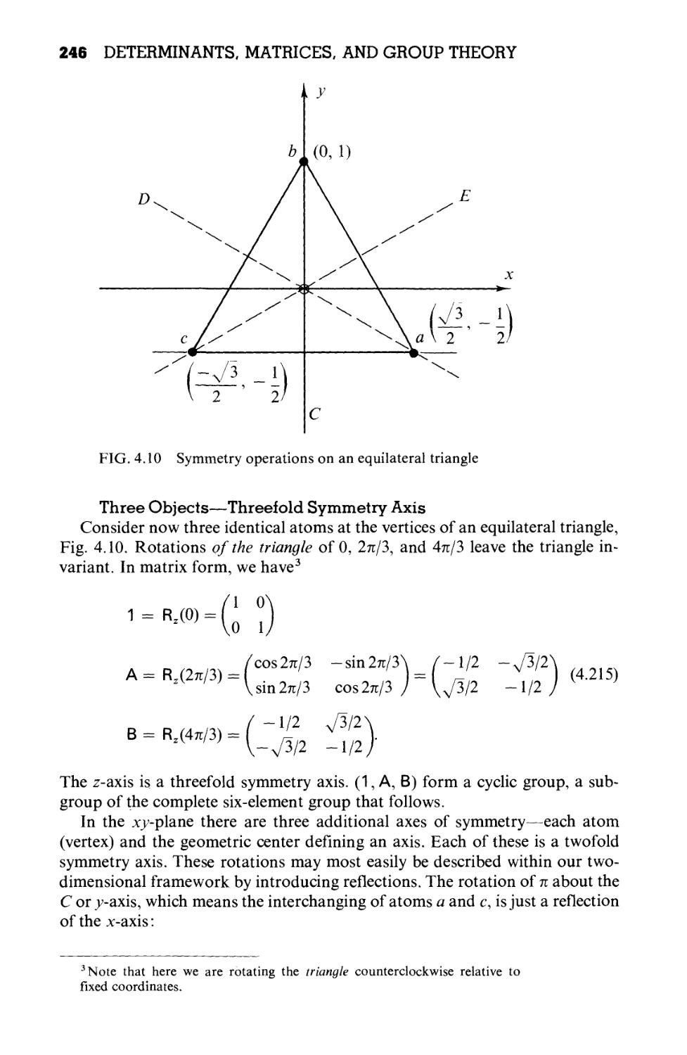
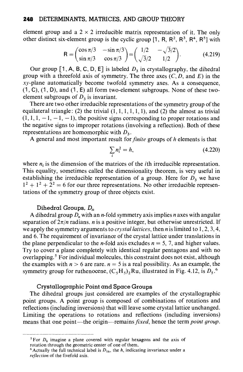
/


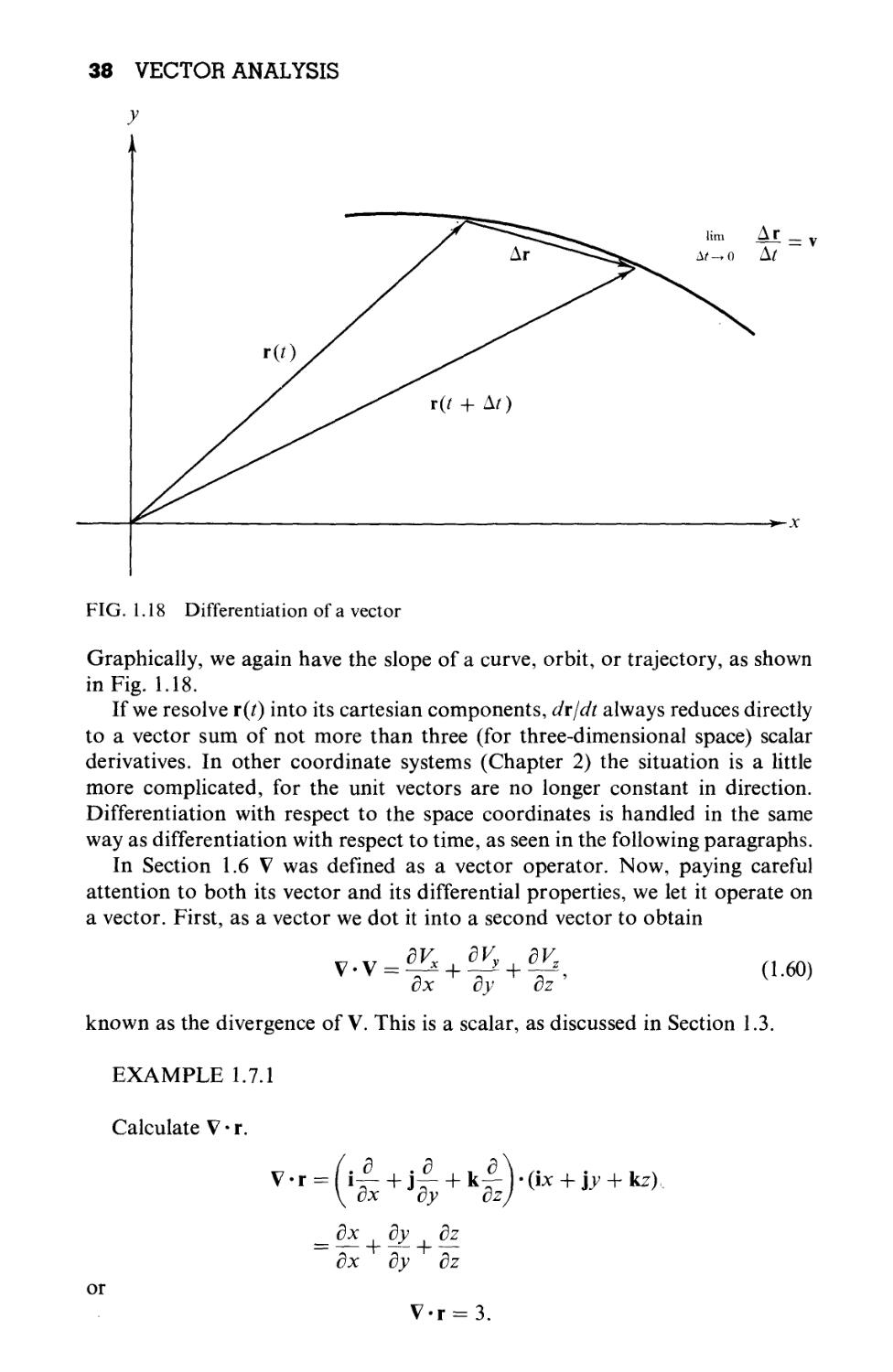


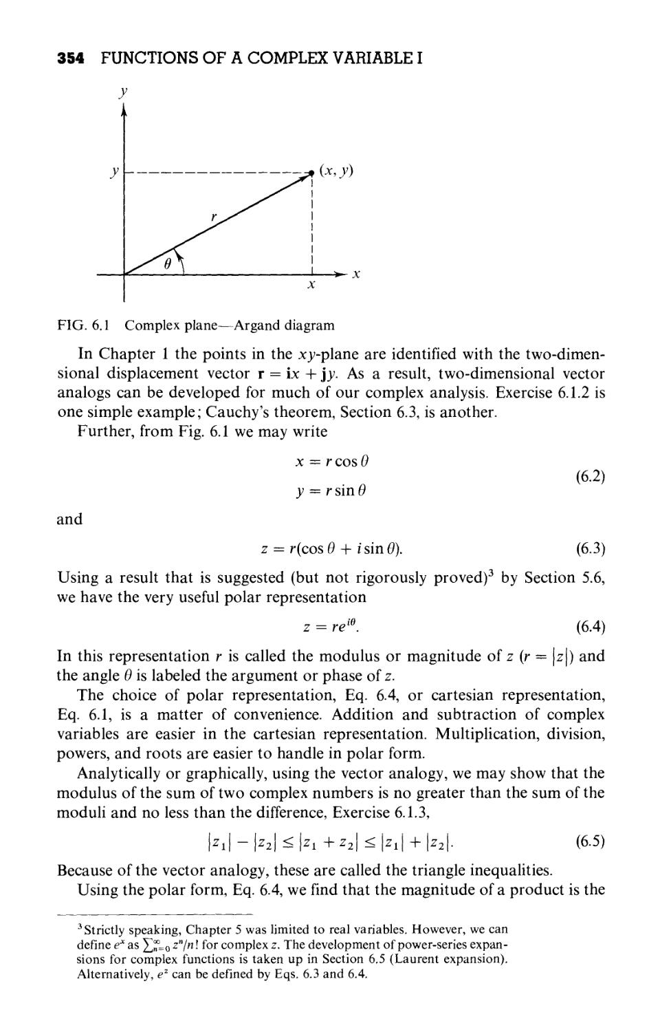
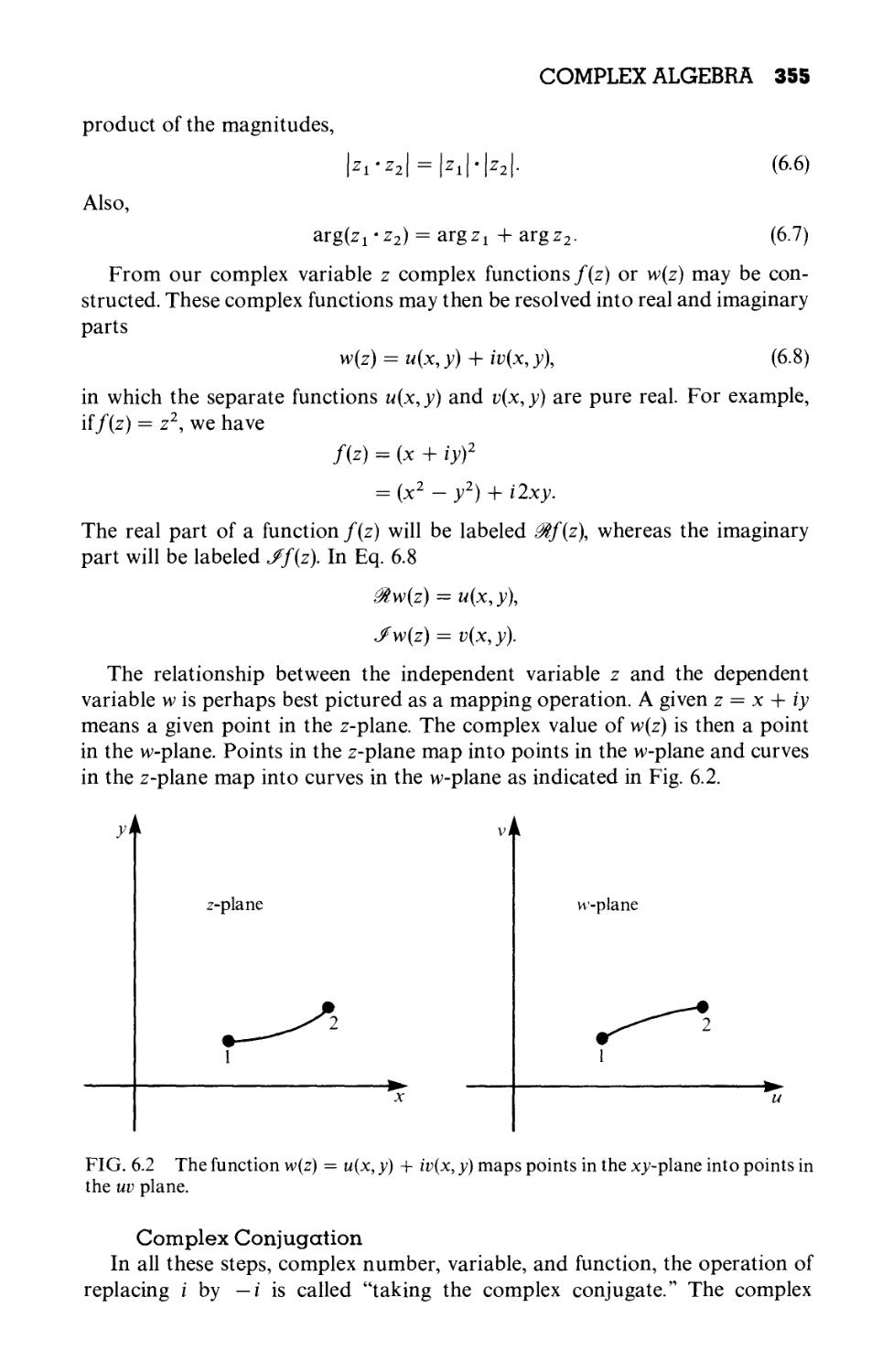


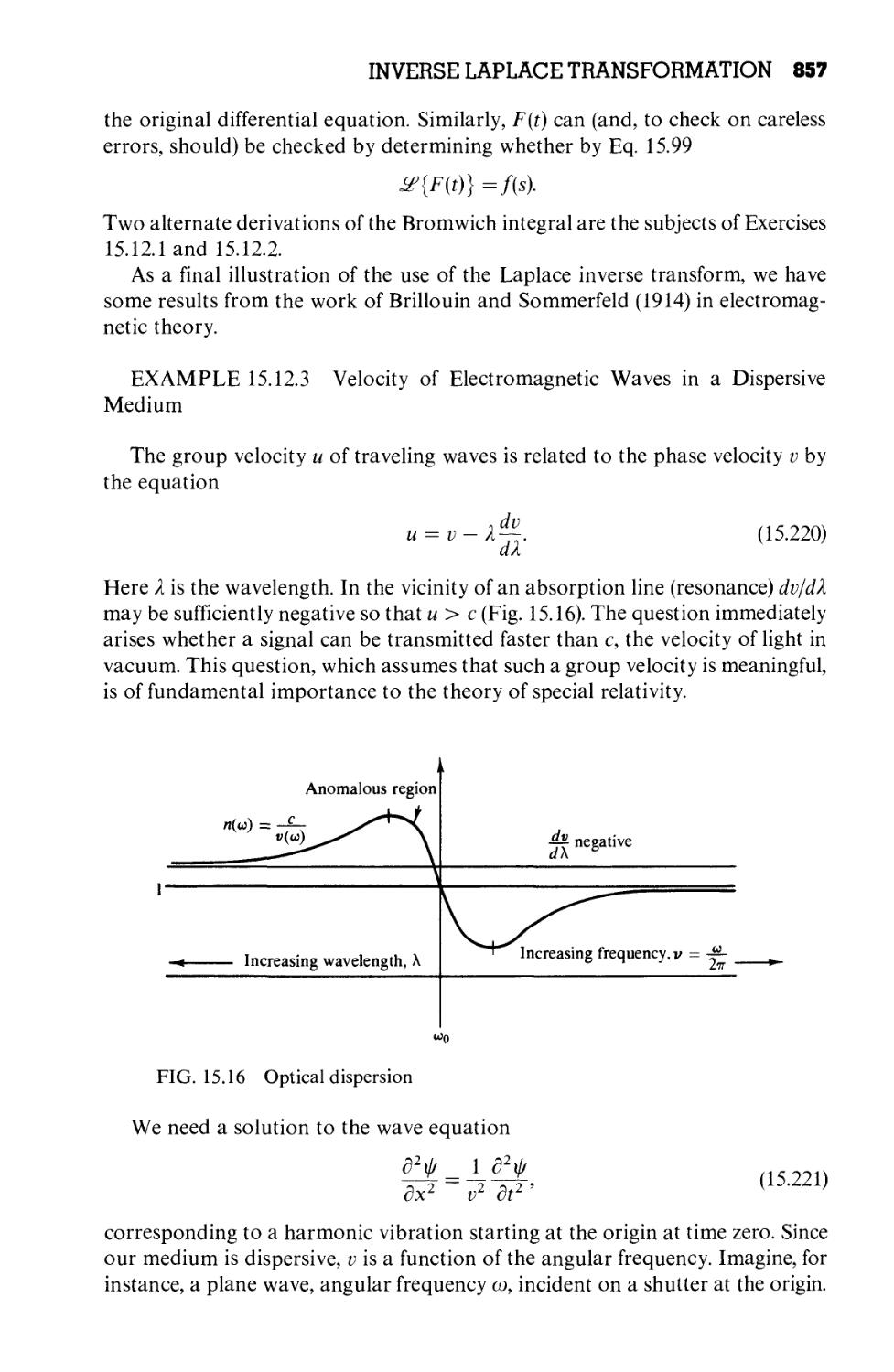


Текст
para/today
no es un proyecto lucrative sino
un esfuerzo colectivo de estudiantes у profesores de la UNAM
para facilitar el acceso a los materiales necesarios para la
education de la mayor cantidad de gente posible. Pensamos
editar en formato digital libros que por su alto costo, о bien
porque ya no se consiguen en bibliotecas у librerias, no son
accesibles para todos.
Invitamos a todos los interesados en participar en este proyecto a
sugerir titulos, a prestarnos los textos para su digitalizacion у а
ayudarnos en toda la labor tecnica que implica su reproduction.
El nuestro, es un proyecto colectivo abierto a la participation de
cualquier persona у todas las colaboraciones son bienvenidas.
Nos encuentras en los Talleres Estudiantiles de la Facultad de
Ciencias у puedes ponerte en contacto con nosotros a la siguiente
direction de correo electronico:
eduktodosG/ hotmail.com
http://eduktodos.dvndns.org
MATHEMATICAL
METHODS
FOR PHYSICISTS
Third Edition
MATHEMATICAL
METHODS
FOR PHYSICISTS
Third Edition
GEORGE ARFKEN
Miami University
Oxford, Ohio
ACADEMIC PRESS, INC.
Harcourt Brace Jovanovich, Publishers
San Diego New York Berkeley Boston
London Sydney Tokyo Toronto
Copyright ©1985 by Academic Press, Inc.
All rights reserved.
No part of this publication may be reproduced or transmitted in any form or by any
means, electronic or mechanical, including photocopy, recording, or any information
storage and retrieval system, without permission in writing from the publisher.
ACADEMIC PRESS, INC.
San Diego, California 92101
United Kingdom Edition Published by Academic Press, Inc. (London) Ltd.,
24/28 Oval Road, London NW1 7DX
ISBN: 0-12-059820-5
ISBN: 0-12-059810-8 (paper)
Library of Congress Catalog Card Number: 84-71328
PRINTED IN THE UNITED STATES OF AMERICA
87 gg 89 9 g 7 6 5 4 3
To Carolyn
CONTENTS
Chapter 1 VECTOR ANALYSIS 1
1.1 Definitions, Elementary Approach 1
1.2 Advanced Definitions 7
1.3 Scalar or Dot Product 13
1.4 Vector or Cross Product 18
1.5 Triple Scalar Product, Triple Vector Product 26
1.6 Gradient 33
1.7 Divergence 37
1.8 Curl 42
1.9 Successive Applications of V 47
1.10 Vector Integration 51
1.11 Gauss's Theorem 57
1.12 Stokes's Theorem 61
1.13 Potential Theory 64
1.14 Gauss's Law, Poisson's Equation 74
1.15 Helmholtz's Theorem 78
Chapter 2 COORDINATE SYSTEMS 85
2.1 Curvilinear Coordinates 86
2.2 Differential Vector Operations 90
2.3 Special Coordinate Systems—Rectangular Cartesian
Coordinates 94
2.4 Circular Cylindrical Coordinates (p,(p,z) 95
2.5 Spherical Polar Coordinates (r, 9, q>) 102
2.6 Separation of Variables 111
Chapter 3 TENSOR ANALYSIS 118
3.1 Introduction, Definitions 118
3.2 Contraction, Direct Product 124
vii
viii CONTENTS
3.3 Quotient Rule 126
3.4 Pseudotensors, Dual Tensors 128
3.5 Dyadics 137
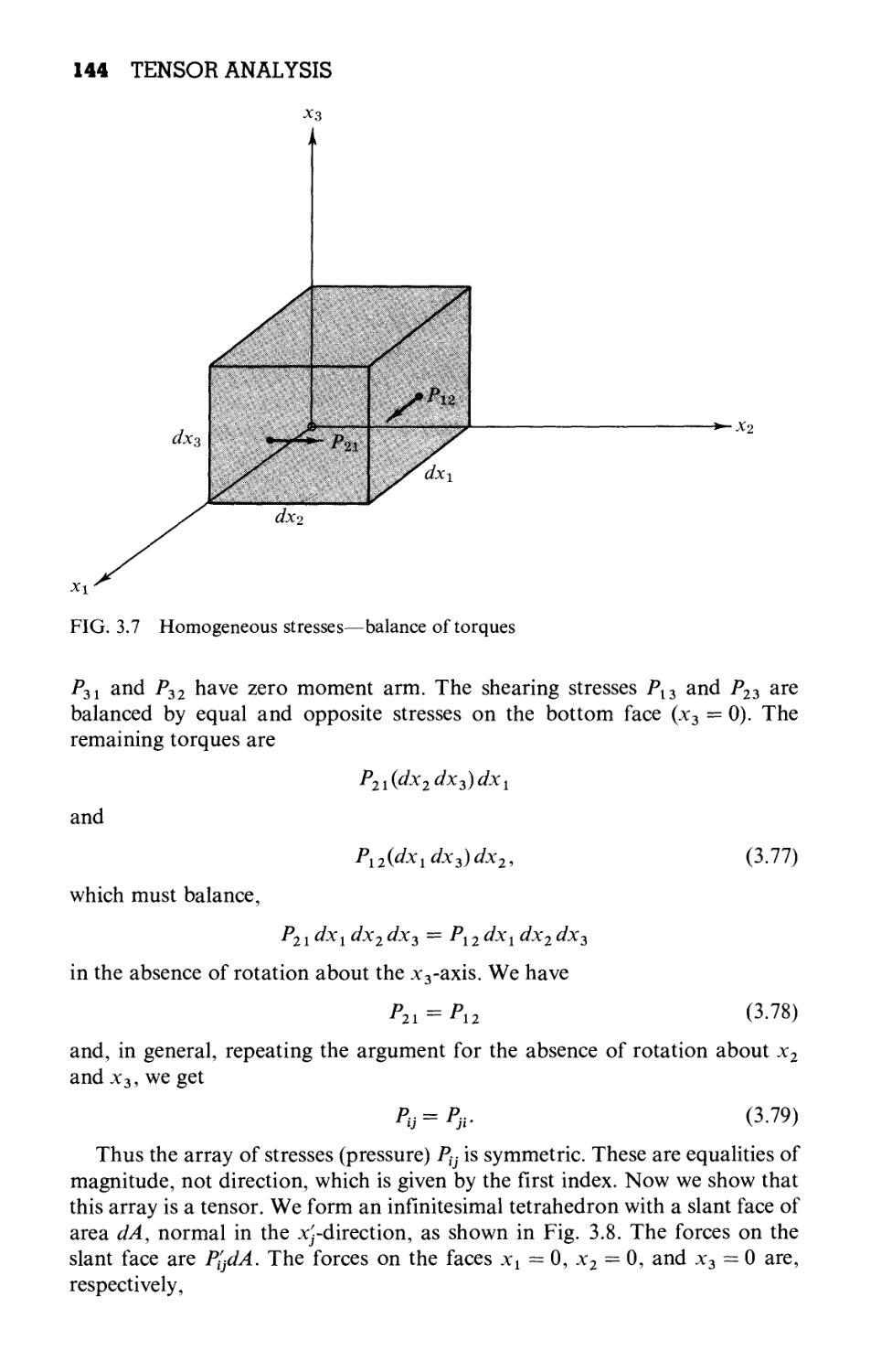
3.6 Theory of Elasticity 140
3.7 Lorentz Covariance of Maxwell's Equations 150
3.8 Noncartesian Tensors, Covariant Differentiation 158
3.9 Tensor Differential Operations 164
Chapter 4
DETERMINANTS, MATRICES, AND GROUP
THEORY 168
4.1 Determinants 168
4.2 Matrices 176
4.3 Orthogonal Matrices 191
4.4 Oblique Coordinates 206
4.5 Hermitian Matrices, Unitary Matrices 209
4.6 Diagonalization of Matrices 217
4.7 Eigenvectors, Eigenvalues 229
4.8 Introduction to Group Theory 237
4.9 Discrete Groups 243
4.10 Continuous Groups 251
4.11 Generators 261
4.12 SUB), SUC), and Nuclear Particles 267
4.13 Homogeneous Lorentz Group 271
Chapter 5 INFINITE SERIES 277
5.1 Fundamental Concepts 277
5.2 Convergence Tests 280
5.3 Alternating Series 293-
5.4 Algebra of Series 295
5.5 Series of Functions 299
5.6 Taylor's Expansion 303
5.7 Power Series 313
5.8 Elliptic Integrals 321
5.9 Bernoulli Numbers, Euler-Maclaurin Formula
5.10 Asymptotic or Semiconvergent Series 339
5.11 Infinite Products 346
327
Chapter 6 FUNCTIONS OF A COMPLEX VARIABLE I 352
6.1 Complex Algebra 353
6.2 Cauchy-Riemann Conditions 360
Chapter 7
Chapter 8
6.3
6.4
6.5
6.6
6.7
CONTENTS ix
Cauchy's Integral Theorem 365
Cauchy's Integral Formula 371
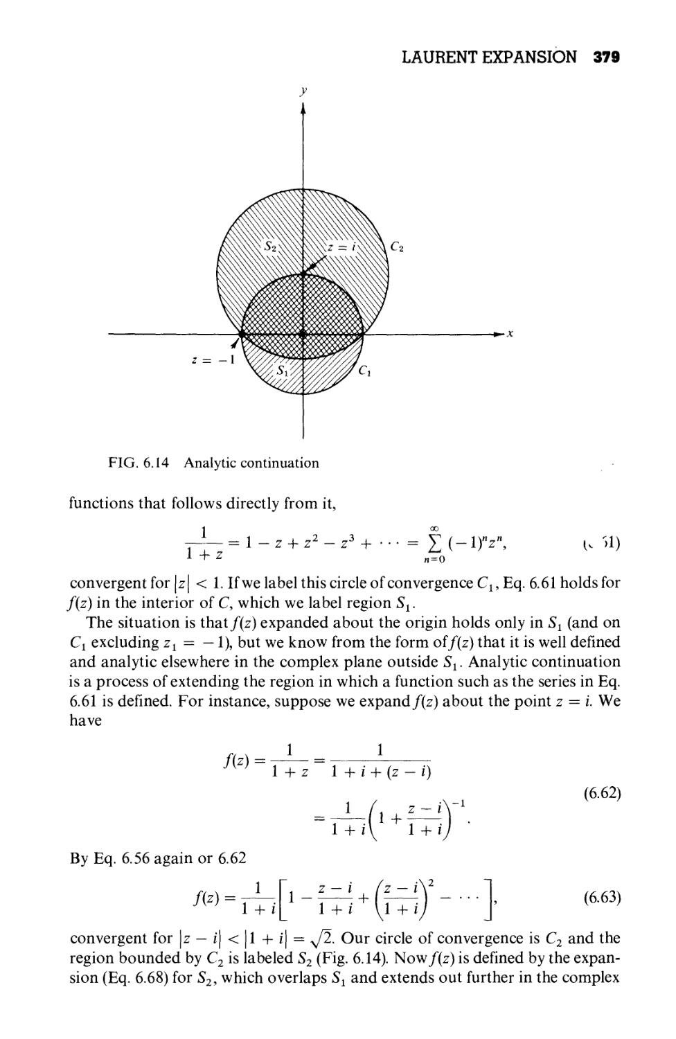
Laurent Expansion 376
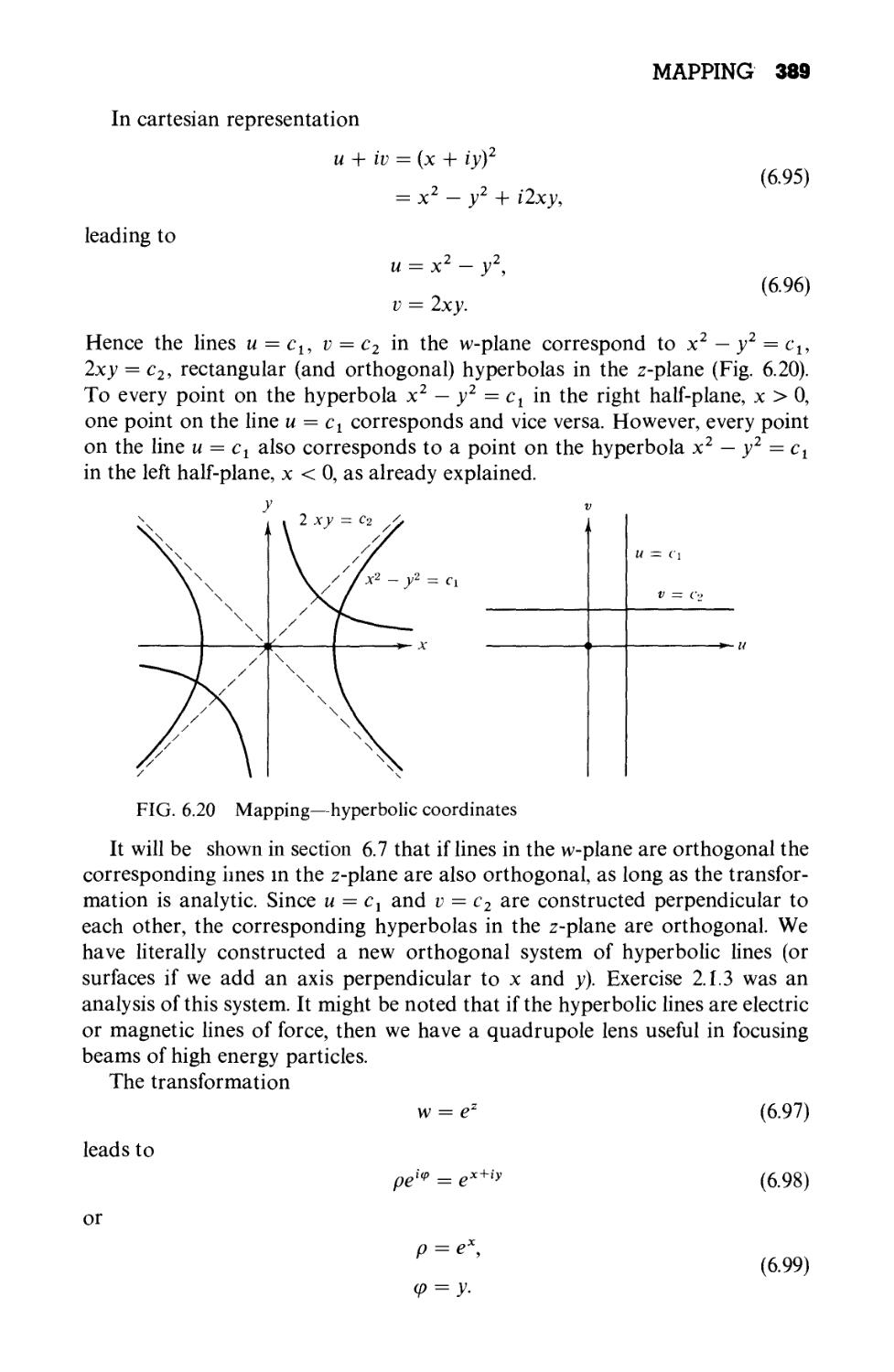
Mapping 384
Conformal Mapping 392
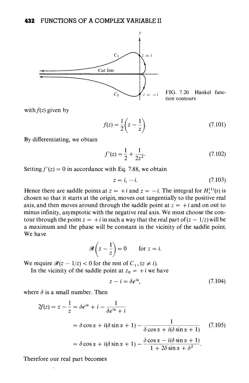
FUNCTIONS OF A COMPLEX VARIABLE II: Calculus
of Residues 396
7.1
7.2
7.3
7.4
Singularities 396
Calculus of Residues 400
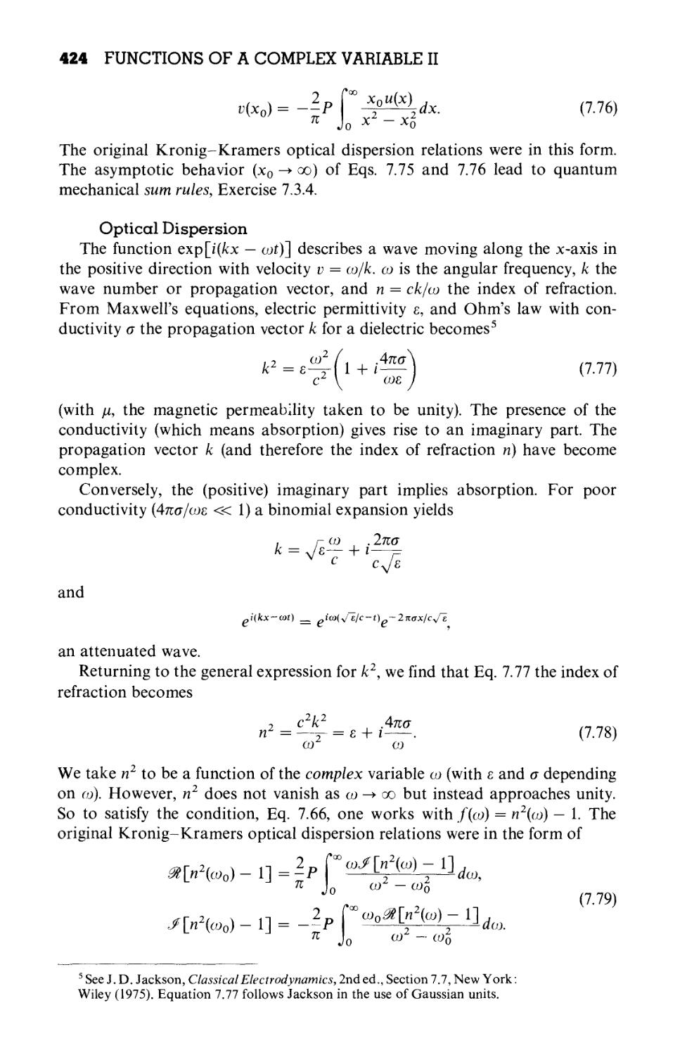
Dispersion Relations 421
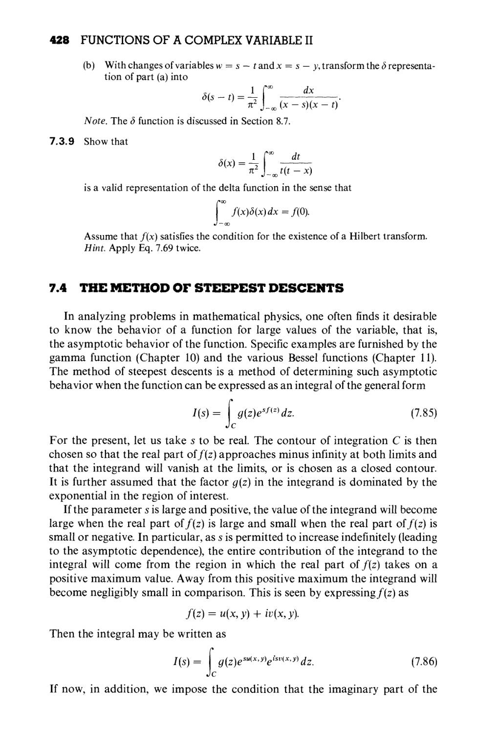
The Method of Steepest Descents 428
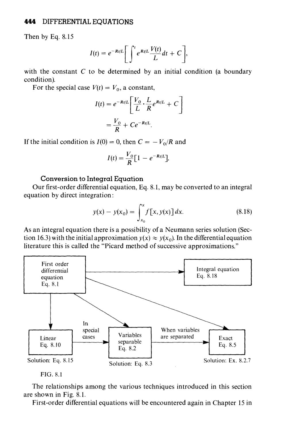
DIFFERENTIAL EQUATIONS 437
8.1
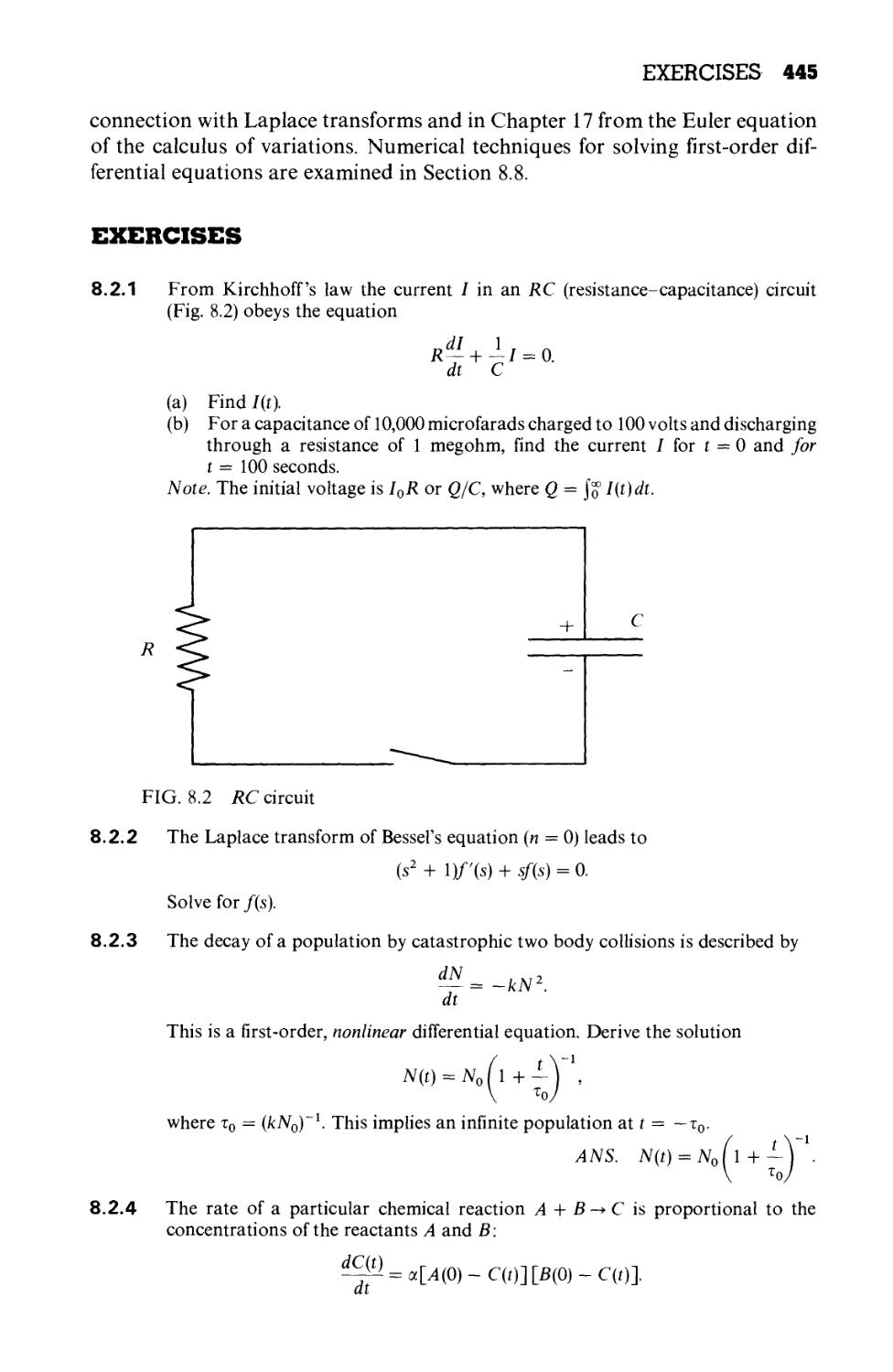
8.2
8.3
8.4
8.5
8.6
8.7
8.8
Partial Differential Equations of Theoretical
Physics 437
First-Order Differential Equations 440
Separation of Variables—Ordinary Differential
Equations 448
Singular Points 451
Series Solutions—Frobenius' Method 454
A Second Solution 467
Nonhomogeneous Equation—Green's Function 480
Numerical Solutions 491
Chapter 9
STURM-LIOUVILLE THEORY—ORTHOGONAL
FUNCTIONS 497
9.1 Self-Adjoint Differential Equations 497
9.2 Hermitian (Self-Adjoint) Operators 510
9.3 Gram-Schmidt Orthogonalization 516
9.4 Completeness of Eigenfunctions 523
Chapter 10 THE GAMMA FUNCTION (FACTORIAL
FUNCTION) 539
10.1 Definitions, Simple Properties 539
10.2 Digamma and Poly gamma Functions 549
10.3 Stirling's Series 555
10.4 The Beta Function 560
10.5 The Incomplete Gamma Functions and Related
Functions 565
x CONTENTS
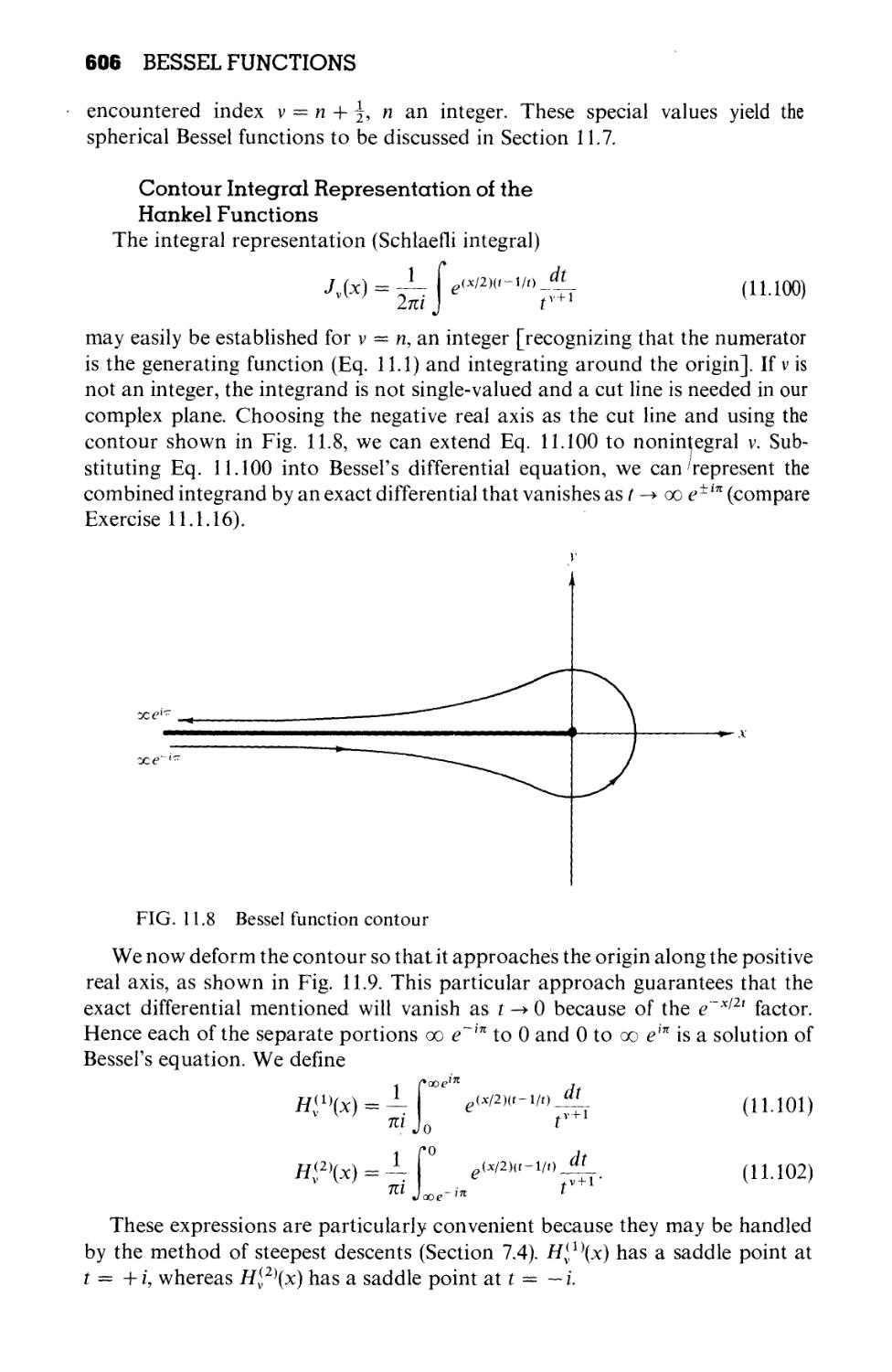
Chapter 11 BESSEL FUNCTIONS 573
11.1 Bessel Functions of the First Kind, Jv(x) 573
11.2 Orthogonality 591
11.3 Neumann Functions, Bessel Functions of the Second
Kind, Nv(x) 596
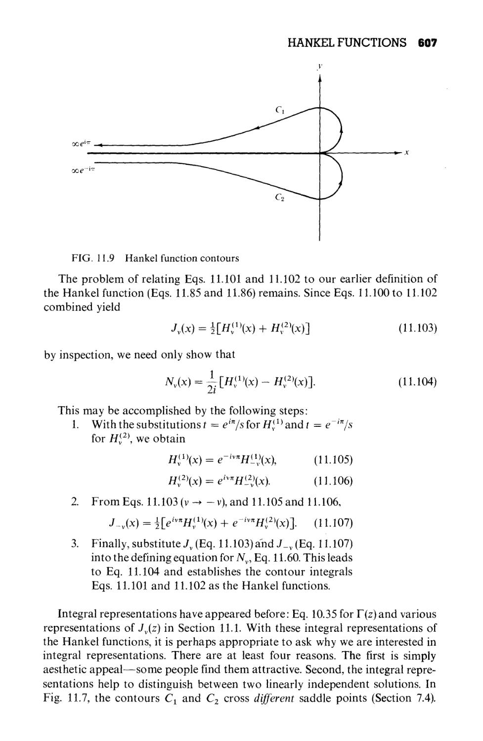
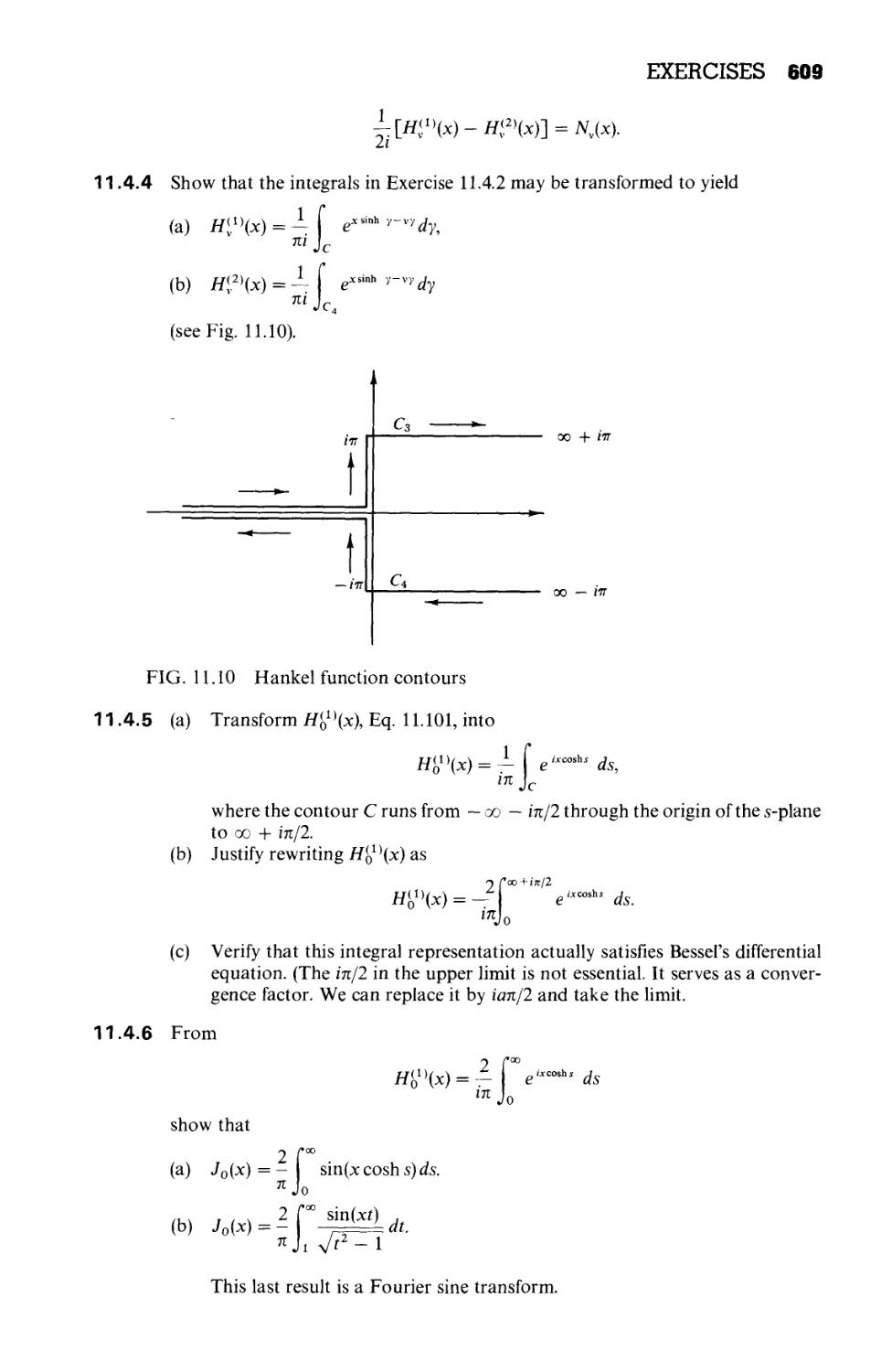
11.4 Hankel Functions 603
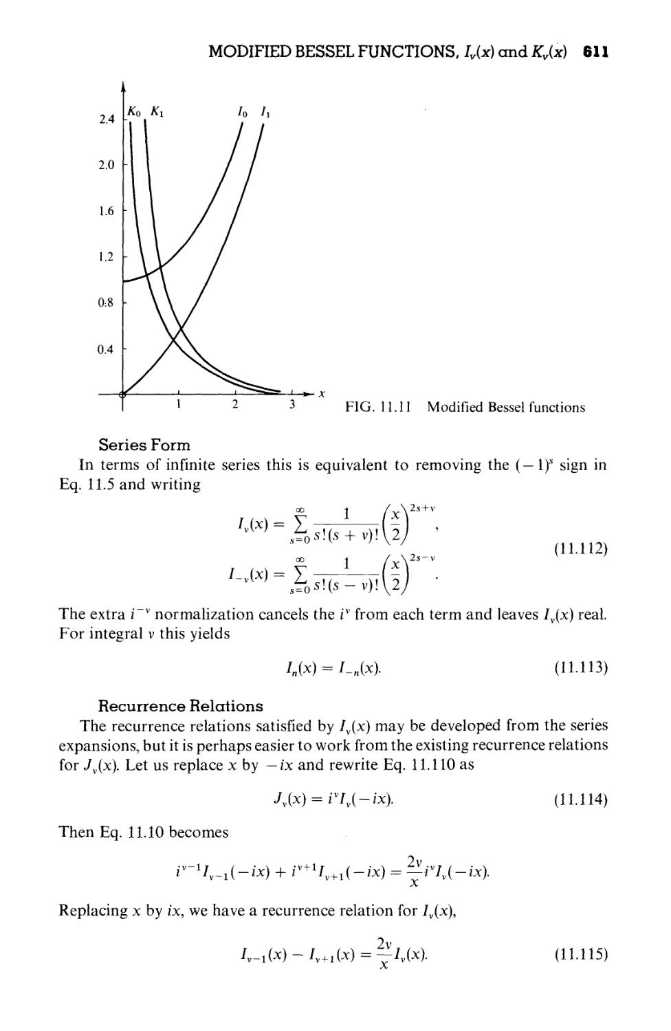
11.5 Modified Bessel Functions, Iv(x) and Kv(x) 610
11.6 Asymptotic Expansions 616
11.7 Spherical Bessel Functions 622
Chapter 12 LEGENDRE FUNCTIONS 637
12.1 Generating Function 637
12.2 Recurrence Relations and Special Properties 645
12.3 Orthogonality 652
12.4 Alternate Definitions of Legendre Polynomials 663
12.5 Associated Legendre Functions 666
12.6 Spherical Harmonics 680
12.7 Angular Momentum Ladder Operators 685
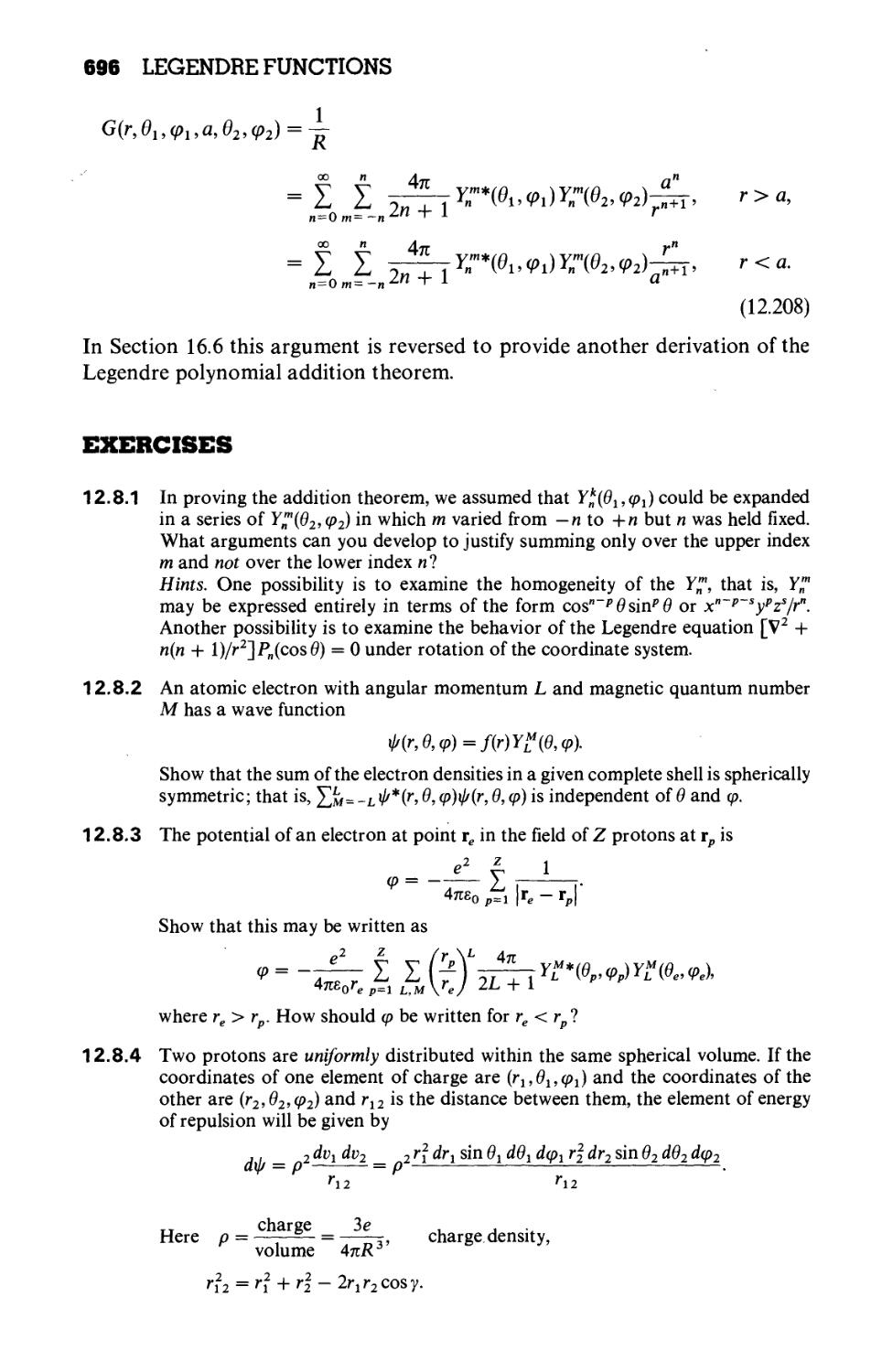
12.8 The Addition Theorem for Spherical Harmonics 693
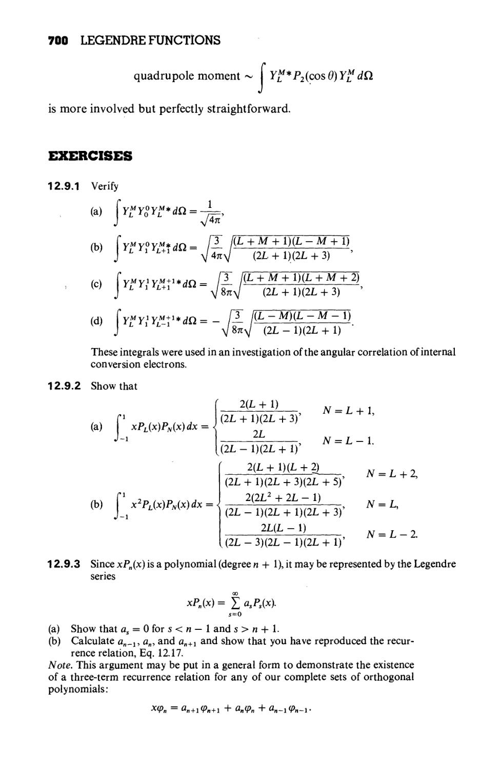
12.9 Integrals of the Product of Three Spherical
Harmonics 698
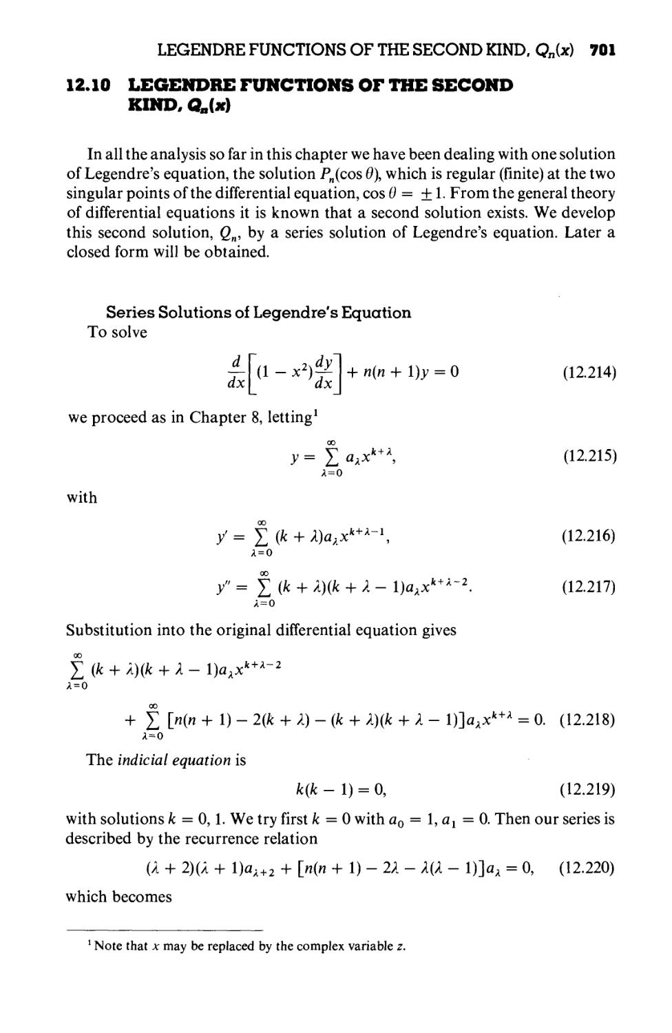
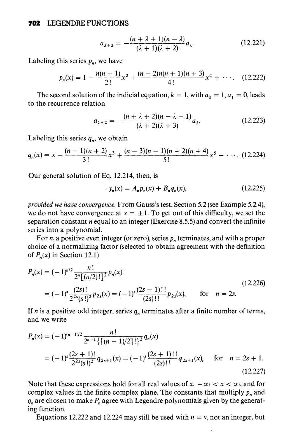
12.10 Legendre Functions of the Second Kind, Qn(x) 701
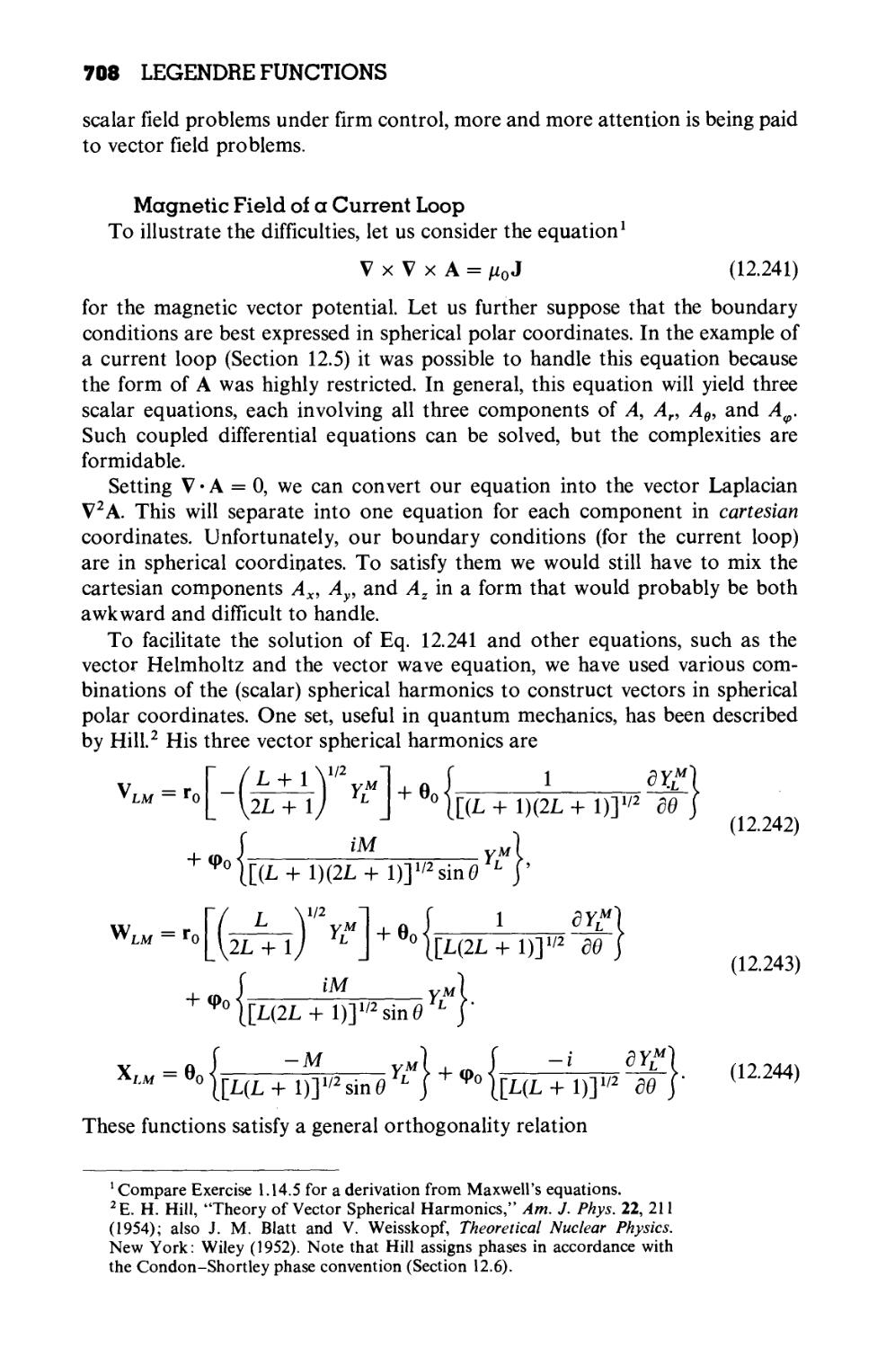
12.11 Vector Spherical Harmonics 707
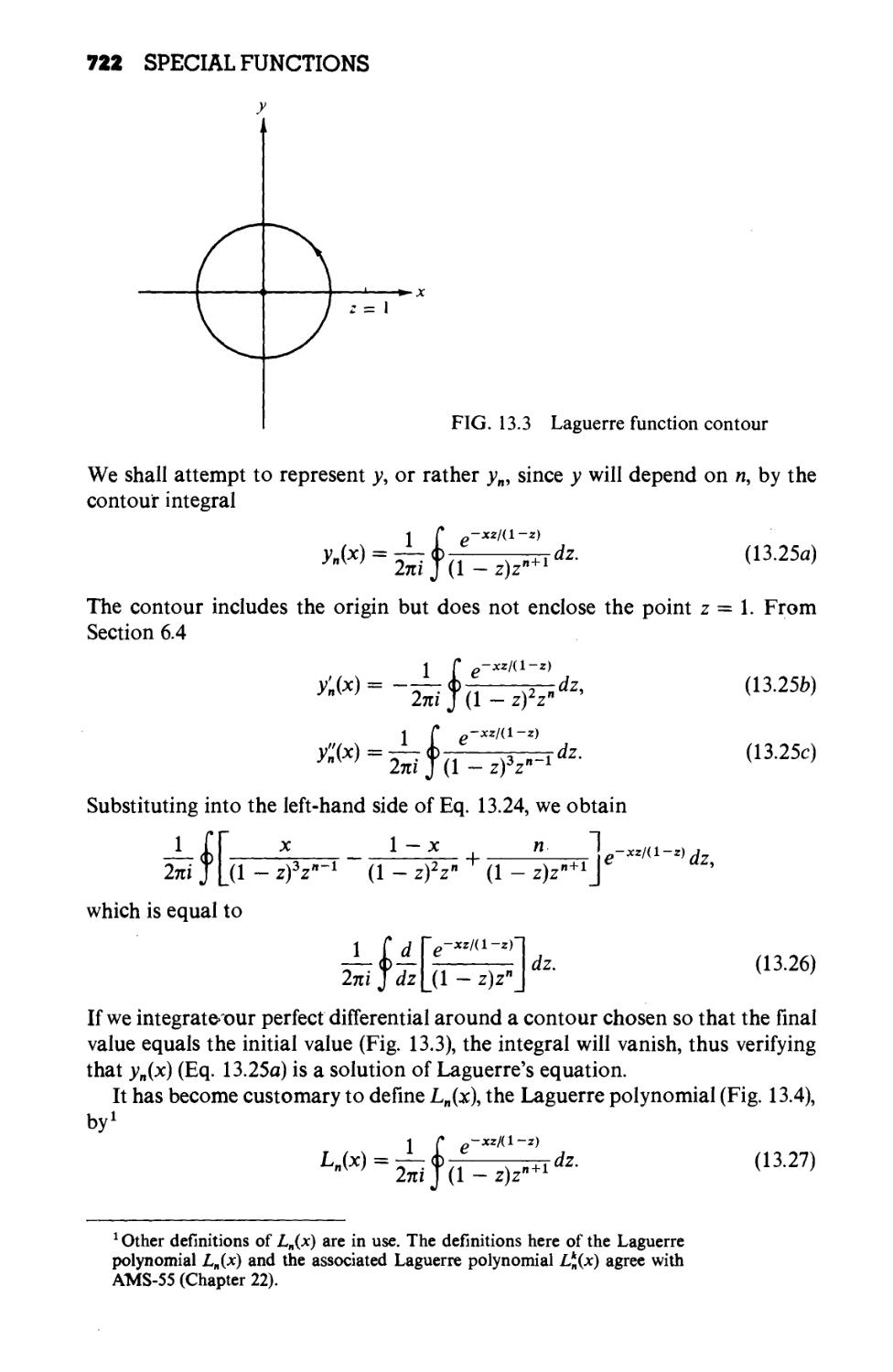
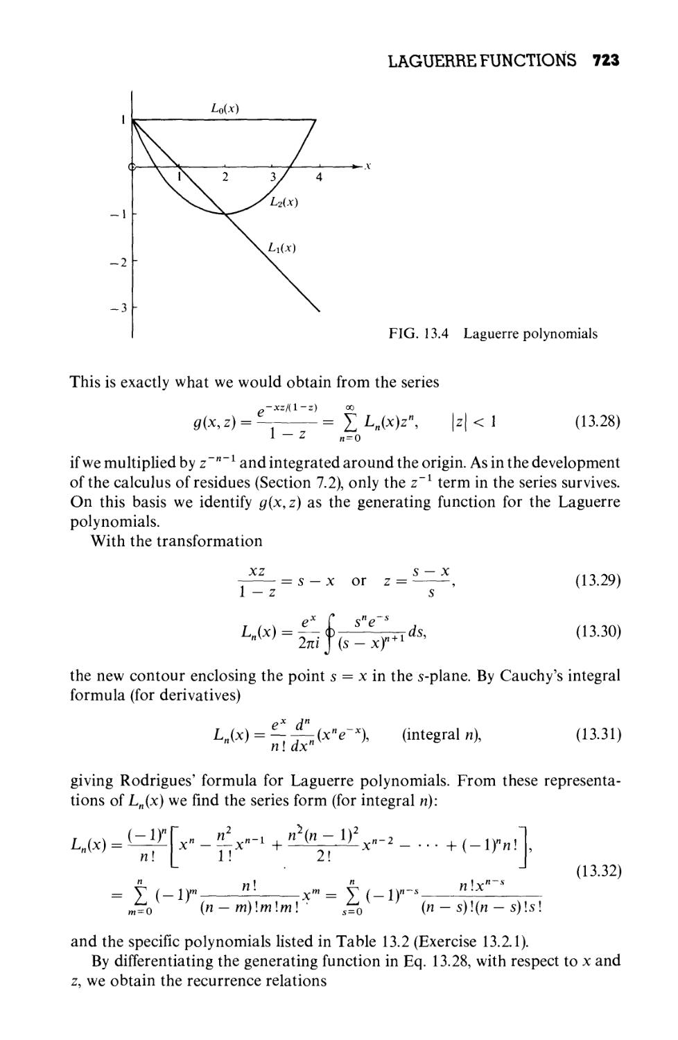
Chapter 13 SPECIAL FUNCTIONS 712
13.1 Hermite Functions 712
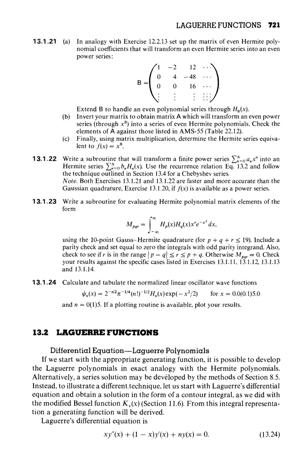
13.2 Laguerre Functions 721
13.3 Chebyshev (Tschebyscheff) Polynomials 731
13.4 Chebyshev Polynomials—Numerical
Applications 740
13.5 Hypergeometric Functions 748
13.6 Confluent Hypergeometric Functions 753
Chapter 14 FOURIER SERIES 760
14.1 General Properties 760
14.2 Advantages, Uses of Fourier Series 766
14.3 Applications of Fourier Series 770
14.4 Properties of Fourier Series 778
14.5 Gibbs Phenomenon 783
14.6 Discrete Orthogonality—Discrete Fourier
Transform 787
CONTENTS xi
Chapter 15 INTEGRAL TRANSFORMS 794
15.1 Integral Transforms 794
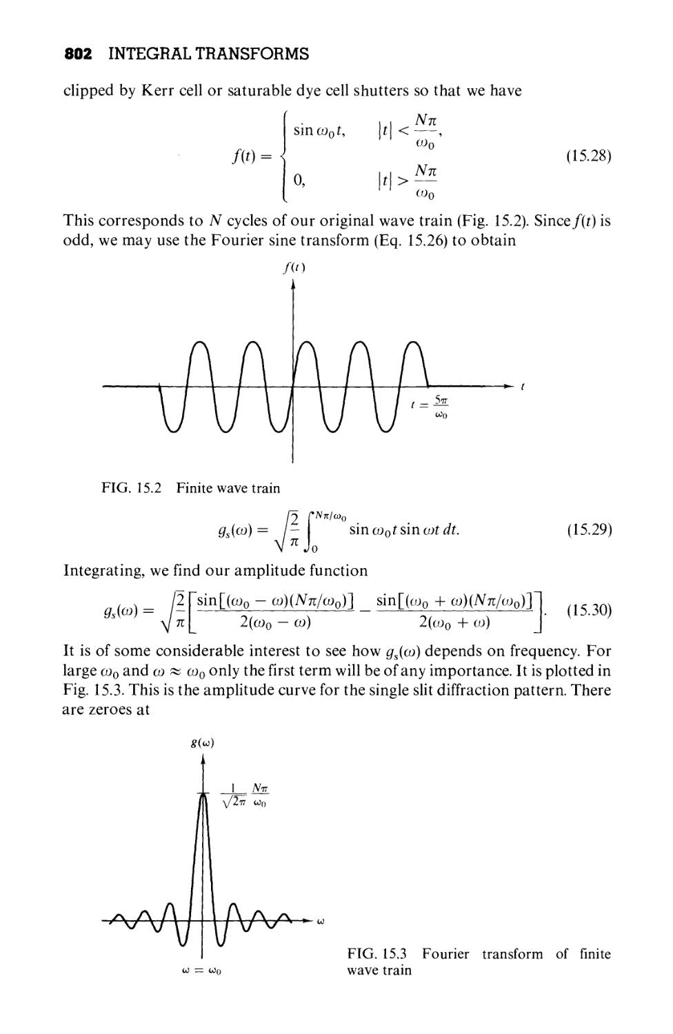
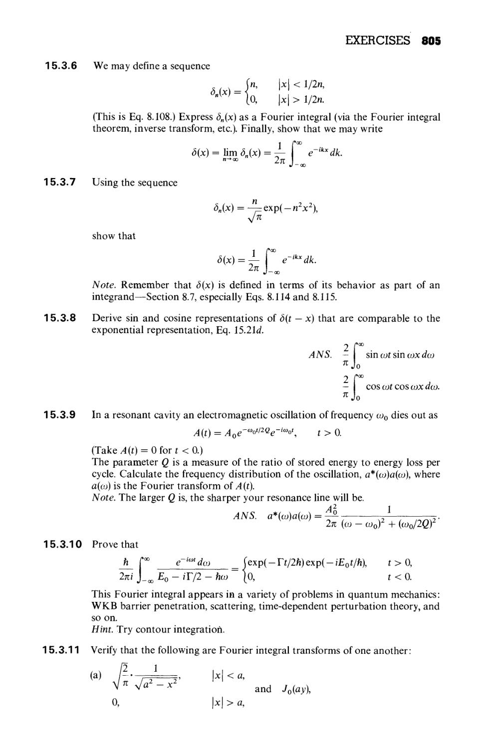
15.2 Development of the Fourier Integral 797
15.3 Fourier Transforms—Inversion Theorem
15.4 Fourier Transform of Derivatives 807
15.5 Convolution Theorem 810
15.6 Momentum Representation 814
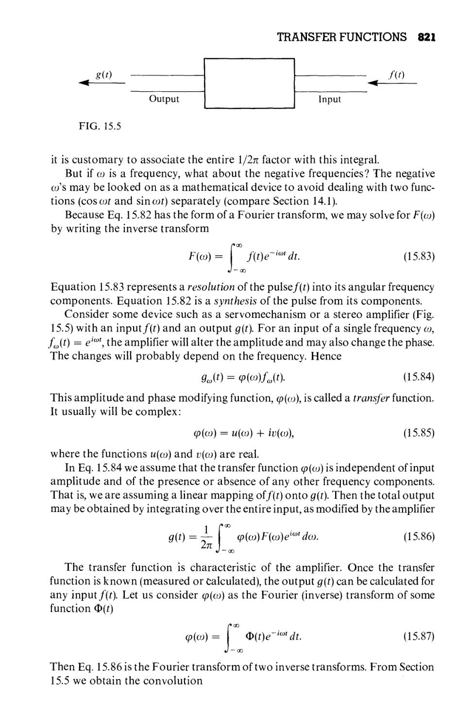
15.7 Transfer Functions 820
15.8 Elementary Laplace Transforms 824
15.9 Laplace Transform of Derivatives 831
15.10 Other Properties 838
15.11 Convolution or Faltung Theorem 849
15.12 Inverse Laplace Transformation 853
800
Chapter 16 INTEGRAL EQUATIONS 865
16.1 Introduction 865
16.2 Integral Transforms, Generating Functions 873
16.3 Neumann Series, Separable (Degenerate) Kernels
16.4 Hilbert-Schmidt Theory 890
16.5 Green's Functions—One Dimension 897
16.6 Green's Functions—Two and Three Dimensions
879
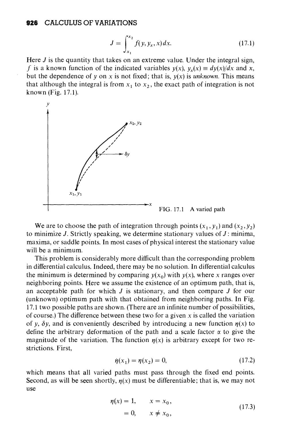
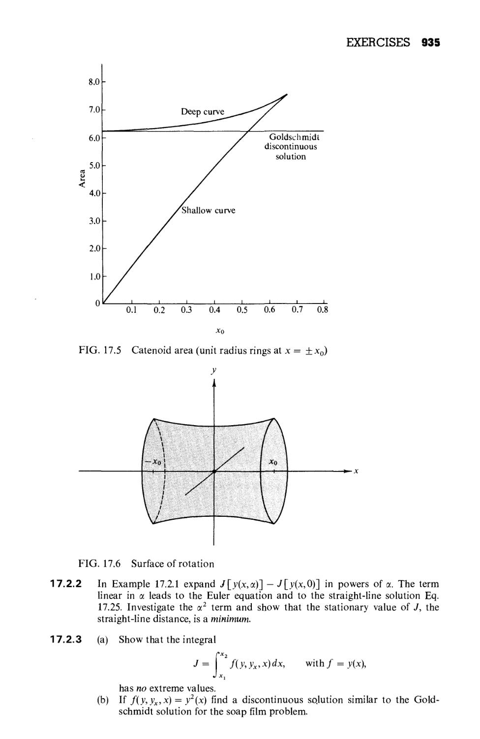
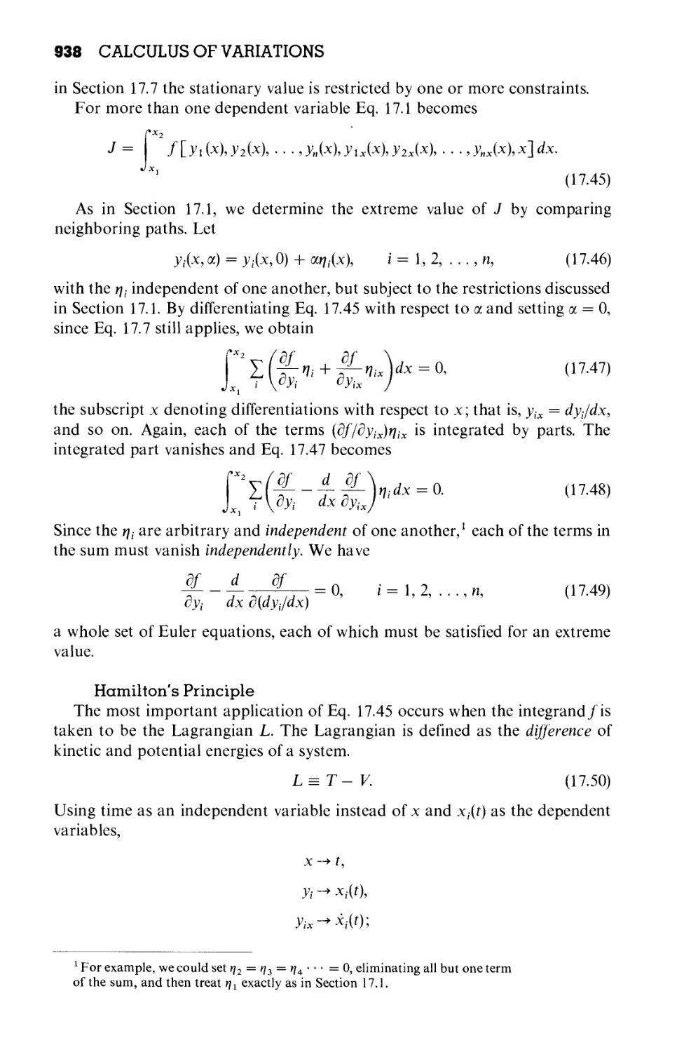
Chapter 17 CALCULUS OF VARIATIONS 925
17.1 One-Dependent and One-Independent Variable 925
17.2 Applications of the Euler Equation 930
17.3 Generalizations, Several Dependent Variables 937
17.4 Several Independent Variables 942
17.5 More Than One Dependent, More Than One
Independent Variable 944
17.6 Lagrangian Multipliers 945
17.7 Variation Subject to Constraints 950
17.8 Rayleigh-Ritz Variational Technique 957
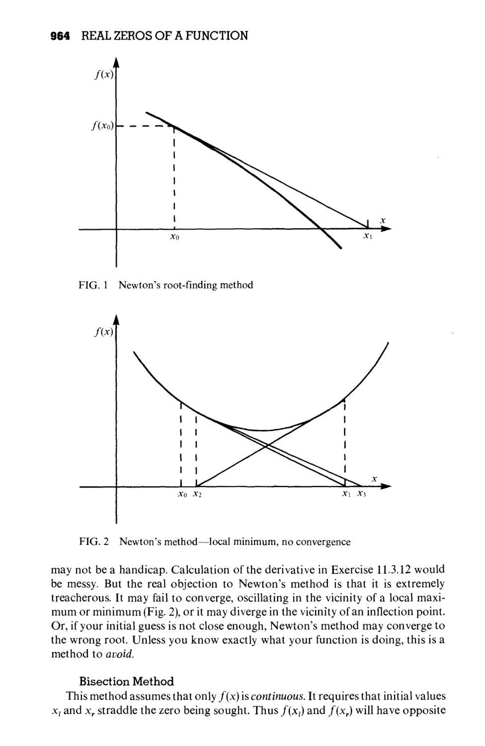
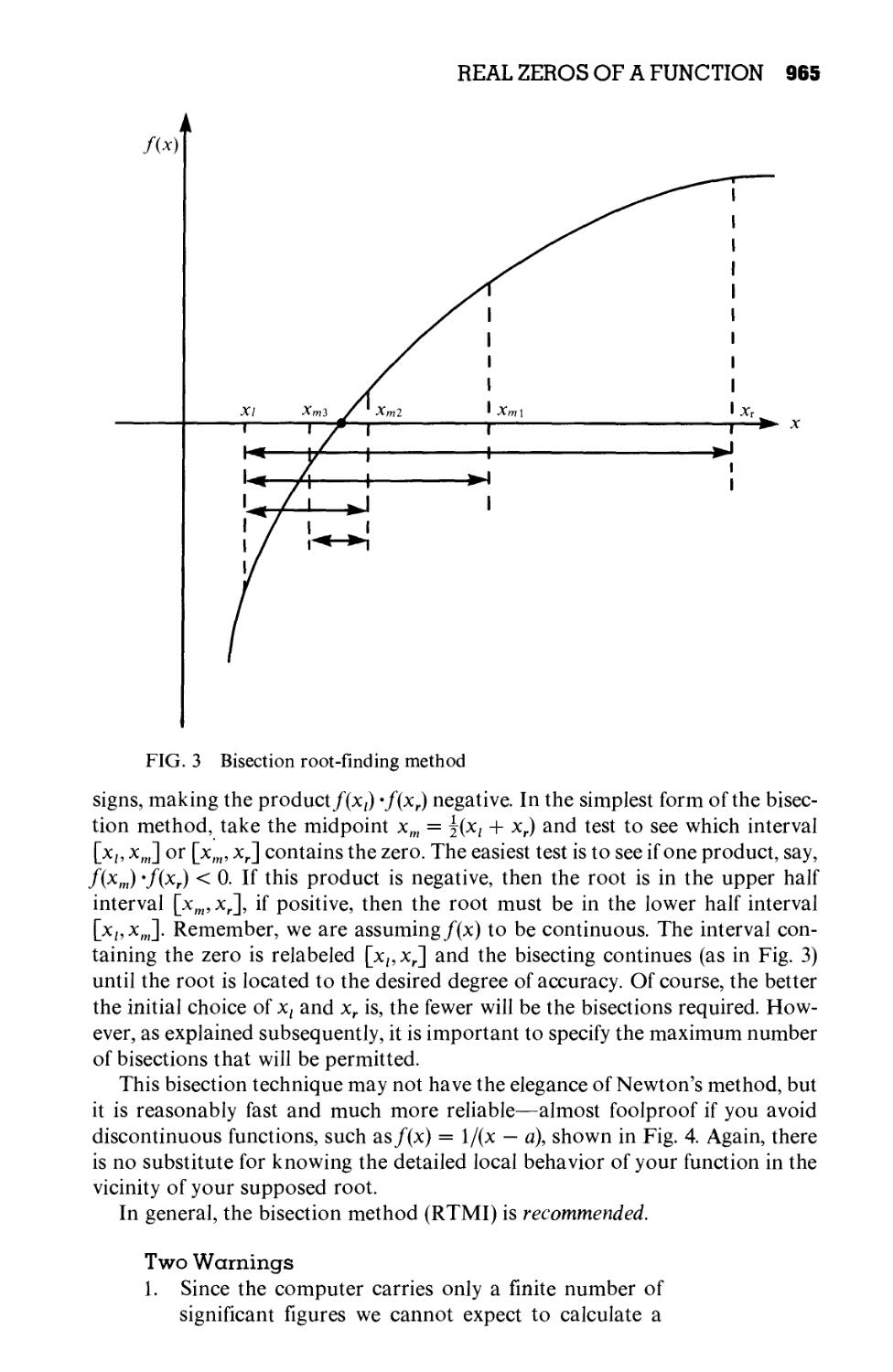
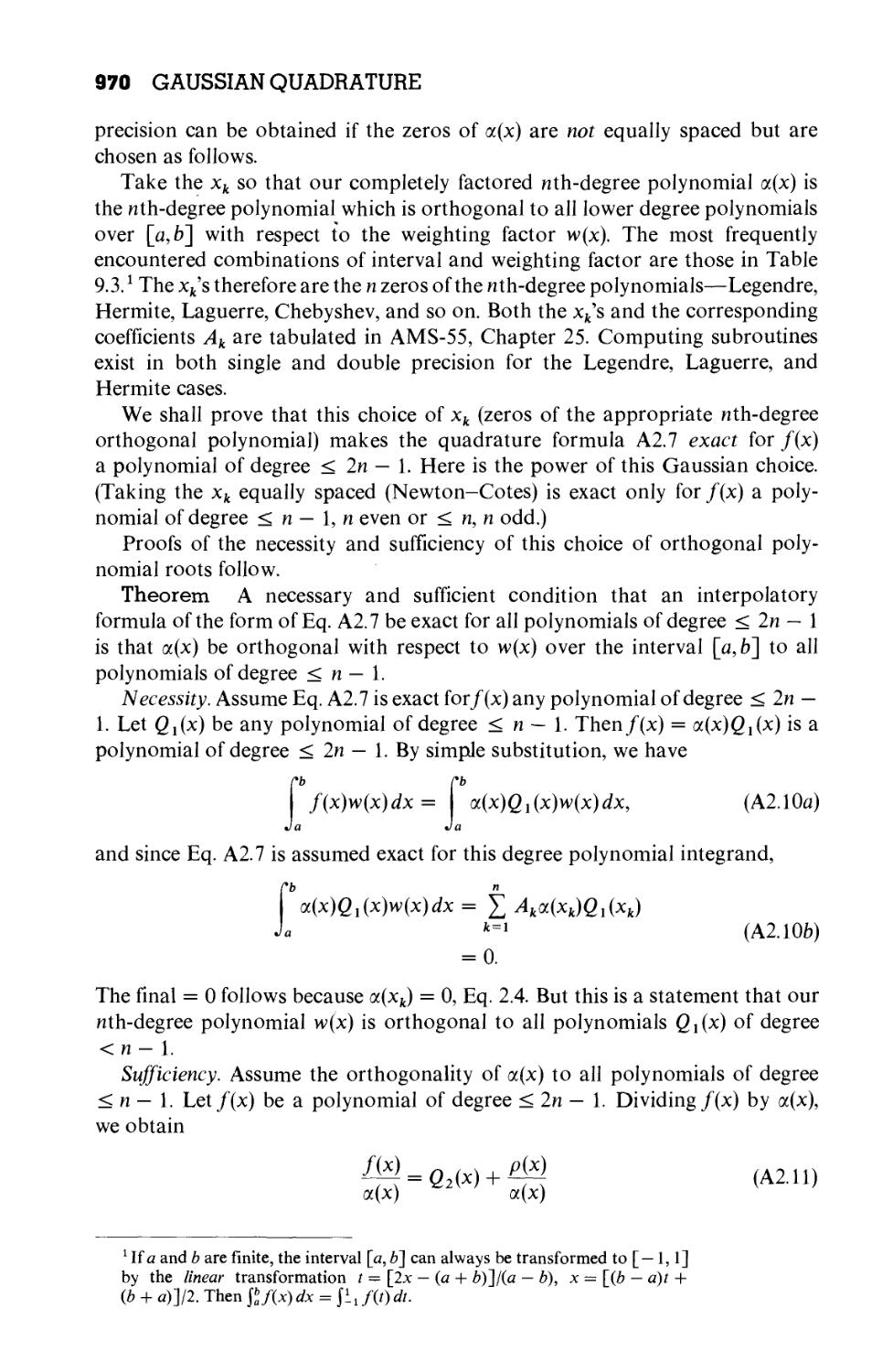
Appendix 1 REAL ZEROS OF A FUNCTION 963
Appendix 2 GAUSSIAN QUADRATURE 968
GENERAL REFERENCES 974
Index 975
PREFACE TO THE
THIRD EDITION
The many additions and revisions in this third edition of Mathematical
Methods for Physicists are based on 15 years of teaching from the second edition,
on the questions from current students, and on the advice of colleagues, reviewers,
and former students. Almost every section has been revised; many of the sections
have been completely rewritten. In most sections, there are new exercises, all class
tested. New sections have been added on non-Cartesian tensors, dispersion
theory, first-order differential equations, numerical application of Chebyshev
polynomials, the fast Fourier transform, and on transfer functions.
Throughout the text, I have placed significant additional emphasis on numer-
numerical applications and on the relation of these mathematical methods to comput-
computing and to numerical analysis.
For students studying graduate level physics, particularly theoretical physics,
a number of topics including Hermitian operators, Hilbert space, and the concept
of completeness have been expanded.
xiii
PREFACE TO THE
SECOND EDITION
This second edition of Mathematical Methods for Physicists incorporates a
number of changes, additions, and improvements made on the basis of experience
with the first edition and the helpful suggestions of a number of people. Major
revisions have been made in the sections on complex variables, Dirac delta func-
function, and Green's functions. New sections have been included on oblique co-
coordinates, Fourier-Bessel series, and angular momentum ladder operators. The
major addition is a series of sections on group theory. While these could have
been presented as a separate group theofy chapter, there seemed to be several
advantages to include them in Chapter 4, Matrices. Since the group theory is
developed in terms of matrices the arrangement seems a reasonable one.
xv
PREFACE TO THE
FIRST EDITION
Mathematical Methods for Physicists is based upon two courses in mathematics
for physicists given by the author over the past fourteen years, one at the junior
level and one at the beginning graduate level. This book is intended to provide
the student with the mathematics he needs for advanced undergraduate and
beginning graduate study in physical science and to develop a strong background
for those who will continue into the mathematics of advanced theoretical physics.
A mastery of calculus and a willingness to build on this mathematical foundation
are assumed.
This text has been organized with two basic principles in view. First, it has been
written in a form that it is hoped will encourage independent study. There are
frequent cross references but no fixed, rigid page-by-page or chapter-by-chapter
sequence is demanded.
The reader will see that mathematics as a language is beautiful and elegant.
Unfortunately, elegance all too often means elegance for the expert and obscurity
for the beginner. While still attempting to point out the intrinsic beauty of mathe-
mathematics, elegance has occasionally been reluctantly but deliberately sacrificed in
the hope of achieving greater flexibility and greater clarity for the student.
Mathematical rigor has been treated in a similar spirit. It is not stressed to the
point of becoming a mental block to the use of mathematics. Limitations are
explained, however, and warnings given against blind, uncomprehending appli-
application of mathematical relations.
The second basic principle has been to emphasize and re-emphasize physical
examples in the text and in the exercises to help motivate the student, to illustrate
the relevance of mathematics to his science and engineering.
This principle has also played a decisive role in the selection and development
of material. The subject of differential equations, for example, is no longer a
series of trick solutions of abstract, relatively meaningless puzzles but the solu-
solutions and general properties of the differential equations the student will most
frequently encounter in a description of our real physical world.
xvii
ACKNOWLEDGMENTS
A major revision of this sort necessarily represents the influence and help of
many people. Many of the revisions resulted from current students' requests for
clarification. Many of the additions were a response to the comments and advice
of former students. To all my students, my thanks for their help. Professor P. A.
Macklin has been most helpful with his suggestions and corrections. The final
form of this text owes much to the talents of Senior Editor Jeff Holtmeier of
Academic Press, Inc. and of Carol Kosik of Editing, Design & Production, Inc. A
special acknowledgment is owed Mrs. Jane Kelly for so patiently and conscien-
conscientiously typing this manuscript.
XIX
INTRODUCTION
Many of the physical examples used to illustrate the applications of mathemat-
mathematics are taken from the fields of electromagnetic theory and quantum mechanics.
For convenience the main equations are listed below and the symbols identified.
References in these fields are also given.
ELECTROMAGNETIC THEORY
MAXWELL'S EQUATIONS (MKS UNITS—VACUUM)
6B
\ D = p V x E= -
dt
VB = 0 V xH = ?U
dt
Here E is the electric field defined in terms of force on a static charge and В the
magnetic induction defined in terms of force on a moving charge. The related
fields D and H are given (in vacuum) by
D = £0E and В = jU0H
The quantity p represents free charge density while J is the corresponding
current. The electric field E and the magnetic induction В are often expressed in
terms of the scalar potential cp and the magnetic vector potential A.
ЗА
E = ?<p B = V x A
dt
For additional details see: J. M. Marion, Classical Electromagnetic Radiation,
New York: Academic Press A965); J. D. Jackson, Classical Electrodynamics, 2nd
ed. New York: Wiley A975).
Note that Marion and Jackson prefer Gaussian units. A glance at the last two
xxi
xxii INTRODUCTION
texts and the great demands they make upon the student's mathematical com-
competence should provide considerable motivation for the study of this book.
QUANTUM MECHANICS
SCHRODINGER WAVE EQUATION (TIME INDEPENDENT)
h2
-—VV +
2m
ф is the (unknown) wave function. The potential energy, often a function of
position, is denoted by V while E is the total energy of the system. The mass of the
particle being described by \jj\sm.h is Planck's constant h divided by In. Among
the extremely large number of beginning or intermediate texts we might note: A.
Messiah, Quantum Mechanics B vols), New York; Wiley A961): R. H. Dicke and J.
P. Wittke, Introduction to Quantum Mechanics, Reading Mass.: Addison-Wesley
A960); E. Merzbacher, Quantum Mechanics, 2nd Ed. New York: Wiley A970).
1 VECTOR
ANALYSIS
1.1 DEFINITIONS, ELEMENTARY APPROACH
In science and engineering we frequently encounter quantities that have
magnitude and magnitude only: mass, time, and temperature. These we label
scalar quantities. In contrast, many interesting physical quantities have mag-
magnitude and, in addition, an associated direction. This second group includes
displacement, velocity, acceleration, force, momentum, and angular momen-
momentum. Quantities with magnitude and direction are labeled vector quantities.
Usually, in elementary treatments, a vector is defined as a quantity having
magnitude and direction. To distinguish vectors from scalars, we identify vector
quantities with boldface type, that is, V.
As an historical sidelight, it is interesting to note that the vector quantities
listed are all taken from mechanics but that vector analysis was not used in the
development of mechanics and, indeed, had not been created. The need for
vector analysis became apparent only with the development of Maxwell's
electromagnetic theory and in appreciation of the inherent vector nature of
quantities such as the electric field and magnetic field.
Our vector may be conveniently represented by an arrow with length propor-
proportional to the magnitude. The direction of the arrow gives the direction of the
vector, the positive sense of direction being indicated by the point. In this
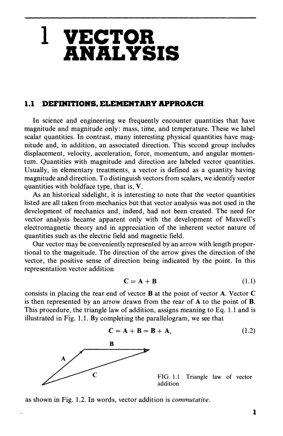
representation vector addition
C = A + B A.1)
consists in placing the rear end of vector В at the point of vector A. Vector С
is then represented by an arrow drawn from the rear of A to the point of B.
This procedure, the triangle law of addition, assigns meaning to Eq. 1.1 and is
illustrated in Fig. 1.1. By completing the parallelogram, we see that
C = A + B = B + A, A.2)
FIG. 1.1 Triangle law of vector
addition
as shown in Fig. 1.2. In words, vector addition is commutative.
2 VECTOR ANALYSIS
FIG. 1.2 Parallelogram law of vec-
vector addition
For the sum of three vectors
D = A + B + C,
Fig. 1.3, we may first add A and В
A + В = E.
Then this sum is added to С
D = E + С.
Similarly, we may first add В and С
В + С = F.
Then
D = A + F.
In terms of the original expression,
(A + В) + С = A + (B + C).
Vector addition is associative.
FIG. 1.3 Vector addition is associa-
associative
A direct physical example of the parallelogram addition law is provided by
a weight suspended by two cords. If the junction point (O in Fig. 1.4) is in
equilibrium, the vector sum of the two forces F2 and F2 must just cancel the
downward force of gravity, F3. Here the parallelogram addition law is subject
to immediate experimental verification.*
1 Strictly speaking the parallelogram addition was introduced as a definition.
Experiments show that if we assume that the forces are vector quantities and
we combine them by parallelogram addition the equilibrium condition of
zero resultant force is satisfied.
DEFINITIONS, ELEMENTARY APPROACH 3
FIG. 1.4 Equilibrium of forces. F1 + F2 = -F3
Subtraction may be handled by defining the negative of a vector as a vector
of the same magnitude but with reversed direction. Then
In Fig. 1.3
A = E - B.
Note that the vectors are treated as geometrical objects that are independent
of any coordinate system. Indeed, we have not yet introduced a coordinate
system. This concept of independence of a preferred coordinate system is
developed in considerable detail in the next section.
The representation of vector A by an arrow suggests a second possibility.
Arrow A (Fig. 1.5), starting from the origin,2 terminates at the point (xt, yx, zx).
Thus, if we agree that the vector is to start at the origin, the positive end may
be specified by giving the cartesian coordinates (xx,yx, zx) of the arrow head.
Although A could have represented any vector quantity (momentum,
electric field, etc.,), one particularly important vector quantity, the displacement
from the origin to the point (xx, yx, zx), is denoted by the special symbol r. We
then have a choice of referring to the displacement as either the vector г or the
collection (xx,y1,z1), the coordinates of its end point.
*,*i). A-3)
2 The reader will see that we could start from any point in our cartesian
reference frame, we choose the origin for simplicity.
4 VECTOR ANALYSIS
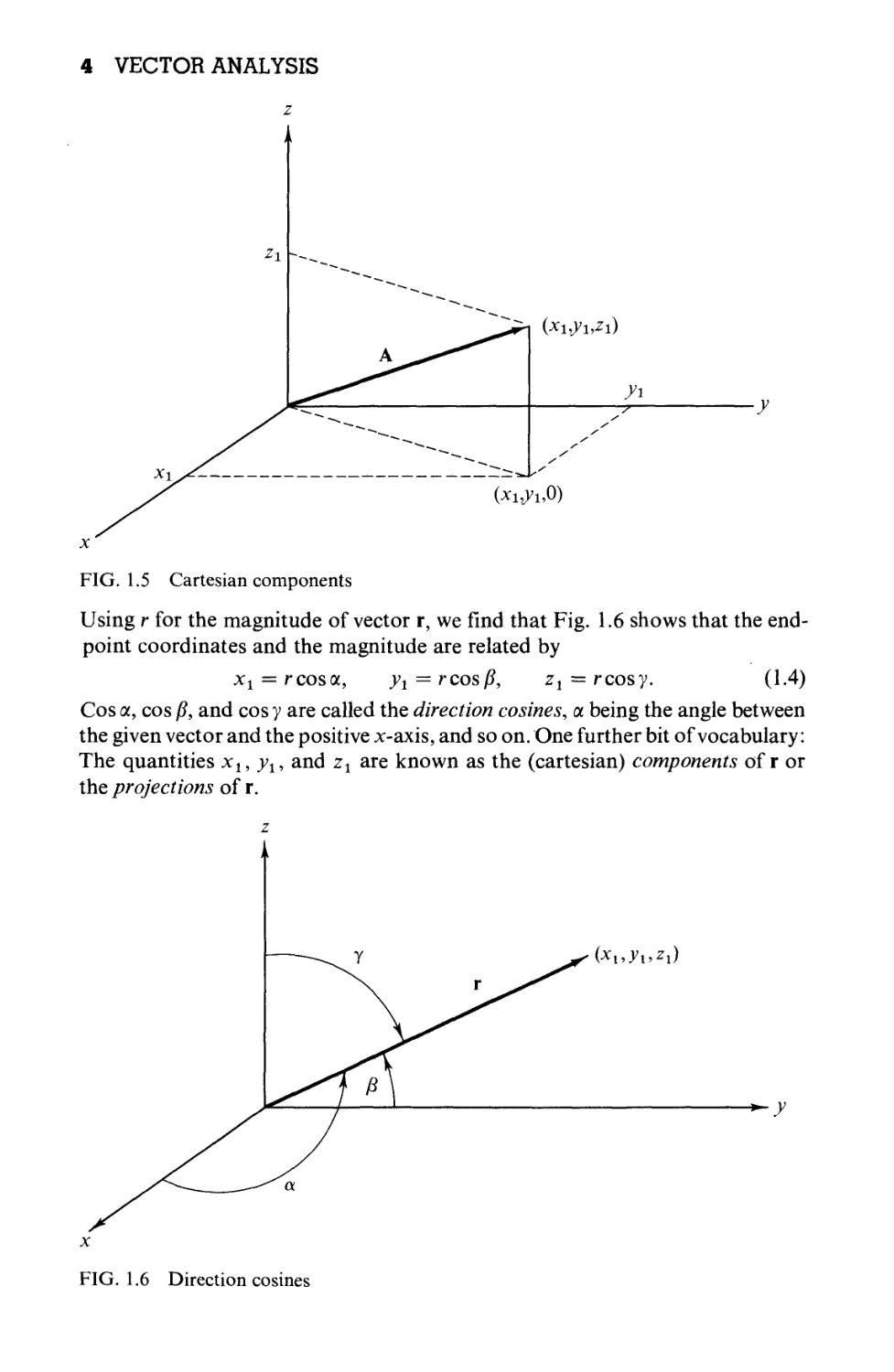
FIG. 1.5 Cartesian components
Using r for the magnitude of vector r, we find that Fig. 1.6 shows that the end-
point coordinates and the magnitude are related by
xt = rcosot, yx = rcos/3, zx = rcosy. A.4)
Cos a, cos /?, and cos у are called the direction cosines, a. being the angle between
the given vector and the positive x-axis, and so on. One further bit of vocabulary:
The quantities xl9 yl, and zx are known as the (cartesian) components of г or
the projections of r.
FIG. 1.6 Direction cosines
DEFINITIONS, ELEMENTARY APPROACH 5
If we proceed in the same manner, any vector A may be resolved into its
components (or projected onto the coordinate axes) to yield
Ax = Acosa, A.5)
in which a is the angle between A and the positive x-axis. Again, we may choose
to refer to the vector as a single quantity A or to its components (Ax,Ay,Az).
Note that the subscript x in Ax denotes the x component and not a dependence
on the variable x. Ax may be a function of x, y, and z as Ax(x,y,z). The choice
between using A or its components (Ax,Ay,Az) is essentially a choice between
a geometric or an algebraic representation. In the language of group theory
(Chapter 4), the two representations are isomorphic.
Use either representation at your convenience. The geometric "arrow in,
space" may aid in visualization. The algebraic set of components is usually
much more suitable for precise numerical or algebraic calculations.
Vectors enter physics in two distinct forms. A) Vector A may represent a
single force acting at a single point. The force of gravity acting at the center of
gravity illustrates this form. B) Vector A may be defined over some extended
region; that is, A and its components may be functions of position: Ax =
Ax(x,y,z), and so on. Examples of this sort include the velocity of a fluid
varying from point to point over a given volume and electric and magnetic
fields. Some writers distinguish these two cases by referring to the vector
defined over a region as a vector field. The concept of the vector defined over a
region and being a function of position will be extremely important in Section
1.2 and in later sections where we differentiate and integrate vectors.
At this stage it is convenient to introduce unit vectors along each of the
coordinate axes. Let i be a vector of unit magnitude pointing in the positive
x-direction, j, a vector of unit magnitude in the positive ^-direction, and к, а
vector of unit magnitude in the positive z-direction. Then \AX is a vector with
magnitude equal to Ax and in the positive x-direction. By vector addition
A = iAx+jAy + kAz, A.6)
which states that a vector equals the vector sum of its components. Note that if
A vanishes, all of its components must vanish individually; that is, if
A = 0, then Ax = Ay = Az = 0.
Finally, by the Pythagorean theorem, the magnitude of vector A is
A = (A2X + A] + Al1I/2. A.7a)
This resolution of a vector into its components can be carried out in a variety
of coordinate systems, as shown in Chapter 2. Here we restrict ourselves to
cartesian coordinates.
Equation 1.6 is actually an assertion that the three unit vectors i, j, and к
span our real three-dimensional space: Any constant vector may be written as
a linear combination of i, j, and k. Since i, j, and к are linearly independent
(no one is a linear combination of the other two), they form a basis for the real
three-dimensional space.
6 VECTOR ANALYSIS
As a replacement of the graphical technique, addition and subtraction of
vectors may now be carried out in terms of their components. For A = \AX +
}Ay + kAz and В = \BX + jBy + kBz,
A + В = i(Ax ± Bx) + j(Ay ± By) + k(Az + Bz). A.76)
EXAMPLE 1.1.1
Let
A = 6i + 4j + 3k
В = 2i - 3j - 3k.
Then by Eq. 1.76
A + В = 8i + j
and
A - В = 4i + 7j + 6k.
It should be emphasized here that the unit vectors i, j, and к are used for
convenience. They are not essential; we can describe vectors and use them
entirely in terms of their components: A<-+(AX, Ay, Az). This is the approach of
the two more powerful, more sophisticated definitions of vector discussed in
the next section. However, i, j, and к emphasize the direction, which will be
useful in Chapter 2.
So far we have defined the operations of addition and subtraction of vectors.
Three varieties of multiplication are defined on the basis of their applicability:
a scalar or inner product in Section 1.3, a vector product peculiar to three-
dimensional space in, Section 1.4, and a direct or outer product yielding a
second-rank tensor in Section 3.2. Division by a vector is not defined. See
Exercises 4.2.21 and 22.
EXERCISES
1.1.1 Show how to find A and B, given A + В and A — B.
1.1.2 The vector A whose magnitude is 10 units makes equal angles with the coordinate
axes. Find Ax, Ay, and Az.
1.1.3 Calculate the components of a unit vector that lies in the xy-plane and makes
equal angles with the positive directions of the x- and j'-axes.
1.1.4 The velocity of sailboat A relative to sailboat B, vrel, is defined by the equation
Vrei = V4 — vB, where V4 is the velocity of A and vB is the velocity of B. Determine
the velocity of A relative to В if
V4 = 30 km/hr east
vB = 40 km/hr north
ANS. vrc, = 50 km/hr, 53.1° south of east.
ADVANCED DEFINITIONS 7
1.1.5 A sailboat sails for 1 hr at 4 km/hr (relative to the water) on a steady compass
heading of 40° east of north. The sailboat is simultaneously carried along by a
current. At the end of the hour the boat is 6.12 km from its starting point. The
line from its starting point to its location lies 60° east of north. Find the x (east-
(easterly) and у (northerly) components of the water's velocity.
ANS. v^t = 2.73 km/hr, t>north = 0 km/hr.
1.1.6 A vector equation can be reduced to the form A = B. From this show that the
one vector equation is equivalent to three scalar equations.
Assuming the validity of Newton's second law F = ma as a vector equation,
this means that ax depends only on Fx and is independent of Fy and Fz.
1.1.7 The vertices of a triangle A, B, and Care given by the points (—1,0,2), @,1,0),
and A, — 1,0), respectively. Find point D so that the figure ABDC forms a plane
parallelogram.
ANS. B,0,-2).
1.1.8 A triangle is defined by the vertices of three vectors, A, B, and С that extend
from the origin. In terms of A, B, and С show that the vector sum of the successive
sides of the triangle (AB + ВС + CA) is zero.
1.1.9 A sphere of radius a is centered at a point r1.
(a) Write out the algebraic equation for the sphere.
(b) Write out a vector equation for the sphere.
ANS. (a) (x-x1J + (y-ylJ + (z-z1J = a2.
(b) г = rj + a.
(a takes on all directions but has a fixed magnitude, a.)
1.1.10 A corner reflector is formed by three mutually perpendicular reflecting surfaces.
Show that a ray of light incident upon the corner reflector (striking all three
surfaces) is reflected back along a line parallel to the line of incidence.
Hint. Consider the effect of a reflection on the components of a vector describing
the direction of the light ray.
1.1.11 Hubble's law. Hubble found that distant galaxies are receding with a velocity
proportional to their distance from where we are on Earth. For the /th galaxy
V; = #or;
with us at the origin. Show that this recession of the galaxies from us does not
imply that we are at the center of the universe. Specifically, take the galaxy
at rx as a new origin and show that Hubble's law is still obeyed.
1.2 ADVANCED DEFINITIONS*
In the preceding section vectors were defined or represented in two equiv-
equivalent ways: A) geometrically by specifying magnitude and direction, as with an
arrow, and B) algebraically by specifying the components relative to cartesian
coordinate axes. The second definition is adequate for the vector analysis of
this chapter. In this section two more refined, sophisticated, and powerful
*This section is optional. It is not essential for the remaining sections of this
chapter.
8 VECTOR ANALYSIS
definitions are presented. First, the vector field is defined in terms of the
behavior of its components under rotation of the coordinate axes. This trans-
transformation theory approach leads into the tensor analysis of Chapter 3. Second,
the component definition of Section 1.1 is refined and generalized according to
the mathematician's concepts of vector and vector space. This approach leads
to function spaces including the Hilbert space—Section 9.4.
ROTATION OF THE COORDINATE AXES
The definition of vector as a quantity with magnitude and direction breaks
down in advanced work. On the one hand, we encounter quantities, such as
elastic constants and index of refraction in anisotropic crystals, that have
magnitude and direction but which are not vectors. On the other hand, our
naive approach is awkward to generalize, to extend to more complex quantities.
We seek a new definition of vector field, using our displacement vector r as a
prototype.
There is an important physical basis for our development of a new definition.
We describe our physical world by mathematics, but it and any physical
predictions we may make must be independent of our mathematical analysis.
Some writers compare the physical system to a building and the mathematical
analysis to the scaffolding used to construct the building. In the end the scaffold-
scaffolding is stripped off and the building stands.
In our specific case we assume that space is isotropic; that is, there is no
preferred direction or all directions are equivalent. Then the physical system
being analyzed or the physical law being enunciated cannot and must not
depend on our choice or orientation of the coordinate axes.
Now we return to the concept of vector r as a geometric object independent
of the coordinate system. Let us look at r in two different systems, one rotated
in relation to the other.
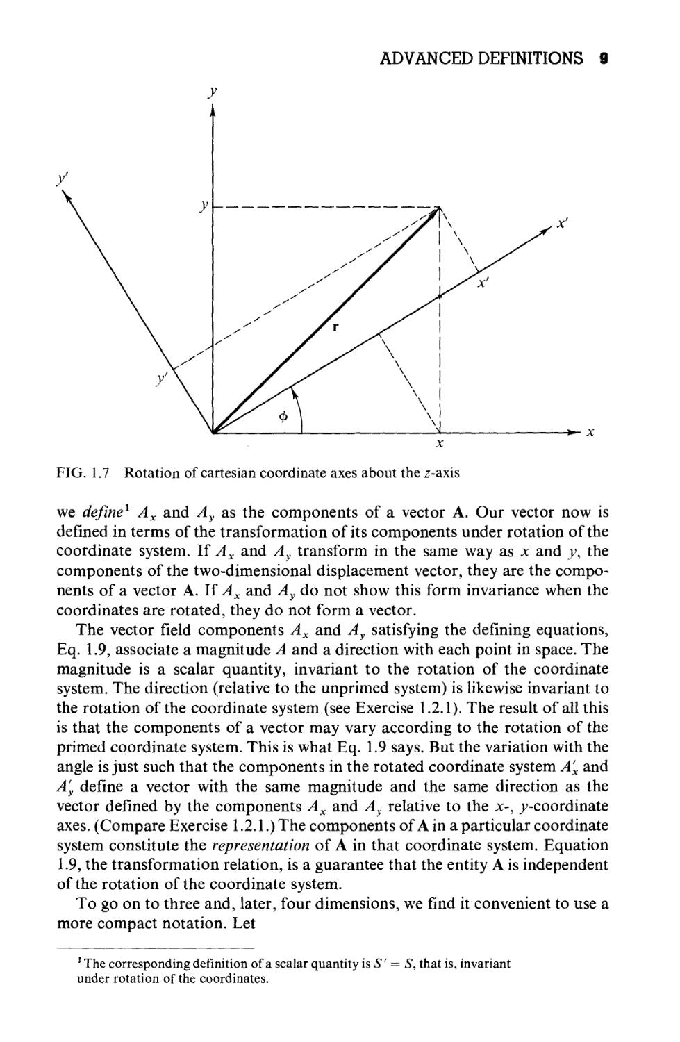
For simplicity we consider first the two-dimensional case. If the x-, y-
coordinates are rotated counterclockwise through an angle cp, keeping г fixed
(Fig. 1.7), we get the following relations between the components resolved in
the original system (unprimed) and those resolved in the new rotated system
(primed):
x' = x cos cp + v sin cp,
A.8)
y' — — x sin cp + у cos cp
We saw in Section 1.1 that a vector could be represented by the coordinates
of a point; that is, the coordinates were proportional to the vector components.
Hence the components of a vector must transform under rotation as coordinates
of a point (such as r). Therefore whenever any pair of quantities Ax(x, y) and
Ay(x, y) in the xy-coordinate system is transformed into (A'x, A'y) by this rotation
of the coordinate system with
A' = Axcoscp + A v sing)
A.9)
A'y = —Ax sin cp + Ay cos cp,
ADVANCED DEFINITIONS 9
*- x
FIG. 1.7 Rotation of cartesian coordinate axes about the z-axis
we define1 Ax and Ay as the components of a vector A. Our vector now is
defined in terms of the transformation of its components under rotation of the
coordinate system. If Ax and Ay transform in the same way as x and y, the
components of the two-dimensional displacement vector, they are the compo-
components of a vector A. If Ax and Ay do not show this form invariance when the
coordinates are rotated, they do not form a vector.
The vector field components Ax and Ay satisfying the defining equations,
Eq. 1.9, associate a magnitude A and a direction with each point in space. The
magnitude is a scalar quantity, invariant to the rotation of the coordinate
system. The direction (relative to the unprimed system) is likewise invariant to
the rotation of the coordinate system (see Exercise 1.2.1). The result of all this
is that the components of a vector may vary according to the rotation of the
primed coordinate system. This is what Eq. 1.9 says. But the variation with the
angle is just such that the components in the rotated coordinate system A'x and
A'y define a vector with the same magnitude and the same direction as the
vector defined by the components Ax and Ay relative to the л>, ^-coordinate
axes. (Compare Exercise 1.2.1.) The components of A in a particular coordinate
system constitute the representation of A in that coordinate system. Equation
1.9, the transformation relation, is a guarantee that the entity A is independent
of the rotation of the coordinate system.
To go on to three and, later, four dimensions, we find it convenient to use a
more compact notation. Let
1 The corresponding definition of a scalar quantity is S' = S, that is, invariant
under rotation of the coordinates.
10 VECTOR ANALYSIS
X~^Xi A.10)
a21 = coscp, a12 =
12 q,
a2l = — sin<p, a22 = coscp.
Then Eq. 1.8 becomes
The coefficient afj- may be interpreted as a direction cosine, the cosine of the
angle between x\ and Xj; that is,
a12 = cos{x1,x2) = sm<p,
a2x = cos(x2, х2) = cos I <p + — I = — sin cp.
The advantage of the new notation2 is that it permits us to use the summation
symbol ]T and to rewrite Eqs. 1.12 as
Note that / remains as a parameter that gives rise to one equation when it is
set equal to 1 and to a second equation when it is set equal to 2. The index j,
of course, is a summation index, a dummy index, and as with a variable of
integration, j may be replaced by any other convenient symbol.
The generalization to three, four, or N dimensions is now very simple. The
set of N quantities, Vj, is said to be the components of an jV-dimensional vector,
V, if and only if their values relative to the rotated coordinate axes are given by
Л i=l,2, ...,#. A.15)
As before, ац is the cosine of the angle between x\ and x}. Often the upper limit
N and the corresponding range of i will not be indicated. It is taken for granted
that the reader knows how many dimensions his or her space has.
From the definition of ai} as the cosine of the angle between the positive x\
2 The reader may wonder at the replacement of one parameter cp by four
parameters a{i. Clearly, the ai} do not constitute a minimum set of parameters.
For two dimensions the four atJ are subject to the three constraints given in
Eq. 1.18. The justification for the redundant set of direction cosines is the
convenience it provides. Hopefully, this convenience will become more
apparent in Chapters 3 and 4. For three dimensional rotations (9 ay but only
three independent) alternate descriptions are provided by: A) the Euler angles
discussed in Section 4.3, B) quaternions, and C) the Cayley-Klein parameters.
These alternatives have their respective advantages and disadvantages.
ADVANCED DEFINITIONS 11
direction and the positive Xj direction we may write (cartesian coordinatesK
Note carefully that these are partial derivatives. By use of Eq. 1.16, Eq. 1.15
becomes
V! = f ™±V-= У —^-V- A17)
1 ^ Fix J ^ fix' r \1-1')
The direction cosines ai} satisfy an orthogonality condition
ijaik = ejk A.18)
or, equivalently,
YJiald = b}k. A.19)
The symbol Sjk is the Kronecker delta defined by
8jk = 1 for у = к,
A.20)
<5д = 0 for ./=£*.
The reader may easily verify that Eqs. 1.18 and 1.19 hold in the two-dimensional
case by substituting in the specific atj from Eq. 1.11. The result is the well-known
identity sin2 cp + cos2 cp = 1 for the nonvanishing case. To verify Eq. 1.18 in
general form, we may use the partial derivative forms of Eqs. 1.16 to obtain
dx' dxl
'i dxl i dx'i дхк дхк'
The last step follows by the standard rules for partial differentiation, assuming
that Xj is a function of x\, x'2, x'3, and so on. The final result, dXjjdxk, is equal
to 5jk, since Xj and xk as coordinate lines (j ф к) are assumed to be perpendicular
(two or three dimensions) or orthogonal (for any number of dimensions).
Equivalently, we may assume that Xj and xk (j ф к) are totally independent
variables. If j = k, the partial derivative is clearly equal to 1.
In redefining a vector in terms of how its components transform under a
rotation of the coordinate system, we should emphasize two points:
1. This definition is developed because it is useful and appropriate in
describing our physical world. Our vector equations will be independent of
any particular coordinate system. (The coordinate system need not even be
cartesian.) The vector equation can always be expressed in some particular
coordinate systeto and, to obtain numerical results, we must ultimately express
the equation in some specific coordinate system.
3 Differentiate x\ — £aikxk with respect to Xj. See the discussion following
Eq. 1.21. Section 4.3 provides an alternate approach.
12 VECTOR ANALYSIS
2. This definition is subject to a generalization that will open up the branch
of mathematics known as tensor analysis (Chapter 3).
A qualification is also in order. The behavior of the vector components
under rotation of the coordinates is used in Section 1.3 to prove that a scalar
product is a scalar, in Section 1.4 to prove that a vector product is a vector,
and in Section 1.6 to show that the gradient of a scalar, Vxjj, is a vector. The
remainder of this chapter proceeds on the basis of the less restrictive definitions
of the vector given in Section 1.1.
Vectors and Vector Space
It is customary in mathematics to label an ordered triple of real numbers
(x2, x2, x3) a vector x. The number xn is called the nth component of vector x.
The collection of all such vectors (obeying the properties that follow) form a
three-dimensional real vector space. We ascribe five properties to our vectors:
If x = (xj,x2,x3) and у = (У!,у2,Уз),
1. Vector equality: x = у means xt = yh i= 1, 2, 3
2. Vector addition: x + у = z means xt + yt = zt,
3. Scalar multiplication: ax<^(axi,ax2,ax3) (with
a real)
4. Negative of a vector: — x = (— l)x •*-►( — x1? — x2,
-x3)
5. Null vector: There exists a null vector 0 <-> @,0,0).
Since our vector components are simply numbers, the following properties
also hold:
1. Addition of vectors is commutative: x + у = у + x.
2. Addition of vectors is associative: (x + y) + z =
x + (y + z).
3. Scalar multiplication is distributive:
a(x + y) = ax + ay, also (a + b)x = ax + bx.
4. Scalar multiplication is associative: {ab)x = a(bx).
Further, the null vector 0 is unique as is the negative of a given vector x.
So far as the vectors themselves are concerned this approach merely for-
formalizes the component discussion of Section 1.1. The importance lies in the
extensions which will be considered in later chapters. In Chapter 4, we show that
vectors form both an Abelian group under addition and a linear space with
the transformations in the linear space described by matrices. Finally, and
perhaps most important, for advanced physics the concept of vectors presented
here may be generalized to A) complex quantities,4 B) functions, and C) an
infinite number of components. This leads to infinite dimensional function
4 The «-dimensional vector space of real n-tuples is often labeled R" and the
«-dimensional vector space of complex n-tuples is labeled C".
SCALAR OR DOT PRODUCT 13
spaces, the Hilbert spaces, which are, important in modern quantum theory. A
brief introduction to function expansions and Hilbert space appears in Section
9.4.
EXERCISES
1.2.1 (a) Show that the magnitude of a vector A, A - (Al + A2I'2 is independent
of the orientation of the rotated coordinate system,
(Al + a)Y* = (л;2 + а;2I'2
;
independent of the rotation angle <p.
This independence of angle is expressed by saying that A is invariant under
rotations.
(b) At a given point (x,y) A defines an angle a relative to the positive x-axis
and a' relative to the positive x'-axis. The angle from x to x' is (p. Show that
A = A' defines the same direction in space when expressed in terms of its
primed components, as in terms of its unprimed components; that is,
a' = a — <p.
1.2.2 Prove the orthogonality condition ^апаш ~ $jk- As a special case of this the
direction cosines of Section 1.1 satisfy the relation
cos2 a + cos2 P + cos2 у = 1,
a result that also follows from Eq. 1.7a.
1.3 SCALAR OR DOT PRODUCT
Having defined vectors, we now proceed to combine them. The laws for
combining vectors must be mathematically consistent. From the possibilities
that are consistent we select two that are both mathematically and physically
interesting. A third possibility is introduced in Chapter 3, in which we form
tensors.
The combination of AB cos в, in which A and В are the magnitudes of two
vectors and в, the angle between them, occurs frequently in physics (Fig. 1.8).
FIG. 1.8 Scalar product A-B =
АВсоьв
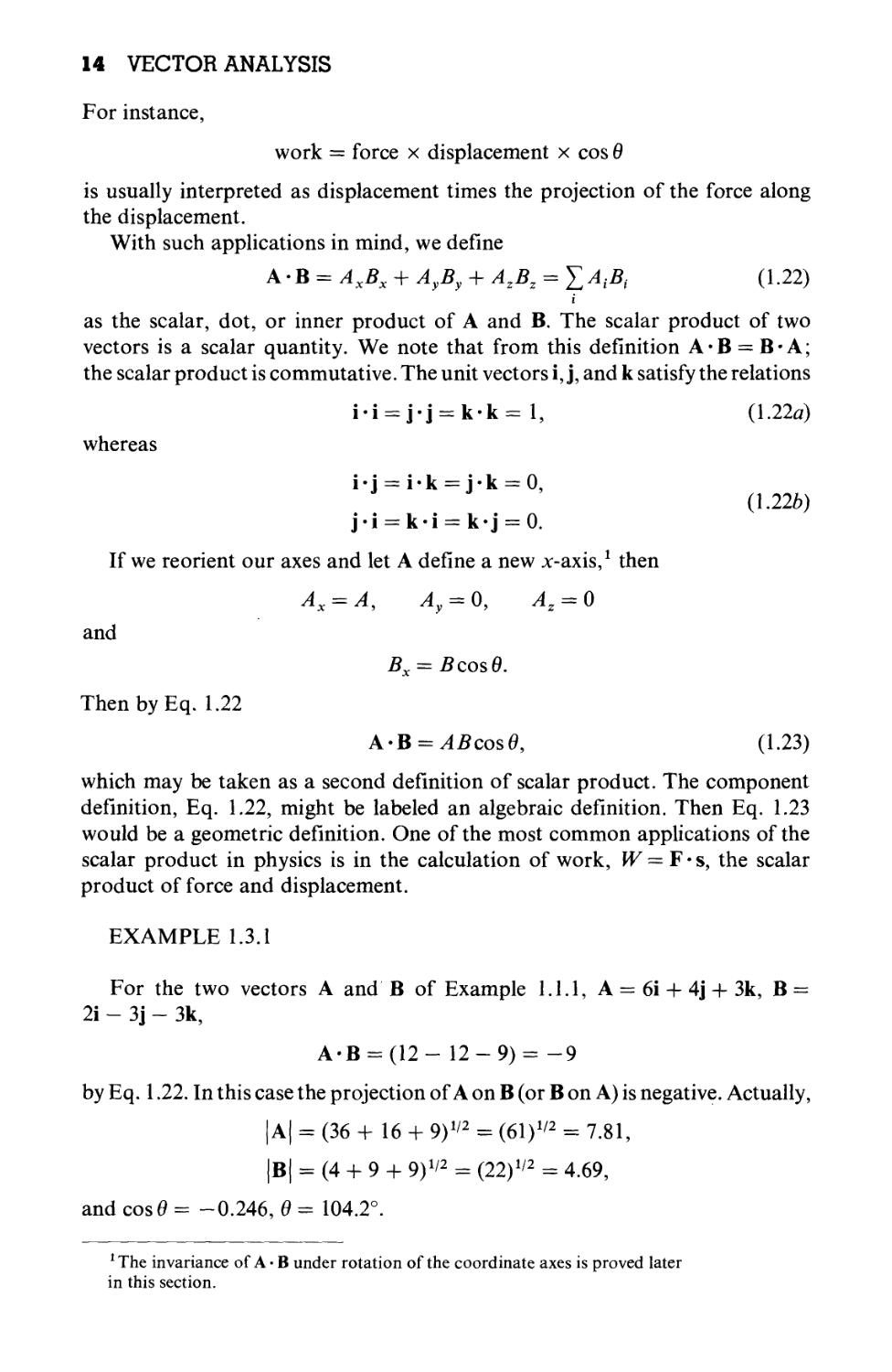
14 VECTOR ANALYSIS
For instance,
work = force x displacement x cos в
is usually interpreted as displacement times the projection of the force along
the displacement.
With such applications in mind, we define
AB = AXBX + AyBy + AZBZ = £ЛД. A.22)
as the scalar, dot, or inner product of A and B. The scalar product of two
vectors is a scalar quantity. We note that from this definition A • В = В • A;
the scalar product is commutative. The unit vectors i, j, and к satisfy the relations
i-i = j-j = k-k = 1, A.22a)
whereas
ij = ik = jk = O,
A.22b)
j-i = k*i = k-j = 0.
If we reorient our axes and let A define a new лг-axis,1 then
and
Bx = В cos в.
Then by Eq. 1.22
A-B = ,4£cos0, A.23)
which may be taken as a second definition of scalar product. The component
definition, Eq. 1.22, might be labeled an algebraic definition. Then Eq. 1.23
would be a geometric definition. One of the most common applications of the
scalar product in physics is in the calculation of work, W=¥-s, the scalar
product of force and displacement.
EXAMPLE 1.3.1
For the two vectors A and В of Example 1.1.1, A = 6i + 4j + Зк, В =
2i — 3j — 3k,
A«B = A2- 12-9)= -9
by Eq. 1.22. In this case the projection of A on В (or В on A) is negative. Actually,
A| = C6 + 16 + 9I/2 = F1I/2 = 7.81,
В | = D + 9 + 9)i/2 = B2I/2 = 4.69,
and cos0 = -0.246, в = 104.2°.
1 The invariance of A ■ В under rotation of the coordinate axes is proved later
in this section.
SCALAR OR DOT PRODUCT 15
If A • В = 0 and we know that А ф 0 and В =/= 0, then from Eq. 1.23 cos в = 0
or 9 = 90°, 270°, and so on. The vectors A and В must be perpendicular.
Alternately, we may say A and В are orthogonal. The unit vectors i, j, and к
are mutually orthogonal. To develop this notion of orthogonality one more
step, suppose that n is a unit vector and г is a nonzero vector in the xy-plane;
that is, г = ix + \y (Fig. 1.9). If
n-r = 0
for all choices of r, then n must be perpendicular (orthogonal) to the xy-plane.
FIG. 1.9 A normal vector
Often it is convenient to replace i, j, and к by subscripted unit vectors em,
m— 1, 2, 3 with i = e1? and so on. Then Eqs. 1.22л and b become
ет*е„ = <5т„. A.22c)
For m Ф n the unit vectors em and е„ are orthogonal. For m = n each vector is
normalized to unity, that is, has unit magnitude. The set em is said to be orthonor-
mal. A major advantage of Eq. 1.22c over Eqs. 1.22йг and b is that Eq. 1.22c
may readily be generalized to ^-dimensional space: m, n = 1, 2, ..., N.
Finally, we are picking sets of unit vectors em that are orthonormal for con-
convenience—a very great convenience. The nonorthogonal situation is explored
in Section 4.4, "Oblique Coordinates."
SCALAR PROPERTY
We have not yet shown that the word scalar is justified or that the scalar
product is indeed a scalar quantity. To do this, we investigate the behavior of
A-B under a rotation of the coordinate system. By use of Eq. 1.15
16 VECTOR ANALYSIS
A'XB'X + A'yB'y + A'ZB'Z = 2>^ %
i j i j i J
A.24)
Using the indices к and / to sum over x, y, and z, we obtain
к I i j
and, by rearranging the terms on the right-hand side, we have
i j I
The last two steps follow by using Eq. 1.18, the orthogonality condition of the
direction cosines, and Eq. 1.20, which defines the Kronecker delta. The effect
of the Kronecker delta is to cancel all terms in a summation over either index
except the term for which the indices are equal. In Eq. 1.26 its effect is to set
j = i and to eliminate the summation over j. Of course, we could equally well
set i =j and eliminate the summation over i. Equation 1.26 gives us
ь A.27)
which is just our definition of a scalar quantity, one that remains invariant under
the rotation of the coordinate system.
In a similar approach which exploits this concept of invariance, we take
С = A + В and dot it into itself.
С • С = (A + В) • (A + В)
A.28)
= AA + BB + 2AB.
Since
CC = C2, A.29)
the square of the magnitude of vector С and thus an invariant quantity, we
see that
A-B = i(C2 -A2 -B2), invariant. A.30)
Since the right-hand side of Eq. 1.30 is invariant—that is, a scalar quantity—
the left-hand side, A • B, must also be invariant under rotation of the coordinate
system. Hence A • В is a scalar.
Equation 1.28 is really another form of the law of cosines which is
C2 = A2 + B2 + 2ABcosd. A.31)
Comparing Eqs. 1.28 and 1.31, we have another verification of Eq. 1.23, or,
if preferred, a vector derivation of the law of cosines (Fig. 1.10).
EXERCISES 17
В
FIG. 1.10 The law of cosines
An interesting illustration of the geometric interpretation of the scalar
product is provided by an example from a branch of general relativity. Consider
a four-dimensional sphere
x2 + y2 + z2 + w2 = 1
in x, y, z, w space. The surface of this four-dimensional sphere may be described
by the vector г = (x,y,z,w) with the restriction that |r| = 1. It is possible to
construct a unit vector t that is tangential to this four-dimensional sphere over
its entire surface. As one possible example,
t = (y, -x,w, -z).
The reader may verify that
therefore unit magnitude, and
therefore tangential, over the entire sphere.
The two-dimensional analog exists but there is no three-dimensional analog.
Hair growing out of a sphere cannot be combed down all over. There will be
a cowlick.
The dot product, given by Eq. 1.22, may be generalized in two ways. The
space need not be restricted to three dimensions. In «-dimensional space,
Eq. 1.22 applies with the sum running from 1 to п. п may be infinity, with the
sum then a convergent infinite series (Section 5.2). The other generalization
extends the concept of vector to embrace functions. The function analog of a
dot or inner product appears in Section 9.4.
EXERCISES
1.3.1 What is the cosine of the angle between the vectors
A = 3i + 4j + к
and
B = i-j + k?
ANS. cos 9 = 0, 6 = -.
18 VECTOR ANALYSIS
1.3.2 Two unit magnitude vectors e; and e,- are required to be either parallel or per-
perpendicular to each other. Show that e^e,- provides an interpretation of Eq. 1.18,
the direction cosine orthogonality relation.
1.3.3 Given that A) the dot product of a unit vector with itself is unity and B) this
relation is valid in all (rotated) coordinate systems, show that i' • Г = 1 (with the
primed system rotated 45° about the z-axis relative to the unprimed) implies that
i-j = 0.
1.3.4 The vector r, starting at the origin, terminates at and specifies the point in space
(x,y, z). Find the surface swept out by the tip of r if
(a) (r-a)-a = 0,
(b) (r - a) • г = 0.
The vector a is a constant (constant in magnitude and direction).
1.3.5 Ml
The interaction energy between two dipoles of moments щ and ц2 may be written
in the vector form
V=- Pi'tb .
Г3
and in the scalar form
V = f^1 B cos 0, cos 62 - sin 0, sin 0, cos <p).
Here Bx and 02 are the angles of ]i1 and ц2 relative to r, while <p is the azimuth of
\i2 relative to the щ — r plane. Show that these two forms are equivalent.
Hint. Eq. 12.198 will be helpful.
1.3.6 A pipe comes diagonally down the south wall of a building, making an angle
of 45° with the horizontal. Coming into a corner, the pipe turns and continues
diagonally down a west-facing wall, still making an angle of 45° with the horizontal.
What is the angle between the south-wall and west-wall sections of the pipe?
ANS. 120°.
1.4 VECTOR OR CROSS PRODUCT
A second form of vector multiplication employs the sine of the included
angle instead of the cosine. For instance, the angular momentum of a body is
defined as
angular momentum = radius arm x linear momentum
= distance x linear momentum x sin в.
For convenience in treating problems relating to quantities such as angular
momentum, torque, and angular velocity, we define the vector or cross product
as
VECTOR OR CROSS PRODUCT 19
Linear momentum
*- x
FIG. 1.11 Angular momentum
with
С = A x B,
С = AB sind.
A.32)
Unlike the preceding case of the scalar product, С is now a vector, and we assign
it a direction perpendicular to the plane of A and В such that A, B, and С form a
right-handed system. With this choice of direction we have
AxB=—BxA, anticommutation.
From this definition of cross product we have
A.32л)
A.326)
whereas
and
ixj = k, j x к = i, kxi = j
j x i = —к, к x j = —i, ixk= —j.
A.32c)
Among the examples of the cross product in mathematical physics are the
relation between linear momentum p and angular momentum L (defining
angular momentum),
L = г x p
and the relation between linear velocity v and angular velocity со,
V = CO X Г.
Vectors v and p describe properties of the particle or physical system. However,
20 VECTOR ANALYSIS
the position vector г is determined by the choice of the origin of the coordinates.
This means that со and L depend on the choice of the origin.
The familiar magnetic induction В is usually defined by the vector product
force equation1
Fm = ?vx B.
Here v is the velocity of the electric charge q and FM is the resulting force on
the moving charge.
The cross product has an important geometrical interpretation which we
shall use in subsequent sections. In the parallelogram defined by A and В
(Fig. 1.12) В sin в is the height if A is taken as the length of the base. Then
A x В | = А В sin в is the area of the parallelogram. As a vector, A x В is the
area of the parallelogram defined by A and B, with the area vector normal to
the plane of the parallelogram. This suggests that area may be treated as a
vector quantity.
В sin 9
FIG. 1.12 Parallelogram representation of the vector product
Parenthetically, it might be noted that Eq. 1.32c and a modified Eq. 1.326
form the starting point for the development of quaternions. Equation 1.326
is replaced byixi = jxj = kxk = —1.
An alternate definition of the vector product С = А х В consists in specifying
the components of С:
Cx = AyBz-AzBy,
— AZBX — AXBZ,
A.33)
or
lrThe electric field E is assumed here to be zero.
VECTOR OR CROSS PRODUCT 21
= AjBk -AkBj, i, j, к all different,
A.34)
and with cyclic permutation of the indices i, j, and к. The vector product С
may be conveniently represented by a determinant2
г-i
i J к
Ax Ay Az
вх ву bz
A.35)
Expansion of the determinant across the top row reproduces the three com-
components of С listed in Eq. 1.33.
Equation 1.32 might be called a geometric definition of the vector product.
Then Eq. 1.33 would be an algebraic definition.
EXAMPLE 1.4.1
With A and В given in Example 1.1.1,
A = 6i + 4j + 3k,
В = 2i - 3j - 3k,
A x B =
1 j к
6 4 3
2 -3 -3
= i(- 12 + 9) - j(- 18 - 6) + k(- 18 - 8)
= -3i + 24j-26k.
To show the equivalence of Eq. 1.32 and the component definition, Eq. 1.33,
let us form A • С and В • С, using Eq. 1.33. We have
A-C = A-(A x B)
= Ax(AyBz - AzBy) + Ay(AzBx - AXBZ) + Az(AxBy - AyBx)
= 0.
Similarly,
BC = B(A x B) = 0.
A.36)
A.37)
Equations 1.36 and 1.37 show that С is perpendicular to both A and В (cos 0 = 0,
в = ± 90°) and therefore perpendicular to the plane they determine. The positive
direction is determined by considering special cases such as the unit vectors
!See Section 4.1 for a summary of determinants.
22 VECTOR ANALYSIS
The magnitude is obtained from
(A x B)-(A x B) = A2B2-(A-BJ
= A2B2-A2B2cos2d A.38)
= A2B2sin20.
Hence
C = ABsmd. A.39)
The big first step in Eq. 1.38 may be verified by expanding out in component
form, using Eq. 1.33 for A x В and Eq. 1.22 for the dot product. From Eqs.
1.36, 1.37, and 1.39 we see the equivalence of Eqs. 1.32 and 1.33, the two
definitions of vector product.
There still remains the problem of verifying that С = А х В is indeed a
vector; that is, it obeys Eq. 1.15, the vector transformation law. Starting in a
rotated (primed system)
C[ = AjB'k — A'kB'j, i,j, and к in cyclic order,
1тВт A.40)
l,m
The combination of direction cosines in parentheses vanishes for m — l. We
therefore have j and к taking on fixed values, dependent on the choice of /,
and six combinations of / and m. If i = 3, then j = 1, к = 2 (cyclic order), and
we have the following direction cosine combinations
atla22 - a2Xal2 = аъъ,
a12a23 - a22ai3 = a31
and their negatives. Equations 1.41 are identities satisfied by the direction
cosines. They may be verified with the use of determinants and matrices
(see Exercise 4.3.3). Substituting back into Eq. 1.40,
С'ъ = a33A1B2 + a32A3B1 + a3iA2B3
-a33A2Bl-a32AlB3-a3lA3B2
= a31C1 + a32C2 + a33C3
By permuting indices to pick up C[ and C2, we see that Eq. 1.15 is satisfied
and С is indeed a vector. It should be mentioned here that this vector nature of
the cross product is an accident associated with the three-dimensional nature
EXERCISES 23
of ordinary space.3 It will be seen in Chapter 3 that the cross product may also
be treated as a second-rank antisymmetric tensor!
If we define a vector as an ordered triple of numbers (or functions) as in the
latter part of Section 1.2, then there is no problem identifying the cross product
as a vector. The cross-product operation maps the two triples A and В into a
third triple С which by definition is a vector.
We now have two ways of multiplying vectors; a third form appears in
Chapter 3. But what about division by a vector? It turns out that the ratio
B/A is not uniquely specified (Exercise 4.2.19) unless A and В are also required
to be parallel. Hence division of one vector by another is not defined.
EXERCISES
1.4.1 Two vectors A and В are given by
A = 2i + 4j + 6k,
В = 3i - 3j - 5k.
Compute the scalar and vector products A • В and A x B.
1.4.2 Show the equivalence of Eq. 1.32 and the component definition Eq. 1.33 by
expanding A, B, and С in С = А х В in cartesian components.
1.4.3 Starting with С = A + B, show that С х С leads to
A x B= -B x A.
1.4.4 Show that
(a) (А-В)-(А + В) = Л2-Я2,
(b) (A - B) x (A + B) = 2A x B.
The distributive laws needed here,
A-(B + C) = A-B + A-C
and
Ax(B + C) = AxB + AxC,
may easily be verified (if desired) by expansion in cartesian components.
1.4.5 Given the three vectors,
P = 3i + 2j - k,
Q= _6i-4j + 2k,
R = i - 2j - k,
find two that are perpendicular and two that are parallel or antiparallel.
3 Specifically Eq. 1.41 holds only for three-dimensional space. Technically, it
is also possible to define a cross product in R1, seven-dimensional space, but
the cross product turns out to have unacceptable (pathological) properties.
24 VECTOR ANALYSIS
1.4.6 IfP = iPx + j/^andQ = \QX -+- JGyare any two nonparallel (also nonantiparallel)
vectors in the xy-plane, show that P x Q is in the z-direction.
1.4.7 Prove that (A x B) • (A x B) = (ABJ - (A • BJ.
1.4.8 Using the vectors
P = icos0 + jsin0,
Q = icos<p — jsin<p,
R = icos<p + }sin<p,
prove the familiar trigonometric identities
sin@ + <p) = sin в cos <p + cos 9 sin <p,
cos@ + (p) = cos 9 cos cp — sin в sin (p.
1.4.9 (a) Find a vector A that is perpendicular to
(b) What is A if, in addition to this requirement, we also demand that it have
unit magnitude?
1.4.10 If four vectors a, b, c, and d all lie in the same plane, show that
(a x b) x (c x d) = 0.
Hint. Consider the directions of the cross-product vectors.
1.4.11 The coordinates of the three vertices of a triangle are B,1,5), E,2,8), and D,8,2).
Compute its area by vector methods.
1.4.12 The vertices of parallelogram ABCD are A,0,0), B,-1,0), @,-1,1), and
(—1,0,1) in order. Calculate the vector areas of triangle ABD and of triangle
BCD. Are the two vector areas equal?
ANS. Area^D = -^(i + j + 2k).
1.4.13 The origin and the three vectors A, B, and С (all of which start at the origin)
define a tetrahedron. Taking the outward direction as positive, calculate the total
vector area of the four tetrahedral surfaces.
Note. In Section 1.11 this result is generalized to any closed surface.
1.4.14 Find the sides and angles of the spherical triangle ABC defined by the three vectors
A = A,0,0),
and
Each vector starts from the origin (Fig. 1.13).
EXERCISES 25
В
FIG. 1.13 Spherical triangle
1.4.15 Derive the law of sines:
sin a _ sin /? _ sin у
*- У
x
1.4.16 The magnetic induction В is defined by the Lorentz force equation
F=^(vx B).
Carrying out three experiments, we find that if
26 VECTOR ANALYSIS
v - i, - = 2k - 4j,
g
v = j, — = 4i - k,
4
and
ь F • т
v = k, — = j - 2i,
From the results of these three separate experiments calculate the magnetic
induction B.
1.5 TRIPLE SCALAR PRODUCT, TRIPLE VECTOR
PRODUCT
TRIPLE SCALAR PRODUCT
Sections 1.3 and 1.4 cover the two types of multiplication of interest here.
However, there are combinations of three vectors, А* (В х QandA x (В х C),
which occur with sufficient frequency to deserve further attention. The com-
combination
A • (B x C)
is known as the triple scalar product. В х С yields a vector which, dotted into
A, gives a scalar. We note that (A • В) х С represents a scalar crossed into a
vector, an operation that is not defined. Hence, if we agree to exclude this
undefined interpretation, the parentheses may be omitted and the triple scalar
product written A • В x C.
Using Eq. 1.33 for the cross product and Eq. 1.22 for the dot product, we
obtain
А-В x С = Ax(ByCz - BzCy) + Ay(BzCx - BXCZ) + Az(BxCy - ByCx)
— R • Г1 v A — С • A у R
= -A-C x B= -C-B x A = -B-A x C, and so on.
A.43)
The high degree of symmetry present in the component expansion should be
noted. Every term contains the factors At, Bj, and Ck. If i,j, and к are in cyclic
order (x,y,z), the sign is positive. If the order is anticyclic, the sign is negative.
Further, the dot and the cross may be interchanged,
A-BxC = AxB-C A.44)
A convenient representation of the component expansion of Eq. 1.43 is provided
by the determinant
A A A
/±x /±y /±z
A-BxC= Bx By Bz A.45)
С С С
y^x y^v W
TRIPLE SCALAR PRODUCT, TRIPLE VECTOR PRODUCT 27
The rules for interchanging rows and columns of a determinant1 provide an
immediate verification of the permutations listed in Eq. 1.43, whereas the
symmetry of A, B, and С in the determinant form suggests the relation given in
Eq. 1.44.
The triple products encountered in Section 1.4, which showed that A x В
was perpendicular to both A and B, were special cases of the general result
(Eq. 1.43).
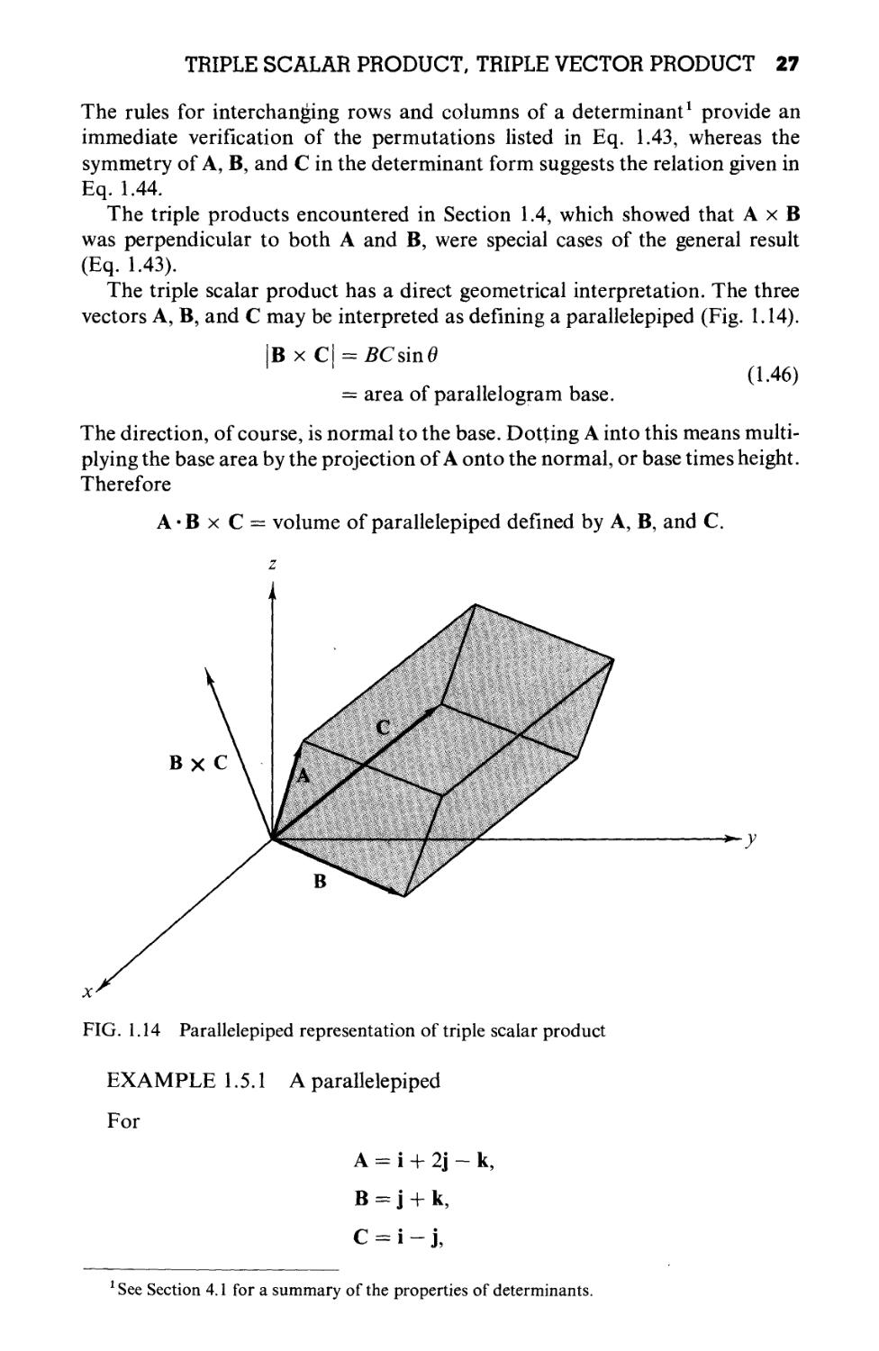
The triple scalar product has a direct geometrical interpretation. The three
vectors A, B, and С may be interpreted as defining a parallelepiped (Fig. 1.14).
В x
= area of parallelogram base.
A.46)
The direction, of course, is normal to the base. Dotting A into this means multi-
multiplying the base area by the projection of A onto the normal, or base times height.
Therefore
A'BxC = volume of parallelepiped defined by A, B, and C.
FIG. 1.14 Parallelepiped representation of triple scalar product
EXAMPLE 1.5.1 A parallelepiped
For
A = i + 2j - k,
1 See Section 4.1 for a summary of the properties of determinants.
28 VECTOR ANALYSIS
AB x C =
1 2 -1
0 1 1
1 -1 0
A.47)
By expansion by minors across the top row the determinant equals
1@ + 1) - 2@ - 1) - 1@ - 1) = 4.
This is the volume of the parallelepiped defined by A, B, and C. The reader
should note that A-BxC may sometimes turn out to be negative! This
problem and its interpretation are considered in Chapter 3.
The triple scalar product finds an interesting and important application
in the construction of a reciprocal crystal lattice. Let a, b, and с (not necessarily
mutually perpendicular) represent the vectors that define a crystal lattice. The
distance from one lattice point to another may then be written
г = naa + nbb + ncc, A-48)
with na,nb, and nc taking on integral values. With these vectors we may form
bxc ., cxa , axb t, ло \
a' = — , b=— , с ' = — . A.48a)
a«b xc a*b x с a*bxc
We see that a' is perpendicular to the plane containing b and с and has a magni-
magnitude proportional to a~x. In fact, we can readily show that
a/'a = b/-b = c'-c= 1, A.486)
whereas
a' • b = a ' • с = b' • a = b ' • с = с • a = с ' • b = 0. A 48c)
It is from Eqs. 1.486 and 1.48c that the name reciprocal lattice is derived. The
mathematical space in which this reciprocal lattice exists is sometimes called
a Fourier space, on the basis of relations to the Fourier analysis of Chapters
14 and 15. This reciprocal lattice is useful in problems involving the scattering
of waves from the various planes in a crystal. Further details may be found in
R. B. Leighton's Principles of Modem Physics, pp. 440-448 [New York:
McGraw-Hill A959)]. We encounter the reciprocal lattice again in an analysis
of oblique coordinate systems, Section 4.4.
TRIPLE VECTOR PRODUCT
The second triple product of interest is A x (В х С). Here the parentheses
must be retained, as may be seen by considering the special case
ix (ix j) = ixk=-j A.49)
but
(i x i) x j = 0.
The fact that the triple vector product is a vector follows from our discussion
TRIPLE SCALAR PRODUCT, TRIPLE VECTOR PRODUCT 29
of vector product. Also, we see that the direction of the resulting vector is
perpendicular to A and to В х С The plane defined by В and С is perpendicular
to В x С and so A x (В x С) lies in this plane. Specifically, if В and С lie in
the xy-plane, then В х С is in the z-direction and A x (В х С) is back in the
xy-plane (Fig. 1.15). This means that A x (В х С) will be a linear combination
of В and C.We find that
A x (B x C) = B(A-C)-C(A-B),
A-50)
a relation sometimes known as the В AC-CAB rule. This result may be verified
by the direct though not very elegant method of expanding into cartesian
components (see Exercise 1.5.2).
'A X (B X C)
FIG. 1.15 В and С are in the
.xy-plane. В x С is perpen-
perpendicular to the xy-plane and is
shown here along the z-axis.
Then A x (B x C) is perpen-
perpendicular to the z-axis and there-
therefore is back in the xy-plane.
An alternate derivation using the Levi-Civita eijk of Section 3.4 is the topic
of Exercise 3.4.8.
The В AC-CAB rule is probably the single most important vector identity.
Because of its frequent use in problems and in future derivations, the rule
probably should be memorized.
It might be noted here that as vectors are independent of the coordinates
so a vector equation is independent of the particular coordinate system. The
coordinate system only determines the components. If the vector equation
can be established in cartesian coordinates, it is established and valid in any
of the coordinate systems to be introduced in Chapter 2.
EXAMPLE 1.5.2 A triple vector product
By using the three vectors given in Example 1.5.1, we obtain
A x (B x C) = (j + k)(l - 2) - (i - j)B - 1)
= -i-k
byEq. 1.50. In detail,
30 VECTOR ANALYSIS
BxC =
0 1 1
1 -1 0
and
A x (B x C) =
1 2 -1
1 1 -1
= -i-k.
Other, more complicated, products may be simplified by using these forms
of the triple scalar and triple vector products.
EXERCISES
1.5.1
1.5.2
1.5.3
One vertex of a glass parallelepiped is at the origin. The three adjacent vertices
are at C,0,0), @,0,2), and @,3,1). All lengths are in centimeters. Calculate the
number of cubic centimeters of glass in the parallelepiped by using the triple
scalar product.
Verify the expansion of the triple vector product
Ax (BxC) = B(AC)-C(AB)
by direct expansion in cartesian coordinates.
Show that the first step in Eq. 1.38, which is
(A x B)(A x B) = A2B2-(A-BJ,
is consistent with the В AC-CAB rule for a triple vector product.
EXERCISES 31
1.5.4 Given the three vectors A, B, and C,
A = i+j,
В = j + k,
С = i - k.
(a) Compute the triple scalar product, A • В x C. Noting that A = В + С, give
a geometric interpretation of your result for the triple scalar product.
(b) Compute A x (В х С).
1.5.5 The angular momentum L of a particle is given by L = r x p = mr x v, where p
is the linear momentum. With linear and angular velocity related by v = и х г,
show that
L = mr2[w-ro(ro.<o)].
Here r0 is a unit vector in the г direction. For г • со = 0 this reduces to L = /to,
with the moment of inertia / given by mr2. In Section 4.6 this result is generalized
to form an inertia tensor.
1.5.6 The kinetic energy of a single particle is given by T—\mv2. For rotational
motion this becomes \rn{m x rJ. Show that
Г=£/и[г2с»2-(г-юJ].
For г ♦ со = 0 this reduces to T = jlco2 with the moment of inertia / given by mr2.
1.5.7 Show that
a x (b x c) + b x (c x a) + с x (a x b) = 0.
1.5.8 A vector A is decomposed into a radial vector Ar and a tangential vector A,.
If r0 is a unit vector in the radial direction, show that
(a) Ar = r0(A-r0)
and
(b) Ar= -r0 x (r0 x A).
1.5.9 Prove that a necessary and sufficient condition for the three (nonvanishing)
vectors A, B, and С to be coplanar is the vanishing of the triple scalar product
A-B x C = 0.
1.5.10 Three vectors A, B, and С are given by
A = 3i - 2j + 2k,
В = 6i + 4j - 2k,
С = - 3i - 2j - 4k.
Compute the values of А-В х С and A x (В х С), С x (A x B) and В х
(C x A).
1.5.11 Vector D is a linear combination of three noncoplanar (and nonorthogonal)
vectors:
D = aA + bB + cC.
Show that the coefficients are given by a ratio of triple scalar products,
D-BxC
a — an(j so on
A-B x С
32 VECTOR ANALYSIS
1.5.12 Show that
(Ax B)(C xD) = (A-C)(B-D)-(A.D)(B-C).
1.5.13 Show that
(A x B) x (C x D) = (AB x D)C - (AB x C)D.
1.5.14 For a spherical triangle such as pictured in Fig. 1.13 show that
sin Л sin В sin С
sin ВС sin С A sin А В
Here sin A is the sine of the included angle at A while ВС is the side opposite
(in radians).
Hint. Exercise 1.5.13 will be useful.
1.5.15 Given
bxc ., cxa , axb , . ,„
a = , b = , с = and a-bxcfO,
a-b x с a-b x с a-b x с
show that
(a) x'-y = Sxy, (x,y = a,b,c),
(b) a b х c=(a-bx c)~\
, . b'xc'
()
1.5.16 If x'-y = 5xy, (x,y = a,b,c), prove that
bxc
a =
a-b x с
(This is the converse of Problem 1.5.15.)
1.5.17 Show that any vector V may be expressed in terms of the reciprocal vectors
a', b, c' by
V = (V-a)a' + (V-b)b'+(V-c)c'.
1.5.18 An electric charge qt moving with velocity vx produces a magnetic induction
В given by
В = ^^211о (mks units),
4л: Г
where r0 points from q^ to the point at which В is measured (Biot and Savart law),
(a) Show that the magnetic force on a second charge q2, velocity v2, is given
by the triple vector product
(b) Write out the corresponding magnetic force Fx that q2 exerts onq1. Define
your unit radial vector. How do Fx and F2 compare?
(c) Calculate ¥Y and F2 for the case of qt and q2 moving along parallel tra-
trajectories side by side.
ANS. (b) Fl
Flf4x(Y2xr0).
In general, there is no simple relation between Fx and
F2. Specifically, Newton's third law, F, = — F2, does not
hold.
GRADIENT, V 33
(С) t у = -—- —-jf- V Го = — * 2 •
Mutual attraction.
1.6 GRADIENT, V
Suppose that cp(x,y,z) is a scalar point function, that is, a function whose
value depends on the values of the coordinates (x,y, z). As a scalar, it must have
the same value at a given fixed point in space, independent of the rotation of
our coordinate system, or
<p'(xfux2ix'3) = q>{xux2,x3). A.51)
By differentiating with respect to x[ we obtain
dcp'{x\, x'2, x3) = dq>jxu x2, хъ)
dx'i dx[
A.52)
JdXjdx; у ijdxj
by the rules of partial differentiation and Eq. 1.16. But comparison with Eq.
1.17, the vector transformation law, now shows that we have constructed a
vector with components dcpjdXj. This vector we label the gradient of (p.
A convenient symbolism is
^ ^ ^ A.53)
6x By
or
3 A54)
dz
\(p (or del cp) is our gradient of the scalar cp, whereas V (del) itself is a vector
differential operator (available to operate on or to differentiate a scalar cp). It
should be emphasized that this operator is a hybrid creature that must satisfy
both the laws for handling vectors and the laws of partial differentiation.
EXAMPLE 1.6.1 The Gradient of a Function of r.
Let us calculate the gradient of/(r) =f(\fxr+y2 +~z*).
+да+
=да+да+k
dx J dy dz
Now/(r) depends on x through the dependence of r on x. Therefore1
1 This is a special case of the chain rule of partial differentiation:
дДг,в,ф) = dfdr d/dl df<hp
dx dr dx дв дх дер dx
Here df/дв = df/d<p - 0, df/dr -> df/dr.
34 VECTOR ANALYSIS
= dfjr) _ dr
dx dr dx
From r as a function of x, y, z
dr ^d^+y2 + z2I12 ^
^ ^ =
dx~ dx ~ (x2 + y2 + z2I12 ~ r '
Therefore
= df(r) x
dx dr r
Permuting coordinates (x-+y, у -» z, z -» x) to obtain the у and z derivatives,
we get
r dr
= T°Jr-
Here r0 is a unit vector (r/r) in the positive radial direction. The gradient of a
function of r is a vector in the (positive or negative) radial direction. In Section
2.5 r0 is seen as one of the three orthonormal unit vectors of spherical polar
coordinates.
A GEOMETRICAL INTERPRETATION
One immediate application of V<p is to dot it into an increment of length
dr = idx+jdy + kdz. A.55)
Thus we obtain
d d d
A.56)
dx dy dz
= d<p,
the change in the scalar function cp corresponding to a change in position dr.
Now consider P and Q to be two points on a surface cp(x,y, z) = C, a constant.
These points are chosen so that Q is a distance dr from P. Then moving from
P to Q, the change in cp(x,y, z) = С is given by
dm = (Va>) • dr
A.57)
= 0,
since we stay on the surface cp(x, y, z) = С This shows that \cp is perpendicular
to dr. Since dr may have any direction from P as long as it stays in the surface
(p, point Q being restricted to the surface, but having arbitrary direction, V<p is
seen as normal to the surface cp = constant (Fig. 1.16).
GRADIENT, V 35
q> (x, y,z) = С
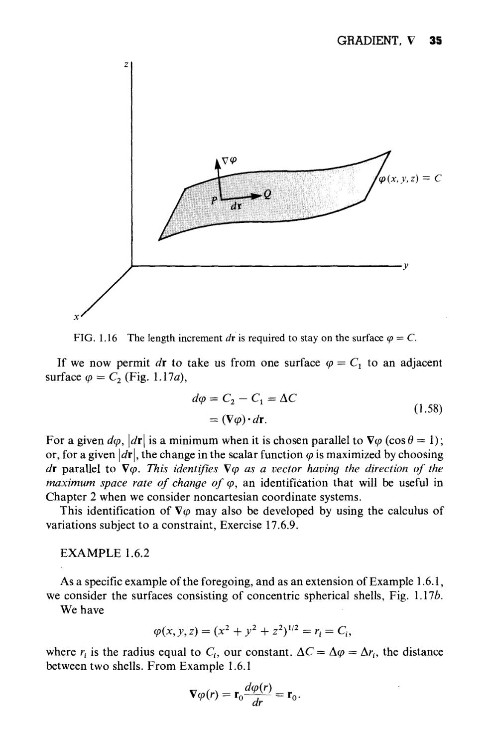
FIG. 1.16 The length increment dr is required to stay on the surface cp — С.
If we now permit dr to take us from one surface cp — C2 to an adjacent
surface cp = C2 (Fig. 1.17л),
dcp = C2 — Cl = AC
A.58)
For a given dcp, \dr\ is a minimum when it is chosen parallel to \cp (cos 0=1);
or, for a given |dr\, the change in the scalar function cp is maximized by choosing
dr parallel to V<p. This identifies \cp as a vector having the direction of the
maximum space rate of change of cp, an identification that will be useful in
Chapter 2 when we consider noncartesian coordinate systems.
This identification of \cp may also be developed by using the calculus of
variations subject to a constraint, Exercise 17.6.9.
EXAMPLE 1.6.2
As a specific example of the foregoing, and as an extension of Example 1.6.1,
we consider the surfaces consisting of concentric spherical shells, Fig. \.\lb.
We have
cp(x,y,z) = (x2 +y2+ z2I'2 = ri = Ch
where r{ is the radius equal to Ch our constant. AC = Acp = Ar,-, the distance
between two shells. From Example 1.6.1
dcp(r)
36 VECTOR ANALYSIS
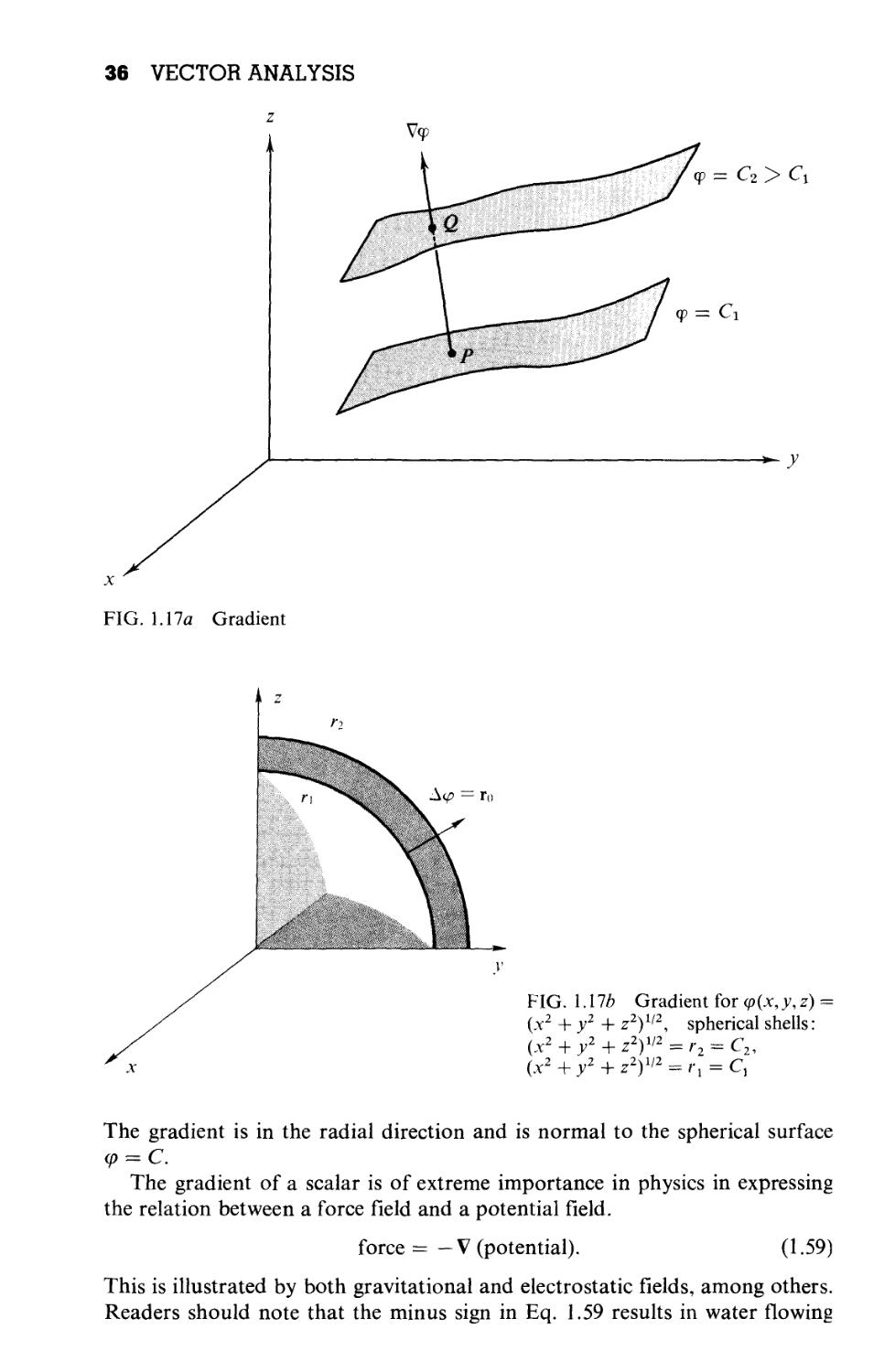
ф = Сг >
Ф =
■^ у
FIG. 1.17a Gradient
FIG. 1.176 Gradient for cp(x,y,z)
{x2 + y2 + z2I'2, spherical shells:
(x2 + y2 + z2I'2 = r2 = C2,
(x2 +y2 + z2I'2 = rj = C,
The gradient is in the radial direction and is normal to the spherical surface
q> = C.
The gradient of a scalar is of extreme importance in physics in expressing
the relation between a force field and a potential field.
force = — V (potential).
A.59)
This is illustrated by both gravitational and electrostatic fields, among others.
Readers should note that the minus sign in Eq. 1.59 results in water flowing
DIVERGENCE, V • 37
downhill rather than uphill! We reconsider Eq. 1.59 in a broader context in
Section 1.13.
EXERCISES
1.6.1 If S(x,y,z) = (x2 +y2 + z2)~3/2, find
(a) \S at the point A,2,3);
(b) the magnitude of the gradient of S,\\S\ at A,2,3);
and
(c) the direction cosines of VS at A,2,3).
1.6.2 (a) Find a unit vector perpendicular to the surface
x2 + y2 + z2 = 3
at the point A,1,1).
(b) Derive the equation of the plane tangent to the surface at A,1,1).
ANS. (a) (i + j V
(b) x + у + z = 3.
1.6.3 Given a vector r12 = i(xy — x2) + \(y1 — y2) + k(zy — z2), show that 4 Jr12 (gra-
(gradient with respect to xlf yt, and zv of the magnitude rl2) is a unit vector in the
direction of rx 2.
1.6.4 If a vector function F depends on both space coordinates (x, y, z) and time t, show
that
<3F
—dt.
at
1.6.5 Show that \(uv) = v\u + uSv, where и and v are differentiable scalar functions
of x, y, and z.
1.6.6 (a) Show that a necessary and sufficient condition that u(x,y, z) and v(x,y,z)
are related by some function/(w, v) = 0 is that (Vm) x (Vu) = 0.
(b) If и = u{x,y) and v = v(x,y), show that the condition (Vh) x (\v) = 0 leads
to the two-dimensional Jacobian
du
дх
dv
дх
du
ду
dv
ду
\x,y/
The functions и and v are assumed differentiable.
1.7 DIVERGENCE, V
Differentiating a vector function is a simple extension of differentiating
scalar quantities. Suppose r(z) describes the position of a satellite at some time
t. Then, for differentiation with respect to time,
r(t + At) - r(Q
lim
dt At-»o At
= v, linear velocity.
38 VECTOR ANALYSIS
FIG. 1.18 Differentiation of a vector
Graphically, we again have the slope of a curve, orbit, or trajectory, as shown
in Fig. 1.18.
If we resolve r(t) into its cartesian components, dr/dt always reduces directly
to a vector sum of not more than three (for three-dimensional space) scalar
derivatives. In other coordinate systems (Chapter 2) the situation is a little
more complicated, for the unit vectors are no longer constant in direction.
Differentiation with respect to the space coordinates is handled in the same
way as differentiation with respect to time, as seen in the following paragraphs.
In Section 1.6 V was defined as a vector operator. Now, paying careful
attention to both its vector and its differential properties, we let it operate on
a vector. First, as a vector we dot it into a second vector to obtain
V-V =
Bx By Bz
A.60)
known as the divergence of V. This is a scalar, as discussed in Section 1.3.
EXAMPLE 1.7.1
Calculate V • r.
V • г = i— + j— +
\ Bx By
_Bx By Bz
dx By Bz
Bz
(ix + }y + kz),
or
DIVERGENCE, V • 39
EXAMPLE 1.7.2
Generalizing Example 1.7.1,
г)+ £#+£&+*.&
r dr r dr r dr
The manipulation of the partial derivatives leading to the second equation in
Example 1.7.2 is discussed in Example 1.6.1.
In particular, if/(r) = rn~x,
V-ror"
= Ъгп~х + (п- l)^ A.60a)
This divergence vanishes for n = —2, an important fact in Section 1.14.
A PHYSICAL INTERPRETATION
To develop a feeling for the physical significance of the divergence, consider
\'(pv) with y(x,y,z), the velocity of a compressible fluid and p(x,y,z), its
density at point (x,y,z). If we consider a small volume dxdydz (Fig. 1.19), the
fluid flowing into this volume per unit time (positive x-direction) through the
face EFGH is (rate of flow in)£FGH = pvx\x=odydz. The components of the flow
pvy and pvz tangential to this face contribute nothing to the flow through this
face. The rate of flow out (still positive x-direction) through face ABCD is
pvx\x=dxdydz. To compare these flows and to find the net flow out, we expand
this last result in a Maclaurin series1, Section 5.6. This yields
(rate of flow out)^BCB = pvx\x=dxdydz
д
dydz.
Here the derivative term is a first correction term allowing for the possibility
of nonuniform density or velocity or both2. The zero-order term pvx\x=0
(corresponding to uniform flow) cancels out.
1A Maclaurin expansion for a single variable is given by Eq. 5.88, Section 5.6.
Here we have the increment x of Eq. 5.88 replaced by dx. We show a partial
derivative with respect to' x since pvx may also depend on у and z.
2 Strictly speaking, pvx is averaged over face EFGH and the expression
pvx + (d/dx)(pvx)dx is similarly averaged over face ABCD. Using an arbi-
arbitrarily small differential volume, we find that the averages reduce to the values
employed here.
40 VECTOR ANALYSIS
С
dz
G
D
H
F
*■ )
dy
FIG. 1.19 Differential rectangular parallelepiped (in first or positive octant)
Net rate of flow out |x = -—(pvx) dxdydz.
Equivalently, we can arrive at this result by
vx(Ax,0,0) - pvx@,0,0) 3 d[pvx(x,y,z)]
Ax
dx
0,0,0
Now the x-axis is not entitled to any preferred treatment. The preceding result
for the two faces perpendicular to the x-axis must hold for the two faces
perpendicular to the y-axis, with x replaced by у and the corresponding changes
for у and z: у -»z, z -»x. This is a cyclic permutation of the coordinates. A
further cyclic permutation yields the result for the remaining two faces of our
parallelepiped. Adding the net rate of flow out for all three pairs of surfaces of
our volume element, we have
net flow out
(per unit time)
ду
= V '(pv) dxdydz
dxdydz A.61)
Therefore the net flow of our compressible fluid out of the volume element
dxdydz per unit volume per unit time is V • (pv). Hence the name divergence. A
direct application is in the continuity equation
A.62)
which simply states that a net flow out of the volume results in a decreased
density inside the volume. Note that in Eq. 1.62 p is considered to be a possible
EXERCISES 41
function of time as well as of space: p(x,y,z, t). The divergence appears in a
wide variety of physical problems, ranging from a probability current density
in quantum mechanics to neutron leakage in a nuclear reactor.
The combination V • (/V), in which / is a scalar function and V a vector
function, may be written
+ v +f + v +
dx +dy y+J dy +<3z 2+/ dz
A.62a)
which is just what we would expect for the derivative of a product. Notice that
V as a differential operator differentiates both/and V; as a vector it is dotted
into V (in each term).
If we have the special case of the divergence of a vector vanishing,
V-B = 0, A.63)
the vector В is said to be solenoidal, the term coming from the example in
which В is the magnetic induction and Eq. 1.63 appears as one of Maxwell's
equations. When a vector is solenoidal it may be written as the curl of another
vector known as the vector potential. In Section 1.13 we shall calculate such a
vector potential.
EXERCISES
1.7.1 For a particle moving in a circular orbit r = ir cos cot + \r sin cot,
(a) evaluate r x r.
(b) Show that f.+ co2r = 0.
The radius r and the angular velocity со are constant.
ANS. (a) kcor2.
Note, r = dr/dt, f = d2r/dt2.
1.7.2 Vector A satisfies the vector transformation law, Eq. 1.15. Show directly that its
time derivative dAjdt also satisfies Eq. 1.15 and is therefore a vector.
1.7.3 Show, by differentiating components, that
/ ч d ,» „, ^A „ dB
(a) _(A.B)-_.B + A~,
(b) J(*xBL»BU»^,
dt dt dt
just like the derivative of the product of two algebraic functions.
1.7.4 In Chapter 2 it will be seen that the unit vectors in noncartesian coordinate systems
are usually functions of the coordinate variables, e, = e(gi,g2,g3) but |e,| = 1.
Show that either deAdqj = 0 or dejdc/j is orthogonal to e,.
1.7.5 Prove V-(a x b) = b-V x a-a-V x b.
Hint. Treat as a triple scalar product.
42 VECTOR ANALYSIS
1.7.6 The electrostatic field of a point charge q is
Лпг0 г2
Calculate the divergence of E. What happens at the origin?
1.8 CURL, Vx
Another possible operation with the vector operator V is to cross it into a
vector. We obtain
V x V = i
i J к
d d d
dx dy dz
К- К, К
A.64)
which is called the curl of V. In expanding this determinant form or in any
operation with V, we must consider the derivative nature of V. Specifically,
V x V is defined only as an operator, another vector differential operator. It is
certainly not equal, in general, to —V x V.1 In the case of Eq. 1.64 the deter-
determinant must be expanded from the top down so that we get the derivatives as
shown in the middle portion of Eq. 1.64. If V is crossed into the product of a
scalar and a vector, we can show
= f
dy dy
dz
A.65)
If we permute the coordinates x -»у, у -*■ z, z -»x to pick up the ^-component
and then permute them a second time to pick up the z-component,
V x (/V) =/V x V + (V/) x V,
A.66)
which is the vector product analog of Eq. 1.62a. Again, as a differential operator
V differentiates both/and V. As a vector it is crossed into V (in each term).
EXAMPLE 1.8.1
Calculate V x rf(r)
ByEq. 1.66
1 In this same spirit, if A is a differential operator, it is not necessarily true
that AxA = 0. Specifically, for the quantum mechanical angular momentum
operator, L = — i(r x V), we find that L x L = /L.
CURL, V x 43
V x rf(r) =f(r)\xr
x r.
First,
V x r =
= 0.
i J к
A A A
dx dy dz
x у z
Second, using V/(r) = ro(df/dr) (Example 1.6.1), we obtain
V x rf(r) =froxr = 0.
dr
A.67)
A.68)
A.69)
The vector product vanishes, since г = ror and r0 x r0 = 0.
To develop a better feeling for the physical significance of the curl, we
consider the circulation of fluid around a differential loop in the xy-plane,
Fig. 1.20.
Although the circulation is technically given by a vector line integral j V • dX
(Section 1.10), we can set up the equivalent scalar integrals here. Let us take
the circulation to be
circulation 1234 = Vx(x,y)dXx+\ Vy(x,y)dXy
A.70)
+ Vx(x,y)dXx+ Vy(x,y)dXy.
J 3 J4
The numbers 1,2, 3, and 4 refer to the numbered line segments in Fig. 1.20.
In the first integral dXx = +dx but in the third integral dXx — — dx because
the third line segment is traversed in the negative x-direction. Similarly, dXy =
+dy for the second integral, —dy for the fourth. Next, the integrands are
referred to the point (x0, y0) with a Taylor expansion2 taking into account the
у
Xo, Уо +
+ dx, yo + dy
+ dx, vc
-► x
FIG. 1.20 Circulation around a differential loop
2 Vy(x0 + dx,y0) = Vy(x0,y0)
dx +
The higher-order terms will drop out in the limit as dx ~* 0. A correction term
for the variation of Vy with у is canceled by the corresponding term in the
fourth integral (see Section 5.6).
44 VECTOR ANALYSIS
displacement of line segment 3 from 1 and 2 from 4. For our differential line
segments this leads to
circulation! 234 = Vx(x0,y0)dx +
dV
dy
ду
dxdy.
дх
(-dx)+VJxo,yo)(-dy) A.71)
\6х ду
Dividing by dx dy, we have
circulation per unit area = V x V|2. A-72)
The circulation3 about our differential area in the xy-plane is given by the
z-component of V x V. In principle, the curl, V x V at (xo,yo), could be
determined by inserting a (differential) paddle wheel into the moving fluid at
point (xo,^o). The rotation of the little paddle wheel would be a measure of the
curl.
We shall use the result, Eq. 1.71, in Section 1.13 to derive Stokes's theorem.
Whenever the curl of a vector V vanishes,
VxV = 0. A.73)
V is labeled irrotational. The most important physical examples of irrotational
vectors are the gravitational and electrostatic forces. In each case
У = СЦ=С~, A.74)
г г
where С is a constant and r0 is the unit vector in the outward radial direction.
For the gravitational case we have С = —Gm1m2, given by Newton's law of
universal gravitation. If С = qxq2jAm0, we have Coulomb's law of electro-
electrostatics (mks units). The force V given in Eq. 1.74 may be shown to be irrotational
by direct expansion into cartesian components as we did in Example 1.8.1.
Another approach is developed in Chapter 2, in which we express V x, the
curl, in terms of spherical polar coordinates. In Section 1.13 we shall see that
whenever a vector is irrotational, the vector may be written as the (negative)
gradient of a scalar potential. In Section 1.15 we shall prove that a vector may
be resolved into an irrotational part and a solenoidal part (subject to conditions
at infinity). In terms of the electromagnetic field this corresponds to the resolu-
resolution into an irrotational electric field and a solenoidal magnetic field.
For waves in an elastic medium, if the displacement u is irrotational,
V x u = 0, planes waves (or spherical waves at large distances) become longitu-
longitudinal. If u is solenoidal, V #u = 0, then the waves become transverse. A seismic
disturbance will produce a displacement that may be resolved into a solenoidal
sIn fluid dynamics V x V is called the "vorticity."
EXERCISES 45
part and an irrotational part (compare Section 1.15). The irrotational part
yields the longitudinal P (primary) earthquake waves. The solenoidal part
gives rise to the slower transverse S (secondary) waves, Exercise 3.6.8.
Using the gradient, divergence, and curl, and of course the BAC-CAB rule,
we may construct or verify a large number of useful vector identities. For
verification, complete expansion into cartesian components is always a possibil-
possibility. Sometimes if we use insight instead of routine shuffling of cartesian compo-
components, the verification process can be shortened drastically.
Remember that V is a vector operator, a hybrid creature satisfying two sets
of rules:
1. vector rules, and
2. partial differentiation rules—including differentia-
differentiation of a product.
EXAMPLE 1.8.2. Gradient of a Dot Product
Verify that
V(A-B) = (B-V)A + (A-V)B + B x (V x A) + A x (V x B). A.75)
This particular example hinges on the recognition that V(A • B) is the type of
term that appears in the BAC-CAB expansion of a triple vector product, Eq.
1.50. For instance,
A x (V x B) = V(A-B)-(A-V)B,
with the V differentiating only B, not A. From the commutativity of factors in
a scalar product we may interchange A and В and write
В x (V x A) = V(A-B)-(B»V)A,
now with V differentiating only A, not B. Adding these two equations, we
obtain V differentiating the product A-B and the identity, Eq. A.75).
This identity is used frequently in advanced electromagnetic theory. Exercise
1.8.15 is one simple illustration.
EXERCISES
1.8.1 Show, by rotating the coordinates, that the components of the curl of a vector
transform as a vector.
Hint. The direction cosine identities of Eq. 1.41 are available as needed.
1.8.2 Show that u x v is solenoidal if u and v are each irrotational.
1.8.3 If A is irrotational, show that A x г is solenoidal.
1.8.4 A rigid body is rotating with constant angular velocity w. Show that the linear
velocity v is solenoidal.
1.8.5 A vector function f(x,y,z) is not irrotational but the product of f and a scalar
46 VECTOR ANALYSIS
function g(x,y,z) is irrotational. Show that
f-V xf=0.
1.8.6 If (a) V = iVx(x,y)+jVy(x,y) and (b) VxV^O, prove that V x V is per-
perpendicular to V.
1.8.7 Classically, angular momentum is given by L = r x p, where p is the linear
momentum. To go from classical mechanics to quantum mechanics, replace p
by the operator —/V (Section 15.6). Show that the quantum mechanical angular
momentum operator has cartesian components
г
(in units of h).
1.8.8 Using the angular momentum operators previously given, show that they satisfy
commutation relations of the form
LAo Ly\ — LxLy — LyLx = iLz
and hence
L x L = /L.
These commutation relations will be taken later as the defining relations as an
angular momentum operator—Exercise 4.2.15 and the following one and Section
12.7.
1.8.9 With the commutator bracket notation \Lx,Ly~\ — LxLy — LyLx, the angular
momentum vector L satisfies [Lx, Ly~\ — iLz, etc. and so on, or L x L = /L.
Two other vectors a and b commute with each other and with L, that is, [a, b] =
[a, L] = [b, L] = 0. Show that
[a-L,b-L] = z(ax b)L.
1.8.10 For A = iAx(x,y, z) and В = iBx(x,y, z) evaluate each term in the vector identity
V(A • B) = (B • V)A + (A • V)B + В x (V x A) + A x (V x B)
and verify that the identity is satisfied.
1.8.11 Verify the vector identity
V x (A x B) = (B«V)A-(A-V)B-B(V«A) + A(V-B).
1.8.12 As an alternative to the vector identity of Example 1.8.2 show that
V(A-B) = (A x V) x B + (B x V) x A + A(V-B) + B(V • A).
1.8.13 Verify the identity
A x (V x A) = iV(v42) - (A-V)A.
1.8.14 If A and В are constant vectors, show that
V(A-B x r) = A x B.
SUCCESSIVE APPLICATIONS OF V 47
1.8.15 A distribution of electric currents creates a constant magnetic moment m. The
force on m in an external magnetic induction В is given by
F = V x (B x m).
Show that
F= V(m-B).
Note. Assuming no time dependence of the fields, Maxwell's equations yield
V x B = 0. AlsoV-B = 0.
1.8.16 An electric dipole of moment p is located at the origin. The dipole creates an
electric potential at г given by
Find the electric field, E = — V^ at r.
1.8.17 The vector potential A of a magnetic dipole, dipole moment m, is given by
A(r) = (до/4л:)(т x r/r3). Show that the magnetic induction В = V x A is given
by
B = Mo3ro(ro-m)-m
An r3
Note. The limiting process leading to point dipoles is discussed in Section 12.1
for electric dipoles, Section 12.5 for magnetic dipoles.
1.8.18 The velocity of a two-dimensional flow of liquid is given by
V = iu(x,y) — jv(x,y).
If the liquid is incompressible and the flow is irrotational show that
du dv , 8u dv
— ОПЛ ~~
dilU
дх dy ду дх
These are the Cauchy-Riemann conditions of Section 6.2.
1.8.19 The evaluation in this section of the four integrals for the circulation omitted
Taylor series terms such as dVJdx, dVy/dy and all second derivatives. Show that
dVJdx, dVy/dy cancel out when the four integrals are added and that the second
derivative terms drop out in the limit as dx -+0,dy-+ 0.
Hint. Calculate the circulation per unit area and then take the limit dx -* 0,
1.9 SUCCESSIVE APPLICATIONS OF V
We have now defined gradient, divergence, and curl to obtain vector,
scalar, and vector quantities, respectively. Letting V operate on each of these
quantities, we obtain
(a) \-\cp (b) VxVip (c) VV-V
(d) V • V x V (e) V x (V x V),
all five expressions involving second derivatives and all five appearing in the
48 VECTOR ANALYSIS
second-order differential equations of mathematical physics, particularly in
electromagnetic theory.
The first expression, V • \cp, the divergence of the gradient, is named the
Laplacian of ср. We have
• ^ , , д \ (. dcp . dcp , dcp
dy dz) \ dx dy dz,
A.76a)
.
,
dx2 dy2 dz2'
When (p is the electrostatic potential, we have
V-W = 0. A.766)
which is Laplace's equation of electrostatics. Often the combination V • V is
written V2.
EXAMPLE 1.9.1
Calculate \-\g(r).
Referring to Examples 1.6.1 and 1.7.2,
r dr dr2'
replacing/(r) in Example 1.7.2 by \\r-dg\dr. \ig{r) = r", this reduces to
V-Vr" = n(n + \)r"~2.
This vanishes for n = 0 \j}{r) = constant] and for n = — 1; that is, g(r) = \jr
is a solution of Laplace's equation, V2gf(r) = 0. This is for r ^ 0. At r = 0 a
Dirac delta function is involved (see Eq. 1.173 and Section 8.7).
Expression (b) may be written
A A A
dx dy dz
dcp dcp d(p
dx dy dz
By expanding the determinant, we obtain
\dy dz dz dy) \dz dx dx dz/ \dx dy dy dx)
= 0,
VxV(p=i
aVV
A.77)
assuming that the order of partial differentiation may be interchanged. This is
true as long as these second partial derivatives of cp are continuous functions.
SUCCESSIVE APPLICATIONS OF V 49
Then, from Eq. 1.77, the curl of a gradient is identically zero. All gradients,
therefore, are irrotational. Note carefully that the zero in Eq. 1.77 comes as a
mathematical identity, independent of any physics. The zero in Eq. 1.766 is a
consequence of physics.
Expression (d) is a triple scalar product which may be written
V-V x V =
A A A
дх ду dz
A A A
дх ду dz
V V V
A.78)
Again, assuming continuity so that the order of differentiation is immaterial,
we obtain
V-VxV = 0. A.79)
The divergence of a curl vanishes or all curls are solenoidal. In Section 1.15 we
shall see that vectors may be resolved into solenoidal and irrotational parts by
Helmholtz's theorem.
The two remaining expressions satisfy a relation
Vx(VxV) = W'V-V-VV. A.80)
This follows immediately from Eq. 1.50, the BAC-CAB rule, which we rewrite
so that С appears at the extreme right of each term. The term V • VV was not
included in our list, but it may be defined by Eq. 1.80. If V is expanded in
cartesian coordinates so that the unit vectors are constant in direction as well
as in magnitude, V • VV, a vector Laplacian, reduces to
V- VV = iV- \VX + jV • \Vy + kV- \VZ,
a vector sum of ordinary scalar Laplacians. By expanding in cartesian coor-
coordinates, we may verify Eq. 1.80 as a vector identity.
EXAMPLE 1.9.2 Electromagnetic Wave Equation
One important application of this vector relation (Eq. 1.80) is in the deriva-
derivation of the electromagnetic wave equation. In vacuum Maxwell's equations
become
VB = 0, A.81a)
V-E = 0, A.81b)
A.81c)
A.81a1)
VxE^p.
ot
Here E is the electric field, В the magnetic induction, e0 the electric permittivity,
SO VECTOR ANALYSIS
and fi0 the magnetic permeability (mks or SI units). Suppose we eliminate В
from Eqs. 1.81c and 1.8 Id. We may do this by taking the curl of both sides of
Eq. 1.8 Id and the time derivative of both sides of Eq. 1.81c. Since the space
and time derivatives commute,
A.82)
ci ci
and we obtain
Я21Г
A.83)
dt2
Application of Eqs. 1.80 and of 1.81b yields
the electromagnetic vector wave equation. Again, if E is expressed in cartesian
coordinates, Eq. 1.84 separates into three scalar wave equations, each involving
a scalar Laplacian.
EXERCISES
1.9.1 Verify Eq. 1.80
V x(V x V) = VVV- VVV
by direct expansion in cartesian coordinates.
1.9.2 Show that the identity
Vx(V x V) = VV-V- V-VV
follows from the BAC-CAB rule for a triple vector product. Justify any alteration
of the order of factors in the ВАС and CAB terms.
1.9.3 Prove that V x (<pV<p) = 0.
1.9.4 You are given that the curl of F equals the curl of G. Show that F and G may
differ by (a) a constant and (b) a gradient of a scalar function.
1.9.5 The Navier-Stokes equation of hydrodynamics contains a nonlinear term
(v'V)v. Show that the curl of this term may be written — V x [v x (V x v)].
1.9.6 From the Navier-Stokes equation for the steady flow of an incompressible
viscous fluid we have the term
V x [v x (V x v)]
where v is the fluid velocity. Show that this term vanishes for the special case
v = iv(y,z).
1.9.7 Prove that (Vw) x (Vu) is solenoidal where и and v are differentiable scalar
functions.
VECTOR INTEGRATION 51
1.9.8 q> is a scalar satisfying Laplace's equation, V2<p = 0. Show that V<p is both sole-
noidal and irrotational.
1.9.9 With ф a scalar function, show that
(r x V)-(r 22 2^ ^
гЧф r^ 2r.
or* or
(This can actually be shown more easily in spherical polar coordinates, Section
2.5).
1.9.10 In a (nonrotating) isolated mass such as a star, the condition for equilibrium is
\P + pV<p = 0.
Неге Р is the total pressure, p the density, and <p the gravitational potential.
Show that at any given point the normals to the surfaces of constant pressure
and constant gravitational potential are parallel.
1.9.11 In the Pauli theory of the electron one encounters the expression
(p - eA) x (p - еА)ф,
where ф is a scalar function. A is the magnetic vector potential related to the
magnetic induction В by В = V x A. Given that p = — /V, show that this ex-
expression reduces to /eBi//.
1.9.12 Show that any solution of the equation
V x V x A - k2A = 0
automatically satisfies the vector Helmholtz equation
V2A + k2A = 0
and the solenoidal condition
V-A = 0.
Hint. Let V • operate on the first equation.
1.9.13 The theory of heat conduction leads to an equation
where Ф is a potential satisfying Laplace's equation: V2<D = 0. Show that a solu-
solution of this equation is
1.10 VECTOR INTEGRATION
The next step after differentiating vectors is to integrate them. Let us start
with line integrals and then proceed to surface and volume integrals. In each
case the method of attack will be to reduce the vector integral to scalar integrals
with which the reader is assumed familiar.
Line Integrals
Using an increment of length dr = i dx + j dy + к dz, we may encounter the
line integrals
52 VECTOR ANALYSIS
Г
A.85a)
A.856)
A.85c)
in each of which the integral is over some contour С that may be open (with
starting point and ending point separated) or closed (forming a loop). Because
of its physical interpretation that follows, the second form, Eq. 1.856 is by far
the most important of the three.
With (p, a scalar, the first integral reduces immediately to
= i (p(x,y,z)dx + j cp(x,y,z)dy
J
+ k q>(x,y,z)dz.
J с
This separation has employed the relation
\icp dx = i \cp dx, A-87)
J J
which is permissible because the cartesian unit vectors i, j, and к are constant
in both magnitude and direction. Perhaps this relation is obvious here, but it
will not be true in the noncartesian systems encountered in Chapter 2.
The three integrals on the right side of Eq. 1.86 are ordinary scalar integrals
and, to avoid complications, we assume that they are Riemann integrals. Note,
however, that the integral with respect to x cannot be evaluated unless у and z
are known in terms of x and similarly for the integrals with respect to у and z.
This simply means that the path of integration С must be specified. Unless the
integrand has special properties that lead the integral to depend only on the
value of the end points, the value will depend on the particular choice of
contour С For instance, if we choose the very special case cp = 1, Eq. 1.85л is
just the vector distance from the start of contour С to the end point, in this
case independent of the choice of path connecting fixed end points. With
dx — \dx + jdy + kdz, the second and third forms also reduce to scalar
integrals and, like Eq. 1.85л, are dependent, in general, on the choice of path.
The form (Eq. 1.856) is exactly the same as that encountered when we calculate
the work done by a force that varies along the path,
W= \F-dr
A.88a)
= \Fx(x,y,z)dx+ \Fy(x,y,z)dy+ \Fz(x,y,z)dz.
In this expression F is the force exerted on a particle.
VECTOR INTEGRATION 53
EXAMPLE 1.10.1
The force exerted on a body is F = — \y + jx. The problem is to calculate
the work done going from the origin to the point A,1).
W= Г ' F-rfr= Г ' (-ydx + xdy). AMb)
Jo,o Jo,o
Separating the two integrals, we obtain
W= - Г ydx + Г xdy. A.88c)
Jo Jo
The first integral cannot be evaluated until we specify the values of у as x
ranges from 0 to 1. Likewise, the second integral requires x as a function of y.
Consider first the path shown in Fig. 1.21. Then
A.88Л)
since у = 0 along the first segment of the path and x = 1 along the second.
If we select the path [x"= 0,0 < у < 1] and [0 < x < I,y = 1], then Eq.
1.88c gives W= — 1. For this force the work done depends on the choice of
path.
W= -| Odx+ Г ldy= 1,
J
У
A,1)
0,0)
FIG. 1.21 A path of integration
Surface Integrals
Surface integrals appear in the same forms as line integrals, the element of
area also being a vector, dc.1 Often this area element is written n dA in which
n is a unit (normal) vector to indicate the positive direction.2 There are two
conventions for choosing the positive direction. First, if the surface is a closed
surface, we agree to take the outward normal as positive. Second, if the surface
1 Recall that in Section 1.4 the area (of a parallelogram) represented a cross-
product vector.
2 Although n always has unit length, its direction may well be a function of
position.
54 VECTOR ANALYSIS
FIG. 1.22 Right-hand rule for the
positive normal
is an open surface, the positive normal depends on the direction in which the
perimeter of the open surface is traversed. If the right-hand fingers are placed
in the direction of travel around the perimeter, the positive normal is indicated
by the thumb of the right hand. As an illustration, a circle in the .xy-plane
(Fig. 1.22) mapped out from x to у to — x to —y and back to x will have its
positive normal parallel to the positive z-axis (for the right-handed coordinate
system). If readers should ever encounter one-sided surfaces, such as Moebius
strips, it is suggested that they either cut the strips and form reasonable, well-
behaved surfaces or label them pathological and send them to the nearest
mathematics department.
Analogous to the line integrals, Eqs. 1.85л, b, c, surface integrals may
appear in the forms
cpda
У-da
V x da.
Again, the dot product is by far the most commonly encountered form.
The surface integral j V • da may be interpreted as a flow or flux through the
given surface. This is really what we did in Section 1.7 to obtain the significance
of the term divergence. This identification reappears in Section 1.11 as Gauss's
theorem. Note that both physically and from the dot product the tangential
components of the velocity contribute nothing to the flow through the surface.
Volume Integrals
Volume integrals are somewhat simpler, for the volume element dx is a
scalar quantity.3 We have
3Frequently the symbols d3r and d3x are used to denote a volume element in
x (xyz or xix2x3) space.
VECTOR INTEGRATION 55
= i Vxdx+\\ Vydx + k\ Vzdx, A.89)
Jv Jv Jv Jv
again reducing the vector integral to a vector sum of scalar integrals.
Integral Definitions of Gradient, Divergence,
and Curl
One interesting and significant application of our surface and volume
integrals is their use in developing alternate definitions of our differential
relations. We find
\q>= hm
JdO
V= hm i-j-j—,
dt^o J dx
= lim
J
J dx
A.90)
A.91)
A.92)
In these three equations \ dx is the volume of a small region of space and da
is the vector area element of this volume. The identification of Eq. 1.91 as the
divergence of V was carried out in Section 1.7. Here we show that Eq. 1.90 is
consistent with our earlier definition of V<p (Eq. 1.53). For simplicity we choose
\dx to be the differential volume dxdydz (Fig. 1.23). This time we place the
С
-у
в
FIG. 1.23 Differential rectangular parallelepiped (origin at center)
origin at the geometric center of our volume element. The area integral leads
to six integrals, one for each of the six faces. Remembering that dc is outward,
dtj'i = —\da\ for surface EFHG, and +\da\ for surface ABDC, we have
\(p da = — i
abdc
56 VECTOR ANALYSIS
aegA 8У 2J Jbfhd
Jabfe\ 8z 2J Jcdhg\ dz 2/
Using the first two terms of a Maclaurin expansion, we evaluate each integrand
at the origin with a correction included to correct for the displacement (±dx/2)
of the center of the face from the origin.4 Having chosen the total volume to be
of differential size (\dx = dxdydz), we drop the integral signs on the right and
obtain
A.93)
j \ ex oy czj
Dividing by
\dx = dx dy dz,
J
we verify Eq. 1.90.
This verification has been oversimplified in ignoring other correction terms
beyond the first derivatives. These additional terms, which are introduced in
Section 5.6 when the Taylor expansion is developed, vanish in the limit
\dx -* 0 (dx -> 0, dy -*0,dz-+ 0).
This, of course, is the reason for specifying in Eqs. 1.90, 1.91, and 1.92 that this
limit be taken.
Verification of Eq. 1.92 follows these same lines exactly, using a differential
volume dxdydz.
EXERCISES
1.10.1 The force field acting on a two-dimensional linear oscillator may be described by
F = — \kx — \ky.
Compare the work done moving against this force field when going from A,1)
to D,4) by the following straight-line paths:
(a) A,1)-D,1)-» D,4)
(b) A,1)-A,4)-D,4)
(c) A,1) —D,4)alongjc = j;.
This means evaluating
fD,4)
F-Jr
along each path.
;The origin has been placed at the geometric center.
GAUSS'S THEOREM 57
1.10.2 Find the work done going around a unit circle in the xy-plane:
(a) counterclockwise from 0 to n,
(b) clockwise from 0 to —n,
doing work against a force field given by
— 2 2 ' 2 . 2 *
Л'2 + >>2 X2 + у2
Note that the work done depends on the path.
1.10.3 Calculate the work you do in going from point A,1) to point C,3). The force
you exert is given by
F = i(x - y) + j(x + y).
Specify clearly the path you choose. Note that this force field is nonconservative.
1.10.4 Evaluate & г -dr.
Note. The symbol $ means that the path of integration is a closed loop.
1.10.5 Evaluate
over the unit cube defined by the point @,0,0) and the unit intercepts on the
positive х-, у-, and z-axes. Note that (a) r-da is zero for three of the surfaces
and (b) each of the three remaining surfaces contributes the same amount to
the integral.
1.10.6 Show, by expansion of the surface integral, that
hm i~ = V x V.
/л-o j dx
Hint. Choose the volume to be a differential volume, dxdydz.
1.11 GAUSS'S THEOREM
Here we derive a useful relation between a surface integral of a vector and
the volume integral of the divergence of that vector. Let us assume that the
vector V and its first derivatives are continuous over the region of interest.
Then Gauss's theorem states that
Г \-dc= j \-\dx. A.94a)
In words, the surface integral of a vector over a closed surface equals the
volume integral of the divergence of that vector integrated over the volume
enclosed by the surface.
Imagine that volume V is subdivided into an arbitrarily large number of
tiny (differential) parallelepipeds. For each parallelepiped
A.946)
six surfaces
from the analysis of Section 1.7, Eq. 1.61, with p\ replaced by V. The summa-
58 VECTOR ANALYSIS
J
FIG. 1.24 Exact cancellation of ato's on interior
surfaces. No cancellation on exterior surface.
tion is over the six faces of the parallelepiped. Summing over all parallelepipeds,
we find that the V • db terms cancel (pairwise) for all interior faces; only the
contributions of the exterior surfaces survive (Fig. 1.24). Analogous to the
definition of a Riemann integral as the limit of a sum, we take the limit as the
number of parallelepipeds approaches infinity (-♦ со) and the dimensions of
each approach zero (-> 0).
\-Vdz
exterior surfaces
volumes
1
1
Г \-d<s= I \-\dt
J S JV
The result is Eq. 1.94л, Gauss's theorem.
From a physical point of view Eq. 1.61 has established V-V as the net
outflow of fluid per unit volume. The volume integral then gives the total net
outflow. But the surface integral j V* Jcr is just another way of expressing this
same quantity, which is the equality, Gauss's theorem.
GREEN'S THEOREM
A frequently useful corollary of Gauss's theorem is a relation known as
Green's theorem. If и and v are two scalar functions, we have the identities
A.95)
A.96)
V • (и щ = и V • \v + (\u) • (Vt>),
V • (v Vm) = v V • \u + (\v) • (Vm).
Subtracting Eq. 1.96 from Eq. 1.95, integrating over a volume (w, v, and their
derivatives, assumed continuous), and applying Eq. 1.94 (Gauss's theorem),
we obtain
v\''S/u)dx=\ (uVv- v\u)-da. A.97)
Jv Js
This is Green's theorem. We use it for developing Green's functions, Chapters
GAUSS'S THEOREM 59
8 and 16. An alternate form of Green's theorem derived from Eq. 1.95 alone is
u\vdo = uV'\vdT+ \u-\vdr. A.98)
Js Jv Jv
This is the form of Green's theorem used in Section 1.15.
ALTERNATE FORMS OF GAUSS'S THEOREM
Although Eq. 1.94 involving the divergence is by far the most important
form of Gauss's theorem, volume integrals involving the gradient and the curl
may also appear. Suppose
V(xj,z)=F(xj!z)a, A.99)
in which a is a vector with constant magnitude and constant but arbitrary
direction. (You pick the direction, but once you have chosen it, hold it fixed.)
Equation 1.94 becomes
a- Vda= Г V
•^ ^v A.100)
= a- Г \Vdx
Jv
by Eq. 1.62a. This may be rewritten
a
Vdo- Wdx
= 0. A.101)
-J S Jv
Since |a| Ф 0 and its direction is arbitrary, meaning that the cosine of the
included angle cannot always vanish, the term in brackets must be zero.1 The
result is
j Vda= j MVdx. A.102)
Js Jv
In a similar manner, using V = a x P in which a is a constant vector, we may
show
Г do x P= V x Prfr. A.103)
Js Jv
These last two forms of Gauss's theorem are used in the vector form of Kirchhoff
diffraction theory. They may also be used to verify Eqs. 1.90 and 1.92.
Gauss's theorem may also be extended to dyadics or tensors (see Section
3.5).
is exploitation of the arbitrary nature of a part of a problem is a valuable
and widely used technique. The arbitrary vector is used again in Sections 1.12
and 1.13. Other examples appear in Section 1.14 (integrands equated) and in
Section 3.3, quotient rule.
60 VECTOR ANALYSIS
EXERCISES
1.11.1 Using Gauss's theorem prove that
Г da = 0,
Js
if 5 is a closed surface.
1.11.2 Show that
Js
where V is the volume enclosed by the closed surface
Note. This is a generalization of Exercise 1.10.5.
1.11.3 If В = V x A, show that
for any closed surface 5.
1.11.4 Over some volume V let ф be a solution of Laplace's equation (with the deriva-
derivatives appearing there continuous). Prove that the integral over any closed
surface in V of the normal derivative of ф, (дф/дп, or \ф • n) will be zero.
1.11.5 In analogy to the integral definitions of gradient, divergence, and curl of Section
1.10, show that
Jdt-0 J dt
1.11.6 The electric displacement vector D satisfies the Maxwell equation V-D = p
where p is the charge density (per unit volume). At the boundary between two
media there is a surface charge density о (per unit area). Show that a boundary
condition for D is
(D2-D1)-n = <r.
n is a unit vector normal to the surface and out of medium 1.
Hint. Consider a thin pillbox as shown in the figure.
1.11.7 From Eq. 1.62a with V the electric field E, and /the electrostatic potential q>,
show that
\ pq>dx = £Q \ E2 dx.
J J
This corresponds to a three-dimensional integration by parts.
Hint. E = — V<p, V-E = p/s0. You may assume that cp vanishes at large r at
least at fast as r~\
1.11.8 A particular steady-state electric current distribution is localized in space.
Choosing a bounding surface far enough out so that the current density J is zero
STOKES'S THEOREM 61
everywhere on the surface, show that
Hint. Take one component of J at a time. With V • J = 0, show that J; = V • xt J
and apply Gauss's theorem.
1.11.9 The creation of a localized system of steady electric currents (current density
J) and magnetic fields may be shown to require an amount of work
W=\ \H-Bdx.
Transform this into
W=\ \i-Kdx.
Here A is the magnetic vector potential: V x A = B.
Hint. In Maxwell's equations take the displacement current term dD/dt = 0.
If the fields and currents are localized, a bounding surface may be taken far
enough out so that the integrals of the fields and currents over the surface
yield zero.
1.11.10 Prove the generalization of Green's theorem:
{v<£u - u<£v)dx = р(иЩ - uS/v)-d<s.
Here S£ is the self-adjoint operator (Section 9.1):
and p, q, u, and v are functions of position, p and q having continuous first
derivatives and и and v having continuous second derivatives.
Note. This generalized Green's theorem appears in Sections 8.7 and 16.6.
1.12 STOKES'S THEOREM
Gauss's theorem relates the volume integral of a derivative of a function to
an integral of the function over the closed surface bounding the volume. Here
we consider an analogous relation between the surface integral of a derivative
of a function and the line integral of the function, the path of integration being
the perimeter bounding the surface.
Let us take the surface and subdivide it into a network of arbitrarily small
rectangles. In Section 1.8 we showed that the circulation about such a differen-
differential rectangle (in the xy-plane) is V x V\zdxdy. From Eq. 1.71 applied to one
differential rectangle
A.104)
four sides
We sum over all the little rectangles as in the definition of a Riemann integral.
The surface contributions (right-hand side of Eq. 1.104) are added together.
The line integrals (left-hand side of Eq. 1.104) of all interior line segments cancel
62 VECTOR ANALYSIS
t
t
FIG. 1.25 Exact cancellation on
interior paths. No cancellation on
exterior path.
identically. Only the line integral around the perimeter survives (Fig. 1.25).
Taking the usual limit as the number of rectangles approaches infinity while
dx -» 0, dy -» 0, we have
\-dl=
\x\-do
exterior
line segments
rectangles
= Vx У-da.
A.105)
This is Stokes's theorem. The surface integral on the right is over the surface
bounded by the perimeter or contour for the line integral on the left.
This demonstration of Stokes's theorem is limited by the fact that we used a
Maclaurin expansion of \(x,y, z) in establishing Eq. 1.71 in Section 1.8.
Actually we need only demand that the curl of \(x,y, z) exists and that it be
integrable over the surface. A proof of the Cauchy integral theorem analogous
to the development of Stokes's theorem here but using these less restrictive
conditions appears in Section 6.3.
Stokes's theorem obviously applies to an open surface. It is possible to con-
consider a closed surface as a limiting case of an open surface with the opening (and
therefore the perimeter) shrinking to zero. This is the point of Exercise 1.12.7.
ALTERNATE FORMS OF STOKES'S THEOREM
As with Gauss's theorem, other relations between surface and line integrals
are possible. We find.
da x
= cb
J
and
(do x\)xP= idlxP.
A.106)
A.107)
Equation 1.106 may readily be verified by the substitution V = щ in which a
is a vector of constant magnitude and of constant direction, as in Section 1.11.
EXERCISES 63
Substituting into Stokes's theorem, Eq. 1.105,
(V x a<p) • da = — a x \q> • da
Js Js
Г 17 А AЛ08)
= -a- \ \<p x do.
Js
For the line integral
A.109)
and we obtain
fh = 0. A.110)
Since the choice of direction of a is arbitrary, the expression in parentheses
must vanish, thus verifying Eq. 1.106. Equation 1.107 may be derived similarly
by using V = a x P, in which a is again a constant vector.
Both Stokes's and Gauss's theorems are of tremendous importance in a wide
variety of problems involving vector calculus. Some idea of their power and
versatility may be obtained from the exercises of Sections 1.11 and 1.12 and the
development of potential theory in Sections 1.13 and 1.14.
EXERCISES
1.12.1 Given a vector t = — \y + jx. With the help of Stokes's theorem, show that
the integral around a continuous closed curve in the xy-plane
Г Г
\ i)t-^ = U (xdy - ydx) = A,
J J
the area enclosed by the curve.
1.12.2 The calculation of the magnetic moment of a current loop leads to the line
integral
<pr x dr.
J
(a) Integrate around the perimeter of a current loop (in the xy-plane) and
show that the scalar magnitude of this line integral is twice the area of
the enclosed surface.
(b) The perimeter of an ellipse is described by г = ia cos 0 + \b sin 0. From
part (a) show that the area of the ellipse is nab.
1.12.3 Evaluate jr x dr by using the alternate form of Stokes's theorem given by
Eq. 1.107:
Take the loop to be entirely in the xy-plane.
64 VECTOR ANALYSIS
1.12.4 In steady state the magnetic field H satisfies the Maxwell equation V x H = J,
where J is the current density (per square meter). At the boundary between
two media there is a surface current density К (per meter). Show that a boundary
condition on H is
n x (H2-Hi) = K.
n is a unit vector normal to the surface and out of medium 1.
Hint. Consider a narrow loop perpendicular to the interface as shown in the
figure.
medium 2
medium 1
1.12.5 From Maxwell's equations, V x H = J with J here the current density and
E = 0. Show from this that
where / is the net electric current enclosed by the loop integral. These are the
differential and integral forms of Ampere's law of magnetism.
1.12.6 A magnetic induction В is generated by electric current in a ring of radius R.
Show that the magnitude of the vector potential A (B = V x A) at the ring is
where q> is the total magnetic flux passing through the ring.
Note. A is tangential to the ring.
1.12.7 Prove that
Г V x V-J<r = 0,
Js
if 5 is a closed surface.
1.12.8 Evaluate §r-dr (Exercise 1.10.4) by Stokes's theorem.
1.12.9 Prove that
Г Г
<bu\rvd'k = — <bv\u-d'k.
J J
1.12.10 Prove that
&db= Г (Vwjx (\v)-d<s.
1.13 POTENTIAL THEORY
Scalar Potential
If a force over a given region of space S can be expressed as the negative
gradient of a scalar function cp,
POTENTIAL THEORY 65
F=-Vq>, A.111)
we call cp a scalar potential. The force F appearing as the negative gradient of
a single-valued scalar potential is labeled a conservative force. We want to know
when a scalar potential function exists. To answer this question we establish
two other relations as equivalent to Eq. 1.111. These are
VxF = 0 A.112)
and
<j)F-ufr = O, A.113)
for every closed path in our region S. We proceed to show that each of these
three equations implies the other two.
Let us start with
F • dx = — ф \q> • dx
F= -\<p. A.114)
Then
VxF=-VxV<p = 0 A.115)
by Eq. 1.77 or Eq. 1.111 implies Eq. 1.112. Turning to the line integral, we have
A.116)
using Eq. 1.56. Now dcp integrates to give ср. Since we have specified a closed
loop, the end points coincide and we get zero for every closed path in our
region S for which Eq. 1.111 holds. It is important to note the restriction here
that the potential be single-valued and that Eq. 1.111 hold for all points in S.
This problem may arise in using a scalar magnetic potential, a perfectly valid
procedure as long as no net current is encircled. As soon as we choose a path
in space that encircles a net current, the scalar magnetic potential ceases to be
single-valued and our analysis no longer applies.
Continuing this demonstration of equivalence, let us assume that Eq. 1.113
holds. If §F'dx = 0 for all paths in S, we see that the value of the integral
joining two distinct points A and В is independent of the path (Fig. 1.26). Our
premise is that
<j) F-dx = 0. A.117)
J ACBDA
Therefore
Г Г Г
A.118)
66 VECTOR ANALYSIS
D
В
FIG. 1.26 Possible paths for doing work
reversing the sign by reversing the direction of integration. Physically, this
means that the work done in going from A to В is independent of the path and
that the work done in going around a closed path is zero. This is the reason for
labeling such a force conservative: Energy is conserved.
With the result shown in Eq. 1.118, we have the work done dependent only
on the end points, A and B. That is,
work done by force =
= (p(A)-cp(B).
A.119)
Eq. 1.119 defines a scalar potential (strictly speaking, the difference in potential
between points A and B) and provides a means of calculating the potential. If
point В is taken as a variable, say, (x,y,z), then differentiation with respect to
x, y, and z will recover Eq. 1.111.
The choice of sign on the right-hand side is arbitrary. The choice here is made
to achieve agreement with Eq. 1.111 and to ensure that water will run downhill
rather than uphill. For points A and В separated by a length dr, Eq. 1.119
becomes
This may be rewritten
F'dr = —dcp
= — \qydr
(F + \q>) - dr = 0,
A.120)
A.121)
and since dr is arbitrary, Eq. 1.111 must follow.
If
F • dr = 0,
A.122)
POTENTIAL THEORY 67
we may obtain Eq. 1.112 by using Stokes's theorem (Eq. 1.109).
F• dx = \\ xF-da.
A.123)
If we take the path of integration to be the perimeter of an arbitrary differential
area da, the integrand in the surface integral must vanish. Hence Eq. 1.113
implies Eq. 1.114.
Finally, if V x F = 0, we need only reverse our statement of Stokes's
theorem (Eq. 1.123) to derive Eq. 1.113. Then, by Eqs. 1.119 to 1.121, the
initial statement F = — \cp is derived. The triple equivalence is demonstrated
(Fig. 1.27).
F= -Vp(l.lll)
V x F = 0A.112)
FIG. 1.27 Equivalent formulations
To summarize, a single-valued scalar potential function cp exists if and only
if F is irrotational or the work done around every closed loop is zero. The
gravitational and electrostatic force fields given by Eq. 1.75 are irrotational and
therefore are conservative. Gravitational and electrostatic scalar potentials
exist. Now, by calculating the work done (Eq. 1.119), we proceed to determine
three potentials, Fig. 1.28.
EXAMPLE 1.13.1 Gravitational Potential
Find the scalar potential for the gravitational force on a unit mass mx,
_ Gmlm2r0_ kr0
r r
By integrating Eq. 1.111 from infinity into position r, we obtain
(Pair)-
FG-dr.
A.125)
By use of FG = — Fapplied, a comparison with Eq. 1.88 shows that the potential
is the work done in bringing the unit mass in from infinity. (We can define only
potential difference. Here we arbitrarily assign infinity to be a zero of potential.)
The integral on the right-hand side of Eq. 1.125 is negative, meaning that <pG(r)
68 VECTOR ANALYSIS
is negative. Since FG is radial, we obtain a contribution to cp only when dx is
radial or
, ч Г00 kdr k
yj. r
t/ Г
_ Gmxm2
The final negative sign is a consequence of the attractive force of gravity.
EXAMPLE 1.13.2 Centrifugal potential
Calculate the scalar potential for the centrifugal force per unit mass, Fc =
co2rr0, radially outward. Physically, this might be you on a large horizontal
spinning disk at an amusement park. Proceeding as in Example 1.13.1, but
integrating from the origin outward and taking фс@) = О, we have
q>c(r)= - Fc-dr=~
co2r2
If we reverse signs, taking FSHO= —кг, we obtain <р8но— ikr2, the simple
harmonic oscillator potential.
*- r
FIG. 1.28 Potential energy versus distance (gravitational, centrifugal, and simple
harmonic oscillator)
The gravitational, centrifugal, and simple harmonic oscillator potentials are
shown in Fig. 1.28. Clearly, the simple harmonic oscillator yields stability and
POTENTIAL THEORY 69
describes a restoring force. The centrifugal potential describes an unstable
situation.
THERMODYNAMICS—EXACT
DIFFERENTIALS
In thermodynamics, which is sometimes called a search for exact differentials,
we encounter equations of the form
df= P(x,y)dx + Q(x,y)dy. A.126)
The usual problem is to determine whether j (P(x, y) dx + Q(x,y)dy) depends
only on the end points, that is, whether df is indeed an exact differential. The
necessary and sufficient condition is that
Y^-dy A.126a)
or that
A.126ft)
Equations 1.1266 depend on the relation
BP(x,y)^BQ(x,y)
dy dx
being satisfied. This, however, is exactly analogous to Eq. 1.116, the requirement
that F be irrotational. Indeed, the z-component of Eq. 1.116 yields
Vector Potential
In some branches of physics, especially electromagnetic theory, it is con-
convenient to introduce a vector potential A, such that a (force) field В is given by
B = VxA. A.127)
Clearly, if Eq. 1.127 holds, VB = 0 by Eq. 1.79 and В is solenoidal. Here we
want to develop a converse, to show that when В is solenoidal a vector potential
A exists. We demonstrate the existence of A by actually calculating it. Suppose
В = ibt + \b2 + kft3 and our unknown A = iax + \a2 + ka3. By Eq. 1.127
*.. 0.128a)
dy dz
70 VECTOR ANALYSIS
^-^ = 63. 0.128c)
ox oy
Let us assume that the coordinates have been chosen so that A is parallel to the
^z-plane; that is, ax = 0.1 Then
b - -
8°3
дх
A.129)
г~~дх~'
Integrating, we obtain
а2 = b3dx+f2(y,z),
A.130)
а3= - b2dx+f3(y,z),
Jx0
where /2 and f3 are arbitrary functions of у and z but are not functions of x.
These two equations can be checked by differentiating and recovering Eq.
1.129. Eq. 1.128a becomes
да-, да? Сx (db*, дЬЛ , d1\ df7
dy dz J V ^y ^z / дУ dz
A.131)
— I ~~^ MA "T" 9
J ex C7 5z
using V • В = 0. Integrating with respect to x, we obtain
da-, da-, , , , . ч 5Д 5A 1Л 1-^1ч
Remembering that/3 and/2 are arbitrary functions of у and z, we choose
/2=0,
Г A.133)
/3 = V^o,.^)^,
so that the right-hand side of Eq. 1.132 reduces to bl(x,y, z) in agreement with
Equation 1.128я. With/2 and/3 given by Eq. 1.133, we can construct A.
b3(x,y,z)dx +k b^Xo,^^)^- b2{x,y,z)dx
. A.134)
This is not quite complete. We may add any constant since В is a derivative of
1 Clearly, this can be done at any one point. It is not at all obvious that this
assumption will hold at all points; that is, A will be two dimensional. The
justification for the assumption is that it works; Eq. 1.134 satisfies Eq. 1.127.
POTENTIAL THEORY 71
A. What is much more important, we may add any gradient of a scalar function
\q> without affecting В at all. Finally, the functions /2 and /3 are not unique.
Other choices could have been made. It will be seen in Section 1.15 that we may
still specify V • A.
EXAMPLE 1.13.3 A Magnetic Vector Potential for a Constant Magnetic
Field
To illustrate the construction of a magnetic vector potential, we take the
special but still important case of a constant magnetic induction
B = kBz, A.135)
in which Bz is a constant. Equation 1.128 becomes
даъ da2 = Q
dy dz
^^ 0, A.136)
dz dx
да2 dax _ „
dx dy
If we assume that ax = 0, as before, then by Eq. 1.134
A = jf Bzdx
J
A.137)
setting a constant of integration equal to zero. It can readily be seen that this A
satisfies Eq. 1.127.
To show that the choice at = 0 was not sacred or at least not required, let us
try setting аъ = 0. From Eq. 1.136
^ 0, A.138a)
0,
dz
^ 0, A.1386)
^ 0,
dz
^ Дг. A.138с)
dx dy
We see ax and a2 are independent of z or
al=a1(x,y), a2 = a2(x,y). A.139)
Equation 1.138c is satisfied if we take
a2=P\ Bzdx=pxBz A.140)
72 VECTOR ANALYSIS
and
a,={p~ 1) ["Bzdy = (p- l)yBg, A.141)
with p any constant. Then
A = i(p-\)yBz+jpxBz. A.142)
Again, Eqs. 1.127, 1.135, and 1.142 are seen to be consistent. Comparison of
Eqs. 1.137 and 1.142 shows immediately that A is not unique. The difference
between Eqs. 1.137 and 1.142 and the appearance of the parameter^ in Eq.
1.142 may be accounted for by rewriting Eq. 1.142 as
A =-±(iy - }x)Bz
+ (P - i)(iy + V)Bt A.143)
with
cp = xy. A.144)
The first term in A corresponds to the usual form
A = i(Bxr) A.145)
for B, a constant.
To summarize this discussion of the vector potential, when a vector В is
solenoidal, a vector potential A exists such that В = V x A. A is undetermined
to within an additive gradient. This corresponds to the arbitrary zero of poten-
potential, a constant of integration for the scalar potential.
In many problems the magnetic vector potential A will be obtained from the
current distribution that produces the magnetic induction B. This means solving
Poisson's (vector) equation (see Exercise 1.14.4).
EXERCISES
1.13.1 If a force F is given by
F = (x2 + y2 + z2)"(ix + iy + kz),
find
(a) V-F,
(b) VxF,
(c) A scalar potential cp(x,y,z) so that F = — S(p.
(d) For what value of the exponent n does the scalar potential diverge at both
the origin and infinity?
ANS. (a) Bn + 3)r2n (c) —r2n+2, пф-\
in+ 2
(b) 0 (d) n= -1, cp= -lnr.
EXERCISES 73
1.13.2 A sphere of radius a is uniformly charged (throughout its volume). Construct
the electrostatic potential <p(r) for 0 < r < со.
Hint. In Section 1.14 it is shown that the Coulomb force on a test charge at
r = rQ depends only on the charge at distances less than rQ and is independent
of the charge at distances greater than r0. Note that this applies to a spherically
symmetric charge distribution.
1.13.3 The usual problem in classical mechanics is to calculate the motion of a particle
given the potential. For a uniform density (p0), nonrotating massive sphere,
Gauss's law of Section 1.14 leads to a gravitational force on a unit mass m0
at a point r0 produced by the attraction of the mass at r < r0. The mass at
r > rQ contributes nothing to the force.
(a) Show that F/ra0 = — DnGpQj3)r, 0 < r < a where a is the radius of the
sphere.
(b) Find the corresponding gravitational potential, 0 < r < a.
(c) Imagine a vertical hole running completely through the center of the earth
and out to the far side. Neglecting the rotation of the earth and assuming
a uniform density pQ = 5.5 gm/cm3, calculate the nature of the motion of
a particle dropped into the hole. What is its period?
Note. Far is actually a very poor approximation. Because of varying density,
the approximation F = constant, along the outer half of a radial line and
Far along the inner half is a much closer approximation.
1.13.4 The origin of the cartesian coordinates is at the Earth's center. The moon is
on the z-axis, a fixed distance R away (center-to-center distance). The tidal
force exerted by the moon on a particle at the earth's surface (point x, y, z)
is given by
Find the potential that yields this tidal force.
ANS ~GMm(z2 1X2 1..2Ч
/IJVij, ~ \Z 2^ 2У )
In terms of the Legendre polynomials of Chapter 12 this becomes
— GMm 2
3— r2P2(cos в).
1.13.5 A long straight wire carrying a current / produces a magnetic induction В with
components
w /
—y
2n \x2+y2'x2+y2
Find a magnetic vector potential, A.
ANS. A = - к(ц?1/4п) ln(x2 + y2).
(This solution is not unique.)
1.13.6 If
ro _ { x У z\
r \r r r I
find a vector A such that V x A = B. One possible solution is
_ \yz jxz
■2\"
r(x2 + yz) r(x2 + y2)
74 VECTOR ANALYSIS
1.13.7 Show that the pair of equations
A = |(Bx r),
В = V x A,
is satisfied by any constant vector В (any orientation).
1.13.8 Vector В is formed by the product of two gradients
В = (уи) х (Щ
where и and v are scalar functions.
(a) Show that В is solenoidal.
(b) Show that
A = \{uVv - vS/u)
is a vector potential for В in that
В = V x A.
1.13.9 The magnetic induction В is related to the magnetic vector potential A by
В = V x A. By Stokes's theorem
В • da = <L A • dr.
Show that each side of this equation is invariant under the gauge transformation,
Note. Take the function ф to be single-valued. The complete gauge transforma-
transformation is considered in Exercise 3.7.4.
1.13.10 With E the electric field and A the magnetic vector potential, show that [E +
dAjdt'] is irrotational and that therefore we may write
1.13.11 The total force on a charge q moving with velocity v is
F = q(E + v x B).
Using the scalar and vector potentials, show that
F = q\ -So-
Note that we now have a total time derivative of A in place of the partial deriva-
derivative of Ex. 1.13.10.
1.14 GAUSS'S LAW, POISSON'S EQUATION
Gauss's Law
Consider a point electric charge q at the origin of our coordinate system.
This produces an electric field E given by1
1 The electric field E is defined as the force per unit charge on a small stationary
test charge. qt: E = ¥jqt. From Coulomb's law the force on q, due to q is
F = (qq,/4neo)(rojr2). When we divide by q, Eq. 1.146 follows.
GAUSS'S LAW, POISSON'S EQUATION 75
•q
FIG. 1.29
A.146)
We now derive Gauss's law which states that the surface integral
0
A.147)
q/e0 if the closed surface S includes the origin (where q is located) and zero if the
surface does not include the origin (Fig. 1.29). The surface S is any closed sur-
surface ; it need not be spherical.
Using Gauss's theorem, Eq. 1.94 (and neglecting the q/4n£0), we obtain
A.148)
by Example 1.7.2, provided the surface S does not include the origin, where the
integrands are not defined. This proves the second part of Gauss's law.
76 VECTOR ANALYSIS
Го
FIG. 1.30 Exclusion of the origin
The first part, in which the surface S must include the origin, may be handled
by surrounding the origin with a small sphere S' of radius S (Fig. 1.30). So that
there will be no question what is inside and what is outside, imagine the volume
outside the outer surface S and the volume inside surface S'(r < S) connected
by a small hole. This joins surfaces 5" and 5", combining them into one single
simply connected closed surface. Because the radius of the imaginary hole may
be made vanishingly small, there is no additional contribution to the surface
integral. The inner surface is deliberately chosen to be spherical so that we will
be able to integrate over it. Gauss's theorem now applies to the volume between
S and S" without any difficulty. We have
A.149)
We may evaluate the second integral, for da' — — roe2dQ, in which JQ is an
element of solid angle. The minus sign appears because we agreed in Section
1.10 to have the positive normal Го outward from the volume. In this case the
outward r'o is in the negative radial direction, r'o = — r0. By integrating over all
angles, we have
r0 • d&
A.150)
independent of the radius 8. With the constants from Eq. 1.146, this results in
A.151)
GAUSS'S LAW, POISSON'S EQUATION 77
completing the proof of Gauss's law. Notice carefully that although the surface
5" may be spherical, it need not be spherical.
Going just a bit further, we consider a distributed charge so that
q= \pdx. A.152)
Jv
Equation 1.151 still applies, with q now interpreted as the total distributed
charge enclosed by surface S.
f E-da= f £-dx. A.153)
Js Jvso
Using Gauss's theorem, we have
Г Г о
V-Erfr= *-dx. A.154)
Jv Jvs°
Since our volume is completely arbitrary, the integrands must be equal or
A.155)
one of Maxwell's equations. If we reverse the argument, Gauss's law follows
immediately from Maxwell's equation.
Poisson's Equation
Replacing E by — V<p, Eq. 1.155 becomes
V-V<p =--£-, A.156)
which is Poisson's equation. For the condition p = 0 this reduces to an even
more famous equation,
V-V<p = 0, A.157)
Laplace's equation. We encounter Laplace's equation frequently in discussing
various coordinate systems (Chapter 2) and the special functions of mathe-
mathematical physics which appear as its solutions. Poisson's equation will be in-
invaluable in developing the theory of Green's functions (Sections 8.7 and 16.5).
From direct comparison of the Coulomb electrostatic force law and New-
Newton's law of universal gravitation
F - ЛЯЯ THh
E~
E~4ne0 r2 F°' *G~ ° r2 °-
All of the potential theory of this section applies equally well to gravitational
potentials. For example, the gravitational Poisson equation is
= +4nGp A.156д)
with p now a mass density.
78 VECTOR ANALYSIS
EXERCISES
1.14.1 Develop Gauss's law for the two-dimensional case in which
2ne0 2neop
Here q is the charge at the origin or the line charge per unit length if the two-
dimensional system is a unit thickness slice of a three-dimensional (circular
cylindrical) system. The variable p is measured radially outward from the line
charge. p0 is the corresponding unit vector (see Section 2.4).
1.14.2 (a) Show that Gauss's law follows from Maxwell's equation
Неге р is the usual charge density.
(b) Assuming that the electric field of a point charge q is spherically symmetric,
show that Gauss's law implies the Coulomb inverse square expression
E= ?r
4n£Qr2'
1.14.3 Show that the value of the electrostatic potential cp at any point P is equal to the
average of the potential over any spherical surface centered on P. There are no
electric charges on or within the sphere.
Hint. Use Green's theorem, Eq. 1.97, with u~l — r, the distance from P, and v =
cp. Also note Eq. 1.173 in Section 1.15.
1.14.4 Using Maxwell's equations, show that for a system (steady current) the magnetic
vector potential A satisfies a vector Poisson equation,
V2A=-/iJ,
provided we require V • A = 0.
1.15 HELMHOLTZ'S THEOREM
In Section 1.13 it was emphasized that the choice of a magnetic vector
potential A was not unique. The divergence of A was still undetermined. In this
section two theorems about the divergence and curl of a vector are developed.
The first theorem is as follows.
A vector is uniquely specified by giving its divergence and its curl within a
region and its normal component over the boundary.
Let us take
V-V1 = j,
A.158)
VxV,=c,
where s may be interpreted as a source (charge) density and c, as a circulation
(current) density. Assuming also that the normal component VXn on the boun-
boundary is given, we want to show that V2 is unique. We do this by assuming the
existence of a second vector V2, which satisfies Eq. 1.158 and has the same
HELMHOLTZ'S THEOREM 79
normal component over the boundary, and then showing that Vv — V2 = 0.
Let
w = vt - v2.
Then
V-W = 0 A.159)
and
VxW = 0. A.160)
Since W is irrotational we may write (by Section 1.13)
W=-V<p. A.161)
Substituting this into Eq. 1.159, we obtain
\-\cp = O, A.162)
Laplace's equation.
Now we draw upon Green's theorem in the form given in Eq. 1.98, letting и
and v each equal ср. Since
K=vln-v2n = o A.163)
on the boundary, Green's theorem reduces to
0. A.164)
J V J V
The quantity W • W = W2 is nonnegative and so we must have
W = V1-V2=0 A.165)
everywhere. Thus Vt is unique, proving the theorem.
For our magnetic vector potential A the relation В = V x A specifies the
curl of A. Often for convenience we set V*A = 0 (compare Exercise 1.14.4).
Then (with boundary conditions) A is fixed.
This theorem may be written as a uniqueness theorem for solutions of
Laplace's equation, Exercise 1.15.1. In this form, this uniqueness theorem is of
great importance in solving electrostatic and other Laplace equation boundary
value problems. If we can find a solution of Laplace's equation that satisfies
the necessary boundary conditions, then our solution is the complete solution.
Such boundary value problems are taken up in Sections 12.3 and 12.5.
Helmholtz's Theorem
The second theorem we shall prove is Helmholtz's theorem.
A vector V satisfying Eq. 1.158 with both source and circulation densities
vanishing at infinity may be written as the sum of two parts, one of which is
irrotational, the other solenoidal.
Helmholtz's theorem will clearly be satisfied if we may write V as
V= -\q> + V x A, A.166)
80 VECTOR ANALYSIS
Source point
FIG. 1.31 Source and field points
— \(p being irrotational and V x A being solenoidal. We proceed to justify
Eq. 1.166.
V is a known vector. Taking the divergence and curl
V x V = c(r),
A.166a)
A.166b)
with s(r) and c(r) now known functions of position. From these two functions
we construct a scalar potential <р(тг),
-dx2,
A.167a)
12
and a vector potential А(гх),
' c(r2)
An
A.167b)
'12
Here the argument rx indicates (xlyl,zl), the field point; r2, the coordinates
of the source point (x2,y2,z2), whereas
- x2)
- y2)
x - z2J]
2-11/2
A.168)
When a direction is associated with rl2, the positive direction is taken to be
away from the source toward the field point. Vectorially, r12 = rx — r2, as
shown in Fig. 1.31. Of course, s and с must vanish sufficiently rapidly at large
distance so that the integrals exist. The actual expansion and evaluation of
integrals such as Eqs. 1.167a and b is treated in Section 12.1
From the uniqueness theorem at the beginning of this section, V is uniquely
HELMHOLTZ'S THEOREM 81
specified by its divergence, s, and curl, с (and boundary conditions). Returning
to Eq. 1.166, we have
A.169a)
the divergence of the curl vanishing and
VxV = VxVxA, A.16%)
the curl of the gradient vanishing. If we can show that
-V-V<p(r1) = j(r1) A.169c)
and
V x V x A(rx) = cO-i), A.169a*)
then V as given in Eq. 1.166 will have the proper divergence and curl. Our
description will be internally consistent and Eq. 1.166 justified.1
First, we consider the divergence of V:
И=-?.^=-1у.?р1,/т2, A.170)
The Laplacian operator, V • V or V2, operates on the field coordinates {xx,yx, zx)
and so commutes with the integration with respect to {хг,уг,2г). We have
v-v=-sjJ(rJV?fe)A»- <U71>
From Example 1.6.1 and the development of Gauss's law in Section 1.14,
depending on whether the integration included the origin r = 0. This result
may be conveniently expressed by introducing the Dirac delta function, S(r),2
V2(-4= -4я<5(г). A.173)
This Dirac delta function is defined by its assigned properties
<5(r) = 0, r±0, A.174a)
h(r)S(r)dx=f@), A-1746)
where/(r) is any well-behaved function and the volume of integration includes
the origin. As a special case of Eq. 1.1746,
1 Alternatively, we could solve Eq. 1.169c, Poisson's equation, and compare
the solution with the constructed potential, Eq. 1.167a. The solution of
Poisson's equation is developed in Section 8.7.
2Compare Section 8.7 for a more extended treatment of the Dirac delta
function.
82 VECTOR ANALYSIS
d{r)dx=\. A.175)
The quantity 8(r) is really not a function at all, since it is undefined (infinite)
at r = 0. However, the crucial property, Eq. 1.1746 can be developed rigorously
as the limit of a sequence of functions, a distribution. This development appears
in Section 8.7. Here we proceed to use the delta function in terms of its defining
properties.
We must make two minor modifications in Eq. 1.173 before applying it.
First, our source is at r2, not at the origin. This means that the An in Gauss's
law appears if and only if the surface includes the point г = r2. To show this,
we rewrite Eq. 1.173:
' l -! -r2). A.176)
12/
This shift of the source to r2 may be incorporated in the defining equations
A.174) as
S(rl-r2) = 01 х,фх2, A.177a)
). A.1776)
Second, noting that differentiating r\\ twice with respect to x2, y2, z2 is the
same as differentiating twice with respect to Xj, yx, zx, we have
1 - x2)
A.178)
We could equally well have noted that from its defining properties
5{xl-x2) = 5{x2-xl). A.179)
Rewriting Eq. 1.171 and using the Dirac delta function, Eq. 1.178, we may
integrate to obtain
Ur2)(-47r)<5(r2 -xl)dx2 A.180)
= s{rx).
The final step follows from Eq. 1.1776 with the subscripts 1 and 2 exchanged.
Our result, Eq. 1.180, shows that the assumed form of V and of the scalar
potential q> are in agreement with the given divergence (Eq. 1.166a).
To complete the proof of Helmholtz's theorem, we need to show that our
assumptions are consistent with Eq. 1.166a, that is, the curl of V is equal to
с(гх). From Eq. 1.166
EXERCISES 83
V x V=Vx V x A
A.181)
= VV-A- V2A.
The first term, VV • A leads to
Г (\ A.182)
by Eq. l Л67b. Again replacing the second derivatives with respect to x1,y1,zl
by second derivatives with respect to x2, y2, z2, we integrate each component3
ofEq. 1.182 by parts :
= V,
c(r2)
(U83)
дх2
The second integral vanishes because the circulation density с is solenoidal.4
The first integral may be transformed to a surface integral by Gauss's theorem.
If с is bounded in space or vanishes faster than 1/r for large r, so that the integral
in Eq. 1.1676 exists, then by choosing a sufficiently large surface the first integral
on the right-hand side of Eq. 1.183 also vanishes.
With VV- A = 0, Eq. 1.181 now reduces to
dx2. A.184)
This is exactly like Eq. 1.171 except that the scalar ^(r2) is replaced by the vector
circulation density c(r2). Introducing the Dirac delta function, as before, as a
convenient way of carrying out the integration, we find that Eq. 1.184 reduces
to Eq. 1.158. We see that our assumed form of V, given by Eq. 1.166, and of
the vector potential A, given by Eq. 1.1676, are in agreement with Eq. 1.158
specifying the curl of V.
This completes the proof of Helmholtz's theorem, showing that a vector
may be resolved into irrotational and solenoidal parts. Applied to the electro-
electromagnetic field, we have resolved our field vector V into an irrotational electric
field E, derived from a scalar potential <p, and a solenoidal magnetic induction
field B, derived from a vector potential A. The source density s(r) may be
interpreted as an electric charge density (divided by electric permittivity e),
whereas the circulation density c(r) becomes electric current density (times
magnetic permeability pi).
EXERCISES
1.15.1 Implicit in this section is a proof that a function ф(г) is uniquely specified by
requiring it to A) satisfy Laplace's equation and B) satisfy a complete set of
boundary conditions. Develop this proof explicitly.
3This avoids creating the tensor c(r2)V2.
4 Remember с = V x V is known.
84 VECTOR ANALYSIS
1.15.2 (a) Assuming that P is a solution of the vector Poisson equation, Vf P(i"i) =
— V(ri), develop an alternate proof of Helmholtz's theorem, showing that
V may be written as
V= -\cp + V x A,
where
A = V x P,
and
(b) Solving the vector Poisson equation, we find
12
Show that this solution substituted into cp and A of part (a) leads to the
expressions given for (p and A in Section 1.15.
REFERENCES
Davis, Harry F. and Arthur D. Snider, Introduction to Vector Analysis, 4th ed. Boston:
Allyn & Bacon A979).
Kellogg, O. D., Foundations of Potential Theory. New York: Dover A953). Originally
published, 1929.
The classic text on potential theory.
Marion, J. В., Principles of Vector Analysis. New York: Academic Press A965).
A moderately advanced presentation of vector analysis oriented toward tensor analysis.
Rotations and other transformations are described with the appropriate matrices.
Wrede, R. C, Introduction to Vector and Tensor Analysis. New York: Wiley A963).
Reprinted, New York: Dover A972).
Fine historical introduction. Excellent discussion of differentiation of vectors and
applications to mechanics.
2 COORDINATE
SYSTEMS
In Chapter 1 we restricted ourselves almost completely to cartesian coor-
coordinate systems. A cartesian coordinate system offers the unique advantage that
all three unit vectors, i, j, and k, are constant in direction as well as in magnitude.
We did introduce the radial distance г but even this was treated as a function
of x, y, and z. Unfortunately, not all physical problems are well adapted to
solution in cartesian coordinates. For instance, if we have a central force prob-
problem, F = r0F(r), such as gravitational or electrostatic force, cartesian coor-
coordinates may be unusually inappropriate. Such a problem literally screams for
the use of a coordinate system in which the radial distance is taken to be one
of the coordinates, that is, spherical polar coordinates.
The point is that the coordinate system should be chosen to fit the problem,
to exploit any constraint or symmetry present in it. Then, hopefully, it will be
more readily soluble than if we had forced it into a cartesian framework. Quite
often "more readily soluble" will mean that we have a partial differential equa-
equation that can be split into separate ordinary differential equations, often in
"standard form" in the new coordinate system. This technique, the separation
of variables, is discussed in Section 2.6.
We are primarily interested in coordinates in which the equation
0 B.1)
is separable. Equation 2.1 is much more general than it may appear. If
к2 = 0 Eq. 2.1 -*■ Laplace's equation,
k2 = ( + ) constant Helmholtz's equation,
k2 = ( —) constant Diffusion equation (space part),
k2 = constant x kinetic energy Schrodinger wave equation.
It has been shown [L. P. Eisenhart, Phys. Rev. 45, 427 A934)] that there are 11
coordinate systems in which Eq. 2.1 is separable, all of which can be considered
particular cases of the confocal ellipsoidal system.
Naturally, there is a price that must be paid for the use of a noncartesian
coordinate system. We have not yet written expressions for gradient, divergence,
or curl in any of the noncartesian coordinate systems. Such expressions are
developed in very general form in Section 2.2. First, we must develop a system
of curvilinear coordinates, a general system that may be specialized to any of
the particular systems of interest. We shall specialize to circular cylindrical
coordinates in Section 2.4 and to spherical polar coordinates in Section 2.5.
85
86 COORDINATE SYSTEMS
2.1 CURVILINEAR COORDINATES
In cartesian coordinates we deal with three mutually perpendicular families
of planes: x = constant, у — constant, and z = constant. Imagine that we super-
superimpose on this system three other families of surfaces. The surfaces of any one
family need not be parallel to each other and they need not be planes. If this is
difficult to visualize, the figure of a specific coordinate system such as Fig. 2.3
may be helpful. The three new families of surfaces need not be mutually perpen-
perpendicular, but for simplicity we quickly impose this condition (Eq. 2.7). We may
describe any point (x, y, z) as the intersection of three planes in cartesian co-
coordinates or as the intersection of the three surfaces that form our new, curvi-
curvilinear coordinates. Describing the curvilinear coordinate surfaces by qx =
constant, q2 — constant, q3 = constant, we may identify our point by (qx, q2, #3)
as well as by (x, y, z). This means that in principle we may write
General curvilinear coordinates Circular cylindrical coordinates
Я\,Яг,Яъ Р> Ф> z
x = x(qx,q2,q3) x = pcoscp
У = У(Я\,Яг,Яъ) y = psmq) B.2)
z = z(gl,q2,q3) z = z
specifying x, y, z in terms of the #'s and the inverse relations,
) B.3)
z = z
As a specific illustration of the general, abstract qx, q2, q3 the transformation
equations for circular cylindrical coordinates (Section 2.4) are included in Eqs.
2.2 and 2.3. With each family of surfaces qt = constant, we can associate a unit
vector e, normal to the surface qt = constant and in the direction of increasing
q{. Then a vector V may be written
Differentiation of x in Eq. 2.2 leads to
дх дх дх ,~ лл
ax = ~^-dqx + ~^-dq2 + ^~dq3, B.4)
oq\ oq2 dq3
and similarly for differentiation of у and z. From the Pythagorean theorem in
cartesian coordinates the square of the distance between two neighboring
points is
ds2 = dx2 +dy2 +dz2. B.4a)
We assume that in our curvilinear coordinate space the square of the distance
element can be written as a general quadratic form:
CURVILINEAR COORDINATES 87
ds2 = glldq2l + g12dq1dq2+ g13dqldq3
+ g2ldq2dqx + g22dq22 + g23dq2dq3
+ g3ldq3dqx + g32dq3dq2 + g33dq2 v ' ;
Spaces for which Eq. 2.5 is a legitimate expression are called metric or Rieman-
nian. Substituting Eq. 2.4 (squared) and the corresponding results for dy2 and
dz2 into Eq. 2.4a and equating coefficients of dqidq^ we find
,jJ = |£|£ + |iJi + |£|£ B.6)
ddq dqdq dq dq
These coefficients gVp which we now proceed to investigate, may be viewed as
specifying the nature of the coordinate system {qx,q2,q3). Collectively these
coefficients are referred to as the metric and in Section 3.3 will be shown to be
a second-rank tensor.2 In general relativity the metric components are deter-
determined by the properties of matter. Geometry is merged with physics.
At this point we limit ourselves to orthogonal (mutually perpendicular sur-
surfaces) coordinate systems, which means (see Exercise 2.1.1K
9ij = 0, i ф]. B.7)
(Nonorthogonal coordinate systems are considered in some detail in Sections
3.8 and 3.9 in the framework of tensor analysis and in Section 4.4 by using
matrix analysis.) Now, to simplify the notation, we write gVl = hf so that
ds2 = (h, dqxJ + Qi2dq2J + (h3 dq3J. B.8)
The specific coordinate systems are described in subsequent sections by specify-
specifying these scale factors hl,h2, and h3. Conversely, the scale factors may be con-
conveniently identified by the relation
ds^h.dq, B.9)
for any given dqh holding the other q's constant. Note that the three curvilinear
coordinates qx,q2, q3 need not be lengths. The scale factors ht may depend on
the q's and they may have dimensions. The product h{dqi must have dimensions
of length. The differential distance vector dv may be written
dx = hx dqx ex + h2dq2e2 + h3dq3e3
lrThe dq's are arbitrary. For instance, setting dq2 = dq3 = 0 isolates дг1. It
might be noted that Eq. 2.6 can be derived from Eq. 2.4 more elegantly with
the matrix notation of Chapter 4. Further, the matrix notation leads directly
to the Jacobian determinant, Exercise 2.1.5. *
2 The tensor nature of the set of gtfs follows from the quotient rule (Section
3.3). Then the tensor transformation law yields Eq. 2.6.
3In relativistic cosmology the nondiagonal elements of the metric gtJ are
usually set equal to zero as a consequence of the physical assumptions of no
rotation and no shear strains (see also Section 3.6).
COORDINATE SYSTEMS
Using this curvilinear component form, we find that a line integral becomes
From Eq. 2.9 we may immediately develop the area and volume elements
da{j = dSi dSj = hthj dqi dq} B.10)
and
dx = dsxds2ds3 = hlh2h3dql dq2dq3.
B.11)
The expressions in Eqs. 2.10 and 2.11 agree, of course, with the results of using
the transformation equations, Eq. 2.2, and Jacobians.
From Eq. 2.10 an area element may be expanded:
da = ds2 ds3 ex + ds3 dsl e2 + dsl ds2 e3
= h2h3dq2dq3el + h3h1dq3dqle2
+ hlh2dqldq2e3
A surface integral becomes
\\-d<r= Vlh2h3dq2dq3+ V2h3hldq3dql
+ V3h1h2dq1dq2.
Examples of such line and surface integrals appear in Sections 2.4 and 2.5.
In anticipation of the new forms of equations for vector calculus that appear
in the next section, the student should clearly understand that vector algebra is
the same in orthogonal curvilinear coordinates as in cartesian coordinates.
Specifically, for the dot product
A-B = A1B1+A2B2+A3B3, B.11a)
where the subscripts indicate curvilinear components. For the cross product
A x B =
A\ A2 A3
Bx B2 B3
B.116)
just like Eq. 1.35.
EXERCISES
2.1.1 Show that limiting our attention to orthogonal coordinate systems implies that
Hint. Construct a triangle with sides dst, ds2, and ds. Equation 2.9 must hold
regardless of whether gtj — 0. Then compare ds2 from Eq. 2.5 with a calculation
using the law of cosines. Show that cos#12 = QJ
EXERCISES 89
2.1.2 In the spherical polar coordinate system qx — r,q2 — 6,q3 — (p. The transformation
equations corresponding to Eq. 2.2 are
x = r sin в cos cp
у — r sin в sin cp
z = rcosO.
(a) Calculate the spherical polar coordinate scale factors: hr, he, and h^.
(b) Check your calculated scale factors by the relation dst = А,-ф,-.
2.1.3 The u-, v-, /-coordinate system frequently used in electrostatics and in hydrody-
hydrodynamics is defined by
xy = u,
x2 - y2 = v,
z = z.
This u-, v-, z-system is orthogonal.
(a) In words, describe briefly the nature of each of the three families of coordinate
surfaces.
(b) Sketch the system in the .xy-plane showing the intersections of surfaces of
constant и and surfaces of constant v with the ху-рЫпе.
(c) Indicate the directions of the unit vector u0 and v0 in all four quadrants.
(d) Finally, is this u-, v-, z-system right-handed (u0 x v0 = +k) or left-handed
(u0 x v0 = -k)?
2.1.4 The elliptic cylindrical coordinate system consists of three families of surfaces:
x2 v2
1. * + У =1
a2 cosh2 и a2 sinh2 и
X2 V2
2. У =1
a2 cos2 v a2 sin2 v
3. z = z
Sketch the coordinate surfaces и — constant and v = constant as they interest
the first quadrant of the .xy-plane. Show the unit vectors u0 and v0. The range of
и is 0 < и < oo. The range of v is 0 < v < 2л.
2.1.5 A fvw-dimensional orthogonal system is described by the coordinates q1 and q2-
Show that the Jacobian
(Al2
\4i» Яг)
is in agreement with Eq. 2.10.
Hint. It's easier to work with the square of each side of this equation.
2.1.6 In Minkowski space we define xl = x, x2 — у, хъ = z, and x4 — ict. This is done
so that the space-time interval ds2 — dx2 + dy2 + dz2 — c2dt2 (c — velocity of
light) becomes ds2 — £f=1 dx2. Show that the metric in Minkowski space is gis — Sy
or
90 COORDINATE SYSTEMS
This indicates the advantage of using Minkowski space in a special relativity
theory: It is a four-dimensional cartesian system. We use Minkowski space in
Sections 3.7 and 4.12 for describing Lorentz transformations.
2.2 DIFFERENTIAL VECTOR OPERATIONS
Gradient
The starting point for developing the gradient, divergence, and curl operators
in curvilinear coordinates is our interpretation of the gradient as the vector
having the magnitude and direction of the maximum space rate of change (com-
(compare Section 1.6). From this interpretation the component of Уф^х, q2, #3) in
the direction normal to the family of surfaces qx = constant is given by1
B.12)
since this is the rate of change of ф for varying qx, holding q2 and q3 fixed. The
quantity dsx is a differential length in the direction of increasing qx (compare
Eq. 2.9). In Section 2.1 we introduced a unit vector ex to indicate this direction.
By repeating Eq. 2.12 for q2 and again for q3 and adding vectorially, we see
that the gradient becomes
1 <з ' J. з ' J a
OS л OS 2 OSr,
1 2 3 B.13)
di// di// дф
1hxdqx 2h2dq2 3h3dq3'
Exercise 2.2.4 offers a mathematical alternative independent of this physical
interpretation of the gradient.
Divergence
The divergence operator may be obtained from the second definition (Eq.
1.91) of Chapter 1 or equivalently from Gauss's theorem, Section 1.11. Let
us use Eq. 1.91:
= Hm i^, B.14)
with a differential volume hxh2h3dqx dq2dq3 (Fig. 2.1). Note that the positive
directions have been chosen so that (qx, q2, q3) or (ex, e2, e3) form a right-handed
set, ex x e2 = e3.
The area integral for the two faces qx = constant is given by
1 Here the use of q> to label a function is avoided because it is conventional to
use this symbol to denote an azimuthal coordinate.
DIFFERENTIAL VECTOR OPERATIONS 91
ds3 =
ds2 = h2 dq2
= hi dqx
FIG. 2.1 Curvilinear volume element
[•
dq2dq3 - Vih2h3dq2dq3
e
B.15)
x dq2 dq3,
exactly as in Sections 1.7 and 1.10.2 Adding in the similar results for the other
two pairs of surfaces, we obtain
[_dqi dq2 z J 1У dq3
Division by our differential volume (Eq. 2.14) yields
B.16)
dqidq2dq3.
dq:
dq2
B.17)
In Eq. 2.17 V; is the component of V in the erdirection, increasing qt; that is,
We may obtain the Laplacian by combining Eqs. 2.13 and 2.17, using
V = \ф(д1, q2, <73). This leads to
2Since we take the limit dqlt dq2, dq3-*0, the second- and higher-order
derivatives will drop out.
92 COORDINATE SYSTEMS
6 (h2h3
]
h дф\ + 6
дд1 \ hi dgj 6g2 \ h2 6g2) дд3 \ h3
. BЛЩ
Curl
Finally, to develop V x V, let us apply Stokes's theorem (Section 1.12) and,
as with the divergence, take the limit as the surface area becomes vanishingly
small. Working on one component at a time, we consider a differential surface
element in the curvilinear surface gi = constant. From
B.186)
=\ x\\ih2h3dg2dq3
J s
(mean value theorem of integral calculus) Stokes's theorem yields
V x V\1h2h3dg2dg3 = <j> V-dr,
B.19)
with the line integral lying in the surface g± = constant. Following the loop
A,2, 3,4) of Fig. 2.2,
V3h3+-^(V3h3)dg2
ддг
dg
dg2
dg2-V3h3dg3 B.20)
dg2dg3
= h3 dq3
У
x
FIG. 2.2 Curvilinear surface element
We pick up a positive sign when going in the positive direction on parts 1 and 2
and a negative sign on parts 3 and 4 because here we are going in the negative
direction. Higher-order terms in Maclaurin or Taylor expansion have been
EXERCISES 93
omitted. They will vanish in the limit as the surface becomes vanishingly small
B.21)
The remaining two components ofV x V may be picked up by cyclic permuta-
permutation of the indices. As in Chapter 1, it is often convenient to write the curl in
determinant form:
From
Eq.
2.
19
V
X
V
1
1 ~ h2h3
dq2
' 6 (h V)
3 dq3
V x V =
6q2 dq.
h2V2
h3V3
B.22)
Remember that because of the presence of the differential operators, this
determinant must be expanded from the top down. Note that this equation is
not identical with the form for the cross product of two vectors, Eq. 2.1 \b.
V is not an ordinary vector; it is a vector operator.
Our geometric interpretation of the gradient and the use of Gauss's and
Stokes's theorems (or integral definitions of divergence and curl) have enabled
us to obtain these quantitites without having to differentiate the unit vectors e;.
There exist alternate ways to determine grad, div, and curl based on direct
differentiation of the e;. One approach resolves the e,- of a specific coordinate
system into its cartesian components (Exercises 2.4.1 and 2.5.1) and differenti-
differentiates this cartesian form (Exercises 2.4.3 and 2.5.2). The point here is that the
derivatives of the cartesian i, j, and к vanish since i, j, and к are constant in
direction as well as in magnitude. A second approach [L. J. Kijewski, Am. J.
Phys. 33, 816 A965)] assumes the equality of dh/dqidqj and dh/dqjdqi and
develops the derivatives of e; in a general curvilinear form. Exercises 2.2.3 and
2.2.4 are based on this method.
EXERCISES
2.2.1 Develop arguments to show that ordinary dot and cross products (not involving
V) in orthogonal curvilinear coordinates proceed as in cartesian coordinates with
no involvement of scale factors.
2.2.2 With et a unit vector in the direction of increasing qt, show that
1 d(h2h3)
(a) V-e,=
h1h2h3 dq,
(b
* Г Shi dhx 1
=— e2—-*--e3—-M.
hi I h3dq3 h2dq2j
Note that even though et is a unit vector, its divergence and curl do not necessarily
vanish.
94 COORDINATE SYSTEMS
2.2.3 Show that the orthogonal unit vectors e,- may be defined by
е{ = ——. (a)
^ dq{
In particular, show that e; • e; = 1 leads to an expression for ht in agreement with
Eq. 2.6.
Eq. (a) may be taken as a starting point for deriving
—- = e-——, /
oq-} hfiqi
and
8ei _ v л 8hi
dqt pt }hjdqj
2.2.4 Derive
W7, дф дф дф
17./- — л ' 'ft ,.1 р .:
1hldql
by direct application of Eq. 1.90,
= lim Ц^-.
ЯгиЛ Evaluation of the surface integral will lead to terms like {hlh2hiyl{djdql)
{elh2hi). The results listed in Ex. 2.2.3 will be helpful. Cancellation of unwanted
terms occurs when the contributions of all three pairs of surfaces are added to-
together.
2.3 SPECIAL COORDINATE SYSTEMS-
RECTANGULAR CARTESIAN COORDINATES
As mentioned in Section 2.1, there are 11 coordinate systems in which the
three-dimensional Helmholtz equation can be separated into three ordinary
differential equations. Some of these coordinate systems have achieved promi-
prominence in the historical development of quantum mechanics. Other systems such
as bipolar coordinates, satisfy special needs. Partly because the needs are rather
infrequent, but mostly because the development of high-speed computing
machines and efficient programming techniques reduces the need for these
coordinate systems, the discussion in this chapter is limited to A) cartesian
coordinates, B) spherical polar coordinates, and C) circular cylindrical co-
coordinates. Specifications and details of the other coordinate systems will be
found in the first two editions of this work and in the references (Morse and
Feshbach, Margenau and Murphy).
Rectangular Cartesian Coordinates
These are the cartesian coordinates on which Chapter 1 is based. In this
simplest of all systems
h1=hx = 1,
h2 = hy=\, B.23)
h3 = hz=l.
CIRCULAR CYLINDRICAL COORDINATES (p, <p, z) 95
The families of coordinate surfaces are three sets of parallel planes: x = con-
constant, у = constant, and z = constant. The cartesian coordinate system is unique
in that all its ht's are constant. This will be a significant advantage in treating
tensors in Chapter 3. Note also that the unit vectors, et, e2, e3 or i, j, k, have
fixed directions.
From Eqs. 2.13, 2.17,2.18, and 2.22 we reproduce the results of Chapter 1,
B.24)
dz
, B.25)
* B.26)
x V =
1
d
Yx
vx
j
d
dy
Vy
к
d
dz
B.27)
2.4 CIRCULAR CYLINDRICAL COORDINATES {p, cp, z)
In the circular cylindrical coordinate system the three curvilinear coordinates
(Я\,Ч2уЯъ) аге relabeled (p,cp,z). The coordinate surfaces, shown in Fig. 2.3,
are
1. Right circular cylinders having the z-axis as a com-
common axis,
p = (x2 + y2I'2 = constant.
2. Half planes through the z-axis,
cp = tan ( - J = constant.
w
3. Planes parallel to the xy-plane, as in the cartesian system,
z = constant.
The limits on p, qy and z are
0 < p < oo, 0 < cp < 2я, and — oo<z<oo.
Note that we are using p for the perpendicular distance from the z-axis and
saving rfor the distance from the origin.
Inverting the preceding equations for p and cp (or going directly to Fig. 2.3),
we obtain the transformation relations
96 COORDINATE SYSTEMS
FIG. 2.3 Circular cylinder coordinates
x = pcos<p,
у = p sin ф,
z = z.
B.28)
The z-axis remains unchanged. This is essentially a two-dimensional curvilinear
system with a cartesian z-axis added on to form a three-dimensional system.
According to Eq. 2.28 or from the length elements dsb the scale factors are
B.29)
The unit vectors el5 e2, e3 are relabeled (po,<po,k), Fig. 2.4. The unit vector
p0 is normal to the cylindrical surface pointing in the direction of increasing
radius p. The unit vector <p0 is tangential to the cylindrical surface, perpendicular
to the half plane <p = constant and pointing in the direction of increasing
azimuth angle (p. The third unit vector, k, is the usual cartesian unit vector.
CIRCULAR CYLINDRICAL COORDINATES (p, q>, z) 97
FIG. 2.4 Circular cylindrical
coordinate unit vectors
A differential displacement dx ipay be written
dx = podsp +
+ kdz
= Po dp + Фо P d(p + к dz.
B.30)
The differential operations involving V follow from Eqs. 2.13, 2.17, 2.18,
and 2.22,
B.31)
B.32)
B.33)
dp
p2 d(pJ
VxV=if
Po
e
dp
vP
РФо
6
6cp
г (О
е
dz
vz
B.34)
Finally, for problems such as circular wave guides or cylindrical cavity resona-
resonators the vector Laplacian V2V resolved in circular cylindrical coordinates is
v2v = v2v Lf ^
р р 1 р 1
р р1 р р1 дер
B.35)
V2V z =
98 COORDINATE SYSTEMS
The basic reason for the form of the z-component is that the z-axis is a cartesian
axis; that is,
= Pof(VP, VJ + <?og(Vp, V9)
The operator V2 operating on the p0, <p0 unit vectors stays in the po<po-plane.
This behavior holds in all such cylindrical systems.
EXAMPLE 2.4.1 A Navier-Stokes Term
The Navier-Stokes equations of hydrodynamics contain a nonlinear term
V x [v x (V x v)],
where v is the fluid velocity. For fluid flowing through a cylindrical pipe in
the z-direction
From Eq. 2.34
Finally,
v = kv(p).
V x v = -
P
= —
v x (V x v) = —
P
ч [\ X ^V X \))
Po
d
dp
0
Фо
Po
0
0
vu
1
P
РФо
d
dcp
0
dv
pa
0
-P
.dv
%-
Po
d
dp
dv
"To
к
d
dz
v(p)
о k
ap
РФо
d
dqy
0
k
dz
0
= 0.
For this particular case the nonlinear term vanishes.
EXERCISES 99
EXERCISES
2.4.1 Resolve the circular cylindrical unit vectors into their cartesian components
(Fig. 2.5).
FIG. 2.5
ANS. p0 = i cos (p + j sin cp,
ф0 = — i sin cp + j cos cp,
2.4.2 Resolve the cartesian unit vectors into their circular cylindrical components.
ANS. i = p0 cos cp — ф0 sin cp,
j = p0 sin cp + ф0 cos q>,
k = k0.
2.4.3 From the results of Ex. 2.4.1 show that
2.4.4
dq>
dq>
and that all other first derivatives of the circular cylindrical unit vectors with
respect to the circular cylindrical coordinates vanish.
Compare V • V (Eq. 2.32) with the gradient operator
д l д , д
V + + k
2.4.5
(Eq. 2.31) dotted into V. Note that the differential operators of V differentiate
both the unit vectors and the components of V.
Hint. mo(lIp)(djd(p)'P0Vo becomes ф0 (p0Vo) and does not vanish.
pdcp
(a) Show that г = pop + koz.
(b) Working entirely in circular cylindrical coordinates, show that
Vt = 3 and Vxr = 0.
100 COORDINATE SYSTEMS
2.4.6 (a) Show that the parity operation (reflection through the origin) on a point
(p, cp,z) relative to fixed х-, y-, z-axes consists of the transformation
q> —> cp + n
z -* —z
(b) Show that p0 and <p0 have odd parity (reversal of direction) and that к
has even parity.
Note. The cartesian unit vectors i, j, and к remain constant.
2.4.7 A rigid body is rotating about a fixed axis with a constant angular velocity w.
Take со to lie along the z-axis. Express г in circular cylindrical coordinates and
using circular cylindrical coordinates,
(a) calculate v = со х г.
(b) calculate V x v.
ANS. (a) v = ф0сор
(b) V x v = 2@
2.4.8 A particle is moving through space. Find the circular cylindrical components
of its velocity and acceleration.
vp = P\ aP = P - P<P2,
% = РФ, % = РФ + 2р'Ф,
vz — z az = z.
Hint.
r@ = po@p@ + kz@
= [icos(p@ + Jsin(p@]p@ + kz(f).
Note, p = dp/dt, p = d2p/dt2, and so on.
2.4.9 Solve Laplace's equation \2ф — 0, in cylindrical coordinates for ф = ф(р).
ANS. ф = к\п^~
Po
2.4.10 In right circular cylindrical coordinates a particular vector function is given by
V(p, cp) = p0 Vp(p, cp) + ф0 V^ip, cp).
Show that V x V has only a z-component. Note that this result will hold for
any vector confined to a surface q3 = constant as long as the products hr Vr and
h2 V2 are each independent of q3.
2.4.11 For the flow of an incompressible viscous fluid the Navier-Stokes equations
lead to
-V x (v x (V x v)) = ^-V2(V x v).
Po
Here ц is the viscosity and p0 the density of the fluid. For axial flow in a cylindrical
pipe we take the velocity v to be
v = kv(p).
From Example 2.4.1
V x (v x (V x v)) = 0
for this choice of v.
EXERCISES 101
Show that
\2(\ x v) = 0
leads to the differential equation
1 d ( d2v\ 1 do л
pdp\ dp2) p dp
and that this is satisfied by
v = vo + a2p2.
2.4.12 A conducting wire along the z-axis carries a current /. The resulting magnetic
vector potential is given by
Show that the magnetic induction В is given by
2np
2.4.13 A force is described by
x2 + у2 х2 + у2
(a) Express F in circular cylindrical coordinates.
Operating entirely in circular cylindrical coordinates for (b) and (c),
(b) calculate the curl of F and
(c) calculate the work done by F in encircling the unit circle once counter-
counterclockwise.
(d) How do you reconcile the results of (b) and (c)?
2.4.14 A transverse electromagnetic wave (ТЕМ) in a coaxial wave guide has an electric
field E = Е(р,<рУ(к2~юг) and a magnetic induction field of В = В(р,<рУ(к2~юГ).
Since the wave is transverse neither E nor В has a z component. The two fields
satisfy the vector Laplacian equation
\2E(p,cp) = 0
(a) Show that E = p0E0(a/p)el(kz~tot) and В = <?0B0(a/p)emz-(Ot) are solutions.
Here a is the radius of the inner conductor and Eo and Bo are amplitudes.
(b) Assuming a vacuum inside the wave guide, verify that Maxwell's equations
are satisfied with
Bo/Eo = к /со = fi0e0(co/k) = l/с.
2.4.15 A calculation of the magnetohydrodynamic pinch effect involves the evaluation of
(B« V)B. If the magnetic induction В is taken to be В = у0Вф(р), show that
2.4.16 The linear velocity of particles in a rigid body rotating with angular velocity
со is given by
v = форю
Integrate §vdk around a circle in the xy-phne and verify that
tvdk
102 COORDINATE SYSTEMS
2.5 SPHERICAL POLAR COORDINATES (г, О, ф)
Relabeling (qx, q2, q3) as (г, 9, <p), we see that the spherical polar coordinate
system consists of the following:
1. Concentric spheres centered at the origin,
r = (x2 + y2 + z2I'2 = constant.
2. Right circular cones centered on the z-(polar) axis,
vertices at the origin,
9 = arc cos -—. ^ =-7tj = constant.
(x2 + y2 + z2I'2
3. Half planes through the z-(polar) axis,
у
Ф = arc tan- = constant.
x
By our arbitrary choice of definitions of 9, the polar angle, and <p, the azimuth
angle, the z-axis is singled out for special treatment. The transformation
equations corresponding to Eq. 2.2 are
x = r sin 9 cos ф,
у = г sin 9 sin ф, B.36)
z = r cos 9,
measuring 9 from the positive z-axis and q> in the x>'-plane from the positive
x-axis. The ranges of values are 0 < r < со, 0 < 9 < n, and 0 < cp < 2%. From
Eq. 2.6
hx=hr= 1,
h2 = he = r, B.37)
h3 = h(p = rsm9.
This gives a line element
dx = rodr + Qord9 + <por sin 9 dcp.
In this spherical coordinate system the area element (for r = constant) is
dA = da$(p = r2 sin 9 d9 dcp, B.38)
the dark, shaded are in Fig. 2.6. Integrating over the aximuth <p, we find that
the area element becomes a ring of width d9,
dA = 2nr2 sin 9 d9. B.39)
This form will appear repeatedly in problems in spherical polar coordinates
with azimuthal symmetry—such as the scattering of an unpolarized beam of
nuclear particles. By definition of solid radians or steradians, an element of
solid angle dQ is given by
SPHERICAL POLAR COORDINATES (r, 9, q>) 103
dip
И А
Integrating over the entire spherical surface, we obtain
du = 471.
From Eq. 2.11 the volume element is
dx = r2 dr sin 9 d9 dcp
= r2drdu.
FIG. 2.6 Spherical po-
polar coordinate area ele-
elements
B.40)
B.41)
The spherical polar coordinate unit vectors are shown in Fig. 2.7.
It must be emphasized that the unit vectors r0, 60, and <p0 vary in direction as the
angles 9 and (p vary. Specifically, the 9 and cp derivatives of these spherical polar
coordinate unit vectors do not vanish (Exercise 2.5.2). When differentiating
vectors in spherical polar (or in any noncartesian system) this variation of the
unit vectors with position must not be neglected. In terms of the fixed direction
cartesian unit vectors i, j, and k,
r0 = i sin 9 cos cp + j sin 9 sin cp + к cos 9,
60 = i cos в cos cp + j cos 9 sin ф — к sin 9, B.42)
<p0 = — i sin cp + j cos cp.
Note that a given vector can now be expressed in a number of different (but
equivalent) ways. For instance, the position vector г may be written
r = ror
= ix + jy + kz
= \r sin 9 cos cp + \r sin 9 sin cp + kr cos 9.
104 COORDINATE SYSTEMS
+» У
FIG. 2.7 Spherical polar coordinates
Select the form that is most useful for your particular problem.
From Section 2.2, relabeling the curvilinear coordinate unit vectors el9 e2,
and e3 as r0, 60, and <p0 gives
v-v =
~^- + в0- -^-
1
1 дф
rsmv ocp
r2 sin в
1
г2 sin в
V x V =
1
r2 sin в
ьтв~(г2
дг \
r0 rQ0 r sin
дг дв дер
К rVe
B.44)
B.45)
B.46)
B.47)
Occasionally, the vector Laplacian V2V is needed in spherical polar co-
coordinates. It is best obtained by using the vector identity (Eq. 1.80) of Chapter 1.
For future reference
SPHERICAL POLAR COORDINATES (г, в, ф) 105
v2vl =( 2 \26 i 62 \ cose 6 i l d2 i * a'V
|r V г2 + г ar+ ar2 + r2 sin0 ae r2ae2 + r2 sin2
sin0 ae r2ae2 + r2 sin
m9
2 2 6Ve 2cos0 2
г 2 2 6Ve 2cos0
r r2 r г2 6в г2 sin в в
sin 0 a«p r2 sin2
r2 r г2 6в г2 sin в в г2 sine dq>'
B.49)
B50)
r2 sin2 0 a«pK }
These expressions for the components of V2V are undeniably messy, but
sometimes they are needed. There is no guarantee that nature will always be
simple.
EXAMPLE 2.5.1
Using Eqs. 2.44 to 2.47, we can reproduce by inspection some of the results
derived in Chapter 1 by laborious application of cartesian coordinates.
From Eq. 2.44
ar B.51)
Vrlf = r0«r"-1.
From Eq. 2.45
r ar B.52)
\-ror" = {n + 2)rn~1.
From Eq. 2.46
f% B.53)
= n(n + l)r"-2. B.54)
Finally, from Eq. 2.47
V x ro/(r) = 0. B.55)
EXAMPLE 2.5.2 Magnetic Vector Potential
The computation of the magnetic vector potential of a single current loop
in the xy-plane involves the evaluation of
106 COORDINATE SYSTEMS
In spherical polar coordinates this reduces as follows
r0 rQ0 rsin9<p0
V = V x
r2sin6
дг ев
дер
О 0 г sin вА^г, в)
= v x
1
Taking the curl a second time, we obtain
r0
V =
r2sm6
дг
A
дв
e
(r sin 6AJ
By expanding the determinant, we have
rdr2
i + J-JLL!
г дв [_sin
= -Фо
в w
B.56)
B.57)
dep
0
B.58)
In Chapter 12 we shall see that V leads to the associated Legendre equation and
that Ay may be given by a series of associated Legendre polynomials.
EXERCISES
2.5.1
2.5.2
Resolve the spherical polar unit vectors into their cartesian components.
ANS. r0 = isin0cos<p + jsin0sin<p -
Bo = i cos в cos <p + j cos в sin <p — к sin 0,
ф0 = — i sin (p + j cos cp.
(a) From the results of Exercise 2.5.1 calculate the partial derivatives of r0,
Qo, and <p0 with respect to г, в, and cp.
(b) With V given by
8 „ 1 8 \ 8
8r r 89 rsinO dep
(greatest space rate of change), use the results of part (a) to calculate V • V^.
This is an alternate derivation of the Laplacian.
Note. The derivatives of the left-hand V operate on the unit vectors of the right-
hand \ before the unit vectors are dotted together.
2.5.3 A rigid body is rotating about a fixed axis with a constant angular velocity w.
Take oo to be along the z-axis. Using spherical polar coordinates,
EXERCISES 107
(a) Calculate
v = ю x r,
(b) Calculate
V x v.
ANS. (a) v = (poa>rsm0
(b) V x v = 2co.
2.5.4 The coordinate system (x,y,z) is rotated through an angle Ф counterclockwise
about an axis defined by the unit vector n into system (x',y',z'). In terms of the
new coordinates the radius vector becomes
r' = rcos<J> + г x nsinO + n(n-r)(l — cos<J>).
(a) Derive this expression from geometric considerations.
(b) Show that it reduces as expected for n = k. The answer, in matrix form,
appears in Section 4.3.
(c) Verify that r'1 = r2,
2.5.5 Resolve the cartesian unit vectors into their spherical polar components.
i = r0 sin в cos cp + Bo cos в cos cp — <p0 sin (p,
j — r0 sin в sin (p + Bo cos 0 sin (p + <p0 cos <p,
к = r0 cos в — % sin 6.
2.5.6 The direction of one vector is given by the angles 91 and ц>х. For a second vector
the corresponding angles are в2 and q>2. Show that the cosine of the included
angle у is given by
cos}' = cos 0t cos 62 + sin 6l sin в2 cos(<p! — (p2).
See Fig. 12.16.
2.5.7 A certain vector V has no radial component. Its curl has no tangential com-
components. What does this imply about the radial dependence of the tangential
components of V?
2.5.8 Modern physics lays great stress on the property of parity—whether a quantity
remains invariant or changes sign under an inversion of the coordinate system.
In cartesian coordinates this means x -* — x, у -» —у, and z -* —z.
(a) Show that the inversion (reflection through the origin) of a point (r, 9, <p)
relative to fixed х-, у-, z-axes consists of the transformation
<p -* (p + я.
(b) Show that r0 and <p0 have odd parity (reversal of direction) and that 60
has even parity.
2.5.9 With A any vector
AVr = A.
(a) Verify this result in cartesian coordinates.
(b) Verify this result using spherical polar coordinates. (Eq. 2.44 provides V.)
In the language of dyadics (Section 3.5), Vr is the indemfactor, a unit dyadic.
2.5.10 A particle is moving through space. Find the spherical coordinate components
of its velocity and acceleration:
108 COORDINATE SYSTEMS
A particle is moving through
of its velocity and acceleration:
vr = r,
ve — гв,
иф = г$твф,
ar = r — гв'2 — r sin2 вф2,
ав = гв + 2гв — rsinOcosOcp2,
a<f, = r sin вф + 2r sin вф + 2r cos ввф.
Hint.
г@ = го(Ог(О
= [i sin 0@ cos (p(t) + j sin d(t) sin (p(t) + к cos 0@] КО-
Note. Using the Lagrangian techniques of Section 17.3, we may obtain these
results somewhat more elegantly. The dot in r means time derivative, r = dr/dt.
The notation was originated by Newton.
2.5.11 A particle m moves in response to a central force according to Newton's second
law
mi = ro/(r).
Show that г x г = с, a constant and that the geometric interpretation of this
leads to Kepler's second law.
2.5.12 Express д/дх, д/ду, д/dz in spherical polar coordinates.
.... й . л д n I d sincp д
ANS. — — sin 0cos ю- + cos0cos(p-— r-^^—,
dx or rod r sin 0 d(p
д . Q . д a . I d cos (p д
= sin 0 sin (p 1- cos 0 sin (p 1-
cy or г дв r sin 0 d(p
— = COS0 Sin0 .
dz 8r г дв
Hint. Equate V,,, and \гвф.
2.5.13 From Exercise 2.5.12 show that
\ By dx/ 8(p
\ By dx/ 8(p
This is the quantum mechanical operator corresponding to the z-component
of angular momentum.
2.5.14 With the quantum mechanical angular momentum operator defined as L =
— i(r x V), show that
(а) «, = ,*(~
\дв д(р/
These are the raising and lowering operators of Sections 12.6 and 7.
EXERCISES 109
2.5.15 Verify that L x L = iL in spherical polar coordinates. L = — i(r x V), the quan-
quantum mechanical angular momentum operator.
Hint. Use spherical polar coordinates for L but cartesian components for the
cross product.
2.5.16 (a) From Eq. 2.44 show that
L=-i(rxV) = i(eo4^-9o;|Y
\ sin в дер до/
(b) Resolving в0 and <p0 into cartesian components, determine Lx, Ly, and Lz
in terms of в, ср, and their derivatives.
(c) From L2 = L2 + L2 + L2 show that
до) sin20V
2.5.17 With L = — it x V verify the operator identities
, ч _ д г х L
(a) v = r0—-i—2-,
or r
(b) rV2-Vn +r —)=i'V xL.
This latter identity is useful in relating angular momentum and Legendre's
differential equation, Exercise 8.3.1.
2.5.18 Show that the following three forms (spherical coordinates) о(\2ф(г) are equiva-
equivalent.
(а)
(b)
1 d Г 2#(гЛ
r2dr\_ dr J'
2 #(r)
The second form is particularly convenient in establishing a correspondence
between spherical polar and cartesian descriptions of a problem. A generalization
of this appears in Exercise 8.6.11.
2.5.19 One model of the solar corona assumes that the steady-state equation of heat flow
is satisfied. Here, k, the thermal conductivity, is proportional to T512. Assuming
that the temperature T is proportional to r", show that the heat flow equation
is satisfied by T= T0(r0/rJn.
2.5.20 A certain force field is given by
_-, 2PCOS0
F = r0 —
(in spherical polar coordinates).
r>P/2,
110 COORDINATE SYSTEMS
(a) Examine V x Fto see if a potential exists.
(b) Calculate <j> F • dk for a unit circle in the plane 9 = л/2.
What does this indicate about the force being conservative or noncon-
servative?
(c) If you believe that F may be described by F= — \ф, find ф. Otherwise
simply state that no acceptable potential exists.
2.5.21 (a) Show that A = — <pocot0/r is a solution of V x A = ro/r2.
(b) Show that this spherical polar coordinate solution agrees with the solution
given for Exercise 1. 13.5:
A — # У2 ' XZ
r(x2 + уГ) 17(хТТуГУ
Note that the solution diverges for 9 = 0, л corresponding to x, у — 0.
(с) Finally, show that A = — eo<psin0/r is a solution. Note that although this
solution does not diverge (г ф 0) it is no longer single-valued for all possible
azimuth angles.
2.5.22 A magnetic vector potential is given by
a -bo mxr
An r3
Show that this leads to the magnetic induction В of a point magnetic dipole,
dipole moment m.
ANS. For m = km,
I? v a r Mo 2mcos 0 „ /i0 msinfl
V X A — Го- 5 1- Wo- з .
4л г3 4л г
Compare Eqs. 12.136 and 12.137.
2.5.23 At large distances from its source, electric dipole radiation has fields
gi(kr-<ot) gi{kr-at)
E i^Bo, B = aBsin0 фо.
r
г
Show that Maxwell's equations
5B 5E
\ x E = —— and V x В = ео/ло —
ct at
are satisfied, if we take
ClE CO _ . \-l/2
ав к
Hint. Since r is large, terms of order r~2 may be dropped.
2.5.24 The magnetic vector potential for a uniformly charged rotating spherical shell is
fioa ceo sin 9
Фо *—ъ—' v > п
3 г
u0acto n
<Po 'r cos 9, r<a.
3
(a — radius of spherical shell, a surface charge density, and со angular velocity.)
Find the magnetic induction В = V x A.
SEPARATION OF VARIABLES HI
ANS. ВЛ^в)^-^.^, r>a
3 гл
sinO
r, r>a
3 г
2ц0аои>
r<a.
2.5.25 (a) Explain why V2 in plane polar coordinates follows from V2 in circular
cylindrical coordinates with z = constant.
(b) Explain why taking V2 in spherical polar coordinates and restricting в
to л/2 does not lead to the plane polar form of V2.
Note.
V2(p) + +
2'
dp2 рдр р2д(р
2.6 SEPARATION ОГ VARIABLES
CARTESIAN COORDINATES
In cartesian coordinates the Helmholtz equation (Eq. 2.1) becomes
using Eq. 2.26 for the Laplacian. For the present let k2 be a constant. Perhaps
the simplest way of treating a partial differential equation such as 2.59 is to
split it into a set of ordinary differential equations. This may be done as follows:
Let
iKx,y,z) = X(x)Y(y)Z(z) B.60)
and substitute back into Eq. 2.59. How do we know Eq. 2.60 is valid? The
answer is very simple. We do not know it is valid! Rather, we are proceeding
in the spirit of let's try and see if it works. If our attempt succeeds, then Eq. 2.60
will be justified. If it does not succeed, we shall find out soon enough and then
we shall try another attack such as Green's functions, integral transforms,
or brute force numerical analysis. With ф assumed given by Eq. 2.60, Eq. 2.59
becomes
j2v J2y Jly
dx1 dy1 dz2
Dividing by ф = XYZ and rearranging terms, we obtain
1 d2X k2±^I
Y dy2 Z dz2'
B 62)
Equation 2.62 exhibits one separation of variables. The left-hand side is a
function of x alone, whereas the right-hand side depends only on у and z.
112 COORDINATE SYSTEMS
So Eq. 2.62 is a sort of paradox. A function of x is equated to a function of j;
and z, but x, y, and z are all independent coordinates. This independence means
that the behavior of x as an independent variable is not determined by у and z.
The paradox is resolved by setting each side equal to a constant, a constant of
separation. We choose1
B63)
1 л2
_£2 L
Y dy2 Z dz2
Now, turning our attention to Eq. 2.64, we obtain
— г-2 _i_ /2 о a<^
~Г7 —~т" — — »v it — ~~ ~—, ^z.ojj
and a second separation has been achieved. Here we have a function of у equated
to a function of z and the same paradox appears. We resolve it as before by
equating each side to another constant of separation, — m2,
— —у = — mz, B.66)
1 ^2-7"
_£2 + /2 + m2= -n\ B.67)
Z dz2 ' '
introducing a constant «2 by £2 = /2 + m2 + «2 to produce a symmetric set of
equations. Now we have three ordinary differential equations B.63, 2.66, and
2.67) to replace Eq. 2.59. Our assumption (Eq. 2.60) has succeeded and is
thereby justified.
Our solution should be labeled according to the choice of our constants /,
m, and n, that is,
4>imn(x,y,z) = ВД ВДад. B.68)
Subject to the conditions of the problem being solved and to the condition
k2 = I2 + m2 + n2, we may choose /, m, and n as we like, and Eq. 2.68 will
still be a solution of Eq. 2.1, provided Xt(x) is a solution of Eq. 2.63, and so on.
We may develop the most general solution of Eq. 2.1 by taking a linear com-
combination of solutions ф1тп,
Ч> — V a i// О 691
x /_i "imnYlmrf \*..\js )
l,m,n
The constant coefficients almn are finally chosen to permit *F to satisfy the
boundary conditions of the problem.
'The choice of sign, completely arbitrary here, will be fixed in specific
problems by the need to satisfy specific boundary conditions.
SEPARATION OF VARIABLES 113
LINEAR OPERATORS
How is this possible? What is the justification for writing Eq. 2.69? The
justification is found in noting that V2 + k2 is a linear (differential) operator.
A linear operator Z£ is defined as an operator with the following two properties:
where a is a constant and
The derivatives d"jdx" and the integral J [ ~\dx are examples of linear
operators. The square ( J and sin are examples of nonlinear operators.
In general, (axJ =f= ax2 and sin@ + cp) ф sin# + sin (p. As a consequence of
the defining properties, any linear combination of solutions of a linear differ-
differential equation is also a solution. From its explicit form V2 + k2 is seen to
these two properties (and is therefore a linear operator). Equation 2.69 then
follows as a direct application of these two defining properties.2
A further generalization may be noted. The separation process just described
would go through just as well for
k2=f(x)+g(y)+h(z) + k'2, B.70)
with k'2 a new constant.
We would simply have
1 d2X
X dx2
+f(x)=-l2 B.71)
replacing Eq. 2.63. The solutions X, Y, and Z would be different, but the
technique of splitting the partial differential equation and of taking a linear
combination of solutions would be the same.
In case the reader wonders what is going on here, this technique of separation
of variables of a partial differential equation has been introduced to illustrate
the usefulness of these coordinate systems. The solutions of the resultant
ordinary differential equations are developed in Chapters 8 through 13.
CIRCULAR CYLINDRICAL COORDINATES
With our unknown function ф dependent on p, cp, and z, the Helmholtz
equation becomes
\2ф(р,ср,2) + к2ф(р,ср,2) = 0, B.72)
or
рдр\ др) рг дер cz*
2 We are especially interested in linear operators because in quantum mechan-
mechanics physical quantities are represented by linear operators operating in a
complex, infinite dimensional Hilbert space.
114 COORDINATE SYSTEMS
As before, we assume a factored form for ф,
B.74)
Substituting into Eq. 2.73, we have
B.75)
All the partial derivatives have become ordinary derivatives. Dividing by РФ2
and moving the z derivative to the right-hand side yields
1 d ( dP\ . 1 d2<b . ,, \ d2Z
B.76)
pP dp\ dp) р2Ф dcp2 Z dz:
Again, we have the paradox. A function of z on the right appears to depend
on a function of p and cp on the left. We resolve the paradox by setting each
side of Eq. 2.76 equal to a constant, the same constant. Let us choose3 — I2.
Then
and
Setting k2 + I2 = n2, multiplying by p2, and rearranging terms, we obtain
B.79)
dp)
We may set the right-hand side equal to m2 and
d2<$>
= -т2Ф. B.80)
dcp1
Finally, for the p dependence we have
0 (Z81)
This is Bessel's differential equation. The solutions and their properties are
presented in Chapter 11.
The original Helmholtz equation, a three-dimensional partial differential
equation, has been replaced by three ordinary differential equation, Eqs. 2.77,
2.80, and 2.81. A solution of the Helmholtz equation is
B.74)
3The choice of sign of the separation constant is arbitrary. However, a minus
sign is chosen for the axial coordinate z in expectation of a possible exponential
dependence on z (from Eq. 2.77). A positive sign is chosen for the azimuthal
coordinate ц> in expectation of a periodic dependence on q> (from Eq. 2.80).
SEPARATION OF VARIABLES 115
Identifying the specific P, Ф, Z solutions by subscripts, we see that the most
general solution of the Helmholtz equation is a linear combination of the
product solutions:
¥(p, cp, z) = X атпРтп(р)Фт(ср)гпB)- B.82)
m,n
SPHERICAL POLAR COORDINATES
Let us try to separate Eq. 2.1, again with k2 constant, in spherical polar
coordinates. Using Eq. 2.46, we obtain
д2ф
1
r2 sin в
дф
дг
дф
l
= -к2ф. B.83)
Now, in analogy with Eq. 2.60 we try
B.84)
By substituting back into Eq. 2.83 and dividing by R&Ф, we have
1 d
1
Rr2drV dr
sin в d6
d ( .
-^ sin
1
d2Ф
dO
Фг2Б1П2в
= -к2. B.85)
Note that all derivatives are now ordinary derivatives rather than partials. By
multiplying by r2 sin2 в, we can isolate (\1Ф)^2Ф^(р2) to obtain4
1 <1Ф 2 . 2a
— -j~t = r2 sin2 в
Ф d(p2
_k2_J_d_(r2dR
r2R dr \ dr
1
r2 sin i
B.86)
Equation 2.86 relates a function of cp alone to a function of r and в alone.
Since г, в, and cp are independent variables, we equate each side of Eq. 2.86 to a
constant. Here a little consideration can simplify the later analysis. In almost
all physical problems cp will appear as an azimuth angle. This suggests a periodic
solution rather than an exponential. With this in mind, let us use — m2 as the
separation constant. Any constant will do, but this one will make life a little
easier. Then
B.87)
and
±_d_fr2dR
1
2R dr\ dr } r2 sin 00
r2sin20
= -k2. B.88)
Multiplying Eq. 2.88 by r2 and rearranging terms, we obtain
RJr
dr
+ r2k2 = г
1
sin i
Те [sinele
sin2 в
B.89)
Again, the variables are separated. We equate each side to a constant Q and
finally obtain
4 The order in which the variables are separated here is not unique. Many
quantum mechanics texts show the r dependence split off first.
116 COORDINATE SYSTEMS
+ k2R - ^v = 0- B.91)
Once more we have replaced a partial differential equation of three variables by
three ordinary differential equations. The solutions of these ordinary differential
equations are discussed in Chapters 11 and 12. In Chapter 12, for example,
Eq. 2.90 is identified as the associated Legendre equation in which the constant
Q becomes /(/ + 1); /is an integer. If к2 is a (positive) constant, Eq. 2.91 becomes
the spherical Bessel equation of Section 11.7.
Again, our most general solution may be written
Фощ(Г, 0, <p) = £ Яа(г)®ат(9)Фт(ср). B.92)
Q,m
The restriction that к2 be a constant is unnecessarily severe. The separation
process will still be possible for A:2 as general as
к2 = Яг) + ~29@) + ^Ь~вК<Р) + k'2. B.93)
In the hydrogen atom problem, one of the most important examples of the
Schrodinger wave equation with a closed form solution, we have k2 =f(r).
Equation 2.91 for the hydrogen atom becomes the associated Laguerre equation.
The great importance of this separation of variables in spherical polar
coordinates stems from the fact that the case k2 — k2{r) covers a tremendous
amount of physics: a great deal of the theories of gravitation, electrostatics,
atomic physics, and nuclear physics. And, with k2 = k2(r), the angular depen-
dependence is isolated in Eqs. 2.87 and 2.90, which can be solved exactly.
Separation of variables and an investigation of the resulting ordinary
differential equations are discussed again in Section 8.3.
EXERCISES
2.6.1 By letting the operator?2 + k2 act on the general form а 1ф1(х,у,г) + а2ф2(х,у,г),
show that it is linear, that is, (V2 + к2){ахфх + а2ф2) = a^V2 + к2)ф1 + а2(Ч2 +
к2)ф2.
2.6.2 Show that the Helmholtz equation
\2ф + к2ф = 0
is still separable in circular cylindrical coordinates if k2 is generalized to k2 +
Яр) + п/р2)д(<р) + h(z).
2.6.3 Separate variables in the Helmholtz equation in spherical polar coordinates split-
splitting off the radial dependence first. Show that your separated equations have the
same form as Eqs. 2.87, 2.90, and 2.91.
2.6.4 Verify that
REFERENCES 117
\2ф(г, в, <р) + \к2 +/(г) + \д(9) + -Y±^-h(cp)\ ф(г, 0, <р) = О
[_ rz r^sin v J
is separable (in spherical polar coordinates). The functions/, g, and h are functions
only of the variables indicated; k2 is a constant.
2.6.5 An atomic (quantum mechanical) particle is confined inside a rectangular box of
sides a, b, and c. The particle is described by a wave function ф which satisfies the
Schrodinger wave equation
-^\2ф = Еф.
2m
The wave function is required to vanish at each surface of the box (but not to be
identically zero). This condition imposes constraints on the separation constants
and therefore on the energy E. What is the smallest value of E for which such a
solution can be obtained?
2.6.6 For a homogeneous spherical solid with constant thermal diffusivity, K, and no
heat sources the equation of heat conduction becomes
at
Assume a solution of the form
T=R(r)T(t)
and separate variables. Show that the radial equation may take on the standard
form
d2 R dR
r2—rj- + 2r у [aV - n(n + \)~\R = 0; n = integer.
dr dr
The solutions of this equation are called spherical Bessel functions.
2.6.7 Separate variables in the thermal diffusion equation of Exercise 2.6.6 in circular
cylindrical coordinates. Assume that you can neglect end effects and take T =
Additional exercises on separation of variables appear at the end of Section 8.3.
REFERENCES
Margenau, H., and G. M. Murphy. The Mathematics of Physics and Chemistry, 2nd ed.
Princeton, N.J.: D. Van Nostrand A956).
Chapter 5 covers curvilinear coordinates and 13 specific coordinate systems.
Morse, P. M., and H. Feshbach. Methods of Theoretical Physics. New York: McGraw-
Hill A953).
Chapter 5 includes a description of several different coordinate systems. Note carefully
that Morse and Feshbach are not above using left-handed coordinate systems even for
cartesian coordinates. Elsewhere in this excellent (and difficult) book there are many
examples of the use of the various coordinate systems in solving physical problems.
Eleven additional fascinating but seldom encountered orthogonal coordinate systems
are discussed in the second A970) edition of Mathematical Methods for Physicists.
3 TENSOR
ANALYSIS
3.1 INTRODUCTION, DEFINITIONS
Tensors are important in many areas of physics, including general relativity
and electromagnetic theory. One of the more prolific sources of tensor quan-
quantities is the anisotropic solid. Here the elastic, optical, electrical, and magnetic
properties may well involve tensors. The elastic properties of the anisotropic
solid are considered in some detail in Section 3.6. As an introductory illustra-
illustration, let us consider the flow of electric current. We can write Ohm's law in the
usual form
J = aE, C.1)
with current density J and electric field E, both vector quantities. * If we have an
isotropic medium, a, the conductivity, is a scalar, and for the x-component, for
example,
Jl = aEl. C.2)
However, if our medium is anisotropic, as in many crystals, or a plasma in the
presence of a magnetic field, the current density in the x-direction may depend
on the electric fields in the y- and z-directions as well as on the field in the
x-direction. Assuming a linear relationship, we must replace Eq. 3.2 with
Jl = allE1 +al2E2 + al3E3, C.3)
and, in general,
tkEk. C.4)
For ordinary three-dimensional space the scalar conductivity a has given way
to a set of nine elements, a!k.
031 °32 °33
This array of nine elements actually forms a tensor, as shown in Section 3.3.
1 Another example of this type of physical equation appears in Section 4.6.
118
INTRODUCTION, DEFINITIONS 119
Generalizing Eq. 3.1, if a relation A = ВС with A and С as nonparallel
vectors holds in all orientations of a cartesian system, then В is a (second-rank)
tensor. This is proven in Section 3.3. Other physical problems giving rise to
tensors include elasticity (Section 3.6), electromagnetism (Section 3.7), the
inertia matrix (Section 4.6), and above all, general relativity.
In Chapter 1 a quantity that did not change under rotations of the coordinate
system, an invariant quantity, was labeled a scalar. A quantity whose com-
components transformed like those of the distance of a point from a chosen origin
(Eq. 1.9, Section 1.2) was called a vector. This transformation property was
adopted as the defining characteristic of a vector. The transformation of the
components of the vector under a rotation of the coordinates just preserves the
vector as a geometric entity (such as an arrow in space), independent of the
orientation of the reference frame.
There is a possible ambiguity in this transformation definition of vector
(Eq. 3.6),
in which aVi is the cosine of the angle between the x--axis and the x^-axis.
If we start with a differential distance vector dx, then, taking dx[ to be a
function of the unprimed variables,
by partial differentiation. If we set
a^% C-S)
Eqs. 3.6 and 3.7 are consistent. Any set of quantities A} transforming according
to
Pr'
4 = £тгЧ C-9)
is defined as a contravariant vector.
However, we have already encountered a slightly different type of vector
transformation. The gradient of a scalar, V<p, defined by
C.10)
OXl OX 2 OX3
(using х^Хз^з for x,y,z), transforms as
dx\ j dxj dx\
using ф = (p(x,y,z) = <p{x',/,z') = cp', cp defined as a scalar quantity. Notice
that this differs from Eq. 3.9 in that we have dxj/dx't instead ofdx'JdXj. Equation
3.11 is taken as the definition of а со variant vector with the gradient as the
prototype.
120 TENSOR ANALYSIS
In cartesian coordinates
я§ = |г = ^' C-12)
and there is no difference between contravariant and covariant transformations.
In other systems Eq. 3.12 in general does not apply, and the distinction between
contravariant and covariant is real and must be observed. This is of prime
importance in the curved Riemannian space of general relativity. A much
simpler example is provided by the oblique coordinates of Section 4.4.
In the remainder of this section the components of a contravariant vector
are denoted by a superscript, A1, whereas a subscript is used for the components
of a covariant vector AL.2
Definition of Second-rank Tensors
To remove some of the fear and mystery from the term tensor, let us rechristen
a scalar as a tensor of rank zero and relabel a vector as a tensor of first rank.
Then we proceed to define contravariant, mixed, and covariant tensors of
second rank by the following equations:
4'ij _ ydx'i °xj Aki
kl oxk oxl
B/l. = y^±^-Bk C 13)
f-,i чг-> OXk OX i „
kl OXi VXj
Clearly, the rank goes as the number of partial derivatives (or direction cosines)
in the definition: zero for a scalar, one for a vector, two for a second-rank
tensor, and so on. Each index (subscript or superscript) ranges over the number
of dimensions of the space. The number of indices (rank of tensor) is indepen-
independent of the dimensions of the space. We see that Akl is contravariant with
respect to both indices, Ckl is covariant with respect to both indices, and Bkx
transforms contravariantly with respect to the first index к but covariantly with
respect to the second index /. Once again, if we are using cartesian coordinates,
all three forms of the tensors of second rank, contravariant, mixed, and co-
covariant are the same.
As with the components of a vector, the transformation laws for the com-
components of a tensor, Eq. 3.13, yield entities (and properties) that are indepen-
independent of the choice of reference frame. This is what makes tensor analysis im-
important in physics. The independence of reference frame (invariance) is ideal
for expressing and investigating universal physical laws.
2This means that the coordinates (x,y,z) should be written (jc1,*2,.*:3) since
r transforms as a contravariant vector. Because we shall shortly restrict our
attention to cartesian tensors (where the distinction between contravariance
and covariance disappears) we continue to use subscripts on the coordinates.
This avoids the ambiguity of x2 representing both x squared and y.
INTRODUCTION, DEFINITIONS 121
The second-rank tensor A (components Akl) may be conveniently repre-
represented by writing out its components in a square array C x 3 if we are in
three-dimensional space),
/A11 A12 A13\
A = Ia21 A22 A23\ C.14)
\A31 A32 A33)
This does not mean that any square array of numbers or functions forms a
tensor. The essential condition is that the components transform according to
Eq. 3.13.
In the context of matrix analysis the preceding transformation equations
become (for cartesian coordinates) an orthogonal similarity transformation,
Section 4.3. A geometrical interpretation of a second-rank tensor (the inertia
tensor) is developed in Section 4.6.
Addition and Subtraction of Tensors
The addition and subtraction of tensors is defined in terms of the individual
elements just as for vectors. To add or subtract two tensors, we add or subtract
the corresponding elements. If
A+B = C, C.15)
then
л ij _|_ nij /~<ij
Of course, A and В must be tensors of the same rank and both expressed in a
space of the same number of dimensions.
Summation Convention
In tensor analysis it is customary to adopt a summation convention to put
Eq. 3.13 and subsequent tensor equations in a more compact (and, for the be-
beginning student, a more obscure) form. As long as we are distinguishing between
contravariance and со variance, let us agree that when an index appears on one
side of an equation, once as a superscript and once as a subscript, we auto-
automatically sum over that index. Then we may write the second expression in
Eq. 3.13 as
Bni = ^^Bkl; C.16)
with the summation of the right-hand side over к and / implied. This is the sum-
summation convention.3
To illustrate the use of the summation convention and some of the techniques
of tensor analysis, let us show that the now familiar Kronecker delta, dkl, is
really a mixed tensor of second rank, S^.4 The question is, does <5* transform
3In this context dx'Jdxk might better be written as a\ and dxjdx] as b'j.
4 It is common practice to refer to a tensor A by specifying a typical component,
Atj. As long as the reader refrains from writing nonsense such as A = Ац, no
harm is done.
122 TENSOR ANALYSIS
according to Eq. 3.13? This is our criterion for calling it a tensor. We have,
using the summation convention,
дхк dx'j дхк
by definition of the Kronecker delta. Now
dxl dxk dx'i
dxk
(ЗЛ8)
by direct partial differentiation of the right-hand side (chain rule). However,
x[ and x'j are independent coordinates, and therefore the variation of one with
respect to the other must be zero if they are different, unity if they coincide;
that is,
|f = ^ C.19)
Hence
J dxk 0Xj
showing that the <5* are indeed the components of a mixed second-rank tensor.
Notice that this result is independent of the number of dimensions of our space.
The Kronecker delta has one further interesting property. It has the same
components in all of our rotated coordinate systems and is therefore called
isotropic. In Section 3.4 we shall meet a third-rank isotropic tensor and three
fourth-rank isotropic tensors. No isotropic first-rank tensor (vector) exists.
Symmetry—Antisymmetry
The order in which the indices appear in our description of a tensor is im-
important. In general, Amn is independent of A"m, but there are some cases of
special interest. If
Amn = Anm^ C 20)
we call the tensor symmetric. If, on the other hand,
Amn=-Anm, C.21)
the tensor is antisymmetric. Clearly, every (second-rank) tensor can be resolved
into symmetric and antisymmetric parts by the identity
Amn = \{A™ + Anm) + \{Amn - Anm), C.22)
the first term on the right being a symmetric tensor, the second, an antisym-
antisymmetric tensor. This resolution into symmetric and antisymmetric tensors will
reappear in the theory of elasticity (Section 3.6). A similar resolution of func-
functions into symmetric and antisymmetric parts is of extreme importance to
quantum mechanics.
EXERCISES 123
Spinors
It was once thought that the system of scalars, vectors, tensors (second-
rank), and so on formed a complete mathematical system, one that is adequate
for describing a physics independent of the choice of reference frame. But the
universe (and mathematical physics) are not this simple. In the realm of elemen-
elementary particles, for example, spin zero particles5 (n mesons, a particles) may be
described with scalars, spin 1 particles (deuterons) by vectors, and spin 2
particles (hypothetical gravitons) by tensors. This listing omits the most com-
common particles: electrons, protons, and neutrons, all with spin \. These particles
are properly described by spinors. A spinor is not a scalar, vector, or tensor. A
brief introduction to spinors in the context of group theory appears in Section
4.10.
EXERCISES
3.1.1 Show that if the components of any tensor of any rank vanish in one particular
coordinate system they vanish in all coordinate systems.
Note. This point takes on especial importance in the four-dimensional curved space
of general relativity. If a quantity, expressed as a tensor, exists in one coordinate
system, it exists in all coordinate systems and is not just a consequence of a choice
of a coordinate system (as are centrifugal and Coriolis forces in Newtonian
mechanics).
3.1.2 The components of tensor A are equal to the corresponding components of tensor
В in one particular coordinate system; that is,
A9.= «9.
Show that tensor A is equal to tensor B, A;j = BVi, in all coordinate systems.
3.1.3 The first three components of a four-dimensional vector vanish in each of two
reference frames. If the second reference frame is not merely a rotation of the first
about the x4 axis, that is, if at least one of the coefficients ai4,(i — 1,2,3) ф 0, show
that the fourth component vanishes in all reference frames. Translated into rela-
tivistic mechanics this means that if momentum is conserved in two Lorentz frames,
then energy is conserved in all Lorentz frames.
3.1.4 From an analysis of the behavior of a general second-rank tensor under 90° and
180° rotations about the coordinate axes, show that an isotropic second-rank
tensor in three-dimensional space must be a multiple of <5,y.
3.1.5 The four-dimensional fourth-rank Riemann-Christoffel curvature tensor of
general relativity, RiUm, satisfies the symmetry relations
With the indices running from 1 to 4, show that the number of independent com-
components is reduced from 256 to 36 and that the condition
5 The particle spin is intrinsic angular momentum (in units of ft). It is distinct
from classical, orbital angular momentum due to motion.
124 TENSOR ANALYSIS
further reduces the number of independent components to 21. Finally, if the com-
components satisfy an identity Riklm + Яцтк + R-mki — 0< show that the number of
independent components is reduced to 20.
Note. The final three-term identity furnishes new information only if all four
indices are different. Then it reduces the number of independent components by
one third.
3.1.6 Tiklm is antisymmetric with respect to all pairs of indices. How many independent
components has it (three-dimensional space)?
3.2 CONTRACTION, DIRECT PRODUCT
Contraction
When dealing with vectors, we formed a scalar product (Section 1.3) by
summing products of corresponding components:
A • В = AiBt (summation convention). C.23)
The generalization of this expression in tensor analysis is a process known as
contraction. Two indices, one covariant and the other contravariant, are set
equal to each other and then (as implied by the summation convention) we sum
over this repeated index. For example, let us contract the second-rank mixed
tensor B/l..
Cl nk
7B i
dxkdxf
C.24)
_ дхг к
by Eq. 3.18 and then by Eq. 3.19
C.25)
Our contracted second-rank mixed tensor is invariant and therefore a scalar.1
This is exactly what we obtained in Section 1.3 for the dot product of two vectors
and Section 1.7 for the divergence of a vector. In general, the operation of con-
contraction reduces the rank of a tensor by 2. An example of the use of contraction
appears in Section 3.6.
Direct Product
The components of a covariant vector (first-rank tensor) at and those of a
contravariant vector (first-rank tensor) Ы may be multiplied component by
component to give the general term atbJ. This, by Eq. 3.13, is actually a second-
rank tensor, for
matrix analysis this scalar is the trace of the matrix, Section 4.2.
CONTRACTION, DIRECT PRODUCT 125
Contracting, we obtain
а\Ъ* = akb\ C.27)
as in Eqs. 3.24 and 3.25 to give the regular scalar product.
The operation of adjoining two vectors a{ and bJ as in the last paragraph is
known as forming the direct product. For the case of two vectors, the direct
product is a tensor of second rank. In this sense we may attach meaning to VE,
which was not defined within the framework of vector analysis. In general, the
direct product of two tensors is a tensor of rank equal to the sum of the two
initial ranks; that is,
AjBkl = Cjkl, C.28)
where Cjkl is a tensor of fourth rank. From Eqs. 3.13
j dxm dx'j 6xp 6xq
The direct product appears in mathematical physics as a technique for
creating new higher-rank tensors. Exercise 3.2.1 is a form of the direct product
in which the first factor is V. Applications appear in Section 3.7.
When T is an nth rank cartesian tensor, (d/dxi)Tjkl..., an element of YT, is a
cartesian tensor of rank n + 1 (Exercise 3.2.1). However, (д/дх()Тщ... is not a
tensor under more general transformations. In noncartesian systems djdx[ will
act on the partial derivatives dxp/dx'q and destroy the simple tensor transforma-
transformation relation.
So far the distinction between a covariant transformation and a contra-
variant transformation has been maintained because it does exist in non-
cartesian space and because it is of great importance in general relativity. In
Sections 3.8 and 3.9 we shall develop differential relations for noncartesian
tensors. Now, however, because of the simplification achieved, we restrict our-
ourselves to cartesian tensors. As noted in Section 3.1, the distinction between
contravariance and covariance disappears and all indices are from now on
shown as subscripts. We restate the summation convention and the operation
of contraction.
Summation Convention
When a subscript (letter, not number) appears twice on one side of an equa-
equation, summation with respect to that subscript is implied.
Contraction
Contraction consists of setting two unlike indices (subscripts) equal to each
other and then summing as implied by the summation convention.
126 TENSOR ANALYSIS
EXERCISES
3.2.1 If T...i is a tensor of rank n, show that dT...JdXj is a tensor of rank n + 1 (cartesian
coordinates).
Note. In noncartesian coordinate systems the coefficients a{j are, in general, func-
functions of the coordinates, and the simple derivative of a tensor of rank n is not a
tensor except in the special case of n — 0. In this case the derivative does yield a
со variant vector (tensor of rank 1) by Eq. 3.11.
3.2.2 If Tijk... is a tensor of rank n, show that '£ldT(jk.../dXj is a tensor of rank n — \
(cartesian coordinates).
3.2.3 The operator
may be written as
4
using x4 = z'cr. This is the four-dimensional Laplacian, usually called the d'Alem-
bertian and denoted by D2. Show that it is a scalar operator.
3.3 QUOTIENT RULE
If Ax and Bj are vectors, as seen in Section 3.2, we can easily show that AtBj
is a second-rank tensor. Here we are concerned with a variety of inverse rela-
relations. Consider such equations as
KtA^B C.29a)
KuAJ = Bt C.29b)
КиА]к = Bik C.29c)
KmAu = Bkl C.29c/)
KViAk = Bijk C.29e)
In each of these expressions A and В are known tensors of rank indicated by the
number of indices and A is arbitrary. In each case i^is an unknown quantity. We
wish to establish the transformation properties of K. The quotient rule asserts
that if the equation of interest holds in all (rotated) cartesian coordinate sys-
systems, К is a tensor of the indicated rank. The importance in physical theory is
that the quotient rule can establish the tensor nature of quantities. Exercise
3.3.1 is a simple illustration of this. The quotient rule (Eq. 3.296) shows that the
inertia matrix appearing in the angular momentum equation L = /со, Section
4.6, is a tensor. And Eq. 3.29c/ is quoted in Section 3.6 to establish the tensor
nature of the generalized Hooke's law "constant" cijkl.
In proving the quotient rule, we consider Eq. 3.29b as a typical case. In our
EXERCISES 127
primed coordinate system
ЩА] = B[ = aikBk, C.30)
using the vector transformation properties of B. Since the equation holds in all
rotated cartesian coordinate systems,
aikBk = а{к(Кк1Аг). C.31)
Now, transforming A back into the primed coordinate system1 (compare Eq.
3.9), we have
ЩА] = aikKkiajlA'j C.32)
Rearranging, we obtain
(Ц-а{калКк1)А^ = 0. C.33)
This must hold for each value of the index / and for every primed coordinate
system. Since the Aj arbitrary,2 we conclude
Ц = а1калКк1, C.34)
which is our definition of second-rank tensor.
The other equations may be treated similarly, giving rise to other forms of
the quotient rule. One minor pitfall should be noted—the quotient rule does
not necessarily apply if В is zero. The transformation properties of zero are
indeterminate.
EXERCISES
3.3.1 The double summation К^АЬВ^ is invariant for any two vectors At and Bj. Prove
that Ky is a second-rank tensor.
Note. In the form ds2 (invariant) = д^йхк dxj, this result shows that gu, the "metric"
is a tensor.
3.3.2 The equation Ki}Ajk = Bik holds for all orientations of the coordinate system. If
A and В are second-rank tensors, show that К is a second-rank tensor also.
3.3.3 The exponential in a plane wave is ехр[/(кт — ш)~\. We recognize хц — {хх,х2,
x3,ict) as a prototype vector in Minkowski space. If k«r — cot is a scalar under
Lorentz transformations (Section 3.7), show that k^ — {kx, k2, k3, ico/c) is a vector
in Minkowski space.
Note. Multiplication by h yields (p, iEjc) as a vector in Minkowski space.
1 Note carefully the order of the indices of the direction cosine aJt in this
inverse transformation. We have
2 We might, for instance, take A\ = \ and A'm = 0 for m ф 1. Then the equa-
equation K{x = aikallKkl follows immediately. The rest of Eq. 3.34 comes from
other special choices of the arbitrary A].
128 TENSOR ANALYSIS
3.4 PSEUDOTENSORS, DUAL TENSORS
So far our coordinate transformations have been restricted to pure rotations.
We now consider the effect of reflections or inversions. If we have transforma-
transformathen by Eq. 3.7
tion coefficients atj = —
C-35)
which is an inversion. Note carefully that this transformation changes our
initial right-handed coordinate system into a left-handed coordinate system.1
Our prototype vector r with components (xux2,x3) transforms to r' =
(x\,x'2,x'3) = ( — xl,—x2, —x3). This new vector r' has negative components,
relative to the new transformed set of axes. As shown in Fig. 3.1, reversing the
directions of the coordinate axes and changing the signs of the components
gives r' = r. The vector (an arrow in space) stays exactly as it was before the
transformation was carried out. The position vector r and all other vectors
whose components behave this way (reversing sign with a reversal of the co-
coordinate axes) are called polar vectors.
У
x'
FIG. 3.1 Inversion of cartesian coordinates—polar vector
A fundamental difference appears when we encounter a vector defined as the
cross product of two polar vectors. Let С = A x B, where both A and В are
polar vectors. From Eq. 1.33 of Section 1.4 the components of С are given by
Cx = A2B3 - A
3*2-
C-36)
and so on. Now when the coordinate axes are inverted, At ->■ —A-, Bj-+ — B]
but from its definition Ck-+ + Ck'; that is, our cross-product vector, vector C,
does not behave like a polar vector under inversion. To distinguish, we label it a
pseudovector or axial vector (see Fig. 3.2). The term axial vector is frequently
used because these cross products often arise from a description of rotation.
'This is an inversion of the coordinate system or coordinate axes, objects in
the physical world remaining fixed.
PSEUDOTENSORS, DUAL TENSORS 129
X X -*
FIG. 3.2 Inversion of cartesian coordinates—axial vector
Examples are
angular velocity,
angular momentum,
torque,
magnetic induction field B,
V = CO X Г
L = г x p,
N = г x f,
ав
8t
= -V x E.
In v = со x r, the axial vector is the angular velocity со, and г and v = drjdt are
polar vectors. Clearly, axial vectors occur frequently in elementary physics,
although this fact is usually not pointed out. In a right-handed coordinate sys-
system an axial vector С has a sense of rotation associated with it given by a right-
hand rule (compare Section 1.4). In the inverted left-handed system the sense
of rotation is a left-handed rotation. This is indicated by the curved arrows in
Fig. 3.2.
The distinction between polar and axial vectors may also be illustrated by a
reflection. A polar vector reflects in a mirror like a real physical arrow, Fig.
З.Зй. In Figs. 3.1 and 3.2 the coordinates are inverted; the physical world re-
remains fixed. Here the coordinate axes remain fixed; the world is reflected—as
in a mirror in the xz-plane. Specifically, in this representation we keep the axes
fixed and associate a change of sign with the component of the vector. For a
mirror in the xz-plane, Py-+ — Py. We have
p = (P p p)
P = {PX,-Py, Pz). polar vector.
An axial vector such as a magnetic field H or a magnetic moment ц
(= current x area of current loop) behaves quite differently under reflection.
Consider the magnetic field H and magnetic moment ц to be produced by an
electric charge moving in a circular path (Exercise 5.8.4 and Example 12.5.1).
130 TENSOR ANALYSIS
FIG. 3.3 a. Mirror in xz-plane; b. Mirror in xz-plane
PSEUDOTENSORS, DUAL TENSORS 131
Reflection reverses the sense of rotation of the charge. The two current loops
and the resulting magnetic moments are shown in Fig. 3.3b. We have
If we agree that the universe does not care whether we use a right- or left-
handed coordinate system, then it does not make sense to add an axial vector to
a polar vector. In the vector equation A = B, both A and В are either polar
vectors or axial vectors.2 Similar restrictions apply to scalars and pseudo-
scalars and, in general, to the tensors and pseudotensors considered sub-
subsequently.
Usually, pseudoscalars, pseudovectors, and pseudotensors will transform as
S' =
a
C- = \a\uijCj,
C.37)
where |a| is the determinant3 of the array of coefficients amn. In our inversion the
determinant is
a
10 0
0-1 0
0 0-1
= -1.
C.38)
For a reflection of one axis, the x-axis,
-10 0
a
0 1 0
0 0 1
= -1,
C.39)
and again the determinant \a\ = — 1. On the other hand, for all pure rotations
the determinant \a\ is always +1. This is discussed further in Section 4.3. Often
quantities that transform according to Eq. 3.37 are known as tensor densities.
They are regular tensors as far as rotations are concerned, differing from tensors
only in reflections or inversions of the coordinates, and then the only difference
is the appearance of an additional minus sign from the determinant \a\.
In Chapter 1 the triple scalar product S = A x В • С was shown to be a scalar
(under rotations). Now by considering the transformation given by Eq. 3.35, we
see that S ->• — S, proving that the triple scalar product is actually a pseudo-
scalar : This behavior was foreshadowed by the geometrical analogy of a volume.
If all three parameters of the volume, length, depth, and height, change from
positive distances to negative distances, the product of the three will be negative.
2The big exception to this is in beta decay, weak interactions. Here the
universe distinguishes between right- and left-handed systems, and we add
polar and axial vector interactions.
3 Determinants are described in Section 4.1.
132 TENSOR ANALYSIS
Levi-Civita Symbol
For future use it is convenient to introduce the three-dimensional Levi-
Civita symbol 8ijk defined by
£123 = £231 = £312 = 1?
all other &ijk = 0.
Note that sijk is totally antisymmetric with respect to all pairs of indices. Sup-
Suppose now that we have a third-rank pseudotensor Sijk, which in one particular
coordinate system is equal to 8ijk. Then
by
by
d'ijk = a aiP
definition of pseudotensor. Now
direct expansion of the determinant,
ajqakr^pqr
pqr — a
showing
that
<5123 = a
C.41)
C.42)
2= l=e123.
Considering the other possibilities one by one, we find
Л' = р И 43^
ijk ijk К ' '
for rotations and reflections. Hence 8ijk is a pseudotensor.4'5 Furthermore, it is
seen to be an isotropic pseudotensor with the same components in all rotated
cartesian coordinate systems.
Dual Tensors
With any antisymmetric second-rank tensor CV} (in three-dimensional space)
we may associate a dual pseudovector C{ defined by
С — ip С И 44^
i — 2 ijk jk * \ * ~~/
Here the antisymmetric Cjk may be written
/ о c12 -с3л
Cjk= I -Q2 0 C23 I. C.45)
\C31 -C23 0 /
We know that C,- must transform as a vector under rotations from the double
contraction of the fifth-rank (pseudo) tensor sijkCmn but that it is really a
4The usefulness of eijk extends far beyond this section. For instance, the
matrices Mk of Exercise 4.2.16 were derived from (Мк)^ = —ieijk. Much of
elementary vector analysis can be written in a very compact form by using
sm and the identity of Exercise 3.4.4. See Evett, A. A. "Permutation Symbol
Approach to Elementary Vector Analysis." Am. J. Phys. 34, 503 A966).
5 The numerical value of eiJk is given by the triple scalar product of coordinate
unit vectors :
j x ek
From this point of view each element of sijk is a pseudoscalar, but the siJk
collectively form a third-rank pseudotensor.
PSEUDOTENSORS, DUAL TENSORS 133
pseudovector from the pseudo nature of 8ijk. Specifically, the components of
С are given by
~~ (^
23?
C.46)
Notice the cyclic order of the indices that comes from the cyclic order of the
components of sijk. This duality, given by Eq. 3.46, means that our three-
dimensional vector product may literally be taken to be either a pseudovector
or an antisymmetric second-rank tensor, depending on how we chose to write
it out.
If we take three (polar) vectors A, B, and C, we may define
с
Bj
вк
лк вк ск
А{В£к - AtBkCj
C.47)
By an extension of the analysis of Section 3.1 each term ApBqCr is seen to be a
third-rank tensor, making Vijk a tensor of third rank. From its definition as a
determinant Vijk is totally antisymmetric, reversing sign under the interchange
of any two indices, that is, the interchange of any two rows of the determinant.
The dual quantity is
clearly a pseudoscalar. By expansion it is seen that
C.48)
V =
A, B,
A2
B2 C2
5, С,
C.49)
our familiar triple scalar product.
For use in writing of Maxwell's equations in covariant form, Section 3.7, we
want to extend this dual vector analysis to four-dimensional space and, in
particular, to indicate that the four-dimensional volume element, dxtdx2dx3
dxA, is a pseudoscalar.
We introduce the Levi-Civita symbol Eijkl, the four-dimensional analog of
sijk. This quantity sijkl is defined as totally antisymmetric in all four indices. If
(ijkl) is an even permutation6 of A,2,3,4), then sijkl is defined as +1; if it is an
odd permutation, then &m is — 1. The Levi-Civita sijkl may be proved a pseudo-
tensor of rank 4 by analysis similar to that used for establishing the nature of
8ijk. Introducing a fourth-rank tensor,
6 A permutation is odd if it involves an odd number of interchanges of adjacent
indices such as A 2 3 4)->(l 3 2 4). Even permutations arise from an even
number of transpositions of adjacent indices. (Actually the word "adjacent"
is not necessary.)
134 TENSOR ANALYSIS
At
AJ
Ai
Bt
Bj
Bk
Bx
Q
ck
Q
A
A
A
C.50)
built from the polar vectors А, В, С, and D, we may define the dual quantity
— . .bijkl**ijkl' yJ.Ji)
We actually have a quadruple contraction which reduces the rank to zero. From
the pseudo nature of e^,, H is a pseudoscalar. Now we let А, В, С, and D be
infinitesimal displacements along the four coordinate axes (Minkowski space),
and
A = (dx1,0,0,0)
В = @,dx2,Q,Q), and so on,
H = dx1 dx2 dx3 dx4,
C.52)
C.53)
The four-dimensional volume element is now identified as a pseudoscalar. We
use this result in Section 3.7. This result could have been expected from the
results of the special theory of relativity. The Lorentz-Fitzgerald contraction
of dx1 dx2dx3 just balances the time dilation of dxA.
We slipped into this four-dimensional space as a simple mathematical exten-
extension of the three-dimensional space and, indeed, we could just as easily have
discussed 5-, 6-, or iV-dimensional space. This is typical of the power of the
component analysis. Physically, this four-dimensional space is usually taken as
Minkowski space,
(xux
2,x3, x
= (x,y, z, ict),
C.54)
where t is time. This is the merger of space and time achieved in special rela-
relativity. The transformations that describe the rotations in four-dimensional
space are the Lorentz transformations of special relativity. We encounter these
Lorentz transformations in Sections 3.7 and 4.13.
Irreducible Tensors
For some applications, particularly in the quantum theory of angular mo-
momentum, our cartesian tensors are not particularly convenient. In mathematical
language our general second-rank tensor Atj is reducible, which means that it
can be decomposed into parts of lower tensor rank. In fact, we have already
done this. From Eq. 3.25
A = Aa
C.55)
is a scalar quantity, the trace of Atj.
7 An alternate approach, using matrices, is given in Section 4.3 (see Exercise
4.3.9).
EXERCISES 135
The antisymmetric portion
Щ = ¥Ац ' Ajd C-56)
has just been shown to be equivalent to a (pseudo) vector, or
Btj = Ck cyclic permutation of i,j, k. C.57)
By subtracting the scalar A and the vector Ck from our original tensor, we have
an irreducible, symmetric, zero-trace second-rank tensor, S^, in which
Stj = \{Atj + An) - ±А6ф C.58)
with five independent components. Then, finally, our original cartesian tensor
may be written
AVi = ±AStj + Ck + Stj. C.59)
The three quantities A,Ck, and Stj form spherical tensors of rank 0, 1, and 2,
respectively, transforming like the spherical harmonics Y^ (Chapter 12) for
L = 0, 1, and 2. Further details of such spherical tensors and their uses will be
found in the book by Rose, cited in Chapter 12.
A specific example of the preceding reduction is furnished by the symmetric
electric quadrupole tensor
u = (IXiXj - r2Sij)p(xl, x2, x3) d3x.
The —r2bV} term represents a subtraction of the scalar trace (the three i=j
terms). The resulting Qtj has zero trace. The strain tensor of Section 3.6 is
another example of this reduction (See Exercise 3.6.7).
EXERCISES
3.4.1 An antisymmetric square array is given by
0
-Q
Q
Q
0
-Q
о/
Г °
\-cl2
\-Ci3
С и
0
-c23
Q3
Q3
0
where (C\, C2, C3) form a pseudovector. Assuming that the relation
1
holds in all coordinate systems, prove that Cjk is a tensor. (This is another form
of the quotient theorem).
3.4.2 Show that the vector product is unique to three-dimensional space, that is, only
in three dimensions can we establish a one-to-one correspondence between the
components of an antisymmetric tensor (second-rank) and the components of a
vector.
136 TENSOR ANALYSIS
3.4.3 Show that
(a) <5, = 3,
(b) «Vi/k = o,
(c) eiP4eJP4 = 2<5i/>
(d) %% = 6.
3.4.4 Show that
Eijkepqk = "ipVjq ~ "iq^jp-
3.4.5 (a) Express the components of a cross-product vector С, С = A x B, in terms
of eiJk and the components of A and B.
(b) Use the antisymmetry of eiJk to show that A • A x В = 0.
ANS. (a) C- = 4kA-3Bk.
3.4.6 (a) Show that the inertia tensor (matrix) of Section 4.6 may be written
hi = т(хях„ди - xtXj)
for a particle of mass m at (xl,x2,x3).
(b) Show that
/..= -Af,,Afy= -meilkxkelJmxm,
where Ma — m1/2eilkxk. This is the contraction of two second-rank tensors
and is identical with the matrix product of Section 4.2.
3.4.7 Write V • V x A and V x \q> in eiJk notation, so that it becomes obvious that each
expression vanishes.
ANS. ^xA = %^,
(V X \)
EiJk<p.
dxj dxk
3.4.8 Expressing cross products in terms of Levi-Civita symbols (eijk), derive the BAC-
CAB rule, Eq. 1.50.
Hint. The relation of Exercise 3.4.4 is helpful.
3.4.9 Verify that each of the following fourth-rank tensors is isotropic, that is, it has
the same form independent of any rotation of the coordinate systems.
(a) Aijkl = ди5к„
(b) Bijkl = 6ikdj, + dt,SJk,
(c) Cijkl = Sikdj, - 6uSJk.
3.4.10 Show that the two index Levi-Civita symbol e^ is a second-rank pseudotensor (in
two-dimensional space). Does this contradict the uniqueness of <Sy (Exercise
3.1.4)?
3.4.11 (a) Represent e^ by a 2 x 2 matrix, and using the 2x2 rotation matrix of
Section 4.3, show that ey is invariant under orthogonal similarity trans-
transformations.
/1 0\
(b) Demonstrate the pseudo nature of e{J by using I I as the transforming
matrix.
3.4.12 Given Ak = %етВу with B{J = —Bjh antisymmetric, show that
"mn ~ emnk^k-
DYADICS 137
3.4.13 Show that the vector identity
(A xB)-(C xD) = (A-C)(B-D)-(A-D)(B-C)
(Exercise 1.5.12) follows directly from the description of a cross product with
eijk and the identity of Exercise 3.4.4.
3.5 DYADICS
Occasionally, particularly in the older literature and older textbooks, the
reader will see references to dyads or dyadics. The dyadic is a somewhat clumsy
device for extending ordinary vector analysis to cover tensors of second rank.
If we adjoin two vectors i and j to form the combination ij, we have a dyad.
Multiplication (scalar or vector) from the left involves the left-hand member of
the pair and leaves the right-hand member strictly alone:
C.60)
Multiplication from the right is just the reverse; that is,
4.A-i[y(iAx + )Ay + kAz)-] ^6i)
= iAy.
From this we see that, in general, the operation of multiplication is non-
commutative. It must be emphasized strongly that the i and j of the dyad ij are
not operating on each other. If they had scalar coefficients, these would be
multiplied together, but as far as the unit vectors are concerned there is no dot
or cross product involved; they are just sitting there. As just shown, the order
is significant ij Ф ji. We thus have a composite quantity that depends in part on
the ordering. This dependence on ordering will reappear when we study matrices
(Chapter 4) and complex quantities (Chapter 6), the complex number being
literally an ordered pair of real numbers.
Extending this construction, we adjoin two vectors A and В to form
kBz)
C.62)
T
= AB =
(L4* +
\\AXBX
+ '№y
+
вх
у "•
ЦА
+ j
kA
xBy
QAy
z)(\Bx+\By
+ \kAxBz
By + }kAyBz
The quantity T = AB is a dyadic formed as shown from a combination of dyads.
We have proved (Section 3.2) that this product of two vectors AB is a tensor of
second rank. Hence, dyadics are tensors of second rank, written in a form that
preserves the vector nature but obscures the tensor transformation properties.
It has already been noted that the multiplication of a vector and a dyadic is
not commutative, but there is an important special case in which the operation
is commutative. We take the dyadic AB and set
138 TENSOR ANALYSIS
a-AB = ABa, C.63)
where a is an arbitrary vector. If a = i, then
AXB = ABX
C.64)
iAxBx + \AxBy + kAxBz = iAxBx + }AyBx + kAzBx.
By equating components, we obtain
AXBX = AXBX,
AxBy=AyBx, C.65)
AXBZ=AZBX,
showing that A = cB, in which с is a constant. In other words, if multiplication
with an arbitrary vector is commutative, the dyadic must be symmetric, and the
coefficient of dyad pq equals the coefficient of dyad qp. Conversely, if the dyadic
is symmetric, multiplication is commutative.
One of the most significant properties of a symmetric dyadic is that it can
always be put in normal or diagonal form by proper choice of the coordinate
axes:
т - атх
тхх
уу C-66)
+ kkTzz,
all the nondiagonal coefficients going to zero. The coordinate transformation
that puts our dyadic in this diagonal form is known as the principal axis trans-
transformation. It is discussed at some length in Section 4.6.
There is an interesting and useful geometric interpretation of a symmetric
dyadic. For simplicity let us assume that our symmetric dyadic T is already in its
diagonal form. Then with r, the usual distance vector, we form the equation
г-Тт=1, C.67)
which limits the length of г according to its orientation. By expanding Eq. 3.67,
we have
(ix + j> + kz) - (nTxx + fiTyy + kkTzz) • (ix + }y + kz) = 1
C.68)
у2Т х«2Т J-72T -1
л jxx~t".X J-yy ~T ^ Jzz — 1*
If Txx > 0, Гу), > 0, and Tzz > 0, then Eq. 3.68 defines an ellipsoid with semiaxes
a, b, and с given by
a — T~1/2 b = T~m с = T~112 C
U J XX 1 U УУ •> ^ J ZZ • VJ-
For the inertia tensor of Section 4.6 these diagonal elements are clearly positive
from their definition (Eq. 4.139). Diagonalizing our dyadic corresponded to
orienting the dyadic ellipsoid so that the ellipsoid axes were lined up with the
coordinate axes.
If U is an antisymmetric dyadic;
EXERCISES 139
Цех — 0, and so on,
Uxy = — Uyx, and so on,
then for any vector a
a-U = -U-a. C.70)
Multiplication of a vector and an antisymmetric dyadic follows an anticom-
mutation rule (See Exercise 3.5.4a).
Dyadics are rather awkward to handle in comparison with the usual tensor
analysis (once the concept of transformation under coordinate rotation has been
absorbed). They are quite unwieldy for representing third- or higher-rank
tensors, so we shall return to tensor analysis and have nothing further to do with
dyadic notation.
EXERCISES
3.5.1 If A and В transform as vectors, Eqs. 3.6 and 3.8, show that the dyadic AB
satisfies the tensor transformation law, Eq. 3.13.
3.5.2 Show that I = ii + jj + kk is a unit dyadic in the sense that for any vector V
I-V = V.
The individual dyads ii, and so on are specific examples of the projection opera-
operators of quantum mechanics.
3.5.3 Show that Vr is equal to the unit dyadic, I.
3.5.4 If U is an antisymmetric dyadic and V a vector, show that
(a) VU= -UV
(b) VUV = 0.
3.5.5 The two-dimensional vectors г = ix + j_y and t = — y\ + \x may be related by the
tensor equation г • U = t.
(a) Find the tensor U, using our earlier component description of tensors.
(b) Find U and treat it as a dyadic.
3.5.6 In an investigation of the interaction of molecules a dyadic is formed from the
unit relative distance vectors e12 given by
For
show that trace U
1 is the unit dyadic
U =
; that
6.
is
e12 = -
U = l
1 = И + jj +
r2 — rx
- 3e12e12
kk.
3.5.7 Show that Gauss's theorem holds for dyadics, that
I do-D = j \-Ddz.
140 TENSOR ANALYSIS
3.5.8 Show that
The function E is a vector function of position. The integration is over a simple
closed surface. This improbable combination of surface integrals actually appears
in the vector Kirchhoff diffraction theory.
3.5.9 Show that the following zero-trace, symmetric, unit tensors
t° = Bkk-H-jj)/V6
satisfy the double contraction relation
t™*t" = S
mn-
These unit tensors are used in defining tensor spherical harmonics, an extension
of the vector spherical harmonics of Section 12.11. The tensor spherical har-
harmonics, in turn, are helpful in describing gravitational waves.
3.5.10 A mass m is being pulled slowly (zero acceleration) up an incline (angle в from
horizontal). The usual coefficient of friction is ц:/= fJ-N, where TV is the normal
force. Define a coordinate system and rewrite this scalar friction equation as a
vector equation replacing the scalar ц by a dyad.
3.5.11 The combination of two vectors AB forms a dyadic but not every dyadic can be
resolved into two vectors. Show that the two-dimensional dyadic
A = ij - ji
cannot be resolved into two two-dimensional vectors.
3.6 THEORY OF ELASTICITY
When an elastic body is subjected to an external force or stress, it becomes
deformed or strained. Our study of elasticity in terms of tensors falls naturally
into three parts: A) a description of the strain or deformation of the elastic
substance, B) a description of the force or stress that produces the deformation,
and C) a generalized Hooke's law in tensor form, relating stress and strain.
Elastic Strain: Deformation
The deformation of our elastic body may be described by giving the change
in relative position of the parts of the body when the body is subjected to some
external stress (Fig. 3.4). Consider a point Po at position г relative to some
fixed origin and a second point Qo displaced from Po by a distance Sx. In the
unstrained state the coordinates of Qo relative to Po are Ex,-; in the strained
state, when Po has been displaced a distance u to point Px and Qo a distance v
to Qt, the coordinates of Qx relative to P1 are byL = дх{ + дщ. The change in
position of Q relative to P is just дщ. Neglecting second- and higher-order
THEORY OF ELASTICITY 141
FIG. 3.4 Elastic strain
differentials,1 a three-dimensional Taylor expansion (Eq. 5.109) yields
c5u = u(r + Sx) - u(r) = (Sx • V)u,
oui=—-Ldxk.
dxk
C.71)
Since щ is the component of a vector, dujdxk is an element of a second-rank
tensor, Vu. Resolving this tensor into symmetric and antisymmetric terms, we
have
ди
- <ЗЛ2)
The antisymmetric part, ^ik, may be identified as a pure rotation (and not a
deformation at all). From Section 3.4 we may associate an axial vector \ with
% = iV x u. C.73)
The displacement Eu corresponding to the antisymmetric part — £ik dxk becomes
<5u = i(V x u) x <5x. C.74)
This is a rotation about an instantaneous axis through Po in the direction
(V x u) through V x u radians. Equation 3.74 is the time integral of v(Z) =
(o(t) x r.
xThe limitation to first-order terms is a rather severe limitation implying
relative strains of no more than perhaps 1 percent in actual application.
142 TENSOR ANALYSIS
The remaining symmetric part of our tension ц^ is taken as a pure strain
tensor. The diagonal elements (^ ltri22,*7зз) of 4tk represent stretches, whereas
the nondiagonal elements represent shear strains.2
This may be seen by considering Qo to be displaced from Po along the x-axis;
Sx = iSx^. From Eq. 3.72
C.75)
8u3 =
Hence the displacement in the strained case is
Syt = SXi + 5щ = A + *7n)<5*i,
Sy2 = Su2 = ri2iSxt, C.76)
8y3 = Su3= rj3iSxt.
For our initial displacement, Sx = iSx1, the diagonal term r\xl contributes to
the 1 component of ^y (stretching) and rj2i and rj3i contribute to 5y2 and дуъ,
respectively, representing shears.
Stress-force
The stresses or forces must be defined carefully. Referring to Fig. 3.5, which
shows a differential volume, we see that the force in the xrdirection acting on
the surface dA whose normal is in the Xy-direction is Pi} dA. The /ys themselves
are actually "pressures" in the sense of being force/area. Whenever the terms
stress or force are used, it is understood that the Ptj are to be multiplied by the
appropriate differential area. These are the forces acting on the small parallel-
parallelepiped of Fig. 3.5. For clarity only the forces on the front three faces are shown.
If we assume that the stresses are homogeneous, the forces on the opposite
faces will be reversed in sign as shown in Fig. 3.6. Note that Plx is the shear
(in the x2-direction) applied to face B. Fot a homogeneous force face A must
apply the same shearing stress P21 to the outside medium. The stress applied to
face A by the outside medium is just the reverse, or P21 directed downward
(in the — x2-direction). Built into this argument are three assumptions that
should be noted explicitly.
1. Homogeneous stress throughout the body.
2. Existence of static equilibrium.
3. Absence of body forces (such as gravity acting on
the mass within the parallelepiped) and body torques
(external magnetic field acting on magnetic do-
domains).
These assumptions permit placement of a further restriction on the Pt/s.
Consider the net torque on the parallelepiped shown in Figs. 3.5 and 3.7 about
the x3-axis. The normal pressures PH exert no net torque. The shearing stresses
2 Clearly, for an ordinary liquid or a gas (which cannot support shear strains),
the nondiagonal elements must vanish.
THEORY OF ELASTICITY 143
FIG. 3.5 Stresses
21
FIG. 3.6 Homogeneous stresses -sign reversal
144 TENSOR ANALYSIS
dx3
t
/ft.
FIG. 3.7 Homogeneous stresses—balance of torques
P3i and P32 have zero moment arm. The shearing stresses Pi3 and P23 are
balanced by equal and opposite stresses on the bottom face (x3 = 0). The
remaining torques are
P2i(dx2dx3)dxi
and
C.77)
Pi2(dxidx3)dx2,
which must balance,
P2idxl dx2 dx3 = Pi2dxi dx2 dx3
in the absence of rotation about the x3-axis. We have
P2l = Pi2 C.78)
and, in general, repeating the argument for the absence of rotation about x2
and x3, we get
P = P
1 ij 1 ji-
C.79)
Thus the array of stresses (pressure) Ptj is symmetric. These are equalities of
magnitude, not direction, which is given by the first index. Now we show that
this array is a tensor. We form an infinitesimal tetrahedron with a slant face of
area dA, normal in the xj-direction, as shown in Fig. 3.8. The forces on the
slant face are P[}dA. The forces on the faces xi ~ 0, x2 = 0, and x3 ~ 0 are,
respectively,
THEORY OF ELASTICITY US
'j (normal to dA)
FIG. 3.8 Differential tetrahedron—balance of forces
and
Pnl(andA),
Pm2(aj2dA),
Pm3(aj3dA),
where ajk dA is the area of the face xk = 0, given by the slant area dA projected
onto the plane xk = 0. Our ajk is the usual direction cosine, the cosine of the
angle between the xj- and the xraxes.
The force PmXajxdA is along xm. Its component in the x--direction is
aimajxPmX dA (no summation). If we now sum over m, the foregoing expression
gives us the sum of the x--components of the three forces on the back face,
xx = 0, in the x--direction. Finally, summing over all three faces, xk = 0, the
total force along x- is
C.80)
for static equilibrium. Since the area dA is arbitrary, we have
P' — a a P C 81)
which by definition makes Pmk a tensor.
We note that the strain tensor щ is found to be a tensor by an essentially
mathematical argument, independent of any physics. Ptj, in contrast, is shown
to be a tensor by physical arguments (equilibrium) that lead directly to the
definition of tensor.
146 TENSOR ANALYSIS
Stress-strain Relations: Hooke's Law
First, let us assume an isotropic elastic solid. Later we shall return to the
general anisotropic case. Consider a uniform rod parallel to the xx-axis.3 Now
let us investigate the effect on the length of the rod of small tensile stresses Px x,
P22, and /33 acting separately. By applying a small tensile stress Pxx, we obtain
^ii = Ai, C.82a)
where E is Young's modulus. Applying a small tensile stress P22, we expect a
contraction along the x-axis and so write
Erjxx = -aP22, C.826)
the minus sign indicating contraction, a is Poisson's ratio. A similar equation
would hold for /33. The effects of Pxx, P22, and P33 together become
Erjxx=Pxx-aP22-aP33. C.83)
All through here we are limiting ourselves to small stresses and small strains so
that the stress-strain relation will be linear. Equation 3.83 may be rewritten
Erjxx = A + a)Pxx - a(Pxx + P22 + P33), C.84)
and similarly for Erj22 and Erj33.
Now rjij and /y are tensors as proved earlier in this section. Because of the
symmetry of our system their nondiagonal components are zero. To find the
generalization of Eq. 3.84 in an arbitrarily oriented cartesian coordinate
system, we rotate the axes
*ij = aikajk^kk-
If we multiply Eq. 3.84 by aixajx, the corresponding equation for Er\22 by
ai2aj2, and the equation for Erj33 by ai3aj3 and add all three equations, we
obtain
j = 0 + °)aikajkpkk ~ °(pnn)aikajk- C-86)
Using Eqs. 3.85 and 3.18, we get
Щ = О + °)Pi - °(Pmm) бФ C-87)
where
(Pmm) = (Pnn) = Рц+Рг2 + Рзз, C-88)
the contracted (and therefore invariant) tensor Piy
It is frequently more convenient to solve for the stresses Pik. We may do
this by setting i =j in Eq. 3.87 and contracting
3This special choice will start us off in a system identified in Chapter 4 as
the principal axis system, the particular coordinate system in which the
shearing strains vanish.
THEORY OF ELASTICITY 147
Erj, = A + a)P:: - laPjj
Uj jj jj
= A - 2а)Рл,
dropping the primes as superfluous. Substituting back into Eq. 3.87, we have
Fn
A + a)Ptj = Ещ + у^-Ч^ц C-90)
or
Рц = 2тц + кцтт6ц, C.91)
where I and /л, known as Lame's constants, are given by
oE E
The constant ц may be identified as the rigidity or shear modulus. Consider a
parallelepiped fixed to the (x3 = 0)-plane with a tangential stress PX2 applied.
The displacement (<5u of Fig. 3.9) is (rjx2,0,0). In terms of our strain tensor,
Eq. 3.72, rjij = 0 except for rjl2 = *72i = 1.4- From Eq. 3.91
Pl2 = 2H'bri = M, C.93)
showing that /i is the ratio of shear stress to shear strain r\.
4*2,
1
1
1
1
1
1
1
6
Л" >
7
/
1
1
1
1
j
' у-
Ji2 FIG. 3.9 Shear stress—shear strain
If the strain is spherically symmetric, as in hydrostatic pressure,
Ч\\=Чгг = Чъъ\ Ч\г = Ч\ъ = Чгъ = 0. C.94)
Then Eq. 3.91 becomes
= ЗЪ/г1,
where
к = X + |/i. C.96)
Since Ъг]хх is the relative change in volume to first order, we identify к as the
bulk modulus.
148 TENSOR ANALYSIS
Generalized Hooke's Law
For the general case covering anisotropic as well as isotropic solids we
express the linear stress-strain relation by a generalized Hooke's law.
C-97)
where cijM is a fourth-rank tensor by the quotient rule, Eq. 3.29d. Since the
stress tensor Pi} and the strain tensor rjkl are both symmetric,
cijkl = Cjikl = Cijlk = cjilk> C.98)
reducing the number of components from 81 C4) to 36. It may further be
shown4 that
Cijkl = Cklijy C.99)
which further reduces the number of independent components to 21.
If we apply our general tensor relation (Eq. 3.97) to an isotropic body, the
elastic constant tensor cijkl must be a linear combination of the most general
isotropic tensors of fourth rank. Using the results of Exercise 3.4.9, we have
itSjd + c[SikSJt - ёпё]к]. (З.ЮО)
By substituting into Eq. 3.97, we obtain
p.. = адучп + b(rjij + rjji) + c(rjij - rjji) C.101)
as before. Since щ is symmetric, this reduces to
ц + 2br1ij
in complete agreement with Eq. 3.91.
The properties and applications of the fourth-rank Hooke's law tensor are
explored further in the exercises.
All the preceding discussion of elasticity has been in a cartesian framework—
to simplify the mathematics. But sometimes problems in the real, physical
world simply demand some other coordinate system. In considering the free
oscillations of the Earth, for instance, we generally rewrite the elastic relations
of this section and the equations of motion in spherical polar coordinates. The
result is a complicated set of simultaneous second-order partial differential
equations which can be solved only by numerical integration (Section 8.8). The
comparison of such theoretical-numerical results and seismological records of
the free oscillations of our elastic Earth has yielded information about the
structure of the Earth's interior.
EXERCISES
3.6.1 The three-dimensional fourth-rank stress-strain tensor cijkl satisfies
Cijkl = Cijlk = Cjilk-
4 Compare I. S. Sokolnikoff, Mathematical Theory of Elasticity. New York:
McGraw-Hill A956).
EXERCISES 149
(a) Show that application of these symmetry conditions reduces the number of
independent components or elements of ciJkl from 81 to 36.
(b) If we further specify that
cijkl = ckliji
show that the number of independent components drops to 21.
3.6.2 (a) What arguments can you adduce to demonstrate that Poisson's ratio a is
nonnegative?
(b) Assuming that the shear modulus ц and the bulk modulus к are each non-
negative, set an upper limit to the value of Poisson's ratio.
ANS. (b) a < 1/2.
3.6.3 Calculate the elastic potential energy (per unit volume) of an elastic isotropic body
subjected to a small strain.
W
ANS. — = Щщд2 + Wyfy
3.6.4 The potential energy density of a strained elastic solid is given by
P-E. = 2cijklrlijrlkh
If the solid has cubic symmetry,
(a) Show that any ciJkl, in which any subscript A,2, 3 or x, y, z) appears an odd
number of times, vanishes; that is,
c1112 = 0.
Hint. Reflect the coordinate appearing an odd number of times.
(b) Show that there remain three distinct nonzero elastic constants
Cllll = C2222 = C3333
cii22 = C22ii = Сизз> and so on
C1212 = C2121 = C1313> and SO ОП
= c1221, and so on
for a total of 21 elements.
3.6.5 If the atomic force between every two atoms of our elastic body is along the line
joining the two atoms and each atom is a center of symmetry, then, as shown by
Cauchy, cijkl = ckjil. Given A) an isotropic elastic body and B) this symmetry
condition of Cauchy, show that the elastic constant tensor cyfc/ is completely
symmetric under all permutations of the indices.
3.6.6 If our elastic solid is isotropic, cijkl will have 21 nonvanishing components. Express
these 21 components in terms of Young's modulus E and Poisson's ratio a.
ANS. Cllll-£frJi^L
1122 A + ff)(l - 2ff)
2A
■> — J-f — /1
|2I2~£2A)-"'
3.6.7 The original strain tensor дщ/дхк is reducible in the sense of Section 3.4. A partial
reduction, the splitting off of the antisymmetric £ik, is carried out in the first part
of Section 3.6. Completing the reduction, we may write
150 TENSOR ANALYSIS
Here rj is the contracted (scalar) rjH.
(a) Show that the tensor vy = \фу describes a change in volume and no change
of shape.
(b) Show that the second tensor stj = щ — \ф(} describes a change in shape
(shear) with no change in volume to first order.
Note. Our elasticity theory here is a first-order theory. Discard second- and
higher-order terms.
3.6.8 (a) Derive the equation for waves in an elastic medium
m d2u/dt2 = (k + f/i)VV • u - /iV x V x u.
Hint. Consider the net force on a unit cube (mass m).
(b) If the displacement u is irrotational, show that the elastic waves are propagated
with a velocity v = {{к + f/i)/w]1/2 and are longitudinal (plane waves or
spherical waves at large distances).
(c) If the displacement u is solenoidal, show that the elastic waves are propagated
with velocity v — (/i/mI/2 and are transverse (plane waves or spherical waves
at large distances).
3.7 LORENTZ COVARIANCE OF MAXWELL'S
EQUATIONS
If a physical law is to hold for all orientations of our (real) special coordinates
(i.e., to be invariant under rotations), the terms of the equation must be со var-
variant under rotations (Sections 1.2. and 3.1). This means that we write the
physical laws in the mathematical form scalar = scalar, vector = vector,
second-rank tensor = second-rank tensor, and so on. Similarly, if a physical
law is to hold for all inertial systems, the terms of the equation must be со variant
under Lorentz transformations.
Using Minkowski space (x = xx,у = x2,z = x3,ict = x4), we have a four-
dimensional cartesian space in that the metric gtj = <5,j (Section 2.1). The
Lorentz transformations take the form of a "rotation" in this four-dimensional
complex space.1
Here we consider Maxwell's equations
VxE=-~, C.102a)
at
pv, C.102b)
xH ^ + pv,
ot
V-D = p, C.102c)
V-B = 0, C.102a1)
and the relations
1A group theoretic derivation of the Lorentz transformation in Minkowski
space appears in Section 4.13. See also H. Goldstein, Classical Mechanics.
Cambridge, Mass.: Addison-Wesley A951), Chapter 6. The tensor equation
for a photon YjxI — 0> independent of reference frame, leads to the Lorentz
transformations.
LORENTZ COVARIANCE OF MAXWELL'S EQUATIONS 151
D = e0E, В =
C.103)
The symbols have their usual meanings as given in the introduction. For
simplicity we assume vacuum (e = e0, /i = /i0).
We assume that Maxwell's equations hold in all inertial systems; that is,
Maxwell's equations are consistent with special relativity. (The covariance of
Maxwell's equations under Lorentz transformations was actually shown by
Lorentz and Poincare before Einstein proposed his theory of special relativity.)
Our immediate goal is to rewrite Maxwell's equations as tensor equations in
Minkowski space. This will make the Lorentz covariance explicit.
In terms of scalar and magnetic vector potentials, we may write2
B= V x A
C.104)
Equation 3.104 specifies the curl of A; the divergence of A is still undefined
(compare Sections 1.13 and 1.15). We may, and for future convenience we do,
impose the further restriction on the vector potential A,
C.105)
This is the Lorentz relation. It will serve the purpose of uncoupling the differen-
differential equations for A and <p that follow. The potentials A and cp are not yet
completely fixed. The freedom remaining is the topic of Exercise 3.7.4.
Now we rewrite the Maxwell equations in terms of the potentials A and ср.
From Eqs. 3.102c for V-D and 3.104
dA
dt
C.106)
whereas Eqs. 3.1026 for V x H and 3.104 and Eq. 1.80 of Chapter 1 yield
df
dt
C.107)
Using the Lorentz relation, Eq. 3.105, and the relation eo/io = 1/c , we obtain
d2'
V2-
2 Я/2
c2 dt
2 dt2
Now the differential operator
c2 dt
V2-
A= -цор\,
„--■£,
C.108)
'Compare Section 1.13, especially Exercise 1.13.10.
152 TENSOR ANALYSIS
becomes in Minkowski space
4
I
Here we adopt Greek indices, as is customary in relativity theory, to indicate a
summation from 1 to 4. This summation,
is a four-dimensional Laplacian, usually called the d'Alembertian and denoted
by П2. It may readily be proved a scalar (see Exercise 3.2.3).
For convenience we define
A A
C.109)
=—^ = ce0A А4
цс
If we further put
e^mil, ^s/2> еь*,„ tp = u, (злю)
C' C' C'
then Eq. 3.108 may be written in the form
Equation 3.111 looks like a tensor equation, but looks do not constitute
proof. To prove that it is a tensor equation, we start by investigating the
transformation properties of the generalized current zM.
Since an electric charge element de is an invariant quantity, we have
de = p dxx dx2 dx3, invariant. C.112)
We saw in Section 3.4 that the four-dimensional volume element, dxxdx2dx3
dx4, was also invariant. Comparing this result, Eq. 3.53 with Eq. 3.112, we see
that the charge density p must transform the same way as dxA, the fourth
component of a four-dimensional vector dxx. We put ip = i4, with i4 now
established as the fourth component of a four-dimensional vector. The other
parts of Eq. 3.110 may be expanded as
_ pvx _ p dxx _ ip dxx
C.113)
1 с с dt ic dt
. dx,
dx4
Since we have just shown that i4 transforms as dx4, this means that ix transforms
as dxx. With similar results for i2 and i3, we have ix transforming as dxx,
proving that ix is a vector, a four-dimensional vector in Minkowski space.
LORENTZ COVARIANCE OF MAXWELL'S EQUATIONS 153
Equation 3.111, which follows directly from Maxwell's equations, Eq. 3.102,
is assumed to hold in all cartesian systems (all Lorentz frames). Then, by the
quotient rule, Section 3.3, A^ is also a vector and Eq. 3.111 is a legitimate
tensor equation.
Now, working backward, Eq. 3.104 may be written
C.114)
<U,*) = 0,2,3)
дхъ'
and cyclic permutations.
We define a new tensor
дх^ дхх ~удл ■/ям'
an antisymmetric second-rank tensor, since A x is a vector. Written out explicitly,
0 cBz
-cBy 0
cBy —cBx 0 —i^z
iEx iEy iEz 0
Notice that in our four-dimensional Minkowski space E and В are no longer
vectors but together form a second-rank tensor. With this tensor we may write
the two nonhomogeneous Maxwell equations C.1026 and 3.102c) combined as
a tensor equation
1Г*=1х. (ЗЛ16)
The left-hand side of Eq. 3.116 is a four-dimensional divergence of a tensor
and therefore a vector. This, of course, is equivalent to contracting a third-rank
tensor dfXfl/dxv (compare Exercises 3.2.1 and 3.2.2). The two homogeneous
Maxwell equations—3.102« for V x E and 3.102^ for V • В—may be expressed
in the tensor form
ММ <^ о C.117)
cxx cx2 ox3
for Eq. 3.102d and three equations of the form
C.118)
+ + =0
OX 2 ОХЪ ОХ 4
for Eq. 3.102«. (A second equation permutes 124, a third permutes 134.) Since
dxv
— lXnv
154 TENSOR ANALYSIS
is a tensor (of third rank), Eqs. 3.102й and 3.102^ are given by the tensor
equation
*AMv+'vAM + W = 0- (ЗЛ19)
From Eqs. 3.117 and 3.118 the reader will understand that the indices I, fi,
and v are supposed to be different. Actually Eq. 3.119 automatically reduces
to 0 = 0 if any two indices coincide. An alternate form of Eq. 3.119 appears
in Exercise 3.7.14.
Lorentz Transformation of E and В
The construction of the tensor equations C.116 and 3.119) completes our
initial goal of rewriting Maxwell's equations in tensor form.3 Now we exploit
the tensor properties of our four vectors and the tensor f^.
For the Lorentz transformation corresponding to motion along the z{x3)-
axis with velocity v, the "direction cosines" are4
C.120)
where
/1
'о
0
Vo
У =
О
1
О
О
A
—
V
с
-Р-
О
О
У
ФУ
2)-1/2
о
Фу
and
C.121)
Using the tensor transformation properties, we may calculate the electric and
magnetic fields in the moving system in terms of the values in the original
reference frame. From Eqs. 3.13, 3.115, and 3.120 we obtain
C.122)
F' — F
and
3 Modern theories of quantum electrodynamics and elementary particles are
often written in this "manifestly covariant" form to guarantee consistency
with special relativity. Conversely, the insistence on such tensor form has
been a useful guide in the construction of these theories.
4 A group theoretic derivation of the Lorentz transformation appears in
Section 4.13. See also Goldstein, Chapter 6.
LORENTZ COVARIANCE OF MAXWELL'S EQUATIONS 155
(зл2з)
This coupling of E and В is to be expected. Consider, for instance, the case
of zero electric field in the unprimed system
F — F — F — 0
Clearly, there will be no force on a stationary charged particle. When the
particle is in motion with a small velocity v along the z-axis,5 an observer on
the particle sees fields (exerting a force on his charged particle) given by
E'x=-vBy,
Щ = vBx,
where В is a magnetic induction field in the unprimed system. These equations
may be put in vector form
E' = vxB
or C.124)
¥= q\ xB,
which is usually taken as the operational definition of the magnetic induction B.
Electromagnetic Invariants
Finally, the tensor (or vector) properties allow us to construct a multitude
of invariant quantities. A more important one is the scalar product of the two
four-dimensional vectors or four vectors Ax and ix. We have
Axix = C8A^ + c&A^
+ ce0Az^ + iso(pip C.125)
с
= eo(A*J — pep), invariant,
with A the usual magnetic vector potential and J the ordinary current density.
The final term pq> is the ordinary static electric coupling with dimensions of
energy per unit volume. Hence our newly constructed scalar invariant is an
energy density. The dynamic interaction of field and current is given by the
product A* J. This invariant Axix appears in the electromagnetic Lagrangians
of Exercise 17.3.6 and 17.5.1.
5 If the velocity is not small (so that v2/c2 is negligible), a relativistic transforma-
transformation of force is needed.
156 TENSOR ANALYSIS
Other possible electromagnetic invariants appear in Exercises 3.7.9 and
3.7.11.
EXERCISES
3.7.1 (a) Show that every four vector in Minkowski space may be decomposed into
an ordinary three-space vector and a three-space scalar. Examples: (r,ict),
(p\/c, ip), (ce0A, ieoq>), (p, iE/c), (k, iw/c).
Hint. Consider a rotation of the three-space coordinates with time fixed,
(b) Show that the converse of (a) is not true—every three vector plus scalar
does not form a Minkowski four vector.
3.7.2 (a) Show that
(b) Show how the previous tensor equation may be interpreted as a statement
of continuity of charge and current in ordinary three-dimensional space
and time.
(c) If this equation is known to hold in all Lorentz reference frames, why can
we not conclude that /M is a vector?
3.7.3 Write the Lorentz condition (Eq. З.Ю5), as a tensor equation in Minkowski
space.
3.7.4 A gauge transformation consists of varying the scalar potential q>x and the
vector potential Ax according to the relation
2 1 dt'
A2 = Aj - \x-
The new function x is required to satisfy the homogeneous wave equation
X~e°fl°~dt2~~
Show the following:
(a) The Lorentz relation is unchanged.
(b) The new potentials satisfy the same inhomogeneous wave equations as
did the original potentials.
(c) The fields E and В are unaltered.
The invariance of our electromagnetic theory under this transformation is called
gauge invariance.
3.7.5 A charged particle, charge q, mass w, obeys the Lorentz covariant equation
dpjdx = (9/£omoc)/MV/V
pv is the four-dimensional momentum vector {Pi,p2>PiJEIc). х is the proper
time; dx = dty/l — v2/c2, a Lorentz scalar. Show that the explicit space-time
forms are
dp/dt = q(E + v x B)
EXERCISES 157
3.7.6 From the Lorentz transformation matrix elements (Eq. 3.120) derive the Einstein
velocity addition law
, и — v и' + v
U = ;г- ОГ U = —
l~(uv/c2) l+(u'v/c2y
where и = icdx3jdxA and u' = icdx'3\dx\.
Hint. If L12(v) is the matrix transforming system 1 into system 2, L23(u') the
matrix transforming system 2 into system 3, L13(u) the matrix transforming
system 1 directly into system 3, then Ь1г{и) = L23(w')L12(y). From this matrix
relation extract the Einstein velocity addition law.
3.7.7 The dual of a four-dimensional second-rank tensor В may be defined by B*,
where the elements of the dual tensor are given by
ft* _ _£.. ft
2!
Show that B* transforms as
(a) a second-rank tensor under rotations,
(b) a pseudotensor under inversions.
Note. The asterisk here does not mean complex conjugate.
3.7.8 Construct f *, the dual of f, where f is the electromagnetic tensor given by Eq.
3.115.
'0
. —, 0
ANS. f * - e0
iEx 0
rcBx -cBy -cBz 0
This corresponds to
cB-» -iE,
- /E -»cB.
This transformation, sometimes called a "dual transformation," leaves Maxwell's
equations in vacuum (p = 0) invariant.
3.7.9 As the quadruple contraction of a fourth-rank pseudotensor and two second-rank
tensors £цхч<т/цл/ч<т is clearly a pseudoscalar. Evaluate it.
ANS. -8/egcB-E.
3.7.10 (a) If an electromagnetic field is purely electric (or purely magnetic) in one
particular Lorentz frame, show that E and В will be orthogonal in other
Lorentz reference systems.
(b) Conversely, if E and В are orthogonal in one particular Lorentz frame, there
exists a Lorentz reference system in which E (or B) vanishes. Find that
reference system.
3.7.11 Show that c2B2 — E2 is a scalar invariant.
3.7.12 Since {dxl,dx2,dx3,dxA) is a vector, dx^dx^ is a scalar. Evaluate this scalar for
a moving particle in two different coordinate systems: (a) a coordinate system
fixed relative to you (lab system), and (b) a coordinate system moving with a
moving particle (velocity v relative to you). With the time increment labeled
dx in the particle system and dt in the lab system, show that
d? = dty/l-v2/c2.
dx or т is the proper time of the particle, a Lorentz invariant quantity.
158 TENSOR ANALYSIS
3.7.13 Expand the scalar expression
in terms of the fields and potentials. The resulting expression is the Lagrangian
density used in Exercise 17.5.1.
3.7.14 Show that Eq. З.П9 may be written
3.8 NONCARTESIAN TENSORS, COVARIANT
DIFFERENTIATION
The distinction between contravariant transformations and covariant trans-
transformations was established in Section 3.1. Then, for convenience, we restricted
our attention to cartesian coordinates (in which the distinction disappears).
Now in these two concluding sections we return to noncartesian coordinates
and resurrect the contravariant and covariant dependence. As in Section 3.1,
a superscript will be used for an index denoting contravariant and a subscript
for an index denoting, covariant dependence. The metric tensor of Section 2.1
will be used to relate contravariant and covariant indices.
The emphasis in this section is on differentiation, culminating in the construc-
construction of the covariant derivative. We saw in Section 3.2 that the derivatives of a
vector yields a second-rank tensor—in cartesian coordinates. The covariant
derivative of a vector yields a second-rank tensor in noncartesian coordinate
systems.
Metric Tensor, Raising and Lowering Indices
Let us start with a set of basis vectors £,- such that an infinitesimal displace-
displacement dv would be given by
dr = £1dqi +z2dq2 + z3dq3. C.126)
For convenience we take cl5 £2, and £3 to form a right-handed set. These
vectors are not necessarily orthogonal. The oblique coordinates of Section 4.4
furnish a convenient example of a nonorthogonal system. Also, a limitation to
three-dimensional space will be required only for the discussions of cross
products and curls. Otherwise these c,- may be in iV-dimensional space, including
the four-dimensional space-time of special and general relativity. The basis
vectors £f may be expressed by
*i = jn> C-127)
dq
as in Exercise 2.2.3. Note, however, that the £; here do not necessarily have unit
magnitude. From Exercise 2.2.3, the unit vectors, are
NONCARTESIAN TENSORS, COVARIANT DIFFERENTIATION 159
e,- = — —- (no summation)
^ dq{
and therefore
£i = hiei (no summation). C.128)
The £г are related to the unit vectors e,- by the scale factors A,- of Section 2.2.
The e,- have no dimensions; the £,- have the dimensions of//,-. In spherical polar
coordinates, as a specific example,
£r = ler
£в = гев C.129)
As in Section 2.1, we construct the square of a differential displacement
(dsJ = dx • dx = A
C.130)
= zt'Zjdqldqj.
Comparing this with (dsJ of Section 2.1, Eq. 2.4, we identify £,-•£,• as the
covariant metric tensor
Ei-EJ = glJ. C.131)
Clearly, gtj is symmetric. The tensor nature of g(j follows from the quotient
rule, Exercise 3.3.1. We take the relation
0*4 = 3 (ЗЛ32)
to define the corresponding contravariant tensor gik. Contravariant glk enters
as the inverse * of covariant gkj. We use this contravariant glk to raise indices,
converting a covariant index into a contravariant index, as shown subsequently.
Likewise the covariant gkj will be used to lower indices. The choice of glk and
gkj for this raising-lowering operation is arbitrary. Any second-rank tensor
(and its inverse) would do. Specifically, we have
glj£j = £l relating covariant and
contravariant basis vectors,
C.133)
glJFj = F' relating covariant and
contravariant vector components.
Then
gij£j = £г as the corresponding index
lowering relations. C.134)
..Fj = F
iJ i
1 If the tensor gkJ is written as a matrix, the tensor glk is given by the inverse
matrix.
160 TENSOR ANALYSIS
As an example of these transformations we start with the contravariant form
of vector
F = F%. C.135)
From Eqs. 3.133 and 3.134
C.136)
the final equality coming from Eq. 3.132. Equation 3.135 gives the contra-
contravariant representation of F. Equation 3.136 gives the corresponding covariant
representation of the same F. Examples of such representation appear in
Section 4.4, "Oblique Coordinates."
It should be emphasized again that the c,- and zj do not have unit magnitude.
This may be seen in Eqs. 3.129 and in the metric tensor gtj for spherical polar
coordinates and its inverse glj:
0 0
0 0 *
r2 sin2 0,
Derivatives, Christoffel Symbols
Let us form the differential of a scalar
f^1'. C.137)
Since the dql are the components of a contravariant vector, the partial deriva-
derivatives дф/дд1 must form a covariant vector—by the quotient rule. The gradient
of a scalar becomes
Vi// = |^T£l'- C-138)
The reader should note that дф/дд1 are not the gradient components of Section
2.2—because £l Ф e; of Section 2.2.
Moving on to the derivatives of a vector, we find that the situation is much
more complicated because the basis vectors £г are in general not constant.
Remember we are no longer restricting ourselves to cartesian coordinates and
the nice, convenient i, j, к!. Direct differentiation yields
ja£ ^|s C139)
cgJ dgJ dgJ
Now d£t/dgj will be some linear combination of the £k with the coefficient
depending on the indices i and j from the partial derivative and index к from
the base vector. We write
NONCARTESIAN TENSORS, COVARIANT DIFFERENTIATION 161
0 = Г*О.£,. C.140a)
Multiplying by £m, we have
The Ткц is a Christoffel symbol (of the second kind). It is also called a "coefficient
of connection." These Тки are not third-rank tensors and the dVl/dgj of Eq.
3.139 are not second-rank tensors. Equation 3.140 should be compared with
the results quoted in Exercise 2.2.3 (remembering that in general c,- =f= e,). In
cartesian coordinates, Tjj = 0 for all values of the indices i, j, and k. These
Christoffel three index symbols may be computed by the techniques of Chapter
2. This is the topic of Exercise 3.8.7. Equation 3.153 at the end of this section
offers an easier method.
Using Eq. 3.127, we obtain
d£t _ d2r _ d£j
dqj ~ dqjdql ~ dql
-г*. <ЗЛ41)
Hence these Christoffel symbols are symmetric in the two lower indices:
Г\ = Г%. C.142)
Covariant Derivative
With the Christoffel symbols, Eq. 3.139 may be rewritten
= —£-+F'rkr C3 143^
dqj l+ ° *• { }
Now i and к in the last term are dummy indices. Interchanging i and k (in this
one term), we have
dqJ
The quantity in parenthesis is labeled a covariant derivative, Vl;j. We have
V1. ■ = —- + VkT\-. C.145)
The ;j subscript indicates differentiation with respect to qj. The differential
d\ becomes
d\ = ~dqJ = \y}jd^]zt. C.146)
A comparison with Eq. 3.126 or 3.135 shows that the quantity in square
brackets is the ith contravariant component of a vector. Since dqj is the yth
contravariant component of a vector (again, Eq. 3.126), Kl,- must be the iyth
162 TENSOR ANALYSIS
component of a (mixed) second-rank tensor (quotient rule). The covariant
derivatives of the contravariant components of a vector form a mixed second-
rank tensor, V.).
Since the Christoffel symbols vanish in cartesian coordinates, the covariant
derivative and the ordinary partial derivative coincide
dVl
~— = V.\ (cartesian coordinates) C.147)
dqJ 'J
The covariant derivative of a covariant vector Vt is given by (Exercise 3.8.8)
Like Kj, Vi;j is a second-rank tensor.
The physical importance of the covariant derivative is that
A consistent replacement of regular partial derivatives by covariant derivatives
carries the laws of physics (in component form) from flat space time into the curved
(Riemannian) space time of general relativity. Indeed, this substitution may be taken
as a mathematical statement of Einstein's principle of equivalence.2
The Christoffel Symbols as Derivatives of the
Metric Tensor
It is often convenient to have an explicit expression for the Christoffel
symbols in terms of derivatives of the metric tensor. As an inital step, we define
the Christoffel symbol of the first kind [ij, k~\ by
1иЛ1^дткТти. C.149)
This [ij,k~\ is not a third-rank tensor. From Eq. 3.1406
0
C.150)
Now we differentiate gtj = £г • с,-, Eq. 3.131:
k dqk j
dqk dqk q
(ЗЛ51)
by Eq. 3.150.
Then
2 Misner, C. W., K. S. Thorne, and J. A. Wheeler, Gravitation. San Francisco:
W. H. Freeman A973), p. 387.
EXERCISES 163
and
1*$?шдЖЫ (ЗЛ53)
2У \dqj dql dqk\'
These Christoffel symbols and the covariant derivatives are applied in the next
section.
EXERCISES
3.8.1 Equations 3.128 and 3.129 use the scale factor ht, citing Exercise 2.2.3. In Section
2.2 we had restricted ourselves to orthogonal coordinate systems, yet Eq. 3.128
holds for nonorthogonal systems. Justify the use of Eq. 3.128 for nonorthogonal
systems.
3.8.2 (a) Show that г1 • г, = dj.
(b) From the result of part (a) show that
Г = ¥-е' and F; = F-8,.
3.8.3 For the special case of three-dimensional space ^, г2, e3 defining a right-handed
coordinate system, not necessarily orthogonal) show that
£i x £k
г' = — , i,j, к = 1, 2, 3 and cyclic permutations.
«i x £k • £.■
Note. These contravariant basis vectors, г', define the reciprocal lattice space
of Sections 1.5 and 4.4.
3.8.4 Prove that the contravariant metric tensor is given by
giJ=ei-eJ.
3.8.4A If the covariant vectors г, are orthogonal, show that
(a) gu is diagonal,
(b) gu = l/gH (no summation),
(с) у| = i/|4
3.8.5 Derive the covariant and contravariant metric tensors for circular cylindrical
coordinates.
3.8.6 Transform the right-hand side of Eq. 3.138
into the e, basis and verify that this expression agrees with the gradient developed
in Section 2.2 (for orthogonal coordinates).
3.8.7 Evaluate dsi/dgj for the spherical polar coordinates, and from these results
calculate the spherical polar coordinate Г^.
Note. Exercise 2.5.1 offers a way of calculating the needed partial derivatives.
Remember
г1 = r0 but £2 = r®o
164 TENSOR ANALYSIS
3.8.8 Show that the covariant derivative of a covariant vector is given by
V = ~—i — v rk
hJ ~ dgj k ij-
Hint. Differentiate
3.8.9 Verify that Vi:j = gik V* by showing that
\bVk
dqJ
3.8.10 From the circular cylindrical metric tensor, gtj, calculate the Г*у for circular
cylindrical coordinates.
Note. There are only three nonvanishing F's.
3.8.11 Using the Г*у from Exercise 3.8. Ю, write out the covariant derivatives V\j of
a vector V in circular cylindrical coordinates.
3.8.12 A triclinic crystal is described, using an oblique coordinate system. The three
covariant base vectors are
г2 = 0.4i + 1.6j
and
£3 = 0.2i + 0.3j+ I.Ok.
(a) Calculate the elements of the covariant metric tensor ди.
(b) Calculate the Christoffel three index symbols, Py. (This is a ""by inspection"
calculation.)
(c) From the cross-product form of Exercise 3.8.3 calculate the contravariant
base vector г3.
(d) Using the explicit forms of e3 and г,, verify that г3 • г; — S?.
Note. If it were needed, the contravariant metric tensor could be determined
by finding the inverse of g{j or by finding the г1 and using gli — s'-sj.
3.8.13 Verify that
■"■" J 2 [dqJ dql dqky
Hint. Substitute Eq. 3.151 into the right-hand side and show that an identity
results.
3.9 TENSOR DIFFERENTIAL OPERATIONS
In this section the covariant derivative of Section 3.8 is applied to rederive
the vector differential operations of Section 2.2 in general tensor form.
Divergence
Replacing the partial derivative by the covariant derivative, we take the
divergence to be
Expressing T\k by Eq. 3.153, we have
ik~2g
TENSOR DIFFERENTIAL OPERATIONS 165
, C.154)
When contracted with gim the last two terms in the curly bracket cancel, since
then
• I (i/7
ik = 29d<f' ( ^
From the theory of determinants Section 4.1,
^~H = 99 TT> (i.lbe)
where gf is the determinant of the metric, g = det (&_,•). Substituting this result
into Eq. 3.157, we obtain
C.159)
z.g от g— oq
This yields
V • V = V'l.{ = -4тг J-k(91'2 yk)- C.160)
To compare this result with Eq. 2.17, note that hih2h3 = gi/2 and V1 (contra-
(contravariant coefficient of £г) = VJhi (no summation), where Vt is the Section 2.2
coefficient of e,-.
Laplacian
In Section 2.2 replacement of the vector V in V • V by \ф led to the Laplacian
V • \ф. Here we have a contravariant V\ Using the metric tensor to create a
contravariant \ф, we make the substitution
9 dqk
Then the Laplacian V • \ф becomes
HJ)- <ЗЛб1)
For the orthogonal systems of Section 2.2 the metric tensor is diagonal and the
contravariant gu becomes
166 TENSOR ANALYSIS
Equation 3.161 reduces to
in agreement with Eq. 2.18a.
Curl
The difference of derivatives that appears in the curl (Eq. 2.21) will be
written
dVL_dV1
6qj dql'
Again, remember that the components Vt here are coefficients of the contra-
variant (nonunit) base vectors c1. The Vt of Section 2.2 are coefficients of unit
vectors et. Adding and subtracting, we obtain
T\j = rkfi,
The characteristic difference of derivatives of the curl becomes a difference of
covariant derivatives and therefore is a second-rank tensor (covariant in both
indices). As emphasized in Section 3.4, the special vector form of the curl exists
only in three-dimensional space.
From Eq. 3.153 it is clear that all the Christoffel three index symbols vanish
in Minkowski space (gXll = SAfl) and in the real space-time of special relativity
with
Here
.x0 = ct, xx = x, x2 = y, and x3 = z.
This completes the development of the differential operators in general
tensor form. (The gradient was given in Section 3.8.) In addition to the fields of
elasticity and electromagnetism, these differential forms find application in
mechanics (Lagranian mechanics, Hamiltonian mechanics, and the Euler equa-
equations for rotation of rigid body); fluid mechanics; and perhaps most important
of all, in the curved space-time of modern theories of gravity.
REFERENCES 167
EXERCISES
3.9.1 Verify Eq. 3.158
dq dqk
for the specific case of spherical polar coordinates.
3.9.2 Starting with the divergence in tensor notation, Eq. 3.160, develop the divergence
of a vector in spherical polar coordinates, Eq. 2.45.
3.9.3 The covariant vector Ai is the gradient of a scalar. Show that the difference of
covariant derivatives А{.} — Aj;i vanishes.
REFERENCES
Heitler, W. The Quantum Theory of Radiation. 2nd ed., Oxford: Oxford University Press
A947). Reprinted, New York: Dover A983).
Jeffreys, Harold, Cartesian Tensors. Cambridge: Cambridge University Press A952).
This is an excellent discussion of cartesian tensors and their application to a wide variety
of fields of classical physics.
Lawden, Derek F.,An Introduction to Tensor Calculus, Relativity and Cosmology, 3rd ed.
New York: Wiley A982).
MisneR, С W., Thorne, K. S., and Wheeler, J. A., Gravitation. San Francisco: W. H.
Freeman A973), p. 387.
Moller, C, The Theory of Relativity. Oxford: Oxford University Press A955). Reprinted
A972).
Most texts on general relativity include a discussion of tensor analysis. Chapter 4
develops tensor calculus, including the topic of dual tensors. The extension to non-
cartesian systems, as required by general relativity, is presented in Chapter 9.
PaimOFSKy, W. K. H., and M. Phillips. Classical Electricity and Magnetism., 2nd ed.
Reading, Mass.: Addison-Wesley A962).
The Lorentz covariance of Maxwell's equations is developed for both vacuum and
material media. Panofsky and Phillips use contravariant and covariant tensors rather
than Minkowski space. Discussions using Minkowski space are given by Heitler and
Stratton.
Sokolnikoff, I. S., Tensor Analysis—Theory and Applications, 2nd ed. New York: Wiley
A964).
Particularly useful for its extension of tensor analysis to non-Euclidean geometries.
Stratton, J. A., Electromagnetic Theory. New York: McGraw-Hill A941).
Weinberg, S. Gravitation and Cosmology; Principles and Applications of the General Theory
of Relativity. New York: Wiley A972).
This book and the one by Misner, Thorne, and Wheeler are the two leading texts on
general relativity and cosmology (with tensors in noncartesian space).
4 DETERMINANTS,
MATRICES, AND
GROUP THEORY
"Disciplined judgement about what is neat
and symmetrical and elegant has time and
time again proved an excellent guide to
how nature works."
Murray Gell-Mann
4.1 DETERMINANTS
We begin our study of matrices by summarizing some properties of deter-
determinants, partly because determinants are useful in matrix analysis and partly
to illustrate, by way of contrast, what matrices are not. The concept of "deter-
"determinant" and the notation were introduced by Leibnitz.
Properties
A determinant is A) a square array of numbers or functions that B) may be
combined together according to the rule that follows. We have
al bi
a2 b2
a* b-,
D.1)
The number of columns (and of rows) in the array is sometimes called the
order of the determinant. In terms of its elements, at, bj, and so on the value of
the determinant D is
p ah с ■ • ■ D 2)
where %..., analogous to the Levi-Civita symbol of Section 3.4 is +1 for even
permutations1 of A,2,3, ...,«), -1 for odd permutations, and zero if any
index is repeated.
*In a linear array abed..., any single, simple transposition of adjacent
elements yields an odd permutation of the original array: abed-* bacd. Two
such transpositions yield an even permutation. In general, an odd number of
such interchanges of adjacent elements results in an odd permutation; an even
number of such transpositions yields an even permutation.
DETERMINANTS 169
Specifically, for the third-order determinant,
D =
al
a3 b3 c3
D.3)
Equation 4.2 leads to
D = + aib2c3 — aib3c2 + a2b3ci — a2bic3
a3bic2 — a3b2clr> D.4)
with six terms in the sum.
The third-order determinant, then, is this particular linear combination of
products. Each product contains one and only one element from each row and
from each column. Each product is added in if the order represents an even
permutation of rows (the columns being in a, b, с or \, 2, 3 order) and sub-
subtracted if we have an odd permutation. Equation 4.3 may be considered
shorthand notation for Eq. 4.4. The number of terms in the sum (Eq. 4.2) is 24
for a fourth-order determinant, n\ for an «th-order determinant. Because of
the appearance of the negative signs in Eq. 4.4 (and possibly in the individual
elements, ah bj, ..., as well), there may be considerable cancellation. It is
quite possible that a determinant of large numbers will have a very small value.
Several useful properties of the «th-order determinants follow from Eq. 4.2.
Again, to be specific, Eq. 4.4 for third-order determinants is used to illustrate
these properties.
Laplacian Development by Minors
Equation 4.4 may be written
D = а1ф2с3 - b3c2) - a2(bic3 -
а3ф1с2 - b2c{)
= a.
b2 c2
b3 c3
a2
b,
b3
c3
+ a3
b,
b2
cl
Сг
D.5)
In general, the «th-order determinant may be expanded as a linear combination
of the products of the elements of any row (or any column) and the (n — 1)-
order determinants formed by striking out the row and column of the original
determinant in which the element appears. This reduced array B x 2 in this
specific example) is called a "minor." If the element is in the /th row and the
/th column, the sign associated with the product is (— \)l+i. The minor with
the sign (— l)l+j is called the "cofactor." If Mtj is used to designate the minor
formed by omitting the /th row and the/th column and CV} is the corresponding
cofactor, Eq. 4.5 becomes
In this case, expanding down the first column, we have/ = 1 and the summation
over /.
This Laplace expansion may be used to advantage in the evaluation of
high-order determinants in which a lot of the elements are zero. For example,
170 DETERMINANTS, MATRICES, AND GROUP THEORY
to find the value of the determinant
0 1 0 0
-10 0 0
0 0 0 1
0 0-10
we expand across the top row to obtain
-1 0 0
Z> = (-lI+2-(l) о 0 1
0-10
Again, expanding across the top row, we get
D.6)
D.7)
0
-1
1
0
1+1
-
= 1.
0
-1
1
0
D.8)
This determinant D (Eq. 4.6) is formed from one of the Dirac matrices appearing
in Dirac's relativistic electron theory.
Antisymmetry
The determinant changes sign if any two rows are interchanged or if any
two columns are interchanged. This follows from the even-odd character of
the Levi-Civita e in Eq. 4.2 or explicitly from the form of Eqs. 4.3 and 4.4.2
This property was used in Section 3.4 to develop a totally antisymmetric
linear combination. It is also frequently used in quantum mechanics in the
construction of a many particle wave function that, in accordance with the
Pauli exclusion principle, will be antisymmetric under the interchange of any
two identical spin \ particles (electrons, protons, neutrons, etc.).
As a special case of antisymmetry, any determinant with two rows equal or
two columns equal equals zero.
If each element in a row or each element in a column is zero, the determinant
is equal to zero.
If each element in a row or each element in a column is multiplied by a
constant, the determinant is multiplied by that constant.
The value of a determinant is unchanged if a multiple of one row is added
(column by column) to another row or if a multiple of one column is added
(row by row) to another column.
We have
2The sign reversal is reasonably obvious for the interchange of two adjacent
rows (or columns), this clearly being an odd permutation. The reader may
wish to show that the interchange of any two rows is still an odd permutation.
DETERMINANTS 171
a2 + kb2 b2 c7
a, + kb-, br, c?
Using the Laplace development on the right-hand side, we obtain
D.9)
a2
«3
+
+
+
kb,
kb2
kb3
bi
Ьг
Ьъ
ci
Сг
Съ
—
Cl i
a2
a3
b\
Ьг
b3
Cl
c2
c3
+ k
b,
Ьг
Ьъ
b, с
b2 с
b3 с
D.10)
then by the property of antisymmetry the second determinant on the right-hand
side of Eq. 4.10 vanishes, verifying Eq. 4.9.
As a special case, a determinant is equal to zero if any two rows are propor-
proportional or any two columns are proportional.
Some useful relations involving determinants of matrices appear in the
exercises of Sections 4.2 and 4.5.
Solution of a Set of Homogeneous Equations
One of the major applications of determinants is in the establishment of a
condition for the existence of a nontrivial solution for a set of linear homo-
homogeneous algebraic equations. Suppose we have three homogeneous equations
with three unknowns (or n equations with n unknowns)
axx + bxy + cxz = 0,
a2x + b2y + c2z = 0,
a3x + b3y + c3z = 0.
D.11)
The problem is to determine whether any solution, apart from the trivial one
x = 0, у = 0, z = 0, exists.
By forming the determinant of the coefficients of Eq. 4.11 and then multiply-
multiplying by x,
x
a2
«3
°i
Ьг
ьъ
Ci
c2
Съ
a^x
a2x
a3x
Di
b2
Ьг
Now, adding to the first column у times the second column and z times the
third column, we get
x
a
a2x
a3x
b2y
b3y
c2z
c3z
bi
b2
b
3 c3
D.12)
This step follows from Eq. 4.9, but by Eq. 4.11 each element of the first column
vanishes. Then
172 DETERMINANTS, MATRICES, AND GROUP THEORY
x
b,
a2
«3
=
0
0
0
b, с,
b2 сг
Ьз съ
= 0.
D.13)
Therefore x (and у and z) must be zero unless the determinant of the coefficients
vanishes. Conversely, we can show that if the determinant of the coefficients
vanishes, a nontrivial solution does indeed exist. This is used in Section 8.6 to
establish the linear dependence or independence of a set of functions.
Solution of a Set of Nonhomogeneous Equations
If our linear algebraic equations are nonhomogeneous, that is, if the zeros
on the right-hand side of Eq. 4.11 are replaced by dlyd2, and d3, respectively,
then from Eq. 4.12 we obtain,3 in place of Eq. 4.13,
x =
ь,
Ьг
«3
D.14)
If the determinant of the coefficients (the denominator) vanishes, the non-
homogeneous set of equations has no solution—unless the numerators also
vanish. In this case solutions may exist but they are not unique (see Exercise
4.1.3 for a specific example).
For numerical work, this determinant solution, Eq. 4.14, is exceedingly
unwieldy. The determinant may involve large numbers with alternate signs,
and in the subtraction of two large numbers the relative error may soar to a
point that makes the result worthless. Also, although the determinant method
is illustrated here with 3 equations and 3 unknowns, we might easily have 20
equations with 20 unknowns. From the definition of determinant (Eq. 4.2),
our «th-order determinant will have n\ terms. If we were to ask a high-speed
electronic computer to compute these n! terms at the rate of one each micro-
microsecond, the computer would still take 20! microseconds or 77,000 years. There
must be a better way.
In fact, there are better ways. One of the best is a straightforward elimination
process often called Gauss elimination. To illustrate this technique, consider
the following set of equations.
EXAMPLE 4.1.4 Gauss Elimination
Solve
3x + 2y + z = 11
2x + 3 у + z = 13
x+ y + 4z=\2.
D.15)
'Exercise 1.5.13 gives the vector analog of Eq. 4.14.
DETERMINANTS 173
For convenience and for the optimum numerical accuracy, the equations
are rearranged so that the largest coefficients run along the main diagonal
(upper left to lower right). This has already been done in the preceding set.
The Gauss technique is to use the first equation to eliminate the first un-
unknown, x, from the remaining equations. Then the (new) second equation is
used to eliminate у from the last equation. In general, we work down through
the set of equations, and then, with one unknown determined, we work back
up to solve for each of the other unknowns in succession.
Dividing each row by its initial coefficient, we see that Eqs. 4.15 become
x + 0.6667.y + 0.3333z = 3.6667
x + 1.5000j> + 0.5000z= 6.5000 D.16)
x + l.OOOOj + 4.0000z = 12.0000.
Now, using the first equation, we eliminate x from the second and third:
x + 0.6667.y + 0.3333z = 3.6667
0.8333j + 0.1667z = 2.8333 D.17)
0.3333>- + 3.6667z = 8.3333,
and
x + 0.6667.y+ 0.3333z= 3.6667
y+ 0.2000z= 3.4000 D.18)
y+ 11.0000z = 25.0000.
Repeating the technique, we use the new second equation to eliminate у
from the third equation:
x + 0.6667.y+ 0.3333z= 3.6667
y+ 0.2000z= 3.4000 D.19)
10.8000z = 21.6000,
or
z= 2.0000.
Finally, working back up, we get
у + 0.2000 x 2.0000 = 3.4000,
or
у = 3.0000.
Then with z and у determined,
x + 0.6667 x 3.0000 + 0.3333 x 2.0000 = 3.6667,
and
174 DETERMINANTS, MATRICES, AND GROUP THEORY
x= 1.0000.
The technique may not seem so elegant as Eq. 4.14, but it is well adapted to
modern computing machines and is far faster than the time spent with deter-
determinants.
This Gauss technique may be used to convert a determinant into triangular
form:
D =
0 b
2
0 0 c3
for a third-order determinant. In this form D = aib2c3. For an «th-order
determinant the evaluation of the triangular form requires only n — 1 multiplica-
multiplications compared with the n\ required for the general case.
A variation of this progressive elimination is known as Gauss-Jordan
elimination. We start as with the preceding Gauss elimination, but each new
equation considered is used to eliminate a variable from all the other equations,
not just those below it. If we had used this Gauss-Jordan elimination, Eq. 4.19
would become
x + 0.2000z= 1.4000
у + 0.2000z = 3.4000 D.20)
z = 2.0000,
using the second equation of Eq. 4.18 to eliminate у from both the first and
third equations. Then the third equation of Eq. 4.20 is used to eliminate z
from the first and second, giving
x = 1.0000
у = 3.0000 D.21)
z = 2.0000.
We return to this Gauss-Jordan technique in Section 4.2 for inverting matrices.
Another technique suitable for computer use is the Gauss-Seidel iteration
technique. Each technique has its advantages and disadvantages. The Gauss
and Gauss-Jordan methods may have accuracy problems for large deter-
determinants. This is also a problem for matrix inversion (Section 4.2). The Gauss-
Seidel method, as an iterative method, may have convergence problems. The
IBM Scientific Subroutine Package {SSP) uses Gauss and Gauss-Jordan tech-
techniques. The Gauss-Seidel iterative method and the Gauss and Gauss-Jordan
elimination methods are discussed in considerable detail by Ralston and Wilf
and also by Pennington.4
4 Ralston, A., and H. Wilf, Eds., Mathematical Methods for Digital Com-
Computers. New York: Wiley A960). Pennington, R. H., Introductory Computer
Methods and Numerical Analysis, New York: Macmillan A970).
EXERCISES 175
EXERCISES
4.1.1 Evaluate the following determinants
(a)
(b)
(c)
1
0
1
1
V2
1
3
0
0
1
0
0
0
0
2
1
3
1
0
0
0
2
1
уз
0
2
0
0
2
0
У5
0
0
0
4.1.2 Test the set of linear homogeneous equations
x + Ъу + 3z = 0,
x - у + z = 0,
2x + у + 3z = 0,
to see if it possesses a nontrivial solution.
4.1.3 Given the pair of equations
x + 2y = 3,
2x + 4y = 6.
(a) Show that the determinant of the coefficients vanishes.
(b) Show that the numerator determinants (Eq. 4.14) also vanish.
(c) Find at least two solutions.
4.1.4 Express the components of A x В as 2 x 2 determinants. Show then that the dot
product A • (A x B) yields a Laplacian expansion of a 3 x 3 determinant. Finally,
note that two rows of the 3x3 determinant are identical and hence A ■ (A x B) = 0.
4.1.5 If Qj is the cofactor of element aV] (formed by striking out the /th row andy'th
column and including a sign (— l)i+j), show that
(a) YjaijCij ~ YjaaCji — И I' where \A \ is the determinant with the elements a^,
i i
(b) £«цса = 5>;А* = 0, ]фк.
4.1.6 A determinant with all elements of order unity may be surprisingly small. The
Hilbert determinant Hu — (i +j — I), /,7=1,2, .. ., n is notorious for its
small values.
(a) Calculate the value of the Hilbert determinants of order n for n = 1,2, and 3.
(b) If an appropriate subroutine is available, find the Hilbert determinants of
order n for n = 4, 5, and 6.
176 DETERMINANTS, MATRICES, AND GROUP THEORY
ANS. n
1
2
3
4
5
6
1.
8.33333
4.62963
1.65344
3.74930
5.36730
X
X
X
X
X
КГ2
10~4
10~7
КГ12
КГ18
4.1.7 Solve the following set of linear simultaneous equations. Give the results to five
decimal places.
0.9*!
0.9x2 H
1.0x2 -
0.8x2 -
0.5x2 -
0.2x2-
0.1x2-
h 0.8x3 H
f O.8X3 -
f 1.0x3 "
t- 0.7x3 -
V 0.4x3 -
f 0.2x3 -
- 0.4x4 H
f 0.5x4 -
f 0.7x4 -
f 1.0x4-
f 0.6x4 -
V 0.3x4 -
-0.
fO.
Ю.
ьо.
Ы.
ьо.
2x3-
4xs H
6xs -
0xs H
5x5-
ЬО.
hO.
hO.
hO.
1*6
■2x6
■3*6
5*6
h 1.0x6
= 1.0
= 0.9
= 0.8
= 0.7
= 0.6
= 0.5
Note. These equations may also be solved by matrix inversion, Section 4.2.
4.2 MATRICES
Matrix analysis is essentially a theory of linear operations (linear algebra).
Suppose, for instance, that a linear operator A is operating in a space that is
described by the usual basis vectors i, j, and k. A operating on i transforms it
into some linear combination of the basis vectors:
A\ = ian + jfl21 + ka31.
(In Section 4.3 the coefficients will be developed in detail for A, a rotation
operator.) Similarly, the effect of A on j is given by a linear combination
ia12 + \a21 + ka32, and on к by ia13 + ja23 + ka33. Then the effect of A on a
vector u is to produce a vector v,
v = Аи
Expanding, we obtain
it?! i(allui+ al2u2 + «i3w3)
+ P2 = +J(«21W1 + «22«2 + «23«3>
+ kv3 +k(a3iui +a32u2 + a33u3).
Equating the i components, we have
з
or, in general,
MATRICES 177
»t=taUuJ> '=1,2,3. D.22)
We label the array of elements aVi a matrix and take the summation of products
in Eq. 4.22 as a definition of matrix multiplication (inner product). Before
passing to formal definitions, the reader should note that operator A is
described or characterized by its effect on the basis vectors. The matrix elements
пц constitute a representation of the operator, a representation that depends on
the choice of the basis.
Basic Definitions
A matrix may be defined as a square or rectangular array of numbers or
functions that obeys certain laws. This is a perfectly logical extension of familiar
mathematical concepts. In arithmetic we deal with single numbers. In the theory
of complex variables (Chapter 6) we deal with ordered pairs of numbers,
A,2) = 1 + 2/, in which the ordering is important. We now consider numbers
(or functions) ordered in a square or rectangular array. For convenience in
later work the numbers are distinguished by two subscripts, the first indicating
the row (horizontal) and the second indicating the column (vertical) in which
the number appears. For instance, ai3 is the matrix element in the first row,
third column. Hence, if A is a matrix with m rows and n columns,
«12 • •
«22 • '
«m2 • ■
■ «1„
• «2л
Perhaps the most important fact to note is that the elements ai} are not combined
with one another. The matrix is not a determinant. It is an ordered array of
numbers, not a single number. It makes no more sense to add or multiply all
the at/s together than it does to write 1 + 2/ = 3!
The matrix A, so far just an array of numbers, has the properties we assign to
it. Literally, this means constructing a new form of mathematics. We postulate
that matrices A, B, and C, with elements ai}, bip and ci}, respectively, combine
according to the following rules:
Equality
Matrix A = Matrix В if and only if aV} = bV} for all values of / and j. This,
of course, requires that A and В each be m by n arrays (m rows, n columns).
Addition
A + В = С if and only if aV} + btj = ctj for all values of / and j, the elements
combining according to the laws of ordinary algebra (or arithmetic if they are
simple numbers). This means that A + В = В + A, commutation. Also, an
associative law is satisfied (A+ B) + C = A + (B + C).
178 DETERMINANTS, MATRICES, AND GROUP THEORY
Multiplication (by a Scalar)
The multiplication of matrix A by the scalar quantity a is defined as
aA = (aA),
in which the elements of a A are aau; that is, each element of matrix A is multi-
multiplied by the scalar factor. This is in striking contrast to the behavior of deter-
determinants in which the factor a multiplies only one column or one row and not
every element of the entire determinant. A consequence of this scalar multi-
multiplication is that
a A = Aa, commutation.
Multiplication (Matrix Multiplication), Inner
Product
А В = С if and only ifx ctJ = £ aikbkj. D.23)
к
The ij element of С is formed as a scalar product of the /th row of A with the
yth column of В (which demands that A have the same number of columns
(«) as В has rows). The dummy index к takes on all the values 1,2, ..., n in
succession, that is,
Сц = апЬц + ai2b2j + ai3b3j D.24)
for n = 3. Obviously, the dummy index к may be replaced by any other symbol
that is not already in use without altering Eq. 4.23. Perhaps the situation may
be clarified by stating that Eq. 4.23 defines the method of combining certain
matrices. This method of combination, to give it a label, is called matrix
multiplication. To illustrate, consider two matrices
and a3= . D.25)
The X1 element of the product, {о1аъI1 is given by the sum of the products
of elements of the first row of ax with the corresponding elements of the first
column of аъ:
1 + 1-0 = 0.
VI O/ViOi -1/
Continuing, we have
/0-1 + 1-0 0-0 + l-(-l)\ /0 -1\
aia3 = ( = . D.26)
3 Vbl+0-0 l-0 + 0-(-iy \1 0/
Here
(ala3)ij = ^iil^31. + а\паъ2-
1 Some authors follow the summation convention here (compare Section 3.1).
MATRICES 179
Direct application of the definition of matrix multiplication shows that
">*'=(-! J) D-27)
and by Eq. 4.23
a3ai = -W3. D.28)
Except in special cases, matrix multiplication is not commutative.2
AB^BA. D.29)
However, from the definition of matrix multiplication we can show that an
associative law holds, (AB)C = A(BC). There is also a distributive law,
A(B + C) = AB + AC.
Direct Product
A second procedure for multiplying matrices, known as the direct tensor or
Kronecker product, follows. If A is an m x m matrix and В an n x n matrix,
then the direct product is
A <g> В = С. D.30)
С is an mn x mn matrix with elements
Ca, = AuBkl. D.31)
with
a = n(i -l) + k, 0 = n(J - 1) + /.
For instance, if A and В are both 2x2 matrices,
. . D-32)
a12b21
21^21 «21^22 «22^21 «22^22^
The direct product is associative but not commutative. As an example of
the direct product, the Dirac matrices of Section 4.5 may be developed as direct
2The reader should note that the basic definitions of equality, addition, and
multiplication are given in terms of the matrix elements, the a-Js, and so on.
All our matrix operations can be carried out in terms of the matrix elements.
However, Cayley A859) showed that we can also treat a matrix as a single
algebraic operator, as in Eq. 4.29. Matrix elements and single operators each
have their advantages as will be seen in the following section. We shall use
both approaches.
3 Commutation or the lack of it is conveniently described by the commutator
. bracket symbol, [A, B] = AB - BA. Equation 4.29 becomes [А, В] ф 0.
180 DETERMINANTS, MATRICES, AND GROUP THEORY
products of the Pauli matrices and the unit matrix. Other examples appear in
the construction of groups in group theory and in vector or Hilbert space in
quantum theory.
The direct product defined here is sometimes called the "standard" form
and denoted by ®. Three other types of direct products of matrices exist as
mathematical possibilities or curiosities but have little or no application in
mathematical physics.
Special Cases
A number of matrices are of special interest. If the matrix has one column and
« rows, it is called a column vector, |x> with components xt,i = 1,2, ...,«.
Similarly, if the matrix has one row and « columns, it is called a row vector,
<xj with components xh i = 1, 2, ..., «. Clearly, if A is an « x « matrix, |x>
an «-component column vector, and <x| an «-component row vector,
A|x> and <x|A
are defined by Eq. 4.23, whereas
A<x| and |x>A
are not defined.
Clearly, the row vector <x| = (xx, x2, ..., xn) and the column vector |x>
with the same components are not independent. Just as clearly they cannot be
added: <x| + |x> is not defined. In quantum theory it is convenient to consider
the column vectors |x> in one space and the row vectors <x| in a different space,
a dual space.
In the remainder of this chapter we confine our attention to column vectors,
row vectors, and square matrices.
The unit matrix 1 has elements 5ti, Kronecker delta, and the property that
1 A = A1 = A for all A.
1 =
/10 0 0
0 10 0
0 0 10
0 0 0 1
\. . . .
\
D.33)
If all elements are zero, the matrix is called the null matrix and is denoted
by O. For all A
= O.
0 =
/000
о о о
о о о
D.34)
It should be noted that it is possible for the product of two matrices to be the
MATRICES 181
null matrix without either one being the null matrix. For example, if
A-f ') and BJ ' °\
\o o/ V-i o/
А В = О. Once more the results of ordinary algebra do not apply directly.
Diagonal Matrices
An important special type of matrix is the square matrix in which all the
nondiagonal elements are zero. Specifically, if a 3 x 3 matrix A is diagonal,
/«11
0
i 0
0
«22
0
0
0
a*
The physical interpretation of such diagonal matrices and the method of
reducing matrices to this diagonal form are considered in Section 4.6. Here
we simply note a significant property of diagonal matrices—multiplication of
diagonal matrices is commutative,
А В = В A, if A and В are each diagonal.
Trace
In any square matrix the sum of the diagonal elements is called the trace.
One of its interesting and useful properties is that the trace of a product of
two matrices A and В is independent of the order of multiplication:
= trace(BA).
This holds even though А В =/= В A. Equation 4.35 means that the trace of any
commutator bracket, [А, В] = А В — В A, is zero.
In Exercise 4.5.23 the operation of taking the trace selects one term out of
a sum of 16 terms. The trace will serve the same function relative to matrices
as orthogonality serves for vectors and functions.
In terms of tensors (Section 3.2) the trace is a contraction and like the
contracted second-rank tensor is a scalar (invariant).
Matrices are used extensively to represent the elements of groups (compare
Exercise 4.2.7 and Sections 4.8 to 4.12). The trace of the matrix representing
the group element is known in group theory as the character. The reason for
the special name and special attention is that while the matrices may vary the
trace or character remains invariant (compare Exercise 4.3.9). Finally, we note
that as an operator the trace is a linear operator.
Matrix Inversion
At the beginning of this section matrix A is introduced as the representation
of an operator that (linearly) transforms the coordinate axes. A rotation would
182 DETERMINANTS. MATRICES, AND GROUP THEORY
be one example of such a linear transformation. Now we look for the inverse
transformation A that will restore the original coordinate axes. This means,
as either a matrix or an operator equation,4
1 = A'1A = 1. D.36)
From Exercise 4.2.32
_, Cit
a
ij
D.37)
with the assumption that the determinant of A (| A|) ф 0. If it is zero, we label
A singular. No inverse exists. This conclusion that we must require |A| ф 0 is
about the only use of Eq. 4.37. As explained at the end of Section 4.1, this
determinant form is totally unsuitedfor numerical work with large matrices.
There is a wide variety of alternative techniques. One of the best and most
commonly used is the Gauss-Jordan matrix inversion technique. The theory is
based on the results of Exercises 4.2.34 and 4.2.35, which show that there exist
matrices ML such that the product MLA will be A but with
a. one row multiplied by a constant, or
b. one row replaced by the original row minus a mul-
multiple of another row, or
c. rows interchanged.
Other matrices MR Operating on the right (AMfi) can carry out the same
operations on the columns of A.
This means that the matrix rows and columns may be altered (by matrix
multiplication) as though we were dealing with determinants, so we can apply
the Gauss-Jordan elimination techniques of Section 4.1 to the matrix elements.
Hence there exists a matrix ML (or MK) such that5
MLA = 1. D.38)
The ML = A. We determine ML by carrying out the identical elimination
operations on the unit matrix. Then
.MJ = ML. D.39)
To clarify this, we consider a specific example.
EXAMPLE 4.2.1 Gauss-Jordan Matrix Inversion
We want to invert the matrix
4 Here and throughout this chapter our matrices have finite rank. If A is an
infinite rank matrix (n x n with n -* oo), then life is more difficult. For A
to be the inverse we must demand that both
AA = 1 and A~1A=1.
One relation no longer implies the other.
5 Remember that det(A) Ф 0.
MATRICES 183
A= 2 3 11. D.40)
For convenience we write A and 1 side by side and carry out the identical
operations on each:
and 0 10. D.41)
To be systematic, we multiply each row to get akl = 1,
'l 0.6667 0.3333\ /0.3333
1 1.5000 0.5000 j and I 0 0.5000 0 }. D.42)
kl 1.0000 4.0000/ \ 0
Subtracting the first row from the second and third, we obtain
'1 0.6667 0.3333\ / 0.3333 0
0 0.8333 0.1667 1 and I -0.3333 0.5000 0 |. D.43)
0.3333 3.6667/ \-0.3333 0
Then we divide the second row (of both matrices) by 0.8333 and subtract 0.6667
times it from the first row, and 0.3333 times it from the third row. The results
for both matrices are
0.2000\ / 0.6000 -0.4000 0\
0.2000 1 and j-0.4000 0.6000 0 J. D.44)
3.6000/ \- 0.2000 -0.2000 1/
We divide the third row (of both matrices) by 3.6. Then as the last step 0.2
times the third row is subtracted from each of the first two rows (of both
matrices). Our final pair is
@.6111 -0.3889 -0.0556\
-0.3889 0.6111 -0.0556 I. D.45)
-0.0556 -0.0556 0.2778/
The check is to multiply the original A by the calculated A^1 to see if we
really do get the unit matrix 1. The result to four decimal places is
/ 0.9999 -0.0001 -0.0002 \
AA~1=( -0.0001 0.9999 -0.0002 I D.46)
\-0.0002 -0.0002 1.0000/
or 1, the unit matrix to within the round-off error (mostly from rounding off
-0.05555-•• to -0.0556).
As with the Gauss-Jordan solution of simultaneous linear algebraic equa-
184 DETERMINANTS, MATRICES, AND GROUP THEORY
tions, this technique is well adapted to large computing machines. Indeed, this
Gauss-Jordan matrix inversion technique will probably be available in the
program library as a subroutine.
4.2.1 Show that matrix multiplication is associative, (AB)C = A(BC).
4.2.2 Show that
(A+ B)(A- B) = A2- B2
if and only if A and В commute,
[A, B] = 0.
4.2.3 Show that matrix A is a linear operator by showing that
ACcjrj + c2r2) = CjArj + c2Ar2.
It can be shown that an « x « matrix is the most general linear operator in
an «-dimensional vector space. This means that every linear operator in this
«-dimensional vector space is equivalent to a matrix.
4.2.4 (a) Complex numbers, a + ib, with a and b real, may be represented by (or,
are isomorphic with) 2x2 matrices:
... (a b\
\-b a)
Show that this matrix representation is valid for (i) addition and (ii) multi-
multiplication,
(b) Find the matrix corresponding to {a + ib)~l.
4.2.5 If A is an « x « matrix, show that
det(-A) = (-l)"detA.
4.2.6 (a) Matrix С is the matrix product of A and B. Show that the determinant of
С is the product of the determinants of A and B.
detC = detA x det B.
Hint. The determinant can be written
(b) If С = А + В, in general,
det С =j=detA + det B.
Construct a specific numerical example to illustrate this inequality.
4.2.7 Given the three matrices
/-1 0\ /0 l\ / 0 -l\
V ° -i/ \i о/ an ~V-i o/
Find all possible products of A, B, and C, two at a time, including squares.
Express your answers in terms of A, B, and C, and 1, the unit matrix.
EXERCISES 185
These three matrices together with the unit matrix form a representation of a
mathematical group, the vierergruppe.
Sections 4.8 and 4.9 (Group Theory) contain repeated references to this group.
4.2.8 Given
о or
-i 0 0
.0 -1 0,
show that
Kn= KKK-- (« factors) =1
(with the proper choice о(п,пф 0).
4.2.9 Verify the Jacobi identity
This is useful in matrix descriptions of elementary particles. As a mnemonic
aid, the reader might note that the Jacobi identity has the same form as the В AC-
CAB rule of Section 1.5.
4.2.10 Show that the matrices
/0 1 0\
A = l 0 0 0 J, B=|
\0 0 0/
satisfy the commutation relations
[A, B] = C, [A,C] = 0, and [B,C] = 0.
4.2.11 Let
i =
0
0
0
0
0
0
°\
o/
c =
r
0
lo
0
0
0
1
0
0
and
Show that
(a) i2 = j2 = k2 = — 1, where 1 is the unit matrix.
(b) jj=-jj=k,
]k= -kj= i,
ki = —ik = j.
These three matrices (i, j, and k) plus the unit matrix 1 form a basis for qua-
quaternions. An alternate basis is provided by the four 2 x 2 matrices, ial, ia2,
— ia3, and 1, where the ct's are the Pauli spin matrices of Exercise 4.2.13.
4.2.12 A matrix with elements au = 0 for у < / may be called upper right triangular.
The elements in the lower left (below and to the left of the main diagonal) vanish.
Examples are the matrices in Chapters 12 and 13 relating power series and
eigenfunction expansions.
186 DETERMINANTS, MATRICES, AND GROUP THEORY
Show that the product of two upper right triangular matrices is an upper right
triangular matrix.
4.2.13 The three Pauli spin matrices are
ai=(> i)- =C o')-and =(i -i)
Show that
(a) a2=1,
(b) a{aj = iak, (ij, k) = A,2,3), B,3,1), C,1,2) (cyclic permutation),
(c) ст,G,+ G;О{ = 2оу1.
These matrices were used by Pauli in the nonrelativistic theory of electron spin.
4.2.14 Using the Pauli ct's of Exercise 4.2.13, show that
(a' a)(c• b) = a • Ы + io• (a x b).
Here
a = \ax + \ay + kaz
and a and b are ordinary vectors.
4.2.15 One description of spin 1 particles uses the matrices
0 1 6\ /0 -i
(l 0 1 , My = ^ i 0
10/ v \0 i 0,
and
/l 0 0N
M2 = I 0 0 0
\0 0 -1,
Show that
(a) [ Mx, My] = / M2, and so on6 (cyclic permutation of indices).
Using the Levi-Civita symbol of Section 3.4, we may write
[M{, Mj] = ieijkMk.
(b) M2 = M2X + M2, + M22 = 21,
where 1 is the unit matrix.
(c) [M2, M,] = 0,+
where
L+ = Mx+ /My,
L" = M,-iMr
4.2.16 Repeat Exercise 4.2.15 using an alternate representation,
/0 0 0 \ /0 0 Г
Mx = l 0 0 -i J, My= I 0 0 0
\0 i 0 / \-i 0 0/
and
бГА,В1 = AB- BA.
EXERCISES 187
@ -i
i О О
OOO/
In Section 4.11 these matrices appear as the generators of the rotation matrices.
4.2.17 Show that the matrix-vector equation
reproduces Maxwell's equations in vacuum. Here ф is a column vector with
components ф-} = Bj — iEj/c, j = x, y, z. M is a vector whose elements are the
angular momentum matrices of Exercise 4.2.16. Note that e0/u0 = 1/c2.
From Exercise 4.2.15(b)
A comparison with the Dirac relativistic electron equation suggests that the
"particle" of electromagnetic radiation, the photon, has zero rest mass anc}
a spin of 1 (in units of ft).
4.2.18 Repeat Exercise 4.2.15, using the matrices for a spin off,
and
0 О
1 О
О -1
О О
4.2.19 An operator P commutes with Jx and Jy, the x and у components of an angular
momentum operator. Show that P commutes with the third component of
angular momentum; that is,
[P,JJ=O.
Hint. The angular momentum components must satisfy the commutation relation
of Exercise 4.2.15(a).
4.2.20 The L+ and L~ matrices of Exercise 4.2.15 are "ladder operators." L+ operating
on a system of spin projection m will raise the spin projection to m + 1 if m is
below its maximum. L+ operating on m yields zero. L~ reduces the spin
projection in unit steps in a similar fashion. Dividing by y/2, we have
/0 1 0\
L+=l 0 0 1 I, L~ =
\0 0 0/
Show that
L+1 -1 > = |0>, L" | -1 > = null column vector,
L+|O> = |1>, L"|O> = |-1>,
L+11 > = null column vector, LT 11 > = 10>,
188 DETERMINANTS, MATRICES, AND GROUP THEORY
where
-1>= 0 , |0>= 1 and
representing states of spin projection —1,0, and 1, respectively.
Note. Differential operator analogs of these ladder operators appear in Exercise
12.6.7.
4.2.21 Vectors A and В are related by the tensor T
B = TA.
Given A and В show that there is no unique solution for the components of T.
This is why vector division B/A is undefined (apart from the special case of
A and В parallel and T then a scalar).
4.2.22 We might ask for a vector A, an inverse of a given vector A in the sense that
A-A = A-A = 1.
Show that this relation does not suffice to define A uniquely. A has literally
an infinite number of inverses.
4.2.23 If A is diagonal, with all diagonal elements different, and A and В commute,
show that В is diagonal.
4.2.24 If A and В are diagonal, show that A and В commute.
4.2.25 Show that trace (ABC) = trace (CBA) if any two of the three matrices commute.
4.2.26 Angular momentum matrices satisfy a commutation relation
[ Мг, My] = / Mk, i,j, к cyclic.
Show that the trace of each angular momentum matrix vanishes.
4.2.27 (a) The operator Tr replaces a matrix A by its trace; that is,
Tr(A) = trace(A) = ][>„.
Show that Tr is a linear operator,
(b) The operator det replaces a matrix A by its determinant; that is,
det(A) = determinant of A.
Show that det is not a linear operator.
4.2.28 A and В anticommute. Also, A2 = 1, B2 = 1. Show that trace(A) = trace( B) = 0.
Note. The Pauli and Dirac (Section 4.5) matrices are specific examples.
4.2.29 With )x> an iV-dimensional column vector and <_y| an jV-dimensional row vector,
show that
Note. \x}(y\ tneans column vector |x> multiplying row vector (y\. The result
is a square matrix N x N.
4.2.30 (a) If two nonsingular matrices anticommute, show that the trace of each
one is zero. (Nonsingular means that the determinant of the matrix elements
EXERCISES 189
(b) For the conditions of part (a) to hold A and В must Ьеяхи matrices with
n even. Show that if n is odd a contradiction results.
4.2.31 If a matrix has an inverse, show that the inverse is unique.
4.2.32 If A has elements
where Cjt is they/th cofactor of | A|, show that
A-XA=1.
Hence A is the inverse of A (if |A| ф 0).
Note. In numerical work it sometimes happens that | A| is almost equal to zero.
Then there is trouble.
4.2.33 Show that det A = (det A).
Hint. Apply Exercise 4.2.6.
Note. If det A is zero, then A has no inverse. A is singular.
4.2.34 Find the matrices ML such that the product MLA will be A but with:
(a) the /th row multiplied by a constant к, (аи -> ka{j,j = 1, 2, 3, ...).
(b) the /th row replaced by the original /th row minus a multiple of the mth
row, (ay -> ay - kamj,j = 1, 2, 3, ...).
(c) the /th and mth rows interchanged, {atj -> amj, amj -> аф) = 1, 2, 3, ...).
4.2.35 Find the matrices MR such that the product A MR will be A but with:
(a) the /th column multiplied by a constant к, (а]{ -> kaJhj = 1, 2, 3, ...).
(b) the /th column replaced by the original /th column minus a multiple of the
mth column, (aJt -> ajt - kajm,j = 1, 2, 3, ...).
(c) the /th and mth columns interchanged, {a]{ -> ajm, a]m -> ajhj = 1, 2, 3, ...).
4.2.36 Find the inverse of
4.2.37 (a) Rewrite Eq. 2.4 of Chapter 2 (and the corresponding equations for dy and
dz) as a single matrix equation
\dxk} = J\dqj}.
J is a matrix of derivatives, the Jacobian matrix. Show that
<dxk\dxk} = <dqi\G\dqj}
with the metric (matrix) G having elements gtj given by Eq. 2.6.
(b) Show that
j dq2 dq3 = dxdydz.
Det(J) is the usual Jacobian.
4.2.38 Matrices are far too useful to remain the exclusive property of physicists. They
may appear wherever there are linear relations. For instance, in a study of
population movement the initial fraction of a fixed population in each of n
areas (or industries or religions, etc.) is represented by an «-component column
vector P. The movement of people from one area to another in a given time is
190 DETERMINANTS, MATRICES. AND GROUP THEORY
described by an n x n (stochastic) matrix T. Here Ttj is the fraction of the popula-
population in the 7th area that moves to the /th area. (Those not moving are covered
by / =7.) With P describing the initial population distribution, the final popula-
population distribution is given by the matrix equation TP = Q.
n
From its definition £ Pt= 1.
(a) Show that conservation of people requires that
(b) Prove that
n
1=1
continues the conservation of people.
4.2.39 Given a 6 x 6 matrix A with elements a{j = 0.5|lWI, i = 0, 1,2, . .., 5;7; = 0, 1,
2, ..., 5. Find A. List the matrix elements аи' to five decimal places.
4
2
0
0
0
0
— 2
5
-2
0
0
0
0
-2
5
-2
0
0
0
0
-2
5
_2
0
0
0
0
-2
5
_2
\
0
0
0
-2
4/
ANS.
\
4.2.40 Exercise 4.1.7 may be written in matrix form
AX-С
Find A and calculate X as A-1C.
4.2.41 (a) Write a subroutine that will multiply complex matrices. Assume that the
complex matrices are in a general rectangular form.
(b) Test your subroutine by multiplying pairs of the Dirac 4x4 matrices of
Table 4.1, Section 4.5.
4.2.42 (a) Write a subroutine that will call the complex matrix multiplication sub-
subroutine of Exercise 4.2.41 and will calculate the commutator bracket of
two complex matrices.
(b) Test your complex commutator bracket subroutine with the matrices of
Exercise 4.2.16.
4.2.43 Interpolating polynomial is the name given to the (n — l)-degree polynomial
determined by (and passing through) n points, (*,-,yt) with all the x,'s distinct.
This interpolating polynomial forms the basis for the numerical quadrature
developed in Appendix 2.
(a) Show that the requirement that an (n — l)-degree polynomial in x passes
through each of the n points (x,, >,) with all x; distinct leads to n simultaneous
equations of the form
и-1
(b) Write a computer program that will read in n data points and return the
n coefficients cij. Use a subroutine to solve the simultaneous equations if
such a subroutine is available.
ORTHOGONAL MATRICES 191
(c) Rewrite the set of simultaneous equations as a matrix equation
XA = Y.
(d) Repeat the computer calculation of part (b) but this time solve for vector
A by inverting matrix X (again, using a subroutine).
4.2.44 A calculation of the values of electrostatic potential inside a cylinder leads to
K@.0) = 52.640 K@.6) = 25.844
V@.2) = 48.292 K@.8) = 12.648
V@A) = 38.270 KA.0) = 0.0
The problem is to determine the values of the argument for which V = 10, 20,
5
30, 40, and 50. Express V(x) as a series £ сцп^1п- (Symmetry requirements in
n=0
the original problem require that V(x) be an even function of л.) Determine the
coefficients a2n. With V(x) now a known function of л% find the root of ^(.х) — 10
= 0, 0 < x < 1. Repeat for V(x) — 20, and so on.
ANS. a0 = 52.640
a2= -117.676
F@.6851) = 20.
4.3 ORTHOGONAL MATRICES
Ordinary three-dimensional space may be described with the familiar
cartesian coordinates (x,y, z). We consider a second set of cartesian coordinates
(x',y', z') whose origin coincides with that of the first set but whose orientation
is different (Fig. 4.1). We can say that the primed coordinate axes have been
rotated relative to the initial, unprimed coordinate axes. Since this rotation
is a linear operation, we expect a matrix equation relating the primed basis to
the unprimed basis.
This section repeats portions of Chapters 1 and 3 in a slightly different
context and with a different emphasis. Previously, attention was focused on
the vector or tensor. In the case of the tensor, transformation properties were
strongly stressed and were critical. Here emphasis is placed on the description
of the coordinate rotation itself—the matrix. Transformation properties, the
behavior of the matrix when the basis is changed, appear at the end of this
section. Sections 4.5 and 4.6 continue with transformation properties in complex
vector spaces.
Direction Cosines
A unit vector along the x'-axis (i') may be resolved into components along
the х-, у-, and z-axes by the usual projection technique.
Г = icos(x\ x) +)cos(x',y) + kcos(x',z). D.47)
Equation 4.47 is a specific example of the linear relations discussed at the
beginning of section 4.2.
For convenience these cosines, which are the direction cosines, are labeled
192 DETERMINANTS, MATRICES, AND GROUP THEORY
X, Xi
FIG. 4.1 Cartesian coordinate systems
y, x2
',x) = i'-i =
cos(x',z) = i'-k = «i3.
Continuing, we have
cos(/,x) = j'-i = a21, (<*21фа12),
cos(y',y) =}'•} = a22, and so on.
Now Eq. 4.47 may be rewritten
i' = ia11 +}a12 + ka13
and also
)' = ia21 +}a22 +ka23,
к' = ш31
D.48)
D.49)
D.50)
We may also go the other way by resolving i, j, and к into components in the
primed system. Then
i = i'a11 +i'a21 +k'a31,
) = i'a12 +)'a22 + k'a32,
к = i'a13 + }'a23 + k'a33.
D.51)
ORTHOGONAL MATRICES 193
Associating i and V with the subscript 1, j and j' with the subscript 2, к and k'
with the subscript 3, we see that in each case the first subscript of аи refers to
the primed unit vector (i'J^k'), whereas the second subscript refers to the
unprimed unit vector (i, j, k).
Applications to Vectors
If we consider a vector whose components are functions of the position in
space, then
= \\x',y',z') = xvx. + j'f; + vv;.,
since the point may be given both by the coordinates (x, y, z) and the coordinates
(x', y', z'). Note that V and V are geometrically the same vector (but with differ-
different components). The coordinate axes are being rotated; the vector stays fixed.
Using Eq. 4.50 to eliminate i, j, and k, we may separate Eq. 4.52 into three
scalar equations.
V* = allVx + a12Vy + a^Vz
K-=a2iVx + a22Vy + a23Vz
and
In particular, these relations will hold for the coordinates of a point (x,y,z)
and {x',y',z'\ giving
x' = a11x + a12y + a13z,
/
and
z' = аЪ1х + аЪ2у + аъъг.
It is convenient to change the notation slightly at this point.
Let
D.55)
and similarly for the primed coordinates. In this notation the set of three
equations D.54) may be written as
x\ = t atjXj, D.56)
i=i
where / takes on the values 1,2, and 3 and the result is three separate equations.
Now let us set aside these results and try a different approach to the same
problem. We consider two coordinate systems (xx, x2, x3) and (x\, x'2, х'ъ) with
194 DETERMINANTS, MATRICES, AND GROUP THEORY
a common origin and one point (xx, x2,x3) in the unprimed system, (x\,х'2,х'ъ)
in the primed system. Note the usual ambiguity. The same symbol x denotes
both the coordinate axis and a particular distance along that axis. Since our
system is linear, x'{ must be a linear combination of the x/s. Let
*'i = t Wr D-57>
The ai} may be identified as our old friends, the direction cosines. This identifi-
identification is carried out for the two-dimensional case later.
If we have two sets of quantities (V1, V2, F3) in the unprimed system and
(VI, V2, F3') in the primed system, related in the same way as the coordinates
of a point in the two different systems (Eq. 4.57),
tUVJ> D-58)
then, as in Section 1.2, the quantities (Vx, V2, V3) are defined as the components
of a vector; that is, a vector is defined in terms of transformation properties
of its components under a rotation of the coordinate axes. In a sense the
coordinates of a point have been taken as a prototype vector. The power and
usefulness of this definition becomes apparent in Chapter 3, in which it is
extended to define pseudovectors and tensors.
From Eq. 4.56 we can derive interesting information about the a£/s which
describe the orientation of coordinate system (x\, х'2,х'ъ) relative to the system
(xx, x2,x3). The length from the origin to the point is the same in both systems.
Squaring, for convenience,
D-59)
},k i
This can be true for all points if and only if
i}aik = 5}k, ./,* =1,2,3. D.60)
Verification of Eq. 4.60, if needed, may be obtained by returning to Eq. 4.59
and setting г = (x1,x2,x3) = A,0,0), @,1,0), @,0,1), A,1,0), and so on to
evaluate the nine relations given by Eq. 4.60. This process is valid, since Eq. 4.59
must hold for all r for a given set of au. Equation 4.60, a consequence of requiring
that the length remain constant (invariant) under rotation of the coordinate
system, is called the orthogonality condition. The ay's, written as a matrix A,
form an orthogonal matrix. Note carefully that Eq. 4.60 is not matrix multi-
multiplication. Rather, it is interpreted later as a scalar product of two columns
of A.
that two independent indices; and к are used.
ORTHOGONAL MATRICES 195
In matrix notation Eq. 4.56 becomes
'> = A
D.61)
Orthogonality Conditions—Two-Dimensional Case
A better understanding of the ay's and the orthogonality condition may be
gained by considering rotation in two dimensions in detail. (This can be thought
of as a three-dimensional system with the xx- x2-axes rotated about x3.) From
Fig. 4.2
Ф
FIG. 4.2
x\ = xx cos (p + x2 sin (p,
x'2= — xt sin (p + x2 cos cp.
D.62)
Therefore by Eq. 4.61
A =
coscp
I—sin (p cos <pj
D.63)
Notice that A reduces to the unit matrix for q> = 0. Zero rotation means nothing
has changed. It is clear from Fig. 4.2 that
= cos (p =
n
a12 = sin (p = cos I - — q> I =
), and so on,
D.64)
thus identifying the matrix elements atj as the direction cosines. Equation 4.60,
the orthogonality condition, becomes
sin2 q> + cos2 (p — 1,
sin (p cos (p — sin (p cos (p = 0.
D.65)
196 DETERMINANTS, MATRICES, AND GROUP THEORY
The extension to three dimensions (rotation of the coordinates through an
angle q> counterclockwise about x3) is simply
D.66)
The агг = 1 expresses the fact that х'ъ = х3, since the rotation has been about
the x3-axis. The zeros guarantee that x\ and x'2 do not depend on x3 and that
х'ъ does not depend on xx and x2. In more sophisticated language, xt and x2
span an invariant subspace, whereas x3 forms an invariant subspace alone. The
general form of A is reducible. Equation 4.66 gives one possible decomposition.
Inverse Matrix, A
Returning to the general transformation matrix A, the inverse matrix A is
defined such that
*> = A^l*'). D.67)
That is, A" describes the reverse of the rotation given by A and returns the
coordinate system to its original position. Symbolically, Eqs. 4.61 and 4.67
combine to give
and since x> is
the unit matrix.
using Eqs. 4.61
arbitrary,
Similarly,
and 4.67 and
jc> = A
A^A =
AA~X =
eliminating
д
= 1
= 1
x>,
> instead
of
D.68)
D.69)
D.70)
Transpose Matrix, A
We can determine the elements of our postulated inverse matrix A by
employing the orthogonality condition. Equation 4.60, the orthogonality con-
condition, does not conform to our definition of matrix multiplication, but it can
be put in the required form by defining a new matrix A such that
4 = au; D.71)
that is, A, called "A transpose, is formed from A by interchanging rows
and columns. Equation 4.60 becomes
AA = 1. D.72)
This is a restatement of the orthogonality condition and may be taken as a
definition of orthogonality. Multiplying Eq. 4.72 by A from the right and
1 Some texts denote A transpose by AT.
ORTHOGONAL MATRICES 197
using Eq. 4.70, we have
A = A~1. D.73)
This important result that the inverse equals the transpose holds only for
orthogonal matrices and indeed may be taken as a further restatement of the
orthogonality condition.
Multiplying Eq. 4.73 by A from the left, we obtain
AA = 1 D.74)
or
«*« = *«, D.75)
which is still another form of the orthogonality condition.
Summarizing, the orthogonality condition may be stated in several equivalent
ways:
*y*i* = 3jk D.76a)
jAi = SJk D.766)
AA = AA = 1 D.76c)
A = A. D.76a?)
Any one of these relations is a necessary and a sufficient condition for A to be
orthogonal.
It is now possible to see and understand why the term orthogonal is appro-
appropriate for these matrices. We have the general form
A=
a matrix of direction cosines in which a-tj is the cosine of the angle between x\ and
Xj. Therefore a11,a12, a13 are the direction cosines of x\ relative io х1,х2,хг.
These three elements of A define a unit length along x\, that is, a unit vector f,
The orthogonality relation (Eq. 4.75) is simply a statement that the unit vectors
i',}', and k' are mutually perpendicular or orthogonal. Our orthogonal trans-
transformation matrix A rotates one orthogonal coordinate system into a second
orthogonal coordinate system.
As an example of the use of matrices, the unit vectors in spherical polar
coordinates may be written as
D.77)
198 DETERMINANTS, MATRICES, AND GROUP THEORY
where С is given in Exercise 2.5.1. This is equivalent to Eq. 4.50 with i', j', and
k' replaced by r0, 00, and q>0. From the preceding analysis С is orthogonal.
Therefore the inverse relation becomes
= с-ч e0 =c e0 , D.78)
and Exercise 2.5.5 is solved by inspection. Similar applications of matrix
inverses appear in connection with the transformation of a power series into
a series of orthogonal functions (Gram-Schmidt orthogonalization) and the
numerical solution of integral equations.
Successive Rotations, Matrix Multiplication
Returning to orthogonal matrices, let the coordinate rotation
x'} = A|x> D.79)
be followed by a second rotation given by matrix В such that
jc"> = B|jc'>. D.80)
In component form
-ZbuZVk D-81)
= Y(Yb-a,)x,
/| ,j \ /, ,j IJ JKs К
к j
The summation over j is matrix multiplication defining a matrix С = В А
such that
ikxk. D.82)
Again, the definition of matrix multiplication is found useful and indeed this is
the justification for its existence. The physical interpretation is that the matrix
product of the two matrices, В A, is the rotation that carries the unprimed
system directly into the double-primed coordinate system.
Euler Angles
Our transformation matrix A contains nine direction cosines. Clearly, only
three of these are independent, Eq. 4.60 providing six constraints. Equivalently,
we may say that two parameters (в and cp in spherical polar coordinates) are
required to fix the axis of rotation. Then one additional parameter describes
the amount of rotation about the specified axis. In the Lagrangian formulation
of mechanics (Section 17.3) it is necessary to describe A by using some set of
ORTHOGONAL MATRICES 199
x"-i Xl = X 3
X 1
X I
line of modes
FIG. 4.3 (a) Rotation about jc3 through angle a; (b) Rotation about x'2 through
angle /?; (c) Rotation about xl through angle y.
three independent parameters rather than the redundant direction cosines. The
usual choice of parameters is the Euler angles.3
The goal is to describe the orientation of a final rotated system (x",x2, x'3")
relative to some initial coordinate system (xl5x2,x3). The final system is
developed in three steps—each step involving one rotation described by one
Euler angle (Fig. 4.3):
1. The x\-, x2-, x'3-axes are rotated about the x3-axis
through an angle a counterclockwise relative toxj,
x2, x3. (The x3- and x'3-axes coincide.)
The x'[-, x2-, x'3-axes are rotated about the x'2-axis4
through an angle ft counterclockwise relative to x'x,
x'2, х'ъ. (The x2- and the x2-&xqs coincide).
The third and final rotation is through an angle у
counterclockwise about the Xj-axis, yielding the xf,
x'2, х'з system. (The х"ъ- and x'3-axes coincide.)
2.
3.
The three matrices describing these rotations are
cos a sin a
—sin a cos a 0
0 0 1
D.83)
exactly like Eq. 4.66,
cos/? 0 —sin/?
О 1 О
f 0 cos£
D.84)
and
3 There are almost as many definitions of the Euler angles as there are authors.
Here we follow the choice generally made by workers in the area of group
theory and the quantum theory of angular momentum (compare Section 4.9).
4 Many authors choose this second rotation to be about the -V
200 DETERMINANTS, MATRICES, AND GROUP THEORY
/ cosy sin у 0\
Rz(y) = (-siny cosy 0 J. D.85)
\ о oi/
The total rotation is described by the triple matrix product.
A(oc, fi, y) = Rz(y) Ry(fi) Rz(a). D.86)
(The component form of successive transformations is considered in Eqs. 4.79
to 4.82.)
Note the order: Rz(a) operates first,, then Ry(fi), and finally Rz(y). Direct
multiplication gives
(cos у cos fi cos a — sin у sin a
— sin у cos fi cos a — cos у sin a
sin fi cos a
cos у cos fi sin a 4- sin у cos a — cos у sin fi
— sin у cos fi sin a 4- cos у cos a sin у sin /?
sin fi sin a cos fi
Equating A(ay) with A(oc,/?, y), element by element, yields the direction
cosines in terms of the three Euler angles. We could use this Euler angle identi-
identification to verify the direction cosine identities, Eq. 1.41, of Section 1.4, but
the approach of Exercise 4.3.3 is much more elegant.
TWO TECHNIQUES
Our matrix description of rotation leads to the Oj group, which will be
discussed in Sections 4.10 and 4.11. Rotations may also be described by the
SUB) group and quaternions. The power and flexibility of matrices pushed
quaternions into obscurity early in this century.5 The SUB) concepts and
techniques are often encountered in modern particle physics. The SUB) group
is also considered in Sections 4.10 and 4.11.
The Euler angle description of rotations forms a basis for developing the
rotation group of Section 4.10.
It will be noted that the matrices have been handled in two ways in the fore-
foregoing discussion: by their components and as single entities. Each technique
has its own advantages. Both are useful.
Consider the evaluation of (ST) where ST is a (product) matrix that has
an inverse. Then, clearly,
(ST)(ST)-1 = 1.
5Stephenson, R. J., "Development of Vector Analysis from Quaternions.'
Am. J. Phys. 34, 194 A966).
ORTHOGONAL MATRICES 201
Multiplying first by S and then by T-1 successively from the left, we have
(ST)~1 = T^S. D.88)
The inverse of a product equals the product of the inverses in reverse order.
This may be readily generalized to any number of factors.
On the other hand, the evaluation of (ST) may perhaps best be carried out
by considering the components. Let U = ST, with S, T, and U not necessarily
orthogonal. Then
uik =
using the definition of transpose. But
Uik
and Eq. 4.83 may be written as
(ST) = T5. D.89)
The transpose of a product equals the product of the transposes in reverse order.
Note that in the two illustrations neither S nor T is required to be orthogonal.
Symmetry Properties
The transpose matrix is useful in a discussion of symmetry properties. If
A = A, аи = ая, D.90)
the matrix is called symmetric, whereas if
A=-A, ац=-а„, D.91)
it is called antisymmetric or skewsymmetric. The diagonal elements vanish.
It is easy to show that any (square) matrix may be written as the sum of a
symmetric matrix and an antisymmetric matrix. Consider the identity
A = i[A + A] + |[A - A]. D.92)
[A + A] is clearly symmetric, whereas [A — A] is clearly antisymmetric. This
is the matrix analog of Eq. 3.22, Chapter 3, for tensors.
Similarity Transformation
So far we have interpreted the orthogonal matrix as rotating the coordinate
system. This changes the components of a fixed vector (not rotating with the
coordinates) (Fig. 1.7, Chapter 1). However, Eq. 4.89 may be interpreted equally
well as a rotation of the vector in the opposite direction (Fig. 4.4).
These two possibilities: A) rotating the vector keeping the basis fixed and
B) rotating the basis (in the opposite sense) keeping the vector fixed have a
202 DETERMINANTS, MATRICES, AND GROUP THEORY
= Ar
• x
FIG. 4.4 Fixed coordinates-rotated vector
direct analogy in quantum theory. Rotation (a time transformation) of the
state vector gives the Schrodinger picture. Rotation of the basis keeping the
state vector fixed yields the Heisenberg picture.
Suppose we interpret matrix A as rotating a vector г into the position shown
by 14.
rx = Ar.
D.93)
Now let us rotate the coordinates by applying matrix B, which rotates (x,y,z)
into (*',/, O,
x = BAr
= BA(B~1B)r
= (BAB~1)Br.
D.94)
Brx is just rx in the new coordinate system with a similar interpretation holding
for Br. Hence in this new system (Br) is rotated into position (BrJ by the
matrix BAB.
Br1 = (BAB~1)Br
1 1 1
т\ = А' г
In the new system the coordinates having been rotated by matrix B, A has the
form A', in which
ORTHOGONAL MATRICES 203
A = BAB1. D.95)
A' operates in the л:', у', z' space as A operates in the x, y, z space.
The transformation defined by Eq. 4.95 with В any matrix, not necessarily
orthogonal, is known as a similarity transformation. In component form Eq.
4.95 becomes
АЛ D.96)
к,I
Now if В is orthogonal,
Ь^ = ЬЦ = Ь„, D.97)
and we have
л- D-98)
It may be helpful to think of A again as an operator, possibly as rotating
coordinate axes, relating current density and electric fields in an anisotropic
crystal (Section 3.1) or angular momentum and angular velocity of a rotating
solid (Section 4.6). Matrix A is the representation in a given coordinate system—
or basis. But there are directions associated with A—crystal axes, symmetry
axes in the rotating solid, and so on—so that the representation A depends
on the basis. The similarity transformation shows just how the representation
changes with a change of basis.
Relation to Tensors
Comparing Eq. 4.98 with the equations of Section 3.1, we see that it is the
definition of a tensor of second rank. Hence a matrix that transforms by an
orthogonal similarity transformation is, by definition, a tensor. Clearly, then,
any orthogonal matrix A, interpreted as rotating a vector (Eq. 4.93), may be
called a tensor. If, however, we consider the orthogonal matrix as a collection
of fixed direction cosines, giving the new orientation of a coordinate system,
there is no tensor transformation involved.
The symmetry and antisymmetry properties defined earlier are preserved
under orthogonal similarity transformations. Let A be a symmetric matrix,
A = A, and
A'=BAB. D.99)
Now
A'= BAB^1 = B-1AB= BAB, D.100)
since В is orthogonal. But A = A. Therefore
1 = A', D.101)
showing that the property of symmetry is invariant under an orthogonal
similarity transformation. In general, symmetry is not preserved under a
nonnorthogonal similarity transformation.
204 DETERMINANTS, MATRICES, AND GROUP THEORY
EXERCISES
Note. Assume all matrix elements are real.
4.3.1 Show that the product of two orthogonal matrices is orthogonal.
Note. This is a key step in showing that all n x n orthogonal matrices form a
group (Section 4.10).
4.3.2 If A is orthogonal, show that its determinant has unit magnitude.
4.3.3 If A is orthogonal and det A = +1, show that ai} = Сф where Ctj is the cofactor
of a-,j. This yields the identities of Eq. 1.41 used in Section 1.4 to show that a
cross product of vectors (in three-space) is itself a vector.
Hint. Note Exercise 4.2.32.
4.3.4 Another set of Euler rotations in common use is
1. a rotation about the x3-axis through an angle cp, counter-
counterclockwise,
2. a rotation about the x'j-axis through an angle 0, counter-
counterclockwise, and
3. a rotation about the x^-axis through an angle ф, counter-
counterclockwise.
If
a = q> — n/2 q> = a + /2
у = ф + п/2 ф = у- n/2,
show that the final systems are identical.
4.3.5 Suppose the Earth is moved (rotated) so that the north pole goes to 30° north,
20° west (original latitude and longitude system) and the 10° west meridian
points due south.
(a) What are the Euler angles describing this rotation?
(b) Find the corresponding direction cosines.
@.9551 -0.2552 -0.1504^
0.0052 0.5221 -0.8529
0.2962 0.8138 0.5000/
4.3.6 Verify that the Euler angle rotation matrix, Eq. 4.87, is invariant under the
transformation
a -> a + я, /? -> — /?, у -> у — я.
4.3.7 Show that the Euler angle rotation matrix A(a, /?, y) satisfies the following
relations:
(a) A~1(a,p,y) = A(aJ,y)
(b) A-1(«,^,y) = A(-y,-^-a).
4.3.8 Show that the trace of the product of a symmetric and an antisymmetric matrix
is zero.
4.3.9 Show that the trace of a matrix remains invariant under similarity transforma-
transformations.
4.3.10 Show that the determinant of a matrix remains invariant under similarity trans-
transformations.
EXERCISES 205
Note. These two exercises D.3.9 and 4.3.10) show that the trace and the determi-
determinant are independent of the basis. They are characteristics of the matrix (operator)
itself.
4.3.11 Show that the property of antisymmetry is invariant under orthogonal similarity
transformations.
4.3.12 A is 2 x 2 and orthogonal. Find the most general form of
Compare with two-dimensional rotation.
4.3.13 |x> and | y> are column vectors. Under an orthogonal transformation S, |x'> =
S|x>, | y'> = S| y>. Show that the scalar product <x| y> is invariant under this
orthogonal transformation.
Note. This is equivalent to the in variance of the dot product of two vectors,
Section 1.3.
4.3.14 Show that the sum of the squares of the elements of a matrix remains invariant
under orthogonal similarity transformations.
Note. In Exercise 3.7.11 c2B2 — E2 may be obtained as the sum of the squares
of the components of the matrix (tensor) f^.
4.3.15 As a generalization of Exercise 4.3.14, show that
jk l,m
where the primed and unprimed elements are related by an orthogonal similarity
transformation. This result is useful in deriving invariants in electromagnetic
theory (compare Section 3.7).
Note. This product MJk = ^S^T^ is sometimes called a Hadamard product.
In the framework of tensor analysis, Chapter 3, this exercise becomes a double
contraction of two second-rank tensors and therefore is clearly a scalar (in-
(invariant)!
4.3.16 A rotation cp1 + cp2 about the z-axis is carried out as two successive rotations
9j and q>2, each about the z-axis. Use the matrix representation of the rotations
to derive the trigonometric identities:
+ <p2) = cos <Pi cos <p2 — sin <pt sin <p2
sin(9j + cp2) = sin <pt cos <p2 4- cos <pt sin <p2.
4.3.17 A column vector V has components Vx and V2 in an initial (unprimed) system.
Calculate V[ and V2 for a
(a) rotation of the coordinates through an angle of в counterclockwise,
(b) rotation of the vector through an angle of в clockwise.
The results for parts (a) and (b) should be identical.
4.3.18 Write a subroutine that will test whether a real N x N matrix is symmetric.
Symmetry may be defined as
0
atJ
an\ < e,
where e is some small tolerance (which allows for truncation error, and so on
in the machine).
206 DETERMINANTS, MATRICES, AND GROUP THEORY
4.4 OBLIQUE COORDINATES
Throughout this book so far—vector analysis, coordinate systems, tensor
analysis, and now matrices—we have always taken our coordinates to be
orthogonal. But sometimes the demands of a physical system force the use of
a nonorthogonal or oblique system of coordinates. In describing the physical
properties of a crystal, for example, we might find it more convenient to use
the coordinate system defined by the axes of this crystal—and these axes are
often oblique.
Consider a coordinate system in which the noncoplanar unit vectors a, b,
and с are not orthogonal. (When we describe a crystal a, b, and с might not
have unit magnitude either. The interatomic spacings would be more appro-
appropriate lengths.) Then an arbitrary vector may be written
V = \VX + )Vy
kVz = ava
bvb
cvc = v.
D.102)
V will denote the vector expressed in the usual rectangular cartesian system,
whereas v is the same vector expressed in the oblique coordinate system.
Equivalently, we can say that (Vx, Vy, Vz) is the representation in the usual
cartesian basis, whereas (va, vb, vc) is the representation of the same vector in the
nonorthogonal basis.
z
У
FIG. 4.5 V=jK,
The special case (really two-dimensional) of j, k, b, c, and V all in the x = 0
plane is shown in Fig. 4.5. Note carefully that the components vb and vc are
found by projecting the tip of V parallel to с for vb and parallel to b for vc. The
general procedure for obtaining one component would be to pass a plane
through the tip of V parallel to the plane defined by the other two unit vectors.
With the components defined this way, the sum of the components is just V
by the triangle or parallelogram laws of vector addition, Section 1.1.
We proceed from Eq. 4.102 exactly as in Section 4.3 with a instead of i', b
instead of j' and с in place of k'. From
OBLIQUE COORDINATES 207
a = \ax + \ay + kaz
b = ibx+)by + kbz D.103)
c = icx+]cy + kcz,
equating cartesian components, we obtain
К = axva + bxvb + cxvc
Vy = ayva + byvb + cyvc D.104)
In matrix form the vector V described by an orthogonal basis is related to
its description in the oblique basis by
V=Pv, D.105)
where
(ax bx cx\
ay by cy\ D.106)
az bz cz)
The transformation matrix P is not orthogonal, since the column vectors
forming it, a, b, and c, are not orthogonal.
Since
v=P-1V, D.107)
we seek P *. The solution is actually developed in Section 1.5. The reciprocal
lattice vectors
c' = -a x b , D.108)
a x b*c a x b*c a x b*c
taken as row vectors, form a matrix Q,
'ax ay az
Q= \K К К \ D.109)
It should be emphasized that a', b', and c7 are not orthogonal. Also, they are
not of unit length, and if a, b, and с have dimensions, then a', b', and c' have
reciprocal dimensions. If a is a length, a' could be a wave number. From the
properties developed in Section 1.5
PQ=QP = 1 D.110)
or
Q= p-1, p= Q-i D.111)
Exercise 4.4.1 outlines a slightly different, but equivalent, derivation of Q.
208 DETERMINANTS, MATRICES, AND GROUP THEORY
FromEqs. 4.107 and 4.111
v=QV. D.112)
Taking the transpose of Eqs. 4.105 and 4.112, we have
<F| = <u|P, <y| = <F|U D.113)
< | denoting a row vector—as in Section 4.2.
V may be resolved in the a, b', c'-space (the reciprocal lattice) exactly as in
the a, b, c-space. From the primed analog of Eqs. 4.102 to 4.104
V= Uv' v' = PV, D.114)
and
<F| = <i/|Q <y| = <J/|P. D.115)
The scalar product of two vectors U and V becomes
<M'||i;> D.116)
from Eqs. 4.112 and 4.115. | > denotes a column vector. The square of a
vector in oblique coordinates is not the sum of the squares of the components,
but rather, the sum of the products of an oblique component and the corre-
corresponding reciprocal lattice component.
If U and V in Eq. 4.116 are the differential length dR = (dx,dy,dz), then
ds2 = idR\\dK) = idr\PP\dry, D.117)
using Eqs. 4.105 and 4.113. ds2 is the square of the distance element; dx is dR
but resolved in the oblique coordinates. Reference to Eq. 2.4 identifies PP as
the metric of our oblique coordinates. The metric of the reciprocal lattice is
QU.
Further development of vector analysis, particularly of a vector calculus in
oblique coordinates, is probably best considered a branch of noncartesian
tensor analysis, Sections 3.8 and 3.9.
v = (va,vb,vc) is a contravariant vector in the language of Section 3.1. The
corresponding covariant components are (v'a,v'b,v'c) in the reciprocal lattice.
From Eqs. 4.105, 4.112, and 4.114
v'.y = рр|у.> and \vt} = Qu|i>;>. D.118)
The metric PP transforms the contravariant vector into covariant form. Its
inverse, QU, transforms the covariant vector into contravariant form. In
contravariant-covariant tensor notation (Section 3.1) the elements of PP are
gtj, whereas the elements of QQ are glJ. We have
(dsJ = gijdxldxJ = glJ
9ij9ik =
v{ (covariant) =
vl (contravariant) =
HERMITIAN MATRICES, UNITARY MATRICES 209
The reader should note that the distinction between covariant and contra-
variant forms vanishes when the coordinates are orthogonal (cartesian).
EXERCISES
4.4.1 From the result of Exercise 4.2.32 qxj = Pnj\ P|, derive the relation
, _ b x с
a x b«c
4.4.2 The vectors defining a particular system of oblique coordinates are
a = i, b = j, and c = (j + k)ly/2.
(a) Find P, Q, and metric PP.
(b) If V = i + 3j + 2k, find v and v'. Verify that
<v'\\v>=V2.
4.4.3 Show that
(a) v'a = a-Y
(b) va = a'-y.
Note that the lattice defining vectors a, a', and so on need not have unit magnitude.
4.4.4 One vector with cartesian components V( and oblique (contravariant) components
v{ and a second with cartesian components Ut and reciprocal lattice (covariant)
components щ are transformed by a rotation of the coordinate systems described
by the (orthogonal) matrix S. By definition of a vector
V> = S|V> and |U'>=S|U>.
(a) Show that
v'> (contravariant) = QSP|v>
u'> (covariant) = P3U|u>
(b) Show that <u' v'> is an invariant, independent of S.
4.4.5 Show that the metric for contravariant vectors, (gy) = PP, is given by
a a • b a • cN
b*a b*b b-c
а с • b с • с,
For oblique coordinates all these dot products and therefore all the #y's are con-
constants.
4.5 HERMITIAN MATRICES, UNITARY MATRICES
Definitions
Thus far it has generally been assumed that our linear vector space is a real
space and that the matrix elements (the representations of the linear operators)
are real. For many calculations in classical physics real matrix elements will
suffice. However, in quantum mechanics complex variables are unavoidable
210 DETERMINANTS, MATRICES, AND GROUP THEORY
because of the form of the basic commutation relations (or the form of the
time-dependent Schrodinger equation). With this in mind, we generalize to
the case of complex matrix elements. To handle these elements, let us define,
or label, some new properties.
1. Complex conjugate, A*, formed by taking the
complex conjugate (/ -* — i) of each element, where
2. Adjoint, A+, formed by transposing A*,
А* = А^ = А*. D.119)
3. Hermitian matrix. The matrix A is labeled Hermitian
(or self-adjoint) if
A = Af. D.120)
In quantum mechanics (or matrix mechanics)
matrices are usually constructed to be Hermitian.
4. Unitary matrix. Matrix U is labeled unitary if
11* = IT1, D.121)
which represents a generalization of the concept of
orthogonal matrix (compare Eq. 4.73).
If the matrix elements are complex, the physicist is almost always concerned
with adjoint matrices, Hermitian matrices, and unitary matrices. Unitary
matrices are especially important in quantum mechanics because they leave
the length of a (complex) vector unchanged-analogous to the operation of an
orthogonal matrix on a real vector. It is for this reason that the S matrix of
scattering theory is a unitary matrix. One important exception to this interest
in unitary matrices is the group of Lorentz matrices, Sections 3.7 and 4.13.
Using Minkowski space, we see that these matrices are orthogonal, not unitary.
If the transforming matrix in a similarity transformation is unitary, the
transformation is referred to as a unitary transformation,
А' = иАи* D.122)
Just as the product of two orthogonal matrices is found to be orthogonal
(Exercise 4.3.1), so we can show that the product of two unitary matrices is
unitary. Let Ux and U2 be unitary. Then
1 =(U1U2)(U1U2r1
= U^U^Ur1 D.123)
= u1u2ut2ul,
using the unitary property. Since the operation of adjoint is the same as trans-
transpose (except for the complex conjugate),
11^ = 11*111, D.124)
HERMITIAN MATRICES, UNITARY MATRICES 211
(Exercise 4.5.3). Substituting into Eq. 4.123, we have
1 =(UlU2)(UlU2y D.125)
Multiplying from the left by (U { U2)'x, we obtain
(U1U2r1=(U1U2)t, D.126)
which shows that the product of two unitary matrices is itself unitary. This is
one of the steps in demonstrating that the n x n unitary matrices form a group
(Section 4.10). Other properties and applications of these concepts are included
in the exercises at the end of this section.
Pauli Matrices
Four by four complex matrices have been used extensively in relativistic
theories of the electron. A convenient starting point for developing the 4x4
matrices is the set of three 2x2 Pauli matrices
(' °Y D.127)
These were introduced by W. Pauli to describe a particle of spin \ (nonrelativistic
theory). It can readily be shown that (compare Exercise 4.2.13) the Pauli a's
satisfy
oioi + Ojdi = 25^, anticommutation D.128)
о-хо-} = юк, cyclic permutation of indices D.129)
(ад2 = ^ D-130)
Dirac Matrices
In 1927 P. A. M. Dirac extended this formalism. Dirac required a set of
four anticommuting matrices. The three Pauli matrices plus the unit matrix
form a complete set; that is, any constant 2x2 matrix M may be written
M =co1 +clal +c2a2 + c3a3, D.131)
where c0, cx, c2, and c3 are constants. Hence the Pauli 2x2 matrices were
inadequate; no fourth anticommuting matrix exists. We can show that 3x3
matrices likewise cannot furnish an anticommuting set of four matrices (Exer-
(Exercise 4.7.8).
Turning to 4 x 4 matrices, we can build up a complete set as direct products1
of the Pauli matrices and the unit matrix. Let
0i, Dirac = 1 ® Of. Pauli D-! 32)
Pj, Dirac =?,\ Pauli® 1- D.133)
For example,
xThe direct product A ® В is defined in Section 4.2.
212 DETERMINANTS, MATRICES, AND GROUP THEORY
1 0
1 0 0
a,=l .'' .. .1=1 „ 0 0
0 1
0 1
0 0
1 0
We can show that these 4x4 matrices satisfy the relations
g(Gj + apt — 2<5y1, anticommutation, D.134)
GiPj — PjGi = [^,-,P/] = 0, commutation, D.135)
and
G;Gj = lGk,
cyclic permutation of indices. D.136)
PiPj = '
It is now possible to set up a matrix multiplication table (Table 4.1).
Dirac originally chose to use the set of four matrices labeled ax, a2, ct3, and
a4, where at = pxot and a4 = p3. Today the set labeled yu i= 1, 2, 3, 4, 5, is
in more common use.
These 4x4 Dirac matrices may be referred to as E^-, in which2
With the understanding that p0 = a0 = 1, the unit matrix, we let the indices i
and j range from 0 to 3. These 16 matrices Etj have a number of interesting
properties :
1. DetE0-=+l.
2 E2 = 1
3. Ey = Ejj; all are Hermitian and then, by property 2,
unitary.
4. Trace (Ey) = 0 except for Eoo = 1, in which case
trace (Eoo) = 4. This property is exploited in Exercise
4.5.23 as the matrix analog of orthogonality.
5. The 16 Eu matrices almost form a mathematical
group.3 Any two of them multiplied together yield
a member of the set within a factor of — 1 or + /.
2 С /г /Оч /r
СУ ~ "i.Pauli ЧУ "j.Pauli1
3The Bi} can be modified so that they satisfy the group property exactly, but
then they are no longer Hermitian and unitary.
HERMITIAN MATRICES, UNITARY MATRICES 213
6. The 16 Efj- are linearly independent. No one can be
written as a linear sum of the other 15.
7. The 16 El7 form a complete set. Any 4x4 matrix
(with constant elements) may be written as a linear
combination of these 16,
A= I fyEtf,
i,j=O
where the coefficients c(j- are constants, real or
complex.
TABLE 4.1 Dirac Matrices
a-,
Pi
Ръ
Anticommuting Sets
From these 16 Hermitian matrices we can form six anticommuting sets of
5 matrices each. Using the labels shown in Table 4.1, we have the following
sets:
214 DETERMINANTS, MATRICES, AND GROUP THEORY
1. au a2, a3, a4, a5.
2. Ki, У2, Уз, У^ Vs-
3. 6U 62, 63, pu p2.
4. au yu 6U a2, ст3.
5. a2, y2, 62, au ст3.
6. a3, y3, 63, au cr2.
Each Ey (exclusive of the unit matrix) appears in two of the preceding sets. In
addition to the set of a's, the set of y's has been used extensively in relativistic
quantum theory.
The largest completely commuting sets of Dirac matrices (including the unit
matrix) have only four matrices.
The discussion of orthogonal matrices in Section 4.3 and unitary matrices
in this section is only a mere beginning. The further extensions are of vital
concern in modern "elementary" particle physics. With the Pauli and Dirac
matrices, we can develop spinors for describing electrons, protons, and other
spin \ particles. The coordinate system rotations lead to Dj(a, /3, }>), the rotation
group usually represented by matrices in which the elements are functions of
the Euler angles describing the rotation. The special unitary group SUC),
(composed of 3 x 3 unitary matrices with determinant +1), has been used
with considerable success to describe mesons and baryons. These extensions
are considered further in Sections 4.10 to 4.12.
EXERCISES
4.5.1 Show that
det(A*) = (det A)* = det(At).
4.5.2 Three angular momentum matrices satisfy the basic commutation relation
(and cyclic permutation of indices). If two of the matrices have real elements,
show that the elements of the third must be pure imaginary.
4.5.3 Show that (AB)f = BfAf.
4.5.4 Matrix С = SfS. Show that the trace is positive definite unless S is the null
matrix in which case trace (C) = 0.
4.5.5 If A and В are Hermitian matrices, show that (А В + В A) and z'(AB - В A)
are also Hermitian.
4.5.6 Matrix С is not Hermitian. Show that С + Cf and z'(C — Cf) are Hermitian.
This means that a non-Hermitian matrix may be resolved into two Hermitian
parts :
С=^(С + С+) + —1(С
2 2i
EXERCISES 215
4.5.7 A and В are two noncommuting Hermitian matrices:
AB- BA = zC.
Prove that С is Hermitian.
4.5.8 Show that a Hermitian matrix remains Hermitian under unitary similarity
transformations.
4.5.9 Two matrices A and В are each Hermitian. Find a necessary and sufficient
condition for their product А В to be Hermitian.
ANS. [A, B]=0.
4.5.10 Show that the reciprocal of a unitary matrix is unitary.
4.5.11 A particular similarity transformation yields
A'= UAIT1
If the adjoint relationship is preserved (Af/ = A'f) and det U = 1, show that U
must be unitary.
4.5.12 Two matrices U and H are related by
U = eiaH
with a real. (The exponential function is defined by a Maclaurin expansion. This
will be done in Section 4.11.)
(a) If H is Hermitian, show that U is unitary.
(b) If U is unitary, show that H is Hermitian. (H is independent of a.)
Note. With H the Hamiltonian,
ф(х, t) = U(x, W(x,0) = ехр(-иИ/к)ф(х,О)
is a solution of the time-dependent Schrodinger equation. \J(x, t) = exp(—it Hjh)
is the "evolution operator."
4.5.13 An operator T(t + e, t) describes the change in the wave function from t to
t + e. For e real and small enough so that e2 may be neglected
(a) If T is unitary, show that H is Hermitian.
(b) If H is Hermitian, show that T is unitary.
Note. When H{t) is independent of time, this relation may be put in exponential
form—Exercise 4.5.12.
4.5.14 Show that an alternate form
17V U ft\ /O&
— ibi\\l)jZ.rl
I it + £, t) =
v ' 1 +1еН@/2й
agrees with the T of part (a) of Exercise 4.5.13 neglecting e2 and is exactly unitary
(for H Hermitian).
4.5.15 Prove that the direct product of two unitary matrices is unitary.
4.5.16 Denoting the 16 Dirac matrices by E,7 = рса^р0 = a0 = 1), show that
(a) Ey = 1 for all i and j,
(b) Ey = Ey (Hermitian).
Hint. Use the known properties of p,- and o).
216 DETERMINANTS, MATRICES, AND GROUP THEORY
4.5.17 Verify Eqs. 4.134 to 4.136 for the 4 x 4 a and p matrices.
4.5.18 Using Eqs. 4.135 and 4.136, show that each of the six sets of Dirac matrices
listed in Eq. 4.137 is actually an anticommuting set.
4.5.19 Using Eqs. 4.135 and 4.136, show that
(a) аха2аъаАа5= +1,
(b) K1K2K3K4K5- +1.
4.5.20 If M = iA + Ys\ show that
M2= M.
Note that y5 may be replaced by any other Dirac matrix (any Ey of Table 4.1).
If M is Hermitian, then this result, M2 = M, is the defining equation for a quan-
quantum mechanical projection operator.
4.5.21 Show that
a x a = 2ia,
where a is a vector whose components are the a matrices,
a = (alta2,a3).
Note that if a is a polar vector (Section 3.4), then a is an axial vector.
4.5.22 Prove that the 16 Dirac matrices form a linearly independent set.
Hint. Assume the contrary. Let Emn be a linear combination of the other Ey's.
Multiply by Emn. Take the trace and show that a contradiction results.
4.5.23 (a) If we assume that a given 4x4 matrix, A (with constant elements), can
be written as a linear combination of the 16 Dirac matrices
i,j=0
show that
cmn = i trace (AEmJ.
(b) If A has one and only one nonvanishing element, show that there will be
exactly four nonvanishing coefficients in its expansion.
(c) Expand
1 0 0 o"
0 0 0 0
A 0 0 0 0
in terms of the Ey.
0 0 0 0
ANS. A = i(E00 + E03 + E30 + E33)
4.5.24 If A is any one of the Dirac matrices (excluding the unit matrix), it will commute
with eight of the Dirac matrices and anticommute with the other eight. List
the eight matrices that anticommute with yx.
ANS. a2, ст3, Pi, or,, Yi, Y3, Рз, <*i-
4.5.25 For investigating questions of covariance under Lorentz transformations, one
usually expresses the Dirac electron theory in terms of уд, /л = 1, 2, 3, 4. Show
that these four matrices together with their products
DIAGONALIZATION OF MATRICES 217
(a) уду, V- f v
(b) Y^YvYa, indices all different
(С) У1У2У3У4
and the unit matrix 1 reproduce all 16 Dirac matrices (apart from constant fac-
factors).
Note. In beta decay theory 1 is used to describe a scalar interaction, the four
y£'s a vector interaction, the six double products (у,Уу) a tensor interaction, the
four triple products (угудк) an axial vector interaction, and the product y5 =
Y1Y2Y3Y4 a pseudoscalar interaction. Experiment shows the actual interaction
is a linear combination of vector and axial vector, not conserving parity.
4.5.26 (a) Givenr'= Ur, with U a unitary matrix and r a (column) vector with complex
elements, show that the norm (magnitude) of r is invariant under this opera-
operation.
(b) The matrix U transforms any column vector r with complex elements into
r' leaving the magnitude invariant: rfr = r'V. Show that U is unitary.
4.5.27 Write a subroutine that will test whether a complex N x N matrix is self-adjoint.
In demanding equality of matrix elements atj = a]j, allow some small tolerance
e to compensate for truncation error, and so on in the machine.
4.5.28 Write a subroutine that will form the adjoint of a complex M x N matrix.
4.5.29 (a) Write a subroutine that will take a complex M x N matrix A and will yield
the product AfA.
Hint. This subroutine can call the subroutines of Exercise 4.2.41 and 4.5.28.
(b) Test your subroutine by taking A to be one or more of the Dirac matrices,
Table 4.1.
4.6 DIAGONALIZATION OF MATRICES
Moment of Inertia Matrix
In many physical problems involving matrices it is desirable to carry out a
(real) orthogonal similarity transformation or a unitary transformation to
reduce the matrix to a diagonal form, nondiagonal elements all equal to zero.
One particularly direct example of this is the moment of inertia matrix I of a
rigid body. From the definition of angular momentum L we have
L=lo> D.138)
o> being the angular velocity.x The inertia matrix I is found to have diagonal
components
i(rf ~ xf)> an so on' D.139)
the subscript i referring to mass m, located at r^ = {xi, yt, zj. For the nondiagonal
components we have the products of inertia.
xThe moment of inertia matrix may also be developed from the kinetic
energy of a rotating body, T — |<ю|1|ю>.
218 DETERMINANTS, MATRICES, AND GROUP THEORY
Pi
P2
P2
FIG. 4.6 Moment of inertia ellipsoid
D.140)
By inspection, matrix I is symmetric. Also, since I appears in a physical equation
of the form D.138), which holds for all orientations of the coordinate system,
it may be considered to be a tensor (quotient rule, Section 3.3).
The problem now is to orient the coordinate axes in space so that the Ixy and
the other nondiagonal elements will vanish. As a consequence of this orientation
and an indication of it, if the angular velocity is along one such realigned axis,
the angular velocity and the angular momentum will be parallel.
Geometrical Picture—Ellipsoid
It is perhaps instructive to consider a geometrical picture of this problem.
If the inertia matrix I is multiplied from each side by a unit vector of variable
direction, n = (a, /?, y),
<и|1|и> = 1, D.141)
where I is a number (scalar) whose magnitude depends on the choice of direction
of n. Carrying out the multiplication, we obtain
To throw this into one of the standard forms for an ellipsoid, we introduce
D-143)
DIAGONALIZATION OF MATRICES 219
in which p is variable in direction am/magnitude. Equation 4.142 becomes
1 = 4cP2 + IyyPl + IzzPl + 2IxyPxp2 + 21Х2рхРъ + 2/vzp2p3. D.144)
This is the general form of an ellipsoid relative to the coordinates pl4 p2, p3.
However, from analytic geometry it is known that the coordinate axes can
always be rotated to coincide with the axes of our ellipsoid. Then
'2
I2p'2
in which p'x, p2, р'ъ is the new set of coordinates.
D.145)
Principal Axes
In many elementary cases, especially when symmetry is present, these new
axes, called the principal axes, can be found by inspection. We now proceed to
develop a general method of finding the diagonal elements and the principal
axes.
Hermitian Matrices
First, let us examine an important theorem about the diagonal elements and
the principal axes. In the equation
A|r> = A|r>
D.146)
A, a number (scalar), is known as the eigenvalue, |r> the corresponding vector,
is the eigenvector.2 The terms were introduced from the early German literature
on quantum mechanics. We now show that if A is a Hermitian matrix,3 its
eigenvalues are real and its eigenvectors orthogonal.
Let A,- and Ay be two eigenvalues and |r,-> and |r,->, the corresponding eigen-
eigenvectors of A, a Hermitian matrix. Then
D.147)
D.148)
D.149)
D.150)
> D.151)
Equation 4.147 is multiplied by <ij
<гу|А|
Equation 4.148 is multiplied by <r,| to give
<ri|A|r/> = ^J<r£
Taking the adjoint* of this equation, we have
2Equation 4.138 will take on this form when to is along one of the principal
axes. Then L = /to and Ira = Ato. In the mathematics literature A is usually
called a characteristic value, to a characteristic vector.
3If A is real, the Hermitian requirement is replaced by a requirement of
symmetry.
*Note <| |
220 DETERMINANTS, MATRICES, AND GROUP THEORY
or
<rJ.|A|r1->=A;<rJ.|r1.> D.152)
since A is Hermitian. Subtracting Eq. 4.152 from Eq. 4.149, we obtain
(Л, - Л/)<г;|г,> = 0. D.153)
This is a general result for all possible combinations of i and/ First, let j = i.
Then Eq. 4.153 becomes
(Л,-Л?)<г,|г,>=0. D.154)
Since <rI-JrI-> = 0 would be a trivial solution of Eq. 4.154, we conclude that
A,- = Af, D.155)
or Я,- is real, for all i.
Second, for i ф j, and hx Ф Xj,
or
D.156)
D.157)
which means that the eigenvectors of distinct eigenvalues are orthogonal, Eq.
4.157 being our generalization of orthogonality in this complex space.4
If A,- = Xj (degenerate case), |r£> is not automatically orthogonal to |r,->, but
it may be made orthogonal.5 Consider the physical problem of the moment of
inertia matrix again. If xx is an axis of rotational symmetry, then we will find
that A2 = A3. Eigenvectors |r2) and |r3) are each perpendicular to the symmetry
axis, |гг>, but they lie anywhere in the plane perpendicular to 1^); that is, any
linear combination of r2> and r3> is also an eigenvector. Consider (a2 r2> -+-
r3>) with a2 and аъ constants. Then
A(a2|r2> + я3|г3» = «2Я2|г2> + «3Я3|г3>
= X2(a2 г2> +а3 г3»,
D.158)
as is to be expected, for xx is an axis of rotational symmetry. Therefore, if
!*!> and |r2) are fixed, |r3) may simply be chosen to lie in the plane perpendic-
perpendicular to |r1> and also perpendicular to |r2). A general method of orthogonalizing
solutions, the Gram-Schmidt process, is applied to functions in Section 9.3.
The set of n orthogonal eigenvectors of our n x n Hermitian matrix forms a
4The corresponding theory for differential operators (Sturm-Liouville
theory) appears in Section 9.2. The integral equation analog (Hilbert-
Schmidt theory) is given in Section 16.4.
5 We are assuming here that the eigenvectors of the и-fold degenerate A, span
the corresponding и-dimensional space. This may be shown by including a
parameter s in the original matrix to remove the degeneracy and then letting
г approach zero (compare Exercise 4.6.30). This is analogous to breaking a
degeneracy in atomic spectroscopy by applying an external magnetic field
(Zeeman effect).
DIAGONALIZATION OF MATRICES 221
complete set, spanning the «-dimensional (complex) space. This fact is useful
in a variational calculation of the eigenvalues, Section 17.8 (Exercise 4.7.19).
Eigenvalues and eigenvectors are not limited to Hermitian matrices. All
matrices have eigenvalues and eigenvectors. For instance, the stochastic
population matrix T satisfies an eigenvalue equation
'/^equilibrium Лг equilibrium n
with Я = 1. However, only Hermitian matrices have all eigenvectors orthogonal
and all eigenvalues real.
Antihermitian Matrices
Occasionally, in quantum theory we encounter antihermitian matrices:
A^ -A.
Following the analysis of the first portion of this section, we can show that
a. The eigenvalues are pure imaginary (or zero).
b. The eigenvectors corresponding to distinct eigen-
eigenvalues are orthogonal.
The matrix R formed from the normalized eigenvectors is unitary. This anti-
antihermitian property is preserved under unitary transformations.
Secular Equation
The preceding demonstration of real eigenvalues and orthogonal eigen-
eigenvectors is essentially an existence theorem. To determine the eigenvalues A;
and the eigenvectors |r,-> actually we return to Eq. 4.146. Assuming |r> to be
multiplied by the unit matrix, we may rewrite Eq. 4.146
(A-A1)|r> = 0, D.159)
in which 1 is the unit matrix. This is a set of simultaneous, homogeneous,
linear equations. By Section 4.1 it has nontrivial solutions only if the deter-
determinant of the coefficients vanishes,
A — Д11 = 0. D.160)
Let us consider the case in which A is a 3 x 3 Hermitian matrix. Then
axx-k ax2 ахг
a2x a22-X a23
азх аЪ2 аъъ-Х
= 0. D.161)
Because of its applications in astronomical theories Eq. 4.161 is usually called
the secular equation.6 Equation 4.161 yields a cubic equation in A, which, of
course, has three roots.7 By Eq. 4.155 we know that these roots are real.
6This equation also appears in second-order perturbation theory in quantum
mechanics.
7 See Exercise 6.4.9.
222 DETERMINANTS, MATRICES. AND GROUP THEORY
Substituting one root at a time back into Eq. 4.159, we can find the correspond-
corresponding eigenvectors.
EXAMPLE 4.6.1 Eigenvalues and Eigenvectors of a Symmetric Matrix
Let
D.162)
The secular equation is
-X 1
0
1
0
-X 0
0 -X
= 0,
or
-X{X2 - 1) = 0,
D.163)
D.164)
expanding by minors. The roots are X= — 1, 0, 1. To find the eigenvector
corresponding to X = — 1, we substitute this value back into the eigenvalue
equation Eq. 4.159
D.165)
With X = -1, this yields
= 0.
D.166)
Within an arbitrary scale factor, and an arbitrary sign (or phase factor),
гг> = A, — 1,0). Note carefully that (for real |r> in ordinary space) the eigen-
eigenvector singles out a line in space. The positive or negative sense is not deter-
determined. This indeterminancy could be expected if we noted that Eq. 4.159 is
homogeneous in |r>. For convenience we will require that the eigenvectors be
normalized to unity, <гг гг> = 1. With this choice of sign,
or rl = (-£=,—^,0
D.167)
is fixed. For X = 0, Eq. 4.159 yields
D.168)
r2> or r2 = @,0,1) is a suitable eigenvector. Finally, for X = 1, we get
= 0,
D.169)
DIAGONALIZATION OF MATRICES 223
or
or
D.170)
The orthogonality of r1? r2, and r3, corresponding to three distinct eigenvalues,
may be easily verified.
EXAMPLE 4.6.2 Degenerate Eigenvalues
Consider
1 0 Ол
А = | 0 0 11.
О 1 0.
D.171)
The secular equation is
1-Я 0 0
0 -Я 1
0 1 -Я
= 0
D.172)
or
A-Я)(Я2-1) = 0, Я = -1,1,1,
a degenerate case. If Я = — 1, the eigenvalue equation D.159) yields
2x = 0,
A suitable normalized eigenvector is
D.173)
D.174)
For Я = 1, we get
D.175)
D.176)
and no further information. We have an infinite number of choices. Suppose,
as one possible choice, r2 is taken as
r2> or r2= 0,
1 1
2\/2
D.177)
which clearly satisfies Eq. 4.176. Then r3 must be perpendicular to rx and may
be made perpendicular to r2 by8
= ri xr2 = A,0,0).
D.178)
8 The use of the cross product is limited to three-dimensional space (see
Section 1.4).
224 DETERMINANTS. MATRICES, AND GROUP THEORY
DiagonaliZation
The equations, developed for our existence theorem at the beginning of this
section, can be used to form a transformation matrix that will convert the
Hermitian matrix A into diagonal form. Let R be a matrix formed from the
three orthonormal column vectors гг>, r2>, and r3> in any desired order.
x2
Уг
z-,
X
D.179)
in which each column {xhyhz^ is an eigenvector rx. Since
D.180)
R is unitary (or simply orthogonal if A, and therefore r, are real). Then, forming
RfAR, we have
D.181)
Hence RfAR is a diagonal matrix with eigenvalues A,-, the order of the eigen-
eigenvalues corresponding to the order of the column vectors r, or |r,> in R. To
develop the geometrical picture, consider A, a real (symmetric) matrix with
real eigenvalues and real eigenvectors. Matrix R corresponds to B in Eq.
4.95 or better, R corresponds to B, R being composed of <rj and so on, the
eigenvectors r, written as row vectors.
<r2
<r3
= I x.
■г Уг
Уг
Л Уг
D.182)
Now the row (bn,bi2,bi3), which defines a unit vector r,- in relation to the
original coordinate system, specifies the three direction cosines of r,- with the
original axes. Remembering that matrix В rotates the coordinate system into
a new system in which (here) A is diagonal, we see that this new system is
specified by the three eigenvectors r,-= (xj,j>,-,z,.). They are the unit vectors
along the principal axes, the axes in relation to which A is diagonal.
The preceding analysis has the advantage of exhibiting and clarifying
conceptual relationships in the diagonalization of matrices. However, for
matrices larger than 3 x 3, or perhaps 4x4, the process rapidly becomes so
EXERCISES 225
cumbersome that we turn gratefully to high-speed computers and iterative
techniques.9 One such technique is the Jacobi method for determining eigen-
eigenvalues and eigenvectors of real symmetric matrices. This Jacobi technique for
determining eigenvalues and eigenvectors and the Gauss-Seidel method of
solving systems of simultaneous linear equations are examples of relaxation
methods. They are iterative techniques in which hopefully the errors will
decrease or relax as the iterations continue. Relaxation methods are used
extensively for the solution of partial differential equations.
EXERCISES
4.6.1 (a) Starting with the angular momentum of the /th element of mass,
L« = r,- x p. = /и,-г,- x (со x rf),
derive the inertia matrix such that L = Ito, |L> = l|co>.
(b) Repeat the derivation starting with kinetic energy
4.6.2 Show that the eigenvalues of a matrix are unaltered if the matrix is transformed
by a similarity transformation. This property is not limited to symmetric or
Hermitian matrices. It holds for any matrix satisfying the eigenvalue equation,
Eq. 4.159. If our matrix can be brought into diagonal form by a similarity
transformation, then two immediate consequences are
1. The trace (sum of eigenvalues) is invariant under a similarity
transformation.
2. The determinant (product of eigenvalues) is invariant under a
similarity transformation.
Note. Prove this separately (for matrices that cannot be diagonalized). The
invariance of the trace and determinant are often demonstrated by using the
Cayley-Hamilton theorem: A matrix satisfies its own characteristic (secular)
equation.
4.6.3 As a converse of the theorem that Hermitian matrices have real eigenvalues and
that eigenvectors corresponding to distinct eigenvalues are orthogonal, show
that if
(a) the eigenvalues of a matrix are real and
(b) the eigenvectors satisfy Eq. 4.180, rjr,- = dy or (<r,-|r/-> = Sy), then the matrix
is Hermitian.
4.6.4 Show that a real matrix that is not symmetric cannot be diagonalized by an
orthogonal similarity transformation.
Hint. Assume that the nonsymmetric real matrix can be diagonalized and develop
a contradiction.
4.6.5 The matrices representing the angular momentum components Jx, Jy, and Jz
are all Hermitian. Show that the eigenvalues of J2 where J2 = J2 4- J2 + J2
are real and nonnegative.
9 In higher-dimensional systems the secular equation may be strongly ill-
conditioned with respect to the determination of its roots (the eigenvalues).
Direct solution by machine may be very inaccurate. Iterative techniques for
diagonalizing the original matrix are usually preferred.
226 DETERMINANTS, MATRICES, AND GROUP THEORY
4.6.6 A has eigenvalues A,- and corresponding eigenvectors |x,>. Show that A has the
same eigenvectors but with eigenvalues Af'.
4.6.7 A square matrix with zero determinant is labeled singular.
(a) If A is singular, show that there is at least one nonzero column vector v
such that
A|v> = 0.
(b) If there is a nonzero vector |v> such that
show that A is a singular matrix. This means that if a matrix (or operator)
has zero as an eigenvalue, the matrix (or operator) has no inverse.
4.6.8 The same similarity transformation diagonalizes each of two matrices. Show
that the original matrices must commute. (This is particularly important in the
matrix (Heisenberg) formulation of quantum mechanics.)
4.6.9 Two Hermitian matrices A and В have the same eigenvalues. Show that A and
В are related by a unitary similarity transformation.
4.6.10 Find the eigenvalues and an orthonormal (orthogonal and normalized) set of
eigenvectors for the matrices of Exercise 4.2.15.
4.6.11 Show that the inertia matrix for a single particle of mass m at (x,y, z) has a zero
determinant. Explain this result in terms of the invariance of the determinant
of a matrix under similarity transformations (Exercise 4.3.10) and a possible
rotation of the coordinate system.
4.6.12 A certain rigid body may be represented by three point masses:
m, = l at A,1,-2)
m2 = 2 at (-1,-1,0)
m3= 1 at A,1,2).
(a) Find the inertia matrix.
(b) Diagonalize the inertia matrix obtaining the eigenvalues and the principal
axes (as orthonormal eigenvectors).
4.6.13 z
A,0, \)f
у j@, 1, 1)
Unit masses are placed as shown in the figure.
EXERCISES 227
(a) Find the moment of inertia matrix.
(b) Find the eigenvalues and a set of orthonormal eigenvectors.
(c) Explain the degeneracy in terms of the symmetry of the system.
/4-1
ANS. 1= -1 4 -1 r, = A/^/3,1/V3, l/>/3)
4.6.14 A mass m, = \ kg is located at A,1,1) (meters), amass m2 = \ kg is at (—1, — 1,
— 1). The two masses are held together by an ideal (weightless, rigid) rod.
(a) Find the moment of inertia tensor of this pair of masses.
(b) Find the eigenvalues and eigenvectors of this inertia matrix.
(c) Explain the meaning, the physical significance of the Я = 0 eigenvalue.
What is the significance of the corresponding eigenvector?
(d) Now that you have solved this problem by rather sophisticated matrix-
tensor techniques, explain how you could obtain
A) Я = 0 and Я = ? — by inspection.
B) гя=0 = ? — by inspection.
(By inspection means using freshman physics.)
4.6.15 Unit masses are at the eight corners of a cube (+1, +1, +1). Find the moment
of inertia matrix and show that there is a triple degeneracy. This means that so
far as moments of inertia are concerned, the cubic structure exhibits spherical
symmetry.
4.6.16 Find the eigenvalues and corresponding orthonormal eigenvectors of the fol-
following matrices (as a numerical check, note that the sum of the eigenvalues equals
the sum of the diagonal elements of the original matrix—Exercise 4.3.9). Note
also the correspondence between det A = 0 and the existence of X = 0—as
required by Exercise 4.6.2 and 4.6.7.
A = ( 0 1 0 |. ANS. Л = 0, 1,2.
4.6.17
ANS. X= -1,0,2.
V о о o/
4.6.18
/ \
ANS. X= -1,1,2.
Vo i i/
4.6.19
/ v \
ANS. к =-3,1,5.
4.6.20
ANS. X = 0, 1, 2.
Vo i \)
4.6.21
/ \
ANS. k= -1,1,2.
228 DETERMINANTS, MATRICES, AND GROUP THEORY
4.6.22
ANS. Я = -
4.6.23
ANS. Я = 0, 2, 2.
Vo i \)
4.6.24
ANS. X= -1,-1,2.
\i i o/
4.6.25
/ \
ANS. k= -1,2,2.
4.6.26
/ \
ANS. Я = 0, 0, 3.
\l 1 \)
4.6.27
/ \
ANS. Я =1,1,6.
\г о г/
4.6.28
ANS. Я = 0, 0, 2.
Vo о о/
4.6.29
А = I 0 3 0 1. ANS. Я = 2,3,6.
V/3 о з/
4.6.30 (a) Determine the eigenvalues and eigenvectors of
CO-
Note that the eigenvalues are degenerate for e = 0 but the eigenvectors are
orthogonal for all e Ф 0 and e -> 0.
(b) Determine the eigenvalues and eigenvectors of
Note that the eigenvalues are degenerate for e = 0 and for this (nonsym-
metric) matrix the eigenvectors (e = 0) do not span the space,
(c) Find the cosine of the angle between the two eigenvectors as a function of
efor 0 < e < 1.
4.6.31 (a) Take the coefficients of the simultaneous linear equations of Exercise 4.1.7
to be the matrix elements ai} of matrix A (symmetric). Calculate the eigen-
eigenvalues and eigenvectors.
EIGENVECTORS. EIGENVALUES 229
(b) Form a matrix R whose columns are the eigenvectors of A and calculate
the triple matrix product RAR.
ANS. X = 3.33163
4.6.32 Repeat Exercise 4.6.31 by using the matrix of Exercise 4.2.39.
4.7 EIGENVECTORS, EIGENVALUES
In Section 4.6 we concentrate primarily on Hermitian or real symmetric
matrices and on the actual process of finding the eigenvalues and eigenvectors.
In this section we generalize to normal matrices with Hermitian and unitary
matrices as special cases. The physically important problem of normal modes
of vibration and the numerically important problem of ill-conditioned matrices
are also considered.
Normal Matrices1
A normal matrix is a matrix that commutes with its adjoint,
[A, At] = 0.
Obvious and important examples are Hermitian and unitary matrices. We will
show that normal matrices have orthogonal eigenvectors (see Table 4.2). We
proceed in two steps.
I. Let A have an eigenvector |x> and corresponding eigenvalue A. Then
A|x> = A|x> D.183)
or
(A-A1)|x> = 0. D.184)
For convenience the combination A — Я1 will be labeled B. Taking the adjoint
of Eq. 4.184, we obtain
| |t. D.185)
Because
we have
[B, Bf] = 0. D.186)
The matrix В is also normal.
1 Normal matrices are the largest class of matrices that can be diagonalized
by unitary transformations. For an extensive discussion of normal matrices,
see "Normal matrices for physicists," P. A. Macklin, Am. J. Phys. 52: 513
A984).
230 DETERMINANTS, MATRICES. AND GROUP THEORY
From Eqs. 4.184 and 4.185 we form
This equals
by Eq. 4.186. Now Eq. 4.188 may be rewritten as
(В
Thus
D.187)
D.188)
D.189)
. D.190)
We see that for normal matrices, Af has the same eigenvectors as A but the
complex conjugate eigenvalues.
II. Now, considering more than one eigenvector-eigenvalue, we have
D.191)
D.192)
D.193)
Multiplying Eq. 4.192 from the left by <хг| yields
Operating on the left side of Eq. 4.193, we obtain
D.194)
From Eq. 4.190 with Af having the same eigenvectors as A but the complex
conjugate eigenvalues
D.195)
Substituting into Eq. 4.193, we have
or
(Л, - Лу)<х,|ху> = О
D.196)
This is the same as Eq. 4.156.
For Xt ф Xj
<х,.|х,> = 0.
The eigenvectors corresponding to different eigenvalues of a normal matrix
are orthogonal. This means that a normal matrix may be diagonalized by a
unitary transformation. The required unitary matrix may be constructed from
the orthonormal eigenvectors as shown earlier in Section 4.6.
The converse of this result is also valid. If A can be diagonalized by a unitary
transformation, then A is normal.
EIGENVECTORS, EIGENVALUES 231
TABLE 4.2
Matrix
Hermitian
Antihermitian
Unitary
Normal
Eigenvalues
Real
Pure imaginary (or zero)
Unit magnitude
If A has eigenvalue A
Ai" has eigenvalue A*.
Eigenvectors
(for different eigenvalues)
Orthogonal
Orthogonal
Orthogonal
Orthogonal
A and A^ have the same eigenvectors.
Normal Modes of Vibration
We consider the vibrations of a classical model of the CO2 molecule. It is
an illustration of the application of matrix techniques to a problem that does
not start as a matrix problem. It also provides an example of the eigenvalues
and eigenvectors of an asymmetric real matrix.
EXAMPLE 4.7.1 Normal Modes
Consider three masses on the x-axis joined by springs as shown in Fig. 4.7.
The spring forces are assumed to be linear (small displacements, Hooke's law)
and the mass is constrained to stay on the x-axis.
m
■ x\
-►X2
"►*}
FIG. 4.7
Using a different coordinate for each mass Newton's second law yields the
set of equations
k ,
X2 — ~~~\X2 ~ X
ZZ
D.197)
The system of masses is vibrating. We seek the common frequencies, cd, such
that all masses vibrate at this same frequency. These are the normal modes. Let
r _ Y J(ot / — 1 0 7,
Л.1 •Al0C 5 l ' ! *•) J'
Substituting into Eq. 4.197, we may rewrite this set as
232 DETERMINANTS. MATRICES, AND GROUP THEORY
к
М
к
т
0
к
М
2к
т
к
М
о\
к
т
к I
м/
x,
D.198)
with the common factor el(Ot divided out. We have a matrix-eigenvalue equation
with the matrix asymmetric. The secular equation is
— со
0
_А
м ~ м
if /IT If
mm m
к к
0
M М
- co:
= 0.
D.199)
This leads to
M
m M
=o.
The eigenvalues are
M
and
M m
all real.
The corresponding eigenvectors are determined by substituting the eigen-
eigenvalues back into Eq. 4.198 one eigenvalue at a time. For со2 = О Eq. 4.198
yields
— x2
=0
— Xj + 2x2 — x3 = 0
Then, we get
— x2
= X2 =
= 0.
This describes pure translation, no relative motion of the masses, no vibration.
For со2 = k/M Eq. 4.198 yields
The two outer masses are moving in opposite direction. The center mass is
stationary.
For со2 = k/M + 2k/m the eigenvector components are
= 2M
1 3' 2 m l'
EIGENVECTORS, EIGENVALUES 233
The two outer masses are moving together. The center mass is moving opposite
to the two outer ones. The net momentum is zero.
Any displacement of the three masses along the x-axis can be described as
a linear combination of these three types of motion: translation plus two forms
of vibration.
Ill-conditioned Systems
A system of simultaneous linear equations may be written as
A|x> =
or
D.200)
with A and |y> known and |x> unknown. The reader may encounter examples
in which a small error in |y> results in a larger error in |x>. In this case the
matrix A is called "ill-conditioned." With |<5x> an error in |x> and |<5y> an
error in |y>, the relative errors may be written as
D.201)
x>
L<y|y>J
Here K(A), a property of matrix A, is labeled the condition number. For A
Hermitian one form of the condition number is given by1
K(A) =
D.202)
An approximate form due to Turing2 is
K(A)=n[Aij]max[A7Jl]mM, D.203)
in which n is the order of the matrix and [А,Л is the maximum element in A.
L_ fj—' ш Ha
EXAMPLE 4.7.2 An Ill-conditioned Matrix
A common example of an ill-conditioned matrix is the Hilbert matrix,
Hij = (i +j— I)- The Hilbert matrix of order 4, H4, is encountered in a least
squares fit of data to a third-degree polynomial. We have
i
4
I
5
1
3
D.204)
The elements of the inverse matrix (order ri) are given by
ш-1л - (-l)i+i - (л + /-1)!(л+у-1)!
i+j-l [(i-
y- 1)!]2(«-
1)!]2(«-0К«-У)-г
D.205)
1 Forsythe, George E., and Cleve B. Moler, Computer Solution of Linear
Algebraic Equations.
2 Compare Todd, John, The Condition of the Finite Segments of the Hilbert
Matrix, in the National Bureau of Standards' Applied Mathematics Series
#313.
234 DETERMINANTS. MATRICES, AND GROUP THEORY
For n = 4
/ 16 -120 240 -140\
-i_| ~120 1200 ~2700 168° |
4 I 240 -2700 6480 -4200 J '
\-140 1680 -4200 2800/
From Eq. 4.203 the Turing estimate of the condition number for H4 becomes
*Tunng = 4 x 1 x 6480
= 2.59 x 10⁴.
This is a warning that an input error may be multiplied by 25,000 in the
calculation of the output result. It is a statement that H4 is ill-conditioned.
If you encounter a highly ill-conditioned system you have two alternatives
(besides abandoning the problem).
a. Try a different mathematical attack.
b. Arrange to carry more significant figures and push
through by brute force.
As previously seen, matrix eigenvector-eigenvalue techniques are not limited
to the solution of strictly matrix problems. A further example of the transfer of
techniques from one area to another is seen in the application of matrix tech-
techniques to the solution of Fredholm eigenvalue integral equations, Section 16.3.
In turn, these matrix techniques are strengthened by a variational calculation
of Section 17.8.
EXERCISES
4.7.1 Show that every 2x2 matrix has two eigenvectors and corresponding eigen-
eigenvalues. The eigenvectors are not necessarily orthogonal. The eigenvalues are not
necessarily real.
4.7.2 As an illustration of Exercise 4.7.1, find the eigenvalues and corresponding
eigenvectors for
Note that the eigenvectors are not orthogonal.
ANS. A,=0, г, =B,-1);
Д2 = 4, r2 = B,l).
4.7.3 If A is a 2 x 2 matrix show that its eigenvalues к satisfy the equation
k2 - к trace(A) + det A = 0.
4.7.4 Assuming a unitary matrix U to satisfy an eigenvalue equation Ur = Яг, show
that the eigenvalues of the unitary matrix have unit magnitude. This same result
holds for real orthogonal matrices.
EXERCISES 235
4.7.5 Since an orthogonal matrix describing a rotation in real three-dimensional
space is a special case of a unitary matrix, such an orthogonal matrix can be
diagonalized by a unitary transformation.
(a) Show that the sum of the three eigenvalues is 1 + 2cos(p; where q> is the
net angle of rotation about a single fixed axis.
(b) Given that one eigenvalue is 1, show that the other two eigenvalues must
be eiv and t?~'v.
Our orthogonal rotation matrix (real elements) has complex eigenvalues.
4.7.6 A is an «th order Hermitian matrix with orthonormal eigenvectors |x;> and
real eigenvalues Ax < A2 < A3 < • • • < An. Show that for a unit magnitude vector
4.7.7 A particular matrix is both Hermitian and unitary. Show that its eigenvalues
are all +1.
Note. The Pauli and Dirac matrices are specific examples.
4.7.8 For his relativistic electron theory Dirac required a set of four anticommuting
matrices. Assume that these matrices are to be Hermitian and unitary. If these
are n x n matrices, show that n must be even. With 2x2 matrices inadequate
(why?), this demonstrates that the smallest possible matrices forming a set of
four anticommuting, Hermitian, unitary matrices are 4x4.
4.7.9 A is a normal matrix with eigenvalues kn and orthonormal eigenvectors |х„>.
Show that A may be written as
Hint. Show that both this eigenvector form of A and the original A give the
same result acting on an arbitrary vector | y>.
4.7.10 A has eigenvalues 1 and —1 and corresponding eigenfunctions Ц) and (°).
Construct A.
4.7.11 A non-Hermitian matrix A has eigenvalues Д,- and corresponding eigenvectors
|u,->. The adjoint matrix Af has the same set of eigenvalues but different corre-
corresponding eigenvectors, |v;>. Show that the eigenvectors form a biorthogonal
set in the sense that
<V,.|U;>=0 to if фк;.
4.7.12 You are given a pair of equations:
A|fn> = An|gn>
A|gn> = An|fn> with A real.
(a) Prove that
(b) Prove that
(c) State how you know that
fn> is an eigenvector of (AA) with eigenvalue X\.
gn> is an eigenvector of (AA) with eigenvalue кгп.
1. The
2. The
fn> form an orthogonal set.
gn> form an orthogonal set.
3. k\ is real.
4.7.13 Prove that A of the preceding problem may be written as
236 DETERMINANTS, MATRICES, AND GROUP THEORY
with the |gn> and <fj normalized to unity.
Hint, (a) Show that A! operating on an arbitrary vector yields the same
result as A operating on that vector,
(b) Expand your arbitrary vector as a linear combination of fn>.
4.7.14 Given
-4,
(a) Construct the transpose A and the symmetric forms AA and AA.
(b) FromAA|gn> = i2|gn>
find Xn and |gn>. Normalize the |gn>'s.
(c) FromAA|fn> = in2|fn>
find kn [same as (b)] and |fn>. Normalize the |fn>'s.
(d) Verify that
| |„> and | j
| |
(e) Verify that
n
4.7.15 Given the eigenvalues Xx = 1, k2 = — 1, and the corresponding eigenvectors
l /Г
(a) Construct A.
(b) Verify that A
(c) Verify that A
§„> = К fn>.
ANS. A =
(
yf2\l
I
4.7.16 This is a continuation of Exercise 4.5.12, where the unitary matrix U and the
Hermitian matrix H are related by
\J =
,iaH
(a) If trace H = 0, show that det U = +1.
(b) If det U = +1, show that trace H = 0.
Hint. H may be diagonalized by a similarity transformation. Then, interpreting
the exponential by a Maclaurin expansion, U is also diagonal. The corresponding
eigenvalues are given by u} = cxp(iahj).
Note. These properties, and those of Exercise 4.5.12, are vital in the development
of the concept of generators in group theory—Section 4.11.
4.7.17 An n x n matrix A has n eigenvalues Аг. If В = eA show that В has the same
eigenvectors as A with the corresponding eigenvalues B, given by Bt = exp(/4,).
Note, e is defined by the Maclaurin expansion of the exponential:
eA = 1 + A +
A2 A2
+ ■
2! 3!
4.7.18 A matrix P is a projection operator satisfying the condition
P2= P.
Show that the corresponding eigenvalues {p2)x and px satisfy the relation
This means that the eigenvalues of P are 0 and 1.
INTRODUCTION TO GROUP THEORY 237
4.7.19 In the matrix eigenvector, eigenvalue equation
A is an n x n Hermitian matrix. For simplicity assume that its n real eigenvalues
are distinct, A, being the largest. If r> is an approximation to Ir,),
i=2
show that
<r|r> -Я'
and that the error in A! is of the order |<5;|2. Take |<5,| « 1.
Hint. The «|r,> form a complete orthogonal set spanning the «-dimensional
(complex) space.
4.7.20 Two equal masses are connected to each other and to walls by springs as shown
in the figure. The masses are constrained to stay on a horizontal line.
(a) Set up the Newtonian acceleration equation for each mass.
(b) Solve the secular equation for the eigenvectors.
(c) Determine the eigenvectors and thus the normal modes of motion.
К
m
m
К
4.8 INTRODUCTION TO GROUP THEORY
The theory of finite groups, developed originally as a branch of pure mathe-
mathematics, can be a beautiful, fascinating toy. For the physicist, group theory, with-
without any loss of its beauty, is also an extraordinarily useful tool for formalizing
semi-intuitive concepts and for exploiting symmetries. Group theory becomes
a useful tool for the development of crystallography and solid state physics
when we introduce specific representations (matrices) and start calculating
group characters (traces). A brief introduction to this area appears in Section
4.9. Perhaps even more important in physics is the extension of group theory to
continuous groups1 and the applications of these continuous groups to quan-
quantum theory and the particles of high energy physics. This is the topic of Sections
4.10 to 4.11.
As knowledge of our physical world expanded almost explosively in the first
third of this century, Wigner and others realized that invariance was a key con-
concept in understanding the new phenomena and in developing appropriate
theories. The mathematical tool for treating invariants and symmetries is group
theory. It represents a unification and formalization of principles such as parity
and angular momentum that are widely used by physicists. Parity is related to
1 These are groups with an infinite number of elements. Each element depends
on one or more parameters which vary continuously.
238 DETERMINANTS, MATRICES, AND GROUP THEORY
invariance under inversion. Conservation of angular momentum is a direct
consequence of rotational symmetry, which means invariance under spatial
rotations. Although the formal techniques of group theory may not be neces-
necessary, these powerful mathematical techniques can save much labor. Group
theory can produce a unification that (once grasped) leads to greater simplicity.
Definition of Group
A group G may be defined as a set of objects or operations (called the
elements) that may be combined or "multiplied" to form a well-defined product
and that satisfy the following four conditions. We label the set of elements
a,b,c, ... :
1. If a and b are any two elements, then the product ab
is also a member of the set.
2. The defined multiplication is associative, (ab)c =
a{bc). This is automatic for matrix multiplication.
3. There is a unit element / such that la = al = a for
every element in the set.2
4. There must be an inverse or reciprocal of each ele-
element. The set must contain an element b = a'1 such
that aa'1 = a a = / for each element of the set.
In physics, these abstract conditions often take on direct physical meaning in
terms of transformations of vectors, spinors, and tensors.
As a very simple, but not trivial, example of a group, consider the set l,a,b,c
that combine according to the group multiplication table3
1
a
b
с
1
1
a
b
с
a
a
b
с
1
i b
\ ь
с
1
a
с
с
1
a
b
Clearly, the four conditions of the definition of "group" are satisfied. The
elements a, b, c, and 1 are abstract mathematical entities, completely unre-
unrestricted except for the preceding multiplication table.
Now, for a specific representation of these group elements, let
1->1, a-+i, b-*-\, c-+-i, D.207)
combining by ordinary multiplication. Again, the four group conditions are
satisfied, and these four elements form a group. We label this group, C4. Since
the multiplication of the group elements is commutative, the group is labeled
2 Following Wigner, the unit element of a group is often labeled E, from the
German Einheit, the unit.
3The order of the factors is row-column: ab = с in the indicated previous
example.
INTRODUCTION TO GROUP THEORY 239
commutative or abelian. Our group is also a cyclic group in that the elements may
be written as successive powers of one element, in this case /", n — 0,1,2, 3. Note
that in writing out Eq. 4.207, we have selected a specific representation for this
group of four objects, Q.
We recognize that the group elements 1, /, — 1, — / may be interpreted as
successive 90° rotations in the complex plane. Then, from Eq. 4.63 we create the
set of four 2x2 matrices (replacing q> by — (p in Eq. 4.63 to rotate a vector
rather than rotate the coordinates.)
'cos(p — sin(/A
Ksir\(p cosq> /'
and for (p = 0, n/2, n, and Зл;/2 we have
1 °)
,0 \ . .
D.208)
/-1 0\ ' ~ -x
B= C =
V 0 -\)
This set of four matrices forms a group with the law of combination being matrix
multiplication. Here is a second representation, now in terms of matrices. A
little matrix multiplication verifies that this representation is also abelian and
cyclic. Clearly, there is a correspondence of the two representations
i i i ; A h 1R с <—> / <—> С D 209^
Homomorphism, Isomorphism
There may be a correspondence between the elements of two groups (or
between two representations), one-to-one, two-to-one, or many-to-one. If this
correspondence satisfies the same group multiplication table, we say that the
two groups are homomorphic. A most important homomorphic correspondence
between the groups O3 and SUB) is developed in Section 4.10. As a special
case, if the correspondence is one-to-one, still preserving the multiplication
table, then the groups are isomorphic.4 In the group C4 the two representations
A, /, — 1, —i) and A; А, В, С) are isomorphic.
In contrast to this, there is no such correspondence between either of these
representations of group C4 and another group of four objects, the vierergruppe
(Exercise 4.2.7), The vierergruppe has a multiplication table:
/
y2
Уз
i
1
yl
y2
Уз
к
vx
1
Уз
y2
y2
y2
Уз
I
Уз
Уз
y2
к
I
4Suppose the elements of one group are labeled gt, the elements of a second
group ht. Then gi*-*hh a one-to-one correspondence for all values of i. Also,
if 9i9j = 9k^ and ^i^j = ^*» then gk and hk must be corresponding elements.
240 DETERMINANTS, MATRICES, AND GROUP THEORY
Confirming the lack of correspondence between the group represented by
A, i, -1, -/) or the matrices A, А, В, С) of Eq. 4.208, note that although the
vierergruppe is abelian, it is not cyclic. The cyclic group C4 and the vierergruppe
are not isomorphic.
Matrix Representations—Reducible and
Irreducible
The representation of group elements by matrices is a very powerful tech-
technique and has been almost universally adopted among physicists. The use of
matrices imposes no significant restriction. It can be shown that the elements of
any finite group and of the continuous groups of Section 4.10 may be repre-
represented by matrices and, in particular, by unitary matrices. In quantum me-
mechanics these unitary representations assume a special importance since unitary
matrices can be diagonalized, and the eigenvalues can serve for the classification
of quantum states.
If there exists a unitary transformation5 that will transform our original
representation matrices into a diagonal or block-diagonal form, for example,
Г2Ъ
'"зз
42 Л43
'l2 '13
г-,, \ I п.,1 п.,-, О О \
D.2Ю)
such that the smaller portions or submatrices are no longer coupled together,
then the original representation is reducible. Equivalently, we have
SRS- = I \. D.2П)
If R is an n x n matrix, we might have P an m x m matrix, and Q an (n — m) x
(n — m) matrix. The O's are then rectangular matrices m x (n — m) and
(n — m) x m with all elements zero. We may write this result as
R=P®Q, D.212)
and say that R has been decomposed into the representations P and Q. For
instance, all representations of dimension greater than 1 of Abelian groups are
reducible. If no such unitary transformation exists, the representation is
irreducible. Among the Dirac matrices of Table 4.1, 1, a1, a2, cr3, p3, 6t, 62,
and 63 are in this reduced form. The topic of Exercise 4.8.1 is to show that the
matrices 1, A, B, and С form a reducible representation and to reduce them to
the irreducible representations. The 2x2 matrix representation of the vierer-
vierergruppe is likewise reducible.
The irreducible representations play a role in group theory that is roughly
analogous to the unit vectors of vector analysis. They are the simplest represen-
representations—all others may be built up from them.
'A unitary matrix remains unitary under a unitary transformation.
INTRODUCTION TO GROUP THEORY 241
Classes and Character
Consider a group element x transformed into a group element у by a simi-
similarity transform with respect to gt, an element of the group
9ixg7x=y. D-213)
The group element у is conjugate to x. A class is a set of mutually conjugate
group elements. In general, this set of elements forming a class does not satisfy
the group postulates and is not a group. Indeed, the unit element 1 which is
always in a class by itself is the only class that is also a subgroup. All members
of a given class are equivalent in the sense that any one element is a similarity
transform of any other element. Clearly, if a group is abelian, every element is a
class by itself. We find that
1. Every element of the original group belongs to one
and only one class.
2. The number of elements in a class is a factor of the
order of the group.
We get a possible physical interpretation of the concept of class by noting
that у is a similarity transform of x. If gt represents a rotation of the coordinate
system, then у is the same operation as x but relative to the new, related co-
coordinates.
In Section 4.3 we see that a real matrix transforms under rotation of the
coordinates by an orthogonal similarity transformation. Depending on the
choice of reference frame, essentially the same matrix may take on an infinity of
different forms. Likewise, our group representations may be put in an infinity
of different forms by using unitary transformations. But each such transformed
representation is isomorphic with the original. From Exercise 4.3.9 the trace of
each element (each matrix of our representation) is invariant under unitary
transformations. Just because it is invariant, the trace (relabeled the character)
assumes a role of some importance in group theory, particularly in applications
to solid state physics. Clearly, all members of a given class (in a given represen-
representation) have the same character. Elements of different classes may have the same
character but elements with different characters cannot be in the same class.
The concept of class is important A) because of the trace or character and
B) because the number of nonequivalent irreducible representations of a group is
equal to the number of classes.
Subgroups and Cosets
Frequently a subset of the group elements (including the unit element /) will
by itself satisfy the four group requirements and therefore is a group. Such a
subset is called a subgroup. Every group has two trivial subgroups: the unit
element alone and the group itself. The elements 1 and b of the four element
group C4 discussed earlier form a nontrivial subgroup. In Section 4.10 we con-
consider O3, the (continuous) group of all rotations in ordinary space. The rota-
rotations about any single axis form a subgroup of O3. Numerous other examples
of subgroups appear in the following sections.
242 DETERMINANTS, MATRICES, AND GROUP THEORY
Consider a subgroup H with elements hx and a group element x not in H.
Then xht and htx are not in subgroup H. The sets generated by
xht /=1,2,... and htx /=1,2, ...
are called cosets, respectively, the left and right cosets of subgroup H with
respect to x. It can be shown (assume the contrary and prove a contradiction)
that the coset of a subgroup has the same number of distinct elements as the
subgroup. Extending this result we may express the original group G as the sum
of H and cosets:
Then the order of any subgroup is a divisor of the order of the group. It is this
result that makes the concept of coset significant. In the next section the six-
element group D3 (order 6) has subgroups of order 1, 2, and 3. D3 cannot (and
does not) have subgroups of order 4 or 5.
The similarity transform of a subgroup H by a fixed group element x not in
H, xHx~l yields a subgroup—Exercise 4.8.8. If this new subgroup is identical
with H for all x,
xHx'1 = #,
then His called an invariant, normal, or self-conjugate subgroup. Such subgroups
are involved in the analysis of multiplets of atomic and nuclear spectra and the
particles discussed in Section 4.12. All subgroups of a commutative (abelian)
group are automatically invariant.
EXERCISES
4.8.1 Show that the matrices 1, A, B, and С of Eq. 4.208 are reducible. Reduce them.
Note. This means transforming A and С to diagonal form (by the same unitary
transformation).
Hint. A and С are anti-Hermitian. Their eigenvectors will be orthogonal.
4.8.2 Possible operations on a crystal lattice include An (rotation by л), т (reflection),
and / (inversion). These three operations combine as
An-m = i, m-i=An, and i-An = m.
Show that the group (\,An,m, i) is isomorphic with the vierergruppe.
4.8.3 Four possible operations in the лу-plane are:
1. no change/
(X -> —A"
2. inversion ■{
{y-> -y
(x -* —x
3. reflection <
[
DISCRETE GROUPS 243
f Л" -> Л"
4. reflection <
[y^ -y-
(a) Show that these four operations form a group.
(b) Show that this group is isomorphic with the vierergruppe.
(c) Set up a 2 x 2 matrix representation.
4.8.4 Rearrangement theorem.
Given a group of n distinct elements (/, a,b,c,..., n), show that the set of products
(al, a2, ab, ac, ..., an) reproduces the n distinct elements in a new order.
4.8.5 Using the 2x2 matrix representation of Exercise 4.2.7 for the vierergruppe,
(a) Show that there are four classes, each with one element.
(b) Calculate the character (trace) of each class. Note that two different classes
may have the same character.
(c) Show that there are three two-element subgroups. (The unit element by
itself always forms a subgroup.)
(d) For any one of the two-element subgroups show that the subgroup and a
single coset reproduce the original vierergruppe.
Note that subgroups, classes, and cosets are entirely different.
4.8.6 Using the 2 x 2 matrix representation, Eq. 4.208, of C4,
(a) Show that there are four classes, each with one element.
(b) Calculate the character (trace) of each class.
(c) Show that there is one two-element subgroup.
(d) Show that the subgroup and a single coset reproduce the original group.
4.8.7 Prove that the number of distinct elements in a coset of a subgroup is the same
as the number of elements in the subgroup.
4.8.8 A subgroup H has elements А,-, л' is a fixed element of the original group G and
is not a member of H. The transform
xhtx~l i = 1, 2, ...
generates a conjugate subgroup л//лм. Show that this conjugate subgroup satisfies
each of the four group postulates and therefore is a group.
4.8.9 (a) A particular group is abelian. A second group is created by replacing gt by
g1x for each element in the original group. Show that the two groups are
isomorphic.
Note. This means showing that if аД = ch then, щхЪ^х = cjl.
(b) Continuing part (a), if the two groups are isomorphic, show that each must
be abelian.
4.9 DISCRETE GROUPS
In physics, groups usually appear as a set of operations that leave a system
unchanged, invariant. This is an expression of symmetry. Indeed, a symmetry
may be defined as the invariance of the Hamiltonian of a system under a group
of transformations. Symmetry in this sense is important in classical mechanics,
but it becomes even more important and more profound in quantum mechanics.
In this section we investigate the symmetry properties of sets of objects (atoms
in a molecule or crystal). This provides additional illustrations of the group
244 DETERMINANTS, MATRICES, AND GROUP THEORY
concepts of Section 4.8 and leads directly to dihedral groups. The dihedral
groups in turn open up the study of the 32 point groups and 230 space groups
that are of such importance in crystallography and solid state physics. It might
be noted that it was through the study of crystal symmetries that the concepts of
symmetry and group theory entered physics.
Two Objects—Twofold Symmetry Axis
Consider first the two-dimensional system of two identical atoms in the xy-
plane at A,0) and (— 1,0), Fig. 4.8. What rotations1 can be carried out (keeping
both atoms in the xy-plane) that will leave this system invariant? The first
candidate is, of course, the unit operator 1. A rotation of n radians about the
z-axis completes the list. So we have a rather uninteresting group of two mem-
members A, — 1). The z-axis is labeled a twofold symmetry axis—corresponding to
the two rotation angles 0 and n that leave the system invariant.
FIG. 4.8 Diatomic molecule H2, N2, O2, Cl2, and so on
Our system becomes more interesting in three dimensions. Now imagine a
molecule (or part of a crystal) with atoms of element X at faon the x-axis,
atoms of element Fat ±b on the j-axis, and atoms of element Z at ±c on the
z-axis as shown in Fig. 4.9. Clearly, each axis is now a twofold symmetry axis.
Using Rx(n) to designate a rotation of л; radians about the x-axis, we may set up
a matrix representation of the rotations as in Section 4.3:
R.00 =
1 =
D.214)
we deliberately exclude reflections and inversions. They must be
brought in to develop the full set of 32 point groups.
DISCRETE GROUPS 245
FIG. 4.9 D2 symmetry
These four elements [1, RxGr), Ry(n), RzGr)] form an abelian group with a
group multiplication table:
1
R*00
RyOO
RZGT)
1
1
R,
R>
R.
R,
1
Rz
R
Rj.(^)
Ry
Rz
1
R,
RzC71)
Rz
R.v
R,
1
The products shown in this table can be obtained in either of two distinct
ways: A) We may analyze the operations themselves—a rotation of n about the
x-axis followed by a rotation of n about the j-axis is equivalent to a rotation of
n about the z-axis: (Ry(n)Rx(n) = RzGr). B) Alternatively, once the matrix
representation is established, we can obtain the products by matrix multiplica-
multiplication. This is where the power of mathematics is shown—when the system is too
complex for a direct physical interpretation.
Comparison with Exercises 4.2.7,4.8.2, or 4.8.3 shows immediately that this
group is the vierergruppe. The matrices of Eq. 4.214 are isomorphic with those
of Exercise 4.2.7. Also, they are obviously reducible—being diagonal. The
subgroups are A, RJ, A, Ry) and A, R2). They are invariant. It should be noted
that a rotation of n about the j-axis and a rotation of n about the z-axis is
equivalent to a rotation of л: about the x-axis. RzGr) Ry(n) = Rx(n). In symmetry
terms, if у and z are twofold symmetry axes, x is automatically a twofold sym-
symmetry axis.
This symmetry group,2 the vierergruppe, is often labeled D2, the D signifying
a dihedral group and the subscript 2 signifying a twofold symmetry axis (and no
higher symmetry axis).
2 A symmetry group is a group of symmetry-preserving operations, that is,
rotations, reflections, and inversions. A symmetric group is the group of
permutations of и distinct objects—of order и!
246 DETERMINANTS. MATRICES, AND GROUP THEORY
D
FIG. 4.10 Symmetry operations on an equilateral triangle
Three Objects—Threefold Symmetry Axis
Consider now three identical atoms at the vertices of an equilateral triangle,
Fig. 4.10. Rotations of the triangle of 0, 2л;/3, and 4n/3 leave the triangle in-
invariant. In matrix form, we have3
1 = R,@) =
A =
в =
1 0s
,0 1
'cos 2 л/3
, sin 2л;/3
— sin27r/3N
cos27r/3 ,
4>/3/2
D.215)
The z-axis is a threefold symmetry axis. A, A, B) form a cyclic group, a sub-
subgroup of the complete six-element group that follows.
In the xy-plane there are three additional axes of symmetry—each atom
(vertex) and the geometric center defining an axis. Each of these is a twofold
symmetry axis. These rotations may most easily be described within our two-
dimensional framework by introducing reflections. The rotation of n about the
С or 7-axis, which means the interchanging of atoms a and c, is just a reflection
of the x-axis:
3Note that here we are rotating the triangle counterclockwise relative to
fixed coordinates.
DISCRETE GROUPS 247
D.216)
We may replace the rotation about the D-axis by a rotation of 4n/3 (about our
z-axis) followed by a reflection of the x-axis (x~* — x) (Fig. 4.11):
D = RD(n) = CB
/-1 0Ч/-1/2 V3/2\
V о i;v-V3/2 -1/2;
r \ D.217)
-V3/2 -1/2 J
FIG. 4.11 The triangle on the right is the triangle on the left rotated 180° about
theZ)-axis. D = CB.
In a similar manner, the rotation of n about the £"-axis interchanging a and b is
replaced by a rotation of 2л;/3 (A) and then a reflection4 of the x-axis (x -»■ — x):
E = RE(n) = CA
= /-l 0Ч/-1/2 -.
V 0 1Д73/2 -1/2
P/ Y D.218)
V3/2 -1/2;
The complete group multiplication table is
1
A
В
С
D
E
1
1
A
В
С
D
E
A
A
В
1
E
С
D
В
В
1
A
D
E
С
С
С
D
E
1
A
В
D
D
E
С
В
1
A
E
С
D
A
В
1
Notice that each element of the group appears only once in each row and in each
column—as required by the rearrangement theorem, Exercise 4.8.4. Also, from
the multiplication table the group is not abelian. We have constructed a six-
4 Note that, as a consequence of these reflections, det(C) = det(D) = det(E) =
— 1. The rotations A and B, of course, have a determinant of +1.
248 DETERMINANTS, MATRICES, AND GROUP THEORY
element group and a 2 x 2 irreducible matrix representation of it. The only
other distinct six-element group is the cyclic group [1, R, R2, R3, R4, R5] with
/ОО8Я/3 -sin*/3\ / 1/2 -V3/2X
Unrc/3 costi/3 J VV3/2 1/2 )' ( j
Our group [1, A, B, C, D, E] is labeled D3 in crystallography, the dihedral
group with a threefold axis of symmetry. The three axes (C, D, and E) in the
xy-plane automatically become twofold symmetry axes. As a consequence,
A, C), A, D), and A, E) all form two-element subgroups. None of these two-
element subgroups of D3 is invariant.
There are two other irreducible representations of the symmetry group of the
equilateral triangle: B) the trivial A,1,1,1,1,1), and B) the almost as trivial
A,1,1, — 1, — 1, — 1), the positive signs corresponding to proper rotations and
the negative signs to improper rotations (involving a reflection). Both of these
representations are homomorphic with D3.
A general and most important result for finite groups of h elements is that
f = h, D.220)
where щ is the dimension of the matrices of the /th irreducible representation.
This equality, sometimes called the dimensionality theorem, is very useful in
establishing the irreducible representation of a group. Here for D3 we have
I2 + I2 + 22 = 6 for our three representations. No other irreducible represen-
representations of the symmetry group of three objects exist.
Dihedral Groups, Dn
A dihedral group Dn with an «-fold symmetry axis implies « axes with angular
separation of 2л;/« radians, « is a positive integer, but otherwise unrestricted. If
we apply the symmetry arguments to crystal lattices, then « is limited to 1,2, 3,4,
and 6. The requirement of invariance of the crystal lattice under translations in
the plane perpendicular to the «-fold axis excludes « = 5, 7, and higher values.
Try to cover a plane completely with identical regular pentagons and with no
overlapping.5 For individual molecules, this constraint does not exist, although
the examples with « > 6 are rare, n = 5 is a real possibility. As an example, the
symmetry group for ruthenocene, (C5H5JRu, illustrated in Fig. 4.12, is D5.6
Crystallographic Point and Space Groups
The dihedral groups just considered are examples of the crystallographic
point groups. A point group is composed of combinations of rotations and
reflections (including inversions) that will leave some crystal lattice unchanged.
Limiting the operations to rotations and reflections (including inversions)
means that one point—the origin—remains fixed, hence the term point group.
5 For D6 imagine a plane covered with regular hexagons and the axis of
rotation through the geometric center of one of them.
6 Actually the full technical label is D5h, the h, indicating invariance under a
reflection of the fivefold axis.
EXERCISES 249
н
н-
Н'
н
FIG. 4.12 Ruthenocene
Including the cyclic groups, two cubic groups (tetrahedron and octahedron
symmetries), and the improper forms (involving reflections), we come to a total
of 32-point groups.
If, to the rotation and reflection operations that produced the point groups,
we add the possibility of translations and still demand that some crystal lattice
remain invariant, we come to the space groups. There are 230 distinct space
groups, a number that is appalling except, possibly, to specialists in the field.
For details (which can cover hundreds of pages) see the references.
EXERCISES
4.9.1 (a) Once you have a matrix representation of any group, a one-dimensional
representation can be obtained by taking the determinants of the matrices.
Show that the multiplicative relations are preserved in this determinant
representation,
(b) Use determinants to obtain a one-dimensional representative of D2.
4.9.2 Explain how the relation
applies to the vierergruppe (h = 4) and to the dihedral group, ZK (h = 6).
4.9.3 Show that the subgroup A, A, B) of D3 is an invariant subgroup.
4.9.4 The group D3 may be discussed as a. permutation group of three objects. Matrix
B, for instance, rotates vertex a (originally in location 1) to the position formerly
occupied by с (location 3). Vertex b moves from location 2 to location 1, and
250 DETERMINANTS, MATRICES, AND GROUP THEORY
so on. As a permutation (a b c)->(b с a). In three dimensions
'0 1 0\ /a\ /bs
0 0 1 \lbUc
0 0/V/ \a,
(a) Develop analogous 3x3 representations for the other elements of D3.
(b) Reduce your 3 x 3 representation to the 2 x 2 representation of this section.
(This 3x3 representation must be reducible or Eq. 4.220 would be violated.)
Note. The actual reduction of a reducible representation may be awkward. It
is often easier to develop directly a new representation of the required dimension.
4.9.5 (a) The permutation group of four objects, />4, has 4! = 24 elements. Treating
the four elements of the cyclic group, C4, as permutations, set up a 4 x 4
matrix representation of C4. C4 becomes a subgroup of PA.
(b) How do you know that this 4x4 matrix representation of C4 must be
reducible?
Note. C4 is abelian and every abelian group of h objects has only h one-
dimensional irreducible representations.
4.9.6 (a) The objects {abed) are permuted to (d а с b). Write out a 4 x 4 matrix
representation of this one permutation.
(b) Is permutation, {a b d c)-*(d а с b), odd or even?
(c) Is this permutation a possible member of the DA group? Why or why not?
4.9.7 The elements of the dihedral group Dn may be written in the form
SaR^Btt/«), Я = 0,1
where RzBn/ri) represents a rotation of 2njn about the «-fold symmetry axis,
whereas S represents a rotation of ж about an axis through the center of the
regular polygon and one of its vertices.
For S = E show that this form may describe the matrices А, В, С, and D of D3.
Note. The elements Rz and S are called the generators of this finite group.
Similarly, i is the generator of the group given by Eq. 4.207.
4.9.8 Show that the cyclic group of n objects, Cn, may be represented by rm, m = 0, 1,
2, ...,«— 1. Here r is a generator given by
r = expB7r is In).
The parameter s takes on the values s = 1, 2, 3, ...,«, each value of s yielding
a different one-dimensional (irreducible) representation of Cn.
4.9.9 Develop the irreducible 2x2 matrix representation of the group of operations
(rotations and reflections) that transform a square into itself. Give the group
multiplication table.
Note. This is the symmetry group of a square and also the dihedral group, DA.
X
у
^' *у
CONTINUOUS GROUPS 251
4.9.10 The permutation group of four objects contains 4! = 24 elements. From Ex.
4.9.9, D4, the symmetry group for a square, has far less than 24 elements. Explain
the relation between DA and the permutation group of four objects.
4.9.11 A plane is covered with regular hexagons, as shown.
(a) Determine the dihedral symmetry of an axis perpendicular to the plane
through the common vertex of three hexagons (A), That is, if the axis has
«-fold symmetry, show (with careful explanation) what n is. Write out the
2x2 matrix describing the minimum (nonzero) positive rotation of the
array of hexagons that is a member of your Dn group.
(b) Repeat part (a) for an axis perpendicular to the plane through the geometric
center of one hexagon (B).
4.9.12 In a simple cubic crystal, we might have identical atoms at r = (la,ma,na), I,
m, and n taking on all integral values.
(a) Show that each cartesian axis js a fourfold symmetry axis.
(b) The cubic group will consist of all operations (rotations, reflections, in-
inversion) that leave the simple cubic crystal invariant. From a consideration
of the permutation of the positive and negative coordinate axes, predict
how many elements this cubic group will contain.
4.9.13 (a) From the Z>3 multiplication table construct a similarity transform table
showing xyx~x, where л: and у each range over all six elements of D3:
1
A
1
1
A
A
1
A
(b) Divide the elements of D3 into classes. Using the 2 x 2 matrix representation
of Eqs. 4.215 to 4.218 note the trace (character) of each class.
4.10 CONTINUOUS GROUPS
Infinite Groups, Lie Groups
All of the groups in the two preceding sections have contained a finite num-
number of elements: four for the vierergmppe, six for D3, and so on. Here we intro-
252 DETERMINANTS, MATRICES, AND GROUP THEORY
duce groups with an infinite number of elements. The group element will con-
contain one or more parameters that vary continuously over some range. The
continuously varying parameter gives rise to a continuum of group elements. In
contrast to the four-member cyclic group A, /, — 1, — /), we might have el<p, with
q> varying continuously over the range [0,2л:]. The Oj and SUB) groups
described subsequently are additional examples.
Among the various mathematical possibilities, the continuous groups known
as Lie groups are of particular interest. The characteristic of a Lie group is that
the parameters of a product element are analytic functions1 of the parameters of
the factors. In the case of transformations, a rotation, for instance, we might
write
*;=/(*!,*2,*э>0) D-221)
(compare Eq. 1.9). For this transformation group to be a Lie group the func-
functions^ must be analytic functions of the parameter 9. This will be true for the
Oj and SUB) groups considered here and in Section 4.11, for SUC) en-
encountered in Section 4.12, and for the Lorentz group of Section 4.13. All are
Lie groups. The analytic nature of the functions (differentiability) allows us to
develop the concept of generator (Section 4.11) and to reduce the study of the
whole group to a study of the group elements in the neighborhood of the identity
element.
If these parameters vary over closed intervals such as [0, я], or [0,2л:] for
angles, the group is compact. An important property of this is that every repre-
representation of a compact group is equivalent to a unitary representation. In con-
contrast, the homogeneous Lorentz group of Section 4.13 is not compact and the
representation L(v) is not unitary.
We now consider two continuous groups: A) the orthogonal group Oj and
B) the special unitary group SUB). A representation of Oj is obtained from
Section 4.3. For SUB) a B/ + 1) x B/ + 1) representation is developed—Eq.
4.235. Then these two groups are shown to be homomorphic, a two-to-one
correspondence. From this homomorphism the SUB) representation provides
a series of representations of rotations and leads to the rotation matrix DJ.
Orthogonal Group, О 3
The set of n x n real orthogonal matrices forms a group. (Check to see that
the group properties of Section 4.8 are satisfied.) Our n x n matrix has
n(n — l)/2 independent parameters. For n = 2, there is only one independent
parameter: one angle in Eq. 4.63. For n = 3 there are three independent parame-
parameters: the three Euler angles of Section 4.3.
We consider in some detail the set of 3 x 3 real orthogonal matrices with a
determinant +1—rotations only, no reflections. This group is frequently
labeled O3, the + indicating that the determinant is +1. From Section 4.3 the
rotations about the coordinate axes are
Analytic, defined in Section 6.2, means having derivatives of all orders.
CONTINUOUS GROUPS 253
D.222)
We are following the conventions of Section 4.3. The rotations are counter-
counterclockwise rotations of the coordinate system to a new orientation. Also, from
Section 4.3 the general member of Oj is the Euler angle rotation
A(a, ft у) = R(a, ft y) = Rz(y) Ry@) R2(a). D.223)
The relation of the Oj group and orbital angular momentum is developed in
Section 4.11. O3 also appears in Section 4.12 leading into SUC) and particle
physics.
Special Unitary Group, SUB)
The set of n x n unitary matrices also forms a group. (Again, check to see
that the group properties are satisfied.) This group is often labeled U(«). We
impose the additional restriction that the determinant of the matrices be + 1 and
obtain the special unitary or unitary unimodular group, SU(«). Our n x n
unitary, unit determinant matrix has n2 — 1 independent parameters. For n = 2
there are three parameters—the same as for O3. For n = 3 there are eight
parameters. This will become the eightfold way of Section 4.12.
For n = 2 we have SUB) with a general group element
a - ' D.224)
with a*a + b*b = 1. As indicated, a and b are complex. These parameters are
often called the Cayley-Klein parameters, having been introduced by Cayley
and Klein in connection with problems of rotation in mechanics. Although not
quite so obvious, an alternate general form is
/ e
U(£,>,,0= -« • -ч
\—e ^sinfy e s cos r\
with the three parameters £, rj, and С real. Both these forms, Eqs. 4.224 and
4.225, may be checked by showing that U 1)т = 1.
Now let us determine the irreducible representations of SUB). Returning to
Eq. 4.224, we see that U describes a transformation of a two-component com-
complex column vector (called a spinor):
/ a b\fu\
4.,-U -A.) <4'226)
or
254 DETERMINANTS, MATRICES, AND GROUP THEORY
и' = аи + bv,
D.227)
i/ = — b*u + a*v.
From the form of this result, if we were to start with a homogeneous polynomial
of the nth degree in и and v and carry out the unitary transformation, Eq. 4.227,
we would still have a homogeneous nth-degree polynomial. This is significant
in that the n + 1 terms u", un~1v, un~2v2, and so on belong to an (n + 1)-
dimensional representation of our special unitary group.
To save algebraic juggling, we follow the choice of Wigner and let n = 2/ and
consider the (monomial) function
uJ+m j-m
Liu, v) = u V -. D.228)
JO + )l(j - m)\
The index m will range from —j to +j, covering all terms of the form upvq with
p + q — 2/. The denominator is a sort of normalizing factor that will make our
representation unitary. If we take the action of U on fm(u, v) to be2
U/m(«,i>) =/„(«', i/), D.229)
then
U/m(«, v) =fm(au + bv, -b*u + a*v)
= (аи + bv)j+m(-b*u + a*v)j-m D.230)
j(j + m)\{j - m)\
Now the job is to express the right-hand side of Eq. 4.230 as a linear combina-
combination of terms of the form offm(u, v). The coefficients in the linear combination
will give us the desired representation. We expand the two binomials by the
binomial theorem (Section 5.6), obtaining
(аи + bv)j+m =
Then
J+mJ "(-I)
k\l\(j + m-k)\(j-m-l)\
X aJ+m~ka*l]jkl)*U-m~l)u2j-k-lvk+l
If we lety — к — I = m',
2jklk + l j+j-m^ D.233)
2 In Section 4.11 the transformation (rotation) of a function is defined in
terms of the inverse rotation of the coordinates. Here we use Eq. 4.229 since
we are setting up a comparison with O3, which is described in terms of rota-
rotations of the coordinates—Eq. 4.222.
CONTINUOUS GROUPS 255
matching the form of Eq. 4.228. Replacing the summation over / by a summa-
summation over rri,
Wm(u,v)= t Umm,fm,(u,v), D.234)
m'=-j
where the matrix element Umm, is given by
j+m
umm,=
k](j — rri — k)\{j + m — A:)! (rri — m + k)\
The index /c starts with zero and runs up to j + m, but the factorials3 in the
denominator guarantee that the coefficient will vanish if any exponent goes
negative.
Equation 4.234 shows that the effect of U operating on/m is given by a linear
combination of fm, with coefficients Umm,. This is the same as the rotation
operator discussed at the beginning of Section 4.2. The rotation operator was
represented by the matrix A. Here the operator U is represented by the matrix
of elements Umm,. Since m and rri each range from —/ to +/ in unit steps, our
matrices (Umm>) representing SUB) have dimensions B/ + 1) x B/ — 1).
To be a little more specific about this—if у = \,
rri =\ m'=-i
identical with Eq. 4.224. The cases for j = 1 and up are most conveniently
handled with trigonometric functions, as shown subsequently.
SUB) — O3 Homomorphism
As just seen, the elements of SUB) describe rotations in a two-dimensional
complex space. (The invariance of sfs, Exercise 4.10.6, suggests a "rotation"
of the spinor s, Eq. 4.226.) The determinant is +1. There are three independent
parameters. Our real orthogonal group OJ, determinant + 1, clearly describes
rotations in ordinary three-dimensional space with the important characteristic
of leaving x2 + y2 + z2 invariant. Also, there are three independent parameters.
The rotation interpretations and the equality of numbers of parameters suggest
the existence of some sort of correspondence between the groups SUB) and
O3. Here we develop this correspondence.
The operation of SUB) on a matrix is given by a unitary transformation,
Eq. 4.122,
M'=UMUf. D.237)
Taking M to be a 2 x 2 matrix, we note that any 2x2 matrix may be written
as a linear combination of the unit matrix and the three Pauli matrices of
3From'Section 10.1 (-и)! = ±oo for n = 1, 2, 3,
256 DETERMINANTS, MATRICES, AND GROUP THEORY
Section 4.2. Let M be the zero-trace matrix,
(z x — iy\
D.238)
x + iy -z )
the unit matrix not entering. Since the trace is invariant under a unitary trans-
transformation (Exercise 4.3.9), M' must have the same form,
( z' x' - iy' \
M' = x'ox + y'a2 + z'a3 =(,,., _ , • D.239)
\x + iy z )
The determinant is also invariant under a unitary transformation (Exercise
4.3.10). Therefore
- (x2 + y2 + z2) = - (x'2 + y'2 + z'\ D.240)
or x2 + y2 + z2 is invariant under this operation of SUB), just as with Oj.
SUB) must, therefore, describe a rotation. This suggests that SUB) and Oj
may be isomorphic or homomorphic.
We approach the problem of what rotation SUB) describes by considering
special cases. Returning to Eq. 4.224 with one eye on Eq. 4.225, let a = e1^
and b — 0, or
(e* 0 \
Uz=( A. D.241)
In anticipation of Eq. 4.245, this U is given a subscript z.
Carrying out a unitary transformation on each of the three Pauli a's, we
have
z°l ' ~ \0 е~1У\1 0 A 0 ely
D.242)
_/ 0 e2i<\
~ \e~2ii 0 )'
We reexpress this result in terms of the Pauli <7rs to obtain
\jzxa1\Jfz = jccos2^a1 — xsin2^a2. D.243)
Similarly,
Uzya? Ut = у sin 2£a, + у cos 2£o->
D.244)
From these double angle expressions we see that we should start with a half-
angle: Z, = a/2. Then, from Eqs. 4.237-4.239, 4.243, and 4.244
x' = x cos a + у sin a
y'= —xsincc + ycosa D.245)
z' = z.
The 2x2 unitary transformation using Uz(a/2) is equivalent to the rotation
operator R(a) of Eq. 4.222.
CONTINUOUS GROUPS 257
The establishment of the correspondence of
/ cos 0/2 sin,
~ \- sin 0/2 cos 0/2,
and Ry@) and of
/cosa>/2 ismq>/2^
\ism(p/2 cos(p/2.
D.246)
D247)
and Rx(<p) are left as Exercise 4.10.7. The reader might note that 1)к(ф/2) has
the general form
D.248)
ик(ф/2) = 1 cos ф/2 + iok sin
where к = x, y, z. We return to this point in Section 4.11.
The correspondence
Uz(a/2) =
0
0
cos a sin a 0
— sin a cos a 0
0
0
1
= R=(a) D.249)
is not a simple one-to-one correspondence. Specifically, as a in R, ranges from
0 to 2n, the parameter in Uz, a/2, goes from 0 to n. We find
Rr(a + 2n) = Rz(a)
Uz(a/2 + n) =
-e
»2
0
D.250)
Therefore Z?o?/? Ur(a/2) and Uz(a/2 + я) = - Uz(a/2) correspond to Rs(a). The
correspondence is 2 to 1, or SUB) and Oj are homomorphic. This establishment
of the correspondence between the representations of SUB) and those of Oj
means that the known representations of SUB) automatically provide us with
the representations4 of Oj.
Combining the various rotations, we find that a unitary transformation
using
U(a,jJ, y) = Uz(y/2)U,(jJ/2)Uz(a/2)
D.251)
corresponds to the general Euler rotation Rz(y)Rv(/f)Rz(oc). By direct
multiplication,
U(oc,/?,y)=
0
— sinp/2 cosp/2/ \ 0
0
_
D.252)
4 Whereas SUB) has representations for integral and half odd integral values
of у (j = 0, ^, 1, |, ...), O3 is limited to integral values of у (j = 0, 1,2, ...).
Further discussion of this point—the relation between O3 and orbital angular
momentum—appears in Sections 4.11 and 12.7.
258 DETERMINANTS, MATRICES, AND GROUP THEORY
This is our alternate general form, Eq. 4.225, with
f = (у + аI2, ц = p/2, C = G- a)/2.
From Eq. 4.252 we may identify the parameters of Eq. 4.225 as
With these, our SUB) representation Umm, of Eq. 4.235 becomes
U ,ia
,2j+m-m'~2k
'— m + 2k
X £>lmyCOS^
-sin I
D.253)
D.254)
D.255)
Here are our irreducible representations in terms of the Euler angles. The
importance of Eq. 4.255 is that it allows us to calculate the B/ + 1) x B/ + 1)
irreducible representations of SUB) for all j (j = 0, \, 1,|, ...) and the
irreducible representations of Oj for integral orbital angular momentum j
Rotation Matrix DJ'(a, fi, y)
In the quantum mechanics literature it is customary to take the adjoint of
m' defining5
For у =
m = —\
Dv (a, p, y) =
rri = -\\еш1
Fory = 1 Eqs. 4.255 and 4.256 lead to
I
= 0
= -' \
rri = 1
rri = -1
— e
_,el -cosв(
iy
cosj?
>'V
\
fe_,y etasm2 gfa1 +cos^ciy
5 The reason for this is that t/mm. is defined here in terms of rotations of
coordinates. DJm-m is used to rotate functions. Further discussion of this point
appears in Section 4.11.
D.256)
D.257)
I. D.258)
D.259)
CONTINUOUS GROUPS 259
x" FIG. 4.13 Euler angle rotations (y = 0)
For у = /, integral, the operation of the rotation matrix D' on the spherical
harmonics (Section 12.6) is given by
D.260)
The point (в', ср') is the same point in space as (в, q>) but measured relative to
the rotated coordinate system rather than relative to the initial system. This
rotated system is specified by the three Euler angles: a, C, and y. The rotation
matrix Dl(a,P,y) rotates the У^(в,(р) the way A(a,£,y), Eq. 4.87, rotates the
coordinates. The first two Euler angles a and /? define a new polar axis, z" in
Fig. 4.13 and a new zero of azimuth. (The third Euler angle у corresponds to a
rotation about the new polar axis and is irrelevant here.) The point (в', q>') is the
same point in space as (9, (p), but is measured relative to the rotated coordinate
system rather than relative to the initial system. Eq. 4.260 has a wide variety
of applications, ranging from the angular correlation of nuclear radiations to
the relation between the body fixed axes of a rotating solid to the space fixed
axes.
Note the analogy with the homogeneous functions/m(M, v) of Eq. 4.228. The
spherical harmonics F/"(#, cp) expressed in cartesian coordinates are homoge-
homogeneous functions of x, y, and z. (Each term of rl F/" has the form xaybzc with
a + b + с = /.) Thus Eq. 4.260 is the analog of Eq. 4.229.
One immediate application of the rotation matrix D^ is in the proof of the
spherical harmonic addition theorem, Exercise 4.10.11. For further details of
D^ the reader should consult the text by Rose, cited in the references at the end
of this chapter.
6The proof of this equation hinges on the identification of Dlmm as a matrix
element of the rotation operator (exp( — in «14), Section 4.12) with the
spherical harmonics taken as the basis functions.
260 DETERMINANTS, MATRICES, AND GROUP THEORY
EXERCISES
4.10.1 Show that an n x n orthogonal matrix has n(n — l)/2 independent parameters.
Hint. The orthogonality condition, Eq. 4.60, provides constraints.
4.10.2 Show that an n x n special unitary matrix has n2 — 1 independent parameters.
Hint. Each element may be complex—doubling the number of possible para-
parameters. Some of the constraining equations are likewise complex—and count
as two constraints.
4.10.3 The special linear group SLB) consists of all 2 x 2 matrices (with complex
elements) having a determinant of +1. Show that such matrices form a group.
Note. The SLB) group can be related to the full Lorentz group, Section 4.13
much as the SUB) group is related to O3.
4.10.4 Show that Rz is (or is not) an invariant subgroup of Ot ■
4.10.5 Prove that the general form of a 2 x 2 unitary, unimodular matrix is
_/ a b
~\~b* a*
with a*a + b*b = 1.
4.10.6 Denoting the spinor (u, v) of Eq. 4.226 by s, show that sfs — /V, the length
of the spinor, is conserved under the transformation U.
4.10.7 (a) Show that 1Ц0/2) corresponds to R^).
(b) Show that Ux((p/2) corresponds to Rx((p).
4.10.8 (a) Show that the a and у dependence of DJ(a, /?, y) may be factored out such
that
(b) Show that AJ(a) and CJ(y) are diagonal. Find the explicit forms.
(c) Show that dJ(£) = Dj@, /?, 0).
Hint. Exercises 4.2.28 and 4.2.29 may be helpful.
4.10.9 By inspection of Eqs. 4.255 and 4.256, or the special cases, Eqs. 4.258 and 4.259,
Explain why this should be so.
4.10.10 For /= 1 Eq. 4.260 becomes
m'=-\
Rewrite these spherical harmonics in cartesian form. Using D1 from Eq. 4.259,
show that the resulting cartesian coordinate equations are equivalent to the
Euler rotation matrix A(a, [5, y), Eq. 4.80, rotating the coordinates.
4.10.11 (a) Assuming that DJ(a, /?, y) is unitary, show that
m=-l
is a scalar quantity (invariant under rotations). This is a function analog
of a scalar product of vectors.
GENERATORS 261
(b) From part (a) derive the spherical harmonic addition theorem, Eq. 12.224:
Hint. Set в1 = 0 (which makes в2 = у) and quote Exercise 12.6.2.
4.11 GENERATORS
Rotations and Angular Momentum
From Section 4.3 we have matrix representations of the rotation of a co-
coordinate system and the rotation of a vector. From Section 4.10 we have matrix
representations of the rotation of functions. In all these cases rotations about
a common axis combine as
Multiplication of these matrices is equivalent to addition of the arguments.
This suggests that we look for an exponential representation of our rotations:
Qxp((p1)-Qxp((p2) = exp(<pj + <p2).
From Exercise 4.5.12 we take two matrices U and H related by
U = eiaH = 1 + wH + (iflHJ/2! + • • •. D.261)
Here a is a real parameter independent of H. The Maclaurin expansion of the
exponential serves to define the exponential. Further, from Exercise 4.5.12,
if H is Hermitian, then U is unitary. Similarly, if U is unitary, H is Hermitian.
Now, in the context of group theory, His labeled a generator,1 the generator
of U. The relation of the generator to the rotation group O3 is indicated
schematically in Fig. 4.14.
1. Starting with the left side of Fig. 4.14, the matrix describing a. finite rotation
of the coordinates through an angle q> counterclockwise about the z-axis is given
by Eq. 4.44 as
(cos q> sin q> 0\
— sirup coscp 0 J. D.262)
0 0 l/
2. Let the rotation described Rz be an infinitesimal rotation through an
angle дц>. Then Rz may be written as
RzE<p)= 1 +ie(pMz, D.263)
where
0
i
0
— i
0
0
0
0
0
Мг= i 0 0 1. D.264)
xThe use of the term generator here for continuous groups is completely
different from the use of this term for finite groups (compare Exercise 4.9.7).
262 DETERMINANTS, MATRICES, AND GROUP THEORY
Infinitesimal
rotation
Orbital angular
momentum
Commutation rules
Structure constants
Differential eq.
iV-fold iteration
Generator—
Exponential
FIG. 4.14 Group-generator relationships
Mz and the corresponding matrices Mx and My appear in Exercise 4.2.16 where
they are shown to satisfy particular commutation relations (as in Exercise 1.8.8).
In Section 12.7 we will show that this identifies the M matrices as an angular
momentum representation. Mz may also be obtained by differentiation. If we
interpret the derivative of a matrix as the matrix of the derivatives, then
dRJd<p\v=0 = i IVL. D.265)
From this point of view, Eq. 4.263 is a Maclaurin expansion of R= with terms
of order {dipJ and beyond omitted. The validity of Eq. 4.265 is a consequence
of the differentiability of Lie groups.
3. Our finite rotation q> may be compounded of successive infinitesimal
rotations 5q>.
M2)A
Let Sq> = (p/N for N rotations, with TV -> oo. Then,
y IVL).
Rz(<p) = lim [1 + (Up/N) M2f = ехр(нрМг).
D.266)
D.267)
From this form we identity Mz as the generator of the group Rr(<p), a subgroup
of O3. The actual reconstruction of Rz(<p) appears subsequently. Two charac-
characteristics are worth noting:
a. Mz is Hermitian and Rr(<p) is unitary.
b. Trace( M2) = 0 and det Rz(<p) = + 1.
In direct analogy with Mz, Mx may be identified as the generator of Rx,
the (sub) group of rotations about the x-axis. And then N\y generates Ry.
4. As indicated in Eq. 4.261, the exponential may be expanded to give
GENERATORS 263
ехр(ир MJ = 1 + Up Mz + {Up M2J/2! + {i<p MzK/3! + • • •
/O 0 0\ /10 0\
= |O 0 O) + (o 1 0 ){1 -(p2/2\ + cp4/4\- •■•} D.268)
\0 0 1/ \0 0 0/
In the second preceding equality the relations
/1 0 0\
M2 = I 0 1 0 ) and M3 = Mz D.269)
\0 0 0/
have been used. Recognizing that the first series is cosq) and the second sin<p,
we have Rz(<p) as given in Eq. 4.262.
5. Returning to the infinitesimal level, our infinitesimal rotations commute:
= [Ry{5q>y), RZ(^J]
] 0
and an infinitesimal rotation about an axis defined by a unit vector n becomes
R {dtp) = 1 + i{5<px Mx + 5<py My + 5(pz Mz)
= 1 + id(pn- M.
6. From Exercise 4.2.16 the generators satisfy the commutation relations
[Mf, Mj] = ieiJkMk D.272)
characteristic of angular momentum, Exercise 1.8.8. Here eijk is the totally
antisymmetric Levi-Civita symbol of Section 3.4. A summation over к is
implied, but there is only one nonvanishing term. The coefficient of Mfe, isijk,
is called the structure constant. The structure constants form the starting point
for the development of a Lie algebra. As previously seen, the group generators
determine the structure constants. Conversely, it may be shown that the
structure constants determine the group.
The result of this manipulation is that
Rz(<p) describes a rotation of the coordinate system about the z-axis and Mz
is identified as an angular momentum matrix. The sign in the exponent is
positive since we have rotated the coordinate system; rotation of a vector
relative to a fixed coordinate system would be described by
It might be noted that Eq. 4.272 has an infinite number of solutions. The three
matrices Mx, My, Mz of Exercise 4.2.15 constitute one solution—correspond-
solution—corresponding to one unit of angular momentum. Other solutions, B/ + 1) x B1 + 1)
264 DETERMINANTS, MATRICES, AND GROUP THEORY
matrices, with / = 2, 3, 4, ... generate the other irreducible representations of
the rotation group, Oj.
Rotation of Functions
In all the foregoing discussion the matrices rotate the coordinates. Any
physical system being described is held fixed. Now let us hold the coordinates
fixed and rotate a function ф(х,у,г) relative to our fixed coordinates. With R
to rotate the coordinates, we introduce an operator 01 to rotate functions.
We define 0t, by
with
x' = Rx.
D.273)
D.274)
In words, 01 operates on the function ф, rotating ф and creating a new function
ф'. This new function ф' is numerically equal to ф(х'), where x' indicates that
the coordinates have been rotated by R. For the special case of a rotation about
the 2-axis
£%2((р)ф(х, у, z) = ф(хсо&(р +ysir\(p), — x sin (p + у cos (p,z). D.275)
To get some understanding of the meaning of Eq. 4.275 consider the case
(p = n/2. Then
-x,z). D.276)
x
FIG. 4.15 Rotation of a function ф(х, у, z)
The function ф may represent a wavefunction or some classical physical system.
Imagine that ф(х,у,г) is large when its first argument is large. Then
^z((p — п/2)ф(х,у, z) will be large when the first argument of ф(у, —x,z) is
large, that is, when у is large. This is pictured in Fig. 4.15. The effect, then, ofMz
is to rotate the pattern of the function ф counterclockwise—the same as R would
rotate the coordinate system.
Returning to Eq. 4.275, consider an infinitesimal rotation again, q> -*■ 6q>.
Then, using Rz, Eq. 4.262, we obtain
GENERATORS 265
,у,г) = ф(х+у5(р,у - xd(p,z). D.277)
The right side may be expanded as a Taylor series (Section 5.6) to give
Ях(д<р)ф(х,у,2) = ф(х,у,г) - 5(р{хдф/ду - удф/дх} + O(ScpJ
= A - i5<pLz)\ff(x,y,z),
the differential expression in curly brackets being iLz, Exercise 1.8.7 again.
Since a rotation of first <p and then 5q> about the z-axis is given by
= 0 - iSq>LJ£x(<P№, D.279)
we have (as an operator equation)
5<p) - 9tz{q>))l5<p = - iLz®z{q>). D.280)
The left side is just d@z(<p)/d<p (for 5q> -»• 0). In this form Eq. 4.280 integrates
immediately to
®z{(p) = exp{-i(pLz), D.281)
Note carefully that £#z((p) rotates functions (counterclockwise) relative to fixed
coordinates and that Lz is our angular momentum operator. The constant of
integration is fixed by the boundary condition ^z@) = 1.
Note the resemblance to Eq. 4.267 and the differences. Rz rotates the
coordinates; Mz rotates functions. Mz is a matrix, Lz a differential operator.
Note also that Lx, Ly, and Lz satisfy exactly the same commutation relation
as Mx, Мя and Mz,
[£„ Lj-\ = isijkLk D.282)
and yield the same structure constants.
Equations 4.281 and 4.267 might also be compared with two equations in
Section 4.3: Eq. 4.89, in which A rotates coordinates counterclockwise, and
Eq. 4.93, in which the same A rotates a vector clockwise. Here we have R
rotating coordinates counterclockwise and Sft, rotating functions counterclock-
counterclockwise. This is a consequence of the negative exponential in Eq. 4.281.
SUB) and the Pauli Matrices
The elements (Ux, U^,, U2) of the two-dimensional unitary group, SUB), may
be generated by
ехр^шаД exp(jiba2) and exp(^/ca3), D.283)
where ox, a2, and ог are the three Pauli spin matrices. The three parameters
a, b, and с are real. Again, note that the a's are Hermitian and have zero trace.
The elements of SUB), Eq. 4.283, are unitary and have a determinant of +1.
It might be noted that the generators in diagonal form such as ог lead to
conserved quantum numbers.
The Pauli a's satisfy commutation relations
[ah aj] = 2isijkak. D.284)
266 DETERMINANTS, MATRICES, AND GROUP THEORY
This differs from the L and M commutation relations, Eqs. 4.272 and 4.282
by a factor of 2. Let us therefore define s,- = \o-x, i= 1, 2, 3. Then
[sif s^ = ietfksk D.285)
exactly like the angular momentum commutation relations,2 Eqs. 4.272 and
4.282, showing that the sh not ah are the dtlgular momentum operators. This
is the reason for including the ^'s in the generator exponentials. Essentially
this is the same as the adoption of the half-angles in the investigation of the
SUB)-O3 homomorphism in Section 4.10. exp(jica3) = exp(/cs3) = U. is the
2x2 analog of Eq. 4.267. Uz is the rotation matrix and s3 = G3/2 is the
corresponding angular momentum matrix.
Equation 4.66 gives the rotation operator for rotating the coordinates in
the three-space. Using the angular momentum matrix s_, we have as the
corresponding coordinate rotation operator in two-dimensional (complex)
space
Mz = exp(i(psz) = Qxp(i(paJ2).
For rotating the two-component column vector wave function (spinor) of a
spin \ particle relative to fixed coordinates, the rotation operator is
Expanding exp(/as1) = Qxp(\iaax) as a Maclaurin series, we obtain
=1{1- («/2J/2! + (a/2L/4! }
+ iax {(a/2) - (a/2K/3! + (a/2M/5! }
}
D.286)
/.cos a/2 г sin a/2\
\/sin a/2 cos a/2 J
= 1 cos a/2 + iax sin a/2,
a special case of Eq. 4.248. The parameter a appears as an angle, the coefficient
of an angular momentum matrix—like <p in Eq. 4.267. But in SUB) form the
angle always appears as a half-angle, a/2. Similarly (completing Eq. 4.248),
/ cos 6/2 sin6/2\ , . ,
exp&ba2) = = 1 cos b/2 + ia2 sin b/2
\ — sinb 2 cosb 2)
D.287)
. /expjic 0 \
exp(yica3) = , = 1 cos c/2 + ia3 sin c/2.
\ 0 exp - jic/
With this identification of the exponentials, the general form of the SUB)
matrix may be written as
U (а, Д, y) = exp(^/ya3)exp(^//?G2)exp(^/aG3). D.288)
2 These structure constants (ieijk) lead to the SUB) representations of dimen-
dimension 2/ + 1 for generators of dimension 2/ + \,j = 0, \, 1, f, . . .. The integral
j cases also lead to the representations of Oj, as discussed in Section 4.10.
SUB), SUC), AND NUCLEAR PARTICLES 267
This reproduces Eq. 4.252 of Section 4.10. With D(oc,£,y) = иЧсх,&у),
and leads to Eq. 4.258. The selection of the Pauli matrices corresponds to the
Euler angle rotations described in Sections 4.3 and 4.10.
Further examples of the infinitesimal rotation—exponentiation generator
technique—appear in Section 4.13.
EXERCISES
4.11.1 A translation operator T(a) converts ф(х) to ф(х + а),
Т(а)ф(х) = ф(х + а).
In terms of the (quantum mechanical) linear momentum operator px = —idjdx,
show that
T(a) = exp(iapx).
Hint. Expand ф(х + a) as a Taylor series.
4.11.2 Consider the general SUB) element Eq. 4.225 to be built up of three Euler
rotations: (i) a rotation of a/2 about the z-axis, (ii) a rotation of b/2 about the
new x-axis, and (iii) a rotation of c/2 about the new z-axis. (All rotations counter-
counterclockwise.) Using the Pauli a generators, show that these rotation angles are
determined by
a = £ - С + n/2 = a + n/2
Ь = 2ц =0
c = Z + C-nl2 = y- n/2.
Note. The angles a and b here are not the a and b of Eq. 4.224.
4.11.3 The angular momentum-exponential form of the Euler angle rotation operators is
= exp(—iyJz •) exp(—ifiJy,) exp( — iaJz).
Show that in terms of the original axes:
0t = exp(—ioJz) exp(—z/Ц) exp( — iyjz)
Hint. The $ operators transform as matrices. The rotation about the /-axis
(second Euler rotation) may be referred to the original j-axis by
exp (— i /Ц,.) = exp (— i oJz) exp (—i /Ц) exp (iaJz).
4.12 SUB), SUC), AND NUCLEAR PARTICLES
The application of group theory to "elementary" particles has been labeled
by Wigner the third stage of group theory and physics. The first stage was
the search for the 32 point groups and the 230 space groups giving crystal
symmetries—Section 4.9. The second stage was a search for representations
268 DETERMINANTS, MATRICES, AND GROUP THEORY
such as the representations of O3 and SUB)—Section 4.10. Now in this third
stage, physicists are back to a search for groups.
In discussing the strongly interacting particles of high energy physics and the
special unitary groups SUB) and SUC), we should look to angular momentum
and the rotation group O3 for an analogy. Suppose we have an electron in
the spherically symmetric attractive potential of some atomic nucleus. The
electron's Schrodinger wavefunction may be characterized by three quantum
numbers n, /, and m. The energy, however, is 2/ + 1-fold degenerate, depending
only on n and Iх. The reason for this degeneracy may be stated in two equivalent
ways :
1. The potential is spherically symmetric, independent
of в and q>, and
2. The Schrodinger Hamiltonian -(h2/2me)\2 + V{r)
is invariant under ordinary spacial rotations (O3).
As a consequence of the spherical symmetry of the potential, the angular
momentum L is conserved. In Section 4.11 the cartesian components of L are
identified as the generators of the rotation group O3. Instead of representing
Lx, Ly, and Lz by operators, let us use matrices. The exercises at the end of
Section 4.2 provide examples for / = \, 1, and f. The Lt matrices are B/ + 1) x
B/ + 1) matrices with the dimension the same as the number of the degenerate
states.2 These Lt matrices generate the B/ + 1) x B/ + 1) irreducible represen-
representations of O3. The dimension 2/+ 1 is identified with the 2/+ 1 degenerate
states.
The common method of eliminating this degeneracy is to introduce a
constant magnetic induction B. This leads to the Zeeman effect. This magnetic
induction adds a term to the Schrodinger Hamiltonian that is not invariant
under O3. This is a symmetry-breaking term.
So much for the analogy. In the case of the strongly interacting particles
(neutrons, protons, etc.) we cannot follow the analogy directly, because we
do not yet fully understand the nuclear interaction. We do not know the
Hamiltonian. So instead, let us run the analogy backward.
In the 1930s Heisenberg proposed that nuclear forces were charge-indepen-
charge-independent, that the only two massive particles (baryons) known then, the neutron
and proton, were two different states of the same particle. Table 4.2 shows that
they have almost the same mass. The fractional difference, (га„ — mp)/mp ъ
0.0014, is small, suggesting that the mass difference is produced by a small
charge-dependent perturbation. It was convenient to describe this near degen-
degeneracy by introducing a quantity I with z-projections /3 = \ for the proton,
— \ for the neutron. The name coined for I was isospin. Isospin had nothing
to do with spin (the particle's intrinsic angular momentum) but the two-
1 If the potential is a pure Coulomb potential, the energy depends only on n
(see Section 13.2).
2 With L, a matrix, the Schrodinger wavefunction \j/(r, в, <p) is replaced by a
state vector—with 2/ + 1 components. Angular momentum and the B/ + 1)-
fold degeneracy are discussed at some length in Section 12.7.
SUB), SUC), AND NUCLEAR PARTICLES 269
TABLE 4.3
Baryons with Spin j Even Parity
E
I
Л
N
E
5Г
IP
£+
Л
n
P
Mass (MeV)
1321.300
1314.900
1197.410
1192.540
1189.470
1115.500
939.550
938.256
Y
-1
0
0
1
I
2
1
0
1
2
/3
1
~2
+ \
_ J
0
+ 1
0
1
2
component isospin state vector obeyed the same mathematical relations as the
spin J =\ state vector, and in particular could be taken to be an eigenvector
of the Pauli ог matrix.
In the absence of charge-dependent forces, isospin is conserved (the proton
and neutron have the same mass) and we have a twofold degeneracy. Equiva-
lently, the unknown nuclear Hamiltonian must be invariant under the group
generated by the isospin matrices. The isospin matrices are just the three Pauli
matrices Bx2 matrices), and the group generated is the SUB) group of
Section 4.10, also 2x2 corresponding to our twofold degeneracy.
By 1961 many more particles had been discovered (or created). The eight
shown in Table 4.3 attracted particular attention.3 It was convenient to describe
them by characteristic quantum numbers, / for isospin, and Y for hypercharge.
The particles may be grouped into charge or isospin multiplets. Then the
hypercharge Y may be taken as twice the average charge of the multiplet. For
the neutron-proton multiplet
Г= 2-^@+1)= 1.
D.289)
The hypercharge and isospin values are listed in Table 4.3.
From scattering and production experiments it had become clear that both
hypercharge Y and isospin / were conserved under stong (nuclear) interaction.
Remember L (or /) is conserved under a spherically symmetric Hamiltonian.
The eight particles thus appeared as an eightfold degeneracy, but now with two
quantities to be conserved. In 1961 Gell-Mann, and independently Ne'eman,
suggested that the strong interaction should be invariant under the three-
dimensional special unitary group, SUC), that is, should have SUC) symmetry.
The choice of SUC) was based first on the existence of two conserved
quantities. This dictated a group of rank 2, a group, two of whose generators
1 All masses are given in energy units, MeV.
270 DETERMINANTS, MATRICES, AND GROUP THEORY
(and only two) commuted. Second, the group had to have an 8 x 8 representa-
representation to account for the eight degenerate baryons. In a sense SUC) was the
simplest generalization of SUB). Gell-Mann set up eight generators: three for
the components of isospin, one for hypercharge, and four additional ones. All
are 3x3, zero-trace matrices. As with O3 and SUB), there are an infinity of
irreducible representations. An eight-dimensional one was associated with the
eight particles of Table 4.3.4
We imagine the Hamiltonian for our eight baryons to be composed of three
parts
■" -"strong 1 -"medium ■ -"electromagnetic1 yt.ZyK))
The first part, #strong, possesses the SUC) symmetry and leads to the eightfold
degeneracy. Introduction of a symmetry breaking interaction, НтЫЫт, removes
part of the degeneracy giving the four isospin multiples S, Z, Л, and N. These
are multiplets because #medium still possesses SUB) symmetry. Finally, the
presence of charge-dependent forces splits the isospin multiplets and removes
the last degeneracy. This imagined sequence is shown in Fig. 4.16.
Applying first-order perturbation theory of quantum mechanics, simple
relations among the baryon masses may be calculated. Also, intensity rules for
decay and scattering processes may be obtained.
Perhaps the most spectacular success of this SUC) model has been its
prediction of new particles. In 1961 four A'and three n mesons (all pseudoscalar;
spin 0, odd parity) suggested another octet, similar to the baryon octet. The
SUC) theory predicted an eighth meson r\°, mass 563 MeV. The rj° meson,
experimentally determined mass 548 MeV, was found soon after. Groupings
of nine of the heavier baryons (all with spin f, even parity) suggested a 10-
member group or decuplet. The missing tenth baryon was predicted to have a
mass of about 1680 MeV and a negative charge. In 1964 the negatively charged
Q~, mass 1675 + 12 MeV, was discovered.
Since the completion of this f+ decuplet, a f ~ (odd parity) multiplet for
baryons and 1" and 2+ multiplets for mesons have been established.
The application of group theory to strongly interacting particles has been
extended beyond SUC). There has been an extensive investigation of SUF)
and of the more complex, higher-dimensional groups. Great attention has been
paid to the group generators and to the structure constants in the generator
commutation relations (such as ieijk for orbital angular momentum). These
structure constants define a Lie algebra. It is possible to associate space integrals
of current densities with the group generators. This leads to a current algebra
far beyond the scope of this discussion.
To keep group theory and its very real accomplishment in proper perspective,
we should emphasize that group theory identifies and formalizes symmetries.
4This application of SUC) has been called by Gell-Mann the "eightfold
way." Note the eight independent parameters of SUC) (from n2 — 1), the
eight generators, the 8x8 representation associated with eight particles. The
name also refers to the Eightfold Way of Buddha.
SUB), SUC), AND NUCLEAR PARTICLES 271
—0
mass
Л
n
... _^
TT
^strong
■ TT
' °medium
1
TT
i*strong
' ^medium
I TT
"I" "^electromagnetic
FIG. 4.16 Baryon mass splitting
It classifies (and sometimes predicts) particles. But aside from saying that one
part of the Hamiltonian has SUB) symmetry and another part has SUC)
symmetry, group theory says nothing about the particle interactions. Remember
that the statement that the atomic potential is spherically symmetric tells us
nothing about the radial dependence of the potential or of the wavefunction.
4.13 HOMOGENEOUS LORENTZ GROUP
Generalizing the approach to vectors of Section 1.2, scientists demand that
our physical laws be со variantl under
a. space and time translations,
b. rotations in real, three-dimensional space, and
с Lorentz transformations.
The demand for covariance under translations is based on the homogeneity of
space and time. Covariance under rotations is an assertion of the isotropy of
space. The requirement of Lorentz covariance is based on acceptance of special
relativity. All three of these transformations together form the inhomogeneous
Lorentz group or the Poincare group. Here we exclude translations. The
space rotations and the Lorentz transformations together form a group—the
homogeneous Lorentz group.
We first generate a subgroup, the Lorentz transformations in which the
1гГо be со variant means to have the same form in different coordinate systems
so that there is no preferred reference system (compare Sections 1.2 and 3.1).
272 DETERMINANTS, MATRICES, AND GROUP THEORY
relative velocity v is along the x = xt axis. The generator may be determined
by considering Lorentz space-time reference frames moving with a relative
velocity dv, an infinitesimal.2 The relations are similar to those for rotations
in real space, Sections 1.2, 3.1, and 4.3, except that here the angle of rotation
is pure imaginary (compare Section 3.7).
We work in Minkowski space with x4 = ict. For an infinitesimal relative
velocity Sv the space-time transformation is Galilean:
xl+id(]x4. D.291)
Here, as usual, fi = v/c. By symmetry we also write
jc; = x4 + iadpxx D.292)
with a a parameter that is fixed by the requirement that x\ + x\ be invariant,
x;2+jc;2 = jc2+x2. D.293)
Remember x^ is the prototype four-dimensional vector in Minkowski space.
Thus Eq. 4.293 is simply a statement of the invariance of the square of the
magnitude of the "distance" vector under rotation in Minkowski space. Here
is where the special relativity is brought into our transformation. Squaring
and adding Eqs. 4.291 and 4.292 and discarding terms of order (dfiK, we find
a — — 1. Equations 4.291 and 4.292 may be combined as a matrix equation
(**) = 0 +SCa2)(Xi). D.294)
\X4/dp \X4
4
a2 happens to be the negative of the Pauli matrix, oy.
The parameter eft represents an infinitesimal change. Using the same
techniques as in Section 4.11, we repeat the transformation N times to develop
a. finite transformation with the velocity parameter 9 = N3C. Then
In the limit as N-+ oo,
lim И + ^ ) = exp ва2. D.296)
N-»oo \ N J
As in Section 4.11, the exponential is interpreted by a Maclaurin expansion
ехрва2 = 1 + ва2 + (в<72J/2\ + {во2)ъ/Ъ\ + ■■■. D.297)
Noting that а22 = 1,
exp 9а2 = 1 cosh в + o2 sinh 0. D.298)
Hence our finite Lorentz transformation is
2This derivation, with a slightly different metric, appears in an article by
Strecker, J. L., Am. J. Phys. 35, 12 A967).
SUB), SUC), AND NUCLEAR PARTICLES 273
D.299)
VA / coshfl isinh0\/x
= 1
x'a/ V — г sinh 0 coshO J\Xa
G2 has generated the representations of this special Lorentz transformation.
Cosh в and sinh в may be identified by considering the origin of the primed
coordinate system, x\ = 0, or xx = vt. Substituting into Eq. 4.299, we have
0 = xx cosh в + jc4i sinh в.
D.300)
With xx = vt and xA = ict.
tanh в = /I = v/c
Note that в Ф v/c except in the limit as v -> 0.
Using 1 - tanh2 в = (cosh2 0)'\
Py. D.301)
The matrix in Eq. 4.299 agrees with the x3 — xA portion of the matrix in Eq.
3.120.
The preceding special case of the velocity parallel to one space axis is easy,
but it illustrates the infinitesimal velocity—exponentiation—generator tech-
technique. Now we apply this exact technique to derive the Lorentz transformation
for the relative velocity v not parallel to any space axis.
Let vx = 1\\\, v2 — fi\v\, and v3 = v|v| with Л, /г, and v the direction cosines
of v. In analogy to Eq. 4.291 we write
xi = xi
x'2 = x2
X3 =
D.302)
Again, by symmetry we try
= x4
iax5fixx + ia2Sfix
D.303)
From
t x? = t
x
l
ax= —X, а2=—ц, and «3=—v.
Rewriting Eqs. 4.302 and 4.303 as a matrix equation, we have
0 0 uSP\ /x
1
0
0
1
I
D.305)
Subtracting out 1 and removing Sfi as a factor, we obtain
x' = A + spa)x.
D.306)
274 DETERMINANTS, MATRICES, AND GROUP THEORY
Here
о =
D.307)
By direct multiplication (with Я + /i + v2 = 1),
Xv
/IV
v2
0
D.308)
and
ог = о. D.309)
As before, we iterate N times with 9 = N5fi. Forming the exponential
lim A + ва/Nf = e0a
= 1 + a sinh 9 + a2 (cosh 0 - 1).
D.310)
a is our generator with the parameters Я, /i, and v defining the direction of
the velocity built in. Writing out the second part of Eq. 4.310, the Lorentz
transformation matrix in all its glory is
L(v) =
/1 +Я2(СО8110- 1)
/
1
\ Av(cosh^-l)
\ — iX sinh 9
Я/i (cosh 9 —
1 + /i2(cosh 9 -
/iv (cosh 9 —
— //i sinh 9
1)
-1)
1)
Яv(cosh 9 —
/iv (cosh 0 —
1 + v2(cosh 9 -
— iv sinh 0
1)
1)
-1)
iX sinh 6>\
г/i sinh 0 \
iv sinh 0 /
cosh 9 J
D.311)
Again, cosh 9 = A - £2)~1/2 = y, sinh 9 = £y.
It is worth noting that the combination of Eqs. 4.310 and 4.311,
L(v) = e0a D.312)
is not in the exact form of Eq. 4.261. The exponent lacks the factor г, and L(v)
is not unitary.
The matrices given by Eq. 4.299 for the case of v = ivx form a subgroup.
The matrices of Eq. 4.311 do not. The product of two Lorentz transformation
matrices, L(vx) and L(v2), yields a third Lorentz matrix L(v3)—if the two
velocities \x and v2 are parallel. The resultant velocity v3 is related to \x and v2
by the Einstein velocity addition law, Section 3.7. If \x and v2 are not parallel,
no such simple relation exists. Specifically, consider three reference frames S,
S', and S", with S and S' related by L(vt), and S and S" related by L(v2).
REFERENCES 275
If the velocity of S" relative to the original system S is v3, S" is not obtained
from S by L(v3) = L(v2) L^). Rather, we find that
L(v3)=RL(v2)L(v1) D.313)
where R is a 3 x 3 space rotation matrix embedded in our four-dimensional
space-time. With Vj, and v2 not parallel, the final system S" is rotated relative
to S. This rotation is the origin of the Thomas precession involved in spin-orbit
coupling terms in atomic and nuclear physics. Because of its presence, the L(v)
by themselves do not form a group.
EXERCISES
4.13.1 Obtain ст(А, ju,v) by differentiating the final matrix, Eq. 4.3П.
4.13.2 Two Lorentz transformations are carried out in succession: vl along the x-axis,
then v2 along the j-axis. Show that the resultant transformation (given by the
product of these two successive transformations) cannot be put in the form of
Eq. 4.311.
Note. The discrepancy corresponds to a rotation.
4.13.3 Rederive the Lorentz transformation working entirely in the real space (xo,Xj,
x2, x3) with x0 = ct. Show that the Lorentz transformation may again be written
L(v) = ехр@ст), Eq. 4.312, but now with
a =
4.13.4 Using the matrix relation, Eq. 4.299, let the velocity parameter 0, relate the
Lorentz reference frames {x\, x4) and (x1, x4). Let 62 relate (x'j", x4) and {x\, x4).
Finally, let в relate (Xj',x4) and (x1?x4). From в = 0x + 62 derive the Einstein
velocity addition law
0
-A
-n
— v
-A
0
0
0
— M
0
0
0
— v
0
0
0
v =
1+^
c2
REFERENCES
Aitken, A. C, Determinants and Matrices. New York: Interscience Publishers A956).
Reprinted, Greenwood A983).
A readable introduction to determinants and matrices.
Bickley, W. G., and R. S. H. G. Thompson, Matrices—Their Meaning and Manipulation.
Princeton, N. J.: Van Nostrand A964).
A comprehensive account of the occurrence of matrices in physical problems, their
analytic properties, and numerical techniques.
Buerger, M. J., Elementary Crystallography. New York: Wiley A956).
A comprehensive discussion of crystal symmetries. Buerger develops all 32 point groups
and all 230 space groups.
276 DETERMINANTS, MATRICES, AND GROUP THEORY
Related books by this author include Contemporary Crystallography. New York:
McGraw-Hill A970), Crystal Structure Analysis, Krieger A979) (reprint, 1960), and
Introduction to Crystal Geometry, Krieger A977) (reprint, 1971).
Burns, G., and A. M. Glazer, Space Groups for Solid State Scientists. New York:
Academjc Press A978).
A well-organized, readable treatment of groups and their application to the solid state.
Falicov, L. M., Group Theory and Its Physical Applications. Notes compiled by A.
Luehrmann. Chicago: University of Chicago Press A966).
Group theory with an emphasis on applications to crystal symmetries and solid state
physics.
Gell-Mann, M., and Ne'eman, Y., The Eightfold Way. New York: Benjamin A965).
A collection of reprints of significant papers on SUC) and the particles of high-energy
physics. The several introductory sections by Gell-Mann and Ne'eman are especially
helpful.
Hamermesh, M., Group Theory and Its Application to Physical Problems. Reading, Mass.:
Addison-Wesley A962).
A detailed, rigorous account of both finite and continuous groups. The 32 point groups
are developed. The continuous groups are treated with Lie algebra included. A wealth
of applications to atomic and nuclear physics.
Higman, В., Applied Group-Theoretic and Matrix Methods. New York: Dover A964),
Oxford: Oxford University Press A955).
A rather complete and unusually intelligible development of matrix analysis and group
theory.
Park, D., "Resource Letter SP-1 on Symmetry in Physics." Am. J. Phys. 36, 577-584
A968).
Includes a large selection of basic references on group theory and its applications to
physics: atoms, molecules, nuclei, solids, and elementary particles.
Ram, В., Am. J. Phys. 35, 16 A967).
An excellent discussion of the application of SUC) to the strongly interacting particles
(baryons). For a sequel to this see R. D. Young, "Physics of the Quark Model." Am.
J. Phys. 41, 472 A973).
Rose, M. E., Elementary Theory of Angular Momentum. New York: Wiley A957).
As part of the development of the quantum theory of angular momentum, Rose includes
a detailed and readable account of the rotation group.
Wigner, E. P., Group Theory and Its Application to the Quantum Mechanics of Atomic
Spectra. Translated by J. J. Griffin. New York and London: Academic Press A959).
This is the classic reference on group theory for the physicist. The rotation group is
treated in considerable detail. There are a wealth of applications to atomic physics.
5 INFINITE SERIES
5.1 FUNDAMENTAL CONCEPTS
Infinite series, literally summations of an infinite number of terms, occur
frequently in both pure and applied mathematics. They may be used by the
pure mathematician to define functions as a fundamental approach to the theory
of functions, as well as for calculating accurate values of transcendental constants
and transcendental functions. In the mathematics of science and engineering
infinite series are ubiquitous, for they appear in the evaluation of integrals
(Section 5.6 and 5.7), in the solution of differential equations (Sections 8.5 and
8.6), and as Fourier series (Chapter 14) and compete with integral representa-
representations for the description of a host of special functions (Chapters 11, 12, and 13).
In Section 16.3 the Neumann series solution for integral equations provides one
more example of the occurrence and use of infinite series.
Right at the start we face the problem of attaching meaning to the sum of an
infinite number of terms. The usual approach is by partial sums. If we have a
sequence of infinite terms ul,u2,u3,u4.,u5, . .., we define the i th partial sum as
st = t un. E.1)
This is a finite summation and offers no difficulties. If the partial sums s,- converge
to a (finite) limit as i -*■ oo,
lim st = S, E.2)
/—►00
the infinite series Y^=i un1S said to be convergent and to have the value S. Note
carefully that we reasonably, plausibly, but still arbitrarily define the infinite
series as equal to S. The reader should also note that a necessary condition for
this convergence to a limit is that Hmn_>00 un = 0. This condition, however, is not
sufficient to guarantee convergence. Equation 5.2 is usually written in formal
mathematical notation:
The condition for the existence of a limit S is that for each с > 0,
there is a fixed N such that
\S — st\ < e, for i > N.
This condition is often derived from the Cauchy criterion applied to the partial
sums s-r The Cauchy criterion is:
A necessary and sufficient condition that a sequence (s,) converge
277
278 INFINITE SERIES
is that for each e > 0 there is a fixed number N such that
\S; — S;
< e for all i, j > N.
This means that the individual partial sums must cluster together as
we move far out in the sequence.
The Cauchy criterion may easily be extended to sequences of functions. We see
it in this form in Section 5.5 in the definition of uniform convergence and in
Section 9.4 in the development of Hilbert space.
Our partial sums s; may not converge to a single limit but may oscillate,
as in the case
и =1-1 + 1-1 + 1 + (- 1)" -f • • •. E.3)
Clearly, s( = 1 for i odd but 0 for i even. There is no convergence to a limit,
and series such as this one are labeled oscillatory.
For the series
1 + 2 + 3+---+И+--- E.4)
we have
As n -> oo,
lim sn = oo. E.6)
Whenever the sequence of partial sums diverges (approaches ±oo), the infinite
series is said to diverge. Often the term divergent is extended to include oscil-
oscillatory series as well.
Because we evaluate the partial sums by ordinary arithmetic, the convergent
series, defined in terms of a limit of the partial sums, assume a position of
supreme importance. Two examples may clarify the nature of convergence or
divergence of a series and will also serve as a basis for a further detailed investiga-
investigation in the next section.
EXAMPLE 5.1.1 The Geometric Series
The geometrical sequence, starting with a and with a ratio r (r > 0), is given
by
The nth partial sum is given by1
a, ar, ar2, ar3, . . ., or" x,
»„ - «^r. E.7)
1 Multiply and divide sn = Y,m=oarm by 1 — r. .
FUNDAMENTAL CONCEPTS 279
Taking the limit as n -*■ oo,
lim sn = , for r < 1. E.8)
n-»oo 1 — Y
Hence, by definition, the infinite geometric series converges for r < 1 and is
given by
„."-1=^-. E.9)
On the other hand, if r > 1, the necessary condition un -*■ 0 is not satisfied and
the infinite series diverges.
EXAMPLE 5.1.2 The Harmonic Series
As a second and more involved example, we consider the harmonic series
„=i
We have the limn_>00 un — Hmn_>001/n = 0, but this is not sufficient to guarantee
convergence. If we group the terms (no change in order) as
i+1 + a+i) + ci+i+т+i) + (b + ■ ■ ■ + iV) + ■ ■ ■, (
it will be seen that each pair of parentheses encloses p terms of the form
p + 1 p + 2 p + p 2p 2
Forming partial sums by adding the parenthetical groups one by one, we obtain
5
Si - , s4>2,
s"
The harmonic series considered in this way is certainly divergent.2 An
alternate and independent demonstration of its divergence appears in Section
5.2.
Using the binomial theorem3 (Section 5.6), we may expand the function
A+хГ1:
2 The (finite) harmonic series appears in an interesting note on the maximum
stable displacement of a stack of coins, Johnson, P. R., "The Leaning Tower
of Lire." Am. J. Phys. 23, 240 A955).
3 Actually Eq. 5.14 may be taken as an identity and verified by multiplying
both sides by 1 + x.
280 INFINITE SERIES
—l— =1-х + х2-х3+---+ (-х)"-1 + • • ■. E.14)
1 + x
If we let x -*■ 1, this series becomes
1 — 1-4-1 — 1-4-1 — 1-4- ---, E.15)
a series that we labeled oscillatory earlier in this section. Although it does not
converge in the usual sense, meaning can be attached to this series. Euler, for
example, assigned a value of \ to this oscillatory sequence on the basis of the
correspondence between this series and the well-defined function A + x).
Unfortunately, such correspondence between series and function is not unique
and this approach must be refined. Other methods of assigning a meaning to a
divergent or oscillatory series, methods of defining a sum, have been developed.
In general, however, this aspect of infinite series is of relatively little interest to
the scientist or the engineer. An exception to this statement, the very important
asymptotic or semiconvergent series, is considered in Section 5.10.
EXERCISES
5.1.1 Show that
„5 B" - DBn + 1) = 2"
Hint. Show (by mathematical induction) that sm = m/Bm + 1).
5.1.2 Show that
CO 1
E —-—=i-
„% П(П + 1)
Find the partial sum sm and verify its correctness by mathematical induction.
Note. The method of expansion in partial fractions, Section 15.8, offers an alterna-
alternative way of solving Exercises 5.1.1 and 5.1.2.
5.2 CONVERGENCE TESTS
Although nonconvergent series may be useful in certain special cases,
(compare Section 5.10), we usually insist, as a matter of convenience if not
necessity, that our series be convergent. It therefore becomes a matter of extreme
importance to be able to tell whether a given series is convergent. We shall
develop a number of possible tests, starting with the simple and relatively insen-
insensitive tests and working up to the more complicated but quite sensitive tests.
For the present let us consider a series of positive terms, an > 0, postponing
negative terms until the next section.
Comparison Test
If term by term a series of terms un < an, in which the а„ form a convergent
series, the series ]Г„ ип is also convergent. Symbolically, we have
CONVERGENCE TESTS 281
а„ = ai+a2+
convergent,
If un < an for all n, then ]Tn un ^ Zn fl« an<^ Z" w« therefore is convergent.
If term by term a series of terms vn > bn, in which the bn form a divergent
series, the series ]Г„ vn is also divergent. Note that comparisons of un with bn or
un with а„ yield no information. Here we have
n = b1 + b2 + b3 +
divergent,
If vn > bn for all n, then ^]„ и„ > ^]„ Ь„ and ^]„ и„ therefore is divergent.
For the convergent series an we already have the geometric series, whereas
the harmonic series will serve as the divergent series bn. As other series are
identified as either convergent or divergent, they may be used for the known
series in this comparison test.
All tests developed in this section are essentially comparison tests. Figure 5.1
exhibits these tests and the interrelationships.
Cauchy
root
Kummer, an
(Comparison with
geometric series)
an =
CD'Alembert, Л
Cauchy ratio J
(Also by comparison
with geometric series)
an = n
Euler Maclaurin
integral
(Comparison
with integral)
1
Raabe
an = n In n
Gauss
FIG. 5.1 Comparison tests
EXAMPLE 5.2.1 The p Series
p> P = 0.999, for convergence. Since n~°"9 > n~\ and bn = n
Test
forms the divergent harmonic series, the comparison test shows that £„ n
is divergent. Generalizing, Yn n~p is seen to be divergent for all p < 1.
-0.999
I
Cauchy Root Test
If (flnI/n < r < 1 for all sufficiently large n, with r independent of n, then
„ an is convergent. If (an)lln > 1 for all sufficiently large n, then £„ an is divergent.
282 INFINITE SERIES
The first part of this test is verified easily by raising (а„I/п < г to the nth
power. We get
an<r" < 1.
Since r" is just the nth term in a convergent geometric series, ^]nfln is convergent
by the comparison test. Conversely, if (anI/n > 1, then an > 1 and the series
must diverge. This root test is particularly useful in establishing the properties
of power series (Section 5.7).
D'Alembert or Cauchy Ratio Test
If an+i/an < r < 1 for all sufficiently large n, and r is independent of n, then
Y,nan is convergent. If an+1/an > 1 for all sufficiently large n, then £nan is
divergent.
Convergence is proved by direct comparison with the geometric series
A + r + r2 + • ■ •). In the second part an+i > an and divergence should be
reasonably obvious. Although not quite so sensitive as the Cauchy root test,
this D'Alembert ratio test is one of the easiest to apply and is widely used. An
alternate statement of the ratio test is in the form of a limit:
If
,. а„+1 4
hm -2—- < 1, convergence,
> 1, divergence, E.16)
= 1, indeterminant.
Because of this final indeterminant possibility, the ratio test is likely to fail
at crucial points, and more delicate, more sensitive tests are necessary.
The alert reader may wonder how this indeterminacy arose. Actually it was
concealed in the first statement an+l/an < r < 1. We might encounter an+l/an < 1
for all finite n but be unable to choose an r < 1 and independent of n such that
an+i/an < r for all sufficiently large n. An example is provided by the harmonic
series
an+i n
an n+
Since
< 1. E.17)
n^oo an
no fixed ratio r < 1 exists and the ratio test fails.
E.18)
EXAMPLE 5.2.2 D'Alembert Ratio Test
Test Yjn n/2" for convergence.
E.19)
an+i _ (n
an n/2" 2 n
CONVERGENCE TESTS 283
Since
< - for n > 2,
4
E.20)
we have convergence. Alternatively,
i- an+i 1
hm -JLtL = -
П-^ОО пп 2
E.21)
and again—convergence.
Cauchy or Maclaurin Integral Test
This is another sort of comparison test in which we compare a series with an
integral. Geometrically, we compare the area of a series of unit-width rectangles
with the area under a curve.
/<■*)
\
i :
УС)
I
(a)
/B) = a2
1 4
г
\
1
. f(\)
(
= ai
3
b)
4
FIG. 5.2 (a) Comparison of integral and sum-blocks leading, (b) Comparison of
integral and sum-blocks lagging
Let/(x) be a continuous, monotonic decreasing function in which/(n) = an.
Then ^„а„ converges if jf f(x)dx is finite and diverges if the integral is infinite.
For the i tjh partial sum
But
Si = I an = I f{n).
Л=1 Л=1
f(x)dx
E.22)
E.23)
by Fig. 5.2a, /(x) being monotonic decreasing. On the other hand, from Fig. 5.2b,
5,-fll< [lf(x)dx, E.24)
in which the series is represented by the inscribed rectangles. Taking the limit
as i -> oo, we have
f{x)dx<
f(x)dx + a1.
E.25)
284 INFINITE SERIES
Hence the infinite series converges or diverges as the corresponding integral
converges or diverges.
This integral test is particularly useful in setting upper and lower bounds on
the remainder of a series after some number of initial terms have been summed.
That is,
oo N oo
Z ttn = Z ttn + Z fl">
n = l n = l n
where
*oo
f(x)dx< Z an <\ f(x)dx +
EXAMPLE 5.2.3 Riemann Zeta Function
The Riemann zeta function is defined by
C(P) = Z n~P- E-26)
n = l
We may take/(x) = x~p and then
x
~p+1
oo
•b "P+li E.27)
= lnx|?, p=l.
The integral and therefore the series are divergent for p < 1, convergent for
p > 1. Hence Eq. 5.26 should carry the condition p > 1. This, incidentally,
is an independent proof that the harmonic series (p = 1) diverges and diverges
logarithmically. The sum of the first million terms £i.ooo,ooon-i^ js oniy
14.392 726....
This integral comparison may also be used to set an upper limit to the
Euler-Mascheroni constant1 defined by
у = lim( У m'1 -Inn ). E.28)
™ \m=i J
Returning to partial sums,
m'1 -lnn< Г ~-lnn+ 1. E.29)
Evaluating the integral on the right, sn < 1 for all n and therefore у < 1. Exercise
5.2.12 leads to more restrictive bounds. Actually the Euler-Mascheroni constant
is 0.577 215 66....
is is the notation of National Bureau of Standards, Handbook of Mathe-
Mathematical Functions. Applied Mathematics Series-55 (AMS-55).
CONVERGENCE TESTS 285
Kummer's Test
This is the first of three tests that are somewhat more difficult to apply than
the preceding tests. Their importance lies in their power and sensitivity. Fre-
Frequently, at least one of the three will work when the simpler easier tests are
indecisive. It must be remembered, however, that these tests, like those pre-
previously discussed, are ultimately based on comparisons. It can be shown that
there is no most slowly converging convergent series and no most slowly
diverging divergent series. This means that all convergence tests given here,
including Kummer's, may fail sometime.
We consider a series of positive terms u{ and a sequence of finite positive
constants a{. If
%— - aH+l > С > 0 E.30)
U
for all n> N, some fixed number,2 then Y?=i ui converges. If
an~"~ - an+1 < 0 E.31)
"n + l
and Yf=i a71 diverges, then Yf=i ui diverges.
The proof of this powerful test is remarkably simple. From Eq. 5.30, with
С some positive constant,
E.32)
< aNuN aN+1uN+l
CuN+2 — aN+\UN+\ ~ aN+2UN+2
n^ -anun
Adding and dividing by С, (С ф 0), we obtain
< «v _ «A E.33)
;=jv+i
Hence for the partial sum, sn,
N aNu}
E.34)
/1 1J
< Z wi + ^L^, a constant, independent of и.
The partial sums therefore have an upper bound. With zero as an obvious
lower bound, the series ]T ut must converge.
Divergence is shown as follows. From Eq. 5.31
2 With um finite, the partial sum sN will always be finite for УУ finite. The
convergence or divergence of a series depends on the behavior of the last
infinity of terms, not on the first N terms.
286 INFINITE SERIES
anun >an^un^ > ■■■ >aNuN, n>N. E.35)
Thus
un > ^ E.36)
and
Ui>aNuN X aj1. E.37)
If Yf=i яГ1 diverges, then by the comparison test £;U; diverges.
Equations 5.30 and 5.31 are often given in a limit form:
lim (ая-р- - an+1) = С E.38)
Thus for С > 0 we have convergence, whereas for С < 0 (and ^af1 divergent)
we have divergence. It is perhaps useful to show the equivalence of Eq. 5.38 and
Eqs. 5.30 and 5.31 and to show why indeterminacy creeps in when the limit
С = 0. From the definition of limit
'и
< 8 E.39)
for all n > N and all g > 0, no matter how small g may be. When the absolute
value signs are removed,
С - g < an-^- - an+1 < С + e. E.40)
Now if С > 0, Eq. 5.30 follows from g sufficiently small. On the other hand,
if С < 0, Eq. 5.31 follows. However, if С = 0, the center term an(ujun+i) — an+1
may be either positive or negative and the proof fails. The primary use of
Kummer's test is to prove other tests such as Raabe's (compare also Exercise
5.2.3).
If the positive constants an of Kummer's test are chosen an = n, we have
Raabe's test.
Raabe's Test
If un > 0 and if
n(~^-l)>P>l E.41)
for all n> N, where N is a positive integer independent of n, then ]Гг щ converges.
If
"(~-lW E-42)
then Y,i и{ diverges (]Г п 1 diverges).
CONVERGENCE TESTS 287
The limit form of Raabe's test is
lim n\
и
U
*- ~ 1 = P.
E.43)
We have convergence for P > 1, divergence for P < 1, and no test for P = 1
exactly as with the Kummer test. This indeterminacy is pointed up by Exercise
5.2.4, which presents a convergent series and a divergent series with both series
yielding P = 1 in Eq. 5.43.
Raabe's test is more sensitive than the d'Alembert ratio test because Y^=i n *
diverges more slowly than £^=11. We obtain a still more sensitive test (and one
that is relatively easy to apply) by choosing а„ = n In n. This is Gauss's test.
Gauss's Test
If un > 0 for all finite n and
и
n+l
n n
2 ■>
E.44л)
in which B(ri) is a bounded function of n for n -*■ oo, then ]Ггм,- converges for
/i > 1 and diverges for ft < 1.
The ratio ujun+i of Eq. 5.44a often comes as the ratio of two quadratic forms:
n + ujU + a0
u
n+1
E.44b)
It may be shown (Exercise 5.2.5) that we have convergence for ay > b^ + 1 and
divergence for ax < bx + 1.
The Gauss test is an extremely sensitive test of series convergence. It will
work for all series the physicist is likely to encounter. For ft > 1 or ft < 1 the
proof follows directly from Raabe's test
lim n
n
n
= lim
л->оо
= ft.
ft
Bib)
n
E.45)
If ft = 1, Raabe's test fails. However, if we return to Kummer's test and use
an = nlnn, Eq. 5.38 leads to
lim < n In n
= lim
= lim (n + 1)
B{n)
n
n
E.46)
In n — In n — In I 1 + -
n
Borrowing a result from Section 5.6 (which is not dependent on Gauss's test),
we have
288 INFINITE SERIES
lim - (n + l)ln( 1 +- ) = lim - (n + 1)( —-^ + —^ • • • )
n-oo \ tlj n^ao \n 2fl2 3fl3 J
= -1 < 0.
Hence we have divergence for h = 1. This is an example of a successful applica-
application of Kummer's test in which Raabe's test had failed.
EXAMPLE 5.2.4 Legendre Series
The recurrence relation for the series solution of Legendre's equation
(Section 8.5) may be put in the form
2/B/ + 1) - /(/ + 1)
a2j B/ + l)By + 2)
This is equivalent to w27+2/w2j for x = +1. For у :» I,3
U2j B/ + l)By + 2) = 2/ + 2
-„« 2;B;+l) " 2^ ^
/
By Eq. 5.44b the series is divergent. Later we shall demand that the Legendre
series be finite at x = 1. We shall eliminate the divergence by setting the para-
parameter n = 2y0, an even integer. This will truncate the series, converting the
infinite series into a polynomial.
Improvement of Convergence
This section so far has been concerned with establishing convergence as an
abstract mathematical property. In practice, the rate of convergence may be
of considerable importance. Here we present one method of improving the rate
of convergence of a convergent series. Other techniques are given in Sections
5.4 and 5.9.
The basic principle of this method, due to Kummer, is to form a linear
combination of our slowly converging series and one or more series whose
sum is known. For the known series the collection
1 =i
„fi n(n + 1)
1 1
«з=Е
n=i n(n + l)(n + 2) 4
1
„fi n(n + 1)(и + 2)(и + 3) 18
aP= I
n=i n(n+ l)---(n + p) p-pl
3The n dependence enters B{n) but does not affect h.
EXERCISES 289
is particularly useful.4 The series are combined term by term and the coefficients
in the linear combination chosen to cancel the most slowly converging terms.
EXAMPLE 5.2.5 Riemann Zeta Function, £C)
Let the series to be summed be Y^=i n~3.In Section 5.9 this is identified as a
Riemann zeta function, £C). We form a linear combination
olx is not included since it converges more slowly than £C). Combining terms,
we obtain on the left-hand side
f J + fl2 1 = у n\\ + a2) + 3n + 2
\ n(n + l)(n + 2)J h n3(n+l)(n
If we choose a2 = — 1, the preceding equations yield
The resulting series may not be beautiful but it does converge as n~4, appreciably
faster than n~3. A more convenient form comes from Exercise 5.2.21. There,
the symmetry leads to convergence as n~5.
The method can be extended including a3a3 to get convergence as n~5,
a^oc^ to get convergence as n~6, and so on. Eventually, you have to reach a
compromise between how much algebra you do and how much arithmetic the
computing machine does. As computing machines get larger and faster, the
balance is steadily shifting to less algebra for you and more arithmetic for the
machine.
EXERCISES
5.2.1 (a) Prove that if
lim при„ ->• A < oo; p > 1,
the series ]Г"=1 и„ converges,
(b) Prove that if
lim nun — A > 0,
H-»00
the series diverges. (The test fails for A = 0.)
These two tests, known as limit tests, are often convenient for establishing the
convergence or divergence of a series. They may be treated as comparison tests,
comparing with
4These series sums may be verified by expanding the forms by partial fractions,
writing out the initial terms and inspecting the pattern of cancellation of
positive and negative terms.
290 INFINITE SERIES
£n~«, \<q<p.
5.2.2 If
lim ^ = K,
n-oo n
a constant with 0 < К < oo, show that ]ГЬИ converges or diverges with ]Г<з„.
шг. If ]Г <з„ converges, use
" 2K "'
If У а„ diverges, use
5.2.3 Show that the complete d'Alembert ratio test follows directly from Rummer's
test with a{ = 1.
5.2.4 Show that Raabe's test is indecisive for P = 1 by establishing that P = 1 for the
series
(a) un = and that this series diverges.
nmn
(b) un = =- and that this series converges.
n(ln nf
Note. By direct addition £'00-000[n(lnnJ]-1 = 2.02288. The remainder of the
series n > 105 yields 0.08686 by the integral comparison test. The total, then, 2
to oo, is 2.1097.
5.2.5 Gauss's test is often given in the form of a test of the ratio
un _n2 + aln + a0
un+l n + b1n + b0
For what values of the parameters ax and hx is there convergence? Divergence?
ANS. Convergent for a, — b, > 1,
divergent for ax — b, < 1.
(d) f [n(n + 1)Г1/2.
00 1
() I
5.2.6
5.2.7
Test
(a)
(b)
(c)
Test
(a)
(b)
(c)
for
n = 2
00
I
00
I
for
00
1
00
I2
00
I
convergence
on»)-.
n\
10""
1
2nBn - 1)"
convergence
1
n(n + 1)
1
n\nn
1
n2"
(e)
EXERCISES 291
5.2.8 For what values of p and q will the following series converge?
OO 1
V i
\p > 1, all q,
ANS. Convergent for <
lp=l, Я>1
,. fp<l, all g,
divergent for <
5.2.9 Determine the range of convergence for Gauss's hypergeometric series
Hint. Gauss developed Gauss's test for the specific purpose of establishing the
convergence of this series.
ANS. Convergent for — 1 < x < 1 and x = + 1 if у > a + /?.
5.2.10 A simple machine calculation yields
100
£ n'3 = 1.202007.
Show that
1.202056 < £ n< 1.202057.
n=l
Hint. Use integrals to set upper and lower bounds on ]Г"=]01 и~3.
Comment. A more exact value for summation ]Tf n~3 is 1.202056903....
5.2.11 Set upper and lower bounds on ^Ji0,00'000^1, assuming that (a) the Euler-
Mascheroni constant is known.
ANS. 14.392 726 < ^Ji0,00-000 n~l < 14.392 727.
(b) The Euler-Mascheroni constant is unknown.
5.2.12 Given ^=i°°ni = 7.485470..., set upper and lower bounds on the Euler-
Mascheroni constant. ANS. 0.5767 < у < 0.5778.
5.2.13 (From Olbers's paradox.) Assume a static universe in which.the stars are uniformly
distributed. Divide all space into shells of constant thickness; the stars in any
one shell by themselves subtend a solid angle of co0. Allowing for the blocking out
of distant stars by nearer stars, show that the total net solid angle subtended by
all stars, shells extending to infinity, is exactly An. (Therefore the night sky
should be ablaze with light.)
5.2.14 Test for convergence
13-5---Bп-1)
2-4-6-..Bл)
1 9 25
+ +
4 64 256
5.2.15 The Legendre series, ]Tyeven мДх), satisfies the recurrence relations
Uj+2\X) = T' 4- ~)\( ' 4- V\ X Uj(X"
in which the index j is even and / is some constant (but, in this problem, not a
nonnegative odd integer). Find the range of values of x for which this Legendre
series is convergent. Test the end points carefully. ANS. — 1 < x < 1.
292 INFINITE SERIES
5.2.16 A series solution (Section 8.5) of the Chebyshev equation leads to successive
terms having the ratio
uj+2(x) _ (k+jJ-n2 2
X
with к — 0 and к = 1. Test for convergence at x = +1. ANS. Convergent.
5.2.17 A series solution for the ultraspherical (Gegenbauer) function C"(x) leads to the
recurrence
aJ+2 = aj-
{k + j)(k +j + 2a) - n(n + 2a)
Investigate the convergence of each of these series at x = ± 1 as a function of the
parameter a. ANS. Convergent for a < j;
divergent for a > \.
5,2.18 A series expansion of the incomplete beta function (Section 10.4) yields
\p p+l
| A - q)B - q) • ■ ■ (n - д)х„ { |
n\(p + n) у
Given that 0<x<l,p>0, and q > 0, test this series for convergence. What
happens at x = 1 ?
5.2.19 Show that the following series is convergent.
V Bs - 1)!!
Note. Bs- l)\l = Bs- I)Bs - 3)-- ■ 3 • 1 with (- 1)!! = \.Bs)\\ = Bs)Bs - 2)
• • • 4 • 2 with 0!! = 1. The series appears as a series expansion of sin A) and
equals я/2.
5.2.20 Show how to combine CB) = VjJLx n~2 with a1 and a2 to obtain a series converging
as n.
Note. CB) is actually available in closed form: £B) = n2/6 (see Section 5.9).
5.2.21 The convergence improvement of Example 5.2.5 may be carried out more
expediently (in this special case) by putting a2 into a more symmetric form:
Replacing n by n — 1, we have
' V 1 1
h
U2 hi (n - l)n(n + 1) 4'
(a) Combine CC) and a'2 to obtain convergence as n.
(b) Let a'4 be a4 with n -» n — 2. Combine (C), a'2, and ol'4 to obtain convergence
7
asn.
(c) If CC) is to be calculated to 6 decimal accuracy (error 5 x 10~7), how many
terms are required for £C) alone? combined as in part (a)? combined as in
part (b)?
Note. The error may be estimated using the corresponding integral.
ANS. (a, ^
5.2.22 Catalan's constant (j8B) of AMS-55, Chapter 23) is defined by
ALTERNATING SERIES 293
) = 1 1 +
k=0 1 J J
0B) = £ (-DfcB/c + I) = 1 _ 1 +
1 J
Calculate CB) to six-digit accuracy.
Hint. The rate of convergence is enhanced by pairing the terms:
1 1 16/c
D/c-lJ D/c+lJ A6/c2 -IJ'
If you have carried enough digits in your series summation, ^=1 16/c/A6/c2 — IJ,
additional significant figures may be obtained by setting upper and lower bounds
on the tail of the series, Yj?=n+i- These bounds may be set by comparison with
integrals as in the Maclaurin integral test.
ANS. )SB) = 0.915965594177
5.3 ALTERNATING SERIES
In Section 5.2 we limited ourselves to series of positive terms. Now, in
contrast, we consider infinite series in which the signs alternate. The partial
cancellation due to alternating signs makes convergence more rapid and much
easier to identify. We shall prove the Leibnitz criterion, a general condition
for the convergence of an alternating series.
Leibnitz Criterion
Consider the series ^°=1 (— l)n+1 an with an > 0. If an is monotonic decreasing
(for sufficiently large n) and limn^0D an = 0, then the series converges.
To prove this, we examine the even partial sums
S2n = al ~ a2 + «3 - • • • - a2n>
s2n + 2 = S2n + (a2n + l ~
Since a2n+i > a2n+2> we nave
s2n+2 > s2n- E-52)
On the other hand,
s2n+2 =a1- (a 2 - a3) ~(a4-a5)- ■■■ - a2n+2. E.53)
Hence, with each pair of terms a2p — a2p+1 > 0,
s2n+2<a1. E.54)
With the even partial sums bounded s2n < s2n+2 < a^ and the terms an decreasing
monotonically and approaching zero, this alternating series converges.
One further important result can be extracted from the partial sums. From
the difference between the series limit S and the partial sum sn
~ Sn = an + l ~ an + 2 + пп+Ъ ~ n + 4
i ъ) - («„+4 - an+5) - ■■ ■
or
294 INFINITE SERIES
S-sn<an+1. E.56)
Equation 5.56 says that the error in cutting off an alternating series after n
terms is less than an+l, the first term dropped. A knowledge of the error obtained
this way may be of great practical importance.
Absolute Convergence
Given a series of terms un in which un may vary in sign, if £|м„| converges,
then Yjun is said to be absolutely convergent. If £wn converges but X|wn
diverges, the convergence is called conditional.
The alternating harmonic series is a simple example of this conditional
convergence. We have
|1(-1Г1п-1 = 1-А + А-А+ ••• + !-•••, E.57)
convergent by the Leibnitz criterion; but
^ = i+M+I+-+!+- E-58)
n=l Z J 4
has been shown to be divergent in Sections 5.1 and 5.2.
The reader will note that all the tests developed in Section 5.2 assume a
series of positive terms. Therefore all the tests in that section guarantee absolute
convergence.
EXERCISES
5.3.1 (a) From the electrostatic two hemisphere problem (Exercise 12.3.20) we obtain
the series
%K n \2 + 2)\\
Test for convergence,
(b) The corresponding series for the surface charge density is
s=o /v Bs)!!
Test for convergence. The !! notation is explained in Section 10.1.
5.3.2 Show by direct numerical computation that the sum of the first 10 terms of
00
limln(l + x) = ln2= X ("~I)""
x~^1 n = l
differs from In 2 by less than the eleventh term: In 2 = 0.69314 71806....
5.3.3 In Exercise 5.2.9 the hypergeometric series is shown convergent for x = +1, if
у > a + /?. Show that there is conditional convergence for x = — 1 for у down to
у > a + (I — 1.
Hint. The asymptotic behavior of the factorial function is given by Stirling's series,
Section 10.3.
ALGEBRA OF SERIES 295
5.4 ALGEBRA OF SERIES
The establishment of absolute convergence is important because it can be
proved that absolutely convergent series may be handled according to the
ordinary familiar rules of algebra or arithmetic.
1. If an infinite series is absolutely convergent, the series
sum is independent of the order in which the terms
are added.
2. The series may be multiplied with another absolutely
convergent series. The limit of the product will be the
product of the individual series limits. The product
series, a double series, will also converge absolutely.
No such guarantees can be given for conditionally convergent series. Again
consider the alternating harmonic series. If we write
i - h + i - i + • • • = i - ft - i) - (i - i) , E.59)
it is clear that the sum
f-iy-V1 <1. E.60)
However, if we rearrange the terms slightly, we may make the alternating
harmonic series converge to f. We regroup the terms of Eq. 5.59, taking
(i + i + i) - ft) + ft + £ + A + * + £) - Й)
E.61)
+ (г/ + • • • + ys) - Й) + (A + • • • + is) - ft) + • • • •
Treating the terms grouped in parenthesis as single terms for convenience,
we obtain the partial sums
st = 1.5333 s2 = 1.0333
s3 = 1.5218 s4 = 1.2718
s5 = 1.5143 s6 = 1.3476
s7 = 1.5103 ss = 1.3853
s9 = 1.5078 s10 = 1.4078
From this tabulation of sn and the plot of sn versus n in Fig. 5.3 the convergence
to § is fairly clear. We have rearranged the terms, taking positive terms until the
partial sum was equal to or greater than f, then adding in negative terms until
the partial sum just fell below f, and so on. As the series extends to infinity,
all original terms will eventually appear, but the partial sums of this rearranged
alternating harmonic series converge to f.
By a suitable rearrangement of terms a conditionally convergent series may
be made to converge to any desired value or even to diverge. This statement is
sometimes given as Riemann's theorem. Obviously, conditionally convergent
series must be treated with caution.
296 INFINITE SERIES
1.500
1.100
FIG. 5.3
1.5
456 789 10
Number of terms in sum, n
Alternating harmonic series—terms rearranged to give convergence to
Improvement of Convergence, Rational Approximations
The series
+x)=
E.61a)
converges very slowly as x approaches +1. The rate of convergence may be
improved substantially by multiplying both sides of Eq. 5.61a by a polynomial
and adjusting the polynomial coefficients to cancel the more slowly converging
portions of the series. Consider the simplest possibility: Multiply ln(l + x) by
1 +
+x)=
n-\
Combining the two series on the right term by term, we obtain
£
fllx)ln(l + x) = x + £ (-
)-1 (\
л = 2
оо
П —
1Г / ччи-l W(l — fli) — 1 „
n=2
n(n - 1)
Clearly, if we take ai =Л, the n in the numerator disappears and our combined
series converges as n~2.
Continuing this process, we find that A + 2x + x2)ln(l + x) vanishes as n~3,
A + 3x + 3x2 + x3)ln(l + x) vanishes as n~4. In effect we are shifting from a
simple series expansion of Eq. 5.61-a to a rational fraction representation in which
the function ln(l + x) is represented by the ratio of a series and a polynomial:
ALGEBRA OF SERIES 297
| =
1 + X
Such rational approximations may be both compact and accurate. The SSP
computer subroutines make extensive use of such approximations.
Rearrangement of Double Series
Another aspect of the rearrangement of series appears in the treatment of
double series (Fig. 5.4):
Let us substitute
Z Z an,m-
m = 0 n = 0
n = q > 0,
m = p — q > 0,
(q < p)-
This results in the identity
ос ос оо P
Z E «„« = E E ««c
m = 0 n = 0 p=0 ^ = 0
E-62)
The summation over p and q of Eq. 5.62 is illustrated in Fig. 5.5. The substitution
m = 0
n = 0
1
2
3
«oo
i
i
i.
«10
I
.a
03
«21
«
i
i
i
30
I
I
I
«
31
«
r /
22
i
1
l
32
i
i
1
„-Г
1
«23
1
1
1
«33
1
1
1
FIG. 5.4 Double series—sum-
series—summation over n indicated by ver-
vertical dashed lines
1
2
p = 0 1
«
00
«
01
«10
«02
l
l
«11
«20
«
«
03
I
I
I
12
«21
«30
FIG. 5.5 Double series—again,
the first summation is represented
by vertical dashed lines but these
vertical lines correspond to diago-
diagonals in Fig. 5.4.
298 INFINITE SERIES
s = 0
1
2
r = 0
«00
1
«01
2
«02
«10
3
«03
«11
4
«04
«12
«20
FIG. 5.6 Double series. The sum-
summation over ^ corresponds to a sum-
summation along the almost horizontal
slanted lines in Fig. 5.4.
n = s > 0,
m — r — 2s >0,
oo [r/2]
fls,r-2s
leads to
E.63)
m=On=O r=Os=O
with [r/2] = r/2 for r even, (r — l)/2 for r odd. The summation over r and s of
Eq. 5.63 is shown in Fig. 5.6. Equations 5.62 and 5.63 are clearly rearrangements
of the array of coefficients anm, rearrangements that are valid as long as we have
absolute convergence.
The combination of Eqs. 5.62 and 5.63,
oo P oo [r/2]
Z Z a4,p-4 = I Z «s,r-2s
p=0q=0 r=0s=0
E.64)
is used in Section 12.1 in the determination of the series form of the Legendre
polynomials.
EXERCISES
5.4.1 Given the series (derived in Section 5.6)
2 3 4
-1 < x < 1,
show that
7 ~\ 4
V V Y
(a) ln(l-x)= -x-y-y-y , -1<х<1.
x3 x5
- 1 < X < 1.
The original series, ln(l + x), appears in an analysis of binding energy in crystals.
It is j the Madelung constant B In 2) for a chain of atoms. The second series (b) is
SERIES OF FUNCTIONS 299
useful in normalizing the Legendre polynomials (Section 12.3) and in developing a
second solution for Legendre's differential equation (Section 12.10).
5.4.2 Determine the values of the coefficients au a2, and a3 that will make A + axx +
a2x2 + a3x3)ln(l + x) converge as n~4. Find the resulting series.
5.4.3 Show that
00
00
where £(n) is the Riemann zeta function.
5.4.4 Write a program that will rearrange the terms of the alternating harmonic series
to make the series converge to 1.5. Group your terms as indicated in Eq. 5.61. List
the first 100 successive partial sums that just climb above 1.5 or just drop below
1.5, and list the new terms included in each such partial sum.
ANS. n sn
1 1.5333
2 1.0333
3 1.5218
4 1.2718
5 1.5143
5.5 SERIES OF FUNCTIONS
We extend our concept of infinite series to include the possibility that each
term un may be a function of some variable, un = un(x). Numerous illustrations
of such series of functions appear in Chapters 11 to 14. The partial sums become
functions of the variable x
sn(x) = Mi(x) + u2(x) + ■ ■ ■ + un(x), E.65)
as does the series sum, defined as the limit of the partial sums
£ un(x) = S(x) = lim sn(x). E.66)
So far we have concerned ourselves with the behavior of the partial sums as
a function of n. Now we consider how the foregoing quantities depend on x.
The key concept here is that of uniform convergence.
Uniform Convergence
If for any small s > 0 there exists a number N, independent ofx in the interval
[a, fe] (a < x < b) such that
|S(x) - sn(x)\ < 8, for all n > N, E.67)
the series is said to be uniformly convergent in the interval [a,b~\. This says
that for our series to be uniformly convergent, it must be possible to find a
300 INFINITE SERIES
*- X
x = a
FIG. 5.7 Uniform convergence
finite N so that the tail of the infinite series, \Y?=n+i щ(х)\, will be less than an
arbitrarily small g for all x in the given interval.
This condition, Eq. 5.67, which defines uniform convergence, is illustrated
in Fig. 5.7. The point is that no matter how small s is taken to be we can always
choose n large enough so that the absolute magnitude of the difference between
S(x) and sn(x) is less than g for all x, a <x <b. If this cannot be done, then
£un(x) is not uniformly convergent in [a,b].
EXAMPLE 5.5.1
= V
E.68)
The partial sum sn(x) = nx(nx + 1) i as may be verified by mathematical
induction. By inspection this expression for sn(x) holds for n = 1,2. We assume
it holds for n terms and then prove it holds for n + 1 terms.
sn+l(x) = sn(x)
X
[nx + l][(n+ l)x+ 1]
nx . x
[nx + 1] [nx + 1] [(и + l)x + 1]
(n + l)x
(n+ l)x+ V
completing the proof.
Letting n approach infinity, we obtain
S@) = lim sn@) = 0,
n-*oo
S(x фО)= lim sn(x ф 0) = 1.
П—*OD
We have a discontinuity in our series limit at x = 0. However, sn(x) is a contin-
SERIES OF FUNCTIONS 301
uous function of x, 0 < x < 1, for all finite n. Equation 5.67 with g sufficiently
small, will be violated for all finite n. Our series does not converge uniformly.
Weierstrass MTest
The most commonly encountered test for uniform convergence is the
Weierstrass M test. If we can construct a series of numbers Ya Mif in which
M{ > |м,-(х)| for all x in the interval [a, fe] and £f M; is convergent, our series
Yaui(x) wiH be uniformly convergent in [a,b].
The proof of this Weierstrass M test is direct and simple. Since £,M; con-
converges, some number N exists such that for n + 1 > N,
£ Mi<£. E.69)
This follows from our definition of convergence. Then, with |w;(x)| < M; for all
x in the interval a < x <b,
Z \щ(х)\<в. E.70)
Hence
- sn(X)\ =
Щ(х)
< e, E.71)
and by definition Y?=i w;(x) is uniformly convergent in [a, fe]. Since we have
specified absolute values in the statement of the Weierstrass M test, the series
Yf=\ ui(x) is also seen to be absolutely convergent.
The reader should note carefully that uniform convergence and absolute
convergence are independent properties. Neither implies the other. For specific
examples,
1 -oo<x<oo E.72)
„tl n + x
and
+x), 0<x<l E.73)
converge uniformly in the indicated intervals but do not converge absolutely.
On the other hand,
oo
X A - x)x" =1, 0 < x < 1
n=0 E.74)
= 0, x = 1
converges absolutely but does not converge uniformly in [0,1].
From the definition of uniform convergence we may show that any series
f{x) = £ un(x) E.75)
302 INFINITE SERIES
cannot converge uniformly in any interval that includes a discontinuity of/(x).
Since the Weierstrass M test establishes both uniform and absolute con-
convergence, it will necessarily fail for series that are uniformly but conditionally
convergent.
Abel's Test
A somewhat more delicate test for uniform convergence has been given by
Abel. If
"„(*) = <*nL(x),
n = A, convergent,
and the functions fn(x) are monotonic [fn+1(x) < /„(x)] and bounded, 0 < fn(x)
< M, for all x in [fl,b], then ^un(x) converges uniformly in [a,b~\.
This test is especially useful in analyzing power series (compare Section 5.7).
Details of the proof of Abel's test and other tests for uniform convergence are
given in the references listed at the end of this chapter.
Uniformly convergent series have three particularly useful properties.
1. If the individual terms un(x) are continuous, the series sum
f(x) = t un(x) E.76)
n = l
is also continuous.
2. If the individual terms un(x) are continuous, the series may be integrated
term by term. The sum of the integrals is equal to the integral of the sum.
["f(x)dx= I ["un(x)dx. E.77)
la " *■ Ja
3. The derivative of the series sum f(x) equals the sum of the individual
term derivatives,
t-/W= 14-»Лх\
ax „=iax
provided the following conditions are satisfied.
, . , duJx) . • г л
un(x) and -■ "■ are continuous in [a, b].
Ш
. - is uniformly convergent in [a, fe].
n=i dx
Term-by-term integration of a uniformly convergent series1 requires only
continuity of the individual terms. This condition is almost always satisfied in
physical applications. Term-by-term differentiation of a series if often not valid
because more restrictive conditions must be satisfied. Indeed, we shall en-
1 Term-by-term integration may also be valid in the absence of uniform
convergence.
TAYLOR'S EXPANSION 303
counter cases in Chapter 14, Fourier Series, in which term-by-term differentia-
differentiation of a uniformly convergent series leads to a divergent series.
EXERCISES
5.5.1 Find the range of uniform convergence of
(a) i^ip
П = 1 П
(b) £ \ ANS. (a) 1 < x < oo.
"=i n* (b) 1 < s < x < oo.
5.5.2 For what range of x is the geometric series Y*=o x" uniformly convergent?
ANS. -1<-s<x<s<1
5.5.3 For what range of positive values of x is ]T"=0 1/A + x")
(a) Convergent ?
(b) Uniformly convergent ?
5.5.4 If the series of the coefficients J^an and ]ГЬИ are absolutely convergent, show that
the Fourier series
(an cos nx + bn sin nx)
is uniformly convergent for — oo < x < oo.
5.6 TAYLOR'S EXPANSION
This is an expansion of a function into an infinite series or into a finite series
plus a remainder term. The coefficients of the successive terms of the series
involve the successive derivatives of the function. We have already used Taylor's
expansion in the establishment of a physical interpretation of divergence
(Section 1.7) and in other sections of Chapters 1 and 2. Now we derive the
Taylor expansion.
We assume that our function/(x) has a continuous nth derivative1 in the
interval a < x <b. Then, integrating this nth derivative n times,
tla
•»x / fx
X) X )a
Continuing, we obtain
1 Taylor's expansion may be derived under slightly less restrictive conditions,
compare Jeffreys and Jeffreys, Methods of Mathematical Physics, Section
1.133.
304 INFINITE SERIES
fM(x)(dxK = /(n~3)(x) - f(n~3\a) - (x - a)fn'2\a)
E.80)
Finally, on integrating for the nth time,
Г • • • [P"\x)(dxT = f(x) - fia) - (x - a)f\a)
E.81)
Note that this expression is exact. No terms have been dropped, no approxima-
approximations made. Now, solving for/(x), we have
f(x) = Да) + (x - a)f'(a)
I» n\2 ( n\n-i E.82)
The remainder, Rn, is given by the n-fold integral
Rn=[ • • • |f"\x)(dxT. E.83)
This remainder, Eq. 5.83, may be put into perhaps more intelligible form by
using the mean value theorem of integral calculus
I a(x\dx = (x — a)a(F} E 84)
with д < ^ < x. By integrating n times we get the Lagrangian form2 of the
remainder:
Kn = j J {Q). E.85J
With Taylor's expansion in this form we are not concerned with any questions
of infinite series convergence. This series is finite, and the only questions
concern the magnitude of the remainder.
When the function/(x) is such that
lim Rn = 0, E.86)
n—>oo
Eq. 5.82 becomes Taylor's series
An alternate form derived by Cauchy is
with a < l, < x.
TAYLOR'S EXPANSION 305
Дх) = Да) + (x- a)f\a) + <*^*£/»(fl) + • • •
E.87)
\
r/()
„o n\
Our Taylor series specifies the value of a function at one point, x, in terms of
the value of the function and its derivatives at a reference point, a. It is an
expansion in powers of the change in the variable, Ax = x — a in this case.
The notation may be varied at the user's convenience. With the substitution
x-+ x + h and a -+ x we have an alternate form
/(x + h)=t -.fn\x).
n
When we use the operator D = d/dx the Taylor expansion becomes
oo UnT)n
Дх + h)= £ ^j-/(x) = ehDf(x).
(The transition to the exponential form anticipates Eq. 5.90 that follows.) An
equivalent operator form of this Taylor expansion appears in Exercise 4.11.1.
A derivation of the Taylor expansion in the context of complex variable theory
appears in Section 6.5.
Maclaurin Theorem
If we expand about the origin (a = 0), Eq. 5.87 is known as Maclaurin's
series
Дх) = ДО) + х/'@) + ^/"@) + • • •
E.88)
oo n
= I ~./(П)@).
An immediate application of the Maclaurin series (or the Taylor series) is in
the expansion of various transcendental functions into infinite series.
EXAMPLE 5.6.1
Let/(x) = ex. Differentiating, we have
/(n)@) = 1 E.89)
for all n, n = 1, 2, 3, .... Then, by Eq. 5.88, we have
x2 x3
1+X + +
00 x"
E.90)
'Note that 0! = 1 (compare Section 10.1).
306 INFINITE SERIES
This is the series expansion of the exponential function. Some authors use this
series to define the exponential function.
Although this series is clearly convergent for all x, we should check the
remainder term, Rn. By Eq. 5.85 we have
E.91)
= —e*, О < £ < X.
п\
Therefore
x"ex
Rn < ~- E.92)
and
lim Rn = 0 E.93)
n—>oo
for all finite values of x, which indicates that this Maclaurin expansion of ex is
valid over the range — oo < x < oo.
EXAMPLE 5.6.2
Let/(x) = ln(l + x). By differentiating, we obtain
™-<1+*>-' ,,94)
/<»>(*) = (-1)»^ - 1)!A + x)'".
The Maclaurin expansion (Eq. 5.88) yields
2 3 4
V V V
fL + fL_^.+ ... +Rn
E.95)
In this case our remainder is given by
—,
Now the remainder approaches zero as n is increased indefinitely, provided
0 < x < I.4 As an infinite series
ln(l+x)= £(-1Гх~, E.97)
П
is range can easily be extended to — 1 < x < 1 but not tox= — 1.
TAYLOR'S EXPANSION 307
which converges for — 1 < x < 1. The range — 1 < x < 1 is easily established
by the d'Alembert ratio test (Section 5.2). Convergence at x = 1 follows by the
Leibnitz criterion (Section 5.3). In particular, at x = 1, we have
the conditionally convergent alternating harmonic series.
Binomial Theorem
A second, extremely important application of the Taylor and Maclaurin
expansions is the derivation of the binomial theorem for negative and/or
nonintegral powers.
Let f(x) = A + x)m, in which m may be negative and is not limited to integral
values. Direct application of Eq. 5.88 gives
A + x)m = 1 + mx + m(m2 {K2 + ... +Rn. E.99)
For this function the remainder is
Rn = ^(l + £f-« x m(m - 1) • • • (m - n + 1) E.100)
and i lies between 0 and x, 0 < £ < x. Now, for n > m, A + £)m~" is a maximum
for £ = 0. Therefore
Rn < —, x m{m - 1) • • • (m - n + 1). E.101)
Note that the m dependent factors do not yield a zero unless m is a nonnegative
integer; Rn tends to zero as n -+ oo if x is restricted to the range 0 < x < 1.
The binomial expansion therefore is shown to be
A + хГ = 1 + mx + m{m- 1]x2 + W(W ~ ffW ~ 2)x3 + • • • ■ E.102)
In other, equivalent notation
E.103)
n=o\n
\x".
The quantity I, which equals ml/n\(m — n)\ is called a binomial coefficient.
\nj
Although we have only shown that the remainder vanishes,
lim Rn = 0,
for 0 < x < 1, the series in Eq. 5.102 actually may be shown to be convergent
308 INFINITE SERIES
for the extended range — 1 < x < 1. For m an integer, (m — n)! = + oo if n > m
(Section 10.1) and the series automatically terminates at n = m.
EXAMPLE 5.6.3 Relativistic Energy
The total relativistic energy of a particle is
/ я2\~1/2
= mcz\ I ~ \ . E.Ю4)
V J
Compare this equation with the classical kinetic energy, \mv2.
By Eq. 5.Ю2 with x = —v2/c2 and m = — \ we have
Г I / v2\ (_i/2)( —3/2) / t;2\2
(-1/2) (-3/2) (-5/2)
3!
, V л/^У -'/^V ^/^/ __ | _(_
\2 + \mv2 +
or
x-i 2iA 7!*^ 7t/i~' 7/t/\l //-чл^/-\
£ = mc +_mrJ+_mBJ.? + _mBJ.^_j +.... E.Ю5)
The first term, me2, is identified as the rest mass energy. Then
. 3t;2 . 5ЛЛ2
' kinetic
2
4c2 8lc'
E.106)
For particle velocity v <<c c, the velocity of light, the expression in the brackets
reduces to unity and we see that the kinetic portion of the total relativistic
energy agrees with the classical result.
For polynomials we can generalize the binomial expansion to
(«i + «2 + • • • + am)n = У f
where the summation includes all different combinations of nlf n2, ..., nm with
Yj=i ni = n- Here nt and n are all integral. This generalization finds considerable
use in statistical mechanics.
Maclaurin series may sometimes appear indirectly rather than by direct use
of Eq. 5.88. For instance, the most convenient way to obtain the series expansion
. _! Д Bn-l)!! x2n+l , x3 3x5 , ,. 1Л, ч
sm х = |-B^-B7ТТ) = х + -б- + Ж+'-'' EЛ06в)
is to make use of the relation
dt
Г
sin i =
We expand A — £2)~1/2 (binomial theorem) and then integrate term by term.
This term-by-term integration is discussed in Section 5.7. The result is Eq. 5.106a.
EXERCISES 309
Finally, we may take the limit as x
Exercise 5.2.5.
1. The series converges by Gauss's test,
Taylor Expansion—More than One Variable
If the function / has more than one independent variable, say, / = j\x, y),
the Taylor expansion becomes
f(x, y) = f(a,
2!
(y -
(x - af
дх'
E.107)
дх ду
3(x - a)(y - b)
8х8у
with all derivatives evaluated at the point {a,b). Using a7t = Xj — xj0, we may
write the Taylor expansion for m independent variables in the symbolic form
f(xj) =
A convenient vector form is
i=l
E.108)
EXERCISES
E.109)
5.6.1 Show that
(a) sinx= К-1Г
,2и + 1
5.6.2
(b) cosx=
In Section 6.1 elx is defined by a series expansion such that
eix = cos x + i sin x.
This is the basis for the polar representation of complex quantities. As a special
case we find, with x = n,
ein = -1.
Derive a series expansion of cot x in increasing powers of x by dividing cosx by
sinx.
Note. The resultant series that starts with 1/x is actually a Laurent series (Section
6.5). Although the two series for sin x and cos x were valid for all x, the convergence
of the series for cot x is limited by the zeros of the denominator, sin x.
310 INFINITE SERIES
5.6.3 (a) Expand A + x)ln(l + x) in a Maclaurin series. Find the limits on x for
convergence,
(b) From the results for part (a) show that
= I + i у (~1)H1
2 2„%п{п+\)
ANS. (a)
5.6.4 The Raabe test for
У (-1)"
„f2
In пГ1 leads to
lim n
"(w + 1) ln(w + 1)
n\nn
-1
Show that this limit is unity (which means that the Raabe test here is indeter-
minant).
5.6.5 Show by series expansion that
th-'f
5.6.6
5.6.7
5.6.8
5.6.9
This identity may be used to obtain a second solution for Legendre's equation.
Show that f(x) = xm (a) has no Maclaurin expansion but (b) has a Taylor
expansion about any point x0 ф 0. Find the range of convergence of the Taylor
expansion about x = x0.
Let x be an approximation for a zero of /(x) and Ax, the correction.
Show that by neglecting terms of order (AxJ
Ax = -Ж
A*)
This is Newton's formula for finding a root. Newton's method has the virtues of
illustrating series expansions and elementary calculus but is very treacherous.
See Appendix Al for details and an alternative.
Expand a function Ф(х, у, z) by Taylor's expansion. Evaluate Ф, the average value
of Ф, averaged over a small cube of side a centered on the origin and show that the
Laplacian of Ф is a measure of deviation of Ф from Ф@,0,0).
The ratio of two differentiable functions /(x) and g(x) takes on the indeterminate
form 0/0 at x = x0. Using Taylor expansions prove L'Hospital's rule
,. Дх) ,. f'{x)
lim -^ = lim^^^
()
5.6.10 With n > 1, show that
(b) i_ Jl±l)>a
n \ n )
Use these inequalities to show that the limit defining the Euler-Mascheroni
constant is finite.
EXERCISES 311
5.6.11 Expand A — 2tz + t2)~112 in powers of t. Assume that t is small. Collect the
coefficients off0, tl and t2. A »rC _ p / \ _ i
Л1\ъ. a0 — rQ{z) — i,
al=Pl(z) = z,
a2 = P2(z) = iCz2 - 1),
where an = Pn(z), the nth Legendre polynomial.
5.6.12 Using the double factorial notation of Section 10.1, show that
for m = 1, 2, 3, ....
5.6.13 Using binomial expansions, compare the three Doppler shift formulas:
/ _ v\~l
(a) v' = v( 1 + - I moving source;
V 4
(b) v' = v( 1 + - J, moving observer;
V 4
(c) v' = v(l±-yi-^2J , relativistic.
Note. The relativistic formula agrees with the classical formulas if terms of order
v2/c2 can be neglected.
5.6.14 In the theory of general relativity there are various ways of relating (defining) a
velocity of recession of a galaxy to its red shift, S. Milne's model (kinematic
relativity) gives
(a) v^cdil+^S),
(b) v2 = cS(l + \S)(l + ЗУ2
(c) 1 + S =
'1 + Уз/с
1 - V3/C
1/2
1. Show that for S « 1 (and v3/c <sc: 1) all three formulas reduce to v = c5.
2. Compare the three velocities through terms of order d2.
Note. In special relativity (with S replaced by z), the ratio of observed wavelength
X to emitted wave length Ao is given by
1 + Z .
Xo \c - vj
5.6.15 The relativistic sum w of two velocities и and v is given by
2'
w _ u/c + v/c
с 1 + uv/c
If
V U
- = - = 1 - a,
с с
where 0 < a < 1, find w/c in powers of a through terms in a3.
5.6.16 The displacement x of a particle of rest mass m0, resulting from a constant force
mog along the x-axis, is
312 INFINITE SERIES
x = —
9
•ЭТЧ
including relativistic effects. Find the displacement x as a power series in time t.
Compare with the classical result
x = \gt2.
5.6.17 By use of Dirac's relativistic theory the fine structure formula of atomic spectros-
copy is given by
E = me2
1 + —
У
2
-1/2
n-\k\J] '
where
s = (\k\2 - y2I12, fc= ±1, ±2, ±3
Expand in powers of y2 through order y4-(y2 = Ze2/hc, with Z the atomic
number.) This expansion is useful in comparing the predictions of the Dirac
electron theory with those of a relativistic Schrodinger electron theory. Experi-
Experimental results support the Dirac theory.
5.6.18 In a head-on proton-proton collision, the ratio of the kinetic energy in the center
of mass system to the incident kinetic energy is
y/2mc2(Ek + 2mc2) - 2mc2
Find the value of this ratio of kinetic energies for
(a) Ek <§c me2 (nonrelativistic)
(b) Ek:» me2 (extreme-relativistic)
ANS. (a) i (b) • 0. The latter an-
answer is a sort of law of diminish-
diminishing returns for high energy
particle accelerators (with sta-
stationary targets).
5.6.19 With binomial expansions
r
1-Х „ = ! X — 1 1-Х
Adding these two series yields ^>=-coxn = 0.
Hopefully, we can agree that this is nonsense but what has gone wrong?
5.6.20 (a) Planck's theory of quantized oscillators led to an average energy
00
У neoexp(-neo//cT)
£ exp(-neo//cT)
n = 0
where e0 was a fixed energy. Identify numerator and denominator as bino-
binomial expansions and show that the ratio is
exp(eo//cT) - 1
(b) Show that the <e> of part (a) reduces to kT, the classical result, for kT:» e0.
5.6.21 (a) Expand by the binomial theorem and integrate term by term to obtain the
Gregory series for tan x:
POWER SERIES 313
(XX I r . 9 л f. \ i
1 + r
Jo 1 ^ l Jo
со V2n + 1
= V (-if- , -1 <x< 1.
„=o 2n + 1
(b) By comparing series expansions, show that
_, (, /1 — гх\
tan 1 x = -In .
2 \l + гх/
Яшг. Compare Exercise 5.4.1.
5.6.22 In numerical analysis it is often convenient to approximate d2ij/(x)/dx2 by
Find the error in this approximation. 4
ANS. Error-— (/><4)(x)
12
5.6.23 You have a function y(x) tabulated at equally spaced values of the argument
х„ = x + nh.
Show that the linear combination
1
I2h
yields
{-y2
Hence this linear combination yields y'o if(hA/6O)y{5) and higher powers of h and
higher derivatives of y(x) are negligible.
5.6.24 In a numerical integration of a partial differential equation the three-dimensional
Laplacian is replaced by
+ h,y,z) + ф(х -h,y,z)
ф(х,у + h,z) + ф(х,у - h,z)+ ij/(x,y,z + h)
ф(х,у,г - h) -
Determine the error in this approximation. Here h is the step size, the distance
between adjacent points in the х-, у-, or z-direction.
5.6.25 Using double precision, calculate e from its Maclaurin series.
Note. This simple, direct approach is the best way of calculating e to high accuracy.
Sixteen terms give e to 16 significant figures. The reciprocal factorials give very
rapid convergence.
5.7 POWER SERIES
The power series is a special and extremely useful type of infinite series of
the form
314 INFINITE SERIES
f{x) = a0 + alx + a2x2 + a3x
E.110)
where the coefficients a; are constants, independent of x.l
Convergence
Equation 5.110 may readily be tested for convergence by either the Cauchy
root test or the d'Alembert ratio test (Section 5.2). If
л-юо
the series converges for — R < x < R. This is the interval or radius of conver-
convergence. Since the root and ratio tests fail when the limit is unity, the end points
of the interval require special attention.
For instance, if an = n~i, then R = 1 and, from Sections 5.1, 5.2, and 5.3, the
series converges for x = — 1 but diverges for x = +1. If an = n\, then R = 0
and the series diverges for all x Ф 0.
Uniform and Absolute Convergence
Suppose our power series (Eq. 5.110) has been found convergent for —R<
x < R; then it will be uniformly and absolutely convergent in any interior
interval, —S < x < S, where 0 < S < R.
This may be proved directly by the Weierstrass M test (Section 5.5) by using
Ml = \ai\Si.
Continuity
Since each of the terms un(x) = anx" is a continuous function of x and
f(x) = Yjanx" converges uniformly for — S < x < S,f{x) must be a continuous
function in the interval of uniform convergence.
This behavior is to be contrasted with the strikingly different behavior of the
Fourier series (Chapter 14), in which the Fourier series is used frequently to
represent discontinuous functions such as sawtooth and square waves.
Differentiation and Integration
With un(x) continuous and ]^anx" uniformly convergent, we find that the
differentiated series is a power series with continuous functions and the same
radius of convergence as the original series. The new factors introduced by
differentiation (or integration) do not affect either the root or the ratio test.
Therefore our power series may be differentiated or integrated as often as
desired within the interval of uniform convergence (Exercise 5.7.13).
Equation 5.110 may be rewritten with z = x + iy, replacing x. The following
sections will then yield uniform convergence, integrability, and differenti-
differentiability in a region of a complex plane in place of an interval on the x-axis.
POWER SERIES 315
In view of the rather severe restrictions placed on differentiation (Section 5.5),
this is a remarkable and valuable result.
Uniqueness Theorem
In the preceding section, using the Maclaurin series, we expanded ex and
ln(l + x) into infinite series. In the succeeding chapters functions are frequently
represented or perhaps defined by infinite series. We now establish that the
power-series representation is unique.
If
f(x)= Xanx", -Ra<x<Ra
E.112)
= £ Kx\ -Rb<x <Rb,
with overlapping intervals of convergence, including the origin, then
an = bn E.113)
for all n; that is, we assume two (different) power-series representations and then
proceed to show that the two are actually identical.
From Eq. 5.112
oo oo
£ anx" = £ bnx\ -R<x<R, E.114)
л=0 л=0
where R is the smaller of Ra, Rb. By setting x = 0 to eliminate all but the constant
terms, we obtain
ao = bo. E.115)
Now, exploiting the differentiability of our power series, we differentiate Eq.
5.113, getting
oo oo
nanx"-1 = X nbnx"~\ E.116)
Л=1 Л=1
We again set x = 0 to isolate the new constant terms and find
ax=bx. E.117)
By repeating this procees n times, we get
an = bn, E.118)
which shows that the two series coincide. Therefore our power-series representa-
representation is unique.
This will be a crucial point in Section 8.5, in which we use a power series to
develop solutions of differential equations. This uniqueness of power series
appears frequently in theoretical physics. The establishment of perturbation
theory in quantum mechanics is one example. The power-series representation
316 INFINITE SERIES
of functions is often useful in evaluating indeterminate forms, particularly when
l'Hospital's rule may be awkward to apply (Exercise 5.7.9).
EXAMPLE 5.7.1
Evaluate
,. 1 — COSX /c 1 1ЛЧ
lim = . E.119)
x-^0 X
Replacing cos x by its Maclaurin series expansion, we obtain
1 - cosx _!-(!- x2/2\ + x4/4! - • • •)
x2
have
_x2/2
_ 1
lim-
jc->0
!-
x2
4!
—
x4/4!
x2
+ -
cosx
x2
x2
+ •••
1
~ 2'
Letting x ->■ 0, we have
1 ГТ\Ч Y 1
E.120)
The uniqueness of power series means that the coefficients an may be identified
with the derivatives in a Maclaurin series. From
oo oo 1
f(x) = £ anx" = £ ^/(n)@)x"
we have
Reversion (Inversion) of Power Series
Suppose we are given a series
У - Уо = аЛх - xo) + ai(x ~ *oJ + • ' •
E.121)
This gives (y — y0) in terms of (x — x0). However, it may be desirable to have
an explicit expression for (x — x0) in terms of (y — y0). We may solve Eq. 5.121
for x — x0 by reversion (or inversion) of our series. Assume that
with the bn to be determined in terms of the assumed known an. A brute-force
EXERCISES 317
approach, which is perfectly adequate for the first few coefficients, is simply to
substitute Eq. 5.121 into Eq. 5.122. By equating coefficients of (x — x0)" on both
sides of Eq. 5.122, since the power series is unique, we obtain
E.123)
b3 = -sBaj- «1«з),
"i
fe4 = —jEala2a3 — a\aA — 5a\), and so on.
a1
Some of the higher coefficients are listed by Dwight.2 A more general and much
more elegant approach is developed by the use of complex variables in the first
and second editions of Mathematical Methods for Physicists.
EXERCISES
5.7.1 The classical Langevin theory of paramagnetism leads to an expression for the
magnetic polarization
P(x) = с (^ - AY
ysinhx xj
Expand P(x) as a power series for small x (low fields, high temperature).
5.7.2 The depolarizing factor L for an oblate ellipsoid in a uniform electric field parallel
to the axis of rotation is
L (l + C2)(lC
where Co defines an oblate ellipsoid in oblate spheroidal coordinates (£,£,<?
Show that
lim L = — (sphere),
Co^00 3e0
lim L = — (thin sheet).
Co-0 e0
5.7.3 The corresponding depolarizing factor (Exercise 5.7.2) for a prolate ellipsoid is
£o V2 По ~
Show that
2Dwight, H. В., Tables of Integrals and Other Mathematical Data, 4th ed.
New York: Macmillan A961). (Compare Formula No. 50.)
318 INFINITE SERIES
lim L = — (sphere),
lo"*00 Збо
lim L = 0 (long needle).
5.7.4 The analysis of the diffraction pattern of a circular opening involves
fin
Jo
Expand the integrand in a series and integrate by using
cos2" (pdm = Г"'. • 2n,
'27Г Bи)!
к,иъ ц) иц) = -
*2п
)o
cos2"+1<pd<p =
The result is 2n times the Bessel function J0(c).
5.7.5 Neutrons are created (by a nuclear reaction) inside a hollow sphere of radius JR.
The newly created neutrons are uniformly distributed over the spherical volume.
Assuming that all directions are equally probable (isotropy), what is the average
distance a neutron will travel before striking the surface of the sphere? Assume
straight line motion, no collisions,
(a) Show that
JT-k2 sin2 Ok2dk sin OdO.
Jo Jo
(b) Expand the integrand as a series and integrate to obtain
, £ 1
r = R
„tl Bи - 1)Bи + 1)Bл + 3
(с) Show that the sum of this infinite series is jj, giving 7 = %R.
Hint. Show that sn = ^ — [4Bn + l)Bn + З)]^1 by mathematical induction.
Then let n -*■ oo.
5.7.6 Given that
dx
= tan x
n
/o ^ ' л о ^
expand the integrand into a series and integrate term by term obtaining3
я . 1 1 1 1 . .,„ 1
which is Leibnitz's formula for n. Compare the convergence (or lack of it) of the
integrand series and the integrated series at x = 1.
Leibnitz's formula converges so slowly that it is quite useless for numerical
work; n has been computed to 100,000 decimals4 by using expressions such as
3The series expansion of tan l x (upper limit 1 replaced by x) was discovered
by James Gregory in 1671, 3 years before Leibnitz. See Peter Beckmann's
entertaining and informative book, A History of Pi, 2nd ed. Boulder, Col.:
The Golem Press, A971).
4Shanks, D., and J. W. Wrench, Jr., "Computation of л to 100,000 decimals,"
Math Computation 16, 76 A962).
EXERCISES 319
л = 24 tan1 + 8 tan" yy + 4 tan 239,
n = 48 tan ts + 32 tan57 - 20 tan jjg
These expressions may be verified by the use of Exercise 5.6.2.
5.7.7 Expand the incomplete factorial function
in a series of powers of x for small values of x. What is the range of convergence
of the resulting series? Why was x specified to be small?
ANS. Г e''t"dt
Jo
H+if 1 x x2
|_(n+l) (и+ 2) 2!(n+3) p
5.7.8 Derive the series expansion of the incomplete beta function
Bx(P,q)= f t'-\l-tf-4t
Jo
[P P+l
for 0 < x < 1, p > 0 and q > 0 (if x = 1).
5.7.9 Evaluate
. ч .. sin(tanx) — tan(sinx)
(a) hm—^ L_ v ^
(b) Итх"иу„(х) for n = 3,
x->0
where jn(x) is a spherical Bessel function (Section 11.7) defined by
ANS. (a) -~,
(b) — >— forn = 3.
W 1 • 3 ■ 5 • • ■ Bn + 1) 105
5.7.10 Neutron transport theory gives the following expression for the inverse neutron
diffusion length of k:
к \)
By series inversion or otherwise, determine k2 as a series of powers of b/a. Give
the first two terms of the series.
5.7.11 Develop a series expansion of sinh x in powers of x by
320 INFINITE SERIES
(a) reversion of the series for sinh y,
(b) a direct Maclaurin expansion.
5.7.12 A function f(z) is represented by a descending power series
00
f(z) = £ anz~\ R<z<cq.
Show that this series expansion is unique; that is, if/(z) = ]Г^0 bnz~", R < z < со,
then а„ = Ь„ for all n.
Jn
5.7.13 A power series given by
00
fix) = У a x"
n=0
converges for — R < x < R. Show that the differentiated series and the integrated
series have the same interval of convergence. (Do not bother about the end
points x = +R.)
5.7.14 Assuming that f(x) may be expanded in a power series about the origin, /(x) =
Х!и°=о anx"i with some nonzero range of convergence. Use the techniques em-
employed in proving uniqueness of series to show that your assumed series is a
Maclaurin series:
5.7.15 The Klein-Nishina formula for the scattering of photons by electrons contains a
term of the form
E) =
J + 2e e
Here e = hv/mc2, the ratio of the photon energy to the electron rest mass energy.
Find
£-*0'
ANS. 4
5.7.16 The behavior of a neutron losing energy by colliding elastically with nuclei of
mass A is described by a parameter £ь
An approximation, good for large A, is
2
Expand ^ and £2 in powers of A 1. Show that £2 agrees with ^ through (A 1J.
Find the difference in the coefficients of the (A'1K term.
5.7.17 Show that each of these two integrals equals Catalan's constant
f1 dt
(a) arc tan t~,
Jo l
ELLIPTIC INTEGRALS 321
5.7.18 Calculate ж (double precision) by each of the following arc tangent expressions:
ж = 16tan A/5) - 4tan(l/239)
ж = 24tan(l/8) + StarT1 A/57) + 4tan(l/239)
n = 48 tan A/18) + 32 tan A/57) - 20 tan A/239).
You should obtain 16 significant figures.
Note. These formulas have been used in some of the more accurate calculations
of?r.5
5.7.19 An analysis of the Gibbs phenomenon of Section 14.5 leads to the expression
(a) Expand the integrand in a series and integrate term by term. Find the
numerical value of this expression to four significant figures.
(b) Evaluate this expression by the Gaussian quadrature (Appendix A2).
ANS. 1.178980.
5.8 ELLIPTIC INTEGRALS
Elliptic integrals are included here partly as an illustration of the use of
power series and partly for their own intrinsic interest. This interest includes
the occurrence of elliptic integrals in physical problems (Example 5.8.1 and
Exercise 5.8.4) and applications in mathematical problems.
EXAMPLE 5.8.1 Period of a Simple Pendulum
Y////////////////
m
FIG. 5.8 Simple pendulum
For small amplitude oscillations our pendulum (Figure 5.8) has simple har-
harmonic motion with a period T = 2n(l/gI12. For a maximum amplitude 0M large
5 Shanks, D., and i. W. Wrench, "Computation of к to 100,000 decimals,"
Math. Computation 16, 76 A962).
322 INFINITE SERIES
enough so that sin6M ф вм, Newton's second law of motion and Lagrange's
equation (Section 17.7) lead to a nonlinear differential equation (sinO is a
nonlinear function of в), so we turn to a different approach.
The swinging mass m has a kinetic energy of jml2(d0/dtJ and a potential
energy of — mgl cos в (в = \п taken for the arbitrary zero of potential energy).
Since dO/dt = 0 at в = вм, the conservation of energy principle gives
-xml2(— ) — mglcosO = — mglcosOM. E.124)
2 \dt)
Solving for dO/dt we obtain
f =±(j-J\cos0-coseMy'2 E.125)
with the mass m canceling out. We take t to be zero when 0 = 0 and dO/dt > 0.
An integration from в = 0 to в = QM yields
(cos<9 -cos(9Mr1/2 dO = (y) dt = \i) L E126)
This is \ of a cycle, and therefore the time t is \ of the period, T. We note that
в < вм, and with a bit of clairvoyance we try the half-angle substitution
^ ( E.127)
With this, Eq. 5.126 becomes
/,\l/2 /V/2 / /д \ \-l/2
^^()) EЛ28)
Although not an obvious improvement over Eq. 5.126, the integral now defines
the complete elliptic integral of the first kind, K(sinOM/2). From the series
expansion, the period of our pendulum may be developed as a power series—
powers of sin 9M/2:
@{ T+--]- EЛ29)
Definitions
Generalizing Example 5.8.1 to include the upper limit as a variable, the
elliptic integral of the first kind is defined as
F(cp\a)=\ A -sin2asm20)~ll2d0 E.130a)
Jo
or
F(x\m)=\ [A -t2)(l -mt2)Yl/2dt, 0 < m < 1. E.130b)
Jo
(This is the notation of AMS-55.) For (p = n/2, x = 1, we have the complete
ELLIPTIC INTEGRALS 323
elliptic integral of the first kind;
fn/2
K(m)= A -msin26T1/2fiM
J° E-131)
= 1A - t2)(l - mt2)]-1* dt,
Jo
with m = sin2 a, 0 < m < 1.
The elliptic integral of the second kind is defined by
E(<p\ol)=\ A - sin2asm20I12dO E.132a)
Jo
or
£(x|m)= (V-^r) Л> 0<m<l. E.132b)
Again, for the case cp = я/2, x = 1, we have the complete elliptic integral of the
second kind:
fn/2
E(m)= A - m sin2 вI'2 dO
Jo E.133)
Г1 /1 - mt2V12
Exercise 5.8.1 is an example of its occurrence. Fig. 5.9 shows the behavior of
K(m) and E(m). Extensive tables are available in AMS-55.
Series Expansion
For our range 0 < m < 1, the denominator of K(m) may be expanded by the
binomial series,
A - m sin2 Oy112 = 1 + im sin2 9 + ^m2 sin4 ()+
E.134)
For any closed interval [0, mmax], mmax < 1 this series is uniformly convergent
and may be integrated term by term. From Exercise 10.4.9
Hence
Similarly,
324 INFINITE SERIES
3.0
2.0
тг/2
1.0
0
.
. ■
Kip
^-—
h--~.
/
в
/
/w)
1
/
0.5
1.0
m
1.0
FIG. 5.9 Complete elliptic
integrals, AT(m) and £(m)
„, ч п L /IV т /l-3Vm2
m3
'1-3-5V m
2-4-6
.. E.137)
(Exercise 5.8.2). In Section 13.5 these series are identified as hypergeometric
functions, and we have
f) = ?2^i(iii;w) E138)
E.139)
Limiting Values
From the series Eqs. 5.136 and 5.137, or from the defining integrals,
lim K(m) = -,
E.140)
lim£(m) = -.
m-*0 2
E.141)
For m -»■ 1 the series expansions are of little use. However, the integrals yield
KmK(m) = oo, E.142)
the integral diverging logarithmically, and
lim£(m) = 1.
E.143)
EXERCISES 325
The elliptic integrals have been used extensively in the past for evaluating
integrals. For instance, integrals of the form
/= R{t,
Jo
a2t
where Я is a rational function of t and of the radical, may be expressed in terms
of elliptic integrals. Jahnke and Emde, Chapter 5, give pages of such trans-
transformations. With high-speed computers available for direct numerical evalua-
evaluation, interest in these elliptic integral techniques has declined. However, elliptic
integrals still remain of interest because of their appearance in physical problems
—Exercises 5.8.4 and 5.8.5.
EXERCISES
5.8.1
The ellipse x2/a2 + y2/b2 = 1 may be represented parametrically by x = asinO,
у = bcosO. Show that the length of arc within the first quadrant is
Here
f/
a I A - m sin2 Of2 dO = aE{m).
Jo
2 b2)/a2
0<m = (a2 - b2)/a2 < 1.
5.8.2 Derive the series expansion
1 \2-4/ 3
?
m"
5.8.3 Show that
»i-o
n
-.
4
5.8.4 A circular loop of wire in the xy-plane, as shown, carries a current /. Given that
the vector potential is
. . . aunl Cn cos a da
Av(p,<i>,z) = u '
2n Jo (a2 + p2 + z2 - 2apcosaI/2'
show that
where
4ap
(a + p) + г
Note. For extension of Exercise 5.8.4 to B, see Smythe, page 270.]
^mythe, W. R., Static and Dynamic Electricity, 3rd ed. McGraw-Hill,
New York A969).
326 INFINITE SERIES
5.8.6
5.8.7
5.8.8
У
-Л (Р, 9, 0)
5.8.5 An analysis of the magnetic vector potential of a circular current loop leads to
the expression
f(k2) = /T2[B - k2)K(k2) - 2Е(к2)],
where K(k2) and E(k2) are the complete elliptic integrals of the first and second
kinds. Show that for k2 <sc 1 (r >s> radius of loop)
nk2
f(k2)
16
Show that
dE(k2)
(a)
dk
dK(k2)
dk /c(l - k2)
tiint. For part (b) show that
К
~k'
"я/2
E(k2) = A - k2) A - /csin2 ()y3l2d0
Jo
by comparing series expansions.
(a) Write a function subroutine that will compute E(m) from the series expan-
expansion, Eq. 5.137.
(b) Test your function subroutine by using it to calculate E(m) over the range
m = 0.0@.1H.9 and comparing the result with the values given by AMS-55.
Repeat Exercise 5.8.7 for K(m). To be written out as in Exercise 5.8.7.
Note. These series for E(m), Eq. 5.137, and K(m), Eq. 5.136, converge only very
slowly for m near 1. More rapidly converging series for E(m) and K(m) exist. See
Dwight's Tables of Integrals:2 No. 773.2 and 774.2. Your computer subroutine
for computing E and К probably uses polynomial approximations: AMS-55,
Chapter 17.
2Dwight, H. В., Tables of Integrals and Other Mathematical Data. New York:
Macmillan Co. A947).
BERNOULLI NUMBERS, EULER-MACLAURIN FORMULA 327
5.8.9 A simple pendulum is swinging with a maximum amplitude of 0M. In the limit as
вм ->• 0, the period is 1 sec. Using the elliptic integral, K(k2), к = sin@M/2) calculate
the period T for 0M = 0 A0°) 90°.
Caution. Some elliptic integral subroutines require к = m1/2 as an input parameter,
not m itself.
Check values. 0 T (sec)
10° 1.00193
50° 1.05033
90° 1.18258
5.8.10 Calculate the magnetic vector potential A(p, <p,z) = ^0Av(p, cp,z) of a circular
current loop (Exercise 5.8.4) for the ranges p/a = 2, 3, 4, and z/a = 0,1, 2, 3, 4.
Note. This elliptic integral calculation of the magnetic vector potential may be
checked by an associated Legendre function calculation, Example 12.5.1.
Check value. For p/a = 3 and z/a = 0;
A(p = 0.029023/V-
5.9 BERNOULLI NUMBERS, EULER-MACLAURIN
FORMULA
The Bernoulli numbers were introduced by Jacques (James, Jacob) Bernoulli.
There are several equivalent definitions, but extreme care must be taken, for
some authors introduce variations in numbering or in algebraic signs. One
relatively simple approach is to define the Bernoulli numbers by the series1
E.144)
ex -
„=o И!
By differentiating this power series repeatedly and then setting x = 0, we obtain
d" I x
Specifically,
- d(
E.145)
xe
{ex - 1У
E.146)
V
as may be seen by series expansion of the denominators.
Since these derivatives are awkward to evaluate, we may introduce instead
a series expansion into the defining expression (Eq. 5.144) to obtain
f )(°+ BiX + BlY\
Using the power-series uniqueness theorem (Section 5.7) with the coefficient of
xThe function x/(ex — 1) may be considered a generating function since it
generates the Bernoulli numbers. Generating functions that generate the
special functions of mathematical physics appear in Chapters 11, 12, and 13.
328 INFINITE SERIES
TABLE 5.1 Bernoulli Numbers
n
0
1
2
4
6
8
10
вп
1
~1
l
6
l
42
_J_
в„
1.000000000
-0.500000000
0.1666 66667
-О.ОЗЗЗЗЗЗЗЗ
0.0238 09524
-О.ОЗЗЗЗЗЗЗЗ
0.0757 57576
x° equal to unity and the coefficient of x"(n =f= 0) equal to zero, we obtain
^Во + В,=0, B1=-i E.148)
~50+^1 + | = 0, B2=\. E.149)
Continuing, we have Table 5.1.
Further values are given in National Bureau of Standards, Handbook of Mathe-
Mathematical Functions (AMS-55).
B2n+i = 0 n = 1, 2, 3, .. .,
If the variable x in Eq. 5.144 is replaced by 2ix (and Bt set equal to —\), we
obtain an alternate (and equivalent) definition of B2n by the expression
xcotx= £(-l)"JB2n^-, -n<x<n. E.150)
n
Using the method of residues (Section 7.2) or working from the infinite product
representation of sin x (Section 5.10), we find that
'2\ n= 1, 2, 3, .. .. E.151)
This representation of the Bernoulli numbers was discovered by Euler. It is
readily seen from Eq. 5.151 that |JB2n| increases without limit as n -»■ oo. Nu-
Numerical values have been calculated by Glaisher.2 Illustrating the divergent
behavior of the Bernoulli numbers, we have
B20 = -5.291 x 10²
E.152)
JB200 = -3.647 x 10215.
2 Glaisher, J. W. L., "Table of the first 250 Bernoulli's numbers (to nine
figures) and their logarithms (to ten figures). Trans. Cambridge Phil. Soc. XII,
390A871-1879).
BERNOULLI NUMBERS, EULER-MACLAURIN FORMULA 329
Some authors prefer to define the Bernoulli numbers with a modified version
of Eq. 5.151 by using
2B)! y1 n-2n (c i «\
, L P > E.153)
the subscript being just half of our subscript and all signs are positive. Again,
when using other texts or references the reader must check carefully to see
exactly how the Bernoulli numbers are defined.
The Bernoulli numbers occur frequently in number theory. The von Standt-
Clausen theorem states tnat
B2n = An-±-±-j- i-, E.154)
Pi Pi Рз Рк
in which An is an integer and pi9p2, ■ ■ ■ ,Pkare prime numbers that exceed by 1,
a divisor of 2n. It may readily be verified that this holds for
B6(A3 = 1, p = 2,3,7),
B8(A* = l P = 2,3,5), E.155)
B10(i45 = l, p = 2,3, 11),
and other special cases.
The Bernoulli numbers appear in the summation of integral powers of the
integers,
N
L JP> p
7-1
and in numerous series expansion of the
tanx,
cotx,
cscx,
In
In
In
sin
cos
tan
tanhx
cothx
integral,
transcendental functions, including
X
X
X
?
>
and
csch x.
For example,
*3 2 5 (_i)«-i22«B2n- l)JB2n 2n< ,_,_„
tanx = x + — + —x5 + • • • + ^ '- -±— L_2nx2n i + ... E.156)
3 15 Bn)!
330 INFINITE SERIES
TABLE 5.2 Bernoulli Functions
B0 = l
B2 = x2 - x + |
B3 = x3 - f x2 + \x
BA = x4 - 2x3 + x2 - м
B5 = x5 - fx4 + |x3 - |
5 = x - fx + |
„6 „5 I 5 4 1 „2 I 1
X — JX T 2~X — 2~X ' 4Г2
В„@) = В„, Bernoulli number
The Bernoulli numbers are likely to come in such series expansions because of
the defining equations E.144) and E.150) and because of their relation to the
Riemann zeta function ^
СBи) = £ p-2". E.157)
Bernoulli Functions
If Eq. 5.144 is generalized slightly, we have
J¥-— = V Bn{s)~ E.158)
defining the Bernoulli functions, Bn(s). The first seven Bernoulli functions are
given in Table 5.2.
From the generating function, Eq. 5.158,
JBn(O) = JBn, n = 0,1,2, ..., E.159)
the Bernoulli function evaluated at zero equals the corresponding Bernoulli
number. Two particularly important properties of the Bernoulli functions
follow from the defining relation: a differentiation relation
B'n(s) = пВп_М п = 1,2,3,..., E.160)
and a symmetry relation
Bn(l) = (-l)"Bn@), « = 0,1,2,.... E.161)
These relations are used in the development of the Euler-Maclaurin integration
formula.
Euler-Maclaurin Integration Formula
One use of the Bernoulli functions is in the derivation of the Euler-Maclaurin
integration formula. This formula is used in Section 10.3 for the development
of an asymptotic expression for the factorial function—Stirling's series.
The technique is repeated integration by parts using Eq. 5.160 to create new
derivatives. We start with
[lf(x)dx= [l f(x)B0(x)dx. E.162)
BERNOULLI NUMBERS, EULER-MACLAURIN FORMULA 331
From Eq. 5.160 and Exercise 5.9.2
B[(x) = B0(x) = 1. E.163)
Substituting B[(x) into Eq. 5.162 and integrating by parts, we obtain
lf(x)dx = /A)^A) - Д0)ВД - [* f(x)Bt(x)dx
= k/(D +/@)] - [l
z Jo
E.164)
Again, using Eq. 5.160, we have
Bt(x) = kB'2{x), E.165)
and integrating by parts
Г f(x)dx = |[/A) + /@)] - ~[/'(lM2(l) - /'@)B2@)]
' E.166)
~ fB)(x)B2(x)dx.
z- Jo
Using the relations,
B2n(i) = B2n@) = B2n, и = 0,1, 2, ...
E.167)
B2n+i(l) = B2n+i@) = 0, n= 1,2,3, ...
and continuing this process, we have
[ f(x)dx = i[/(l) + /@)] - t J
j
o t P=i{P) E.168«)
f
This is the Euler-Maclaurin integration formula. It assumes that the function
f(x) has the required derivatives.
The range of integration in Eq. 5.168fl may be shifted from [0,1] to [1,2]
by replacing/(x) by/(x + 1). Adding such results up to [n — 1, n],
(* f(x)dx = i/@) + /A) + /B) +...+/(„- l) + if(n)
В1Г2^\) Р2^\ОI E.168b)
+ remainder term.
The terms г/@) + /A) + ' '' + i/(n) appear exactly as in trapezoidal
integration or quadrature. The summation over p may be interpreted as a
correction to the trapezoidal approximation. Equation 5.168b is the form used
in Exercise 5.9.5 for summing positive powers of integers and in Section 10.3
for the derivation of Stirling's formula.
332 INFINITE SERIES
TABLE 5.3 Riemann Zeta Function
s
2
3
4
5
6
7
8
9
10
C(s)
1.64493 40668
1.20205 69032
1.08232 32337
1.03692 77551
1.01734 30620
1.0083492774
1.00407 73562
1.ОО2ОО83928
1.0009945751
The Euler-Maclaurin formula is often useful in summing series by converting
them to integrals.3
Riemann Zeta Function
This series £^=1 p~2" was used as a comparison series for testing convergence
(Section 5.2) and in Eq. 5.151 as one definition of the Bernoulli numbers, B2n.
It also serves to define the Riemann zeta function by
C(s) =f>~s, 5>1. E.169)
Table 5.3 lists the values of £(s) for integral s, s = 2, 3, . .., 10. Closed forms for
even s appear in Exercise 5.9.6. Figure 5.10 is a plot of £(s) - 1. An integral
expression for this Riemann zeta function appears in Section 10.2 as part of
the development of the gamma function.
Another interesting expression for the Riemann zeta function may be derived
as follows:
CM(l-2")-l+l + l+... -A + 1 + 1+...), E.170)
eliminating all the n~s, where n is a multiple of 2. Then
A,1 ± \ EЛ71)
\3S 9s + 15s + /
eliminating all the remaining terms in which n is a multiple of 3. Continuing,
we have £(s)(l - 2~s)(l - 3~s)(l - 5"s) • • • A - P~s\ where P is a prime
number, and all terms n~\ in which n is a multiple of any integer up through
P, are canceled out. As P -*■ oo,
3 Compare Boas, R. P., and С Stutz, "Estimating Sums with Integrals,"
Am. J. Phys. 39, 745 A971) for a number of examples.
BERNOULLI NUMBERS, EULER-MACLAURIN FORMULA 333
IO.Of
J.O
O.I
0.01
0.00 J
00001
2"
I I \ |
j i I
12 3 4 5 6 8 10 12 14
FIG. 5.10 Riemann zeta function, C(s) — 1 versus s
- 2~s)(l - 3~s) • • • A - P-) = C(s) П A - p's) = 1- E-172)
P(prime) = 2
Therefore
П a-p-
p( prime)— 2
-1
E.173)
giving C(s) as an infinite product.4
This cancellation procedure has a clear application in numerical computa-
computation. Equation 5.170 will give C(s)(l — 2~s) to the same accuracy as Eq. 5.169
gives £(s), but with only half as many terms. (In either case, a correction would
be made for the neglected tail of the series by the Maclaurin integral test
technique—replacing the series by an integral, Section 5.2.)
Along with the Riemann zeta function, AMS-55 (Chapter 23) defines three
other functions of sums of reciprocal powers:
oo
ф) = £ (-1Г~1п-' = A- 2l-'K(s\ n = 1,2, . ..
4 This is the starting point for the extensive applications of the Riemann zeta
function to the number theory. See Edwards, H. M., Riemann''s Zeta Function.
New York: Academic Press A974).
334 INFINITE SERIES
oo
A(s) = £ Bn + I)"» = A - 2-%(s), n = 2,3, .. .
n = 0
and
P(s)= f (-Щ2И+1П /7 = 1,2,....
n = 0
From the Bernoulli numbers (Exercise 5.9.6) or Fourier series (Example 14.3.3
and Exercise 14.3.13) special values are
2
1 1 n
+ +
_ 1 1 _ 7l4
4D) -1 + 24 + 34+-"-9o
22 З2 12
1 1
Catalan's constant,
0B) = 1 - -1 + JL _ . . . = 0.9159 6559. . .,
is the topic of Exercise 5.2.22.
Improvement of Convergence
If we are required to sum a convergent series £^=1 an whose terms are rational
functions of n, the convergence may be improved dramatically by introducing
the Riemann zeta function.
EXAMPLE 5.9.1 Improvement of convergence
The problem is to evaluate the series £^°=i 1/A + и2). Expanding A + n2)'1 ~
n~2(l + n~2)~i by direct division, we have
EXERCISES 335
A + n2)-1 = п~2(л - n'2 + n~A -
'2 + n~A
_ 1 1.1
Therefore
I
n2 n4 n6
The С functions are tabulated and the remainder series converges as n~8. Clearly,
the process can be continued as desired. You make a choice between how much
algebra you will do and how much arithmetic the computing machine will do.
Other methods for improving computational effectiveness are given at the
end of Sections 5.2 and 5.4.
EXERCISES
5.9.1 Show that
» (-l)»-^2"^2"- \)B2n 2„_! П П
= £ —2—m X ' K % K 2
Hint, tan x — cot x — 2 cot 2x.
5.9.2 The Bernoulli numbers generated in Eq. 5.144 may be generalized to Bernoulli
polynomials,
xexs £ „ , X
ex
^— = У Bn(s)-.
-1 „% n\
Show that
B0(s) = 1
8,(8) = S-^
B2(s) = s2-s + i
Note that £„@) = Bn, the Bernoulli number.
5.9.3 Show that B'n(s) = nB^^s), n= 1,2,3, ....
Hint. Differentiate the equation in Exercise 5.9.2.
5.9.4 Show that
В„A) = (-1)"В„@).
Hint. Go back to the generating function, Eq. 5.158 or Exercise 5.9.2.
5.9.5 The Euler-Maclaurin integration formula may be used for the evaluation of
finite series:
t /И = [ f{x)dx + \f{\) + \f{n) + %f
m=l J ILL
Show that
[ \f{\) + \
m=l Ji IL
336 INFINITE SERIES
(a) £ m = \n(n + 1).
m = l
(b) £ m2 = %n(n + l)Bn + 1).
(c) X m3 = \n2(n + IJ.
m — 1
(d) £ m4 = ^и(и + 1)Bи + l)Cn2 + 3n - 1).
m = l
5.9.6 From
Show that
(a) CB) = ^ (d)
4 _10
(b) CD) = ~ (e) CUO) = —
@ ^
5.9.7 Planck's black-body radiation law involves the integral
ex
o c
Show that this equals 6 CD). From Exercise 5.9.6
Hint. Make use of the gamma function, Chapter 10.
5.9.8 Prove that
Г x"exdx
Assuming n to be real, show that each side of the equation diverges if n = 1.
Hence the preceding equation carries the condition n > 1. Integrals such as this
appear in the quantum theory of transport effects—thermal and electrical
conductivity.
5.9.9 The Bloch-Gruneissen approximation for the resistance in a monovalent metal
is
^T5 Г1Т x5dx
C
06JO (e* - l)(l - в'*)
where 0 is the Debye temperature characteristic of the metal,
(a) For T-» oo show that
С T
P 4 02
EXERCISES 337
(b) For T -> 0, show that
©е
5.9.10 Show that
•4n(l + xK 1
(a)
o x
, . f ln(l — x) , ,,
(b) hm — -dx = CB).
^ J
o *
2/
From Exercise 5.9.6, £B) = n2/6. Note that the integrand in part (b) diverges for
a = 1 but that the integrated series is convergent.
5.9.11 The integral
*i
, dx
[ln(l-x)]2-
Jo x
appears in the fourth-order correction to the magnetic moment of the electron.
Show that it equals 2 CC).
Hint. Let 1 - x = e~l.
5.9.12 Show that
By contour integration (Exercise 7.2.17), this may be shown equal to я3/8.
5.9.13 For "small" values of x
ln(x!)= -yx+ X(-l)"^x",
П
where у is the Euler-Mascheroni constant and C(n) the Riemann zeta function.
For what values of x does this series converge?
ANS. ~ 1 < x < 1.
Note that if x = 1, we obtain
a series for the Euler-Mascheroni constant. The convergence of this series is
exceedingly slow. For actual computation of y, other, indirect approaches are
far superior (see Exercises 5.9.17, 5.10.11, and 10.5.16).
5.9.14 Show that the series expansion of ln(x!) (Exercise 5.9.13) may be written as
1 / nx \ °° CBn + 1)
(a) ln(x!) = -ln -^x~£ ч——~x2n+1,
2 ysin nxj „tri 2n + 1
,, , , ,. 1, / nx \ 1, /1 + x\ ,.
(b) ln(x!) = -ln -^ln\~i + 0- ~ У)х
2 \smnxj 2 yl — x)
- t [£Bn + 1) - 1]
x2n+1
2n+l
Determine the range of convergence of each of these expressions.
338 INFINITE SERIES
5.9.15 Show that Catalan's constant, AB), may be written as
oo _2
k=l
Hint, n2 = 6CB).
5.9.16 Derive the following expansions of the Debye functions
e> -
00
f? v
2<c
2/c
Ixl <2n,n> 1,
(b)
,—kx
x" nx"
n\
x > 0, n > 1.
The complete integral @, oo) equals n\ £(n + 1), Exercise 10.2.15.
5.9.17 Derive the following Bernoulli number series for the Euler-Mascheroni constant.
и 1 D
V -1 1 V 2fc
s=i ^n t=1 Bk)n2k
Hint. Apply the Euler-Maclaurin integration formula to /(x) = x-1 over the
range [n,iV].
5.9.18 (a) Show that the equation In 2 =
rewritten as
00
In 2= Y 2-41(s)
Li(—l)s+1s l. (Exercise 5.4.1) may be
V -»-if J_
h L 2p
шг. Take the terms in pairs,
(b) Calculate In 2 to six significant figures.
5.9.19 (a) Show that the equation я/4 = ]i>=1 (- l)"+1Bn - I) (Exercise 5.7.6) may
be rewritten as
- = 1 - 2 t 4-2sCBs)
4 s=l
- 2 I Dp)
P=i
(b) Calculate я/4 to six significant figures.
-2и-2
1-1
1 -
5.9.20 Write a function subprogram ZETA(iV) that will calculate the Riemann zeta
function for integer argument. Tabulate C(s) for s = 2, 3, 4, . .., 20. Check your
values against Table 5.3 and AMS-55, Chapter 23.
Hint. If you simply supply the function subprogram with the values of £B), CC),
and CD), you avoid the more slowly converging series. Calculation time may be
further shortened by using Eq. 5.170.
5.9.21 Calculate the logarithm (base 10) of |B2n|, n = 10, 20, ..., 100.
Hint. Program the zeta function as a function subprogram, Exercise 5.9.20.
Check values, log |B1Oo| = 78.45
log|B200| = 215.56.
ASYMPTOTIC OR SEMICONVERGENT SERIES 339
5.10 ASYMPTOTIC OR SEMICONVERGENT SERIES
Asymptotic series frequently occur in physics. In numerical computations
they are employed for the accurate computation of a variety of functions. We
consider here two types of integrals that lead to asymptotic series: first, an
integral of the form
where the variable x appears as the lower limit of an integral. Second, we consider
the form
I2(x)= e~"/(^W
with the function / to be expanded as a Taylor series (binomial series). Asymp-
Asymptotic series often occur as solutions of differential equations. An example of
this appears in Section 11.6 as a solution of Bessel's equation.
Incomplete Gamma Function
The nature of an asymptotic series is perhaps best illustrated by a specific
example. Suppose that we have the exponential integral function1
Ei(x)= ~du, E.174)
J -co
or
— Ei( — x) = —du = £j(x), E.175)
Jx
to be evaluated for large values of x. Better still, let us take a generalization of
the incomplete factorial function (incomplete gamma function),2
/*OD
I(x,p)= e~uu~pdu = ГA — р,х), E.176)
Jx
in which x and p are positive. Again, we seek to evaluate it for large values of x.
Integrating by parts, we obtain
e-x
I(x,P)= — -P e uu p ldu
E-177)
xp
JThis function occurs frequently in astrophysical problems involving gas with
a Maxwell-Boltzmann energy distribution.
2 See also Section 10.5.
340 INFINITE SERIES
Continuing to integrate by parts, we develop the series
гл, ^-^/! P , P(P±J) \
)
7 E.178)
v* У v* У ' А -у* Р
This is a remarkable series. Checking the convergence by the d'Alembert
ratio test, we find
и- 1)! x
- E.179)
= 00
for all finite values of x. Therefore our series as an infinite series diverges every-
everywhere! Before discarding Eq. 5.178 as worthless, let us see how well a given
partial sum approximates the incomplete factorial function, I(x,p).
I(x,p) - sn(x,p) = (- 1) p—^7 е-'м-*-"-1 du = Rn(x,p). E.180)
In absolute value
\l(x,p) - sn(x,p)\ <|P_ "*' е'ии'р~п~1 du.
When we substitute и = v + x the integral becomes
e-°[l+-) dv.
л Jo
For large x the final integral approaches 1 and
|/(x,p) - sn(x,p)\ « 1£+^.-|^. E.181)
This means that if we take x large enough, our partial sum sn is an arbitrarily
good approximation to the desired function I(x,p). Our divergent series (Eq.
5.178) therefore is perfectly good for computations. For this reason it is some-
sometimes called a semiconvergent series. Note that the power of x in the denominator
of the remainder (p + n + 1) is higher than the power of x in the last term
included in sn(x, p), (p + n).
Since the remainder Rn(x, p) alternates in sign, the successive partial sums give
alternately upper and lower bounds for I(x,p). The behavior of the series (with
ASYMPTOTIC OR SEMICONVERGENT SERIES 341
0.20
0.19
0.18
0.17
0.16
0.15
0.14
0.1704
- 0.1741
0.1664
Sn(X = 5)
12 3 4 5 6
FIG. 5.11 Partial sums of ехЕх(х)\х=5
10
p = 1) as a function of the number of terms included is shown in Fig. 5.11. We
have
exEi(x) =
и
du
E.182)
x x2 x3 x4
which is evaluated at x = 5. For a given value of x the successive upper and lower
bounds given by the partial sums first converge and then diverge. The optimum
determination of exEi(x) is then given by the closest approach of the upper and
lower bounds, that is, between s4 = s6 = 0.1664 and s5 = 0.1741 for x = 5.
Therefore
0.1664 < exE1(x)\x=5 < 0.1741. E.183)
Actually, from tables,
ex£1(x)|x=5 = 0.1704,
E.184)
within the limits established by our asymptotic expansion. Note carefully that
inclusion of additional terms in the series expansion beyond the optimum point
literally reduces the accuracy of the representation.
As x is increased, the spread between the lowest upper bound and the highest
lower bound will diminish. By taking x large enough, one may compute exE1(x)
to any desired degree of accuracy. Other properties of Ei (x) are derived and
discussed in Section 10.5.
342 INFINITE SERIES
Cosine and Sine Integrals
Asymptotic series may also be developed from definite integrals—if the
integrand has the required behavior. As an example, the cosine and sine integrals
(Section 10.5) are defined by
J*oo
— dt, E.185)
X
/•oo
si(x)= - —dt. E.186)
J X
Combining these with regular trigonometric functions, we may define
/•oo •
f(x) = Ci(x) sin x — si(x) cos x = — dy,
J° У + Х E.187)
/•oo v '
t \ /-•/■ \ -t \ • cosy ,
g(x) = —Ci(x) cos x — si(x)sm x = —dy,
Jo У + x
with the new variable у = t — x. Going to complex variables, Section 6.1,
we have
g(x) + if(x) =
——
o 37 + x
Ai, E-188)
i
Jo 1 + iu
in which w = —iy/x. The limits of integration, 0 to oo, rather than 0 to — ioo,
may be justified by Cauchy's theorem, Section 6.3. Rationalizing the de-
denominator and equating real part to real part and imaginary part to imaginary
part, we obtain
/*oo —xu
tie
e(x) = J тт?*1
Д
For convergence of the integrals we must require that M(x) > 0.3
Now, to develop the asymptotic expansions, let v = xu and expand the factor
[1 + (y/xJ] by the binomial theorem.4 We have
1 Г00 oo 2n 1 oo /">иМ
> V2n
, E-190)
x^ V2«
/О л=0 л л n=0 л
ъ 3%{x) = real part of (complex) x (compare Section 6.1).
4This step is valid for v < x. The contributions from v > x will be negligible
(for large x) because of the negative exponential. It is because the binomial
expansion does not converge for v > x that our final series is asymptotic rather
than convergent.
sinx
X „
COS
X
oo
X
Э
n = 0
x:
f П"
t)!
Bn)!
x2n
cosx
x2
sin
X'
V
n = 0
-A- v^ i , л
ri = 0
(in + 1)
x2n
x2"
!
1)!
i
ASYMPTOTIC OR SEMICONVERGENT SERIES 343
From Eqs. 5.187 and 5.190
E.191)
the desired asymptotic expansions.
This technique of expanding the integrand of a definite integral and integrat-
integrating term by term is applied in Section 11.6 to develop an asymptotic expansion
of the modified Bessel function Kv and in Section 13.6 for expansions of the
two confluent hypergeometric functions M(a,c;x) and U(a,c;x).
Definition of Asymptotic Series
The behavior of these series (Eqs. 5.178 and 5.191) is consistent with the
defining properties of an asymptotic series.5 Following Poincare, we take6
x"Rn(x) = x"[/(x) - sn(x)l
where
E.193)
The asymptotic expansion of/(x) has the properties that
lim хиЯ„(х) = О, for fixed n, E.194)
x-+oo
and
lim xnRn(x) = oo, for fixed x.7 E.195)
For power series, as assumed in the form of sn(x),Rn(x) — x"". With conditions
E.194) and E.195) satisfied, we write
f(x) * f anx~". E.196)
n = 0
Note the use of » in place of =. The function/(x) is equal to the series only
in the limit as x ->■ go.
5 It is not necessary that the asymptotic series be a power series. The required
property is that the remainder Rn(x) be of higher order than the last term
kept—as in Eq. 5.194.
6Poincare's definition allows (or neglects) exponentially decreasing functions.
The refinement of Poincare's definition is of considerable importance for the
advanced theory of asymptotic expansions, particularly for extensions into
the complex plane. However, for purposes of an introductory treatment and
especially for numerical computation with x real and positive, Poincare's
approach is perfectly satisfactory.
7 This excludes convergent series of inverse powers of x. Some writers feel that
this distribution, this exclusion, is artificial and unnecessary.
344 INFINITE SERIES
Asymptotic expansions of two functions may be multiplied together and the
result will be an asymptotic expansion of the product of the two functions.
The asymptotic expansion of a given function f(t) may be integrated term by
term (just as in a uniformly convergent series of continuous functions) from
x < t < oo and the result will be an asymptotic expansion of j^ j\t)dt. Term-by-
term differentiation, however, is valid only under very special conditions.
Some functions do not possess an asymptotic expansion; ex is an example
of such a function. However, if a function has an asymptotic expansion, it has
only one. The correspondence is not one to one; many functions may have
the same asymptotic expansion.
One of the most useful and powerful methods of generating asymptotic
expansions, the method of steepest descents, will be developed in Section 7.4.
Applications include the derivation of Stirling's formula for the (complete)
factorial function (Section 10.3) and the asymptotic forms of the various Bessel
functions (Section 11.6). Asymptotic series occur fairly often in mathematical
physics. One of the earliest and still important approximation treatments of
quantum mechanics, the WKB expansion, is an asymptotic series.
Applications to Computing
Asymptotic series are frequently used in the computations of functions by
modern high-speed electronic computers. This is the case for the Neumann
functions N0(x) and ATx(x), and the modified Bessel functions In(x) and Kn(x).
The relevant asymptotic series are given as Eqs. 11.127, 11.134, and 11.136.
A further discussion of these functions is included in Section 11.6. The asymp-
asymptotic series for the exponential integral, Eq. 5.182, for the Fresnel integrals,
Exercise 5.10.2, and for the Gauss error function, Exercise 5.10.4, are used for
the evaluation of these integrals for large values of the argument. How large
the argument should be depends on what accuracy is required. In actual practice,
a finite portion of the asymptotic series is telescoped by using Chebyshev
techniques to optimize the accuracy as discussed in Section 13.4.
EXERCISES
5.10.1 Stirling's formula for the logarithm of the factorial function is
12 + (/ + Лшх E x1'2"
1п(х!Iп2я + (х + Лшхх E x.
} 2 \ 2) £ Bл)Bл - 1)
The B2n are the Bernoulli numbers (Section 5.9). Show that Stirling's formula is
an asymptotic expansion.
5.10.2 Integrating by parts, develop asymptotic expansions of the Fresnel integrals.
(a) C(x) = I cos аи
Jo 2
Cx 2
(b) S(x)= sin—du.
Jo 2
These integrals appear in the analysis of a knife-edge diffraction pattern.
EXERCISES 345
5.10.3 Rederive the asymptotic expansions of Ci(x) and si(x) by repeated integration
by parts.
Hint. Ci{x) + isi{x) = - —dt.
J X
5.10.4 Derive the asymptotic expansion of the Gauss error function
__2_ Г -t*d
^Jo
"'Л 1 , ЬЗ 1-3-5
\ 2x2 22x4 23x6
2 Г00
Hint. erf(x) = 1 - erfc(x) = 1 - — e~'2 A.
№ -л.
Normalized so that erf(oo) = 1, this function plays an important role in probabil-
probability theory. It may be expressed in terms of the Fresnel integrals (Exercise 5.10.2),
the incomplete gamma functions (Section 10.5), and the confluent hypergeomet-
ric functions (Section 13.6).
5.10.5 The asymptotic expressions for the various Bessel functions, Section 11.6,
contain the series
P(z)~l + Y( irrb2"i[4v2-Bs-D2]
CO
„+ills=i l>2-Bs- IJ]
Show that these two series are indeed asymptotic series.
5.10.6 Forx>l
1 y, „1
Test this series to see if it is an asymptotic series.
5.10.7 In Exercise 5.9.17 the Euler-Mascheroni constant у is expressed with a Bernoulli
number series:
kti Bk)n2k'
Show that this is an asymptotic series.
5.10.8 Develop an asymptotic series for
Л0О
e'xv(l + v2y2dv.
Jo
Take x to be real and positive.
5.10.9 Calculate partial sums of exE1{x) for x = 5, 10, and 15 to exhibit the behavior
shown in Fig. 5.11. Determine the width of the throat for x = 10 and 15 anal-
analogous to Eq. 5.183.
ANS. Throat width: n = 10, 0.000051
и = 15, 0.0000002.
346 INFINITE SERIES
5.10.10 The knife-edge diffraction pattern is described by
/ = 0.5/0{[C(u0) + 0.5]2 + [S(u0) + 0.5]2},
where C(u0) and S(u0) are the Fresnel integrals. Here Io is the incident intensity
and / the diffracted intensity. u0 is proportional to the distance away from the
knife edge (measured at right angles to the incident beam). Calculate I/Io for
u0 varying from —1.0 to +4.0 in steps of 0.1. Tabulate your results and, if a
plotting routine is available, plot them.
Check value. u0 = 1.0, ///„ = 1.259226.
5.10.11 The Euler-Maclaurin integration formula of Section 5.9 provides a way of
calculating the Euler-Mascheroni constant у to high accuracy. Using/(x) = 1/x
in Eq. 5.168fc (with interval [l,n]) and the definition of 7, Eq. 5.28, we obtain
y=Ys-l-\nn- — + У^Ц
Using double precision arithmetic, calculate y.
Note. Knuth, D. E., "Euler's constant to 1271 places," Math. Computation 16,
275 A962). An even more precise calculation appears in Exercise 10.5.16.
ANS. For n = 1000,
7 = 0.57721566 4901.
5.11 INFINITE PRODUCTS
Consider a succession of positive factors f1' f2' /з' f* • • • fn, (ft > 0). Using
capital pi to indicate product, as capital sigma indicates a sum, we have
E-197)
We define pn, a partial product, in analogy with sn the partial sum,
Pn = Ylft E-198)
i = l
and then investigate the limit
lim pn = P. E.199)
If P is finite (but not zero), we say the infinite product is convergent. If P is
infinite or zero, the infinite product is labeled divergent.
Since the product will diverge to infinity if
lim fn > 1 E.200)
n — co
or to zero for
lim/n<l, (and >0), E.201)
it is convenient to write our infinite product as
ft A + «,)•
INFINITE PRODUCTS 347
The condition an -*■ 0 is then a necessary (but not sufficient) condition for
convergence.
The infinite product may be related to an infinite series by the obvious method
of taking the logarithm
In ft A + an) = £ ln(l + an). E.202)
n = l n = l
A more useful relationship is stated by the following theorem.
Convergence of Infinite Product
If 0 < an < 1, the infinite products f]^=1 A + an) and f[*=i 0 - an) converge
if Z^°=i an converges and diverge if £^=1 an diverges.
Considering the term 1 + о„, we see from Eq. 5.90
1 + an < ea«. E.203)
Therefore for the partial product pn
Pn < es", E.204)
and, letting n -+ oo,
oo
П A + an) < exp X any E.205)
n=l n=l
thus establishing an upper bound for the infinite product.
To develop a lower bound, we note that
Pn = 1 + X«;+ Z Z«;flj+ •••> >s«' E-206)
since fl; > 0. Hence
oo oo
П A + «J > Z *»• E.207)
n=l n=l
If the infinite sum remains finite, the infinite product will also. If the infinite
sum diverges, so will the infinite product.
The case of f] A — an) is complicated by the negative signs, but a proof that
depends on the foregoing proof may be developed by noting that for an<\
(remember an -*■ 0 for convergence)
A - an) < A + flj-1
and
A - an) > A + 2anyK E.208)
Sine, Cosine, and Gamma Functions
The reader will recognize that an nth-order polynomial Pn(x) with n real
roots may be written as a product of n factors:
Pn(x) = (x- Xi)(x - x2) ■ ■ ■ (x - xn) = П (x - xt). E.209)
348 INFINITE SERIES
In much the same way we may expect that a function with an infinite number
of roots may be written as an infinite product, one factor for each root. This is
indeed the case for the trigonometric functions. We have two very useful infinite
product representations,
oo /
sinx = x Y\ ( 1 —
n2n2
cos x =
1 -
2_2
Bи - 1Jя
E.210)
E.211)
The most convenient and perhaps most elegant derivation of these two expres-
expressions is by the use of complex variables.1 By our theorem of convergence,
Eqs. 5.210 and 5.211 are convergent for all finite values of x. Specifically, for
the infinite product for sin x, an = x2/n2n2,
2 oo
E.212)
by Exercise 5.9.6. The series corresponding to Eq. 5.211 behaves in a similar
manner.
Equation 5.210 leads to two interesting results. First, if we set x = я/2,
we obtain
_ oo
i=fn
Solving for я/2, we have
1 -
1
Bnf
ft
BnJ
Bn)
E.213)
Bn - l)Bn + 1)
2-2 4-4 6-6
1-з"з-5*5-7 * "'
E.214)
which is Wallis's famous formula for я/2.
The second result involves the gamma or factorial function (Section 10.1).
One definition of the gamma function is
—I *
Г(х) =
-x/r
E.215)
where у is the usual Euler-Mascheroni constant (compare Section 5.2). If we
take the product of Г(х) and Г( — х), Eq. 5.215 leads to
1 The derivation appears in Mathematical Methods for Physicists, 1 st and
2nd eds. (Section 7.3). As an alternative Eq. 5.210 can be obtained from the
Weierstrass factorization theorem.
EXERCISES 349
Г(х)Г(-х)= -
X
г
г
х'г
-1
г=1
-1
E.216)
Using Eq. 5.210 with x replaced by nx, we obtain
n
Г(х)Г(-х)= -,
x sin nx
E.217)
Anticipating a recurrence relation developed in Section 10.1, we have — хГ( — х)
= ГA — x). Eq. 5.217 may be written as
Г(х)ГA - x) = -
n
E.218)
This will be useful in treating the gamma function (Chapter 10).
Strictly speaking, we should check the range of .x for which Eq. 5.215 is
convergent. Clearly, individual factors will vanish for x = 0, — 1, —2, .... The
proof that the infinite product converges for all other (finite) values of x is left
as Exercise 5.11.9.
These infinite products have a variety of uses in analytical mathematics.
However, because of rather slow convergence, they are not suitable for precise
numerical work.
EXERCISES
5.11.1 Using
In Г] A ± an) = £ ln(l + а„)
n~\
and the Maclaurin expansion of ln(l ± а„), show that the infinite product
ПГ=1 A ± an) converges or diverges with
5.11.2 An infinite product appears in the form
Г=1 A ± an) converges or diverges with the infinite series £^=1 а„.
Л + Ф
where a and Ъ are constants. Show that this infinite product converges only if
a = b.
5.11.3 Show that the infinite product representations of sin x and cos x are consistent
with the identity 2 sin x cos x = sin2x.
5.11.4 Determine the limit to which
»=2
converges.
350 INFINITE SERIES
5.11.5 Show that
00 ~
~ 1 -
5.11.6 Prove that
5 - ф
ИМИ
5.11.7 Using the infinite product representations of sin x, show that
oo / „ \2m
xcotx = l-2 I (±) ,
m,n = l \n7t/
hence that the Bernoulli number
~M v ' {2nf
5.11.8 Verify the Euler identity
5.11.9 Show that Y[T=i (* + x/r)e'xlr converges for all finite x (except for the zeros of
1 + x/r).
Hint. Write the nth factor as 1 + а„.
а„.
5.11.10 Calculate cos x from its infinite product representation, Eq. 5.211, using (a) 10,
(b) 100, and (c) 1000 factors in the product. Calculate the absolute error. Note
how slowly the partial products converge—making the infinite product quite
unsuitable for precise numerical work.
ANS. For 1000 factors cos я = - 1.00051.
REFERENCES
Bender, С. М., and S. Orszag, Advanced Mathematical Methods for Scientists and
Engineers. New York: McGraw-Hill A978).
Particularly recommended for methods of accelerating convergence.
Davis, H. Т., Tables of Higher Mathematical Functions. Bloomington, lnd.: Principia Press
A935).
Volume II contains extensive information on Bernoulli numbers and polynomials.
Dingle, R. B. Asymptotic Expansions: Their Derivation and Interpretation. London and
New York: Academic Press A973).
Gradshteyn, I. S., and I. N. Ryzhik, Table of Integrals, Series and Products. Corrected and
enlarged edition prepared by Alan Jeffrey. New York: Academic Press A980).
Hansen, E., A Table of Series and Products. Englewood Cliffs, N.J.: Prentice-Hall, Inc.
A975).
A tremendous compilation of series and products.
Hardy, G. H., Divergent Series. Oxford: Clarendon Press A956).
A standard, comprehensive work on methods of treating divergent series. Hardy in-
includes an instructive account of the gradual development of the concepts of conver-
convergence and divergence.
Knopp, Konrad, Theory and Application of Infinite Series. London: Blackie and Son
(reprinted 1946).
REFERENCES 351
This is a thorough, comprehensive, and authoritative work, which covers infinite series
and products. Proofs of almost all of the statements not proved in Chapter 5 will be
found in this book.
Mangulis, V., Handbook of Series for Scientists and Engineers. New York and London:
Academic Press A965).
A most convenient and useful collection of series. Includes algebraic functions, Fourier
series, and series of the special functions: Bessel, Legendre, and so on.
Olver, F. W. J., Asymptotics and Special Functions. New York: Academic Press A974).
A detailed, readable development of asymptotic theory. Considerable attention is paid
to error bounds for use in computation.
Rainville, E. D., Infinite Series. New York: Macmillan Co. A967). A readable and useful
account of series—constants and functions.
Sokolnikoff, I. S., and R. M. Redheffer, Mathematics of Physics and Modern Engineer-
Engineering, 2nd ed. New York: McGraw-Hill A966).
A long Chapter 2 A01 pages) presents infinite series in a thorough but very readable
form. Extensions to the solutions of differential equations, to complex series, and to
Fourier series are included.
The topic of infinite series is treated in many texts on advanced calculus.
6 FUNCTIONS OF A
COMPLEX
VARIABLE I
ANALYTIC PROPERTIES
MAPPING
The imaginary numbers are a wonderful
flight of God's spirit; they are almost an
amphibian between being and not being.
GOTTERFIED WlLHELM VON LEIBNITZ, 1702
We turn now to a study of functions of a complex variable. In this area we
develop some of the most powerful and widely useful tools in all of mathematical
analysis. To indicate, at least partly, why complex variables are important, we
mention briefly several areas of application.
1. For many pairs of functions и and v, both и and v satisfy Laplace's
equation
Hence either w.or v may be used to describe a two-dimensional electrostatic
potential. The other function that gives a family of curves orthogonal to those
of the first function, may then be used to describe the electric field E. A similar
situation holds for the hydrodynamics of an ideal fluid in irrotational motion.
The function и might describe the velocity potential, whereas the function v
would then be the stream function.
In many cases in which the functions и and v are unknown, mapping or
transforming in the complex plane permits us to create a coordinate system
tailored to the particular problem.
2. In Chapter 8 we shall see that the second-order differential equations of
interest in physics may be solved by power series. The same power series may
be used in the complex plane to replace x by the complex variable z. The
dependence of the solution/(z) at a given z0 on the behavior of/(z) elsewhere
gives us greater insight into the behavior of our solution and a powerful tool
(analytic continuation) for extending the region in which the solution is valid.
3. The change of a parameter к from real to imaginary, к -> г/с, transforms
the Helmholtz equation into the diffusion equation. The same change transforms
352
COMPLEX ALGEBRA 353
the Helmholtz equation solutions (Bessel and spherical Bessel functions) into
the diffusion equation solutions (modified Bessel and modified spherical Bessel
functions).
4. Integrals in the complex plane have a wide variety of useful applications.
a. Evaluating definite integrals.
b. Inverting power series.
с Forming infinite products.
d. Obtaining solutions of differential equations for large
values of the variable (asymptotic solutions).
e. Investigating the stability of potentially oscillatory
systems.
f. Inverting integral transforms.
5. Many physical quantities that were originally real become complex as
a simple physical theory is made more general. The real index of refraction
of light becomes a complex quantity when absorption is included. The real
energy associated with a nuclear energy level becomes complex when the finite
lifetime of the energy level is considered.
6.1 COMPLEX ALGEBRA
A complex number is nothing more than an ordered pair of two ordinary
numbers, (a, b) or a + ib, in which i is ( —1I/2. Similarly, a complex variable is
an ordered pair of two real variables,
z = (x,y) = x + iy. F.1)
The reader will see that the ordering is significant, that in general a + ib is not
equal to b + ia and x + iy is not equal to у + ix.i
It is frequently convenient to employ a graphical representation of the com-
complex variable. By plotting x—the real part of z—as the abscissa and у—the
imaginary part of z—as the ordinate, we have the complex plane or Argand
plane shown in Fig. 6.1. If we assign specific values to x and y, then z corresponds
to a point (x, y) in the plane. In terms of the ordering mentioned before, it is
obvious that the point (x, y) does not coincide with the point (y,x) except for
for the special case of x = y.
All our complex variable analyses can be developed in terms of ordered
pairs2 of numbers (a, b), variables {x,y), and functions (u(x,y), v(x,y)). The i is
not necessary but it is convenient. It serves to keep pairs in order—somewhat
like the unit vectors of Chapter 1.
1 The algebra of complex numbers, a + ib, is isomorphic with that of matrices
of the form
(compare Exercise 4.2.4).
2This is how a computer would do complex arithmetic.
354 FUNCTIONS OF A COMPLEX VARIABLE I
У
У
(x,y)
x
X
FIG. 6.1 Complex plane—Argand diagram
In Chapter 1 the points in the xy-plane are identified with the two-dimen-
two-dimensional displacement vector r = ix + jy. As a result, two-dimensional vector
analogs can be developed for much of our complex analysis. Exercise 6.1.2 is
one simple example; Cauchy's theorem, Section 6.3, is another.
Further, from Fig. 6.1 we may write
x = rcos 0
у = rsinO
F.2)
and
z = r(cos0 + ism в). F.3)
Using a result that is suggested (but not rigorously provedK by Section 5.6,
we have the very useful polar representation
z = re .
F.4)
In this representation r is called the modulus or magnitude of z (r = \z\) and
the angle в is labeled the argument or phase of z.
The choice of polar representation, Eq. 6.4, or cartesian representation,
Eq. 6.1, is a matter of convenience. Addition and subtraction of complex
variables are easier in the cartesian representation. Multiplication, division,
powers, and roots are easier to handle in polar form.
Analytically or graphically, using the vector analogy, we may show that the
modulus of the sum of two complex numbers is no greater than the sum of the
moduli and no less than the difference, Exercise 6.1.3,
zj — \z2\ < \zy + z2\ <\zl\ + \z2\. F.5)
Because of the vector analogy, these are called the triangle inequalities.
Using the polar form, Eq. 6.4, we find that the magnitude of a product is the
3 Strictly speaking, Chapter 5 was limited to real variables. However, we can
define <?*as £"=az7n-' for complex z. The development of power-series expan-
expansions for complex functions is taken up in Section 6.5 (Laurent expansion).
Alternatively, ez can be defined by Eqs. 6.3 and 6.4.
COMPLEX ALGEBRA 355
product of the magnitudes,
Also,
F.6)
z2) = argZi + argz2. F.7)
From our complex variable z complex functions/(z) or w(z) may be con-
constructed. These complex functions may then be resolved into real and imaginary
parts
w(z) = u(x, y) + iv(x, y), F.8)
in which the separate functions u{x, y) and v{x, y) are pure real. For example,
if/(z) = z2, we have
f(z) = (x + iyJ
= {x2 — y2) + i2xy.
The real part of a function f(z) will be labeled Mf{z\ whereas the imaginary
part will be labeled Jf{z). In Eq. 6.8
= v(x, y).
The relationship between the independent variable z and the dependent
variable w is perhaps best pictured as a mapping operation. A given z = x + iy
means a given point in the z-plane. The complex value of w(z) is then a point
in the w-plane. Points in the z-plane map into points in the w-plane and curves
in the z-plane map into curves in the w-plane as indicated in Fig. 6.2.
У-
vi к
z-plane
w-plane
и
FIG. 6.2 The function w(z) = u(x, y) + iv(x, y) maps points in the xy-plane into points in
the uv plane.
Complex Conjugation
In all these steps, complex number, variable, and function, the operation of
replacing i by — i is called "taking the complex conjugate." The complex
356 FUNCTIONS OF A COMPLEX VARIABLE I
У
*-x
I
, —i') FIG. 6.3 Complex conjugate points
conjugate of z is denoted by z*, where4
z* = x - iy. F.9)
The complex variable z and its complex conjugate z* are mirror images of each
other reflected in the x-axis, that is, inversion of the y-axis (compare Fig. 6.3).
The product zz* leads to
zz* = (x + iy){x — iy) = x2 + y2
F.10)
= r2.
Hence
the magnitude of z.
Functions of a Complex Variable
All the elementary functions of real variables may be extended into the
complex plane—replacing the real variable x by the complex variable z. This is
an example of the analytic continuation mentioned in Section 6.5. The extremely
important relation, Eq. 6.4, is an illustration of this. Moving into the complex
plane opens up new opportunities for analysis.
EXAMPLE 6.1.1 De Moivre's Formula
If Eq. 6.3 is raised to the nth power, we have
e'n() = (cos6> +isin6>)n. F.11)
Expanding the exponential now with argument nO, we obtain
cos nO + i sin nO = (cos 0 + i sin 0)". F.12)
This is De Moivre's formula.
Now if the right-hand side of Eq. 6.12 is expanded by the binomial theorem,
we obtain cos пв as a series of powers of cos 9 and sin 0, Exercise 6.1.6.
Numerous other examples of relations among the exponential, hyperbolic,
and trigonometric functions in the complex plane appear in the exercises.
Occasionally there are complications. The logarithm of a complex variable
may be expanded using the polar representation
4The complex conjugate is often denoted by z.
EXERCISES 357
lnz = \nrew
F.13a)
= In r + i0.
This is not complete. To the phase angle 0, we may add any integral multiple
of 2л without changing z. Hence Eq. 6.13a should read
\nz = \nreHe+2nn)
F.13b)
= In r + i@ + Inn).
The parameter n may be any integer. This means that lnz is a multivalued
function having an infinite number of values for a single pair of real values r
and в. To avoid ambiguity, we usually agree to set n = 0 and limit the phase
to an interval of length 2л such as (— л, л). The line in the z-plane that is not
crossed, the negative real axis in this case, is labeled a cut line. The value of In z
with n = 0 is called the principal value of In z.
Further discussion of these functions, including the logarithm, appears in
Section 6.6.
EXERCISES
6.1.1 (a) Find the reciprocal of x + iy, working entirely in the cartesian representa-
representation.
(b) Repeat part (a), working in polar form but expressing the final result in
cartesian form.
6.1.2 The complex quantities a — и + iv and b = x + iy may also be represented as
two-dimensional vectors, a = ш + \v, b = i.x + \y. Show that
a*b = a • b + /k • a x b.
6.1.3 Prove algebraically thai
\zl\-\z2\<\zi +z2\:
Interpret this result in terms of vectors.
Prove that
6.1.4 We may define a complex conjugation operator К such that Kz = z*. Show that
К is not a linear operator.
6.1.5 Show that complex numbers have square roots and that the square roots are
contained in the complex plane. What are the square roots of/?
6.1.6 Show that
(a) cos л0 = cos" 0 - Г jcos"-2Osin2ft + Г jcos"~4tf sin4U - •••.
(b) sinn0 = (" ) cos""" ^ sin0-Г jcos"~30sin3 0 + Г )cos"0sin5 ^ - •••.
Note. The quantities ( I are binomial coefficients:
\mj \m/ (n — m)\m\
358 FUNCTIONS OF A COMPLEX VARIABLE I
6.1.7 Prove that
/ ч N\-^ siniV(x/2) x
(a) > cosnx = —Lcos(N — 1)-,
„=o sinx/2 2
... V . siniV(x/2) . IKr .x
(b) У sinnx = ^-^sin(JV - 1)-.
„=o sin x/2 2
These series occur in the analysis of the multiple-slit diffraction pattern. Another
application is the analysis of the Gibbs phenomenon, Section 14.5.
Hint. Parts (a) and (b) may be combined to form a geometric series (compare
Section 5.1).
6.1.8 For — 1 < p < 1 prove that
. , ^ „ 1 — pcosx
(a) 2. P cos nx = \ о 2'
„=o l-2pcosx + p
,,, у „ ■ psinx
„=o l
These series occur in the theory of the Fabry- Perot interferometer.
6.1.9 Assume that the trigonometric functions and the hyperbolic functions are defined
for complex argument by the appropriate power series
oo „и oa _2.v+ 1
sinz= У (-l)(»-1)/2^-= У (-l)s-~ ,
oo _n oo _2.v
cos z = У (- I)"'2 - = У (- 1)* t—,
oo _n oo ^2s + l
sinhz = У —= У —"- ,
»=Kodd«r- s=oBs+l)I
со п oo _2.v
cosh г = У — = У ,
^«! B5)!
(a) Show that
i sin z = sinh iz, sin /r = i sinh z,
cos z = cosh iz, cos iz = cosh z.
(b) Verify that familiar functional relations such as
coshz = ,
sin(zt + z2) = sinzj cosz2 + sinz2cosZ),
still hold in the complex plane.
6.1.10 Using the identities
cosz = ,
sinz =
2x
established from comparison of power series, show that
(a) sin(x + iy) = sin x cosh у + i cos x sinh y,
cos(x + iy) — cos x cosh у — i sin x sinh y,
EXERCISES 359
(b) |sin z\2 = sin2 x + sinh2 y,
|cosz|2 = cos2x + sinh2y.
This demonstrates that we may have sin 2, cos z > 1 in the complex plane.
6.1.11 From the identities in Ex. 6.1.9 and 6.1.10 show that
(a) sinh(x + iy) = sinh x cos у + i cosh x sin y,
cosh(x + iy) = cosh x cos у + i sinh x sin y,
(b) |sinhz|2 = sinh2x + sin2 y,
|coshz|2 = sinh2x + cos2 y.
6.1.12 Prove that
(a) |sin21 > |sinx|
(b) |cosz| > |cosx|.
6.1.13 Show that the exponential function ez is periodic with a pure imaginary period
of 2m.
6.1.14 Show that
sinhx + isiny
(a) tanh(z/2) =
(b) coth(z/2) =
coshx + cosy'
sinhx — isiny
cosh x — cos у
6.1.15 Find all the zeros of
(a) sin z, (c) sinh z,
(b) cos 2, (d) cosh z.
6.1.16 Show that
(a) sin 2 = - iln(iz ± J\ - z\ (d) sinh z = InB +
s 2 = -i\n(z ± yfz2 - 1) (e) cosh
(b) cos 2 = -ПпB ± y/z2 - 1), (e) cosh z = ln(z + y/z2 - 1),
(c) tan2=^ln(^—-), (f) tanh~lz = -\n(-—-).
2 \i-zj 2 \l-zj
Hint. 1. Express the trigonometric and hyperbolic functions in terms of exponen-
exponentials. 2. Solve for the exponential and then for the exponent.
6.1.17 In the quantum theory of the photoionization we encounter the identity
(ia - lYb
( ) = exp( —2fecot ' a),
\ia + \)
in which a and b are real. Verify this identity.
6.1.18 A plane wave of light of angular frequency w is represented by
imit-nx/c)
In a certain substance the simple real index of refraction n is replaced by the
complex quantity n — ik. What is the effect of к on the wave? What does к corre-
correspond to physically? The generalization of a quantity from real to complex form
occurs frequently in physics. Examples range from the complex Young's modulus
of viscoelastic materials to the complex potential of the "cloudy crystal ball"
model of the atomic nucleus.
6.1.19 We see that for the angular momentum components defined in Exercise 2.5.14
(Lx - iLy) ф (Lx + iLy)*
Explain why this occurs.
360 FUNCTIONS OF A COMPLEX VARIABLE I
6.1.20 Show that the phase of/B) = и + iv is equal to the imaginary part of the log-
logarithm of/B). Exercise 10.2.13 depends on this result.
6.1.21 (a) Show that elnZ always equals z.
(b) Show that \nez does not always equal z.
6.1.22 The infinite product representations of Section 5.11 hold when the real variable
x is replaced by the complex variable z. From this, develop infinite product
representations for
(a) sinh z
(b) cosh z.
6.1.23 The equation of motion of a mass m relative to a rotating coordinate system is
d2x _
m—=- = F — mco x
dt2
. _ / dr\ (dm \
(со х r) — 2m to x — — m { —- x r .
V dtJ \dt )
Consider the case F = 0, r = ix + jy, and со = wk, with w constant. Show that
the replacement of r = ix + jy by z = x + iy leads to
d2z „ dz ,
-7-y + i2c»~— ojzz = 0.
dt2 dt
Note. This differential equation may be solved by the substitution a = [е~'ш.
6.1.24 Using the complex arithmetic available in FORTRAN IV, write a program that
will calculate the complex exponential ez from its series expansion (definition).
Calculate ez for z = е'"ж1в, n = 0, 1, 2, . .., 12. Tabulate the phase angle («я/6),
0l{z), J{z), &(ez), J{ez) \e% and the phase of ez.
Check value, n = 5, & = 2.61799, St(z) = -0.86602,
J(z) = 0.50000, 2t(ez) = 0.36913, J{ez) = 0.20166,
|ez| = 0.42062, phase(r) = 0.50000.
6.1.25 Using the complex arithmetic available in FORTRAN IV, calculate and tabu-
tabulate ^(sinh2), J^(sinhz), |sinhz|, and phase(sinhz) for .x = 0.0 @.1) l.O and у
= 0.0@.1) 1.0.
Hint. Beware of dividing by zero if calculating an angle as an arc tangent.
Check value, z = 0.2 + O.li, ^f(sinhz) = 0.20033,
^(sinhz) = 0.10184, |sinhz| = 0.22473,
phase(sinhz) = 0.47030.
6.1.26 Repeat Exercise 6.1.25 for cosh 2.
6.2 СAUCHY-RIEMANN CONDITIONS
Having established complex functions of a complex variable, we nowproceed
to differentiate them. The derivative of f(z), like that of a real function, is defined
by
Ez-0 Z + OZ — Z dz-O OZ
F.14)
i
or
CAUCHY-RIEMANN CONDITIONS 361
У
5х->
5у =
0
0 ' ]
►
Sx
8у
= 0
X
FIG. 6.4 Alternate approaches to
provided that the limit is independent of the particular approach to the point z.
For real variables we require that the right-hand limit (x -»■ x0 from above)
and the left-hand limit (x -> x0 from below) be equal for the derivative df(x)/dx
to exist at x = x0. Now, with z (or z0) some point in a plane, our requirement
that the limit be independent of the direction of approach is very restrictive.
Consider increments dx and dy of the variables x and y, respectively. Then
Also,
so that
dz = Sx + iSy.
df = du + idv,
§f
dz
du + idv
Sx + idy
F.15)
F.16)
F.17)
Let us take the limit indicated by Eq. 6.14 by two different approaches as shown
in Fig. 6.4. First, with Sy = 0, we let Sx -»■ 0. Equation 6.14 yields
hm -~ = nm
Й2-0 dz дх
du
—
ox
F.18)
assuming the partial derivatives exist. For a second approach, we set dx = 0
and then let Sy -»■ 0. This leads to
,. Sf .. / .du , dv
lim -f- = hm -1 — + -—
&-0 OZ dy-*O \ dy dy/
_ .du dv
dy dy
F-19)
If we are to have a derivative df/dz, Eqs. 6.18 and 6.19 must be identical.
Equating real parts to real parts and imaginary parts to imaginary parts (like
components of vectors), we obtain
du
dv
dv_
dx
F.20)
dx dy' dy
These are the famous Cauchy-Riemann conditions. They were discovered by
362 FUNCTIONS OF A COMPLEX VARIABLE I
Cauchy and used extensively by Riemann in his theory of analytic functions.
These Cauchy-Riemann conditions are necessary for the existence of a deriva-
derivative of/(z), that is, ifdf/dz exists, the Cauchy-Riemann conditions must hold.
Conversely, if the Cauchy-Riemann conditions are satisfied and the partial
derivatives of u(x, y) and v(x,y) are continuous, the derivative df/dz exists.
This may be shown by writing
The justification for this expression depends on the continuity of the partial
derivatives of и and v. Dividing by Sz, we have
8f _ (ди/дх + i(dv/dx))dx + (ди/ду + i(du/dy))dy
Sz dx + iSy
F.22)
= (ди/дх + i{dv/dx)) + (ди/ду + i(dv/dy))dy/Sx
1 + i(dy/8x)
Ifdf/dz is to have a unique value, the dependence on ду/дх must be eliminated.
Applying the Cauchy-Riemann conditions to the у derivatives, we obtain
du .du dv .du .fdu .dv\ .._
— + i— =-— + i— = i l — + i—\ F.23
cy dy dx dx \dx dx)
Substituting Eq. 6.23 into Eq. 6.22, we may cancel out the ду/дх dependence
and
which shows that lim df/dz is independent of the direction of approach in the
complex plane as long as the partial derivatives are continuous.
It is worthwhile noting that the Cauchy-Riemann conditions guarantee
that the curves и = cx will be orthogonal to the curves v = c2 (compare Section
2.1). This is fundamental in application to potential problems in a variety of
areas of physics. If и = c1 is a line of electric force, then v = c2 is an equipotential
line (surface), and vice versa. A further implication for potential theory is
developed in Exercise 6.2.1.
Analytic Functions
Finally, if/(z) is differentiable at z = z0 and in some small region around z0,
we say that/(z) is analytic1 at z = z0. If/(z) is analytic everywhere in the (finite)
complex plane, we call it an entire function. Our theory of complex variables
here is essentially one of analytic functions of complex variables, which points
up the crucial importance of the Cauchy-Riemann conditions. The concept of
analyticity carried on in advanced theories of modern physics plays a crucial
role in dispersion theory (of elementary particles). If f\z) does not exist at
L Some writers use the term holomorphic.
EXERCISES 363
z = z0, then z0 is labeled a singular point and consideration of it is postponed
until Section 7.1.
To illustrate the Cauchy-Riemann conditions, consider two very simple
examples.
EXAMPLE 6.2.1
Let/(z) = z2. Then the real part u(x,y) = x2 — y2 and the imaginary part
v(x, y) = 2xy. Following Eq. 6.20,
du _ _ _ dv du _ _ _ dv
дх ду' ду Ox
We see that/(z) = z2 satisfies the Cauchy-Riemann conditions throughout the
complex plane. Since the partial derivatives are clearly continuous, we conclude
that/(z) = z2 is analytic.
EXAMPLE 6.2.2
Let f(z) = z*. Now и = x and v = — y. Applying the Cauchy-Riemann
conditions, we obtain
du _ . dv
Ix~~ ФТу
The Cauchy-Riemann conditions are not satisfied and /(z) = z* is not an
analytic function of z. It is interesting to note that /(z) = z* is continuous,
thus providing an example of a function that is everywhere continuous but
nowhere differentiable.
The derivative of a real function of a real variable is essentially a local
characteristic, in that it provides information about the function only in a local
neighborhood—for instance, as a truncated Taylor expansion. The existence
of a derivative of a function of a complex variable has much more far-reaching
implications. The real and imaginary parts of our analytic function must
separately satisfy Laplace's equation. This is Exercise 6.2.1. Further, our analytic
function is guaranteed derivatives of all orders, Section 6.4. In this sense the
derivative not only governs the-local behavior of the complex function, but
controls the distant behavior as well.
EXERCISES
6.2.1 The functions u(x, y) and v(x,y) are the real and imaginary parts, respectively, of
an analytic function w(z).
(a) Assuming that the required derivatives exist, show that
V2u = \2v - 0.
Solutions of Laplace's equation such as u(x, y) and v(x, y) are called harmonic
functions.
364 FUNCTIONS OF A COMPLEX VARIABLE I
(b) Show that
ди ди dv dv _
дх ду дх ду
and give a geometric interpretation.
Hint. The technique of Section 1.6 allows you to construct vectors normal to the
curve u(x,y) = C; and v(x,y) — cy
6.2.2 Show whether or not the function f(z) = ^P(z) = x is analytic.
6.2.3 Having shown that the real part u(x, y) and the imaginary part v{x, y) of an analytic
function w(z) each satisfy Laplace's equation, show that u(x,y) and v(x,y) cannot
have either a maximum or a minimum in the interior of any region in which w(z)
is analytic. (They can have saddle points.)
6.2.4 Let A = d2w/dx2, В = d2w/dxdy, С = d2w/dy2. From the calculus of functions
of two variables, w(x, y), we have a saddle point if
B2 - AC> 0.
With f(z) = u(x,y) + iv(x,y), apply the Cauchy-Riemann conditions and show
that neither u(x, y) nor v(x, y) has a maximum or a minimum in a finite region of
the complex plane.
6.2.5 Find the analytic functions
w(z) = u{x, y) + iv(x, y)
if
(a) u(x,y) = x3 — 3xy2,
(b) v (x, y) = e~y sin x.
6.2.6 If there is some common region in which w{ = u(x,y) + iv(x,y) and w2 = wf =
u(x,y) — iv(x, y) are both analytic, prove that u(x,y) and v(x,y) are constants.
6.2.7 The function/(z) = u(x,y) + iv(x,y) is analytic. Show that f*{z*) is also analytic.
6.2.8 Using f{reie) = R(r,0)ei@(r-e\ in which R(r,0) and Q(r,0) are differentiable real
functions of r and в, show that the Cauchy-Riemann conditions in polar coor-
coordinates become
dR _R d®
or r dv
(b) ^M
rdO dr
Hint. Set up the derivative first with 5z radial and then with 5z tangential.
6.2.9 As an extension of Exercise 6.2.8 show that ®(r, 0) satisfies Laplace's equation in
polar coordinates, Eq. 2.33 (without the final term).
6.2.10 Two-dimensional irrotational fluid flow is conveniently described by a complex
potential f(z) = u(x, v) + iv(x, y). We label the real part u(x, y), the velocity poten-
potential and the imaginary part v(x,y), the stream function. The fluid velocity V is
given by V = \u. Iff(z) is analytic,
(a) Show that df/dz = Vx - iVy,
(b) Show that V • V = 0 (no sources or sinks),
(c) Show that V x V = 0 (irrotational, nonturbulent flow).
CAUCHY'S INTEGRAL THEOREM 365
6.2.11 A proof of the Schwarz inequality (Section 9.4) involves minimizing an expression
The i/^'s are integrals of products of functions; фаа and фьь are real, фаЪ is complex.
Я is a parameter, possibly complex.
(a) Differentiate the preceding expression with respect to A*, treating A as an
independent parameter, independent of A*. Show that setting the derivative
df/дХ* equal to zero yields
(b) Show that df/дк = 0 leads to the same result.
(c) Let A = x + iy, A* = x — iy. Set the x and у derivatives equal to zero and
show that again
Л=~Ф?ь/Фьь-
This independence of A and A* appears again in Section 17.7.
6.2.12 The function f(z) is analytic. Show that the derivative of/B) with respect to z*
vanishes.
Hint. Use the chain rule and take x = (z + z*)/2, у = (z — z*)/2i.
Note. This result emphasizes that our analytic function j\z) is not just a complex
function of two real variables x and y. It is a function of the complex variable
x + iy.
6.3 CAUCHY'S INTEGRAL THEOREM
Contour Integrals
With differentiation under control, we turn to integration. The integral of a
complex variable over a contour in the complex plane may be defined in close
analogy to the (Riemann) integral of a real function integrated along the real
x-axis.
We divide the contour zoz'o into n intervals by picking n — 1 intermediate
points zu z2, . . ., on the contour (Figure 6.5). Consider the sum
t - z^X F.25)
where £,- is a point on the curve between zj and z^x. Now let n -> 00 with
zj ~ zJ-
0
for ally. If the limn^0D Sn exists and is independent of the details of choosing the
points zj and £y, then
.-Z)= f(z)dz. F.26)
к
The right-hand side of Eq. 6.26 is called the contour integral of/(z) (along the
specified contour С from z = z0 to z = z'o).
The preceding development of the contour integral is closely analogous to
the Riemann integral of a real function of a real variable. As an alternative,
the contour integral may be defined by
366 FUNCTIONS OF A COMPLEX VARIABLE I
у
= Zn
-•»- X
FIG. 6.5
'2 (%Х2>У2
f(z) dz = I [u(x, y) + iv{x, y)~] [dx + i dy]
[u{x,y)dx - v(xty)dy]
[v(xty)dx + u(x,y)dy],
with the path joining (x^y^ and ix2,y2) specified. This reduces the complex
integral to the complex sum of real integrals. It's somewhat analogous to the
replacement of a vector integral by the vector sum of scalar integrals, Section
1.10.
Stokes's Theorem Proof
Cauchy's integral theorem is the first of two basic theorems in the theory of
the behavior of functions of a complex variable. First, a proof under relatively
restrictive conditions—conditions that are intolerable to the mathematician
developing a beautiful abstract theory but that are usually satisfied in physical
problems.
If a function /(z) is analytic (therefore single-valued) and its partial derivatives
are continuous throughout some simply connected region R,1 for every closed
path С (Fig. 6.6) in R the line integral of/(z) around С is zero or
f(z)dz=hf(z)dz =
F.27)
1A simply connected region or domain is one in which every closed contour
in that region encloses only the points contained in it. If a region is not simply
connected, it is called multiply connected. As an example of a multiply con-
connected region, consider the z-plane with the interior of the unit circle excluded.
CAUCHY'S INTEGRAL THEOREM 367
FIG. 6.6 A closed contour С within
a simply connected region
The symbol § is used to emphasize that the path is closed. The reader will recall
that in Section 1.13 such a function/(z), identified as a force, was labeled
conservative.
In this form the Cauchy integral theorem may be proved by direct appli-
application of Stokes's theorem (Section 1.12). With f(z) = u(x, y) + iv(x, y) and
dz = dx + i dy,
p f(z) dz = cp (u + iv) (dx + i dy)
ic Jc
= <p (u dx — v dy) + i <p (v dx + и dy).
Jc J
F.28)
These two line integrals may be converted to surface integrals by Stokes's
theorem, a procedure that is justified if the partial derivatives are continuous
within C. In applying Stokes's theorem, the reader might note that the final
two integrals of Eq. 6.28 are completely real. Using
we have
(Vxdx+V,dy) =
-Vе)
dxdy.
jc J \дх дУ)
For the first integral in the last part of Eq. 6.28 let и = Vx and v
<t (udx-vdy)= J) (Vxdx + Vvdy)
F.29)
-Kr2Then
dx dy
dv du
F.30)
For the second integral on the right side of Eq. 6.28 we let и = Vy and v
Using Stokes's theorem again, we obtain
= Vx
2 In the proof of Stokes's theorem, Section 1.12, Vx and Vy are any two func-
functions (with continuous partial derivatives).
368 FUNCTIONS OF A COMPLEX VARIABLE I
i (v dx + и dy) =
- — )dxdy.
F.31)
On applicat'ion of the Cauchy-Riemann conditions that must hold, since/(z)
is assumed analytic, each integrand vanishes and
F.32)
= 0.
Cauchy-Goursat Proof
This completes the proof of Cauchy's integral theorem. However, the proof
is marred from a theoretical point of view by the need for continuity of the first
partial derivatives. Actually, as shown by Goursat, this condition is not essential.
An outline of the Goursat proof is as follows. We subdivide the region inside
the contour С into a network of small squares as indicated in Fig. 6.7. Then
у
u
a
FIG. 6.7 Cauchy-Goursat con-
contours
f(z)dz
F.33)
all integrals along interior lines canceling out. To attack the §c.f(z)dz, we
construct the function
df(z)
Z — Z;
dz
F.34)
with Zj an interior point of thej'th subregion. Note that [/(z) — /(z,)]/(z — z7)
is an approximation to the derivative at z = zy Equivalently, we may note that
if/(z) had a Taylor expansion (which we have not yet proved), then <5;(z, z,-)
would be of order z — z,, approaching zero as the network was made finer.
We may make
с g, F.35)
CAUCHY'S INTEGRAL THEOREM 369
where s is an arbitrarily chosen small positive quantity.
Solving Eq. 6.34 for/(z) and integrating around C,, we obtain
f(z)dz=l (z-z^zjdz, F.36)
the integrals of the other terms vanishing.3 When Eqs. 6.35 and 6.36 are com-
combined, one may show that
r
< As, F.37)
where Л is a term of the order of the area of the enclosed region. Since s is
arbitrary, we let s -»■ 0 and conclude that:
If a function/(z) is analytic on and within a closed path C,
Lf(z)dz = 0. F.38)
Details of the proof of this significantly more general and more powerful form
can be found in Churchill and in the other references cited. Actually we can still
prove the theorem for/(z) analytic within the interior of С and only continuous
on С
The consequence of the Cauchy integral theorem is that for analytic functions
the line integral is a function only of its end points, independent of the path of
integration:
[Z2 f{z)dz = F(z2) - F(Zl) = - Г f{z)dz, F.39)
JZl Jz2
again exactly like the case of a conservative force, Section 1.13.
Multiply Connected Regions
The original statement of our theorem demanded a simply connected region.
This restriction may easily be relaxed by the creation of a barrier, a cut line.
Consider the multiply connected region of Fig. 6.8, in which/(z) is not defined
for the interior R. Cauchy's integral theorem is not valid for the contour C,
as shown, but we can construct a contour С for which the theorem holds.
We cut from the interior forbidden region R to the forbidden region exterior
to R and then run a new contour C", as shown in Fig. 6.9.
The new contour С through ABDEFGA never crosses the cut line that
literally converts R into a simply connected region. The three-dimensional
analog of this technique was used in Section 1.14 to prove Gauss's law. By
Eq. 6.39
[Af(z)dz= -[Df(z)dz, F.40)
3jdz and §zdz = 0.
370 FUNCTIONS OF A COMPLEX VARIABLE I
*~x FIG. 6.8 A closed contour С in
a multiply connected region
FIG. 6.9 Conversion of a mul-
*~x tiply connected region into a sim-
simply connected region
/(z) having been continuous across the cut line and line segments DE and GA
arbitrarily close together. Then
b f(z)dz= f{z)dz+ J\z)dz
I c Jabd Jefg
= 0
F.41)
by Cauchy's integral theorem, with region R now simply connected. Applying
Eq. 6.39 once again with ABD -> C\ and EFG -> —C'2, we obtain
f(z)dz=h f(z)dz,
F.42)
in which C[ and C2 are both traversed in the same (counterclockwise) direction.
It should be emphasized that the cut line here is a matter of mathematical
convenience, to permit the application of Cauchy's integral theorem. Since /(z)
is analytic in the annular region, it is necessarily single-valued and continuous
across any such cut line. When we consider branch points (Section 7.1) our
functions will not be single-valued and a cut line will be required to make them
single-valued.
EXERCISES
6.3.1 Show that fef(z)dz = -fcj{z)dz.
6.3.2 In the Goursat proof of Cauchy's integral theorem we take
CAUCHY'S INTEGRAL FORMULA 371
<b z dz = 0.
Show that this expression holds, taking the path of integration to be the unit
circle, Ы = 1.
6.3.3 Prove that
f(z)dz
•L,
where |/|max is the maximum value of \f(z)\ along the contour С and L is the length
of the contour.
6.3.4 Verify that
z*dz
/0,0
depends on the path by evaluating the integral for the two paths shown in Fig. 6.10.
Recall that f(z) = z* is not an analytic function of z and that Cauchy's integral
theorem therefore does not apply.
FIG. 6.10
6.3.5 Show that
dz
= 0,
in which the contour С is a circle defined by \z\ = R > 1.
Hint. Direct use of the Cauchy integral theorem is illegal. Why? The integral may
be evaluated by transforming to polar coordinates and using tables. The preferred
technique would be the calculus of residues, Section 7.2. This yields 0 for R > 1
and 2ni for R < 1.
6.4 CAUCHY'S INTEGRAL FORMULA
As in the preceding section, we consider a function f(z) that is analytic on
a closed contour С and within the interior region bounded by С We seek to
prove that
f(z)
— z,
= 2nif{z0),
F.43)
372 FUNCTIONS OF A COMPLEX VARIABLE I
in which z0 is some point in the interior region bounded by C. This is the second
of the two basic theorems mentioned in Section 6.2. Note carefully that since
z is on the contour С while z0 is in the interior, z — z0 Ф 0 and the integral
Eq. 6.43 is well defined.
у
FIG. 6.11 Exclusion of a singular point
Although /(z) is assumed analytic, the integrand is f{z)/(z — z0) and is not
analytic at z = z0. If the contour is deformed as shown in Fig. 6.11 (or Fig. 6.9,
Section 6.3), Cauchy's integral theorem applies. By Eq. 6.42
0, F.44)
where С is the original outer contour and C2 is the circle surrounding the point
z0 traversed in a counterclockwise direction. Let z = z0 + re'e, using the polar
representation because of the circular shape of the path around z0. Here r is
small and will eventually be made to approach zero. We have
Taking the limit as r -*■ 0, we obtain
dz = if(z0) dO
z° Jc2 F.45)
= 2nif(z0),
since/(z) is analytic and therefore continuous at z = z0. This proves the Cauchy
integral formula.
Here is a remarkable result. The value of an analytic function/(z) is given
at an interior point z = z0 once the values on the boundary С are specified.
This is closely analogous to a two-dimensional form of Gauss's law (Section 1.14)
in which the magnitude of an interior line charge would be given in terms of
the cylindrical surface integral of the electric field E.
A further analogy is the determination of a function in real space by an
integral of the function and the corresponding Green's function (and their
derivatives) over the bounding surface. Kirchhoff diffraction theory is an
example of this.
It has been emphasized that z0 is an interior point. What happens if z0 is
exterior to C? In this case the entire integrand is analytic on and within C.
Cauchy's integral theorem, Section 6.3, applies and the integral vanishes. We
CAUCHY'S INTEGRAL FORMULA 373
have
_L L f^dz = №o), zo interior
2?n" Jc z ~ z° I0» zo exterior.
Derivatives
Cauchy's integral formula may be used to obtain an expression for the
derivative of/(z). From Eq. 6.43, with/(z) analytic,
fir, L Zr, \ fir, \ 1 / Г flr,\
dz-
Sz0 2ni6zo\J z - z0 - Sz0
Then, by definition of derivative (Eq. 6.14),
'(z0) = hm —
йо 2rci
0 J (z - z0 - <5zo)(z - z0)
UJz.
2711 J (Z - Z0J
The alert reader will see that this result could have been obtained by differ-
differentiating Eq. 6.43 under the integral sign with respect to z0. This formal or
turning-the-crank approach is valid, but the justification for it is contained in
the preceding analysis.
This technique for constructing derivatives may be repeated. We write
/'(z0 + <5z0) and/'(z0), using Eq. 6.46. Subtracting, dividing by <5z0, and finally
taking the limit as Sz0 -*■ 0, we have
Note that /B)(z0) is independent of the direction of <5z0 as it must be. Continuing,
we get
that is, the requirement that/(z) be analytic not only guarantees a first derivative
but derivatives of all orders as well! The derivatives of/(z) are automatically
analytic. The reader should notice that this statement assumes the Goursat
version of the Cauchy integral theorem. This is why Goursat's contribution is so
significant in the development of the theory of complex variables.
Morera's Theorem
A further application of Cauchy's integral formula is in the proof of Morera's
theorem, which is the converse of Cauchy's integral theorem. The theorem states
'This expression is the starting point for defining derivatives of fractional
order. See A. Erdelyi, et al., Tables of Integral Transforms, Vol. 2, New York:
McGraw-Hill A954). For recent applications to mathematical analysis see
T. J. Osier, "An integral analogue of Taylor's series and its use in computing
Fourier transforms." Math. Computation 26, 449 A972) and his references.
374 FUNCTIONS OF A COMPLEX VARIABLE I
the following:
If a function f(z) is continuous in a simply connected region R and §cf(z)dz = 0
for every closed contour С within R, thenfiz) is analytic throughout R.
Let us integrate/(z) from zt to z2. Since every closed path integral of/(z)
vanishes, the integral is independent of path and depends only on its end points.
We label the result of the integration F(z), with
F{z2)-F{zt)= \2f(z)dz. F.48)
Jz,
As an identity,
F(z2) - F(Zi)
l
using t as another complex variable. Now we take the limit as z2 -»■ zx.
lim = 0, F.50)
since/(t) is continuous.2 Therefore
Hm -^ ^ii = F'(z)
z2~*zi z2 — zt
by definition of derivative (Eq. 6.14). We have proved that F'(z) at z = zx exists
and equals/^zj. Since zt is any point in R, we see that F(z) is analytic. Then by
Cauchy's integral formula (compare Eq. 6.47) F'(z)=f(z) is also analytic,
proving Morera's theorem.
Drawing once more on our electrostatic analog, we might use/(z) to represent
the electrostatic field E. If the net charge within every closed region in R is zero
(Gauss's law), the charge density is everywhere zero in R. Alternatively, in terms
of the analysis of Section 1.13,/(z) represents a conservative force (by definition
of conservative), and then we find that it is always possible to express it as the
derivative of a potential function F(z).
EXERCISES
6.4.1 Show that
л = - 1,
n ф - 1,
where the contour С encircles the point z — z0 in a positive (counterclockwise)
sense. The exponent n is an integer.
The calculus of residues, Chapter 7, is based on this result.
1 We can quote the mean value theorem of calculus here.
EXERCISES 375
6.4.2 Show that
1 Г
— <b zm " 1dz, m and n integers
2ni Г
(with the contour encircling the origin once counterclockwise), is a representation
of the Kronecker delta bmn.
6.4.3 Solve Exercise 6.3.5 by separating the integrand into partial fractions and then
applying Cauchy's integral theorem for multiply connected regions.
Note. Partial fractions are explained in Section 15.7 in connection with Laplace
transforms.
6.4.4 Evaluate
Г dz
where С is the circle \z\ — 2.
6.4.5 Assuming that f(z) is analytic on and within a closed contour С and that the
point z0 is within C, show that
Jc (z - z0) Jc (z - zof
6.4.6 You know that /(z) is analytic on and within a closed contour C. You suspect
that the nth derivative /(n)(z0) is given by
; ^
c(z-z0)"+l
Using mathematical induction, prove that this expression is correct.
6.4.7 Show that
where R is the radius of a circle centered at z = z0 and M is the maximum value
of |/(z)| on that circle. Assume that /(z) is analytic on and within the circle.
6.4.8 If/(z) is analytic and bounded [|/(z)| < M, a constant] for all z, show that/(z)
must be a constant. This is Liouville's theorem.
6.4.9 Fundamental theorem of algebra. As a corollary of Liouville's theorem, Exercise
6.4.8, show that every polynomial equation,
P(z) = a0 + axz + ■■■ + anz" = 0
has at least one root. Here n > 0 and а„ ф 0.
Hint. Consider /(z) = 1/P(z).
Note. Once the preceding result is established we can divide out the root and
repeat the process for the resulting (n — l)-degree polynomial. This leads to the
conclusion that P(z) has exactly n roots.
6.4.10 (a) A function f(z) is analytic within a closed contour С (and continuous on C).
If f(z) ф 0 within С and |/(z)| > M on C, show that
for all points within C.
Hint. Consider w(z) = l//(z).
376 FUNCTIONS OF A COMPLEX VARIABLE I
6.4.11
(b) If j\z) = 0 within the contour C, show that the foregoing result does not
hold, that it is possible to have j/(z)j = 0 at one or more points in the interior
with j/(z)j > 0 over the entire bounding contour. Cite a specific example of
an analytic function that behaves this way.
Using the Cauchy integral formula for the nth derivative, convert the following
Rodrigues formulas into the corresponding Schlaefli integrals,
(a) Legendre
2nn\dxn
ANS.
2"
2ni
(b) Hermite
(c) Laguerre
ex d"
n\ ax"
Note. From the Schlaefli integral representations one can develop generating
functions for these special functions. Compare Sections 12.4, L nd 13.2.
6.5 LAURENT EXPANSION
Taylor Expansion
The Cauchy integral formula of the preceding section opens up the way for
another derivation of Taylor's series (Section 5.6), but this time for functions of a
complex variable. Suppose we are trying to expand/(z) about z = z0 and we have
z = z1 as the nearest point on the Argand diagram for which/(z) is not analytic.
We construct a circle С centered at z = z0 with radius \z' — zo| < \zi — zo\ (Fig.
6.12). Since zy was assumed to be the nearest point at which/(z) was not analytic,
f(z) is necessarily analytic on and within C.
FIG. 6.12
LAURENT EXPANSION 377
From Equation 6.43, the Cauchy integral formula,
z'-z
f(z')dz'
2ni ]r (z' - z0) - (z - z0)
F.52)
27iiJc(z'-z0)[l-(z-z0)/(z'-z0)]-
Here z' is a point on the contour С and z is any point interior to C. It is not quite
rigorously legal to expand the denominator of the integrand in Eq. 6.52 by the
binomial theorem, for we have not yet proved the binomial theorem for complex
variables. Instead, we note the identity
1
1 -t
= 1 + t + t2 + t3 +
F.53)
which may easily be verified by multiplying both sides by 1 — t. The infinite
series, following the methods of Section 5.2, is convergent for \t\ < 1.
Now for point z interior to C, \z — zo| < |z' — zo|, and, using l 6.53, Eq.
6.52 becomes
- z0Tf(z')dz'
F.54)
Interchanging the order of integration and summation (valid since Eq. 6.53 is
uniformly convergent for It < 1), we obtain
F.55)
Referring to Eq. 6.47, we get
f(z) =Y(z- z0)^
n\
F.56)
which is our desired Taylor expansion. Note that it is based only on the assump-
assumption that /(z) is analytic for
z — z(
z, - z(
. Just as for real variable power
series (Section 5.7), this expansion is unique for a given z0.
From the Taylor expansion for/(z) a binomial theorem may be derived—
Exercise 6.5.2.
Schwarz Reflection Principle
From the binomial expansion of g(z) = (z — x0)" for integral n it is easy to
see that the complex conjugate of the function is the function of the complex
conjugate,
g*(z) = (z- x0)"* = (z* - xoy = g(z*).
F.57)
378 FUNCTIONS OF A COMPLEX VARIABLE I
f{z) — u(x, y) + iv(x, y)
=f*(z*) = u{x, - y) - iv(x, - y)
и
f(z*) = u(x, - y) + iv(x, - v)
=/*(z) = u(x, y) - iv(x, y)
FIG. 6.13 Schwarz reflection
This leads us to the Schwarz reflection principle:
If a function f(z) is A) analytic over some region including the real axis and B)
real when z is real, then
f*(z)=f(z*).
(see Fig. 6.13).
Expanding/(z) about some (nonsingular) point x0 on the real axis,
F.58)
f(z) =
- *оГ
n\
F.59)
by Eq. 6.56. Since/(z) is analytic at z = x0, this Taylor expansion exists. Since
/(z) is real when z is real,/(n)(x0) must be real for all n. Then when we use Eq.
6.57, Eq. 6.58, the Schwarz reflection principle, follows immediately. Exercise
6.5.6 is another form of this principle.
Analytic Continuation
In the foregoing discussion we assumed that/(z) has an isolated nonanalytic
or singular point at z = zl (Fig. 6.12). For a specific example of this behavior
consider
1
1+z'
F.60)
which becomes infinite at z = — 1. Therefore/(z) is nonanalytic at zx = — 1 or
zy= — 1 is our singular point. By Eq. 6.56 or the binomial theorem for complex
LAURENT EXPANSION 379
FIG. 6.14 Analytic continuation
functions that follows directly from it,
1
= 1 - z -f z2 - z3 +
convergent for |z| < 1. If we label this circle of convergence Cu Eq. 6.61 holds for
/(z) in the interior of C, which we label region St.
The situation is that/(z) expanded about the origin holds only in S^ (and on
C\ excluding zx = — 1), but we know from the form of/(z) that it is well defined
and analytic elsewhere in the complex plane outside Sy. Analytic continuation
is a process of extending the region in which a function such as the series in Eq.
6.61 is defined. For instance, suppose we expand/(z) about the point z = i. We
have
1
1
+z
F.62)
By Eq. 6.56 again or 6.62
№ =
l
F.63)
convergent for \z — i\ < |1 + i| = л/2. Our circle of convergence is C2 and the
region bounded by C2 is labeled S2 (Fig. 6.14). Now/(z) is defined by the expan-
expansion (Eq. 6.68) for S2, which overlaps S^ and extends out further in the complex
380 FUNCTIONS OF A COMPLEX VARIABLE I
plane.1 This extension is an analytic continuation, and when we have only
isolated singular points to contend with, the function can be extended in-
indefinitely. Equations 6.60, 6.61, and 6.63 are three different representations of
the same function. Each representation has its own domain of convergence.
Equation 6.61 is a Maclaurin series. Equation 6.63 is a Taylor expansion about
z = i and from the following paragraphs Eq. 6.60 is seen to be a one-term
Laurent series.
Analytic continuation may take many forms and the series expansion just
considered is not necessarily the most convenient technique. As an alternate
technique we shall use a recurrence relation in Section 10.1 to extend the factorial
function around the isolated singular points, z = — n, n = 1,2, 3 • • •. As another
example, the hypergeometric equation is satisfied by the hypergeometric func-
function defined by the series, Eq. 13.114, for \z\ < 1. The integral representation
given in Exercise 13.5.8 permits a continuation over the entire complex plane.
Permanence of Algebraic Form
All our elementary functions, ez, sinz, and so on can be extended into the
complex plane (compare Exercise 6.1.9). For instance, they can be defined by
power-series expansions such as
for the exponential. Such definitions agree with the real variable definition
along the real x-axis and literally constitute an analytic continuation of the
corresponding real functions into the complex plane. This result is often called
permanence of the algebraic form.
Laurent Series
We frequently encounter functions that are analytic in an annular region, say,
of inner radius r and outer radius R, as shown in Fig. 6.15. Drawing an imaginary
cut line to convert our region into a simply connected region, we apply Cauchy's
integral formula, and for two circles, C2 and Ct, centered at z = z0 and with
radii r2 and r1? respectively, where r < r2 < rt < R, we have2
F.65)
1 One of the most powerful and beautiful results of the more abstract theory
of functions of a complex variable is that if two analytic functions coincide
in any region, such as the overlap of 5\ and S2, or coincide on any line segment,
they are the same function in the sense that they will coincide everywhere as
long as they are both well defined. In this case the agreement of the expansions
(Eqs. 6.61 and 6.63) over the region common to 5j and S2 would establish
the identity of the functions these expansions represent. Then Eq. 6.63 would
represent an analytic continuation or extension of f{z) into regions not
covered by Eq. 6.61. We could equally well say that/(r) = 1/A + z) is itself
an analytic continuation of either of the series given by Eqs. 6.61 and 6.63.
2 We may take r2 arbitrarily close to r and rl arbitrarily close to R, maximizing
the area enclosed between Q and C2.
LAURENT EXPANSION 381
FIG. 6.15 \z' - zo|Ci >\z- zo\; \z' -
\z - zo
Note carefully that in Eq. 6.65 an explicit minus sign has been introduced so that
contour C2 (like Ct) is to be traversed in the positive (counterclockwise) sense.
The treatment of Eq. 6.65 now proceeds exactly like that of Eq. 6.62 in the
development of the Taylor series. Each denominator is written as (z' — z0) —
(z — z0) and expanded by the binomial theorem which now follows from the
Taylor series (Eq. 6.56).
Noting that for Q,
find
z' - z
z — z(
while for С2,
z -
Z - Zr
, we
n=0
:1>-*оГ"ф (z'-zo)"-lf(z')dz'.
и=1
The minus sign of Eq. 6.65 has been absorbed by the binomial expansion.
Labeling the first series St and the second S2,
F.67)
„to
= r<
which is the regular Taylor expansion, convergent for \z — zo\ < \z' — z0
that is, for all z interior to the larger circle, Cv For the second series in Eq. 6.66
we have
F.68)
n=l
382 FUNCTIONS OF A COMPLEX VARIABLE I
convergent for \z — zo\ > \z' — zo\ = r2, that is, for all z exterior to the smaller
circle C2. Remember, C2 now goes counterclockwise.
These two series may be combined into one series3 (a Laurent series) by
f{z)= £ an(z-z0)n, F.69)
n— — oo
where
1 f flfcW (&70)
" 2niJc(z'-zoy
Since, in Eq. 6.70, convergence of a binomial expansion is no longer a problem,
С may be any contour within the annular region r < \z — zo\ < R encircling z0
once in a counterclockwise sense. If we assume that such an annular region of
convergence does exist, Eq. 6.69 is the Laurent series or Laurent expansion of
Л4
The use of the cut line (Fig. 6.15) is convenient in converting the annular
region into a simply connected region. Since our function is analytic in this
annular region (and therefore single-valued), the cut line is not essential and,
indeed, does not appear in the final result, Eq. 6.70. In contrast to this, functions
with branch points must have cut lines—Section 7.1.
Laurent series coefficients need not come from evaluation of contour inte-
integrals (which may be very intractable). Other techniques such as ordinary series
expansions may provide the coefficients.
Numerous examples of Laurent series appear in Chapter 7. We limit our-
ourselves here to one simple example to illustrate the application of Eq. 6.69.
EXAMPLE 6.5.1
Let f{z) = [z{z - I)]. If we choose z0 = 0, then r = 0 and R = 1, f(z)
diverging at z = 1. From Eqs. 6.70 and 6.69
1 f dz'
a- - Vrv -1)
F.71)
Again, interchanging the order of summation and integration (uniformly con-
convergent series), we have
If we employ the polar form, as in Eq. 6.47 (or compare Exercise 6.4.1),
'Replace «by — n in S2 and add.
EXERCISES 383
F.73)
In other words,
f-1 for n> -1,
" @ for n < — 1.
The Laurent expansion (Eq. 6.69) becomes
lz^^
- 1) z
F.75)
For this simple function the Laurent series can, of course, be obtained by a
direct binomial expansion.
The Laurent series differs from the Taylor series by the obvious feature of
negative powers of (z — z0). For this reason the Laurent series will always
diverge at least at z = z0 and perhaps as far out as some distance r (Fig. 6.15).
EXERCISES
6.5.1 Develop the Taylor expansion of ln(l + z). ANS. X (-I)
00 _П
"'1
n
6.5.2 Derive the binomial expansion
m(m — 1) ,
A + zf = 1 + mzH v '-2 '
n = 0 \n/
for m any real number. The expansion is convergent for \z\ < 1.
6.5.3 A function f(z) is analytic on and within the unit circle. Also, |/(z)j < 1 for \z\ < 1
and /@) = 0. Show that \f(z)\ < \z\ for \z\ < 1.
Hint. One approach is to show that f(z)/z is analytic and then express [/(zo)/zo]n
by the Cauchy integral formula. Finally, consider absolute magnitudes and take
the nth root. This exercise is sometimes called Schwarz's theorem.
6.5.4 If /(z) is a real function of the complex variable z and the Laurent expansion
about the origin, f(z) = }]anzn, has а„ = 0 for n < — JV, show that all of the
coefficients, an, are real.
6.5.5 A function f(z) = u(x,y) + iv(x,y) satisfies the conditions for the Schwarz reflec-
reflection principle. Show that
384 FUNCTIONS OF A COMPLEX VARIABLE I
(a) и is an even function of y.
(b) v is an odd function of y.
6.5.6 A function /(z) can be expanded in a Laurent series about the origin with the
coefficients а„ real. Show that the complex conjugate of this function of z is the
same function of the complex conjugate of z; that is,
/*(z)=/(z*).
Verify this explicitly for
(a) /(z) = z", n an integer,
(b) /(z) = sin z.
If/(z) = iz, (at = i), show that the foregoing statement does not hold.
6.5.7 The function /(z) is analytic in a domain that includes the real axis. When z is
real (z = x), f(x) is pure imaginary.
(a) Show that
(b) For the specific case /(z) = iz, develop the cartesian forms of/(z), /(z*), and
/*(z). Do not quote the general result of part (a).
6.5.8 Develop the first three nonzero terms of the Laurent expansion of
/(z) = (ez - I)
about the origin. Notice the resemblance to the Bernoulli number generating
function, Eq. 5.144 of Section 5.9.
6.5.9 Prove that the Laurent expansion of a given function about a given point is
unique; that is, if
/(z) = jr an(z-z0)"= t K(z-z0T,
n=-N n=-N
show that а„ = Ь„ for all n.
Hint. Use the Cauchy integral formula.
6.5.10 (a) Develop a Laurent expansion of/(z) = [z{z — I)] about the point z—\
valid for small values of |z — l|. Specify the exact range over which your
expansion holds. This is an analytic continuation of Eq. 6.75.
(b) Determine the Laurent expansion of/(z) about z = 1 but for \z — 1| large.
6.5.11 (a) Given /t(z) = J* e~zidt (with t real), show that the domain in which j\(z)
exists (and is analytic) is !M(z) > 0.
(b) Show that /2(z) = 1/z equals /t (z) over 9l{z) > 0 and is therefore an analytic
continuation of/t(z) over the entire z-plane except for z = 0.
(c) Expand 1/z about the point z = i. You will have /3(z) = Y^=oan(z ~ 0"-
What is the domain of /3(z)?
ANS. - = - i X (if(z - if, \z - i\ < 1
Z n = 0
6.6 MAPPING
In the preceding sections we have defined analytic functions and developed
some of their main features. From these developments the integral relations of
Chapter 7 follow directly. Here we introduce some of the more geometric aspects
MAPPING 385
of functions of complex variables, aspects that will be useful in visualizing the
integral operations in Chapter 7 and that are valuable in their own right in
solving Laplace's equation in two-dimensional systems.
In ordinary analytic geometry we may take у =f{x) and then plot у versus x.
Our problem here is more complicated, for z is a function of two variables x and
y. We use the notation
w =f(z) = u{x,y) + iv{x,y).
F.76)
Then for a point in the z-plane (specific values for x and y) there may correspond
specific values for u(x,y) and v(x, y) which then yield a point in the w-plane. As
points in the z-plane transform or are mapped into points in the w-plane, lines
or areas in the z-plane will be mapped into lines or areas in the w-plane. Our
immediate purpose is to see how lines and areas map from the z-plane to the
w-plane for a number of simple functions.
Translation
w = z + z0.
The function w is equal to the variable z plus a constant, z0
6.1 and 6.76
и = x + x0,
F.77)
x0 + iy0. By Eqs.
F.78)
representing a pure translation of the coordinate axes as shown in Fig. 6.16.
У
-*~x
-*- и
FIG. 6.16 Translation
Here
then
Rotation
it is convenient
w =
to return to
pe1*, z =
W = ZZq
the polar
: rew,
representation,
and z0 = r0
using
el\
F.79)
F.80)
386 FUNCTIONS OF A COMPLEX VARIABLE I
@. 1)
A.0)
FIG. 6.17 Rotation
-*- x
p = '"'о
4< = в + 6lo
-*•- w
or
pei(p = rr0
P = rro,
F.81)
F.82)
Two things have occurred. First, the modulus r has been modified, either
expanded or contracted, by the factor r0. Second, the argument 0 has been
increased by the additive constant в0 (Fig. 6.17). This represents a rotation
the complex variable through an angle 0o. For the special case of z0 = i, we
have a pure rotation through л/2 radians.
Inversion
w =
Again, using the polar form, we have
pel<p =
1
re
ifl
Г
which shows that
P =
cp= -в.
F.83)
F.84)
F.85)
The first part of Eq. 6.85 shows that inversion clearly. The interior of the unit
circle is mapped onto the exterior and vice versa (Fig. 6.18). In addition, the
second part of Eq. 6.85 shows that the polar angle is reversed in sign. Equation
6.83 therefore also involves a reflection of the y-axis exactly like the complex
conjugate equation.
To see how lines in the z-plane transform into the w-plane, we simply return
to the cartesian form:
и + iv =
1
x + iy
F.86)
MAPPING 387
(О, 1)
(О, 1)
*- х
*- и
FIG. 6.18 Inversion
Rationalizing the right-hand side by multiplying numerator and denominator
by z* and then equating the real parts and the imaginary parts, we have
и =
x
X =
и
и2 + v2'
'6.87)
v = — -
У
и2 + v2'
A circle centered at the origin in the z-plane has the form
x2 + y2 = r2
and by Eq. 6.87 transforms into
u2
(и2 + v2J (и2 + v2J
Simplifying Eq. 6.89, we obtain
1
F.88)
F.89)
U? + V* = -=■ =
rz
F.90)
which describes a circle in the w-plane also centered at the origin.
The horizontal line у = ct transforms into
— v
u2 + v2
or
= c.
1
u
ci {2c tY
F.91)
F.92)
388 FUNCTIONS OF A COMPLEX VARIABLE I
у
FIG. 6.19 Inversion, line <-»■ circle
which describes a circle in the w-plane of radius A/2)^ and centered at и = 0,
v= -ki (Fig. 6.19).
The reader may pick up the other three possibilities, x = ±ct, у = — cl5 by
rotating the xy-axes. In general, any straight line or circle in the z-plane will
transform into a straight line or a circle in the w-plane (compare Exercise 6.6.1).
The three transformations just discussed have all involved one-to-one corre-
correspondence of points in the z-plane to points in the w-plane. Now to illustrate
the variety of transformations that are possible and the problems that can
arise, we introduce first a two-to-one correspondence and then a many-to-one
correspondence. Finally, we take up the inverses of these two transformations.
Consider first the transformation
w = z ,
which leads to
<p = 20.
F.93)
F.94)
Clearly, our transformation is nonlinear, for the modulus is squared, but the
significant feature of Eq. 6.94 is that the phase angle or argument is doubled.
This means that the
first quadrant of z, 0 < в < | -> upper half-plane of w, 0 < (p < n,
upper half-plane of z, 0 < 9 < n -*■ whole plane of w, 0 < <p < In.
The lower half-plane of z maps into the already covered entire plane of w, thus
covering the w-plane a second time. This is our two-to-one correspondence,
two distinct points in the z-plane, z0 and zoein = -z0, corresponding to the
single point w = z%.
MAPPING 389
In cartesian representation
и + iv = (x + iyJ
= x2 — y2 + Hxy,
F.95)
leading to
и = x2 — у2,
v = 2xy.
F.96)
Hence the lines и = ct, v = c2 in the w-plane correspond to x2 — y2 = ct,
2xy = с2, rectangular (and orthogonal) hyperbolas in the z-plane (Fig. 6.20).
To every point on the hyperbola x2 — y2 = ct in the right half-plane, x > 0,
one point on the line и = ct corresponds and vice versa. However, every point
on the line и = ct also corresponds to a point on the hyperbola x2 — y2 = ct
in the left half-plane, x < 0, as already explained.
U - d
V = C->
FIG. 6.20 Mapping—hyperbolic coordinates
It will be shown in section 6.7 that if lines in the w-plane are orthogonal the
corresponding hnes in the z-plane are also orthogonal, as long as the transfor-
transformation is analytic. Since и = cx and v = c2 are constructed perpendicular to
each other, the corresponding hyperbolas in the z-plane are orthogonal. We
have literally constructed a new orthogonal system of hyperbolic lines (or
surfaces if we add an axis perpendicular to x and y). Exercise 2.1.3 was an
analysis of this system. It might be noted that if the hyperbolic lines are electric
or magnetic lines of force, then we have a quadrupole lens useful in focusing
beams of high energy particles.
The transformation
F.97)
leads to
or
w =
w =
pew =
F.98)
F.99)
390 FUNCTIONS OF A COMPLEX VARIABLE I
у
Cut line
FIG. 6.21 A cut line
If у ranges from 0 < у < 2% (or — n < у < п), then cp covers the same range.
But this is the whole w-plane. In other words, a horizontal strip in the z-plane
of width 2я maps into the entire w-plane. Further, any point x + i{y + 2nn),
in which n is any integer, maps into the same point (by Eq. 6.99), in the w-plane.
We have a many-(infinitely many)-to-one correspondence.
The inverse of the fourth transformation (Eq. 6.93) is
w = z1'2. F.100)
From the relation
pei<p = rU2eW/2^ F 1Q1)
and
2cp = 0, F.102)
we now have two points in the w-plane (arguments cp and cp + n) corresponding
to one point in the z-plane (except for the point z = 0). Or, to put it another way,
6 and 0 + 2n correspoi г to cp and cp + n, two distinct points in the w-plane.
This is the compler .~ analog of the simple real variable equation y2 = x,
in which two values of y, plus and minus, correspond to each value of x.
The important point here is that we can make the function w of Eq. 6.100 a
single-valued function instead of a double-valued function if we agree to restrict
6 to a range such as 0 < 0 < 2n. This may be done by agreeing never to cross
the line в = 0 in the z-plane (Fig. 6.21). Such a line of demarcation is called a
cut line. The point of termination (z = 0, here) in a multivalued function is
known as a branch point. It is a form of a singular point (compare Section 7.1),
f(z) not being analytic at z = 0.
Any line running from z = 0 out to infinity would serve equally well. The
purpose of the cut line is to restrict the argument of z. The points z0 and z0e2ni
coincide in the z-plane but yield different points w and wein = — w in the w-plane.
Hence in the absence of a cut line the function w = z1/2 is ambiguous.
We shall encounter branch points and cut lines frequently in Chapter 7.
Finally, as the inverse of the fifth transformation (Eq. 6.97), we have
w = lnz. F.103)
MAPPING 391
FIG. 6.22 Ln z, a multivalued function
By expanding it, we obtain
и + iv = In re'9
F.104)
= ln r + W.
For a given point z0 in the z-plane the argument 9 is unspecified within an
integral multiple of 2л. This means that
v = 9 + 2nn, F.105)
and as in the exponential transformation, we have an infinitely many-to-one
correspondence.
Equation 6.103 has a nice physical representation. If we go around the unit
circle in the z-plane, r = 1, and by Eq. 6.104 и = Inr = 0; but v = 0, and 6 is
steadily increasing and continues to increase as 0 continues, past 2л. The
behavior in the w-plane as we go around and around the unit circle in the z-plane
is like the advance of a screw as it is rotated or the ascent of a person walking
up a spiral staricase (Fig. 6.22).
As in the preceding example, we make the correspondence unique (and
Eq. 6.103 unambiguous) by restricting в to a range such as 0 < 0 < 2% by
.aking the line 9 = 0 (positive real axis) as a cut line. This is equivalent to
taking one and only one complete turn of the spiral staircase.
It is because of the multivalued nature of ln z that the contour integral
Ф0,
integrating about the origin. This property appears in Exercises 6.4.1 and 6.4.2
and is the basis for the entire calculus of residues (Chapter 7).
The concept of mapping is a very broad and useful one in mathematics.
Our mapping from a complex z-plane to a complex w-plane is a simple generali-
generalization of one definition of function: a mapping of x (from one set) into у in a
second set. A more sophisticated form of mapping appears in Section 8.7 where
we use the Dirac delta function d{x — a) to map a function/(x) into its value
at the point a. Then in Chapter 15 integral transforms are used to map one
function/(x) in x-space into a second (related) function F(t) in t-space.
392 FUNCTIONS OF A COMPLEX VARIABLE I
plane
FIG. 6.23 Bessel function integration contour
EXERCISES
6.6.1 How do circles centered on the origin in the z-plane transform for
(a)
z
(b) w2(z) = z - -,
z
for z ф 0?
What happens when \z\ ->• 1?
6.6.2 What part of the z-plane corresponds to the interior of the unit circle in the w-plane
if
(a) w =
z-J.
(b) w=
- -
z + i
6.6.3 Discuss the transformations
(a) w(z) = sin z, (c) w(z) = sinhz,
(b) w(z) = cos z, (d) w(z) = cosh z.
Show how the lines x ~ ct, у = с2 map into the w-plane. Note that the last three
transformations can be obtained from the first one by appropriate translation
and/or rotation.
6.6.4 Show that the function
w(z) = (z2 - 1)
1/2
is smgte-\alued ft we take
— 1 < x < 1, y = 0asa cut line.
6.6.5 Show that negative numbers have logarithms in the complex plane. In particular,
findln(-l). ANS. 1п(-1) = 1Я.
6.6.6 An integral representation of the Bessel function follows the contour in the t-plane
shown in Fig. 6.23. Map this contour into the 0-plane with t = ee. Many additional
examples of mapping are given in Chapters 11, 12, and 13.
6.7 CONFORM AL MAPPING
In Section 6.6 hyperbolas were mapped into straight lines and straight lines
were mapped into circles. Yet in all these transformations one feature stayed
CONFORMAL MAPPING 393
у
z - plane
w- plane
FIG. 6.24 Conformal mapping—preservation of angles
constant. This constancy was a result of the fact that all the transformations of
Section 6.6 were analytic.
As long as w = /(z) is an analytic function, we have
df dw
dz dz
Aw
o Az
F.106)
Assuming that this equation is in polar form, we may equate modulus to modulus
and argument to argument. For the latter (assuming that df/dz ф 0)
,. Aw ,. Aw
arg hm —- = hm arg —-
Az->o Az Az->o Az
= Iim arg Aw — Iim argAz
Az->0 Az->0
df
= arg-f- = a,
dz
F.107)
where a, the argument of the derivative, may depend on z but is a constant for a
fixed z, independent of the direction of approach. To see the significance of this,
consider two curves, Cz in the z-plane and the corresponding curve Cw in the
w-plane (Fig. 6.24). The increment Az is shown at an angle of 0 relative to the
real (x) axis, whereas the corresponding increment Aw forms an angle of cp
with the real (u) axis. From Eq. 6.107
cp = 6 + oc, F.108)
or any line in the z-plane is rotated through an angle a in the w-plane as long
as w is an analytic transformation and the derivative is not zero.!
Since this result holds for any line through z0, it will hold for a pair of lines.
Then for the angle between these two lines
(p2-(p1=
a) - (в, +сс) = в2- 0lt
F.109)
which shows that the included angle is preserved under an analytic trans-
transformation. Such angle-preserving transformations are called conformal. The
1 If df/dz = 0, its argument or phase is undefined and the (analytic) trans-
transformation will not necessarily preserve angles.
394 FUNCTIONS OF A COMPLEX VARIABLE I
rotation angle a will, in general, depend on z. In addition \f\z)\ will, usually
be a function of z.
Historically, these conformal transformations have been of great importance
to scientists and engineers in solving Laplace's equation for problems of electro-
electrostatics, hydrodynamics, heat flow, and so on. Unfortunately, the conformal
transformation approach, however elegant, is limited to problems that can be
reduced to two dimensions. The method is often beautiful if there is a high degree
of symmetry present but often impossible if the symmetry is broken or absent.
Because of these limitations and primarily because high-speed electronic com-
computers offer a useful alternative (iterative solution of the partial differential
equation), the details and applications of conformal mapping are omitted.
EXERCISES
6.7.1 Expand w(x) in a Taylor series about the point z = z0 where f'{z0) ~ 0. (Angles
not preserved.) Show that if the first n — 1 derivatives vanish but f(n)(z0) ф 0, then
angles in the z-plane with vertices at z = z0 appear in the w-plane multiplied by n.
6.7.2 Develop the transformations that create each of the four cylindrical coordinate
systems:
(a) Circular cylindrical x = p cos cp,
у — p sin cp.
(b) Elliptic cylindrical x = a cosh и cos v,
у = a sinh и sin v.
(c) Parabolic cylindrical x = £,r\,
у = htf - a.
a sinh ц
(d) Bipolar x =
cosh n — cos
У , ,-
cosh r\ — cos с
Note. These transformations are not necessarily analytic.
6.7.3 In the transformation
a — w
ez =
a + w
how do the coordinate lines in the z-plane transform? What coordinate system
have you constructed?
REFERENCES
AhlfORS, L. V., Complex Analysis, 3rd ed. New York: McGraw-Hill A979).
This text is detailed, thorough, rigorous, and extensive.
Churchill, R. V., J. W. Brown, and R. F. Verkey, Complex Variables and Applications,
3rd ed. New York: McGraw-Hill A974).
This is an excellent text for both the beginning and advanced student. It is readable and
quite complete. A detailed proof of the Cauchy-Goursat theorem is given in Chapter 5.
REFERENCES 395
Greenleaf, F. P., Introduction to Complex Variables. Philadelphia: W. B. Saunders
A972).
This very readable book has detailed, careful explanations.
Kyrala, A., Applied Functions of a Complex Variable. New York: Wiley-Interscience
A972).
An intermediate level text designed for scientists and engineers. Includes many physical
applications.
Levinson, N., and R. M. Redheffer, Complex Variables. San Francisco: Holden-Day
A970).
This text is written for scientists and engineers who are interested in applications.
Morse, P. M., and Feshbach, H., Methods of Theoretical Physics. New York: McGraw-
Hill A953).
Chapter 4 is a presentation of portions of the theory of functions of a complex variable
of interest to theoretical physicists.
Sokolnikoff, I. S., and Redheffer, R. M., Mathematics of Physics and Modern Engineer-
Engineering, 2nd ed. New York: McGraw-Hill A966).
Chapter 7 covers complex variables.
Spiegel, M. R., Theory and Problems of Complex Variables. New York: Schaum A964).
An excellent summary of the theory of complex variables for scientists.
Watson, G. N., Complex Integration and Cauchy's Theorem. New York: Hafner (orig.
1917).
A short work containing a rigorous development of the Cauchy integral theorem and
integral formula. Applications to the calculus of residues are included. Cambridge
Tracts in Mathematics, and Mathematical Physics, No. 15.
Other references are given at the end of Chapter 15.
7 FUNCTIONS OF A
COMPLEX
VARIABLE II
CALCULUS OF
RESIDUES
7.1 SINGULARITIES
In this chapter we return to the line of analysis that started with the Cauchy-
Riemann conditions in Chapter 6 and led on through the Laurent expansion
(Section 6.5). The Laurent expansion represents a generalization of the Taylor
series in the presence of singularities. We define the point z0 as an isolated
singular point of the function/(z) if/(z) is not analytic at z = z0 but is analytic
at neighboring points. A function that is analytic throughout the entire finite
complex plane except for isolated poles is called meromorphic.
Poles
In the Laurent expansion of/(z) about z0
00
f(z)= X an{z-z0)n. G.1)
If an = 0 for n < — m < 0 and a_m Ф 0, we say that z0 is a pole of order m.
For instance, if m = 1; that is, if a~xl(z — z0) is the first nonvanishing term in
the Laurent series, we have a pole of order one, often called a simple pole.
If, on the other hand, the summation continues to n = — oo, the z0 is a pole
of infinite order and is called an essential singularity. These essential singularities
have many pathological features. For instance, we can show that in any small
neighborhood of an essential singularity of f(z) the function f(z) comes arbi-
arbitrarily close to any (and therefore every) preselected complex quantity Wq.1
Literally, the entire w-plane is mapped into the neighborhood of the point z0.
One point of fundamental difference between a pole of finite order and an
essential singularity is that a pole of order m can be removed by multiplying
f(z) by (z — zo)m. This obviously cannot be done for an essential singularity.
The behavior of f(z) as z -*■ oo is defined in terms of the behavior of /(I/O
as t -*■ 0. Consider the function
1This theorem is due to Picard. A proof is given by E. С Titchmarsh, The
Theory of Functions, 2nd ed. New York: Oxford University Press A939).
396
SINGULARITIES 397
As z -*■ oo, we replace the z by 1/t to obtain
Clearly, from the definition, sin z has an essential singularity at infinity. This
result could be anticipated from Exercise 6.1.9 since
sin z = sin iy, when x = 0,
= i sinh y,
which approaches infinity exponentially as у -*■ oo.
Branch Points
There is another sort of singularity that will be important in the later sections
of this chapter. Consider
= Л
in which a is not an integer.2 As z moves around the unit circle from e° to e2ni,
f(z) - e2** ф eOi,
for nonintegral a. As in Section 6.6, we have a branch point. The points e°l
and e2ni in the z-plane coincide but these coincident points lead to different
values of/(z); that is,/(z) is a multivalued function. The problem is resolved
by constructing a cut line so that/(z) will be uniquely specified for a given point
in the z-plane.
Note carefully that a function with a branch point and a required cut line
will not be continuous across the cut line. In general, there will be a phase
difference on opposite sides of this cut line. Hence line integrals on opposite
sides of this branch point cut line will not generally cancel each other. Numerous
examples of this appear in the exercises.
The cut line used to convert a multiply connected region into a simply con-
connected region (Section 6.3) is completely different. Our function is continuous
across the cut line, and no phase difference exists.
EXAMPLE 7.1.1
Consider the function
f(z) = (z2 - II'2 =(z+ iy/2(z - I). G.4)
2z = 0 is technically a singular point, for z" has only a finite number of deriva-
derivatives, whereas an analytic function is guaranteed an infinite number of deriva-
derivatives (Section 6.4). The problem is that/(z) is not single-valued as we encircle
the origin. The Cauchy integral formula may not be applied.
398 FUNCTIONS OF A COMPLEX VARIABLE II
у
FIG. 7.1
The first factor on the right-hand side, (z + 1I/2, has a branch point at z = — 1.
The second factor has a branch point at z = +1. To check on the possibility
of taking the line segment joining z = +1 and z = — 1 as a cut line, let us
follow the phases of these two factors as we move along the contour shown in
Fig. 7.1.
For convenience in following the changes of phase let z + 1 = re'e and
z — 1 = pei(p. Then the phase of f(z) is (в + cp)/2. We start at point 1 where
both z + 1 and z — 1 have a phase of zero. Moving from point 1 to point 2, <p,
the phase of z — 1 = pei<p increases by n. (z — 1 becomes negative.) cp then
stays constant until the circle is completed, moving from 6 to 7. 0, the phase
of z + 1 = re'e shows a similar behavior increasing by 2л as we move from
3 to 5. The phase of the function/(z) = (z + lI/2(z - 1I/2 = rV2pwene+4»i2 is
@ + (p)/2. This is tabulated in the final column of Table 7.1.
TABLE
Phase
Point
1
2
3
4
5
6
7
7.1
Angle
в
0
0
0
71
2я
2я
2я
0
л
л
л
л
л
2п
(в + <р)/2
0
71/2
7Г/2
тс
Зтс/2
Зтс/2
2я
Two features emerge;
1. The phase at points 5 and 6 is not the same as the
phase at points 2 and 3. This behavior can be excepted
at a branch point cut line.
2. The phase at point 7 exceeds that at point 1 by 2л
and the function/(z) = {z2 — 1I/2 is therefore single-
valued for the contour shown, encircling both branch
points.
EXERCISES 399
If we take the x-axis — 1 < x < 1 as a cut line, f(z) is uniquely specified.
Alternatively, the positive x-axis for x > 1 and the negative x-axis for x < — 1
may be taken as cut lines. The branch points cannot be encircled and the
function remains single-valued.
Generalizing from this example, we have that the phase of a function
is the algebraic sum of the phase of its individual factors:
arg/(z) = arg/,(z) + arg/2(z) + arg/3(z) + • • •.
The phase of an individual factor may be taken as the arctangent of the ratio
of its imaginary part to its real part,
arg/(z) = tan (v,/Ui).
For the case of a factor of the form
ft{z) = (z- z0)
the phase corresponds to the phase angle of a two-dimensional vector from
+ z0 to z, the phase increasing by 2тс as the point +z0 is encircled. Conversely,
the traversal of any closed loop not encircling z0 does not change the phase of
z- z0.
As a final note on singularities, Liouville's theorem (Exercise 6.4.8) states
"A function that is everywhere finite (bounded) and analytic must be a constant."
This is readily proved by the use of Cauchy's integral formula. Conversely,
the slightest deviation of an analytic function from a constant value implies
that there must be at least one singularity somewhere in the infinite complex
plane. Apart from the trivial constant functions, then, singularities are a fact
of life, and we must learn to live with them. But we shall do more than that. We
shall use singularities to develop the powerful and useful calculus of residues.
EXERCISES
7,1.1 The function /(z) expanded in a Laurent series exhibits a pole of order m at z = z0.
Show that the coefficient of (z — zo)~l, u_1; is given by
1 d
m-l
(z - zo
1 (m- 1)! dzm'1
with
fl-i = [(z - zo)/(z)]z=z0,
■] ■
when the pole is a simple pole (m = 1). These equations for a_t are extremely
useful in determining the residue to be used in the residue theorem of the next
section.
Hint. The technique that was so successful in proving the uniqueness of power
series, Section 5.7, will work here also.
400 FUNCTIONS OF A COMPLEX VARIABLE II
7.1.2 A function /(z) can be represented by
in which /i(z) and /2(z) are analytic. The denominator /2(z) vanishes at z = z0
showing that /(z) has a pole at z = z0. However, fi{z0) Ф 0, fi(z0) ф 0. Show that
a_l5 the coefficient of (z — Zq) in a Laurent expansion of/(z) at z = z0, is given
by
This result leads to the Heaviside expansion theorem, Section 15.12.
7.1.3 In analogy with Example 7.1.1 consider in detail the phase of each factor and the
resultant overall phase of/(z) = (z2 + 1I/2 following a contour similar to that of
Fig. 7.1, but encircling the new branch points.
7.1.4 The Legendre function of the second kind, Qv(z), has branch points at z = ±1. The
branch points are joined by a cut line along the real (x) axis.
(a) Show that Q0(z) — jln((z + l)/(z — 1)) is single-valued (with the real axis
— 1 < x < 1 taken as a cut line).
(b) For real argument x and |x| < 1 it is convenient to take
Show that
Here x + Ю indicates z approaches the real axis from above, x — Ю indicates
an approach from below.
7.1.5 As an example of an essential singularity consider e1/z as z approaches zero. For
any complex number zo,zo Ф 0, show that
has an infinite number of solutions.
7.2 CALCULUS OF RESIDUES
Residue Theorem
If the Laurent expansion of a function/(z) = ]Г*= _да an(z — z0)" is integrated
term by term by using a closed contour that encircles one isolated singular
point z0 once in a counterclockwise sense, we obtain (Exercise 6.4.1)
n+1 *, G.5)
= 0 for all n ф - 1.
However, if n = — 1,
4-1 a [irewd0
) dz = a <b
0) j
Summarizing Eqs. 7.5 and 7.6, we have
G.6)
CALCULUS OF RESIDUES 401
(г
\
м
<~2 //
7
/
J
2ni
FIG. 7.2 Excluding isolated singularities
G.7)
The constant a_j, the coefficient of (z — z0) ! in the Laurent expansion, is called
the residue of/(z) at z = z0.
A set of isolated singularities can be handled very nicely by deforming our
contour as shown in Fig. 7.2. Cauchy's integral theorem (Section 6.3) leads to
<£ f(z)dz + <£ f(z)dz + | f(z)dz + | f(z)dz + ■ ■ ■ = 0. G.8)
The circular integral around any given singular point is given by Eq. 7.7.
f(z)dz = —
G-9)
assuming a Laurent expansion about the singular point, z = z-r The negative
sign comes from the clockwise integration as shown in Fig. 7.2. Combining
Eqs. 7.8 and 7.9, we have
f(z)dz =
G.10)
= 2ni (sum of enclosed residues).
This is the residue theorem. The problem of evaluating one or more contour
integrals is replaced by the algebraic problem of computing residues at the
enclosed singular points.
We first use this residue theorem to develop the concept of the Cauchy
principal value. Then in the remainder of this section we apply the residue
theorem to a wide variety of definite integrals of mathematical and physical
interest. In Section 7.3 the concept of Cauchy principal value is used to obtain
the important dispersion relations. The residue theorem will also be needed in
Chapter 16 for a variety of integral transforms, particularly the inverse Laplace
transform.
Cauchy Principal Value
Occasionally an isolated first-order pole will be directly on the contour of
integration. In this case we may deform the contour to include or exclude the
residue as desired by including a semicircular detour of infinitesimal radius.
402 FUNCTIONS OF A COMPLEX VARIABLE II
FIG. 7.3 By-passing singular points
This is shown in Fig. 7.3. The integration over the semicircle then gives
! if counterclockwise,
, if clockwise.
This contribution, + or —, appears on the left-hand side of Eq. 7.10. If our
detour were clockwise, the residue would not be enclosed and there would be
no corresponding term on the right-hand side of Eq. 7.10. However, if our
detour were counterclockwise, this residue would be enclosed by the contour
С and a term 2nia^l would appear on the right-hand side of Eq. 7.10. The net
result for either clockwise or counterclockwise detour is that a simple pole on
the contour is counted as one half what it would be if it were within the contour.
This corresponds to taking the Cauchy principal value.
x FIG. 7.4 Closing the contour with an in-
infinite radius semicircle
For instance, let us suppose that f(z) with a simple pole at z = x0 is integrated
over the entire real axis. The contour is closed with an infinite semicircle in the
upper half-plane (Fig. 7.4). Then
>f(z)dz =
f(x)dx+ f(z)dz
Jcv_
f(x)dx
G.11)
c infinite semicircle
= 2ni Y, enclosed residues.
If the small semicircle Cx includes x0 (by going below the x-axis, counter-
counterclockwise), x0 is enclosed, and its contribution appears twice—as ma-x in fc
and as 2ma_x in the term 2m 2^ enclosed residues—for a net contribution of
7иа_!. If the upper small semicircle is elected, x0 is excluded. The only contribu-
contribution is from the clockwise integration over CXq which yields -ш_,. Moving
this to the extreme right of Eq. 7.11, we have +nia-i, as before.
The integrals along the x-axis may be combined and the semicircle radius
permitted to approach zero. We have
f(x)dx
f(x)dx{t =
f(x)dx.
G.12)
CALCULUS OF RESIDUES 403
fix)*
x - x0
FIG. 7.5
Гхо+»
Jxn~d
f(x)dx
P indicates the Cauchy principal value and represents the preceding limiting
process. Note carefully that the Cauchy principal value is a balancing or cancel-
canceling process. In the vicinity of our singularity at z = x0,
f(x)
x — x(
G.13)
This is odd, relative to x0. The symmetric or even interval (relative to x0)
provides cancellation of the shaded areas, Fig. 7.5. The contribution of the
singularity is in the integration about the semicircle.
Sometimes, this same limiting technique is applied to the integration limits
+ oo. We may define
f(x)dx = lim f(x)dx.
G.14)
An alternate treatment moves the pole off the contour and then considers
the limiting behavior as it is brought back. This technique is illustrated in
Example 7.2.4, in which the singular points are moved off the contour in such
a way that the solution is forced into the form desired to satisfy the boundary
conditions of the physical problem.
Evaluation of Definite Integrals
Definite integrals appear repeatedly in problems of mathematical physics as
well as in pure mathematics. Three moderately general techniques are useful in
evaluating definite integrals: A) contour integration, B) conversion to gamma
404 FUNCTIONS OF A COMPLEX VARIABLE II
or beta functions (Chapter 10), and C) numerical quadrature (Appendix A2).
Other approaches include series expansion with term-by-term integration and
integral transforms. As will be seen subsequently, the method of contour
integration is perhaps the most versatile of these methods, since it is applicable
to a wide variety of integrals.
Evaluation of Definite Integrals—
ion/(sin0,cos0)d0
The calculus of residues is useful in evaluating a wide variety of definite
integrals in both physical and purely mathematical problems. We consider,
first, integrals of the form
/= /(sin0,cos0)d0, G.15)
Jo
where/is finite for all values of 6. We also require/to be a rational function
of sin в and cos 6 so that it will be single-valued. Let
z = eie, dz = ieied0.
From this,
dz z-z'1 z + z~l
z 2i
Our integral becomes
G.16)
with the path of integration the unit circle. By the residue theorem, Eq. 7.10,
/ = (— iJni £ residues within the unit circle. G.18)
Note that we are after the residues off{z)/z. Illustrations of integrals of this type
are provided by Exercises 7.2.7 to 7.2.10.
EXAMPLE 7.2.1
Our problem is to evaluate the definite integral
Jo 1 + scosO'
By Eq. 7.17 this becomes
_.Г dz
dz
£ J z2 +B/s)z+ 1'
The denominator has roots
CALCULUS OF RESIDUES 405
_ = Jl - s2 and z+ = f- -Jl - s2.
z+ is within the unit circle; z_ is outside. Then by Eq. 7.18 and Exercise 7.1.1
1
= —i-'2ni
z + 1/e + A/eb/l - e:
We obtain
•2я
1+8COS0
< 1.
Evaluation of Definite Integrals—
Suppose that our definite integral has the form
/ =
f{x)dx
and satisfies the two conditions:
a. f(z) is analytic in the upper half-plane except for a
finite number of poles. (It will be assumed that there
are no poles on the real axis. If poles are present on
the real axis, they may be included or excluded as
discussed earlier in this section.)
b. f(z) vanishes as strongly1 as 1/z2 for
0 < arg z < n.
GO,
G.19)
FIG. 7.6
With these conditions, we may take as a contour of integration the real axis
and a semicircle in the upper half-plane as shown in Fig. 7.6. We let the radius R
of the semicircle become infinitely large. Then
)f(z)dz= lim f(x)dx+ lim f(Rew)iRew dO
J — R JO
= 2ni Y, residues (upper half-plane).
G.20)
could use/(z) vanishes faster than 1/z, but we wish to have f{z) single-
valued.
406 FUNCTIONS OF A COMPLEX VARIABLE II
From the second condition the second integral (over the semicircle) vanishes
and
/•00
f(x)dx = 2niZresidues (upper half-plane). G21)
J-00
EXAMPLE 7.2.2
Evaluate
/•00
J —00
From Eq. 7.21
/•00 I
dx
^-i- G-22)
1 + x
x2
= 2ni ]T residues (upper half-plane).
I — 00
Here and in every other similar problem we have the question—where are the
poles? Rewriting the integrand as
1 ' l G.23)
z2 + 1 z + i z - i
we see that there are simple poles (order 1) at z = i and z = —i.
A simple pole at z = z0 indicates (and is indicated by) a Laurent expansion of
the form x
+ ao+Y an(z - z0)". G.24)
Z0 n = l
The residue a^x is easily isolated as (Exercise 7.1.1)
a_t ={z- zo)f{z)\z=ZQ. G.25)
Using Eq. 7.25, we find that the residue at z = i is l/2i, whereas that at z = —i
is -1/2/.
Then лоо , .
•/ — oo
Here we have used a_t = l/2i for the residue of the one included pole at z = i.
Readers should satisfy themselves that it is possible to use the lower semicircle
and that this choice will lead to the same result, I = n. A somewhat more delicate
problem is provided by the next example.
Evaluation of Definite Integrals—
Consider the definite integral
/= Г f(x)eiaxdx, G.27)
CALCULUS OF RESIDUES 407
with a real and positive. This is a Fourier transform, Chapter 15. We assume the
two conditions:
a. f(z) is analytic in the upper half-plane except for a
finite number of poles.
b.
lim f(z) = 0, 0 < arg z <n.
W-00
G.28)
Note that this is a less restrictive condition than the second condition imposed
on/(z) for integrating ^aof(x)dx previously.
FIG. 7.7 (а) у = B/7i)fl, (b) у = sin в
We employ the contour shown in Fig. 7.6. The application of the calculus of
residues is the same as the one just considered, but here we have to work a little
harder to show that the integral over the (infinite) semicircle goes to zero. This
integral becomes
IR= f(Reie)eiaRcose~aRsineiReiede.
Jo
Let R be so large that \f(z)\ = \f(Rew)\ < s. Then
G.29)
\Ir\ <£R\ e
Jo
-aR sine
d6
G.30)
= 2sR
o
In the range [0, тг/2]
Therefore (Fig. 7.7)
-0<sin0
n
IR < 2eR
n/2
G.31)
Now, integrating by inspection, we obtain
IR < 2eR
- e
'aR
Finally,
aR2/n
lim IR < — e.
G.32)
408 FUNCTIONS OF A COMPLEX VARIABLE II
From Eq. 7.28 s -► 0 as R -► oo and
lim \IR = 0.
G.33)
This useful result is sometimes called Jordan's lemma. With it, we are prepared to
tackle Fourier integrals of the form shown in Eq. 7.27.
Using the contour shown in Fig. 7.6, we have
ЛОО
f(x)eiaxdx + lim IR = 2ni £ residues (upper half-plane).
J — 00
Since the integral over the upper semicircle IR vanishes as R -► oo, (Jordan's
lemma),
/•00
f{x)eiaxdx = 2ш X residues (upper half-plane), (a > 0) G.34)
' -00
EXAMPLE 7.2.3 Singularity on Contour of Integration
The problem is to evaluate
sinx
X
dx.
G.35)
This may be taken as the imaginary part2 of
,G.36)
Now the only pole is a simple pole at z = 0 and the residue there by Eq. 7.25
is a_! = 1. We choose the contour shown in Fig. 7.8 A) to avoid the pole, B) to
FIG. 7.8
include the real axis, and C) to yield a vanishingly small integrand for z = iy,
у ->■ oo. Note that in this case a large (infinite) semicircle in the lower half-plane
2One can use J[(e'z — e <z)l2iz]dz, but then two different contours will be
needed for the two exponentials (compare Example 7.2.4).
CALCULUS OF RESIDUES 409
would be disastrous. We have
Ceizdz Гт ■ dx С eizdz CReixdx Г eiz d
e dz
---^ = 0, G.37)
Z
Cl Z I X JC2
the final zero coming from the residue theorem (Eq. 7.10). By Jordan's lemma
Г ^1^ = 0, G.38)
)c2 z
and
dz f00 eixdx
a^ + pi e_ax = Q ^
Z J
j Z JCl Z J-CO X
The integral over the small semicircle yields (—) ni times the residue of 1, minus,
as a result of going clockwise. Taking the imaginary part,3 we have
Л 00
dx = n G.40)
x
or
I ^/x = *. G.41)
Jo * 2
The contour of Fig. 7.8, although convenient, is not at all unique. Another
choice of contour for evaluating Eq. 7.35 is presented as Exercise 7.2.15.
EXAMPLE 7.2.4 Quantum Mechanical Scattering
The quantum mechanical analysis of scattering leads to the function
f00 xsinxdx
<742»
where a is real and positive. From the physical conditions of the problem there
is a further requirement: I (a) is to have the form eia so that it will represent an
outgoing scattered wave.
Using
sin z = - sinh iz
ii <743)
i
= —- e'z — —-
2
e
2i
'Alternatively, we may combine the integrals of Eq. 7.37 as
410 FUNCTIONS OF A COMPLEX VARIABLE II
we write
with
Eq.
7.42 in the complex plane
т .
1\ ■
г -
J2 ■
/(*) =
J — oo
- * Г
"Л
as
h + h,
ZelZ dz
2 2 Z
zz — a1
30 ze'iz
z2~a2
-Ой
G.44)
G.45)
dz.
Integral It is similar to Example 7.2.3 and, as in that case, we may complete the
contour by an infinite semicircle in the upper half-plane. For I2 the exponential
is negative and we complete the contour by an infinite semicircle in the lower
half-plane, as shown in Fig. 7.9. As in Example 7.2.3, neither semicircle con-
contributes anything to the integral—Jordan's lemma.
FIG. 7.9
There is still the problem of locating the poles and evaluating the residues.
We find poles at z = + a and z = —a on the contour of integration. The residues
are (Exercises 7.1.1, 7.2.1):
z — о
z = —a
Detouring around the poles, as shown in Fig. 7.9 (it matters little whether we go
above or below), we find that the residue theorem leads to
4-.\^ = 2ni
G.46)
for we have enclosed the singularity at z = a but excluded the one at z = — a.
In similar fashion, but noting that the contour for I2 is clockwise,
CALCULUS OF RESIDUES 411
Adding Eqs. 7.46 and 7.47, we have
PI{a) = PIt + PI2 = %ia + e'ia) = ncoshia
2 G.48)
= 7TCOSCT.
This is a perfectly good evaluation of Eq. 7.42, but unfortunately the cosine
dependence is appropriate for a standing wave and not for the outgoing scattered
wave as specified.
To obtain the desired form, we try a different technique. Instead of dodging
around the singular points, let us move them off the real axis. Specifically, let
a -*■ a + iy, — a^—a — iy, where у is positive but small and will eventually be
made to approach zero, that is,
+ iy). G.49)
With this simple substitution, the first integral It becomes
/l\eHa+iy)
jj G.50)
by direct application of the residue theorem. Also,
hip + iy) = ~2nihif-Y~- G-51>
Adding Eqs. 7.50 and 7.51 and then letting у -> 0, we obtain
I+(a) = lim [I Ao + iy) + I2{a + iy)]
y->0
G.52)
a result that does fit the boundary conditions of our scattering problem.
It is interesting to note that the substitution a -*■ a — iy would have led to
/_(<r) = ne'l\ G.53)
which could represent an incoming wave. Our earlier result (Eq. 7.48) is seen to
be the arithmetic average of Eqs. 7.52 and 7.53. This average is the Cauchy
principal value of the integral. Note that we have these possibilities (Eqs. 7.48,
7.52, and 7.53) because our integral is an improper integral. It is not uniquely
defined until we specify the particular limiting process (or average) to be used.
Evaluation of Definite Integrals—
Exponential Forms
With exponential or hyperbolic functions present in the integrand, life gets
somewhat more complicated than before. Instead of a general overall prescrip-
412 FUNCTIONS OF A COMPLEX VARIABLE II
tion, the contour must be chosen to fit the specific integral. These cases are also
opportunities to illustrate the versatility and power of contour integration.
As an example, we consider an integral that will be quite useful in developing
a relation between z! and (— z)!. Notice how the periodicity along the imaginary
axis is exploited.
EXAMPLE 7.2.5 Factorial Function
We wish to evaluate
dx,
G.54)
The limits on a are necessary (and sufficient) to prevent the integral from diverg-
diverging as x -► ± go. This integral (Eq. 7.54) may be handled by replacing the real
variable x by the complex variable z and integrating around the contour shown
in Fig. 7.10. If we take the limit as R -► oo, the real axis, of course, leads to the
integral we want. The return path along у = 2л is chosen to leave the denomina-
denominator of the integral invariant, at the same time introducing a constant factor
numerator we have, in the complex plane,
еажа ш
paz / [>R ах
^~—dz = lim ( ~ dx - ei2na
1+e-
:dx
= A - ei2na)
00 eax
G.55)
dx.
/-00
i
- R + 2m
-R
R + 2-ni
R
FIG. 7.10
In addition there are two vertical sections @ < у < 2л), which vanish (exponen-
(exponentially) as R -*■ oo.
Now where are the poles and what are the residues? We have a pole when
e* = exeiy= -1. G.56)
Equation 7.56 is satisfied at z = 0 + m. By a Laurent expansion4 in powers of
41 +ez = 1 +ez'inein
= 1 - ez'iK
2!
3!
CALCULUS OF RESIDUES 413
(z — in) the pole is seen to be a simple pole with a residue of — eina. Then, apply-
applying the residue theorem once more,
i2na) [
A - ei2na) [ -r^-^dx = 2ni(~eina). G.57)
1 + e*
J — 00
This quickly reduces to
ax n
n
dx = ——, 0 < a < 1. G.58)
' — 00
1 + e* sin an
Using the beta function (Section 10.4), we can show the integral to be equal to
the product (a — 1)! ( — a)!. This results in the interesting and useful factorial
function relation
™L G.59)
sin тш
Although Eq. 7.58 holds for real a, 0 < a < 1, Eq. 7.59 may be extended by
analytic continuation to all values of a, real and complex, excluding only real
integral values.
As a final example of contour integrals of exponential functions, we consider
Bernoulli numbers again.
EXAMPLE 7.2.6 Bernoulli Numbers
In Section 5.9 the Bernoulli numbers were defined by the expansion
x". G.60)
ex - 1 „tb n!
Replacing x with z (analytic continuation), we have a Taylor series (compare
Eq. 6.60) with
n\ С z dz
where the contour Co is around the origin counterclockwise with \z\ < In to
avoid the poles at ±2ni.
For n — 0 we have a simple pole at z = 0 with a residue of +1. Hence by
Eq. 7.10
Я0=~.2тиA)=1. G.62)
2ni
For n = 1 the singularity at z = 0 becomes a second-order pole. The residue may
be shown to be — \ by series expansion of the exponential, followed by a binomial
expansion. This results in
44)=4 (X63)
414 FUNCTIONS OF A COMPLEX VARIABLE II
FIG. 7.11 Contour of integration for
Bernoulii numbers
For n > 2 this procedure becomes rather tedious, and we resort to a different
means of evaluating Eq. 7.61. The contour is deformed, as shown in Fig. 7.11.
The new contour С still encircles the origin, as required, but now it also
encircles (in a negative direction) an infinite series of singular points along the
imaginary axis at z = ±p2ni, p = 1, 2, 3, .... The integration back and forth
along the x-axis cancels out, and for R -► oo the integration over the infinite
circle yields zero. Remember that n > 2. Therefore
= — 2ni £ residues
(z = ±p2ni).
G.64)
At z = p2ni we have a simple pole with a residue {p2ni) ". When n is odd, the
residue from z = p2ni exactly cancels that from z= —p2ni and ВпоЛЛ = 0,
n = 3, 5, 7, and so on. For n even the residues add, giving
В =
n\
2m
(-l)"'22n\
B71)"
(-l)n/22n!
Bn)"
с»
1.P-"
G.65)
{n even),
where £(n) is the Riemann zeta function introduced in Section 5.9. Equation 7.65
corresponds to Eq. 5.151 of Section 5.9.
Branch Points, Cut Lines
Sometimes the integrand will contain z to a fractional power. The integrand
is multivalued. There is a branch point and a cut line is required. Exercises
7.2.18, 7.2.19, and 7.2.23 are examples of this situation. A key point to remember
is that the function can be expected to be discontinuous across this mandatory
cut line. The integral along one side of the cut line will probably not equal the
integral along the other side.
EXERCISES 415
EXERCISES
7.2.1 Determine the nature of the singularities of each of the following functions and
evaluate the residues (a > 0).
1
(a)
(c)
(e)
z2 + a2'
z2
(z2 + a2J
ze+iz
z2 + a2'
e+iz
(b)
(d)
(f)
sin
z2 -+
ze~
z2-
z~*
1
i-a2
1/z
- a2'
Viz
-a2'
r
7.2.2 Locate the singularities and evaluate the residues of each of the following
functions
(a) z-"(ez-iy\ z^O,
(b)
1+e
2z"
7.2.3 The statement that the integral halfway around a singular point is equal to
one half the integral all the way around was limited to simple poles. Show, by
a specific example, that
Г f(z)dz = H f(z)dz
J Semicircle ^ J circle
does not necessarily hold if the integral encircles a pole of higher order.
Hint. Try/(z) = z.
7.2.4 A function /(z) is analytic along the real axis except for a third-order pole at
z = x0. The Laurent expansion about z = x0 has the form
(z - xoy (z - x0)
with g(z) analytic at z = x0. Show that the Cauchy principal value technique
is applicable in the sense that
(a) Нт|Г0 */(*)<**+[ f(x)dx\
is well behaved.
(b) f f(z)dz= ±ina.lf
К
where Cx denotes a small semicircle about z = xn.
7.2.5 The unit step function is defined as (compare Exercise 8.7.13)
JO, s<a
[I, s> a.
Show that u(s) has the integral representations
416 FUNCTIONS OF A COMPLEX VARIABLE II
1 f e
(a) u(s) = lim — dx,
e-*o+2nij_aax-ie
1
(b) «W-j
. The parameter s is real.
7.2.6 Most of the special functions of mathematical physics may be generated
(defined) by a generating function of the form
Given the following integral representations, derive the corresponding generat-
generating function:
(a) Bessel
"v ' 2ni>
(b) Modified Bessel
т / ч 1 I
2m
(c) Legendre
P(X) = — \>(l-2tx+ t2yll2rn~l dt.
2ni
(d) Hermite
(e) Laguerre
Hn(x) = ~ Ье-'2+21хГ"~1 dt.
2ni I
e-xt/(l-t)
(f) Chebyshev
1 С (I - t2)t~"~l
Г„(.х)
— <b -^—b!i— л.
4ra J A - 2tx + t2)
Each of the contours encircles the origin and no other singular points.
7.2.7 Generalizing Example 7.2.1, show that
C2n dB C2n dB 2n
Jo a + bcos0 JO a±bsinB (a2 - b2I'2
What happens if \b\ > \a\l
7.2.8 Show that
Г dB = тш
Jo (a+cos6J~(a2-lK/2'
7.2.9 Show that
С2л dB 2%
for a > \b\.
a> 1.
o 1 -2;cos6+ t2~ 1 - t2'
for Ы < 1.
What happens if 11\ > 1?
What happens if \t\ = 1?
7.2.10 With the calculus of residues show that
EXERCISES 417
n = 0, 1, 2, ....
(The double factorial notation is defined in Section 10.1).
Hint, cos в = \(ew + e~ie) = £(z + z~l), \z\ = 1.
7.2.11 Evaluate
cos bx — cos ax
a > о > 0.
7.2.12 Prove that
sin2x, n
—:—ax = -.
?i(a - b).
Hint, sin2 x = ^A — cos 2x).
7.2.13 A quantum mechanical calculation of a transition probability leads to the
function f(t, со) = 2A — cos cot)/aJ. Show that
ЛОО
f(t, to) dco = 2nt.
7.2.14 Show that (a > 0)
(a)
(b)
cosx
-e "
a
How is the right side modified if cosx is replaced by cos /ex?
xsinx
dx = же ".
How is the right side modified if sin x is replaced by sin/ex?
These integrals may also be interpreted as Fourier cosine and sine transforms—
Chapter 15.
7.2.15 Use the contour shown (Fig. 7.12) with R -» oo to prove that
sinx
dx = n.
-R + iR
R + iR
7.2.16
R FIG. 7.12
In the quantum theory of atomic collisions we encounter the integral
418 FUNCTIONS OF A COMPLEX VARIABLE II
in which p is real. Show that
/ = 0, \p\ > 1
/ = n, \p\ < 1.
What happens if p = ± 1 ?
7.2.17 Evaluate
(a) by appropriate series expansion of the integrand to obtain
n = 0
(b) by contour integration to obtain
8
Hint, x -* z = e\ Try the contour shown in Fig. 7.13, letting R -* со.
У
-R + iir
-R
R + iir
R
7.2.18 Show that
FIG. 7.13
x" , na
—rdx = -
where — 1 < a < 1. Here is still another way of deriving Eq. 7.59.
Hint. Use the contour shown in Fig. 7.14, noting that z = 0 is a branch point
and the positive x-axis is a cut line. Note also the comments on phases following
Example 7.1.1.
7.2.19 Show that
FIG. 7.14
x a , n
-ax = -—
x+ 1
sin ал;
EXERCISES 419
у
-•-л:
FIG. 7.15
where 0 < a < 1. This opens up another way of deriving the factorial function
relation given by Eq. 7.59.
Hint. You have a branch point and you will need a cut line. Recall that z" = w
in polar form is
w
-" = ре19,
which leads to —ав — 2апп = (p.
You must restrict n to zero (or any other single integer) in order that q> may
be uniquely specified. Try the contour shown in Fig. 7.15.
7.2.20 Show that
7.2.21 Evaluate
dx
n
4a3'
a>0.
:d.X.
7.2.22 Show that
ANS.
cos(f2)df= sin(f2)df =
Jo Jo
Hint. Try the contour shown in Fig. 7.16.
Note. These are the Fresnel integrals for the special case of infinity as the upper
limit. For the general care of a varying upper limit, asymptotic expansions of
the Fresnel integrals are the topic of Exercise 5.11.2. Spherical Bessel expansions
are the subject of Exercise 11.7.13.
7.2.23 Several of the Bromwich integrals, Section 15.12, involve a portion that may be
approximated by
Га+iy ezt
- I T~^dz.
lo+iy
Here a and t are positive and finite. Show that
lim l{y) = 0.
420 FUNCTIONS OF A COMPLEX VARIABLE II
:►■*•
FIG. 7.16
7.2.24 Show that
1 , n/n
-dx = ~-
Jo 1 + x" sin(n/n)
Hint. Try the contour shown in Fig. 7.17.
FIG. 7.17
7.2.25 (a) Show that
/(z) = z4-2cos20z2 + 1
has zeros at ew, e~w, —ew, and — e"ie.
(b) Show that
ax n
2sin0
ж
Exercise 7.2.24 (n — 4) is a special case of this result.
DISPERSION RELATIONS 421
7.2.26 Show that
Г x2dx к
ix4-2cos20x2+ 1 2sin0
n
-cos26I/2"
Exercise 7.2.21 is a special case of this result.
7.2.27 Apply the techniques of Example 7.2.4 to the evaluation of the improper
integral
/ — 00
(a) Let a -*■ a + iy.
(b) Let a -*■ a — iy.
(c) Take the Cauchy principal value.
7.2.28 The integral in Exercise 7.2.17 may be transformed into
16
Evaluate this integral by the Gauss-Laguerre quadrature, Appendix A2, and
compare your result with n3/16.
ANS. Integral = 1.93775 A0 points).
7.3 DISPERSION RELATIONS
The concept of dispersion relations entered physics with the work of Kronig
and Kramers in optics. The name dispersion comes from optical dispersion,
a result of the dependence of the index of refraction on wavelength or angular
frequency. The index of refraction n may have a real part determined by the
phase velocity and a (negative) imaginary part determined by the absorption—
see Eq. 7.79. Kronig and Kramers showed that the real part of (n2 — 1) could
be expressed as an integral of the imaginary part. Generalizing this, we shall
apply the label dispersion relations to any pair of equations giving the real
part of a function as an integral of its imaginary part and the imaginary part
as an integral of its real part—Eqs. 7.71a and 1.11b that follow. The existence
of such integral relations might be suspected as an integral analog of the
Cauchy-Riemann differential relations, Section 6.2.
The applications in modern physics are widespread. For instance, the real
part of the function might describe the forward scattering of a gamma ray in
a nuclear Coulomb field (a dispersive process). Then the imaginary part would
describe the electron-positron pair production in that same Coulomb field
(the absorptive process). As will be seen later, the dispersion relations may be
taken as a consequence of causality and therefore are independent of the details
of the particular interaction.
We consider a complex function/(z) that is analytic in the upper half-plane
and on the real axis. We also require that
422 FUNCTIONS OF A COMPLEX VARIABLE II
У
-R
FIG. 7.18
lim
Ы-00
= 0, 0<argz<7r,
G.66)
in order that the integral over an infinite semicircle will vanish. The point of
these conditions is that we may express/(z) by the Cauchy integral formula,
Eq. 6.43,
/Ы =
1
dz.
2ni J z - z0
The integral over the upper semicircle1 vanishes and we have
G.67)
/Ы =
1
fix)
dx.
G.68)
The integral over the contour shown in Fig. 7.18 has become an integral along
the x-axis.
Equation 7.68 assumes that z0 is in the upper half-plane—interior to the
closed contour. If z0 were in the lower half-plane, the integral would yield zero
by the Cauchy integral theorem, Section 6.3. Now, either letting z0 approach
the real axis from above (z0 -► x0), or placing it on the real axis and taking an
average of Eq. 7.68 and zero, we find that Eq. 7.68 becomes
/(Xo) = ±,> Г JM.
ni 1 x-x.
dx,
G.69)
where P indicates the Cauchy principal value.
Splitting Eq. 7.69 into real and imaginary parts2 yields
/(x0) = m(x0) + iv(x0)
u(x)
G.70)
71 X — Xo П X — X(
«/-00 u «/ - 00 L
dx.
Finally, equating real part to real part and imaginary part to imaginary part,
we obtain
1 The use of a semicircle to close the path of integration is convenient, not
mandatory. Other paths are possible.
2The second argument, у = 0, is dropped. м(л:о,0) -> u(x0).
DISPERSION RELATIONS 423
G.71a)
G.71b)
These are the dispersion relations. The real part of our complex function is
expressed as an integral over the imaginary part. The imaginary part is expressed
as an integral over the real part. The real and imaginary parts are Hilbert
transforms of each other. Note that these relations are meaningful only when
f(x) is a complex function of the real variable x. Compare Exercise 7.3.1.
From a physical point of view u(x) and/or v(x) represent some physical
measurements. Then f(z) = u(z) + iv(z) is an analytic continuation over the
upper half-plane, with the value on the real axis serving as a boundary condition.
Symmetry Relations
On occasion/(x) will satisfy a symmetry relation and the integral from — oo
to + oo may be replaced by an integral over positive values only. This is of
considerable physical importance because the variable x might represent a
frequency and only zero and positive frequencies are available for physical
measurements. Suppose3
/(-x) = /•(*)• G-72)
Then
u( — x) + iv( — x) = u(x) — iv(x). G.73)
The real part of/(x) is even and the imaginary part is odd.4 In quantum me-
mechanical scattering problems these relations (Eq. 7.73) are called crossing
conditions. To exploit these crossing conditions, we rewrite Eq. 7.71a as
u{x0) = l-P Г J>®-dx + ip Г-^-dx. G.74)
7Г J^X-Xo 7Г Jo X-X0
Letting x -> — x in the first integral on the right-hand side of Eq. 7.74 and
substituting v( — x)= —v(x) from Eq. 7.73, we obtain
1 1 ] ,
+ > dx
x - xo\
} G.75)
Similarly,
, , dx.
x2 -xl
3This is not just a happy coincidence. It ensures that the Fourier transform
off(x) will be real. In turn, Eq. 7.72 is a consequence of obtaining/(x) as the
Fourier transform of a real function.
4u(x,0) = m( — x,O), v(x,0) = —v( — x,0). Compare these symmetry condi-
conditions with those that follow from the Schwarz reflection principle, Section
6.5.
424 FUNCTIONS OF A COMPLEX VARIABLE II
xou{x)
dx. G.76)
The original Kronig-Kramers optical dispersion relations were in this form.
The asymptotic behavior (x0 -► oo) of Eqs. 7.75 and 7.76 lead to quantum
mechanical sum rules, Exercise 7.3.4.
Optical Dispersion
The function exp[i(/cx — cot)] describes a wave moving along the x-axis in
the positive direction with velocity v = со/к, со is the angular frequency, к the
wave number or propagation vector, and n = ck/co the index of refraction.
From Maxwell's equations, electric permittivity e, and Ohm's law with con-
conductivity a the propagation vector к for a dielectric becomes5
k2 = s^(l + i4™) G.77)
c2 \ a>e J
(with fi, the magnetic permeability taken to be unity). The presence of the
conductivity (which means absorption) gives rise to an imaginary part. The
propagation vector к (and therefore the index of refraction n) have become
complex.
Conversely, the (positive) imaginary part implies absorption. For poor
conductivity Dтгсг/со£ « 1) a binomial expansion yields
, _ г- со . 2na
and
an attenuated wave.
Returning to the general expression for k2, we find that Eq. 7.77 the index of
refraction becomes
n2 = i^ = e + ,*£. G 78)
CO CO
We take n2 to be a function of the complex variable со (with s and a depending
on со). However, n2 does not vanish as со -> oo but instead approaches unity.
So to satisfy the condition, Eq. 7.66, one works with f(co) = п2(ш) — 1. The
original Kronig-Kramers optical dispersion relations were in the form of
G.79)
5 See J. D. Jackson, Classical Electrodynamics, 2nd ed., Section 7.7, New York:
Wiley A975). Equation 7.77 follows Jackson in the use of Gaussian units.
DISPERSION RELATIONS 425
Knowledge of the absorption coefficient at all frequencies specifies the real
part of the index of refraction and vice versa.
The Parseval Relation
When the functions u(x) and v(x) are Hilbert transforms of each other and
each is square integrable,6 the two functions are related by
Лоо Лоо
\u(x)\2dx= \v(x)\2dx. G.80)
J — QO J — 00
This is the Parseval relation.
To derive Eq. 7.80, we start with
n s - x n } t - x
•У — 00 «/—00 «/—00 «/—00
using Eq. 7.71a twice.
Integrating first with respect to x, we have
Лоо Лоо Лоо .. Лоо j
\u(x)\2dx=\ ~\ y- -v(s)dsv(t)dt. G.81)
From Exercise 7.3.8 the x integration yields a delta function:
1 ax с/ ч
J — oo ^ ' ^ '
We have
poo Лоо Лоо
u(x)\2dx=\ v{s)S{s-t)dsv{t)dt. G.82)
' — oo •/ -oo
Then the s integration is carried out by inspection, using the defining property
of the delta function.
Л0О
v(s)d(s-t)ds=v(t). G.83)
J-oo
Substituting Eq. 7.83 into Eq. 7.82, we have Eq. 7.80, the Parseval relation.
Again, in terms of optics, the presence of refraction over some frequency range
(n ф 1) implies the existence of absorption and vice versa.
Causality
The real significance of the dispersion relations in physics is that they are a
direct consequence of assuming that the particular physical system obeys
causality. Causality is awkward to define precisely but the general meaning is
that the effect cannot precede the cause. A scattered wave cannot be emitted
by the scattering center before the incident wave has arrived. For linear systems
the most general relation between an input function G (the cause) and an output
function H (the effect) may be written as
This means that j^ \u(x)\2 dx and j^ |K*)|2 dx are finite.
426 FUNCTIONS OF A COMPLEX VARIABLE II
Лоо
H(t)= F(t-t')G(t')dt'. G.84)
J —oo
Causality is imposed by requiring that
F(t -t') = 0 for t-f<0.
Equation 7.84 gives the time dependence. The frequency dependence is obtained
by taking Fourier transforms. By the Fourier convolution theorem, Section
15.5,
h(w) = f(to)g(a>),
where/(со) is the Fourier transform of F(t), and so on. Conversely, F(t) is the
Fourier transform of/(со).
The connection with the dispersion relations is provided by the Titchmarsh
theorem.7 This states that if /(со) is square integrable over the real co-axis, then
any one of the following three statements implies the other two.
1. The Fourier transform of/(со) is zero for t < 0: Eq.
7.84.
2. Replacing со by z, the function/(z) is analytic in the
complex z plane for у > 0 and approaches/(x) almost
everywhere as у -*■ 0. Further,
Лоо
\f(x + iy)\2dx<K for>>>0,
J —oo
that is, the integral is bounded.
3. The real and imaginary parts of f(z) are Hilbert
transforms of each other: Eqs. 7.71a and 1.11b.
The assumption that the relationship between the input and the output of
our linear system is causal (Eq. 7.84) means that the first statement is satisfied.
If/(со) is square integrable, then the Titchmarsh theorem has the third statement
as a consequence and we have dispersion relations.
EXERCISES
7.3.1 The function /(z) satisfies the conditions for the dispersion relations. In addition,
/(z)=/*(z*), the Schwarz reflection principle, Section 6.5. Show that /(z) is
identically zero.
7.3.2 For /(z) such that we may replace the closed contour of the Cauchy integral
formula by an integral over the real axis we have
7 Refer to E. C. Titchmarsh, Introduction to the Theory of Fourier Integrals,
2nd ed., New York: Oxford University Press 1937. For a more informal
discussion of the Titchmarsh theorem and further details on causality see
J. Hilgevoord, Dispersion Relations and Causal Description. Amsterdam:
North-Holland Publishing Co. A962).
EXERCISES 427
Here Cx designates a small semicircle about x0 in the lower half-plane. Show that
this reduces to
_ Ар
which is Eq. 7.69.
7.3.3 (a) For f(z) = eiz, Eq. 7.66 does not hold at the end points, argz = 0, ж. Show,
with the help of Jordan's lemma, Section 7.2, that Eq. 7.67 still holds,
(b) For f(z) = eiz verify the dispersion relations, Eq. 7.71 or Eqs. 7.75 and 7.76,
by direct integration.
7.3.4 With f(x) = u(x) + iv(x) and f(x) = f*(-x), show that as x0
oo,
2 f00
(a) u(x0) ~ 2\ *v{x)dx,
rocojo
2 f00
(b) v(x0) ~ u(x)dx.
j
In quantum mechanics relations of this form are often called sum rules.
7.3.5 (a) Given the integral equation
__L__!pf "(*) иг
1 4- x2 n x - x
use Hilbert transforms to determine u(x0).
(b) Verify that the integral equation of part (a) is satisfied.
(c) From /(z)|j,=0 = u(x) + iv(x), replace x by z and determine /(z). Verify that
the conditions for the Hilbert transforms are satisfied.
(d) Are the crossing conditions satisfied?
ANS. (a) u(x0) =
x0
(i + 4У
(c) f(z) = (z + i)-\
7.3.6 (a) If the real part of the complex index of refraction (squared) is constant (no
optical dispersion), show that the imaginary part is zero (no absorption),
(b) Conversely, if there is absorption, show that there must be dispersion. In
other words, if the imaginary part of n2 — 1 is not zero, show that the real
part of n2 — 1 is not constant.
7.3.7 Given u(x) — x/(x2 + 1) and v(x) = — l/(x2 + 1), show by direct evaluation of each
integral that
ЛОО Л00
\u(x)\2dx= \v(x)\2dx.
-oo
лоо
ANS. | \u(x)\2dx= \v(x)\2dx = -.
I —oo
7.3.8 Take u(x) = S(x), a delta function, and assume that the Hilbert transform equations
hold,
(a) Show that
428 FUNCTIONS OF A COMPLEX VARIABLE II
(b) With changes of variables w — s — t and x — s — y, transform the 5 representa-
representation of part (a) into
1/*0D 7
j ax
d(s — t) = — .
Note. The 5 function is discussed in Section 8.7.
7.3.9 Show that
л, л { Г dt
is a valid representation of the delta function in the sense that
f f(xM(x)dx=f@).
J — oo
Assume that f(x) satisfies the condition for the existence of a Hilbert transform.
Hint. Apply Eq. 7.69 twice.
7.4 THE METHOD OF STEEPEST DESCENTS
In analyzing problems in mathematical physics, one often finds it desirable
to know the behavior of a function for large values of the variable, that is,
the asymptotic behavior of the function. Specific examples are furnished by the
gamma function (Chapter 10) and the various Bessel functions (Chapter 11).
The method of steepest descents is a method of determining such asymptotic
behavior when the function can be expressed as an integral of the general form
I(s)= g{z)esf(z) dz. G.85)
Jc
For the present, let us take s to be real. The contour of integration С is then
chosen so that the real part of/(z) approaches minus infinity at both limits and
that the integrand will vanish at the limits, or is chosen as a closed contour.
It is further assumed that the factor g(z) in the integrand is dominated by the
exponential in the region of interest.
If the parameter s is large and positive, the value of the integrand will become
large when the real part of f(z) is large and small when the real part of/(z) is
small or negative. In particular, as s is permitted to increase indefinitely (leading
to the asymptotic dependence), the entire contribution of the integrand to the
integral will come from the region in which the real part of/(z) takes on a
positive maximum value. Away from this positive maximum the integrand will
become negligibly small in comparison. This is seen by expressing/(z) as
f{z) = u{x,y) + iv{x,y).
Then the integral may be written as
I{s)= g{z)esu{x'y)eisv(x'y)dz. G.86)
Jc
If now, in addition, we impose the condition that the imaginary part of the
THE METHOD OF STEEPEST DESCENTS 429
exponent, iv(x, y), be constant in the region in which the real part takes on its
maximum value, that is, v(x,y) = v(xo,yo) = v0, we may approximate the
integral by
I{s) « eisv° g{z)esu{x-y) dz. G.87)
Jc
Away from the maximum of the real part, the imaginary part may be permitted
to oscillate as it wishes, for the integrand is negligibly small and the varying
phase factor is therefore irrelevant.
The real part of sf(z) is a maximum for a given s when the real part of/(z),
u(x, y), is a maximum. This implies that
ди _ди п
дх ду
and therefore, by use of the Cauchy-Riemann conditions of Section 6.2
df(z)
dz
= 0. G.88)
We proceed to search for such zeros of the derivative.
It is essential to note that the maximum value of u{x, y) is the maximum
only along a given contour. In the finite plane neither the real nor the imaginary
part of our analytic function possesses an absolute maximum. This may be
seen by recalling that both и and v satisfy Laplace's equation
~г + ~,=0- G-89)
ox cy
From this, if the second derivative with respect to x is positive, the second
derivative with respect to у must be negative, and therefore neither и nor v
can possess an absolute maximum or minimum. Since the function f(z) was
taken to be analytic, singular points are clearly excluded. The vanishing of the
derivative (Eq. 7.88) then implies that we have a saddle point, a stationary
value, which may be a maximum of u(x,y) for one contour and a minimum
for another (Fig. 7.19).
Our problem, then, is to choose the contour of integration to satisfy two
conditions. A) The contour must be chosen so that u(x, y) has a maximum at
the saddle point. B) The contour must pass through the saddle in such a way
that the imaginary part, v(x, y), is a constant. This second condition leads to
the path of steepest descent and gives the method its name. From Section 6.2,
especially Exercise 6.2.1, we know that the curves corresponding to и = constant
and v = constant form an orthogonal system. This means that a curve v = c;,
constant, is everywhere tangential to the gradient of u, \u. Hence the curve
v = constant is the curve that gives the line of steepest descent from the saddle
point.1
lrThe line of steepest ascent is also characterized by constant г;. The saddle
point must be inspected carefully to distinguish the line of steepest descent
from the line of steepest ascent. This is discussed later in two examples.
430 FUNCTIONS OF A COMPLEX VARIABLE II
u{x,y)
, 1'aili o!" steepest descent
x ' Contour lines, и = constant
FIG. 7.19 A saddle point
At the saddle point the function f(z) can be expanded in a Taylor series to
give
f(z) = f(z0) + \{z - zoJf"(zo) + • • •. G.90)
The first derivative is absent, since obviously Eq. 7.88 is satisfied. The first
correction term, \{z — zoJf"(zo), is real and negative. It is real, for we have
specified that the imaginary part shall be constant along our contour and
negative because we are moving down from the saddle point or mountain
pass. Then, assuming that/"(z0) ф 0, we have
f(z) - f(z0) « i(z - zoJf"{zo) = -It2,
G.91)
which serves to define a new variable t. If (z — z0) is written in polar form
(z - z0) = deia, G.92)
(with the phase a held constant), we have
t2 = -sf"{z0)d2e2ia. G.93)
Since t is real,2 it may be written as
t = ±d\sf"(zo)\112- G.94)
Substituting Eq. 7.91 into Eq. 7.85, we obtain
2 The phase of the contour (specified by a) at the saddle point is chosen so
that J\_f{z) -/(z0)] = 0, that is, \{z ~ zoJ/"(zo) must be real.
THE METHOD OF STEEPEST DESCENTS 431
С00 А
« g{zo)esflz°) e~t2'2 j- dt. G.95)
J — qo
We have
dz fdt
from Eqs. 7.92 and 7.94. Equation 7.95 becomes
G.97)
It will be noted that the limits have been set as minus infinity to plus infinity. This
is permissible, for the integrand is essentially zero when t departs appreciably
from the origin. Noting that the remaining integral is just a Gauss error integral
equal to y/2n, we finally obtain
G.98)
The phase a was introduced in Eq. 7.92 as the phase of the contour as it passed
through the saddle point. It is chosen so that the two conditions given [a =
constant; £%f{z) = maximum] are satisfied. It sometimes happens that the con-
contour passes through two or more saddle points in succession. If this is the case,
we need only add the contribution made by Eq. 7.98 from each of the saddle
points in order to get an approximation for the total integral.
One note of warning: We assumed that the only significant contribution to
the integral came from the immediate vicinity of the saddle point(s) z = z0, that
is,
0t\_f(z)~\ = u(x,y) 4: u(xo,yo)
over the entire contour away from z0 = x0 + iy0. This condition must be
checked for each new problem (Exercise 7.4.5).
EXAMPLE 7.4.1 Asymptotic Form of the Hankel Function, H(vl){s)
In Section 11.4 it is shown that the Hankel functions, which satisfy Bessel's
equation, may be defined by
G.99)
G.Ю0)
The contour Q is the curve in the upper half-plane of Fig. 7.20. The contour C2
is in the lower half-plane. We apply the method of steepest descents to the first
Hankel function, Hll)(s), which is conveniently in the form specified by Eq. 7.85,
432 FUNCTIONS OF A COMPLEX VARIABLE II
FIG. 7.20 Hankel func-
function contours
with/(z) given by
G.101)
By differentiating, we obtain
G.102)
Setting/'(z) = 0 in accordance with Eq. 7.88, we obtain
z = i,~i. G.103)
Hence there are saddle points at z = +i and z = — i. The integral for H(vl)(s) is
chosen so that it starts at the origin, moves out tangentially to the positive real
axis, and then moves around through the saddle point at z = +i and on out to
minus infinity, asymptotic with the negative real axis. We must choose the con-
contour through the point z = +i'm such a way that the real part of (z — 1/z) will be
a maximum and the phase will be constant in the vicinity of the saddle point.
We have
Ml z 1 = 0 for z = i.
We require &(z - 1/z) < 0 for the rest of Сх,{гФ i).
In the vicinity of the saddle point at z0 = +iwe have
-i = dei
G.104)
where д is a small number. Then
= д cos a + i(<5sina + 1) —
= д cos a + i(S sin a + 1) —
1
3 cos a + i(<5sina + 1)
8 cos a — i(Esina + 1)
1 + 25 sin a + S2
G.105)
Therefore our real part becomes
THE METHOD OF STEEPEST DESCENTS 433
0t(z --| = 5cosa-5cosa(l + 25 sin a + S2)'1. G.106)
z
Recalling that 3 is small, we expand by the binomial theorem and neglect terms
of order E3 and higher.
&(z--\ = 2d2 cos a sin a + O(d3) * d2 sin 2a. G.107)
We see that the real part of (z — 1/z) will take on an extreme value if sin 2a is
an extremum, that is, if 2a is л/2 or Зя/2. Hence the phase of the contour a should
be chosen to be я/4 or Зя/4. One choice will represent the path of steepest descent
that we want. The other choice will represent a path of steepest ascent that we
must avoid. We distinguish the two possibilities by substituting in the specific
values of a. For a = я/4
G.108)
For this choice z = i is a minimum.
For a = Зя/4
z--\=-d2 G.109)
and z = i is a maximum. This is the phase we want.
Direct substitution into Eq. 7.98 with a = Зя/4 now yields
1 / Л GU0)
7"
By combining terms, we finally obtain
GЛП)
as the leading term of the asymptotic expansion of the Hankel function
Additional terms, if desired, may be picked up by assuming a series of descending
powers and substituting back into Bessel's equation.
EXAMPLE 7.4.2 Asymptotic Form of the Factorial Function, s!
In many physical problems, particularly in the field of statistical mechanics,
it is desirable to have an accurate approximation of the gamma or factorial
function of very large numbers. As developed in Section 10.1, the factorial
function may be defined by the integral
( Г es{lnz-z)dz. G.112)
oe
434 FUNCTIONS OF A COMPLEX VARIABLE II
Here we have made the substitution p = zs in order to throw the integral into the
form required by Eq. 7.85. As before, we assume that s is real and positive, from
which it follows that the integrand vanishes at the limits 0 and oo. By differen-
differentiating the z-dependence appearing in the exponent, we obtain
, G.113)
(lnz2) l,
dz dz z
which shows that the point z = 1 is a saddle point. We let
z-l=deia, G.114)
with д small to describe the contour in the vicinity of the saddle point. Sub-
Substituting into/(z) = lnz — z, we develop a series expansion
/(z) = ln(l + 8eia) - A + 3eia)
= 3eia - \b2e2iCL + ■ ■ ■ ~ 1 — deia G.115)
From this we see that the integrand takes on a maximum value {e s) at the saddle
point if we choose our contour С to follow the real axis, a conclusion that the
reader may well have reached more or less intuitively.
Direct substitution into Eq. 7.98 with a = 0 now gives
s+l _-s
2 G-116)
Thus the first term in the asymptotic expansion of the factorial function is
se~s. G.117)
This result is the first term in Stirling's expansion of the factorial function. The
method of steepest descent is probably the easiest way of obtaining this first
term. If more terms in the expansion are desired, then the method of Section
10.3 is preferable.
In the foregoing example the calculation was carried out by assuming s to be
real. This assumption is not necessary. The student may show (Exercise 7.4.6)
that Eq. 7.117 also holds when s is replaced by the complex variable w, provided
only that the real part of w is required to be large and positive.
EXERCISES
7.4.1 Using the method of steepest descents, evaluate the second Hankel function given
by
J Г (s/2)(z-l/z)^L
with contour C2 as shown in Fig. 7.20.
ANS.
EXERCISES 435
7.4.2 The negative square root in Eq. 7.94 does not appear in Eq. 7.97. What is the
justification for dropping it? Illustrate your argument by detailed reference to
^), Example 7.4.1.
7.4.3 (a) In applying the method of steepest descent to the Hankel function H[l\s),
show that
for z on the contour Cl but away from the point z = z0 — i.
(b) Show that
for 0<r<l,
and for r > 1, — < 0 <-
(Fig. 7.21). 2 2
This is why Q may not be deformed to pass through the second saddle point
z = — i.
FIG. 7.21
7.4.4 Determine the asymptotic dependence of the modified Bessel functions
given
2ni
l/x)
JL
The contour starts and ends at t = — oo, encircling the origin in a positive sense.
There are two saddle points. Only the one at z = +1 contributes significantly to
the asymptotic form.
7.4.5 Determine the asymptotic dependence of the modified Bessel function of the
second kind, Kv(x), by using
1 /*°°
7.4.6 Show that Stirling's formula
s!
holds for complex values of s (with M{s) large and positive).
Hint. This involves assigning a phase to s and then demanding that J [s/(z)] =
constant in the vicinity of the saddle point.
436 FUNCTIONS OF A COMPLEX VARIABLE II
7.4.7 Assume H[l)(s) to have a negative power-series expansion of the form
„=0
with the coefficient of the summation obtained by the method of steepest descent.
Substitute into Bessel's equation and show that you reproduce the asymptotic
series for H^is) given in Section 11.6.
REFERENCES
Nussenzveig, H. M., Causality and Dispersion Relations. New York: Academic Press
A972). Volume 95 in Mathematics and Engineering series.
This is an advanced text covering causality and dispersion relations in the first chapter
and then moving on to develop the implications in a variety of areas of theoretical
physics.
Wyld, H. W., Mathematical Methods for Physics. Reading, Mass.: Benjamin/Cummings
A976).
This is a relatively advanced text that contains an extensive discussion of the dispersion
relations.
8 DIFFERENTIAL
EQUATIONS
8.1 PARTIAL DIFFERENTIAL EQUATIONS OF
THEORETICAL PHYSICS
Almost all the elementary and numerous advanced parts of theoretical
physics are formulated in terms of differential equations, often partial differential
equations. Among the most frequently encountered are the following:
1. Laplace's equation, \2ф = 0.
This very common and very important equation
occurs in studies of
a. electromagnetic phenomena including electro-
electrostatics, dielectrics, steady currents, and magne-
tostatics,
b. hydrodynamics (irrotational flow of perfect
fluid and surface waves),
с heat flow,
d. gravitation.
2. Poisson's equation, \2ф = — p/s0.
In contrast to the homogeneous Laplace equation,
Poisson's equation is nonhomogeneous with a
source term — p/e0.
3. The wave (Helmholtz) and time-independent diffu-
diffusion equations, \2ф ± к2ф = О.
These equations appear in such diverse phenomena
as
a. elastic waves in solids including vibrating
strings, bars, membranes,
b. sound or acoustics,
с electromagnetic waves,
d. nuclear reactors.
4. The time-dependent diffusion equation
r a2 dt
and the corresponding four-dimensional forms
involving the d'Alembertian, a four-dimensional
437
438 DIFFERENTIAL EQUATIONS
analog of the Laplacian in Minkowski space,
d2 d2 . d2 . d2 . d2
= V
дх\ дх2 ду2 8z2 (icJ8t2'
5. The time-dependent wave equation, п2ф = О.
6. The scalar potential equation, п2ф = — p/s0.
Like Poisson's equation this equation is non-
homogeneous with a source term — p/e0.
7. The Klein-Gordon equation, и2ф = \12ф, and the
corresponding vector equations in which the scalar
function ф is replaced by a vector function.
Other more complicated forms are common.
8. The Schrodinger wave equation,
-~vv + уф = ihd4~
2m v v dt
and
-~\2ф + Уф = Еф
2m
for the time-independent case.
9. The equations for elastic waves and for viscous
fluids and the telegraphy equation.
10. Maxwell's coupled partial differential equations for
electric and magnetic fields and those of Dirac for
relativistic electron wave functions. For Maxwell's
equations see the Introduction and also Section 1.9.
All these equations can be written in the form
in which Я is a differential operator,
uf8 8 8 д
\cx cy cz dt
F is a known function, and ф is the unknown scalar (or vector) function.
Two characteristics are particularly important:
1. All these equations are linear1 in the unknown func-
function ф. As the easier physical and mathematical
problems are being solved, nonlinear differential
equations such as those describing shock wave
phenomena are receiving more and more attention.
The fundamental equations of atmospheric physics
1 Compare Section 2.6 for definition of linearity.
PARTIAL DIFFERENTIAL EQUATIONS OF THEORETICAL PHYSICS 439
are nonlinear. Turbulence, perhaps the most impor-
important unsolved problem of classical physics, is basi-
basically nonlinear. However, both the nonlinear differ-
differential equations themselves and the numerical
techniques to which we often resort for determining
solutions are beyond the scope of this book.
2. These equations are all second-order differential
equations [Maxwell's and Dirac's equations are
first-order but involve two unknown functions.
Eliminating one unknown yields a second-order
differential equation for the other (compare Section
1.9).]
Occasionally, we encounter equations of higher order. In both the theory of
the slow motion of a viscous fluid and the theory of an elastic body we find the
equation
Fortunately, for introductory treatments such as this one these higher-order
differential equations are relatively rare.
Although not so frequently encountered and perhaps not so important as
second-order differential equations, first-order differential equations do appear
in theoretical physics. The solutions of some of the more important types of
first-order (ordinary) equations are developed in Section 8.2.
Some general techniques for solving the partial differential equations are
discussed in this section.
1. Separation of variables. The partial differential equa-
equation is split into ordinary differential equations that
may be attacked by Frobenius's method, Section 8.5.
This separation technique is introduced in Section
2.6 and is discussed further in Section 8.3. It does not
always work but is often the simplest method when
it does.
2. Integral solutions employing a Green's function. An
introduction to the Green's function technique is
given in Section 8.7. A more detailed treatment
appears in Chapter 16.
3. Other analytical methods such as the use of integral
transforms. Some of the techniques in this class are
developed and applied in Chapter 15.
4. Numerical calculations. The development of modern
high-speed computing machines has opened up a
wealth of possibilities based on the calculus of finite
differences. Here we have the relaxation methods.
In Section 8.8 two numerical methods, the Runge-
440 DIFFERENTIAL EQUATIONS
Kutta and a predictor-corrector are applied to
ordinary differential equations.2
8.2 FIRST-ORDER DIFFERENTIAL EQUATIONS
Physics involves some first-order differential equations. For completeness
(and possible review) it seems desirable to touch on them briefly.
We consider here differential equations of the general form
Equation 8.1 is clearly a first-order, ordinary differential equation. It is first-
order because it contains the first and no higher derivatives. Ordinary because
the only derivative dy/dx is an ordinary or total derivative. Equation 8.1 may or
may not be linear, although we shall treat the linear case explicitly later, Eq.
8.10.
Separable Variables
Frequently Eq. 8.1 will have the special form
<tPM (8.2)
fix,y)
dx Q{y)
Then it may be rewritten as
P{x)dx + Q{y)dy = 0.
Integrating from (xo,yo) to {x,y) yields
P(x)dx+ (Q{y)dy = 0. (8.3)
J
Jx0 Jy0
Since the lower limits x0 and y0 contribute constants, we may ignore the lower
limits of integration and simply add a constant of integration. Note that this
separation of variables technique does not require that the differential equation
be linear.
EXAMPLE 8.2.1 Boyle's Law
In differential form Boyle's gas law is
dP P
for the volume Fof a fixed quantity of gas at pressure P (and constant tempera-
temperature). Separating variables, we have
2 For further details of numerical computation the reader could start with
R. W. Hamming's Numerical Methods/or Scientists and Engineers. New York:
McGraw-Hill A973) and proceed to specialized references.
FIRST-ORDER DIFFERENTIAL EQUATIONS 441
V P
or
In 7= -1пР+ С
With two logarithms already, it is most convenient to rewrite the constant of
integration С as In k. Then
and
PV=k.
Exact Differential Equations
We rewrite Eq. 8.1 as
P(x,y)dx + Q(x,y)dy = O. (8.4)
This equation is said to be exact if we can match it to a differential dcp,
dx + ^dy. (8.5)
ex cy
Since Eq. 8.4 has a zero on the right, we look for an unknown function cp{x, y) =
constant and dcp = 0.
We have (if such a function cp{x,y) exists)
P(x,y)dx + Q(x,y)dy = ^dx + ^-dy (8.6)
and
The necessary and sufficient condition for our equation to be exact is that the
second, mixed partial derivatives of cp{x, y) (assumed continuous) are indepen-
independent of the order of differentiation :
d2g> = 8P(x,y) = 8Q(x,y) = d\p_ g)
дудх ду дх дхду'
Note the resemblance to the equations of Section 1.13, "Potential Theory." If
Eq. 8.4 corresponds to a curl (equal to zero), then a potential, cp{x,y), must exist.
If q>{x,y) exists then from Eqs. 8.4 and 8.6 our solution is
<p{x,y) = C. (8.9)
We may construct q>{x,y) from its partial derivatives just as we constructed a
magnetic vector potential in Section 1.13 from its curl.
It may well turn out that Eq. 8.4 is not exact, that Eq. 8.8 is not satisfied.
However, there always exists at least one and perhaps an infinity of integrating
factors, a{x,y), such that
442 DIFFERENTIAL EQUATIONS
<x{x, y)P{x, y) dx + <x{x,y)Q{x,y)dy = 0
is exact. Unfortunately, an integrating factor is not always obvious or easy to
find. Unlike the case of the linear first-order differential equation to be con-
considered next, there is no systematic way to develop an integrating factor for
Eq. 8.4.
A differential equation in which the variables have been separated is auto-
automatically exact. An exact differential equation is not necessarily separable.
Linear First-order Differential Equations
If/(x, y) in Eq. 8.1 has the form — p{x)y + q(x), then Eq. 8.1 becomes
(8.10)
Equation 8.10 is the most general linear first-order differential equation. If
q(x) = 0, Eq. 8.10 is homogeneous (in y). A nonzero q(x) may represent a source
or a driving term. Equation 8.10 is linear; each term is linear in у or dy/dx. There
are no higher powers; that is, y2, and no products, y(dy/dx). Note that the
linearity refers to the у and dy/dx; p(x) and q(x) need not be linear in x. Equation
8.10, the most important of these first-order differential equations for physics,
may be solved exactly.
Let us look for an integrating factor a(x) so that
a(x)^ + a(x)p(x)y = a(x)q(x) (8.11)
may be rewritten as
£loc(x)y-] = oc(x)q(x). (8.12)
The purpose of this is to make the left-hand side of Eq. 8.10 a derivative so that
it can be integrated—by inspection. It also, incidentally, makes Eq. 8.10 exact.
Expanding Eq. 8.12, we obtain
, ,dy da / w л
«M/ + -7-У = oc{x)q{x).
dx dx
Comparison with Eq. 8.11 shows that we must require
^=a(x)p(x). (8.13)
dx
Here is a differential equation for a(x), with the variables a and x separable. We
separate variables, integrate, and obtain
<x(x) = exp
p(x) dx
(8.14)
as our integrating factor.
With a(x) known we proceed to integrate Eq. 8.12. This, of course, was the
point of introducing a in the first place. We have
FIRST-ORDER DIFFERENTIAL EQUATIONS 443
Cx A Cx
— [aL{x)y{x)']dx= cc{x)q{x)dx.
Now integrating by inspection, we have
oc{x)y(x) = <x(x)q(x)dx + С
J
The constants from a constant lower limit of integration are lumped into the
constant C. Dividing by a(x), we obtain
y(x) = [a(
a{x)q(x)dx + C\.
Finally, substituting in Eq. 8.14 for a yields
y(x) = exp
- p(t)dt
exp
p{t)dt
q{s)ds
(8.15)
Here the (dummy) variables of integration have been rewritten to make them
unambiguous. Equation 8.15 is the complete general solution of the linear,
first-order differential equation, Eq. 8.10. The portion
x) = С exp
- Pit)dt
(8.16)
corresponds to the case q{x) = 0 and is a general solution of the homogeneous
differential equation. The other term in Eq. 8.15,
y2(x) = exp
- p(t)dt
exp
p(t)dt
q(s)ds,
(8.17)
is a particular solution corresponding to the specific source term q(x).
The reader might note that if our linear first-order differential equation is
homogeneous (q = 0), then it is separable. Otherwise, apart from special cases
such as p = constant, q = constant, or q(x) = ap{x), Eq. 8.10 is not separable.
EXAMPLE 8.2.1 RL Circuit
For a resistance-inductance circuit Kirchhoff's law leads to
=
at
for the current I(t), where L is the inductance and R the resistance, both constant.
V(t) is the time-dependent impressed voltage.
From Eq. 8.14 our integrating factor a{i) is
a{t) = exp —dt
= eRt/L.
444 DIFFERENTIAL EQUATIONS
Then by Eq. 8.15
щ = e~Rt/L
i>
with the constant С to be determined by an initial condition (a boundary
condition).
For the special case V(t) = Vo, a constant,
= e'RtlL
L R
eRtlL + С
Ce
'RtlL
If the initial condition is 1@) = 0, then С = - Vo/R and
Conversion to Integral Equation
Our first-order differential equation, Eq. 8.1, may be converted to an integral
equation by direct integration:
y(x)-y{xo)= f[x,y{x)]dx.
(8.18)
As an integral equation there is a possibility of a Neumann series solution (Sec-
(Section 16.3) with the initial approximation y{x) ж у(х0). In the differential equation
literature this is called the "Picard method of successive approximations."
First order
differential
equation
Eq. 8.1
Integral equation
Eq. 8.18
In
special
cases
Solution: Eq. 8.15
FIG. 8.1
Variables
separable
Eq. 8.2
When variables
are separated
Solution: Eq. 8.3
Solution: Ex. 8.2.7
The relationships among the various techniques introduced in this section
are shown in Fig. 8.1.
First-order differential equations will be encountered again in Chapter 15 in
EXERCISES 445
connection with Laplace transforms and in Chapter 17 from the Euler equation
of the calculus of variations. Numerical techniques for solving first-order dif-
differential equations are examined in Section 8.8.
EXERCISES
8.2.1 From Kirchhoff's law the current / in an RC (resistance-capacitance) circuit
(Fig. 8.2) obeys the equation
dt С
(a) Find I(t).
(b) For a capacitance of 10,000 microfarads charged to 100 volts and discharging
through a resistance of 1 megohm, find the current / for t = 0 and for
t = 100 seconds.
Note. The initial voltage is I0R or Q/C, where Q = Jo I(t)dt.
R
С
FIG. 8.2 RC circuit
8.2.2 The Laplace transform of Bessel's equation (n = 0) leads to
(s2 + l)f'(s) + sf(s) = 0.
Solve for f(s).
8.2.3 The decay of a population by catastrophic two body collisions is described by
— = ~kN2.
dt
This is a first-order, nonlinear differential equation. Derive the solution
W. + iY1,
where т0 = (kN0)~l. This implies an infinite population at t = — x0.
ANS. N(t) = AU 1 + —
-i
8.2.4 The rate of a particular chemical reaction A + В -* С is proportional to the
concentrations of the reactants A and B:
d£(t)
dt
= ф4@)-С@][В@)-С@].
446 DIFFERENTIAL EQUATIONS
(a) Find C(t) for A@) ф В@).
(b) Find C(t) for АЩ = B@).
The initial condition is that C@) = 0.
8.2.5 A boat, coasting through the water, experiences a resisting force proportional to
if, v being the boat's instantaneous velocity. Newton's second law leads to
dv .
m— = —kv.
dt
With v(t = 0) = v0, x(t = 0) = 0, integrate to find oasa function of time and v
as a function of distance.
8.2.6 In the first-order differential equation dy/dx = f(x,y) the function f(x,y) is a
function of the ratio y/x:
~ = g(y/x).
dx
Show that the substitution of и = y/x leads to a separable equation in и and x.
8.2.7 The differential equation
P(x,y)dx + Q(x,y)dy = 0
is exact. Construct a solution
q>(x,y)= P(x,y)dx+ Q(xo,y)dy = constant.
8.2.8 The differential equation
P(
is exact. If
<p(x,y)= P(x,y)dx+ Q(xo,y)dy,
JxQ Jy0
show that
Hence <p(x, y) = constant is a solution of the original differential equation.
8.2.9 Prove that Eq. 8.11 is exact in the sense of Eq. 8.8, provided that a(x) satisfies
Eq. 8.13.
8.2.10 A certain differential equation has the form
f(x)dx + g(x)h(y)dy = 0,
with none of the functions f(x), g(x), h(y) identically zero. Show that a necessary
and sufficient condition for this equation to be exact is that g(x) = constant.
8.2.11 Show that
y(x) = exp
- P(t)dt
exp
p(t)dt \q(s)ds+ С
J
is a solution of
EXERCISES 447
dv
^ + p(x)y(x) = q(x)
by differentiating the expression for y(x) and substituting into the differential
equation.
8.2.12 The motion of a body falling in a resisting medium may be described by
dv ,
m— = ma — bv
dt У
when the retarding force is proportional to the velocity, v. Find the velocity.
Evaluate the constant of integration by demanding that v@) = 0.
8.2.13 Radioactive nuclei decay according to the law
dN
dt
= -AN.
N being the concentration of a given nuclide and A, the particular decay constant.
In a radioactive series of n different nuclides, starting with N,,
dt L x
'ijNj — X2N2, and so on.
dN2
dt
Find N2(t) for the conditions Nt@) = No and JV2@) = 0.
8.2.14 The rate of evaporation from a particular spherical drop of liquid (constant
density) is proportional to its surface area. Assuming this to be the sole mechanism
of mass loss, find the radius of the drop as a function of time.
8.2.15 In the linear homogeneous differential equation
dv
-—= -av
dt
the variables are separable. When the variables are separated the equation is
exact. Solve this differential equation subject to v{0) = v0 by the following three
methods:
(a) Separating variables and integrating.
(b) Treating the separated variable equation as exact.
(c) Using the result for a linear homogeneous differential equation.
ANS. v(t) = voe~a.
8.2.16 Bernoulli's equation,
dy r. . . ч „
т + J(x)y = g(x)y
dx
is nonlinear for n Ф 0 or 1. Show that the substitution и — у1 ~" reduces Bernoulli's
equation to a linear equation.
ANS. ^ + A - n)j\x)u = A - n)g(x).
dx
8.2.17 Solve the linear, first-order equation, Eq. 8.10, by assuming y(x) = u(x)v(x), where
v(x) is a solution of the corresponding homogeneous equation [q(x) = 0]. This
is the method of variation of parameters due to Lagrange. We apply it to second-
order equations in Exercise 8.6.25.
448 DIFFERENTIAL EQUATIONS
8.3 SEPARATION OF VARIABLES—ORDINARY
DIFFERENTIAL EQUATIONS
The equations of mathematical physics listed in Section 8.1 are all partial
differential equations. Our first technique for their solution splits the partial
differential equation of n variables into n ordinary differential equations. Each
separation introduces an arbitrary constant of separation. If we have n variables,
we have to introduce n — 1 constants, determined by the conditions imposed in
the problem being solved.
In Section 2.6 the technique of separation of variables was illustrated for the
wave equation in cartesian, circular cylindrical, and spherical polar coordinates.
In the spherical polar coordinate system the wave equation
\2ф + к2ф=0 (8.19)
led to an azimuthal equation
^Ш + тгЩч>) = о, ,8.20)
dcp'
in which — m2 is a separation constant. As an illustration of how the constant is
restricted, we note that cp in spherical polar coordinates is an azimuth angle. If
this is a classical problem, we shall certainly require that the azimuthal solution
Ф{ср) be single-valued, that is,
Ф{ср + 2n) = Ф{ср). (8.21)
This is equivalent to requiring the azimuthal solution to have a period of 2% or
some integral multiple of it.1 Therefore m must be an integer. Which integer it is
depends on the details of the problem. This is discussed in Chapter 9. Whenever
a coordinate corresponds to an axis of translation or to an azimuth angle the
separated equation always has the form
= — т2Ф(ср)
dip2
for, cp, the azimuth angle, and
dz
= ±a2Z{z) (8.22)
for z, an axis of translation in one of the cylindrical coordinate systems. The
solutions, of course, are sin az and cosaz for —a2 and the corresponding hyper-
hyperbolic function (or exponentials) sinh az and cosh az for + a2.
The Legendre equation,
1This also applies in most quantum mechanical problems but the argument
is much more involved. If m is not an integer, rotation group relations (Section
4.9) and ladder operator relations (Section 12.7) are disrupted. Compare
E. Merzbacher, "Single Valvedness of Wave Functions." Am. J. Phys. 30,
237A962).
SEPARATION OF VARIABLES—ORDINARY DIFFERENTIAL EQUATIONS 449
(8.23)
г 9 -wv 4- Ш 4- 11v = О
dx dx
and the associated Legendre equation
1 d ( . nd&\ ,,, ,ч„ m2 _ л
—- —[ sin#—- + 1A + 1H j~Q = 0,
sin у dO \ dO } sin 0
(8.24)
also appear frequently. As noted in Section 2.6, these equations appear when V2
is used in spherical polar coordinates. Prolate and oblate spheroidal coordinates
also give rise to the Legendre and associated Legendre equations.
A third equation frequently encountered is Bessel's differential equation,
^ ^x2-n2)y = 0. (8.25)
In Sections 2.4 and 2.5 circular cylindrical and spherical polar coordinates
yielded varieties of Bessel's equation. The separation of variables of Laplace's
equation in parabolic coordinates also gives rise to Bessel's equation. It may be
noted that the Bessel equation is notorious for the variety of disguises it may
assume. For an extensive tabulation of possible forms the reader is referred to
Tables of Functions by Jahnke and Emde.3
Other occasionally encountered ordinary differential equations include the
Laguerre and associated Laguerre equations from the supremely important
hydrogen atom problem in quantum mechanics:
iy = 0, (8.26)
dx dx
dx2 dx
From the quantum mechanical theory of the linear oscillator we have Hermite's
equation,
p-2 - 2x^ + 2ocy = 0. (8.28)
dxz dx
Finally, from time to time we find the Chebyshev differential equation
~x^ + n2y = 0. (8.29)
dx2 dx
2These are equivalent algebraic forms in which * = cos в.
3Fourth revised edition. New York: Dover A945), p. 146. Also, E. Jahnke,
F. Emde, and F. Losch, Tables of Higher Functions, 6th ed. New York:
McGraw-Hill A960).
450 DIFFERENTIAL EQUATIONS
TABLE 8.1 Solutions in Spherical Polar Coordinates*
Ф = _аыФ\т
2
3.
,()H^(
k,(kr)} [<2,m(cos 0)j [ sin m<p)
* References for some of the functions are P,m(cos0), m = 0,
Section \2Л;тф О, Section 12.5; QT(cos в), Section 12.10;
ji(kr), n,(kr), i,(kr), and k,(kr), Section 11.7.
fcosm<p and sinm<p may be replaced by e±"n'p
TABLE 8.2 Solutions in Circular Cylindrical Coordinates
Ф=_ атЖ,«, У2Ф = 0
a
b ф = { 7т(аР)] |cosm<pj|cosaz")
Tf л, л л ч / Ь9 cosm^
с. It a = 0 (no z-dependence) ^ <
* References for the radial functions are Jm(ctp), Section 11.1; Nm{a.p),
Section 11.3; Im(ap) and Km(ap), Section 11.5.
For convenient reference, the forms of the solutions of Laplace's equation,
Helmholtz's equation, and the diffusion equation for spherical polar coor-
coordinates are collected in Table 8.1. The solutions of Laplace's equation in circular
cylindrical coordinates are presented in Table 8.2.
For the Helmholtz and the diffusion equation the constant + k2 is added to
the separation constant ±a2 to define a new parameter y2 or — y2. For the
choice +y2 (with y2 > 0) we get Jm{yp) and NJyp). For the choice — y2 (with
y2 > 0) we get Im{yp) and KJyp) as previously.
These ordinary differential equations and two generalizations of them will be
examined and systematized in the next section. General properties following
from the form of the differential equations are discussed in Chapter 9. The
individual solutions are developed and applied in Chapters 10 to 13.
The practicing physicist may and probably will meet other second-order
ordinary differential equations, some of which may possibly be transformed into
the examples studied here. Some of these differential equations may be solved by
the techniques of Sections 8.5 and 8.6. Others may require a calculating machine
for a numerical solution.
SINGULAR POINTS 451
EXERCISES
8.3.1 The quantum mechanical angular momentum operator is given by L = — г(г х V).
Show that
LLij/ = /(/+ 1)ф
leads to the associated Legendre equation.
Hint. Exercises 1.9.9 and 2.5.16 may be helpful.
8.3.2 The one-dimensional Schrodinger wave equation for a particle in a potential field
V = \kx2 is
2m dx2 2
(a) Using £ = ax and a constant A, we have
1/4
2£ /m\1/2
1 = ir[j :
show that
(b) Substituting
show that y(£) satisfies the Hermite differential equation.
8.3.3 Verify that the following are solutions of Laplace's equation:
(a) ф, = \/г,
(b) <k=lin^±l
2r r — z
8.3.4 If T is a solution of Laplace's equation, \24* = 0, show that дЧ'/дг is also a solu-
solution.
Note. The z derivatives of 1/r generate the Legendre polynomials, Pn(cos^),
Exercise 12.1.7. The z derivatives of (l/2r)ln [(r + z)/(r — z)] generate the Legendre
functions, Qn(cos в).
8.4 SINGULAR POINTS
In this section the concept of a singular point or singularity (as applied to a
differential equation) is introduced. The interest in this concept stems from its
usefulness in A) classifying differential equations and B) investigating the fea-
feasibility of a series solution. This feasibility is the topic of Fuchs's theorem,
Sections 8.5 and 8.6. First, a definition.
All the ordinary differential equations listed in Section 8.3 may be solved for
452 DIFFERENTIAL EQUATIONS
d2y/dx2. Using the notation d2y/dx2 = y", we have1
y"=f(x, >-,/). (8.30)
Now, if in Eq. 8.30 у and y' can take on all finite values at x = x0 and y" remains
finite, point x = x0 is an ordinary point. On the other hand, if y" becomes in-
infinite for any finite choice of у and y', point x = x0 is labeled a singular point.
Another way of presenting this definition of singular point is to write our
homogeneous differential equation as
/ + P(x)y' + Q(x)y = 0. (8.31)
Now, if the functions P(x) and Q{x) remain finite at x = x0, point x = x0 is an
ordinary point. However, if either P(x) or Q(x) (or both) diverges as x ->x0,
point x0 is a singular point.
Using Eq. 8.31, we may distinguish between two kinds of singular points.
1. If either P{x) or Q(x) diverges as x -► x0 but (x — x0)
P(x) and (x — x0J Q(x) remain finite as x -► x0, then
x = x0 is called a regular or nonessential singular
point.
2. If P(x) diverges faster than l/(x — x0), so that (x — x0)
P(x) goes to infinity as x -> x0, or Q(x) diverges faster
than l/(x — x0J so that (x — x0J Q(x) goes to in-
infinity asx->x0, then point x = x0 is labeled an ir-
irregular or essential singularity.
These definitions hold for all finite values of x0. The analysis of point x -> oo
is similar to the treatment of functions of a complex variable (Section 6.6). We
set x = 1/z, substitute into the differential equation, and then let z -► 0. By
changing variables in the derivatives, we have
dy(x) = dyjz'1) dz = 1 dyjz'1) = ,2 dy(z~l)
dx dz dx x2 dz dz
d2y{x) _ d
dx2 ~ dz
~dy(x)l dz =
dx \dx
d2yjz-1)
dz
Using these results, we transform Eq. 8.31 into
dz dz2
di -u ~" (8-33)
z*^| + [2z3 - z2P{z-ly]^+ Q{z~l)y = 0. (8.34)
The behavior at x = oo (z = 0) then depends on the behavior of the new
1 This prime notation, / = dy/dx, was introduced by Lagrange in the late
eighteenth century as an abbreviation for Leibnitz's more explicit but more
cumbersome dy/dx.
EXERCISES 453
coefficients
^—" and ^H
zz z*
as z -> 0. If these two expressions remain finite, point x = oo is an ordinary
point. If they diverge no more rapidly than 1/z and 1/z2, respectively, point
x = oo is a regular singular point, otherwise an irregular singular point (an
essential singularity).
EXAMPLE 8.4.1
Bessel's equation is
x2y" + xy' + (x2 - пг)у = 0. (8.35)
Comparing it with Eq. 8.31, we have
P{x) = i Q(x) = 1 - ^,
which shows that point x = 0 is a regular singularity. By inspection we see that
there are no other singular points in the finite range. As x -► oo (z -> 0), from
Eq. 8.34 we have the coefficients
2z - z . 1 - n2z2
—Y~ and z—.
zz z*
Since the latter expression diverges as z4, point x = oo is an irregular or essential
singularity.
The ordinary differential equations of Section 8.3, plus two others, the hyper-
hypergeometric and the confluent hypergeometric, have singular points, as shown in
Table 8.3.
It will be seen that the first three equations in the preceding tabulation, hyper-
hypergeometric, Legendre, and Chebyshev, all have three regular singular points. The
hypergeometric equation with regular singularities at 0, 1, and oo is taken as the
standard, the canonical form. The solutions of the other two may then be
expressed in terms of its solutions, the hypergeometric functions. This is done
in Chapter 13.
In a similar manner, the confluent hypergeometric equation is taken as the
canonical form of a linear second-order differential equation with one regular
and one irregular singular point.
EXERCISES
8.4.1 Show that Legendre's equation has regular singularities at x = — 1, 1, and x>.
8.4.2 Show that Leguerre's equation, like the Bessel equation, has a regular singularity
at x = 0 and an irregular singularity at x = oo.
454 DIFFERENTIAL EQUATIONS
TABLE 8.3
Equation
1.
2.
3.
4.
5.
6.
7.
8.
Hypergeometric
x(x - l)y" + [A + a + b)x - c] / + aby = 0.
Legendre*
A - x2)y" - 2xy' + 1A + l)y = 0.
Chebyshev
A - x2)y" - xy' + n2y = 0.
Confluent hypergeometric
xy" + (c - x)yr -ay = 0.
Bessel
x2y" + хУ + (x2 -n2)y = 0.
Laguerre*
xy" + A - x)y' + ay = 0.
Simple harmonic oscillator
/ + Ш2у = 0.
Hermite
y" - 2xy' + 2ay = 0.
Regular
Singularity
Л' =
0, 1, oo
-1, 1, oo
-1, 1, oo
0
0
0
—
—
Irregular
Singularity
Л' =
—
—
—
CO
00
00
CO
00
*The associated equations have the same singular points.
8.4.3 Show that the substitution
1 - x
a=-l,
converts the hypergeometric equation into Legendre's equation.
8.5 SERIES SOLUTIONS—FROBENIUS' METHOD
In this section we develop a method of obtaining one solution of the linear,
second-order, homogeneous differential equation. The method, a series expan-
expansion, will always work, provided the point of expansion is no worse than a
regular singular point. In physics this very gentle condition is almost always
satisfied.
A linear, second-order, homogeneous differential equation may be put in the
form
pL + P(x)^ + Q(x)y = 0. (8.36)
dx
dx dx
The equation is homogeneous because each term contains y{x) or a derivative;
linear because each y, dy/dx, or d2y/dx2 appears as the first power—and no
products. In this section we develop (at least) one solution of Eq. 8.36. In Section
8.6 we develop a second, independent solution and prove that no third, inde-
SERIES SOLUTIONS—FROBENIUS' METHOD 455
pendent solution exists. Therefore the most general solution of Eq. 8.36 may
be written as
y{x) = clyl{x) + c2y2{x). (8.37)
Our physical problem may lead to a nonhomogeneous, linear, second-order
differential equation
0 + P(x)£ + Q(x)y = F(x). (8.38)
The function on the right, F(x), represents a source (such as electrostatic charge)
or a driving force (as in a driven oscillator). Specific solutions of this nonhomo-
nonhomogeneous equation are touched on in Exercise 8.6.25. They are explored in some
detail, using Green's function techniques, in Sections 8.7, 16.5, and 16.6, and
with a Laplace transform technique in Section 15.11. Calling this solution yp,
we may add to it any solution of the corresponding homogeneous equation
(Eq. 8.36). Hence the most general solution of Eq. 8.38 is
y(x) = ciyi(x) + c2y2(x) + yp(x). (8.39)
The constants ct and c2 will eventually be fixed by boundary conditions.
For the present, we assume that F(x) = 0, that our differential equation is
homogeneous. We shall attempt to develop a solution of our linear, second-
order, homogeneous differential equation, Eq. 8.36, by substituting in a power
series with undetermined coefficients. Also available as a parameter is the power
of the lowest nonvanishing term of the series. To illustrate, we apply the method
to two important differential equations. First, the linear oscillator equation
+ и2 у = 0, (8.40)
with known solutions у = sin cox, cos cox.
We try
y(x) = xk{a0 + atx + a2x2 + a3x3 + • • •)
(8.41)
xxk+\ a ф 0
= X axxk+\ a0 ф 0,
л=о
with the exponent к and all the coefficients ax still undetermined. Note that к
need not be an integer. By differentiating twice, we obtain
00
л=о
оо
= Z ax{k + № + Я -
By substituting into Eq. 8.40, we have
£ ал{к + X){k + X - \)xk+x~2 + cc2 £ axxk+x = 0. (8.42)
л=о л=о
456 DIFFERENTIAL EQUATIONS
From our analysis of the uniqueness of power series (Chapter 5) the coefficients
of each power of x on the left-hand side of Eq. 8.42 must vanish individually.
The lowest power of x appearing in Eq. 8.42 is xk~2, for Я = 0 in the first
summation. The requirement that the coefficient vanish1 yields
aok{k - 1) = 0.
We had chosen a0 as the coefficient of the lowest nonvanishing terms of the series
(Eq. 8.41), hence, by definition, a0 ^ 0. Therefore we have
k(k - 1) = 0. (8.43)
This equation, coming from the coefficient of the lowest power of x, we call the
indicial equation. The indicial equation and its roots are of critical importance to
our analysis. Clearly, in this example we must require either that к = 0 or к = 1.
Before considering these two possibilities for k, we return to Eq. 8.42 and
demand that the remaining net coefficients, say, the coefficient of xk+l (/ > 0),
vanish. We set Я = ; + 2 in the first summation and Я = j in the second. (They
are independent summations and Я is a dummy index.) This results in
aJ+2(k +j+ 2)(/c + j + 1) + со2 uj = 0
or
This is a two-term recurrence relation.2 Given ap we may compute aj+2 and then
cij+4., aj+6, and so on up as far as desired. The reader will note that for this
example, if we start with a0, Eq. 8.44 leads to the even coefficients a2, a4, and so
on, and ignores ax, a3, a5> and so on. Since ax is arbitrary, let us set it equal to
zero (compare Exercises 8.5.3 and 8.5.4) and then by Eq. 8.44
a3 = a5 = a-j = • • • =0,
and all the odd numbered coefficients vanish. Do not worry about the lost
terms; the object here is to get a solution. The rejected powers of x will actually
reappear when the second root of the indicial equation is used.
Returning to Eq. 8.43, our indicial equation, we first try the solution к = 0.
The recurrence relation (Eq. 8.44) becomes
aj+2 = -dj - —. , (8.45)
which leads to
1 Uniqueness of power series, Section 5.7.
2The recurrence relation may involve three terms: that is, aJ+2, depending
on uj and cij-2- Equation 13.12 for the Hermite functions provides an example
of this behavior.
SERIES SOLUTIONS—FROBENIUS' METHOD 457
a* = -i
со
со2
CD2
CO
со6
a
0'
—^a0, and so on.
6!
By inspection (and mathematical induction)
a0,
and our solution is
1 (^*J |
2!
4!
{ojxf
6!
+
= a0 cos cox.
(8.46)
(8.47)
If we choose the indicial equation root /c = 1 (Eq. 8.44), the recurrence
relation becomes
aj+2 = -ar
co
Substituting in j = 0, 2, 4, successively, we obtain
со2 со2
(8.48)
со2
со4
co2 со6 ,
a6 = -а±-т-~ = -irra0, and so on.
6 • 7 7!
Again, by inspection and mathematical induction,
со
2и
(8.49)
For this choice, к = 1, we obtain
y{x)k=l - aox
CO
1 -
{cox)
{coxJ {coxL {coxN
3! 5! 7!
{coxK {coxM {coxI
3!
5!
7!
a0 .
= — sin cox.
CO
(8.50)
458 DIFFERENTIAL EQUATIONS
I
aok(k-\)
xk 2+
II
L_.
n
III
a2(k + 2)(k + 1)
aoa
>2
0
x* +
x" +
IK
a3(k + 3)(A- + 2),
2
— =0
= 0
FIG. 8.3
To summarize this approach, we may write Eq. 8.42 schematically as shown
in Fig. 8.3. From the uniqueness of power series (Section 5.7), the total coefficient
of each power of x must vanish—all by itself. The requirement that the first
coefficient A) vanish leads to the indicial equation, Eq. 8.43. The second coeffi-
coefficient is handled by setting at = 0. The vanishing of the coefficient of xk (and
higher powers, taken one at a time) leads to the recurrence relation Eq. 8.44.
This series substitution, known as Frobenius' method, has given us two
series solutions of the linear oscillator equation. However, there are two points
about such series solutions that must be strongly emphasized:
1. The series solution should always be substituted back
into the differential equation, to see if it works, as a
precaution against algebraic and logical errors.
Conversely, if it works, it is a solution.
2. The acceptability of a series solution depends on its
convergence (including asymptotic convergence). It
is quite possible for Frobenius' method to give a
series solution that satisfies the original differential
equation when substituted in the equation but that
does not converge over the region of interest.
Legendre's differential equation illustrates this
situation.
Expansion about xo
Equation 8.41 is an expansion about the origin, x0 — 0. It is perfectly possible
to replace Eq. 8.41 with
y(x) = £ ax{x - x0)
(8.51)
л=о
Indeed, for the Legendre, Chebyshev, and hypergeometric equations the choice
x0 = 1 has some advantages. The point x0 should not be chosen at an essential
singularity—or our Frobenius method will probably fail. The resultant series
(x0 an ordinary point or regular singular point) will be valid where it converges.
You can expect a divergence of some sort when \x — xo\ = \zs — xo\, where zs
is the closest singularity to x0 in the complex plane.
Symmetry of Solutions
The alert reader will note that we obtained one solution of even symmetry,
yt(x) = yt( — x), and one of odd symmetry, y2(x) = — y2{ — x). This is not just
an accident but a direct consequence of the form of the differential equation.
Writing a general differential equation as
SERIES SOLUTIONS—FROBENIUS' METHOD 459
&{x)y{x) = 0, (8.52)
in which J2?(x) is the differential operator, we see that for the linear oscillator
equation (Eq. 8.40) J£(x) is even; that is,
Se{x) = Se{-x\ (8.53)
Often this is described as even parity.
Whenever the differential operator has a specific parity or symmetry, either
even or odd, we may interchange +x and — x, and Eq. 8.52 becomes
±&{x)y{-x) = 0, (8.54)
+ if J2?(x) is even, — if У{х) is odd. Clearly, if y{x) is a solution of the differential
equation, y( — x) is also a solution. Then any solution may be resolved into even
and odd parts,
y(x) = ±[y{x) + y{-x)] + Цу(х) -y{-x)l (8.55)
the first bracket on the right giving an even solution, the second an odd solution.
If we refer back to Section 8.4, we can see that Legendre, Chebyshev, Bessel,
simple harmonic oscillator, and Hermite equations (or differential operators)
all exhibit this even parity. Solutions of all of them may be presented as series
of even powers of x and separate series of odd powers of x. The Laguerre
differential operator has neither even nor odd symmetry; hence its solutions
cannot be expected to exhibit even or odd parity. Our emphasis on parity stems
primarily from the importance of parity in quantum mechanics. We find that
wave functions usually are either even or odd, meaning that they have a definite
parity. Most interactions (beta decay is the big exception) are also even or odd
and the result is that parity is conserved.
Limitations of Series Approach—Bessel's
Equation
This attack on the linear oscillator equation was perhaps a bit too easy.
By substituting the power series (Eq. 8.41) into the differential equation (Eq.
8.40), we obtained two independent solutions with no trouble at all.
To get some idea of what can happen we try to solve Bessel's equation,
x2y" + xy' + {x2 - n2)y = 0, (8.56)
using y' for dy/dx and y" for d2y/dx2. Again, assuming a solution of the form
У{х) =
л=о
we differentiate and substitute into Eq. 8.56. The result is
00 00
£ ax{k + X)(k + X - \)xk+x + £ ax{k + X)xk+X
(8.57)
00 00
+ v-i t_i_ 2 + 7 v-i
460 DIFFERENTIAL EQUATIONS
By setting X = 0, we get the coefficient of xk, the lowest power of x appearing
on the left-hand side:
ao[k{k - 1) + к - n2] = 0, (8.58)
and again a0 ^ 0 by definition. Equation 8.58 therefore yields the indicial
equation
k2-n2 = 0 (8.59)
with solutions к = ±n.
It is of some interest to examine the coefficient of xk+l also. Here we obtain
al[{k + l)k + k+ 1 -и2] = 0
or
at{k+l -n)(k+ l + n) = 0. (8.60)
For к = ± n neither к + 1 — n nor к + 1 + n vanishes and we must require
at = 0.3
Proceeding to the coefficient of xk+j for к = n, we set X = j in the first, second,
and fourth terms of Eq. 8.57 and X = j — 2 in the third term. By requiring the
resultant coefficient of xk+j to vanish, we obtain
+j-l) + (n+j) - n2] + a,_2 = 0.
When у is replaced by у + 2, this can be rewritten as
which is the desired recurrence relation. Repeated application of this recurrence
relation leads to
1 aon\
a2 = -a0: ~
2{2n + 2)
1 _ , aon\
= —a7-~—■—- = +
2 л о™ _l л\ 24
2!(n
a6 = -
and in general;
^. (8-62)
Inserting these coefficients in our assumed series solution, we have
y(x) = aox"
n\x2 nix4
242!(n
(8.63)
= ±_n— — \ are exceptions.
SERIES SOLUTIONS—FROBENIUS' METHOD 461
In summation form
(8.64)
= ao2"n\
In Chapter 11 the final summation is identified as the Bessel function Jn{x).
Notice that this solution Jn{x) has either even or odd symmetry4 as might be
expected from the form of Bessel's equation.
When к = —n and n is not an integer, we may generate a second distinct
series to be labeled J-n{x). However, when — n is a negative integer, trouble
develops. The recurrence relation for the coefficients a3 is still given by Eq. 8.61,
but with 2n replaced by — 2n. Then, when j + 2 = 2n or j = 2(n — 1), the
coefficient aj+2 blows up and we have no series solution. This catastrophe can
be remedied in Eq. 8.64, as it is done in Chapter 11, with the result that
J_n(x) = (- l)Vn(x), n an integer. (8.65)
The second solution simply reproduces the first. We have failed to construct a
second independent solution for Bessel's equation by this series technique when
n is an integer.
By substituting in an infinite series, we have obtained two solutions for the
linear oscillator equation and one for Bessel's equation (two if n is not an integer).
To the questions "Can we always do this? Will this method always work?"
the answer is no, we cannot always do this. This method of series solution will
not always work.
Regular and Irregular Singularities
The success of the series substitution method depends on the roots of the
indicial equation and the degree of singularity of the coefficients in the differ-
differential equation. To understand better the effect of the equation coefficients on
this naive series substitution approach, consider four simple equations:
(8.66a)
f-
y"
f
X2
x2)
~x~*}
2
~x~2}
2
~x~2}
'-0,
' = 0,
' = 0,
(8.66c)
(8.6&0
The reader may show easily that for Eq. 8.66a the indicial equation is
AJn{x) is an even function if n is an even integer, an odd function if и is an odd
integer. For nonintegral n the x" has no such simple symmetry.
462 DIFFERENTIAL EQUATIONS
к2 - к - 6 = О,
giving к = 3, — 2. Since the equation is homogeneous in x (counting d2/dx2 as
x'2), there is no recurrence relation; a,- = 0 for i > 0. However, we are left with
two perfectly good solutions, x3 and x".
Equation 8.66b differs from Eq. 8.66a by only one power of x, but this sends
the indicial equation to
-6ao = 0,
with no solution at all, for we have agreed that a0 =fc 0. Our series substitution
worked for Eq. 8.66a, which had only a regular singularity, but broke down at
Eq. 8.66b, which has an irregular singular point at the origin.
Continuing with Eq. 8.66c, we have added a term y'/x. The indicial equation
is
k2 - a2 = 0,
but again, there is no recurrence relation. The solutions are у = ха, x~", both
perfectly acceptable one term series.
When we change the power of x in the coefficient of / from —1 to — 2,
Eq. 8.66d, there is a drastic change in the solution. The indicial equation (with
only the y' term contributing) becomes
/c = 0.
There is a recurrence relation
Unless the parameter a is selected to make the series terminate, we have
lim
J-+OO
a
7+1
a,-
= lim
JU -
/-+00 j
Hence our series solution diverges for all x =fc 0. Again, our method worked
for Eq. 8.66c with a regular singularity but failed when we had the irregular
singularity of 8.66d.
Fuchs's Theorem
The answer to the basic question when the method of series substitution
can be expected to work is given by Fuchs's theorem, when asserts that we can
always obtain at least one power-series solution, provided we are expanding
about a point that is an ordinary point or at worst a regular singular point
If we attempt an expansion about an irregular or essential singularity, our
method may fail as it did for Eqs. 8.66b and 8.66d. Fortunately, the more
important equations of mathematical physics listed in Section 8.4 have no
irregular singularities in the finite plane. Further discussion of Fuchs's theorem
appears in Section 8.6.
EXERCISES 463
From Table 8.3, Section 8.4, infinity is seen to be a singular point for all
equations considered. As a further illustration of Fuchs's theorem, Legendre's
equation (with infinity as a regular singularity) has a convergent series solution
in negative powers of the argument (Section 12.10). In contrast, Bessel's equation
(with an irregular singularity at infinity) yields asymptotic series (Sections 5.10
and 11.6). Although extremely useful, these asymptotic solutions are technically
divergent.
Summary
If we are expanding about an ordinary point or at worst about a regular
singularity, the series substitution approach will yield at least one solution
(Fuchs's theorem).
Whether we get one or two distinct solutions depends on the roots of the
indicial equation.
1. If the two roots of the indicial equation are equal,
we can obtain only one solution by this series sub-
substitution method.
2. If the two roots differ by a nonintegral number, two
independent solutions may be obtained.
3. If the two roots differ by an integer, the larger of the
two will yield a solution.
The smaller may or may not give a solution, depending on the behavior of the
coefficients. In the linear oscillator equation we obtain two solutions; for Bessel's
equation, only one solution.
The usefulness of the series solution in terms of what is the solution (i.e.,
numbers) depends on the rapidity of convergence of the series and the avail-
availability of the coefficients. Many, probably most, differential equations will not
yield nice simple recurrence relations for the coefficients. In general, the available
series will probably be useful for |x| (or |x — xo|) very small. Computers can
be used to determine additional series coefficients using a language such as
FORMAC. Often, however, for numerical work a direct numerical integration
will be preferred—Section 8.8.
EXERCISES
8.5.1 Uniqueness theorem. The function y(x) satisfies a second-order, linear, homo-
homogeneous differential equation. At x = x0, y(x) = y0, and dy/dx = /0. Show that
y(x) is unique in that no other solution of this differential equation passes through
the point (xo,yo) with a slope of y'o.
Hint. Assume a second solution satisfying these conditions and compare the
Taylor series expansions.
8.5.2 A series solution of Eq. 8.36 is attempted, expanding about the point x — x0.
If x0 is an ordinary point show that the indicial equation has roots к = 0, 1.
464 DIFFERENTIAL EQUATIONS
8.5.3 In the development of a series solution of the simple harmonic oscillator equation
the second series coefficient ux was neglected except to set it equal to zero. From
the coefficient of the next to the lowest power of x, xk~\ develop a second indicial
type equation.
(a) (SHO equation with к — 0). Show that ai may be assigned any finite value
(including zero).
(b) (SHO equation with к = 1). Show that ut must be set equal to zero.
8.5.4 Analyze the series solutions of the following differential equations to see when ay
may be set equal to zero without irrevocably losing anything and when ax must
be set equal to zero.
(a) Legendre, (b) Chebyshev, (c) Bessel, (d) Hermite.
ANS. (a) Legendre, (b) Chebyshev, and (d) Hermite: For к — 0, ay may
be set equal to zero; For к = 1, ax must be set equal to zero,
(c) Bessel: a, must be set equal to zero (except for к = ±n = —5).
8.5.5 Solve the Legendre equation
A - x2)y" - 2xy' + n(n + l)y = 0
by direct series substitution.
(a) Verify that the indicial equation is
k(k - 1) = 0.
(b) Using к = 0, obtain a series of even powers of x, (at = 0).
v _ a Pi
У even = a0 1
X H
where
a - ЛУ + 1) - Ф + 1
J+2~ (
1H4-2) J
(с) Using к = 1, develop a series of odd powers of x (a, = 0).
[(n — i){n + 2) з (и — l)(n — 3)(w + 2)(n + 4) 5
x _ x + - .X- +
where
Us.
u — u
(У + 2)(; + 3)
(d) Show that both solutions, у even and у odd, diverge for x — ±1 if the scries
continue to infinity.
(e) Finally, show that by an appropriate choice of n, one series at a time may
be converted into a polynomial, thereby avoiding the divergence catastrophe.
In quantum mechanics this restriction of n to integral values corresponds
to quantization of angular momentum.
8.5.6 Develop series solutions for Hermite's differential equation
(a) y" - 2xy' + 2ay = 0.
ANS. k(k — 1) = 0, indicial equation.
For к = 0
ul+2 = 2a: , (/' even),
(У +DC/ + 2)
2(-a)x2
_L_J_
EXERCISES 465
For к = 1
- -rr, U even),
Г 2A - a)x3 22A - a)C - a)x5 1
yodd = a0 x+ v 3; + —* ^ ^-+ ••• .
(b) Show that both series solutions are convergent for all x, the ratio of successive
coefficients behaving, for large index, like the corresponding ratio in the
expansion of expBx2).
(c) Show that by appropriate choice of a the series solutions may be cut off and
converted to finite polynomials. (These polynomials, properly normalized,
become the Hermite polynomials in Section 13.1.)
8.5.7 Laguerre's differential equation is
хЩх) + A - x)L'n(x) + nfn(x) = 0.
Develop a series solution selecting the parameter n to make your series a poly-
polynomial.
8.5.8 Solve the Chebyshev equation
by series substitution. What restrictions are imposed on n if you demand that
the series solution converge for x = ± 1 ?
ANS. The infinite series does con-
converge for x — ±1. Therefore no
restriction on n exists (compare
Exercise 5.2.16).
8.5.9 Solve
A - x2)U:(x) - ЗхВД + n(n + 2)Un(x) = 0,
choosing the root of the indicial equation to obtain a series of odd powers of x.
Since the series will diverge for x = 1, choose n to convert it into a polynomial.
k(k - 1) = 0.
For к = 1
„ _(; D(; )( )
(; + 2)(; + 3)
8.5.10 Obtain a series solution of the hypergeometric equation
x(x - 1)/' + [A + a + b)x -c]y' + aby = 0.
Test your solution for convergence.
8.5.11 Obtain two series solutions of the confluent hypergeometric equation
xy" + (c — x)y' — ay = 0.
Test your solutions for convergence.
8.5.12 A quantum mechanical analysis of the Stark effect (parabolic coordinates) leads
to the differential equation
d (\,du\ /1 m
2
466 DIFFERENTIAL EQUATIONS
Here a is a separation constant, E is the total energy, and F is a constant, where
Fz is the potential energy added to the system by the introduction of an electric
field.
Using the larger root of the indicial equation, develop a power series solution
about £ = 0. Evaluate the first three coefficients in terms of a0.
m2
Indicial equation k2 = 0,
m + 1 2(m + l)(m + 2) 4(m + 2)
Note that the perturbation E does not appear until a3 is included.
8.5.13 For the special case of no azimuthal dependence, the quantum mechanical
analysis of the hydrogen molecular ion leads to the equation
— A - rj2)-— + оси + flr\2u = 0.
drj [_ drj J
Develop a power-series solution for u(rj). Evaluate the first three nonvanishing
coefficients in terms of a0.
Indicial equation k(k — 1) = 0,
- 2-oc . , ГB-а)A2-а) 0
a 2 fB-a
120 20
8.5.14 To a good approximation, the interaction of two nucleons may be described by
a meson potential
Ae~ax
x
attractive for A negative. Develop a series solution of the resultant Schrodinger
wave equation
through the first three nonvanishing coefficients.
<Afc=i = ao{x + \Ax2 + \\_\A'2 -Е- аЛ']х3 + •••},
where the prime indicates multiplication by 2m/h2.
8.5.15 Near the nucleus of a complex atom the potential energy of one electron is given
ЬУ
V = — A + btr + b2r2),
r
where the coefficients bx and b2 arise from screening effects. For the case of zero
angular momentum show that the first three terms of the solution of the
Schrodinger equation have the same form as those of Exercise 8.5.14. By appro-
appropriate translation of coefficients or parameters, write out the first three terms in
a series expansion of the wave function.
8.5.16 If the parameter a2 in Eq. S.66d is equal to 2, Eq. S.66d becomes
/' + \y' - \y = o.
xz x
From the indicial equation and the recurrence relation derive a solution у =
4{1 + b + b~2
A SECOND SOLUTION 467
1 + 2x + 2x2. Verify that this is indeed a solution by substituting back into the
differential equation.
8.5.17 The modified Bessel function /0(x) satisfies the differential equation
Y2 J (y\ i yS_] (y\ _ Y2r /v\ _ A
»9 OV / ^^ 7 OV f 0\ / —
ax ax
From Exercise 7.4.4 the leading term in an asymptotic expansion is found to be
h(x)
Assume a series of the form
/0(x) t=={1 + bi* + b2x~
yJ2nx
Determine the coefficients bx and b2.
ANS. bx = |,
Ьг ~ TIs-
8.5.18 The even power-series solution of Legendre's equation is given by Exercise 8.5.5.
Take a0 = 1 and n not an even integer, say, n = 0.5. Calculate the partial sums
of the series through x200, x400, x600, ..., x2000 for x = 0.95@.01I.00. Also,
write out the individual term corresponding to each of these powers.
Note. This calculation does not constitute proof of convergence at x = 0.99 or
divergence at x = 1.00, but perhaps you can see the difference in the behavior
of the sequence of partial sums for these two values of x.
8.5.19 (a) The odd power-series solution of Hermite's equation is given by Exercise
8.5.6. Take a0 = 1. Evaluate this series for a = 0, x = 1, 2, 3. Cut off your
calculation after the last term calculated has dropped below the maximum
term by a factor of 106 or more. Set an upper bound to the error made in
ignoring the remaining terms in the infinite series.
(b) As a check on the calculation of part (a), show that the Hermite series
yodd(a = 0) corresponds to feexp(x2)dx.
(c) Calculate this integral for x = 1, 2, 3.
8.6 A SECOND SOLUTION
In Section 8.5 a solution of a second-order homogeneous differential equation
was developed by substituting in a power series. By Fuchs's theorem this is
possible, provided the power series is an expansion about an ordinary point
or a nonessential singularity.1 There is no guarantee that this approach will
yield the two independent solutions we expect from a linear second-order
differential equation. Indeed, the technique gave only one solution for Bessel's
equation (n an integer). In this section we develop two methods of obtaining a
second independent solution: an integral method and a power series containing
a logarithmic term. First, however, we consider the question of independence of
a set of functions.
lrThis is why the classification of singularities in Section 8.4 is of vital
importance.
468 DIFFERENTIAL EQUATIONS
Linear Independence of Solutions
Given a set of functions, cpx, the criterion for linear dependence is the existence
of a relation of the form
У k^cpi = 0, (8.67)
X
in which not all the coefficients kx are zero. On the other hand, if the only
solution of Eq. 8.67 is kx = 0 for all A, the set of functions cpx is said to be linearly
independent.
It may be helpful to think of linear dependence of vectors. Consider A, B, and
С in three-dimensional space with A-fixC^O. Then no relation of the form
aA + bB + cC = 0 (8.68)
exists. A, B, and С are linearly independent. On the other hand, any fourth
vector D may be expressed as a linear combination of A, B, and С (see Section
4.4). We can always write an equation of the form
D - aA - bB - cC = 0, (8.69)
and the four vectors are not linearly independent. The three noncoplanar vectors
А, В and С span our real three-dimensional space.
If a set of vectors or functions are mutually orthogonal, then they are auto-
automatically linearly independent. Orthogonality implies linear independence. This
can easily be demonstrated by taking inner products (scalar or dot product for
vectors, orthogonality integral of Section 9.2 for functions).
Let us assume that the functions cpx are differentiable as needed. Then,
differentiating Eq. 8.67 repeatedly, we generate a set of equations
= 0 (8.70)
= 0, and so on. (8.71)
This gives us a set of homogeneous linear equations in which kx are the unknown
quantities. By Section 4.1 there is a solution kx ф 0 only if the determinant of
the coefficients of the kxs vanishes. This means
W1 ^n =0. (8.72)
This determinant is called the Wronskian.
1. If the Wronskian is not equal to zero, then Eq. 8.67
has no solution other than kx = 0. The set of functions
cpx is therefore independent.
2. If the Wronskian vanishes at isolated values of the
argument, this does not necessarily prove linear
dependence (unless the set of functions has only two
functions). However, if the Wronskian is zero over
A SECOND SOLUTION 469
the entire range of the variable, the functions cpx
are linearly dependent over this range2 (compare
Exercise 8.5.2 for the simple case of two functions).
EXAMPLE 8.6.1 Linear Independence
The solutions of the linear oscillator equation 8.40 are q>x = sin cox, cp2 =
cos cox. The Wronskian becomes
sin cox cos cox
со cos cox — со sin cox
= — со ф 0.
These two solutions, cpt and cp2, are therefore linearly independent. For just two
functions this means that one is not a multiple of the other, which is obviously
true in this case.
You know that
sin cox = ±A — cos2coxI/2,
but this is not a linear relation, of the form of 8.67.
EXAMPLE 8.6.2 Linear Dependence
For an illustration of linear dependence, consider the solutions of the one-
dimensional diffusion equation. We have cpt = ex and c/>2 = e~x, and we add
c/>3 = cosh x, also a solution. The Wronskian is
ex e x coshx
ex —e~x sinhx
ex e~x coshx
= 0.
The determinant vanishes for all x because the first and third rows are identical.
Hence ex, e~x, and cosh x are linearly dependent, and indeed, we have a relation
of the form of Eq. 8.67:
ex + e~x - 2coshx = 0 with kx + 0.
A Second Solution
Returning to our linear, second-order, homogeneous, differential equation
of the general form
y" + P(x)/ + Q(x)y = 0, (8.73)
let yt and y2 be two independent solutions. Then the Wronskian, by definition,
is
2 Compare page 187 of H. Lass, Elements of Pure and Applied Mathematics.
New York: McGraw-Hill A957) for proof of this assertion. It is assumed that
the functions have continuous derivatives and that at least one of the minors
of the bottom row of Eq. 8.72 (Laplace expansion) does not vanish in [а,Л],
the interval under consideration.
470 DIFFERENTIAL EQUATIONS
W = yiy'2-y\y2. (8.74)
By differentiating the Wronskian, we obtain
Wf = y\y'2 + y1y'2:-y'iy2-y\y'2
= yi[-P{x)?2 - №Ы - yil-PWi - Q{x)yx~\ (8 75)
= -Р{х){у,у'2-у\у2).
The expression in parentheses is just W, the Wronskian, and we have
W' = -P{x)W. (8.76)
IfP(x) = O;thatis,
f + Q{x)y = 0, (8.77)
the Wronskian
W = yly'2- y\y2 = constant. (8.78)
Since our original differential equation is homogeneous, we may multiply the
solutions yx and y2 by whatever constants we wish and arrange to have the
Wronskian equal to unity (or — 1). This case, P(x) = 0, appears more frequently
than might be expected. The reader will recall that V2 in cartesian coordinates
contains no first derivative. Similarly, the radial dependence of \2(гф) in
spherical polar coordinates lacks a first derivative. Finally, every linear second-
order differential equation can be transformed into an equation of the form of
Eq. 8.77 (compare Exercise 8.6.11).
Let us now assume that we have one solution of Eq. 8.73 by a series sub-
substitution (or by guessing). We now proceed to develop a second, independent
solution. Rewriting Eq. 8.76 as
dw da
we integrate, from xx =atox, = x to obtain
or3
W{x) = W(a
But
(8.79)
3If P(xJ remains finite, a < хг < x, W{x) ф 0 unless W{a) = 0. That is,
the Wronskian of our two solutions is either identically zero or never zero.
A SECOND SOLUTION 471
By combining Eqs. 8.79 and 8.80, we have
dx\y,J y\
Finally, by integrating Eq. 8.81 from x2 = b to x2 = x we get
^P^x2. (8.82)
Here a and b are arbitrary constants and a term ^(x) y2{b)/yx{b) has been
dropped, for it leads to nothing new. Since W(a), the Wronskian evaluated at
x = a, is a constant and our solutions for the homogeneous differential equation
always contain an unknown normalizing factor, we set W{a) = 1 and write
^^dx2. (8.83)
Note that the lower limits Xj = a and x2 = b have been omitted. If they are
retained, they simply make a contribution equal to a constant times the known
first solution, y^x), hence add nothing new.
If we have the important special case of P(x) = 0, Eq. 8.83 reduces to
rx dx2
This means that by using either Eq. 8.83 or 8.84 we can take one known solution
and by integrating can generate a second independent solution of Eq. 8.73. This
technique is used in Section 12.10 to generate a second solution of Legendre's
differential equation.
EXAMPLE 8.6.3 A Second Solution for the Linear Oscillator Equation
From d2y/dx2 + у = 0 with P(x) = 0 let one solution be yt = sinx. By
applying Eq. 8.84, we obtain
dx2
J
= sinx( — cotx) = —cosx,
which is clearly independent (not a linear multiple) of sin x.
Series Form of the Second Solution
Further insight into the nature of the second solution of our differential
equation may be obtained by the following sequence of operations:
1. Express P(x) and Q{x) in Eq. 8.73 as
QO 00
P(x) = X Pix\ Q(x) = X qjXJ. (8.85)
The lower limits of the summations are selected to
create the strongest possible regular singularity (at
472 DIFFERENTIAL EQUATIONS
the origin). These conditions just satisfy Fuchs's
theorem and thus help us gain a better understanding
of Fuchs's theorem.
2. Develop the first few terms of a power-series solution,
as in Section 8.5.
3. Using this solution as yx, obtain a second series type
solution, y2, with Eq. 8.83, integrating term by term.
Proceeding with step 1, we have
y" + (р^лГ1 + Po + PiX + •••)/ + {Q-2X~2 + 4-\x l + • • -)У = ®-> (8-86)
in which point x = 0 is at worst a regular singular point. If p_j = q_x — q_2 = 0,
it reduces to an ordinary point. Substituting
00
y= Y axxk+x
(step 2), we obtain
00 00 00
(fc I "i\(h i ~i 1\Л „к+Л-2 , V ~ „i V 11, i П^ ,,fc + A-l
9j E x = 0.
j=-2 Я = 0
Assuming that p_x ф 0, q_2 ^0, our indicial equation is
k{k - \) + p-ik + q_2 =0,
which sets the net coefficient of xk~2 equal to zero. This reduces to
к2 + (р_, - l)/c + ^_2 = 0. (8.88)
We denote the two roots of this indicial equation by к = a and к = a — n, where
n is zero or a positive integer. (If n is not an integer, we expect two independent
series solutions by the methods of Section 8.5 and there is no problem.) Then
{k - a)(/c - a + n) = 0, (8.89)
or
k2 + (n - 2a)k + a(a - n) = 0,
and equating coefficients of к in Eqs. 8.88 and 8.89, we have
p_, - 1 = w - 2a. (8.90)
The known series solution corresponding to the larger root к = a may be
written as
У1 = x*
л=о
Substituting this series solution into Eq. 8.83 (step 3), we are faced with
A SECOND SOLUTION 473
ехЫ — fx2 Y°° r> x'Их )
(8.91)
where the solutions yx and y2 have been normalized so that the Wronskian,
W(a) = 1. Tackling the exponential factor first, we have
Pix\ dxx = p_, lnx2
(8.92)
Hence
(8.93)
"Л2
This final series expansion of the exponential is certainly convergent if the
original expansion of the coefficient P(x) was convergent.
The denominator in Eq. 8.69 may be handled by writing
00 N
,2a/ V n УЯ
"ЯЛ2
,Я=0
= X
-2a
(8.94)
_ v~2a V Ь хх
я=о
Neglecting constant factors that will be picked up anyway by the requirement
that W(a) = 1, we obtain
"X /да
x?->-4
\Я=0
dx
2.
(8.95)
By Eq. 8.90
x-p-t-z* = x-«-i5 (8.96)
and we have assumed here that n is an integer. Substituting this result into
Eq. 8.95, we obtain
У2{х) = Уг{х) f (сохГ^1 + c.xl" + c2x+1 + ■■■ + cnx-' + ■ ■ -)dx2. (8.97)
The integration indicated in Eq. 8.97 leads to a coefficient of yx (x) consisting of
two parts:
1. A power series starting with x~".
2. A logarithm term from the integration of x (when
Я = n). This term always appears when n is an integer
unless cn fortuitously happens to vanish.4
parity considerations, In x is taken to be In \x , even.
474 DIFFERENTIAL EQUATIONS
EXAMPLE 8.6.4 A Second Solution of Bessel's Equation
From Bessel's equation, Eq. 8.56 (divided by x2 to agree with Eq. 8.73), we
have
P(x) = x~! Q(x) = 1 for the case n = 0.
Hence p_! = 1, q0 = 1; all other p,'s and g/s vanish. The BesseJ indicial equation
is
/c2=0
(Eq. 8.59) with n = 0). Hence we verify Eqs. 8.88 to 8.90 with n and a = 0.
Our first solution is available from Eq. 8.64. Relabeling it to agree with
Chapter 11 (and using a0 = 1), we obtain5
- O(x6). (8.98a)
4 o4
Now, substituting all this into Eq. 8.83, we have the specific case corresponding
toEq. 8.91:
y2{x) = J0{x)
From the numerator of the integrand
;dx7.
(8.986)
exp
= exp[ —lnx2] =
Л2
This corresponds to the x2Pl in Eq. 8.93. From the denominator of the in-
integrand, using a binomial expansion, we obtain
i X2 , X2
X"T + 64
Corresponding to Eq. 8.95, we have
Cx 1
y2{x) = J0{x) —
J X2\
V4
X2
X2
T'1 32
x2
X2
dx.
(8.98c)
Let us check this result. From Eq. 11.63, which gives the standard form of the
second solution,
N0(x) = ^[lnx - In2 + y]J0{x) + Ц~ -
5 The capital О (order of) as written here means terms proportional to xb
and possibly higher powers of x.
A SECOND SOLUTION 475
Two points arise: A) Since Bessel's equation is homogeneous, we may multiply
y2{x) by any constant. To match N0{x), we multiply our y2(x) by 2/n. B) To our
second solution B/7i)y2{x), we may add any constant multiple of the first solu-
solution. Again, to match N0(x) we add
2,
n
where у is the usual Euler-Mascheroni constant (Section 5.2).6 Our new,
modified second solution is
2 2
y2(x) = -[Inx - In2 + y]J0{x) + -Jo
n n
Now the comparison with N0(x) becomes a simple multiplication of J0(x) from
Eq. 8.98a and the curly bracket of Eq. 8.98c. The multiplication checks—through
terms of order x2 and x4, which is all we carried. Our second solution from Eqs.
8.83 and 8.91 agrees with the standard second solution, the Neumann function,
N0(x).
From the preceding analysis, the second solution of Eq. 8.73, y2{x), may be
written as
00
у2{х) = уЛх)\пх+ У djxi+a, (8.98/)
the first solution times lnx and another power series, this one starting with
xa~", which means that we may look for a logarithmic term when the indicial
equation of Section 8.5 gives only one series solution. With the form of the
second solution specified by Eq. 8.98/ we can substitute Eq. 8.98/ into the
original differential equation and determine the coefficients d- exactly as in
Section 8.5. It may be worth noting that no series expansion of In x is needed. In
the substitution Inx will drop out; its derivatives will survive.
The second solution will usually diverge at the origin because of the logarith-
logarithmic factor and the negative powers of x in the series. For this reason y2{x) is often
referred to as the irregular solution. The first series solution, yx (x), which usually
converges at the origin, is called the regular solution. The question of behavior
at the origin is discussed in more detail in Chapters 11 and 12 in which we take
up Bessel functions, modified Bessel functions, and Legendre functions.
Summary
These two sections (together with the exercises) provide a complete solution
of our linear, homogeneous, second-order differential equation—assuming
that the point of expansion is no worse than a regular singularity. At least one
solution can always be obtained by series substitution (Section 8.5). A second,
linearly independent solution can be constructed by the Wronskian double
6 The Neumann function No is defined as it is in order to achieve convenient
asymptotic properties, Section 11.6.
476 DIFFERENTIAL EQUATIONS
integral, Eq. 8.83. This is all there are: no third, linearly independent solution
exists (compare Exercise 8.6.10).
The nonhomogeneous, linear, second-order differential equation will have an
additional solution: the particular solution. This particular solution may be
obtained by the method of variation of parameters, Exercise 8.6.25, or by tech-
techniques such as Green's functions, Section 8.7.
EXERCISES
8.6.1 You know that the three unit vectors i, j, and к are mutually perpendicular
(orthogonal). Show that i, j, and к are linearly independent. Specifically, show
that no relation of the form of Eq. 8.67 exists for i, j, and k.
8.6.2 The criterion for the linear independence of three vectors A, B, and С is that the
equation
aA + bB + cC = 0
(analogous to Eq. 8.67) has no solution other than the trivial a = b = с = 0. Using
components A = (АЛ,А2,А3), and so on, set up the determinant criterion for the
existence or nonexistence of a nontrivial solution for the coefficients a, b, and c.
Show that your criterion is equivalent to the scalar product A • В х С.
f x"
8.6.3 Using the Wronski determinant, show that the set of functions Л,—(n = 1,2,
..., N) v is linearly independent.
8.6.4 If the Wronskian of two functions yt and y2 is identically zero, show by direct
integration that
Ух =су2;
that is, >>! and y2 are dependent. Assume the functions have continuous deriva-
derivatives and that at least one of the functions does not vanish in the interval under
consideration.
8.6.5 The Wronskian of two functions is found to be zero at x = x0. Show that this
Wronskian vanishes for all x and that the functions are linearly dependent.
8.6.6 The three functions sinx, ex, and e~x are linearly independent. No one function
can be written as a linear combination of the other two. Show that the Wronskian
of sin x, ex, and e'x vanishes but only at isolated points.
ANS. ^=4sinx,
W = 0 for x = ±nn n = 0, 1, 2, ....
8.6.7 Consider two functions <pl = x and q>2 = \x\ = xsgnx (Fig. 8.4). The function
sgnx is just the sign of x. Since q>\ = 1 and q>'2 = sgnx, W{q>l,q>2) = 0 for any
interval including [ — 1, +1]. Does the vanishing of the Wronskian over [ — 1, +1]
prove that (py and q>2 are linearly dependent? Clearly, they are not. What is
wrong?
8.6.8 Explain that linear independence does not mean the absence of any dependence.
Illustrate your argument with coshx and ex.
8.6.9 Legendre's differential equation
A - x2)y" - 2xy' + n(n + l)y = 0
EXERCISES 477
FIG. 8.4 x and \x\
has a regular solution Р„(х) and an irregular solution Qn(x). Show that the
Wronskian of Р„ and Qn is given by
1-х2'
with А„ independent of x.
8.6.10 Show, by means of the Wronskian, that a linear, second-order, homogeneous,
differential equation of the form
f(x) + P(x)y'(x) + Q(x)y(x) = 0
cannot have three independent solutions. (Assume a third solution and show
that the Wronskian vanishes for all x.)
8.6.11 Transform our linear, second-order, differential equation
y" + P(x)y> + Q(x)y = 0
by the substitution
у — z exp
-- P(t)dt
and show that the resulting differential equation for z is
z" + q{x)z = 0,
where
q(x) = Q(x) - {P'{x) - \P2(x).
Note. This substitution can be derived by the technique of Exercise 8.6.24.
8.6.12 Use the result of Exercise 8.6.11 to show that the replacement of <p(r) by rcp(r)
may be expected to eliminate the first derivative from the Laplacian in spherical
polar coordinates. See also Exercise 2.5.18 (b).
8.6.13 By direct differentiation and substitution show that
satisfies
ds
478 DIFFERENTIAL EQUATIONS
y'2\x) + Р(х)у'2(х) + Q(x)y2(x) = 0.
Note. The Leibnitz formula for the derivative of an integral is
d P(a> . , ChMdf(x,a) ,
f(x,a)dx= ^±-^dx
L*) d(X
-xdg{a)
rn, ч -xdhOx)
+ f[h(a), «]-j^ ~
da
8.6.14 In the equation
f*exp[-J'P(f)A]
уi (x) satisfies
y'i + P(x)y\ + Q(x)y, = 0.
The function y2(x) is a linearly independent second solution of the same equation.
Show that the inclusion of lower limits on the two integrals leads to nothing new;
that is, it throws in only overall factors and/or a multiple of the known solution
8.6.15 Given that one solution of
r r2
is R = rm, show that Eq. 8.83 predicts a second solution, R = r~m.
8.6.16 Using yy(x) = ^=0(-l)"x2n+1/Bn + 1)! as a solution of the linear oscillator
equation, follow the analysis culminating in Eq. 8.98/ and show that ct = 0 so
that the second solution does not, in this case, contain a logarithmic term.
8.6.17 Show that when n is not an integer the second solution of Bessel's equation,
obtained from Eq. 8.83, does not contain a logarithmic term.
8.6.18 (a) One solution of Hermite's differential equation
y" - 2xy' + 2ay = 0
for a = 0 is yx(x) = 1. Find a second solution y2(x), using Eq. 8.83. Show
that your second solution is equivalent to _yodd (Exercise 8.5.6).
(b) Find a second solution for a = 1, where y^x) = x, using Eq. 8.83. Show that
your second solution is equivalent to ycven (Exercise 8.5.6).
8.6.19 One solution of Laguerre's differential equation
xy" + A - x)y' + ny = 0
for n = 0 is yy(x) = 1. Using Eq. 8.83, develop a second, linearly independent
solution. Exhibit the logarithmic term explicitly.
8.6.20 For Laguerre's equation with n = 0
(a) Write y2(x) as a logarithm plus a power series.
(b) Verify that the integral form of y2(x), previously given, is a solution of
Laguerre's equation (n = 0) by direct. differentiation of the integral and
substitution into the differential equation.
(c) Verify that the series form of y2(x), part (a), is a solution by differentiating
the series and substituting back into Laguerre's equation.
EXERCISES 479
8.6.21 One solution of the Chebyshev equation
A - x2)y" - xy' + n2y = 0
for n = 0 is yy = 1.
(a) Using Eq. 8.83, develop a second, linearly independent solution.
(b) Find a second solution by direct integration of the Chebyshev equation.
Hint. Let v = y' and integrate. Compare your result with the second solution given
in Section 13.3.
ANS. (a) y2 = sin~lx.
(b) The second solution, Vn(x), is not defined for n = 0.
8.6.22 One solution of the Chebyshev equation
for n = 1 is >>! (x) = x. Set up the Wronskian double integral solution and derive
a second solution, y2(x).
ANS. y2= -A -x2I/2
8.6.23 The radial Schrodinger wave equation has the form
h2 d2 ,., „ h2 "i
+ /(/ + 1)—^ + V{r) \y(r) = Ey(r).
2m dr 2mr J
The potential energy V(r) may be expanded about the origin as
b_t
r
(a) Show that there is one (regular) solution starting with r'+l.
(b) From Eq. 8.84 show that the irregular solution diverges at the origin as r~l.
8.6.24 Show that if a second solution, y2, is assumed to have the form y2(x) = yy(x)f(x),
substitution back into the original equation
У2 + Р(х)У2 + Q(x)y2 = 0
leads to
in agreement with Eq. 8.83.
8.6.25 If our linear, second-order differential equation is nonhomogeneous, that is, of
the form of Eq. 8.38, the most general solution is
y(x) = yi(x) + y2(x) + yp(x).
(yl and y2 are solutions of the homogeneous equation.)
Show that
with Wly^s), y2(s)} the Wronskian of y^s) and y2(s).
Hint. As in Exercise 8.6.24, let yp(x) = yy(x)v(x) and develop a first-order differen-
differential equation for v'(x).
8.6.26 (a) Show that
Ax
480 DIFFERENTIAL EQUATIONS
has two solutions:
(b) For a = 0 the two linearly independent solutions of part (a) reduce to
У10 = aox1/2. Using Eq. 8.84 derive a second solution
У20М = aoxi/2lnx.
Verify that y20 is indeed a solution.
(c) Show that the second solution from part (b) may be obtained as a limiting
case from the two solutions of part (a):
8.7 NONHOMOGENEOUS EQUATION—GREEN'S
FUNCTION
The series substitution of Section 8.5 and the Wronskian double integral of
Section 8.6 provide the most general solution of the homogeneous, linear, second-
order differential equation. The specific solution, yp, linearly dependent on the
source term (F(x) of Eq. 8.78) may be cranked out by the variation of parameters
method, Exercise 8.6.25. In this section we turn to a different method of solution
—Green's functions.
For a brief introduction to Green's function method, as applied to the solu-
solution of a nonhomogeneous partial differential equation, it is helpful to use the
electrostatic analog. In the presence of charges the electrostatic potential ф
satisfies Poisson's nonhomogeneous equation (compare Section 1.14)
V2iA=-A (mks units) (8.99)
«о
and Laplace's homogeneous equation,
V2iA = 0, (8.100)
in the absence of electric charge (p = 0). If the charges are point charges qh we
know that the solution is
0 Y
a superposition of single-point charge solutions obtained from Coulomb's law
for the force between two point charges qY and q2,
(8102)
4пвог
By replacement of the discrete point charges with a smeared out distributed
charge, charge density p, Eq. 8.101 becomes
NONHOMOGENEOUS EQUATION—GREEN'S FUNCTION 481
4iZ80
p(r)
dx
(8.103)
or, for the potential at r = r: away from the origin and the charge at r = r2,
P(r2)
r, - r
dx-,.
(8.104)
Dirac Delta Function
A formal derivation and generalization of this result is facilitated by using
<5(x), the Dirac delta function, as in Section 1.15. For the one-dimensional case
the Dirac delta function is often defined by the following properties:
S(x) = 0,
S(x)dx = 1,
(8.105)
(8.106)
and
f(x)S(x)dx=f@).
(8.107)
Here it is assumed that/(x) is continuous at x = 0.
From these defining equations <5(x) must be an infinitely high, infinitely thin
spike—as in the description of an impulsive force (Section 15.9) or charge
density for a point charge.1 The problem is that no such function exists in the
usual sense of function. It is possible to approximate the delta function by a
variety of functions, Eqs. 8.108 to 8.111 and Figs. 8.5 to 8.8:
Ш =
fo,
w,
lo,
n
X < —
1
~Yn<
2w
x
1
—~
In
x > —
In
Sn(x)=-1=exp{-n2x2)
1
n
n 1 + n2x
2V2
ш = -
sinnx
nx
In
, ixt
dt.
(8.108)
(8.109)
(8.110)
(8.111)
1-rhe delta function is frequently invoked to describe very short range forces
such as nuclear forces. It also appears in the normalization of continuum wave
functions of quantum mechanics. Compare Eq. 15.21c/ for plane wave
eigenfunctions.
482 DIFFERENTIAL EQUATIONS
FIG. 8.5 ^-sequence function
FIG. 8.6 ^-sequence function
These approximations have varying degrees of usefulness. Equation 8.108 is
useful in providing a simple derivation of the integral property, Eq. 8.107.
Equation 8.109 is convenient to differentiate. Its derivatives lead to the Hermite
polynomials, Eq. 13.7. Equation 8.111 is particularly useful in Fourier analysis
and in its applications to quantum mechanics. In the theory of Fourier series,
Eq. 8.111 often often appears (modified) as the Dirichlet kernel:
(8.112)
In using these approximations in Eq. 8.107 and later, we assume that/(x) is well
behaved—it offers no problems at large x.
For most physical purposes such approximations are quite adequate. From a
mathematical point of view the situation is still unsatisfactory: The limits
lim Sn(x)
do not exist.
NONHOMOGENEOUS EQUATION—GREEN'S FUNCTION 483
FIG. 8.7 ^-sequence function
♦- x
FIG. 8.8 E-sequence function
A way out of this difficulty is provided by the theory of distributions. Recog-
Recognizing that Eq. 8.107 is the fundamental property, we focus our attention on it
rather than on S(x) itself. Equations 8.108 to 8.111 with n = 1, 2, 3, .. . may be
interpreted as sequences of normalized functions:
Sn(x)dx = l.
J — oo
The sequence of integrals has the limit
lim Г Sn(x)f(x)dx =/@).
(8.113)
(8.114)
484 DIFFERENTIAL EQUATIONS
Note carefully that Eq. 8.114 is the limit of a sequence of integrals. Again, the
limit of Sn(x), n -+ oo, does not exist. (The limits for all four forms of Sn(x) diverge
at x = 0).
We may treat S(x) consistently in the form
Л» Лоо
d(x)f(x)dx=\im\ 5n{x)f{x)dx. (8.115)
J — oo J — oo
S(x) is labeled a distribution (not a function) defined by the sequences Sn(x) as
indicated in Eq. 8,115. We might emphasize that the integral on the left-hand side
of Eq. 8.115 is not a Riemann integral.2 It is a limit.
This distribution S(x) is only one of an infinity of possible distributions, but
it is the one we are interested in because of Eq. 8.107.
We use S(x) frequently and call it the Dirac delta function3—for historical
reasons. Remember that it is not really a function. It is essentially a shorthand
notation, defined implicitly as the limit of integrals of a sequence, Sn(x), accord-
according to Eq. 8.115. It should be understood that our Diract delta function has
significance only as part of an integrand and never as an end result. In this spirit
the Dirac delta function is often regarded as an operator, a linear operator:
d(x — x0) operates on/(x) and yields/(x0).
&(хо)Лх) = Г S(x - xo)f(x)dx =f(x0). (8.116)
J — oo
It may also be classified as a linear mapping or simply as a generalized function.
Shifting our singularity to the point x = x', we write the Dirac delta function as
S(x — x'). Equation 8.107 becomes
Лоо
f(x)S(x-x')dx=f(x'), (8.117)
J — oo
As a description of a singularity at x = x', the Dirac delta function may be
written as S(x — x') or as S(x' — x). Going to three dimensions and using
spherical polar coordinates, we obtain
Г П Г Г S(r)r2dr sin вdOd(p= I I I d(x)d(y)d{z)dxdydz = l. (8.118)
Jo Jo Jo
This corresponds to a singularity (or source) at the origin. Again, if our source is
at r = r1; Eq. 8.118 becomes
<S(r2 - rjr2 dr2 sin 02 dO2 d(p2 = 1. (8.119)
2 It can be treated as a Stieltjes integral if desired. d(x)dx is replaced by du(x),
where u(x) is the Heaviside step function (compare Exercise 8.7.13).
3 Dirac introduced the delta function to quantum mechanics. Actually the
delta function can be traced back to Kirchhoff, 1882. For further details see
M. Jammer, The Conceptual Development of Quantum Mechanics. McGraw-
Hill, New York A966).
NONHOMOGENEOUS EQUATION—GREEN'S FUNCTION 485
As already mentioned,
S(r2 - rj = <$(!-! - r2). (8.120)
Poisson's Equation—Green's Function Solution
Returning to our electrostatic problem, we use ф as the potential correspond-
corresponding to the given distribution of charge and therefore satisfying Poisson's equation
\2ф= —£-, (8.121)
«о
whereas a function G, which we label Green's function, is required to satisfy
Poisson's equation with a point source at the point defined by r2 :
\2G= -Sir, -r2). (8.122)
Physically, then, G is the potential at r: corresponding to a unit source (e0) at r2.
By Green's theorem (Section 1.11)
f(t//V2G- GV2il/)dt2 = f(j/fVG-GV«/O-da. (8.123)
Assuming that the integrand falls off faster than r~2, we may simplify our
problem by taking the volume so large that the surface integral vanishes, leaving
j ij/\2Gdx2 = ГG\2ij/dx2 (8.124)
or by substituting in Eqs. 8.121 and 8.122, we have
f 1 - r2)dr2 = - f ^^^dr2. (8.125)
Integration by employing the defining property of the Dirac delta function
(Eq. 8.107) produces
№1) = -[G(rur2)P(T2)dx2. (8.126)
£oJ
Note that we have used Eq. 8.122 to eliminate \2G but that the function G
itself is still unknown. In Section 1.14, Gauss's law, we found that
0 if the volume did not include the origin and — 4тг if the origin were included.
This result from Section 1.14 may be rewritten as
corresponding to a shift of the electrostatic charge from the origin to the position
r = r2. Here r12 = \rY — r2|, and the Dirac delta function S(rl — r2) vanishes
unless rj = r2. Therefore in a comparison of Eqs. 8.122 and 8.128 the function
486 DIFFERENTIAL EQUATIONS
G (Green's function) is given by
i(8.129)
-г2
The solution of our differential equation (Poisson's equation) is
(8.130)
in complete agreement with Eq. 8.104. Actually ^(гД Eq. 8.130, is the particular
solution of Poisson's equation. We may add solutions of Laplace's equation
(compare Eq. 8.39). Such solutions could describe an external field.
In Sections 16.5 and 16.6 these results will be generalized to the second-order
linear but nonhomogeneous, differential equation
The Green's function is taken to be a solution of
&G{TltT2)= -<$(!■!-r2) (8.132)
(analogous to Eq. 8.122). Then the particular solution y^J becomes
(8.133)
(There may also be an integral over a bounding surface depending on the con-
conditions specified.)
In summary, Green's function, often written G(rl,r2) as a reminder of the
name, is a solution of Eq. 8.122. It enters in an integral solution of our differential
equation, as in Eq. 8.104. For the simple, but important, electrostatic case we
obtain Green's function G(rY, r2) by Gauss's law, comparing Eqs. 8.122 and 8.128.
Finally, from the final solution (Eq. 8.130) it is possible to develop a physical
interpretation of Green's function. It occurs as a weighting function or influence
function that enhances or reduces the effect of the charge element p(r2)dx2
according to its distance from the field point xx. Green's function, G(rx,r2), gives
the effect of a unit point source at r2 in producing a potential at rx. This is how
it was introduced in Eq. 8.122; this is how it appears in Eq. 8.130.
Symmetry of Green's Function
An important property of Green's function is the symmetry of its two vari-
variables, that is,
G(r1,r2) = G(r2,r1). (8.134)
Although this is obvious in the electrostatic case just considered, it can be
proved under much more general conditions. In place of Eq. 8.122, let us
require that G(r, rj satisfy4
4Equation 8.135 is a three-dimensional version of the self-adjoint eigenvalue
equation, Eq. 9.4.
NONHOMOGENEOUS EQUATION—GREEN'S FUNCTION 487
r1)= -<S(r-ri), (8.135)
corresponding to a mathematical point source at r = r^ Here the functions
p(r) and q(r) are well behaved but otherwise arbitrary functions of r. Green's
function, G(r, r2), satisfies the same equation but the subscript 1 is replaced by
subscript 2.
V-[p(r)VG(r,r2)] + ^(r)G(r,r2)= -<S(r-r2). (8.136)
Then G(r, r2) is a sort of potential at r, created by a unit point source at r2. We
multiply the equation for G(r, rj by G(r, r2) and the equation for G(r, r2) by
G(r, rj and then subtract the two:
G(r,r2)\-[p(r)\G(r,ri)] - G(r,ri)V-|>(r)VG(r,r2)]
= -G(r,r2)«$(r - r,) + G(r,ri)<S(r - r2). (8.137)
The first term in Eq. 8.137,
G(r,r2)V.[p(r)VG(r,ri)]
may be replaced by
V • [G(r, r2)p(r) V G(r, r J] - V G(r, r2) • p(r) V G(r, r J.
A similar transformation is carried out on the second term. Then integrating
over whatever volume is involved and using Green's theorem, we obtain a
surface integral:
f [G(r,r2)p(r)VG(r,ri) - G(r,ri)p(r)VG(r,r2)] -da = -G(rbr2) + G(r2,ri).
Js
(8.138)
The terms on the right-hand side appear when we use the Dirac delta functions
and carry out the volume integration. Under the requirement that Green's
functions, G(r, rj and G(r, r2), have the same values over the surface 5 and that
their normal derivatives have the same values over the surfaces S, or that the
Green's functions vanish (Dirichlet boundary conditions, Section 9.1M over the
surface S, the surface integral vanishes and
G(r1,r2)=G(r2,r1), (8.139)
which shows that Green's function is symmetric. If the eigenfunctions are com-
complex, boundary conditions corresponding to Eqs. 9.20 to 9.22 are appropriate.
Equation 8.139 becomes
G(r1,r2)=G*(r2,r1). (8.140)
Note that this symmetry property holds for Green's function in every equation
in the form of Eq. 8.135. In Chapter 9 we shall call equations in this form self-
5 Any attempt to demand that the normal derivatives vanish at the surface
(Neumann's conditions, Section 9.1) leads to trouble with Gauss's Law. It is
like demanding that J E • do = 0 when you know perfectly well that there is
some electric charge inside the surface.
488 DIFFERENTIAL EQUATIONS
adjoint. The symmetry is the basis of various reciprocity theorems; the effect of
a charge at r2 on the potential at r: is the same as the effect of a charge at r:
on the potential at r2.
This use of Green's functions is a powerful technique for solving many of the
more difficult problems of mathematical physics. We return to it when we take
up integral equations in Chapter 16.
EXERCISES
8.7.1 Let
8.7.2
о,
x <
In
0,
2Й
< x.
Show that
lim [ f(x)dB{x)dx=№,
J — oo
assuming that /(x) is continuous at x = 0.
Verify that the sequence <5„(х), based on the function
_ fO, x<0
3" = \ne-"x, x > 0,
is a delta sequence (satisfying Eq. 8.114). Note that the singularity is at +0, the
positive side of the origin.
Hint. Replace the upper limit (oo) by c/n, where с is large but finite and use the
mean value theorem of integral calculus.
8.7.3 For
Ш = -
(Eq. 8.110), show that
n 1 + nzx2
3n(x)dx=L
8.7.4
Demonstrate that 3„ = sin nx/nx is a delta distribution by showing that
Лгл „, . sin nx ,
lim
nx
Assume that /(x) is continuous at x = 0 and vanishes asx-> ± oo.
Hint. Replace x by y/n and take lim n —► oo before integrating. The needed integral
is evaluated in Sections 7.2 and 15.7.
8.7.5 Fejer's method of summing series is, associated with the function
1
2nn
sin (nf/2)T
EXERCISES 489
Show that 3n(t) is a delta distribution in the sense that
lim
Inn
f«) -:
sin(nf/2)"
sin(f/2)
dt=f(O).
8.7.6 Prove that
Г i W-Li \
[Q\X XjJJ — O\X XjJ.
a
Note. If 3[a{x — xj] is considered even relative to xb the relation holds for
negative a and I/a may be replaced by \/\a .
8.7.7 Show that
<5[(x - Xj)(x - x2)] = [<5(x - xj + 8{x - x2)]/|xj - x2|.
Hint. Try using Exercise 8.7.6.
8.7.8 Using the Gauss error curve delta sequence (д„), show that
x—e5(x) = -d(x),
dx
treating <5(x) and its derivative as in Eq. 8.115.
8.7.9 Show that
Г 3'(x)flx)dx=-f'@).
J — oo
Here we assume that f'(x) is continuous at x = 0.
8.7.10 Prove that
df{x)
dx
-i
3(x - x0),
where x0 is chosen so that /(x0) = 0.
Hint. Note that 3(f)df - 3(x)dx.
8.7.11 Show that in spherical polar coordinates (r, cos в, <p) the delta function д(гх — r2)
becomes
((p1 — <p2).
Generalize this to the curvilinear coordinates (qi,q2,q3) of Section 2.1 with scale
factors /il5 h2, and h3.
8.7.12 A rigorous development of Fourier transforms (Sneddon, Fourier TransformsN
includes as a theorem the relations
.. 2 f*2 „. .sinax ,
lim - flu + x) dx
flu + 0) + flu - 0), X! < 0 < x2
flu + 0), x, = 0 < x2
flu - 0), x, < 0 = x2
0 Xj < x2 < 0 or 0 < x1 < x2
Verify these results using the Dirac delta function.
6Sneddon, I. N., Fourier Transforms. New York: McGraw-Hill A951).
490 DIFFERENTIAL EQUATIONS
FIG. 8.9 ^[1 + tanhwx] and the Heaviside unit step function
8.7.13 (a) If we define a sequence 3„(х) = п/B cosh2 nx), show that
3n(x)dx — 1, independent of n.
J — oo
(b) Continuing this analysis, show that*
dn(x)dx — \[\ + tanhnx] = un(x)
J — oo
and
,. . . fO, x<0,
hm uJx) = <
{l, x > 0.
This is the Heaviside unit step function.
8.7.14 Show that the unit step function u(x) may be represented by
ixtdi
t '
2 2ш !
щ/ CO
where P means Cauchy principal value (Section 7.2).
8.7.1 5 As a variation of Eq. 8.111, take
1 p° . _
"W ~ 2n I e
4/ — GO
Show that this reduces to {n/n)-1/A + и2х2), Eq. 8.110, and that
Лоо
dn{x)dx=l.
J — oo
Note. In terms of integral transforms, the initial equation here may be interpreted
as either a Fourier exponential transform of e~|r|/n or a Laplace transform of eixt.
8.7.16 Show that
_1Л|Г,—Г2|
- г2
is a Green's function satisfying the differential equation
(V2+/c2)G(ri,r2)= -<5(Г1-г2).
* Many other symbols are used for this function. This is the AMS-55 notation:
и for unit.
NUMERICAL SOLUTIONS 491
This involves two parts:
(a) Show that G(rl,r2) satisfies the homogeneous differential equation away
from Tj = r2.
(b) Show that
r2eV.
8.8 NUMERICAL SOLUTIONS
The analytic solutions and approximate solutions to differential equations in
this chapter and in succeeding chapters may suffice to solve the problem at hand
—particularly if there is some symmetry present. The power-series solutions
show how the solution behaves at small values of x. The asymptotic solutions
(compare Sections 11.6 and 12.10) show how the solution behaves at large values
of x. These limiting cases and also the possible resemblance of our differential
equation to the standard forms with known solutions (Chapters 11 to 13) are
invaluable in helping us gain an understanding of the general behavior of our
solution.
However, the usual situation is that we have a different equation, perhaps a
different potential in the Schrodinger wave equation, and we want a reasonably
exact solution. So we turn to numerical techniques.
First-Order Differential Equations
The differential equation involves a continuity of points. The independent
variable x is continuous. The (unknown) dependent variable y(x) is assumed
continuous. The concept of differentiation demands continuity. Our numerical
processes replace these continua by discrete sets. We consider x at
x0, x0 + h, x0 + 2h, x0 + 3h, and so on,
where h is some small interval. The smaller h is, the better the approximation
is—in principle. But if h is made too small, the demands on machine time will be
excessive, and accuracy may actually decline because of accumulated round-off
errors. We refer to the successive discrete values of x as xn, xn+l, and so on, and
the corresponding values of y(x) as y(xn) = yn. If x0 and y0 are given, the problem
is to find yl5 then to find y2, and so on.
Taylor Series Solution
Consider the ordinary (possibly nonlinear) first-order differential equation
£y(x) = f(x,y) (8.141)
with the initial condition y(x0) — y0. In principle, a step-by-step solution of the
first-order equation, Eq. 8.141, may be developed to any degree of accuracy by
a Taylor expansion
492 DIFFERENTIAL EQUATIONS
У(х0 + h) = y(x0) + hy'(x0) + ~у"Ы + ■■■ + ^/я)(х0) + ■ ■ ■ > (8-142)
(assuming the derivatives exist and the series is convergent). The initial value
y(x0) is known and y'(x0) is given as/(x0, y0). In principle, the higher derivatives
may be obtained by differentiating y'(x) = f(x, y). In practice, this differentiation
may be tedious. Now, however, this differentiation can be done by computer,
using languages such as FORMAC. For equations of the form encountered in
this chapter a large computer has no trouble generating and evaluating ten or
more derivatives.
The Taylor series solution is a form of analytic continuation, Section 6.5.
If the right-hand side of Eq. 8.142 is truncated after two terms, we have
(
= yo + hf(xo,yo),
neglecting the terms of order h2. Eq. 8.143 is often called the Euler solution.
Clearly, it is subject to serious error with the neglect of terms of order h2.
Runge-Kutta Method
The Runge-Kutta method is a refinement of this, with an error of order h5.
The relevant formulas are
(8-144)
where
К = hf(xn,yn),
y.. + £*oX ,o _
(8.145)
h, yn + i/cj,
кз = hf(xn + h,yn + k2).
A derivation of these equations appears in Ralston and Wilf: (Chapter 9 by
M. J. Romanelli).
Equations 8.144 and 8.145 define what might be called the classic fourth-order
Runge-Kutta method (accurate through terms of order hA). This is the form
followed in IBM's Scientific Subroutine Package (SSP). Many other Runge-
Kutta methods exist. Lapidus and Seinfeld (see references) analyze and compare
other possibilities and recommend a fifth-order form due to Butcher as slightly
superior to the classic method.
The form of Eqs. 8.144 and 8.145 is assumed and the parameters adjusted
to fit a Taylor expansion through /i4. From this Taylor expansion viewpoint
the Runge-Kutta method is also an example of analytic continuation.
For the special case in which dy/dx is a function of x alone [f{x,y) in Eq.
1 A. Ralston, and H. S. Wilf, eds., Mathematical Methods for Digital Com-
Computers. New York: Wiley A960)
NUMERICAL SOLUTIONS 493
8.141 ->/(x)], the last term in Eq. 8.144 reduces to a Simpson rule numerical
integration from xn to xn+1.
The Runge-Kutta method is stable, meaning that small errors do not get
amplified. It is self-starting, meaning that we just take the x0 and y0 and away
we go. But it has disadvantages. Four separate calculations of f(x, y) are required
at each step. The errors, although of order h5 per step, are not known. One
checks the numerical solution by cutting h in half and repeating the calculation.
If the second result argees with the first, then h was small enough.
Finally, the Runge-Kutta method can be extended to a set of coupled
first-order equations:
du f
(8.146)
— = j2(x, u, v), and so on,
with as many dependent variables as desired. Again, Eq. 8.146 may be nonlinear,
an advantage of the numerical solution.
Predictor-Corrector Methods
As an alternate attack on Eq. 8.141, we might estimate or predict a tentative
value of yn+l by
JU, =>.-,y. (8147)
)
This is not quite the same as Eq. 8.143. Rather, it may be interpreted as
кУя~1' (8Л48)
the derivative as a tangent being replaced by a chord. Next we calculate
y'n+l = f(xn+1,yn+i). (8.149)
Then to correct for the crudeness of Eq. 8.147, we take
Уп+,=Уп + \(Уп+1+У'п)- (8-150)
Here the finite difference ratio Ay/h is approximated by the average of the two
derivatives. This technique—a prediction followed by a correction (and iteration
until agreement is reached)—is the heart of the predictor-corrector method.
It should be emphasized that the preceding set of equations is intended only to
illustrate the predictor-corrector method. The accuracy of this set (to order h3)
is usually inadequate.
The iteration (substituting yn+l from Eq. 8.150 back into Eq. 8.149 and
recycling until yn+l settles down to some limit) is time-consuming in a computing
machine operation. Consequently, the iteration is usually replaced by an
intermediate step (the modifier) between Eqs. 8.147 and 8.149.
494 DIFFERENTIAL EQUATIONS
This modified predictor-corrector method has the major advantage over
the Runge-Kutta method of requiring only two computations of/(x, y) per
step, instead of four. Unfortunately, the method as originally developed was
unstable—small errors (round-off and truncation) tended to propagate and
become amplified.
This very serious problem of instability has been overcome in a version of
the predictor-corrector method devised by Hamming. The formulas (which
are moderately involved), a partial derivation, and detailed instructions for
starting the solution are all given by Ralston (Chapter 8 of Ralston and Wilf).
Hamming's method is accurate to order h4. It is stable for all reasonable values
of h and provides an estimate of the error. Unlike the Runge-Kutta method,
it is not self-starting. For example, Eq. 8.147 requires both yn_1 and yn. Starting
values (Уо,У1,У2>Уз) f°f tne Hamming predictor-corrector method may be
computed by series solution (power series for small x, asymptotic series for
large x) or by the Runge-Kutta method.
The Hamming predictor-corrector method may be extended to cover a set
of coupled first-order differential equations, that is, Eq. 8.146.
Second-Order Differential Equations
Any second-order differential equation
f(x) + P(x)y'(x) + Q(x)y(x) = F(x), (8.151)
may be split into two first-order differential equations by writing
y'(x) = z(x), (8.152)
and then
z\x) + P(x)z(x) + Q(x)y(x) = F(x), (8.153)
These coupled first-order differential equations may be solved by either the
Runge-Kutta or Hamming predictor-corrector techniques previously
described.
As a final note—a thoughtless turning the crank application of these powerful
numerical techniques is an invitation to disaster. The solution of a new and
different differential equation will usually involve a mixture of analysis and
numerical calculation. There is little point in trying to force a Runge-Kutta
solution through a singular point where the solution is going to blow up.
EXERCISES
8.8.1 The Runge-Kutta method, Eq. 8.144, is applied to a first-order differential equation
dy/dx = f(x). Note that this function f(x) is independent of y. Show that in this
special case the Runge-Kutta method reduces to Simpson's rule for numerical
quadrature, Appendix A2.
8.8.2 (a) A body falling through a resisting medium is described by
dv
EXERCISES 495
(for a retarding force proportional to the velocity). Take the constants to
be g = 9.80 (meters/sec2) and a = 0.2 (sec). The initial conditions are t = 0,
v = 0. Integrate this equation out to t = 20.0 in steps of 0.1 sec. Tabulate the
value of the velocity for each whole second, uA.0), uB.0), and so on. If a
plotting routine is available, plot v(t) versus t.
(b) Calculate the ratio of uB0.0) to the terminal velocity u(oo).
Check value. uA0) = 42.369 meters/sec.
ANS. (b) 0.9817.
8.8.3 The differential equation for the population of a radioactive daughter element is
dN2(t) ,
dt
-А2ЛГ2,
XY exp( — XYt) being the rate of production resulting from the decay of the parent
element. Xv = 0.10 sec, X2 = 0.08 sec. Integrate this differential equation from
t = 0 out to t = 40 seconds for the initial condition N2@) = 0. Tabulate and plot
N2(t) vs t.
8.8.4 The time-reversed asteroid depletion equation is
dN
dt
= kN2.
Solve this equation by using a Runge-Kutta or equivalent subroutine. The initial
conditions are
t0 = 0 (years)
No = 100 (asteroids)
к = 0.25 x 101 (years) (asteroid).
Carry out your solution as far as you can. (There will be trouble as you approach
t = 5 x 10⁹ years.) Tabulate N(t) versus t, with At = 5 x 10⁷ years.
Note. Exercise 8.2.3 (with к replaced by —k) gives the analytic solution.
8.8.5 Integrate Legendre's differential equation, Exercise 8.5.5, from x = 0 to x = 1
with the initial conditions y@) = l,/@) = 0 (even solution). Tabulate y(x) and
dy/dx at intervals of 0.05. Take n — 2.
8.8.6 The Lane-Emden equation of astrophysics is
dx x dx
Take y@) = 1, /@) = 0, and investigate the behavior of y(x) for s = 0, 1, 2, 3, 4, 5,
and 6. In particular, locate the first zero of y(x).
Hint. From a power-series solution y"@) = — 5.
Note. For s = 0, y(x) is a parabola, for 5 = 1, a spherical Bessel function, Jq{x).
As 5 -»• 5, the first zero moves out to 00, and for 5 > 5, y{x) never crosses the positive
x-axis.
ANS. For y(xs) = 0, xo = 2.45(V6),
xt = 3.14(л), x2=4.35,
x3 = 6.90.
8.8.7 As a check on Exercise 8.6.18(a), integrate Hermite's equation
dx dx
496 DIFFERENTIAL EQUATIONS
from x = 0 out to x = 3. The initial conditions are y@) = 0, y'@) — 1. Tabulate
y(l),yB),andyC).
ANS. y(l) = 1.463
yB) = 16.45
yC) = 1445.
REFERENCES
Bateman, H., Partial Differential Equations of Mathematical Physics. New York: Dover
A944; first edition, 1932).
A wealth of applications of various partial differential equations in classical physics.
Excellent examples of the use of different coordinate systems—ellipsoidal, parabo-
loidal, toroidal coordinates, and so on.
Davis, P. J. and P. Rabinowitz, Numerical Integration. Waltham, Mass.: Blaisdell A967).
This book covers a great deal of material in a relatively easy-to-read form. Appendix 1
(On the Practical Evaluation of Integrals by M. Abramowitz) is excellent as an overall
view.
Hamming, R. W., Numerical Methods for Scientists and Engineers, 2nd ed. New York:
McGraw-Hill A973).
This well-written text discusses a wide variety of numerical methods from zeros of
functions to the fast Fourier transform. All topics are selected and developed with a
modern high-speed computer in mind.
Ince, E. L., Ordinary Differential Equations. New York: Dover A926).
The classic work in the theory of ordinary differential equations.
Lapidus, L., and J. H. Seinfeld, Numerical Solutions of Ordinary Differential Equations.
New York: Academic Press A971).
A detailed and comprehensive discussion of numerical techniques with emphasis on the
Runge-Kutta and predictor-corrector methods. Recent work on the improvement of
characteristics such as stability is clearly presented.
Miller, R. K., and A. N. Michel, Ordinary Differential Equations. New York: Academic
Press A982).
Murphy, G. M., Ordinary Differential Equations and Their Solutions. Princeton, N.J.:
Van Nostrand A960).
A thorough, relatively readable treatment of ordinary differential equations, both
linear and nonlinear.
Ralston, A., and H. Wilf, Eds., Mathematical Methods for Digital Computers. New York:
Wiley A960).
Ritger, P. D., and N. J. Rose, Differential Equations with Applications. New York:
McGraw-Hill A968).
Stroud, A. H., Numerical Quadrature and Solution of Ordinary Differential Equations,
Applied Mathematics Series, Vol. 10. New York: Springer-Verlag A974).
A balanced, readable, and very helpful discussion of various methods of integrating
differential equations. Stroud is familiar with recent work in this field and provides
numerous current references.
9 STURM-
LIOUVILLE
THEORY-
ORTHOGONAL
FUNCTIONS
In the preceding chapter we developed two linearly independent solutions
of the second-order linear homogeneous differential equation and proved that
no third, linearly independent solution existed. In this chapter the emphasis
shifts from solving the differential equation to developing and understanding
general properties of the solutions. In Section 9.1 the concepts of self-adjoint
operator, eigenfunction, eigenvalue, and Hermitian operator are presented. The
concept of adjoint operator, given first in terms of differential equations is then
redefined in accordance with usage in quantum mechanics. The vital properties
of reality of eigenvalues and orthogonality of eigenfunctions are derived in
Section 9.2. In Section 9.3 we discuss the Gram-Schmidt procedure for system-
systematically constructing sets of orthogonal functions. Finally, the general property
of the completeness of a set of eigenfunctions is explored in Section 9.4.
9.1 SELF-ADJOINT DIFFERENTIAL EQUATIONS
In Chapter 8 we we studied, classified, and solved linear, second-order, differ-
differential equations corresponding to linear, second-order, differential operators
of the general form
)f-u{x) + Pl(x)~u(x) + p2(x)u(x). (9.1)
The functions po(x), рДх), and p2(x) are not to be confused with the constants
Pi of Section 8.6. Reference to Eq. 8.73 shows that P(x) — Pi(x)/po(x) and
Q(x) = P2(x)/Po(x)-
These coefficients, po(x), Pi(x), and p2(x) are real functions of x and over the
region of interest, a < x < b, the first 2 — i derivatives of p,(x) are continuous.
Further, po(x) does not vanish for a < x < b. Now, the zeros of po(x)are singular
points (Section 8.4), and the preceding statement simply means that we choose
497
498 STURM-LIOUVILLE THEORY—ORTHOGONAL FUNCTIONS
our interval [a, fr] so that there are no singular points in the interior of the
interval. There may be and often are singular points on the boundaries.
It is convenient in the mathematical theory of differential equations to define
an adjoint1 operator if by
1х1^Р°и^ ~~dx^PlU^ +PlU
(9.2)
d2u ._ , .du , ..
= Po~dx1 + ( Po ~ Pl)~dx + ^Po ~ Pl + Pl)U'
In a comparison of Eqs. 9.1 and 9.2 the necessary and sufficient condition that
if = if is that
). (9.3)
их
When this condition is satisfied,
du{x)
4
dx
P(x)-
dx
+ q(x)u(x) (9.4)
and the operator f£ is said to be self-adjoint. Here, for the self-adjoint case,
po(x) is replaced by p(x) and p2(x) by q(x) to avoid unnecessary subscripts.
The importance of the form of Eq. 9.4 is that we will be able to carry out two
integrations by parts-Eq. 9.21 and following.2
In a survey of the differential equations introduced in Section 8.3, Legendre's
equation and the linear oscillator equation are self-adjoint, but others, such as
the Laguerre and Hermite equations, are not, However, the theory of linear,
second-order, self-adjoint differential equations is perfectly general because we
can always transform, the non-self-adjoint operator into the required self-adjoint
form. Consider Eq. 9.1 with p'o ф рх. If we multiply ^£ by3
1
Po(x)
exp
Pott)
dt
we obtain
JThe adjoint operator bears a somewhat forced relationship to the adjoint
matrix. A better justification for the nomenclature is found in a comparison
of the self-adjoint operator (plus appropriate boundary conditions) with the
self-adjoint matrix. The significant properties are developed in Section 9.2.
Because of these properties, we are interested in self-adjoint operators.
2The full importance of the self-adjoint form (plus boundary conditions) will
become apparent in Section 9.2. In addition, self-adjoint forms will be required
for developing integral equations and Green's functions in Section 16.5.
3If we multiply <£ by f{x)/po{x) and then demand that
/'(*)= ^,
so that the new operator will be self-adjoint, we obtain
SELF-ADJOINT DIFFERENTIAL EQUATIONS 499
Po(x)
exp
Ml
Po(t)'
dt
dx
,exp
-dt
du{x))
dx
(9.5)
which is clearly self-adjoint. Notice the po(x) in the denominator. This is why
we require po(x) ф 0, a < x < b. In the following development we assume that
if has been put into self-adjoint form.
Eigenfunctions, Eigenvalues
From separation of variables or directly from a physical problem we have a
linear second-order differential equation of the form
Xw{x)u(x) = 0.
(9.6)
Here Я is a constant and w(x) is a known function of x, called a density or
weighting function. The significance of these labels will appear in subsequent
sections. We require that w(x) > 0, except possibly at isolated points at which
w(x) = 0. For a given choice of the parameter Я, a function ил(х), which satisfies
Eq. 9.6 and the imposed boundary conditions, is called an eigenfunction corre-
corresponding to Я. The constant X is then called an eigenvalue. There is no guarantee
that an eigenfunction ux{x) will exist for any arbitrary choice of the parameter X.
Indeed, the requirement that there be an eigenfunction often restricts the
acceptable values of Я to a discrete set. Examples of this for the Legendre,
Hermite, and Chebyshev equations appear in the exercises of Section 8.5.
Here we have one mathematical approach to the process of quantization in
quantum mechanics.
The major example of Eq. 9.6 in physics is the Schrodinger wave equation
Нф(х) = Еф{х),
where the differential operator J? becomes the Hamiltonian H and the eigen-
eigenvalue (~X) becomes the total energy E of the system. The eigenfunction ф(х)
is usually called a wave function. A variational derivation of this Schrodinger
equation appears in Section 17.7.
EXAMPLE 9.1.1 Legendre's Equation
Legendre's equation is given by
A - x2)y" - Ixy' + n(n + l)y = 0. (9.7)
From Eqs. 9.1 and 9.6
po(x) = 1 - x2 = p w{x) = 1,
Pl(x) = -2x = p' X = n(n+ 1), (9.8)
p2(x) = 0 = q.
The reader will recall that our series solutions of Legendre's equation (Section
500 STURM-LIOUVILLE THEORY—ORTHOGONAL FUNCTIONS
TABLE 9.1
Equation
Legendre
Shifted Legendre
Associated Legendre
Chebyshev I
Shifted Chebyshev I
Chebyshev II
Ultraspherical (Gegenbauer)
Bessel*
Laguerre
Associated Laguerre
Hermite
Simple harmonic oscillator1
p(x)
1-х2
x(l - x)
1 - x2
A _ x2I/2
[x(l -x)]1/2
A - x2K'2
A - x2f+1/2
X
xe~x
e~*2
1
q(x)
0
0
-m2/(l
0
0
0
0
n2
X
0
0
0
0
л
/(/ + 1)
Id + 1)
- x2) /(/ + 1)
n2
n2
n(n + 2)
n(n + 2a)
a2
a
a-k
2a
n2
w(x)
1
1
1
A-х2Г1/2
[x(l-x)]-1'2
A - x2)
A - х2Г1/2
X
e~x
xke~x
e~x2
1
* Orthogonality of Bessel functions is rather special. Compare Section 11.2
for details. A second type of orthogonality is developed in Section 11.7.
fThis will form the basis for Chapter 14, Fourier series.
8.5L diverged unless n was restricted to one of the integers. This represents a
quantization of the eigenvalue X.
When the equations of Chapter 8 are transformed into self-adjoint form,
we find the following values of the coefficients and parameters (Table 9.1).
The coefficient p(x) is the coefficient of the second derivative of the eigen-
eigenfunction and hopefully can be identified with no difficulty. The eigenvalue X is
the parameter of function of the parameter that is available [in a term of the
form Xw(x)y(xj]. Any x dependence apart from the eigenfunction becomes the
weighting function w(x). If there is another term containing the eigenfunction
(not the derivatives), the coefficient of the eigenfunction in this additional term
is identified as q(x). If no such term is present, q(x) is simply zero.
EXAMPLE 9.1.2 Deuteron
Further insight into the concepts of eigenfunction and eigenvalue may be
provided by an extremely simple model of the deuteron. The neutron-proton
nuclear interaction is represented by a square well potential: V = Vo < 0 for
0 < r < a, V = 0 for r > a. The Schrodinger wave equation is
^2ф + уф = Еф- {99)
With \jj = ф(г), we may write u(r) = гф(г), and using Exercise 2.5.18, the wave
equation becomes
4Compare also Sections 5.2 and 12.10.
SELF-ADJOINT DIFFERENTIAL EQUATIONS 501
d2u
dr2
with
kfu = 0, (9.10)
Л_1М
h2
k\=~-(E- Fo)>0 (9.11)
for the interior range, 0 < r < a. Here M is the reduced mass of the neutron-
proton system. For a < r < oo, we have
dht. 2 _
dr2 *2W-U' (9.12)
with
*1--^><1 (9.13)
From the boundary condition that ф remain finite, u@) = 0 and
u^r) = s'mk1r, 0 < r < a. (9.14)
In the range outside the potential well, we have a linear combination of the two
exponentials,
u2(r) = Aexpk2r + Bexp( — k2r), a < r < oo. (9.15)
Continuity of particle density and current demand that u^a) = u2{a) and that
u\(a) = u'2(a). These joining conditions give
tan/c,a = — t^ = —
^a = Aexpk2a + p( 2),
(9.16)
kx coskxa = k2Aexpk2a — k2Bexp( — k2a).
The condition that we actually have one proton-neutron combination is that
j ф*ф dx = 1. This constraint can be met if we impose a boundary condition
that ф(г) remain finite as r -*■ oo. And this, in turn, means that A = 0. Dividing
the preceding pair of equations (to cancel B), we obtain
(9.17)
a transcendental equation for the energy E with only certain discrete solutions.
If E is such that Eq. 9.17 can be satisfied, our solutions w}(r) and u2(r) can
satisfy the boundary conditions. If Eq. 9.17 is not satisfied, no acceptable solution
exists. The values of E for which Eq. 9.17 is satisfied are the eigenvalues; the
corresponding functions uy and u2 (or ф) are the eigenfunctions. For the actual
deuteron problem there is one (and only one) negative value of E satisfying
Eq. 9.17, that is, the deuteron has one and only one bound state.
Now, what happens if £ does not satisfy Eq. 9.17, if £ is not an eigenvalue?
In graphical form, imagine that E and therefore kx are varied slightly.
For E = Ex < Eo, kx is reduced, and sin/c^a has not turned down as much.
502 STURM-LIOUVILLE THEORY—ORTHOGONAL FUNCTIONS
ф)
V а
\ "
>Е0
Е = Е
Е = £
,<Е0
FIG. 9.1 A deuteron eigenfunction
The joining conditions, Eq. 9.16, require A > 0 and the wave function goes to
+ oo, exponentially. For E = E2 > Eo, kx is larger, sin kY a peaks sooner and is
descending more rapidly at r = a. The joining conditions demand A < 0, and
the wave function goes to — oo, exponentially. Only for E = Eo, an eigenvalue,
will the wave function have the required negative exponential asymptotic
behavior.
Boundary Conditions
In the foregoing definition of eigenfunction, it was noted that the eigen-
eigenfunction ux(x) was required to satisfy certain imposed boundary conditions.
These boundary conditions may take three forms:
1. Cauchy boundary conditions. The value of a function
and normal derivative specified on the boundary. In
electrostatics this would mean (p, the potential, and
En the normal components of the electric field.
2. Dirichlet boundary conditions. The value of a func-
function specified on the boundary.
3. Neumann boundary conditions. The normal deriva-
derivative (normal gradient) of a function specified on the
boundary. In the electrostatic case this would be En
and therefore a, the surface charge density.
A summary of the relation of these three types of boundary condition to the
three types of two-dimensional partial differential equation is given in Table
9.2. For extended discussions of these partial differential equations the reader
may consult Sommerfeld, Chapter 2, or Morse and Feshbach, Chapter 6
(see General References).
Parts of Table 9.2 are simply a matter of maintaining internal consistency,
of common sense. For instance, for Poisson's equation with a closed surface,
Dirichlet conditions lead to a unique, stable solution. Neumann conditions,
SELF-ADJOINT DIFFERENTIAL EQUATIONS 503
TABLE 9.2
Boundary
conditions
Cauchy
Open surface
Closed surface
Dirichlet
Open surface
Closed surface
Neumann
Open surface
Closed surface
Type of partial
Elliptic
Laplace, Poisson
in (x, y)
Unphysical results
(instability)
Too restrictive
Insufficient
Unique, stable
solution
Insufficient
Unique, stable
solution
differential equation
Hyperbolic
Wave equation
in (x, t)
Unique, stable
solution
Too restrictive
Insufficient
Solution not
unique
Insufficient
Solution not
unique
Parabolic
Diffusion equation
in (x, t)
Too restrictive
Too restrictive
Unique, stable
solution in
one direction
Too restrictive
Unique, stable
solution in
one direction
Too restrictive
independent of the Dirichlet conditions, likewise lead to a unique stable solution
independent of the Dirichlet solution. Therefore Cauchy boundary conditions
(meaning Dirichlet plus Neumann) could lead to an inconsistency.
The term boundary conditions includes as a special case the concept of
initial conditions. For instance, specifying the initial position x0 and the initial
velocity v0 in some dynamical problem would correspond to the Cauchy
boundary conditions. The only difference in the present usage of boundary
conditions in these one-dimensional problems is that we are going to apply
the conditions on both ends of the allowed range of the variable.
Usually the form of the differential equation or the boundary conditions
on the solutions will guarantee that at the ends of our interval (that is, at the
boundary) the following products will vanish:
p(x)v*(x)
du(x)
and
p(x)v*(x)
dx
du{x)
= 0.
(9.18)
dx
= 0.
Here u(x) and v(x) are solutions of the particular differential equation (Eq. 9.6)
being considered. We can, however, work with a somewhat less restrictive set
of boundary conditions,
v*pu'\x=a = v*pu'\x=b, (9.19)
in which u(x) and v(x) are solutions of the differential equation corresponding
504 STURM-LIOUVILLE THEORY—ORTHOGONAL FUNCTIONS
to the same or to different eigenvalues. Equation 9.19 might well be satisfied
if we were dealing with a periodic physical system such as a crystal lattice.
Equations 9.18 and 9.19 are written in terms of v*, complex conjugate.
When the solutions are real, v = v* and the asterisk may be ignored. However,
in Fourier exponential expansions and in quantum mechanics the functions
will be complex and the complex conjugate will be needed.
These properties (Eq. 9.18 or 9.19) are so important for the concept of
Hermitian operator (which follows) and the consequences (Section 9.2) that
literally the interval (a, b) will be chosen to ensure that Eq. 9.18 or 9.19 are
satisfied. If our solutions are polynomials, the coefficient p(x) will determine the
range of integration. Note that p(x) also determines the singular points of the
differential equation, Section 8.3. For nonpolynomial solutions, for example,
sin we, cosnx; (p = 1), the range of integration is determined by properties of
the solutions—as in Example 9.1.3.
EXAMPLE 9.1.3 Choice of Integration Interval, [a,b]
For if = d2/dx2 a possible eigenvalue equation is
d y(x) + n2y{x) = 0, (9.20)
dx
with eigenfunctions
un = cos nx
vm = sin mx.
Equation 9.19 becomes
— n sin mx sin nx
or
mcosmxcosnx|^ = 0,
interchanging un and vm. Since sin mx and cos nx are periodic with period 2л
(for n and m integral), Eq. 9.19 is clearly satisfied if a = x0 and fr = x0 + 2n.
The interval is chosen so that the boundary conditions (Eq. 9.19, etc.) are
satisfied. For this case (Fourier series) the usual choices are x0 = 0 leading to
@, In) and x0 = — n leading to ( — n, л). Here and throughout the following
several chapters the integration interval is chosen so that the boundary conditions
(Eq. 9.19) will be satisfied. The interval [a, b] and the weighting factor w(x)
for the most commonly encountered second-order differential equations are
listed in Table 9.3.
Hermitian Operators
We now prove an important property of the combination self-adjoint,
second-order differential operator (Eq. 9.6), plus solutions u(x) and v(x) that
satisfy boundary conditions given by Eq. 9.19.
SELF-ADJOINT DIFFERENTIAL EQUATIONS 505
TABLE 9.3
Equation
Legendre
Shifted Legendre
Associated Legendre
Chebyshev I
Shifted Chebyshev I
Chebyshev II
Laguerre
Associated Laguerre
Hermite
Simple harmonic oscillator
a
-1
0
-1
-1
0
-1
0
0
— oo
0
— n
b
1
1
1
1
1
1
oo
oo
oo
2n
n
w(x)
1
1
1
A - x2)/2
[x(l - x)]-1'2
A - x2I/2
e~x
xke~x
e~x2
1
1
Note. 1. The orthogonality interval [a, b] is determined by the boundary
conditions of Section 9.1.
2. The weighting function is established by putting the differential
equation in self-adjoint form.
By integrating v* (complex conjugate) times the second-order self-adjoint
differential operator if (operating on u) over the range a < x < b, we obtain
ль ль ль
v*£?udx= v*(pu')'dx+ v*qudx (9.21)
Ja Ja Ja
using Eq. 9.4. Integrating by parts, we have
v*(puj dx = v*pu'
- v*'pu'dx. (9.22)
The integrated part vanishes on application of the boundary conditions (Eq.
9.19). Integrating the remaining integral by parts a second time, we have
— v*'pu' dx — —v*'pu
+ u(pv*')'dx. (9.23)
Again, the integrated part vanishes in an application of Eq. 9.19. A combination
of Eqs. 9.21 to 9.23 gives us
v*^udx= u£fv*dx. (9.24)
J a J a
This property, given by Eq. 9.24, is expressed by saying that the operator if is
Hermitian with respect to the functions u(x) and v(x) which satisfy the boundary
conditions specified by Eq. 9.19. Note carefully that this Hermitian property
follows from self-adjointness plus boundary conditions.
Hermitian Operators in Quantum Mechanics
The preceding development in this section has focused on the classical
second-order differential operators of mathematical physics. Generalizing our
506 STURM-LIOUVILLE THEORY—ORTHOGONAL FUNCTIONS
Hermitian operator theory as required in quantum mechanics, we have an
extension: The operators need be neither second-order differential operators
nor real. px = — ih(d/dx) will be an Hermitian operator. We simply assume
(as is customary in quantum mechanics) that the wave functions satisfy appro-
appropriate boundary conditions: vanishing sufficiently strongly at infinity or having
periodic behavior (as in a crystal lattice, or unit intensity for waves). The
operator if is called Hermitian if
ФХ^ф^х = (&\lix)*\li2dT. (9.25)
Apart from the simple extension to complex quantities, this definition is identical
with Eq. 9.24.
The adjoint A1' of an operator A is defined by
= \(Аф1)*ф2 d'x. (9.26)
This is quite different from our classical, second derivative operator-oriented
definition, Eq. 9.2. Here the adjoint is defined in terms of the resultant integral,
with the Af as part of the integrand. Clearly, if A = Af (self-adjoint), then A is
Hermitian. The converse is not so simple (and not always true), but in quantum
mechanics the two terms self-adjoint and Hermitian are usually taken to be
synonymous. (This is also done in matrix analysis, Section 4.5.)
The expectation value of an operator if is defined as
<J^>= ij/*£eil/dx. (9.27a)
In the framework of quantum mechanics <if > corresponds to the result of a
measurement of the physical quantity represented by if when the physical
system is in a state described by the wave function ф. If we require ^£ to be
Hermitian, it is easy to show that (J^} is real (as would be expected from a
measurement in a physical theory). Taking the complex conjugate of Eq. 9.27a,
we obtain
= фg'*ф*dx.
Rearranging the factors in the integrand, we have
<J^>*= {&ф)*ф dx.
Then, applying our definition of Hermitian operator, Eq. 9.25, we get
(9.27b)
or (J^y is real. It is worth noting that ф is not necessarily an eigenfunction
ofJS?.
EXERCISES 507
EXERCISES
9.1.1 Show that Laguerre's equation may be put into self-adjoint form by multiplying
by e~x and that w(x) = e~x is the weighting function.
9.1.2 Show that the Hermite equation may be put into self-adjoint form by multiplying
by e~x and that this gives w(x) = e~x as the appropriate density function.
9.1.3 Show that the Chebyshev equation (type I) may be put into self-adjoint form by
multiplying by A — x2)~1/2 and that this gives w(x) = A — x2)~1/2 as the ap-
appropriate density function.
9.1.4 Show the following when the linear second-order differential equation is expressed
in self-adjoint form:
(a) The Wronskian is equal to a constant divided by the initial coefficient p.
(b) A second solution is given by
9.1.5 Un(x), the Chebyshev polynomial (type II) satisfies the differential equation
A - x2)U:(x) - ЗхВД + n(n + 2)Un(x) = 0.
(a) Locate the singular points that appear in the finite plane and show whether
they are regular or irregular.
(b) Put this equation in self-adjoint form.
(c) Identify the complete eigenvalue.
(d) Identify the weighting function.
9.1.6 For the very special case 1 = 0 and q(x) = 0 the self-adjoint eigenvalue equation
becomes
d_
dx
p(x)
du(xj~
~dx~
satisfied by
du 1
dx p(x)
Use this to obtain a "second" solution of the following:
(a) Legendre's equation,
(b) Laguerre's equation,
(e) Hermite's equation.
ANS. (a) ы
(х) 1п
2 1-х
f* dt
(b) M2(x)- u2(x0)= e1—,
r-x ^ *^o
(c) u2(x)= e'2dt.
Jo
These second solutions illustrate the divergent behavior usually found in a
second solution.
Note. In all three cases u^x) — 1.
9.1.7 Given that ^u — 0 and gi£u is self-adjoint, show that for the adjoint operator
]?, Щди) = О.
508 STURM-LIOUVILLE THEORY—ORTHOGONAL FUNCTIONS
9.1.8 For a second-order differential operator -Sf that is self-adjoint show that
\\ *х = Р(У\У2 - УхУ'г%
9.1.9 Show that if a function ф is required to satisfy Laplace's equation in a finite region
of space and to satisfy Dirichlet boundary conditions over the entire closed
bounding surface, then ф is unique.
Hint. One of the forms of Green's theorem, Section 1.11 will be helpful.
9.1.10 Consider the solutions of the Legendre, Chebyshev, Hermite, and Laguerre
equations to be polynomials. Show that the ranges of integration that guarantee
that the Hermitian operator boundary conditions will be satisfied are
(a) Legendre [—1,1],
(b) Chebyshev [-1,1],
(c) Hermite (—oo, oo),
(d) Laguerre [0, oo).
9.1.11 Within the framework of quantum mechanics (Eqs. 9.25 and following), show
that the following are Hermitian operators:
(a) momentum p = — ih\ ~ i—V
h
(b) angular momentum L = — ihr x V = i — г х V
2n
Hint. In cartesian form L is a linear combination of noncommuting Hermitian
operators.
9.1.12 (а) Л is a non-Hermitian operator. In the sense of Eqs. 9.25 and 9.26, show that
A + Af and i(A - Af)
are Hermitian operators.
(b) Using the preceding result, show that every non-Hermitian operator may
be written as a linear combination of two Hermitian operators.
9.1.13 U and V are two arbitrary operators, not necessarily Hermitian. In the sense of
Eq. 9.26, show that
(UV)* = VfUf.
Note the resemblance to Eq. 4.124 for adjoint matrices.
Hint. Apply the definition of adjoint operator—Eq. 9.26.
9.1.14 Prove **iat the product of two Hermitian operators is Hermitian (Eq. 9.25) if
and only .1" the two operators commute.
9.1.15 A and В are noncommuting quantum mechanical operators:
AB - BA = iC.
Show that С is Hermitian. Assume that appropriate boundary conditions are
satisfied.
9.1.16 The operator if is Hermitian. Show that <if2> > 0.
9.1.17 A quantum mechanical expectation value is defined by
= [ф*{х)Аф{х)йх,
where Л is a linear operator. Show that demanding that <Л> be real means that
A must be Hermitian—with respect to ф{х).
EXERCISES 509
9.1.18 From the definition of adjoint, Eq. 9.26, show that Лп = A in the sense that
j ф*Аfti//2 dz = j ф*Аф2 dr. The adjoint of the adjoint is the original operator.
Hint. The function i//j and ф2 of Eq. 9.26 represent a class of functions. The sub-
subscripts 1 and 2 may be interchanged or replaced by other subscripts.
9.1.19 The Schrodinger wave equation for the deuteron (with a Woods-Saxon potential)
is
VV+чф Еф.
2M W \ + exp[(r - ro)/aY W
Here E = —2.224 MeV. a is a "thickness parameter," 0.4 x 1СГ13 centimeters.
Expressing lengths in fermis A0~13 centimeters) and energies in million electron
volts (MeV), we may rewrite the wave equation as
+
dr2" T/ A\A1
1 -t- exp
г - rn
(гф) = О.
E is assumed known from experiment. The game is to find Vo for a specified value
of r0, (say, r0 = 2.1). If we let y(r) = гф(г), then y@) = 0 and we take y'{0) — 1.
Find Vo such that yB0.0) = 0. (This should be y(oo), but r = 20 is far enough
beyond the range of nuclear forces to approximate infinity.)
ANS. For a = 0.4 and r0 = 2.1 fm., Vo = -34.159 MeV.
9.1.20 Determine the nuclear potential well parameter Vo of Exercise 9.1.19 as a function
of r0 for r = 2.00@.05) 2.25 fermis.
Express your results as a power law
Determine the exponent v and the constant k. This power law formulation is
useful for accurate interpolation.
9.1.21 In Exercise 9.1.19 it was assumed that 20 fermis was a good approximation to
infinity. Check on this by calculating Vo for гф(г) — 0 at (a) r = 15, (b) r — 20,
(c) r = 25 and (d) r = 30. Sketch your results. Take r0 = 2.10 and a = 0.4 (fermis).
9.1.22 For a quantum particle moving in a potential well, V(x) = \moJx2, the Schrodin-
Schrodinger wave equation is
h2 й2ф{х) 1 2 2
2х2
2m dx 2
or
1 2 2 / / Ч ЕМ, Ч
-ты2х2ф(х) = Еф(х),
2
^j 2ф(г) ф(г),
dz no)
where z = (moj/hI/2x. Since this operator is even, we expect solutions of definite
parity. For the initial conditions that follow integrate out from the origin and
determine the minimum constant 2E/hw that will lead to ф(со) = 0 in each case.
(You may take z = 6 as an approximation of infinity.)
(a) For an even eigenfunction,
ф@) = 1., ^'@) = 0.
(b) For an odd eigenfunction
^@) = 0., ^'@) = 1.
Note. Analytical solutions appear in Section 13.1.
510 STURM-LIOUVILLE THEORY—ORTHOGONAL FUNCTIONS
9.2 HERMITIAN (SELF-AD JOINT) OPERATORS
Hermitian or self-adjoint operators have three properties that are of extreme
importance in physics, both classical and quantum.
1. The eigenvalues of an Hermitian operator are real.
2. The eigenfunctions of an Hermitian operator are
orthogonal.
3. The eigenfunctions of an Hermitian operator form
a complete set.1
Real Eigenvalues
We proceed to prove the first two of these three properties. Let
,. + k{wut = 0. (9.28)
Assuming the existence of a second eigenvalue and eigenfunction
£eUj + Xjwuj = 0. (9.29)
Then, taking the complex conjugate, we obtain
&uf + Xfwuf = 0. (9.30)
Here ££ is a real operator (p and q are real functions of x) and w(x) is a real
function. But we permit Xk, the eigenvalues, and uk, the eigenfunctions, to be
complex. Multiplying Eq. 9.28 by uf and Eq. 9.30 by щ and then subtracting,
we have
и*&щ - u^uf = (Xf - Xi)wUiUf. (9.31)
We integrate over the range a < x < b,
ль ль гь
- щ<£uf dx = {Xf - A,-) u{ufwdx. (9.32)
a Ja
Since if is Hermitian, the left-hand side vanishes by Eq. 9.26 and
(Xf-X{) uiUfwdx = 0. (9.33)
Ja
If i = ;, the integral cannot vanish [w(x) > 0, apart from isolated points], except
in the trivial case ut = 0. Hence the coefficient (A* — A,) must be zero,
A* = A,-, (9.34)
which is a mathematical statement that the eigenvalue is real. Since A,- can
represent any one of the eigenvalues, this proves the first property. This is an
exact analog of the nature of the eigenvalues of real symmetric (and of Hermitian)
matrices (compare Section 4.6).
1 This third property is not universal. It does hold for our linear, second-order
differential operators in Sturm-Liouville (self-adjoint) form. Completeness
is defined and discussed in Section 9.4. A proof that the eigenfunctions of our
linear, second-order, self-adjoint, differential equations form a complete set
may be developed from the calculus of variations of Section 17.8.
HERMITIAN (SELF-ADJOINT) OPERATORS 511
This reality of the eigenvalues of Hermitian operators has a fundamental
significance in quantum mechanics. In quantum mechanics the eigenvalues
correspond to precisely measurable quantities, such as energy and angular
momentum. With the theory formulated in terms of Hermitian operators, this
proof of the reality of the eigenvalues guarantees that the theory will predict
real numbers for these measurable physical quantities. In Section 17.8 it will
be seen that the set of real eigenvalues has a lower bound.
Orthogonal Eigenfunctions
If we now take i ф j and if А,- ф A,, the integral of the product of the two
different eigenfunctions must vanish.
= 0. (9.35)
This condition, called orthogonality, is the continuum analog of the vanishing
of a scalar product of two vectors.2 We say that the eigenfunctions u,(x) and
Uj(x) are orthogonal with respect to the weighting function w(x) over the interval
[а, b]. Equation 9.35 constitutes a partial proof of the second property of our
Hermitian operators. Again, the precise analogy with matrix analysis should
be noted. Indeed, we can establish a one-to-one correspondence between this
Sturm-Liouville theory of differential equations and the treatment of Hermitian
matrices. Historically, this correspondence has been significant in establishing
the mathematical equivalence of matrix mechanics developed by Heisenberg
and wave mechanics developed by Schrodinger. Today, the two diverse ap-
approaches are merged into the theory of quantum mechanics and the mathe-
mathematical formulation that is more convenient for a particular problem is used
for that problem. Actually the mathematical alternatives do not end here.
Integral equations, Chapter 16, form a third equivalent and sometimes more
convenient or more powerful approach.
This proof of orthogonality is not quite complete. There is a loophole,
because we may have i ф j but still have A; = A,. Such a case is labeled degenerate.
Illustrations of degeneracy are given at the end of this section. If A,- = A,, the
integral in Eq. 9.33 need not vanish. This means that linearly independent
eigenfunctions corresponding to the same eigenvalue are not automatically
orthogonal and that some other method must be sought to obtain an orthogonal
set. Although the eigenfunctions in this degenerate case may not be orthogonal,
they can always be made orthogonal. One method is developed in the next
section.
2 From the definition of Riemann integral
f "f(x)g(x) dx = lim ( £ f(Xl)g(x,)) A*,
where x0 = a, xN = b, and xt — X;^ = Ax. If we interpret f(x;) and g(x;) as
the z'th components of an N component vector, then this sum (and therefore
this integral) corresponds directly to a scalar product of vectors, Eq. 1.22.
The vanishing of the scalar product is the condition for orthogonality of the
vectors—or functions.
512 STURM-LIOUVILLE THEORY—ORTHOGONAL FUNCTIONS
We shall see in succeeding chapters that it is just as desirable to have a given
set of functions orthogonal as it is to have an orthogonal coordinate system.
We can work with nonorthogonal functions, but they are likely to prove as
messy as an oblique coordinate system
EXAMPLE 9.2.1 Fourier Series: Orthogonality
Continuing Example 9.1.3, the eigenvalue equation, Eq. 9.20,
dx2 '
perhaps describes a quantum mechanical particle in a box, perhaps a vibrating
violin string with (degenerate) eigenfunctions—cos nx, sin nx.
With n real (here taken to be integral), the orthogonality integrals become
a. sin mx sin nx dx = CnSnm,
b. cosmxcosnxdx = Dndnm,
с sin mx cos nx dx = 0.
J XQ
For an interval of 2n the preceding analysis guarantees the Kronecker delta in
(a) and (b) but not the zero in (c) because (c) involves degenerate eigenfunctions.
However, inspection shows that (c) always vanishes for all integral m and n.
Our Sturm-Liouville theory says nothing about the values of Cn and Dn.
Actual calculation yields
c = к п ф о,
"[О, п = 0,
к и ф о,
" ~ \2n, n = 0.
These orthogonality integrals form the basis of the Fourier series developed
in Chapter 14.
EXAMPLE 9.2.2 Expansion in Orthogonal Eigenfunctions: Square Wave
The property of completeness means that certain classes of function (i.e.,
sectionally or piecewise continuous) may be represented by a series of orthogonal
eigenfunctions to any desired degree of accuracy. Consider the square wave
-, 0 < x < n,
f(X)= I h (<
—-, — n < x < 0.
HERMITIAN (SELF-ADJOINT) OPERATORS 513
This function may be expanded in any of a variety of eigenfunctions—Legendre,
Hermite, Chebyshev, and so on. The choice of eigenfunction is made on the
basis of convenience. To illustrate the expansion technique, let us choose the
eigenfunctions of Example 9.2.1, cos nx and sin nx.
The eigenfunction series is conveniently (and conventionally) written as
f(X) = ~^ + Yj (an COS ПХ + К Sm ПХ)-
From the orthogonality integrals of Example 9.2.1 the coefficients are given by
i Г
an = ~\ f(t) cos ntdt,
J — n
i Г
bn = ~\ f(t)sinntdt, n = 0, 1, 2, ....
J — n
Direct substitution of ±h/2 for f(t) yields
which is expected here because of the antisymmetry, and
10, n even,
bn = ^(l-cosnn)=U nQdd
[nn'
Hence the eigenfunction (Fourier) expansion of the square wave is
m = 2£ f sinBn+l)x_ (9_37)
Additional examples, using other eigenfunctions, appear in Chapters 11 and 12.
Degeneracy
The concept of degeneracy was introduced earlier. If N linearly independent
eigenfunctions correspond to the same eigenvalue, the eigenvalue is said to be
ЛГ-fold degenerate. A particularly simple illustration is provided by the eigen-
eigenvalues and eigenfunctions of the linear oscillator equation, Example 9.2.1. For
each value of the eigenvalue n, there are two possible solutions: sin nx and cos nx
(and any linear combination). We may say the eigenfunctions are degenerate or
the eigenvalue is degenerate.
A more involved example is furnished by the physical system of an electron in
an atom (nonrelativistic treatment, spin neglected). From the Schrodinger
equation, Eq. 13.53 for hydrogen, the total energy of the electron is our eigen-
eigenvalue. We may label it EnLM by using the quantum numbers n, L, and M as
subscripts. For each distinct set of quantum numbers (n, L, M) there is a distinct,
linearly independent eigenfunction ф„ш(г, О, cp). For hydrogen, the energy EnLM
is independent of L and M. With 0 < L < n — 1 and —L<M<L, the eigen-
eigenvalue is n2-fold degenerate (including the electron spin would raise this to 2n2).
In atoms with more than one electron the electrostatic potential is no longer a
514 STURM-LIOUVILLE THEORY—ORTHOGONAL FUNCTIONS
simple r potential. The energy depends on L as well as on n, although not on
M. EnLM is still BL + l)-fold degenerate. This degeneracy may be removed by
applying an external magnetic field, giving rise to the Zeeman effect.
EXERCISES
9.2.1 The functions u1(x) and u2{x) are eigenfunctions of the same Hermitian operator
but for distinct eigenvalues kx and k2. Prove that ul(x) and u2(x) are linearly
independent.
9.2.2 (a) The vectors е„ are orthogonal to each other: е„-еш = 0 for n ф т. Show
that they are linearly independent.
(b) The functions ф„(х) are orthogonal to each other over the interval [a, b] and
with respect to the weighting function w(x). Show that the ф„(х) are linearly
independent.
9.2.3
,, /1 + x\
P1(x) = x and
1 -x,
are solutions of Legendre's differential equation corresponding to different
eigenvalues.
(a) Evaluate their orthogonality integral
f1 x /1 + x\
J-i 2 V ~ x/
(b) Explain why these two functions are not orthogonal, why the proof of
orthogonality does not apply.
9.2.4 70(x) = 1 and V^x) = A - x2I/2 are solutions of the Chebyshev differential
equation corresponding to different eigenvalues. Explain, in terms of the boundary
conditions, why these two functions are not orthogonal.
9.2.5 (a) Show that the first derivatives of the Legendre polynomials satisfy a self-
adjoint differential equation with eigenvalue к = n(n + 1) — 2.
(b) Show that these Legendre polynomial derivatives satisfy an orthogonality
relation
f1
P'{x)P'n{x)(i - x2)dx = 0, m ф n.
J-i
Note. In Section 12.5 A — x2)ll2P'n(x) will be labeled an associated Legendre
polynomial, P*(x).
9.2.6 A set of functions un(x) satisfy the Sturm-Liouville equation
d Г , ,d ,
;['
^ I rvv J..-HV-, + ^nW(xK(x) = 0.
The functions um(x) and м„(х) satisfy boundary conditions that lead to orthogonal-
orthogonality. The corresponding eigenvalues km and km are distinct. Prove that for appro-
appropriate boundary conditions u'm{x) and u'n{x) are orthogonal with p(x) as a weighting
function.
SIS
9.2.7 A linear operator A has n distinct eigenvalues and n corresponding eigenfunc-
eigenfunctions. Аф{ = Я,|//,-. Show that the n eigenfunctions are linearly independent. A is
not necessarily Hermitian.
Hint. Assume linear dependence, that ф„ = ^"Г^а,!//,-. Use this relation and the
operator-eigenfunction equation first in one order, then in the reverse order.
Show that a contradiction results.
9.2.8 A set of functions are mutually orthogonal. Show that they are automatically
linearly independent, that orthogonality implies linear independence.
9.2.9 The ultraspherical polynomials С„(а)(х) are solutions of the differential equation
1A - x2)— - Ba + \)x~ + n(n + 2a)}c>(x) = 0.
( dx ax J
(a) Transform this differential equation into self-adjoint form.
(b) Show that the C^\x) are orthogonal for different n. Specify the interval of
integration and the weighting factor.
Note. Assume that your solutions are polynomials.
+
= 0
j = 0.
; dx =
uiPov'j
««(Pi -
b
= Vjl
a
- Po)vj
b
—
a
b
a
0.
9.2.10 With if not self-adjoint,
and
(a) Show that
provided
and
(b) Show that the orthogonality integral for the eigenfunctions u, and Vj becomes
9.2.11 In Exercise 8.5.8 the series solution of the Chebyshev equation is found to be
convergent for all n. Therefore n is not quantized by the argument used for
Legendre (Exercise 8.5.4). Calculate the sum of the к = 0 Chebyshev series for
n = v = 0.8, 0.9, and 1.0 and for x = 0.0@.1H.9.
Note. The Chebyshev series recurrence relation is given in Exercise 5.2.16.
9.2.12 (a) Evaluate the n = v = 0.9, к = 0 Chebyshev series for x = 0.98, 0.99, and
1.00. The series converges very slowly at x = 1.00. You may wish to use
double precision. Upper bounds to the error in your calculation can be set
by comparison with the v = 1.0 case which corresponds to A — x2I/2.
(b) These series solutions for v = 0.9 and for v = 1.0 are obviously not or-
orthogonal despite the fact that they satisfy a self-adjoint eigenvalue equation
with different eigenvalues. From the behavior of the solutions in the vicinity
of x = 1.00 try to formulate a hypothesis as to why the proof of orthogonality
does not apply.
516 STURM-LIOUVILLE THEORY—ORTHOGONAL FUNCTIONS
9.2.13 The Fourier expansion of the (asymmetric) square wave is given by Eq. 9.37. With
h — 2, evaluate this series for x = ОGг/18)я/2, using the first (a) 10 terms, (b) 100
terms of the series.
Note. For 10 terms and x = л/18 or 10° your Fourier representation has a sharp
hump. This is the Gibbs phenomenon of Section 14.5. For 100 terms this hump
has been shifted over to about 1°.
9.2.14 The symmetric square wave
\
Ь \x
/(*) =
n
<\
1 n i
— 1, - < |X
< 71
has a Fourier expansion
n n=0 In + 1
Evaluate this series for x = ОGг/18Oг/2 using the first
(a) 10 terms,
(b) 100 terms of the series.
Note. As in Exercise 9.2.13, the Gibbs phenomenon appears at the discontinuity.
This means that a Fourier series is not suitable for precise numerical work in the
vicinity of a discontinuity.
9.3 GRAM-SCHMIDT ORTHOGONALIZATION
The Gram-Schmidt orthogonalization is a method that takes a nonor-
nonorthogonal set of linearly independent functions1 and literally constructs an
orthogonal set over an arbitrary interval and with respect to an arbitrary weight
or density factor. In the language of linear algebra the process is equivalent to a
matrix transformation relating an orthogonal set of basis vectors (functions) to
a nonorthogonal set. A specific example of this matrix transformation appears
in Exercise 12.2.1. The functions involved may be real or complex. Here for con-
convenience they are assumed to be real. The generalization to the complex case
should offer little difficulty.
Before taking up orthogonalization, we should consider normalization of
functions. So far no normalization has been specified. This means that
n
(pfwdx = N,2,
J a
but no attention has been paid to the value of Nt. Since our basic equation, (Eq.
9.6), is linear and homogeneous, we may multiply our solution by any constant
1 Such a set of functions might well arise from the solutions of a (partial)
differential equation in which the eigenvalue was independent of one or more
of the constants of separation. As an example, we have the hydrogen atom
problem (Sections 9.2 and 13.2). The eigenvalue (energy) is independent of
both the electron orbital angular momentum and its projection on the z-axis,
m. The student should note, however, that the origin of the set of functions
is irrelevant to the Gram-Schmidt orthogonalization procedure.
GRAM-SCHMIDT ORTHOGONALIZATION 517
and it will still be a solution. We now demand that each solution cp^x) be multi-
multiplied by Л/, so that the new (normalized) cp{ will satisfy
Гь
(p?(x)w(x)dx = 1 (9.38)
or
(b(pi(x)(Pj(x)W(x)dx = SiJ. (9.39)
Ja
Equation 9.38 says that we have normalized to unity. Including the property of
orthogonality, we have Eq. 9.39. Functions satisfying this equation are said to be
orthonormal (orthogonal plus unit normalization). It should be emphasized that
other normalizations are possible, and indeed, by historical convention, each of
the special functions of mathematical physics treated in Chapters 12 and 13 will
be normalized differently!
We consider three sets of functions: an original, given set un(x\ n = 0,1,2, ...;
an orthogonalized set ф„(х) to be constructed; and a final set of functions (pn(x)
which are the normalized t/^'s. The original wn's may be degenerate eigenfunc-
tions, but this is not necessary. We shall have
linearly independent linearly independent linearly independent
nonorthogonal orthogonal orthogonal
unnormalized unnormalized normalized
(orthonormal)
The Gram-Schmidt procedure is to take the nth ф function (фп) to be un(x)
plus an unknown linear combination of the previous (p's. The presence of the
new un(x) will guarantee linear independence. The requirement that фп{х) be
orthogonal to each of the previous (p's yields just enough constraints to deter-
determine each of the unknown coefficients. Then the fully determined фп will be
normalized to unity, yielding (pn(x). Then the sequence of steps is repeated for
Starting with n = 0, let
фо(х) = ио(х) (9.40)
with no "previous" (p's to worry about. Normalizing,
For n = 1, let
ф1(х) = WiW + ai0(p0(x). (9.42)
We demand that ф^(х) be orthogonal to (po(x). (At this stage the normalization
of ф^(х) is irrelevant.) This demand of orthogonality leads to
518 STURM-LIOUVILLE THEORY—ORTHOGONAL FUNCTIONS
al0
J (9.43)
= 0.
Since (p0 is normalized to unity (Eq. 9.41), we have
аю = — u^wdx, (9.44)
J
fixing the value of a10. Normalizing, we define
<\ wdx) '
Generalizing, we have
(pi(x) = 2— Г2 {9.Щ
where
ф.(х) = щ + ai0(p0 + aiticp1+ • • • + <*,•,,•_!%•_,. (9.47)
The coefficients atj are given by
atj= — u;(pjWdx. (9.48)
J
Equation 9.48 is for unit normalization. If some other normalization is
selected, then
Equation 9.46 is replaced by
and aV] becomes
Equations 9.47 and 9.48 may be rewritten in terms of projection operators,
Pj. If we consider the (pn(x) to form a linear vector space, then the integral in
Eq. 9.48 may be interpreted as the projection of w, into the cpj "coordinate" or
the yth component of u-v With
PjU;(x) = ) MvjiMQ
Eq. 9.47 becomes
GRAM-SCHMIDT ORTHOGONALIZATION 519
) = у- L^-K-M- (9-47«)
Subtracting off the;th components,; = 1 to i — 1 leaves ф;(х) orthogonal to all
the (pj(x).
It will be noticed that although this Gram-Schmidt procedure is one possible
way of constructing an orthogonal or orthonormal set, the functions <p,(x) are
not unique. There is an infinite number of possible orthonormal sets for a given
interval and a given density function. As an illustration of the freedom involved,
consider two (nonparallel) vectors A and В in the xy-plane. We may normalize
A to unit magnitude and then form B' = aA + В so that B' is perpendicular to
A. By normalizing B' we have completed the Gram-Schmidt orthogonalization
for two vectors. But any two perpendicular unit vectors such as i and j could
have been chosen as our orthonormal set. Again, with an infinite number of
possible rotations of i and j about the z-axis, we have an infinite number of
possible orthonormal sets.
EXAMPLE 9.3.1 Legendre Polynomials by Gram-Schmidt Orthogonali-
Orthogonalization
Let us form an orthonormal set from the set of functions un(x) — x", n =
0, 1, 2, .... The interval is — 1 < x < 1 and the density function is w(x) = 1.
In accordance with the Gram-Schmidt orthogonalization process described,
m0 = 1 and <po = ^=. (9.49)
Then
,/, (Y\ — Y _|_ n _!_ (Q Z()\
т IV / — ' 10 I— ^y.JUJ
and
by symmetry. Normalizing ф1, we obtain
(9.52)
Continuing the Gram-Schmidt process, we define
ф2(х) = х2 + а20~~= +а21 -x, (9.53)
where
3 '
(9.54)
520 STURM-LIOUVILLE THEORY—ORTHOGONAL FUNCTIONS
«2i = - I l-x*dx = O, (9.55)
again by symmetry. Therefore
and, on normalizing to unity, we have
<Pi(x)= \^'\{Ъх2-\). (9.57)
V2 2
The next function (p3(x) is
/7 1 ,
(рз(х) = / Ex — 3x). (9.58)
V2 2
Reference to Chapter 12 will show that
<Pn(x)= l2rL^Pn(x\
where Pn(x) is the nth-order Legendre polynomial. Our Gram-Schmidt process
provides a possible but very cumbersome method of generating the Legendre
polynomials.
The equations for Gram-Schmidt orthogonalization tend to be ill-condi-
ill-conditioned because of the subtractions. A technique for avoiding this difficulty using
the polynomial recurrence relation is discussed by Hamming2.
In Example 9.3.1 we have specified an orthogonality interval [— 1,1], a unit
weighting function, and a set of functions, x", to be taken one at a time in
increasing order. Given all these specifications the Gram-Schmidt procedure is
unique (to within a normalization factor and an overall sign as discussed sub-
subsequently). Our resulting orthogonal set, the Legendre polynomials, Po up
through Р„, form a complete set for the description of polynomials of order <n
over [—1,1]. This concept of completeness is taken up in detail in Section 9.4.
Expansions of functions in series of Legendre polynomials are found in Section
12.3.
Orthogonal Polynomials
This particular example has been chosen strictly to illustrate the Gram-
Schmidt procedure. Although it has the advantage of introducing the Legendre
polynomials, the initial functions un = x" are not degenerate eigenfunctions and
are not solutions of Legendre's equation. They are simply a set of functions that
we have here rearranged to create an orthonormal set for the given interval and
given weighting function. The fact that we obtained the Legendre polynomials
is not quite black magic but a direct consequence of the choice of interval and
2R. W. Hamming, Numerical Methods for Scientists and Engineers, 2nd ed.
New York: McGraw-Hill A973). See Section 27.2 and references given there.
EXERCISES 521
TABLE 9.4 Orthogonal Polynomials Generated by
Gram-Schmidt Orthogonalization ofun(x) = x", n = 0, 1,2, ...
Polynomials
Legendre
Shifted
Legendre
Chebyshev I
Shifted
Chebyshev I
Chebyshev II
Laguerre
Associated
Laguerre
Hermite
Interval
-1 ^x< 1
0<x < 1
-1 <x< 1
0 < x < 1
-1 <x < 1
0 < x < oo
0 < x < oo
— oo < x < oo
Weighting
function
w(x)
1
1
(i - xT1/2
A -x2I'2
e"x
к — x
x e
Standard normalization
\\^)У^ = 2,~Л
Г Г * I2 '
Jo Х=2"И"-П
[ [Г„(х)]2A-х2)-1'2<Ух = |7ГА
f1[7*(x)]2[x(l ~x)y1'2dx = I*1'
* 0
[Un(x)]2(l - x2)I/2dx = ?
J-i
Jo
lL.(x)jxe'xdx = -—~-'-
n\
Г [HJx)ye~*2dx = 2»nilzn\
n =
0
0
weighting function. The use of un(x) = x" but with other choices of interval and
weighting function leads to other sets of orthogonal polynomials as shown in
Table 9.4. We consider these polynomials in detail in Chapters 12 and 13 as
solutions of particular differential equations.
An examination of this orthogonalization process will reveal two arbitrary
features. First, as emphasized before, it is not necessary to normalize the func-
functions to unity. In the example just given we could have required
Г (pn(x)q>m(x)dx = 2^-jA».' (9-6°)
and the resulting set would have been the actual Legendre polynomials. Second,
the sign of cpn is always indeterminate. In the example we chose the sign by
requiring the coefficient of the highest power of x in the polynomial to be posi-
positive. For the Laguerre polynomials, on the other hand, we would require the
coefficient of the highest power to be (—!)"/«•'
EXERCISES
9.3.1 Rework Example 9.3.1 by replacing (р„(х) by the conventional Legendre polyno-
polynomial, Pn(x).
Г [Pn(x)Ydx= 2
2n+l
Using Eqs. 9.37a, 9.46a, and 9.48a, construct Po, P,(x), and P2(x).
522 STURM-LIOUVILLE THEORY—ORTHOGONAL FUNCTIONS
ANS. Po = 1,
Pi=x,
P — ^Y2 — J-
9.3.2 Following the Gram-Schmidt procedure, construct a set of polynomials P*(x)
orthogonal (unit weighting factor) over the range [0,1] from the set {l,x}. Nor-
Normalize so that P*(l) = 1.
ANS. P$(x) = 1,
P*(x) = 2x - 1,
P*(x) = 6x2 - 6x + 1,
P3*(x) = 20x3 - 30x2 + 12x - 1.
These are the first four shifted Legendre polynomials.
Note. The "*" is the standard notation for "shifted": [0,1] instead of [-1,1]. It
does not mean complex conjugate.
9.3.3 Apply the Gram-Schmidt procedure to form the first three Laguerre polynomials
un{x) = x", n = 0, 1, 2, . . .,
0 < x < oo,
w(x) = e~x.
The conventional normalization is
Lm(x)Ln(x)e~xdx = 3mn
Jo
ANS. Lo = 1,
Lx = 1 - x,
B-4x + x2)
T _
L2-
9.3.4 You are given
(a) a set of functions un(x) = x", n = 0, 1, 2, ...,
(b) an interval @, oo),
(c) a weighting function w(x) = xe~x.
Use the Gram-Schmidt procedure to construct the first three orthonormalfunctions
from the set м„(х) for this interval and this weighting function.
ANS. (po{x)=l,
<pl(x) = (x-2)/y/2,
<p2(x) = (x2 - 6x + 6)/2,/3.
9.3.5 Using the Gram-Schmidt orthogonalization procedure, construct the lowest three
Hermite polynomials:
м„(х) = x", n = 0, 1, 2, ... — oo < x < go, w(x) = e~x .
For this set of polynomials the usual normalization is
Hm{x)Hn{x)w{x)dx = 3mn2mrn\n1'2.
J — GO
ANS. Ho = 1,
Ях = 2x,
H2 = Ax2 - 2.
9.3.6 Use the Gram-Schmidt orthogonalization scheme to construct the first three
Chebyshev polynomials (type I).
и„(х) = x", n = 0, 1, 2, ... - 1 < x < 1, w(x) = A - xT1/2.
COMPLETENESS OF EIGENFUNCTIONS 523
Take the normalization
.x (n, m = n = 0
Tm(x)Tn(x)w(x)dx = 3mn J n m = n>{
Hint. The needed integrals are given in Exercise 10.4.3. ANS. To = 1,
7,=x,
T2 = 2x2 - 1,
G3 = 4x3 - 3x).
9.3.7 Use the Gram-Schmidt orthogonalization scheme to construct the first three
Chebyshev polynomials (type II).
un(x) = x", n = 0, 1, 2, .. . - 1 < x < 1, w(x) = A - x2)+1/2.
Take the normalization to be
Hint.
1 1Л 2U/2 In л П 1 ' 3 • 5 • ' • B« — 1) 1 л т
A - xzyl2x2"dx = - x ^ '-, n== 1,2,3, ...
/ 2 468B 2)'
\
ANS.
U, = 2x,
h
U7 = Ax2 - 1.
9.3.8 As a modification of Exercise 9.3.5, apply the Gram-Schmidt orthogonalization
procedure to the set un(x) = x", n = 0, 1, 2, ..., 0 < x < oo. Take w(x) to be
exp[ —x2]. Find the first two nonvanishing polynomials. Normalize so that the
coefficient of the highest power of x is unity. In Exercise 9.3.2 the interval (— oc, oc)
led to the Hermite polynomials. These are certainly not the Hermite polynomials.
ANS. (p0 = 1,
9.3.9 Form an orthogonal set over the interval 0 < x < oo, using и„(х) = e~nx, n = 1,
2, 3, .... Take the weighting factor, w(x), to be unity. These functions are solutions
of u"n — п2и„ = 0, which is clearly already in Sturm-Liouville (self-adjoint) form.
Why doesn't the Sturm-Liouville theory guarantee the orthogonality of these
functions?
9.4 COMPLETENESS OF EIGENFUNCTIONS
The third important property of an Hermitian operator is that its eigen-
functions form a complete set. This completeness means that any well-behaved
(at least piecewise continuous) function F(x) can be approximated by a series
F(x) = £ ancpn(x) (9.61)
524 STURM-LIOUVILLE THEORY—ORTHOGONAL FUNCTIONS
to any desired degree of accuracy.1 More precisely, the set (pn{x) is called com-
complete2 if the limit of the mean square error vanishes;
lim
F(x) - £ an(pn{x)
w(x)dx = 0. (9.62)
Technically, the integral here is a Lebesgue integral. We have not required that
the error vanish identically in [a, b] but only that the integral of the error squared
go to zero.
This convergence in the mean, Eq. 9.62, should be compared with uniform
convergence, Section 5.5, Eq. 5.67. Clearly, uniform convergence implies con-
convergence in the mean but the converse does not hold; convergence in the mean
is less restrictive. Specifically, Eq. 9.62 is not upset by piecewise continuous
functions, a finite number of finite discontinuities. Equation 9.62 is perfectly
adequate for our purposes and is far more convenient than Eq. 5.67. Indeed,
since we frequently use eigenfunctions to describe discontinuous functions,
convergence in the mean is all we can expect.
In the language of linear algebra, we have a linear space, a function space. The
linearly independent, orthonormal functions cpn{x\ form the basis for this
(infinite-dimensional) space. Equation 9.61 is a statement that the functions
(р„(х) span this linear space. With an inner product defined by Eq. 9.64, our linear
space is a Hilbert space.
The question of completeness of a set of functions is often determined by
comparison with a Laurent series, Section 6.5. In Section 14.1 this is done for
Fourier series, thus establishing the completeness of Fourier series. For all
orthogonal polynomials mentioned in Section 9.3 it is possible to find a poly-
polynomial expansion of each power of z,
z" = £ af-Az), (9.63)
;=o
where P^z) is the zth polynomial. Exercises 12.4.6, 13.1.8, 13.2.5, and 13.3.22 are
specific examples of Eq. 9.63. Using Eq. 9.63, we may reexpress the Laurent
expansion of f(z) in terms of the polynomials, showing that the polynomial
expansion exists (and existing, it is unique, Exercise 9.4.1). The limitation of this
Laurent series development is that it requires the function to be analytic.
Equations 9.61 and 9.62 are more general. F(x) may be only piecewise con-
continuous. Numerous examples of the representation of such piecewise continuous
functions appear in Chapter 14 (Fourier series). A proof that our Sturm-
Liouville eigenfunctions form complete sets appears in Courant and Hilbert.3
In Eq. 9.61 the expansion coefficients am may be determined by
1 If we have a finite set, as with vectors, the summation is over the number of
linearly independent members of the set.
2 Many authors use the term closed here.
3R. Courant and D. Hilbert, Methods of Mathematical Physics, Vol. 1
(English translation). New York: Interscience Publishers A953), Chapter 6,
Section 3.
COMPLETENESS OF EIGENFUNCTIONS 525
С
Powers of x:
Section 5.7
V
С
Eigenfunctions
/Sections 9.1, 9.2N
/ Degenerate
/ eigenvalues
Ex. 9.2.2
Nondegenerate
eigenvalues
Orthogonal
Linearly independent \<- / "H"«6"'""
set of functions: un{x)l >Л. set of functions: (p,,{x)
Section 8.6
Uniqueness of
power series
i
Gram-Schmidt
orthogonalization Section 9.4
Section 9.3
Eq. 9.64
Unique representation
of function: f(x)
Unique representation
of function: f(x)
Ex. 9.4.2
FIG. 9.2 Linear independence, orthogonality, and uniqueness.
Ex. 9.4.1
am=
F{x)(pm{x)w{x)dx.
(9.64)
This follows from multiplying Eq. 9.61 by (pm(x)w{x) and integrating. From the
orthogonality of the eigenfunctions, (р„(х), only the mth term survives. Here we
see the value of orthogonality. Equation 9.64 may be compared with the dot or
inner product of vectors, Section 1.3, and am interpreted as the mth projection of
the function F(x). Often the coefficient am is called a generalized Fourier
coefficient.
For a known function, F(x), Eq. 9.64 gives am as a definite integral which can
always be evaluated, by machine if not analytically.
For examples of particular eigenfunction expansions, see the following:
Fourier series,'Section 9.2 and Chapter 14; Bessel and Fourier-Bessel expan-
expansions, Section 11.2; Legendre series, Section 12.3; Laplace series, Section 12.6;
Her mite series, Section 13.1; Laguerre series, Section 13.2; and Chebyshev series,
Section 13.3.
It may also happen that the eigenfunction expansion, Eq. 9.61, is the expan-
expansion of an unknown F(x) in a series of known eigenfunctions (pn(x) with unknown
coefficients а„. An example would be the quantum chemist's attempt to describe
an (unknown) molecular wave function as a linear combination of known
atomic wave functions. The unknown coefficients а„ would be determined by a
variational technique—Rayleigh-Ritz, Section 17.8.
The relationships among eigenfunctions, orthogonal sets of functions,
linearly independent sets of functions, and uniqueness of representations are
presented schematically in Fig. 9.2.
526 STURM-LIOUVILLE THEORY—ORTHOGONAL FUNCTIONS
Bessel's Inequality
If the set of functions (pn(x) does not form a complete set, possibly because we
simply have not included the required infinite number of members of an infinite
set, we are led to Bessel's inequality. First, consider the finite case. Let A be an n
component vector,
A = e^! + e2a2 + • • • + е„а„, (9.65)
in which e,- is a unit vector and a-v is the corresponding component (projection)
of A, that is,
a,- = A • e,. (9.66)
Then
UX (9.67)
If we sum over all n components, clearly, the summation equals A by Eq. 9.65
and the equality holds. If, however, the summation does not include all n com-
components, the inequality results. By expanding Eq. 9.67 and remembering that the
unit vectors satisfy an orthogonality relation,
erej = <S;;, (9.68)
we have
2J>2 (9.69)
This is Bessel's inequality.
For functions we consider the integral
fix) -~
w(x)dx>0. (9.70)
This is the continuum analog of Eq. 9.67, letting n -> oo and replacing the sum-
summation by an integration. Again, with the weighting factor w(x) > 0, the inte-
integrand is nonnegative. The integral vanishes by Eq. 9.61 if we have a complete
set. Otherwise it is positive. Expanding the squared term, we obtain
£ f(x)(Pi(x)w(x)dx + ^af> 0. (9.71)
' Ja
Applying Eq. 9.64, we have
b
^f (9.72)
Hence the sum of the squares of the expansion coefficients at is less than or equal
to the weighted integral of [/(x)]2, the equality holding if and only if the expan-
expansion is exact, that is if the set of functions (pn{x) is a complete set.
In later chapters when we consider eigenfunctions that form complete sets
COMPLETENESS OF EIGENFUNCTIONS 527
(such as Legendre polynomials), Eq. 9.72 with the equal sign holding will be
called a Parseval relation.
Bessel's inequality has a variety of uses, including proof of convergence of the
Fourier series.
Schwarz Inequality
The frequently used Schwarz inequality is similar to the Bessel inequality.
Consider the quadratic equation
(a{x + bd2 = t aKx + bja-f = 0. (9.73)
jai = constant, c, then the solution is x = —c. Yib-Ja^ is not a constant, all
terms cannot vanish simultaneously for real x. So the solution must be complex.
Expanding, we find that
x21>? + 2x |>Д + |>? = 0, (9.74)
I i i
and since x is complex (or = — b;/a;), the quadratic formula4 for x leads to
(НЧИЙ4 (9-75)
the equality holding when bjai equals a constant.
Once more, in terms of vectors, we have
(a-bJ = a2b2 cos2 6 <a2b2, (9.76)
where 0 is the included angle.
The Schwarz inequality for functions has the form
f*{x)g(x)dx
< f*{x)f{x)dx g*(x)g(x)dx, (9.77)
the equality holding if and only if g(x) = ccf{x), a being a constant. To prove this
function form of the Schwarz inequality,5 consider a complex function ф(х) =
f(x) + kj{x) with X a complex constant. The functions f(x) and g(x) are any
two functions (for which the integrals exist). Multiplying by the complex
conjugate and integrating, we obtain
(Ъ ij/*il/dx= Г f*fdx + X Г f*g dx + X* \g*fdx + XX* j g*g dx > 0.
Ja Ja Ja Ja Ja
(9.78)
The >0 appears since ф*ф is nonnegative, the equal ( = ) sign holding only
if ф(х) is identically zero. Noting that X and X* are linearly independent, we
4 With discriminant b2 — Лас negative (or zero).
5 An alternate derivation is provided by the inequality
-f(y)g{x)-]dxdy > 0.
528 STURM-LIOUVILLE THEORY—ORTHOGONAL FUNCTIONS
differentiate with respect to one of them and set the derivative equal to zero
to minimize \ьаф*фdx:
Я 2
8 fb Г fb
1 ф*фйх= g*fdx + A\ g*gdx = 0.
*
a
This yields
A = -Ш±. (9.79a)
\bag*gdx
Taking the complex conjugate, we obtain
A* = _
\bag*gdx
Substituting these values of X and A* back into Eq. 9.78, we obtain Eq. 9.77,
the Schwarz inequality.
In quantum mechanics f(x) and g(x) might each represent a state or con-
configuration of a physical system. Then the Schwarz inequality guarantees that
the inner product \haf*(x)g{x)dx exists. In some texts the Schwarz inequality
is a key step in the derivation of the Heisenberg uncertainty principle.
The function notation of Eqs. 9.77 and 9.78 is relatively cumbersome. In
advanced mathematical physics and especially in quantum mechanics it is
common to use a different notation:
<f\g>= \b f*(x)g(x)dx.
Ja
Using this new notation, we simply understand the range of integration, (a, b),
and any weighting function. In this notation the Schwarz inequality becomes
(9.77а)
If g(x) is a normalized eigenfunction, (pt(x), Eq. 9.77 yields [here w(x) = 1]
afai< Сf*(x)f(x)dx, (9.80)
Ja
a result that also follows from Eq. 9.72.
Dime Delta Function
Let us assume that we have a complete, orthonormal set of real functions,
(р„(х), and use them to represent the Dirac delta function. We assume an expan-
expansion of the form
S(x-t)= ^ an(t)cpn(x) (9.81)
(Eq. 9.61), with the coefficients an functions of the variable t. Multiplying by
(pm(x) and integrating over the orthogonality interval (Eq. 9.64), we have
COMPLETENESS OF EIGENFUNCTIONS 529
ajt) = Г S(x - t)<pjx) dx = <pm(t) (9.82)
Ja
or
S(x - 0 = I <рн(хШ) = S(t - x). (9.83)
n = 0
(For convenience we assume that (р„(х) has been redefined to include [w(x)]1/2
if w(x) Ф 1.) This series in Eq. 9.83 is assuredly not uniformly convergent, but
it may be used as part of an integrand in which the ensuing integration will
make it convergent (compare Section 5.5).
Suppose we form the integral
[F(t)8(t-x)dx,
where it is assumed that F(t) can be expanded in a series of eigenfunctions,
cpp(t). We obtain
apcpp(t) £ <pH(x)q>H(t)dt
„=o 4)
F(t)S(t -x)dx=
the cross products (pp(pn (n Ф p) vanishing by orthogonality (Eq. 9.39). Referring
back to the definition of the Dirac delta function (Sections 1.15 and 8.7), we see
that our series representation, Eq. 9.83, satisfies the defining property of the
Dirac delta function and therefore is a representation of it. This representation
of the Dirac delta function is called closure. The assumption of completeness
of a set of functions for expansion of S(x — t) yields the closure relation. The
converse, that closure implies completeness, is the topic of Exercise 9.4.10.
Green's Function
A series somewhat similar to that representing S(x — t) results when we
expand the Green's function in the eigenfunctions of the corresponding homo-
homogeneous equation. In the inhomogeneous Helmholtz equation we have
V2.A(r) + к2ф(т) = -p(r). (9.85)
The homogeneous Helmholtz equation is satisfied by its eigenfunctions cpn.
\2<р„(г) + к2ж(г) = О. (9.86)
As outlined in Section 8.7, the Green's function G(rbr2) satisfies the point
source equation
V2G(ri,r2) + k2G(rur2) = -Sir, - r2). (9.87)
We expand the Green's function in a series of eigenfunctions of the homogeneous
equation (9.86), that is,
530 STURM-LIOUVILLE THEORY—ORTHOGONAL FUNCTIONS
G(rur2) = £ an{r2)cpn{^\ (9-88)
n = 0
and by substituting into Eq. 9.87 obtain
oo oo oo
- £ an(r2)k2n(pn(ri) + k2 X ан(т2)<ря(Г1) = - £ <pH(ri)%(T2). (9.89)
Here E^! — r2) has been replaced by its eigenfunction expansion, Eq. 9.82.
When we employ the orthogonality of ^(rj to isolate an and then substitute
into Eq. 9.88, the Green's function becomes
)^). (9.90)
n=0
a bilinear expansion, symmetric with respect to гг and r2 as expected. Finally,
^(гД the desired solution of the inhomogeneous equation, is given by
ф(т1)= fG(r1(r2)p(r2)</T2. (9.91)
If we generalize our inhomogeneous differential equation to
&\j/+ Ц/= -p (9.92)
where if is an Hermitian operator, we find that
fe), (9.93)
„=o
where Xn is the nth eigenvalue and (pn, the corresponding orthonormal eigen-
eigenfunction of the homogeneous differential equation
&ф + hji = 0. (9.94)
The Green's function will be encountered again in Section 16.5, in which we
investigate it in more detail and relate it to integral equations.
Summary—Linear Vector Spaces—
Completeness
Here we summarize some properties of linear vector space, first with the
vectors taken to be the familiar real vectors of Chapter 1 and then with the
vectors taken to be ordinary functions—polynomials. The concept of complete-
completeness is developed for finite vector spaces and carried over into infinite vector
spaces.
lv. We shall describe our linear vector space with a set of n linearly inde-
independent vectors ef, i = 1, 2, . . ., и. If и = 3, et = i, e2 = j, and e3 = k. The ne;
span the linear vector space.
If. We shall describe our linear vector (function) space with a set of n
linearly independent functions, (p-Xx), i = 0, 1, . . ., n — 1. The index i starts
with 0 to agree with the labeling of the classical polynomials. Here cp^x) is
assumed to be a polynomial of degree /. The пср;(х) span the linear vector
(function) space.
COMPLETENESS OF EIGENFUNCTIONS 531
2v. The vectors in our linear vector space satisfy the following relations
(Section 1.2; the vector components are numbers):
a.
b.
с
d.
e.
f.
Vector addition is commutative
Vector addition is associative
There is a null vector
Multiplication by a scalar
Distributive
Distributive
Associative
Multiplication
By unit scalar
By zero
Negative vector
U + V = V + U
[u + v] + w = u +
0 + v = v
a[u + v] = аи + ay
(a + b)u = аи + bu
a[bu] = (ab)u
lu = u
0u = 0
(-l)u= -u
2f. The functions in our linear function space satisfy the properties listed
for vectors (substitute "function" for "vector").
fix) + g(x) = g(x) + j\x)
[/(x) + g(x)] + h(x) = f(x) + [g(x) + Л(х)]
0 + fix) = f(x)
a[f(x) + g{x)~] = af(x) + ag(x)
(a + b)f(x) = af(x) + bf(x)
a[bf(x)-] = (ah) f(x)
l-f(x) = f(x)
0-/(x) = 0
(-l)./(x)= -f{x)
3v. In n-dimensional vector space an arbitrary vector с is described by its
n components {cr,c2, . . ., с„) or
= I c,.e...
i*=i
When A) ne; are linearly independent and B) span the n-dimensional vector
space, then the e; form a basis and constitute a complete set.
3f. In n-dimensional function space a polynomial of degree m < n — 1 is
described by
"£
fix) = £
;=o
When A) the n(pt(x) are linearly independent and B) span the n-dimensional
function space, then the (pt(x) form a basis and constitute a complete set (for
describing polynomials of degree m <n — 1).
4v. An inner product (scalar, dot product) is defined by
532 STURM-LIOUVILLE THEORY—ORTHOGONAL FUNCTIONS
(If с and d have complex components, the inner product is defined as Yj=\ cNr)
The inner product has the properties of
a. Distributive law of addition c-(d + e) = c-d + c-e
b. Scalar multiplication с • ad = ac • d
с Complex conjugation cd = (d*c)*
4f. An inner product is defined by
<f\g> = \b f*(x)g(x)w(x)dx.
Ja
The choice of the weighting function w(x) and the interval (a, b) follows from
the differential equation satisfied by (pi(x) and the boundary conditions—Section
9.1. In matrix terminology, Section 4.2, \g} is a column vector and </| is a row
vector, the adjoint of |/>.
The inner product has the properties listed for vectors:
а-
b. </|ад
с <f\g> = <g\f>
5v. Orthogonality.
If the net are not already orthogonal, the Gram-Schmidt process may be used
to create an orthogonal set.
5f. Orthogonality.
P
pj)= (p?(x)(pj(x)w(x)dx = Q,
J
If the ncpi(x) are not already orthogonal, the Gram-Schmidt process (Section
9.3) may be used to create an orthogonal set.
6v. Definition of norm.
Y2
с =
The basis vectors e, are taken to have unit norm (length) e,-*e,- = 1. The com-
components of с are given by
с ■ = e • • с /=12 n
6f. Definition of norm.
= </|/>1/2 =
\f(x)\2w(x)dx
1/2
"n-1
E
;=o
1/2
C;
COMPLETENESS OF EIGENFUNCTIONS 533
Parseval's identity. ||/|| > 0 unless/(x) is identically zero. The basis functions
(pi(x) may be taken to have unit norm (unit normalization),
Ml = i-
The expansion coefficients of our polynomial/(x) are given by
ct = (<Pt\f\ » = 0, 1 и — 1.
7v. Bessel's inequality.
с • с > £ cf.
i
If the = sign holds for all c, it indicates that the e,- span the vector space; that is,
they are complete.
7f. Bessel's inequality.
If the equal sign holds for all allowable/'s, it indicates that the (p,(x) span the
function space, that is, they are complete.
8v. Schwarz inequality.
C'd < |c| *|d .
The equal sign holds when с is a multiple of d. If the angle included between с
and d is в, then |cos Q\ < 1.
8f. Schwarz inequality.
The equals sign holds when/(x) and g(x) are linearly dependent, that is, when
f(x) is a multiple of g(x).
Now, let n -> oo, forming an infinite-dimensional linear vector space, I2.
9v. In an infinite-dimensional space our vector с is
We require that
oo
С = > C'd'
оо
cf < oo.
The components of с are given by
с • = e • • с i=1 2 oo
exactly as in a finite-dimensional space.
Then let n -> oo, forming an infinite-dimensional linear vector (function)
space, L2. Then L stands for Lebesgue, the superscript 2 for the 2 in |/(x)|2.
Our functions need no longer be polynomials but we do require that f(x) be
at least piecewise continuous (Dirichlet conditions for Fourier series) and that
</|/) = Ja |/(*)|2w(x)dx exist. This latter condition is often stated as a require-
requirement that f(x) be square integrable.
534 STURM-LIOUVILLE THEORY—ORTHOGONAL FUNCTIONS
9f. Cauchy sequence.
Let
If
or
||/(x) - /я(х)|| - 0 as n -> oo
lim
/(К) -
w(x) dx = 0,
then we have convergence in the mean. This is analogous to the partial sum—
Cauchy sequence criterion for the convergence of an infinite series, Section 5.1.
If every Cauchy sequence of allowable vectors (square integrable, piecewise
continuous functions) converges to a limit vector in our linear space, the space
is said to be complete. Then
fix) = Z ct(Pi(x) (almost everywhere)
;=o
in the sense of convergence in the mean. As noted before, this is a weaker require-
requirement than point-wise convergence (fixed value of x) or uniform convergence.
Expansion (Fourier) Coefficients
ct = <(pi\f), i = 0, 1, . . ., oo,
exactly as in a finite-dimensional space. Then
A linear space (finite- or infinite-dimensional) that A) has an inner product
defined (</|#>) and B) is complete is a Hilbert space.
Infinite-dimensional Hilbert space provides a natural mathematical frame-
framework for modern quantum mechanics. Away from quantum mechanics, Hilbert
space retains its abstract mathematical power and beauty but the necessity for
its use is reduced.
EXERCISES
9.4.1
A function fix) is expanded in a series of orthonormal eigenfunctions
00
fix) = I а„<р„{х).
n = 0
Show that the series expansion is unique for a given set of (р„(х). The functions
<pnix) are being taken here as the basis vectors in an infinite dimensional Hilbert
space.
9.4.2 A function fix) is represented by a finite set of basis functions (p,(x),
EXERCISES 535
N
f(x) = Y, ci<P;(x)-
Show that the components cs are unique, that no different set c\ exists.
Note. Your basis functions are automatically linearly independent. They are
not necessarily orthogonal.
9.4.3 A function /(x) is approximated by a power series Yl!=ocix' over *ne interval
[0,1]. Show that minimizing the mean square error leads to a set of linear equa-
equations
Ac = b,
where
f1 1
Au=\ xl+Jdx = - : , /,7 = 0, 1,2, ...,n- 1
Jo i+j+l
and
fe. = Г x'f(x)dx, i = 0, 1, 2, . . ., n - 1.
Jo
Note. The A{j are the elements of the Hilbert matrix of order n. The determinant
of this Hilbert matrix is a rapidly decreasing function of n. For n — 5, det A =
3.7 x 1(T12 and the set of equations Ac = b is becoming ill-conditioned and
unstable.
9.4.4 In place of the expansion of a function F(x) given by
GO
F(x) = £ an(pn(x),
n=O
with
an = F(x)(pn(x)w(x)dx,
Ja
take the finite series approximation
m
г \л) ~ /_, cn(Pn\XJ-
Show that the mean square error
"b
'■) ~ X cn(Pn(x) w(x)dx
n = O
is minimized by taking cn = an.
Note. The values of the coefficients are independent of the number of terms in
the finite series. This independence is a consequence of orthogonality and would
not hold for a least-squares fit using powers of x.
9.4.5 From Example 9.2.2
J /г/2, 0 < x < n) _ 2/г ^ sinBn + l)x
-/г/2, -7r<x<0j n „tt, 2n + l
(a) Show that
Г [f(x)Ydx = ^h2
536 STURM-LIOUVILLE THEORY—ORTHOGONAL FUNCTIONS
For a finite upper limit this would be Bessel's inequality. For the upper limit,
oo, as shown, this is Parseval's identity,
(b) Verify that
»=o
by evaluating the series.
Hint. The series can be expressed as a Riemann zeta function.
9.4.6 Differentiate Eq. 9.78:
<</#> = </|/> + Kf\Q> + **<g\f> + U*(g\g}
with respect to /* and show that you get the Schwarz inequality, Eq. 9.77.
9.4.7 Derive the Schwarz inequality from the identity
f(x)g(x)dx
lg{x)fdx
\ I I lf(x)g(y)-f(y)g(x)Ydxdy.
9.4.8 If the functions /(x)andg(x)of the Schwarz inequality, Eq. 9.77, may be expanded
in a series of eigenfunctions (p,(x), show that Eq. 9.77 reduces to Eq. 9.75 (with
n possibly infinite).
Note the description of /(x) as a vector in a function space in which <p,(x) corre-
corresponds to the unit vector e,-.
9.4.9 The operator H is Hermitian and positive definite, that is,
I f*Hfdx > 0.
Ja
Prove the generalized Schwarz inequality:
f*Hgdx
< f*Hfdx g*Hgdx.
9.4.10 (a) The Dirac delta function representation given by Eq. 9.83
00
<5(x -0=1 (pn(x)(pn(t)
n = 0
is often called the closure relation. For an orthonormal set of functions,
cpn, show that closure implies completeness, that is, Eq. 9.61 follows from
Eq. 9.83.
Hint. One can take
F(x)= \F(t)S(x-t)dt.
(b) Following the hint of part (a) you encounter the integral J F(t)<pn(t)dt. How
do you know that this integral is finite?
9.4.11 For the finite interval (— n, n) expand the Dirac delta function <5(x — t) in a series
of sines and cosines: sin их, cos их, n = 0, 1, 2, .... Note that although these
functions are orthogonal, they are not normalized to unity.
9.4.12 Substitute Eq. 9.90, the eigenfunction expansion of Green's function, into Eq.
EXERCISES 537
9.91 and then show that Eq. 9.91 is indeed a solution of the nonhomogeneous
Helmholtz equation (9.85).
9.4.13 (a) Starting with a one-dimensional nonhomogeneous differential equation,
(Eq. 9.92), assume that ф(х) and p(x) may be represented by eigenfunction
expansions. Without any use of the Dirac delta function or its representa-
representations, show that
Note that A) if p = 0, no solution exists unless Я = Я„ and B) if A = А„,
no solution exists unless p is orthogonal to (pn. This same behavior will
reappear with integral equations in Section 16.4.
(b) Interchanging summation and integration, show that you have constructed
the Green's function corresponding to Eq. 9.93.
9.4.14 The eigenfunctions of the Schrodinger equation are often complex. In this case
the orthogonality integral, Eq. 9.39, is replaced by
<p?(x)<pj(x)w(x)dx = dij.
Ja
Instead of Eq. 9.83, we have
00
<5(r, - r2) = £ <pn{r,)(p*{r2).
n = 0
Show that the Green's function, Eq. 9.90, becomes
G{r^r^= Lo-"k2_"k2 -
= G*(r2,r,).
9.4.15 A normalized wave function ф(х) = Y^=oan(Pn(x)- The expansion coefficients
an are known as probability amplitudes. We may define a density matrix p with
elements p^ = ataf. Show that
(P% = Pu
or
This result, by definition, makes p a projection operator.
Hint.
ф*фAх= 1.
9.4.16 Show that
(a) the operator
operating on
yields
538 STURM-LIOUVILLE THEORY—ORTHOGONAL FUNCTIONS
(b) 1|ф,-|
i
This operator is a projection operator projecting /(x) onto the /th co-
coordinate, selectively picking out the ith component с,|ф,(х)> of f(x).
Hint. The operator operates via the defined inner product.
REFERENCES
Byron, F. W., Jr., and R. W. Fuller, Mathematics of Classical and Quantum Physics.
Reading, Mass.: Addison-Wesley A969).
Miller, K. S., Linear Differential Equations in the Real Domain. New York: Norton A963).
Titchmarsh, E. C, Eigenfunction Expansions Associated with Second Order Differential
Equations. London: Oxford University Press, Vol. I, 2nd ed. A962), Vol. II A958).
10 THE GAMMA
FUNCTION
(FACTORIAL
FUNCTION)
THE GAMMA FUNCTION (FACTORIAL FUNCTION)
The gamma function appears occasionally in physical problems such as the
normalization of Coulomb wave functions and the computation of probabilities
in statistical mechanics. In general, however, it has less direct physical applica-
application and interpretation than, say, the Legendre and Bessel functions of Chapters
11 and 12. Rather, its importance stems from its usefulness in developing other
functions that have direct physical application. The gamma function, therefore,
is included here. A discussion of the numerical evaluation of the gamma function
appears in Section 10.3.
10.1 DEFINITIONS, SIMPLE PROPERTIES
At least three different, convenient definitions of the gamma function are in
common use. Our first task is to state these definitions, to develop some simple,
direct consequences, and to show the equivalence of the three forms.
Infinite Limit (Euler)
The first definition, named after Euler is
r(z)=lim- *'213»'Л л. ^ z^°. -1. ~2' -3, .... (ЮЛ)
n-oo z(z + l)(z + 2) • • • (z + n)
This definition of T(z) is useful in developing the Weierstrass infinite-product
form of F(z) and Eq. 10.16 and in obtaining the derivative of In F(z) (Section
10.2). Here and elsewhere in this chapter z may be either real or complex.
Replacing z with z + 1, we have
Viz + 1) = lim 1-2-3--- n nr+1
„-.oo (z _|_ i)(z + 2)(z + 3) • • • (z + n + 1)
,. nz 1 -2*3 • • • П „ /1ПЛЧ
= lim n- A0.2)
«-oo Z + П + 1 Z(Z + 1)(Z + 2) • • • (Z + П)
= zY{z).
539
540 THE GAMMA FUNCTION (FACTORIAL FUNCTION)
This is the basic functional relation for the gamma function. It should be noted
that it is a difference equation. It has been shown that the gamma function is
one of a general class of functions that do not satisfy any differential equation
with rational coefficients. Specifically, the gamma function is one of the very
few functions of mathematical physics that does not satisfy either the hyper-
hypergeometric differential equation (Section 13.5) or the confluent hypergeometric
equation (Section 13.6).
Also, from the definition
1-2-3 ••• n
«-co 1-2-3 ••• n(n+ 1) jia3j
= 1.
Now, application of Eq. 10.2 gives
ГB) = 1,
ГC) = 2ГB) = 2, A0.4)
Г(п)= 1-2-3 • • - (и — 1) = (и - 1)!
Definite Integral (Euler)
A second definition, also frequently called Euler's form, is
Лоо
T(z)= e'ltz~ldt, Щг)>0. A0.5)
Jo
The restriction on z is necessary to avoid divergence of the integral. When the
gamma function does appear in physical problems, it is often in this form or
some variation such as
Лоо
T(z) = 2 «T'V* dt, M{z) > 0, A0.6)
J
o
,„
i
dt, Щг) > О. A0.7)
When z = j, Eq. 10.6 is just the Gauss error function, and we have the interesting
result
Щ) = ^п. A0.8)
Generalizations of Eq. 10.6, the Gaussian integrals, are considered in Exercise
10.1.11. This definite integral form of T(z), Eq. 10.5, leads to the beta function,
Section 10.4.
To show the equivalence of these two definitions, Eqs. 10.1 and 10.5, consider
the function of two variables
F(z, n) = ( 1 - ~) t*'1 dt> ®(z) > °>
DEHNITIONS, SIMPLE PROPERTIES 541
with n a positive integer.1 Since
limn --) =e~\ A0.10)
from the definition of the exponential
lim F(z,n) = F(z, oo) = e~4z~x dt
Jo A0.11)
= T{z)
by Eq. 10.5.
Returning to F(z,ri), we evaluate it in successive integrations by parts. For
convenience let и = t/n. Then
F(z,n) = пг\ A - ufuz~x du. A0.12)
Jo
Integrating by parts, we obtain
F(z,n) _n ,nuz
1
n
+ - A -uf~xuzdu. A0.13)
о z Jo
Repeating this with the integrated part vanishing at both end points each time,
we finally get
n \ z n(n — 1) • • • 1 f1 z+n-\ j
Г
z(z + 1) • • • (z + n - 1) Jo
Jo A0.14)
1-2-3 - - -n
-nz.
z(z + l)(z + 2) • • • (z + n)
This is identical with the expression on the right side of Eq. 10.1. Hence
lim F(z, n) = F(z, oo) = T(z). A0.15)
n—>oo
by Eq. 10.1, completing the proof.
Infinite Product (Weierstrass)
The third definition (Weierstrass's form) is
Щ = z?yz П (l + ^VZ/"' A016)
where у is the usual Euler-Mascheroni constant,
у = 0.577216.... A0.17)
This infinite-product form may be used to develop the reflection identity,
Eq. 10.23, and applied in the exercises, such as Exercise 10.1.19. This form can
be derived from the original definition (Eq. 10.1) by rewriting it as
1-The form of F(z, n) is suggested by the beta function (compare Eq. 10.60).
542 THE GAMMA FUNCTION (FACTORIAL FUNCTION)
1-2-3 •• • n
F(z) = lim
z(z + 1) • • • (z + n)
-n*
A0.18)
Inverting and using
we obtain
Jr = z\ime{-lnn)zf\(i+-\
F(z) n-+oo m = l\ m)
A0.19)
A0.20)
Multiplying and dividing by
exp
we get
n
= П <'-"".
A0.21)
= zhimexp
zh
1 (Zj [n
X
m=l
-( ln/i z
и /
A0.22)
As shown in Section 5.2, the infinite series in the exponent converges and defines
y, the Euler-Mascheroni constant. Hence Eq. 10.16 follows.
It was shown in Section 5.11 that the Weierstrass infinite-product definition
of F(z) led directly to an important identity,
Г»ГA-2) =
n
sinzTr
A0.23)
This identity may also be derived by contour integration (Example 7.2.5 and
Exercises 7.2.18 and 7.2.19) and the beta function, Section 10.4. Setting z = \
in Eq. 10.23, we obtain
Г(£) = ^/п A0.24)
(taking the positive square root) in agreement with Eq. 10.8.
The Weierstrass definition shows immediately that F(z) has simple poles at
z = 0, — 1, —2, —3, . . ., and that [Цг)] has no poles in the finite complex
plane, which means that Y(z) has no zeros. This behavior may also be seen in
Eq. 10.23, in which we note that 7r/(sin nz) is never equal to zero.
Actually the infinite-product definition of T(z) may be derived from the
Weierstrass factorization theorem with the specification that [F(z)]"^1 have
simple zeros at z = 0, —1,2, — 3, .... The Euler-Mascheroni constant is fixed
by requiring ГA) = 1.
In probability theory the gamma distribution (probability density) is given
by
DEFINITIONS, SIMPLE PROPERTIES 543
/(*) =
0,
x>0
x <
A0.24a)
The constant [/?°T(a)] * is chosen so that the total (integrated) probability
will be unity. For x -*■ E, kinetic energy, а -> § and /? -> /cT, Eq. 10.24a yields
the classical Maxwell-Boltzmann statistics.
Factorial Notation
So far this discussion has been presented in terms of the classical notation. As
pointed out by Jeffreys and others, the — 1 of the z — 1 exponent in our second
definition (Eq. 10.5) is a continual nuisance. Accordingly, Eq. 10.5 is rewritten as
A0.25)
to define a factorial function z!. Occasionally we may still encounter Gauss's
notation, FI(z), for the factorial function
Y[(z) = zl A0.26)
The Г notation is due to Legendre. The factorial function of Eq. 10.25 is, of
course, related to the gamma function by
T(z) = (z-
or
T(z + l) = z!
If z -- n, a positive integer (Eq. 10.4) shows that
z\ = n\ = l -2- 3---n,
A0.27)
A0.28)
the familiar factorial. However, it should be noted carefully that since z! is now
defined by Eq. 10.25 (or equivalently by Eq. 10.27) the factorial function is no
FIG. 10.1 The factorial function-
extension to negative arguments
544 THE GAMMA FUNCTION (FACTORIAL FUNCTION)
-1.0
FIG. 10.2 The factorial function and the first two derivatives of In (л!)
longer limited to positive integral values of the argument (Figure 10.1). The
difference relation (Eq. 10.2) becomes
B-1)! =
z!
This shows immediately that
0! = 1
and
n ! = + oo for n, a negative integer.
In terms of the factorial function Eq. 10.23 becomes
и \ i _ nz
sin %z'
A0.29)
A0.30)
A0.31)
A0.32)
By restricting ourselves to the real values of the argument, we find that x!
defines the curve shown in Fig. 10.2. The minimum of the curve is
xl = @.461,63 •••)! = 0.885,60 •••.
A0.33)
Double Factorial Notation
In many problems of mathematical physics, particularly in connection with
Legendre polynomials (Chapter 12), we encounter products of the odd positive
integers and products of the even positive integers. For convenience these are
given special labels: double factorials.
DEFINITIONS, SIMPLE PROPERTIES 545
• 3 • 5 ■■■Bn+ l) = Bn + 1)!!
2 • 4 • 6 • • • Bn) = Bn)!!
Clearly, these are related to the regular factorial functions by
Bn)ll = 2nnl and Bn+ l)!! = (?l±il
A0.336)
A0.33c)
FIG. 10.3 (Гор) Factorial function contour
Cut line
00
FIG. 10.4 (Bottom) The contour of Fig. 10.3 deformed
Integral Representation
An integral representation that is useful in developing asymptotic series for
the Bessel functions is
A0.34)
where С is the contour shown in Fig. 10.3. This contour integral representation
is particularly useful when v is not an integer, z — 0 then being a branch point.
Equation 10.34 may be readily verified for v > — 1 by deforming the contour as
shown in Fig. 10.4. The integral from oo into the origin yields — (v!), placing the
phase of z at 0. The integral out to oo (in the fourth quadrant) then yields e2nivv!,
the phase of z having increased to 2л. Since the circle around the origin contri-
contributes nothing when v > — 1, Eq. 10.34 follows.
It is often convenient to throw this result into a more symmetrical form
546 THE GAMMA FUNCTION (FACTORIAL FUNCTION)
e~z(-z)vdz = 2isinv7ivl A0.35)
Jc
This corresponds to choosing the phase of z to have a range of —я to +n in
Eq. 10.34.
This analysis establishes Eqs. 10.34 and 10.35 for v> — 1. It is relatively
simple to extend the range to include all nonintegral v. First, we note that the
integral exists for v < — 1 as long as we stay away from the origin. Second, inte-
integrating by parts we find that Eq. 10.35 yields the familiar difference relation
(Eq. 10.29). If we take the difference relation to define the factorial function of
v < — 1, then Eqs. 10.34 and 10.35 are verified for all v (except negative integers).
EXERCISES
10.1.1 Derive the recurrence relations
ГB + 1) = zT{z)
from the Euler integral form (Eq. 10.5),
/•со
Y(z) = e-ftz-ldt.
Jo
10.1.2 In a power-series solution for the Legendre functions of the second kind we
encounter the expression
(и + 1)(и + 2)(и + 3) • • • (и + 2s - 1)(и + 2s)
2-4-6-8 • • • Bs - 2)Bs)-Bn + 3)Bи + 5)Bи + 7) • • • (In + 2s + 1)'
in which s is a positive integer. Rewrite this expression in terms of factorials.
10.1.3 Show that
Bs -2и)! (n-s)[
Here s and n are integers with s < n. This result can be used to avoid negative
factorials such as in the series representations of the spherical Neumann func-
functions and the Legendre functions of the second kind.
10.1.4 Show that Y(z) may be written
Л 00
Y(z) = 2 «T'V2 dt, &(z) > 0,
Jo
_, гт, пм-чи mz)>o.
10.1.5 In a Maxwellian distribution the fraction of particles between the speed v and
v + dv is
dN . ( m V/2
J*= \2nkf)
N being the total number of particles. The average or expectation value of v" is
defined as <u"> = N~l$v"dN. Show that
EXERCISES 547
10.1.6 By transforming the integral into a gamma function, show that
f1 1
— xk\nxdx= r k> —
Jo (* + IJ
10.1.7 Show that
10.1.8 Show that
lim'"-
im.
*-o (x - 1)! a
10.1.9 Locate the poles of T(z). Show that they are simple poles and determine the
residues.
10.1.10 Show that the equation x! = к, к ф 0, has an infinite number of real roots.
10.1.11 Show that
ЛСО
(a) x2
Jo ' 2а»+1"
(b) Г*:
Jo *■"
= Bs- 1)'! /^
2S+V >/a"
These Gaussian integrals are of major importance in statistical mechanics.
10.1.12 (a) Develop recurrence relations for (In)!! and for (In + 1)!!.
(b) Use these recurrence relations to calculate (or to define) 0!! and ( — 1)!!.
ANS. 0!! =
10.1.13 For s a nonnegative integer, show that
(-2s — 1)!! =
Bs- 1)!! Bs)!
10.1.14 Express the coefficient of the nth term of the expansion of A + xI/2
(a) in terms of factorials of integers.
(b) in terms of the double factorial (!!) functions.
/J/VS n —I 1V+1 ' ~ ' ' — i 1 y+l \^П ~ 3) ■ ■ _ ~ т .
22n~2n!(n-2)! (ln)\\
10.1.15 Express the coefficient of the nth term of the expansion of A + x)/2
(a) in terms of the factorials of integers.
(b) in terms of the double factorial (!!) functions.
- = ( — !)"- —, «=1,2,3,
10.1.16 The Legendre polynomial may be written as
548 THE GAMMA FUNCTION (FACTORIAL FUNCTION)
Pn(cos0) = 2^=^p jcosnO + f^T7cos(
1-3 n(n~\)
1 «2Bn - l)Bn - 3)
1-3-5 и(и-1)(и-2)
1 • 2• 3 Bn — l)Bn — 3)Bn — 5) J
For и we let и = 2s + 1. Then Pn(cos0) = P2s+1(cos(J) = ^,=0amcosBm + 1H.
Find am in terms of factorials and double factorials.
am
10.1.17 (a) Show that
where n is an integer.
(b) Express T(\ + n) and T(j — n) separately in terms of nl/2 and a !! function.
ANS. ,. ....
«2"^
10.1.18 From one of the definitions of the factorial or gamma function, show that
|(bc).f r^.
sinh nx
10.1.19 Prove that
This equation has been useful in calculations in the theory of beta decay.
10.1.20 Show that
1/2 П
П
s=1
for n, a positive integer.
10.1.21 Show that
for all x. The variables x and у are real.
10.1.22 Show that
cosh ny
10.1.23 The probability density associated with the normal distribution of statistics is
given by
with ( — oo, oo) for the range of x. Show that
(a) the mean value of x, <x> is equal to /z.
(b) the standard deviation (<x2> — <x>2I/2 is given by a.
10.1.24 From the gamma distribution of Eq. 10.33a
DIGAMMA AND POLYGAMMA FUNCTIONS 549
/(*) =
о,
1
-x* ]
e xip,
X
X
<o,
show that
(a) <x> (mean) = a/?.
(b) a2 (variance) = <x2> - <x>2 = ajS2.
10.1.25 The wave function of a particle scattered by a pure Coulomb potential is ф(г, О).
At the origin the wave function becomes
iy),
where у = ZlZ2e2/hv. Show that
10.1.26 Derive the contour integral representation
2isinv7iv! = e~z(-z)vdz.
Jc
10.1.27 Write a function subprogram FACT(N) (fixed point independent variable) that
will calculate N!. Include provision for rejection and appropriate error message
if N is negative.
Note. For small N direct multiplication is simplest. For large N, if large N are
considered, Eq. 10.55, Stirling's series would be appropriate.
10.1.28 (a) Write a function subprogram to calculate the double factorial ratio
BN — 1)! !/BiV)!!. Include provision for N = 0 and for rejection and an
error message if N is negative. Calculate and tabulate this ratio for N =
1AI00.
(b) Check your function subprogram calculation of 199П/200!! against the
value obtained from Stirling's series (Section 10.3).
ANS. ^^ = 0.056348
200!!
10.1.29 Using either the Fortran supplied GAMMA or a library supplied subroutine
for x! or F(x), determine the value of x for which F(x) is a minimum A <, x < 2)
and this minimum value of F(x). Notice that although the minimum value of
F(x) may be obtained to about six significant figures (single precision), the
corresponding value of x is much less accurate. Why this relatively low accuracy?
10.1.30 The factorial function expressed in integral form can be evaluated by the
Gauss-Laguerre quadrature. For a 10-point formula Appendix 2 guarantees
the resultant x! theoretically exact for x an integer, 0 up through 19. What
happens if x is not an integer? Use the Gauss-Laguerre quadrature to evaluate
x!, x = 0.0@.1J.0. Tabulate the absolute error as a function of x.
Check value. x\exact— x!quadrature= 0.00034 for x = 1.3.
10.2 DIGAMMA AND POLYGAMMA FUNCTIONS
Digamma Functions
As may be noted from the three definitions in Section 10.1, it is inconvenient
to deal with the derivatives of the gamma or factorial function directly. Instead,
550 THE GAMMA FUNCTION (FACTORIAL FUNCTION)
it is customary to take the natural logarithm of the factorial function, (Eq. 10.1),
convert the product to a sum, and then differentiate, that is,
z! = zT\z) = lim "• j-r—y A0.36)
n-co(z + 1)(Z + 2) ■ ■ ■ (Z + П)
and
ln(z!) = lim [ln(n !) + z In n - ln(z + 1)
A0.37)
- ln(z + 2) - • • ■ - ln(z + n)],
in which the logarithm of the limit is equal to the limit of the logarithm. Differen-
Differentiating with respect to z, we obtain
^-ln(z!) = F(z) = lim (Inn Ц- l— - ■■■ -— ), A0.38)
dz K w «-oo ^ z + 1 z + 2 z + nj K
which defines F(z), the digamma function. From the definition of the Euler-
Mascheroni constant1 Eq. 10.38 may be rewritten as
F(z)= -y-
„=i rc(rc + z)
One application of Eq. 10.39 is in the derivation of the series form of the
Neumann function (Section 11.3). Clearly,
F@)= -y= -0.577 215 664901 • • • 2 A0.40)
Another, perhaps more useful, expression for F(z) is derived in Section 10.3.
Polygamma Function
The digamma function may be differentiated repeatedly, giving rise to the
polygamma function:
A0.41)
A' w' J' ' * * *
у
Li /_
n = l \Z
A plot of F(x) and F'(x) is included in Fig. 10.1. Since the series in Eq. 10.41
defines the Riemann zeta function3 (with z = 0),
1 Compare Sections 5.2 and 5.6. We add and subtract £"=1 s l.
2y has been computed to 1271 places by D. E. Knuth, Math. Сотр. 16, 275
A962) and to 3566 decimal places by D. W. Sweeney, Math. Сотр. 17, 170
A963). It may be of interest that the fraction 228/395 gives у accurate to six
places.
3 Section 5.9. For z Ф 0 this series may be used to define a generalized zeta
function.
DIGAMMA AND POLYGAMMA FUNCTIONS 551
CO 1
CM = I ^, A0.42)
we have
F(m)(O) = (-l)m+1m! C(w+ 1), m= 1,2,3,.... A0.43)
The values of the polygamma functions of positive integral argument, F("°(rc),
may be calculated by using Exercise 10.2.6.
In terms of the perhaps more common Г notation,
In F(z) = — \l/(z) = ij/M(z). A0.44a)
From Eq. 10.27
фМ(г) = F(n)(z - 1). A0.44b)
Maclaurin Expansion, Computation
It is now possible to write a Maclaurin expansion for In (z!).
ln(z!)= l^
"~ХП' A0.44г)
CO H
convergent for |z | < l;forz = x, the range is — 1 < x < 1. Alternate forms of this
series appear in Exercise 5.9.14. Equation 10.44c is a possible means of comput-
computing z! for real or complex z, but Stirling's series (Section 10.3) is usually better,
and in addition, is an excellent table of values of the gamma function for complex
arguments based on the use of Stirling's series and the recurrence relation (Eq.
10.29) is now available.4
Series Summation
The digamma and polygamma functions may also be used in summing series.
If the general term of the series has the form of a rational fraction (with the
highest power of the index in the numerator at least two less than the highest
power of the index in the denominator), it may be transformed by the method of
partial fractions'(compare Section 15.8). The infinite series may then be expressed
as a finite sum of digamma and polygamma functions. The usefulness of this
method depends on the availability of tables of digamma and polygamma func-
functions. Such tables and examples of series summation are given in AMS-55,
Chapter 6.
EXAMPLE 10.2.1 Catalan's Constant
Catalan's constant, Exercise 5.2.22, or /JB) of Section 5.9 is given by
4 Table of the Gamma Function for Complex Arguments, National Bureau of
Standards, Applied Mathematics Series No. 34.
552 THE GAMMA FUNCTION (FACTORIAL FUNCTION)
* = № =
fe=0
Grouping the positive and negative terms separately and starting with unit
index (to match the form of FA), Eq. 10.41), we obtain
K = l+ У ,, 1 ..,-i- У
CO 1 1 СО
9
Now, quoting Eqs. 10.41 and 10.44b, we get
10.44e)
= ! + ^A)(l+i)-^A)d+3).
Using the values of t//A) from Table 6.1 of AMS-55, we obtain
K = 0.9159 6559....
Compare this calculation of Catalan's constant with the calculations of Chapter
5, either direct summation by machine or a modification using Riemann zeta
functions and then a (shorter) machine computation.
EXERCISES
10.2.1 Verify that the following two forms of the digamma function,
and
00
x
are equal to each other (for x a positive integer).
10.2.2 Show that F (z) has the series expansion
F(z)= -y+ f (-irC(n)z"-1.
10.2.3 For a power series expansion of ln(z!) AMS-55 lists
GO
ln(z!)= -ln(l+z) + z(l-y)+ 1(-1Г№)-1;
n = 2
(a) Show that this agrees with Eq. 10.44c for |z| < 1.
(b) What is the range of convergence of this new expression?
10.2.4 Show that
2 П
Hint. Try Eq. 10.32.
10.2.5 Write out a Weierstrass infinite product definition of ln(z!). Without differentiat-
differentiating, show that this leads directly to the Maclaurin expansion of ln(z!), Eq. 10.44c.
EXERCISES 553
10.2.6 Derive the difference relation for the polygamma function
, «!_
(z + 1)"
F(m>(z + 1) = F<m>(z) + (- 1Г-_ , ;,m+1, m = 0, 1, 2, .. ..
10.2.7 Show that if
Г(х + iy) = и + iv
then
Г(х — iy) = и — iv.
This is a special case of the Schwarz reflection principle, Section 6.5.
10.2.8 The Pochhammer symbol (a)n is defined as
(a)n = a{a+ \) ■ ■ ■ (a + n - 1)
(fl)o = 1
(for integral и).
(a) Express (а)„ in terms of factorials.
(b) Find {d/da){a)n in terms of (а)„ and digamma functions.
ANS. j-(a)n = (a)n[F(a + n-l)~F(a~ 1)].
da
(c) Show that
10.2.9 Verify the following special values of the ф form of the di- and polygamma
functions
A(i)= -y
•AB)(l)= -2CC).
10.2.10 Derive the polygamma function recurrence relation
t//m)(l + Z) = фЫB) + (- irm!/zm+1, m = 0, 1, 2, ....
10.2.11 Verify
(a) e~r In rdr = —y.
Jo
(b) re~rlnrdr = 1 — y.
Jo
(c) r"e-r\nrdr = (n- 1)! + и r^^-'lnrdr, и = 1, 2, 3, .. ..
Jo Jo
Hint. These may be verified by integration by parts, three parts, or differentiating
the integral form of n! with respect to n.
10.2.12 Dirat relativistic wave functions for hydrogen involve factors such as [2A —
a2Z2I/2] ! where a, the fine structure constant, is yj^ and Z is the atomic number.
Expand [2A — a2Z2I/2] ! in a series of powers of a2Z2.
10.2.13 The quantum mechanical description of a particle in a coulomb field requires
a knowledge of the phase of the complex factorial function. Determine the phase
of(l + ib)\ for small 6.
554 THE GAMMA FUNCTION (FACTORIAL FUNCTION)
1 0.2.14 The total energy radiated by a black body is given by
_ 8тгУсГ f x A
c3h3 L ex - 1
о
4/
Show that the integral in this expression is equal to 3! £D). [CD) = 7i4/90 =
1.0823....] The final result is the Stefan-Boltzmann law.
10.2.1 5 As a generalization of the result in Exercise 10.2.14, show that
o
10.2.16 The neutrino energy density (Fermi distribution) in the early history of the
universe is given by
An Г x3
3 H ехр(х//сГ)+1
Show that
7л5
10.2.17 Prove that
Г xs
Exercise 10.2.15 and 10.2.17 actually constitute Mellin integral transforms
(compare Section 15.1).
10.2.18 Prove that
10.2.19 Using di- and polygamma functions sum the series
(a)
(b)
GO (
у l
Note. You can use Exercise 10.2.6 to calculate the needed digamma functions.
10.2.20 Show that
(b-a)
а Ф b, and neither a nor 6 is a negative integer. It is of some interest to compare
this summation with the corresponding integral
Г" dx 1
)l (x + a)(x + b) b-a
{ln(l + b) - ln(l + a)}.
STIRLING'S SERIES 555
The relation between ф(х) (or F(x)) and lnx is made explicit in Eq. 10.51 in the
next section.
10.2.21 Verify the contour integral representation of £(s),
The contour С is the same as that for Eq. 10.35. The points z = ±2nni, n =
1, 2, 3 ... are all excluded.
10.2.22 Show that £(s) is analytic in the entire finite complex plane except at s = 1
where it has a simple pole with a residue of + 1.
Hint. The contour integral representation will be useful.
10.2.23 Using the complex variable capability of FORTRAN IV calculate 0t{\ + ib)!,
«/A + ib)!, |A + tf>)!| and phase A + ib)! for b = 0.0@.1I.0. Plot the phase of
A + ib)\ versus b.
Hint. Exercise 10.2.3 offers a convenient approach. You will need to calculate
C(n).
10.3 STIRLING'S SERIES
For computation of In (z!) for very large z (statistical mechanics) and for
numerical computations at nonintegral values of z a series expansion of In (z!)
in negative powers of z is desirable. Perhaps the most elegant way of deriving
such an expansion is by the method of steepest descents (Section 7.4). The
following method, starting with a numerical integration formula, does not
require knowledge of contour integration and is particularly direct.
Derivation from Euler-Maclaurin Integration Formula
The Euler-Maclaurin formula for evaluating a definite integral1 is
f(x)dx = i/@) + /A) + /B) + • • • + У\п)
Jo A0.45)
-b2U'(n) -/'@)] - bA\_fm(n) -/'"@)] ,
in which the b2n are related to the Bernoulli numbers B2n (compare Section 5.9)
by
Bn)lb2n = B2n, A0.46)
#0 = 1' B6 = ^,
B2=l B8 = -3L A0.47)
B4. = -M' B10 = ^, and so on.
By applying Eq. 10.45 to the definite integral, we have
Г dx 1
J z
A0.48)
1 Obtained by repeated integration by parts, Section 5.9.
556 THE GAMMA FUNCTION (FACTORIAL FUNCTION)
(for z not on the negative real axis), we obtain
1= 1 +f">(z)-^-^*-.... A0.49)
z 2z zJ z
This is the reason for using Eq. 10.48. The Euler-Maclaurin evaluation yields
FA)(z), which is d2 ln(z \)/dz2.
Using Eq. 10.46 and solving for FA)(z), we have
2z z z
A0.50)
2z
,
Since the Bernoulli numbers diverge strongly, this series does not converge! It
is a semiconvergent or asymptotic series, useful for computation despite its
divergence (compare Section 5.10).
Integrating once, we get the digamma function
ID D
_ . . .... . -О? *-*А.
2z 2z2 4z4
A0.51)
Integrating Eq. 10.51 with respect to z from z — 1 to z and then letting z ap-
approach infinity, Cl5 the constant of integration may be shown to vanish. This
gives us a second expression for the digamma function, often more useful than
Eq. 10.38.
Stirling's Series
The indefinite integral of the digamma function (Eq. 10.51) is
ln(z!) = C2 + (z + \)]nz - z + f2- + • • • + Bln 2n_x + • ■ •, A0.52)
у 2y 2z 2nBn — X)zln
in which С2 is another constant of integration. To fix C2 we find it convenient to
use the doubling or Legendre duplication formula derived in Section 10.4,
zl(z- i)! = 2~2V/2Bz)! A0.53)
This may be proved directly when z is a positive integer by writing Bz)! as a
product of even terms times a product of odd terms and extracting a factor of
two from each term (Exercise 10.3.5). Substituting Eq. 10.52 into the logarithm
of the doubling formula, we find that C2 is
С2=|1п2тг, A0.54)
giving
1 / 1 \ 11 1
- • • •. A0.55)
STIRLING'S SERIES 557
0.93
0.92
).83% low
12 3 4 5 6 7
9 10
FIG. 10.5 Accuracy of Stirling's formula
This is Stirling's series, an asymptotic expansion. The absolute value of the error
is less than the absolute value of the first term neglected.
The constants of integration Q and C2 may also be evaluated by comparison
with the first term of the series expansion obtained by the method of "steepest
desceat." This is carried out in Section 7.4.
To help convey a feeling of the remarkable precision of Stirling's series for s!
the ratio of the first term of Stirling's approximation to s! is plotted in Fig. 10.5.
A tabulation gives the ratio of the first term in the expansion to s! and the ratio
of the first two terms in the expansion to s! (Table 10.2). The derivation of these
forms is Exercise 10.3.1.
TABLE
s
1
2
3
4
5
6
7
8
9
10
10.2
s\
0.92213
0.95950
0.97270
0.97942
0.98349
0.98621
0.98817
0.98964
0.99078
0.99170
V&+1/2e~s[l
s!
0.99898
0.99949
0.99972
0.99983
0.99988
0.99992
0.99994
0.99995
0.99996
0.99998
, i и
+ 12.vJ
558 THE GAMMA FUNCTION (FACTORIAL FUNCTION)
Numerical Computation
The possibility of using the Maclaurin expansion* Eq. 10.44c, for the numeri-
numerical evaluation of the factorial function is mentioned in Section 10.2. However,
for large x, Stirling's series, Eq. 10.55, gives much more rapid convergence. The
Table of the Gamma Function for Complex Arguments, National Bureau of
Standards, Applied Mathematics Series No. 34, is based on the use of Stirling's
series for z = x + iy, 9 < x < 10. Lower values of x are reached with the recur-
recurrence relation, Eq. 10.29. Now suppose the numerical value of x! is needed for
some particular value of x in a program in a large, high-speed digital computer.
How shall we instruct the computer to compute x !? Stirling's series followed by
the recurrence relation is a good possibility. An even better possibility is to fit
x!, 0 < x < 1, by a short power series (polynomial) and then calculate x!
directly from this empirical fit. Presumably, the computing machine has been
told the values of the coefficients of the polynomial. Such polynomial fits
have been made by Hastings2 for various accuracy requirements. For example,
with
b2 =
x! =
-0.57719 1652
0.988205891
-0.89705 6937
0.91820 6857
„х" + e(x),
A0.56a)
b7 =
-0.756704078
0.48219 9394
-0.19352 7818
0.03586 8343
A0.56b)
with the magnitude of the error |e(x)| < 3 x 10 7, 0 < x < 1.
This is not a least-squares fit. Hastings employed a Chebyshev polynomial
technique similar to that described in Section 13.4 to minimize the maximum
value of |e(x)|.
10.3.1
10.3.2
10.3.3
10.3.4
10.3.5
Rewrite Stirling's series to give z! instead of ln(z!).
ANS. z\
12z 288z2 51,840z3 )
Use Stirling's formula to estimate 52!, the number of possible rearrangements
of cards in a standard deck of playing cards.
By integrating Eq. 10.51 from z — 1 to z and then letting z -> oo, evaluate the
constant Cy in the asymptotic series for the digamma function F(z).
Show that the constant C2 in Stirling's formula equals \\n2% by using the
logarithm of the doubling formula.
By direct expansion verify the doubling formula for z = n + \; n is an integer.
2С Hastings, Jr., Approximations for Digitial Computers. Princeton, NJ:
Princeton University, Press A955).
EXERCISES 559
1 0.3.6 Without using Stirling's series show that
(a) In (и!) < lnxdx,
i
(b) ln(n!)> lnxdx; n is an integer > 2.
Ji
Notice that the arithmetic mean of these two integrals gives a good approxima-'
tion for Stirling's series.
10.3.7 Test for convergence
П2 x 2p+l = f
J 2p + 2 p%
p%l p! J 2p + 2 p% Bp)!!Bp + 2)!!
This series arises in an attempt to describe the magnetic field created by and
enclosed by a current loop.
10.3.8 Show that
(x + b)!
1 0.3.9 Show that
.. Bn- 1)!! 1/2 _1/2
nm n =7i .
»-<*> Bи)!!
("> \
I to six significant figures for n = 10, 20,
/
and 30. Check your values by
(a) a Stirling series approximation through terms in n~',
(b) a double precision calculation.
ANS. () = 1.84756 x 10⁵
\io/
()= 1-37846 x 10u
|) = 1.18264 x 10¹⁷.
V30/
10.3.11 Write a program (or subprogram) that will calculate Iog10(x!) directly from
Stirling's series. Assume that x > 10. (Smaller values could be calculated via
the factorial recurrence relation.) Tabulate Iog10(x!) versus x for x = 10A0K00.
Check your results against AMS-55 or by direct multiplication (for n = 10, 20,
and 30).
Check value. Iog10A00!) = 157.97.
10.3.12 Using the complex capability of FORTRAN IV, write a subroutine that will
calculate ln(z!) for complex z based on Stirling's series. Include a test and an
appropriate error message if z is too close to a negative real integer. Check your
subroutine against alternate calculations for z real, z pure imaginary, and
z = 1 + ib (Exercise 10.2.23).
Check values. |(i0.5) !| = 0.82618
phase (/0.5)! = -0.24406.
560 THE GAMMA FUNCTION (FACTORIAL FUNCTION)
x — a
*~ x
FIG. 10.6 Transformation from car-
cartesian to polar coordinates
10.4 THE BETA FUNCTION
Using the integral definition (Eq. 10.25), we write the product of two factorials
as the product of two integrals. To facilitate a change in variables, we take the
integrals over a finite range.
Г f Щт) > -1,
m!n!=lim e~uu'"du\ e~vv"dv, A0.57a)
' ' ' .ЗД>-1. l ;
1
o Jo
Replacing и with x and v with у , we obtain
x2x2m+l dx \ e~y2yZn+1dy.
a—►oo
Transforming to polar coordinates gives us
mini = lim 4
o->oo
•*/2
lo
dr I cos2m+1Osin2"+1(JM
Jo
,2m+l /) о-„2и+1
= (m + n + 1)!2 cos2m+1 Osin2n+1 OdO.
Jo
A0.57b)
A0.58)
Here the cartesian area element dx dy has been replaced by r dr dO (Fig. 10.6). The
last equality in Eq. 10.58 follows from Exercise 10.1.11.
The definite integral, together with the factor 2, has been named the beta
function
B{m+l,n+ l) =
mini
(m + n + 1)!
Equivalently, in terms of the gamma function
B(p,q) =
sin2"+1 OdO
= B(n + l,m + 1).
A0.59a)
A0.5%)
THE BETA FUNCTION 561
The only reason for choosing m + 1 and n + 1, rather than m and n, as the argu-
arguments of В is to be in agreement with the conventional, historical beta function.
In this manipulation the transformation from cartesian to polar coordinates
needs some justification. As seen in Fig. 10.6, the shaded area is being neglected.
However, the maximum value of the integrand in this region is e~a2m+2n+3
which vanishes so strongly as a approaches infinity that the integral over the
neglected region vanishes.
Definite Integrals, Alternate Forms
The beta function is useful in the evaluation of a wide variety of definite
integrals. The substitution t — cos2 В converts Eq. 10.59a to1
B(m + 1, n + 1) = ?^i_- = Г tm(l - tfdt. A0.60a)
(т + и+l)! Jo
Replacing t by x2, we obtain
mini f1
mn- -= x2m+1(l -x2)"dx. A0.60b)
^ '' Jo
The substitution t = u/(\ + u) in Eq. 10.60a yields still another useful form,
oo
mini и
,m
(m + n+ 1)! Jo A + u)
m+n + 2
du. A0.61)
The beta function as a definite integral is useful in establishing integral repre-
representations of the Bessel function (Exercise 11.1.18) and the hypergeometric
function (Exercise 13.5.7).
Verification of тгсг/sin па Relation
If we take m = a, n = —a, — 1 < a < 1, then
ua
o a +«)
= a\(-a)\ A0.62)
By contour integration this integral may be shown to be equal to 7ra/sin7ra
(Exercise 7.2.18), thus providing another method of obtaining Eq. 10.32.
Derivation of Legendre Duplication Formula
The form of Eq. 10.59 suggests that the beta function may be useful in deriving
the doubling formula used in the preceding section. From Eq. 10.60a with
m = n = z and M{z) > — 1,
—^^-—= tz{\-tfdt. A0.63)
^ Jo
1 The Laplace transform convolution theorem provides an alternate derivation
of Eq. 10.60a, compare Exercise 15.11.2.
562 THE GAMMA FUNCTION (FACTORIAL FUNCTION)
By substituting t = A + s)/2, we have
z!z! 2~2^Г (ls2f
A -s2fds
A -s2fds.
A0.64)
2f
o
The last equality holds because the integrand is even. Evaluating this integral as
a beta function (Eq. 10.60b), we obtain
z!z! 2-a.-,z!i-j)! (]065)
Bz+l)! (z + i)!
Rearranging terms and recalling that ( — \)\ = тг1/2, we quickly reduce these
equations to one form of the Legendre duplication formula,
z!(z + i)! = 2~2z-17r1/2Bz +1)!. A0.66a)
Dividing by (z + j), we obtain an alternate form of the duplication formula.
z!(z - i)! = 2~2V/2Bz)!. A0.666)
Although the integrals used in this derivation are defined only for M{z) > — 1,
the results (Eqs. 10.66a and 10.666) hold for all z by analytic continuation.2
Using the double factorial notation (Section 10.1), we may rewrite Eq. 10.66a
(with z = n, an integer) as
(и + i)! = nl/2Bn + l)!!/2"+1. A0.66c)
This is often convenient for eliminating factorials of fractions.
Incomplete Beta Function
Just as there is an incomplete gamma function (Section 10.5), there is also
an incomplete beta function,
Bx(p,q) = tp \1 - tf i dt, 0 < x < 1
p > 0 A0.67)
g>0(ifx = 1).
Clearly, Bx=l(p,q) becomes the regular (complete) beta function, Eq. 10.60. A
power-series expansion of Bx(p,q) is the subject of Exercises 5.2.18 and 5.7.8.
The relation to hypergeometric functions appears in Section 13.5.
The incomplete beta function makes an appearance in probability theory in
calculating the probability of at most к successes in n independent trials.3
2 If 2z is a negative integer, we get the valid but unilluminating result oo = x>.
3 W. Feller, An Introduction to Probability Theory and Its Applications. 3rd ed.,
Section V1.10. New York: Wiley A968).
EXERCISES 563
EXERCISES
10.4.1 Derive the doubling formula for the factorial function by integrating (sin20Jn+1
= Bsin0cos0Jn+1 (and using the beta function).
10.4.2 Verify the following beta function identities:
(a) B(a, b) = B(a +1,6) + B(a, b + 1),
(b) B(a,b) = a~^B(a,b+l),
о
(c) В(а,Ь) = ^±В(а + 1,Ь-1\
a
(d) B(a, b)B(a + b,c) = B(b, c)B(a, b + c).
10.4.3 (a) Show that
71/2
-x2)mx2ndx =
i-i
n
Bи + 2)!!'
n = 1, 2, 3, ....
(b) Show that
i-i
n
n
(In- 1)!!
Bи)М '
n= 1, 2, 3, ....
10.4.4 Show that
-x2)"dx =
i-i
п + 1)!!'
и = 0, 1, 2, ....
10.4.5 Evaluate jii A + х)аA — xf dx in terms of the beta function.
ANS. h
10.4.6 Show, by means of the beta function, that
f2 dx n
0 < а < 1.
Jt \z ~ x> Ух ~ l> sin na
This result is used in Section 16.2 to solve Abel's generalized integral equation.
10.4.7 Show that the Dirichlet integral
Яр алл PW B(P + !'<? + 1)
xpyqdA = ^—^ = —— -,
У (p + q + 2)\ p + q + 2
where the range of integration is the triangle bounded by the positive x- and
y-axes and the line x + у = 1.
10.4.8 Show that
o Jo
What are the limits on 91
Hint. Consider oblique xy coordinates.
ANS. -n<0<n.
564 THE GAMMA FUNCTION (FACTORIAL FUNCTION)
10.4.9 Evaluate (using the beta function)
fn/2 (?tt\3/2
(a) 1 "*U1'«-mar-
(Ь) Jo Jo 2(n/2)!
for n odd,
и!!
к (п- 1)!! .
_. i l— for n even.
2 и!!
10.4.10 Evaluate te A - хА)'щ dx as a beta function.
ANS. -'\/2 = 1.311028777.
10.4.11 Given
9 / \2 Ля/2
л (y_ ,B)
show, with the aid of beta functions, that this reduces to the Bessel series
00 1 /z\2s+v
identifying the initial Jv as an integral representation of the Bessel function,
Jv (Section 11.1).
10.4.12 Given that the associated Legendre polynomial Р„7(х) = Bm - 1)!!A - x2)^2,
Section 12.5, show that
f1 , 2
(a) [P™(*)] dx = -Bm)!, m = 0, 1, 2, ....
J-i Bm+1)
(b) Г [РДх)]2 dx 2 = 2-Bm-l)!, m = 1,2,3, ....
J-i 1-х
10.4.13 Show that
(a) [1(x2)s+1/2(l -x2r1'2dx= {2s)U ,
Jo B5+1)!!'
(b) \\x2n\-x2fdx = \
Jo 2
10.4.14 A particle of mass m moving in a symmetric potential that is well described by
V(x) = A\x\n has a total energy \m{dx/dtJ + V(x) = E. Solving for dx/dt and
integrating, we find that the period of motion is
т ят— f *max dx
Jo *• '
where xmax is a classical turning point given by Лх^ах = E. Show that
_2 [Ъш/EV1"
10.4.1 5 Referring to Exercise 10.4.14,
(a) Determine the limit as n -> oo of
THE INCOMPLETE GAMMA FUNCTIONS AND RELATED FUNCTIONS 565
nyj E \a)
(b) Find lim т from the behavior of the integrand, (£ — Ax")12.
n—* oo
(c) Investigate the behavior of the physical system (potential well) as n -> oo.
Obtain the period from inspection of this limiting physical system.
10.4.16 Show that
Г00 sinhax
H cosh^x 2 \ 2 ' 2
- 1 < a < p.
Hint. Let sinh2 x = u.
10.4.17 The beta distribution of probability theory has a probability density
with x restricted to the interval @,1). Show that
(a) <x>(mean) = .
(b) a (variance) = <x2> — <x>2 =
(a + ft) (<x + p -
10.4.18 From
Ля/2
sin2" 0 dO
lim -i = 1
sin2n+1 OdO
Jo
derive the Wallis formula for n:
n 2*2 4»4 6-6
10.4.19 Tabulate the beta function B(p,q) for p and <? = 1.0@.1J.0, independently.
Check value. BA.3,1.7) = 0.40774.
10.4.20 (a) Write a subroutine that will calculate the incomplete beta function Bx(p, q).
For 0.5 < x < 1 you will find it convenient to use the relation
Bx(p,q) = B(p,q)-Bl.x{q,P)-
(b) Tabulate fix(f,f)- Spot check your results by using the Gauss-Legendre
quadrature.
10.5 THE INCOMPLETE GAMMA FUNCTIONS AND
RELATED FUNCTIONS
Generalizing the Euler definition of the gamma function (Eq. 10.5), we define
the incomplete gamma functions by the variable limit integrals
y(a,x)= е~Ча~1 dt,
Jo
566 THE GAMMA FUNCTION (FACTORIAL FUNCTION)
and A0.68)
Лоо
Г(а,х) = e~4a~l dt.
Jx
Clearly, the two functions are related, for
y(a,x) + Г(а,х) = Г (а). A0.69)
The choice of employing y(a,x) or Г(а,х) is purely a matter of convenience.
If the parameter a is a positive integer, Eqs. 10.68 may be integrated completely
to yield
J7 A0.70)
^, n = 1, 2, . . ..
s=0 S-
For nonintegral a a power-series expansion of y{a,x) for small x and an
asymptotic expansion of Г(а,х) are developed in Sections 5.7 and 5.10.
x"
„to
Г(а,х) = x'-le- t 7ТЦ
„to(a- 1 - и)
} (-a)'- *"•
These incomplete gamma functions may also be expressed quite elegantly in
terms of confluent hypergeometric functions (compare Section 13.6).
Exponential Integral
Although the incomplete gamma function Г(а, x) in its general form (Eq.
A0.68)is only infrequently encountered in physical problems, a special case is
quite common and very useful. We define the exponential integral by1
-Ei(-x)= e-^dt = Ex{x). A0.72)
(See Fig. 10.7). To obtain a series expansion for small x, we proceed as follows.
Then
£1(х) = Г@,х)
A0.73)
= lim[F(a) - y{a,x)~\.
Caution is needed here, for the integral in Eq. 10.72 diverges logarithmically as
1 The appearance of the two minus signs in — Ei( — x) is an historical monstros-
monstrosity. AMS-55 denotes this integral as El(x).
THE INCOMPLETE GAMMA FUNCTIONS AND RELATED FUNCTIONS 567
0.2 0.4 0.6 0.8 1.0 1.2 1.4 1.6
FIG. 10.7 The exponential integral, £\(x) = — Ei( — x)
x —► 0. We may split the divergent term in the series expansion for y(a,x),
E^(x) = lim
aT\a) - xa~
a
(-1)"*"
п-п\
\
A0.74)
Using l'Hospital's rule (Exercise 5.6.9) and
j-{aY{a)} = j-a\ = jUln(a!> = a!
da da da
A0.74a)
and then Eq. 10.40,2 we obtain
Ei(x)= -y -lnx -
(-1)"*"
A0.75)
useful for small x. An asymptotic expansion is given in Section 5.10.
Further special forms related to the exponential integral are the sine integral,
cosine integral (Fig. 10.8), and logarithmic integral defined by3
si(x) = - ~Y~
/*oo
Ci(x) = —
dt
A0.76)
H(x) =
du
In и
= Ei(\n x).
By transforming from real to imaginary argument, we can show that
si(x) = ^.
- Ei(-ix)] = ~[_Ex{ix) - Ex{-
whereas
2dxa/da = xa lnx.
3 Another sine integral is given by Si(x) = si(x) + я/2.
A0.77)
568 THE GAMMA FUNCTION (FACTORIAL FUNCTION)
1.0 -
*~x
-1.0
FIG. 10.8 Sine and cosine integrals
I.
21
i<
argx
n
A0.78)
Adding these two relations, we obtain
Ei(ix) = Ci(x)
s/Ы ПО 791
13М-Л-^5 111». / -/I
to show that the relation among these integrals is exactly analogous to that
among elx, cosx, and sinx. In terms of £j
Asymptotic expansions of Ci(x) and si(x) are developed in Section 5.10.
Power-series expansions about the origin for Ci(x), s/(x), and H(x) may be
obtained from those for the exponential integral, El (x), or by direct integration,
Exercise 10.5.10. The exponential, sine, and cosine integrals are tabulated in
AMS-55, Chapter 5.
Error Integrals
The error integrals
erfz =
e~t2dt,
n
erfcz = 1 — erfz =
n
A0.80a)
e't2dt
(normalized so that erfoo = 1) are introduced in Section 5.10 (Fig. 10.9).
Asymptotic forms are developed there. From the general form of the integrands
and Eq. 10.6 we expect that erfz and erfc z may be written as incomplete gamma
EXERCISES 569
erf x
н +- x
FIG. 10.9 Error function, erf x
functions with a = \. The relations are
_ _-1/2т-/1 _2\
— 71 1 (j,Z ).
The power-series expansion of erf z follows directly from Eq. 10.71.
EXERCISES
10.5.1 Show that
A0.80b)
(a) By repeatedly integrating by parts.
(b) Demonstrate this relation by transforming it into Eq. 10.71.
10.5.2
Show that
dm
(a)
dxm
dm
[x~ay(a,x)] = (-
m,x),
(а — m)
10.5.3
Show that y(a, x) and Г(а, х) satisfy the recurrence relations
(a) у (a + 1, x) = ay(a, x) — xae~x,
(b) Г(а + 1, x) = аГ(а, х) + xae'x.
10.5.4 The potential produced by a Is hydrogen electron is (Exercise 12.8.6) given by
V(r) =
(a) For r«l show that
j^-7C,2г)+ГB,2гI.
V(r) =
oao
3
(b) For r >>> 1 show that
V(r) =
1
4neoao r
Here r is a pure number, the number of Bohr radii, a0.
Note. For computation at intermediate values of r, Eqs. 10.70 are convenient.
10.5.5 The potential of a 2p hydrogen electron is found to be (Exercise 12.8.7)
570 THE GAMMA FUNCTION (FACTORIAL FUNCTION)
0 24a0
4тге0 120ao[r3/v" '
Here r is expressed in units of a0, the Bohr radius. P2(cos^) is a Legendre
polynomial Section 12.1).
(a) For r«l, show that
1 a fl 1 , ">
V(t) = — < r2l
V 4тге0 ao[4 120
(b) For r » 1, show that
10.5.6 Prove that the exponential integral
)x t n% n-n\
у is the Euler-Mascheroni constant.
10.5.7 Show that E^{z) may be written as
Show also that we must impose the condition |argz| < л/2.
10.5.8 Related to the exponential integral (Eq. 10.72) by a simple change of variable is
the function
Show that En{x) satisfies the recurrence relation
En+i(x) = -e-x~-En{x), n= 1,2,3, ....
n n
10.5.9 With Е„(х) defined in Exercise 10.5.8, show that £„@) = 1/(и - 1), n > 1.
10.5.10 Develop the following power-series expansions
, ч ., ч Л г A)"+1
(а) 5г(х)= —+ V
2 4ь
2 я4ьBи+1)Bи+1)!
00 ( ]\" Y2"
( —
(b) Ci(x) = у+ 1пх+ £\
10.5.11 An analysis of a center-fed linear antenna leads to the expression
Cxl - cost ,
dt.
Jo t
Show that this is equal to
у + In x - Ci(x).
EXERCISES 571
\ Point
: „„^
charge
potential
charge
potential
i i
FIG. 10.10 Distributed charge potential produced by a IS hydrogen electron,
Exercise 10.5.14.
10.5.12 Using the relation
show that if y(a,x) satisfies the relations of Exercise 10.5.2, then F(a,x) must
satisfy the same relations.
10.5.13 (a) Write a subroutine that will calculate the incomplete gamma functions:
y(n, x) and Г(и, x) for n a positive integer. Spot check Г(п,х) by Gauss-
Laguerre quadratures—Appendix 2.
(b) Tabulate y(n,x)and F(n,x) for x = 0.0@.1I.0 and n = 1, 2, and 3.
10.5.14 Calculate the potential produced by a Is hydrogen electron (Exercise 10.5.4)
(Fig. 10.10). Tabulate V(r)/(q/4n£oao) for x = 0.0@.1L.0. Check your calcula-
calculations for г <к 1 and for r » 1 by calculating the limiting forms given in Exercise
10.5.4.
10.5.1 5 Using Eqs. 5.204 and 10.75, calculate the exponential integral £,(x) for
(a) x = 0.2@.2I.0,
(b) x-6.0B.0I0.0.
Program your own calculation but check each value, using a library subroutine
if available. Also check your calculations at each point by a Gauss-Laguerre
quadrature.
You should find that the power-series converges rapidly and yields high
precision for small x. The asymptotic series, even for x = 10, yields relatively
poor accuracy.
Check values. £,A.0) = 0.219384
£,A0.0) = 4.15697 x 10
-6
10.5.16 The two expressions for £j(x), A) Eq. 5.204, an asymptotic series and B) Eq.
10.75, a convergent power series, provide a means of calculating the Euler-
Mascheroni constant у to high accuracy. Using double precision, calculate у
from Eq. 10.75 with Er{x) evaluated by Eq. 5.204.
Hint. As a convenient choice take x in the range 10 to 20. (Your choice of x
will set a limit on the accuracy of your result.) To minimize errors in the alternat-
alternating series of Eq. 10.75, accumulate the positive and negative terms separately.
ANS. For x = 10 and "double precision" у = 0.5772 1566.
572 THE GAMMA FUNCTION (FACTORIAL FUNCTION)
REFERENCES
AMS-55, Handbook of Mathematical Functions with Formulas, Graphs, and Mathematical
Tables, U.S. Department of Commerce, National Bureau of Standards, Applied
Mathematics Series-55, M. Abramowitz and I. A. Stegun, Eds.
Contains a wealth of information about gamma functions, incomplete gamma func-
functions, exponential integrals, error functions, and related functions-Chapters 4 to 6.
Artin, Emil, The Gamma Function. (Translated by Michael Butler.) New York: Holt,
Rinehart and Winston A964).
Demonstrates that if a function/(x) is smooth (log convex) and equal to (n — 1)! when
x — n, it is the gamma function.
Davis, H. Т., Tables of the Higher Mathematical Functions. Bloomington, Ind.: Principia
Press A933).
Volume I contains extensive information on the gamma function and the polygamma
functions.
Luke, Y. L., The Special Functions and Their Approximations, Vol. I. New York and
London: Academic Press A969).
Luke, Y. L., Mathematical Functions and Their Approximations. New York: Academic
Press A975).
This is an updated supplement to Handbook of Mathematical Functions with Formulas,
Graphs, and Mathematical Tables (AMS-55). Chapter 1 deals with the gamma function.
Chapter 4 treats the incomplete gamma function and a host of related functions.
11 BESSEL
FUNCTIONS
11.1 BESSEL FUNCTIONS OF THE FIRST KIND, /v(x)
Bessel functions appear in a wide variety of physical problems. In Section 2.6
separation of the Helmholtz or wave equation in circular cylindrical coordinates
led to Bessel's equation. In Section 11.7 we will see that the Helmholtz equation
in spherical polar coordinates also leads to a form of Bessel's equation. Bessel
functions may also appear in integral form—integral representations. This may
result from integral transforms (Chapter 15) or from the mathematical elegance
of starting the study of Bessel functions with Hankel functions, Section 11.4.
Bessel functions and closely related functions form a rich area of mathe-
mathematical analysis with many representations, many interesting and useful
properties, and many interrelations. Some of the major interrelations developed
in Section 11.1 and in succeeding sections are outlined in Fig. 11.1. Note that
Bessel functions are not restricted to Chapter 11. The asymptotic forms are
developed in Section 7.4 as well as in Section 11.6. The confluent hypergeometric
representations appear in Section 13.6.
Generating Function, Integral Order, Jn(x)
Although Bessel functions are of interest primarily as solutions of differential
equations, it is instructive and convenient to develop them from a completely
different approach, that of the generating function.1 This approach also has the
advantage of focusing on the functions themselves rather than on the differential
equations they satisfy. An outline of the development of Bessel and related
functions from the generating function is shown in Fig. 11.1. Let us introduce
a function of two variables,
Expanding this function in a Laurent series (Section 6.5), we obtain
00
i/t) = £ Jn(x)t\ A1.2)
1 Generating functions have already been used in Chapter 5. In Section 5.6
the generating function (l+.v)" generated the binomial coefficients. In
Section 5.9 the generating function x(ex — I) generated the Bernoulli
numbers.
573
574 BESSEL FUNCTIONS
(Neumann Л
function, Nv J
Л
V
Bessel function
Л
Modified Bessel
. function, /v j
^Generating function
integral n
'Spherical Bessen
i function, jn J
Limits, bounds
Addition
theorems
f Integral
lrepresentations;
(Asymptotic Л
forms J
Orthogonality J ». ( Bessel series J
D
Confluent hypergcometric
representation
FIG. 11.1 Bessel function interrelations
BESSEL FUNCTIONS OF THE FIRST KIND, Jv(x) 575
FIG. 11.2 Bessel functions, J0(x), 7, (x), and J2(x)
The coefficient of t", Jn(x), is defined to be a Bessel function of the first kind of
integral order n. Expanding the exponentials, we have a product of Maclaurin
series in xt/2 and —x/2t, respectively,
vf/2 — v/?f
For a given s we get t" (n > 0) from r = n + s
, 11+S
A1.3)
t
A1.4)
The coefficient of t" is then2
Ш =
n+ 2s
X
n+2
—- +
2"n\ 2n+2(n+\)\
A1.5)
This series form exhibits the behavior of the Bessel function Jn(x) for small x
and permits numerical evaluation of Jn(x). The results for ,/0, Jl4 and J2 are
shown in Fig. 11.2. From Section 5.3 the error in using only a finite number of
terms in numerical evaluation is less than the first term omitted. For instance,
if we want Jn{x) to ± 1% accuracy, the first term alone of Eq. 11.5 will suffice,
provided the ratio of the second term to the first is less than 1% (in magnitude)
or x < 0.2(n + 1I/2. The Bessel functions oscillate but are not periodic—except
in the limit as x -> oo (Section 11.6). The amplitude of Jn(x) is not constant but
decreases asymptotically as x~1/2.
Equation 11.5 actually holds for n < 0, also giving
2s — n
A1.6)
which amounts to replacing n by — n in Eq. 11.5. Since n is an integer (here),
(s — n)\ -> oo for s = 0, . . ., (n — 1). Hence the series may be considered to start
2 From the steps leading to this series and from its convergence characteristics
it should be clear that this series may be used with x replaced by z and with z
any point in the finite complex plane.
576 BESSEL FUNCTIONS
with s = n. Replacing s by s + n, we obtain
h+2s
showing immediately that Jn(x) and J-n(x) are not independent but are related
by
J_B(x) = (- 1)"Л(х), (integral n). A1.8)
These series expressions (Eqs. 11.5 and 11.6) may be used with n replaced by v
to define Jv(x) and J_v(x) for nonintegral v (compare Exercise 11.1.7).
Recurrence Relations
The recurrence relations for Jn(x) and its derivatives may all be obtained by
operating on the series, Eq. 11.5, although this requires a bit of clairvoyance
(or a lot of trial and error). Verification of the known recurrence relations is
straightforward, Exercise 11.1.7. Here it is convenient to obtain them from the
generating function, g(x, t). Differentiating Eq. 11.1 partially with respect to t,
we find that
4 ' A1.9)
nJH(x)t»-\
and substituting Eq. 11.2 for the exponential and equating the coefficients of
like powers of t,3 we obtain
Jn_1(x) + Jn+1(x) = ^Jn(x). A1.10)
This is a three-term recurrence relation. Given Jo and Jl, for example, J2 (and
any other integral order Jn) may be computed.
With the opportunities offered by modern digital computers (and the
demands they levy), Eq. 11.10 has acquired an interesting new application.
In computing a numerical value ofJN(x0) for a given x0, one could use Eq. 11.5
for small x, or the asymptotic form, Eq. 11.144 of Section 11.6 for large x. A
better way, in terms of accuracy and machine utilization, is to use the recurrence
relation, Eq. 11.10, and work down.4 With ny> N and n » x0, assume
Л+1(*о) = ° and Л(*о) = а,
i
where a is some small number. Then Eq. 11.10 leads to Jn_l(x0), Jn-2{xoX
and so on, and finally, to J0(x0). Since a is arbitrary, the Jn's are all off by a
3This depends on the fact that the power-series representation is unique
(Sections 5.7, 6.5).
41. A. Stegun, M. Abramowitz, "Generation of Bessel functions on high
speed computers," Mathematical Tables and Other Aids for Computation, 11,
255-257A957).
BESSEL FUNCTIONS OF THE FIRST KIND, Jv(x) 577
common factor. This factor is determined by the condition
-J2«(*o)=l. A1.10a)
(Set t = 1 in Eq. 11.2.) The accuracy of this calculation is checked by trying again
at ri = n + 3. This technique yields the desired Jjv(x0) and all the lower integral
index J's down to Jo. This is the technique employed by the FORTRAN SSP
subroutine BESJ.
High-speed, high-precision numerical computation is more or less an art.
Modifications and refinements of this and other numerical techniques are being
proposed year by year. For information on the current "state of the art" the
student will have to go to the literature, and this means primarily to the journal
Mathematics of Computation.
Differentiating Eq. 11.1 partially with respect to x, we have
()
4 J A1.11)
oo
= £ J'n(x)t".
n= -co
Again, substituting in Eq. 11.2 and equating the coefficients of like powers oft,
we obtain the result
. A1.12)
As a special case of this general recurrence relation,
Jo(x)= -J,(x). A1.13)
Adding Eqs. 11.10 and 11.12 and dividing by 2, we have
^ . A1.14)
Multiplying by x" and rearranging terms produces
£[хЧп(х)]=хЧп^(х). A1.15)
Subtracting Eq. 11.12 from 11.10 and dividing by 2 yields
Jn+i(x) = ~Jn(x)-J'n(x). A1.16)
Multiplying by x~" and rearranging terms, we obtain
£ ). A1.17)
Bessel's Differential Equation
Suppose we consider a set of functions Zv(x) which satisfies the basic recur-
recurrence relations (Eqs. 11.10 and 11.12), but with v not necessarily an integer and
578 BESSEL FUNCTIONS
Zv not necessarily given by the series (Eq. 11.5). Equation 11.14 may be rewritten
(n -> v) as
x) = xZv_1(x)-vZv(.x). A1.18)
On differentiating with respect to x, we have
xz;'(x) + (v + i)z;-xz;., -zv_x = o. A1.19)
Multiplying by x and then subtracting Eq. 11.18 multiplied by v gives us
x2z; + xz; - v2zv + (v - i)xzv_t - x2z;_j = o. A1.20)
Now we rewrite Eq. 11.16 and replace n by v — 1.
xZ(,_! = (v — l)Zv_j — xZv. A1.21)
Using this to eliminate Zv_j and Z'v_t from Eq. 11.20, we finally get
x2z; + xz; + (x2 - v2)zv = o. A1.22)
This is just Bessel's equation. Hence any functions, Zv(x), that satisfy the recur-
recurrence relations (Eqs. ll.lOand 11.12, 11.14, and 11.16, or 11.15and 11.17) satisfy
Bessel's equation; that is, the unknown Zv are Bessel functions. In particular,
we have shown that the functions Jn(x), defined by our generating function,
satisfy Bessel's equation. If the argument is kp rather than x, Eq. 11.22 becomes
)~ZV(M + (/cV - v2)Zv(M = 0. A1.22a)
Integral Representation
A particularly useful and powerful way of treating Bessel functions employs
integral representations. If we return to the generating function (Eq. 11.2),
and substitute t = е1в,
eixsine = Jo(x) + 2(J2(x)cos20 + J4(x)cos4() + ■ ■ •)
+ 2/(J1(x)sin0 + J3(x)sin3() + ■ ■ ■),
in which we have used the relations
= 2/J1(x)sin0, A1.24)
J2(x)e2w + J_2(x)e-2ie = 2J2(x)cos20,
and so on.
In summation notation
cos(x sin в) = J0(x) + 2
"=1 A1.25)
00
sin(x sin в) = 2 Y, J2n-i(x)sinlBn — 1H],
BESSEL FUNCTIONS OF THE FIRST KIND, Jv{x) 579
equating real and imaginary parts, respectively. It might be noted that angle 0
(in radians) has no dimensions. Likewise sin 9 has no dimensions and the
function cos(x sin 9) is perfectly proper from a dimensional point of view.
By employing the orthogonality properties of cosine and sine,5
cos пв cos mO dO =-dnm A1.26a)
J 2
o
c
sin n9 sin m0d9 = ~Snm, A1.26b)
Jo ^
in which n and m are positive integers (zero is excluded),6 we obtain
1 Г / • m пап fJ»(*)' neven' mm
- cosixsm 9) cos n9d9 = { ,, A1.27)
n Jo @, n odd,
1 С71 ГО, и even,
- sin(xsin0)sinn0d0 = J 4 ' A1.28)
If these two equations are added together,
1 Cn
jn(x) = - [cos(x sin 0)cos n9 + sin(x sin O)sin n(T\ dO
П^° A1.29)
1 f*
= - cos(n6 — x sin 9) d9, n = 0, 1, 2, 3, . ...
71 Jo
As a special case,
jo(x) = - I cos(x sin 0)d0. A1.30)
71 Jo
Noting that cos(x sin 9) repeats itself in all four quadrants @x = 0,02 = n — 0,
03 = n + 9,94 = — 9), we may write Eq. 11.30 as
j(x) = _L Г \Os(x sin 9) dO. A1.30a)
2n Jo
On the other hand, sin(x sin 9) reverses its sign in the third and fourth quadrants
so that
— n%in(xsin<9)d0 = 0. A1.30b)
2n Jo
Adding Eq. 11.30a and i times Eq. 11.30b, we obtain the complex exponential
representation
5 They are eigenfunctions of a self-adjoint equation (linear oscillator equation)
and satisfy appropriate boundary conditions (compare Sections 9.2 and
14.1).
6 Equations 11.26a and b hold for either m or n = 0. If both m and n = 0, the
constant in 11.26a becomes n; the constant in Eq. 11.26Й becomes 0.
580 BESSEL FUNCTIONS
Г
.ixsin 0
2п
Л2я ;
1 C
— e
2n}0
ixcosO
d0
dO.
A1.30c)
This integral representation (Eq. 11.29) may be obtained somewhat more
directly by employing contour integration (compare Exercise 11.1.16).7 Many
other integral representations exist (compare Exercise 11.1.18).
I II HI
Incident waves
v
-+~ X
FIG. 11.3 Fraunhofer diffraction—circular aperture
EXAMPLE 11.1.1 Fraunhofer Diffraction, Circular Aperture
In the theory of diffraction through a circular aperture we encounter the
integral
Ф~ elbrco*ed0rdr A1.31)
Jo Jo
for Ф, the amplitude of the diffracted wave.8 Here 0 is an azimuth angle in the
7 For n — 0 a simple integration over в from 0 to 2л will convert Eq. 11.23
intoEq. 11.30c.
8 The exponent ibr cos в gives the phase of the wave on the distant screen at
angle a relative to the phase of the wave incident on the aperture at the point
(г, в). The imaginary exponential form of this integrand means that the
integral is technically a Fourier transform, Chapter 15. In general, the
Fraunhofer diffraction pattern is given by the Fourier transform of the
aperture.
BESSEL FUNCTIONS OF THE FIRST KIND, Цх) 581
TABLE 11.1 Zeros of the Bessel Functions and Their
First Derivatives
Number
of zero
1
2
3
4
5
1
2
3
J0(x)
2.4048
5.5201
8.6537
11.7915
14.9309
J'0(x)
3.8317
7.0156
10.1735
3.8317
7.0156
10.1735
13.3237
16.4706
J[(x)
1.8412
5.3314
8.5363
J2(x)
5.1356
8.4172
11.6198
14.7960
17.9598
J'lix)
3.0542
6.7061
9.9695
J3(x)
6.3802
9.7610
13.0152
16.2235
19.4094
Ji(x)
4.2012
8.0152
11.3459
J4(x)
7.5883
11.0647
14.3725
17.6160
20.8269
Js(x)
8.7715
12.3386
15.7002
18.9801
22.2178
Note. Jq(x) = -Jiix).
plane of the circular aperture of radius a, and a is the angle defined by a point
on a screen below the circular aperture relative to the normal through the
center point. The parameter b is given by
b = ^sinoe, A1.32)
A
with X the wavelength of the incident wave. The other symbols are defined by
Fig. 11.3. From Eq. 11.30c we get9
Ф~2я I J0(br)rdr. A1.33)
Jo
Equation 11.15 enables us to integrate Eq. 11.33 immediately to obtain
, 2nab T , ,4 acl T Bna . \ ,.л .,,
ф j (ajj\ J, —-sina . A1.34)
bl sin a \ a )
The intensity of the light in the diffraction pattern is proportional to Ф2 and
ф2 ^ ЩBпа/А) sin a]J
[ sin a j
From Table 11.1, which lists the zeros of the Bessel functions and their first
derivatives,10 the expression 11.35 will have a zero at
2na sin a = 3.8317... A1.36)
or
9 We could also refer to Exercise 11.1.16(b).
10 Additional roots of the Bessel functions and their first derivatives may be
found in C. L. Beattie, "Table of First 700 Zeros of Bessel Functions," Bell
Tech. J. 37, 689 A958) and Bell Monograph 3055.
582 BESSEL FUNCTIONS
3.8317Я ,л л -,~ч
sma = . A1.37)
2na
For green light X = 5.5 x 1(T5 cm. Hence, if a = 0.5 cm,
a » sin a = 6.7 x 10~5 (radian)
A1.38)
л 14 seconds of arc,
which shows that the bending or spreading of the light ray is extremely small.
If this analysis had been known in the seventeenth century, the arguments
against the wave theory of light would have collapsed.
In mid-twentieth century this same diffraction pattern appears in the scatter-
scattering of nuclear particles by atomic nuclei—a striking demonstration of the wave
properties of the nuclear particles.
A further example of the use of Bessel functions and their roots is provided by
the electromagnetic resonant cavity, Example 11.1.2 that follows and the
example and exercises of Section 11.2.
EXAMPLE 11.1.2 Cylindrical Resonant Cavity
In the interior of a resonant cavity electromagnetic waves oscillate with a
time dependence e~lon. Maxwell's equations lead to
V x V x E = oc2E
for the space part of the electric field with a2 = ш2е0/л0 (Example 1.9.2). With
V • E = 0 (vacuum, no charges),
V2E + oe2E = 0.
Separating variables in circular cylindrical coordinates (Section 2.4), we find
that the z-component (£z, space part only) satisfies the scalar Helmholtz
equation
V2Ez + a2Ez = 0, A1.39)
where a2 = со2е0/л0 = w2/c2. Further,
(Ez)mnk = I Uymnp)e±im(p[amn sinkz + bmn coskz]. A1.40)
m.n
The parameter к is a separation constant introduced in splitting off the z
dependence of Ez(p, q>, z). Similarly, m entered in splitting off the q> dependence.
у enters as a2 — k2 and is quantized by the requirement that ya be a root of the
Bessel function Jm (Eq. 11.43 which follows). Then the n in ymn designates the nth
root of Jm.
For the end surfaces at z = 0 and z = I (as in Fig. 11.4), let us set amn = 0, and
fc = £p p = 0,1,2,.... A1.41)
Maxwell's equations then guarantee that the tangential electric fields Ep and
Ещ will vanish at z = 0 and I. This is the transverse magnetic or TM mode of
BESSEL FUNCTIONS OF THE FIRST KIND, Цх) 583
у
FIG. 11.4 Cylindrical resonant cavity
oscillation. We have
2
y2 =
A1.42)
CO
/
But there is the usual boundary condition that Ez(p = a) = 0. Hence we must
set
Ути
оеи
A1.43)
where amn is the «th zero of Jm.
The result of the two boundary conditions and the separation constant m2
is that the angular frequency of our oscillation depends on three discrete
parameters
= с
a
I
2 '
m = 0, 1, 2
n = 1, 2, 3
P = 0, 1, 2
A1.44)
These are the allowable resonant frequencies for our TM mode. The ТЕ mode
of oscillation is the topic of Exercise 11.1.26.
Alternate Approaches
Bessel functions are introduced here by means of a generating function,
Eq. 11.2. Other approaches are possible. Listing the various possibilities,
584 BESSEL FUNCTIONS
we have
1. Generating function (magic), Eq. 11.2.
2. Series solution of Bessel's differential equation,
Section 8.5.
3. Contour integrals: Some writers prefer to start with
contour integral definitions of the Hankel functions,
Sections 7.4 and 11.4, and develop the Bessel function
Jv(x) from the Hankel functions.
4. Direct solution of physical problems: Example 11.1.1,
Fraunhofer diffraction with a circular aperture, illus-
illustrates this. Incidentally, Eq. 11.31 can be treated by
series expansion, if desired. Feynman11 develops
Bessel functions from a consideration of cavity
resonators.
In case the generating function seems too arbitrary, it can be derived from
a contour integral, Exercise 11.1.16, or from the Bessel function recurrence
relations, Exercise 11.1.6.
Bessel Functions of Nonintegral Order
These different approaches are not exactly equivalent. The generating
function approach is very convenient for deriving two recurrence relations,
Bessel's differential equation, integral representations, addition theorems
(Exercise 11.1.2), and upper and lower bounds (Exercise 11.1.1). However, the
reader will probably have noticed that the generating function defined only
Bessel functions of integral order, Jo, Jl5 J2, and so on. This is a great limitation
of the generating function approach. But the Bessel function of the first kind
Jv(x), may easily be defined for nonintegral v by using the series (Eq. 11.5)
as a new definition.
The recurrence relations may Ъе verified by substituting in the series form
of Jv(x) (Exercise 11.1.7). From these relations Bessel's equation follows. In fact,
if v is not an integer, there is actually an important simplification. It is found that
Jv and J_v are independent, for no relation of the form of Eq. 11.8 exists. On the
other hand, for v = n, an integer, we need another solution. The development
of this second solution and an investigation of its properties form the subject
of Section 11.3.
EXERCISES
11.1.1 From the product of the generating functions g(x, t) • g{x, — t) show that
1 = [J0(x)Y + 2ГУЛХ)]2 + 2[J2(x)]2 + • • •
1' R. P. Feynman, R. B. Leighton, and M. Sands, The Feynman Lectures on
Physics, Vol. II, Chap. 23. Reading, Mass.: Addison-Wesley A964).
EXERCISES 585
and therefore that \J0(x)\ < 1 and \Jn(x)\ < 1Д/2, n = 1, 2, 3,
гт. Use uniqueness of power series, Section 5,7.
11.1.2 Using a generating function g(x, t) = g{u + v, t) = g(u, t)-g(v, t), show that
00
(a) Jn{u + v)= I Js{u)-Jn.M
s= — oo
00
(b) J0(u + v) = J0(u)J0(v) + 2 X JMJ-M
s=l
These are addition theorems for the Bessel functions.
11.1.3 Using only the generating function
and not the explicit series form of Jn(x), show that Jn(x) has odd or even parity
according to whether n is odd or even, that is,12
11.1.4 Derive the Jacobi-Anger expansion
e'zcose= £ imjm{z)eime.
m= —Qo
This is an expansion of a plane wave in a series of cylindrical waves.
11.1.5 Show that
00
(a) cosx = J0(x) + 2^(-lfJ2n(x),
(b) sinx = 2f;(-l)"+1J2n+1(x).
11.1.6 To help remove the generating function from the realm of magic, show that it
can be derived from the recurrence relation, Eq. 11.10.
Hint. 1. Assume a generating function of the form
g(x,t)= £ Jm(x)t"'.
m— — oo
2. Multiply Eq. 11.10 by t" and sum over n.
3. Rewrite the preceding result as
\ tj x dt
4. Integrate and adjust the function of integration (a function of x) so
that the coefficient of t° is J0{x) as given by Eq. 11.5.
11.1.7 Show, by direct differentiation, that
satisfies the two recurrence relations
12
This is easily seen from the series form (Eq. 11.5).
586 BESSEL FUNCTIONS
and
r ( ) 1 j
v-l X
■/„_,(*)-J
Bessel's differential equation
11.1.8 Prove that
(a)
Hint
may
— 1 f (у-ппсП\гг\ъП ИП
x Jo
1 Ли/2
— 1 Jiijoueyiui;.
x Jo
. The definite integral
ft/2
cos2s+1 OdO
Jo
be useful.
r , л
V+l ^
2.
1-3
=
—
■4
•5
2v
X
25
v2
•6
J ( )
vx,
Ы
VAx) =
■ ■ ■ Bs)
■ Bs +
-.0
1)
11.1.9 Show that
r . . 2 Г1 cosxf
This integral is a Fourier cosine transform (compare Section 15.3). The corre-
corresponding Fourier sine transform,
. . . 2 Г smxt ,
J0{x) = ~\ du
is established in Section 11.4, using a Hankel function integral representation.
11.1.10 Derive
Hint. Try mathematical induction.
11.1.11 Show that between any two consecutive zeros of Jn(x) there is one and only one
zero of Jn+1(x).
Hint. Equations 11.15 and 11.17 may be useful.
11.1.12 An analysis of antenna radiation patterns for a system with a circular aperture
involves the equation
0(")= f(r)J0(ur)rdr.
Jo
If f(r) = 1 - r2, show that
g(u) - -jJ2(u).
и
11.1.13 The differential cross section in a nuclear scattering experiment is given by
da/dQ. = |/(#)|2. An approximate treatment leads to
EXERCISES 587
— ik C2n CR
fF) = exp [ikp sin 0 sirj cpl p dp dcp.
271 Jo Jo
Here в is an angle through which the scattered particle is scattered. R is the
nuclear radius. Show that
n\_ sinO
11.1.14 A set of functions С„(х) satisfies the recurrence relations
(a) What linear second-order differential equation does the С„(х) satisfy?
(b) By a change of variable transform your differential equation into Bessel's
equation. This suggests that Cn(x) may be expressed in terms of Bessel
functions of transformed argument.
11.1.15 A particle (mass m) is contained in a right circular cylinder (pillbox) of radius R
and height H. The particle is described by a wave function satisfying the
Schrodinger wave equation
h2
- ;r- V2 ф(р, <p, z) = Еф(р, <p, z)
2m
and the condition that the wave function go to zero over the surface of the
pillbox. Find the lowest (zero point) permitted energy.
where zpq is the qth zero of Jp, the index p fixed by the azimuthal dependence.
2m \\ R J \HJ J
11.1.16 (a) Show by direct differentiation and substitution that
2ni)c
or that the equivalent equation
satisfies Bessel's equation. С is the contour shown in Fig. 11.5. The negative real
axis is cut line.
Hint. Show that the total integrand (after substituting in Bessel's differential
equation) may be written as a total derivative:
d\
JtTV
(b) Show that the first integral (with n an integer) may be transformed into
1 [2n
2nJo
Г" Г-
588 BESSEL FUNCTIONS
— 00
FIG. 11.5 Bessel function contour
11.1.17 The contour С in Exercise 11.1.16 is deformed to the path — oo to — 1, unit
circle e~ln to ein, and finally — 1 to — oo. Show that
l Г
j (X) = - cos(vO - x sin 0)d0
SinV7T
n
e(-v0-x sinh
This is Bessel's integral.
Hint. The negative values of the variable of integration и may be handled by
using
и = te±in.
11.1.18 (a) Show that
'x
С nil
cos(x sin 0) cos2v 0 dO,
where v > — \.
Hint. Here is a chance to use series expansion and term-by-term integration.
The formulas of Section 10.4 will prove useful,
(b) Transform the integral in part (a) into
1
' X
' X
' X
cos(x cos 0) sin2v 0 dO
, v Г1
?±ixcdsesin2v0d0
e±ipx(l - p2y~112dp.
These are alternate integral representations of Jv(x).
11.1.19 (a) From
derive the recurrence relation
v
t.
EXERCISES 589
(b) From
j(x)
2ni
derive the recurrence relation
11.1.20 Show that the recurrence relation
follows directly from differentiation of
l Г
Jn(x) = - cos(nO — x sin 0)d0.
71 Jo
11.1.21 Evaluate
e~axJ0(bx)dx, a,b>0.
Jo
Actually the results hold for a > 0, — oo < b < со. This is a Laplace transform
of Jo.
Hint. Either an integral representation of Jo or a series expansion will be
helpful.'
11.1.22 Using trigonometric forms, verify that
J0{br) = — f K eibrsinOd0.
2n)o
11.1.23 (a) Plot the intensity (Ф2 of Eq. 11.35) as a function of (sin а/Я) along a diameter
of the circular diffraction pattern. Locate the first two minima,
(b) What fraction of the total light intensity falls within the central maximum?
Hint. [J!(x)]2/x may be written as a derivative and the area integral of the
intensity integrated by inspection.
11.1.24 The fraction of light incident on a circular aperture (normal incidence) that is
transmitted is given by
C2ka dx 1 f2ka
T2l JA}l
Here a is the radius of the aperture, and к is the wave number, 2л://. Show that
(a) T=l-±- tJ2n+iBka),
Ka n = O
X Г2ка
(b) T=l-— J0(x)dx.
2kaH
11.1.25 The amplitude U(p, (p, t) of a vibrating circular membrane of radius a satisfies
the wave equation
Here v is the phase velocity of the wave fixed by the elastic constants and
whatever damping is imposed,
(a) Show that a solution is
U(p,q>,t) = JJkp^a.e^ + a^'^b^ + Ь2е~ш).
590 BESSEL FUNCTIONS
(b) From the Dirichlet boundary condition, J,,,(ka) = 0, find the allowable
values of the wavelength A. (k = 2%/X).
Note. There are other Bessel functions besides Jn, but they all diverge at p = 0.
This is shown explicitly in Section 11.3. The divergent behavior is actually
implicit in Eq. 11.6.
11.1.26 Example 11.1.2 describes the TM modes of electromagnetic cavity oscillation.
The transverse electric (ТЕ) modes differ in that we work from the z component
of the magnetic induction B:
with boundary conditions
Bz@) = B.(l) = 0 and -^
dp
Show that the ТЕ resonant frequencies are given by
= 0.
p= 1,2,3, ....
11.1.27 Plot the three lowest TM and the three lowest ТЕ angular resonant frequencies,
ojmnp, as a function of the radius/length (a/I) ratio for 0 < a/I < 1.5.
Hint. Try plotting со2 (in units of c2/a2) versus (a/IJ. Why this choice?
11.1.28 A thin conducting disk of radius a carries a charge q. Show that the potential
is described by
/ ч Я f°° -*ыг „ 4sinfca ..
(П \ Y 7l — * I P lzl/ \Ur\ ——— n v
4neoa Jo к
where Jo is the usual Bessel function and r and z are the familiar cylindrical
coordinates.
Note. This is a difficult problem. One approach is through Fourier transforms
such as Exercise 15.3.11. For a discussion of the physical problem see Jackson
(Classical Electrodynamics).
11.1.29 Show that
xmJn(x)dx, m>n>0.
Jo
(a) is integrable in terms of Bessel functions and powers of x [such as apJq(a)]
for m + n odd;
(b) may be reduced to integrated terms plus j0 J0(x)dx for m + n even.
11.1.30 Show that
Г*Оп / v \ 1 fX0r,
Jo V W «On Jo
Here aOn is the nth root of J0(y). This relation is useful in computation (Exercise
11.2.11). The expression on the right is easier and quicker to evaluate—and
much more accurate. Taking the difference of two terms in the expression on
the left leads to a large relative error.
11.1.31 Write a program that will compute successive roots of the Bessel function
Jn(x), that is, ans, where Jn(ans) = 0. Tabulate the first five roots of Jo, J,, and
of J2.
Hint. See Appendix 1 for root-finding techniques and recommendations.
Check value, a,2 - 7.01559.
ORTHOGONALITY 591
11.1.32 The circular aperature diffraction amplitude Ф of Eq. 17.35 is proportional
to f(z) = J{(z)/z. The corresponding single slit diffraction amplitude is pro-
proportional to g(z) = sin z/z.
(a) Calculate and plot /(z) and g{z) for z = 0.0@.2) 12.0.
(b) Locate the two lowest values of z (z > 0) for which j\z) takes on an extreme
value. Calculate the corresponding values of /(z).
(c) Locate the two lowest values of z (z > 0) for which g{z) takes on an extreme
value. Calculate the corresponding values of g{z).
11.1.33 Calculate the electrostatic potential of a charged disk (p(r,z)/(q/4n£0a) from
the integral form of Exercise 11.1.28. Calculate the potential for r/a — 0.0@.5J.0
and z/o = 0.25@.25I.25. Why is z/a = 0 omitted? Exercise 12.3.17 is a spherical
harmonic version of this same problem.
Hint. Try a Gauss-Laguerre quadrature, Appendix 2.
11.2 ORTHOGONALITY
If Bessel's equation, Eq. 11.22a, is divided by x, we see that it becomes self-
adjoint, and therefore by the Sturm-Liouville theory, Section 9.2, the solutions
are expected to be orthogonal—if we can arrange to have appropriate boundary
conditions satisfied. To take care of the boundary conditions, for a finite interval
[0, a], we introduce parameters a and avm into the argument of Jv to get
Jv(avmp/a). Here a is the upper limit of the cylindrical radial coordinate p.
From Eq. 11.22a
Hdp2 v\ vmaj dp д ■■a/
Changing the parameter oevm to avn, we find that Jv(otvnp/a) satisfies
d2 , / p\ d
I 7 VI Vn II ^
a) dp \ a/ \ a'
Proceeding as in Section 9.2, we multiply Eq. 11.45 by Jv(avnp/a) and Eq. 11.45a
by Jv(avmp/a) and subtract, obtaining
J ( n —
A1.46)
a \ a) \ a
Integrating from p — 0 to p = a, we obtain
— JAOL
dp v
majo>
vm~~ )
dp
A1.47)
a
592 BESSEL FUNCTIONS
Upon integrating by parts, we see that the left-hand side of Eq. 11.47 becomes
nJ
PJv
p\d J
a dp
a.
ajdp
a,
A1.48)
For v > 0 the factor p guarantees a zero at the lower limit, p = 0. Actually the
lower limit on the index v may be extended down to v > — 1, Exercise 11.2.4.1
At p = a, each expression vanishes if we choose the parameters avn and avm
to be zeros or roots of Jv; that is, Jv(oevm) = 0. The subscripts now become
meaningful: avm is the mth zero of Jv.
With this choice of parameters, the left-hand side vanishes (the Sturm-
Liouville boundary conditions are satisfied) and for m ф п
a
a
A1.49)
This gives us orthogonality over the interval [0, a].
Normalization
The normalization integral may be developed by returning to Eq. 11.48,
setting avn = avm + e, and taking the limit e -> 0 (compare Exercise 11.2.2). With
the aid of the recurrence relation, Eq. 11.16, the result may be written as
a
of
T
A1.50)
Bessel Series
If we assume that the set of Bessel functions Jv(avmp/a) (v fixed, m = 1,2,3, . ..)
is complete, then any well-behaved but otherwise arbitrary function /(p) may
be expanded in a Bessel series (Bessel-Fourier or Fourier-Bessel)
ЯР) =
CvmJv
p
la
0 < p <a, v > -1.
The coefficients cvm are determined by using Eq. 11.50,
2 Г ' '
a2[Jv+1(avm)]2 Jo
A1.51)
A1.52)
A similar series expansion involving Jv(f$vmp/a) with {d/dp)Jv{fivmp/a)\p=a = 0
is included in Exercises 11.2.3 and 11.2.6(b).
EXAMPLE 11.2.1 Electrostatic Potential in a Hollow Cylinder
From Table 8.2 of Section 8.3 (with a replaced by k) our solution of Laplace's
equation in circular cylindrical coordinates is a linear combination of
= Pkm{p)<&m{(p)Zk{z)
[am sin m<p + bm cos тер] ■ \cxekz + c2e ks].
A1.53)
хТЬе case v = — 1 reverts to v = +1, Eq. 1 \.i
ORTHOGONALITY 593
The particular linear combination is determined by the boundary conditions
to be satisfied.
Our cylinder here has a radius a and a height /. The top end section has a
potential distribution ф(р,(р). Elsewhere on the surface the potential is zero.2
The problem is to find the electrostatic potential
ф{р, <p, z) = £ фкт(р, (p, z) A1.54)
k,m
everywhere in the interior.
For convenience, the circular cylindrical coordinates are placed as shown
in Fig. 11.4. Since ф(р,(р,0) = 0, we take Cj = — c2 = \. The z dependence
becomes sinhkz, vanishing at z = 0. The requirement that i^ = 0on the cylin-
cylindrical sides is met by requiring the separation constant к to be
k = kmn = amn/a, A1.55)
where the first subscript m gives the index of the Bessel function, whereas the
second subscript identifies the particular zero of Jm.
The electrostatic potential becomes
ij/(p,(p,z)= X Z Jm \amn- )-[amn sin тер+ bmn cos тер]-sinh a - . A1.56)
m=0n=l \ U/ V /
Equation 11.56 is a double series: a Bessel series in p and a Fourier series in (p.
At z = l,ij/ = ф(р, ср), a known function of p and q>. Therefore
Ф(р,ф)= Z Л Jm\^mn~)'lamn^m(p + bmncosm(p]-sinh[at-\. A1.57)
m=0n=i \ U/ \ "/
The constants amn and bmn are evaluated by using Eqs. 11.49 and 11.50 and the
•corresponding equations for sin q? and cos<p (Example 9.2.1 and Eqs. 14.7 to
14.9). We find3
~
A1.58)
sin rrupl
}pdpd(p.
o Jo V aj[cosmcp\
These are definite integrals, that is, numbers. Substituting back into Eq. 11.56
the series is specified and the potential ф(р, q>, z) is determined. The problem is
solved.
Continuum Form
The Bessel series, Eq. 11.51, and Exercise 11.2.6 apply to expansions over
the finite interval [0, a]. If a -> oo, then the series forms may be expected to go
over into integrals. The discrete roots oevm become a continuous variable a.
2 If ф = 0 at z^O, /, but ф Ф 0 for p = a, the modified Bessel functions,
Section 11.5, are involved.
3If m = 0, the factor 2 is omitted (compare Eq. 14.8).
594 BESSEL FUNCTIONS
A similar situation is encountered in the Fourier series, Section 14.2. The
development of the Bessel integral from the Bessel series is left as Exercise
11.2.8.
For operations with a continuum of Bessel functions, Jv(ap), a key relation
is the Bessel function closure equation
/•00 ,
Jv(ap)Jv(a'p)pdp = ^8(a-a'), v > -£. A1.59)
Jo a
This may be proved by the use of Hankel transforms, Section 15.1. An alternate
approach, starting from a relation similar to Eq. 9.82, is given by Morse and
Feshbach, Section 6.3.
A second kind of orthogonality (varying the index) is developed for spherical
Bessel functions in Section 11.7.
EXERCISES
11.2.1 (a) Show that
(a2 - b2) ГJv(ax)Jv(bx)xdx = P[bJv(aP)J'v(bP) - aJ[{aP)Jv{bP)l
Jo
with
Jo 2 { \ а2Р2) v° У
These two integrals are usually called the first and second Lommel integrals.
Hint. We have the development of the orthogonality of the Bessel functions as
an analogy.
11.2.2 Show that
,2
[['■HJ
Here avm is the mth zero of Jv.
Hint. With avn = avm + e, expand Jv[(avm + e)p/a] about avmp/a by a Taylor
expansion.
11.2.3 (a) If /?vm is the mth zero of {d/dp)Jv(Pvmp/a% show that the BesseL functions
are orthogonal over the interval [0, a] with an orthogonality integral
= 0, m ф n, v > — 1.
(b) Derive the corresponding normalization integral (m = n).
AAJ e _ / 1 \ Г T I R \~\2 i. >> 1
I ~*t I v\nWJ ' '
■^ \ rxm/
11.2.4 Verify that the orthogonality equation, Eq. 11.49 and the normalization equa-
equation, Eq. 11.50 hold for v > - 1.
EXERCISES 595
Hint. Using power-series expansions, examine the behavior of Eq. 11.48 as
11.2.5 From Eq. 11.49 develop a proof that Jv(z), v > — 1, has no complex roots.
Hint.
(a) Use the series form of Jx(z) to exclude pure imaginary roots.
(b) Assume avm to be complex and take avn to be a*m.
11.2.6 (a) In the series expansion
f(P) = I cvmJy («vm-\ 0 < p < a, v - 1,
a
m=l \ a
with Jv(avm) = 0, show that the coefficients are given by
c = 2 Г f, „ч r („ PN
vm fl2[Jv+1(avm)]2 Jo
(b) In the series expansion
= £ dvmJv /?vm^ , 0<p<a, v>-l,
with (d/<ip)./v(/?vmP/a)|p=a — 0, show that the coefficients are given by
2 Г
11.2.7 A right circular cylinder has an electrostatic potential of ф(р, ср) on both ends.
The potential on the curved cylindrical surface is zero. Find the potential at
all interior points.
Hint. Choose your coordinate system and adjust your z dependence to exploit
the symmetry of your potential.
11.2.8 For the continuum case, show that Eqs. 11.51 and 11.52 are replaced by
f(p) = a{a)Jv(ap)da,
Jo
/•oo
fl(a) = a f(p)Jv(ap)pdp.
Jo
Hint. The corresponding case for sines and cosines is worked out in Section 15.2.
These are Hankel transforms. A derivation for the special case v = 0 is the
topic of Exercise 15.1.1.
11.2.9 A function f(x) is expressed as a Bessel series:
f(x) = £ anJm(u.nmx),
n = \
with <xmn the nth root of Jm. Prove the Parseval relation
f' [f(x)]2xdx = \ X a2n{Jm+l{amn)f
o n=i
11.2.10 Prove that
Hint. Expand xm in a Bessel series and apply the Parseval relation.
596 BESSEL FUNCTIONS
11.2.11 A right circular cylinder of length / has a potential
фB= ±//2)=100(l-p/fl),
where a is the radius. The potential over the curved surface (side) is zero. Using
the Bessel series from Exercise 11.2.7, calculate the electrostatic potential for
p/a = 0.0@.2I.0 and z/l = 0.0@.1H.5. Take a/I = 0.5.
Hint. From Exercise 11.1.30 you have
10
Show that this equals
1
J0(y)dy.
Numerical evaluation of this latter form rather than the former is both faster
and more accurate.
Note. For p/a = 0.0 and z/l = 0.5 the convergence is slow, 20 terms giving
only 98.4 rather than 100.
Check value. For p/a = 0.4 and z/l = 0.3,
ф = 24.558.
11.3 NEUMANN FUNCTIONS, BESSEL FUNCTIONS
OF THE SECOND KIND, Nv{x)
From the theory of differential equations it is known that Bessel's equation
has two independent solutions. Indeed, for nonintegral order v we have already
found two solutions and labeled them Jv(x) and J-V(x), using the infinite series
(Eq. 11.5). The trouble is that when v is integral Eq. 11.8 holds and we have but
one independent solution. A second solution may be developed by the methods
of Section 8.6. This yields a perfectly good second solution of Bessel's equation
but is not the usual standard form.
Definition
As an alternate approach, we take the particular linear combination of JY(x)
and J_v(x)
= COSVT^X) - J_V(X)
sin vn
This is the" Neumann function (Fig. 11.6).1 For nonintegral v, Nv(x) clearly
satisfies Bessel's equation, for it is a linear combination of known solutions,
Jv(x) and J-V(x). However, for integral v, v = n, Eq. 11.8 applies and Eq. 11.60
becomes indeterminate. The definition of Nv(x) was chosen deliberately for this
indeterminate property. Evaluating Nn{x) by l'Hospital's rule for indeterminate
forms, we obtain
1ln AMS-55 and in most mathematics tables, this is labeled Yv(x).
NEUMANN FUNCTIONS, BESSEL FUNCTIONS OF THE SECOND KIND, NJx) 597
-1.0 -I
FIG. 11.6 Neumann functions, N0(x), N^x), and N2(x)
_ (d/dv) [cos vnJv(x) — J-v
(d/dv) sin vn
— nsinnnJn{x) + [cos пк д JJdv — dJ-Jdv]
"ад
dv
ncos пк
dv
A1.61)
Series Form
A series expansion2 gives the horrible result
n+2r
F{n
A1.62)
l"^(n-r-l)\ x
Г!
which exhibits the logarithmic dependence that was to be expected. This,
of course, verifies the independence of Jn and Nn. F(r) is the digamma function
that arises from differentiating the factorials in the denominator of Jv(x)
(compare Section 10.2 and especially Eq. 10.39). Using the properties of the
digamma function, we rewrite Eq. 11.62 in the only slightly less horrible form
'■ Using (d/dv)xv = xv In x.
598 BESSEL FUNCTIONS
n
лм
I
р р + п
\ -п + 2г
For n = 0we have the limiting value
N0(x) = -(In x + у - In 2) + O(x2)
and for v > 0
A1.63)
A1.64)
A1.65)
As with all the other Bessel functions, iVv(x) has integral representations.
For N0(x) we have
2 f°°
2 f
JV0(x) =— cos(xcosht)^
2 cos(xt) ,
A1.65a)
x>a
These forms can be derived as the imaginary part of the Hankel representations
_jof Exercise 11.4.5. The latter form is a Fourier cosine transform.
To verify that iVv(x), our Neumann function (Fig. 11.6) or Bessel function
of the second kind, actually does satisfy Bessel's equation for integral n, we may
proceed as follows. Differentiating Bessel's equation for J±v{x) with respect to v,
we have
- v2)^ = 2vJ
±,
A1.66)
Multiplying the equation for J_v by (—l)v, subtracting from the equation for
Jv (as suggested by Eq. 11.61), and taking the limit v -> n, we obtain
A1.67)
For v = n, an integer, the right-hand side vanishes by Eq. 11.8 and Nn(x) is
seen to. be a solution of Bessel's equation. The most general solution for any v
can therefore be written as
y(x) = AJv(x) + BNv(x).
A1.68)
It is seen from Eq. 11.62 that Nn diverges at least logarithmically. Any boundary
condition that requires the solution to be finite at the origin [as in our vibrating
circular membrane (Section 11.1)] automatically excludes Nn(x). Conversely,
in the absence of such a requirement Nn(x) must be considered.
3 Note that this limiting form applies to both integral and nonintegral values
of the index v.
NEUMANN FUNCTIONS, BESSEL FUNCTIONS OF THE SECOND KIND, Nv(x) 599
To a certain extent the definition of the Neumann function Nn(x) is arbitrary.
Equation 11.63 contains terms of the form anJn(x). Clearly, any finite value of
the constant an would still give us a second solution of Bessel's equation. Why
should an have the particular value shown in Eq. 11.63? The answer involves
the asymptotic dependence developed in Section 11.6. If Jn corresponds to a
cosine wave, then Nn corresponds to a sine wave. This simple and convenient
asymptotic phase relationship is a consequence of the particular admixture of
Jn in Nn.
Recurrence Relations
Substituting Eq. 11.60 for Nv(x) (nonintegral v) or Eq. 11.61 (integral v)
into the recurrence relations (Eqs. 11.10 and 11.12) for Jn(x), we see immediately
that Nv(x) satisfies these same recurrence relations. This actually constitutes
another proof that Nv is a solution. Note carefully that the converse is not
necessarily true. All solutions need not satisfy the same recurrence relations.
An example of this sort of trouble appears in Section 11.5.
Wronskian Formulas
From Section 8.6 and Exercise 9.1.4 we have the Wronskian formula4
for solutions of the Bessel equation
mv(xK(x) - <(x)vv(x) = ф. A169)
in which Av is a parameter that depends on the particular Bessel functions
uv(x) and vv(x) being considered. It is a constant in the sense that it is independent
of x. Consider the special case
uv(x) = Jv(x), vv(x) = J_v(x), A1.70)
JJLJ'J =
Since Av is a constant, it may be identified at any convenient point such as
x = 0. Using the first terms in the series expansions (Eqs. 11.5 and 11.6), we
obtain
xv 2vx~v
2vv!' v (-v)!'
A1.72)
1 21
2 v! (~v)'
Substitution Eq. 11.69 yields
J (y)J' (x) — J'(x)J (x) = ~
xv!(-v)!
A1.73)
2 sin vn
nx
4This result depends on P(x) of Section 8.5 being equal to p'(x)/p(x), the
corresponding coefficient of the self-adjoint form of Section 9.1.
600 BESSEL FUNCTIONS
using Eq. 10.32, we have
v !( — v)! =
smnv
Note that Av vanishes for integral v, as it must, since the nonvanishing of the
Wronskian is a test of the independence of the two solutions. By Eq. 11.73
Jn and J_n are clearly linearly dependent.
Using our recurrence relations, we may readily develop a large number of
alternate forms, among which are
^ A1-74)
^ A1.75)
JvNv+l~Jv+iNv= -—. A1.77)
nx
Many more will be found in the references given.
The reader will recall that in Chapter 8 Wronskians were of great value in
two respects: A) in establishing the linear independence or linear dependence
of solutions of differential equations and B) in developing an integral form of a
second solution. Here the specific forms of the Wronskians and Wronskian-
derived combinations of Bessel functions are useful primarily to illustrate the
general behavior of the various Bessel functions. Wronskians are of great use
in checking tables of Bessel functions. In Chapter 16 Wronskians reappear in
connection with Green's functions.
EXAMPLE 11.3.1 Coaxial Wave Guides
We are interested in an ^electromagnetic wave confined between the con-
concentric, conducting cylindrical surfaces p = a and p = b. Most of the mathe-
mathematics is worked out in Section 2.6 and Example 11.1.2. To go from the standing
wave of these examples to the traveling wave here, we let amn = ibmn in Eq. 11.40
and obtain
К = I bmnJm(yp)e±i^e^-^. A1.78)
>n,n
Additional properties of the components of the electromagnetic wave in the
simple cylindrical wave guide are explored in Exercises 11.3.9 and 10. For the
coaxial wave guide one generalization is needed. The origin p = 0 is now
excluded @ < a < p < b). Hence the Neumann function Nm(yp) may not be
excluded. Ez(p, q>, z, t) becomes
Ez = £ [bmnJm(yp) + cmnNm(yp)]e±im^k^\ A1.79)
m,n
EXERCISES 601
With the condition
Hz = 0, A1.80)
we have the basic equations for a TM (transverse magnetic) wave.
The (tangential) electric field must vanish at the conducting surfaces (Dirichlet
boundary condition) or
bmnUya) + cmnNm(ya) = 0. A1.81)
bmjm{yb) + cmnNm{yb) = 0. A1.82)
These transcendental equations may be solved for у (утп) and the ratio cmjbmn.
From Example 11.1.2,
2
К —- CO JUqBq у ——■ тг~ у . ^ll.O-Эу
Since k2 must be positive for a real wave, the minimum frequency that will be
propagated (in this TM mode) is
a> = yc, A1.84)
with у fixed by the boundary conditions, Eqs. 11.81 and 11.82. This is the cutoff
frequency of the wave guide.
There is also а ТЕ (transverse electric) mode with Ez = 0, and Hz given by
Eq. 11.79. Then we have Neumann boundary conditions in place of Eqs. 11.81
and 11.82. Finally, for the coaxial guide {not for the plain cylindrical guide,
a = 0), а ТЕМ (transverse electromagnetic) mode, Ez = Hz ~ 0, is possible.
This corresponds to a plane wave as in free space.
The simpler cases (no Neumann functions, simpler boundary conditions) of
a circular wave guide are included as Exercises 11.3.9 and 11.3.10.
To conclude this discussion of Neumann functions, we introduce the Neu-
Neumann function, Nv(x), for the following reasons:
1. It is a second, independent solution of Bessel's equa-
equation, which completes the general solution.
2. It is required for specific physical problems such as
electromagnetic waves in coaxial cables.
3. It leads to a Green's function for the Bessel equation
(Sections 16.5 and 16.6).
4. It leads directly to the two Hankel functions (Section
11.4).
EXERCISES
11.3.1 Verify the expansions (leading term only)
(l+l2)
X « 1.
602 BESSEL FUNCTIONS
For N0(x) differentiate the definition of the Neumann function as indicated
inEq. 11.61.
11.3.2 Prove that the Neumann functions Nn (with n an integer) satisfy the recurrence
relations
NII_1(x) + NB+1(x) = —Nn(x)
x
Hint. These relations may be proved by differentiating the recurrence relations
for Jv or by using the limit form of Nv but not dividing everything by zero.
11.3.3 Show that
11.3.4 Show that
JV0(x) = -ЛМх).
11.3.5 If У and Z are any two solutions of Bessel's equation, show that
x '
in which Av may depend on v but is independent of x. This is really a special
case of Exercise 9.1.4.
11.3.6 Verify the Wronskian formulas
/ ч , , ч 2 sin vn
Jv(x)J_v+1(x)-bJ_v(x
nx
2_
nx
11.3.7 As an alternative to letting x approach zero in the evaluation of the Wronskian
constant, we may invoke uniqueness of power series (Section 5.7). The coefficient
of x in the series expansion of uv(x)v'v(x) — u'v(x)vv(x) is then Av. Show by
series expansion that the coefficients of x° and x1 of Jv(x)Jlv(x) — J^(x)J_v(x)
are each zero.
11.3.8 (a) By differentiating and substituting into Bessel's differential equation, show
that
Лес
cos(x cosh t) dt
Jo
is a solution.
Hint. You can rearrange the final integral as
Г d
(b) Show that
is linearly independent of J0(x).
{x sin(x cosh t) sinh t} dt.
2 f*
~ — cos(x cosh t) dt
n
HANKEL FUNCTIONS 603
11.3.9 A cylindrical wave guide has radius r0. Find the nonvanishing components
of the electric and magnetic fields for
(a) TM01, transverse magnetic wave (Hz = Hp = E^ = 0),
(b) TE0!, transverse electric wave (Ez = Ep = Hv = 0).
The subscripts 01 indicate that the longitudinal component (E. or Hz) involves
Jo and the boundary condition is satisfied by the first zero of Jo or J'o.
Hint. All components of the wave have the same factor: e\pi{kz — tot).
11.3.10 For a given mode of oscillation the minimum frequency that will be passed by a
circular cylindrical wave guide (radius r0) is
11.3.11
in which Xc is fixed by the boundary condition
= 0
for TMnm mode,
= 0 for ТЕит mode.
The subscript n denotes the order of the Bessel function and m indicates the
zero used. Find this cut-off wavelength, kc for the three TM and three ТЕ modes
with the longest cut-off wavelengths. Explain your results in terms of the graph
ofj0, Jx, and J2, (Fig. 11.2).
Write a program that will compute successive roots of the Neumann function
Nn(x); that is, ans, where Nn(ans) = 0. Tabulate the first five roots of iV0, Nl5
and N2. Check your values for the roots against those listed in AMS-55
(Chapter 9).
Hint. See Appendix 1 for root-finding techniques and recommendations.
Check value. a12 = 5.42968.
5 ■
ч
5 ■
У
А
0
V
Ч
i i
Л
л
1
УоBх) Уо(л-)
М)Bдг) М)(дг)
Ч
Л
1
4x6
10
FIG. 11.7
604 BESSEL FUNCTIONS
11.3.12 For the case m = 0, a = 1, and b = 2 the coaxial wave guide boundary con-
conditions lead to
f(x\ = Jo(
N
N0Bx) NQ(x)
(Fig. 11.7).
(a) Calculate/(x) for x = 0.0@.1I0.0 and plot f(x) versus x to find the approxi-
approximate location of the roots.
(b) Call a root-finding subroutine to determine the first three roots to higher
precision.
ANS. 3.1230,6.2734,9.4182.
Note. The higher roots can be expected to appear at intervals whose length
approaches n. Why? AMS-55, Section 9.5, gives an approximate formula for
the roots. The function g(x) = J0(x)N0Bx) — J0{2x)N0(x) is much better be-
behaved than f(x) previously discussed.
11.4 HANKEL FUNCTIONS
Many authors prefer to introduce the Hankel functions by means of integral
representations and then use them to define the Neumann function, NY(z).
An outline of this approach is given at the end of this section.
Definitions
As we have already obtained the Neumann function by more elementary
(and less powerful) techniques, we may use it to define the Hankel functions,
) and Щ2\х):
= Jv(x) + iNv(x) A1.85)
and
H{v2)(x) = Jv(x)-iNv(x). A1.86)
This is exactly analogous to taking
e±w = cos6±isin0. A1.87)
For real arguments HvA) and H(v2) are complex conjugates. The extent of the
analogy will be seen even better when the asymptotic forms are considered
(Section 11.6). Indeed, it is their asymptotic behavior that makes the Hankel
functions useful.
Series expansion of Я^1}(х) and H(vZ)(x) may be obtained by combining Eqs.
11.5 and 11.63. Often only the first term is of interest; it is given by
i-lnx + 1 + i-{y - In2) + • • •, A1.88)
-*(V~1)!(|) + •••> v>0'
Щ2Хх) « -i-lnx + 1 - i~(y - In2) + • • •, A1.90)
/С 7С
v>0. A1.91)
HANKEL FUNCTIONS 605
Since the Hankel functions are linear combinations (with constant coeffi-
coefficients) of Jv and iVv, they satisfy the same recurrence relations (Eqs. 11.10 and
11.12).
Яу_,(х) + Яу+1(х) = ^Hv(x), A1.92)
хХ A1.93)
for both Яла)(х) and Щ2)(х).
A variety of Wronskian formulas can be developed:
А-, A1-94)
шх
^ A1.95)
inx
(П.96)
EXAMPLE 11.4.1 Cylindrical Traveling Waves
As an illustration of the use of Hankel functions, consider a two-dimensional
wave problem similar to the vibrating circular membrane of Exercise 11.1.25.
Now imagine that the waves are generated at r = 0 and move outward to
infinity. We replace our standing waves by traveling ones. The differential
equation remains the same, but the boundary conditions change. We now
demand that for large r the solution behave like
U -» е*кг~аа) A1.97)
to describe an outgoing wave. As before, к is the wave number. This assumes,
for simplicity, that there is no azimuthal dependence, that is, no angular
momentum, or m = 0. In Sections 7.4 and 11.6, H^Xkr) is shown to have the
asymptotic behavior
H^\kr)-*eikr. A1.98)
This boundary condition at infinity then determines our wave solution as
U{r,t) = H^\kr)e~i<ot. A1.99)
This solution diverges as r -> 0, which is just the behavior to be expected with
a source at the origin.
The choice of a fwo-dimensional wave problem to illustrate the Hankel
function Щ1](г) is not accidental. Bessel functions may appear in a variety of
ways, such as in the separation of conical coordinates. However, they enter
most commonly from the radial equations from the separation of variables in
the Helmholtz equation in cylindrical and in spherical polar coordinates. We
have taken a degenerate form of cylindrical coordinates for this illustration.
Had we used spherical polar coordinates (spherical waves), we should have
606 BESSEL FUNCTIONS
encountered index v = n + \, n an integer. These special values yield the
spherical Bessel functions to be discussed in Section 11.7.
Contour Integral Representation of the
Hankel Functions
The integral representation (Schlaefli integral)
2ni
= ^r~ \ e
v+7
A1.100)
may easily be established for v = n, an integer [recognizing that the numerator
is the generating function (Eq. 11.1) and integrating around the origin]. If v is
not an integer, the integrand is not single-valued and a cut line is needed in our
complex plane. Choosing the negative real axis as the cut line and using the
contour shown in Fig. 11.8, we can extend Eq. 11.100 to nonintegral v. Sub-
Substituting Eq. 11.100 into Bessel's differential equation, we can'represent the
combined integrand by an exact differential that vanishes as / -> oo e±in (compare
Exercise 11.1.16).
осе
FIG. 11.8 Bessel function contour
We now deform the contour so that it approaches the origin along the positive
real axis, as shown in Fig. 11.9. This particular approach guarantees that the
exact differential mentioned will vanish as t -> 0 because of the e~x/2t factor.
Hence each of the separate portions oo e~'n to 0 and 0 to oo e'n is a solution of
Bessel's equation. We define
1 f00*'* dt
e(*/2)<«-i/t)_ffL A1.101)
/0 *
П1
1
ni
A1.102)
These expressions are particularly convenient because they may be handled
by the method of steepest descents (Section 7.4). H^Xx) has a saddle point at
t = +1, whereas ЯуB)(х) has a saddle point at t — — i.
HANKEL FUNCTIONS 607
ooe'
ooe
FIG. 11.9 Hankel function contours
The problem of relating Eqs. 11.101 and 11.102 to our earlier definition of
the Hankel function (Eqs. 11.85 and 11.86) remains. Since Eqs. 11.100 to 11.102
combined yield
)] A1.103)
A1.104)
by inspection, we need only show that
Nv(x) = ±
This may be accomplished by the following steps:
1. With the substitutions t = ein/s for Щ1) and t = e~in/s
for H[2\ we obtain
A1.105)
Щ2\х) = eh*H(_2J{x). A1.106)
2. From Eqs. 11.103 (v -» - v), and 11.105 and 11.106,
)']. A1.107)
3. Finally, substitute Jv (Eq. 11.103) and J_v(Eq. 11.107)
into the defining equation for Nv, Eq. 11.60. This leads
to Eq. 11.104 and establishes the contour integrals
Eqs. 11.101 and 11.102 as the Hankel functions.
Integral representations have appeared before: Eq. 10.35 for F(z) and various
representations of Jv(z) in Section 11.1. With these integral representations of
the Hankel functions, it is perhaps appropriate to ask why we are interested in
integral representations. There are at least four reasons. The first is simply
aesthetic appeal—some people find them attractive. Second, the integral repre-
representations help to distinguish between two linearly independent solutions. In
Fig. 11.7, the contours Q and C2 cross different saddle points (Section 7.4).
608 BESSEL FUNCTIONS
For the Legendre functions the contour for Pn(z) (Fig. 12.9) and that for Qn{z)
encircle different singular points.
Third, the integral representations facilitate manipulations, analysis, and the
development of relations among the various special functions. Fourth, and
probably most important of all, the integral representations are extremely useful
in developing asymptotic expansions. One approach, the method of steepest
descents, appears in Section 7.4. A second approach, the direct expansion of
an integral representation is given in Section 11.6 for the modified Bessel func-
function Kv(z). This same technique may be used to obtain asymptotic expansions
of the confluent hypergeometric functions, M and U—Exercise 13.6.13.
In conclusion, the Hankel functions are introduced here for the following
reasons:
1. As analogs of e±lx they are useful for describing
traveling waves.
2. They offer an alternate (contour integral) and a rather
elegant definition of Bessel functions.
3. H{vl) is used to define the modified Bessel function Kv
of Section 11.5.
EXERCISES
11.4.1 Verify the Wronskian formulas
(a) Jv
(b)
(с)
(d)
(e)
(f)
(g)
11.4.2 Show that the integral forms
1
nx
nx
-2
nx
-2
nx
x) =
x> ~
2
-/4
nx
4
inx'
inx
171
satisfy Bessel's differential equation. The contours C{ and C2 are shown in Fig.
11.9.
11.4.3 Using the integrals and contours given in problem 11.4.2, show that
EXERCISES 609
11.4.4 Show that the integrals in Exercise 11.4.2 may be transformed to yield
ni]c
(a) H
(b) Щ
ni
e*sinh y~v
(see Fig. 11.10).
G7
— G7
c.
00 + G7
00 — G7
FIG. 11.10 Hankel function contours
11.4.5 (a) Transform H@1](x), Eq. 11.101, into
Hlol){x) =
i
ds,
in
where the contour С runs from —ею — in/2 through the origin of the s-plane
to oo + in/2.
(b) Justify rewriting H(q\x) as
f oo + in/2
/x cosh я
(c) Verify that this integral representation actually satisfies Bessel's differential
equation. (The in/2 in the upper limit is not essential. It serves as a conver-
convergence factor. We can replace it by ian/2 and take the limit.
11.4.6 From
show that
2 Г00
(a) J0(x) = -\ sin(x cosh s) ds.
71 Jo
(b) J0{x) = -
dt.
This last result is a Fourier sine transform.
610 BESSEL FUNCTIONS
11.4.7 From
2 f00
fj(l)(x) = -^— I p «cosh i J,,
Ы Jo
show that
2 f00
(a) N0(x) =— cos (x cosh s)rfs.
71 Jo
,, -. xr , . 2 Г00 cos(xt) ,
(b) N0(x) = -- -~=Ldt.
These are the equations given as Eq. 11.65a.
This last result is a Fourier cosine transform.
11.5 MODIFIED BESSEL FUNCTIONS, Iv(x) and Kv{x)
The Helmholtz equation,
VV + к2ф = 0,
separated in circular cylindrical coordinates, leads to Eq. 11.22a, the Bessel
equation. Equation 11.22a is satisfied by the Bessel and Neumann functions
Jv(kp) and Nv(kp) and any linear combination such as the Hankel functions
H(vX){kp) and Hl2\kp). Now the Helmholtz equation describes the space part
of wave phenomena. If instead we have a diffusion problem, then the Helmholtz
equation is replaced by
= 0. A1.108)
The analog to Eq. 11.22a is
>4~ yv(M - (k2p2 + v2)Yv(kp) = 0. A1.109)
The Helmholtz equation may be transformed into the diffusion equation by
the transformation к -*■ ik. Similarly, к -*■ ik changes Eq. 11.22a into Eq. 11.109
and shows that
Yv(kp) = Zv(ikp)-
The solutions of Eq. 11.109 are Bessel functions of imaginary argument. To
obtain a solution that is regular at the origin, we take Zv as the regular Bessel
function Jv. It is customary (and convenient) to choose the normalization so
that
Yv(kp) = /v(x) = rvJv(ix). A1.110)
(Here the variable kp is being replaced by x for simplicity.) Often this is written
as
/v(x) = e~vnil2JY{xein'2). A1.111)
/0 and It are shown in Figure 11.11.
MODIFIED BESSEL FUNCTIONS, Iv(x) and Kv(x) 611
2.4
2.0
1.6
1.2
0:8
0.4
Ко К\
1
/о /,
/ /
//
//
/
/
2
3
FIG. 11.11 Modified Bessel functions
Series Form
In terms of infinite series this is equivalent to removing the (—l)s sign in
Eq. 11.5 and writing
oo 1 /„\2s + v
/-v(*) -
1 X
,2s-v
A1.112)
The extra i v normalization cancels the iv from each term and leaves Jv(x) real.
For integral v this yields
/„(x) = /_„(х).
A1.113)
Recurrence Relations
The recurrence relations satisfied by /v(x) may be developed from the series
expansions, but it is perhaps easier to work from the existing recurrence relations
for Jv(x). Let us replace x by —ix and rewrite Eq. 11.110 as
A1.114)
Then Eq. 11.10 becomes
2vM
Replacing x by ix, we have a recurrence relation for Iv(x),
A1.115)
612 BESSEL FUNCTIONS
Equation 11.12 transforms to
/v_1(x) + /v+1(x) = 2/;(x). A1.116)
These are the recurrence relations used in Exercise 11.1.14.
It is worth emphasizing that although two recurrence relations, Eqs. 11.115
and 11.116 or Exercise 11.5.7, specify the second-order differential equation,
the converse is not true. The differential equation does not uniquely fix the
recurrence relations. Equations 11.115 and 11.116 and Exercise 11.5.7 provide
an example.
From Eq. 11.113 it is seen that we have but one independent solution when
v is an integer, exactly as in the Bessel functions Jv. The choice of a second,
independent solution of Eq. 11.108 is essentially a matter of convenience. The
second solution given here is selected on the basis of its asymptotic behavior—
as shown in the next section. The confusion of choice and notation for this
solution is perhaps greater than anywhere else in this field.1 Many authors2
choose to define a second solution in terms of the Hankel function Hl>1)(x) by
A1.117)
The factor /v+1 makes Kv(x) real when x is real. Using Eqs. 11.60 and 11.110,
we may transform Eq. 11.117 to3
, A1.118)
analogous to Eq. 11.60 for Nv(x). The choice of Eq. 11.117 as a definition is
somewhat unfortunate in that the function KY(x) does not satisfy the same
recurrence relations as Iv(x) (compare Exercises 11.5.7 and 11.5.8). To avoid
this annoyance other authors4 have included an additional factor of cosine
nn. This permits Kv to satisfy the same recurrence relations as /v, but it has the
disadvantage of making Kv = 0 for v = \, \, f, ....
The series expansion of Kv(x) follows directly from the series form of Hli](ix).
The lowest order terms are
K0(x) = -\nx - у + In2 +
(H-119)
Kv(x) = V-1(v-iy.x-v+ ....
Because the modified Bessel function Jv is related to the Bessel function Jv,
much as sinh is related to sine, Iv and the second solution Kv are sometimes
referred to as hyperbolic Bessel functions.
'A discussion and comparison of notations will be found in MTAC 1,
207-308 A944).
2 Watson, Morse and Feshbach, Jeffreys and Jeffreys (without the л/2).
3 For integral index n we take the limit as v -> n.
4Whittaker and Watson.
EXERCISES 613
/0(x) and K0(x) have the integral representations
A1.120)
K0(x)= Г cos(xsinht)dt= Г ™2^Х^2, х>0. A1.121)
J J
Equation 11.120 may be derived from Eq. 11.30 for J0(x) or may be taken
as a special case of Exercise 11.5.4, v = 0. The integral representation of Ko,
Eq. 11.121, is a Fourier transform and may best be derived with Fourier trans-
transforms, Chapter 15, or with Green's functions, Section 16.6. A variety of other
forms of integral representations (including v Ф 0) appear in the exercises.
These integral representations are useful in developing asymptotic forms (Sec-
(Section 11.6) and in connection with Fourier transforms, Chapter 15.
To put the modified Bessel functions /v(x) and Kv(x) in proper perspective,
we introduce them here because:
1. These functions are solutions of the frequently en-
encountered modified Bessel equation.
2. They are needed for specific physical problems such
as diffusion problems.
3. Kv(x) provides a Green's function, Section 16.6.
4. Kv(x) leads to a convenient determination of asym-
asymptotic behavior (Section 11.6).
EXERCISES
11.5.1 Show that
thus generating modified Bessel functions, In(x).
11.5.2 Verify the following identities
(a) l=I0(x) + 2t(-m2n(x),
CO
00
(d)
(e)
11.5.3 (a) From the generating function of Exercise 11.5.1 show that
614 BESSEL FUNCTIONS
(b) For n = v, not an integer, show that the preceding integral representation
may be generalized to
1 f r ^ dt
I (x) = — exp[(x/2)(t + 1АЛ-ТГ-
tv
The contour С is the same as that for Jv(x), Fig. 11.8.
11.5.4 For v > — j show that /v(z) may be represented by
Jo—
11.5.5 A cylindrical cavity has a radius a and a height I, Fig. 11.4. The ends, z = Oand
/, are at zero potential. The cylindrical walls, p = a, have a potential V = И(<р, z).
(a) Show that the electrostatic potential Ф(р, ф, z) has the functional form
00 00
Ф(р, <p,z)= £ X 4Д„Р) sin knz • {amn sin шф + bmn cos m<p),
where kn = —.
(b) Show that the coefficients amn and bmn are given by5
„ 1 1 Г2п П [sin
b™,J nllm(kna)jo Jo ' " ' (cos шф
/пг. Expand К(ф, z) as a double series and use the orthogonality of the trigono-
trigonometric functions.
11.5.6 Verify that Kv(x) is given by
л /_v(x) - /v(x)
2 sin vn
and from this show that
Kv(x) = K_v(x).
11.5.7 Show that Kv(x) satisfies the recurrence relations
Kv.l(x)-Kv+l(x)= -~Ky{x),
x
Kv^(x) + Kv+i(x)= -2K'v(x).
11.5.8 If Jfv = eyniKv, show that Jfv satisfies the same recurrence relations as /v.
' When m = 0, the 2 in the coefficient is replaced by 1.
EXERCISES 615
11.5.9 For v > — j show that Kv(z) may be represented by
_l/2 /_\v foo
vV 7 (v-i)!V2/J 2
_l/2 /V\v f°°
11.5.10 Show that Iv(x) and ^v(x) satisfy the Wronskian relation
This result is quoted in Section 16.6 in the development of a Green's function.
11.5.11 If r = (x2 + y2I'2, prove that
1 2 f00
- = - cos(xt)K0(yt)dt.
r n Jo
This is a Fourier cosine transform of Ko.
11.5.12 (a) Verify that
l Г
I0(x) = - cosh (x cos O)dO
71 Jo
satisfies the modified Bessel equation, v = 0.
(b) Show that this integral contains no admixture of K0{x), the irregular
second solution.
(c) Verify the normalization factor 1/л.
11.5.13 Verify that the integral representations
i Г
71 Jo
Kv(z) = e~z cosh 'cosh(vt)^, &(z) > 0,
Jo
satisfy the modified Bessel equation by direct substitution into that equation.
How can you show that the first form does not contain an admixture of Kn,
that the second form does not contain an admixture of /v? How can you check
the normalization?
11.5.14 Derive the integral representation
1 Г
ln(x) = ~ exco*ecos(n0)d0.
71 Jo
Hint. Start with the corresponding integral representation of Jn(x). Equation
11.120 is a special case of this representation.
11.5.15 Show that
K0(z)= e-'^'dt
Jo
satisfies the modified Bessel equation. How can you establish that this form is
linearly independent of/0(z)?
616 BESSEL FUNCTIONS
11.5.16 Show that
00
eax = I0(a)T0(x) + 2 £ In{a)Tn(x), - 1 < x < 1.
n = l
Tn(x) is the nth-order Chebyshev polynomial, Sections 13.3 and 13.4.
Hint. Assume a Chebyshev series expansion. Using the orthogonality and
normalization of the Tn(x), solve for the coefficients of the Chebyshev series.
11.5.17 (a) Write a double precision subroutine to calculate ln(x) to 12-decimal place
accuracy for n = 0, 1, 2, 3, ... and 0 < x < 1. Check your results against
the 10 place values given in AMS-55, Table 9.11.
(b) Referring to Exercise 11.5.16, calculate the coefficients in the Chebyshev
expansions of cosh x and of sinh x.
Note. An alternate calculation of these coefficients is one of the topics of Section
13.4.
11.5.18 The cylindrical cavity of Exercise 11.5.5 has a potential along the cylinder walls
= jlOOz/Z, 0 < z/l < 1/2
j 100A -z/l), 1/2 < z/l < I.
With the radius-height ratio a/I = 0.5, calculate the potential for z/l = 0.1@.1H.5
and p/a = 0.0@.2I.0.
Check value. For z/l -0.3 and p/a - 0.8, V = 26.396.
11.6 ASYMPTOTIC EXPANSIONS
Frequently in physical problems there is a need to know how a given Bessel
or modified Bessel function behaves for large values of the argument, that is,
the asymptotic behavior. This is one occasion when computers are not very
helpful. One possible approach is to develop a power-series solution of the
differential equation, as in Section 8.5, but now using negative powers. This is
the Stokes's method, Exercise 11.6.5. The limitation is that starting from some
positive value of the argument (for convergence of the series), we do not know
what mixture of solutions or multiple of a given solution we have. The problem
is to relate the asymptotic series (useful for large values of the variable) to the
power series or related definition (useful for small values of the variable). This
relationship can be established by introducing a suitable integral representation
and then using either the method of steepest descent, Section 7.4, or the direct
expansion as developed in this section.
Expansion of an Integral Representation, Kv{z)
As a direct approach, consider the integral representation (Exercise 11.5.9)
1/2
Kv{z)=v^w.u) \
For the present let us take z to be real, although Eq. 11.136 may be established
for — n/2 < argz < n/2(M(z) > 0). We have three problems: A) to show that
Kv as given in Eq. 11.122 actually satisfies the modified Bessel equation A1.108);
B) to show that the regular solution /v is absent; and C) to show that Eq. 11.122
has the proper normalization.
ASYMPTOTIC EXPANSIONS 617
1. The fact that Eq. 11.122 is a solution of the modified
Bessel equation may be verified by direct substitu-
substitution. We obtain
-l)v+ll2]dx = 0,
n ax
which transforms the combined integrand into the
derivative of a function that vanishes at both end
points. Hence the integral is some linear combina-
combination of Iv and Kv.
2. The rejection of the possibility that this solution
contains /v constitutes Exercise 11.6.1.
3. The normalization may be verified by substituting
x = 1 + t/z.
1/2 /_\v Л«
71 lZX ' e-xx(x2 - \y-uldx
dt,(l 1.123b)
taking out t2/z2 as a factor. This substitution has
changed the limits of integration to a more conve-
convenient range and has isolated the negative exponential
dependence, e~z. The integral in Eq. 11.123b may be
evaluated for z = 0 to yield Bv — 1)! Then, using
the duplication formula (Section 10.4), we have
(v _ i)\2v~1
limKv(z) = - -r , v > 0, A1.124)
in agreement with Eq. 11.119, which thus checks
the normalization.1
Now to develop an asymptotic series for Kv(z), we may rewrite 11.123a as
A1.125)
(taking out 2t/z as a factor).
We expand A + t/2z)v~112 by the binomial theorem to obtain
AU26)
1 For v = 0 the integral diverges logarithmically in agreement with the
logarithmic divergence of K0(z) (Section 11.5).
618 BESSEL FUNCTIONS
Term-by-term integration (valid for asymptotic series) yields the desired
asymptotic expansion of Kv(z).
~~ Dv2-l2) , Dv2 - I2)Dv2 - 32) ,
£
|
l!8z
2!(8zJ
A1.127)
Although the integral of Eq. 11.122, integrating along the real axis, was conver-
convergent only for — n/2 < argz < я/2, Eq. 11.127 may be extended to — Зтг/2 <
argz < Зтг/2. Considered as an infinite series, Eq. 11.127 is actually divergent.2
However, this series is asymptotic in the sense that for large enough z, Kv(z)
may be approximated to any fixed degree of accuracy. (Compare Section 5.10
for a definition and discussion of asymptotic series.)
It is convenient to rewrite Eq. 11.127 as
'z
A1.128)
where
- 9) (/г - l)(/i - 9)(/i - 25)(/i - 49)
2!(8zJ ' 4!(8zL
1 (/i-l)(/i-9)(/i-25)
3!(8zK
, A1.129a)
A1.129b)
and
= 4v2.
It should be noted that although Pv(z) of Eq. 11.129a and Qv(z) of Eq. 11.12%
have alternating signs, the series for Pv{iz) and Qv{iz) of Eq. 11.128 have all signs
positive. Finally, for z large, Pv dominates.
Then with the asymptotic form of Kv(z), Eq. 11.128, we can obtain expan-
expansions for all other Bessel and hyperbolic Bessel functions by defining relations:
1. From
A1.130)
we have
— n< arg z < 2n.
A1.131)
2 Our binomial expansion is valid only for t < 2z and we have integrated / out
to infinity. The exponential decrease of the integrand prevents a disaster but
the resultant series is still only asymptotic, not convergent. By Table 8.3
z = oo is an essential singularity of the Bessel (and modified Bessel) equations.
Fuchs's theorem does not guarantee a convergent series and we do not get a
convergent series.
ASYMPTOTIC EXPANSIONS 619
2. The second Hankel function is just the complex
conjugate of the first (for real argument),
H[2\z)= /—exp-i
KZ
[ад - tQv(z)l
— 2n< arg z < n.
A1.132)
An alternate derivation of the asymptotic behav-
behavior of the Hankel functions appears in Section 7.4 as
an application of the method of steepest descents.
3. Since Jv(z) is the real part of H[1](z),
( *V
— n < arg z < n.
A1.133)
4. The Neumann function is the imaginary part of
), or
Nv(z)= —\Py{z) sin
— n< argz < n.
A1.134)
5. Finally, the regular hyperbolic or modified Bessel
function Iv(z) is given by
Iv(z) = r*
A1.135)
or
'2nz
n n
-<argz<-.
A1.136)
This completes our determination of the asymptotic expansions. However, it is
perhaps worth noting the primary characteristics. Apart from the ubiquitous
z~l/2, Jv and Nv behave as cosine and sine, respectively. The zeros are almost
evenly spaced at intervals of n; the spacing becomes exactly n in the limit as
z -> go. The Hankel functions have been defined to behave like the imaginary
620 BESSEL FUNCTIONS
| 0.00 0.80 1.60 2.40 3.20 4.00 4.80 5.60
FIG. 11.12 Asymptotic approximation of J0(x)
exponentials, and the modified Bessel functions, Iv and Kv, go into the positive
and negative exponentials. This asymptotic behavior may be sufficient to
eliminate immediately one of these functions as a solution for a physical
problem. We should also note that the asymptotic series Pv(z) and Qv(z), Eqs.
11.129a and b, terminate for v = ±1/2, +3/2, . . . and become polynomials
(in negative powers of z). For these special values of v the asymptotic approxima-
approximations become exact solutions.
It is of some interest to consider the accuracy of the asymptotic forms,
taking just the first term, for example (Fig. 11.12),
COS
A1.137)
Clearly, the condition for the validity of Eq. 11.137 is that the sine term be
negligible; that is
8x»4rc2-l. A1.138)
For n or v > 1 the asymptotic region may be far out.
As pointed out in Section 11.3, the asymptotic forms may be used to evaluate
the various Wronskian formulas (compare Exercise 11.6.3).
Numerical Evaluation
When a program in a large high-speed computing machine calls for one of
the Bessel or modified Bessel functions, the programmer has two alternatives:
EXERCISES 621
to store all the Bessel functions and tell the computer how to locate the required
value or to instruct the computer to simply calculate the needed value. The
first alternative would be fairly slow and would place unreasonable demands
on the storage capacity. Thus our programmer adopts the "compute it your-
yourself" alternative.
The computation of Jn{x) using the recurrence relation, Eq. 11.10, is discussed
in Section 11.1. For Nn, /„, and Kn the preferred methods are the series if x is
small and the asymptotic forms (with many terms in the series of negative
powers) if x is large. The criteria of large and small may vary as shown in
Table 11.2.
TABLE 11.2 Equations for the Computation of Neumann
and the Modified Bessel Functions
Power Series
Asymptotic Series
Nn(x)
Kn(x)
Eq. 11.63, x<4
Eq. 11.112, x<12or<n
Eq. 11.119, x<l
Eq. 11.134,
Eq. 11.136,
Eq. 11.127,
x > 4
x > 12 and > n
x> 1
In actual practice, it is found convenient to limit the series (power or asymptotic) com-
computation of Nn(x) and Kn(x) to n = 0, 1. Then Nn(x), n > 2 is computed using the recurrence
relation, Eq. 11.10. К„(х), п > 2 is computed using the recurrence relations of Exercise
11.5.7. In(x) could be handled this way, if desired, but direct application of the power series
or asymptotic series is feasible for all values of n and x.
EXERCISES
11.6.1 In checking the normalization of the integral representation of Kv(z) (Eq. 11.122),
we assumed that /v(z) was not present. How do we know that the integral repre-
representation (Eq. 11.122) does not yield Kv(z) + e/v(z) with e + 0?
11.6.2 (a) Show that
= zv \e-z'{t2 - iy-ll2dt
satisfies the modified Bessel equation, provided the contour is chosen so that
e~zl(t2 - l)v+1/2
has the same value at the initial and final points of the contour,
(b) Verify that the contours shown in Fig. 11.13 are suitable for this problem.
-1
plane
B)
A)
FIG. 11.13 Modified Bessel function contours
622 BESSEL FUNCTIONS
11.6.3 Use the asymptotic expansions to verify the following Wronskian formulas:
(a) Jv(*)J-,-Ax) + J-w(x)Jv+1(x) = 2sinv7r
nx
(b) Jv(x)Nv+l(x) - Jv+1(x)Nv(x) = -—,
nx
(c) Jv{x)H£\{x) - Л-iWtff \x) = r2-,
J7TX
(d) Ux)K'v(x)-i:(x)Kv{x)=--,
(e) /v(x)Kv+1(x) + /v+1(x)Kv(x) = -.
11.6.4 From the asymptotic form of Kv(z) Eq. 11.127, derive the asymptotic form of
), Eq. 11.131. Note particularly the phase, (v + j)n/2.
11.6.5 Stokes's method.
(a) Replace the Bessel function in Bessel's equation by x~1/2y(x) and show that
y(x) satisfies
(b) Develop a power-series solution with negative powers of x starting with
the assumed form
00
y(x) = eix X anx~".
n = 0
Determine the recurrence relation giving an+i in terms of an. Check your
result against the asymptotic series, Eq. 11.131.
(c) From the results of Section 7.4 determine the initial coefficient, a0.
11.6.6 Calculate the first 15 partial sums of P0(x) and Q0(x), Eqs. 11.129a and 11.1296.
Let x vary from 4 to 10 in unit steps. Determine the number of terms to be retained
for maximum accuracy and the accuracy achieved as a function of x. Specifically,
how small may x be without raising the error above 3 x 10~6?
ANS. xmm = 6.
11.6.7 (a) Using the asymptotic series (partial sums) P0(x) and Q0(x) determined in
Exercise 11.6.6, write a function subprogram FCT(X) that will calculate
J0(x), x real, for x >xmin.
(b) Test your function by comparing it with the J0(x) (tables or computer
library subroutine) for x = xminA0)xmin + 10.
Note. A more accurate and perhaps simpler asymptotic form for J0(x) is given
in AMS-55, Eq. 9.4.3.
11.7 SPHERICAL BESSEL FUNCTIONS
When the Helmholtz equation is separated in spherical coordinates the
radial equation has the form
+ 2f + ^кггг _ n[n + 1}]я = 0 A1.139)
drl dr
SPHERICAL BESSEL FUNCTIONS 623
This is Eq. 2.91 of Section 2.6. The parameter к enters from the original Helm-
holtz equation while n(n + 1) is a separation constant. From the behavior of
the polar angle function (Legendre's equation, Sections 8.5 and 12.7), the
separation constant must have this form, with n a non-negative integer. Equa-
Equation 11.139 has the virtue of being self-adjoint but clearly it is not Bessel's
equation. However, if we substitute
(кгУ
Equation 11.139 becomes
2d2Z dZ
r
dr
Z = 0, A1.140)
which is Bessel's equation. Z is a Bessel function of order n + \ (n an integer).
Because of the importance of spherical coordinates, this combination,
Zn+V2{kr)
(krI12 '
occurs quite often.
Definitions
It is convenient to label these functions spherical Bessel functions with the
following defining equations
■/„(*) = /^„
A1.141)
K2)(x) = [~Кг\,г
= jn(x)~inn(x).
These spherical Bessel functions (Figs. 11.14 and 11.15) can be expressed in
series form by using the series (Eq. 11.5) for Jn, replacing n with n + \.
A1.142)
Using the Legendre duplication formula,
z\(z + I)! = 2~2z^1nll2Bz + 1I, A1.143)
^his is possible because cos(« + \)n = 0.
624 BESSEL FUNCTIONS
0.6 -
-0.
-0.2 -
-0.3 -
*- v
FIG. 11.14 Spherical Bessel functions
0.3
0.2
0.1
0
-0.1
-0.2
-0.3 -
-0.4
*- л
FIG. 11.15 Spherical Neumann functions
SPHERICAL BESSEL FUNCTIONS 625
we have
/A V (-l)s22s+2n+1(s + n)! /x\2s+"+1/2
j 7r1/2Bs + 2n + l)!s! Ы
ч 7 A1.144)
(-ms + n)\ 2s
\B 2l)\ '
Now Nn+ll2(x) = (- l)"+1J_n_1/2(x) and from Eq. 11.5 we find that
J_n_ll2(x)= f] — (~1)S 1 t (^\ s " l' _ A1.145)
This yields
.2s
The Legendre duplication formula can be used again to give
**. (Ч-147)
These se>ies forms, Eqs. 11.144 and 11.147, are useful in three ways: A) limiting
values as x ->• 0, B) closed form representations for n = 0, and, as an extension
of this, C) an indication that the spherical Bessel functions are closely related
to sine and cosine.
For the special case n = 0we find from Eq. 11.144
A1.148)
_ sinx
X
whereas for n0 Eq. 11.147 yields
no{x)= . A1.149)
From the definition of the spherical Hankel functions (Eq. 11.141),
) = -(sinx — icosx) = —e'x
X X
A1.150)
) = -(sinx + icosx) = -e~lx.
X X
Equations 11.148 and 11.149 suggest expressing the spherical Bessel functions
as combinations of sine and cosine. The appropriate combinations can be
developed from the power-series solution, Eqs. 11.144 and 11.147, but this
approach is awkward. Actually the trigonometric forms are already available
as the asymptotic expansion of Section 11.6. From Eqs. 11.131 and 11.129a
626 BESSEL FUNCTIONS
2z "
A1.151)
— {Pn + UzW
z
Now Pn+1/2 and Qn+1/2 are polynomials. This means that Eq. 11.151 is mathe-
mathematically exact, not simply an asymptotic approximation. We obtain
z A()()
A1.152)
^r-ir— f _J!_(?L±i)l
1 ' z sfos!Bz)s(n-s)r
Often a factor (-if = (e~in'2f will be combined with the <?'" to give e**-»*i2\
For z геа1у„(г) is the real part of this, nn(z) the imaginary part, and hB)(z) the
complex conjugate.
Specifically,
eix (--- — ) A1.153a)
V x x J
е^(~-\-^\ A1.153b)
^X X X J
sinx cosx
A1.154)
ьх =K smx ^cosx,
\хл xj xl
, . cosx sinx
«lW = 2 '
X X
A1.155)
/3 1\ 3 .
n2 (x) = — [ —5- cos x rsin x,
\x^ x/ xz
and so on.
Limiting Values
For x « I,2 Eqs. 11.144 and 11.147 yield
_П" + 1 Г —иМ _и1
A1.157)
nn\
2The condition that the second term in the series be negligible compared to
the first is actually x « 2[Bи + 2)Bи + 3)/(и + 1)]1/2 for;n(.\).
SPHERICAL BESSEL FUNCTIONS 627
The transformation of factorials in the expressions for nn(x) employs Exercise
10.1.3. The limiting values of the spherical Hankel functions go as ±inn(x).
The asymptotic values ofjn, nn, h{n2\ and h{n1) may be obtained from the Bessel
asymptotic forms, Section 11.6. We find
^Y A1.158)
п„(х)~ -Icos/'x-yY A1.159)
ix pi(x-nn/2)
h(^(x) ~ (-i)"+1 — = (-0- , A1.160a)
p — ix p~i(x-nn/2)
/i<,2>(x)~i"+1—= (/)- . A1.160b)
The condition for these spherical Bessel forms is that x » n(n + l)/2. From
these asymptotic values we see that jn(x) and nn(x) are appropriate for a de-
description of standing spherical waves; №п1](х) and h{2\x) correspond to traveling
spherical waves. If the time dependence for the traveling waves is taken to be
e~l0}t, then ^1}(х) yields an outgoing traveling spherical wave, h(n2)(x) an incoming
wave. Radiation theory in electromagnetism and scattering theory in quantum
mechanics provide many applications.
Recurrence Relations
The recurrence relations to which we now turn provide a convenient way
of developing the higher-order spherical Bessel functions. These recurrence
relations may be derived from the series, but as with the modified Bessel func-
functions, it is easier to substitute into the known recurrence relations (Eqs. 11.10
and 11.12). This gives
ЛЛ) + /W = —/.D
nfn^(x) - (n + 1)/„+1(х) = {In + 1)/Лх). A1.162)
Rearranging these relations (or substituting into Eqs. 11.15 and 11.17), we
obtain
A1.163)
— [х-"/„(х)] = -х-"/„+1(х). A1.164)
Here /„ may represent;,,, п„, h(^\ or h\f\
The specific forms, Eqs. 11.154 and 11.155, may also be readily obtained from
Eq. 11.164.
By mathematical induction we may establish the Rayleigh formulas
628 BESSEL FUNCTIONS
A1.167)
Numerical Computation
The spherical Bessel and modified Bessel functions may be computed using
the same techniques described in Sections 11.1 and 11.6 or evaluating the
Bessel functions. For jn(x) and in{xK it is convenient to use Eq. 11.161 and
Exercise 11.7.18 and work downward, as is done for Jn(x). Normalization is
accomplished by comparing with the known forms of;0(x) and io{x), Eq. 11.15
and Exercise 11.7.15. For nn(x) and kn(x), Eq. 11.161 and Exercise 11.7.19 are
used again, but this time working upward, starting with the known forms of
no(x), nt(x), ko(x), and кх(х\ Eq. 11.155 and Exercise 11.7.17.
Orthogonality
We may take the orthogonality integral for the ordinary Bessel functions
(Eq. Ц50),
JJ avp^ \Jjavqh- \pdp = ^[Jv+i(O]4« A1168)
Here anp and anq are roots of jn.
This represents orthogonality with respect to the roots of the Bessel func-
functions. An illustration of this sort of orthogonality is provided later in this
section by the problem of a particle in a sphere. Equation 11.170 guarantees
orthogonality of the wave functions jn(r) for fixed n. (If n varies, the spherical
harmonic will provide orthogonality.)
EXAMPLE 11.7.1. Particle in a Sphere
An illustration of the use of the spherical Bessel functions is provided by the
problem of a quantum mechanical particle in a sphere of radius a. Quantum
theory requires that the wave function \jj, describing our particle, satisfy
and substitute in the expression for )„ to obtain
„р)]Чг (П-169)
3The spherical modified Bessel functions, in(x) and kn(x), are defined in
Exercise 11.7.15.
SPHERICAL BESSEL FUNCTIONS 629
A1.170)
and the boundary conditions A) ф(г < a) remains finite, B) ij/(a) = 0. This
corresponds to a potential V = 0, r < a, and V = oo, r > a. Here h is Planck's
constant (divided by 2n), m, the mass of our particle, and E, its energy. Let us
determine the minimum value of the energy for which our wave equation has an
acceptable solution. Equation 11.170 is just Helmholtz's equation with a radial
part (compare Section 2.6 for separation of variables):
d2R 2dR
dr r dr
П(П
r
2
= 0, A1.171)
with к2 = 2mE/h2. Hence by Eq. 11.139, with n = 0,
R = Ajo(kr) + Bno(kr).
We choose the index n = 0, for any angular dependence would raise the energy.
The spherical Neumann function is rejected because of its divergent behavior at
the origin. Technically, the spherical Neumann function n0 is a Green's function
satisfying Green's equation and not satisfying the Schrodinger wave equation
at the origin. To satisfy the second boundary condition (for all angles), we require
ka =
where a is a root ofy0, that is,jo(a) = 0. This has the effect of limiting the allow-
allowable energies to a certain discrete set or, in other words, application of boundary
condition B) quantizes the energy E. The smallest a is the first zero of;0,
a = n
and
^^ AL173)
which means that for any finite sphere the particle will have a positive minimum
or zero-point energy. This is an illustration of the Heisenberg uncertainty
principle.
In solid state physics, astrophysics, and other areas of physics we may wish
to know how many different solutions (energy states) correspond to energies
less than or equal to some fixed energy Eo. For a cubic volume (Exercise 2.6.5)
the problem is fairly simple. The considerably more difficult spherical case is
worked out by R. H. Lambert, Am. J. Phys. 36, 417, 1169 A968).
Another form, orthogonality with respect to the indices, may be written as
/»O0
;и(х);л(х)^х = 0, т ф и, m, n > 0. A1.174)
J —OO
The proof is left as Exercise 11.7.10. If m = n (compare Exercise 11.7.11), we have
630 BESSEL FUNCTIONS
"dx = —H—. A1.175)
Most physical applications of orthogonal Bessel and spherical Bessel func-
functions involve orthogonality with varying roots and an interval [0, o], Eqs.
11.168 and 11.169. Orthogonality with varying index, Eq. 11.174, is mainly a
mathematical curiosity.
The spherical Bessel functions will enter again in connection with spherical
waves, but further consideration is postponed until the corresponding angular
functions, the Legendre functions, have been introduced.
EXERCISES
11.7.1 Show that if
nn{x)= h~
it automatically equals
11.7.2 Derive the trigonometric-polynomial forms of;',,(z) and nn(z).
(a) jn{z) — - si
z "~ V" 2 ) s% Bs)!BzJs(n - 2s)!
1 / nn\ [("^y2] (-Щи + 2s + 1)!
+ -COSJZ- * V У >У '
z V 2
(b) nn(z) — — cos (z
s%Bs)l{2zJs(n-2s)\
(~ !)s(" + 2s + 1)!
z \ 2 у stb Bs + l)\BzJs+l(n - 2s
11.7.3 Use the integral representation of Jv(x),
to show that the spherical Bessel functions jn(x) are expressible in terms of
trigonometric functions; that is, for example,
Joix)
Ji(x)
smx
X
sinx
x2
cosx
X
11.7.4 (a) Derive the recurrence relations
4The upper limit on the summation [и/2] means the largest integer that does
not exceed и/2.
EXERCISES 631
i/,-iW - (и
satisfied by the spherical Bessel functions, jn(x), п„(х), К1](х), and hB\x).
(b) Show, from these two recurrence relations, that the spherical Bessel func-
function jn(x) satisfies the differential equation
x2f;'(x) + 2xf:(x) + [x2 - n(n + l)]/n(x) = 0.
11.7.5 Prove by mathematical induction that
for n an arbitrary nonnegative integer.
11.7.6 From the discussion of orthogonality of the spherical Bessel functions, show
that a Wronskian relation for jn(x) and nn{x) is
Ux)K(x) -Jn(x)nn{x) = —2.
•A
11.7.7 Verify
11.7.8 Verify Poisson's integral representation of the spherical Bessel function,
11.7.9 Show that
Ш = ^~{ rcos(zcosO)sin2n+11)dO.
f00 r . . _ , Jx 2 sinUfi v)rc/2]
o x n /r v2
11.7.10 Derive Eq. 11.174:
11.7.11 Derive Eq. 11.175:
2п
11.7.12 Set up the orthogonality integral for jL{kr) in a sphere of radius R with the
boundary condition
- o.
The result is used in classifying electromagnetic radiation according to its
angular momentum.
11.7.13 The Fresnel integrals (Fig. 11.16) occurring in diffraction theory are given by
С
x(t)= cos(v2)dv,
Jo
632 BESSEL FUNCTIONS
0.5
1.0 2
FIG. 11.16 Fresnel integrals
V V
-**- X
y{t) = sin(v2)dv.
Jo
Show that these integrals may be expanded in series of spherical Bessel functions,
y{S) ~ 2 JO\U)U MM — Л ^ J2n+l(Sh
Jo n=o
'int. To establish the equality of the integral and the sum, you may wish to
work with their derivatives. The spherical Bessel analogs of Eqs. 11.12 and 11.14
are helpful.
11.7.14 A hollow sphere of radius a (Helmholtz resonator) contains standing sound
waves. Find the minimum frequency of oscillation in terms of the radius a and
the velocity of sound v. The sound waves satisfy the wave equation
_1_5V
v2 ~dt2
and the boundary condition
dr
= 0,
r = a.
This is a Neumann boundary condition. Example 11.7.1 has the same differential
equation but with a Dirichlet boundary condition.
EXERCISES 633
'o(-v)
12 3 4 5
FIG. 11.17 Spherical modified Bessel functions
ANS. vrain= 0.3313 v/a,
A™., = 3.018a.
11.7.1 5 Defining the spherical modified Bessel functions (Fig. 11.17) by
show that
io(x) =
Kn+i/2{x),
sinhx
ko{x) =
Note that the numerical factors in the definitions of in and kn are not identical.
11.7.16 (a) Show that the parity of/„(x) is (-1)".
(b) Show that kn(x) has no definite parity.
11.7.17 Show that the spherical modified Bessel functions satisfy the following relations:
(a) in(x) = rnjn(ix),
kn(x)= -(iyh^iix),
634 BESSEL FUNCTIONS
(b)
dx{
с
~ X J iX *Fl)>
ax
. „ / d V sinh x
=x" —- ,
\x ax/ x
x
11.7.18 Show that the recurrence relations for in(x) and kn(x) are
. , , . , , 2n + 1. , ч
(a)
(b)
(n
= Bn + l)C(x),
= к„(х),
x
11.7.19 Derive the limiting values for the spherical modified Bessel functions
v"
(a) in(>
Kix)
(b) Kix)
Ш
Bn+ 1)!!
Bn- 1)!!
1.
x ?t> n(n
11.7.20 Show that the Wronskian of the spherical modified Bessel functions is given by
in(x)K(x) - i'n{x)K(x) = - A-
X
11.7.21 A quantum particle is trapped in a "square" well of radius a. The Schrodinger
equation potential is
-Vo, 0<r<a
V{r) =
[0,
r > a.
The particle's energy E is negative (an eigenvalue).
(a) Show that the radial part of the wave function is given by jt(k, r) for 0 <
r < a and kl(k2r) for r > a. (We require that i^@) and ф{со) be finite.) Here
k\ — 2M(E + V0)/h2, k\ = —2ME/h2, and / is the angular momentum (n
inEq. 11.139).
(b) The boundary condition at r = a is that the wave function ф(г) and its
first derivative be continuous. Show that this means
dr
dr
kt{k2r)
EXERCISES 635
This equation determines the energy eigenvalues.
Note. This is a generalization of Example 9.1.2.
11.7.22 The quantum mechanical radial wave function for a scattered wave is given by
_ sin(/cr + 60)
кг
where к is the wave number, к = yj2mE/h, and <50 is the scattering phase shift.
Show that the normalization integral is
Гфк(г)ФАг)г2^ = ~3(к-к).
Hint. You can use a sine representation of the Dirac delta function. See Exercise
15.3.8.
11.7.23 Derive the spherical Bessel function closure relation
Г M)j(bJd S(b)
Note. An interesting derivation involving Fourier transforms, the Rayleigh
plane wave expansion, and spherical harmonics has been given by P. Ugincius,
Am. J. Phys., 40, 1690 A972).
11.7.24 (a) Write a subroutine that will generate the spherical Bessel functions, jn(x),
that is, will generate the numerical value ofjn{x) given x and n.
Note. One possibility is to use the explicit known forms of j0 and;\ and
to develop the higher index jn by repeated application of the recurrence
relation.
(b) Check your subroutine by an independent calculation such as Eq. 11.153.
If possible, compare the machine time needed for this check with the time
required for your subroutine.
11.7.25 The wave function of a particle in a sphere (Example 11.7.1) with angular
momentum / is ф{г,О,ср) = Aj,l— r) Y,"'@,(p). The Y"\O,(p) is a spherical
V h J
harmonic, described in Section 12.6. From the boundary condition ф{а, 0, cp) — O
/J2ME \
or j,\ -—-—a = 0 calculate the 10 lowest energy states. Disregard the m
\ h )
degeneracy B1 + 1 values of m for each choice of /). Check your results against
AMS-55, Table 10.6.
Hint. You can use your spherical Bessel subroutine and a root-finding sub-
subroutine.
Check values. j,{ah) = 0,
a01 = 3.1416
au =4.4934
a21 = 5.7635
a02 = 6.2832.
11.7.26 Let Example 11.7.1 be modified so that the potential is a finite Vo outside
(r > a).
(a) For E < Vo show that
636 BESSEL FUNCTIONS
(b) The new boundary conditions to be satisfied at r = a are
ф-1П{а,0,(р) = фош{а,0,ср)
— фш(а, 0,<р) = — фош (а, 0, <p)
or or
or
Фт Sr
For I = 0 show that the boundary condition at r = a leads to
= 0,
where к = J2ME/h and fc' = ^ /
(c) With a = Ih2/Me2 (Bohr radius) and Fo = 4Me4/2h2, compute the possible
bound states, @ < E < Vo).
Hint. Call a root-finding subroutine after you know the approximate
location of the roots of
/(£), @, Vo).
(d) Show that when a = Ih2/Me2 the minimum value of Vo for which a bound
state exists is Vo = 2A674Me4/2h2.
11.7.27 In some nuclear stripping reactions the differential cross section is proportional
to (j';(xJ, where / is the angular momentum. The location of the maximum on
the curve of experimental data permits a determination of /, if the location of
the (first) maximum of j,(x) is known. Compute the location of the first maximum
ofji{x),j2(x),andj3(x).
Note. For better accuracy look for the first zero of j,'(x). Why is this more accurate
than direct location of the maximum?
REFERENCES
McBride, E. В., Obtaining Generating Functions. New York: Springer-Verlag A971).
An introduction to methods of obtaining generating functions.
Watson, G. N., A Treatise on the Theory of Be sse I Functions, 2nd ed. Cambridge: Cam-
Cambridge University Press A952).
This is the definitive text on Bessel functions and their properties. Although difficult
reading, it is invaluable as the ultimate reference.
Watson, G. N., Theory of Bessel Functions. Cambridge: Cambridge University Press.
See also the references listed at the end of Chapter 13.
12 LEGENDRE
FUNCTIONS
12.1 GENERATING FUNCTION
Legendre polynomials may appear in many different mathematical and phys-
physical situations: A) They may originate as solutions of the Legendre differential
equation which we have already encountered in the separation of variables
(Section 2.6) for Laplace's equation, Helmholtz's equation, and similar differ-
differential equations in spherical polar coordinates. B) They may enter as a con-
consequence of a Rodrigues' formula (Section 12.4). C) They may be constructed
as a consequence of demanding a complete, orthogonal set of functions over
the interval [—1,1] (Gram-Schmidt orthogonalization, Section 9.3). D) In
quantum mechanics they (really the spherical harmonics, Sections 12.6 and 12.7)
represent angular momentum eigenfunctions. E) They may be generated by a
generating function. We introduce Legendre polynomials here by way of a
generating function. The development of the various properties and related
functions is shown schematically in Fig. 12.1.
Physical Basis—Electrostatics
As with Bessel functions, it is convenient to introduce the Legendre poly-
polynomials by means of a generating function. However, a direct physical inter-
interpretation is possible. Consider an electric charge q placed on the z-axis at z = a.
As shown in Fig. 12.2, the electrostatic potential of charge q is
*± (SI units). A2.1)
4тге0
Our problem is to express the electrostatic potential in terms of the spherical
polar coordinates r and 0 (the coordinate q> is absent because of symmetry
about the z-axis). Using the law of cosines, we obtain
tp = -^—{r2 + a2 - 2arcostfr1/2. A2.2)
4tzs0
Legendre Polynomials
Consider the case of r > a or, more precisely, r2 > \a2 — 2arcos0|. The
radical may be expanded by the binomial series to give
A2.3)
637
638 LEGENDRE FUNCTIONS
, /НypcrgeometricN
"" V representationJ
( Schlaefli integral J
Associated
Legendre
functions
Legendre series
Spherical
harmonics
I
Vector >.
spherical 1
harmonics/
FIG. 12.1 Legendre function interrelations
a series of powers of (a/r) with the coefficient of the nth power denoted by
Pn(cos0). The Pn are the Legendre polynomials (Fig. 12.3) and may be defined
by
g(t,x) = A - 2xt + г2)'1'2 = У Pn(x)t\ t < 1.
A2.4)
GENERATING FUNCTION 639
FIG. 12.2 Electrostatic potential.
Charge q displaced from origin
FIG. 12.3 Legendre polynomials, Л (v),
P3(x), P4{x), and P5(x)
This is equivalent to equating the right-hand sides of Eqs. 12.2 and 12.3 with
cosO replaced by x and a/r replaced by t. Equation 12.4 is our generating
function. In the next section it is shown that |Pn(cos0)| < 1, which means that
the series expansion (Eq. 12.4) is convergent for \t\ < I.1 Indeed, the series is
convergent for |t| = 1 except for |x| = 1.
Actually since Eq. 12.4 defines the Legendre polynomials, Pn(x), convergence
of the series is not necessary. We can still obtain the explicit values of the
polynomials and develop useful relations between them even when the series
diverges. However, the property of convergence is convenient in order to be
able to exploit the properties of power series (Section 5.7).
In physical applications Eq. 12.4 often appears in the vector form
1
A2.4a)
where
that the series in Eq. 12.3 is convergent for r > a even though the
binomial expansion involved is valid only for r > (a2 + 2ar)vz, cos в = — 1.
640 LEGENDRE FUNCTIONS
and
r> =
r< =
r> =
r< =
Г2
r2
for
for
Using the binomial theorem (Section 5.6) and Exercise 10.1.15, we expand
the generating function as follows:
- ъх
A2.5)
„=o {2n)\\
For the first few Legendre polynomials, say, Po, Pl5 and P2, we need the co-
coefficients oft0, tl, and t2. These powers oft appear only in the terms n — 0,1, and
2 and hence we may limit our attention to the first three terms of the infinite
series:
0!
2H
2°
(oiy
- t2)
2!
4!
24B!)
2J
- t2)
= lt° +xt
'3
Then, from Eq. 12.4 (and uniqueness of power series)
P0(*)=l, P!(x) = x, P2(x) = |x2-i
We repeat this limited development in a vector framework later in this section.
In employing a general treatment, we find that the binomial expansion of the
Bxt — t2)" factor yields the double series
(] _
(i
r1/2 -
)
^„t
n!
,n—ktk
{2x)n-kt
\n—k + n+k
A2.6)
n = 0 k=0
From Eq. 5.64 of Section 5.4 (rearranging the order of summation), Eq. 12.6
becomes
[n/2]
- 2XI
Bn-2k)\
Bx)n'2ktn. A2.7)
with the variable t independent of the index k.2 Now, equating our two power
' [и/2] = n/2 for n even, (и - 1)/2 for и odd.
GENERATING FUNCTION 641
series (Eqs. 12.4 and 12.7) term by term, we have3
2nk\{n - k)l(n - 2k)\
x
n~2k
A2.8)
Linear Electric Multipoles
Returning to the electric charge on the z-axis, we demonstrate the usefulness
and power of the generating function by adding a charge — q at z = — a, as
shown in Fig. 12.4. The potential becomes
A2.9)
4neo\rx r2f
and by using the law of cosines, we have
4nsor
-1/2
1 + 27
(r > a).
Clearly, the second radical is like the first, except that a has been replaced by —a.
Then, using Eq. 12.4, we obtain
. 4nsor
_ 2q
n=o
n=o
4пвог
The first term (and dominant term for r » a) is
__ 2aq ^(cosfl)
A2.10)
A2.11)
which is the usual electric dipole potential. Here 2aq is the dipole moment
(Fig. 12.4).
This analysis may be extended by placing additional charges on the z-axis so
that the P1 term, as well as the Po (monopole) term, is canceled. For instance,
charges of q at z = a and z — — a, — 2q at z = 0 give rise to a potential whose
series expansion starts with P2(cos 6). This is a linear electric quadrupole. Two
linear quadrupoles may be placed so that the quadrupole term is canceled, but
the P3, the octupole term, survives.
Vector Expansion
We consider the electrostatic potential produced by a distributed charge
3 Equation 12.8 starts with x". By changing the index, we can transform it
into a series that starts with x° for n even and x1 for и odd. These ascending
series are given as hypergeometric functions in Eqs. 13.104 and 13.105,
Section 13.5.
642 LEGENDRE FUNCTIONS
FIG. 12.4 Electric dipole
4п£0
-r
dz-,.
A2.12a)
This expression has already been encountered in Sections 1.15 and 8.7. Taking
the denominator of the integrand, using first the law of cosines and then a
binomial expansion, yields
1
ri -г2
, 2
1
_ 1
-1/2
for rl > r2
A2.12b)
1 +
\r\
(For rx — 1, r2 = t, and rj т2 = xt Eq. 12.12b reduces to the generating func-
function, Eq. 12.4.)
The first term in the square bracket, 1, yields a potential
4nsor1
A2.12c)
The integral is just the total charge. This part of the total potential is an electric
monopole.
The second term yields
A2.12c/)
Here the charge p(r2) is weighted by a moment arm r2. We have an electric
dipole potential. For atomic or nuclear states of definite parity p(r2) is an even
function and the dipole integral is identically zero.
GENERATING FUNCTION 643
The last two terms, both of order 0/riJ> таУ Ъе handled by using cartesian
coodinates
(=1 j=l
Rearranging variables to keep the x2's inside the integral yields
II3
)rfT2- A2.12e)
This is the electric quadrupole term. We note that the square bracket in the
integrand forms a symmetric, zero trace tensor.
A general electrostatic multipole expansion can also be developed by using
Eq. 12.12a for the potential (pir^ and replacing 1/D^^! — r2|) by Green's func-
function, Eq. 16.169. This yields the potential cp (r 1) as a (double) series of the spherical
harmonics Y,m(#i,<Pi) and Ylm{02,(p2).
Before leaving multipole fields, perhaps we should emphasize three points.
First, an electric (or magnetic) multipole has an absolute significance only if all
lower-order terms vanish. For instance, the potential of one charge q at z — a
was expanded in a series of Legendre polynomials. Although we may refer to
the P^cosO) term in this expansion as a dipole term, it should be remembered
that this term exists only because of our choice of coordinates. We actually have
a monopole, P0(cos£>).
Second, in physical systems we do not encounter pure multipoles. As an
example, the potential of the finite dipole (q at z = a, — q at z = — a) contained
a P3(cos9) term. These higher-order terms may be eliminated by shrinking the
multipole to a point multipole, in this case keeping the product qa constant
(a -> 0, q -> oo) to maintain the same dipole moment.
Third, the multipole theory is not restricted to electrical phenomena. Plane-
Planetary configurations are described in terms of mass multipoles, Sections 12.3 and
12.5. Gravitational radiation depends on the time behavior of mass quadrupoles.
(The gravitational radiation field is a tensor field. The radiation units, gravitons,
carry two units of angular momentum.)
It might also be noted that a multipole expansion is actually a decomposition
into the irreducible representations of the rotation group (Section 4.10).
Extension to Ultraspherical Polynomials
The generating function, g(t, x), used here is actually a special case of a more
general generating function,
1 00
i =YCf(x)tn. A2.13)
A - 2xt + t2f nh
The coefficients C(na)(x) are the ultraspherical polynomials (proportional to the
Gegenbauer polynomials). For a = 1/2 this equation reduces to Eq. 12.4; that
is; C^1/2)(x) = Pn{x). The cases a = 0 and a = 1 are considered in Chapter 13 in
connection with the Chebyshev polynomials.
644 LEGENDRE FUNCTIONS
EXERCISES
12.1.1
Develop the electrostatic potential for the array of charges shown. This is a
linear electric quadrupole (Fig. 12.5).
ч
■е-
2q
z = — a
е-
— a
FIG. 12.5 Linear electric quadrupole
12.1.2 Calculate the electrostatic potential of the array of charges shown (Fig. 12.6).
Here is an example of two equal but oppositely directed dipoles. The dipole
contributions cancel. The octupole terms do not cancel.
+2q
-2q
q
z — ~2a -a a 2a
FIG. 12.6 Linear electric octopole
12.1.3 Show that the electrostatic potential produced by a charge q at z = a for r < a is
4neoa „% \a
12.1.4 Using E = — \(p, determine the components of the electric field corresponding
to the (pure) electric dipole potential
Here it is assumed that r » a.
4пе0г2
, _ AaqcosO
4пеогъ
2aq sin I)
4п£ог3
Ee=
12.1.5 A point electric dipole of strength pA) is placed at z = a; a second point electric
dipole of equal but opposite strength is at the origin. Keeping the product pA)a
constant, let a -*■ 0. Show that this results in a point electric quadrupole.
Hint. Exercise 12.2.5 (when proved) will be helpful.
12.1.6 A point charge q is in the interior of a hollow conducting sphere of radius r0.
The charge q is displaced a distance a from the center of the sphere. If the con-
conducting sphere is grounded, show that the potential in the interior produced by
q and the distributed induced charge is the same as that produced by q and its
RECURRENCE RELATIONS AND SPECIAL PROPERTIES 645
image charge q'. The image charge is at a distance a = Гд/а from the center,
colinear with q and the origin (Fig. 12.7).
Hint. Calculate the electrostatic potential for a <r0 < a'. Show that the potential
vanishes for r = r0 if we take q' = — qro/a.
FIG. 12.7
12.1.7 Prove that
и! dz"\r
Hint. Compare the Legendre polynomial expansion of the generating function
(a, Fig. 12.2 -> Az) with a Taylor series expansion of 1/r, where z dependence of
r changes from z to z — Az (Fig. 12.8).
FIG. 12.8
12.1.8 By differentiation and direct substitution of the series form, Eq. 12.8, show that
Pn(x) satisfies the Legendre differential equation. Note that there is no restriction
upon x. We may have any x, — со < x < со and indeed any z in the entire finite
complex plane.
12.1.9 The Chebyshev polynomials (type II) are generated by (Eq. 13.62, Section 13.3)
Using the techniques of Section 5.4 for transforming series, develop a series
representation of Un{x).
12.2 RECURRENCE RELATIONS AND SPECIAL
PROPERTIES
Recurrence Relations
The Legendre polynomial generating function provides a convenient way of
deriving the recurrence relations1 and some special properties. If our generating
1 We can also apply the explicit series form (Eq. 12.8) directly.
646 LEGENDRE FUNCTIONS
TABLE 12.1 Legendre Polynomials
P0(x) = 1
Pl(x) = x
P4{x) = |C5x4 - 30x2 + 3)
P5(x) = |F3x5 - 70x3 + 15*)
P6(x) = ygB31x6 - 315x4 + 105x2 - 5)
P7(x) = т^D29х7 - 693x5 + 315x3 - 35л-)
P8(X) = -^F435x8 - 12012л:6 + 6930x4 - 1260л:2 +35)
function (Eq. 12.4) is differentiated with respect to t, we obtain
5f ~ A - 2xt +12K'2 ~ „%
By substituting Eq. 12.4 into this and rearranging terms, we have
00 00
t2) X nP(x)tn~l
A - 2xt + t2) X nPn(x)tn~l + (t - x) X Ря{х)Г = О. A2.15)
n=0 n~0
The left-hand side is a power series in t. Since this power series vanishes for all
values of t, we may put the coefficient of each power of t equal to zero, that is,
our power series is unique (Section 5.7). This may be done easily by separating
the individual summations and using distinctive summation indices,
1 - Y. 2nxPn{x)t" +
A2.16)
00 00
Ps(x)ts+1 - У xPn(x)t" = 0.
s
s=0 n=0
Now letting m = n + 1, s = n — 1, we find
{In + 1)хРп(х) = (и + 1)РЛ+1(х) + nPn_!(x), n = 1,2,3, .... A2.17)
This is another three-term recurrence relation similar to (but not identical to) the
recurrence relation for Bessel functions. With this recurrence relation we may
easily construct the higher Legendre polynomials. If we take n = 1 and insert the
easily found values of P0(x) and Pj(x) (Exercise 12.1.7 or Eq. 12.8), we obtain
= 2P2(x) + P0(x) A2.18)
or
iCx2-l). A2.19)
This process may be continued indefinitely. The first few Legendre polynomials
are listed in Table 12.1.
RECURRENCE RELATIONS AND SPECIAL PROPERTIES 647
Cumbersome as it may appear at first, this technique is actually more efficient
for a large digital computer than is direct evaluation of the series (Eq. 12.8). For
greater stability (to avoid undue accumulation and magnification of round off
error), Eq. 12.17 is rewritten as
Pn+1(x) = 2xPn(x) - Pn^(x) - [xPn(x) - Рп-Лх)]/(п + 1). A2.17a)
One starts with P0(x) — 1, Pi(x) = x, and computes the numerical values of all
the Pn{x) for a given value of x up to the desired PN(x). The values of Pn(x),
0 < n < N are available as a fringe benefit.
Differential Equations
More information about the behavior of the Legendre polynomials can be
obtained if we now differentiate Eq. 12.4 with respect to x. This gives
cg(t,x) t Y P'(x)t" A2 20)
or
00 00
A - 2xt + t2) £ P;(x)t" - t £ Pn(x)t" = 0. A2.21)
«=0 n=0
As before, the coefficient of each power of t is set equal to zero and we obtain
Р„'+1(х) + P^ix) = 2xP;(x) + Pn(x). A2.22)
A more useful relation may be found by differentiating Eq. 12.17 with respect
to x and multiplying by 2. To this we add Bn + 1) times Eq. 12.22, canceling the
P'n term. The result is
n
) - P^(x) = Bn + l)Pn(x). A2.23)
From Eqs. 12.22 and 12.23 numerous additional equations may be de-
developed,2 including
= (n + l)Pn(x) + xP;(x), A2.24)
= ~nPn(x) + xP;(x), A2.25)
2 Using the equation number in parentheses to denote the entire equation,
we may write the derivations as
2-—A2.17) + {In + 1)-A2.22)=*A2.23)
dx
| {A2.22) + A2.23)} =* A2.24)
^{A2.22)-A2.23)} => A2.25)
A2.24)„_я_1+х.( 12.25)=* A2.26)
—A2.26) + n • A2.25) => A2.28)
dx
648 LEGENDRE FUNCTIONS
(х) - nxPn(x), A2.26)
- х2)РДх) = {n+ l)xPn(x) - (n + 1)Ри+1(х). A2.27)
By differentiating Eq. 12.26 and using Eq. 12.25 to eliminate Pn'_j (x), we find that
Р„{х) satisfies the linear, second-order differential equation
A - х2)Р„"(х) - 2xPB'(x) + n(n + l)Pn(x) = 0. A2.28)
The previous equations, Eqs. 12.22 to 12.27, are all first-order differential equa-
equations, but with polynomials of two different indices. The price for having all
indices alike is a second-order differential equation. Equation 12.28 is Legendre's
differential equation. We now see that the polynomials Р„(х) generated by the
expansion of A — 2xt + £2)~1/2 satisfy Legendre's equation which, of course, is
why they are called Legendre polynomials.
In Eq. 12.28 differentiation is with respect to x(x = cos(i). Frequently, we
encounter Legendre's equation expressed in terms of differentiation with respect
to0,
;ю( *» )+ "+ '" '= '
Special Values
Our generating function provides still more information about the Legendre
polynomials. If we set x = 1, Eq. 12.4 becomes
1 1
A - It + t2I12 1 - t
A2.30)
using a binomial expansion. But
1 ^
^ __ = V Pn(l)t".
ц — ztx -f i )x=1 „=o
Comparing the two series expansions (uniqueness of power series, Section 5.7),
we have
Р„A)=1. A2.31)
If we let x = — 1, the same sort of analysis shows that
Pn(-l) = (-1)". A2.32)
For obtaining these results, we find that the generating function is more con-
convenient than the explicit series form.
If we take x = 0, using the binomial expansion
RECURRENCE RELATIONS AND SPECIAL PROPERTIES 649
we have3
) = 0, n = 0,1,2,.... A2.35)
These results also follow from Eq. 12.8 by inspection.
Parity
Some of these results are special cases of the parity property of the Legendre
polynomials. We refer once more to Eq. 12.4. If we replace x by — x and t by —t,
the generating function is unchanged. Hence
g(t,x) = g(-t, -x)
= [l-2(-t)(-x) + (-tJ]/2
= I p.(-*H-tr a2-36)
n = 0
00
= I PJL*)tn.
n = 0
Comparing these two series, we have
A2.37)
that is, the polynomial functions are odd or even (with respect to x — 0,0 = я/2)
according to whether the index n is odd or even. This is the parity4 or reflection
property that plays such an important role in quantum mechanics. For central
forces the index n is a measure of the orbital angular momentum, thus linking
parity and orbital angular momentum.
The reader will see this parity property confirmed by the series solution and
for the special values tabulated in Table 12.1. It might also be noted that Eq.
12.37 may be predicted by inspection of Eq. 12.17, the recurrence relation.
Specifically, if Pn_i(x) and xPn(x) are even, then Pn+1{x) must be even.
Upper and Lower Bounds for Pn(cos в)
Finally, in addition to these results, our generating function enables us to set
an upper limit on |Pn(cos0)|. We have
3The double factorial notation is defined in Section 10.1.
Bи - 1)!! = 1-3-5 • • • B/i - 1).
4 In spherical polar coordinates the inversion of the point (r,e,q>) through
the origin is accomplished by the transformation [r -> г, в -»n — в, and
Ф -»cp ± я]. Then, cos в -»■ cosGr — в) — — cos в, corresponding to x-»-i
(compare Exercise 2.5.8).
650 LEGENDRE FUNCTIONS
TABLE 12.2 Comparison of Generating
Function plus Recurrence Relations and Series
Expansion, Eq. 12.8
Application
Table 12.1
numerical value
Derivation of differential
equation, Eq. 12.27
Р„A), Eq. 12.30
Р„@), Eq. 12.34
Parity, Eq. 12.36
Bounds, Eq. 12.38
Generating function
recurrence relations
Eqs. 12.4, 12.17, and
12.22
Computer choice
Moderately involved
Easy
Easy
Easy
Fairly easy
Series
Eq. 12.8
More direct
Verification easy,
Derivation requires
Clairvoyance
Awkward
By inspection
By inspection
Awkward
t2y112 = A - te
= A +
- te~i0y112
+ lt2e2i0 +
A2.38)
with all coefficients positive. Our Legendre polynomial, Pn(cos0), still the co-
coefficient of tn, may now be written as a sum of terms of the form
am{em0 + e~im0)/2 = amcoshim0
with all the am positive. Then
Pn(cos 0) =
= am cos ml)
amcosm6.
A2.39a)
A2.3%)
m = 0or 1
This series (Eq. 12.39b) is clearly a maximum when 0 = 0 and cosmO = 1. But
for x = cos 0=1, Eq. 12.31 shows that P,,(l) = 1. Therefore
Pn(cos0)\ < Pn(l) = 1. A2.39c)
A fringe benefit of Eq. 12.39b is that it shows that our Legendre polynomial
is a linear combination of cos тв. This means that the Legendre polynomials
form a complete set for any functions that may be expanded by a Fourier cosine
series (Section 14.1) over the interval @, n).
In this section various useful properties of the Legendre polynomials are
derived from the generating function, Eq. 12.4. The explicit series representa-
representation, Eq. 12.8, offers an alternate and sometimes superior approach. Table 12.2
offers a comparison of the two approaches.
EXERCISES 651
EXERCISES
12.2.1 Given the series
a0 + a2 cos2 0 + a4 cos4 0 + a6 cos6 0 = a0P0 + a2P2 + a4P4 + a6P6.
Express the coefficients a; as a column vector a and the coefficients a, as a
column vector a and determine the matrices A and В such that
Aa = a and Ba = a.
Check your computation by showing that AB = 1 (unit matrix). Repeat for
the odd case
0 + a5cos50 + a7cos70 = alPl + a3P3 + a5P5 + a1P1.
Note. Pn(cos9) and cos"# are tabulated in terms of each other in AMS-55.
12.2.2 By differentiating the generating function, g{t,x), with respect to t, multiplying
by 2t, and then adding g(t, x), show that
1 — t2 °°
This result is useful in calculating the charge induced on a grounded metal
sphere by a point charge q.
12.2.3 (a) Derive Eq. 12.27
A - х2)Р„'(х) = (n + 1)хР„(х) - (и + 1)Ря+1(х).
(b) Write out the relation of Eq. 12.27 to preceding equations in symbolic
form analogous to the symbolic forms for Eqs. 12.23 to 12.26.
12.2.4 A point electric octupole may be constructed by placing a point electric quadru-
pole (pole strength pB) in the z-direction) at z = a and an equal but opposite
point electric quadrupole at z = 0 and then letting a-*0, subject to pB)a =
constant. Find the electrostatic potential corresponding to a point electric
octupole. Show from the construction of the point electric octupole that the
corresponding potential may be obtained by differentiating the point quadru-
quadrupole potential.
12.2.5 Operating in spherical polar coordinates, show that
Pn+l{cos0)
- ~(n + 1) -^ .
This is the key step in the mathematical argument that the derivative of one
multipole leads to the next higher multipole.
Hint. Compare Exercise 2.5.12.
12.2.6 From
PL{cos0) = j-}jl{l -2tcosO + t2rl'2\!=0
show that
12.2.7 Prove that
652 LEGENDRE FUNCTIONS
12.2.8 Show that Pn(cos0) = (— l)"Pn{ — cosO) by use of the recurrence relation relating
Pn, Pn+1, and Pn_x and your knowledge of Po and P,.
12.2.9 From Eq. 12.38 write out the coefficient of t2 in terms of cos nO, n < 2. This
coefficient is P2(cos0).
12.2.10 Write a program that will generate the coefficients as in the polynomial form
of the Legendre polynomial,
Р„(х) = £ asx\
12.2.11 (a) Calculate P,0(x) over the range [0,1] and plot your results.
(b) Calculate precise (at least to five decimal places) values of the five positive
roots of PioW- Compare your values with the values listed in AMS-55
(Table 25.4).
Hint. See Appendix 1 for root-finding techniques.
12.2.12 (a) Calculate the largest root of Pn(x) for n = 2AM0.
(b) Develop an approximation for the largest root from the hypergeometric
representation of Pn(x) (Section 13.4) and compare your values from part
(a) with your hypergeometric approximation. Compare also with the
values listed in AMS-55 (Table 25.4).
12.2.13 (a) From Exercise 12.2.1 and AMS-55 (Table 22.9) develop the 6 x 6 matrix
В that will transform a series of even order Legendre polynomials through
Pl0(x) into a power series £*=0 oi2nx2n.
(b) Calculate A as B~*. Check the elements of A against the values listed in
AMS-55 (Table 22.9).
(c) By using matrix multiplication, transform some even power series
^=0a2nx2" into a Legendre series.
12.2.14 Write a subroutine that will transform a finite power series Y,n=oanx" mt0 a
Legendre series ^=0Ь„Р„{х). Use the recurrence relation Eq. 12.17 and follow
the technique outlined in Section 13.3 for a Chebyshev series.
12.3 ORTHOGONALITY
Legendre's differential equation A2.28) may be written in the form
£[A - x2)P;(x)~] + n(n + l)Pn(x) = 0, A2.40)
showing clearly that it is self-adjoint. Subject to satisfying certain boundary
conditions, then, it is known that the solutions Pn(x) will be orthogonal. Re-
Repeating the Sturm-Liouville analysis (Section 9.2), we multiply Eq. 12.40 by
Pm{x) and subtract the corresponding equation with m and n interchanged.
Integrating from — 1 to + 1, we get
r A2.41)
= [m(m + 1) - n{n + 1)] Pn(x)Pm(x)dx.
ORTHOGONALITY 653
Integrating by parts, the integrated part vanishing because of the factor A - x2),1
we have
[m{m + 1) - n(n + 1)] Pn(x)Pm(x)dx = 0. A2.42)
Then for m =/= n
j A2.43)
Pn(cos 0)PJcos 0) sin 0 d() = 0,
Jo
showing that Р„(х) and Pm(x) are orthogonal for the interval [—1,1]- This
orthogonality may also be demonstrated quite readily by using Rodrigues'
definition of Pn(x) (compare Section 12.4, Exercise 12.4.2).
We shall need to evaluate the integral (Eq. 12.42) when n = m. Certainly
it is no longer zero. From our generating function
- 2tx
I ад^"
2
A2.44)
Integrating from x = — 1 to x = +1, we have
f1 dx °° C1
ЦА = V t2" [P <x\l2 dx- П245^
1 _ 9fv 4- tl *—* \
the cross terms in the series vanish by means of Eq. 12.43. Using у = 1 — 2tx + t2,
we obtain
f1 dx .ir4jJl+[^ A2.46)
J^l-^x + t2 2tja__tJ у t \l~t
Expanding this in a power series (Exercise 5.4.1) gives us
Since our power-series representation is known to be unique, we must have
-i
'This of course is why the limits were chosen as — 1 and + 1.
2 In Section 9.4 such integrals are intepreted as inner products in a linear
vector (function) space. Alternate notations are
Pn(x)Pm(x)dx = {Р„(х)\Рт(х)У
' = (ря(х), ад).
The < > form, popularized by Dirac, is common in physics literature. The
( ) form is more common in the mathematics literature.
654 LEGENDRE FUNCTIONS
We shall return to this result in Section 12.6 when we construct the orthonormal
spherical harmonics.
Expansion of Functions, Legendre Series
In addition to orthogonality, the Sturm-Liouville theory shows that the
Legendre polynomials form a complete set. Let us assume, then, that the series
f anPn(x) = f(x\ A2.49)
n = 0
in the sense of convergence in the mean (Section 9.4) in the interval [— 1,1].
This demands that f(x) and f'(x) be at least sectionally continuous in this
interval. The coefficients an are found by multiplying the series by Pm(x) and
integrating term by term. Using the orthogonality property expressed in Eqs.
12.43 and 12.48, we obtain
2 а„ = [ f(x)Pm(x)dx. A2.50)
2m + 1
We replace the variable of integration x by f and the index m by n. Then,
substituting into Eq. 12.49, we have
fix) = f 2rL~1( P f(t)Pn(t)dt)pn(x). A2.51)
»=o l VJ-i /
This expansion in a series of Legendre polynomials is usually referred to as a
Legendre series.3 Its properties are quite similar to the more familiar Fourier
series (Chapter 14). In particular, we can use the orthogonality property,
(Eq. 12.43), to show that the series is unique.
On a more abstract (and more powerful) level, Eq. 12.51 gives the repre-
representation of/(x) in the linear vector space of Legendre polynomials (a Hilbert
space, Section 9.4).
From the viewpoint of integral transforms (Chapter 15) Eq. 12.50 may be
considered a finite Legendre transform of/(x). Equation 12.51 is then the
inverse transform. It may also be interpreted in terms of the projection operators
of quantum theory. We may take
9 = P
as an (integral) operator, ready to operate on/(t). [The/(f) would go in the
square bracket as a factor in the integrand.] Then, from Eq. 12.50
The operator 0>т projects out the mth component of the function/.
3Note that Eq. 12.50 gives am as a definite integral, that is, a number for a
given f(x).
4The dependent variables are arbitrary. Here x came from the x in 3?m while
/ is a dummy variable of integration.
ORTHOGONALITY 655
Equation 12.3, which leads directly to the generating function definition of
Legendre polynomials, is a Legendre expansion of \frx-. This Legendre expansion
of \/ri or l/r12 appears in several exercises of Section 12.8. Going beyond a
simple Coulomb field, the l/r12 is often replaced by a potential K(|rj — r2|)
and the solution of the problem is again effected by a Legendre expansion.
In nuclear physics calculations the coefficients an may be' computed (by a
computing machine) up through a100.
The Legendre series, Eq. 12.49, has been treated as a known function/(x)
that we arbitrarily chose to expand in a series of Legendre polynomials. Some-
Sometimes the origin and nature of the Legendre series is different. In the next
examples we consider unknown functions we know can be represented by a
Legendre series because of the differential equation the unknown functions
satisfy. As before, the problem is to determine the unknown coefficients in the
series expansion. Here, however, the coefficients are not found by Eq. 12.50.
Rather, they are determined by demanding that the Legendre series match a
known solution at a boundary. These are boundary value problems.
EXAMPLE 12.3.1 Earth's Gravitational Field
An example of a Legendre series is provided by the description of the earth's
gravitational potential U (for exterior points), neglecting azimuthal effects.
With
R = equatorial radius
= 6378.1 ±0.1 km
GM
R
we write
GM
= 62.494 ± 0.001 km2/sec
U(r, в) =
R
r
n+\
A2.52)
a Legendre series. Artificial satellite motions have shown that
a2 = A,082,635 ± 11) x 10 9
a3 = (-2,531 ±7) x 10"9.
This is the famous pear-shaped deformation of the earth,
a4 = (-1,600 ± 12) x 10 "9.
Other coefficients have been computed through n = 20. The reader might note
that Pt is omitted, since it would represent a displacement and not a deformation.
More recent satellite data permit a determination of the longitudinal depen-
dependence of the earth's gravitational field. Such dependence may be described by a
Laplace series (Section 12.6).
656 LEGENDRE FUNCTIONS
v = о
FIG. 12.9 Conducting sphere in a uni-
uniform field
EXAMPLE 12.3.2 Sphere in a Uniform Field
Another illustration of the use of Legendre polynomials is provided by the
problem of a neutral conducting sphere (radius r0) placed in a (previously)
uniform electric field (Fig. 12.9). The problem is to find the new, perturbed,
electrostatic potential. Calling the electrostatic potential V5,
V2 V = 0,
A2.53)
Laplace's equation. We select spherical polar coordinates because of the spheri-
spherical shape of the conductor. (This will simplify the application of the boundary
condition at the surface of the conductor.) Separating variables and glancing at
Table 8.1 if necessary, we can write the unknown potential V{r,0) as a linear
combination of solutions.
V(r,0) = £ anr»Pn(cos0) +
A2.54)
No «^-dependence appears because of the axial symmetry of our problem. (The
center of the conducting sphere is taken as the origin and the z-axis is oriented
parallel to the original uniform field.)
It might be noted here that n is an integer, because only for integral n is the 0
dependence well behaved at cos (9 = ±1. For nonintegral n the solutions of
Legendre's equation diverge at the ends of the interval [ — 1,1], the poles 0 = 0,
n of the sphere (compare Example 5.2.4 and Exercises 5.2.15 and 8.5.5). It is for
this same reason that the second solution of Legendre's equation, Qn, is also
excluded.
Now we turn to our (Dirichlet) boundary conditions to determine the
unknown an's and bn's of our series solution, Eq. 12.54. If the original unperturbed
electrostatic field is Eo, we require, as one boundary condition,
V(r -> со) = — Eoz = — Eor cos 0
A2.55)
5 It should be emphasized that this is not a presentation of a Legendre series
expansion of a known F(cos в). Here we are back to boundary value problems.
ORTHOGONALITY 657
Since our Legendre series is unique, we may equate coefficients of Pn(cos 0) in
Eq. 12.54 (r -> go) and Eq. 12.55 to obtain
an — 0, n > 1,
A2.56)
a, = -£0.
If <яп ^ 0 for n > 1, these terms would dominate at large r and the boundary
condition (Eq. 12.55) could not be satisfied.
As a second boundary condition, we may choose the conducting sphere and
the plane в = к/2 to be at zero potential, which means that Eq. 12.54 now
becomes
V(r - r0) = a0 + bf
r
A2.57)
= 0.
In order that this may hold for all values of 0, each coefficient of Pn(cos 0) must
vanish.6 Hence
a0 — b0 = 0,7
A2.58)
bn = 0, n > 2,
whereas
b, = Еогъо. A2.59)
The electrostatic potential (outside the sphere) is then
V= - ЕогРг (cos 0) + Щ^-Р^ (cos 0)
A2.60)
In Section 1.15 it was shown that a solution of Laplace's equation that
satisfied the boundary conditions over the entire boundary was unique. The
electrostatic potential V, as given by Eq. 12.60, is a solution of Laplace's equa-
equation. It satisfies our boundary conditions and therefore is the solution of
Laplace's equation for this problem.
It may further be shown (Exercise 12.3.13) that there is an induced surface
charge density
a = — e
dV
о
= 3eoEocos0 A2.61)
6 Again, this is equivalent to saying that a series expansion in Legendre poly-
polynomials (or any complete orthogonal set) is unique.
7The coefficient of Po is a0 + bQ/r0. We set 60 = 0 (and therefore a0 = 0 also),
since there is no net charge on the sphere. If there is a net charge a, then
Ьф0
658 LEGENDRE FUNCTIONS
on the surface of the sphere and an induced electric dipole moment (Exercise
12.3.13)
P = 4nr30e0E0.
EXAMPLE 12.3.3 Electrostatic Potential of a Ring of Charge
A2.62)
As a further example, consider the electrostatic potential produced by a con-
conducting ring carrying a total electric charge q (Fig. 12.10). From electrostatics
(and Section 1.14) the potential ф satisfies Laplace's equation. Separating
variables in spherical polar coordinates (compare Table 8.1), we obtain
r > a.
A2.63a)
Here a is the radius of the ring that is assumed to be in the 0 = тс/2 plane. There is
no q? (azimuthal) dependence because of the cylindrical symmetry of the system.
(r,0)
FIG. 12.10 Charged, conducting ring
The terms with positive exponent radial dependence have been rejected since
the potential must have an asymptotic behavior
q
a.
A2.63b)
The problem is to determine the coefficients an in Eq. 12.63a. This may be done
by evaluating ф(г, 9) at в = 0, r = z, and comparing with an independent cal-
calculation of the potential from Coulomb's law. In effect, we are using a boundary
condition along the z-axis. From Coulomb's law (with all charge equidistant),
1
0 (z2+a2I12'
r — z,
I(-l)s
Bs) I
а
,2s
A2.63c)
22s
(sIJ \z
z > a.
The last step uses the result of Exercise 10.1.15. Now, Eq. 12.63a evaluated at
Q = 0,r = z (with Pn(l) = 1), yields
a"
EXERCISES 659
= z. A2.63d)
Comparing Eqs. 12.63c and 12.63d, we get an = 0 for n odd. Setting n - 2s, we
have
T, A2.63c)
and our electrostatic potential ф(г, О) is given by
^|^(^р r>a. A263Л
The magnetic analog of this problem appears in Section 12.5—Example 12.5.1.
EXERCISES
12.3.1 You have constructed a set of orthogonal functions by the Gram-Schmidt
process (Section 9.3), taking un(x) = x", n = 0, 1, 2, . . ., in increasing order with
w(x) = 1 and an interval — 1 < x < 1. Prove that the nth such function con-
constructed is proportional to Р„{х).
Hint. Use mathematical induction.
12.3.2 Expand the Dirac delta function in a series of Legendre polynomials, using the
interval — 1 < x < 1.
12.3.3 Verify the Dirac delta function expansions
<5A - x) = £ -^Pn{x)
l
S(l+x)=
n = 0
These expressions appear in a resolution of the Rayleigh plane wave expansion
(Exercise 12.4.7) into incoming and outgoing spherical waves.
Note. Assume that the entire Dirac delta function is covered when integrating
over [ —1,1].
12.3.4 Neutrons (mass 1) are being scattered by a nucleus of mass A(A > 1). In the
center of the mass system the scattering is isotropic. Then, in the lab system the
average of the cosine of the angle of deflection of the neutron is
<cos«/,>=- __^-L_LJ sini)d(i
2H(A2 + 2AcosO+\)l>2
2
Show, by expansion of the denominator, that <cos ф} = —.
12.3.5 A particular function f(x) defined over the interval [—1,1] is expanded in
a Legendre series over this same interval. Show that the expansion is unique.
12.3.6 A function f(x) is expanded in a Legendre series j\x) = Y?=o anPn{x). Show that
660 LEGENDRE FUNCTIONS
This is the Legendre form of the Fourier series Parseval identity, Exercise
14.4.2. It also illustrates Bessel's inequality, Eq. 9.72, becoming an equality for
a complete set.
12.3.7 Derive the recurrence relation
A - x2)Pn'(x) = nPn^(x) - nxPn(x)
from the Legendre polynomial generating function.
12.3.8 Evaluate ^0Pn(x)dx.
ANS. n = 2s; 1 for s = 0, 0 for s > 0,
n = 2s + 1; P2s{0)/Bs + 2) = (- If Bs - 1)! !/Bs + 2)!!
Hint. Use a recurrence relation to replace Pn(x) by derivatives and then integrate
by inspection! Alternatively, you can integrate the generating function.
show that
l-i n=o
Bи + 2)М
(b) By testing the series, prove that the series is convergent.
12.3.10 Prove that
x(l - хг)Р'пР'т dx = 0, unless m = n±l.
12.3.11 The amplitude of a scattered wave is given by
f@) = t £ B/ + l)exp[i<5,]sin<5,P,(cos0).
1 = 0
Here в is the angle of scattering, / the angular momentum, and S, the phase
shift produced by the central potential that is doing the scattering. The total
cross section is atot = \f*@)f{0)du. Show that
00
atot = 4n22 X B/+ I)sin2<5,.
/=o
12.3.12 The coincidence counting rate, W@), in a gamma-gamma angular correlation
experiment has the form
W@) = £ a2nP2n(cos 0).
«=o
Show that data in the range л/2 < 0 < n can, in principle, define the function,
WF), (and permit a determination of the coefficients a2n). This means that
although data in the range 0 < 0 < л/2 may be useful as a check, they are not
essential.
12.3.13 A conducting sphere of radius r0 is placed in an initially uniform electric field,
Eo. Show the following:
(a) The induced surface charge density is
о = 3eo£0 cos 0.
(b) The induced electric dipole moment is
P = 4лг^ео£о.
EXERCISES 661
The induced electric dipole moment can be calculated either from the
surface charge [part (a)], or by noting that the final electric field E is the
result of superimposing a dipole field on the original uniform field.
12.3.14 A charge q is displaced a distance a along the z-axis from the center of a spherical
cavity of radius R.
(a) Show that the electric field averaged over the volume a < r < R is zero.
(b) Show that the electric field averaged over the volume 0 < r < a is
= k£, = -k
(SI units)
4л:е0о2'
_ ьп4а
Зе0'
where n is the number of such displaced charges per unit volume. This is a
basic calculation in the polarization of a dielectric.
Hint. E = - \q>.
12.3.15 Determine the electrostatic potential (Legendre expansion) of a circular ring of
electric charge for r < a.
12.3.16 Calculate the electric field produced by the charged conducting ring of Example
12.3.3 for
(a) r> a,
(b) r <a.
12.3.17 As an extension of Example 12.3.3, find the potential ф{г,0) produced by a
charged conducting disk, Fig. 12.11, for r > a, the radius of the disk.
The charge density о (on each side of the disk) is
a p2 = x2+ y2.
4na(a2 - p2I'2'
FIG. 12.11 Charged, conducting disk
Hint. The definite integral you get can be evaluated as a beta function, Section
10.4.
,2/
ANS.
- P2l(cos6).
12.3.18 From the result of Exercise 12.3.17 calculate the potential of the disk. Since you
are violating the condition r > a, justify your calculation carefully.
Hint. You may run into the series given in Exercise 5.2.14.
12.3.19 The hemisphere defined by r — a, 0 < 0 < л/2 has an electrostatic potential
+ Vo. The hemisphere r = а, л/2 < 0 < n has an electrostatic potential — Vo.
Show that the potential at interior points is
662 LEGENDRE FUNCTIONS
. You need exercise 12.3.8.
12.3.20 A conducting spheres of radius a is divided into two electrically separate
hemispheres by a thin insulating barrier at its equator. The top hemisphere is
maintained at a potential Vo, the bottom hemisphere at — Vo.
(a) Show that the electrostatic potential exterior to the two hemispheres is
s = 0 \^л "Т" Ч ■ ■ V /
(b) Calculate the electric charge density a on the outside surface. Note that
your series diverges at cos 0 — ± 1 as you expected from the infinite
capacitance of this system (zero thickness for the insulating barrier).
dV
ANS. <r = SoEn=-eo-~-
or
г ~ а
= £o^o) ( —l)D.v + 3)-
s = 0
12.3.21 In the notation of Section 9.4 |фч> = лДЗТТТу^РДх), a Legendre polynomial
is renormalized to unity. Explain how |<ps> <</>x| acts as a projection operator. In
particular, show that if |/> = Y*a'n\(pn}, then
12.3.22 Expand x8 as a Legendre series. Determine the Legendre coefficients from Eq.
12.50,
I-1
Check your values against AMS-55, Table 22.9. This illustrates the expansion
of a simple function. Actually if/(x) is expressed as a power series, the technique
of Exercise 12.2.14 is both faster and more accurate.
Hint. Gaussian quadrature can be used to evaluate the integral.
12.3.23 Calculate and tabulate the electrostatic potential created by a ring of charge.
Example 12.3.3, for r/a = 1.5@.5M.0 and в = 0°A5°)90°. Carry terms through
P22(cos0).
Note. The convergence of your series will be slow for r/a = 1.5. Truncating the
series at P22 limits you to about a four significant figure accuracy.
Check value. For r/a = 2.5 and 0 = 60°, ф = 0A0272(q/4ne0r).
12.3.24 Calculate and tabulate the electrostatic potential created by a charged disk,
Exercise 12.3.17, for r/a = 1.5@.5M.0 and 0 = 0°A5°)90°. Carry terms through
Check value. For r/a = 2.0 and 0=15°,^ = 0.46638(q/4neQr).
12.3.25 Calculate the first five (nonvanishing) coefficients in the Legendre series expan-
expansion of f(x) = 1 — |x| using Eq. 12.51—numerical integration. Actually these
coefficients can be obtained in closed form. Compare your coefficients with
those obtained from Exercise 13.4.4.
ALTERNATE DEFINITIONS OF LEGENDRE POLYNOMIALS 663
ANS. a0 = 0.5000
a2 = -0.6250
a4 = 0.1875
a6 = -0.1016
as = 0.0664.
12.3.26 Calculate and tabulate the exterior electrostatic potential created by the two
charged hemispheres of Exercise 12.3.20, for r/a = 1.5(O.5M.Oand0 = 0°A5°)90°.
Carry terms through P23(cos0).
Check value. For r/a = 2.0 and в = 45°,
V = 0.27066F0.
12.3.27 (a) Given f(x) = 2.0, |x| < 0.5; 0, 0.5 < |x| < 1.0. Expand f(x) in a Legendre
series and calculate the coefficients а„ through a80 (analytically),
(b) Evaluate %%% anPn(x) for x = 0.400@.005H.600. Plot your results.
Note. This illustrates the Gibbs phenomenon of Section 14.5 and the danger of
trying to calculate with a series expansion in the vicinity of a discontinuity.
12.4 ALTERNATE DEFINITIONS OF LEGENDRE
POLYNOMIALS
Rpdrigues' Formula
The series form of the Legendre polynomials (Eq. 12.8) of Section 12.1 may
be transformed as follows. From Eq. 12.8
For n an integer
A2.64a)
Y2n-2r
2Hn\\dxJ r%r\{n-r)\
Note the extension of the upper limit. The reader is asked to show in Exercise
12.4.1 that the additional terms [и/2] + 1 to n in the summation contribute
nothing. However, the effect of these extra terms is to permit the replacement of
the new summation by (x2 — 1)" (binomial theorem once again) to obtain
A2.65)
This is Rodrigues' formula. It is useful in proving many of the properties of the
Legendre polynomials such as orthogonality. A related application is seen in
Exercise 12.4.3. The Rodrigues definition is extended in Section 12.5 to define
the associated Legendre functions. In Section 12.7 it is used to identify the orbital
angular momentum eigenfunctions.
664 LEGENDRE FUNCTIONS
Cut line
-1
t plane
FIG. 12.12 Schlaefli integral contour
Schlaefli Integral
Rodrigues' formula provides a means of developing an integral representa-
representation of Pn{z). Using Cauchy's integral formula (Section 6.4)
with
we have
L
2ni ] t — z
f(z) = (z2 - 1)",
L
A2.66)
A2.67)
2ni T t — z
Differentiating n times with respect to z and multiplying by 1/2"и! gives
A2.68)
2""
~ 1)"
A2.69)
with the contour enclosing the point t = z.
This is the Schlaefli integral. Margenau and Murphy1 use this to derive the
recurrence relations we obtained from the generating function.
The Schlaefli integral may readily be shown to satisfy Legendre's equation by
differentiation and direct substitution (Fig. 12.12). We obtain
d2Pn
dPn
n + 1 Г d
\t2 -
(t - z)
л + 2
dt. A2.70)
For integral n our function (r — l)n+i/(t — z)"+ is single-valued, and the in-
'H. Margenau, and G. M. Murphy, The Mathematics of Physics and Chem-
Chemistry, 2nd ed., Section 3.5. Princeton, N.J.' Van Nostrand A956).
EXERCISES 665
tegral around the closed path vanishes. The Schlaefli integral may also be used
to define Pv(z) for nonintegral v integrating around the points t = z, t = 1, but
not crossing the cut line — 1 to — со. We could equally well encircle the points
t — z and t = — 1, but this would lead to nothing new. A contour about t = +1
and t = — 1 will lead to a second solution Qv(z), Section 12.10.
EXERCISES
12.4.1 Show that each term in the summation
vanishes (r and n integral).
12.4.2 Using Rodrigues' formula, show that the Р„М are orthogonal and that
Г [Pn(x)Ydx= 2
2n
Hint. Use Rodrigues' formula and integrate by parts.
12.4.3 Show that J^ xmPn(x)dx = 0 when m < n.
Hint. Use Rodrigues' formula.
2n+inlnl
12.4.4 Show that
x"Pn(x) dx =
Note. You are expected to use Rodrigues' formula and integrate by parts but
also see if you can get the result from Eq. 12.8 by inspection.
12.4.5 Show that
12.4.6 As a generalization of Exercises 12.4.4 and 12.4.5, show that the Legendre
expansions of Xs are
4п + 1)Bг)!(г + п)!
K h
n% Br + 2n + l)!(r - n)\
(b) x- = t 2Dn + 3)Br + l)!(, + n + l)!
W „% {2г + 2п + Ъ)\{г-п)\ 2п+Л
12.4.7 A plane wave may be expanded in a series of spherical waves by the Rayleigh
equation
00
eikrmy= £ ajn(kr)Pn(cosy).
n = 0
Show that an = i"Bn + 1).
Hint. 1. Use the orthogonality of the Pn to solve for ajn(kr).
2. Differentiate n times with respect to (kr) and set r = 0 to eliminate
the r-dependence.
3. Evaluate the remaining integral by Exercise 12.4.4.
666 LEGENDRE FUNCTIONS
Note. This problem may also be treated by noting that both sides of the equation
satisfy the Helmholtz equation. The equality can be established by showing that
the solutions have the same behavior at the origin and also behave alike at large
distances. A "by inspection" type solution is developed in Section 16.6 using
Green's functions.
12.4.8 Verify the Rayleigh equation of Exercise 12.4.7 by starting with the following
steps:
1. Differentiate with respect to (kr) to establish
£>j,;(/cr)Pn(cosy) = i^ajn{kr) cos уPn(cosy).
n n
2. Use a recurrence relation to replace cos yPn(cos y) by a linear
combination of Pn_1 and Pn+1-
3. Use a recurrence relation to replace^ by a linear combina-
combination of./„_! andjn+1.
12.4.9 From Exercise 12.4.7 show that
This means that (apart from constant factors) the spherical Bessel function
jn(kr) is the Fourier transform of the Legendre polynomial Рп{ц).
12.4.10 The Legendre polynomials and the spherical Bessel functions are related by
Uz) = !(-/)" fV eosePn{cos6)smed0, n = 0, 1, 2, ....
Jo
Verify this relation by transforming the right-hand side into
2n + \
2n+1«!jo
cos(zcos0)sin2n+10d0
and using Exercise 11.7.9.
12.4.11 By direct evaluation of the Schlaefli integral show that Pn(l) = 1.
12.4.12 Explain why the contour of the Schlaefli integral, Eq. 12.69, is chosen to enclose
the points t = z and t=\ when n -> v, not an integer.
12.4.13 In numerical work (such as the Gauss-Legendre quadrature of Appendix 2)
it is useful to establish that Pn(x) has n real zeros in the interior of [—1,1].
Show that this is so.
Hint. Rolle's theorem shows that the first derivative of (x2 — IJ" has one zero
in the interior of [— 1,1]. Extend this argument to the second, third, and ulti-
ultimately to the nth derivative.
12.5 ASSOCIATED LEGEHDRE FUNCTIONS
When Helmholtz's equation is separated in spherical polar coordinates (Sec-
(Section 2.6), one of the separated ordinary differential equations is the associated
Legendre equation
1 d ( . „dP? cos 6s
sinO d6\ d9
n(n + 1) -
m
2
A2.71)
ASSOCIATED LEGENDRE FUNCTIONS 667
With x = cos в, this becomes
n{n
m
= 0 A2.72)
Only if the azimuthal separation constant m2 = 0 do we have Legendre's equa-
equation, Eq. 12.28.
One way of developing the solution of the associated Legendre equation is to
start with the regular Legendre equation and convert it into the associated
Legendre equation by using multiple differentiation. We take Legendre's
equation
A - х2)Р„" - 2хР„' + n{n + l)Pn = 0, A2.73)
and with the help of Leibnitz's formula1 differentiate m times. The result is
A - x2)w" - 2x(m + l)w' + (n - m)(n + m + \)u = 0, A2.74)
where
dm
u = j-^Pn(x). A2.75)
Equation 12.74 is not self-adjoint. To put it into self-adjoint form, we replace
u(x) by
/7mP (y\
v(x) = A - x2)ml2u(x) = A - x2)m/2 . , „, -
Solving for и and differentiating, we obtain
u' = (v' + ^)(l-x2T™>2,
A2.76)
A2.77)
u" =
„ 2mxv' mv
V H - ^- H ;
m(m + 2)x2v
1-х
2\2
A - X2)
■A-х2Гт/2 A2.78)
Substituting into Eq. 12.74, we find that the new function v satisfies the
differential equation
л
" - 2xv'
n{n
m
1 -JC'
v = 0,
A2.79)
which is the associated Legendre equation reducing to Legendre's equation, as
it must when m is set equal to zero. Expressed in spherical polar coordinates, the
associated Legendre equation is
1 Leibnitz's formula for the nth derivative of a product is
ax" s% \sj dx
a binomial coefficient.
dx
n\
s) (n-s)lsl
668 LEGENDRE FUNCTIONS
1
sin в de
n(n + 1
2
■sin2 0
v = 0. A2.80)
Associated Legendre Functions
The regular solutions, relabeled P™(x), are
v = P»(x) = A - х2Г'2 ^Р„(х). A2.81)
These are the associated Legendre functions.2 Since the highest power of x in
Р„(х) is x", we must have m < n (or the m-fold differentiation will drive our func-
function to zero). In quantum mechanics the requirement that m < n has the physical
interpretation that the expectation value of the square of the z-component of the
angular momentum is less than or equal to the expectation yalue of the square
of the angular momentum vector L, <L2> < <L2>.
From the form of Eq. 12.81 we might expect m to be nonnegative, differen-
differentiating a negative number of times not having been defined. However, if Pn(x) is
expressed by Rodrigues' formula, this limitation on m is relaxed and we may
have —n < m < n, negative as well as positive values of m being permitted.
Using Leibnitz's differentiation formula once again, the reader may show
(Exercise 12.5.1) that
Р„т(х) and P~m(x) are related by
РГЫ = (- !Г jJj-=^C(*)- A2.81a)
From our definition of the associated Legendre functions, P™{x),
P» = Pn{x). A2.82)
In addition, we may develop Table 12.3.
As with the Legendre polynomials, a generating function for the associated
Legendre functions does exist:
Bm)!(l - x )m £, , M2 831
t2)m+1/2 k '
2"m !A - 2tx + t2)
However, because of its more cumbersome form and lack of any direct physical
application, it is seldom used.
Recurrence Relations
As expected, the associated Legendre functions satisfy recurrence relations.
Because of the existence of two indices instead of just one, we have a wide
variety of recurrence relations:
2 Occasionally (as in AMS-55), the reader will find the associated Legendre
functions defined with an additional factor of (— l)m. This (— l)m seems an
unnecessary complication at this point. It will be included in the definition
of the spherical harmonics Y™(Q,q>) in Section 12.6.
ASSOCIATED LEGENDRE FUNCTIONS 669
TABLE 12.3 Associated Legendre
Functions
p}(x) = ЗхA - x2I/2 = 3 cos в sin0
P22(x) = 3(l -x2) = 3sin20
P32(x) = 15x(l - x2) = 15 cos 0 sin2 в
/>з3(х) = 15A - x2K/2 = 15 sin3 в
p^x) = §Gx3 -3x)(l -x2I/2 = |Gcos30-3cos0)sin0
i 4 ()C\ —— 2 v '-^ /V *^ J ~~ ~2^ v COS t/ — i j Sill t/
Pl(x) = 105x(l - x2K/2 = 10
/>4(x) = 105A - x2J = 105 sin4 в
[n{n + 1) - m(m - 1)]РГ1 = 0, A2.84)
Bи + 1)хР„т = (и + т)Р™^ +{п-т+ 1)Р™+1, A2.85)
Bи + 1)A - х2I/2Р„т
рт + 1 рт+1
— -Гп+1 ~" ^п-1
= (и + т)(и + т - l)?^1 - (и - т + 1)(и - т + 2)Р„т+"Л A2.86)
- i(n + т)(и -т+ 1)РГХ. A2.87)
These relations, and many other similar ones, may be verified by use of the
generating function (Eq. 12.4), by substitution of the series solution of the
associated Legendre equation A2.79) or reduction to the Legendre polynomial
recurrence relations, using Eq. 12.81. As an example of the last method, consider
the third equation in the preceding set. It is similar to Eq. 12.23:
{In + l)Pn(x) = P;+1(x) - P;_t(x). A2.88)
Let us differentiate this Legendre polynomial recurrence relation m times to
obtain
A2.89)
ra + 1 dm + 1
= dxm+1 ^"+1^ ~ dxm+1
Now multiplying by A — x2)(m+1)/2 and using the definition of P^(x), we obtain
Eq. 12.86.
Parity
The parity relation satisfied by the associated Legendre functions may be
determined by examination of the defining equation A2.81). As x-> —x, we
670 LEGENDRE FUNCTIONS
already know that Pn(x) contributes a (— 1)". The m-fold differentiation yields a
factor of (— l)m. Hence we have
P™(-x) = (-l)n+mP™(x). A2.90)
A glance at Table 12.3 verifies this for 1 < m < n < 4.
Also, from the definition in Eq. 12.81
0, for тфО. A2.91)
Orthogonality
The orthogonality of the P™(x) follows from the differential equation just as
in Р„(х) (Section 12.3); the term —m2/(l — x2) cancels out, assuming m is the
same in both cases. However, it is instructive to demonstrate the orthogonality
by another method, a method that will also provide the normalization constant.
Using the definition in Eq. 12.81 and Rodrigues' formula (Eq. 12.65) for Pn{x),
we find
Л1 / 1\т Л1 Jv+m ja+m
A2.92)
dxq+l
The function X is given by X = (x2 — 1). If p i= q, let us assume that p < q.
Notice that the superscript m is the same for both functions. This is an essential
condition. The technique is to integrate repeatedly by parts; all the integrated
parts will vanish as long as there is a factor X = x2 — 1. Let us integrate q + m
times to obtain
The integrand on the right-hand side is now expanded by Leibnitz^s formula to
give
d ( d \ f(q + m)l d d
d«+m\ dp+m ) 4 i\{ i)\ d^'1 dp+m+i '
( f
dx«+m\ dxp+m ) ,4 i\{q + m - i)\ dx^'1 dxp+m+i
A2.94)
Since the term Xm contains no power of x greater than x2m, we must have
q + m~i<2m A2.95)
or the derivative will vanish. Similarly,
p + m + i<2p. A2.96)
In the solution of these equations for the index i the conditions for a nonzero
result are
i>q-m, i <p -m. A2.97)
If p < q, as assumed, there is no solution and the integral vanishes. The same
result obviously must follow if p > q.
ASSOCIATED LEGENDRE FUNCTIONS 671
For the remaining case, p = q, we may still have the single term correspond-
corresponding to i = q — m. Putting Eq. 12.94 into Eq. 12.93, we have
)\dx* )
A2.98)
Since
Xm = (x2 - l)m = x2m - mx2m'2 + ■ ■ ■, A2.99)
£^*m = Bm)!, A2.100)
Eq. 12.98 reduces to
The integral on the right is just
^^22^'9' A2.102)
B«+l)!
(compare Exercise 10.4.9). Combining Eqs. 12.101 and 12.102, we have the
orthogonality integral
1J-1.^±^Sm (Ш03)
or, in spherical polar coordinates,
p;(cos 0)p,"(cos в) sin в de = --—^ • |g +_ ^; bPtq.. A2.104)
The orthogonality of the Legendre polynomials is actually a special case of
this result, obtained by setting m equal to zero; that is, for m = 0, Eq. 12.103
reduces to Eqs. 12.43 and 12.48. In both Eqs. 12.103 and 12.104 our Sturm-
Liouville theory of Chapter 9 could provide the Kronecker delta. A special
calculation, such as the analysis here, is required for the normalization constant.
The orthogonality of the associated Legendre functions over the same interval
and with the same weighting factor as the Legendre polynomials does not con-
contradict the uniqueness of the Gram-Schmidt construction of the Legendre
polynomials, Example 9.3.1. Table 12.3 suggests (and Section 12.4 verifies) that
]lt P™{x)P™{x)dx may be written as
Here
pWx)(l - x2)'2 = PWx).
672 LEGENDRE FUNCTIONS
The functions p™(x) may be constructed by the Gram-Schmidt procedure with
the weighting function w(x) = A — x2).
It is possible to develop an orthogonality relation for associated Legendre
functions of the same lower index but different upper index. We find
I
- x2)'1 dx =
m{n-m)\m'k'
A2.105)
Note that a new weighting factor, A-х2) \ has been introduced. This form is
essentially a mathematical curiosity. In physical problems orthogonality of the
cp dependence ties the two upper indices together and leads to Eq. 12.104.
EXAMPLE 12.5.1 Magnetic Induction Field of a Current Loop
Like the other differential equations of mathematical physics, the associated
Legendre equation is likely to pop up quite unexpectedly. As an illustration,
consider the magnetic induction field В and magnetic vector potential A created
by a single circular current loop in the equatorial plane (Fig. 12.13).
d\
FIG. 12.13 Circular current loop
We know from electromagnetic theory that the contribution of current
element / dk to the magnetic vector potential is
A2.106)
(This follows from Exercise 1.14.4). Equation 12.106, plus the symmetry of our
system, shows that A has only a cp0-component and that the component is
independent of <p3
A =
(r, в).
A2.107)
3Pair off corresponding current elements
<P ~ <Pi = Я>2 - <P-
and IdX(<p2), where
ASSOCIATED LEGENDRE FUNCTIONS 673
By Maxwell's equations
V x H = J, (dD/dt = 0, SI units). A2.108)
Since
^0H = В = V x A, A2.109)
we have
A2.110)
where J is the current density. In our problem J is zero everywhere except in the
current loop. Therefore, away from the loop,
Vx УхФо^(г,0) = О, A2.111)
using Eq. 12.107.
From the expression for the curl in spherical polar coordinates (Section 2.5),
we obtain (Example 2.5.2)
v x v x (p0A (r, 0) = ф0 —2 ^ 2 ~~52>2 2 ~57>(cc>t vAq,)
v dr r or r cu r cO v
= 0. A2.112)
Letting A^ir, 0) = R(r)€)@) and separating variables, we have
г?т-г* + 2^ ~ п(п + 1)Л = О, A2.113)
dr1 dr
A ^ + cot в^ + п(п+ 1H-tt^ = O. A2.114)
The second equation is the associated Legendre equation A2.80) with m = 1, and
we may immediately write
0@) = P,,1 (cos 0). A2.115)
The separation constant n(n + 1) was chosen to keep this solution well behaved.
By trial, letting R(r) = r2, we find that a = n, — n — 1. The first possibility is
discarded, for our solution must vanish as r -*■ oo. Hence
n+1
\ Pi (cos 0) A2.116)
and
АДг,в) = Z c« -) *V(cos0), (r > a). A2.117)
Here a is the radius of the current loop.
Since Ay must be invariant to reflection in the equatorial plane by the sym-
symmetry of our problem,
) = A^r, -cosfl), A2.118)
the parity property of P^(cos 0) (Eq. 12.90) shows that cn = 0 for n even.
674 LEGENDRE FUNCTIONS
To complete the evaluation of the constants, we may use Eq. 12.117 to cal-
calculate Bz along the z-axis [Bz = Br(r, в = 0)] and compare with the expression
obtained from the Biot and Savart law. This is the same technique that is used
in Example 12.3.3. We have (compare Eq. 2.47)
Br = V x A|r
The Biot and Savart law states that
2
г 'ж*гдв'
Using
дРЦсоьв)_ dPj (cos в)
л/1 — Sill I/ ,
A2.120)
- 1 р2 , П{П + 1) ро
(Eq. 12.87) and then Eq. 12.84 with m = 1:
Pn2(cos0) ?^7-P,}(cos0) + n(n + l)Pn(cos0) = 0, A2.121)
we obtain
QO /7n + 1
Br(r,0) = V cnn{n + l)^T2Pn(cose), r>a A2.122)
(for all 0). In particular, for 6 = 0,
00 ЛП + ^
В_(r,0) = У cnn(n + 1)^7. A2.123)
A V"+2
We may also obtain
A2.124)
« (cos 0)» r > a-
° (SI units). A2.125)
I
4я г
We now integrate over the perimeter of our loop (radius a). The geometry is
shown in Fig. 12.14. The resulting magnetic induction field is kBz, along the
z-axis, with
ASSOCIATED LEGENDRE FUNCTIONS 675
dB (out of paper)
Id\
r =
FIG. 12.14 Law of Biot and Savart applied to a circular loop
2 zA z2
Expanding by the binomial theorem, we obtain
т
-ir^ipfff, -*.
A2.126)
A2.127)
Equating Eqs. 12.123 and 12.127 term by term (with r = z),4 we find
C2 — C4 = ■ ■ • =0.
4'
16'
cn = (-
A2.128)
2и(и+1)
и odd.
Equivalently, we may write
*The descending power series is also unique.
676 LEGENDRE FUNCTIONS
C2n + l
= f iv Vo1 . Bw)! = f
77 A2129)
and
A2.130)
Вг(г,в) = 4 I
r
n
+ l)Bn + 2)f-YF2n+1(cos0), A2.131)
W
(cos 0).
A2.132)
These fields may be described in closed form by the use of elliptic integrals.
Exercise 5.8.4 is an illustration of this approach. A third possibility is direct
integration of Eq. 12.106 by expanding the factor 1/r as a Legendre polynomial
generating function. The current is specified by Dirac delta functions. These
methods have the advantage of yielding the constants cn directly.
A comparison of magnetic current loop dipole fields and finite electric dipole
fields may be of interest. For the magnetic current loop dipole the preceding
analysis gives
A2.133)
A2.134)
From the finite electric dipole potential of Section 12.1 we have
A2.135)
A2.136)
The two fields agree in form as far as the leading term is concerned (г 3Pl), and
this is the basis for calling them both dipole fields.
(г, 0, ф)
— a
FIG. 12.15 Electric dipole
As with electric multipoles, it is sometimes convenient to discuss point mag-
magnetic multipoles. For the dipole case, Eqs. 12.133 and 12.134, the point dipole is
formed by taking the limit a -> 0, / -> oo with la2 held constant. With n a unit
vector normal to the current loop (positive sense by right-hand rule, Section
1.10) the magnetic moment m is given by m = nlna2.
EXERCISES 677
EXERCISES
12.5.1 Prove that
12.5.4
12.5.5
12.5.6
{n
where Pnm(x) is defined by
п+т
^
Hint. One approach is to apply Leibnitz's formula to (x + l)"(x — 1)".
12.5.2 Show that
pi @) = 0
' v ' B"«!J
by each of the three methods:
(a) use of recurrence relations,
(b) expansion of the generating function,
(c) Rodrigues' formula.
Bn)!!
12.5.3 Evaluate Pnm@).
ANS. Pnm@) =
(-1)'
0,
in-тП .
(n - m)!
(n - m)!!
Show that
Pn"(cos 0) = Bи - 1)!! sin" в, п = 0, 1, 2,
Derive the associated Legendre recurrence relation
n + m even,
n + m odd.
n + m even.
Р„(х)-
2mx
гРДх) + [n(n + 1) - m(m -
= 0.
Develop a recurrence relation that will yield P*(x) as
rn W — Jl\.x>n)"Ax) + J2\x>n)"n-l\.xh
Follow either (a) or (b).
(a) Derive a recurrence relation of the preceding form. Give fx (x, n) and /2(x, n)
explicitly.
(b) Find the sought for recurrence relation in print.
A) Give the source.
B) Verify the recurrence relation.
12.5.7 Show that
678 LEGENDRE FUNCTIONS
12.5.8 Show that
dP? m*P:Pf\ _ 2n(n + 1) („+»,)!
d6+ i2 )smede- 2 l )! "
0[de d6+ sin20
(
o Vsin? de
These integrals occur in the theory of scattering of electromagnetic waves by
spheres.
12.5.9 As a repeat of Exercise 12.3.6, show, using associated Legendre functions, that
J-1X{1
2n + l 2n-l (n- 2)! m>" l
12.5.10 Evaluate
I sin2OP*{cos6)dd.
J
12.5.11 The associated Legendre polynomial P™{x) satisfies the self-adjoint differential
equation
A - x2)Pnm'(x) - 2xPnm'(x) + \n{n + 1) - j-^i|P"W = 0.
From the differential equations for P™(x) and P*(x) show that
\n{n + 1) - j-^
J-i 1-*
for к Ф m.
12.5.12 Determine the vector potential of a magnetic quadrupole by differentiating
the magnetic dipole potential.
ANS. AMQ = ^(Ia2)(dz)q>0 2^ ; + higher-order terms.
= HQ{Ia2){dz)\- -■"—> . a -2 (cos0I
J 3P2(C
)\ ro-^i
This corresponds to placing a current loop of radius a at z = Jz, an oppositely
directed current loop at z = — dz, and letting a-»0 subject to (dz)x (dipole
strength) equal constant.
Another approach to this problem would be to integrate dA (Eq. 12.106),
to expand the denominator in a series of Legendre polynomials, and to use the
Legendre polynomial addition theorem (Section 12.8).
12.5.13 A single loop of wire of radius a carries a current /.
(a) Find the magnetic induction В for r < a.
(b) Calculate the integral of the magnetic flux (B • da) over the area of the
current loop, that is,
ANS. x.
EXERCISES 679
The earth is within such a ring current in which / approximates millions
of amperes arising from the drift of charged particles in the Van Allen belt.
12.5.14 (a) Show that in the point dipole limit the magnetic induction field of the
current loop becomes
Lit Г
with m = Ina2.
(b) Compare these results with the magnetic induction of the point magnetic
dipole of Exercise 1.8.17. Take m = km.
12.5.15 A uniformly charged spherical shell is rotating with constant angular velocity.
(a) Calculate the magnetic induction В along the axis of rotation outside the
sphere.
(b) Using the vector potential series of Section 12.5, find A and then В for
all space outside the sphere.
12.5.16 In the liquid drop model of the nucleus the spherical nucleus is subjected to
small deformations. Consider a sphere of radius r0 that is deformed so that
its new surface is given by
r = ro[l + a2P2(cos0)].
Find the area of the deformed sphere through terms of order a2.
Hint.
Г /drVl1'2
dA = \r2 + I — I r sin OdOdcp.
ANS. A = 4nr%[l + $a| + 0(a|)].
Note. The area element dA follows from noting that the line element ds for
fixed <p is given by
ds = {r2d62 + dr2I12 = (r2 + (dr/dOJI12 dO.
12.5.17 A nuclear particle is in a potential V(r, 0, <p) = 0 for 0 < r < a and oo for r > a.
The particle is described by a wave function ф(г, О, ср) which satisfies the wave
equation
and the boundary condition
ф(г = a) = 0.
Show that for the energy £ to be a minimum there must be no angular de-
dependence in the wave function; that is, ф = ф(г).
Hint. The problem centers on the boundary condition on the radial function.
12.5.18 (a) Write a subroutine to calculate the numerical value o.f the associated
Legendre function P,v(x) for given values of N and x.
Hint. With the known forms of P/ and Pj you can use the recurrence
relation Eq. 12.85 to generate P£, N > 2.
(b) Check your subroutine by having it calculate Р^(х) for x = 0.0@.5I.0
and N = 1AI0. Check these numerical values against the known values
of PjJ(O) and Py(l) and against the tabulated values of
680 LEGENDRE FUNCTIONS
12.5.19 Calculate the magnetic vector potential of a current loop, Example 12.5.1.
Tabulate your results for r/a = 1.5@.5M.0 and в = 0°A5°)90°. Include terms
in the series expansion, Eq. 12.130, until the absolute values of the terms drop
below the leading term by a factor of 105 or more.
Note. This associated Legendre expansion can be checked by comparison with
the elliptic integral solution, Exercise 5.8.4.
Check value. For r/a = 4.0 and 0 = 20°,
AJnol = 4.9398 x 10~3.
12.6 SPHERIC AL HARMONICS
In the separation of variables of A) Laplace's equation, B) Helmholtz's or
the space-dependence of the classical wave equation, and C) the Schrodinger
wave equation for central force fields,
ф = 0, A2.137)
the angular dependence, coming entirely from the Laplacian operator, is1
Azimuthal Dependence—Orthogonality
The separated azimuthal equation is
sfe^—'• <12139)
with solutions
Ф((р) = e~im<p, eim<p, A2.140)
which readily satisfy the orthogonal condition
= 2nSmi<m2. A2.141)
Notice'that it is the product Ф*1((р)ФП12((р) that is taken and that * is used to
indicate the complex conjugate function. This choice is not required, but it is
convenient for quantum mechanical calculations. We could have used
Ф = sin тер, cos тер A2.142)
and the conditions oi" orthogonality that form the basis for Fourier series
(Chapter 14). For applications such as describing the earth's gravitational or
magnetic field sin пкр and cos пкр would be the preferred choice (see Example
12.6.1).
In electrostatics and most other physical problems we require m to be an
integer in order that Ф(ср) may be a single-valued function of the azimuth angle.
1 For a separation constant of the form n(n + 1) with n an integer, a Legendre
equation series solution becomes a polynomial. Otherwise both series solu-
solutions diverge, Exercise 8.5.5.
SPHERICAL HARMONICS 681
In quantum mechanics the question is much more involved because the observ-
observable quantity that must be single-valued is the square of the magnitude of the
wave function, Ф*Ф. However, it can be shown that we must still have m integral.
Compare footnote in Section 8.3.
By means of Eq. 12.141,
^ A2.143)
is orthonormal (orthogonal and normalized) with respect to integration over
the azimuth angle cp.
Polar Angle Dependence
Splitting off the azimuthal dependence, the polar angle dependence (9) leads
to the associated Legendre equation A2.80), which is satisfied by the associated
Legendre functions; that is, 0@) = P™(cos6). To include negative values of m,
we use Rodrigues* formula, Eq. 12.65, in the definition of Pnm(cos0). This leads
to
i rim+n
PB"(cos0) = —7(l - x2r'2^rn(x2 - If, -n<m<n. A2.144)
2"n\ ax
/'„'"(cos 6) and Pn"m(cos в) are related as indicated in Exercise 12.5.1. An advantage
of this approach over simply defining P™(cos в) for 0 < m < n and requiring
that P~m = P™ is that the recurrence relations valid for 0 < m < n remain valid
for — n < m < 0.
Normalizing the associated Legendre function by Eq. 12.103, we obtain the
orthonormal function
2 (n + m)!
-n<m<n. A2.145)
Spherical Harmonics
The function Фт(<р) (Eq. 12.143) is orthonormal with respect to the azimuthal
angle q>, whereas the function ^"(cos в) (Eq. 12.145) is orthonormal with respect
to the polar angle в> We take the product of the two and define
^^P^cos0)e A2.146)
to obtain functions of two angles (and two indices) which are orthonormal over
the spherical surface. These У„т@, q>) are spherical harmonics. The complete
orthogonality integral becomes
^Щ 1,21,2 A2.147)
<p = O Jo = O
The extra ( — l)m included in the defining equation of У„т@, ф) deserves some
comment. It is clearly legitimate, since Eq. 12.137 is linear and homogeneous.
It is not necessary, but in moving on to certain quantum mechanical calculations,
682 LEGENDRE FUNCTIONS
TABLE 12.4 Spherical
Harmonics (Condon-
Shortley Phase)
Yo°F,<p)=
Y-\e,(p)= + /A i
j on
у-\в, (р)= + /— 3 sin 0 cos
у24л:
у *(в, <p)=- P- 3 sin в cos ве*
у 24л:
particularly in the quantum theory of angular momentum (Section 12.7), it is
most convenient. The factor (— l)m is a phase factor, often called the Condon-
Shortley phase, after the authors of a classic text on atomic spectroscopy. The
effect of this (-If (Eq. 12.146) and the (-l)m of Eq. 12.81a for P~m(cos0)
is to introduce an alternation of sign among the positive m spherical harmonics.
This is shown in Table 12.4.
The functions УД0, q>) acquired the name "spherical harmonics" first because
they are defined over the surface of a sphere with 0 the polar angle and q> the
azimuth. The "harmonic" was included because solutions of Laplace's equation
were called harmonic functions and У„т@, <р) is the angular part of such a
solution.
In the framework of quantum mechanics Eq. 12.138 becomes an orbital
angular momentum equation and the solution Y^@, cp) (n replaced by L, m,
by M) is an angular momentum eigenfunction: L being the angular momentum
quantum number and M the z-axis projection of L. These relationships are
developed in detail in Section 12.7.
Laplace Series, Fundamental Expansion
Theorem
Part of the importance of spherical harmonics lies in the completeness
property, a consequence of the Sturm-Liouville form of Laplace's equation.
SPHERICAL HARMONICS 683
This property, in this case, means that any function fF, ф) (with sufficient
continuity properties) evaluated over the surface of the sphere can be expanded
in a uniformly convergent double series of spherical harmonics2 (Laplace's
series).
Л6,(р)=£атп¥птF,(р). A2.148)
m,n
Iff (в, (р) is known, the coefficients can be immediately found by the use of the
orthogonality integral. Within the framework of the theory of linear vector
spaces, the completeness of the spherical harmonics follows from Weierstrass's
theorem.
EXAMPLE 12.6.1 Laplace Series—Gravity Fields
The gravity fields of the earth, moon, and Mars have been described by a
Laplace series with real eigenfunctions:
U(r, в, <p) =
GM
r
--II -
Г \r
R
■ • ** fit v^ v ^ ^^
A2.148л)
Here M is the mass of the body, R the equatorial radius. The real functions
Y:n and Уш°„ are defined by
Y*nF,<p) = P?(cos в) cos mcp
Y°n(d,(p) = P?(cosd)smm(p.
For applications such as this the real trigonometric forms are preferred to the
imaginary exponential form of Y^F,(p). Satellite measurements have led to
the numerical values shown in Table 12.5.
TABLE 12.5 Gravity Field Coefficients,
Eq. 12.148л
Earth Moon Mars
C20 1.083 x 1(Г3 @.200 ± 0.002) x КГ3 A.96 ± 0.01) x 10'3
C22 0.16 x 10~5 B.4 ± 0.5) x 10~5 (-5±l)xlO~5
S22 -0.09 x 10 @.5+0.6) x 10 C + 1) x 10
C20 represents an equatorial bulge, whereas C22 and 522 represent an azimuthal
dependence of the gravitational field.
2 For a proof of this fundamental theorem see E. W. Hobson, The Theory of
Spherical and Ellipsoidal Harmonics. New York: Chelsea A955), Chapter VII.
Iff (в, q>) is discontinuous we may still have convergence in the mean, Section
9.4.
684 LEGENDRE FUNCTIONS
EXERCISES
12.6.1» Show that the parity of Jf@, ф) is (- l)L. Note the disappearance of any M
dependence.
Hint. For the parity operation in spherical polar coordinates see Section 2.5
and a footnote in Section 12.2.
12.6.2 Prove that
12.6.3 In the theory of Coulomb excitation of nuclei we encounter Y^(n/2,0). Show
that
(L+M)/2
умЫ q] _ [2L + 1Y'2 [(L -M)\{L + M)!]
L \Г ) \ An ) (L - Af)!!(L + M)!! V '
for L + M even
= 0 for L + M odd.
Here Bи)!! = 2иBи-2).-- 6-4-2,
Bи + 1)!! = Bи + 1)Bи - 1) ■ • • 5 • 3 • 1.
12.6.4 (a) Express the elements of the quadrupole moment tensor x,xy as a linear
combination of the spherical harmonics Y™ (and Yq ).
Note. The tensor х,х7- is reducible. The Y£ indicates the presence of a
scalar component,
(b) The quadrupole moment tensor is usually defined as
with p(r) the charge density. Express the components of (Зх,х7- — г2д^) in
terms of r2Yf.
(c) What is the significance of the — r2d^ term?
Hint. Compare Section 3.4.
12.6.5 The orthogonal azimuthal functions yield a useful representation of the Dirac
delta function. Show that
1 °°
) Z fi^ )]
12.6.6 Derive Jhe spherical harmonic closure relation
j — cos
12.6.7 The quantum mechanical angular momentum operators Lx ± iLy are given by
Show that
ANGULAR MOMENTUM AND LADDER OPERATORS 685
(a) (Lx + iLy)Y"{e,q>) = +^(Ь - M)(L + M
(b) (Lx - iLy)Y?@,<p) =
12.6.8 With L± given by
show that
(a) ГГ^Ш^ИЛ-П
(b) y,m-
12.6.9 In some circumstances it is desirable to replace the imaginary exponential of
our spherical harmonic by sine or cosine. Morse and Feshbach define
where
Г Г[г,уо(е,»)]28ше<ш»= ** iw" + m?l for « = 1,2,3,...
Jo Jo 2Bn + l)(n-m)!
= 4л: for n = О (Уо°о does not exist).
These spherical harmonics are often named according to the patterns of their
positive and negative regions on the surface of a sphere—zonal harmonics for
m = 0, sectoral harmonics for m = n, and tesseral harmonics for 0 < m < n.
For Y£n, n = 4, m = 0, 2,4, indicate on a diagram of a hemisphere (one diagram
for each spherical harmonic) the regions in which the spherical harmonic is
positive.
12.6.10 A function f(r, в, ф) may be expressed as a Laplace series
With < > sphere used to mean the average over a sphere (centered on the origin),
show that
<f(rA<P» sphere = /@,0,0).
12.7 ANGULAR MOMENTUM AND LADDER
OPERATORS
Orbital Angular Momentum
The classical concept of angular momentum L dassical = r x p is presented in
Section 1.4 to introduce the cross product. Following the usual Schrodinger
representation of quantum mechanics, the classical linear momentum p is
replaced by the operator — iV. The quantum mechanical angular momentum
operator becomes1
1 For simplicity, the h is dropped. This means that the angular momentum
is measured in units of h.
686 LEGENDRE FUNCTIONS
LQM= -irx V. A2.149)
This is used repeatedly in Sections 1.8,1.9, and 2.4 to illustrate vector differential
operators. From Exercise 1.8.6 the angular momentum components satisfy a
commutation relation
The eijk is the Levi-Civita symbol of Section 3.4. A summation over the index к
is understood.
From Exercises 2.5.12 and 2.5.13 we find
Lz =-//-, A2.151)
dip
in spherical polar coordinates. Hence
Lz 7LM@, cp) = MY?{e, cp). A2.152)
The differential operator corresponding to the square of the angular momentum
L2 = L-L = L2 + L2 + L2 A2.153)
may be determined from
L-L=-(r x V)-(r x V), A2.154)
which is the subject of Exercises 1.9.9 and 2.5.17(b). From these we find that
L • L operating on a spherical harmonic yields2
Г 1 Я / Я \ 1 Я2 ~)
\Y™{e,cp\ A2.155)
дв
V. \ /
or
L-LY^(e,cp) = L(L+ l)Y^(e,cp). A2.156)
This is Exercise 8.3.1.
Equation 12.150 presents the basic commutation relations of the components
of the quantum mechanical angular momentum. Indeed, within the framework
of quantum mechanics, these commutation relations define an angular momen-
momentum operator. From Eq. 12.152 our spherical harmonic Y^(9,cp) is an eigen-
function of Lz with eigenvalue M. Finally, from Eq. 12.156, Y^F, cp) is also an
eigenfunction of L2 with eigenvalue L(L + 1).
General Operator Approach
Apart from the replacement of p by — iV, the analysis so far has been in terms
of classical mathematics. Let us start anew with a more typical quantum
mechanical analysis.
2 In addition to these eigenvalue equations, the relation of L to rotations of
coordinate systems and to rotations of functions is examined in Sections 4.10
to 4.12.
ANGULAR MOMENTUM AND LADDER OPERATORS 687
1. We assume an Hermitian operator J whose com-
components satisfy the commutation relations .
Vi>Ji] = bukJk- A2-157)
Otherwise J is arbitrary.
2. We assume that \j/JM is simultaneously a normalized
eigenfunction (or eigenvector) of Jz with eigenvalue
M and an eigenfunction of J2 with eigenvalue
J(J + I):3
A2.158)
- A2-159)
Otherwise \j/JM is assumed unknown.
Let us see what general conclusions we can develop. Then we shall let our
general operators Jx, Jy, and Jz become the specific orbital angular momentum
operators Lx, Ly, and Lz. \j/JM will then become a function of the spherical polar
coordinate angles в and cp. We derive its form—in terms of Legendre poly-
polynomials and differential operators—and identify it with the spherical harmonic
Yf{0, ф). This will illustrate the generality and power of operator techniques—
particularly the use of ladder operators.* It will also make clear the basis of the
Condon-Shortley phase factor, the association of the (— 1)M with the positive
M spherical harmonics.
The ladder operators are defined as
J+ = Jx + Uy,
У A2.160)
J.=JX- Uy.
In terms of these operators J2 may be rewritten as
J2 = \{J+J- + J-J+) + J2. A2.161)
From the commutation relations, Eq. 12.157, we find
[JZ,J+] = +J+, [Л,-/-] = -J-, [J+,J-1 = 2JZ. A2.162)
Since J + commutes with J2 (Exercise 12.7.1),
J2(^+<Ajm) = -MJVjm) = J(J + 1)C/+<Ajm). A2.163)
Therefore, J+ij/jM is still an eigenfunction of J2 with eigenvalue J(J + 1).
Similarly, for J_\j/JM. But from Eq. 12.162
JzJ+=J+(Jz + l), A2.164)
or
<AJM)- A2.165)
3 That ij/JM is an eigenfunction of both Jz and J2 is a consequence of [Jz, J2] =0.
4 Ladder operators can be developed for other mathematical functions.
Compare Section 13.1 for Hermite polynomials.
688 LEGENDRE FUNCTIONS
Therefore J+ \j/JM is still an eigenfunction of Jz but now with eigenvalue M + 1.
J+ has raised the eigenvalue by 1 and so is .often called a raising operator.
Similarly, J_ lowers the eigenvalue by 1 and so is often called a lowering operator.
With respect to rotations (J2,Jz,J+,J_), the \j/JM form an irreducible, in-
invariant subspace; M varies and J is fixed. In Section 4.10 this property appears
as the rotation group operating on the spherical harmonics, Y™; m varies and /
is fixed.
Now what is the effect of letting first J + and then J_ operate on «AJM? The
answer comes from expressing J_J+ (and J+J-) in terms of J2 and Jz. From
Eqs. 12.157 and 12.161,
J_J+=J2-JZ(JZ + 1),
A2.166)
J+J_=J2-JZ(JZ-1).
Then using Eqs. 12.158, 12.159, and 12.166,
1) - M(M + 1)]«AJM = (J- M)(J + M +
(lz.167)
+ i) - м(м - i)]«AJM = (j + M)(j -м + i)«AJM.
Now, multiply by i/^m and integrate (over all angles for the spherical harmonics).
Since the \\iJM have been assumed normalized,
= (J- M){J + M + 1) > 0,
A2.168)
= (J + M)(J - M + 1) > 0.
The >0 part is worth a comment. In the language of quantum mechanics, J+
and J_ are Hermitian conjugates,5
J\=J_, P_=J+. A2.169)
Examples of this are provided by the matrices of Exercises 4.2.13 (spin y), 4.2.15
(spin 1), and 4.2.18 (spin 3/2). Therefore
J-J+=JIJ+, J+J_=J1J_, A2.170)
and the expectation values, Eq. 12.168, must be positive or zero.6 For our par-
particular orbital angular momentum ladder operators, L+ and L_, explicit forms
are given in Exercises 2.5.14 and 12.6.7. The reader can show (Exercise 12.7.2)
that
f [ A2.171)
5 The Hermitian conjugation or adjoint operation is defined for matrices in
Section 4.5, for operators in general in Section 9.1.
6 For an excellent discussion of adjoint operators and Hilbert space see
A. Messiah, Quantum Mechanics, Chapter 7. New York: Wiley A961).
ANGULAR MOMENTUM AND LADDER OPERATORS 689
This is a sort of integration by parts (with the extra minus sign in L_ canceled
by the minus sign in the integration by the parts formula). Actually the equality
is most easily verified by evaluating each side of Eq. 12.171, using Exercise 12.6.7.
From the right-hand side of Eq. 12.171 it is clear that the >0 in Eq. 12.168 is
valid. With the >0 justified, we must have M restricted to the range — J <
M <J.
Since J + raises the eigenvalue M to M + 1, we relabel the resultant eigen-
function «Aj>m+i- The normalization is given by Eq. 12.168 as
M + 1)</0,м+1, A2.172)
taking the positive square root and not introducing any phase factor. By the
same arguments
^^. A2.173)
Both ij/j^M+i and <Aj,m-i remain normalized to unity. An explicit calculation of
these results (using known ladder operators and known spherical harmonics) is
the topic of Exercise 12.6.7. In Eqs. 12.172 and 12.173 the positive square root
has been taken. Then the relative phase of t/o>M±i and tyJM is determined by the
ladder operators.
Repeated application of J + leads to
(J+Mjm = CJMnxlfJM+n. A2.174)
This operation must stop at M' = M + n = J, or else we would jump to M' > J
and be in contradiction with the conclusion from Eq. 12.168, M < J. Equiva-
lently, we may say that whatever Mmax is, since J + \j/JM = 0, the left-hand side
of Eq. 12.172 is zero, and therefore the right-hand sidle is zero. This yields
Mmax = J. In the same fashion,
(J_)>JM = DJMn<AJ>M_n A2.175)
must terminate at M" = M — n = — J. We conclude from this first, that
J+il/j,j = 0, J_il/j,_j = 0. A2.176)
Second, since M ranges from + J to — J in unit steps, 2 J must be an integer. J is
either an integer or half of an odd integer. As seen later, orbital angular momen-
momentum is described with integral J. But from the spins of some of the fundamental
particles and of some nuclei, we get J = \, f, f, • • •. Our angular momentum is
quantized—essentially as a result of the commutation relations.
Orbital Angular Momentum Operators
Now we return to our specific orbital angular momentum operators, Lx, Ly,
and Lz. Equation 12.158 becomes
, V) =
The explicit form of Lz indicates that \j/LM{9, q>) has a cp dependence of eiM<p—with
M an integer to keep \j/LM single-valued. And if M is an integer, then L is an
integer also.
690 LEGENDRE FUNCTIONS
To determine the 9 dependence of фш{в, (р), we proceed in two main steps:
A) the determination of ij/LLF, q>) and B) the development of \j/LM{9, q>) in terms
of \j/LL with the phase fixed by \j/LO.
Let
il/LM@, q>) = e
A2.177)
From Eq. 12.176, using the form of L+ given in Exercises 2.5.14 and 12.6.7, we
have
'd_
dd
and
Normalizing, we obtain
A2.178)
A2.179)
ctcL
sin2L+1eddd(p=l.
A2.180)
The 0 integral may be evaluated as a beta function (Exercise 10.4.9) and
l1 V 4nBL)ll ^lTV4^-
This completes our first step.
To obtain the \j/LM, M ф ±L, we return to the ladder operators. From
Eqs. 12.172 and 12.173 (J+ replaced by L+ and J_ replaced by L_),
A2.182)
Again, note that the relative phases are set by the ladder operators. L+ and
L_ operating on ®LM@)eiM<p may be written as
Ь+&ш(в)еш<р = el
a(cos t^)
= -em~1)<p
•}
A2.183)
a (cos a)
Repeating these operations n times yields
ANGULAR MOMENTUM AND LADDER OPERATORS 691
(L+)nGLM@)eiM<p = {-\)n^
d ^
A2.184)
From Eq. 12.182
and for M = — L
d(cos6YL A2.186)
Note the characteristic (— 1)L phase of \j/Lt-L relative to \l/LtL. This (— 1)L enters
from
0 = A - x2)L = (- l)L(x2 - l)L- A2.187)
Combining Eqs. 12.182, 12.184, and 12.186, we obtain
A2.188)
Equations 12.185 and 12.188 agree that
fe^ A2189)
Using Rodrigues's formula, Eq. 12.65, we have
A2.190)
The last equality follows from Eq. 12.181. We now demand that i/fLO@,0) be
real and positive. Therefore
With (-l^cJlcJ = 1, фьо@,<р) in Eq. 12.190 may be identified with the
spherical harmonic Y°F, cp) of Section. 12.6.
When we substitute (- l)LcL into Eq. 12.188,
692 LEGENDRE FUNCTIONS
I{2L)\ I2L + 1 / (L-M)\
L+M
sin2L6>
= 2L+1 {L-M)\ iM M
J An J(L4 — V ]
A2.192)
dx
L+M ~|
, M>0.
L+M'
The expression in the curly bracket is identified as the associated Legendre
function, (Eq. 12.144), and we have
ФьмФ, <р) = If (в, q>)
A2.193)
у 4я (L + M)!
in complete agreement with Section 12.6. Then by Eq. 12.81a, Y^f for negative
superscript is given by
YlMF, q>) = (- 1)мУ*<*(в, cp). A2.194)
Our angular momentum eigenfunctions tyLM{Q,<P) are identified with the
spherical harmonics. The phase factor (—1)M is associated with the positive
values of M and is seen to be a consequence of the ladder operators.
Our development of spherical harmonics here may be considered a portion
of Lie algebra—related to group theory—Section 4.10.
EXERCISES
12.7.1 Show that
(a) [J+,J2] = 0,
(b) [J_,J2] = 0.
12.7.2 Using the known forms of L+ and L_ (Exercises 2.5.14 and 12.6.7), show that
jYf*L_(L+ Y?)dQ = i(L+ Y?)*(L+ Yfi
12.7.3 Derive the relations
12.7.4 Derive the multiple operator equations
THE ADDITION THEOREM FOR SPHERICAL HARMONICS 693
(а) (Ь+)пеш(в)еШч> = (-\fei(M+n)<psm"+Mв d flV,siiTMв ®ш(в\
(b)
{в)еШч> = ei(M~nk> sin"~M в
d(cosdy
smM в QLMF).
Hint. Try mathematical induction.
12.7.5 Show, using (L _ f, that
12.7.6 Verify by explicit calculation that
(a) L+ У°@,<р) = - /5-si
(b) L_ Y?@, <p) =
The signs (Condon-Shortley phase) are a consequence of the ladder operators,
L+ andL_.
12.8 THE ADDITION THEOREM FOR SPHERICAL
HARMONICS
Trigonometric Identity
In the following discussion {вх, (р^) and F2, (p2) denote two different directions
in our spherical coordinate system, separated by an angle y. (Fig. 12.16). These
FIG. 12.16
694 LEGENDRE FUNCTIONS
angles satisfy the trigonometric identity
cos у = cos 9l cos 62 + sin 6X sin 62 cos^j — (p2), A2.195)
which is perhaps most easily proved by vector methods (compare Chapter 1).
The addition theorem, then, asserts that
>2), A2.196)
Zfl -\~ 1 m= — n
or equivalently,
Att n
A2.197)
In terms of the associated Legendre functions the addition theorem is
= Pn(cos91)Pn(cose2)
n ( _ ч, A2.198)
+ 2 X ^-^Pn"I(cos01)Pn"I(cos02)cosrn((Pl - cp2).
Equation 12.195 is a special case of Eq. 12.198.
Derivation of Addition Theorem
We now derive Eq. 12.197. Let g(9, cp) be a function that may be expanded in
a Laplace series
д(в1,<р1)= i;m@i><Pi) relative to xl,y1,z1
A2.199)
= £ anmYnm(y,ij/) relative to x2,y2,z2.
m= —n
Actually the choice of the 0 of the azimuth angle ф is irrelevant. At у = 0 we have
=o = ano(^~1) , A2.200)
since Р„A) = 1, whereas РД1) = 0 (m ф 0). Multiplying Eq. A2.199) by Yn°*(y, ф)
and integrating over the sphere, we obtain
ъф = an0. A2.201)
Now, using Eq. 12.199, we may rewrite Eq. 12.201 as
J Гп"Ч61,<р1)Гп°*(у,ф)<т = an0. A2.202)
As for Eq. 12.199, we assume that Pn(cosy) has an expansion of the form
Pn(cosy)= X Ь„тУД0,,Ы A2-203)
1 The asterisk may go on either spherical harmonic.
THE ADDITION THEOREM FOR SPHERICAL HARMONICS 695
where the bnm will, of course, depend on 62,(p2, that is, on the orientation of the
z2-axis. Multiplying by Y™*{dl,(pl) and integrating with respect to вх and q>x
over the sphere, we have
^<Pi = bnm. A2.204)
In terms of spherical harmonics Eq. J ° ^<A becomes
/ An Y/2 Г
Yn°(y,il/)Ynm*(ei,(pl)dQ = bnm. A2.205)
\2n + \j J
Note that the subscripts have been dropped from the solid angle element dQ.
Since the range of integration is over all solid angles, the choice of polar axis
is irrelevant. Then in a comparison of Eqs. 12.202 and 12.205,
=o by Eq. 12.200 A2.206)
471 Yn62,<p2) by Eq. 12.199.
2n+ 1
The change in subscripts occurs because
for у -> 0.
ty\ —* tyi
Substituting back into Eq. 12.203, we obtain Eq. 12.197, thus proving our
addition theorem.
The reader familiar with group theory will find a much more elegant proof
of Eq. 12.197 by using the rotation group.2 This is Exercise 4.10.11.
One application of the addition theorem is in the construction of a Green's
function for the three-dimensional Laplace equation in spherical polar co-
coordinates. If the source is on the polar axis at the point (r = а, в = 0, cp = 0),
then by Eq. 12.4
1 1 Д a"
A2.207)
rn
a
r <a.
Rotating our coordinate system to put the source at (a, 62, q>2) and the point of
observation at (г, вг, cp^, we obtain
2 Compare M. E. Rose, Elementary Theory of Angular Momentum. New York:
Wiley A957).
696 LEGENDRE FUNCTIONS
n=Om=-n
A2.208)
In Section 16.6 this argument is reversed to provide another derivation of the
Legendre polynomial addition theorem.
EXERCISES
12.8.1 In proving the addition theorem, we assumed that Y^F1,(p1) could be expanded
in a series of Y™F2,(p2) in which m varied from — n to + n but n was held fixed.
What arguments can you develop to justify summing only over the upper index
m and not over the lower index n?
Hints. One possibility is to examine the homogeneity of the Ynm, that is, Ynm
may be expressed entirely in terms of the form cos"~p0sinp0 or x"~p~sypzs/r".
Another possibility is to examine the behavior of the Legendre equation [V2 +
n(n + l)/r2]Pn(cos0) = 0 under rotation of the coordinate system.
12.8.2 An atomic electron with angular momentum L and magnetic quantum number
M has a wave function
ф(г,в,<р)=Яг)Г11(в,<р).
Show that the sum of the electron densities in a given complete shell is spherically
symmetric; that is, Y!m= -l Ф*(г> 6, ф)Ф(г, Q> <P) is independent of в and q>.
12.8.3 The potential of an electron at point re in the field of Z protons at rp is
e2 * 1
4та
=1 |ге-гр|
Show that this may be written as
е p=1 LM\rej ll -v i
where re > rp. How should q> be written for re<rpl
12.8.4 Two protons are uniformly distributed within the same spherical volume. If the
coordinates of one element of charge are (rl,el,q>l) and the coordinates of the
other are (г2,62,(р2) and r12 is the distance between them, the element of energy
of repulsion will be given by
2dvx dv2 _ 2r\drx sinQx ddx dcpx r\dr2sinв2dd2dq>2
r\i r12
tt charge 3e , ,
Here p = — = r, charge density,
volume 47гК
EXERCISES 697
Calculate the total electrostatic energy (of repulsion) of the two protons. This
calculation is used in accounting for the mass difference in "mirror" nuclei, such
asO15andN15.
ANS. For r2>r1 - —
5 R
5R
2
A?- (total).
This is double that required to create a uniformly charged sphere because we have
two separate cloud charges interacting, not one charge interacting with itself
(with permutation of pairs not considered).
12.8.5 Each of the two Is electrons in helium may be described by a hydrogenic wave
function
/73\l/2
И) () -**-
in the absence of the other electron. Here Z, the atomic number, is 2. The symbol
a0 is the Bohr radius, h2/me2. Find the mutual potential energy of the two electrons
given by
ANS.
8fl0
Note. d3rx= rfdrx %\пвх d6x d<px,
*1 -
12.8.6 The probability of finding a Is hydrogen electron in a volume element r2dr
sin в d6 dq> is
exp [ — 2r/o0] r2 dr sin edddcp.
Find the corresponding electrostatic potential. Calculate the potential from
Г12
with rx not on the z-axis. Expand r12. Apply the Legendre polynomial addition
theorem and show that the angular dependence of F(rx) drops out.
4 [2 j j
\у()
12.8.7 A hydrogen electron in a 2p orbit has a charge distribution
P=^2li2
where a0 is the Bohr radius, h2/me2. Find the electrostatic potential corresponding
to this charge distribution.
12.8.8 The electric current density produced by a Ip electron in a hydrogen atom is
698 LEGENDRE FUNCTIONS
Using
find the magnetic vector potential produced by this hydrogen electron.
Hint. Resolve into cartesian components. Use the addition theorem to eliminate
y, the angle included between rx and r2.
12.8.9 (a) As a Laplace series and as an example of Eq. 9.80 (now with complex func-
functions), show that
-Q2)=l
n,m
(b) Show also that this same Dirac delta function may be written as
">*, _i_ 1
d(Q1 - Q2) =
Now, if you can justify equating the summations over n term by term, you have
an alternate derivation of the spherical harmonic addition theorem.
12.9 INTEGRALS OF THE PRODUCT OF THREE
SPHERICAL HARMONICS
Frequently in quantum mechanics we encounter integrals of the general form
in which the integration is over all solid angles. The first factor in the integrand
may come from the wave function of a final state and the third factor from an
initial state, whereas the middle factor may represent an operator that is being
evaluated or whose "matrix element" is being determined.
By using group theoretical methods, as in the quantum theory of angular
momentum, we may give a general expression for the forms listed. The analysis
involves the vector-addition or Clebsch-Gordan coefficients, which have been
tabulated. Three general restrictions appear.1 A) The integral vanishes unless the
vector sum of the L's (angular momentum) is zero, \LX — L3\ < L2 < Lx + L3.
B) The integral vanishes unless M2 + M3 = Mt. Here we have the theoretical
foundation of the vector model of atomic spectroscopy. C) Finally, the integral
vanishes unless the product Y^Y^Y^ is even, that is, unless L^ + L2 + L3
is an even integer. This is a parity conservation law.
Details of this general and powerful approach will be found in the references.
1E. U. Condon and G. H. Shortley, The Theory of Atomic Spectra. Cambridge:
Cambridge University PressA951); M. E. Rose, Elementary Theory of Angular
Momentum. New York: Wiley A957); A. Edmonds, Angular Momentum in
Quantum Mechanics. Princeton, N.J.: Princeton University Press A957);
E. P. Wigner, Group Theory and Its Applications to Quantum Mechanics
(translated by J. J. Griffin). New York: Academic Press A959).
INTEGRALS OF THE PRODUCT OF THREE SPHERICAL HARMONICS 699
The reader will note that the vector-addition coefficients are developed in terms
of the Condon-Shortley phase convention in which the (— l)m of Eq. 12.146 is
associated with the positive m.
It is possible to evaluate many of the commonly encountered integrals of this
form with the techniques already developed. The integration over azimuth may
be carried out by inspection.
A2.209)
Physically this corresponds to the conservation of the z-component of angular
momentum.
Application of Recurrence Relations
A glance at Table 12.4 will show that the ^-dependence of 7L 2, that is,
P^F) can be expressed in terms of cos в and sin в. However, a factor of cos 0
or sin в may be combined with the Y^13 factor by using the associated Legendre
polynomial recurrence relations. For instance, from Eqs. 12.85 and 12.86 we get
11/2
cos в Y? = +
(L- M + 1)(L + M + 1)
BL + 1)BL + 3)
~(L -M)(H
M
A2.210)
BL - 1)BL + 1)J L~*
(L + M + 1)(L + M + 2)"
BL + 1)BL + 3)
"(L - M)(L - M - 1)'
BL - 1)BL + 1)
(L-M + 1)(L-MH
BL + 1)BL + ЗГ
~(L + M)(L + M - 1)"
1/2
1/2
2)"
1/2
A2.211)
1/2
M-1
BL - 1)BL + 1)
A2.212)
M-l
Using these equations, we obtain
"(L - M + 1)(L + M + 1)
BL + 1)BL + 3)
n
(L -M)(L + M)
BL - 1)BL + 1)
1/2
A2.213)
"L,,L-
The occurrence of the Kronecker delta (Ьг,Ь ± 1) is an aspect of the conserva-
conservation of angular momentum. Physically, this integral arises in a consideration of
ordinary atomic electromagnetic radiation (electric dipole). It leads to the
familiar selection rule that transitions to an atomic level with orbital angular
momentum quantum number Lt can originate only from atomic levels with
quantum numbers Lt — 1 or Lx + 1. The application to expressions such as
700 LEGENDRE FUNCTIONS
quadrupole moment ~ Y?*P2(cos0Of du
j
is more involved but perfectly straightforward.
EXERCISES
12.9.1 Verify
(a) [y?
47Г
(b)
BL + l)BL
MyiyM+i
j S
L + M+ 1)(L + M + 2)
BL + 1)BL + 3)
VW BL-1)BL + 1) "
These integrals were used in an investigation of the angular correlation of internal
conversion electrons.
12.9.2 Show that
(a)
xPL(x)PN(x)dx =
i-i
2(L + 1)
BL + 1)BL + 3)'
2L
BL - 1)BL + 1)'
2(L + 1)(L + 2)
(b)
x2PL(x)PN(x)dx =
BL + 1)BL + 3)BL + 5)'
2BL2 + 2L - 1)
BL - 1)BL + 1)BL + 3)'
2L(L - 1)
BL - 3)BL - 1)BL + 1)'
2,
N = L,
N = L-2.
12.9.3 Since xPn(x) is a polynomial (degree n + 1), it may be represented by the Legendre
series
xPn(x) = £ flsPs(x).
s=0
(a) Show that os = 0 for s < n — 1 and s > n + 1.
(b) Calculate an_l5 an, and an+1 and show that you have reproduced the recur-
recurrence relation, Eq. 12.17.
Note. This argument may be put in a general form to demonstrate the existence
of a three-term recurrence relation for any of our complete sets of orthogonal
polynomials:
LEGENDRE FUNCTIONS OF THE SECOND KIND. Qn(x) 701
12.10 LEGENDRE FUNCTIONS OF THE SECOND
KIND, Qa(x)
In all the analysis so far in this chapter we have been dealing with one solution
of Legendre's equation, the solution Pn(cos 9), which is regular (finite) at the two
singular points of the differential equation, cos в = ± 1. From the general theory
of differential equations it is known that a second solution exists. We develop
this second solution, Qn, by a series solution of Legendre's equation. Later a
closed form will be obtained.
Series Solutions of Legendre's Equation
To solve
d
dx
we proceed as in Chapter
with
y' =
dx
+ n(n + l)y = 0
8, letting1
oo
A = 0
00
I (k + X)a,
A = 0
A2.214)
A2.215)
A2.216)
y" = £ (k + X)(k + X- 1)аххк+л~2. A2.217)
A=0
Substitution into the original differential equation gives
£ (k + A)(fc + X- l)axxk+x~2
+ £ [w(w + 1) - 2(/c + Я) - (k + X)(k + X- 1)]алхк+х = О. A2.218)
The indicial equation is
k(k - 1) = 0, A2.219)
with solutions к = 0,1. We try first к = 0 with a0 = 1, ax = 0. Then our series is
described by the recurrence relation
(X + 2)(X + l)ax+2 + [n(n + 1) - 2X - X(X - l)]aA = 0, A2.220)
which becomes
1 Note that x may be replaced by the complex variable z.
702 LEGENDRE FUNCTIONS
(n + к + l)(n - k)
Labeling this series pn, we have
pJx) . i _ ^ti)x' + <" - 2)"(+ 1)|n + 3)x* + ■ ■ ■. A2.222)
The second solution of the indicia] equation, к = 1, with a0 = 1, a^ = 0, leads
to the recurrence relation
{n + к + 2)(и - Я - 1) „ o --,.
e*« = ~ a + 2)a + 3) "" A1223)
Labeling this series ^„, we obtain
Our general solution of Eq. 12.214, then, is
*,(*) = ЛпРп(х) + Bnqn{x\ A2.225)
provided we have convergence. From Gauss's test, Section 5.2 (see Example 5.2.4),
we do not have convergence at x = ± 1. To get out of this difficulty, we set the
separation constant n equal to an integer (Exercise 8.5.5) and convert the infinite
series into a polynomial.
For n, a positive even integer (or zero), series pn terminates, and with a proper
choice of a normalizing factor (selected to obtain agreement with the definition
ofPn(x) in Section 12.1)
Bs)!!
A2.226)
If и is a positive odd integer, series qn terminates after a finite number of terms,
and we write
P (x) = (—
n\
nI«»W
k\ for n =
) { f Bs)!!
A2.227)
Note that these expressions hold for all real values of x, — oo < x < oo, and for
complex values in the finite complex plane. The constants that multiply pn and
qn are chosen to make Pn agree with Legendre polynomials given by the generat-
generating function.
Equations 12.222 and 12.224 may still be used with n = v, not an integer, but
LEGENDRE FUNCTIONS OF THE SECOND KIND. Qn(x) 703
i
1.5
1.0
0.5
0
-0.5
-1.0
-
-
\ 0.2
см*)
Qo(x)
1
0.4
X
У
У
1
0.6
/
/ \
\
/
] \
/ол 1 1.о
FIG. 12.17 Second Legendre function, Qn{x), 0 <, x < 1
now the series no longer terminates, and the range of convergence becomes
— 1 < x < 1. The end points, x = ± 1 are not included.
It is sometimes convenient to reverse the order of the terms in the series. This
may be done by putting
n
in the first form of Pn(x),
n even,
s =
n- 1
— X in the second form of Pn(x), n odd,
so that Eqs. 12.230 and 12.231 become
X
n-2s
A2.228)
where the upper limit s = n/2 (for n even) or (n — l)/2 (for n odd). This reproduces
Eq. 12.8 of Section 12.1, which is obtained directly from the generating function.
This agreement with Eq. 12.8 is the reason for the particular choice of normaliza-
normalization in Eqs. 12.226 and 12.227.
Qn(x), Functions of the Second Kind
It will be noticed that we have used only pn for n even and qn for n odd (be-
(because they terminated for this choice of n). We may now define a second solution
of Legendre's equation (Fig. 12.17) by
704 LEGENDRE FUNCTIONS
10°
ю-1
10-2
I0-3
CoM
10
x FIG. 12.18 Second Legendre function,
Qn(x), x > 1
&(*) = (-17
и/2[>/2)!]22"
n\
Bs)!!
Bs - 1)!!
q2six\ f°r n even, и = 2s,
A2.229)
= (-1)
Bs)!!
Bs + 1)!!
A2.230)
n = 2s + \.
This choice of normalizing factors forces Qn to satisfy the same recurrence rela-
relations as Р„. This may be verified by substituting Eqs. 12.229 and 12.230 into
Eqs. 12.17 and 12.26. Inspection of the (series) recurrence relations (Eqs. 12.221
and 12.223), that is, by the Cauchy ratio test, sEows that Qn(x) will converge for
— 1 < x < 1. If |x| > 1, these series forms of our second solution diverge. A
solution in a series of negative powers of x can be developed for the region
|x| > 1 (Fig. 12.18) but we proceed to a closed form solution that can be used
over the entire complex plane (apart from the singular points x = ± 1 and with
care on cut lines).
Closed Form Solutions
Frequently, a closed form of the second solution, Qn(z), is desirable. This may
be obtained by the method discussed in Section 8.6. We write
dx
A2.231)
in which the constant An replaces the evaluation of the integral at the arbitrary
lower limit. Both constants, An and Bn, may be determined for special cases.
LEGENDRE FUNCTIONS OF THE SECOND KIND. Qn(x) 705
For n = 0, Eq. 12.231 yields
Q(z) = P(z)U +B Г ^ ]
Г °J d-x2)[P0(x)]2j
= A0 + B0Un^- A2.232)
( z3 z5 z2s+1 \
=л0+в0B+т+-+...+_+...I
the last expression following from a Maclaurin expansion of the logarithm.
Comparing this with the series solution (Eq. 12.224), we obtain
_3 _5 z25+1
Q0(z) = qo(z) = z + - + -+••• + -^-j + • • •, A2.233)
we have Ao = 0, Bo = 1. Similar results follow for и = 1. We obtain
dx
Al+Bl
j A — *2)*2,
'1, 1+z 1
A2.234)
Expanding in a power series and comparing with Qx{z)= —pl(z), we have
A1 = 0, B1 = 1. Therefore we may write
r»/\ 1, 1 + Z
A2.235)
Ql(z) \z]n\1, |
2 1 — z '
Perhaps the best way of determining the higher-order Qn(z) is to use the
recurrence relation (Eq. 12.17), which may be verified for both x2 < 1 and for
x2 > 1 by substituting in the series forms. This recurrence relation technique
yields
е2оо = |вд1п^з|-|лD A2.236)
Repeated application of the recurrence formula leads to
- • • • • A2.237)
From the form In [A + z)/(l — z)] it will be seen that for real z these expres-
expressions hold in the range — 1 < x < 1. If we wish to have closed forms valid outside
this range, we need only replace
, 1 + x , , z + 1
In- by In
1х
by In.
1-х z— 1
708 LEGENDRE FUNCTIONS
When using the latter form, valid for large z, we take the line interval — 1 < x < 1
as a cut line. Values of Qn(x), on the cut line, are customarily assigned by the
relation
= \ Ш* + Ю) + Qn(x - Ю)],
A2.238)
the arithmetic average of approaches from the positive imaginary side and from
the negative imaginary side. The reader will note that for z -> x > 1, z — 1 ->
A — x)e±in. The result is that for all z, except on the real axis — 1 < x < 1,
we have
Q0(z) =
1 , z + 1
A2.239)
A2.240)
and so on.
For convenient reference some special values of Qn(z) are given.
1. Qn{\) = oo, from the logarithmic term (Eq. 12.237).
2. б„(оо) = О. This is best obtained from a representa-
representation of Qn(x) as a series of negative powers of x,
Exercise 12.10.4.
Qn(-z) = (- l)n+1en(z). This follows from the series
form. It may also be derived by using Q0{z), Qi(z) and
the recurrence relation (Eq. 12.17).
б„@) = 0, for n even, by C).
3.
4.
5.
n\
= (-1)
,s + l
B5)!!
Bs + 1)!!'
for n odd, n = 2s + 1.
This last result comes from the series form (Eq. 12.230) with р„@) = 1.
EXERCISES
12.10.1 Derive the parity relation for Qn(x).
12.10.2 From Eqs. 12.226 and 12.227 show that
Bл+2s- 1)!
(а) Р2,.(*)=Ут1(-1I
Z s=0
Bs)\(n
Bn + 2s+ 1)!
Z
s=0
Check the normalization by showing that one term of each series agrees with
the corresponding term of Eq. 12.8.
VECTOR SPHERICAL HARMONICS 707
12.10.3 Show that
Q2n(x)-(-D2 ^(-
2s+l
Bs + 1)!Bh-2s)!
22" У (и + 5)!B5"
(b) С2,+1(х) = (-1Г122(-1
, 22П+, у (w+s)!Bs-2w-2)! 2,
Jii B5IE-И-1)! '
12.10.4 (a) Starting with the assumed form
Qn(x) = £ Ь_лхк-\
show that
2,
(b) The standard choice of b0 is
2"{n\J
u Bи + 1)!
Show that this choice of b0 brings this negative power series form of Qn(x)
into agreement with the closed form solutions.
12.10.5 Verify that the Legendre functions of the second kind, Qn{x), satisfy the same
recurrence relations as Pn{x), both for |x| < 1 and for |x| > 1.
Bл + l)xQn{x) = {n н
12.10.6 (a) Using the recurrence relations, prove (independently of the Wronskian
relation) that
n[PH(x)Qn-i(x) ~ Рп-ЛхШх)] = РЛхШх) - Р0Ш:(х).
(b) By direct substitution show that the right-hand side of this equation
equals 1.
12.10.7 (a) Write a subroutine that will generate Qn(x) and lower index Q's based on
the recurrence relation for these Legendre functions of the second kind.
Take x to be within (— 1,1)—excluding the end-points.
Hint. Take Q0(x) and Qi(x) to be known.
(b) Test your subroutine for accuracy by computing Ql0(x) and comparing
with the values tabulated in AMS-55 (Chapter 8).
12.11 VECTOR SPHERICAL HARMONICS
Most of our attention in this chapter has been directed toward solving the
equations of scalar fields such as the electrostatic field. This was done primarily
because the scalar fields are easier to handle than vector fields! However, with
708 LEGENDRE FUNCTIONS
scalar field problems under firm control, more and more attention is being paid
to vector field problems.
Magnetic Field of a Current Loop
To illustrate the difficulties, let us consider the equation1
V x V x A = fi0 J
A2.241)
for the magnetic vector potential. Let us further suppose that the boundary
conditions are best expressed in spherical polar coordinates. In the example of
a current loop (Section 12.5) it was possible to handle this equation because
the form of A was highly restricted. In general, this equation will yield three
scalar equations, each involving all three components of A, Ar, Ae, and Av.
Such coupled differential equations can be solved, but the complexities are
formidable.
Setting V • A = 0, we can convert our equation into the vector Laplacian
V2A. This will separate into one equation for each component in cartesian
coordinates. Unfortunately, our boundary conditions (for the current loop)
are in spherical coordiijates. To satisfy them we would still have to mix the
Ay
awkward and difficult to handle.
To facilitate the solution of Eq. 12.241 and other equations, such as the
vector Helmholtz and the vector wave equation, we have used various com-
combinations of the (scalar) spherical harmonics to construct vectors in spherical
polar coordinates. One set, useful in quantum mechanics, has been described
by Hill.2 His three vector spherical harmonics are
cartesian components Ax, Ay, and Az in a form that would probably be both
*LM — Г0
<Po
iM
A2.242)
'Ml
l)]1/2sin0 L у
' LM — M0
,1/2
'M
2L + 1
<Po
iM
[LBL + l)]1/2sin0
A2.243)
Л.Г Vf
-M
Y? +
— i
6Y,M)
\[L(L+l)Y12sine'L j ' ™[[L(L
These functions satisfy a general orthogonality relation
6в
A2.244)
1 Compare Exercise 1.14.5 for a derivation from Maxwell's equations.
2E. H. Hill, "Theory of Vector Spherical Harmonics," Am. J. Phys. 22, 211
A954); also J. M. Blatt and V. Weisskopf, Theoretical Nuclear Physics.
New York: Wiley A952). Note that Hill assigns phases in accordance with
the Condon-Shortley phase convention (Section 12.6).
VECTOR SPHERICAL HARMONICS 709
J = 5AB5LL.5MM., A2.245)
where A and В may be V, X, or W. This may be verified by using the definitions
of V, X, and W and reducing the integral to one of ordinary orthonormal
spherical harmonics, Y^@, q>).
Under the parity operations (coordinate inversion) the vector spherical
harmonics transform as
LM@, cp), A2.246)
XLMF',(p') = (-l)LXLMF,(p),
where
& = n-e
A2.247)
q>' = л + <p.
In verifying these relations, the reader should remember that the spherical polar
coordinate unit vectors r0 and <p0 are odd and 90 is even. These properties may
be verified by expressing the unit vectors r0, 90, and <p0 in terms of the cartesian
unit vectors i, j, and к and spherical polar coordinates.
To demonstrate the use of the vector spherical harmonics, consider Eq. 12.241
again. From Hill's table of differential relations
2L + 1
1/2
dr r
) WLM@,«>)] =
1/2
Y"@,cp), A2.248)
A2.249)
dr r -_p —
V-[F(r)XLM(O,^)]=a A2.250)
The condition
V-A = 0 A2.251)
eliminates VLM and WLM, leaving only XLM. In the absence of current (J = 0),
that is, away from the current loop, Eq. 12.241, subject to Eq. 12.251, becomes
V2A = 0. A2.252)
Using another Hill differential relation with ALM = R(r)XLM@, cp), we obtain
\2[R(r)XLMF,<p)-\ =
d2R 2<iR L(L+1)R
XLM = 0, A2.253)
dr2 r dr r2
in agreement with our Eq. 12.113. We have
ALM = cLLMr-L~lXLM{0, cp). A2.254)
We note that there can be no azimuthal dependence because of the symmetry
of our loop, M = 0, and our solution reduces to
710 LEGENDRE FUNCTIONS
A2255)
This is equivalent to Eq. 12.116. The constants aL are determined by fitting
boundary conditions, as done in Section 12.5 for cn. The magnetic field may be
found from
V x [F(r)XLM] = i[^~^ , —--.-, rLM
A2.256)
fLM>
which corresponds to Eq. 12.119. [Here F(r) = aLr~L~\~\
The definitions of the vector spherical harmonics given here are dictated
by convenience, primarily in quantum mechanical calculations, in which the
angular momentum is a significant parameter. Morse and Feshbach describe
another set of vector spherical harmonics, В, С, and P, in which the radial
dependence is entirely in P and the angular dependence entirely in В and C.
This set offers advantages in treating the wave equation when we want to
separate the longitudinal and transverse parts of the wave.
Further examples of the usefulness and power of the vector spherical har-
harmonics will be found in Blatt and Weisskopf, in Morse and Feshbach, and in
Jackson's Classical Electrodynamics, which uses vector spherical harmonics in
a description of multiple radiation and related electromagnetic problems.
Vector spherical harmonics may be developed as the result of coupling L
units of orbital angular momentum and 1 unit of spin angular momentum.
An extension, coupling L units of orbital angular momentum and 2 units of
spin angular momentum to form tensor spherical harmonics, is presented by
Mathews.2 The major application of tensor spherical harmonics is in the
investigation of gravitational radiation.
EXERCISES
12.11.1 Construct the / = 0, m = 0 and / = 1, m = 0 vector spherical harmonics.
ANS. \00=-г0DпГ1/2
Xoo=0
V,o = -rpB7rr1/2cos0 - eo(87rr1/2sin0
W,o = го°DтгГ1/2 cos 0 - воDтгГ1/2 sin в.
12.11.2 Verify that the parity of \LM isV 1)L+1, the parity of XLM is (- 1)L, and that of
WLM is (- 1)L+1. What happened to the M-dependence of the parity?
Hint. r0 and <p0 have odd parity; 90 has even parity (compare Exercise 2.5.8).
2J. Mathews, "Gravitational Multipole Radiation," in H. P. Robertson, In
Memoriam. Philadelphia: Society for Industrial and Applied Mathematics
A963).
REFERENCES 711
12.11.3 Verify the orthonormality of the vector spherical harmonics VLM, XLM, and
wLM.
12.11.4 In Classical Electrodynamics 2nd ed., Jackson defines XLM by the equation
Хш(в, ф) = / LYi?@, <p),
in which the angular momentum operator L is given by
L= -i(r x V).
Show that this definition agrees with Eq. 12.244.
12.11.5 Show that
£ X^@,<p)-XLM|?,«p) = ^A
Hint. One way is to use Exercise 12.11.4 with L expanded in cartesian coordinates
using the raising and lowering operators of Section 12.7.
12.11.6 Show that
J-
The integrand represents an interference term in electromagnetic radiation
that contributes to angular distributions but not to total intensity.
REF
Hobson, E. W., The Theory of Spherical and Ellipsoidal Harmonics. New York: Chelsea
A955).
This is a very complete reference, which is the classic text on Legendre polynomials and
all related functions.
See also the references listed at the end of Chapter 13.
13 SPECIAL
FUNCTIONS
In this chapter we shall study four sets of orthogonal polynomials, Hermite,
Laguerre, and Chebyshev1 of first and second kinds. Although these four sets
are of less importance in mathematical physics than the Bessel and Legendre
functions of Chapters 11 and 12, they are used occasionally and therefore
deserve at least a little attention. Section 13.4 is devoted to important numerical
applications of Chebyshev polynomials. Because the general mathematical
techniques duplicate those of the preceding two chapters, the development of
these functions is only outlined. Detailed proofs, along the lines of Chapters 11
and 12, are left to the reader. To conclude the chapter, we express these poly-
polynomials and other functions in terms of hypergeometric and confluent hyper-
geometric functions.
13.1 HERMITE FUNCTIONS
Generating Functions—Hermite Polynomials
The Hermite polynomials (Fig. 13.1), Hn(x), may be defined by the generating
function2
Нн(х)—. A3.1)
п = 0 П-
Recurrence Relations
Note the absence of a superscript, which distinguishes it from the unrelated
Hankel functions. From the generating function we find that the Hermite
polynomials satisfy the recurrence relations
Hn+1(x) = 2xHn(x) - 2nHn_l(x) A3.2)
and
= 2nHn_1(x). A3.3)
'This is the spelling choice of AMS-55. However, a variety of forms such as
Tschebyscheff is encountered.
2 A derivation of this Hermite generating function is outlined in Exercise
13.1.3.
712
HERMITE FUNCTIONS 713
10'
H0{x)
/T
-*-x
FIG. 13.1 Hermite polynomials
Equation 13.2 may be obtained by differentiating the generating function with
respect to t; differentiation with respect to x leads to Eq. 13.3.
Direct expansion of the generating function easily gives H0(x) = 1 and
H1(x) = 2x. Then Eq. 13.2 permits the construction of any Hn(x) desired
(integral n). For convenient reference the first several Hermite polynomials
are listed in Table 13.1.
Special values of the Hermite polynomials follow from the generating
function; that is,
A3.4)
n\
Я2п+1@) = 0. A3.5)
We also obtain from the generating function the important parity relation
Hn(x) = (-l)"Hn(-x). A3.6)
Alternate Representations
Differentiation of the generating function3 n times with respect to t and then
setting t equal to zero yields
= (-l)"ex2£-n(e~x2).
A3.7)
This gives us a Rodrigues representation of Hn(x). A second representation may
be obtained by using the calculus-of residues (Chapter 7). If we multiply Eq. 13.1
by t~m~1 and integrate around the origin, only the term with Hm(x) will survive.
Hm{x) =
dt.
A3.8)
3 Rewrite the generating function as g(x, t) = ex2e " xJ. Note that
Yx
А„-«-хJ — <Lp-«-xJ
714 SPECIAL FUNCTIONS
TABLE 13.1 Hermite
Polynomials
Mo(x) = 1
= 4jc2 - 2
#3(jc) = Sx3 - 12*
Я4(х) = 16x4 - 48jc2 + 12
Я5(х) = 32x5 - 160jc3 + 120*
H6(x) = 64x6 - 480x4 + 72(bc2 - 120
Also, from Eq. 13.1 we may write our Hermite polynomial Я„(х) in series form.
Bx)" - <^fenBхГ 2 + ог^шBхГ 4l •3 ■ ■ ■
[n/2] / \
25 1-3-5- -B5- 1) A3.9)
\2sJ
[n/2]
This terminates for integral n and yields our Hermite polynomial.
Orthogonality
The recurrence relations (Eqs. 13.2 and 13.3) lead to the second-order linear
differential equation
Щ(х) - 2хЩ(х) + 2пНп(х) = 0, A3:10)
which is clearly not self-adjoint.
To put Eq. 13.10 i» self-adjoint form, we multiply by exp( — x2), Exercise 9.1.2.
This leads to the orthogonality integral
/*QO
Hm(x)Hn(x)e~x2 dx = 0, тфп, A3.10a)
J-QO
with the weighting function exp( — x2) a consequence of putting the differential
equation into self-adjoint form. The interval ( — 00,00) is selected to satisfy the
Hermitian operator boundary conditions, Section 9.1. It is sometimes conve-
convenient to absorb the weighting function into the Hermite polynomials. We may
define
<pn(x) = e~x2l2Hn(x) A3.11)
with (pn(x) no longer a polynomial.
Substitution into Eq. 13.10 yields, the differential equation for q>n(x),
Bn + l- x2)q>n(x) = 0. A3.12)
This is the differential equation for a quantum mechanical, simple harmonic
HERMITE FUNCTIONS 715
oscillator which is perhaps the most important single application of the Hermite
polynomials. Equation 13.12 is self-adjoint and the solutions <pn(x) are ortho-
orthogonal for the interval ( — oo < x < oc) with a unit weighting function.
The problem of normalizing these functions remains. Proceeding as in
Section 12.3, we multiply Eq. 13.1 by itself and then by e~x\ This yields
,, m t n
ш.„=о mini
When we integrate over x from — oo to + oo the cross terms of the double sum
drop out because of the orthogonality property4
/ct\n Г00
~ e~x\Hn{x)]2dx=
= 0 • •
n=o n\
By equating coefficients of like powers of st, we obtain
\x)]2dx = 2nnmn[. A3.15)
Quantum Mechanical Simple Harmonic Oscillator
As already indicated, the Hermite polynomials are used in analyzing the
quantum mechanical simple harmonic oscillator. For a potential energy
V = \Kz2 = jmoJz2 (force F = —\V= —Kz), the Schrodinger wave equation
is
V44z) + KzV{z) EV{z). A3.16)
2m 2
Our oscillating particle has mass m and total energy E. By use of the
abbreviations
. . 4 mK m2to2
x = olz with a = -tt~ — ~ i^r~'
hz hz
h
A3.17)
\1/2=2£
2£/m\1/22£
in which о is the angular frequency of the corresponding classical oscillator,
Eq. 13.16 becomes [with T(z) ^ Т(х/а) = ^(jc)]
d2\jj(x)
dx:
(л-х2)ф(х) = 0. A3.18)
4The cross terms (m Ф n) may be left in, if desired. Then, when the coefficients
of sxtfi are equated, the orthogonality will be apparent.
716 SPECIAL FUNCTIONS
FIG. 13.2 Quantum mechanical oscil-
oscillator wave functions: the heavy bar on the
x-axis indicates the allowed range of the
classical oscillator with the same total
energy
This is Eq. 13.12 with X = In + 1. Hence (Fig. 13.2),
фп(х) = 2~nl2n-ll4(n !Г1/2е-*2/2Я„(х) (normalized).
A3.19)
The requirement that n be an integer is dictated by the boundary conditions of
the quantum mechanical system,
lim
z->±oo
Specifically, if n -*■ v, not an integer, a power-series solution of Eq. 13.10 (Exercise
8.5.6) shows that Hv(x) will behave as xve*2 for large x. The functions ij/v(x) and
^(z) will therefore blow up at infinity, and it will be impossible to normalize
the wave function 4>(z). With this requirement, energy E becomes
±)hco.
A3.20)
As n ranges over integral values (n > 0), we see that the energy is quantized and
that there is a minimum or zero point energy
£Bto=i*o>- A3-21)
This zero point energy is an aspect of the uncertainty principle, a purely quantum
phenomenon.
Raising and Lowering Operators
An alternate treatment of the quantum mechanical oscillator found in many
quantum mechanics texts employs raising and lowering operators:
EXERCISES 717
пШф"'1{х)- A1226)
Often in quantum mechanics the raising operator is labeled a creation operator,
a\ and the lowering operator an annihilation operator, a. The wave function фп
(actually given by Eq. 13.19) is unknown. The development is similar to the use
of the raising and lowering operators presented in Section 12.7. The minimum
energy or ground state wave function, ф0, satisfies the equation
= 0. A2.23)
Normalized to unity,
I / \ ~ 1/4. y^/2 / 1 Л Л Т \
i//0(x) = n ' e ' , A2.23a)
in agreement with Eq. 13.19. The excited state wave functions, i//,, i//2,and soon,
are then generated by the raising operator—Eq. 13.22a. The verification of these
raising and lowering operators, Eqs. 13.22a and 13.226, is left as Exercise 13.1.16.
In quantum mechanical problems, particularly in molecular spectroscopy,
a number of integrals of the form
xre~x2Hn(x)HJx)dx
J — oo
are needed. Examples for r = 1 and r = 2 (with n — m) are included in the
exercises at the end of this section. A large number of other examples are
contained in Wilson, Decius, and Cross.5
The oscillator potential has also been employed extensively in calculations
of nuclear structure (nuclear shell model).
There is a second independent solution of Eq. 13.10. This Hermite function
of the second kind is an infinite series (Sections 8.5, 8.6) and of no physical
interest, at least not yet.
EXERCISES
13.1.1 Assume the Hermite polynomials are known as solutions of the differential
equation A3.10) and from this the recurrence relation, Eq. 13.3, and the values
of Hn@) are also known,
(a) Assume the existence of a generating function
g(x,t)= I Hn(x)C/n\.
n-0
'E. B. Wilson, Jr., J. С Decius, and P. С Cross. Molecular Vibrations.
New York: McGraw-Hill A955).
718 SPECIAL FUNCTIONS
(b) Differentiate g(x, t) with respect to x and using the recurrence relation
develop a first-order differential equation for g(x, t).
(c) Integrate with respect to x, holding t fixed.
(d) Evaluate g@, t) using Eqs. 13.4 and 13.5. Finally, show that
g(x,t) = exp(-t2 +2tx).
13.1.2 In developing the properties of the Hermite polynomials, you could start at a
number of different points such as:
1. Hermite differential equations, Eq. 13.10,
2. Rodrigues' formula, Eq. 13.7,
3. Integral representation, Eq. 13.8,
4. Generating function, Eq. 13.1,
5. Gram-Schmidt construction of a complete set of orthogonal
polynomials over ( — 00,00) with a weighting factor of
exp(-jc2), Section 9.3.
Outline how you can go from any one of these starting points to all the other
points.
13.1.3 From the generating function show that
[n/2] „ |
l2
13.1.4 From the generating function derive the recurrence relations
Hn+1(x) = 2xHn(x)-2nHn^(x),
13.1.5 Prove that
Hint. Check out the first couple of examples and then use mathematical induc-
induction.
13.1.6 Prove that
\Hn(x)\ < \Hn(ix)\.
13.1.7 Rewrite the series form of #„(*), Eq. 13.9, as an ascending power series.
J\ Bn) i
ANS u '~* ' iw v / iw>~\2s \"ч•
\2s+l
13.1.8 (a) Expand x2r in a series of even order Hermite polynomials,
(b) Expand x2r+1 in a series of odd order Hermite polynomials
ANS. (a) ** = ££t H2»(X)
22> n%{2n)\{r-n)\
f Я2п+1(х)
(b) х= f
W * 22-1 Д
Hint. Use a Rodrigues representation of H2n{x) and integrate by parts.
EXERCISES 719
13.1.9 Show that
Г r ■> -, Bтгл!/(л/2)!, «even
(b) хЯп(х)ехр[-х2/2]</х =
О, п even
_ (л + 1)! , .
2л- — , «odd.
13.1.10 Show that
Г
х"'е х Hn(x)dx = 0 for m an integer, 0 < т < п — I.
J-x-
13.1.11 The transition probability between two oscillator states, m and n, depends on
[ xe*2Hn(x)HJx)dx.
J - x
Show that this integral equals л'/22"~'п !<)'„,_„_, + л1/22"(« + 1)! SIIKlH ,.
This result shows that such transitions can occur only between states of adjacent
energy levels, m = n + 1.
Hint. Multiply the generating function (Eq. 13.1) by itself using two different sets
of variables (x,.v) and (x,/). Alternatively, the factor x may be eliminated by the
recurrence relation Eq. 13.2.
13.1.12 Show that
x2e xlH,,(x)H,,(x)dx = nil22"n\(n + -J.
This integral occurs in the calculation of the mean-square displacement of our
quantum oscillator.
Hint. Use the recurrence relation Eq. 13.2 and the orthogonality integral.
13.1.13 Evaluate
f x2cxp[-x2]//n(x)Hm(xMx
I — x
in terms of n and m and appropriate Kronecker delta functions.
ANS. 2"~V/2Bn + 1)л!<)„„, + 2"я1/2(» + 2)!<5И,2.1И + 2"-2nnlSn. 2.m.
13.1.14 Show that
= rn P>>
J да B"n ' (n + /•)•, P = r-
n, p, and r are nonnegative integers.
Hint. Use the recurrence relation, Eq. 13.2, p times.
13.1.1 5 (a) Using the Cauchy integral formula, develop an integral representation of
Hn(x) based on Eq. 13.1 with the contour enclosing the point z = — x.
ANS. Hn(x) = -"V2 <f . -[_~'z--dz.
2ni J (r + x)"
(b) Show by direct substitution that this result satisfies the Hermite equation.
720 SPECIAL FUNCTIONS
13.1.16 With
ф„(х) = е
verify that
апфп{х) = -jJx + £\фп(х) = птфп^ (х),
Note. The usual quantum mechanical operator approach establishes these
raising and lowering properties before the form of ф„(х) is known.
13.1.17 (a) Verify the operator identity
x - £ = -exP[x2/2]£exp[-x2/2].
(b) The normalized simple harmonic oscillator wave function is
ф„(х) = {nll22nn\rli2^Vi-x2/2-\Hn{x).
Show that this may be written as
ф„(х) = {пш2пп\)-(х - £Yexp[-x2/2].
Note. This corresponds to an n-fold application of the raising operator of
Exercise 13.1.16.
13.1.18 (a) Show that the simple oscillator Hamiltonian (from Eq. 13.18) may be
written as
Н + 2(+аа>
Hint. Express E in units of hw.
(b) Using the creation—annihilation operator formulation of part (a)—show
that
Нф(х) = (п + \)ф{х).
This means the energy eigenvalues are E = (n + |)(йсо), in agreement with
Eq. 13.20.
13.1.19 Write a program that will generate the coefficients as in the polynomial form
of the Hermite polynomial, Hn(x) = Y^=oasxS-
13.1.20 A function f(x) is expanded in an Hermite series:
.f(x) = £ anHn(x)-
n=0
From the orthogonality and normalization of the Hermite polynomials the
coefficient an is given by
For f(x) = x8 determine the Hermite coefficients а„ by the Gauss-Hermite
quadrature (Appendix 2). Check your coefficients against AMS-55, Table 22.12.
LAGUERRE FUNCTIONS 721
13.1.21 (a) In analogy with Exercise 12.2.13 set up the matrix of even Hermite poly-
polynomial coefficients that will transform an e.ven Hermite series into an even
power series:
'1 -2 12
0 4 -48
B=l 0 0 16
Extend В to handle an even polynomial series through Hs(x).
(b) Invert your matrix to obtain matrix A which will transform an even power
series (through x8) into a series of even Hermite polynomials. Check the
elements of A against those listed in AMS-55 (Table 22.12).
(c) Finally, using matrix multiplication, determine the Hermite series equiva-
equivalent to f(x) = x8.
13.1.22 Write a subroutine that will transform a finite power series Y*=oanx" mto an
Hermite series ^п=оЬ„Н„(х). Use the recurrence relation Eq. 13.2 and follow
the technique outlined in Section 13.4 for a Chebyshev series.
Note. Both Exercises 13.1.21 and 13.1.22 are faster and more accurate than the
Gaussian quadrature, Exercise 13.1.20, if fix) is available as a power series.
13.1.23 Write a subroutine for evaluating Hermite polynomial matrix elements of the
form
Mpqr= f Hpix)Hqix)xre-x2dx,
J — oo
using the 10-point Gauss-Hermite quadrature (for p + q + r < 19). Include a
parity check and set equal to zero the integrals with odd parity integrand. Also,
check to see if r is in the range \p — q\ < r < p + q. Otherwise Mpqr = 0. Check
your results against the specific cases listed in Exercises 13.1.11, 13.1.12, 13.1.13
and 13.1.14.
13.1.24 Calculate and tabulate the normalized linear oscillator wave functions
ф„(х) = 2'nl2n-minl)~il2Hnix)expi-x2/2) for x = 0.0@.1M.0
and n = 0AM. If a plotting routine is available, plot your results.
13.2 LAGUERRE FUNCTIONS
Differential Equation—Laguerre Polynomials
If we start with the appropriate generating function, it is possible to develop
the Laguerre polynomials in exact analogy with the Hermite polynomials.
Alternatively, a series solution may be developed by the methods of Section 8.5.
Instead, to illustrate a different.technique, let us start with Laguerre's differential
equation and obtain a solution in the form of a contour integral, as we did with
the modified Bessel function Kvix) (Section 11.6). From this integral representa-
representation a generating function will be derived.
Laguerre's differential equation is
x/(x) + A - x)/(x) + ny(x) = 0. A3.24)
722 SPECIAL FUNCTIONS
FIG. 13.3 Laguerre function contour
We shall attempt to represent y, or rather yn, since у will depend on n, by the
contour integral
2*iJ(l-
тп+1
dz.
The contour includes the origin but does not enclose the point z
Section 6.4
i Г o-xzl(l-z)
-xz/(l-z)
Substituting into the left-hand side of Eq. 13.24, we obtain
X 1 — X П ~\ -
A3.25a)
1. From
A3.25b)
A3.25c)
1 Г
brij
xz/(l-z) j
which is equal to
dz.
A3.26)
If we integrate>our perfect differential around a contour chosen so that the final
value equals the initial value (Fig. 13.3), the integral will vanish, thus verifying
that yn(x) (Eq. 13.25a) is a solution of Laguerre's equation.
It has become customary to define Ln(x), the Laguerre polynomial (Fig. 13.4),
by1
LJx) =
,-ХГ/A-2)
dz.
A3.27)
1 Other definitions of Ln(x) are in use. The definitions here of the Laguerre
polynomial Ln{x) and the associated Laguerre polynomial Lj(x) agree with
AMS-55 (Chapter 22).
LAGUERRE FUNCTIONS 723
*-.v
FIG. 13.4 Laguerre polynomials
This is exactly what we would obtain from the series
z) oo
g(x,z) =
1 -z
= I K{x)z\
< 1
A3.28)
if we multiplied by z " l and integrated around the origin. As in the development
of the calculus of residues (Section 7.2), only the z term in the series survives.
On this basis we identify g(x,z) as the generating function for the Laguerre
polynomials.
With the transformation
xz s — x
= s — x or z = .
1 -z
sne~s
A3.29)
A3.30)
the new contour enclosing the point s = x in the s-plane. By Cauchy's integral
formula (for derivatives)
Ln(x) = ^£-„(*"e~x), (integral n\
A3.31)
giving Rodrigues' formula for Laguerre polynomials. From these representa-
representations of Ln(x) we find the series form (for integral n):
(-1)"
n\
n
= E(-
-
(n
П2 „_! П2(
1!X +
— m)! m! m !
n — IJ
2! X
~ s = 0
n
s)
!(n-
-
5)
s!
A3.32)
and the specific polynomials listed in Table 13.2 (Exercise 13.2.1).
By differentiating the generating function in Eq. 13.28, with respect to x and
z, we obtain the recurrence relations
724 SPECIAL FUNCTIONS
TABLE 13.2 Laguerre Polynomials
L0(x) = 1
Li(x)= -x+ 1
2\L2(x) = x2-4x + 2
3\L3(x)= -x3 +9x2- 18jc+6
4!L4(x) = x4 - 16x3 + 12x2 - 96л: + 24
5!L5(jc) = -x5 + 25jc4 - 200jc3 + 600jc2 - 600* + 120
6!L6Qc) = x6 - 36x5 + 450x4 - 2400л:3 + 5400л:2 - 4320л: + 720
(и + l)LB+1(x) = Bи + 1 - x)Ln(x) - nL^ix), A3.33)
xL'n(x) = nLn(x) - nL^ix). A3.34)
Equation 13.33, modified to read
Lrt+l(x) = 2Ln(x) - Ln^(x)
A3.33a)
- [A + x)Ln(x) - I^-AxWn + 1),
for reasons of economy and numerical stability, is used for machine computa-
computation of numerical values of Ln(x). The computing machine starts with known
numerical values of L0(x) and L^x), Table 13.2, and works up step by step—in
milliseconds. This is the same technique discussed for computing Legendre
polynomials, Section 12.2.
Also, from Eq. 13.28 we find the special value
Ln@) = 1. A3.35)
As may be seen from the form of the generating function, the form of Laguerre's
differential equation, or from Table 13.2, the Laguerre polynomials have neither
odd nor even symmetry (parity).
The Laguerre differential equation is not self-adjoint and the Laguerre poly-
polynomials, Ln(x), do not by themselves form an orthogonal set. However, follow-
following the method of Section 9.1, we may multiply Eq. 13.24 by e~x (Exercise 9.1.1)
and obtain
f e~xLm(x)Ln(x)dx = 6min. A3.36)
Jo
This orthogonality is a consequence of the Sturm-Liouville theory, Section 9.1.
The normalization follows from the generating function. It is sometimes con-
convenient to define orthogonalized Laguerre functions (with unit weighting func-
function) by
cpn(x) = e-x'2Ln(x) A3.37)
Our new orthonormal function q>n(x) satisfies the differential equation
(p'n(x) + (n + \~f\ <Pn(x) = 0, A3.38)
LAGUERRE FUNCTIONS 725
which is seen to have the Sturm-Liouville form (self-adjoint). Note that it is
the boundary conditions in the Sturm-Liouville theory that fix our interval as
@ < x < oo).
Associated Laguerre Polynomials
In many applications, particularly in quantum theory, we need the associated
Laguerre polynomials defined by2
A3.39)
From the series form of Ln(x)
Lk0(x) = 1
L\(x) = — x + к + 1
A3.40)
In general,
Lj(x)= £(-1Г7 ТУ7ГгЧт-Тх'"' k>~L
m=0 (n-m)l(k + m)\m\
A generating function may be developed by differentiating the Laguerre
generating function к times. Adjusting the index to Ln+k, we obtain
^рт I H1- A3-42)
From this
Lj@) = &L+M1. A3.43)
n\k\
Recurrence relations can easily be derived from the generating function or by
differentiating the Laguerre polynomial recurrence relations. Among the nu-
numerous possibilities are
(n + l)Lkn+l(x) = Bn + k + l- x)Lkn(x) -(n + k)Lkn^(x) A3.44)
xLkn'(x) = nLk(x) -(n + /c)Lti(x). A3.45)
From these or from differentiating Laguerre's differential equation к times we
have the associated Laguerre equation
xL*"(x) + (k + 1 - x)Lk'(x) + nLk(x) = 0. A3.46)
When associated Laguerre polynomials appear in a physical problem it is
usually because that physical problem involves Eq. 13.46.
2Sortie authors use j£?nk+k(x) = (dk/dxk)[Ltt+k(x)~\. Hence our
726 SPECIAL FUNCTIONS
A Rodrigues representation of the associated Laguerre polynomial is
Lkn{x)=e~^r£~»{e~xxn+k)- (l3-47)
The reader will note that all these formulas for Lk(x) reduce to the corresponding
expressions for Ln(x) when к = 0.
The associated Laguerre equation A3.46) is not self-adjoint but it can be put
in self-adjoint form by multiplying by e~xxk, which becomes the weighting func-
function (Section 9.1). We obtain
Г -*xkLk(x)Lk
Г e-*xkLkn(x)Lkm(x)dx = {^~^Ьтж A3.48)
Jo
Equation 13.48 shows the same orthogonality interval @, oo) as that for the
Laguerre polynomials, but with a new weighting function we have a new set of
orthogonal polynomials, the associated Laguerre polynomials.
By letting ^*(x) = e~x/2xk/2Lk(x), ф^(х) satisfies the self-adjoint equation
xtf"(x) + itf'(x) + (-*+ 2П + * + * ~ *£\#(*) = a A3.49)
The \J/^(x) are sometimes called Laguerre functions. Equation 13.36 is the special
case к = 0.
A further useful form is given by defining3
Фкп(х) = e-xl2x(k+mLkn{x). A3.50)
Substitution into the associated Laguerre equation yields
n v' V 4 2x
The corresponding normalization integral is
e-xxk+lLk(x)Lk(x)dx = (n+|/c)!Bn + к + 1). A3.52)
o
The reader may show that the Ф£(х) do not form an orthogonal set (except with
x as a weighting function) because of the x~l in the term Bn + к + l)/2x.
The Laguerre functions Ц(х) in which the indices v and /i are not integers may
be defined using the confluent hypergeometric functions of Section 13.6.
EXAMPLE 13.2.1 The Hydrogen Atom
Perhaps the most important single application of the Laguerre polynomials
is in the solution of the Schrodinger wave equation for the hydrogen atom. This
equation is
3This corresponds to modifying the function ф in Eq. 13.49 to eliminate the
first derivative (compare Exercise 8.6.11).
LAGUERRE FUNCTIONS 727
2 ^ A3.53)
\ф ф
in which Z = 1 for hydrogen, 2 for singly ionized helium, and so on. Separating
variables, we find that the angular dependence of ф is У^@, ср). The radial part,
R(r\ satisfies the equation
M\*l J!L!4k+ll A3.54)
-.}I(rR + R
2m r dry dr J r 2m r
By use of the abbreviations
., 2 SmE „ _
p = ar with a = —-^-, E < 0,
A3.55)
: _ 2mZe
л — j2 5
an
Eq. 13.54 becomes
BШ\ A1 Mk+ll) o. A3.56)
p2 dp\ dp ) \p 4 P /
where x(p) = R(p/a). A comparison with Eq. 13.51 for Ф^(х) shows that Eq. 13.56
is satisfied by
PX(P) = e-<»2pL+'LlL_tUp), A3-57)
in which к is replaced by 2L + 1 and n by A — L — 1.
We must restrict the parameter A by requiring it to be an integer n, n =
1, 2, 3, ... .4 This is necessary because the Laguerre function of nonintegral n
would diverge as p"ep, which is unacceptable for our physical problem in which
lim R(r) = 0.
r-»oo
This restriction on A, imposed by our boundary condition, has the effect of
quantizing the energy
Z2meA
En = - 2 2 . A3.58)
The negative sign enters because we are dealing here with bound states, E = 0,
corresponding to an electron that is just able to escape to infinity. Using this
result for £„, we have
n,
.we Z 2Z
a = 2 —2 =
n n na0
A3.59)
p = r
na0
4This is the conventional notation for X. It is not the same n as the index n
in Ф„к(х).
728 SPECIAL FUNCTIONS
with
h2
a0 = —=■ the Bohr radius.
The final normalized hydrogen wave function may be written as
A3.60)
EXERCISES
13.2.1 Show with the aid of the Leibnitz formula, that the series expansion of Ln(x)
(Eq. 13.32) follows from the Rodrigues representation (Eq. 13.31).
13.2.2 (a) Using the explicit series form (Eq. 13.32) show that
Ц@)= -п
(b) Repeat without using the explicit series form of Ln(x).
13.2.3 From the generating function derive the Rodrigues representation
13.2.4 Derive the normalization relation (Eq. 13.48) for the associated Laguerre
polynomials.
13.2.5 Expand xr in a series of associated Laguerre polynomials Lk(x\ к fixed and n
ranging from 0 to r (or to oo if r is not an integer).
Hint. The Rodrigues form of Lj(x) will be useful.
ANS. х' = (г
£ ^\.» 0^x<oo.
„to (n + k)\(r - n)\
13.2.6 Expand e~ax in a series of associated Laguerre polynomials L*(x), к fixed and n
ranging from 0 to oo.
(a) Evaluate directly the coefficients in your assumed expansion.
(b) Develop the desired expansion from the generating function.
13.2.7 Show that
f
Jo
e'xxk+lLk(x)Lk(x)dx = *и + **!Bи + к + 1).
о nl
Hint. Note that
xL* = (In + к + l)Lkn ~(n + /c)L*_, - (n + i)Lk+l.
13.2.8 Assume that a particular problem in quantum mechanics has led to the dif-
differential equation
EXERCISES 729
0
dx2 I 4x2 2x _|
Write y(x) as
y(x) = A(x)B(x)C(x)
with the requirement that
(a) A(x) be a negative exponential giving the required asymptotic behavior of
y(x) and
(b) B{x) be a positive power of x giving the behavior of y{x) for x« 1.
Determine A(x) and B(x). Find the relation between C(x) and the associated
Laguerre polynomial.
ANS. A{x) = e"*'2
B{x) = x(k+1)/2,
C{x) = Lkn(x).
13.2.9 From Eq. 13.60 the normalized radial part of the hydrogenic wave function is
n"w [. 2n{n + L)l
in which a = 2Z/na0 = 2Zme2/nh2. Evaluate
(a) <r>=[ rKni(ar)KnL(ar)r2c/r, (b) {Г1} = f r'^^iarJR^^r2^.
Jo Jo
The quantity <r> is the average displacement of the electron from the nucleus,
whereas <r-1> is the average of the reciprocal displacement.
ANS. <r> = ^ O2 - L(L + 1)]
n ar
13.2.10 Derive the recurrence relation for the hydrogen wave function expectation
values.
^<rs+1> - Bs + 3)ao<rs> + i±A[BL + IJ - (s + lJ]^^) = 0
withs> -2L - 1. <rs> = Л
Яшг. Transform Eq. 13.56 into a form analogous to Eq. 13.51. Multiply by
ps+2u' — cps+1u. Here u = рФ. Adjust с to cancel terms that do not yield
expectation values.
13.2.11 The hydrogen wave functions, Eq. 13.60, are mutually orthogonal as they should
be, since they are eigenfunctions of the self-adjoint Schrodinger equation.
Yet the radial integral has-the (misleading) form
^l ЦМJ dr,
which appears to match Eq. 13.52 and not the associated Laguerre orthogonality
relation, Eq. 13.48. How do you resolve this paradox?
ANS. The parameter a is dependent on n. The first three a's previously
shown are 2Z/n1a0. The last three are 2Z/n2a0. For щ — n2
Eq. 13.52 applies. For ny ф n2 neither Eq. 13.48 nor Eq. 13.52
is applicable.
730 SPECIAL FUNCTIONS
13.2.12 A quantum mechanical analysis of the Stark effect (parabolic coordinate) leads
to the differential equation
dtydtj \2 * 4
Here F is a measure of the perturbation energy introduced by an external electric
field. Find the unperturbed wave functions (F = 0) in terms of associated
Laguerre polynomials.
ANS. u(£) = £T£4/2£m/2^(e£), with г = yf^TE > 0, p = а/г - (m + l)/2,
a nonnegative integer.
13.2.13 The wave equation for the three-dimensional harmonic oscillator is
Here со is the angular frequency of the corresponding classical oscillator. Show
that the radial part of ф (in spherical polar coordinates) may be written in terms
of associated Laguerre functions of argument (/fr2), where /? = Mw/h.
Hint. As in Exercise 13.2.8, split off radial factors of rl and e~Pr2/2. The associated
Laguerre function will have the form ^tf2
13.2.14 Write a program that will generate the coefficients as in the polynomial form
of the Laguerre polynomial, Ln(x) £s
13.2.15 (a) Write a subroutine that will transform a finite power series Y^=o anx"mto
a Laguerre series ^=obnLn(x). Use the recurrence relation Eq. 13.33 and
follow the technique outlined in Section 13.4 for a Chebyshev series.
13.2.16 Tabulate L10(x) for x = 0.0@.1K0.0. This will include the 10 roots of L10.
Beyond x = 30.0, L10(x) is monotonic increasing. If a plotting subroutine is
available, plot your results.
Check value. Eighth root = 16.279.
13.2.17 Determine the 10 roots of Li0(x) using a root-finding subroutine (compare
Appendix 1). You may use your knowledge of the approximate location of the
roots or develop a search routine to look for the roots. The 10 roots of L10(x)
are the evaluation points for the 10-point Gauss-Laguerre quadrature (compare
Appendix 2). Check your values by comparing with AMS-55 (Table 25.9).
13.2.18 Calculate the coefficients of a Laguerre series expansion (Ln(x),k = 0) of the
exponential e~x. Evaluate the coefficients by the Gauss-Laguerre quadrature
(compare Eq. 9.^4). Check your results against the values given in Exercise
13.2.6.
Note. Direct application of the Gauss-Laguerre quadrature with /(x) =
Ln(x)e~x gives poor accuracy because of the extra e~x. Try a change of variable,
у = 2х, so that the function appearing in the integrand will be simply Ln(y/2).
13.2.19 (a) Write a subroutine to calculate the Laguerre matrix elements
AC- ГLm(x)LH(x)x>e-'dx.
Г
Jo
Include a check that the condition \m — n\ <, p < m + n. (If p is outside
this range, Mmnp = 0: Why?)
Note. A 10-point Gauss-Laguerre quadrature will give accurate results
for m + n + p < 19.
CHEBYSHEV (TSCHEBYSCHEFF) POLYNOMIALS 731
(b) Call your subroutine to calculate a variety of Laguerre matrix elements.
Check Mnnl against Exercise 13.2.7.
13.2.20 Write a subroutine to calculate the numerical value of Lkn{x) for specified values
of n, k, and x. Require that n and к be nonnegative integers and x be > 0.
Hint. Starting with known values of Lk0 and L\{x), we may use the recurrence
relation, Eq. 13.44, to generate Lkn(x), n = 2, 3, 4, ....
13.2.21 Write a program to calculate the normalized hydrogen radial wave function
Фпь(г)- This is \jjnLM of Eq. 13.60, omitting the spherical harmonic Y^{0,(p).
Take Z = 1 and a0 — 1. (which means that r is being expressed in units of Bohr
radii). Accept n and L as input data. Tabulate фпЬ{г) for r = 0.0@.2)i? with R
taken large enough to exhibit the significant features of ф. This means roughly
R = 5 for n = 1, 10 for n = 2, and 30 for n = 3.
13.3 CHEBYSHEV (TSCHEBYSCHEFF)
POLYNOMIALS
In this section two types of Chebyshev polynomials are developed as special
cases of ultraspherical polynomials. Their properties follow from the ultra-
spherical polynomial generating function. The primary importance of the
Chebyshev polynomials is in numerical analysis. Section 13.4 is devoted to these
numerical applications.
Generating Functions
In Section 12.1 the generating function for the ultraspherical or Gegenbauer
polynomials
was mentioned, with a = j giving rise to the Legendre polynomials. In this
section we first take a = 1 and then a = 0 to generate two sets of polynomials
known as the Chebyshev polynomials.
Type II
With a = 1 and C{n1](x) = Un(x), Eq. 13.61 gives
1 °°
IW N1 |«|1 (B.62)
These functions, Un(x), generated by A — 2xt + t2) ' are labeled Chebyshev
polynomials type II. Although these polynomials have few applications in
mathematical physics, one unusual application is in the development of four-
dimensional spherical harmonics used in angular momentum theory.
Type I
With a = 0 there is difficulty. Indeed, our generating function reduces to the
constant 1. We may avoid this problem by first differentiating Eq. 13.61 with
732 SPECIAL FUNCTIONS
respect to t. This yields
-<x(-2x
A - 2xt + t2f+1
or
x — t £ n
= У
A - 2xt + t2f+l „ti 2
We de/ше qO)(x) by
A3.64)
«-►o a
A3.65)
The purpose of differentiating with respect to t was to get an alpha in the
denominator and to create an indeterminant form. Now multiplying Eq. 13.64
by It and adding 1 = A - 2xt + r2)/(l - 2xt + t2), we obtain
r^I £f),.. A3.66,
We define Tn(x) by
I1 A367)
Notice the special treatment for n = 0. This is similar to the treatment of n = 0
term in the Fourier series. Also, note carefully that C^0) is the limit indicated in
Eq. 13.65 and not a literal substitution of a = 0 into the generating function
series. With these new labels,
1 1 ~/l t2 = W + 2 £ адг, |*|<1_И<1. • A3.68)
i — zxr -t- r „=i
We call Г„(х) the Chebyshev polynomials, type I. The reader should be warned
that the notation for these functions differs from reference to reference. There is
almost no general agreement. Here we follow the usage of AMS-55.
These Chebyshev polynomials (type I), which combine useful features of A)
the Fourier series and B) orthogonal polynomials, are of great interest in
numerical computation. For example, a least-squares approximation minimizes
the average squared error. An approximation using Chebyshev polynomials
allows a larger average squared error but may keep extreme errors down,
Section 13.4.
Differentiating the generating function (Eqs. 13.62 and 13.68) with respect to
t, we obtain recurrence relations
Tn+l(x) - 2xTn(x) + Tn_,(x) = 0, A3.69)
Un+l(x) - -2xUn(x) +Vn^(x) = 0 A3.70)
(see Table 13.3).
CHEBYSHEV (TSCHEBYSCHEFF) POLYNOMIALS 733
TABLE 13.3 Orthogonal Polynomial
Recurrence Relation0
Legendre
Chebyshev I
Shifted Chebyshev I
Chebyshev II
Shifted Chebyshev II
Laguerre Associated
Laguerre
Hermite
PJLx)
PnU)
Ux)
T*(x)
UH(x)
U*{x)
Lf{x)
Я„(х)
aPn is any orthogonal polynomial.
TABLE 13.4
Chebyshev
Polynomials,
Type 1
T0=l
T2 = 2x2 - 1
T3 = 4a3 - 3a-
TA = 8x4 - 8a-2 + 1
T5 = 16a5 - 20a3 + 5x
T6 = 32x6 - 48x4 + 18x2
TABLE 13.5
Chebyshev
Polynomials,
Type II
U0=l
Ut =2x
U2 = 4x2 - 1
U3 = 8x3 - 4x
U4 = 16x4 - 12x2 + 1
U5 = 32x5 - 32x3 + 6x
U6 = 64x6 - 80x4 + 24x:
i .
г _ i
An
2n+ 1
n + 1
2
4
2
4
1
n+ 1
2
0
0
-2
0
-2
2n + fc + 1
n + 1
0
с
1
n-f 1
1
1
1
1
n + k
n+ 1
2/7
734 SPECIAL FUNCTIONS
-i
FIG. 13.5 Chebyshev polynomials, Т„(х)
FIG. 13.6 Chebyshev polynomials, Un(x)
Then, using the generating functions for the first few values of n and these
recurrence relations for the higher-order polynomials, we get Tables 13.4 and
13.5 (see also Figs. 13.5 and 13.6).
As with the Her mite polynomials, Section 13.1, the recurrence relations, Eqs.
13.60 and 13.70, together with the known values of T0(x), T^x), U0(x), and
U^x), provide a convenient—that is, for a high-speed electronic computer—
means of getting the numerical value of any Tn(x0) or Un(x0), with x0 a given
number. Again, from the generating functions, we have the special values
CHEBYSHEV (TSCHEBYSCHEFF) POLYNOMIALS 735
A3.71)
Un(l) = n+\
(-l)=<-lr<n+l)
)
The parity relations for Tn and Un are
(-1)"Т„(-х) A3.73)
(-l)"Un(-x). A3.74)
Rodrigues representations of Tn(x) and £/„(*) are
Г(Х) А' ^/2
and
(!)>+ lOr^ </" 2 +1/2
Recurrence Relations-Derivatives
From the generating functions for Tn(x) and Un(x) differentiation with respect
to x leads to a variety of recurrence relations involving derivatives. Among the
more useful equations are
A - х2)Т„'(х) = -ихТ„(х) + иТя_,(х), A3.77)
and
П — x2)U'(x) — — nxlJ (x) 4- (n 4- UU ,(x) П3 78)
From Eqs. 13.69 and 13.77 Т„(х) the Chebyshev polynomial type I satisfies
A - х2)Т„"(х) - хТя'(х) + п2Т„(х) = 0. A3.79)
Un(x) the Chebyshev polynomial .of type II satisfies
A - х2)Щ(х) - Зх1/Я'(х) + п(п + 2I/я(х) = 0. A3.80)
The ultraspherical equation
= 0A3.81)
is a generalization of these differential equations, reducing to Eq. 13.79 for
a — 0 and Eq. 13.80 for a = 1 (and to Legendre's equation for a — }).
736 SPECIAL FUNCTIONS
Trigonometric Form
At this point in the development of the properties of the Chebyshev solutions
it is beneficial to change variables replacing x by cos 6. With x = cos в and
d/dx = (- 1/sin e)(d/d6). Equation 13.79 becomes
^ + п2Т„ = 0, A3.82)
the simple harmonic oscillator equation with solutions cos пв and sin пв. The
special values (boundary conditions) identify
Tn = cos пв = cos «(arc cos x). A3.83a)
A second linearly independent solution of Eqs. 13.79 and 13.82 is labeled
Vn = sin пв = sin «(arc cos x). A3.836)
The solutions of the type II Chebyshev equation, Eq. 13.80, become
= sin(n+lH
sin0
_ cos(H + l)fl
sin#
The two sets of solutions, type I and type II are related by
Vn(x) = (l-x2f2Un_l(x) A3.85a)
Wn(x) = (l-x2rl'2Tn+1(x). A3.85b)
As already seen from generating functions, Tn(x) and Un(x) are polynomials.
Clearly, Vn{x) and Wn(x) are not polynomials.
From
Tn(x) + iVn(x) = cos пв + i sin пв
= (cos0 + isin0)" A3.86)
= [x + i(l - x2)]", |x| < 1
we obtain expansions
ВД = хп - (П\хп~2{\ - х2) + ("]хпA - х2J , A3.87а)
and
Лх"-* - (П\хн~3A - x2) + (П\хп~5{\ - x2J - • •
vn(X) = Vi-^
L\V W W
A3.876)
Here the binomial coefficient (£) is given by
ml m\(n — m)!
EXERCISES 737
From the generating functions, or from the differential equations, power-series
representations are
v, ["W (v, _ m - \\\
Bxf'2m A3.88a)
and
ад =
m\(n-
A3.886)
Orthogonality
If Eq. 13.79 is put into self-adjoint form (Section 9.1), we obtain w(x) =
A — x2)~1/2 as a weighting factor. For Eq. 13.81 the corresponding weighting
factor is A — x2)+1/2. The resulting orthogonality integrals are
Тт(х)Тя(х){1 - x2)-1'2dx = <
Vm(x)Vn(x)(l -
dx= \
o,
n
r
n,
o,
n
2'
0,
m ф n,
m = n ф 0,
m — n = 0,
тфп,
m — n ф 0,
m = n = 0,
A3.89)
A3.90)
A3.91)
1-1
and
n .
A3.92)
This orthogonality is a direct consequence of the Sturm-Liouville theory,
Chapter 9. The normalization values may best be obtained by using x — cos 0
and converting these four integrals into Fourier normalization integrals (for the
half integral [0, л]).
EXERCISES
13.3.1 Another Chebyshev generating function is
\t\<
How is Xn(x) related to Т„(х) and Un(x)l
13.3.2 Given
738 SPECIAL FUNCTIONS
A - x2)U;'(x) - 3xl/n'(x) + n(n + 2)Un(x) = 0,
show that Vn(x) satisfies
A - x2)V;\x) - xVJ(x) + n2Vn(x) = 0,
which is Chebyshev's equation.
13.3.a Show that the Wronskian of Tn{x) and Vn(x) is given by
n
- Tn'(x)Vn(x) = ~
A-х2I12'
This verifies that Tn and Vn(n Ф 0) are independent solutions of Eq. 13.79.
Conversely, for n = 0, we do not have linear independence. What happens at
n = 0? Where is the "second" solution?
13.3.4 Show that Wn(x) = A - x2)/27n+1(x) is a solution of
A - x2)Wn"(x) - 3xWB'(x) + n(n + 2)Wn(x) = 0
13.3.5 Evaluate the Wronskian of Un{x) and Wn{x) = A - x2)~1/27n+1(x).
13.3.6 Vn{x) »A - x2I/2C/n_!(x) is not defined for n = 0. Show that a second and
independent solution of the Chebyshev differential equation for 7^(x), (n = 0)
is V0(x) = arccosx (or arc sin x).
13.3.7 Show that Vn(x) satisfies the same three-term recurrence relation as 7^(x)
(Eq. 13.69).
13.3.8 Verify the series solutions for 7n(x) and C/n(x) (Eqs. 13.88a and 13.88b).
13.3.9 Transform the series form of 7n(x), Eq. 13.88a, into an ascending power series.
ass. ад -,-ir.jh-irilii^
13.3.10 Rewrite the series form of Un{x), Eq. 13.886, as an ascending power series.
ass. ^„(-irt^-irj-fei^
13.3.11 Derive the Rodrigues representation of 7^(x).
( % J
2"(n-t)! dx"
Hints. One possibility is to use the hypergeometric function relation
^(a.b.cjz) = A - z)~Fl(a,c -b,c;-
1-z/
with z = A — x)/2. An alternate approach is to develop a first-order differential
equation for у = A - x2y~1/2. Repeated differentiation of this equation leads
to the Chebyshev equation.
13.3.12 (a) From the differential equation for Tn (in self-adjoint form) show that
_j dx ax
EXERCISES 739
m ф п.
(b) Confirm the preceding result by showing that
^ = «£/,-, W.
dx
13.3.13 The expansion of a power of x in a Chebyshev series leads to the integral
(a) Show that this integral vanishes for m < n.
(b) Show that this integral vanishes for m + n odd.
13.3.14 Evaluate the integral
for m > n and m + n even by each of two methods:
(a) Operate with x as the variable replacing Tn by its Rodrigues representation.
(b) Using x = cos#, transform the integral to a form with 0 as the variable.
.... F ml (m — n — 1)!!
ANS. lmn = n -51 —, m>n, m-\r n even.
(m-n)\ (m + n)U
13.3.1 5 Establish the following bounds, - 1 < x < 1:
(a) \Un{x)\<n+\,
(b)
d
Ux)
2
<n\
dx
13.3.16 (a) Establish the following bound, -1 < x < 1:
Vn{x) = 1.
(b) Show that Wn(x) is unbounded in — 1 < x < 1.
13.3.17 Verify the orthogonality-normalization integrals for
(a) Tm(x), Tn(x)
(b) Vm(x), Vn(x)
(c) Um(x), UH(x)
(d) Wm{x), Wn{x).
Hint. All these can be converted to Fourier orthogonality-normalization
integrals.
13.3.18 Show whether
(a) Tm(x) and Vn(x) are or are not orthogonal over the interval [ — 1,1] with
respect to the weighting factor A — x2)~1/2.
(b) Um(x) and Wn(x) are or are not orthogonal over the interval [ — 1,1] with
respect to the weighting factor A — x2I/2.
13.3.19 Derive
(a) Т„+1(х)+ Г„_1(х) = 2хТ„(х),
(b) Tm+n(x) + Tm_n(x) = 2Tm(x)Tn(x),
from the "corresponding" cosine identities.
13.3.20 A number of equations relate the two types of Chebyshev polynomials. As
UQ SPECIAL FUNCTIONS
examples show that
and
13.3.21 Show that
Tn(x)
(a) using the trigonometric forms of Vn and Т„,
(b) using the Rodrigues representation.
13.3.22 Starting with x = cos в and 7n(cos в) - cos пв, expand
x =
e» 4-
and show that
xk = r^r \Tk(x) + ( ) 7fc_2(x) + Г) Tk_4(x) +•.•],
^ L V1/ W J
//д lA\
the series in brackets terminating with I 1Tj (x) for к = 2m 4-1 or -1 1 To
\m/ 2\mJ
for fc = 2m.
13.3.23 (a) Calculate and tabulate the Chebyshev functions Vt(x), V2(x), and V3(x)
forx= -1.0@.1I.0.
(b) A second solution of the Chebyshev differential equation, Eq. 13.79, for
n = 0 is y(x) = sin"! x. Tabulate and plot this function over the same range:
-1.0@.1I.0.
13.3.24 Write a program that will generate the coefficients as in the polynomial form of
the Chebyshev polynomial, 7n(x) = ^=0 a^.
13.3.25 Tabulate T10(x) for 0.00@.01I.00. This will include the five positive roots of
Ti0. If a plotting subroutine is available, plot your results.
13.3.26 Determine the five positive roots of Ti0(x) by calling a root-finding subroutine
(compare Appendix 1). Use your knowledge of the approximate location of
these roots from Exercise 13.3.25 or write a search routine to look for the roots.
These five positive roots (and their negatives) are the evaluation points of the
10-point Gauss-Chebyshev quadrature method (Appendix 2).
xk = cos[Bfc - 1)я/20], к = 1, 2, 3, 4, 5.
13.4 CHEBYSHEV POLYNOMIALS—NUMERICAL
APPLICATIONS
In contrast with the Legendre, Hermite, and Laguerre polynomials, the
Chebyshev polynomials (Tn(x)) play no significant role in a direct description
of the physical world. Their importance stems from a rapidly growing wealth
of applications in numerical analysis. The following are examples:
CHEBYSHEV POLYNOMIALS—NUMERICAL APPLICATIONS 741
a. Chebyshev polynomials. They provide a convenient
and rather accurate approximation to a minimax
approximation of a function over [—1,1]. This
minimax approximation is an approximation in
which the maximum magnitude of the error (of the
approximation) is minimized.
b. Numerical evaluation of integrals, Gauss-Chebyshev
quadrature. Compare Appendix 2.
с A variety of miscellaneous applications, including
matrix inversion and numerical integration of
differential equations.
Here we concentrate on (a), Chebyshev series and their use in approximating
functions.
TRIGONOMETRIC FORM
From the preceding section
rn(cos в) = cos nO A3.93a)
or
Tfl(x) = cos(ncos'ix). A3.936)
From this trigonometric form we obtain the properties that make these ortho-
orthogonal polynomials so useful in numerical analysis (over the orthogonality
interval [-1,1]).
а- |ВД|<1
b. Max Tn(x) = + 1, min Tn(x) = - 1 A3.94)
for all maxima and minima. This leads to the
equiripple property discussed later,
с The maxima and minima are spread reasonably
uniformly over the range [— 1,1].
Chebyshev Series
The representation of a function/(x) by a series of Chebyshev polynomials
has some significant advantages over the regular power series: A) The conver-
convergence is much more rapid,1 B) the technique of telescoping series to obtain a
more compact representation is opened up, and C) a minimax approximation
is approached.
From
oo
f(x)= %аяТя(х) A3.95)
n = 0
the coefficients а„ can be calculated by using the orthogonality of the Chebyshev
polynomials and the normalization, Eq. 13.87. We obtain
/(х)Тя(х)A - x2y1/2dx, n = 1, 2, 3 A3.96)
■i
1 The basic theorem was proved by Chebyshev.
742 SPECIAL FUNCTIONS
and half of this for a0. This anomalous behavior of the first coefficient is repeated
in the Fourier cosine series of Chapter 14. Note that this is a least-squares fit.
Actually the Chebyshev series is a Fourier cosine series in disguise. With
Eq. 13.93a, Eq. 13.95 becomes
/(cos0)= £ ancosnd, A3.97)
n=0
similar to Eq. 14.1.
Uf(x) is a finite power series (polynomial), the Chebyshev coefficients may
be determined by other techniques that are faster and more accurate than the
direct integration of Eq. 13.96. We have
£ bnx"= £>„ВД. A3.98)
n=0 n=0
The equality of upper limits n = N is plausible if we recall that Tn(x) has x" as
its highest power. The Tn(x) then are a reordering of the powers of x appearing
in the power series. This argument can be made rigorous by mathematical
induction or the Gram-Schmidt orthogonalization of Section 9.3.
With the power-series coefficients bn known, there are various techniques
for determining the unknown Chebyshev coefficients, an.
Matrix Multiplication In direct analogy with Exercise 12.2.1 for Legendre
polynomials we can set up the Chebyshev transformation matrix and obtain
the an coefficients by matrix multiplication.
We may write
x
n=£cnsTs, A3.99)
s=0
with the cns tabulated in AMS-55, Table 22.3. Substituting into Eq. 13.98
(with the dummy index n on the right replaced by s) and equating coefficients
of the same Т„ we obtain
where <Ь„| and <as| are row vectors (bars) and cns is a matrix, actually lower
left triangular. Taking the adjoint
(csn)\bn> = K>, A3.100)
we have |Ь„> and |as> as column vectors (kets). The power series to Chebyshev
series transformation (csn), now an upper right triangular matrix, is given by
2
0
1
2
0
0
0
0
з
4
0
4
0
0
8
0
4
8
0
8
0
0
10
16
0
0
CHEBYSHEV POLYNOMIALS—NUMERICAL APPLICATIONS 743
The right-hand column of this matrix is taken from
x5 = -{lOT.ix) + 5T3(x) + lT5(x)},
a special case of Eq. 13.99 for n = 5. For n > 0 the nth column contains a
factor of 1/2" ~1 which may be factored out.
A significant limitation of this matrix transformation technique, Eq. 13.100,
is that the matrix size and therefore the upper limit N is fixed. In the preceding
case N = 5. If you wish to handle N = 6, then the coefficients of x6 in Eq. 13.99
must be added on the right (and zeros at the bottom).
Fast Fourier Transform Method This is discussed in Chapter 14.
Recurrence Relation Iteration This technique is discussed subsequently.
Power Series to Chebyshev Series
Let us rewrite our polynomial in a nested multiplication form
f(x) = bo + x(b, + ■■■ + x{bN_2 + x{bN^ + xbN))). A3.102)
We employ, Eq. 13.69, the recurrence relation as
xTn(x) = iTB+1(x) + K-i(*), n = l,2, ... A3.103)
and
xT0 = T1 (forn = 0). A3.104)
Starting with the innermost parentheses, we obtain
bN_i + xbN = bN_l T0(x) + buT^x) A3.105)
(from Table 13.3). Multiplying by x and using Eqs. 13.103 and 13.104, we have
bN_2 + х(Ь^_! + xbN) = bN_2T0 + х(Ь^_! To + bNT^
I i i-^ A3-106)
= bN_2T0 + Ьдг.! Tx + \bNT0 + \bNT2.
Collecting coefficients, we get
bN-2 + x(bw-i + xbN) = (bN_2 + ±bN)T0 + Vx 7\ + l2bNT2. A3.107)
Schematically, we have (coefficient of Tn in the column labeled Tn, each row down
giving the result of one more iteration):
т0 тх т2 т3
bjv-i
The coefficient of TN will be aN = 2"(iV)biV.
Note the following features:
744 SPECIAL FUNCTIONS
1. In the wth row aN_m is added into the To column.
(bN appears in the Tj column in the first row.)
2. The To coefficient of one row is shifted to the Tt
column in the next row down (solid arrows).
3. All other entries (Tl9 T2, ... columns) are shifted to
both right and left but with a coefficient of \—in
accordance with Eq. 13.103. (Dotted arrows).
This procedure continues until the last coefficient b0 has been fed into the To
column and that row is complete. The number then appearing in the Tm column
is its coefficients am. As a computing program this procedure is fast and accurate.
It also has the advantage of not requiring any knowledge of the coefficients of
the Chebyshev polynomials (beyond To and TJ.
Telescoping Series (Economization)
Suppose that coshx is represented in the interval [— 1,1] by the truncated
Maclaurin series
6
cosh* % £ b2nx2n, A3.108)
n = 0
with b2n = l/Bn)\. Since the coefficients form a rapidly decreasing sequence,
the maximum error (at x = 1) is approximately the first term omitted —1/A4)! =
1.147 x 101. Transforming to a series of Chebyshev polynomials through
Tl2(x), we obtain
cosh* * t b2n*2n = t «2„Т2„(х). A3.109)
n = 0 n = 0
The Maclaurin series coefficients and the Chebyshev coefficients are shown in
Table 13.6. The ratio a2jb2n is also included—to exhibit the much more rapid
convergence of the corresponding Chebyshev series.
TABLE
n
0
2
4
6
8
10
12
13.6
Maclaurin series
coefficients"
Eq. 13.108
1.000 x 10°
5.000 x 10
4.167 x 10'2
1.389 x 10'3
2.480 x 10
2.756 x 10
2.088 x 10"9
6
cosh x v £ b2nx2n
n=0
Chebyshev series
coefficients'
Eq. 13.109
1.26606587 7749 6
0.271495339529 8
0.005474240439 3
0.00004497 73215
0.0000001992120
0.0000000005505
0.0000000000010
6
= I a2nT2n(x).
n=0
dlJbln
Chebyshev
Maclaurin
1.27
5.43 x 10
1.31 x 10
3.24 x 10
8.03 x 10
2.00 x 10
4.88 x 10
'All coefficients are calculated to 13 decimal accuracy.
CHEBYSHEV POLYNOMIALS—NUMERICAL APPLICATIONS 745
TABLE 13.7 Approximations to cosh jc
n
0
2
4
6
8
10
12
Maximum
error
Maximum
error in
7
Seven-term
Maclaurin series
К
1.000000000000
0.500000000000
0.0416 6666 6667
0.0013 8888 8889
0.0000 2480 1587
0.00000027 5573
0.00000000 2088
( —I.147 x 10*"
Maclaurin series of same
ib2nx2»
Telescoped to
six terms
К
0.9999 99999999
0.500000000073
0.0416 6666 5810
0.0013 8889 2542
0.0000 24794541
0.000000281836
—
1.3 x 10*"
( —J.1 x 10~9
number of terms
Telescoped to
five terms
К
1.000000000549
0.49999997 2550
0.04166688 5995
0.0013 8827 6026
0.0000 25499132
—
5.6 x 1O~10
(-J.8 x 10~7
The final ratio al2/bl2 is 2 11, as expected, to within the accuracy of the
Chebyshev coefficient.
Now the final term in this seven-term Chebyshev series is 1.0 x 10~12T12(x),
with the maximum magnitude of 1.0 x 10² by Eq. 13.94. Since our original
approximation of coshx (Eq. 13.108) is accurate only to 1.1 x 101, this T12
term may be dropped without any significant loss of accuracy! If desired, the
shortened six-term Chebyshev series may be transformed back into a power
series through x10. And this telescoped power series has essentially the same
accuracy as the original series-through x12.
This process of dropping the highest order term of the Chebyshev series
(telescoping) may be continued as desired. Table 13.7 gives the resulting power-
series coefficients.
The maximum error in the six-term telescoped series is comparable to the
maximum error in the original seven-term series. The maximum error in the
five-term telescoped series is appreciably less than the maximum error in the
six-term Maclaurin series. This process of telescoping reduces the maximum
error (comparing telescoped and Maclaurin series of the same number of terms)
and distributes it more uniformly across the interval [— 1, l] instead of con-
concentrating it at x = ±1. For a fixed number of terms we have approached a
minimization of the maximum error—a minimax approximation. This redistri-
redistribution of the error (shown in Fig. 13.7) is given approximately by the last
bm Tm(x) dropped—approximately equiripple.
Our Chebyshev approximations
5
coshx^ X b'2nx2n A3.108a)
У2'„х2" A3.1О8Ь)
746 SPECIAL FUNCTIONS
50 X 10"S-4
■50 X \0'Щ
FIG. 13.7 Errors in representations of cosh x
(T) Error in seven-term Maclaurin series telescoped to five terms. ©
Error in five-term Maclaurin series. ® Error in six-term Maclaurin
series.
of Table 13.7 are not exact minimax approximations nor is the error curve,
Fig. 13.7, exactly equiripple. The approximation may be modified to be exactly
minimax or the error exactly equiripple by iterative numerical techniques, but
for almost all purposes the Chebyshev approximations will suffice.
Shifted Chebyshev Polynomials
Our Chebyshev polynomials are defined and are orthogonal over the specific
interval [ — 1,1]. Since any finite interval a <, x ^ b can be transformed into
— 1 <L t < 1 by the linear transformation
_ ^ ~ a i
x — - t н
a
A3.110)
the choice [ — 1,1] is perfectly general. However, it is often convenient to work
in the interval [0,1] and to define polynomials orthogonal over this interval.
Following Eq. 13.110 we use Tn(t) = TnBx - 1) and define these to be the
shifted Chebyshev polynomials T*(x):
EXERCISES 747
Г„*(х) = ГнBх - 1), 0<х<1 и = 0,1,2...... A3.111)
The shifted Chebyshev polynomials may be expressed in terms of an angle 0.
We have
2x — 1 = cos U
as the argument of Tn. Then
1 + costf 20 . 1in,
x = = cos2-. A3.112)
Since we have made a linear transformation in going from Tn to Tn*, we still
have
T*(x) = cos nO,
but now x and 0 are related by Eq. 13.112. The properties of Tn*(x) may be
derived from the corresponding Tn(x) properties. Again, because of the occa-
occasional usefulness of the shifted Chebyshev polynomials,4 the IBM Scientific
Subroutine Package (SSP), including appropriate subroutines, is provided.
EXERCISES
13.4.1 Derive the relations
dx
x - x2I12
0
n
2
n
m
m
—
n
n
= 0.
13.4.2 (a) Show that T*(x) = 1 and T*(x) = 2x - 1.
(b) Derive the shifted Chebyshev polynomial recurrence relation
T*+l(x) = 2Bx - 1)Г*(х) - Г„* ,(х).
With this recurrence relation and the results of part (a), all the other shifted
Chebyshev polynomials can be developed.
13.4.3 Develop the following Chebyshev expansions (for [— 1,1]):
(a) A - x2I'2 = -[l - 2 £ Ds2 - 1)"] T2s(x)}.
s=i
+ 1, 0<*<П 4£ ,
-1, -1 < x < Oj n s%
13.4.4 (a) For the interval [-1,1] show that
Я 7TS=! 4S" - 1
(b) Show that the ratio of the coefficient of T2s{x) to that of P2s(x) approaches
748 SPECIAL FUNCTIONS
(us) 1/2 as s -> oo. This illustrates the relatively rapid convergence of the
Chebyshev series.
Hint. Legendre—with the Legendre recurrence relations, rewrite xPn(x) as
a linear combination of derivatives. Chebyshev—the trigonometric substitu-
substitution x = cos в, Т„(х) — cos пв is most helpful.
13.4.5 Show that
тг2 00
_ = 1 + 2 £ Ds2 - I).
° s = l
Hint. Apply Parseval's identity (or the completeness relation) to the results of
Exercise 13.4.4.
13.4.6 Show that
(a)
(b) sin-*-- f * 1ч2Г2я+1(х).
13.4.7 (a) Write a double precision subroutine that will transform a finite power series
Y*=o bnxH into a Chebyshev series ££L0 anTn(x). Use the recurrence relation
iteration technique outlined in this section.
(b) Call your subroutine to find the Chebyshev series coefficients for A) e*,
B) e~x, C) coshx, and D) sinhx Carry terms through Tl2(x).
Note. Exercise 11.5.16 is a calculation of these Chebyshev coefficients in
terms of modified Bessel functions, /„.
13.4.8 (a) Using the double precision Chebyshev coefficients for sinhx from Exercise
13.4.7 or 11.5.16 through anTxl, drop the ОцГц term. Compare the error
in your telescoped series with the error in A) the original series and B) the
error in the Maclaurin series of the same number of terms as your telescoped
series. Convert your new Chebyshev series into a power series,
(b) Repeat part (a), dropping a9T9. Calculate the approximately equiripple
error curve and compare with the error curve for the Maclaurin series
through
13.5 HYPERGEOMETRIC FUNCTIONS
In Chapter 8 the hypergeometric equation1
x(l - x)y"(x) + [c - (a + b + l)x]y'(x) - aby(x) = 0 A3.113)
was introduced as a canonical form of a linear second-order differential equation
with regular singularities at x = 0, 1, and oo. One solution is
y(x) = 2F1(a,b,c;x)
с V. c(c + 1) 2!
'This is sometimes called Gauss's differential equation. The solutions then
become Gauss functions.
HYPERGEOMETRIC FUNCTIONS 749
which is known as the hypergeometric function or hypergeometric series.
The range of convergence |x| < 1 and x = 1, for с > a + b, and x = — 1, for
с > a + b — 1. In terms of the often used Pochhammer symbol
{a)n = a(a + \){a + 2) ■ • • (a + n - 1) = ~ * "_~U} ,
(a l)- A3.115)
(fl)o = 1.
the hypergeometric function becomes
2F1(a,b,c;x)= t^¥^"^- A3.116)
In this form the subscripts 2 and 1 become clear. The leading subscript 2
indicates that two Pochhammer symbols appear in the numerator and the
final subscript 1 indicates one Pochhammer symbol in the denominator.2 The
confluent hypergeometric function 1Fl with one Pochhammer symbol in the
numerator and one in the denominator appears in Section 13.6.
From the form of Eq. 13.114 we see that the parameter с may not be zero
or a negative integer. On the other hand, if a or b equals 0 or a negative integer,
the series terminates and the hypergeometric function becomes a simple
polynomial.
Many more or less elementary functions can be represented by the hyper-
hypergeometric function.3 We find
ln(l + x) = x2Fl{l, 1,2; -x). A3.117)
For the complete elliptic integrals К and E
Лтг/2
K(k2)= A - k2 sin2 0)~112 dO
^° A3.118)
71 с / 1 1 i 7 2 1
= ^2^11 ^^»i;* )■>
Лтг/2
E(k2)= A - k2 sin2 OI'2 dO
0 A3.119)
= 7^2Fl (-, --,l;/c2).
The explicit series forms and other properties of the elliptic integrals are
developed in Section §.8.
The hypergeometric equation as a second-order linear differential equation
2 The Pochhammer symbol is often useful in other expressions involving
factorials, for instance,
'With three parameters, a, b, and c, we can represent almost anything.
750 SPECIAL FUNCTIONS
has a second independent solution. The usual form is
y(x) = x1-c2F1(a+ 1 -c,b+ 1 -c,2-c;x), с ф 2, 3,4,.... A3.120)
The reader may show (Exercise 13.5.1) that if с is an integer either the two
solutions coincide or (barring a rescue by integral a or integral b) one of the
solutions will blow up. In such a case the second solution is expected to include
a logarithmic term.
Alternate forms of the hypergeometric equation include
- 2c)] £ у (l-=^- J - aby
d2
Ba + 2b+ \)z
1 -2c
d
y(z2) - 4aby(z2) = 0.
dz' A3.122)
Contiguous Function Relations
The parameters a, b, and с enter in the same way as the parameter «of Bessel,
Legendre, and other special functions. As we found with these functions, we
expect recurrence relations involving unit changes in the parameters a, b, and
c. The usual nomenclature for the hypergeometric functions in which one
parameter changes by + or — 1 is a "contiguous function." Generalizing this
term to include simultaneous unit changes in more than one parameter, we
find 26 functions contiguous to 2^i(fl> b, c;x). Taking them two at a time,
we can develop the formidable total of 325 equations among the contiguous
functions. One typical example is
(a-b){c(a + b- 1)+ 1 -a2 - b2 + [(a - bJ - 1]A - x)} 2F1(a,b,c;x)
= (c -a)(a-b+ l)b2F1(a- 1,6+ l,c;x) A2.123)
+ (c -b)(a -b - l)a2Fl(a+ 1,6- l,c;x).
Another contiguous function relation appears in Exercise 13.5.10.
Hypergeometric Representations
Since the ultraspherical equation A3.81) in Section 13.3 is a special case of
Eq. 13.113, we see that ultraspherical functions (and Legendre and Chebyshev
functions) may be expressed as hypergeometric functions. For the ultraspherical
function we obtain
^У A3-124)
For Legendre and associated Legendre functions
ЗД = 2F1 (-n,n + 1,1;^\ A3.125)
EXERCISES 751
-х2)ш/2 „ / , . 1-х
Alternate forms are
22 )
A3.127)
,Л2п- 1)!! „ / 1 1 2\
)F Wl lfVM + "; I
rBn + l)lx^ ( nn | 3^3. Л
A3.128)
In terms of hypergeometric functions the Chebyshev functions become
2Fi (~и'и4 ;ir^)' A3129)
A3.130)
=
К„(х) = VT^x1^ 2F} (-n +ln+ 1,|; -=-Y A3.131)
The leading factors are determined by direct comparison of complete power
series, comparison of coefficients of particular powers of the variable, or evalua-
evaluation at x = 0 or 1, and so on.
The hypergeometric series may be used to define functions with nonintegral
indices. The physical applications are minimal.
EXERCISES
13.5.1 (a) For c, an integer, and a and b, nonintegral, show that
2Fl(a,b,c;x) and хг~сzFx(a + 1 - c,b + 1 - c-,2 - c;x)
yield only one solution to the hypergeometric equation,
(b) What happens if a is an integer, say, a = — 1, and с = —2?
13.5.2 Find the Legendre, Chebyshev I, and Chebyshev 11 recurrence relations corre-
corresponding to the contiguous hypergeometric function equation A3.123).
13.5.3 Transform the following polynomials into hypergeometric functions of argu-
argument x2. (a) T2n(x); (b) x-lT2n+l(x); (c) U2n(x); (d) x'lV2n+l(x).
ANS. (a) T2n(x) = (-l)Fl(-n,nA;x2).
(b) x~1r2n+1(x) = (-l)"B«+lJF1(-n,«+l,|;x2).
(c) l/2lI(x) = (-l)/\(-n,n+l,i;x2).
(d) x-lU2n+1(x) = (- 1)"Bи + 2JF1(-n,n + 2,l;x2).
752 SPECIAL FUNCTIONS
13.5.4 Derive or verify the leading factor in the hypergeometric representations of the
Chebyshev functions.
13.5.5 Verify that the Legendre function of the second kind, Qv(z), is given by
/v 1 v v 3 Л
|z|>l, |argz|<7r, хф -1, -2, -3, ....
13.5.6 Analogous to the incomplete gamma function, we may define an incomplete
beta function by
Bx(a,b)= (Vm-OH1*.
Jo
Show that
Bx(a,b) = a~lxa2Fl{a,l -b,a+ l;x).
13.5.7 Verify the integral representation
What restrictions must you place on the parameters b and c, on the variable z?
Note. The restriction on |z| can be dropped—analytic continuation. For
nonintegral a the real axis in the z-plane 1 to oo is a cut line.
Hint. The integral is suspiciously like a beta function and can be expanded into
a series of beta functions.
ANS. 0t(c) > ЩЬ) > 0,
and \z\ < 1.
13.5.8 Prove that
£ c*0,l,2,..., oa +
- b)
Hint. Here is a chance to use the integral representation, Exercise 13.5.7.
13.5.9 Prove that
( ~X *
2Fx(a,b,c;x) = A - xfa jFx (a,c - b,c;
1 - x
Hint. Try the integral representation, Exercise 13.4.7.
Note. This relation is useful in developing a Rodrigues representation of Т„(х)
(compare Exercise 13.3.11).
13.5.10 Verify
Hint. Here is a chance to use the contiguous function relation
[2a-c + (b- a)x]F(a, b,c;x) = a(l - x)F(a + 1, b, c; x) - (c - a)F(a - 1, b,
c;x) and mathematical induction. Alternatively, you can use the integral
representation and the beta function.
CONFLUENT HYPERGEOMETRIC FUNCTIONS 753
13.6 CONFLUENT HYPERGEOMETRIC FUNCTIONS
The confluent hypergeometric equation1
x/'(x) + (с - х)У(х) - ay(x) = 0 A3.132)
may be obtained from the hypergeometric equation of Section 13.5 by merging
two of its singularities. The resulting equation has a regular singularity at x = 0
and an irregular one at x = oo. One solution of the confluent hypergeometric
equation is
y(x) = iFifacix) = M(a,c;x)
«A 2feLLU|!..., СФ0.-1.-2 A3.133)
с 1! c{c + 1) 2 !
This solution is convergent for all finite x (or z). In terms of the Pochhammer
symbols, we have
00 (n\ y"
M(a,c;x)= Erv—r {\3.\3A)
„=o (c)n n \
Clearly, M(a,c;x) becomes a polynomial if the parameter a is 0 or a negative
integer. Numerous more or less elementary functions may be represented by
the confluent hypergeometric function. Examples are the error function and the
incomplete gamma function.
^ jV |A,|;-x2\ A3.135)
y(a,x) = e lta l dt
Jo A3.136)
= a~lxaM(a,a + 1; -x), from Eq. 10.71 ?J(a) > 0.
Clearly, this coincides with the first solution for с = 1. The error function and
the incomplete gamma function are discussed further in Section 10.5.
A second solution of Eq. 13.132 is given by
y(x) = x1-cM(a+l-c,2-c;x), с ф 2,3,4, .. .. A3.137)
The standard form of the second solution of Eq. 13.132 is a linear combination
ofEqs. 13.133 and 13.137.
U(a,c;x) =
n
sinTic
M(a, c;x) xl cM(a + 1 — c,2 — c;x)
(а-с)!(с-1)! (я - 1IA -c)!
A3.138)
Note the resemblance to our definition of the Neumann function, Eq. 11.60. As
with our Neumann function, Eq. 11.60, this definition of U(a, c;x) becomes in-
indeterminate in this case for с an integer.
2This is often called Kummer's equation. The solutions, then, are Rummer
functions.
754 SPECIAL FUNCTIONS
An alternate form of the confluent hypergeometric equation that will be
useful later is obtained by changing the independent variable from x to x2.
d
2
■y(x2)
c- 1
x
-2x
dx
y(x2) - 4ay(x2) = 0. A3.139)
As with the hypergeometric functions, contiguous functions exist in which the
parameters a and с are changed by +1. Including the cases of simultaneous
changes in the two parameters,2 we have eight possibilities. Taking the original
function and pairs of the contiguous functions, we can develop a total of 28
equations.3
Integral Representations
It is frequently convenient to have the confluent hypergeometric functions in
integral form. We find (Exercise 13.6.10)
M(a,c;x) = ~-^ ГехЧа-1A-1Га-Ы1, ®{c) > ®{a) > 0, A3.140)
r(a)r(cfl)J
U(a,c;x) = -J— Г e-^f-^l + ty'"'1 dt, 9t{x) > 0,@(a) > 0. A3.141)
r(fl)Jo
Three important techniques for deriving or verifying integral representations
are as follows:
1. Transformation of generating function expansions
and Rodrigues representations: The Bessel and
Legendre functions provide examples of this ap-
approach.
2. Direct integration to yield a series: This direct tech-
technique is useful for a Bessel function representation
(Exercise 11.1Д8) and a hypergeometric integral
(Exercise 13.5.7).
3. (a) Verification that the integral representation satis-
satisfies the differential equation, (b) Exclusion of the
other solution, (c) Verification of normalization.
This is the method used in Section 11.6 to establish
an integral representation of the modified Bessel
function, Kv(z). It will work here to establish Eqs.
13.140 and 13.141.
Bessel and Modified Bessel Functions
Kummer's first formula,
M(a,c;x) = exM(c -a,c;-x), A3.142)
2 Slater refers to these as associated functions.
3The recurrence relations for Bessel, Hermite, and Laguerre functions are
special cases of these equations.
CONFLUENT HYPERGEOMETRIC FUNCTIONS 755
is useful in representing the Bessel and modified Bessel functions. The formula
may be verified by series expansion or use of an integral representation (compare
Exercise 13.6.10).
As expected from the form of the confluent hypergeometric equation and the
character of its singularities, the confluent hypergeometric functions are useful
in representing a number of the special functions of mathematical physics. For
the Bessel functions
whereas for the modified Bessel functions of the first kind,
A3.144)
Hermite Functions
The Hermite functions are given by
^^ A3.146)
using Eq. 13.139.
Comparing the Laguerre differential equation with the confluent hyper-
hypergeometric equation, we have
Ln(x) = M(-n,l;x). A3.147)
The constant is fixed as unity by noting Eq. 13.35 for x — 0. For the associated
Laguerre functions
dxm
A3.148)
(n + m)\ , .
= - — My — n,m + l;x).
nlml
Alternate verification is obtained by comparing Eq. 13.148 with the power-series
solution (Eq. 13.41 of Section 13.2). Note that in the hypergeometric form, as
distinct from a Rodrigues representation, the indices n and m need not be in-
integers and, if they are not integers, L™{x) will not be a polynomial.
Miscellaneous Cases
There are certain advantages in expressing our special functions in terms of
hypergeometric and confluent hypergeometric functions. If the general behavior
of the latter functions is known, the behavior of the special functions we have
investigated follows as a series of special cases. This may be useful in determining
asymptotic behavior or evaluating normalization integrals. The asymptotic be-
756 SPECIAL FUNCTIONS
havior of M(a,c;x) and U(a,c;x) may be conveniently obtained from integral
representations of these functions, Eqs. 13.140 and 13.141. The further advantage
is that the relations between the special functions are clarified. For instance, an
examination of Eqs. 13.145, 13.146, and 13.148 suggests that the Laguerre and
Hermite functions are related.
The confluent hypergeometric equation A3.132) is clearly not self-adjoint.
For this and other reasons it is convenient to define
Mk(l{x) = е-х/2х"+1/2М(д - к + \,2ц + l;x). A3.149)
This new function Mkfi(x) is a Whittaker function which satisfies the self-adjoint
equation
" \ 4 x xl )
The corresponding second solution is
Wkfl(x) = e~x/2xM+1/2C/(// - fc + \,2\i + l;x). A3.151)
EXERCISES
13.6-1 Verify the confluent hypergeometric representation of the error function
' n1'2 yrr л /
13.6.2 Show that the Fresnel integrals C(x) and S(x) of Exercise 5.10.2 may be expressed
in terms of the confluent hypergeometric function as
C(x) + iS(x) = xM(\\^y)-
13.6.3 By direct differentiation and substitution verify that
у = ax'a e~'ta~l dt = ax~ay(a,x)
Jo
actually does satisfy
xy" + (a + 1 + x)y' + ay = 0.
13.6.4 Show that the modified Bessel function of the second kind Kv(x) is given by
Xv(x) = ni/2e~xBx)vU{v + £,2v + l;2x).
13.6.5 Show that the cosine and sine integrals of Section 10.5 may be expressed in
terms of confluent hypergeometric functions as
Ci(x) + isi(x) = -eixU{i, 1; -ix).
This relation is useful in numerical computation of Ci(x) and si(x) for large
values ofx.
13.6.6 Verify the confluent hypergeometric form of the Hermite polynomial Я2п+1(х)
(Eq. 13.146) by showing that
EXERCISES 757
(a) H2n+1(x)/x satisfies the confluent hypergeometric equation with a = — n,
с = т and argument x2,
(b)
(lr.
13.6.7 Show that the contiguous confluent hypergeometric function equation,
(c - a)M(a - l,c;x) + Ba - с + x)M(a,c;x) - aM(a + l,c;x) = 0,
leads to the associated Laguerre function recurrence relation (Eq. 13.44).
13.6.8 Verify the Kummer transformations:
(a) M(a,c;x) = exM(c — a,c;—x)
(b) U(a,c;x) = x1~cU(a-c+ 1,2-c;x).
13.6.9 Prove that
(a) ^ ^
^M(a,c;x) ^
dx" [b)n
(b) £-nU(a,c;x) = (- Ща^Ща + п,с + п;х).
13.6.10 Verify the following integral representations:
(a) M(a,c;x) = —-^ Г extta^(l ~ t)c~a~ldt, Щс) > <#{a) > 0,
Г(а)Г(с -a)J0
(b) U(a,c;x) = —\ e~xtta~\l + tf-"'1 dt, Щх)>0, Ща)>0.
r(«) Jo
Under what conditions can you accept M(x) = 0 in part (b)?
13.6.11 From the integral representation of M(a,c;x), Exercise 13.6.10(a), show that
M{a,c;x) = exM(c — a,c; —x).
Hint. Replace the variable of integration t by 1 — s to release a factor ex from
the integral.
13.6.12 From the integral representation of U{a,c;x), Exercise 13.6.10(b), show that
the exponential integral is given by
Hint. Replace the variable of integration t in E1{x) by x(l + s).
13.6.13 From the integral representations of M(а,с;х) and U(a, с;х) in Exercise 13.6.10
develop asymptotic expansions of
(a) M{a,c;x),
(b) U(a,c;x).
Hint. You can use the technique that was employed with Kv(z), Section 11.6.
W + + +
т^/ л с — а I { 1
1 [ аA + а - с) а(а + 1)A + а - с)B + а - с)
(b) |1 ++ , +|.
13.6.14 Show that the Wronskian of the two confluent hypergeometric functions,
M(a, с ;x) and U(a, c;x) is given by
(c nt ex
MU'-M'U= -[^
(a- l)!xf
What happens if a is 0 or a negative integer?
758 SPECIAL FUNCTIONS
13.6.15 The Coulomb wave equation (radial part of the Schrodinger wave equation
with Coulomb potential) is
d2y ,
dp2
Show that a regular solution, у = FL(n, p), is given by
Fl(i,P) = CL(n)pL+1e-ipM(L + 1 - in,2L + 2;2ip).
13.6.16 (a) Show that the radial part of the hydrogen wave function, Eq. 13.60, may
be written as
(n + L)\
(b) It was assumed previously that the total (kinetic + potential) energy E
of the electron was negative. Rewrite the (unnormalized) radial wave
function for the free electron E > 0.
ANS. e+ixr/2((xr)LM(L+ 1 - in,2L + 2, -iar), outgoing wave. This
representation provides a powerful alternative technique for
the calculation of photoionization and recombination co-
coefficients.
13.6.17 Show that the Laplace transform of M(a, c; x) is
13.6.18 Evaluate
(а) Г\_МкA(х)]Чх
Jo
(b)
Jo x
where 2ц = 0, 1, 2, ... ,k - ц - { = 0, 1, 2, ..., a > -2ц - 1.
ANS. (a) Bfx)\2k.
(b) Bfx)l
(c) B(х)\Bку.
REFERENCES
Abramowitz, M., and I. A. Stegun, eds., Handbook of Mathematical Functions. Washing-
Washington, D.C.: National Bureau of Standards, Applied Mathematics Series-55 A964).
Paperback edition, New York: Dover A964).
Chapter 22 is a detailed summary of the properties and representations of orthogonal
polynomials. Other chapters summarize properties of Bessel, Legendre, hypergeometric,
and confluent hypergeometric functions and much more.
H. Buchholz, The Confluent Hypergeometric Function. New York: Springer-Verlag A952,
translated 1969).
Buchholz strongly emphasizes the Whittaker rather than the Kummer forms. Applica-
Applications to a variety of other transcendental functions,
A. Erdelyi, W. Magnus, F. Oberhettinger, and F. G. Tricomi Higher Transcendental
Functions, Three vols. New York: McGraw-Hill A953; reprinted 1981).
REFERENCES 759
A detailed, almost exhaustive listing of the properties of the special functions of mathe-
mathematical physics.
L. Fox, and I. B. Parker, Chebyshev Polynomials in Numerical Analysis. Oxford: Oxford
University Press A968).
A detailed, thorough but very readable account of Chebyshev polynomials and their
applications in numerical analysis.
Lebedev, N. N., Special Functions and their Applications. Translated by R. A. Silverman.
Englewood Cliffs, N.J.: Prentice-Hall A965). Paperback, New York: Dover A972).
Luke, Y. L., The Special Functions and Their Approximations. Academic Press: New York
A969).
Two volumes; Volume 1 is a thorough theoretical treatment of gamma functions,
hypergeometric functions, confluent hypergeometric functions, and related functions.
Volume 2 develops approximations and other techniques for numerical work.
Luke, Y. L. Mathematical Functions and Their Approximations. New York: Academic
Press A975).
This is an updated supplement to Handbook of Mathematical Functions with Formulas,
Graphs and Mathematical Tables (AMS-55).
Magnus, W., F. Oberhettinger, and R. P. Soni, Formulas and Theorems for the Special
Functions of Mathematical Physics. Springer: New York A966).
This is a new and enlarged edition. An excellent summary of just what the title says,
including the topics of Chapters 10 to 13.
Rainville, E. D., Special Functions. New York: Macmillan A960).
This book is a coherent, comprehensive account of almost all the special functions of
mathematical physics that the reader is likely to encounter.
Sansone, G. Orthogonal Functions. Translated by A. H. Diamond. New York: Interscience
Publishers A959; reprinted 1977).
Slater, L. J., Confluent Hypergeometric Functions. Cambridge: Cambridge University
Press A960).
This is a clear and detailed development of the properties of the confluent hyper-
hypergeometric functions and of relations of the confluent hypergeometric equation to other
differential equations of mathematical physics.
I. N. Sneddon, Special Functions of Mathematical Physics and Chemistry, 3rd ed. New
York: Longman A980).
14 FOURIER SERIES
14.1 GENERAL PROPERTIES
Fourier Series
A Fourier series may be defined as an expansion of a function or representa-
representation of a function in a series of sines and cosines such as
f(x) = -r- + ) я„ cos nx + > Ъ„ sin nx.
Z n=l n=l
The coefficients a0, an, and bn are related to the given function/(x) by definite
integrals: Eqs. 14.11 and 14.12. You will notice that a0 is singled out for special
treatment by the inclusion of the factor \. This is done so that Eq. 14.11 will apply
to all an,n = 0 as well as n > 0.
The conditions imposed onf(x) to make Eq. 14.1 valid are that/(x) has only
a finite number of finite discontinuities and only a finite number of extreme
values, maxima, and minima.1 Functions satisfying these conditions may be
called piecewise regular. The conditions themselves are known as the Dirichlet
conditions. Although there are some functions that do not obey these Dirichlet
conditions, they may well be labeled pathological for purposes of Fourier expan-
expansions. In the vast majority of physical problems involving a Fourier series these
conditions will be satisfied. In most physical problems we shall be interested in
functions that are square integrable (in the Hilbert space L2 of Section 9.4). In
this space the sines and cosines form a complete orthogonal set. And this in turn
means that Eq. 14.1 is valid in the sense of convergence in the mean.
Expressing cos nx and sin nx in exponential form, we may rewrite Eq. 14.1 as
/(*)= £ cneinx A4.2)
n = — oo
in which
cn - 2{an - ibn), (i4 ^
and
Cn = тип-
1 These conditions are sufficient but not necessary.
760
GENERAL PROPERTIES 761
Completeness
The problem of establishing completeness may be approached in a number
of different ways. One way is to transform the trigonometric Fourier series into
exponential form and compare it with a Laurent series. If we expand /(z) in a
Laurent series2 (assuming/(z) is analytic),
f(z)= X dnz". A4.4)
n= — oo
On the unit circle z = е1в and
f(z)=f(eie)= X dneM. A4.5)
The Laurent expansion on the unit circle (Eq. 14.5) has the same form as the
complex Fourier series (Eq. 14.2), which shows the equivalence between the two
expansions. Since the Laurent series as a power series has the property of com-
completeness, we see that the Fourier functions, e'"x, form a complete set. There is a
significant limitation here. Laurent series and power series cannot handle dis-
discontinuities such as a square wave or the sawtooth wave of Fig. 14.1.
The theory of linear vector spaces provides a second approach to the com-
completeness of the sines and cosines. Here completeness is established by the
Weierstrass theorem for two variables.
The Fourier expansion and the completeness property may be expected, for
the functions sin юс, cos юс, етх are all eigenfunctions of a self-adjoint linear
differential equation,
f + n2y = 0. A4.6)
We obtain orthogonal eigenfunctions for different values of the eigenvalue n by
choosing the interval [0,pn], p an integer, to satisfy the boundary conditions in
the Sturm-Liouville theory (Chapter 9). If we further choose p = 2, the different
eigenfunctions for the same eigenvalue n may be orthogonal. We have
sin mx sin nx dx = 1 "''"' ' A4.7)
[0, m = 0,
cos mx cos nx dx = ) m'"' ' A4.8)
,0 [2n, m = n = 0,
sin mx cos nx dx .= 0 for all integral m and n. A4.9)
Note carefully that any interval x0 < x < x0 + 2n will be equally satisfactory.
Frequently, we shall use x0 = —л to obtain the interval — n < x <n. For the
complex eigenfunctions e±inx orthogonality is usually defined in terms of the
complex conjugate of one of the two factors,
2 Section 6.5.
762 FOURIER SERIES
Г
Jo
(eimx)*einxdx = 2пдт>п. A4.10)
This agrees with the treatment of the spherical harmonics (Section 12.6).
Sturm-Liouville Theory
The Sturm-Liouville theory guarantees the validity of Eq. 14.1 (for functions
satisfying the Dirichlet conditions) and, by use of the orthogonality relations,
Eqs. 14.7, 8 and 9, allows us to compute the expansion coefficients
"n = -fV(O cos ntdt, A4.11)
71 Jo
К = - ГV@ sin ntdt, n = 0,1,2,.-... A4.12)
This, of course, is subject to the requirement that the integrals exist. They do if
f(t) is piecewise continuous (or square integrable). Substituting Eqs. 14.11 and
14.12 into Eq. 14.1, we write our Fourier expansion as
f(x) = — f(t) dt + - У I cos nx f(t) cos nt dt + sin nx f(t) sin nt dt)
2n)o Я»=А Jo Jo /
- x)dt, A4.13)
the first (constant) term being the average value off(x) over the interval [0,2я].
Equation 14.13 offers one approach to the development of the Fourier integral
and Fourier transforms, Section 15.1.
Another way of describing what we are doing here is to say that/(x) is part of
an infinite-dimensional Hilbert space, with the orthogonal cos nx and sin nx as
the basis. (They can always be renormalized to unity if desired.) The statement
that cos nx and sin nx (n = 0,1,2, • • •) span this Hilbert space is equivalent to
saying that they form a complete set. Finally, the expansion coefficients an and
bn correspond to the projections oif{x) with the integral inner products (Eqs.
14.11 and 14.12) playing the role of the dot product of Section 1.3. These points
are outlined in Section 9.4.
Sawtooth Wave
An idea of the convergence of a Fourier series and the error in using only a
finite number of terms in the series may be obtained by considering the expan-
expansion of
/<x) = f , ^X<*: A4.14)
\x — 2n, n < x <, 2n.
This is a sawtooth wave, and for convenience we shall shift our interval from
[0,2я] to [ — я, я]. In this interval we have simply/(x) = x. Using Eqs. 14.11 and
14.12, we may show the expansion to be
GENERAL PROPERTIES 763
fix)
10 terms
f(x) = x = 2
sin 2x sin 3x
sin x 1 —
FIG. 14.1 Fourier representation of saw-
sawtooth wave
A4.15)
n
Figure 14.1 shows/(x) for 0 < x < n for the sum of 4, 6, and 10 terms of the
series. Three features deserve comment.
1. There is a steady increase in the accuracy of the
representation as the number of terms included is
increased.
2. All the curves pass through the midpoint у = 0 at
x = n.
3. In the vicinity of x = n there is an overshoot that
persists and shows no sign of diminishing.
As a matter of incidental interest, setting x = n/2 in Eq. 14.15 provides an
alternate derivation of Leibnitz's formula, Exercise 5.7.6.
Behavior of Discontinuities
The behavior at x = n is an example of a general rule that at a finite discon-
discontinuity the series converges to the arithmetic mean. For a discontinuity at
x = x0 the series yields
the arithmetic mean of the right and left approaches to x — x0. A general proof
using partial sums, as in Section 14.5, is given by Jeffreys and by Carslaw. The
proof may be simplified by the use of Dirac delta functions—Exercise 14.5.1.
The overshoot just before x = n is an example of the Gibbs phenomenon,
discussed in Section 14.5.
Summation of a Fourier Series
Usually in this chapter we shall be concerned with finding the coefficients of
the Fourier expansion of a known function. Occasionally, we may wish to
reverse this process and determine the function represented by a given Fourier
series.
Consider the series ^°=1^coswc, @,2л). Since this series is only con-
conditionally convergent (and diverges at x = 0), we take
cosnx ,. ^ rncosnx
hm >
764 FOURIER SERIES
_1~Т~=г1Ш?1 ^ ' A4Л7)
absolutely convergent for \r\ < 1. Our procedure is to try forming power series
by transforming the trigonometric functions into exponential form:
Now these power series may be identified as Maclaurin expansions of
- In A - z), z = reix, re~ix (Eq. 5.95), and
У r"cosnx = -i[ln(l - reix) + ln(l - re.*)]
«=i и 2 A4.19)
+ r2)-2rcosx]1/2.
Letting r = 1,
£ cosnx .
2, = — lnB —
A4.20)
@,2я).3
Both sides of this expression diverge as x -*■ 0 and 2я.
EXERCISES
14.1.1 A function f(x) (quadratically integrable) is to be represented by a finite Fourier
series. A convenient measure of the accuracy of the series is given by the integrated
square of the deviation
J'2* Г a " "I2
/(*) - -7 - Z (ancosnx + bnsinnx) dx.
0 L 2 "=i J
Show that the requirement that Ap be minimized, that is,
for all n, leads to choosing an and bn, as given in Eqs. 14.11 and 14.12.
Note. Your coefficients а„ and bn are independent of p. This independence is
a consequence of orthogonality and would not hold for powers of x, fitting a
curve with polynomials.
14.1.2 In the analysis of a complex waveform (ocean tides, earthquakes, musical tones,
etc.) it might be more convenient to have the Fourier series written as
3The limits may be shifted to [ — я, я] (and x Ф 0) using |x| on the right-hand
side.
EXERCISES 765
Show that this is equivalent to Eq. 14.1 with
bn = ansin0n, tan 0n = bJan.
Note. The coefficients a2 as a function of n define what is called the power spec-
spectrum. The importance of a2 lies in its invariance under a shift in the phase ()„.
14.1.3 A function /(x) is expanded in an exponential Fourier series
f(x)= t СУХ-
n= — oo
If f(x) is real, f(x) = /*(x), what restriction is imposed on the coefficients с„?
14.1.4 Assuming that §1K f(x) dx and |1„ [/(x)]2 dx are finite, show that
lim am = 0, lim bm = 0.
ш-^оо ш->оо
Яш^. Integrate [/(x) — sn(x)]2, where sn(x) is the nth partial sum and use Bessel's
inequality, Section 9.4. For our finite interval the assumption that j\x) is square
integrable (§1к\Дх)\2dx is finite) implies that |!1я|/(х)|с/х is also finite. The
converse does not hold.
fix)
J
TV
2
Ax)
TV
~ 2
=]£
я = 1
1 .
-sin
TV
nx
FIG. 14.2
14.1.5 Apply the summation technique of this section to show that
I
sin nx
у(я — x), 0 < x < я
j(n + x), -к<х<0
(Fig. 14.2).
14.1.6 Sum the trigonometric series
766 FOURIER SERIES
and show that it equals x/2.
14.1.7 Sum the trigonometric series
sinB«
I
n = 0
and show that it equals
14.1.8 Calculate the sum of the finite Fourier sine series for the sawtooth wave, j\x) = x,
,(-я,я), Eq. 14.15. Use 4-, 6-, 8-, and 10-term series and х/я = 0.00@.02I.00.
If a plotting routine is available, plot your results and compare with Fig. 14.1.
14.2 ADVANTAGES, USES OF FOURIER SERIES
Discontinuous Function
One of the advantages of a Fourier representation over some other represen-
representation, such as a Taylor series, is that it may represent a discontinuous function.
An example is the sawtooth wave in the preceding section. Other examples are
considered in Section 14.3 and in the exercises.
Periodic Functions
Related to this advantage is the usefulness of a Fourier series in representing
a periodic function. If/(x) has a period of 2тг, perhaps it is only natural that we
expand it in a series of functions with period 2тг, 2тг/2, 2тг/3, .... This guarantees
that if our periodic/(x) is represented over one interval [0,2л] or [ — л, л] the
representation holds for all finite x.
At this point we may conveniently consider the properties of symmetry. Using
the interval [ — л, л], sinx is odd and cosx is an even function of x. Hence by
Eqs. 14.11 and 14.12,1 if/(x) is odd, all an = 0 and iff{x) is even all />,, = 0. In
other words,
f(x) = ^ + £ an cos их, j\x) even, A4.21)
2
„=\
fix) = £ bn sin их, /(x)odd. A4.22)
Frequently these properties are helpful in expanding a given function.
We have noted that the Fourier series is periodic. This is important in con-
considering whether Eq. 14.1 holds outside the initial interval. Suppose we are given
only that
1 With the range of integration — л < x < n.
ADVANTAGES, USES OF FOURIER SERIES 767
./(
i
y^. 77 -
\S 1 x
277 -77 ^S
/^Taylor series
' Xx^ Fourier cosine >
77 / 277
у,' Fourier sine ser
FIG. 14.3 Comparison of Fourier cosine series, Fourier sine series, and Taylor
series
/(x) = x, 0 < x < n
A4.23)
and are asked to represent/(x) by a series expansion. Let us take three of the
infinite number of possible expansions.
1. If we assume a Taylor expansion, we have
fix) = x,
A4.24)
a one-term series. This (one-term) series is defined for
all finite x.
2. Using the Fourier cosine series (Eq. 14.21), we predict
that
f(x) = — x, — n < x < 0,
A4.25)
f(x) = 2n — x, n < x < In.
3. Finally, from the Fourier sine series (Eq. 14.22), we
have
f(x) = x, — n < x < 0,
A4.26)
/(x) = x — 2тг, п < x < 2n.
These three possibilities, Taylor, series, Fourier cosine series, and Fourier sine
series, are each perfectly valid in the original interval [0, n\. Outside, however,
their behavior is strikingly different (compare Fig. 14.3). Which of the three, then,
is correct? This question has no answer, unless we are given more information
about/(x). It may be any of the three or none of them. Our Fourier expansions
are valid over the basic interval. Unless the function/(x) is known to be periodic
with a period equal to our basic interval, or (l/n)th of our basic interval, there is
no assurance whatever that the representation (Eq. 14.1) will have any meaning
outside the basic interval.
768 FOURIER SERIES
It should be noted that the set of functions cos юс, n = 0,1,2, . . ., forms a
complete orthogonal set over [0, л]. Similarly, the set of functions sin юс,
n = 1,2,3, .. ., forms a complete orthogonal set over this same interval. Unless
forced by boundary conditions or a symmetry restriction, the choice of which
set to use is arbitrary.
In addition to the advantages of representing discontinuous and periodic
functions, there is a third very real advantage in using a Fourier series. Suppose
that we are solving the equation of motion of an oscillating particle subject to a
periodic driving force. The Fourier expansion of the driving force then gives us
the fundamental term and a series of harmonics. The (linear) differential equa-
equation may be solved for each of these harmonics individually, a process that may
be much easier than dealing with the original driving force. Then, as long as the
differential equation is linear, all the solutions may be added together to obtain
the final solution.2 This is more than just a clever mathematical trick. It cor-
corresponds to finding the response of the system to the fundamental frequency and
to each of the harmonic frequencies.
One question that is sometimes raised is, "Were the harmonics there all along
or were they created by our Fourier analysis?" One answer compares the func-
functional resolution into harmonics with the resolution of a vector into rectangular
components. The components may have been present in the sense that they may
be isolated and observed, but the resolution is certainly not unique. Hence many
authorities prefer to say that the harmonics were created by our choice of expan-
expansion. Other expansions in other sets of orthogonal functions would give different
results. For further discussion the reader should consult a series of notes and
letters in the American Journal of Physi'cs.3
Change of Interval
So far attention has been restricted to an interval of length 2n. This restriction
may easily be relaxed. If/(x) is periodic with a period 2L, we may write
r< \ ao \г Г ппх и ■ nnx~] /1/1->-n
f(x)=-£-+L flncos—7- + bnsin—- , A4.27)
with
n = 0,1,2,3,..., A4.28)
"= 1.2,3,.... A4.29)
2 One of the nastier features of nonlinear differential equations is that this
principle of superposition is not valid.
3 B. L. Robinson, "Concerning frequencies resulting from distortion," Am. J.
Phys. 21, 391 A953).
F. W. Van Name, Jr., "Concerning frequencies resulting from distortion," Am. J.
Phys. 22, 94 A954).
EXERCISES 769
replacing x in Eq. 14.1 with nx/L and t in Eqs. 14.11 and 14.12 with nt/L. (For
convenience the interval in Eqs. 14.11 and 14.12 is shifted to — n < t < n.) The
choice of the symmetric interval ( — L,L) is not essential. For/(x) periodic with a
period of 2L, any interval (xo,xo + 2L) will do. The choice is a matter of con-
convenience or literally personal preference.
EXERCISES
14.2.1 The boundary conditions (such as ф@) = фA) = 0) may suggest solutions of the
form sm(nnx/l) and eliminate the corresponding cosines.
(a) Verify that the boundary conditions used in the Sturm-Liouville theory
are satisfied for the interval @, /). Note that this is only half the usual Fourier
interval.
(b) Show that the set of functions (pn(x) = sm(nnx/l), n = 1, 2, 3, ... satisfies
an orthogonality relation
14.2.2 (a) Expand /(x) = x in the interval @,2L). Sketch the series you have found
(right-hand side of Ans.) over ( —2L, 2L).
..._ , 2LS1 . (nnx\
ANS. x = L У -sin .
- \L I
„=i
(b) Expand f(x) = x as a sine series in the half interval @, L). Sketch the series
you have found (right-hand side of Ans.) over ( —2L, 2L).
2L £, , _„+, . /пжх\
ANS. x =
sin
14.2.3 In some problems it is convenient to approximate sinnx over the interval [0,1]
by a parabola ax(l — x), where a is a constant. To get a feeling for the accuracy
of this approximation, expand 4x(l — x) in a Fourier sine series:
Ux(l-x), 0<x<l} * .
f(x) =
Dx(l + x),
-1 <x<0
1ИЯХ
ANS.
32 1 , ,
?„ = —j#—3, n odd
n even
(Fig. 14.4).
FIG. 14.4
770 FOURIER SERIES
/(*)
-277
— 77
2т7
FIG. 14.5 Square wave
14.3 APPLICATIONS OF FOURIER SERIES
EXAMPLE 14.3.1 Square Wave—High Frequencies
One simple application of Fourier series, the analysis of a "square" wave
(Fig. 14.5) in terms of its Fourier components, may occur in electronic circuits
designed to handle sharply rising pulses. Suppose that our wave is defined by
/(x) = 0, -7i<x<0,
f(x) = h, 0 < x < п.
From Eqs. 14.11 and 14.12 we find
1 P
ao=-\ hdt = h,
71 Jo
i Г
a =— hcosntdt = 0, n = 1, 2, 3,
71 Jo
Ь„ = — hsmntdt = —A — cosmr);
A4.30)
2h
mi
n odd,
n even.
A4.31)
A4.32)
A4.33)
A4.34)
A4.35)
A4.36)
Except for the first term which represents an average of/(x) over the interval
[ — я, я], all the cosine terms have vanished. Since/(x) — h/2 is odd, we have a
Fourier sine series. Although only the odd terms in the sine series occur, they
fall only as n~1. This is similar to the convergence (or lack of convergence)
of the harmonic series. Physically this means that our square wave contains a
lot of high-frequency components. If the electronic apparatus will not pass these
The resulting series is
r h 2hfsmx sin3x sin5x
J{x) = 2 + "тГГГ + ~Y~+ ~~Г
APPLICATIONS OF FOURIER SERIES 771
•- u-V
-2т:
FIG. 14.6 Full wave rectifier
components, our square wave input will emerge more or less rounded off,
perhaps as an amorphous blob.
EXAMPLE 14.3.2 Full Wave Rectifier
As a second example, let us ask how well the output of a full wave rectifier
approaches pure direct current (Fig. 14.6). Our rectifier may be thought of as
having passed the positive peaks of an incoming sine wave and inverting the
negative peaks. This yields
fit) = sin cot, 0 < cot < n,
f{t) = —sincot, — n < cot < 0.
A4.37)
Since fit) defined here is even, no terms of the form sin mot will appear.
Again, from Eqs. 14.11 and 14.12, we have
if0 if"
— — sin cotdicot) + - sin (otd((ot)
J — ж Jo
2
= — sin tot
nJo
4
—,
n
A4.38)
an = —\ sin cot cos ncotdicot)
71 Jo
Tin2 - 1'
= 0,
n even
n odd.
A4.39)
Note carefully that [0, n\ is not an orthogonality interval for both sines and
cosines together and we do not get zero for even n. The resulting series is
/v ч _ 2 4 ^, cos not
11 "-« = 2,4.6
772
П
A4.40)
The original frequency со has been eliminated. The lowest frequency oscillation
772 FOURIER SERIES
is 2c;. The high-frequency components fall off as и'2, showing that the full
wave rectifier does a fairly good job of approximating direct current. Whether
this good approximation is adequate depends on the particular application.
If the remaining ac components are objectionable, they may be further sup-
suppressed by appropriate filter circuits.
These two examples bring out two features characteristic of Fourier
expansions.1
1. If/(x) has discontinuities (as in fhe square wave in
Example 14.3.1), we can expect the nth coefficient to
be decreasing as \/n. Convergence is relatively slow.2
2. If/(.x) is continuous (although possibly with dis-
discontinuous derivatives as in the full wave rectifier of
Example 14.3.2), we can expect the /?th coefficient to
be decreasing as \jn2.
EXAMPLE 14.3.3 Infinite Series, Riemann Zeta Function
As a final example, we consider the purely mathematical problem of expand-
expanding x2. Let
j\x) = x2, — n < x < n. A4.41)
By symmetry all bn = 0. For the an's we have
1 2 2тг
aQ = ~ x'dx = --- ,
J - n
a,= 2- x2 cos nxdx A4.42)
71 Jo
2 2n
1
n
= (-1)"—. A4.43)
/r
From this we obtain
n2 x' cos и x
x2 = H 4 У (- 1)" - —-- ■ A4.44)
3 „=i n-
As it stands, Eq. 14.44 is of no particular importance, but if we set x = n,
cos»7c = (-l)" A4.45)
and Eq. 14.44 becomes3
1 G. Raisbeck, "Order of Magnitude of Fourier Coefficients." Am. Math.
Monthly 62. 149- 155A955).
2 A technique for improving the rate of convergence is developed in the
exercises of Section 14.4.
3Note that the point д- = п is not a point of discontinuity.
APPLICATIONS OF FOURIER SERIES 773
„=i n
A4.46)
or
A4.47)
thus yielding the Riemann zeta function, £B), in closed form (in agreement with
the Bernoulli number result of Section 5.9). From our expansion of x2 and
expansions of other powers of .x numerous other infinite series can be evaluated.
A few are included in the subsequent list of exercises.
Fourier Series
1. У -sinюс =
n
ifa + x),
iGl - X),
-n <x<0
0 < X < П
2.
1 .
n
sinBn+
00
3. У
oo i
4. У -cosюс = — In
— тг/2
+ 7Г/2,
2 sin I -—
5. £ (-l)"-cosnx= -In
2 cos -
— п < х < О
О < х < п
— 71 < X < 71
— 71 < X < 71
Reference
Exercise 14.1.5
Exercise 14.3.3
Exercise 14.1.6
Exercise 14.3.2
Exercise 14.1.7
Eq. 14.36
Eq. 14.20
Exercise 14.3.15
Exercise 14.3.15
00 1
6. z'2^-7
1
cosBn + l)x = -In
cot-
x
— 71 < X < 71
Complex Variables—Abel's Theorem
Consider a function/(z) represented by a convergent power series
/(z) = £ cnz" = £ спг"еш.
A4.48)
This is our Fourier exponential series, Eq. 14.2. Separating real and imaginary
parts
A4.49)
the Fourier cosine and sine series. Abel's theorem asserts that if u(\,0) and
v(l, 0) are convergent for a given 0, then
u(r,0)= 2_, cnr"cosn0
00
v(r,O) = Y, cnr" sin nO,
iv(l,0) = Iim f(rew).
A4.50)
An application of this appears as Exercise 14.3.15.
774 FOURIER SERIES
EXERCISES
14.3.1 Develop the Fourier series representation of
— n < iot < 0.
0 < at < n.
fit) = :
This is the output of a simple half-wave rectifier. It is also an approximation
of the solar thermal effect that produces "tides" in the atmosphere.
.,,„ '■ 11. 2 ^ cos mot
ANS. /(') = - + -sino;r - - >j —, r.
я 2 n
n-2.4.6...
even
14.3.2 A sawtooth wave is given by
fix) = x, —n<x<n.
Show that
/(x) = 2X( i}-si
14.3.3 A different sawtooth wave is described by
Show that j\x) = X^--i isin nx/n).
sin /;.v.
-л < x < 0
0 < л < п.
14.3.4 A triangular wave (Fig. 14.7) is represented by
j x, 0 < л < n
[-a\ -л<х<0.
Represent /(л) by a Fourier series.
2 я .-us
odd
/(V)
— 477 —377 —277 —77
77 277 ЗТГ 477
FIG. 14.7 Triangular wave
14.3.5 Expand
in the interval [ — n. n\.
fix) =
la
x2 < x20
x2 > x2
EXERCISES 775
-v
FIG. 14.8
Note. This variable width square wave is of some importance in electronic
music.
14.3.6 A metal cylindrical tube of radius a is split lengthwise into two nontouching
halves. The top half is maintained at a potential + V, the bottom half at a
potential — V (Fig. 14.8). Separate the variables in Laplace's equation and solve
for the electrostatic potential for r < a. Observe the resemblance between your
solution for r = a and the Fourier series for a square wave.
14.3.7 A metal cylinder is placed in a (previously) uniform electric field, £0, the axis
of the cylinder perpendicular to that of the original field.
(a) Find the perturbed electrostatic potential.
(b) Find the induced surface charge on the cylinder as a function of angular
position.
14.3.8 Transform the Fourier expansion of a square wave, Eq. 14.3.6, into a power
series. Show that the coefficients of x1 form a divergent series. Repeat for the
coefficients of x3.
A power series cannot handle a discontinuity. These infinite coefficients are
the result of attempting to beat this basic limitation on power series.
14.3.9 (a) Show that the Fourier expansion of cos ax is
cos ax =
2a sin ал f 1
cos x cos 2x
ft [2a2 a2 - I2 a2 - 22
„ч„ 2a sin aft
14.3.10
"" v x/ n(a2 - n2)
(b) From the preceding result show that
00
aft-cotaft = 1 - 2 X Шр)а2р.
p=i
This provides an alternate derivation of the relation between the Riemann
zeta function and the Bernoulli numbers, Eq. 5.151.
Derive the Fourier series expansion of the Dirac delta function 5{x) in the
interval — n < x < n.
(a) What significance can be attached to the constant term?
(b) In what region is this representation valid?
(c) With the identity
776 FOURIER SERIES
Д sin(Nx/2) [~/ 1\ "
) cos их =—-—— cos\\N + - x/2
„% sin(;c/2) [I 2/ .
show that your Fourier representation of S(x) is consistent with Eq. 8.83d.
14.3.11 Expand <5(x — t) in a Fourier series. Compare your result with the bilinear
form of Eq. 9.83.
1 Iе0
ANS. 6(x — l) = h - У (cosnxcosnt + sinnxsin«0
2л яи=1
1 1 °°
—^" Xcos n(x ~~
2
14.3.12 Verify that
is a Dirac delta function by showing that it satisfies the definition of a Dirac
delta function:
Г /(Ф.к1- £ e^r^dcp,=f{<p2).
Hint. Represent Д(р{) by an exponential Fourier series.
Note. The continuum analog of this expression is developed in Section 15.2.
The most important application of this expression is in the determination of
Green's functions, Section 16.6.
14.3.13 (a) Using
f(x) = x2, — n < x < я,
show that
n% n2 12"
(b) Using the Fourier series for a triangular wave developed in Exercise 14.3.4,
show that
£ 1^ __ _ я2 _
(c) Using
/(x) = x4, — n < x < n,
show that
П 1Л)
n-l
(d) Using
| x)' 0 < x < л.
f,x) = |
|х(л -f x), — n < x < 0,
EXERCISES 777
derive
/w=8 £ sinnx
Яп = 1,3,5,... П
odd
and show that
oo -lit __3
X (-ir1)/2«-3 = i-l-fl-l+--- = ^ = m
11=1,3.5,... -1 3 ' 32
odd
(e) Using the Fourier series for a square wave, show that
00 1 1 1 7Г
„=iL...(~1)(" 1>/2" 1 = 1"з + 5+'" = 4 = ЖЦ
odd
This is Leibnitz's formula for л, obtained by a different technique in Exercise
5.7.6.
Note. The rj{2), jjD), ЯB), /5A), and /5C) functions are defined by the indi-
indicated series. General definitions appear in Section 5.9.
14.3.14 (a) Find the Fourier series representation of
JO, - л < x < 0
~\x, 0 < x < я.
(b) From your Fourier expansion show that
14.3.15 Let f(z) = ln(l + z) = У^°=1 (-l)n+1zn/«. (This series converges to ln(l + z) for
\z\ < 1, except at the point z = — 1.)
(a) From the imaginary parts show that
In 2cos- = У (-1)"+ , -n<0<n.
V У -=i "
(b) Using a change of variable, transform part (a) into
, /, . cp\ S cosncp . .
-In 2sin-^-= У ^, 0 < <p < In.
14.3.16 A symmetric triangular pulse of adjustable height and width is described by
[O, 6 < |x| < n.
(a) Show that the Fourier coefficients are
ab lab t ,.., ,.-,
a0 = —,. а„ = A - cos nb)/(nb).
л л
Sum the finite Fourier series through n = 10 and through и = 100 for
х/л = 0A/9I. Take a = 1 and b = я/2.
(b) Call a Fourier analysis subroutine (if available) to calculate the Fourier
coefficients of/(x), a0 through a10.
14.3.17 (a) Using a Fourier analysis subroutine, calculate the Fourier cosine coeffi-
coefficients a0 through a10 of
778 FOURIER SERIES
(b) Spot check by calculating some of the preceding coefficients by direct
numerical quadrature.
Check values. a0 = 0.785, a2 = 0.284.
14.3.18 Using a Fourier analysis subroutine, calculate the Fourier coefficients through
al0 and b10 for
(a) a full-wave rectifier, Example 14.3.2,
(b) a half-wave rectifier, Exercise 14.3.1. Check your results against the analytic
forms given (Eq. 14.39 and Exercise 14.3.1).
14.4 PROPERTIES OF FOURIER SERIES
Convergence
It might be noted, first, that our Fourier series should not be expected to be
uniformly convergent if it represents a discontinuous function. A uniformly
convergent series of continuous functions (sin их, cos ил) always yields a con-
continuous function (compare Section 5.5). If, however, (a) f(x) is continuous,
— n < x < я, (b) J\ — n) = /D-я), and (c) f\x) is sectionally continuous, the
Fourier series for f(x) will converge uniformly. These restrictions do not demand
that f(x) be periodic, but they will be satisfied by continuous, differentiable,
periodic functions (period of 2я). For a proof of uniform convergence the
reader is referred to the literature.1 With or without a discontinuity in/(x),
the Fourier series will yield convergence in the mean, Section 9.4.
Integration
Term-by-term integration of the series
a x
a
j\x) = — 4- £ a„ cos nx + Y, bnsmnx A4.51)
„ = i n -1
yields
oc
a
4- У —" sin nx
n
h
— У -"cosих
n
A4.52)
Clearly, the effect of integration is to place an additional power of n in the
denominator of each coefficient. This results in more rapid convergence than
before. Consequently, a convergent Fourier series may always be integrated
term by term, the resulting series converging uniformly to the integral of the
original function. Indeed, term-by-term integration may be valid even if the
original series (Eq. 14.51) is not itself convergent! The function/(x) need only
be integrable. A discussion will be found in Jeffreys and Jeffreys, Section 14.06.
Strictly speaking, Eq. 14.52 may not be a Fourier series; that is, if a0 Ф 0,
there will be a term \aox. However,
1 See. for instance, R. V. Churchill. Fourier Series and Boundary Value Prob-
Problems. New York: McGraw-Hill A941), Section 38.
EXERCISES 779
f(x)dx-\aox A5.53)
will still be a Fourier series.
Differentiation
The situation regarding differentiation is quite different from that of integra-
integration. Here the word is caution. Consider the series for
/(x) = x, ~n<x<n. A4.54)
We readily find (compare Exercise 14.3.2) that the Fourier series is
-n<x<n. A4.55)
n
Differentiating term by term, we obtain
1 = 2 X (-l)"+1cosnx, A4.56)
which is not convergent! Warning. Check your derivative.
For a triangular wave (Exercise 14.3.4), in which the convergence is more
rapid (and uniform),
Ax)_|_i £ £2!«. ,14.57)
Differentiating term by term
Л GO Ci'n J1V
f{x)=l £ ^^ (R58)
which is the Fourier expansion of a square wave
( 1, 0 < x < n,
f(x) = \ ' A4-59)
(_—1, — 71 < X < 0.
Inspection of Fig. 14.7 verifies that this is indeed the derivative of our triangular
wave.
As the inverse of integration, the operation of differentiation has placed an
additional factor n in the numerator of each term. This reduces the rate of
convergence and may, as in the first case mentioned, render the differentiated
series divergent.
In general, term-by-term differentiation is permissible under the same condi-
conditions listed for uniform convergence.
EXERCISES
14.4.1 Show that integration of the Fourier expansion of/(x) = x, — n < x < я, leads
to
780 FOURIER SERIES
12 „V
= 1— 4 + 9 — Тб + ■■'■
14.4.2 Parseval's identity.
(a) Assuming that the Fourier expansion of f(x) is uniformly convergent, show
that
This is Parseval's identity. It is actually a special case of the completeness
relation, Eq. 9.72.
(b) Given
7 Я2 . S ( — 1)" COS ИХ
x2 = h 4 У —. , -я<х<я,
3 „ti n2
apply Parseval's identity to obtain (D) in closed form.
(c) The condition of uniform convergence is not necessary. Show this by
applying the Parseval identity to the square wave
f-1, -я< x <0
_ 4 »
2n-l
14.4.3 Show that integrating the Fourier expansion of the Dirac delta function
(Exercise 14.3.10) leads to the Fourier representation of the square wave, Eq.
14.3.6, with ft = 1.
Note. Integrating the constant term A/2я) leads to a term х/2я. What are you
going to do with this?
14.4,ЗА Integrate the Fourier expansion of the unit step function
,( , JO, -я<х<0
fix) = <
[x, 0 < x < я.
Show that your integrated series agrees with Exercise 14.3.14.
14.4.4 In the interval (- я, я),
д„(х) — n, for |x| < —,
0, for |x|>f
' ' 2n
(Fig. 14.9).
(a) Expands <5n(x) as a Fourier cosine series.
(b) Show that your Fourier series agrees with a Fourier expansion of <5(x) in
the limit as n -> oo.
14.4.5 Confirm the delta function nature of your Fourier series of Exercise 14.4.4 by
showing that for any f(x) that is finite in the interval [ — я, я] and continuous
at x = 0,
Г
j(x) [Fourier expansion of дх (x) J «be = /"@).
EXERCISES 781
— n
1
• ш
1
n
X
n
14.4.6
14.4.7
14.4.8
In
In
FIG. 14.9 Rectangular pulse
(a) Show that the Dirac delta function d(x — a), expanded in a Fourier sine
series in the half interval @, L), @ < a < L), is given by
5(x-a) =
. fnna\ . (nnx\
sin — sin — - .
\ L J \L J
Note that this series actually describes
— d(x + a) + d(x — a) in the interval ( — L,L).
(b) By integrating both sides of the preceding equation from 0 to x, show that
the cosine expansion of the square wave
/(*) =
U,
0 < x < a
a < x < L,
is
ft , 2 » 1 . /nna\ 2 » 1 . nnd\ (nnx\
f{x) = - X -sin —)-- X -sin -—)cos —- ,
0 <x <L.
(c) Verify that the term
2 £, 1 . (nna\ . . „ чч
- £ -sin — is </(*)>.
Verify the Fourier cosine expansion of the square wave, Exercise 14.4.6(b), by
direct calculation of the Fourier coefficients.
(a) A string is clamped at both ends x = 0 and x = L. Assuming small ampli-
amplitude vibrations, we find that the amplitude y(x, t) satisfies the wave equation
8x2~lS 8t2'
Here v is the wave velocity. The string is set in vibration by a sharp blow
at x — a. Hence we have
dy{x,t)
ct
= Lvod(x — a) at t = 0.
The constant L is included to compensate for the dimensions (inverse
length) of d(x — a). With d(x — a) given by Exercise 14.4.6(a), solve the
wave equation subject to these initial conditions.
..._ , . 2vQL S 1 . nna . mix . nnvt
ANS. y(x,t) — —^— > -sin sin sin .
nv „=, n L L L
782 FOURIER SERIES
(b) Show that the transverse velocity of the string ' is given by
dt
dy(x, t) » ^ . nna . nnx nnvt
-¥_ = 2,,0Xsin —an —cos—.
14.4.9 A string, clamped at x — 0 and at x = I, is vibrating freely. Its motion is described
by the wave equation
d2u(x,t) __ 2d2u(x,t)
dt2 ~V dx2 '
Assume a Fourier expansion of the form
u(x,t) = £ bn(t) sin—-
and determine the coefficients bn(t). The initial conditions are
q
u(x, 0) = f(x) and -- u(x, 0) = g(x).
dt
Note. This is only half the conventional Fourier orthogonality integral interval.
However, as long as only the sines are included here, the Sturm-Liouville
boundary conditions are still satisfied and the functions are orthogonal.
ANS. bn(t) = Ancos—— + Bnsin——,
2 f' nnx , 2 C' nnx ,
Л = т /Wsin——dx, Bn = gixjsm—y-dx.
1 Jo ' nnv Jo '
14.4.10 (a) Continuing the vibrating string problem, Exercise 14.4.9, the presence
of a resisting medium will damp the vibrations according to the equation
_ 2d2u(x,t) kdu(x,t)
d2
k
dt2 dx2 dt
Assume a Fourier expansion
/ 4 £ L /4 • ППХ
u(x,t)= 2, bn(t)sin-—
n = l '
and again determine the coefficients bn{t). Take the initial and boundary
conditions to be the same as in Exercise 14.4.9. Assume the damping to
be small.
(b) Repeat but assume the damping to be large.
ANS. (a) bn(t) = e~ktl2{Ancoscont + Bnsintont\,
2 f' nnx
Л =7 /(x)sin—-dx,
1 Jo
2 Г' ч . nnx J к A , fnnv\2 fk\2
«n/J0 / 2ш„ \ / / V2/
(b) Ь„@ = e~ktl2 {An cosh an? + Bn sinh an?},
. 2 f' , . . иях
Л = 7 /Wsm—rfx,
5„ = —г ^(x)sin-r«fx + —-Д„ап2= - - —-
*J Jo / 2an V \l
GIBBS PHENOMENON 783
14.4.11 Find the charge distribution over the interior surfaces of the semicircles of
Exercise 14.3.6.
Note. You obtain a divergent series and this Fourier approach fails. Using
conformal mapping techniques, we may show the charge density to be pro-
proportional to esc 0. Does esc 0 have a Fourier expansion?
Л АЛЛ 2 Given
<Pi(x)=
sin их
— (я + x), — я<х<0
-(я — х) 0 < х < я,
show by integrating that
cos их
14.4.13 Given
(я + xJ я2
__ _)
(я - xJ n2
4 12
sin их
COS ПХ
~n < x < 0
0 < x < n.
Develop the following recurrence relations:
(а) ф2*(х)= Ф2*-Лх)<1х
(b)
= CBs + 1) -
Jo
Note. These functions ф„(х) and the cpn(x) of the preceding exercise are known
as Clausen functions. In theory they may be used to improve the rate of con-
convergence of a Fourier series. As with the series of Chapter 5, there is always the
question of how much analytical work we do and how much arithmetic work
we demand that the computing machine do. As machines become steadily
more powerful, the balance progressively shifts so that we are doing less and
demanding that the machines do more.
14.4.14 Show that
/M =
may be written as
= ф1(х)-<р2(х)+
cos их
„=, п\п + 1)
Note. ф^(х) and ф2(х) are defined in the preceding exercises.
14.5 GIBBS PHENOMENON
The Gibbs phenomenon is an overshoot, a peculiarity of the Fourier series
and other eigenfunction series at a simple discontinuity. An example is seen in
Fig. 14.1.
784 FOURIER SERIES
Summation of Series
In Section 14.1 the sum of the first several terms of the Fourier series for a
sawtooth wave was plotted (Fig. 14.1). Now we develop an analytic method of
summing the first r terms of our Fourier series.
From Eq. 14.13
1 Г
an cos nx + bn sin nx = - j (t) cos n(t — x)dt. A4.60)
Then the rth partial sum becomes1
ancos nx + К sin tlx)
A4.61)
1
e
-i(t-x)n
dt.
n
2
Summing the finite series of exponentials (geometric progression),2 we obtain
A4.62)
This is convergent at all points, including t = x. The factor
is the Dirichlet kernel mentioned in Section 8.7 as a Dirac delta distribution.
Square Wave
For convenience of numerical calculation we consider the behavior of the
Fourier series that represents the periodic square wave
fix) =
-, 0 < X < 71,
■-, — n < x < 0.
A4.63)
This is essentially the square wave used in Section 14.3, and we see immediately
that the solution is
n \ 1 3 5 /
Applying Eq. 14.62 to our square wave (Eq. 14.63), we have the sum of the
first r terms (plus ^a0, which is zero here).
1 It is of some interest to note that this series also occurs in the analysis of the
diffraction grating (r slits).
2 Compare Exercise 6.1.7 with initial value я = 1.
GIBBS PHENOMENON 785
, ч h Сж sin(r + h(t — x) , h f ° sin(r + ^)(t — x)
4л: L smMt — x) An smMt — x)
h sin(r + i)(f — x)
4n
n sin(r + i)
A4.65)
4n
10 "ixi ^V" -"V '"'JO
This last result follows from the transformation
t = —t in the second integral.
Replacing t — x in the first term with s and t + x in the second term with s,
we obtain
■•7Г-Х
^4-— ds. A4.66)
I» sin is
sin^s
A
4тг
V////A
— x
V////
//////////
77
-4r-
77 + .V
77 — .V
77 + .V
FIG. 14.10 Intervals of integration—Eq. 14.66
The intervals of integration are shown in Fig. 14.10 (top). Because the inte-
integrands have the same mathematical form, the integrals for x to n — x cancel
leaving the integral ranges shown in the bottom portion of Fig. 14.10.
/ ^ h
S1112S
sin is
A467)
Consider the partial sum in the vicinity of the discontinuity at x = 0. As
x -> 0, the second integral becomes negligible, and we associate the first integral
with the discontinuity at x = 0. Using (r + \) = p and ps = £, we obtain
A
2тг
■•px
sin t,
A4.68)
Calculation of Overshoot
Our partial sum, sr(x), starts at zero when x = 0 (in agreement with Eq. 14.16)
and increases until £ = ps = л, at which point the numerator, sin £, goes negative.
786 FOURIER SERIES
For large r, and therefore for large p, our denominator remains positive. We get
the maximum value of the partial sum by taking the upper limit px = n. Right
here we see that x, the location of the overshoot maximum, is inversely propor-
proportional to the number of terms taken
P r
The maximum value of the partial sum is then
h 1 [**
2 n L sin(£/2p)p
J» A4.69)
h 2
In terms of the sine integral, si(x) of Section 10.5,
f sl£i^ = ^ + SiW A4.70)
Jo ^ ^
The integral is clearly greater than л/2, since it can be written as
We saw in Section 7.2 that the integral from 0 to со is n/2. From this integral
we are subtracting a series of negative terms. A Gaussian quadrature (Appendix
2) or a power-series expansion and term-by-term integration yields
1 Г ^|i^= 1.1789797..., A4.72)
which means that the Fourier series tends to overshoot the positive corner by
some 18 percent and to undershoot the negative corner by the same amount,
as suggested in Fig. 14.11. The inclusion of more terms (increasing r) does
nothing to remove this overshoot but merely moves it closer to the point of
discontinuity. The overshoot is the Gibbs phenomenon, and because of it the
Fourier series representation may be highly unreliable for precise numerical
work, especially in the vicinity of a discontinuity.
The Gibbs phenomenon is not limited to the Fourier series. It occurs with
other eigenfunction expansions. Exercise 12.3.27 is an example of the Gibbs
phenomenon for a Legendre series.
EXERCISES
14.5.1 With the partial sum summation techniques of this section, show that at a
discontinuity in f(x) the Fourier series for j\x) takes on the arithmetic mean of
the right- and left-hand limits:
DISCRETE ORTHOGONALITY—DISCRETE FOURIER TRANSFORM 787
100 terms
80 60 40
1.2
1.0
0.8
0.6
0.4
0.2
0.1
0.02 0.04 0.06 0.08
FIG. 14.11 Square wave—Gibbs phenomenon
20 terms
0.10
In evaluating lim sr(x0) you may find it convenient to identify part of the integrand
r-»oo
as a Dirac delta function.
14.5.2 Determine the partial sum, sn, of the series in Eq. 14.64 by using
, . sinmx Cx ,
(a) = cos my dy
m
and
sin2ny
y
(b) X cosBp-l)y=
Do you agree with the result given in Eq. 14.68?
14.5.3 Evaluate the finite step function series, Eq. 14.64, h = 2., using 100, 200, 300,
400, and 500 terms for x = 0.0000@.0005H.0200. Sketch your results (five curves)
or if a plotting routine is available, plot your results.
14.5.4 (a) Calculate the value of the Gibbs's phenomenon integral
2 psinf
я
dt
/о
t
by numerical quadrature accurate to 12 significant figures,
(b) Check your result by A) expanding the integrand as a series, B) integrating
term by term, and C) evaluating the integrated series. This calls for double
precision calculation.
ANS. 7 = 1.178979744472.
14.6 DISCRETE ORTHOGONALITY—DISCRETE
FOURIER TRANSFORM
For many physicists the Fourier transform is automatically the continuous
Fourier transform of Chapter 15. The use of the electron digital computer,
however, necessarily replaces a continuum of values by a discrete set; an inte-
788 FOURIER SERIES
gration is replaced by a summation. The continuous Fourier transform becomes
the discrete Fourier transform and an appropriate topic for this chapter.
Orthogonality Over Discrete Points
The orthogonality of the trigonometric functions and the imaginary expo-
exponentials is expressed in Eqs. 14.7 to 14.10. This is the usual orthogonality for
functions: integration of a product of functions over the orthogonality interval.
The sines, cosines, and imaginary exponentials have the remarkable property
that they are also orthogonal over a series of discrete, equally spaced points
over the period (the orthogonality interval).
Consider a set of 2N time values
t — о T z\H v^' v П4 7^
for the time interval @, T). Then
kT
' n * " ^AT - 1. A4.74)
We shall prove that the exponential functions expBniptJT) and expBniqtk/T)
satisfy an orthogonality relation over the discrete points tk:
2N-1
Y, [ехрB7гф/уТ)]*ехрBл:/д/уТ) = 2N3pq±2nN- A4.75)
fc = 0
Here n, p, and q are all integers.
Replacing q — p by s, we find that the left-hand side of Eq. 14.75 becomes
2N-1 2/V-l
X expB7Hs^/r) = X expBnisk/2N).
k=0 k=0
This right-hand side is obtained by using Eq. 14.74 to replace T. This is a finite
geometric series with an initial term 1 and a ratio
r = exp(nis/N).
From Eq. 5.7
2N~X 2 L_ = 0, Гф\
1 - r ^ A4.76)
2iV, r = 1,
establishing Eq. 14.75, our basic orthogonality relation. The upper value, zero,
is a consequence of
r2N = expB7ris) = 1
for s an integer. The lower value, 2N, for r = 1 corresponds to p = q.
The orthogonality of the corresponding trigonometric functions is left as
Exercise 14.6.1.
DISCRETE ORTHOGONALITY—DISCRETE FOURIER TRANSFORM 789
Discrete Fourier Transform
To simplify the notation slightly and to make more direct contact with
physics, we introduce the (reciprocal) co-space, angular frequency, with
cop = 2np/T, p = 0, 1, 2, . . ., 2JV - 1. A4.77)
We make p range over the same integers as k. The exponential exp(±2niptk/T)
of Eq. 14.75 becomes exp(±icoptk). The choice of whether to use the + or the —
sign is a matter of convenience or convention. In quantum mechanics the
negative sign is selected when expressing the time dependence.
Consider a function of time defined (measured) at the discrete time values tk.
We may construct
i 2N-1
I f(h)eica^. A4.78)
k=0
Employing the orthogonality relation, we obtain
i 2N-1
L £
£ (gAVmjVV* = 5mk, A4.78a)
2J\ p=0
and then replacing subscript m by k, we find that the amplitudes,/^), become
2N-1
Ж)= I F{cop)e-ia*. A4.79)
p = 0
The time function f(tk), к = 0, 1, 2, . .., 2JV — 1, and the frequency function
F(cop), p = 0, 1,2, . . ., 2JV — 1, are discrete Fourier transforms of each other.1
Compare Eqs. 14.78 and 14.79 with the corresponding continuous Fourier
transforms Eqs. 15.22 and 15.23 of Chapter 15.
Limitations
Taken as a pair of mathematical relations, the discrete Fourier transforms
are exact. We can say that the 2N 2N component vectors exp( — ia)ptk), к — 0,
1, 2, . . ., 2jV — 1, form a complete set2 spanning the ^-space. Then f(tk) in
Eq. 14.79 is simply a particular linear combination of these vectors. Alter-
Alternatively, we may take the 2jV measured components f(tk) as defining a 2N
component vector in ^-space. Then, Eq. 14.78 yields the 2jV component vector
F(cop) in the reciprocal ctyspace. Equations 14.78 and 14.79 become matrix
equations with exp(icoptk)/BNI12 the elements of a unitary matrix.
The limitations of the discrete Fourier transform arise when we apply
Eqs. 14.78 and 14.79 to physical systems and attempt physical interpretation
and the generalization F{cop) ->> F(co). Example 14.6.1 illustrates the problem that
can occur. The most important precaution to be taken to avoid trouble is to
1 The two transform equations may be symmetrized with a resulting BN) 1/2
in each equation if desired.
2 By Eq. 14.76 these vectors are orthogonal and are therefore linearly
independent.
790 FOURIER SERIES
take JV sufficiently large so that there is no angular frequency component of a
higher angular frequency than coN = 2nN/T. For details on errors and limita-
limitations in the use of the discrete Fourier transform the reader is referred to
Bergland and Hamming.
EXAMPLE 14.6.1 Discrete Fourier Transform—Aliasing
Consider the relatively simple case of T = 2n, N = 2, and f(tk) = costk.
From
tk = kT/4 = kn/2, к = 0, 1, 2, 3 A4.80)
f(tk) = cos(tk) is represented by the four-component vector
/(tk) = (l,0,-l,0). A4.81)
The frequencies, (jop are given by Eq. 14.77:
wp = 2np/T = p. A4.82)
Clearly, cos tk implies a p = 1 component and no other frequency components.
The transformation matrix
B/Vr1 exp{ia)ptk) = BN)~l exp(ipkn/2)
becomes
A4.83)
Note that the 2N x 2N matrix has only 2JV independent components. It is the
repetition of values that makes the fast Fourier transform technique possible.
Operating on column vector f(tk), we find that this matrix yields a column
vector
F(a)p) = @A,0A). (H-84)
Apparently, there is a p = 3 frequency component present. We reconstruct f(tk)
by Eq. 14.79, obtaining
= y-^ + ^e~3itK A4.85)
Taking real parts, we can rewrite the equation as
f(tk) = % cos tk + $ cos 3tk. A4.86)
Obviously, this result, Eq. 14.86, is not identical with our original f(tk) = costk.
But cos tk = \ cos tk + \ cos 3tk at tk = 0, л/2, п; and Зл:/2. The cos tk and cos 3tk
mimic each other because of the limited number of data points (and the partic-
particular choice of data points). This error of one frequency mimicking another is
known as aliasing. The problem can be minimized by taking more data points.
EXERCISES 791
Fast Fourier Transform
The fast Fourier transform is a particular way of factoring and rearranging
the terms in the sums of the discrete Fourier transform. Brought to the attention
of the scientific community by Cooley and Tukey,3 its importance lies in the
drastic reduction in the number of numerical operations required. Because of
the tremendous increase in speed achieved (and reduction in cost), the fast
Fourier transform has been hailed as one of the few really significant advances
in numerical analysis in the past few decades.
For jV time values (measurements) a direct calculation of a discrete Fourier
transform would mean about N2 multiplications. For jV a power of 2 the fast
Fourier transform technique of Cooley and Tukey cuts the number of multi-
multiplications required to (jV/2)log2 N. If N = 1024 (= 210), the fast Fourier trans-
transform achieves a computational reduction by a factor of over 200. This is why
the fast Fourier transform is called fast and why it has literally revolutionized
the digital processing of waveforms.
The fast Fourier transform should be available at every computation center.
It is included in the SSP. Details on the internal operation will be found in the
paper by Cooley and Tukey and in the paper by Bergland.4
EXERCISES
14.6.1 Derive the trigonometric forms of discrete orthogonality corresponding to Eq.
14.75:
2JV-1
X cosBnptk/T)sinBnqtk/T) = 0
cosBnptk/T)cosBnqt,JT) =
2N,
2JV-1
X sinBnptk/T) sinBnqtJT) = <N, p = q ф 0, N
k=° { 0, p = q = 0, N.
Яш£. Trigonometric identities such as
sin A cos В = ^[sin(y4 + B) + sin(/l - B)]
are useful.
14.6.2 Equation 14.75 exhibits orthogonality summing over time points. Show that we
have the same orthogonality summing over frequency points.
1 2JV-1
— Xo (е'юр'»>)*ешр'к = ётк.
3 J. W. Cooley and J. W. Tukey, Math. Computation 19, 297 A965).
4G. D. Bergland, A Guided Tour of the Fast Fourier Transform, IEEE Spec-
Spectrum, pp. 41-52 (July 1969).
792 FOURIER SERIES
14.6.3 Show, in detail, how to go from
1 2JV-1.
to
2JV-1
f(h)= I F{wp)e'kaPlK
p = 0
14.6.4 The functions f(tk) and F((op) are discrete Fourier transforms of each other.
Derive the following symmetry relations:
(a) If f(tk) is real, F(wp) is Hermitian symmetric; that is,
v "' \ T
(b) If f(tk) is pure imaginary,
F(wp)= -F*
p) Y
Note. The symmetry of part (a) is an illustration of aliasing. The frequency
4nN/T — wp masquerades as the frequency wp.
14.6.5 Given N = 2, T = 2л, and f(tk) = sin tk.
(a) Find F(wp), p = 0, 1, 2, 3.
(b) Reconstruct f(tk) from F(iop) and exhibit the aliasing of w, = 1 and w3 = 3.
^N5. (a) F(wp) = @, i/2,0, - i/2)
(b) /('*) = 2sinrfc-isin3tfc.
14.6.6 Show that the Chebyshev polynomials 7^n(x) satisfy a discrete orthogonality
relation
, 0, тфп
Here xs = cos 6S, where the (N + l)^s's are equally spaced along the 0 axis:
REFERENCES
Carslaw, H. S., Introduction to the Theory of Fourier's Series and Integrals. 2nd ed.
London: Macmillan A921); 3rd ed., paperback, New York: Dover A952).
This is a detailed and classic work, which includes a considerable discussion of Gibbs
phenomenon in Chapter IX.
Hamming, R. W., Numerical Methods for Scientists and Engineers, 2nd ed. New York:
McGraw-Hill A973).
Chapter 33 provides an excellent description of the fast Fourier transform.
Jeffreys, H. and B. S. Jeffreys, Methods of Mathematical Physics, 3rd ed. Cambridge:
Cambridge University Press A966).
Kufner, A. and J. Kadlec, Fourier Series. London: Iliffe A971).
This book is a clear account of Fourier series in the context of Hilbert space.
REFERENCES 793
Lanczos, С. Applied Analysis. Englewood Cliffs, N.J.: Prentice-Hall A956).
The book gives a well-written presentation of the Lanczos convergence technique
(which suppresses the Gibbs phenomenon oscillations). This and several other topics
are presented from the point of view of a mathematician who wants useful numerical
results and not just abstract existence theorems.
Oberhettinger, F., Fourier Expansions, A Collection of Formulas. New York and London:
Academic Press A973).
Zygmund, A., Trigonometric Series. Cambridge: Cambridge University Press A977).
The volume contains an extremely complete exposition, including relatively recent
results in the realm of pure mathematics.
15 INTEGRAL
TRANSFORMS
15.1 INTEGRAL TRANSFORMS
Frequently in mathematical physics we encounter pairs of functions related
by an expression of the following form:
g(a)= (bf(t)K(a,t)dt. A5.1)
J a
The function g(a) is called the (integral) transform off(t) by the kernel K(a, t).
The operation may also be described as mapping a function/(г) in г-space into
another function g(a) in a-space. This interpretation takes on physical signifi-
significance in the time-frequency relation of Example 15.3.1 and in the real space-
momentum space relations of Section 15.6.
Fourier Transform
One of the most useful of the infinite number of possible transforms is the
Fourier transform given by
0(a) = -4= Г f(t)eiMdt. A5.2)
Two modifications of this form, developed in Section 15.3, are the Fourier
cosine and Fourier sine transforms:
/2 f°°
gc(a) = /- f{t)cosatdt, A5.3)
&(«)= /- Г f(t) sin at dt. A5.4)
The Fourier transform is based on the kernel еш and its real and imaginary parts
taken separately, cos at and sin at. Because these kernels are the functions used
to describe waves, Fourier transforms appear frequently in studies of waves and
the extraction of information from waves, particularly when phase information
is involved. The output of a stellar interferometer, for instance, involves a Fourier
transform of the brightness across a stellar disk. The electron distribution in an
atom may be obtained from a Fourier transform of the amplitude of scattered
X-rays. In quantum mechanics the physical origin of the Fourier relations of
794
INTEGRAL TRANSFORMS 795
Section 15.6js the wave nature of matter and our description of matter in terms
of waves.
Laplace, Mellin, and Hankel Transforms
Three other useful kernels are
в'*', Un(at), t'~l.
These give rise to the following transforms
9(<*)= f(t)e~atdt, Laplace transform A5.5)
Jo
Лоо
g(a) = f(t)Un(at)dt, Hankel transform (Fourier-Bessel) A5.6)
Jo
Лоо
g{a)= f{t)ta-4t, Mellin transform. A5.7)
Jo
Clearly, the possible types are unlimited. These transforms have been useful in
mathematical analysis and in physical applications. We have actually used the
Mellin transform without calling it by name; that is, gr(a) = (a — 1)! is the Mellin
transform of/(f) = e~'. Of course, we could just as well say g(a) = n !/a"+1 is the
Laplace transform of/(f) = t". Of the three, the Laplace transform is by far the
most used. It is discussed at length in Sections 15.8 to 15.12. The Hankel trans-
transform, a Fourier transform for a Bessel function expansion, represents a limiting
case of a Fourier-Bessel series. It occurs in potential problems in cylindrical
coordinates and has been applied extensively in acoustics.
Linearity
All these integral transforms are linear; that is,
= I cJl{t)K{oi,t)dt+ Г c2f2(t)K(ot,t)dt, A5.8)
J a J a
Fcf(t)K{a,t)dt = с [Ъf{t)K{v,t)dt, A5.9)
J a J a
where cx and c2 are constants and/^f) and/2@ are functions for which the
transform operation is defined.
Representing our linear integral transform by the operator £f, we obtain
A5.10)
We expect an inverse operator <£~x exists such that1
1 Expectation is not proof, and here proof of existence is complicated because
we are actually in an /«/гиг'ге-dimensional Hilbert space. We shall prove
existence in the special cases of interest by actual construction.
796 INTEGRAL TRANSFORMS
Problem in
transform space
Integral
transform
Original
problem
FIG. 15.1
Relatively easy solution
Difficult solution
Solution in
transform space
Inverse
| „..„„.„
Solution of
original problem
A5.11)
For our three Fourier transforms if ~* is given in Section 15.3. In general, the
determination of the inverse transform is the main problem in using integral
transforms. The inverse Laplace transform is discussed in Section 15.12. For
details of the inverse Hankel and inverse Mellin transforms the reader is referred
to the references at the end of the chapter.
Integral transforms have many special physical applications and interpreta-
interpretations that are noted in the remainder of this chapter. The most common ap-
application is outlined in Fig. 15.1. Perhaps an original problem can be solved only
with difficulty, if at all, in the original coordinates (space). It often happens that
the transform of the problem can be solved relatively easily. Then, the inverse
transform returns the solution from the transform coordinates to the original
system. Example 15.4.1 and Exercise 15.4.1 illustrate this technique.
EXERCISES
15.1.1 The Fourier transforms for a function of two variables are
\f(x,y)e(lux+ry)dxdy,
^ J-00 J
fix, У) = ^-[ ! F(u, ю)е~1Ых+^ dudv.
Using f(x,y) = f(\_x2 + у2У/2), show that the zero-order Hankel transforms
F(p)= f rf(r)J0(pr)dr,
Jo
f(r)= f pF(p)J0(pr)dp,
Jo
are a special case of the Fourier transforms.
This technique may be generalized to derive the Hankel transforms of order
v, v = 0, j, 1, §, . .. (compare Sneddon, Fourier Transforms). A more general
approach, valid for v > —\, is presented in Sneddon's The Use of Integral
DEVELOPMENT OF THE FOURIER INTEGRAL 797
Transforms. It might also be noted that the Hankel transforms of nonintegral
order v = ±\ reduce to Fourier sine and cosine transforms.
15.1.2 Assuming the validity of the Hankel transform-inverse transform pair of equa-
equations
Q(OL)= f f(t)Jn(OLt)tdt
Jo
Лео
f(t)= g(a)Jn(at)*da,
Jo
show that the Dirac delta function has a Bessel integral representation
Лео
d(t- f)=t\ Jn(oct)Jn(at')ocdoc.
Jo
This expression is useful in developing Green's functions in cylindrical coordi-
coordinates, where the eigenfunctions are Bessel functions.
15.1.3 From the Fourier transforms, Eqs. 15.22 and 15.23, show that the transformation
t -> In x
iaj -» a — у
leads to
Лео
G(a)= F(x)xccdx
Jo
and
1 Л у+ ioo
F(x) = — G(a)x~*da.
2ni
J y — ico
These are the Mellin transforms. A similar change of variables is employed in
Section 15.12 to derive the inverse Laplace transform.
15.1.4 Verify the following Mellin transforms:
foo
(a) x"-lsin(kx)dx = k~"(oL- l)!sin —, -1<а<1.
Jo 2
Лоо
(b) x"-1 cos(kx)dx = k-«(a - 1)! cos--, 0 < а < 1.
Jo 2
Hint. You can force the integrals into a tractable form by inserting a convergence
factor e~bx and (after integrating) letting b -> 0. Also, cos kx + г sin kx = exp ikx.
15.2 DEVELOPMENT OF THE FOURIER INTEGRAL
In Chapter 14 it was shown that Fourier series are useful in representing
certain functions A) over a limited range [0,2л], [ — L,L], and so on, or B) for
the infinite interval ( — oo, oo), if the function is periodic. We now turn our atten-
attention to the problem of representing a nonperiodic function over the infinite
range. Physically this means resolving a single pulse or wave packet into
sinusoidal waves.
798 INTEGRAL TRANSFORMS
We have seen (Section 14.2) that for the interval \_ — L,L] the coefficients an
and bn could be written as
I Г/Wcos^A A5.12)
~ Г f(t)sinn^dt. A5.13)
The resulting Fourier series is
dJ] cos -— /(О cos
A5.14)
sin
or
] T%A ^ A5.15)
We now let the parameter L approach infinity, transforming the finite interval
[ — L,L] into the infinite interval (— oc, oo). We set
Then we have
-j- = со, — = Аю, with L -> oo.
1 00 /*0O
/(x) -> - 2 Aw /(*) cos a){t -x)dt A5.16)
or
•oo
l f00 fc
/(x) = - dco \ f{t) cos co{t - x)dt, A5.17)
^Jo J-oo
replacing the infinite sum by the integral over со. The first term (corresponding to
a0) has vanished, assuming that ^^/(tfdt exists.
It must be emphasized that this result (Eq. 15.17) is purely formal. It is not
intended as a rigorous derivation, but it can be made rigorous (compare I. N.
Sneddon, Fourier Transforms, Section 3.2). We take Eq. 15.17 as the Fourier
integral. It is subject to the conditions that/(x) is A) piecewise continuous, B)
differentiable, and C) absolutely integrable—that is, j00^ |/(x)| dx is finite.
Fourier Integral—Exponential Form
Our Fourier integral (Eq. 15.17) may be put into exponential form by noting
that
/(x) = x-\ dw \ f{t)costo{t - x)dt, A5.18)
— oo J — oo
DEVELOPMENT OF THE FOURIER INTEGRAL 799
whereas
-t Л oo Л oo
— dto\ f(t)sma)(t-x)dt = O; A5.19)
2n
J — oo »/ — oo
cosco(£ — x) is an even function of со and sinco(£ — x) is an odd function of со.
Adding Eqs. 15.18 and 15.19 (with a factor i), we obtain
2n . - — j f(t)eltaldt. A5.20)
J —oo J — oo
The variable со introduced here is an arbitrary mathematical variable. In many
physical problems, however, it corresponds to the angular frequency w. We may
then interpret Eq. 15.18 or 15.20 as a representation of/(x) in terms of a distribu-
distribution of infinitely long sinusoidal wave trains of angular frequency ш in which this
frequency is a continuous variable.
Dirac Delta Function Derivation
If the order of integration of Eq. 15.20 is reversed, we may rewrite it as
/(*) = f(t)fc\ e'^x)d(Adt A5.20a)
J —oo v. J —oo J
Apparently the quantity in curly brackets behaves as a delta function—S(t — x).
We might take Eq. 15.20a as presenting us with a representation of the Dirac
delta function. Alternatively, we take it as a clue to a new derivation of the
Fourier integral theorem.
From Eq. 8.114 (shifting the singularity from t = 0 to t = x)
C<x>
f(tKn(t - x)dt, A5.21a)
n->oo
J — oo
where 5n(t — x) is a sequence defining the distribution 3(t — x). Note that Eq.
15.21a assumes that/(г) is continuous at t = x.
We take Sn(t - x) to be
_ smn(t - x) If" еЫ1-х) d^ 52{b)
n(t — x) 2n
using Eq. 8.111. Substituting into Eq. 15.21a, we have
j ЛОО Лл
/(x)=lim— f(t)\ ei(a(t~x)dtodt. A5.21c)
2n
Interchanging the order of integration and then taking the limit as n —> oo, we
have Eq. 15.20, the Fourier integral theorem.
With the understanding that it belongs under an integral sign as in Eq. 15.21a,
the identification
_ x) = ~ Г eico(t'x)da>, A5.2Ы)
2n
J — oo
800 INTEGRAL TRANSFORMS
provides a very useful representation of the delta function. It is used to great
advantage in Sections 15.5 and 15.6.
15.3 FOURIER TRANSFORMS—INVERSION
THEOREM
Let us define g{co), the Fourier transform of the function/(г), by
1 [ f(t)emtdt. A5.22)
2n
Exponential Transform
Then from Eq. 15.20 we have the inverse relation
/(*) = -?== g(a>)e^*da>. A5.23)
It will be noted that Eqs. 15.22 and 15.23 are almost but not quite symmetrical,
differing in the sign of i.
Here two points deserve comment. First, the l/y/2n symmetry is a matter of
choice, not of necessity. Many authors will attach the entire 1/2л factor of Eq.
15.20 to one of the two equations: to Eq. 15.22 or Eq. 15.23. Second, although
the Fourier integral Eq. 15.20 has received much attention in the mathematics
literature, we shall be primarily interested in the Fourier transform and its
inverse. They are the equations with physical significance.
When we move the Fourier transform pair to three-dimensional space,
it becomes
d(k) = тЛщ [f(r)eik-rd3x A5.23a)
Bn) J
4 [-** d3k. A5.23b)
The integrals are over all space. Verification, if desired, follows immediately by
substituting the left-hand side of one equation into the integrand of the other
equation and using the three-dimensional delta function.1 Equation 15.23b may
be interpreted as an expansion of a function /(r) in a continuum of plane wave
eigenfunctions. g(k) then becomes the amplitude of the wave exp( — ik т)„
! - г2) = 5(дс, — х2) д(у1 - у2) d(zx - z2)
If00 1
= z- exp^Mxj - *2)] **i 'T
2nJ-o
00
'00
00
— I exp[ife3(z1-z2)]dfe3
J — 00
1
Bn)-
FOURIER TRANSFORMS—INVERSION THEOREM 801
Cosine Transform
If/(x) is odd or even, these transforms may be expressed in a somewhat
different form. Consider, first, /(x) = /( — x), even. Writing the exponential of
Eq. 15.22 in trigonometric form, we have
1 f°°
gc(co) = —j== fc(t)(coscot + i sin (ot)dt
V2^J-oo'
/2 f°° A5.24)
= /~ fc(t) cos cot dt,
the sin cot dependence vanishing on integration over the symmetric interval
(-co, oo). Similarly, since cos art is even, Eq. 15.23 transforms to
gc{co) cos fox dco. A5.25)
Equations 15.24 and 15.25 are known as Fourier cosine transforms.
Sine Transform
The corresponding pair of Fourier sine transforms is obtained by assuming
that /(x) = —/(— x), odd, and applying the same symmetry arguments. The
equations are
9s(<o)= - Г fs(t) sin ojtdt,2 A5.26)
Vя Jo
з
gs(co) sin cox dco. A5.27)
From the last equation we may develop the physical interpretation that/(x) is
being described by a continuum of sine waves. The amplitude of sin wx is given
by y/2/n gs(co), in which gs(co) is the Fourier sine transform offs(x). It will be seen
that Eq. 15.27 is the integral analog of the summation (Eq. 14.18). Similar inter-
interpretations hold for the cosine and exponential cases.
If we take Eqs. 15.22, 15.24, and 15.26 as the direct integral transforms,
described by <£ in Eq. 15.10 (Section 15.1), the corresponding inverse transforms,
j^1 of Eq. 15.11, are given by Eqs. 15.23, 15.25, and 15.27.
The reader will note that the Fourier cosine transforms and the Fourier sine
transforms each involve only positive values (and zero) of the arguments. We
use the parity off(x) to establish the transforms, but once the transforms are
established, the behavior of the functions / and g for negative argument is
irrelevant. In effect, the transform equations themselves impose a definite
parity; even for the Fourier cosine transform and odd for the Fourier sine
transform.
EXAMPLE 15.3.1 Finite Wave Train
An important application of the Fourier transform is the resolution of a
finite pulse into sinusoidal waves. Imagine that an infinite wave train sin(o0£ is
!Note that a factor—i has been absorbed into this g(a>).
802 INTEGRAL TRANSFORMS
clipped by Kerr cell or saturable dye cell shutters so that we have
Nn
f(t) =
smco0t,
0,
Ntz
co0
A5.28)
This corresponds to N cycles of our original wave train (Fig. 15.2). Since/(г) is
odd, we may use the Fourier sine transform (Eq. 15.26) to obtain
FIG. 15.2 Finite wave train
gs(co)= -
n
sm co0t sin cot dt.
A5.29)
Integrating, we find our amplitude function
gs(co)= -
\ n
sin[(co0 — co)(Nn/co0)'] sin [(io0 + to)(Nn/to0)]
2(co0 - со)
2(to0 + со)
A5.30)
It is of some considerable interest to see how gs(co) depends on frequency. For
large co0 and со ж со0 only the first term will be of any importance. It is plotted in
Fig. 15.3. This is the amplitude curve for the single slit diffraction pattern. There
are zeroes at
1 N-n
to =; too
FIG. 15.3 Fourier transform of finite
wave train
EXERCISES 803
coo — со Лео ,1 ,2 , ,.,„,
—- = — =+—, + —, and so on. A5.31)
coo w0 N N
gs(ao) may also be interpreted as a Dirac delta distribution as in Section 8.7.
Since the contributions outside the central maximum are small, we may take
^ A5.32)
as a good measure of the spread in frequency of our wave pulse. Clearly, if jV is
large (a long pulse), the frequency spread will be small. On the other hand, if our
pulse is clipped short, N small, the frequency distribution will be wider.
Uncertainty Principle
Here is a classical analog of the famous uncertainty principle of quantum
mechanics. If we are dealing with electromagnetic waves,
— = E, energy (of our wave pulse or photon)
2n
hAco AJ7 A5-33)
-^— = A£,
h being Planck's constant, which represents an uncertainty in the energy of our
pulse. There is also an uncertainty in the time, for our wave of jV cycles requires
2Nn/coo seconds to pass. Taking
21^ A5.34)
we have the product of these two uncertainties:
hAco 2nN
AE-At =
2nN
The Heisenberg uncertainty principle actually states
2n w0
= h. A5.35)
AE-At>~, A5.36)
4n
and this is clearly satisfied in our example.
EXERCISES
15.3.1 (a) Show that g( — w) — g*{a)) is a necessary and sufficient condition for f(x)
to be real,
(b) Show that g( — w) = —g*(a)) is a necessary and sufficient condition for
f(x) to be pure imaginary.
Note. The condition of part (a) is used in the development of the dispersion
relations of Section 7.3.
804 INTEGRAL TRANSFORMS
15.3.2 Let F(co) be the Fourier (exponential) transform of /(x) and G(co) the Fourier
transform of g{x) = f(x + a). Show that
15.3.3 The function
G(oi) = e~iataF{aj\
f(x) =
[0,
x\ < 1
x|> 1
is a symmetrical finite step function.
(a) Find the gc(a>), Fourier cosine transform of f(x).
(b) Taking the inverse cosine transform, show that
/(*) = -
я
sin со cos cox
to
(c) From part (b) show that
sin со cos cox
CO
da) —
fo,
n
4'
n
2'
da).
\x\ > 1,
\x\ = 1.
Ixl < 1.
15.3.4 (a) Show that the Fourier sine and cosine transforms of e "' are
. , /2 w
n aJ + a2
gc[w)= /
я
a
я to + fl
шг. Each of the transforms can be related to the other by integration by
parts,
(b) Show that
a) sin cox ■ _ я _ux
^ z~ а со — t? .
w2 + a2 2
cos cox" , я _„,
—r—Idw = —e "
со + a 2a
x>0,
x> 0.
These results may also be obtained by contour integration (Exercise 7.2.14).
15.3.5 Find the Fourier transform of the triangular pulse
Note. This function provides another delta sequence with h = a and a -> со.
EXERCISES 805
15.3.6 We may define a sequence
(Vi, |x| < I/In,
Ш = |o, \x\ > 1/2*.
(This is Eq. 8.108.) Express dn(x) as a Fourier integral (via the Fourier integral
theorem, inverse transform, etc.). Finally, show that we may write
d(x) = Urn д„(х) = — I e~ikxdk.
2я J
ёп{х) = —-exp(-nV),
15.3.7 Using the sequence
show that
1 f00
d{x)=in\ e~ikxdL
Note. Remember that d(x) is defined in terms of its behavior as part of an
integrand—Section 8.7, especially Eqs. 8.114 and 8.115.
15.3.8 Derive sin and cosine representations of 5(t — x) that are comparable to the
exponential representation, Eq. 15.2Ы.
2 Г
ANS. - sin uit sin a>x da>
71 Jo
2 Г
- cos a>t cos (ox da>.
71 Jo
15.3.9 In a resonant cavity an electromagnetic oscillation of frequency aH dies out as
A(t) = Aoe'^tl2Qe-i(°o\ t > 0.
(Take A(t) = 0 for t < 0.)
The parameter Q is a measure of the ratio of stored energy to energy loss per
cycle. Calculate the frequency distribution of the oscillation, a*(a>)a(a>), where
a(oj) is the Fourier transform of A(t).
Note. The larger Q is, the sharper your resonance line will be.
A2 1
ANS a*( \n( \ — -
- 2n{oj_ WoJ + {aJo/2QJ'
15.3.10 Prove that
h Г00 e~i(Otd(o (e\p( — Yt/2h)exp( — iEot/h), t > 0,
i J.^ Eo - iT/2 - йсо [0, t < 0.
This Fourier integral appears in a variety of problems in quantum mechanics:
WKB barrier penetration, scattering, time-dependent perturbation theory, and
so on.
Hint. Try contour integration.
15.3.11 Verify that the following are Fourier integral transforms of one another:
and J0(ay),
(a) / , . ., \x\<a,
Vя y/a2 - x2
0, \x\ > a,
806 INTEGRAL TRANSFORMS
(b) 0, Ы < a,
and N0(a\y\),
\x\ > a,
(c) /-—=== and K0{a
(d) Can you suggest why /о(аУ) is not included in this list?
Hint. Jo, No, and Ko may be transformed most easily by using an exponential
representation, reversing the order of integration, and employing the Dirac
delta function exponential representation (Section 15.2). These cases can be
treated equally well as Fourier cosine transforms.
Note. The Ko relation appears as a consequence of a Green's function equation
in Exercise 16.6.14.
15.3.12 A calculation of the magnetic field of a circular current loop in circular cylin-
cylindrical coordinates leads to the integral
coskzkK^kdjdk.
Jo
Show that this integral is equal to
na
Hint. Try differentiating Exercise 15.3.11 (c).
15.3.13 As an extension of Exercise 15.3.11, show that
(a)
(b)
(c)
Jo
Jo
Jo
J0(y)dy =
N0(y)dy =
K0(y)dy =
1,
o,
n
2'
15.3.14 The Fourier integral, Eq. 15.18, has been held meaningless for f(t) — cosat.
Show that the Fourier integral can be extended to cover f(i) = cos at by use of
the Dirac delta function.
15.3.15 Show that
sin kaJ0(kp)dk =<
Jo 1°. P > a-
Here a and p are positive. The equation comes from the determination of the
distribution of charge on an isolated conducting disk, radius a.
Note that the function on the right has an infinite discontinuity at p = a.
Note. A Laplace transform approach appears in Exercise 15.10.8.
15.3.16 The function /(r) has a Fourier exponential transform
Determine fix).
Hint. Use spherical polar coordinates in /c-space.
ANS. /(r)=
FOURIER TRANSFORM OF DERIVATIVES 807
15.3.17 (a) Calculate the Fourier exponential transform of f(x) = e'"M.
(b) Calculate the inverse transform by employing the calculus of residues
(Section 7.2).
15.3.18 Show that the following are Fourier transforms of each other
i"Jn(t) and
0, |x| >
Tn(x) is the nth-order Chebyshev polynomial.
Hint. With Tn(cos6) = cosnO, the transform of Tn(x)(l — x2)'112 leads to an
integral representation of Jn{t).
15.3.19 Show that the Fourier exponential transform of
(o, Ja*| > i
is Bi"/2n)jn(kr). Here Рп(ц) is a Legendre polynomial and jn(kr) is a spherical
Bessel function.
15.3.20 Show that the three-dimensional Fourier exponential transform of a radially
symmetric function may be rewritten as a Fourier sine transform:
-^ Г /0У- d'x 4. /? Г О/О")] sin krdr.
15.3.21 (a) Show that f(x) = x~112 is a self-reciprocal under both Fourier cosine and
sine transforms; that is,
/2 f00
/-
я Jo
/2 Г00
/-
я Jo
= Г1/2
= Г1/2.
(b) Use the preceding results to evaluate the Fresnel integrals Jo°cos(y2)dy
and Jo°sin(y2)<y.
15.4 FOURIER TRANSFORM OF DERIVATIVES
In Section 15.1 Fig. 15.1 outlines the overall technique of using Fourier
transforms and inverse transforms to solve a problem. Here we take an initial
step in solving a differential equation—obtaining the Fourier transform of a
derivative.
Using the exponential form, we determine that the Fourier transform of
f(x) is
#(«)= * f f(x)ei(axdx A5.37)
and for df(x)/dx
* П ^dx. A5.38)
2n dx
-oo
808 INTEGRAL TRANSFORMS
Integrating Eq. 15.38 by parts, we obtain
e
uox
ICO
Лоо
f(x)ei<DXdx. A5.39)
' —oo
If/(x) vanishes1 asx-> + oo, we have
g1{co)= -ico g{со); A5.40)
that is, the transform of the derivative is (— ico) times the transform of the original
function. This may readily be generalized to the nth derivative to yield
gn{co) = {-Uo)ng{co), A5.41)
provided all the integrated parts vanish as x -> ±00. This is the power of the
Fourier transform, the reason it is so useful in solving (partial) differential equa-
equations. The operation of differentiation has been replaced by a multiplication.
EXAMPLE 15.4.1 Wave Equation
This technique may be used to advantage in handling partial differential
equations. To illustrate the technique let us derive a familiar expression of
elementary physics. An infinitely long string is vibrating freely. The amplitude
у of the (small) vibrations satisfies the wave equation
A5.42)
We shall assume an
initial
82y
дх2
condition
У{х,
0)
1 e2y
v2 dt2 ■
A5.43)
Applying our Fourier transform, which means multiplying by eiax and inte-
integrating over x, we obtain
дх2 v2 dV
1 — 00 j — 00
or
( in\2 Yin a— K ' ' П5 45^
v dt
Here we have used
y{x,t)eiaxdx A5.46)
and Eq. 15.41 for the second derivative. Note that the integrated part of Eq.
15.39 vanishes. The wave has not yet gone to oo. Since no derivatives with
1 Apart from cases such as Exercise 15.3.6,/(x) must vanish as x-* ±oo
in order for the Fourier transform of/(x) to exist.
EXERCISES 809
respect to a appear, Eq. 15.45 is actually an ordinary differential equation—in
fact, the linear oscillator equation. This transformation, from a partial to an
ordinary differential equation, is a significant achievement. We solve Eq. 15.45
subject to the appropriate initial conditions. At t = 0, applying Eq. 15.43, Eq.
15.46 reduces to
f'oo
f(x)eiaxdx
A5.47)
= F(a).
The general solution of Eq. 15.45 in exponential form is
Y{a,t) = F{a)e±ivat. A5.48)
Using the inversion formula (Eq. 15.23), we have
Y(a,t)e~iaxda A5.49)
/2n
v
and, by Eq. 15.48,
1 f00
y(x,t) = ~~\ F{a)e~ia(x+Vt)da. A5.50)
'2n I
Since/(x) is the Fourier inverse transform of F(a),
y(x,t)=f(x+vt), A5.51)
corresponding to waves advancing in the + x- and — x-directions, respectively.
The particular linear combinations of waves is given by the boundary con-
condition of Eq. 15.43 and some other boundary condition such as a restriction on
dy/dt.
The accomplishment of the Fourier transform here deserves special emphasis.
Our Fourier transform converted a partial differential equation into an ordinary
differential equation, where the "degree of transcendence" of the problem was
reduced. In Section 15.9 Laplace transforms are used to convert ordinary
differential equations (with constant coefficients) into algebraic equations.
Again, the degree of transcendence is reduced. The problem is simplified—as
outlined in Fig. 15.1.
EXERCISES
15.4.1 The one-dimensional Fermi age equation for the diffusion of neutrons slowing
down in some medium (such as graphite) is
д2д{х,т)
dx2 dz
Here q is the number of neutrons that slow down, falling below some given
energy per second per unit volume. The Fermi age, т, is a measure of the energy
loss.
810 INTEGRAL TRANSFORMS
If q(x,0) = SS(x\ corresponding to a plane source of neutrons at x = 0,
emitting S neutrons per unit area per second, derive the solution
1 " Г2
yJAm
Hint. Replace q(x, т) with
i f00
q{x,x)eikx dx.
This is analogous to the diffusion of heat in an infinite medium.
15.4.2 Equation 15.41 yields
g2 (w)= -aJg{w)
for the Fourier transform of the second derivative of f(x). The condition
f(x) -> 0 for x -> +oo may be relaxed slightly. Find the least restrictive Condition
for the preceding equation for g2{oj) to hold.
ANS. №{X)
dx
15.4.3 The one-dimensional neutron diffusion equation with a (plane) source is
= 0.
— oo
where cp(x) is the neutron flux, Qd(x) is the (plane) source at x = 0, and D and
K2 are constants. Apply a Fourier transform. Solve the equation in transform
space. Transform your solution back into x-space.
ANS. ср(х) = -Я-е~^.
ZJS.L/
15.4.ЗА For a point source at the origin the three-dimensional neutron diffusion
equation becomes
-D\2<p(r) + K2D<p(r) = Qe(r).
Apply a three-dimensional Fourier transform. Solve the transformed equa-
equation. Transform the solution back into r-space.
1 5.4.4 (a) Given that F(k) is the three-dimensional Fourier transform of /(r) and
Ft(k) is the three-dimensional Fourier transform of V/(r), show that
This is a three-dimensional generalization of Eq. 15.40.
(b) Show that the three-dimensional Fourier transform of V' V/(r) is
F2(k) = (-ikJF(k).
Note. Vector к is not the unit vector along the z-axis. It is a vector in the
transform space. In Section 15.6 we shall have hk = p, linear momentum.
15.5 CONVOLUTION THEOREM
We shall employ convolutions to solve differential equations, to normalize
momentum wave functions (Section 15.6), and to investigate transfer functions
(Section 15.7).
CONVOLUTION THEOREM 811
FIG. 15.4
Let us consider two functions/(x) and g(x) with Fourier transforms F(t) and
G(t), respectively. We define the operation
f*9 =
1
9{y)f(x-y)dy
A5.52)
as the convolution of the two functions/and g over the interval (— oo, oo). This
form of an integral appears in probability theory in the determination of the
probability density of two random, independent variables. Our solution of
Poisson's equation, Eq. 8.99, may be interpreted as a convolution of a charge
distribution, p(r2), and a weighting function, D^0^! — r2\)~1- In other works
this is sometimes referred to as the Faltung, to use the German term for
"folding. We now transform the integral in Eq. 15.52 by introducing the
Fourier transforms:
9(y)f(x - y)dy =
1
F{t)e'it(x'y)dtdy
g(y)eltydy
-J -oo
e~itxdt A5.53)
F(t)G(t)e'!txdt,
interchanging the order of integration and transforming g(y). This result may be
interpreted as follows: The Fourier inverse transform of a product of Fourier
transforms is the convolution of the original functions, f*g.
For the special case x = 0we have
F(t)G(t)dt= f(-y)g(y)dy.
A5.54)
1 For/(j) = e y,f{y) and/(x — y) are plotted in Fig. 15.4. Clearly,/(j) and
f(x — y) are mirror images of each other in relation to the vertical line у = x/2,
that is, we could generate/(x — y) by folding over/(y) on the line у = x/2.
812 INTEGRAL TRANSFORMS
The minus sign in — у suggests that modifications be tried. We now do this with
g* instead of g using a different technique.
Parseval's Relation
Results analogous to Eqs. 15.53 and 15.54 may be derived for the Fourier sine
and cosine transforms (Exercises 15.5.1 and 15.5.2). Equation 15.54 and the cor-
corresponding sine and cosine convolutions are often labeled "Parseval's relations"
by analogy with Parseval's theorem for Fourier series (Chapter 14, Exercise
14.4.2).
The Parseval relation2'3
Лоо лоо
F(co)G*(co)dco= f(t)g*{t)dt, A5.55)
J — oo J — oo
may be derived very beautifully using the Dirac delta function representation,
Eq. 15.2W. We have
ЛОО ЛОО ч Лоо -i ЛОО
f(t)g*(t)dt= \ —= F(a>)e~icotda>--^=\ G*(x)eixt dxdt, A5.56)
^J-oo V270-oo
-oo
with attention to the complex conjugation in the G*(x) to g*(t) transform. In-
Integrating over t first, and using Eq. 15.2W, we obtain
Лоо Лоо
ftt)g*(t)dt=\ F(co) G*(x)S(x-(o)dxd(o
L" A5.57)
F(co)G*(co) dco,
our desired Parseval relation. Iff(t) = g(t), then the integrals in the Parseval
relation are normalization integrals (Section 9.4). Equation 15.57 guarantees
that if a function/(t) is normalized to unity, its transform F(co) is likewise nor-
normalized to unity. This is extremely important in quantum mechanics as de-
developed in the next section.
It may be shown that the Fourier transform is a unitary operation (in the
Hilbert space L2, square integrable functions). The Parseval relation is a
reflection of this unitary property—analogous to Exercise 4.5.26 for matrices.
In Fraunhofer diffraction optics the diffraction pattern (amplitude) appears
as the transform of the function describing the aperture (compare Exercise
15.5.5). With intensity proportional to the square of the amplitude the Parseval
relation implies that the energy passing through the aperture seems to be some-
somewhere in the diffraction pattern—a statement of the conservation of energy.
Parseval's relations may be developed independently of the inverse Fourier
transform and then used rigorously to derive the inverse transform. Details are
given by Morse and Feshbach,4 Section 4.8 (see also Exercise 15.5.4).
2 Note that all arguments are positive in contrast to Eq. 15.54.
3Some authors prefer to restrict Parseval's name to series and refer to Eq.
15.55 as Rayleigh's theorem.
4P. M. Morse, and H. Feshbach, Methods of Theoretical Physics. New York:
McGraw-Hill A953).
EXERCISES 813
EXERCISES
15.5.1 Work out the convolution equation corresponding to Eq. 15.53 for
(a) Fourier sine transforms
ЛОО ЛОО
2 9(y)f(x-y)dy= -\ Fs(s)Gs(s)cossxds,
J-oo Jo
where / and g are odd functions.
(b) Fourier cosine transforms
ЛОО ЛОО
2 9{y)f{x~y)dy= \ Fc(s)Gc(s) cos sxds,
J-oo Jo
where / and g are even functions.
15.5.2 F(p) and G(p) are the Hankel transforms of f(r) and g(r), respectively (Exercise
15.1.1). Derive the Hankel transform Parseval relation:
ЛОО ЛОО
F*(p)G(p)pdp= f*{r)g{r)rdr.
Jo Jo
15.5.3 Show that for both Fourier sine and Fourier cosine transforms Parseval's relation
has the form
ЛОО ЛОО
F(t)G(t)dt= f(y)g(y)dy
Jo Jo
15.5.4 Starting from Parseval's relation (Eq. 15.54), let g(y) = 1, 0 < у < a, and zero
elsewhere. From this derive the Fourier inverse transform (Eq. 15.23).
Hint. Differentiate with respect to a.
15.5.5 (a) A rectangular pulse is described by
|l, |x| < a
Show that the Fourier exponential transform is
F(t)= /?EL*.
"Vя t
Here is the single slit diffraction problem of physical optics. The slit is
described by f(x). The diffraction pattern amplitude is given by the Fourier
transform F(i).
(b) Use the Parseval relation to evaluate
Лоо • 2
~-dt.
This integral may also be evaluated by using the calculus of residues,
Exercise 7.2.12.
ANS. (b) я.
15.5.6 Solve Poisson's equation \2ф(г) = —p(r)/s0 by the following sequence of
operations:
(a) Take the Fourier transform of both sides of this equation. Solve for the
Fourier transform of ф(т).
(b) Carry out the Fourier inverse transform by using a three-dimensional
analog of the convolution theorem, Eq. 15.53.
814 INTEGRAL TRANSFORMS
15.5.7 (a) Given f(x) = 1 — \x/2\, —2 < x < 2 and zero elsewhere, show that the
с • с e r/ \ • г, \ Д /sin Л2
Fourier transform of/(x) is Fit) = /-( .
Vn t )
(b) Using the Parseval relation, evaluate
"°° /sin tY
ANS. (b) —.
15.5.8 With F(t) and G(t) the Fourier transforms of f(x) and g(x), respectively, show that
f |/(x) - g(x)\2 dx = Г \F(t) - G(t)\2 dt.
J — oo J — oo
If g(x) is an approximation to f(x), the preceding relation indicates that the
mean square deviation in t-space is equal to the mean square deviation in x-space.
15.5.9 Use the Parseval relation to evaluate
Л00 j
(a) Jo(^T??.
(b) Гг^з-
j0 уш -г и )
Hint. Compare Exercise 15.3.4.
ANS. (a)
4a3'
л
4a'
15.6 MOMENTUM REPRESENTATION
In advanced dynamics and in quantum mechanics linear momentum and
spacial position occur on an equal footing. In this section we shall start with the
usual space distribution and derive the corresponding momentum distribution.
For the one-dimensional case our wave function ф(х), a solution of the Schrodin-
ger wave equation, has the following properties:
1. if/*(x)ij/(x)dx is the probability of finding the quan-
quantum particle between x and x + dx and
Лоо
2. ф*{х)ф{х)<1х = 1, A5.58)
J — со
corresponding to one particle (along the x-axis).
In addition, we have
Лоо
3. <x> = ф*(x)xф(x)dx A5.59)
— oo
for the average position of the particle along the x-
axis. This is often called an expectation value.
MOMENTUM REPRESENTATION 815
We want a function g(p) that will give the same information about the
momentum.
1- 9*(P)g(P)dp is the probability that our quantum
particle has a momentum between p and p + dp.
Лоо
2. g*(p)g(p)dp=L A5.60)
' — oo
Лоо
3. (рУ= g*(p)pg(p)dp. A5.61)
As subsequently shown, such a function is given by the Fourier transform of our
space function ф(х). Specifically,1
1 f°°
g(p) = -— ф(х)е'1рх1Ых A5.62)
I -co
лоо
A5.63)
The corresponding three-dimensional momentum function is
To verify Eqs. 15.62 and 15.63, let us check on properties 2 and 3.
Property 2, the normalization, is automatically satisfied as a Parseval rela-
relation, Eq. 15.55. If the space function ф(х) is normalized to unity, the momentum
function g(p) is also normalized to unity.
To check on property 3, we must show that
Г00 Г°° h й
<P>=\ g*(p)P9(P)dp= r{x)n.^{x)dx> A5.64)
J —oo J — oo
where (h/i)(d/dx) is the momentum operator in the space representation. We
replace the momentum functions by Fourier transformed space functions, and
the first integral becomes
oo
\\\~ip(x-x)l^*(W()dd'd A5.65)
Now
1 The h may be avoided by using the wave number k, p = kh (and p = kh),
so that
An example of this notation appears in Section 16.1.
816 INTEGRAL TRANSFORMS
d
-ipix-х'Ш = U _'±e-ip(x-x')lh ц566)
dx i
Substituting into Eq. 15.65 and integrating by parts, holding x' and p constant,
we obtain
"JL Г
J —
e
'x')lhdp
oo
i dx
A5.67)
Here we assume ф(х) vanishes as x-> +oo, eliminating the integrated part.
Again using the Dirac delta function, Eq. 15.21c, Eq. 15.67 reduces to Eq. 15.64
to verify our momentum representation. The reader will note that technically we
have employed the inverse Fourier transform in Eq. 15.62. This was chosen
deliberately to yield the proper sign in Eq. 15.67.
EXAMPLE 15.6.1 Hydrogen Atom
The hydrogen atom ground state2 may be described by the spacial wave
function
1 <Tr/ao, A5.68)
a0 being the Bohr radius, h2/me2. We now have a three-dimensional wave func-
function. The transform corresponding to Eq. 15.62 is
Uw'M d3r. A5.69)
Substituting Eq. 15.68 into Eq. 15.69 and using
[e -ar+ib-r d3r = -^2^2-2, A5-7°)
we obtain the hydrogenic momentum wave function
23/2
n (alp2 + h2J'
Such momentum functions have been found useful in problems like Compton
scattering from atomic electrons, the wavelength distribution of the scattered
radiation, depending on the momentum distribution of the target electrons.
The relation between the ordinary space representation and the momentum
representation may be clarified by considering the basic commutation relations
of quantum mechanics. We can go from a classical Hamiltonian to the Schrodin-
2 See E. V. Ivash, "A momentum representation treatment of the hydrogen
atom problem," Am. J. Phys. 40, 1095 A972) for a momentum representation
treatment of the hydrogen atom, / = 0 states.
MOMENTUM REPRESENTATION 817
ger wave equation by requiring that momentum p and position x not commute.
Instead, we require that
[p,x] = (px - xp) = -ih. A5.72)
For the multidimensional case Eq. 15.72 is replaced by
[pi,xj]= -ihSu. A5.73)
The Schrodinger (space) representation is obtained by using
Xj -> Xj,
-> -ih— {x)
replacing the momentum by a partial space derivative. The reader will easily
see that
[р,х]ф(х)= -Щ{х\ A5.74)
However, Eq. 15.72 can equally well be satisfied by using
xj
dPj (p)
Pi -+ Pi-
This is the momentum representation. Then
[p,x]g(p)= -ihg(p). A5.75)
Hence the representation (x) is not unique; (p) is an alternate possibility.
In general, the Schrodinger representation (x) leading to the Schrodinger
wave equation is more convenient because the potential energy Fis generally
given as a function of position V(x,y,z). The momentum representation (p)
usually leads to an integral equation (compare Chapter 16 for the pros and cons
of the integral equations). For an exception, consider the harmonic oscillator.
EXAMPLE 15.6.2 Harmonic Oscillator
The classical Hamiltonian (kinetic energy + potential energy = total energy)
is
A5.76)
Where k is the Hooke's law constant.
In the Schrodinger representation we obtain
l2 d2
tl2 d2lj/(x) . 1, 2// ч V I , \ M<77\
fY- + -kx2i//(x ) = Еф(х). A5.77)
2m ax 2
For total energy E equal to J(k/m)h/2 there is a solution (Section 13.1)
818 INTEGRAL TRANSFORMS
ф(х) = e-(V"^2ft)*2 A5.78)
The momentum representation leads to
Again, for
E= \-\ A5.80)
у т 2
the momentum wave equation A5.79) is satisfied by
g(p) = е~р2К2ь^к)_
Either representation, space or momentum (and an infinite number of other
possibilities), may be wed, depending on which is more convenient for the par-
particular problem uncfer attack.
The demonstration that g(p) is the momentum wave function corresponding
to Eq. 15.78—that it is the Fourier inverse transform of Eq. 15.78—is left as
Exercise 15.6.3.
EXERCISES
15.6.1 The function e'k'T describes a plane wave of momentum p = ftk normalized to
unit density. (Time dependence of e~iM is assumed.) Show that these plane wave
functions satisfy an orthogonality relation
I (e*' )*e'"'•' dxdydz = BлK<5(к - к').
15.6.2 An infinite plane wave in quantum mechanics may be represented by the
function
ф(х) = eip1xlh.
Find the corresponding momentum distribution function. Note that it has an
infinity and that ф(х) is not normalized.
15.6.3 A linear quantum oscillator in its ground state has a wave function
ф(х) = a~ll2n'^e~x2/2a2.
Show that the corresponding momentum function is
g(p) = a1/2n~ll4h-ll2e'a2p2/2h2.
15.6.4 The nth excited state of the linear quantum oscillator is described by
фп(х) = а^22'^тг^\пГХ11е~^2а2Яп{х1а);
where Hn(x/a) is the nth Hermite polynomial, Section 13.1. As an extension
of Exercise 15.6.3, find the momentum function corresponding to фп(х).
Hint. фп(х) may be represented by <£\ фо(х), where ^+ is the raising operator,
Exercise 13.1.16.
15-6.5 A free particle in quantum mechanics is described by a plane wave
EXERCISES 819
Combining waves of adjacent momentum with an amplitude weighting factor
(p(k), we form a wave packet
4f(x,t)= Г (p(k)ei[kx^hk2l2m)t]dk.
J — oo
(a) Solve for cp(k) given that
(b) Using the known value of cp(k), integrate to get the explicit form of 4>(x, t).
Note that this wave packet diffuses or spreads out with time.
-{x2/2[(a2 + (ift/m)(])
ANS. 4>(X,t)^~ — j—rjj.
v [1 + (iht/ma2)]112
Note. An interesting discussion of this problem from the evolution operator
point of view is given by S. M. Blinder, "Evolution of a Gaussian wavepacket."
Am. J.Phys.36, 525 A968).
15.6.6 Find the time-dependent momentum wave function g(k, i) corresponding to
4*(x, t) of Exercise 15.6.5. Show that the momentum wave packet g*(k,t)g(k,t)
is independent of time.
15.6.7 The deuteron, Example 9.1.2, may be described reasonably well with a Hulthen
wave function
with A, a, and /? constants. Find g(p) the corresponding momentum function.
Note. The Fourier transform may be rewritten as Fourier sine and cosine
transforms or as a Laplace transform, Section 15.8.
15.6.8 The nuclear form factor F(k) and the charge distribution p(r) are three-dimen-
three-dimensional Fourier transforms of each other:
If the measured form factor is
у а
find the corresponding charge distribution.
ANS. p(r) = —
a2 e~ar
15.6.9 Check the normalization of the hydrogen momentum wave function
23/2
An r
я (a2p2+h2J
by direct evaluation of the integral
\g*(p)g(p)d3p.
15.6.10 With ф(г) a wave function in ordinary space and <p(p) the corresponding mo-
momentum function, show that
/\ ■*■ I I / \ inn/ft |1
820 INTEGRAL TRANSFORMS
1 r 2 _.rf/h 3
(Ь) B^йр J Г ^(г)в d X ~~
Note. \p is the gradient in momentum space:
. д , . д , , д
дрх дру dpz
These results may be extended to any positive integer power of r and therefore
to any (analytic) function that may be expanded as a Maclaurin series in r.
15.6.11 The ordinary space wave function ф(х, t) satisfies the time-dependent Schrodin-
ger equation
dt 2m т У'т
Show that the corresponding time-dependent momentum function satisfies the
analogous equation
Note. Assume that V(x) may be expressed by a Maclaurin series and use Exercise
15.6.10.
V(ih\p) is the same function of the variable ih\p that V(x) is of the variable r.
15.6.12 The one-dimensional time-independent Schrodinger wave equation is
2m dxz
For the special case of V(x) an analytic function of x, show that the corresponding
momentum wave equation is
Derive this momentum wave equation from the Fourier transform, Eq. 15.62,
and its inverse. Do not use the substitution x -* ih(d/dp) directly.
15.7 TRANSFER FUNCTIONS
A time-dependent electrical pulse may be regarded as built-up as a super-
superposition of plane waves of many frequencies. For angular frequency со we have a
contribution
F(co)eimt.
Then the complete pulse may be written as
/(j) = _L F(co)eicotd(D. A5.82)
27Г I
J — oo
Because the angular frequency со is related to the linear frequency v by
@
v = —~,
2n
TRANSFER FUNCTIONS 821
g(t)
FIG. 15.5
Output
no
Input
it is customary to associate the entire l/2n factor with this integral.
But if со is a frequency, what about the negative frequencies? The negative
co's may be looked on as a mathematical device to avoid dealing with two func-
functions (cos cor and sin со?) separately (compare Section 14.1).
Because Eq. 15.82 has the form of a Fourier transform, we may solve for F(a>)
by writing the inverse transform
ЛО0
F(co)= f(t)e~iM dt. A5.83)
J —oo
Equation 15.83 represents a resolution of the pulse/(£) into its angular frequency
components. Equation 15.82 is a synthesis of the pulse from its components.
Consider some device such as a servomechanism or a stereo amplifier (Fig.
15.5) with an input/(?) and an output g(t). For an input of a single frequency w,
fm(t) = ela", the amplifier will alter the amplitude and may also change the phase.
The changes will probably depend on the frequency. Hence
gjt) = (p(w)fjt). A5.84)
This amplitude and phase modifying function, cp(co), is called a transfer function.
It usually will be complex:
cp(co) = u{co) + iv{co), A5.85)
where the functions Цсо) and v(co) are real.
In Eq. 15.84 we assume that the transfer function <p(co) is independent of input
amplitude and of the presence or absence of any other frequency components.
That is, we are assuming a linear mapping of/(£) onto g(t). Then the total output
may be obtained by integrating over the entire input, as modified by the amplifier
g{t) = ±-\ (p(co)F(co)eiiatd(o. A5.86)
2n
J — oo
The transfer function is characteristic of the amplifier. Once the transfer
function is known (measured or calculated), the output g(t) can be calculated for
any input f(t). Let us consider <p(co) as the Fourier (inverse) transform of some
function
cp(co)= 0>{t)e-iaadt. A5.87)
J —oo
Then Eq. 15.86 is the Fourier transform of two inverse transforms. From Section
15.5 we obtain the convolution
822 INTEGRAL TRANSFORMS
Лоо
g(t)= /(т)Ф(Г-т)<*т. A5.88)
J —oo
Interpreting Eq. 15.88, we have an input—a "cause"—/(x), modified by
<D(£ — т), producing an output—an "effect"—g(t). Adopting the concept of
causality—that the cause precedes the effect—we must require x < t. We do
this by requiring
- т) = 0, t > t. A5.89)
Then Eq. 15.88 becomes
g(t)= Г /(т)Ф(*-т)<*т. A5.90)
J — oo
The adoption of Eq. 15.89 has profound consequences here and equivalently
in the dispersion theory, Section 7.3.
Significance
To see the significance of Ф, let/(x) be a sudden impulse starting at т = 0,
f(x) = S(x),
where S(x) is a Dirac delta distribution on the positive side of the origin. Then
Eq. 15.90 becomes
g(t)= Г d(x)O(t-x)dx
J — oo
(ФA), t > 0
{
This identifies Ф(£) as the output function corresponding to a unit impulse at
t = 0. Equation 15.91 also serves to establish that Ф(£) is real. Our original
transfer function gives the steady-state output corresponding to a unit amplitude
single frequency input. Ф(£) and (p(co) are Fourier transforms of each other.
From Eq. 15.87 we now have
Лоо
(p(co)= ФA)е~ш dt, A5.92)
Jo
with the lower limit set equal to zero by causality (Eq. 15.89). With Ф(£) real from
Eq. 15.91 we separate real and imaginary parts and write
u(co) =
° A5.93)
Лоо v '
v(co) = — Q>(t) sin cot dt, t > 0.
Jo
From this we see that the real part of (p(co), u(co) is even, whereas the odd part of
(p(co), v(co) is odd:
EXERCISES 823
u(— со) = u(co)
v( — co)= —v(co).
Compare this result with Exercise 15.3.1.
Interpreting Eq. 15.93 as Fourier cosine and sine transforms, we have
ФA) = — u(co) cos cotdco
° A5.94)
2 f°°
= — v(co) sin cot dco, t > 0.
71 Jo
Combining Eqs. 15.93 and 15.94, we obtain
Лео Г2 Л oo Л
u(eo) = - sincot<- u(co') cos со't dco'}dt, A5.95)
Jo I71 Jo J
showing that if our transfer function has a real part, it will also have an imaginary
part (and vice versa). Of course, this assumes that the Fourier transforms exist,
thus excluding cases such as Ф(со) = 1.
The imposition of causality has led to a mutual interdependence of the real
and imaginary parts of the transfer function. The reader should compare this
with the results of the dispersion theory of Section 7.3, also involving causality.
It may be helpful to show that the parity properties of u(to) and v(to) require
Ф(Г) to vanish for negative t. Inverting Eq. 15.87, we have
1 f00
ФA) = — \u(co) + i v{co)~] [cos cot + i sin cot] dco. A5.96)
2л:
J — oo
With m(co) even and v(co) odd, Eq. 15.96 becomes
If00 If00
Ф@ = - u(co) cos cot dco v(co) sin cot dco, t > 0. A5.97)
Jo Jo
From Eq. 15.94
poo Лоо
u(co) cos cot dco = — v(co) sin cot dco, t > 0. A5.98)
Jo Jo
If we reverse the sign oft, sin cot reverses sign and from Eq. 15.97
O(t) = 0, t < 0
(demonstrating the internal consistency of our analysis).
EXERCISE
15.7.1 Derive the convolution
g(t)=
824 INTEGRAL TRANSFORMS
15.8 ELEMENTARY LAPLACE TRANSFORMS
Definition
The Laplace transform/(s) or & of a function F(t) is defined by1
e'stF(t)dt
л» ° A5-99)
e-stF(t)dt.
Jo
A few comments on the existence of the integral might be in order. The infinite
integral of F(t),
J'oo
F(t)dt,
о
need not exist. For instance, F(t) may diverge exponentially for large t. However,
if there is some constant s0 such that
e~s^F(t)\<M, A5.100)
a positive constant for sufficiently large t, t > t0, the Laplace transform (Eq.
15.99), will exist for s > s0; F(t) is said to be of exponential order. As a counter-
counterexample, F(t) — et2 does not satisfy the condition given by Eq. 15.100 and is not
of exponential order. <£{et2} does not exist.
The Laplace transform may also fail to exist because of a sufficiently strong
singularity in the function F(t) as t -> 0; that is,
e'stt"dt
Jo
diverges at the origin for n < — 1. The Laplace transform SC{t"} does not exist
for n < — 1.
Since, for two functions F(t) and G{t), for which the integrals exist
yiaFiu + bG(t)\ = a^iFitW + bSC(G(t)\ A5 101)
the operation denoted by J? is linear.
Elementary Functions
To introduce the Laplace transform, let us apply the operation to some of the
elementary functions. In all cases we assume that F(t) = 0 for t < 0.
F(t) =1, t > 0.
lrThis is sometimes called a one-sided Laplace transform; the integral from
— oo to + oo is referred to as a two-sided Laplace transform. Some authors
introduce an additional factor of s. This extra s appears to have little advantage
and continually gets in the way (compare Jeffreys and Jeffreys, Section 14.13
for additional comments). Generally, we take s to be reai and positive. It is
possible to have s complex provided 0l{s) > 0.
ELEMENTARY LAPLACE TRANSFORMS 825
Then
£e{l}=\ e~stdt = -, fors>0. A5.102)
Jo s
Again, let
F(t) = ekt, t > 0.
The Laplace transform becomes
fors>fc. A5.103)
s — к
Jo
Using this relation, we may easily obtain the Laplace transform of certain
other functions. Since
cosh kt = \{ekt + e~kt\
A5.104)
sinh kt = \{ekx - e~kt),
we have
к
2{s-k s + kj s2-k2"
both valid for s > k. We have the relations
coskt = coshikt,
A5.106)
sin kt = —i sinh ikt.
Using Eqs. 15.88 with к replaced by ik, we find that the Laplace transforms are
se'{cos/a} =-t4tT'
s + к
A5.107)
^{sin kt} =-у—7т,
s + к
both valid for s > 0. Another derivation of this last transform is given in the
next section. Note that Нт^0 £f {sin kt} = l/k. The Laplace transform assigns a
value of l/k to j" sin ktdt.
Finally, for F(t) = t", we have
Лоо
c£\tn} = e'sttndt,
Jo
which is just the factorial function. Hence
^ s>0, n> -I. A5.108)
826 INTEGRAL TRANSFORMS
The reader will note that in all these transforms we have the variable s in the
denominator—negative powers of s. In particular, lim^^ f(s) = 0. The sig-
significance of this point is that if/(s) involves positive powers of «(lim^^/^) -> go),
then no inverse transform exists.
Inverse Transform
There is little importance to these operations unless we can carry out the
inverse transform, as in Fourier transforms. That is, with
} =f(s),
then
1 A5.109)
Taken literally, this inverse transform is not unique. Two functions F^t) and
F2(t) may have the same transform,/(s). However, in this case
F1(t)-F2(t) =
where N(t) is a null function (Fig. 15.6) indicating that
По
N(t)dt = 0.
Jo
for all positive t0. This result is known as Lerch's theorem. Therefore to the
physicist and engineer N(t) may almost always be taken as zero and the inverse
operation becomes unique.
N(t)
• (single point)
FIG. 15.6 A possible null function
The inverse transform can be determined in various ways. A) A table of
transforms can be built-up and used to carry out the inverse transformation
exactly as a table of logarithms can be used to look up antilogarithms. The pre-
preceding transforms constitute the embryonic beginnings of such a table. For a
more complete set of Laplace transforms see Table 15.2 or AMS-55, Chapter 29.
Employing partial fraction expansions and various operational theorems, which
are considered in succeeding sections, may facilitate use of the tables. There is
some justification for suspecting that these tables are probably of more value in
solving textbook exercises than in solving real-world problems. B) A general
technique for ^'1 will be developed in Section 15.12 by using the calculus of
ELEMENTARY LAPLACE TRANSFORMS 827
residues. C) The difficulties and the possibilities of a numerical approach—
numerical inversion—are considered at the end of this section.
Partial Fraction Expansion
Utilization of a table of transforms (or inverse transforms) is facilitated by
expanding/(s) in partial fractions.
Frequently f(s), our transform, occurs in the form g(s)/h(s), where g(s) and
h(s) are polynomials with no common factors, g(s) being of lower degree than
h(s). If the factors of h(s) are all linear and distinct, then by the theory of partial
fractions we may write
f(s) = -^— + -^- + • • • + -?*-, A5.110)
s — ax s — a2 s — an
where the c,'s are independent of s. The a,'s are the roots ofh(s). If any one of the
roots, say a1? is multiple (occurring m times), then/(s) has the form
s — «! i=2
Finally, if one of the factors is quadratic, (s2 + ps + q\ the numerator, instead of
being a simple constant, will have the form
as + b
s2 + ps + q
There are various ways of determining the constants introduced. For in-
instance, in Eq. 15.110 we may multiply through by (s — a{) and obtain
A5.112)
In elementary cases a direct solution is often the easiest.
EXAMPLE 15.8.1 Partial Fraction Expansion
Let
/7 4 к2 с as + b /ic nix
j(s) = 2 Г2\ = ~ + 1 Г2- A5.113)
Putting the right side of the equation over a common denominator and equating
like powers of s in the numerator, we obtain
k2 . c(s2 + k2) + s(as + b)
s(s2 + к2) s(s2 + k2)
с + a = 0, s2,
/7 = 0, S1,
and
A5.114)
828 INTEGRAL TRANSFORMS
ck2 =k2,
Solving these (s Ф 0), we have
giving
and
byEqs. 15.102 and 15.107.
b = 0,
a= -1,
_ 1. s_
= 1 -cos
A5.115)
A5.116)
EXAMPLE 15.8.2 A Step Function
As one application of Laplace transforms, consider the evaluation of
F(t) =
sin
dx.
X
A5.117)
Suppose we take the Laplace transform of this definite (and improper)
integral:
SllHX
X
dx\ =
-st
sin tx
X
dxdt.
A5.118)
IJO " ) JO JO
Now interchanging the order of integration (which must be justified!),2 we get
e st sin txdt
LJo
dx =
dx
s2 + x2''
A5.119)
since the factor in square brackets is just the Laplace transform of sin tx. From
the integral tables
dx
1
s2 + x2 s
'X
s
A5.120)
By Eq. 15.102 we carry out the inverse transformation to obtain
n
F(t) = 'j, t > 0,
A5.121)
in agreement with an evaluation by the calculus of residues (Section 7.2). It has
been assumed that t > 0 in F(t). For F( — t) we need note only that sin ( — tx) =
— sin tx, giving F( — t)= — F(t). Finally, if t = 0, F@) is clearly zero. Therefore
!See Jeffreys and Jeffreys, Chapter 1 (uniform convergence of integrals).
ELEMENTARY LAPLACE TRANSFORMS 829
F(t)
-O
2
FIG. 15.7 F{t)=
a step function
sintx
dx =
n
0, t = 0
A5.122)
n
Note that J" (sin tx/x) dx, taken as a function of t, describes a step function
(Fig. 15.7), a step of height n at £ = 0. This is consistent with Eq. 8.111.
The technique in the preceding example was to A) introduce a second integra-
integration—the Laplace transform, B) reverse the order of integration and integrate,
and C) take the inverse Laplace transform. There are many opportunities where
this technique of reversing the order of integration can be applied and proved
very useful. Exercise 15.8.6 is a variation of this.
Numerical Inversion
As an integration the Laplace transform is a highly stable operation—stable
in the sense that small fluctuations (or errors) in F(t) are averaged out in the
determination of the area under a curve. Also, the weighting factor, e~st, means
that the behavior of F(t) at large t is effectively ignored—unless s is small. As a
result of these two effects, a large change in F(t) at large t indicates a very small,
perhaps insignificant change, in/(s). In contrast to the Laplace transform opera-
operation, going from/(s) to F(t), is highly unstable. A tiny change in/(s) may result
in a wild variation of F{t). All significant figures may disappear. In a matrix
formulation the matrix is ill-conditioned with respect to inversion.
There is no general, completely satisfactory numerical method for inverting
Laplace transforms. However, if we are willing to restrict attention to relatively
smooth functions, various possibilities open up. Bellman, Kalaba, and Lockett3
convert the Laplace transform to a Mellin transform (x = e~l) and use numerical
quadrature based on shifted Legendre polynomials, P*(x) = Р„A — 2х). The
key step is analytic inversion of the resulting matrix. Krylov and Skoblya4 focus
3R. Bellman, R. E. Kalaba, and J. A. Lockett, Numerical Inversion of the
Laplace Transforms. New York: American Elsevier A966).
4 V. I. Krylov, and N. S. Skoblya, Handbook of Numerical Inversion of Laplace
Transforms. Translated by D. Louvish. Jerusalem: Israel Program for Scien-
Scientific Translations A969).
830 INTEGRAL TRANSFORMS
on evaluation of the Bromwich integral (Section 15.12). As one technique, they
replace the integrand with an interpolating polynomial of negative powers and
integrate analytically.
EXERCISES
15.8.1 Prove that
lim sf{s) = lim F(t).
t + 0
Hint. Assume that F(t) can be expressed as F(t) =
15.8.2 Show that
15.8.3 Verify that
- lim <£{cos xt} = <5(x).
fcoSClt- COS bt}_ S ,,2/1,2
j b2-a2 } " (s2 + a2)(s2 + b2)' t
1 5.8.4 Using partial fraction expansions, show that
(b) V<°} ^^^1
\(s + a)(s + b)) a-b
15.8.5 Using partial fraction expansions, show that
1 {sin at sin bt)
a2)(s2
1 5.8.6 The electrostatic potential of a charged conducting disk is known to have the
general form (circular cylindrical coordinates)
ф(р, z) = Г e~klzlJ0(kp)f(k) dk,
Jo
with f(k) unknown. At large distances (z -> oo) the potential must approach the
Coulomb potential Q/4neoz. Show that
hm/(/c)= Q
4ne0'
Hint. You may set p = 0 and assume a Maclaurin expansion of f(k) or, using
e~kz, construct a delta sequence.
15.8.7 Show that
. coss л:
(a) ^s = , 0 < v < 1,
v Jo sv 2(v - 1)! сов(уя/2)
LAPLACE TRANSFORM OF DERIVATIVES 831
,. . Sin S , Л
(b) ds = , 0 < v < 2.
У ' Jo sv 2(v - 1)! sin(vrc/2)
Why is v restricted to @,1) for (a), to @,2) for (b)? These integrals may be
interpreted as Fourier transforms of s~v and as Mellin transforms of sins and
coss.
Hint. Replace s~v by a Laplace transform integral: ££{tv~l}/(v — 1)!. Then
integrate with respect to s. The resulting integral can be treated as a beta function
(Section 10.4).
15.8.8 A function F(t) can be expanded in a power series (Maclaurin); that is,
F(t) = X ant".
n = 0
Then
n
0
Show that /(s), the Laplace transform of F(t), contains no powers of s greater
than s. Check your result by calculating £f{5{t)} and comment intelligently
on this fiasco.
15.9 LAPLACE TRANSFORM OF DERIVATIVES
Perhaps the main application of Laplace transforms is in converting differen-
differential equations into simpler forms that may be solved more easily. It will be seen,
for instance, that coupled differential equations with constant coefficients trans-
transform to simultaneous linear algebraic equations.
Let us transform the first derivative of F(t).
Integrating by parts, we obtain
= e-stF(t)
s e~stF(t)dt
Jo A5.123)
= s&{F(t)} - F@).
Strictly speaking, F@) = F( + 0I and dF/dt is required to be at least piecewise
continuous for 0 < t < oo. Naturally, both F(t) and its derivative must be such
that the integrals do not diverge. Incidentally, Eq. 15.123 provides another proof
of Exercise 15.8.1.
An extension gives
7'( + 0), A5.124)
1 Zero is approached from the positive side.
832 INTEGRAL TRANSFORMS
A5.125)
The Laplace transform like the Fourier transform replaces differentiation with
multiplication. In the following examples differential equations become alge-
algebraic equations. The degree of transcendence is reduced, and the solution is
simplified. Here is the power and the utility of the Laplace transform. But see
Example 15.10.3 for what may happen if the coefficients are not constant.
Note carefully how the initial conditions, F( + 0), F'( + 0), and so on, are
incorporated into the transform. Equation 15.124 may be used to derive
JS?'{sin kt}. We use the identity
— k2sinkt =-rj sin kt. A5.126)
dt2
Then, applying the Laplace transform operation, we have
-k2g>{sinkt} = £e j^l
*■ ^ A5.127)
= s2 У {sin kt} — ssin@) — —sinkt\t=0.
%A к-
Since sin@) = 0 and d/dt sin kt\t=o = k,
^{sinkt} = 2 k ,2, A5.128)
sz + kz
verifying Eq. 15.107.
EXAMPLE 15.9.1 Simple Harmonic Oscillator
As a simple but reasonably physical example, consider a mass m oscillating
under the influence of an ideal spring, spring constant k. As usual, friction is
neglected. Then Newton's second law becomes
A5.129)
UL
also
X@) = Xo,
X'@) = 0.
Applying the Laplace transform, we obtain
= 0, A5.130)
and by use of Eq. 15.124 this becomes
ms2x(s) - msX0 + к x(s) = 0, A5.131)
LAPLACE TRANSFORM OF DERIVATIVES 833
x(s) = X0-
with con = —•
m
A5.132)
From Eq. 15.107 this is seen to be the transform of cosco0t, which gives
X(t) = Xo cos co0t, A5.133)
as expected.
EXAMPLE 15.9.2 Earth's Nutation
A somewhat more involved example is provided by the nutation of the earth's
poles (force-free precession). Treating the earth as a rigid (oblate) spheroid, the
Euler equations of motion reduce to
dX_
dt
dY_
dt
= -aY
= +aX
A5.134)
where a = \_(IZ — /J/Jjco
X = cox,
z>
Y = соy with angular velocity vector со = (cox, coy, coz) (Fig. 15.8),
out the z-axis and I
about x- (or y-) axis.
Iz = moment of inertia about the z-axis and Iy = Ix moment of inertia
FIG. 15.8
The z-axis coincides with the axis of symmetry of the earth. It differs from the
axis for the earth's daily rotation, со, by some 15 meters, measured at the poles.
Transformation of these coupled differential equations yields
sx{s)-X@)= -ay(s),
s y(s) - 7@) = a x(s).
Combining to eliminate y(s), we have
A5.135)
834 INTEGRAL TRANSFORMS
s2x(s) - sX(Q) + a 7@) = -a2x(s)
or
x(s) = X@)-r^-2 - YiO)-^. A5.136)
Л "г" W о \~ (Л
Hence
X(t) = X@) cos at - 7@) sin at. A5.137)
Similarly,
7@ = Z@)sinat + 7@) cos at. A5.138)
This is seen to be a rotation of the vector (X, 7) counterclockwise (for a > 0)
about the z-axis with angle в = at and angular velocity a.
A direct interpretation may be found by choosing the time axis so that
7@) = 0. Then
X(t) = X@) cos at,
A5.139)
= X@)smat,
which are the parametric equations for rotation of (X, Y) in a circular orbit of
radius X@), with angular velocity a in the counterclockwise sense.
In the case of the earth's angular velocity vector X@) is about 15 meters,
whereas a, as defined here, corresponds to a period Bn/a) of some 300 days.
Actually because of departures from the idealized rigid body assumed in setting
up Euler's equations, the period is about 427 days.2
If in Eq. 15.134 we set
X(t) = Lx,
Y(t) = Ly,
where Lx and Ly = the x- and y-components of the angular momentum L,
a = ~gLBz,
9l = gyromagnetic ratio,
Bz = magnetic field (along the z-axis),
Eq. 15.134 describes the Larmor precession of charged bodies in a uniform
magnetic field, Bz.
Dirac Delta Function
For use with differential equations one further transform is helpful—the
Dirac delta function:3
2D. Menzel, ed., Fundamental Formulas of Physics, p. 695. En glewood Cliffs,
NJ: Prentice-Hall A955).
3 Strictly speaking, the Dirac delta function is undefined. However, the integral
over it is well defined. This approach is developed in Section 8.7 using delta
sequences.
LAPLACE TRANSFORM OF DERIVATIVES 835
Лоо
e'st«, for t0 > 0, A5.140)
and for t0 = 0
} = 1, A5.141)
where it is assumed that we are using a representation of the delta function
such that
Лоо
6(t)dt=l, E@ = 0, forr>0. A5.142)
Jo
As an alternate method, S(t) may be considered the limit as e -> 0 of F(t), where
0, t < 0,
s'\ 0<t<s, A5.143)
0, t > e.
By direct calculation
1 p — tS
}= Z ■ A5.144)
Taking the limit of the integral (instead of the integral of the limit), we have
or Eq. 15.141
\\mg>{F{t)} = 1
This delta function is frequently called the impulse function because it is so
useful in decribing impulsive forces, that is, forces lasting only a short time.
EXAMPLE 15.9.3 Impulsive Force
Newton's second law for impulsive force acting on a particle of mass m
becomes
A5.145)
dt
where P is a constant.
Transforming, we obtain
ms2x(s) - msX@) - mX'@) = P. A5.146)
For a particle starting from rest X'@) = 0.4 We shall also take X@) = 0. Then
x(s) = £~2, A5.147)
and
4This really should be X'( + 0). To include the effect of the impulse, consider
that the impulse will occur at t = г and let e -> 0.
836 INTEGRAL TRANSFORMS
X(t) =
dX(t)
dt
m
P^
m
a constant.
A5.148)
A5.149)
The effect of the impulse PS(t) is to transfer (instantaneously) P units of
linear momentum to the particle.
A similar analysis applies to the ballistic galvanometer. The torque on the
galvanometer is given initially by ki, in which i is a pulse of current and к is a
proportionality constant. Since i is of short duration, we set
ki = kqS(t), A5.150)
where q is the total charge carried by the current i. Then, with / the moment
of inertia,
Л2в
~
A5.151)
and transforming as before, we find that the effect of the current pulse is a
transfer of kq units of angular momentum to the galvanometer.
EXERCISES
15.9.1 Use the expression for the transform of a second derivative to obtain the transform
of cos kt.
15.9.2 A mass m is attached to one end of an unstretched spring, spring constant k.
At time t = 0 the free end of the spring experiences a constant acceleration a,
away from the mass. Using Laplace transforms,
(a) Find the position x of m as a function of time.
(b) Determine the limiting form of x(t) for small t.
ANS. (a) x = -at2- —
2 со1
o» *-
- coseit)
2 к
со2 =—,
m
cot
1.
m
EXERCISES 837
15.9.3 Radioactive nuclei decay according to the law
dN
dt
= -AN,
N being the concentration of a given nuclide and A, the particular decay constant.
This equation may be interpreted as stating that the rate of decay is proportional
to the number of these radioactive nuclei present. They all decay independently.
In a radioactive series of и different nuclides, starting with Ny,
dNl -AN
dt
= Aj^Ny — A2N2, and so on
dN2
dt
= An.lNn.l, stable.
Find NM N2(t), and N3(t), n = 3, with Ny@) = No, N2@) = N3@) = 0.
ANS. Nl{t) = Noe-^t,
A2 — /Ц
Find an approximate expression for N2 and N3, valid for small f when Ay « A2.
ANS. N2*N0Art
Find approximate expressions for N2 and N3, valid for large t, when
(a) Ay » A2, ANS. (a) N2 « Noe~^<
(b) Ay « A2. N3 « N0(l - e-^'), Axt » 1.
(b) N2*N0~±e-^,
N3*N0(l-e-^), A2t»l.
15.9.4 The formation of an isotope in a nuclear reactor is given by
= nvayNl0 - A2N2(t) - nvo2N2{t).
dN2
dt
Here the product nv is the neutron flux, neutrons per cubic centimeter, times
centimeters per second mean velocity; ax and a2 (cm2) are measures of the proba-
probability of neutron absorption by the original isotope, concentration N10, which
is assumed constant and the newly formed isotope, concentration N2, respectively.
The radioactive decay constant for the isotope is A2.
(a) Find the concentration N2 of the new isotope as a function of time.
(b) If the original element is Eu153, ox = 400 barns = 400 x 10~24 cm2, a2 =
1000 barns = 1000 x'l0~24 cm2, and A2 = 1.4 x 10~9 sec. If Nl0 = 1020
and (nv) = 109 cm sec, find N2, the concentration of Eu154 after one
year of continuous irradiation. Is the assumption that Nt is constant
justified?
15.9.5 In a nuclear reactor Xe135 is formed as both a direct fission product and a decay
product of I135, half-life, 6.7 hours. The half-life of Xe135 is 9.2 hours. As Xe135
838 INTEGRAL TRANSFORMS
strongly absorbs thermal neutrons thereby "poisoning" the nuclear reactor, its
concentration is a matter of great interest. The relevant equations are
dN
^ XN + N - XXNX - cpoxNx.
Here NY = concentration of I135 (Xe135, U235). Assume Nv = constant.
yY = yield of I135 per fission = 0.060,
yx = yield of Xe135 direct from fission = 0.003,
ti35,v 135ч л ln2 0.693
Al = ll (Xe ) decay constant = =
Of = thermal neutron fission cross section for U235,
ox = thermal neutron absorption cross section for Xe135 = 3.5 x 10⁶ barns,
= 3.5 x 10'18 cm2.
(oj, the absorption cross section of I135 is negligible.)
(p = neutron flux = neutrons/cm3 x mean velocity (cm/sec)
(a) Find Nx(t) in terms of neutron flux cp and the product ofNv.
(b) Find Nx(t -* oo).
(c) After Nx has reached equilibrium, the reactor is shut down, cp = 0. Find
Nx(t) following shut down. Notice the increase in Nx, which may for a few
hours interfere with starting the reactor up again.
15.10 OTHER PROPERTIES
Substitution
If we replace the parameter s by s — a in the definition of the Laplace trans-
transform (Eq. 15.99), we have
J'oo Лоо
e'(s'a)tF(t)dt = e~ste'"F(t)dt
о Jo A5.152)
= &{eatF(t)}.
Hence the replacement of s with s — a corresponds to multiplying F(t) by eat
and conversely. This result can be used to good advantage in extending our
table of transforms. From Eq. 15.107 we find immediately that
=^--±Tp-, A5.153)
also
1 s (s-aJ + k2
EXAMPLE 15.10.1 Damped. Oscillator
These expressions are useful when we consider an oscillating mass with
damping proportional to the velocity. Equation 15.129, with such damping
added, becomes
mX"(t) + bX'(t) + kX(t) = 0, A5.154)
OTHER PROPERTIES 839
in which b is a proportionality constant. Let us assume that the particle starts
from rest at X@) = Xo, X'@) = 0. The transformed equation is
m[s2x(s) - sX0] + b[s x(s) - Zo] + к x(s) = 0 A5.155)
and
x(s) = X0
msz + bs
This may be handled by completing the square of the denominator,
2 Ь к ( ЬУ ( к Ь2\ /1С1С7Ч
s2 +— s + — = s + — + T-2- A5.157)
m m \ 2mJ \m 4m J
If the damping is small, b2 < 4 km, the last term is positive and will be denoted
by co\.
x(s) = X0 S + Ъ'т
(s + b/2mJ + со2,
A5.158)
_ s + b/2m (b/2mW[)w,
(s + b/2m) + co\ (s + b/2m) + co\
ByEq. 15.153
X(t) = Xoe'W2m)t( cos co^ + ~^—sinw^J
V 2mco, /
4 У A5.159)
°co1 '
where
2 к
u m
Of course, as b -> 0, this solution goes over to the undamped solution,
(Section 15.9).
RLC Analog
It is worth noting the similarity between this damped simple harmonic
oscillation of a mass on a spring and an RLC circuit (resistance, inductance,
and capacitance) (Fig. 15.9). At any instant the sum of the potential differences
around the loop must be zero (Kirchhoff's law, conservation of energy). This
gives
ьЦ- + RI + -4 Idt = O. A5.160)
dt С J
Differentiating the current / with respect to time (to eliminate the integral),
we have
840 INTEGRAL TRANSFORMS
FIG. 15.9 RLC circuit
dt
dt С
A5.161)
Ifwe replace/(Г) with Z(r), L withm, R with/?, С 1 with/c, Eq. 15.161 is identical
with the mechanical problem. It is but one example of the unification of diverse
branches of physics by mathematics. A more complete discussion will be found
in Olson's book.1
Translation
This time let/(s) be multiplied by e'bs, b > 0.
-bsf(s) = e'bs
e'stF(t)dt
A5.162)
f
e-s{t+b)F{t)dt.
Jo
Now let t + b = т. Equation 15.162 becomes
f00
e~bsf(s)= e'STF(x - b)dx
Jb
Лоо
e'STF(x-b)u(x-b)dx,
J
A5.163)
where u(x — b) is the unit step function. This relation is often called the "Heavi-
side shifting theorem" (Fig. 15.10).
-*-1
Fit - b)
FIG. 15.10 Translation
1H. F. Olson, Dynamical Analogies. New York: Van Nostrand A943).
OTHER PROPERTIES 841
Since F(t) is assumed to be equal to zero for t < 0, F(x — b) = 0 for 0 < т < b.
Therefore we can extend the lower limit to zero without changing the value of
the integral. Then, noting that т is only a variable of integration, we obtain
A5.164)
EXAMPLE 15.10.2 Electromagnetic Waves
The electromagnetic wave equation with E = Ey or Ez, a transverse wave
propagating along the x-axis. is
d2E(x,t) _ J_ d2E(x, t)
v2 dt2
dx
= 0.
A5.165)
Transforming this equation with respect to t, we get
О ^„(^, 4i S ^„t^, Ч-. S _,. „, I CtLyX, t)
dx:
If we have the initial condition £(x, 0) = 0 and
dE(x, t)
v2 dt
= 0. A5.166)
( = 0
dt
= 0,
( = 0
then
A5.167)
The solution (of this ordinary differential equation) is
c2e+{slv)x.
A5.168)
The "constants" c1 and c2 are obtained by additional boundary conditions.
They are constant with respect to x but may depend on s. If our wave remains
finite as x -> oo, JS?{£(x, t)} will also remain finite. Hence c2 = 0.
If £@, t) is denoted by F(t), then c1 = f(s) and
A5.169)
From the translation property (Eq. 15.164) we find immediately that
E(x,t)=
o,
'>--»■
x
t <-.
v
A5.170)
Differentiation and substitution into Eq. 15.165 verifies Eq. 15.170. Our solution
represents a wave (or pulse) moving in the positive x-direction with velocity v.
Note that for x > vt the region remains undisturbed; the pulse has not had
time to get there. If we had wanted a signal propagated along the negative
x-axis, Cj would have been set equal to 0 and we would have obtained
842 INTEGRAL TRANSFORMS
E(x,t) =
a wave along the negative x-axis.
o, t < -x-.
A5.171)
Derivative of a Transform
When F(t), which is at least piecewise continuous, and s are chosen so that
e~stF(t) converges exponentially for large s, the integral
Лоо
e'stF(t)dt
Jo
is uniformly convergent and may be differentiated (under the integral sign)
with respect to s. Then
f'(s)= I (-t)e-nF{t)dt = &{-tF(t)}. A5.172)
Jo
Continuing this process, we obtain
P"\s) = ^{{-t)"F{t)}. A5.173)
All the integrals so obtained will be uniformly convergent because of the
decreasing exponential behavior of e'stF(t).
This same technique may be applied to generate more transforms. For
example,
Лоо
^{ekt} = e'stektdt
Jo A5.174)
= r, s>k.
s — к
Differentiating with respect to s (or with respect to k), we obtain
£>{tekt}=-—^, s>k. A5.175)
EXAMPLE 15.10.3 Bessel's Equation
An interesting application of a differentiated Laplace transform appears in
the solution of Bessel's equation with n = 0. From Chapter 11 we have
x2y"(x) + xy'(x) + x2y(x) = 0. A5.176)
Dividing by x and substituting t = x and F(t) = y(x) to agree with the present
notation, we see that the Bessel equation becomes
tF"(t) + F'(t) + tF(t) = 0. A5.177)
We need a regular solution, in particular, F@) = 1. From Eq. 15.177 with t = 0,
OTHER PROPERTIES 843
F'( + 0) = 0. Also, we assume that our unknown F(t) has a transform. Then,
transforming and using Eqs. 15.124 and 15.172, we have
—f-[s2/(s) - s] + sf(s) - 1 - 4/(s) = 0- A5.178)
as as
Rearranging Eq. 15.178, we obtain
(s2 + l)/'(s) + sf(s) = 0 A5.179)
or
%=-^-t A5.180)
/ sz + 1
a first-order differential equation. By integration,
ln/(s)= -yln(s2 + l) + lnC, A5.181)
which may be rewritten as
f(s)= JL A5.182)
To make use of Eq. 15.108, we expand/(s) in a series of negative powers of s,
convergent for s > 1:
A5.183)
J_ 1-3 (-l)"Bn)!
2s2 22-2!s4 '" + B"n!Js2n
Inverting, term by term, we obtain
= CT Ь-^. A5.184)
„=o
When С is set equal to 1, as required by the initial condition F@) = 1, F(t) is
just J0(t), our familiar Bessel function of order zero. Hence
1 A5.185)
Note that we assumed s > 1. The proof for s > 0 is left as a problem.
It is perhaps worth noting that this application was successful and relatively
easy because we took n = 0 in Bessel's equation. This made it possible to divide
out a factor of x (or t). If this had not been done, the terms of the form t2F(t)
would have introduced a second derivative of/(s). The resulting equation
would have been no easier to solve than the original one.
When we go beyond linear differential equations with constant coefficients,
the Laplace transform may still be applied, but there is no guarantee that it
will be helpful.
844 INTEGRAL TRANSFORMS
The application to Bessel's equation, n Ф 0, will be found in the references.
Alternatively, we can show that
Se{JH(at)} = a(yft+Zr sl A5.186)
V + a2
by expressing Jn(t) as an infinite series and transforming term by term.
Integration of Transforms
Again, with F(t) at least piecewise continuous and x large enough so that
e~xtF(t) decreases exponentially (as x -> oo), the integral
Лоо
f(x)= e'xtF(t)dt A5.187)
Jo
is uniformly convergent with respect to x. This justifies reversing the order of
integration in the following equation:
f(x)dx = e'xtF(t)dtdx
Is Js Jo
A5.188)
-e-bt)dt,
Jo l
on integrating with respect to x. The lower limit s is chosen large enough so that
f(s) is within the region of uniform convergence. Now letting b -> oo, we have
f°° P* F(t)
f(x)dx= -j-le stdt
js Jo A5.189)
- У \F^\
~ US'
provided that F(t)/t is finite at t = 0 or diverges less strongly than C1 (so that
Se{F(t)lt) will exist).
Limits of Integration—Unit Step Function
The actual limits of integration for the Laplace transform may be specified
with the (Heaviside) unit step function
f 0, t < к
u(t-k) = <
1 ll, t>k.
For instance,
£>{u(t-k)}= e~stdt
Jk
1 -ks
= -e .
s
A rectangular pulse of width к and unit height is described by F(t) =
845
u(t) — u(t — к). Taking the Laplace transform, we obtain
- u(t -k)}= e
Jo
1
dt
The unit step function is also used in Eq. 15.163 and could be invoked in
Exercise 15.10.13.
EXERCISES
15.10.1 Solve Eq. 15.154, which describes a damped simple harmonic oscillator for
X@) = Xo, X'@) = 0, and
(a) b2 = 4 km (critically damped),
(b) b2 > 4 km (overdamped).
ANS. (a) X(t) = X0e-{bl2m)t(l + — Л
V 2m J
15.10.2 Solve Eq. 15.154, which describes a damped simple harmonic oscillator for
ANS. (a) X(t) = -^~ e-{bl2m)t sin wrt,
(b) X(t) = v0te~(b'2m)t.
(a) b2 < 4 km (underdamped),
(b) b2 = 4 km (critically damped),
(c) b2 > 4 km (overdamped).
15.10.3 The motion of a body falling in a resisting medium may be described by
when the retarding force is proportional to the velocity. Find X(t) and dX(t)/dt
for the initial conditions
X@) =
dX
dt
= 0.
( = 0
15.10.4 Ringing circuit. In certain electronic circuits resistance, inductance, and
capacitance are placed in the plate circuit in parallel (Fig. 15.11). A constant
voltage is maintained across the parallel elements, keeping the capacitor
charged. At time t = 0 the circuit is disconnected from the voltage source.
С
^f 1'
_ <. <
~* R < «
\ r
1
[
7
e
э
D /
Э
FIG. 15.11 Ringing circuit
846 INTEGRAL TRANSFORMS
Find the voltages across the parallel elements R, L, and С as a function of
time. Assume R to be large-
Hint. By Kirchhoff 's laws
Ir + Ic + Il = 0 and ER = Ec = EL,
where
th~L dt'
q0 = initial charge of capacitor.
With the DC impedance of L = 0, let /L@) = /0, £L@) = 0. This means q0 = 0.
15.10.5 With J0(t) expressed as a contour integral, apply the Laplace transform
operation, reverse the order of integration, and thus show that
= (s2 + 1)~1/2, for s > 0.
15.10.6 Develop the Laplace transform of Jn(t) from £?{J0(t)} by using the Bessel
function recurrence relations.
Hint. Here is a chance to use mathematical induction.
15.10.7 A calculation of the magnetic field of a circular current loop in circular cylin-
cylindrical coordinates leads to the integral
f e'kzU1(ka)dk, Щг)>0.
Jo
Show that this integral is equal to a/(z2 + a2f12.
15.10.8 The electrostatic potential of a point charge q at the origin in circular cylin-
cylindrical coordinates is
e~%zJJkp)dk = -2—.— —- 0t(z) > 0.
From this relation show that the Fourier cosine and sine transforms ofJ0(kp)
are
(a) -Fc{J0{kp)}= J0(kp)coskCdk = <
V2 Jo I0' P<£-
(b) [^Fs{ ^2_p2yl/2
Hint. Replace z by z + iC and take the limit as z -> 0.
15.10.9 Show that
&{I0{at)} = (s2 - a2)-1'2, s > a.
15.10.10 Verify the following Laplace transforms:
, , „, . , ., rn (sinat) 1 _, /s\
(a) £e{jo{at)} = £e\ l = -cotM-,
{ at \ a \aj
(b) ^{no(at)} does not exist,
EXERCISES 847
/ ч mi- < м „fsinhaf) 1 . s + a
(с) &{io{at)} = &\ f = 4~ln
[ at \ 2a s - a
a \al
(d) £?{ko(at)} does not exist.
15.10.11 Develop a Laplace transform solution of Laguerre's equation
tF"(t) + A - t)F'{t) + nF(t) = 0.
Note that you need a derivative of a transform and a transform of derivatives.
Go as far as you can with n = n; then (and only then) set n = 0.
15.10.12 Show that the Laplace transform of the Laguerre polynomial Ln(at) is given
by
<£{Ln(at)) = ^ J* ? s > 0.
s"
15.10.13 Show that
1
i£\Ex{f)\ = -ln(s + 1), s > 0,
where
Г00 &~x Ит Г00 &~xt
El(t) =
Jr T J
E^f) is the exponential-integral function.
15.10.14 (a) From Eq. 15.189 show that
/(*)<*X =
Jo Jo l
provided the integrals exist.
(b) From the preceding result show that
r°sinf, я
Jo ' 2
in agreement with Eqs. 15.122 and 7.41.
15.10.15 (a) Show that
(b) Using this result (with к = 1), prove that
_ _l
s
where
.. , Г sinx, .. ■ ■ . i
si(t) = — ax, the sine integral.
J, x
15.10.16 If F(t) is periodic (Fig. 15.12) with a period a so that F(t + a) = F(t) for all
t > 0, show that
848 INTEGRAL TRANSFORMS
F(t)
FIG. 15.12 Periodic function
la
Ъа
e~stF{t)dt
- e
with the integration now over only the first period of F(t).
15.10.17 Find the Laplace transform of the square wave (period a) defined by
11, 0 < t < a/2
F(t) =
[0, a/2 < t < a.
1 1 _
ANS. f(s) = -
Jy ' s
15.10.18 Show that
(a) <£(cosh at cos at} — -r
s4
(b) <e {cosh at sin at) =
s4 + 4a*
as2 + 2a3
^
/ ч m ( ■ i i as2 — 2a3
(с) У {smh at cos at} = -^——T,
(d) ^{sinh at sin at} =-j
15.10.19 Show that
S4" + 4(
2a2s
s4 + 4a4'
(a) Se 1{(s2 + a2) 2} =—з sin at jt cos at,
(b)
(c)
+ a2)~2} =—tsinat,
2a
+ a2)'2} = —sin at +-t cos at,
s l-e~
(d) yl{s3(s2 + a2)'2} = cos at --t sin at.
CONVOLUTION OR FALTUNG THEOREM 849
15.10.20 Show that
&{{t2 - k2ymu(t - к)} - K0(ks).
Hint. Try transforming an integral representation of K0(ks) into the Laplace
transform integral.
15.10.21 The Laplace transform
f00 «
e~xsxJo(x)dx = —r-
Jo (s H
may be rewritten as
which is in Gauss-Laguerre quadrature form. Evaluate this integral for
s = 1.0, 0.9, 0.8, ... decreasing s in steps of 0.1 unitl the relative error rises to
10 percent. (The effect of decreasing s is to make the integrand oscillate more
rapidly per unit length of y, thus decreasing the accuracy of the numerical
quadrature.)
15.10.22 (a) Evaluate
e~kzkJx{ka)dk
Jo
by the Gauss-Laguerre quadrature. Take a = 1 and z = 0.1@.1I.0.
(b) From the analytic form, Exercise 15.10.7, calculate the absolute error
and the relative error.
15.11 CONVOLUTION OR FALTUNG THEOREM
One of the most important properties of the Laplace transform is that given
by the convolution or faltung theorem.1 We take two transforms
Ms) = &{Fl(t)} and f2(s) = &{F2(t)} A5.190)
and multiply them together. To avoid complications when changing variables,
we hold the upper limits finite:
e-"F2(y)dy. A5.191)
The upper limits are chosen so that the area of integration, shown in Fig. 15.13a,
is the shaded triangle, not the square. If we integrate over a square in x_y-plane,
we have a parallelogram in the £z-plane, which simply adds complications.
This modification is permissible because the two integrands are assumed to
decrease exponentially. In the limit a ->■ oo the integral over the unshaded
triangle will give zero contribution. Substituting x = t — z, у = z the region
rAn alternate derivation employs the Bromwich integral (Section 15.12).
This is Exercise 15.12.3.
850 INTEGRAL TRANSFORMS
(a, a)
>- x
(a, a)
(a, o) " (a, o)
FIG. 15.13 Change of variables, (a) xy-plane (b) z/-plane
of integration is mapped into the triangle shown in Fig. 15.13b. To verify the
mapping, map the vertices: t = x + y, z = y. Using Jacobians to transform the
element of area, we have
dxdy =
ex
dt
dx
dz
dy
dt
dy
dz
dtdz =
1
-1
0
1
dtdz
A5.192)
or dxdy = dtdz. With this substitution Eq. 15.191 becomes
Г - P
/1 (s)*/2(s) = nm e st F\{t ~ z)F2(z)dzdt
a"°°Jo Jo
CP 1
= ^<^ Л(г-7)^2B)^2^.
Uo J
For convenience this integral is represented by the symbol
[ Fl(t-z)F2(z)dz = F1*F2
A5.193)
A5.194)
and referred to as the convolution, closely analogous to the Fourier convolution
(Section 15.5). If we substitute w = t — z, we find
Fl*F2=F2*Fl, A5.195)
showing that the relation is symmetric.
Carrying out the inverse transform, we also find
£{fi(s)'f2(s)} =
- z)F2(z)dz.
A5.196)
This can be useful in the development of new transforms or as an alternative to
a partial fraction expansion. One immediate application is in the solution of
integral equations (Section 16.2). Since the upper limit t is variable, this Laplace
convolution is useful in treating Volterra integral equations. The Fourier
convolution with fixed (infinite) limits would apply to Fredholm integral
equations.
CONVOLUTION OR FALTUNG THEOREM 851
EXAMPLE 15.11.1 Driven Oscillator with Damping
As one illustration of the use of the convolution theorem, let us return to
the mass m on a spring, with damping and a driving force F(t). The equation
of motion A5.129) now becomes
mX"(t) + bX'(t) + kX(t) = F(t).
A5.197)
Initial conditions X@) = 0, X'@) = 0 are used to simplify this illustration,
and the transformed equation is
ms2x(s) + bs x(s) + к x(s) = f(s)
or
A5.198)
A5Л99)
where co\ = k/m — b2/4m2, as before.
By the convolution theorem (Eq. 15.193 or 15.196),
1 Г
X(t) = —!— F(t - z)e~{bl2m)zsmoj1zdz.
mco
1Jo
If the force is impulsive, F(t) = PS(tJ
X(t)= P
sin
A5.200)
A5.201)
P represents the momentum transferred by the impulse and the constant P/m
takes the place of an initial velocity X'@).
If F(t) = Fo sin cot, Eq. 15.200 may be used, but a partial fraction expansion
is perhaps more convenient. With
Eq. 15.199 becomes
x(s) = -5- x
x
m
Foco
sz + со1 ls + bjlmJ + coi
m
a's + b'
c's + d'
s2 + со2 (s + b/2mJ + col
A5.202)
The coefficients a', b', d', and d' are-independent of s. Direct calculation shows
Щ
a1 = -co2 + ~(cozo - со1I,
m b
m t 2
f = -T«»o -
b »2 + ~(wl - »2J
m
m
~b
!Note that d(t) lies inside the interval [0, t\.
852 INTEGRAL TRANSFORMS
Since c' and d' will lead to exponentially decreasing terms (transients), they
will be discarded here. Carrying out the inverse operation, we find for the
steady-state solution
X(t) =
\co + m
where
bco
tamp =
m(too — to )
Differentiating the denominator, we find that the amplitude has a maximum
when
b2 b2
0 2m2 4m2 v
This is the resonance condition.3 At resonance the amplitude becomes FJbcO]^,
showing that the mass m goes into infinite oscillation at resonance if damping
is neglected (b = 0). It is worth noting that we have had three different charac-
characteristic frequencies :
22b
too = ton —
2m
resonance for forced oscillations, with damping,
b2
CO]_ — CO0 — 2,
Am
free oscillation frequency, with damping,
2 к
0H = m>
free oscillation frequency, no damping. They coincide only if the damping is
zero.
Returning to Eqs. 15.197 and 15.199, Eq. 15.197 is our differential equation
for the response of a dynamical system to an arbitrary driving force. The final
response clearly depends on both the driving force and the characteristics of
our system. This dual dependence is separated in the transform space. In
Eq. 15.199 the transform of the response (output) appears as the product of
two factors, one describing the driving force (input) and the other describing
the dynamical system. This latter part, which modifies the input and yields
the output, is often called a transfer function. Specifically, [(s + b/2mJ + cof]'1
is the transfer function corresponding to this damped oscillator. The concept
of a transfer function is of great use in the field of servomechanisms. Often the
3The amplitude (squared) has the typical resonance denominator, the Lorentz
line shape, Exercise 15.3.9.
INVERSE LAPLACE TRANSFORMATION 853
characteristics of a particular servomechanism are described by giving its
transfer function. The convolution theorem then yields the output signal for
a particular input signal.
EXERCISES
15.11.1 From the convolution theorem show that
15.11.2 IfF(t) = f and G(t) = tb, a> -1, b>-\
(a) Show that the convolution
F*G = ta+b+1 f ya(l-yfdy.
Jo
(b) By using the convolution theorem, show that
When replacing a by a — 1 and b by b — 1, we have the Euler formula for the
beta function (Eq. 10.60).
15.11.3 Using the convolution integral, calculate
15.11.4 An undamped oscillator is driven by a force Fo sin a>t. Find the displacement as
a function of time. Notice that it is a linear combination of two simple harmonic
motions, one with the frequency of the driving force and one with the frequency
w0 of the free oscillator. (Assume X@) = X'@) = 0).
ANS. X(t)= °'m (—sin (D0t-sin cot),
w -wo\cyo /
Other exercises involving the Laplace convolution appear in Section 16.2.
15.12 INVERSE LAPLACE TRANSFORMATION
Broftiwich Integral
We now develop an expression for the inverse Laplace transform,
appearing in the equation
}. A5.205)
One approach lies in the Fourier transform for which we know the inverse
relation. There is a difficulty, however. Our Fourier transformable function
had to satisfy the Dirichlet conditions. In particular, we required that
lim G((o) = 0 A5.206)
854 INTEGRAL TRANSFORMS
so that the infinite integral would be well defined.1 Now we wish to treat
functions, F(t), that may diverge exponentially. To surmount this difficulty,
we extract an exponential factor, eyt, from our (possibly) divergent Laplace
function and write
Fit) = e7tG(t). A5.207)
If F(t) diverges as eat, we require у to be greater than a so that G{t) will be
convergent. Now, with G(t) = 0 for t < 0 and otherwise suitably restricted so
that it may be represented by a Fourier integral (Eq. 15.20),
oo Лоо
hit
<du G{v)e"luv dv. A5.208)
'o
Using Eq. 15.207, we may rewrite A5.208) as
3
F(v)e~yve~iuvdv. A5.209)
/o
Now with the change of variable,
s = у + iu, A5.210)
the integral over v is thrown into the form of a Laplace transform
/»oo
F{v)e'svdv=f{s); A5.211)
Jo
s is now a complex variable and M(s) > у to guarantee convergence. Notice that
the Laplace transform has mapped a function specified on the positive real axis
onto the complex plane, M(s) >y.2
With у as a constant, ds = idu. Substituting Eq. 15.211 into Eq. 15.209, we
obtain
-i Лу + i'oo
-— 1 estf(s)ds. A5.212)
Here is our inverse transform. We have rotated the line of integration through
90° (by using ds = idu). The path has become an infinite vertical line in the com-
complex plane, the constant у having been chosen so that all the singularities of/(s)
are on the left-hand side (Fig. 15.14).
Equation 15.212, our inverse transformation, is usually known as the
Bromwich integral, although sometimes it is referred to as the Fourier-Mellin
theorem or Fourier-Mellin integral. This integral may now be evaluated by the
regular methods of contour integration (Chapter 7). If t > 0, the contour may be
closed by an infinite semicircle in the left half-plane. Then by the residue theorem
(Section 7.2)
1 If delta functions are included, G(co) may be a cosine. Although this does
not satisfy Eq. 15.206, G(a>) is still bounded.
2 For a derivation of the inverse Laplace transform using only real variables
see C. L. Bohn and R. W. Flynn, "Real Variable Inversion of Laplace Trans-
Transforms: An Application in Plasma Physics." Am. J. Phys. 46, 1250 A978).
INVERSE LAPLACE TRANSFORMATION 855
Possible singularities
of e-"'/(i)
y-plane
FIG. 15.14 Singularities of e*f(s)
F(t) = £ (residues included for Щб) < у).
A5.213)
Possibly this means of evaluation with M{s) ranging through negative values
seems paradoxical in view of our previous requirement that M(s) > y. The
paradox disappears when we recall that the requirement 8#(s) > у was imposed
to guarantee convergence of the Laplace transform integral that defined f(s).
Once/(s) is obtained, we may then proceed to exploit its properties as an analy-
analytical function in the complex plane wherever we choose.3 In effect we are
employing analytical continuation to get S£?{F(i)} in the left half-plane exactly
as the recurrence relation for the factorial function was used to extend the Euler
integral definition (Eq. 10.5) to the left half-plane.
Perhaps a pair of examples may clarify the evaluation of Eq. 15.212.
EXAMPLE 15.12.1 Inversion via Calculus of Residues
If/(s) = a/(s2 - a2), then
f(s) =
ae
ae
st
s —a (s + a)(s — a)
A5.214)
The residues may be found by using Exercise 7.1.1 or various other means. The
first step is to identify the singularities, the poles. Here we have one simple pole
at s = a and another simple pole at s = — a. By Exercise 7.1.1 the residue at
s = a is (j)eat and the residue at s = —a is ( — y)<Tat. Then
Residues =
in agreement .with Eq. 15.105.
EXAMPLE 15.12.2
If
- e~at) = sinhaf = F(t)
A5.215)
f(s) =
1 -e
3In numerical work/E) may well be available only for discrete real, positive
values of s. Then numerical procedures are indicated. See Section 15.8 and
the reference to Krylov and Skoblya.
856 INTEGRAL TRANSFORMS
then we have
st
A5.216)
The first term on the right has a simple pole at s = 0, residue = 1. Then by Eq.
15.213
f 1, t > 0,
Fi(t) = \' ' A5.217)
[0, t < 0,
= u{t),
where u(t) is the unit step function. Neglecting the minus sign and the e~as, we
find that the second term on the right also has a simple pole at s = 0, residue = 1.
Noting the translation property (Eq. 15.164), we have
Л. 1 1 »- / ■Х
[О, t - а < О,
= ^(г — а).
Therefore
ГО, t < О,
F(t) = F1(t)-F2(t)= < 1, 0<г<а,
I 0, г > а,
= u{t) — u(t — а)
a step function of unit height and length a (Fig. 15.15).
A5.218)
A5.219)
t-a
*~l
FIG. 15.15 Finite-length step function
u(t) - u(t - a)
Two general comments may be in order. First, these two examples hardly be-
begin to show the usefulness and power of the Bromwich integral. It is always avail-
available for inverting a complicated transform when the tables prove inadequate.
Second, this derivation is not presented as a rigorous one. Rather, it is given
more as a plausibility argument, although it can be made rigorous. The deter-
determination of the inverse transform is somewhat similar to the solution of a
differential equation. It makes little difference how you get the solution. Guess
at it if you want. The solution can always be checked by substitution back into
INVERSE LAPLACE TRANSFORMATION 857
the original differential equation. Similarly, F(t) can (and, to check on careless
errors, should) be checked by determining whether by Eq. 15.99
&{F(t)} =f(s).
Two alternate derivations of the Bromwich integral are the subjects of Exercises
15.12.1 and 15.12.2.
As a final illustration of the use of the Laplace inverse transform, we have
some results from the work of Brillouin and Sommerfeld A914) in electromag-
electromagnetic theory.
EXAMPLE 15.12.3 Velocity of Electromagnetic Waves in a Dispersive
Medium
The group velocity и of traveling waves is related to the phase velocity v by
the equation
. dv
и=v-A—
dX
A5.220)
Here X is the wavelength. In the vicinity of an absorption line (resonance) dv/dX
may be sufficiently negative so that и > с (Fig. 15.16). The question immediately
arises whether a signal can be transmitted faster than c, the velocity of light in
vacuum. This question, which assumes that such a group velocity is meaningful,
is of fundamental importance to the theory of special relativity.
Anomalous region
dv
dX
negative
Increasing wavelength, X
Increasing frequency, v = -£-
FIG. 15.16 Optical dispersion
We need a solution to the wave equation
д2ф 1 д2ф
дх2 v2 dt
2 '
A5.221)
corresponding to a harmonic vibration starting at the origin at time zero. Since
our medium is dispersive, v is a function of the angular frequency. Imagine, for
instance, a plane wave, angular frequency со, incident on a shutter at the origin.
858 INTEGRAL TRANSFORMS
At t = 0 the shutter is (instantaneously) opened, and the wave is permitted to
advance along the positive x-axis.
Let us then build up a solution starting at x = 0. It is convenient to use the
Cauchy integral formula, Eq. 6.43,
,-izr
,/,@, t) = — i— dz = e-iz°f.
2ni J z — z0
(for a contour encircling z = z0 in the positive sense). Using s = — iz and z0 = со,
we obtain
1 Лу+ioo st f() t < 0
,/,@, *) = — ~^—ds = J ' . A5.222)
To be complete, the loop integral is over the vertical line M{s) = у and an infinite
semicircle as shown in Fig. 15.17. The location of the infinite semicircle is chosen
i
r
— /'to <
J
)
)
■4
\
\
\
\
\
\
i
i
\
■ib-
FIG. 15.17 Possible closed contours
so that the integral over it vanishes. This means a semicircle in the left half-plane
for t > 0 and the residue is enclosed. For t < 0 we pick the right half-plane and
no singularity is enclosed. The fact that this is just the Bromwich integral may
be verified by noting that
F(t) = 1°' . l < °' A5.223)
\e'lcat, t>0,
and applying the Laplace transform. The transformed function/(s) becomes
1
f(s) =
A5.224)
S + ICO
Our Cauchy-Bromwich integral provides us with the time dependence of a
signal leaving the origin at t = 0. Tq include the space dependence, we note that
es(t-x/v)
satisfies the wave equation. With this as a clue, we replace tby t — x/v and write
a solution
EXERCISES 859
fy + ico s(t-x/v)
—ds. A5.225)
ly — ico
It was seen in the derivation of the Bromwich integral that our variable s
replaces the со of the Fourier transformation. Hence the wave velocity v becomes
a function of s, that is, v(s). Its particular form need not concern us here. We need
only the property
lim v(s) = constant, с A5.226)
N-oo
This is suggested by the asymptotic behavior of the curve on the right side of
Fig. 15.16.4
Evaluating Eq. 15.225 by the calculus of residues, we may close the path of
integration by a semicircle in the right half-plane, provided
t - - < 0.
с
Hence
ф(х, t) = 0, t - - < 0, A5.227)
с
which means that the velocity of our signal cannot exceed the velocity of light in
vacuum c. This simple but very significant result was extended by Sommerfeld
and Brillouin to show just how the wave advanced in the dispersive medium.
Summary—Inversion of Laplace Transform
1. Direct use of tables, Table 15.2, and references; use
of partial fractions (Section 15.8) and the operational
theorems of Table 15.1.
2. Bromwich integral, Eq. 15.212, and the calculus of
residues.
3. Numerical inversion, Section 15.8, and references.
EXERCISES
15.12.1 Derive the Bromwich integral from Cauchy's integral formula.
Hint. Apply the inverse transform <£~x to
1 Лу + roe /Y_4
f(s) = ± Hm Ш-dz,
where f(z) is analytic for Щг) > у.
4Equation 15.226 follows rigorously from the theory of anomalous disper-
dispersion. See also the Kronig-Kramers optical dispersion relations of Section 7.3.
860 INTEGRAL TRANSFORMS
15.12.2 Starting with
i Лу + ioo
— estf(s)ds,
show that by introducing
/(s) = e'szF{z)dz,
Jo
we can convert one integral into the Fourier representation of a Dirac delta
function. From this derive the inverse Laplace transform.
15.12.3 Derive the Laplace transformation convolution theorem by use of the Brom-
Bromwich integral.
15.12.4 Find
\s2 - k2
(a) by a partial fraction expansion,
(b) repeat, using the Bromwich integral.
15.12.5 Find
(a) by using a partial fraction expansion,
(b) repeat using the convolution theorem,
(c) repeat using the Bromwich integral.
ANS. F(t)= I-coskt.
15.12.6 Use the Bromwich integral to find the function whose transform is/(s) = s~1/2.
Note that /(s) has a branch point at s = 0. The negative x-axis may be taken
as a cut line.
ANS. F(t) = 12
15.12.7 Show that
by evaluation of the Bromwich integral.
Hint. Convert your Bromwich integral into an integral representation of J0(t).
Figure 15.18 shows a possible contour.
15.12.8 Evaluate the inverse Laplace transform
by each of the following methods:
(a) Expansion in a series and term-by-term inversion,
(b) Direct evaluation of the Bromwich integral,
(c) Change of variable in the Bromwich integral: s = ~(z + z~l).
15.12.9 Show that
„_, fins) .
* \-\=-[n"ъ
where у = 0.5772..., the Euler-Mascheroni constant.
EXERCISES 861
FIG. 15.18 A possible contour for the inver-
son of /o@
15.12.10 Evaluate the Bromwich integral for
Jy' (з2 + а2Г
15.12.11 Heaviside expansion theorem. If the transform /(s) may be written as a ratio
ns) h(sy
where g(s) and h(s) arc analytic functions, h(s) having simple, isolated zeros
at s = s,, show that
)h(s) *? h'(st)
Hint. See Exercise 7.1.2.
15.12.12 Using the Bromwich integral, invert /(s) = s'2e'ks. Express F(t) = <£~x {/(s)}
in terms of the (shifted) unit step function u(t — k).
ANS. F.(t) = (t- k)u(t - k).
15.12.13 You have a Laplace transform:
1
(s + a)(s + b)
Invert this transform by each of three methods:
(a) Partial fractions and use of tables,
(b) Convolution theorem,
(c) Bromwich integral.
афЪ.
ANS. F(t) =
e'"' - e'at
a-b '
862 INTEGRAL TRANSFORMS
TABLE 15.1 Laplace Transform Operations
Operations
Equation
1. Laplace transform
2. Transform of derivative
3. Transform of integral
4. Substitution
5. Translation
6. Derivative of transform
f(s)=<e{F(t)}= e-stF(t)dt
J
A5.99)
A5.123)
s2f(s) - s
f{s-a)=<£{eatF{t)}
e'bsf(s) - <£{F(t - b)}
7. Integral of transform Г f(x)dx = & I—
J S V. J
8. Convolution
9. Inverse transform,
Bromwich integral
= &{F"(t)}
(Exercise 15.11.1)
A5.152)
A5.164)
A5.173)
A5.189)
z)F2{z)dz\ A5.193)
A5.212)
Jy—ioo
EXERCISES 863
TABLE 15.2 Laplace Transforms
1.
2.
3.
4.
5.
6.
7.
8.
9.
10.
11.
12.
13.
14.
15.
16.
17.
18.
19.
20.
f(s)
1
1
s
n!
s"+1
1
s-k
1
(* - kf
s
s2-k2
к
s2-k2
s
S2 + k2
к
s2 + k2
s — a
(s - aJ + k2
к
(s - aJ + k2
s2-k2
(s2 + k2J
2ks
(s2 + k2J
(s2 + a2)'112
(s2 - a2)'1'2
a \a)
1 s + a ]
la s — a
a \a)
(s - af
sn+1
-s\n(s+l)
Ins
s
F(t)
e(t)
1
t"
ekt
tekt
cosh kt
sinh kt
cos kt
sin kt
eat cos kt
eat sin kt
t cos kt
t sin kt
J0(at)
I0(at)
Ш)
io(at)
Ln(at)
El (x) = — Ei( — x)
-Int-C
Limitation Equation
Singularity at+0 A5.141)
s> 0
s> 0
n> -1
s > к
s> к
s> к
s > к
s>0
s> 0
s > a
s > a
s> 0
s>0
s>0
s > a
s> 0
s > a
s> 0
s> 0
s> 0
A5.102)
A4.108)
A5.103)
A5.175)
A5.105)
A5.105)
A5.107)
A5.107)
A5.153)
A5.153)
A5.172)
A5.172)
A5.185)
(Exercise 15.10.10)
(Exercise 15.10.11)
(Exercise 15.10.11)
(Exercise 15.10.13)
(Exercise 15.10.14)
(Exercise 15.12.9)
A more extensive table of Laplace transforms appears in Chapter 29 of AMS-55.
864 INTEGRAL TRANSFORMS
REFERENCES
Champeney, D. C, Fourier Transforms and Their Physical Applications. New York:
Academic Press A973).
Fourier transforms are developed in a careful, easy to follow manner. Approximately
60 percent of the book is devoted to applications of interest in physics and engineering.
Erdelyi, A., Ed., Tables of Integral Transforms, Vols. I and II. Bateman Manuscript
Project. New York: McGraw-Hill. Vol. I: Fourier, Laplace, Mel/in Transforms. Vol. II:
Hankel Transforms and Special Functions.
An encyclopedic compilation of transforms, special functions, and their properties,
this is book is useful primarily as a reference.
Erdelyi, A., W. Magnus, F. Oberhettinger, and F. G. Tricomi, Tables of Integral
Transforms, two vols. New York: McGraw-Hill A954).
This text contains extensive tables of Fourier sine, cosine, and exponential transforms,
Laplace and inverse Laplace transforms, Mellin and inverse Mellin transforms, Hankel
transforms, and other more specialized integral transforms.
Hanna, J. R., Fourier Series and Integrals of Boundary Value Problems. Somerset, N.J.:
Wiley A982).
This book is a broad treatment of the Fourier solution of boundary value problems.
The concepts of convergence and completeness are given careful attention.
Jeffreys, H., and B. S. Jeffreys, Methods of Mathematical Physics, 3rd ed. Cambridge:
, Cambridge University Press A966).
Krylov, V. I., and N. S. Skoblya, Handbook of Numerical Inversion of Laplace Transform.
Jerusalem: Israel Program for Scientific Translations A969).
LePage, W. R., Complex Variables and the Laplace Transform for Engineers. New York:
McGraw-Hill A961); New York: Dover A980).
A complex variable analysis which is carefully developed and then applied to Fourier
and Laplace transforms. It is written to be read by students, but intended for the serious
student.
McCollum, P. A., and B. F. Brown, Laplace Transform Tables and Theorems. New York:
Holt, Rinehart and Winston A965).
Miles, J. W., Integral Transforms in Applied Mathematics. Cambridge: Cambridge
University Press A971).
This is a brief but interesting and useful treatment for the advanced undergraduate.
It emphasizes applications rather than abstract mathematical theory.
Papoulis, A., The Fourier Integral and Its Applications. New York: McGraw-Hill A962).
This is a rigorous development of Fourier and Laplace transforms and has extensive
applications in science and engineering.
Roberts, G. E., and H. Kaufman, Table of Laplace Transforms. Philadephia: W. B.
SaundersA966).
Sneddon, I. N., Fourier Transforms. New York: McGraw-Hill A951).
A detailed comprehensive treatment, this book is loaded with applications to a wide
variety of fields of modern and classical physics.
Sneddon, I. H., The Use of Integral Transforms. New York: McGraw-Hill A972).
Written for students in science and engineering in terms they can understand, this book
covers all the integral transforms mentioned in this chapter as well as in several others.
Many applications are included.
Van der Pol, В., and H. Bremmer, Operational Calculus Based on the Two-sided Laplace
Integral. 2nd ed. Cambridge: Cambridge University Press A955).
Here is a development based on the integral range — oo to + oo, rather than the useful
0 to +oo. Chapter V contains a detailed study of the Dirac delta function (impulse
function).
Wolf, К. В., Integral Transforms in Science and Engineering. New York: Plenum Press
A979).
This book is a very comprehensive treatment of integral transforms and their
applications.
16 INTEGRAL
EQUATIONS
16.1 INTRODUCTION
With the exception of the integral transforms of the last chapter, we have
been considering equations with relations between the unknown function cp(x)
and one or more of its derivatives. We now proceed to investigate equations
containing the unknown function within an integral. As with differential equa-
equations, we shall largely confine our attention to linear relations, linear integral
equations. Integral equations are classified in two ways:
1. If the limits of integration are fixed, we call the equa-
equation a Fredholm equation; if one limit is variable,
it is a Volterra equation.
2. If the unknown function appears only under the
integral sign, we label it "first kind." If it appears
both inside and outside the integral, it is labeled,
"second kind."
Definitions
Symbolically, we have Fredholm equation of the first kind:
f(x)= F K(x,t)q>(t)dt. A6.1)
Ja
Fredholm equation of the second kind:
cp(x) =f(x) + X K{x,t)q>{t)dt. A6.2)
J a
Volterra equation of the first kind:
/(*)= f K(x,t)(p(t)dt. A6.3)
J a
Volterra equation of the second kind:
q>(x)=f(x)+ j K(x,t)cp(t)dt. A6.4)
In all four cases cp(t) is the unknown function. K(x, t), which we call the kernel,
865
866 INTEGRAL EQUATIONS
and/(x) are assumed to be known. When/(x) = 0, the equation is said to be
homogeneous.
The reader may wonder, with some justification, why we bother about in-
integral equations. After all, the differential equations have done a rather good
job of describing our physical world so far. There are several reasons for intro-
introducing integral equations here.
We have placed considerable emphasis on the solution of differential equa-
equations subject to particular boundary conditions. For instance, the boundary con-
condition at r = 0 determines whether the Neumann function Nn(r) is present when
Bessel's equation is solved. The boundary condition for r -> oo determines
whether the In(r) is present in our solution of the modified Bessel equation. The
integral equation relates the unknown function not only to its values at neigh-
neighboring points (derivatives) but also to its values throughout a region, including
the boundary. In a very real sense the boundary conditions are built into the
integral equation rather than imposed at the final stage of the solution. It will be
seen later, when we construct kernels (Section 16.5), that the form of the kernel
depends on the values on the boundary. The integral equation, then, is compact
and may turn out to be a more convenient or powerful form than the differential
equation. Mathematical problems such as existence, uniqueness, and complete-
completeness may often be handled more easily and elegantly in integral form. Finally,
whether or not we like it, there are some problems, such as some diffusion and
transport phenomena, that cannot be represented by differential equations. If
we wish to solve such problems, we are forced to handle integral equations. A
most important example of this sort of physical situation follows.
EXAMPLE 16.1.1 Neutron Transport Theory—Boltzmann Equation
The fundamental equation of neutron transport theory is an expression of the
equation of continuity for neutrons:
Production = losses + leakage.
Under production we have sources
S(v,fl,r)dvdfl
representing the introduction of S neutrons per cubic centimeter per second with
speeds between v and v + dv and direction of motion £1 within a solid angle dfl.
An additional source is provided by scattering collisions that scatter neutrons
into the ranges just listed. The rate of scattering is given by
where £s is the (macroscopic) probability that a neutron of speed r', direction
£1', will be scattered with resultant speed v, direction £1. The quantity (p(v',£l',r)
is the neutron flux. Expressed as a vector, <p = flcp has the direction of the
neutron velocity and a magnitude equal to the number of neutrons per second
of speed v crossing a unit area at position г and in a direction £1 (Fig. 16.1).
INTRODUCTION 867
Neutrons
FIG. 16.1 Neutron flux
Integrating over available initial speeds (i/) and over all directions (£1% we
obtain
' V, fl, П')ф', Cl, r) dv' dil'
for the second production term.
Losses come from leakage given by
and from absorption and scattering into another (lower) velocity range. These
are
2» +Loo
(p(v,Cl,r).
If the medium is not homogeneous and isotropic, the £'s may have position
and direction-dependence in addition to the indicated speed or energy depen-
dependence.
Our equation of continuity finally becomes
, v', n, ii')(p(v', a, r) dv' da + s(v, a,
<p(v, Q r).
A6.5)
This is the steady-state Boltzmann equation, an integro-differential equation. In
this form the Boltzmann equation is almost impossible to handle. Most of
neutron transport theory is a development of methods that are compromises
between physical accuracy and mathematical feasibility.1
An integral equation may also appear as a matter of deliberate choice based
on convenience or the need for the mathematical power of an integral equation
formulation.
EXAMPLE 16.1.2 Momentum Representation in Quantum Mechanics
The Schrodinger equation (in ordinary space representation) is
1 Compare H. Soodak, Ed., Reactor Handbook, 2nd ed., vol. Ill, part A,
Physics. New York: Interscience Publishers A962). Compare Chapter 3.
868 INTEGRAL EQUATIONS
\ = Еф{г) A6.6)
or
(-V2 + а2)ф(г) = и(г)ф(г), A6.7)
where
i 2m ^
, ч 2m
v(r) = ТУ
We may generalize Eq. 16.7 to
(-V2 + а2)ф(г) = v(r,r'№(r')d3r'. A6.8)
For the special case of
v(r,r') = v(r')S(r-r'), A6.9)
which represents local interaction Eq. 16.8 reduces to Eq. 16.7. Equation 16.8
is now subject to the Fourier transform (compare Section 15.6).
1 Г _.k>r 3
{2П) [ A6-10)
Here the abbreviation
7 = k (wave number) A6.11)
h
has been introduced. Developing Eq. 16.10, we obtain
(-V2 + а2)ф(г)е"к-г d3r = u(r,r')iA(r> ~ik43r'd3r. A6.12)
Note that the V2 on the left operates only on the ф(г). Integrating the left-hand
side by parts and substituting Eq. 16.10 for i^(r') on the right, we get
(k2 + а2)ф(г)е-1к-Ч3г = BтгK/2(/с2 + а2)Ф(к)
A6-13)
If we use
i CC
A6.14)
INTRODUCTION 869
Eq. 16.13 becomes
(к2 + а2)Ф(к) = /(к,к')Ф(к') d3kr, A6.15)
a homogeneous Fredholm equation of the second kind in which the parameter
a2 corresponds to the eigenvalue.
For our special but important case of local interaction, application of
Eq. 16.9 leads to
/(k,k') = /(k-k'). A6.16)
This is our momentum representation equivalent to an ordinary static
interaction potential in ordinary space. Our momentum function Ф(к) satisfies
the integral equation (Eq. 16.15). It must be emphasized that all through here
we have assumed that the required Fourier integrals exist. For a linear oscillator
potential, V(r) = r2, the required integrals would not exist. Equation 16.10
would lead to divergent oscillations and we would have no Eq. 16.15.
Transformation of a Differential Equation into
an Integral Equation
Often we find that we have a choice. The physical problem may be represented
by a differential or an integral equation. Let us assume that we have the differ-
differential equation and wish to transform it into an integral equation. Starting
with a linear second-order differential equation
y" + A(x)y' + B(x)y = g(x) A6.17)
with initial conditions
У (a) = Уо>
У (a) = /0,
we integrate to obtain
/=- Ay'dx- Bydx+ gdx + y'o. A6.18)
Integrating the first integral on the right by parts yields
у = -Ay- (В- A')ydx + \ gdx + A(a)y0 + y'o. A6.19)
J a J a
Notice how the initial conditions are being absorbed into our new version.
Integrating a second time, we obtain
y=-\ Aydx-\ [B(t)-A'(t)]y(t)dtdx
J" fx " j" A6-20)
+ g(t)dtdx+[A(a)yo + y'o](x-a) + yo.
J a J a
To transform this equation into a neater form, we use the relation
870 INTEGRAL EQUATIONS
f(t)dtdx= (x-t)f(t)dt. A6.21)
J a J a J a
This may be verified by differentiating both sides. Since the derivatives are equal,
the original expressions can differ only by a constant. Letting x -> a, the constant
vanishes and Eq. 16.21 is established. Applying it to Eq. 16.20, we obtain
y(x) = - j {A(t) + (x- t)\B{t) - A'(t)]}y(t)dt
" A6.22)
+ (x - t)g(t)dt + [A(a)y0 + y'0](x - a) + y0.
J a
If we now introduce the abbreviations
K(x,t) = (t- x)[B(t) - АЩ - A(t),
л, A6.23)
f(x) = (x - t)g(t)dt + [A(a)y0 + y'0](x - a) + y0,
J a
Eq. 16.22 becomes
y(x) = f(x)+ Г K(x,t)y(t)dt, A6.24)
J a
which is a Volterra equation of the second kind. This reformulation as a Volterra
integral equation offers certain advantages in investigating questions of existence
and uniqueness.
EXAMPLE 16.1.3 Linear Oscillator Equation
As a simple illustration, consider the linear oscillator equation
f + со2 у = 0 A6.25)
with
y@) = 0
У@) = i.
This yields
A(x) = 0,
B{x) = w2,
g(x) = 0.
Substituting into Eq. 16.22 (or Equations 16.23 and 16.24), we find that the
integral equation becomes
y(x) = x + a>2\ (t-x)y(t)dt. A6.26)
Jo
This integral equation, Eq. 16.26, is equivalent to the original differential equa-
INTRODUCTION 871
tion plus the initial conditions. The reader may show that each form is indeed
satisfied by y(x) = A/co) sin cox.
Let us reconsider the linear oscillator equation A6.25) but now with the
boundary conditions
У@) = 0,
уф) = О-
Since /@) is not given, we must modify the procedure. The first integration
gives
,2
у = -co2 \ ydx + /@). A6.27)
Jo
Integrating a second time and again using Eq. 16.21, we have
y^-co2 (x - t)y{t)dt + /@)x. A6.28)
Jo
To eliminate the unknown /@), we now impose the condition y(b) = 0. This
gives
to2 Г Ф ~ t)y(t)dt = by'@). A6.29)
Jo
Substituting this back into Eq. 16.28, we obtain
y(x) = -co2 Г (x - t)y{t)dt + to2* I (b - t)y{t)dt. A6.30)
Jo °Jo
Now let us break the interval [0, fr] into two intervals [0, x] and [x,fr].
Since
\(b-t)-{x-t) = Ub-x), A6.31)
о b
we find
t
,2 I
b
y(x) = oj2 -(b - x)y{t)dt + v/ -(b - t)y{t)dt. A6.32)
Jo b Jxb
Finally, if we define a kernel (Fig. 16.2)
уф — x), t < x,
K(x,t) =
уф - t), x < t,
\ b
A6.33)
we have
f*b
y(x) = co2 K(x,t)y(t)dt, A6.34)
Jo
a homogeneous Fredholm equation of the second kind.
872 INTEGRAL EQUATIONS
K(x,t)
*~ t
FIG. 16.2
Our new kernel, K(x, t), has some interesting properties.
1. It is symmetric, K(x,t) = K(t,x).
2. It is continuous in the sense that
lib - x)
x
t = X l = X
3. Its derivative with respect to t is discontinuous. As t
increases through the point t = x, there is a dis-
discontinuity of — 1 in dK(x, t)/dt.
We shall return to these properties in Section 16.5 in which we identify K(x, t)
as a Green's function.
In the transformation of a linear, second-order differential equation into an
integral equation, the initial or boundary conditions play a decisive role. If we
have initial conditions (only one end of our interval), the differential equation
transforms into a Volterra integral equation. For the case of the linear oscillator
equation with boundary conditions (both ends of our interval), the differential
equation leads to a Fredholm integral equation with a kernel that will be a
Green's function.
It might be noted that the reverse transformation (integral equation to
differential equation) is not always possible. There exist integral equations for
which no corresponding differential equation is known.
EXERCISES
16.1.1 Starting with the differential equation, integrate twice and derive the Volterra
integral equation corresponding to
(a) y"{x)-y(x) = 0; y@) = 0, /@) = 1.
ANS. у = (x -t)y(t)dt + x.
(b) y"(x) - y(x) = 0; y@) = 1, /@) = - 1.
ANS. у = {х- t)y(t)dt - x + 1.
Jo
Check your results with Eq. 16.23.
16.1.2 Derive a Fredholm integral equation corresponding to
y"(x) - y(x) = 0; y(l) = 1,
INTEGRAL TRANSFORMS, GENERATING FUNCTIONS 873
(a) by integrating twice,
(b) by forming the Green's function.
ANS. y(x)= 1 - f K(x,t)y(t)dt,
ft(l-x)(t+l\ x>t,
K(x, t) = <,
У [i(l - t)(x +1), x < t.
16.1.3 (a) Starting with the given answers of Exercise 16.1.1, differentiate and recover
the original differential equations and the boundary conditions.
(b) Repeat for Exercise 16.1.2.
16.1.4 The general second-order linear differential equation with constant coefficients
is
Given the boundary conditions
integrate twice and develop the integral equation
y(x)= f K(x,t)y(t)dt,
Jo
with
(a2t(l-x) + a1(x-l), t<x,
K(x, t) = <
[a2x(l - t) + a,x, x <t.
Note that K{x, t) is symmetric and continuous if ax =0. How is this related
to self-adjointness of the differential equation?
16.1.5 Verify that fcfcf(t)dtdx = J*(x - t)f(t)dt for all f(t) (for which the integrals
exist).
16.1.6 Given (p{x) — x — Jo(? — x)cp(t)dt. Solve this integral equation by converting it
to a differential equation (plus boundary conditions) and solving the differential
equation (by inspection).
16.1.7 Show that the homogeneous Volterra equation of the second kind
has no solution (apart from the trivial ф = 0).
Hint. Develop a Maclaurin expansion of ф{х). Assume ф(х) and K{x, t) are
differentiable with respect to x as needed.
16.2 INTEGRAL TRANSFORMS, GENERATING
FUNCTIONS
To put the problem of solving integral equations in perspective, we compare
differentiation and integration:
874 INTEGRAL EQUATIONS
Differentiation Integration
Rules, systematic procedures Often no integrated
function exists in
closed form
Computing machine can be Numerical integration
instructed to do analytic may have to be used
differentiation
Analogous to differentiation, linear differential equations are solved com-
completely in Chapter 8. Analogous to integration, there is no general method
available for inverting integral equations. However, certain special cases may
be treated with our integral transforms (Chapter 15). For convenience these are
listed here. If
ф(х) =
then
<p(x) = -^=\ e'ix^(t)dt (Fourier). A6.35)
If
Лоо
ф(х)= e~xt<p(t)dt,
Jo
then
лу + ioo
(p(x) = ~\ ext\j/(t)dt (Laplace). A6.36)
If
Лоо
ф(х)= tx'l(p{t)dt,
Jo
then
<p(x)=— x~lil/{t)dt (Mellin). A6.37)
2nl Jy-ioo
If
Лоо
ф(х) = t(p(t)Jv(xt)dt,
Jo
then
Лоо
(p(x)=\ t\ff{t)Jv{xt)dt (Hankel). A6.38)
Jo
Actually the usefulness of the integral transform technique extends a bit
beyond these four rather specialized forms.
INTEGRAL TRANSFORMS, GENERATING FUNCTIONS 875
EXAMPLE 16.2.1 Fourier Transform Solution
Let us consider a Fredholm equation of the first kind with a kernel of the
general type k(x — t):
Лоо
f(x)= k(x-t)w(t)dt, A6.39)
J — oo
in which w(t) is our unknown function. Assuming that the needed transforms exist,
we apply the Fourier convolution theorem (Section 15.5) to obtain
Лоо
f(x)= K(co)<X>(co)e-i<axdoj. A6.40)
J — oo
The functions K(co) and Ф(со) are the Fourier transforms of k(x) and cp(x),
respectively. Inverting, by Eq. 16.35, we have
= wzl f(x)ei<*xdx = ^=l. A6.41)
'2n
Then
ф(ю) = . (ы> t A6.42)
and again inverting we have
A6.43)
For a rigorous justification of this result the reader is invited to follow Morse
and Feshbach across complex planes. An extension of this transformation
solution appears as Exercise 16.2.1.
EXAMPLE 16.2.2 Generalized Abel Equation, Convolution Theorem
The generalized Abel equation is
f* wit) f/M known,
Я*) = dt ° <a < ! with 1 , ч , A6-44)
[(t) nkw
Jo (x - tf [(p(t) unknown.
Taking the Laplace transform of both sides of this equation, we obtain
A6,45)
the last step following by the Laplace convolution theorem (Section 15.11).
Then
Sl~'fffi*)}- A6-46)
876 INTEGRAL EQUATIONS
Dividing by s,1 we obtain
A6.47)
Combining the factorials (Eq. 10.32), and applying the Laplace convolution
theorem again, we discover that
1 ' ,-, sin7ra ,л f f^ fit) ,] ,,. ,m
)}=—.S^j^n^j. A6.48)
Inverting with the aid of Exercise 15.11.1, we get
and finally, by differentiating,
;a d Г f(t)
— n dxH(x-tr«-
Generating Functions
Occasionally, the reader may encounter integral equations that involve
generating functions. Suppose we have the admittedly special case
We notice two important features:
1. A — 2xt + x2)'1'2 generates the Legendre poly-
polynomials.
2. [ — 1,1] is the orthogonality interval for the Legendre
polynomials.
If we now expand the denominator (property 1) and assume that our unknown
(p(t) may be written as a series of these same Legendre polynomials,
/(*) = Г I aHPH(t) I Pr(t)x'dt. A6.52)
Utilizing the orthogonality of the Legendre polynomials (property 2), we obtain
We may identify the an's by differentiating n times and then setting x = 0.
s1 a does not have an inverse for 0 < a < 1.
Hence
EXERCISES 877
A6.54)
Similar results may be obtained with the other generating functions (compare
Exercise 15.2.9). Actually the technique of expanding in a series of special
functions is always available. It is worth a try whenever the expansion is possible
(and convenient) and the interval is appropriate.
EXERCISES
16.2.1 The kernel of a Fredholm equation of the second kind,
Л0О
(p(x) = f(x) + X K(x,t)<p(t)dt,
J — qo
is of the form k(x — t).2 Assuming that the required transforms exist, show that
(p(x) =
F(t) and K(t) are the Fourier transforms of f(x) and k(x\ respectively.
16.2.2 The kernel of a Volterra equation of the first kind,
f(x)= f K(x,t)cp(t)dt,
Jo
has the form k(x — t). Assuming that the required transforms exist, show that
v 2ni . K(s)
F{s) and K(s) are the Laplace transforms of f(x) and k(x), respectively.
16.2-3 The kernel of a Volterra equation of the second kind,
ср(х) = /(х) + л Г K(x,t)<p(t)dt
Jo
has the form k(x — t). Assuming that the required transforms exist, show that
I Гу + ico p, ч
. 1 - AK(s)
16.2.4 Using the Laplace transform solution (Exercise 16.2.3), solve
rx
(a) <p(x) = x + (t - x)<p(t)dt,
Jo
ANS.
2 This kernel and a range 0 < x < oo are the characteristics of integral equa-
equations of the Wiener-Hopf type. Details will be found in Chapter 8 of Morse
and Feshbach.
878 INTEGRAL EQUATIONS
(b) (p(x) = x- (t-x)(p(t)dt.
Jo
ANS.
Check your results by substituting back into the original integral equations.
16.2.5 Reformulate the equations of Example 16.2.1 (Eqs. 16.39 to 16.43), using Fourier
cosine transforms.
1 6.2.6 Given the Fredholm integral equation,
e~x2= f e-{x~tJ(p(t)dt,
J — 00
apply the Fourier convolution technique of Example 16.2.1 to solve for q>(t).
16.2.7 Solve Abel's equation,
by the following method:
(a) Multiply both sides by (z — x)* and integrate with respect to x over the
range 0 < x < z.
(b) Reverse the order of integration and evaluate the integral on the right-hand
side (with respect to x) by the beta function.
Note.
Г^ = B(l -a,a)
Г
sin not
16.2.8 Given the generalized Abel equation with f(x) = 1,
Solve for cp(t) and verify that cp(t) is a solution of the preceding equation.
16.2.9 A Fredholm equation of the first kind has a kernel e
Лео
f(x) = «Г*"' "
J — oo
Show that the solution is
ANS.
<p(t) =
smna
n
in which Я„(х) is an nth-order Hermite polynomial.
16.2.10 Solve the integral equation
NEUMANN SERIES, SEPARABLE (DEGENERATE) KERNELS 879
for the unknown function q>(t) if
(a) /(x) = x2s,
(b) /(x) = x2s+1.
ANS. (a) (p(t)
4.v + 3
(b) 9@ = ----—P2.,+ 1(f).
16.2.11 A Kirchhoff diffraction theory analysis of a laser leads to the integral equation
K(r1,r2)v(rl)dA.
The unknown u(rj) gives the geometric distribution of the radiation field over
one mirror surface; the range of integration is over the surface of that mirror.
For square confocal spherical mirrors the integral equation becomes
in which b is the centerline distance between the laser mirrors. This can be put
in a somewhat simpler form by the substitutions
kxf yl kyf 2 , ka2 2na2 2
-j^ = tf, -jr = fh and -j- = —.- = <*•
Ь Ь Ъ AD
(a) Show that the variables separate and we get two integral equations.
(b) Show that the new limits ± a may be approximated by + go for a mirror
dimension a » /,.
(c) Solve the resulting integral equations.
16.3 NEUMANN SERIES, SEPARABLE
(DEGENERATE) KERNELS
Many and probably most integral equations cannot be solved by the spe-
specialized integral transform techniques of the preceding section. Here we develop
three rather general techniques for solving integral equations. The first, due
largely to Neumann, Liouville, and Volterra, develops the unknown function
(p(x) as a power series in k, where к is a given constant. The method is applicable
whenever the series converges.
The second method is somewhat restricted because it requires that the two
variables appearing in the kernel K(x, t) be separable. However, there are two
major rewards: A) the relation between an integral equation and a set of
simultaneous linear algebraic equations is shown explicitly, and B) the method
leads to eigenvalues and eigenfunctions—in close analogy to Section 4.6.
Third, a technique for numerical solution of Fredholm equations of both the
first and second kind is outlined. The problem posed by ill-conditioned matrices
is emphasized.
Neumann Series
We solve a linear integral equation of the second kind by successive approx-
approximations; our integral equation is the Fredholm equation
880 INTEGRAL EQUATIONS
K(x,t)<p{t)dt
A6.56)
in which/(x) ф 0. If the upper limit of the integral is a variable (Volterra equa-
equation), the following development will still hold, but with minor modifications.
Let us try (there is no guarantee that it will work) to approximate our unknown
function by
<p{x) * (po(x) = f(x).
A6.57)
This choice is not mandatory. If you can make a better guess, go ahead and
guess. The choice here is equivalent to saying that the integral or the constant
X is small. To improve this first crude approximation, we feed (po{x) back into
the integral, Eq. 16.56, and get
= /(*) +A K(x,t)f(t)dt.
A6.58)
Repeating this process of substituting the new wn(x) back into Eq. 15.56, we
develop the sequence
(Pi M = Ях) + / К (x, t, )f(t 1)dtl
and
where
(Pn(x) = £
;=o
«oW = f(x)
u1(x)= K(x,t1)f(t1)dt1
u2(x) =
K(xttl)K(tlJ2)f(t2)dt2dtl
A6.59)
A6.60)
A6.61)
un{x) = KfrtJKit^tJ ■ ■ ■ K(tn-l4tH)-f(tH)dtH ■ ■ ■ dlx.
We expect that our solution cp{x) will be
n
cp(x) = lim (pn{x) = lim У Я'мДх),
A6.62)
provided that our infinite series converges.
We may conveniently check the convergence by the Cauchy ratio test,
Section 5.2, noting that
A6.63)
NEUMANN SERIES. SEPARABLE (DEGENERATE) KERNELS 881
using |/|max to represent the maximum value of |/(x)| in the interval [a,b~\ and
^|max to represent the maximum value of \K(x,t)\ in its domain in the x,
f-plane. We have convergence if
\ЩК\тах\Ь - a\ < L A6.64)
Note that Awn(max) is being used as a comparison series. If it converges, our
actual series must converge. If this condition is not satisfied, we may or may not
have convergence. A more sensitive test is required. Of course, even if the
Neumann series diverges, there still may be a solution obtainable by another
method.
To see what has been done with this iterative manipulation, we may find it
helpful to rewrite the Neumann series solution, Eq. 16.59, in operator form.
We start by rewriting Eq. 16.56 as
(p = AK(p + f,
where К represents the integration operator $,K{x, /) [ ]dt. Solving for q>,
we obtain
<p = A - ЖУ1/.
Binomial expansion leads to Eq. 16.59. The convergence of the Neumann series
is a demonstration that the inverse operator A — Ж) exists.
EXAMPLE 16.3.1 Neumann Series Solution
To illustrate the Neumann method, we consider the integral equation
(p(x) = x + i (t- x)(p(t)dt. A6.65)
To start the Neumann series, we take
(po(x) = x. A6.66)
Then
) = x+i (t-x)tdt
'-1
^ 1.3 U2 1
9^1 ~ 21 Л _
l
Substituting (p^x) back into Eq. 16.65, we get
1 Г1 1 f1 1
cp2(x) = x + -\ (t- x)tdt + - {t - x)-dt
, l x
-y- _l_
Continuing this process of substituting back into Eq. 16.65, we obtain
882 INTEGRAL EQUATIONS
and by induction
cp2n(x) = x+ fc-ir^-'-xfc-ir^"'. A6.67)
s=l s=l
Letting n -> oo, we get
<p(x) = fx+i A6.68)
This solution can (and should) be checked by substituting back into the original
equation, Eq. 16.65.
It is interesting to note that our series converged easily even though Eq. 16.64
is not satisfied in this particular case. Actually Eq. 16.64 is a rather crude upper
bound on a. It can be shown that a necessary and sufficient condition for the
convergence of our series solution is that \k\ < \Xt\, where al, is the eigenvalue
of smallest magnitude of the corresponding homogeneous equation [/(.x) = 0)].
For this particular example Ae = y/3/2. Clearly, л = \ < Ae = ^3/2.
One approach to the calculation of time-dependent perturbations in quantum
mechanics starts with the integral equation for the evolution operator
U{t,to)=\-l-\ F(f1)L/(r1,f0)Jf1. A6.69a)
Iteration leads to
U(t,to)={ -~\ Vit^dt.+lj) Г V{t1)V(t2)dt2dtl + •••. A6.6%)
hk W к к
The evolution operator is obtained as a series of multiple integrals of the perturb-
perturbing potential V(t), closely analogous to the Neumann series, Eq. 16.60. For
V = Vo, independent off, the evolution operator becomes
U(tut0) = Qxp[-i(t - to)Vo/hl
A second and similar relationship between the Neumann series and quantum
mechanics appears when the Schrodinger wave equation for scattering is
reformulated as an integral equation. The first term in a Neumann series
solution is the incident (unperturbed) wave. The second term is the Born
approximation, Eq. 16.191 of Section 16.6.
The Neumann method may also be applied to Volterra integral equations
of the second kind, Eq. 16.4 or Eq. 16.56 with the fixed upper limit b replaced
by a variable x. In the Volterra case the Neumann series converges for all a
as long as the kernel is square integrable.
Separable Kernel
The technique of replacing our integral equation by simultaneous algebraic
equations may also be used whenever our kernel K(xj) is separable in the
sense that
NEUMANN SERIES, SEPARABLE (DEGENERATE) KERNELS 883
K(x,t)= £ M/xJN/f), A6.70)
j=i
where n, the upper limit of the sum, is finite. Such kernels are sometimes called
degenerate. Our class of separable kernels includes all polynomials and many
of the elementary transcendental functions; that is,
cos(t — x) = cos t cos x + sin t sin x. A6.70a)
If Eq. 16.70 is satisfied, substitution into the Fredholm equation of the second
kind, Eq. 16.2, yields
<p(x) = f(x) + к £ Mj{x) ["Nj(t)<p(t)dt, A6.71)
interchanging integration and summation. Now the integral with respect to t
is a constant,
j( Cj, A6.72)
J a
Hence Eq. 16.71 becomes
cp(x) = f{x) + к t CjMjix). A6.73)
This gives us cp(x), our solution, once the constants c, have been determined.
Equation 16.73 further tells us the form of <p(x):/(x), plus a linear combination
of the x-dependent factors of the separable kernel.
We may find c, by multiplying Eq. 16.73 by N{(x) and integrating to eliminate
the x-dependence. Use of Eq. 16.72 yields
с,- = bt + к | аиср A6.74)
where
t= Г N,(x)f(x)dx,
la
au= [ Nt(x)Mj(x)dx.
A6.75)
It is perhaps helpful to write Eq. 16.74 in matrix form, with A = (я0).
b = с - kAc = A - AA)c, A6.76a)
or1
Ь. A6.76b)
Equation 16.76a is equivalent to a set of simultaneous linear algebraic equations
1 Notice the similarity to the operator form of the Neumann series.
884 INTEGRAL EQUATIONS
a^ \ п i i
— А(Лц)С± — AU±2L2 — Аи^-^С-^ — — t/j,
-Xa2lcl + A - Xa22)c2 - Ха2Ъсъ - ■ ■ ■ = b2, A6.77)
— Xa3>lcl — Хаъ2с2 + A — Хаъъ)съ — ■ • ■ = b3, and so on.
If our integral equation is homogeneous, \_j\x) = 0], then b = 0. To get a
solution, we set the determinant of the coefficients of c, equal to zero,
|1 - AA\ = 0, A6.78)
exactly as in Section 4.6. The roots of Eq. 16.78 yield our eigenvalues. Sub-
Substituting into A — AA)c = 0, we find the c,'s and then Eq. 16.73 gives our
solution.
EXAMPLE 16.3.2
To illustrate this technique for determining eigenvalues and eigenfunctions
of the homogeneous Fredholm equation, we consider the simple case
Here
cp(x) = X \ (t + x)(p(t)dt.
M, = 1, M2(x) = x,
A6.79)
Equation 16.75 yields
«11 =«22 =0,
«21 =2-
Equation 16.78, our secular equation, becomes
Expanding, we obtain
2X
-2X
= 0.
A6.80)
■4
'■
A6.81)
Substituting the eigenvalues X = ±^/3/2 into Eq. 16.76, we have
с -
1 +
- 0
A6.82)
NEUMANN SERIES. SEPARABLE (DEGENERATE) KERNELS 885
Finally, with a choice of c-, = 1, Eq. 16.73 gives
^ /- = ~< A683)
Since our equation is homogeneous, the normalization of </>(.v) is arbitrary.
If the kernel is not separable in the sense of Eq. 16.70, there is still the possi-
possibility that it may be approximated by a kernel that is separable. Then we can get
the exact solution of an approximate equation, an equation that approximates
the original equation. The solution of the separable approximate kernel problem
can then be checked by substituting back into the original, unseparable kernel
problem.
Numerical Solution
There is extensive literature on the numerical solution of integral equations,
much of it concerns special techniques for certain situations. One method of
fair generality is the replacement of the single integral equation by a set of
simultaneous algebraic equations. And again matrix techniques are invoked.
This simultaneous algebraic equation-matrix approach—is applied here to two
different cases. For the homogeneous Fredholm equation of the second kind
this method works well. For the Fredholm equation of the first kind the method
is a disaster. First we deal with the disaster.
We consider the Fredholm integral equation of the first kind
./(•*)= K(xj)(p(t)dl, A6.84«)
Jn
with/(x) and K(x, t) known and cp(t) unknown. The integral can be evaluated
(in principle) by quadrature techniques. For maximum accuracy the Gaussian
method (Appendix 2) is recommended (if the kernel is continuous and has
continuous derivatives). The numerical quadrature replaces the integral by a
summation:
with Ak the quadrature coefficients. We abbreviate/(.v,) as j], (p(tk) as q>k, and
AkK(xhtk) as Blk. In effect we are changing from a function description to a
vector-matrix description with the n components of the vector (/,) defined as
the values of the function at the n discrete points [./(.v,)]. Equation 16.84b
becomes
./; = tв
k = l
a matrix equation. Inverting (Bik), we obtain
886 INTEGRAL EQUATIONS
<РЫ = <Pk=t вы% A6.84с)
k=i
and Eq. 16.84a is solved—in principle. In practice, the quadrature coefficient-
kernel matrix is often "ill-conditioned" (with respect to inversion). This means
that in the inversion process small (numerical) errors are multiplied by large
factors. In the inversion process all significant figures may be lost and Eq. 16.84c
becomes numerical nonsense.
This disaster should not be entirely unexpected. Integration is essentially a
smoothing operation. j\x) is relatively insensitive to local variation of q>{t).
Conversely, cp(t) may be exceedingly sensitive to small changes in/(x). Small
errors in f(x) or in B are magnified and accuracy disappears. This same
behavior shows up in attempts to invert Laplace transforms numerically—
Section 15.8.
When the quadrature—matrix technique is applied to the integral equation
eigenvalue problem, the symmetric kernel, homogeneous Fredholm equation
of the second kind,2
Г
к<р{х)= K(x,t)<p(t)dt, A6.84cf)
the technique is far more successful. Replacing the integral by a set of simul-
simultaneous algebraic equations (numerical quadrature, Appendix 2), we have
Яф,-= £лкК!к<рк, A6.84*)
fc=i
with q>{ = (p(Xi) as before. The points xh i = 1, 2, . . ., n are taken to be the
same (numerically) as tk, к = 1, 2, . . ., n, so that Kik will be symmetric. The
system is symmetrized by multiplying by AI2 so that
2cp) = X (АУ2К1кА1к12)(А1к'2срк). A6.84/)
fc=i
Replacing А}12(р: by (Д, and Afl2KjkAl12 by Sjk, we obtain
^ = S(A, A6.840)
with S symmetric (since the kernel K(x, t) was assumed symmetric, ф, of course,
has components ф{ = ф(х(). Equation 16.84$ is our matrix eigenvalue equation,
Eq. 4.146. The eigenvalues are readily obtained by calling the SSP EIGEN.3
For kernels such as those of Exercise 16.3.15 and using a 10-point Gauss-
Legendre quadrature, EIGEN determines the largest eigenvalue to within about
0.5 percent for the cases where the kernel has discontinuities in its derivatives.
If the derivatives are continuous, the accuracy is much better.
2The eigenvalue I has been written on the left side, multiplying the eigen-
function, as is customary in matrix analysis (Section 4.6). In this form I will
take on a maximum value.
3The corresponding subroutine in the PL/I Scientific Subroutine Package is
MSDU.
EXERCISES 887
Linz4 has described an interesting variational refinement in the determination
of Amax to high accuracy. The key to his method is Exercise 17.8.7. The compo-
components of the eigenfunction vector are obtained from Eq. 16.84J with cp(tk) now
known and (p^ = <p(.x,) generated as required. (The x, are no longer tied to the tk.)
EXERCISES
16.3.1 Using the Neumann series, solve
(a) (p(x)= 1-2 t(p(t)dt,
r-x° ANS. (a) <p(x) = e~*2.
(b) ф) = х+ (t - x)<p(t)dt,
Jo
(c) cp(x) = x— (t — x)(p(t)dt.
Jo
16.3.2 Solve the equation
f1
cp(x) = x + И (t + x)(p(t)dt
J-i
by the separable kernel method. Compare with the Neumann method solution
of Section 16.3.
ANS. <p(x) = iCx + 1).
16.3.3 Find the eigenvalues and eigenfunctions of
q>(x) = A {t-x)(p(t)dt.
16.3.4 Find the eigenvalues and eigenfunctions of
cp(x) = X cos(x — t)cp(t)dt.
Jo
ANS. Я1=Я2=-1-,
n
q>{x) = y4cosx + Bsinx.
16.3.5 Find the eigenvalues and eigenfunctions of
у(х) = Л Г (x-tJy(t)dt.
Hint. This problem may be treated by the separable kernel method or by a
Legendre expansion.
16.3.6 If the separable kernel technique of this section is applied to a Fredholm
equation of the first kind, (Eq. 16.1), show that Eq. 16.76 is replaced by
In general the solution for the unknown cp(t) is not unique.
4Peter Linz, "On the numerical computation of eigenvalues and eigenvectors
of symmetric integral equations." Math. Computation, 24, 905 A970).
888 INTEGRAL EQUATIONS
16.3.7 Solve
A + xt)\jj{t)dt
o
by each of the following methods:
(a) the Neumann series technique,
(b) the separable kernel technique,
(c) educated guessing.
16.3.8 Use the separable kernel technique to show that
ф(х) = A cos x sin til/(t)dt
Jo
has no solution (apart from the trivial ф = 0). Explain this result in terms of
separability and symmetry.
16.3.9 Solve
<p(x)= 1 + A2 (x-t)<p(t)dt
Jo
by each of the following methods:
(a) Reduction to a differential equation (including establishment of boundary
conditions),
(b) The Neumann series,
(c) The use of Laplace transforms.
ANS. cp(x) = cosh Ax.
16.3.10 (a) In Eq. 16.69a take V = Vo, independent of t. Without using Eq. 16.69b,
show that Eq. 16.69a leads directly to
-to) = exp[-i(t-to)Vo/ti].
(b) Repeat for Eq. 16.69b without using Eq. 16.69a.
16.3.11 Given cp(x) = л Jo A + xt)(p(t) dt, solve for the eigenvalues and the eigenfunctions
by the separable kernel technique.
16.3.12 Knowing the form of the solutions can be a great advantage, for the integral
equation
cp(x) = A A + xt)cp(t)dt,
Jo
assume cp(x) to have the form 1 + bx. Substitute into the integral equation.
Integrate and solve for b and A.
16.3.13 The integral equation
is approximated by
J0(axt)(p(t)dt, J0(ot) =
o
EXERCISES 889
q){x) = k Г [1 - x2t2](p(t)dt.
Jo
Find the minimum eigenvalue X and the corresponding eigenfunction cp(t) of
the approximate equation.
ANS. Amin= 1.112486
(p(x)= 1.-0.303337*2.
16.3.14 You are given the integral equation
f1
cp(x) — X \ sin nxt (p(t) dt.
Jo
Approximate the kernel by
K(x, t) = 4(xf)(l - xt) ^ sin nxt.
Find the positive eigenvalue and the corresponding eigenfunction for the
approximate integral equation.
Note. For K(x, t) = sin nxt, X = 1.6334.
ANS. X = 1.5678
ф) = x - 0.6955x2
4,Я^ = -V3T-4)
16.3.15 The equation
"b
f(x)= K(x,t)cp(t)dt
la
has a degenerate kernel K(x, t) ~ YH=i Mi(x)Nj(t).
(a) Show that this integral equation has no solution unless f(x) can be written
as
f(x) = t /;M,.(x),
with the /; constants.
(b) Show that to any solution q>(x) we may add ф(х), provided ф(х) is ortho-
orthogonal to all Nj(x):
Ni(x)il/(x)dx = O for alii.
Ja
16.3.16 Using numerical quadrature, convert
<jo(x) = A J0(axt)(p(t)dt, J0(oc) = 0
Jo
to a set of simultaneous linear equations.
(a) Find the minimum eigenvalue Я.
(b) Determine q>(x) at discrete values of x and plot q>(x) versus x. Compare
with the approximate eigenfunction of Exercise 16.3.13.
ANS. (a) Xmm = 1.14502.
16.3.17 Using numerical quadrature, convert
f1
(p(x) = X\ sin nxt cp(t)dt
Jo
890 INTEGRAL EQUATIONS
to a set of simultaneous linear equations.
(a) Find the minimum eigenvalue A.
(b) Determine q>(x) at discrete values of x and plot q>(x) versus x. Compare
with the approximate eigenfunction of Exercise 16.3.14.
ANS. (a) Amln = 1.6334
16.3.18 Given a homogeneous Fredholm equation of the second kind
Acp(x) = K(x,t)(p(t)dt.
Jo
(a) Calculate the largest eigenvalue Ao. Use the 10-point Gauss-Legendre
quadrature technique. For comparison the eigenvalues listed by Linz are
givenasAexact.
(b) Tabulate q>(xk), where the xk are the 10 evaluation points in [0,1].
(c) Tabulate the ratio
K{x,t)(p{t)dt/ko(p(x) forx = xk.
Jo
This is the test of whether or not you really have a solution.
(a) K(x,t) = ext.
ANS. Aexact = 1.35303.
(b) K(x,t) = <
[Щ2 - x), x > t.
ANS. Aexact = 0.24296.
(c) K(x,t) = \x-t\.
ANS. Aexacl = 0.34741.
(d) K(x,t) = \*' X<\
[t, x > t.
ANS. Aexact = 0.40528.
Note. A) The evaluation points x( of Gauss-Legendre quadrature for [— 1,1]
may be linearly transformed into [0,1],
Then the weighting factors Ax are reduced in proportion to the length of the
interval
16.3.19 Using the matrix variational technique of Exercise 17.8.7, refine your calculation
of the eigenvalue of Exercise 16.3.18(c)[X(x, t) = |x — t|]. Try a 40 x 40 matrix.
Note. Your matrix should be symmetric so that the (unknown) eigenvectors
will be orthogonal.
ANS. D0 point Gauss-Legendre quadrature) 0.34727.
16.4 HILBERT-SCHMIDT THEORY
Symmetrization of Kernels
This is the development of the properties of linear integral equations
(Fredholm type) with symmetric kernels.
K(x,t) = K(t,x). A6.85)
Before plunging into the theory, we note that some important nonsymmetric
HILBERT-SCHMIDT THEORY 891
kernels can be symmetrized. If we have the equation
(p(x) = f(x) + A K(x,t)p(t)(p(t)dt, A6.86)
Ja
the total kernel is actually K(x,t)p(t), clearly not symmetric if K(x, t) alone is
symmetric. However, if we multiply Eq. 16.86 by yfp(x) and substitute
y/plx)<p{x) = ф(х), A6.87)
we obtain
. Cb .
ф(х) = Jp(x)f(x) + A [K(x,t)Jp{x)p{t)~]\l/{t)dt, A6.88)
with a symmetric total kernel, K(x, t)yjp(x)p(t). We shall meet p(x) later as a
weighting factor in this integral equation Sturm-Liouville theory.
Orthogonal Eigenf unctions
We now focus on the homogeneous Fredholm equation of the second kind:
(p(x) = A\ K{x,t)(p{t)dt. A6.89)
We assume that the kernel K(x,t) is symmetric and real. Perhaps one of the
first questions the mathematician might ask about the equation is, "Does it
make sense?" or more precisely, "Does an eigenvalue A satisfying this equation
exist?" With the aid of the Schwarz and Bessel inequalities, Courant and Hilbert
(Chapter III, Section 4) show that if K(x,t) is continuous, there is at least one
such eigenvalue and possibly an infinite number of them.
We show that the eigenvalues, A, are real and that the corresponding eigen-
functions, <p,(x), are orthogonal. Let A,-, A,- be two different eigenvalues and <p,(x),
cpj{x\ the corresponding eigenfunctions. Equation 16.89 then becomes
<p.(x) = A,. K(x, 1)^A) dt, A6.90a)
a
(pj(x) = Aj\ K(x,t)(pj(t)dt. A6.90/?)
J и
If we multiply Eq. 16.90a by А^Дх), Eq. 16.90/? by A,^,(x), and then integrate
with respect to x, the two equations become1
Aji (pi(x)(pj(x)dx = AiAj\ Kix.Oqj^qj^dtdx, A6.91a)
J a J a J a
ГЬ ГЪ ГЬ
A- (pi(x)(pj(x)dx = AiAj\ K(x,t)(pj(t)(pi(x)dtdx. A6.91/?)
J a J a J a
1 We assume that the necessary integrals exist. For an example of a simple
pathological case, see Exercise 16.4.3.
892 INTEGRAL EQUATIONS
Since we have demanded that K(x, t) be symmetric, Eq. 16.91/? may be rewritten
as
гь гь гь
Л (P;{x)(pj{x)dx = A{Xj \ K(x,t)(pi(t)(pj(x)dtdx. A6.92)
J a J a J a
Subtracting Eq. 16.92 from Eq. 16.91a, we obtain
(Я,- - Я,) j (Pi(x)(pj(x)dx = 0. A6.93)
This has the same form as Eq. 9.33 in the Sturm-Liouville theory. Since k{ ^ X.-n
Г
<P;{x)(pj{x)dx = 0, i±j, A6.94)
J a
proving orthogonality. Note that with a real symmetric kernel no complex
conjugates are involved in Eq. 16.94. For the self-adjoint or Hermitian kernel
see Exercise 16.4.1.
If the eigenvalue /; is degenerate,2 the eigenfunctions for that particular
eigenvalue may be orthogonalized by the Gram-Schmidt method (Section 9.3).
Our orthogonal eigenfunctions may, of course, be normalized, and we assume
that this has been done. The result is
fb
(P;(x)q)j(x)dx = dr. A6.95)
Ja
To demonstrate that the Xi are real, we need to get into complex conjugates.
Taking the complex conjugate of Eq. 16.90a, we have
A6.96)
provided the kernel K(x,t) is real. Now, using Eq. 16.96 instead of Eq. 16.90/?,
we see that the analysis leads to
№-Ъ) \b(phx)(Pi(x)dx = 0. A6.97)
J a
This time the integral cannot vanish (unless we have the trivial solution,
(Pi(x) = 0) and
Af = k-x A6.98)
or Xh our eigenvalue, is real.
If readers feel that somehow this state of affairs is vaguely familiar, they are
right. This is the third time we have passed this way, first with Hermitian
matrices, then with Sturm-Liouville (self-adjoint) equations, and now with
Hilbert-Schmidt integral equations. The correspondence between the Hermit-
Hermitian matrices and the self-adjoint differential equations shows up in modern.
2 If more than one distinct eigenfunction corresponds to the same eigenvalue
(satisfying Eq. 16.89), that eigenvalue is said to be degenerate.
HILBERT-SCHMIDT THEORY 893
physics as the two outstanding formulations of quantum mechanics—the
Heisenberg matrix approach and the Schrodinger differential operator ap-
approach. In Section 16.5 we shall explore further the correspondence between
the Hilbert-Schmidt symmetric kernel integral equations and the Sturm-
Liouville self-adjoint differential equations.
The eigenfunctions of our integral equation form a complete set3 in the sense
that any function g(x) that can be generated by the integral
g{x)= K(x,t)h{t)dt, A6.99)
in which h(t) is any piecewise continuous function, can be represented by a
series of eigenfunctions,
00
g{x)= ^ancpn(x). A6.100)
n = \
The series converges uniformly and absolutely.
Let us extend this to the kernel, K(x, t), by asserting that
K(x,t)= £>ж@, A6.101)
n=l
and an = an(x). Substituting into the original integral equation (Eq. 16.89) and
using the orthogonality integral, we obtain
cp-Xx) = A.fl,.(x). A6.102)
Therefore for our homogeneous Fredholm equation of the second kind the
kernel may be expressed in terms of the eigenfunctions and eigenvalues by
K(x,t)= X (?"(x)(?»(f), (zero not an eigenvalue). A6.103)
Here we have a bilinear expansion, a linear expansion in (pn(x) and linear in
(pn(t). Similar bilinear expansions appear in Section 8.7. It is possible that the
expansion given by Eq. 16.101 may not exist. As an illustration of the sort of
pathological behavior that may occur, the reader is invited to apply this analysis
to
(p{x) = I e~xt(p{t)dt
(compare Exercise 16.4.3).
It should be emphasized that this Hilbert-Schmidt theory is concerned with
the establishment» of properties' of the eigenvalues (real) and eigenfunctions
(orthogonality, completeness), properties that may be of great interest and
value. The Hilbert-Schmidt theory does not solve the homogeneous integral
equation for us any more than the Sturm-Liouville theory of Chapter 9 solved
1 For a proof of this statement see Courant and Hilbert, Chapter III, Section 5.
894 INTEGRAL EQUATIONS
the differential equations. The solutions of the integral equation come from
Sections 16.2 and 16.3 (including numerical analysis).
Nonhomogeneous Integral Equation
We need a solution of the nonhomogeneous equation
(p(x) = f(x) + к K(x,t)(p(t)dt. A6.104)
J a
Let us assume that the solutions of the corresponding homogeneous integral
equation are known.
(pn(x) = K K(x,t)(pn(t)dt, A6.105)
J и
the solution (р„(х) corresponding to the eigenvalue /„. We expand both <p(x)
and/(x) in terms of this set of eigenfunctions
00
cp(x) = Y, an(P,Xx\ (an unknown) A6.106)
/1—1
00
f(x) = £ bncpnix). фя known) A6.107)
Substituting into Eq. 16.104, we obtain
ancpn(x) = £ bn(pn(x) + A K(x,t) £ an(pn(t)dt. A6.108)
n=l n=l Ja n=l
By interchanging the order of integration and summation, we may evaluate the
integral by Eq. 16.105, and we get
WnW = X bncpnix) + к £ ^^. A6.109)
n—\ n—\ n=l ^n
If we multiply by <p,(x) and integrate from x = a to x = b, the orthogonality
of our eigenfunctions leads to
a; = bi + k^-. A6.110)
/I;
This can be rewritten as
a. = b- + ^--rb, A6.111)
A; — /
which brings us to our solution
„ { At)<p,{t)dt
cp(x) = f(x) + к X ^Ц cp-Xx). A6.112)
Here it is assumed that the eigenfunctions, <p,(x), are normalized to unity.
Note that if f(x) = 0 there is no solution unless к = к{. This means that our
EXERCISES 895
homogeneous equation has no solution (except the trivial (p(x) = 0) unless A
is an eigenvalue, 1-.
In the event that A for the nonhomogeneous equation A6.104) is equal to one
of the eigenvalues, Ap, of the homogeneous equation, our solution (Eq. 16.112)
blows up. To repair the damage we return to Eq. 16.J 10 and give the value
ap = bp + Ap°^ = bp + ap A6.113)
special attention. Clearly, ap drops out and is no longer determined by bp,
whereas bp = 0. This implies that \j\x)cpp{x)dx = 0, that is,/(.x) is orthogonal
to the eigenfunction (pp(x). If this is not the case, we have no solution.
Equation 16.111 still holds for i j= p, so we multiply by <p,(.x) and sum over
щ ф n) to obtain
<p(x) = f(x) + ap% + kp Y~-~, ; Ф,-(х); A6.114)
/,• — Ap
the prime emphasizes that the value i = p is omitted. In this solution the ap
remains as an undetermined constant.4
EXERCISES
16.4.1 In the Fredholm equation
= k K(x,t)(p(t)dl
the kernel K(x, t) is self-adjoint or Hermitian.
K(x,t) = K*(t,x).
Show that
(a) the eigenfunctions are orthogonal in the sense
P
(p*(x)(pn(x)dx = 0, т±п
Ja
(b) the eigenvalues are real.
16.4.2 Solve the integral equation
x + U (t + x)(p(t)dt
(compare Exercise 16.3.2) by the Hilbert-Schmidt method.
The application of the Hilbert-Schmidt technique here is somewhat like using
a shotgun to kill a mosquito, especially when the equation can be solved in about
15 seconds by expanding in Legendre polynomials.
4This is like the inhomogeneous linear differential equation. We may add to
its solution any constant times a solution of the corresponding homogeneous
differential equation.
896 INTEGRAL EQUATIONS
16.4.3 Solve the Fredholm integral equation
<p(x) = Я e-x'(p(t)dt.
Jo
Note. A series expansion of the kernel e~xt would permit a separable kernel-type
solution (Section 16.3), except that the series is infinite. This suggests an infinite
number of eigenvalues and eigenfunctions. If you stop with
Ф) = x~m,
Я = П-1'2,
you will have missed most of the solutions! Show that the normalization integrals
of the eigenfunctions do not exist. A basic reason for this anomalous behavior
is that the range of integration is infinite, making this a "singular" integral
equation.
16.4.4 Given
f1
y(x) = x + Я xty(t)dt.
Jo
(a) Determine y(x) as a Neumann series.
(b) Find the range of Я for which your Neumann series solution is convergent.
Compare with the value obtained from
№|max<i.
(c) Find the eigenvalue and the eigenfunction of the corresponding homoge-
homogeneous integral equation.
(d) By the separable kernel method show that the solution is
3x
У(х) = -.
3 — л
(e) Find y(x) by the Hilbert-Schmidt method.
16.4.5 In Exercise 16.3.4
K(x,t) = cos(x - t).
The (unnormalized) eigenfunctions are cos x and sin x.
(a) Show that there is a function h(t) such that K(x, s), considered as a function
of s alone, may be written as
K(x,s)= K(s,t)h(t)dt.
Jo
(b) Show that K(x, t) may be expanded as
n = \
16.4.6 The integral equation q>(x) = Я jo(l + xt)cp(t)dt has eigenvalues kx = 0.7889 and
Я2 = 15.211 and eigenfunctions срг — 1 + 0.5352x and <p2 = 1 — 1.8685.x.
(a) Show that these eigenfunctions are orthogonal over the interval [0,1].
(b) Normalize the eigenfunctions to unity.
(c) Show that
K(x t) =
GREEN'S FUNCTIONS—ONE DIMENSION 897
ANS. (b) <p,(x) = 0.7831 +0.4191*
(p2(x) = 1.8403 - 3.4386x.
16.4.7 An alternate form of the solution to the nonhomogeneous integral equation,
Eq. 16.104, is
cp(x) = f ^
тсрДх).
i — A
(a) Derive this form without using Eq. 16.112.
(b) Show that this form and Eq. 16.112 are equivalent.
16.4.8 (a) Show that the eigenfunctions of Exercise 16.3.5 are orthogonal,
(b) Show that the eigenfunctions of Exercise 16.3.11 are orthogonal.
16.5 GREEN'S FUNCTIONS—ONE DIMENSION
As part of the investigation of differential operators in Section 8.7, we see that
Poisson's equation of electrostatics
\2(p(r)= -^ A6.115)
has a solution
^[^2 A6.116)
Here we have the infinite case in which the range of integration covers all space.
If desired, the potential (p(rx) may be developed for a finite case by using appro-
appropriate charge and dipole layer distributions on the boundaries.1
Equation 16.116 may be given two interpretations.
1. If the potential function (p(xx) is known and we seek
the charge distribution p(r2), which produces the
given potential, Eq. 16.116 is an integral equation for
2. If the charge distribution p(r2) is known, Eq. 16.116
yields the electrostatic potential (p(rx) as a definite
integral.
Following up this second (and more frequently encountered) situation, we
may use the physicists' customary"cause and effect vocabulary. We might label
p(r2) the "cause" that gives rise to the "effect" (pirj; that is, the charge distribu-
distribution produces a potential field. However, the effectiveness of the charge in
producing this potential depends on the distance between the element of charge
p(r2)dx2 and the point of interest given by rt. This effectiveness or, let us say,
the influence of the element of charge is given by the function Dя)г, — r2\)~l.
1 Compare J. A. Stratton, Electromagnetic Theory. New York: McGraw-Hill
A941).
898 INTEGRAL EQUATIONS
For this reason D^|rj — r2 j)" is often called an influence function. Although
we relabel it a Green's function, the physical basis for the term influence function
remains important and may well be helpful in determining the form of other
Green's functions.
Also in Section 8.7, the Green's function (for the operator V2) is described as
satisfying the point source equation
V2G(r,,r2) = -5(r, -r2). (8.122)
A detailed discussion of the Dirac delta function in terms of sequences is
included. Using Eq. 8.122 and Green's theorem, Section 1.11, the Green's
function is shown to be symmetric:
G(r1,r2) = G(r2,r1). (8.139)
In Section 9.4 the Dirac delta and Green's functions are expanded in series
of eigenfunctions. These expansions make the symmetry properties explicit.
Moving into this chapter, in Section 16.1 it is seen that the integral equation
corresponding to a differential equation and certain boundary conditions may
lead to a peculiar kernel. This kernel is our Green's function.
The development of Green's functions from Eq. 8.122 for two- and three-
dimensional systems is the topic of Section 16.6. Here, for simplicity, we restrict
ourselves to one-dimensional cases and follow a somewhat different approach.2
Defining Properties
In our one-dimensional analysis we consider first the nonhomogeneous
Sturm-Liouville equation (Chapter 9)
A6.117)
in which J2? is the self-adjoint differential operator
As in Section 9.1, y(x) is required to satisfy certain boundary conditions at the
end points a and b of our interval [a,b~\. Indeed, the interval may well be chosen
so that appropriate boundary conditions can be satisfied. We now proceed to
define a rather strange and arbitrary function G over the interval [a, b~\. At this
stage the most that can be said in defense of G is that the defining properties
are legitimate, or mathematically acceptable.3 Later, it is hoped, G may appear
reasonable if not obvious.
1. The interval a < x < b is divided by a parameter t.
2 Equation 8.122 can be used for one-dimensional systems. The relationship
between these two different approaches to Green's functions is shown at the
end of this section.
3Note, however, that these properties are just those of the kerne! of the
Fredholm equation that had been derived from a self-adjoint differential
equation, Example 16.1.3.
GREEN'S FUNCTIONS—ONE DIMENSION 899
We label G(x) = Gj(x) for a < x < t and G(x) =
G2{x) for t < x < b.
2. The functions Gj(x) and G2(x) each satisfy the
homogeneous4 Sturm^Liouville equation; that is,
<£GX (x) = 0, a < x < t,
A6.119)
S£G2{x) = 0, t <x<b.
3. At x = a, Gj(x) satisfies the boundary conditions we
impose on y(x). At x = b, G2(x) satisfies the boundary
conditions imposed on y(x) at this end point of the
interval. For convenience in renormalizing the
boundary conditions are taken to be homogeneous;
that is, at x = a
У(а) = 0,
or
/(«) = 0,
or
ay {a) + fiy'{a) = 0
and similarly for x = b.
4. We demand that G{x) be continuous,5
lim Gj(x)= Km G2(x). A6.120)
5. We require that G\x) be discontinuous, specifically
that5
d
ax
Pit)
where p(t) comes from the self-adjoint operator, Eq.
16.118. Note that with the first derivative discontin-
discontinuous the second derivative does not exist.
These requirements, in effect, make G a function of two variables, G{x, t).
Also, we note that G(x, t) depends, on both the form of the differential operator
S£ and the boundary conditions that y(x) must satisfy.
Now, assuming that we can find a function G(x, t) that has these properties,
we label it a Green's function and proceed to show that a solution of Eq. 16.117
is
4 Homogeneous with respect to the unknown function. The function /(.v) in
Eq. 16.117 is set equal to zero.
5 Strictly speaking, this is the limit as a- -> t.
900 INTEGRAL EQUATIONS
y(x)= Г G(x,t)f(t)dt. A6.122)
Ja
To do this we first construct the Green's function, G(x, t). Let u{x) be a solution
of the homogeneous Sturm—Liouville equation that satisfies the boundary
conditions at x = a and v(x) is a solution that satisfies the boundary conditions
at x = b. Then we may take6
(c,u(x\ a < x < t,
G(x,t) = < 1 У J ~ A6.123)
{c2v{x\ t < x <b.
Continuity at x = t (Eq. 16.120) requires
c2v(t)- clu(t) = 0. A6.124)
Finally, the discontinuity in the first derivative (Eq. 16.121) becomes
c2v\t)-Clu'{t)= -~ A6.125)
There will be a unique solution for our unknown coefficients cx and c2 if the
Wronskian determinant
;/ ;/ =u(t)v'(t)-v(t)u'(t)
u'(t) v'(t)
does not vanish. We have seen in Section 8.6 that the nonvanishing of this
determinant is a necessary condition for linear independence. Let us consider
u(x) and v(x) to be indepeftdent. The contrary, which occurs when u(x) satisfies
the boundary conditions at both end points, requires a generalized Green's
function. Strictly speaking, no Green's function exists when u(x) and v(x) are
linearly dependent. This is also true when л = 0 is an eigenvalue of the homoge-
homogeneous equation. However, a "generalized Green's function" may be defined.
This situation, which occurs with Legendre's equation, is discussed in Courant
and Hilbert and other references. For independent u(x) and v(x) we have the
Wronskian (again from Section 8.6 or Exercise 9.1.4)
u(t)v'(t)-v(t)u'(t) = ^~, A6.126)
in which A is a constant. Equation 16.126 is sometimes called Abel's formula.
Numerous examples have appeared in connection with Bessel and Legendre
functions. Now, from Eq. 16.125, we identify
A6.127)
6The "constants" cx and c2 are independent of x, but they may (and do)
depend on the other variable, t.
GREEN'S FUNCTIONS—ONE DIMENSION 901
Equation 16.124 is clearly satisfied. Substitution into Eq. 16.123 yields our
Green's function.
G(x,t) =
u(x)v(t), a < x < t,
—--u{t)v{x\ t <x <b.
A6.128)
Note carefully that G(x, t) = G(f, x). This is the symmetry property that was
proved earlier in Section 8.7. Its physical interpretation is given by the reciproc-
reciprocity principle (via our influence function)—a cause at t yields the same effect at
x as a cause at x produces at t. In terms of our electrostatic analogy this is
obvious, the influence function depending only on the magnitude of the distance
between the two points
Green's Function Integral—Differential Equation
We have constructed G(x, t), but there still remains the task of showing that
the integral (Eq. 16.122) with our new Green's function is indeed a solution of
the original differential equation A6.117). This we do by direct substitution.
With G(x, t) given by Eq. 16.128,7 Eq. 16.122 becomes
y{x) = -~ [*v{x)u{t)f(t)dt - ~ Г u(x)v(t)f(t)dt. A6.129)
J a Jx
Differentiating, we obtain
У'(х)= -~ Г v\x)u{t)j\t)dt--j I"u\x)v{t)j\t)dU A6.130)
Ja Jx
the derivatives of the limits canceling. A second differentiation yields
/(*)= ~ f v"(x)u(t)f(t)dt-~ [bu"{x)v{t)j\t)dt
^ л A6.131)
- ~[u(x)v'(x) - v(x)u'(x)]f(x).
By Eqs. 16.125 and 16.127 this may be rewritten as
v"(x) Г u"ix) Ch fix)
/'(*)= _i-W u(t)f{t)dt - ±±4 \ V(t)f(t)dt-J^. A6.132)
/ж I /1 I 1/1Л/
Ja Jx
Now, by substituting into Eq. 16.118, we have
u(t)j\t)dt-^^f^ v{t)j\t)dt-j\x).
A Jx
A6.133)
7In the first integral a < t < x. Hence G(x, t) = G2{x, t) = ~{\jA)u{t) v(x).
Similarly, the second integral requires G = Gx.
902 INTEGRAL EQUATIONS
Since u(x) and v(x) were chosen to satisfy the homogeneous Sturm-Liouville
equation, the factors in brackets are zero and the integral terms vanish. Trans-
Transposing f(x), we see that Eq. 16.117 is satisfied.
We must also check that y(x) satisfies the required boundary conditions.
At point x = a
y{a) = -^ I bv(t)f(t)dt = cu(a), A6.134)
la
v(t)f{t)dt = cu'(al A6.135)
la
since the definite integral is a constant. We chose u(x) to satisfy
(a) + Pu'(a) = 0. A6.136)
Multiplying by the constant c, we verify that y(x) also satisfies Eq. 16.136. This
illustrates the utility of the homogeneous boundary conditions: The normaliza-
normalization does not matter. In quantum mechanical problems the boundary condition
on the wave function is often expressed in terms of the ratio
ф{х) dx
equivalent to Eq. 16.136. The advantage is that the wave function need not be
normalized.
Summarizing, we have Eq. 16.122
y(x)= [Ь G{x,t)f{t)dt,
Ja
which satisfies the differential equation (Eq. 16.117)
&y(x) + j\x) = 0
and the boundary conditions, these boundary conditions having been built into
the Green's function G(x, t).
Basically, what we have done is to use the solutions of the homogeneous
Sturm-Liouville equation to construct a solution of the nonhomogeneous
equation. Again, Poisson's equation is an illustration. The solution (Eq. 16.116)
represents a weighted [p(r2)] combination of solutions of the corresponding
homogeneous Laplace's equation. (We did this same sort of thing in Section
16.4).
It should be noted that our y(x), Eq. 16.122, is actually the particular solution
of the differential equation, Eq. 16.117. Our boundary conditions exclude the
addition of solutions of the homogeneous equation. In an actual physical
problem we may well have both types of solutions. In electrostatics, for instance
(compare Section 8.7), the Green's function solution of Poisson's equation gives
the potential created by the given charge distribution. In addition, there may
be external fields superimposed. These would be described by solutions of the
homogeneous equation, Laplace.
GREEN'S FUNCTIONS—ONE DIMENSION 903
Eigenfunction, Eigenvalue Equation
The preceding analysis placed no special restrictions on our f(x). Let us
now assume that f(x) = Ap(x)y(x).8 Then we have
y(x) = а СG(x,t)p(t)y(t)dt A6.137)
as a solution of
&y{x) + Я p(x)y{x) = 0 A6.138)
and its boundary conditions. Equation 16.137 is a homogeneous Fredholm
equation of the second kind and Eq. 16.138 is the Sturm-Liouville eigenvalue
equation of Chapter 9 [with the weighting function w(x) replaced by p(x)].
Notice the change from Eqs. 16.117 and 16.122 to 16.137 and 16.138. There
is a corresponding change in the interpretation of our Green's function. It
started as an importance or influence function, a weighting function giving the
importance of the charge p(r2) in producing the potential (p{rx). The charge p
was the nonhomogeneous term in the nonhomogeneous differential equation
16.117. Now the differential equation and the integral equation are both
homogeneous. G(x, t) has become a link relating the two equations, differential
and integral.
To complete the discussion of this differential equation—integral equation
equivalence—let us now show that Eq. 16.138 implies Eq. 16.137; that is, a
solution of our differential equation A6.138) with its boundary conditions
satisfies the integral equation A6.137). We multiply Eq. 16.138 by G(x,t), the
appropriate Green's function, and integrate from x = a to x = b to obtain
G{x,t)&y(x)dx + Я G{x,t)p(x)y{x)dx = 0. A6.139)
Ja Ja
The first integral is split in two (x < t,x > t), according to the construction of
our Green's function, giving
- Gl{x,t)£ey{x)dx- G2{x,t)^y{x)dx = Я G(xj)p(x)y(x)dx.
Ja Jt Ja
A6.140)
Note that t is the upper limit for the G{ integrals and the lower limit for the G2
integrals. We are going to reduce the left-hand side of Eq. 16.140 to y(t). Then,
with G(x,t) = G(t,x), we have Eq. 16.137 (with x and t interchanged).
Applying Green's theorem to the left-hand side or, equivalently, integrating
by parts, we obtain
q(x)y{x)
dx
= -\G1(x,t)p(x)y'(x)\ta+ G'l(x,t)p(x)y'(x)dx- Gi(x,t)q(x)y(x)dx,
J a J a
A6.141)
*The function p(x) is a weighting function, not a charge density.
904 INTEGRAL EQUATIONS
with an equivalent expression for the second integral. A second integration by
parts yields
- Gx{x,t)<ey{x)dx = - y(x)^G1(x,t)dx
Ja * a
- Gl{x,t)p{x)y\x)\[l + \G'1{x,t)p{x)y{x)\ta. A6.142)
The integral on the right vanishes because <£GX = 0. By combining the inte-
integrated terms with those from integrating G2, we have
t) ~ G[(t,t)y(t) - G2(t,t)y'(t) + G'2(t,t)y(t)]
+ p{a)lGl{a,t)y\a) - G[[a,t)y(a)\ - p(b)[G2(b,t)y'(b) - G2(b,t)y(b)].
A6.143)
Each of the last two expressions vanishes, for G(x,t) and y(x) satisfy the same
boundary conditions. The first expression, with the help of Eqs. 16.120 and
16.121, reduces to y(t). Substituting into Eq. 16.140, we have Eq. 16.137, thus
completing the demonstration of the equivalence of the integral equation and
the differential equation plus boundary conditions.
EXAMPLE 16.5.1. Linear Oscillator
As a simple example, consider the linear oscillator equation (for a vibrating
string)
у"(х) + Лу{х) = 0. A6.144)
We impose the conditions y@) = y(l) = 0, which correspond to a string clamped
at both ends. Now, to construct our Green's function, we need solutions of the
homogeneous Sturm-Liouville equation, <Уу(х) = 0, which is y"(x) = 0. To
satisfy the boundary conditions, we must have one solution vanish at x = 0,
the other at x = 1. Such solutions (unnormalized) are
u(x) = x,
A6.145)
v(x) = 1 - x.
We find that
uv' - vu' = -1 A6.146)
or, by Eq. 16.126 with p(x) = 1, A = — 1. Our Green's function becomes
(x(l - t), 0 < x < t,
G(x,t) = l У h A6.147)
; [t(l - x), t < x < 1.
Hence by Eq. 16.137 our clamped vibrating string satisfies
у(х) = л G(x,t)y(t)dt. A6.148)
Jo
This is Eq. 16.34 with b = 1 and w2 = X.
GREEN'S FUNCTIONS—ONE DIMENSION 905
G{x,t)
t(\ - x)
FIG. 16.3 A linear oscillator Green's
x = t x = 1 function
The reader may show that the known solutions of Eq. 16.144.
у = sin nnx, a = n2n2,
do indeed satisfy Eq. 16.148. Note that our eigenvalue X is not the wavelength.
Green's Function and the Dirac Delta
Function
One more approach to the Green's function may shed additional light on
our formulation and particularly on its relation to physical problems. Let us
refer once more to Poisson's equation, this time for a point charge
Ppoin
V>(r) = -
A6.149)
The Green's function solution of this equation was developed in Section 8.7.
This time let us take a one-dimensional analog
/Wpoint = °-
A6.150)
Here /(x)point refers to a unit point "charge" or a point force. We may represent it
by a number of forms, but perhaps the most convenient is
X /point
—, t — e < x < t + e,
2
A6.151)
0, elsewhere,
which is essentially the same as Eq. 8.108. Then, integrating Eq. 16.150, we have
<ey(x)dx=-\ f(x)pomtdx
Jt~E Jt-E
= -1
from the definition of j\x). Let us examine Уу{х) more closely. We have
rt+E d rt+E
A6.152)
dx
-[p(x)y'(x)]dx+ \ q(x)y(x)dx
lt-г
*t+£
A6.153)
= \р(х)у'(х)\\+4+ q(x)y(x)dx= -1.
In the limit e ->■ 0 we may satisfy this relation by permitting y'(x) to have a
discontinuity of — l/p(x) at x = t, y(x) itself remaining continuous.9 These,
9 The functions p(x) and q(x) appearing in the operator if are continuous
functions. With y(x) remaining continuous. J q(x)y{x) dx is certainly continu-
continuous. Hence this integral over an interval 2e (Eq. 16.153) vanishes as t vanishes.
906 INTEGRAL EQUATIONS
however, are just the properties used to define our Green's function, G(x, t).
In addition, we note that in the limit e ->■ 0
/(x)point = 5{x - t), A6.154)
in which S(x — t) is our Dirac delta function, defined in this manner in Section
8.7. Hence Eq. 16.150 has become
J5fG(x,0= -S(x- t). A6.155)
This is Eq. 8.132, which we exploit for the development of Green's functions
in two and three dimensions—Section 16.6. It will be recalled that we used
this relation in Section 8.7 to determine our Green's functions.
Equation 16.155 could have been expected since it is actually a consequence
of our differential equation, Eq. 16.117, and Green's function integral solution,
Eq. 16.122. If we let <£x (subscript to emphasize that it operates on the
x-dependence) operate on both sides of Eq. 16.122, then
&ху{х)=&х [ЪG{x,t)j\t)dt.
By Eq. 16.117 the left-hand side is just —f(x). On the right Z£x is independent
of the variable of integration t, so we may write
-f(x)= Г {J?xG(x,t))j\t)dt.
Jci
By definition of Dirac delta function, Eqs. 8.107 and 8.117, we have Eq. 16.155.
EXERCISES
16.5.1 Show that G(x, *) = •{' ^ x < l>
v \t, t<x<:l.
is the Green's function for the operator Z£ = d2/dx2 and the boundary condi-
conditions
У@) = 0,
/A) = 0.
16.5.2 Find the Green's function for
—
ax
(b) Уу(х) = —^~ - y(x), y(x) finite for - oo < x < oo.
ax
16.5.3 Find the Green's function for the operators
ANS. (a) G(x,t) = \
l—lnx, t < x < 1,
EXERCISES 907
16.5.5
with y(Q) finite and y(l) = 0.
(b) G(x,t) =
'X
0 < x < t,
t <x< 1.
The combination of operator and interval specified in Exercise 16.5.3(a) is
pathological in that one of the end points of the interval (zero) is a singular
point of the operator. As a consequence, the integrated part (the surface integral
of Green's theorem) does not vanish. The next four exercises explore this situa-
situation.
16.5.4 (a) Show that the particular solution of
dx
dx
y(x)\=-l
is yP(x) = — x.
(b) Show that
yP(x)= -хф G(x,t)(-l)dt,
where G(x, t) is the Green's function of Exercise 16.5.3(a).
Show that Green's theorem, Eq. 1.97 in one dimension with a Sturm-Liouville
type operator —p(t)— replacing V • V, may be rewritten as
dt dt
dt wrw dt
16.5.6 Using the one-dimensional form of Green's theorem of Exercise 16.5.5, let
v(t) = y(t) and
dt
dt J
/ч ^/ч i d( . .dG(x,t)\ -.
u(t) = G(x, t) and — p{t)—y—L-L = -6(x- t).
Show that Green's theorem yields
y(x)= [b-G{x,t)f{t)dt
■+
G(x,t)p(t)^-y(t)p(t)j-tG(x,t)
^
jt
16.5.7 For p(t) = t, y(t)=-t,
\ - In x t < x < Г
verify that the integrated part does not vanish.
908 INTEGRAL EQUATIONS
16.5.8 Construct the Green's function for
subject to the boundary conditions
У@) = 0,
y(l) = 0.
16.5.9 Given
dx2 dx
and
G( ± 1, t) remains finite.
Show that no Green's function can be constructed by the techniques of this
section. (u(x) and v(x) are linearly dependent.)
16.5.10 Construct the infinite one-dimensional Green's function for the Helmholtz
equation
(V2 + к2)ф(х) = g(x).
The boundary conditions are those for a wave advancing in the positive x
direction—assuming a time dependence е~ш.
ANS. G(x!,x2) = — exp(ik\xl — x2|).
16.5.11 Construct the infinite one-dimensional Green's function for the modified
Helmholtz equation
(V2 - к2Щх) = f(x).
The boundary conditions are that the Green's function must vanish for x -> oo
and x -> — oo.
ANS. G(xl,x2) = —exp(-k\xl-x2\).
16.5.12 From the eigenfunction expansion of the Green's function show that
n j2_ у sin nnx sin nnt _ |x(l - t), 0 < x < t,
n2 „t; n2 ~ \t(l - x), t < x < 1.
... 2 S sin(n + j)nx sin(n + \)nt {x, 0 < x < t,
я2 ^ in + xJ = 11 t<x<\
Note. In Section 9.4 the Green's function of Z£ + X is expanded in eigenfunctions.
The X there is an adjustable parameter, not an eigenvalue.
16.5.13 In the Fredholm equation,
f(x) = X2 I" G{x,t)(p(t)dt,
Ja
G(x, t) is a Green's function given by
byx,t) — 2_ ~~r^ t^-
GREEN'S FUNCTIONS—TWO AND THREE DIMENSIONS 909
Show that the solution is
oo " 2 i2 ГЬ
n=l ^2 Jfl
16.5.14 Show that the Green's function integral transform operator
G(x,t)[ ]dt
Ja
is equal to — <£~x in the sense that
(a) S£x [Ъ G{x,t)y{t)dt= -y(x),
Ja
(b) Г G(x,t)&ty(t)dt = -y(x).
Ja
Note. Take &у(х) + f(x) = 0, Eq. 16.117.
16.6 GREEN'S FUNCTIONS—TWO AND THREE
DIMENSIONS
As in the preceding section (and in Section 8.7), we consider a nonhomo-
geneous differential equation
1)= -Л'!)- A6.156)
We seek a solution that might be represented by
y(r1)=-J?-\f(rl). A6.156a)
It might be expected that with S£ a differential operator, the inverse operator
££~x will involve integration. To proceed further, we define the Green's function
corresponding to the differential operator 5£ as a solution of the point source
nonhomogeneous equation1
^,G(r,,r2)= -<3(r, -r2), A6.156/7)
which satisfies the required boundary conditions. Here the subscript 1 on if
emphasizes that if operates on i-j .
Let us assume that ££x is a self-adjoint differential operator of the general
form2
М+<*(!•,). A6.156c)
Then, as a simple generalization of Green's theorem, Eq. 1.97, we have
\= \ p(v\2u-u\2v)-da2, A6.156J)
1 This equation appears in different forms in different references. Some authors
write the right-hand side as — 4nd(rl — r2), others use + <Hri ~ гг)- As stressed
in Section 8.7, the delta function will be part of an integrand.
2^fx may be in 1, 2, or 3 dimensions (with appropriate interpretation of V,).
910 INTEGRAL EQUATIONS
in which all quantities have r2 as their argument. (To verify Eq. 16.156d, take
the divergence of the integrand of the surface integral.) We let u(r2) = y{r2)
so that Eq. 16.156 applies and v(r2) = G(rl5r2) so that Eq. 16.156/? applies.
(Remember G(rj, r2) = G(r2, i-j ), Section 8.7.) Substituting into Green's theorem
{-G(r,,r2)/(r2) + Яг2)<3(г, - r2)} dx2
A6.156*)
= \p(r2){G(rl,r2)\2y(r2)-y(r2)\2G(rl,r2)}-d<;2.
Integrating over the Dirac delta function
y(rl)= ГG(r,,r2)/( [{}
A6.156/)
Our solution to Eq. 16.156 appears as a volume integral plus a surface integral.
If у and G both satisfy Dirichlet boundary conditions, or if both satisfy Neumann
boundary conditions, the surface integral vanishes and we regain Eq. 16.122.
The volume integral is a weighted integral over the source term /(r2) with our
Green's function G(rl5r2) as the weighting function.
Form of Green's Functions
For the special case of p(rj = 1 and q^J = О, У is V2, the Laplacian.
Let us integrate
V2G(r1?r2)= -EA4-r2) A6.157)
over a small volume including the point source. Then
^ A6.157a)
The volume integral on the left may be transformed by Gauss's theorem as in
the development of Gauss's law—Section 1.14. We find that
\\lG(r1,r2)-dal = -1. A6.158)
This shows, incidentally, that it may not be possible to impose a Neumann
boundary condition, that the normal derivative of the Green's function, dG/dn,
vanishes over the entire surface.
If we are in three-dimensional space, Eq. 16.158 is satisfied by taking
■G(rl5r2)= -—•- —s, r12=rl-r2. A6.158a)
drl2 yit " An
-r2
The integration is over the surface of a sphere centered at r2. The integral
ofEq. 16.158a is
GREEN'S FUNCTIONS—TWO AND THREE DIMENSIONS 911
- —
15 2 4тг
in agreement with Section 1.14.
If we are in two-dimensional space Eq. 16.158 is satisfied by taking
A6.159)
dp
-G(pi,p2)= —x-
1
12
Pi -P2
A6.160)
with r being replaced by p, p = (x2 + y2I12 and the integration being over the
circumference of a circle centered on p2. Here pl2 = |рж — p2|. Integrating Eq.
16.160, we obtain
1
G(Pi,P2)= -^-
2n
A6.161)
To G(p1?p2) (and to G(rl,r2)) we may add any multiple of the regular
solution of the homogeneous equation as needed to satisfy boundary conditions.
The behavior of the Laplace operator Green's function in the vicinity of the
source point rt = r2 shown by Eqs. 16.159 and 16.161 facilitates the identification
of the Green's functions for the other cases, such as the Helmholtz and modified
Helmholtz equations.
1. For rt j= r2, G(rl5r2) must satisfy the homogeneous
differential equation
•1,r2) = 0, r,^r2. A6.162)
2. As гх
(or
f
2тг
J_
4тг
Pi -P2
two-dimensional
space,
A6.163)
three-dimensional
space.
A6.163a)
The term ±k2 in the operator does not affect the behavior of G near the singular
point rt = r2. For convenience, the Green's functions for the Laplace, Helm-
Helmholtz, and modified Helmholtz operators are listed in Table 16.1.
Spherical Polar Coordinate Expansion
As an alternate determination of the Green's function of the Laplace operator,
let us assume a spherical harmonic expansion of the form
A6.164)
G(r1,r2)=£
1 = 0 m=-l
We will determine gl(rl,r2). From Exercises 8.6.7 and 12.6.6
912 INTEGRAL EQUATIONS
TABLE 16.1 Green's Functions"
Laplace
V2
Helmholtz
V2 + A2
Modified
Helmholtz
V2 - A2
One-dimensional space No solution for —exp(//r|.v1 — .v->|) — exp(— A|.Yi — x2\)
(-00,00) 2k ' 2k
Two-dimensional space In|pj — p2
Three-dimensional space
2л
JL.
4л'
2k
-P2|) --AToC/rjp, — p2j)
in
ехр(—
4л
4л
г, ~г2
"These are the Green's functions satisfying the boundary condition G(r,, r2) = 0 as r, -> 00
for the Laplace and modified Helmholtz operators. For the Helmholtz operator, G(r!,r2)
corresponds to an outgoing wave, //q1* is the Hankel function of Section 11.4. Ko is the
modified Bessel function of Section 11.5.
1
x — cosO2)S{(pl — (p2)
A6.165)
1 = 0 m=-l
Substituting Eqs. 16.164 and 16.165 into the Green's function differential equa-
equation, Eq. 16.157, and making use of the orthogonality of the spherical harmonics,
we obtain a radial equation:
- 1A
,r2) = -
- r2).
A6.166)
This is now a one-dimensional problem. The solutions3 of the corresponding
homogeneous equation are r[ and г^1~х. If we demand that g, remain finite as
г, ->• 0 and vanish as rx ->■ 00, the technique of Section 16.5 leads to
1
21 + 1
rx <r2,
r, >r2,
A6.167)
or
1
21+ 1
A6.168)
Hence our Green's function is
со I
A6.169а)
1 = 0 m=-l Zi + 1 Г>
Since we already have G(rl,r2) in closed form, Eq. 16.159, we may write
3 Compare Table 8.1.
GREEN'S FUNCTIONS—TWO AND THREE DIMENSIONS 913
J_
4тг
-r2
= 1 I
t% mf_, 21+Ir
/+1
>
A6.16%)
One immediate use for this spherical harmonic expansion of the Green's
function is in the development of an electrostatic multipole expansion. The
potential for an arbitrary charge distribution is
l
P(r2)
(which is Eq. 8.81). Substituting Eq. 16.16%, we get
[p(T2)Yr(e2i<p2)rl2d(p2sine2d02r22dr2\t
J
•A(ri)=1Z t Li
e0 i=o m=-i lZi "•
for
> r2.
This is the multipole expansion. The relative importance of the various terms
in the double sum depends on the form of the source p(r2).
FIG. 16.4
Legendre Polynomial Addition Theorem
From the generating expression for Legendre polynomials, Eq. 12.4a,
J
1
1
-r2
A6.170)
where у is the angle included between vectors i^ and r2, Fig. 16.4. Equating
Eqs. 16.169 and 16.170, we have the Legendre polynomial addition theorem
A6.171)
914 INTEGRAL EQUATIONS
Compare the simplicity (once Green's functions are understood) of this deriva-
derivation with the relatively cumbersome derivation of Section 12.8.
Circular Cylindrical Coordinate Expansion
In analogy with the preceding spherical polar coordinate expansion, we
write
- r2) = —
Pi
i ~ z2)
= —d(pl-p2)-^- У ^^"i-^J-
Pi 2ТГ m^-oo 2n
A6.172)
using Exercise 12.6.5 and Eq. 15.2Ы. But why this choice? Why a summation
for the ^-dependence and an integration for the z-dependence? The requirement
that the azimuthal dependence be single-valued quantizes m, hence the sum-
summation. No such restriction is expected on k.
To avoid problems later with negative values of k, we rewrite Eq. 16.172 as
1 1 °° if00
O[T i — I2) — O\Pl — Pi) 7—1 — I COS/v^Zj — ^2)^'^i
Pi 2пт=-ао П Jo
A6.172a)
using the Cauchy principal value. We assume a similar expansion of the Green's
^ ' *'»<«..—-> 1 cos/c(z, -z2)dk, A6.173)
with the p-dependent coefficients gj^p^, p2) to be determined. Substituting into
Eq. 16.157, now in circular cylindrical coordinates, we find that if gM(Pi,p2)
satisfies
Pi
dgm
dpi
k2Pl
m
Pi
9m = -Hpi ~ Pi\
A6.174)
then Eq. 16.157 is satisfied.
The operator in Eq. 16.174 is identified as the modified Bessel operator (in
self-adjoint form). Hence the solutions of the corresponding homogeneous
equation are ut = Im(kp), u2 = Km(kp). As in the spherical polar coordinate
case, we demand that G be finite at pl = 0 and vanish as px ->■ oo. Then the
technique of Section 16.5 yields
9m(Pi,p2)= —
A6.175)
This corresponds to Eq. 16.128. The constant A comes from the Wronskian:
A
Im(kp)K'm(kp) - Im(kp)Km(kp) =
p{kp)
A6.175a)
From Exercise 11.5.10 A = — 1 and
GREEN'S FUNCTIONS—TWO AND THREE DIMENSIONS 915
= IJkp^KJkp,). A6.176)
Therefore our circular cylindrical coordinate Green's function is
/71 |n
A6.177)
Exercise 16.6.14 is a special case of this result.
EXAMPLE 16.6.1 Quantum Mechanical Scattering—Neumann Series
Solution
The quantum theory of scattering provides a nice illustration of integral
equation techniques and an application of a Green's function. Our physical
picture of scattering is as follows. A beam of particles moves along the negative
z-axis toward the origin. A small fraction of the particles is scattered by the
potential V(r) and goes off as an outgoing spherical wave. Our wave function
ф(г) must satisfy the time-independent Schrodinger equation
^ = Еф(г) A6.178a)
or
2m
У(г)ф(г)
A6.178/7)
WW + к2ф(г) = -
with
k2 = 2mE/h2.
From the physical picture just presented we look for a solution having an
asymptotic form
ifcr
p)—. A6.179)
Here e'k°'r is the incident plane wave4 with k0 the propagation vector carrying
the subscript 0 to indicate that it is in the 6 = 0 (z-axis) direction. The magni-
magnitudes k0 and к are equal. elkr/f is the outgoing spherical wave with an angular-
(and energy) dependent amplitude factor fk(9, cp).5 Vector к has the direction of
the outgoing scattered wave. In quantum mechanics texts it is shown that the
4 For simplicity we assume a continuous incident beam. In a more sophis-
sophisticated and more realistic treatment Eq. 16.179 would be one component of
a Fourier wave packet.
5 If V(r) represents a central force, fk will be a function of 0 only, independent
of azimuth.
916 INTEGRAL EQUATIONS
differential probability of scattering, da/dCl, the scattering cross section per
unit solid angle, is given by \fk{9, (p)\2.
Identifying
2m
with /(r) of Eq. 16.156, we have
h
,,r2)d3r2 A6.180)
by Eq. 16.156/. This does not have the desired asymptotic form Eq. 16.179,
but we may add to Eq. 16.180 e'k°'r\ a solution of the homogeneous equation
and put ф(г) into the desired form:
,т2)<13г2, A6.181)
№
Our Green's function is the Green's function of the operator J2? = V2 + k2
(Eq. 16.178/?) satisfying the boundary condition that it describe an outgoing
wave. Then, from Table 16.1, G(rl,r2) = ехр^Тс^ — г2|)/Dтг|г1 — r2|)and
h
r2
d3r2. A6.182)
This integral equation analog of the original Schrodinger wave equation is
exact.
Employing the Neumann series technique of Section 16.3 (remember, the
scattering probability is very small), we have
фо(Г1) = **•>"., A6.183a)
which has the physical interpretation of no scattering.
Substituting фо(г2) = elko'12 into the integral, we obtain the first correction
term
\£±k^d'r2. A6.183/7)
i -r2
This is the famous Born approximation. It is expected to be most accurate for
weak potentials and high incident energy. If a more accurate approximation
is desired the Neumann series may be continued.6
EXAMPLE 16.6.2 Quantum Mechanical Scattering—Green's Function
Again, we consider the Schrodinger wave equation (Eq. 16.178/?) for the
scattering problem. This time we use Fourier transform techniques and derive
the desired form of the Green's function by contour integration. Substituting
the desired asymptotic form of the solution (with к replaced by k0)
ikor
., eiko
,iknz , /■ 1 r\ 4 е-
ф(г) ~ elk°z + fko@,<p)-— = eik°z + Ф(г) A6.179a)
6This assumes the Neumann series is convergent. In some physical situations
it is not convergent and then other techniques are needed.
GREEN'S FUNCTIONS—TWO AND THREE DIMENSIONS 917
into the Schrodinger wave equation, Eq. 16.178/?, yields
(V2 + ^)Ф(г) = U(r)eik°s + С/(г)Ф(г). A6.184a)
Here
~ U(r) = F(r),
2m
the scattering (perturbing) potential. Since the probability of scattering is
much less than one, the second term on the right-hand side of Eq. 16.184a is
expected to be negligible (relative to the first term on the right-hand side) and
thus we drop it. Note that we are approximating our differential equation with
(V2 + ^)Ф(г) = U(r)eik*=. A6.1846)
We now proceed to solve Eq. 16.184/?, a nonhomogeneous differential equa-
equation. The differential operator V2 generates a continuous set of eigenfunctions
V2<Ak(r) = -к2фк(г), A6.185)
where
<Ak(r) = B7r)-3/Vk-r.
These eigenfunctions form a continuous but orthonormal set in the sense that
(compare Eq. 15.2Ы).7 We use these eigenfunctions to derive a Green's function.
We expand the unknown function Ф(г^ in these eigenfunctions,
ФA)= |\<Mri)d3*i A6186)
a Fourier integral with Ak the unknown coefficients. Substituting Eq. 16.186
into Eq. 16.184/? and using Eq. 16.185, we obtain
I Ak{k20 - к2)фк(г)^к = U{r)eik»z. A6.187)
Using the now familiar technique of multiplying by ф*2(г) and integrating over
the space coordinates, we have
pki(/c2 - k^d'k, Lk*(i#ki(r)d3r = Аф20 - к\)
** ^ A6.188)
Solving for Ak and substituting into Eq. 16.186, we have
Ф(г2)= ("[(fro-*!) Ul(r1)U(rl)eiko^d3rl]ij,k(r2)d3k2. A6.189)
7 J3
d r = dxdydz, a (three-dimensional) volume element in r-space.
918 INTEGRAL EQUATIONS
Hence
ФОГ1) = |Vkl0ri)(*o - к])'1 d3k, L*(r2)U(r2)eik°^d3r2. A6.190)
replacing k2 by kx and r, by r2 to agree with Eq. 16.186. Reversing the order
of integration, we have
ФС1) = - iGko(r1,r2)U(r2)eiko^d3r2, A6.191)
where Gko(rl,r2), our Green's function, is given by
G(Tr) = ^ ^ l)
A6.192)
analogous to Eq. 9.91 of Section9.4 for discrete eigenfunctions. Equation 16.191
should be compared with the Green's function solution of Poisson's equation
A6.116).
It is perhaps worth evaluating this integral to emphasize once more the vital
role played by the boundary conditions. Using the eigenfunctions from Eq.
16.185 and
d3k = k2dk sin в dBdcp, A6.193)
we obtain
GkjTj,r2) = ——\ V2 ridcp sin() dOk2dk. A6.194)
Bn> Jo Jo Jo k ~ ko
Here kp cos в has replaced к-(г, — r2), with p = i^ — r2 indicating the polar
axis in /c-space. Integrating over q> by inspection, we pick up a 2n. The 0-integra-
tion then leads to
1 Г00 (P'kP _ p~ikP)
Gk(r1,r2) = —~\ — -=—-Y-kdK A6.195)
4тг pi Jo к -к0
and since the integrand is an even function of k, we may set
1 f00 (eix _ e-i«)
Gko(rl,r2)=—^—\ ¥-2—-^KdK. A6.196)
' J — oc
The latter step is taken in anticipation of the evaluation of Gk (r,, r2) as a contour
integral. The symbols к and a (a > 0) represent kp and kop, respectively.
If the integral in Eq. 16.196 is interpreted as a Riemann integral, the integral
does not exist. This implies that i? does not exist, and in a literal sense it
does not. J2? = V2 + k2 is singular since there exist nontrivial solutions ф for
which the homogeneous equation Sfty = 0 (compare Exercise 4.6.6). We avoid
this problem by introducing a parameter y, defining a different operator J£~l
and taking the limit as у ->■ 0.
Splitting the integral into two parts so each part may be written as a suitable
contour integral gives us
GREEN'S FUNCTIONS—TWO AND THREE DIMENSIONS 919
G(rl,r2) =
Sn2pi
ке1Кйк
~кГ^а2~
+
ке
Sn2pi
A6.197)
Contour Q is closed by a semicircle in the upper half-plane, C2 by a semicircle
in the lower half-plane. These integrals were evaluated in Chapter 7 by using
appropriately chosen infinitesimal semicircles to go around the singular points
K = ±а. As an alternative procedure, let us first displace the singular points
from the real axis by replacing a by a + iy and then, after evaluation, taking the
limit as у -> 0 (Fig. 16.5).
I.P.(K)
FIG. 16.5 Possible Green's func-
function contours of integration
For у positive, contour Cl encloses the singular point к — a + iy and the
first integral contributes
2ni-ieila+iy).
From the second integral we also obtain
2ni-ieila+iy\
the enclosed singularity being к = — {a + iy). Returning to Eq. 16.197 and
letting у ->■ 0, we have
= -A r, A6.198)
4n\rl -r2|
in full agreement with Exercise 8.7.16. This result depends on starting with у
920 INTEGRAL EQUATIONS
positive. Had we chosen у negative, our Green's function would have included
е~ш, which corresponds to an incoming wave. The choice of positive у is dictated
by the boundary conditions we wish to satisfy.
Equations 16.191 and 16.198 reproduce the scattered wave in Eq. 16.183/?
and constitute an exact solution of the approximate Eq. 16.184/?. Exercises
16.6.18 to 16.6.20 extend these results.
EXERCISES
16.6.1 Verify Eq. 16.156d,
(yi?2w — wi?2y)^T2 — /?(yV2w — u\2 v) • do 2 ■
J J
16.6.2 Show that the terms- + k2 in the Helmholtz operator and —k2 in the modified
Helmholtz operator do not affect the behavior of G(r!,r2) in the immediate
vicinity of the singular point i^ = r2. Specifically, show that
Г
lim k2G{xl, r2) dx2 = 0.
l'.-'2ho
16.6.3 Show that
exp(i/c|ri -r2|)
~ Г2
satisfies the two appropriate criteria and therefore is a Green's function for the
Helmholtz equation.
16.6.4 (a) Find the Green's function for the three-dimensional Helmholtz equation,
Exercise 8.7.16, when the wave is a standing wave,
(b) How is this Green's function related to the spherical Bessel functions?
16.6.5 The homogeneous Helmholtz equation
has eigenvalues Xf and eigenfunctions <p,-. Show that the corresponding Green's
function that satisfies
?2G(rlsr2) + A2G(r1,r2)= -<5(r,-r2)
may be written as
An expansion of this form is called a bilinear expansion. If the Green's function
is available in closed form, this provides a means of generating functions.
16.6.6 An electrostatic potential (mks units) is
Z e~ar
<p(r) =
4ns0 r
Reconstruct the electrical charge distribution that will produce this potential.
Note that cp(r) vanishes exponentially for large r, showing that the net charge is
zero.
EXERCISES 921
7a2 p'"r
ANS. p(r) = Zd(r) .
An r
16.6.7 Transform the differential equation
lip - k2y(r) + V0~-y(r) = 0,
dr r
and the boundary conditions y@) = у (со) = 0 into a Fredholm integral equa-
equation of the form
J'OO —J
G(r,t)Z-y(t)dt.
о l
The quantities Vo and k2 are constants. The differential equation is derived from
the Schrodinger wave equation with a meson potential.
-e kt sinh kr, 0 < r < t,
к
G(r,t) =
-e'^sinhkt, t < r < oo.
к
16.6.8 A charged conducting ring of radius a (Example 12.3.3) may be described by
Using the known Green's function for this system, find the electrostatic poten-
potential.
Hint. Exercise 12.6.3 will be helpful.
16.6.9 Changing a separation constant from k2 to — k2 and putting the discontinuity
of the first derivative into the z-dependence, show that
1 1 со Л°°
= — У £»«(«>,-<p2)j (kp1)Jm(kp2)e~klz<~z^dk.
An Tj - r2 Anm^aa}0
Hint. The required ё(р1 — р2) may be obtained from Exercise 15.1.2.
16.6.10 Derive the expansion
exp[i/c|r! —
An\vx -
l h
' Г\ <Г2
m=-l Г2>Г2.
Hint. The left side is a known Green's function. Assume a spherical harmonic
expansion and work on the-remaining radial dependence. The spherical har-
harmonic closure relation, Exercise 12.6.6, covers the angular dependence.
16.6.11 Show that the modified Helmholtz operator Green's function, exp( — /c|Г! — r2|)/
Dтг|г1 — r2|) has the spherical polar coordinate expansion
gxn( к\т г I) °° '
— Г2| /=0 m=_,
e. The modified spherical Bessel functions i,(kr) and k,(kr) are defined in
Exercise 11.7.15.
922 INTEGRAL EQUATIONS
16.6.12 From the spherical Green's function of Exercise 16.6.10, derive the plane wave
expansion
00
where у is the angle included between к and r. This is the Rayleigh equation of
Exercise 12.4.7.
Hint. Take r2 » Tj so that
I I kri
|rl r21 *■ r2 ~~ г20 Г1 "~ '2 "~ i •
Let r2 -*■ oo and cancel a factor of e'kr2/r2.
16.6.13 From the results of Exercises 16.6.10 and 16.6.12, show that
eix = У i'Bl + 1)/ (x)
16.6.14 (a) From the circular cylindrical coordinate expansion of the Laplace Green's
function (Eq. 16.177), show that
—2——j-tjj = - K0(kp) cos kz dk.
This same result is obtained directly in Exercise 15.3.11.
(b) As a special case of part (a) show that
16.6.15 Noting that
*,
is an eigenfunction of
(Eqs. 16.183 and 16.184), show that the infinite Green's function of S£ = V2
may be expanded as
1 = 1 Г ft1ri_ri) fk
4тг|Г1-г2| BтгK J ^ /c2'
16.6.16 Using Fourier transforms, show that the Green's function satisfying the non-
homogeneous Helmholtz equation
is
in agreement with Eq. 16.192.
16.6.17 The basic equation of the scalar Kirchhoff diffraction theory is
REFERENCES 923
where ф satisfies the homogeneous Helmholtz equation and r = |гг — r2|.
Derive this equation. Assume that r1 is interior to. the closed surface S2.
Hint. Use Green's theorem.
16.6.18 The Born approximation for the scattered wave is given by Eq. 16.183b (and
Eq. 16.191). From the asymptotic form, Eq. 16.179,
ik 2 Г Ик!
,^__2m
г " h2 )У(Г2Lп\г-г2\е"°'2аГ2-
For the scattering potential V(r2) independent of angles and for
that
fk@, q>) = -
Here k0 is in the в = 0 (original z-axis) direction, whereas к is in the @, cp)
direction. The magnitudes are equal: |ko| = |k|. m is the reduced mass.
Hint. You have Exercise 16.6.12 to simplify the exponential and Exercise 15.3.20
to transform the three-dimensional Fourier exponential transform into a one-
dimensional Fourier sine transform.
16.6.19 Calculate the scattering amplitude fk@, q>) for a meson potential V(r) = Vo .
car
Hint. This particular potential permits the Born integral, Exercise 16.6.18 to
be evaluated as a Laplace transform.
ANS. /k@,0=_^>-_J _
ft a a2 + (k0 - kf
16.6.20 The meson potential V(r) = F0(e~ar/ar) may be used to describe the Coulomb
scattering of two charges ql and q2. We let a -»■ 0 and Vo -*■ 0 but take the ratio
V0/ol to be q^qj/^nEQ. (For Gaussian units omit the 47re0.) Show that the dif-
differential scattering cross section da/dQ = \fk(O,(p)\2) is given by
( £
\4m0) 16£2sin4@/2)' 2m 2m '
It happens (coincidentally) that this Born approximation is in exact agreement
with both the exact quantum mechanical calculations and the classical Ruther-
Rutherford calculation.
REFERENCES
Bocher, M., An Introduction to the Study of Integral Equations. Cambridge Tracts in
Mathematics and Mathematical Physics, No. 10. New York: Hafner A960).
This is a very helpful introduction to integral equations.
Cochran, J. A., The Analysis of Linear Integral Equations. New York: McGraw-Hill
A972). .
This is a comprehensive treatment of linear integral equations which is intended for
applied mathematicians and mathematical physicists. It assumes a moderate to high
level of mathematical competence on the part of the reader.
Courant, R., and D. Hilbert, Methods of Mathematical Physics, vol. 1 (English ed.).
New York: Interscience A953).
This is one of the classic works of mathematical physics. Originally published in German
in 1924, the revised English edition is an excellent reference for a rigorous treatment of
924 INTEGRAL EQUATIONS
integral equations, Green's functions, and a wide variety of other topics on mathematical
physics.
Golberg, M. A., Ed., Solution Methods of Integral Equations. New York: Plenum Press
A979).
This is a set of papers from a conference on integral equations. The initial chapter is
excellent for up-to-date orientation and a wealth of current references.
Kanwal, R. P., Linear Integral Equations. New York: Academic Press A971).
This book is a detailed but readable treatment of a variety of techniques for solving
linear integral equations.
Morse, P. M., and H. Feshbach, Methods of Theoretical Physics. New York: McGraw-Hill
A953).
Chapter 7 is a particularly detailed, complete discussion of Green's functions from the
point of view of mathematical physics. Note, however, that Morse and Feshbach
frequently choose a source of An6(v — r') in place of our <5(r — r'). Considerable atten-
attention is devoted to bounded regions.
Stakgold, I., Green's Functions and Boundary Value Problems. New York: Wiley A979).
17 CALCULUS OF
VARIATIONS
Uses of the Calculus of Variations
Before plunging into this new and rather different branch of mathematical
physics, let us summarize some of its uses in both physics and mathematics.
1. Existing physical theories:
a. Unification of diverse areas of physics—using
energy as a key concept.
b. Convenience in analysis—Lagrange equations,
Section 17.3.
с Convenient introduction of constraints, Section
17.7.
2. Starting point for new, complex areas of physics and
engineering. In general relativity the geodesic is taken
as the minimum path of a light pulse in curved
Riemannian space. Variational principles appear in
modern quantum field theory. Variational principles
have been applied extensively in modern control
theory.
3. Mathematical unification. Variational analysis pro-
provides a proof of the completeness of the Sturm-
Liouville eigenfunctions, Chapter 9, and establishes
a lower bound for the eigenvalues. Similar results
follow for the eigenvalues and eigenfunctions of the
Hilbert-Schmidt integral equation, Section 16.4.
4. Calculation techniques, Section 17.8. Calculation of
the eigenfunctions and eigenvalues of the Sturm-
Liouville equation. Integral equation eigenfunctions
and eigenvalues may be calculated using numerical
quadrature and matrix techniques, Section 16.3.
17.1 ONE-DEPENDENT AND ONE-INDEPENDENT
VARIABLE
Concept of Variation
The calculus of variations involves problems in which the quantity to be
minimized (or maximized) appears as an integral. As the simplest case, let
925
926 CALCULUS OF VARIATIONS
J =
f(y,yx,x)dx.
A7.1)
Here J is the quantity that takes on an extreme value. Under the integral sign,
/ is a known function of the indicated variables y(x), yx(x) = dy(x)/dx and x,
but the dependence of у on x is not fixed; that is, y(x) is unknown. This means
that although the integral is from xt to x2, the exact path of integration is not
known (Fig. 17.1).
У
FIG. 17.1 A varied path
We are to choose the path of integration through points (xl,yl) and (x2,y2)
to minimize J. Strictly speaking, we determine stationary values of J: minima,
maxima, or saddle points. In most cases of physical interest the stationary value
will be a minimum.
This problem is considerably more difficult than the corresponding problem
in differential calculus. Indeed, there may be no solution. In differential calculus
the minimum is determined by comparing y(x0) with y(x), where x ranges over
neighboring points. Here we assume the existence of an optimum path, that is,
an acceptable path for which J is stationary, and then compare J for our
(unknown) optimum path with that obtained from neighboring paths. In Fig.
17.1 two possible paths are shown. (There are an infinite number of possibilities,
of course.) The difference between these two for a given x is called the variation
of y, Sy, and is conveniently described by introducing a new function r](x) to
define the arbitrary deformation of the path and a scale factor a to give the
magnitude of the variation. The function ^(x) is arbitrary except for two re-
restrictions. First,
fi(Xl) = n(x2) = 0, A7.2)
which means that all varied paths must pass through the fixed end points.
Second, as will be seen shortly, r\(x) must be differentiable; that is, we may not
use
rj(x) =1, x = x0,
= 0, x^x0,
A7.3)
ONE-DEPENDENT AND ONE-INDEPENDENT VARIABLE 927
but we can choose r\(x) to have a form similar to the functions used to represent
the Dirac delta function (Chapters 8 and 16) so that r\(x) differs from zero only
over an infinitesimal region.1 Then, with the path described with a and r\(x),
and
y(x, a) = y(x, 0) + ащ{х\
dy = y(x, a) - y(x, 0) = щ(х).
A7.4)
A7.5)
Let us choose y(x, a = 0) as the unknown path that will minimize J. Then
y(x, a) describes a neighboring path. In Eq. 17.1 J is now a function2 of our new
parameter a:
*X2
J(a)= f\_y(x,a),yx(x,a),x]dx,
and our condition for an extreme value is that
~dJ(a)
A7.6)
дх
= 0,
A7.7)
analogous to the vanishing of the derivative dy/dx in differential calculus.
Now the a-dependence of the integral is contained in y(x,oc) and yx(x, a) =
(д/дх)у(х, a). Therefore3
dJ(a)
da
From Eq. 17.4
Equation 17.8 becomes
dJ(a)
da
ду da дух да
dy(x,a) =
da
dyx(x, a) = dr](x)
da dx
df
A7.8)
A7.9)
A7.10)
A7.11)
Integrating the second term by parts, we obtain
drj(x) df
dx =
dx dyx
The integrated part vanishes by Eq. 17.2 and Eq. 17.11 becomes
A7.12)
1 Compare H. Jeffreys, and B. S. Jeffreys, Methods of Mathematical Physics,
3rd ed. Cambridge: Cambridge University Press A966), Chapter 10, for a
more complete discussion of this point.
2 Technically, J is a functional, depending on the functions y{x, a) and yx(x, a):
Note that у and yx are being treated as independent variables.
928 CALCULUS OF VARIATIONS
dy dx dyx
rj(x)dx = 0. A7.13)
In this form a has been set equal to zero and, in effect, is no longer part of the
problem.
Occasionally we will see Eq. 17.13 multiplied by a, which gives
8f d df
dy dxdyj
dJ
= SJ = 0.
Since r](x) is arbitrary (as already discussed), we may choose it to have the same
sign as the bracketed expression whenever the latter differs from zero. Hence
the integrand is always nonnegative. Equation 17.13, our condition for the
existence of a stationary value, can then be satisfied only if the bracketed term
itself is identically zero. The condition for our stationary value is thus a partial
differential equation,4
—- —сУ-- = 0, A7.15)
dy dx dyx
known as the Euler equation, which can be expressed in various other forms.
Alternate Forms of Euler Equations
One other form (Exercise 17.1.1), which is often useful is
In problems in which/ = f(y,yx) and x does not appear explicitly, Eq. 17.16
reduces to
jLff_yxEL\ = Q A7.17)
or
/ - yx-^~ = constant. A7.18)
It is clear that Eq. 17.15 or 17.16 must be satisfied for J to take on a stationary
value, that is, for Eq. 17.14 to be satisfied. Equation 17.15 is necessary, but it
is by no means sufficient.5 Courant and Robbins illustrate this very nicely by
It is important to watch the meaning of д/дх and d\dx closely. For example,
dx dx dy dx
The first term on the right gives the explicit x-dependence. The second term
gives the implicit x-dependence.
5 For a discussion of sufficiency conditions and the development of the calculus
of variations as a part of modern mathematics see G. M. Ewing, Calculus of
Variations with Applications, Norton, New York A969). Sufficiency conditions
are also covered by Sagan (reference listed at the end of this chapter).
EXERCISES 929
FIG. 17.2 Stationary paths over a sphere
considering the distance over a sphere between points on the sphere, A and В
Fig. 17.2. Path A), a great circle route, is found from Eq. 17.15. But path B),
the remainder of the great circle through points A and B, also satisfies the Euler
equation. Path B) is a maximum but only if we demand that it be a great circle
and then only if we make less than one circuit; that is, path B) + n complete
revolutions is also a solution. If the path is not required to be a great circle,
any deviation from B) will increase the length. This is hardly the property of
a local maximum, and that is why it is important to check the properties of
solution of Eq. 17.15 to see if they satisfy the physical conditions of the given
problem.
EXERCISES
17.1.1 Show the equivalence of the two forms of Euler's equation:
ду dx дух
and
ox dx \
17.1.2 Derive Euler's equation by expanding the integrand of
in powers of a, using a Taylor (Maclaurin) expansion with у and yx as the two
variables (Section 5.6).
Note. The stationary condition is 8J(a)/8a = 0, evaluated at a = 0. The terms
quadratic in a may be useful in establishing the nature of the stationary solution
(maximum, minimum, or saddle point).
1 7.1.3 Find the Euler equation corresponding to Eq. 17.15 if/ = f(yxx,yx,y,x).
ANS.
dx2 \8yxxJ dx \dyj dy
with и(х,
17.1.4 The integrand f(y,yx,x) of Eq. 17.1 has the form
,Ух,х) = Mx,y) + f2(x,y)yx-
930 CALCULUS OF VARIATIONS
(a) Show that the Euler equation leads to
ду дх
(b) What does this imply for the dependence of the integral J upon the choice
of path?
17.1.5 Show that the condition that
J= [f{x,y)dx
have a stationary value
(a) leads to f(x, y) independent of у and
(b) yields no information about any x-dependence.
We get no (continuous, differentiable) solution. To be a meaningful variational
problem dependence on yx or higher derivatives is essential.
Note. The situation will change when constraints are introduced (compare
Exercise 17.7.7).
17.2 APPLICATIONS OF THE EULER
EQUATION
EXAMPLE 17.2.1 Straight Line
Perhaps the simplest application of the Euler equation is in the determination
of the shortest distance between two points in the xy-plane. Since the element of
distance is
ds = [{dxJ + (dyJ]112 = [1 + yl]llldx, A7.19)
the distance J, may be written as
J =[ 2'Ъds = f "[I + y2Yl2dx. A7.20)
Jxl,yl Jxl
Comparison with Eq. 17.1 shows that
f(y,yx,x) = (l + y2I'2. A7.21)
Substituting into Eq. 17.16, we obtain
1 1
A7.22)
or
This
and
is satisfied
by
A
У,
d
dx
1
+ У2Х)Щ
1
= C, a
a second
J-
constant
constant
A7.23)
A7.24)
APPLICATIONS OF THE EULER EQUATION 931
y = ax + b, A7.25)
which is the familiar equation for a straight line. The constants a and b, of course,
are chosen so that the line passes through the two points {x^y^ and (x2,y2).
Hence the Euler equation predicts that the shortest6 distance between two fixed
points is a straight line.
The generalization of this in curved four-dimensional space-time leads to the
important relativity concept, the geodesic.
EXAMPLE 17.2.2 Soap Film
As a second illustration (Fig. 17.3), consider a surface of revolution generated
by revolving a curve y(x) about the x-axis. The curve is required to pass through
fixed end points {x1,y1) and (x2,y2)- The variational problem is to choose
the curve y(x) so that the area of the resulting surface will be a minimum.
FIG. 17.3 Surface of rotation—soap film problem
For the element of area shown in Fig. 17.3
dA = 2nyds = 2ny(l + y2I'2 dx.
The variational equation is then
J =- 2ny(l + y2I12 dx.
Neglecting the 2n, we obtain
A7.26)
A7.27)
A7.28)
Since df/дх = 0, we may apply Eq. 17.18 directly and get
6Technically, we have a stationary value. From the a2 terms it can be identified
as a minimum (Exercise 17.2.1).
932 CALCULUS OF VARIATIONS
y(i + Л2I/2 - уу1тл—^тпп = ci' A7-29)
or
^T172=ci- A7-3°)
Squaring, we get
^—2 = c\ withc2<j;2min, A7.31)
and
^ ч/V2 ~ c\
This may be integrated to give
x = c1cosh~1^- + c2. A7.33)
Solving for y, we have
y = cl cosh f^—^A A7 34)
V ci /
and again cx and c2 are determined by requiring the hyperbolic cosine to pass
through the points (xi,}>i) and (x2,y2)- Our "minimum" area surface is a
catenary of revolution or a catenoid.
Soap Film—Minimum Area
This calculus of variations contains many pitfalls for the unwary. (Remember
the Euler equation is a necessary condition assuming a differenttable solution.
The sufficiency conditions are quite involved. See the references for details.)
Perhaps respect for some of these hazards may be developed by considering
a specific physical problem, for example, the minimum area problem with
(xi,.yi) = ( — x0,1), (x2,y2) = ( + x0,1). The minimum surface is a soap film
stretched over the two rings of unit radius at x = ±x0. The problem is to predict
the curve y(x) assumed by the soap film.
By referring to Eq. 17.34, we find that c2 = 0 by the symmetry of the problem.
Then
y = c1cosh|—Y A7.34л)
w
If we take x0 = \, we obtain the transcendental equation for ct,
1 =c1cosh/'^-\ A7.35)
We find that this equation has two solutions; cx = 0.2350, leading to a "deep"
APPLICATIONS OF THE EULER EQUATION 933
curve, and ct — 0.8483, leading to a "flat" curve. Which is our minimum? Which
curve is assumed by the soap film? Before answering these questions, consider
the physical situation with the rings moved apart so that x0 = 1. Then Eq.
17.34a becomes
1 = c, cosh
\ClJ
A7.36)
which has no real solutions! The physical significance is that as the unit radius
rings were moved out from the origin a point was reached at which the soap
film could no longer maintain the same horizontal force over each vertical
section. Stable equilibrium was no longer possible. The soap film broke (ir-
(irreversible process) and formed a circular film over each ring (with a total area
of 2n = 6.2832. . .). This is the Goldschmidt discontinuous solution.
1.0
0.9
0.8
0.7
0.6
0.5
0.4
0.3
0.2
0.1
-с
-
-
^^ 1 = с cosh (^2. |
^•ч^ \ С /
\. Shallow
\ curve
\
/Deep
/ curve
0.1 0.2 0.3 0.4 0.5 0.6 0.7 0.8 FIG. 17.4 Solutions of Eq. 17.34a for
•xo unit radius rings at .v = +.v0
The next question is—how large may x0 be and still give a real solution
for Eq. 17.34a?7 Letting c^1 = p, Eq. 17.34a becomes,
p = coshpx0.
A7.37)
To find x0 max we could solve for x0 (as in Eq. 17.33) and then differentiate with
respect to p. Finally, with an eye on Fig. 17.4, dxo/dp would be set equal to zero.
Alternatively, direct differentiation of Eq. 17.37 with respect to p yields
1 = sinhpxo[xo + pdxo/dp].
The requirement that dxo/dp vanish, leads to
1 = xosinhpxo. A7.38)
Equations 17.37 and 17.38 may be combined to form
7 From a numerical point of view it is easier to invert the problem. Pick a
value of cx and solve for x0. Equation 17.34a becomes x0 = ct cosh A/c,).
This has numerical solutions in the range 0 < c, < 1.
934 CALCULUS OF VARIATIONS
px0 = cothpx0 A7.39)
with the root
px0 = 1.1997. A7.40)
Substituting into Eqs. 17.37 or 17.38, we obtain
p= 1.810 cx = 0.5524 A7.41)
and
xOmax = 0.6627. A7.42)
Returning to the question of the solution of Eq. 17.35 that describes the
soap film, let us calculate the area corresponding to each solution. We have
Cx° Att Cx°
A = 4n\ y(i + y2xf12 dx = — y2 dx (by Eq. 17.30)
J c J
= nc\
A7.43)
sinh/^Л + Ы
Cl / Cl
For x0 = j, Eq. 17.35 leads to
cx = 0.2350-+ A = 6.8456,
cl = 0.8483-^/1 = 5.9917,
showing that the former can at most be only a local minimum. A more detailed
investigation (compare Bliss, Calculus of Variations, Chapter IV) shows that
this surface is not even a local minimum. For x0 = \ the soap film will be de-
described by the flat curve
() A744)
This flat or shallow catenoid (catenary of revolution) will be an absolute
minimum for 0 < x0 < 0.528. However, for 0.528 < x < 0.6627 its area is
greater than that of the Goldschmidt discontinuous solution F.2832) and it
is only a relative minimum (Fig. 17.5).
For an excellent discussion of both the mathematical problems and experi-
experiments with soap films, the reader is referred to Courant and Robbins.
EXERCISES
17.2.1 A soap film is stretched across the space between two rings of unit radius
centered at + x0 on the x-axis and perpendicular to the x-axis. Using the solution
developed in Section 17.2, set up the transcendental equations for the condition
that x0 is such that the area of the curved surface of rotation equals the area of
the two rings (Goldschmidt discontinuous solution). Solve for x0 (Fig. 17.6).
EXERCISES 935
8.0
7.0
6.0
5.0
4.0
3.0
2.0
1.0
n
Deep curve^_^^--*
. /
/
/Shallow curve
- /
- /
/
Goldschmidt
discontinuous
solution
i i >
0.1 0.2 0.3 0.4 0.5 0.6 0.7 0.
FIG. 17.5 Catenoid area (unit radius rings at x = ±x0)
У
~x0
FIG. 17.6 Surface of rotation
17.2.2 In Example 17.2.1 expand J\_y(x,u)\ — J\_y(x,0)~\ in powers of a. The term
linear in a leads to the Euler equation and to the straight-line solution Eq.
17.25. Investigate the a2 term and show that the stationary value of J, the
straight-line distance, is a minimum.
, Уху X) dx> Wlttl / =
17.2.3 (a) Show that the integral
has no extreme values.
(b) If f(y,yx,x) = y2(x) find a discontinuous so.lution similar to the Gold-
schmidt solution for the soap film problem.
936 CALCULUS OF VARIATIONS
17.2.4 Fermat's principle of optics states that a light ray will follow the path, y{x),
for which
n{y,x)ds
is a minimum when n is the index of refraction. For y2 = y1 = 1, — Xj = x2 = 1
find the ray path if
(a) n = ey\
(b) n = a{y-y0), y>y0-
17.2.5 A frictionless particle moves from point A on the surface of the earth to point
В by sliding through a tunnel. Find the differential equation to be satisfied if
the transit time is to be a minimum.
Note. Assume the earth to be nonrotating sphere of uniform density.
ANS. (Eq. 17.15) r<pv{r3 - га2) + r2Ba2 - г2) + д2г2 = О,
r(<p = 0) = ro,
rv(ip = 0) = О,
r(q> = ч>л) = о,
r{<P = <Рв) = а-
п1,-2 г2 - г2
(Eq. 17.18) г2 ^-V"Ч-
»о а — г
The solution of these equations is a hypocycloid, generated by a circle of radius
\{a — r0) rolling inside the circle of radius a. The student might like to show
that the transit time is
For details see P. W. Cooper, Am. J. Phys, 34, 68 A966); G. Venezian et al.,
Am. J. Phys. 34, 701-704 A966).
17.2.6 A ray of light follows a straight-line path in a first homogeneous medium, is
refracted at an interface, and then follows a new straight-line path in the second
medium. Use Fermat's principle of optics to derive Snell's law of refraction:
n1 sin 0j = n2 sin 02.
Hint. Keep the points (x^^) and (x2,y2) fixed and vary x0 to satisfy Fermat
(Fig. 17.7). This is not an Euler equation problem. (The light path is not dif-
ferentiable at x0.)
17.2.7 A second soap film configuration for the unit radius rings at x = ±x0 consists
of a circular disk, radius a, in the x = 0 plane and two catenoids of revolution,
one joining the disk and each ring. One catenoid may be described by
y = Cjcosh/ —+ cA.
(a) Impose boundary conditions at x = 0 and at x = x0.
(b) Although not necessary, it is convenient to require that the catenoids
form an angle of 120° where they join the central disk. Express this third
boundary condition in mathematical terms.
(c) Show that the total area of catenoids plus central disk is
. \ci J ci J
Note. Although this soap film configuration is physically realizable and stable,
the area is larger than that of the simple catenoid for all ring separations for
which both films exist.
GENERALIZATIONS, SEVERAL DEPENDENT VARIABLES 937
FIG. 17.7
ANS. (a) ,
a — c1 coshc3,
(b) f-
ax
17.2.8 For the soap film described in Exercise 17.2.7 find (numerically) the maximum
value of x0.
Note. This calls for a hand computer with hyperbolic functions or a table of
hyperbolic cotangents.
ANS. xOmax = 0.4078.
17.2.9 Find the root of px0 — cothpx0 (Eq. 17.39) and determine the corresponding
values of p and x0 (Eqs. 17.41 and 42). Calculate your values to five significant
figures.
Hint. Try one of the root-determining subroutines listed in Appendix 1.
17.2.10 For the two-ring soap film problem of this section calculate and tabulate x0,
p, p~l, and A, the soap film area for px0 = 0.00@.02I.30.
17.2.11 Find the value of x0 (to five significant figures) that leads to a soap film area,
Eq. 17.43 equal to In, the Goldschmidt discontinuous solution.
ANS. x0 = 0.52770.
17.3 GENERALIZATIONS, SEVERAL DEPENDENT
VARIABLES
Our original variational problem. Equation 17.1, may be generalized in
several respects. In this section we consider the integrand, /, to be a function
of several dependent variables, yl{x), y2{x), y3{x), . . ., all of which depend on x,
the independent variable. In Section 17.4 / again will contain only one unknown
function y, but у will be a function of several independent variables (over which
we integrate). In Section 17.5 these two generalizations are combined. Finally,
938 CALCULUS OF VARIATIONS
in Section 17.7 the stationary value is restricted by one or more constraints.
For more than one dependent variable Eq. 17.1 becomes
J= f[yi{x),y2{x),...,yn{x),ylx{x),y2x{x),...,ynx{x),x']dx.
Jx.
A7.45)
As in Section 17.1, we determine the extreme value of J by comparing
neighboring paths. Let
у({х, a) = y;(x, 0) + аг1,{х), i = 1, 2, ...,n, A7.46)
with the r]i independent of one another, but subject to the restrictions discussed
in Section 17.1. By differentiating Eq. 17.45 with respect to a and setting a = 0,
since Eq. 17.7 still applies, we obtain
the subscript x denoting differentiations with respect to x; that is, yix = dyjdx,
and so on. Again, each of the terms {df/dy!x)r]!x is integrated by parts. The
integrated part vanishes and Eq. 17.47 becomes
r-rff'f),^ ,17.48,
Since the r\{ are arbitrary and independent of one another,1 each of the terms in
the sum must vanish independently. We have
31 d 8f =0, 1 = 1,2,....и, A7.49)
dyi dx d(dy;/dx)
a whole set of Euler equations, each of which must be satisfied for an extreme
value.
Hamilton's Principle
The most important application of Eq. 17.45 occurs when the integrand/is
taken to be the Lagrangian L. The Lagrangian is defined as the difference of
kinetic and potential energies of a system.
L=T-V. A7.50)
Using time as an independent variable instead of x and x,(f) as the dependent
variables,
x—>t,
У1 -> x,-@>
1 For example, we could set r\2 = Чъ = I* ''' = 0, eliminating all but one term
of the sum, and then treat r\x exactly as in Section 17.1.
GENERALIZATIONS. SEVERAL DEPENDENT VARIABLES 939
Xi(t) is the location and x,- = dx-Jdt, the velocity of particle i as a function of
time. The equation SJ = 0 is then a mathematical, statement of Hamilton's
principle of classical mechanics,
L(xl5x2, .. . ,xn,x1,x2, . .. ,xn;t)dt = 0. A7.51)
In words, Hamilton's principle asserts that the motion of the system from time
tl to t2 is such that the time integral of the Lagrangian L has a stationary value.
The resulting Euler equations are usually called the Lagrangian equations of
motion,
ddLSL
dt dx; ox i
These Lagrangian equations can be derived from Newton's equations of motion
and Newton's equations can be derived from Lagrange's. The two sets of
equations are equally "fundamental."
The Lagrangian formulation has certain valuable advantages over the
conventional Newtonian laws. Whereas Newton's equations are vector equa-
equations, we see that Lagrange's equations involve only scalar quantities. The
coordinates xl9 x2, ■ ■ ■ need not be any standard set of coordinates or lengths.
They can be selected to match the conditions of the physical problem. The
Lagrange equations are invariant with respect to the choice of coordinate
system. Newton's equations (in component form) are not invariant. Exercise
2.5.10 shows what happens to F = ma resolved in spherical polar coordinates.
Exploiting the concept of energy, we may easily extend the Lagrangian
formulation from mechanics to diverse fields such as electrical networks and
acoustical systems. Extensions to electromagnetism appear in the exercises. The
result is a unity of otherwise separate areas of physics. In the development of
new areas the quantization of Lagrangian particle mechanics provided a model
for the quantization of electromagnetic fields and led to the modern theory of
quantum electrodynamics.
One of the most valuable advantages of the Hamilton principle—Lagrange
equation formulation—is the ease in seeing a relation between a symmetry and
a conservation law. As an example, let x; = cp, an azimuthal angle. If our
Lagrangian is independent of cp (i.e., cp is an ignorable coordinate), there are
two consequences: A) an axial (rotational) symmetry and B) from Eq. 17.52
dL/дф = constant. Physically, this corresponds to the conservation or invar-
iance of a component of angular momentum. Similarly, invariance under
translation leads to conservation of linear momentum. Noether's theorem is a
generalization of this invariance (symmetry)—the conservation law relation.
EXAMPLE 17.3.1. Moving Particle—Cartesian Coordinates
Consider Eq. 17.50 which describes one particle with kinetic energy
T = \mx2 A7.53)
940 CALCULUS OF VARIATIONS
and potential energy V(x), in which, as usual, the force is given by the negative
gradient of the potential,
F(X) = -^^. A7.54)
dx
From Eq. 17.52
= mx-F{x) = 0, A7.55)
dtv ' dx
which is simply Newton's second law of motion.
EXAMPLE 17.3.2. Moving Particle—Circular Cylindrical Coordinates
Now let us describe a moving particle in cylindrical coordinates (z = 0)-
plane. The kinetic energy is
T = |m(x2 + y2) = \m{p2 + р2ф2), A7.56)
and we take V = 0.
The transformation of x2 + y2 into circular cylindrical coordinates could be
carried out by taking x(p,(p) and y(p, q>), Eq. 2.28, and differentiating with
respect to time and squaring. It is much easier to interpret x2 + y2 as v2 and
just write down the components of v as po(dsp/dt) = pop, and so on. (The dsp
is an increment of length, p changing by dp, q> remaining constant. See Sections
2.1 and 2.4.)
The Lagrangian equations yield
т(тр)-трф2 = 0,
dt
A7.57)
тр1ф) = О.
dt ™П
The second equation is a simple statement of conservation of angular momen-
momentum. The first may be interpreted as radial acceleration2 equated to centrifugal
force. In this sense the centrifugal force is a real force. It is of some interest
that this interpretation of centrifugal force as a real force is supported by the
general theory of relativity.
EXERCISES
17.3.1 (a) Develop the equations of motion corresponding to L = \m(x2 + y2).
(b) In what sense do your solutions minimize the integral J'r2 L dt 1
Compare the result for your solution with x = const., у = const.
17.3.2 From the Lagrangian equations of motion, Eq. 17.52, show that a system in
stable equilibrium has a minimum potential energy.
!Here is a second method of attacking Exercise 2.4.8.
EXERCISES 941
17.3.3 Write out the Lagrangian equations of motion of a particle in spherical coordi-
coordinates for potential V equal to a constant. Identify the terms corresponding to
(a) centrifugal force and (b) Coriolis force.
17.3.4 The spherical pendulum consists of a mass on a wire of length /, free to move
in polar angle в and azimuth angle <p (Fig. 17.8).
(a) Set up the Lagrangian for this physical system.
(b) Develop the Lagrangian equations of motion.
FIG. 17.8 Spherical pendulum
17.3.5 Show that the Lagrangian
L = moc2 11 -
leads to a relativistic form of Newton's second law of motion,
d ( mov; \
in which F; = — дУ/дх{.
17.3.6 The Lagrangian for a particle with charge q in an electromagnetic field de-
described by scalar potential cp and vector potential A is
L = \mv2 —
qA-\.
Find the equation of motion of the charged particle.
d дА- дА-
Hint. —A, = —- + У —-X:. The dependence of the force fields E and В upon
dt J 8t 7 dx:
the potentials q> and A is developed in Section 1.13 (compare Exercise 1.13.10).
ANS. mx; = q[E + \ x B],,
17.3.7 Consider a system in which the Lagrandian is given by
where q{ and q, represent sets of variables. The potential energy V is independent
of velocity and neither T nor V have any explicit time dependence,
(a) Show that
d_
Jt
(b) The constant quantity
942 CALCULUS OF VARIATIONS
defines the Hamiltonian H. Show that under the preceding assumed con-
conditions, H = T + V, the total energy.
Note. The kinetic energy Г is a quadratic function of the <j,'s.
17.4 SEVERAL INDEPENDENT VARIABLES
Sometimes the integrand / of Eq. 17.1 will contain one unknown function и
which is a function of several independent variables, и = u(x,y,z), for the three-
dimensional case. Equation 17.1 becomes
J = \f\u,ux,uy,uz,x,y,z]dxdydz, A7.58)
ux indicating ди/дх, and so on. The variational problem is to find the function
u(x, y, z) for which J is stationary,
zi dJ
SJ = a
= 0. A7.59)
a=0
да
Generalizing Section 17.1, we let
u(x,y,z,a) = u(x,y, z, 0) + arj(x,y, z). A7.60)
u(x, y, z, a = 0) represents the (unknown) function for which Eq. 17.59 is satisfied,
whereas again r)(x,y, z) is the arbitrary deviation that describes the varied
function u(x, y, z, a). This deviation, r](x, y, z) is required to be differentiable and
to vanish at the end points. Then from Eq. 17.60,
ux(x, y, z, a) = ux(x,y,z,0) + arjx, A7.61)
and similarly for uy and uz.
Differentiating the integral (Eq. 17.58) with respect to the parameter a and
then setting a = 0, we obtain
-zf %f %f \
= 0. A7.62)
da
Again, we integrate each of the terms (df/du^rj-, by parts. The integrated part
vanishes at the end points (because the deviation ц is required to go to zero at
the end points) and
'д/ д df д df в df\_,_, „w^,.^ = a, A763)
x dux dy
y
1 Again, it is imperative that the precise meaning of partial derivatives be
understood fully. Specifically, in Eq. 17.63 д/дх is a partial derivative, in that
у and z are constant. But д/дх is also a total derivative in that it acts on implicit
x-dependence as well as on explicit x-dependence. In this sense
Э {8f\__jy_ + J*f_u +d*fu +JH_U +J^U
дхдих дидих х ди2 хх диудих ху ди,дих
EXERCISES 943
Since the variation r](x, y, z) is arbitrary, the term in large parenthesis may be set
equal to zero. This yields the Euler equation for (three) independent variables,
Ztftf*f = 0. Ц7.64)
cu ox cu dy cu c du
EXAMPLE 17.4.1 Laplace's Equation
An example of this sort of variational problem is provided by electrostatics.
The energy of an electrostatic field is
energy density = je£2, A7.65)
in which E is the usual electrostatic force field. In terms of the static potential cp,
energy density = jE(\cpJ. A7.66)
Now let us impose the requirement that the electrostatic energy (associated
with the field) in a given volume be a minimum. (Boundary conditions on E
and cp must still be satisfied.) We have the volume integral2
J= I I \(\(pJdxdydz
•'•'•' A7.67)
= \\\(cp2 + (p2 + (p2)dxdydz.
With
f(q>, (px,q>y,(pz, x, y, z)=cp2 + (p2 + (p2z, A7.68)
the function cp replacing the и of Eq. 17.64, Euler's equation (Eq. 17.64) yields
-2(cpxx + cpyy + cpzz) = 0 A7.69)
or
V2cp(x,y,z) = 0, A7.70)
which is just Laplace's equation of electrostatics.
Closer investigation shows that this stationary value is indeed a minimum.
Thus the demand that the field energy be minimized leads to Laplace's equation.
EXERCISES
17.4.1 The Lagrangian for a vibrating string (small amplitude vibrations) is
L= f (ipu,2 - ituxVx,
where p is the (constant) linear mass density and т is the (constant) tension. The
x-integration is over the length of the string. Show that application of Hamilton's
2 Remember that the subscript x indicates the x-partial derivative, not an
x-component.
944 CALCULUS OF VARIATIONS
principle to the Lagrangian density (the integrand), now with two independent
variables, leads to the classical wave equation
д2и р д2и
дх2 т 8t
2 ■
17.4.2 Show that the stationary value of the total energy of the electrostatic field of
Example 17.4.1 is a minimum.
Hint. Use Eq. 17.61 and investigate the a2 terms.
17.5 MORE THAN ONE DEPENDENT, MORE THAN
ONE INDEPENDENT VARIABLE
In some cases our integrand / contains more than one dependent variable
and more than one independent variable. Consider
/ = f[p(x,y, z\px,py,pz,q(x,y, z\ qx,qy, qz,r(x,y, z), rx,ry, rz,x,y,z].
A7.71)
We proceed as before with
p(x, y, z, a) = p(x, y, z, 0) + a£(x, y, z),
q(x,y,z,a) = q{x,y,z,0) + ccr](x,y,z), A7.72)
r(x, y, z, a) = r(x, y, z, 0) + a((x, y, z), and so on.
Keeping in mind that £, ц, and ( are independent of one another, as were the
г]{ in Section 17.3, the same differentiation and then integration by parts leads to
Z°2Ltf-tf = 0, A7.73)
dp ex dp cy cp cz dp
with similar equations for functions q and r. Replacing p, q, r, ... with yt and
x, y, z, . . . with Xj, we can put Eq. 17.73 in a more compact form:
— X — I -^— 1 = 0, i = 1, 2, . . ., A7.73a)
dy( j cXj \oyijl
in which
Уц = ^-
An application of Eq. 17.73 appears in Section 17.7.
Relation to Physics
The calculus of variations as developed so far provides a convenient and
perhaps elegant description of a wide variety of physical phenomena. The
physics includes ordinary mechanics, Section 17.3; relativistic mechanics, Exer-
Exercise 17.3.5; electrostatics, Example 17.4.1; and electromagnetic theory in Exer-
Exercise 17.5.1. The convenience and elegance should not be minimized, but at
LAGRANGIAN MULTIPLIERS 945
the same time the student should be aware that in these cases the calculus of
variations has only provided an alternate description of what was already
known. It has not provided any new physics.
The situation does change with the challenging and incomplete theories
of modern particle and field physics. Here the basic physics is not yet known
and a postulated variational principle can be a useful starting point.
EXERCISE
17.5.1 The Lagrangian (per unit volume) of an electromagnetic field with a charge
density p is given by
1 / D2\
— pep + pv • A.
Show that Lagrange's equations lead to two of Maxwell's equations. (The re-
remaining two are a consequence of the definition of E and В in terms of A and <p.)
This Lagrangian density comes from a scalar expression in Section 3.7.
Hint. Take AX,A2, A3, and cp as dependent variables, x, y, z, and t as independent
variables. E and В are given in terms of A and ц> by Eq. 3.104.
17.6 LAGRANGIAN MULTIPLIERS
In this section the concept of a constraint is introduced. To simplify the
treatment, the constraint appears as a simple function rather than as an integral.
In this section we are not concerned with the calculus of variations, but in
Section 17.7 the constraints, with our newly developed Lagrangian multipliers,
are incorporated into the calculus of variations.
Consider a function of three independent variables, f(x, y, z). For the func-
function / to be a maximum (or extremeI
df = 0. A7.74)
The necessary and sufficient condition for this is
|£_&_ft A7.75)
cy cz
in which
df =^-dx + ^-dy + ^~dz. A7.76)
дх су cz
Often in physical problems, the variables x, y, z are subjected to constraints
so that they are no longer all independent. It is possible, at least in principle,
to use each constraint to eliminate one variable and to proceed with a new and
smaller set of independent variables.
1 Including a four-dimensional saddle point.
946 CALCULUS OF VARIATIONS
The use of Lagrangian multipliers is an alternate technique that may be
applied when this elimination of variables is inconvenient or undesirable. Let
our equation of constraint be
cp(x,y,z) = 0, A7.77)
from which
^ d^ ^ = O. A7.78)
^dx + ^dy + ^
ox dy dz
Returning to Eq. 17.74, we see that Eq. 17.75 no longer follows because there
are now only two independent variables. If we take x and у as these independent
variables, dz is no longer arbitrary. However, we may add Eq. 17.76 and a
multiple of Eq. 17.78 to obtain
df
Our Lagrangian multiplier A is chosen so that
f- + A^ = O, AX80)
dz dz
assuming that dcp/dz j= 0. Equation 17.79 now becomes
However, we took dx and dy to be arbitrary and the quantities in parentheses
must vanish,
df dq> _
\- A~r~ — U,
dx dx
A7.82)
dy dy
When Eqs. 17.80 and 17.82 are satisfied, df = 0 and/is an extremum. Notice
that there are now four unknowns: x, y, z, and A. The fourth equation is, of course,
the constraint A7.77). Actually we want only x, y, and z; X need not be deter-
determined. For this reason X is sometimes called Lagrange's undetermined multi-
multiplier. This method will fail if all the coefficients of A vanish at the extremum,
dcp/dx, dcp/dy, dcp/dz = 0. It is then impossible to solve for A.
The reader might note that from the form of Eqs. 17.80 and 17.82, we could
identify / as the function taking an extreme value subject to q>, the constraint
or identify / as the constraint and q> as the function.
If we have a set of constraints q>k, then Eqs. 17.80 and 17.82 become
dx,
LAGRANGIAN MULTIPLIERS 947
with a separate Lagrange multiplier Ak for each cpk.
EXAMPLE 17.6.1 Particle in a Box
As an example of the use of Lagrangian multipliers, consider the quantum
mechanical problem of a particle (mass m) in a box. The box is a rectangular
parallelepiped with sides a, b, and c. The ground state energy of the particle is
given by
We seek the shape of the box that will minimize the energy £, subject to
constraint that the volume is constant,
V(a,b,c) = abc = k. A7.84)
With/(a, b, c) = E(a, b, c) and q)(a, b, c) = abc — к = 0, we obtain
— + A^- = --A-r + Abe = 0. A7.85)
da da 4ma
Also,
h2
4mb'
h2
4mc2
+ kac = 0,
+ Aab = 0.
Multiplying the first of these expressions by a, the second by b, and the third
by c, we have
2 h2 h2
h h h
Aabc = -Ц = i = /Ц. A7.86)
Ama 4mb 4mc
Therefore our solution is
a = b = c, a cube. A7.87)
Notice that A has not been determined. It remains an undetermined multiplier.
EXAMPLE 17.6.2 Cylindrical Nuclear Reactor
A further example is provided by the nuclear reactor theory. Suppose a
(thermal) nuclear reactor is to have the shape of a right circular cylinder of
radius R and height H. Neutron diffusion theory supplies a constraint:
cp(R,H) = f^48Y + (Л2 = constant.2 A7.88)
V R J \HJ
!2.4048. . . is the lowest root of Bessel function J0(R) (compare Section 11.1).
948 CALCULUS OF VARIATIONS
We wish to minimize the volume of the reactor
f(R,H) = nR2H. A7.89)
Application of Eq. 17.82 leads to
A7.90)
By multiplying the first of these equations by R/2 and the second by H, we obtain
A7.91)
R H
or
2.4048
for the minimum volume right-circular cylindrical reactor.
Strictly speaking, we have found only an extremum. Its identification as a
minimum follows from a consideration of the original equations.
EXERCISES
The following problems are to be solved by using Lagrangian multipliers.
17.6.1 The ground state energy of a particle in a pillbox (right-circular cylinder) is
given by
e = — A2-4048J + nL\
in which R is the radius and H, the height of the pillbox. Find the ratio of R
to H that will minimize the energy for a fixed volume.
17.6.2 Find the ratio of #(radius) to H(height) that will minimize the total surface
area of a right-circular cylinder of fixed volume.
17.6.3 The U.S. Post Office limits first class mail to Canada to a total of 36 inches,
length plus girth. Using a Lagrange multiplier, find the maximum volume and
the dimensions of a (rectangular parallelepiped) package subject to this con-
constraint.
17.6.4 A thermal nuclear reactor is subject to the constraint
m(a, b, c) = l~) +(-) +{-) = B2, a constant.
\aj \bj усу
Find the ratios of the sides of the rectangular parallelepiped reactor of minimum
volume.
ANS. a = b = c, cube.
EXERCISES 949
17.6.5 For a simple lens of focal length / the object distance p and the image distance
q are related by \/p + \/q = \/f.
Find the minimum object-image distance (p + q) for fixed /. Assume real object
and image (p and q both positive).
17.6.6 You have an ellipse (x/aJ + (y/bJ = 1. Find the inscribed rectangle of maximum
area. Show that the ratio of the area of the maximum area rectangle to the area
of the ellipse is B/я) = 0.6366.
17.6.7 A rectangular parallelepiped is inscribed in an ellipsoid of semiaxes a, b, and с
Maximize the volume of the inscribed rectangular parallelepiped. Show that
the ratio of the maximum volume to the volume of the ellipsoid is 2/я^/З » 0.367.
17.6.8 A deformed sphere has a radius given by r = ro{ao + a2P2(cos $)}> where a0 * 1
and ot2 ~ 0. From Exercise 12.5.14 the area and volume are
Terms of order a\ have been neglected.
(a) With the constraint that the enclosed volume be held constant, that is,
V — Апг^/Ъ, show that bounding surface of minimum area is a sphere,
(ao = 1, a2 = 0).
(b) With the constraint that the area of the bounding surface be held constant;
that is, A — Anrl. Show that the enclosed volume is a maximum when the
surface is a sphere.
17.6.9 Find the maximum value of the directional derivative of q> (x, y, z),
dcp dcp dcp o dcp
—^- = -г- cos a + —— cos p + ~- cos y.
ds ox oy oz
subject to the constraint
cos2 a + cos2 A + cos2 у = 1.
Note concerning the following exercises:
In a quantum-mechanical system there are gt distinct quantum states be-
between energy £; and E( + dEr The problem is to describe how nx particles are
distributed among these states subject to two constraints:
(a) Fixed number of particles:
Хл = п.
i
(b) Fixed total energy:
17.6.10 For identical particles obeying the Pauli exclusion principle the probability of
a given arrangement is
950 CALCULUS OF VARIATIONS
Show that maximizing WFO subject to a fixed number of particles and fixed
total energy leads to
П; =
With Ях = — E0/kTand A2 = 1/kT, this yields Fermi-Dirac statistics.
Hint. Try working with In W and using Stirling's formula, Section 10.3. The
justification for differentiation with respect to щ is that we are dealing here with
a large number of particles, Ant/nt « 1.
17.6.11 For identical particles but no restriction on the number in a given state the
probability of a given arrangement is
ш -n("i + gi~1)!
Show that maximizing Wm, subject to a fixed number of particles and fixed
total energy, leads to
„. = il
' t + W
With A2 — 1/fcT*, this yields Bose-Einstein statistics.
Note. Assume that g{ :» 1.
17.6.12 Photons satisfy WBE and the constraint that total energy is constant. They
clearly do not satisfy the fixed number constraint. Show that eliminating the
fixed number constraint leads to the foregoing result but with Xl = 0.
17.7 VARIATION SUBJECT TO CONSTRAINTS
As in the preceding sections, we seek the path that will make the integral
stationary. This is the general case in which x} represents a set of independent
variables and yt, a set of dependent variables. Again,
SJ = 0. A7.94)
Now, however, we introduce one or more constraints. This means that the
y/s are no longer independent of each other. Not all the ^,'s may be varied
arbitrarily and Eqs. 17.62 or 17.73a would not apply. The constraint may have
the form
%(tt,x,.) = 0, A7.95)
as in Section 17.6. In this case we may multiply by a function of Xj, say, /lk(xy)
and integrate over the same range as in Eq. 17.93 to obtain
jxj)dxj = 0. A7.96)
Then clearly
VARIATION SUBJECT TO CONSTRAINTS 951
<5 k(*MU,*;)^i = 0. A7.97)
Alternatively, the constraint may appear in the form of an integral
(pk(yi,dyi/dxj,xj)dxj= constant A7.98)
J
We may introduce any constant Lagrangian multiplier and again Eq. 17.97
follows—now with A a constant.
In either case, by adding Eqs. 17.94 and 17.97, possibly with more than one
constraint, we obtain
X: = 0. A7.99)
The Lagrangian multiplier Ak may depend on x3- when cp(yhxJ) is given in the
form of Eq. 17.95.
Treating the entire integrand as a new function
gl уь~~-,Х] I,
we obtain
A7л00)
If we have Ny^s (/=1,2,..., N) and m constraints (к = 1, 2, ..., m), N — m
of the 77,'s may be taken as arbitrary. For the remaining mrj^s, the A's may, in
principle, be chosen so that the remaining Euler-Lagrange equations are
satisfied, completely analogous to Eq. 17.80. The result is that our composite
function g must satisfy the usual Euler-Lagrange equations
^ <Ш01>
with one such equation for each dependent variable yi (compare Eqs. 17.64
and 17.73). These Euler equations and the equations of constraint are then solved
simultaneously to find the function yielding a stationary value.
Lagrangian Equations -
In the absence of constraints Lagrange's equations of motion (Eq. 17.52)
were found to be1
dt dqi dq{
1 The symbol q is customary in advanced mechanics. It serves to emphasize
that the variable is not necessarily a cartesian variable (and not necessarily
a length).
952 CALCULUS OF VARIATIONS
with t (time) the one independent variable and q((t) (particle position) a set of
dependent variables. Usually the generalized coordinates qs are chosen to
eliminate the forces of constraint, but this is not necessary and not always
desirable. In the presence of constraints q>k Hamilton's principle is
dt = O,
and the constrained Lagrangian equations of motion are
d dL dL
A7.102)
A7.103)
Usually q>k = (pk(qi,t), independent of the generalized velocities q{. In this case
the coefficient aik is given by
A7.104)
dq{
If q{ is a length, then a[kkk (no summation) represents the force of the /cth con-
constraint in the g,-direction, appearing in Eq. 17.103 in exactly the same way as
-dV/dqr
EXAMPLE 17.7.1 Simple Pendulum
To illustrate, consider the simple pendulum, a mass m, constrained by a
wire of length / to swing in an arc (Fig. 17.9). In the absence of the one constraint
V//////////////////A
FIG. 17.9 Simple pendulum
(pi=r - 1 = 0
A7.105)
there are two generalized coordinates r and в (motion in vertical plane). The
Lagrangian is
L = T -V
= jm(f2 + г2в2) + mgr cos в.
A7.106)
taking the potential V to be zero when the pendulum is horizontal, в = я/2.
By Eq. 17.103 the equations of motion are
VARIATION SUBJECT TO CONSTRAINTS 953
dt
d
dt
dr
dL
dO
dr
dL
dO
= 1, aei = 0),
A7.107)
or
dt
(mr) — mrO2 — mg cos в — Xx,
—-(тг2в) + mgrs'md = 0.
A7.108)
Substituting in the equation of constraint (r = l,r = 0), we have
mid2 + mg cos в = —Лг,
т12в + mgl sin6 = 0.
A7.109)
The second equation may be solved for 6(t) to yield simple harmonic motion
if the amplitude is small (sin# = в), whereas the first equation expresses —/ll5
the tension in the wire in terms of в and в.
Note that since the equation of constraint, Eq. 17.105, is in the form of
Eq. 17.95, the Lagrange multiplier A may be (and here is) a function of t (or of в).
EXAMPLE 17.7.2 Sliding Off a Log
Closely related to this is the problem of a particle sliding on a cylindrical
surface. The object is to find the critical angle 6C at which the particle flies off
from the surface. This critical angle is the angle at which the radial force of
constraint goes to zero (Fig. 17.10).
FIG. 17.10 A particle sliding on a cylindrical
surface
We have
L=T - V = \т{гг + г2в2) - mgr cos 0
and the one equation of constraint
<p, = r - / = 0.
Proceeding as in Example 17.7.1 with a = 1,
mr — тгв2 + mg cose = AX(Q),
тг2в + imrr'Q — mgr sin в = 0,
A7.110)
A7.111)
A7.112)
954 CALCULUS OF VARIATIONS
in which the constraining force Aj@) is a function of the angle 0.2 Since r = /,
f = r = 0, Eq. 17.112 reduces to
-mid2 + тдсо$в = Л,@), A7.113а)
ml29 - mgl sin в = 0. A7.113/?)
Differentiating Eq. 17.113a with respect to time and remembering that
we obtain
-2mlO - mgsind = *Щ^. A7.115)
аи
Using Eq. 17.113b to eliminate the 0 term and then integrating, we have
Al(Q) = 3mgcos0 + C. A7.116)
Since
*i@) = mg, A7.117)
C=-2mg. A7.118)
The particle m will stay on the surface as long as the force of constraint is
nonnegative, that is, as long as the surface has to push outward on the particle
Ц0) = Ътд cos в - 2mg > 0. A7.119)
The critical angle lies where AFC) = 0, the force of constraint going to zero.
FromEq. 17.119
cos0c = §, or0f = 48°ll' A7.120)
from the vertical. At this angle (neglecting all friction) our particle takes off.
It must be admitted that this result can be obtained more easily by con-
considering a varying centripetal force furnished by the radial component of the
gravitational force. The example was chosen to illustrate the use of Lagrange's
undetermined multiplier without confusing the reader with a complicated
physical system.
EXAMPLE 17.7.3 The Schrodinger Wave Equation
As a final illustration of a constrained minimum, let us find the EuJer equa-
equations for the quantum mechanical problem
\l/*{x,y,z)H\l/{x,y,z)dxdydz = 0, A7.121)
2 Note carefully that Xx is the radial force exerted by the cylinder on the
particle. Consideration of the physical problem should show that A, must
depend on the angle Q. We permitted A = A(f). Now we are replacing the
time-dependence by an (unknown) angular deperienc
VARIATION SUBJECT TO CONSTRAINTS 955
with the constraint
[[[ф*фйхйуйг= 1. A7.122)
Equation 17.121 is a statement that the energy of the system is stationary, H
being the quantum mechanical Hamiltonian for a particle of mass m, a dif-
differential operator,
H= -^\2 + V(x,y,z). A7.123)
2m
Equation 17.122, the constraint, is the condition that there will be exactly one
particle present; ф is the usual wave function, a dependent variable, and ф*,
its complex conjugate, is treated as a second2 dependent variable.
The integrand in Eq. 17.121 involves second derivatives, which can be
converted to first derivatives by integrating by parts:
'*+* ^-dx. A7.124)
дх дх
We assume either periodic boundary conditions (as in the Sturm-Liouville
theory, Chapter 9) or that the volume of integration is so large that ф and ф*
vanish strongly4 at the boundary. Then the integrated part vanishes and Eq.
17.121 may be rewritten as
h
2m
The function g of Eq. 17.100 is
\ф*-\ф + Уф*ф
dxdydz = 0. A7.125)
g =^-\ф*.\ф + уф*ф -
Z A7Л26)
again using the subscript x to denote д/дх. For y{ = ф* Eq. 17.101 becomes
dg д dg д dg д dg _
дф* дх дф* ду дф* dz дф.
This yields
Уф - # - ^(фхх + фуу + ф22) = о
or
к 2
-—\2ф +Уф = Аф. A7.127)
2т
'Compare Section 6.1.
956 CALCULUS OF VARIATIONS
Reference to Eq. 17.123 enables us to identify A physically as the energy of the
quantum mechanical system. With this interpretation, Eq. 17.127 is the cele-
celebrated Schrodinger wave equation. This variational approach is more than
just a matter of academic curiosity. It provides a very powerful method of
obtaining approximate solutions of the wave equation (Rayleigh-Ritz varia-
variational method, Section 17.8).
EXERCISES
17.7.1 A particle, mass m, is on a frictionless horizontal surface. It is constrained to move
so that в = cot (rotating radial arm, no friction). With the initial conditions
t = 0, r = r0, f = 0,
(a) find the radial positions as a function of time. ANS. r(t) = r0 cosh cot.
(b) find the force exerted on the particle by the constraint.
ANS. F(c) = 2mr'co — 2mrocoz sinhart.
17.7.2 A point mass m is moving over a flat, horizontal, frictionless plane. The mass is
constrained by a string to move radially inward at a constant rate. Using plane
polar coordinates (p, cp), p = p0 — kt
(a) Set up the Lagrangian.
(b) Obtain the constrained Lagrange equations.
(c) Solve the (^-dependent Lagrange equation to obtain co(t), the angular
velocity. What is the physical significance of the constant of integration
that you get from your "free" integration?
(d) Using the co(t) from part (b), solve the p-dependent (constrained Lagrange
equation to obtain A(t). In other words, explain what is happening to the
force of constraint as p -»■ 0.
17.7.3 A flexible cable is suspended from two fixed points. The length of the cable is
fixed. Find the curve that will minimize the total gravitational potential energy
of the cable.
ANS. Hyperbolic cosine.
17.7.4 A fixed volume of water is rotating in a cylinder with constant angular velocity
со. Find the curve of the water surface that will minimize the total potential
energy of the water in the combined gravitational-centrifugal force field.
ANS. Parabola.
17.7.5 (a) Show that for a fixed-length perimeter the figure with maximum area is a
circle.
(b) Show that for a fixed area the curve with minimum perimeter is a circle.
Hint. The radius of curvature R is given by
R = (r2 + r2f2/(rree - 2r2 - r2).
Note. The problems of this section, variation subject to constraints, are often
called isoperimetric. The term arose from problems of maximizing area subject
to a fixed perimeter-—as in Exercise 17.7.5(a).
17.7.6 Show that requiring J, given by
J= С(p(x)y2 - q(x)y2)dx,
RAYLEIGH-RITZ VARIATIONAL TECHNIQUE 957
to have a stationary value subject to the normalizing condition
y2w(x)dx = 1
Ja
leads to the Sturm-Liouville equation of Chapter 9:
Note. The boundary condition
РУХУ\Ьа = О
is used in Section 9.1 in establishing the Hermitian property of the operator.
17.7.7 Show that requiring J, given by
J = Г ^ K{x,t)q>{x)(p(t)dxdt,
Ja Ja
to have a stationary value subject to the normalizing condition
Cb
<p2(x)dx = 1
leads to the Hilbert-Schmidt integral equation, Eq. 16.89.
Note. The kernel K(x, t) is symmetric.
17.8 RAYLEIGH-RITZ VARIATIONAL TECHNIQUE
Exercise 17.7.6 opens up a relation between the calculus of variations and
eigenfunction-eigen value problems. We may rewrite the expression of Exercise
17.7.6 as
(РУ2х ~ qy2)dx
F[y(x)-] = ^—p , A7.128)
y2wdx
Ja
in which the constraint appears in the denominator as a usual normalizing
condition. The quantity F, a function of the function y(x), is sometimes called
a functional. Since the denominator is constant (for normalized functions), the
stationary values of J correspond to the stationary values of F. Then from
Exercise 17.7.6 when y(x) is such that J and F take on a stationary value, the
optimum function y(x) satisfies the Sturm-Liouville equation
with X the eigenvalue (not a Lagrangian multiplier). Integrating the numerator
of Eq. 17.128 by parts and using the boundary condition,
pyxy\ba = 0, A7.130)
we obtain
958 CALCULUS OF VARIATIONS
„ y{£{pt)+qy}dx
F[y(x)l = ~ гь " —• A7-131)
y2wdx
Then substituting in Eq. 17.129, the stationary values of F[);(x)] are given by
x)]=An, A7.132)
with Xn the eigenvalue corresponding to the eigenfunction yn. Equation 17.132
with F given by either Eq. 17.128 or 17.131 forms the basis of the Rayleigh-Ritz
method for the computation of eigenfunctions and eigenvalues.
Ground State Eigenfunction
Suppose that we seek to compute the ground state eigenfunction y0 and
eigenvalue1 Ao of some complicated atomic or nuclear system. The classical
example for which no exact solution exists is the helium atom problem. The
eigenfunction y0 is unknown, but we shall assume we can make a pretty good
guess at an approximate function y, so that mathematically we may write2
The c/s are small quantities. (How small depends on how good our guess was.)
The y,-'s are normalized eigenfunctions (also unknown), and therefore our trial
function у is not normalized.
Substituting the approximate function у into Eq. 17.131 and noting that
= -*Aj, A7.134)
^o + Z cfAt
i=i
1 + Z cf
A7.135)
i—i
Here we have taken the eigenfunctions to be orthogonal—since they are solu-
solutions of the Sturm-Liouville equation, Eq. 17.129. We also assume that y0 is
nondegenerate. Now, if we expand the denominator of Eq. 17.135 by the
binomial theorem and discard terms of order cf,
00
F[y(x)]=to+ £c?(A,.-A0). A7.136)
i=i
Equation 17.136 contains two important results.
lrrhis means that Яо is the lowest eigenvalue. It is clear from Eq. 17.128 that
if/>(•*) > 0 and q{x) < 0 (compare Table 9.1), then F[j(x)] has a lower bound
and this lower bound is nonnegative. Recall from Section 9.1 that w(x) > 0.
2 We are guessing at the form of the function. The normalization is irrelevant.
RAYLEIGH-RITZ VARIATIOKAL TECHNIQUE 959
1. Whereas the error in the eigenfunction у was 0(c{),
the error in к is O(cf). Even a poor approximation of
the eigenfunctions may yield an accurate calculation
of the eigenvalue.
2. If k0 is the lowest eigenvalue (ground state), then since
k{ - k0 > 0,
F[y(x)] = k>k0, A7.137)
or our approximation is always on the high side be-
becoming lower, converging on k0 as our approximate
eigenfunction у improves (c, -> 0). Note that Eq.
17.137 is a direct consequence of Eq. 17.135 inde-
independent of our binomial approximation.
EXAMPLE 17.8.1 Vibrating String
A vibrating string, clamped at x = 0 and 1, satisfies the eigenvalue equation
d2y
dx:
+ ky = 0, A7.138)
and the boundary condition y@) = y(l) = 0. For this simple example the student
will recognize immediately that yo(x) = smnx (unnormalized) and ko = n2.
But let us try out the Rayleigh-Ritz technique.
With one eye on the boundary conditions, we try
y(x) = x(l - x). A7.139)
Then with p = 1 and w = 1, Eq. 17.128 yields
(l-2xJdx
A7.140)
This result, к = 10, is a fairly good approximation A.3% errorK of k0 = n2 =
9.8696. The reader may have noted that y(x), Eq. 17.139, is not normalized
to unity. The denominator in F[y(x)] compensates for the lack of unit nor-
normalization.
In the usual scientific calculation the eigenfunction would be improved by
3The closeness of the fit may be checked by a Fourier sine expansion (compare
Exercise 14.2.3 over the half interval [0, 1] or, equivalently, over the interval
[—1,1], with y(x) taken to be odd). Because of the even symmetry relative
to x = 1/2, only odd n terms appear:
. . ., ч /8\Г. sin37LX sin57LX
y(x) = x{\ - x) = -r sin nx + —-=— + —=— + •
960 CALCULUS OF VARIATIONS
introducing more terms and adjustable parameters such as
y = x(l-x) + a2x2{\ - xf. A7.141)
It is convenient to have the additional terms orthogonal, but it is not necessary.
The parameter a2 is adjusted to minimize F[y(x)]. In this case, choosing a2 =
1.1353 drives F[y(x)] down to 9.8697, very close to the exact eigenvalue value.
EXERCISES
17.8.1 From Eq. 17.128 develop in detail the argument that A > 0. Explain the circum-
circumstances under which X = 0 and illustrate with several examples.
17.8.2 An unknown function satisfies the differential equation
and the boundary conditions
№ = 1, y(l) = 0.
(a) Calculate the approximation
for
У trial = 1 -X2.
(b) Compare with the exact eigenvalue.
ANS. (a) X = 2.5
(b) ~ = 1.013.
A exact
17.8.3 In Exercise 17.8.2 use a trial function
у = I - x".
(a) Find the value of n that will minimize F[3/trial].
(b) Show that the optimum value of n drives the ratio ЯДемс, down to 1.003.
ANS. (a) n = 1.7247.
17.8.4 A quantum mechanical particle in a sphere (Example 11.7.1) satisfies
with k2 = 2mE/h2. The boundary condition is that ф(г = a) = 0, where a is the
radius of the sphere. For the ground state [where ф = ф{г)] try an approximate
wave function
and calculate an approximate eigenvalue k2.
Hint. To determine p(r) and w(r), put your equation in self-adjoint form (in
spherical polar coordinates).
ANS. ki = 1^
az
exact 2 "
REFERENCES 961
17.8.5 The wave equation for the quantum mechanical oscillator may be written as
dx2
with X = 1 for the ground state (Eq. 13.18). Take
_ fl - (x2/a2), x2 < a2
Y trial ) o 7 2
@, xz > a
for the ground-state wave function (with a2 an adjustable parameter) and calculate
the corresponding ground-state energy. How much error do you have?
Note. Your parabola is really not a very good approximation to a Gaussian
exponential. What improvements can you suggest?
17.8.6 The Schrodinger equation for a central potential may be written as
The /(/ + 1) term comes from splitting off the angular dependence (Section 2.5).
Treating this term as a perturbation, use your variational technique to show that
E > Eo, where Eo is the energy eigenvalue of ^u0 = Eouo corresponding to
/ = 0. This means that the minimum energy state will have / = 0, zero angular
momentum.
Hint. You can expand u(r) as uo(r) + Yl=\ ciuo wnere ^ui — £;M;> E, > Eo.
17.8.7 In the matrix eigenvector, eigenvalue equation
Ar, = Я,г;,
where A is an n x n Hermitian matrix. For simplicity, assume that its n real
eigenvalues (Section 4.6) are distinct, kx being the largest. If г is an approximation
tOTj,
n
r = ri + X siTi>
1 = 2
show that
rfAr .
and that the error in Xx is of the order |<5;|2. Take |<5(| « 1.
Hint, the n r, form a complete orthogonal set spanning the «-dimensional
(complex) space.
17.8.8 The variational solution of Example 17.8.1 may be refined by taking у = x(l — x)
+ a2x2(\ — xJ. Using the numerical quadrature, calculate Aapprox= F[y(x)],
Eq. 17.128, for a fixed value of a2- Vary a2 to minimize A. Calculate the value of
a2 that minimizes Я and Я itself to five significant figures. Compare your eigenvalue
Я with n2.
REFERENCES
Bliss, G. A., Calculus of Variations. The Mathematical Association of America, Open
Court Publishing Co. 111.: LaSalle A925).
As one of the older texts, this is still a valuable reference for details of problems such
as minimum area problems.
962 CALCULUS OF VARIATIONS
Courant, R., and H. Robbins, What Is Mathematics? 2nd ed. New York: Oxford Univer-
University Press A979).
Chapter VII contains a fine discussion of the calculus of variations, including soap
film solutions to minimum area problems.
Lanczos, C, The Variational Principles of Mechanics 4th ed. Toronto: University of
Toronto Press A970).
This book is a very complete treatment of variational principles and their applications
to the development of classical mechanics.
Sagan, H., Boundary and Eigenvalue Problems in Mathematical Physics. New York:
Wiley A961).
This delightful text could also be listed as a reference for Sturm-Liouville theory,
Legendre and Bessel functions, and Fourier Series. Chapter 1 is an introduction to
the calculus of variations with applications to mechanics. Chapter 7 picks up the
calculus of variations again and applies it to eigenvalue problems.
Sagan, H., Introduction to the Calculus of Variations. New York: McGraw-Hill A969).
This is an excellent introduction to the modern theory of the calculus of variations
which is more sophisticated and complete than his 1961 text. Sagan covers sufficiency
conditions and relates the calculus of variations to problems of space technology.
Weinstock, R., Calculus of Variations. New York: McGraw-Hill A952). (Also in paper,
Dover)
A detailed, systematic development of the calculus of variations and applications to
Sturm Liouville theory and physical problems in elasticity, electrostatics, and quantum
mechanics.
Yourgrau, W., and S. Mandelstam, Variational Principles in Dynamics and Quantum
Theory, 3rd ed. Philadelphia: Saunders A968). (Also in Dover, 1979)
This is a comprehensive, authoritative treatment of variational principles. The discus-
discussions of the historical development and the many metaphysical pitfalls are of particular
interest.
APPENDIX 1
REAL ZEROS OF A
FUNCTION
The demand for the values of the real zeros of a function occurs frequently in
mathematical physics. Examples include the boundary conditions on the solu-
solution of a coaxial wave guide problem, Example 11.3.1, eigenvalue problems in
quantum mechanics such as the deuteron with a square well potential, Example
9.1.2, and the location of the evaluation points in Gaussian quadrature (Appen-
(Appendix 2).
The IBM Scientific Subroutine Package (SSP) offers three subroutines for
determining the real zeros of functions. These are A) RTWI, an iteration tech-
technique due to Wegstein, B) RTMI, Mueller's bisection iteration technique and
C) RTNI, Newton's method, hallowed in introductory calculus. All three
methods require close initial guesses of the zero or root. How close depends on
how wildly your function is varying and what accuracy you demand. All are
methods for refining a good initial value. To obtain the good initial value and
to locate pathological features that must be avoided (such as discontinuities or
singularities), you should make a reasonably detailed graph of the function.
There is no real substitute for a graph. Exercise 11.3.12 emphasizes this point.
Newton's Method
This is commonly presented in differential calculus because it illustrates
differential calculus. It may sometimes be a good method—if you know exactly
what your function is doing.
Newton's method assumes the function/(x) to have a continuous first deriva-
derivative. From the geometrical interpretation of a derivative as the tangent to the
curve, Fig. 1,
-^-=-ГЫ (Al.l)
or
With x0 as the initial guess, calculate xt from Eq. A1.2). Iterating, from xt you
calculate x2 and hopefully converge rapidly on the root.
Newton's method does require computation of the derivative. This may or
963
964 REAL ZEROS OF A FUNCTION
fix)
f(Xo)
Xo
\
X\
FIG. 1 Newton's root-finding method
/(*)
FIG. 2 Newton's method—local minimum, no convergence
may not be a handicap. Calculation of the derivative in Exercise 11.3.12 would
be messy. But the real objection to Newton's method is that it is extremely
treacherous. It may fail to converge, oscillating in the vicinity of a local maxi-
maximum or minimum (Fig. 2), or it may diverge in the vicinity of an inflection point.
Or, if your initial guess is not close enough, Newton's method may converge to
the wrong root. Unless you know exactly what your function is doing, this is a
method to avoid.
Bisection Method
This method assumes that only f(x) is continuous. It requires that initial values
x, and xr straddle the zero being sought. Thus f(xt) and f{xr) will have opposite
REAL ZEROS OF A FUNCTION 965
x
FIG. 3 Bisection root-finding method
signs, making the product/(x,) */(xr) negative. In the simplest form of the bisec-
bisection method, take the midpoint xm = |(x, + xr) and test to see which interval
[x,, xm] or [xm, xr] contains the zero. The easiest test is to see if one product, say,
/(xm) */(xr) < 0. If this product is negative, then the root is in the upper half
interval [xm, xr], if positive, then the root must be in the lower half interval
[x,,xm]. Remember, we are assuming/(x) to be continuous. The interval con-
containing the zero is relabeled [x,,xr] and the bisecting continues (as in Fig. 3)
until the root is located to the desired degree of accuracy. Of course, the better
the initial choice of x, and xr is, the fewer will be the bisections required. How-
However, as explained subsequently, it is important to specify the maximum number
of bisections that will be permitted.
This bisection technique may not have the elegance of Newton's method, but
it is reasonably fast and much more reliable—almost foolproof if you avoid
discontinuous functions, such as/(x) = l/(x — a), shown in Fig. 4. Again, there
is no substitute for knowing the detailed local behavior of your function in the
vicinity of your supposed root.
In general, the bisection method (RTMI) is recommended.
Two Warnings
1. Since the computer carries only a finite number of
significant figures we cannot expect to calculate a
966 REAL ZEROS OF A FUNCTION
FIG. 4 A simple pole,/(л:,) -f{xr) < 0 but no root
zero with infinite precision. It is necessary to specify
some tolerance. All three SSP subroutines RTWI,
RTMI, and RTNI require that some tolerance be
specified (input parameter EPS). When the root is
located to within this tolerance the subroutine
returns control to the main calling program.
2. All the approaches mentioned here are iteration
techniques. How many times do you iterate? How
do you decide to stop? It is possible to program the
iteration so that it continues until the desired ac-
accuracy is obtained. The danger is that some factor
may prevent reasonable convergence. Then your
tolerance is never achieved and you have an infinite
loop. It is far safer to specify in advance a maximum
number of iterations. Again, this is the approach of
all three SSP subroutines. (Input parameter IEND).
Thus these subroutines will stop when either a zero
is determined to within your specified tolerance or
the number of iterations reaches your specified
maximum—whichever occurs first. With a simple
bisection technique the selection of a number of
iterations depends on the initial spread xr — x, and
on the precision you demand. Each iteration will
cut the range by a factor of 2. Since 210 = 1024 л
103, 10 iterations should add 3 significant figures,
20 should add 6 significant figures to the location of
the root.
REFERENCES 967
EXERCISES
1.1 Given /(x) = x — ax3. How small must |xo| be for Newton's method to converge to
x = 0?
1.2 Try Newton's method (RTNI or your own program) to locate a root of the following
functions
(a) /(x) = x2 + 1, and x0 = 0.9, 1.0
(b) /(x) = (x2 + 1I/2, xo = 0.9, 1.0
(c) /(x) = sinx, x0 = 1.0, 1.1, 1.2
(d) /(x)-tanhx, x0 = 0.9, 1.0, 1.1.
RTNI demands that you write a subroutine to supply RTNI with/(x) and its deriva-
derivative. Write out x and /(x) everytime the subroutine is called, so that you can trace the
sequence of extrapolations.
1.3 As an example of what Newton's method can do, call RTNI to find the largest root
of the Chebyshev polynomial Tl0(x). Try a succession of initial values x = 0.95,0.96,
0.97, and 0.98. Explain in detail what has happened.
Note. RTNI demands a subprogram that will supply the function (T10(x)) and its
derivative. SSP subroutine CNP will provide Г10(х) and lower index T's. Г/0(х) may
be calculated from Eq. 13.77 (x ф ± 1).
ANS. maximum root = 0.98769.
1.4 Write a simple bisection root determination subroutine that will determine a simple
real root once you have straddled it. Test your subroutine by determining the roots
of one or more polynomials or elementary transcendental functions.
1.5 The theory of free radial oscillations of a homogeneous earth leads to an equation
tanx = - j-2.
1 — azxz
The parameter a depends on the velocities of the primary and secondary waves. For
a — 1.0, find the first three positive roots of this equation.
ANS. x, = 2.7437 x2 = 6.1168 x3 = 9.3166.
1.6 (a) Using the Bessel function J0(x) generated by SSP subroutine BESJ, locate
consecutive roots of J0(x): а„ and а„+1 for n = 5, 10, 15, ..., 30. Tabulate а„,
а„+1, (а„+1 — а„) and (а„+1 — сс„)/п. Note how this last ratio is approaching unity.
Hint. RTMI will pinpoint the root once you have straddled it.
(b) Compare your values of а„ with values calculated from McMahon's expansion,
AMS-55, Eq. 9.5.12.
REFERENCES
Hamming, R. W., Introduction to Applied Numerical Analysis. New York: McGraw-Hill
A971), especially Chap. 2.
In terms of the author's insight into numerical computation and his ability to com-
communicate to the average reader, this book is unexcelled.
APPENDIX 2
GAUSSIAN
QUADRATURE
Interpolatory Formulas
The problem is to find the numerical value of a definite integral
/= (" f(x)w(x)dx.
We approximate our integral by a finite sum
The sum in Eq. A2.1 contains In + 1 parameters:
n xk's, points for evaluating f(x)
n Ak's, coefficients
and
1 the choice of n itself.
We proceed by replacing/(x) by an interpolating polynomial P(x) of degree
n — 1 and a remainder term:
/(x) = P(x) + r(x). (A2.2)
P(x) is fitted to f(x) at the n xk [P(xk) = f(xk)~] by the choice
ем = t fa TLx)f(Xkl (A2J)
k=1 (x — xkja^xkj
where a(x) is a completely factored nth-degree polynomial,
a(x) = (x - Xj)(x - x2) • • • (x - х„). (А2.4)
Note that
lim ^-— = 1. (A2.5)
х^хк(х -хк)а(х)
For /(x) a polynomial of degree n — 1 the remainder term r(x) is zero and
Eq. A2.3 becomes an identity. Specifically (using Eq. A2.5), P(xk) = f(xk), the
(n — l)-degree polynomial is fitted to/(x) at nxk.
968
GAUSSIAN QUADRATURE 969
When the integral of the remainder term is small
fb fb
/(x)w(x) dx * P(x)w(x) dx
la Ja
(A2.6)
using Eq. A2.3. Interchanging summation and integration, we obtain
n
I/(
.
Quadrature formulas of this type are labeled interpolator)?. Since every
polynomial /(x) of degree и — 1 may be represented exactly [r(x) = 0] by our
n-point-fit interpolating polynomial P(x), Eq. A2.7 is exact for such polynomial
functions,/(x).
The locations of the xk, the zeros of a(x) in Eq. A2.7 have not been specified.
Taking them to be equally spaced leads to the various Newton-Cotes formulas.
Of these Simpson's rule (Eq. A2:8) is probably the best known and, among the
simpler formulas, it is the most accurate.
Г' f{x)dx * \{f{a) + 4f(a + h) + 2f(a + 2h) + 4f(a + 3h)
1° J (A2.8)
+ 2f(a + Щ+..-+ 4f(b -h)
Here h is the distance between the equally spaced points, h = x2 — xt = x3 — x2,
and so on. Equation A2.8 may be considered a sum of three-point fits
Cc+2h h
f(x) dx*^ {/(c) + 4/(c + h) + f(c + 2/i)}, (A2.9)
which is expected to be exact if/(x) is of degree <2 over the interval [с, с + 2ti].
Actually Simpson's rule is better than this. An analysis of the error shows
that the error in Simpson's rule is given by — /i5/D)(£)/90 where £ is a point in
[c,c + 2h]. For f(x) = x3, /D)(x) = 0 and Simpson's rule is exact for cubic
equations. The reader may verify this by showing that JqX3^x is given exactly
by Eq. A2.8.
This result may be interpreted as a consequence of symmetry principles:
A) the coefficients in Simpson's rule are symmetric with respect to the middle
xk; 1, 4, 1 for Eq. A2.9. B) For Simpson's rule n = 3, odd and x3 is an odd
function. If we set с = —h,c + h = 0, then both sides of Eq. A2.9 vanish—by
(anti) symmetry. This additional degree of precision appears for each of the
Newton-Coles formulas where n is odd.
Gaussian Quadrature
It was pointed out by Gauss that the locations of xk represent unused para-
parameters that may be used to improve the accuracy of Eq. A2.7, that greater
970 GAUSSIAN QUADRATURE
precision can be obtained if the zeros of a(x) are not equally spaced but are
chosen as follows.
Take the xk so that our completely factored nth-degree polynomial a(x) is
the nth-degree polynomial which is orthogonal to all lower degree polynomials
over [a,b~\ with respect to the weighting factor w(x). The most frequently
encountered combinations of interval and weighting factor are those in Table
9.3.1 The xk's therefore are the n zeros of the nth-degree polynomials—Legendre,
Hermite, Laguerre, Chebyshev, and so on. Both the xk's and the corresponding
coefficients Ak are tabulated in AMS-55, Chapter 25. Computing subroutines
exist in both single and double precision for the Legendre, Laguerre, and
Hermite cases.
We shall prove that this choice of xk (zeros of the appropriate nth-degree
orthogonal polynomial) makes the quadrature formula A2.7 exact for /(x)
a polynomial of degree < 2n — 1. Here is the power of this Gaussian choice.
(Taking the xk equally spaced (Newton-Cotes) is exact only for/(x) a poly-
polynomial of degree < n — 1, n even or < n, n odd.)
Proofs of the necessity and sufficiency of this choice of orthogonal poly-
polynomial roots follow.
Theorem A necessary and sufficient condition that an interpolatory
formula of the form of Eq. A2.7 be exact for all polynomials of degree < 2n — 1
is that a(x) be orthogonal with respect to w(x) over the interval [a, b] to all
polynomials of degree < n — 1.
Necessity. Assume Eq. A2.7 is exact for/(x) any polynomial of degree < 2n —
1. Let Qj(x) be any polynomial of degree < n — 1. Then/(x) = a(x)Q1(x) is a
polynomial of degree < 2n — 1. By simple substitution, we have
f(x)w(x)dx = a(x)Ql(x)w(x)dx, (A2.10a)
Ja Ja
and since Eq. A2.7 is assumed exact for this degree polynomial integrand,
J'b n
cc(x)Ql(x)w(x)dx = X4«W6iW
k=1 (A2.106)
= 0.
The final = 0 follows because a(xk) = 0, Eq. 2.4. But this is a statement that our
nth-degree polynomial w(x) is orthogonal to all polynomials Qi(x) of degree
<n- 1.
Sufficiency. Assume the orthogonality of a(x) to all polynomials of degree
< n — 1. Let/(x) be a polynomial of degree < 2n — 1. Dividing/(x) by a(x),
we obtain
1 If a and b are finite, the interval [a, b\ can always be transformed to [— 1,1]
by the linear transformation t — \2x — (a + b)~\/(a — b), x — [(b — a)t +
(b + e)]/2. Then $f{x)dx = \Uf(t)dt.
GAUSSIAN QUADRATURE 971
or
f(x) = a(x)Q2(x) + p(x), (A2.12)
with Q2(x) and P(x) polynomials of degree < n — 1. Integrating yields
f(x)w(x)dxr a(x)Q2(x)w(x)dx + p(x)w(x)dx. (A2.13)
Ja Ja Ja
The first integral on the right vanishes because of our postulated orthogonality.
Then, because the degree of p(x) is < n — 1, Eq. 2.7 (which is interpolatory)
is exact and we have
(bf(x)w(x)dx = t AkP{xk). (A2.14)
Ja k = 1
Since oc(xk) = 0, Eq. A2.12 yields
P(xk) = /(**)•
Therefore
(bf(x)w(x)dx = t AJ(xkl (A2.15)
a
exact. This is Eq. A2.7, exact for/(x), any polynomial of degree < 2n — 1.
As a specific example of Eq. A2.15, consider the case where [a, b] = [— 1,1]
with w(x) = 1. The polynomials orthogonal over this interval with respect to
this weighting function are the Legendre polynomials of Chapter 12. For the
choice n = 10 the xk are the 10 roots of Pl0(x). The values of Ak are given in
principle by Eq. 2.7. A more convenient expression is derived by Krylov2.
Finally, with the numerical values of Ak and xk, Eq. A2.15 becomes
f(x)dx= +0.0666 7134Д + 0.9739 0652)
+ 0.1494 5134/( +0.8650 6336)
+ 0.2190 8636/( + 0.6794 0956)
+ 0.2692 6671 /( + 0.4333 9539)
+ 0.2955 2422/(+ 0.1488 7433)
(A2.16)
+ 0.2955 2422/(-0.1488 7433)
+ 0.2692 6671/(-0.43339539)
+ 0.2190 8636/( - 0.6794 0956)
+ 0.1494 5134/(-0.86506336)
+ 0.0666 7134/(-0.9739 0652),
exact (to the number of digits listed) for/(x) a polynomial of degree < 19.
2Tabulations of the Ak and xk are found in the references that follow and in
AMS-55 (Chapter 25).
972 GAUSSIAN QUADRATURE
The actual usefulness of Gaussian integration is contingent upon two factors
A) the availability of computers and B) the availability of the values of/(x)
at x = xk. This generally means that/(x) be expressed in closed form or approx-
approximated in some convenient form so that/(xk) may readily be calculated. If/(x)
is given only as equally spaced tabulated values, Simpson's rule is probably
the best choice for the numerical integration.
Warning. Our fundamental assumption is that/(x) can be accurately repre-
represented by a Bn — l)-degree polynomial with n reasonably small. If/(x) has a
singularity in the integration interval, this assumption of a polynomial repre-
representation is obviously not valid. Even if/(x) remains finite, the presence of an
infinite slope means our assumption is poor and that numerical accuracy will
be relatively low. Exercise A2.7 illustrates these points.
EXERCISES
2-1 (a) Verify Eq. A2.5.
(b) With P(x) a polynomial of degree < n — 1 and <x(x) given by Eq. A2.4, verify that
k=1 (x - xk)cc (xk)
2.2 Using a 10-point Gauss-Legendre subroutine, evaluate
xndx for и = 0AL0.
Jo
Tabulate the computed value of the integral, the exact value, and the relative error.
Plot log (relative error) versus n.
2-3 Using a 10-point Gauss-Laguerre subroutine, evaluate
xne"xdx for и = 0AJ5.
Jo
Tabulate the computed value of the integral, the exact value, and the relative error.
Plot log (relative error) versus n.
2.4 Using a 10-point Gauss-Hermite subroutine, evaluate
xne~x2dx for и = 0BJ2.
J — oo
Tabulate the computed value of the integral, the exact value, and the relative error.
Plot log (relative error) versus n.
2.5 (a) Write a double precision Gauss-Chebyshev subroutine that will evaluate
integrals of the form
Г л*) dx
using 20 points, the 20 roots of the Chebyshev polynomial, Г20(х). These roots
and the coefficients Ak are tabulated by Stroud and Secrest.
(b) Check your subroutine by using it to compute
REFERENCES 973
Г 2n(
Y2"C1 _ Y2W'2 Jv
x ц — x ^ ax
J-i
for и = 0BK0. Tabulate the computed value of the integral, the exact value, and
the relative error. Plot log (relative error) versus n.
2.6 Evaluate
. f1 dx
using Gauss-Legendre quadrature. How many evaluation points are needed to
obtain a result accurate to 5 significant figures? to 12 significant figures?
ANS. 4 point Gauss-Laguerre quadrature => 5 significant figures
12 points => 12 significant figures
2.7 From Exercise 10.2.11 the Euler-Mascheroni constant у may be written as
1. у = — In re~~r dr
Jo
2. 7 = 1.0- r\nre~rdr
Jo
[32 points => 3 significant figures]
3. 7 = 1.5-0.5 r2\nre~rdr.
Jo
(a) Explain why Gauss-Laguerre quadrature should not be attempted on the first
integral.
(b) Evaluate B) and C) using a 32-point Gauss-Laguerre quadrature and explain
the very limited accuracy of your results.
2.8 (a) Evaluate the integral
, Г e~x2dx
Ljw\
using Gauss-Hermite quadrature formulas for several values of n (number of
evaluation points),
(b) Rewrite the integral as
7 = 2 Tz-e~xdx>
Jo !+*
and evaluate by Gauss-Laguerre quadrature for several values of n.
ANS. (b) 1.2103.
REFERENCES
Davis, P. J., and P. Rabinowitz. Methods of Numerical Integration. Orlando: Academic
A975).
Krylov, V. I. (translated by A. H. Stroud), Approximate Calculation of Integrals. New
York: Macmillan A962).
This is a very clearly written book, which covers virtually all aspects of the approximate
calculation of integrals, and is an excellent discussion of Gaussian and other methods of
974 GAUSSIAN QUADRATURE
numerical quadrature. Tables of evaluation points and weighting factors are also
included.
Stroud, A. H. Numerical Quadrature and Solution of Ordinary Differential Equations,
Applied Mathematics Series, vol. 10. New York: Springer-Verlag A974).
As an excellent discussion of Gaussian and other methods of numerical quadrature,
this volume also includes tables of evaluation points and weighting factors.
Stroud, A. H.,andD. Secrest, Gaussian Quadrature Formulas. Englewood, N.J.: Prentice-
Hall A966).
This is a valuable book primarily because it contains extensive tables of xk and Ak for
a wide variety of intervals and weighting factors.
GENERAL REFERENCES
1. E. T. Whittaker and G. N. Watson, A Course of Modern Analysis, 4th ed.
Cambridge: Cambridge University Press A962) paperback.
Although this is the oldest (original edition 1902) of the references, it
still is the classic reference. It leans strongly to pure mathematics, as of
1902, with full mathematical rigor.
2. P. M. Morse and H. Feshbach, Methods of Theoretical Physics B Vols).
New York: McGraw-Hill Book Company A953).
This work presents the mathematics of much of theoretical physics in
detail but at a rather advanced level. It is recommended as the outstanding
source of information for supplementary reading and advanced study.
3. H. S. Jeffreys and B. S. Jeffreys, "Methods of Mathematical Physics"
3rd Ed. Cambridge, England: Cambridge Univ. Press A956).
This is a scholarly treatment of a wide range of mathematical analysis, in
which considerable attention is paid to mathematical rigor. Applications
are to classical physics and to geophysics.
4. R. Courant and D. Hilbert, Methods of Mathematical Physics, Col. I,
1st English ed. New York: Wiley (Interscience) A953).
As a reference book for mathematical physics, it is particularly valuable
for existence theorems and discussions of areas such as eigenvalue problems,
integral equations, and calculus of variations.
5. F. W. Byron, jr. and R. W. Fuller, "Mathematics of Classical and
.Quantum Physics". Reading, Mass.: Addison-Wesley A969).
This is an advanced text that presupposes a moderate knowledge of
mathematical physics.
6. С. М. Bender and S. A. Orszag, Advanced Mathematical Methods for
Scientists and Engineers. New York: McGraw-Hill A978).
7. Handbook of Mathematical Functions with Formulas, Graphs, and Mathe-
Mathematical Tables. Applied Mathematics Series .55 (AMS-55), National
Bureau of Standards, U.S. Department of Commerce A964).'
As a tremendous compilation of just what the title says, this is an
extremely useful reference.
Additional more specialized references are listed at the end of each chapter.
INDEX
Abel's equation, 875,878
Addition theorem
Bessel functions, 585
Legendre polynomial, spherical harmonic,
261,693-698,913
Adjoint operator, 498
Analytic continuation, 378-380
Bromwich integral, 855
factorial reflection relation, 413, 542
gamma function, 545
Analytic functions, 362
Cauchy integral formula and, 371-376
Cauchy integral theorem and, 365-371
conformal mapping and, 392-394
Angular momentum operator, 42, 46, 108, 109,
451,684-^92
associated Legendre equation, 451
vector spherical harmonics, 711
Anomalous dispersion, 857-859
Antisymmetry, determinants, 170
Associated Laguerre equation, polynomials. See
Laguerre equation; Laguerre functions
Associated Legendre equation, functions. See Leg-
Legendre equation; Legendre functions
Asymptotic series, 339-346
applications to computing, 344
Bessel functions, 617-620
confluent hypergeometric functions, 757
cosine, sine integrals, 342
incomplete gamma function, 339
integral representation expansion, 339-343,
616-618, 757
steepest descent, 431-436
Stokes' method, 622
Axial vector. See Pseudovector
Bernoulli functions, 330
Bernoulli numbers, 327-330, 350, 413, 414,
555, 775
Bessel equation, 114, 577
Laplace transform solution, 842-844
self-adjoint form, 500
series solution, 459, 474
singularities, 453
spherical, 116, 622
Bessel functions, 573-636
asymptotic expansion, 616-622
Bessel series, 592
confluent hypergeometric representation, 755,
756
cylindrical waveguide, 600
first kind, 573-591
Fourier transform, 805, 806, 847
generating function, 573, 575, 585
Hankel functions. See Hankel functions
integral representation, 578-580. 588
Laplace transform, 843, 846
modified. See Modified Bessel functions
nonintegral order, 584
orthogonality, 591-596
recurrence relations, 576
second kind. See Neumann functions
series form, 459, 575
spherical, 622-636
asymptotic forms, 627
definitions, 623
orthogonality, 628, 629
recurrence relations, 627
spherical modified, 633, 634
Wronskian relation, 631, 634
Wronskian formulas, 599, 602, 605, 608, 622
zeros, 581
Bessel inequality, 526, 533
Bessel integral, 588
Beta function, 560-565
incomplete, 292, 319, 562, 752
Laplace convolution, 853
Binomial theorem, 307
Biot and Savart law, 32, 674
Bisection (root finding), 964
Boltzmann equation, 866
Born approximation, 916, 923
Bose-Einstein statistics, 950
Boundary conditions, 502
hollow cylinder, 592, 614
integral equations and, 871, 899, 902
magnetic field of current loop, 672-676
ring of charge, 658
sphere in uniform electric field, 656
Sturm-Liouville theory, 503
waveguide, coaxial cable, 600
Branch points, 397
Bromwich integral, 419, 853-861
Calculus of residues, 396-421
evaluation of definite integrals, 403-421, 856
Jordan's lemma, 408
Calculus of variations, 925-974
constraints, 945, 950
Euler equation, 928
975
Hamilton's principle, 938
Hilbert-Schmidt integral equation, 957
integral equations, applications to, 887
Lagrangian equations, 939, 951
Lagrangian multipliers, 945-950
Rayleigh-Ritz variational technique, 957-961
soap films, 931-937
Sturm-Liouville equation, 957
surface of revolution, 931
Catalan's constant, 292, 320, 334, 551
Cauchy convergence tests, 281-283
Cauchy principal value, 401, 422, 490, 914
Cauchy-Riemann conditions, 360-365, 429
fluid flow, 47, 364
Laplace's equation, 363
polar coordinates, 364
Cauchy's integral formula, 371-376
calculus of residues, 374
derivatives of analytic functions, 373
Cauchy's integral theorem, 365-371
Cauchy-Goursat proof, 368, 369
Causality, 425, 822
Cayley-Klein parameters, 10, 253
Cavity, cylindrical resonant, 582, 590
Chebyshev equations, 735
convergence of series solution, 292
self-adjoint form, 500
singularities, 454
Chebyshev functions, 731-748
discrete orthogonality, 792
Fourier transform, 807
/generating functions, 731,737
Gram-Schmidt construction, 522, 523
hypergeometric representations, 751
orthogonality, 737
recurrence relations, 732
series of
numerical applications, 740-748
truncation, telescoping, 744-746
shifted, 746
trigonometric form, 736, 741
Christoffel symbol, 160, 162
Circular cylindrical coordinates, 95-101
Circular membrane, Bessel functions, 589
Clausen functions, 783
Closure, 529, 536
Bessel functions, 594, 635
spherical harmonics, 684
Completeness
eigenfunctions of Hilbert-Schmidt integral
equation, 893
Fourier series, 761
Sturm-Liouville eigenfunctions, 523-538
Complex variables, 352-395, 396-436
calculus of residues, 396-421
Cauchy-Riemann conditions, 360-365
Cauchy's integral formula, 371-376
Cauchy's integral theorem, 365-371
complex algebra, 353-360
contour integrals, 365,919
mapping, 384-392
conformal, 392-394
Confluent hypergeometric equation, 753
second solution, 753
singularities, 454
Confluent hypergeometric functions, 753-758
asymptotic expansions, 757
Bessel functions, 755, 756
Hermite functions, 755
Laguerre functions, 755
Whittaker functions, 756
Wronskian relation, 757
Conformal mapping, 392-394
Continuity equation, 40
Contraction of tensors, 124
Contravariant tensor, 120
Convergence, 280-293. See also Infinite series
analytic continuation and, 378-380
improvement of, 288, 296, 334
series solution of
Chebyshev equation, 292
Legendre equation, 288, 291, 464
ultraspherical equation, 292
Convolution theorem
Fourier transforms, 810-814
Laplace transforms, 849-853, 860
Coordinate system. See specific coordinate system
Cosine x, infinite product representation, 348
Cosine integral, 565
asymptotic expansion, 342, 343
confluent hypergeometric representation, 756
Covariant differentiation, 161
Covariant tensor, 120
Cross product of vectors. See Vector product of
vectors
Crossing conditions, 423
Curl
coordinates, cartesian, 42-47
circular cylindrical, 97
curvilinear, 92
spherical polar, 104
integral definition, 55
irrotational, 44, 49, 67, 79, 150
tensor, 166
Curvilinear coordinates, 86-90
differential vector operations, 90-94
metric, 87
scale factors, 87
D'Alembertian, 126, 152, 437
Degeneracy, eigenvalues, 220, 223, 228, 513
Del, 33
successive applications, 47-51
Delta function, Dirac, 81, 481-^84
Bessel representation, 797
eigenfuriction expansion, 528, 684
Fourier integral, 799, 800
Green's function and, 485, 905, 909
impulse force, 835, 836
Laplace transform, 834
point source, 905, 909
quantum theory, 816
976 INDEX
sequences, 483, 484,488,490, 780, 804, 805
sine, cosine representations, 805
spherical polar coordinates, 484
theory of distributions, 483, 484
De Moivre's formula, 356
Deuteron, eigenfunction-eigenvalue, 500-502,
819
Descending power series solution, 320
Determinants, 168-176
antisymmetry, 170
Laplacian development by minors, 169
representation of a vector product, 21, 93, 97,
104
secular equation, 221
solution of set
of homogeneous equations, 171, 222, 884
of nonhomogeneous equations, 172
Gauss elimination, 172
Gauss-Jordan elimination, 173
Differentian equations, 437-496. See also spe-
specific differential equation
eigenfunctions, eigenvalues, 499
first order, 440-447
exact, 441
linear, 442
separable, 440
Fuchs's theorem, 462, 472
nonhomogeneous
Green's function solution, 480-491
particular solution, 455, 479
numerical solutions, 491-496
second order, absence of third solution, 477
second solution, 467-^*80, 507
logarithmic term, 473
self-adjoint, 497-509
separation of variables, 111-117, 440, 448-^*51
series solution (Frobenius), 454—467
singular points, 451-454
Diffusion equation, solutions, 450
Dipoles. See also Electric dipole; Magnetic dipole
interaction energy, 18
radiation fields, 110
Dirac delta function. See Delta function; Dirac
Dirac matrices, 211-213
Direct product
matrices, 179
tensors, 124
Direction cosines, 4, 191. See also Matrices,
orthogonal
identities, 22
orthogonality condition, 11,194,195
Dirichlet integral, 563
Dirichlet kernel, 482
Dispersion, anomalous, 857-859
Dispersion theory, 421-^28, 803
crossing relations, 423
Hilbert transform, 423
sum rules, 424
symmetry, 423
Divergence
coordinates, cartesian, 37-42
circular cylindrical, 97
curvilinear, 90
spherical polar, 104
integral definition, 55
solenoidal, 41, 49, 79, 150
tensor, 164
Dot product of vectors. See Scalar product of
vectors
Dual tensor, 132, 157. See also Pseudotensor
Duplication formula for factorial functions. See
Legendre duplication formula
Dyadics, 137-140
Eigenfunctions, 499
completeness of, 523-538, 893
degeneracy, 513
expansion of Dirac delta function, 528
of Green's function, 529
of square wave, 512
Hermitian differential operators, 511
integral equations, 891
orthogonality, 511
variational calculation, 958
Eigenvalues, 499, 892
Hermitian differential operators, 510
Hermitian matrices, 219
Hilbert-Schmidt integral equations, 892
normal matrices, 229
real, 219, 892
variational principle for, 958
Eigenvectors
Hermitian matrices, 219
normal matrices, 229
Eight-fold way, 270
Einstein velocity addition law, 157, 275
Elasticity, 140-150
cubic symmetry, 149
Hooke's law, 146, 148
isotropic solid, 149
stress, 142
strain, 140
Electric dipole, 47, 641
Legendre expansion, 641, 676
Electromagnetic invariants, 155, 157
Elliptic integrals, 321-327
first kind, 322
hypergeometric representations, 749
second kind, 323
Error integrals, 568
asymptotic expansion, 345
confluent hypergeometric representation, 756
Essential singularity, 396, 400, 452
Euler angles, 10, 198-200, 204, 256-259
Euler equation, 928
Euler identity, 350
Euler-Maclaurin integration formula, 330-332,
555
Euler-Mascheroni constant, 284, 291, 310, 338,
346, 550, 571, 860
Exponential integral function, 339-341, 566
Laplace transform, 847
INDEX 977
Factorial function, 433, 539-572. See also
Gamma function
complex argument, 548
contour integrals, 545
digamma function, 549-556, 597
double factorial notation, 292, 544
infinite product, 541
integral representation, 540, 545
Legendre duplication formula, 556, 561
Maclaurin expansion, 551
poly gamma functions, 550
reflection relation, 544
contour integrals, 412, 413, 418
infinite products, 348, 349
relation to gamma function, 543
steepest descent asymptotic formula, 433
Stirling's series, 555-560
Fast Fourier transform, 791
Fermat's principle, . 936
Fermi age equation, 809
Fermi-Dirac statistics, 950
Force-potential relation, 36, 64-69
Fourier-Bessel series, 592
Fourier-Mellin integral, 854
Fourier series, 760-793
advantages, 766-769
completeness, 761
differentiation, 779
Gibbs phenomenon, 783-787
integration, 778
interval, change of, 768
orthogonality, 512, 761
square wave, 512, 770, 784
Sturm-Liouville theory, 512, 762
summation of, 763
uniform convergence, 303
Fourier transform, 794-823
aliasing, 790
convolution theorem, 810-814
delta function derivation, 799
discrete transform, 787-792
fast Fourier transform, 791
finite wave train, 801-803
Fourier integral, 797-799
inversion theorem, 800-807
momentum representation, 814-820
solution of integral equation, 875
transfer functions, 820-823
transform of derivatives, 807-810
Fraunhofer diffraction, Bessel functions, 580
Fredholm integral equation, 865. See also Inte-
Integral equations
Fresnel integrals, 419, 632, 756, 807
Frobenius' method. See Series solution of differen-
differential equations
Fuchs's theorem, 462, 472
Gamma function, 433, 539-572. See also Fac-
Factorial function
complex argument, 548, 551
definite integral (Euler) definition, 540
digamma function, 549-555
infinite limit (Euler) definition, 539
infinite product (Weierstrass) definition, 541
polygamma functions, 550
recurrence relation, 539, 546
reflection identity, 542
Gauge transformation, 74, 156
Gauss' differential equation. See Hypergeometric
differential equation
Gauss' error function, asymptotic expansion, 345
Gauss' law, 74-77, 485
two dimensional case, 78
Gauss' theorem, 57-61, 75, 90
dyadics, 139
Gaussian quadrature, 968-974. See also
Quadrature
Gegenbauer polynomials. See Ultraspherical
polynomials
Generating function, for
Bernoulli numbers, 327
Bessel functions, 416, 573, 575, 585
modified Bessel functions, 416, 613
Chebyshev polynomials, 416, 731
Hermite polynomials, 416, 712
Laguerre polynomials, 416, 723
associated Laguerre polynomials; 725
Legendre polynomials, 416, 637
associated Legendre functions, 668
ultraspherical polynomials, 731
Generators, group, 261-267
Gibbs phenomenon, 783-787
Gradient
constrained derivative, 949
coordinates, cartesian, 33-37
circular cylindrical, 97
curvilinear, 90
spherical polar, 104
integral definition, 55
force-potential relationship, 64-69
Gram-Schmidt orthogonalization, 516-523
Green's functions, 897-923
construction of
one dimension, 898-901
two, three dimensions, 910, 911
delta function, 905, 909
eigenfunction expansion, 529
electrostatic analog, 480, 897
Helmholtz equation, 529, 908, 912
integral equation-differential equation
equivalence, 901-904
Laplace operator, 910-912
circular cylindrical expansion, 914
spherical polar expansion, 911-913
modified Bessel function, 915
modified Helmholtz equation, 908, 912
PoissonV equation, 485, 897
spherical Bessel functions, 921
symmetry property, 486, 901
Green's theorem, 58, 79
Group theory, 237-275
978 INDEX
character, 241
continuous groups, 251-275
generator, 261-267
homomorphism, SUB)-O3+ 255-258
Lorentz group, 271-275
orthogonal group, O3+ 252
rotation matrix, 258, 259
special unitary group, SUB), 253
definitions, 238
discrete groups, 243-251
dihedral groups, 244
irreducible representations, 240
isomorphism, 239, 242
permutation groups, 249
vierergruppe, 239, 245
variational analog, 957
Hilbert transforms, 423
Hubble's law, 7
Hydrogen atom, 726-728
associated Laguerre equation, 727
electrostatic potentials, 569, 697
momentum representation, 816
Hydrogen molecular ion, 466
Hypergeometric equation, 748
alternate forms, 750
second independent solution, 750
singularities, 454
Hypergeometric functions, 748-752
Chebyshev functions, 751
Legendre functions, 750
Hadamard product, 205
Hamilton's principle and Lagrange equations of
motion, 938-940
Hankel functions, 603-610
asymptotic forms, 431, 618, 619
integral representations, 606-610
series expansion, 604
spherical, 623
Wronskian formulas, 605, 608
Hankel transforms, 795-797
Harmonics. See also Spherical harmonics
sectoral, tesseral, zonal, 685
tensor spherical, 140
vector spherical, 707-711
Heaviside expansion theorem, 400, 861
Heaviside shifting theorem, 840
Heaviside unit step function, 484, 490. See also
Step function
Helmholtz equation, 85, 437, 610, 622, 666
Green's function, 490, 908, 912
solutions, 450
Helmholtz theorem, 78-84
Hermite equation, 714
convergence of series solution, 464
self-adjoint form, 500
singularities, 454
Hermite functions, 712-721
confluent hypergeometric representation, 755
generating function, 712
Gram-Schmidt construction, 522
orthogonality, 714
recurrence relations, 712
Hermitian differential operator, 504, 510-516
completeness of eigenfunctions, 523-538
eigenfunctions, orthogonal, 511
eigenvalues, real, 510
integration interval, 504
in quantum mechanics, 505
Hermitian matrices, 209
real eigenvalues, orthogonal eigenvectors,
219-221
Hilbert matrix, determinant, 175, 233, 535
Hilbert space, 13, 534, 760, 795, 812
Hilbert-Schmidt integral equation, 890-897
Ill-conditioned systems, 233, 535, 829
Impulse function. See Delta function, Dirac
Incomplete gamma function, 319, 339-341,
565-571
confluent hypergeometric representation,. 753
recurrence relations, 569
Indicial equation, 456
Inertia, moment of, 217-219
Infinite products, 346-350
convergence, 347
cosine, 347
gamma function, 347, 541
sine, 347
Infinite series, 277-351
algebra of series, 295-299
double series, 297, 298
alternating series, 293, 294
Cauchy criterion, 277
Chebyshev truncation, 744-746
convergence
absolute, 294
conditional, 294
improvement of, 288, 296, 334
uniform, 299
convergence, tests for, 280-293
Abel's, 302
Cauchy integral, 283
Cauchy ratio, 282
Cauchy root, 281
comparison, 280
D'Alembert ratio, 282
Gauss', 287, 290
Rummer's, 285
Maclaurin integral, 283
Raabe's, 286
Weierstrass M, 301
functions, series of, 299-303
geometric series, 278
harmonic series, 279
Leibnitz criterion, 293
partial sums, 277, 340
power series, 313-321
Riemann's theorem, 295
telescoping, 744-746
INDEX 979
Integral equations, 865-924
delta function, Dirac, 905, 909
differential equation-integral equation transfor-
transformation, 869, 901-904
Fredholm equation, 865
Hilbert-Schmidt theory, 890-897
integral transforms, 874, 875
Neumann series, 879-882, 915
nonhomogeneous integral equation, 894
numerical solution, 885-887
orthogonal eigenfunctions, 891
separable kernel, 882-885
solution by generating function, 876
Volterra equation, 865
Integral transforms, 794-864. See also Fourier
transform; Hankel transform; Laplace
transform; Mellin transform
Fourier, 794-823
Hankel, 795-797
Laplace, 795, 824-863
Mellin, 795, 797
Integrals
contour, 365, 919
differentiation of, 478
evaluation by
beta functions, 560-565
contour integration, 403-421
Lebesgue, 524
Riemann, 365, 511
Stieltjes, 484
Integration, vector, 51-57
line integrals, 51
surface integrals, 53
volume integrals, 54
Interpolating polynomial, 190, 968
Inverse operator, uniqueness of, 826
Inversion of power series, 316
Irreducible
groups, 240
tensors, 134
Isomorphic, 4, 184, 239
Jacobi-Anger expansion, 585
Jacobi identity, 185
Jacobian, 37, 89
Jordan's lemma, 408
Kernels, of integral equations of form k(x -
t), 875, 877
separable, 882-886
Kirchhoff diffraction theory, 879, 922
Kronecker delta, 11
mixed second-rank tensor, 122
Kronig-Kramers dispersion relations, 421, 424
Kummer's equation. See Confluent hyper-
geometric equation
Kummer's first formula, 754
Lagrangian, 939
Lagrangian multipliers, 945-950
Laguerre equation, 721
associated Laguerre equation, 116, 500, 725
self-adjoint form, 500
self-adjoint form, 500
singularities, 454
Laguerre functions, 721-731
associated Laguerre polynomials, 725-728
orthogonality, 726
recurrence relations, 725
Rodrigues' representation, 726
confluent hypergeometric representation, 755
generating function, 723
Gram-Schmidt construction, 522
integral representation, 722
Laplace transform, 847
orthogonality, 724
recurrence relations, 724
Lame's constants, 147
Laplace equation, 48, 79, 437, 480
minimum energy, 943
solutions, 450, 451
uniqueness of, 79
Laplace transform, 795, 824-863
convolution theorem, 849-853, 860, 875
derivative of transform, 842,843
integratioin of transforms, 844,845
inverse transformation, 826-830, 853-861
solution of integral equation, 875
substitution, 838
table of operations, 862
of transforms, 863
transform of derivatives, 831-838
translation, 840
Laplacian
scalar, 48, 60
coordinates, cartesian, 48
circular cylindrical, 97
curvilinear, 92
spherical polar, 104
tensor, 165
vector, 49
coordinates, cartesian, 49
circular cylindrical, 97
spherical polar, 105
Laurent expansion, 308-383, 573, 761
Legendre duplication formula, 556, 561, 623
Legendre equation, 448, 647
associated Legendre equation, 116, 666
self-adjoint form, 500
convergence of series solution, 291, 464
self-adjoint form, 500
singularities, 454
Legendre functions, 637-711
associated Legendre functions, 106, 666-680
orthogonality, 670-672
parity, 669
recurrence relations, 668
relation between +M and — M, 668, 677
electric multipoles, 641-644, 651, 676
980 INDEX
Fourier transform, 807
generating function, 637, 876
Gram-Schmidt construction, 519
hypergeometric representations, 750
Legendre differential equation, 647
Legendre polynomials, 637
Legendre series, 654
orthogonality, 652-663
parity, 649
polarization of dielectric, 661
recurrence relations, 645, 707
ring of electric charge, 658
Rodrigues' formula, 663, 670, 691
Schlaefli integral, 664
second kind, 701-707
closed form solutions, 704-706
series solution of Legendre equation, 464,
701-703
shifted Legendre functions, 522
sphere in uniform electric field, 656
spherical harmonics. See Spherical harmonics
Legendre polynomial addition theorem
derivation from Green's function, 913
group theory, 261
two spherical polar coordinate systems,
693-698
Leibnitz formula, for
differentiating an integral, 478
differentiating a product, 667, 670
it, 318,763,777
Lerch's theorem, 826
Levi-Civita symbol, 132, 133, 168
Lie groups, 252
generators, 252, 273
L'Hospital's rule, 310, 567, 596
Linear independence, 5,468
Linear operator, 113,184,188
differential operator, 113
integral transforms, 795, 824
Liouville's theorem, 375, 399
Liquid drop model, 679, 949
Logarithmic integral function, 567
Lommel integrals, 594
Lorentz covariance of Maxwell's equations,
150-164
Lorentz relation, 151
Lorentz transformation, 154, 273
Maclaurin series, 40, 551
Maclaurin theorem, 305
Madelung constant, 298
Magnetic dipole, 47, 110, 676
Magnetic field of current loop, 325, 672-676,
806,846
Magnetic vector potential. See Potential theory,
vector potential
Mapping, conformal. See Conformal mapping
Matrices, 176-237
adjoint, 210
angular momentum matrices, 186, 187, 262
anticommuting sets, 211-213
antihermitian, 221
definition, 177
direct product, 179
diagonalization, 217-229
Dirac, 211-213
Euler angle rotation, 198-200
Hermitian, 210, 219
unitary relation, 215, 236, 261
ill-conditioned, 233
inverse, 181, 196
Gauss-Jordan matrix inversion, 182
ladder operators, 187
matrix multiplication, 178
moment of inertia, 217
normal, 229-231
orthogonal, 191-205
Pauli spin, 186, 211
quaternions, 185
relation to tensors, 203
similarity transformation, 201-203
trace, 181, 188
transpose, 196
unitary, 210
vector transformation law, 194
Maxwell's equations
derivation of wave equation, 49
dual transformation, 157
Gauss' law relation, 77
Lagrangian for, 945
Lorentz covariance, 150-158
Mellin transforms, 795, 797
Metric, 87, 127, 158, 162, 208
Minkowski space, 134, 152, 272
Mixed tensor, 120
Modified Bessel functions, 610-616
asymptotic expansion, 618, 619
Fourier transform, 806
generating function, 613
Iv, Kv, 610, 612
integral representation, 613-616
Laplace transform, 846
recurrence relations, 611, 614
series form, 611
Wronskian relation, 615
Momentum representation, Schrodinger wave
equation, 814-820,867-869
Morera's theorem, 373, 374
Navier-Stokes equation, 50, 98, 100
Neumann functions, 596-604
asymptotic form, 619
Fourier transform, 806
recurrence relations, 599
series form, 474, 597
spherical Neumann functions, 623
Wronskian formulas, 599, 602
Neutron diffusion theory, 319, 810
Boltzmann transport equation, 866
Newton's root finding formula, 310, 963
INDEX 981
Normal matrices, 229-231
Normal modes of vibration, 231-233
Numerical analysis
asymptotic series, 339-346
Bessel, modified Bessel functions, 620,621
cosine, sine integrals, 342, 343
exponential integral, 339-341
Gauss error function, 345
Stirling's series, 344
Chebyshev truncation, telescoping, 744—746
computation
Bessel functions, 577, 621
Chebyshev polynomials, 734
factorial functions, 556-558
Hermite polynomials, 713
Laguerre polynomials, 724
Legendre polynomials, 647
spherical Bessel functions, 628
convergence of series, improvement of, 288,
296, 334
differential equations, 491-496
first-order, 491
predictor-corrector methods, 493
Runge-Kutta method, 492
second-order, 494
factorial function, 557, 558
integral equations, 885-887
inverse Laplace transform, 829
Rayleigh-Ritz variational technique, 957-961
Nutation, earth's, 833
Oblique coordinates, 164, 206-209, 563
Olber's paradox, 291
Operators. See also Angular momentum operator
adjoint, 498
del, 33
integral. See Integral transforms
ladder (raising, lowering)
Hermite functions, 716
matrices, 187
spherical harmonics, 687-691
linear differential, 113,497
Optical dispersion, 424, 857-859
Orthogonal eigenfunctions
Hilbert-Schmidt integral equations, 891
Sturm-Liouville differential equations, 511
Orthogonal polynomials, 520
Orthogonality
curvilinear coordinates, 87
functions, 511
vectors, 15
Orthogonality condition, 11,194, 197
Orthogonalization, Gram-Schmidt method,
516-523
Oscillator, linear
damping
driving force included, Laplace transform
solution, 851
Laplace transform solution, 838, 845
Green's function, 904
integral equations for, 870, 904
Laplace transform solutions, 832
momentum wave function, 818
quantum mechanical development, 715, 716
scalar potential, 68
self-adjoint equation, 500
series solution of equation, 455
singularities in equation, 454
Parity, 107
Bessel functions, 585
Chebyshev functions, 735
differential operator, 459
Fourier cosine, sine transforms, 801
Hermite functions, 713
Legendre functions, 649
associated, 669
second kind, 706
spherical harmonics, 684
spherical modified Bessel functions, 633
spherical polar coordinates, 107
vector spherical harmonics, 709
Parseval's identity, 780
Parseval's relation, 425, 812
Partial differential equations, 437
boundary conditions, 502
Partial fractions, 827
Particle, quantum mechanical
Lagrangian multipliers, 947
in rectangular box, 117, 947
in right circular cylinder, 587, 948
in sphere, 628, 634, 960
Pauli spin matrices, 186, 211
special unitary group, SUB), 265-267
Pi (it)
Leibnitz formula, 318, 763, 777
Wallis formula, 348, 565
Pochhammer symbol, 533, 749, 753
Poisson equation, 77, 437, 813
Green's function, 480, 485, 897
Poisson's ratio, 146, 149
Polar vectors, 128
Potential theory, 64-74
conservative force, 65
scalar potential, 64, 80
electrostatic, 151, 592, 596, 614, 656-659,
830, 846
gravitational, 67, 655, 683
vector potential, 47,69,80,105,110,151,325,
678
current loop, 105, 325, 672-676, 708-710
Power series, 313-321
differentiation, integration, 314, 315
inversion, 3-16
solution of differential equations, 454-467,
473
uniqueness theorem, 315, 320
Principal axes, 219
Projection operators, 518, 538, 654
Pseudoscalar, 131
982 INDEX
Pseudotensor, 128-137
definition of, 131
Pseudovector, 131
Quadrature
Gaussian, 968-974
interpolatory formulas, 968
Simpson's rule, 969
Quantum mechanics
angular momentum. See Angular momentum
operator deuteron, 500-502
expectation values, 506, 815
hydrogen atom
associated Laguerre polynomials, 726-728
momentum representation, 816, 817
hydrogen molecular ion, 466
momentum representation, 814-820, 867
particle. See Particle, quantum mechanical
scattering, 409-411, 660, 915-920
Schrodinger representation, 817
Schrodinger wave equation, 954
sum rules, 427
wave packet, 819
Quaternions, 10, 20, 185
Quotient rule, 126, 127, 135
Radioactive decay, 837
Rayleigh equation, 665, 922
Rayleigh formulas, 628
Rayleigh-Ritz variational method, 957-961
Reciprocity principle, Green's functions, 488,
901
Recurrence relations
Bessel functions, 576
spherical Bessel functions, 627
Chebyshev functions, 732
confluent hypergeometnc functions, 757
exponential integral function, 570
factorial functions, 544
gamma functions, 539
Hankel functions, 605
Hermite functions, 712
hypergeometric functions, 750
incomplete gamma function, 569
Laguerre functions, 724
associated Laguerre functions, 725
Legendre functions, 645
associated Legendre functions, 668
second kind, 705
modified Bessel functions, 611, 614
spherical modified Bessel functions, 634
Neumann functions, 599
poly gamma functions, 553
Relativistic particle, Lagrangian, 941
Residues
Bromwich integral, 853-861
calculus of residues, 396-421
residue theorem, 400
Riemann-Christoffel curvature tensor, 123
Riemann zeta function, 284, 289, 332, 333, 550
Fourier series evaluation, 772, 773, 775
table of values, 332
Rodrigues representation
Chebyshev polynomials, -735, 738
Hermite polynomials, 713
Laguerre polynomials, 723
associated Laguerre polynomials, 726, 728
Legendre polynomials, 663
associated Legendre polynomials, 681
Rotation
angular momentum and, 261-264
of coordinates, 8-12, 119, 120, 191-203,
261-264
of functions, 264
of vectors, 201,202
Runge-Kutta solution, 492
Saddle point. See Steepest descent, method of
Scalar, definition of, 1, 9, 16, 119
Scalar potential, 64, 80
Scalar product of vectors, 13-18, 511
Scattering, quantum mechanical, Green's function,
Schmidt orthogonalization. See Gram-Schmidt
orthogonalization
Schrodinger wave equation
hydrogen atom, 726
momentum representation, 820, 867
particle in a sphere, 928
scattering, 915-920
variational approach, 954
Schwarz inequality, 527, 533
generalized, 536
Schwarz reflection principle, 377, 378, 553
Secular equation, 221, 884
Self-adjoint differential equations, 497-509
Self-adjoint differential operator. See Hermitian
differential operator
Semiconvergent series. See Asymptotic series
Separation of variables, 111-117, 440, 448-451
Series solution of differential equations, 451-467
Bessel's equation, 459
Chebyshev series, range of convergence, 292
Hermite's equation, 464
hypergeometric series, range of convergence,
291
incomplete beta function, 292
Legendre's equation, 464, 701-704
range of convergence, 288, 291
recurrence relation, 456
ultraspherical equation, range of convergence,
292
Shifted polynomials
Chebyshev, 746, 747
Legendre, 522
Sine x, infinite product representation, 348
Sine integral, 567
asymptotic representation, 342, 343
confluent hypergeometric representation, 756
Laplace transform, 847
INDEX 983
Singularity, 396-400
branch point, 397
differential equation, 451-454, 461
Laurent series, 396
on contour of integration, 408-411
pole, 396
Special unitary group, SUB), 253, 267
O^homomorphism, 255-258
Pauli spin matrices, 265-267
Special unitary group, SUC), 269
Spherical Bessel functions. See Bessel functions
Spherical harmonics, 680-685
addition theorem, 261, 693-698
Condon-Shortley phase, 682, 692
harmonics; sectoral, tesseral, zonal, 685
tensor spherical, 140, 710
vector spherical, 707-711
integrals, 698-700
ladder operators, 687-691
Laplace series, 682, 685
orthogonality, 681
Spherical polar coordinates, 102-111
Spherical tensor, 135
Spinors, 123, 214
Stark effect, 465
Steepest descent, method of, 428-436
factorial functions, 433
Hankel functions, 431
modified Bessel functions, 435
Step function, 415, 484, 490, 804, 828, 840, 844
Stirling's series, 434, 555-559
Stokes' theorem, 61-64, 92
application to Cauchy integral theorem,
366-368
Stress-strain tensors, 140-145
Sturm-Liouville theory, 497-538, 652, 762, 903
variational analog, 957
Summation convention, 121, 125
Symmetry
differential operators, 459
dispersion relations, 423
dyadics, 138
functions, 458
Green's function, 486, 901
kernels, 890
matrices, 201
tensors, 122
Taylor expansion, 43, 303-313, 376, 377, 491,
767
more than one variable, 309
Tensor analysis, 118-167
contravariant vector, 119
covariant vector, 119
definition of second rank tensor, 120
differential operations, 164-167
isotropic tensor, 122, 123, 136
noncartesian tensors, 158-164
scalar quantity, 119
symmetry-antisymmetry, 122
tensor transformation law, 120
Tensor density. See Pseudotensor
Thermodynamics, exact differentials, 69
Thomas precession, 275
Titchmarsh theorem, 426
Transfer functions, 820-823
Triple scalar product of vectors, 26-28
Triple vector product of vectors, 28-30
В AC-CAB rule, 29, 45, 49, 50
Tschebycheff. See Chebyshev
Ultraspherical equation, 735
polynomials, 643, 731
self-adjoint form, 500
Uncertainty principle in quantum theory, 629,
716, 803
Uniqueness
descending power series, 320, 675
differential equation solution, 463
inverse operator, 826
Laurent expansion, 384
power series, 315, 320, 456
solutions of Laplace's equation, 79
Unit vectors
coordinates, cartesian, 5
circular cylindrical, 96
spherical polar, 103
Variational principles. See Calculus of variations
Vector analysis, 1-84. See also Tensor analysis
components, 4
normal vectors, 15
orthogonal vectors, 15
reciprocal lattice, 28, 32, 207
rotation of coordinates, 8,193
scalars, 1, 16
triangle law of addition, 1
vector, definitions of, 1, 7-13
vector components, 4
vector transformation law, 10,119,194
Vector Laplacian. See Laplacian, vector
Vector potential, 47, 69, 110, 325, 672
Vector product of vectors, 18-26
Vector space, 12, 530-534
Vector spherical harmonics, 707-711
Vierergruppe, 185, 239, 240, 242, 243
Volterra integral equation, 865. See also Integral
equations
Wallis formula for it, 348, 565
Wave equation,
anomalous dispersion, 857-859
derivation from Maxwell's equations, 49
Fourier transform solution, 808, 809
Laplace transform solution, 841, 842
Waveguide, coaxial, 101, 600, 603
Whittaker functions, 756
Work, potential, 66
984 INDEX
Wronskian solutions of self-adjoint differential equation,
absence of third solution, 477 469-471, 507
Bessel functions, 599, 602, 605, 608, 622
spherical, 631, 634
Chebyshev functions, 738 Young's modulus, 146, 149
confluent hypergeometric functions, 757
Green's function, construction of, 900
linear independence of functions, 468 Zeta function. See Riemann zeta function
second solution of differential eqtiation, 469, Zeros, of functions, 636,652,963-967
507 of Bessel functions, 581
INDEX 985